Study Guide: Intro to Computing with Finite Di erence Methodshplgit.github.io/INF5620/doc/pub/lecture_decay-beamer.pdf · Study Guide: Intro to Computing with Finite ... C, C++, and

Study Guide: Intro to Computing with FiniteDifference Methods

Hans Petter Langtangen1,2

Center for Biomedical Computing, Simula Research Laboratory1

Department of Informatics, University of Oslo2

Dec 14, 2013

INF5620 in a nutshell

Numerical methods for partial differential equations (PDEs)

How to we solve a PDE in practice and produce numbers?

How to we trust the answer?

Approach: simplify, understand, generalize

After the course.

You see a PDE and can’t wait to program a method and visualizea solution! Somebody asks if the solution is right and you can giveconvincing answer.

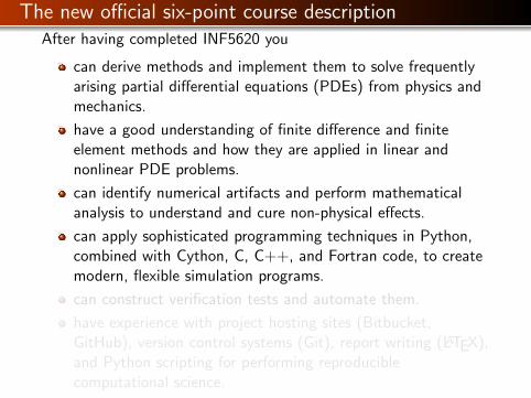
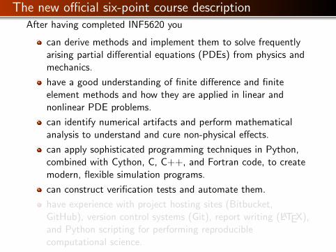
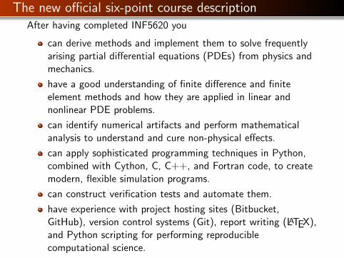
The new official six-point course descriptionAfter having completed INF5620 you

can derive methods and implement them to solve frequentlyarising partial differential equations (PDEs) from physics andmechanics.

have a good understanding of finite difference and finiteelement methods and how they are applied in linear andnonlinear PDE problems.

can identify numerical artifacts and perform mathematicalanalysis to understand and cure non-physical effects.

can apply sophisticated programming techniques in Python,combined with Cython, C, C++, and Fortran code, to createmodern, flexible simulation programs.

can construct verification tests and automate them.

have experience with project hosting sites (Bitbucket,GitHub), version control systems (Git), report writing (LATEX),and Python scripting for performing reproduciblecomputational science.











































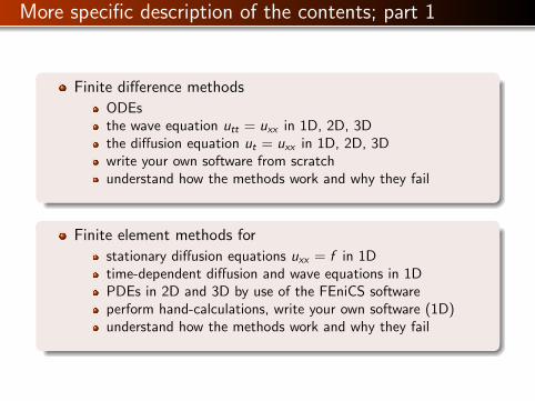
More specific description of the contents; part 1

Finite difference methods

ODEsthe wave equation utt = uxx in 1D, 2D, 3Dthe diffusion equation ut = uxx in 1D, 2D, 3Dwrite your own software from scratchunderstand how the methods work and why they fail

Finite element methods for

stationary diffusion equations uxx = f in 1Dtime-dependent diffusion and wave equations in 1DPDEs in 2D and 3D by use of the FEniCS softwareperform hand-calculations, write your own software (1D)understand how the methods work and why they fail

More specific description of the contents; part 2

Nonlinear PDEs

Newton and Picard iteration methods, finite differences andelements

More advanced PDEs for fluid flow and elasticity

Parallel computing

Philosophy: simplify, understand, generalize

Start with simplified ODE/PDE problems

Learn to reason about the discretization

Learn to implement, verify, and experiment

Understand the method, program, and results

Generalize the problem, method, and program

This is the power of applied mathematics!

The exam

Oral exam

6 problems (topics) are announced two weeks before the exam

Work out a 20 min presentations (talks) for each problem

At the exam: throw a die to pick your problem to be presented

Aids: plots, computer programs

Why? Very effective way of learning

Sure? Excellent results over 15 years

When? Late december

The exam

Oral exam







When? Late december

The exam

Oral exam







When? Late december

The exam

Oral exam







When? Late december

The exam

Oral exam







When? Late december

The exam

Oral exam







When? Late december

The exam

Oral exam







When? Late december

The exam

Oral exam







When? Late december

The exam

Oral exam







When? Late december

Required software

Our software platform: Python (sometimes combined withCython, Fortran, C, C++)

Important Python packages: numpy, scipy, matplotlib,sympy, fenics, scitools, ...

Suggested installation: Run Ubuntu in a virtual machine

Alternative: run a (course-specific) Vagrant machine

Assumed/ideal background

INF1100: Python programming, solution of ODEs

Some experience with finite difference methods

Some analytical and numerical knowledge of PDEs

Much experience with calculus and linear algebra

Much experience with programming of mathematical problems

Experience with mathematical modeling with PDEs (fromphysics, mechanics, geophysics, or ...)

Start-up example for the course

What if you don’t have this ideal background?

Students come to this course with very different backgrounds

First task: summarize assumed background knowledge bygoing through a simple example

Also in this example:

Some fundamental material on software implementation andsoftware testingMaterial on analyzing numerical methods to understand whythey can failApplications to real-world problems

Start-up example

ODE problem.

u′ = −au, u(0) = I , t ∈ (0,T ],

where a > 0 is a constant.

Everything we do is motivated by what we need as building blocksfor solving PDEs!

What to learn in the start-up example; standard topics

How to think when constructing finite difference methods,with special focus on the Forward Euler, Backward Euler, andCrank-Nicolson (midpoint) schemes

How to formulate a computational algorithm and translate itinto Python code

How to make curve plots of the solutions

How to compute numerical errors

How to compute convergence rates

What to learn in the start-up example; programming topics

How to verify an implementation and automate verificationthrough nose tests in Python

How to structure code in terms of functions, classes, andmodules

How to work with Python concepts such as arrays, lists,dictionaries, lambda functions, functions in functions(closures), doctests, unit tests, command-line interfaces,graphical user interfaces

How to perform array computing and understand thedifference from scalar computing

How to conduct and automate large-scale numericalexperiments

How to generate scientific reports

What to learn in the start-up example; mathematicalanalysis

How to uncover numerical artifacts in the computed solution

How to analyze the numerical schemes mathematically tounderstand why artifacts occur

How to derive mathematical expressions for various measuresof the error in numerical methods, frequently by using thesympy software for symbolic computation

Introduce concepts such as finite difference operators, mesh(grid), mesh functions, stability, truncation error, consistency,and convergence

What to learn in the start-up example; generalizations

Generalize the example to u′(t) = −a(t)u(t) + b(t)

Present additional methods for the general nonlinear ODEu′ = f (u, t), which is either a scalar ODE or a system of ODEs

How to access professional packages for solving ODEs

How our model equations like u′ = −au arises in a wide rangeof phenomena in physics, biology, and finance

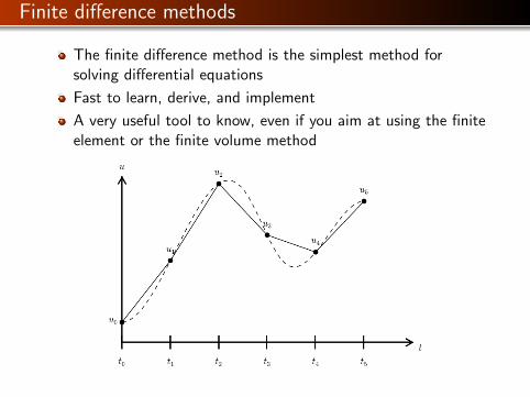
Finite difference methods

The finite difference method is the simplest method forsolving differential equations

Fast to learn, derive, and implement

A very useful tool to know, even if you aim at using the finiteelement or the finite volume method

Topics in the first intro to the finite difference method

How to derive a finite difference discretization of an ODE

Key concepts: mesh, mesh function, finite differenceapproximations

The Forward Euler, Backward Euler, and Crank-Nicolsonmethods

Finite difference operator notation

How to derive an algorithm and implement it in Python

How to test the implementation

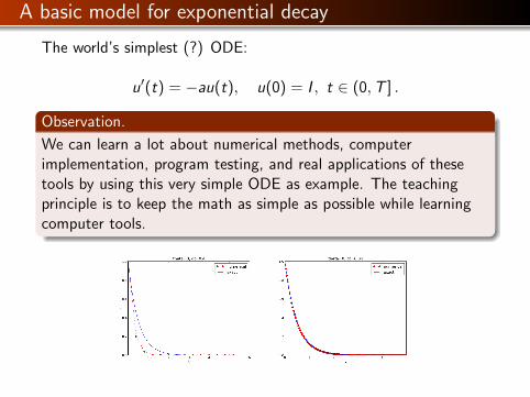
A basic model for exponential decay

The world’s simplest (?) ODE:

u′(t) = −au(t), u(0) = I , t ∈ (0,T ] .

Observation.

We can learn a lot about numerical methods, computerimplementation, program testing, and real applications of thesetools by using this very simple ODE as example. The teachingprinciple is to keep the math as simple as possible while learningcomputer tools.

Applications

Growth and decay of populations (cells, animals, human)

Growth and decay of a fortune

Radioactive decay

Cooling/heating of an object

Pressure variation in the atmosphere

Vertical motion of a body in water/air

Time-discretization of diffusion PDEs by Fourier techniques

See the text for details.

http://tinyurl.com/k3sdbuv/pub/decay-sphinx/._main_decay008.html

Continuous problem

u′ = −au, t ∈ (0,T ], u(0) = I . (1)

Solution of the continuous problem (”continuous solution”):

u(t) = Ie−at .

(special case that we can derive a formula for the discrete solution)

Discrete problem

un ≈ u(tn) means that u is found at discrete time pointst1, t2, t3, . . .Typical computational formula:

un+1 = Aun .

The constant A depends on the type of finite difference method.Solution of the discrete problem (”discrete solution”):

un+1 = IAn .

(special case that we can derive a formula for the discrete solution)

The steps in the finite difference method

Solving a differential equation by a finite difference methodconsists of four steps:

1 discretizing the domain,

2 fulfilling the equation at discrete time points,

3 replacing derivatives by finite differences,

4 formulating a recursive algorithm.

Step 1: Discretizing the domain

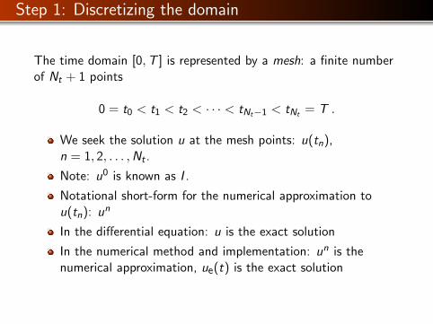
The time domain [0,T ] is represented by a mesh: a finite numberof Nt + 1 points

0 = t0 < t1 < t2 < · · · < tNt−1 < tNt = T .

We seek the solution u at the mesh points: u(tn),n = 1, 2, . . . ,Nt .

Note: u0 is known as I .

Notational short-form for the numerical approximation tou(tn): un

In the differential equation: u is the exact solution

In the numerical method and implementation: un is thenumerical approximation, ue(t) is the exact solution

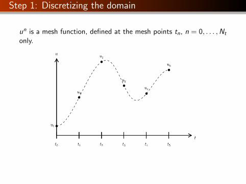
Step 1: Discretizing the domain

un is a mesh function, defined at the mesh points tn, n = 0, . . . ,Nt

only.

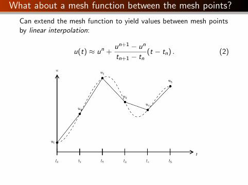
What about a mesh function between the mesh points?

Can extend the mesh function to yield values between mesh pointsby linear interpolation:

u(t) ≈ un +un+1 − un

tn+1 − tn(t − tn) . (2)

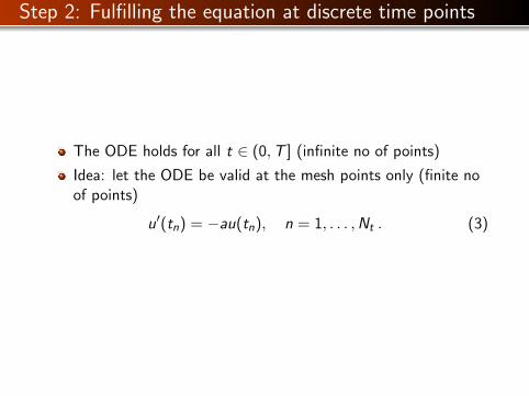
Step 2: Fulfilling the equation at discrete time points

The ODE holds for all t ∈ (0,T ] (infinite no of points)

Idea: let the ODE be valid at the mesh points only (finite noof points)

u′(tn) = −au(tn), n = 1, . . . ,Nt . (3)

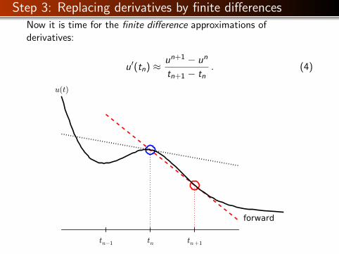
Step 3: Replacing derivatives by finite differencesNow it is time for the finite difference approximations ofderivatives:

u′(tn) ≈ un+1 − un

tn+1 − tn. (4)

forward

u(t)

tntn−1 tn+1

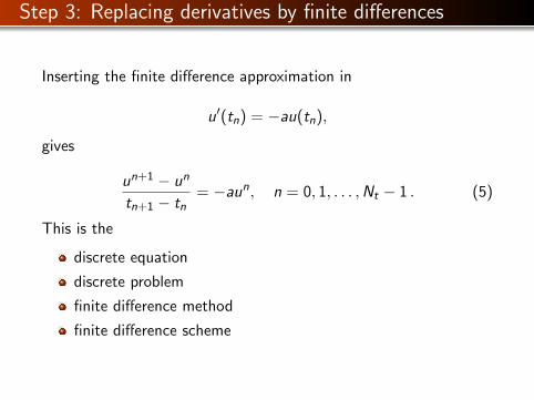
Step 3: Replacing derivatives by finite differences

Inserting the finite difference approximation in

u′(tn) = −au(tn),

gives

un+1 − un

tn+1 − tn= −aun, n = 0, 1, . . . ,Nt − 1 . (5)

This is the

discrete equation

discrete problem

finite difference method

finite difference scheme

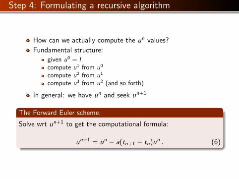
Step 4: Formulating a recursive algorithm

How can we actually compute the un values?

Fundamental structure:

given u0 = Icompute u1 from u0

compute u2 from u1

compute u3 from u2 (and so forth)

In general: we have un and seek un+1

The Forward Euler scheme.

Solve wrt un+1 to get the computational formula:

un+1 = un − a(tn+1 − tn)un . (6)

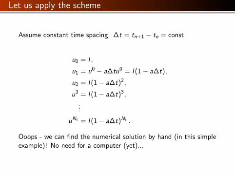
Let us apply the scheme

Assume constant time spacing: ∆t = tn+1 − tn = const

u0 = I ,

u1 = u0 − a∆tu0 = I (1− a∆t),

u2 = I (1− a∆t)2,

u3 = I (1− a∆t)3,

...

uNt = I (1− a∆t)Nt .

Ooops - we can find the numerical solution by hand (in this simpleexample)! No need for a computer (yet)...

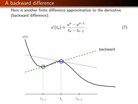
A backward differenceHere is another finite difference approximation to the derivative(backward difference):

u′(tn) ≈ un − un−1

tn − tn−1. (7)

backward

u(t)

tntn−1 tn+1

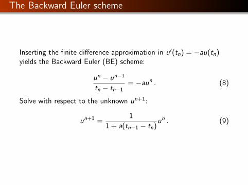
The Backward Euler scheme

Inserting the finite difference approximation in u′(tn) = −au(tn)yields the Backward Euler (BE) scheme:

un − un−1

tn − tn−1= −aun . (8)

Solve with respect to the unknown un+1:

un+1 =1

1 + a(tn+1 − tn)un . (9)

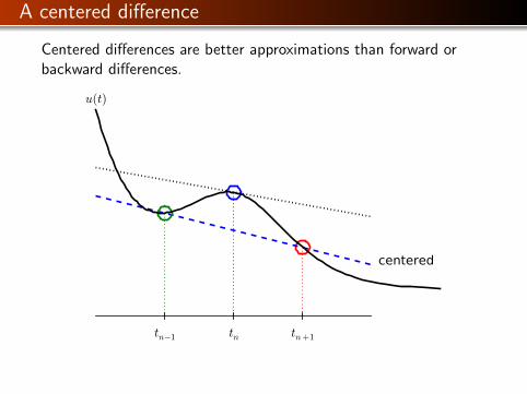
A centered difference

Centered differences are better approximations than forward orbackward differences.

centered

u(t)

tntn−1 tn+1

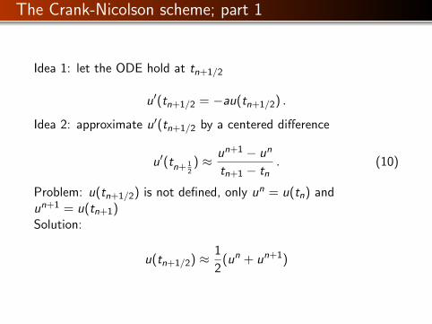
The Crank-Nicolson scheme; part 1

Idea 1: let the ODE hold at tn+1/2

u′(tn+1/2 = −au(tn+1/2) .

Idea 2: approximate u′(tn+1/2 by a centered difference

u′(tn+ 12) ≈ un+1 − un

tn+1 − tn. (10)

Problem: u(tn+1/2) is not defined, only un = u(tn) andun+1 = u(tn+1)Solution:

u(tn+1/2) ≈ 1

2(un + un+1)

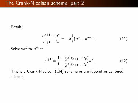
The Crank-Nicolson scheme; part 2

Result:

un+1 − un

tn+1 − tn= −a

1

2(un + un+1) . (11)

Solve wrt to un+1:

un+1 =1− 1

2 a(tn+1 − tn)

1 + 12 a(tn+1 − tn)

un . (12)

This is a Crank-Nicolson (CN) scheme or a midpoint or centeredscheme.

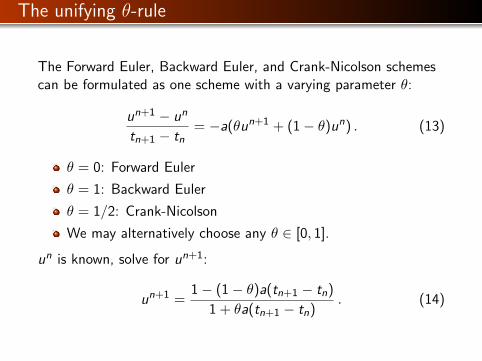
The unifying θ-rule

The Forward Euler, Backward Euler, and Crank-Nicolson schemescan be formulated as one scheme with a varying parameter θ:

un+1 − un

tn+1 − tn= −a(θun+1 + (1− θ)un) . (13)

θ = 0: Forward Euler

θ = 1: Backward Euler

θ = 1/2: Crank-Nicolson

We may alternatively choose any θ ∈ [0, 1].

un is known, solve for un+1:

un+1 =1− (1− θ)a(tn+1 − tn)

1 + θa(tn+1 − tn). (14)

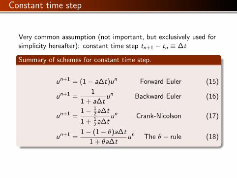
Constant time step

Very common assumption (not important, but exclusively used forsimplicity hereafter): constant time step tn+1 − tn ≡ ∆t

Summary of schemes for constant time step.

un+1 = (1− a∆t)un Forward Euler (15)

un+1 =1

1 + a∆tun Backward Euler (16)

un+1 =1− 1

2 a∆t

1 + 12 a∆t

un Crank-Nicolson (17)

un+1 =1− (1− θ)a∆t

1 + θa∆tun The θ − rule (18)

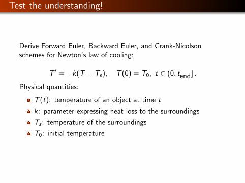
Test the understanding!

Derive Forward Euler, Backward Euler, and Crank-Nicolsonschemes for Newton’s law of cooling:

T ′ = −k(T − Ts), T (0) = T0, t ∈ (0, tend] .

Physical quantities:

T (t): temperature of an object at time t

k: parameter expressing heat loss to the surroundings

Ts : temperature of the surroundings

T0: initial temperature

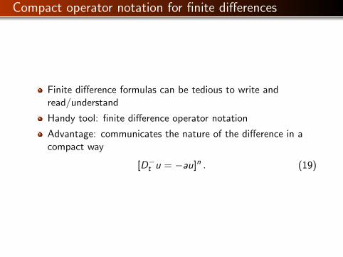
Compact operator notation for finite differences

Finite difference formulas can be tedious to write andread/understand

Handy tool: finite difference operator notation

Advantage: communicates the nature of the difference in acompact way

[D−t u = −au]n . (19)

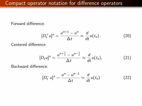
Compact operator notation for difference operators

Forward difference:

[D+t u]n =

un+1 − un

∆t≈ d

dtu(tn) . (20)

Centered difference:

[Dtu]n =un+ 1

2 − un− 12

∆t≈ d

dtu(tn), (21)

Backward difference:

[D−t u]n =un − un−1

∆t≈ d

dtu(tn) (22)

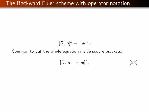
The Backward Euler scheme with operator notation

[D−t u]n = −aun .

Common to put the whole equation inside square brackets:

[D−t u = −au]n . (23)

The Forward Euler scheme with operator notation

[D+t u = −au]n . (24)

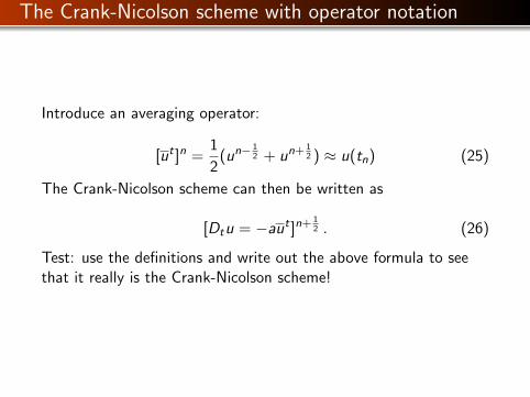
The Crank-Nicolson scheme with operator notation

Introduce an averaging operator:

[ut ]n =1

2(un− 1

2 + un+ 12 ) ≈ u(tn) (25)

The Crank-Nicolson scheme can then be written as

[Dtu = −aut ]n+ 12 . (26)

Test: use the definitions and write out the above formula to seethat it really is the Crank-Nicolson scheme!

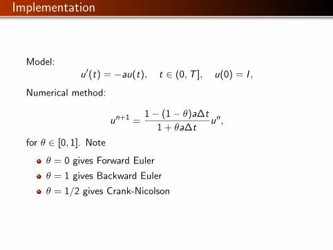
Implementation

Model:u′(t) = −au(t), t ∈ (0,T ], u(0) = I ,

Numerical method:

un+1 =1− (1− θ)a∆t

1 + θa∆tun,

for θ ∈ [0, 1]. Note

θ = 0 gives Forward Euler

θ = 1 gives Backward Euler

θ = 1/2 gives Crank-Nicolson

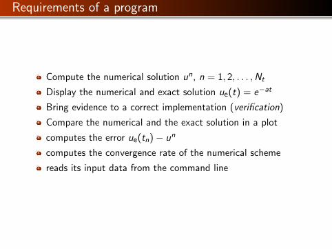
Requirements of a program

Compute the numerical solution un, n = 1, 2, . . . ,Nt

Display the numerical and exact solution ue(t) = e−at

Bring evidence to a correct implementation (verification)

Compare the numerical and the exact solution in a plot

computes the error ue(tn)− un

computes the convergence rate of the numerical scheme

reads its input data from the command line

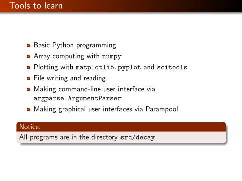
Tools to learn

Basic Python programming

Array computing with numpy

Plotting with matplotlib.pyplot and scitools

File writing and reading

Making command-line user interface viaargparse.ArgumentParser

Making graphical user interfaces via Parampool

Notice.

All programs are in the directory src/decay.

http://python.org

http://numpy.org/

http://matplotlib.sourceforge.net/

http://code.google.com/p/scitools/

https://github.com/hplgit/parampool

http://tinyurl.com/jvzzcfn/decay

Why implement in Python?

Python has a very clean, readable syntax (often known as”executable pseudo-code”).

Python code is very similar to MATLAB code (and MATLABhas a particularly widespread use for scientific computing).

Python is a full-fledged, very powerful programming language.

Python is similar to, but much simpler to work with andresults in more reliable code than C++.

Why implement in Python?

Python has a rich set of modules for scientific computing, andits popularity in scientific computing is rapidly growing.

Python was made for being combined with compiledlanguages (C, C++, Fortran) to reuse existing numericalsoftware and to reach high computational performance of newimplementations.

Python has extensive support for administrative task neededwhen doing large-scale computational investigations.

Python has extensive support for graphics (visualization, userinterfaces, web applications).

FEniCS, a very powerful tool for solving PDEs by the finiteelement method, is most human-efficient to operate fromPython.

Algorithm

Store un, n = 0, 1, . . . ,Nt in an array u.

Algorithm:1 initialize u0

2 for t = tn, n = 1, 2, . . . ,Nt : compute un using the θ-ruleformula

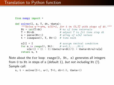
Translation to Python function

from numpy import *

def solver(I, a, T, dt, theta):"""Solve u’=-a*u, u(0)=I, for t in (0,T] with steps of dt."""Nt = int(T/dt) # no of time intervalsT = Nt*dt # adjust T to fit time step dtu = zeros(Nt+1) # array of u[n] valuest = linspace(0, T, Nt+1) # time mesh

u[0] = I # assign initial conditionfor n in range(0, Nt): # n=0,1,...,Nt-1

u[n+1] = (1 - (1-theta)*a*dt)/(1 + theta*dt*a)*u[n]return u, t

Note about the for loop: range(0, Nt, s) generates all integersfrom 0 to Nt in steps of s (default 1), but not including Nt (!).Sample call:

u, t = solver(I=1, a=2, T=8, dt=0.8, theta=1)

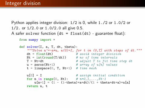
Integer division

Python applies integer division: 1/2 is 0, while 1./2 or 1.0/2 or1/2. or 1/2.0 or 1.0/2.0 all give 0.5.A safer solver function (dt = float(dt) - guarantee float):

from numpy import *

def solver(I, a, T, dt, theta):"""Solve u’=-a*u, u(0)=I, for t in (0,T] with steps of dt."""dt = float(dt) # avoid integer divisionNt = int(round(T/dt)) # no of time intervalsT = Nt*dt # adjust T to fit time step dtu = zeros(Nt+1) # array of u[n] valuest = linspace(0, T, Nt+1) # time mesh


u[n+1] = (1 - (1-theta)*a*dt)/(1 + theta*dt*a)*u[n]return u, t

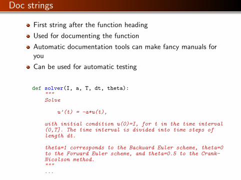
Doc strings

First string after the function heading

Used for documenting the function

Automatic documentation tools can make fancy manuals foryou

Can be used for automatic testing

def solver(I, a, T, dt, theta):"""Solve

u’(t) = -a*u(t),

with initial condition u(0)=I, for t in the time interval(0,T]. The time interval is divided into time steps oflength dt.

theta=1 corresponds to the Backward Euler scheme, theta=0to the Forward Euler scheme, and theta=0.5 to the Crank-Nicolson method."""...

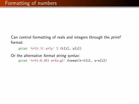
Formatting of numbers

Can control formatting of reals and integers through the printfformat:

print ’t=%6.3f u=%g’ % (t[i], u[i])

Or the alternative format string syntax:print ’t={t:6.3f} u={u:g}’.format(t=t[i], u=u[i])

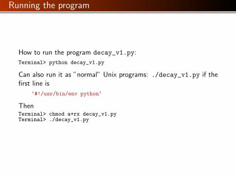
Running the program

How to run the program decay_v1.py:

Terminal> python decay_v1.py

Can also run it as ”normal” Unix programs: ./decay_v1.py if thefirst line is

‘#!/usr/bin/env python‘

ThenTerminal> chmod a+rx decay_v1.pyTerminal> ./decay_v1.py

https://github.com/hplgit/INF5620/blob/gh-pages/src/decay/decay_v1.py

Verifying the implementation

Verification = bring evidence that the program works

Find suitable test problems

Make function for each test problem

Later: put the verification tests in a professional testingframework

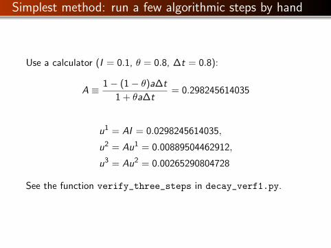
Simplest method: run a few algorithmic steps by hand

Use a calculator (I = 0.1, θ = 0.8, ∆t = 0.8):

A ≡ 1− (1− θ)a∆t

1 + θa∆t= 0.298245614035

u1 = AI = 0.0298245614035,

u2 = Au1 = 0.00889504462912,

u3 = Au2 = 0.00265290804728

See the function verify_three_steps in decay_verf1.py.

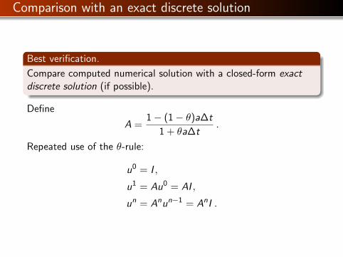
http://tinyurl.com/jvzzcfn/decay/decay_verf1.py

Comparison with an exact discrete solution

Best verification.

Compare computed numerical solution with a closed-form exactdiscrete solution (if possible).

Define

A =1− (1− θ)a∆t

1 + θa∆t.

Repeated use of the θ-rule:

u0 = I ,

u1 = Au0 = AI ,

un = Anun−1 = AnI .

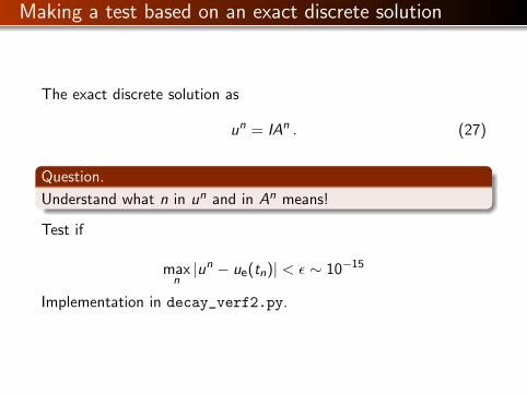
Making a test based on an exact discrete solution

The exact discrete solution as

un = IAn . (27)

Question.

Understand what n in un and in An means!

Test if

maxn|un − ue(tn)| < ε ∼ 10−15

Implementation in decay_verf2.py.

http://tinyurl.com/jvzzcfn/decay/decay_verf2.py

Test the understanding!

Make a program for solving Newton’s law of cooling

T ′ = −k(T − Ts), T (0) = T0, t ∈ (0, tend] .

with the Forward Euler, Backward Euler, and Crank-Nicolsonschemes (or a θ scheme). Verify the implementation.

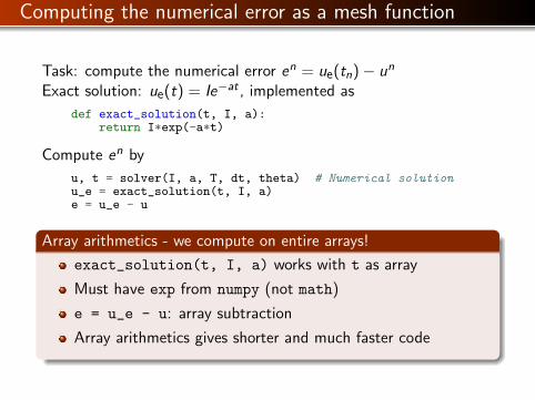
Computing the numerical error as a mesh function

Task: compute the numerical error en = ue(tn)− un

Exact solution: ue(t) = Ie−at , implemented as

def exact_solution(t, I, a):return I*exp(-a*t)

Compute en by

u, t = solver(I, a, T, dt, theta) # Numerical solutionu_e = exact_solution(t, I, a)e = u_e - u

Array arithmetics - we compute on entire arrays!

exact_solution(t, I, a) works with t as array

Must have exp from numpy (not math)

e = u_e - u: array subtraction

Array arithmetics gives shorter and much faster code

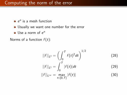
Computing the norm of the error

en is a mesh function

Usually we want one number for the error

Use a norm of en

Norms of a function f (t):

||f ||L2 =

(∫ T

0f (t)2dt

)1/2

(28)

||f ||L1 =

∫ T

0|f (t)|dt (29)

||f ||L∞ = maxt∈[0,T ]

|f (t)| (30)

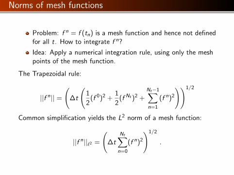
Norms of mesh functions

Problem: f n = f (tn) is a mesh function and hence not definedfor all t. How to integrate f n?

Idea: Apply a numerical integration rule, using only the meshpoints of the mesh function.

The Trapezoidal rule:

||f n|| =

(∆t

(1

2(f 0)2 +

1

2(f Nt )2 +

Nt−1∑n=1

(f n)2

))1/2

Common simplification yields the L2 norm of a mesh function:

||f n||`2 =

(∆t

Nt∑n=0

(f n)2

)1/2

.

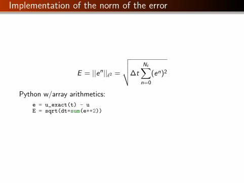
Implementation of the norm of the error

E = ||en||`2 =

√√√√∆tNt∑n=0

(en)2

Python w/array arithmetics:

e = u_exact(t) - uE = sqrt(dt*sum(e**2))

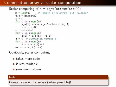
Comment on array vs scalar computation

Scalar computing of E = sqrt(dt*sum(e**2)):m = len(u) # length of u array (alt: u.size)u_e = zeros(m)t = 0for i in range(m):

u_e[i] = exact_solution(t, a, I)t = t + dt

e = zeros(m)for i in range(m):

e[i] = u_e[i] - u[i]s = 0 # summation variablefor i in range(m):

s = s + e[i]**2error = sqrt(dt*s)

Obviously, scalar computing

takes more code

is less readable

runs much slower

Rule.

Compute on entire arrays (when possible)!

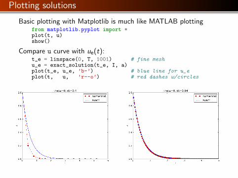
Plotting solutions

Basic plotting with Matplotlib is much like MATLAB plottingfrom matplotlib.pyplot import *plot(t, u)show()

Compare u curve with ue(t):t_e = linspace(0, T, 1001) # fine meshu_e = exact_solution(t_e, I, a)plot(t_e, u_e, ’b-’) # blue line for u_eplot(t, u, ’r--o’) # red dashes w/circles

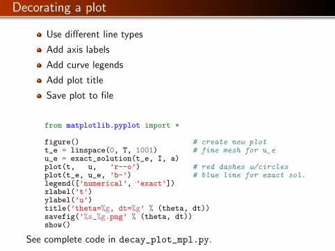
Decorating a plot

Use different line types

Add axis labels

Add curve legends

Add plot title

Save plot to file

from matplotlib.pyplot import *

figure() # create new plott_e = linspace(0, T, 1001) # fine mesh for u_eu_e = exact_solution(t_e, I, a)plot(t, u, ’r--o’) # red dashes w/circlesplot(t_e, u_e, ’b-’) # blue line for exact sol.legend([’numerical’, ’exact’])xlabel(’t’)ylabel(’u’)title(’theta=%g, dt=%g’ % (theta, dt))savefig(’%s_%g.png’ % (theta, dt))show()

See complete code in decay_plot_mpl.py.

http://tinyurl.com/jvzzcfn/decay/decay_plot_mpl.py

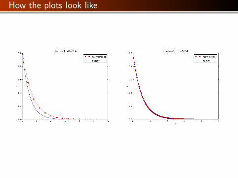
How the plots look like

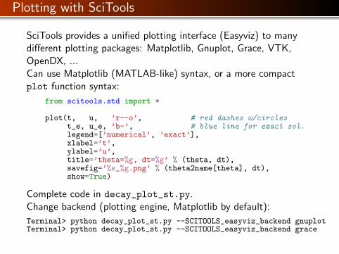
Plotting with SciTools

SciTools provides a unified plotting interface (Easyviz) to manydifferent plotting packages: Matplotlib, Gnuplot, Grace, VTK,OpenDX, ...Can use Matplotlib (MATLAB-like) syntax, or a more compactplot function syntax:

from scitools.std import *

plot(t, u, ’r--o’, # red dashes w/circlest_e, u_e, ’b-’, # blue line for exact sol.legend=[’numerical’, ’exact’],xlabel=’t’,ylabel=’u’,title=’theta=%g, dt=%g’ % (theta, dt),savefig=’%s_%g.png’ % (theta2name[theta], dt),show=True)

Complete code in decay_plot_st.py.Change backend (plotting engine, Matplotlib by default):

Terminal> python decay_plot_st.py --SCITOOLS_easyviz_backend gnuplotTerminal> python decay_plot_st.py --SCITOOLS_easyviz_backend grace

http://code.google.com/p/scitools

https://github.com/hplgit/INF5620/blob/gh-pages/src/decay/decay_plot_st.py

Creating user interfaces

Never edit the program to change input!

Set input data on the command line or in a graphical userinterface

How is explained next

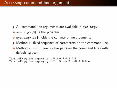
Accessing command-line arguments

All command-line arguments are available in sys.argv

sys.argv[0] is the program

sys.argv[1:] holds the command-line arguments

Method 1: fixed sequence of parameters on the command line

Method 2: --option value pairs on the command line (withdefault values)

Terminal> python myprog.py 1.5 2 0.5 0.8 0.4Terminal> python myprog.py --I 1.5 --a 2 --dt 0.8 0.4

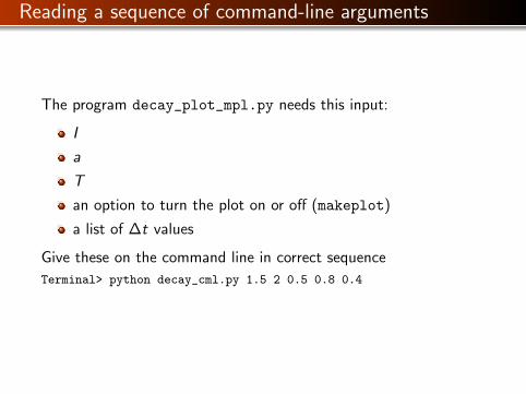
Reading a sequence of command-line arguments

The program decay_plot_mpl.py needs this input:

I

a

T

an option to turn the plot on or off (makeplot)

a list of ∆t values

Give these on the command line in correct sequence

Terminal> python decay_cml.py 1.5 2 0.5 0.8 0.4


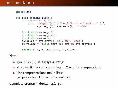
Implementation

import sys

def read_command_line():if len(sys.argv) < 6:

print ’Usage: %s I a T on/off dt1 dt2 dt3 ...’ % \sys.argv[0]; sys.exit(1) # abort

I = float(sys.argv[1])a = float(sys.argv[2])T = float(sys.argv[3])makeplot = sys.argv[4] in (’on’, ’True’)dt_values = [float(arg) for arg in sys.argv[5:]]

return I, a, T, makeplot, dt_values

Note:

sys.argv[i] is always a string

Must explicitly convert to (e.g.) float for computations

List comprehensions make lists:[expression for e in somelist]

Complete program: decay_cml.py.

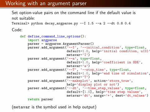
http://tinyurl.com/jvzzcfn/decay/decay_cml.py

Working with an argument parser

Set option-value pairs on the command line if the default value isnot suitable:Terminal> python decay_argparse.py --I 1.5 --a 2 --dt 0.8 0.4

Code:

def define_command_line_options():import argparseparser = argparse.ArgumentParser()parser.add_argument(’--I’, ’--initial_condition’, type=float,

default=1.0, help=’initial condition, u(0)’,metavar=’I’)

parser.add_argument(’--a’, type=float,default=1.0, help=’coefficient in ODE’,metavar=’a’)

parser.add_argument(’--T’, ’--stop_time’, type=float,default=1.0, help=’end time of simulation’,metavar=’T’)

parser.add_argument(’--makeplot’, action=’store_true’,help=’display plot or not’)

parser.add_argument(’--dt’, ’--time_step_values’, type=float,default=[1.0], help=’time step values’,metavar=’dt’, nargs=’+’, dest=’dt_values’)

return parser

(metavar is the symbol used in help output)

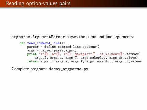
Reading option-values pairs

argparse.ArgumentParser parses the command-line arguments:

def read_command_line():parser = define_command_line_options()args = parser.parse_args()print ’I={}, a={}, T={}, makeplot={}, dt_values={}’.format(

args.I, args.a, args.T, args.makeplot, args.dt_values)return args.I, args.a, args.T, args.makeplot, args.dt_values

Complete program: decay_argparse.py.

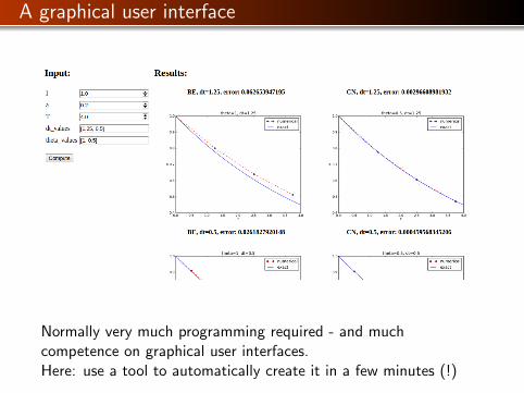
http://tinyurl.com/jvzzcfn/decay/decay_argparse.py

A graphical user interface

Normally very much programming required - and muchcompetence on graphical user interfaces.Here: use a tool to automatically create it in a few minutes (!)

The Parampool package

Parampool is a package for handling a large pool of inputparameters in simulation programs

Parampool can automatically create a sophisticatedweb-based graphical user interface (GUI) to set parametersand view solutions

Remark.

The forthcoming material aims at those with particular interest inequipping their programs with a GUI - others can safely skip it.

https://github.com/hplgit/parampool

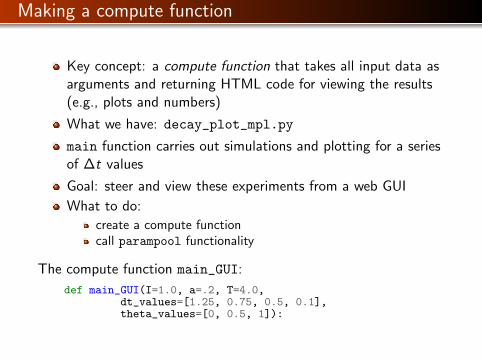
Making a compute function

Key concept: a compute function that takes all input data asarguments and returning HTML code for viewing the results(e.g., plots and numbers)

What we have: decay_plot_mpl.py

main function carries out simulations and plotting for a seriesof ∆t values

Goal: steer and view these experiments from a web GUI

What to do:

create a compute functioncall parampool functionality

The compute function main_GUI:

def main_GUI(I=1.0, a=.2, T=4.0,dt_values=[1.25, 0.75, 0.5, 0.1],theta_values=[0, 0.5, 1]):


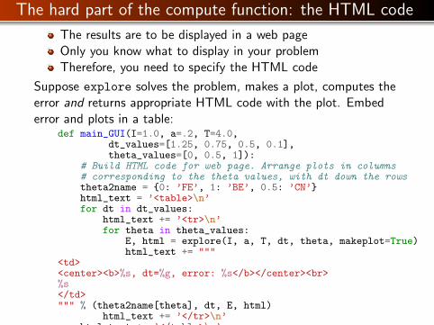
The hard part of the compute function: the HTML code

The results are to be displayed in a web pageOnly you know what to display in your problemTherefore, you need to specify the HTML code

Suppose explore solves the problem, makes a plot, computes theerror and returns appropriate HTML code with the plot. Embederror and plots in a table:

def main_GUI(I=1.0, a=.2, T=4.0,dt_values=[1.25, 0.75, 0.5, 0.1],theta_values=[0, 0.5, 1]):

# Build HTML code for web page. Arrange plots in columns# corresponding to the theta values, with dt down the rowstheta2name = {0: ’FE’, 1: ’BE’, 0.5: ’CN’}html_text = ’<table>\n’for dt in dt_values:

html_text += ’<tr>\n’for theta in theta_values:

E, html = explore(I, a, T, dt, theta, makeplot=True)html_text += """

<td><center><b>%s, dt=%g, error: %s</b></center><br>%s</td>""" % (theta2name[theta], dt, E, html)

html_text += ’</tr>\n’html_text += ’</table>\n’return html_text

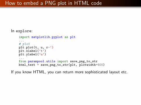
How to embed a PNG plot in HTML code

In explore:

import matplotlib.pyplot as plt...# plotplt.plot(t, u, r-’)plt.xlabel(’t’)plt.ylabel(’u’)...from parampool.utils import save_png_to_strhtml_text = save_png_to_str(plt, plotwidth=400)

If you know HTML, you can return more sophisticated layout etc.

Generating the user interface

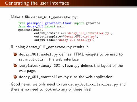
Make a file decay_GUI_generate.py:

from parampool.generator.flask import generatefrom decay_GUI import maingenerate(main,

output_controller=’decay_GUI_controller.py’,output_template=’decay_GUI_view.py’,output_model=’decay_GUI_model.py’)

Running decay_GUI_generate.py results in

1 decay_GUI_model.py defines HTML widgets to be used toset input data in the web interface,

2 templates/decay_GUI_views.py defines the layout of theweb page,

3 decay_GUI_controller.py runs the web application.

Good news: we only need to run decay_GUI_controller.py andthere is no need to look into any of these files!

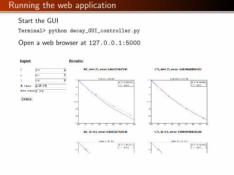
Running the web application

Start the GUI

Terminal> python decay_GUI_controller.py

Open a web browser at 127.0.0.1:5000

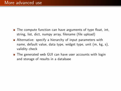
More advanced use

The compute function can have arguments of type float, int,string, list, dict, numpy array, filename (file upload)

Alternative: specify a hierarchy of input parameters withname, default value, data type, widget type, unit (m, kg, s),validity check

The generated web GUI can have user accounts with loginand storage of results in a database

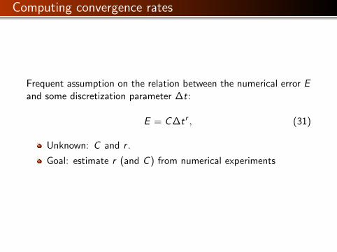
Computing convergence rates

Frequent assumption on the relation between the numerical error Eand some discretization parameter ∆t:

E = C ∆tr , (31)

Unknown: C and r .

Goal: estimate r (and C ) from numerical experiments

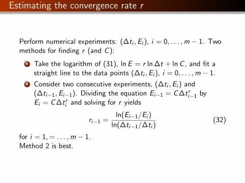
Estimating the convergence rate r

Perform numerical experiments: (∆ti ,Ei ), i = 0, . . . ,m − 1. Twomethods for finding r (and C ):

1 Take the logarithm of (31), ln E = r ln ∆t + ln C , and fit astraight line to the data points (∆ti ,Ei ), i = 0, . . . ,m − 1.

2 Consider two consecutive experiments, (∆ti ,Ei ) and(∆ti−1,Ei−1). Dividing the equation Ei−1 = C ∆tri−1 byEi = C ∆tri and solving for r yields

ri−1 =ln(Ei−1/Ei )

ln(∆ti−1/∆ti )(32)

for i = 1,= . . . ,m − 1.Method 2 is best.

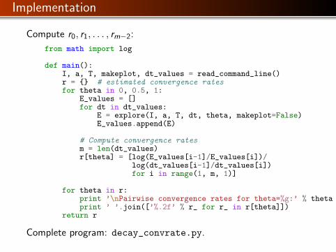
Implementation

Compute r0, r1, . . . , rm−2:

from math import log

def main():I, a, T, makeplot, dt_values = read_command_line()r = {} # estimated convergence ratesfor theta in 0, 0.5, 1:

E_values = []for dt in dt_values:

E = explore(I, a, T, dt, theta, makeplot=False)E_values.append(E)

# Compute convergence ratesm = len(dt_values)r[theta] = [log(E_values[i-1]/E_values[i])/

log(dt_values[i-1]/dt_values[i])for i in range(1, m, 1)]

for theta in r:print ’\nPairwise convergence rates for theta=%g:’ % thetaprint ’ ’.join([’%.2f’ % r_ for r_ in r[theta]])

return r

Complete program: decay_convrate.py.

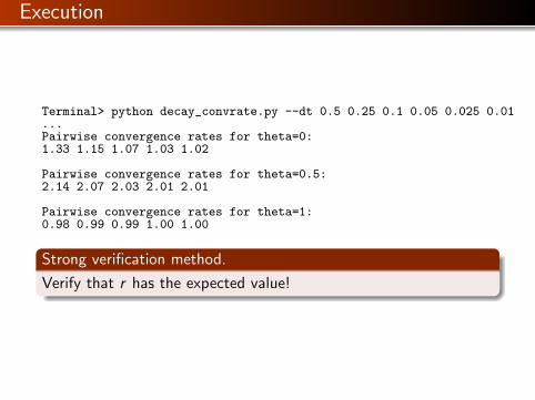
https://github.com/hplgit/INF5620/blob/gh-pages/src/decay/decay_convrate.py

Execution

Terminal> python decay_convrate.py --dt 0.5 0.25 0.1 0.05 0.025 0.01...Pairwise convergence rates for theta=0:1.33 1.15 1.07 1.03 1.02

Pairwise convergence rates for theta=0.5:2.14 2.07 2.03 2.01 2.01

Pairwise convergence rates for theta=1:0.98 0.99 0.99 1.00 1.00

Strong verification method.

Verify that r has the expected value!

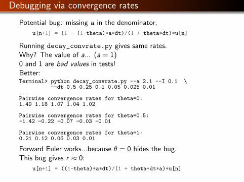
Debugging via convergence rates

Potential bug: missing a in the denominator,

u[n+1] = (1 - (1-theta)*a*dt)/(1 + theta*dt)*u[n]

Running decay_convrate.py gives same rates.Why? The value of a... (a = 1)0 and 1 are bad values in tests!Better:Terminal> python decay_convrate.py --a 2.1 --I 0.1 \

--dt 0.5 0.25 0.1 0.05 0.025 0.01...Pairwise convergence rates for theta=0:1.49 1.18 1.07 1.04 1.02

Pairwise convergence rates for theta=0.5:-1.42 -0.22 -0.07 -0.03 -0.01

Pairwise convergence rates for theta=1:0.21 0.12 0.06 0.03 0.01

Forward Euler works...because θ = 0 hides the bug.This bug gives r ≈ 0:

u[n+1] = ((1-theta)*a*dt)/(1 + theta*dt*a)*u[n]

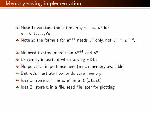
Memory-saving implementation

Note 1: we store the entire array u, i.e., un forn = 0, 1, . . . ,Nt

Note 2: the formula for un+1 needs un only, not un−1, un−2,...

No need to store more than un+1 and un

Extremely important when solving PDEs

No practical importance here (much memory available)

But let’s illustrate how to do save memory!

Idea 1: store un+1 in u, un in u_1 (float)

Idea 2: store u in a file, read file later for plotting

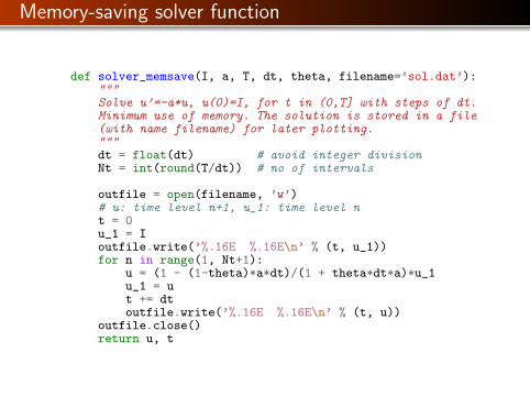
Memory-saving solver function

def solver_memsave(I, a, T, dt, theta, filename=’sol.dat’):"""Solve u’=-a*u, u(0)=I, for t in (0,T] with steps of dt.Minimum use of memory. The solution is stored in a file(with name filename) for later plotting."""dt = float(dt) # avoid integer divisionNt = int(round(T/dt)) # no of intervals

outfile = open(filename, ’w’)# u: time level n+1, u_1: time level nt = 0u_1 = Ioutfile.write(’%.16E %.16E\n’ % (t, u_1))for n in range(1, Nt+1):

u = (1 - (1-theta)*a*dt)/(1 + theta*dt*a)*u_1u_1 = ut += dtoutfile.write(’%.16E %.16E\n’ % (t, u))

outfile.close()return u, t

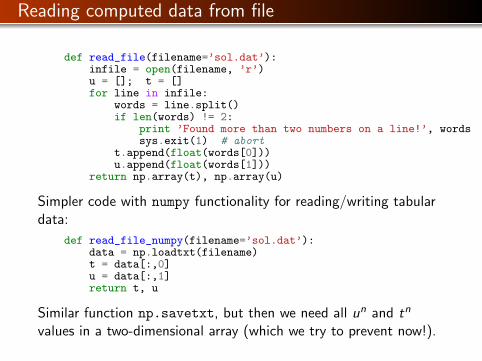
Reading computed data from file

def read_file(filename=’sol.dat’):infile = open(filename, ’r’)u = []; t = []for line in infile:

words = line.split()if len(words) != 2:

print ’Found more than two numbers on a line!’, wordssys.exit(1) # abort

t.append(float(words[0]))u.append(float(words[1]))

return np.array(t), np.array(u)

Simpler code with numpy functionality for reading/writing tabulardata:

def read_file_numpy(filename=’sol.dat’):data = np.loadtxt(filename)t = data[:,0]u = data[:,1]return t, u

Similar function np.savetxt, but then we need all un and tn

values in a two-dimensional array (which we try to prevent now!).

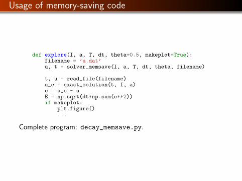
Usage of memory-saving code

def explore(I, a, T, dt, theta=0.5, makeplot=True):filename = ’u.dat’u, t = solver_memsave(I, a, T, dt, theta, filename)

t, u = read_file(filename)u_e = exact_solution(t, I, a)e = u_e - uE = np.sqrt(dt*np.sum(e**2))if makeplot:

plt.figure()...

Complete program: decay_memsave.py.

https://github.com/hplgit/INF5620/blob/gh-pages/src/decay/decay_memsave.py

Software engineering

Goal: make more professional numerical software.Topics:

How to make modules (reusable libraries)

Testing frameworks (doctest, nose, unittest)

Implementation with classes

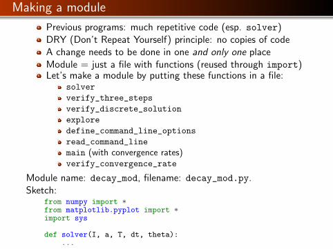
Making a module

Previous programs: much repetitive code (esp. solver)DRY (Don’t Repeat Yourself) principle: no copies of codeA change needs to be done in one and only one placeModule = just a file with functions (reused through import)Let’s make a module by putting these functions in a file:

solver

verify_three_steps

verify_discrete_solution

explore

define_command_line_options

read_command_line

main (with convergence rates)verify_convergence_rate

Module name: decay_mod, filename: decay_mod.py.Sketch:

from numpy import *from matplotlib.pyplot import *import sys

def solver(I, a, T, dt, theta):...

def verify_three_steps():...

def verify_exact_discrete_solution():...

def exact_solution(t, I, a):...

def explore(I, a, T, dt, theta=0.5, makeplot=True):...

def define_command_line_options():...

def read_command_line(use_argparse=True):...

def main():...

That is! It’s a module decay_mod in file decay_mod.py.Usage in some other program:

from decay_mod import solveru, t = solver(I=1.0, a=3.0, T=3, dt=0.01, theta=0.5)

Test blockAt the end of a module it is common to include a test block:

if __name__ == ’__main__’:main()

If decay_mod is imported, __name__ is decay_mod.If decay_mod.py is run, __name__ is __main__.Use test block for testing, demo, user interface, ...

Extended test block:if __name__ == ’__main__’:

if ’verify’ in sys.argv:if verify_three_steps() and verify_discrete_solution():

pass # okelse:

print ’Bug in the implementation!’elif ’verify_rates’ in sys.argv:

sys.argv.remove(’verify_rates’)if not ’--dt’ in sys.argv:

print ’Must assign several dt values’sys.exit(1) # abort

if verify_convergence_rate():pass

else:print ’Bug in the implementation!’

else:# Perform simulationsmain()

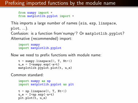
Prefixing imported functions by the module name

from numpy import *from matplotlib.pyplot import *

This imports a large number of names (sin, exp, linspace,plot, ...).Confusion: is a function from‘numpy‘? Or matplotlib.pyplot?Alternative (recommended) import:

import numpyimport matplotlib.pyplot

Now we need to prefix functions with module name:

t = numpy.linspace(0, T, Nt+1)u_e = I*numpy.exp(-a*t)matplotlib.pyplot.plot(t, u_e)

Common standard:

import numpy as npimport matplotlib.pyplot as plt

t = np.linspace(0, T, Nt+1)u_e = I*np.exp(-a*t)plt.plot(t, u_e)

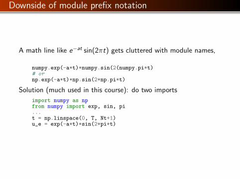
Downside of module prefix notation

A math line like e−at sin(2πt) gets cluttered with module names,

numpy.exp(-a*t)*numpy.sin(2(numpy.pi*t)# ornp.exp(-a*t)*np.sin(2*np.pi*t)

Solution (much used in this course): do two imports

import numpy as npfrom numpy import exp, sin, pi...t = np.linspace(0, T, Nt+1)u_e = exp(-a*t)*sin(2*pi*t)

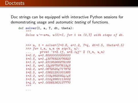
Doctests

Doc strings can be equipped with interactive Python sessions fordemonstrating usage and automatic testing of functions.

def solver(I, a, T, dt, theta):"""Solve u’=-a*u, u(0)=I, for t in (0,T] with steps of dt.

>>> u, t = solver(I=0.8, a=1.2, T=4, dt=0.5, theta=0.5)>>> for t_n, u_n in zip(t, u):... print ’t=%.1f, u=%.14f’ % (t_n, u_n)t=0.0, u=0.80000000000000t=0.5, u=0.43076923076923t=1.0, u=0.23195266272189t=1.5, u=0.12489758761948t=2.0, u=0.06725254717972t=2.5, u=0.03621291001985t=3.0, u=0.01949925924146t=3.5, u=0.01049960113002t=4.0, u=0.00565363137770"""...

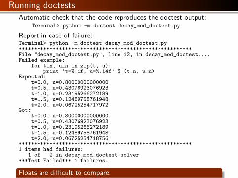
Running doctestsAutomatic check that the code reproduces the doctest output:

Terminal> python -m doctest decay_mod_doctest.py

Report in case of failure:Terminal> python -m doctest decay_mod_doctest.py********************************************************File "decay_mod_doctest.py", line 12, in decay_mod_doctest....Failed example:

for t_n, u_n in zip(t, u):print ’t=%.1f, u=%.14f’ % (t_n, u_n)

Expected:t=0.0, u=0.80000000000000t=0.5, u=0.43076923076923t=1.0, u=0.23195266272189t=1.5, u=0.12489758761948t=2.0, u=0.06725254717972

Got:t=0.0, u=0.80000000000000t=0.5, u=0.43076923076923t=1.0, u=0.23195266272189t=1.5, u=0.12489758761948t=2.0, u=0.06725254718756

********************************************************1 items had failures:

1 of 2 in decay_mod_doctest.solver***Test Failed*** 1 failures.

Floats are difficult to compare.

Limit the number of digits in the output in doctests! Otherwise,round-off errors on a different machine may ruin the test.

Complete program: decay_mod_doctest.py.

http://tinyurl.com/jvzzcfn/decay/decay_mod_doctest.py

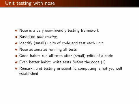
Unit testing with nose

Nose is a very user-friendly testing framework

Based on unit testing

Identify (small) units of code and test each unit

Nose automates running all tests

Good habit: run all tests after (small) edits of a code

Even better habit: write tests before the code (!)

Remark: unit testing in scientific computing is not yet wellestablished

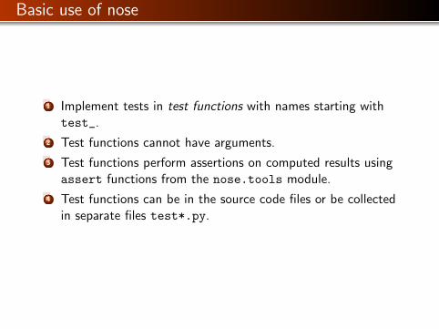
Basic use of nose

1 Implement tests in test functions with names starting withtest_.

2 Test functions cannot have arguments.

3 Test functions perform assertions on computed results usingassert functions from the nose.tools module.

4 Test functions can be in the source code files or be collectedin separate files test*.py.

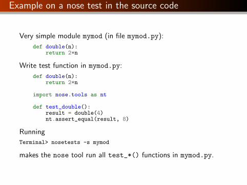
Example on a nose test in the source code

Very simple module mymod (in file mymod.py):

def double(n):return 2*n

Write test function in mymod.py:

def double(n):return 2*n

import nose.tools as nt

def test_double():result = double(4)nt.assert_equal(result, 8)

Running

Terminal> nosetests -s mymod

makes the nose tool run all test_*() functions in mymod.py.

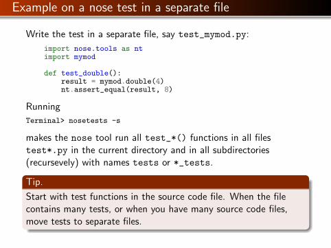
Example on a nose test in a separate file

Write the test in a separate file, say test_mymod.py:

import nose.tools as ntimport mymod

def test_double():result = mymod.double(4)nt.assert_equal(result, 8)

Running

Terminal> nosetests -s

makes the nose tool run all test_*() functions in all filestest*.py in the current directory and in all subdirectories(recursevely) with names tests or *_tests.

Tip.

Start with test functions in the source code file. When the filecontains many tests, or when you have many source code files,move tests to separate files.

The habit of writing nose tests

Put test_*() functions in the module

When you get many test_*() functions, collect them intests/test*.py

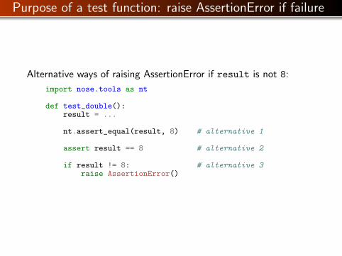
Purpose of a test function: raise AssertionError if failure

Alternative ways of raising AssertionError if result is not 8:


def test_double():result = ...

nt.assert_equal(result, 8) # alternative 1

assert result == 8 # alternative 2

if result != 8: # alternative 3raise AssertionError()

Advantages of nose

Easier to use than other test frameworks

Tests are written and collected in a compact and structuredway

Large collections of tests, scattered throughout a directorytree can be executed with one command (nosetests -s)

Nose is a much-adopted standard

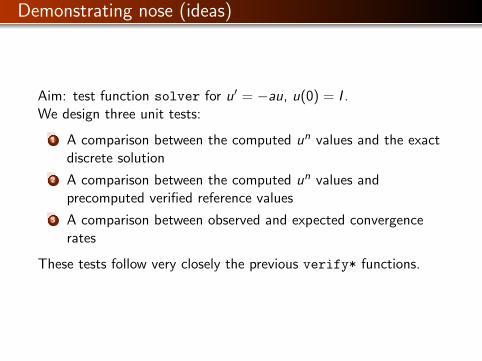
Demonstrating nose (ideas)

Aim: test function solver for u′ = −au, u(0) = I .We design three unit tests:

1 A comparison between the computed un values and the exactdiscrete solution

2 A comparison between the computed un values andprecomputed verified reference values

3 A comparison between observed and expected convergencerates

These tests follow very closely the previous verify* functions.

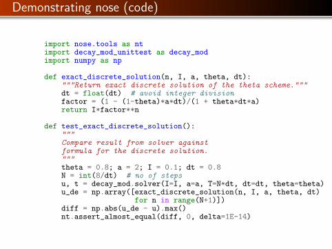
Demonstrating nose (code)

import nose.tools as ntimport decay_mod_unittest as decay_modimport numpy as np

def exact_discrete_solution(n, I, a, theta, dt):"""Return exact discrete solution of the theta scheme."""dt = float(dt) # avoid integer divisionfactor = (1 - (1-theta)*a*dt)/(1 + theta*dt*a)return I*factor**n

def test_exact_discrete_solution():"""Compare result from solver againstformula for the discrete solution."""theta = 0.8; a = 2; I = 0.1; dt = 0.8N = int(8/dt) # no of stepsu, t = decay_mod.solver(I=I, a=a, T=N*dt, dt=dt, theta=theta)u_de = np.array([exact_discrete_solution(n, I, a, theta, dt)

for n in range(N+1)])diff = np.abs(u_de - u).max()nt.assert_almost_equal(diff, 0, delta=1E-14)

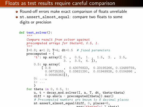
Floats as test results require careful comparison

Round-off errors make exact comparison of floats unreliablent.assert_almost_equal: compare two floats to somedigits or precision

def test_solver():"""Compare result from solver againstprecomputed arrays for theta=0, 0.5, 1."""I=0.8; a=1.2; T=4; dt=0.5 # fixed parametersprecomputed = {

’t’: np.array([ 0. , 0.5, 1. , 1.5, 2. , 2.5,3. , 3.5, 4. ]),

0.5: np.array([ 0.8 , 0.43076923, 0.23195266, 0.12489759,

0.06725255, 0.03621291, 0.01949926, 0.0104996 ,0.00565363]),

0: ...,1: ...}

for theta in 0, 0.5, 1:u, t = decay_mod.solver(I, a, T, dt, theta=theta)diff = np.abs(u - precomputed[theta]).max()# Precomputed numbers are known to 8 decimal placesnt.assert_almost_equal(diff, 0, places=8,

msg=’theta=%s’ % theta)

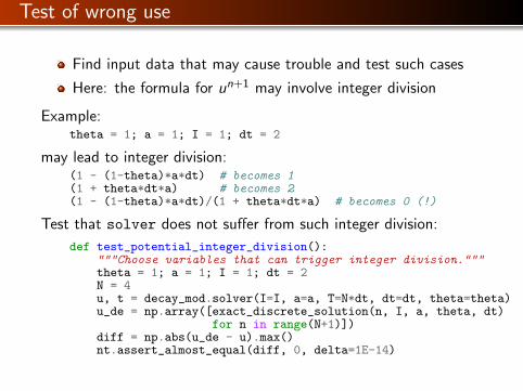
Test of wrong use

Find input data that may cause trouble and test such cases

Here: the formula for un+1 may involve integer division

Example:theta = 1; a = 1; I = 1; dt = 2

may lead to integer division:(1 - (1-theta)*a*dt) # becomes 1(1 + theta*dt*a) # becomes 2(1 - (1-theta)*a*dt)/(1 + theta*dt*a) # becomes 0 (!)

Test that solver does not suffer from such integer division:

def test_potential_integer_division():"""Choose variables that can trigger integer division."""theta = 1; a = 1; I = 1; dt = 2N = 4u, t = decay_mod.solver(I=I, a=a, T=N*dt, dt=dt, theta=theta)u_de = np.array([exact_discrete_solution(n, I, a, theta, dt)

for n in range(N+1)])diff = np.abs(u_de - u).max()nt.assert_almost_equal(diff, 0, delta=1E-14)

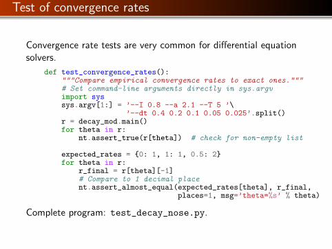
Test of convergence rates

Convergence rate tests are very common for differential equationsolvers.

def test_convergence_rates():"""Compare empirical convergence rates to exact ones."""# Set command-line arguments directly in sys.argvimport syssys.argv[1:] = ’--I 0.8 --a 2.1 --T 5 ’\

’--dt 0.4 0.2 0.1 0.05 0.025’.split()r = decay_mod.main()for theta in r:

nt.assert_true(r[theta]) # check for non-empty list

expected_rates = {0: 1, 1: 1, 0.5: 2}for theta in r:

r_final = r[theta][-1]# Compare to 1 decimal placent.assert_almost_equal(expected_rates[theta], r_final,

places=1, msg=’theta=%s’ % theta)

Complete program: test_decay_nose.py.

http://tinyurl.com/jvzzcfn/decay/tests/test_decay_nose.py

Classical unit testing with unittest

unittest is a Python module mimicing the classical JUnitclass-based unit testing framework from Java

This is how unit testing is normally done

Requires knowledge of object-oriented programming

Remark.

You will probably not use it, but you’re not educated unless youknow what unit testing with classes is.

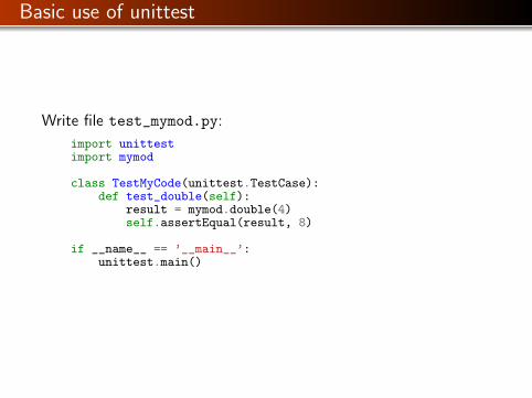
Basic use of unittest

Write file test_mymod.py:

import unittestimport mymod

class TestMyCode(unittest.TestCase):def test_double(self):

result = mymod.double(4)self.assertEqual(result, 8)

if __name__ == ’__main__’:unittest.main()

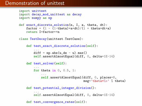
Demonstration of unittestimport unittestimport decay_mod_unittest as decayimport numpy as np

def exact_discrete_solution(n, I, a, theta, dt):factor = (1 - (1-theta)*a*dt)/(1 + theta*dt*a)return I*factor**n

class TestDecay(unittest.TestCase):

def test_exact_discrete_solution(self):...diff = np.abs(u_de - u).max()self.assertAlmostEqual(diff, 0, delta=1E-14)

def test_solver(self):...for theta in 0, 0.5, 1:

...self.assertAlmostEqual(diff, 0, places=8,

msg=’theta=%s’ % theta)

def test_potential_integer_division():...self.assertAlmostEqual(diff, 0, delta=1E-14)

def test_convergence_rates(self):...for theta in r:

...self.assertAlmostEqual(...)

if __name__ == ’__main__’:unittest.main()

Complete program: test_decay_unittest.py.

http://tinyurl.com/jvzzcfn/decay/tests/test_decay_nose.py

Implementing simple problem and solver classes

So far: programs are built of Python functions

New focus: alternative implementations using classes

Class-based implementations are very popular, especially inbusiness/adm applications

Class-based implementations scales better to large andcomplex scientific applications

What to learn

Tasks:

Explain basic use of classes to build a differential equationsolver

Introduce concepts that make such programs easily scale tomore complex applications

Demonstrate the advantage of using classes

Ideas:

Classes for Problem, Solver, and Visualizer

Problem: all the physics information about the problem

Solver: all the numerics information + numericalcomputations

Visualizer: plot the solution and other quantities

The problem class

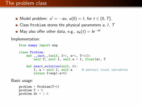
Model problem: u′ = −au, u(0) = I , for t ∈ (0,T ].

Class Problem stores the physical parameters a, I , T

May also offer other data, e.g., ue(t) = Ie−at

Implementation:

from numpy import exp

class Problem:def __init__(self, I=1, a=1, T=10):

self.T, self.I, self.a = I, float(a), T

def exact_solution(self, t):I, a = self.I, self.a # extract local variablesreturn I*exp(-a*t)

Basic usage:

problem = Problem(T=5)problem.T = 8problem.dt = 1.5

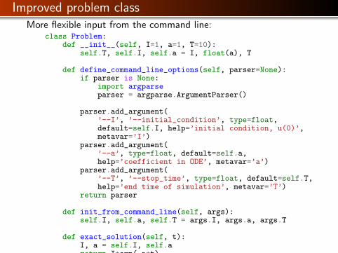
Improved problem classMore flexible input from the command line:

class Problem:def __init__(self, I=1, a=1, T=10):

self.T, self.I, self.a = I, float(a), T

def define_command_line_options(self, parser=None):if parser is None:

import argparseparser = argparse.ArgumentParser()

parser.add_argument(’--I’, ’--initial_condition’, type=float,default=self.I, help=’initial condition, u(0)’,metavar=’I’)

parser.add_argument(’--a’, type=float, default=self.a,help=’coefficient in ODE’, metavar=’a’)

parser.add_argument(’--T’, ’--stop_time’, type=float, default=self.T,help=’end time of simulation’, metavar=’T’)

return parser

def init_from_command_line(self, args):self.I, self.a, self.T = args.I, args.a, args.T

def exact_solution(self, t):I, a = self.I, self.areturn I*exp(-a*t)

Can utilize user’s ArgumentParser, or make oneNone is used to indicate a non-initialized variable

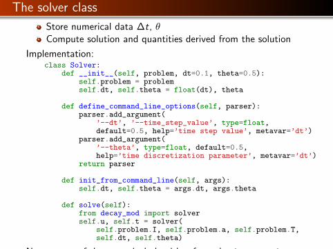
The solver class

Store numerical data ∆t, θCompute solution and quantities derived from the solution

Implementation:class Solver:

def __init__(self, problem, dt=0.1, theta=0.5):self.problem = problemself.dt, self.theta = float(dt), theta

def define_command_line_options(self, parser):parser.add_argument(

’--dt’, ’--time_step_value’, type=float,default=0.5, help=’time step value’, metavar=’dt’)

parser.add_argument(’--theta’, type=float, default=0.5,help=’time discretization parameter’, metavar=’dt’)

return parser

def init_from_command_line(self, args):self.dt, self.theta = args.dt, args.theta

def solve(self):from decay_mod import solverself.u, self.t = solver(

self.problem.I, self.problem.a, self.problem.T,self.dt, self.theta)

Note: reuse of the numerical algorithm from the decay_mod

module (i.e., the class is a wrapper of the proceduralimplementation).

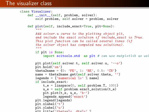
The visualizer classclass Visualizer:

def __init__(self, problem, solver):self.problem, self.solver = problem, solver

def plot(self, include_exact=True, plt=None):"""Add solver.u curve to the plotting object plt,and include the exact solution if include_exact is True.This plot function can be called several times (ifthe solver object has computed new solutions)."""if plt is None:

import scitools.std as plt # can use matplotlib as well

plt.plot(self.solver.t, self.solver.u, ’--o’)plt.hold(’on’)theta2name = {0: ’FE’, 1: ’BE’, 0.5: ’CN’}name = theta2name.get(self.solver.theta, ’’)legends = [’numerical %s’ % name]if include_exact:

t_e = linspace(0, self.problem.T, 1001)u_e = self.problem.exact_solution(t_e)plt.plot(t_e, u_e, ’b-’)legends.append(’exact’)

plt.legend(legends)plt.xlabel(’t’)plt.ylabel(’u’)plt.title(’theta=%g, dt=%g’ %

(self.solver.theta, self.solver.dt))plt.savefig(’%s_%g.png’ % (name, self.solver.dt))return plt

Remark: The plt object in plot adds a new curve to a plot,which enables comparing different solutions from different runs ofSolver.solve

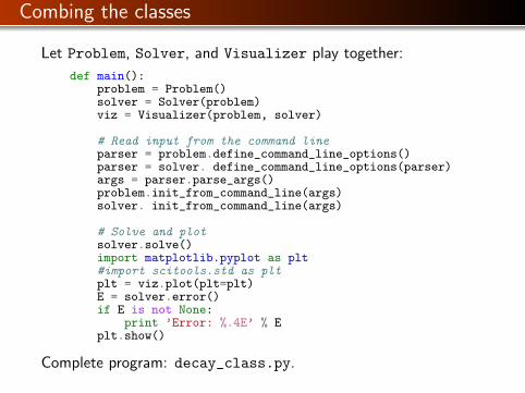
Combing the classes

Let Problem, Solver, and Visualizer play together:

def main():problem = Problem()solver = Solver(problem)viz = Visualizer(problem, solver)

# Read input from the command lineparser = problem.define_command_line_options()parser = solver. define_command_line_options(parser)args = parser.parse_args()problem.init_from_command_line(args)solver. init_from_command_line(args)

# Solve and plotsolver.solve()import matplotlib.pyplot as plt#import scitools.std as pltplt = viz.plot(plt=plt)E = solver.error()if E is not None:

print ’Error: %.4E’ % Eplt.show()

Complete program: decay_class.py.

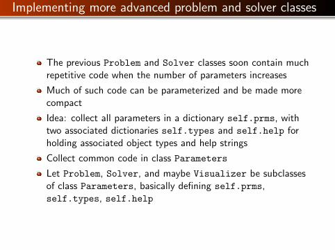
http://tinyurl.com/jvzzcfn/decay/decay_class.py

Implementing more advanced problem and solver classes

The previous Problem and Solver classes soon contain muchrepetitive code when the number of parameters increases

Much of such code can be parameterized and be made morecompact

Idea: collect all parameters in a dictionary self.prms, withtwo associated dictionaries self.types and self.help forholding associated object types and help strings

Collect common code in class Parameters

Let Problem, Solver, and maybe Visualizer be subclassesof class Parameters, basically defining self.prms,self.types, self.help

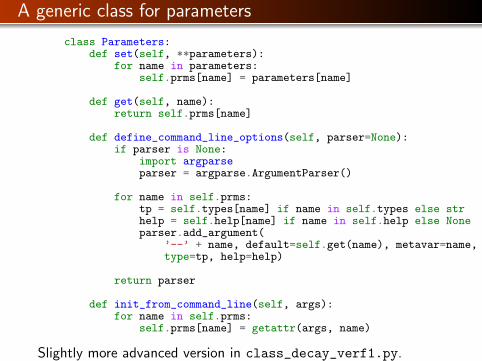
A generic class for parameters

class Parameters:def set(self, **parameters):

for name in parameters:self.prms[name] = parameters[name]

def get(self, name):return self.prms[name]

def define_command_line_options(self, parser=None):if parser is None:

import argparseparser = argparse.ArgumentParser()

for name in self.prms:tp = self.types[name] if name in self.types else strhelp = self.help[name] if name in self.help else Noneparser.add_argument(

’--’ + name, default=self.get(name), metavar=name,type=tp, help=help)

return parser

def init_from_command_line(self, args):for name in self.prms:

self.prms[name] = getattr(args, name)

Slightly more advanced version in class_decay_verf1.py.

http://tinyurl.com/jvzzcfn/decay/class_decay_verf1.py

The problem class

class Problem(Parameters):"""Physical parameters for the problem u’=-a*u, u(0)=I,with t in [0,T]."""def __init__(self):

self.prms = dict(I=1, a=1, T=10)self.types = dict(I=float, a=float, T=float)self.help = dict(I=’initial condition, u(0)’,

a=’coefficient in ODE’,T=’end time of simulation’)

def exact_solution(self, t):I, a = self.get(’I’), self.get(’a’)return I*np.exp(-a*t)

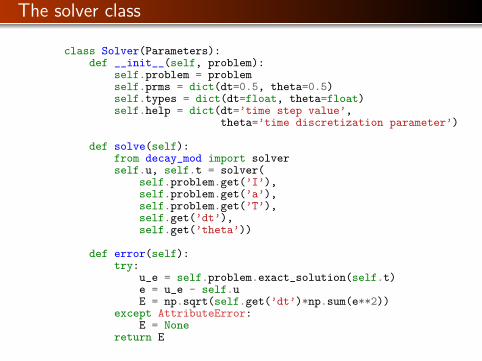
The solver class

class Solver(Parameters):def __init__(self, problem):

self.problem = problemself.prms = dict(dt=0.5, theta=0.5)self.types = dict(dt=float, theta=float)self.help = dict(dt=’time step value’,

theta=’time discretization parameter’)

def solve(self):from decay_mod import solverself.u, self.t = solver(

self.problem.get(’I’),self.problem.get(’a’),self.problem.get(’T’),self.get(’dt’),self.get(’theta’))

def error(self):try:

u_e = self.problem.exact_solution(self.t)e = u_e - self.uE = np.sqrt(self.get(’dt’)*np.sum(e**2))

except AttributeError:E = None

return E

The visualizer class

No parameters needed (for this simple problem), no need toinherit class Parameters

Same code as previously shown class Visualizer

Same code as previously shown for combining Problem,Solver, and Visualizer

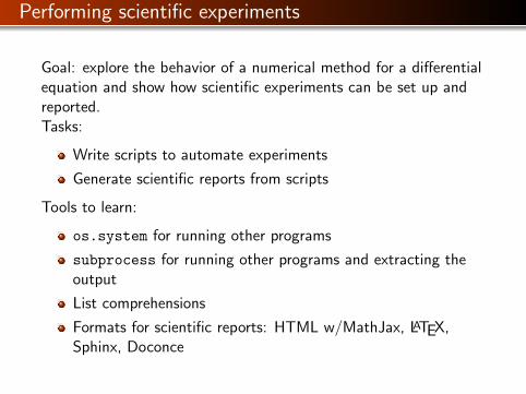
Performing scientific experiments

Goal: explore the behavior of a numerical method for a differentialequation and show how scientific experiments can be set up andreported.Tasks:

Write scripts to automate experiments

Generate scientific reports from scripts

Tools to learn:

os.system for running other programs

subprocess for running other programs and extracting theoutput

List comprehensions

Formats for scientific reports: HTML w/MathJax, LATEX,Sphinx, Doconce

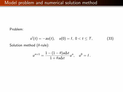
Model problem and numerical solution method

Problem:

u′(t) = −au(t), u(0) = I , 0 < t ≤ T , (33)

Solution method (θ-rule):

un+1 =1− (1− θ)a∆t

1 + θa∆tun, u0 = I .

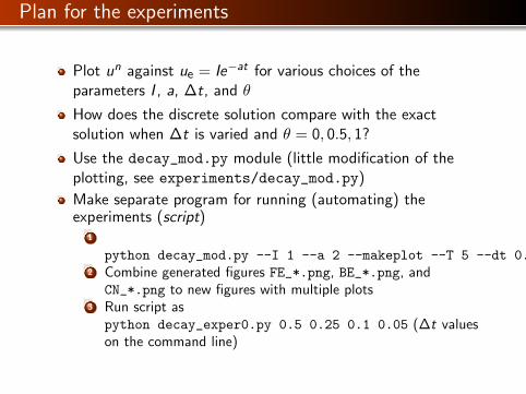
Plan for the experiments

Plot un against ue = Ie−at for various choices of theparameters I , a, ∆t, and θ

How does the discrete solution compare with the exactsolution when ∆t is varied and θ = 0, 0.5, 1?

Use the decay_mod.py module (little modification of theplotting, see experiments/decay_mod.py)

Make separate program for running (automating) theexperiments (script)

1

python decay_mod.py --I 1 --a 2 --makeplot --T 5 --dt 0.5 0.25 0.1 0.052 Combine generated figures FE_*.png, BE_*.png, and

CN_*.png to new figures with multiple plots3 Run script as

python decay_exper0.py 0.5 0.25 0.1 0.05 (∆t valueson the command line)

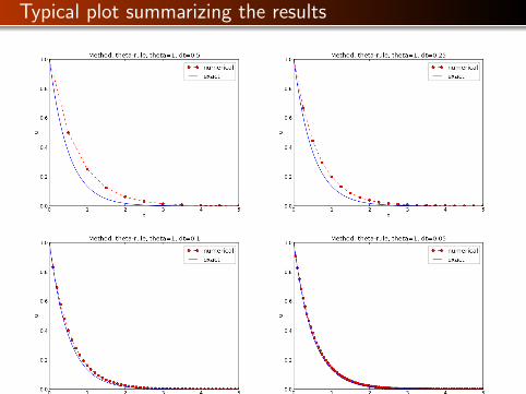
http://tinyurl.com/jvzzcfn/decay/decay_mod.py

http://tinyurl.com/jvzzcfn/decay/experiments/decay_mod.py

Typical plot summarizing the results

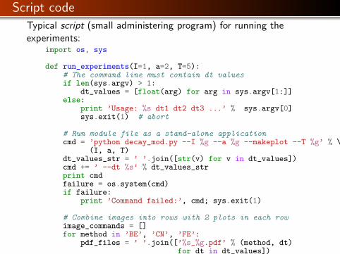
Script codeTypical script (small administering program) for running theexperiments:

import os, sys

def run_experiments(I=1, a=2, T=5):# The command line must contain dt valuesif len(sys.argv) > 1:

dt_values = [float(arg) for arg in sys.argv[1:]]else:

print ’Usage: %s dt1 dt2 dt3 ...’ % sys.argv[0]sys.exit(1) # abort

# Run module file as a stand-alone applicationcmd = ’python decay_mod.py --I %g --a %g --makeplot --T %g’ % \

(I, a, T)dt_values_str = ’ ’.join([str(v) for v in dt_values])cmd += ’ --dt %s’ % dt_values_strprint cmdfailure = os.system(cmd)if failure:

print ’Command failed:’, cmd; sys.exit(1)

# Combine images into rows with 2 plots in each rowimage_commands = []for method in ’BE’, ’CN’, ’FE’:

pdf_files = ’ ’.join([’%s_%g.pdf’ % (method, dt)for dt in dt_values])

png_files = ’ ’.join([’%s_%g.png’ % (method, dt)for dt in dt_values])

image_commands.append(’montage -background white -geometry 100%’ +’ -tile 2x %s %s.png’ % (png_files, method))

image_commands.append(’convert -trim %s.png %s.png’ % (method, method))

image_commands.append(’convert %s.png -transparent white %s.png’ %(method, method))

image_commands.append(’pdftk %s output tmp.pdf’ % pdf_files)

num_rows = int(round(len(dt_values)/2.0))image_commands.append(

’pdfnup --nup 2x%d tmp.pdf’ % num_rows)image_commands.append(

’pdfcrop tmp-nup.pdf %s.pdf’ % method)

for cmd in image_commands:print cmdfailure = os.system(cmd)if failure:


# Remove the files generated above and by decay_mod.pyfrom glob import globfilenames = glob(’*_*.png’) + glob(’*_*.pdf’) + \

glob(’*_*.eps’) + glob(’tmp*.pdf’)for filename in filenames:

os.remove(filename)

if __name__ == ’__main__’:run_experiments()

Complete program: experiments/decay_exper0.py.

http://tinyurl.com/jvzzcfn/decay/experiments/decay_exper0.py

Comments to the code

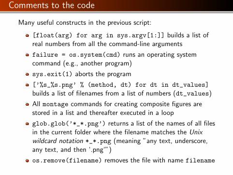
Many useful constructs in the previous script:

[float(arg) for arg in sys.argv[1:]] builds a list ofreal numbers from all the command-line arguments

failure = os.system(cmd) runs an operating systemcommand (e.g., another program)

sys.exit(1) aborts the program

[’%s_%s.png’ % (method, dt) for dt in dt_values]

builds a list of filenames from a list of numbers (dt_values)

All montage commands for creating composite figures arestored in a list and thereafter executed in a loop

glob.glob(’*_*.png’) returns a list of the names of all filesin the current folder where the filename matches the Unixwildcard notation *_*.png (meaning ”any text, underscore,any text, and then ‘.png‘”)

os.remove(filename) removes the file with name filename

Interpreting output from other programs

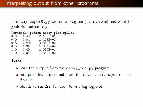
In decay_exper0.py we run a program (os.system) and want tograb the output, e.g.,

Terminal> python decay_plot_mpl.py0.0 0.40: 2.105E-010.0 0.04: 1.449E-020.5 0.40: 3.362E-020.5 0.04: 1.887E-041.0 0.40: 1.030E-011.0 0.04: 1.382E-02

Tasks:

read the output from the decay_mod.py program

interpret this output and store the E values in arrays for eachθ value

plot E versus ∆t, for each θ, in a log-log plot

Code for grabbing output from another program

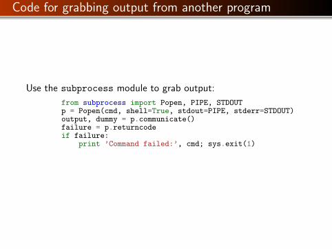
Use the subprocess module to grab output:

from subprocess import Popen, PIPE, STDOUTp = Popen(cmd, shell=True, stdout=PIPE, stderr=STDOUT)output, dummy = p.communicate()failure = p.returncodeif failure:


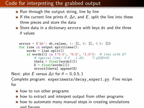
Code for interpreting the grabbed output

Run through the output string, line by lineIf the current line prints θ, ∆t, and E , split the line into thesethree pieces and store the dataStore data in a dictionary errors with keys dt and the threeθ values

errors = {’dt’: dt_values, 1: [], 0: [], 0.5: []}for line in output.splitlines():

words = line.split()if words[0] in (’0.0’, ’0.5’, ’1.0’): # line with E?

# typical line: 0.0 1.25: 7.463E+00theta = float(words[0])E = float(words[2])errors[theta].append(E)

Next: plot E versus ∆t for θ = 0, 0.5, 1Complete program: experiments/decay_exper1.py. Fine recipefor

how to run other programshow to extract and interpret output from other programshow to automate many manual steps in creating simulationsand figures

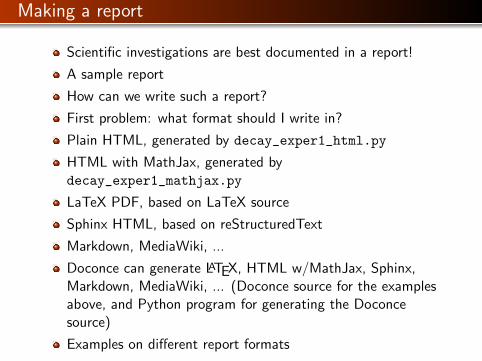
http://tinyurl.com/jvzzcfn/decay/experiments/decay_exper1.py

Making a report

Scientific investigations are best documented in a report!

A sample report

How can we write such a report?

First problem: what format should I write in?

Plain HTML, generated by decay_exper1_html.py

HTML with MathJax, generated bydecay_exper1_mathjax.py

LaTeX PDF, based on LaTeX source

Sphinx HTML, based on reStructuredText

Markdown, MediaWiki, ...

Doconce can generate LATEX, HTML w/MathJax, Sphinx,Markdown, MediaWiki, ... (Doconce source for the examplesabove, and Python program for generating the Doconcesource)

Examples on different report formats

http://hplgit.github.com/INF5620/doc/writing_reports/sphinx-cloud/

http://hplgit.github.com/INF5620/doc/writing_reports/report_html.html

http://tinyurl.com/jvzzcfn/decay/experiments/decay_exper1_html.py

http://hplgit.github.com/INF5620/doc/writing_reports/report_html_mathjax.html

http://tinyurl.com/jvzzcfn/decay/experiments/decay_exper1_html.py

http://hplgit.github.com/INF5620/doc/writing_reports/report.pdf

http://hplgit.github.com/INF5620/doc/writing_reports/report.tex.html

http://hplgit.github.com/INF5620/doc/writing_reports/sphinx-cloud/index.html

http://hplgit.github.com/INF5620/doc/writing_reports/report_sphinx.rst.html

https://github.com/hplgit/doconce

http://hplgit.github.com/INF5620/doc/writing_reports/report.do.txt.html

http://tinyurl.com/jvzzcfn/decay/experiments/decay_exper1_do.py

http://tinyurl.com/jvzzcfn/decay/experiments/decay_exper1_do.py

http://hplgit.github.com/INF5620/doc/writing_reports/

Publishing a complete project

Make folder (directory) tree

Keep track of all files via a version control system (Mercurial,Git, ...)

Publish as private or public repository

Utilize Bitbucket, Googlecode, GitHub, or similar

See the intro to such tools

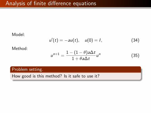
http://hplgit.github.com/teamods/bitgit/html/

Analysis of finite difference equations

Model:u′(t) = −au(t), u(0) = I , (34)

Method:

un+1 =1− (1− θ)a∆t

1 + θa∆tun (35)

Problem setting.

How good is this method? Is it safe to use it?

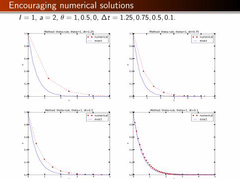
Encouraging numerical solutionsI = 1, a = 2, θ = 1, 0.5, 0, ∆t = 1.25, 0.75, 0.5, 0.1.

0 1 2 3 4 5t

0.0

0.2

0.4

0.6

0.8

1.0

u

Method: theta-rule, theta=1, dt=1.25

numericalexact

0 1 2 3 4 5 6t

0.0

0.2

0.4

0.6

0.8

1.0

u


numericalexact

0 1 2 3 4 5t

0.0

0.2

0.4

0.6

0.8

1.0

u


numericalexact

0 1 2 3 4 5t

0.0

0.2

0.4

0.6

0.8

1.0

u


numericalexact

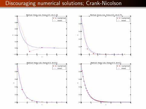
Discouraging numerical solutions; Crank-Nicolson

0 1 2 3 4 5t

0.2

0.0

0.2

0.4

0.6

0.8

1.0

u

Method: theta-rule, theta=0.5, dt=1.25

numericalexact

0 1 2 3 4 5 6t

0.0

0.2

0.4

0.6

0.8

1.0

u


numericalexact

0 1 2 3 4 5t

0.0

0.2

0.4

0.6

0.8

1.0

u


numericalexact

0 1 2 3 4 5t

0.0

0.2

0.4

0.6

0.8

1.0

u


numericalexact

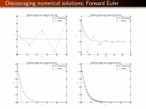
Discouraging numerical solutions; Forward Euler

0 1 2 3 4 5t

4

2

0

2

4

6u


numericalexact

0 1 2 3 4 5 6t

0.5

0.0

0.5

1.0

u


numericalexact

0 1 2 3 4 5t

0.0

0.2

0.4

0.6

0.8

1.0

u


numericalexact

0 1 2 3 4 5t

0.0

0.2

0.4

0.6

0.8

1.0

u


numericalexact

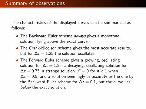
Summary of observations

The characteristics of the displayed curves can be summarized asfollows:

The Backward Euler scheme always gives a monotonesolution, lying above the exact curve.

The Crank-Nicolson scheme gives the most accurate results,but for ∆t = 1.25 the solution oscillates.

The Forward Euler scheme gives a growing, oscillatingsolution for ∆t = 1.25; a decaying, oscillating solution for∆t = 0.75; a strange solution un = 0 for n ≥ 1 when∆t = 0.5; and a solution seemingly as accurate as the one bythe Backward Euler scheme for ∆t = 0.1, but the curve liesbelow the exact solution.

Problem setting

Goal.

We ask the question

Under what circumstances, i.e., values of the input data I , a,and ∆t will the Forward Euler and Crank-Nicolson schemesresult in undesired oscillatory solutions?

Techniques of investigation:

Numerical experiments

Mathematical analysis

Another question to be raised is

How does ∆t impact the error in the numerical solution?

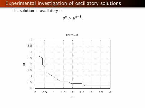
Experimental investigation of oscillatory solutionsThe solution is oscillatory if

un > un−1,

Seems that a∆t < 1 for FE and 2 for CN.

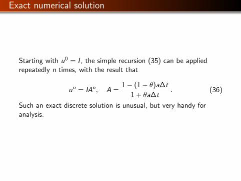
Exact numerical solution

Starting with u0 = I , the simple recursion (35) can be appliedrepeatedly n times, with the result that

un = IAn, A =1− (1− θ)a∆t

1 + θa∆t. (36)

Such an exact discrete solution is unusual, but very handy foranalysis.

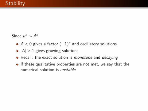
Stability

Since un ∼ An,

A < 0 gives a factor (−1)n and oscillatory solutions

|A| > 1 gives growing solutions

Recall: the exact solution is monotone and decaying

If these qualitative properties are not met, we say that thenumerical solution is unstable

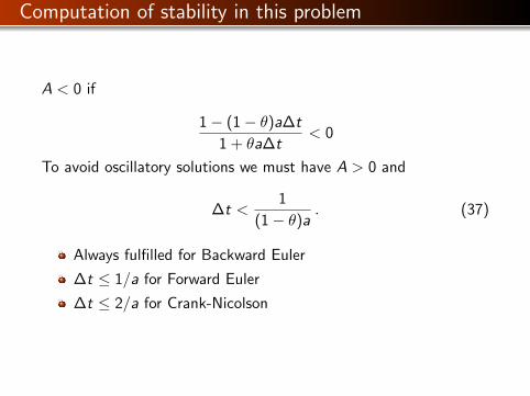
Computation of stability in this problem

A < 0 if

1− (1− θ)a∆t

1 + θa∆t< 0

To avoid oscillatory solutions we must have A > 0 and

∆t <1

(1− θ)a. (37)

Always fulfilled for Backward Euler

∆t ≤ 1/a for Forward Euler

∆t ≤ 2/a for Crank-Nicolson

Computation of stability in this problem

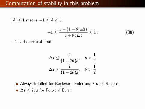
|A| ≤ 1 means −1 ≤ A ≤ 1

−1 ≤ 1− (1− θ)a∆t

1 + θa∆t≤ 1 . (38)

−1 is the critical limit:

∆t ≤ 2

(1− 2θ)a, θ <

1

2

∆t ≥ 2

(1− 2θ)a, θ >

1

2

Always fulfilled for Backward Euler and Crank-Nicolson

∆t ≤ 2/a for Forward Euler

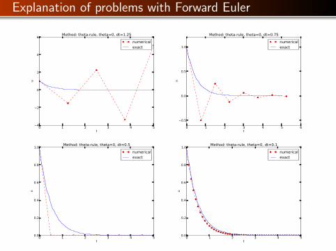
Explanation of problems with Forward Euler

0 1 2 3 4 5t

4

2

0

2

4

6u


numericalexact

0 1 2 3 4 5 6t

0.5

0.0

0.5

1.0

u


numericalexact

0 1 2 3 4 5t

0.0

0.2

0.4

0.6

0.8

1.0

u


numericalexact

0 1 2 3 4 5t

0.0

0.2

0.4

0.6

0.8

1.0

u


numericalexact

a∆t = 2 · 1.25 = 2.5 and A = −1.5: oscillations and growtha∆t = 2 · 0.75 = 1.5 and A = −0.5: oscillations and decay∆t = 0.5 and A = 0: un = 0 for n > 0Smaller Deltat: qualitatively correct solution

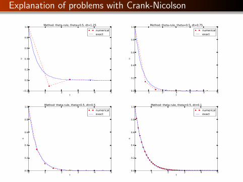
Explanation of problems with Crank-Nicolson

0 1 2 3 4 5t

0.2

0.0

0.2

0.4

0.6

0.8

1.0

u


numericalexact

0 1 2 3 4 5 6t

0.0

0.2

0.4

0.6

0.8

1.0

u


numericalexact

0 1 2 3 4 5t

0.0

0.2

0.4

0.6

0.8

1.0

u


numericalexact

0 1 2 3 4 5t

0.0

0.2

0.4

0.6

0.8

1.0

u


numericalexact

∆t = 1.25 and A = −0.25: oscillatory solutionNever any growing solution

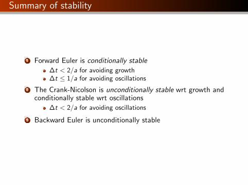
Summary of stability

1 Forward Euler is conditionally stable

∆t < 2/a for avoiding growth∆t ≤ 1/a for avoiding oscillations

2 The Crank-Nicolson is unconditionally stable wrt growth andconditionally stable wrt oscillations

∆t < 2/a for avoiding oscillations

3 Backward Euler is unconditionally stable

Comparing amplification factors

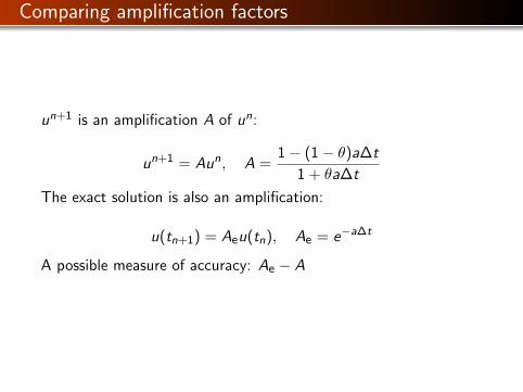
un+1 is an amplification A of un:

un+1 = Aun, A =1− (1− θ)a∆t

1 + θa∆t

The exact solution is also an amplification:

u(tn+1) = Aeu(tn), Ae = e−a∆t

A possible measure of accuracy: Ae − A

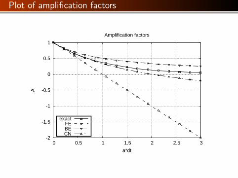
Plot of amplification factors

-2

-1.5

-1

-0.5

0

0.5

1

0 0.5 1 1.5 2 2.5 3

A

a*dt

Amplification factors

exactFEBECN

Series expansion of amplification factors

To investigate Ae − A mathematically, we can Taylor expand theexpression, using p = a∆t as variable.

>>> from sympy import *>>> # Create p as a mathematical symbol with name ’p’>>> p = Symbol(’p’)>>> # Create a mathematical expression with p>>> A_e = exp(-p)>>>>>> # Find the first 6 terms of the Taylor series of A_e>>> A_e.series(p, 0, 6)1 + (1/2)*p**2 - p - 1/6*p**3 - 1/120*p**5 + (1/24)*p**4 + O(p**6)

>>> theta = Symbol(’theta’)>>> A = (1-(1-theta)*p)/(1+theta*p)>>> FE = A_e.series(p, 0, 4) - A.subs(theta, 0).series(p, 0, 4)>>> BE = A_e.series(p, 0, 4) - A.subs(theta, 1).series(p, 0, 4)>>> half = Rational(1,2) # exact fraction 1/2>>> CN = A_e.series(p, 0, 4) - A.subs(theta, half).series(p, 0, 4)>>> FE(1/2)*p**2 - 1/6*p**3 + O(p**4)>>> BE-1/2*p**2 + (5/6)*p**3 + O(p**4)>>> CN(1/12)*p**3 + O(p**4)

Error in amplification factors

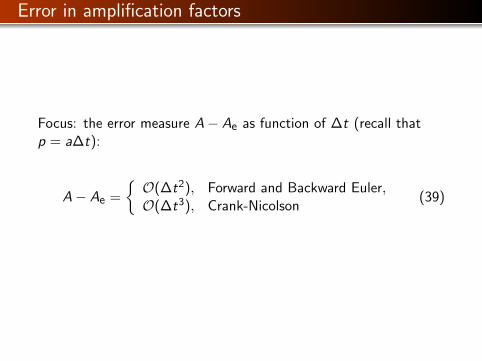
Focus: the error measure A− Ae as function of ∆t (recall thatp = a∆t):

A− Ae =

{O(∆t2), Forward and Backward Euler,O(∆t3), Crank-Nicolson

(39)

The fraction of numerical and exact amplification factors

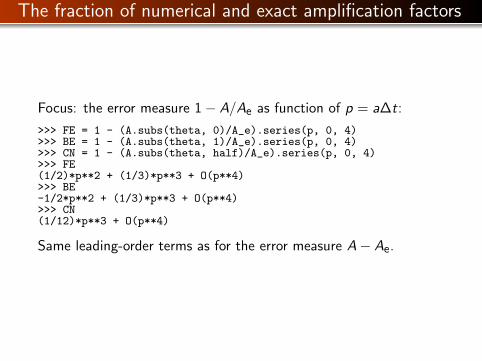
Focus: the error measure 1− A/Ae as function of p = a∆t:

>>> FE = 1 - (A.subs(theta, 0)/A_e).series(p, 0, 4)>>> BE = 1 - (A.subs(theta, 1)/A_e).series(p, 0, 4)>>> CN = 1 - (A.subs(theta, half)/A_e).series(p, 0, 4)>>> FE(1/2)*p**2 + (1/3)*p**3 + O(p**4)>>> BE-1/2*p**2 + (1/3)*p**3 + O(p**4)>>> CN(1/12)*p**3 + O(p**4)

Same leading-order terms as for the error measure A− Ae.

The true/global error at a point

The error in A reflects the local error when going from onetime step to the next

What is the global (true) error at tn?en = ue(tn)− un = Ie−atn − IAn

Taylor series expansions of en simplify the expression

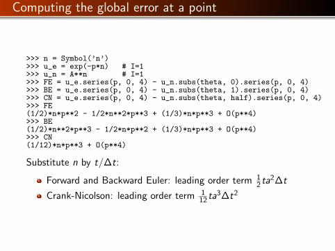
Computing the global error at a point

>>> n = Symbol(’n’)>>> u_e = exp(-p*n) # I=1>>> u_n = A**n # I=1>>> FE = u_e.series(p, 0, 4) - u_n.subs(theta, 0).series(p, 0, 4)>>> BE = u_e.series(p, 0, 4) - u_n.subs(theta, 1).series(p, 0, 4)>>> CN = u_e.series(p, 0, 4) - u_n.subs(theta, half).series(p, 0, 4)>>> FE(1/2)*n*p**2 - 1/2*n**2*p**3 + (1/3)*n*p**3 + O(p**4)>>> BE(1/2)*n**2*p**3 - 1/2*n*p**2 + (1/3)*n*p**3 + O(p**4)>>> CN(1/12)*n*p**3 + O(p**4)

Substitute n by t/∆t:

Forward and Backward Euler: leading order term 12 ta2∆t

Crank-Nicolson: leading order term 112 ta3∆t2

Convergence

The numerical scheme is convergent if the global error en → 0 as∆t → 0. If the error has a leading order term ∆tr , theconvergence rate is of order r .

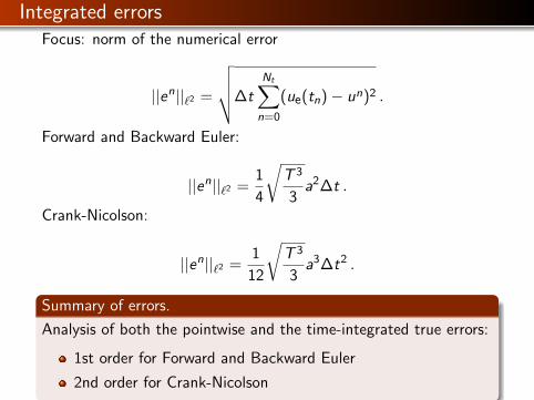
Integrated errorsFocus: norm of the numerical error

||en||`2 =

√√√√∆tNt∑n=0

(ue(tn)− un)2 .

Forward and Backward Euler:

||en||`2 =1

4

√T 3

3a2∆t .

Crank-Nicolson:

||en||`2 =1

12

√T 3

3a3∆t2 .

Summary of errors.

Analysis of both the pointwise and the time-integrated true errors:

1st order for Forward and Backward Euler

2nd order for Crank-Nicolson

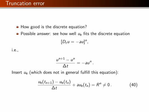
Truncation error

How good is the discrete equation?

Possible answer: see how well ue fits the discrete equation

[Dtu = −au]n,

i.e.,

un+1 − un

∆t= −aun .

Insert ue (which does not in general fulfill this equation):

ue(tn+1)− ue(tn)

∆t+ aue(tn) = Rn 6= 0 . (40)

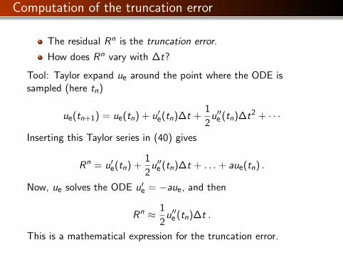
Computation of the truncation error

The residual Rn is the truncation error.

How does Rn vary with ∆t?

Tool: Taylor expand ue around the point where the ODE issampled (here tn)

ue(tn+1) = ue(tn) + u′e(tn)∆t +1

2u′′e (tn)∆t2 + · · ·

Inserting this Taylor series in (40) gives

Rn = u′e(tn) +1

2u′′e (tn)∆t + . . .+ aue(tn) .

Now, ue solves the ODE u′e = −aue, and then

Rn ≈ 1

2u′′e (tn)∆t .

This is a mathematical expression for the truncation error.

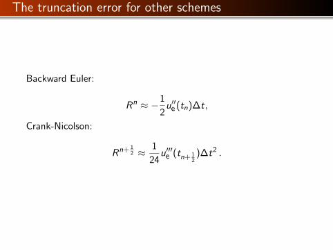
The truncation error for other schemes

Backward Euler:

Rn ≈ −1

2u′′e (tn)∆t,

Crank-Nicolson:

Rn+ 12 ≈ 1

24u′′′e (tn+ 1

2)∆t2 .

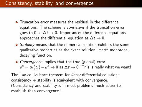
Consistency, stability, and convergence

Truncation error measures the residual in the differenceequations. The scheme is consistent if the truncation errorgoes to 0 as ∆t → 0. Importance: the difference equationsapproaches the differential equation as ∆t → 0.

Stability means that the numerical solution exhibits the samequalitative properties as the exact solution. Here: monotone,decaying function.

Convergence implies that the true (global) erroren = ue(tn)−un → 0 as ∆t → 0. This is really what we want!

The Lax equivalence theorem for linear differential equations:consistency + stability is equivalent with convergence.(Consistency and stability is in most problems much easier toestablish than convergence.)

Model extensions

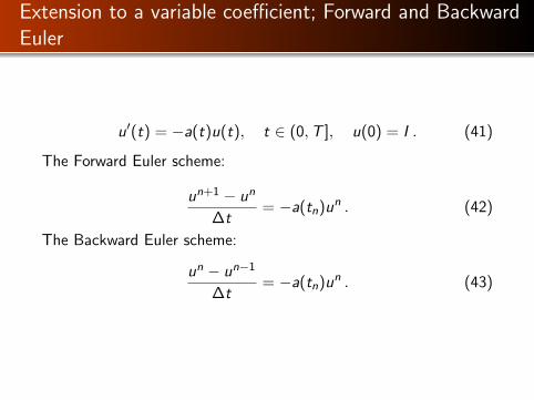
Extension to a variable coefficient; Forward and BackwardEuler

u′(t) = −a(t)u(t), t ∈ (0,T ], u(0) = I . (41)

The Forward Euler scheme:

un+1 − un

∆t= −a(tn)un . (42)

The Backward Euler scheme:

un − un−1

∆t= −a(tn)un . (43)

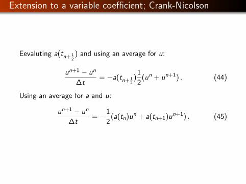
Extension to a variable coefficient; Crank-Nicolson

Eevaluting a(tn+ 12) and using an average for u:

un+1 − un

∆t= −a(tn+ 1

2)

1

2(un + un+1) . (44)

Using an average for a and u:

un+1 − un

∆t= −1

2(a(tn)un + a(tn+1)un+1) . (45)

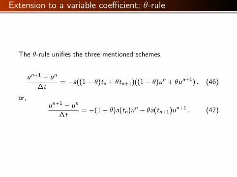
Extension to a variable coefficient; θ-rule

The θ-rule unifies the three mentioned schemes,

un+1 − un

∆t= −a((1− θ)tn + θtn+1)((1− θ)un + θun+1) . (46)

or,un+1 − un

∆t= −(1− θ)a(tn)un − θa(tn+1)un+1 . (47)

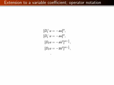
Extension to a variable coefficient; operator notation

[D+t u = −au]n,

[D−t u = −au]n,

[Dtu = −aut ]n+ 12 ,

[Dtu = −aut ]n+ 12 ,

.

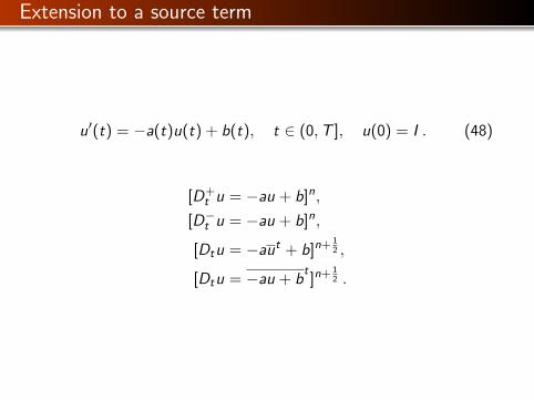
Extension to a source term

u′(t) = −a(t)u(t) + b(t), t ∈ (0,T ], u(0) = I . (48)

[D+t u = −au + b]n,

[D−t u = −au + b]n,

[Dtu = −aut + b]n+ 12 ,

[Dtu = −au + bt]n+ 1

2 .

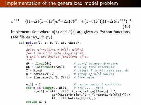
Implementation of the generalized model problem

un+1 = ((1−∆t(1−θ)an)un+∆t(θbn+1+(1−θ)bn))(1+∆tθan+1)−1 .(49)

Implementation where a(t) and b(t) are given as Python functions(see file decay_vc.py):

def solver(I, a, b, T, dt, theta):"""Solve u’=-a(t)*u + b(t), u(0)=I,for t in (0,T] with steps of dt.a and b are Python functions of t."""dt = float(dt) # avoid integer divisionNt = int(round(T/dt)) # no of time intervalsT = Nt*dt # adjust T to fit time step dtu = zeros(Nt+1) # array of u[n] valuest = linspace(0, T, Nt+1) # time mesh


u[n+1] = ((1 - dt*(1-theta)*a(t[n]))*u[n] + \dt*(theta*b(t[n+1]) + (1-theta)*b(t[n])))/\(1 + dt*theta*a(t[n+1]))

return u, t

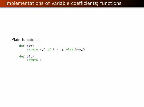
https://github.com/hplgit/INF5620/blob/gh-pages/src/decay/decay_vc.py

Implementations of variable coefficients; functions

Plain functions:

def a(t):return a_0 if t < tp else k*a_0

def b(t):return 1

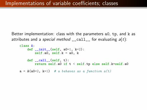
Implementations of variable coefficients; classes

Better implementation: class with the parameters a0, tp, and k asattributes and a special method __call__ for evaluating a(t):

class A:def __init__(self, a0=1, k=2):

self.a0, self.k = a0, k

def __call__(self, t):return self.a0 if t < self.tp else self.k*self.a0

a = A(a0=2, k=1) # a behaves as a function a(t)

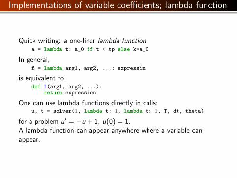
Implementations of variable coefficients; lambda function

Quick writing: a one-liner lambda functiona = lambda t: a_0 if t < tp else k*a_0

In general,f = lambda arg1, arg2, ...: expressin

is equivalent todef f(arg1, arg2, ...):

return expression

One can use lambda functions directly in calls:u, t = solver(1, lambda t: 1, lambda t: 1, T, dt, theta)

for a problem u′ = −u + 1, u(0) = 1.A lambda function can appear anywhere where a variable canappear.

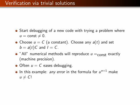
Verification via trivial solutions

Start debugging of a new code with trying a problem whereu = const 6= 0.

Choose u = C (a constant). Choose any a(t) and setb = a(t)C and I = C .

”All” numerical methods will reproduce u =const exactly(machine precision).

Often u = C eases debugging.

In this example: any error in the formula for un+1 makeu 6= C !

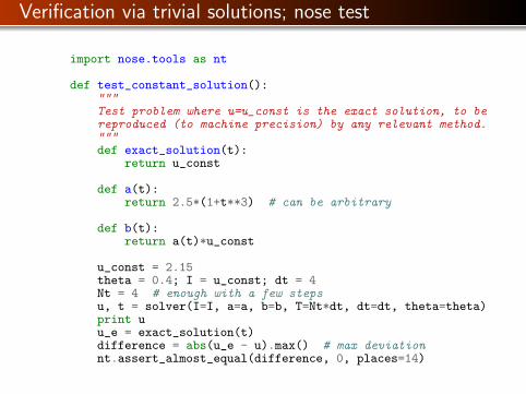
Verification via trivial solutions; nose test


def test_constant_solution():"""Test problem where u=u_const is the exact solution, to bereproduced (to machine precision) by any relevant method."""def exact_solution(t):

return u_const

def a(t):return 2.5*(1+t**3) # can be arbitrary

def b(t):return a(t)*u_const

u_const = 2.15theta = 0.4; I = u_const; dt = 4Nt = 4 # enough with a few stepsu, t = solver(I=I, a=a, b=b, T=Nt*dt, dt=dt, theta=theta)print uu_e = exact_solution(t)difference = abs(u_e - u).max() # max deviationnt.assert_almost_equal(difference, 0, places=14)

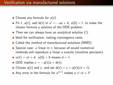
Verification via manufactured solutions

Choose any formula for u(t).

Fit I , a(t), and b(t) in u′ = −au + b, u(0) = I , to make thechosen formula a solution of the ODE problem.

Then we can always have an analytical solution (!).

Ideal for verification: testing convergence rates.

Called the method of manufactured solutions (MMS)

Special case: u linear in t, because all sound numericalmethods will reproduce a linear u exactly (machine precision).

u(t) = ct + d . u(0) = 0 means d = I .

ODE implies c = −a(t)u + b(t).

Choose a(t) and c , and set b(t) = c + a(t)(ct + I ).

Any error in the formula for un+1 makes u 6= ct + I !

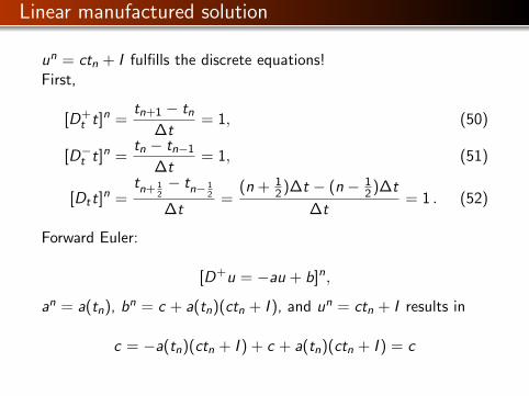
Linear manufactured solution

un = ctn + I fulfills the discrete equations!First,

[D+t t]n =

tn+1 − tn∆t

= 1, (50)

[D−t t]n =tn − tn−1

∆t= 1, (51)

[Dtt]n =tn+ 1

2− tn− 1

2

∆t=

(n + 12 )∆t − (n − 1

2 )∆t

∆t= 1 . (52)

Forward Euler:

[D+u = −au + b]n,

an = a(tn), bn = c + a(tn)(ctn + I ), and un = ctn + I results in

c = −a(tn)(ctn + I ) + c + a(tn)(ctn + I ) = c

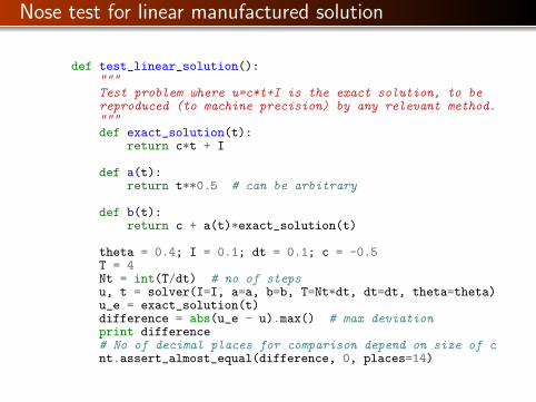
Nose test for linear manufactured solution

def test_linear_solution():"""Test problem where u=c*t+I is the exact solution, to bereproduced (to machine precision) by any relevant method."""def exact_solution(t):

return c*t + I

def a(t):return t**0.5 # can be arbitrary

def b(t):return c + a(t)*exact_solution(t)

theta = 0.4; I = 0.1; dt = 0.1; c = -0.5T = 4Nt = int(T/dt) # no of stepsu, t = solver(I=I, a=a, b=b, T=Nt*dt, dt=dt, theta=theta)u_e = exact_solution(t)difference = abs(u_e - u).max() # max deviationprint difference# No of decimal places for comparison depend on size of cnt.assert_almost_equal(difference, 0, places=14)

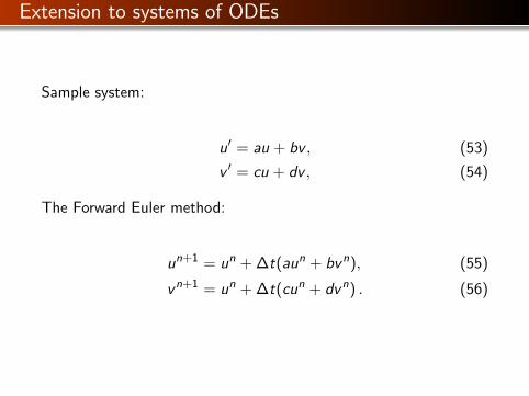
Extension to systems of ODEs

Sample system:

u′ = au + bv , (53)

v ′ = cu + dv , (54)

The Forward Euler method:

un+1 = un + ∆t(aun + bvn), (55)

vn+1 = un + ∆t(cun + dvn) . (56)

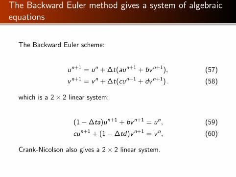
The Backward Euler method gives a system of algebraicequations

The Backward Euler scheme:

un+1 = un + ∆t(aun+1 + bvn+1), (57)

vn+1 = vn + ∆t(cun+1 + dvn+1) . (58)

which is a 2× 2 linear system:

(1−∆ta)un+1 + bvn+1 = un, (59)

cun+1 + (1−∆td)vn+1 = vn, (60)

Crank-Nicolson also gives a 2× 2 linear system.

General first-order ODEs

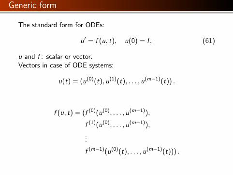
Generic form

The standard form for ODEs:

u′ = f (u, t), u(0) = I , (61)

u and f : scalar or vector.Vectors in case of ODE systems:

u(t) = (u(0)(t), u(1)(t), . . . , u(m−1)(t)) .

f (u, t) = (f (0)(u(0), . . . , u(m−1)),

f (1)(u(0), . . . , u(m−1)),

...

f (m−1)(u(0)(t), . . . , u(m−1)(t))) .

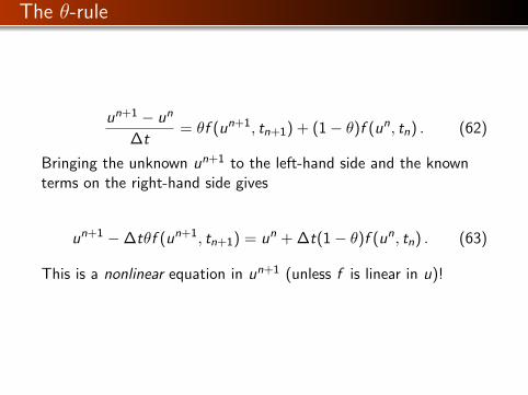
The θ-rule

un+1 − un

∆t= θf (un+1, tn+1) + (1− θ)f (un, tn) . (62)

Bringing the unknown un+1 to the left-hand side and the knownterms on the right-hand side gives

un+1 −∆tθf (un+1, tn+1) = un + ∆t(1− θ)f (un, tn) . (63)

This is a nonlinear equation in un+1 (unless f is linear in u)!

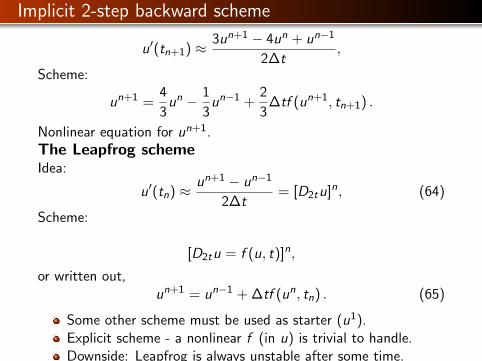
Implicit 2-step backward scheme

u′(tn+1) ≈ 3un+1 − 4un + un−1

2∆t,

Scheme:

un+1 =4

3un − 1

3un−1 +

2

3∆tf (un+1, tn+1) .

Nonlinear equation for un+1.The Leapfrog schemeIdea:

u′(tn) ≈ un+1 − un−1

2∆t= [D2tu]n, (64)

Scheme:

[D2tu = f (u, t)]n,

or written out,un+1 = un−1 + ∆tf (un, tn) . (65)

Some other scheme must be used as starter (u1).Explicit scheme - a nonlinear f (in u) is trivial to handle.Downside: Leapfrog is always unstable after some time.

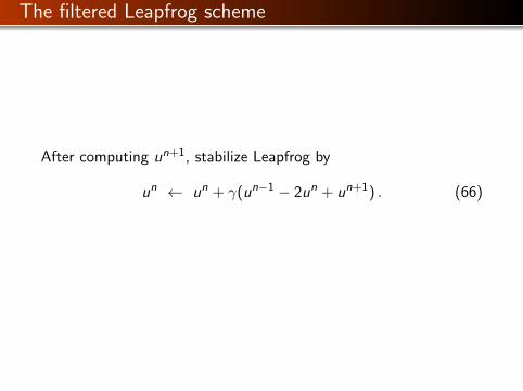
The filtered Leapfrog scheme

After computing un+1, stabilize Leapfrog by

un ← un + γ(un−1 − 2un + un+1) . (66)

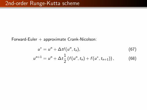
2nd-order Runge-Kutta scheme

Forward-Euler + approximate Crank-Nicolson:

u∗ = un + ∆tf (un, tn), (67)

un+1 = un + ∆t1

2(f (un, tn) + f (u∗, tn+1)) , (68)

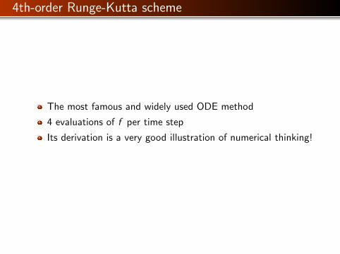
4th-order Runge-Kutta scheme

The most famous and widely used ODE method

4 evaluations of f per time step

Its derivation is a very good illustration of numerical thinking!

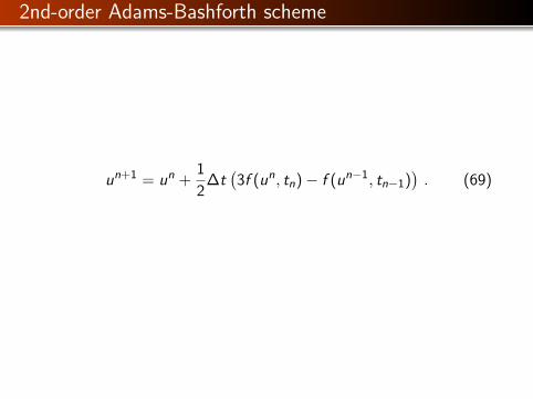
http://tinyurl.com/k3sdbuv/pub/decay-sphinx/._main_decay007.html#th-order-runge-kutta-scheme

2nd-order Adams-Bashforth scheme

un+1 = un +1

2∆t(3f (un, tn)− f (un−1, tn−1)

). (69)

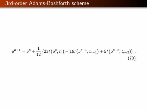
3rd-order Adams-Bashforth scheme

un+1 = un +1

12

(23f (un, tn)− 16f (un−1, tn−1) + 5f (un−2, tn−2)

).

(70)

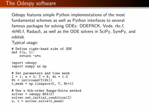
The Odespy software

Odespy features simple Python implementations of the mostfundamental schemes as well as Python interfaces to severalfamous packages for solving ODEs: ODEPACK, Vode, rkc.f,rkf45.f, Radau5, as well as the ODE solvers in SciPy, SymPy, andodelab.Typical usage:

# Define right-hand side of ODEdef f(u, t):

return -a*u

import odespyimport numpy as np

# Set parameters and time meshI = 1; a = 2; T = 6; dt = 1.0Nt = int(round(T/dt))t_mesh = np.linspace(0, T, Nt+1)

# Use a 4th-order Runge-Kutta methodsolver = odespy.RK4(f)solver.set_initial_condition(I)u, t = solver.solve(t_mesh)

https://github.com/hplgit/odespy

https://computation.llnl.gov/casc/odepack/odepack_home.html

https://computation.llnl.gov/casc/odepack/odepack_home.html

http://www.netlib.org/ode/rkc.f

http://www.netlib.org/ode/rkf45.f

http://www.unige.ch/~hairer/software.html

http://docs.scipy.org/doc/scipy/reference/generated/scipy.integrate.ode.html

http://docs.sympy.org/dev/modules/mpmath/calculus/odes.html

http://olivierverdier.github.com/odelab/

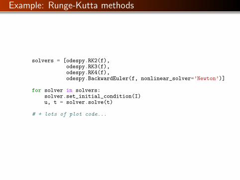
Example: Runge-Kutta methods

solvers = [odespy.RK2(f),odespy.RK3(f),odespy.RK4(f),odespy.BackwardEuler(f, nonlinear_solver=’Newton’)]

for solver in solvers:solver.set_initial_condition(I)u, t = solver.solve(t)

# + lots of plot code...

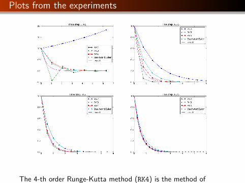
Plots from the experiments

The 4-th order Runge-Kutta method (RK4) is the method ofchoice!

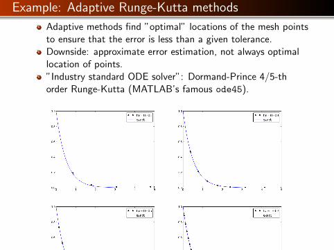
Example: Adaptive Runge-Kutta methods

Adaptive methods find ”optimal” locations of the mesh pointsto ensure that the error is less than a given tolerance.Downside: approximate error estimation, not always optimallocation of points.”Industry standard ODE solver”: Dormand-Prince 4/5-thorder Runge-Kutta (MATLAB’s famous ode45).

Documents

Study Guide: Intro to Computing with Finite Di erence Methodshplgit.github.io/INF5620/doc/pub/lecture_decay-beamer.pdf · Study Guide: Intro to Computing with Finite ... C, C++, and