Ministry Of Higher Education

And Scientific Research

University Of Diyala

College Of Engineering

Communication Engineering Department

Study and Simulation of least square channel

estimation of OFDM systems

A project

Submitted to the Department of Communications University of

Diyala-College of Engineering in Partial Fulfillment of the

Requirement for Degree Bachelor in Communication

Engineering

BY

Hajer Khalil Ibrahim

Noor Iqbal Abdul Kareem

Supervised by

Dr. Montadar Abbas Taher

Mr. Ahmed Mohamed Ahmed

May/2016 8341/رجب

بسن الله الرحوي الرحين

اى في خلك السوىاث و الأرض واختلاف اليل و النهار و الفلك التي تجري

فاحيا به الأرض هاءهي السواءفي البحر بوا ينفع الناس وها أزل الله هي

تصريف الرياح و السحاب المسخر بعذ هىتها و بث فيها هي كل دآبت و

(461لقىم يعقلىى ) لآياثوالأرض السواءبيي

العظينالعلي صذق الله

سىرة البقرة

Dedication

TO

MY " FAMILY " WITH LOVE

Acknowledgement

We wish to thank our family for their understanding and

support including our parents , siblings , our big family and our

friends inside and outside university.

We wish to express our deepest gratitude to our Advisor Dr.

Montadar Abbas Taher and Mr. Ahmed Mohamed Ahmed for his

guidance and friendship during our study. And at last we want to

thank the department of communication for giving us the chance to

work on as a fine project as this one.

ABSTRACT

The concept of OFDM is not new but receiver designs are constantly

improved. With new advances in DSP technologies, OFDM has become

popular for the reasons of efficient bandwidth usage and ease of synthesis

with new DSP technology. However, it is sensitive to synchronization

error and has a relatively large peak to average power ratio. This thesis

will provide an overall look into OFDM systems and its developments. It

will also look into the challenges OFDM faces and concentrate on one

main aspect of an OFDM receiver design, it is the channel estimation.

I

CHAPTER TITLE PAGE

TABLE OF CONTENTS I

LIST OF FIGURES I

LIST OF ABBREVIATIONS IV

LIST OF SYMBOLS V

1 INTRODUCTION

1.1 Introduction 1

1.2 Problem Statement 2

1.3 Objectives 2

1.4 Organization of research 2

2 OFDM BASICS

2.1

2.2

2.3

Introduction 4

Advantages / Disadvantages 8

Orthogonality 8

2.3.1 OFDM sub-carriers 9

2.3.2 OFDM Spectrum 10

2.4

2.5

2.6

2.7

Inter symbol Interference 11

Inter Carrier Interference 11

Cyclic Prefix ( Guard Interval ) 12

Inverse Discrete Fourier Transform 13

3

3.1

3.2

CHANNEL ESTIMATION

Introduction 14

System Environment 14

II

3.2.1

3.2.2

3.2.3

3.2.4

3.3

3.3.1

3.3.2

3.3.3

3.3.4

3.3.5

3.4

3.5

3.6

4

4.1

4.2

5

5.1

5.2

Wireless 14

Multipath Fading 14

Fading Effects due to Multi-path Fading 15

White noise 15

Channel Model 16

Rayleigh Distribution 19

Power Delay Profile 20

AWGN 20

Channel Synchronisation 21

Assumptions on channel 21

Pilot Based Channel Estimation 22

Least Squares Estimator 23

Linear Minimum Mean Square Error Estimator 24

RESULTS & DISCUSSION

Introduction 27

Results and Discussion 27

CONCLUSION

Conclusion 35

Future Work 35

REFERENCE 36

III

LIST OF FIGURE

FIGURE NO. TITLE PAGE

2.1

2.2

2.3

2.4

2.5

2.6

2.7

3.1

3.2

3.3

4.1

4.2

4.3

4.4

4.5

4.6

4.7

4.8

4.9

4.10

Block diagram of OFDM system

The construction diagram

Cyclic prefix of OFDM symbol

Showing the multipath channel

Pilot value is equal in transmitter and varies in the Receiver

because noise

Fourier series frequency harmonic

OFDM time domain spectrum

Parallel Gaussian channels

Resampling a non-sample-spaced channel extends the channel

Length

An example of block based pilot information

Comb-type pilot distribution configuration for 10,000 OFDM

symbols

The three paths estimated and actual channels

BER performance of the first scenario

Pilot subcarriers configuration for the second scenario

Actual and estimated channel parameters for the second

scenario

BER performance of the second scenario

Channel estimation parameters for the third scenario

Channel estimation parameters for the fourth scenario

BER performance of the third scenario

BER performance of the fourth scenario

4

5

6

6

7

10

11

16

21

23

27

28

29

30

31

31

32

33

33

34

IV

LIST OF ABBREVIATIONS

AWGN – Additive White Gaussian Noise

ICI – Interchannel Interference

ISI – Inter symbol Interference

DFT _ Discrete Fourier Transform

DMT _ Discrete Modulation

DSL _ Digital subscariber line

DAB _ Digital Audio Broadcasting

SNR _ The Signal-To-Noise Ratio

QAM _ Quadrature Amplitude Modulation

IDFT _ Inverse Discrete Fourier Transform

FFT _ Fast Fourier Transform

IFFT _ Inverse Fast Fourier Transform

LOS _ Line of Sight

PDP _ Power Delay Profile

LS _ The Least Square

LMMSE _ The Linear Minimum Mean Squares Error

MSE _ The mean square error

V

LIST OF SYMBOLS

P/S _ Parallel to series

S/P _ Series to parallel

_ Fundamental frequency

y _ The received vector of signaling points

x _ The transmitted signaling points

Hc _ The diagonalised channel attenuation vector

n _ A vector of complex

Ts _ The sampling period of the system

H[k] _ The attenuation

_ Independent zero mean

_ The delay of the kth impulse

N0 _ The noise power density

F _ Operation frequency

1

1.1 Introduction

Where did it begin?

In 1966 Robert W. Chang published a paper on the synthesis of band limited

orthogonal signals for multichannel data transmission [1]. It describes a method in

which signal can be simultaneously transmitted through a band limited channel

without ICI (Interchannel Interference) and ISI (Inter symbol Interference). The idea

of dividing the spectrum into several channels allowed transmission at a low enough

data rate to counter the effect of time dispersion in the channel. As the sub channels

are orthogonal they can overlap providing a much more efficient use of the available

spectrum.

In 1971, S.B. Weinstein and P.M. Ebert introduced the DFT (Discrete Fourier

Transform) to perform the baseband modulation and demodulation [2] This replaced

the traditional bank of oscillators and multipliers needed to create and modulate onto

each subcarrier.

In 1980, A.Peled and A. Ruiz introduced the cyclic prefix [3].This takes the

last part of the symbol and attaches it to the front. When this extension is longer than

the channel impulse response, the channel matrix is seen as circulate and orthogonally

of the subcarriers is maintained over the time dispersive channel.

OFDM is currently used in European Digital Audio Broadcasting (DAB.)

OFDM is used in DSL (Digital Subscriber Line) where it is know as DMT )Discrete

Multitone). It is used in the European standard Hyperlan/2 and in IEEE 802.11a. This

thesis will explore concepts and designs which have already been established and look

into some newer technologies. However, we will concentrate on what really makes an

OFDM system work, for which a certain degree of knowledge and understanding of

signal processing and digital communications is necessary. From here, we will launch

into important background information which did take a somewhat long time to

understand.

2

1.2 Problem Statement

Multicarrier modulation, which is represented here by the OFDM system, is

sensitive to multipath fading channels. In an OFDM system, the transmitter modulates

the message bit sequence into PSK/QAM symbols, performs IFFT on the symbols to

convert them into time-domain signals, and sends them out through a (wireless)

channel. The received signal is usually distorted by the channel characteristics. In

order to recover the transmitted bits, the channel effect must be estimated and

compensated in the receiver. Each subcarrier can be regarded as an independent

channel, as long as no ICI (Inter-Carrier Interference) occurs, and thus preserving the

orthogonality among subcarriers. The orthogonality allows each subcarrier component

of the received signal to be expressed as the product of the transmitted signal and

channel frequency response at the subcarrier. Thus, the transmitted signal can be

recovered by estimating the channel response just at each subcarrier. In general, the

channel can be estimated by using a preamble or pilot symbols known to both

transmitter and receiver, which employ various interpolation techniques to estimate

the channel response of the subcarriers between pilot tones. In general, data signal as

well as training signal, or both, can be used for channel estimation. In order to choose

the channel estimation technique for the OFDM system under consideration, many

different aspects of implementations, including the required performance,

computational complexity and time-variation of the channel must be taken into

account.

1.3 Objective

The study of OFDM performance over AWGN channel and Rayleigh channel

using MATLAB simulation

1.4 Organization Of Research

Chapter 1 introduces a basic history of OFDM systems. Chapter 2 shows the

general theory of the OFDM system. Chapter 3 speaks about the channel estimation of

the OFDM system and the important methods for channel estimation. Chapter 4

includes the results and the discussion of the results, which had obtained by using

3

Matlab software. While Chapter 5 will talk about the conclusion of the research and a

recommendation for future work.

4

2.1 Introduction

OFDM is a modulation technique in that it modulates data onto equally spaced

sub-carriers. The information is modulated onto the sub-carrier by varying the phase,

amplitude, or both. Each sub-carrier then combined together by using the inverse fast

Fourier transform to yield the time domain waveform that is to be transmitted. To

obtain a high spectral efficiency the frequency response of each of the sub-carriers are

overlapping and orthogonal. This orthogonally prevents interference between the sub-

carriers and is preserved even when the signal passes through a multipath channel by

introducing a Cyclic Prefix, which prevents Inter-symbol Interference (ISI) on the

carriers. This makes OFDM especially suited to wireless communications application .

A simple block diagram for the OFDM system can be seen in Figure 2.1.

Fig 2.1: Block diagram of OFDM

In Figure (2.1):-

Data : can be Discrete [ 0 , 1 , 3 ……. M-1 ] or binary [ 01010…. ], where M

is the constellation order, or it is called the baseband modulation order.

5

Mapping ( baseband modulation ) : distributing the data on the construction

diagram, in Figure (2.2)

Fig 2.2 : The construction diagram

S/P ( De-Multiplexing ) : Any symbol contain set of serial bits entered to serial

to parallel convertor , that is register has one input and several output

IDFT (Inverse Discrete Fourier Transform) :

( )

∑ ( )

(2.1)

(2.2)

Cyclic Prefix : this can be ( 8% to 25% ) of the symbol length data copied to

the front of the OFDM symbol to prevent the ISI during transmission through

the propagation channel as shown in Figure (2.3)

6

Fig 2.3: Cyclic Prefix of OFDM symbol

Channel : Is contain multi-path effect and noise, this can be seen in Figure

(2.4)

Fig 2.4: Showing the multipath channel

( ) ( ) ( ) (2.3)

Channel Estimation :

7

Pilot should be known value at the receiver and transmitter.

Pilot value is equal in transmitter and varies in the Receiver because

noise. In Figure (2.5), a simple pilot distribution can be seen.

Y(f) = H(f) X(f)

Fig 2.5: Pilot value is equal in transmitter and varies in the Receiver

because noise.

In The Receiver:

The cyclic prefix will be removed

Transform from time domain to frequency domain will be achieved by

Discrete Fourier Transform (DFT).

P/S ( Multiplexing )

Output data

8

2.2 Advantages / Disadvantages

OFDM has the following advantages[4]:

OFDM is an efficient way to deal with multipath; implementation

complexity is significantly lower than single carrier with equalizer.

In relatively slow time-varying channels, performance can be enhanced

by the adaptability of the data rate according to the SNR ratio of that

sub-carrier.

OFDM is robust against narrowband interference, because such

interference affects only a small number of sub-carriers.

OFDM makes single-frequency networks possible, which is especially

attractive for broadcasting applications.

On the other hand, OFDM has the following disadvantages compared to

single-carrier modulation:

OFDM is more sensitive to frequency offsets and phase noise.

OFDM has a relatively large peak-to-average power ratio, which

reduces the power efficiency of the RF amplifier.

2.3 Orthogonality

Two periodic signals are orthogonal when the integral of their product over

one period is equal to zero

For the case of continuous time:

9

∫ (2𝜋𝑛 𝑡) (2𝜋𝑛 𝑡)𝑑𝑡 0, (𝑚 ≠ 𝑛)

(2.4)

For the case of discrete time:

∑ (

) (

) 𝑑𝑡 0, (𝑚 ≠ 𝑛)

(2.5)

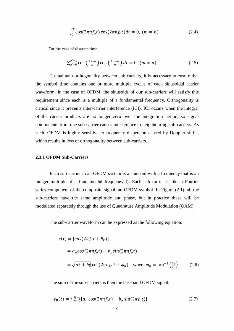
To maintain orthogonality between sub-carriers, it is necessary to ensure that

the symbol time contains one or more multiple cycles of each sinusoidal carrier

waveform. In the case of OFDM, the sinusoids of our sub-carriers will satisfy this

requirement since each is a multiple of a fundamental frequency. Orthogonality is

critical since it prevents inter-carrier interference (ICI). ICI occurs when the integral

of the carrier products are no longer zero over the integration period, so signal

components from one sub-carrier causes interference to neighbouring sub-carriers. As

such, OFDM is highly sensitive to frequency dispersion caused by Doppler shifts,

which results in loss of orthogonality between sub-carriers.

2.3.1 OFDM Sub-Carriers

Each sub-carrier in an OFDM system is a sinusoid with a frequency that is an

integer multiple of a fundamental frequency f˳. Each sub-carrier is like a Fourier

series component of the composite signal, an OFDM symbol. In Figure (2.1), all the

sub-carriers have the same amplitude and phase, but in practice these will be

modulated separately through the use of Quadrature Amplitude Modulation (QAM).

The sub-carrier waveform can be expressed as the following equation:

( ) , 𝑜 (2𝜋 𝑡 )-

𝑜 (2𝜋𝑛 𝑡) 𝑛(2𝜋𝑛 𝑡)

√

(2𝜋𝑛 𝑡 ), where .

/ (2.6)

The sum of the sub-carriers is then the baseband OFDM signal:

( ) ∑ * (2𝜋𝑛 𝑡) (2𝜋 𝑡)+ (2.7)

11

Fig 2.6: Fourier series frequency harmonic

2.3.2 OFDM Spectrum

Our OFDM symbol is a sum of sinusoids of a fundamental frequency and its

harmonics in the time domain. The rectangular windowing of the transmitted OFDM

symbol results in a sinc function at each sub-carrier frequency in the frequency

response. Thus, the frequency spectrum of an OFDM symbol is as shown below: The

Figure (2.2) is not the actual spectrum of OFDM. The spectrum of each sub-carrier

has been superimposed to illustrate the orthogonally of the sub-carriers. Although

overlapping, the sub-carriers do not interfere with each other since each sub-carrier

peak corresponds to a zero crossing for all other sub-carriers.

11

Fig 2.7 : OFDM time domain spectrum

2.4 Inter Symbol Interference

Inter symbol interference (ISI) is when energy from one symbol spills over to

the next symbol. This is usually caused by time dispersion in multi-path when

reflections of the previous symbol interfere with the current symbol. In OFDM,

because each sub-carrier is transmitting at a lower data rate (longer symbol duration),

this will negate the effects of time dispersion, which results in ISI.

2.5 Inter Carrier Interference

Inter carrier interference (ICI) is occurs when the sub carriers lose their

orthogonally, causing the sub carriers to interfere with each other. This can arise due

to Doppler shifts and frequency and phase offsets.

12

2.6 Cyclic Prefix ( Guard Interval )

The Cyclic Prefix is a periodic extension of the last part of an OFDM symbol

that is added to the front of the symbol in the transmitter, and is removed at the

receiver before demodulation.

The Cyclic Prefix has two important benefits:

The Cyclic Prefix acts as a guard space between successive OFDM symbols

and therefore prevents Inter-symbol Interference (ISI), as long as the length of

the CP is longer than the impulse response of the channel.

The Cyclic Prefix ensures orthogonality between the sub-carriers by keeping

the OFDM symbol periodic over the extended symbol duration, and therefore

avoiding Inter-carrier Interference (ICI).

Mathematically, the Cyclic Prefix / Guard Interval converts the linear

convolution with the channel impulse response into a cyclic convolution. This results

in a diagonalised channel, which is free of ISI and ICI interference.

The disadvantage of the Cyclic Prefix is that there is a reduction in the Signal

to Noise Ratio due to a lower efficiency by duplicating the symbol. This SNR loss is

given by:

𝑺𝑵𝑹𝒍𝒐 10 𝑙𝑜𝑔 (1

) (2.8)

where Tcp is the length of the Cyclic Prefix and T = Tcp +Ts is the length of

the transmitted symbol and Ts is the signal transmission.

To minimize the loss of SNR, the CP should not be made longer than

necessary to avoid ISI and ICI.

13

2.7 Inverse Discrete Fourier Transform

OFDM modulation is applied in the frequency domain. The complex QAM

data symbols are modulated onto orthogonal sub-carriers. But in order to transmit

over a channel, we need a signal in the time domain. To do this, we apply the Inverse

Discrete Fourier Transform (IDFT) in the transmitter to convert the signal from

frequency domain to an OFDM symbol in the time domain. Because the IDFT is a

linear transformation, the DFT can be applied at the receiver to convert the data back

into the frequency domain. This section will provide an explanation of the IDFT /

DFT and why it is a key component of an OFDM system.

To implement the multi-carrier system using a bank of parallel oscillators and

modulators would not be very efficient in analog hardware. However, in the digital

domain, multicarrier-modulation can be done very efficiently with the current DSP

hardware and software.

To do this modulation we exploit the properties of the Discrete Fourier

Transform (DFT) and the Inverse DFT (IDFT). From Fourier, we know that when the

DFT of a sampled time signal is taken, the frequency domain results are the

components of the signal with respect to the Fourier Basis which are multiples of a

fundamental frequency as a function of the sampling period and the number of

samples. The IDFT performs the opposite the DFT. It takes the signal defined by the

frequency components and converts them to a time signal.

In OFDM, we compose the signal in the frequency domain. Since the Fourier

Basis is orthogonal, we just take the IDFT of the N inputs which are our frequency

components to convert to a time domain equivalent for transmission over the channel.

In practice, the Fast Fourier Transform (FFT) and IFFT are used instead of the

DFT and IDFT because of their lower hardware complexity. All further references

will be to FFT and IFFT.

14

3.1 Introduction

In a wireless environment, the channel is much more unpredictable than a wire

channel because of a combination of factors such as multi-path, frequency offset,

timing offset, and noise. This results in random distortions in amplitude and phase of

the received signal as it passes through the channel. These distortions change with

time since the wireless channel response is time varying. Channel estimation attempts

to track the channel response by periodically sending known pilot symbols, which

enables it to characterize the channel at that time. This pilot information is used as a

reference for channel estimation. The channel estimate can then be used by an

equalizer to correct the received constellation data so that they can be correctly

demodulated to binary data.

Modulation can be classified as differential or coherent. For differential,

information is encoded in the difference between two consecutive symbols so no

channel estimate is required. However, this limits the number of bits per symbol and

results in a 3-dB loss in SNR. Coherent modulation allows the use of arbitrary

signaling constellations, allowing for a much higher bit rate than differential

modulation and better efficiency. This chapter will give a description of our system

environment, the channel model and present several channel estimation techniques

that are required for the case of coherent Modulation.

3.2 System Environment

3.2.1 Wireless

The system environment we will be considering in this thesis will be wireless

indoor and urban areas, where the path between transmitter and receiver is blocked by

various objects and obstacles. For example, an indoor environment has walls and

furniture, while the outdoor environment contains buildings and trees. This can be

characterized by the impulse response in a wireless environment.

15

3.2.2 Multipath Fading

Most indoor and urban areas do not have direct line of sight propagation

between the transmitter and receiver. Multi-path occurs as a result of reflections and

diffractions by objects of the transmitted signal in a wireless environment. These

objects can be such things as buildings and trees. The reflected signals arrive with

random phase offsets as each reflection follows a different path to the receiver. The

signal power of the waves also decreases as the distance increases. The result is

random signal fading as these reflections destructively and constructively

superimpose on each other. The degree of fading will depend on the delay spread (or

phase offset) and their relative signal power.

3.2.3 Fading Effects due to Multi-path Fading

Time dispersion due to multi-path leads to either flat fading or frequency

selective fading:

Flat fading occurs when the delay is less than the symbol period and affects all

frequencies equally. This type of fading changes the gain of the signal but not

the spectrum. This is known as amplitude varying channels or narrowband

channels, since the bandwidth of the applied signal is narrow compared to the

channel bandwidth.

Frequency selective fading occurs when the delay is larger than the symbol

period. In the frequency domain, certain frequencies will have greater gain

than others frequencies.

3.2.4 White noise

In wireless environments, random changes in the physical environment

resulting in thermal noise and unwanted interference from many other sources can

cause the signal to be corrupted. Since it is not possible to take into account all of

16

these sources, we assume that they produce a single random signal with uniform

distributions across all frequencies. This is known as white noise.

3.3 Channel Model

This section will show how the channel will become diagonalised from a

cyclic convolution due to the insertion of the Cyclic Prefix. If the Cyclic Prefix is

longer than the impulse response of the channel, we can show that the OFDM channel

can be viewed as a set of parallel Gaussian channel (a complex gain followed by

Additive White Gaussian noise) that is free of ISI and ICI.

Fig 3.1: Parallel Gaussian channels

First, let our QAM signalling symbols be expressed as

[

] (3.1)

After we apply the IFFT to s, our OFDM symbol becomes

[

] (3.2)

where the matrix F is the DFT matrix. For the channel impulse response

[

] (3.3)

17

where m is less than the length of the cyclic prefix.

To simplify our derivation, we will choose N = 4 sub-carriers and m = 2 tap

impulse response, but this proof will generally apply as long as m satisfies the above

condition. So after passing through the multi-path channel, the received OFDM

symbol can be expressed as a convolution, h* x. In matrix form, this becomes

(3.4)

If we insert the cyclic prefix before sending across the channel, this

convolution becomes

(3.5)

And after removing the cyclic prefix at the receiver, we can express this as

(3.6)

This is equivalent to a circular convolution. The channel matrix is now a

circulant matrix and X’ is the cyclically extended symbol.

18

We can now use the property of circular convolution on finite length

sequences

, - , -, k = (0,…,N-1) (3.7)

This property means every circulant matrix is diagonalised by the DFT

matrix F.

, [[ ,0- 0

0 , 1-

]] (3.8)

So our multi-path fading channel can be written as:

𝑛 (3.9)

where y is the received vector of signaling points, x is the transmitted

signaling points, is the diagonalised channel attenuation vector, and n is a vector of

complex, zero mean, Gaussian noise with variance

The attenuation on each tone is given by

, - .

/ , 0, , 1 (3.10)

where G(.) is the frequency response of the channel during the current OFDM

symbol and is the sampling period of the system.

The impulse response of the channel can be expressed as

( ) ∑ ( ) (3.11)

where are independent zero mean, complex Gaussian random variables,

and is the delay of the kth impulse. The next few sections will talk about our

19

considerations regarding some issues on the wireless channel and the justifications for

our channel model.

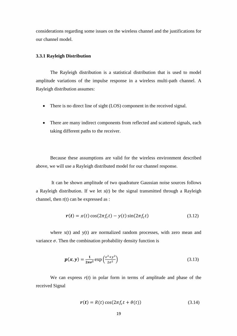
3.3.1 Rayleigh Distribution

The Rayleigh distribution is a statistical distribution that is used to model

amplitude variations of the impulse response in a wireless multi-path channel. A

Rayleigh distribution assumes:

There is no direct line of sight (LOS) component in the received signal.

There are many indirect components from reflected and scattered signals, each

taking different paths to the receiver.

Because these assumptions are valid for the wireless environment described

above, we will use a Rayleigh distributed model for our channel response.

It can be shown amplitude of two quadrature Gaussian noise sources follows

a Rayleigh distribution. If we let s(t) be the signal transmitted through a Rayleigh

channel, then r(t) can be expressed as :

( ) (𝑡) (2𝜋 𝑡) (𝑡) (2𝜋 𝑡) (3.12)

where x(t) and y(t) are normalized random processes, with zero mean and

variance . Then the combination probability density function is

( , )

.

/ (3.13)

We can express r(t) in polar form in terms of amplitude and phase of the

received Signal

( ) (𝑡) (2𝜋 𝑡 (𝑡)) (3.14)

21

where R(t) and (t) are given by

𝑹( ) √( )

( ) .

/ (3.15)

By using the polar transformation, the probability density function now

becomes:

(𝑹, )

(

) (3.16)

Integrating p(R, ) over from 0 to 2𝜋, we obtain the probability density

function p(R):

(𝑹)

(

) (3.17)

which follows a Rayleigh distribution.

3.3.2 Power Delay Profile

The Power Delay Profile (PDP) describes the envelope of the impulse

response as a function of the delay. The PDP of an urban and indoor environment is

generally described by an exponential, since each delayed impulse usually has less

power than the previous ones. Thus, our PDP is described by the following equation

( ) .

/ (3.18)

3.3.3 AWGN

When the signal passes through the channel, it is corrupted by white noise.

This is modelled by the addition of white Gaussian noise (AWGN). AWGN is a

random process with power spectral density as follows:

21

( )

[

⁄ ] (3.19)

where is a constant and often called the noise power density.

3.3.4 Channel Synchronization

There are two types of channel synchronisation models - Sample spaced and

Non sample spaced synchronization[5].

Sample spaced synchronisation assumes all delayed impulses of its channel

impulse response are at integer multiples of the sampling period T.

In non sample spaced channels, the delayed impulses are not at periods of the

sampling period T, thus the most of the impulse power is spread locally among

the closest sampling intervals at the receiver, and leads to a larger impulse

response at the receiver as shown in figure 3.2.

Fig 3.2: Resampling a non-sample-spaced channel extends the channel length.

22

For simplicity, we will only consider synchronised sample spaced channels for

channel estimation in this thesis.

3.3.5 Assumptions on channel

To simplify our simulated channel, the following are assumed to hold:

The impulse response is shorter than the Cyclic Prefix. Therefore, there is no

ISI and ICI and the channel is therefore diagonal.

The channel is a synchronized, sample spaced channel.

Channel noise is additive, white and complex Gaussian.

The fading on the channel is slow enough to be considered constant during

one OFDM frame.

3.4 Pilot Based Channel Estimation

The following estimators use on pilot data that is known to both transmitter

and receiver as a reference in order to track the fading channel. The estimators use

block based pilot symbols, meaning that pilot symbols are sent across all sub-carriers

periodically during channel estimation. This estimate is then valid for one OFDM

frame before a new channel estimate will be required.

Since the channel is assumed to be slow fading, our system will assume a

frame format, transmitting one channel estimation pilot symbol, followed by five data

symbols, as indicated in the time frequency lattice shown in figure3.3. Thus each

channel estimate will be used for the following five data symbols

23

3.5 Least Squares Estimator

The simplest channel estimator is to divide the received signal by the input

signals, which should be known pilot symbols. This is known as the Least Squares

(LS) Estimator and can simply be expressed as:

𝑺

(3.20)

This is the most naive channel estimator as it works best when no noise is

present in the channel. When there is no noise the channel can be estimated perfectly.

This estimator is equivalent to a zero-forcing estimator.

Fig 3.3: An example of block based pilot information

The main advantage is its simplicity and low complexity. It only requires a

single division per sub-carrier. The main disadvantage is that it has high mean-square

24

error. This is due to its use of an oversimplified channel and does not make use of the

frequency and time correlation of the slow fading channel.

An improvement to the LS estimator would involve making use of the channel

statistics. We could modify the LS estimator by tracking the average of the most

recently estimated channel vectors.

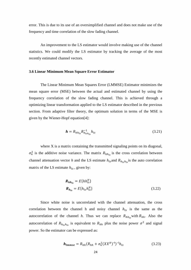
3.6 Linear Minimum Mean Square Error Estimator

The Linear Minimum Mean Squares Error (LMMSE) Estimator minimizes the

mean square error (MSE) between the actual and estimated channel by using the

frequency correlation of the slow fading channel. This is achieved through a

optimizing linear transformation applied to the LS estimator described in the previous

section. From adaptive filter theory, the optimum solution in terms of the MSE is

given by the Wiener-Hopf equation[4]:

(3.21)

where X is a matrix containing the transmitted signaling points on its diagonal,

is the additive noise variance. The matrix

is the cross correlation between

channel attenuation vector h and the LS estimate and is the auto correlation

matrix of the LS estimate , given by:

𝑹 𝒍 *

+

𝑹 𝒍 *

+ (3.22)

Since white noise is uncorrelated with the channel attenuation, the cross

correlation between the channel h and noisy channel is the same as the

autocorrelation of the channel h. Thus we can replace with . Also the

autocorrelation of is equivalent to plus the noise power and signal

power. So the estimator can be expressed as:

𝒍 ( ( ) ) (3.23)

25

The above equation seems to pose a contradiction since we need the

autocorrelation of our desired channel vector in order to estimate an optimum channel

vector. But we do not know what our desired channel vector since we do not know the

channel. To overcome this problem, we replace the autocorrelation with its expected

value. This can be done in two ways:

By theoretically calculating the expected value based on assumed or known

channel statistics. This simplifies the complexity as the inverse only needs to

be calculated once, which will be explained further on. The values will need to

be recalculated each time the statistics of the channel changes.

Through realization, the autocorrelation matrix can be averaged each time

channel estimation occurs. This approach will converge slower than the above

method since the expected value is calculated adaptively but is more flexible

since it does not assume any fixed channel statistics.

For our OFDM channel estimation, we will use the first approach because of

its lower complexity and easier implementation.

The main disadvantage of this estimator is that it has a very high complexity.

The evaluation of inverse R and involves the inversion of a matrix of dimension

N x N which makes this estimator computationally complex.

By using statistics that we know about the additive noise and the transmitted

data, we can simplify the estimator. Since the binary data is completely random, we

can assume equal probability on all constellation points, and we can replace by

its expected value

* + |

|

(3.24)

Thus our simplified estimator can be expressed as:

26

𝒍 (

)

(3.25)

where I is the Identity matrix, SNR is the average signal-to-noise ratio is

defined as | | . is a signal constellation dependent constant. For the case of

16-QAM

| | |1 ⁄ |

1 ⁄ (3.26)

Thus the inverse need only be calculated once every time channel estimation

occurs, or just once if set to theoretical values.

27

4.1 Introduction

In this chapter, the results of lest squares channel estimation will be shown.

Different scenarios will be considered as will be shown later, where all scenarios will

be implemented using Matlab for Quadrature Amplitude Modulation family type.

4.2 Results and Discussion

In our project, we have considered four scenarios, the first scenario is an

OFDM symbol length N = 256 subchannels, a constellation order M = 4, pilot

frequency of 4, pilot energy = 4 times the largest point in the constellation diagram,

cyclic prefix length of N/8, and last but not least the number of paths was 3.

Figure (4.1) shows the comb-type of our configuration in the Matlab simulation for

the first scenario. Where the number of the simulated OFDM symbols was 10,000.

However, the vertical axis represents the frequency-domain and the horizontal axis

stands for the time-domain. As we have explained in chapter three, we used the

comb-type pilot assisted channel estimation for fast channel varying, in other words,

for fast mobility as in the fourth generation (4G).

Fig 4.1: Comb-type pilot distribution configuration for 10,000 OFDM symbols.

28

Least squares channel estimation needs to do a mathematical operation called

interpolation, see chapter 3, where we need to extend the size of the estimated channel

length to the actual channel length which is N. for more information, the reader can

refer to chapter 3. Figure (4.2) shows the channel parameters estimation compared

with the actual channel. As aforementioned above, this scenario adopted three

randomly generated paths for the simulation. However, it can be seen at the most

bottom of the figure that the actual subchannel do not matches the estimated, where

we have plotted only 45 points up of 256 points for clarity. This mismatch will be

reflected on the BER performance behavior, as shown in Figure (4.3).

Fig 4.2: The three paths estimated and actual channels.

Figure (4.3) depicts the BER performance of the first scenario. It is shown that

the required SNR for the estimated channel needs to be higher with respect to the

actual, which is equivalent to as there is only AWGN channel, i.e., only one path

channel.

29

Fig 4.3: BER performance of the first scenario.

The second scenario is an OFDM symbol length N = 256 subchannels, a

constellation order M = 16, pilot frequency of 4, pilot energy = 4 times the largest

point in the constellation diagram, cyclic prefix length of N/8, and the number of

paths still 3. Thus, only the constellation order has been changed, to see the effect of

higher modulation orders on the performance of the OFDM system with multipahts.

In Figure (4.4), the pilot distribution can be seen, where it is similar to the one

in Figure (4.1), but here it is higher energy and constellation order. It is shown that the

time-axis shows the number 10,000, which is the total number of the randomly

generated OFDM symbols for the simulation. While the Frequency axis, shows the

total number of the OFDM size, which is 256 subcarrier in our simulations.

31

Fig 4.4: Pilot subcarriers configuration for the second scenario.

The estimated channels were shown in Figure (4.5) for this second scenario,

where it can be seen that some of the black points do not match the red points, that is

why the BER performance was degraded significantly, as shown in Figure (4.6).

however, we have drawn only 35 points for clarity purposes.

31

Fig 4.5: Actual and estimated channel parameters for the second scenario

Fig 4.6: BER performance of the second scenario

On the other hand, the third and fourth scenarios has a slightly different

parameters, where the channel length, or the number of multipaths has been increased

by one path, thus, these scenarios will achieve four multipaths. That is - the pilot

32

distribution will not be changed for the third scenario with respect to the first

scenario, thus, there is no need to re-plot it. The same pilot distribution for the fourth

scenario is similar to the second scenario, hence, it is not necessary to re-plot is also.

Figure (4.7) explains the channel estimation parameters for the third scenario, while

Figure (4.8) shows the channel estimation parameters for the fourth scenario. In both

figures, there are only 35 subchannels where plotted for simplicity.

Figures 4.9 and 4.10 show the BER performances, respectively, of the third and fourth

scenarios. It can be concluded that the number of multipaths has a recognized effect

on the BER performance, where the SNR for both figures was increased to reach the

required BER performance for acceptable quality.

Fig 4.7: Channel estimation parameters for the third scenario.

33

Fig 4.8: Channel estimation parameters for the fourth scenario.

Fig 4.9: BER performance of the third scenario.

34

Fig 4.10: BER performance of the fourth scenario.

35

5.1 Conclusion

From the 1960s to today, we can see that OFDM is another tool for which the

engineer can use to overcome channel effects in a wireless environment. The are

many advantages in OFDM, but there are still many complex problems to solve.

We hope this thesis has provided a basic simulation tool for future students to

use as a starting point in their theses. It is our motivation that by using the parameters

of a working system, a much clearer and insightful explanation of the fundamentals of

OFDM have been presented.

Channel Estimation is an important part of an OFDM receiver, especially in

wireless environments where the channel is unpredictable and changing continuously.

A good channel estimation will allow the equalizer to correct the fading effects of the

channel. Of the three channel estimators studied in this thesis, the low rank

approximate estimator seems to be the most practical in terms of good performance

and low complexity. The LS does not perform well in low SNR environments while

the LMMSE estimator complexity seems too high for a small performance

improvement.

In OFDM equalization, it seems that the adaptive algorithms used in the

OFDM did not add many special benefits. It’s adaptive capability allowed the

equalizer coefficients to change with time but it is done on the basis on resynthesized

symbols for which noise and rounding errors may accumulate. These algorithm did

not exploit OFDM characteristics which the zero forcing and LMMSE did. It may be

wise to incorporate LMMSE design into a DFE. Because the zero forcing and

LMMSE equalizers exploit the OFDM design by equalizing in the frequency domain,

it is very simple, especially compared the complexities of the adaptive algorithms.

5.2 Future Work

This work can be extended to verifying the part next:

1. The cyclic prefix for OFDM can require up to 15-20% bandwidth overhead. It

is desirable to develop techniques that eliminate or reduce the cyclic prefix.

2. Channel estimation techniques for space-time and space-frequency coded

OFDM systems.

36

Reference:

1. H. Harada, R. Prasad, “Simulation and software radio for mobile

communications” , Artech House Publishers.

2. R.W. Chang. “Synthesis of bandlimited orthogonal signals for multichannel

data transmission.”, Bell System Tech. Journal, 45 pp. 1775–1796, Dec. 1966.

3. D.S. Taubman, “Elec4042: Signal Processing 2 Complete Set of Written

Materials Session 1, 2003”, 2003.

4. R. van Nee, R. Prasad, “OFDM for Wireless Multimedia Communications” ,

Artech House, 2000.

5. M. Engels, “Wireless OFDM Systems How to make them work?”, Kluwer

Academic Publishers, Massachusets, USA, 2002.

انخلاصة

انيدف ين ىرا انشسع ى يضاعفت انتسدد انتعايد

بانتمسى انري ى يفتاح تكن انتكننجا نعظى أنظت

ذاث يعدل نمم انباناث الاتصالاث انلاسهكت انذانت

( يمازنت بانطسق OFDMانصة انسئست نهـ )انعان.

انعسض انى انتمهدت ى أنو ذل انمناة ذاث اننطاق

لناث فسعت ضمت يتاشت تسخ بتمدس انمناة تكافؤ

ف يجال انتسدد بسط نسبا عند انستهى. تعتبس ىره

انتمنت فعانت نهتغهب عهى تأثساث انمناة يثم الانتشاز

( ين خلال الاستفادة ISIانتعدد انتداخم بن انسيش )

نعائك انسئست ين انبادئت اندزت انناسبت. اددة ين ا

( ى أنو أكثس دساست لأخطاء انصاينت OFDMف )

ين نظسائو ذاث اننالم اناددة.

انعه انعان انبذث انتعهى شازة

دانى جايعت

تانيندس كهت

الأتصالاث لسى ىندست

بانتقسيى يضاعفة انتردد انتعايذ

يشسع

يمدو انى لسى ىندست الأتصالاث

كهت انيندست كجصء ين يتطهباث نم دزجت انبكهزض –ف جايعت دانى

ف ىندست الأتصالاث

ين لبم

هاجر خهيم ابراهيى

نور اقبال عبذانكريى

بأشراف

د. ينتظر عباس طاهر

و.و احذ يحذ احذ

May/2016 /8341رجب