Studies on Variation of Drag Coefficient for Flow past Cylindrical

Bodies Using ANSYS

A Thesis Submitted in Partial Fulfillment of the Requirements for

the Degree of

Master of Technology

In

Civil Engineering

ANTA MURMU

DEPARTMENT OF CIVIL ENGINEERING

NATIONAL INSTITUTE OF TECHNOLOGY, ROURKELA

2015

Studies on Variation of Drag Coefficient for Flow past

Cylindrical Bodies Using ANSYS

A Thesis Submitted in Partial Fulfillment of the Requirements for the Degree of

Master of Technology in

Civil Engineering

WITH SPECIALIZATION IN

WATER RESOURCES ENGINEERING

Under the guidance and supervision of Prof Awadhesh Kumar

Submitted By:

ANTA MURMU

(ROLL NO. 213CE4105)

DEPARTMENT OF CIVIL ENGINEERING

NATIONAL INSTITUTE OF TECHNOLOGY, ROURKELA

2015

National Institute of Technology

Rourkela

Certificate

This is to certify that the thesis entitled “STUDIES ON VARIATION OF DRAG

COEFFICIENT FOR FLOW PAST CYLINDRICAL BODIES USING ANSYS” being

submitted by ANTA MURMU in partial fulfilment of the requirement for the award of

MASTER OF TECHNOLOGY Degree in CIVIL ENGINEERING with specialization in Water

Resources Engineering at National Institute of Technology Rourkela, is an authentic work

carried out by him under my guidance and supervision.

To the best of my knowledge, the matter embodied in this Project Report has not been

submitted to any other University/Institute for the award of any Degree/Diploma.

Prof. Awadhesh Kumar

Place:Rourkela Department of Civil Engineering

Date: National Institute of Technology,

Rourkela, Odisha.

ACKNOWLEDGEMENTS

I consider the completion of this research as dedication and support of a group of people rather

than my individual effort. I wish to express gratitude to everyone who assisted me to fulfill this

work.

First and foremost I offer my sincerest gratitude to my supervisor, Dr. Awadhesh Kumar, who has

supported me throughout my thesis with his patience and knowledge while allowing me the room

to work in my own way. I attribute the level of my Master’s degree to his encouragement and effort

and without him this thesis, too, would not have been completed or written. One simply could not

wish for a better or friendlier supervisor.

I am very grateful to all other faculty members for their helpful suggestions during my entire course

work and the Head of the Department of Civil Engineering and Dean SRICCE of NIT Rourkela

for providing all the facilities specially the library and the books that needed for this project work.

I also wish to extend my thanks to all my friends Arunima, Deepika, Sumit, Rajender, Sanoj and

Ranjit who really helped me in every possible way they could.

Last but certainly not least, I would like to express my gratitude to my parents for their

encouragement. The goal of obtaining a Master’s degree is a long term commitment, and their

patience and moral support have seen me through to the end.

Date: (Anta Murmu)

iii

Table of Contents List of Figures v List of Tables vii List of Notations viii ABSTRACT ix 1 CHAPTER I

INTRODUCTION

1.1 General 1 1.2 Fluid dynamics 1 1.2.1 Aerodynamics 1 1.2.2 Hydrodynamic 2 1.3 Flow classification 2 1.3.1 Uniform and Non-uniform Flow 2 1.3.2 Compressible and Incompressible 3 1.3.3 Steady and Unsteady Flow 3 1.3.4 Laminar, Transient and Turbulent Flow 4 1.3.5 Sub-sonic, Sonic, Super-sonic flow 4 1.4 Drag Force 4 1.4.1 Drag force Expression 4 1.4.2 Coefficient of Drag 5

1.5 Numerical Modelling 5 1.5.1 Pre-processing 6 1.5.2 Solver 6 1.5.3 Post-processing 6 1.6 Importance and Objective of The Research 7 1.7 Organisation of Thesis 8 2

CHAPTER 2

LITERATURE STUDY

2.1 GENERAL 10 2.2 Pre-Study on Numerical Analysis 10 2.3 Variation Of Drag Coefficient For Different Range Of Reynolds

Number

13

2. 4 Reduction of Drag For a Circular Cylinder 16 2.5 Pre-Research and Experimentation Done on Bluff Bodies And Their

Drag Coefficient

18

2.5.1 Cylindrical Bodies 19 2.6 Surface Roughening Of Cylindrical Bodies 19 2.7 Distribution Of Pressure 20 3 CHAPTER 3

COMPUTATIONAL MODELLING

3.1. General 22 3.2. Governing Equation And Numerical Models For CFD 22

3.3. Governing Equation 22 3.3.1 Continuity Equation 24 3.3.2 Momentum Equation 24

3.4. Design of Turbulence Models 24 3.4.1 List of models 24

3.5. Discretization Technique 27 3.5.1 Finite Difference Method 27

3.5.2 Finite Volume Method 27

iv

3.5.3 Pressure-Velocity coupling 28

4 CHAPTER 4

NUMERICAL ANALYSIS

4.1 Methodology 29

4.1.1 Pre-Processing 29 4.1.1(a) Creation of Model and Domain 29 4.1.1(b) Generation of Mesh for the Domain 30

4.1.2 Solver modelling for the Domain 32 4.1.3 Post-Processing 33 4.2 Physical Setup For The Study Area 33 4.2.1 Boundary and Cell Zone Condition 34 4.3. Turbulence solution 35

5 CHAPTER 5

EXPERIMENTATION

5.1 General 36 5.2 Equipment used 36

5.3 Experiment Method and Procedure 37 5.3.1 Pressure Distribution Technique 38

6 CHAPTER 6

DISCUSSION OF RESULTS

6.1 General 40

6.2 Numerical Results 40 6.2.1 Flow velocity 40 6.2.2 Size of the cylinder 41 6.2.3 Surface Roughness 42

6.2.4 Reynolds Number and water as the fluid 45 6.2.5 Contour 48

6.3 Experiment Results 52

6.4 Development of Correlation 54 7 CHAPTER 7

CONCLUSIONS AND FUTURE SCOPE

7.1 General 59

7.2 Drag Force 59

7.3 Scope of the Study 60

REFERENCES 61

v

LIST OF FIGURES

Fig. No. Description Page No.

1.1 Forces on Aerofoil 1

1.2 Drag Force on The Cylinder 5

3.1 Conservation of Mass in 2-D Domain 24

3.2 Structured Mesh For Finite Volume Method 29

4.1 Replication of Apparatus Into ANSYS Geometry Model 31

4.2 Computational Fluid Domain 31

4.3 Tetrahedral Mesh of Domain 32

4.4 Solver Selection 34

4.5 Choosing of Pressure-Velocity Coupling 34

4.6 Flow Domain 35

5.1 Smooth cylinder 36

5.2 Cylinder of varying roughness 36

5.3 Cylinders fitted to circular disc with angular calibrations 37

5.4 Schematic picture of Airflow bench 38

5.5 Pressure Measurement Setup 38

5.6 Pressure Distribution Method 39

6.1 Drag force on cylinder of different radius 40

6.2 Variation of Drag Force Due To Change in Area 41

6.3 Variation of Drag Force with Varying Length of the Cylinder 42

6.4 Different Roughness with varying Velocity. 42

6.5 Effect of roughness for R=6.25mm 43

6.6 Effect of roughness for R=7.5mm 43

6.7 Effect of roughness for R=10mm 44

6.8 Effect of roughness for R=12.5mm 44

6.9 Drag Vs Reynolds No. for R=10mm 45

6.10 Drag Vs Reynolds No. for R=12.5mm 45

6.11 Coefficient of Drag Vs Reynolds No. for R=7.5mm; ks=0µm 46

6.12 Coefficient of Drag Vs Reynolds No. for R=7.5mm; ks=348µm 46

6.13 Coefficient of Drag Vs Reynolds No. for R=7.5mm; ks=265µm 47

vi

6.14 Coefficient of Drag Vs Reynolds No. for R=7.5mm; ks=165µm 47

6.15 Pressure Contour for R=6.25mm 48

6.16 Pressure Contour for R=7.5mm 48

6.17 Pressure Contour for R=10mm 49

6.18 Pressure Contour for R=12.5mm 49

6.19 Velocity Contour for R=6.25mm 49

6.20 Velocity Contour for R=7.5mm 50

6.21 Velocity Contour for R=10mm 50

6.22 Velocity Contour for R=12.5mm 50

6.23 Velocity Vector for R=6.25mm 51

6.24 Velocity Vector for R=7.5mm 51

6.25

(a) Close View of Velocity Vector around the Cylinder; (B)

Velocity Profile and (C) Flow Separation

52

6.26 Pressure coefficient for R=7.5mm; k=348µm 53

6.27 Pressure coefficient for R=7.5mm; k=265µm 53

6.28 Drag force against varying roughness 54

6.29 Drag force against varying roughness 55

6.30 Drag force against varying roughness 55

6.31 The relationship between Drag force and x 56

6.32 Final correlation 56

6.33 Comparison plot for varying Velocity 57

6.34 Comparison plot for varying Diameter 57

6.35 Comparison plot for varying Roughness 58

vii

LIST OF TABLES

Table no. Description Page no. 3.1 Turbulence Model 25

4.1 Mesh Quality 31

5.1 Detail Of Geometric Parameter 37

viii

List of Notations A Projected area

𝐶𝐷 Drag coefficient

𝐶𝑓 Skin friction coefficient

𝐶𝑃 Pressure coefficient

D Diameter of cylinder

𝐹𝐷 Drag force

Ks Roughness

L Length of cylinder

M Mass

Ps surface pressure

𝑝0 Static pressure

𝑃 Total pressure

R Gas constant

𝑅𝑒 Reynolds Number

𝑅2 Regression coefficient

T Time

U Uniform Speed

V Velocity

X Independent Variable

ν Kinematic viscosity

μ Dynamic viscosity

ρ Density

τ Shear stress

Ɵ Angle of incidence in degree

ABSTRACT

The fluid in motion exerts a force on the solid body immersed in it or the solid body moving

in a fluid resulting the force exerted on the solid by the fluid such as flow around an airplane,

the drag force acting on automobile, trees and underwater pipelines. The Drag Force is the

function of drag co-efficient which is mainly depended on the flow velocity, surface body

roughness, body orientation immersed in the fluid with the direction of fluid flow and the object

configuration i.e. shape and size of the object. Literature review speaks about the different

shape and size of the cylinder that had been taken for the study of drag force over the cylindrical

bodies. The selected shape of the cylinder that had been used for experimentation are circular

cylinder, wavy cylinder, and the square shape cylinder. These all investigation over the

different shape of cylinder give us quite explanation about the dependency of drag force on the

cylinder and its shape by the flowing fluid with its qualitative and quantitative conclusion.

However the duration of carrying these experiment is more and consuming space for large wind

tunnel with constant voltage power supply to maintain the flowing velocity. The change in the

power supply causes change in the flow velocity resulting error in the drag force calculation.

Some literature shows numerical approach use of software like ANSYS Fluent, CFX, etc. for

the calculation of drag force over body in a flowing fluid with more effective and efficient. The

application of software provides opportunity for desirable change in the shape and size, surface

roughness of the test object or body without extra cost or no more of new model for the

experiment.

The present work is the advancement of Researcher with their research to the growing digital

world. The paper shows the importance of the software and its effective work in the field of

research. Thesis involves the experimentation and numerical approach for calculation of drag

force over the circular cylinder of different length, different diameter and different surface

roughness for different range of flow velocity. The experimentation is carried out on the Air

flow bench (AF12), with the application of direct weighing method, pressure distribution

method, the co-efficient of drag is obtained and for the numerical approach the ANSYS Fluent

software is used for the simulation. Numerical method involve the application of

Computational Fluid Dynamics (CFD).CFD follows the computational code based on Navier-

Stokes equation to solve the fluid flow problem, providing satisfactory result with significant

cost reduction in comparison to the experiment model. The turbulence model, k-Ɛ model and

Finite Volume Method (FVM) with SIMPLE spatial discretization method of second order

correction is used for the calculation of drag force over the circular cylinder of varying diameter

and varying length and varying surface roughness .

Drag force, co-efficient of drag resulted for varying diameter, surface roughness of the circular

cylinder is noted and a comparison graph has been plotted between experimental and numerical

result. The comparison shows the numerically predicted data to be within the acceptable error

range of 15% which is comparatively less than the error range of 20% as per the literature.

After validating the numerical results, the numerical model was run again taking the liquid

water as the flowing fluid and results obtained are shown.

Keywords: Computational Fluid Dynamics, Finite Volume Method, ANSYS Fluent,

Discretization, Drag Force, Coefficient

INTRODUCTION

1 | P a g e

CHAPTER 1

INTRODUCTION

1.1.GENERAL

In our daily living world, the solid bodies are repeatedly subjected to fluid flow, such as

the flow of air over buildings, trees resulting drag force on it and on automobiles. The

underwater flow like submarines; flow of fluid in pipes; flying of birds and jets are due to lift

generated by fluid flow. The drag produce by the heavy wind flow like storm causing toppling

of trees, house, vehicle and also reduction automobile speed, high consumption of fuel;

generation of noise and vibration in solid bodies due to flowing fluid. Therefore, it is important

to understand the fluid flow properties and the drag force exerted on the bodies submerged in

it, which helps us to develop certain model to study the forces acting on the body that can

reduce the drag resulting in high speed, less fuel consumption, stability of the building, bridges

and reduction in head loss in pipe flow.

1.2.Fluid Dynamics

Fluid Dynamics is the branch of science that deals with the flow of fluid (i.e. liquids and

gases) or fluid in motion. It is one part of the fluid mechanics and other part is the fluid

statics, which deals with the fluid at rest. Fluid Dynamics is subdivided into aerodynamics

and hydrodynamics.

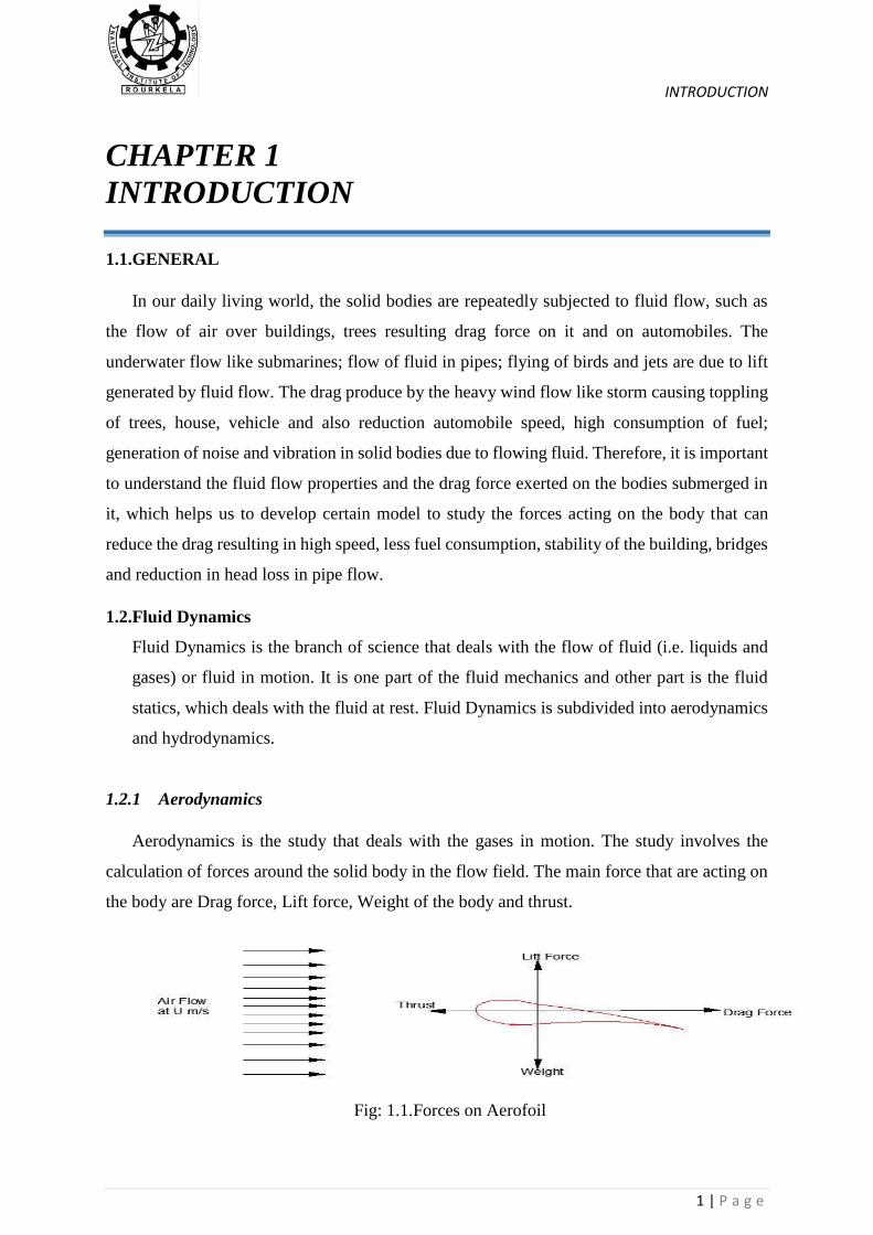
1.2.1 Aerodynamics

Aerodynamics is the study that deals with the gases in motion. The study involves the

calculation of forces around the solid body in the flow field. The main force that are acting on

the body are Drag force, Lift force, Weight of the body and thrust.

Fig: 1.1.Forces on Aerofoil

CHAPTER 1

2 | P a g e

Drag force affects the speed and fuel consumption for the most of automobiles. Therefore

to achieve higher speed with low fuel consumption drag force must be reduce either by

streamlining the bodies or by giving the smooth contour in front of the vehicle (Gorsche,

2001).

1.2.2 Hydrodynamics

Hydrodynamic deals with the liquid (generally water) in motion and the forces acting on

it. It includes the calculation of properties like density, flow velocity, pressure.

Flow velocity is the free stream velocity i.e. the fluid velocity that’s approaching the body

immersed in it. It is denoted as 𝑈𝑠 or V. when flow is along x-axis it is symbolize as ’u’

because u represent the x-component. For the convenience flow velocity is assumed to be

uniform and steady.

1.3 Flow Classification

The grouping or categorising of Fluid flow in given class with respect to flow speed, fluid

properties in the flow field with time and space and with given constant like Reynolds

number(Re), Mach number is termed as the flow classification. The flow of fluids are classified

as Uniform and Non-uniform flow, Compressible and Incompressible flow, Steady and

Unsteady flow, Laminar flow, Transient flow, Turbulent flow, subsonic flow, Supersonic flow,

transonic flow, hypersonic flow and different flow regimes.

1.3.1 Uniform and Non-uniform Flow

Flow is said to be Uniform, when the velocity of flow remain constant at any given time

along the length of direction of flow (i.e. with space).

Mathematically,

(𝜕𝑉

𝜕𝑠)

𝑡=𝑐𝑜𝑛𝑠𝑡𝑎𝑛𝑡= 0

Where 𝜕𝑉= change of velocity

𝜕𝑠= length of flow in the direction S

Non-uniform Flow is the flow of fluid in which the velocity varies at any given time with

the space.

Mathematically,

(𝜕𝑉

𝜕𝑠)

𝑡=𝑐𝑜𝑛𝑠𝑡𝑎𝑛𝑡≠ 0

INTRODUCTION

3 | P a g e

1.3.2 Compressible and Incompressible

Flow of fluid in which fluid density varies from point to point is said to be Compressible

Flow.

ρ ≠ constant

Incompressible Flow is the flow where density of the fluid is constant throughout the

flow.

ρ = constant

1.3.3 Steady and Unsteady Flow

The kind of flow where the fluid properties like density, pressure, velocity, etc.at a

point does not varies with time.

Mathematically,

(𝜕𝑉

𝜕𝑡)

𝑥0,𝑦0,𝑧0

= 0, (𝜕𝑝

𝜕𝑡)

𝑥0,𝑦0,𝑧0

= 0, (𝜕𝜌

𝜕𝑡)

𝑥0,𝑦0,𝑧0

= 0

Where (𝑥0, 𝑦0, 𝑧0) is a fixed point.

Unsteady Flow is the flow of fluid where the fluid properties changes at a given point

with time.

Mathematically,

(𝜕𝑉

𝜕𝑡)

𝑥0,𝑦0,𝑧0

≠ 0, (𝜕𝑝

𝜕𝑡)

𝑥0,𝑦0,𝑧0

≠ 0, (𝜕𝜌

𝜕𝑡)

𝑥0,𝑦0,𝑧0

≠ 0

1.3.4 Laminar, Transient and Turbulent Flow

The fluid flow in which the fluid particle follow stream line path of flow, and the stream

lines are parallel to each other. These kind of flow is termed to be laminar flow.

The turbulent flow is generally known by the formation of wakes or eddies behind the solid

object in the flow. The fluid particles follow a zigzag flow path. Turbulent flows occurs

due to the interaction of inertia and viscous term in the equation of Momentum.

The flow are categorised by the Reynolds number as follows:

When Reynolds number (𝑅𝑒) is less than 2200; the flow is said to be laminar flow.

Reynolds number more than 4000 is known to be turbulent flow.

CHAPTER 1

4 | P a g e

The flow is said to be transient when the Re value is in between 2200 and 4000.

1.3.5 Sub-sonic, Sonic, Super-sonic flow

For compressible flow Mach number a dimensionless parameter play an important role

in classifying the flow. Mach number is the square root of ratio of inertia force to the elastic

force or it is the ratio of velocity of fluid / body moving in fluid to the velocity of sound in

the fluid. Mathematically

𝑀 =𝑉

𝐶

Where

V is the velocity of fluid

C is the velocity of sound in the fluid

A flow is known as Sub-sonic if the flow velocity is less than that of the sound i.e. M<1.

When the velocity of the fluid equals that of the sound and Mach numbers attains the value

of 1, the flow is termed as sonic flow. Super-sonic flow is the flow which velocity is more

than that of the Sonic flow i.e. value of Mach number M>1.

1.4 DRAG FORCE

When a body is subjected to the flowing fluid or the body is moving within the fluid, an effective

opposing force is exerted on the body by the fluid, this restrictive force felt by the body is known as

Drag Force. The drag force is always along the direction flowing fluid.

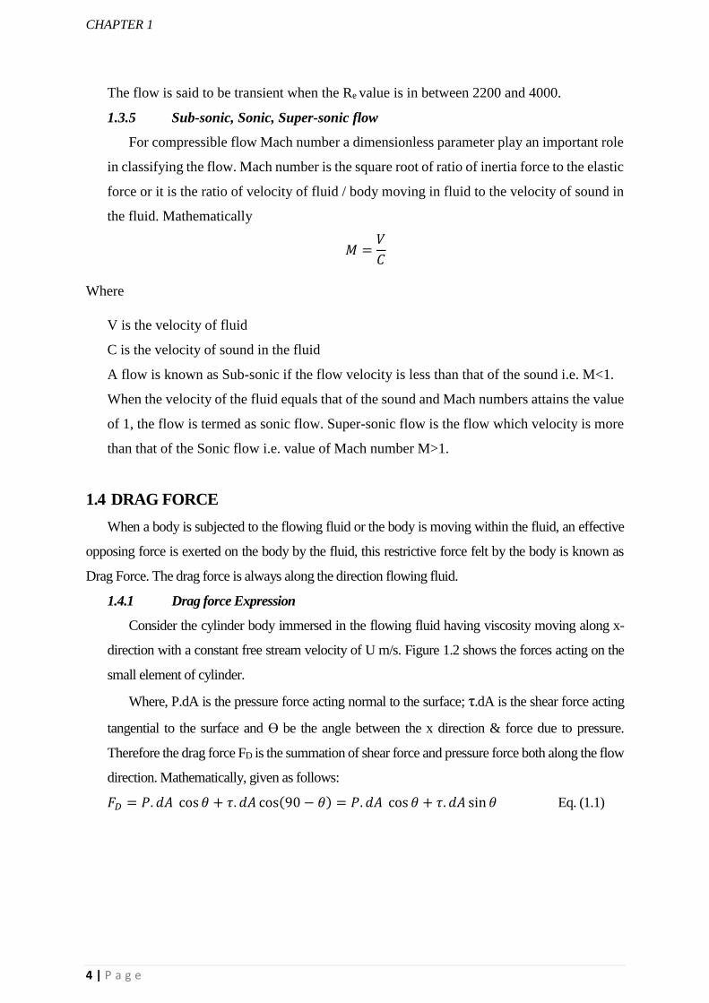
1.4.1 Drag force Expression

Consider the cylinder body immersed in the flowing fluid having viscosity moving along x-

direction with a constant free stream velocity of U m/s. Figure 1.2 shows the forces acting on the

small element of cylinder.

Where, P.dA is the pressure force acting normal to the surface; τ.dA is the shear force acting

tangential to the surface and Ɵ be the angle between the x direction & force due to pressure.

Therefore the drag force FD is the summation of shear force and pressure force both along the flow

direction. Mathematically, given as follows:

𝐹𝐷 = 𝑃. 𝑑𝐴 cos 𝜃 + 𝜏. 𝑑𝐴 cos(90 − 𝜃) = 𝑃. 𝑑𝐴 cos 𝜃 + 𝜏. 𝑑𝐴 sin 𝜃 Eq. (1.1)

INTRODUCTION

5 | P a g e

. .̇ 𝐹𝐷 = ∫ 𝑃 cos 𝜃 𝑑𝐴 + ∫ 𝜏 sin 𝜃𝑑𝐴 Eq. (1.2)

Fig. 1.2: Drag force on the Cylinder

The pressure force on the cylinder surface is also known as pressure drag or form drag and the

shear force is called as skin drag or friction drag or shear drag. The total drag for the moving fluid over

the stationary body can be calculated by the following equation:

𝐹𝐷 =1

2𝐶𝐷𝐴𝜌𝑈2 Eq. (1.3)

Where, CD =coefficient of drag,

ρ = fluid density,

A=projected area,

U= free stream velocity.

1.4.2 Coefficient of Drag

The coefficient of drag is the ratio of total drag to term(1

2𝐴𝜌𝑈2). It is dimensionless and

depends on geometry of the body, stream velocity, Reynolds No. and angle of impact.

1.5 NUMERICAL MODELLING

In our daily life we come across many fluid flow problem which are being passed un-

noticed. We travel lots from one place to other through various means of transportation like

bus, trains, cars, motor-cycle, airplane, ship etc. I’m sure everyone has experienced Most of

the numerical models are based on Computational Fluid Dynamics (CFD), which involve

numerical methodology to solve heat transfer, fluid flow problem and chemical reaction by the

means of software packages for the simulation in the computers.

CFD is a very magnificent and powerful technique with vast field of application in both

industrial and non-industrial areas. The availability of user friendly graphical interface software

package like ANSYS INC. and high performance computers has increased the interest among

CHAPTER 1

6 | P a g e

the researchers and engineers to work on the simulation based on CFD. The technique or

methodology applied by CFD can be used in various field like hydrodynamics of submarine,

ships; aerodynamics of automobile, airplane; flows in rivers, channel, oceans; weather

prediction; wind load over the building; diffusers; distribution of pollutants. The CFD works

with the certain group of code and numerical algorithm to solve the problem associated with

the fluid flow. There are three codes that the user must follow to get the desired solution. The

code involves are: (i) Pre-processing;

(ii) Solver;

(iii) Post-processing

1.5.1 Pre-processing

In a CFD program it plays a role of input part or initiating part for the flow problem.

There are few steps that the user must carry out which are as follows:

Geometry formation, constituting the computational domain

Sub-dividing the domain into small number of cells

Applying suitable model required as per the physical phenomena

Defining the fluid properties

Giving boundary condition

1.5.2 Solver

The software like CFX/ANSYS, FLUENT, PHOENICS, and STAR-CD uses finite

difference formulation technique which is one of the three numerical method that based on the

CFD solver. The numerical technique are: Finite volume method; Finite element method and

Finite Difference method. The steps that involves in the solver are

Fluid flow governing equation are integrated over the cells of domain

Discretization: the integral equation are converted into a algebraic equations

Interpolation of algebraic equation is done for the solution

The complex physical phenomena and non-linear equation are solved iteratively.

TDMA (tri-diagonal matrix algorithm) and SIMPLE algorithm are used to solve the algebraic

equation line-by-line and to provide a good linkage between pressure and velocity.

1.5.3 Post-processing

This act as the last procedure in the CFD programing tool. It is an interesting tools of

recording the results with versatile visualization technique, high graphics and operator-friendly

interface.

It includes:

INTRODUCTION

7 | P a g e

Display of mesh and domain

Contour visualization

Plotting vectors

Surface plot

1.6 Importance and Objective of the Research

The current work is focus on the drag force and drag coefficient over the cylindrical body

mainly circular. Mostly drag is an unwanted force that we have to dealt with, it reduces speed

of the vehicle and increases the fuel consumption, in pipe flow it decreases the flow speed and

heavy winds can even disrupt the high building. Therefore it is important for us to diminish the

effect of drag force or reduce it for the better speed of the automobile, safety of the buildings

and have good fuel efficiency. The study explains about the factors that affects the value of

drag on the circular cylinder and suggest a suitable methods to reduce it. There are two

approaches that have been employed in this study to find the drag force over the cylindrical

bodies and they are: Numerical and Experimentation. For the Numerical study, ANSYS

FLUENT is used and pressure distribution technique for the experimentation. The calculation

drag requires great concern about the parameters that it depends on like velocity of the flow,

surface roughness of the body, projected area of the body i.e. length and diameter for the

circular cylinder. The aim of the study are listed below:

1. Numerical methods:

To find the drag force under varying free stream velocity, changing diameter and

length of cylinder, taking different surface roughness.

The visualization of pressure contour and velocity contour distribution for the flow.

To measure the coefficient of drag for different flow velocity and Reynolds No.

taking liquid water as the flowing fluid.

2. Experiment approach:

Using pressure method to calculate the drag force for various flow, different

diameter of the cylinder and varying roughness.

To measure the coefficient of pressure on cylinders for varying parameter like

velocity and surface roughness.

To purpose a correlation for the drag force.

Finally comparing the results obtain from the above two mentioned methods and the

predicted value produced by the developed correlation.

CHAPTER 1

8 | P a g e

1.7 Organisation of Thesis

The paper contain seven different chapters. General introductory part is provided in

Chapter 1, literature review is briefly described in Chapter 2, numerical models are detailed in

Chapter 3, numerical analysis and experimental works are explained in Chapter 4, the results

and discussion are part of chapter 5, the correlation was being developed in chapter 6 and lastly

conclusions is drawn, future scope and references are delivered in Chapter 7.

Chapter-1 the introduction of fluid mechanics, flow classification, various nature of drag force

with its effect on the drag coefficient and distribution of pressure and the aim of the research

are detailed.

Chapter–2 shows the summary of literature review as per the date-to-date research work have

been carried out related to the prediction drag force either by numerical or experimental

methods considering different parameter like drag coefficient, pressure coefficient, different

shape and size of the body, and surface roughness.

Chapter–3 describes the numerical model with details of governing equation: conservation of

mass, momentum and energy. The various method of investigation are outlined. The parameter

includes the cylinders of different radius, varying roughness and change in the free stream

velocities.

Chapter- 4 presents numerical analysis. The analysis of drag coefficient (CD) i.e. the ratio of

drag force to 0.5𝜌𝐴𝑣2. Thus, the coefficient of drag is a function of drag force (FD). The drag

force is calculated by using the ANSYS model. The standard k-Ɛ model is applied to get the

solution. The different contour are obtained in the CFD post. The different boundary condition

are used and different inlet velocity are chosen according to the experimental information. The

surface roughness and fluid properties are assigned at the boundary condition.

Chapter- 5 represent the experimentation procedure and the equipment set up. Pressure

distribution technique is employed to find the coefficient pressure and then it is used to

calculate the CD over the cylinder and finally the drag force is obtained.

Chapter -6 gives the results, plots that are being found and obtained by the use of different

method described in the chapter 4 & 5. The comparison is drawn for the different results and

solution. The angle is noted down where the flow get separated. The correlation is being

generated by applying the dimension analysis. The drag force is expressed as:

(i) Dimensional terms: 𝐹𝐷 = 𝐶(𝑉𝑛1)(𝐷𝑛2)(𝑘𝑛3)

(ii) Dimensionless terms: 2𝐹𝐷

𝜌𝐴𝑉2= 𝐶(𝑅𝑒)𝑛1(

𝑘

𝐷)𝑛2

INTRODUCTION

9 | P a g e

The developed correlation is used to predict the drag force over the cylindrical bodies for

varying parameter involving the geometry of the cylinders and flowing fluid property. The

predicted drag is compared with numerical and experimental value.

Chapter-7 holds the summary and conclusion of the present study. It describe the characteristic

of drag, and shows how drag change with change in the system parameter. Future scope of the

study are outlined.

References are provided at the end of the paper.

CHAPTER 2

10 | P a g e

CHAPTER 2

LITERATURE STUDY

2.1 GENERAL

A literature covers varieties of theories and experimental studies both analytical and

numerical. In this we will have a quick review that will focus on important aspect of theories

that has been develop constantly in these past years. The topic contains the past research works

that has been the applied for the study of science theory and for the betterment of livelihood.

The study of forces acting on the solid body submerged in the fluid (air or water) is of great

importance in our daily living life. A fine piece of work and great effort has been done by the

researchers in the past. The combination of coefficient of pressure drag and the coefficient of

friction drag form the coefficient of drag or drag coefficient. Drag coefficient is function of

various factor like relative velocity of flow, relative surface roughness, shape and size of the

object, orientation of the body with the flow and the properties of the fluid. The flow in pipe

or the flight of a bird or plane and the speed of the moving vehicle all of these are mostly

depended on the drag coefficient, such facts brought the importance and has motivated many

researchers to carry out the study on the various parameter involving the pressure distribution

around the body, physical properties of fluid and solid. Therefore this chapter will describe the

drag force and how it varies with the geometric parameter of the body and the flow speed of

the fluid.

2.2 Pre-Study on Numerical Analysis

M.N. Zakharenkov (1997) the beginning of separated partition is considered on the premise

of a numerical arrangement of the full Navier-Stokes equation. Fluxes of vortices with

distinctive signs produced with double the recurrence of cylinder oscillating from the cylinder

to the external surface of a confined fluid layer as concentric rings. Close to the critical layer

between the connected layer and the primary flow these rings are torn and pleated to the areas

of isolated vortices of the comparing sign. The type of confined isolated vortices is like that of

vortices starting from a circular cylinder at rest in a uniform flow. Movement of the flow to a

non-symmetric structured with Karman vortex road created at a Reynolds number (taking into

account the radius) more prominent than 17 is uncovered. This critical Reynolds number is

littler than that for a circular cylinder with no velocity in a stream having viscosity (where

LITERATURE WRITNG

11 | P a g e

Re=20 has been found as the value of critical Re) and relates to the Reynolds number

extrapolated from the critical value for the stationary cylinder by expanding the radius by the

appended layer thickness. The flux vortices from the cylinder surface quickly into the separated

area diminishes as the cylinder frequency increments with oscillation. Generation of vorticity

on the exterior surface was mainly due to flow potential violation in unattached separation area.

Guo-ping and Shih (1999) A hybrid finite difference and vortex method (HFDV), in light of

the domain decomposition method (DDM), is utilized for computing the stream around a

turning circular cylinder at Reynolds number Re=1000, 200 and the angular-to-rectilinear pace

proportion α=(0.5, 3.25) separately. A completely understood implicit equation was solved

using third-order finite difference method, and the derived expansive wide band matrix was

solved by an exceptionally proficient altered inadequate LU disintegration conjugate

inclination system gradient (MILU-CG). The long-lasting, completely created highlights about

the varieties of the vortex designs in the wake, and additionally the drag and lift constrains on

the barrel, are given. The computed streamline shapes are in great concurrence with the

tentatively imagined stream pictures. The presence of the basic state is affirmed once more,

and the single side shed vortex design at the basic state is indicated surprisingly. Additionally,

the enhanced lift-to-drag power proportion was found close the critical state.

Mittal and Raghuvanshi (2001) we have seen via analysts before that vortex shedding behind

round cylinder can be modified, and now and again smothered, more than a constrained scope

of Reynolds numbers by fitting arrangement of a second, much littler, "control" cylinder in the

close wake of the principle cylinder. For such circumstances the results are displayed by the

numerical calculations. The Navier–Stokes equation for incompressible flow was discretised

by the application of finite element method. At a relative location of primary and control

cylinder with the less Reynolds numbers, the vortex shedding from the primary chamber is

totally stifled. Amazing assertion was seen between the current processing’s and experimental

discoveries of different scientists. With an end goal to clarify the component of control of

vortex shedding, the stream wise pressure variation near the shear layer of the primary cylinder

was measured and analysed for different cases, with the presence of control cylinder and

without the control chamber. The shear layer is balanced by the positive pressure gradient

produced by the control cylinder when the vortex shedding close to wake is smothered.

CHAPTER 2

12 | P a g e

Yan-Xing et.al (2004) a numerical approach was performed to explore the flow impelled by a

sphere moving along the axis of a rotating cylinder which was packed with the fluid having

viscous. Three-dimensional incompressible Navier–Stokes mathematical statements are

fathomed utilizing a finite element technique. The goal of this study is to analyse the highlight

of waves produced by the Coriolis force at moderate Rossby numbers and that what exactly

degree the Taylor–Proudman hypothesis is legitimate for the rotating viscous flow at low

Rossby number and substantial Reynolds number. Computations have been attempted at the

Rossby numbers (Ro) of 1 and 0.02 and the Reynolds numbers (Re) of 200 and 500. At the

point when Ro=O(1), inertia are shown in the rotating sphere. The effects of the Reynolds

number and the proportion of the sphere radius and that of the revolving cylinder on the flow

structure are inspected. At the point when Ro << 1, as anticipated by the Taylor–Proudman

hypothesis for inviscid flow, the alleged 'Taylor section' is too produced in the thick fluid flow

after a developmental course of vortical flow structures. The beginning development and final

arrangement of the 'Taylor section' are displayed. As indicated by the present estimation, it has

been verified that major hypothetical articulation about the turning flow of the inviscid fluid

might still roughly foresee the turning flow structure of the viscous fluid in a certain Reynolds

number regime.

Yang and Shao (2005) we show a drag part conspire for surfaces of different harshness

densities. The aggregate drag is apportioned into three segments: a weight drag, a skin drag

because of force exchange to the surfaces of rough components and a surface drag because of

energy exchange to the ground surface. We present a viable frontal range record to describe

the shared shielding impact of harshness components on drag segment and propose a system

for the count of the drag parts. The drag segment plan is then connected to the figuring of mass

amounts, for example, harshness length and zero-plane removal stature. The outcomes are

contrasted and wind-tunnel estimations. Harshness length is found to increment with frontal

area index λ to a greatest at about λ= 0:2, and afterward diminishes with λ. This finding is in

concurrence with perceptions. The drag segment plan has applications to concentrating on

scalar trade in limit layers over unpleasant surfaces, for example, urban limit layers.

Jones and Clarke (2008) flow over the sphere was investigated by the application of fluent

code of computational fluid dynamics for the various flows. The type of flows that are

considered for the simulation of purpose are steady-state and time-dependent laminar flow for

the Re value of 100 and 300 respectively, and for the flow to be turbulent Reynolds number

are taken as 104 and 106 .this study shows the accuracy of code and to understand flows over

LITERATURE WRITNG

13 | P a g e

the bluff body, like submarine and other vehicles. The results are contrasted both computational

and experimental and we have seen that the numerical approach on the fluid characteristic for

sphere gives comparatively good result

Niels and Zahel (2010)This article depicts the use of the relationship based transient model of

Menter et al. in blend with the Detached Eddy Simulation (DES) approach to two cases with

huge level of flow division ordinarily considered hard to simulate. Firstly, the flow is solve on

circular cylinder from Re = 10 to 1 × 106 giving drag crisis. The solution indicate great

quantitative and subjective concurrence with the conduct seen in investigations. This case

demonstrates that the methods works easily from the laminar cases at low Re to the turbulent

cases at high Re. Besides, the flow is processed more than a thick air foil at high angle, for this

situation the DU-96- W351 is considered. These reckonings demonstrate that a transient model

is expected to acquire right drag forecasts at low angle, and that the blend of transient and the

DES system enhance understanding in the profound slow down area.

.Karim and Rahman (1996)This paper presents limited volume system in view of Reynolds-

found the middle value of Navier-Stokes (RANS) comparisons for calculation of 2D

axisymmetric stream around uncovered submarine frame utilizing unstructured network. The

body utilized for this intention is a standard DREA (Defense Research Establishment Atlantic)

exposed submarine structure. Shear Stress Transport (SST) k-ω model has been utilized to

mimic turbulent stream past the structure surface. At last, figured results utilizing unstructured

matrix are contrasted and those utilizing organized network furthermore with distributed

exploratory estimations. The registered results demonstrate great concurrence with the test

estimations.

2.3 VARIATION OF DRAG COEFFICIENT FOR DIFFERENT RANGE

OF REYNOLDS NUMBER

Many researcher has done good work and research to explain how the drag coefficient

of the body varies with the change of Reynolds number. Some of the research predict the value

of drag Coefficient for different range of Reynolds number for circular cylinder, wavy cylinder,

square cylinder etc.

Roshko (1961) carried out the measurements on a large circular cylinder in a pressurized wind

tunnel for Reynolds numbers ranges from 106 to 107 and showed that at high Reynolds number

transition of drag coefficient increases from its low supercritical value to a value of 0.7 at Re =

CHAPTER 2

14 | P a g e

3.5 x l06 and then the values are constant. The definite vortex shedding occurs, with Strouthal

number 0.27 for the Reynolds number more than 3.5 x 106.

Achenbach and Heinecke (1981) they investigated vortex shedding phenomena and effect of

relative roughness on drag for the flow past circular cylinder in the range of Reynolds number

6×103 to 5×106.

Shih and Wang et al (1993) the effect of Reynolds number on the distribution of pressure is

studied at low value of Re. The model of three different relative roughness for cylinder was

tested on the low turbulence pressure tunnel. The test showed how the coefficient of pressure

depends on Re and roughness, with the increase in roughness the pressure coefficient happens

to be independent of Re when the Re is above 2x106.

P Catalano, Wang and Parviz (2003) The viability and accuracy of large-eddy simulation

(LES) with wall modeling for high Reynolds number complex turbulent flows is investigated

by considering the flow around a circular cylinder in the supercritical regime. A simple wall

stress model is employed to provide approximate boundary conditions to the LES. The results

are compared with those obtained from steady and unsteady Reynolds-averaged Navier–Stokes

(RANS) solutions and the available experimental data. The LES solutions are shown to be

considerably more accurate than the RANS results.

K. Mahesh, and Moin (2003) DNS was performed at cylinder Reynolds numbers of 20, 100

and 300, and LES was performed at a Reynolds number of 3900.The results obtained from the

Re= 3900 LES. Global variables such as recirculation length, separation point, and profiles of

the mean velocities and turbulent Reynolds stresses are seen to be in good agreement with

experiments.

Lee and Cheol (2004) flow control method has been investigated. The flow control method

that had been proposed are: The first method that controlling the shear layers separation and

the second method controlling surface flow over the bluff bodies. A small rod was setup on the

upstream of the bodies to control the separation of shear layers, while to control the surface

flow different Reynolds number ranges from 1.5 ×104 to 6.2×104 was set.

Timmer and Schaffarczyk (2004) The modified airfoil was studied and wind tunnel

measurement was performed and found that the higher Reynolds numbers had a positive effect

on the section roughness sensitivity, due to thinner and more stable boundary layers. The use

of wrap-around Carborundum 60 roughness led to significantly more loss of maximum lift than

LITERATURE WRITNG

15 | P a g e

the use of zigzag tape, due to increased boundary layer thickness. The maximum lift/drag ratio

decreased with increasing Reynolds number.

Mittal and Singh (2005) a numerical model solving the unsteady incompressible two

dimensional Navier-Stokes equations was applied to studied the instability of shear layer and

drag effect over the flow past a circular cylinder for Re ranges from 100 to 107.

Triyogi et al. (2009) used of passive control method to reduce the drag over the I-type small

cylinder was carried out, the cutting angle of Ɵ𝑠 = 650 is provided as passive control.

M. Sami and M. Salih (2009) The computational results for streamline patterns, vortices

contours, velocity distributions, and drag and lift force coefficients are compared with those of

the experiments to examine the effect of mesh size on the numerical simulations using the three

turbulence models.

Chang-yue et. al. (2010) Numerical investigation of the compressible flow past a wavy

cylinder was carried out by means of an LES technique for a free-stream. The mean drag

coefficient of the wavy cylinder is less than that of a corresponding circular cylinder with a

drag reduction up to 26%.

Larose Guy and Steve (2012) presented the investigation of reducing drag for a speed skater

due to the turbulence effect of wind. The different range of Reynolds numbers are considered

for calculating the drag coefficient. The flow separation over circular cylinder results in high

dynamic drag force.

Butt and Egbers (2013) Flow over circular cylinders with the hexagonal patterned surfaces is

investigated and discussed taking Reynolds numbers ranging from 3.14E+04 to 2.77E+05 into

consideration and the well-known characteristics of flows over rough surface. The

investigations revealed that a patterned cylinder with patterns pressed outwards (can be referred

as hexagonal bumps) has a drag coefficient equal to 65% of the smooth one.

M. Mallick and A. Kumar (2014) a comparison has been made between the co-efficient of

drag obtained by two methods. The co-efficient of drag obtained by weighing method is more

accurate than those obtained from pressure distribution method. The drag force increases with

increase in diameter of the cylinder. Also, for a cylinder of particular diameter, drag force has

been found to increase with increase in air velocity.

CHAPTER 2

16 | P a g e

2. 4 REDUCTION OF DRAG FOR A CIRCULAR CYLINDER

Lemay and Bouak (2001) the value obtained for the single cylinder is about 32% less than of

the reduction of mean drag coefficient by claimed other authors. This result gained at Re values

ranging from 1.5×104 to 4.0×104,S/d=2.55,and ds/d=1.25.

Grosche and Meier (2001) an experimental study has been carried on the bluff body and its

aerodynamics. Paper includes the research for the drag reduction as follows: (a) providing

passive ventilation on the wake region of the body in order to reduce the drag over the body,

(b) optimization of shape can efficiently reduce the drag as well as trailing of vortices for the

automobiles, (c) understanding the cause of loud noise and its source for the high speed trains,

(d) the separation of flow are delayed on active flow control.

Tsutsui and Igarashi (2002) reduction of drag around the circular cylinder submerged in the

air stream was investigated. It show that the pressure distribution around the small cylinder as

symmetry all over the surface. The formation of quasi-static vortex among the I-type small and

large cylinder, results in zero or negative value of pressure coefficient at the front portion of

cylinders, while the pressure coefficient (𝐶𝑝) attains the maximum value of 0.1-0.2 at the

region where the separated shear layer gets reattached. The different I-type small cylinders are

used to reduce the drag over the large cylinder, implying passive control method. The I-type

cylinders are formed by cutting them at certain angle (Ɵ) parallel to their axis. The different

cutting angle are: θ=0◦ (circular), 10◦, 20◦, 30◦, 45◦, 53◦ and 65◦. The Reynolds number was set

as per the free flow velocity and the diameter of the cylinder i.e. Re =5.3x104. The cutting angle

θ =650 provide good results in the reduction of drag over the large circular cylinder placed at

downstream as compared with the other cutting angles and gives 0.52 times less drag than that

of a single cylinder.

Alma and Moriya (2003) the two cylinders are suited side-by-side for studying the

characteristics of vortices, varying force of fluid, and wake formation behind the object. The

different shape of cylinders are considered i.e. two circular cylinder as well as two square

cylinder for the test. The vortex shedding in transitional flow was found to have a dominating

character in both different shape of cylinders. For different gap spacing (T) between cylinders

of diameter (D) considered as T=D>0:20 in which lift force was found to be repulsive on both

case, while in T=D¼0:10, the lift force acting on the cylinder results inward narrow wake and

outward wake on the other cylinder.

LITERATURE WRITNG

17 | P a g e

Pasto (2008) the laminar and turbulent flows are considered to study the behavior of circular

cylinder vibrating freely. The experimentation was done on the wind tunnel with varying

roughness of cylinder and mass-damping. The vortex-induced vibration was noticed on the

cylinder in the critical regime.

Mohammad and Islam et al. (2010) in the fluid mechanics and aerodynamics, drag force has

important role to play for all type of object moving in the fluid. In some circumstance, drag

can be undesirable for causing structural damage, consuming more power, decreasing speed

for automobile, and high consumption of fuel. Therefore, it’s important for the researcher to

reduce drag by adapting or changing different parameter for different object. In this topic, a

circular ring has been attached to the circular cylinder for reducing the drag. The drag force

was obtained by external balance method, first drag for the cylinder without ring was recorded

than with the ring attached to cylinder was calculated. The experimentation shows that the drag

on the cylinder without ring was less than that of the cylinder with the ring this was because

the ring increases the projected area of the plain cylinder and results in more attached flow.

The maximum percent reduction of drag was found to be 25%, when ring was 1.3D and

approximate value of aspect ratio was 12 for the cylinder.

Tamayol (2013) the arrays of cylinder placed in the micro channel was experimented to

understand the pressure drop on these cylinders. The geometrical parameters like height and

width of the channel, diameter, and spacing among the cylinders. The Deep Reacting Ion

Etching (DRIE) technique was used to verify the model and the pressure drop was measured

by applying nitrogen flow for the span of 0.1 to 35 sccm. The performed research suggest the

minimum pressure drop for the higher micro-cylinder diameter.

M. Mallick and A. Kumar (2014) the study was carried out on the cylindrical bodies with

varying cylinders diameters, surface roughness and air velocity. A comparison for the drag co-

efficient and pressure distribution between the smooth and rough surfaces of the cylinders are

presented. In the smooth surface cylinder, the separation angles for different diameter of

cylinder calculation are found to be around 80°~90° on either side of the cylinder from the

upstream stagnation point.

CHAPTER 2

18 | P a g e

2.5 PRE-RESEARCH AND EXPERIMENTATION DONE ON BLUFF BODIES AND

THEIR DRAG COEFFICENT

The study includes different types of cylindrical objects and various parameter with

surface roughness. The review describes the effect and nature of drag force on the bluff bodies

and suggests a suitable method to reduce its effect to achieve fine efficiency of the body moving

in a fluid.

Alridge and Hunt (1978) a porous nature of circular cylinder was considered and fitted among

the hemisphere solid with such arrangement the drag force and drag coefficient was measured

for the Re value varying from 104 to 2.6x105 and five aspect ratio value from 7.92 to 2.67. The

recorded data and the calculation described that the increasing aspect ratio, increases the drag

coefficients. Flow passing the cylinders are visualized and weak vortex are seen behind the

solids. Therefore, if we can decrease the aspect ratio of the bodies which will ultimately reduce

the drag affecting the solid bodies.

Protas (2002) we invested in distinguishing the physical components that go with mean drag

alterations in the barrel wake stream subject to turning control in this paper. We contemplated

basic control laws where the snag turns pleasingly with frequencies differing from half to more

than five regular frequencies. In our examination we mulled over the solution of the numerical

re-enactments at Re=150. All the re-enactments and analysis were performed utilizing the

vortex system. We affirm the concerning mean drag lessening at higher compelling

frequencies. The principle result is that progressions of the mean drag are accomplished by

altering the Reynolds stress and the related mean stream amendment. It is contended that mean

drag diminishment is joined with control driving the mean stream toward the precarious the

fundamental stream.

Richter and Petr (2012) for the particle study, different shape particles are considered such as

spherical and non-spherical. The fluid and heat was supplied over the particle of non-spherical

shape and the drag was noted. The approach in semi-exact models, distributed relationships

for drag coefficient and nusselt number are enhanced and the exactness of terminations

produced for drag coefficient and nusselt number is examined in an examination with

distributed models.

LITERATURE WRITNG

19 | P a g e

2.5.1 Cylindrical Bodies

Balachander and Mittal (1995) depicted the impact of three dimensional on the drag and lift

force of ostensibly two-dimensional cylinder which is helpful to portray the variety of

numerical solutions between two dimensional and three dimensional examination.

Laurent and Michel (2007) to study the wake of cylinder, active control method was followed

for the Re value of 100 so that the stream is in the laminar. The results of the examination

indicate the reduction of mean total drag as the managing function of time, harmonic radial

velocity of revolving cylinder.

Z.C. Zheng et.al. (2008) experimented frequency range or recurrence extents are to be

considered for both close and far from the common recurrence of wake vortex shedding.

Thusly, the impacts of recurrence lock-in, superposition and de augmentation on lift and drag

are changed in light of the spectrum investigation on past time for drag and lift. A transverse

oscillating or wavering cylinder in a constant flow or stream is displayed to explore frequency

impacts of flow instigated wake on drag and lift forces of the cylinder. Most likely,

demonstrated unsteady or fluctuating fluid are simulated utilizing an inundated boundary

technique in an stable Cartesian cell to foresee the stream structure around the cylinder and

visualize how the integration and coordination of surface pressure and shear circulations gives

lift and drag on the wavering cylinder.

2.6 SURFACE ROUGHENING OF CYLINDRICAL BODIES

The common method used to diminish the drag over the bluff bodies like cylinder,

sphere is applying surface irregularity or roughness. Many researcher has shown how the drag

reduces for the sphere e.g. dimpled surface of gulf ball, fuzz on tennis ball etc. It delays the

flow separation, narrowed the wake and consequently reduce the pressure drag for the

roughened sphere surface.

Merrick and Girma (1982) a few troubles are experienced while analysing the super-critical

regime with high Reynolds number for the stream over surfaces curvature of a building in a

low velocity wind tunnel because of the sensitive to Re. Surface harshness on the exterior of

the cylinder can influence the area of the detachment point and the degree of the wake on the

rear face, whereupon the wind-incited reactions are subordinate. This study endeavours to

control the stream around a ring-shaped cylinder through the use of counterfeit surface

roughness over the outside of the cylinder. Later, the measure of the counterfeit roughness will

be related with Re variance through a computational fluid flow wind stream analysis. These

CHAPTER 2

20 | P a g e

relationships will help in selecting the suitable manufactured roughness that will bring the

boundary layer translation at a position resembling to super-critical Re examined. Some

roughness examples were tried over the cylinder, which were subjected to air flow with change

in the turbulence magnitude. Estimations of pressure dispersion over the body exterior have

been acquired for the Re limit of 1x104 to 2x105 in a BLWT. The outcomes are directly applied

on the models in low speed BLWTs where super-critical stream flow attributes are foreseen.

They portrayed the impact of surface irregularity for stream flow over a body at high Reynolds

number utilizing wind tunnel.

Harvey and Bearman (1993)the pressure dispersion over the cylinder was modified by giving

the irregularity or harshness around the surface of the body like providing dimpled exterior,

roughening by sticking sand paper of different grade.

Nicolas and Lyotard (2007) utilizing a constant ultrasound method, estimating the speed of

sphere made of steel falling freely through fluid. Then again, arbitrary surface irregularity

and/or high fixation polymer arrangements decreases the drag bit by bit and prevent the drag

crisis. We additionally show a subjective contention which ties the drag diminishment saw in

low fixation polymer results to the Weissenberg number and ordinary stress distinction.

2.7 DISTRIBUTION OF PRESSURE

Josue and Libii (2010) Handy activities were prepared and examined in a subsonic wind tunnel

to survey the pressure circulations around a round cylinder in the flow. They permitted

understudies to gather their own information and utilization them to understand how the

pressure over the cylinder surface varies with two unique parameter: the area of a given point

along the outline of the mid-cross cylinder segment and the value of the Reynolds number of

the stream. Plotted information delivered curves fundamentally the same to those in the

literature writing. Detailing of investigated solution showed how viscous flow behaves in the

upstream portion of body in contrast to its downstream portion. The impact of the Reynolds

number on the capacity of the viscous flow to recoup pressure on the downstream was

illustrated.

Rasim and Hodzic (2011) in fluid mechanics, flight science or aerodynamics studies relative

movement of air around the body from hypothetical and exploratory aspect. These two

methodologies won't give the same results if we utilize hypothetical laws taking into account

perfect ideal procedure, on the grounds that exploratory examination is the presentation of real

and genuine Process. Wind passage tunnel is an instrument that can be utilized for trial

examination. Consequences of pressure circulation around the cylinder, profited by exploratory

LITERATURE WRITNG

21 | P a g e

examination in wind tunnel are introduced in this study. Produced experimented results are

contrasted and hypothetical results, and on the premise of that information certain conclusions

are made.

Rakibul Islam (2013) a numerical study was carried on the circular cylinder at rest applying

Favre-averaged Navier-Stokes equation and finite volume method was followed to solve the

desired problem at Re value of 105 for the flow motion. Numerical perceptions and simulated

solution are checked with the test results and with experiment works of different analysts.

Distinctive flow phenomena, for example, flow division, pressure dissemination over the solid,

drag and so on are additionally learned at diverse boundary conditions. In the event of smooth

solid, the division plots for experimentation figuring are discovered to be around 80~90° in

either side of the solid cylinder from the upstream stagnation point. The drag coefficients for

smooth solid surface are 0.771 and 0.533 for experimentation count separately and consequent

changes in drag because of induced surface irregularity are illustrated. The critical surface

irregularity was discovered to be around 0.004 with drag coefficient of 0.43. They portrayed

partition plot for flow over the cylinder at low Reynolds number. They examined the impacts

of surface irregularity on pressure and dynamic forces on a roundabout cylinder for the

Reynolds number scope of 6x104 to 1x104 in mesh produced flow turbulent streams. They

acquired irregular cylinder by wrapping the exterior with business sandpapers to create isolated

areas and pressure dissemination comparing to a higher proportionate Reynolds number on a

smooth barrel. The Reynolds number in the flow is gained by expansion of wind passage

blockage or turbulent intensity. The mean and varying pressure disseminations on barrels or

cylinder of distinctive surface harshness in smooth and turbulent flow are plotted. They

demonstrated that the varying pressure for the irregular barrels at distinctive Reynolds numbers

are near to that smooth barrel at supercritical Reynolds number. Accordingly he gave the

database to further research on irregular or rough cylinder for Reynolds number more than

1x106.

Pilla and Kumar (2012) low Reynolds number are considered for predicting the drag and its

coefficient for the cylinder. Flow are considered as sub-critical, critical, and super-critical with

the increasing value of Reynolds number, which mainly affects the drag force of the substance.

The study involve the flow past circular cylinder for the high value of Reynolds number i.e.

108 for the current research work, through the experimentation drag has been predicted for the

cylinder and a curve was plotted for the change in the coefficient of drag with Reynolds

number. Pressure circulation describe the drag importance on the physic of the object.

NUMERICAL ANALYSIS

22 | P a g e

CHAPTER 3 COMPUTATIONAL MODELLING

3.1. General

The Experimentation and Computer-aided engineering (CAE) are the important tools

used for the analysis of the system. CFD is one of the CAE tools, designed for analysing the

problem involved in the fluid motion, heat exchange etc. it provides good approximate result

and has certain advantage over the experiment approach as mentioned in the chapter 1. The

optimisation of models are easily done by the computer based software like Auto-Cad, Ansys

Design Modular and Solid Works. The governing differential equation of flow are converted

to transport equation for the numerical algorithm which is later followed by the software for

simulation purpose.

3.2. GOVERNING EQUATION AND NUMERICAL MODELS FOR CFD

The Numerical methods are very handy in solving the complex problem associate with model

geometry, experimental procedure, setups, and solving high order differential equation that

govern the fluid flow. These equations are the mathematical representation of conservation

laws of the nature or say physics. The physical law of conservation for the fluid dynamics

mainly follows the certain quantities to be conserved i.e. Mass; Newton’s second law and the

First law of thermodynamics.

3.3. GOVERNING EQUATION

To analyse the flow problem, CFD apply the governing equation which is based on the

continuity equation; momentum equation and the energy equation.

3.3.1. Continuity equation

The continuity equation is the mass conservation and is expressed in Cartesian coordinate as

𝜕𝜌

𝜕𝑡+

𝜕(𝜌𝑢)

𝜕𝑥+

𝜕(𝜌𝑣)

𝜕𝑦+

𝜕(𝜌𝑤)

𝜕𝑧= 0 Eq. (3.1)

Where the V velocity of fluid at any point, is describe as the velocity component (u, v, w)

along the direction (x, y, and z) with t time. This equation is re-written for the incompressible

fluid as the density remain constant throughout the flow .i.e.

𝑑𝑢

𝑑𝑥+

𝑑𝑣

𝑑𝑥+

𝑑𝑤

𝑑𝑥= 0 Eq. (3.2)

CHAPTER 3

23 | P a g e

The mass applied or given as input to the domain of control volume is equivalent to the mass

at the exit of the same control volume.

Fig 3.1: Conservation of Mass in 2D domain

The flow rate of mass for a given area of cross-section (A), density of fluid (ρ) and velocity

of fluid (u) is given as follows:

𝑚 = 𝜌𝐴𝑢 Eq. (3.3)

From the above figure it was clearly observed that the mass of fluid at inlet section 1-1 and

mass escaping at outlet section 2-2 are conserved i.e. mass inlet, m1 is equivalent to mass outlet,

m2., which is mathematically represented as shown below:

𝑚1=𝑚2

𝑚1 = 𝜌1𝑢1𝐴1 And 𝑚2 = 𝜌2𝑢2𝐴2 Eq. (3.4)

NUMERICAL ANALYSIS

24 | P a g e

3.3.2. Momentum Equation

It is based on the second law of Newton, the forces acting on the particle of fluid element are

equal to the product of element mass and its acceleration along the flow direction. In the flow,

momentum conservation is also called as Navier-Stokes equation (Jiyaun tu, 2008) for 2D

incompressible flow and neglecting body force is given as follows:

along x-direction

𝜕𝑢

𝜕𝑡+ 𝑢

𝜕𝑢

𝜕𝑥+ 𝑣

𝜕𝑢

𝜕𝑦= −

1

𝜌

𝜕𝑝

𝜕𝑥+ 𝜗

𝜕2𝑢

𝜕𝑥2 + 𝜗𝜕2𝑢

𝜕𝑦2 Eq. (3.5)

along y-direction

𝜕𝑢

𝜕𝑡+ 𝑢

𝜕𝑢

𝜕𝑥+ 𝑣

𝜕𝑢

𝜕𝑦= −

1

𝜌

𝜕𝑝

𝜕𝑥+ 𝜗

𝜕2𝑢

𝜕𝑥2 + 𝜗𝜕2𝑢

𝜕𝑦2 Eq. (3.6)

3.4. Design of Turbulence Models

Before carving the model for turbulent fluid flow, one must have a general idea of such flows

and its characteristic. The nature of flow are describe by Reynolds number as mentioned in

Chapter 1. If the Re value of the flow is above the critical Reynolds number Rcr , the flow is

termed as turbulent. The turbulent flow are characterized with random unsteady motion of the

fluid stream and formation of wake in the object’s rear. The property of flow like velocity etc.

are seen to be fluctuating with time in the turbulent flow. The interaction of inertia and viscous

phrase in the Navier-Stokes equation causes the flow to turbulent. The velocity v in the

turbulent flow regime at an instantaneous time is composed of uniform mean velocity V and

its fluctuating part v’(t) , which is superimposed to give v(t)=V+v’(t). These fluctuating nature

of turbulent flow have character of 3-D space and flow visualization method reveals the eddies

with large range of turbulent scale.

3.4.1. List of models

In fluent the models has been classified as per the number of equation used and according to

the nature of the fluid that need to be solve. The available models in ANSYS Fluent are listed

below:

Laminar viscous model

Turbulence viscous model

The present study deal with the turbulence flow around the cylinder as the calculated Reynolds

number is more than the critical Reynolds number. “The critical Reynolds No. (Recr) for flow

around the cylinder is given about Recr =2x105.”(Cengel, 2014).

CHAPTER 3

25 | P a g e

The involving turbulence model are shown in table1:

Table 3.1: Turbulence Model

In CFD, the time-dependent flow properties like mean velocity, mean pressure etc. are solve

by the time-averaged equation or RANS equation given by ANSYS Tutorial as shown below:

The Reynolds stresses are solved by the two model given as we proceed further.

NUMERICAL ANALYSIS

26 | P a g e

The Standard k-Ɛ model was developed by Launder and Spalding, 1974. The transport equation

for Standard k-Ɛ model is given as follows:

Where k and Ɛ must be given at boundary condition, which can be done by the help of simple

mathematical form given as:

𝑘 =2

3(𝑈𝑟𝑒𝑓𝑇𝑖)

2 Eq. (3.14)

𝜀 = 𝐶𝜇3/4 𝑘3/2

𝑙 Eq. (3.15)

Where, l=0.07L, L is the characteristic length, Ti is turbulence intensity.

The constant present in the transport equation are given as:

Cµ =0.09; σk =1; σƐ =1.3; C1Ɛ =1.44; C2Ɛ =1.92

In fluent, normal turbulence intensity ranges from 1% to 5%. The default value for it is 5%.

CHAPTER 3

27 | P a g e

3.5. Discretization Technique

There are various numerical methods to solve governing equation for the conservation of

fluid. These are available in numerous out of which few are stated below:

1.Finite Different Method

2.Finite Volume Method

3.Finite Element Method

As per the thesis need only finite difference and finite volume has been describe in this

paper.

3.5.1. Finite Difference Method

The finite difference method solves the partial differential governing flow equation.

The grid and nodes of the computational domain represents the fluid flow. The Taylor series

expansion method is employed to get the partial differential form of governing equation at

nodes of domain. The Taylor expansion results in finite solution which is converted to

algebraic form that are applied to each node of the computational domain for the analysis of

the flow.

The conversion of differential equation to algebraic equation is done by the following

three method stated below:

a) Forward Difference

b) Backward Difference

c) Central Difference

3.5.2 Finite Volume Method

In this method, governing equation in integral form are being discretizes spatially

directly. The domain representing the flow are divided into finite small volume with

contiguous nodes connecting the grids to each other. The parameter are solve at the centre of

the grid resulting the conserved equation expression by the help of interpolation and

quadrature formula. It can adopt the grid of all kind i.e. structured or unstructured gird etc.

For example the generic fluid parameter ϕ form, the surface area is perpendicular to the

volume surface as shown in Fig: 3.2. The projected areas 𝐴𝑖𝑥 and 𝐴𝑖

𝑦 along the x & y direction

respectively. The 2-D, volume integral 1st order derivative of ϕ is given by Gauss theorem

along the x-direction as follows:

(𝜕𝜙

𝜕𝑥) =

1

Δ𝑉∫

𝜕𝜙

𝜕𝑥 𝑑𝑉 =

1

Δ𝑉∫ =

𝐴𝑉𝜙𝑑𝐴𝑥 ≈

1

Δ𝑉∑ 𝜙𝑖𝐴𝑖

𝑥𝑁𝑖=1

Eq. (3.16)

NUMERICAL ANALYSIS

28 | P a g e

Where ϕi = variable at surface;

N=No. of bounding surfaces.

Fig.3.2: Structured mesh for finite volume method

3.5.3 Pressure-Velocity coupling

The flow chart has been shown, illustrating the working of SIMPLE SCHEME. The

scheme uses the assumed pressure field for solving momentum equation and equation of

pressure correction from the mass conservation is applied to have correct pressure field which

is continuously improved by the interpolation till the solution is conserved.

CHAPTER 3

29 | P a g e

CHAPTER 4 NUMERICAL ANALYSIS

4.1.METHODOLOGY

The simulation procedure and steps followed were already been introduced in chapter 1. In

this section we will stick to the rules of CFD solving technique and apply them to solve and to

understand the flow around cylinder possessing rough surface. Before jumping into the solution

we must be doctor to understand the nature of the problem that we are dealing with and then

we look for the fittest method or model to eliminate the disease.

The current paper deals with the flow around the circular cylinder of different diameter,

length and varying surface roughness. For the flow fluid air and water are taken into

consideration of varying velocity to obtain the drag force imposed on the cylinder. To do this

we follow the stepwise procedure starting with identification of objective or problem and going

on to the proceeding steps as Pre-processing, solver which ends with Post-processing.

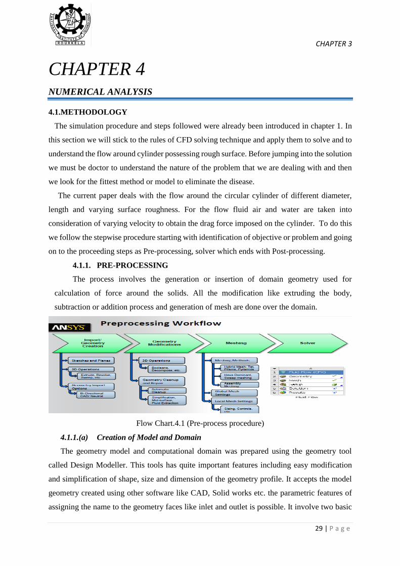
4.1.1. PRE-PROCESSING

The process involves the generation or insertion of domain geometry used for

calculation of force around the solids. All the modification like extruding the body,

subtraction or addition process and generation of mesh are done over the domain.

Flow Chart.4.1 (Pre-process procedure)

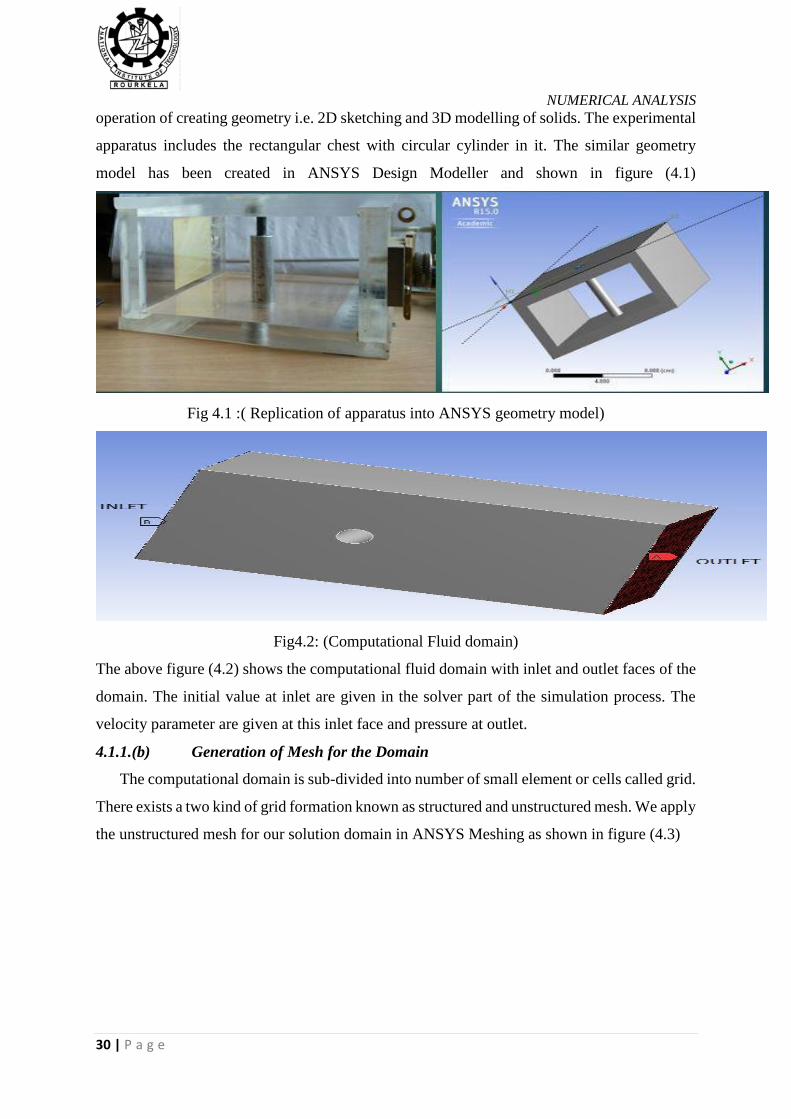
4.1.1.(a) Creation of Model and Domain

The geometry model and computational domain was prepared using the geometry tool

called Design Modeller. This tools has quite important features including easy modification

and simplification of shape, size and dimension of the geometry profile. It accepts the model

geometry created using other software like CAD, Solid works etc. the parametric features of

assigning the name to the geometry faces like inlet and outlet is possible. It involve two basic

NUMERICAL ANALYSIS

30 | P a g e

operation of creating geometry i.e. 2D sketching and 3D modelling of solids. The experimental

apparatus includes the rectangular chest with circular cylinder in it. The similar geometry

model has been created in ANSYS Design Modeller and shown in figure (4.1)

Fig 4.1 :( Replication of apparatus into ANSYS geometry model)

Fig4.2: (Computational Fluid domain)

The above figure (4.2) shows the computational fluid domain with inlet and outlet faces of the

domain. The initial value at inlet are given in the solver part of the simulation process. The

velocity parameter are given at this inlet face and pressure at outlet.

4.1.1.(b) Generation of Mesh for the Domain

The computational domain is sub-divided into number of small element or cells called grid.

There exists a two kind of grid formation known as structured and unstructured mesh. We apply

the unstructured mesh for our solution domain in ANSYS Meshing as shown in figure (4.3)

CHAPTER 3

31 | P a g e

Fig4.3: Tetrahedral mesh of domain

The ANSYS meshing is adaptable in generating mesh for various physics obtain from CFD:

PLOYFLOW, CFX and Fluent. The generated mesh helps in solving the governing equation

flow at each cell or nodal points. The meshing technique is very important part of the numerical

simulation process in order to capture boundary layer variation and to have easy convergence.

The mesh discretized in these small cell to solve the Navier-Stokes equation. Therefore it is

important to take special care about the mesh quality. The mesh quality are checked either by

the orthogonal quality or by skewness of mesh. The range for the quality mesh is shown below:

Table 4.1: Mesh quality

The quality of mesh for the prepared mesh for the domain are as follows:

Once we achieve the good quality mesh, can go for the solver portion for further analysis. If

not, mesh are re-sized, re-fined or different type of mesh are given e.g. Hexa, prism, or multi-

method mesh to have the desired quality of mesh. For discretizing the domain into mesh three

well known method of Finite volume method, Finite difference method and Finite element

NUMERICAL ANALYSIS

32 | P a g e

method are used. In this paper Finite volume method is employed to create unstructured mesh

for the computational domain.

4.1.2 Solver modelling for the Domain

In every analysis, there must be an input to have output as the result and this is done in the

solver setting. The input parameters are initialized at inlet of the domain and necessary

boundary condition are applied and calculation is carried out. There are few steps that need to

be taken care of, such as selection of solver models and discretization schemes (i.e. finite

volume, finite difference scheme). A flow chart is shown, describing the necessary steps to be

carried out for the simulation. The analysis starts with setting of solution parameter i.e.

Choosing solver and the solution are initialize to a point stating that the calculation from that

point, we choose the inlet face as our point of initialization. Once the solution is initialized we

can run the calculation.

Flow Chart 4.2: Steps for solver

Solver are of two types, Pressure based and Density based. We have used pressure based solver

for our study as the flow is incompressible across the cylinder with Mach no less than 0.3. The

CHAPTER 3

33 | P a g e

discretization scheme is done by selecting suitable Pressure-Velocity Coupling scheme in

solution methods as shown below:

Fig. 4.4: Solver selection Fig. 4.5: Choosing Pressure-Velocity Coupling scheme

After completion of running calculation the results are analysed and visualized in the next

section of Post-processing.

4.1.3 Post-Processing

In Post-processing, the results obtained around the flow system are both quantitative and

qualitative. It provides easy visualization of flow field through pressure, velocity contour and

vector magnitude. Different types of plot like x-y; histogram etc. are easily obtain for the better

analysis of simulated result. For the current study every contours, velocity profile and different

plots are describe in the next chapter Discussion of Results.

The above mentioned methods and procedure are well followed to operate the

simulation of flow around the circular cylinder.

4.2 PHYSICAL SETUP FOR THE STUDY AREA

For the simulation we need to create a computational domain of fluid with cylinder in it.

The domain was prepared in Design Modeller in such a manner that the flow of fluid was along

the x-direction and cylinder was placed perpendicular to the direction of flow field. According

to the flow direction, the naming of the faces are done, which help in implementing the initial

and boundary condition for the flow system. The well meshed domain is shown with the

necessary boundary condition.

NUMERICAL ANALYSIS

34 | P a g e

Fig 4.6: Flow field Domain

4.2.1 Boundary and Cell Zone Condition

There are many different boundary condition that need to be applied to domain for doing

the numerical simulation. The flow parameters are set at inlet, outlet, wall and the surface

body. Boundary condition provided to the study area are as follows:

a) Inlet boundary condition

At inlet, the velocity of flow is considered and different velocities are given for different

system. The range of velocity taken for the current study is from 8 m/s to 26.14 m/s so that

the numerical results can be check with the experimental study. The velocity ux imposed at

inflow is along the x-axis so the velocity component (u, v, w) along (x, y, z) receptively is

given as u=ux; v=w=0 at the inlet. More details are provided in the chapter 5.

b) Outlet boundary condition

The outflow was set as pressure outlet, to have constant pressure outflow. For the

present case the pressure taken is zero Pascal so that it will have low influence in the

upstream inflow.

c) Wall and surface body condition

The wall is considered to be a stationary wall for both cylinder wall and rectangular box

wall (i.e. conduit in which fluid flows) and no-slip condition is applied at these wall. The

surface of the cylinder is provided with different roughness height (ks). The given surface

height are in micron ranging as (82; 265; 348).

CHAPTER 3

35 | P a g e

Cell Zone condition

The small discrete cell are assigned material properties like fluid or solid as per the

requirement. I have considered cell zone as fluid (i.e. air and liquid water) for solution of

fluid problem. One could choose different material from the material database present in

the Fluent.

4.3. Turbulence solution

As described in chapter 4, the turbulence model say RANS model is used to solve the

flow turbulence. We apply the Standard k-Ɛ RANS model for the study flow past circular

cylinder. The momentum equation and transport equation is employed for the numerical

analysis given in chapter 3. The Fluent converts these equation into algebraic form using Finite

volume method. The SIMPLE pressure correction technique is used. The solution was run and

the drag force recorded as per the procedure.

4.3.1 Wall Modelling

The wall needs to be designed in such a manner that it captures all possible value

required for the simulation. To use the wall function one must locate the 1st cell i.e. y+ , for

low Reynolds No. y+ must not be less than 30.

CHAPTER 5

36 | P a g e

CHAPTER 5

EXPERIMENTATION

5.1 General

In this chapter we are going to carry out few procedure that will determine the drag

over the cylinder. When the air flows over the body it imposed normal thrust on the surface

and parallel shear along the body surface. The application of pressure distribution method is

described and used to measure the drag force over the cylinder of varying diameter, surface

roughness at different air velocity.

5.2 Equipment used

The study involve the use of many apparatus starting from Air Flow bench to cylinders..

The pressure variance is observed through Multi-tube manometer. There are four circular

cylinder of same length (70cm) with different radius i.e. (12.5, 10, 7.5, 6.25) mm are considered

for the study of drag force and its coefficient variation varying air flow velocity. The different

roughness parameter are taken to study the surface roughness effect on the drag force. The

detail specification of cylinders dimension and roughness height are presented in table and

theirs figures are shown:

.

Fig.5.1: Smooth Surface Cylinders Fig.5.2: Cylinders of Varying Roughness

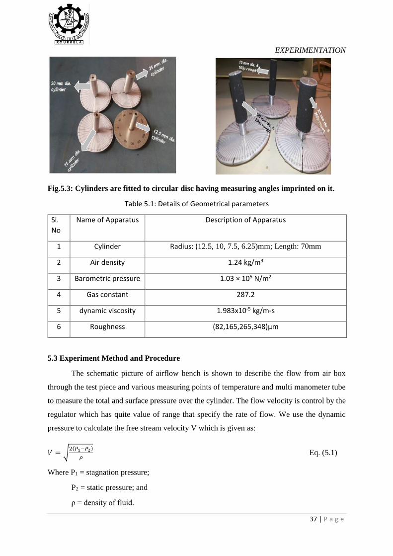
EXPERIMENTATION

37 | P a g e

Fig.5.3: Cylinders are fitted to circular disc having measuring angles imprinted on it.

Table 5.1: Details of Geometrical parameters

Sl.

No

Name of Apparatus Description of Apparatus

1 Cylinder Radius: (12.5, 10, 7.5, 6.25)mm; Length: 70mm

2 Air density 1.24 kg/m3

3 Barometric pressure 1.03 × 105 N/m2

4 Gas constant 287.2

5 dynamic viscosity 1.983x10-5 kg/m-s

6 Roughness (82,165,265,348)µm

5.3 Experiment Method and Procedure

The schematic picture of airflow bench is shown to describe the flow from air box

through the test piece and various measuring points of temperature and multi manometer tube

to measure the total and surface pressure over the cylinder. The flow velocity is control by the

regulator which has quite value of range that specify the rate of flow. We use the dynamic

pressure to calculate the free stream velocity V which is given as:

𝑉 = √2(𝑃1−𝑃2)

𝜌 Eq. (5.1)

Where P1 = stagnation pressure;

P2 = static pressure; and

ρ = density of fluid.

CHAPTER 5

38 | P a g e

The value of P1 & P2 are obtained from Pitot-static probe used in the experiment.

Fig.5.4: Schematic picture of Airflow bench.

5.3.1 Pressure Distribution Technique

To carry out the process we follow the certain steps of measuring the difference in

pressure distribution over the circular cylinder which is the test specimen of the study. The

procedure are listed below one after the other and the setup is shown for pressure measurement.

Fig.5.5: Pressure Measurement Setup

Step1: First the cylinders are joined to the calibrated disc showing division of angle in it. The

cylinder is set at a zero angle and then the velocity regulator is set to maximum value. The

initial barometric pressure and temperature are recorded. The manometer tube is connected to

the cylinder for measuring the surface pressure. For measurement of total pressure and static

pressure Pitot-tube is used. The total pressure obtain is rechecked with the box pressure which

must be equivalent.

EXPERIMENTATION

39 | P a g e

Step2: Once the all required instrument are fitted, the motor is on and the air flow starts. Now

we record the total pressure, surface pressure and the static pressure from the multi-manometer

tube for each 50 angle of rotation up to 900 and then from 900 -1800 the cylinder is rotated at

100 .

Step 3: The above steps are repeated for different range of velocity and varying surface

roughness.

Fig.5.6: Pressure Distribution Method

When all the required data are obtained, calculate the drag coefficient by the help of the

following equation:

Eq. (5.2)

Where, CP is the pressure coefficient and given by:

Eq. (5.3)

Here, P= surface pressure;

po = static pressure;

𝜌 = air density;

U= velocity.

The shear is neglected because the pressure force was found to be dominated, so only the term

is considered for the calculation of drag coefficient. Therefore the Eq. (5.2) changes and is

given as:

Eq. (5.4)

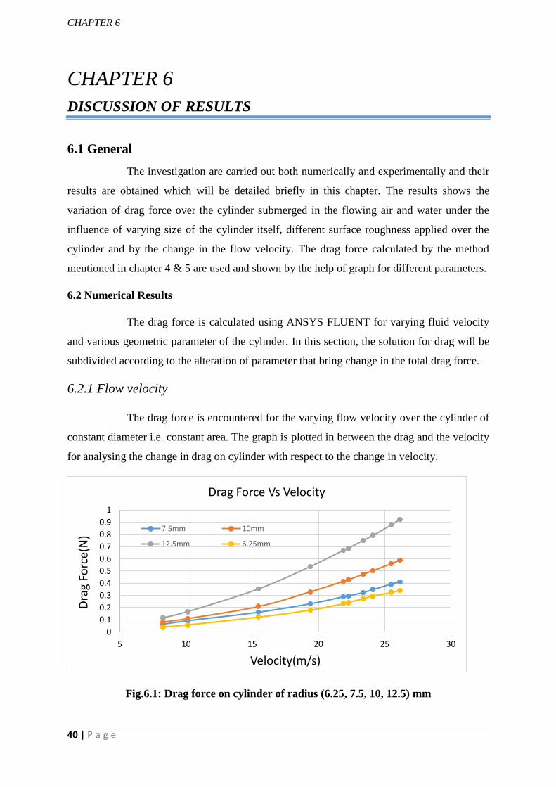
CHAPTER 6

40 | P a g e

CHAPTER 6

DISCUSSION OF RESULTS

6.1 General

The investigation are carried out both numerically and experimentally and their

results are obtained which will be detailed briefly in this chapter. The results shows the

variation of drag force over the cylinder submerged in the flowing air and water under the

influence of varying size of the cylinder itself, different surface roughness applied over the

cylinder and by the change in the flow velocity. The drag force calculated by the method

mentioned in chapter 4 & 5 are used and shown by the help of graph for different parameters.

6.2 Numerical Results

The drag force is calculated using ANSYS FLUENT for varying fluid velocity

and various geometric parameter of the cylinder. In this section, the solution for drag will be

subdivided according to the alteration of parameter that bring change in the total drag force.

6.2.1 Flow velocity

The drag force is encountered for the varying flow velocity over the cylinder of

constant diameter i.e. constant area. The graph is plotted in between the drag and the velocity

for analysing the change in drag on cylinder with respect to the change in velocity.

Fig.6.1: Drag force on cylinder of radius (6.25, 7.5, 10, 12.5) mm

0

0.1

0.2

0.3

0.4

0.5

0.6

0.7

0.8

0.9

1

5 10 15 20 25 30

Dra

g Fo

rce(

N)

Velocity(m/s)

Drag Force Vs Velocity

7.5mm 10mm

12.5mm 6.25mm

DISCUSSION OF RESULTS

41 | P a g e

There is increase in the drag force has been noticed for the increase in the flow

velocity. It is because the drag is directly proportional to the velocity, so for the particular

radius of cylinder drag force gets raise for the growing speed of the stream. Form the graph it

is observed that at the low velocity nearly 8m/s there slight change in the drag which is due to

laminar sub-layer.

6.2.2 Size of the cylinder

For this, velocity is kept constant and the size of the cylinder is being changed by

increasing the radius of the cylinder. The graph of different uniform velocity for different radius

is drawn. The effect of change in the radius change the projected area which is directly

responsible for the drag force.

Fig.6.2: Variation of Drag Force Due To Change in Area of the Cylinder

The drag was found to be going up with the increase in the radius of the circular cylinder. The

drag force is directly proportional to the area, thus when the radius of cylinder is increased the

area of the cylinder gets bigger and consequently increases the drag force.

The length of the cylinder also plays the same role of increasing the drag when

projected area of the cylinder gets increased due to increase in the cylinder length. This

variation can also observed by the plot shown:

0

0.1

0.2

0.3

0.4

0.5

0.6

0.7

0.8

0.9

1

6 7 8 9 10 11 12 13

Dra

g fo

rce(

N)

Radius(mm)

Drag force Vs Radiusv=22.6m/s

v=8.6m/s

v=25.3m/s

v=16.12m/s

v=10.2m/s

v=19.1m/s

v=21.23m/s

v=23.1m/s

v=24.5m/s

v=26.4m/s

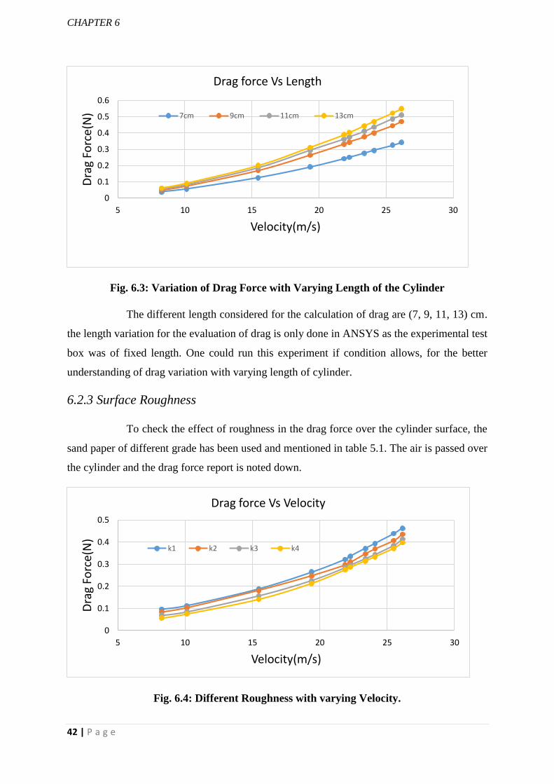
CHAPTER 6

42 | P a g e

Fig. 6.3: Variation of Drag Force with Varying Length of the Cylinder

The different length considered for the calculation of drag are (7, 9, 11, 13) cm.

the length variation for the evaluation of drag is only done in ANSYS as the experimental test

box was of fixed length. One could run this experiment if condition allows, for the better

understanding of drag variation with varying length of cylinder.

6.2.3 Surface Roughness

To check the effect of roughness in the drag force over the cylinder surface, the

sand paper of different grade has been used and mentioned in table 5.1. The air is passed over

the cylinder and the drag force report is noted down.

Fig. 6.4: Different Roughness with varying Velocity.

0

0.1

0.2

0.3

0.4

0.5

0.6

5 10 15 20 25 30

Dra

g Fo

rce(

N)

Velocity(m/s)

Drag force Vs Length

7cm 9cm 11cm 13cm

0

0.1

0.2

0.3

0.4

0.5

5 10 15 20 25 30

Dra

g Fo

rce(

N)

Velocity(m/s)

Drag force Vs Velocity

k1 k2 k3 k4

DISCUSSION OF RESULTS

43 | P a g e

For the constant roughness, constant radius of 7.5 mm and varying stream

velocity, the drag is increasing but it reduces the drag that obtained from the smooth cylinder.

The drag force for varying surface roughness at a constant velocity and constant radius of the

cylinder is plotted and compared with the experiment data results for each radius.

Fig.6.5 Effect of roughness for R=6.25mm

Fig.6.6 Effect of roughness for R=7.5mm

0.241

0.242

0.243

0.244

0.245

0.246

0.247

100 150 200 250 300 350

Dra

g Fo

rce(

N)

Roughness(micron)

constant velocity=21.23m/s, Radius=6.25mm

Ansys Experiment

0.39

0.4

0.41

0.42

0.43

0.44

0.45

0.46

0.47

100 150 200 250 300 350

Dra

g Fo

rce(

N)

Roughness(micron)

Constant Velocity=26.4m/s; R=7.5mm

Ansys

Experiment

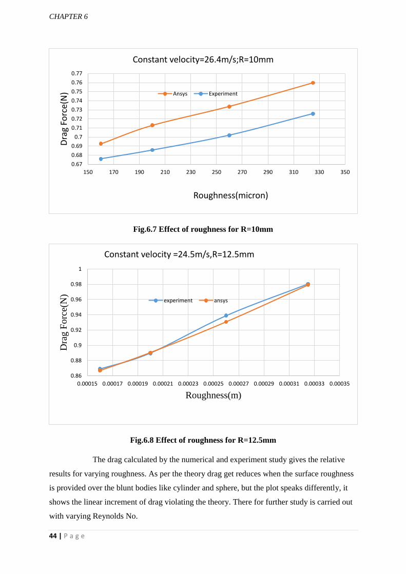
CHAPTER 6

44 | P a g e

Fig.6.7 Effect of roughness for R=10mm

Fig.6.8 Effect of roughness for R=12.5mm

The drag calculated by the numerical and experiment study gives the relative

results for varying roughness. As per the theory drag get reduces when the surface roughness

is provided over the blunt bodies like cylinder and sphere, but the plot speaks differently, it

shows the linear increment of drag violating the theory. There for further study is carried out

with varying Reynolds No.

0.67

0.68

0.69

0.7

0.71

0.72

0.73

0.74

0.75

0.76

0.77

150 170 190 210 230 250 270 290 310 330 350

Dra

g Fo

rce(

N)

Roughness(micron)

Constant velocity=26.4m/s;R=10mm

Ansys Experiment

0.86

0.88

0.9

0.92

0.94

0.96

0.98

1

0.00015 0.00017 0.00019 0.00021 0.00023 0.00025 0.00027 0.00029 0.00031 0.00033 0.00035

Dra

g F

orc

e(N

)

Roughness(m)

Constant velocity =24.5m/s,R=12.5mm

experiment ansys

DISCUSSION OF RESULTS

45 | P a g e

6.2.4 Reynolds Number and water as the fluid

The flowing fluid has been changed from air to water liquid in the ANSYS and

simulation was processed for calculating the drag force over the cylinder. On modifying the

fluid the fluid properties like density (ρ) and dynamic viscosity (µ) also gets modified. Thus

the value are given as: ρ= 1000 kg/m3 & µ= 8.90x10-4 .

The graphs are been plotted for the range of Reynolds No. and particular cylinder having

same radii.

Fig.6.9: Drag Vs Reynolds No. for R=10mm

Fig.6.10: Drag Vs Reynolds No. for R=12.5mm

0

50

100

150

200

250

300

350

400

450

500

0 100000 200000 300000 400000 500000 600000 700000

Dra

g Fo

rce(

N)

Reynolds Number

K=0

K1=0.000165

K2=0.000265

K3=0.000348

0

100

200

300

400

500

600

700

800

0 100000 200000 300000 400000 500000 600000 700000 800000

Dra

g Fo

rce(

N)

Reynolds Number

K=0

K1=0.000165

K2=0.000265

K3=0.000348

CHAPTER 6

46 | P a g e

From the graph, it found to be believed that there is very slight change in the drag

corresponding to the close value of roughness. The variation of drag coefficient can enlighten

the drag dependence on the Re value, which is displayed on the below plot.

Fig.6.11: Coefficient of Drag Vs Reynolds No. for R=7.5mm; ks=0µm.

Fig.6.12: Coefficient of Drag Vs Reynolds No. for R=7.5mm; ks=348µm.

The fig.6.11 describe the reduction in the drag coefficient with increase in the

Reynolds No. the flow is turbulent as critical value 2x105 is exceeded for the flow. There linear

decrease in the value of CD as the surface of the cylinder is smooth and velocity is directly

responsible for the cause. When the surface roughness is applied over the cylinder surface, the

0.862

0.864

0.866

0.868

0.87

0.872

0.874

0.876

0.878

0 100000 200000 300000 400000 500000

Co

effo

cien

t o

f D

rag

Reynolds number

0.872

0.873

0.874

0.875

0.876

0.877

0.878

0.879

0.88

0 100000 200000 300000 400000 500000

Co

effo

cien

t o

f D

rag

Reynolds number

DISCUSSION OF RESULTS

47 | P a g e

drag coefficient goes slightly up near the critical Re value, then it get reduce after the approx.

value of Re = 3x105 as observed in fig.6.12.

Fig.6.13: Coefficient of Drag Vs Reynolds No. for R=7.5mm; ks=265µm.

Fig.6.14: Coefficient of Drag Vs Reynolds No. for R=7.5mm; ks=165µm.

The repetition of providing roughness gives the reduced drag as compared to the

smoother one, but not much difference is seen over the variation of CD .

0.8845

0.885

0.8855

0.886

0.8865

0.887

0.8875

0.888

0 100000 200000 300000 400000 500000

Co

effo

cien

t o

f D

rag

Reynolds number

1.117

1.118

1.119

1.12

1.121

1.122

1.123

0 100000 200000 300000 400000 500000

Co

effo

cien

t o

f D

rag

Reynolds number

CHAPTER 6

48 | P a g e

6.2.5 Contour

The different contour like pressure contour and velocity contour are shown to

study the pressure and velocity distribution over the cylinder. The velocity vector magnitude

is also obtained and presented.

a) Pressure contour:

The pressure contour for different radius of cylinder is presented with the

constant velocity of 22.6 m/s.

Fig.6.15: Pressure Contour for R=6.25mm

Fig.6.16: Pressure Contour for R=7.5mm

DISCUSSION OF RESULTS

49 | P a g e

Fig.6.17: Pressure Contour for R=10mm

Fig.6.18: Pressure Contour for R=12.5mm

b) Velocity Contour

The corresponding velocity contour are presented for the constant velocity of 22.6

m/s of varying radius of the cylinder.

Fig.6.19: Velocity Contour for R=6.25mm

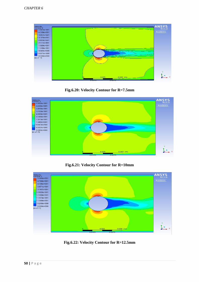
CHAPTER 6

50 | P a g e

Fig.6.20: Velocity Contour for R=7.5mm

Fig.6.21: Velocity Contour for R=10mm

Fig.6.22: Velocity Contour for R=12.5mm

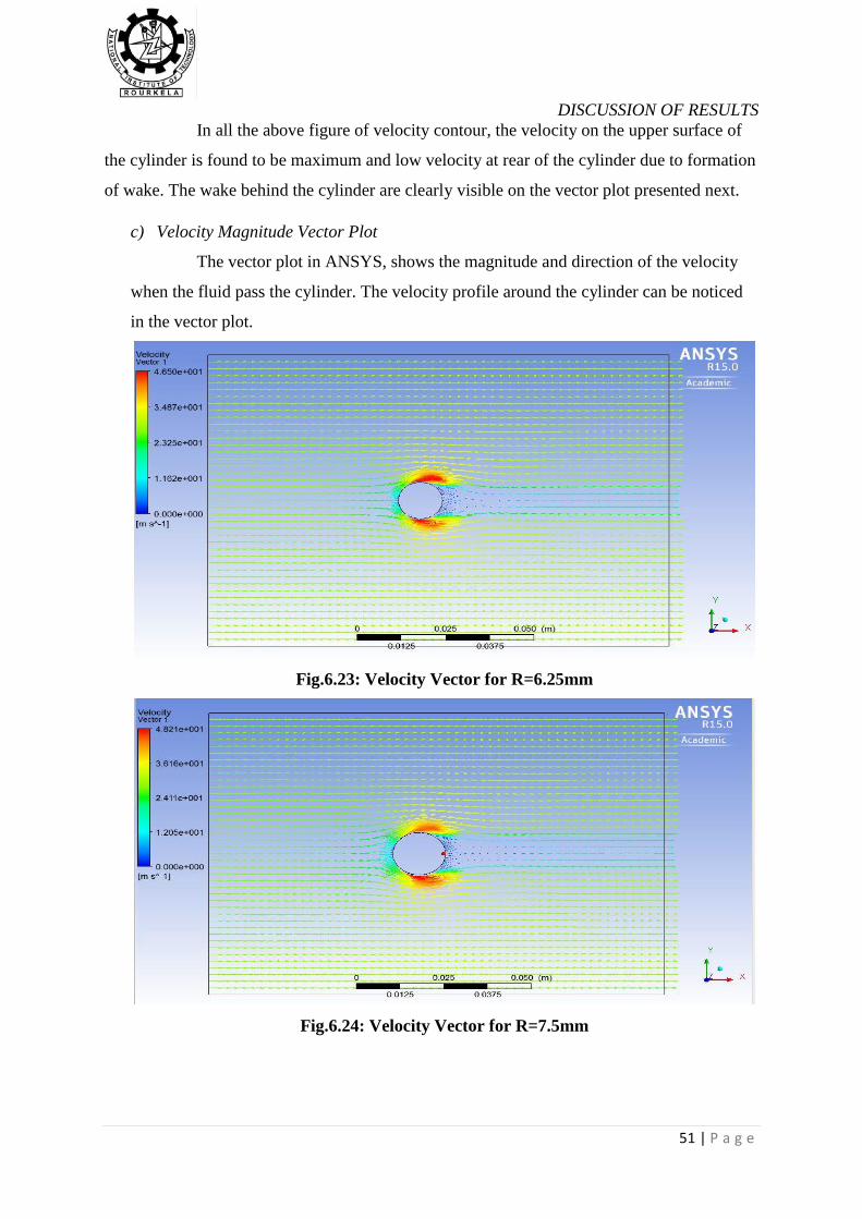
DISCUSSION OF RESULTS

51 | P a g e

In all the above figure of velocity contour, the velocity on the upper surface of

the cylinder is found to be maximum and low velocity at rear of the cylinder due to formation

of wake. The wake behind the cylinder are clearly visible on the vector plot presented next.

c) Velocity Magnitude Vector Plot

The vector plot in ANSYS, shows the magnitude and direction of the velocity

when the fluid pass the cylinder. The velocity profile around the cylinder can be noticed

in the vector plot.

Fig.6.23: Velocity Vector for R=6.25mm

Fig.6.24: Velocity Vector for R=7.5mm

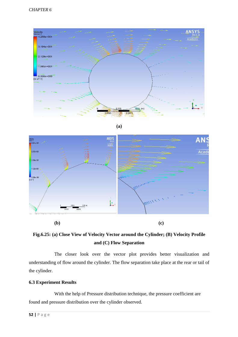
CHAPTER 6

52 | P a g e

(a)

(b) (c)

Fig.6.25: (a) Close View of Velocity Vector around the Cylinder; (B) Velocity Profile

and (C) Flow Separation

The closer look over the vector plot provides better visualization and

understanding of flow around the cylinder. The flow separation take place at the rear or tail of

the cylinder.

6.3 Experiment Results

With the help of Pressure distribution technique, the pressure coefficient are

found and pressure distribution over the cylinder observed.

DISCUSSION OF RESULTS

53 | P a g e

The coefficient of drag over the cylinder is calculated from the pressure

coefficient as mentioned in the previous chapter. The coefficient of pressure is plotted against

the angle of rotation of cylinder. Integrating area under this curve gives the CD . The plot of

pressure coefficient for different surface roughness is presented.

Fig.6.26: Pressure coefficient for R=7.5mm; k=348µm

Fig.6.27: Pressure coefficient for R=7.5mm; k=265µm

The pressure coefficient plot describe the flow to be separated at 800 nearly which

is similar to the value obtained by numerical study. All the plot has not been shown here.

-1.4

-1.2

-1

-0.8

-0.6

-0.4

-0.2

0

0.2

0.4

0.6

0 20 40 60 80 100 120 140 160 180 200

Co

effi

cien

t o

f P

ress

ure

Angle(Ɵ)

-1.4

-1.2

-1

-0.8

-0.6

-0.4

-0.2

0

0.2

0.4

0.6

0 20 40 60 80 100 120 140 160 180 200

Co

effi

cien

t o

f P

ress

ure

Angle(Ɵ)

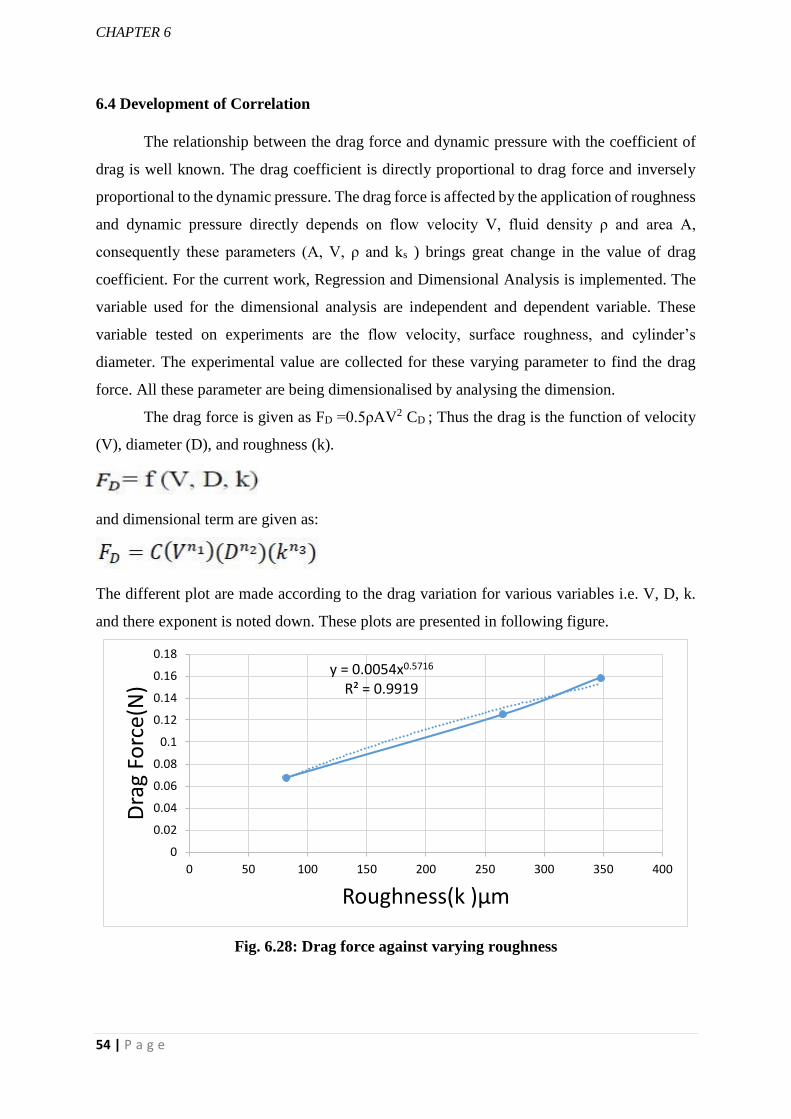
CHAPTER 6

54 | P a g e

6.4 Development of Correlation

The relationship between the drag force and dynamic pressure with the coefficient of

drag is well known. The drag coefficient is directly proportional to drag force and inversely

proportional to the dynamic pressure. The drag force is affected by the application of roughness

and dynamic pressure directly depends on flow velocity V, fluid density ρ and area A,

consequently these parameters (A, V, ρ and ks ) brings great change in the value of drag

coefficient. For the current work, Regression and Dimensional Analysis is implemented. The

variable used for the dimensional analysis are independent and dependent variable. These

variable tested on experiments are the flow velocity, surface roughness, and cylinder’s

diameter. The experimental value are collected for these varying parameter to find the drag

force. All these parameter are being dimensionalised by analysing the dimension.

The drag force is given as FD =0.5ρAV2 CD ; Thus the drag is the function of velocity

(V), diameter (D), and roughness (k).

and dimensional term are given as:

The different plot are made according to the drag variation for various variables i.e. V, D, k.

and there exponent is noted down. These plots are presented in following figure.

Fig. 6.28: Drag force against varying roughness

y = 0.0054x0.5716

R² = 0.9919

0

0.02

0.04

0.06

0.08

0.1

0.12

0.14

0.16

0.18

0 50 100 150 200 250 300 350 400

Dra

g Fo

rce(

N)

Roughness(k )µm

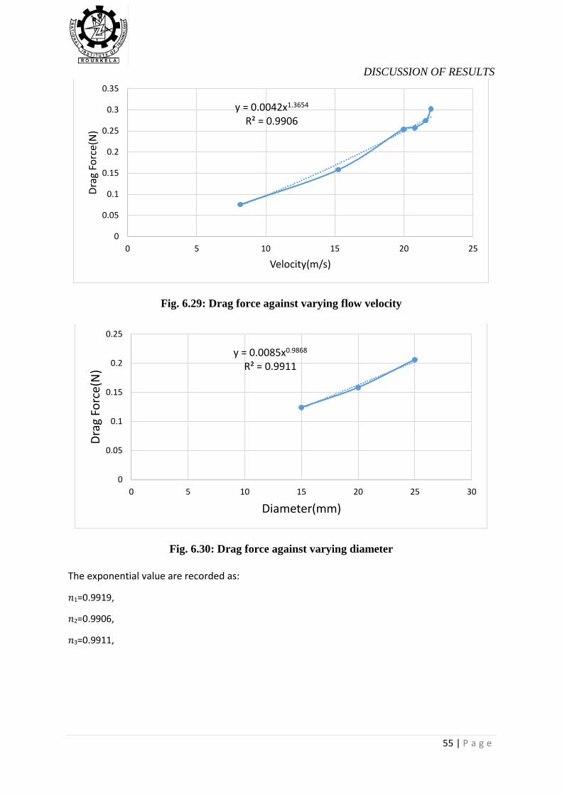
DISCUSSION OF RESULTS

55 | P a g e

Fig. 6.29: Drag force against varying flow velocity

Fig. 6.30: Drag force against varying diameter

The exponential value are recorded as:

𝑛1=0.9919,

𝑛2=0.9906,

𝑛3=0.9911,

y = 0.0042x1.3654

R² = 0.9906

0

0.05

0.1

0.15

0.2

0.25

0.3

0.35

0 5 10 15 20 25

Dra

g Fo

rce(

N)

Velocity(m/s)

y = 0.0085x0.9868

R² = 0.9911

0

0.05

0.1

0.15

0.2

0.25

0 5 10 15 20 25 30

Dra

g Fo

rce(

N)

Diameter(mm)

CHAPTER 6

56 | P a g e

Fig.6.31 The relationship between Drag force and x

The exponential term are used to find the X, which is given as: 𝑋 = (𝑉)𝑛1(𝐷)𝑛2(𝑘)𝑛3

and the graph has been drawn for the drag force and X.

y = 18.836x1.0003

R² = 0.9906

Fig.6.32: Final correlation

The final correlation plot is given in the figure 6.31showing the combine effect of diameter,

roughness and velocity. With the help of correlation established, the drag force is calculated

or predicted and compared with the value of ANSYS and experiment, which is presented in

the form of graph.

y = 18.836x1.0003

R² = 0.9906

0

0.05

0.1

0.15

0.2

0.25

0.3

0.35

0 0.002 0.004 0.006 0.008 0.01 0.012 0.014 0.016

Dra

g Fo

rce(

N)

x

y = 19.65x1.0155

R² = 0.9712

0

0.05

0.1

0.15

0.2

0.25

0.3

0.35

0 0.002 0.004 0.006 0.008 0.01 0.012 0.014 0.016

Dra

g Fo

rce(

N)

Effect of velocity Effect of roughness Effect of diameter

total effect Power (total effect)

DISCUSSION OF RESULTS

57 | P a g e

Fig.6.33: Comparison plot for varying velocity

Fig.6.34: Comparison plot for varying Diameter

The drag force obtained from all method are quite satisfying with minimum

error of 3.2% and graph plotted in between them are good.

0

0.05

0.1

0.15

0.2

0.25

0.3

0.35

5 7 9 11 13 15 17 19 21 23

Dra

g Fo

rce(

N)

Velocity(m/s)

Velocity Vs Drag

experiment Ansys Calculated drag force

0.1

0.12

0.14

0.16

0.18

0.2

0.22

10 12 14 16 18 20 22 24 26

Dra

g Fo

rce(

N)

Diameter(mm)

Fd Vs Diameter

Experiment ansys calculated

CHAPTER 6

58 | P a g e

Fig.6.35: Comparison plot for varying Roughness

The results obtained from the numerical methods are quite easy in conducting and time

saving. In comparison to the experiment it is cost effective i.e. no extra cost required for the

modification of model.

0

0.02

0.04

0.06

0.08

0.1

0.12

0.14

0.16

0.18

0 50 100 150 200 250 300 350 400

Dra

g Fo

rce(

N)

Roughness(ks )µm

Fd Vs Ks;D=20mm

experiment ansys calculated

CONCLUSIONS AND FUTURE SCOPE

59 | P a g e

CHAPTER 7

CONCLUSIONS AND FUTURE SCOPE

7.1 GENERAL

The study holds the fine literature writing and good work of analysis. The drag force

calculated by ANSYS software, experimental method has achieved the agreeable and satisfied

solution by ensuring with the predicted data obtained from the developed correlation. This

chapter describe the short view on the drag variation and its dependence on the flow and

physical property of cylinder.

7.2 Drag Force

The nature of drag force is listed as it react to the different parameter considering the

fluid properties and geometric properties of the cylinder.

When the area of the cylinder is increased by increasing the diameter or length, the drag

force found to be increasing.

With the increase in velocity of the fluid flow, the drag increases but its coefficient gets

reduced.

In comparison to the smooth cylinder i.e. no roughness height and the cylinder having

any roughness height, the drag force on the smooth cylinder is more.

The cylinder having increase in the roughness by increasing the previous rough surface,

the drag force in such was seen to be increased.

The drag force gets increased when the Re value is increased, but the CD drops down.

The drag coefficient CD is found to be increase for the transition range.

The velocity profile observed explains the formation of boundary layer over the

cylinder surface which force the flow to be turbulent, reducing the pressure force and

thus the drag gets decreased on application of roughness.

The flow separation occurred as the consequence of distributed pressure over the

cylinder was found at an angle 700 - 800 .

At a uniform Reynolds No. the drag force is increased and coefficient of drag is reduced

for the increase in relative roughness value.

All the method employed are compared with each other and found to good and

acceptable value with error percentage of 3%.

CHAPTER 7

60 | P a g e

7.3 Scope of the Study

This is an important study having many application in pipe flow; aerodynamic study of

vehicle, buildings, high towers, and the underwater vehicle e.g. submarine.

The investigated results can be compared with the experimentation done in wind tunnel.

Different types of model differ in shapes can tested. The shapes can be square, triangle,

elliptical, concave or convex etc.

The hydrodynamic force acting on the body submerged in the water can be studied and

drag imposed on the body could be determined.

The numerical study can be done on the turbine.

REFERENCE

61 | P a g e

REFERENCES

Achenbach, E., and E. Heinecke. "On vortex shedding from smooth and rough cylinders

in the range of Reynolds numbers 6× 103 to 5× 106." Journal of fluid mechanics 109

(1981): 239-251.

Akoz, M. S., & Kirkgoz, M. S. (2009). Numerical and experimental analyses of the flow

around a horizontal wall-mounted circular cylinder. Transactions of the Canadian Society

for Mechanical Engineering, 33(2), 189-215.

Alam, M. M., Moriya, M., & Sakamoto, H. (2003). Aerodynamic characteristics of two

side-by-side circular cylinders and application of wavelet analysis on the switching

phenomenon. Journal of Fluids and Structures, 18(3), 325-346.

Alridge, T. R., Piper, B. S., & Hunt, J. C. R. (1978). The drag coefficient of finite-aspect-

ratio perforated circular cylinders. Journal of Wind Engineering and Industrial

Aerodynamics, 3(4), 251-257.

Bearman, P. W., & Harvey, J. K. (1993). Control of circular cylinder flow by the use of

dimples. AIAA journal, 31(10), 1753-1756.

Bergmann, M., Cordier, L., & Brancher, J. P. (2007). Drag minimization of the cylinder

wake by trust-region proper orthogonal decomposition. In Active Flow Control (pp. 309-

324). Springer Berlin Heidelberg.

Bouak, F., & Lemay, J. (2001). Use of the wake of a small cylinder to control unsteady

loads on a circular cylinder. Journal of visualization, 4(1), 61-72.

Butt, U., & Egbers, C. (2013). Aerodynamic Characteristics of Flow over Circular

Cylinders with Patterned Surface. J. Materials, Mechanics, Manufacturing, 1(2).

CHAPTER 7

62 | P a g e

Catalano, P., Wang, M., Iaccarino, G., & Moin, P. (2003). Numerical simulation of the flow

around a circular cylinder at high Reynolds numbers. International Journal of Heat and

Fluid Flow, 24(4), 463-469.

D'auteuil, A., Larose, G. L., & Zan, S. J. (2012). Wind turbulence in speed skating:

measurement, simulation and its effect on aerodynamic drag. Journal of Wind Engineering

and Industrial Aerodynamics, 104, 585-593.

Grosche, F. R., & Meier, G. E. A. (2001). Research at DLR Göttingen on bluff body

aerodynamics, drag reduction by wake ventilation and active flow control.Journal of Wind

Engineering and Industrial Aerodynamics, 89(14), 1201-1218.

Hodžić, N., & Begagić, R. (2011). EXPERIMENTAL INVESTIGATION OF

BOUNDARY LAYER SEPARATION INFLUENCE OF PRESSURE DISTRIBUTION

ON CYLINDER SURFACE IN WIND TUNNEL ARMFIELD C15-10. Trends in the

Development of Machinery and Associated Technology.

Islam, T., & Hassan, S. R. (2013). Experimental and Numerical Investigation of Flow over

a Cylinder at Reynolds Number 10 5. Journal of Modern Science and Technology, 1(1),

52-60.

Jones, D. A., & Clarke, D. B. (2008). Simulation of the Flow Past a Sphere using the Fluent

Code.

Lee, S. J., Lee, S. I., & Park, C. W. (2004). Reducing the drag on a circular cylinder by

upstream installation of a small control rod. Fluid dynamics research, 34(4), 233-250.

Ling, G. P., & Shih, T. M. (1999). Numerical study on the vortex motion patterns around a

rotating circular cylinder and their critical characters.International journal for numerical

methods in fluids, 29(2), 229-248.

Lyotard, N., Shew, W. L., Bocquet, L., & Pinton, J. F. (2007). Polymer and surface

roughness effects on the drag crisis for falling spheres. The European Physical Journal B-

REFERENCE

63 | P a g e

Condensed Matter and Complex Systems, 60(4), 469-476.

Mahesh, K., Constantinescu, G., & Moin, P. (2004). A numerical method for large-eddy

simulation in complex geometries. Journal of Computational Physics, 197(1), 215-240.

Mashud, M., Islam, M. S., Bari, G. S., & Islam, M. R. (2010). Reduction of Drag Force

of a Cylinder by Attaching Cylindrical Rings. Proceedings of the 13th Asian Congress of

Fluid Mechanics, (2010), Dhaka, Bangladesh.

Merrick, Ryan, and Girma Bitsuamlak. (1982). Control of flow around a circular cylinder

by the use of surface roughness: A computational and experimental approach. Journal of

Fluid Mechanics,123, 363-378.

Mittal, R., & Balachandar, S. (1995). Effect of three‐dimensionality on the lift and drag

of nominally two‐dimensional cylinders. Physics of Fluids (1994-present), 7(8), 1841-

1865.

Mittal, S., & Raghuvanshi, A. (2001). Control of vortex shedding behind circular cylinder

for flows at low Reynolds numbers. International Journal for Numerical Methods in

Fluids, 35(4), 421-447.

Mittal, S., & Singh, S. (2005). Vortex-induced vibrations at subcritical Re.Journal of

Fluid Mechanics, 534, 185-194.

Monalisa Mallick and A. Kumar (2014),” Study on Drag Coefficient for the Flow Past a

Cylinder” International Journal of Civil Engineering Research. Volume 5,pp. 301-306

Monalisa Mallick and A. Kumar (2014),”Experimental Investigation of Flow past a Rough

Surfaced Cylinder” International Journal of Engineering Research and Applications.

Nils P. van Hinsberg (2014),”The Reynolds number effect from subcritical to high trans-

critical on steady and unsteady loading on a rough circular cylinder” International

Conference on Structural Dynamics. 978-972-752-165-4

Njock Libii, J. (2010). Using wind tunnel tests to study pressure distributions around a

CHAPTER 7

64 | P a g e

bluff body: the case of a circular cylinder. Transactions on Engineering and Technology

Education, 8(3).

Protas, B., & Wesfreid, J. E. (2002). Drag force in the open-loop control of the cylinder

wake in the laminar regime. Physics of Fluids (1994-present), 14(2), 810-826.

Richter, A., & Nikrityuk, P. A. (2012). Drag forces and heat transfer coefficients for

spherical, cuboidal and ellipsoidal particles in cross flow at sub-critical Reynolds

numbers. International Journal of Heat and Mass Transfer, 55(4), 1343-1354.

Shao, Y., & Yang, Y. (2005). A scheme for drag partition over rough surfaces.Atmospheric

Environment, 39(38), 7351-7361.

Shih, W. C. L., Wang, C., Coles, D., & Roshko, A. (1993). Experiments on flow past

rough circular cylinders at large Reynolds numbers. Journal of Wind Engineering and

Industrial Aerodynamics, 49(1), 351-368.

Singh, S. P., & Mittal, S. (2005). Flow past a cylinder: shear layer instability and drag

crisis. International Journal for Numerical Methods in Fluids, 47(1), 75-98.

Sørensen, N. N., Bechmann, A., & Zahle, F. (2011). 3D CFD computations of transitional

flows using DES and a correlation based transition model. Wind Energy, 14(1), 77-90.

Tamayol, A., Yeom, J., Akbari, M., & Bahrami, M. (2013). Low Reynolds number flows

across ordered arrays of micro-cylinders embedded in a rectangular

micro/minichannel. International Journal of Heat and Mass Transfer,58(1), 420-426.

Timmer, W. A., & Schaffarczyk, A. P. (2004). The effect of roughness at high Reynolds

numbers on the performance of aerofoil DU 97‐W‐300Mod. Wind Energy, 7(4), 295-307.

Triyogi, Y., D. Suprayogi, and E. Spirda. (2009)."Reducing the drag on a circular

cylinder by upstream installation of an I-type bluff body as passive control. “Proceedings

of the Institution of Mechanical Engineers, Part C: Journal of Mechanical Engineering

Science 223.10: 2291-2296.

REFERENCE

65 | P a g e

Tsutsui, T., & Igarashi, T. (2002). Drag reduction of a circular cylinder in an air-

stream. Journal of Wind Engineering and Industrial Aerodynamics, 90(4), 527-541.

Wang, Y. X., Lu, X. Y., & Zhuang, L. X. (2004). Numerical analysis of the rotating

viscous flow approaching a solid sphere. International journal for numerical methods in

fluids, 44(8), 905-925. Roshko, A. (1961). Experiments on the flow past a circular cylinder

at very high Reynolds number. Journal of Fluid Mechanics, 10(03), 345-356.

Williamson, C. H. (1996). Vortex dynamics in the cylinder wake. Annual review

of fluid mechanics, 28(1), 477-539.

Xu, C. Y., Chen, L. W., & Lu, X. Y. (2010). Large-eddy simulation of the compressible

flow past a wavy cylinder. Journal of Fluid Mechanics, 665, 238-273.

Zakharenkov, M. N. (1997). Unsteady detached separation from a circular cylinder

performing rotational oscillations in a uniform viscous incompressible flow. International

journal for numerical methods in fluids, 25(2), 125-142.

Zheng, Z. C., & Zhang, N. (2008). Frequency effects on lift and drag for flow past an

oscillating cylinder. Journal of Fluids and Structures, 24(3), 382-399.