Embed Size (px)
Citation preview
Crechula de Cristina Matsinhe
Studies on the influence of organic
waste biodegradability in the
composting process
September 2011

Studies on the influence of organic waste
biodegradability in the composting process
Dissertação apresentada à Faculdade de Ciências e Tecnologia da Universidade
de Coimbra, com vista à obtenção do grau de Mestre em Engenharia Química.
Crechula de Cristina Matsinhe
Orientador: Professora Doutora Margarida Maria João de Quina
Departamento de Engenharia Química
Faculdade de Ciências e Tecnologia
Universidade de Coimbra
Coimbra, 2011
“Continuous effort,
not strength or intelligence,
is the key to unlocking our potential.”
Winston Churchill
“The important thing is not to stop questioning.”
Albert Einstein
“O Homem é do tamanho do seu sonho.”
Fernando Pessoa
ACKNOWLEDGMENTS
It is a pleasure to thank those who made this thesis possible by providing the support,
trust, help and sympathy during this work.
I owe my deepest gratitude to Professor Margarida Quina for all the support, guidance,
availability and help during this work, but also for all the friendship and sympathy,
demonstrated along the work.
I am heartily thankful to Engineer Micaela Soares, whose encouragement, guidance
and support from the beginning to the end of the work enabled me to develop an
understanding of the subject under analysis.
I would like to thank the industry SIA- Sociedade Industrial Aperitivos, Lda. for
providing the samples of potatoes- peel for this work.
I would like to thank Iberplant and AAC (Associação Académica de Coimbra), for
supplying the grass clippings used in this work.
I would also like to thank ESAC- Escola Superior Agrária de Coimbra by the facilities
provided to accomplish this work.
To chemical engineering department employees for all their cooperation to accomplish
this work, my thanks.
I am grateful to my friends and family, particularly to my parents for unconditionally
support me during my academic life.
Lastly, I offer my regards and blessings to all of those who supported me in any
respect during the accomplishment of the thesis.

i
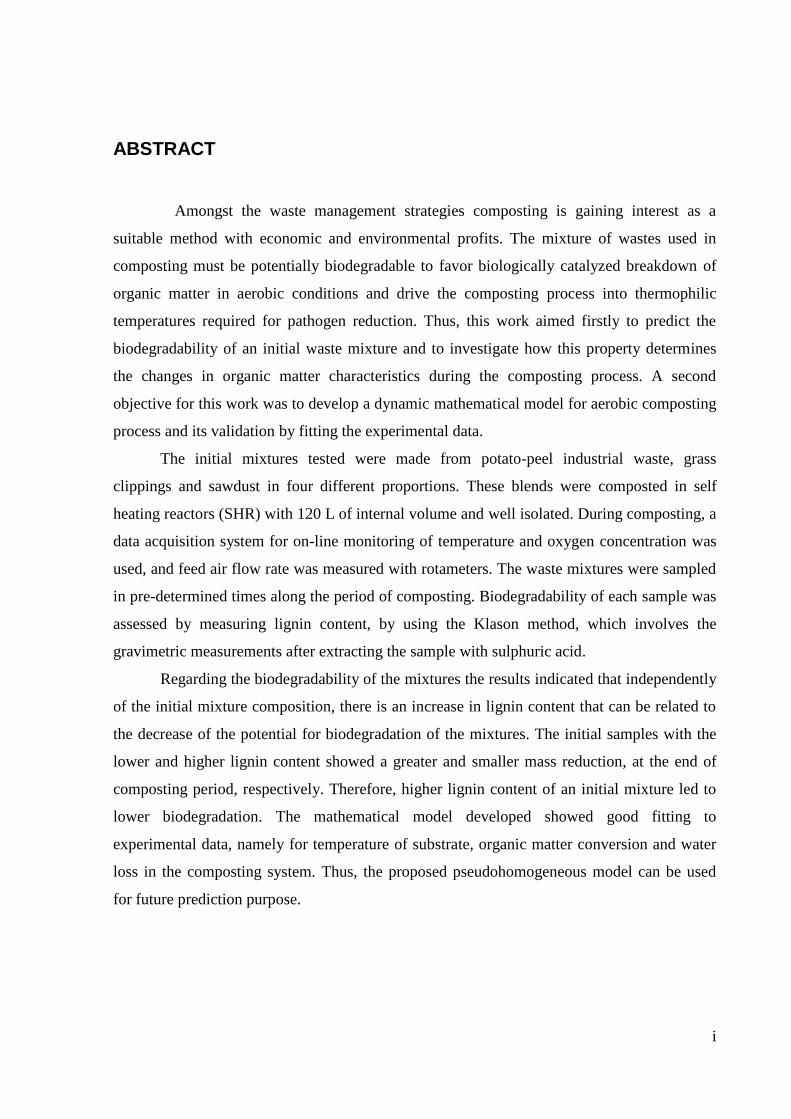
ABSTRACT
Amongst the waste management strategies composting is gaining interest as a
suitable method with economic and environmental profits. The mixture of wastes used in
composting must be potentially biodegradable to favor biologically catalyzed breakdown of
organic matter in aerobic conditions and drive the composting process into thermophilic
temperatures required for pathogen reduction. Thus, this work aimed firstly to predict the
biodegradability of an initial waste mixture and to investigate how this property determines
the changes in organic matter characteristics during the composting process. A second
objective for this work was to develop a dynamic mathematical model for aerobic composting
process and its validation by fitting the experimental data.
The initial mixtures tested were made from potato-peel industrial waste, grass
clippings and sawdust in four different proportions. These blends were composted in self
heating reactors (SHR) with 120 L of internal volume and well isolated. During composting, a
data acquisition system for on-line monitoring of temperature and oxygen concentration was
used, and feed air flow rate was measured with rotameters. The waste mixtures were sampled
in pre-determined times along the period of composting. Biodegradability of each sample was
assessed by measuring lignin content, by using the Klason method, which involves the
gravimetric measurements after extracting the sample with sulphuric acid.
Regarding the biodegradability of the mixtures the results indicated that independently
of the initial mixture composition, there is an increase in lignin content that can be related to
the decrease of the potential for biodegradation of the mixtures. The initial samples with the
lower and higher lignin content showed a greater and smaller mass reduction, at the end of
composting period, respectively. Therefore, higher lignin content of an initial mixture led to
lower biodegradation. The mathematical model developed showed good fitting to
experimental data, namely for temperature of substrate, organic matter conversion and water
loss in the composting system. Thus, the proposed pseudohomogeneous model can be used
for future prediction purpose.

iii
RESUMO
De entre as estratégias de gestão de resíduos, a compostagem tem vindo a ganhar
interesse e com benefícios económicos e ambientais. Os resíduos submetidos a compostagem
devem ser potencialmente biodegradáveis para favorecer a degradação biológica da matéria
orgânica em condições aeróbias que conduzam a manutenção de temperaturas termofílicas no
sistema de compostagem, necessárias para a higienização do composto.
Este trabalho teve como objectivos principais prever a biodegradabilidade de uma
mistura inicial de resíduos e desenvolver e avaliar um modelo matemático em regime
dinâmico para o processo de compostagem.
As misturas testadas foram obtidas a partir de casca de batata, aparas de relva e
serradura, em quatro proporções diferentes. Estas misturas foram submetidas a compostagem
em reactores de auto-aquecimento com 120 L de volume e adequadamente isolados. Durante
a compostagem, a temperatura e o oxigénio foram medidos a partir de um sistema de
aquisição de dados com monitorização on-line e a taxa de alimentação de ar foi medida com
rotâmetros. Diversas amostras foram recolhidas em tempos pré-determinados durante todo o
processo de compostagem. A avaliação da biodegradabilidade de cada amostra foi realizada a
partir da determinação do teor de lenhina, utilizando o método de Klason, que envolve
medições gravimétricas após a extracção da amostra com ácido sulfúrico.
Em relação a biodegradabilidade, os resultados obtidos indicaram que,
independentemente da composição da mistura inicial, durante o processo de compostagem há
um aumento no teor de lenhina que pode ser relacionado com a diminuição do potencial de
biodegradação das misturas testadas. As amostras iniciais com os teores de lenhina inferior e
superior mostraram uma redução de massa maior e menor, respectivamente, no final do
período de compostagem. Os resultados permitem concluir que o alto teor de lenhina de uma
mistura inicial leva a um baixo potencial de biodegradação da mesma.
A comparação entre os resultados da simulação numérica e os resultados
experimentais mostraram que o modelo desenvolvido prevê com sucesso o comportamento
das principais variáveis de compostagem. Nomeadamente, o perfil de temperatura no
substrato, a conversão da matéria orgânica e a perda de água no sistema de compostagem são
razoavelmente previstos com a proposta de abordagem pseudohomogênea.

v
CONTENTS
ABSTRACT ................................................................................................................................ i
RESUMO .................................................................................................................................. iii
FIGURES INDEX .................................................................................................................... vii
TABLES INDEX ....................................................................................................................... ix
ACRONYMS ............................................................................................................................ xi
NOMENCLATURE ................................................................................................................ xiii
1. INTRODUCTION ................................................................................................................ 1
2. THEORETICAL FOUNDATIONS OF COMPOSTING .................................................... 3
2.1. Composting process ......................................................................................................... 3
2.2. Composting substrates ..................................................................................................... 5
2.2.1. Waste management ................................................................................................... 5
2.2.2. Municipal solid waste................................................................................................ 6
2.3. Composting systems ........................................................................................................ 8
2.4. Stages of composting process ........................................................................................ 10
2.5. Factors affecting the composting process ...................................................................... 13
2.6. Finished compost Properties .......................................................................................... 19
2.7. Biodegradability of organic matter ................................................................................ 20
2.7.1. Methods to assess the biodegradability of organic matter ...................................... 22
3. MATHEMATICAL MODELING OF COMPOSTING PROCESS .................................. 27
3.1. Description of model ..................................................................................................... 27
3.1.1. Process kinetic ......................................................................................................... 29
3.1.2. Mass balance ........................................................................................................... 30
3.1.3. Energy balance ........................................................................................................ 31
3.1.4. Initial conditions ...................................................................................................... 32
3.1.5. Inputs of mathematical model ................................................................................. 33
4. STATE OF THE ART ........................................................................................................ 35
5. EXPERIMENTAL METHODS ......................................................................................... 39
5.1. Experimental apparatus ................................................................................................. 39
5.2. Materials ........................................................................................................................ 40
5.2.1. Mixture design......................................................................................................... 40
5.3. Monitoring of composting process ................................................................................ 41
5.3.1. Temperature and air flow rate ................................................................................. 42
5.3.2. Moisture content ...................................................................................................... 42
5.3.3. Organic matter content ............................................................................................ 43
5.3.4. Bulk density............................................................................................................. 43
5.3.5. pH ............................................................................................................................ 44
vi
5.3.6. Elemental composition ........................................................................................... 44
5.3.7. Free air space .......................................................................................................... 44
5.3.8. Biodegradability ................................................................................................. 45
6. ANALYSIS AND DISCUSSION OF RESULTS ............................................................. 47
6.1. Formulation of mixtures for composting ...................................................................... 47
6.2. Monitoring the composting process .............................................................................. 50
6.2.1. Temperature profiles ............................................................................................... 50
6.2.2. Composting material profile ................................................................................... 52
6.2.3. Organic matter biodegradation by lignin assessment ............................................. 54
6.2.4. Water content profile .............................................................................................. 56
6.2.5. C:N ratio ................................................................................................................. 56
6.2.6. Monitoring of other parameters .............................................................................. 57
6.3. Stability analysis of the finished compost ..................................................................... 59
6.4. Model evaluation........................................................................................................... 61
6.4.1. Model Simulations .................................................................................................. 61
6.4.2. Analysis of sensitivity............................................................................................. 64
7. CONCLUSIONS AND PROSPECTS FOR FUTURE WORK ........................................ 69
8. BIBLIOGRAPHY .............................................................................................................. 71
Appendix A - Characteristics of the equipment used
Appendix B – Elemental composition of the samples
Appendix C – Mathematical model program
vii
FIGURES INDEX
Figure 2.1- Evolution of the total production and annual per capita MSW between 2005 and 2009. .... 7
Figure 2.2 - Composition of the municipal solid waste in Portugal in 2008. .......................................... 7
Figure 2.3 - Classification of composting systems. ................................................................................. 9
Figure 2.4 - Generalized diagram for composting process stages. ........................................................ 11
Figure 2.5 - Temperature and pH variation during composting process. .............................................. 13
Figure 2.6 - Three mechanisms of heat loss from a composting pile . .................................................. 15
Figure 2.7 - Generalized bar diagram showing the components for substrate mixture and compost
product. ......................................................................................................................................... 21
Figure 2.8 - Lignin polymer of softwood. ............................................................................................. 25
Figure 3.1- Mass and heat transfer phenomena included in the model. ................................................ 28
Figure 5.1 - Schem of the pilot-scale experimental apparatus. ............................................................. 39
Figure 5.2 - Feed air flow measuring. ................................................................................................... 42
Figure 6.1- Effects of the individual materials fractions on a) moisture content, b) C:N ratio c) FAS. 48
Figure 6.2 - Overlaid contour plots for blend with PP, GC and SD ...................................................... 49
Figure 6.3 - Temporal profile of temperature ....................................................................................... 51
Figure 6.4 Temporal evolution of the percentage of dry matter, volatile solids and the conversion
of volatile solids .......................................................................................................................... 52
Figure 6.5 - Composting mass during the process ............................................................................... 53
Figure 6.6- Conversion of organic matter obtained experimentally and by measured from
the quantification of lignin . ......................................................................................................... 55
Figure 6.7- Water content profile in the composting material during the process a) mass content, b)
percentage content. ....................................................................................................................... 56
Figure 6.8 - Evolution of the C:N ratio . ............................................................................................... 57
Figure 6.9 - Evolution of bulk density, a) and b), and the free air space, c) and d), during the
composting process ..................................................................................................................... 58
Figure 6.10 - Evolution of the pH during the process .......................................................................... 59
Figure 6.11 - Products at 46 days of the composting process ............................................................... 60
Figure 6.12 - Comparison of experimental data and model predictions for temperature .................... 62
Figure 6.13 - Comparison of experimental data and model predictions for volatile solids conversion 63
Figure 6.14 - Comparison of experimental data and model predictions for water loss ....................... 64
Figure 6.15 - Effect of overall heat transfer coefficient, U, variation on the a) temperature, b) organic
matter conversion and c) water. .................................................................................................... 65
Figure 6.16 - Effect of reaction enthalpy , variation on the a) temperature, b) organic matter
conversion and c) water. ............................................................................................................... 66
Figure 6.17 - Sensitivity analysis with the effect of the correction factors (F(T), F(W), F(O2) and
F(FAS)) on the reaction rate constant. .......................................................................................... 67
Figure 6.18 - Analysis of the effect of initial inorganic matter content variation on the a) temperature
and b) organic matter conversion. ................................................................................................ 68

ix
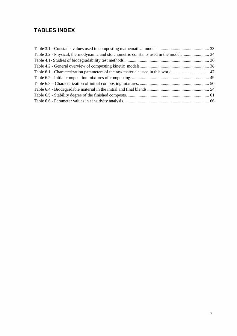
TABLES INDEX
Table 3.1 - Constants values used in composting mathematical models. ............................................. 33
Table 3.2 - Physical, thermodynamic and stoichometric constants used in the model. ........................ 34
Table 4.1- Studies of biodegradability test methods ............................................................................. 36
Table 4.2 - General overview of composting kinetic models. .............................................................. 38
Table 6.1 - Characterization parameters of the raw materials used in this work. ................................. 47
Table 6.2 - Initial composition mixtures of composting. ...................................................................... 49
Table 6.3 – Characterization of initial composting mixtures. ............................................................... 50
Table 6.4 - Biodegradable material in the initial and final blends. ....................................................... 54
Table 6.5 - Stability degree of the finished composts. .......................................................................... 61
Table 6.6 - Parameter values in sensitivity analysis. ............................................................................. 66

xi
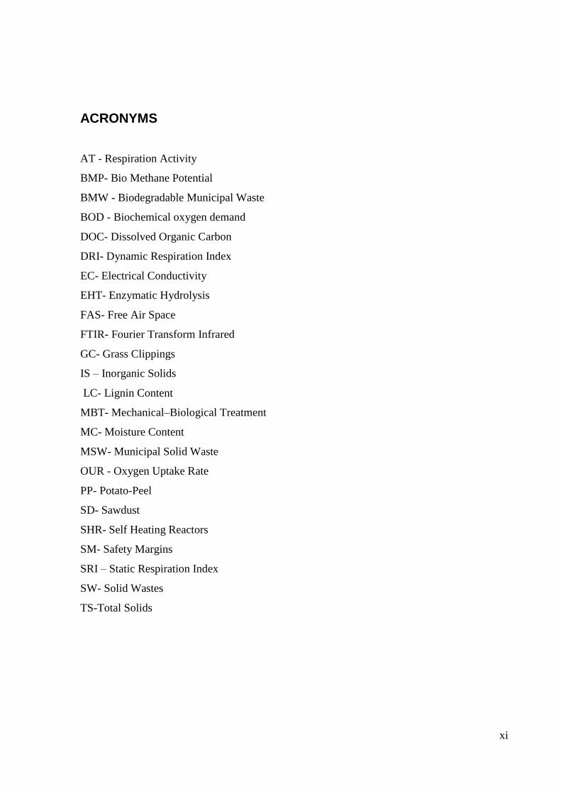
ACRONYMS
AT - Respiration Activity
BMP- Bio Methane Potential
BMW - Biodegradable Municipal Waste
BOD - Biochemical oxygen demand
DOC- Dissolved Organic Carbon
DRI- Dynamic Respiration Index
EC- Electrical Conductivity
EHT- Enzymatic Hydrolysis
FAS- Free Air Space
FTIR- Fourier Transform Infrared
GC- Grass Clippings
IS – Inorganic Solids
LC- Lignin Content
MBT- Mechanical–Biological Treatment
MC- Moisture Content
MSW- Municipal Solid Waste
OUR - Oxygen Uptake Rate
PP- Potato-Peel
SD- Sawdust
SHR- Self Heating Reactors
SM- Safety Margins
SRI – Static Respiration Index
SW- Solid Wastes
TS-Total Solids

xiii
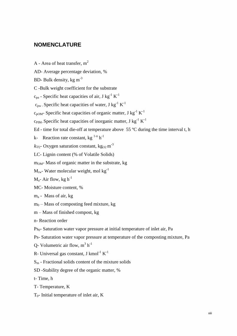
NOMENCLATURE
A - Area of heat transfer, m2
AD- Average percentage deviation, %
BD- Bulk density, kg m-3
C -Bulk weight coefficient for the substrate
cpa - Specific heat capacities of air, J kg-1
K-1
cpw - Specific heat capacities of water, J kg-1
K-1
cpOM- Specific heat capacities of organic matter, J kg-1
K-1
cPIM- Specific heat capacities of inorganic matter, J kg-1
K-1
Ed - time for total die-off at temperature above 55 ºC during the time interval t, h
k- Reaction rate constant, kg 1-n
h-1
2- Oxygen saturation constant, kgO2 m-3
LC- Lignin content (% of Volatile Solids)
mOM- Mass of organic matter in the substrate, kg
Mrw- Water molecular weight, mol kg-1
Ma- Air flow, kg h-1
MC- Moisture content, %
ma - Mass of air, kg
m0 – Mass of composting feed mixture, kg
m – Mass of finished compost, kg
n- Reaction order
Ps0- Saturation water vapor pressure at initial temperature of inlet air, Pa
Ps- Saturation water vapor pressure at temperature of the composting mixture, Pa
Q- Volumetric air flow, m3 h
-1
R- Universal gas constant, J kmol-1
K-1
Sm - Fractional solids content of the mixture solids
SD -Stability degree of the organic matter, %
t- Time, h
T- Temperature, K
T0- Initial temperature of inlet air, K
xiv
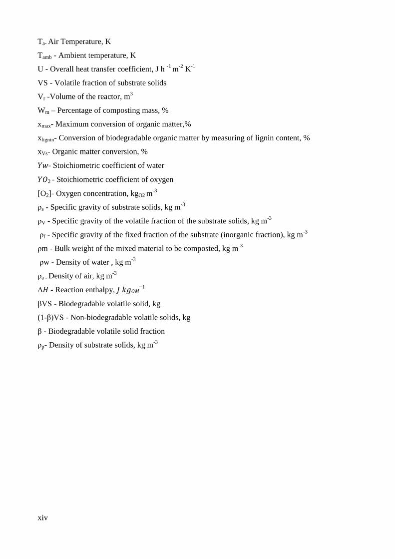
Ta- Air Temperature, K
Tamb - Ambient temperature, K
U - Overall heat transfer coefficient, J h -1
m-2
K-1
VS - Volatile fraction of substrate solids
Vr -Volume of the reactor, m3
Wm – Percentage of composting mass, %
xmax- Maximum conversion of organic matter,%
xlignin- Conversion of biodegradable organic matter by measuring of lignin content, %
xVs- Organic matter conversion, %
- Stoichiometric coefficient of water
2 - Stoichiometric coefficient of oxygen
[O2]- Oxygen concentration, kgO2 m-3
ρs - Specific gravity of substrate solids, kg m-3
ρV - Specific gravity of the volatile fraction of the substrate solids, kg m-3
ρf - Specific gravity of the fixed fraction of the substrate (inorganic fraction), kg m-3
ρm - Bulk weight of the mixed material to be composted, kg m-3
ρw - Density of water , kg m-3
ρa - Density of air, kg m-3
Δ - Reaction enthalpy, −1
βVS - Biodegradable volatile solid, kg
(1-β)VS - Non-biodegradable volatile solids, kg
β - Biodegradable volatile solid fraction
ρp- Density of substrate solids, kg m-3
1.INTRODUCTION
1
1. INTRODUCTION
The decomposition of organic materials in fertilizers is considered a practice as old as
the emergence of agriculture. In this scope, the process of composting, which refers to the
controlled decomposition of organic materials, has been used by humans since prehistoric
times to recycle wastes and make them useful for plant growth. In the nature, composting
process occurs when leaves pile up and begin to decay with some of them returning to the
soil, where living roots reclaim their nutrients. Since prehistoric times, composting has been
used for the benefit of agriculture. However, research studies, as well as the development of
this technology has just begun in the early 20th
century with the first attempt to give a
scientific basis occurring in 1924-1926 by Howard and Wad [1,2]
.
Since the Second World War, as the growing fields have become larger and the work
became mechanized, the use of fertilizers and other traditional means of improving soil
productivity decreased. Recently, a renewed attention in the composting process has been
observed. Restrictive legislation in many environmental areas have been responsible for
encouraging this interest, which led to the development of a new generation of composting
facilities throughout Europe [3]
.
The amount and diversity of solid wastes (SW) produced around the world has been
increased in recent decades, mainly due to the growth of the population, industrialization and
use of disposables. These residues must be then managed under appropriate disposal practices
to avoid negative impacts on the environment becoming difficult for governmental agencies
to face the challenge of handling such enormous quantities produced worldwide. Composting
cannot be considered a new technology, but amongst the waste management strategies it is
gaining interest as a suitable method with economic and environmental profits. The finished
composts are mainly used in agriculture as soil improvers to increase organic matter that is
important for plant growth and decrease of the risk of erosion. Nowadays, there is an intensive
research in order to obtain scientific information for building more efficient composting
systems [4-6]
.
This work has two main objectives. The first one is to predict the biodegradability of
an initial waste mixture and to investigate how this property progresses during the composting
2
process in a pilot-scale reactor. The biodegradability assessment in the starting materials
seems to be an important parameter in order to determine the self heating capabilities of a
blend, enabling thus to foresee if a specific mixture is adequate to be further composted. The
second objective is to develop a dynamic mathematical model for the aerobic composting
process under analysis and its validation by using experimentally measured dynamic state
variables.
The initial mixtures that were tested were made from potato-peel industrial waste (PP),
grass clippings (GC) and sawdust (SD) in four different proportions. These blends were
composted in isolated self heating reactors (SHR) with 120 L of internal volume. During
composting, a data acquisition system was used for on-line monitoring of temperature and
oxygen concentration, and feed air flow rate was measured with rotameters. The waste
mixtures were sampled in pre-determined times along the period of composting and
biodegradability of each sample was assessed by measuring lignin content, through the
Klason lignin method.
This work is organized into seven chapters. Chapter 1 is the introductory part. In
chapter 2 an overview of the composting process is made and the substrates usually used are
characterized. The existing composting systems were also described in this chapter.
In Chapter 3 a full description of the mathematical model developed is provided, and
all variables and parameters are defined. Chapter 4 focus the state of the art with reference
to studies that have been made in assessing the biodegradability of solid wastes, as well
as those related with the development of models that describe the composting
process. The experimental methodology used, monitoring strategies and quantification
of various parameters are described in Chapter 5.
Finally, Chapter 6 presents the analysis and discussion of the results obtained during
the work and Chapter 7 summarizes the main conclusions and prospects for future work.
2.THEORETICAL FOUDATIONS OF COMPOSTING
3
2. THEORETICAL FOUNDATIONS OF COMPOSTING
An approach to the composting technology is given in this section, including the
analysis of important process factors and microbiological aspects.
2.1. Composting process
Composting can be defined as the aerobic microbial decomposition of organic matter
of vegetable and animal origin, under conditions that allow the development of thermophilic
temperatures as a result of the heat produced by biological reactions. Involving the
mineralization and partial humification of the organic matter, this process will lead to a
stabilized and hygienized final product (i.e. free of pathogens and seeds) commonly known as
compost. Thus, this technique permits waste stabilization under special conditions of mixing
and aeration in order to reach the required thermophilic temperatures responsible for
microbial growth, weed seeds elimination, pathogen inactivation and helminthes kill,
avoiding generation of noxious gases as well [7,8]
.
Composting is thus a microbiological process based on the activity of various bacteria,
actinomycetes and fungi. The main product is rich in humus and plant nutrients such as
nitrogen and phosphorous, and the foremost reaction by-products are carbon dioxide, water,
ammonium and heat (equation (2.1)). The CO2 and water losses can amount to half the weight
of the initial materials, thereby reducing the volume and mass of the final product. In this
procedure, aerobic microorganisms use organic matter as energy source by decomposing
substrates, turning them into simpler compounds. This transformation is conditioned by the
nature of the initial substances and its degradability character, an important property that
affects decomposition rates, gas emissions, process duration and oxygen requirements. The
labile organic compounds such as simple carbohydrates, fats and amino acids are quickly
transformed (oxidized) through successive activities of different microbes. Meanwhile, the
residual organic matter as cellulose, hemicellulose and lignin become more and more resistant
to microbial biodegradation and are partially converted into stable organic matter, which
chemically and biologically resembles humic substances. The extent of these changes depends
on the available substrates and the process variables used to control the composting [1,4,9]
.
4
(2.1)
During composting, mineralization and humification occur simultaneously and are the
main processes causing the degradation of the fresh organic matter. The humified fraction
(humus) is the principal responsible for the organic fertility functions in the soil as it is the most
resistant to microbial degradation, being considered a major reservoir of organic carbon in soil.
Humus is then the final product of the humification process, in which natural materials are
partially transformed into humic substances nearly inert mainly formed of lignin,
polysaccharides and nitrogenous species. Thus, these compounds are not totally mineralized
during composting. In fact, the humification of the organic matter during composting is revealed
by the formation of humic acids with increasing molecular weight, aromatic characteristics,
oxygen and nitrogen concentrations and functional groups, in agreement with the generally
accepted humification theories of soil organic matter. During composting, humic substances are
produced and humic acid-like organic increases, while fulvic acid-like organic and water-
extractable organic decrease due to microbial degradation [4]
.
The chemical steps of organic matter to form humus are very complex and involve a
number of degradative and condensation reactions. Lignin is degraded by extracellular enzymes
to smaller units, which are then absorbed into microbial cells partially converted further into
phenols and quenones. When placed into soil, these substances along with the oxidative enzymes
polymerize by a free radical mechanism. The structure of humic compounds is not yet well
known, being usually divided into three groups based on chemical fractionation: humin
(insoluble in water at any pH), humic acids (insoluble in water under acidic conditions) and
fulvic acids (soluble in water under all pH conditions) [10]
.
The objective of composting has traditionally been to convert biologically degradable
organic materials to a stable and hygienized form also characterized by reduced odor because of
the low rate of decomposition of such resistant compounds. This compost may finally serve as a
source of organic matter with beneficial effects when applied to land either as fertilizer (source
of nitrogen or phosphorus), soil corrector (transfer of specific physical properties), or as crop
substrate to agricultural lands, green areas, forests and home gardening. When used as soil
corrector, it improves the drainage of water, increases water and nutrients retention capacity and
acts as pH regulator. It also allows adjust temperature, control erosion, improve aeration, slowly
release nutrients to the soil, increase the cation exchange capacity of sandy soils, and prevent
desertification and floods [11]
.
2.THEORETICAL FOUDATIONS OF COMPOSTING
5
In general, composts may contain important nutrients including nitrogen, phosphorus,
potassium, and a variety of small quantities of other essential elements. This nutrient content is
mainly related to the quality of the original substrates and operating process conditions.
However, most of the composts are poor in nutrients to be classified as fertilizers so, their main
applications are as soil conditioners and landfill cover [7]
. Compost may also help to increase the
effectiveness of chemical fertilizers and consequently, emissions of CO2 and other green houses
gases related to fertilizers production may be indirectly decreased. Finally, it is important to note
that organic material in soil may have a key role in the global warming control. Indeed, there is a
good interaction between land use, optimization of waste management and carbon sequestration.
The organic matter stability, along with other characteristics, may be essential to achieve this
positive interaction and for the maximization of soil carbon fixation, and thus, for the reduction
of the emission of CO2 to the atmosphere [6]
.
2.2. Composting substrates
Composting is usually applied to any biodegradable organic solid and semi-solid
material, and thus, the amount of substrates potentially suitable for composting is really huge.
However, it is important to stress that the optimum feedstock for it should be mainly from
source separated organic materials. The main categories of composting substrates include
municipal solid waste (MSW), industrial and agricultural waste [11]
.
2.2.1. Waste management
The Decreto-Lei n. ° 73/2011 established the general regime of waste management in
Portugal, by repealing the previous diploma, the Decreto-Lei n. ° 178/2006 of September 9th
.
This legislation defines waste as ―any substance or object which the holder discards or intends
to or is obliged to discard, particularly those indentified in the European Waste List.‖ It also
defines the general principles of waste management, the hierarchy of waste management
operations, which state that the landfill should be the last management option, only justified
when others are technically and financially inviable. In fact, it is well known that the waste
disposal in landfill has negative impacts on the environment. The legislation issued during the
past few years has a key role in addressing this situation by imposing targets on the
6
elimination of organic waste and simultaneously encouraging waste management based on a
hierarchy in which are privileged solutions to waste reduction, recycling, recovery energy
instead of disposal in landfill. Requiring a progressive reduction of the quantities deposition
of biodegradable waste in landfills, Decreto-Lei n. °152/2002 of May 23th
concerning the
disposal of waste into landfills, presents an important challenge. This law aims to improve the
general conditions of landfill operation, preventing or reducing as far as possible the adverse
environmental effects of disposing waste in landfills. In this context, all types of depositions,
including water monitoring and leachate management, protection of soil and groundwater and
gas monitoring were regulated. It also requires the implementation of strategies in order to
gradually reduce the amount of organic waste going to landfill. Thus, the total amount (by
weight) of biodegradable municipal land filled in 1995 was expected to decrease to 75% in
2006, 50% in 2009 and 35% in 2016. Decreto-Lei n. ° 152/2002 of May 23th
was recently
repealed by Decreto-Lei n. ° 183/2009 of August10th
, which delays in four years the time
limits specified in the previous draft, imposing tough new targets to reduce landfill disposal of
biodegradable municipal waste, also in relation to 1995 data is expected to decrease to 50% in
2013 and 35% in 2020. Limiting the amount of biodegradable waste going to landfill implies
the diversion of this waste towards appropriate treatment options such as composting. This
waste treatment technology will clearly have an important role in processing much of the
biodegradable waste, which in future will have to be diverted from landfill [2]
.
2.2.2. Municipal solid waste
The quantity and diversity of MSW produced around the world has increased in recent
decades. There are several factors that have contributed to this growing production of waste,
such as the population explosion and economic growth. In mainland Portugal, the production
of municipal waste was approximately 5.184 million tons in 2009. With regard to the amount
of MSW generated per capita, 511 kg/(hab.year) were produced in 2009, which corresponds
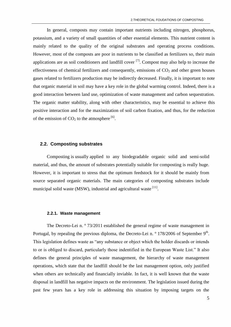
to a daily production of 1.4 kg of MSW per capita. Figure 2.1 shows the amount of MSW
produced between 2005 and 2009[12]
.
2.THEORETICAL FOUDATIONS OF COMPOSTING
7
Figure 2.1- Evolution of the total production and annual per capita MSW between 2005 and
2009 (redrawn from [12]).
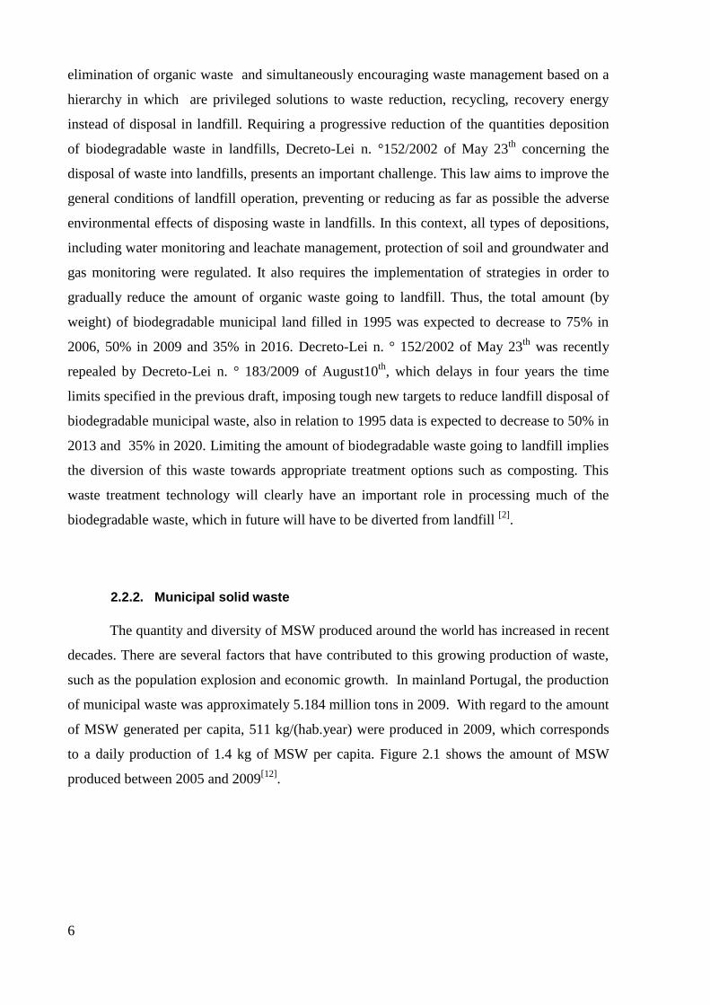
Besides the waste production, is also important to know their composition, which
often varies depending on a number of factors: geographical location, seasons, urban or rural
area, cultural and dietary habits, standards of living, characteristics of collection services
offered and the level of promotion of home composting. According to its composition MSW
may be grouped by type and the quantity is expressed as percentages. Figure 2.2 shows the
composition of MSW in Portugal, where the major fractions correspond to fermentable
materials often referred to as ―kitchen waste‖ and paper and paperboard. Kitchen waste is
usually rich in organic that may have more than 90% of biodegradability. The paper is also
part of the biodegradable fraction. Although, it is often assumed that paper recycling is a
better option than the use of biological treatment, depending on local conditions and
availability of infrastructure and outlets for the paper recycling, waste paper and paperboard
can sometimes serve as a valuable source of carbon, allowing the composting of food waste
[13,11].
Figure 2.2 - Composition of the municipal solid waste in Portugal in 2008 (redrawn from [13]).
8
Figure 2.2 confirms that the organic matter often represents the most significant
fraction of the waste stream.
The main options for the treatment of biodegradable MSW are composting, anaerobic
digestion, incineration, gasification and pyrolysis. In the last decades composting has gained
an important role on MSW management, and it can be applied both to mixed MSW and to
separately collected biodegradable fraction. When the substrate is mixed MSW, the
infrastructure for its treatment is called a mechanical–biological treatment (MBT) plant. This
includes a combination of mechanical, other physical and biological processes that are mainly
used to reduce the volume and weight and stabilize the fermentable fraction of MSW [14]
.
In Europe the concept of large-scale municipal composting was originated in Holland
in 1929, and the facility was used to dispose of the refuse from several cities to produce
compost. However, the first serious attempts to use large-scale composting to treat mixed
MSW in Europe began in the 1970s and extended into the 1980s, at which time it was
expected that these plants could treat approximately 35% of the total MSW [2]
.
2.3. Composting systems
Today, different composting technologies are used depending on the location, the
substrate, the scale of operation, time required to reach compost stability and maturity, the
availability of land, and the skills and the machinery available. Among the composting
technology, the most basic distinction is between reactor and non reactor systems, Figure 2.3.
Reactor technology is often termed ―in-vessel‖, whereas non reactors are open systems. The
―non reactors‖ includes the ones used from prehistoric times to the windrows, static pile, and
household systems used in the present days.
―Non reactor‖ systems may be categorized on the basis of the aeration method. Thus,
these systems are divided in agitated solids bed and static bed. An agitated solid bed means
that the composting mixture is disturbed or broken up in some manner to introduce oxygen as
well as to (and accordingly) control the temperature, and effect mixing of the material during
the composting cycle. The agitation may be by periodic turning, tumbling, or other methods
of agitation. The windrow and the static pile processes are examples of the agitated and the
static bed aeration systems, respectively [1,7]
.
2.THEORETICAL FOUDATIONS OF COMPOSTING
9
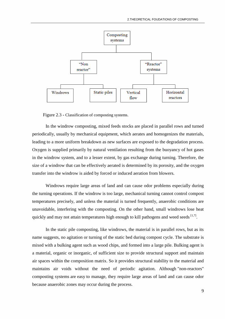
Figure 2.3 - Classification of composting systems.
In the windrow composting, mixed feeds stocks are placed in parallel rows and turned
periodically, usually by mechanical equipment, which aerates and homogenizes the materials,
leading to a more uniform breakdown as new surfaces are exposed to the degradation process.
Oxygen is supplied primarily by natural ventilation resulting from the buoyancy of hot gases
in the windrow system, and to a lesser extent, by gas exchange during turning. Therefore, the
size of a windrow that can be effectively aerated is determined by its porosity, and the oxygen
transfer into the windrow is aided by forced or induced aeration from blowers.
Windrows require large areas of land and can cause odor problems especially during
the turning operations. If the windrow is too large, mechanical turning cannot control compost
temperatures precisely, and unless the material is turned frequently, anaerobic conditions are
unavoidable, interfering with the composting. On the other hand, small windrows lose heat
quickly and may not attain temperatures high enough to kill pathogens and weed seeds [1,7]
.
In the static pile composting, like windrows, the material is in parallel rows, but as its
name suggests, no agitation or turning of the static bed during compost cycle. The substrate is
mixed with a bulking agent such as wood chips, and formed into a large pile. Bulking agent is
a material, organic or inorganic, of sufficient size to provide structural support and maintain
air spaces within the composition matrix. So it provides structural stability to the material and
maintains air voids without the need of periodic agitation. Although "non-reactors"
composting systems are easy to manage, they require large areas of land and can cause odor
because anaerobic zones may occur during the process.
10
―Reactor‖ systems are design according to engineering principles and may be
categorized according to the manner of solids flow as either vertical flow reactors (towers) or
horizontal flow reactors. In these systems the waste is made to undergo decomposition within
an enclosed space, which makes possible to be rigorously controlled. Various forced aeration
and mechanical turning devices are used to optimize aeration in these systems.
Vertical flow reactors systems are further defined according to bed conditions in the
reactor and are divided into those that allow agitation of solids during transit down the
reactor, which are termed moving agitated bed reactors and those that where the composting
mixture occupies the entire bed volume and is not agitated. These systems are termed moving
packed bed.
Horizontal flow includes a number of reactors types in which the reactor is inclined
slightly from the horizontal to promote solids flow. This horizontal flow reactors fall into
three categories: tumbling solids bed reactors, which employ a rotating or rotary drum;
agitated solids bed reactors, which use a bin structure with agitation; and static solids bed
reactor, which also use a bin structure but with a static solid bed.
The ―reactor‖ systems enable composted larger masses of waste within much shorter
land spaces than conventional composting methods. But the use of machinery and power
places significant cost burden on in-vessel systems, making them more expensive than the
conventional systems [1,2,7]
.
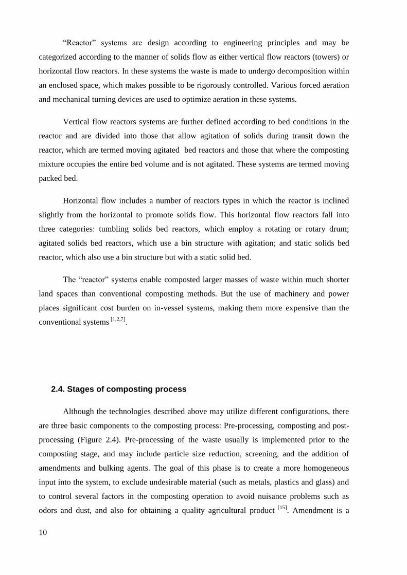
2.4. Stages of composting process
Although the technologies described above may utilize different configurations, there
are three basic components to the composting process: Pre-processing, composting and post-
processing (Figure 2.4). Pre-processing of the waste usually is implemented prior to the
composting stage, and may include particle size reduction, screening, and the addition of
amendments and bulking agents. The goal of this phase is to create a more homogeneous
input into the system, to exclude undesirable material (such as metals, plastics and glass) and
to control several factors in the composting operation to avoid nuisance problems such as
odors and dust, and also for obtaining a quality agricultural product [15]
. Amendment is a
2.THEORETICAL FOUDATIONS OF COMPOSTING
11
material added to other substrates to condition the feed mixture and is divided into two types:
structural or drying amendment, which is an organic material added to reduce bulk weight and
increase air voids allowing for proper aeration and energy or fuel amendment, which is an
organic material added to increase the quantity of biodegradable organics in the mixture and,
thereby, increase the energy content of the mixture.
Figure 2.4 - Generalized diagram for composting process stages.
Once the pre-processing is complete, the organic waste is loaded into the composting
system, and the process may begin as soon as the raw materials are mixed together.
Composting stage can be divided into three phases, based on the temperature of the system:
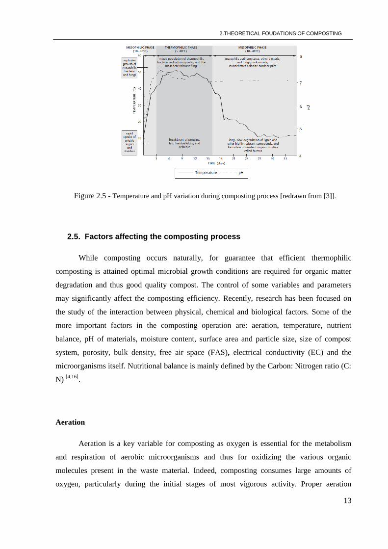
(1) a mesophilic, or moderate-temperature phase (up to 40 °C), which typically lasts for a
couple of days; (2) a thermophilic, or high temperature phase (over 40 °C), which can last
from a few days to several months; and (3) a several-month mesophilic curing or maturation
phase (Figure 2.5). The length of the composting phases depends on the composition of the
organic matter being composted and the efficiency of the process, which is determined for
example by the degree of aeration, agitation, and the size of the system [3]
.
At the start, the raw materials are at ambient temperature and usually slightly acidic.
During the initial stages of the process, oxygen and soluble, easily degradable components of
the materials are rapidly consumed by the microorganisms. Firstly, mesophilic bacteria
actinomycetes, fungi, and protozoa colonize the biodegradable solid waste. These
microorganisms grow between 10 and 45˚C and break down easily degradable components
such as monosaccharides, starch and lipids. Due to the oxidative action of microorganisms,
the temperature increases and there is a drop in pH at the very beginning of composting,
caused by the formation of fatty acids from the biodegradable compounds during degradation.
12
Once temperatures exceed 40°C, the mesophilic microorganisms become less competitive and
are replaced by thermophilic ones. At this thermophilic phase, high temperatures accelerate
the breakdown of proteins and fatty acids formed at the mesophilic phase, resulting in the
liberation of ammonium and an increase in the pH. After the easily degradable carbon sources
have been consumed, more resistant compounds such as cellulose, hemicellulose and lignin
are partly degraded. The optimum temperature for thermophilic micro-fungi and
actinomycetes which mainly degrade lignin is 40–50˚C. Above 60˚C, these microorganisms
cannot grow and lignin degradation is slowed down. After the thermophilic phase the
microbial activity decreases, and mesophilic microorganisms once again take over for the
final phase of ―curing‖ or maturation. Although the compost temperature is close to the
ambient, this last phase is important because, chemical reactions continue to occur that make
the remaining organic matter become more stable and additional humus-like substances are
produced to form mature compost [1,3,9,10]
. Once the compost is finished in the curing or
maturation phase, it may be post- processed according to the feedstock characteristics and
desired product quality.
2.THEORETICAL FOUDATIONS OF COMPOSTING
13
Figure 2.5 - Temperature and pH variation during composting process [redrawn from [3]].
2.5. Factors affecting the composting process
While composting occurs naturally, for guarantee that efficient thermophilic
composting is attained optimal microbial growth conditions are required for organic matter
degradation and thus good quality compost. The control of some variables and parameters
may significantly affect the composting efficiency. Recently, research has been focused on
the study of the interaction between physical, chemical and biological factors. Some of the
more important factors in the composting operation are: aeration, temperature, nutrient
balance, pH of materials, moisture content, surface area and particle size, size of compost
system, porosity, bulk density, free air space (FAS), electrical conductivity (EC) and the
microorganisms itself. Nutritional balance is mainly defined by the Carbon: Nitrogen ratio (C:
N) [4,16]
.
Aeration
Aeration is a key variable for composting as oxygen is essential for the metabolism
and respiration of aerobic microorganisms and thus for oxidizing the various organic
molecules present in the waste material. Indeed, composting consumes large amounts of
oxygen, particularly during the initial stages of most vigorous activity. Proper aeration
14
controls the growth of adequate aerobic microbe populations, the development of stabilizing
temperature and removes excess moisture and CO2 as well. If oxygen supply is limited, the
composting process may turn anaerobic, which is a much slower and odorous process. The
aeration flow rate must supply the depleted oxygen to the composting mixture and carries
away excess heat from the system with fresh air. A minimum oxygen concentration of 5%
within the pore spaces of the compost is necessary for aerobic composting. However, the
optimum O2 concentration is between 15% and 20% and the air flow rate should maintain
temperatures below 60–65 ˚C. Therefore, compost systems need to be designed to provide
adequate air flow using either passive or forced aeration systems [3,4,9]
.
Temperature
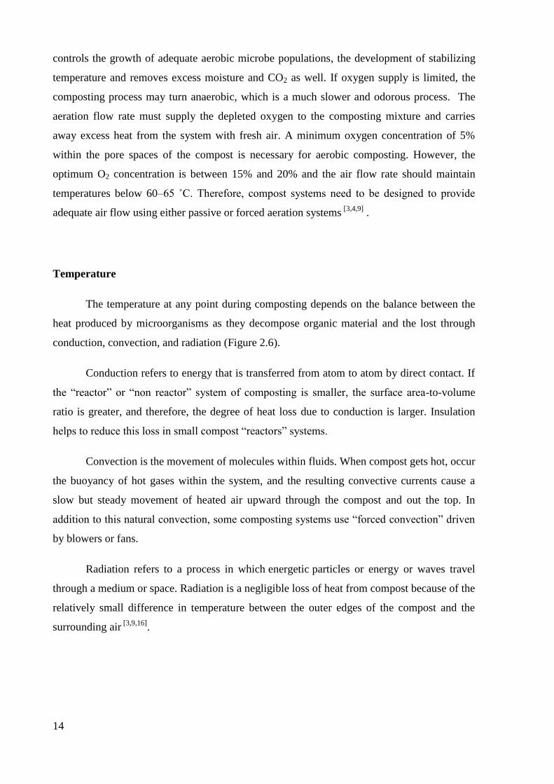
The temperature at any point during composting depends on the balance between the
heat produced by microorganisms as they decompose organic material and the lost through
conduction, convection, and radiation (Figure 2.6).
Conduction refers to energy that is transferred from atom to atom by direct contact. If
the ―reactor‖ or ―non reactor‖ system of composting is smaller, the surface area-to-volume
ratio is greater, and therefore, the degree of heat loss due to conduction is larger. Insulation
helps to reduce this loss in small compost ―reactors‖ systems.
Convection is the movement of molecules within fluids. When compost gets hot, occur
the buoyancy of hot gases within the system, and the resulting convective currents cause a
slow but steady movement of heated air upward through the compost and out the top. In
addition to this natural convection, some composting systems use ―forced convection‖ driven
by blowers or fans.
Radiation refers to a process in which energetic particles or energy or waves travel
through a medium or space. Radiation is a negligible loss of heat from compost because of the
relatively small difference in temperature between the outer edges of the compost and the
surrounding air [3,9,16]
.
2.THEORETICAL FOUDATIONS OF COMPOSTING
15
Figure 2.6 - Three mechanisms of heat loss from a composting pile [3]
.
Composting will essentially take place within two temperature ranges known as
mesophilic (10-40 °C) and thermophilic (over 40 °C). The temperature of the compost is a
good indicator of the microbial activity. Temperatures greater than 60 °C reduce the activity
of many of the active organisms. Therefore, the optimum temperature range is between 32 °C
and 60 °C. There is a direct relation between temperature and rate of oxygen consumption.
Higher temperature led to greater oxygen uptake and faster rate of decomposition.
Temperatures of composting materials characteristically follow a pattern of rapid increase to
55 – 60 °C and remain near this thermophilic level for several days or weeks. Temperatures
gradually drop to 38°C and finally drop to ambient air temperature.
It is important to note that for destroying pathogenic microorganism the temperature
should reach at last 55 °C for some hours to a few days.
Carbon: Nitrogen ratio (C:N)
Carbon, nitrogen, phosphorous, and potassium are the primary nutrients required by
the microorganisms involved in composting. The optimum value of the carbon-to-nitrogen
ratio (C:N ratio) is also an essential factor for microorganisms decompose of organic wastes
during composting processes, as it usually ensures that the other required nutrients are present
in adequate amounts. Carbon serves primarily as energy source for the microorganisms, while
a small fraction of the carbon is incorporated into the microbial cells. Nitrogen is essential for
microbial population growth, as it is a constituent of protein that forms over 50% of dry
bacterial cell mass.
16
Raw materials blended to provide a C:N ratio of 25:1 to 30:1 are ideal for active
composting, but initial C:N ratios from 15:1 up to 40:1 consistently give good composting
results. High C:N ratios make the process very slow as there is not enough N available for
the growth of microorganisms which results in a longer time for composting process. But with
a low C:N ratio there is an excess of N per degradable C which can mineralize into ammonia
it can be lost through ammonia volatilization, leaching from the composting mass and
denitrification producing unpleasant odors. Denitrification can occur as a result of the
development of anaerobic micro sites within the material. Thus, the aerobic conditions of the
compost should be ensured throughout the process.
Most materials available for composting do not fit the ideal C:N ratio, so different
materials must be blended to meet the required ratio. The carbon sources for microorganisms
usually come from bulking agents such as sawdust and wood chip. Green wastes, such as
foliage and manure, contain relatively high proportions of nitrogen and thus can be used as
nitrogen sources [1,4,8,9,17]
.
pH of materials
Another parameter that greatly affects the composting process is the pH of the blend.
During the course of composting, the pH in general varies between 5.5 and 8.5. The range of
pH values suitable for bacterial development is 6.0–7.5, while fungi prefer an environment in
the range of pH 5.5–8.0.
Composting itself leads to major changes in materials and in pH as well. In the early
stages of composting, organic acids accumulate as a by-product of the organic matter
degradation by bacteria and fungi and may, temporarily or locally, lower the pH (increase
acidity). Usually, the organic acids break down further during the composting process, and the
production of ammonia from nitrogenous compounds may raise the pH (increase alkalinity).
Thus, the pH is very relevant factor for controlling N-losses by ammonia volatilization, which
can be particularly high at pH >7.5. Later in the composting process, the pH tends to become
neutral as a result of humus formation with its pH buffering capacity at the end of composting
activity. Finished compost should have pH within the range of 5.0 to 8.0 to be compatible with
plant growth and to avoid odors [1,3,4,16]
.
2.THEORETICAL FOUDATIONS OF COMPOSTING
17
Moisture
Moisture plays an essential role in the metabolism of microorganisms and indirectly in
the supply of oxygen, as it provides a medium for the transport of dissolved nutrients required
for the metabolic and physiological activities of microorganisms. The optimum water content
for composting varies with the waste to be composted, but an initial moisture content of 40–
75% by weight is generally considered optimum because it provides sufficient water to
maintain microbial growth but not so much that air flow is blocked. When the moisture
content is too high (over 75%) nutrients may be leached, air volume is reduced and will close
the air pores, reduce the oxygen content and consequently turns composting into an anaerobic
process. Experience has shown that the bacterial activity will slow down when the moisture
content is below 40%, and will cease entirely below 15 % [1,3,16,17]
.
Particle size and surface area
Microbial activity occurs at the interface of particle surfaces and air. Therefore, the
rate of aerobic decomposition increases with smaller particle size, because high surface areas
allows microorganisms to digest more material, and generate more heat, and so improve the
biological activity and rate of composting. Smaller particles, however, may reduce the
effectiveness of oxygen movement within the composting system, and thus the oxygen
available to microorganisms decreases. Optimum composting conditions are usually obtained
with particle sizes ranging from 5 to 12.5 cm of average diameter [3,9,16]
.
Size of compost system
The system volume can have great influence on the degradation rate of the material.
The system must be large enough to prevent rapid dissipation of heat and moisture, yet small
enough to allow good air circulation for the microbial activity [3]
.
Porosity and free air space
Substrate porosity carries a great influence on composting performance since
appropriate conditions of the physical environment for air distribution must be maintained
18
during the process. Porosity refers to the spaces between particles in the compost system. If
the material is not saturated with water, these spaces are partially filled with air that can
supply oxygen to decomposers and provide a path for air circulation. As the material becomes
water saturated, the space available for air decreases [4,16]
.
Free air space (FAS) is a representation of the available air filled voids in a
composting matrix. This parameter is very important as it is intrinsically related to the
availability of water and oxygen, which are determinant factors for the biological activity of
the microorganisms. The maintenance of optimum oxygen concentration is important to
remove carbon dioxide and excess moisture, as well as to avoid or prevent an excessive heat
accumulation, which depends on the air content and its movement trough composting
material. Thus, maintaining adequate FAS levels satisfies the oxygen concentration required
to achieve desired composting conditions. Minimum FAS requirements were established at
35% while maximum FAS levels recommended in order to avoid heat losses varies according
to the wastes composition [19]
.
Bulk density
Bulk density is a property of particulate materials, and corresponds to the mass of
many particles of the material per unit of bed volume, including the pore space. It is a useful
indicator of materials compaction and so must be controlled [18]
.
Electrical conductivity (EC)
Electrical conductivity (EC) is expression of the ability of an aqueous solution to carry
an electrical current. It is generally related to the total solute concentration and can be used as
a quantitative measure of dissolved salt concentration, even though it is also affected by the
mobility, charge and relative concentration of each individual ion present in the solution.
Generally, EC increases during composting as volatile solids(VS) are degraded and the
amount of water-soluble salts increases on a total solids (TS) basis[1,20]
.
Microorganisms
2.THEORETICAL FOUDATIONS OF COMPOSTING
19
Organic matter decomposition is carried out by many different groups of microbial
populations. The microorganisms involved in composting develop according to the
temperature of the mass, which defines the different steps of the process. Naturally occurring
microorganisms and invertebrates are the primary decomposers that accomplish composting.
These microorganisms include bacteria, fungi, actinomycetes and protozoa. Different
decomposers prefer different organic materials and temperatures and therefore, the microbial
populations should be diverse. Changing operating conditions during the composting process
lead to an ever-changing ecosystem of decomposition organisms. Among all microorganisms,
aerobic bacteria are the most important initiators of decomposition and temperature increase
within the compost system. Fungi are present during all the process but predominate at water
levels below 35% and are not active at temperatures over 60 °C. Actinomycetes predominate
during stabilization and curing, and together with fungi are able to degrade resistant polymers.
The ability of microorganisms to assimilate the organic matter depends on its capacity
to produce enzymes necessary for degradation of specific substrate. The more complex the
substrate, more varied enzymes system is needed. Through the synergic action of
microorganisms, complex organic compounds are degraded to smaller molecules that can be
used by microbial cells [4,10,16]
.
2.6. Finished compost Properties
The aim of composting should be to yield consistent product quality. However, the
effectiveness of compost with regard to beneficial effects on soil depends on its quality,
whose properties vary widely, as a function of the initial ingredients, the process used, and the
age of the compost. Physical characteristics such as color, odor and temperature give a
general idea of the decomposition stage reached, but give little information about the quality
of the compost. In fact, the quality criteria for compost are usually established in terms of:
nutrient content humified and stabilized organic matter, the maturity degree, the hygienization
and the presence of certain toxic compounds such as heavy metals and soluble salts. The
principal requirement for it safe use in soil is a high degree of stability and maturity, which
implies stable organic matter content and the absence of phytotoxic compounds and
pathogens. Phytotoxicity is mainly attributed to the presence of fatty acids but may also be
caused by salinity, heavy metal, NH3 and some toxic trace elements..
20
The terms stability and maturity are both commonly used to define the degree of
decomposition of organic matter during the composting process even if they are conceptually
different. Compost stability refers to a specific stage of decomposition during composting,
which is related to the types of organic compounds remaining and the resultant biological
activity that can be measured, for example, by respiration rates. When compost is unstable,
microbial activity is high and the substrates pass through rapid changes. Maturity is the
degree or level of completeness of composting and implies improved qualities resulting from
‗ageing‘ or ‗curing‘ of a product. Therefore, it is related to suitability in final use and crop
growing. The use of immature compost is adverse to soil as anaerobic conditions develop as
the microorganisms in soil use oxygen to decompose the compost, letting plant roots without
oxygen and potentially generating toxic intermediates. Stability and maturity usually go hand
in hand, since phytotoxic compounds are produced by the microorganisms in unstable
composts.
Several variables have been proposed for monitoring the composting process and
evaluating the stability of the compost. These variables may include physical, chemical, and
biological parameters of the organic material, such as temperature, degree of self-heating
capacity, oxygen consumption, biochemical parameters of microbial activities, analysis of
biodegradable constituents, phytotoxicity assays, organic matter nutrient content, C/N ratio,
and humus content and quality [1,4,6,10]
.
2.7. Biodegradability of organic matter
The definition of the criteria by which a material can be considered as compostable is
a topical issue for the use of composting as a feasible waste management treatment. Among
other criteria mentioned above, the biodegradability of materials in composting conditions is a
key property. However, the practice to determine the biodegradability of waste is not very
common, and the composting systems are usually designed based on assumed
biodegradability of the waste reported on previous studies.
Biodegradability is defined as the biologically catalyzed breakdown of organic matter
carried out by microorganisms. As in the natural environment or in technical facilities, there
2.THEORETICAL FOUDATIONS OF COMPOSTING
21
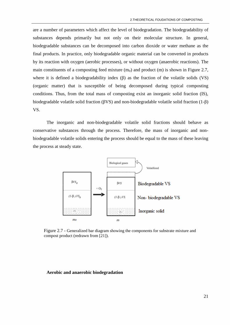
are a number of parameters which affect the level of biodegradation. The biodegradability of
substances depends primarily but not only on their molecular structure. In general,
biodegradable substances can be decomposed into carbon dioxide or water methane as the
final products. In practice, only biodegradable organic material can be converted in products
by its reaction with oxygen (aerobic processes), or without oxygen (anaerobic reactions). The
main constituents of a composting feed mixture (m0) and product (m) is shown in Figure 2.7,
where it is defined a biodegradability index (β) as the fraction of the volatile solids (VS)
(organic matter) that is susceptible of being decomposed during typical composting
conditions. Thus, from the total mass of composting exist an inorganic solid fraction (IS),
biodegradable volatile solid fraction (βVS) and non-biodegradable volatile solid fraction (1-β)
VS.
The inorganic and non-biodegradable volatile solid fractions should behave as
conservative substances through the process. Therefore, the mass of inorganic and non-
biodegradable volatile solids entering the process should be equal to the mass of these leaving
the process at steady state.
Figure 2.7 - Generalized bar diagram showing the components for substrate mixture and
compost product (redrawn from [21]).
Aerobic and anaerobic biodegradation
22
Aerobic biodegradation is the breakdown of an organic compound by microorganisms
in the presence of oxygen into carbon dioxide, water and mineral salts of any other elements
present (mineralization) plus new biomass. Therefore, the chemistry of the system,
environment, or organism is characterized by oxidative conditions. Aerobic bacteria use
oxygen as an electron acceptor, and breakdown organic chemicals into smaller organic
compounds, often producing carbon dioxide and water as the final product.
Aerobic biodegradation is also known as aerobic respiration.
Anaerobic digestion occurs when microorganisms breakdown biodegradable material
in the absence of oxygen. Generally the breakdown in anaerobic conditions proceeds
sequentially from the complex to the simple molecules. The process begins with bacterial
hydrolysis of complex particulate materials in order to break down insoluble organic
polymers such as proteins, carbohydrates and lipids to yield monomers like amino acids,
sugars, and high molecular fatty acids and make them available for other bacteria. Amino
acids and sugars are converted into acids, carbon dioxide, hydrogen, ammonia, and organic
acid. The resulting organic acids are converted into acetic acid, along with additional
ammonia, hydrogen, and carbon dioxide. Finally these products may be converted to methane
and carbon dioxide [22-25].
2.7.1. Methods to assess the biodegradability of organic matter
Test methods used to estimate biodegradability are an important part of organic waste
characterization as they can be used to predict the biodegradation behavior of a test material
and to assess the effectiveness of a certain treatment process, including composting. The
degradation processes can occur in very different environmental situations. Thus, there are
several biological and non-biological testing methods available for assessing this propertiy.
Biodegradability tests typically involve incubation of the organic waste in the presence of live
microorganisms that decompose the organic matter (biological test methods). The basic
principle of these tests is to assess how much of the carbon can be mineralized and how
quickly it will be degraded. Therefore, the degree to which the rate of biodegradability of the
waste is reduced, and the extent of decomposition achieved, can both be used as an indication
of the performance and efficiency of the treatment process. The biodegradability tests may be
carried out under anaerobic or aerobic conditions and are monitored by measuring biogas
2.THEORETICAL FOUDATIONS OF COMPOSTING
23
production (CH4 and CO2) in anaerobic tests and either O2 consumption or CO2 production in
aerobic tests [6,26].
Anaerobic methods
Anaerobic test methods measure the biodegradability of a material in the absence of
oxygen by measuring the amount of biogas released (CO2 and CH4) resulting from the
decomposition of organic materials carried out by methanogenic bacteria. An example of this
decomposition for cellulose and hemicellulose is shown in Eqs. (2.2a) and (2.2b),
respectively.
(2.2a)
(2.2b)
The Bio Methane Potential (BMP) test is one method that can be used to estimate the
amount of methane that could be produced from anaerobically digesting organic matter in a
temperature controlled system [26]
.
Aerobic methods
Aerobic test methods measure the biodegradability of a material in the presence of oxygen by
measuring the O2 consumption or CO2 production of a test material. The aerobic
biodegradation of cellulose and hemicelluloses are shown as example in equations (2.3a) e
(2.3b), respectively.
(2.3a)
(2.3b)
There are several aerobic waste biodegradability test methods as well as different monitoring
techniques and ways of expressing results. They can be classified as ‗dynamic‘ or ‗static‘
depending on whether or not the sample is aerated, respectively. Oxygen uptake rate (OUR)
and dynamic respiration index (DRI) are examples of static and dynamic test method,
24
respectively, and both were developed and designed to assess the degree of biological stability
of waste derived materials.
Biological methods are referred in literature as the most suitable stability
determination and are also proposed as a biodegradability measure. Although, the BMP
method has been reported to show good reproducibility it has the disadvantage of require long
periods to be complete, thereby not providing rapid feedback on routine monitoring. Aerobic
methods including the DRI test have other disadvantages such as preferentially decomposing
the readily biodegradable components of the material and therefore may not indicate potential
long-term biodegradability. Therefore most of current microbial based biodegradability test
methods have limitations and none of them is suitable for the whole range of biodegradability
testing requirements [26]
.
Since biological tests are time consuming and costly it is desirable to have simpler,
rapid and cheaper methods that may be a useful surrogate for biological tests.
Alternative method
A large proportion of MSW consists of biopolymers (proteins, fats, polysaccharides
and lignin). Lignin-containing materials are often referred as poorly biodegradable, so as a
general rule, the higher the lignin content, the lower biodegradable is the substrate. On other
hand, lignin is also the main precursor for humic substances and it is mainly humified (not
mineralized) during degradation in compost or soil. Therefore, the assessment of the material
lignin content may provide a non-biological test method of assessing biodegradability [7].
Lignin is a natural composite material in all vascular plants, which provides plant
strength and resistance to microbial degradation by decreasing water permeation across the
cell wall. It is an amorphous, aromatic, water insoluble, heterogeneous, three-dimensional,
and cross-linked polymer (Figure 2.8).
2.THEORETICAL FOUDATIONS OF COMPOSTING
25
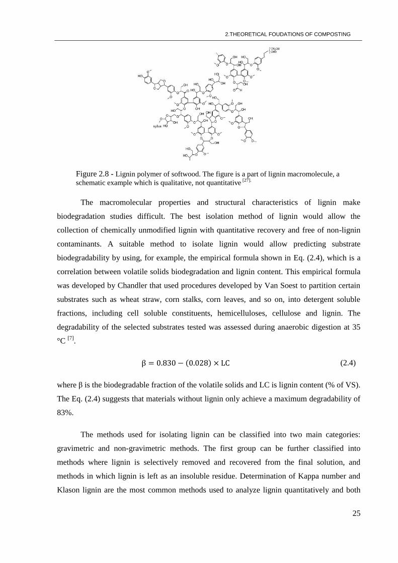
Figure 2.8 - Lignin polymer of softwood. The figure is a part of lignin macromolecule, a
schematic example which is qualitative, not quantitative [27].
The macromolecular properties and structural characteristics of lignin make
biodegradation studies difficult. The best isolation method of lignin would allow the
collection of chemically unmodified lignin with quantitative recovery and free of non-lignin
contaminants. A suitable method to isolate lignin would allow predicting substrate
biodegradability by using, for example, the empirical formula shown in Eq. (2.4), which is a
correlation between volatile solids biodegradation and lignin content. This empirical formula
was developed by Chandler that used procedures developed by Van Soest to partition certain
substrates such as wheat straw, corn stalks, corn leaves, and so on, into detergent soluble
fractions, including cell soluble constituents, hemicelluloses, cellulose and lignin. The
degradability of the selected substrates tested was assessed during anaerobic digestion at 35
°C [7]
.
(2.4)
where β is the biodegradable fraction of the volatile solids and LC is lignin content (% of VS).
The Eq. (2.4) suggests that materials without lignin only achieve a maximum degradability of
83%.
The methods used for isolating lignin can be classified into two main categories:
gravimetric and non-gravimetric methods. The first group can be further classified into
methods where lignin is selectively removed and recovered from the final solution, and
methods in which lignin is left as an insoluble residue. Determination of Kappa number and
Klason lignin are the most common methods used to analyze lignin quantitatively and both
26
are gravimetric. The non-gravimetric methods include spectroscopy such as Fourier transform
infrared (FTIR) and those based on optical properties of lignin.
Klason lignin is determined gravimetrically after extracting the sample with sulphuric
acid 72% to dissolve out the other components. Kappa number is usually used in the pulp and
paper industry and it is determined by oxidizing lignin selectively from pulp using a solution
of potassium permanganate. So Kappa number represents the amount of permanganate
consumed by the pulp sample [10, 28]
.
3. MATHEMATICAL MODEL OF COMPOSTING PROCESS
27
3. MATHEMATICAL MODELING OF COMPOSTING PROCESS
Composting is a process that involves many coupled physical, chemical and biological
mechanisms that are challenging to analyze both empirical and theoretically. Kinetics
behavior is an example of a major issue in the study of composting facilities, as well as, to
know how operating factors affect process rate. Mathematical modelling has been widely
used in science and engineering in order to allow an integration of knowledge on the
considered phenomena, resulting on an improved understanding of the behavior of systems,
to orientate experimental design, explore new theoretical concepts, predict system
performance and test hypothesis. Mathematical modelling may be particularly important to
reduce, or even replace, the need for physical experimentation when exploring new material
and/or process options [29].
3.1. Description of model
The system under analyses is heterogeneous and involves solid, liquid and gaseous
phases. However, in this study the modelling approach is pseudo-homogeneous. Thus, the
basic approach used to model composting processes is to couple derived substrate degradation
kinetics with mass and energy balances for the physical state variable such as temperature (T),
water content (mW) and oxygen concentration ( ). These state variables are the most
important ones for representing the compost process dynamics. In this work, the mathematical
model involves three parts based on basic principle of chemical reaction engineering: organic
matter biodegradation kinetics, energy balance equation and mass balance equation.
Through mass and energy balances, transport processes and thermodynamics, a set of
equations describing a composting process were derived. The general form adopted for
analysis is as shown in Eq. (3.1).
(3.1)
At the beginning of the process, the material of composting consists of inorganic part,
organic part and water. The Organic part is degraded by biochemical exothermic reactions
with consumption of oxygen and generation of carbon dioxide, water and ammonia as shown
in Eq. (3.2)
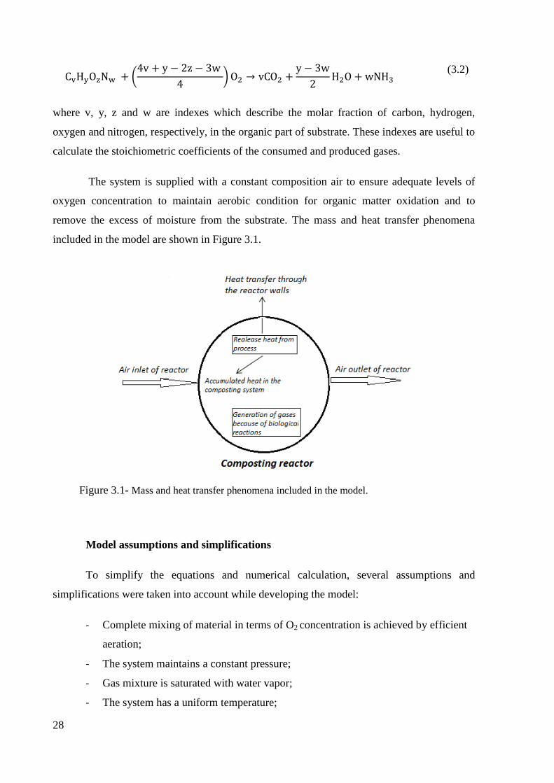
28
(3.2)
where v, y, z and w are indexes which describe the molar fraction of carbon, hydrogen,
oxygen and nitrogen, respectively, in the organic part of substrate. These indexes are useful to
calculate the stoichiometric coefficients of the consumed and produced gases.
The system is supplied with a constant composition air to ensure adequate levels of
oxygen concentration to maintain aerobic condition for organic matter oxidation and to
remove the excess of moisture from the substrate. The mass and heat transfer phenomena
included in the model are shown in Figure 3.1.
Figure 3.1- Mass and heat transfer phenomena included in the model.
Model assumptions and simplifications
To simplify the equations and numerical calculation, several assumptions and
simplifications were taken into account while developing the model:
- Complete mixing of material in terms of O2 concentration is achieved by efficient
aeration;
- The system maintains a constant pressure;
- Gas mixture is saturated with water vapor;
- The system has a uniform temperature;
3. MATHEMATICAL MODEL OF COMPOSTING PROCESS
29
- The temperature of compost, water and air is equal in each point of the reactor;
- The temperature of the outlet air is equal to the composting material temperature;
- The mass of air flow rate remains constant;
- The composting material is a homogeneous mixture of uniform composition;
- All heat specific capacities are constant;
- The gaseous phase behaves as ideal gas.
3.1.1. Process kinetic
The composting reaction is described by the organic matter degradation rate, through
the kinetic Eq. (3.3) [29]
(3.3)
where mOM is the mass of organic matter in the substrate (kg), t the time (h), k the rate
constant (kg1-n
h-1
) and n the reaction order.
Reaction rate constant is dependent on the system design, the type of material under
treatment, and other factors that may affect the overall system performance. In our work , this
constant is defined as a function of temperature, oxygen concentration, moisture and free air
space as shown in Eq. (3.4) [7]
(3.4)
where F(T), F(O2), F(W), and F(FAS) are the correction factors for temperature, oxygen
concentration, moisture content and free air space, respectively.
There is an extensive set of equations in literature to describe the dependence of the
reaction rate on temperature. In our study, the Eq. (3.5) was used [29]
.
(3.5)
where a, b and c are constants determined empirically through an optimization method.
The dependence of reaction rate constant on oxygen concentration is estimated using
the Eq. (3.6)
30
(3.6)
where is oxygen concentration (kgO2 m
-3) and
is oxygen saturation constant (kgO2 m-3
)
For modelling the effect of moisture content on the reaction rate the correction factor
developed by Haug (Eq. 3.7) was used [7]
.
(3.7)
where Sm is fractional solids content of the mixture solids. The model equation used for FAS
correction is shown in Eq. (3.8)
(3.8)
Fractional free air space of the composting material was calculated using the Eq. (3.9) [7]
(3.9)
(3.10)
(3.11)
where Vs is volatile fraction of substrate solids, ρs is specific gravity of substrate solids
(kg/m3), ρV is specific gravity of the volatile fraction of the substrate solids, ρf is specific
gravity of the fixed fraction of the substrate (inorganic fraction), ρm is unit bulk weight of the
mixed material to be composted, (kg/m3), ρw is density of water (kg/m
3), C is bulk weight
coefficient for the substrate, range from 0.15 to 0.4. The specific gravity of the volatile solids
normally is about 1.0 and that of fixed solids about 2.5.
3.1.2. Mass balance
The mass changes of oxygen and moisture in the substrate were estimated based on the
principle of mass conservation.
3. MATHEMATICAL MODEL OF COMPOSTING PROCESS
31
Water mass balance
The water mass balance in composting material is shown in Eq. (3.12) and it relates
water transport by the air flow throughout the reactor and the water formed in the composting
reaction.
(3.12)
where Ps0 and Ps are saturation water vapor pressure (Pa) at initial temperature of inlet air and
at temperature of the composting mixture, respectively; T0 is the initial temperature of inlet air
(K); Q the volumetric air flow (m3 h
-1); the stoichiometric coefficient of water; R the
universal gas constant (J kmol-1
K-1
) and Mrw is water molecular weight (mol kg-1
).
Oxygen mass balance
The oxygen concentration in the compost was estimated by Eq.(3.13)
(3.13)
where is the concentration of oxygen in the reactor (kgO2 m
-3), Ma the air flow (kg h
-1);
Vr is the working volume of the reactor (m3);
the stoichiometric coefficient of oxygen; and
ρa the density of air (kg m-3
), which was calculated based on psychometric relationships from
the temperature and humidity ratio [30]
.
3.1.3. Energy balance
As aforementioned the heterogeneous nature of the system under analysis was
modeled assuming pseudo-homogeneous approach. Thus, the temperature of solid, liquid and
gaseous phase is the same inside the reactor. The overall heat capacity was calculated from
the heat content of the organic matter, inorganic matter, water and dissolved gas in interstitial
water. The temperature variation in the system along time was calculated by Eq. (3.14)
32
(3.14)
where cpa, cpw,cpOM,cPIM are specific heat capacities of air, water, organic matter and inorganic
matter, respectively, (J kg-1
K-1
); Ta the air Temperature (K), is the reaction enthalpy
( ); U the overall heat transfer coefficient (J h
-1m
-2 K
-1); A the area of heat transfer (m
2),
ma the mass of air and Tamb is ambient temperature (K).
The specific heat capacities and overall heat transfer coefficient used in the model are
from the literature. The reaction enthalpy is calculated by Eq. (3.15) [7]
(3.15)
where C, H, O, S and N are the weight percentages of carbon, hydrogen, oxygen, sulfur and
nitrogen, respectively, on an ash-free basis. The Eq. (3.15) is known as the modified Dulong
formula and is useful in estimating gross heating values from the composting feed
composition. This equation requires an ultimate analysis of composting mixture to determine
the percentages of C, H, O, S and N.
3.1.4. Initial conditions
For solving the differential equations of the model, Eqs.(3.3), (3.12), (3.13) and (3.14) it is
necessary to establish the initial conditions (IC). In our simulations, the IC used are the ones
indicated in Eq. (3.16) to (3.19).
(3.16)
(3.17)
(3.18)
(3.19)
The initial mass values of water and organic matter were calculated using the experimental
data. The initial oxygen concentration was calculated using the equations of ideal gases at
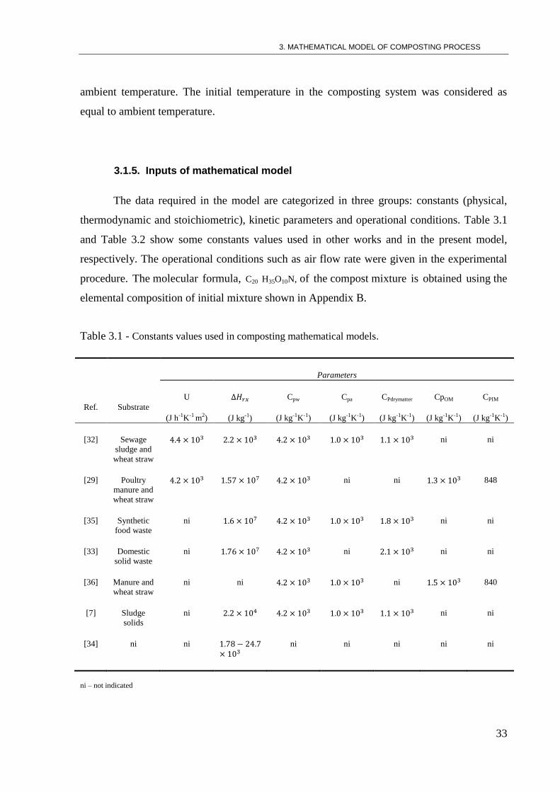
3. MATHEMATICAL MODEL OF COMPOSTING PROCESS
33
ambient temperature. The initial temperature in the composting system was considered as
equal to ambient temperature.
3.1.5. Inputs of mathematical model
The data required in the model are categorized in three groups: constants (physical,
thermodynamic and stoichiometric), kinetic parameters and operational conditions. Table 3.1
and Table 3.2 show some constants values used in other works and in the present model,
respectively. The operational conditions such as air flow rate were given in the experimental
procedure. The molecular formula, C20 H35O10N, of the compost mixture is obtained using the
elemental composition of initial mixture shown in Appendix B.
Table 3.1 - Constants values used in composting mathematical models.
Ref.
Substrate
Parameters
U
(J h-1K-1 m2)
(J kg-1)
Cpw
(J kg-1K-1)
Cpa
(J kg-1K-1)
CPdrymatter
(J kg-1K-1)
CpOM
(J kg-1K-1)
CPIM
(J kg-1K-1)
[32] Sewage
sludge and
wheat straw
ni ni
[29] Poultry
manure and
wheat straw
ni ni 848
[35] Synthetic
food waste
ni ni ni
[33] Domestic
solid waste
ni ni ni ni
[36] Manure and
wheat straw
ni ni ni 840
[7] Sludge
solids
ni ni ni
[34] ni ni
ni ni ni ni ni
ni – not indicated
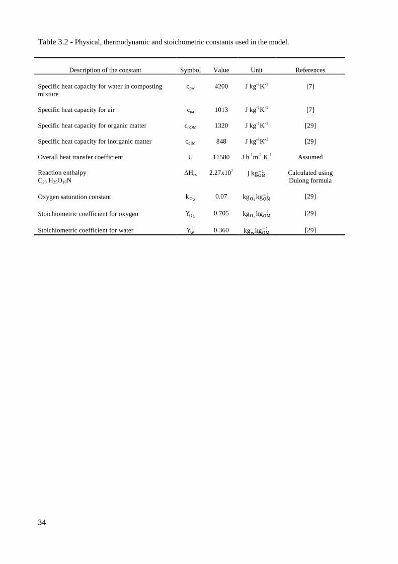
34
Table 3.2 - Physical, thermodynamic and stoichometric constants used in the model.
Description of the constant Symbol Value Unit References
Specific heat capacity for water in composting
mixture
cpw 4200 J kg-1
K-1
[7]
Specific heat capacity for air cpa 1013 J kg-1
K-1
[7]
Specific heat capacity for organic matter cpOM 1320 J kg-1
K-1
[29]
Specific heat capacity for inorganic matter cpIM 848 J kg-1
K-1
[29]
Overall heat transfer coefficient U 11580 J h-1
m-2
K-1
Assumed
Reaction enthalpy
C20 H35O10N ΔHrx 2.27x10
7
Calculated using
Dulong formula
Oxygen saturation constant 0.07
[29]
Stoichiometric coefficient for oxygen 0.705
[29]
Stoichiometric coefficient for water 0.360 [29]
4. STATE OF THE ART
35
4. STATE OF THE ART
The increasing amount of organic solid wastes generated has become a worldwide
problem, and thus, the number of treatment facilities based on biological processes has been
increasing the last years. These installations are receiving municipal and industrial organic
wastes with the common main goal of reducing their biodegradable organic matter content.
Among the available biological technologies to treat and recycle organic wastes, composting
is referred as one of the most useful options to recycle organic materials to obtain a valuable
organic fertilizer or amendment known as compost. The proper knowledge of the
characteristics of the wastes to be composted is essential to carry out the process in a
favorable way to obtain the desirable compost quality. The measurement of biodegradable
organic matter content is of most importance for the proper analysis and design of the
composting treatment facilities. However, consensus has not been reached about which shall
be the most suitable method measuring biodegradability organic matter content in a solid
organic waste. In fact, a wide range of biological and non biological test methods are now
available. Table 4.1 provides a summary of the key aspects of number studies of
biodegradability test methods which can be correlated with the stability assessment.
Suitability factors of the test methods include the timescale, applicability to a wide
range of materials and ability to indicate the long-term biodegradability of organic materials
samples. Among the methodologies suggested, aerobic respiration indices have been
highlighted as the most suitable tool for biodegradability assessment. However, these test
methods are time consuming and costly. Thus, it is desirable to have efficient, simpler, rapid
and cheaper methods, as the assessment of lignin content, which may be a useful surrogate for
aerobic method. The evaluation of lignin content to assess the substrate biodegradability can
be useful when long term biodegradability studies cannot be performed, which is the approach
used in our work.
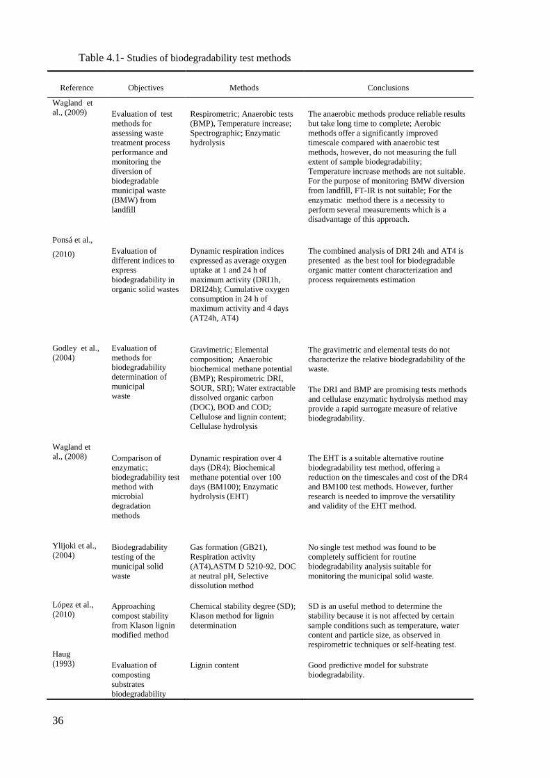
36
Table 4.1- Studies of biodegradability test methods
Reference Objectives Methods Conclusions
Wagland et
al., (2009) Evaluation of test
methods for
assessing waste
treatment process
performance and
monitoring the
diversion of
biodegradable
municipal waste
(BMW) from
landfill
Respirometric; Anaerobic tests
(BMP), Temperature increase;
Spectrographic; Enzymatic
hydrolysis
The anaerobic methods produce reliable results
but take long time to complete; Aerobic
methods offer a significantly improved
timescale compared with anaerobic test
methods, however, do not measuring the full
extent of sample biodegradability;
Temperature increase methods are not suitable.
For the purpose of monitoring BMW diversion
from landfill, FT-IR is not suitable; For the
enzymatic method there is a necessity to
perform several measurements which is a
disadvantage of this approach.
Ponsá et al.,
(2010) Evaluation of
different indices to
express
biodegradability in
organic solid wastes
Dynamic respiration indices
expressed as average oxygen
uptake at 1 and 24 h of
maximum activity (DRI1h,
DRI24h); Cumulative oxygen
consumption in 24 h of
maximum activity and 4 days
(AT24h, AT4)
The combined analysis of DRI 24h and AT4 is
presented as the best tool for biodegradable
organic matter content characterization and
process requirements estimation
Godley et al.,
(2004)
Evaluation of
methods for
biodegradability
determination of
municipal
waste
Gravimetric; Elemental
composition; Anaerobic
biochemical methane potential
(BMP); Respirometric DRI,
SOUR, SRI); Water extractable
dissolved organic carbon
(DOC), BOD and COD;
Cellulose and lignin content;
Cellulase hydrolysis
The gravimetric and elemental tests do not
characterize the relative biodegradability of the
waste.
The DRI and BMP are promising tests methods
and cellulase enzymatic hydrolysis method may
provide a rapid surrogate measure of relative
biodegradability.
Wagland et
al., (2008) Comparison of
enzymatic;
biodegradability test
method with
microbial
degradation
methods
Dynamic respiration over 4
days (DR4); Biochemical
methane potential over 100
days (BM100); Enzymatic
hydrolysis (EHT)
The EHT is a suitable alternative routine
biodegradability test method, offering a
reduction on the timescales and cost of the DR4
and BM100 test methods. However, further
research is needed to improve the versatility
and validity of the EHT method.
Ylijoki et al.,
(2004) Biodegradability
testing of the
municipal solid
waste
Gas formation (GB21),
Respiration activity
(AT4),ASTM D 5210-92, DOC
at neutral pH, Selective
dissolution method
No single test method was found to be
completely sufficient for routine
biodegradability analysis suitable for
monitoring the municipal solid waste.
López et al.,
(2010) Approaching
compost stability
from Klason lignin
modified method
Chemical stability degree (SD);
Klason method for lignin
determination
SD is an useful method to determine the
stability because it is not affected by certain
sample conditions such as temperature, water
content and particle size, as observed in
respirometric techniques or self-heating test.
Haug
(1993) Evaluation of
composting
substrates
biodegradability
Lignin content Good predictive model for substrate
biodegradability.
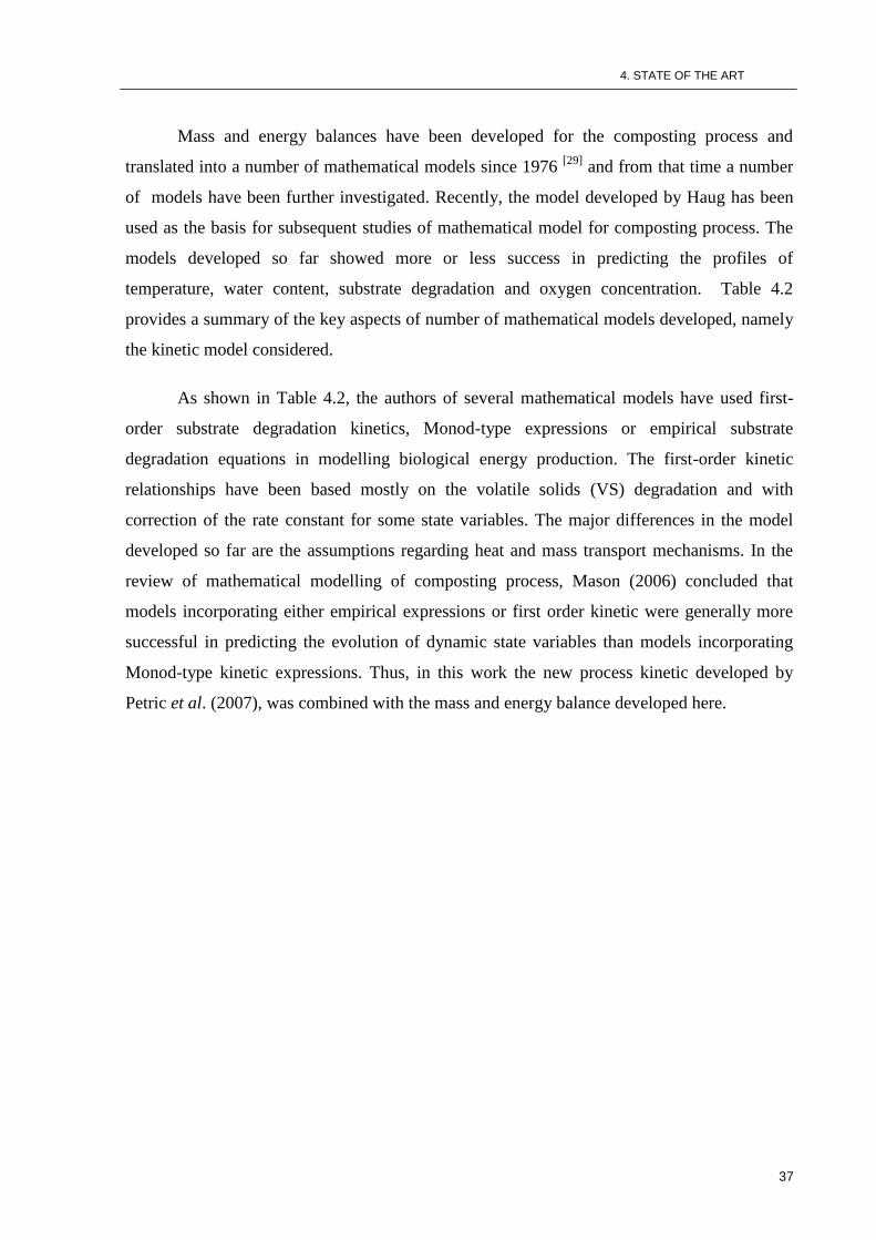
4. STATE OF THE ART
37
Mass and energy balances have been developed for the composting process and
translated into a number of mathematical models since 1976 [29]
and from that time a number
of models have been further investigated. Recently, the model developed by Haug has been
used as the basis for subsequent studies of mathematical model for composting process. The
models developed so far showed more or less success in predicting the profiles of
temperature, water content, substrate degradation and oxygen concentration. Table 4.2
provides a summary of the key aspects of number of mathematical models developed, namely
the kinetic model considered.
As shown in Table 4.2, the authors of several mathematical models have used first-
order substrate degradation kinetics, Monod-type expressions or empirical substrate
degradation equations in modelling biological energy production. The first-order kinetic
relationships have been based mostly on the volatile solids (VS) degradation and with
correction of the rate constant for some state variables. The major differences in the model
developed so far are the assumptions regarding heat and mass transport mechanisms. In the
review of mathematical modelling of composting process, Mason (2006) concluded that
models incorporating either empirical expressions or first order kinetic were generally more
successful in predicting the evolution of dynamic state variables than models incorporating
Monod-type kinetic expressions. Thus, in this work the new process kinetic developed by
Petric et al. (2007), was combined with the mass and energy balance developed here.
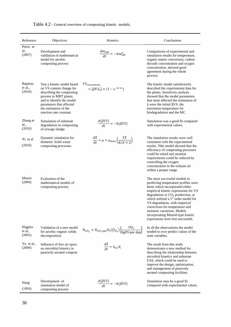
38
Table 4.2 - General overview of composting kinetic models.
Reference Objectives Kinetics Conclusions
Petric et
al.,
(2007) Development and
validation of mathematical
model for aerobic
composting process
Comparisons of experimental and
simulation results for temperature,
organic matter conversion, carbon
dioxide concentration and oxygen
concentration, showed good
agreement during the whole
process.
Baptista
et al.,
(2010)
Test a kinetic model based
on VS content change for
describing the composting
process in MBT plants,
and to identify the model
parameters that affected
the estimation of the
reaction rate constant.
The kinetic model satisfactorily
described the experimental data for
the plants. Sensitivity analysis
showed that the model parameters
that most affected the estimation of
k were the initial βVS, the
maximum temperature for
biodegradation and the MC
Zhang et
al.,
(2010)
Simulation of substrate
degradation in composting
of sewage sludge.
Simulation was a good fit compared
with experimental values.
Xi et al
(2010)
Dynamic simulation for
domestic Solid waste
composting processes
The simulation results were well
consistent with the experimental
results. Tthe model showed that the
efficiency of composting processes
could be raised and aeration
requirements could be reduced by
controlling the oxygen
concentration in the exhaust air
within a proper range.
Mason
(2006) Evaluation of the
mathematical models of
composting process
The most successful models in
predicting temperature profiles were
those which incorporated either
empirical kinetic expressions for VS
degradation or CO2 production, or
which utilized a 1st order model for
VS degradation, with empirical
corrections for temperature and
moisture variations. Models
incorporating Monod-type kinetic
expressions were less successful.
Higgins
et al.,
(2001)
Validation of a new model
for aerobic organic solids
decomposition
In all the observations the model
tended to over predict values of the
state variables.
Yu et al.,
(2009) Influence of free air space
on microbial kinetics in
passively aerated compost
The result from this study
demonstrates a new method for
describing the relationship between
microbial kinetics and substrate
FAS, which could be used to
improve the design, optimization,
and management of passively
aerated composting facilities.
Haug
(1993)
Development of
simulation model of
composting process
Simulation may be a good fit
compared with experimental values.
5. EXPERIMENTAL METHODS
39
5. EXPERIMENTAL METHODS
5.1. Experimental apparatus
Experiments were performed in a system of four self-heating reactors (SHR) with 120
L of internal volume and isolated with a rubber based elastomeric material (Aeroflex MSR)
arranged in parallel. The experimental reactors system is shown schematically in Figure 5.1.
where
1- Compressed air inlet 7- Temperature sensor
2- On/off valve 8 - Gases outlet
3- Air moisture regulator 9 - Condensate retention system
4- Rotameter 10- Oxygen sensor
5- Insulation layer (Aeroflex MSR) 11- Data acquisition system
6- Perforated plate 12- Computer
Figure 5.1 - Schem of the pilot-scale experimental apparatus.
The reactors have a side hole that allowed the entry of compressed air that is
uniformly distributed across a perforated Perspex plate. On the top of the reactors there are
two openings for the introduction of a temperature sensor and another to allow the release
of gases generated in the biological reactions along the process, as well as the release of
the excess air.
40
5.2. Materials
The components used to experiments were from different sources and included potato-
peel industrial waste (PP) from a Portuguese industry of potato chips, grass clippings (GC)
from a garden centre and a football stadium, and sawdust (SD). Potato-peel is classified as
waste and its identification according to the European Waste List is 020399. These individual
raw materials were blended in four different formulations. The initial mixtures tested were
formulated in order to ensure proper conditions, such as nutrient balance (C:N ratio), moisture
content (MC) and FAS, for optimal microbial growth and organic matter degradation. For
achieve the specification concerning to C: N ratio (15:1 to 40:1) and MC (40-75%) for the
composting mixture is only necessary to know the nitrogen, carbon and moisture content of
the individual ingredients as it is shown in the mass balance Eqs. (5.1) and (5.2) for C:N ratio
and moisture content, respectively. These equations were solved exactly for the considered
mixture of three materials.
(5.1)
(5.2)
where C:Nm is the C:N ratio of compost mixture, MCm the moisture content of composting
mixture (%), mi the mass fraction of material i (i=1,2,3), Ci is carbon fraction of material i,
Ni the nitrogen fraction of material i and MCi is moisture content of material i (a fraction in
equation (5.1) and a percentage in Eqs.( 5.2)).
The approach described above for C:N ratio and MC is not applicable for FAS because
this parameter depends on the structural characteristics of the material and not on its
elemental composition. Therefore, appropriated method for this purpose such as Mixture
Design was used.
5.2.1. Mixture design
Mixture design is statistical methodology that allows varying the proportions of two or
more ingredients of a mixture to study the influence of individual proportions of the
components tested in a measured response, which is dependent on the ingredient composition.
5. EXPERIMENTAL METHODS
41
Then, the method use response surface approach to identify the area (mixture region) where
all specifications can be achieved. The effect of composition in a response variable, Y, can be
described by the polynomial shown in Eq. (5.3) [31]
(5.3)
where xi represent the independent variable i , γj correspond to the polynomial coefficients j, q
is number of the mixture components and ε is the variable response estimative error.
The experimental design was obtained by using Design-Expert® version 8.0.4 software
using the simplex-centroid mixture design augmented. The working strategy for mixture
design applied to the present work materials (potato peel, grass clippings and sawdust) was
according to Eriksson (1998)[31]
. After defining the factors and bounds for the mixture design
map and also the experimental objective and mixture model (quadratic), a simple-centroid
design was generated. The design points correspond to all permutations of the pure blends
(e.g., 1 0 0; 0 1 0; 0 0 1), the permutations of the binary blends (½ ½ 0; ½ 0 ½; 0 ½ ½), the
permutations of the blends involving three components, and so on, given a total of thirteen
experiments. Each blend was characterized experimentally including the determination of the
desired parameter (FAS). Then, the software analyzed these data and evaluated the best model
that described the composition effects of the individual materials fractions in the FAS.
5.3. Monitoring of composting process
The reactors are equipped with a data acquisition system for on-line monitoring of
temperature and oxygen concentration, and feed air flow rate was measured with rotameters.
The air flow rate was controlled in order to firstly maintain the oxygen concentration of the
outlet gas in the range of 5 to 15% (v/v) and at the same time control the temperature of the
composting material in the reactor. The mixtures were sampled in pre-determined times (once
a week) along the period of composting after revolving the reactors to ensure the
representativeness of the samples. The samples were obtained from a set of sub-samples
randomly collected at several different points for each of the reactors. The mass of each
sample was on average 500 g. To quantify some parameters, the samples were pre-dried and
milled. Characterization of the samples at each time included the determination of moisture
42
content, organic matter content, pH, elemental composition, bulk density, FAS and
biodegradability. Biodegradability of each sample was assessed by measuring lignin content
using the Klason lignin method .All the determinations were performed in triplicates except
the lignin content that was in duplicate due to the method time scale.
5.3.1. Temperature and air flow rate
Temperature monitoring was performed by inserting a probe into the geometric
center of each of the reactors, and the data acquisition was made by an online system.
Aeration of the reactors was made through a compressed air line linked on the bases
of the reactors. Measurement of air flows rates for each reactor was made using rotameters
(Figure 5.2).
Figure 5.2 - Feed air flow measuring.
5.3.2. Moisture content
1. Weigh a small container;
2. Weigh about 20 g of compost into the container;
3. Dry the sample for 24 h in a 105 °C oven;
4. After drying, cool the sample in a desiccator and reweigh.
The percentage of moisture is calculated using Eq. (5.4).
5. EXPERIMENTAL METHODS
43
(5.4)
5.3.3. Organic matter content
1. Weigh a porcelain crucible;
2. Weigh about 2.5 g of compost into the porcelain crucible;
3. Calcinate the sample in a muffle furnace for 4 h at 550 °C;
4. After calcination, cool the sample in a desiccator and weigh.
The percentage of organic matter is calculated by Eq. (5.5)
(5.5)
5.3.4. Bulk density
The bulk density was determined according to the method described in TMECC (Test
methods of the examination of composting and compost).
1. Weigh the tare of a graduated beaker;
2. Transfer a 600 cm3 aliquot of compost into the graduated beaker through a funnel;
3. To ensure uniform packing of compost throughout the graduated beaker, allow beaker
to fall freely onto an adequate support from height of 15 cm;
4. Repeat the filling with 600 mL and free falling operation, two more times (three times
total). After the third free-fall drop, fill the graduated beaker to volume with sample
material, 1800 mL;
5. Weigh and record gross weight of the filled graduated beaker containing 1800 mL of
compost.
The bulk density is calculated by Eq. (5.6)
(5.6)
44
5.3.5. pH
1. Weigh an amount of sample equivalent to 20 mL, estimated from the bulk density of
the mixture, into a flask;
2. Add 100 mL of distilled water to the flask;
3. Agitate the suspension for 2 h;
4. Measure the pH using the specific equipment.
5.3.6. Elemental composition
The elemental composition of the samples was determined by using the EA1108
CHNS-O – Fisons equipment that measured the total amount of C, H, N, S and O.
5.3.7. Free air space
The free air space depends on the bulk density (BD) and the density of substrate solids
(ρp) and was determined using Eq. (5.7)
The determination of the density of substrate solids, ρp, was as follow:
1. Using a clean and dry graduate beaker of known mass, measure the density of
kerosene by adding a specific volume and weighing the beaker;
2. Using another clean and dry graduate beaker of known mass, add some particulate
matter of compost and weigh its mass in the graduate beaker;
3. Add kerosene until all the particles are covered and read the total volume as well as
weigh the graduate beaker and its content;
4. From the kerosene mass added, compute the volume from the density in step 1; the
difference in volume is that of the particles;
5. Calculate the particles density using the mass and volume calculated in the steps
above.
(5.7)
5. EXPERIMENTAL METHODS
45
5.3.8. Biodegradability
The biodegradable fraction of the volatile solids, β, is defined as the biodegradable
amount of VS (βVS) divided by the total VS input to the process. The biodegradable amount
of VS is determined by measuring lignin content (LC) in percentage of VS, which means it is
considered that the lignin content represent the non biodegradable fraction. The biodegradable
amount of VS is calculated by Eq. (5.8) and the biodegradable fraction by Eq. (5.9)
(5.8)
(5.9)
The lignin content (L) is determined using the Klason method.
1. Weigh 0.5 g of dry compost into a beaker;
2. Add gradually to the beaker containing the compost 7.5 mL of 72% sulfuric acid in
small increments while stirring the suspension;
3. Keep the beaker in a bath at 20 °C during dispersion of the material. After the material
is dispersed keep the beaker in the bath for 2 h and stir the material frequently during
this time to ensure complete dissolution;
4. Add about 150 mL of water to a flask and transfer the material from the beaker to the
flask. Rinse and dilute with water to 3% concentration of sulfuric acid, to total volume
of 287.5 mL;
5. Boil the solution for 4 h, maintaining constant volume by addition of hot water;
6. Allow the insoluble material (lignin) to settle ―overnight‖;
7. Without stirring up the precipitate, filtering the supernatant solution. Then transfer the
lignin quantitatively to the filter and wash it with hot water;
8. Transfer the filter with lignin and dry in an oven at 105 °C during 4 h. Cool in a
desiccator and weigh;
9. Take the sample to a muffle furnace for 4 hours at 550 °C;
10. After the 4 h in the muffle, cool the sample in desiccators and weigh.
The lignin content is determined by Eq. (5.10).
(5.10)

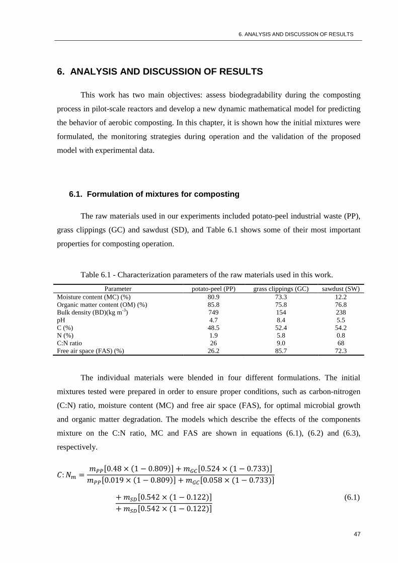
6. ANALYSIS AND DISCUSSION OF RESULTS
47
6. ANALYSIS AND DISCUSSION OF RESULTS
This work has two main objectives: assess biodegradability during the composting
process in pilot-scale reactors and develop a new dynamic mathematical model for predicting
the behavior of aerobic composting. In this chapter, it is shown how the initial mixtures were
formulated, the monitoring strategies during operation and the validation of the proposed
model with experimental data.
6.1. Formulation of mixtures for composting
The raw materials used in our experiments included potato-peel industrial waste (PP),
grass clippings (GC) and sawdust (SD), and Table 6.1 shows some of their most important
properties for composting operation.
Table 6.1 - Characterization parameters of the raw materials used in this work.
Parameter potato-peel (PP) grass clippings (GC) sawdust (SW)
Moisture content (MC) (%) 80.9 73.3 12.2
Organic matter content (OM) (%) 85.8 75.8 76.8
Bulk density (BD)(kg m-3
) 749 154 238
pH 4.7 8.4 5.5
C (%) 48.5 52.4 54.2
N (%) 1.9 5.8 0.8
C:N ratio 26 9.0 68
Free air space (FAS) (%) 26.2 85.7 72.3
The individual materials were blended in four different formulations. The initial
mixtures tested were prepared in order to ensure proper conditions, such as carbon-nitrogen
(C:N) ratio, moisture content (MC) and free air space (FAS), for optimal microbial growth
and organic matter degradation. The models which describe the effects of the components
mixture on the C:N ratio, MC and FAS are shown in equations (6.1), (6.2) and (6.3),
respectively.
(6.1)
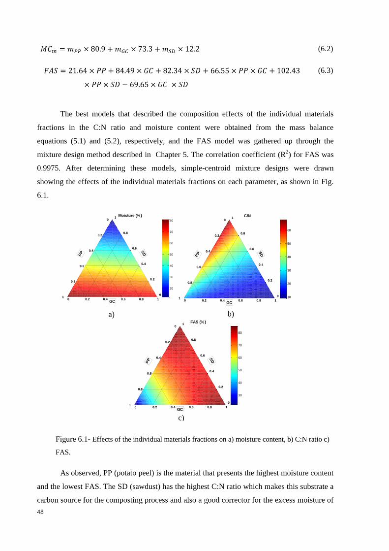
48
(6.2)
(6.3)
The best models that described the composition effects of the individual materials
fractions in the C:N ratio and moisture content were obtained from the mass balance
equations (5.1) and (5.2), respectively, and the FAS model was gathered up through the
mixture design method described in Chapter 5. The correlation coefficient (R2) for FAS was
0.9975. After determining these models, simple-centroid mixture designs were drawn
showing the effects of the individual materials fractions on each parameter, as shown in Fig.
6.1.
Figure 6.1- Effects of the individual materials fractions on a) moisture content, b) C:N ratio c)
FAS.
As observed, PP (potato peel) is the material that presents the highest moisture content
and the lowest FAS. The SD (sawdust) has the highest C:N ratio which makes this substrate a
carbon source for the composting process and also a good corrector for the excess moisture of
0
1
0.2
SD
0.4
0.8
0.6
0.8
0.6
1
GC
Moisture (%)0
0.4
0.2
0.4
0.2
PP
0.6
0.8
0 1
20
30
40
50
60
70
80
0
1
0.2
SD
0.4
0.8
0.6
0.8
0.6
1
GC
C/N0
0.4
0.2
0.4
0.2
PP
0.6
0.8
0 1 10
20
30
40
50
60
0
1
0.2
SD
0.4
0.8
0.6
0.8
0.6
1
GC
FAS (%)0
0.4
0.2
0.4
0.2
PP
0.6
0.8
0 1
30
40
50
60
70
80
a) b)
c)
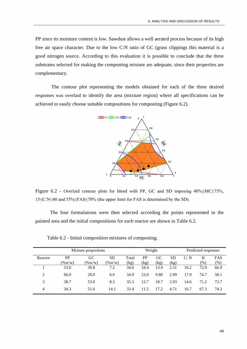
6. ANALYSIS AND DISCUSSION OF RESULTS
49
PP since its moisture content is low. Sawdust allows a well aerated process because of its high
free air space character. Due to the low C:N ratio of GC (grass clippings this material is a
good nitrogen source. According to this evaluation it is possible to conclude that the three
substrates selected for making the composting mixture are adequate, since their properties are
complementary.
The contour plot representing the models obtained for each of the three desired
responses was overlaid to identify the area (mixture region) where all specifications can be
achieved to easily choose suitable compositions for composting (Figure 6.2).
Figure 6.2 - Overlaid contour plots for blend with PP, GC and SD imposing 40%≤MC≤75%,
15≤C:N≤40 and 55%≤FAS≤70% (the upper limit for FAS is determined by the SD).
The four formulations were then selected according the points represented in the
painted area and the initial compositions for each reactor are shown in Table 6.2.
Table 6.2 - Initial composition mixtures of composting.
Mixture proportions Weight Predicted responses
Reactor PP
(%w/w)
GC
(%w/w)
SD
(%w/w)
Total
(kg)
PP
(kg)
GC
(kg)
SD
(kg)
C: N H
(%)
FAS
(%)
1 53.0 39.8 7.2 34.8 18.4 13.9 2.51 16.2 72.9 66.9
2 66.0 28.0 6.0 34.9 23.0 9.80 2.09 17.9 74.7 58.1
3 38.7 53.0 8.3 35.3 13.7 18.7 2.93 14.6 71.2 73.7
4 34.3 51.6 14.1 33.4 11.5 17.2 4.71 16.7 67.3 74.3
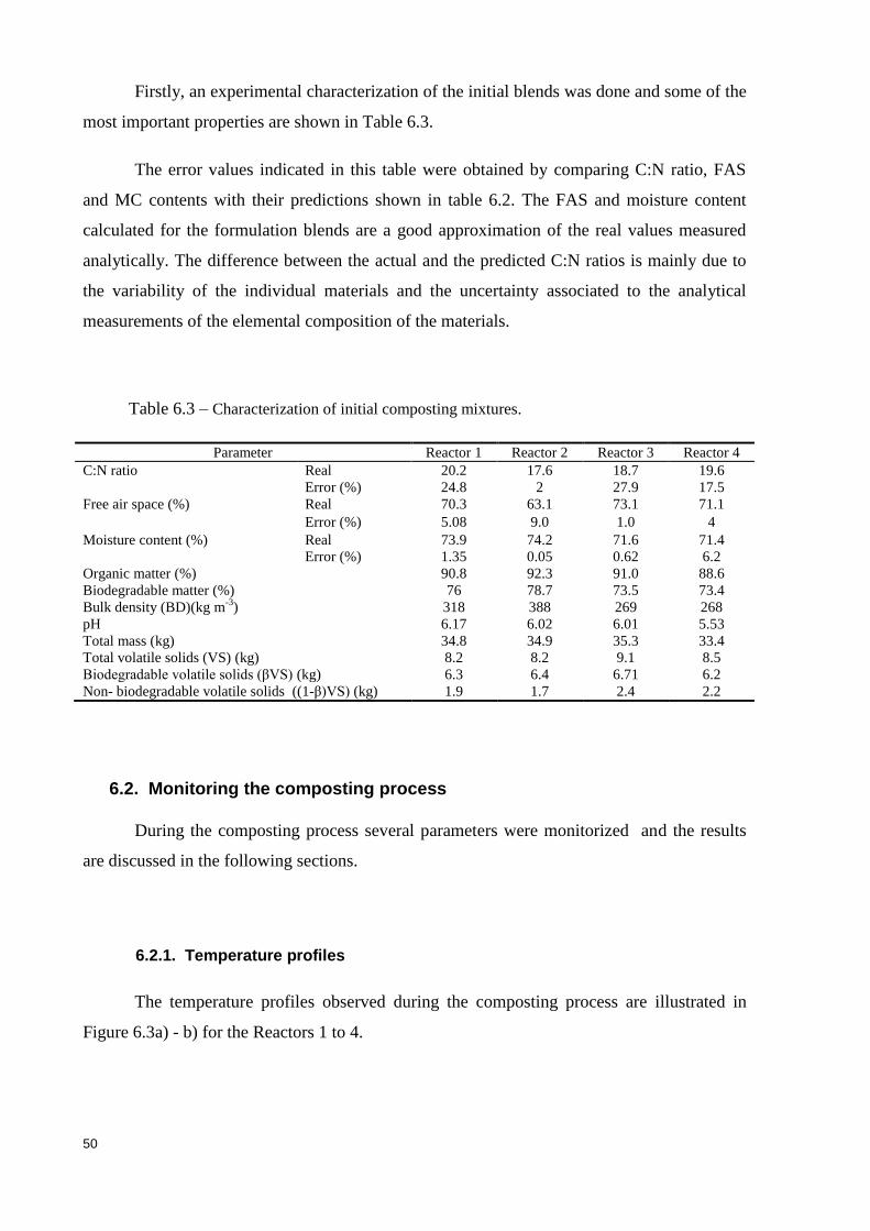
50
Firstly, an experimental characterization of the initial blends was done and some of the
most important properties are shown in Table 6.3.
The error values indicated in this table were obtained by comparing C:N ratio, FAS
and MC contents with their predictions shown in table 6.2. The FAS and moisture content
calculated for the formulation blends are a good approximation of the real values measured
analytically. The difference between the actual and the predicted C:N ratios is mainly due to
the variability of the individual materials and the uncertainty associated to the analytical
measurements of the elemental composition of the materials.
Table 6.3 – Characterization of initial composting mixtures.
Parameter Reactor 1 Reactor 2 Reactor 3 Reactor 4
C:N ratio Real 20.2 17.6 18.7 19.6
Error (%) 24.8 2 27.9 17.5
Free air space (%) Real 70.3 63.1 73.1 71.1
Error (%) 5.08 9.0 1.0 4
Moisture content (%) Real 73.9 74.2 71.6 71.4
Error (%) 1.35 0.05 0.62 6.2
Organic matter (%) 90.8 92.3 91.0 88.6
Biodegradable matter (%) 76 78.7 73.5 73.4
Bulk density (BD)(kg m-3
) 318 388 269 268
pH 6.17 6.02 6.01 5.53
Total mass (kg) 34.8 34.9 35.3 33.4
Total volatile solids (VS) (kg) 8.2 8.2 9.1 8.5
Biodegradable volatile solids (βVS) (kg) 6.3 6.4 6.71 6.2
Non- biodegradable volatile solids ((1-β)VS) (kg) 1.9 1.7 2.4 2.2
6.2. Monitoring the composting process
During the composting process several parameters were monitorized and the results
are discussed in the following sections.
6.2.1. Temperature profiles
The temperature profiles observed during the composting process are illustrated in
Figure 6.3a) - b) for the Reactors 1 to 4.
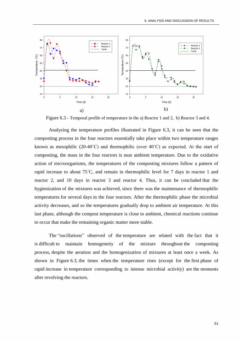
6. ANALYSIS AND DISCUSSION OF RESULTS
51
Time (d)
0 5 10 15 20
Tem
pera
ture
(º
C)
10
20
30
40
50
60
70
80
Reactor 1
Reactor 2
Tamb
Time (d)
0 5 10 15 20
Tem
pera
ture
(ºC
)
10
20
30
40
50
60
70
80
Reactor 3
Reactor 4
Tamb
Figure 6.3 - Temporal profile of temperature in the a) Reactor 1 and 2, b) Reactor 3 and 4.
Analyzing the temperature profiles illustrated in Figure 6.3, it can be seen that the
composting process in the four reactors essentially take place within two temperature ranges
known as mesophilic (20-40˚C) and thermophilic (over 40˚C) as expected. At the start of
composting, the mass in the four reactors is near ambient temperature. Due to the oxidative
action of microorganisms, the temperatures of the composting mixtures follow a pattern of
rapid increase to about 75˚C, and remain in thermophilic level for 7 days in reactor 1 and
reactor 2, and 10 days in reactor 3 and reactor 4. Thus, it can be concluded that the
hygienization of the mixtures was achieved, since there was the maintenance of thermophilic
temperatures for several days in the four reactors. After the thermophilic phase the microbial
activity decreases, and so the temperatures gradually drop to ambient air temperature. At this
last phase, although the compost temperature is close to ambient, chemical reactions continue
to occur that make the remaining organic matter more stable.
The ―oscillations‖ observed of the temperature are related with the fact that it
is difficult to maintain homogeneity of the mixture throughout the composting
process, despite the aeration and the homogenization of mixtures at least once a week. As
shown in Figure 6.3, the times when the temperature rises (except for the first phase of
rapid increase in temperature corresponding to intense microbial activity) are the moments
after revolving the reactors.
a) b)
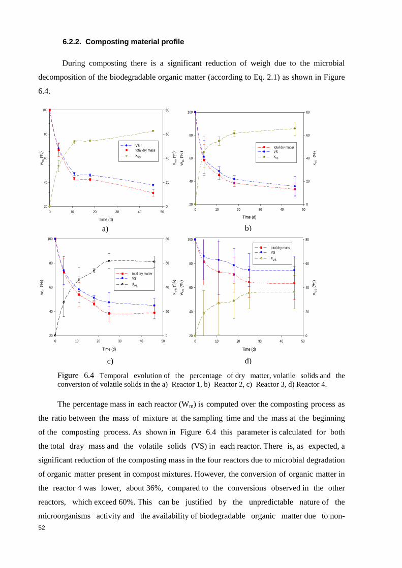
52
6.2.2. Composting material profile
During composting there is a significant reduction of weigh due to the microbial
decomposition of the biodegradable organic matter (according to Eq. 2.1) as shown in Figure
6.4.
Time (d)
0 10 20 30 40 50
20
40
60
80
100
wm (
%)
xV
S (%
)
0
20
40
60
80
VS
total dry mass
xVS
Time (d)
0 10 20 30 40 50
wm (
%)
20
40
60
80
100
xV
S (
%)
0
20
40
60
80
total dry matter
VS
xVS
Time (d)
0 10 20 30 40 50
wm (
%)
20
40
60
80
100
xV
S (%
)
0
20
40
60
80
total dry matter
VS
xVS
Time (d)
0 10 20 30 40 50
wm (
%)
20
40
60
80
100
xV
S (%
)
0
20
40
60
80
total dry mass
VS
xVS
Figure 6.4 Temporal evolution of the percentage of dry matter, volatile solids and the
conversion of volatile solids in the a) Reactor 1, b) Reactor 2, c) Reactor 3, d) Reactor 4.
The percentage mass in each reactor (Wm) is computed over the composting process as
the ratio between the mass of mixture at the sampling time and the mass at the beginning
of the composting process. As shown in Figure 6.4 this parameter is calculated for both
the total dray mass and the volatile solids (VS) in each reactor. There is, as expected, a
significant reduction of the composting mass in the four reactors due to microbial degradation
of organic matter present in compost mixtures. However, the conversion of organic matter in
the reactor 4 was lower, about 36%, compared to the conversions observed in the other
reactors, which exceed 60%. This can be justified by the unpredictable nature of the
microorganisms activity and the availability of biodegradable organic matter due to non-
a) b)
d) c)
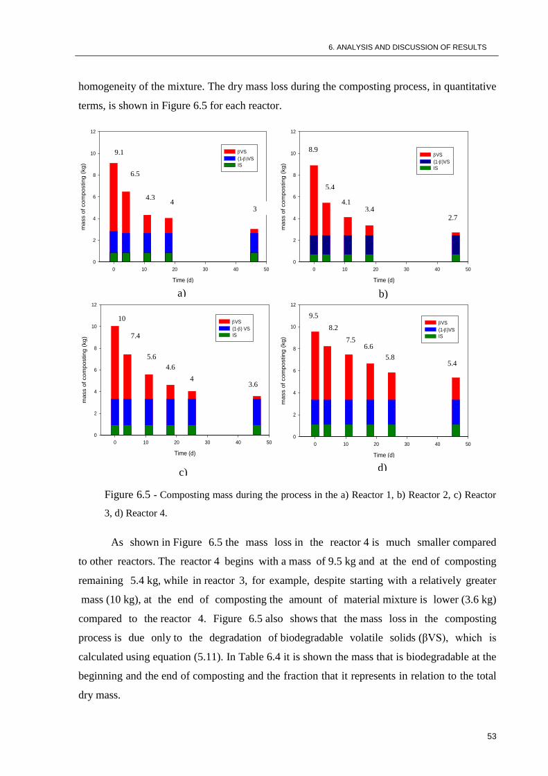
6. ANALYSIS AND DISCUSSION OF RESULTS
53
homogeneity of the mixture. The dry mass loss during the composting process, in quantitative
terms, is shown in Figure 6.5 for each reactor.
Time (d)
0 10 20 30 40 50
mass o
f com
posting (
kg)
0
2
4
6
8
10
12
VS
(1-VS
IS
Time (d)
0 10 20 30 40 50
mass o
f com
posting (
kg)
0
2
4
6
8
10
12
VS
(1-)VS
IS
Time (d)
0 10 20 30 40 50
mass o
f com
posting (
kg)
0
2
4
6
8
10
12
VS
(1-) VS
IS
Time (d)
0 10 20 30 40 50
mass o
f co
mp
ostin
g (
kg
)
0
2
4
6
8
10
12
VS
(1-)VS
IS
Figure 6.5 - Composting mass during the process in the a) Reactor 1, b) Reactor 2, c) Reactor
3, d) Reactor 4.
As shown in Figure 6.5 the mass loss in the reactor 4 is much smaller compared
to other reactors. The reactor 4 begins with a mass of 9.5 kg and at the end of composting
remaining 5.4 kg, while in reactor 3, for example, despite starting with a relatively greater
mass (10 kg), at the end of composting the amount of material mixture is lower (3.6 kg)
compared to the reactor 4. Figure 6.5 also shows that the mass loss in the composting
process is due only to the degradation of biodegradable volatile solids (βVS), which is
calculated using equation (5.11). In Table 6.4 it is shown the mass that is biodegradable at the
beginning and the end of composting and the fraction that it represents in relation to the total
dry mass.
9.1
6.5
4.3 4
3
a) b)
c) d)
8.9
5.4
4.1
2.7 3.4
5.6
10
7.4
4.6
4 3.6
9.5
8.2
7.5 6.6
5.8 5.4
a)
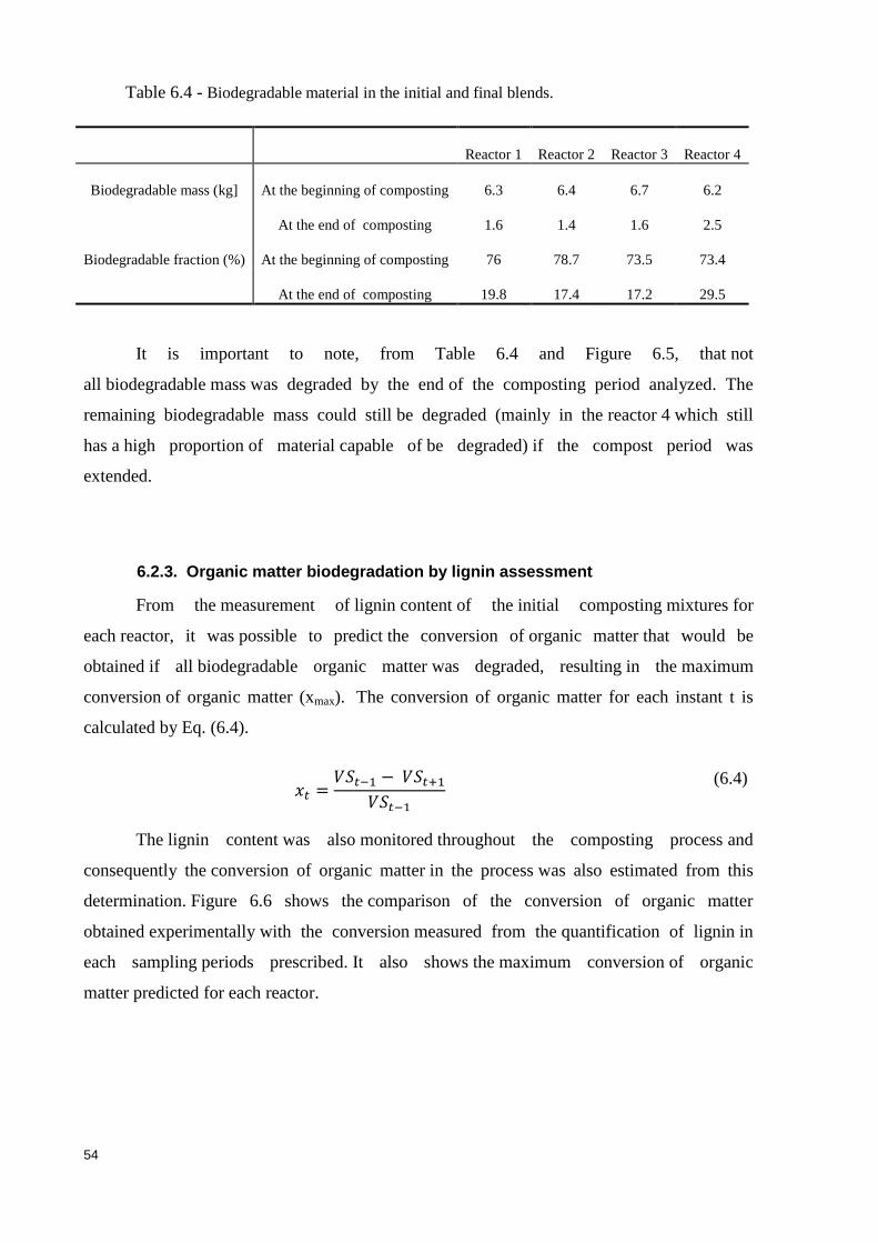
54
Table 6.4 - Biodegradable material in the initial and final blends.
Reactor 1 Reactor 2 Reactor 3 Reactor 4
Biodegradable mass (kg] At the beginning of composting 6.3 6.4 6.7 6.2
At the end of composting 1.6 1.4 1.6 2.5
Biodegradable fraction (%) At the beginning of composting 76 78.7 73.5 73.4
At the end of composting 19.8 17.4 17.2 29.5
It is important to note, from Table 6.4 and Figure 6.5, that not
all biodegradable mass was degraded by the end of the composting period analyzed. The
remaining biodegradable mass could still be degraded (mainly in the reactor 4 which still
has a high proportion of material capable of be degraded) if the compost period was
extended.
6.2.3. Organic matter biodegradation by lignin assessment
From the measurement of lignin content of the initial composting mixtures for
each reactor, it was possible to predict the conversion of organic matter that would be
obtained if all biodegradable organic matter was degraded, resulting in the maximum
conversion of organic matter (xmax). The conversion of organic matter for each instant t is
calculated by Eq. (6.4).
(6.4)
The lignin content was also monitored throughout the composting process and
consequently the conversion of organic matter in the process was also estimated from this
determination. Figure 6.6 shows the comparison of the conversion of organic matter
obtained experimentally with the conversion measured from the quantification of lignin in
each sampling periods prescribed. It also shows the maximum conversion of organic
matter predicted for each reactor.
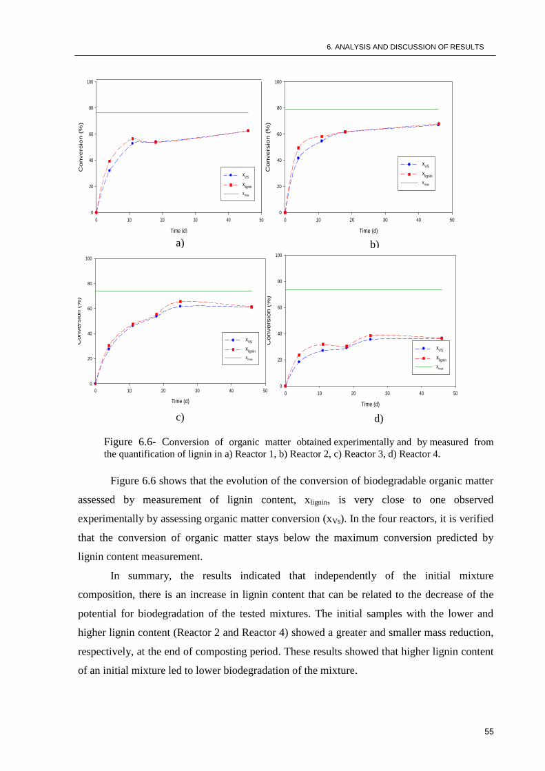
6. ANALYSIS AND DISCUSSION OF RESULTS
55
Time (d)
0 10 20 30 40 50
Convers
ion (
%)
0
20
40
60
80
100
xVS
xlignin
xmax
Time (d)
0 10 20 30 40 50
Convers
ion (
%)
0
20
40
60
80
100
xVS
xlignin
xmax
Time (d)
0 10 20 30 40 50
Co
nve
rsio
n (
%)
0
20
40
60
80
100
xVS
xlignin
xmax
Time (d)
0 10 20 30 40 50
Co
nve
rsio
n (
%)
0
20
40
60
80
100
xVS
xlignin
xmax
Figure 6.6- Conversion of organic matter obtained experimentally and by measured from
the quantification of lignin in a) Reactor 1, b) Reactor 2, c) Reactor 3, d) Reactor 4.
Figure 6.6 shows that the evolution of the conversion of biodegradable organic matter
assessed by measurement of lignin content, xlignin, is very close to one observed
experimentally by assessing organic matter conversion (xVs). In the four reactors, it is verified
that the conversion of organic matter stays below the maximum conversion predicted by
lignin content measurement.
In summary, the results indicated that independently of the initial mixture
composition, there is an increase in lignin content that can be related to the decrease of the
potential for biodegradation of the tested mixtures. The initial samples with the lower and
higher lignin content (Reactor 2 and Reactor 4) showed a greater and smaller mass reduction,
respectively, at the end of composting period. These results showed that higher lignin content
of an initial mixture led to lower biodegradation of the mixture.
a) b)
c) d)
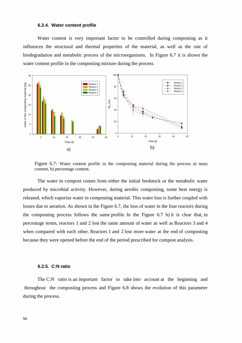
56
6.2.4. Water content profile
Water content is very important factor to be controlled during composting as it
influences the structural and thermal properties of the material, as well as the rate of
biodegradation and metabolic process of the microorganisms. In Figure 6.7 it is shown the
water content profile in the composting mixture during the process.
Time (d)
0 10 20 30 40 50
wa
ter
in th
e c
om
postin
g m
ate
ria
l (k
g)
0
5
10
15
20
25
30
Reactor 1
Reactor 2
Reactor 3
Reactor 4
Time (d)
0 10 20 30 40 50
Ww (
%)
0
20
40
60
80
100
Reactor 1
Reactor 2
Reactor 3
Reactor 4
Figure 6.7- Water content profile in the composting material during the process a) mass
content, b) percentage content.
The water in compost comes from either the initial feedstock or the metabolic water
produced by microbial activity. However, during aerobic composting, some heat energy is
released, which vaporize water in composting material. This water loss is further coupled with
losses due to aeration. As shown in the Figure 6.7, the loss of water in the four reactors during
the composting process follows the same profile. In the Figure 6.7 b) it is clear that, in
percentage terms, reactors 1 and 2 lost the same amount of water as well as Reactors 3 and 4
when compared with each other. Reactors 1 and 2 lost more water at the end of composting
because they were opened before the end of the period prescribed for compost analysis.
6.2.5. C:N ratio
The C:N ratio is an important factor to take into account at the beginning and
throughout the composting process and Figure 6.8 shows the evolution of this parameter
during the process.
a) b)
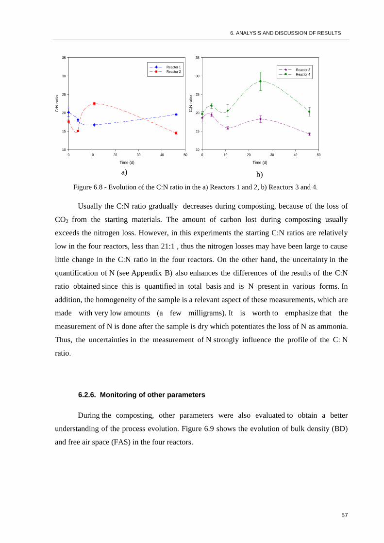
6. ANALYSIS AND DISCUSSION OF RESULTS
57
Time (d)
0 10 20 30 40 50
C:N
ratio
10
15
20
25
30
35
Reactor 1
Reactor 2
Time (d)
0 10 20 30 40 50
C:N
ra
tio
10
15
20
25
30
35
Reactor 3
Reactor 4
Figure 6.8 - Evolution of the C:N ratio in the a) Reactors 1 and 2, b) Reactors 3 and 4.
Usually the C:N ratio gradually decreases during composting, because of the loss of
CO2 from the starting materials. The amount of carbon lost during composting usually
exceeds the nitrogen loss. However, in this experiments the starting C:N ratios are relatively
low in the four reactors, less than 21:1 , thus the nitrogen losses may have been large to cause
little change in the C:N ratio in the four reactors. On the other hand, the uncertainty in the
quantification of N (see Appendix B) also enhances the differences of the results of the C:N
ratio obtained since this is quantified in total basis and is N present in various forms. In
addition, the homogeneity of the sample is a relevant aspect of these measurements, which are
made with very low amounts (a few milligrams). It is worth to emphasize that the
measurement of N is done after the sample is dry which potentiates the loss of N as ammonia.
Thus, the uncertainties in the measurement of N strongly influence the profile of the C: N
ratio.
6.2.6. Monitoring of other parameters
During the composting, other parameters were also evaluated to obtain a better
understanding of the process evolution. Figure 6.9 shows the evolution of bulk density (BD)
and free air space (FAS) in the four reactors.
a) b)
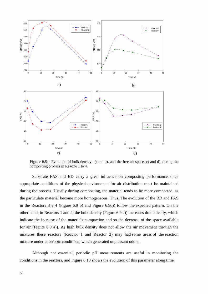
58
Time (d)
0 10 20 30 40 50
BD
(kg/m
^3)
250
300
350
400
450
500
550
600
Reactor 1
Reactor 2
Time (d)
0 10 20 30 40 50
BD
(kg/m
^3)
300
400
500
600
Reactor 3
Reactor 4
Time (d)
0 10 20 30 40 50
FA
S (
%)
30
40
50
60
70
80
Reactor 1
Reactor 2
Time (d)
0 10 20 30 40 50
FA
S (
%)
30
40
50
60
70
80
Reactor 3
Reactor 4
Figure 6.9 - Evolution of bulk density, a) and b), and the free air space, c) and d), during the
composting process in Reactor 1 to 4.
Substrate FAS and BD carry a great influence on composting performance since
appropriate conditions of the physical environment for air distribution must be maintained
during the process. Usually during composting, the material tends to be more compacted, as
the particulate material become more homogeneous. Thus, The evolution of the BD and FAS
in the Reactors 3 e 4 (Figure 6.9 b) and Figure 6.9d)) follow the expected pattern. On the
other hand, in Reactors 1 and 2, the bulk density (Figure 6.9 c)) increases dramatically, which
indicate the increase of the materials compaction and so the decrease of the space available
for air (Figure 6.9 a)). As high bulk density does not allow the air movement through the
mixtures these reactors (Reactor 1 and Reactor 2) may had some areas of the reaction
mixture under anaerobic conditions, which generated unpleasant odors.
Although not essential, periodic pH measurements are useful in monitoring the
conditions in the reactors, and Figure 6.10 shows the evolution of this parameter along time.
a) b)
c) d)
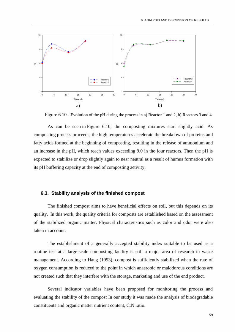
6. ANALYSIS AND DISCUSSION OF RESULTS
59
Time (d)
0 5 10 15 20 25 30
pH
2
4
6
8
10
Reactor 1
Reactor 2
Time (d)
0 5 10 15 20 25 30
pH
2
4
6
8
10
Reactor 3
Reactor 4
Figure 6.10 - Evolution of the pH during the process in a) Reactor 1 and 2, b) Reactors 3 and 4.
As can be seen in Figure 6.10, the composting mixtures start slightly acid. As
composting process proceeds, the high temperatures accelerate the breakdown of proteins and
fatty acids formed at the beginning of composting, resulting in the release of ammonium and
an increase in the pH, which reach values exceeding 9.0 in the four reactors. Then the pH is
expected to stabilize or drop slightly again to near neutral as a result of humus formation with
its pH buffering capacity at the end of composting activity.
6.3. Stability analysis of the finished compost
The finished compost aims to have beneficial effects on soil, but this depends on its
quality. In this work, the quality criteria for composts are established based on the assessment
of the stabilized organic matter. Physical characteristics such as color and odor were also
taken in account.
The establishment of a generally accepted stability index suitable to be used as a
routine test at a large-scale composting facility is still a major area of research in waste
management. According to Haug (1993), compost is sufficiently stabilized when the rate of
oxygen consumption is reduced to the point in which anaerobic or malodorous conditions are
not created such that they interfere with the storage, marketing and use of the end product.
Several indicator variables have been proposed for monitoring the process and
evaluating the stability of the compost In our study it was made the analysis of biodegradable
constituents and organic matter nutrient content, C:N ratio.
a) b)
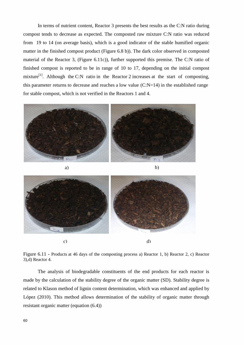
60
In terms of nutrient content, Reactor 3 presents the best results as the C:N ratio during
compost tends to decrease as expected. The composted raw mixture C:N ratio was reduced
from 19 to 14 (on average basis), which is a good indicator of the stable humified organic
matter in the finished compost product (Figure 6.8 b)). The dark color observed in composted
material of the Reactor 3, (Figure 6.11c)), further supported this premise. The C:N ratio of
finished compost is reported to be in range of 10 to 17, depending on the initial compost
mixture[1]
. Although the C:N ratio in the Reactor 2 increases at the start of composting,
this parameter returns to decrease and reaches a low value (C:N=14) in the established range
for stable compost, which is not verified in the Reactors 1 and 4.
Figure 6.11 - Products at 46 days of the composting process a) Reactor 1, b) Reactor 2, c) Reactor
3),d) Reactor 4.
The analysis of biodegradable constituents of the end products for each reactor is
made by the calculation of the stability degree of the organic matter (SD). Stability degree is
related to Klason method of lignin content determination, which was enhanced and applied by
López (2010). This method allows determination of the stability of organic matter through
resistant organic matter (equation (6.4))
a) b)
c) d)
6. ANALYSIS AND DISCUSSION OF RESULTS
61
(6.5)
where βend is the fraction of biodegradable organic matter at the end of compost. The SD of
the four reactors were calculated using the Eq. (6.1) and the results are shown in Table 6.5.
Table 6.5 - Stability degree of the finished composts.
Reactor 1 Reactor 2 Reactor 3 Reactor 4
Stability degree SD (%) 80.2 82.6 82.8 70.5
As shown in Table 6.5, the Reactors 2 and 3 achieved the highest stability degree of
the organic matter at end of composting. Reactor 4, on the other hand, reached the lowest
degree of stability since the percentage biodegradable organic matter available at end was
high. The determination of lignin content was based on two replicates in each sample;
therefore, the values indicated in Table 6.5 are mean values between the two determinations.
6.4. Model evaluation
The model presented in Chapter 3 was used simulate profiles of temperature, VS and
water for each reactor along time. A simple sensitivity analysis was also performed to
evaluate the relative importance of selected model parameters. All the calculations and
simulations were made in Matlab R2009b.
6.4.1. Model Simulations
By comparing model prediction with experimental data, the mathematical model may
be validated and a quantitative measure of performance was calculated. The quality of the
model fitting to the experimental data was evaluated by the average percentage deviation of
the estimates (AD), which was calculated using Eq. (6.6).
(6.6)
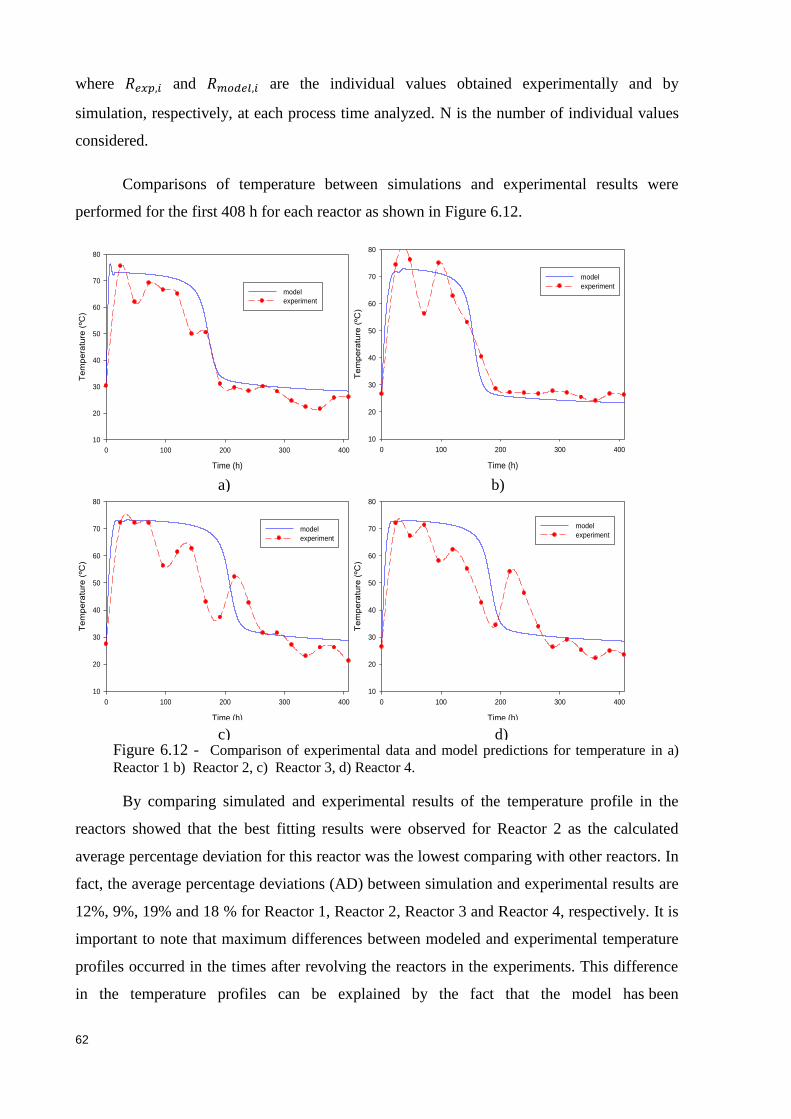
62
where and are the individual values obtained experimentally and by
simulation, respectively, at each process time analyzed. N is the number of individual values
considered.
Comparisons of temperature between simulations and experimental results were
performed for the first 408 h for each reactor as shown in Figure 6.12.
Time (h)
0 100 200 300 400
Te
mp
era
ture
(ºC
)
10
20
30
40
50
60
70
80
model
experiment
r2
Time (h)
0 100 200 300 400
Te
mp
era
ture
(ºC
)
10
20
30
40
50
60
70
80
model
experiment
Time (h)
0 100 200 300 400
Tem
pe
ratu
re (
ºC)
10
20
30
40
50
60
70
80
model
experiment
Time (h)
0 100 200 300 400
Tem
pe
ratu
re (
ºC)
10
20
30
40
50
60
70
80
model
experiment
Figure 6.12 - Comparison of experimental data and model predictions for temperature in a)
Reactor 1 b) Reactor 2, c) Reactor 3, d) Reactor 4.
By comparing simulated and experimental results of the temperature profile in the
reactors showed that the best fitting results were observed for Reactor 2 as the calculated
average percentage deviation for this reactor was the lowest comparing with other reactors. In
fact, the average percentage deviations (AD) between simulation and experimental results are
12%, 9%, 19% and 18 % for Reactor 1, Reactor 2, Reactor 3 and Reactor 4, respectively. It is
important to note that maximum differences between modeled and experimental temperature
profiles occurred in the times after revolving the reactors in the experiments. This difference
in the temperature profiles can be explained by the fact that the model has been
a)
d)
b)
c)
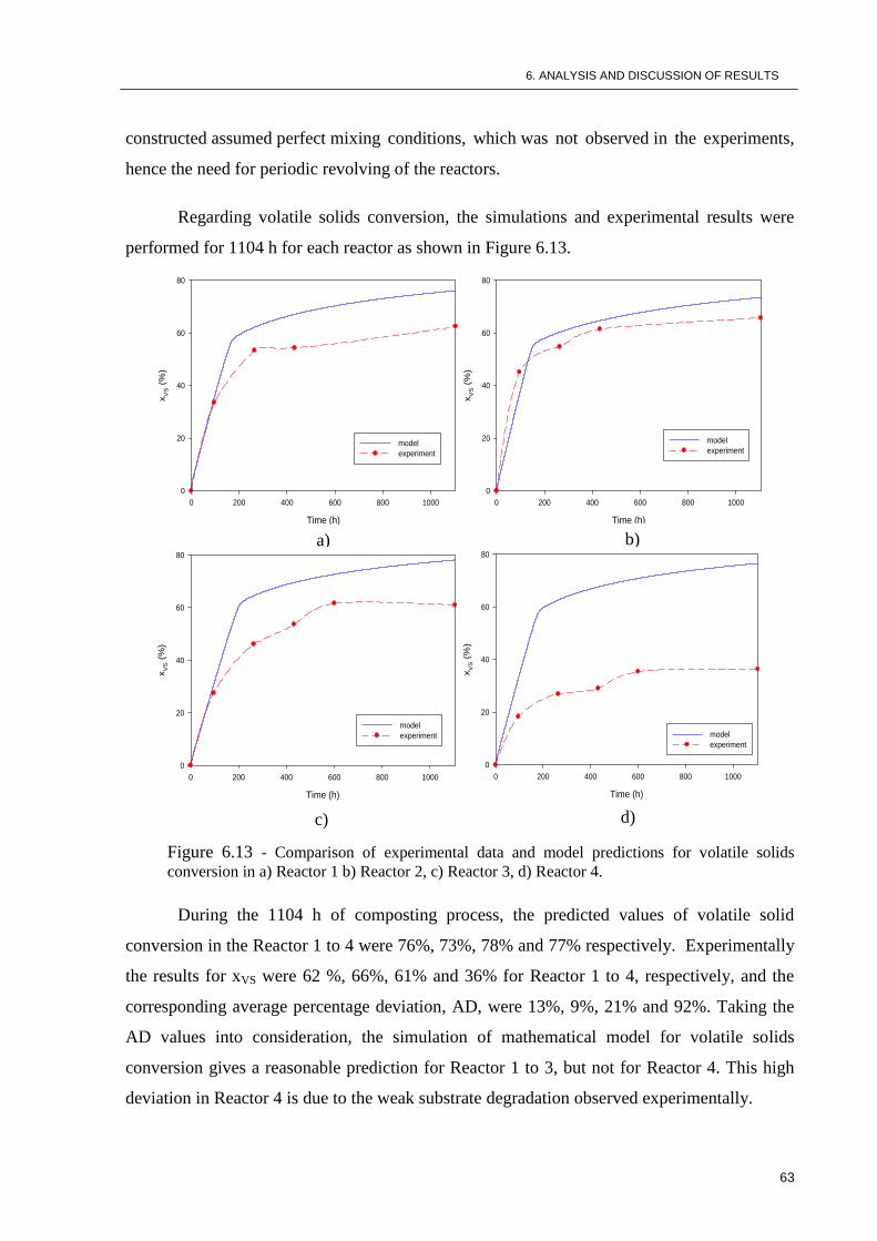
6. ANALYSIS AND DISCUSSION OF RESULTS
63
constructed assumed perfect mixing conditions, which was not observed in the experiments,
hence the need for periodic revolving of the reactors.
Regarding volatile solids conversion, the simulations and experimental results were
performed for 1104 h for each reactor as shown in Figure 6.13.
Time (h)
0 200 400 600 800 1000
xV
S (
%)
0
20
40
60
80
model
experiment
Time (h)
0 200 400 600 800 1000
xV
S (
%)
0
20
40
60
80
model
experiment
Time (h)
0 200 400 600 800 1000
xV
S (
%)
0
20
40
60
80
model
experiment
Time (h)
0 200 400 600 800 1000
xV
S (
%)
0
20
40
60
80
model
experiment
Figure 6.13 - Comparison of experimental data and model predictions for volatile solids
conversion in a) Reactor 1 b) Reactor 2, c) Reactor 3, d) Reactor 4.
During the 1104 h of composting process, the predicted values of volatile solid
conversion in the Reactor 1 to 4 were 76%, 73%, 78% and 77% respectively. Experimentally
the results for xVS were 62 %, 66%, 61% and 36% for Reactor 1 to 4, respectively, and the
corresponding average percentage deviation, AD, were 13%, 9%, 21% and 92%. Taking the
AD values into consideration, the simulation of mathematical model for volatile solids
conversion gives a reasonable prediction for Reactor 1 to 3, but not for Reactor 4. This high
deviation in Reactor 4 is due to the weak substrate degradation observed experimentally.
a) b)
c) d)
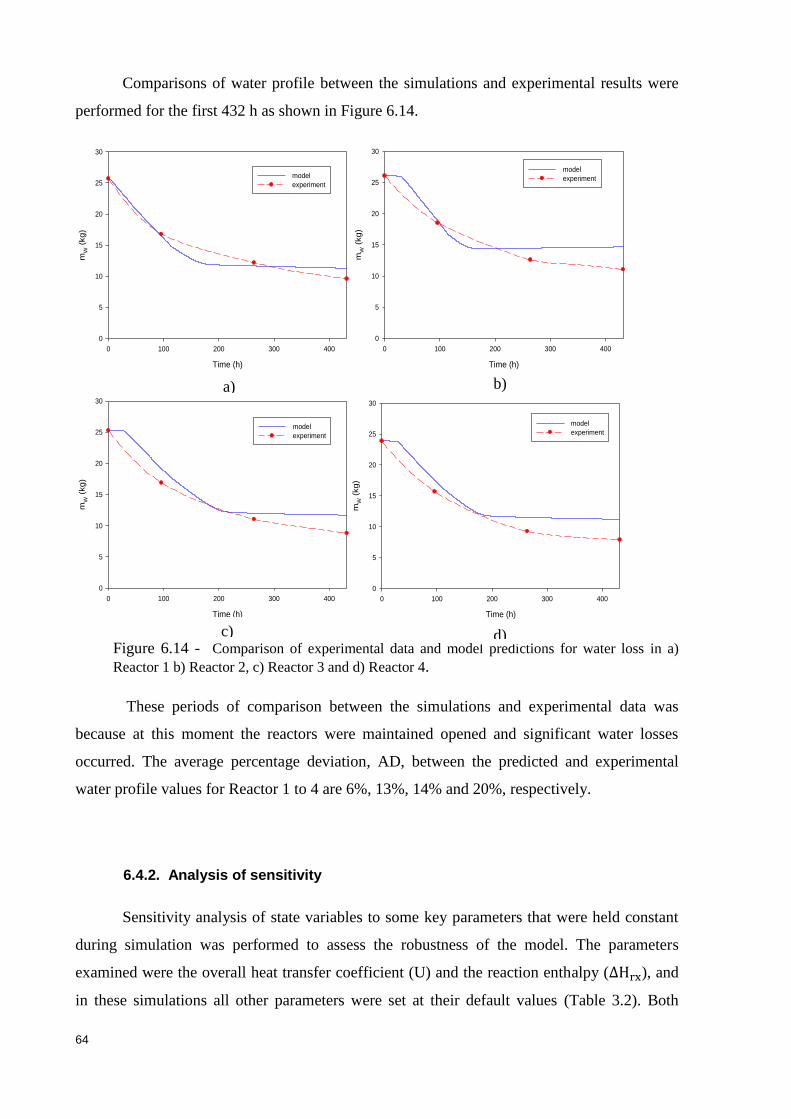
64
Comparisons of water profile between the simulations and experimental results were
performed for the first 432 h as shown in Figure 6.14. r1
Time (h)
0 100 200 300 400
mW
(kg
)
0
5
10
15
20
25
30
model
experiment
r2
Time (h)
0 100 200 300 400m
W (
kg
)
0
5
10
15
20
25
30
model
experiment
r3
Time (h)
0 100 200 300 400
mW
(kg
)
0
5
10
15
20
25
30
model
experiment
r4
Time (h)
0 100 200 300 400
mW
(kg
)
0
5
10
15
20
25
30
model
experiment
Figure 6.14 - Comparison of experimental data and model predictions for water loss in a)
Reactor 1 b) Reactor 2, c) Reactor 3 and d) Reactor 4.
These periods of comparison between the simulations and experimental data was
because at this moment the reactors were maintained opened and significant water losses
occurred. The average percentage deviation, AD, between the predicted and experimental
water profile values for Reactor 1 to 4 are 6%, 13%, 14% and 20%, respectively.
6.4.2. Analysis of sensitivity
Sensitivity analysis of state variables to some key parameters that were held constant
during simulation was performed to assess the robustness of the model. The parameters
examined were the overall heat transfer coefficient (U) and the reaction enthalpy ( ), and
in these simulations all other parameters were set at their default values (Table 3.2). Both
a) b)
c) d)
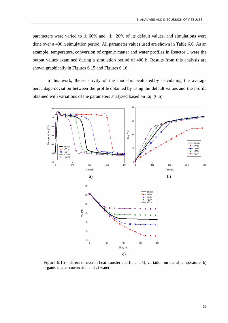
6. ANALYSIS AND DISCUSSION OF RESULTS
65
parameters were varied to 60% and 20% of its default values, and simulations were
done over a 400 h simulation period. All parameter values used are shown in Table 6.6. As an
example, temperature, conversion of organic matter and water profiles in Reactor 1 were the
output values examined during a simulation period of 400 h. Results from this analysis are
shown graphically in Figures 6.15 and Figures 6.16
In this work, the sensitivity of the model is evaluated by calculating the average
percentage deviation between the profile obtained by using the default values and the profile
obtained with variations of the parameters analyzed based on Eq. (6.6).
Time (h)
0 100 200 300 400
Te
mp
era
ture
(ºC
)
20
30
40
50
60
70
80
default
-60 %
-20 %
+20 %
+60 %
Time (h)
0 100 200 300 400
xV
S (
%)
0
20
40
60
80
default
-60 %
-20 %
+20%
+60 %
Time (h)
0 100 200 300 400
mW
(kg)
0
5
10
15
20
25
30
default
-60 %
-20 %
+20 %
+60 %
Figure 6.15 - Effect of overall heat transfer coefficient, U, variation on the a) temperature, b)
organic matter conversion and c) water.
a) b)
c)
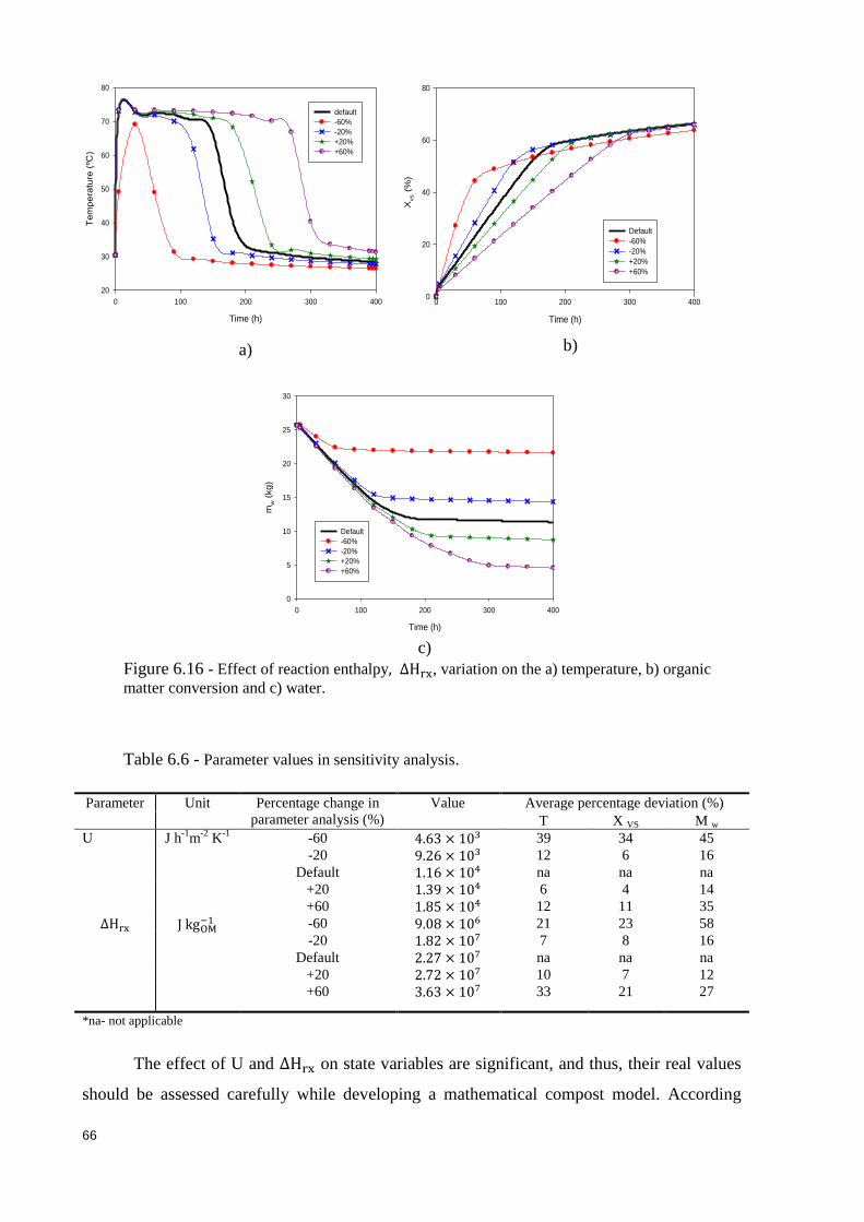
66
2D Graph 3
Time (h)
0 100 200 300 400
Te
mp
era
ture
(ºC
)
20
30
40
50
60
70
80
default
-60%
-20%
+20%
+60%
2D Graph 4
Time (h)
0 100 200 300 400
Xvs (
%)
0
20
40
60
80
Default
-60%
-20%
+20%
+60%
2D Graph 5
Time (h)
0 100 200 300 400
mw (
kg
)
0
5
10
15
20
25
30
Default
-60%
-20%
+20%
+60%
Figure 6.16 - Effect of reaction enthalpy , variation on the a) temperature, b) organic
matter conversion and c) water.
Table 6.6 - Parameter values in sensitivity analysis.
Parameter Unit Percentage change in
parameter analysis (%)
Value Average percentage deviation (%)
T X VS M w
U J h-1
m-2
K-1
-60 39 34 45
-20 12 6 16
Default na na na
+20 6 4 14
+60 12 11 35
-60 21 23 58
-20 7 8 16
Default na na na
+20 10 7 12
+60 33 21 27
*na- not applicable
The effect of U and on state variables are significant, and thus, their real values
should be assessed carefully while developing a mathematical compost model. According
c)
a) b)
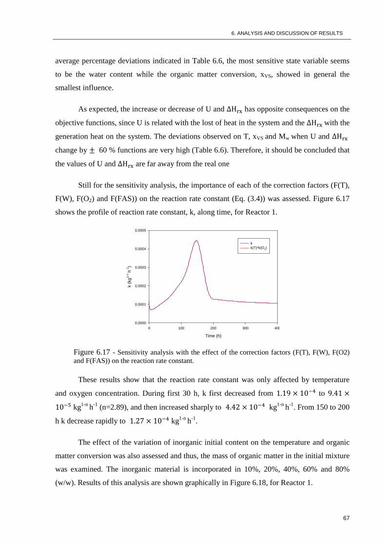
6. ANALYSIS AND DISCUSSION OF RESULTS
67
average percentage deviations indicated in Table 6.6, the most sensitive state variable seems
to be the water content while the organic matter conversion, xVS, showed in general the
smallest influence.
As expected, the increase or decrease of U and has opposite consequences on the
objective functions, since U is related with the lost of heat in the system and the with the
generation heat on the system. The deviations observed on T, xVS and Mw when U and
change by 60 % functions are very high (Table 6.6). Therefore, it should be concluded that
the values of U and are far away from the real one
Still for the sensitivity analysis, the importance of each of the correction factors (F(T),
F(W), F(O2) and F(FAS)) on the reaction rate constant (Eq. (3.4)) was assessed. Figure 6.17
shows the profile of reaction rate constant, k, along time, for Reactor 1.
Time (h)
0 100 200 300 400
k (
kg
1-n
h-1
)
0,0000
0,0001
0,0002
0,0003
0,0004
0,0005
k
k(T)*k(O2)
Figure 6.17 - Sensitivity analysis with the effect of the correction factors (F(T), F(W), F(O2)
and F(FAS)) on the reaction rate constant.
These results show that the reaction rate constant was only affected by temperature
and oxygen concentration. During first 30 h, k first decreased from to
kg1-n
h-1
(n=2.89), and then increased sharply to kg1-n
h-1
. From 150 to 200
h k decrease rapidly to kg1-n
h-1
.
The effect of the variation of inorganic initial content on the temperature and organic
matter conversion was also assessed and thus, the mass of organic matter in the initial mixture
was examined. The inorganic material is incorporated in 10%, 20%, 40%, 60% and 80%
(w/w). Results of this analysis are shown graphically in Figure 6.18, for Reactor 1.
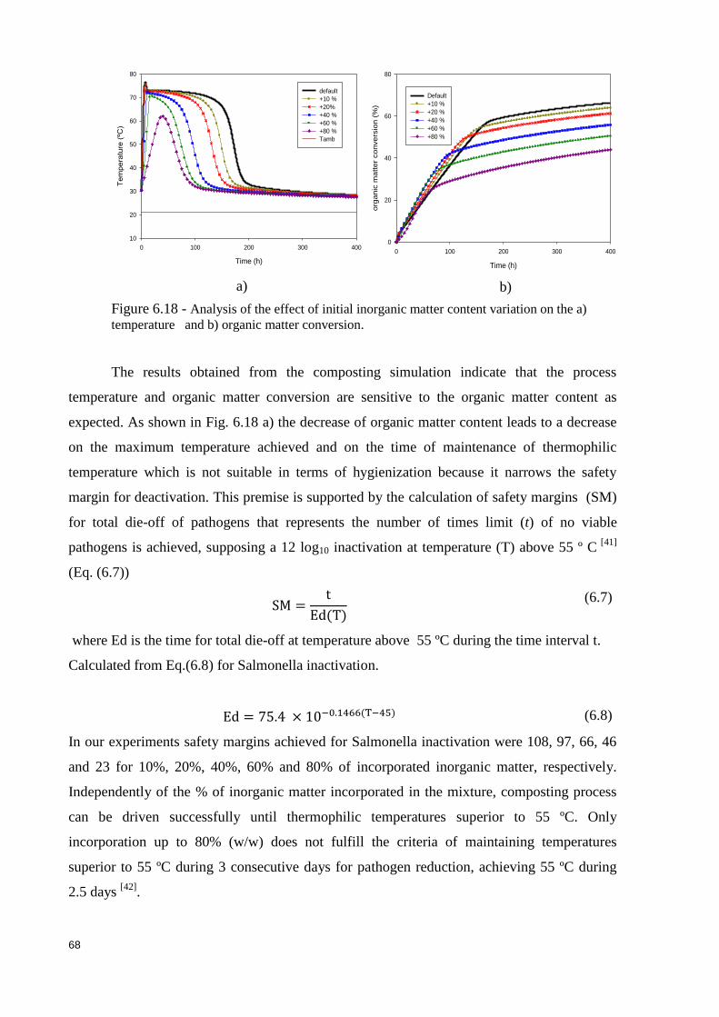
68
Time (h)
0 100 200 300 400
Tem
pera
ture
(ºC
)
10
20
30
40
50
60
70
80
default
+10 %
+20%
+40 %
+60 %
+80 %
Tamb
Time (h)
0 100 200 300 400
org
an
ic m
atte
r co
nve
rsio
n (
%)
0
20
40
60
80
Default
+10 %
+20 %
+40 %
+60 %
+80 %
Figure 6.18 - Analysis of the effect of initial inorganic matter content variation on the a)
temperature and b) organic matter conversion.
The results obtained from the composting simulation indicate that the process
temperature and organic matter conversion are sensitive to the organic matter content as
expected. As shown in Fig. 6.18 a) the decrease of organic matter content leads to a decrease
on the maximum temperature achieved and on the time of maintenance of thermophilic
temperature which is not suitable in terms of hygienization because it narrows the safety
margin for deactivation. This premise is supported by the calculation of safety margins (SM)
for total die-off of pathogens that represents the number of times limit (t) of no viable
pathogens is achieved, supposing a 12 log10 inactivation at temperature (T) above 55 º C [41]
(Eq. (6.7))
(6.7)
where Ed is the time for total die-off at temperature above 55 ºC during the time interval t.
Calculated from Eq.(6.8) for Salmonella inactivation.
(6.8)
In our experiments safety margins achieved for Salmonella inactivation were 108, 97, 66, 46
and 23 for 10%, 20%, 40%, 60% and 80% of incorporated inorganic matter, respectively.
Independently of the % of inorganic matter incorporated in the mixture, composting process
can be driven successfully until thermophilic temperatures superior to 55 ºC. Only
incorporation up to 80% (w/w) does not fulfill the criteria of maintaining temperatures
superior to 55 ºC during 3 consecutive days for pathogen reduction, achieving 55 ºC during
2.5 days [42]
.
a) b)
7. CONCLUSIONS AND PROSPECTS FOR FUTURE WORK
69
7. CONCLUSIONS AND PROSPECTS FOR FUTURE WORK
This work had two main objectives. The first one was to predict the biodegradability
of initial waste mixtures and to investigate how this property progresses during the
composting process in pilot-scale reactors. The second objective was to develop a dynamic
mathematical model for aerobic composting process and its validation by fitting experimental
data.
The experimental apparatus consisted in four self heating reactors with 120 L of
internal volume and isolated where four different blends made from potato-peel industrial
waste, grass clippings and sawdust were composted.
The process monitoring included temperature, mass content, moisture content, pH,
bulk density, free air space, biodegradability of organic matter and other parameters.
Concerning to the temperature monitoring, it was found that the four reactors quickly reached
thermophilic temperatures and remained in this range for several days, which allowed the
compost hygienization. The organic matter conversion was above 60% except for Reactor 4,
which only reached the maximum organic matter conversion of 36%.
The assessment of biodegradability of organic matter by determining of lignin content
proved to be an appropriate methodology for this purpose since the predictions for the
biodegradation of organic matter were consistent with those obtained experimentally. The
estimation of the maximum biodegradation of organic matter was made considering that all
biodegradable organic matter present in the initial mixture will be degraded. In practice, the
degradation of organic matter is not complete, which explains the difference between the
maximum biodegradation estimated from the determination of lignin and the one observed
experimentally. The great disadvantage of this methodology is related to the time scale to
determine the lignin content in each sample (approximately 2 days). Reducing the time
required for lignin determination is a challenge to be evaluated in future work because it
would allow the suitability of this method in cases of full-scale composting. In terms of
compost characterization, Reactors 2 and 3 present the best results as the finished compost
had good level of stabilized humified and organic matter.
By comparing simulation and experimental results it was concluded that the developed
model could be used for simulating solid waste composting processes. Namely, temperature
70
of substrate, organic matter conversion and water profile in the composting system fitting well
the experimental data. The model was described by a set of 4 differential equations state
variables (3 corresponding to mass balances and 1 related with energy balance. Since the
model showed good results, it could be used for explaining and demonstrating the complex
interactions which occur in the composting process and also to simulate the efficiency and
cost of compost processes under different operation conditions. Adjusting operation
conditions by changing key factors (eg. Overall heat transfer coefficient), optimal operation
condition could be determined. For future work in this area, the overall heat transfer
coefficient and reaction enthalpy should be determined specifically for the system analyzed,
since both have significant effect on the model predictions. Other important aspect to be
improved in future is the fact that the model could take in account the heterogeneous nature of
the system.
8. BIBLIOGRAPY
71
8. BIBLIOGRAPHY
[1] Gajalakshmi S., Abbasi S. A., (2008), Solid waste management by composting,
Environmental Science and Technology, 38, 311–400.
[2] Slater R. A., Frederickson J., (2001), Composting municipal waste in the UK: some lessons from
Europe, Resources, Conservation and Recycling, 32, 359–374.
[3] Trautmann N. M., Krasny, M. E., (1997),Composting in the Classroom, Cornell Waste
Management Institute, USA.
[4] Bernal M. P., Alburquerque JA., Moral R., (2009).,Composting of animal manures and chemical
criteria for compost maturity assessment. Bioresource Technology,
100, 5444–5453.
[5] Francou C., Linères M., Derenne S.,Villio-Poitrenaud M., Houot S., (2008), Influence of green
waste, biowaste and paper–cardboard initial ratios on organic matter transformations during
composting. Bioresource Technology, 99, 8926–8934.
[6] López M., Huerta-Pujol O., Martínez-Farré. FX, Soliva M., (2010), Approaching compost
stability from Klason lignin modified method: Chemical stability degree for OM and N quality
assessment, Resources, Conservation and Recycling, 55, 171–181.
[7] Haug R. T., (1993), The practical handbook of compost engineering. Boca Raton, Florida.
[8] Rynk, R., (1992), On-Farm Composting Handbook, Ithaca, New York.
[9] Pace M. G., Miller B. E., Farrell-Poe K. L., (1995), The Composting Process. Utah State
University is an Equal Opportunity / Affirmative Action Institution.
[10] Tuomela M., Vikman M., Hatakka A., Itavaara M., (2000), Biodegradation of lignin in a
compost environment: a review. Bioresource Technology, 72, 169-183.
[11] Hannequart J. P., Radermaker F., Saintmard C., (2005), Gestão de resíduos domésticos
biodegradáveis: Que perspectivas para as autoridades locais europeias? Association of cities and
regions for recycling and sustainable resource management.
[12] AGÊNCIA PORTUGUESA DO AMBIENTE, (2010), Caracterização da Situação dos
Resíduos Urbanos em Portugal Continental em 2009.
[13] AGÊNCIA PORTUGUESA DO AMBIENTE, (2008), Dossier de Prevenção (redução) de
Resíduos.
[14] Baptista M., Antunes F., Gonçalves M.S., Morvan B., Silveira A., (2010). Composting kinetics
in full-scale mechanical–biological treatment plants, Waste Management,30,1908–1921.
[15] Rudder W., O‘Sullivan M., Bischoff R.., (2005), Review of Alternative Solid Waste
Management Methods, Earth Tech Canada Inc.
[16] Ministry of Agriculture & Food, (1996), The composting process, Resource Management
Branch, Abbotsford BC, CANADA
72
[17] Abdullah N., N.L. Chin., (2010), Simplex-centroid mixture formulation for optimised
composting of kitchen waste, Bioresource Technology, 101, 8205–8210.
[18] Rivenshield A., Bassuk N L., (2007), Using Organic Amendments to Decrease Bulk Density
and Increase Macroporosity in Compacted Soils, Arboriculture & Urban Forestry, 33, 140–146.
[19] Ruggieri L., Gea T., Artola A., Sánchez A., (2009), Air filled porosity measurements by air
pycnometry in the composting process: A review and a correlation analysis, Bioresource
Technology, 100, 2655–2666.
[20] Johnsson L., Nilsson S. I., Jennische P., (2005), Desk study to assess the feasibility of a draft
horizontal standard for electrical conductivity, Swedish University of Agricultural Sciences.
[21] Gomes A. P., and Pereira F A ., (2008), Mathematical modelling of a composting process, and
validation with experimental data, Waste Management & Research,26, 276–287.
[22] Pagga U., (1997), Testing biodegradability with standardized methods. Chemosphere, 12, 2953-
2972.
[23] Ylijoki J. L., Syrjä J. J., Wahlström M., (2004), Biodegradability testing of the municipal solid
waste reject. Nordic Innovation Centre Project, 1644-03.
[24] Tosin M., Degli-Innocenti F., Bastioli C., (1996), Effect of the composting substrate on
biodegradation of solid materials under controlled composting conditions, Journal of
Environmental polymer Degradation, 4, 55-63.
[25] Wagland S.T., Tyrrel S.F., (2010), Test methods to aid in the evaluation of the diversion of
biodegradable municipal waste (BMW) from landfill, Waste Management, 30, 934–935.
[26] Wagland S.T., Tyrrel S.F., Godley A.R., Smith R., (2009), Test methods to aid in the evaluation
of the diversion of biodegradable municipal waste (BMW) from landfill. Waste Management,
29, 1218– 1226.
[27] Tuomela M., (2002), Degradation of lignin and other 14C-labelled compounds in compost and
soil with an emphasis on white-rot fungi, Academic dissertation in microbiology.
[28] Santana M., Cavali J., (2006), Fundamentos e Avaliação Comparativa de Métodos para Análise
de Lignina em Forragens, Revista Electrónica de Veterinaria REDVET, VII, 1695-7504.
[29] Petric I., Selimbaˇsi´c V., (2008), Development and validation of mathematical model for
aerobic composting process, Chemical Engineering Journal, 139, 304–317.
[30] Maloney J O., (2008), Perry´s Chemical Engineering Handbook, 8th
Edition, McGraw-Hill
Companies, Inc.
[31] Eriksson L., Johansson E., Wikstro¨m C., (1988), Mixture design—design generation, PLS
analysis, and model usage, Chemometrics and Intelligent Laboratory Systems, 43, 1-24.
[32] Zhang J., (2010), Simulation of substrate degradation in composting of sewage sludge, Waste
Management, 30, 1931–1938.
[33] Xi B., Wei Z., Liu H., (2010), Dynamic Simulation for Domestic Solid Waste composting
Processes. Academia Arena.
[34] Mason I.G., (2006), Mathematical modelling of the composting process: A review, Waste

8. BIBLIOGRAPY
73
Management, 26, 3-31.
[35] Higgins C. W., Walker L. P., (2001), Validation of a new model for aerobic organic solids
decomposition: simulations with substrate specific kinetics. Process Biochemistry, 36, 875–884.
[36] Yu S., Clark O. G., Leonard J. J., (2009), Influence of free air space on microbial kinetics in
passively aerated compos,. Bioresource Technology, 100, 782-790.
[37] MINISTÉRIO DO AMBIENTE, DO ORDENAMENTO DO TERRITÓRIO E DO
DESENVOLVIMENTO REGIONAL, Decreto-Lei n.º 183/2009 de 10 de Agosto.
[38] MINISTÉRIO DO AMBIENTE, DO ORDENAMENTO DO TERRITÓRIO E DO
DESENVOLVIMENTO REGIONAL, Decreto-Lei n.o 178/2006 de 5 de Setembro
[39 ] Quina M. M. J., (2005), PROCESSOS DE INERTIZAÇÃO E VALORIZAÇÃO DE CINZAS
VOLANTES - Incineração de Resíduos Sólidos Urbanos. Dissertação apresentada à Faculdade
de Ciências e Tecnologia da Universidade de Coimbra, com vista à obtenção do grau de Doutor
em Engenharia Química.
[40] Godley A., Lewin K., Graham A., Barker H., Smith R., (2004), Biodegradability determination
of municipal waste: an evaluation of methods, Integrated Waste Management and Pollution
Control: Policy and Practice, Research and Solutions, 40-49.
[41 ] Vinnera B., Bjorklund, A., Jonsson, H., (2008), Thermal composting of faecal matter as
treatment and possible disinfection method––laboratory-scale and pilot-scale studies, Bioresource
Technology, 88, 47–54.
[42] Wichuk K. M., McCartney, D., A review of the effectiveness of current time– temperature
regulations on pathogen inactivation during composting, J. Environ. Eng. Sci, 6 (2007) 573–586.

APPENDIX
APPENDIX
A- Characteristics of the equipment used
B- Elemental composition of the samples
C- Mathematical model program in Matlab
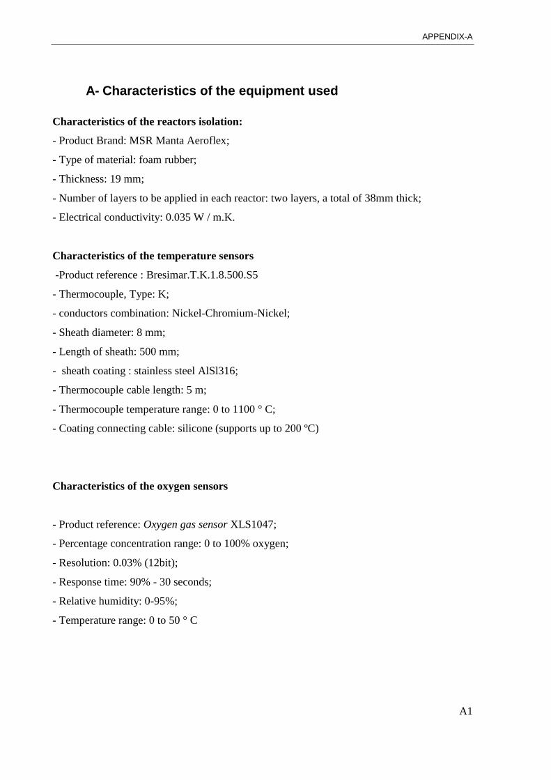
APPENDIX-A
A1
A- Characteristics of the equipment used
Characteristics of the reactors isolation:
- Product Brand: MSR Manta Aeroflex;
- Type of material: foam rubber;
- Thickness: 19 mm;
- Number of layers to be applied in each reactor: two layers, a total of 38mm thick;
- Electrical conductivity: 0.035 W / m.K.
Characteristics of the temperature sensors
-Product reference : Bresimar.T.K.1.8.500.S5
- Thermocouple, Type: K;
- conductors combination: Nickel-Chromium-Nickel;
- Sheath diameter: 8 mm;
- Length of sheath: 500 mm;
- sheath coating : stainless steel AlSl316;
- Thermocouple cable length: 5 m;
- Thermocouple temperature range: 0 to 1100 ° C;
- Coating connecting cable: silicone (supports up to 200 ºC)
Characteristics of the oxygen sensors
- Product reference: Oxygen gas sensor XLS1047;
- Percentage concentration range: 0 to 100% oxygen;
- Resolution: 0.03% (12bit);
- Response time: 90% - 30 seconds;
- Relative humidity: 0-95%;
- Temperature range: 0 to 50 ° C
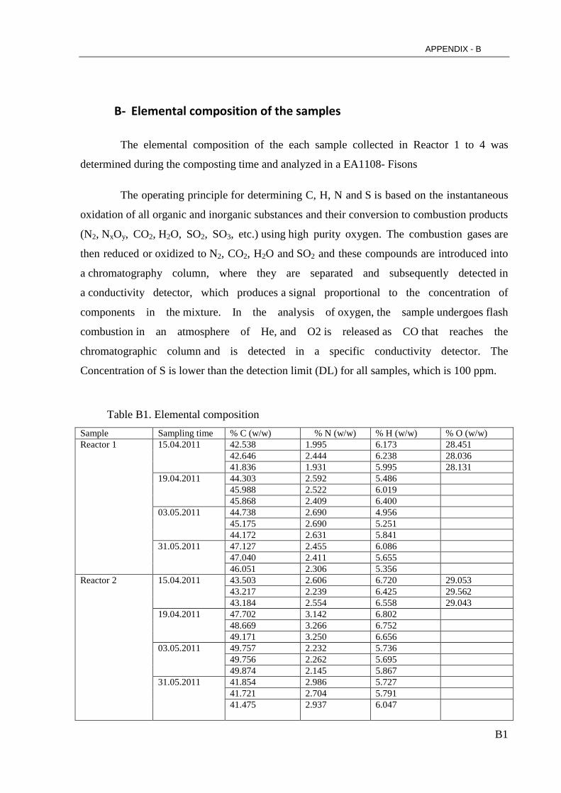
APPENDIX - B
B1
B- Elemental composition of the samples
The elemental composition of the each sample collected in Reactor 1 to 4 was
determined during the composting time and analyzed in a EA1108- Fisons
The operating principle for determining C, H, N and S is based on the instantaneous
oxidation of all organic and inorganic substances and their conversion to combustion products
(N2, NxOy, CO2, H2O, SO2, SO3, etc.) using high purity oxygen. The combustion gases are
then reduced or oxidized to N2, CO2, H2O and SO2 and these compounds are introduced into
a chromatography column, where they are separated and subsequently detected in
a conductivity detector, which produces a signal proportional to the concentration of
components in the mixture. In the analysis of oxygen, the sample undergoes flash
combustion in an atmosphere of He, and O2 is released as CO that reaches the
chromatographic column and is detected in a specific conductivity detector. The
Concentration of S is lower than the detection limit (DL) for all samples, which is 100 ppm.
Table B1. Elemental composition
Sample Sampling time % C (w/w) % N (w/w) % H (w/w) % O (w/w)
Reactor 1 15.04.2011 42.538 1.995 6.173 28.451
42.646 2.444 6.238 28.036
41.836 1.931 5.995 28.131
19.04.2011 44.303 2.592 5.486
45.988 2.522 6.019
45.868 2.409 6.400
03.05.2011 44.738 2.690 4.956
45.175 2.690 5.251
44.172 2.631 5.841
31.05.2011 47.127 2.455 6.086
47.040 2.411 5.655
46.051 2.306 5.356
Reactor 2 15.04.2011 43.503 2.606 6.720 29.053
43.217 2.239 6.425 29.562
43.184 2.554 6.558 29.043
19.04.2011 47.702 3.142 6.802
48.669 3.266 6.752
49.171 3.250 6.656
03.05.2011 49.757 2.232 5.736
49.756 2.262 5.695
49.874 2.145 5.867
31.05.2011
41.854 2.986 5.727
41.721 2.704 5.791
41.475 2.937 6.047
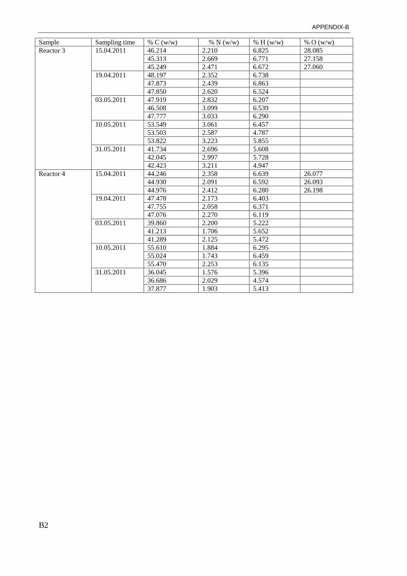
APPENDIX-B
B2
Sample Sampling time % C (w/w) % N (w/w) % H (w/w) % O (w/w)
Reactor 3 15.04.2011 46.214 2.210 6.825 28.085
45.313 2.669 6.771 27.158
45.249 2.471 6.672 27.060
19.04.2011 48.197 2.352 6.738
47.873 2.439 6.863
47.850 2.620 6.524
03.05.2011 47.919 2.832 6.207
46.508 3.099 6.539
47.777 3.033 6.290
10.05.2011 53.549 3.061 6.457
53.503 2.587 4.787
53.822 3.223 5.855
31.05.2011 41.734 2.696 5.608
42.045 2.997 5.728
42.423 3.211 4.947
Reactor 4 15.04.2011 44.246 2.358 6.639 26.077
44.930 2.091 6.592 26.093
44.976 2.412 6.280 26.198
19.04.2011 47.478 2.173 6.403
47.755 2.058 6.371
47.076 2.270 6.119
03.05.2011 39.860 2.200 5.222
41.213 1.706 5.652
41.289 2.125 5.472
10.05.2011 55.610 1.884 6.295
55.024 1.743 6.459
55.470 2.253 6.135
31.05.2011 36.045 1.576 5.396
36.686 2.029 4.574
37.877 1.903 5.413
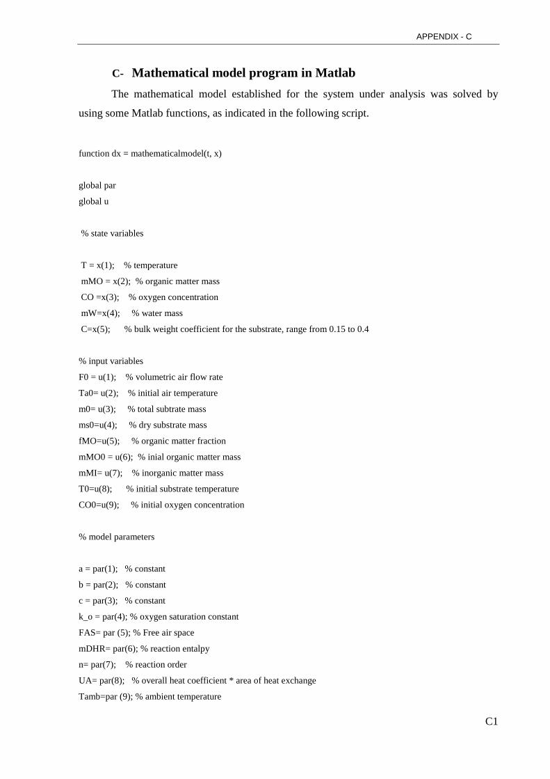
APPENDIX - C
C1
C- Mathematical model program in Matlab
The mathematical model established for the system under analysis was solved by
using some Matlab functions, as indicated in the following script.
function dx = mathematicalmodel(t, x)
global par
global u
% state variables
T = x(1); % temperature
mMO = x(2); % organic matter mass
CO =x(3); % oxygen concentration
mW=x(4); % water mass
C=x(5); % bulk weight coefficient for the substrate, range from 0.15 to 0.4
% input variables
F0 = u(1); % volumetric air flow rate
Ta0= u(2); % initial air temperature
m0= u(3); % total subtrate mass
ms0=u(4); % dry substrate mass
fMO=u(5); % organic matter fraction
mMO0 = u(6); % inial organic matter mass
mMI= u(7); % inorganic matter mass
T0=u(8); % initial substrate temperature
CO0=u(9); % initial oxygen concentration
% model parameters
a = par(1); % constant
b = par(2); % constant
c = par(3); % constant
k_o = par(4); % oxygen saturation constant
FAS= par (5); % Free air space
mDHR= par(6); % reaction entalpy
n= par(7); % reaction order
UA= par(8); % overall heat coefficient * area of heat exchange
Tamb=par (9); % ambient temperature
APPENDIX-C
C2
YW= par(10); % Stoichiometric coefficient for water
Vr= par (11); % reactor volume
MrW=par(12); % water molar mass
R= par(13); % universal gases constant
Patm=par(14);
Mra= par(15); % air molar mass;
MrMO = par(16);% organic matter molar mass
MrMI= par(17); % massa molar da matéria inorgânica
C1=par(18); % contsant
C2=par(19); % constant
C3=par(20); % constant
C4=par(21); % constant
C5=par(22); % constant
% --------------------------------------------------
% Mathematical model
% --------------------------------------------------
%% mass balance
m = mW+mMO+mMI;
ms=m-mW;
Sm = ms./m; % fractional solids content of the mixture solids
rho = C/Sm; % unit bulk weight of the mixed material to be composted
Vm = m/rho;
Vg= Vr-Vm; % gas volume
rhoW=1; % density of water
Vs=mMO/ms; % voltalite solids fraction
Gv=1; % specific gravity of the volatile fraction of the substrate solids
Gf=2.5; % specific gravity of the fixed fraction of the substrate (inorganic fraction)
Gs= 1/((Vs/Gv)+(1-Vs)/Gf); % specific gravity of substrate solids
FAS1= 1-((rho/1000)*Sm/(Gs*rhoW))- ((rho/1000)*(1-Sm)/rhoW);
% cinética da degradação do substrato
kT = a*(b^(T-273.15-20)-c^(T-273.15-60)); % temperature correction function
kO = CO/(k_o + CO); % oxygen correction function
kW = 1/(exp(-17.684*(1-Sm)+7.0622)+1); % moisture correction function
kF = 1/(exp(-23.67*FAS1+3.4945)+1); % free air space correction function
k= kT*kO*kW*kF; % reaction rate constant
rMO= -k*mMO^n;
APPENDIX - C
C3
dmMO = rMO;
% water balance
Pvs = exp(C1 + (C2/T) + C3*log(T)+ C4*T^C5); water % saturation pressure at temperature T
Pvs0 = exp(C1 + (C2/Ta0) + C3*log(Ta0)+ C4*Ta0^C5);% saturation pressure at temperature T0
Mar0=(Patm-Pvs0)*F0*Mra/(R*Ta0); % mass air flow rate at temperature
Mar=(Patm-Pvs)*F0*Mra/(R*T);
rW=Pvs0*F0*MrW/(R*Ta0)-YW*rMO-Pvs*F0*MrW/(R*T);
dmW= rW;
% Oxygen balance
rhoa0=1.18; % air specif gravity
rhoa =Mra*(Patm-Pvs)/(R*T);
dCO =CO0*Mar0/(Vr*rhoa0) -(CO*Mar0/(Vr*rhoa))+0.705*rMO/Vr;
dC=0.01;
%% enthalpy balance
cpai= 1009; % air specific heat
cpW= 4200; % water specific heat
cpMO= 1320; % organic matter specific heat
cpMI= 848; % inorganic matter specific heat
Var= FAS1*Vm; % air volume
mar= rhoa*Var; % mass volume
dT = (F0*cpai*rhoa0*(Ta0-T)+ mDHR*rMO-UA*(T-Tamb)) /
(cpW*mW+cpMO*mMO+cpMI*mMI+cpai*mar);
dx = [dT;dmMO;dCO;dmW;dC];
end
clc
clear
global par % parameters vector
APPENDIX-C
C4
global u % input variables vector
% Reactor 1
%% inputs variables
F0 = 0.56 ; % m^3/h
Ta0 = 20+273.15; % K
m0 = 34.8; % kg
ms0= 9.0954; % kg
fMO= 0.908;
mMO0 =fMO*ms0 ; % kg
mMI= (1-fMO)*ms0; % kg
T0= 20+273.15; % K
CO0 =0.2609 ; % kg_O2*m^-3
u = [F0;Ta0;m0;ms0;fMO;mMO0;mMI;T0;CO0]; % input variable inputs
% state variables on steady state
T = 30.4 +273.15; % K
mMO= mMO0; % kg
CO = 0.2609; % kg_O2*m^-3
mW= 25.7046; % kg_O2*m^-3
C=83;
x=[T;mMO;CO;mW;C]; % state variables vectors
% model parameters
a = 0.0000883; % kg^(1-n)*h^-1
b = 1.0533;
c= 1.2247;
k_o = 0.07; % kg_O2*m^-3
FAS= 0.5322;
mDHR= -2.27*10^7; % J*kg_MO^-1
n= 2.8944;
UA= 12800; % J*h^-1*K^-1
Tamb=25+273.15; % K
mMI= mMI ; % kg
YW= 0.360 ; % kg_H2O*kg^-1
kLW= 1*10^-4; % kg*h^-1*Pa^-1
Vr= 0.12; % m^3
MrW=18*10^-3; % kg/mol
R= 8.314; % J*mol^-1*K
Patm= 101325; % Pa
APPENDIX - C
C5
Mra= 28.96*10^-3; % kg/mol
MrMO = 449*10^-3; % kg/mol usando a fórmula C20H35105N
MrMI= 60.07*10^-3; % kg/mol usando a fórmula SiO2
C1=73.649;
C2=-7258.2;
C3=-7.3037;
C4=4.1653*10^-6;
C5=2;
% vector parameters
par =
[a;b;c;k_o;FAS;mDHR;n;UA;Tamb;mMI;YW;kLW;Vr;MrW;R;Patm;Mra;MrMO;MrMI;C1;C2;C3;C4;C5];
%outros parâmetros do modelo
cpai= 1009; % J mol^-1 K^-1
cpW= 4200; % J mol^-1 K^-1
cpMO= 1320; % J mol^-1 K^-1
cpMI= 848; % J mol^-1 K^-1
m = mW+mMO+mMI; % kg
ms=m-mW; %kg
Sm = ms./m;
rho = C/Sm; % kg/m^3
Vm = m/rho; % m^3
Vg= Vr-Vm; % m^3
rhoW=1; % kg/m^3
Vs=mMO/ms;
Gv=1;
Gf=2.5;
Gs= 1/((Vs/Gv)+(1-Vs)/Gf); % kg/m^3
FAS1= 1-((rho/1000)*Sm/(Gs*rhoW))- ((rho/1000)*(1-Sm)/rhoW);
kT = a*(b^(T-273.15-20)-c^(T-273.15-60));
kO = CO/(k_o + CO);
kW = 1/(exp(-17.684*(1-Sm)+7.0622)+1);
kW0=1/(exp(-17.684*(1-(ms0/m))+7.0622)+1);
kF = 1/(exp(-23.67*FAS1+3.4945)+1);
k= kT*kO*kW*kF;
rMO= -k*mMO^n;
Pvs = exp(C1 + (C2/T) + C3*log(T)+ C4*T^C5); % Pa
Pvs0 = exp(C1 + (C2/Ta0) + C3*log(Ta0)+ C4*Ta0^C5); % Pa
Mar0=(Patm-Pvs0)*F0*Mra/(R*Ta0); % kg h^-1
APPENDIX-C
C6
Mar=(Patm-Pvs)*F0*Mra/(R*T); % kg h^-1
rhoa=Mra*(Patm-Pvs)/(R*T); % kg/m^3
rW=Pvs0*F0*MrW/(R*Ta0)-YW*rMO-Pvs*F0*MrW/(R*T);
Var= FAS1*Vm; % m^3
mar= rhoa*Var; % m^3
%--------------------------------------------------------------------------
sampling time
%-------------------------------------------------------------------------
dt =5; % h
% initial time
t = 0; % h
imax =250;
tres = zeros (1, imax);
xres = zeros (length (x), imax);
ures = zeros (length (u), imax);
Cres= zeros (1, imax);
for i=1:imax
% F0 perturbance
if ( i == 7)
F0 = 0.56;
u( 1 ) = F0;
elseif (i==8)
F0=0.59;
u( 1 ) = F0;
elseif (i==10)
F0=0.52;
u( 1 ) = F0;
elseif (i==20)
F0=0.52;
u( 1 ) = F0;
elseif (i==24)
F0=0.37;
u( 1 ) = F0;
elseif (i==39)
F0=0.24;
u( 1 ) = F0;
elseif (i==58)
F0=0.27;
APPENDIX - C
C7
u( 1 ) = F0;
elseif (i==75)
F0=0.27;
u( 1 ) = F0;
end
tres(:,i) = t;
xres(:,i) = x;
ures(:,i) = u;
tnew = t + dt;
[tsol,xsol] = ode45('mathematicalmodel',[t tnew],x);
x = xsol(end,:)';
t = tsol(end);
end
% organic matter conversion
y= ((xres(2,1)-xres(2,:))/xres(2,1))*100;
%% Figures
figure (1)
subplot(2,1,1)
plot(tres,xres(1,:)-273.15);
title ('Temperature profile')
ylabel('T / ºC')
xlabel('t / h')
axis([0 415 20 80]);
hold off
subplot(2,1,2)
plot(tres,xres(2,:));
title ('organic matter mass')
ylabel('mMO / kg')
xlabel('t / h')
hold off;
figure (2)
subplot(2,1,1)
plot(tres,xres(3,:));
title('oxygen concentration ')
ylabel('CO /kg_O2*m^-3 ')
APPENDIX-C
C8
xlabel('t / h')
hold off;
subplot(2,1,2)
plot(tres,O);
title ('oxygen percentage')
ylabel('O/ %')
xlabel('t / h')
hold off;
figure (3)
subplot(2,1,1)
plot(tres,y);
title('organic matter conversion ')
ylabel('x_V_S / %')
xlabel('t / h')
axis([0 1120 0 80])
hold off;
subplot(2,1,2)
plot(tres,xres(4,:));
title ('water mass')
ylabel('mW / kg')
xlabel('t / h')
axis([0 440 0 30])
hold off;
figure (4)
subplot(2,1,1)
plot(tres,k);
title('reaction rate constant ')
ylabel('k / ')
xlabel('t / h')
hold off;
subplot(2,1,2)
plot(tres,kT);
title(' kT ')
ylabel('kT / ')
xlabel('t / h')
hold off;
APPENDIX - C
C9
figure (5)
subplot(2,1,1)
plot(tres,kW);
title(' kW ')
ylabel('kW / ')
xlabel('t / h')
hold off;
subplot(2,1,2)
plot(tres,kO);
title(' kO ')
ylabel('kO / ')
xlabel('t / h')
hold off;
figure (6)
subplot(2,1,1)
plot(tres,YFAS1);
title (' FAS')
ylabel('FAS/ % ')
xlabel('t / h')
axis([0 440 0 100])
hold off;
subplot(2,1,2)
plot(tres,kF);
title('kF ')
ylabel('kF / ')
xlabel('t / h')
hold off;
figure (7)
subplot(3,1,1)
plot(tres,ures(1,:));
title('evolução do caudal de entrada no reactor ')
ylabel('F0 / m3/h')
xlabel('t / h')
hold off;