STUDIES ON CONDUCTING POLYMERS AND

CONDUCTIVE ELASTOMER COMPOSITES

Thesis submitted to the

COCUIN UNIVERSITY Of

SCIENCE AND TECUNOLOGY

by

PKIfYCY K. G.

in partial ftdfillment of the requirementsfor the award of the degree of

DOCTOR Of FUILOSOFUY

DEPARTMENT OF POLYMER SCIENCE AND RUBBER TECHNOLOGY

COCHIN UNIVERSITY OF SCIENCE AND TECHNOLOGYKOCHI- 682 022

JUNE 2002

C!tcrtifirut.e

This is to certifiJ that this thesis entitled "Studies on Conducting

Polymers and Conductive Elastomer Composites" is a report of the original

workcarried out by Smi. PrinC1J K. G. underour supervision and guidance in the

Department of Polymer Science and Rubber Technology. No part of the work

reported in this thesis has been presented for any other degree from any other

institution.

.~~Dr. Rani Joseph

Professor, Dept. of Polymer Scienceand Rubber Technology

Cochin University of Scienceand Technology

A~S~~Dr. C. Sudha Kartha

Kochi-2222nd June 2002

Reader, Dept. of Physics,Cochin University of Science

and Technology

DECLARATION

I hereby declare that the thesis entitled "Studies on Conducting

Polymers and Conductive Elastomer Composites" is the original work carried

out by me under the supervision of Dr. Rani Joseph, Professor, Department of

Polymer Science and Rubber Technology, and Dr. C. Sudha Kariha, Reader,

Department of Physics, Kochi 682 022, and no part of this thesis has been

presented for any other degreefrom any other institution.

py; N.-y k .c"; (f2c./Princy K. G.

Kochi-22220d June 2002

to

my

family

ACKNOWLEDGEMENT

With deep pleasure and great satisfaction, I express the first and foremost

word of my profound gratitude to my supervising teachers, Prof. Rani Joseph,

Department of Polymer Science and Rubber Technology, and Dr. C. Sudha Kartha,

Department of Physics, for their support and enthusiastic guidance; and inspiring

encouragement throughout the course of my research work.

I am extremely grateful to Prof. K.E. George, Head of the Department of

Polymer Science and Rubber Technology, for his timely help and valuable

suggestions; and for providing all facilities during my research.

I am greatly indebted to Prof. A. P. Kuriakose, and Dr. D. Joseph Francis,

former Heads of the Department of Polymer Science and Rubber Technology, for

their advice and moral encouragement. I am sincerely thankful to all other

members of faculty and non-teaching staff of the department for their timely help

and encouragement rendered to me during this period. I express my sincere

gratitude to Dr. K.P. Vijayakumar, Head of the Department of Physics, CUSAT, for

his timely help and forproviding the facilities in the department.

My special thanks go to Dr. K. T. Mathew and the research scholars of the

Department of Electronics for helping me to take the dielectric properties

measurements. I express my sincere thanks to Chemical Engineering Department

of University of Eindhoven, for helping me to take TGA and IR spectra. I express

my special thanks to OUo van Asselen, for taking the IR spectra and interpreting

the results.

I also thank, the Manager, the Principal and all the faculty members of the

Department (Chemistry), Carmel College, Mala, for, their co-operation and

encouragement throughout the work.

I bow down to my parents and family members for their moral

encouragement, immense patience and loving care, which could give me the

strength to pursue my goal with success and dedication. Above all, the

unconditional and zealous attitude of my husband, P. Y. John, who instilled me the

fervour to complete my research work without any hindrance.

I am indebted to my friends and colleagues in the Department of PS & RT

and Physics Department for their wholehearted co-operation and help.

Princy K. G.

PREFACE

Conducting polymers, because of their unusual properties, have attracted

great interest in recent years. Despite the short history, they have found a place in

various applications. This thesis is about the development of conductive silicone

rubber and nitrile rubber; and the synthesis, characterization and properties of novel

conducting polymer -poly (p-phenylenediazomethine) and their blends with

polyethylene, PVC and silica.

This thesis is divided into seven chapters as follows:

Chapter 1 presents a review of the literature in this field and the scope of the

present investigation.

Chapter 2 deals with the materials used and the experimental procedures

adopted for the study.

Chapter 3 is divided into three parts; Part-I reports the effect of different

types of carbon blacks [e.g., acetylene black, lamp black, and ISAF (N-234) black],

copper powder, and graphite on the electrical conductivity and mechanical

properties of silicone rubber. Part -11 reports the effect of different types of carbon

blacks [e.g., N-220, N-347, and N-339 carbon blacks] on the electrical conductivity

and mechanical properties of silicone rubber. The effect of temperature on the

conductivity of silicone rubber vulcanizates is also studied. Part-Ill reports the effect

of blending silicone rubber with high-density polyethylene on the conductivity and

mechanical properties of the vulcanizates.

Chapter 4 is divided into two parts; Part I deals with the effect of

concentration of acetylene black on the electrical conductivity and mechanical

properties of nitrile rubber vulcanizates. Part 11 deals with the effect of blending of

NBR with other polymers on the electrical conductivity and mechanical properties

of the vulcanizates at the same dosage of acetylene black. Preparation of nitrile

rubber blends with NR, EPDM and PVC and the measurement of electrical

conductivity and mechanical properties are reported. Part "' deals with the

variation in conductivity and mechanical properties of the vulcanizates with different

composition of NBR/NR blends at the same dosage of acetylene black. Part -IV

deals with the effect of temperature on the electrical conductivity of these

vulcanizates.

Chapter 5 includes the synthesis and characterization of a new conducting

polymer based on glyoxal and p-phenylene diamine. The synthesis of poly(p­

phenylenediazomethine) was carried out in different solvents, like, methanol,

toluene, m-cresol and DMF. D.e. conductivity, dielectric properties and thermal

diffusivity of the polymer prepared in different solvents were determined. Effect of

dopants on the d.c. conductivity and dielectric properties was also investigated.

Chapter 6 includes in-situ polymerization of glyoxal and p-phenylenediamine

in different solvents containing different amounts of PE, PVC, and silica. The d.c.

conductivity and microwave conductivity of each sample was measured. The effect

of dopants like HCI04, HCI and 12 on conductivity was also studied.

Summary and conclusions of the present investigation is described in the

last chapter, Chapter 7.

At the end of each chapter a list of references has been given. A list of

abbreviations used in this thesis is also cited.

Contents

1 Introduction 1

1.1 Synthesis of conducting polymers 2

1.2 Doping 5

1.3 Temperature characteristics of conductors 7

1.4 Electrical conductivity and carrier transport 9

1.5 Charged defects in conjugated polymers 10

1.6 Microwave conductivity 11

1.7 Poly (azomethine)s 12

1.8 Conducting polymer blends 14

1.9 Electrically conductive elastomers 14

1.10 Conductive fillers 15

1.11 Electrical conduction in carbon black loaded rubber

vulcanizates 16

1.12 Elastomer blends 19

1.13 Conductive elastomer blends 22

1.14 Scope and objectives of the present work 23

1.15 References 25

2 Experimental Techniques 33

2.1 Materials used 33

2.2 Experimental methods 41

2.3 Physical test methods 44

2.4 References 53

Contents

3 Studies on Conductive Silicone Rubber

Vulcanizates 55

3.1 Introduction 55

3.2 Materials used 57

3.3 Effect of carbon black, copper powder and graphite on

conductivity of silicone rubber 58

3.4 Effect of addition of different carbon blacks in silicone

rubber 82

3.5 Conductive silicone rubber/HOPE blends 88

3.6 Conclusions 92

3.7 References 93

4 Development of Conductive Nitrile Rubber 95

4.1 Introduction 95

4.2 Experimental 98

4.3 Studies on conductive nitrile rubber 98

4.4 Studies on conductivity of blends of NBR with

NR, EPDM and PVC 104

4.5 Studies on conductive NBR/NR blends 109

4.6 Effect of temperature on the electrical conductivity of

NBR and its blends with NR, EPDM, and PVC 114

4.7 Conclusions 122

4.8 References 123

5 Preparation and Characterization of a New Conducting

Polymer- Poly (p-phenylenediazomethine) 125

5.1 Introduction 125

5.2

5.3

5.4

5.5

5.6

5.7

Experimental

Polymer characterization

Measurements

Results and discussion

Conclusions

References

Contents

129

131

131

133

154

155

6 Preparation and Conductivity Studies of Blends of

Conducting Polymer with Polyethylene,

Poly(vinyl chloride) and Silica 157

6.1 Introduction 157

6.2 Experimental 159

6.3 Measurements 161

6.4 Results and discussion 163

6.5 Conclusions 185

6.6 References 187

7 Summary and Conclusions 189

List of Publications 193

List of Abbreviations and Symbols 195

Chapter1

INTRODUCTION

The possibility of improving the conductivity of polymers, which are

conventionally insulators, to metallic levels has attracted not only chemists, but

also physicists and even material scientists. Many researchers have tried to

combine the processability and other attractive properties of polymers with the

electronic properties of metals or semiconductors. Conducting polymers are

different from electrically conductive polymers as they are conductive only if the

individual conductive particles are in contact and form a coherent phase'.

A major breakthrough in the search for conducting polymers

occurred in 19772-4 with the discovery that polyacetylene could be readily oxidized

by electron acceptors such as iodine or arsenic pentafluoride or reduced by donors

Chapter 1

such as lithium. The resulting material had a conductivity that was orders of

magnitude greater than the original, untreated sample. The redox reaction can be

carried out in the vapour phase, in solution, or electrochemically.

A significant development occurred in 1979 with the discovery 5 that poly

(p-phenylene) could also be doped with AsFs to high conductivity. It demonstrated

that polyacetylene is not unique and this led to the development of a number of

new poly aromatic-based conducting systems, including poly (p-phenylene

sulphide) 6,7, polypyrrole", polythlophene", and polyanitine'",

Another important development was the discovery of conducting polymer

solutions. Films with high conductivity and mechanical integrity can be cast from

these solutions, Composites and blends are also being investigated as means for

processing and shaping conducting polymers for a wide spectrum of

applications11,12.

1.1 Synthesis of conducting polymers

Since the conductivity of conducting polymers are known to depend on the

method of synthesis, a large number of preparatory methods have been developed

to improve the conductivity. Addition, condensation, electrochemical, ring opening,

and plasma polymerisation are the most notable and widely used techniques in this

regard. Other methods include Diels-Alder elimination, Wittig reaction, Ziegler­

Natta catalysis, Friedel Crafts reaction and nucleophilic displacement reaction. In

designing polymer synthesis, the incorporation of extended pi-electron conjugation

is of foremost importance.

Polyacetylene films are prepared by exposure of acetylene gas to smooth

surfaces wetted with solutions of the Ziegfer-Natta polymerisation catalyse. It exists

predominantly as the cis isomer with a high degree of crystallinity. Isomerization to

the more stable trans form can be induced by heat or dopants" 13·16 • Polyacetylene

2

1"traduction

can also be synthesized by the retro Diels Alder reaction 17,18 • Copolymers of

acetylene units alternate with an electron rich unit include polyvinylenephenylene",

polytvinylenesulfidel'", and polytvinylenephenylenepyrrole)".

CH!CH~ "

polyacetylene poly(vinylenephenylene)

LS_CHJ'CHtpoly(vinylene sulfide)

n

poly(vinylenephenylene pyrrolc)

Polymers of heterocycles such as pyrrole and thiophene can be viewed as

derivatives of polyacetylene in which adjacent olefinic moieties have been bridged

with nitrogen or sulphur. Pyrrole and its alkylated derivatives are usually

polymerised electrochemically from a solution of the appropriate rnonorner".

Typically, application of a potential of 0.5 V between two electrodes in an

acetonitrile solution containing AgCI04 electrolyte and pyrrole monomer proceeds

with the accumulation of an oxidized polypyrrole film on the anode. This film, as

3

Chapter 1

prepared, is conductive, since it incorporates inorganic counter ions (CI0 4 • ion)

from the solution as it is oxidatively synthesized. In a similar manner other

conducting polymers have been prepared electrochemically, including

polythiophene23•24

, polycarbazole, polyazulene, and polyisothianaphtnene'",

Electrochemical polymerisation offers the advantages of homogeneous

incorporation of dopant counter ions into the polymer film as it is grown and control

over the polymerisation parameters of current density and voltage. The method is

limited, however, by the fact that the yield of polymer is restricted to the area of

working electrode in the electrochemical apparatus.

HI

Vpolypyrrole

n

polycarbazole

s

V s

polythiophenepoly(dibenzothiophene sunioe)

Polymers containing phenyl group constitute a large class of conducting

polymers, which are thermally, and oxidatively more stable than other polymers.

Phenyl rings are there in the polymer backbone as repeat units in aniline

(polyaniline), phenol (Poly(p-phenylene OXide», thiophenol (poly(p-phenylene

SUlphide», or simply as phenyl (poly{p-Phenylene».

4

Introduction

Poly(p-phenylene) is obtained when benzene is coupled by aluminium

chloride/cupric chloride at 35 0 C in benzene solvent 26 . Poly(p-phenylene oxide),

which can be rendered conducting by doping has been prepared by an Ullman

condensation of sodium p-bromophenolate 27,28 • Poly (p-phenylene sulphide) can

be industrially prepared by the high temperature coupling of sodium sulphide and

p-dihalobenzene'". Polyaniline is an electro active organic polymer that

displays good environmental stability. The acid doped polymer is the precipitated

product from an aqueous solution containing ammonium per sulphate, hydrochloric

acid and aniline 30,31. Variations of the synthesis of polyaniline have included

electrochemical techniques 10,32 and different solvent/acid media.

polyaniline

-+s~

poly(p-phenylene sulphide

1.2 Doping

poly(p-phenylene oxide)

poly(p-phenylene)

The conductivity 'c', of any conducting material is proportional to

the product of the free-carrier concentration, n, and the carrier mobility, u,

cr =t::nll

where 'e' is the unit electronic charge. Since conjugated polymers have relatively

large band gaps, the concentration of free carriers is very low at normal

5

Chapter 1

temperatures. Therefore, even though conjugated polymers have high carrier

mobility, the low carrier concentration results in low conductivity.

Doping is a process in which a virgin polymer is treated with a strong

oxidizing or reducing agent that either abstracts electrons from the polymer or

donates electrons to it through the formation of a charge carrier into the polymer for

the enhancement of it's conductivity.

Polymer + acceptor dopant (oXidatio~ (polymer + dopant )

(reduction)

Polymer + donor dopant ~polymer - dopant +)

The doping of conjugated polymers increases the carrier concentration.

Doping in polymers is a redox process involving charge transfer with subsequent

creation of charged species. With polymers, electronic excitations are

accompanied by a disorder or relaxation of the lattice around the excitation, and

thus structural and electronic excitation will result in structural defects along the

polymer chain. Removal of an electron leaves an unpaired spin near the valence

band (p- doping) and addition of an electron fills the corresponding state near the

conduction band (n- doping)33.

Oxidative dopants are usually electron-attracting substances. The common

p-type dopants are Br2, '2 ,AsFs, H2S04, HC104• BCI3 , PFs, 8bFa , CH3F, N02F,

N02, NO+SbCla', 803, FeCI3, etc. n-type dopants are electron donating substances

like sodium naphthalide, NalK alloy, molten potassium, Lil etc.. There are a number

of ways by which doping can be carried out. Essentially, these different methods

can be broadly summarized as being solution doping, vapour phase doping and

electrochemical doping.

In conducting polymers the doping process can be reversed, i.e, the

conducting polymer can be converted to insulator by neutralization back to the

6

Introduction

uncharged state. This return to neutrality is called compensation. Exposure of

oxidatively doped polymer to electron donors, or, conversely, of reductively doped

polymers to electron acceptors effects compensation. This property is made use of

in the construction of rechargeablebatteries.

1.3 Temperature characteristics of conductors

The temperature characteristics are of importance when considering

possible applications tor conductors. Generally speaking, the conductivity of a

metal falls as the temperature is raised because of the scattering of the carriers

and this is recognized by an increase in resistance. In this case, the temperature

coefficient of the resistance is positive (PTC). If the temperature of a

semiconductor such as silicon is raised the conductivity increases because of the

rise in the number of carriers. Such materials are said to have a negative

temperature coefficient (NTC). The situation with a typical macromolecular

conductor such as polyacetylene differs according to the doping concentration.

Even though many conducting polymers show metallic level of

conductivity, the temperature dependence of conductivity is not like metal. In most

of the cases, the dependence is like that of a semiconductor. The semiconductor

like behaviour of conductivity can be explained on the basis of the existence of

potential barriers between highly conducting regions. These barriers are due to

conjugational defects or other inhomogeneities in the polymer chain. The charge

carriers will have to hop or tunnel through the potential barriers. Since tunnelling by

itself is a temperature independent process, the temperature dependence of

conductivity must arise from other processes influencing the charge transfer

between highly conducting regions. The models of Sheng34, take into account the

charging energy of conducting regions of the random thermal motion of charge

carriers on both sides of the tunnel junctlorr", and the derived transport

characteristics have been the most successful ones in describing the conductivity

of highly doped conjugated polymers.

7

Chapter 1

When the size of highly conducting regions or islands are sufficiently small

(less than 20nm), the energy required to move an electron from an electrically

neutral island become significant. If the voltage between two adjacent islands is

small compared to kT/e, charge carriers can be generated only by thermal

activation, making conductivity temperature dependent and limited by only the

charging energy. The charge carriers will then percolate along the path with least

resistance. The conductivity varies with temperature as 34,

er (T) ;: ero exp {(-Tc1T) 1/2}

where ero and Toare material constants.

If the size of the highly conducting regions is larger than about 20nm.

charging energy becomes negligible. Sheng's second model for inhomogeneous

conductors is based on fluctuation-induced tunneling of charge carriers between

highly conducting islands. This model applies to larger conducting regions, typically

of the order of a micrometer. The theory assumes that the random thermal motion

of the charge carriers within the conducting islands induces a randomly alternating

voltage across the gap between neighbouring islands. The temperature

dependence of the conductivity arises from thermal fluctuation-induced tunnelling

of charge carriers "between" highly conducting island 35 and is expressed as follows:

er (T) ;: er, exp {-Tl/(T2+T)}

where T1 and T2 are material constants depending on the width and height of the

tunnelling barrier".

Effects such as doping resulting in inhomogeneously distributed dopants,

fibrillar morphology, interchain transport. transport through grain boundaries etc.

can be well explained by the above mentioned models.

The values of the conductivity at zero temperature are a distinguishable

difference between tunnelling and hopping conduction. Since tunnelling between

localized electronic states is phonon assisted • the hopping conductivity vanishes

as the temperature falls to zero. Since tunnelling process is temperature

8

Introduction

independent, and depends only on the height and shape of the potential barrier

separating the carriers, conductivity does not extrapolate to zero. As the

temperature is decreased, fewer states fall within the allowed energy range and the

average hopping distance increases. As a result, the hopping probability and thus,

conductivity decrease.

1.4 Electrical conductivity and carrier transport

A great deal of work had been done for the characterization and

understanding of electrical transport in conducting polymers. The factor limiting the

conductivity is the carrier mobility, along with the carrier concentration. The doping

process produces a generous supply of potential carriers, but to contribute to

conductivity they must be mobile. There are at least three elements contributing to

the carrier mobility: single chain or intramolecular transport, interchain transport,

and interparticle contact. These three elements comprise a complicated resistive

network (illustrated in the Fig. 1. 1), which determines the effective mobility of the

carriers. Thus, the mobility and therefore the conductivity are determined on both a

microscopic (intra- and interchain ) and a macroscopic (interparticle) level 37.

In'con]ugated polymers, ionisation results in substantial distortion of the

lattice around the ionised states, similar to all organic materials. So, as a charge

carrier moves through the polymer, due to this distortion of the lattices, mobility is

reduced. Since disorder plays such a dominant role in conducting polymer

systems, the mechanism of carrier transport is more akin to that in amorphous

semiconductors (hopping transport) 38.

9

Chapter 1

Fig.1.1 Conductivity network of a conducting polymer with A

indicating intrachain transport of charge, B indicating interchain

transport, C indicating interparticle transport, and arrows showing

path of a charge carrier migrating through the material

1.5 Charged defects in conjugated polymers: Theory of conduction

The theoretical work on conducting polymers has been mainly concerned

with radical and ionic sites, referred to as neutral and charged defects,

respectively. The movement of the defect can be described mathematically as a

solitary wave, or "soliton" in the language of field theory 39~2. The radical defect is

referred to as a neutral soliton; the anion and cation defects are charged solitons.

Charged solitons (anions or cations) can explain the spinless transport, since they

carry charge but no spin.

The initial species formed on the ionisation of a conjugated polymer is a

radical ion, which possess both spin and charge43•

44• In the language of solid-state

physics, the radical ion is referred to as a polaron. A polaron is either a positively

10

Introduction

charged hole site (radical cation) or a negatively charged electron site (radical

anion), plus a lattice relaxation (distortion) around the charge. Theoretical models"

demonstrate that two radical ions (polarons)on the same chain react exothermically

to produce a dication or dianion (bipolaron) ,which are responsible for spin less

conductivity in these polymers.

1.6 Microwave conductivity

All dielectric materials are characterized by their dielectric

parameters such as dielectric constant, conductivity and polanzanon":". In

conjugated polymers, ionisation results in substantial distortion of the lattice around

the ionised states, similar to all organic materials. So, as a charge carrier moves

through the polymer, due to this distortion of the lattices, mobility is reduced. Since

disorder plays such a dominant role in conducting polymer :systems, the

mechanism of carrier transport is more akin to that in amorphous semiconductors

(hopping transport) 38.

Microwave technology owes its origin to the design and development of

Radar. In the earlier stages of development, phased array technique is used for the

beam steering in Radar. It is a very complicated design and it needs mechanical

work for the beam steering. Poly o-toluidine can easily undergo a dipolar

polarizationwhen the microwave frequency is apptled". This property can be

utilized for developing systems for electronic beam forming in Radar. The materials

with low D.G. conductivity, but high microwave conductivity (poly o-toluldine) can

be used to develop microwave communication link48. It is also very useful in

satellite communication, Le, to prohibit stray signals and to allow the passage of

microwave signals.

The determination of the complex permittivity and conducuvity is based on

the theory of perturbation. When a dielectric material is introduced in a cavity

11

Chapter 1

resonator at the position of maximum electric field, the contribution of magnetic

field for the perturbation is minimum.

In microwave studies the conductivity can be calculated using the

equation,

Conductivity, a::: 21tfsEoE,"

where 'f' is the resonant frequency. Eo is the permittivity of vacuum and E," is the

imaginary part of the complex permittivity. which is given by the equation,

E," = (Vc 14Vs)(Q,-o,1QIQS )

where,' Vc' is the volume of cavity, Vs is the volume of sample, O, is the quality

factor of the cavity loaded with the sample and Q, is the quality factor of the cavity

with the empty sample holder. Quality factor 'a' is given by

Q :::flLit

where 'f' is the resonant frequency and 'Lit 'is the corresponding 3dB bandwidth.

The real part of the complex permittivity 'E,' is usually known as dielectric constant

of the material. It can be calculated from the equation,

Er' =1 + (f, -fs)/ 2fs (Vc N s)

where' f, • is the resonant frequency of the unloaded cavity and' fs 'is the resonant

frequency of the cavity loaded with the sample. The imaginary part, E; of the

complex permittivity is associated with dielectric loss of the material.

1.7 Poly (azomethine)s

Poly (azomethine)s. sometimes called poly(schiff bases), are a group of

polymers which are catching more attention due to the following reasons. Fully

aromatic poly (azomethine)s are highly thermo-stable in analogy to aromatic

polyethers. Further more, fully aromatic poly (azornethmejs may possess a

conjugated main chain and, after suitable doping, may show an attractive level of

electric conductivity.

12

Introduction

Most polycondensations of aromatic dialdehydes and diamines were

conducted in soiutions". Three kinds of solvents were used: benzene and

tolueneSO-52 to allow azeotropic removal of water, polar aprotic solvents, such as

DMF, DMA. NMP or DMS053-s7 or, protic solvents such as acetic acid and m­

cresoi". Regardless of solvent most aromatic poly (azomethine)s are insoluble in

common organic solvents and precipitate from the reaction medium, in particular if

they are built up by para-substituted monomer units. Precipitation entails an

almost complete stop of the chain growth process, and thus, strongly limits the

resulting molecularweights. Azeotropic distillation of water with benzene or toluene

accelerates the condensation and enhances the yields, but it does not significantly

increase the degree of polymerisation, which is limited by the solubility of the

polymers in the reaction medium. In this regard polar aprotic solvents, or the

aforementioned protic solvents are advantageous, because poly (azomethine)s are

better soluble in these polar reaction media. When the reaction is carried out in m­

cresol at 200°C, the polymers remained in solution over the whole course of the

condensation and the molecular weight of the polymer is comparatively high.

Only a few poly (azomethine)s derived from aliphatic dialdehydes and

aromatic diamines were described in literature, and most of them were prepared by

solution condensation of diamines and glyoxal 59-61. High yields and satisfactory

elemental analyses were reported, but no information on viscosity and molecular

weights.

In the present study, the monomers, glyoxal and p-phenylene diamine was

selected for the synthesis of a new conducting polymer. P-phenylene diamine

introduces an aromatic ring in the polymer that helps to increase the thermal

stability of the polymer. Solvents selected for carrying out the condensation

reactions are methanol, DMF, m-cresol and toluene, which include all types of

solvents mentioned above. This helps to compare the properties of the polymer

formed under different conditions.

13

Chapter 1

1.8 Conducting polymer blends

Conducting polymer composites have drawn considerable interest in

recent years because of their numerous applications in a variety of areas of

electrical and electronic industry62-e4. Most of the conducting polymers are insoluble

in common organic solvents and so the casting of it into film or other forms that are

useful for different applications is very difficult. Similarly, conducting polymers like

polyacetylene are unstable in air and their conductivity changes with time due to

their interaction with air, oxygen, etc. The major drawbacks of conducting

polymers like environmental instability and difficult processibility can be overcome

by preparing their composites with other polymers. Incorporation of conducting

polymers into a host polymer substrate, forming a blend, composite or

interpenetrated bulk network has been used as an approach to combine electrical

conductivities with desirable mechanical strength of polymers". Interpenitrating

network conducting composites result though in situ polymerizationof monomers of

conducting polymers inside the matrices of the conventional linear polymers.

Conducting polymer blends with unusually low percolation threshold has

been reported for polyaniline and styrene -butyl acrylate copolymer blenos'".

Polyaniline - Epoxy Novolac Resin composite has been reported to be useful for

antistatic applications". Interpenetrating networks of potypyrrole filaments in

swellable insulating plastic matrices have been produced in electrochemical

cells68•69

•

1.9 Electrically Conductive Elastomers

Elastomers and plastics are insulators to which conductivity is imparted by the

addition of fin~ly divided or colloidal filler of high intrinsic conductivity, such as

carbon black. Conductive rubber compounds were first put to use for the

prevention of corona discharge in cables. Large quantities of graphite or other

14

Introduction

coarse carbon blacks or powdered metals were employed to produce conductivity

in rubbers. Addition of acetylene black and other conductive blacks yielded

conductive rubber with improved mechanical properties. Rubbers filled with furnace

black showed antistatic properties. Non-insulating antistatic rubbers are now used

in many situations where explosive (or inflammable) vapours, liquids, or powders

are being handled. Effect of temperature on conductivity follows Arrhenius type of

equation and estimation of activation energy for electrical conduction is possible.

Conductive rubbers are used in various disciplines. E.g. sensors, electrochromic

displays, EMI shielding, electrostatic discharge dissipation (ESDD), conductive

pressure sensitive rubbers, fuel cells, circuit boards etc".

The basic and generally accepted concepts of conductivity are based on the

fact that carbon black forms aggregates or network structures in the

compositions71•72

• The degree of conductivity depends on the nature of these chain

structures. In recent years papers relating to the effect of various factors

influencing the conductivity of polymer compositions containing carbon black have

been published- like type of carbon black": 72, concentration of carbon black", type

. of poly'mer73•74

, temperature72,7S and degree of dispersion of carbon black in the

polymer matrix76,n . The effect of mixing time on electrical and mechanical

properties on SBR vulcanizates has been reported".

Bulgin79 has critically analyzed the importance of cure conditions with

reference to the electrical properties. The effect of processing parameters on

resistivity of NR vulcanizates is also reported". Jana 81 reports electrical conduction

in short carbon fibre filled polychloroprene composites. Abo-Hashem etal.82 reports

the effect of concentration and temperature dependence of butyl rubber mixed with

SRF carbon black.

1.10 Conductive fillers

For many years, finely divided carbon black has been a valuable addition

to electrically conductive polymers, including rubber compounds and the resulting

15

Chapter 1

composite materials exhibit a wide spectrum of conductivity depending on the

loading of the carbon black. It is used to enhance their conductivity and cost

effectiveness. Many grades like channel black, thermal black, furnace black,

acetylene black etc. are available from the combustion of hydrocarbon feed

stocks. The high structure and surface area of conducting carbon blacks facilitate

the contact probability of aggregated carbon black by decreasing the particle -to­

particle distance. Sometimes carbon black can be hybridised with carbon fibre in

compounding so as to reach the optimum electrical conductivity, enhanced

mechanical properties, and improved processability.

Acetylene blacks have been attractive to compounders desiring high

electrical conductivity. X-ray spectrographic analysis shows acetylene black to

have, in part, a graphite structure with a lace-like acicular or fibrous aggregate of

carbon particles. About 70% of the particles occur in the 25 to 60 nanometer size

range. 'Vulean" XC-72 carbon black also appears to fall in this range of good

electrically conductive carbon black. "ketjen" carbon black is also well

recommended. Furnace blacks produced by thermal decomposition of oil fed

stocks, and channel blacks produced by natural gas flames on water-cooled

channel iron have prominent roles in materials used by the plastics and the rubber

industry83-84.

Other conductive additives are.- polyacrylontrile (PAN) carbon fiber, metal­

coated carbon fiber and in particular nickel-coated graphite fiber, stainless steel

fibers, aluminium fibers, metallized glass fibers, aluminium flakes, metal powders,

metal-coated glass beads, metal-coatedmica and graphite powder.

1.11Electrical conduction in carbon black loaded rubber vulcanizates

The p?rl.;,..lo,:, of carbon black are not discrete but are fused 'clusters' of

individual particles84,85. These aggregates are the working unit in vulcanized

rubber. At low loadings of carbon black, the conductivity of the composite is very

16

Introduction

low. It is shown that starting at a certain level, an increase in the amount of carbon

black in a composition leads to a marked increase in conductivity and this then

tends asymptotically to a finite value. The entire region of conductivity increase is

called the percolation region. In this region, conductivity is limited by barriers to

passage of the charge carries (electrons) from one carbon black aggregate to

another, which is close but not touching. The electron must surmount a potential

barrier to get out of the carbon black aggregate and cross the gap.

In 1957 Polley and Boonstra'" proposed that electrons "jump" across this gap.

Five years later, van Beek and van Pul87 proposed that electron passage in these

systems is due to tunneling which is a special case of internal field emission. In the

case of carbon black filled composites, Sheng, Sichel and Gittleman35, have shown

that a special type of tunneling, activated by thermal fluctuations of the electric

potential, is the dominant mechanism.

According to Medalia88, the tunneling current is an exponential function of the

gap width; thus tunneling takes place between very closely neighbouring carbon

black aggregates, with virtually no conduction between aggregates, which are

separated by somewhat larger gaps. As the loading density is increased, the

aggregates are more tightly packed and pressed against each other. This results in

reduction of internal contact resistance, and hence conductivity increases. Once a

high enough loading is reached, so that contact resistance between aggregates is

no longer significant, further increase in loading would not be expected to cause

any significant increase in conductivity. Thus at high loading, "through going

chains" are formed.

In summary, it appears that for composites at normal loadings and normal

temperatures, the dominant mechanism of conduction is either tunneling through

the gap, assisted by thermal fluctuations, or thermal activation of electrons over the

potential barrier of the gap. For conductive blacks at high frequencies and high

loadings, conduction is not limited by the electron transport across the gap but by

17

Chapter 1

the intrinsic conductivity of the carbon black (i.e., within the carbon black

aggregates)

The "structure" or bulkiness of the carbon black aggregates also affect the

conductivity similar to that of loading, since aggregate of higher structure occupy, in

effect , a higher volume of the composite". Janzen's theory 90 predicts that high­

structure blacks should have a low percolation threshold, and at a given loading, a

high- structure black would have a higher conductivity than a low-structure black.

The conductivity depends considerably on the state of dispersion of the black

in the percolation region. Experimentally, the conductivity of a carbon black-rubber

composite increases rapidly during the very stages of mixing, as carbon black is

incorporated and pathways are established between the islands of rubber-filled

pellet fragments; and the conductivity then decreases gradually during the later

stages of mixing, as the agglomerates are broken down and the gap between

individual aggregates is increased91•92

•

Particle size of the carbon black also influences the conductivity of carbon

black loaded rubbers. The conductivity decreases with increasing particle size of

the carbon black It has been argued 86 on purely geometric grounds, that smaller

particle size should lead to smaller gap width and leads to more conducting paths

per unit volume. It has also been suggested thatBB the smaller particles arrange

themselves more easily into chains than do the coarser types.

Effect of temperature on the conductivity of various elastomer-carbon black

composites is reported. Abo-Hashem etal82 reports that the variation of conductivity

with temperature below the percolation threshold was characterized by thermally

activated behavior above a certain temperature. The temperature dependence of

conductivity above the percolation threshold was attributed to both breakdown and

re-formation of carbon clusters with temperature. At ordinary and elevated

temperatures. rubber compounds with normal loadings of carbon black show a

decrease in conductivity with increase in temperature93•95

• This is due to increase in

18

Introduction

gap width due to the thermal expansion of the rubber. Compounds with very low

loadings show the reverse behavior. At relatively high temperature, conductivity is

increasingly activated with increasing temperature. Here rubbers behave like

semiconductors and follow the Arrhenius equation;

o =C exp(-Ea/kT)

in which C is a pre-exponential factor and Ea represents an activation energy. In

this region, the distance between carbon black aggregates becomes large enough

to give rise to extrinsic conduction, and the conductivity originates mainly in the

charge carriers of the rubber matrix.

1.12 Elastomer blends

All rubbers have shortcomings in one or more properties. Therefore, by

blending two rubbers, it should be possible to obtain the right compromise in

properties". Blending can reduce the difficulties experienced in processing some

rubbers. There are economic reasons also for blending the rubbers.

Polymer blends are mixtures of structurally different homopolymers, co­

polymers, terpolymers and the like. They can be homogeneous (miscible) or

heterogeneous (multi-phase). Many polymer pairs are known to be miscible or

partially miscible, and many have become commercially important. The criteria for

polymer/polymer miscibility are embodied by the equation for the free energy of

mixing

~Gm = ~Hm - T~Sm

where ~Gm is the change in Gibbs Free energy, ~Hm the change in enthalpy, ~Sm

the change in entropy upon mixing and T is the absolute temperature. The

necessary condition for miscibility is that AGm<O. Hence, two polymers can be

expected to be miscible only when there is a very close match in cohesive energy

density or in specific interactions, which produces a favourable enthalpy of mixing.

Most blends of elastomers are immiscible because mixing is endothermic and the

19

Chapter I

entropic contribution is small because of high molecular weight. True miscibility is

not required for good rubber properties even though, adhesion between the

polymer phases is necessary and the respective interfacial energies are important

in this respect", The following definitions are assigned for the various classes of

polymer blends:

i. Polymer blends (PS): the all-inclusive term for any mixture of

homopolymersand copolymers.

ii. Miscible polymer blends: a class of PS referring to those blends which

exhibit single phase behavior

iii. Immiscible polymer blends: a subclass of PB referring to those blends that

exhibit two or more phases at all compositions and temperature.

iv. Partially miscible polymer blends: a subclass of PS including those blends

that exhibit miscibility only at certain concentrationsand temperature.

v. Compatible polymer blends: a utilitarian term, indicating commercially

useful materials, a mixture of polymers without strong repulsive forces that

is homogeneous to the eye.

vi. Interpenetrating polymer network (IPN): a subclass of PB reserved for

mixtures of two polymers where both components form continuous phases

and at least one is synthesizedor cross linked in the presence of the other.

1.12.1 Silicone rubber/HOPE blends

Silicone rubber can be blended with other elastomers and plastics like

polyethylanes!'". This makes it possible to obtain a sufficiently high electrical

conductivity with reduced filler content owing to the accumulation of carbon black in

the phase of one of the polymers. By miXing silicone rubber with polyethylenes.

vutcanizateswith high electrical conductivity along with good mechanical properties

can be prepared. The property of high temperature stability and chemical

resistance are maintained in the conducting vulcanizates.

20

Introduction

1.12.2 NBR/NR blends

The blending together of NR and NBR is carried out with the intention of

producing a vulcanizate with the best properties of the two components, for

example, nitrile rubber's high oil resistance and NR's good strength properties. NR

and NBR widely differ in polarity and hence maldistribution of cross-links can arise

through preferential solubility of the curatives and vulcanisation intermediates in

one of the phases. The difference in polarity of the rubbers causes high interfacial

tension. NR and NBR have quite different solubility parameters and this limited

degree of mixing at the interface of a blend.

The amount of conductive fillers required to impart conductivity to NBRlNR

blend is very low due to the selective localization of the conductive filler at the

interface of these two components or in anyone of the phase.

1.12.3 NBRlEPDM blends

NBR. has excellent oil resistance but is subject to degradation at high

temperature and addition of antidegradents is not effective. Further, NBR is a polar

rubber and is fast curing than EPDM. EPDM has excellent resistance to ozone and

oxygen and hence excellent weatherability even without antioxidants and

antiozonants. NBR/EPDM blend was prepared with the intention of producing a

vulcanizate with the best properties of the two components.

The amount of conductive fillers required to impart conductivity to

NBRlEPDM blend is very low due to the selective localization of the conductive

filler at the interface of these two components or in anyone of the phase.

21

Chapter 1

1.12.4 NBRJPVC blends

Miscibility of polymer blends was first observed with NBRlPVC systems.

NBR having an acrylonitrile content in the range of 25 to 40 wt.% is completely

miscible with PVC98•99

• Small amount of NBR in PVC can improve the impact

strength of rigid PVC compositions. The properties of NBR/PVC blends are

sensitive to blending conditions and variations in the individual polymers used.

NBR acts as a solid plasticizer for PVC and at the same time PVC

improves the ozone, thermal ageing and chemical resistance of NBR. NBR of

certain composition exhibits compatibility with PVC that is unusual among

polymers100• NBR can produce compatible and semi compatible blends with PVC

according to the acrylonitrile content of the rubber.

1.13 Conductive elastomer blends

The amount of electrically conductive fillers required to impart high electrical

conductivity to an insulating polymer can be dramatically decreased by the

selective localization of the filler in one of the phase or at the interphase of a

continuous two-phase polymer blend 101.106. Not only the final cost of the material

is decreased, but the problems associated with an excess of filler on the

processing and mechanical properties of the final composites are alleviated. The

localization of carbon black in an immiscible polymer blend is basically controlled

by the mutual polymer-polymer and polymer -filler interaction 107.108. When carbon

black is localized at the interface of continuous polyethylene/polystyrene 103 and

polystyrene/polyisoprena'" blends, the carbon black percolation threshold may be

as small as 0.2 %. Sircar has observed that carbon black originally dispersed in a

rubber migrates to the interface with another immiscible rubber as a result of more

favourable interactions with this second polymeric cornponent'". An improved

electrical conductivity is observed when several conditions are fulfilled (i) the two

rubbers must be immiscibie, (ii) there must be a large difference in the carbon

.22

Introduction

black-rubber interactions and (iii) the rubber less interacting with carbon black

should be less viscous.

El- Mansy and Hassan109 reports the electrical conductivity of NRlSBR

rubber composites filled with HAF black. The variation in conductivity with the

amount of carbon black and temperature is the same as that in the case of a single

elastomer.

1.14 Scope and objectives ofthe present work

At present conductive rubbers are being imported at a high cost. So the

development of conductive rubbers in India is of prime importance. The primary

aim of this work have been the development of conductive silicone rubber, which is

used for making conductive pads in telephone sets and calculators. The work

envisages the comparison of electrical conductivity and mechanical properties of

silicone rubber vulcanizates loaded with different amounts of acetylene black, lamp

black and ISAF black. The effect of temperature on these vulcanizates also

proposed to be studied with the intention of generating a conductive rubber, which

can be used !or long-term and for high temperature applications. Nitrile rubber is

also proposed to be loaded with varying amounts of acetylene black and the

mechanical properties and electrical conductivity of the vulcanizates are proposed

to be studied. Conductive nitrile rubber vulcanizates may be advantageously used

where mechanical strength and oil resistance is needed along with electrical

conductivity,

Since polymer blends are likely to show higher conductivity than pure

elastomers when loaded with the same amount of acetylene black, the effect of

conductive fillers on the conductivity and mechanical properties of silicone rubber f

nitrile rubber is also proposed to be investigated. Silicone rubber is proposed to be

blended with high-density polyethylene and nitrile rubber with polyvinyl chloride,

ethylene propylene diene rubber and natural rubber.

23

Chapter 1

The specific objectives of the work can be summarised as follows: -

1. To develop conducting silicone rubber vulcanizates with high temperature

stability and good mechanical properties.

2. To develop nitrile rubber vulcanizates with good electrical conductivity and

mechanical properties.

3. To prepare a new conducting polymer based on p-phenylene diamine and

glyoxal - poly(p-phenylenediaminedizomethine) - . which has high thermal

stability.

4. To prepare blends of the newly prepared polymer with polyethylene, polyvinyl

chloride, and silica to improve the processability and to decreases cost of the

conducting polymer.

5. To study the d.c. conductivity and microwave conductivity of the conducting

polymer and their blends.

24

Introduction

1.15 References

1. Edward S. Wilks (editor), Industrial Polymers Handbook, Wiley-VCH, Vol.3,

ch.1, 1209, (2001).

2. C. K. Chiang, C. R. Fincher, Y. W. Park, A. J. Heeger, H. Shirakawa, E. J.

Louis, S. C. Gau, and A. G. Mac.Diarmid, Phys. Rev. Lett., 39, 1098,

(1977).

3. H. Shirakawa, E. J. Louis, A. G. Mac.Diarmid, C. K. Chiang, A. J. Heeger,

J. Chem. Soc. Chem. Commun.. 578, (1977).

4. H. Shirakawa, and S. Ikeda, Polym. J., 2, 231, (1971).

5 D. M. Ivory, G. G. Miller, J. M. Sowa, R. L. Shacklette, R. R. Chance, and

R. H. Baughman, J. Chem. Phys., 71, 1506, (1979).

6 R. R. Chance, L. W. Shacklette, G. G. Miller, D. M. Ivory, J.M. Sowa, R. L.

Elsenbaumer, and R. H. Baughman, J. Chem. Soc. Chem. Commun., 348,

(1980).

7 J. F. Rabolt, T. C. Clarke, K. K. Kanazawa, J. R. Reynolds, and G. B.

street, J. Chem. Soc. Chem. Commun., 347. (1980).

8 K. K. Kanazawa, A. F. Diaz, R. H. Geiss. W. D. Gill, J. F. Kwak, J. A.

Logan, J. F. Rabolt, and G. B. street, J. Chem. Soc. Chem. Commun., 854,

(1979).

9 J.W. P. Lin, and L. P. Dudek, J. Polym. Sci. Polym. Lett. Ed. 18, 2869,

(1980).

10 T. Ohsaka, Y. Ohnuki, N. Oyarna, G. Katagiri, and K. Kamisako, J.

Electroanal. Chem., 161, 399, (1984).

11 S. E. Lindsey, and G. B. Street, Synth. Met., 10,67, (1984).

12 O. Niwa, and T. Tamamura, J. Chem. Soc. Chem. Commun.,817, (1984).

13 H. Eckhardt, J. Chem. Phys.,79, 2085, (1983).

25

Chapter L

14 D. M. Hoffman, H. W. Gibson, A. J. Epstein, and D. B. Tanner, Phys.Rev.,

B 27 , 1454, (1983).

15 B. Francois, M. Bernard, and J. Andre, J. Chem. Phys., 75, 4142. (1981).

16 T. Ito, H. Shirakawa, and S. Ikeda, J. Polym. Sci. Polym. Chem. Ed.,

13,1943, (1975).

17 J. H. Edwards, and W. J. Feast, Polymer, 21, 595, (1980).

18 J. H. Edwards, W. J. Feast, and D.C. Bott, Polymer, 25, 395. (1984).

19 G. E. Wnek, J. C. Chein, F. E. Karasz, and C. P. Lillya, Polymer, 20,1441,

(1979).

20 Y. lkeda, O. Masaru, and T. Arakawa, J. Chem. Soc. Chem.

Commun.,1518, (1983).

21 K. Y. Jen, M. P.Cava, W. S. Huang. and A. G. Mac.Diarmid, J. Chem. Soc.

Chem. Commun., 1502, (1983).

22 A. F. Diaz, K.K. Kanazawa, and G. P. Gardini, J. Chem. Soc. Chem.

Commun., 635, (1979).

23 G. Tourillon, and F. Gamier, J. Electroanal. Chem., 135, 173, (1982).

24 K. Kaneto, Y. Kohno, K. Yoshino, and Y. lnuishi, J. Chem. Soc. Chem.

Commun., 382, (1983).

25 F. Wudl, M. Kobayashi, and A. J. Heeger, J. Org. Chem., 49. 3382, (1984).

26 P. Kovacic, and J. Oiiomek, J. Org. Chem., 29, lOO, (1964).

27 J. Frommer, Chem. Eng. News, 23, (April4, 1983).

28 H. M. VanDort, C. A. Hoefs, E. P. Magre, A. J. Schoff, and K. Yntema,

Europ. Polym. J., 4, 275, (1968).

29 J. T. Edmonds, and H.W. Hill, U. S. Pat.3, 354, 129, (1967).

30 A. G. Green and A. E. Woodhead, J. Chem. Soc., 2388, (1910).

31 M. Jozefowicz, L. T. Vu, G. Belorgey, and R. Buvet, J. Polym. Sci. Part C,

15,2943, (1967).

32 T. Kobayashi, HYoneyama, and H. Tamura, J. Electroanal. Chem.,161,

419, (1984).

26

Introduction

33 Hari Singh Nalwa, Handbook of Organic Conductive Molecules and

Polymers, Vo1.2, John Wiley and Sons, England, 11 (1997).

34 P.Sheng and J. Klafter, Phys.Rev., B 27 ,2583, (1983).

35 P. Sheng, E.K.Sichel and J. I. Gittleman , Phys.Rev. Lett., 40 ,1197,

(1978).

36 Handbook of Thermoplastics, OlaGoke Olabisi(Ed.), Marcel Dekker, lnc.,

851,(1997).

37 Encyclopaedia of Polymer science and Engineering, second edition, Vol.5,

Mark Bikales over Berger Menges John Wiley and Sons Inc., (1986).

:38 N. F. Mott and E. A. Danis, Electronic Processes in Non crystalline

Materials, 2 od ed., Clarendon press, Oxford. 1979.

39 W. P. Suo J. R. Schrieffer, and A. J. Heeger. Phys. Rev. Lett. 42,

1698(1979); Phys. Rev. B 22, 2099, (1980).

40 M. J. Rice, Phys. Lett. A. 71,152, (1979).

41 Y. R. Lin-Liu, and K. Maki, Phys. Rev. B 26,955, (1982).

42 J. Tinka Gammel, and J. A. Krumhansl, Phys. Rev. B 24,1035, (1981).

43 J. L. Bredas, J. C. Scott, K. Yakushi, and G. B. Street, Phys. Rev. B

30,1023,(1984).

44 J. L. Bredas, R. R. Chance, and R. Silbey, Phys. Rev. B 26, 58431,

(1982).

45 M. Martinelli, P.A. Rolla and E. Tombari, IEEE Trans. Microwave theory

and Techniques, 33, 779, (1985).

46 Y. Xu, F.M. Ghannouchi and R.C.Bosisio, IEEE Trans. Microwave theory

and Techniques, 40.143, (1992).

47 S. Biju Kumar, Honey John, Rani Joseph, M. Hajian, L.P. Ligthart, K.T.

Mathew, Journal of the European Ceramic Society, 21, 2677,(2001).

48 Honey John, K.T.Mathew and Rani Joseph, Proceedings of the fourteenth

Kerala Science Congress, 518, (2002).

49 Kricheldorf and Schwarz, Handbook of Polymer Synthesis, Part B., 1673

(1992).

27

Chapter 1

50 A.V. Topehiev, V.V. Korshak, V.A. Popov and L. D. Rosenstein ,J. Polym.

Sei. C., 4 ,1305, (1963).

51 C.F. Beam, J. Brown, RW. Hall, F.C. Bernhardt, K.L. Sides, N.H. Mack

and D.A. Lakatosh, J. Polym. Sci. Polym. Chem. Ed., 16,2679,(1978).

52 P.W. Morgan, S.L. Rowlek, and T.C. Pletcher, Macromolecules, 20,729

(1987).

53 JW. Akitt, F.W. Kayem, B.E. Lee and A.M. Noth, Makromol. Chem.,

56,195 (1962).

54 S.S. Stivalla, G.R Saur and L. Reich, Polymer Letters, 2 ,943 (1964).

55 A.A. Patel, and S.R Patel, Eur. Polym. J., 19,561 (1983).

56 K.A .Lee and J.C. Won, MakromoI.Chem., 190 ,154 (1989).

57 CA, 109,150134 c (1988).

58 K.Suematsu, Macromolecules, 18,2083 (1985).

59 CA, 94,103963 m (1981).

60 CA, 10, 70670 d (1986).

61 CA, 67, 117405 k (1967).

62 TA Skotheim, Handbook of conducting polymers, Marcel Dekker, New

York, (1986).

63 J. Margolis, Conducting Polymers and Plastics, Chapman and Hall,

London, (1993).

64 B. Wessling, Polym. Eng. ScL, 31,1200 (1991).

65 S.S. Im and SW. Byun, J. Appl. Polym. ScL, 51, 1221 (1994).

66 Pallab Banarjee, T.K. Mandal, S.N. Bhattacharya and B.M. Mandal,

Proceedings of the International Symposium on Macromolecules, 674

(1995).

67 T. Jeevananda, S. Palaniappan, S. Seetharamu, and Siddaramaiah,

Proceedings of the IUPAC International Symposium on Advances in

Polymer Science and Technology, 335 (1998).

68 S. E. Lindsey and G.B. Street, Synth. Met., 10, 67, (1984).

69 O. Niwa and T. Tamamura, J. Chem. Soc. Chem. Commun., 817 (1984).

28

Introduction

70 J. A. Chilton, and M. T. Goosey, 'Special Polymers for Electronics and

Optoelectronics', London, Chapman and Hall, 18, (1995).

71 A. I. Medalia, Rubber Chem. Technol., 54,42 (1980).

72 K. G. Princy, Rani Joseph, and C. Sudha Kartha, J. Appl. Polym. Sci., 69,

1043 (1998).

73 A. E. Zaikin, V. A. Nigmatullin and V. P. Arkhireev, Int. Polym. set.

Technol.,23, T/82 (1996).

74 S.K. Bhattacharya and A.C.D. Chaklader , Polym. Plast. Technol. Eng. ,

19,21, (1982).

75 Andries Voet, Rubber Chem. Technol. , 54 ,42 (1981).

76 W. M. Hess, C. E. Scott, and J. E. Callan, Rubber Chem. Technol., 40,

371, (1967).

77 K. Naito, Int. Polym. ScL Technol.,24, T/67 (1997).

78 B. B. Boonstra and A. I. Medalia, Rubber age, 892 (1963).

79 D. Bulgin, Rubber Chem. Technol. ,667 (1946).

80 K. Balasubramanian, J. Maria Devadasan and Nalini, Proceedings of the

National Rubber Conference, 402 (1994).

81 P.B. Jana, Plast. Rubber Compos. Process. Appl. , 20,107 (1993).

82 A .Abo-Hashern, H.M. Saad and A.H. Ashor, Plast. Rubber Compos.

Process. Appl., 21, 125, ( 1994).

83 John. Delmonte, Metall Polymer Composites, Van Nostrand Reinhold,

New york, eh. 4, 77, (1990).

84 N. Probst and H. Smet, , Int. Polym. ScL Technol.,24, T/17 (1997).

85 W. F. Verhelst, K.G. Wolthuis, A. Voet, P. Ehrburger, and J. B. Donnet,

Rubber Chem. Technol. ,50,735, (1977).

86 M.H. Polley and B. B. Boonstra, Rubber Chem. Technol., 30, 170, (1957).

87 L.K.H. Van Beek and B. l. C. F. Van Pul , J. Appl. Polym. se., 6, 651,

(1962); reprinted in Rubber Chem. Technol. ,36,740, (1963).

88 A. I. Medalia, Rubber Chem. Technol., 59 , 432, (1986).

89 A. I. Medalia. Rubber Chem. TechnoL 45, 1171 (1972).

29

Chapter 1

90 J. Janzen, J. Appl. Phys. 46, 966, (1975).

91 B. B. Boonstra and A. I. Medalia, Rubber Chem. Technol.,36, 115, (1963).

92 R. J. Cembrola, Polym. Eng. SeL, 22, 601, (1982).

93 S.N. Korchemkin, V. M. Kharchevnikov, and I. P. Zubarel, Int. Polym. ScL

Technol., 23, T/18 , (1996).

94 Wolter, Eur. Rubber J. 159, 16, (1977).

95 A. A. Blinov, V.S. Zhuravlev, and A. E. Kornev, Int. Polym. ScL Technol., 3,

T/33 , (1976)

96 P. J. Corsh, Rubber Chem. Technol. 40.324, (1967).

97 W.M. Hess, C.R. Herd and P. C. Vegvar, Rubber Chem. Technol., 66,

329 (1993).

98 N. Nakajima and J.L. Liu, Rubber chem. Technol., 65, 453 (1992).

99 Kenzo Fukumori, Norio Sato and Toshio Kurauchi, Rubber Chem.

Technol., 64. 522 (1991).

100 L. Nielsen, J. Am. Chem. Soc., 75, 1435 (1953).

101 M. Sumitha, K. Sakata, S. Asai, K. Miyasaka. and H. Nakagawa, Polym.

Bull., 25. 265, (1991).

102 S. Asal, K. Sakata, M. Sumitha , and K. Miyasaka , Polym. J. ,24 ,415,

(1992}.

103F. Gubbe.ls. R. Jerorne, Ph. Teyssie, E. Vanlathem, R. Deltour, A.

Calderone, V. Parents. and J. L. Bredas, Macromolecules, 27, 1972,

(1994).

104B. G. Soares, F.Gubbels, R. Jerorns, Ph. Teyssie, E. Vanlathem, and R.

Deltour, Polym. BUll., 35, 223, (1995).

105M. Kluppel and R.H. Schuster, Rubber Chem. Technol., 72,91 (1999).

106 A. K. Sircar , Rubber Chem. Technol., 54 .820, (1981).

107C.Sirisinha. J. Thunyarittikorn and S. Yartpakdee, Plast. Rubber

Compos. Process. Appl., 27. 373, (1988).

108 B. G. Soares, F. Gubbbels , and R. Jerome , Rubber Chem. Technol. ,70,

60. (1988).

30

Introduction

109M. K. EI-Mansy and H. H. Hassan, lnt. Polym. Sci. Technol., 15, T/7

(1988).

110 J. R. Falender, S. E. Lindsey and J. C. Saam, Polym. Eng. Sci., 16, 54,

(1976)

31

Chapter 2

EXPERIMENTAL TECHNIQUES

The materials used and the experimental procedures adopted in the

present investigations are given in this chapter.

2.1 'Materials Used

2.1.1 Polymers

1 Silicone rubber

Neutral

40 (Shore A)

FSE 7140

1.41

Grade

Density, g/cm3

Appearance

Silicone rubber used in the present investigation was general­

purpose silicone rubber supplied by GE Silicones, having the following

specifications:

Hardness

33

0.957

5.2

Chapter 2

2 High density polyethylene (HOPE)

High-density polyethylene used was Indothene HO, supplied by

Indian Petrochemical Corporation Ltd, Vadodara, which had the following

properties:

Density, gm/cm3

Melt flow index (gm/10 min)

3 Nitrile rubber (NBR)

Nitrile rubber (NBR), used in the present study was supplied by Apar

India, Mumbai that had the following specifications:

Grade Aparene N-553 NS

Acrylonitrile content 33%

Mooney viscosity [ML (1+4)] at 100°C 48

4 Natural rubber (NR)

Natural rubber used was solid block rubber ISNR-5 grade obtained

from Rubber Research Institute of India, Kottayam, having the Mooney

viscosity [ML (1 +4)] at 100°C =85.3. The Bureau of Indian standard (8IS)

specifications for this grade of rubber is given below.

1. Dirt content, % by mass, max 0.05

2. Volatile mater, max 1.00

3. Nitrogen content, max 0.70

4. Ash content 0.60

5. Initial Plasticity, Po, min 30.00

6. Plasticity retention index, PRI, min 60.00

5 Ethylene -pr=j:~'~:~~-dienc rubber (EPOM)

Ethylene -propylene-diene rubber used has the following

specifications:

34

Grade

Ethylene content

SR EP 33

33 mole%

Experimental Techniques

0.922

105-110

6.0

Diene content 1 mole%

Mooney viscosity [ML (1+4)] at 100°C 52.

6 Low density polyethylene (LOPE)

Low-density polyethylene used was Indothene 24 FS 040 grade

obtained from Indian Petrochemical Corporation Ltd, Vadodara, which had

the following properties

Density, gm/cm3

Melting range.QC

Melt flow index at 190°C (gm/10 min)

7 Polyvinylchloride (PVC)

Polyvinyl chloride used was Emulsion grade having the K value

70.5, supplied by Indian Petrochemical Corporation Ltd, Vadodara.

2.1.2 Additives

1 Acetylene black (AB)

Acetylene black used in the study was supplied by Travancore

Electrochemicals, Kerala, having the following specifications:

Average EM particle diameter 41 nm

Dibutylphthalate (DBP) absorption 310 mL 100g,1 .

High structure ISAF black (N-234)

High structure ISAF black used was supplied by Cabot India Ltd.

(Mumbai, India), having the following specifications:

35

Chapter 2

Average particle diameter

DBP absorption

3 Lamp black (LB)

23nm

125 mL 100 g-l

Lamp black used was supplied by Cabot India Ltd.(Mumbai) ,with

an average particle diameter, 100 nrn.

4 High Structure HAF black (N-339)

Improved High Structure HAF (N-339) black used was supplied

by Cabot India Ltd. (Mumbai, India), having a D B P absorption of

120 mL 100 g-l and average particle diameter of 26 nrn.

5 High Structure HAF black (N-347)

High Structure HAF (N-347) black used was supplied by Cabot

India Ltd.·(Mumbai, India), having a DBP absorption of 124 rnL 100 g'l and

average particle diameter of 27 nm.

6 Intermediate Super Abrasion Furnace black (ISAF, N- 220)

Intermediate Super Abrasion Furnace (ISAF, N- 220) black) used was

supplied by Cabot India Ltd. (Mumbai, India), with a DBP absorption of

114 mL 100 g-l and average particle diameter of 21 nm.

7 Graphite powder

Graphite powder used in the study was supplied by Asian ~~;~~rals

(Chennai), having the following specifications:

Density, g/cm3 2.25

36

Mohs' hardness

8 Copper powder

1.0

Experimental Techniques

8.94

1083

3.0

Electrolytic purpose grade copper powder supplied by E. Merck (India)

Ltd.,Mumbai, was used in the present study, having the following

Specifications;

Density, glcm3

Melting Point, QC

Mohs' hardness

9 40% active dicumyl peroxide (DCP)

Dicumyl peroxide used was a crystal with a purity of 99% and

density, 1.02 (gm ern"). The recommended processing temperature of the

material is 160-200oC.

10 Zinc Oxide (ZnO)

Zinc Oxide was supplied by Mls Meta Zinc Lld; mumbai, having

the following specifications:

Specific gravity 5.5

Zinc Oxide content 99.5 %

Acidity

Heat loss (2 hours at 100°C)

11 Stearic acid

0.4 % max

0.5% max

Stearic acid used in the study was supplied by Godrej Soaps (Pvt)

Lld; Mumbai having the following specifications.

Melting point 50-69°C

Acid number 185 - 210

37

Chapter 2

Iodine value

12 Oibenzthiazyl disulphide (MBTS)

9.5 max

Dibenzthiazyldisulphide used in the study was supplied by Saver

Chemicals, Mumbai and had the following specifications:

Specific gravity 1.34

Melting point 16SoC

13 Tetramethyl thiruam disulphide (TMTO)

Tetramethylthiuramdisulphide (TMTD), was supplied by ICI India

Ltd., Mumbai, having the specifications:

Specific gravity 1.42

Melting point 140°C

14 Sulphur (S)

Sulphur (soluble), was supplied by Standard Chemical Company Pvt.

Ltd., Chennai having the following specifications:

Specific gravity 2.05

Acidity 0.01 % max

Ash 0.Q1% max

Solubility in CS2 98% max

15 Oioctylphthalate (OOP)

Dioctylphthalate used was commercial grade, supplied by Rubo-Synth

Impex Pvt. Ud., having the following specifications:

Specific gravity 0.986

Viscosity, cps 60

38

Experimental Techniques

16 Magnesium oxide (MgO)

Magnesium oxide used was commercial grade calcined light

magnesia with a specific gravity of 3.6, supplied by Central Drug House

Pvt. Ltd., Mumbai.

2.1.3 Materials used in the synthesis

1 Para-phenylene diamine (PPD)

Para-phenylene diamine used for the synthesis was LR grade,

supplied by Central Drug House (P) Ltd., Mumbai, having the following

specifications:

Melting point

Boiling point

2 Glyoxal

Glyoxal used for the synthesis was of two types:

:(a) Glyoxal 40 % solution, supplied by Kemphasol, Mumbai, having

the following specifications:

Density, g/cm3 1.29

Boiling point Sl°C and

(b) Glyoxal hydrate (trimer) for synthesis, supplied by Merck-Schuchardt,

Hohenbrunn, which is colourless crystalline powder.

3 N,N-Dimethyl formamide (DMF)

N,N-Dimethyl farmamide used had an assay (GC) af 99.5%,

boiling point of 153°C, density of 0.9445 g!cm 3 and was supplied by E.

Merck (India) Ltd., Mumbai.

39

Chapter 2

4 m-Cresol

m-Cresol used was 98 % pure , LR grade. supplied by Central

Drug House (P) Ltd., Mumbai, having boiling point of 202°C and density of

1.034 g1cm3•

5 Toluene

Toluene used in the present study was sulphur free, LR grade,

supplied by s.d. fiNE-CHEM Ltd., Mumbai, having boiling point of 110°C

and density otO.866 g1cm3.

6 Methanol

Methanol used in the present study was AR grade, supplied by

s.dJiNE-CHEM Ltd., Mumbai having boiling point of 6SoC and density of

0.7866 g/cm 3•

6 Tetrahydrofuran (THF)

Tetrahydrofuran used was supplied by E. Merck (India) Ltd.,

Mumbai, having boiling point of 66°C and density of 0.8892 g1cm3•

8 Acetone

Acetone used in the present study was LR grade, supplied by

s.d.fiNE-CHEM Ltd., Mumbai.

9 Silica

Silica used was Ultracil VN-3, having a surface area of 170 rn2g'1

and particle size range 11·19 nrn, supplied by United Silica Industrial Ltd.,

Taiwan.

40

Experimental Techniques

10 Hydrochloric acid (HCI)

Hydrochloric acid used was LR grade. haVing an assay

(acidimetric) of 35-38 %. supplied by E. Merck (India) Ltd.. Mumbai.

11 Perchloric acid (HCI04)

Perchloric acid used was 60 %. LR grade. supplied by Citra

Diagnostics. Kochi.

Iodine used was LR grade. supplied by Qualigens fine chemicals,

Mumbai.

13 Carbon tetra chloride (CCI4)

Carbon tetra chloride used was supplied by E. Merck (India) Ltd.,

Mumbai.

14 Sodiumhydroxide (NaOH)

Sodiumhydroxide used in the present study was LR grade.

supplied by s.d.fiNE-CHEM Ltd., Mumbai.

2.2 Experimental methods

2.2.1 Brabender Mixing

Brabender Plasticorder (a type of torque rheometer made by M/s

Brabender OHG Duisburg, Germany. Model PL 38) has been widely used for

polymer blending, processability studies of polymers. modelling processes such as

extrusion and evaluation of the rheological properties of the polymer melts 1-5. The

41

Chapter 2

torque rheometer is essentially a device for measuring the torque generated due to

the resistance of a material being mixed or flowing under preselected conditions of

shear and temperature. The heart of the torque rheometer is a jacketed mixing

chamber whose volume is approximately 40 cc for the model used. Two horizontal

rotors with protrusions do mixing or shearing of the material in the mixing chamber.

The resistance generated by the material is made available with the help of a

dynamometer. The dynamometer is attached to a precise mechanical measuring

system, which indicates and records the torque. A DC thyrister controlled drive is

used for speed control of the rotors (0 to 150 rpm range). Circulating hot silicone

oil controls the temperature of the mixing chamber. The temperature can be varied

up to 300°C. Thermocouple with a temperature recorder is used for control and

measurement of temperature. Different types of rotors can be employed

depending upon the nature of the polymers.

The rotors can be easily mounted and dismounted by simple fastening and

coupling system. Once test conditions (rotor, type, rpm and temperature) are set,

sufficient time should be given for the temperature to attain the set value and

become steady, subsequently the material can be charged into the mixing

chamber.

2.2.2 Mill Mixing and Homogenization using Mixing Mill

Mixing and homogenization of elastomers and compounding ingredients

were done on a laboratory size (15 x 33 cm) two-roll mill at a friction ratio of 1:1.25.

The elastomer was given one pass through the nip of (0.002 X 100)". Then it was

given two passes through the nip of (0.002 x 10)" and allowed to band at the nip of

(0.002 x 55)" after the nerve had disappeared. The compounding ingredients were

added as per ASTM D 3184 (1980). The band was properly cut from both sides to

improve the homogeneity of the compound.

42

Experimental Techniques

After completion of the mixing. the compound was homogenized by

passing six times endwise through a tight nip and finally the batch was sheeted out

as very thin sheet (2 mm thickness).

2.2.3 Cure characteristics using Goettfert Elastograph.

The cure characteristics of the compounds were determined using a

Goettfert Elastograph model 67.85. It is a microprocessor controlled rotor less cure

meter with a quick temperature control mechanism and well defined homogeneous

temperature distribution in the die or test chamber. In this instrument. a specimen

of definite size is kept in the lower half of the cavity, which is oscillated through a

small deformation angle (±0.2\ The frequency is 50 oscillations per minute. The

torque is measured on the lower oscillating die half.

The following data can be taken from the torque-time curve.

1. Minimum torque: torque obtained by the mix after homogenizing at the test

temperature before the onset of cure.

2. Maxlmurn torque: this is the torque recorded after the curing of the mix is

completed.

3. Scorch time (tlO) : this is the time for attaining 10% of the maximum torque.

4. Optimum cure time (t90) : This is the time taken for attaining 90% of the

maximum torque.

5. Cure rate: Cure rate was determined from the following equation

Cure rate (Nm/min) = (Trnax" Tmin)/(tgo - t 10)

where Trnax and Tmin are the maximum and minimum torque respectively and t90 and

t lO are the times corresponding the optimum cure time and scorch time respectively.

The elastograph microprocessor evaluates the vulcanization and prints out

these data after each measurement.

43

Chapter 2

2.2.4 Moulding of test specimens

The test specimens for determining the physical properties were molded in

standard mould by compression molding in an electrically heated hydraulic press

having 45 x 45 cm platens at a pressure of 200 kg/cm2 in the mould. The rubber

compounds were vulcanized up to their respective optimum cure times at specified

temperatures. Upon completion of the required cure cycle, the pressure was

released and the sheet was stripped off from the mould and suddenly cooled by

plunging into cold water. After a few seconds, the samples were taken from the

cold water; and stored in a cold dark place for 24 h and were used for the

subsequent tests.

2.3 Physical test methods

For parameters described below, at least three specimens per sample were

tested for each property and the mean values reported.

2.3.1 Tensile strength, elongation at break and modulus

These parameters were determined according to ASTM D 412 (1980) test

method, using dumb bell shaped test pieces. The samples were punched out from

the moulded sheets using C-type die along the mill grain direction of the vulcanized

sheets. The thicknesses of the narrow portion of specimens were measured

using a dial gauge. The specimens were tested on a Zwick universal testing

machine (UTM) model 1445 at 28±2oC and at a crosshead speed of 500 mm per

minute. The tensile strength, elongation at break and modulus were recorded on a

strip chart recorder. The machine had a sensitivity of 0.5 % of full-scale load.

44

Experimenta I Techniques

The ultimate tensile strength (TS) of the sample was measured as the force

measured by the load cell at the time of break divided by the original cross

sectional area of the sample at the point of minimum cross section.

Ultimate tensile strength = Force (N)/cross sectional Area (mm2)

The elongation at break (EB %) of the sample was measured in terms of its

initial length 'Lo' and final length 'L1' as,

EB = (L1 - Lo) x 100/Lo

2.3.2 Tear strength

The samples were cut from the compression-molded sheets parallel to the

mill grain direction. The test was carried out on a Zwick Universal Testing Machine

(UTM) as per ASTM D 624 91981) using the unnicked, 90° angle test pieces. The

speed of extension was 500 mm/min and the test temperature 28±20C.

2.3.3 Hardness

The hardness of the samples was tested using Zwick 3114 hardness tester

(shore A) in accordance with ASTM D 2240 (1981). The tests were performed on

mechanically unstressed samples. A load of 12.5 N was applied and the readings

were taken after 10 seconds of indentation after firm contact had been established

with the specimens.

2.3.4 Density

The prepared polymer samples were compressed into pellets in a

pelletizer. The mass of the pellet and thickness of the pellet was determined and

the volume of the pellet was calculated using the equation, V= 1[( t, where'V' is the

volume of the pellet, ' r • , is the radius of the pellet and T is the thickness of the

pellet. The density of the sample is then calculated from the equation,

45

Chapter 2

Density = Mass I Volume

2.3.5 Measurement of D.e. conductivity

The problems due to external electrical pick-ups and varying humidity in

the laboratory can be minimized by holding the samples inside a metal chamber as

shown in the figure 2.1. Figure 2.1 shows various parts of the conductivity cell. The

chamber was well grounded and could be evacuated to 10.2 torr so that it acted as

a shield to the electrical pick-ups and ambient humidity. The chamber had a

metallic cylindrical body of height 30 cm and diameter of 10 cm. It also had a

pumping port, which could be connected to a rotary pump. The top of the cell was

closed vacuum tight using a circular metal plate, from which a sample holder was

connected by welding. This holder was provided with a heater (-40W) in order to

vary the temperature of the sample for measurement purposes. The heating rate of

the sample can be maintained constant, throughout the experiment by carefully

adjusting the voltage. All insulations of the holder were made from Teflon. The

heater could go up to - 200°C. A chromel-Alumel thermocouple was used to

measure the temperature. The electrodes of the holder were copper blocks

mounted on Teflon strips. The electrical connections were taken out through BNCs.

Shielded cables were used outside the metallic cell, to make connections to d. c.

power supply and electrometer.

A steady d.e. power supply (6 V) was used as the voltage source. The

current flowing through the sample was measured by a digital multimeter (APLAB

model 1087). For low conductivity samples, Keithley 236 Source Measurement Unit

was used for the current measurement.

Schematic diagram of experimental setup used for D.e. conductivity

measurernenr In the present work is shown in the figure 2.2. For electrical

conductivity measurements the silver electrodes were deposited in the planar

rubber sample with a gap in between them. The d.c. voltage was applied across

46

Experimental Techniques

the samples. The voltage was measured using a high impedance digital voltmeter.

The electrometer was connected in series with the power supply and the samples.

The pressure inside was maintained constant at 10'2 torr using a Rotary pump for

rubber samples. The measurements were done at atmospheric pressure for the

synthesized samples in the pellet form. The temperature was noted by measuring

the voltage across the thermocouple. The d.c. bias (6V) was applied as shown in

Fig. 2.2 The temperature of the sample was slowly increased at a constant rate

using the variable D.C. power supply. Then the current through the sample was

monitored using the digital multimeter at different temperatures, from 25°C to

150oC.The electrical conductivity, 'a ' can be calculated using the equation,

a = Current density 'J'I Field strength 'E'

J = Current '1'1 Area' A'

E;:: Applied voltage 'V'I Distance between the two electrodes 'd'

l.a.j o = IdlAV

Resistivity is the reciprocal of conductivity.

The temperature dependence of the electrical conductivity is described by

an expression of the type

;:: ao exp(-E I kT)

where, a is the conductivity of the sample at a temperature, T, ao is the constant

which is characteristic of the material, E is the energy of activation, and k is the

Boltzmann constant.

log a = log ao ~ (E 1kT)

47

Chapter 2

6

.J

E :3

11

B

IE~f

\

1 11 11I

11I,I

II.

! Ila

I:2 ri

1. M~td~ cy~indp-r

3. D.N.C.'5 _ Tc=~or:. ~l.o~~~

7. Sub5~rate ~j_~h f~lm

9. E.1ect.r-o:::'c--B:"C: inte.=-ce':"":ne~=·_ ~(">::l.a

J :1. P-.....:.....~;>i:"!..::; ~-<:::.= CS

~. r G1~ss wi.ndow-s , ~N2 ch'amber

6 - 'E.1octrQ-dc .:6. Heat~r/Substr~ta ho~~cn

1. G. £~£ct:%"':!.cal CO!"'H"'lect:l.oll»J to t."e hc-atcr.. .;.. 'rhe ::T."O~O'..1P::'f;;!

Fig. 2.1 Conductivity cell

48

Experimental Techniques

de poa.wr SLWIY

~ f-----

Heater

I E1edJuluer1-f-

I---- QrdJctivity cell

Terrperatlref-- controller- -

Sa11Jle

Tovaca.m fX.I'T1)

Fig. 2.2 Schematic diagram of experimental set up for d.e. conductivity

measurement

2.3.6 Measurement of microwave conductivity

The dielectric properties and conductivity of the samples were measured

using cavity perturbation technlque". The experimental set up consists of a HP

8510 vector network analyzer, sweep oscillator, S-parameter test set and

rectangular cavity resonator. The measurements were done in S-band at 2.17GHz

at room temperature (2S°C).

In microwave studies the conductivity can be calculated using the

equation,

Conductivity, er ~ 2nfsEoE:"

49

Chapter 2

where 'fs' is the resonant frequency, 'Eo' is the dielectric constant of air and Er" is

the imaginary part of the complex permittivity, which is given by the equation,

Er" = (Vc 14Vs )(01 -o, /0105)

where,' v;' is the volume of cavity, 'Vs' is the volume of sample, 'Os' is the quality

factor of the cavity loaded with the sample and '01' is the quality factor of the cavity

with the empty sample holder.

The real part of the complex permittivity Er' is usually known as dielectric

constant of the material. It can be calculated from the equation,

Er' ;;;1 + (rl -fs)/ 2fs (Vc N s )

where 'ft' is the resonant frequency of the unloaded cavity and 'fs ' is the resonant

frequency of the cavity loaded with the sample.

The pellelized samples were inserted into the cavity and the perturbations

produced at a particular microwave frequency were noted. The resonant frequency

and quality factor were recorded and dielectric constant and microwave

conductivity were calculated using the above equations.

2.3.7 Thermal diffusivity

Thermal properties of polymeric materials are always important and often

critical in both processing stages and product uses. Thermal diffusivity is an

important material property, determining the temperature distributions in

nonsteady-state heat conduction. It can be defined by the mathematical

expression, a. := KI p cp, where 'K' is the thermal conductivity, 'p' is the density

and 'c,' is the specific capacity at constant pressure. In general, thermal

conductivity of polymers are quite low and of the order of 0.1 -0.3 x 10-6 m2/Sec.

Thermal diffusivity was determined by photo acoustic technique.

50

Experimental Techniques

2.3.8 Infrared spectroscopy

Infrared (IR) spectra are generated by the absorption of electromagnetic

radiation in the frequency range 400 to 4000 ern" by organic molecules. Different

functional groups and structural features in the molecule absorb the characteristic

frequencies. The frequency and intensity of absorption are indication of the bond

strengths and structural geometry in the molecule. Particles of the polymer

samples were flattened by means of cold compression between two diamond

windows, IR spectra of the samples were recorded with a Biorad UMA 500infrared

microscope, which is coupled to a Biorad FTS 6000 spectrometer. Spectra were

recorded with a resolution of 4 cm -1 co-adding 100 scans.

2.3.9 Thermo gravimetric analysis (TGA)

TGA measures the change in the mass of a sample as it is heated. cooled,

or held isothermally. Therefore, a TGA can detect percentage of moisture and

volatiles, percentage of fillers and additives in multicomponent system,

compositional difference in blends, degradation temperature and decomposition

kinetics study of a sample. The two most important information that can be

extracted out of the thertmogram are. (a) the extrapolated onset temperature,

which provides indication of the thermal stability of the specimen, and (b) the

percentage weight of loss of the components present, which enables quantification

of organic polymer and additives. Thermo gravimetric analysis was recorded on

Perkin-Elmer TGA-7 instrument at a heating rate of 10°C/min. from 35°C to 800°C

in nitrogen atmosphere.

2.3.10 Molecular weight determination

Molecular weight of the polymer was determined by Gel Permeation

Chromatography. GPC (Waters WISP 710 B) equipped with PFG columns,

provided by PSS polymer standard services. Measurements were conducted in

51

Chapter 2

Hexa fluoro isopropanol at 25°C at a flow rate of 0.4 mll min. using a UV detector

(Waters 490).

2.3.11 UV- Visible spectroscopy

UV spectra of the palletized polymer samples were taken using HITACHI

330 spectrophotometer.

52

Experimental Techniques

2.4 References

1. Z. Bartha, P. Erdos and J. Matis , Int. Polyrn.Sci. Technol., 10(6), T/50 (1983).

2. N. John, K. A. Job and Rani Joseph, Proceedings of the National Rubber

Conference,cochin, 200, (1994).

3. N. V. Zakharenko. F. B. Yremchuk, Int. Polym. Sci. Technol., 12(9), T/23

(1985)

4. H. P. Schreiber and A. Olguin polym. Eng. Sci. 23. 129 (1983)

5. G. C. N. Lee and J. R. purdon, Polym. Eng. ScL, 9, 360, (1969).

6. S. Biju Kumar, Honey John, Rani Joseph, M. Hajian, L. P. Ligthart, K. T.

Mathew, J. of the European Ceramic Society, 21.2677, (2001).

53

Chapter 3

STUDIES ON CONDUCTIVE SILICONE

RUBBER VULCANIZATES

3.1 Introduction

The chain structure of silicone rubbers does not involve a long chain of

carbon atoms but a sequence of silicon and oxygen atoms. This siloxane structure

results in a very flexible chain with extremely weak interchain forces. Hence the

silicone rubbers are noted for high heat resistance, low glass transition

temperature, high permeability to gases and high compressibility of silicones.

Further, the inorganic backbone is responsible for the fungus resistance of

silicones and their lack of appeal to rodents1.

Silicone rubber retains its properties at high temperature. It doesn't contain

any carbon - carbon double bonds in the backbone and hence it has high

55

Chapter 3

resistance to ozone. oxygen and ultraviolet light. The rubber has good resistance to

dilute acids and bases and salts normally found in surface water.

Silicone rubber is odourless, tasteless, and non-toxic. When properly

fabricated, it does not stain, corrode, or in any way deteriorate materials with which

it comes in contact. So it finds application in gas masks, food and medical-grade

tubing, and even in surgical implants in the human body.

A typical silicone rubber formulation contains a silicone polymer,

reinforcing and (or) extending fillers, process aids or softeners to plasticize and

retard crepe ageing, special additives for heat ageing and flame retardant

additives, colour pigments, and one or more peroxide as curing agent.

Silicone rubber may be compounded in conventional equipment, such as

Doughmixers, Banburys and two-roll mills.

Electrical conductivity is important in many rubber and plastic goods for

antistatic applications, wire and cable sheathing, shielding against electromagnetic

interference, etc. Elastomers and plastics are insulators to which conductivity is

imparted by the addition of finely divided fillers of high intrinsic conductivity, such

as carbon black.2.3 The structures of carbon blacks and the influence of the

structure on the properties of filled rubbers are well established.2.4.5.

Conductive silicone rubber has received considerable attention, probably

because of its stable current time characteristics, controlled thermal coefficient of

resistivity, high thermal limits, and capability of being fabricated by conventional

techniques. Numerous research papers 6·11 and review articles12 have been

published on conductive polymers.

Silicone rubber can be blended with other elastomers and plastics like

polyethylene. This makes it possible to obtain a sufficiently high electrical

conductivity with low filler content owing to the accumulation of carbon black in the

56

Conductive silicone ntbbcr

phase of one of the polymers. By mixing silicone rubber with polyethylenes,

vulcanizates with high electrical conductivity along with good mechanical properties

can be prepared. The property of high temperature stability and chemical

resistance are maintained in the conducting vulcanizates.

This chapter is divided into three parts; Part-I reports the effect of different

types of carbon blacks [e.g., acetylene black, lamp black, and ISAF (N-234) black],

copper powder, and graphite on the electrical conductivity and mechanical

properties of silicone rubber. Part -11 reports the effect of different types of carbon

blacks [e.g., N-220, N-347, and N-339 carbon blacks] on the electrical conductivity

and mechanical properties of silicone rubber. The effect of temperature on the

conductivity of silicone rubber vulcanizates is also studied. Part-Ill reports the effect

of blending silicone rubber with high-density polyethylene on the conductivity and

mechanical properties of the vulcanizates.

3. 2 Materials Used

. General purpose silicone rubber, High density polyethylene, Acetylene

black, Intermediate Super Abrasion Furnace black [(ISAF) (N-234)], Lamp black,

Intermediate Super Abrasion Furnace black (ISAF, N- 220), High Abrasion Furnace

black (HAF, N-339 and N-347), Graphite powder, Copper powder, and 40% active

dicumyl peroxide (DCP) were used in the present investigation conforming to the

specifications given in Chapter 2.

57

Chapter 3

3.3 Part I

Effect Of Carbon Black, Copper Powder And Graphite On

Conductivity of Silicone Rubber

3.3.1 Sample Preparation

The compounds as per the formulation given in Table 3.1 (a-d) were mixed

in a Brabender Plasticorder PL3S with a rotor speed of 50 rpm at room

temperature for 6 min. Each batch was then sheeted out by passing through a two

roll mill of size (15 x 33 cm), which was convenient for the subsequent preparation

of test specimens. The compounds were kept for 24 h for maturation. The

optimum cure time (time for attaining 90% of the maximum torque) of each sample

was determined at 180°C using Goettfert Elastograph model 67.85.

The compounds were compression moulded at 180°C. in an electrically

heated hydraulic press, into 1-mm-thicksheets. For this, the mould was preheated

to 180°C, a piece of preformed material was placed directly in the mould cavity,

and compressed under an hydraulic clamp pressure of 200 kg ern", Upon

completion of the required cure cycle, the pressure was released and the sheet

was stripped from the mould and suddenly cooled by plunging into cold water.

After a few seconds, the samples were taken from the cold water. When the

amount of acetylene black and ISAF black was above 40phr, the strength of the

sheets were very low and hence the concentration of acetylene black and ISAF

black was limited to 40 phr.

Dumbbell shaped test specimens were punched out of these compression­

moulded sheets along the mill grain direction. The tensile properties were

measured on a Zwick UTM mode11445 Lising a crosshead speed of 500 mm min"

58

Conductive silicone mbber

according to ASTM D 412. Data presented are average values after testing three

samples.

Tear strength of the vulcanizates were measured on the Zwick UTM

according to ASTM D 264 using angular test specimens. The hardness (Shore A)

of each sample was also noted, according to ASTM D 2240.

Table 3.1 (a) Formulation of compounds

Mix A, A2 A3 A4 As

Silicone rubber 100 100 100 100 100

Dicumylperoxide 2.5 2.5 2.5 2.5 2.5

Acetylene black 5 10 20 30 40

Table 3.1 (b) Formulation of compounds

Mix 8 1 8 2 83 84 8s 86 87

Silicone rubber 100 100 100 100 100 100 100

Dicumylperoxide 2.5 2.5 2.5 2.5 2.5 2.5 2.5

Lamp black 5 10 20 30 40 50 60

Table 3.1 (c) Formulation of compounds

Mix C, C2 C3 C4 Cs

Silicone rubber 100 100 100 100 100

Dicumylperoxide 2.5 2.5 2.5 2.5 2.5

ISAF black 5 10 20 30 40'--

59

Chapter 3

Table 3.1 (d) Formulation of compounds

Mix D1 O2 D3 D4 El E2 E3 E4

Silicone rubber 100 100 100 100 100 100 100 100

Oicumylperoxide 2.5 2.5 2.5 2.5 2.5 2.5 2.5 2.5

Copper powder 5 15 40 75 25 25 25 25

Graphite powder - - - - 10 10 10 10

Acetylene black - . - - - 10 20 30

Resistivity of each sample was determined using the two-probe method.

Data presented are the average of two samples. The samples with typical

dimensions of 3 x 1.5 x 0.1 cm" were prepared for direct current electrical resistivity

measurements. The sample was inserted between two electrodes. The contact

resistance between the electrode and the sample was minimized using silver paint.

A potential of 6 V was applied, and the resulting current through the circuit was

noted at a rotary vacuum of 10.2 torr. For high resistivity samples, the resulting

current through the circuit was measured using an electrometer amplifier (model

no. EA 815). For low resistivity samples, the resulting current was measured using

a digital multimeter (APLAB model 1087). Resistance of the samples was

calculated using the equation, R= V/I, where 'V' is the applied voltage and 'I' is the

resulting current. The resistivity in each case was calculated using the equation,

p=(RNt), where 'A' is the area of the sample and 't' is the thickness of the sample.

The temperature dependence of resistivity was measured in the temperature range

of 25 to 150°C by raising the temperature at a heating rate of 2°C rnln" and then by

slow cooling up to SOoC. The cooling rate was controlled by adjusting the voltage

given to the heating coil. The cooling rate was 1.SoC rnln' up to 75°C and then it

60

Conductive silicone rubber

was 1°C rnin' up to 50°C. To test the reproducibility of the experimental results,

the temperature cycling was repeated for the same test piece.

3. 3.2 Results and discussion

The cure times of compounds A,-A s decreased as the concentration of

acetylene black increased as shown in the figure 3.1. The decrease in cure time

may be due to the accelerating effect of acetylene black in silicone rubber. For the

compounds B,-B7 and Cl-CS cure time increased gradually as the concentration of

lamp black and ISAF (N-234) black increased as shown in the figure 3.2. This may

be due to the retarding effect of lamp black and ISAF black. For compounds D1-D4 •

the cure time increased with increase in the concentration of copper powder as

shown in the figure 3.3. For compounds E,-E 4• the cure time decreased with

increasing concentration of acetylene black, similar to those for compounds A1-As

and it is shown in the figure 3.4.

1.8

:r:::: 1.6e-QI 1.4E~

1.241...~(J

0 10 20

....

30

....

40 50

Co ncentration of a cetyle ne black (phr)

Fig.3.1 Variation in cure time with concentration of

acetylene black

61

Chapter 3

3

~2.5

g 2euE=15~.

8 1

o 10 20 30 40 50 60 70

Concentration (phr)

,--·--·--------,-----·--······1

20 40 60Concentration of copper(phr}

Fig. 3.2 Variation in cure time with concentration of

Lamp black and ISAF (N-234) black

3 l2.5 I

Ic 21'E :-1.5 -I

~ 1 j8°.5 I

o+-1------,--

o 80

62

Fig.3.3 Variation in cure time with concentration of copper powder

Conductive silicone robber

1.05 --

-C 1g1IJE '= 0.95-if -::::l Iu '

o.s .o

- ._0'- ._.0.- _

10 20 30

Concentration of acetylene black(phr)

40

Fig.3.4 Variation in cure time with concentration of acetylene black

along with 10 phr graphite and 25 phr copper powder

The variation in the mechanical properties like tensile strength, tensile

modulus at 100% elongation, tear strength, elongation at break, and hardness of

different vulcanizates are given in the figures 3.5 - 3.19. With increasing the

amount of different blacks, tensile strength, tear strength and elongation at break

gradually decreased. The decrease in tensile and tear strength was due to the

decreasing volume fraction of silicone rubber in the compounds containing a higher

concentration of carbon blacks. As the concentration of carbon black increased,

there were not enough rubber matrixes to hold the particles of the carbon black;

thus the tensile and tear strength was decreased. Elongation at break also

decreased with an increase in carbon black loading. The tensile strength, tear

strength and elongation at break also decreased with increase in the concentration

of copper powder. The reason for this behaviour is the same as that in the case of

compounds containing carbon black.

63

Chapter 3

20

~--~,---

40 60 80

Concentration of carbon black (phr)

\------------------_._----_. ----~

~~cetyleneblack ---~black -..-~3~~~~J

Fig.3.5 Variation in tensile strength.with concentration of

different carbon blacks

40302010

~5.3 1

5.2E'E 5.1 -~ 5_£; i0' 4.9 -!c '~ 4.8 iQI 4.7 ~:= I~ 4.61I- 4.5 +1-----,---------,-----.

oConcentration of copper (phr)

Fig.3.6 Variation in tensile strength with concentration of copper powder

64

Conductive silicone mbbcr

_ 5.6N

'E 5.5E 5.4~ 5.3·=5.2~ 5.1Cl) 5

: 4.9'US 4.8c:Cl) 4.7 II- 4.6t-

o 20 40 60 80

Concentration of acetylene black (phr)

Flg.3.7 Variation in tensile strength with concentration'

of acetylene black along with 10 phr graphite

and 25 phr copper powder

3.5.;-- 3

: ~ 2.5~ 2~ 1.5

~ 1o~ 0.5

0+

o 10 20 30 40 50 60

Concentration of Carbon black (phr)

i_Acetylene black - Lamp black -.- N-234 black iI. _..._ .. .... . .. ~

Fig.3.B Variation in modulus with concentration of

different carbon blacks

65

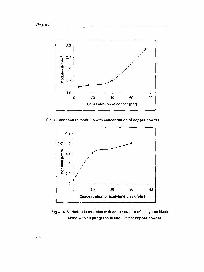
Chapter 3

2,3

806040

-r---'~~ --,-------,-----.".. --1

20

IIi1.7 1i

~E 2.1 ,E i~III 1.9~

~

1Jo~

1,5j-~o

Concentration of copper (phr)

Fig.3.9 Variation in modulus with concentration of copper powder

4.5

"rf" 4

EE 3.5~III:::J:;'Co~ 2.5

2------- --~-- -

o 10

----r------' ._-..--_.

20 30 40

Concenb'ation of acetylene black (phr)

Fig.3.10 Variation in modulus with concentration of acetylene black

along with 10 phr graphite and 25 phr copper powder

66

Conductive silicone rubber

30

E 25

~ 20

~ 15s::::

e 101ll...III 5~ o

o 20

-.'-'. -'--r" -- .------.

40 60 80

Concentration of carbon black (phr)

i_AcetYlene black --- Lamp black -.-N-234 black iL. .__ . 'o _

Fig.3.11 Variation in tear strength with concentration of

different carbon blacks

18

14 I

o 20 40 60 80

Concentration of copper (phr)

Fig.3.12 Variation in tear strength with concentration of copper powder

67

Chapter 3

25

10 20 30 40

Concentration of acetylene black(phr)

Fig.3.l3 Variation in tear strength with concentration of acetylene

black along with 10 phr graphite and 25 phr copper powder

~--_.---y------_.. ._-------,--- _._-,,---_._-

~ 500- j

~

~AOO -j'e~ 300iIII I5 2001;:l

~ 100 ~

~ 0 jo 20 40 60 80

Concentration of carbon black (phr)

- Acetylene black _lamp black -.-N-234 black I-- .-._.. --

Fig.3.14 Variation in elongation at break with concentration of

different carbon blacks

68

Conductive silicone rubber

305

~285.¥fa

1i 265..faC

~ 245fat:n :c: i

.E 225 ;_.W

o-,

20 40 60 80

Concentration ofcopper (phr)

Fig.3.tS Variation in elongation at break with concentration of

copper powder

300

~e:..250.¥~

~.a 200­IV

C

~ 150,fa !t:n IC !,g 100 .w

o 10 20 30 40

Concentration ofacetylene black (phr)

Fig.3.16 Variation in elongation at break with concentration of acetylene

black along with 10 phr graphite and 2S phr copper powder

69

Chapter 3

801

<60.1~ ,

~401~a=;;-~­

i 2°1~ 0 -1------ --,.----- ------.--,------,-------------'

:c o 20 40 60 80

Concentration ofcarbon black (phr)

~~ne black -.- Lamp black -'-N~2~~J

Fig.3.17 Variation in hardness with concentration of

different carbon blacks

~5150 -I

~ i~45 .:

~401~ ;CIJ I-E 35 -;

~301o

- -------, -'-r--·-'-----

20 40

------'1 --.

60 80

Concentration ofcopper (phr)

Fig.3.18 Variation in hardness with concentration of copper powder

70

Conductive silicone rubber

-,------- ------,----- ---,-----_.

70 l

«'60eo~ 50-la~ 40­"Ecv:J: 30 +---

o 10 20 30

··---1

40

Concentration ofacetylene black (phr)

Fig.3.19 Variation in Hardness with concentration of acetylene

black along with 10 phr graphite and 25 phr copper powder

Figure 3.20 shows the variation in resistivity of silicone rubber vulcanizates

with the concentration of different blacks at room temperature. At low loadings of

carbon black, the conductivity of the compounds was very low. This was because

the carbon black particles were isolated from each other, and there was no

conducting path. As the loading of carbon blacks was increased, the conductivity

increased rapidly up to a particular concentration, thereafter, the increase in

conductivity was not so rapid. This is because, when the amount of carbon black

was increased, cluster or aggregates of carbon blacks were formed and a

conducting path was formed. Thus, the internal contact resistance between the

aggregates decreased as the loading level increased. Once a high enough loading

was reached so that contact resistance between the aggregates was no longer

significant and there was no significant increase in conductivity with a further

increase in Im'lrlin!J.

71

CJrapt('r3

16

E 14

~ 12EJ: 100::; 8."~ 6-.~• ,0~

'"2

00

II AB

£:} ISAF

Ii LB

5 10 20 )0 ' 0 50 60

c o nc e ntratio n of carbon black(phr)

Flg.3.20 Variat ion In resisttvlty of silicone rubber compounds

with the concentration of different blacks

A comparative electrical conductivity study of the vulcanizates revealed

that the conductivity of the vulcanizates filled with acetylene black was higher than

that with ISAF black, which had conductivity higher than that of vulcanizates

containing lamp black. This behaviour can be explained by considering the very

high structure of acetylene black. When acetylene black was added to silicone

rubber aggregates of acetylene black comes in contact with each other and a

conducting path was easily formed in a concentration range of 10-15 phr by weight.

Because the structure of ISAF black was not as high as acetylene black, the

compounds filled with ISAF black has lower conductivity, compared with acetylene

black. Because lamp black has a still lower structure, the conductivity was low

even when a higher amount of lampblack was added.

Figures 3. 21 and 3.22 show the temperature dependence Of resistivity fer

the vulcanlzates containing 30 and 40 phr acetylene black, respectively. As the

72

Conductive silicone rubber

temperature was increased, the conductivity decreased. This behaviour may be

due to two factors:

1. The thermal expansion of sllicone rubber was higher than that of

acetylene black and so the gap width between the aggregates was

increased resulting in a decrease in conductivity; and

2. When temperature was increased, some of the aggregates of carbon

black break down and so the gap width between the aggregates was

increased and so conductivity was decreased.

On cooling, the conductivity was increased. This may be either due to the

contraction of silicone rubber so that the gap width decreases or due to the

reagglomeration of the particles resulting in gap width decrease and therefore

conductivity was increased.2,10,13

The nature of the hysteresis loop in the p = ~T) curve during the heating­

cooling cycle is shown in figure 3.21 and 3.22. It is reported that the hysteresis loop

results from the thermal mismatch between filler and polymer.11,13 The uneven

70

E 60<oE 50s:o~ 40os:~ 30 -III

~ 20

10 --_._.

25 50 75 100 125

Temperature(°C)

150

.. I1-- firstheating cycle -<>- firstcooling cycle '

L~ second heati~~ cycle -tr- ~~co~d_~ooli~~ycle

Fig.3.21 Resistivity variation with temperature for silicone rubber

vulcanizate containing 30 phr acetylene black

73

Chapter B

IS

-H~ 13

~ 12o

;;:; 11

'5 10t;'01 9

'"Cl:

2S SO 75 100

TemoeraturefD

Cl

125 150

---+- first he ating cycle --6- first co 0 ling cycle

---'second heating cycle -- second cooling cycle

Fig.3.22 Resistivity variation with temperature for silicone rubber

vulcanizate containing 40 phr acetylene black

thermal expansion of rubber and acetylene black may be one of the reasons for the

creation of a hysteresis loop. Also, during cooling, the size of the aggregates of

acetylene black may be greater than that at the heating time. This may be one of

the reasons for the higher conductivity on cooling than on heating; thus the

hysteresis loop resulted. Also, it has been reported 9 that the resistivity of the

compound was decreased after heat ageing at 150-2500C and the decrease in

resistivity during ageing was explained, due to the increase in the concentration of

the carbon black in the system, as a result of a loss of mass (3.8% after 55000 hrs

at 150° C). Here also, after heating cycle, ageing of silicone rubber took place, and

the conductivity on cooling was higher than on heating; thus, the hysteresis loop

was formed.

The resistivity values shown in the grapi-I dudng ti-Ie cooling cycle is only up

to 50°C, because the cooling rate was very low below 50°C. If we extrapolate the

curve w room temperature, the cooling cycle endpoint will be the same as that start

74

Conductive silicone rubber

point of the second heating cycle. The heating-cooling cycle was repeated for

checking the reproducibility of the variation in conductivity with temperature. The

nature of the curve was the same, but the area of the hysteresis loop decreased

during the second cycle. This was because, some permanent change due to

ageing took place for the rubber and a steady state was reached after one cycle.

Figures 3.23 and 3.24 show the temperature dependence of resistivity for

vulcanizates containing 40 and 50 phr lamp black, respectively. On heating, the

conductivity decreased, due to the thermal expansion of the silicone rubber. This

may also be due to the disintegration of lamp black aggregates. On cooling, the

conductivity was increased due to the contraction of silicone rubber and may also

be due to the reagglomeration of lamp black particles. The overlap of the cooling

cycle curves in Figure 3.23 may be due to the same size of the aggregates of lamp

black during the cooling process.

C"l13c:>..

~ 16

E 11o

E 12

c100

»,8+'

~.-+'...-....a::

0

25 50 15 100 125 150

T • m p s r I tu r. [" C)

_ Tlu 1 I tat 119 eve It --<:>--11111 CoOll19 cyclt

_JtCOIQ Ha1hg e v c ie -D-ttCOIQ c o o In q c v c ie

Fig. 3.23 Resistivity variation with temperature for silicone rubber

vulcanizate containing 4~ phr of Lamp ~~~~k

75

ChapterS

30N 70=....

:le 60-e- 50'"E 40.c0

~30

=- 20i'. 10Q)

Cl: 0

25 50 75 100 125 150

Te mperature('"'C}

---.-1irst heating cycle -<r-1irst cooling cycle

-.- se co nd he atin 9 cycle ----;r-- se cond co oling cycle

Fig.3.24 Resistivity variation with temperature for silicone rubber

vulcanizate containing 50 phr Lamp black

When the concentration of lampblack was increased to 50 phr, overlapping of the

cooling curves takes place at a temperature lower than 80° e. This may be

because the size of the aggregates remained unchanged only at a low

temperature,

Figures 3.25 and 3.26 show the temperature dependence of resistivity for

the vulcanizates containing 30 and 40 phr ISAF carbon black, respectively. The

resistivity was increased on heating up to 800e. It has been repeatedly observed in

several samples that there was an increase in resistivity up to 800e and then a

decrease in its value. A similar observation has been reported earlier by Abo­

Hashem and colleagues10 in butyl rubber mixed with SRF carbon black. They have

observed a decrease in conductivity below 600e for the composites containing 40

and 70 pnr SRF; above 60°C. thermally activated behaviour showing an increase in

conductivity during the heating cycle was noted.

76

Conductive silicone rubber

M~ 2

~ 1.8

5 1.6

E 1.4 -I.z::..,g. 12~ '1~.~ 0.8Q,l~ 0.6

25 50 75 100 125

Temperaturel C)

150

i -- first heating cycle ~ first cooling cycle

--..- s~<:?~J1eGltil1g c)'(;le -.!r- ~~l:0nd co~l!llg cycle

Fig.3.25 Resistivity variation with temperature for silicone rubber

vulcanizate containing 30 phr ISAF black

15050 75 1CD 125Tarpe'3:Lre ( () C)

N

~ 7xE 6u

{ :.~ '3oil:~ 2 +--T---=--,----...-----_r---------.

25

--+-fir9Jemrg Qlde ---0- fir.tmoirg eyde

-a- seord remrg Cyde --tt- seemcodirg eyde

Fig.3.26 Resistivity variation with temperature for silicone rubber

vulcanizate containing 40 phr ISAF black

77

Chapter 3

The changes in resistivity during the heating cycle for the compounds containing

ISAF black may also be similar to this due to the breakage of the clusters of ISAF

black below BOoe and reformation above so'c. On cooling, only the reformation of

ISAF black aggregates takes place and there was no increase in the resistivity

versus temperature cooling curve, thus showing that the resistivity was decreased

on cooling.

The addition of copper powder and graphite powder into silicone rubber

has only very little effect on resistivity as shown in Figure 3.27.The density of

copper powder was high compared to that of carbon blacks. So large amount of

copper powder was necessary to lower the resistivity of silicone rubber. Also,

during vulcanization of silicone rubber, at high temperature, partial oxidation of

copper takes place and this also tends to increase the resistivity.

6

5o

13

E 12

~ 11E"5 10~'s 9

~ 8~ (C)o

20 40 60 80

Concentration of copper(phr)

Fig.3. 27 Variation in resistivity of silicone rubber vulcanizates

with the amount of copper powder

78

Conductive silicone rubber

The effect of addition of copper powder, graphite, and acetylene black on

the conductivity of silicone rubber was also studied. The combined effect of these

fillers was very low. This was because; carbon black is capable of forming a

secondary structure in the form of particle aggregates. which leads to the formation

of conducting three-dimensional channels. Even though the conductivity of graphite

is more than that of carbon blacks, graphite does not possess this capacity.

Composites containing carbon black as the filler are therefore characterized by

higher conductivity than composites with an equivalent graphite content. Particles

of carbon black with lower electrical conductivity form a secondary structure in the

form of bridges between the more conductive graphite particles, thereby including

the latter in the overall conducting system" in a compound containing both carbon

black and graphite. As the amount of acetylene black was increased, resistivity

decreased as shown in the figure 3.28.

12

ECJ 10E.t: 80~;t: 6>..III

4.U)(I)...en 20

0

0 10 20 30 40

Concentration of acetylene black{phr)

Fig.3. 28 Variation in resistivity of silicone rubber compounds

containing 25 phr copper powder and 10 phr of

graphite with the concentration of acetylene black

79

Chapter 3

The temperature dependence of resistivity of these vulcanizates was also

noted. Figures 3.29 and 3.30 show the temperature dependence of resistivity for

vulcanizates containing 20 and 30 phr of acetylene black. along with 25 phr of

copper powder and 10 phr of graphite powder. The nature of the curve was similar

to that of composites containing acetylene black alone. The conductivity of the

vulcanizates was decreased with increase of temperature on heating and the

conductivity was increased with decreasing temperature on cooling.

Figure 3.31 shows the variation in the resistivity of silicone rubber

vulcanizates containing copper powder and 15 phr acetylene black with

temperature. The nature of the curve is similar to that of composites containing

acetylene black alone. On heating, the resistivity was increased, due to the thermal

expansion of the silicone rubber. This may also be due to the disintegration of

acetylene black aggregates. On cooling, the resistivity was decreased due to the

contraction of silicone rubber and may also be due to the reagglomeration of

acetylene black particles. The addition of copper powder has very little effect on

the resistivity of the vulcanizates. This may be due to the oxidation of the copper

during vulcanization.

2.0C'l...- 2 2..

"E' 1.8~.c0 1 <I~...'ii'lII54>~ (I I

25 50 7'5 100 125 150

T e m perature (a C)

1----- he a:ting -0- co oling t

Fig.3.29 Resistivity variation with temperature for silicone rubber

vulcanizate containing 20 phr of acetylene black, 25 phr of copper

powder and 10 phr of graphitG powder.

80

Conductive silicone mbber

50

'E" 45c.:oE: 40

'6 35

i 30:>

'i3 25'IJ 20a::

15

25 50 75 100 125 150

Temperature (u c )

• first heating cycle -<:>--first cooling cycle

_second heating cycle -o--second cooling cycle

Fig.3.30 Resistivity variation with temperature for silicone rubber

vulcanizate containing 30 phr of acetylene black, 25 phr of copper

powder and 10 phr of graphite powder.

1501251007550

3

><E 2.5uE 2J:.o~ 1.5 tt~~~~"""''''''''''''-~>:;;.!!!III

~ 0.525

'"o...

Temperaturet" C)

..--_.- ... _-------._-----_.-.

~ Cu-40,AB-15 heating -<r- Cu-40, AB-15 cooling',

L- CU-~~~~~.15he_a~~.~_~Cu-~~~~~:}_~~~olingi

Fig.3.31 Resistivity variation with temperature for silicone rubber

vulcanizate containing 15 phr of acetylene black, and 25 phr of

copper powder and 40 phr of copper powder.

81

Chapter 3

3.4 PART-II

Effect Of Addition Of Different Carbon Blacks In Silicone Rubber

In this section, the effect of addition of different carbon blacks like ISAF

N- 220 black. HAF N-339 black, and HAF N-347 black on the electrical conductivity

and mechanical properties of silicone rubber is reported. The influence of

temperature on the conductivity of silicone rubber vulcanizates containing different

types of carbon black was also studied.

3.4.1 Sample preparation

The compounds as per the formulation given in Table 3.2 were mixed in a

Brabender Plasticorder PL3S with a rotor speed of 50 rpm at room temperature for

6 min.

Table 3.2 (a) Formulation of compounds

Mix H1 H2 H3 H4 11 12 13 14

Silicone rubber 100 100 100 100 100 100 100 100

Dicumylperoxide 2.5 2.5 2.5 2.5 2.5 2.5 2.5 2.5

N-220 black 10 20 30 40 - - - -N-339 black - - - - 10 20 30 40

Table 3.2 (b) Formulation of compounds

Mix J 1 J2 J3 J 4

Silicone rubber 100 100 100 100

Dicumylperoxide 2.5 2.5 2.5 2.5

N-347 black 10 20 30 40

82

C01ldwtive silicone rubber

3.4.2 Results and discussion

For these compounds, the cure time was increased gradually as the

concentration of carbon blacks was increased as shown in figure 3.32. This may

be due to the retarding effect of carbon blacks in silicone rubber. Figure 3. 33 show

the variation in resistivity of silicone rubber vulcanizates with the concentration of

carbon blacks like N- 220 black, N-339 black. and N-347 black at room

temperature.

_ 2

.6..sQ.I 1.6E

:Df 1.2::s .u

10

0.8 T-~­

o··-1-

20 30 40 50

Concentration of carbonblack(phr)

;~N-220 ""-'-N-339 -;-N-347 ii . __._ _J

Fig.3.32 Variation in cure time with concentration of carbon black

At low loadings of carbon black, the conductivity of the compounds

was very low. This was because the carbon black particles were isolated from each

other, and there was no conducting path. As the loading of carbon blacks was

increased, the conductivity increased rapidly up to a particular concentration

region; thereafter, the increase in conductivity was not so rapid. This was because,

when the amount of carbon black was increased. cluster er aggregates of carbon

blacks were formed and a conducting path was formed. Thus, the internal contact

83

Clltl pttr J

resistance between the aggregates decreased as the loading level increased.

Once a high enough loading was reached so that contact resistance between the

aggregates was no longer significant and there was not any significant increase in

Conductivity with a further increase in loading.

A comparative electrical conductivity Sludy of the compounds revealed

lha l the condue tivily 01 the vulcanizates filled with N·220 black was higher than that

with N-347 black, and N·339 black. This behaviour can be expla ined by

considering the smaller particle size of N·220 black compared 10the particle size of

N·347 black and N·339 black. The conduct ivily was deereased with increasing

10 20 30 40

Concentrationolcarbonblack(phr )laN·339 ,!-N'3~7_cN·2~

Fig . 3.33 Variation in resistivity of silicone rubber vulcanizates

with amount of carbon black

particle size of the carbon black. It has been argued 3 on purely geometric grOl,nds

that smaller particle size should lead to smaller gap width. 11 has also been arglled2

that smaller particle size leads to more conducting paths per unit volume. 11 has

also been suggested thaf the smaller particles arrange themselves more easily

into chains than do the coarser types . The part icle sue of N·347 carbon black and

84

Conductive silicone rubber

N-339 carbon black is almost the same and hence their conductivity values were

almost the same in silicone rubber vulcanizates. The conductivity of the

vulcanizates increased rapidly with the addition of carbon blacks initially up to

about 20 phr of carbon blacks and thereafter the increase in conductivity with the

addition of carbon blacks was very slow. It was because; a through going

conducting path was already formed. Once a high enough loading was reached so

that contact resistance between the aggregates was no longer significant and there

was not any significant increase in conductivity with a further increase in loadin{l.

Properties of the mixes loaded with different types of carbon blacks, likl3 N­

220, N-339 and N-347 are given in Table 3.3

Table 3.3 Properties of the vulcanizates

Modulus Modulus

Tensile at 100% at 200% Hardness Tear Elongation

Mix strength Elongation Elongation (Shore A) strength at break

No. (Nmm'2) (Nmm'2) (Nrnrn") (Nmm· 1) (%)

HI 9.66 2.10 4.17 35 12.6 391.31

H2 4.38 1.73 3.22 40 17.59 305.32

H3 0.9 - - 50 11.77 36.36

H4 - . - 57 - -11 7.92 2.42 5.71 45 20.35 308.98

12 6.95 2.35 4.05 50 18.62 259.22

13 3.82 2.27 - 55 13.97 183.55-

14 - - - 59 - -.-

J1 7.3 2.02 3.99 30 7.67 319.78

J2 5.43 1.69 3.03 40 15.23 297.52

J3 2.5 0.86 - 49 13.72 164.61

J4 - - - 53 - -

85

Chapter s

The tensile strength and modulus of the vutcanizates was decreased with

an increase in the concentration of carbon blacks. The decrease in tensile strength

was due to the decreasing volume fraction of silicone rubber in the vulcanizates. As

the concentration of carbon black was increased, there were not enough rubber

matrixes to hold the particles of the carbon black together. The hardness of the

vulcanizates was increased with an increase in the concentration of carbon black.

Tear strength and elongation at break of the vulcanizates were increased

initially up to a concentration of 20 phr of carbon black and then decreased with an

increase in carbon black loading. It was because, small amounts of carbon black

acts as a reinforcing filler and when the amount of carbon black was increased

above 20 phr, there was not enough rubber matrix to hold the particles together

and the tear strength was decreased.

Figures 3.34 - 3.36 show the variation in the resistivity of silicone rubber

vulcanizates with temperature (25- 150°C), filled with 40 phr of N-220, N-347 and

N-339 carbon black respectively..

5 ,I

~ 4.5 ~)( ,

5 4'E-g 3.5

~'s 3i'Illell 2.5~

2. .---- .~--..

25 50 75 100

Temperature(DC)

125 150

I

J

Fig. 3.34 Variation in resistivity with temperature. of silicone rubber

vulcanizates with 40 phr of N-22C carbon black

86

Conductive silicone mbber

As the temperature was increased, the resistivity was increased. This

behaviour may be due to the thermal expansion of silicone rubber and also, some

of the aggregates of carbon black break down, so that the gap width between the

carbon black aggregates was increased resulting in an increase in resistivity, On

cooling, reagglomeration of the particles takes place. the gap width was decreased,

and the resistivity was decreased. During cooling. the size of the aggregates of

acetylene black may be greater than that at the heating time. This may be one of

the reasons for the lower resistivity on cooling than on heating; thus the hysteresis

loop was resulted.

75 100 125 150

Ternperaturet" C)

~heating -o-cooling

Fig. 3.35 Variation in the resistivity of silicone rubber vulcanizates

with temperature. filled with 40 phr of N-347 carbon black

87

Chapter 3

r---'-

- '-1'----- -- - ·-·---T----~------f"-·-- ---------1

35N

o 30....~ 25E~ 20Es:~ 15~

~ 10';]1

&. 51o j

25 50 75 100 125 150

3.5

Temperaturet" C)

l---=- heating ---{)- cooling!

Fig. 3.36 Variation in the resistivity of silicone rubber vulcanizates

with temperature, filled with 40 phr of N-339 carbon black

PART-Ill

Conductive Silicone Rubber IHOPE Blends

3.5.1 Sample preparation

The compounds as per the formulation given in Table 3.4 were mixed in a

Brabender Plasticorder PL3S at a rotor speed of 50 rpm and temperature of 160°C.

HOPE was first added, and allowed to melt and homogenize for 2 minutes, the

silicone rubber was added and allowed to mix well with HOPE for 2 minutes. 30 phr

of acetylene black was added slowly. After adding the acetylene black completely,

the mixing was continued for 10 minutes more. Finally, DC? was added and the

compound was taken out from the Brabender. The compounds were kept for 24

hrs for maturation.

88

Conductive silicone rulJ/Jer

Table 3.4 Formulation of compounds

Mix K, K2 K3 K.; Ks Ks K7

SR 100 80 70 50 30 20 -HOPE - 20 30 50 70 80 100

AB 30 30 30 30 30 30 30

OCP 2.5 2.5 2.5 2.5 2.5 2.5 2.5

The compounds were compression moulded at 180oC, in an electrically

heated hydraulic press, into 1-mm-thick sheets. For this, the mould was preheated

to 180°C. a piece of preformed material was placed directly in the mould cavity,

and compressed under an hydraulic clamp pressure of 200 kg cm", After 10

minutes, the mould was allowed to cool to room temperature and then the mould

was opened and the samples were taken out.

3.5.2 Results and discussion

The variation in the resistivity of different silicone rubber/HOPE

blends containing 30 phr of acetylene black is shown in Fig.3.37. SRlHOPE blends

had more conductivity than pure silicone rubber vulcanizate at the same dosage of

acetylene black (30phr). This behaviour can be explained by the difference in the

dispersion of acetylene black in different phases 3S well as in the interphase.

Blends always have more conductivity compared to the individual polymer. This

was due to the selective localization of acetylene black in one phase or at the

interphase of the polymer matrix". 70/30 SRlHOPE blends had the lowest

resistivity among the different SRlHDPE blends. This can be explained by the

difference in the interaction of polymer and acetylene black. 70/30 SRlHOPE

blends may have the maximum phase separation, and therefore the acetylene

black aggregates may be formed in the interphase of silicone rubber and HOPE.

So conducting paths were easily formed and hence the conductivity was increased.

89

C1Iapttr 3

30

E 25uE 20~ .oS. 15 J

{ 1O ja:: 5 ..

I

o I,20180 30170 50150 70130 80120 100.()

SRJiDPEcomposition

Fig . 3.37 The variation In the co nducti vity of different SRlHOPE

blend s contain in g 30 phr of acetylene black

Starting from left to right, resistivity decreased with increase in the amount 01

silicone rubber until it reached a minimum, and then it was 'ound to be increasing,

probably at the point of reversal of continuous phase ' S.1' . Initially acetylene black

was dispersed in silicone rubber. When the amount 01HOPE increases, the prase

separation increases, and the AB gets dispersed at the interphase and hence

resistivity decreased. At 70130 SA/HOPE compositions, there was maximum phase

separation. Alter that, the continuous phase changes to HOPE. Then there was

redistribution 01AB and the resistivity was increased.

The variation in tensile strength and elongation at break of different

SA/HOPE blends are shown in the figures 3.38 and 3.39. Tensile strength of the

blends was decreased with increase in the amount 01 silicone rubber. This was

because. HOPE, which is a thermoplastic material can improve the strength 01 a

vulcanizate. Elongation at break of the blends was increased on increasing (he

amount of silicone rubber, due to its increase in elastic nature.

90

30f/0 50/SO 70{30

SR,.HDPE composition

25-,~ 20z:s 15~

c~ 10 '~ I~ 5!c::.

O '20,llO

..--~- :,80/20 I

Fig. 3.38 The variation in tensile strength of different SR/HOPE

blends conta ining 30 phr of acetylene black

2018

~ 16:;' 14~ 12~ 10

~ 8 11,g 6

f ~ ' . _ _ _

II

20,ll0 30110 50,';0 70/30 80/20

SR,liDPE composition

Fig . 3.39 The variation in elongation at break of different SRfHDPE

blends containing 30 phr of acety lene black

9 1

Cltapter3

3. 6 Conclusions

The following conclusions can be drawn from this investigation.

1. The resistivity of the vulcanizates that contain carbon blacks and other

conductive fillers like acetylene black, lamp black, ISAF black, N-220 black, N­

339 black, N-347 black, copper powder, graphite etc. was decreased as the

concentration of carbon blacks and other conductive fillers was increased.

2. The mechanical properties like tensile strength, tear strength and elongation at

break were decreased, while hardness' was' increased as the amount of

conductive fillers increased.

3. Resistivity of the silicone rubber vulcanizates was increased on heating but

decreased on cooling in the case of all conductive fillers except ISAF black (N­

247). For ISAF black, resistivity was first increased, reached a maximum at

so'c, and then decreased on heating.

4. The area of the hysteresis loop during the heating-cooling cycle depends on

the carbon black concentration.

5. The conductivity of silicone rubber vulcanizates containing acetylene black was

higher than that of other vulcanizates filled with other conductive fillers.

6. The conductivity of SRlHDPE blends was higher than that of pure silicone

rubber vulcanizates.

7. 70/30 SRlHDPE blends show the least resistivity among the different

SRlHDPE blends.

8. The tensile strength of the SA/HDPE blend was higher than that of pure

silicone rubber vulcanizates.

92

3.7 References

1. Maurice Morton (Ed.), Rubber Technology, 3'd ed., Chapman and Hall, Ch.13.

375, (1995).

2. A. I. Medalia, Rubber Chem. Technol., 59, 432 (1986)

3. M. H. Polleyand B. B. Boonstra, Rubber Chem. Technol., 30, 170 (1957).

4. C. M. Blow and C. Hepburn, Rubber Technology and Manufacture, 2nd ed.,

Butterworths, New York, 202, (1982).

5. A. K. Sircar and T. G. Lamond, Rubber Chem. Technol., 51, 126 (1978).

6. D. N. Aneli, D. I. Gventsadze, and L. G. Shamanauri, Int. Polym. Sci. Technol.,

20, T/78 (1993).

7. L. K. H. Van Beek and B. I. C. F. Van Pul, Rubber Chem. Technol., 37, 348

(1964).

8. V. P. Malhotra, R. Chandra, R. K. Garg, and S. Motsara, Ind. J. Chem., 33A,

595 (1994).

9. I. Ya. Poddubnyi, S. V. Aver'yanov, L. A. Aver'yanova, and M. P. Grinblat, Int.

Polym. Sci. Technol., 8, T/74 (1981).

10. A. Abo-hashem, H.M. Saad, and A. H. Ashor, Plast. Rubber Compos.

Process. App1., 21,125 (1994).

11. P. B.Jana, Plast. Rubber Compos. Process. Appl., 20, 107(1993).

12. S. Miyat'chi, lnt. Polym. Sci. Tehcnol., 12, T/49 (1985).

13. S. K. Bhattacharya and A. C. D. Chaklader, Polym. Plast. Technol. Eng., 19,

21 (1982).

14. M. K. EI-Mansy and H. H. Hassan, Int. Polym. Sci. Technol., 15, T/7, (1988).

15. A. K. Sircar , Rubber Chem. Technol., 54,820, (1981) .

16. B. G. Soares, F. Gubbels , and R. Jerome , Rubber Chem. Technol., 70,60,

(1988)

93

Deuelopntent of cututuctiuc nitrile rubber

Chapter 4

DEVELOPMENT OF CONDUCTIVE NITRILE RUBBER

4.1 Introduction

Nitrile rubber, a copolymer of butadiene and acrylonitrile has good

resistance to a wide variety of oils and solvents and hence is widely used in

products like oil seals, pipe protectors and blowout preventors etc. The acrylonitrile

(ACN) content varies usually from 20-50% by weight and accordingly NBR is

usually classified into three types, viz., tow acrylonitrile content NBR with less than

25%, medium with 25·35 % and high acrylonitrile content NBR with 35-50 %. NBR

gives low gum strength, as there is no crystallinity in the polymer. The service

temperature in presence of oxygen is estimated to be 130°C.

Major properties of the elastomer depend on the acrylonitrile content. As

the acrylonitrile content increases, the oil resistance increases. Other properties

affected by monomer ratio are processability, cure rate, heat resistance, and

resistance to permanent set. With increased acrylonitrile content, processabiliry is

easier, cure rate is faster and heat resistance is better'. But, resistance to

'15

Chapter 4

permanent set and die swell is decreased, and viscosity is increased as the

acrylonitrile content increases.

The most common way to classify nitrile rubbers is by their bound

acrylonitrile content, and by their viscosity. The bound acrylonitrile content as

described above goes from about 20 - 50 % with the bulk as 25 - 40 % range.

Mooney viscosity ordinarily ranges from 30 - 80.

Basically nitrile rubbers are compounded much like natural rubber. Since it

does not crystallise, reinforcing fillers are necessary to obtain reasonable tensile,

tear and abrasion properties. In black compounds, reinforcement is proportional to

the amount and fineness of the black. Non-black fillers give best heat resistance

and also can be used with compound used for food contact applications.

Fine precipitated silica is the most reinforcing among the non-black fillers.

Plasticizers are used in almost all nitrile compounds first to aid processing and then

to improve low temperature flexibility, resilience, and flexing, or to reduce

hardness. Plasticizer level will ordinarily vary from 5 - 50 phr.

Nitrile rubber requires age resistors in addition to those they already have

in order to give long service, Where staining is not a problem, amine type

antioxidants may be used. If staining is objectionable, then phosphates or hindered

phenol antioxidants will serve better.

Vulcanization of nitrile rubber is usually accomplished with sulphur.

accelerator, and ZnO in combination with fatty acid as activator. In special cases,

peroxide may also be used. NBR cures relatively fast, the higher acrylonitrile

content, faster the cure rate. The amount of sulphur used is based on butadiene

content and is generally lower than that used for natural rubber and ranges from

0.7-2.3 phr. The solubility of sulphur is considerably less and affect it's uniform

dispersion, for this reason, sulphur Is added early in the mix.

Development of conductive nitrile mbbef

Because of the relatively fast rate of cure, NBR is usually compounded

with one accelerator, often of the sulphenamide class. Accelerator of the thiazole

type like tatramethylthiuram monosulfide (TMTM) or tetramethylthiuram disulfide

(TMTD) might be used when a faster curing is needed.

Electrically conductive polymer composites are widely used in various

branches of engineering in many rubber and plastic products. Some of these

applications include plastic batteries, sensors, electro chromic displays, EMI

shielding, fuel cells, circuit boards etc2• The basic and generally accepted concepts

of conductivity are based on the fact that carbon black forms aggregates or

network structures in the cornposlnons'". The degree of conductivity depends on

the nature of these chain structures. In recent years papers relating to the effect of

various factors influencing the conductivity of polymer compositions containing

carbon black have been published- like type of carbon black 3.4, concentration of

carbon black4.5

, type of polymer", temperature'" and degree of dispersion of

carbon black in the polymer matrix'". It is shown that starting at a certain level, an

increase in the amount of carbon black in a composition leads to a marked

increase in conductivity and this then tends asymptotically to a finite value.

The amount of electrically conductive fillers required to impart high

conductivity to an tnsutatlnq polymer can be dramatically decreased by the

selective localization of the filler in one of the phase or at the interphase of a

polymer blend 6,9. Not only the final cost of the material is decreased, but the

problems associated with the excess of filler on the processing and mechanical

properties of the final composites are alleviated. The localization 01 carbon black in

an immiscible polymer blend is basically controlled by the mutual polymer-polymer

and polymer -filler interaction 10,11.

This chapter is divided into four parts; Part I deals with the effect of

concentration of acetylene black on the electrical conductivity and mechanical

properties of nitrile rubber vulcanizates. Part II deals with the effect of blending of

97

Chapter 4

NBR with other polymers on the electrical conductivity and mechanical properties

of the vulcanizates at the same dosage of acetylene black. Nitrile rubber blends

with NR, EPDM and PVC was prepared and the electrical conductivity and

mechanical properties are reported. Part III deals with the variation in conductivity

and mechanical properties of the vulcanizates with different composition of

NBR/NR blends at the same dosage of acetylene black. Part -IV deals with the

effect of temperature on the electrical conductivity of these vulcanizates.

4.2 Experimental

4.2.1 Materials Used

Nitrile rubber (NBR), Natural rubber (NR), Polyvinylchloride (PVC),

Ethylene -propylene-diene rubber (EPDM), Acetylene black (AB), Zinc oxide

(ZnO), Magnesium' oxid~ (MgO), Stearic acid (SA), Oibenzthiazyldisulphide

(MBTS), Sulphur. Tetramethylthiuramdisulphide (TMTO), and Oioctylphthalate

(OOP) conforming to the specifications given in Chapter 2 were used in the

present investigation.

4.3 Part-I Studies On Conductive Nitrile Rubber

4.3.1 Sample Preparation

The compounds were prepared as per the formulation given in Table- 4.1

on a two-roll mill of size (15 x 33 cm). The compounds were kept for 24 hrs. for

maturation.

The optimum cure time (time for attaining 90% of the maximum torque) of

each sample was determined at 150°C using Goettfert Elastograph Model 67.85

98

Development of conductive nitrile rlIbbe,.

The compounds were compression molded at 150uC in an electrically

heated hydraulic press, into 2mm thick sheets. For this, the mould was pre-heated

to 150 QC; a piece of preformed material was placed directly in the mould cavity,

and compressed under a hydraulic pressure of 200 Kgcm-2• Upon completion of the

required cure cycle, the pressure was released and the sheet was stripped off from

the mould and suddenly cooled by plunging into cold water. After a few seconds,

the samples were taken from water. Dumb-bell shaped specimens were punched

out of these compression-moulded sheets along the mill grain direction. The tensile

properties were measured on a Zwick UTM model 1445 according to ASTM D 412

at a crosshead speed of 500 mm/min. The values presented are the average of

three samples.

Table 4.1 Formulation of compounds

Mix A1 A2 As ~ As Ae A7 Aa Ag A IO All

NBR 100 100 100' 100 100 100 100 100 100 100 100-,

AB 0 10 20 30 40 50 60 70 80 90 100

2nO 4 4 4 4 4 4 4 4 4 4 4

SA 2 2 2 2 2 2 2 2 2 2 2,--f----,-- -_.,_...•. --- _.._.- _.._--,. 1--'--f----" " ..'- _.. ,.~.- f------

S 1.5 1.5 1.5 1.5 1.5 1.5 1.5 1.5 1.5 1.5 1.5,

MBTS 1 1 1 1 1 1 1 1 1 1 1

TMTD 0.5 0.5 0.5 0.5 0.5 0.5 0.5 0.5 0.5 0.5 0.5-

DOP - 1 2 3 4 5 6 7 8 9 10,,___ '-.~L,_ -- --- ._.' -------"

The Hardness (Shore-A) of each sample was noted according to ASTM D

2240. Resistivity of each sample was determined using two- probe method. Data

presented are the average of three samples. The samples with typical dimensions

of 3xl x2 cm were prepared for direct current electrical conductivity measurements.

The sample was inserted between two electrodes. The contact resistance between

~~:;) sample and the electrode was minimized using silver paint. A potential of 6 V

99

Chapter 4

was applied and the resulting current through the circuit was noted. Measurements

were carried at a rotary vacuum of 10.2 torr. The current was measured using a

digital multimeter (APLAB model 1087). Resistance of the samples were calculated

using the equation, R= VII. where, 'V' is the applied voltage and 'I' is the resulting

current. The resistivity in each sample was calculated using the equation, p =R Alt,

where 'A' is the area of the sample, and 'I' is the thickness of the sample.

Conductivity is the reciprocal of resistivity.

4.3.2 Results and discussion

Figures 4.1- 4.5 shows the physical properties of the vulcanlzates, It was

found that cure time of the compounds was decreased as the amount of acetylene

black increased as shown in Figure 4.1 because of the accelerating effect of

acetylene black on vulcanization, up to about 60 phr of acetylene black. Above 60

phr, the change in cure time with the concentration of acetylene black was

negligible and it remained almost constant.

14

lil 12Ql

:; 10.S.s 8Ql 6E;: 4E

, 8 2

oo 50 100 150

Concentration of acetylene black (phr)

Flg.4.1 Variation in cure time of the compounds of NBR

Containing different amounts of acetylene black

100

Deuelopment ofconductive nitrile rubber

Hardness (Shore-A) of the compounds increased with an increase in

the concentration of acetylene black. Bul above 60 phr of acetylene black, the

change in hardness with increase in the amount of acetylene black was negligible.

This was because, a saturation point was reached at a concentration of 60 phr of

acetylene black as shown in Figure 4.2. Figure 4.3 shows the variation in

elongation at break of the vulcanizates containing different amounts of acetylene

black. Elongation at break decreased with an increase in the amount of acetylene

black as expected up to about 60 phr of acetylene black and thereafter it remained

almost as constant.

Tensile strength of the vulcanizates was increased as the

concentration of acetylene black increased as shown in the Figure 4.4. It was

because; acetylene black was acting as reinforcing filler in nitrile rubber.

100

90.-..cr-I! 800

.s::.l!!. 70IIIQ)e'E 60IQ:J:

50 '

40 '0 20 40 60 80

-

100

Concentration of acetylene black(phr)

Fig. 4.2 Variation in hardness of vulcanizates with the

amount of acetylene black

101

Chapter 4

700

_ 600 '~

~ 500e.a 400..III

:s 300..III

~ 200om

100

oo 20 40 60 BO 100

Concentration of acetylene black(phr)

Fig. 4.3 Variation in elongation at break of vulcanizates

with the amount of acetylene black

25

e:'E 20E~=15Clc

i 10.!!·ill

~ 5I-

oo 20 40 60 80 100 120

Concentration of acetylene black( phr)

Fig. 4.4 Variation in tensile strength of vulcanizates

with the amount of acetylene black

102

Vevel0I'/IIC11t of conductiue nitrile mbber

As the amount of acetylene black was increased, the modulus of the

vulcanizales increased as shown in the figure 4.5. As the amount of acetylene

black was increased, the conductivity of the composites was increasing. Figure 46

shows the variation in resistivity of pure nitrile rubber vulcanizates with the

concentration of acetylene black at room temperature. At low concentration of

acetylene black, the resistivity of the sample was very high. This was because. the

particles of acetylene black were isolated from each other and a conducting

through-going path was not formed. As the amount of acetylene black was

increased, the resistivity decreased rapidly up to 40 phr of acetylene black and

there after, the decrease in resistivity was very slow. It was due to the formation of

aggregates of acetylene black particles to form a conducting path through the

polymer chain. Once saturation was reached. contact resistance between the

clusters was no longer significant and so at higher loadings, the decrease in

resistivity was not rapid.

20-':'E 15E~ 10~

~

-g 5~

oo 20 40 60 80 100 120

Concentration of acetylene balck(phr)

;- 100% elongation~ 200% elongation

i -+-- 300% elongation

Fig. 4.5 Variation in modulus of vulcanizates with the

amount of acetylene black

!O)

Chapter A

12

I

o I

o- .--··---r - .

20 40 60 80 100

Concentration of acetylene black(phr)

4.4

4.4.1

Fig. 4.6 Variation in resistivityof vulcanizates with the

amount of acetylene black

PART 11

Studies On Conductivity of Blends of NBR

With NR, EPDM And PVC

Sample preparation

NBR/NR and NBRlEPDM blends were prepared by masticating the

individual rubbers separately and then mixing well on the two-roll mill and the other

ingredients were added according to the formulation given in the Table 4.2.

NBRlPVC blend was prepared on a Brabender Plasticorder PL3S at a rotor

::;peed of 40 rpm at 1500 C as per the formulation given in Table 4.3. PVC was

104

Development of conductive nitrile rubber

Table 4. 2 Formulation of compounds (phr)

Mix B, B2 B3

NBR 80 80 80

NR 20 - -

EPOM - 20 -PVC - - 20

AB 60 60 60

ZnO 4 4 4

SA 2 2 2

S 1.5 1.5 1.5

MBTS 1 1 1

TMTO 0.5 0.5 0.5

OOP .6 6 6

Table 4.3 Formulation of PVC Mix

Materials Amount (phr)

PVC 20

DOP 6

MgO 0.6

ZnO 0.6

SA 0.4

mixed with OOP and stabilizer I melted in the Plasticorder .then NBR was added

and mixing was continued for 5 more minutes. Other ingredients were added to this

NBR/PVC mix on a two-roll mill as per the formulation given in Table 4. 2.

105

Chapter 4

4.4.2 Results and discussion

The cure time and the mechanical properties of different blends of

NBR with NR, EPDM and PVC are given in Table 4.4. NBR/PVC blend was having

more hardness than NBRlNR and NBR/EPDM blends. It was due to the presence

of PVC in the vulcanizate, which is a thermoplastic material. At the same dosage of

acetylene black, the NBRlPVC vulcanizate had higher tensile strength and

modulus compared to NBRlNR and NBR/EPDM blend. The tensile strength and

modulus of the blend depends on the individual polymers and their compatibility.

Table 4.4 Properties of the Mixes

80120 Blend Cure Hardness Elongation Tensile Modulus at

Time at (Shore A) at Break Strength 100%

150°C (%)(N mm") elongation

(in min.) (N mm")

NBRlNR 4.16 83 189.58 15.69 9.97

NBR/EPDM 3.64 80 221.42 9.62 9.37

NBRlPVC 4.6 90 186.86 17.26 13.59

The variation in electrical resistivity on adding acetylene black to different

blends of nitrile rubber with PVC, NR and EPDM is shown in Figure 4.7. NBR/NR

blend had low resistivity than NBRlEPDM blend whose resistivity was lower than

NBR/PVC blend. This behavior can be explained by the difference in the

dispersion of acetylene black in different phases as well as in the interphase.

Blends always have more conductivity compared to the individual polymer. This

was due to the selective localization of acetylene black in one phase or at the

interphase of the polymer matrix".

106

l)r vd opllllmt "/ fill/ ell/C liVI' "ilrill' rnbbl.'r

700

600

100

o i -NBR,I<R-80/20 NB R~ POM~/20 NBRfl>VC-80/20

Fig . 4.7 Variation in resistivit y of vulcanlzates with the

amount of acetyl ene blac k

With some exceptions. compalibility 01 the componenls 01 a blend may

roughly be predicted by the solubility parameters of the components. The nearer

the values 01 solubility parameters. the better will be the comoanbiktv. Table 4.5

shows the solubility parameters ot ni e polymers used".

Table- 4.5 Solubility parameter of the polymors

Polymer

EPOM 16

NA 16.2- -- - ----1-----

PVC 19.8

20.5NBA'-- L _

107

Chapter A

NR and NBR differ widely in polarity. NBR is a polar rubber, while NR is a

nonpolar rubber. They have quite different solubility parameters as given in Table­

4.5 and this results in limited degree of mixing at the interphase of the blend. So

when their blends were prepared, the acetylene black got dispersed at the

interphase between the two rubbers. So the number of contact points was

increased and the gap width between the aggregates of acetylene black particles

were decreased. So a conducting path was easily formed and the conductivity was

increased. The conductivity of NBR/NR blend was more than that 01 pure NBR and

NR vulcanizates.

NBRlPVC blend is technically compatible at all ratios. Their solubility

parameters are very close to each other. NBR acts as a nonmigrating plasticizer

to PVC13• Presence of a plasticizer decreases the conductivity. It can be explained

by the well dispersion of acetylene black in NBRlPVC blend. There was no

localization of acetylene black aggregates, by which, the number of contact points

were decreased and the gap width was increased. Therefore the conductivity was

lower than pure NBR vulcanizates as well as NBR/NR and NBRlEPDM blends.

It is evident from Table- 4.5 that the NBRlEPDM blend, which has a large

difference in solubility parameter, should form an incompatible blend, and indeed it

does. EPDM is generally placed between unsaturated, high diene rubbers (NR,

SBR, BR, CR, NBR) and HR (weak interaction), with regard to its interaction with

black. Therefore, even though the NBR/EPDM blend is more incompatible than

NBRlNR blend, the conductivity of NBRlEPDM blend was lower than that of

NBR/NR blend. The exceptional behavior of NBR/EPDM blend is already

reported",

108

4.5

Development ofconductive nitrile nlbber

PART-Ill

Studies On Conductive NBRlNR Blends

4.5.1 Sample preparation

NBRlNR blends of varying composition were prepared as per the

formulation given in Table 4.6.80/20 NBRlNR blends containing different amounts

of acetylene black were prepared and the electrical conductivity and mechanical

properties of the vulcanizates were studied,

Table 4.6 Formulation of compounds

--021-'D~"

--Mix Cl C2 C3 C4 Cs 0, 04

.- -NBR 80 70 50 30 20 80 80 80 80

NR 20 30 50 70 80 20 20 20 20-'AB

.,60 60 60 60 60 60 70 80 90

-ZnO 4 4 4 4 4 4 4 4 4

If-- ..- -

SA 2 2 2 2 2 2 2 2 2f--

S 1.5 1.5 1.5 1.5 1.5 1.5 1.5 1.5 1.5

MBTS 1 1 1 1 1 1 1 1 1

TMTO a,s 0.5 0.5 0.5 0.5 0.5 0.5 0,5 0.5

OOp 6 6 6 6 6 6 7 8 9'------ _. l.... __ • ----.'--- ----

4.5.2 Results and discussion

Figure 4,8 represents the variation in cure time of NBRlNR blends of

varying composition. at the same dosage of acetylene black (60 phr). Cure time of

the compounas was decreased with increase in the amount of NR in the blend,

109

CIl" p t"r 4

5

4cg 3E2'"~ 1 '" Iu ,

O! 11 I80/20 70/30 50/50 30/70 20/80

NBR,fiR composition

Fig. 4.8 Variation in cure time of vulcanizates with Ihe composilion

of NBRlNR blends conlainlng 60 phr of acelylene black

4.2

4.1c.- 4.s~

E 3.9 ·''" I~ 18 !

3.7 I.

50 60 70 80 90 100

Concentration ofacetylene black (Ph,)

Fig. 4.9 Variation in cure lime of vulcanizales of 80120NBRlNR

blends wilh Ihe concentralion of acetylene black

110

Development ofconductive nitrile rubber

This was because, the dispersion of sulphur was easier when the amount of NR

was increased, and therefore fast curing takes place. Figure 4.9 shows the

variation in cure time of 80/20 NBRlNR blends with the concentration of acetylene

black. Cure time of the blends decreased with increase in the amount of acetylene

black due to the accelerating effect of acetylene black on vulcanization. Table 4.7

gives the hardness, tensile strength and elongation at break of various blends.

4.2 I

4.15 J""':- 4.1 i.~ 4.05 -- 4·~Cl)E 3.95 ,;: 3.9;Cl)

:i 3.85"o 3.8.

3.75 .:3.7 -­

50 60 70 80 90 100

Concentration of acetylene black (phr)

Fig.4.9 Variation in cure time of 80/20 NBRlNR blends with

the concentration of acetylene black.

Figure 4.10 represents the variation in resistivity of NBR/NR blends of

varying composition, at the same dosage of acetylene black (60 phr). The 80/20 ­

NBRlNR blends had the lowest resistivity compared to other blends. The graph

shows there was a decrease in resistivity, and it reached a minimum value near

80/20-blend. This can be explained by the fact that, when the amount of one phase

was small and the other phase was large, the acetylene black will be dispersed

nonuniformly in the continuous phase and so the number of contact points were

increased and the gap width was decreased. When both the polymer become

approximately equal, the acetylene black will be uniformly dispersed in both phases

111

Chapter 4

and the continuity of the conducting path will be decreased, which resulted in a

decrease in conductivity. Depending on the interaction of polymer with the

acetylene black, there may be redistribution of acetylene black from the component

with less interaction with the elastomer zone with more black-rubber interaction (at

the interface of two elastomers) 9,10. The distribution of acetylene black also

depends on the solubility parameter of the individual elastomers of the blends.

Table 4. 7 Properties of the Mixes

Mix No. Hardness Elongation at Tensile

(Shore A) Break(%) Strength

(N mm·2)

Cl 83 189.58 15.69

C2 90 182.81 14.66

C3 85 176.88 14.86

C4 90 154.3 13.8

Cs 80 221.3 17.46

0 1 83 189.58 15.69

O2 90 132.86 16.7

03 90 160.45 17.99

0 4 91 143.51 18.77

Figure 4.11 shows the variation in resistivity of 80/20-NBR/NR blends

with the concentration of acetylene black. Resistivity was decreased with increase

of acetylene black concentration. i.e., the electrical conductivity of the vulcanizates

increased with increase in the amount of acetylene black similar to NBR

vuicanizates.

112

250 I

o100,11 80/20 70[30 50/50 30{lO 20/80

NBR~R composition

Fig. 4.10 Variation in resistivity of vulcan izates with the composition

of NBRJNR blends containing 60 phr of acetylene black

20

18E~ 16!·f 14'R'.~ 12

1050 60 70 80 90 100

COllcenll'alionofacetylene black (ph r)

Fig . 4.11 Variation in reelsuvt tyc t 80/20 NBRtNR blends with the

concentration of acetylene black

113

Chapter A

4.6 PART-IV

Effect Of Temperature On The Electrical Conductivity Of

NBR And Its Blends With NR, EPDM And PVC

4.6.1 Results and Discussion

Figures 4.12- 4.19 represents the variation in resistivity of different

vulcanizates with temperature. When temperature was increased from 25°C to

150°C, the resistivity of all compounds increased at first, and then decreased.

Similarly, on cooling, the resistivity of all compounds at first decreased, and then at

low temperature, the resistivity further increased with temperature. For different

vulcanizates, the temperature at which the change in resistivity takes place was

different and it depends on the composition of the different vulcanizates. All

compounds which contain acetylene black has a chain of aggregates of acetylene

black as well as there are insulating interlayers of the polymer.

As the temperature was increased, the resistivity at first increased and at

higher temperature region, the resistivity of the vulcanizates slightly decreased.

This unexpected behaviour in NBR vulcanizates was attributed to the simultaneous

occurrence of two competing processes. First, there was an increase in resistivity,

due to the thermal expansion of nitrile rubber, which was higher than that of

acetylene black, resulting in an increase in the gap width between the aggregates;

and with increasing temperature, some of the aggregates of acetylene black breaks

down and so the gap width between the aggregates increased and so conductivity

was decreased. The second process comprises activation of conductivity at

relatively high temperatures, as in non-crystalline semi-conductors 12. The

114

Development of conductive nitrile rubber

occurrence of the observed anomalies depends on the nature and the degree of

filling of the carbon black used 14, on the mixing process, and on the extent of

thermo-oxidative ageing15.

On cooling, the resistivity of the vulcanizates at first decreased. This may

be either due to the contraction of nitrile rubber so that the gap width between

aggregates of acetylene black decreased or due to the reagglomeration of the

particles resulting in a decrease in gap width3,5,6. At low temperature, the resistivity

further increased or remained as constant. This was because, at low temperature,

the reagglomeration of the acetylene black particles may be complete in NBR and

also, the contraction of the rubber may not be changing the gap width between the

aggregates.

The nature of the hysteresis loop in the p = f(T) curve during the heating­

cooling cycle is shown in figures 4.12- 4.19 . It has reported that the hysteresis loop

results from the thermal mismatch between filler and polymer'':". The uneven

thermal expansion of nitrile rubber and acetylene black may be one of the reasons

for the creation of a hysteresis loop.

Figure 4.12 shows the variation in the resistivity of nitrile rubber vulcanizate

with 60 phr of acetylene black with temperature. When temperature was increased,

some of the aggregates of carbon black break down and the gap width between

the aggregates increased and so the resistivity was increased up to about 550eand thereafter the resistivity decreased with increase in temperature. The decrease

in resistivity may be due to the thermal activation ot charge carriers present in the

rubber matrix". A similar observation has been reported earlier by Abo-Hashem

and coneaques" in butyl rubber mixed with SRF carbon black. They have observed

a decrease in conductivity below 600e for the composites containing 40 and 70 phr

~D~: above 60°C, thermally activated behaviour show an increase in conductivity

during the heating cycle. It was reported that the structure of SRF black suffers

from slight breakage below eo-c and reformation above 60De, wherein the

115

Chapter A

increase in free volume holes becomes appreciable. Silicone rubber containing

ISAF black (N-234) also has been reported" to show an unexpected observation

like this. So the resistivity decrease may also be due to the reformation of

acetylene black aggregates in the heating cycle itself.

300

- 250E()

E 200s:..2-~ 150">i 100­"i15

~ 50 ~

0";·

25 50 75 100 125

._------,

150

Temperature(OC)

----<>- First heating _ First coolingI

;~ Second heating -.- Second coolin.!iJ-----_._-_._' •• - _ ..•. ,---_•. _._- ._----_.•. _ .•. ....>

Fig.4.12 Variation in resistivity with temperature for nitrile rubber

vulcanizate with 60 phr acetylene black

On cooling, reagglomeration of the particles took place, the gap width

between the aggregates of acetylene black decreased, and the conductivity

increased. During cooling, the size of the aggregates of acetylene black may be

greater than that at the heating time. This may be one of the reasons for the higher

conductivity on cooling than on heating; thus the hysteresis loop resulted. Also, it

has been reported 9 that the resistivity of silicone rubber compounds decreased

after heat ageing at 150-2500C. The decrease in resistivity during aaeing was

explained to be due to the increase in the concentration of the carbon black in the

system, as a result of a loss of mass (3.8% after 55000 hrs at 150° C). Here also

116

Development of conductiuc nitrile ntbbl'l'

after heating cycle, aging of nitrile rubber takes place, and the conductivity on

cooling was higher than on heating; thus, the hysteresis loop was formed.

The resistivity values shown in the graph during the cooling cycle was only

up to so-e. because the cooling rate was very low below so'c. If we extrapolate

the curve to room temperature. the cooling cycle endpoint will be the same as that

of the starting point of the second heating cycle. The heating-cooling cycle was

repeated for checking the reproducibility of the variation in conductivity with

temperature. The resistivity was decreased on heating and remained constant on

cooling during second cycle. This was because. some permanent change due to

ageing takes place for the rubber and a steady state was reached after one cycle.

Figure 4.13 shows the variation in the resistivity of 80/20 NBRJPVe blend

with temperature containing 60 phr of acetylene black On heating, resistivity of the

vulcanizate was increased up to 40°C and thereafter the resistivity decreased with

increase of temperature. On cooling. the change in resistivity was very low

compared to that in the heating cycle, and the resistivity slowly decreased with

decrease in the temperature .In the second cycle. the variation in resistivity with

temperature was very low. This may be because. a steady state might have

reached after one heating -cooling cycle from 2S- 1S00 C.

Figure 4.14 shows the temperature dependence of resistivity for 80/20

NBRJEPDM blend containing 60 phr of acetylene black. On heating. the resistivity

increased up 10 7SoC, due to Ihe thermal expansion of the nitrile rubber. This may

also be due to the disintegration of acetylene black aggregates. At higher

temperature. the resistivity decreased with increase of temperature. On cooling. the

resistivity decreased due to the contraction of nitrile rubber and may also be due to

the reagglomeration of acetylene black particles. In the second cycle. the variation

in resistivity with temperature was very low. This may be due to the steady state

reached after one heating -cooling cycle from 2S- 150°e as in NBR/PVC blend.

117

Chapter A

800 i

- 700 :E~ 600

,g 500o~ 400's 300i

, '11l 200Q)

~ 100

o25

-------,-------.. "I

50 75

... -,."'T'-.--.-------,--~".

100 125 150

Temperature(°C)

[

-<>-- First heating _ First cooling ,

~.Se~~d_heating Second cooling'

Fig.4.13 Resistivity variation with temperature for 80/20 NBRlPVC

blend containing 60 phr of acetylene black

50 75 100 125

TemperabJret'C)

150

-<>-- Firstheating - FirstcoolingI

----o-Second heating -.- Second cooling

Fig.4.14 Resistivity variation with temperature for 80/20 NBRlEPDM

blend containing 60 phr of acetylene black

118

Deoelopment of couductiue nitrile rubber

Figures 4.15- 4.19 shows the temperature dependence of resistivity for

NBRlNR blends of different composition containing 60 phr of acetylene black. On

heating, the resistivity was increased first, due to the thermal expansion of the

nitrile rubber and disintegration of acetylene black aggregates. At higher

temperature, the resistivity decreased with increase of temperature, due to the

thermal activation of conductivity. On cooling, the resistivity decreased, and the

change in resistivity was similar to that of pure NBR vulcanizate mixed with

acetylene black. In the second cycle, the variation in resistivity with temperature

was very low.

25-EuE20.c,g,.b.s; 15~·in

:10

25 50 75 100 125

TemperabJre~ C)

150

i-0-- Firstheating ------Firstcooling

-lr-Second heating -.--Second cooling

Fig.4.15 Resistivity variation with temperature for 80/20 NBR/NR

blend containing 60 phr of acetylene black

119

75 100 125 150

Temperature('C)

Chapter A .

55'e- 50~ 45~ 40

~ 35'; 30~ 25'Vi 20tU L..-\-/rl!J,.tr/:r'~~~=a: 15 I

10 I ----

25 50

.,._._,.

175

,-: -<>- First heating - First cooling I

! -tr- Second heating -.- Second cooling

Fig.4.16 Resistivity variation with temperature for 70/30 NBRlNR

blend containing 60 phr of acetylene black

10 -'------ ---~

25 50 75 100

TemperaturefC)

125 150

i

l ----<}- Firstheating --+- Firstcooling

~ -tr--Second heating ----.-Second cooling

Fig. 4.17 Resistivity variation with temperature for SO/50 NBR/NR

blend containing 60 phr of acetylene black

120

Deuelopment of conductive nitrile rubber

35

E'-! 30Es:o

- ~ 25I ._>

~ 20

~15

25 50 75 100 125 150

Temperature(°C)

-0- First heating _ First cooling

i -f:s- Second heating -6- Second coolingI ._. _

Fig. 4.18 Resistivity variation with temperature for 30/70 NBRlNR

blend containing 60 phr of acetylene black

Temperature(°C)

- -0- First heating _ First cooling

_-f:s- Second heating --.- Second cooling,

Fig. 4.19 Resistivity variation with temperature for 20/80 NBRlNR

blend containing 60 phr of acetylene black

121

Chapter A

4.7 Conclusions

1 The electrical conductivity of nitrile rubber vulcanizates was increased with

the amount of acetylene black.

2 Blends of nitrile rubber with NR, PVC and EPDM were more conducting

than pure NBR vulcanizates, containing the same amount of acetylene

black.

3 NBRlNR blends were more conducting than NBRlEPDM and NBR/PVC

blend, at the same dosage of acetylene black.

4 80120 - NBRlNR blend was more conducting than other NBR/NR blends, at

the same dosage of acetylene black.

5 Electrical conductivity depends on the degree of dispersion of acetylene

black at the interphase and the polymer matrix in the case of polymer

blends.

6 The electrical conductivity of the NBR vutcanizates decreased with increase

in temperature at first and thereafter the conductivity increased with

increase in temperature during the heating cycle.

7 During the cooling cycle, the conductivity increased at first and then

decreased slowly.

8 The change in conductivity during the cooling cycle was negligible

compared to that during the heating cycle.

9 The change in conductivity during the second heating-cooling cycle was

very low compared to that in the first cycle.

122

Deuelcpmeut of conductive nitrile m!Jbcl'

4.8 References

1. Maurice Morton (Ed.), Rubber Technology, 3 ro ed., Chapman and Hall,

Ch.11, 322, (1995).

2. J. A. Chilton, and M. T. Goosey, 'Special Polymers for Electronics and

Oploelectronics', 18, London, Chapman and Hall, (1995).

3. A. I. Medalia, Rubber Chem. Technol., 59, 432, (1986).

4. K. G. Princy, Rani Joseph, and C. Sudha Kartha, J. Appl. Polym. Sci., 69,

1043, (1998).

5. A.Abo-Hashem, H.M. Saad and A.H. Ashor, Plast. Rubber Compos.

Process. Appl., 21,125, (1994).

6. S.K. Bhattacharya and A.C.D. Chaklader , Polym. Plast. Technol. Eng.,

19, 21, (1982).

7. Andries Voel, RubberChem. Technol.. 54,42, (1981).

8. M. Kluppel and R.H. Schuster, RubberChem. Technol. ,72, 91, (1999).

9. A. K. Sircar , Rubber Chem. Technol. , 54 ,820, (19B1) .

10. B. G. Soares, F. Gubbels , and R. Jerome , Rubber Chem. Technol., 70,

60, (1988) .

11. C.Sirisinha. J. Thunyarittikorn and S. Yartpakdee. Plas!. Rubber Compos.

Process. Appl., 27, 373. (1988).

12. M. K. EI-Mansy and H. H. Hassan. Int. Polym. Sci. Technol.. 15, T/7,

(1988).

13. N. L. Thomas and R. J. Harvey, Progress In Rubber And Plastic Technol..

17,1, (2001).

14. E. M. Abdel-Bary et al., J. Polym. Sci., Polym. Chem. Ed., 17, 2163.

(1979).

15. E. M. Abdel-Bary el al., J. Polym. Sci., Chem. Ed., 15, 197. (1977).

16. P. B. Jana, Plast. Rubber Compos. Process. Appl., 20,107 (1993).

17. I. Ya. Poddubnyi, S. V. Aver'yanov, L. A. Aver'yanova, and M. P. Grinblal,

In!. Polym. Sci. Technol., 8, T/74 (1981).

123

Preparation and characterization of poly(p-pllCllyllledillzollletl,ill(')

ChapterS

PREPARATION AND CHARACTERIZATION OF A NEW

CONDUCTING POLYMER .

POly(p. PHENYlENEDIAZOMETHINE)

5.1 Introduction

Conducting polymers offer two potential advantages over the traditional

inorganic materials used as conductors. First, processing of conducting polymers

by moulding and other plastics processing techniques into various electrical and

electronic devices and forms is easy compared to metallurgical processes used for

inorganic conducting materials. Second, the lightweight property of polymeric

materials would make certain types of applications more practical and economical.

The biggest and most immediate potential application tor conducting polymers l':'

lightweight rechargeable batteries for portable tools and vehicles. Conducting

12)

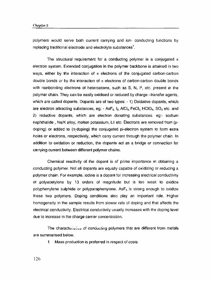
Chapter 5

polymers would serve both current carrying and ion- conducting functions by

replacing traditional electrode and electrolyte substances'.

The structural requirement for a conducting polymer is a conjugated It

electron system. Extended conjugation in the polymer backbone is attained in two

ways, either by the interaction of rr electrons of the conjugated carbon-carbon

double bonds or by the interaction of 1't electrons of carbon-carbon double bonds

with nonbonding electrons of heteroatoms, such as 8, N, P, etc. present in the

polymer chain. They can be easily oxidised or reduced by charge -transfer agents,

which are called dopants. Dopants are of two types: - 1) Oxldative dopants, which

are electron attracting substances, eg; - AsFs. 12. AICI3. FeCI:l, HCI04 , 803 etc. and

2) reductive dopants, which are electron donating substances. eg:- sodium

naphthalide , NalK alloy, molten potassium, Lil etc. Electrons are removed from (p­

doping) or added to (n-doptnp) the conjugated pi-electron system to form extra

holes or electrons, respectively, which carry current through the polymer chain. In

addition to oxidation or reduction, the dopants act as a bridge or connection for

carrying current between different polymer chains.

Chemical reactivity of the dopant is of prime importance in obtaining a

conducting polymer. Not all dopants are equally capable ofoxidizing or reducing a

polymer chain. For example, iodine is a dopant for increasing electrical conductivity

of polyacetylene by 13 orders of magnitude but is too weak to oxidize

polyphenylene sulphide or polyparaphenylene. Asf, is strong enough to oxidize

these two polymers. Doping conditions also play an important role. Higher

homogeneity in the sample results from slower rate of doping and that affects the

electrical conductivity. Electrical conductivity usually increases with the doping level

due to increase in the charge carrier concentration.

The characte.ts:...." ut conducting polymers that are different from metals

are summarised below.

Mass production is preferred in respect of costs.

126

Preparation ami characterization ofpoly(/'-phellylllediazomethine)

2 These are of low density and therefore conducive to energy

conservation.

3 They can be made into films very easily to provide materials which

have a large surface area

4 They are very sensitive to external stimuli.

5 Electrically anisotropic materials can be obtained.

6 These materials are not so liable to the effects of oxidation.

7 These materials have the ability to absorb large quantities of liquids

and gases.

B They have good processabilities

9 Porous conductors can be made without difficulty.

In recent years, the synthesis of conducting polymers has attracted great

interest due to their electrical, electrochemical and optical properties". They have

widespread applications in rechargeable batteries 3.4, erectrochromic devices s, gas

separation membranes 6, and enzyme immobilization 7. The conducting polymers

such as polypyrrole, polythiophene, polyfuran and polyaniline have been examined

for electronic and chemical applications'i", Applications of polythiophene for

electrooptical switching and memory devices10, and organic batteries 11 have been

proposed. Polypyrrole doped with sulphonate derivatives of metallo porphyrin is

reported to be useful in the cathodic reduction of oxygen in acidic and basic

solutions, which find applications in fuel cells and metal/air batteries 12. It has been

demonstrated thae s the chloride-doped polypyrrole film shows a stable and

selective response towards er ions in solution. It has been also reported that PI

electrode modified with polypyrrole can be used as a nitrate sensor".

Mac Diarmid et.al. have assembled a battery, making use of the

amphoteric nature of polyacetylene, to provide a prototype of plastic battery".

Rechargeable bat.eries jnvolvi,,~ fJuiyaniline, polypyrrcle, or polyparaphenylene /

alkali metal cathode also has been developed". Narkis17 has suggested that cross­

linked polyethylene filled with carbon black is ideal as a material for preventing the

127

Chapter 5

build-up of static electricity. Polyphenylenevinylene and derivatives are used as

light-emitting diodes, and lightly doped polyaniline film membranes are used tor the

separation of gases.

Poly (azomethine)s, sometimes called poly(schiff bases), are a group of

polymers which are catching more attention due to the following reasons. Aromatic

poly( azomethine)s are highly thermo-stable in analogy to aromatic polyethers.

Further more, poly (azomethine)s may possess a conjugated main chain and, after

suitable doping, may show an attractive level of electric conductivity 18.

Only a few poly (azomethine)s derived from aliphatic dialdehydes and

aromatic diamines were described in literature, and most of them were prepared by

solution condensation of diamines and glyoxal 19-21. High yields and satisfactory

elemental analyses were reported, but no information on viscosity and molecular

weights.

In the present study, a new conducting polymer based on glyoxal and p­

phenylene diamine was synthesized The synthesis of poly(p­

phenylenediazomethine) was carried out in different solvents, like, methanol,

toluene, m-cresol and DMF. First the reaction was carried out in methanol. Since

the conductivity of the product formed was very low, the polymerization was

repeated in toluene solvent. In this medium also, the conductivity of the product

formed was very low and the reaction was repeated in m-cresol. Even though the

conductivity of the product was higher than other samples already prepared, the

yield of the product was very low. So the polymerization was carried out in DMF as

the solvent.

128

Preparation and characterization of poly(p-phclly/llcdiazolllel1/i/ll')

5.2 Experimental

5.2.1 Materials

P-phenylene diamine, Glyoxal 40 % solution, Glyoxal hydrate (trimer),

N,N-Dimethyl formamide (DMF) , m-Cresol , Toluene , Methanol. Acetone ,

Hydrochloric acid (HCI), Perchloric acid (HCI04) , Iodine (12) , and Carbon tetra

chloride (CCI4) was used in the present investigation conforming to the

specifications given in Chapter 2.

5.2.2 Synthesis of poly(p-phenylenediazomethine) in methanol

0.1mole of p-phenylene diamine was dissolved in methanol (300ml) and

0.1mole glyoxal (40% solution) was added drop wise with continuous stirring for 2

hours. By that time, 'precipitation of the product takes place. The product was

washed with water and then with methanol and dried well at room temperature

under vacuum.

5.2.3 Synthesis of poly(p-phenylenediazomethine) in toluene

0.1mole of p-phenylene diamine was added to 400 ml of toluene and was

dissolved by stirring. Then 0.1 mole of glyoxal was added to it and stirred well. The

mixture was slowly heated to boiling. with continuous stirring, and was refluxed at

the boiling temperature for 5 hours. By that time, the precipitation of the product

takes place. It was then allowed to cool to room temperature and then poured into

excess of ice-cold water. It was allowed to settle, filtered, washed with plenty of

water until the filtrate was colorless. Then it was washed with methanol, and

allowed to dry at room temperature in air for one day. Then the final drying of the

sample was done at 70°C under vacuum.

J29

Chapter 5

5.2.4 Synthesis of poly(p-phenylenediazomethine) in m-cresol

0.1mole of p-phenylene diamine was added to 100 ml of m-cresol and was

dissolved by stirring. Then 0.1 mole of glyoxal was added to it and stirred well. The

mixture was slowly heated to boiling, with continuous stirring, and was refluxed at

the boiling temperature for 4 hours. It was then allowed to cool to room

temperature and then poured into excess of ice-cold water. The precipitate was

allowed to settle, filtered, washed with plenty of water until the filtrate was

colourless. Then it was washed with methanol, and allowed to dry at room

temperature in air for one day. Then the final drying of the sample was done at

70°C under vacuum.

5.2.5 Synthesis of poly(p-phenylenediazomethine} in N,N-dimethyl­

formamide

0.1mole of p-phenylene diamine was added to 300 ml of DMFand was

dissolved by stirring. Then 0.1 mole of glyoxal was added to it and stirred well. The

mixture was slowly heated to boiling, with continuous stirring, and was refluxed at

the boiling temperature for 4 hours. By that time, the precipitation of the product

takes place. It was then allowed to cool to room temperature and then poured into

excess of ice-cold water. It was allowed to settle, filtered, washed with plenty of

water until the filtrate was colourless. Then it was washed with methanol, and

allowed to dry at room temperature in air for one day. Then the final drying of the

sample was done at 70°C under vacuum.

The dried samples were powdered well, and, pelletized for the density and

conductivity measurements. For the spectral and thermal studies, the sample was

extracted with acetone until the extract was colorless, and dried well.

130

Preparation and characterization of poly(p-phenylllediazomethille)

5.2.6 Doping

19 of each sample was put in 50ml each of 1M HCI solution, 1M HCI04

solution and saturated solution of 12 in CCI4 and kept for 24 hours. Then it was

filtered, washed with a little amount of acetone and dried at 70° C under dynamic

vaccum for one hour.

5.3 Polymer Characterization

The prepared polymer samples were characterized by IR spectra, UV

spectra, TGA, and Molecular weight determination (GPC), as explained in

Chapter 2.

5.4 Measurements

5.4.1 D.e. conductivity

D.C. conductivity of the pressed pellets was determined by the two-probe

technique. The samples were sandwiched between two copper electrodes and a

constant voltage (6V) was applied to the sample. The current flowing through the

sample was measured using a digital multimeter (APLAB model 1087). The

conductivity of the sample was calculated using the equation, a = t j RA ,where

't' is the thickness of the pellet, 'R' is the resistance of the sample ( R =Ell, where

'E' is the applied voltage and '1' is the resulting current through the sample), and 'A'

is the area of cross section of the pellet(A = 1t( , where 'r' is the diameter of the

pellet).

5.4.2 Density

Density of the pressed pellets were determined using the equation.

o = MN , where 'M' is the mass of the pellet and 'V' is the volume of the pellet.

131

Chapter 5

5.4.3 Microwave conductivity and Complex permittivity

The dielectric properties and conductivity of the samples were measured

using cavity perturbation technique". The experimental set up consists of a

HP8510 vector network analyzer; sweep oscillator, S-parameter test set and

rectangular cavity resonator. The measurements were done at 2.17 GHz at room

temperature (25°C).

In microwave studies the conductivity can be calculated using the

equation,

Conductivity .c = 21tfsEoEr"

where 'fs' is the resonant frequency, EO is the complex permittivity of free space

and Er" is the imaginary part of the complex permittivity . which is given by the

equation,

Er" == (Vc !4V5 )(Qt -Qs ! QtQs)

where,' Vc' is the volume of cavity, Vs is the volume of sample, O, is the quality

factor of the cavity loaded with the sample and Qt is the quality factor of the cavity

with the empty sample holder.

The real part of the complex permittivity er' is usually known as dielectric

constant of the material. It can be calculated from the equation,

Er' == 1 + (ft -fs)1 2fs (Vc N 5)

where ft ==resonant frequency of the unloaded cavity and t, is the resonant

frequency of the cavity loaded with the sample.

The pelletized samples were inserted into the cavity and the perturbation

produced at a particular microwave frequency was noted. The resonant frequency

and quality factor were recorded and dielectric constant and microwave

conductivity were calculated using the above equations.

132

Preparation and characterization ojpoly{p-plzellyl"ediazometltille)

5.4.4 Thermal diffusivity

Thermal diffusivity was determined by photo acoustic technique. It can be

defined by the mathematical expression,a == Ki p cp , where 'K' is the thermal

conductivity, 'p' is the density and 'c,' is the specific capacity at constant pressure.

5.5 Results and discussion

5.5.1 IR spectra

IR spectra of the polymer prepared in different solvents are given in the

figures 5.1- 5.4. Figure 5.1 shows the IR spectrum of the sample prepared in

methanol. The absorption band at 1678 ern" should be assigned to carbonyl

absorption, possibly carbonyl of an amide qroup. The absorption band at 3306 ern"

should be ascribed to a N-H stretching vibration. In literature the absorption of the ­

C=N~ group is found between 1675 and 1660 ern", However, if it is conjugated to

an aromatic ring it shifts to a lower wave number, between 1635 and 1625 ern".

The absorption bands at 1517 and 1609 cm' shows the presence of an aromatic

ring .The absorption band at 833 cm' can be assigned to the C-H out of plane

vibration of the aromatic ring. Figure 5.2 shows the IR spectra of the sample

prepared in toluene. This spectrum shows various spectra! bands, which also

occurs in the spectrum of p-phenylene diamine such as the bands at 3328,

3221,1855, 1639, and 1130cmo1• From the spectrum, it may be concluded that the

reaction was not completed in toluene solvent, hence the molecular weight of the

product was very low, and hence the conductivity also was very low. The

absorption band at 1662cm-' should be assigned to carbonyl absorption, possibly a

carbonyl of an amide group or to the -C=N- group. Fig.5.3 shows the lR spectra of

the sample prepared in DMF. The absorption band at 1625 ern" may be assigned

to a C=N stretching vibration. The absorption band at 1670 ern" should be

assigned to carbonyl absorption, possibly a carbonyl of an amide group.

133

Chapter 5

IIIIlllllilIaIlID)

11

l.l

'0

09

oe0.1

~ Oiis 05i

04

03

02

0.1

00

~.I

Fig. 5.1 IR spectrum of the sample prepared in methanol

1.

o.

o.

o.

0.1

o.

3800 3llOO 30100 3200 3DOO 2tlOO 2600 2400 22CO 200Q 1800 leoo 1_ '2<lO 1000 100w_Fig.5.2 IR spectrum of the sample prepared in Toluene

134

Preparation and characterization of poly(p-phenylnediazomethille)

25

20

..vc..ofconJJoi

3500 1500

Fig.5.3 IR spectra of the sample prepared in DMF

The absorption band at 3350 cm' should be ascribed to/a N-H stretching vibration,

The absorption bands at 1512 and 1609 ern" shows the presence of aromatic

ring.The absorption band at 833 cm' can be assigned to the C-H out of plane

stretching vibration of aromatic ring.

Fig.5, 4 shows the IR spectrum of the sample prepared in m-cresol. This

spectrum was comparable with that of sample prepared in DMF, Figure 5.5

compares the spectrum of the samples prepared in m-cresol and DMF. The main

difference was the position and the intensity of the carbonyl band. In this sample,

the center of this absorption wasat 1699 ern", while it was positioned at 1670cm'l

in sample prepared in DMF. Again there was an absorption band at 3350 ern" that

can be assigned to an N-H stretching mode. Because of hydrogen bonding this

absorption band was shifted to a lower wave number.

135

Chapter 5

2~,

i'(

2.0

35~O 3C80 2580 2CJOWave NUr'lbel

Fig.5. 4 IR spectrum of the sample prepared in m-cresol

10

OB

•u~ 06~

~

15CO 'I)))

Fig.5.S IR Spectra of the polymer prepared in (a) DMF and (b) m-cresol

136

Preparation ami characterization of poly(p-pllclIylllediazomethille)

Figure 5.6 compares the IR spectrum of the polymer prepared in toluene

as the solvent and the monomer glyoxal. From the spectrum, it was clear that

unreacted glyoxal was not present in the polymer prepared in toluene., since no

peaks due to unreacted glyoxal was present in the spectrum.

10

09

oe

n7

D6

~ esi~

O.

OJ

02 I /D' - -../cc

0'

lJIl :ID) JoOO lXlJ Im 2IIJJ 2IIJJ lOlIl 2DJ lllXl ,m '1lJI ..m 12111 1a:D mW..A"'"lbI'

Fig.5.6 IR spectra of (a) polymer prepared in toluene and (b) the

rnonomer - glyoxal

Figure 5.7 shows the comparison of the polymer prepared in toluene and

the monomer paraphenylene diamine. This spectrum shows various spectral

bands, which was also present in the spectrum of p-phenylene diamine such as the

bands at 3328,3221,1855,1639, and 1130cm 1. From the spectrum, it may be

concluded that the reaction was not completed in toluene solvent and some

amount of unreacted paraphenylene diamine was present in the polymer sample.

137

Chapter S

11

1I

10-

09

08

07

os05

0.4-

03

o.Ol~ .../

00-

01

lDl liOO 3400 T.m :DD ;m) 2600 1400 220l 20ll ien 1600 1100 1<00 11DJ aoW~numb.r

Fig. 5.7 IR spectra of.(a} polymer - prepared in toluene and

(b) monomer - paraphenylene diamine

Figure 5.8 shows the comparison of the spectrum of the polymer prepared

in toluene and DMF. The two spectra were different from each other. The

absorption band at 1639 cm" disappeared and a new band at 1625 crn' was

present, which can be assigned to the -C=N· stretching vibration. The absorption

band at 1670 ern" was present in both samples. Various spectral bands due to the

presence of unreacted monomers disappeared in the spectrum of the poiymer

prepared in DMF.

Fig.5.9 shows the comparison of the spectrum of the polymer prepared in

DMF and the monomers, glyoxal and p-phenylene diamine. From the figure, it was

evident that, chemical reaction took place almost completely in the medium of

DMF, since there was no spectral bands in the polymer sample due to the

unreacted monomers, glyoxal and paraphenylene diamine.

138

Chapter S

'"-

3IDl 3liOO ].lOO 3200 lID ;lm l603 ,COO 2200 2COC 'ill) 1600 1400 IlOO 100 OCCW",numb'l

Fig. 5.7 IR spectra of.(a) polymer - prepared in toluene and

(b) monomer • paraphenylene diamine

Figure 5.8 shows the comparison of the spectrum of the polymer prepared

in toluene and DMF. The two spectra were different from each other. The

absorption band at 1639 ern" disappeared and a new band at 1625 ern" was

present, which can be assigned to the -C=N- stretching vibration. The absorption

band at 1670 cm' was present in both samples. Various spectral bands due to the

presence of unreacted monomers disappeared In the spectrum of the poiymer

prepared in DMF.

Fig.5.9 shows the comparison of the spectrum of the polymer prepared in

DMF and the monomers, glyoxal and p-phenytene diamine. From the figure, it was

evident that, chemical reaction took place almost completely in the medium of

DMF, since there was no spectral bands in the polymer sample due to the

unreacted monomers, glyoxal and paraphenylene diamine.

138

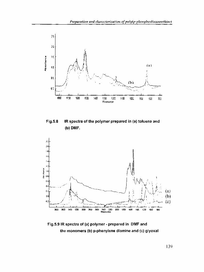
Preparation and characterization ofpoly(p-I"1Ctlylllt'diazomethillt')

25

2.0r

:1'..

"[ r" ~ ~' hc"€

d~V,\0.. 10~ I .1 I, . I/' l... "," ~ .".' ., .

I'

OH I,t ./ .

.--" /oc I-

,-,''.-

(::l \

.'~ ;:-.. <, )1 ,;

_' V'~,,"",. rh) )'\_f" .~~------/i'~

"--'-. .__ .

lfm 1700 1&)) 15)) 1400 1300 lLOJ 1100 lOOJ 9JO 800 700Wi,eoum,er

Fig.5.S IR spectra of the polymer prepared in (a) toluene and

(b) DMF.

n

(a)(b)(c)

I.

10

20

O~

16

1 e

12

06

~:~1

r I·~"-." I,.-; J I1

04_._ ../ _. 1 .h~ I_~" ., I' ' o.

02 /' .. ~-. \! \, ,"" ", r : • '_. : \1/ i'J (r'l'\ '"'""~-------- ,I j\ I ,\ .,/ ,i\~ - J "~I ;1 \ I, J\ '

/ . '~ ,. "I'.' - •.•

~__/_ __'·C.>~_ _,=-:=.j>;~-tJ'.:;-.(l]

l:W 3600 l4rx; ]JX) lID YJ) lWJ ]4Ill ]JX) xro 18)) 1600 14UJ I iOO 10Cll EmWMflumb.,

Fig.5.9 IR spectra of (a) polymer- prepared in DMF and

the monomers (b) p-phenylene diamine and (c) glyoxal

139

Chapter S

Figure 5.10 gives the IR spectrum of the sample prepared in DMF,

which was treated with triethyl amine. It was clear from the spectrum that there was

no chemical change during this treatment. It was clear from the IR spectrum.

Figure 5.11 compares the spectrum of the samples treated with trlethyl amine and

the original sample. The IR spectra of the samples do not differ from each other.

"1,~·

j

o

e 0

L

Fig.5.10 IR spectrum ofthe polymer prepared in DMF treated with

triethyl amine

Effect of doping on the structure of the polymer was clear from the IR

spectrum of the polymer prepared in DMF. Figure 5.12 shows the IR spectrum of

the polymer doped with Hel. The additional peaks at 1016, 1124, and 1203 cm'!

can be assigned to be present due to the charge delocalization on the polymer

backoone'". Broad peak in the region of 2500 - 2800 cm" was due to protonation

on the polymer chain. Other peaks present in the spectrum were same as that

present in the undoped poiyrner as given In figure 5.3.

140

Preparation and characterization of poly(p-phenylnediazomethine)

1.8

1.6

1.4

1.2

1.0

G.B />:0.6~ A. ~0.4 ~0.21--__-

3SOO 2SXl 2IXXlWavenumb.r

1500 um

(a)(b)

Fig.5.11 IR spectra of (a) polymer prepared in DMF

(b) polymer treated with triethyl amine

0.7

o.

o..

1500 \000

Fig.5.12IR spectrum of the polymer doped with HCL

141

Chapter S

Figure 5.13 shows the IR spectrum of the polymer doped with HCI04 The

additional peaks at 1056 cm' can be assigned to be present due to the charge

delocalization on the polymer bachbone. Broad peak in the region of 3200 ern"

was due to protonation on the polymer chain. The peak at 3300 cm" of the

undoped polymer had been shifted to 3500 cm". Other peaks present in the

spectrum were same as that present in the undoped polymer as given in figure 5.3.

o. , l'i

ii I,I ,

o.

-------~ /\-,I ~ \, I

" '-.....-. i/ ",-- jI ---- -----"

j

0.1

3000 2500 2000

III\,

Fig.5.13 IR spectrum of the polymer doped with HCI04

On comparing the two spectra, from the intensity of the additional

peaks due to the dopanl molecules, we can say that HC104 is a more stable dopant

than HCI. The absorption bands at 1408 cm" and 1511 cm'cue to the quinoid and

benzenoid rings attached to N atom in the undoped polymer are shifted to 1410

and 1505 cm" ; and 1413 and 1508 cm" respectivelv for HCI and HCI04 doped

samples.

142

Preparation ami churacteriza tion of po[y(p-plIeIlY[lIeliiazometlIillt'l

5.5.2 UV Spectra

UV absorption spectra of the polymer prepared in different solvents are

shown in the figure 5.14. On changing the solvent from methanol to DMF, the

wavelength at which maximum absorption occurs shifts to longer wavelength

region. This shift is due to the extension of conjugation. All spectra show

absorption in the region of 190-290nm. The absorption bands in this region is

attributed to the n - n' transition of the C=N chrornophore". Amax of the polymer

prepared in DMF is higher than that of other samples. This observation shows that

the polymer has more conjugated double bonds when the synthesis was carried

out in DMF as the solvent and minimum conjugation in. the polymer prepared in

toluene. This observation can also be related to molecular weight and conductivity

of the polymer prepared in different solvents. D. C. conductivity of the polymer

prepared in DMF is higher than that of other samples.

7

6

Ql 50e

4lU..c...

3~..cet 2

0150 200 250 300 350 400

Wavelength (nm)

. ........- DMF ---.- m- cresol - Toluene _ Methanol

Fig.5.14 UV spectra OT poly(p-phenyienediazometnine) prepared

in different solvents

143

Chapter S

5.5.3 GPC

The molecular weight of the polymer prepared in m-cresol as the

solvent was determined using Hexafluroiso propanol as the eluent. Gel permeation

chromatogram is shown in the figure 5.15. GPC distribution plot is given in Figure

5.16 and the results are given in Table 5,1. The number average molecular weight

of the polymer was 25660 and the weight average molecular weight was 69123.

The result shows that polymerization reaction takes place to a great extent.

1.

o.

NO.U(jj

O.

~

11

I:!:nIi.':i:1

11.. !1~ I!.- 1::

•._._.- •.•~\ ,) I

......................................................................l\ .i. -:.::":.:: :~~:-:;.. \-.-._ .I I'

0.00 10.00 20.00 30.00 40.00 SO.OO 60.00 70.00tJ;nutes

Flg.5.15 gel permeation chromatogram of the polymer

Table 5.1 GPC results

M peak Mn Mw Mz Mw!--

13551 25660 69123 228717 2.6

144

-~---

Mn Mz/ Mw

3.309

Preparation and characterization ofpoly(p-phenylnediazomethine)

"-;

0.00+----

7.00 6.00 5.00 4.00Slice Log WNV

3.00

Fig.5.16 GPC distribution plot of the polymer

From the above results, the reaction between glyoxal and paraphenylene

diamine to form the polymer, poly(p-phenylenediazomethine) can be represented

by Scheme 5.1. Condensation reaction took place between p-phenylene diamine

and glyoxal by the elimination of water molecule, forming a C= N bond .

..~.~H2N~ NH2 +H-R

o

H~N -~ N-C-C-H~/" I rI

H H 0- 0

145

Chapter S

H H"~II

"H2N ~N==C-C-H+ 11

o

SoOn

f®-N =CH-CH=N -(Q)-- N =CH-CH=NjU

Reductbn1lOxidation

I

H H +A-

f®-~-CH =CH-N =< >=!'!-GH=CH-~-Ju

Scheme 5.1

146

Preparation and characterization of poly(p-phellyblediazomethine)

5.5.4 TGA

In the thermo gravimetric analysis of the sample prepared in DMF

(fig.5.17), there was about 10% weight loss at 300°C and about 20% weight loss at

400°C and as the temperature was increased, there was continuous weight loss.

The initial weight loss may be due to volatilization of water molecules and the

weight loss at high temperature was related to the degradation of the polymer

backbone due to the production of gases such as acetylene and ammonia. Thermo

gravimetric analysis of the sample prepared in m-cresol is shown in Figure 5.18.

Compared to the sample prepared in DMF, about 25% weight loss existed at

300°C and about 50% weight loss at 400°C occurred for this sample. This may be

due to the thermal decomposition of the polymer similar to that prepared in DMF.

35 100 200 300

Temperature (0 C)

400 500 600 700

Fig.5.17 TGA of the polymer prepared in DMF

147

Chapter S

<,---...- ...... _- -'--,100

90

80

70~ 60~

1: 50Cl'ij)

3: 4030

20

10

035 100 200 300 400 500 600 70(

Temperature (0 C )

Fig. 5.18 TGA of the polymer prepared in m-cresol

5.5.5 D.C. Conductivity

The d.c, conductivity and density of the prepared samples are given the

Table 5. 2. Conductivity of the undoped samples was changed with the solvent in

which the reaction was carried out. The variation in conductivity may be due to tne

difference in the degree of polymerization in different solvents. The conductivity of

the sample prepared in DMF was greater than other samples. DMF is a polar

aprotic solvent and the polymer formed were more soluble in DMF than in toluene

and methanol, that helped to increase the degree of polymerization, which in turn

increased the conjugation length and hence the conductivity was increased. In

methanol and toluene, precipitation of the product takes place easily and hence

further reaction may not take place. So the conductivity is very low in the samples

prepared in methanol and toluene. Thp ~nnductivity of the undoped sample

prepared in m-cresol is similar to that prepared in DMF.

148

Preparation and characterization ofpoly(p-phenylnediazomethitle)

Table 5.2 Density and conductivity of poly(p-phenylenediazomethine)

prepared in different solvents

Conductivity(S/m)

Solvent Density Dopants

(g ern")..

Undoped HCI HCI04 12

DMF 1.0906 1.164 x 10'" 8.604 x 10'" 2.801 x 10''> 1.019x10''>

m-Cresol 0.7096 2.415 x 10':> 3.663 x 10'" 6.061 x 10''> 4.082 x 10':>

Toluene 1.1309 6.25 x 10'0 2.463 x 10'" 9.709 x 10''> 9.009 x 10'"

Methanol 1.1432 3.597 x 10'1l 2.198 x 10'0 8.422 x 10'0 3.086 x 10'0

The conductivity of the doped samples was more than that of the undoped

samples. This was because, after doping, more charge carriers were introduced

into the polymer chain, which helped to increase the conductivity. Conductivity of

acid doped samples was more than that of 12 doped samples. This may be due to

the attachment of W ions to the N atom of the polymer using the lone pair of

electrons, which results in the oxidation of the polymer chain. Charge delocalisation

on the polymer chain helped to increase the conductivity, which was evident from

the IR spectra of acid doped samples (Fig.5.12, 5.13). The low conductivity of the 12

doped samples may be due to the fact that the oxidation of the polymer chain by

iodine was very low. Also, on drying the samples, the action of heat and vacuum

may be removing the iodine easily. This observation was verified by measuring the

conductivity of the doped samples after one week. After one week, the conductivity

of 12 and HCI doped samples were decreased very much, while the conductivity of

HCI04 doped samples remained almost the same as given in Table 5.3. So HCI04

was the better doping agent for poly(p-phenylenediazomethine).

149

Chapter 5

Table 5.3 Conductivity of poly(p-phenylenediazomethine) prepared in DMF

I Doping agent

I

conductivity Conductivity after one

(S/m) week(S/m)1--------

HCI 8.604 x 10'" 6.855 x 10''1

HCI04 2.801 x 10-" 1.825 x 10'"

12 1.019 X lO'J 1.242 X 10.4

The conductivity of the samples doped with different dopants depends on

the nature of the counter ion also. Small nucleophilic counter ions appear to bind

tightly to the chain, thus limiting the mobility of the charge, and larger, delocalized

counter ions have a more diffuse charge and do not associate highly with the

polymer chain25• Thus, in perchtonc acid doped samples, the larger CI04' counter

ion helped to increase the conductivity.

5.5.6 Thermal diffusivity

Thermal diffusivity of the polymer samples prepared in different

experimental conditions is given in Table 5.4. The thermal diffusivity of poly(p­

phenylenediazomethine) prepared in m-cresol solvent was very high and it was in

between that of Al and Fe. So poly (p-phenylenediazomethine) was a good

conductor of heat.

5.5.7 Dielectric parameters

Figures 5.19- 5.21 show the variation in the dielectric constant,

dielectric loss factor, and microwave conductivity of poly(p-

phenylenediazomethine) prepared in different solvents at the microwave

frequency of 2.17 GHz at 25°C. The microwave conductivity was less than that of

150

Preparation twd characterization ofpoly(p-phenylllediazomethine)

a conductor, but greater than that of an insulator at microwave frequencies.

Because of this property, it can be used to construct microwave components like

filters.

Table 5.4 Thermal diffusivity of poly(p-phenylenediazomethine)

prepared in different solvents

Solvent Thermal diffusivity

(cm 2 s -1)

Methanol 0.0536

Toluene 0.0368

DMF 0.5037

m-Cresol 0.5088

The real part of the complex permittivity, i.e., dielectric constant of the

material was increased when they were doped with HCI and HC104• On doping,

due to the presence of additional charge carriers, and their movement were

restricted in the polymer chain, local accumulation of charge will induce its image

charge on an electrode and give rise to interfacial polarization. So dielectric

constant was increased on doping, as shown in the figure 5.19. Dielectric

constant of the material doped with HCI04 was more than that of undoped and

HCI doped samples. This may be due to the effect of introducing more charge

carriers, because, HCI04 is a strong oxidizing agent than HCI.

151

~' --_.. ,

• Undoped n HO n HCI04 ,-- - - - . - ~-----_... . .

CJr"pter 5

8

C ,• 6 i1>l I0 j0u I

4,

u .-c-u.! 2•is

0Methanol Toluene DMF m-cresol

Fig . 5.19 Dielectric constant of poly(p-phenylened iazometh ine)

prepared In different solvents

Figure 5.20 shows the variation in the imaginary part of the complex

permittivity. i.e.• dielectric loss factor of different doped and undoped samples.

Imaginary pan of the complex permittivity or the dielectric loss factor, e " is a direct

function of relaxation process and the origin of this relaxation is due to the local

motion of polar groups. Dielectric loss factor of the material was increased on

doping except for the polymer prepared in methanol. The increase in dielectric loss

factor ma~' be due to the increase in the polarity of the molecule on doping. For the

large molecule, the rotary motion of the molecules was not sufficiently rapid for the

attainment of equilibrium wilh the field. So more time was required for the dipole 10

reortent . and hence dielectric loss factor was increased. For the polymer prepared

in methanol, the molecular weight of the polymer was very low due to the

precipitation of the product , and the reaction was carried out at room temperature.

So the time for the molecule to reorfent with the field was low and hence on doping,

the dielectric loss factor was decreased. Microwave conductivity is a direct function

of dielectric loss factor. Hence, the increase in conductivity on doping was due to

the increase in die lectric loss factor of the material as shown in the figure 5.21.

152

P" paration alld dlaracterizat ion o{poly(p-phcny lncdiazomt fhillf!J

1.6 .

ij " 1l! 1.2~ 1 j

.5! 0.8u

~ 06 ,'.. 004i5 0.2

oMethanol

K JToluene DMF m-cresol

--- - -- ~~I . Undoped C HCI C HCIQ4 !~- _. . ,

Fig. 5.20 Dielectric loss factor of poly(p-phenylenediazomethine)

prepared In different solvents

0.2. I

Methanol Toluene DMF m-cresol

• Undopcd IS! HCI [J HCI04

Fig. 5.21 Microwave conductivity of po ly(p-phenylenedi azom ethine)

prepared In different solvents

15J

Chapter 5

5.6 Conclusions

1. Condensation reaction took place between glyoxal and p-phenylene

diamine to form the conducting polymer poly(p-

phenylenediazomethine).

2. The molecular weight of the polymer prepared in m-cresol solvent was,

Mn = 25660 and Mw = 69123.

3. The polymer was thermally stable up to about 400°C.

4. D.C. Conductivity of the polymer prepared in DMF was more than that

of other samples prepared in m-cresol, methanol and toluene.

5. Doping increased the d.c. conductivity of the polymers prepared by the

condensation reaction between glyoxal and p-phenylene diamine.

6. HCI04 was a better ~oping agent for poly(p-phenylenediazomethine)

compared to HCI and 12

7. Thermal diffusivity of the polymer was in between that of AI and Fe. So

it was a good conductor of heat.

8. Dielectric properties like dielectric constant, dielectric loss and

microwave conductivity increased on doping with HCI and HCI04 .

154

Preparation ami characterization of poly(p-p/lellylllcdiazomethill(')

5.7 References

Hari Singh Nalwa, Handbook of Conductive Molecules and Polymers, Vol.

2, John WHey and Sons, England, 11, (1997).

2 A. Skotheim (ed.), Handbook of Conducting Polymers, Marcel Oekker,

New York, (1986).

3 N. V. Shat and S. Yasmin, J. Appl. Polym. ScL, 55, 1827 (1995).

4 R. C. D. Peres and M. A. DePaoli, J. Pow. Sour., 40,229, (1992).

5 A. F. Dlaz, J, I. Castillo, T. A. Logan, and W. J. Lee, ElectroanaI.Chem.,

129,115, (1981).

6 J. Pellegrino, R. Radebaugh and B. R. Mattes, Macromolecules, 29, 4985,

(1996).

7 N. Kizilyar, N. Y. Ozden, L. Toppare, and Y. yagci, Synth. Met., 104, 45.

(1999).

8 A. F. Diaz, K. K. Kanazawa, and G. P. Gardini, J. Chem. Soc. Chem.

Commun. , 635, (1979).

9 K. K. Kanazawa, A. F. Diaz. W. D. Gill, P. M. Grant, G. B. Street, G. P.

Gardini, and J, F. Kwak, Synth. Met., 329,(1979/1980).

10 K. Yoshino, K. Kaneto, and Y. Inuishi, Jpn. J. Appl. Phys., 22, L157 (1983).

11 K. Kaneto, K. Yoshino, and Y. Inuishi, Jpn. J. Appl. Phys.. 22, L567 (1983).

12 Eui-hwan Song, and Woon-kie Palk, Bull. Korean Chem. Soc. 19, 183,

(1998).

13 S. Song, Z. Sun, and Z. Lu, Analyst, 113,1525. (1988).

14 Sung Chul Kang, Keun-sun Lee, Jin-Doo Kirn, and Kang-Jin Kim, Bull.

Korean Chem. Soc. 11,124, (1990).

15 J. H. Kaufman, Phys. Rev., 26, 2327, (1982).

16 A. G. MacOiarmid, and A. J, Epstein, Frontiers of Polymer Research,

Edited by P. N. Prasad. and J. K. Nigam, Plenum press. New York, 259.

(1991).

17 M. Narkis, Modern Plastics International, 28, June (1983).

155

Chapter S

18 Kricheldort and Schwarz, Hand-Book of Polymer Synthesis, Marcel

Dekker, New York, Part B, ch.27, 1673, 1992).

19 CA, 94,103963 m (1981).

20 CA, 10,70670 d (1986).

21 C.A., 67 , 117405 k (1967).

22 S. Biju Kumar, Honey John, Rani Joseph, M. Hajian. L. P. Ligthart, K. 1.

Mathew, J. of the European Ceramic Society, 21, 2677. (2001).

23 S. K. Dhawan, and S. Chandra, Macro'98, Macromolecules-New Frontiers,

Allied Publishers Ltd., Vol.t , 320, (1998).

24 Sir Geoffrey Wilkinson ( Ed.). Comprehensive Coordination Chemistry,

Vo1.2. 715. (1987).

25 James M. Margolis (Ed.), Conductive Polymers and Plastics,Chapman and

Hall, Ch.l, 18, (1989).

156

Chapter 6

PREPARATION AND CONDUCTIVITY STUDIES OF

BLENDS OF CONDUCTING POLYMER WITH

POLYETHYLENE, POLY (VINYLCHLORIDE)

AND SILICA

6.1 Introduction

The electrically conducting polymers such as polypyrrole, poly thiophene,

polyfuran and polyaniline have been examined for possible electronic and chemical

applications1-3. However, the use of electrically conducting polymers has been

limited in the past by problems associated with poor environrnentat stability and/or

157

Chapterti

poor mechanical propernss'". As the interchain electron transfer interactions of

conjugated polymers are relatively strong compared to the Vander Waals and

hydrogen bonding typical of saturated polymers. the conducting polymers tend to

be insoluble and infusible. Conducting polymer composites have drawn

considerable interest in recent years because of their numerous applications in a

variety of areas of electrical and electronic industry7-9. In most of these

applications, the main concern is to obtain sufficient level of conductivity in the

material.

This chapter reports our investigations done for obtaining conducting

polymer blends. Preparation of blends. composites and interpenetrating network

has been Widely used as an approach to combine electrical conductiVity with

desirable mechanical strength of polymers". Three principal approaches have

been reported for increasing the processability of conducting polymers- (1)

polymerising appropriately substituted monomers so that the conducting polymers

become soluble and still retain substantial conductivity, (2) Preparing the polymer

in dispersion form and (3) polymerising the monomers of the respective conducting

polymer inside the matrices of conventional polymers leading to composite films5.

Several attempts have been described to produce conducting polymer

composites with better physical properties by either chemically or

electrochemically11-15. Several composites of conducting polymers have been

prepared for the simple reason of havinq polymers with good thermal and physical

characteristics16--22. Charge transport mechanism in conducting polymer

composites was reported by Radhakrishnan et.aI.23.

In-situ polymerization of glyoxal and p-phenylenediamine was done in

different solvents containing different amounts of PE, PVC, and silica. The d.c.

conductivity and microwave conductivity of each sarnnte was measured. The effect

of dopants like HCI04 , Hel and 12 on conductivity was also studied.

158

Conducting polymer composites ioitl: PE, PVC and silica

6.2 Experimental

6.2.1 Materials used

Paraphenylene diamine, Glyoxal hydrate (trimer), Polyethylene,

Polyvinylchloride, Ultrafine silica, N,N-Dimethyl formamide, Toluene,

Tetrahydrofuran, Methanol, Acetone, Hydrochloric acid. Perchloric acid, Iodine,

and Carbon tetra chloride were used in the present investigation conforming to the

specifications given in Chapter 11.

6.2.2 Synthesis of poly (p-phenylenediazomethine) -Polyethylene

conducting polymer blends

Polyethylene (5g) was dissolved in 400 ml of toluene by gentle heating

along with continuous mechanical stirring. 0.1mole of p-phenylene diamine was

added to it and was dissolved in it by stirring. Then 0.1 mole of glyoxal was added

and stirred well. Then the temperature of the reaction medium was increased

slowly to boiling, with continuous stirring, and was refluxed at the boiling

temperature for 5 hours. By that time, the precipitation of the product takes place. It

was then allowed to cool to room temperature. Excess of toluene was allowed to

evaporate until the precipitation of polyethylene started and then poured into

excess of ice-cold water. It was allowed to settle, filtered, washed with plenty of

water until the filtrate was colorless. Then it was washed with methanol, and

allowed to dry at room temperature in air for one day. Then the final drying of the

sample was done at 700e in vacuum.

The same procedure was repeated by varying the amount of polyethylene

in the reaction mixture. The dried samples were powdered well in a mortar and

then pelletized for the measurements. For the spectral and thermal studies, the

sample was extracted with acetone until the extract was colorless, and dried well.

159

Chapterii

6.2.3 Synthesis of poly(p-phenylenediazomethine) -Polyvinylchloride

conducting polymer blends

PVC (5g) was dissolved in 50 ml of Tetrahydrofuran. 0.1mole of p­

phenylene diamine was added to 300 ml of N,N-dimethylformamide and was

dissolved in it by stirring. Then 0.1 mole of glyoxal was added to it and stirred well.

The solution of PVC in THF was added to the above reaction mixture and stirred

well. Then the temperature of the reaction medium was increased slowly to boiling,

with continuous stirring, and was refluxed at the boiling temperature for 4 hours. By

that time, the precipitation of the product takes place. It was then allowed to cool to

room temperature and then poured into excess of ice-cold water with stirring. It was

allowed to settle. filtered, washed with plenty of water until the filtrate was

colourless. Then it was washed with methanol. and allowed to dry at room

temperature in air for one day. Then the final drying of the sample was done at

70°C in vacuum.

The same procedure was repeated by varying the amount of PVC. For this,

10 gm of PVC was dissolved in 100ml of THF, 15 gm of PVC was dissolved in

150ml of THF, and 20 gm of PVC was dissolved in 200ml of THF and was added to

the reaction mixture containing glyoxal and p-phenylenediamine in DMF.

The dried sample was powdered well. and, pelletized for the density and

d.c. conductivity measurements. For the spectral and thermal studies. the sample

was extracted with acetone until the extract was colorless, and dried well.

6.2.4 Synthesis of poly(p-phenylenediazomethine) -silica

conducting polymer composites

0.1mole of p-phenylene diamine was added to 300 ml of DMF and was

dissolved in it by stirring. 5 gm of ultratine silica was added to it and stirred well.

Then 0.1 mole of glyoxal was added to it and stirred well. Then the iemperature of

the reaction medium was increased slowly to boiling, with continuous stirring, and

160

Conducting polymer composites uritl: PE, PVC and silica

was refluxed at the boiling temperature for 4 hours. By that time, the precipitation of

the product takes place. It was then allowed to cool to room temperature and then

poured into excess of ice-cold water with stirring. It was allowed to settle, filtered,

washed with plenty of water until the filtrate was colourless. Then it was washed

with methanol, and allowed to dry at room temperature in air for one day. Then the

final drying of the sample was done at 70°C in vacuum.

The same procedure was repeated by varying the amount of silica to the

reaction mixture containing glyoxal and p-phenylenediamine in DMF.

The dried sample was powdered well, and, pelletized for the density and

d.c. conductivity measurements. For the spectral and thermal studies, the sample

was extracted with acetone until the extract was colorless, and dried well.

6.2.5 Doping

19 each of the sample was added to 50ml each of 1M HCI solution, 1M

HCI04 solution and saturated solution of 12 in CC14 and kept for 24 hours. Then it

was filtered, washed with a little amount of acetone and dried at 70° C in dynamic

vaccum for one hour.

6.3 Measurements

6.3.1 IR spectra

Particles of the polymer samples were flattened by means of cold

compression between two diamond windows. IR spectra of the samples were

recorded with a Biorad UMA 500infrared microscope, which is coupled to a Biorad

FTS 6000 spectrometer. Spectra were recorded with a resolution of 4 cm -1

co-adding 100 scans.

161

Chaptem

6.3.2. D.C. conductivity

D.C. conductivity of the pressed pellets was determined by the two-probe

technique. The samples were sandwiched between two copper electrodes and a

constant voltage (6V) was applied to the sample. The current flowing through the

sample was measured using a digital multimeter (APLAB model 1087). The

conductivity of the sample was calculated using the equation, o =t I RA, where 't'

is the thickness of the pellet, 'R' is the resistance of the sample (R = Ell, where 'E'

is the applied voltage and 'I' is the resulting current through the sample). and 'A' is

the area of cross section of the pellet (A = rr( , where 'r' is the diameter of the

pellet).

6.3.3 Density

Density of the pressed pellets were determined using the equation, D =MN , where 'M' is the mass of the pellet and 'V' is the volume of the pellet.

6.3.4 Microwave conductivity and Complex permittivity

The dielectric properties and conductivity of the samples were measured

using cavity perturbation technique24. The measurements were done at a

microwave frequency of 2.17 GHz at room temperature (25°C).

In microwave studies the conductivity can be calculated using the

equation,

Conductivity .o = 21tfsEoE,"

where 'fs' is the resonant frequency, £0 is the complex permittivity of free space

and Er" is the imaginary part of the complex permittivity , which is given by the

equation,

Er" = (Vc /4Vs )(O,-Os / 0 105 )

162

Conducting polymer composites witlz PE, PVC and silica

where,' Vc I is the volume of cavity, Vs is the volume of sample, as is the quality

factor of the cavity loaded with the sample and a, is the quality factor of the cavity

with the empty sample holder.

The real part of the complex permittivity Er' is usually known as dielectric

constant of the material. It can be calculated from the equation,

Er' =1 + (I. -fsl/ 2fs (Vc Nsl

where ft =resonant frequency of the unloaded cavity and fs is the resonant

frequency of the cavity loaded with the sample.

6.4 Results and discussion

6.4.1 Poly(p-phenylenediazomethine)-polyethylene blends

Fig.6.l gives the IR spectrum of the conducting polymer composites with

polyethylene.

1 ~

'f

"'

g"11

~

Of

J(

O'

01

All m J<OC W. m m:I ;raJ l..:c im lllIl '(ID IfDl '0]) 1200 1~ ID)WM~~"'l~'1

Fig. 6.1 IR spectrum of the conducting polymer-polyethylene blend

163

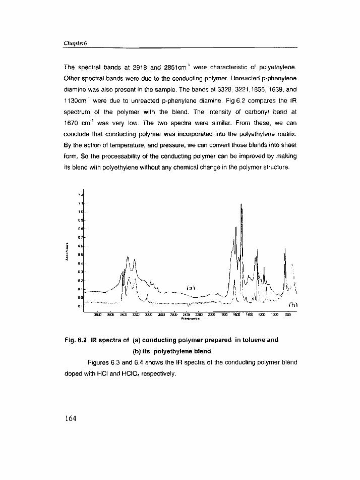
Chaptetis

The spectral bands at 2918 and 2851cm-1 were characteristic of polyethylene.

Other spectral bands were due to the conducting polymer. Unreacted p-phenylene

diamine was also present in the sample. The bands at 3328, 3221,1855, 1639, and

1130cm l were due to unreacted p-phenylene diamine. FiQ_6_2 compares the IR

spectrum of the polymer with the blend. The intensity of carbonyl band at

1670 crn' was very low. The two spectra were similar. From these, we can

conclude that conducting polymer was incorporated into the polyethylene matrix.

By the action of temperature, and pressure, we can convert these blends into sheet

form. So the processability of the conducting polymer can be improved by making

its blend with polyethylene without any chemical change in the polymer structure.

1 i-

11-

10·

o -

06-

07-

06·

J!Il) 3600 )l(J() 3200 DD :I9ll ~ 1400 2<lIJ 2IlIl '600 \600 1400 12llJ 100) 600WnemJfTlb,r

Fig. 6.2 IR spectra of (a) conducting polymer prepared in toluene and

(b) its polyethylene blend

Figures 6.3 and 6.4 shows the IR spectra of the conducting polymer blend

doped with HCI and HCI0 4 respectively.

164

Conducting polymer composites toitl: PE, PVC alld silica

Fig. 6.3 IR spectrum ~f the conducting polymer-polyethylene blend

doped with HCI

O'~""'----------~-----------l

!

I

O.

'000

Wevenumber

Fig. 6.4 IR spectrum of the conducting polymer-polyethylene blend

doped with HCI04

165

CI/apter6

The absorption bands at 3325, 3219, and 1637 cm" of unreacted p-phenylene

diamine were disappeared on doping. This was because, on treating the blend with

acids, unreacted p-phenylene diamine dissolved in it and was removed on filtration.

The absorption band at 3419 cm" in the undoped blend was shifted to a broad

band at 3336 cm" and 3537 cm" due to protonation, in HCI and HCI04 doped

samples respectively. Strong bands at 2914 and 2845 ern" were due to PE. The

bands at 1508 and 1463 ern" were due to benzenoid and quinoid ring attached to

N atom respectively. The very weak peak at 1050 cm" was due to HCI dopant and

the strong peak at 1080 cm" was due to HCI04 dopant. Other absorption bands

were the same as that in the undoped sample.

Figure 6.5 shows the density of the blends of the conducting polymer

based on glyoxal, p-phenylene diamine and varying amounts of polyethylene.

1.2

lof" 1.1EoSsUlc:::~ 0.9

2015105

0.8 +-----,-----,.-----.-----,

oAmount of polyethylene (9)

Fig. 6. 5 Density of the conducting polymer-polyethylene blends

The density of the blends were lower than that of poly{p-phenylenediazomethine).

It was because; the density of polyethylene was lower than that of the polymer

prepared in toluene solvent. The density of the blends was decreased with

increase in the amount of polyethylene in the blend.

166

Conducting polymer composites with PE, PVC and silica

The d.c. conductivity of the blends was decreased with increase in the

amount of polyethylene as given in figure 6.6. It was because, polyethylene is an

insulator and the presence of polyethylene in the composite prevented the free

movement of electrons through the conducting polymer chain.

The conductivity of the doped samples was more than that of the undoped

samples. This was because, after doping, more charge carriers were introduced

into the polymer chain, which helped to increase the conductivity. Conductivity of

perchloric acid doped samples was more than that of other doped samples. This

may be due to the attachment of W ions to the N atom of the polymer using the

lone pair of electrons. Oxidation of the polymer chain takes place and the electron

transfer occurs between the polymer chain and through the polymer chain.

Conductivity of the 12 doped samples were lower than that of samples doped with

HCI and HCI04 •

'-~ t!

i -2e '-3~~ -4:~ -5'0g ·6uen -7o- -8

-9

5 10 15 20 25

Amount of PE(9)

Fig. 6. 6 Conductivity of the undoped and iodine doped

polyethylene blends

167

Clrapter6

~ 90~ 80)( 70-..e. 60~ 50

f 40'u 30i 206 10u 0

o 5 10 15 20 25

Amount of PE (g)

Fig. 6. 7 D.C. conductivity of the conducting polymer/polyethylene

blends doped with HCI04

30..,~ 25)(

I 20~

15f~ 10~

-g 5<3

oo 5 10 15 20 25

Amount of PE (9)

Fig. 6. 8 D.C. Conductivity of the conducting polymer/polyethylene

blends doped with Hel

168

Conducting polymer composites with PE, PVC and silica

It may be due to the fact that the binding force between iodine and polymer chain

was very low. Also, on drying the samples, the action of heat and vacuum may be

removing the iodine easily, compared to HCI and HCI0425

• This observation was

verified by measuring the conductivity of the doped samples after one week as

reported in Chapter V. HCI04 was found to be the better doping agent. It was

because, the size of CI04- counter ion is large, compared to cr ion and so the H'

ions were more tightly attached to the polymer chain. Hence the removal of the

dopant was not occurring readily. The stability of the HC104 dopant was also

evident from the IR spectra. The intensity of the absorption band due to HCl04 was

more, while that of HCI was very weak.

6.4.2 Poly(p-phenylenediazomethine)-polyvinylchloride blends

Figure 6.9 gives the IR spectrum of the conducting polymer blends with

PVC. A broad band existed between 3200 and 2400 ern". These bands can be

assigned to the -(N~Hx)-CI strtetching vibration of amine salts. Other spectral

bands were due to the conducting polymer. Some more absorption bands can be

ascribed to the PVC spectrum. Figure 6.10 compares the IR spectrum of the

conducting polymer with that of the blend. Some of the spectral bands were

common in both of the spectra. From these, we can conclude that conducting

polymer was incorporated into the PVC matrix.

As the amount of PVC was increased in the blends, the solubility of the

polymer was increased. This may be due to the effect of two solvents, THF and

DMF, in the reaction medium, or, it may be due to the removal of HCI from PVC by

the action of heat during the course of the reaction. The presence of acid was

found to increase the solubility of the conducting polymer. In concentrated acids,

the polymer was soluble at high temperature. So the processability of the

conducting polymer can be improved by making its blends with PVC without any

chemical change in the polymer structure.

169

Chapter6

u

~ 0

i 0

~ 0

0.1

Fig. 6.9 IR spectrum Qf the conducting polymer- PVC blend

, 5

. :0

!~;:t O.

oo-

t<~ ......-· ~'_" (h)<. \ .

. '

- -v..-,.-

XOO~\·_".nun,:.t~f

15:0

Fig. 6.10 IR spectra of (a) conducting polymer prepared In DMF and

(b) its blend with PVC

170

Conducting polymer composites with PE, PVC and silica

Figures 6.11 and 6.12 show the IR spectra of the conducting polymer IPVC blends

doped with HCI and HCI04•

Fig. 6.11 IR spectrum of the conducting polymer/PVC blends

doped with HCI

0.,...._----------------------------,

0.'

3500 2000 1500 1000

Fig. 6.12 IR spectrum of the conducting polymer/PVC blend

doped with HCI04

171

Chapterii

The absorption peak at 3345 cm' in the undoped polymer was shifted to a

broad band in the region of 3338 and 3360 crn' in HCI and HCI04 doped samples

respectively. The strong peak at 1628 ern" was characteristic of C=N bond in

conjugated polymers. The bands at 1094 and 1084 cm -1 were due to the dopant

molecules HCI and HCI04. The bands at 1512 and 1425 cm -1 showed the

benzenoid and qumotd rings attached to N atom. Other bands were same in

undoped and doped samples.

D.C. conductivity of the blends of the conducting polymer based on glyoxal,

p-phenylene diamine and varying amounts of polyvinyl chloride is shown in the

figure6.13.

0 ------,

E 5 10 15 20 25- -2UJ->.- -4's;..o;:,

-6"Cc0o 8 IC)

-1·0 ]0

Amount of PVC(g)

l=--undoped __ Iodinedoped I

Fig. 6.13 D.C. Conductivity of the conducting polymer/PVC blends

The d.c. conductivity of the undoped blends decreased with increase in the

amount of PVC. It was because, PVC is an insulator and the presence of

nonconducting PVC in the composite prevented the free movement of electrons

through the conducting polymer chain. Here, the conducting region was

separated by a nonconducting region, so that the jumping of electrons from one

conducting region to other became difficult. Hence the conductivity was decreased

as in the case of polyethylene blends.

172

Conducting polymer composites ioith PE, PVC and silica

The variation in d.c, conductivity of the doped samples with the amount of

PVC is given in tigure.6.14.

'? 100c....)( 80E§. 60 .-

~'S; 40;l0:J 20't:IC0o 0

0 5 10 15 20 25

Amount of PVC (9)

-_. -----,-+- HCl04 HCI !

_ .__J

Fig.6.14 D.e:;. Conductivity of Hel and HCI04 doped

conducting polymerl PVC blends

The d.c. conductivity of the doped samples was more than that at the undoped

samples. This was because, after doping, more charge carriers were introduced

into the polymer chain, which helped to increase the conductivity. Conductivity of

perchloric acid doped samples containing higher amount of PVC were more than

that of other doped samples. HCI0 4 was found to be the better doping agent

because, of the large size of CI0 4' counter ion, which helped to tightly attach the

dopant to the polymer chain. Hence the removal of the dopant was difficult. This

may be due to the attachment of W ions to the N atom of the polymer using the

lone pair of electrons to increase the charge delocalization as it is clear from the IR

spectra.. Conductivity of the 12 doped samples were lower than that of other

samples doped with HCI and HCI04 as shown if Fig.6.13. It may be due to the fact

that charge delocalization due to iodine on the polymer chain was very low. Also,

on drying the samples, the action of heat and vacuum may be removing the iodine

easily, compared to acid dopants.

173

Chapter6

The d.c. conductivity of perchloric acid doped blends were more than that

of the pure conducting polymer doped with perchloric acid. As the amount of PVC

was increased, d.e. conductivity was increased and remained almost constant at

higher amount of PVC. This was because, PVC present in the blend is polar in

nature, and the charge delocalization and oxidation takes place with the conducting

polymer as well as with PVC molecules as shown in the IR spectra. So the removal

of the dopant molecule may be difficult during the drying process and since the

charge carriers were not lost, the conductivity was higher for the blends. After a

saturation point was reached, the increase in conductivity was negligible because,

the amount of insulating region of PVC was increased in the blend.

Dielectric properties of conducting polymer/PVC blends are given in the

figures 6.15-6.17 at room temperature in the microwave frequency of 2.17 GHz.

Figure 6.15 shows the variation in dielectric constant of acid doped and undoped

PVC blends.

6-5e~-I/) 4c0<J 3u'':::- 2 JUJ!1ellC

0

0 5 10 15 20 25

Amount of PVC (9)

i - Undoped - HC] -.- HCI04 ,

Fig.6.15 Dielectric constant of conducting polymer/PVC blends

174

Conducting polipner composites toith PE. PVC and silica

The dielectric constant of the HCI doped blends were more than that of undoped

samples. On doping, due to the presence of additional charge carriers, and their

movement were restricted in the polymer chain, local accumulation of charge will

induce its image charge on an electrode and give rise to interfacial polarization.

Dielectric constant of HCI04 doped samples were less than that of undoped

samples. This may be due to orientation polarization of the dipoles caused by the

alternating accumulation of charges at the interfaces between different phases of

rnatenats-l.e., between PVC and poly(p-phenylenediazomethine), even though

more charge carriers were introduced. As the amount of PVC was increased.

dielectric constant was increased first, up to about 10g of PVC was added in the

blend. This was due to the presence of additional charge carriers, i.e., HCI

eliminated from PVC, act as dopant. As the amount of PVC was increased more,

dielectric constant was decreased due to the insulating effect of PVC.

Figure 6.16 shows the variation in the imaginary part of the complex

permittivity, i.e., dielectric loss factor of the conducting polymer/PVC blends.

1

ell 0.8ell.2

0.6Ev 0.4 .J!~

0.2

0

0 5 10 15 20 25

Amount of PVC (g)

-+- Undoped --HCI ---1Ift- HCI04 :

Fig.6.16 Dielectric loss factor of conducting polymer/PVC blends

175

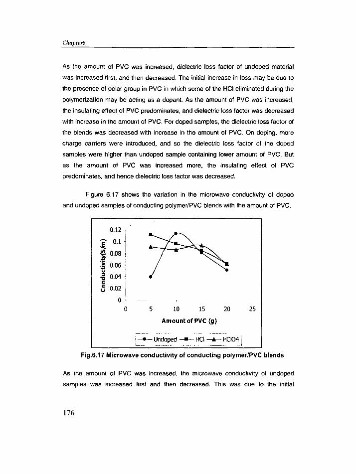
Chaptero

As the amount of PVC was increased, dielectric loss factor of undoped material

was increased first, and then decreased. The initial increase in loss may be due to

the presence of polar group in PVC in which some of the HCI eliminated during the

polymerization may be acting as a dopant. As the amount of PVC was increased,

the insulating effect of PVC predominates, and dielectric loss factor was decreased

with increase in the amount of PVC. For doped samples, the dielectric loss factor of

the blends was decreased with increase in the amount of PVC. On doping, more

charge carriers were introduced, and so the dielectric loss factor of the doped

samples were higher than undoped sample containing lower amount of PVC. But

as the amount of PVC was increased more, the insulating effect of PVC

predominates, and hence dielectric loss factor was decreased.

Figure 6.17 shows the variation in the microwave conductivity of doped

and undoped samples of conducting polymer/PVC blends with the amount of PVC.

0.12i

i 0.1-'

!!!. 0.08 I~ ,:~ 0.06 :v !

~ 0.04"C '

8 0.02 1

O·o 5 10 15 20

Amount of PVC (9)

25

Fig.6.17 Microwave conductivity of conducting polymer/PVC blends

As the amount of PVC was increased, the microwave conductivity of undoped

samples was increased first and then decreased. This was due to the initial

176

Conducting polymer composites with PE, PVC and silica

increase and then decrease in the dielectric loss factor of the blends with the

amount of PVC. Microwave conductivity is a direct function of dielectric loss. So the

change in the microwave conductivity was the same as that of dielectric loss factor.

For acid doped samples, the conductivity was decreased as the amount of PVC

increased due to the increase in the insulating effect of PVC.

6.4.3 Poly(p-phenylenediazomethine)- si lica composites

Figure 6.18 shows the IR spectrum of the conducting polymer composite

with silica. The absorption bands at 1657, 1108, and 803 ern" were characteristic

of silica present in the composite. Other spectral bands were due to the conducting

polymer prepared in DMF. Figure 6.19 gives the comparison of the IR spectra of

the conducting polymer and their composite with silica. The two spectra have many

absorption bands, which were similar. The spectrum of the polymer composite had

the same spectral features as that of the pure polymer.

IJ,

I

\\\,.

\ 1'-'"\,

p ~ ~ m ~ D ~ ~ ~ m ~ ~ ~ ~ ~ a-Fig. 6.18 IR spectrum of the conducting polymer- silica composite

177

Chapter6

(a)

-----,(b)

s _ _ • m _ _ ~ m m ~ • ~ ~ ~ e~

Fig. 6.19 IR spectra of (a) conducting polymer prepared in DMF and

(b) it's composite with silica

IR spectra of the silica composite doped with HCI and HCI04 are given in

the figures 6.20 and 6.21. The absorption band 3345 cm" in the undoped polymer

was shifted to a broad band in the region of 3364 and 3485 cm" in HCI and HCI04

doped samples respectively. The strong peak at 1626 ernwas characteristic of

C=N bond in conjugated polymers. The bands at 1061 and 1045 cm -1 was due to

the dopant molecules HCI and HCI04 . The bands at 1508 and 1045 cm -1 showed

the benzenoid and quinoid rings attached to N atom. Other bands were same in

undoped and doped samples.

178

or'--'"I

o.

Conducting polymer composites toitlt PE, PVC and silica

-----_.----_.._.,'--_ .._--~'---- '-,

i~ 0 -

D.

iiI!,,

I

Ir

"'. I/ J''----r-'~-

100D

Fig.6.20 IR spectrum of the conducting polymerl silica composite

doped with HCI

1 -

I.

o.

o

_._------/' - ..._-J ---,.-..-.o. ---

I'

//\,J\. __"J

!;1f!

I1i II 1I i

I

3500 3000 2500

Fig.6.21 IR spectrum of the conducting polymer/silica composite

doped with HCI04

179

Chapter6

Figure 6.22 shows the density of the composites of the conducting polymer

based on glyoxal, p-phenylene diamine and varying amounts of fine silica.

1.15

'1 1.05EC,) 0.95C)-i' 0.85c:~ 0.75

252015105

0.65 +-----.------,-----.----.,..---------,

oAmount of silica (g)

Figure 6.22 Density of the silica composites

The density of the composites were lower than that of poly(p­

phenylenediazomethine). It was because; the density of silica is lower than that of

the polymer prepared in DMF solvent. The density of the composites was found to

decrease with increase in the amount of silica in the composite.

The d.c. conductivity of the undoped composites and iodine doped

composites was decreased with increase in the amount of silica similar to the

observation for the composites with polyethylene and PVC and is shown in the

figure 6.23. It was because: silica, which is an insulator, prevents the free

movement of electrons through the conducting polymer chain. Here also, a

nonconducting region separates the conducting region, so that the jumping of

electrons from one conducting region to other becomes difficult. Hence the d.c.

conductlvlty v--v decreased with an increase in the amount of silica in the

composite. For HCI doped samples also, conductivity decreased with the amount

of silica in the composite as shown in figure 6.24.

180

Conducting polymer composites with PE, PVC and silica

"l1200.....

)( 100E 80!a~

60.:;

40~U:J 20'0C

00c0 5 10 15 20

·---"1

25

Figure 6.23 D.C.Conductivity of undoped and iodine

doped conducting polymer/silica composites

12 -~0

10.....)(-. 8E-~ 6~

4.:;

~ 2-:J'0C 00o

-2 0 5 10 15 20 25

Amount of silica (g)

;-+- HC104 _ HCI i___ __ J

Figure 6.24 D.C. Conductivity of HCI and HCI04 doped

conducting polymer/silica composites

181

Cltapter6

The d.c. conductivity of the doped samples was more than that of the

undoped samples. This was because, after doping, more charge carriers were

introduced into the polymer chain, which helped to increase the conductivity.

Conductivity of perchloric acid doped samples was more than that of other doped

samples. HCI0 4 was found to be the better doping agent because, of the large size

of CI04 ' counter ion, which helped to tightly attach the dopant to the polymer chain

and due to its higher oxidizing effect. Hence the removal of the dopant was difficult.

This may be due to the attachment of H+ ions to the N atom of the polymer using

the lone pair of electrons. Hence charge delocalization was increased which is

clear from the IR spectra. D.C.conductivity of the 12 doped samples was lower than

that of other samples doped with HCI and HCI0 4 as in the case of PE and PVC

composites.

The d.c.conductivity of perchloric acid doped composites were more than

that of the pure conducting poyrner doped with perchloric acid and as the amount

of silica was increased, the conductivity increased first up to about 15 9 of silica

present in the composite. As the amount of silica was increased further,

conductivity decreased due to insulating nature of silica. The conduction process

can be accounted for in terms of electrons hopping between localized states under

the assistance of proton transfer, for which the presence of water plays an

essential role26.27

. Silica as well as perchloric acid can adsorb water molecules and

the presence of moisture increased the d.c. conductivity. Conductivity of HC! doped

samples was decreased with increase in the amount of silica, due to the insulating

effect of silica.

The changes in the dielectric parameters of silica composites at 2.17GHz

at room temperature are given in the figures 6.25-6.27. The variation in dielectric

constant for the doped and undoped samples is shown in the figure6.25. Dielectric

constant of HCI04 doped samples was more than that of undoped and HCl doped

samples. It was due to the presence of moisture in the samples due to the

hygroscopic nature of silica and HCi04 • Hence as the amount of silica was

182

Conducting polymer composites ioitlt PE, PVC and silica

increased, dielectric constant was increased for HCI0 4 doped samples. For

undoped and Hel doped samples. dielectric constant was decreased with increase

in the amount of silica due to the polarization caused by the alternating

accumulation of charges at the interfaces between different phases of materials

due to the orientation polarization of the dipoles. At higher amount of silica, the

slight increase in dielectric constant may be due to the moisture present in the

sample.

1: ~ 'jIV..

5 ~VIC0 4u.2 3..-u 2sCl) 1 ~is

o J0 5 10 15 20 25

Amount of silica (9)

t~.n Undoped.-.- H~'" '~-HCI04 j

Fig. 6.25 Dielectric constant of conducting polymer/silica composites

Figure 6.26 and 6.27 shows the variation in dielectnc loss factor and

microwave conductivity of the silica composites. For undoped samples, dielectric

loss and conductivity was decreased as the amount of silica was increased. This

was due to the insulatinq effect of silica. For doped samples, dielectric loss factor

and hence the microwave conductivity increased at first, with increase in the

amount of silica, reached a maximum value, and then decreased. The increase in

the values was due to the presence of moisture in the samples. At higher amount

of silica, the insulating effect was predominated and hence microwave conductivity

and dielectric loss factor was decreased.

183

Chapter6

2.5 IIII 2 IIII

I.!i! 1.5liv 1 1.9! i,.!!!

0.5 ~c

o <------T·-- . -,--~~-----,- - -----,

o 5 10 15 20 25

Amountof silica (g)

I _.- ,

: -Undoped -----HCI -k-HCI04 J;-_...~---_ ..... ,".",-.... ....._.,~-~~-~.-

Fig. 6.26 Dielectric loss factor of conducting polymer/silica composites

0.1 ..

0.05 .J

Io +--o

0.3 -~ iE 0.25 -t

c;; I~ 0.2 ~.~ I; 0.15 ~o;:)'0C

8

5 10 15 20 25

Amount of silica (g)

,~----.---..._ .. __._._,. .__w._... 1

i - Undoped ----- HCI ---a---- HCI04 I.__ .._._.- - _... - - ... ,_.._-~_._--~--- - ~

Fig. 6.27 Microwave conductivity of conducting polymer/silica composites

184

Conducting polymer composites with PE, PVC and silica

6.5 Conclusions

1. The d.c. conductivity of the undoped conducting polyme blends was lower

than the d.c. conductivity of the conducting polymer.

2. The d.e. conductivity of the undoped polymer blends was decreased with

increase in the amount of polyethylene, PVC. and silica.

3. The d.c, conductivity of the conducting polymer blends was increased on

doping with HCI, HCI04 and iodine.

4. The d.o. conductivity of all blends of conducting polymer with polyethylene

doped with HCI, HCI04 and iodine was decreased with increase in the amount

of polyethylene.

5. The d.c. conductivity of the blends of conducting polymer with PVC doped with

HCI and iodine was decreased with increase in the amount of PVC, but it was

increased on doping with HCI04 and it remained constant at higher

concentration of PVC.

6. The d.c. conductivity of the composites of conducting polymer with silica

doped with HCI and iodine was decreased with increase in the amount of

silica, but on doping with HC104 , it increased first up to about 15 g of silica

content and then decreased with increase in the amount of silica.

7. On doping with HCI. the dielectric constant of the conducting polymer blend

with PVC was increased. Dielectric constant was decreased when the

samples were doped with HC104 •

8. As the amount of PVC was increased. the dielectric constant,dielectric loss

factor and microwave conductivity of undoped conducting polymer blend with

PVC was increased first and then decreased and their values decreased for

doped samples.

9. For silica composites,dielectric constant of HCI04 doped samples was more

than undoped and HCI doped samples.

10. For undoped silica composites, dielectric loss and conductivity was decreased

as the amount of silica VV...~ ;, icreased. For doped samples, dielectric loss

185

Chapteni

factor and hence the microwave conductivity increased at first, with increase in

the amount of silica, reached a maximum value, and then decreased.

11. As the amount of silica was increased, dielectric constant was increased for

HCI04 doped samples. For undoped and HCI doped samples, dielectric

constant was decreased with increase in the amount of silica.

12. For undoped samples, dielectric loss and conductivity was decreased as the

amount of silica was increased.

13. For doped samples, dielectric loss factor and hence the microwave

conductivity increased at first, with increase in the amount of silica, reached a

maximum value, and then decreased.

186

Conducting polymer composites toith PE, PVC and silica

6.6 References

1. A. F. Diaz, K. K. Kanazawa. and G. P. Gardini. J. Chem. Commun.. 635.

(1979).

2. J. Pellegrino, R. Radebaugh, and B. R. Mattes, Macromolecules, 29,

4985,(1996).

3. S. E. Lindsey and G. B. Street. Synth. Met.. 10. 67, (1984).

4. H. Lindenberger, D. Schafer-Siebert, S. Roth, and H. Hanack, Synth. Met.,

18,37. (1987).

5. M. Zagorcska, A. pron, S. Lefrant, E. Kucharski, J. Suwalski, and P.

Bernier, Synth. Met., 18,43, (1987).

6. R. Quian, J. Qiu, and D. Shen, Synth. Met., 18, 13. (1987).

7. T. A. Skotheim, Handbook of Conducting Polymers, Marcel Dekker, New

York, (1986).

8. J. Margolis, Conducting Polymers and Plastics, Chapman and Hall,

London, (1993).

9. B. Wessling, Polym. Eng. ScL ,31,1200, (1991).

10. S. S.lm and S. W. Byun, J. Appl. Polym. ScL, 51, 1221. (1994).

11. O. Niwa, and T. Tamamura, J. Chem. Soc., Chem. Commun. , 817,

(1984).

12. M. De Paoli, R. J. Wallman, A. F. Diaz, and J. Bargon, J. Chem. Soc.,

Chem. Commun. , 1015, (1984).

13. M. De Paoli, R. J. Waltman, A. F. Diaz, and J. Bargon, J. Polym. SeL,

Polym. Chem. Ed., 23,1687, (1985).

14. O. Niwa. T. Tamamura, and M. Kakuchi, Macromolecules, 20. 749, (1987).

15. E. Kalaycioglu, L. Toppare, and U. Akbulut, J. Appl. Polym. SeL, 61,1067,

(1996).

16. Guerrero Carlos, Aleman Carlos, and Garza Rene, J. Polym. Eng., 17, 95,

(1998).

IS7

Cltapterb

17. H. L. Wang, L. Toppare, and J. E. Fernandez, Macromolecules, 23,1053,

(1990).

18. S. Oogan, L. Toppare, and U. Akbulut, Synth. MeL, 53,29, (1992).

19. F. Selampynar, L. Toppare, and U. Akbu!ut, T. Yalcin, and S. Suzer,

Synth. Met., 62, 201, (1994).

20. Semih Yigit. Jate Hacaloglu, Ural Akbulut, and Levent Toppare, Synth.

Met.. 79,11, (1996).

21. Semih Vigit, Jale Hacaloglu, Ural Akbulut, and Levent Toppare, Synth.

MeL, 84, 205, (1997).

22. N. Kizilyar, U. Akbulut,Y. Ozen, and L. Toppare, Synth. Met., 104, 45,

(1999).

23. S. Radhakrishnan and B. S. Hande, Proceedings of the "International

Symposium on Macromolecules", Jan.11-13, Vo1.2, 617, (1995).

24. S. Biju Kumar, Honey John, Rani Joseph, M. Hajian, L. P. Ligthart, K. T.

Mathew, J. of the European Ceramic Society, 21, 2677, (2001).

25. Honey John, S. Biju Kumar, K. T. Mathew, and Rani Joseph, J. Appl.

Polym. Sci., 83, 2008, (2002).

26. J. P. Travers, and M. Nechtschein, Synth. Met., 21,135, (1987).

27. D. Bloor, and A. Monkman, Synth. MeL, 21,175, (1987).

188

Chapter 7

Chapter 7

.SUMMARY AND CONCLUSIONS

The primary aim of this work has been to develop conductive silicone and

nitrile rubbers, which are extensively used for making conductive pads in telephone

sets, calculators and other applications. Another objective of the work has been to

synthesise and characterize novel conducting polymers based on glyoxal and

paraphenylenediamine- poly(p-phenylenediazomethine. Conducting polymer

matrices were developed from polymer blends such as poly(p­

phenylenediazomethine), polyethylene, PVC and silica and their properties were

studied. The contents of the various chapters in this thesis are summarised below.

An introduction about conducting polymers and conductive rubbers and their

composites are given in chapter 1. The various factors affecting the conductivity

and the mechanism of conduction are discussed in detail. A brief history of the

synthesis of various conducting polymers is also given. The advantage of

189

SI/J/Il11anj awl Conclusion

conducting polymers and conductive elastomer composites are highlighted. The

objectives of the present study are also listed.

The specifications of all the materials used in the study and different

experimental techniques used are described in chapter 2.

The studies on silicone rubber compounds are given in chapter 3. Silicone

rubber was made conducting by the incorporation of different types of carbon

blacks such as acetylene black, lamp black, HAF black and ISAF black. The effect

of concentration of carbon black on the conductivity of silicone rubber was

investigated. It was found that conductivity increases with the amount of blacks.

The influence of particle size, structure and the type of the carbon black was

studied by comparing the conductivity of different vulcanizates loaded with the

same amount of different blacks. It was found that the conductivity of silicone

rubber loaded with acetylene black was higher than those of other samples loaded

with other carbon blacks. The effect of temperature on the conductivity of these

vutcanizates was also studied in the temperature range of 250 C to 1500 C. The

mechanical properties such as tensile strength tear strength, hardness, elongation

at break etc. of each vulcanizates were also determined. Silicone rubber was

blended with high-density polyethylene and their electrical conductivity and

mechanical properties were determined after incorporating acetylene black.

Development of conductive nitrile rubber and its blends with natural rubber,

polyvinyl chloride and ethylene-propylene-diene rubber is described in chapter 4.

Nitrile rubber was made conducting by the incorporation of acetylene black. The

change in electrical conductivity and mechanical properties with the amount of

acetylene black was studied. The conductivity and mechanical properties improved

with the amount of acetylene black. Nitrile rubber was blended with NR, PVC, and

EPDM and their electrical conductivity and mechanical properties were determined

after incorporating acetylene black. NBR/NR blends were found to be more

conducting than NBR alone, NBRlPVC and NBRlEPDM blends. NBR/NR blends of

different compositions were prepared and their conductivity and mechanical

190

Chapter 7

properties were evaluated. The effect of temperature on the conductivity of different

vulcanizates was also studied. The mechanical properties of conductive nitrile

rubber were found to be better than those of silicone rubber loaded with the same

amount of acetylene black. But the conductivity of silicone rubber is higher than

that of NBR loaded with the same amount of acetylene black.

Preparation and characterization of a new conducting polymer, poly(p­

phenylenediazomethine) is described in Chapter 5. This conjugated polymer based

on glyoxal and p-phenylene diamine was prepared by the condensation reaction

under different experimental conditions. The polymer formed was characterised by

GPC, infrared spectra (IR). thermogravimetric analysis (TGA), and UV spectra. The

effect of solvent and temperature on the polymerization reaction was studied by

carrying out the reaction in different solvents such as N,N-Dimethylformamide

(DMF), m-cresol, toluene and methanol. The d.c. conductivity of the samples

prepared in DMF was found to be the highest. The molecular weight of the polymer

prepared in m-cresol solvent is, Mn = 25660 and Mw = 69123.The polymer is

thermally stable up to about 400°C Thermal diffusivity of the polymer lies in

between that of aluminium and iron, showing high thermal conductivity for the

newly synthesized conducting polymer. The effect of dopants on the conductivity of

the polymers was determined by doping the polymer with one molar solution of

HCI, HCI04 and 12 in CCI4 • Perchloric acid was found to be a potential doping agent

for the samples. The microwave conductivity and complex permittivity of the

samples prepared in different solvents and doped with different doping agents was

also determined.

To improve the processability of the novel conducting polymer prepared,

blends of the polymer was prepared with polyethylene, poly(vinyl, chloride), and

silica and their properties were evaluated. The details of such studies are

presented in Chapter 6. The effect of addition of polyethylene, polyvinyl chloride

and ultra fine silica to the conducting polymer was studied by the in-situ

polvmerizatlon of qlvoxal and p-phenylene diamine in different solvents, which

191

Slll1l1llanj and Conclusion

contained different amounts of PE, PVC, and silica. The d.c. conductivity and

microwave conductivity of each sample was measured. The effect of dopants like

HCI04 • HCI and 12 on the conductivity was also studied. The d.c. conductivity of the

undoped polymer blends was decreased with increase in the amount of

polyethylene, PVC. and silica. The d.c. conductivity of the blend was increased on

doping with HCI, HCI04 and iodine. The d.c. conductivity of all blends with

polyethylene doped with HCI, HCI04 and iodine was decreased with increase in

the amount of polyethylene. The d.c. conductivity of the blends with PVC and silica

doped with HCI and iodine was decreased with increase in the amount of PVC and

silica, but it increased first, and then remained almost constant or slightly

decreased on doping with HCI04 • Microwave conductivity, dielectric constant, and

dielectric loss factor of the conducting polymer blends with silica and PVC were

also determined at a frequency of 2.17 GHz. Effect of doping on the values of

these dielectric properties were also studied

192

LIST OF PUBLICA nONS FROM THE WORK

1. K. G. Princy, Rani Joseph and C. Sudha Kartha, Studies on conductive

silicone rubber compounds, Journal of applied polymer science, 69,

1043-1050, (1998).

2. K. G. Princy, Rani Joseph and C. Sudha Kartha, Studies on conductivity of

nitrile rubber and it's blends with NR, EPDM and PVC, Plastics Rubber

and Composites. (Accepted for publication)

3. K. G. Princy, Rani Joseph, and C. Sudha Kartha, Effect Of Temperature On

Conductivity Of Nitrile Rubber Vulcanizates, Plastics Rubber and

Composites, (Communicated).

4. K. G. Princy, Rani Joseph, K. T. Mathew, Otto van Asselen, and C. Sudha

Kartha, Synthesis And Characterization Of A Novel Conducting Polymer­

Poly (P-Phenylenediazomethine), Synthetic Metals, (Communicated).

5. K. G. Princy, Rani Joseph, K. T. Mathew, Otto van Asselen, and C. Sudha

Kartha, Synthesis And Characterization Of Conducting Polymer Blends Of

Poly (P·Phenylenediazomethine) With PE, PVC And Silica, Synthetic

Metals, (communicated).

193

List of Abbreviations

AB Acetylene black

ASTM American society for testing and materials

CCI4 Carbon tetrachloride

cm Centimetre

DC Degree Celsius

D.C. Direct current

DBP Dibutyl phthalate

DCP Dicumyl peroxide

DMF N,N-Diinethylformamide

DOP Dioctyl phthaate

EMI Electromagnetic interference

EPDM Ethylene propylene diene rubber

G Graphite

GHz Giga hertz

gm Gram

GPC Gel permeation chromatography

HAF High abrasion furnace

HCI Hydrochloric acid

HCI04 Perchloric acid

HOPE High density polyethylene

12 Iodine

IPN Interpenetrating polymer network

195

IR

ISAF

LB

LOPE

MBTS

MgO

min

mL

ML(1+4)

mm

NBR

nm

Nm

NR

PPO

PRI

pvc

rpm

S

S

SA

SBR

sec

196

Infrared

Intermediate super abrasion furnace

Lamp black

Low density polyethylene

Dibenzthiazyldisu!phide

Magnesium oxide

Minutes

Millilitre

Mooney viscosity determined using large rotor after a dwell time ofone minute and rotor run of 4 minutes

Millimetre

Nitrile rubber

Nanometre

Newton metre

Natural rubber

Percentage

p-phenylenediamine

Plasticity retention index

Poly (vinyl chloride)

Rotations per minute

Seimen

Sulphur

Stearic acid

Styrene butadiene rubber

Seconds

SR Silicone rubber

TGA Thermo gravimetric analysis

THF Tetrahydrofuran

TMTD Tetramethyl thiuram disulphide

UTM Universal testing machine

V Volts

ZnO Zinc oxide

Wavelength

p Resistivity

197