STUDIES OF A GINZBURG{LANDAU MODEL FOR d · STUDIES OF A GINZBURG{LANDAU MODEL FOR d-WAVE SUPERCONDUCTORS QIANG DUy SIAM J. APPL. MATH. °c 1999 Society for Industrial and Applied

STUDIES OF A GINZBURG–LANDAU MODEL FOR d-WAVESUPERCONDUCTORS∗

QIANG DU†

SIAM J. APPL. MATH. c© 1999 Society for Industrial and Applied MathematicsVol. 59, No. 4, pp. 1225–1250

Abstract. In this paper, we study a recently proposed Ginzburg–Landau-type model for somehigh-Tc superconductors with d-wave pairing symmetry. The scalar complex order parameter usedin the conventional Ginzburg–Landau models for low-Tc superconductors is replaced by a multi-component complex order parameter, and the free energy functional is modified accordingly to ac-count for the symmetry properties in the setting of the d-wave pairing. A brief introduction to thephysical and mathematical background of the d-wave models is provided first. We then present somerigorous mathematical analysis and discuss the relation between the new model and the conventionalGinzburg–Landau models. Various limiting cases such as the high-κ, high-field regime are examined.Numerical methods for the approximations of the new model are also considered along with resultsfrom numerical simulations that illustrate the complex structures for isolated vortices, vortex latticesand vortex motion driven by the applied current in the context of d-wave models.

Key words. Ginzburg–Landau model of superconductivity, s-wave and d-wave, pairing sym-metry, vortices, numerical approximations

AMS subject classifications. 65, 35, 82

PII. S0036139997329902

1. Introduction. The Ginzburg–Landau-type models [19] have been well accep-ted as valid models for low-Tc superconductors. They have been used extensivelyby physicists to study vortex phenomena in conventional superconductors. Rigor-ous mathematical analysis and large scale numerical simulations based on Ginzburg–Landau models have been carried out by many mathematicians and computationalscientists in recent years (see [1, 2, 3, 4, 5, 6, 7, 8, 9, 10, 11, 12, 13, 14, 15, 18, 22, 23, 24,26, 33] and the references cited therein). For high-Tc superconductors, in spite of thelack of satisfactory microscopic models, generalizations of Ginzburg–Landau modelsto account for high-Tc properties such as the anisotropy and the inhomogeneity havebeen proposed and analyzed.

Recently, in contrast to the conventional s-wave pairing in low-Tc materials, boththeory and experiments have produced strong evidence for d-wave pairing symmetryin some high-Tc superconductors; see, for example, [21, 28, 34, 48, 50, 51, 57, 58].More detailed studies of the vortex state in d-wave superconductors can be helpful toreconcile theory with experiments in determining the pairing mechanism in high-Tcmaterials.

The d-wave superconductors have been studied using various models, such as theHubbard model [55], the t−J model [56], the quasi-classical (Eilenberger) model [43,44], the Bogoliubov–de Gennes equations [52, 53], and the Ginzburg–Landau models[17, 20, 21, 25, 29, 30, 31, 32, 35, 36, 37, 38, 39, 40, 41, 42, 45, 46, 47]. A basic featureof the Ginzburg–Landau models is the use of multicomponent order parameters. Thefree energy densities are expansions of terms invariant under tetragonal symmetry(for the s+ d pairing) and orthorhombic symmetry (for the pure d-wave pairing). In

∗Received by the editors November 12, 1997; accepted for publication (in revised form) March10, 1998; published electronically April 7, 1999. This research was supported in part by NSF grantMS-9500718 and in part by a Hong Kong RGC grant and a DAG grant from HKUST.

http://www.siam.org/journals/siap/59-4/32990.html†Department of Mathematics, Hong Kong University of Science and Technology, Clear Wa-

ter Bay, Hong Kong, and Department of Mathematics, Iowa State University, Ames, IA 40011([email protected]).

1225

1226 QIANG DU

[21], discussions of the upward curvature of the Hc2 curve in the H-T phase diagramwere made. In a series of papers [25, 31, 32], Ginzburg–Landau-type models forboth the s-wave and the d-wave pairing were derived from the phenomenologicalGorkov equations (see also [39]). In [17, 20, 31] studies of the structure of a singlevortex were made, and in [20, 31, 46, 49] Abrikosov-type vortex lattices were analyzedand oblique lattices were found. These generalized Ginzburg–Landau models havebuilt a reasonable basis upon which detailed studies of the fine vortex structures insome high-Tc materials have become possible. Nevertheless, they consist of systemsof nonlinear partial differential equations that are even more complicated than theoriginal (or conventional) Ginzburg–Landau equations [19]. Analytical studies of theGinzburg–Landau models for d-wave superconductors are still limited [16, 17, 32, 45].Numerical solutions of the model have been obtained in [16, 17, 20, 29, 30, 31] forvarious simple cases. To get a better understanding of the pairing mechanism in high-Tc superconductors, and to see how the macroscopic properties of the materials withd-wave pairing would differ from those conventional superconductors, it is desirable tohave more rigorous analysis of the new models and more efficient codes when solvingthem.

In this paper, we examine a Ginzburg–Landau model for d-wave superconductors(GLd) that was first derived in [25] (see also [31, 32, 35, 36, 37, 38] and similar modelsin [17, 20, 21])and establish a rigorous mathematical framework. Comparison with theconventional Ginzburg–Landau model for low-Tc superconductors is made. We alsostudy various simplifications and reductions of the model, as well as their numericalapproximations. In addition, our numerical results illustrate various new and exoticstructures in the vortex solutions of the GLd model.

The rest of the paper is organized as follows. In section 2, we describe theGinzburg–Landau-type functional for d-wave (or mixed (s+d) wave) superconductorsand the basic terminology. In section 3, we study various mathematical properties ofthe free energy functional, including the existence of its minimizers. In section 4, thefull set of Ginzburg–Landau-type equations and the corresponding boundary condi-tions are given. Energy lower bounds and trivial constant solutions are discussed insection 5. In section 6, several limiting regimes are discussed and the leading orderequations are derived. Comparison with the conventional Ginzburg–Landau modelis considered. In section 7, a time-dependent Ginzburg–Landau model is generalizedfor d-wave superconductors. Numerical approximations of the models are discussedin section 8. Results of numerical simulations are presented in section 9, and somefinal comments are given in section 10.

2. Ginzburg–Landau models for superconductivity. This section is con-cerned with some basic questions related to the Ginzburg–Landau-type models ford-wave superconductors. For an introduction to the theory of superconductivity, see[27]. The conventional Ginzburg–Landau model for low-Tc superconductors is simplyreferred to as the GL model. In this paper, as an illustration of the models for d-wave pairing and the mixed (s + d) pairing, we use the equations derived in [25] asmodel equations; they are referred as the GLd models. Detailed derivations of theGLd models from the phenomenological Gorkov equations can be found in [25, 32].

Let Ω ⊂ R2 denote the region occupied by the superconducting sample. Through-out the discussion, unless otherwise noted, we will assume that Ω is a bounded, con-nected polygonal domain with boundary Γ. Let H be a constant applied magneticfield. Recall that the variables employed in the conventional GL models for supercon-ductivity are the real, vector-valued magnetic potential A and the complex, scalar-

GL MODEL FOR d-WAVE SUPERCONDUCTORS 1227

valued order parameter ψ. They are related to the (appropriately nondimensionalized)physical variables as follows:

magnetic field h = curl A,current j = curl h,density of superconducting charge carriers Ns = |ψ|2 .

(2.1)

With proper nondimensionalization, the conventional GL functional is given by

G(ψ,A) =

∫Ω

(1

2(1− |ψ|2)2 + |(i∇−A)ψ|2 +

1

κ2|curl A−H|2

)dΩ,(2.2)

where κ is the GL parameter which is the ratio of the coherence length ξ and thepenetration depth λ. In the GLd model given in [25, 31], there are two complex scalarorder parameters ψd and ψs along with the magnetic vector potential A. The modi-fied Ginzburg–Landau free energy functional with d-wave pairing symmetry is given by

Gd(ψs, ψd,A) =

∫Ω

1

8π|curl A−H|2 − 2 ln

(Ts0T

)|ψs|2 − ln

(Td0

T

)|ψd|2

+ αλd

(|ψs|4 +

3

8k3|ψd|4 + (k1 + k2)|ψs|2|ψd|2 +

1

2k1(ψs

2ψd∗2 + ψd

2ψs∗2)

)(2.3)

+1

4λdv

2F

(2k1|Πψs|2 + k3|Πψd|2 + 2k2<Π∗xψsΠxψd

∗ −Π∗yψsΠyψd∗) dΩ,

where (·)∗ denotes the complex conjugate; <· denotes the real part; Π = i∇− 2eAwith components Πx,Πy; e is the electric charge; α, λd, v

2F , and the coefficients

k1,k2,k3 are all positive constants; T is the temperature; and Ts0 and Td0 are thecritical temperatures for the s-wave and d-wave components.

We assume that the three coefficients k1, k2, and k3 satisfy

ki > 0, i = 1, 2, 3 and k1k3 ≥ k22.(2.4)

In [31], those constants are given by

ki = ki(s) = ξ2∞∑n=0

1

(2n+ 1 + s)i(2n+ 1)3−i(2.5)

for some positive constant ξ and some positive parameter s that depends on thetemperature T . Direct calculation shows that

k1k3 − k22 = ξ2

∞∑n,m=0

2s2(m− n)2

(2n+ 1 + s)3(2n+ 1)2(2m+ 1 + s)3(2m+ 1)2≥ 0 ∀s > 0,

so the inequalities in (2.4) are indeed satisfied.

Remark 1. One may modify the coefficient in front of |ψd|2 to include the effectof nonmagnetic impurities [32].

Remark 2. For models dealing with orthorhombic symmetry, the free energydensity is an expansion of the multicomponent d-wave parameters rather than theexpansion of both the s- and d-wave order parameters [15, 20].

1228 QIANG DU

3. Some properties of the Ginzburg–Landau d-wave functional. We useHm(Ω) to denote the standard Sobolev space of real-valued functions and we useH1(Ω) and H1(Ω) to denote similar function spaces of complex-valued functions andvector-valued functions, respectively. The norm in Hm(Ω) is denoted by ‖ · ‖m,Ω and‖·‖m,p,Ω denotes the norm in Wm,p(Ω). In order to state some rigorous mathematicalproperties, we let

H1n(Ω) = Q ∈ H1(Ω) : Q · n = 0 on Γ ,

H1n(div ; Ω) = Q ∈ H1(Ω) : div Q = 0 in Ω and Q · n = 0 on Γ.

Similar to the conventional Ginzburg–Landau functional, (2.2) also has an im-portant gauge invariance property. To be specific, for any φ ∈ H2(Ω), let the lineartransformation Tφ be defined by

Tφ(ψs, ψd,A) = (ψseiφ, ψde

iφ, A +∇φ) ∀ (ψs, ψd,A) ∈ H1(Ω)2 ×H1(Ω).

Then, direct calculation gives the following proposition.

Proposition 3.1. For all φ ∈ H2(Ω) and (ψs, ψd,A) ∈ H1(Ω)2 × H1(Ω),

Gd(ψs, ψd,A) = Gd(Tφ(ψs, ψd,A)); that is, Gd is invariant under the gauge trans-formation Tφ.

With a properly chosen φ [10], we also have the following lemma.

Lemma 3.2. Any element (ψs, ψd,A) ∈ H1(Ω)2 ×H1(Ω) is gauge equivalent to

an element (ξs, ξd,Q) of H1(Ω)2 ×H1

n(div ; Ω).We now consider the modified functional

Fd(ψs, ψd,A) = Gd(ψs, ψd,A) +

∫Ω

|div A|2dΩ.

By conditions on kis and the equivalence of norms between ‖curl A‖20 +‖div A‖201/2and ‖A‖1 in the space H1

n(Ω), we can check that there exist positive constants C1, C2

such that

Fd(ψs, ψd,A) ≥ C1‖ψs‖21 + ‖ψd‖21 + ‖ψs‖21 + ‖A‖21 + ‖ψs‖40,4 + ‖ψd‖40,4 − C2

∀(ψs, ψd,A) ∈ H1(Ω)2 ×H1

n(Ω). Moreover,

2k1|Πψs|2 + k3|Πψd|2 + k2(Π∗xψsΠxψd∗ −Π∗yψsΠyψd

∗ + Πxψs∗Π∗xψd −Πyψs

∗Π∗yψd)

is convex in (ψs, ψd). Combining with the compact imbedding theorem, we find that

F is lower semicontinuous in the weak topology of H1(Ω)2 ×H1

n(Ω). Thus, standardvariational arguments imply the following proposition.

Proposition 3.3. Fd has at least one minimizer belonging to H1(Ω)2 ×H1

n(Ω).Using the gauge invariance property, we may show the following [10].

Theorem 3.4. Gd has at least one minimizer belonging to H1(Ω)2 ×H1(Ω).

Moreover,

minH1(Ω)2×H1(Ω)

Gd = minH1(Ω)2×H1

n(div ;Ω)Gd = min

H1(Ω)2×H1n(Ω)Fd .(3.1)

The last statement provides a variational formulation for finding a minimizer of Gdin which the divergence free constraint may be imposed implicitly. Similar conclusionscan be made for the GLd models with orthorhombic symmetry given in [20, 21].


4. The GLd model. The Ginzburg–Landau-type models are in general validonly for T near the critical transition temperature. It is obvious that for the GLdmodel, when T > maxTs0, Td0, we have the normal state as the minimizer. For thisreason, we concentrate on the more interesting regime where T < Td0 so that a purenormal state for the d-wave component is not energetically favorable. For simplicity,we follow [10, 31] and take k1 = k2 = k3 = 1. In this case, we may introduce anondimensionalized form similar to that in [10, 31]:

Gd(ψs, ψd,A) =

∫Ω

[κ2|curl A−H|2 − 2β|ψs|2

+1

2(1− |ψd|2)2 +

4

3|ψs|4 +

8

3|ψs|2|ψd|2 +

2

3

(ψs

2ψd∗2 + ψd

2ψs∗2)(4.1)

+ 2|Πψs|2 + |Πψd|2 + 2<Π∗xψsΠxψd∗ −Π∗yψsΠyψd

∗] dΩ,

where Π = i∇−A, κ is the GL parameter, β is related to the ratio

ln(Ts0/T )

ln(Td0/T ),

and we see that β < 0 if T > Ts0, hence β > 0 if T < Ts0. Moreover, if Ts0 < T < Td0,then β → −∞ as T → Td0. The minimization of Gd with respect to variations in ψs, ψdand A yields the (s+ d) Ginzburg–Landau equations

2Π2ψs + (Π2x −Π2

y)ψd − 2βψs +8

3|ψs|2ψs +

8

3|ψd|2ψs +

4

3ψd

2ψs∗ = 0 in Ω,(4.2)

Π2ψd + (Π2x −Π2

y)ψs − ψd + |ψd|2ψd +8

3|ψs|2ψd +

4

3ψs

2ψd∗ = 0 in Ω,(4.3)

curl curl A = − iκ2 (ψs

∗Πψs − ψsΠ∗ψ∗s )− i2κ2 (ψd

∗Πψd − ψdΠ∗ψ∗d)

− i2κ2

(ψs∗Πxψd − ψsΠ∗xψ∗d

ψsΠ∗yψ∗d − ψs∗Πyψd

)− i

2κ2

(ψd∗Πxψs − ψdΠ∗xψ∗s

ψdΠ∗yψ∗s − ψd∗Πyψs

)in Ω.

(4.4)

Candidate minimizers of Gd are not a priori constrained to satisfy any boundaryconditions. Let Γ denote the boundary of Ω and n = (n1, n2) the unit outer nor-mal vector to Γ. Then, the minimization process also yields the natural boundaryconditions

2(i∇ψs −Aψs) · n + (i∇ψd −Aψd) · n′ = 0 on Γ(i∇ψd −Aψd) · n + (i∇ψs −Aψs) · n′ = 0 on Γ,

(4.5)

where n′ = (n1,−n2) and

curl A = H on Γ.(4.6)

More general boundary conditions may also be considered; see [5]. The equations areagain gauge invariant. A common gauge choice is the Coulomb gauge in which

div A = 0 in Ω, and A · n = 0 on Γ.(4.7)

To recover the physical variables, the induced magnetic field is given by h = curl Aand the supercurrent j is given by

j = − i

κ2(ψs∗Πψs − ψsΠ∗ψ∗s )− i

2κ2(ψd∗Πψd − ψdΠ∗ψ∗d)

− i

2κ2



)− i

2κ2



).

1230 QIANG DU

The GLd functional given in (4.1) is only one particular form of the many free en-ergy functionals proposed in the literature for the (s+d) or pure d-wave superconduc-tors. Analytic and numerical techniques developed for (4.1) may also find applicationsto the study of the other forms as well.

5. Energy lower bounds and trivial solutions. We first provide some en-ergy lower bounds and investigate whether these bounds may be attained by trivialsolutions.

Note that for any element (ψs, ψd,A) in H1(Ω)2 ×H1(Ω), the GLd energy func-

tional satisfies

Gd(ψs, ψd,A) ≥∫

Ω

1

2− |ψd|2 − 2β|ψs|2 +

1

2|ψd|4 +

4

3|ψs|4 +

4

3|ψs|2|ψd|2

dΩ.

(5.1)

Thus, if β ≤ 2/3, we get

Gd(ψs, ψd,A) ≥∫

Ω

1

6(1− |ψd|2)2 + 2(

2

3− β)|ψs|2 +

1

3

(|ψd|2 + 2|ψs|2 − 1)2

dΩ,(5.2)

and if β ≥ 2/3, we have

Gd(ψs, ψd,A)

≥∫

Ω

1

6((3− 3β)− |ψd|2)2 +

1

3

(|ψd|2 + 2|ψs|2 − 3

2β

)2

− 1

4(3β − 2)2

dΩ.(5.3)

Thus we get

Gd(ψs, ψd,A) ≥

0 if β ≤ 2

3 ,

− 14 (3β − 2)2|Ω| if 1 ≥ β ≥ 2

3 ,2−3β2

4 |Ω| if β ≥ 1.

(5.4)

It is interesting to see if the energy lower bound can be attained by trivial solutionsof the GLd equations given in the previous section. That is, we assume that allvariables ψs, ψd, and A are constants. Consequently, the applied magnetic field is setto be zero.

Let G(2)sd (ψs, ψd,A) denote the Hessian matrix of Gd(ψs, ψd,A) with respect to

the (real and imaginary) components of (ψs, ψd) and the components of A. In the

case A = 0, we also use G(2)sd (ψs, ψd) to denote the Hessian matrix of Gd(ψs, ψd,0)

with respect to the (real and imaginary) components of (ψs, ψd).Now, let us consider a number of cases.Case a. If ψs = ψd = 0 (then A is arbitrary), then

Gd(ψs, ψd,A) = |Ω|/2and

G(2)sd (ψs, ψd,A) =

−2β 0 0 0 0 0

0 −2β 0 0 0 00 0 −1 0 0 00 0 0 −1 0 00 0 0 0 0 00 0 0 0 0 0

.


Obviously, this implies that, for any β, the pure normal state is unstable (a non-minimizer of the energy) without the applied field (or if the applied magnetic field isvery small).

Case b. We assume that |ψs|+ |ψd| 6= 0. Due to the boundary condition (4.5), weget A = 0. There are several possibilities.

(1) If ψd = 0, then |ψs|2 = 3β/4 (if β > 0), and using gauge transformation, wemay assume that ψs is real and positive so that ψs =

√3β/2. This is the constant

s-wave solution.Simple calculation shows that

Gd(ψs, ψd,0) =2− 3β2

4|Ω|,

G(2)sd (ψs, ψd) =

4β 0 0 00 0 0 00 0 3β − 1 00 0 0 β − 1

.

Thus, when 0 < β < 1, the constant s-wave solution is unstable (not a local minimizerof the energy) without the applied field (or if the applied magnetic field is very small).

(2) If ψd 6= 0, then using gauge transformation, we may assume that ψd is realand positive so that (4.2), (4.3) reduce to

−1 + ψ2d +

8

3|ψs|2 +

4

3ψ2s = 0,(

8

3|ψs|2 +

4

3ψ2d − 2β

)ψsi = 0,(

8

3|ψs|2 + 4ψ2

d − 2β

)ψsr = 0.

Moreover,

G(2)sd (ψs, ψd) =

4ψ2d + 8ψ2

sr + 83ψ

2si − 2β 0 8ψdψsr

83ψdψsi

0 43ψd

2 + 83ψ

2sr + 8ψ2

si − 2β 83ψdψsi

83ψdψsr

8ψdψsr83ψdψsi 3ψd

2 + 4ψ2sr + 4

3ψ2si − 1 8

3ψsrψsi

83ψdψsi

83ψdψsr

83ψsrψsi ψ2

d + 43ψ

2sr + 4ψ2

si − 1

.

(2i) If ψs = 0, then ψd = 1 and we have the d-wave state.

Gd(ψs, ψd,0) = 0,

G(2)sd (ψs, ψd) =

4− 2β 0 0 0

0 43 − 2β 0 0

0 0 2 00 0 0 0

.

Thus, when β > 2/3, the constant d-wave solution is unstable (not a local minimizerof the energy) without the applied field (or if the applied magnetic field is very small).

1232 QIANG DU

(2ii) If ψsi = 0, ψsr 6= 0, then

8

3ψ2sr + 4ψ2

d − 2β = 0,

4ψ2sr + ψ2

d = 1.

Thus, ψd =√

(3β − 1)/5 and ψsr = ±√(6− 3β)/20 (which implies that 1/3 < β <2). This is referred to as the constant (s+ d)-wave solution;

Gd(ψs, ψd,0) =3

20(2− β)2|Ω|.

G(2)sd (ψs, ψd) =

1

5

4(2− β) 0 ±4

√(3β − 1)(6− 3β) 0

0 83(1− 3β) 0 ± 4

3

√(3β − 1)(6− 3β)

±4√

(3β − 1)(6− 3β) 0 2(3β − 1) 0

0 ± 43

√(3β − 1)(6− 3β) 0 2(β − 2)

.Here, G(2)

sd (ψs, ψd) is always indefinite for 2 > β > 1/3. Thus, the constant (s+d)-wavesolution is never locally stable without the applied field (or if the applied magneticfield is very small), as claimed in [31].

(2iii) If ψsi 6= 0, ψsr = 0, then

8

3ψ2si +

4

3ψ2d − 2β = 0,

4

3ψ2si + ψ2

d = 1.

In turn, we get ψd =√

3− 3β and ψsi = ±√(9β − 6)/4. (Again, this is possible onlyif 2/3 < β < 1.) This is the constant (s+ id)-wave solution, symbolizing the relativephase shift of π/2 between the two order parameters:

Gd(ψs, ψd,0) = −1

4(3β − 2)2|Ω|.

G(2)sd (ψs, ψd)

=

8(1− β) 0 0 ±4

√(3β − 2)(1− β)

0 4(3β − 2) ±4√

(3β − 2)(1− β) 0

0 ±4√

(3β − 2)(1− β) 6(1− β) 0

±4√

(3β − 2)(1− β) 0 0 2(3β − 2)

.

The matrix is positive semidefinite, with a kernel spanned by (±√(3β − 2), 0, 0,

−√(1− β)). From the higher-order expansions of the free energy in the eigenspace,the local stability of the constant (s + id)-wave state can be made. In fact, we seethat among all trivial solutions, the (s+ id)-wave state has the lowest energy. Thus,it is reasonable to expect that the most stable state in the (s+ d) superconductors isthe (s+ id) state.

A pictorial description of the constant solutions given above and the branch thatattains the global minimum are given in Figure 5.1. The bold lines (including bolddashed line segments) are labeled according to the cases to which they correspond,e.g., Γb2i stands for the constant d-wave solution.


aΓ

ψs| | 2

b2iΓ

ψd| | 2

Γ

Γ

Γb2ii

b2iii

b1

β

-1

12

0

1

2

0-1

1

2ψ

d| | 2

b2iΓ

ψs| | 2

Γb2iii

-1

12

1

1

2

0

0

β

Γb1

-1

Fig. 5.1. Constant solutions of the GLd equations (left) and the branch with the minimumenergy (right).

More rigorously, using the inequality (5.4), we immediately have the followingtheorem.

Theorem 5.1. Assume that the applied field H = 0. Then the constant d-wavepairing solution is a global minimizer of the GLd energy functional (4.1) for β ≤ 2/3;the constant (s+ id)-wave pairing solution is a global minimizer of (4.1) for 1 > β >2/3; and the constant s-wave pairing solution is a global minimizer of (4.1) for β ≥1.

Note that even though these results apply only to the case H = 0, it is expectedthat if the applied field is weak, the superconductor should display the correspondingfeatures similar to H = 0 with respect to various values of β.

6. Various limiting regimes. In this section, we discuss the behavior of thesolutions of the GLd models in several limiting cases.

6.1. The high-κ, high-field limiting regimes. One limiting regime is thecase of large κ. Then similar to [2, 9], one may make the following expansions:

A =

∞∑j=0

1

κ2jAj , ψs =

∞∑j=0

1

κ2jψsj , ψd =

∞∑j=0

1

κ2jψdj .(6.1)

We now examine in more detail the relation between minimizers of the GLdfunctional and the high-κ formulation.

Let ε = 1/κ, H = H0 (independent of κ), and

curl A0 = H0 in Ω,div A0 = 0 in Ω,A0 · n = 0 on Γ = ∂Ω.

(6.2)

Using the present scalings, let us define

Fd(ψs, ψd,A) = Gd(ψs, ψd,A) + κ2

∫Ω

|div A|2dΩ.(6.3)

The limiting functional of (4.1) is given by

F (0)d (ψs, ψd) =

1

6

∫Ω

3(1− |ψd|2)2 − 12β|ψs|2 + 8|ψs|4 + 16|ψs|2|ψd|2 + 8<ψs2ψd

∗2(6.4)

+ 12|Π0ψs|2 + 6|Π0ψd|2 + 6<Π0∗x ψsΠ

0xψd

∗ −Π0∗y ψsΠ

0yψd

∗ dΩ,

1234 QIANG DU

where Π0 = i∇−A0.We are interested in the minimizers of (2.3) and the minimizer of (6.4).

Lemma 6.1. For any ε > 0, let (ψεs, ψεd,A

ε) ∈ H1(Ω)2 ×H1

n(div ; Ω) be a mini-mizer of the functional Gd. Then

Fd(ψεs, ψεd,Aε) ≤ |Ω|/2 .(6.5)

Proof. In (6.4), set ξ = 0 and Q = 0. Then, Fd(0, 0,A0) = |Ω|/2. The resultthen follows since (ψεs, ψ

εd,A

ε) minimizer of the functional Fd.We may easily deduce the following result.

Lemma 6.2. (ψεs, ψεd,A

ε) is uniformly bounded in H1(Ω)2 × H1

n(div ; Ω) forε > 0.

Then there exists a sequence εk → 0, such that the sequence of corresponding

solutions (ψεks , ψεkd ,Aεk) converges weakly to some element (ψ0s , ψ

0d, A0) inH1(Ω)

2×H1n(div ; Ω), and consequently, we have the following result.

Corollary 6.3. For any p such that p ≥ 1,

limεk→0

‖ψεks − ψ0s‖Lp(Ω) = 0,

limεk→0

‖ψεkd − ψ0d‖Lp(Ω) = 0,

limεk→0

‖Aεk − A0‖Lp(Ω) = 0.

The above result implies almost everywhere (a.e.) convergence in the domain Ω.Using the weak formulations of (4.1)–(4.3) and standard techniques for passing to thelimit in the nonlinear terms, we deduce the strong convergence of the subsequence.

Lemma 6.4. Any convergent subsequence of (ψεs, ψεd,A

ε) converges strongly to

(ψ0s , ψ

0d, A0) in H1(Ω)

2 ×H1n(div ; Ω). Moreover,∫

Ω

|curl A0 −H|2 + |div A0|2 dΩ = 0 .

Consequently, we have A0 = A0 and the following proposition.Proposition 6.5.

limεk→0

Fd(ψεks , ψεkd ,Aεk) = F (0)d (ψ0

s , ψ0d).

Proof. If we use the imbedding theorems and the strong convergence in H1(Ω)2×

H1n(div ; Ω) of (ψεks , ψ

εkd ,A

εk) to (ψ0s , ψ

0d,A0), we easily deduce that

limεk→0

1

6

∫Ω

3(1− |ψεkd |2)2 − 12β|ψεks |2 + 8|ψεks |4 + 16|ψεks |2|ψεkd |2 + 8<ψεks 2ψεkd

∗2

+12|Π0ψεks |2 + 6|Π0ψεkd |2 + 6<Π0∗x ψ

εks Π0

xψεkd∗ −Π0∗

y ψεks Π0

yψεkd∗dΩ

= F (0)d (ψ0

s , ψ0d).

Multiplying (4.4) by Aεk−A0, integrating over Ω, and applying Holder’s inequal-ity, we have

1

ε2k

∫Ω

|curl Aεk −H|2 + |div Aεk |2 dΩ

≤ c(‖ψεks ‖0,4 + ‖ψεkd ‖0,4)(‖Πψεks ‖0 + ‖Πψεkd ‖0)‖Aεk −A0‖0,4→ 0 as εk → 0.


so that

limεk→0

1

ε2k

∫Ω

|curl Aεk −H|2 + |div Aεk |2 dΩ = 0.

This completes the proof.

Proposition 6.6. (ψ0s , ψ

0d) is a global minimizer of F (0)

d in(H1(Ω)

)2.

Proof. Suppose the result is not true. Then there exists (ξs, ξd) ∈(H1(Ω)

)2such

that

F (0)d (ξs, ξd) < F (0)

d (ψ0s , ψ

0d).

But then, for sufficiently small ε,

Fd(ξs, ξd,A0) = F (0)d (ξs, ξd) < Fd(ψεks , ψεkd ,Aεk),

which, of course, is a contradiction to the definition of (ψεks , ψεkd ,Aεk).

6.2. The limit as β → ∞. It is understood that as T → Td0, the supercon-ductor will be completely d-wave like if Ts0 < Td0 [31]. More rigorously, we have thefollowing.

Theorem 6.7. For any β < 0, let (ψβs , ψβd ,A

β) be a minimizer of Gd in H1(Ω)2×

H1n(div ; Ω). Then, as β → −∞, there exists a subsequence βn → −∞ such that

(ψβns , ψβnd ,Aβn)→ (0, ψ,A)

strongly in H1(Ω)2 ×H1

n(div ; Ω) for some minimizer (ψ,A) of G.

Proof. First of all, we have the uniform boundedness of (ψβs , ψβd ,A

β) in H1(Ω)2×

H1n(div ; Ω) for large β > 0. Thus, a subsequence converges weakly to some element

(ψs, ψd,A) in H1(Ω)2×H1

n(div ; Ω), and the convergence can be assumed to be strongin Lp for any p <∞ by the compact imbedding theorem.

Meanwhile, we have the uniform boundedness of the term

−βn∫

Ω

|ψβns |2dΩ.

This implies that ψs = 0. Now, by the lower semicontinuity of Gd in the weak topology

of H1(Ω)2 ×H1

n(div ; Ω), we have

Gd(0, ψd,A) ≤ limn→∞Gd(ψ

βns , ψβnd ,Aβn).

On the other hand,

G(ψd,A) = Gd(0, ψd,A) ≥ Gd(ψβns , ψβnd ,Aβn),

so we must have

Gd(0, ψd,A) = limn→∞Gd(ψ

βns , ψβnd ,Aβn).(6.6)

This implies that (ψd,A) is a minimizer of G. If not, then for some (0, ψd, A) ∈H1(Ω)

2 ×H1n(div ; Ω), we have

Gd(0, ψd, A) = G(ψd, A) > G(ψd,A) = Gd(0, ψd,A).

1236 QIANG DU

Thus, for large n,

Gd(ψβns , ψβnd ,Aβn) > Gd(0, ψd, A).

This is in contradiction to the definition of (ψβns , ψβnd ,Aβn). Now, we may use (4.7)

and the weak forms for both (ψ,A) and (ψβns , ψβnd ,Aβn) to get the strong convergence

of the subsequence in H1(Ω)2 ×H1

n(div ; Ω).Theorem 6.7 indicates that to the leading order, the d-wave component and the

magnetic potential of minimizers of the GLd energy converge to a minimizer of theconventional GL energy, and the s-wave component diminishes to leading order asβ → −∞. That is, if we assume that

ψβd = ψ0d + β−1ψ1

d +O(β−2),

ψβs = ψ0s + β−1ψ1

s +O(β−2),

and

Aβ = A0 + β−1A1 +O(β−2),

then ψ0s = 0 and (ψ0

d,A0) satisfies the conventional GL equations:

Π20ψd − ψd + |ψd|2ψd = 0 in Ω,(6.7)

where Π0 = i∇−A0, and

curl curl A0 = − i

2κ2(ψ0∗d Π0ψ

0d − ψ0

dΠ∗0ψ0∗d ) in Ω,(6.8)

with A0 in the Coulomb gauge. From (4.2), we also see clearly that the next ordercorrection ψ1

s for the s component is given by

2ψ1s = (Π2

0x −Π20y)ψ0

d.(6.9)

Thus, the approximation

ψβs ≈1

βψ1s =

1

2β(Π2

0x −Π20y)ψ0

d(6.10)

provides reasons to expect the fourfold symmetry in the s-wave component. By con-sidering the effect of the correction term in the d-wave component, the fourfold sym-metry in the d-wave solution also becomes transparent. With this type of correction,a modified energy functional for the d-wave order parameter only can be defined (see,for example, [54]). Detailed numerical studies will be given later.

If one considers the limit β → +∞, i.e., Td0 < Ts0, then using the discussion insection 5, one may get from the energy lower bound (5.4) that

Fd(ψβs , ψβd ,Aβ) +3

4β2|Ω| ≤ 1

2|Ω|.

Therefore, using proper scaling and the compact imbedding theorems, one may showthe following.


Theorem 6.8. As β → +∞, there exists a subsequence βn → +∞ such that(1√βnψβns , ψβnd ,Aβn

)→ (ψ0, 0, 0)

weakly in H1(Ω)2 ×H1

n(div ; Ω) for some ψ0 that satisfies

|ψ0| =√

3

2a.e. in Ω.

The above results indicate that for large and positive β, the s-wave componentbecomes dominant and the minimizers approach to the constant solution given in Caseb1, even if the applied field H is present. If one considers cases where H depends onβ, then more refined studies are needed in order to determine the asymptotic behaviorof minimizers of the energy.

To summarize, the full GL models for the d-wave superconductors may be verycomplicated, but results of this section indicate that it is reasonable to study thevortex structures in the d-wave models using some simplified models that are asymp-totically valid in some limiting cases.

7. A time-dependent model. As with the conventional GL models, we mayconsider the time-dependent versions of the GLd equations. A particular form maybe given by

∂ψs∂t

+iΦψs − 2Π2ψs − (Π2x −Π2

y)ψd + 2βψs

−8

3|ψs|2ψs − 8

3|ψd|2ψs − 4

3ψd

2ψs∗ = 0 in Ω,(7.1)

∂ψd∂t

+iΦψd −Π2ψd − (Π2x −Π2

y)ψs + (1− |ψd|2)ψd

−8

3|ψs|2ψd − 4

3ψs

2ψd∗ = 0 in Ω,(7.2)

σ

(∂A

∂t+∇Φ

)+ curl curl A = − i

κ2(ψs∗Πψs − ψsΠ∗ψ∗s )− i

2κ2(ψd∗Πψd − ψdΠ∗ψ∗d)

− i

2κ2



)− i

2κ2



)in Ω,(7.3)

where σ is a positive relaxation constant and Φ is the electric potential.The boundary conditions are

2(i∇ψs −Aψs) · n + (i∇ψd −Aψd) · n′ = 0 on Γ,(i∇ψd −Aψd) · n + (i∇ψs −Aψs) · n′ = 0 on Γ,

(7.4)

where n = (n1, n2) is the unit normal of the boundary Γ and n′ = (n1,−n2),(∂A

∂t+∇Φ

)· n = E on Γ,(7.5)

1238 QIANG DU

and

curl A = H on Γ,(7.6)

where H and E are the applied magnetic field and the applied electric field. Theinitial conditions are given by

ψs(x, y, 0) = ψs0(x, y), ψd(x, y, 0) = ψd0(x, y), and A(x, y, 0) = A0(x, y) in Ω.

(7.7)

The above system of equations also satisfies the gauge invariance. With properchoices of the gauge, one may prove the existence and uniqueness of the solutionsand study their asymptotic behaviors for large time, using ideas similar to those in[7, 13, 22, 23] and [26]. Simplifications can again be discussed for limiting cases suchas the high-κ, high-field regime [9].

Solutions of the time-dependent equations may be used to simulate the pene-tration of the magnetic flux into the superconductor and, for type II materials, theinteraction and the motion of vortices under applied current. Such work has beenpreviously carried out in [30, 45, 47].

8. Numerical approximations.

8.1. Finite element approximation. Finite element approximations of theconventional GL models have been studied in detail in [6, 10, 11]. They are based onthe standard Ritz–Galerkin approach. The discrete approximation results in problemslike

minVh×Vh

Gd(ψh,Ah),(8.1)

where Vh and Vh are finite element subspaces of H1(Ω) and H1(Ω).One can follow the arguments given in [10] to prove the convergence of the finite

element approximation of the GLd models given by

min(Vh)2×Vh

Gd(ψhs , ψhd ,Ah).(8.2)

Again, an implicit discrete enforcement of the divergence-free gauge conditionmay be given by an equivalent formulation,

min(Vh)2×Vh

n

Fd(ψhs , ψhd ,Ah),(8.3)

where Vhn is the subspace of Vh whose elements have normal component zero on the

boundary of Ω. Error estimates of the form

‖ψs − ψhs ‖1 + ‖ψd − ψhd‖1 + ‖A−Ah‖1 ≤ chr(8.4)

may be derived for finite element spaces containing piecewise polynomials of degree rand for exact solutions of the GLd equations on a regular branch. The constant c isa generic constant that depends on the regularity of the solutions.

8.2. Other type of approximations. In general, discrete approximations givenby (8.2) no longer enjoy the gauge invariant property even in the discrete sense. Forproblems in a rectangular region, a discrete gauge invariant difference approximationmay be constructed for (4.2)–(4.6), similar to that given in [5]. For more generaltriangular grid, covolume approximations may also be constructed and analyzed forthe GLd models using the ideas of [14] so that the discrete gauge invariance propertiesare satisfied.


8.3. Discretizations of the time-dependent equations. The finite elementapproximations and the gauge invariant difference can both be generalized to time-dependent models, as was done in [4, 6, 8]. For the discretization in time, one can usethe implicit Euler method or the second-order Crank–Nicolson scheme. If the appliedelectric field is zero, then at each time step, both methods can be implemented as asolution of a minimization problem similar to (8.1). These stable schemes also provideways to solve the steady state equations when one views time as a relaxation param-eter. A code using the finite element approximations of the system (7.1)–(7.7) hasbeen developed based on an existing code for the conventional GL models. Numer-ical results are reported in the next section. Implementation of the backward Eulerschemes and other time-stepping schemes based on the finite element discretizationin space has also been done in [29, 30].

For the gauge invariant difference methods, discrete gauge invariance can also bepreserved with the modified Euler scheme, which retains first-order accuracy in thetime step [8].

9. Some computational results. We now present some numerical solutionsof the GLd models based on the finite element approximations described above. Wetake piecewise biquadratic polynomials on a rectangular grid as the underlying finiteelement space. Although we shall limit ourselves mostly to the steady state solu-tions, these codes are developed for time-dependent equations with a backward Eulerscheme for the time discretization. The nonlinear systems of equations are solved byNewton’s method whereas we employ a conjugate-gradient (CG) solver for the lin-earized systems. For each experiment, the solutions are usually solved for a sequenceof refined grids to assure the convergence of the numerical solutions.

9.1. Comparisons of the solutions of the GLd model on different grids.To illustrate the convergence of the numerical algorithms, we present results for asquare sample of dimension 15ξ × 15ξ, where ξ is the GL coherence length. With aconstant applied field H = 0.27, κ = 3, and β = −0.01, we solved the GLd equationson a sequence of different grids, and the results are very consistent when the grid isfine enough to resolve the vortices.

In Figure 9.1, three-dimensional views of the solutions are given; they consist ofsurface plots of curl A (between 0.0 and 0.45), |ψs| (between 0.0 and 0.1), and |ψd|(between 0.1 and 1.0) for solutions on a 16× 16 grid and a 32× 32 grid, respectively.

9.2. Comparisons of the GLd model and the conventional GL model.We have seen from previous sections that as β → −∞, the GLd model is closelyrelated to the conventional GL model. We solved both models for the same set ofparameters. More specifically, we take a square sample of dimension 8ξ× 8ξ, where ξis the GL coherence length. With a constant applied field, we solved the conventionalGL equations first; the solution formed a vortex in the center of the box with degree 1.Then, we varied the values of β and solved the GLd model under the same conditions.

In Figure 9.2, the plots of the maximum of |ψs| and the free energy differencesagainst log10(10β) are given based on the numerical solutions for β = −0.1,−1.0,−10.0,−100.0, and β = −1000.0. The contour plots of the magnitude of ψd with β =−0.10,−10.0,−1000.0 and the magnitude of ψ, the solution of the conventional GLmodel (or the limiting solution as β → −∞), are given in Figure 9.3. As β increases,‖ψs‖∞ approaches zero, and the contours of ψd become more circular.

9.3. Solution with a single vortex. With a constant applied field H = 0.27,κ = 3, β = −0.01, and a 15ξ × 15ξ box, the three-dimensional views of the induced

1240 QIANG DU

Fig. 9.1. curl A, |ψs|, and |ψd| for the 16× 16 (top) and 32× 32 grids.

1 2 3 4

0.05

0.1

0.15

0.2

1 2 3 4

0.2

0.4

0.6

0.8

1

Fig. 9.2. ‖ψs‖∞ and Gd − G for solutions of the GLd equations vs. log10(10β).

Fig. 9.3. |ψd| for solutions of the GLd equations with β = −0.1,−10.0,−1000.0 and |ψ|.

magnetic field and the magnitudes of the s- and d-wave components are presentedin Figure 9.1. In Figure 9.4, the contour plots of |ψs| (between 0.0 and 0.15) and|ψd| (between 0.0 and 1.0) are presented. The contour plots of the magnetic fieldh = curl A (between 0.0 and 0.45) and the amplitude of the supercurrent |j| (between0.0 and 0.45) are given in Figure 9.5.

In Figures 9.4 and 9.5, the solutions are dominantly d-wave-like. Similar picturescan be found in [31], where the solutions are solved using periodic boundary condi-tions and in [17] where Dirichlet-type boundary conditions are used (see also [20]).For the single vortex case, a common feature of the our calculations and all the pre-vious calculations is that the d-wave component displays single vortex structure withwinding number 1 at the center while the s-wave order parameter has a relativelysmaller magnitude and displays a single vortex with winding number −1 at the cen-ter. However, there are also various different features. First, the existence of the fouroff-center single vortices with winding number 1 located on the axis for the s-wavecomponent is consistent with the results of [17, 20], along with the four-leafed clover


Fig. 9.4. |ψs| and |ψd| for solutions of the GLd equations with β = −0.01.

Fig. 9.5. curl A and |j| for the solution of the GLd equations with β = −0.01.

Fig. 9.6. |ψs| (bottom curves) and |ψd| (top curves) along axes (left) and diagonals (right).

Fig. 9.7. h = curl A, |ψs|, and |ψd| for solutions of the GLd equations with κ = 2.

structure away from the core of the central vortex, but differs from the calculationsgiven in [20]. The fourfold symmetry away from the vortex core is also reflected inFigures 9.4 and 9.5. The absence of the off-center vortices located on the axes in thecalculation of [31] has been attributed to the fact that κ = 2 by the authors of [20].In our calculations, with κ = 2, H = 0.3, β = −0.1, and in a 15ξ × 15ξ box, thesolutions have the same structure as in the case κ = 3 (see Figure 9.7).

Calculations for even smaller values of κ (such as κ = 1.8) result in pictures

1242 QIANG DU

similar to Figure 9.7. Based on these numerical experiments, we speculate that thedisappearance of off-center vortices observed in [31] may not be related to κ < 2.Instead, it may be related to the use of the periodic boundary conditions, whichcould determine the total winding number of both the s- and d-wave components inadvance. Interestingly, our numerical solution also illustrates the possible existenceof the s-wave vortices on the diagonals of the box (see the contour plot of ψs andthe vector field plot). The cores of the s-wave vortices located on the diagonals areseverely stretched, and they almost appear as “channels.” The stretching is perhapsdue to the boundary effect.

In the literature, the existence of such diagonal vortices has been ruled out basedon topological arguments that are valid only under the assumption that |∇ψs| <<|∇ψd|. This assumption, nevertheless, may not be true for the numerical solutionpresented here so that no valid topological arguments could lead to the nonexistenceof diagonal vortices in this case. The winding numbers of the diagonal vortices balanceout the winding number of those vortices on the axes so that the total winding numberfor the s-wave component in the far field remains −1, rather than +3. The decaybehaviors of |ψs| and |ψd| along the axes and the diagonals are shown in Figure 9.6.With properly chosen values for the parameters δ1, δ2, δ3, a function of the formf(r, θ) = (δ1r+δ2r

3)e−iθ+δ3e3iθ would give a vortex at the center and four off-center

vortices on the axes and four off-center vortices on the diagonals.Similar calculations were also carried out for a rectangular domain of size 13ξ ×

17ξ, with H = 0.3 and κ = 2. The qualitative structures of the solutions are the sameas those corresponding to a square domain (see Figure 9.8).

Fig. 9.8. curl A, |ψs|, and |ψd| for solutions of GLd, equations with κ = 2 in a 13ξ × 17ξ box.

Obviously, solutions of the GLd models depend on the parameter β. Althoughthe s-component is greatly suppressed for β → −∞, it grows with increasing valuesof β. When β becomes positive, the structure of the single vortex begins to change.The solutions are given in Figure 9.9 for β = 11/12, H = 0.3, κ = 2, and a 15ξ × 15ξbox. Interestingly, both vortices are of the same winding number.

For even larger β, the dominance of the d-wave component shifts to the s-wavecomponent. For β = 1.5, H = 0.3, κ = 2, and a 15ξ × 15ξ box. The solutions aregiven in Figure 9.10.

9.4. d-wave-like solution with two vortices (β = −0.001). With H = 0.6,κ = 10, and a 30ξ × 30ξ box, a solution with a dominantly d-wave component is


Fig. 9.9. curl A, |ψs|, and |ψd| for solutions of GLd equations with β = 11/12 in a 15ξ × 15ξ box.

Fig. 9.10. curl A, |ψs|, and |ψd| for solutions of GLd equations with β = 1.5 and κ = 2.

obtained. The d-wave component has a pair of single vortices; the correspondings-wave component has five vortices accompanying each d-wave vortex. The pair ofd-wave vortices is sufficiently far apart and the interaction between them is weakenough that they simply duplicate the pictures for the single vortex case twice (seeFigure 9.11). The contour plots of the d-wave components are for values between 0.5and 1.0; the contours for the s-wave components range from 0.0 to 0.12.

Fig. 9.11. Solution of the GLd model with d-wave component having a pair of vortices (right)and the corresponding s-wave component (left).

1244 QIANG DU

9.5. d-wave-like solution with several vortices (β = −0.1). With H = 3,κ = 10, and a 12ξ×12ξ box, we have four d-wave-like vortices as shown in Figure 9.12.Notice that in the center of the s-wave component, a double vortex (winding numberequal to 2) is formed, and there are eight single vortices present other than the onein the center. Four of these have winding number 1 and are located at the center ofthe d-wave vortex cores; the remaining four are vortices with winding number −1.

Fig. 9.12. Solution of the GLd model with d-wave component having four vortices (right) andthe corresponding s-wave component (left).

9.6. Vortex lattice of d-wave vortices with β = −0.001. We computedthe solution in a 40ξ × 40ξ sample with κ = 10 and H = 5.0. In the middle of thesample, the vortices form a rectangular lattice rather than a triangular lattice as forthe conventional GL equations [12, 27]. The contour plot of the magnitude of ψd(between 0.0 and 0.6) of the solution is given in Figure 9.13.

9.7. Double vortex solution (β = 0.6). For the conventional GL vortices,single vortices are more energetically favored than vortices with large winding num-bers. Computational simulations rarely show vortices with winding numbers largerthan 1 due to their instabilities. Because of the similarity between the conventionalGL model and the GLd model with β << 0, all of the d-wave vortices found in thenumerical experiements are single vortices. When β > 0, we have been able to obtainsolutions with a double vortex in the d-wave component. With H = 3.0, κ = 10,β = 0.6, and in a 12ξ × 12ξ box, we have numerically integrated the time-dependentGLd equations (7.1)–(7.7) from the initial constant (s + d) state given in Case b2ii.The surface plots of the steady state solutions are as shown in Figure 9.14. A sequenceof pictures of the contour plots for the time evolution of |ψs| (between 0.0 and 0.8)and |ψd| (between 0.0 and 0.15) is shown in Figure 9.15. In our numerical experi-ments, the double vortex remains stable under certain small perturbations which areartificially constructed in the numerical simulation. The s-wave component appearsto have a complicated structure, but the important features are the off-center vorticeslocated on the axes and the vortices located on the diagonals. It can once again beapproximated by fitting to a function of the form ψs(r, θ) = f1(r) + f2(r)e4iθ for the


Fig. 9.13. Rectangular lattice formed by the solutions of the GLd model.

Fig. 9.14. Steady state solution of the time-dependent GLd model with d-wave componenthaving a double vortex (right) and the corresponding s-wave component (left).

Fig. 9.15. The d-wave component of the time-dependent solution of the GLd model.

s-wave component, corresponding to a fitting of the type ψd = g1(r)ei2θ for the d-wavecomponent.

9.8. s-wave-like solution with two vortices (β = 11/12). In contrast withthe case where β < 0, when β is positive, the s-wave component becomes comparablewith the d-wave component.

WithH = 3.0, κ = 10, and a 12ξ×12ξ box, a solution with comparable s-wave andd-wave components is obtained. The s-wave component has a pair of single vorticeslocated on one diagonal of the box while the corresponding d-wave component also hasa pair of vortices which are located, however, on a different diagonal (see Figure 9.16).The contour plots of the s-wave components are between 0.0 and 1.0; the contoursfor the d-wave components range from 0.0 to 0.8.

9.9. s-wave-like solution with two vortices (β = 3.0). In contrast withthe case where β < 0, when β is positive and large, the s-wave becomes dominant.

1246 QIANG DU

Fig. 9.16. Solution of the GLd model with s-wave component having a pair of vortices (left)and the corresponding d-wave component (right) (β = 11/12).

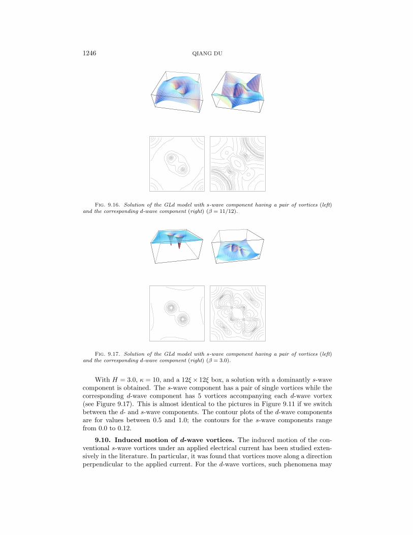
Fig. 9.17. Solution of the GLd model with s-wave component having a pair of vortices (left)and the corresponding d-wave component (right) (β = 3.0).

With H = 3.0, κ = 10, and a 12ξ× 12ξ box, a solution with a dominantly s-wavecomponent is obtained. The s-wave component has a pair of single vortices while thecorresponding d-wave component has 5 vortices accompanying each d-wave vortex(see Figure 9.17). This is almost identical to the pictures in Figure 9.11 if we switchbetween the d- and s-wave components. The contour plots of the d-wave componentsare for values between 0.5 and 1.0; the contours for the s-wave components rangefrom 0.0 to 0.12.

9.10. Induced motion of d-wave vortices. The induced motion of the con-ventional s-wave vortices under an applied electrical current has been studied exten-sively in the literature. In particular, it was found that vortices move along a directionperpendicular to the applied current. For the d-wave vortices, such phenomena may


not be duplicated. Here, we present some numerical results based on a high-κ simpli-fication of the time-dependent d-wave GL equations.

Fig. 9.18. Motion of d-wave vortices under an applied current with β = 0.25. (Top: the d-wavecomponent. Bottom: the s-wave component).

Fig. 9.19. Motion of d-wave vortex lattice under an applied current with β = 0.25.

0 0.2 0.4 0.6 0.8 1 1.2 1.4 1.60

0.01

0.02

0.03

0.04

0.05

0.06

0.07

0.08

0.09

0.1

Fig. 9.20. Difference of angles between the moving path of d-wave vortices and the conventionals-wave vortices.

In Figure 9.18, we give a few contour plots of the magnitude of the order param-eters when the applied current is aligned with the horizontal axis. In Figure 9.19,we show some contour plots of the magnitude of the d-wave component of the orderparameters for a vortex lattice when the applied current is aligned with the diagonalof the square sample.

Finally, by maintaining the strength of a constant applied electrical current whilevarying the angle of the current with respect to a square sample, we have measuredthe differences between the averaged angle of motion path for the d-wave vortices andthat of the conventional s-wave vortices. These data are shown in Figure 9.20. Wesee that the difference peaks when the current is aligned with the diagonals of thesquare; there is no difference when the current is aligned with the sides of the square.

1248 QIANG DU

10. Conclusions. In this paper, we have studied various issues related to an(s + d)-GL model for some high-Tc superconductors with d-wave or (s + d)-wavepairing. In doing so, we also wish to bring the new GLd models to the attention ofmore applied mathematicians and computational scientists. The determination of thepairing symmetry is a fundamental issue in the studies of high-Tc superconductivity.The GLd-type models may be a useful tool for the study of vortex motion in high-Tcmaterials. The numerical experiments presented in the paper are very preliminary.Although some of the results confirm findings of previous studies of the d-wave vor-tices, there are also a number of results illustrating novel features that have not beendiscussed in the literature. They demonstrate the existence of various exotic vortexstructures in the d-wave and (s+d)-wave vortices. Many important questions remainto be answered, e.g., a detailed study of the phase diagram in relation to the strengthof the applied magnetic field including the characterization of the lower and uppercritical fields. Certainly there are many more debatable issues for the use of GLdmodels to examine the pairing symmetry in high-Tc materials. Further mathematicaland computational studies will no doubt lead to a better understanding of the modelsand will help physicists in the study of high-Tc superconductivity.

Acknowledgments. The author would like to thank Dr. Z. D. Wang of thePhysics Department at Hong Kong University for bringing the problem of the d-wavepairing to his attention. The author also acknowledges communications from Dr. C.Ting of the Texas Center of Superconductivity (TcSUH), University of Houston, andfrom Drs. J. Clem and V. Kogan of the Ames National Laboratory and Iowa StateUniversity. Finally, the author would like to thank an anonymous referee for bringingadditional references on d-wave superconductors to the author’s attention.

REFERENCES

[1] S. Chapman, S. Howison, and J. Ockendon, Macroscopic models of superconductivity, SIAMRev., 34 (1992), pp. 529–560.

[2] S. Chapman, Q. Du, M. Gunzburger, and J. Peterson, Simplified Ginzburg–Landau modelsfor superconductivity valid for high kappa and high fields, Adv. Appl. Math., 5 (1995),pp. 193–218.

[3] S. Chapman and G. Richardson, Motion and homogenization of vortices in anisotropic Type-II superconductors, SIAM J. Appl. Math, 58 (1998), pp. 587–606.

[4] Z. Chen and K.-H. Hoffmann, Numerical studies of a nonstationary Ginzburg–Landau modelfor superconductivity, Adv. Math. Sci. Appl., 5 (1994), pp. 363–389.

[5] M. Doria, J. Gubernatis, and D. Rainer, Solving the Ginzburg–Landau equations by simu-lated annealing, Phys. Rev. B, 41 (1990), pp. 6335–6340.

[6] Q. Du, Finite element methods for the time dependent Ginzburg–Landau model of supercon-ductivity, Comput. Math. Appl., 27 (1994), pp. 119–133.

[7] Q. Du, Global existence and uniqueness of solutions of the time-dependent Ginzburg–Landaumodel for superconductivity, Appl. Anal., 53 (1994), pp. 1–17.

[8] Q. Du, Discrete gauge invariant approximations of a time-dependent Ginzburg–Landau Modelfor superconductivity, Math. Comp., 67 (1998), pp. 965–986.

[9] Q. Du and P. Gray, High-kappa limits of the time-dependent Ginzburg–Landau model, SIAMJ. Appl. Math., 56 (1996), pp. 1060–1093.

[10] Q. Du, M. Gunzburger, and J. Peterson, Analysis and approximation of the Ginzburg–Landau model for superconductivity, SIAM Rev., 34 (1992), pp. 54–81.

[11] Q. Du, M. Gunzburger, and J. Peterson, Solving the Ginzburg–Landau equations by finiteelement methods, Phys. Rev. B, 46 (1992), pp. 9027–9034.

[12] Q. Du, M. Gunzburger, and J. Peterson, Computational simulation of type-II supercon-ductivity including pinning phenomena, Phys. Rev. B, 51 (1995), pp. 16194–16203.


[13] F.-H. Lin and Q. Du, Ginzburg–Landau vortices: Dynamics, pinning and hysteresis, SIAM J.Math. Anal., 28 (1997), pp. 1265–1293.

[14] Q. Du, R. Nicolaides, and X. Wu, Analysis and convergence of covolume approximation ofthe Ginzburg–Landau model of superconductivity, SIAM J. Numer. Anal., 35 (1998), pp.1049–1072.

[15] Y. Enomoto and R. Kato, Computer simulation of a two-dimensional type-II superconductorin a magnetic field, J. Phys. Condens. Matter, 3 (1991), pp. 375–380.

[16] A. Filippov, A. Radievksy, and A. Zeltser, Kinetics of vortex formation in superconductorswith d pairing, Phys. Rev. B, 54 (1996), pp. 3504–3507.

[17] M. Franz, C. Kallin, P. Soininen, A. Berlinsky, and A. Fetter, Vortex state in a d-wavesuperconductor, Phys. Rev. B, 53 (1996), pp. 5795–5814.

[18] L. Freitag, M. Jones, and P. Plassmann, New Techniques for Parallel Simulation of HighTemperature Superconductors, MCS preprint, Argonne National Laboratory, Argonne, IL,1994.

[19] V. Ginzburg and L. Landau, On the theory of Superconductivity, Zh. Eksper. Teoret. Fiz.,20 (1950), pp. 1064–1082 (in Russian). Men of Physics: L. D. Landau, I, D. ter Haar, ed.,Pergamon, Oxford, 1965, pp. 138–167 (in English).

[20] R. Heeb, A. Otterlo, M. Sigrist, and G. Blatter, Vortices in d-wave superconductors,Phys. Rev. B, 54 (1996), pp. 9385–9398.

[21] R. Joynt, Upward curvature of Hc2 in high-Tc superconductors: Possible evidence for s + dpairing, Phys. Rev. B, 41 (1990), pp. 4271–4277.

[22] F.-H. Lin, Some dynamic properties of Ginzburg–Landau vortices, Comm. Pure Appl. Math.,49 (1996), pp. 323–359.

[23] F.-H. Lin, Solutions of Ginzburg–Landau equations and critical points of the renormalizedenergy, Ann. Inst. H. Poincare Anal. Non Lineaire, 12 (1995), pp. 599–622.

[24] F. Liu, M. Mondello, and N. Goldenfeld, Kinetics of the superconducting transition, Phys.Rev. Lett., 66 (1991), pp. 3071–3074.

[25] Y. Ren, J. Xu, and C. Ting, Ginzburg–Landau equations for mixed s+d symmetry supercon-ductors, Phys. Rev. B, 53 (1996), pp. 2249–2252.

[26] Q. Tang and S. Wang, Ginzburg–Landau Equations of Superconductivity, preprint, 1995.[27] M. Tinkham, Introduction to Superconductivity, McGraw-Hill, New York, 1975.[28] C. Tsuei, J. Kirtley, M. Rupp, J. Sun, A. Gupta, M. Ketchen, C. Wang, Z. Ren, J.

Wang, and M. Bhushan, Pairing symmetry in single-layer tetragonal T l2Ba2CuO6+δ

superconductors, Science, 271 (1996), pp. 329–332.[29] Q. Wang and Z. D. Wang, Vortex state and dynamics of a d-wave superconductor: Finite-

element analysis, Phys. Rev. B, 55 (1997), pp. 11756–11765.[30] Z. D. Wang and Q. Wang, Simulating the time-dependent dx2−y2 Ginzburg–Landau equations

using the finite-element method, Phys. Rev. B, 54 (1996), pp. R15645–15648.[31] J. Xu, Y. Ren, and C. Ting, Structures of single vortex and vortex lattice in a d-wave super-

conductor, Phys. Rev. B, 53 (1996), pp. R2991–R2993.[32] W. Xu, Y. Ren, and C. Ting, Ginzburg–Landau equations for a mixed s+ d symmetry super-

conductor with nonmagnetic impurities, Phys. Rev. B, 53 (1996), pp. 12481–12495.[33] Y. Yang, Boundary value problems of the Ginzburg–Landau equations, Proc. Roy. Soc. Edin-

burgh, 114A (1990), pp. 355–365.[34] E. Dagotto, Correlated electrons in high-temperature superconductors, Rev. Mod. Phys., 66

(1994), p. 763.[35] Y. Ren, J. Xu, and C. Ting, Ginzburg–Landau equations and vortex structure of a dx2−y2

superconductor, Phys. Rev. Lett., 74 (1995), p. 3680.[36] Y. Ren, J. Xu, and C. Ting, Spontaneous generation of s-wave component in a purely d-wave

superconductor, J. Phys. Chem. Solids, 56 (1995), p. 1749.[37] W. Kim and C. Ting, Ginzburg–Landau Equations for a d-Wave Superconductor with Para-

magnetic Impurities, preprint, TcSUH, 1997.[38] J. Xu, Y. Ren, and C. Ting, Ginzburg–Landau theory of a d-wave superconductor with

mass anisotropy–pairing symmetry and vortex structures, Internat. J. Modern Phys. B,10 (1996), p. 2699.

[39] D. Feder and C. Kallin, Microscopic derivation of the Ginzburg–Landau equations for ad-wave superconductor, Phys. Rev. B, 55 (1997), pp. 559–574.

[40] D. Feder, A. Beardsall, A. Berlinsky, and C. Kallin, Twin boundaries in d-wave super-conductors, Phys. Rev. B, 56 (1997), pp. 5751R–5754R.

[41] Q. Han and L. Zhang, Ginzburg–Landau theory and vortex structure for a d+ s-wave super-conductor with orthorhombic distortion, Phys. Rev. B, 56 (1997), pp. 11942–11951.

1250 QIANG DU

[42] K. Maki and M. Beal-Monod, Ginzurg-Landau equation and upper critical field in anisotropic(d+ s)-wave superconductivity, Phys. Rev. B, 55 (1997), p. 11730.

[43] G. Volovik, Fermionic entropy of the vortex state in d-wave superconductors, JETP Lett., 65(1997), p. 491.

[44] N. Kopnin and G. Volovik, Singularity of the vortex density of states in d-wave supercon-ductors, JETP Lett., 64 (1996), p. 690.

[45] D. Chang, C. Mou, B. Rosenstein, and C. Wu, Static and dynamical anisotropy effects inmixed state of d-wave superconductors, Phys. Rev. B, 57 (1998), pp. 7955–7969.

[46] D. Chang, C. Mou, B. Rosenstein, and C. Wu, The Effect of Anisotropy on Vortex LatticeStructure and Flux Flow in d-Wave Superconductors, LANL preprint, cond-mat/9704116,Los Alamos National Laboratory, Los Alamos, NM,

[47] J. Alvarez, D. Dominguez, and C. Balseiro, Dynamics of d-Wave Vortices: Angle-Dependent Nonlinear Hall Effect, LANL preprint cond-mat/9704188, Los Alamos NationalLaboratory, Los Alamos, NM,

[48] M. Kulic and V. Oudovenko, Why Is d-Wave Pairing in HTS Robust in the Presence ofImpurities?, LANL preprint cond-mat/9612211, Los Alamos National Laboratory, LosAlamos, NM,

[49] J. Shiraishi, M. Kohmoto, and K. Maki, Novel Vortex Lattice Transition in d-Wave Su-perconductors, LANL preprint cond-mat/9802067, Los Alamos National Laboratory, LosAlamos, NM,

[50] C. Kuebert and P. Hirschfeld, Vortex contribution to specific heat of dirty d-wave super-conductors: Breakdown of scaling, Solid State Comm., 105 (1998), p. 459.

[51] P. Hirschfeld and W. Putikka, Theory of thermal conductivity in Y Ba2Cu3O7−δ, Phys.Rev. Lett., 77 (1996), pp. 3909–3912.

[52] M. Franz and Z. Tesanovik, Self-Consistent Electronic Structure of a dx2−y2 and a dx2−y2 +idxy Vortex, LANL preprint cond-mat/9710258, Los Alamos National Laboratory, LosAlamos, NM,

[53] Y. Morita, M. Kohmoto, and K. Maki, Quasi-particle Spectra around a Single Vortex ind-Wave Superconductor, LANL preprint cond-mat/9608078, Los Alamos National Labo-ratory, Los Alamos, NM,

[54] N. Enomoto, M. Ichioka, and K. Machida, Ginzburg–Landau theory for d-wave pairing andfourfold symmetric vortex core structure, J. Phys. Soc. Japan., 66 (1997), p. 204.

[55] T. Dahm, D. Manske, and L. Tewordt, Charge-density-wave and superconductivity d-wavegaps in the Hubbard model for underdoped high-Tc cuprates, Phys. Rev. B, 56 (1997),pp. R11419–R11422.

[56] M. Plakida, V. Oudovenko, P. Horsch, and A. Liechtenstein, Superconducting pairing ofspin polarons in the t-J model, Phys. Rev. B, 55 (1997), pp. R11997–R12000.

[57] S. Dorbolo, M. Aisloos, and M. Houssa, Electronic specific heat of superconductors withVan Hove singularities: Effects of a magnetic field and thermal fluctuations, Phys. Rev.B, 57 (1998), pp. 5401–5411.

[58] D. Van Harlingen, RMP Colloquium: Phase-sensitive tests of the symmetry of the pair-ing state in the high-temperature superconductors—Evidence for dx2−y2 symmetry, Rev.Modern, Phys., 67 (1995), p. 515.

Documents

STUDIES OF A GINZBURG{LANDAU MODEL FOR d · STUDIES OF A GINZBURG{LANDAU MODEL FOR d-WAVE SUPERCONDUCTORS QIANG DUy SIAM J. APPL. MATH. °c 1999 Society for Industrial and Applied