Embed Size (px)
Citation preview


STUDIES IN APPLIED AND FUNDAMENTAL
QUANTUM MECHANICS: CRYPTOGRAPHY,
TOMOGRAPHY, HOLOGRAPHY AND DUALITY
Eliot Bolduc
Thesis Submitted to the Faculty of Graduate and Postdoctoral Studies
In partial fulfillment of the requirements
for the degree of
Master of Science in Physics
Ottawa-Carleton Institute of Physics
Department of Physics
University of Ottawa
c© Eliot Bolduc, Ottawa, Canada, 2013

Abstract
This thesis encompasses a collection of four pieces of work on wave-particle dual-
ity, weak-value-assisted tomography, high-dimensional quantum key distribution, and
phase-only holograms. Although there are connections between the subjects, the par-
ticipants of each project conducted them independently of the other projects. In the
work on duality, we derive a novel duality relation, and we sketch a thought experi-
ment that leads to an apparent violation of the duality principle. This work improves
the current fundamental understanding of duality and outlines the experimental pro-
cedure for new tests of the duality principle. In the project on tomography, we
perform a state determination procedure on the polarization state of light by measur-
ing an informationally complete set of weak values, and we study the accuracy of the
method. Our experiment provides a proof-of-principle demonstration of weak-value-
assisted tomography on a two-dimensional state, and our study shows the pros and
cons of the method compared to standard tomography. In the quantum cryptography
project, we optimize the parameters of an experimental implementation of the key
features of a quantum cryptography system where two parties share information with
the orbital angular momentum degree of freedom of entangled photon pairs. Our
analysis gives the pathway to efficient implementations of high-dimensional quantum
key distribution systems. Finally, in the work on holography, we establish the exact
solution to the encryption of both phase and amplitude of an optical spatial transverse
mode in a phase-only hologram, and experimentally demonstrate its application to
spatial light modulators. This work allows for the accurate generation and detection
of arbitrary transverse spatial modes. The four projects provide improvements on
measurement procedures in applied and fundamental quantum mechanics.
ii
Resume
Cette these comprend quatre projets portant soit sur les fondements ou les appli-
cations de la mecanique quantique. Ils portent notamment sur la dualite onde-
particule, la tomographie d’etats quantiques avec des valeurs faibles, la distribution
de clefs quantiques en hautes dimensions, ainsi que sur les hologrammes a modula-
tion de phase. Bien qu’il y ait quelques liens entre les projets, ils ont ete complete
independamment les uns des autres. En premier lieu, apres la derivation d’une
nouvelle relation de dualite, nous expliquons une violation apparente de la dualite
onde-particule. En deuxieme lieu, nous appliquons une procedure de tomographie
quantique sur un etat de polarisation de la lumiere en mesurant des valeurs faibles.
En troisieme lieu, nous implementons un systeme de cryptographie quantique selon
lequel deux interlocuteurs partagent de l’information avec le moment angulaire or-
bital de paires de photons intriques. Finalement, nous demontrons la solution exacte
a l’encodage simultane de la phase et de l’amplitude d’un mode spatial transverse
dans un hologramme a modulation de phase.
iii

Contents
Abstract ii
Resume iii
List of Figures vii
1 Introduction 4
2 A fair-sampling perspective on an apparent violation of duality 7
2.1 Introduction . . . . . . . . . . . . . . . . . . . . . . . . . . . . . . 7
2.1.1 Duality and its apparent violation . . . . . . . . . . . . . . 7
2.1.2 Fair sampling . . . . . . . . . . . . . . . . . . . . . . . . . 8
2.1.3 Summary . . . . . . . . . . . . . . . . . . . . . . . . . . . 8
2.2 The duality relations . . . . . . . . . . . . . . . . . . . . . . . . . 8
2.2.1 The Greenberger-Yasin relation . . . . . . . . . . . . . . . 9
2.2.2 The Englert-Bergou relation . . . . . . . . . . . . . . . . . 9
2.2.3 Our new tight duality relation . . . . . . . . . . . . . . . . 10
2.3 A theoretical example of an apparent violation . . . . . . . . . . . 11
2.3.1 The theory of degenerate spontaneous parametric down-
conversion . . . . . . . . . . . . . . . . . . . . . . . . . . . 12
2.3.2 Theoretical description of our thought experiment . . . . . 13
2.4 Conclusions . . . . . . . . . . . . . . . . . . . . . . . . . . . . . . 18
2.5 Supplementary material . . . . . . . . . . . . . . . . . . . . . . . 19
2.5.1 Details of our numerical calculations . . . . . . . . . . . . 19
2.5.2 Impact of the HG01 pump mode . . . . . . . . . . . . . . . 20
2.5.3 An experimental confirmation . . . . . . . . . . . . . . . . 22
3 Weak-value-assisted tomography 25
3.1 Introduction to standard quantum state tomography . . . . . . . 25
iv

CONTENTS v
3.2 Accuracy of weak-value-assisted tomography . . . . . . . . . . . . 27
3.2.1 Relation Between Weak Values and the State-Vector . . . 28
3.2.2 Exact model of weak-coupling measurements . . . . . . . . 29
3.2.3 Average fidelity between the initial state and the mea-
sured state . . . . . . . . . . . . . . . . . . . . . . . . . . . 31
3.2.4 Conclusions . . . . . . . . . . . . . . . . . . . . . . . . . . 33
3.3 Publication: Full characterization of polarization states of
light via direct measurement . . . . . . . . . . . . . . . . . . . . . 34
3.4 Publication: Supplementary information . . . . . . . . . . . . . 40
4 Optimal quantum key distribution with photons entangled
in orbital angular momentum 45
4.1 Introduction to quantum key distribution . . . . . . . . . . . . . . 45
4.1.1 The BB84 protocol . . . . . . . . . . . . . . . . . . . . . . 45
4.1.2 The Ekert protocol . . . . . . . . . . . . . . . . . . . . . . 46
4.2 Introduction to orbital angular momentum states of light . . . . . 47
4.3 Publication: Secure information capacity of photons entan-
gled in many dimensions . . . . . . . . . . . . . . . . . . . . . . . 48
5 Simultaneous intensity and phase encryption on a hologram 52
5.1 Introduction to phase-only holograms . . . . . . . . . . . . . . . . 52
5.1.1 Intensity masking techniques . . . . . . . . . . . . . . . . . 52
5.2 Publication: Exact solution to simultaneous intensity and
phase encryption with a single phase-only hologram . . . . . . . . 55
5.3 Supplementary information . . . . . . . . . . . . . . . . . . . . . 59
5.3.1 Pixelated holograms . . . . . . . . . . . . . . . . . . . . . 59
5.3.2 Implications on the results of chapter 4 . . . . . . . . . . . 59
5.3.3 Computer program . . . . . . . . . . . . . . . . . . . . . . 59
6 Conclusions and Outlook 60
A MATLAB code for our thought experiment on duality 63
A.0.4 Function “pumpterm” . . . . . . . . . . . . . . . . . . . . 67
A.0.5 Function “phasematchingterm” . . . . . . . . . . . . . . . 67
B MATLAB code for computer-generated holograms 68

CONTENTS vi
B.0.6 Function “ComputeHologram” . . . . . . . . . . . . . . . . 69
B.0.7 Function “LG mode” . . . . . . . . . . . . . . . . . . . . . 70
Bibliography 72

List of Figures
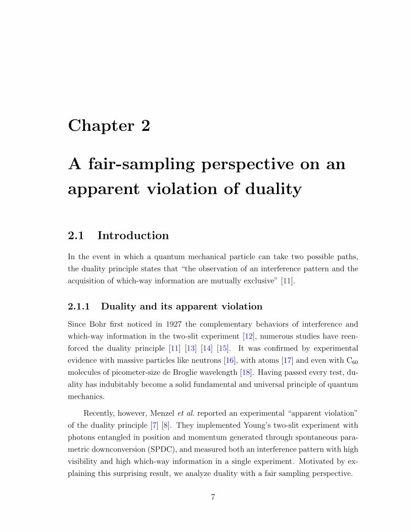
2.1 Our thought experiment, inspired by Menzel et al.. Photon
pairs entangled in position and momentum are generated through
degenerate SPDC with a type I crystal and a wide Gaussian
pump mode. The signal and idler photons are separated by
a 50/50 beam-splitter. On the path of the signal photon, the
plane of the crystal is imaged with unit magnification to the
plane of a two-slit mask made of slit T at rs,y = d/2 and slit
B at rs,y = −d/2. While the signal photon traverses the mask,
the idler photon is collected by an optical fiber (MMF), whose
input facet is in the image plane of the crystal and centered at
ri,y = d/2 and ri,x = 0. Through position correlations, we gain
which-slit information of the signal photon upon detection of
the idler photon. We collect the signal photons in the far-field
of the mask with a scanning point detector (SPD). All measure-
ments are performed in coincidence, such that the interference
pattern of the signal photons is conditional on the detection of
idler photons. In a real experiment, interference filters would
be placed before the detectors to ensure degenerate SPDC. . . . . 14
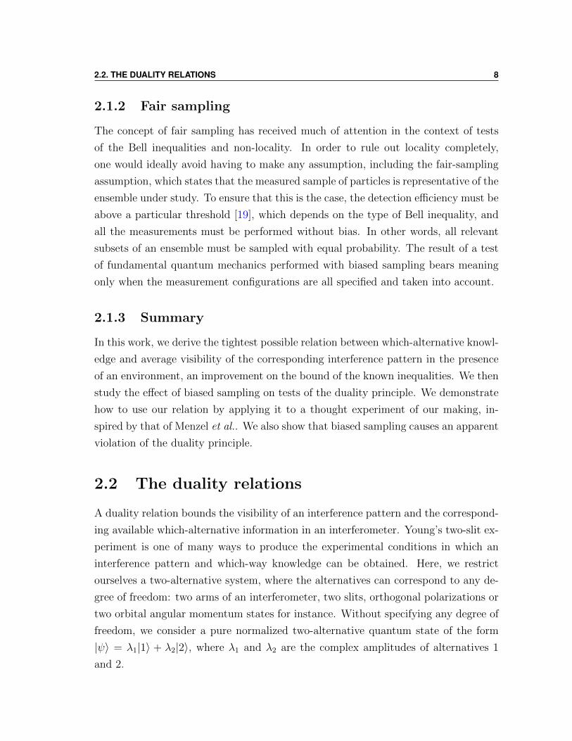
2.2 Theoretically predicted interference pattern of the signal pho-
tons in the far-field of the two-slit mask conditioned on the
detection of idler photons: P ′W (ps|φi). . . . . . . . . . . . . . . . . 15
vii

LIST OF FIGURES viii
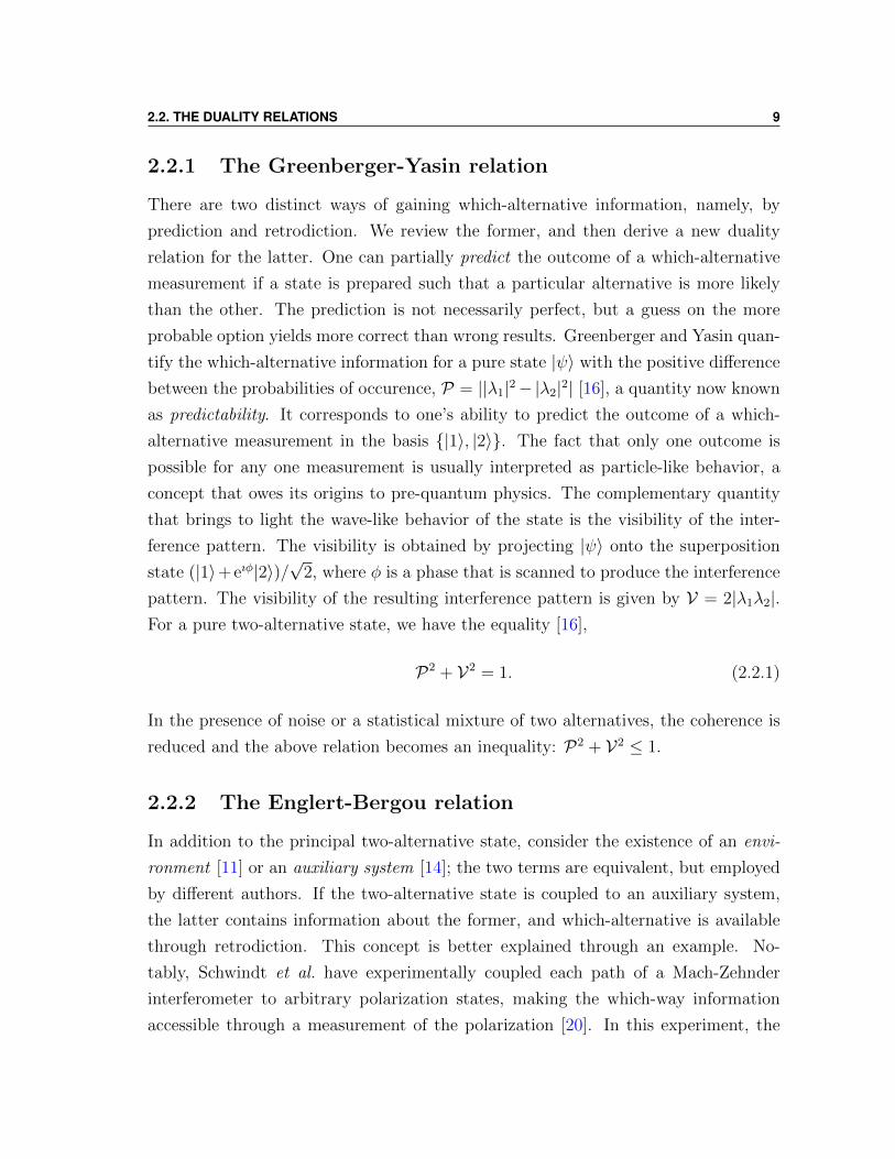
2.3 Plot of (blue) the probability distribution MW (ps,x) of the sig-
nal photons in wavevector space conditional on the detection
of idler photons. The scale for MW (ps,x) has been modified to
fit the distribution on the same graph as the two other curves,
which correspond to (red) the predictability P and (green) the
visibility V as a function of the degree of freedom of the envi-
ronment. These quantities satisfy the equality P2 +V2 = 1 for
all values of ps,x. . . . . . . . . . . . . . . . . . . . . . . . . . . . 18
2.4 Far-field distribution of the signal photons conditional on the
detection of idler photons when a) slit B is blocked and b) slit T
is blocked. The photons arriving at position |ps,x| = 0.5 µm−1
almost exclusively come from slit T, whereas photons arounds
|ps,x| = 0 µm−1 do not carry much which-slit information, if
any, which is consistent with the observed high visibility at
this position in the superposition state distribution P ′W (ps|φi)in Fig. 2.2. The scale of the distribution of P ′B(ps|φi) is divided
by 5 for better image contrast. . . . . . . . . . . . . . . . . . . . . 19
2.5 Conditional interference pattern, P ′W (ps|φi), obtained in our
thought experiment with an HG01 pump mode. The visibility
of the interference pattern is lower than for the HG00 pump
mode (Fig. 2.2). While the number of bright fringes on the
top or bottom of the ring is odd for the HG00 pump mode, it
is even for the HG01 pump mode. . . . . . . . . . . . . . . . . . . 20
2.6 (blue) Marginal probability distribution of the signal photon,
(red) predictability and (green) visibility as a function of the
degree of freedom of the environment for an HG01 pump mode.
Although the visibility is generally lower than for a gaussian
pump mode, the predictability is higher. . . . . . . . . . . . . . . 21

LIST OF FIGURES ix
2.7 (Exp) Experimentally recorded and (Th) theoretically obtained
distribution of the singles in the near-field of the two-slit mask.
In the experiment, a microscope cover slip induces a π-jump
in the middle of the pump beam, creating an HG01-like mode.
We simply chose an HG01 pump mode in our model. The real
slit separation is 345±50 µm and the magnification from the
plane of the crystal to that of the camera is 3.0±0.5, but the
scale is shown for a unit magnification for both the experiment
and the theory. . . . . . . . . . . . . . . . . . . . . . . . . . . . . 22
2.8 a) Experimental setup that we use to record images of the
single counts. We insert a microscope cover slip in half of the
pump beam in order to control the phase difference between
each half. The plane of the crystal is imaged to a two-slit mask
with a magnification of 3. In the configuration shown here, an
EMCCD camera is located in the far-field of the mask, but we
also record the near-field by adding a second lens (not shown)
between the mask and the camera. We control the bandwidth
of the SPDC light with a 10-nm interference filter. Shown
are the experimentally recorded (Exp) and (Th) theoretically
modelled distribution of the singles in the far-field of the two-
slit mask for an b) HG00 and c) HG01 pump mode. For the
latter, we observe the characteristic intensity dip in the middle
of each interference pattern, on the top and the bottom. In
other words, the number of bright fringes goes from being odd
to even when the pump mode changes from HG00 to HG01. . . . 23
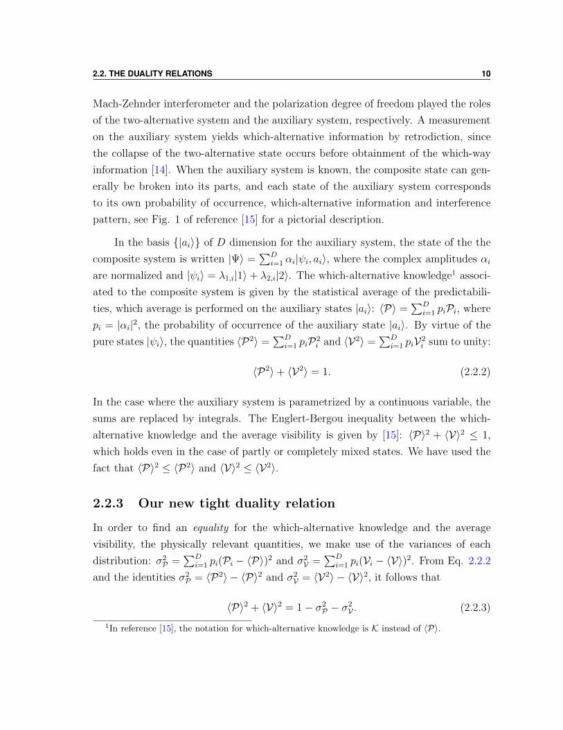
3.1 Fidelity between the initial state |Ψ〉 and the measured state
|Ψm〉 through the tomographic process with weak values as
function of the strength of the measurement. For a measure-
ment strength of s = 2, the distance between the eigenvalues of
|1〉 and |2〉 (2d) is equal to the 1/e width of the initial pointer.
In this strong measurement regime, the eigenvalues are distin-
guishable, and the phase information is lost. . . . . . . . . . . . . 32

CV
Publications:
1. J. Leach, E. Bolduc, D. J. Gauthier, and R. W. Boyd, “Secure informationcapacity of photons entangled in many dimensions,” Physical Review A, vol. 85,no. 6, p. 060304, 2012
2. J. Z. Salvail, M. Agnew, A. S. Johnson, E. Bolduc, J. Leach, and R. W. Boyd,“Full characterization of polarization states of light via direct measurement,”Nature Photonics, vol. 7, pp. 316–321
3. E. Bolduc, N. Bent, E. Santamato, E. Karimi, and R. W. Boyd, “Exact so-lution to simultaneous intensity and phase masking with a single phase-onlyhologram,” Optics Letters, 2013, [Accepted, but not officially published beforesubmission of the thesis]
Conference Proceedings
1. E. Bolduc, J. Leach, and R. Boyd, “The secure information capacity of pho-tons entangled in high dimensions,” in Quantum Information and Measurement,Optical Society of America, 2012
2. E. Bolduc, J. Leach, and R. W. Boyd, “The secure information capacity of pho-tons entangled in high dimensions,” in Frontiers in Optics 2012/Laser ScienceXXVIII, p. FTh4B.7, Optical Society of America, 2012
3. E. Bolduc, J. Leach, F. Miatto, G. Leuchs, and R. Boyd, “How to achieve highvisibility and high which-way information in a single experiment,” in Physicsof Quantum Electronics, 2013
1

Statement of originality and
collaborative contributions
To the best of his knowledge, the author states that the four projects described in this
Master’s thesis constitute original research in the field of physics. In the following
paragraphs, we provide the collaborative contributions of each participant in the
projects, which are presented in chronological order of start date.
The work on quantum cryptography described in chapter 4 was mainly done by
Eliot Bolduc and Dr Jonathan Leach, who was a research assistant in the group of
Prof. Robert W. Boyd at the time. J. Leach had the idea, initiated the work and
designed the experiment. Both J. Leach and E. Bolduc performed the experiment
and analyzed the data. E. Bolduc theoretically generalized the results. The work
resulted in publication 1. All authors contributed to writing the paper.
Jeff Salvail, who was a Coop student at the time, initiated the work on tomog-
raphy with weak values described in chapter 3. It resulted in publication 2. The
experiment was designed by J. Salvail, A. Johnson, J. Leach and E. Bolduc. The
experiment was performed mostly by J. Salvail and the results were also analyzed
by J. Salvail. Megan Agnew and Allan Johnson, two undergraduate students at the
time, helped in the experiment. All authors participated to writing the paper. E.
Bolduc later theoretically elaborated on the accuracy of the method.
Prof. R. W. Boyd initiated the work of chapter 2. J. Leach had an intuitive
explanation for the apparent violation reported by Menzel et al. [7]. E. Bolduc later
derived a novel duality relation and precisely explained their results.
Ebrahim Karimi, a post-doctoral fellow, had the idea and derived the theory of
the hologram encryption method of chapter 5. E. Karimi and E. Bolduc designed the
experiment. E. Bolduc wrote the hologram encryption programs. E. Bolduc and Nico-
2

LIST OF FIGURES 3
las Bent performed the experiment. All authors contributed to writing publication 3.
Chapter 1
Introduction
The author decided to take part in four projects which developed in the course of his
Master’s degree. Each project was conducted independently of the others, and suc-
cessfully completed. They all provide advances in fundamental or applied quantum
mechanics. In each body of work, we study the impact of the measurement procedure
on the outcome of an experiment and suggest or implement possible improvements.
Instead of the chronological order, we present the four projects in order of the more
fundamental to the more applied: wave-particle duality in the presence of an environ-
ment, weak-value-assisted tomography, high-dimensional quantum key distribution
and modal encryption of phase-only holograms.
According to wave-particle duality, a building block of fundamental quantum
mechanics, the wave-like and particle-like behaviors of a quantum state in an inter-
ferometer are mutually exclusive. Wave-like behavior refers to the observation of
an interference pattern, while particle-like behavior alludes to the which-way infor-
mation. If this information is completely available, no interference pattern can be
observed. In chapter 2, we derive a new duality relation that bounds the visibility
of an interference pattern and the which-way knowledge in an interferometer where
two paths are coupled to an auxiliary system. We then show how biased sampling
of a subset of the auxiliary system can lead to an apparent violation of the duality
principle. This work improves the current understanding of duality and helps to solve
the case of a controversial experiment on fundamental quantum mechanics [7, 8].
The experimental determination of a quantum state is in general not a straight-
forward task because a quantum state-vector is specified with complex coefficients, but
the outcome of a measurement is always real-valued. In standard quantum state to-
4

5
mography, the state-vector is unambiguously identifiable by the real-valued outcomes
of an informationally complete set of projective measurements. Alternatively, one
can retrieve the state-vector by measuring weak values instead of projections [9, 10].
In chapter 3, we provide the proof-of-principle demonstration of weak-value-assisted
tomography of a two-dimensional state, namely, the polarization state of light. We
also study the accuracy of the method as a function of the weakness of the measure-
ments. The method is very direct in that the coefficients of the state under study are
proportional to the weak values, and no post-measurement processing is required.
Quantum key distribution (QKD) protocols offer the holy grail of cryptogra-
phy: absolute security in a communication channel between two parties. The laws of
quantum mechanics forbid perfect cloning of a state, and, as a consequence, eaves-
dropping inherently introduces noise into a QKD system. Absolute security is only
ensured when the observed noise level is below the eavesdropping-caused threshold. In
a realistic QKD system, noise is always present, and for the sake of absolute security,
it must be considered as coming from an eavesdropper. In chapter 4, we discuss our
implementation of important elements of a secure quantum communication channel
with photons entangled in the orbital angular momentum (OAM) degree of freedom.
In principle, the OAM space is discrete and infinite, and the information encoded in
a photon pair is unbounded. In practice, we consider a finite subset of this infinite
space. The ability to generate a high number of different OAM modes with high
signal to noise ratio is technologically challenging. Given a set of experimental pa-
rameters such as detection efficiency and photon production rate, we find the OAM
subspace dimension that maximizes the secure information shared between two par-
ties. This work opens up the way for efficient implementations of QKD systems in
high dimensions.
Computer generated phase-only holograms, such as spatial light modulators, can
be used to control both the phase and the intensity profile of an optical beam. An
important application of phase-only holograms is the generation of arbitrary trans-
verse spatial modes. Numerous encryption methods already exist to perform such a
task, but their theoretical result is always an approximation to the desired transverse
spatial mode. In chapter 5, we provide the exact solution to simultaneous phase and
intensity encryption of a phase-only hologram, such that the result is in principle
exactly equal to the desired mode. We expect that our method will have a high

6
impact in optical communications, quantum tomography of transverse spatial modes
and experiments in fundamental quantum mechanics.
Chapter 2
A fair-sampling perspective on an
apparent violation of duality
2.1 Introduction
In the event in which a quantum mechanical particle can take two possible paths,
the duality principle states that “the observation of an interference pattern and the
acquisition of which-way information are mutually exclusive” [11].
2.1.1 Duality and its apparent violation
Since Bohr first noticed in 1927 the complementary behaviors of interference and
which-way information in the two-slit experiment [12], numerous studies have reen-
forced the duality principle [11] [13] [14] [15]. It was confirmed by experimental
evidence with massive particles like neutrons [16], with atoms [17] and even with C60
molecules of picometer-size de Broglie wavelength [18]. Having passed every test, du-
ality has indubitably become a solid fundamental and universal principle of quantum
mechanics.
Recently, however, Menzel et al. reported an experimental “apparent violation”
of the duality principle [7] [8]. They implemented Young’s two-slit experiment with
photons entangled in position and momentum generated through spontaneous para-
metric downconversion (SPDC), and measured both an interference pattern with high
visibility and high which-way information in a single experiment. Motivated by ex-
plaining this surprising result, we analyze duality with a fair sampling perspective.
7
2.2. THE DUALITY RELATIONS 8
2.1.2 Fair sampling
The concept of fair sampling has received much of attention in the context of tests
of the Bell inequalities and non-locality. In order to rule out locality completely,
one would ideally avoid having to make any assumption, including the fair-sampling
assumption, which states that the measured sample of particles is representative of the
ensemble under study. To ensure that this is the case, the detection efficiency must be
above a particular threshold [19], which depends on the type of Bell inequality, and
all the measurements must be performed without bias. In other words, all relevant
subsets of an ensemble must be sampled with equal probability. The result of a test
of fundamental quantum mechanics performed with biased sampling bears meaning
only when the measurement configurations are all specified and taken into account.
2.1.3 Summary
In this work, we derive the tightest possible relation between which-alternative knowl-
edge and average visibility of the corresponding interference pattern in the presence
of an environment, an improvement on the bound of the known inequalities. We then
study the effect of biased sampling on tests of the duality principle. We demonstrate
how to use our relation by applying it to a thought experiment of our making, in-
spired by that of Menzel et al.. We also show that biased sampling causes an apparent
violation of the duality principle.
2.2 The duality relations
A duality relation bounds the visibility of an interference pattern and the correspond-
ing available which-alternative information in an interferometer. Young’s two-slit ex-
periment is one of many ways to produce the experimental conditions in which an
interference pattern and which-way knowledge can be obtained. Here, we restrict
ourselves a two-alternative system, where the alternatives can correspond to any de-
gree of freedom: two arms of an interferometer, two slits, orthogonal polarizations or
two orbital angular momentum states for instance. Without specifying any degree of
freedom, we consider a pure normalized two-alternative quantum state of the form
|ψ〉 = λ1|1〉 + λ2|2〉, where λ1 and λ2 are the complex amplitudes of alternatives 1
and 2.
2.2. THE DUALITY RELATIONS 9
2.2.1 The Greenberger-Yasin relation
There are two distinct ways of gaining which-alternative information, namely, by
prediction and retrodiction. We review the former, and then derive a new duality
relation for the latter. One can partially predict the outcome of a which-alternative
measurement if a state is prepared such that a particular alternative is more likely
than the other. The prediction is not necessarily perfect, but a guess on the more
probable option yields more correct than wrong results. Greenberger and Yasin quan-
tify the which-alternative information for a pure state |ψ〉 with the positive difference
between the probabilities of occurence, P = ||λ1|2−|λ2|2| [16], a quantity now known
as predictability. It corresponds to one’s ability to predict the outcome of a which-
alternative measurement in the basis |1〉, |2〉. The fact that only one outcome is
possible for any one measurement is usually interpreted as particle-like behavior, a
concept that owes its origins to pre-quantum physics. The complementary quantity
that brings to light the wave-like behavior of the state is the visibility of the inter-
ference pattern. The visibility is obtained by projecting |ψ〉 onto the superposition
state (|1〉+eıφ|2〉)/√
2, where φ is a phase that is scanned to produce the interference
pattern. The visibility of the resulting interference pattern is given by V = 2|λ1λ2|.For a pure two-alternative state, we have the equality [16],
P2 + V2 = 1. (2.2.1)
In the presence of noise or a statistical mixture of two alternatives, the coherence is
reduced and the above relation becomes an inequality: P2 + V2 ≤ 1.
2.2.2 The Englert-Bergou relation
In addition to the principal two-alternative state, consider the existence of an envi-
ronment [11] or an auxiliary system [14]; the two terms are equivalent, but employed
by different authors. If the two-alternative state is coupled to an auxiliary system,
the latter contains information about the former, and which-alternative is available
through retrodiction. This concept is better explained through an example. No-
tably, Schwindt et al. have experimentally coupled each path of a Mach-Zehnder
interferometer to arbitrary polarization states, making the which-way information
accessible through a measurement of the polarization [20]. In this experiment, the
2.2. THE DUALITY RELATIONS 10
Mach-Zehnder interferometer and the polarization degree of freedom played the roles
of the two-alternative system and the auxiliary system, respectively. A measurement
on the auxiliary system yields which-alternative information by retrodiction, since
the collapse of the two-alternative state occurs before obtainment of the which-way
information [14]. When the auxiliary system is known, the composite state can gen-
erally be broken into its parts, and each state of the auxiliary system corresponds
to its own probability of occurrence, which-alternative information and interference
pattern, see Fig. 1 of reference [15] for a pictorial description.
In the basis |ai〉 of D dimension for the auxiliary system, the state of the the
composite system is written |Ψ〉 =∑D
i=1 αi|ψi, ai〉, where the complex amplitudes αi
are normalized and |ψi〉 = λ1,i|1〉+ λ2,i|2〉. The which-alternative knowledge1 associ-
ated to the composite system is given by the statistical average of the predictabili-
ties, which average is performed on the auxiliary states |ai〉: 〈P〉 =∑D
i=1 piPi, where
pi = |αi|2, the probability of occurrence of the auxiliary state |ai〉. By virtue of the
pure states |ψi〉, the quantities 〈P2〉 =∑D
i=1 piP2i and 〈V2〉 =
∑Di=1 piV2
i sum to unity:
〈P2〉+ 〈V2〉 = 1. (2.2.2)
In the case where the auxiliary system is parametrized by a continuous variable, the
sums are replaced by integrals. The Englert-Bergou inequality between the which-
alternative knowledge and the average visibility is given by [15]: 〈P〉2 + 〈V〉2 ≤ 1,
which holds even in the case of partly or completely mixed states. We have used the
fact that 〈P〉2 ≤ 〈P2〉 and 〈V〉2 ≤ 〈V2〉.
2.2.3 Our new tight duality relation
In order to find an equality for the which-alternative knowledge and the average
visibility, the physically relevant quantities, we make use of the variances of each
distribution: σ2P =
∑Di=1 pi(Pi − 〈P〉)2 and σ2
V =∑D
i=1 pi(Vi − 〈V〉)2. From Eq. 2.2.2
and the identities σ2P = 〈P2〉 − 〈P〉2 and σ2
V = 〈V2〉 − 〈V〉2, it follows that
〈P〉2 + 〈V〉2 = 1− σ2P − σ2
V . (2.2.3)
1In reference [15], the notation for which-alternative knowledge is K instead of 〈P〉.

2.3. A THEORETICAL EXAMPLE OF AN APPARENT VIOLATION 11
Since predictability and visibility are bounded between 0 and 1, each variance can
take a maximum value of 1/4. The RHS of Eq. 2.2.3 is thus inherently greater or
equal to 1/2. In the presence of noise or uncontrolled coupling to the environment,
the RHS of Eq. 2.2.3 becomes an upper bound to the LHS, which upper bound is as
tight as possible.
Eq. 2.2.3 holds only when all states of the environment |ai〉 are sampled with
equal probability. Since the environment is comprised of D states, the sampling
probability for any state |ai〉 should be 1/D. When this part of the fair sampling
assumption is reduced, the measured statistics do not represent the state at hand
and the RHS of Eq. 2.2.3 no longer bounds its LHS. In particular, this occurs when
selecting only a subset of the auxiliary system while rejecting the rest. For instance,
one could only measure the subset which corresponds to the highest predictability
Pmax and also the one corresponding to the maximum visibility Vmax. For non-zero
variances, the maximum value in each distribution is greater than its respective av-
erage value: Pmax > 〈P〉 and Vmax > 〈V〉. Since the quantity (P2max + V2
max) can
in principle approach 2, it is possible to observe both high predictability and high
visibility in a single experiment. This can appear to be a violation of the duality
principle, but it rather is a consequence of biased sampling in the measurement of
which-alternative information and visibility.
2.3 A theoretical example of an apparent violation
The table is now set to show the conditions that lead to an apparent violation of
duality in the context of a realistic experiment. We build a thought experiment
inspired by the work of Menzel et al.. In summary, we start from a two-photon
state generated through SPDC. One of the photons traverses a two-slit mask, while
the other is used to measured the which-slit information. We then calculate the
two-dimensional interference pattern in the far-field of the mask given that partial
which-slit information is acquired. In the two-dimensional interference pattern, one
of the dimensions acts as an auxiliary system. We calculate the quantities appearing
in Eq. 2.2.3 for a given set of experimental parameters and show the impact of
biased sampling of a subset of the auxiliary system on the outcome of the thought
experiment.

2.3. A THEORETICAL EXAMPLE OF AN APPARENT VIOLATION 12
2.3.1 The theory of degenerate spontaneous parametric down-
conversion
For our purposes, it suffices to consider the SPDC process with a type I crystal,
whose theoretical description is simpler than that of a type II crystal. When there
is no walk-off, the two-photon transverse spatial mode function of degenerate SPDC
has a simple analytical form [21] [22]. As a function of the transverse wavevectors of
the signal ps and idler pi photons with p = pxx + pyy, it is given by
Φ(ps,pi) = N E (ps + pi) F
(ps − pi
2
), (2.3.1)
where N is a normalization constant, E(p) is the angular spectrum of the pump
laser, and F is the phase-matching function. Under the assumption that the trans-
verse wavevectors of the signal and idler photons are much smaller than their total
wavevectors2, the phase-matching function is of the form F (p) = sinc(ϕ+L |p|2/kp),where ϕ is the phase mismatch parameter, L is the thickness of the crystal and kp is
the wavevector of the pump inside the crystal.
Because of momentum conservation, the signal and idler photons are anti-correlated
in transverse wavevector space. The momentum correlations are mostly determined
by the angular spectrum of the pump, while the phase-matching function dictates
the general shape of the two-dimensional probability distribution of the individual
photons, which we shall refer to as “the singles”. If the pump beam is collimated and
has infinite width at the crystal, its angular spread approaches the Dirac distribution
δ(ps − pi). In this limit, it is easy to show that the intensity profile of the singles in
the far-field of the crystal is exactly given by |F (ps,i)|2, where ps,i is the transverse
wavevector of either the signal or the idler photon.
In order to describe the position correlations in coordinate space, we perform
a 4-dimensional Fourier transform on the two-photon mode function: Ψ(rs, ri) =
FT[Φ(ps,pi)], where r = rxx + ryy is the transverse coordinate in the plane of the
crystal. Since the mode function in wavevector space is separable in (ps + pi) and
2In our thought experiment below, we have |ps|/|ks| ≈ |pi|/|ki| ≈ 0.07, where ks (ki) is the totalwavevector of the signal (idler) photon.

2.3. A THEORETICAL EXAMPLE OF AN APPARENT VIOLATION 13
(ps−pi), the mode function at the output facet of the crystal is written [23] [24] [25]
Ψ(rs, ri) = N ′E (rs + ri)F (rs − ri), (2.3.2)
where N ′ is a normalization constant, E(2r) is the transverse spatial mode of the
pump at the crystal and F (r) is the phase-matching function in coordinate space:
F (r) = (2π)−1∫
sinc(ϕ + L |p|2/kp)e−ıp·r dp. If the phase mismatch parameter is
different from zero, ϕ 6= 0, this integral has no known analytical solution and has to
be performed numerically. Its result determines the position correlations between the
signal and idler photons. In the limit of a crystal with an infinitely small thickness,
the phase-matching function in coordinate space approaches a Dirac distribution,
(F (r) → δ(r)). In this limit, the signal and idler photons are perfectly correlated in
coordinate space, and the general shape of the singles is exactly given by the intensity
profile of the pump at the crystal. However, when the thickness of the crystal is of
the same order of magnitude as the features in the transverse intensity profile of the
pump, the latter appears smeared out in the distribution of the singles3 [21].
2.3.2 Theoretical description of our thought experiment
In our thought experiment, we use a two-slit mask with a slit separation d in the
image plane of the output facet of the crystal on the signal photon side. Upon
measurement of the idler photon position, the correlations allow one to gain knowledge
about which slit the signal photon traverses while measuring the interference pattern
in the far-field of the two-slit mask. We model the mask with the transmission
function W (rs,y) = T (rs,y)+B(rs,y), where T and B stand for the “top” and “bottom”
slits and correspond to rectangle functions of width ∆ at positions d/2 and −d/2,
respectively4. The unnormalized two-photon mode function after the mask is given
by ΨS(rs, ri) = Ψ(rs, ri)S(rs,y), where S can be replaced by W , T or B. The single-
slit amplitudes ΨT (rs, ri) and ΨB(rs, ri) are needed in the thorough analysis of the
test of the duality principle and are physically obtainable by blocking the bottom
3Fig. 2.7 shows the singles for an HG01 pump mode which width is comparable to the width ofthe correlations. The intensity profile of the singles does not vanish in the center because of thesmearing out effect, which is not due to imperfect imaging, but to the large thickness of the crystal.We give more details on this subject in section 2.5.2.
4We chose the letter W for the two-slit mask because it looks like what it represents: two slitswith light diffracting out.

2.3. A THEORETICAL EXAMPLE OF AN APPARENT VIOLATION 14
type I
50/50
rs,y
rs,x
ri,y
ri,x
ps,y
ps,xTB
SPD
MMF
Figure 2.1: Our thought experiment, inspired by Menzel et al.. Photon pairs entan-gled in position and momentum are generated through degenerate SPDC with a typeI crystal and a wide Gaussian pump mode. The signal and idler photons are separatedby a 50/50 beam-splitter. On the path of the signal photon, the plane of the crystalis imaged with unit magnification to the plane of a two-slit mask made of slit T atrs,y = d/2 and slit B at rs,y = −d/2. While the signal photon traverses the mask,the idler photon is collected by an optical fiber (MMF), whose input facet is in theimage plane of the crystal and centered at ri,y = d/2 and ri,x = 0. Through positioncorrelations, we gain which-slit information of the signal photon upon detection ofthe idler photon. We collect the signal photons in the far-field of the mask with ascanning point detector (SPD). All measurements are performed in coincidence, suchthat the interference pattern of the signal photons is conditional on the detection ofidler photons. In a real experiment, interference filters would be placed before thedetectors to ensure degenerate SPDC.

2.3. A THEORETICAL EXAMPLE OF AN APPARENT VIOLATION 15
−0.6
−0.4
−0.2
0
0.2
0.4
0.6
0
0.2
0.4
0.6
0.8
1
0−0.5 0.5
W (p
s |φ) (a.u.)
ps,x (µm-1)
p s,y (µm
-1)
P’
Figure 2.2: Theoretically predicted interference pattern of the signal photons in thefar-field of the two-slit mask conditioned on the detection of idler photons: P ′W (ps|φi).
slit or the top slit, respectively. As we are interested in the joint probability of the
signal photon being detected in the far-field of the mask and the idler photon in
the near-field of the crystal, we perform a Fourier transform on the signal photon:
Ψ′S(ps, ri) = (2π)−1∫dr ΨS(r, ri) eır·ps .
The idler photon is detected with a multimode fiber of width wf at position
(ri,x = 0, ri,y = d/2). We model this fiber with a gaussian function: φi(ri) =
exp[−(r2i,x + (ri,y − d/2)2)/(2w2f )]. Upon detection of an idler photon, the conditional
distributions of the signal photon after the mask in coordinate space and wavevector
space are respectively written
PS(rs|φ) = NP
∫dr′i |ΨS(rs, r
′i)φi(r
′i)|2 and (2.3.3)
P ′S(ps|φ) = NP
∫dr′i |Ψ′S(ps, r
′i)φi(r
′i)|2 , (2.3.4)
where the normalization constant is given by N−1P =∫ ∫
dr′sdr′i |ΨW (r′s, r
′i)φi(r
′i)|2.
In view of the duality relations, the probability distribution P ′W (ps|φi) is com-
prised of one main degree of freedom and one that belongs to the environment: the
vertical and horizontal directions, respectively. In general, the visibility of the inter-
ference pattern depends on the degree of freedom of the environment and can thus
vary as a function of ps,x. In their experiment, Menzel et al. selected one partic-
2.3. A THEORETICAL EXAMPLE OF AN APPARENT VIOLATION 16
ular value of ps,x for the observation of the interference pattern, which, as we will
show, happens to correspond to the maximum value of the visibility Vmax. For the
which-alternative measurement however, they acquired the average predictability by
measuring the two-dimensional position correlations in coordinate space, that is in
the plane of the slit. In our formalism, the average predictability in coordinate space
is expressed as
〈P〉 =
∫dr′s |PT (r′s|φi)− PB(r′s|φi)|. (2.3.5)
We rather obtain the average predictability in wavevector space, which allows us to
retrieve the which-alternative knowledge in the same basis as the visibility. We re-
trieve P ′T (ps|φi) and P ′B(ps|φi) by way of sequentially blocking slit T and B. We then
integrate the distributions in wavevector space over the main degree of freedom, py,
and obtain the marginal probability distributions MT (ps,x) =∫dp′s,yP
′T (ps,x, p
′s,y|φi)
and MB(ps,x) =∫dp′s,yP
′B(ps,x, p
′s,y|φi). For brevity, we henceforth omit writing the
argument ps,x. The marginal signal probability distribution for the two slits simulta-
neously in the same basis is MW = MT +MB. Predictability and visibility can both
be expressed as a function of ps,x: P = |MT −MB|/MW and V = 2√|MTMB|/MW .
The average predictability and average visibility are respectively given by
〈P〉 =
∫dps,x |MT −MB| and (2.3.6)
〈V〉 =
∫dps,x 2
√|MTMB| . (2.3.7)
Because the which-way knowledge is independent of the basis chosen to perform its
measurement, the two ways of retrieving it are equivalent. The last quantities left to
find are the following variances:
σ2P =
∫dps,xMW (P − 〈P〉)2 and (2.3.8)
σ2V =
∫dps,xMW (V − 〈V〉)2. (2.3.9)
Using Eq. 2.3.2 to 2.3.9, we check that Eq. 2.2.3 is satisfied with a numerical example.
In our model, the pump spatial transverse mode does not play a key role and need not
be of any special kind. We thus consider a plane-wave, which consists in a very good
approximation to a collimated Gaussian beam at the crystal. The pump term in Eq.

2.3. A THEORETICAL EXAMPLE OF AN APPARENT VIOLATION 17
2.3.2 can then be ignored, making the SPDC mode function completely determined
by the phase-matching function. For the numerical calculations, the set of parameters
that we use is ϕ = −19, L = 2 mm, d = 70 µm, ∆ = d/4 µm, wf = 10 µm, n =
1.65, λp = 405 nm, with kp = 2πn/λp.
Since there are no known analytical form for the phase-matching function, we
compute Eq. 2.3.3 and 2.3.4, for S = W,T and B, numerically. The two-
dimensional interference pattern P ′W (ps|φi) is shown in Fig. 2.2. The visibility is
strongly dependent on the degree of freedom of the environment, ps,x. This strong
dependence is explained by the fact that the sinc term in the phase-matching func-
tion is non-separable in px and py. This effect can be fully described with classical
optics. For instance, consider a two-dimensional classical transverse spatial mode
Ω(px, py), which is sent to the two-slit mask W (ry). Through the convolution the-
orem, the resulting two-dimensional interference pattern I(px, py) is determined by
the convolution of the input mode in wavevector space with the Fourier transform
of the two-slit mask: I(px, py) ∝ |Ω(px, py) ∗ FT[W (ry)](py)|2. Hence, the resulting
interference pattern at a given value of px only depends on the input distribution at
the same value of px. If the input mode is non-separable in its two arguments, the
input distribution along py depends on px and so does the interference pattern.
We can now compute the relevant quantities: 〈P〉 = 0.816, 〈V〉 = 0.331, Vmax =
0.982, σ2P = 0.077, σ2
V = 0.148. The total marginal probability, the predictability
and the visibility as a function of ps,x are shown in Fig. 2.3. In our example, we
have 〈P〉2 + 〈V〉2 = 1 − σ2P − σ2
V = 0.775, which is consistent with Eq. 2.2.3. The
apparent violation occurs only when we consider the visibility at ps,x = 0 instead of
the average visibility. Here, the biased sampling relation B = 〈P〉2 + V2max reaches a
value of 1.630, which is more than twice as much as the limit for the averages, thus
showing high which-alternative information and high visibility in a single experiment.
It is this quantity B that can be deduced from the reported results of Menzel et al..
The apparent violation of the duality principle is due to the fact that they (and
we) favor one specific subset of the environment, ps,x = 0, which corresponds to the
maximum visibility Vmax in the distribution. This is a form of biased sampling, or a
break-down of the fair sampling assumption.
The measured subset for the measurement of the visibility must have a low
probability of occurrence for B to surpass Eq. 2.2.3 by a large amount. Notably, in

2.4. CONCLUSIONS 18
0
0.2
0.4
0.6
0.8
1
−0.5 0 0.5
ps,x (µm-1)
MW
P
V(a
.u.)
Figure 2.3: Plot of (blue) the probability distribution MW (ps,x) of the signal photonsin wavevector space conditional on the detection of idler photons. The scale forMW (ps,x) has been modified to fit the distribution on the same graph as the twoother curves, which correspond to (red) the predictability P and (green) the visibilityV as a function of the degree of freedom of the environment. These quantities satisfythe equality P2 + V2 = 1 for all values of ps,x.
the ideal case where i) a single state of the environment has vanishing probability and
a corresponding value of Vmax = 1, and ii) all other visibilities are zero, B approaches
the value of 2. As indicated in Fig. 2.3, the probability of finding a signal photon
where the visibility is the highest, the region around ps,x = 0, is indeed low albeit
non-zero. This low probability of occurrence is an important factor contributing to
the apparent violation of the duality principle.
2.4 Conclusions
In conclusion, we have derived the tightest possible relation between the average
predictability and the average visibility of a two-alternative system in the presence
of an environment. This duality relation proved useful in the analysis of an apparent
violation of the duality principle, similar to the one reported by Menzel et al.. The
selection of one particular subset of the environment for the measurement of the
visibility is the key to understand this apparent violation. According to our analysis,
the duality principle is safe and sound, but our new duality relation remains to be
thoroughly tested.

2.5. SUPPLEMENTARY MATERIAL 19
0−0.5 0.5ps,x (µm-1)
−0.5
0
0.5
p s,y (µm
-1)
P’T (ps|φ) P’B (ps|φ)
0−0.5 0.5ps,x (µm-1)
0.0
1.0 0.2
0.0
Figure 2.4: Far-field distribution of the signal photons conditional on the detection ofidler photons when a) slit B is blocked and b) slit T is blocked. The photons arrivingat position |ps,x| = 0.5 µm−1 almost exclusively come from slit T, whereas photonsarounds |ps,x| = 0 µm−1 do not carry much which-slit information, if any, whichis consistent with the observed high visibility at this position in the superpositionstate distribution P ′W (ps|φi) in Fig. 2.2. The scale of the distribution of P ′B(ps|φi) isdivided by 5 for better image contrast.
2.5 Supplementary material
2.5.1 Details of our numerical calculations
The transverse two-photon mode function has four degrees of freedom in coordinate
space and four corresponding degrees of freedom in wavevector space: rs, ri and
ps,pi. Numerical manipulation of the two-photon mode function can be computa-
tionally intensive. For example, if one wants to specify each degree of freedom with
512 pixels each, the total number of discrete positions is greater than 1010, which
is too much for a normal computer to handle. We thus manipulate small subsets
of the whole state at a time. For the calculation of P ′W (ps|φ) in Fig. 2.2 for in-
stance, we numerically specify the amplitude distribution of ΨW (rs, ri = r′i) for one
specific value of r′i and perform a fast Fourier transform on this high resolution dis-
tribution, which yields Ψ′W (ps, ri = r′i). We repeat the process for all values of r′i;
we truncate at |ri| = 3wf . We finally add the corresponding probability distribu-
tions |Ψ′W (ps, ri = r′i)|2 together, weighted by the optical fiber function φ(r′i). See
MATLAB code in the appendix A.
In Fig. 2.4, we depict two intermediate steps in the calculation of the visibility

2.5. SUPPLEMENTARY MATERIAL 20
−0.6
−0.4
−0.2
0
0.2
0.4
0.6
0
0.2
0.4
0.6
0.8
1
0−0.5 0.5
W (p
s |φ) (a.u.)
ps,x (µm-1)
p s,y (µm
-1)
P’
Figure 2.5: Conditional interference pattern, P ′W (ps|φi), obtained in our thoughtexperiment with an HG01 pump mode. The visibility of the interference pattern islower than for the HG00 pump mode (Fig. 2.2). While the number of bright fringeson the top or bottom of the ring is odd for the HG00 pump mode, it is even for theHG01 pump mode.
and the predictability: the result of the computation of P ′T (ps|φi) and P ′B(ps|φi).The integrals of these quantities over ps,y give the marginal distribution MT (ps,x) and
MB(ps,x), respectively, which are directly used in the calculation of the visibility and
the predictability.
2.5.2 Impact of the HG01 pump mode
In their original paper [7], Menzel et al. make a case that their choice of an HG01
pump mode had a special role in the apparent violation of the duality principle. We
thus study the impact of replacing our Gaussian pump mode by an HG01 pump mode
in our thought experiment. We find that there is a significant change in the average
visibility and average predictability and that the duality relations remain satisfied.
The pump term in Eq. 2.3.2 becomes
E(rx, ry) = N ry exp
(−(r2y + r2x)
8w20
), (2.5.1)
such that E(2r) accurately describes the pump mode with w0 as the 1/e width. To
account for a small experimental misalignment, we also sightly change the position

2.5. SUPPLEMENTARY MATERIAL 21
0.2
0.4
0.6
0.8
1.0
−0.5 0 0.5ps,x (µm-1)
MW
P
V(a
.u.)
0.0
Figure 2.6: (blue) Marginal probability distribution of the signal photon, (red) pre-dictability and (green) visibility as a function of the degree of freedom of the envi-ronment for an HG01 pump mode. Although the visibility is generally lower than fora gaussian pump mode, the predictability is higher.
of the optical fiber by an amount δ: φ(ri) = exp[−(r2i,x + (ri,y − d/2 + δ)2)/(2w2f )].
We chose the same set of parameter as above, for the Gaussian pump beam, except
for w0 = 35 µm, δ = 7 µm. By choosing a non-zero δ, we also allow for a stronger
apparent violation in the case of an HG01 pump mode.
The two-dimensional conditional far-field distribution of the signal photons is
illustrated in Fig. 2.5. Also, the marginal probability distribution for the signal
photon along ps,x, the predictability and the visibility are shown in Fig. 2.6. We
obtain the following results: 〈P〉 = 0.974, 〈V〉 = 0.1538, Vmax = 0.477, σ2P =
0.0015, σ2V = 0.0253. The biased sampling relation amounts to B = 1.176, which
still appears to be a violation of our duality relation, but Eq. 2.2.3 is in fact satisfied
with an HG01 pump mode. The main change from the case of a Gaussian pump
beam is that the which-slit information is now close to unity, but at the expense of
a correspondingly low average visibility. The reason for this difference is explained
by the intensity dip in the middle of the HG01 pump mode, which help us predict
which slit the signal photon traverses. To gain intuition about this effect, we can
picture the two-slit mask at its exit facet with conceptual back-projection. In the ray
picture, the signal and idler photons are generated at the very same position inside
the crystal in 3-dimensional space and with exactly opposite momentum. Because of
the momentum anti-correlations, the only way that the two photons of a given pair
can pass through opposite slits is when they are born around ry = 0. However, there

2.5. SUPPLEMENTARY MATERIAL 22
(Exp) (Th)
115 µm
Figure 2.7: (Exp) Experimentally recorded and (Th) theoretically obtained distri-bution of the singles in the near-field of the two-slit mask. In the experiment, amicroscope cover slip induces a π-jump in the middle of the pump beam, creating anHG01-like mode. We simply chose an HG01 pump mode in our model. The real slitseparation is 345±50 µm and the magnification from the plane of the crystal to thatof the camera is 3.0±0.5, but the scale is shown for a unit magnification for both theexperiment and the theory.
is no light in this region of the HG01 mode. This intuitively explains the increase in
predictability and the corresponding decrease in visibility.
2.5.3 An experimental confirmation
In addition to the conditional behavior of the signal photon, our theory can predict
the unconditioned behavior of the signal photon, that is the singles in SPDC light.
The singles can easily be obtained from Eq. 2.3.3 and 2.3.4 with wf → ∞. If the
optical fiber that collects the idler photon is wide enough to cover all space, the
conditional probability distributions of the signal photon, PW (rs|φ) and P ′W (ps|φ)
with wf →∞, become identical to that of the singles.
Since it is very easy to measure the singles in the laboratory, we experimentally
record the their two-dimensional profile in the near-field and the far-field of a two-slit
mask with an EMCCD camera and compare the result with theory as a test for the
validity of our model. Our experimental setup is depicted in Fig. 2.8 a). We can
transform the input Gaussian pump mode into an HG01-like mode with a microscope
cover slip that we insert in half of the beam, see Fig. 2.7. If the cover slip produces a
phase shift of β2π, where β is an integer, the input mode is effectively unchanged. The
cover slip turns the input mode into the HG01-like mode by producing a phase shift of
(2β+1)π in half of the beam. The input parameters in our model are ϕ = −19, L =

2.5. SUPPLEMENTARY MATERIAL 23
pstype I crystal
mirror
EMCCD camera
cover slip
115 µm
HG00
(Th)
a)
(Th) (Exp)
HG01 b) c)
(Exp)
Figure 2.8: a) Experimental setup that we use to record images of the single counts.We insert a microscope cover slip in half of the pump beam in order to control thephase difference between each half. The plane of the crystal is imaged to a two-slitmask with a magnification of 3. In the configuration shown here, an EMCCD camerais located in the far-field of the mask, but we also record the near-field by adding asecond lens (not shown) between the mask and the camera. We control the bandwidthof the SPDC light with a 10-nm interference filter. Shown are the experimentallyrecorded (Exp) and (Th) theoretically modelled distribution of the singles in the far-field of the two-slit mask for an b) HG00 and c) HG01 pump mode. For the latter,we observe the characteristic intensity dip in the middle of each interference pattern,on the top and the bottom. In other words, the number of bright fringes goes frombeing odd to even when the pump mode changes from HG00 to HG01.

2.5. SUPPLEMENTARY MATERIAL 24
3 mm, d = 115 µm, ∆ = d/3 µm, n = 1.65, λp = 355 nm, w0 = 70 µm, δ = 0.The experimental results are in excellent agreement with the theoretical predictions,
see Fig. 2.8 b) and c). As mentioned above, the intensity dip in the center of the
HG01 mode causes the position correlations to be very high and the visibility of the
interference pattern to drop. We even see this effect in visibility of the the singles,
which is lower for the HG01 pump mode. We attribute the slight difference between
the frequency of the fringes in the theory and the experiment to the experimental
uncertainty on the magnification of the optical system.
Chapter 3
Weak-value-assisted tomography
This chapter is based on the following paper:
1. J. Z. Salvail, M. Agnew, A. S. Johnson, E. Bolduc, J. Leach, and R. W. Boyd,“Full characterization of polarization states of light via direct measurement,”Nature Photonics, vol. 7, pp. 316–321
3.1 Introduction to standard quantum state to-
mography
In the process of standard quantum state tomography, one performs an informa-
tionally complete set of projective measurements on a quantum state in order to
reconstruct its density matrix. Here, we show the relation between the measurement
outcomes and the density matrix of a discrete quantum state of finite dimension.
Retrieving the density matrix from the measurement outcomes amounts to a simple
linear algebra problem. The theory presented in this introduction is already known;
see the work of A. J. Scott for instance [26]. In order to write the state reconstruction
in a simple formula, we use a formalism that might be new to the reader.
The density matrix of a D-dimensional state is completely specified by D2 pa-
rameters, which also corresponds to the minimum number of projective measurements
required to determine a density matrix unambiguously. Instead of writing a projec-
tor on the state |A〉 in its usual matrix form, A = |A〉〈A|, it is more convenient
in the context of standard tomography to write it as a D2-dimensional line-vector,
(A| = 〈A| ⊗ 〈A|, where ⊗ is the Knonecker product. In this notation, the line-vector
25

3.1. INTRODUCTION TO STANDARD QUANTUM STATE TOMOGRAPHY 26
(i| has a dimension of D2 and is filled with zeros except at the ith position, where the
value is unity. The transpose of the line-vector (i| is the column-vector |i). We can
build a D2-dimensional matrix S with a set of D2 projectors Ai stacked on top of
each other:
S =D2∑
i=1
|i)(Ai|. (3.1.1)
Each line of this D2 by D2 matrix indeed corresponds to a projector. The conven-
tional and general form of the density matrix is ρ =∑D
i=1 pi|ψi〉〈ψi|, where pi is the
probability of finding state |ψi〉. The density matrix is a statistical mixture of the
pure states ψi. Instead of using the conventional form and without loss of general-
ity, we write the density matrix in a single column1, a notation compatible with the
matrix S,
|ρ) =D∑
i=1
pi|ψi〉 ⊗ |ψi〉. (3.1.2)
After performing all the projective measurements, the outcomes are then stacked in
a vector |M) to satisfy the linear relation S|ρ) = |M). Finally, the density matrix is
retrieved through inversion of the matrix of projectors:
|ρ) = S−1|M). (3.1.3)
The condition for the inverse matrix S−1 to exist is that all of its projectors must be
linearly independent. Eq. 3.1.3 shows that the minimum number of measurements
required to retrieve the density matrix is indeed D2 when we make no assumption
about its form. If inferior to D2, the number of equations is lower than the number
unknowns in the density matrix, and the linear algebra problem is underdetermined.
Although its result is theoretically exact, one drawback of this method is that
the matrix found with Eq. 3.1.3 is not necessarily a physical density matrix because
of the experimental errors on the outcomes. There is no restriction yet to the form
of the result. In order to find a result which lies in the space of density matrices, one
must perform a search for the density matrix which has the maximum likelihood of
producing the measured outcomes. This post-measurement processing can be com-
1It then becomes the density vector of dimension D2, but we keep referring to it as the densitymatrix.

3.2. ACCURACY OF WEAK-VALUE-ASSISTED TOMOGRAPHY 27
putationally intensive for a very high-dimensional density matrix and can even render
the task impossible.
3.2 Accuracy of weak-value-assisted tomography
It was shown by Lundeen et al. that so-called weak values can be used to perform
quantum state tomography [9]. The exact form of the weak value is accessible for an
infinitely weak coupling strength between the system to be measured and the pointer
used to measure it, but in the realistic scenario where this is not the case, only an
approximation to the weak value can be retrieved experimentally. Here, we theoret-
ically study the accuracy of the tomographic procedure of a two-dimensional state
with weak measurements. This work relates to publication 2, where a polarization
qubit was experimentally coupled to two positions in space.
The direct result of the weak-coupling tomographic method introduced in [9] is a
physical state vector. It makes the assumption that the state under study is pure, but
it requires no matrix inversion and no post-measurement processing. In high Hilbert
space dimensions, the absence of post-processing can save a significant amount of
time. The directness and the time-efficient nature of the weak-coupling tomographic
method makes it attractive for quantum state determination in photonics, in which
the pure-state assumption is often valid. The drawback of this technique, however,
lies in the inherent uncertainty on the retrieved quantum state. With the standard
procedure, the weak value cannot be measured with infinite precision even in the ideal
case of a noiseless experimental apparatus.
In this work, we quantify the accuracy of the weak-coupling tomographic method
applied to a two-dimensional state. In order to achieve this, we show the exact
relation between weak values and the coefficients of the state vector. We then derive
the exact outcome of a standard weak measurement, which gives an approximation
to the weak value. From the outcome of the weak measurements, we construct the
two-dimensional state that would be the result of an experimental procedure, and
compare it with the actual initial state by calculating their fidelity.

3.2. ACCURACY OF WEAK-VALUE-ASSISTED TOMOGRAPHY 28
3.2.1 Relation Between Weak Values and the State-Vector
We perform a theoretical tomographic procedure on the two-dimensional state
|Ψ〉 = cosα eiϕ|1〉+ sinα|2〉, (3.2.1)
where the real parameters α and ϕ determine the complex coefficients of the eigen-
states |1〉 and |2〉. We shall refer to the quantum state under study, |Ψ〉, as the main
system. As it is not always possible to directly perform a measurement on the main
degree of freedom, the standard procedure is to couple it to the spatial degree of free-
dom2. After an interaction and a measurement, the spatial degree of freedom points
towards a particular outcome or eigenvalue. We thus call the state of the spatial
degree of freedom the pointer. When strongly coupled to position, the eigenstates
are sent to very different positions, such that they are very well resolved. In the
weak coupling regime however, there is an important overlap between the pointers of
each eigenstates. Upon projection of the main system into a final post-selected state,
the pointer behaves in a peculiar way. In order to describe the behavior of the this
post-selected state, Aharonov, Albert and Vaidman introduced the weak value of an
operator A [27]:
〈A〉W =〈f |A|Ψ〉〈f |Ψ〉 . (3.2.2)
where |f〉 is a final post-selected state.
Before showing how to measure a weak value, let us make the link between weak
values and tomography. Let A1 and A2 be the eigenstate observables |1〉〈1| and |2〉〈2|and the final state be a superposition state, namely |f〉 = (|1〉+ eiγ|2〉)/
√2, where γ
is an arbitrary phase, which we set to γ = 0. From the initial state 3.2.1, the weak
values of A1 and A2 are respectively given by
〈A1〉W = ν−1 cosα eiϕ and
〈A2〉W = ν−1 sinα, (3.2.3)
where ν = eiϕ cosα + sinα. The pure two-dimensional quantum state can be written
2For example, a polarizing beam-splitter is used to separate the polarization eigenstates.

3.2. ACCURACY OF WEAK-VALUE-ASSISTED TOMOGRAPHY 29
in terms of the above weak values [9]:
|Ψ〉 = ν〈A1〉W |1〉+ ν〈A2〉W |2〉, (3.2.4)
Since ν has the role of a normalizing constant, its measurement is not required in the
tomographic process. Because of the identity 〈A1〉W+〈A2〉W = 1 [2], the measurement
of a single weak value suffices to construct the state vector. Eq. 3.2.4 is exact, but
a weak value cannot be retrieved exactly in a realistic scenario, where the coupling
is never infinitely weak. The accuracy on the measurements of the weak values has a
direct impact on the precision of the retrieved state from Eq. 3.2.4.
3.2.2 Exact model of weak-coupling measurements
In order to show the accuracy of the tomographic procedure, we model every step
of the weak value measurement exactly. Firstly, let us weakly couple the eigenstates
of the main system, |1〉 and |2〉, to different positions in space, such that they can
be partially resolved. Consider an initial one-dimensional Gaussian pointer state
centered on x = 0:
φ(x) =1
(σ2π)1/4exp
(−x22σ2
), (3.2.5)
where σ is the 1/e width of the pointer. Upon an arbitrary interaction which need
not be specified in details, eigenstates 1 and 2 translate from average position x = 0
to average positions x = d and x = −d, respectively. The composite state of the main
system and the pointer is given by |Ψ′〉 = W cosα eiϕ|1〉|φ(x−d)〉+W sinα |2〉|φ(x+
d)〉, where W is a normalization constant. The eigenstates are quasi-perfectly resolved
under the condition that d > 3σ. The strength of the measurement s can be quantified
with the ratio of the displacement of the pointer to its width: s = d/σ. Our weak
measurement procedure requires a projection of the main system onto the final state,
namely |f〉 = (|1〉+ |2〉)/√
2. The projection results in |Ψ′′〉 = N cosα eiϕ|φ(x− d)〉+N sinα |φ(x + d)〉, where N is the new normalization constant. The coefficients of
the main system are simply transferred to the pointer state. In other words, all the
information about the main system is now contained in the pointer state. After the
interaction and the post-selection, the expectation value of the pointer in coordinate
space is given by
〈Ψ′′|x|Ψ′′〉 =−d cos(2α)
1 + exp (−s2) cosϕ sin(2α). (3.2.6)

3.2. ACCURACY OF WEAK-VALUE-ASSISTED TOMOGRAPHY 30
The main result of Aharonov, Albert and Vaidman in [27] is that the real and
imaginary parts of the weak value are respectively related in a simple way to the
expectation value of the post-interaction pointer in coordinate space and momentum
space. In our case, the relations are
<[〈A1〉W ] ≈ d+ 〈x〉2d
, =[〈A〉1] ≈−σ2〈k〉
2d,
<[〈A2〉W ] ≈ d− 〈x〉2d
, =[〈A〉2] ≈σ2〈k〉
2d, (3.2.7)
where k is the wavenumber of the pointer. The parameters d and σ both have to be
measured to retrieve the weak values. We don’t show the lengthy derivation of the
above relations, but a very similar derivation can be found in [27].
To read the imaginary part of the weak values, we need to express the post-
interaction state in momentum space. After a Fourier transform, we find |Ψ′′′〉 =
N cosα eiϕ|Φ(k)〉 + N sinα |Φ(−k)〉, with Φ(k) = (σ2/π)1/4
exp (−k2σ2/2) exp(ikd).
The expectation value of the post-interaction pointer state in momentum space is
given by
〈Ψ′′′|k|Ψ′′′〉 =1
σ2
d exp(−s2) sin(2α) sinϕ
1 + exp (−s2) cosϕ sin(2α). (3.2.8)
The table is now set to construct the initial state (Eq. 3.2.4) with the exact
outcomes of the weak measurements (Eq. 3.2.7). After a lengthy but straightforward
calculation, we find that the constructed state |Ψc〉 is given by
|Ψc〉 = D1 cosα eiϕ|1〉+D2 sinα |2〉, with
D1 =(
cosα eiϕ + e−s2
sinα)/√M and
D2 =(
cosα eiϕ e−s2
+ sinα)/√M, (3.2.9)
whereM = cos4 α+sin4 α+2−1 sin2(2α) e−2s2+sin(2α) cosϕ e−s
2. In the limit of strong
measurements, s → ∞, the constructed state takes the form |Ψstrongc 〉 = cos2 α|1〉 +
sin2 α|2〉. The phase information is completely lost, and the real amplitudes are
squared. In this case, the measured state does not represent the main system well
unless the latter is one of the two eigenstates.

3.2. ACCURACY OF WEAK-VALUE-ASSISTED TOMOGRAPHY 31
3.2.3 Average fidelity between the initial state and the mea-
sured state
We quantify the general accuracy of the method as a function of the weakness of the
measurements with the fidelity between the constructed state and the initial state:
F (s) = |〈Ψc|Ψ〉|. We let the parameters α and ϕ have any value between −π and π,
such that all possible initial states are covered with equal probability. The average
fidelity is then
〈F (s)〉 =1
π2
∫ π2
−π2
∫ π2
−π2
dα dϕ |〈Ψc|Ψ〉|. (3.2.10)
The above integral does not have a known analytical solution. We thus perform it
numerically by breaking the continuous variables into n discrete points. Here we study
the specific case of a two-dimensional state, but one could generalize the integrals to
higher dimensions. In D dimensions, the number of parameters required to specify a
state-vector is 2D−2. The total number of discrete points in the numerical calculation
then scales exponentially with dimension: n2D−2, and the integral quickly becomes
impossible to solve. One can however highly reduce the number of points by assuming
that the fidelity is unity for states which satisfy the condition 〈f |Ψ〉 > δ, where δ is
small enough to ensure that the relations 3.2.7 are nearly exact. As a consequence, the
integrals must only be numerically performed in the small region satisfying 〈f |Ψ〉 ≤ δ.
For future use, it might be more convenient to manipulate an analytical formula
rather than the numerically solving Eq. 3.2.10. We thus fit the result to an expo-
nential function of the form a+ (1− a)exp(−(s/b)c), where the optimal values of the
parameters are a = 0.873, b = 1.14, c = 2.46. Fig. 3.1 shows a plot of the average
fidelity as a function of the strength of the measurements and the exponential fit. The
first parameter a is determined by the saturation value of the fidelity in the strong
coupling regime. The other parameters, b and c, are determined by the width and
the steepness of the exponential curve, respectively.
The tomographic procedure yields accurate results in the very weak coupling
regime. Notably, for s ≤ 1/4, the fidelity is above 0.998. However, in this weak
coupling regime, there is an important experimental disadvantage. When the initial
state is nearly orthogonal to the final state, 〈f |Ψ〉 ≈ 0, the post-interaction state and
the final state are also nearly orthogonal, and the probability of detection is extremely
low: |〈f |Ψ′〉|2 ≈ 0. When the detection probability reaches the level of the noise in

3.2. ACCURACY OF WEAK-VALUE-ASSISTED TOMOGRAPHY 32
0 0.5 1 1.5 2 2.5 30.86
0.88
0.9
0.92
0.94
0.96
0.98
1
s
F
Real curve
Exponential fit
Figure 3.1: Fidelity between the initial state |Ψ〉 and the measured state |Ψm〉 throughthe tomographic process with weak values as function of the strength of the measure-ment. For a measurement strength of s = 2, the distance between the eigenvaluesof |1〉 and |2〉 (2d) is equal to the 1/e width of the initial pointer. In this strongmeasurement regime, the eigenvalues are distinguishable, and the phase informationis lost.
the system, the accuracy on the measured values of 〈x〉 and 〈k〉 is strongly affected.
This effect is not taken into account in the current analysis, but it is important to
consider it in the design of an experiment. Stronger coupling regimes do not suffer
from low detection probability, which make their experimental implementation easier
to achieve.
In the regime of moderate coupling, for 1/4 < s < 2, the measured state does
not generally correspond to the actual state under study. It is possible, however, to
construct the actual state with arbitrary accuracy from the imperfect measurements
of the weak values. The approximation in the simple relations Eq. 3.2.7 break down
when the main system and the post-selected states are about orthogonal, i.e. when
〈f |Ψ〉 ≈ 0. We can avoid this break down by choosing a different superposition for the
post-selected state. For instance, we could chose |f ′〉 = (|1〉−|2〉)/√
2 upon realization
that |f〉 = (|1〉+ |2〉)/√
2 is too close to being orthogonal to the main system, which
realization is made through observation of the low probability associated with near-
orthogonal projection. Changing the post-selected state is not necessarily the best
solution since it requires reconfiguration of the experimental setup. Instead, we can
find the parameters of the main system, α and ϕ, from the outcomes of the expectation

3.2. ACCURACY OF WEAK-VALUE-ASSISTED TOMOGRAPHY 33
values, 〈x〉 and 〈k〉. Recall that the displacement d and the width of the initial pointer
state σ are measured properties of the experiment. We thus have two independent
equations, Eq. 3.2.6 and 3.2.8, and two unknowns. The outcomes of the measurements
form an informationally complete set, and identify the initial state unambiguously.
To find the exact values of α and ϕ, we can solve the equations for these parameters.
In doing so, we lose the directness of Eq. 3.2.4, but we retrieve the wave vector
exactly.
3.2.4 Conclusions
In conclusion, we have calculated the average fidelity between an arbitrary two-
dimensional quantum state and the state retrieved through a weak-value-assisted
tomographic procedure. We modelled an interaction which couples with arbitrary
strength the two-dimensional state to positions in space. The initial gaussian pointer
had a 1/e width of σ, and after interaction, the pointer was shifted by an amount
d for one eigenstate and −d for the other. The strength of the measurement was
quantified as s = d/σ. In the very weak coupling regime, namely s < 1/4, the aver-
age fidelity was higher than 0.998, while in the strong coupling regime (s ≥ 2), the
average fidelity saturated to the value of 0.873. Our analysis could be generalized to
D-dimensional systems.
In the following publication, we describe an experiment where we use weak-
value-assisted tomography to experimentally retrieve polarization states of light. We
directly determine the coefficients of a two-dimensional pure state with the technique
developed by Lundeen et al. (2011) [9]. We also measure the elements of the Dirac dis-
tribution, which is informationally equivalent to the density matrix, with the method
of Lundeen et al. (2012) [10]. Our experimental setup is based on that of Ritchie
et al. [28], who performed the first experimental realization of a measurement of a
weak value. Their pointer displacement was d = 0.32 µm and the 1/e width of the
pointer was σ = 39 µm. The strength of the coupling was thus less than 0.01, allow-
ing high accuracy for a tomographic procedure even though they were not necessarily
aware of the possibility.

© 2013 Macmillan Publishers Limited. All rights reserved.
Full characterization of polarization states of lightvia direct measurementJeff Z. Salvail1*, Megan Agnew1, Allan S. Johnson1, Eliot Bolduc1, Jonathan Leach1
and Robert W. Boyd1,2
Ascertaining the physical state of a system is vital in order to understand and predict its behaviour. However, due to theirfragile nature, the direct observation of quantum states has, until recently, been elusive. Historically, determination of thequantum state has been performed indirectly through the use of tomography. We report on two experiments showing thatan alternative approach can be used to determine the polarization quantum state in a simple, fast and general manner.The first experiment entails the direct measurement of the probability amplitudes describing pure polarization states oflight, the first such measurement on a two-level system. The second experiment entails the direct measurement of theDirac distribution (a phase-space quasi-probability distribution informationally equivalent to the density matrix),demonstrating that the direct measurement procedure is applicable to general (that is, potentially mixed) quantum states.Our work has applications to measurements in foundational quantum mechanics, quantum information andquantum metrology.
Measurement plays a vital role in the practice of science. Thisis especially so in the case of quantum mechanics, wherethe measurement process is fundamental to the formul-
ation of the theory. A crucial feature of quantum mechanics isthat a measurement of one variable of a system erases informationabout the corresponding conjugate variable. The classic exampleis that determining the position of a particle disturbs its momentum,and vice versa. These measurements, known as strong measure-ments, collapse the wavefunction such that no additional infor-mation can be obtained.
To completely determine a quantum state, which is described ingeneral by complex numbers, one must perform multiple measure-ments on many identical copies of the system. Quantum tomogra-phy1 is one method of quantum state determination that usesstrong measurements2–6. Tomographic reconstruction entails esti-mating the complex numbers that describe the state from the real-valued probabilities that result from strong measurements.Consequently, this approach can be considered indirect state deter-mination due to the requirement for post-processing.
The first demonstration of direct quantum wavefunction measure-ment was reported recently7. In this study, the transverse spatial wave-function, that is, the probability amplitude for photon detection ateach position, was measured directly. In contrast to tomography,this method is considered direct because the measurement apparatusrecords the complex probability amplitudes describing the state, sothere is no need for post-processing. The technique for directquantum state determination is applicable to many differentsystems, which, as the authors of ref. 7 point out, includes the polar-ization degree of freedom. Recently it has been proposed that thistechnique can be generalized to measure all aspects of a generalquantum state, that is, so that it is compatible with mixed states8.
Although familiar and convenient, the density matrix is not theonly way to describe a general quantum state. A state can beexpressed in terms of its Dirac quasi-probability distribution (orphase-space representative), which is informationally equivalent tothe density matrix r (refs 8–11). Quasi-probability distributions
have been studied theoretically, in the context of discretesystems12,13, and measured directly, for the case of the spatialWigner function14,15. The Dirac distribution is particularly usefulbecause of its relation to the direct measurement technique8.
Directly measuring a quantum system relies on the technique ofweak measurement: extracting so little information from a singlemeasurement that the state does not collapse16–30. The first measure-ment of a weak value was the amplified transverse displacementbetween the polarization components of light induced by a birefrin-gent crystal19. More recently, the technique has been used to observethe transverse displacement of a beam of light by only severalangstroms25 and an angular rotation on the order of femtoradians26.Weak measurement was recently proposed as a tool to study non-linear optical phenomena with single photons by amplifying theapparent photon number29. Weak measurements have also allowedobservation of apparent super-luminal velocity21 and the mappingof average photon trajectories after they pass through a double slit28.
The main results of our Article are the direct measurements ofthe wavefunction and Dirac distributions for polarization states oflight. These results are the first direct measurements that are appli-cable to qubits—the fundamental unit of quantum information. Wedemonstrate direct state measurement in a two-dimensional Hilbertspace by weakly coupling the polarization state of light to the spatialdegree of freedom. This study extends previous work on polarizationweak measurements17,19,24. We obtain the weak value by introducinga small spatial shift between the horizontal and vertical polarizationcomponents, then strongly measuring the polarization in thediagonal/antidiagonal basis. Importantly, our experimentalimplementation determines the general description of the state,and, in contrast with previous experimental work, it is not limitedto pure states.
In our experimental procedure, we use direct measurement todetermine the polarization state of the photons in an intensebeam of light that has been prepared such that each photon isin the same quantum polarization state. Thus, even though thelight beam is intense, our procedure determines the quantum
1Department of Physics, University of Ottawa, Ottawa, Canada K1N 6N5, 2Institute of Optics, University of Rochester, Rochester, New York 14627, USA.
*e-mail: [email protected]
ARTICLESPUBLISHED ONLINE: 3 MARCH 2013 | DOI: 10.1038/NPHOTON.2013.24
NATURE PHOTONICS | ADVANCE ONLINE PUBLICATION | www.nature.com/naturephotonics 1
© 2013 Macmillan Publishers Limited. All rights reserved.

© 2013 Macmillan Publishers Limited. All rights reserved.
polarization state of each photon. We note that the technique out-lined in this Article could be used for single-photon states, althoughthe detection process would need to be altered accordingly. Thebasic procedure outlined in this Article could still be used in thissituation, although the detection process would need to be per-formed using single-photon detectors. In this regard, we note thatrecent work has shown that cooled28 or commercial electron-multi-plying31 charge-coupled device (CCD) cameras can be operated atthe single-photon level with sufficient sensitivity to determinequantum features of the light field.
TheoryIn any quantum measurement, the observer couples an unknownprobe state to a pointer that reads out the value. For example, a bire-fringent crystal can couple the polarization state of light to thespatial degree of freedom; in this case, the initial polarization stateis called the probe state, and the spatial degree of freedom of thelight is considered the pointer. If the pointer state is a Gaussianmode with width w, a strong measurement separates the eigenstatesof the measurement operator A by an amount d≫ w, such that theeigenstates are completely resolved.
Weak measurements occur in the opposite regime, where thecoupling is much less than the pointer width, d≪ w. In this case,the eigenstates of A are not resolved by the pointer, so the wavefunc-tion does not collapse. Therefore, a subsequent measurement per-formed on the quantum state can be used to extract furtherinformation. If the subsequent measurement is strong, such that theeigenstates are resolved, we can choose to consider only the statisticsof one particular outcome; this is called post-selection and the chosenoutcome of interest is the post-selected state. The average result of theweak measurement is called the weak value and is given by
kAlWf = kf|Ar|fl
kf|r|fl(1)
where r is the density operator that describes the initial state and |flis the final, post-selected, state20,23. In the case where the initial stateis pure and may be described by the state vector |cl (that is,r¼ |clkc|), the weak value in equation (1) simplifies to the formfirst introduced by Aharonov, Albert and Vaidman16:
kAlWf = kf|A|cl
kf|cl(2)
In the case where |cl¼ |fl, the expectation value of the weakmeasurement is equal to the standard expectation value of the oper-ator A. In general, the initial and final states may differ, and the weakvalue can be complex. For the specific case where the initial and finalstates are nearly orthogonal, the weak value can become arbitrarilylarge, leading to the amplification effect discussed above. Thecomplex nature of the weak value, combined with the fact thatweak measurement does not significantly disturb the system,enables the direct measurement of the quantum state viaweak measurements.
The complex weak value is determined by characterizing thepointer. The pointer’s position indicates the real part of the weakvalue Re[kAlW
f ], and the pointer’s momentum indicates the imagin-ary part Im[kAlW
f ] (ref. 32).In the specific case that the weak and final measurements are of
mutually unbiased33 variables (Supplementary Note S1), the weakvalues have a direct relationship to the state description. The coeffi-cients ci of a wave vector |cl that describes a pure quantum state canbe written in terms of specific weak values:
ci = kai|cl = nkpailW
bj(3)
Here, the weakly measured observable pai= |ailkai| is the projector
into the ith state of the basis A (ref. 7). The factor v is a constant ofnormalization independent of i and may be taken to be real.Equation (3) shows that the wavefunction describing a pure statecan be directly measured by scanning weak measurements in basisA and post-selecting on a fixed state in the mutually unbiasedbasis B, then normalizing the wavefunction.
The procedure that uses equation (3) can be extended to give atechnique to directly measure the most general description of thequantum state. The simplest such generalization entails measuringweakly in basis A, followed by recording the results of all outcomesof the strong measurement in basis B. In terms of the density oper-ator r, the elements of the Dirac distribution9, which describes ageneral quantum state, can be written in terms of specific weakvalues as
Sij = kbj|ailkai|r|bjl = pbjkpai
lWbj
(4)
That is to say, the (i,j )th element of the Dirac distribution is equal tothe result of the weak measurement of pai
followed by post-selectionon state bj , multiplied by the probability of successful post-selectionpbj¼ kbj|r|bjl (ref. 8). Importantly, one can always invert equation (4)
and calculate the density matrix r from the measured Diracdistribution S. For further details on equations (3) and (4), seeSupplementary Notes S2 and S3.
The Dirac distribution is an underused but elegant way todescribe a general quantum state. In particular, it is very usefulfor visualizing discrete systems. In our work, we use the ‘left’phase-space representative of Chaturvedi et al.10 throughout, anddiscuss only the discrete (that is, N-level) Hilbert space version.The connection between Dirac distribution, joint probabilities andthe weak value was also explored by Hofmann11.
An important result is that a single weak value completely deter-mines the wavefunction of a qubit (Supplementary Note S2). For asingle photon, the weak measurement has very large uncertainty, sothe above procedure must be repeated on many photons, or equiva-lently on a classical light beam, to establish the weak value with ahigh degree of confidence.
ExperimentWe performed two experiments. First, we implemented the tech-nique encapsulated by equation (3) to measure a variety of purepolarization wavefunctions. Second, we applied the technique sum-marized by equation (4) to measure the Dirac distribution of avariety of states. The only difference between the two experimentsis in the nature of the strong measurement: in the first experiment,a single strong measurement outcome is required, whereas in thesecond experiment, all eigenstates of the strong measurementare recorded.
A brief summary of the experimental procedures is now given(see Fig. 1 for a schematic). The probe (polarization) and pointer(spatial mode) states were first prepared (Fig. 1a). The weakmeasurement was then performed with a quartz plate, which slightlydisplaces the two orthogonal polarization components |Hl and |Vlof the probe laterally (Fig. 1b). Third, the strong measurement in theD/A basis was performed (Fig. 1c). To measure the wavefunction,we post-selected the final state by projecting the polarization intothe diagonal state |Dl using a linear polarizer (LP) oriented to trans-mit diagonally polarized light. To measure the Dirac distribution,a calcite crystal was used to separate components |Dl and |Al sothat they did not overlap. Finally, the wavefunction or Dirac distri-bution was read out by imaging the near- and far-fields of the planeimmediately after the quartz onto separate regions of interest ofa CCD camera (Fig. 1d). Two regions were used to read out thewavefunction and four were needed to read out theDirac distribution.
ARTICLES NATURE PHOTONICS DOI: 10.1038/NPHOTON.2013.24
NATURE PHOTONICS | ADVANCE ONLINE PUBLICATION | www.nature.com/naturephotonics2
© 2013 Macmillan Publishers Limited. All rights reserved.

© 2013 Macmillan Publishers Limited. All rights reserved.
To demonstrate our ability to perform the direct measurement ofthe polarization state, we measured the probability amplitudes ofthree sets of input polarization states, each corresponding to adifferent great circle on the Poincare sphere. The states werecreated by appropriate orientation of a half-wave plate and, option-ally, a quarter-wave plate. In the second experiment, we created anumber of states in the same fashion and measured their Diracdistributions, then calculated the associated density matrix.
ResultsFigure 2 shows the measured weak values and corresponding polar-ization probability amplitudes as a function of input polarizationangle. Figure 3 shows the calculated Stokes parameters for eachmeasured |cl in Fig. 2 (blue points). We also show calculatedStokes parameters for two additional paths around the Poincaresphere. Measured weak values and probability amplitudes areincluded in Supplementary Figs S1 and S2 for all these states.
Figure 4 shows directly measured Dirac distributions and thecorresponding density matrices of different polarization states. Avariety of states were created for calibration, as in the first exper-iment, but here all outcomes of the strong measurementare considered.
DiscussionFigure 2 shows that the largest divergence between theory and resultin experiment 1 occurs when the initial state is antidiagonal andtherefore orthogonal to the post-selected state of the diagonal. Inthis limit, the weak value is undefined, whereas the pointerreaches a maximum displacement (see refs 16,34). This difficultyis overcome by the full state characterization technique performedin experiment 2. Recalling equation (4), it is precisely in thisregime where pbj
goes to zero, cancelling the effect of the breakdownof the weak-value approximation.
We note that density matrices determined by the techniquedemonstrated herein are not guaranteed to be precisely Hermitiandue to measurement noise. For example, the density matrices
shown in Fig. 4 have small imaginary components along the diag-onal, with a magnitude on the order of the measurement uncer-tainty (3%).
The similarity between equations (3) and (4) suggests a simpleconnection between the coefficients of the wavefunction and theentries of its Dirac distribution. In the case that the state is pure,we may combine the two equations to determine the real constantof proportionality that relates the two:
ci =n
pbj
Sij (5)
We see that there is a column j of the Dirac distribution that is pro-portional to the wavefunction ci. It is, in particular, the column cor-responding to the choice of post-selection in equation (3) thatrenders v independent of i (and hence v can be taken to be real).
Equation (5) has particular relevance to our experiment for thestates that have a constant of normalization v equal to unity and aprobability of post-selection equal to one-half. These states lie onthe great circle of the Poincare sphere that includes |Hl, |Rl, |Vl,|Ll (red points in Fig. 3, weak values and probability amplitudesin Supplementary Fig. S1). Each state on this circle is from a basisthat is mutually unbiased with respect to the strong measurementpD. For these states, we see that ci¼ 2Sij and hence the wavefunctionis twice a column of the Dirac distribution. See Fig. 4 fortwo examples.
The technique we demonstrate compares favourably withquantum tomography with regard to inferring the density matrixfrom measurement results. Tomography via maximum likelihoodestimation or least-squares fitting, which is an example of aninverse problem, becomes prohibitively difficult as the dimensionof the state or number of particles in a multipartite state increases.The difficulty arises from the computational requirements ofvarying the vast number of fit parameters needed to estimate thestate6,35. In contrast, no fitting is required to determine the densitymatrix from the directly measured Dirac distribution because it is
NF
FF
NF
FF
Experiment 1
LP
Dirac distributionExperiment 2
CalciteNF
or
Quartz crystal
PBS
NPBS
λ/2
λ/2
λ/4SMF
a
b
cd
Statepreparation Weak
measurement
CCD
Strongmeasurement
Readout
|ψ
|D
|V
|D
|H
|AWavefunction
Figure 1 | Schematic representation of the experiment. a, The output of the single-mode fibre (SMF) is a near-Gaussian transverse mode of light.
A polarizing beamsplitter (PBS) and waveplate(s) create a known pure polarization state. b, A quartz crystal at an oblique angle performs the weak
measurement by introducing a small (compared to the beam waist) lateral displacement between horizontal and vertical polarization components. c, A strong
measurement in a basis (diagonal/antidiagonal) mutually unbiased from the weak measurement is used to complete the direct measurement. Inset: To
measure the wavefunction, a linear polarizer oriented to transmit diagonally polarized light performs the strong measurement and post-selection. To measure
the Dirac distribution, a l/2 wave-plate and calcite beam displacer carry out the strong measurement. d, A 50:50 non-polarizing beamsplitter (NPBS) splits
the light into two sub-ensembles. These are imaged in the near-field (dotted line, NF) and far-field (dashed line, FF) of the quartz crystal onto non-
overlapping regions of the CCD camera.
NATURE PHOTONICS DOI: 10.1038/NPHOTON.2013.24 ARTICLES
NATURE PHOTONICS | ADVANCE ONLINE PUBLICATION | www.nature.com/naturephotonics 3
© 2013 Macmillan Publishers Limited. All rights reserved.

© 2013 Macmillan Publishers Limited. All rights reserved.
calculated analytically. Hence, we anticipate that for high-dimen-sional quantum systems in particular, direct measurement willbecome a widely used technique for quantum state determination.
The technique we present has several logical extensions, such asdirectly measuring polarization of single photons or multipartitestates. Because, for the case of coherent states, the photon detectionamplitude is analogous to the classical Maxwell field, the maindifference between our experiment and the single-photon exper-iment is one of a technical nature. One possibility is to measurethe spatial distribution of the single photons with a cooled CCD28
or electron-multiplying CCD31. To measure the Dirac distributiondescribing polarization-entangled photons, our weak and strongmeasurement schemes would be duplicated for the signal andidler photons, together with a multiplexed coincident measurementscheme. The required sixteen post-selection probabilities and jointweak values32 can be established by measuring all four combinationsof position and momentum of both pointers, for each of the four
−45° (V)−67.5° (A) −22.5° (D) 22.5° (A)0° (H)Half-wave plate angle (input polarization state)
a
b
Wea
k va
lue
4.0
2.0
−4.0
−2.0
0.0
1.0
0.5
−1.0
−0.5
0.0
Prob
abili
ty a
mpl
itude
Norm
alize
Re[α]
Im[α]
Re[β]
Im[β]
Re[ πH ] WD
Im[ πH ] WD
Re[ πV ] WD
Im[ πV ] WD
Figure 2 | Results of experiment 1 with linearly polarized probe states.
a, Measured average weak values plotted as a function of input polarization
angle; 08 is defined as parallel to the optical table. For clarity, error bars are
shown only for the red points, and indicate the standard deviation of 100
independently measured weak values. b, Real and imaginary components of
the probability amplitudes determined by normalizing the weak values of
each test state, where |cl¼a|Hlþb|Vl. For both panels, the solid lines are
the theoretical predictions of the real components, and the dotted lines are
the theoretical predictions of the imaginary components. Inset: a Poincare
sphere with the path taken indicated by the blue line.
1.0
0.5
0.0σy
σ x σ z
−0.5
−1.0
0.0−0.5
0.51.0 1.0
0.50.0
−0.5−1.0
|D
|V
|L
|A
|H
|R
Figure 3 | Measured states on the Poincare sphere. A Poincare sphere with the
set of directly measured states, indicated by their calculated Stokes parameters
ksxl¼ kc | (pD 2pA)|cl, ksyl¼ kc| (pR 2pL)|cl, kszl¼ kc| (pH 2pV)|cl.Blue points indicate states created by rotating the half-wave plate. Red
(green) points indicate calculated Stokes parameters for states created by
rotating the half-wave plate, followed by a quarter-wave plate at fixed angle
of 08 (458). Solid lines indicate paths taken for each data set.
Dirac distribution Density matrixb
Dirac distribution Density matrixa
Re[ρ]
Im[ρ]
Re[ρ]
Im[ρ]
Re[S]
Im[S]
1.0
0.5
−0.5
0.0
−1.0
1.0
0.5
−0.5
0.0
−1.0
1.0
0.5
−0.5
0.0
−1.0
1.0
0.5
−0.5
0.0
−1.0
1.0
0.5
−0.5
0.0
−1.0
1.0
0.5
−0.5
0.0
−1.0
1.0
0.5
−0.5
0.0
−1.0
1.0
0.5
−0.5
0.0
−1.0
Re[S]
Im[S]
V|H|
V|H|
V|H|
V|H|
V|H|
V|H|
V|H|
V|H|
|D|A
|D|A
|D|A
|D|A
|V
|V
|H|V
|H
|V|H|H
Figure 4 | Results of experiment 2. a,b, The directly measured Dirac distributions (left) and corresponding density matrices (right) for the horizontal linear
polarization state |Hl (a) and left-hand circular polarization state |Ll¼ 1/2((1þ i)|Hlþ (1 — i)|Vl) (b). The axes of the Dirac distribution are the mutually
unbiased bases H/V and D/A; the density matrix describes the state in terms of only one basis, H/V. Red towers indicate negative values.
ARTICLES NATURE PHOTONICS DOI: 10.1038/NPHOTON.2013.24
NATURE PHOTONICS | ADVANCE ONLINE PUBLICATION | www.nature.com/naturephotonics4
© 2013 Macmillan Publishers Limited. All rights reserved.

© 2013 Macmillan Publishers Limited. All rights reserved.
post-selection outcomes. This could be achieved with presentlyavailable technology using screening slits in the appropriateplanes, and triggered bucket detectors.
Direct measurement can also be extended to study other discretesystems, such as the coupled spin qubits that exist in solid-stateimplementations of quantum information experiments36,37. Theentire direct measurement process can be viewed as a quantumcircuit, where the weak interaction is viewed as an entangling oper-ation between the pointer and probe (see, for example, ref. 38). Thismeans the complex-valued description of an unknown state can bedetermined and used within the context of a larger quantum algor-ithm. Additionally, the relationship between the number of photonsand the associated uncertainty of the measured state is an openquestion, and this is an area currently under investigation.
ConclusionIn summary, we have performed the first direct measurements ofgeneral polarization states of light. We obtained our resultsthrough parallel measurements of the real and imaginary com-ponents of the weak value of polarization. An important result isthat a single weak value, corresponding to the weak measurementof only one observable, determines both complex coefficients ofthe pure state of a qubit. We provide some ideas for plausible exten-sions to this work. Direct measurement using weak values is poisedto be a very promising alternative to quantum tomography. This isespecially the case in discrete high-dimensional systems or exper-iments where the quantum state must be recorded directly bythe apparatus.
MethodsA near-Gaussian pointer state was prepared by passing HeNe laser light through asingle-mode fibre (SMF). The probe was then prepared by polarizing the light with apolarizing beamsplitter (PBS), then rotating the angle of polarization with a half-wave plate (l/2) and/or quarter-wave plate (l/4).
The weak measurement was performed by coupling polarization information tothe spatial degree of freedom of the light. Light incident at an oblique angle on anX-cut quartz crystal undergoes a polarization-dependent parallel displacement. Byaligning the extraordinary axis with the x-axis and rotating the crystal about they-axis, horizontal and vertical polarizations become slightly separated in x. We tookthe z-axis to be the direction of propagation of the light, x to be the transversedirection parallel to the optical table, and y to be the transverse directionperpendicular to the table. The angle of incidence was adjusted to 408 to ensure thetwo optical paths through the crystal were equal, mod 2p, through the ordinary andextraordinary axes (based on a crystal thickness of 700 mm).
It is important that the pointer state be a Gaussian with a flat phase-front.We collected the SMF output with a microscope objective (×10) and focused thelight onto the quartz crystal (45 cm away). This ensured that the phase-frontwas approximately flat over the region of interaction with the quartz.
After strong measurement, the real part of the weak value is proportional to theaverage position kxl of the post-selected intensity distribution immediately behindthe quartz. The quartz plane was imaged onto the camera by two sets of relay optics.The first set imaged (2f122f2 imaging system, f1¼ 100 mm, f2¼ 125 mm) to aspatial filter (adjustable iris) that allowed us to eliminate back-reflections createdin the quartz crystal. The second set imaged (2f122f2 imaging system, f1¼ 75 mm,f2¼ 250 mm) the iris plane onto the camera. The imaginary part of the weak valueis proportional to the average position of the intensity distribution in the far-fieldkpxl of the quartz plane. A Fourier-transform lens ( f¼ 300 mm) mapped thefar-field distribution of the iris plane onto the camera.
We established the expectation value of each pointer by first integrating eachintensity distribution I(x, y) along y to find I(x)¼
∑y pixels I(x, y)Dy, followed by
finding the average kxl¼∑
x pixelsxI(x)Dx/∑
x pixelsI(x)Dx. This procedure wasrepeated with the image of the far-field to establish kpxl, and for each strongmeasurement outcome.
The expectation values kxl and kpxl of the pointer, and their correspondingstandard deviations, were established by averaging 100 CCD images, each with a2,000-ms exposure time. The only exception was for the data used to calibrate theweak values for Fig. 4b, where we averaged over 50 CCD images, each with a 500-msexposure time. This was to reduce the effect of spot drift over the course of thecalibration run where many states were measured sequentially.
A simple background subtraction was performed before calculating the pointer’sposition and momentum. We subtracted the value of the minimum pixel from allpixels on each exposure to reduce the effect that the background had on calculatingthe average. For the post-selection probability measurements used to determine theDirac distribution, background subtraction was performed for each region of interest
by subtracting the recorded intensity when the laser was blocked. The intensity afterbackground subtraction of the near-field image corresponding to the outcome |Dlwas ID and for |Al was IA. Thus, the probabilities were calculated according topD¼ ID/(IDþ IA) and pA¼ IA/(IDþ IA).
The weak value was obtained from average pixel number by
kpH lWD = akxl − b + i(ckpxl − d) (6)
where a, b, c, d are constants that must be determined by calibrating themeasurement apparatus. Another set of calibration constants a′ , b′ , c′ , d′ must bedetermined for the post-selection of |Al to convert average pixel to kpHlA
W. Weperformed calibrations of the measurement apparatus by measuring thewavefunctions and Dirac distributions of known pure states and comparing kxland kpxl to theoretically calculated weak values.
Received 20 August 2012; accepted 14 January 2013;published online 3 March 2013
References1. D’Ariano, G. M., Paris, M. G. A. & Sacchi, M. F. Quantum tomography.
Adv. Imag. Electron. Phys. 128, 205–308 (2003).2. Banaszek, K., D’Ariano, G. M., Paris, M. G. A. & Sacchi, M. F. Maximum-
likelihood estimation of the density matrix. Phys. Rev. A 61, 010304 (1999).3. White, A. G., James, D. F. V., Munro, W. J. & Kwiat, P. G. Exploring Hilbert
space: accurate characterization of quantum information. Phys. Rev. A 65,012301 (2001).
4. Itatani, J. et al. Tomographic imaging of molecular orbitals. Nature 432,867–871 (2004).
5. Resch, K. J., Walther, P. & Zeilinger, A. Full characterization of a three-photonGreenberger–Horne–Zeilinger state using quantum state tomography. Phys. Rev.Lett. 94, 070402 (2005).
6. Agnew, M., Leach, J., McLaren, M., Roux, F. S. & Boyd, R. W. Tomography ofthe quantum state of photons entangled in high dimensions. Phys. Rev. A 84,062101 (2011).
7. Lundeen, J. S., Sutherland, B., Patel, A., Stewart, C. & Bamber, C. Directmeasurement of the quantum wavefunction. Nature 474, 188–191 (2011).
8. Lundeen, J. S. & Bamber, C. Procedure for direct measurement of generalquantum states using weak measurement. Phys. Rev. Lett. 108, 070402 (2012).
9. Dirac, P. A. M. On the analogy between classical and quantum mechanics.Rev. Mod. Phys. 17, 195–199 (1945).
10. Chaturvedi, S. et al. Wigner–Weyl correspondence in quantum mechanicsfor continuous and discrete systems—a Dirac-inspired view. J. Phys. A 39,1405–1423 (2006).
11. Hofmann, H. F. Complex joint probabilities as expressions of reversibletransformations in quantum mechanics. New J. Phys. 14, 043031 (2012).
12. Feynman, R. P. Negative probability. In Quantum Implications: Essays in Honourof David Bohm Ch. 13 (eds Healy, B. J. & Peat, F. D.) 235–248 (Routledge, 1987).
13. Leonhardt, U. Quantum-state tomography and discrete Wigner function. Phys.Rev. Lett. 74, 4101–4105 (1995).
14. Mukamel, E., Banaszek, K., Walmsley, I. & Dorrer, C. Direct measurement ofthe spatial Wigner function with area-integrated detection. Opt. Lett. 28,1317–1319 (2003).
15. Smith, B. J., Killett, B., Raymer, M., Walmsley, I. & Banaszek, K. Measurement ofthe transverse spatial quantum state of light at the single-photon level. Opt. Lett.30, 3365–3367 (2005).
16. Aharonov, Y., Albert, D. Z. & Vaidman, L. How the result of a measurement of acomponent of the spin of a spin-1/2 particle can turn out to be 100. Phys. Rev.Lett. 60, 1351–1354 (1988).
17. Duck, I. M., Stevenson, I. M. & Sudarshan, E. C. G. The sense in which a weakmeasurement of a spin-1/2 particle’s spin component yields a value 100.Phys. Rev. D 40, 2112–2117 (1989).
18. Knight, J. M. & Vaidman L. Weak easurement of photon polarization. Phys. Lett.A 143, 357–361 (1990).
19. Ritchie, N. W. M., Story, J. G. & Hulet, R. G. Realization of a measurement of aweak value. Phys. Rev. Lett. 66, 1107–1110 (1991).
20. Wiseman, H. Weak values, quantum trajectories, and the cavity-QEDexperiment on wave–particle correlation. Phys. Rev. A 65, 032111 (2002).
21. Solli, D. R., McCormick, C. F., Chiao, R. Y., Popescu, S. & Hickmann, J. M.Fast light, slow light, and phase singularities: A connection to generalizedweak values. Phys. Rev. Lett. 92, 043601 (2004).
22. Resch, K. J., Lundeen, J. S. & Steinberg, A. M. Experimental realization of thequantum box problem. Phys. Lett. A 324, 125–131 (2004).
23. Johansen, L. Weak measurements with arbitrary probe states. Phys. Rev. Lett. 93,120402 (2004).
24. Pryde, G. J., O’Brien, J. L., White, A. G., Ralph, T. C. & Wiseman, H. M.Measurement of quantum weak values of photon polarization. Phys. Rev. Lett.94, 220405 (2005).
25. Hosten, O. & Kwiat, P. Observation of the spin hall effect of light via weakmeasurements. Science 319, 787–790 (2008).
NATURE PHOTONICS DOI: 10.1038/NPHOTON.2013.24 ARTICLES
NATURE PHOTONICS | ADVANCE ONLINE PUBLICATION | www.nature.com/naturephotonics 5
© 2013 Macmillan Publishers Limited. All rights reserved.

© 2013 Macmillan Publishers Limited. All rights reserved.
26. Dixon, P. B., Starling, D. J., Jordan, A. N. & Howell, J. C. Ultrasensitivebeam deflection measurement via interferometric weak value amplification.Phys. Rev. Lett. 102, 173601 (2009).
27. Popescu, S. Viewpoint: weak measurements just got stronger. Physics 2, 32 (2009).28. Kocsis, S. et al. Observing the average trajectories of single photons in a two-slit
interferometer. Science 332, 1170–1173 (2011).29. Feizpour, A., Xing, X. & Steinberg, A. M. Amplifying single-photon nonlinearity
using weak measurements. Phys. Rev. Lett. 107, 133603 (2011).30. De Gosson, M. A. & de Gosson, S. M. Weak values of a quantum observable
and the cross-Wigner distribution. Phys. Lett. A 376, 293–296 (2012).31. Edgar, M. P. et al. Imaging high-dimensional spatial entanglement with a
camera. Nature Commun. 3, 984 (2012).32. Lundeen J. S. & Resch, K. J. Practical measurement of joint weak values and
their connection to the annihilation operator. Phys. Lett. A 334, 337–344 (2005).33. Wootters, W. K. & Fields, B. D. Optimal state-determination by mutually
unbiased measurements. Ann. Phys. 191, 363–381 (1989).34. Geszti, T. Postselected weak measurement beyond the weak value. Phys. Rev. A
81, 044102 (2010).35. Agnew, M., Leach, J. & Boyd, R. W. Observation of entanglement witnesses for
orbital angular momentum states. Eur. Phys. J. D 66, 156 (2012).36. Simmons, S. et al. Entanglement in a solid-state spin ensemble. Nature 470,
69–72 (2011).37. Steger, M. Quantum information storage for over 180 s using donor spins in a
28Si ‘semiconductor vacuum’. Science 336, 1280–1283 (2012).
38. Di Lorenzo, A. Full counting statistics of weak-value measurement. Phys. Rev. A85, 032106 (2012).
AcknowledgementsThe authors thank K. Piche and F. Miatto for helpful discussions, and P.B. Corkum andC. Zhang for lending us the quartz crystal. This work was supported by the CanadaExcellence Research Chairs (CERC) Program. In addition, R.W.B. acknowledges supportfrom the DARPA InPho program.
Author contributionsJ.Z.S. initiated the study. The experiment was designed by J.Z.S., A.S.J., E.B. and J.L. Theexperiment was performed by J.Z.S., M.A. and A.S.J., and data analysis was performedby J.Z.S. R.W.B. supervised all aspects of the project. All authors contributed to the textof the manuscript.
Additional informationSupplementary information is available in the online version of the paper. Reprints andpermission information is available online at http://www.nature.com/reprints. Correspondenceand requests for materials should be addressed to J.Z.S.
Competing financial interestsThe authors declare no competing financial interests.
ARTICLES NATURE PHOTONICS DOI: 10.1038/NPHOTON.2013.24
NATURE PHOTONICS | ADVANCE ONLINE PUBLICATION | www.nature.com/naturephotonics6
© 2013 Macmillan Publishers Limited. All rights reserved.
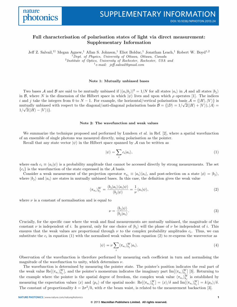
Full characterisation of polarisation states of light via direct measurement:Supplementary Information
Jeff Z. Salvail,1† Megan Agnew,1 Allan S. Johnson,1 Eliot Bolduc,1 Jonathan Leach,1 Robert W. Boyd1,21Dept. of Physics, University of Ottawa, Ottawa, Canada
2Institute of Optics, University of Rochester, Rochester, USA and†e-mail: [email protected]
Note 1: Mutually unbiased bases
Two bases A and B are said to be mutually unbiased if |〈ai|bj〉|2 = 1/N for all states |ai〉 in A and all states |bj〉in B, where N is the dimension of the Hilbert space in which |ψ〉 lives and upon which ρ operates [1]. The indicesi and j take the integers from 0 to N − 1. For example, the horizontal/vertical polarisation basis A = |H〉, |V 〉 ismutually unbiased with respect to the diagonal/anti-diagonal polarisation basis B = |D〉 = 1/
√2(|H〉+ |V 〉), |A〉 =
1/√2(|H〉 − |V 〉).
Note 2: The wavefunction and weak values
We summarize the technique proposed and performed by Lundeen et al. in Ref. [2], where a spatial wavefunctionof an ensemble of single photons was measured directly, using polarisation as the pointer.
Recall that any state vector |ψ〉 in the Hilbert space spanned by A can be written as
|ψ〉 =∑
i
ci|ai〉, (1)
where each ci ≡ 〈ai|ψ〉 is a probability amplitude that cannot be accessed directly by strong measurements. The setci is the wavefunction of the state expressed in the A basis.
Consider a weak measurement of the projection operator πai≡ |ai〉〈ai|, and post-selection on a state |φ〉 = |bj〉,
where |bj〉 and |ai〉 are states in mutually unbiased bases. In this case, the definition gives the weak value
〈πai〉Wbj =〈bj |ai〉〈ai|ψ〉
〈bj |ψ〉=
1
ν〈ai|ψ〉, (2)
where ν is a constant of normalisation and is equal to
ν =〈bj |ψ〉〈bj |ai〉
. (3)
Crucially, for the specific case where the weak and final measurements are mutually unbiased, the magnitude of theconstant ν is independent of i. In general, only for one choice of |bj〉 will the phase of ν be independent of i. Thisensures that the weak values are proportional through ν to the complex probability amplitudes ci. Thus, we cansubstitute the ci in equation (1) with the normalised weak values from equation (2) to re-express the wavevector as
|ψ〉 = ν∑
i
〈πai〉Wbj |ai〉. (4)
Observation of the wavefunction is therefore performed by measuring each coefficient in turn and normalising themagnitude of the wavefunction to unity, which determines ν.
The wavefunction is determined by measuring the pointer state. The pointer’s position indicates the real part ofthe weak value Re[〈πai〉Wbj ], and the pointer’s momentum indicates the imaginary part Im[〈πai
〉Wbj ] [3]. Returning to
the example where the pointer is the spatial degree of freedom, the complex weak value 〈πai〉Wbj is established by
measuring the expectation values 〈x〉 and 〈px〉 of the spatial mode: Re[〈πai〉Wbj ] = 〈x〉/δ and Im[〈πai
〉Wbj ] = k〈px〉/δ.The constant of proportionality k = 2σ2/, with σ the beam waist, is related to the measurement backaction [3].
SUPPLEMENTARY INFORMATIONDOI: 10.1038/NPHOTON.2013.24
NATURE PHOTONICS | www.nature.com/naturephotonics 1
© 2013 Macmillan Publishers Limited. All rights reserved.

2
In our work, we make use of the fact that not all the weak values 〈πai〉Wbj are independent. Taking the sum of a
complete set of weak values corresponding to projectors |ai〉〈ai| with fixed post-selection |bj〉, we obtain unity:
N−1∑
i=0
〈πai〉Wbj =
∑
i
〈bj |ai〉〈ai|ρ|bj〉〈bj |ρ|bj〉
= 〈bj |(∑
i
|ai〉〈ai|)
ρ|bj〉〈bj |ρ|bj〉
= 1. (5)
This result is true for any post-selection |bj〉 = |φ〉 and relies on the fact that∑
i |ai〉〈ai| is equal to the identity operatorwhen the set of all |ai〉 is a complete basis. Therefore, measuring all but one weak value is sufficient to determine thewavefunction. Importantly, for a qubit, a single weak value determines the pure state in the two-dimensional Hilbertspace.
We now consider the direct measurement of the polarisation wavefunction of a photon. Although the context ofour work is polarisation, these results are general and apply to all two-state quantum systems. The polarisation stateof a photon can be written as a linear combination of basis elements
|ψ〉 = α|H〉+ β|V 〉, (6)
where α, β are complex probability amplitudes, and |α|2 + |β|2 = 1. Recalling equation (4), we may express thepolarisation state as
|ψ〉 = ν(〈πH〉WD |H〉+ 〈π
V〉WD |V 〉
), (7)
where the post-selected state is |D〉, and therefore mutually unbiased with respect to the measurement operatorsπ
H= |H〉〈H| and π
V= |V 〉〈V |. The constant ν is simply found by normalising the wavefunction and is equal to
(|〈πH〉WD |2 + |〈π
V〉WD |2)− 1
2 . We now see that the wavefunction is defined in terms of quantities that we can directlymeasure in the lab. Equation (7) can be simplified by using the fact that 〈π
V〉WD + 〈π
H〉WD = 1 as in equation (5).
Thus, we may eliminate 〈πV〉WD , and the wavefunction is defined entirely in terms of 〈π
H〉WD .
The weak value 〈πH〉WD can be calculated from its definition and the polarisation state (equation (6)):
〈πH〉WD =
〈D|H〉〈H|ψ〉〈D|ψ〉 =
α
α+ β
=cos θ
cos θ + eiϕ sin θ. (8)
We take the convention here that the horizontal component has a real coefficient, such that the coefficients are definedby α = cos θ and β = eiϕ sin θ, where θ is the polarisation angle and ϕ is the phase difference between components.The result of equation (8) can also be obtained through the methods of classical optics. The locations of the peaksof the intensity distributions obtained from the interference of two overlapping Gaussian modes, in the near- andfar-fields, are proportional to the real and imaginary parts of equation (8), respectively [4]. In this representation,the two degrees of freedom of a polarisation qubit are θ and ϕ; in terms of weak values, they are the independent realand imaginary parts of 〈π
H〉WD . Setting a convention such as this for the phase fixes the gauge, or reference frame,
with respect to which the wavefunction is measured. Choosing ν real actually sets a different phase convention,where the wavevector has an additional global phase coefficient exp(−i arg[α + β]). We plot the wavefunctions inmain text Fig. 2, Fig. S1, and Fig. S2 using this phase convention, since it is the natural choice that comes fromexperiment. The theory curves of main text Fig. 2, Fig. S1, and Fig. S2 are calculated according to equation (8) bysetting ϕ = 0, π/2, π/4 respectively, then setting the wavefunction’s phase as discussed above.
Note 3: The Dirac distribution and weak values
We summarize the technique proposed by Lundeen and Bamber in Ref. [5]. The Dirac distribution, named for Diracwho proposed it in Ref. [6], is investigated thoroughly by Chaturvedi et al. in Ref. [7]. In our work, we use Chaturvediet al.’s “left” phase-space representative (Dirac distribution) throughout, and discuss only the discrete (i.e., N -level)
2 NATURE PHOTONICS | www.nature.com/naturephotonics
SUPPLEMENTARY INFORMATION DOI: 10.1038/NPHOTON.2013.24
© 2013 Macmillan Publishers Limited. All rights reserved.

3
Hilbert space version. The connection between Dirac distribution, conditional probabilities and the weak value wasalso explored by Hofmann in [8].
The entry in the ith row and the jth column of the Dirac distribution of the state described by ρ is given by
Sij = 〈bj |ai〉〈ai|ρ|bj〉. (9)
Recalling the weak value’s definition, for weak measurement of a projector πai, we obtain
〈πai〉Wbj =〈bj |πai
ρ|bj〉〈bj |ρ|bj〉
=〈bj |ai〉〈ai|ρ|bj〉
〈bj |ρ|bj〉. (10)
Substituting equation (10) into equation (9), we now see that the elements of the Dirac distribution that describes ageneral quantum state can be written in terms of particular weak values that can be directly measured:
Sij = 〈bj |ρ|bj〉〈πai〉Wbj = pbj 〈πai〉Wbj . (11)
That is to say, the (i, j)th element of the Dirac distribution is equal to the result of the weak measurement of πaiwith
a post-selection on state bj , multiplied by the probability of successful post-selection pbj = 〈bj |ρ|bj〉. The generalisedtechnique uses the outcome of the strong measurement, and since a mixed state density matrix (and hence Diracdistribution) has more degrees of freedom (N2−1) than a pure state vector (2N−2), the strong measurement projectionmust be scanned through the basis B, in addition to scanning the weak measurement through the complimentarybasis A.
To calculate the density matrix ρ from the Dirac distribution S, a simple row-by-row discrete Fourier transformcan be used, since the H/V basis and D/A basis are not only mutually unbiased but Fourier bases. The relation is
ρij =
N−1∑
k=0
Sik exp
(2πı
N(i− k)j
). (12)
In equation (12), we use ı to denote the imaginary unit which is distinct from the index i.In terms of experiment outcomes, the Dirac distribution is
S =
(p
D〈π
H〉WD
pA〈π
H〉WA
pD〈π
V〉WD
pA〈π
V〉WA
)
︸ ︷︷ ︸Right basis axis |D〉, |A〉
Left basis axis 〈H|, 〈V |. (13)
Using equation (12) with N = 2, we obtain the density matrix
ρ =
(p
D〈π
H〉D+ p
A〈π
H〉A
pD〈π
H〉D− p
A〈π
H〉A
pD〈π
V〉D− p
A〈π
V〉A
pD〈π
V〉D+ p
A〈π
V〉A
). (14)
Both axes of this density matrix use the H/V basis.
NATURE PHOTONICS | www.nature.com/naturephotonics 3
SUPPLEMENTARY INFORMATIONDOI: 10.1038/NPHOTON.2013.24
© 2013 Macmillan Publishers Limited. All rights reserved.

4
Additional Data
Wea
k va
lue
1.0
0.5
-1.0
-0.5
0.0
1.0
0.5
-1.0
-0.5
0.0
Norm
alise
Prob
abilit
y am
plitu
de
0o (H)-22.5o (L) 22.5o (R) 67.5o (L)45o (V)Half-wave plate angle (input polarisation state)
a
b
Fig. S1: Results of experiment 1 with elliptically polarised probe states. These states created by passing linearlypolarised light through a quarter-wave plate with fast axis at 0. a, Measured average weak values plotted as a function ofhalf-wave plate angle, 0 is defined as fast-axis parallel to the optical table. Error bars are shown only for the red points forclarity, and indicate the standard deviation of 100 independently measured weak values. b, Real and imaginary components ofthe probability amplitudes determined by normalising the weak values of each test state, where |ψ〉 = α|H〉+ β|V 〉. For bothpanels, the solid lines are the theoretical predictions of the real components, and the dotted lines are the theoretical predictionsof the imaginary components. Inset: A Poincare sphere with the path taken indicated by the red line.
4 NATURE PHOTONICS | www.nature.com/naturephotonics
SUPPLEMENTARY INFORMATION DOI: 10.1038/NPHOTON.2013.24
© 2013 Macmillan Publishers Limited. All rights reserved.

5
Norm
alise
-45o (L) -22.5o (D) 22.5o (A)0o (R)
Half-wave plate angle (input polarisation state)
Wea
k va
lue
3.0
1.5
-3.0
-1.5
0.0
1.0
0.5
-1.0
-0.5
0.0Pr
obab
ility
ampl
itude
-67.5o (A)
a
b
Fig. S2: Results of experiment 1 with elliptically polarised probe states. These states created by passing linearlypolarised light through a quarter-wave plate with fast axis at 45. a, Measured average weak values plotted as a function ofhalf-wave plate angle, 0 is defined as fast-axis parallel to the optical table. Error bars are shown only for the red points forclarity, and indicate the standard deviation of 100 independently measured weak values. b, Real and imaginary components ofthe probability amplitudes determined by normalising the weak values of each test state, where |ψ〉 = α|H〉+ β|V 〉. For bothpanels, the solid lines are the theoretical predictions of the real components, and the dotted lines are the theoretical predictionsof the imaginary components. Inset: A Poincare sphere with the path taken indicated by the green line.
[1] Wootters, W. K. & Fields, B. D. Optimal state-determination by mutually unbiased measurements. Ann. Phys., 191,363-381 (1989).
[2] Lundeen, J. S., Sutherland, B., Patel, A., Stewart, C. & Bamber, C. Direct measurement of the quantum wavefunction.Nature, 474, 188-191 (2011).
[3] Lundeen J. S. & Resch, K. J. Practical measurement of joint weak values and their connection to the annihilation operator.Phys. Lett. A, 334. 337-344 (2005).
[4] Ritchie, N. W. M., Story, J. G. & Hulet, R. G. Realization of a measurement of a weak value. Phys. Rev. Lett., 66,1107-1110 (1991).
[5] Lundeen J. S. & Bamber, C. Procedure for direct measurement of general quantum states using weak measurement. Phys.Rev. Lett., 108, 70402 (2012).
[6] Dirac, P. A. M. On the analogy between classical and quantum mechanics. Rev. Mod. Phys., 17, 195-199 (1945).[7] Chaturvedi, S. et al. Wigner-Weyl correspondence in quantum mechanics for continuous and discrete systems—a Dirac-
inspired view, J. Phys. A, 39, 1405-1423 (2006).[8] Hofmann, H. F. Complex joint probabilities as expressions of reversible transformations in quantum mechanics. New J.
Phys., 14, 043031 (2012).
NATURE PHOTONICS | www.nature.com/naturephotonics 5
SUPPLEMENTARY INFORMATIONDOI: 10.1038/NPHOTON.2013.24
© 2013 Macmillan Publishers Limited. All rights reserved.

Chapter 4
Optimal quantum key distribution
with photons entangled in orbital
angular momentum
This chapter is based on the following paper:
1. J. Leach, E. Bolduc, D. J. Gauthier, and R. W. Boyd, “Secure informationcapacity of photons entangled in many dimensions,” Physical Review A, vol. 85,no. 6, p. 060304, 2012
4.1 Introduction to quantum key distribution
Quantum key distribution (QKD) is a quantum cryptography protocol which guar-
antees absolute security between two communicating parties, Alice and Bob. The
shared information is secure in the sense that the presence of an eavesdropper can
always be detected. We first review a famous QKD protocol which works with single
photons and then describe a variant of this protocol for entangled photons.
4.1.1 The BB84 protocol
After the publication of the no-cloning theorem by Wootter and Zurek in 1982 [29],
Bennet and Brassard realized that the laws of quantum mechanics allow for absolute
security. They developed a quantum key distribution protocol now known as the BB84
protocol [30], whereby Alice securely communicates a private key to Bob. Essentially,
45

4.1. INTRODUCTION TO QUANTUM KEY DISTRIBUTION 46
Alice prepares a two-dimensional quantum state |ψ〉 in one of the four following
forms: |1〉, |2〉, |+〉 or |−〉, where |+〉 and |−〉 are the superposition states (|1〉 +
|2〉)/√
2 and (|1〉−|2〉)/√
2, respectively. The states |1〉 and |2〉 can correspond to any
degree of freedom of light, but Bennet and Brassard chose polarization in the original
proposal. After Alice sends her prepared state through a communication channel,
Bob receives it and performs a single projective measurement either in the eigenstate
basis |1〉, |2〉 or the superposition basis |+〉, |−〉. If his choice of basis is the same
one as Alice’s, the outcome of a measurement corresponds exactly to the prepared
state. However, if Alice’s and Bob’s choices differ, there is a 50% chance that the
outcome of Bob’s measurement be wrong. For example, if Alice prepared the state
|+〉, but Bob performs a projective measurement in the eigenstate basis |1〉, |2〉, the
outcome is completely random: |〈+|1〉|2 = |〈−|1〉|2 = 1/2. Therefore, Alice and Bob
discard the events where their choice of basis differ, and only keep the informationally
relevant ones. They repeat the above process until the key is long enough for their
purposes.
Let us study the presence of an eavesdropper, otherwise called Eve, on the result
of the protocol. Eve intercepts the state prepared by Alice and performs a projective
measurement on it in one of the two bases. She then prepares a state which cor-
responds to the outcome of her measurement, and sends it to Bob. She tries to go
unnoticed, but this is fundamentally impossible. When Alice and Bob make the same
choice of basis, Eve makes the wrong one 50% of the time and introduces errors in
the communication. For instance, if alice prepares the state |+〉 and Eve choses the
wrong basis, the outcome of her measurement will either correspond to |1〉 or |2〉 with
equal probability of 1/2. Bob then makes a measurement in the right basis, but, after
the intervention of Eve which irreversibly changed the state, the incorrect outcome
|−〉 is now possible. A careful analysis shows that the above eavesdropping strategy
introduces 25% of errors in the system. To check for security, Alice and Bob simply
have to compare a subset of their results and verify the error statistics.
4.1.2 The Ekert protocol
In the Ekert protocol [31], Alice and Bob each receive one photon of an entangled
photon pair. The source of photons produces a Bell state, which could be of the form
|ψBell〉 = |1〉A|1〉B + |2〉A|2〉B, where the subscripts A and B stand for Alice’s and
4.2. INTRODUCTION TO ORBITAL ANGULAR MOMENTUM STATES OF LIGHT 47
Bob’s photon, respectively. Alice’s and Bob’s photons are maximally correlated. For
instance, the above Bell state can be rewritten in the basis |+〉, |−〉, and still be
correlated: |ψBell〉 = |+〉A|+〉B + |−〉A|−〉B. If they choose the same basis to perform
their preojective measurement, the outcome of both measurements will be same for
every event. When Eve tries to detect and resend one of the photons, she breaks the
entanglement and thus the correlations also. Again, to check for her presence, Alice
and Bob verify the error statistics.
Alice and Bob must find the maximum amount of extractable secure information
given the fraction of noise that they observe. In general, one must assume that Eve
optimally uses the laws of quantum mechanics to achieve her goal. In publication 1, we
rely on the theory of Cerf et al. to quantify the secure bit rate of our implementation
of the communication channel of a QKD system [32]. Instead of the above two-
dimensional states, we use orbital angular momentum d-dimensional states.
4.2 Introduction to orbital angular momentum states
of light
In 1992, Allen et al. noticed that light beams can carry orbital angular momentum
(OAM) [32]. The Laguerre-Gaussian (LG) transverse spatial modes are specified with
two quantum numbers: i) the azimuthal number ` and ii) the radial number p. The
modes, with notation LG`p, carry `~ units of OAM. In our work, we ignore the radial
part of the LG modes and only consider the azimuthal part, which is mathematically
defined by an azimuthally varying phase: LG` ∝ exp(i`φ), where φ is the azimuthal
degree of freedom in transverse cylindrical coordinates. All the modes LG`, with
` ∈ Z, are mutually orthogonal. In our implementation of high-dimensional QKD, we
use a finite subset of the infinite OAM space. As shown in publication 1, we construct
a superposition basis with this subset. Before performing a projective measurement,
Alice and Bob both choose either the OAM basis and the superposition basis. They
only keep the events where they selected the same basis. In the following work, we
measure the correlations in both the OAM basis and the superposition basis and
calculate the extractable secure information.

RAPID COMMUNICATIONS
PHYSICAL REVIEW A 85, 060304(R) (2012)
Secure information capacity of photons entangled in many dimensions
Jonathan Leach,1 Eliot Bolduc,1 Daniel J. Gauthier,2 and Robert W. Boyd1,3
1Department of Physics, University of Ottawa, Ottawa, Ontario, Canada2Department of Physics, Duke University, Durham, North Carolina, USA
3Institute of Optics, University of Rochester, Rochester, New York, USA(Received 9 March 2012; published 28 June 2012)
We quantify precisely the maximum secure information capacity of photons entangled in high dimensionsfor entanglement in the orbital angular momentum and angular degrees of freedom. Our analysis takes carefulaccount of the influence of experimental imperfections, such as nonunity detection efficiency, on the degree ofEinstein-Podolsky-Rosen (EPR) entanglement and hence on the secure information capacity of the photon pairs.We find that there is is an optimal dimension that maximizes the secure information capacity whose value can bepredicted analytically from the knowledge of only a few experimental parameters.
DOI: 10.1103/PhysRevA.85.060304 PACS number(s): 03.67.Hk, 03.67.Bg, 03.67.Mn, 42.50.−p
Introduction. Entanglement is one of the defining propertiesof quantum mechanics and is a key resource for many quantuminformation protocols. Systems entangled in high dimensionshave recently been proposed as a resource for loophole-freetests of nonlocality [1] in addition to providing dense codingfor quantum key distribution (QKD) [2–11]. It is thereforeimportant to understand the mechanisms that affect the degreeof entanglement in high-dimensional systems.
The characteristic signature of quantum entanglement isthe observation of correlations of spatially separated particlesin two or more mutually unbiased bases. One can deducethat the particles are entangled provided that the correlationsviolate appropriate bounds for separability [12]. The degreeof violation of the bound is an important quantity in certainquantum information protocols such as QKD. Crucially, it isknown that entanglement is a precondition for secure quantumkey distribution [13] and that all entangled states contain secretcorrelations [14].
Quantum key distribution is a protocol that allows twoparties, Alice and Bob, to generate a secure key with whichto encode a private message [15–17]. In the Ekert protocol forQKD, Alice and Bob make use of pairs of entangled photons.The protocol is secure against attacks by an eavesdropper,who would necessarily have to disturb the system whenattempting to intercept the key. QKD implemented in ahigh dimensionally entangled space provides the advantagesof increased information capacity and higher tolerance toeavesdropping [2–11].
Recent work on high-dimensional spatial entanglement hasincluded studies of full-field position and momentum corre-lations [18,19] and orbital angular momentum (OAM) andangular position correlations [20–24]. Here, the large Hilbertspace of the spatial degree of freedom enables increasedinformation-carrying capacity of the photons compared thetwo-dimensional polarization degree of freedom.
In this Rapid Communication, we demonstrate the relation-ship between the degree of Einstein-Podolsky-Rosen (EPR)entanglement of high dimensionally entangled photon pairsand their maximal secure information-carrying capacity. Thediscrete nature of the OAM states allows us to directly controlthe size of the state space over a wide range. We find that,because of unavoidable experimental imperfections, there existboth an optimal dimension that maximizes the degree of
entanglement and a threshold dimension beyond which thereis no entanglement and therefore no secure information. Byextracting the key parameters that influence our experiment,we provide a model to predict the maximal secure informationcapacity of general high dimensionally entangled systems.
OAM states, angle states, and entanglement. We considerthe OAM modes of light for which there are, in principle, aninfinite number of discrete eigenstates. The OAM eigenstates,associated with helical phase fronts exp(iφ), are denoted by|〉. Restricting the size of the state space to a D-dimensionalspace enables the photons to act as quDits. The specificOAM states we consider in our experiment range from min =−[(D − 1)/2] to max = [D/2], where [x] is the integer partof x. Consequently, a basis mutually unbiased with respect tothe OAM basis is the angle basis in which the eigenstates aredefined by [25–27]
|φ〉 = 1√D
max∑=min
eiφ|〉. (1)
Here, φ = 2πn/D and n is an integer that ranges from 1 to D.The two photons produced through parametric down-
conversion (PDC) are entangled in the OAM and angle degreesof freedom [20–23,28]. The entangled state in the OAM basisis given by
|〉 =∞∑
=−∞c|A〉|−B〉, (2)
where c is the complex coefficient of the modes, the range of|c|2 is considered as the spiral bandwidth, and subscripts A
and B refer to the signal and idler modes. We probe the statedefined in Eq. (2), and we restrict the dimension of the statespace by projecting over a finite range of modes.
Entropic uncertainty relations. To establish the informationcontent present in a high dimensionally entangled system,consider first the implications of an entropic form of theuncertainty principle for a single particle and then for twoentangled particles. For a single particle, one form of theuncertainty principle, which relates the entropies of conjugatevariables X and Y , is [29,30]
H (X) + H (Y ) log2 D. (3)
060304-11050-2947/2012/85(6)/060304(4) ©2012 American Physical Society

RAPID COMMUNICATIONS
LEACH, BOLDUC, GAUTHIER, AND BOYD PHYSICAL REVIEW A 85, 060304(R) (2012)
The Shannon entropy H (X), which is a measure of informationcontent, is defined by
H (X) = −D∑
n=1
P (xn) log2 P (xn), (4)
where P (xn) is the probability of the outcome xn and D is thedimension of the space. As it is not possible for a single particleto violate inequality (3), it follows that one has completeuncertainty regarding one variable [H (Y ) or H (X)= log2 D]if one has complete knowledge about the other [H (X) orH (Y ) = 0].
Now consider a pair of high dimensionally entangledparticles in systems A and B that exhibit correlations inconjugate degrees of freedom. EPR entanglement can bedemonstrated by the violation of the entropic uncertaintyrelation [12,22,31,32],
HInf(XB) + HInf(YB) log2 D. (5)
Here, HInf(XB) = H (XB |XA) and HInf(YB) = H (YB |YA) arethe inferred entropies of B, given precise knowledge of thestate of A, for the variables X and Y . For a maximallyentangled system with no noise, perfect correlations will beobserved [HInf(XB) = HInf(YB) = 0], and the inequality willbe maximally violated.
Finally, consider the implications of Eq. (5) for the secureinformation capacity of photons entangled in the OAM andangle degrees of freedom. The inferred entropies, HInf (XB) andHInf(YB), become HInf(B) and HInf(φB) respectively, when weassociate X with the OAM basis and Y with the angle basis.For the most general eavesdropping attack ( i.e., a coherentattack) the EPR entanglement condition requires the violationof Eq. (5) to have a secure information capacity greater thanzero [4,13,14]. Thus, we reformulate Eq. (5) to provide theupper limit of the secure information capacity measured inbits per photon pair, defined through the relation
I log2 D − [HInf(B) + HInf(φB)]. (6)
We note that due to the symmetry of the system and the factthat the OAM and angle measurements are mutually unbiased,Eq. (6) is consistent with the general result of Berta et al., whorecently considered the uncertainty principle in the presenceof quantum memory [33–35].
Experiment. A brief summary of the experimental proce-dure is as follows. First, we choose a pump power to set thephoton-pair generation rate. Second, we select a dimensionsize to restrict the number of states in the Hilbert space.Third, we record the coincidence rates for the projectivemeasurements over ranges A and B ∈ min, . . . ,max, andφA and φB ∈ 2π/D, . . . ,2π. From the resulting data set,we calculate the secure information capacity via Eq. (6). Thesecond and third stages are repeated for a range of dimensions.Finally, we repeat the above procedures for a range of differentpump powers.
To produce entangled photons, we use a 3-mm-long typeI BBO (β barium borate) crystal pumped with mode-lockedultraviolet laser of 150 mW average power and λ = 355 nm(Xcyte, JDSU); see Fig. 1. We use the first diffracted ordersof spatial light modulators (Pluto, Holoeye) in combinationwith optical fibers, 10-nm bandpass filters (Chroma), and
SLMA
150 mWat 355 nm
SLMB
L1
L2
L2 L3
L3 L4
L4
Coincidence
detection
BBOND
IF
IF
FIG. 1. (Color online) ND, neutral density filter; BBO, β bariumborate crystal; SLM, spatial light modulator; IF, interference filter;L1, 150 mm; L2, 500 mm; L3, 1000 mm; and L4, 1.45 mm. Thecombination of the lenses L1 and L2 (L3 and L4), act as a 4f imagingsystem; thus the distance from the crystal to each SLM is 1300 mm(the distance from the SLMs to the fibers is ∼2003 mm).
single-photon avalanche photodiodes (Perkin-Elmer) to makeprojective mode measurements on the entangled photons. Thecoincidence counting is performed with a timing resolution of25 ns (National Instruments, PCI-6601). While faster timingelectronics are available, our coincidence electronics enablesus to investigate the interplay between coincidence ratesarising from correlated and uncorrelated events.
For state-space sizes ranging from D = 2 to D = 31, weperform projective measurements for all possible combina-tions of the eigenstates in both the OAM and angle bases. Thesemeasurements are repeated for four separate pump powers of0.47, 1.5, 47, and 150 mW. The coincidence counts in the OAMbasis are measured using phase-only holograms and single-mode fibers. The angle-state coincidence counts are measuredusing multimode fibers with the holograms on the SLMsencoded with both the phase and intensity profile of the mode.
Results. Samples of the measured correlations are shown inFig. 2. The two identifiable sources of errors in the data arecross-talk events and uncorrelated coincidences that arise froma nonunity heralding efficiency and finite-timing coincidenceelectronics. To quantify the degree of EPR entanglement, wecalculate HInf(B) and HInf(φB) for all of the state space sizesand pump powers; see Fig. 3. As a result of the reduceduncorrelated coincidence count rate, the maximal violationoccurs with lowest pair generation rate (ND = 1.5). We cansee clearly that increasing the state-space size beyond a certainthreshold leads to an inability to confirm the entanglement.
Estimation of the secure information. In our model weassume that we generate a maximally entangled state and thatthe signal and idler arms have identical properties. Thus, the
FIG. 2. (Color online) Coincidence count rates for the OAM basis(a) and the angle basis (b) for the case of D = 11. For this data set,there is no neutral density filter placed between the pump and theBBO crystal. The integration time for each measurement point is 1 s.
060304-2
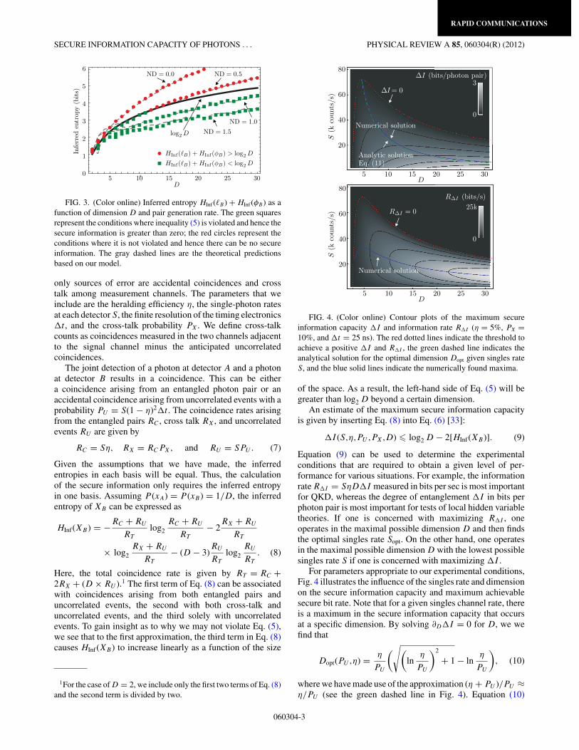
RAPID COMMUNICATIONS
SECURE INFORMATION CAPACITY OF PHOTONS . . . PHYSICAL REVIEW A 85, 060304(R) (2012)
1
2
3
4
5
6
5 10 15 20 25 300
D
HInf( B) +HInf(φB) > log2 D
HInf( B) +HInf(φB) < log2 D
log2 D
ND = 1.0
ND = 0.0
ND = 1.5
ND = 0.5Inferred
entropy(bits)
FIG. 3. (Color online) Inferred entropy HInf (B ) + HInf (φB ) as afunction of dimension D and pair generation rate. The green squaresrepresent the conditions where inequality (5) is violated and hence thesecure information is greater than zero; the red circles represent theconditions where it is not violated and hence there can be no secureinformation. The gray dashed lines are the theoretical predictionsbased on our model.
only sources of error are accidental coincidences and crosstalk among measurement channels. The parameters that weinclude are the heralding efficiency η, the single-photon ratesat each detector S, the finite resolution of the timing electronicst , and the cross-talk probability PX. We define cross-talkcounts as coincidences measured in the two channels adjacentto the signal channel minus the anticipated uncorrelatedcoincidences.
The joint detection of a photon at detector A and a photonat detector B results in a coincidence. This can be eithera coincidence arising from an entangled photon pair or anaccidental coincidence arising from uncorrelated events with aprobability PU = S(1 − η)2t . The coincidence rates arisingfrom the entangled pairs RC , cross talk RX, and uncorrelatedevents RU are given by
RC = Sη, RX = RCPX, and RU = SPU . (7)
Given the assumptions that we have made, the inferredentropies in each basis will be equal. Thus, the calculationof the secure information only requires the inferred entropyin one basis. Assuming P (xA) = P (xB) = 1/D, the inferredentropy of XB can be expressed as
HInf(XB) = −RC + RU
RT
log2RC + RU
RT
− 2RX + RU
RT
× log2RX + RU
RT
− (D − 3)RU
RT
log2RU
RT
. (8)
Here, the total coincidence rate is given by RT = RC +2RX + (D × RU ).1 The first term of Eq. (8) can be associatedwith coincidences arising from both entangled pairs anduncorrelated events, the second with both cross-talk anduncorrelated events, and the third solely with uncorrelatedevents. To gain insight as to why we may not violate Eq. (5),we see that to the first approximation, the third term in Eq. (8)causes HInf(XB) to increase linearly as a function of the size
1For the case of D = 2, we include only the first two terms of Eq. (8)and the second term is divided by two.
40
30205 10 15 25
20
60
80
ΔI= 0
D
40
30205 10 15 25
20
60
80
D
0
0
3
25k
Numerical solution
Analytic solutionEq. (11)
Numerical solution
RΔI = 0
RΔI (bits/s)
ΔI (bits/photon pair)
S(k
counts/s)
S(k
counts/s)
FIG. 4. (Color online) Contour plots of the maximum secureinformation capacity I and information rate RI (η = 5%, PX =10%, and t = 25 ns). The red dotted lines indicate the threshold toachieve a positive I and RI , the green dashed line indicates theanalytical solution for the optimal dimension Dopt given singles rateS, and the blue solid lines indicate the numerically found maxima.
of the space. As a result, the left-hand side of Eq. (5) will begreater than log2 D beyond a certain dimension.
An estimate of the maximum secure information capacityis given by inserting Eq. (8) into Eq. (6) [33]:
I (S,η,PU ,PX,D) log2 D − 2[HInf(XB)]. (9)
Equation (9) can be used to determine the experimentalconditions that are required to obtain a given level of per-formance for various situations. For example, the informationrate RI = SηDI measured in bits per sec is most importantfor QKD, whereas the degree of entanglement I in bits perphoton pair is most important for tests of local hidden variabletheories. If one is concerned with maximizing RI , oneoperates in the maximal possible dimension D and then findsthe optimal singles rate Sopt. On the other hand, one operatesin the maximal possible dimension D with the lowest possiblesingles rate S if one is concerned with maximizing I .
For parameters appropriate to our experimental conditions,Fig. 4 illustrates the influence of the singles rate and dimensionon the secure information capacity and maximum achievablesecure bit rate. Note that for a given singles channel rate, thereis a maximum in the secure information capacity that occursat a specific dimension. By solving ∂DI = 0 for D, we wefind that
Dopt(PU,η) = η
PU
(√(ln
η
PU
)2
+ 1 − lnη
PU
), (10)
where we have made use of the approximation (η + PU )/PU ≈η/PU (see the green dashed line in Fig. 4). Equation (10)
060304-3

RAPID COMMUNICATIONS
LEACH, BOLDUC, GAUTHIER, AND BOYD PHYSICAL REVIEW A 85, 060304(R) (2012)
provides the optimal dimension for both I and, to firstapproximation, the equation scales as 1/S.
The secure information capacity and maximum secureinformation rate can fall to zero; the threshold for this behavioris indicated in the figure by the red dotted lines. A secureinformation capacity of zero occurs at high single-photonrates, where uncorrelated coincidences dominate, and whenthe dimension of the space is low, where cross talk dominates.In addition, the maximum secure information rate is optimizedby maximizing D and then finding the appropriate singles rateS. As ∂SRI = 0 is not easily solved for S, we numericallysolve to find the optimal singles rate for a given dimension.
Conclusions. We experimentally demonstrate the rela-tionship between state-space size and the degree of EPR
entanglement for the case of high dimensionally entangledphotons. By relating the degree of entanglement of the photonpairs to the maximal secure information-carrying capacity,we find that, because of experimental limitations, there is anoptimal dimensionality that maximizes the secure informa-tion capacity. Under the conditions of our experiment, themaximum secure information per photon I is 1.3 bits. Themodel presented here provides a clear pathway for obtainingeven larger values of I , for example by using coincidencecircuitry with a smaller time window t .
Acknowledgments. We thank N. Lutkenhaus for discussionsregarding this work. This work was supported by the CanadaExcellence Research Chairs (CERC) Program and the DARPAInPho program.
[1] T. Vertesi, S. Pironio, and N. Brunner, Phys. Rev. Lett. 104,060401 (2010).
[2] H. Bechmann-Pasquinucci and W. Tittel, Phys. Rev. A 61,062308 (2000).
[3] N. Gisin et al., Rev. Mod. Phys. 74, 145 (2002).[4] N. Cerf, M. Bourennane, A. Karlsson, and N. Gisin, Phys. Rev.
Lett. 88, 127902 (2002).[5] F. Grosshans and P. Grangier, Phys. Rev. Lett. 88, 057902 (2002).[6] F. Grosshans and N. J. Cerf, Phys. Rev. Lett. 92, 047905 (2004).[7] J. Barreiro, N. K. Langford, N. A. Peters, and P. G. Kwiat, Phys.
Rev. Lett. 95, 260501 (2005).[8] S. Groblacher et al., New J. Phys. 8, 75 (2006).[9] I. Ali-Khan and J. C. Howell, Phys. Rev. A 73, 031801 (2006).
[10] I. Ali-Khan, C. J. Broadbent, and J. C. Howell, Phys. Rev. Lett.98, 060503 (2007).
[11] L. Zhang, C. Silberhorn, and I. A. Walmsley, Phys. Rev. Lett.100, 110504 (2008).
[12] M. Reid et al., Rev. Mod. Phys. 81, 1727 (2009).[13] M. Curty, M. Lewenstein, and N. Lutkenhaus, Phys. Rev. Lett.
92, 217903 (2004).[14] A. Acın and N. Gisin, Phys. Rev. Lett. 94, 020501 (2005).[15] C. Bennett and G. Brassard, Proceedings of IEEE International
Conference on Computers, Systems and Signal Processing(IEEE, Ottawa, Canada, 1984), p. 175.
[16] A. K. Ekert, Phys. Rev. Lett. 67, 661 (1991).[17] A. Ekert, B. Huttner, G. M. Palma, and A. Peres, Phys. Rev. A
50, 1047 (1994).
[18] J. Leach et al., Phys. Rev. A 85, 013827 (2012).[19] P. B. Dixon, G. A. Howland, J. Schneeloch, and J. C. Howell,
Phys. Rev. Lett. 108, 143603 (2012).[20] A. Mair et al., Nature (London) 412, 313 (2002).[21] J. Goette, S. Franke-Arnold, and S. M. Barnett, J. Mod. Opt. 53,
627 (2006).[22] J. Leach et al., Science 329, 662 (2010).[23] A. Dada et al., Nat. Phys. 7, 677 (2011).[24] M. Agnew, J. Leach, M. McLaren, F. S. Roux, and R. W. Boyd,
Phys. Rev. A 84, 062101 (2011).[25] E. Yao et al., Opt. Express 14, 9071 (2006).[26] B. Jack, M. Padgett, and S. Franke-Arnold, New J. Phys. 10,
103013 (2008).[27] S. Franke-Arnold et al., New J. Phys. 6, 103 (2004).[28] J. Torres, A. Alexandrescu, and L. Torner, Phys. Rev. A 68
(2003).[29] H. Maassen and J. B. M. Uffink, Phys. Rev. Lett. 60, 1103
(1988).[30] A. Rojas Gonzalez, J. Vaccaro, and S. M. Barnett, Phys. Rev. A
205, 247 (1995).[31] S. Walborn, B. G. Taketani, A. Salles, F. Toscano, and R. L. de
Matos Filho, Phys. Rev. Lett. 103, 160505 (2009).[32] S. P. Walborn, A. Salles, R. M. Gomes, F. Toscano, and P. H.
Souto Ribeiro, Phys. Rev. Lett. 106, 130402 (2011).[33] M. Berta et al., Nat. Phys. 6, 659 (2010).[34] Prevedel et al., Nat. Phys. 7, 757 (2011).[35] C. F. Li et al., Nat. Phys. 7, 752 (2011).
060304-4

Chapter 5
Simultaneous intensity and phase
encryption on a hologram
This chapter is based on the following paper:
1. E. Bolduc, N. Bent, E. Santamato, E. Karimi, and R. W. Boyd, “Exact so-lution to simultaneous intensity and phase masking with a single phase-onlyhologram,” Optics Letters, 2013, [paper accepted in Optics Letters, but notpublished yet]
5.1 Introduction to phase-only holograms
A hologram is commonly thought of as the result of holography, an optical method for
physically encoding the intensity and the phase of a coherently illuminated object [33].
In a more general sense, it consists in a pixelated plane which controls the transmission
efficiency and the phase shift of a transverse spatial optical field as a function its
two coordinates. More specifically, a phase-only hologram only offers the ability to
directly modulate the phase profile of an optical field. For instance, a spatial light
modulators (SLM) can display a computer-generated hologram where each pixel is
fully transparent and applies an arbitrary phase shift.
5.1.1 Intensity masking techniques
There exists methods to control the phase profile of an optical field and indirectly
modulate its intensity profile with phase-only holograms [34–36]. All of them make
52

5.1. INTRODUCTION TO PHASE-ONLY HOLOGRAMS 53
use of a modulated phase carrier frequency on the hologram, i.e., a grating with
varying diffraction efficiency. The intensity modulation appears in the first diffracted
order of the grating. Usually, the encryption of a phase-only hologram is specified
by three functions of the transverse coordinates x and y: i) the phase encryption
function F(x, y) ii) the intensity masking function M(x, y) and iii) the carrier fre-
quency function C(x, y), which is optimal in the case of a blazed grating of the form
2πx/Λ, where Λ is the period of the grating. If the incident field on the hologram is a
plane wave, the phase encryption function F(x, y) and the intensity masking function
M(x, y) depend on the desired output field. In the following discussions, we assume
that the incident field is a plane wave, and that the desired output mode is of the
form Ψ(x, y) = A(x, y)exp(iΦ(x, y)), where A(x, y) is its real amplitude distribution,
and Φ(x, y) is its phase profile. For brevity, we will omit to write the argument (x, y)
of all the functions.
If no intensity masking is required, the encryption of the phase-only hologram
T (x, y) takes the simplest form: T = exp[iMod(F + C, 2π)], where F = Φ and
C = 2πx/Λ. The phase encryption function directly imprints the phase of the desired
mode and the grating function sends the mode into the first order efficiently.
The difference between the intensity masking methods lies in the mathematical
form of the grating modulation. In the method of Kirk and Jones [34], the grating
is directly modulated by the intensity masking function. In this case, the imprinted
phase profile T (x, y) on the hologram is of the form
TKirk = exp[iMod(F +M C, 2π)], (5.1.1)
with F = Φ, M = 1 + sinc−1(A′)/π with A′ = A/max(A), C = 2π x/Λ. The authors
find the form of the intensity masking function through a Fourier analysis. Notably,
the phase encryption function is still identically equal to the phase profile of the
desired output mode.
In the method of Davis et al., the intensity masking function simultaneously
modulates the phase encryption function and the grating:
TDavis = exp[iMMod(F + 2π x/Λ, 2π)], (5.1.2)
where M and F are left unspecified for the moment. Crucially, Davis et al. derive

5.1. INTRODUCTION TO PHASE-ONLY HOLOGRAMS 54
the form of the field in the plane of the hologram as a function of the diffraction
orders. A detailed derivation can be found in the appendix of reference [35]. The
field before spatial filtering can be written in terms of all the orders of diffractions n
as follows: TDavis =∑Tnexp[inF ], where Tn = exp[i(n−M)π]sinc(π(n−M)). After
spatial filtering of all orders except the first one, we find that the resulting spatial
mode is given by
T1,Davis = exp[i(1−M)π + iF ]sinc(π(1−M)). (5.1.3)
In the our publication 3, we use a hologram encryption method of the type 5.1.2.
By setting T1,Davis(x, y) = Ψ(x, y), we show the form of F andM required to produce
the desired optical field exactly.
Exact solution to simultaneous intensityand phase encryption
with a single phase-only hologramEliot Bolduc,1 Nicolas Bent,1 Enrico Santamato,2 Ebrahim Karimi,1,* and Robert W. Boyd1,3
1Department of Physics, University of Ottawa, 150 Louis Pasteur, Ottawa, Ontario K1N 6N5, Canada2Dipartimento di Scienze Fisiche, Università di Napoli “Federico II”, Complesso di Monte S. Angelo, 80126 Napoli, Italy
3Institute of Optics, University of Rochester, Rochester, New York 14627, USA*Corresponding author: [email protected]
Received July 19, 2013; revised August 12, 2013; accepted August 13, 2013;posted August 14, 2013 (Doc. ID 194221); published September 5, 2013
A phase-only hologram applies a modal transformation to an optical transverse spatial mode via phase encodingand intensity masking. Accurate control of the optical field crucially depends on the method employed to encodethe hologram. In this Letter, we present a method to encode the amplitude and the phase of an optical field into aphase-only hologram, which allows the exact control of spatial transverse modes. Any intensity masking methodmodulates the amplitude and alters the phase of the optical field. Our method consists in correcting for thisunwanted phase alteration by modifying the phase encryption accordingly. We experimentally verify the accuracyof our method by applying it to the generation and detection of transverse spatial modes in mutually unbiased basesof dimension two and three. © 2013 Optical Society of AmericaOCIS codes: (090.1760) Computer holography; (100.5090) Phase-only filters; (070.2580) Paraxial wave optics;
(260.6042) Singular optics; (270.5568) Quantum cryptography.http://dx.doi.org/10.1364/OL.38.003546
The generation of optical fields possessing specifictransverse intensity and phase distributions is highlyimportant in many different research areas such as stimu-lated emission depletion microscopy, optical trapping,optical tweezers, communication, data storage, andfundamental quantum mechanics [1–5]. Nowadays, tech-nologies such as spatial light modulators (SLMs) andassorted controllable micromirrors provide an easyway to generate and manipulate optical fields from com-puter generated phase-only holograms, otherwise calledholographic kinoforms [6,7]. Generating an arbitrarybeam accurately requires engineering both phase andamplitude structures simultaneously. The current avail-able devices are fabricated to physically control onlythe phase or amplitude of an optical field, but not bothat the same time. Combining these two devices togetherallows one to control both the phase and amplitude ofan optical field. However, there exists techniques tomodulate both properties simultaneously with a singledevice [8].Over the course of the last five decades, many inten-
sity-masking methods for holographic kinoforms wereproposed by many different groups [9–12]. All these tech-niques make use of a grating pattern whose diffractionefficiency is modulated by a function of the amplitudeof the beam. Indeed, intensity masking, i.e., encryptingan arbitrary function of the amplitude onto a holographickinoform, is a selective process that diffracts only thedesired part of the incoming beam into the first orderof diffraction and the undesired part, depending on thetechniques, remains in the zero order, diffracts intohigher orders or both. The diffraction efficiency dependson the depth of phase of the blazing in the grating pattern;the closer to a full-phase, i.e., 2π, variation in the blazing,the more light diffracts [10]. Such a phase modulationgives the ability to control the diffracted intensity as afunction of the transverse coordinates and thus allows
one to generate or transform any transverse spatial modewithin the capabilities of the device.
Recently, Ando et al. numerically compared thepurity of the generated mode of different intensitymasking methods [13]. These methods can yield goodapproximations to the desired mode transformation,but an exact solution was yet to be found. In this Let-ter, we present the exact solution to the necessaryphase encoding and intensity masking on a phase-onlyhologram for any given paraxial mode transformation.We experimentally put our technique to the test bygenerating and detecting orbital angular momentum(OAM) states of light with two SLMs. We chooseOAM subspaces of two and three dimensions and con-sider the states in all mutually unbiased bases (MUBs),which consists of both eigenstates and superpositionstates.
In solving the problem of encryption of a holographickinoform, we use a plane wave as the incident opticalfield, and define the desired output beam as the followingscalar paraxial field:
Er⊥; z0≔Ar⊥; z0eiΦr⊥;z0; (1)
where r⊥ stands for the transverse coordinate,Ar⊥; z0≔jEr⊥; z0j and Φr⊥; z0≔ArgEr⊥; z0 arethe amplitude and phase of the optical field at thez z0 plane, respectively. As Eq. (1) suggests, a scalaroptical field is well-defined in the entire space by twoindependent real functions, one specifying the amplitudeprofile and the other specifying the phase distribution.This is fundamentally governed by the angular spectrummethod, which defines the optical field at any given zplane uniquely if the initial pupil field function is given.In our derivations, we specify A and Φ in the plane ofthe hologram (z 0).
3546 OPTICS LETTERS / Vol. 38, No. 18 / September 15, 2013
0146-9592/13/183546-04$15.00/0 © 2013 Optical Society of America

Let us first consider the simple case of a holographickinoform with no intensity masking and an imprintedphase profile of Ψm;n ModΦm;n 2πm∕Λ;2π,where m and n are the pixel coordinates and Λ is theperiod of the blazed grating pattern—the type ofgrating that maximizes the diffraction efficiency. AFourier analysis shows that, in the limit of infinitely manypixels, the optical field in the first order of diffractionis simply given by ~Eout FTexpiΦm;n, where FTcorresponds to the Fourier transform. To express theoutput beam in the near-field of the hologram, the stan-dard procedure is to insert a spatial filter that selectsonly the first diffracted order and go to the Fourierplane of the spatial filter. The output beam in thenear-field of the hologram is then written Eout expiΦm;n. The encrypted phase profile Φm;n isdirectly transferred to the output optical field, whose am-plitude stays uniform. In the following section, we showhow to simultaneously obtain the exact desired ampli-tude and phase profiles in the image plane, or near-field,of a hologram.We now consider a very general case of simultaneous
phase and amplitude encoding of a phase-only hologram.The imprinted phase profile on the hologram is given byΨm;n Mm;nModF m;n 2πm∕Λ; 2π, whereM is a normalized bounded positive function of ampli-tude, i.e., 0 ≤ M ≤ 1, and F is an analytical functionof the amplitude and phase profiles of the desired field.Just after passing through the hologram, the input planewave acquires the imprinted phase profile and isgiven by
Tm;n eiMm;nModF m;n2πm∕Λ;2π: (2)
A calculation based on a Taylor–Fourier expansionshows that the action of this particular optical phaseobject—after spatial filtering of all orders except thefirst one—can be expressed as
T1m;n −sincπM − πeiFπM; (3)
where M and F are both functions of the transversecoordinates on the hologram, i.e., fm;ng [10]. Sincethe output mode must be exactly equal to the desiredfield of Eq. (1), we find that the two modulation functionsare given by
M 1 1πsinc−1A
F Φ − πM; (4)
where sinc−1· stands for the inverse function of the sinc,and sincx sin x∕x is an unnormalized sinc functionin the domain of −π; 0, which accounts for the minussign in Eq. (3). The form of the intensity modulationfunction M is such that there is a linear relationshipbetween the desired amplitude and the encoded ampli-tude, see solid red curve in Fig. 1. Moreover, we cancelthe unwanted phase πM in Eq. (3) by subtracting it in thephase encoding function F . Crucially, Eq. (4) decouplesthe generated phase profile from the two-dimensionalamplitude distribution. Replacing the terms of Eq. (4)into Ψm;n, the imprinted phase profile on the
hologram, completes the description of our method.Since this result is exact, the fidelity of the generatedmodes should now only be limited by the capabilitiesof the device it is used with.
In order to test for the ability to encode and decodeinformation on transverse spatial modes, we experimen-tally applied our method to the generation and detectionof states in MUBs. Eigenstates of fjuiig and fjvjig arecalled MUBs in the Hilbert space of dimension d ifjhuijvjij2 1∕d for any i and j. For a given generatedmode, we perform a complete set of projections, whoseoutcomes allow us to determine the generated mode. Theprocess of reconstructing a state from a complete set ofmeasurement outcomes is know as quantum state tomog-raphy. This test is experimentally very reliable, and itis exhaustive, since it requires the generation anddetection of all informationally independent eigenstatesand superposition states.
Without loss of generality and only for this test, weneglect the radial dependence of the optical field, andwe consider only the azimuthal part associated with op-tical OAM. An optical beam with an azimuthal phaseprofile of the form expilϕ carries a well-definedOAM value of lℏ per photon, where ϕ is the cylindricalcoordinate. These beams are eigenstates of the z-component of the OAM operator and form a completebasis in the azimuthal coordinate, hrjli expilϕ [5].
MUBs form a complete set of bases. For a Hilbertspace of dimension d equal to a prime or the power ofa prime, the total number of MUBs is known to be d1 [14]. In the d 2 OAM Hilbert subspace, the (2 1)MUBs are eigenstates of the Pauli matrices. In analogywith polarization, this state space can be mapped onan OAM Poincaré sphere [15]. The set of MUBs intwo-dimensional Hilbert space are given by
fIg fj0i; j1ig
fIIg j0i j1i
2p ;
j0i − j1i2
p
fIIIg j0i ij1i
2p ;
j0i − ij1i2
p: (5)
For a three-dimensional OAM Hilbert subspace, the(3 1) MUBs are given by
0.0 0.2 0.4 0.6 0.8 1.00.0
0.2
0.4
0.6
0.8
1.0
Normalized A
Am
plit
ude
ofge
nera
ted
beam
Fig. 1. Amplitude of the generated beam, after selection of thefirst order of diffraction, as a function of the normalized desiredamplitude of Eq. (1). The solid-red curve corresponds to ourexact hologram encryption method; the generated amplitudeis equal to the desired amplitude. The blue dashed curve isbased on the technique reported in [10].
September 15, 2013 / Vol. 38, No. 18 / OPTICS LETTERS 3547

fIgfj0i;j1i;j2ig
fIIgj0ij1ij2i
3p ;
j0iωj1iω2j2i3
p ;j0iω2j1iωj2i
3p
fIIIgj0iωj1iωj2i
3p ;
j0iω2j1ij2i3
p ;j0ij1iω2j2i
3p
fIVgj0iω2j1iω2j2i
3p ;
j0iωj1ij2i3
p ;j0ij1iωj2i
3p
;
(6)
where ω expi2π∕3 [16,17].We implement our method in computer-generated
holograms displayed on cost-effective Cambridge Corre-lators SLMs, with a resolution of 1024 × 786 pixels. A lay-out of the experimental setup used to perform the MUBtest is shown in Fig. 2. A 3 mm wide single-mode HeNelaser beam goes through a polarizer that optimizes thediffraction efficiency of SLM-A. This SLM transformsthe input flat-phase field into any of the states given inEqs. (5) and (6). The beam then traverses a spatial filterthat selects out all but the first order of diffraction. Thehalf-wave plate modifies the polarization to optimize thediffraction efficiency of SLM-B, which applies a secondmodal transformation to the laser beam. Together withthe single-mode fiber (SMF) and an iris, SLM-B projectsthe generated mode onto an arbitrary mode in Eqs. (5)and (6). We measure the strength of the projections witha power-meter at the output of the SMF. In other words,SLM-A forms the state and SLM-B and SMF together ana-lyze the state.Because of the fact that we use intensity masking, we
have to normalize each projective measurement by thereflection efficiencies of the displayed holograms oneach SLM. For example, when displaying an OAMeigenstate on SLM-A, no intensity masking is neededbecause we ignore the radial degree of freedom and ithas a flat azimuthal intensity distribution. However, a
superposition state, a so-called angle state, requiresintensity masking since the azimuthal symmetry is bro-ken. In dimension two, half of the light will be lost.We have to take this mode-dependent reflection effi-ciency into account. Thus, for each hologram displayedon SLM-A and SLM-B, we measure the power of the re-flected light in the first order of diffraction of each SLM,and normalize the projection outcomes by the reflectionefficiencies of each SLM. Figure 3 shows the normalizedoutcomes of the projections for d 2 and d 3 OAMHilbert subspaces. We measure the quality of the systemwith a figure of merit called similarity S [18], an analo-gous quantity to the fidelity in the case of pair of states.Our system yields similarities of S 0.993 and S 0.927for dimension two and three, respectively.
Our method requires the calculation of the inverse sincfunction for every pixel on the hologram, and this taskcan be computationally intensive for a standard com-puter. For simplicity and speed, it is sometimes moreconvenient to implement a hologram encryption methodthat only requires standard functions, unlike the inversesinc function. We thus propose a simple improvementover the already simple technique first reported by Daviset al. [10]. In the case where the intensity modulationfunction is given by M A and F Φ, as proposedby Davis et al., the optical transverse mode after spatialfiltering is equal to sincπA − 1 expiΦ πA in thenear-field of the hologram. For this method, the ampli-tude profile of the generated beam sincπA − 1 is al-ways rather close to that of the desired amplitude A[see dashed blue curve in Fig. 1]. In fact, the normalizedgenerated and desired amplitudes are never further apartthan 0.161, jsincπA − 1 − Aj < 0.161. The difference inamplitude distributions is not as significant as the differ-ence in phase profiles. The generated phase profile canbe completely modified by the supplementary term πA inthe exponential. We thus propose a simple improvementthat consists in modifying the phase encryption F as inEq. (4): F Φ − πA. In principle, this new method doesnot yield an exact replica of the desired field since it doesnot correct for the gap in amplitude, but it should givegood approximations because it solves the problem ofthe extra phase term, which is much more important.
Fig. 2. Layout of the experimental setup used to encode anddetect OAM qubit and qutrit states based on our new method.A HeNe laser beam illuminates SLM-A, which generates any ofthe MUBs. The 4f systems made of the lenses L1,L2 image theplane of SLM-A to that of SLM-B with unit magnification. TheSLM-B and a SMF act together as a mode projector on any ofthe MUBs states. We sequentially display all MUBs states onSLM-A and SLM-B, and acquire all combinations of projections.The last set of lenses, composed of L3,L4, microscope objec-tive, take the far-field of SLM-B to the entrance facet of theSMF. The irises act as spatial filters which select the first orderof diffraction of SLM-A and SLM-B. As SLMs are polarizationsensitive, the polarizer (POL) and the half-wave plate (λ∕2)optimize the diffraction efficiency.
Fig. 3. Experimental projections between states in all MUBsin (a) d 2 and (b) d 3 OAM Hilbert subspaces, i.e.,Pij jhαijβjij2.
3548 OPTICS LETTERS / Vol. 38, No. 18 / September 15, 2013
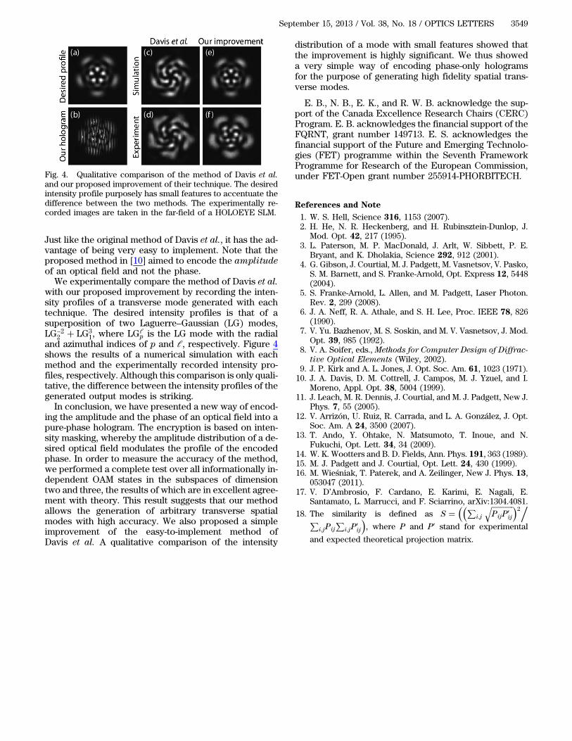
Just like the original method of Davis et al., it has the ad-vantage of being very easy to implement. Note that theproposed method in [10] aimed to encode the amplitudeof an optical field and not the phase.We experimentally compare the method of Davis et al.
with our proposed improvement by recording the inten-sity profiles of a transverse mode generated with eachtechnique. The desired intensity profiles is that of asuperposition of two Laguerre–Gaussian (LG) modes,LG−2
2 LG31, where LGl
p is the LG mode with the radialand azimuthal indices of p and l, respectively. Figure 4shows the results of a numerical simulation with eachmethod and the experimentally recorded intensity pro-files, respectively. Although this comparison is only quali-tative, the difference between the intensity profiles of thegenerated output modes is striking.In conclusion, we have presented a new way of encod-
ing the amplitude and the phase of an optical field into apure-phase hologram. The encryption is based on inten-sity masking, whereby the amplitude distribution of a de-sired optical field modulates the profile of the encodedphase. In order to measure the accuracy of the method,we performed a complete test over all informationally in-dependent OAM states in the subspaces of dimensiontwo and three, the results of which are in excellent agree-ment with theory. This result suggests that our methodallows the generation of arbitrary transverse spatialmodes with high accuracy. We also proposed a simpleimprovement of the easy-to-implement method ofDavis et al. A qualitative comparison of the intensity
distribution of a mode with small features showed thatthe improvement is highly significant. We thus showeda very simple way of encoding phase-only hologramsfor the purpose of generating high fidelity spatial trans-verse modes.
E. B., N. B., E. K., and R. W. B. acknowledge the sup-port of the Canada Excellence Research Chairs (CERC)Program. E. B. acknowledges the financial support of theFQRNT, grant number 149713. E. S. acknowledges thefinancial support of the Future and Emerging Technolo-gies (FET) programme within the Seventh FrameworkProgramme for Research of the European Commission,under FET-Open grant number 255914-PHORBITECH.
References and Note
1. W. S. Hell, Science 316, 1153 (2007).2. H. He, N. R. Heckenberg, and H. Rubinsztein-Dunlop, J.
Mod. Opt. 42, 217 (1995).3. L. Paterson, M. P. MacDonald, J. Arlt, W. Sibbett, P. E.
Bryant, and K. Dholakia, Science 292, 912 (2001).4. G. Gibson, J. Courtial, M. J. Padgett, M. Vasnetsov, V. Pasko,
S. M. Barnett, and S. Franke-Arnold, Opt. Express 12, 5448(2004).
5. S. Franke-Arnold, L. Allen, and M. Padgett, Laser Photon.Rev. 2, 299 (2008).
6. J. A. Neff, R. A. Athale, and S. H. Lee, Proc. IEEE 78, 826(1990).
7. V. Yu. Bazhenov, M. S. Soskin, and M. V. Vasnetsov, J. Mod.Opt. 39, 985 (1992).
8. V. A. Soifer, eds., Methods for Computer Design of Diffrac-tive Optical Elements (Wiley, 2002).
9. J. P. Kirk and A. L. Jones, J. Opt. Soc. Am. 61, 1023 (1971).10. J. A. Davis, D. M. Cottrell, J. Campos, M. J. Yzuel, and I.
Moreno, Appl. Opt. 38, 5004 (1999).11. J. Leach, M. R. Dennis, J. Courtial, and M. J. Padgett, New J.
Phys. 7, 55 (2005).12. V. Arrizón, U. Ruiz, R. Carrada, and L. A. González, J. Opt.
Soc. Am. A 24, 3500 (2007).13. T. Ando, Y. Ohtake, N. Matsumoto, T. Inoue, and N.
Fukuchi, Opt. Lett. 34, 34 (2009).14. W. K. Wootters and B. D. Fields, Ann. Phys. 191, 363 (1989).15. M. J. Padgett and J. Courtial, Opt. Lett. 24, 430 (1999).16. M. Wieśniak, T. Paterek, and A. Zeilinger, New J. Phys. 13,
053047 (2011).17. V. D’Ambrosio, F. Cardano, E. Karimi, E. Nagali, E.
Santamato, L. Marrucci, and F. Sciarrino, arXiv:1304.4081.
18. The similarity is defined as S P
i;j
PijP0
ij
q 2.
Pi;jPij
Pi;jP
0ij
, where P and P0 stand for experimental
and expected theoretical projection matrix.
Fig. 4. Qualitative comparison of the method of Davis et al.and our proposed improvement of their technique. The desiredintensity profile purposely has small features to accentuate thedifference between the two methods. The experimentally re-corded images are taken in the far-field of a HOLOEYE SLM.
September 15, 2013 / Vol. 38, No. 18 / OPTICS LETTERS 3549

5.3. SUPPLEMENTARY INFORMATION 59
5.3 Supplementary information
5.3.1 Pixelated holograms
Our method does not take into account the pixelated nature of the hologram. If the
number of pixels in one period of the grating is very low, namely, between 2 and 6,
the pixelated nature of the hologram becomes important. High carrier frequencies are
advantageous in experiments where the desired mode in the first order of diffraction
must be as far as possible from the other orders. This occurs when the mode in
question is very large. It would thus be relevant to test our method for such high
carrier frequencies, and develop a more accurate one for this particular case.
5.3.2 Implications on the results of chapter 4
In the work on quantum key distribution with orbital angular momentum states
(OAM) in chapter 4, we were using SLMs to detect OAM states and superpositions of
OAM states. We didn’t know about the new method presented here and implemented
the intensity masking method of Davis et al. to calculate the computer-generated holo-
grams for the superposition states, which intensity varies angularly. The inaccuracy
of the employed method was thus a source of noise which was unaccounted for at
the time. The noise was simply considered as coming from an eavesdropper. As a
consequence, we could increase the secure information capacity of our quantum key
distribution system by implementing the new hologram encryption method.
5.3.3 Computer program
We implemented our method in MATLAB, see appendix B. The program generates
a pixelated hologram in the middle of a monitor chosen by the user. This program is
also available on the website of the group of Prof. Boyd at the University of Ottawa:
http://www.quantumphotonics.uottawa.ca/home.php.
Chapter 6
Conclusions and Outlook
We have completed four projects, all of which provide improvements to experimental
procedures in either applied or fundamental quantum mechanics.
In the work on duality, we derived a novel relation between average visibility 〈V〉of an interference pattern and which-alternative knowledge 〈P〉 in the presence of an
environment: 〈P〉2 + 〈V〉2 = 1 − σ2P − σ2
V , where σ2P and σ2
V are the variances of the
predictability and visibility distributions, respectively. The environment allowed the
interference pattern to vary, and its visibility has to be viewed as a distribution rather
than a single value. Our relation is an equality when the pure state assumption is
valid and turns into an inequality when we make no assumption. In the latter case,
the bound is as tight as possible and cannot be improved. We pointed out that,
instead of measuring the average visibility, Menzel et al. observed a single value of
the visibility, which corresponded to a single element of the environment. As they did
not measure the visibility for every slice of the two-dimensional interference pattern,
our relation could not have been tested. Instead, they measured what we call the
biased sampling relation: B = V2max + 〈P〉2, which is allowed by the laws of quantum
mechanics to exceed unity. Duality was safe in this respect, but we went even further
and theoretically modeled a similar experiment to that of Menzel et al. to test our
new duality relation. Our relation is particularly relevant when the visibility varies
significantly as a function of the degree of freedom of the environment, which was the
case of our thought experiment. As expected, our relation was satisfied. This work
explains the surprising experimental results of Menzel et al., and improves the theory
on duality. Our relation still has to be experimentally tested.
The second project was on quantum state determination with weak values. We
60

61
performed two experiments: i) we directly determined the two complex coefficients
of a polarization state of light and ii) directly determined the elements of the corre-
sponding 2-dimensional Dirac distribution. In both experiments, we measured weak
values by weakly coupling the polarization state to the spatial degree of freedom with
a tilted birefringent crystal. After a projection onto a final polarization state, the
real and imaginary parts of a weak value were approximately related to the average
position and average momentum of the spatial mode, respectively. In the first ex-
periment, we assumed that the polarization state was pure, and we only needed one
weak value to identify the state vector. We applied this procedure to many known
initial states. The retrieved states corresponded almost exactly to the expected states
except when the expected state was orthogonal to the final projection. In this case,
the experimental result diverged from the expected one, because the weak-value ap-
proximation broke down. We theoretically quantified the effect of this break down by
calculating the average fidelity between arbitrary initial states and the corresponding
retrieved states with weak-value-assisted tomography. We found that the method is
very accurate in the regime of very weak coupling. It yields an average fidelity higher
than 0.998 when the spatial shift of the initial spatial mode is less than half of its 1/e
width. The average fidelity decreases exponentially fast with the coupling strength
and saturates at 0.873. This analysis was done for two-dimensional initial states, but
could be generalizable to D-dimensional systems.
In the work on quantum key distribution, we experimentally implemented im-
portant features of quantum key distribution using photons entangled in the angular
momentum degree of freedom. Photons pairs were generated through spontaneous
parametric downconversion, and their transverse spatial modes were detected with
spatial light modulators and singles mode fibers. We recorded the modal correla-
tions between the photon pairs and calculated the amount of extractable secure in-
formation. By performing this analysis for many dimensions of the orbital angular
momentum state-space, we found the one that maximized the secure information.
We theoretically generalized this result by taking into account the photon generation
rate, the coincidence detection time window and the non-unity detection efficiency.
The experimental results showed that the maximum amount of extractable secure in-
formation was 1.3 bits per photon pair. Our theoretical model indicates the changes
that have to be made in order to reach a given value of the secure information rate.
Notably, it would be very helpful for future experiments if we were to change the

62
detection electronics to reduce the coincidence time window.
Finally, we showed how to obtain arbitrary spatial modes with a single phase-only
hologram. Solutions to this problem already existed, but they were all approximate.
We gave the exact solution to simultaneous encryption of the intensity and the phase
of a given spatial transverse mode into a phase-only hologram. We quantitatively
tested our method with state projections in mutually unbiased bases. In dimension
2 and 3, the metric for how close the results were to the theory, the similarity, was
0.993 and 0.927, respectively. Our method could be computationally intensive for it
requires the calculation of a non-standard sinc inverse function. We thus provided
an improvement over the easy-to-implement technique of Davis et al.. We applied an
amplitude dependent correction on the phase encryption. As this correction is simple,
it doesn’t require much computing power. We qualitatively tested this method by
observing the intensity pattern of a given mode in the far-field of a spatial light mod-
ulator. The improvement was fast and strikingly good. We expect our method to be
used for engineering purposes, multiplexing and demultiplexing of spatial transverse
modes for instance, and in many areas of research, such as quantum state tomogra-
phy, microscopy and fundamental quantum mechanics. Since we assumed an infinite
number of pixels on the holograms, it would be interesting to study the impact of
finite pixel number on our method.
Appendix A
MATLAB code for our thought
experiment on duality
%%%%% Program that computes the two-photon mode functions in the near-field
%%%%% and the far-field of the two-slit mask in a thought experiment
%%%%% inspired by the work of Menzel et. al.
clc;clear;
%%%%%%%%% DEFINE PARAMETERS..................(Experiment of Menzel et. al.)
mum=1E-6; %micrometer............................................
phi=-19; %phase-mismatch parameter...........................(?)
L=0.002; %crystal thickness................................(2mm)
d=70*mum; %slit separation....................................(?)
delta=d/4; %slit width.......................................(d/4)
w0=100*mum; %pump width.....................................(25mum)
HG=1; %1 (0) corresponds to a HG01 (Gaussian) pump mode...(1)
lambda=0.405*mum; %wavelength in vacuum...........................(405nm)
n=1.65; %index of refraction in the crystal..............(1.65)
kp=2*pi/lambda*n; %total wavevector of the pump beam inside the crystal
N=1024; %number of points in computation
wf=10*mum; %1/e^(1/2) width of the fiber
dell=0; %offset of the optical fiber
ctrfbr=-d/2-dell; %y position of the optical fiber
63

64
speed=0; %if speed=1, reduced resolution on the idler photon
%%%%%%%%% END DEFINE PARAMETERS %%%%%%%%%%%%%%%%%%%%%%%%%%%%%%%%%%%%%%%%%%%
%define coordinate space and wavevector space
xmax=500*mum; %maximum value in coordinate space
X=linspace(-xmax,xmax,N); %coordinate space
res=X(2)-X(1); %resolution in coordinate space
prange=2*pi/res; %wavevector range
P=linspace(-prange/2,prange/2,N); %wavevector space
%specify the pump term and the phasematching term in Psi(r_s,r_i=0)
E0=pumpterm(w0,X,HG); %CALL pumpterm function
[F0 Ftilde]=phasematchingterm(X,P,phi,L,kp); %CALL phasematchingterm func.
%create the slit functions
[W T B] = CreateSlits(X,d,delta);
%Compute the signal probability distribution conditioned on an idler photon
%detection. Two loops scan r_ix and r_iy with resolution idlerres.
idlerres=2*res; if speed==1 idlerres=10*res; end
fmax=3*wf;
Rx=-fmax:idlerres:fmax;
Ry=Rx+ctrfbr;
lengthComp=length(Rx)^2; %length of computation
%initialize the results of the integrals
PT=zeros(N);PB=PT;PTprime=PT;PBprime=PT;PWprime=PT;
iteration=0;
for rix=Rx
ri.x=rix;
for riy=Ry
ri.y=riy;
iteration=iteration+1;
disp(iteration/lengthComp*100); %degree of completion

65
E=zeros(N);F=E; %initialize E and F
% We need to compute F(r_s-r_i) and E(r_s+r_i). For a given value
%of r_i, these function are identical to F0(r) and E0(r) up to a
%translation in coordinate space. In order to computer F and E, we
%thus move the center the matrix F0(r) at r=r_i and the center of
%the matrix E0(r) at r=-r_i.
b=centering(ri,N,res); %CALL centering function
%(not shown in thesis)
%move the center of F0 at r=r_i, and the center of E0 at r=-r_i
F(b.Xbox,b.Ybox) =F0(b.Xbox0,b.Ybox0);
E(b.Xbox0,b.Ybox0)=E0(b.Xbox,b.Ybox);
%Define the conditional modes after the slits
PsiCond=F.*E;
PsiW=W.*PsiCond;
PsiT=T.*PsiCond;
PsiB=B.*PsiCond;
%Apply a two-dimensional fft to the conditional mode after the
%slits to obtain the far-fiels interference pattern.
PhiT=fft2(PsiT);
PhiB=fft2(PsiB);
PhiW=PhiT+PhiB;
%calculate the optical fiber function
phix=exp(-rix.^2/2/wf^2);
phiy=exp(-(riy-ctrfbr).^2/2/wf^2);
phi2=abs(phix*phiy)^2;
%compute conditional probability distribution of
PTi=PsiT.*conj(PsiT)*phi2; %near-field of top slit
PBi=PsiB.*conj(PsiB)*phi2; %near-field of bottom slit
66
PTprimei=PhiT.*conj(PhiT)*phi2; %far-field of top slit
PBprimei=PhiB.*conj(PhiB)*phi2; %far-field of bottom slit
PWprimei=PhiW.*conj(PhiW)*phi2; %far-field of the two slits
%perform the integrals
PT=PT+PTi;
PB=PB+PBi;
PTprime=PTprime+PTprimei;
PBprime=PBprime+PBprimei;
PWprime=PWprime+PWprimei;
end
end
PW=PT+PB;
%The marginal distributions
Nnorm=sum(sum(PWprime)); %normalization constant
MT=sum(PTprime’)/Nnorm;
MB=sum(PBprime’)/Nnorm;
MW=MT+MB;
%The visibility, predictability as a function of the environment
Visibility= 2*sqrt(MT.*MB)./MW;
Predictability= abs(MT-MB)./MW ;
%Display relevant quantities;
rel.avgV=sum(MW.*Visibility);
rel.avgP=sum(MW.*Predictability);
rel.maxV=Visibility(ceil(N/2));
rel.varV=sum(MW.*(Visibility-rel.avgV).^2);
rel.varP=sum(MW.*(Predictability-rel.avgP).^2);
rel.OurEquality=rel.avgV^2+rel.avgP^2+rel.varV+rel.varP;
rel.ApparantViolation=rel.avgP^2+rel.maxV^2;
disp(rel)

67
%plotting the relevant quantities by calling function PlotRelevant
PlotRelevant(X,P*1E-5,E0,W,PW,PWprime,PT,PTprime,PB,PBprime,Visibility,...
Predictability,MW,8,8,10);
A.0.4 Function “pumpterm”
%%%Specify the joint wavefunction in the near-field
function E=pumpterm(w0,RS,HG,ri)
if ~exist(’ri’) ri.x=0;ri.y=0; end
%pump field at the entrance facet of the crystal
Ex=exp(-(RS+ri.x).^2/8/w0^2);
Ey=exp(-(RS+ri.y).^2/8/w0^2);
if HG==1 Ey=(RS+ri.y).*Ey; end
E=Ex’*Ey;
A.0.5 Function “phasematchingterm”
%%%%% Generate phase-matching term
function [F Ftilde]=phasematchingterm(X,P,phi,L,kp)
%specify the sinc function
a=0;
for py=P
a=a+1;
%note that sinc(x)=sin(pi*x)/(pi*x) in the version of MATLAB in which
%this program was written. One must check if it is still the case.
Ftilde(:,a)=sinc((phi+L/kp*(P.^2+py^2))/pi);
end
F=fftshift(fft2(Ftilde));

Appendix B
MATLAB code for
computer-generated holograms
%%% Example program using the ComputeHologram function
% With 1024 pixels, our hologram takes about 0.35 second to calculate on an
% old laptop(to be compared with 0.23 second for the simple method of
% Davis et al.). Here, we only consider the time taken to calculate M and
% F, not the time taken to calculate the desired modes.
clc;clear;close all;
%Inputs with their suggested values
dp=16;%16 %Distance between two pixels on the SLM
pixels=512;%512 %Number of used pixels on one line of the desired mode
N=8;%8 %Number of pixels in one period of the grating
domain=dp*pixels; %Length of the used domain of the SLM
w=600;%600 %Width of the desired mode in microns (near-field)
%Desired mode
%Superposition of LG modes (as shown in the paper)
LG1=LG_mode(-2,2,w,pixels,domain);LG1=LG1/sqrt(sum(sum(abs(LG1)^2)));
LG2=LG_mode(3,1,w,pixels,domain); LG2=LG2/sqrt(sum(sum(abs(LG2)^2)));
LG=LG1+LG2;inputMode=LG;
68

69
%Gaussian input beam (instead of a plane wave), for simulation purposes
gau=LG_mode(0,0,w*6,pixels,domain);
%Compute hologram (this takes around 350 ms)
OurHologram=ComputeHologram(inputMode,N);
% Display the hologram on the SLM
SingleKinoform(OurHologram,2,1);
% % or Display two holograms on one SLM (uncomment to try)
% TwoDisplaysOnSingleSLM(OurHologram,OurHologram’,2,1);
% Transformed gaussian input beam, just after the hologram
PHI=gau.*exp(1i*OurHologram);
%Simulate the first order of diffraction of the SLM
PSI=fftshift(fft2(PHI,1024, 1024)); %Mode in the far-field of the SLM
mid=ceil(1024/2);
firstOrderx=mid+[round(-54):round(54)];
firstOrdery=mid+[round(-54):round(54)]+round(130*8/N);
I=PSI(firstOrderx,firstOrdery).^2; %Intensity profile in first order
figure(2);imagesc(abs(I)); %Display intensity
axis image;colormap hot;
title(’Intensity profile in the first order of diffraction’)
B.0.6 Function “ComputeHologram”
function Hologram=ComputeHologram(inputMode,N)
% program optimized for mode fidelity
% The grating is made of N pixels, where N is an integer.
% INPUTS
% inputMode: desired mode in the near-field of the hologram
% N: number of pixels in one period of the blazed grating
%

70
% OUTPUT
% Hologram: Hologram as displayed on the SLM
% Number of pixels on one line of the desired mode
N2=size(inputMode);pixels=N2(1);
% Create grating pattern
step=2*pi/N;saw=[0:step:2*pi-step];nbsaw=floor(pixels/N);tgra=zeros(pixels);
grating=[]; for i=1:nbsaw grating=[grating saw];end
grating(length(grating):pixels)=0;for i=1:pixels tgra(i,:)=grating;end
% Generate sinc function
X=linspace(0,1,100000);y=sinc(X);
% Generate a table for the sinc inverse function
%(duration of 20 ms on a bad laptop)
t=0; g=10000-1; yy=round(y*g);
for i=1:length(y) if yy(i)==g-t
t=t+1; sincinverse(g-t+2)=i/length(y);
end; end
% Normalize the hologram profile such that the maximum is 1
inputMode=inputMode/max(max(abs(inputMode)))+1E-20;
% Time-efficient computation of the M function with the inverse sinc
M=1-sincinverse(ceil(abs(inputMode)*length(sincinverse)));
% Calculate hologram with Eq. 4 in the paper
F=angle(inputMode)-pi*M;
Hologram=mod(tgra+F,2*pi).*M;
B.0.7 Function “LG mode”
%Function that calculates an LG mode with azimuthal number l and radial
%number p. Its width is w, and it is calculated over the region "domain"

71
%with a number of pixels equal to pixelsXpixels.
%This function is not optimized for speed.
function LG = LG_mode(l,p,w,pixels,domain)
if ~exist(’domain’) domain=1000E-6; end
if ~exist(’pixels’) pixels=64; end
X=linspace(-domain,domain,pixels);
Y=linspace(-domain,domain,pixels);
a=0;
LG = zeros(length(X),length(Y));
for x=X
a=a+1;ii=0;
for y=Y
ii=ii+1;
rho=sqrt(x^2+y^2); phi=atan2(x,y);
LG(a,ii)=(rho*sqrt(2)/w)^(abs(l))*exp(-rho^2/w^2)*...
L_polynomial(p,abs(l),(2*rho^2/w^2))*exp(1i*l*phi);
end
end
%Calculate the Laguerre polynomial
function LaguerreL = L_polynomial(p,l,x)
L1= 0; LaguerreL= 1;
for i= 1 : p
L0= L1; L1= LaguerreL;
LaguerreL= ((2* i- 1+ l- x).* L1- (i- 1+ l).* L0)/ i;
end

Bibliography
[1] J. Leach, E. Bolduc, D. J. Gauthier, and R. W. Boyd, “Secure informationcapacity of photons entangled in many dimensions,” Physical Review A, vol. 85,no. 6, p. 060304, 2012.
[2] J. Z. Salvail, M. Agnew, A. S. Johnson, E. Bolduc, J. Leach, and R. W. Boyd,“Full characterization of polarization states of light via direct measurement,”Nature Photonics, vol. 7, pp. 316–321.
[3] E. Bolduc, N. Bent, E. Santamato, E. Karimi, and R. W. Boyd, “Exact solutionto simultaneous intensity and phase masking with a single phase-only hologram,”Optics Letters, 2013.
[4] E. Bolduc, J. Leach, and R. Boyd, “The secure information capacity of pho-tons entangled in high dimensions,” in Quantum Information and Measurement,Optical Society of America, 2012.
[5] E. Bolduc, J. Leach, and R. W. Boyd, “The secure information capacity of pho-tons entangled in high dimensions,” in Frontiers in Optics 2012/Laser ScienceXXVIII, p. FTh4B.7, Optical Society of America, 2012.
[6] E. Bolduc, J. Leach, F. Miatto, G. Leuchs, and R. Boyd, “How to achieve highvisibility and high which-way information in a single experiment,” in Physics ofQuantum Electronics, 2013.
[7] R. Menzel, D. Puhlmann, A. Heuer, and W. P. Schleich, “Wave-particle dualismand complementarity unraveled by a different mode,” Proceedings of the NationalAcademy of Sciences, vol. 109, no. 24, pp. 9314–9319, 2012.
[8] R. Menzel, A. Heuer, D. Puhlmann, K. Dechoum, M. Hillery, M. Spahn, andW. Schleich, “A two-photon double-slit experiment,” Journal of Modern Optics,vol. 60, no. 1, pp. 86–94, 2013.
[9] J. S. Lundeen, B. Sutherland, A. Patel, C. Stewart, and C. Bamber, “Directmeasurement of the quantum wavefunction,” Nature, vol. 474, no. 7350, pp. 188–191, 2011.
72

BIBLIOGRAPHY 73
[10] J. S. Lundeen and C. Bamber, “Procedure for direct measurement of generalquantum states using weak measurement,” Physical review letters, vol. 108, no. 7,p. 070402, 2012.
[11] B.-G. Englert, “Fringe visibility and which-way information: An inequality,”Physical review letters, vol. 77, no. 11, pp. 2154–2157, 1996.
[12] N. Bohr, “Albert einstein: Philosopher-scientist,” Open Court, La Salle, Illinois,pp. 200–241, 1949.
[13] W. K. Wootters and W. H. Zurek, “Complementarity in the double-slit experi-ment: Quantum nonseparability and a quantitative statement of bohr’s princi-ple,” Physical Review D, vol. 19, no. 2, p. 473, 1979.
[14] G. Jaeger and A. Shimony, “Optimal distinction between two non-orthogonalquantum states,” Physics Letters A, vol. 197, no. 2, pp. 83–87, 1995.
[15] B.-G. Englert and J. A. Bergou, “Quantitative quantum erasure,” Optics com-munications, vol. 179, no. 1, pp. 337–355, 2000.
[16] D. M. Greenberger and A. Yasin, “Simultaneous wave and particle knowledge ina neutron interferometer,” Physics Letters A, vol. 128, no. 8, pp. 391–394, 1988.
[17] O. Carnal and J. Mlynek, “Young’s double-slit experiment with atoms: A simpleatom interferometer,” Physical review letters, vol. 66, no. 21, p. 2689, 1991.
[18] M. Arndt, O. Nairz, J. Vos-Andreae, C. Keller, G. Van der Zouw, andA. Zeilinger, “Wave–particle duality of c60 molecules,” nature, vol. 401, no. 6754,pp. 680–682, 1999.
[19] M. Giustina, A. Mech, S. Ramelow, B. Wittmann, J. Kofler, J. Beyer, A. Lita,B. Calkins, T. Gerrits, S. W. Nam, et al., “Bell violation using entangled photonswithout the fair-sampling assumption,” Nature, 2013.
[20] P. D. Schwindt, P. G. Kwiat, and B.-G. Englert, “Quantitative wave-particleduality and nonerasing quantum erasure,” Physical Review A, vol. 60, no. 6,p. 4285, 1999.
[21] C. H. Monken, P. S. Ribeiro, and S. Padua, “Transfer of angular spectrum andimage formation in spontaneous parametric down-conversion,” Physical ReviewA, vol. 57, no. 4, p. 3123, 1998.
[22] H. D. L. Pires and M. van Exter, “Observation of near-field correlations in spon-taneous parametric down-conversion,” Phys. Rev. A, vol. 79, p. 041801, 2009.

BIBLIOGRAPHY 74
[23] W. H. Peeters, J. J. Renema, and M. P. van Exter, “Engineering of two-photonspatial quantum correlations behind a double slit,” Physical Review A, vol. 79,no. 4, p. 043817, 2009.
[24] K. Chan, J. Torres, and J. Eberly, “Transverse entanglement migration in hilbertspace,” Physical Review A, vol. 75, no. 5, p. 050101, 2007.
[25] H. D. L. Pires and M. van Exter, “Near-field correlations in the two-photonfield,” Physical Review A, vol. 80, no. 5, p. 053820, 2009.
[26] A. J. Scott, “Tight informationally complete quantum measurements,” Journalof Physics A: Mathematical and General, vol. 39, no. 43, p. 13507, 2006.
[27] Y. Aharonov, D. Z. Albert, and L. Vaidman, “How the result of a measurementof a component of the spin of a spin-1/2 particle can turn out to be 100,” Physicalreview letters, vol. 60, no. 14, p. 1351, 1988.
[28] N. Ritchie, J. Story, and R. G. Hulet, “Realization of a measurement of a ??weakvalue??,” Physical review letters, vol. 66, no. 9, p. 1107, 1991.
[29] W. K. Wootters and W. H. Zurek, “A single quantum cannot be cloned,” Nature,vol. 299, no. 5886, pp. 802–803, 1982.
[30] C. H. Bennett, G. Brassard, et al., “Quantum cryptography: Public key distri-bution and coin tossing,” in Proceedings of IEEE International Conference onComputers, Systems and Signal Processing, vol. 175, New York, 1984.
[31] A. K. Ekert, “Quantum cryptography based on bell’s theorem,” Physical reviewletters, vol. 67, no. 6, pp. 661–663, 1991.
[32] N. J. Cerf, M. Bourennane, A. Karlsson, and N. Gisin, “Security of quantumkey distribution using d-level systems,” Physical Review Letters, vol. 88, no. 12,p. 127902, 2002.
[33] D. Gabor, “A new microscopic principle,” Nature, vol. 161, no. 4098, pp. 777–778, 1948.
[34] J. P. Kirk and A. L. Jones, “Phase-only complex-valued spatial filter,” JOSA,vol. 61, no. 8, pp. 1023–1028, 1971.
[35] J. A. Davis, D. M. Cottrell, J. Campos, M. J. Yzuel, and I. Moreno, “Encodingamplitude information onto phase-only filters,” Applied optics, vol. 38, no. 23,pp. 5004–5013, 1999.
[36] V. Arrizon, U. Ruiz, R. Carrada, and L. A. Gonzalez, “Pixelated phase computerholograms for the accurate encoding of scalar complex fields,” JOSA A, vol. 24,no. 11, pp. 3500–3507, 2007.