Embed Size (px)
Citation preview

Students’ understanding of transformations of
sinusoidal functions
by
Masomeh Jamshid Nejad
B.Sc. (Mathematics), Chamran University, 2001
M.A. (Mathematics Education) University of British Columbia, 2012
Dissertation Submitted in Partial Fulfillment of the
Requirements for the Degree of
Doctor of Philosophy
in the
Mathematics Education Program
Faculty of Education
Masomeh Jamshid Nejad 2017
SIMON FRASER UNIVERSITY
Spring 2017

iii
Ethics Statement

iv
Abstract
Trigonometry is one of the fundamental topics taught in high school and university curricula. However, it is considered as one of the most challenging subjects for teaching and learning. Contributing to research on learning trigonometry, this dissertation sheds light on aspects of undergraduate students’ understanding of transformations of sinusoidal functions. Six undergraduate students participated in the study. Two types of tasks – (A) Identifying sinusoidal functions and (B) Assigning coordinates – were presented to participants in a clinical interview.
To analyze the collected data, three theoretical frameworks, Mason’s theory of shifts of attention, Presmeg’s visual imagery and Carlson, Jacobs, Coe, Larsen, and Hsu covariational reasoning were used in this dissertation. Mason’s theory provided opportunity to study the critical role of attention and awareness in learning and understanding mathematics, and in particular the concept of transformation of sinusoidal functions. Presmeg’s classification of visual imagery was applied for investigating students’ visual mental constructs since the participants applied their imagery on different occasions when they completed the interview tasks. Lastly, participants’ solution approaches were evaluated using covariational reasoning, focusing on Carlson’s et al. description of mental actions associated with developmental levels.
The results of this research show that undergraduate students participating in this study experienced difficulty in identifying a phase shift/ horizontal transformation of the sinusoidal functions. They, in fact, determined “BC” as the amount of the phase shift instead of “C” when they relied on the representation of sinusoids as 𝑓(𝑥) = 𝐴 𝑠𝑖𝑛/𝑐𝑜𝑠((𝐵(𝑥 + 𝐶)) + 𝐷. Some participants were also unable to complete tasks in which coefficient of x was a fraction. I conclude this dissertation with some pedagogical suggestions in terms of learning and teaching transformations of sinusoidal functions.

v
Keywords: Sinusoidal function, transformation, horizontal shift, periodicity, phase
shift.

vi
To my family.

vii
Acknowledgements
First, my sincere and high appreciations go to my senior supervisor Prof. Rina Zazkis for
her academic guidance. Her careful and thoughtful revisions greatly contributed to the
preparation of this thesis. I am thankful to Dr.Peter Liljedahl and my other PhD
committee members, for helpful inputs and valuable discussions. Special gratitude is
given to my father, my mother, my brothers, and my sister. They provided me with
constant support and encouragement during my studies. Last but not least, I want to
express my deepest appreciation to my husband, Mohsen, and my children, Taha and
Sana. This work was not possible without their unlimited patience, co-operation,
motivation and love.
viii
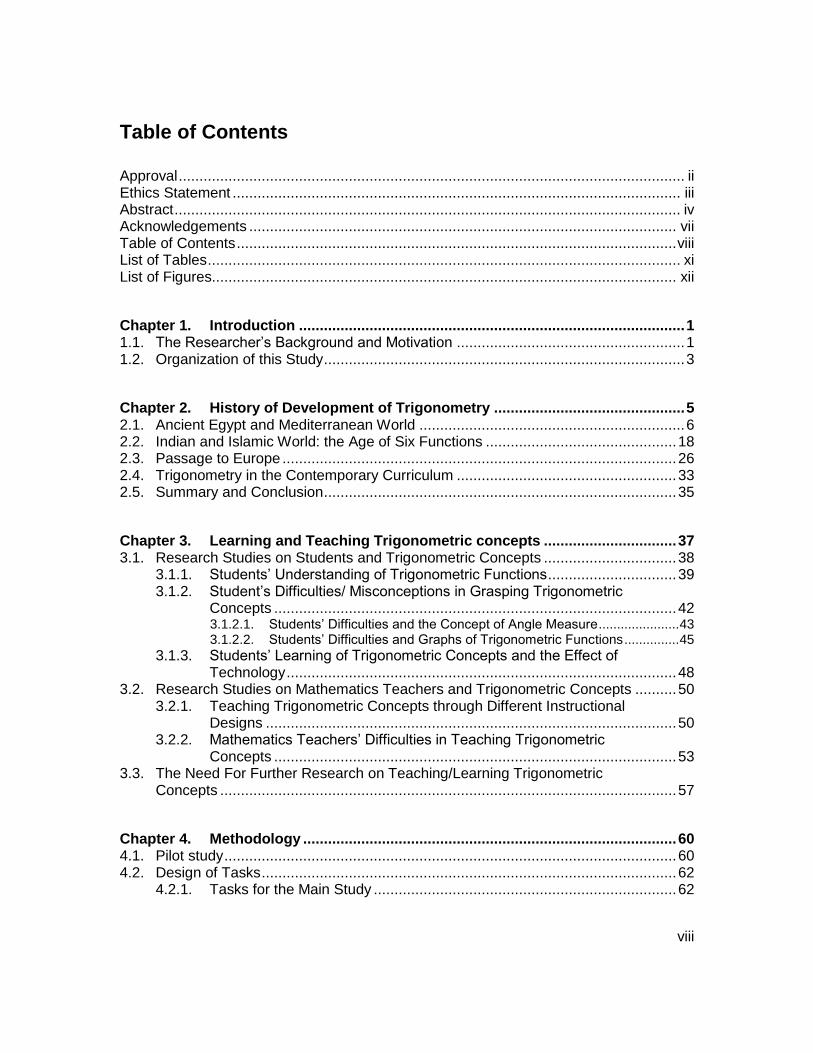
Table of Contents
Approval .......................................................................................................................... ii Ethics Statement ............................................................................................................ iii Abstract .......................................................................................................................... iv Acknowledgements ....................................................................................................... vii Table of Contents .......................................................................................................... viii List of Tables .................................................................................................................. xi List of Figures................................................................................................................ xii
Chapter 1. Introduction ............................................................................................. 1 1.1. The Researcher’s Background and Motivation ....................................................... 1 1.2. Organization of this Study ....................................................................................... 3
Chapter 2. History of Development of Trigonometry .............................................. 5 2.1. Ancient Egypt and Mediterranean World ................................................................ 6 2.2. Indian and Islamic World: the Age of Six Functions .............................................. 18 2.3. Passage to Europe ............................................................................................... 26 2.4. Trigonometry in the Contemporary Curriculum ..................................................... 33 2.5. Summary and Conclusion ..................................................................................... 35
Chapter 3. Learning and Teaching Trigonometric concepts ................................ 37 3.1. Research Studies on Students and Trigonometric Concepts ................................ 38
3.1.1. Students’ Understanding of Trigonometric Functions ............................... 39 3.1.2. Student’s Difficulties/ Misconceptions in Grasping Trigonometric
Concepts ................................................................................................. 42 3.1.2.1. Students’ Difficulties and the Concept of Angle Measure ...................... 43 3.1.2.2. Students’ Difficulties and Graphs of Trigonometric Functions ............... 45
3.1.3. Students’ Learning of Trigonometric Concepts and the Effect of Technology .............................................................................................. 48
3.2. Research Studies on Mathematics Teachers and Trigonometric Concepts .......... 50 3.2.1. Teaching Trigonometric Concepts through Different Instructional
Designs ................................................................................................... 50 3.2.2. Mathematics Teachers’ Difficulties in Teaching Trigonometric
Concepts ................................................................................................. 53 3.3. The Need For Further Research on Teaching/Learning Trigonometric
Concepts .............................................................................................................. 57
Chapter 4. Methodology .......................................................................................... 60 4.1. Pilot study ............................................................................................................. 60 4.2. Design of Tasks .................................................................................................... 62
4.2.1. Tasks for the Main Study ......................................................................... 62

ix
4.2.2. Sketches.................................................................................................. 63 4.2.3. Tasks 1, 2 and 3 ...................................................................................... 66
4.2.3.1. Task 1 .................................................................................................... 66 4.2.3.2. Task 2 .................................................................................................... 67 4.2.3.3. Task 3 .................................................................................................... 67
4.2.4. Tasks 4 and 5 .......................................................................................... 68 4.3. Participants ........................................................................................................... 70
4.3.1. Emma, Rose and Sally ............................................................................ 71 4.3.2. Kate and Mia ........................................................................................... 71 4.3.3. Andy ........................................................................................................ 72
4.4. Data Collection ..................................................................................................... 72 4.5. Data Analysis ....................................................................................................... 73
Chapter 5. Theoretical Considerations ................................................................... 75 5.1. Mason’s Theory of Shifts of Attention ................................................................... 75 5.2. Presmeg’s visual imagery ..................................................................................... 77 5.3. Carlson’s et al. Covariational Reasoning .............................................................. 80 5.4. Application of the Frameworks in Data Analysis ................................................... 85
Chapter 6. Data Analysis: The Case of Andy ......................................................... 89 Part 1: Andy’s Story, Account-Of ................................................................................... 89
6.1.1. Task 1: Identifying the Function of 𝒇(𝒙) = 𝒔𝒊𝒏(𝟐𝒙) from the Given Graph ...................................................................................................... 89
6.1.2. Task 2: Identifying the Function 𝒇(𝒙) = 𝒔𝒊𝒏(𝟐𝟑𝒙) from the Given Graph ...................................................................................................... 91
6.1.3. Task 3: Identifying the Function of 𝒇(𝒙) = 𝒄𝒐𝒔(𝟐𝟓𝒙 − 𝛑𝟓) from the Given Graph. ........................................................................................... 93
6.1.4. Task 4: Assigning Coordinates to Represent 𝒇(𝒙) = 𝒔𝒊𝒏(𝟒𝒙) .................. 96 6.1.5. Task 5: Assigning Coordinates to Represent 𝒇(𝒙) = 𝒄𝒐𝒔(𝟑𝒙 − 𝝅 𝟒) ........ 97
6.2. Part: 2 Andy’s Story, Accounting-For .................................................................... 99 6.2.1. Shifts of Attention .................................................................................... 99
6.2.1.1. Task 1: Identifying the Function 𝒇(𝒙) = 𝒔𝒊𝒏(𝟐𝒙) from the Given Graph. .............................................................................................................. 99
6.2.1.2. Task 2: Identifying the Function 𝒇(𝒙) = 𝒔𝒊𝒏(𝟐𝟑𝒙) from the Given Graph ............................................................................................................. 102
6.2.1.3. Task 3: Identifying the Function 𝒇𝒙 = 𝒄𝒐𝒔(𝟐𝟓𝒙 − 𝝅𝟓 ) from the Given Graph .................................................................................................. 104
6.2.1.4. Task 4: Assigning Coordinates to Represent 𝒇(𝒙) = 𝒔𝒊𝒏(𝟒𝒙) ............. 106 6.2.1.5. Task 5: Assigning Coordinates to Represent 𝒇(𝒙) = 𝒄𝒐𝒔 (𝟑𝒙 −
𝝅𝟒) 108 6.2.2. Visual Imagery ....................................................................................... 110
6.2.2.1. Task 1: Identifying the Function of 𝒇(𝒙) = 𝒔𝒊𝒏(𝟐𝒙) from the Given Graph .................................................................................................. 110
6.2.2.2. Task 2: Identifying the Function of 𝒇(𝒙) = 𝒔𝒊𝒏(𝟐𝟑𝒙) from the Given Graph .................................................................................................. 112

x
6.2.2.3. Task 3: Identifying the Function of 𝒇(𝒙) = 𝒄𝒐𝒔(𝟐𝟓𝒙 − 𝝅𝟓) from the Given Graph ............................................................................................ 117
6.2.2.4. Task 4: Assigning Coordinates to Represent 𝒇𝒙 = 𝒔𝒊𝒏𝟒𝒙 .................. 119 6.2.2.5. Task 5: Assigning Coordinates to Represent 𝒇𝒙 = 𝒄𝒐𝒔𝟑𝒙 − 𝝅 𝟒 ....... 121
6.2.3. Covariational Reasoning ........................................................................ 122 6.3. Summary ............................................................................................................ 126
Chapter 7. Data Analysis: The case of the “Other Five Students” ..................... 128 7.1. Shift of Attention and Visual Imagery: Identifying the Period (coefficient B of
x) ........................................................................................................................ 1297.1.1. Identifying Period in Task 1.................................................................... 130
7.1.1.1. Initial Confusion ................................................................................... 130 7.1.1.2. Importance of Computer Feedback ..................................................... 134
7.1.2. Identifying Period in Tasks 2 and 3 ........................................................ 141 7.1.3. Identifying the Period in Tasks 4 and 5 .................................................. 144
7.2. Shift of Attention and Visual Imagery: Identifying the Phase Shift (C in the canonical function) .............................................................................................. 146
7.3. Covariational Reasoning ability: Identifying Period and Phase Shift.................... 152
Chapter 8. Discussion ........................................................................................... 156 8.1. Research Findings and Comments ..................................................................... 156 8.2. Contributions of the Study .................................................................................. 161 8.3. Research Limitations .......................................................................................... 163 8.4. Pedagogical Implications and Suggestions ......................................................... 164 8.5. Reflection of this Journey ................................................................................... 166
References .............................................................................................................. 168

xi
List of Tables
Figure 2.2. The relation between the chord function aTable 2.1nd the modern sine .......................................................................................................... 8
Table 3.1. The literature review outline ................................................................... 38
Table 3.2. Summary of Literature Review ............................................................... 56
Table . 5.1. Covariational reasoning with respect to general and trigonometric functions ................................................................................................ 82
Table 5.2. Levels of the Covariation Framework ..................................................... 88
Table 7.1. Students’ performance in the interview tasks ....................................... 129
Table 7.2. Students’ developmental levels ............................................................ 153
xii
List of Figures
Figure 2.1. Ancient Egyptians gnomon ....................................................................... 6
Figure 2.2. The relation between the chord function aTable 2.1nd the modern sine .......................................................................................................... 8
Figure 2.3. Supplementary angles............................................................................ 10
Figure 2.4. The theorem of plane triangles ............................................................... 12
Figure 2.5. Menelaus’s theorem ............................................................................... 12
Figure 2.6. d = Crdθ = 2Rsin𝜃
2 ................................................................................. 14
Figure 2.7. Ptolemy’s table known as sine table ....................................................... 15
Figure 2.8. Ptolemy's theorem.................................................................................. 16
Figure 2.9. Ptolemy’s theorem and sum of two angles ............................................. 17
Figure 2.10. Aryabhata’s definition of jya and utkrama-jya ......................................... 19
Figure 2.11. Aryabhaṭa's table of sine ........................................................................ 20
Figure 2.12. Six trigonometric functions in one diagram ............................................ 22
Figure 2.13. Law of sines in a spherical triangle ........................................................ 24
Figure 2.14. The half and multiple angle for tangent ................................................. 24
Figure 2.15. Six trigonometric functions in gnomonic context .................................... 25
Figure 2.16. Law tangent .......................................................................................... 28
Figure 2.17. logarithm of the sine of the angle .......................................................... 30
Figure 2.18. logarithm of the sine of the angle in right triangle .................................. 30
Figure 2.19. A geometric interpretation of Euler's formula ......................................... 32
Figure 2.20. Trigonometric function as ratio ............................................................... 33
Figure . 4.1. Snapshot of an example of the first sketch. ............................................ 64
Figure. 4.2. Snapshot of an example of the second sketch. ...................................... 65
Figure. 4.3. Sketch represents the function f(x) = sin(2x), Task 1. ........................... 66
Figure. 4.4. Sketch of f(x) = sin(2
3x), Task 2. ............................................................ 67
Figure 4.5. Sketch of f(x) = cos2
5x −
𝜋
5, Task 3. ....................................................... 68
Figure 4.6. Snapshot of Task 4, f(x) = sin4x. ........................................................... 69
Figure 4.7. Sketch of f(x) = sin(4x), solution to Task 4. ........................................... 69

xiii
Figure 4.8. Snapshot Task 5, f(x) = cos3x −𝜋
4. ....................................................... 70
Figure 4.9. Sketch of f(x) = cos3x −𝜋
4, solution to Task 5. ....................................... 70
Figure 6.1. Graph of f(x) = sin(2x) ........................................................................... 90
Figure 6.2. Graph of f(x) = cos2x +𝜋
4 ...................................................................... 91
Figure 6.3. Graph of f(x) = sin(2
3x) .......................................................................... 92
Figure 6.4. Graph of f(x) = cos(2
3x − (
2
3×
3𝜋
4)) ...................................................... 93
Figure 6.5. Graph of f(x) = cos(2
5x −
𝜋
5) ................................................................... 93
Figure 6.6. Determining the period of the given cosine function ............................... 94
Figure 6.7. Graph of f(x) = cos (2
5x −
2𝜋
3−
𝜋
3) ........................................................... 95
Figure 6.8. Graph of f(x) = sin(2
5x −
3𝜋
4) ................................................................... 96
Figure 6.9. Sinusoidal curve ..................................................................................... 96
Figure 6.10. Representing graph of f(x) = sin(4x) ..................................................... 97
Figure 6.11. Assigning the y-axes and the point 𝜋
4 ..................................................... 98
Figure 6.12. Changing the assigned axes .................................................................. 98
Figure 6.13. Graph of f(x) = cos3x − 𝜋
4 ...................................................................... 99
Figure 6.14. Snapshot of two graph f(x) = cos (2
3x +
3𝜋
4) and f(x) = sin (
2
3x) ............ 104
Figure 6.15. Intersecting the axes and the curve in the origin................................... 107
Figure 6.16. Putting π on the x-axes ........................................................................ 107
Figure 6.17. Assigning the coordinates on the sinusoidal curve ............................... 108
Figure 6.18. Putting 2π on the curve ........................................................................ 109
Figure 6.19. Shifting the sinusoidal curve to the left ................................................. 110
Figure 6.20. Andy’s right index to represent two cycles ............................................ 111
Figure 6.21. Pointing to 𝜋
2 ......................................................................................... 111
Figure 6.22. Andy positioned his hand horizontally .................................................. 112
Figure 6.23. Showing the oscillating function ........................................................... 113
Figure 6.24. Student positioned his hands parallel to each other ............................. 113
Figure 6.25. Student positioned his hands in the open parentheses position ........... 114
Figure 6.26. Showing the end point of one cycle of the sine curve ........................... 115

xiv
Figure 6.27. Andy’s pointing to the y-axes................................................................ 116
Figure 6.28. Andy moved his hand from left to right ................................................. 117
Figure 6.29. Andy was pointing to the point −3𝜋
4 ..................................................... 118
Figure 6.30. Andy was showing the half of period .................................................... 118
Figure 6.31. Andy showing the intersection between y-axes and the curve .............. 118
Figure 6.32. Student counted four full cycles ............................................................ 120
Figure 7.1. Period of a canonical function .............................................................. 130
Figure 7.2. Rose’s pictorial image of sinusoidal function ........................................ 132
Figure 7.3. Sally’s usage of her two fingers to show that the curve was shrunk...... 133
Figure 7.4. Graph of f(x) = sin(1
2x) and f(x) = sin(2x) .......................................... 135
Figure 7.5. Sally’s pointing to the B value in the suggested function ...................... 136
Figure 7.6. Emma showed relationship between periods in both graph using the pointer. ........................................................................................... 138
Figure 7.7. The end point of the curve #2 displaced by the computer pointer ......... 140
Figure 7.8. Rose was pointing to 2π ....................................................................... 140
Figure 7.9. Mia used the pointer to show the end point of the Curve #1 ................. 141
Figure 7.10. Mia counting the blocks between the points ......................................... 144
Figure 7.11. Kate placed the 4 cycles in the interval [0, 2π] ..................................... 145
Figure 7.12. Mia misplaced the point 𝜋
2 ..................................................................... 146
Figure 7.13. Identifying phase shift/horizontal shift ................................................... 147
1
Chapter 1. Introduction
Trigonometry has been used in various applications such as architecture,
astronomy and geography. Trigonometry is one of the fundamental topics taught in high
school and university curricula, but it is considered as one of the most challenging
subjects for teaching and learning. Despite its importance and its complexity, research
on trigonometry is sparse and quite limited. In the literature, only a small number of
studies concentrate on students’ learning of trigonometric concepts (e.g., Gray and Tall,
1991; Brown, 2005; Weber, 2005; Moor, 2010), and on teaching trigonometry (e.g.,
Akkoç and Gül, 2010 and Moor, 2012). In the succeeding chapter, the findings on
aspects of trigonometric topics in the mathematics education literature are presented in
greater detail.
In what follows, I begin with a brief description of my academic background and I
then outline some personal experience that led my research towards trigonometric
functions. I wrap up the chapter with an overview of sequencing chapters in this
dissertation.
1.1. The Researcher’s Background and Motivation
I came from a country where mathematics is the one of the most important topics
amongst other subjects in the school curriculum. In my country, Iran, students begin to
learn mathematics when they are very young, in Grade 1, and they all need to pass a
final mathematics exam in order to become eligible to study the following grade.
Furthermore, the majority of Iranian families are interested in sending their children to

2
high quality schools, where students are required to successfully complete the schools’
entrance exams, which mostly focus on their knowledge of various mathematics topics..
As such, there are very tough competitions amongst students to learn, practice
and earn high marks on the mathematics exams. The importance of mathematics exams
becomes more highlighted for high schoolers, who need to successfully pass the
university entrance exam, which is comprised of the mathematics topics students
learned in Grades 9-12.
The vital role that Mathematics plays in a student’s future life makes mathematics
classrooms boring and stressful for most of students. However, in my school life, I had a
great mathematics teacher for the last three years of high school. She was the most
well-educated, patient and friendly teacher I ever had in my school years. She was my
inspiration to choose mathematics as my major in post-secondary education.
Fortunately, I passed the university entrance exam successfully and I started my
bachelors in the subject of “Pure mathematics.”
Graduating from university, I became a high school mathematics teacher. As a
young and energetic teacher, I often tried my best to be an effective and helpful teacher
for my students. As I knew that mathematics classrooms are often boring, I attempted to
create a fun and interesting learning environment for my students. I showed my students
examples of the application of mathematics in real life and I provided them with in-class
activities. In spite of all the efforts I made, there still were some students who hated
mathematics and therefore they did not make enough effort to learn mathematics. At that
stage, I noted that I needed to learn more about teaching mathematics as well.
Observing students’ struggles to understand and deal with a subject in which
they had no interest, motivated me to learn more about various effective teaching
methods. I began my master’s studies at the University of British Columbia (UBC),
where I learned about teaching mathematics from different angles. Meanwhile, I tutored
some high school and university students in Vancouver.

3
When I worked as a tutor in Vancouver, I realized that students’ difficulties in
some specific topics in mathematics were similar to those with which my students
struggled in my home country. Not only Canadian high school students, but also
university students encountered similar difficulties. Knowing university students’
difficulties with some mathematics topics inspired me to explore and to do research
related to teaching mathematics at the undergraduate level. Therefore, after graduating
from UBC in the summer 2012, I began my PhD program in the fall 2012 at Simon
Fraser University.
As a first year PhD student I worked as a Teaching Assistant (TA) for the Applied
Calculus Workshop (ACW), where I helped students who were registered in Calculus I or
Calculus II in doing the assignments and answering their questions about the lecture
notes. Helping students in ACW made me realize that one of the difficult topics for
undergraduate students is “trigonometry.” Discussing with some Mathematics instructors
at SFU Mathematics department about students’ struggles in the calculus courses
assured me that “trigonometry” is indeed one of the most challenging topics for
undergraduate students. Parallel with my own experience, the SFU instructors agreed
that graphing trigonometric functions is one of the hardest parts in trigonometry in a
Calculus course. As such, for this PhD dissertation, I decided to investigate the way
undergraduate students deal with this challenging topic.
1.2. Organization of this Study
This dissertation is comprised of eight chapters including the introduction
presented in this chapter. Chapter 2 presents a review of the historical development of
trigonometry. The chapter begins with the ways the ancient Egyptians and Babylonians
used trigonometry in 3000 BCE, and it continues with the birth of trigonometric functions
by a Persian mathematician, Al-Khawarizmi (c. 780- c. 850).
In Chapter 3, I review the research studies focused on trigonometry from
different points of view. Students’ understanding and misunderstanding of aspects of

4
trigonometric functions, as well as the influence of technology on pupils’ grasping of
trigonometric topics are covered in the first part of Chapter 3. The rest of the chapter is
devoted to the review of research studies focused on teachers’ conceptions of
trigonometry, as well as various methods mathematics’ teachers often employ when
teaching trigonometric concepts. I wrap up Chapter 3 with a brief description of gaps in
the area of research on learning trigonometric concepts and the need for further
research on this important topic.
The following chapter is devoted to the methodology of this study. In Chapter 4 of
this dissertation, I state the main goal of this study followed by the general research
questions. I then provide a review of the pilot study and describe how the interview tasks
were designed for the purpose of this study. The participants for the main study and their
academic backgrounds are presented next. At the end of this chapter, I describe the way
I collected data and how I analyzed the data according to the three frameworks. The
three theoretical frameworks (Mason’s (2008) theory of shifts of attention, Presmeg’s
(1989) visual imagery, and Carlson’s et al. (2002) covariational reasoning) which I
employ for analyzing the data collected for this study. These are explained in Chapter 5.
In Chapter 6, I analyze the response of one of the participants, Andy, in detail
with respect to the three theoretical frameworks. There, I describe how he completed
each interview task, the difficulties he encountered and the errors he made during the
interview. The analysis of the responses of the rest of the participants to each of the
interview tasks is presented in the Chapter 7. To complete a comprehensive analysis; I
compared the answers of five students with each other and with Andy’s responses.
Finally, the conclusion of this dissertation comes in Chapter 8, where the
research questions are restated and answered. In this chapter, I present a summary of
the findings and then I state the contributions of this study. The limitations of this study,
the applications of the findings in teaching transformations of sinusoidal functions, and
the need for further research are noted at the end of this dissertation in Chapter 8.

5
Chapter 2.
History of Development of Trigonometry
Looking at the trigonometry history shows that it took long time to develop, the
first stages of development date back to about 3000 BCE. Reading several history books
about the development of mathematics, and trigonometry in particular, shows how
people in ancient times used it for multiple purposes such as exploring astronomy (e.g.,
recording the rising and setting of stars and calculating the time of day). However,
reviewing the developmental history illustrates that since the beginning, trigonometry
was a difficult topic for human beings and it has taken thousands of years for
mathematicians and astronomers to grasp the content. In spite of the historical difficulty
of trigonometry, which caused its slow progress, teachers often expect students to
understand the topic in a short time. Looking at the historical development of
trigonometric concepts, however, helps in gaining appreciation of the discipline and of
potential struggle of learners. In what follows the key people who have had fundamental
contributions in the development of trigonometry, the difficulties they encountered and
the ways they solved them are explained in this paper.
The historical development of trigonometry is described in this chapter in three
different sections. In the first section, I explain the use of trigonometry in the “Ancient
Egypt and Mediterranean World” The second one is related to the arrival of
trigonometry in the “Indian and Islamic world” and the next section deals with the
history of progression of trigonometry to “European World.” In the last section, I also
talk about Trigonometry in the Contemporary Curriculum. This chapter concludes
with a summary of the development of trigonometry from the earliest times to the
modern period.

6
2.1. Ancient Egypt and Mediterranean World
The term “trigonometry” came from the Greek words trigonon, meaning “triangle,”
and the Greek word -metria, meaning “measurement.” As the name implies,
trigonometry emerged from the study of right triangles and the relationships among the
lengths of the sides and the angles of the triangle (Steckroth, 2007). The origin of
trigonometry came from the ancient Egyptians and Babylonians, who developed and
used theorems on ratios of the sides of similar triangles without being actually aware of
trigonometry in the modern form (Adamek, Penkalski, and Valentine, 2005). The ancient
Egyptians utilized trigonometry in land surveying, constructing their pyramids, and
correlating shadow lengths of a vertical stick (gnomon) with the time of day (see Figure
2.1). The shadow tables are the ancestors of cotangent and tangent (Maor, 1998).The
Babylonian astronomers also related trigonometric functions to arcs of circles and to the
lengths of chords subtending the arcs to develop astronomers’ records of the events of
the lunar month, the rising and setting of stars and the motion of planets and of the solar
system (Van Brummelen, 2009).
Figure 2.1. Ancient Egyptians gnomon
Although the primitive forms of trigonometry (e.g., gnomon) were in existence
previously, the development of modern trigonometry into an ordered science began

7
slowly with the introduction of the common unit of angular measure, the degree,
originated by the Babylonians (Maor, 1998). Some historians believe that the Babylonian
astronomers first divided a circle into 360 parts. The reasons for this division might be
because of the intimacy of this number (360) to the number of days in the year, 365
days, or the possibility of dividing a circle naturally into six equal parts, each subtending
a chord equal to the radius (Maor, 1998). What is historically clear is the fact that the
system fit very well into the Babylonian sexagesimal (which is based on 60 rather than
our current decimal number system based on ten) numeration system. The early
Greeks, later, adopted the Babylonian sexagesimal number system and they introduced
the degree for the first time (Van Brummelen, 2009). Greeks used the word µοιρα
(moira) to refer to degree. The Arabs translated µοιρα into daraja, which, then, became
the Latin word de gradus from which came the word degree (Maor, 1998).
Other than what is known about the Babylonian astronomers and the Greeks’
adoption of the degree, there is a gap in the history of the development of trigonometry
until the improvement of trigonometry by the Greek astronomer Hipparchus of Nicaea
(ca.190-120 B.C.).
Hipparchus came to be known as “the father of trigonometry” and is the first
person whose use of trigonometry is documented (Adamek et al., 2005). His work
stressed the need for a system that provided a unit of measure for arcs and angles
(Sozio, 2005).In astronomy, Hipparchus is credited with discovering the procession of
the equinoxes (a slow circular motion of celestial poles once every 26700 years),
determining the celestial longitude and latitude of 1000 stars and recording their
positions on a map. He also classified stars according to their brightness by introducing
a scale in which the magnitude of the brightest stars is 1 and the faintest stars have a
magnitude of 6 (Maor, 1998). Hipparchus was the first person to determine exactly the
times of the rising and setting of the zodiacal signs and also to estimate the size and
distances of the sun and moon (Van Brummelen, 2009).
To be able to do his calculations for his astronomical work, Hipparchus needed a
table of trigonometric ratios (Maor, 1998). However, since there was not such a table, he

8
had to compute his own table (this is considered as one of the beginning difficulties of
developing trigonometry). Hipparchus considered every triangle (planar or spherical) as
being inscribed in a circle of large fixed radius (see Figure 2.2), so that each side of the
triangle became a chord (a straight line drawn between two points on a circle) (Maor,
1998). In order to calculate the length of various parts of the triangle, Hipparchus had to
figure out the length of the chord as a function of the central angle (Half of this chord
later became the sine function (Van Brummelen, 2009)). The length of the chord is
denoted by Crd.
Figure 2.2. The relation between the chord function aTable 2.1nd the modern sine
Using basic circle properties, 𝐶𝑟𝑑(𝑎) = 2𝑅 sin(𝑎 2⁄ ) ( Or sin(𝑎 2⁄ ) = 𝐶𝑟𝑑(𝑎) 2𝑅⁄ ).
Hipparchus chose a large fixed radius, R, to avoid fractions [when the radius is chosen
large enough (R= 3438 in sexagesimal system), when divisions are made, these parts
become whole numbers (Adamek et al., 2005)]. Maor (1998) states that from his
calculations, Hipparchus borrowed the idea from the Babylonian astronomers who
divided every circle into 360 degree and he, thus, began with the chord of 60° equal with
the radius of the circle (R= 60°) when he constructed his table.
To complete his table and find other angles (except R=60), Hipparchus needed
to know how to calculate the chord of the supplement of a given arc (which is written as:

9
𝐶𝑟𝑑(180 − 𝛼) = √((2𝑅)2 − (𝐶𝑟𝑑(𝛼))2
) ) and also the formula for the chord of
half angle: (𝐶𝑟𝑑𝛼
2)
2= 𝑅 (2𝑅 − 𝐶𝑟𝑑(180 − 𝛼) (Van Brummelen, 2009). As such, although
Hipparchus, as an astronomer, was mainly concerned with spherical triangle (Maor,
1998 and Hunt, 2000), he still would have needed to know many formulas of plane
trigonometry (as mentioned these lack of knowledge, made the development of
trigonometry a difficult task for ancient people) which are in the modern form as:
(sin 𝛼)2 + (cos 𝛼)2 = 1
(which is a trigonometric version of the Pythagorean Theorem),
(sin 𝛼 2⁄ )2 = (1 − cos 𝛼) 2⁄ , or
sin(𝛼 + 𝛽) = sin 𝛼 × cos 𝛽 + cos 𝛼 × sin 𝛽
Hunt(2000) and Van Brummelen (2009) indicate that Hipparchus used, for
example, Pythagorean Theorem [according to Thales’s theorem if two angles (α and
180- α) are supplementary angles, the triangle having two sides Crd (α) and Crd (180- α)
is a right triangle ( see Figure 2.3)] for the supplementary formula as:
𝐶𝑟𝑑(180 − 𝛼) = √(2𝑅)2 − (𝐶𝑟𝑑 (𝛼))2 (Formula 1)

10
Figure 2.3. Supplementary angles
Since he knew:
𝐶𝑟𝑑(𝛼) = 2𝑅 × sin 𝛼 2⁄ (Formula 2)
𝐶𝑟𝑑(180 − 𝛼) = 2𝑅 sin (180 − 𝛼) 2 = 2𝑅 × cos 𝛼 2⁄ .⁄ (Formula 3)
Thus, from formula (1), (2) and (3):
2𝑅 cos(𝛼 2⁄ ) = √(2𝑅)2 − (2𝑅 sin(𝛼 2⁄ ))2
(2𝑅)2 (cos 𝛼 2⁄ )2 = (2𝑅)2 − (2𝑅 sin 𝛼 2⁄ )2 (Formula 4)
Therefore, both sides of the equation (Formula 4) will be equal because
Hipparchus knew sin(𝛼 2⁄ )2 + cos(𝛼 2⁄ )2 = 1 (Van Brummelen, 2009).
Hipparchus wrote twelve books on the computation of chords in a circle.
Unfortunately, however, all his works were lost and most of what is known about his
works is through later references in Ptolemy's Almagest (explained later in this paper),
written three centuries after Hipparchus died.

11
The next Greek mathematician known to have made a great contribution to
trigonometry and in particular to spherical trigonometry was Menelaus of Alexandria
(c.a. 100 A.D.) (Maor, 1998). Menelaus wrote a six-book treatise on chords, but those
books (e.g., On the Triangle and Elements of Geometry) have all been lost. Menelaus,
however, authored a three-book work called Spherics which is his only surviving work.
Although the Greek version of this text is lost, and all that remains is an Arabic version
translated a thousand years after Menelaus wrote the original version, this work still
provides a good source for the development of spherical trigonometry (Van Brummelen,
2009).
The first book of the Sphaerica is geometric in content and deals systematically
with the conception and definition of a spherical triangle for the first time. Menelaus
described a spherical triangle as the area included by the arcs of great circles on the
surface of a sphere subject to the restriction that each of the sides or legs of the triangle
is an arc less than a semicircle (Van Brummelen, 2009). He then imitated the theorems
of Euclid's propositions about plane triangles and extending them to give the main
propositions about spherical triangles (e.g., the two triangles on the base of any
spherical triangle with two equal sides are themselves equal). In this book, however,
Menelaus avoided proving any theorem (Van Brummelen, 2009).
The second book has astronomical interest only, whereas the third book
contains some important information about the development of trigonometry and it deals
with spherical trigonometry and includes the Menelaus's theorem (Van Brummelen,
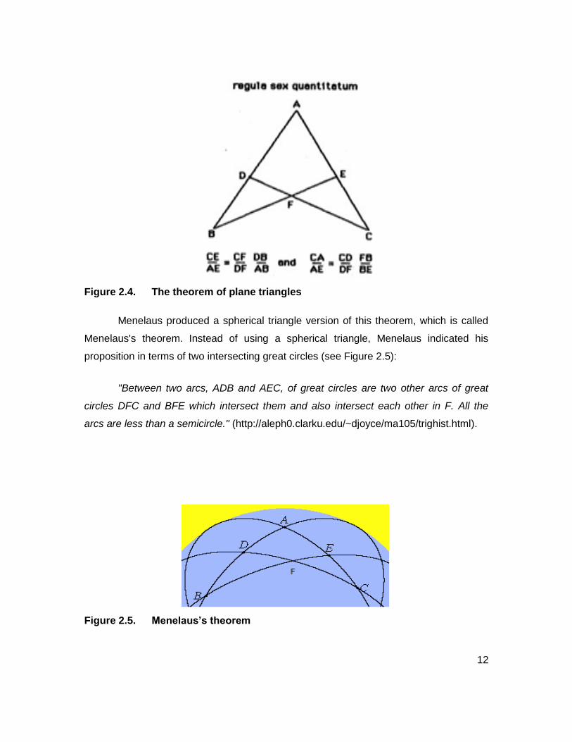
2009). For plane triangles the theorem was known before Menelaus (see Figure 2.4):
... if a straight line crosses the three sides of a triangle (one of the sides is
extended beyond the vertices of the triangle), then the product of three of the
nonadjacent line segments thus formed is equal to the product of the three remaining
line segments of the triangle.
12
Figure 2.4. The theorem of plane triangles
Menelaus produced a spherical triangle version of this theorem, which is called
Menelaus's theorem. Instead of using a spherical triangle, Menelaus indicated his
proposition in terms of two intersecting great circles (see Figure 2.5):
"Between two arcs, ADB and AEC, of great circles are two other arcs of great
circles DFC and BFE which intersect them and also intersect each other in F. All the
arcs are less than a semicircle." (http://aleph0.clarku.edu/~djoyce/ma105/trighist.html).
Figure 2.5. Menelaus’s theorem

13
According to Menelaus’s theorem:
𝐶𝑟𝑑(2𝐴𝐸) 𝐶𝑟𝑑 (2𝐶𝐸) = 𝐶𝑟𝑑 (2𝐴𝐵) 𝐶𝑟𝑑(2𝐵𝐷) × 𝐶𝑟𝑑 (2𝐷𝐹) 𝐶𝑟𝑑 (2 𝐹𝐶)⁄⁄⁄ .
and
𝐶𝑟𝑑(2𝐴𝐶) 𝐶𝑟𝑑(2𝐴𝐸) = 𝐶𝑟𝑑 (2𝐶𝐷) 𝐶𝑟𝑑 (2𝐷𝐹) × 𝐶𝑟𝑑 (2𝐵𝐹) 𝐶𝑟𝑑 (2𝐵𝐸).⁄⁄⁄
If Menelaus's theorem for spherical trigonometry was written in terms of modern
sines, they would be as follows:
sin(𝐴𝐸) sin(𝐶𝐸) = sin(𝐴𝐵) sin(𝐵𝐷) × sin(𝐷𝐹) sin(𝐹𝐶)⁄⁄ ⁄
sin(𝐴𝐶) sin(𝐴𝐸)⁄ = sin(𝐶𝐷) sin(𝐷𝐹) × sin(𝐵𝐹) sin(𝐵𝐸)⁄⁄
Though Menelaus’s developments were very important, the first major and the
most influential work on trigonometry is The Mathematical Syntaxis, usually known as
the Almagest which is a work of thirteen books by Ptolemy of Alexandria (ca. 85-ca. 165
A.D) (Maor, 1998).
Ptolemy focused on a combination of both astronomy and trigonometry in
Almagest. The book is based upon the assumption that a motionless earth sits at the
center of the universe and the heavenly bodies move around it in their prescribed orbits
(Maor, 1998). In order to accomplish his goal (recording the motions of all celestial
objects), Ptolemy noticed that he needed a substantial trigonometric tool. Therefore, the
subject of chapters 10 and 11 of the Almagest is about Ptolemy’s table and a detailed
set of instructions (containing some of the earliest extent derivations of common
trigonometric results) on how to construct the table (Van Brummelen, 2009). Almagest is
reliant on much of the work of Hipparchus and Menelaus (Adamek et al., 2005). Some
historians believe that Ptolemy completed Hipparchus’s work through adding some
necessary details and constructing new tables. However, since much of Hipparchus’
work was lost, it is difficult to distinguish between what additions and modifications
Ptolemy made, and what already existed (Adamek et al., 2005).

14
Figure 2.6. 𝒅 = 𝑪𝒓𝒅𝜽 = 𝟐𝑹 𝐬𝐢𝐧 𝜽 𝟐⁄
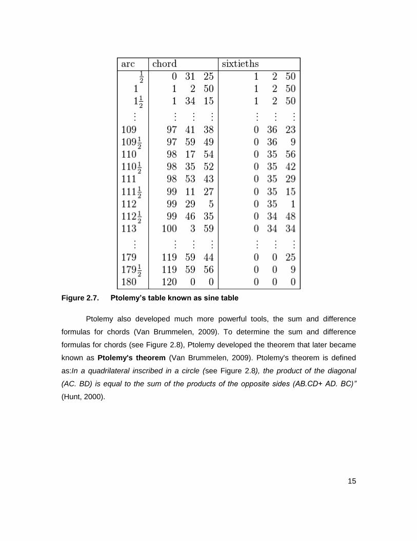
Ptolemy's table gives the length of a chord in a circle as a function of the central
angle (see Figure 2.6) that subtend it for angles increasing from 0 degrees to 180
degrees at intervals of half a degree (Maor, 1998). He took the diameter of the circle to
be 120 units and thus R= 60. Ptolemy's table of chord is essentially a table of sines
because 𝑑 = 𝐶𝑟𝑑𝜃 = 2𝑅 sin 𝜃 2⁄ or 𝑑 = 𝐶𝑟𝑑𝜃 = 120 sin 𝜃 2⁄ . As is clear from the
equation, apart from proportionality factor 120, Ptolemy’s table is equivalent to a table of
value of sin(θ/2) and thus, by doubling the angle it is a table of sin(θ) (Maor, 1998). In
other words, the table is the earliest trigonometric table of sines.
In his table, Ptolemy carried out his calculations to three sexagesimal places to
achieve the accuracy of the chord length (Maor, 1998). Apart from two separate columns
for arcs and chords, Ptolemy's table was comprised of a column of “sixtieths” (see Figure
2.7). The column of “sixtieths” allows one to incorporate between successive entries: it
gives the mean increment in the chord length from one entry to the next (Maor, 1998)
15
Figure 2.7. Ptolemy’s table known as sine table
Ptolemy also developed much more powerful tools, the sum and difference
formulas for chords (Van Brummelen, 2009). To determine the sum and difference
formulas for chords (see Figure 2.8), Ptolemy developed the theorem that later became
known as Ptolemy's theorem (Van Brummelen, 2009). Ptolemy's theorem is defined
as:In a quadrilateral inscribed in a circle (see Figure 2.8), the product of the diagonal
(AC. BD) is equal to the sum of the products of the opposite sides (AB.CD+ AD. BC)”
(Hunt, 2000).

16
Figure 2.8. Ptolemy's theorem
When AD is a diameter of the circle, where O is the center of the circle and d the
diameter, then the theorem says:
𝐶𝑟𝑑(𝐴𝑂𝐶)𝐶𝑟𝑑(𝐵𝑂𝐷) = 𝐶𝑟𝑑 (𝐴𝑂𝐵) 𝐶𝑟𝑑(𝐶𝑂𝐷) + 𝑑 𝐶𝑜𝑟𝑑 (𝐵𝑂𝐶).
Therefore, if “a” is for angle AOB and b for angle AOC, and then there is:
𝐶𝑟𝑑(𝑏)𝐶𝑟𝑑(180 − 𝑎) = 𝐶𝑟𝑑 (𝑎)𝐶𝑟𝑑(180 − 𝑏) + 𝑑𝐶𝑟𝑑(𝑏 − 𝑎)
which gives the different formula:
𝐶𝑟𝑑(𝑏 − 𝑎)= 𝐶𝑟𝑑(𝑏) 𝐶𝑟𝑑(180 − 𝑎) − 𝐶𝑑𝑟(𝑎)𝐶𝑟𝑑(180 − 𝑏) 𝑑⁄ (formula (1)).
and since:
sin 𝑎 = (1 𝑑⁄ )𝐶𝑟𝑑(2𝑎) and cos 𝑎 = (1 𝑑⁄ )𝐶𝑟𝑑(180 − 2𝑎) (formula (2)),
therefore, formula (1) corresponds to the difference formulas for modern trigonometry
as:
sin(𝑎 − 𝑏) = sin 𝑎 × cos 𝑏 − sin 𝑏 × cos 𝑎.
Using Ptolemy’s theorem to find the sum of two chords is not quite as
straightforward (Van Brummelen, 2009).

17
Figure 2.9. Ptolemy’s theorem and sum of two angles
If BF extended to E, thus α = AB=DE and β= BC. Therefore, application of
Ptolemy’s theorem to BCDE gives (see Figure 2.9):
𝐶𝑟𝑑(180 − (𝛼 + 𝛽)) = 𝐶𝑟𝑑(180 − 𝛼)𝐶𝑟𝑑(180 − 𝛽) − 𝐶𝑟𝑑(𝛼) 𝐶𝑟𝑑(𝛽) 2𝑅⁄ (formula (3))
From formula (2) and (3) one could conclude the modern sum formula for cos:
cos(𝑎 + 𝑏) = cos(𝑎) cos(𝑏) − sin(𝑎) sin(𝑏) (Bressoud, 2010).
Ptolemy's theorem not only leads to the equivalent of the sum-and-difference formulas
for sine and cosine that are today known as Ptolemy's formulas, it also helps to derive
the equivalent of the half-angle formula for trigonometric functions, sin(𝑎)2 =
√(1 − cos 𝑎) (I do not explain it here due to lack of space) (Van Brummelen, 2009).
After the early trigonometry, the Indian and Islamic trigonometry will be described
in detail in the next section.

18
2.2. Indian and Islamic World: the Age of Six Functions
After Ptolemy, Greek trigonometry had little development (Van Sickle, 2011). No
documented evidence is available for the arrival of Greek astronomical models in India
(Van Brummelen, 2009). The earliest Indian work believed to come from the influence of
Greek trigonometry is Siddhantas (late fourth or early fifth century A.D.). It contains a
table which is a modified version of Ptolemy’s table of chord (Maor, 1998). The
trigonometry of Ptolemy was based on the functional relationship between the chords of
a circle and the central angles they subtend. But, the authors of the Siddhantas (its
original version is by an unknown author) focused on a study of the relationship between
half of a chord of a circle and half of the angle subtended at the center by the whole
chord (Adamek et al., 2005). From this stemmed the ancestor of the modern
trigonometric function known as the sine of the angle (although it still was not called
“sine”). Therefore, the main contribution of India and particularly the Siddhantas is the
more formal introduction of the sine function to the history of mathematics (Adamek et
al., 2005).
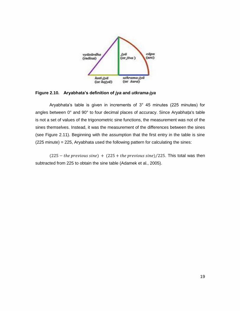
Aryabhata (AD 476-550), an Indian mathematician and astronomer, collected
and expanded upon the developments of the Siddhantas with his book entitled
Aryabhatiya. It is believed that Aryabhatiya is the primary original Hindu work in which
for the first time in the history of trigonometry the sine as a function of an angle was
named. In his work which focused on calculating a table of “sine differences”, Aryabhata
used the word ardha-jya to refer to the half-chord and sometimes the word turned
around to jya-ardha, chord-half. In order to shorten the word, Aryabhata used jya or jiva
(Maor, 1998). Like the chord, the jya was defined as the length of a certain line segment
in a circle (see Figure 2.10). The relationship between jaya and the modern sine is: jaya
(α) = 𝑅 sin(𝑎) where R is a radius of the base circle (R= 3438). Also the utkrama-jya
(reversed sine) or versed sine is: Vers(𝑎) = 1 − cos(𝑎).
19
Figure 2.10. Aryabhata’s definition of jya and utkrama-jya
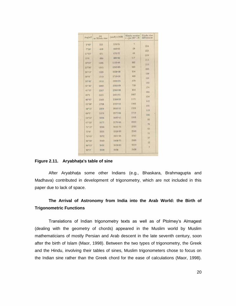
Aryabhata’s table is given in increments of 3° 45 minutes (225 minutes) for
angles between 0° and 90° to four decimal places of accuracy. Since Aryabhaṭa's table
is not a set of values of the trigonometric sine functions, the measurement was not of the
sines themselves. Instead, it was the measurement of the differences between the sines
(see Figure 2.11). Beginning with the assumption that the first entry in the table is sine
(225 minute) = 225, Aryabhata used the following pattern for calculating the sines:
(225 − 𝑡ℎ𝑒 𝑝𝑟𝑒𝑣𝑖𝑜𝑢𝑠 𝑠𝑖𝑛𝑒) + (225 + 𝑡ℎ𝑒 𝑝𝑟𝑒𝑣𝑖𝑜𝑢𝑠 𝑠𝑖𝑛𝑒) 225⁄ . This total was then
subtracted from 225 to obtain the sine table (Adamek et al., 2005).
20
Figure 2.11. Aryabhaṭa's table of sine
After Aryabhaṭa some other Indians (e.g., Bhaskara, Brahmagupta and
Madhava) contributed in development of trigonometry, which are not included in this
paper due to lack of space.
The Arrival of Astronomy from India into the Arab World: the Birth of
Trigonometric Functions
Translations of Indian trigonometry texts as well as of Ptolmey‘s Almagest
(dealing with the geometry of chords) appeared in the Muslim world by Muslim
mathematicians of mostly Persian and Arab descent in the late seventh century, soon
after the birth of Islam (Maor, 1998). Between the two types of trigonometry, the Greek
and the Hindu, involving their tables of sines, Muslim trigonometers chose to focus on
the Indian sine rather than the Greek chord for the ease of calculations (Maor, 1998).
21
Abu Ja'far Muhammad ibn Musa al-Khwarizmi Al-Khwarizmi, a Persian
mathematician, astronomer, astrologer, geographer and a scholar, introduced the Indian
computational and mathematical methods to Arabs for the first time.
Al-Khawarizmi (c. 780- c. 850) translated the Aryabhatiya, into Arabic language,
in his famous book entitled Zij al-Arjabhar. In his translation, al-Khwarizmi kept the word
jiva without translating its meaning. Since in Arabic words consist mostly of consonants,
and vowels are interpreted by context, jiva could also be pronounced as jaib, which
means bosom, or bay. Therefore, when the Arabic version of Aryabhatiya was translated
into Latin, they translated jaib into sinus or sine, which means bosom or bay. The cosine
function which first arose for the need to compute the sine of the complementary angle
is a Latin translation of the word Kotijya of Aryabhata (Maor, 1998).
Al-Khwarizmi also wrote a book called Zij al-Sindhind, which contains an
accurate sine and cosine table in which R=60 for the interval of 1 degree. Al-Khwarizmi's
Zij also includes a table of versed sine to solve astronomical problems (Van Sickle,
2011). To solve attitude problems using gnomons and shadows, Al-Khwarizmi
constructed the first table of tangent in the history of mathematics (although, he still did
not call it “tangent”) in his famous book Al-Jabr wa-al-Muqabilah. He was also the
inventor of spherical trigonometry.
To calculate various astronomical coefficients with great accuracy, following al-
Khwarizmi, another Arab astronomer, Abdallah Muhammad Ibn Jabir Ibn Sinan al-
Battani (around 858-929) introduced the trigonometric ratio in mathematical
calculation (e.g., tan 𝑎 = sin 𝑎 cos 𝑎⁄ and cot 𝑎 = cos 𝑎 sin 𝑎⁄ ) which formed the basis of
modern trigonometry (Maor, 1998). Al-Battani used the following rule for finding the rise
of the sun above the horizon in terms of the length “m” of the shadow by a vertical
gnomon of height “h”:
𝑚 = ℎ sin(90 − 𝛼) sin(𝛼)⁄ or 𝑚 = ℎ cot(𝛼).
22
In his book Zij al-Sabi, al-Battani applied the above formula to produce the table
of cotangents for the first time, which he referred to as a "table of shadows" (in
reference to the shadow of a gnomon) and he called it zill mabsut (or umbra recta in
Latin) by degree from 1° to 90° to solve astronomical problems. He was also the first
person to introduce the reciprocal functions of secant and cosecant (Maor, 1998). Al-
Battani also provided important trigonometric formulas for right-angled triangles (with
side length of a, b and c), such as the following formula (instead of using geometrical
methods, as Ptolemy had done):
𝑏 sin(𝐴) = 𝑎 sin(90 − 𝐴)
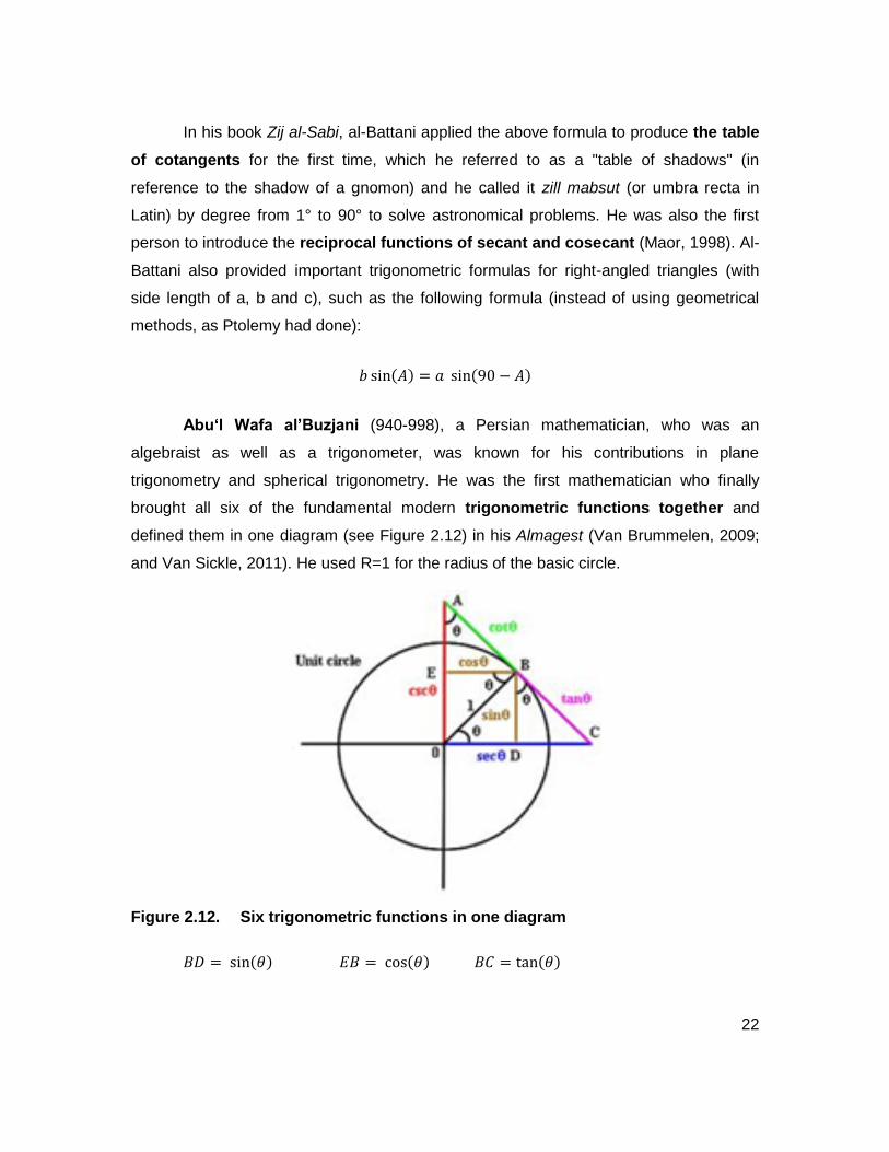
Abu‘l Wafa al’Buzjani (940-998), a Persian mathematician, who was an
algebraist as well as a trigonometer, was known for his contributions in plane
trigonometry and spherical trigonometry. He was the first mathematician who finally
brought all six of the fundamental modern trigonometric functions together and
defined them in one diagram (see Figure 2.12) in his Almagest (Van Brummelen, 2009;
and Van Sickle, 2011). He used R=1 for the radius of the basic circle.
Figure 2.12. Six trigonometric functions in one diagram
𝐵𝐷 = sin(𝜃) 𝐸𝐵 = cos(𝜃) 𝐵𝐶 = tan(𝜃)
23
𝐴𝐵 = cot(𝜃) 𝑂𝐷 = sec(𝜃) 𝑂𝐸 = csc(𝜃).
Applying all of the modern trigonometric functions, in fact, assisted Abu‘lWafa to
make trigonometric calculations much more easily and quickly than before, although
initially only some of his colleagues appreciated this change (Van Sickle, 2011). He
contributed a table of tangents using all six of the common trigonometric functions
(Maor, 1998). Abu‘lWafa also constructed a new sine table, using eight decimal places.
Abu‘lWafa proved several identities known today as the Pythagorean identities,
such as:
tan(𝑎)2 + 1 = 𝑠𝑒𝑐(𝑎)2 and 1 + cot(𝛼)2 = csc(𝑎)2 (Van Brummelen, 2009).
Furthermore, he developed the following trigonometric formula:
sin(𝑎 ± 𝑏) = sin(𝑎) cos(𝑏) ± cos(𝑎) sin(𝑏).
sin(2𝑎)= 2sin(𝑎) cos(𝑎) (Ptolemey had expressed the equivalent identities in
terms of chords)
cos(2𝑎) = 1 − 2 sin(2𝑎) (Adamek et al., 2005).
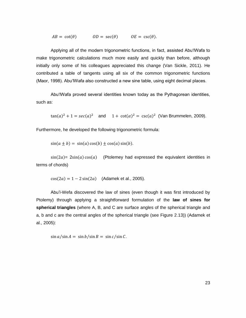
Abu’l-Wefa discovered the law of sines (even though it was first introduced by
Ptolemy) through applying a straightforward formulation of the law of sines for
spherical triangles (where A, B, and C are surface angles of the spherical triangle and
a, b and c are the central angles of the spherical triangle (see Figure 2.13)) (Adamek et
al., 2005):
sin 𝑎 sin 𝐴 = sin 𝑏 sin 𝐵 = sin 𝑐 sin 𝐶⁄⁄⁄ .
24
Figure 2.13. Law of sines in a spherical triangle
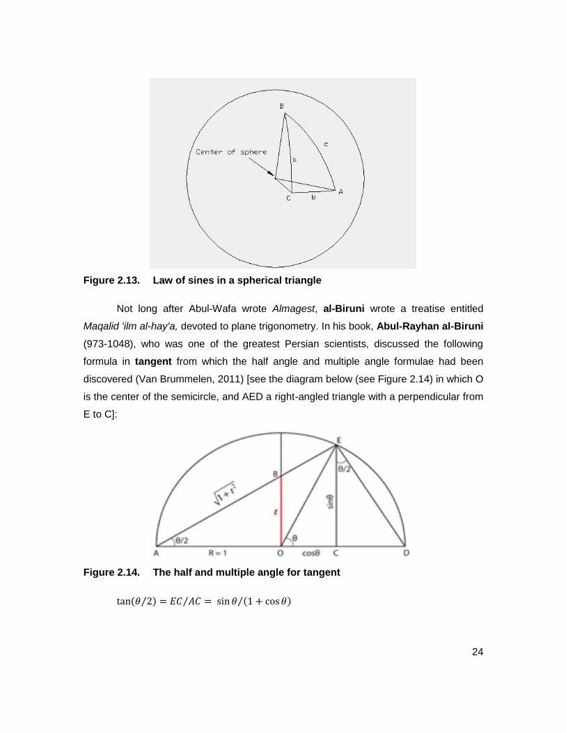
Not long after Abul-Wafa wrote Almagest, al-Biruni wrote a treatise entitled
Maqalid 'ilm al-hay'a, devoted to plane trigonometry. In his book, Abul-Rayhan al-Biruni
(973-1048), who was one of the greatest Persian scientists, discussed the following
formula in tangent from which the half angle and multiple angle formulae had been
discovered (Van Brummelen, 2011) [see the diagram below (see Figure 2.14) in which O
is the center of the semicircle, and AED a right-angled triangle with a perpendicular from
E to C]:
Figure 2.14. The half and multiple angle for tangent
tan(𝜃 2⁄ ) = 𝐸𝐶 𝐴𝐶 = sin 𝜃 (1 + cos 𝜃)⁄⁄

25
and
tan (𝜃) 2 = 𝐷𝐶 𝐸𝐶 = (1 − cos 𝜃) sin 𝜃⁄⁄⁄ .
Al-Biruni also wrote three major books in trigonometry: Qanun-i Masoodi, Ketāb
maqālīd ʿelm al-hayʾa, and Ketāb fī efrād al-maqāl fī amr al-ẓelāl. In the Qānūn, al-Biruni
proposed trigonometric theorems equivalent to those related to the sums and differences
of angles. In his Ketāb maqālīd ʿelm al-hayʾa, Al-Biruni focused mainly on the
applications of spherical trigonometry in astronomy and evaluated Khawrazmi’s results
to provide more accurate detailed classification of spherical triangles and their solutions.
Furthermore, in Ketāb fī efrād al-maqāl fī amr al-ẓelāl he discussed the familiar
trigonometric definitions further and applied them to religious matters (e.g., determining
times of prayer and finding the direction of Mecca). Bīrūnī, for example, used all six
trigonometric functions (but in gnomonic context) to measure the time of day (for
praying) using the shadows of a gnomon (in spherical triangles). As can be noticed in
Figure 2.15, the gnomon is vertical; with α length of the direct shadow corresponds to
cotangent, whereas the hypotenuse of the direct shadow is secant. On the other hand,
when the gnomon is horizontal, the length of the reversed shadow is the tangent and the
hypotenuse of the reversed shadow is the cosecant (Van Brummelen, 2009).
Figure 2.15. Six trigonometric functions in gnomonic context
In the 13th century, Nasīr al-Dīn al-Tūsī (1201-1274), a Persian mathematician,
was the first person to consider trigonometry as a mathematical discipline independent
from astronomy. He helped to differentiate plane trigonometry and spherical

26
trigonometry (Adamek et al., 2005). He also stated six fundamental formulas for the
solution of spherical right-angled triangles. In his book entitled, On the Sector Figure, Al-
Tusi determined the law of sines for plane triangle [𝑎 sin 𝐴 = 𝑏 sin 𝐵 = 𝑐 sin 𝐶⁄⁄⁄ where
a, b, and c are the lengths of the sides of a triangle, and A, B, and C are the opposite
angles]. He also provided proof for the law of sines for spherical triangles, which was
identified by Abu’l-Wefa. Furthermore, he discussed and proved the law of tangents for
spherical triangles [tan(𝐴 − 𝐵) 2⁄ tan(𝐴 + 𝐵) 2 = tan(𝑎 − 𝑏) 2⁄ tan(𝑎 + 𝐵) 2⁄⁄⁄⁄ ] where
A, B, C are the angles at the three vertices of the triangle and lower-case a, b, c are
respective lengths of the opposite sides] in his book (On the Sector Figure) (Lennart,
2007).
This concludes the contribution of Arab and Persian mathematicians to the
development of trigonometry (Although some other Persians attempted to develop
trigonometry, because of limited space they cannot be explained here). In the next
section, the contribution of Europeans and their influences on the progression of
trigonometry will be described in detail.
2.3. Passage to Europe
In the medieval West, knowledge of trigonometry gradually reached Europe
through translation of the texts written by Muslim mathematicians and astronomers such
as Mohammed ibn al-Khowarizmi and al-Battani (Maor, 1998). Regiomontanus (also
known by his given name, Johann Muller), a German astronomer (1436-1476), wrote the
first comprehensive book on trigonometry, De triangulis Omnimodis libri quinque (“of
triangles of every kind in five books”). He, in fact, is the first person who removed
trigonometry as a science separate from astronomy and made it into its own field
(although Tusi treated trigonometry as a separate discipline in mathematics,
Regiomontanus was the first who wrote a book on trigonometry).
In his De triangulis Omnimodis (which contains five books), Regiomontanus
included all knowledge of trigonometry from Ptolemy, Hindu and Arab scholars, and in
27
doing so created a rebirth of trigonometry in Europe (Zeller, 1941). The first book of De
triangulis Omnimodis begins with fifty propositions on the solutions of triangles using the
properties of right triangles. The second part of Regiomontanus’s De triangulis
Omnimodis includes the formula for determining the area of a plane triangle in terms of
two sides and the included angle. The third book determines theorems found on Greek
before the use of trigonometry, and the last two books are based on spherical
trigonometry (Maor, 1998).
It is strange for historians that Regiomontanus’ first trigonometry did not contain
tangent although he must have been familiar with it from the Arabs’ use of it in
connection with shadow reckoning (Maor, 1998). Therefore, Regiomontanus’ first
trigonometry was not as advanced as some Arabic authors of the same time period.
Later, however, when he wrote Tabula Directionum in 1467, Regiomontanus created a
table of sines as well as a table of tangents that shows his awareness of tangents as
well (Adamek et al., 2005; Zeller, 1941). Throughout this time, there was still
disagreement as to the names of the trigonometric functions and whether tangent,
cotangent, secant, and cosecant were proper trigonometric functions (Van Brummelen,
2009).
After Regiomontanus, Nicholas Copernicus (1473-1543), who was an
astronomer and a trigonometer, completed a treatise known as De revolutionibus orbium
coelestium. This work includes information on trigonometry and it is very similar to that of
Regiomontanus (Van Brummelen, 2009). Copernicus’ student, George Joachim
Rheticus (1514-1574), an Indian mathematician, combined the trigonometric works of
both Copernicus and Regiomontanus and eventually published his significant advances
in trigonometry, a two-volume work called Opus palatinum de triangulus (Canon of the
Science of Triangles) (Maor, 1998). In fact, this book creates a revolution in
trigonometry.
The functions with respect to the arc of a circle were omitted from Rheticus’s
work, although most previous work had been done using spherical triangles. He, instead,
constructed a right triangle where the trigonometric functions: sine, cosine, tangent,

28
cotangent, secant and cosecant depended on the angles of the right triangle (Zeller,
1941, Adamek et.al, 2005). In his work, Rheticus, in fact, used all six trigonometric
functions and he had calculated tables of them given to seven decimal places, although
he never had time to finish the tables of tangents and secants (Van Brummelen, 2009).
However, like Copernicus, Rheticus took a student, Valentinus Otho who supervised the
calculation (by hand) of some one hundred thousand ratios to at least ten decimal
places, filling some 1,500 pages and finally completing the tables in 1596. These tables
are accurate enough to be used as the basis for astronomical calculations up to the early
20th century (Van Brummelen, 2009).
The next trigonometer was Franscicus Viete (also known as François Viete), a
French mathematician in medieval trigonometry. Like his predecessors, Regiomontanus
and Rheticus, Viete thought of trigonometry as an independent branch of mathematics.
In his two significant books, entitled the Canon Mathematicus and Universalium
Inspectionum Liber Singularis, Viete (in 1579) made tables for all six trigonometric
functions for angles to the nearest minute (Adamek et al., 2005). Viete was one of the
first to apply a statement similar to the formula for the law of tangents in which a, b, and
c are the lengths of the three sides of the triangle, and α, β, and γ are the angles
opposite those three respective sides (see Figure 2.16):
(𝑎 − 𝑏) (𝑎 + 𝑏) = tan((𝛼 − 𝛽) 2⁄ ) tan(𝛼 + 𝛽) 2⁄⁄⁄ .
Figure 2.16. Law tangent
Viète, also, was the first who applied algebraic methods to trigonometry and he
eventually founded modern analytic trigonometry (Adamek et al., 2005). Viete, in fact,
tried to reduce the emphasis on the calculation of solutions of triangles and instead he
29
increased the focus on analytic functional relationships ( Merzbach and Boyer, 2011;
Adamek et al., 2005). For instance, to derive the multiple-angle formula for sin(𝑛𝛼)and
cos(𝑛𝛼) in terms of the powers of sin(𝛼) and cos(𝛼), by letting 𝑋 = 2 cos 𝛼 and 𝑌𝑛 =
cos(𝑛𝛼), he obtained the recurrence formula of:
𝑌𝑛 = 𝑋𝑌𝑛−1 − 𝑌𝑛−2
which, when changed back into trigonometry, becomes the formula:
cos(𝑛𝛼) = 2 cos 𝛼 cos(𝑛 − 1)𝛼 − cos(𝑛 − 2)𝛼 (Maor, 1998).
The term 'trigonometry' first appears as the title of a book Trigonometriae Sive,
de dimensione triangulis, Liber (Book of trigonometry, or the measurement of triangles)
by Bartholomaeus Pitiscus (1561-1613). The book includes descriptions of how to
construct sine and other tables, and a number of theorems on plane and spherical
trigonometry with their proofs. Pitiscus also corrected Rheticus' Opus Palatinum which
contains serious errors in the tangent and secant tables at the ends near 1° and 90°
(Maor, 1998). Thereafter, Pitiscus published his own new work in 1600 incorporating that
of Rheticus with a table of sines calculated to fifteen decimal places entitled the
Thesaurus Mathematicus (Rogers, 2006). Pitiscus also was the first who discovered the
formulas for sin 2𝑥, sin 3𝑥, cos 2𝑥, cos 3𝑥 (Robertson, 2006). Some historians believe that
Pitiscus’s discovery of sin 2𝑥, sin 3𝑥, cos 2𝑥, cos 3𝑥 later directed Viete to introduce
sin(𝑛𝛼)and cos(𝑛𝛼) in 1593 (Maor, 1998).
Next, in the early 17th century, John Napier (1550-1617), a Scottish
mathematician, invented logarithms primarily for the purpose of simplifying numerical
calculations in trigonometry and in 1614 he published the Mirifici logarithmorum canonis
description (The Description of the Marvelous Rule of Logarithm).The book includes a
description of a set of tables of the logarithms of trigonometric functions. Napier’s book
also contains some rules/propositions which unify and simplify the process of solving
right-angled spherical triangles. For instance, one of the propositions is:

30
“In any triangle: the sum of the Logarithms of any angle and side enclosing the
same is equal to the sum of the Logarithms of the side, and the angle opposite to them”.
It is indicated that when Napier writes “the logarithm of an angle,” he implicitly meant the
“logarithm of the sine of the angle.” (p.35, Maor, 1998, see Figure 2.17). Therefore:
𝑙𝑛(sin 𝐴)= 𝑙𝑛(sin 𝐶) +𝑙𝑛𝑎 − 𝑙𝑛𝑐 (Roegel, 2012).
Figure 2.17. logarithm of the sine of the angle
The book also involves the proposition for the diff erential, which corresponds to
the logarithm of the tangent. The proposition is thus:
“In a right angled triangle the Logarithm of any leg is equal to the sum of the
Deferential of the opposite angle, and the Logarithm of the leg remaining (Roegel, 2012).
As an example is:
𝑙𝑛𝑏 = 𝑙𝑛𝑐 + 𝑙𝑛(sin 𝐵) − 𝑙𝑛(cos 𝐵) (see Figure 2.18)
Figure 2.18. logarithm of the sine of the angle in right triangle

31
Around 1635, analytical trigonometry again became more prevalent with the work
of Roberval and Torricelli, though Viete was one of the first mathematicians to focus on
this new branch of trigonometry (Adamek et al., 2005). Torricelli and his student
Roberval were the first to invent the graph of half an arch of a sine curve. Adamek et al.,
(2005) express that this invention was important in the progression of trigonometry and
its moving from a computational emphasis to a functional approach.
About fifty years after Napier's publication of his logarithms, Isaac Newton
(1643-1727), a Scottish mathematician, developed the differential and integral calculus.
One of the foundations of Newton's work was his demonstration of many functions as
infinite series in the powers of x:
(𝑋𝑛+1 = 𝑋𝑛 − [𝑓(𝑥) 𝑓′(𝑥)⁄ ]). Newton in 1676 invented the infinite series for
sin(x) and similar series for cos(x) and tan(x) in his paper "Treatise on the methods of
series and fluxions" (Ball, 2010). The discovery of infinite series representations for the
trigonometric functions illustrates the influence of trigonometry on calculus which was
mainly for measuring geometric figures. Later, in 1719, Isaac Newton and James
Stirling, a Scottish mathematician, developed the general Newton–Stirling interpolation
formula for trigonometric functions (Maor, 1998; Adamek et al., 2005; Ball, 2010).
The next trigonometer, a Swiss mathematician, Leonhard Euler (1707- 1783)
also had great impact on the development of trigonometry in the 18th century. He
developed the language of functions that is used today in applied mathematics (Van
Brummelen, 2009). In fact, the idea of function that became an integral part of
trigonometry and analysis is credited to Euler and his work, Introduction Analysis
Infinitorum (Maor, 1998).
Around 1730, Euler argued that trigonometric functions are important in solving
differential equations representing harmonic oscillations. Therefore, as a result of this
invention, he noticed a significant interrelation between trigonometric functions of
sines/cosines and exponential functions such as: 𝑒𝑖𝑥 = cos 𝑥 + 𝑖 sin 𝑥 which is now well
known as Euler’s formula (Van Brummelen, 2009). At this time, indeed, the strict

32
analysis of trigonometric functions was established and they also introduced to the world
the hyperbolic trigonometric functions: (cos 𝑥 = 𝑒𝑖𝑥 + 𝑒−𝑖𝑥 2⁄ and
sin 𝑥 = (𝑒𝑖𝑥 − 𝑒−𝑖𝑥) 2𝑖⁄ ).
Euler also invented the power series expansions for e and the inverse tangent
function: acrtanz = ∑ (−1)z2n+1 2n + 1⁄∞n=0 . Van Sickle (2011) states that when
trigonometry became analytic and involved complex numbers, the trigonometric
functions were thought of completely apart from their line representations and the circles
on which they originated; rather, they transformed into a number or ratio, the ordinate
point on a unit circle (Figure 2.19).
Figure 2.19. A geometric interpretation of Euler's formula
It is possible that Euler might have got the idea of trigonometric functions from
Georg Simon Klugel (1739-1812), the author of a mathematical dictionary. He first
introduced the term “trigonometric functions” in Analytische Trigonometrie in 1770 (Van
Sickle, 2011). Klugel also defined the trigonometric functions as ratios for the first
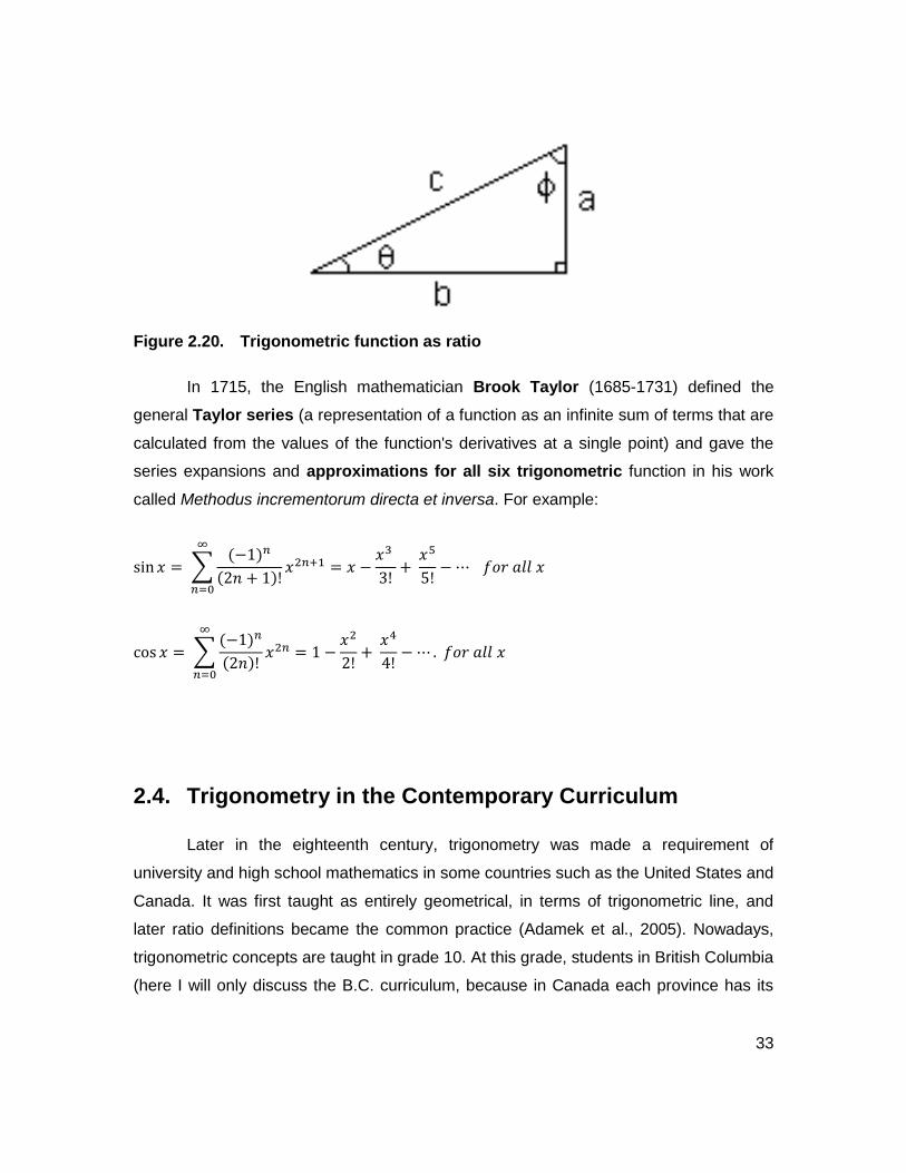
time (Figure 2.20):
sin 𝜃 = 𝑎 𝑐⁄ cos 𝜃 = 𝑏 𝑐⁄ tan 𝜃 = 𝑎 𝑏⁄ sec 𝜃 = 𝑐 𝑏⁄ csc 𝜃 = 𝑐 𝑎⁄ cot 𝜃 = 𝑏 𝑎⁄
33
Figure 2.20. Trigonometric function as ratio
In 1715, the English mathematician Brook Taylor (1685-1731) defined the
general Taylor series (a representation of a function as an infinite sum of terms that are
calculated from the values of the function's derivatives at a single point) and gave the
series expansions and approximations for all six trigonometric function in his work
called Methodus incrementorum directa et inversa. For example:
sin 𝑥 = ∑(−1)𝑛
(2𝑛 + 1)!
∞
𝑛=0
𝑥2𝑛+1 = 𝑥 −𝑥3
3!+
𝑥5
5!− ⋯ 𝑓𝑜𝑟 𝑎𝑙𝑙 𝑥
cos 𝑥 = ∑(−1)𝑛
(2𝑛)!
∞
𝑛=0
𝑥2𝑛 = 1 −𝑥2
2!+
𝑥4
4!− ⋯ . 𝑓𝑜𝑟 𝑎𝑙𝑙 𝑥
2.4. Trigonometry in the Contemporary Curriculum
Later in the eighteenth century, trigonometry was made a requirement of
university and high school mathematics in some countries such as the United States and
Canada. It was first taught as entirely geometrical, in terms of trigonometric line, and
later ratio definitions became the common practice (Adamek et al., 2005). Nowadays,
trigonometric concepts are taught in grade 10. At this grade, students in British Columbia
(here I will only discuss the B.C. curriculum, because in Canada each province has its

34
own curriculum and students learn trigonometry in different levels according to their
province’s curriculum) understand primary trigonometric ratios (sine, cosine, tangent)
through applying similarity to right triangles, generalizing patterns from similar right
triangles, and solving trigonometric problems.
The following year (grade 11), students learn how to solve a contextual problem
that involves two or three right triangles, using the primary trigonometric ratios. While in
grade 10 and 11, B.C. students learn trigonometry in the geometry section, there is a
separate section called trigonometry in Pre-calculus 11 and 12. In Pre-calculus 11,
pupils establish an understanding of angles in standard position [0° to 360°], solve
problems using primary trigonometric ratios for angles from 0° to 360° and then solve
problems using the cosine law and sine law. In Pre-calculus 12, students gain an
understanding of angles in degrees and radians, develop and apply the equation of the
unit circle and solve problems through using the six trigonometric ratios for angles. At
this level, students also have opportunities to graph and analyze the trigonometric
functions (sine, cosine and tangent), to solve the first and second degree trigonometric
equations with the domain expressed in degrees and radians and to prove trigonometric
identities (e.g., reciprocal identities, sum or difference identities and double-angle
identities).
In most of the current textbooks, trigonometry is initially introduced with triangle
trigonometry and then circle trigonometry. However, as Bressoud (2010) indicated, this
type of teaching practice (teaching first through triangle trigonometry followed by circle
trigonometry) is often problematic because this practice leads to student
misconceptions. For instance, students often have a difficult time conceiving of sine
(which is half of that chord) as a periodically varying function when students are first
taught to think of sine as opposite over hypotenuse (Van Sickle, 2011; and Bressoud,
2010). However, students are still forced to learn first through triangle trigonometry
because it is thought to be simpler, even though history suggests just the opposite (Van
Sickle, 2011). Bressoud (2010) expresses:

35
“Trigonometry arose in the study of the heavens among the classical Greeks,
and this was always circle trigonometry. It took over a thousand years before the
first intimations of triangle trigonometry appeared, and it was not until the 16th
century that it became generally used as a tool for surveying. The switch in
instructional emphasis from circle trigonometry to triangle trigonometry did not
occur until the mid- to late-19th century” (p. 1).
Van Sickle, (2011) indicates that teachers assist students’ understanding of
trigonometry through reviewing the history of the development of trigonometry from the
past to the present. Studying the history of trigonometry and informing students about
the origins of trigonometry could help students discovering where their trigonometric
formulas, for instance, come from, rather than simply memorizing them. Teachers, also,
by knowing about the history of trigonometry, might apply some of the earlier theorems
in order to help students comprehended the present concepts.
2.5. Summary and Conclusion
Trigonometry in general and trigonometric functions in particular have a long
history as thousands years ago ancient Greek and Babylonian astronomers used
trigonometry for their calculations. The slow gradual development of trigonometry, in
fact, illustrates the chronological difficulty of the topic. The history of trigonometry shows
that trigonometry was further expanded and developed by Arab and Persian
mathematicians and eventually it was noticed by Europeans as a scientific subject
independent from astronomy.
According to historians’ reports, it was in the eighteenth century that trigonometry
became a subject in high schools and universities. Mathematics textbooks often begin
with some basic ideas such as angle and radian and then, trigonometric functions are
introduced to students through right triangle strategy. Afterward, the trigonometric
functions are presented to students in the unit circle. As can be seen from the history of

36
the development of trigonometry, this way of teaching trigonometric concepts from right
triangle to the unit circle is opposite to the history of trigonometry.
Having looked at the historical development, in the next chapter I turn to discuss
research studies focused on teaching and learning trigonometry.

37
Chapter 3. Learning and Teaching Trigonometric concepts
This literature review aims to discuss existing research on the teaching and
learning of trigonometry; it is divided into three parts, based on the specific focus of the
identified studies. The first part presents an overview of the studies focused on students
and trigonometric concepts. This part itself is divided into three sections. The first section
provides insights into students’ thinking and understanding of trigonometric functions.
The second section investigates a group of studies addressing students’ misconceptions
and difficulties of trigonometric functions and some related topics (e.g., angle measure).
The final section of the first part addresses the effect of technology and students’ leaning
of trigonometric concepts. The second part of this literature review addresses studies
that focus teachers and trigonometric topics. This part covers research on various
teaching methods that are able to effectively support the learning of trigonometry by
students. The final section of the second part discusses teachers’ difficulties in grasping
trigonometric concepts. This review will conclude with the third part, which will highlight
the need for further research on teaching and learning trigonometric concepts and in
particular transformations of sinusoidal functions.
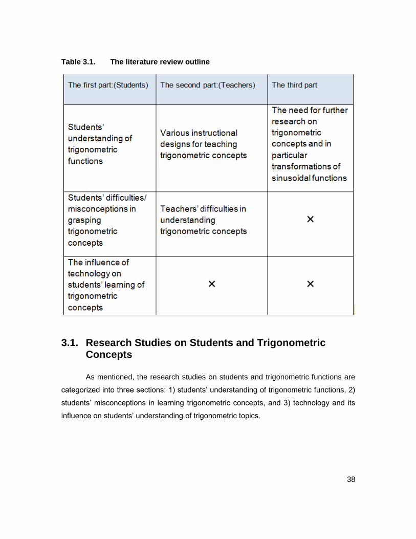
38
Table 3.1. The literature review outline
3.1. Research Studies on Students and Trigonometric Concepts
As mentioned, the research studies on students and trigonometric functions are
categorized into three sections: 1) students’ understanding of trigonometric functions, 2)
students’ misconceptions in learning trigonometric concepts, and 3) technology and its
influence on students’ understanding of trigonometric topics.

39
3.1.1. Students’ Understanding of Trigonometric Functions
Undergraduate students of sciences, are required to study trigonometry,
especially trigonometric functions, because a strong foundation in trigonometric
functions will likely strengthen their learning of various mathematical topics, such as
Fourier series and integration techniques (Moor, 2010). It is shown that understanding
calculus and analysis is dependent on learning of trigonometric functions (Hirsh,
Weinhold and Nicolas, 1991; Demir, 2011). However, while other functions (e.g.,
logarithmic functions) can be computed by performing certain arithmetic calculations
expressed by an algebraic formula, trigonometric functions involve geometric, algebraic
and graphical concepts and procedures, simultaneously (Weber, 2005, Demir, 2011). In
other words learning and understanding trigonometric functions is a difficult and
challenging task for students, compared to other mathematics functions, such as
polynomial functions, exponential and logarithmic functions.
To gain insights into students’ understanding of trigonometric functions, Weber
(2005) studied a group of college students who were taught trigonometric functions with
two different instructional approaches: experimental instruction and lecture- based
instruction. The experimental instruction used was based on Gray and Tall’s (1994)
theoretical notion of procept (the amalgam of three components: a process that
produces a mathematical object and a symbol which is used to represent either process
or object). The fundamental goal of this instructional approach was to provide
opportunities to the students to participate in the class activities included construction of
the unit circle, and drawing angles and related line segments corresponding to their
trigonometric values (Weber, 2005). In the traditional, lecture-based, textbook-driven
approach, the main emphasis was on developing students’ procedural skills. Most of the
class time was devoted to providing students with explanation on how to do particular
exercises, with illustrative examples. After completing the procedure, all the students
were asked a series of questions such as:
“Which is bigger sin 37° or sin 23°? Explain why.”
40
“Without measuring, estimate the sin of 170°.”
“Is sin 145° positive and why?”
“Explain why sin θ can never equal 2.”
The findings of the study demonstrated that the traditional approach provided a
limited understanding of trigonometric functions to the students; no student could give
justification for the reason why sin(θ) could never be 2. Students were often unable to
rationalize various properties of trigonometric functions or reasonably estimate the
output values of trigonometric functions for various input values. Although the students
were reminded of the definition of functions, “for each input there can be only one
output,” none of students could propose reasonable answer for the question of “why sine
is a function” (Weber, 2005). Consistent with these results, Challenger (2009), Gür
(2009) and Marchi’s (2012) studies reported a fragmented understanding of
trigonometric functions for groups of high school students taught in a traditional lecture-
based course.
In Weber’s study (2005), however, the experimental student groups were able to
approximate values of basic trigonometric expressions, and they could determine
properties of trigonometric functions. Weber realized that at least 30 out of a class of 40
students were able to describe sine function in terms of a process between an input and
output quantity. The students could also discuss why these functions have the properties
that they do. Weber (2005) found that the students in the experimental group were able
to describe the process of drawing the angle and defining its sine, and then clarify that
for each angle there was only one possible point of intersection with the circle. He
concluded that these students (the experimental group) were able to understand
trigonometric functions because they could develop images of the geometric processes
used to obtain those values in context of the unit circle. Similar to Moor (2010), Weber
(2005) indicated that there is a close relationship between the unit circle representations
of trigonometric expressions and students’ understanding of these functions. However,
these results contradict the findings of Kendal and Staceys’ study (1997).

41
Kendal and Stacey (1997) assessed 178 high school students’ understanding of
trigonometric functions through two different methods: ratio and unit circle. The research
shows that students had a better understanding of trigonometric functions where
functions were defined in terms of ratios of sides of right angled triangles (students often
taught SOHCAHTOA as a memory aid), rather than with the unit circle method. These
results are consistent with those of Palmer’s study (1980) in which the students were
randomly assigned either a ratio or unit circle instruction to inspect which group grasped
more trigonometric functions. The students in the ratio classes outperformed their unit
circle counterparts. Burch (1981) also concluded that the participant students had
difficulty interpreting trigonometric functions in the unite circle, recognizing that x and y
coordinates of a point on the unit circle are cosine and sine values of corresponding
angles compared with other determined trigonometric functions in terms of right triangle.
Brown (2005), Demir (2011) and Marchi (2012) suggest that students would
better understand trigonometric functions if they have more opportunities to take part in
a learning trajectory where both the unit circle and right triangles are utilized, rather than
learning trigonometric functions through instructional designs which focused on only one
of these two methods. To examine high school students’ understanding of trigonometric
functions, Brown (2005) developed a model of students’ understanding of trigonometric
functions within the geometry world of triangles and angles (in degrees), and within the
context of the unit circle. In this model, the sine and cosine of an angle can be defined in
three different ways: as ratios, as distances, and as coordinates. The results of Brown’s
(2005) investigations of 120 high school students revealed that those students who were
able to use and connect all interpretations ( ratios in right triangle, directed distances and
coordinates) and moved flexibly between them, could define trigonometric functions and
were also better problem solvers. However, Brown (2005) noticed that the majority of the
students could still define trigonometric functions and work effectively with only one view,
instead of making connections between all three representations. Brown concluded that
most students had an incomplete understanding of trigonometric functions.
Following the students’ lack of understanding of trigonometric functions in the
learning model developed by Brown (2005), Demir (2011) modified Brown’s model and

42
he established a new learning trajectory comprised of three different representations i.e.
right triangle, unit circle, and graph. Demir studied 24 students aged 16-17, and found
that the new learning trajectory could support students’ understanding of trigonometric
functions in all aspects: the unit circle context (e.g. students knew coordinate definitions
of sine and cosine, and utilized them appropriately to point to the correct position with
the correct direction); the connections between unit circle and triangle context (e.g.,
students could determine a required reference triangle, and a proper trigonometric ratio
to calculate the required trigonometric value, e.g., sin 45˚ for sin 225˚); and the graph
context (e.g., students were successful in interpreting the trigonometric graphs to state
the domain and range of the trigonometric functions). As reported by Weber (2005) and
Challenge’s (2009) studies in which the students demonstrate a certain lack of reasoning
about trigonometric functions, the results of Demir’s study (2011) show that even with
the new learning trajectory, a number of students were still unable to explain why sine
and cosine are functions.
This section of the literature review focused on the research studies (e.g., Weber
2005 and Demir, 2011) that examined students’ understanding of trigonometric
functions. The results of the limited number of research studies show that students often
encountered various difficulties (e.g., reasoning why sin 𝜃 could never be 2) when
learning trigonometric functions. There have been some studies (e.g., Orhun, 2001 and
Tuna, 2013) which connected students’ misconceptions of trigonometric functions with
difficulties in understanding some other trigonometric concepts such as angle measures,
and graphs of trigonometric functions. In next section, studies focusing on students’
conceptions of angle measure and graph of trigonometric function are reviewed.
3.1.2. Student’s Difficulties/ Misconceptions in Grasping Trigonometric Concepts
In this section, the research studies focused on the difficulties students often
encountered when completing trigonometric tasks are described in detail.
43
3.1.2.1. Students’ Difficulties and the Concept of Angle Measure
A number of studies (e.g., Demir, 2011 and Tuna, 2013) have stressed that a
deeper comprehension of the concept of angle measure facilitates students’
understanding of trigonometric functions. Degree and radian are used as units of
measurement for an angle. Some researchers (e.g., Weber, 2005; Brown, 2006;
Challanger, 2009 and Demir, 2011) highlight students’ difficulties in understanding angle
measures in degrees, especially if they are required to work with acute angle such as
sin 23˚ (Weber, 2005 and Demir, 2011), negative angles such as sin(−45˚) (Challanger,
2009) or if the angle is greater than 360 degrees such as sin 405˚(Brown, 2006).
Therefore, Martinez-Sierra (2008) and Tuna (2013) emphasize the use of radian to
calculate the angle of trigonometric functions.
Tuna (2013) expressed that mathematicians often introduce radian as “the ratio
of the length of the arc faced by a central angle to the length of the radius of the circle.”
This definition refers to the proportion of two lengths and, then, produces the radiant unit
of a real number, which can be attributed to the correspondent radiant measure by the
wrapping function (defined by wrapping a real number line around unit circle).
Essentially, this is the way mathematicians have expressed trigonometric functions over
real numbers (Akkoç and Gül, 2010). However, degree is defined by breaking a unit
circle into 360 equal parts, and in turn, cannot be used as the domain of trigonometric
functions. The formation of such a relationship between the concepts of radian and
trigonometric functions is of crucial significance for students’ understanding of
trigonometric functions (Tuna, 2013).
Although the use of radian has a positive impact on understanding trigonometric
functions, some studies (e.g., Fi, 2003 and Akkoc, 2008) pointed to students’ difficulty in
the conceptualization of angle measurements in radian. For instance, Fi (2003), in study
of 14 undergraduate students, found that the students lacked understanding of radian.
11 of the 14 participants presented an understanding of the methods for converting
between degree and radian measures (“2π” radians are equal to 360°), in contrast with
results of the Orhun (2001), Steckroth (2007) and Akkoç’s (2008) studies in which

44
students had difficulties changing degree to radian, and vice versa. However, none of
the participants gave an accurate definition for radian measure. Akkoç (2008) and
Tuna’s (2013) research confirms Fi’s (2003) results. Akkoç (2008) indicated that the
majority of 42 undergraduate students were unable to define radian, and only one
defined radian as the length of an arc: “radian is the angle measurement which is equal
to the arc length on the unit circle” (p. 862). Tuna (2013) also found that while 90% of
undergraduate students participating in his study were unable to define radian in a circle,
a large number of students were able to define the concept of angle correctly.
It was not only undergraduate students who appear to have difficulty in grasping
the definition of the concept of radian, as suggested by Fi (2003), Akkoç (2008), and
Tuna (2013). Orhun (2001), and Akkoc and Gül (2010) also show the same problem with
high school participants. Akkoc and Gül (2010) noticed that high school students (grade
10) could not define radian as ratio of two lengths: the length of the arc of a central angle
of a circle, and the radius of the circle. Orhun (2001) asked 17 students from grade 10 to
answer the following two questions: “What is the arc length subtended by a central angle
60 degrees in a unit circle?” and “What is the measure of a central angle x subtends an
arc of length pi/3 radian?” He found that only 19.5% were successful in calculating
angles from given arc lengths. However, 70.1% could find the arc length subtended by
an angle in a unit circle correctly. In other words, the students who participated in
Orhun’s (2001) study had difficulties similar to the participants of Akkoc and Gül (2010)
and Tuna (2013).
In addition to students’ difficulty in defining radian, these studies (e.g., Orhun,
2001 and Fi, 2003) reported students’ misunderstanding of the symbol 𝜋. Orhun (2001)
reports that many of grade 10 students determined 𝜋 as the unit for radian measure, and
that the students argued that 1 radian equaled to 180° instead of a number close to 3.14.
Fi (2003) and Akkoç (2008) find exactly the same difficulties for participant
undergraduate students. In other words, students do not view 𝜋 radian as a real number
when discussed in a trigonometry context (Tuna, 2013).
45
The aforementioned misconceptions of angle measure, which have a direct
influence on the understanding of trigonometric functions, are not the only difficulties
students may encounter. There are also some other important aspects such as the
conception of graphs, which is a very useful tool for students in learning trigonometric
functions. In what follows, students’ understanding of graph of trigonometric functions is
reviewed in detail.
3.1.2.2. Students’ Difficulties and Graphs of Trigonometric Functions
Another important issue relating to students’ difficulties in understanding
trigonometric functions deals with graphs of trigonometric functions (Demir, 2011).
Breslich (1928) and Orhun (2001) stated that students, without using graphs, would
understand only one aspect of trigonometric functions, the ratio aspect, and they would
miss the function aspect entirely. Brown (2006) and Demir (2011) expressed that if
teaching trigonometric functions occurred in the context of graphs, students would have
a greater chance of conceptualizing sine and cosine as functions of real numbers, and
explaining why sine and cosine graphs represent functions by utilizing the formal
definition “There is only one y for every x”, or the process definition based on an input-
output mechanism, or a combined conception of the first two, like “There is only one
output for every input”.
Although students’ conceptions of trigonometric functions rely heavily on their
comprehension in the area of graphs of trigonometric functions (Vinner, 1983 and Demir,
2011), many researchers (e.g., Baki and Kutluca, 2009; and Rose, Bruce and Sibbald,
2011) signified graphs of trigonometric functions as the most challenging topic that
students typically encounter in mathematics classrooms. In a survey, 65.9% of 123
grade 10 students and even 93% of 146 mathematics teachers described trigonometric
functions and graphs of trigonometric functions as the most difficult topics (for students)
in the area of trigonometry (Baki and Kutluca 2009). Studies of Adamek, Penkalski, and
Valentine (2005) and Tatars, Okur, and Tuna (2008) support the complexity and difficulty
of this topic.

46
Students’ difficulties in understanding graphs of trigonometric functions can be
traced to the following contexts, in which students are required to 1) make connections
between algebraic and graphical representations (Lambertus, 2007), and 2) make
transitions between the unit circle and the graphs, which are considered to be a
fundamental aspect for understanding trigonometric functions (Rose et al., 2011; Demir,
2011; Brown, 2006). Whereas the first context is common among trigonometric functions
and other mathematics functions (e.g., algebraic functions as mentioned in Gagatsis,
Elia & Kyriakides, 2003), the second one is only specific to trigonometric functions.
In studies involving undergraduate student participants, Leinhardt, Zaslavsky and
Stein (1993), Yerushalmy and Schwartz (1993), and Knuth (2000) recognized that the
majority of students were limited by their focus on using algebraic representations to
solve the mathematics problems. When they were asked to complete a task by plugging
values into an equation or finding points on a graph, they chose the algebraic approach.
Even when students had to approximate a y-value on a graph, they plugged the value
into the equation instead of using the graph. As a result, students could not develop the
skills of flexibly employing, selecting, and moving between algebraic and graphical
representations. In other words, many students had difficulties in understanding the links
between equations and their graphs (Knuth, 2000). Although these previously mentioned
studies worked on other functions instead of trigonometric functions, Challenger (2009)
noticed that some high school students had common types of difficulties. For example,
students had difficulty when asked to find the coordinates of the point where a given
graph of a particular trigonometric function crossed the y-axis (both equation and the
graph given to the students). Challenger observed that the students ignored the given
graphs and they only tried to find the points where the equations equal zero. In other
words, the students were unable to provide a link between graphical and algebraic
representations in the context of trigonometry. Similarly, Marchi (2012), in a study of high
school students, indicated that none of the high school students who participated in the
study utilized a graphical representation to find the answer for tasks such as “Explain
how you would solve the following equations: sin 𝑥 =1
3 and 2 sin 𝑥 + 1 =
2
3,” unless it

47
was suggested to do so. Marchi concluded that the students, in fact, did not know that
using a graph was a method for finding a solution.
As mentioned previously, the other set of research focused on graphs of
trigonometric functions to explore students’ abilities in making connections between the
unit circle and graphs. Brown (2005), found that some honors high school students
(grade 10) were unable to connect a rotation on the unit circle with a point on a graph of
sine or cosine, and only a few students could conceptualize trigonometric graphs
through the arc lengths on the unit circle and the corresponding horizontal position. The
results of Brown’s study confirmed the findings of Marchi’s (2012) study in which some
high school students could not correctly recall information and were not able to make the
right connections when trying to connect the graph for sin 𝑥 with the unit circle. Similarly,
Demir (2011) noticed that in spite of some students’ success, a number of high school
students (grade 11) still had difficulties explaining the coordinates on the graphs as arc
lengths and vertical positions on the unit circle, or marking the point on the graph
corresponding to a given position on the unit circle.
To sum up, students’ difficulties in the concepts of angle measure (degrees and
radian) and graphs of trigonometric functions are discussed in this section. The results of
a number of research studies (e.g., Tuna, 2013) illustrate that students often
encountered difficulties in defining radian and grasping 𝜋 as a real number. The studies
(e.g., Marchi, 2012 and Brown, 2005) also reported students’ inabilities to make
connections between algebraic and graphical representations as well as to connect the
unit circle and the trigonometric graphs when working with trigonometric curves. To
overcome the reported difficulties in using graphs for trigonometric functions, Zengin,
Furkan and Kutluca (2011) advise teachers to use technical devices such as GeoGebra
to improve students’ learning of graphs of trigonometric functions. In the next section,
the effect of technology on students’ understanding of trigonometry, both in general, and
specifically on graphs of trigonometric functions, is described.

48
3.1.3. Students’ Learning of Trigonometric Concepts and the Effect of Technology
There have been limited number of research studies (e.g., Blackett and Tall,
1991; Yenitepe 2002; and Choi-Koh, 2003) on the influence of technology on the
learning of trigonometric concepts. Robison (1996), for instance, investigated the impact
of the use of Mathematica by 99 college students taking a course in trigonometry. The
researcher divided students into two groups: a group that received instruction that
included Mathematica (a computational software program used in mathematical field)
and another group that was presented with static image and they were asked to use
their imaginations for solving trigonometric problems. The results of the study illustrate
that there is no difference in achievement between the group taught with animation
(Mathematica) and the group taught with static images. However, these findings are in
contrast with the results of Blackett and Tall’s (1991) study, which shows that
implementing a computer software package on the topic of triangle trigonometry had a
positive impact on students’ understanding of trigonometric concepts. In a study by
Yenitepe (2002), 78 high school students participated in a class lecture about unit circle
trigonometry without technology and with technology; Yenitepe (2002) noticed that the
students involved in technology-based instruction outperformed their counterparts in the
exams.
Research studies (e.g., Choi-Koh, 2003; Army, 1991; Stacey and Ball, 2001)
specified that technology plays a fundamental role in understanding graphs of
trigonometric functions. Choi-Koh (2003) said that graphs in traditional teaching methods
have served as “a display representations mean” because teachers have had only static
media. In both the table and formula environments, graphical variations in the display
are not continuous; they are drawn according to the discrete data. Technology, on the
other hand, provides students with an opportunity to use tools to manipulate graphic
objects freely (Choi-Koh, 2003) and it release students from the tediousness of
sketching time-consuming graphs by hand, conserving their mental energy for
conceptual development (Kissane & Kemp, 2009 and Rose et al., 2011).

49
To investigate the impact of graphing calculators on students’ mathematics
achievements, Choi-Koh (2003) invited a 10th grade student to work on seven tasks
including creating a graph of trigonometric functions. The results of the case study
illustrated that the student utilized the graphing calculator as a tool to successfully graph
sine functions and also to detect the changes in the graphs with varying coefficients.
Choi-Koh (2003) consistent with Yerushalmy (1988), Army (1991), Stacey and Ball
(2001) and (Lambertus, 2007) concluded that technology-based learning environments
provide a chance for students to strengthen the connection between graphs and
symbolic representations, to address their main difficulties in graphing trigonometric
functions regarding this connection (between analytical and graphical representation).
These results contrast a few investigations such as Colgan’s (1992) study on eight
students in grades 11 and 12. In this study, the students were able to use a computer-
based graphing tool (Zap-a-Graph) when studying the graph of trigonometric functions.
Colgan (1992) noticed that this technical tool did not help students to make connections
between algebraic and graphic representations of trigonometric functions and even in
some cases led to misunderstandings. The students stated that Zap-a-Graph was not
easy to use because it could not plot graphs of trigonometric functions in different colors
and used only black and white images.
Garofalo, Drier, Harper, Timmerman, and Shockey (2000), and Demir (2011)
expressed that technical tools such as GeoGebra are cognitive tools that support
students in understanding connections among different representational systems in
trigonometry. They mentioned that use of technology in mathematics classrooms,
specifically, would allow students to establish the connections between unit circle and
graphs, one of the most problematic areas for students studying trigonometry (in the
area of graphing trigonometric functions). Similarly, Kissane and Kemp (2009), and
Zengin, Furkan, and Kutluca (2012) suggest that Dynamic Geometry software would
enable students to form relationships between graphical representations of trigonometric
functions and positions of points on the unit circle. These results are consistent with
Tall’s (1986) study in which ‘A’ level students utilized computer graphics as part of a
planned teaching strategy. It showed that students were able to link unit circle and
trigonometric graphs successfully.
50
To sum up, a few research studies have focused on the influence of technology
on students’ learning of trigonometric concepts. While the results of some studies such
as Colgan (1992), and Robison (1996) show no differences between the performances
of students who have been taught with technology and those who have been taught
without it, other studies found the opposite, especially in the area of graphs of
trigonometric functions. All the studies (e.g., Zengin et al., 2012 and Garofalo et al.,
2000) proposed that technology environments such as Geo-Gebra and Dynamic
Geometry software would develop students’ achievements in the area of graphing
trigonometric functions by providing students with opportunities to make connections
between unit circle and graph of trigonometric functions, as well as to connect analytical
representations with graphical representations. In other words, technical devices are
appropriate pedagogical tools that teachers could implement in classrooms to improve
students’ performance in depicting graphs of trigonometric functions. The next section
describes in detail some other important teaching strategies researchers suggest for
teaching trigonometric concepts.
3.2. Research Studies on Mathematics Teachers and Trigonometric Concepts
In this section, the research studies focused on mathematics teachers and
trigonometric concepts are presented in two parts: 1) teaching trigonometric concepts
through different instructional designs and 2) teachers’ difficulties in teaching
trigonometric concepts.
3.2.1. Teaching Trigonometric Concepts through Different Instructional Designs
There is a bulk of published research which studies how to teach trigonometry
effectively; however, researchers do not agree on a specific instructional method which
will guarantee students’ success in learning trigonometry. In this part, I summarize
important outcomes of these researches. Weber (2005) suggests that students would

51
not benefit if instructors concentrate on teaching trigonometry through traditional,
textbook-driven lessons. He says that students would conceptually understand
trigonometric concepts and in particular trigonometric functions when teachers provide
opportunities for reasoning with numerical values and connecting them with geometric
processes, like creating the unit circle. Weber (2005) and Marchi (2012) state that this
can only be achieved if various representations are introduced and utilized along with
class discussion of their relationships when teaching trigonometry.
Some other researchers such as Kendal and Stacey (1997) advised teachers to
teach trigonometric functions through the ratio method because students who had been
taught through this method in their study earned higher marks in a trigonometry exam
compared to the group who learned trigonometry by the unit circle method. By
comparing the techniques and content utilized to teach trigonometry by Turkish and
British teachers, Delice and Monaghan (2005) found that mathematics teachers need to
develop students’ performance at algebraic aspects of trigonometry like “simplifying”
trigonometric expressions (because they noticed that the students typically had
difficulties in simplifying trigonometric expressions). They add that those mathematics
teachers who emphasize trigonometric applications in real-life situations as part of their
method of instruction, better support students’ success by providing students with
relevant challenges. In a similar study, Gould and Schmidt (2010) invited high school
teachers to ask their students to create digital story problems about real-life situations
and then apply trigonometric functions to solve those problems. The authors expressed
that the combination of students’ motivation and this non-traditional activity approach
would assist students in learning trigonometry successfully.
Barnes (1999) stated that teachers could develop students’ achievements in
trigonometry by giving them chances to participate in creative writing. She gave her own
high school students a set of word problems (related to trigonometric concepts) to solve
in groups and then asked students to explain their mathematics accurately in writing. Not
only did this exercise reportedly help students to be less afraid to tackle word problems,
it also improved their understanding of trigonometric concepts, whereas they had not
understood it well, previously.
52
In a study of 21 grade 10 students over four weeks of trigonometry lessons, Gur
(2009) realized that the majority of students could not justify their answers and often
preferred to use a formula driven method (like the unit circle) according to mathematics
textbooks instead of establishing a conceptual context for what the formula meant. After
his observations, Gur (2009) encouraged teachers to allow the students to describe
trigonometric definitions or concepts in their own words instead of inviting them to
memorize information without understanding it conceptually. Gur (2009), similar to
Orhun (2001), stated that following the memorizing formula teaching strategy would
often provide students with the knowledge of trigonometry, only for a short period of
time. Meanwhile, students would encounter difficulties in remembering and
understanding the formula later, and in transferring the principle learned to new
situations.
In addition to advising teachers to teach trigonometric functions through
employing their graphs to help students better understand trigonometric concepts, Orhun
(2001), Topçu et al., (2006), and Akkoc (2008) suggest that mathematics teachers begin
defining trigonometric functions before they teach its relationship to angles. Orhun urge
that this change in teaching trigonometry is necessary because the measurement of an
angle in degree opposes the general definitions and concepts in trigonometry, and this
often confuses students. Byers (2010) and Pesek and Kirshner (2000) have another
suggestion for teachers. They propose that mathematics teachers avoid teaching
trigonometry by beginning the instruction with definitions of trigonometric concepts first
and then spending remaining class time on concept development, during which time
students often experience greater difficulty when trying to construct trigonometric
representations. Instead, the teachers require teaching trigonometric facts through
various representations such as the unit circle, vector, ratio and functions (suggested by
Weber (2005) as well).
Subsequent to their findings on students’ difficulties in understanding radian (as
mentioned in the section 3.1.2.1) and in order to address and eliminate this difficulty,
Akkoç and Gül (2010) recommend that mathematics teachers teach radian by clearly
explaining its connection to arcs. They state that if teachers provide students with

53
opportunities to participate in a learning trajectory based on computer programs which
can explore relations between arc lengths and angles in circles, and identify
trigonometric functions primarily in domain of arc lengths, then, students would better
understand the concept of radian. Moreover, Moor (2012), encourages mathematics
teachers to use an arc approach to angle measurement by which students could develop
an understanding of angle measurement as a process based on calculating an arc
length subtending a fraction of circle circumference. According to this approach, radians
and degrees measure the same quantity and are thus scaled versions of one another.
One degree is 1/360th of circumference of any circle centered at the vertex of angle and
an angle that measures, and 1 radian subtends 1/2pi of circumference of any circle
centered at vertex of angle. Moor’s suggestions of using an arc approach to teaching
have the potential to be quite impactful.
To conclude, the different studies suggest various teaching methods, including
unit circle, right triangle, story writing, real-word problems, and computer programs to
better support students in understanding trigonometric concepts and eliminate related
comprehension difficulties. In addition to the proposed teaching methods, the issue of
mathematics teachers’ difficulties in teaching students trigonometric concepts is an
important part of the research literature, and will be described in the following section.
3.2.2. Mathematics Teachers’ Difficulties in Teaching Trigonometric Concepts
Trigonometry is not only a challenging topic for students; it is also difficult for
teachers to understand. Limited number of research studies focus on teachers and their
understandings of trigonometric concepts, revealing the teachers’ difficulties, which are
often similar to some of the students’ difficulties in understanding the concepts of
trigonometry (as mentioned in the previous section). For example, radian which is one of
the challenging trigonometric concepts for students is considered a difficult topic for
mathematics teachers too. In a study of 14 mathematics high school teachers, Topçu,
Kertil, Akkoc, Kamil, and Osman (2006) explored that most teachers had a lack of
understandings of radian. For instance, in the following question:

54
f : R → R and f(x) = x sin x is given. Plot the following points on the Cartesian
plane.
a) (30, f(30)) = ? b) ( 𝜋
2, f(
𝜋
2)) c) (
𝜋
6, f (60)) ? d) (2, f(
𝜋
3))?
Topçu et al., (2006) noticed that only 3.9% of the teachers considered “sin 30” in
radians and 90.2% of them considered “sin 30” in degrees. In other words, the
researchers realized that the majority of teachers did not consider radian as a real
number although the trigonometric functions that were given to them were explicitly
defined as a set of real numbers. These results are in line with the findings of Cizmesija
and Siqus’s (2013) study in which the participant teachers refer to pi as the unit for
measuring radian, whereas real numbers not being of the form q 𝜋 (q, 𝜋), q ∈ℚ, are not
realized as the radian measures of an angle. Furthermore, the results of both
aforementioned studies illustrate that the teachers preferred to answer the given
trigonometric tasks in degree rather than in radian. For example, to find a length of an
arc subtending central angle given in radians, the teachers preferred to change radians
into degrees. Topçu et al., (2006) and Cizmesija and Siqus’s (2013) conclude that this
tendency to convert radian into degrees might be because of the teachers’ lack of
understanding of radian, since almost none of the participant teachers could successfully
define the radian as a ratio of two lengths: the length of the arc of a central angle of a
circle, and the radius of the circle. These findings are consistent with Fi’s (2006) study in
which teachers encountered similar difficulties in understanding the concept of radian.
These teachers’ mistakes are in line with the misconceptions of students as reported in
Moore (2010), Demir (2011), and Moor, LaForest and Kim (2012).
Teachers’ misconceptions of inverse trigonometric functions are also another the
difficulties noticed in Fi’s (2006) study. Although the teachers recognized that the given
trigonometric functions were the inverse functions, they discussed them in terms of
reciprocal functions. Fi stated that the reason for these teachers’ mistakes might be due
to their confusion with the real number reciprocal written form. For a non-zero real

55
number x, the multiplicative inverse is written 𝑋−1 and it is equal to 1
𝑋, the reciprocal of x,
but this is not the case for trigonometric functions. Fi (2006) also indicated that none of
the teachers who participated in the study had a conceptual understanding of the co-
concept (sine - cosine, tangent - cotangent, and secant – cosecant). The researcher
concluded that the teachers often assumed inverse, reciprocal, and co-function as
equivalent ideas when answering the interview questions.
In this section, the results of the limited number of research studies that focused
on teachers’ difficulties in the area of trigonometric concepts such as conception of
radian, inverse trigonometric functions and co-functions, are summarized. Some of the
teachers’ difficulties in understanding the definition of radian and converting radian to
angle and vice versa, are similar with the students’ misconceptions of trigonometric
functions. Therefore, it is not surprising that one concludes that the students often make
the mentioned mistakes when working with trigonometric concepts because the
mathematics teachers teaching the concepts of trigonometry do not fully grasp these
complex concepts themselves. What is missing from all of this literature is a closer look
at transformations of trigonometric function. It is exactly this phenomenon that I am
interested in.

56
Table 3.2. Summary of Literature Review
Researcher(s) Focus of the research(s) Result(s)
Kendal and Staceys,1997; Weber, 2005; Brown, 2005; Orhun, 2001; Kang, 2003.
Students’ understanding of trigonometric functions
Students often have lack of ability in conceptualizing trigonometric functions
Yerushalmy and Schwartz 1993; Knuth, 2000;
Fi, 2003; Martinez-Sierra, 2008;
Akkoç and Akbaş Gül, 2010; Tuna, 2013; Brown, 2006
Students’ conception of angle measure and graph of trigonometric functions
Students often encounter difficulties in defining radian
and recognizing1 radian equaled to 180° instead of a number close to 3.14. They also are unable to make 1)
connections between algebraic and graphical representations and 2) transition between unit
circle and the graphs.
Blackett and Tall, 1991; Yenitepe, 2002; Choi-Koh, 2002;
Kissane and Kemp, 2009; Zengin, Furkan, and Kutluca,
2012.
Effect of technology on learning trigonometric concepts
Technology often has a positive influence on students’
conception of trigonometric concepts.
Pesek and Kirshner, 2000; Orhun, 2001; Weber, 2005; Akkoc, 2008; Byers, 2010; Moor, 2012.
Designing appropriate instruction for teaching trigonometric concepts
Teaching different trigonometric topics through the unit circle, right triangle, graph, real-life problems and story writing.
Topçu, et.al., 2006; Fi, 2006;
Moor, LaForest and Kim, 2012, Čižmešija and Šipuš, 2013.
Teachers’ misconception of trigonometric concepts
Teachers’ difficulties in understanding the concept of radian; reciprocal and inverse
trigonometric functions.
57
3.3. The Need For Further Research on Teaching/Learning Trigonometric Concepts
The review of the literature on teaching/learning trigonometric concepts (e.g.,
Brown, 2005 and Fi, 2006) looked at the issue through diverse lenses. A number of
research studies discussed various teaching strategies (such as the unit circle and right
triangle) for trigonometric concepts, while some others focused on teachers’ difficulties
such as the misconceptions of the concept of radian, which is interconnected with their
understanding of trigonometric functions. Students’ understanding of trigonometry and in
particular trigonometric functions was examined by a few research studies such as Kang
(2003) and Weber (2005), while other research studies (e.g., Moor, 2010) rooted the
conception of trigonometric functions into students’ ability to identify and reason with
trigonometric functions as functions or to correctly define angle measurements,
especially radian (Akkoç & Gül, 2010). There have also been some studies, such as
Orhun (2001) and Demir (2011), which connect the students’ identifications of
trigonometric functions to their inadequate understanding of trigonometric graphs, and
these authors promote teaching trigonometric functions through graphs. What is missing
from all of this literature is a closer look at transformations of trigonometric functions. It is
exactly this phenomenon that I am interested in.
Although the concept of transformation of mathematics functions (except
trigonometric functions) in analytical and graphical contexts is subject of several studies
(e.g., Eisenberg & Dreyfus,1994; Baker, Hemenway, & Trigueros, 2000; Chiu, Kessel,
Moschkovich, & Munoz-Nunezby, 2001; Zazkis, Liljedahl & Gadowsky, 2003; Lage &
Gaisman, 2006 and Consciência & Oliveira, 2011) that focus on students’ understanding
of transformations of mathematics functions and some existing obstacles, there has
been limited number of research studies focus on transformation of trigonometric
functions and in particular sinusoidal functions. One of the sparse studies on the
transformation of trigonometric functions, Ng and Hu (2006), examined the impact of
using Trigonometric Graphs, a teacher created web-based simulation, and
asynchronous online discussion on students’ performance in sketching transformation of
trigonometric curves. Rose et al., (2011) looked at whether technology has a greater
58
impact on student achievement and attitudes towards transformation of trigonometric
functions if it is implemented before or after whole class teaching. Furthermore, Zengin
et al., (2011) examined the effect of dynamic mathematics software Geogebra on
student achievement in learning transformation of trigonometric functions by comparing
two groups of high school students: the experimental group (subjected to lessons
arranged with the GeoGebra software in computer assisted teaching), and the control
group (subjected to the lessons shaped with constructivist instruction). As it appears
from the above mentioned research studies, the main purpose of these researches is
examining the influence of technology on students’ learning of trigonometry and in
particular transformation of trigonometric functions. However, these studies have not
addressed questions such as, how do undergraduate students complete mathematics
tasks involving the transformation of sinusoidal functions? What are the common
mistakes students often encounter when they work with transformations of sinusoidal
functions?
The importance of research on the transformation of sinusoidal functions is
rooted in my experience as an assistant teacher at a university. When assisting students
with their homework, and having discussions with some of the Calculus instructors at
Simon Fraser University, I have noted that transformation of trigonometric functions and
in particular sinusoidal functions is a complex topic in which numerous students face
major difficulties. Students often become confused when they need to identify
transformations in analytical and graphical contexts, especially if the sinusoidal functions
are transformed horizontally. Even if some students could identify the transformations,
the majority of them repeatedly make mistakes in graphing the transformed functions,
interpreting the transformed graphs or transformed trigonometric functions. Therefore,
the main purpose of my study is examining students’ reasoning and abilities of
transformation of sinusoidal functions since the number of studies focused on this
important and challenging topic is very limited. There is not much research on how
students work in situations that involve transformation of sinusoidal functions, whether
they are able to recognize transformations and whether they have the skills to identify
the influence of transformations on sinusoidal graphs. In other words, none of the
aforementioned studies on teaching and learning of trigonometry investigated the way

59
undergraduate students complete tasks involving transformations of sinusoidal functions,
types of difficulties they might encounter, and to what degree the barriers in completing
tasks are related to students’ lack of understanding of trigonometric functions as cited in
the literature.
Taken together, for this thesis the major goals are gaining greater insight into
undergraduate students’ replies to mathematics tasks involving the transformation of
sinusoidal functions and the common mistakes they encounter when completing the
tasks. I am interested to discover if students’ difficulties are connected to algebraic or
graphical representation contexts or if those difficulties are related to the way their
teachers represent the key concepts. Some of these questions have answers in the
context of general mathematics functions. However, there is no sufficient attention to
these questions in the context of sinusoidal functions. I believe that by conducting this
research study and answering these kinds of questions, I will be able to extend our
knowledge to enhance teaching of trigonometry functions and improve the experience
and outcomes for students.

60
Chapter 4. Methodology
In what follows I review the pilot study and describe how I select and design the
tasks for the main study. Then, the undergraduate students who participated in my
research are introduced. Data collection and analysis are described in the last part of
this chapter.
The specific research questions are in chapter 5 following the description of
theoretical frameworks. The general main goal of my study is to respond to the following
research questions:
1) How do undergraduate students complete mathematics tasks involving
transformations of sinusoidal functions?
2) What are the common mistakes that students encounter when they work with
transformations of sinusoidal functions?
4.1. Pilot study
Conducting a pilot study can provide valuable insights for researchers, and it
increases the likelihood of success in the main study. Thus, I used the data collected
from the interviews with eight students in the pilot study in order to design the interview
tasks used in my actual research. Three male and five female students volunteered their
time. Two students were registered in Calculus I, the rest of them was in Calculus II at
the time of the pilot study.

61
In particular, eight students were required to complete five tasks that involved
sinusoidal functions (transformed horizontally/vertically and both) and their sketches (I
describe the sketches later in this section).
Considering the standard general form of the sinusoidal function: 𝑓(𝑥) =
𝐴 𝑠𝑖𝑛(𝐵(𝑥 + 𝐶) + 𝐷) or 𝑓(𝑥) = 𝐴 𝑐𝑜𝑠(𝐵(𝑥 + 𝐶)) + 𝐷), transformations can be applied
by changing the amplitude (A represents the amplitude, or steepness), the period (B
helps determine the period of the graph (the length of the interval in which the graph of
the sinusoidal function start repeating itself)), or by shifting the sinusoidal functions
horizontally (which is determining by C ), or vertically (which is determined by D).
For the pilot study, I gave the participants the interview tasks in which A, B, C
and D was changing in the sinusoidal functions or their sketches. All eight interviews
were videotaped and the interviews were carefully transcribed. To analyze the data
initially I labeled the interview tasks as easy, medium and hard, based on my perceived
difficulty related to the amount of change from the canonical sinusoid. For instance, I
consider the task easy when the participants were required to identify the function
𝑓(𝑥) = 𝑐𝑜𝑠(𝑥) − 1 from its given corresponding graph, or to adjust coordinates on the
given sinusoidal curve to represent the function𝑓(𝑥) = 𝑠𝑖𝑛(𝑥). Determining the function
of 𝑓(𝑥) = 3𝑠𝑖𝑛 (𝑥 −𝜋
6) from its given graph, or to adjust axes on the wavy displace to
show the function of 𝑓(𝑥) = 2𝑐𝑜𝑠(𝑥) + 3 I considered as medium-difficulty tasks.
Identifying the function 𝑓(𝑥) = 1
2𝑠𝑖𝑛 (
2
3𝑥) + 2 or 𝑓(𝑥) = 3𝑐𝑜𝑠 (2𝑥 +
𝜋
5) − 4 from their
given corresponding graphs were considered as difficult tasks. Reviewing the
transcripts, watching videos, and comparing students’ responses to each task led me to
realize students' varying success on some items and this led me to the detailed analysis
of transformations.
The data analysis showed that the eight students could easily recognize the
sinusoidal functions and their graphs in which “A” and “D” were changing, (compared
with the canonical sinusoidal function). However, they encountered difficulties when the
change was in coefficients “B” and “C”. In other words; it was not easy for the
62
participants to connect the parameter B in the given sinusoidal function with period and
the number of repeated sine cycles in the corresponding graphs.
Furthermore, the data illustrated that the participants in the pilot study could not
identify the phase shift (C) from the given sinusoidal graphs or functions properly. They
were unable to link the coefficient of x in the given functions and the represented
numbers for C with a phase shift. Participants unsuccessfully realized the amount of the
radian by which the sinusoidal functions transformed to the right or left. Therefore, in
designing tasks for my main study I focus on the changes in the two parameters B and C
in the general form of a sinusoidal function.
4.2. Design of Tasks
The interview tasks selected for this dissertation are based upon reviewing the
results of the pilot study, which are described in the previous section.
4.2.1. Tasks for the Main Study
For the purpose of this dissertation, based upon students’ answers to the pilot
study tasks and their common mistakes, I decided to modify the interview tasks for the
main study. Therefore, in the next set of the interview tasks (used for this dissertation),
the participants were given the sinusoidal functions transformed horizontally (in other
words, those tasks in which “B” and “C” were changing).
The tasks which were designed according to the students’ difficulties in the pilot
study, aimed at investigating whether students are able to identify the functions
transformed horizontally, how they determine the period, and how they connect the
geometric representation with the symbolic representations of sinusoidal functions. For
instance, in Task 4, students were given a sinusoidal curve and asked to label the
coordinates such that the curve represented the function 𝑓(𝑥) = 𝑠𝑖𝑛(4𝑥). The successful
participants would complete this task by connecting the number four (from the given
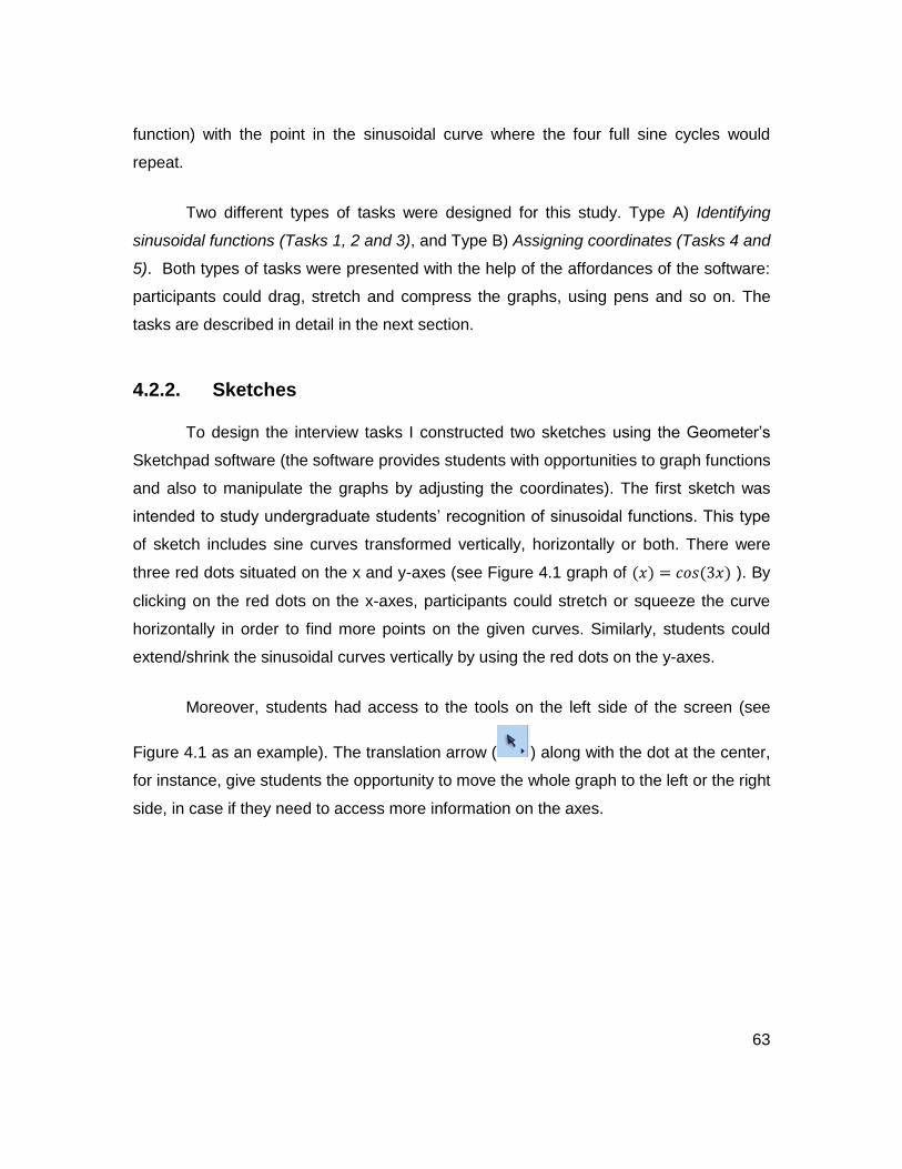
63
function) with the point in the sinusoidal curve where the four full sine cycles would
repeat.
Two different types of tasks were designed for this study. Type A) Identifying
sinusoidal functions (Tasks 1, 2 and 3), and Type B) Assigning coordinates (Tasks 4 and
5). Both types of tasks were presented with the help of the affordances of the software:
participants could drag, stretch and compress the graphs, using pens and so on. The
tasks are described in detail in the next section.
4.2.2. Sketches
To design the interview tasks I constructed two sketches using the Geometer’s
Sketchpad software (the software provides students with opportunities to graph functions
and also to manipulate the graphs by adjusting the coordinates). The first sketch was
intended to study undergraduate students’ recognition of sinusoidal functions. This type
of sketch includes sine curves transformed vertically, horizontally or both. There were
three red dots situated on the x and y-axes (see Figure 4.1 graph of (𝑥) = 𝑐𝑜𝑠(3𝑥) ). By
clicking on the red dots on the x-axes, participants could stretch or squeeze the curve
horizontally in order to find more points on the given curves. Similarly, students could
extend/shrink the sinusoidal curves vertically by using the red dots on the y-axes.
Moreover, students had access to the tools on the left side of the screen (see
Figure 4.1 as an example). The translation arrow ( ) along with the dot at the center,
for instance, give students the opportunity to move the whole graph to the left or the right
side, in case if they need to access more information on the axes.

64
Figure. 4.1. Example of the first sketch.
The second sketch was comprised of a plain sinusoidal curve and no coordinate
axes (see Figure 4.2) were visible. Students could click on the given curve or the arrow
on the right side to move the curve to the right/left. Using the segment straightedge tool
( ), participants could assign the x and y-axes on the sine cycle. To mark any point
on the adjusted axes, students could also apply the tools on the right side (“A” and the
pen tools). Moreover, students can use the tools to write the sinusoidal functions
represented by the given graph either using the pen tool ( ) to write the function in
their own handwriting, or the tool which helps them write in text format (see Figure
4.2, as an example). All these tools gave students opportunities to assign coordinates
and the points on the curve to represent the given function.
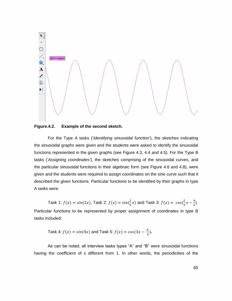
65
Figure. 4.2. Example of the second sketch.
For the Type A tasks (‘Identifying sinusoidal function’), the sketches indicating
the sinusoidal graphs were given and the students were asked to identify the sinusoidal
functions represented in the given graphs (see Figure 4.3, 4.4 and 4.5). For the Type B
tasks (‘Assigning coordinates’), the sketches comprising of the sinusoidal curves, and
the particular sinusoidal functions in their algebraic form (see Figure 4.6 and 4.8), were
given and the students were required to assign coordinates on the sine curve such that it
described the given functions. Particular functions to be identified by their graphs in type
A tasks were:
Task 1: 𝑓(𝑥) = 𝑠𝑖𝑛(2𝑥), Task 2: 𝑓(𝑥) = 𝑠𝑖𝑛(2
3𝑥) and Task 3: 𝑓(𝑥) = 𝑐𝑜𝑠(
2
5𝑥 −
π
5).
Particular functions to be represented by proper assignment of coordinates in type B
tasks included:
Task 4: 𝑓(𝑥) = 𝑠𝑖𝑛(4𝑥) and Task 5: 𝑓(𝑥) = 𝑐𝑜𝑠(3𝑥 − 𝜋
4).
As can be noted, all interview tasks types “A” and “B” were sinusoidal functions
having the coefficient of x different from 1. In other words, the periodicities of the

66
functions were different from 2π (which is the period of the canonic sine and cosine
functions). The coefficient of x in each of the tasks was either a whole number (in Tasks
1, 4 and 5) or a fraction (in tasks 2 and 3). Moreover, two interview tasks, (Tasks 3 and
5) included a phase shift.
4.2.3. Tasks 1, 2 and 3
In this part, I describe each of the Tasks 1, 2 and 3 in detail along with their
graphs.
4.2.3.1. Task 1
Task 1, in which I had students identify the sinusoidal function(s), is shown in
Figure 4.3. As can be seen from the figure, the function described the curve associated
with the function 𝑓(𝑥) = 𝑠𝑖𝑛(2𝑥) (or (𝑥) = 𝑐𝑜𝑠(2𝑥 −𝜋
2 )). In fact, the sine function
(𝑓(𝑥) = 𝑠𝑖𝑛(2𝑥)) was not presented in the task, students were asked to identify it by
considering the graph (see Figure 4.3).
Figure. 4.3. Sketch represents the function 𝒇(𝒙) = 𝒔𝒊𝒏(𝟐𝒙), Task 1.
When students completed the first part of the task and they explained their
thinking, I encouraged them to complete the second part of the task which was

67
determining a cosine function for the curve if they indicated the function 𝑓(𝑥) = 𝑠𝑖𝑛(2𝑥),
or a sine function if they determined 𝑓(𝑥) = 𝑐𝑜𝑠(2𝑥 −𝜋
2) for the given curve.
4.2.3.2. Task 2
To complete Task 2 (𝑓(𝑥) = 𝑠𝑖𝑛(2
3𝑥)), the sketch shown in Figure 4.4 was given
to the participants, and similar to Task 1, the sinusoidal functions needed to be identified
from the given sinusoidal curve. Although it appears that Tasks 1 and 2 were similar, as
they both represent the sinusoidal functions transformed horizontally, they had a major
difference. While the coefficient of x in the sinusoidal function associated with Task 1
was a whole number, it was a fraction in Task 2. These types of tasks are not addressed
in the literature focused on trigonometric functions and students’ (mis)understandings.
As such, in this research I aimed to investigate whether students identify the graphs
representing the sinusoidal functions having whole and fractional periodicity.
Figure. 4.4. Sketch of 𝒇(𝒙) = 𝒔𝒊𝒏(𝟐
𝟑𝒙), Task 2.
4.2.3.3. Task 3
For Task 3 (𝑓(𝑥) = cos (2
5𝑥 −
π
5)) students were required to deal with a fractional
coefficient of x in the given function which was shifted horizontally (see Figure 4.5). The
purpose of this task was to assess students’ perception of horizontal/phase shifts

68
obtained by determining the change being made to the x value. Students, in fact, needed
to realize that the coefficient of x (i.e., 2
5) should be factored from the whole argument
(i.e., (2
5𝑥 −
π
5)) in order to represents the function in its canonical form,
𝑓(𝑥) = 𝑐𝑜𝑠(2
5(𝑥 −
π
2)). In other words, the goal of the task was to investigate whether
students recognize the function shifted horizontally to the right by π
2, or they wrongly
determine π
5 as a phase shift.
Figure 4.5. Sketch of 𝒇(𝒙) = 𝒄𝒐𝒔 (𝟐
𝟓𝒙 −
𝛑
𝟓), Task 3.
4.2.4. Tasks 4 and 5
The next task (Task 4) was from the Type B of interview tasks, ‘Assigning
coordinates’. In this task a sinusoidal curve (see Figure 4.6), along with the sinusoidal
function, were given. Students were required to assign the coordinates on the sinusoidal
curve to represent the graph of 𝑓(𝑥) = 𝑠𝑖𝑛(4𝑥) (see Figure 4.7). While Task 4 deals
with the period concept (similar to Tasks 1 and 2), the last interview task (Task 5) was
similar to Task 3 in which students were required to identify the period as well as the
horizontal shift (see Figure 4.8 and 4.9). In Task 5, students were asked to adjust axes
on the given curve to display the graph of the function 𝑓(𝑥) = 𝑐𝑜𝑠(3𝑥 −𝜋
4).
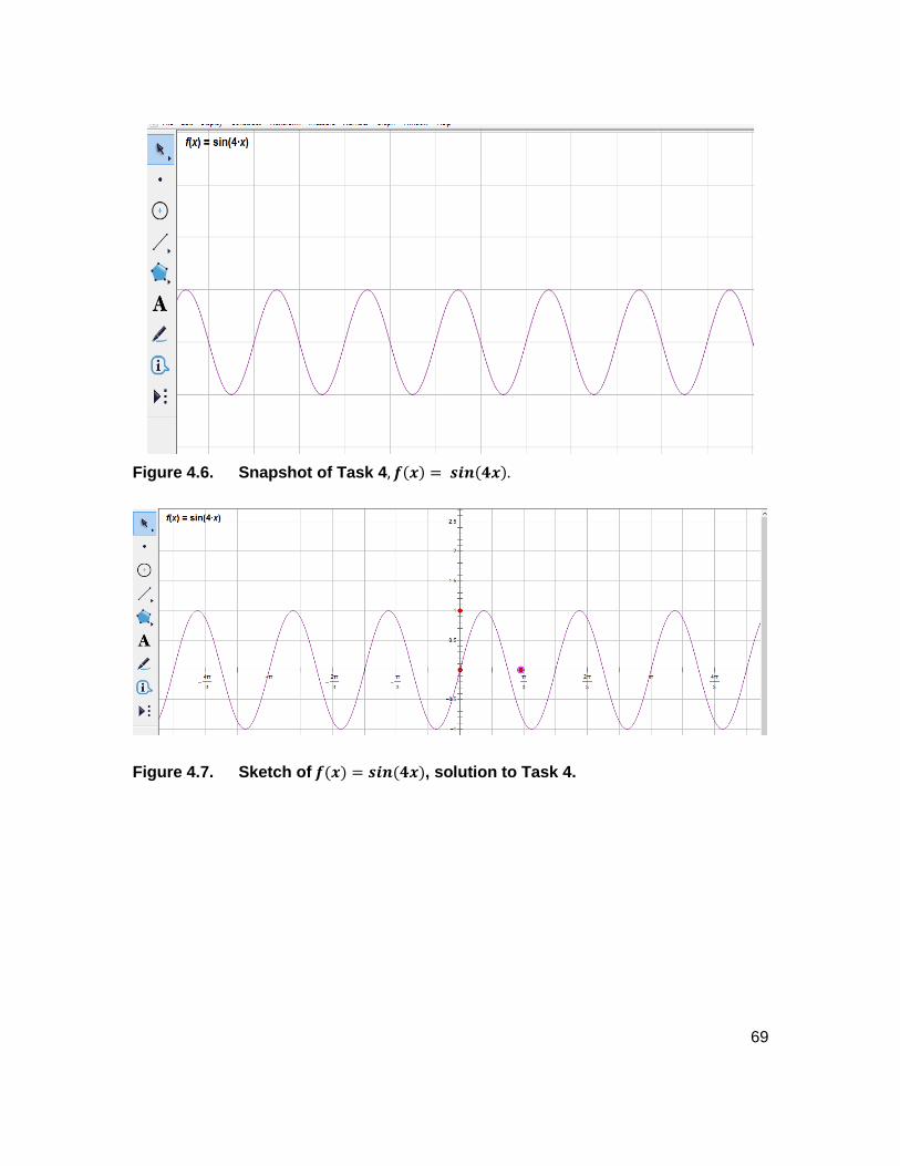
69
Figure 4.6. Snapshot of Task 4, 𝒇(𝒙) = 𝒔𝒊𝒏(𝟒𝒙).
Figure 4.7. Sketch of 𝒇(𝒙) = 𝒔𝒊𝒏(𝟒𝒙), solution to Task 4.

70
Figure 4.8. Snapshot Task 5, 𝒇(𝒙) = 𝒄𝒐𝒔 (𝟑𝒙 −𝛑
𝟒).
Figure 4.9. Sketch of 𝒇(𝒙) = 𝒄𝒐𝒔 (𝟑𝒙 −𝛑
𝟒), solution to Task 5.
4.3. Participants
Six students participated in my main study. The participants were from a large
North American university. They were selected from among students who had either
completed a Calculus I course and were enrolled in a Calculus II, or were in a Calculus I
course at the time of the interview. The participants were students who had volunteered

71
to participate in the study after I had made a general request to all the Math 154/155
(Calculus I and II for the Biological Sciences) and Math 157/158 (Calculus I and II for the
Social Sciences) classes in the Mathematics Department.
Six undergraduate students who participated in the main study were a male and
five females. The participants all volunteered their time. None of the six participants
(Andy, Emma, Sally, Rose, Mia and Kate, all pseudonyms) were familiar with Sketchpad,
but they all sketched the trigonometric functions using Sketchpad without any difficulty.
The participants all knew me because I was working as a Teaching Assistant in the
Applied Calculus Workshops at the time of data collection.
4.3.1. Emma, Rose and Sally
Emma, Rose and Sally were all first year students registered in Calculus I at the
time of the interview. It was their first semester at the University. They stated that they
initially learned trigonometry when they were students in high school. While Emma found
trigonometry a hard subject amongst other mathematics topics in Calculus, Sally and
Rose believed that trigonometry was an interesting subject. Emma and Rose mentioned
that they earned over 85% in the high school Calculus course they took in their grade
12, and they earned above 60% for the first midterm in Calculus I (the interview was
conducted after the first midterm). Sally noted that she earned above 80% in both
Calculus-12 and in the first midterm in Calculus I at the University.
4.3.2. Kate and Mia
Kate and Mia were second year students pursuing Bachelor’s Degrees in
Business and Applied Science. Kate and Mia successfully completed Calculus I and
were enrolled in Calculus II at the time of the interview. It was the first time they used
Sketchpad in mathematics, but they had previous experience in working with a similar
Dynamic Geometry software. Before conducting the interviews, Mia stated that she
might have forgotten the trigonometric facts, but she hoped that she could remember
them all when working on the tasks. Kate requested to practice working with Sketchpad

72
and reviewing some properties of transformations of sinusoidal functions before actually
recording the interview.
4.3.3. Andy
Having completed AP Calculus (Advanced Placement) as a high school student,
Andy was enrolled in Calculus II as well as in Applied Linear Algebra at the time of the
interview. He was a first year student persuing a bachelor’s degree in Applied Science.
He wanted to be an engineer in the future. His grades in high school and University
mathematics courses were high.
4.4. Data Collection
Data were collected using one-on-one, task-based semi-structured, clinical
interviews. Each interview conducted was about 60 minutes long, and they were
videotaped. In order to complete the interview tasks, a laptop was given to each
participant. To provide a comfortable environment, all the interviews took place in the
Science Department. To ensure students were familiar with the topic, all students
participated in a brief informal conversation about sinusoidal functions as well as the
transformation of sinusoidal functions before conducting the actual interviews. In
particular, during the informal conservation, we discussed how sinusoidal functions
might transform horizontally or vertically. The participants described how each of the
elements: A, B, C and D in the general sinusoidal function (𝑓(𝑥) = 𝐴 𝑠𝑖𝑛𝑒/𝑐𝑜𝑠(𝐵(𝑥 +
𝐶) + 𝐷) might affect the graphs of the functions. The students also talked about the
difficulties they encountered when working with the transformation of sinusoidal
functions during their Calculus courses at high school as well as at university. The
participants also had time to experience working with the sketchpad.
The participants’ interactions with the sketches, their dialogues, bodily
movements and what the participants wrote during the interviews were captured on the
videotapes.
73
The use of semi-structured task-based clinical interviewing was fit for data
collection with respect to my research questions. It is indicated that Piaget was one of
the people who used clinical interviews for the first time to determine the construction of
the individuals’ thoughts, the richness of their thoughts and also to assess the
individuals’ cognitive competence (Ginsburg, 1981). To identify the process of the
individuals’ thoughts, the clinical interview may involve some degree of standardization
and the interviewer’s prompts are dependent on the participant’s involvement in the
interview tasks. In this study, I used a few prompts to direct the discussion towards the
purpose of the research. The prompting follow up questions were different for each
participant according to the participants’ interaction and their responses to the interview
tasks.
4.5. Data Analysis
In order to carry out analysis, I used the three theoretical frameworks (Mason’s
shift of attention, Presmeg’ visual imagery and Carlson’s et al. convarasional reasoning).
In the following chapter, I describe the frameworks and the way I analyse data according
to the frameworks. To analyze the data, the videotapes were watched several times. The
students’ conversations were listened to several times and they were transcribed
carefully. I reviewed the performance of each participant on each interview task. The
data analysis is detailed in Chapter 5.

74

75
Chapter 5. Theoretical Considerations
In this study, the data consist of interviewing six participants. In order to analyze
the participants’ responses to the interview tasks, I describe several theoretical
frameworks involved in the data analysis (in this chapter). In each section of Chapter 6
and 7, the collected data are analyzed and interpreted according to three theoretical
frameworks. Mason’s theory of shifts of attention is the first framework described below.
Mason’s theory provides opportunity to study the critical role of attention and awareness
in learning and understanding mathematics and in particular the concept of graphing
sinusoidal functions. Then, Presmeg’s (1989) five different category of visual imagery is
reviewed. As a broad theory, it is used for investigating students’ visual mental
constructs since the participants applied their imagery skills in different occasions when
they completed the interview tasks. The ability of students is evaluated by Covariational
reasoning focusing on Carlson’s et al. (2002) collection of mental action and
developmental levels. At the end of this chapter, I describe data analysis with respect to
the three frameworks.
5.1. Mason’s Theory of Shifts of Attention
Among all aspects of the human psyche being discussed in psychological
literature (e.g., Piaget (1954/1981)), Mason (2008) relies on two particular aspects of the
human psyche, attention and awareness, in his theoretical framework. He believes that
attention and awareness are human constructs in an attempt to define components of
‘being human’, and more specifically, ‘being mathematical’. While some researchers,
such as, Aguirre,Turner, Gau Bartell, Kalinec-Craig, Foote, McDuffie, and Drake, (2012)

76
define awareness as understandings, insights, knowledge, and beliefs about teaching
and learning mathematics, Mason (2008) refers to awareness as what enables people to
act, calling upon our conscious and unconscious powers. He argues that awareness
may exist in our body as we may initiate an action that our consciousness is able to build
a narrative on only later in time, although we might be unable to speak about what we
are doing.
To educate one’s awareness, we need to shift our attention to actions which are
being carried out and to encourage individuals to think about ‘what comes to mind’ in a
situation (Mason, 2008). Mason argues that attention “is not an all-or-nothing
experience”(p.8): its structure is comprised of a macro (what is attended to by an
individual (i.e., what objects are in one’s focus of attention)), and a micro level (how the
objects of attention are attended to).
Mason (2008) believes that at the macro structure of attention (what is being
attended to) learners can attend to more than one thing at once and that learners’ macro
attention is usually caught up with their current action. He states that at the macro level,
attention can vary in multiplicity, locus, focus and sharpness. To address the “how-
question (how something is being attended to)” (micro qualities), He distinguishes five
different structures of attention. These are: holding wholes, discerning details,
recognizing relationships, perceiving properties, and reasoning on the basis of agreed
properties. He believes that when students are holding wholes, they may gaze at a
geometric diagram or some particular part of a diagram. It can also occur when students
gaze at a collection of symbols and “waiting for it to speak to you” or in the other words,
“waiting for things to come to mind” (p.37). Holding wholes may last not too long (only a
few micro-seconds) before students can discern details. Discerning details is a structure
of attention, in which students’ attention is caught by a specific detail that becomes
recognized from the rest of the elements of the attended object. He states that
discerning details, which often does not happen all at once, is neither algorithmic nor
logically sequential. Determining details provides students opportunities to recognize
relationships between specific elements or between symbolic and geometric
representations of a concept. Mason asserts that there is an essential shift between

77
recognizing relationships between symbolic and graphical representation of a
mathematics concept to perceiving properties. Mason refers perceiving properties as
“when you are aware of a possible relationship and you are looking for elements to fit it,
you are perceiving a property” (p. 38). Reasoning on the basis of perceived properties is
considered as the final structure of attending in which students can perceive properties
as the only basis for further reasoning.
It appears that Mason’s framework of shifts of attention is appropriate for
analyzing the collected data in my research. Applying this framework would support me
in gaining insights not only into “what” undergraduate students attend to when
completing mathematics tasks related to transformation of sinusoidal functions, but also
“how” they shift their attention.
Mason’s terms for different structures of attention also provide a language for
analyzing students’ work. For example, when students gaze at the given curves or
sinusoidal functions, they are holding wholes Students who look for particular details
from the given sinusoidal functions or the given sinusoidal curve (e.g., they seek the
point where the graph intersects the y-axis), they are, in fact, discerning details.
Students are recognizing relationship when are able to find connection between the
graphical representation of sinusoidal functions and their symbolic representations.
When students consider a particular graph and recognize its shape as representing a
sinusoidal function because the amplitude is 1 and a full sine cycle ended in 2π, they are
perceiving properties of sinusoidal functions. When students determine the graph
represents f(x) = 2sin(x) because its amplitude is 2 times the amplitude of a canonical
sine function, they are reasoning based on perceived properties.
5.2. Presmeg’s visual imagery
Visualization is increasingly being accepted as an important aspect of
mathematical reasoning by all branches of mathematics studies (not merely of
“obviously visual” branches such as geometry) (Presmeg, 2006, Wheatley and Brown,

78
1994). Visualization often occurs when “thinking is spontaneously accompanied and
supported by images” (Mariottii & Pesci, 1994, p.45). Elliott (1998) regards visualization
as the “ability to create rich, mental images which the individual can manipulate in his
mind, rehearse different representations of the concept and, if necessary, use paper or a
computer screen to express the idea in question” (p.45).
In studying the overall role of imagery in the conceptual understanding of
mathematics concepts, Presmeg (1986a, 1986b, 1989, and 1992) identified five main
types of visual imagery: (1) concrete, pictorial imagery; (2) pattern imagery; (3) memory
images of formulae; (4) kinesthetic imagery; and (5) dynamic (moving) imagery.
Based on the Presmeg’s classification, imagery is called concrete imagery if an
individual has a picture of an object in his/her mind. For example, when students in a
mathematics word problem are asked to divide a large pizza into some triangular slices,
they have a concrete image of triangle in their mind. Pattern imagery is defined as an
imagery in which pure relationships depicted of concrete details. Pattern imagery may
appear when students required finding 𝑠𝑖𝑛(450°), which they visualize repeating pattern
on the sinusoidal curve. Another type is memory images of formulae by which students
typically "saw" a imprinted formula in their minds, written on a blackboard or in their
notebooks. For instance students often used the formula of (y =a(x– h)2+k) in their minds
when looking for the vertex point (h, k) of a quadratic function (e.g., y=x2 ). Kinaesthetic
imagery involves physical movement in evoking mathematical concepts especially when
students could not remember the words. Kinesthetic imagery appears when a learner
"walks" around imaginary quadrants with her fingers to identify where the tangent at an
angle is negative. The last category of imagery is Dynamic imagery which involves
moving and transforming objects in the mind like when students shift horizontally the
graph of y=x2.
In a study of 54 high school students, Presmeg (1997a, 1992) found that each of
these five types of visualization play an important role in students’ mathematical
understanding. She considered the pattern imagery as an important essence in
conceptualizing mathematics concepts because it allows learners to concentrate on the
79
rational aspect of the mathematics problem and it lacks superfluous details. Relying on
the results of her study, however, Presmeg noticed that the concrete imagery was the
least effective type of visualization dealing with students’ understanding of mathematical
contents (Presmeg, 1989).
The five categories of Presmeg’s visualization are applicable when considering
transformations and graphing of sinusoidal functions. Concrete imagery could occur
when students visualize a general picture of sinusoidal functions. They can visualize that
a cosine graph going down, intersects the x-axes, continues going down and then goes
up, intersecting the x-axes again and keeps going up, while a sine curve goes up, then
down, intersecting the x-axes, goes down and up. Pattern imagery in the context of a
sinusoidal function is identified when students can visualize a certain pattern in the
graphical or symbolical representations. For instance, when students notice that in the
function 𝑓(𝑥) = 𝑐𝑜𝑠(5𝑥), five sine cycles will repeat between the interval [0, 2𝜋]. For the
other category of visual imagery, the memory image of formula, undergraduate students
can use the canonical formula (𝑓(𝑥) = 𝐴 𝑠𝑖𝑛(𝐵(𝑥 + 𝐶) + 𝐷 and 𝑓(𝑥) = 𝐴 cos (𝐵(𝑥 +
𝐶)+D) while describe their thinking, or when they are able to change a cosine function
into a sine function having the formula 𝑐𝑜𝑠(𝑥) = 𝑠𝑖𝑛(𝑥 − 𝜋
2) in their mind.
The last two categories of visual imagery involving movement are kinesthetic and
dynamic imagery. Kinesthetic imagery occurs when students involve their body, such as
their hands, to represent the expansion of the sine curve, or when they use their index
finger to show the value in which the sine curve intersects the x-axes. Dynamic imagery
involves moving and transforming a given sine curve into a cosine curve in a student’s
mind.
It is important to note that in this research study, I used the terms kinesthetic
imagery and pattern imagery slightly different from Presmeg’s definition. She applied
primarily kinesthetic imagery in her research studies when participants cannot remember
the mathematics terms and instead they expressed them by their body. However, in this
study I apply kinesthetic imagery when students used their fingers or hands to explain
their thinking, regardless of their memory of the mathematics facts related to the

80
transformation of sinusoidal functions. I use the notion of pattern imagery in a similar
way.
5.3. Carlson’s et al. Covariational Reasoning
Covariational reasoning, defined as cognitive activities involved in coordinating
two quantities, varies in tandem (Moor, 2010). In the studies of undergraduate students,
for instance, Carlson, Jacobs, Coe, Larsen, and Hsu (2002) and Moor (2010) noticed
that covariational reasoning is central for supporting undergraduate students’
construction of trigonometric functions while dealing with the angle measure, the
covariation of angle measure and the trigonometric ratio. The outcomes of research
studies by Thompson, 1994, Carlson, 1998; Zandieh, 2000; Carlson, Jacobs, Coe,
Larsen, and Hsu, 2002; Moore, and Bowling, 2008 also illustrate that covariational
reasoning plays a critical role in developing students’ understanding of graphs as
representations of the relationship between two quantities’ values.
Following the essential and crucial role of covariational reasoning in learning
Calculus topics, Carlson (1998) provided a framework as a means to study multiple
behaviors of a group of undergraduate students involved in interpreting and representing
dynamic function situations. Carlson’s (1998) framework consists of five mental actions
(MA#) specific to the behavior displayed:
1) Coordinating the value of one variable with changes in the other (Mental action
1, M#1),
2) Coordinating the direction of the change of one variable with changes in the
other variable (Mental action 2, M#2),
3) Coordinating the amount of change of one variable with changes in the other
variable (Mental action 3, M#3),

81
4) Coordinating the average rate-of change of the function with uniform
increments of change in the input variable (Mental action 4, M#4), and
5) Coordinating the instantaneous rate of change of the function with continuous
changes in the independent variable for the entire domain of the function (Mental action
5, M#5).
Table 5.1 presents a summary of verbal behaviors related to general functions
and trigonometric function (Carlson, et al., 2002; Carlson & Oehrtman, 2004; Oehrtman,
et al., 2008, Moor, 2010).
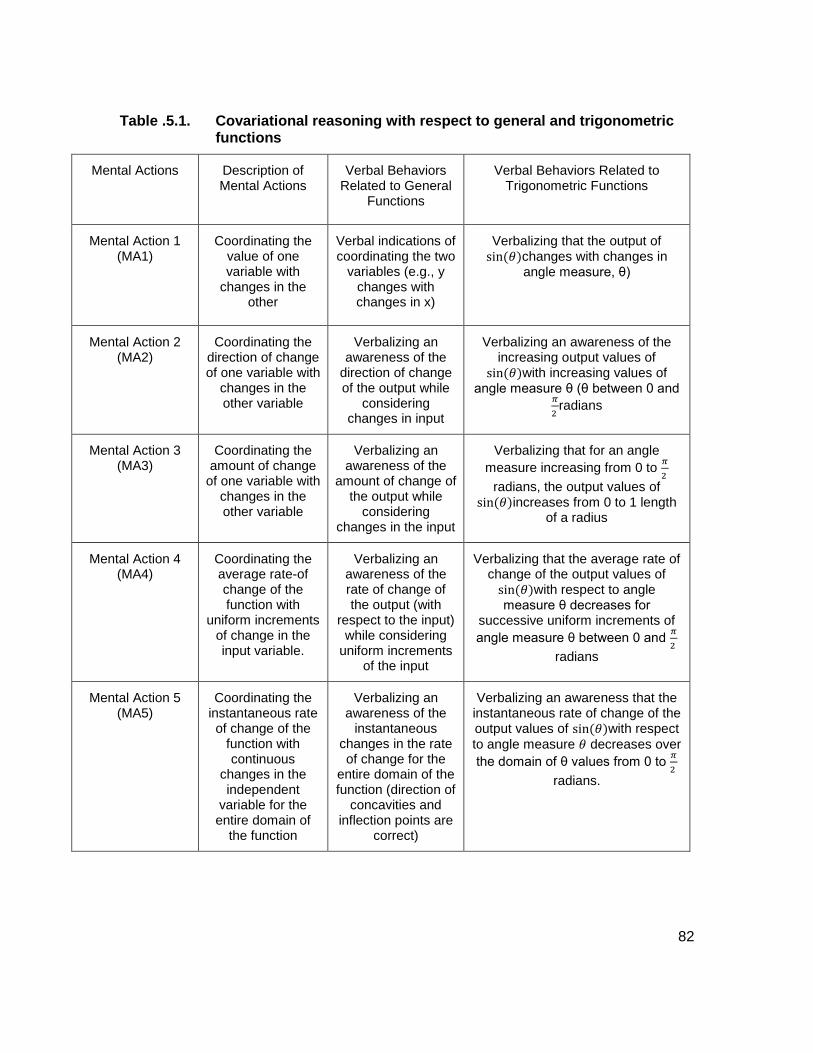
82
Table . 5.1. Covariational reasoning with respect to general and trigonometric functions
Mental Actions Description of Mental Actions
Verbal Behaviors Related to General
Functions
Verbal Behaviors Related to Trigonometric Functions
Mental Action 1 (MA1)
Coordinating the value of one variable with
changes in the other
Verbal indications of coordinating the two
variables (e.g., y changes with changes in x)
Verbalizing that the output of sin (𝜃)changes with changes in
angle measure, θ)
Mental Action 2 (MA2)
Coordinating the direction of change of one variable with
changes in the other variable
Verbalizing an awareness of the
direction of change of the output while
considering changes in input
Verbalizing an awareness of the increasing output values of
sin (𝜃)with increasing values of angle measure θ (θ between 0 and
𝜋
2 radians
Mental Action 3 (MA3)
Coordinating the amount of change
of one variable with changes in the other variable
Verbalizing an awareness of the
amount of change of the output while
considering changes in the input
Verbalizing that for an angle
measure increasing from 0 to 𝜋
2
radians, the output values of sin (𝜃)increases from 0 to 1 length
of a radius
Mental Action 4 (MA4)
Coordinating the average rate-of change of the function with
uniform increments of change in the input variable.
Verbalizing an awareness of the rate of change of the output (with
respect to the input) while considering
uniform increments of the input
Verbalizing that the average rate of change of the output values of
sin (𝜃)with respect to angle measure θ decreases for
successive uniform increments of
angle measure θ between 0 and 𝜋
2
radians
Mental Action 5 (MA5)
Coordinating the instantaneous rate of change of the
function with continuous
changes in the independent
variable for the entire domain of
the function
Verbalizing an awareness of the
instantaneous changes in the rate of change for the
entire domain of the function (direction of
concavities and inflection points are
correct)
Verbalizing an awareness that the instantaneous rate of change of the output values of sin (𝜃)with respect
to angle measure 𝜃 decreases over
the domain of θ values from 0 to 𝜋
2
radians.

83
In spite of the fact that, previous research studies (e.g., Carlson, 1998, Zandieh,
2000) attended to covariational reasoning related to trigonometric functions, as it has
been shown in the above table, further elaboration is essential to account for connecting
sinusoidal functions to their graphs. In what follows I elaborate on mental actions 1, 2
and 3 associated with transformation of sinusoidal functions.
Mental action 1: Students are aware of the fact that the graphs of sinusoidal
functions or sine curves change as periodicity (B) is changing in the sinusoidal functions.
They may also recognize that as a phase shift (C) is adding or subtracting from the
argument x in the sinusoidal function, the graph should shift accordingly. Or if the given
curve does not intersect the origin (0, 0) or y-axes at y=1, the curve should shift
horizontally and therefore the represented sinusoidal function should comprise of a
phase shift.
Mental action 2: Students realize that as the coefficient of argument x in the
sinusoidal functions increases (if it is a number more than 1), the number of repeated full
cycles would increase in the interval [0, 2𝜋]. However, if the coefficient of x in the
sinusoidal function is decreasing (it is a fraction less than 1) the number of full sine
curves will decrease in the interval [0, 2𝜋]. Students verbalize that the direction of
shifting the graph to the right or left depends all on the phase shift added or subtracted
from the argument in the sinusoidal function (e.g., if the phase shift added to the
argument the graph shifted to the left).
Mental action 3: Students connect the amount of changes in period and phase
shift and their influence in the sinusoidal graphs or functions. For example, from the
given function 𝑓(𝑥) = 𝑐𝑜𝑠(3𝑥 − 𝜋) students acknowledge that there should be three
sine cycles in the interval [0, 2𝜋] because the coefficient of x in the given function is 3.
They also identify the phase shift as 𝜋
3, so that the graph should be shifted to the right
side of y-axes by 𝜋
3.
84
It is important to note that in my study the mental actions #4 and 5 do not appear,
because in the tasks related to a sinusoidal function there is no “average rate-of change”
(M#4) or an “instantaneous rate of change” (M#5).
Four years after Carlson (1998) introduced her framework; Carlson et al. (2002)
modified it. During their investigations of the complexity of high-performing 2nd-semester
Calculus students’ ability for the “construction of mental processes involving the rate of
change as it continuously changes in a functional relationship”(p.352), Carlson et al.
(2002) noticed that the mental actions determined in the Carlson’s (1998) framework
were insufficient to classify undergraduate students’ covariational reasoning aptitude.
They found that the covariational reasoning abilities can be interpreted from the
collection of behaviors and mental actions shown when engaging in a mathematics
problem or situation. In order to describe this collection, Carlson et al. (2002) extended
the covariation framework by adding five distinct developmental levels of covariational
reasoning (L#) that parallel the five mental actions (see Table 5.2). A student’s
covariational reasoning ability is said to reach a certain level (e.g., Level 3) when it
supports not only the mental action associated with that given level, but also with all
mental actions associated with lower levels (e.g., MA1 and MA2 abilities).
It is important to note that the above mentioned three frameworks affect the
research questions respectively. In Chapters 3 and 4 two general research questions
were stated. In what follows, the two research questions (questions #2 and 3) are added
to the two previously mentioned questions (questions #1 and 4). As such, in my research
I am interested to answer the following questions:
1) How do undergraduate students complete mathematics tasks involving
the transformation of sinusoidal functions?
2) What is undergraduate students’ covariational reasoning and visual
imagery of the transformation of sinusoidal functions?
3) How do students shift their attention when completing interview tasks?
4) What are the common mistakes students often encounter when they work
with transformations of sinusoidal functions?

85
In what follows, I describe in detail how the data analysis was conducted with
respect to the three frameworks. .
5.4. Application of the Frameworks in Data Analysis
In order to carry out my analysis, I used the three theoretical frameworks
(Mason’s shift of attention, Presmeg’s visual imagery and Carlson’s et al. convarasional
reasoning). To analyze the data, the videotapes were watched several times. The
students’ conversations were listened to several times and they were transcribed
carefully. I reviewed the performance of each participant on each interview task. When
watching the videos, I zoomed in on all the details students’ focused on. For instance, if
students put once the computer pointer on the origin and the point 2𝜋, and then on the
points 𝜋
2 and
𝜋
4 in the graph, I considered it important to investigate how they shifted their
attention from the properties of sinusoidal functions to the details of the graph (these are
important according to Mason’s theory). Meanwhile, the participants’ hand movements
(e.g., to show the function is extended horizontally), explanations and sketches helped
me to analyze their work in respect to the Presmeg’s visual imagery framework.
Listening to the students’ discussions and watching the videotapes also provided me the
opportunity to classify undergraduate students’ covariational reasoning aptitude, which
can be interpreted from the collection of behaviors and mental actions shown when
engaging in the interview tasks.
When analysing students’ replies to Task 1, I reviewed each student’s work
separately. In order to describe how students recognize the point 𝜋 on the x-axes and
consequently choose 2 for the coefficient of x in the sinusoidal function, I relied on the
three frameworks. I found all students’ words; hand written notes, sketches, and body
movements essential in analysing the ways students connect the number of the full sine
cycles to the periodicity of the function. Afterward, I compared the participants’
approaches. In this way, I found similarities and differences among students when
completing Task 1.
86
I followed the same procedure for Task 2 (based on the three theoretical
frameworks). In Task 2, it was imperative for me to investigate how students provided a
link between the length of a full sine curved ended at the point 3𝜋 and the argument of x,
which was a fraction. Watching videos several times also helped me investigate whether
students could identify a phase shift and periodicity from the given graph in Task 3. I was
interested to inspect the points (on the x-axes) that the participants found important to
zoom in, when they were identifying periodicity and phase shift. I was also curious to see
which properties of sinusoidal functions they focused on and how they shifted their
attention from the detail they discerned from the given graph to relationship between the
graphical and symbolic representations. Moreover, I paid attention to students’
hands/fingers movements and their explanations to identify their dynamic and some
other visual imagery as well as their covaritional reasoning. Listening to the students’
discussion and reviewing the transcripts directed me to examine whether students made
similar mistakes in Tasks 2 and 3 when identifying the coefficient of x which was a
fraction.
For Task 4, while listening to each student’s discussion, I inspected whether
participants found the number 4 important in the given task. I considered it significant to
see where the student put the axes on the given sinusoidal curve, which points she/he
put on the x and y-axes, and how and why the student might change the points or the
place of the coordinates (if any). Similar to the other tasks, I was looking for each
participant’s explanations as well as the computer pointer’s movement to determine their
mental actions.
The approach I use to analyse Task 5 was similar to that used for Task 4,
except I paid extra attention to the participants’ thinking about a phase shift (as I did for
Task 3). I wanted to study what aspects of the given function directed participants to
realize a phase shift correctly, whether they noticed the relationship between the
numbers 3, π
4 and the phase shift. It was also vital for me to determine what mislead
them to identify inappropriate graphs for the given function.
87
For the purpose of this study, the data analysis is presented in the following two
chapters, where Chapter 6 focuses on Andy’s responses to the interview tasks, and
Chapter 7 describes the rest of the students’ responses to the tasks. The choice to
present the data analysis in two separate chapters on the one hand introduces sufficient
detail in presenting a particular case, but on the other hand does not bore the reader
with unnecessary redundancy.
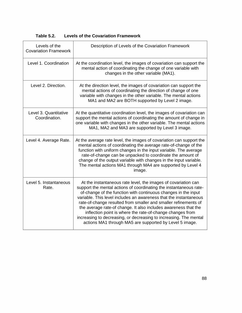
88
Table 5.2. Levels of the Covariation Framework
Levels of the Covariation Framework
Description of Levels of the Covariation Framework
Level 1. Coordination At the coordination level, the images of covariation can support the mental action of coordinating the change of one variable with
changes in the other variable (MA1).
Level 2. Direction. At the direction level, the images of covariation can support the mental actions of coordinating the direction of change of one
variable with changes in the other variable. The mental actions MA1 and MA2 are BOTH supported by Level 2 image.
Level 3. Quantitative Coordination.
At the quantitative coordination level, the images of covariation can support the mental actions of coordinating the amount of change in one variable with changes in the other variable. The mental actions
MA1, MA2 and MA3 are supported by Level 3 image.
Level 4. Average Rate. At the average rate level, the images of covariation can support the mental actions of coordinating the average rate-of-change of the function with uniform changes in the input variable. The average
rate-of-change can be unpacked to coordinate the amount of change of the output variable with changes in the input variable. The mental actions MA1 through MA4 are supported by Level 4
image.
Level 5. Instantaneous Rate.
At the instantaneous rate level, the images of covariation can support the mental actions of coordinating the instantaneous rate-
of-change of the function with continuous changes in the input variable. This level includes an awareness that the instantaneous rate-of-change resulted from smaller and smaller refinements of the average rate-of change. It also includes awareness that the
inflection point is where the rate-of-change changes from increasing to decreasing, or decreasing to increasing. The mental
actions MA1 through MA5 are supported by Level 5 image.

89
Chapter 6. Data Analysis: The Case of Andy
As mentioned, the first analysis chapter focuses in detail on one student,
Andy. This analysis is presented in 2 parts. In Part 1, I summarize Andy’s approaches to
the presented tasks. In Part 2 I analyze Andy’s work on the presented tasks according to
the theoretical frameworks that were described in Chapter 5: Mason’s (2008) theory of
shift of attention, Presmeg’ (1986) visual imagery and Carlson, Jacobs, Coe, Larsen,
and Hsu’s (2002) covariational reasoning.
Using Mason’s (2002) terms, Part 1 can be seen as ‘account-of’ Andy’s solutions,
while Part 2 is ‘accounting-for.’ The term account-of refers to a brief description of the
key elements of the story, suspending as much as possible emotion, evaluation,
judgment or explanations. This serves as data for accounting-for, which provides
explanation, interpretation, value judgement or theory-based analysis.
Part 1: Andy’s Story, Account-Of
6.1.1. Task 1: Identifying the Function of 𝒇(𝒙) = 𝒔𝒊𝒏(𝟐𝒙) from the Given Graph
I showed Andy Task 1 which was the graph of 𝑓(𝑥) = 𝑠𝑖𝑛(2𝑥) (See Figure 6.1)
and I asked him to identify a function represented by this graph.
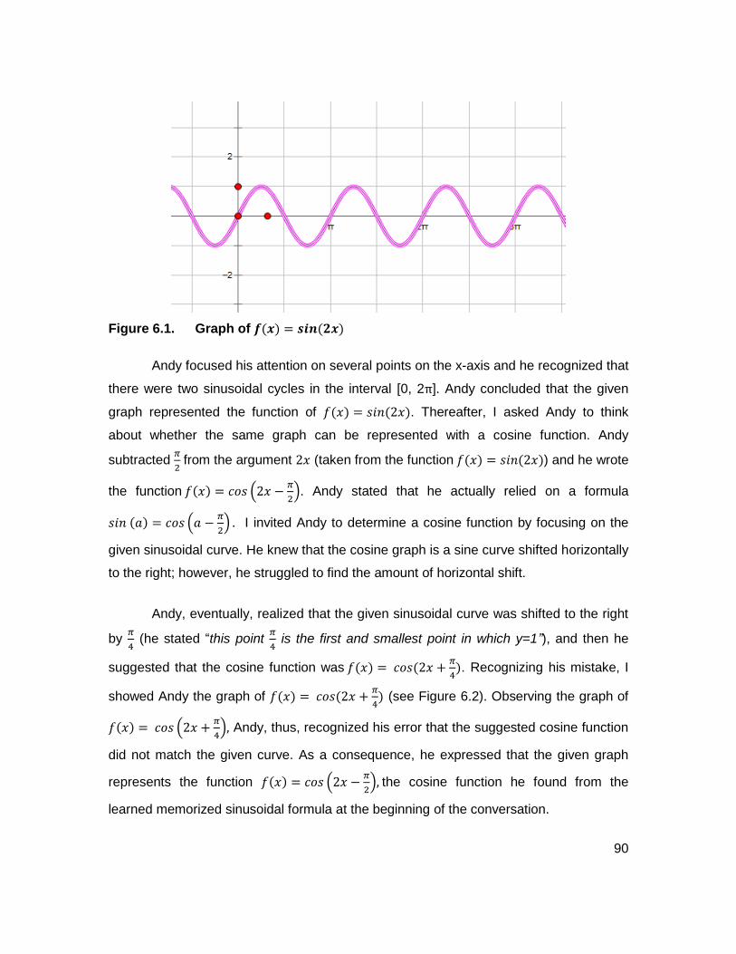
90
Figure 6.1. Graph of 𝒇(𝒙) = 𝒔𝒊𝒏(𝟐𝒙)
Andy focused his attention on several points on the x-axis and he recognized that
there were two sinusoidal cycles in the interval [0, 2π]. Andy concluded that the given
graph represented the function of 𝑓(𝑥) = 𝑠𝑖𝑛(2𝑥). Thereafter, I asked Andy to think
about whether the same graph can be represented with a cosine function. Andy
subtracted 𝜋
2 from the argument 2𝑥 (taken from the function 𝑓(𝑥) = 𝑠𝑖𝑛(2𝑥)) and he wrote
the function 𝑓(𝑥) = 𝑐𝑜𝑠 (2𝑥 −𝜋
2). Andy stated that he actually relied on a formula
𝑠𝑖𝑛 (𝑎) = 𝑐𝑜𝑠 (𝑎 −𝜋
2) . I invited Andy to determine a cosine function by focusing on the
given sinusoidal curve. He knew that the cosine graph is a sine curve shifted horizontally
to the right; however, he struggled to find the amount of horizontal shift.
Andy, eventually, realized that the given sinusoidal curve was shifted to the right
by 𝜋
4 (he stated “this point
𝜋
4 is the first and smallest point in which y=1”), and then he
suggested that the cosine function was 𝑓(𝑥) = 𝑐𝑜𝑠(2𝑥 +𝜋
4). Recognizing his mistake, I
showed Andy the graph of 𝑓(𝑥) = 𝑐𝑜𝑠(2𝑥 +𝜋
4) (see Figure 6.2). Observing the graph of
𝑓(𝑥) = 𝑐𝑜𝑠 (2𝑥 +𝜋
4), Andy, thus, recognized his error that the suggested cosine function
did not match the given curve. As a consequence, he expressed that the given graph
represents the function 𝑓(𝑥) = 𝑐𝑜𝑠 (2𝑥 −𝜋
2), the cosine function he found from the
learned memorized sinusoidal formula at the beginning of the conversation.

91
Figure 6.2. Graph of 𝒇(𝒙) = 𝐜𝐨𝐬 (𝟐𝒙 +𝝅
𝟒)
6.1.2. Task 2: Identifying the Function 𝒇(𝒙) = 𝒔𝒊𝒏(𝟐
𝟑𝒙) from the
Given Graph
For Task 2, I showed Andy the graph of 𝑓(𝑥) = 𝑠𝑖𝑛(2
3𝑥) (see Figure 6.3) and I
asked him to identify a sinusoidal function represented by the given curve. Following the
same pattern as his response to the previous task, Andy attempted to figure out the
number of full cycles within the interval [0, 2𝜋]. Soon he realized that the given curve
completed one cycle in the interval [0, 3𝜋], about half a cycle more than the canonical
sinusoidal curve completed at 2𝜋. Andy, thus, concluded that the length of the given
graph was about 3
2= 1.5 times a basic canonical sinusoidal curve. In order to find a
related function, he used a reciprocal of the fraction 3
2 and he offered that the function
was 𝑓(𝑥) = 𝑠𝑖𝑛(2
3𝑥).

92
Figure 6.3. Graph of 𝒇(𝒙) = 𝒔𝒊𝒏(𝟐
𝟑𝒙)
I then, asked Andy to identify a cosine function represented by the given curve.
Similar to the previous task, he subtracted π
2 from the argument
2
3 x (taken from the
function 𝑓(𝑥) = sin (2
3𝑥)) and he wrote 𝑓(𝑥) = cos (
2
3 𝑥 −
π
2). However, when I asked him
to determine the cosine function by focusing on the graph rather than applying his
learned formula, Andy made a similar mistake as in the previous question (Task 1). Andy
stretched the x-axes and then noticed that the graph was shifted to the right by 3π
4 (since
the first point (on the x-axes) by which the graph had y=1 was x=3π
4). He, therefore,
expressed that the cosine function for the given curve should be 𝑓(𝑥) = 𝑐𝑜𝑠(2
3𝑥 +
3π
4)
which is different from his previous mentioned function. It is important to note that Andy
did not consider the aforementioned suggested function in the general standard format
(𝑓(𝑥) = 𝐴 𝑐𝑜𝑠(𝐵(𝑥 + 𝐶) + 𝐷)) and this interfered with his ability to identify the correct
function. Andy recognized his mistake after he saw the graph of the suggested cosine
function (See Figure 6.4). Then, he used his previous learned knowledge related to the
transformation of sinusoidal functions and he stated that we need to multiply the
coefficient of 2
3 by
3π
4 . Eventually he wrote the function as 𝑓(𝑥) = 𝑐𝑜𝑠(
2
3 𝑥 − (
2
3 ×
3π
4))
(see Figure 6.4) and then determined the function 𝑓(𝑥) = 𝑐𝑜𝑠( 2
3 𝑥 −
π
2) which was the
correct function for the graph.

93
Figure 6.4. Graph of 𝒇(𝒙) = 𝒄𝒐𝒔( 𝟐
𝟑 𝒙 − (
𝟐
𝟑 ×
𝟑𝛑
𝟒)
6.1.3. Task 3: Identifying the Function of 𝒇(𝒙) = 𝒄𝒐𝒔(𝟐
𝟓𝒙 −
𝛑
𝟓) from
the Given Graph.
Figure 6.5. Graph of 𝒇(𝒙) = 𝒄𝒐𝒔(𝟐
𝟓𝒙 −
𝛑
𝟓)
For the next task, Andy stated that
“…the given graph could be written as a sine or cosine function, but I want to
write a cosine function for the curve.”
In order to find the period of the cosine function, Andy looked for two
consecutive points in which the curve intersects the x-axis. He expressed that the curve
could complete one sinusoidal cycle (the curve going up, down and up again) from −3π
4
to 17π
4 (the midpoint between 4π and
9
2π) (see Figure 6.6). By this calculation, Andy

94
concluded that the cosine function has a period of 5π =17π
4− (−
3π
4) because the cosine
curve repeats every 5π radians.
Figure 6.6. Determining the period of the given cosine function
After that, Andy realized that the given curve shifted horizontally because the
graph did not intersect the y-axes at the point 1. To determine the amount of horizontal
shift (B in canonical1 representation), he stretched the x-axes. Andy, then stated that
“Ok, it is one [y=1] in between 𝜋
3 and
2𝜋
3.”
Thus, Andy concluded that the function was 𝑓(𝑥) = 𝑐𝑜𝑠 (2
5𝑥 − (
2π
3−
π
3))
(Function 1) (see Figure 6.7). Note that his approximation from the graph is imprecise
and this influences his next decisions.
1 I refer to the form 𝑓(𝑥) = 𝐴 𝑠𝑖𝑛/𝑐𝑜𝑠 (𝐵(𝑥 + 𝐶 )) + 𝐷 as the canonical representation of a
trigonometric function
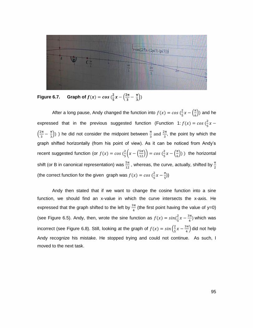
95
Figure 6.7. Graph of 𝒇(𝒙) = 𝒄𝒐𝒔 (𝟐
𝟓𝒙 − (
𝟐𝛑
𝟑−
𝛑
𝟑))
After a long pause, Andy changed the function into 𝑓(𝑥) = 𝑐𝑜𝑠 (2
5𝑥 − (
π
6)) and he
expressed that in the previous suggested function (Function 1: 𝑓(𝑥) = 𝑐𝑜𝑠 (2
5𝑥 −
(2π
3−
π
3)) ) he did not consider the midpoint between
π
3 and
2π
3, the point by which the
graph shifted horizontally (from his point of view). As it can be noticed from Andy’s
recent suggested function (or 𝑓(𝑥) = 𝑐𝑜𝑠 (2
5(𝑥 − (
5π
12)) = 𝑐𝑜𝑠 (
2
5𝑥 − (
π
6)) ) the horizontal
shift (or B in canonical representation) was 5π
12 , whereas, the curve, actually, shifted by
π
2
(the correct function for the given graph was 𝑓(𝑥) = 𝑐𝑜𝑠 (2
5𝑥 −
𝜋
5))
Andy then stated that if we want to change the cosine function into a sine
function, we should find an x-value in which the curve intersects the x-axis. He
expressed that the graph shifted to the left by 3π
4 (the first point having the value of y=0)
(see Figure 6.5). Andy, then, wrote the sine function as 𝑓(𝑥) = 𝑠𝑖𝑛(2
5𝑥 −
3π
4) which was
incorrect (see Figure 6.8). Still, looking at the graph of 𝑓(𝑥) = 𝑠𝑖𝑛 (2
5𝑥 −
3π
4) did not help
Andy recognize his mistake. He stopped trying and could not continue. As such, I
moved to the next task.

96
Figure 6.8. Graph of 𝒇(𝒙) = 𝒔𝒊𝒏(𝟐
𝟓𝒙 −
𝟑𝛑
𝟒)
6.1.4. Task 4: Assigning Coordinates to Represent 𝒇(𝒙) = 𝒔𝒊𝒏(𝟒𝒙)
Figure 6.9. Sinusoidal curve
For Task 4, I showed Andy a sinusoidal curve (see Figure 6.9) and I asked him to
assign the axis and coordinates such that it represents the graph of 𝑓(𝑥) = 𝑠𝑖𝑛(4𝑥).
Since the coefficient of x was 4 in the given sine function (𝑓(𝑥) = 𝑠𝑖𝑛(4𝑥)), following the
same method as in the previous tasks, Andy recognized that there should be 4 full
cycles in the interval of [0, 2π]. To show that, he considered 2 full periods and then
placed the point π on the x-axes. He then marked the points 1 and -1 on the y-axes (see
Figure 6.10). Andy stated that the two consecutive cycles of the sine graph represented
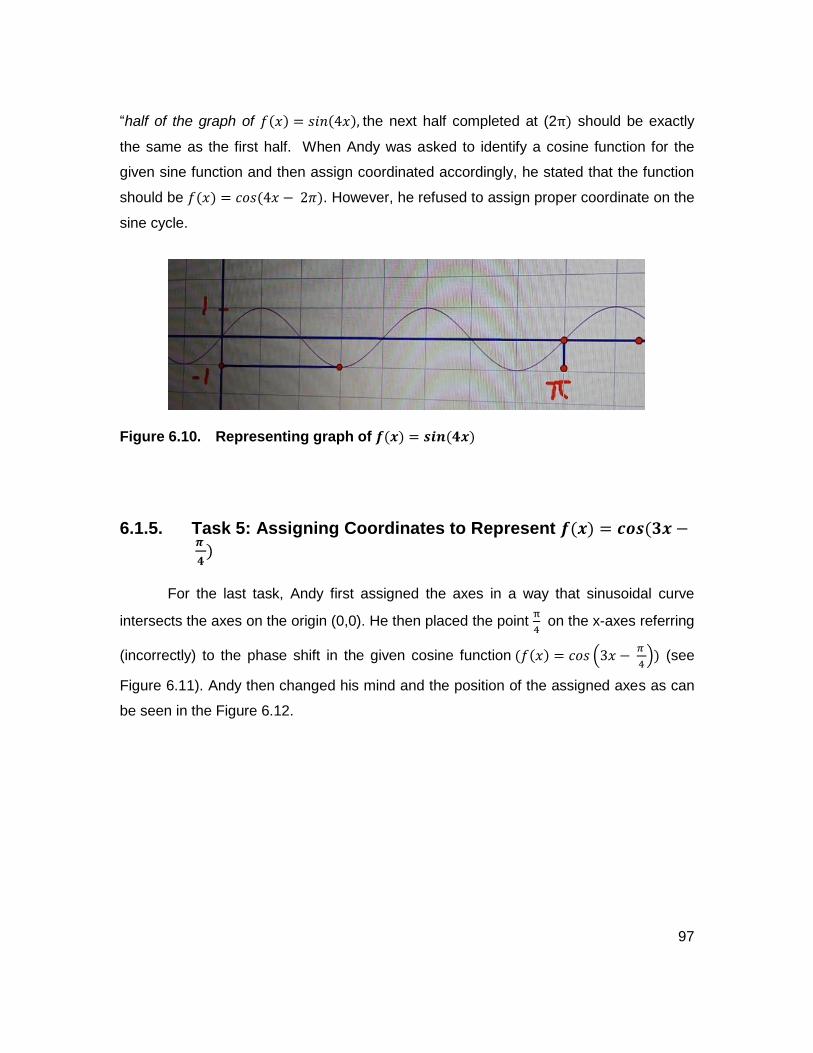
97
“half of the graph of 𝑓(𝑥) = 𝑠𝑖𝑛(4𝑥), the next half completed at (2π) should be exactly
the same as the first half. When Andy was asked to identify a cosine function for the
given sine function and then assign coordinated accordingly, he stated that the function
should be 𝑓(𝑥) = 𝑐𝑜𝑠(4𝑥 − 2𝜋). However, he refused to assign proper coordinate on the
sine cycle.
Figure 6.10. Representing graph of 𝒇(𝒙) = 𝒔𝒊𝒏(𝟒𝒙)
6.1.5. Task 5: Assigning Coordinates to Represent 𝒇(𝒙) = 𝒄𝒐𝒔(𝟑𝒙 −
𝝅
𝟒)
For the last task, Andy first assigned the axes in a way that sinusoidal curve
intersects the axes on the origin (0,0). He then placed the point π
4 on the x-axes referring
(incorrectly) to the phase shift in the given cosine function (𝑓(𝑥) = 𝑐𝑜𝑠 (3𝑥 − 𝜋
4)) (see
Figure 6.11). Andy then changed his mind and the position of the assigned axes as can
be seen in the Figure 6.12.
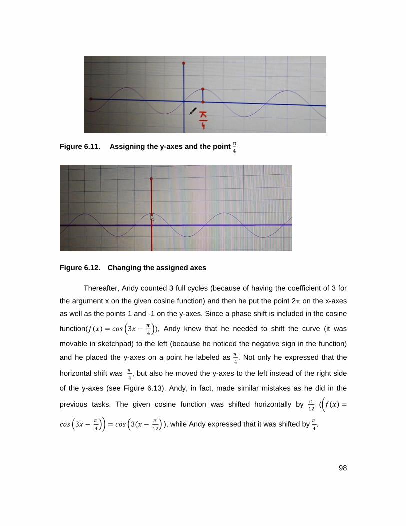
98
Figure 6.11. Assigning the y-axes and the point 𝛑
𝟒
Figure 6.12. Changing the assigned axes
Thereafter, Andy counted 3 full cycles (because of having the coefficient of 3 for
the argument x on the given cosine function) and then he put the point 2π on the x-axes
as well as the points 1 and -1 on the y-axes. Since a phase shift is included in the cosine
function(𝑓(𝑥) = 𝑐𝑜𝑠 (3𝑥 − 𝜋
4)), Andy knew that he needed to shift the curve (it was
movable in sketchpad) to the left (because he noticed the negative sign in the function)
and he placed the y-axes on a point he labeled as 𝜋
4. Not only he expressed that the
horizontal shift was 𝜋
4, but also he moved the y-axes to the left instead of the right side
of the y-axes (see Figure 6.13). Andy, in fact, made similar mistakes as he did in the
previous tasks. The given cosine function was shifted horizontally by 𝜋
12 ((𝑓(𝑥) =
𝑐𝑜𝑠 (3𝑥 − 𝜋
4)) = 𝑐𝑜𝑠 (3(𝑥 −
𝜋
12) ), while Andy expressed that it was shifted by
𝜋
4.

99
Figure 6.13. Graph of 𝒇(𝒙) = 𝒄𝒐𝒔 (𝟑𝒙 − 𝝅
𝟒)
6.2. Part: 2 Andy’s Story, Accounting-For
In Part 6.2, I focus on ‘accounting for’ (Mason, 2002) Andy’s solutions,
considering them according to three frameworks (1- Shift of attention, 2- Visualization, 3-
Mental action).
6.2.1. Shifts of Attention
6.2.1.1. Task 1: Identifying the Function 𝒇(𝒙) = 𝒔𝒊𝒏(𝟐𝒙) from the Given Graph.
In order to complete Task 1, Andy first focused his attention on the given graph
and waited for visual feedback from the graph (his attention was holding wholes
according to Mason’s classification). He then realized that the graph went through the
origin (0,0). This shows that Andy was able to discern a very specific detail from the
graph. Thereafter, in order to identify the type of trigonometric function, he locked again
his attention for a few seconds on the graph as a whole. Andy then stated that the given
graph represented a sine function because it “started” from the point (0,0). One could
conclude that Andy was able to perceive properties of a sine curve (a cyclic graph
started at (0,0)).

100
Andy gazed at the graph again for a while. He then shifted his attention to
discerning more details about the curve. He, therefore, focused on the specific points
such as (0,0), (𝜋
4, 1), (
𝜋
2, 0), (
3𝜋
4, -1) and (𝜋,0) within the interval [0, 𝜋] . Andy realized that
the same pattern had been repeated for the second cycle from 𝜋 to 2 𝜋 (e.g., (5𝜋
4, 1), (
3𝜋
2,
0) and so on). Matching the details of where the two cycles of a sine curve intersected
the x-axis (one cycle from 0 to 𝜋 and another one from 𝜋 to 2𝜋) and then finding the
related points on the y-axis led to Andy’s conclusion that the length of the period was not
the same as the canonical sinusoidal curve. In other words, Andy realized that the given
graph was squeezed compared with the original sine curve in the interval [0, 2 𝜋].
Therefore he articulated that:
“It is a sine curve but with a factor, because a regular sine graph is a periodic
function of 2𝜋, but here at 2𝜋 there is two cycles.”
The above statement illustrates that Andy knew that there is a relationship
between the geometric representations of the given graph and the number of repeated
cycles in the given intervals. Then he indicated that the function should be 𝑓(𝑥) =
𝑠𝑖𝑛(2𝑥). This means that from reasoning on the perceived properties of the sine curve
Andy was able to introduce a correct sinusoidal function for the given graph.
To write a different equation for the given graph (as a cosine function), Andy
focused his attention, this time, on those details that would lead him to find a cosine
function. To do so, Andy compared the changes in the x and y-values of the given graph
with the canonical cosine graph as he indicated that:
“Because the cosine graph starts at the points where x=0 and y=1, so I basically
need to look at the first instance on the domain that give me y=1.”
This shows that Andy was aware of the fact that the basic canonical cosine
function intersects the y-axes at one. This suggests that Andy perceived properties of
cosine function. Thereafter, he gazed at the graph as a whole for a while until he
focused his attention on more details embedded in the given sinusoid graph. Andy, thus,

101
found that the points in which the graph interconnect the x-axes were 𝜋
2 as well as 𝜋.
Here, he again shifted his attention to y=1 and indicated that the graph did not intersect
the y-axes at the point 1, as in the canonical cosine curve. Therefore, Andy interpreted
the given curve as a graph shifted horizontally to the right. However, he still could not
realize the amount by which the graph shifted as he stated “… I do not know what this
point is.” He gazed at the graph as a whole again. Andy finally figured out that the graph
transformed horizontally by 𝜋
4 to the right because the value of y equals 1 for x=
𝜋
4.
Afterwards, he determined the cosine function while reasoning on the perceived
properties of the transformed sine function. He stated that “this one [the given curve]
starts from ( 𝜋
4, 1), so it is 𝑓(𝑥) = 𝑐𝑜𝑠(2𝑥 +
𝜋
4) because it is shifted to the right so I need
to have a positive sign.”
It is clear from the above-suggested function (𝑓(𝑥) = 𝑐𝑜𝑠(2𝑥 +𝜋
4)) that Andy
knew that the coefficient of the argument of x should be 2 because there were 2 full
cycles on the given graph. However, Andy made two mistakes. First, since the point
(𝜋
4, 1) was on the right side of the y-axes, he added
𝜋
4 to the argument 2x in the cosine
function. Second, he did not pay any attention to the effect of periodicity on the shifted
point when he added 𝜋
4 to (2𝑥). These errors illustrate that Andy had some difficulties in
perceiving properties of transformation of sinusoidal functions because if graph shifted to
the right, the length of horizontal shift should be subtracted from the argument of x
embedded in the sinusoidal function. Thus, I sketched 𝑓(𝑥) = 𝑐𝑜𝑠 (2𝑥 +𝜋
4) using a
sketchpad to investigate if Andy could realize the mistakes he made in determining the
cosine function.
After sketching the graph of 𝑓(𝑥) = 𝑐𝑜𝑠 (2𝑥 +𝜋
4) Andy immediately recognized
his error, noting that
“Ok, I made some incorrect calculation, but I think I should do something with the
coefficient of x which is 2.”

102
The feedback he got from the graph of his suggested function made him realize
that there is a connection between the arguments of x and the point by which the graph
is shifted. In other words, Andy noticed the relationship between the graphical
representations of periodicity and the cosine function transformed horizontally. He then
continued, stating
“Basically since the coefficient of x is 2, it needs to be multiplied by 𝜋
4 on 2,
because the x has 2 multiplications. So the function should be 𝑓(𝑥) = 𝑐𝑜𝑠(2𝑥 −
𝜋
2).”
From Andy’s suggested function (𝑓(𝑥) = 𝑐𝑜𝑠 (2𝑥 +𝜋
4) and 𝑓(𝑥) = 𝑐𝑜𝑠(2𝑥 −
𝜋
2)), it
is unclear whether Andy returned to his previous suggestion based on the known
relationship between sine and cosine ( 𝑠𝑖𝑛(𝑎) = 𝑐𝑜𝑠 (𝑎 −𝜋
2) ) or whether he recognized
the importance of the brackets 𝑓(𝑥) = 𝑐𝑜𝑠(2𝑥 −𝜋
2) is indeed equivalent 𝑓(𝑥) =
𝑐𝑜𝑠(2(𝑥 −𝜋
4)) , and that is how the recognized shift by
𝜋
4 is featured in the formula.
6.2.1.2. Task 2: Identifying the Function 𝒇(𝒙) = 𝒔𝒊𝒏(𝟐
𝟑𝒙) from the Given
Graph
Andy gazed at the whole graph for a while and then he discerned some details
on the values of x and y on the origin. Andy noticed that the graph intersected the origin
at the point (0, 0), so he knew that the curve was related to a sine function. He then
looked for more details and he realized that the horizontal length of the graph stretched
more compared with the canonical sine curve. In fact, he noticed that the graph hit the x-
axes at 0, 3𝜋
2 and 3 𝜋. This observation of the details directed Andy to find a relationship
between the graphical representations and the symbolic representations of the sine
function. In other words, he knew that the argument of x was the reverse of the

103
horizontal length or the periodicity of the graph. As a result, he introduced 2
3 for the
coefficient of x and thus, the sinusoidal function was 𝑓(𝑥) = 𝑠𝑖𝑛(2
3𝑥).
In order to identify a cosine function for the given graph, he initially spent several
minutes finding the point on the x-axes having the value of y=1. To do so, he observed
that the graph had the value of y= 1 between the points (0, 0) and (3𝜋
2, 0). He then
zoomed in for more details on the x-axes and he eventually found a point on the x-axes
having the value of y=1. Andy recognized that the graph had the value of y=1 for a point
between 𝜋
2 and 𝜋 which was
3𝜋
4. Thus, he expressed that the graph was shifted by
3𝜋
4. As
a result, he could provide a relationship between the graph shifting horizontally and its
transformed function. Andy stated that the product of the horizontal transformation was
𝑓(𝑥) = 𝑐𝑜𝑠 (2
3𝑥 +
3𝜋
4). Observing the graph of his suggested function, 𝑓(𝑥) = 𝑐𝑜𝑠 (
2
3𝑥 +
3𝜋
4), made Andy gaze at the whole graph again, while comparing both graphs (his
suggested graph and the original given curve) (see Figure 6.14). Andy discerned some
details on both graphs. For instance, he noticed that the point (3𝜋
2) had the value of y=1
in the original graph (graph of 𝑓(𝑥) = 𝑠𝑖𝑛 (2
3𝑥)), but the y-value was not the same for his
suggested graph (graph of 𝑓(𝑥) = 𝑐𝑜𝑠 (2
3𝑥 +
3𝜋
4)). He also found that the new suggested
graph (graph of 𝑓(𝑥) = 𝑐𝑜𝑠 (2
3𝑥 +
3𝜋
4 )) did not pass the origin (0,0), while the given graph
(graph of 𝑓(𝑥) = 𝑠𝑖𝑛 (2
3𝑥)) intersects the origin.
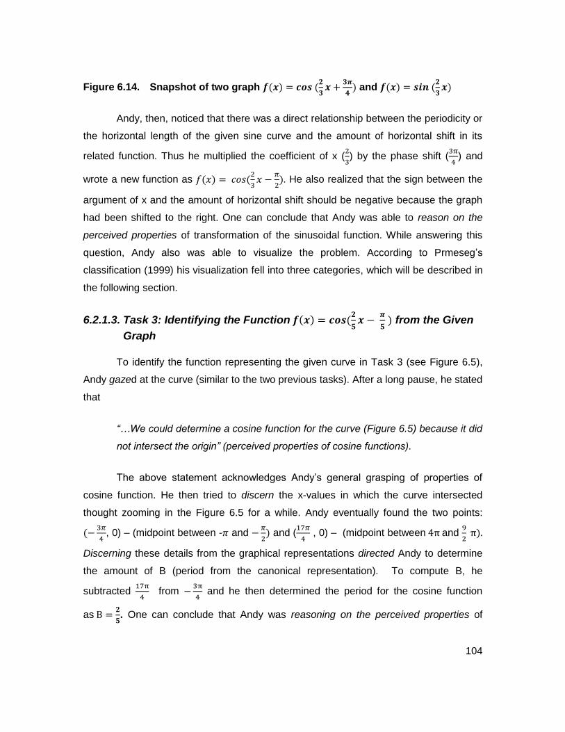
104
Figure 6.14. Snapshot of two graph 𝒇(𝒙) = 𝒄𝒐𝒔 (𝟐
𝟑𝒙 +
𝟑𝝅
𝟒) and 𝒇(𝒙) = 𝒔𝒊𝒏 (
𝟐
𝟑𝒙)
Andy, then, noticed that there was a direct relationship between the periodicity or
the horizontal length of the given sine curve and the amount of horizontal shift in its
related function. Thus he multiplied the coefficient of x (2
3) by the phase shift (
3𝜋
4) and
wrote a new function as 𝑓(𝑥) = 𝑐𝑜𝑠(2
3𝑥 −
𝜋
2). He also realized that the sign between the
argument of x and the amount of horizontal shift should be negative because the graph
had been shifted to the right. One can conclude that Andy was able to reason on the
perceived properties of transformation of the sinusoidal function. While answering this
question, Andy also was able to visualize the problem. According to Prmeseg’s
classification (1999) his visualization fell into three categories, which will be described in
the following section.
6.2.1.3. Task 3: Identifying the Function 𝒇(𝒙) = 𝒄𝒐𝒔(𝟐
𝟓𝒙 −
𝝅
𝟓 ) from the Given
Graph
To identify the function representing the given curve in Task 3 (see Figure 6.5),
Andy gazed at the curve (similar to the two previous tasks). After a long pause, he stated
that
“…We could determine a cosine function for the curve (Figure 6.5) because it did
not intersect the origin” (perceived properties of cosine functions).
The above statement acknowledges Andy’s general grasping of properties of
cosine function. He then tried to discern the x-values in which the curve intersected
thought zooming in the Figure 6.5 for a while. Andy eventually found the two points:
(−3𝜋
4, 0) – (midpoint between -𝜋 and −
𝜋
2) and (
17𝜋
4 , 0) – (midpoint between 4π and
9
2 π).
Discerning these details from the graphical representations directed Andy to determine
the amount of B (period from the canonical representation). To compute B, he
subtracted 17π
4 from −
3π
4 and he then determined the period for the cosine function
as B =𝟐
𝟓. One can conclude that Andy was reasoning on the perceived properties of
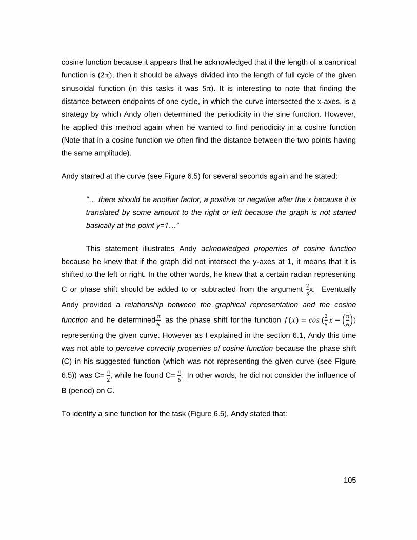
105
cosine function because it appears that he acknowledged that if the length of a canonical
function is (2π), then it should be always divided into the length of full cycle of the given
sinusoidal function (in this tasks it was 5π). It is interesting to note that finding the
distance between endpoints of one cycle, in which the curve intersected the x-axes, is a
strategy by which Andy often determined the periodicity in the sine function. However,
he applied this method again when he wanted to find periodicity in a cosine function
(Note that in a cosine function we often find the distance between the two points having
the same amplitude).
Andy starred at the curve (see Figure 6.5) for several seconds again and he stated:
“… there should be another factor, a positive or negative after the x because it is
translated by some amount to the right or left because the graph is not started
basically at the point y=1…”
This statement illustrates Andy acknowledged properties of cosine function
because he knew that if the graph did not intersect the y-axes at 1, it means that it is
shifted to the left or right. In the other words, he knew that a certain radian representing
C or phase shift should be added to or subtracted from the argument 2
5x. Eventually
Andy provided a relationship between the graphical representation and the cosine
function and he determined π
6 as the phase shift for the function 𝑓(𝑥) = 𝑐𝑜𝑠 (
2
5𝑥 − (
π
6))
representing the given curve. However as I explained in the section 6.1, Andy this time
was not able to perceive correctly properties of cosine function because the phase shift
(C) in his suggested function (which was not representing the given curve (see Figure
6.5)) was C= π
2, while he found C=
π
6. In other words, he did not consider the influence of
B (period) on C.
To identify a sine function for the task (Figure 6.5), Andy stated that:

106
“…the cosine function (𝑓(𝑥) = 𝑐𝑜𝑠 (2
5𝑥 − (
𝜋
6)) should be shifted to the here by a
factor of 3𝜋
4 ,so the sine function is 𝑓(𝑥) = 𝑠𝑖𝑛 (
2
5𝑥 −
3𝜋
4)…”
As it appears from the above statement, Andy made similar mistake as he did in
the cosine function (𝑓(𝑥) = 𝑐𝑜𝑠 (2
5𝑥 − (
π
6))). He found the x-value (
3π
4) at which the
curve intersected the x-axis and then he subtracted it to the argument without paying
attention to the value “B” and its effect on “C” in the canonical representation. This
shows Andy’s lack of reasoning on the perceived properties of the sinusoidal functions
as well as inability in connecting a graphical representation with the Canonical
representation).
6.2.1.4. Task 4: Assigning Coordinates to Represent 𝒇(𝒙) = 𝒔𝒊𝒏(𝟒𝒙)
In order to assign coordinates to the given graph, Andy looked at the function for
a while. It seems that he was analyzing and computing something in his mind as he
whispered some unclear words. He then looked at the given sinusoidal curve and he
expressed that he first needed to sketch the y and x- axes. To adjust the y and x-axes
on the curve, Andy acknowledged that:
“…the sine curve always begins at the point (0,0)” (as he also explained it in the
previous tasks).
As such, he placed the x and y-axes as shown in Figure 6.15. One can conclude
that Andy perceived properties of a sine curve (e.g., the sine graph begins at (0,0)).
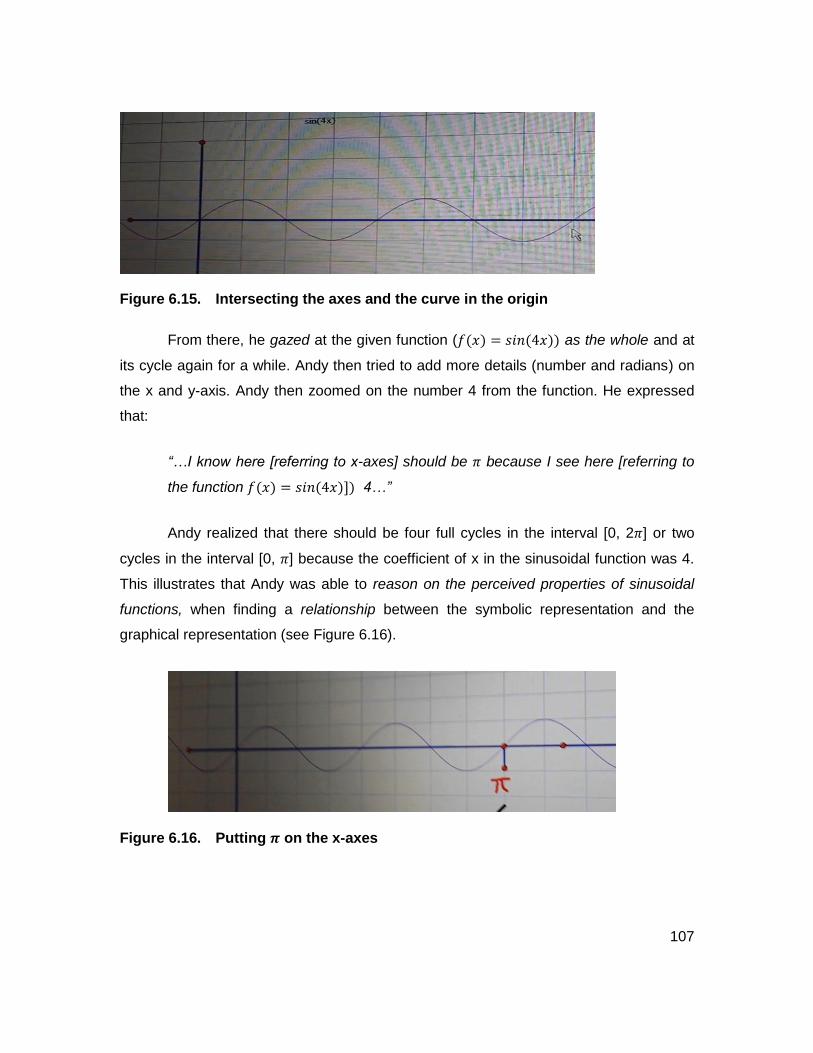
107
Figure 6.15. Intersecting the axes and the curve in the origin
From there, he gazed at the given function (𝑓(𝑥) = 𝑠𝑖𝑛(4𝑥)) as the whole and at
its cycle again for a while. Andy then tried to add more details (number and radians) on
the x and y-axis. Andy then zoomed on the number 4 from the function. He expressed
that:
“…I know here [referring to x-axes] should be 𝜋 because I see here [referring to
the function 𝑓(𝑥) = 𝑠𝑖𝑛(4𝑥)]) 4…”
Andy realized that there should be four full cycles in the interval [0, 2𝜋] or two
cycles in the interval [0, 𝜋] because the coefficient of x in the sinusoidal function was 4.
This illustrates that Andy was able to reason on the perceived properties of sinusoidal
functions, when finding a relationship between the symbolic representation and the
graphical representation (see Figure 6.16).
Figure 6.16. Putting 𝝅 on the x-axes
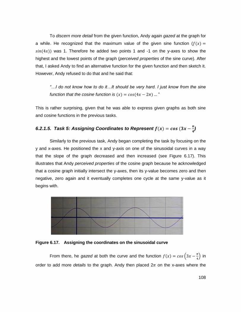
108
To discern more detail from the given function, Andy again gazed at the graph for
a while. He recognized that the maximum value of the given sine function (𝑓(𝑥) =
𝑠𝑖𝑛(4𝑥)) was 1. Therefore he added two points 1 and -1 on the y-axes to show the
highest and the lowest points of the graph (perceived properties of the sine curve). After
that, I asked Andy to find an alternative function for the given function and then sketch it.
However, Andy refused to do that and he said that:
“…I do not know how to do it…It should be very hard. I just know from the sine
function that the cosine function is (𝑥) = 𝑐𝑜𝑠(4𝑥 − 2𝜋) … ”
This is rather surprising, given that he was able to express given graphs as both sine
and cosine functions in the previous tasks.
6.2.1.5. Task 5: Assigning Coordinates to Represent 𝒇(𝒙) = 𝒄𝒐𝒔 (𝟑𝒙 −𝝅
𝟒)
Similarly to the previous task, Andy began completing the task by focusing on the
y and x-axes. He positioned the x and y-axis on one of the sinusoidal curves in a way
that the slope of the graph decreased and then increased (see Figure 6.17). This
illustrates that Andy perceived properties of the cosine graph because he acknowledged
that a cosine graph initially intersect the y-axes, then its y-value becomes zero and then
negative, zero again and it eventually completes one cycle at the same y-value as it
begins with.
Figure 6.17. Assigning the coordinates on the sinusoidal curve
From there, he gazed at both the curve and the function 𝑓(𝑥) = 𝑐𝑜𝑠 (3𝑥 −𝜋
4) in
order to add more details to the graph. Andy then placed 2𝜋 on the x-axes where the
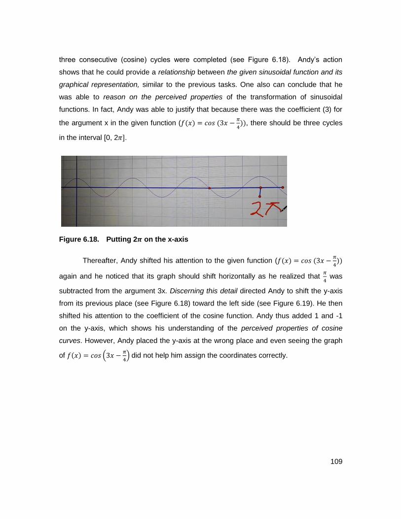
109
three consecutive (cosine) cycles were completed (see Figure 6.18). Andy’s action
shows that he could provide a relationship between the given sinusoidal function and its
graphical representation, similar to the previous tasks. One also can conclude that he
was able to reason on the perceived properties of the transformation of sinusoidal
functions. In fact, Andy was able to justify that because there was the coefficient (3) for
the argument x in the given function (𝑓(𝑥) = 𝑐𝑜𝑠 (3𝑥 −𝜋
4)), there should be three cycles
in the interval [0, 2𝜋].
Figure 6.18. Putting 2𝝅 on the x-axis
Thereafter, Andy shifted his attention to the given function (𝑓(𝑥) = 𝑐𝑜𝑠 (3𝑥 −𝜋
4))
again and he noticed that its graph should shift horizontally as he realized that 𝜋
4 was
subtracted from the argument 3x. Discerning this detail directed Andy to shift the y-axis
from its previous place (see Figure 6.18) toward the left side (see Figure 6.19). He then
shifted his attention to the coefficient of the cosine function. Andy thus added 1 and -1
on the y-axis, which shows his understanding of the perceived properties of cosine
curves. However, Andy placed the y-axis at the wrong place and even seeing the graph
of 𝑓(𝑥) = 𝑐𝑜𝑠 (3𝑥 −𝜋
4) did not help him assign the coordinates correctly.

110
Figure 6.19. Shifting the sinusoidal curve to the left
6.2.2. Visual Imagery
6.2.2.1. Task 1: Identifying the Function of 𝒇(𝒙) = 𝒔𝒊𝒏(𝟐𝒙) from the Given Graph
In finding the sinusoidal function described by the given graph (Task 1,𝑓(𝑥) =
𝑠𝑖𝑛(2𝑥)), Andy repeatedly stated that because the shape of the graph is oscillating or it
is “like a wave”, it should be a sine function. One could conclude that Andy had a
pictorial image of sinusoidal curves in his mind. Then, Andy described that there should
be two completed sinusoidal curves within the interval [0, 2𝜋], when he used his right
index finger to show the full cycles (see Figure 6.20). He again used his index finger and
pointed to the point 𝜋 on the x-axis to show the period of the first cycle. He repeated the
same action again for the second sinusoidal curve. He moved his hand very quickly to
represent the fact that the given curve is more squeezed compared with the canonic sine
curve. Andy’s gesture indicates visual kinesthetic communication when working on the
given sinusoidal functions. Eventually he stated that the graph belongs to the function of
𝑓(𝑥) = 𝑠𝑖𝑛(2𝑥) because “there are two waves squeezed between 0 and 2𝜋.” This
indicated that Andy considered a certain pattern (two full cycles) repeated within the
interval [0, 2𝜋], so therefore he had the pattern imagery of periodicity in sine functions.

111
Figure 6.20. Andy’s right index to represent two cycles
To determine a cosine function for the given graph, Andy pointed to a point in the
graph (using his right index) to show that the graph should be translated by 𝜋
2 and then
he wrote 𝑓(𝑥) = 𝑐𝑜𝑠(2𝑥 −𝜋
2) (see Figure 6.21). As Figure 6.21 shows, Andy actually
pointed to 𝜋
4, however, he referred to it as
𝜋
2, maybe because he had a pictorial imagery
of canonical function in his mind (in a canonical cosine function, y=1 for x=𝜋
2). He then
moved his right hand across the x-axes to show the horizontal shift of the curve to the
right (see Figure 6.22), while he expressed that “a cosine graph is a sine graph
translated to the right by a factor of 𝜋
2. "
Figure 6.21. Pointing to a point on the graph

112
Figure 6.22. Andy moved his hand across the x-axes
One can conclude that Andy had a kinesthetic imagery of the horizontal
transformation of a sinusoidal curve since he used his right index finger and his right
hand to show his understanding of the content. Also Andy’s response indicates that he
had memory image of formula of sinusoidal function because he acknowledged that we
can obtain the sine curve from the cosine curve by shifting it 𝜋
2 units to the
right. However, when I asked him to show me this relationship in the given graph (see
Figure 6.21), he changed the function from 𝑓(𝑥) = 𝑐𝑜𝑠 (2𝑥 −𝜋
2) into 𝑓(𝑥) = 𝑐𝑜𝑠 (2𝑥 +
𝜋
4)
because he noticed the point y=1 and x=𝜋
4. After realizing his initial mistake in
determining the cosine function (by comparing the graph of 𝑓(𝑥) = 𝑐𝑜𝑠 (2𝑥 +𝜋
4) and
𝑓(𝑥) = 𝑠𝑖𝑛(2𝑥)), Andy indicated that he did not consider the effect of periodicity (B in
canonical representation) on phase shift (or C) . In the other words, Andy noticed that he
displaced the bracket in his suggested formula. This illustrates again that Andy had a
memory image of the formula of the transformation of a sinusoidal function since 𝑓(𝑥) =
𝑐𝑜𝑠 (2𝑥 −𝜋
2) equals 𝑓(𝑥) = 𝑐𝑜𝑠 (2 (𝑥 −
𝜋
4)).
6.2.2.2. Task 2: Identifying the Function of 𝒇(𝒙) = 𝒔𝒊𝒏(𝟐
𝟑𝒙) from the Given
Graph
To complete Task 2 (similar to Task 1), Andy used the word oscillation
repeatedly as he expressed:

113
“Again it is a basic oscillating function has an oscillation and its oscillation starts
from 0.”
At the same time, Andy moved his two fingers like a wave across (see Figure
6.23) the given curve to demonstrate that the given curve represents an oscillating
function beginning at (0,0).
Figure 6.23. Showing the oscillating function
Andy stated that the coefficient of the argument x represents how much the
graph was squeezed or extended by a factor. To exemplify a compressed graph having
a whole number for the coefficient of x, he used both his hands and he put them parallel
to each other (see Figure 6.24). His hands were like two closed parentheses.
Figure 6.24. Student positioned his hands parallel to each other

114
However he expressed that since the given graph completed between 0 and 3𝜋,
it means that the canonical sinusoidal curve was stretched and the coefficient of x is a
fraction. Andy used both his hand to show the extended graph, but this time he opened
his hand like an open parentheses (see Figure 6.25). This indicates that Andy identified
the symbolic representation of sinusoidal functions, when focusing on the graphical
representations of the related sine functions. As with the previous task, Andy’s
kinesthetic imagery led him to conclude that the sinusoidal function had a fractional
argument of x because the length of a full sine cycle in the given graph is bigger than the
length of full cycle in the graph of canonical function. He concluded that because the
graph was stretched, the coefficient of x should be a fractional number (smaller than 1).
Figure 6.25. Student positioned his hands in the open parentheses position
Andy, then, expressed that in order to find periodicity (B in canonical
representation); he first needed to find a point by which the sinusoidal curve had a
completed cycle (3𝜋). He stated
“…usually the graph complete one cycle at 2 𝜋 but here the graph finished a full
cycle at 3 𝜋 so this point is 3𝜋 …”.
He used his right index finger to show me the point 3𝜋 (see Figure 6.26).

115
Figure 6.26. Showing the end point of one cycle of the sine curve
Then Andy moved his right hand from left to right across the x-axes and added
that,
“…then we see that the graph is longer than the original sine graph by factor of
3 𝜋
2.” … so there is a coefficient before x in the function. This means that the
coefficient of x is 2
3. So the function is 𝑓(𝑥) = 𝑠𝑖𝑛(
2
3𝑥)”
Andy’s hand movements and his statement are evidence that not only was he
able to communicate kinaesthetically about the sine function, he had the memory image
of the formula of the transformation as he said “the coefficient of x is 2
3… So the function
is 𝑓(𝑥) = 𝑠𝑖𝑛(2
3𝑥)”, although he did not explicitly talk about the periodicity formula:
𝑃𝑒𝑟𝑖𝑜𝑑 =2𝜋
𝐵. In other words, he knew that when the sinusoidal graph stretches
horizontally, the arguments of the function change respectively.
To find an alternative function for the given graph, he expressed that
"…to have a cosine function we know that the graph should begin from y=1 at
here…"
In his mind, he moved the y-axes to the right side of the graph. This phase illustrates
that Andy had dynamic imagery when solving the question. One also can state that he
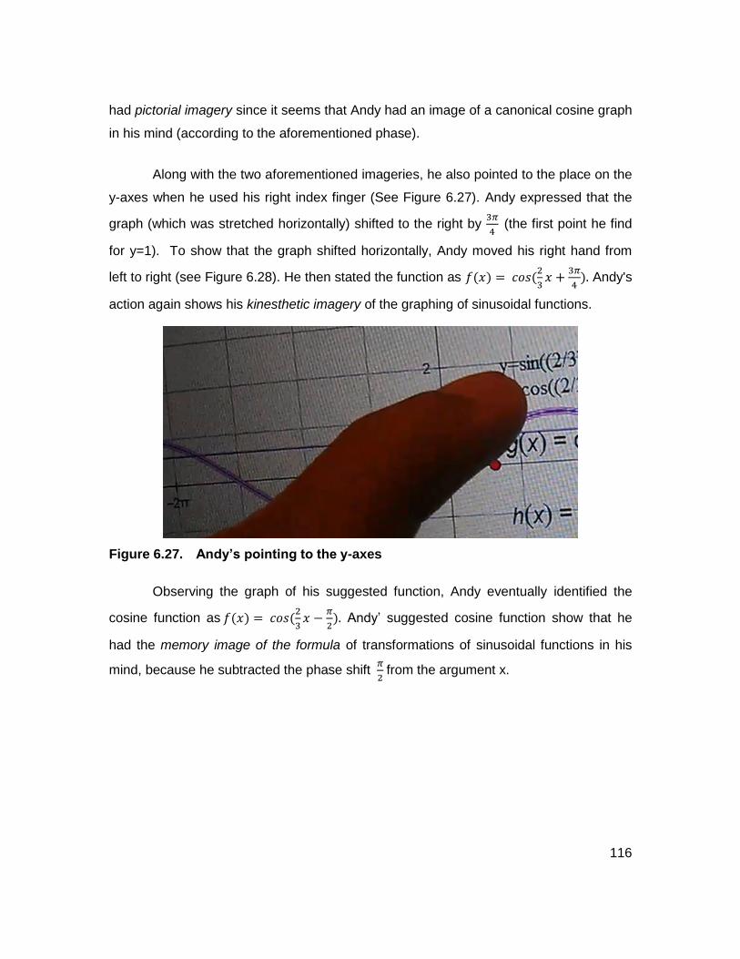
116
had pictorial imagery since it seems that Andy had an image of a canonical cosine graph
in his mind (according to the aforementioned phase).
Along with the two aforementioned imageries, he also pointed to the place on the
y-axes when he used his right index finger (See Figure 6.27). Andy expressed that the
graph (which was stretched horizontally) shifted to the right by 3𝜋
4 (the first point he find
for y=1). To show that the graph shifted horizontally, Andy moved his right hand from
left to right (see Figure 6.28). He then stated the function as 𝑓(𝑥) = 𝑐𝑜𝑠(2
3𝑥 +
3𝜋
4). Andy's
action again shows his kinesthetic imagery of the graphing of sinusoidal functions.
Figure 6.27. Andy’s pointing to the y-axes
Observing the graph of his suggested function, Andy eventually identified the
cosine function as 𝑓(𝑥) = 𝑐𝑜𝑠(2
3𝑥 −
𝜋
2). Andy’ suggested cosine function show that he
had the memory image of the formula of transformations of sinusoidal functions in his
mind, because he subtracted the phase shift 𝜋
2 from the argument x.

117
Figure 6.28. Andy moved his hand from left to right
To sum up, it seems that Andy had a pictorial imagery of the original sinusoidal
curves and he was able to imagine how to displace the y-axis from a given graph to
have a cosine function (dynamic imagery). His answer to this question also indicates that
he had memory image of the formula of a sinusoidal function because when the graph
stretched or squeezed. Andy used the incorrect phase shift without considering the
multiplication of the coefficient of x on the shift. He knew that periodicity would change
and he therefore had to change the coefficient of the argument in the function. He also
knew that if the graph shifted horizontally by a value, it should be added/subtracted to
the coefficient of x (although his suggested function often had the wrong sign). In most of
his answers, he often used his right index or his right hand and this shows that he was
able to communicate kinetically when discussing the tasks.
6.2.2.3. Task 3: Identifying the Function of 𝒇(𝒙) = 𝒄𝒐𝒔(𝟐
𝟓𝒙 −
𝝅
𝟓) from the
Given Graph
Similar to the other 2 previous tasks, Andy used his hands several times when he
was completing Task 3. When discussing the period of the sine cycle (B), for instance,
he used his right index finger to show the x-value (− 3π
4) by which a sinusoidal function
intersected the x-axes (see the yellow arrow in Figure 6.29). He considered the point
(− 3π
4, 0) as the starting point of a full sine cycle. Andy applied the same gesture to show
where the particular full sine curve ended. Furthermore, Andy moved his both indexes
fingers (see Figure 6.30) to show the length of half of cycle.

118
Figure 6.29. Andy was pointing to the point − 𝟑𝛑
𝟒
Figure 6.30. Andy was showing the half of period
To show that the graph did not intersect the y-axis at 1, and that as a result it
shifted horizontally, he again used his right index finger (see Figure 6.31).
Figure 6.31. Andy showing the intersection between y-axes and the curve

119
All the above-mentioned instances witnessed Andy’s kinesthetic imagery of
sinusoidal function. Moreover, the last incident (see Figure 6.31) illustrates that Andy
had the formula image of sinusoidal function. Andy identified that the curve (see Figure
6.6) did not interconnect to the y-axes at one. Therefore, a phase shift (C) needed to
subtract from the argument of x in the cosine function (𝑓(𝑥) = 𝑐𝑜𝑠 (2
5𝑥 − (
π
6)) . However,
as data show, the memory image of formula transformations of sinusoidal function, did
not eventually support Andy to suggest a proper function for the given graph. He was
also unsuccessful in suggesting a proper alternative sine function for the given task due
to his limited image of formula transformations of sinusoidal function.
6.2.2.4. Task 4: Assigning Coordinates to Represent 𝒇(𝒙) = 𝒔𝒊𝒏(𝟒𝒙)
For Task 4, Andy expressed that:
“…since there is 4 here is a factor of x, there should be 1, 2, 3 and 4 full sine
curves between 0 and 2 𝜋,”
Andy used his right index to count the number of cycles in the interval (see
Figure 6.32, kinesthetic imagery). This statement indicates that Andy realized that there
was a certain pattern to the repeated cycles. In fact he noticed that a sine curve should
be repeated 4 times in a certain interval. According to Prmesg (1986), Andy had the
pattern imagery of a sinusoidal function. He also situated the two numbers 1 and -1 on
the y-axes and he expressed that:
“as the amplitude or the coefficient of 𝑠𝑖𝑛(4𝑥) is 1, we should put 1 and -1
here…”
He again used his right index finger to pointe to the numbers 1 and -1, while he
emphasized that:
“…yes, we need to show these two numbers [1,-1] here.” (see Figure 6.33)

120
Andy’s response to this task indicated that he had also a memory image of
formula of transformation of sinusoidal function since he knew that the coefficient of x (B
in the canonical representation) represents the number of sine curves appearing
between 0 and 2𝜋. Andy also knew that the coefficient of 𝑠𝑖𝑛(4𝑥) (or “A” according to
Canonical representation) represents the amplitude or the maximum and minimum
values for the y-axis. Although Andy’s actions and his words in the previous tasks
represent his memory image of the formula of a sinusoidal function, he never referred to
the amplitude of the sinusoidal functions in the first two tasks. It was in Task 3 when
Andy discussed the coefficient of the sine function (“as the amplitude or the coefficient of
𝑠𝑖𝑛(4𝑥) is 1”).
Figure 6.32. Student counted four full cycles
Figure 6.33. Student pointed to the number 1 and -1
121
He then changed 𝑓(𝑥) = 𝑠𝑖𝑛(4𝑥) into 𝑓(𝑥) = 𝑐𝑜𝑠(4𝑥 − 2𝜋 ). Since in Task 1
(𝑓(𝑥) = 𝑠𝑖𝑛(4𝑥)) Andy subtracted 𝜋
2 from the cosine function but in Task 3 he
subtracted 2𝜋, I asked him for his reason for doing so. Andy expressed that
“…because of having the number four behind the argument x in the cosine
function, when we multiply four by 𝜋
2 , we have 2𝜋"
This indicates that Andy applied his memory image of formula of a sinusoidal
function he experienced in the previous tasks. As we saw in the previous tasks, Andy
often made errors and after visiting the graph of his suggested functions, he
remembered the learned formula interconnecting a sine function into a cosine function.
Or one can also conclude that Andy remembered the canonical representation in which
B (period) influences directly C (or phase shift).
6.2.2.5. Task 5: Assigning Coordinates to Represent 𝒇(𝒙) = 𝒄𝒐𝒔 (𝟑𝒙 − 𝝅
𝟒)
In contrast with other tasks in which Andy used his hand and fingers in different
situations, he did not use his body while he described his thoughts on the last task.
However, similarly to the previous tasks, he showed his pictorial imagery of the cosine
function coordinating when he positioned the y and x-axes on the given graph. This
indicates that Andy was aware of the general shape of cosine function. Andy also
focused on his memory image of the formula of a sinusoidal function. He recognized that
there was a coefficient bigger than 1 for the x (or B> 1) in the given function. From there,
he interpreted that the graph should be squeezed between the points 0 and 2 𝜋. By
getting help of his formula image, Andy, also, found that “A” or the coefficient of
𝑐𝑜𝑠(3𝑥 −𝜋
4) was one. As such, he acknowledged that the maximum and the minimum
values the function reached should be +1 and -1. In other words, since “nothing was
multiplied to the 𝑐𝑜𝑠(3𝑥 −𝜋
4)” – referring to the ‘A’ value of 1 – it means that the graph
should not stretch or squeeze vertically. It was in Task 4 and 5 that Andy discussed the
vertical shift. In the previous tasks, he often focused his attention to the horizontal shift
and periodicity. The formula image also guided Andy to conclude (incorrectly) that the

122
graph should shift horizontally because 𝜋
4 was subtracted from the argument 3x in the
given function. However, as we saw in the sections 6.1 and 6.2 Andy was unable in
recognizing correctly phase shift (C) according to canonical formula (while C was 𝜋
12 he
talked about 𝜋
4 as a phase shift). Furthermore, Andy expressed that the graph should
have 3 cycles in the certain interval [0, 2𝜋] (similar to the previous tasks) as he counted
“one, two, three sine cycles.” This shows that Andy had pattern imagery of sinusoidal
functions.
6.2.3. Covariational Reasoning
In this section I analyze and interpret Andy’s responses to the interview tasks
according to Covariational reasoning framework created by Carlson et al. (2002). As it
was described in the section 5.3, Carlson et al’s., framework comprised of five distinct
developmental levels of covariational reasoning (L#) that parallel the five mental actions
(M#).
As we saw in the previous analysis (in section 6.2), Andy recognized that there
was a close relationship between the coefficient of the argument in the sine function
(e.g., 𝑓(𝑥) = 𝑠𝑖𝑛(2𝑥)) and the number of full cycles repeated in the interval [0, 2𝜋]
(M1: Coordinating the value of one variable with changes in the other). Andy stated that
his reason for focusing on this certain interval [0, 2𝜋] was the fact that a canonic sine
function began from 0 and completed at 2𝜋. In other words, a full cycle or periodicity
happens between 0 and 2𝜋. While completing Task 1, therefore, Andy interpreted that
having more than one cycle, between 0 and 𝜋 (one cycle) and from 𝜋 to 2 𝜋 (another
cycle), in this interval means having a coefficient of x bigger than one in the sinusoidal
function. Increasing the number of full sine cycles in the interval [0, 2𝜋], in fact,
coordinate increasing the coefficient of the argument x in the sinusoidal functions
(M2: Coordinating the direction of change of one variable with changes in the other
variable). As such, he expressed that the function representing the graph should be
𝑓(𝑥) = 𝑠𝑖𝑛 (2𝑥). There is, in fact, a relationship between the number of full equal cycles
between 0 and 2 𝜋 and finding the periodicity of a sine function. Thus, if there were two
123
cycles in the given curve (for Task 1, graph of 𝑓(𝑥) = 𝑠𝑖𝑛(2𝑥)), the number presented
the periodicity (or B) in the sine function was the number 2 (M3: Coordinating the
amount of change of one variable with changes in the other variable). The behavior
exhibited by this student when responding to this task suggested that Andy was at
quantitative coordination level (L3: At the quantitative coordination level, the images of
covariation can support the mental actions of coordinating the amount of change in one
variable with changes in the other variable. The mental actions MA1, MA2 and MA3 are
supported by Level 3 image). Andy’s responses to this task, in fact, supported all three
mental actions M1, M2 and M3.
For Task 2 (𝑓(𝑥) = 𝑠𝑖𝑛 (2
3𝑥)) Andy again verbalized that the graph of sine
function and as a result the number of sine cycles in and beyond the interval [0, 2 𝜋]
changes with change in period (compared with the canonical functions) (M1). He stated
that the smaller the coefficient of x than 1 required a larger cycle compared with the
canonic sine curve (M2). As we saw in the previous sections (sections 6.1.2 and 6.2.2),
Andy was able to recognize the amount of the periodicity or the coefficient of x and
therefore the proper sine function in the task (M3). Similar to the task 1, his response
showed that Andy had the quantitative coordination level (L3) of ability of covariational
reasoning of sinusoidal functions.
Andy showed exactly the same level of covariational reasoning ability and mental
action (in identifying periodicity) in Task 3 (𝑓(𝑥) = 𝑐𝑜𝑠(2
5𝑥 −
π
5)), which was different from
the other two tasks because a phase shift was added to the argument of this cosine
function. Andy acknowledged that there is a connection between the coefficient of x (2
5)
and the number cycles repeated in its relevance graph (M1). In addition, Andy
recognized that as the coefficient of x in the cosine function decreasing
(2
5 <1), the length of full sine cycle is extending (compared with the length of a canonical
cosine function) (M2). Similar to the first two tasks, he was able to determine the amount
of periodicity (M3). The Andy’s behavior directed me to conclude that he had the
quantitative coordination level (L3) of covariational reasoning with respect to period,

124
because all his three mental actions M1, M2 and M3 supported him to coordinate the
amount of change of period with the number of repeated sine cycles in interval [0, 2π].
Andy also repeated the same mental action (M1, M2 and M3) (as the previous
tasks) for Task 4 (𝑓(𝑥) = 𝑠𝑖𝑛 (4𝑥)) and Task 5 (𝑓(𝑥) = 𝑐𝑜𝑠 (3𝑥 −𝜋
4)) in determining
periodicity. For instance, Andy indicated that since in each of the sinusoidal functions the
coefficient of x was more than one (e.g. the factor of x was 4 in the Task 4), we have
more than one sine cycle in the interval [0, 2 𝜋]. In other words, he realized that the
bigger the coefficient of x, the more cycles in the interval [0 and 2 𝜋] (M2) (this is in
contrast, for Task 2 (𝑓(𝑥) = 𝑠𝑖𝑛 (2
3𝑥))and Task 3 (𝑓(𝑥) = 𝑐𝑜𝑠(
2
5𝑥 −
π
5)) the smaller the
coefficient of x than one required a larger cycle compared with the canonic sine curve
(M2)). As we saw in the previous sections (e.g., 6.1.4), Andy recognized the amount of
the periodicity of the coefficient of x and therefore the corresponding sine functions or
their related graph in Tasks 4 and 5 (M3). As such, Andy had the quantitative
coordination level (L3) of ability of covariational reasoning of sinusoidal functions, when
identifying periodicity in Tasks 4 and 5.
Andy was not successful in identifying the phase shift in Tasks 3 and 5. When
completing Task 3, Andy acknowledged that since the graph’s intersection point
changed from (𝜋
2 ,1) (the point from the canonical cosine graph) to another point, the
whole argument of the function and as a result the cosine function should change (M1).
He also admitted that a certain radian subtracted from the whole argument, because the
graph shifted to the right (M2). However, Andy determined unsuccessfully the amount of
phase shift. He identifies 𝜋
6 for a phase shift, instead of
𝜋
2. Therefore, Andy’s ability for
covariational reasoning was direction level (L2) with respect to phase shift. To deal with
phase shift in Task 5, Andy realized (similar to Task 3) that since a certain radian was
subtracted from the argument of x, the graph should be shifted accordingly (M2).
However, Andy was unable to determine the amount of phase shift and to express the
influence of the amount of periodicity on the phase shift and on the graph. In other
words, while the phase shift was 𝜋
12 (𝑓(𝑥) = 𝑐𝑜𝑠(3𝑥 −
𝜋
4) = 𝑐𝑜𝑠(3(𝑥 −
𝜋
12)), he
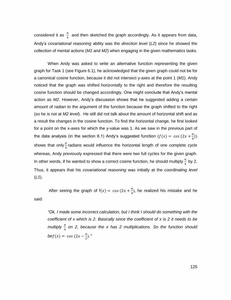
125
considered it as 𝜋
4 and then sketched the graph accordingly. As it appears from data,
Andy’s covariational reasoning ability was the direction level (L2) since he showed the
collection of mental actions (M1 and M2) when engaging in the given mathematics tasks.
When Andy was asked to write an alternative function representing the given
graph for Task 1 (see Figure 6.1), he acknowledged that the given graph could not be for
a canonical cosine function, because it did not intersect y-axes at the point 1 (M1). Andy
noticed that the graph was shifted horizontally to the right and therefore the resulting
cosine function should be changed accordingly. One might conclude that Andy’s mental
action as M2. However, Andy’s discussion shows that he suggested adding a certain
amount of radian to the argument of the function because the graph shifted to the right
(so he is not at M2 level). He still did not talk about the amount of horizontal shift and as
a result the changes in the cosine function. To find the horizontal change, he first looked
for a point on the x-axes for which the y-value was 1. As we saw in the previous part of
the data analysis (in the section 6.1) Andy’s suggested function (𝑓(𝑥) = 𝑐𝑜𝑠 (2𝑥 +𝜋
4))
shows that only 𝜋
4 radians would influence the horizontal length of one complete cycle
whereas, Andy previously expressed that there were two full cycles for the given graph.
In other words, if he wanted to show a correct cosine function, he should multiply 𝜋
4 by 2.
Thus, it appears that his covariational reasoning was initially at the coordinating level
(L1).
After seeing the graph of f(𝑥) = 𝑐𝑜𝑠 (2𝑥 +𝜋
4), he realized his mistake and he
said:
“Ok, I made some incorrect calculation, but I think I should do something with the
coefficient of x which is 2. Basically since the coefficient of x is 2 it needs to be
multiply 𝜋
4 on 2, because the x has 2 multiplications. So the function should
be𝑓(𝑥) = 𝑐𝑜𝑠 (2𝑥 −𝜋
2).”

126
The feedback Andy received from the graph of his suggested function led him to
realize that the periodicity should directly affect the whole part, x and the amount of shift,
if he wanted to have a proper sinusoidal function. Andy was able to realize the amount of
the phase shift and its effect on the cosine function (M3). He also noticed that since the
graph shifted to the right, the amount of phase shift should be subtracted from the
argument 2x (M2). Observing the graph of the proposed function (the incorrect functions)
supported Andy to transit the level of his covariational reasoning from coordinating level
(L1) to quantitative coordination (L3). In the other words, the collection of mental actions
(M1, M2 and M3) helped Andy to coordinate successfully the change of the argument
with the amount of change in the phase shift and then, obtaining the correct sinusoidal
function.
To identify an alternative function for the given graph, Andy primarily was not
able to recognize the horizontal shift in the Task 2 and he made the same error as he did
(initially) in Task 1 (𝑓(𝑥) = 𝑐𝑜𝑠(2
3𝑥 +
3𝜋
4)). Getting feedback from the graph of his
suggested function led him to find the correct horizontal shift and as a result, the
corresponding cosine function representing the given graph (𝑓(𝑥) = 𝑐𝑜𝑠(2
3𝑥 −
𝜋
2))(M3).
The data illustrate that similar to Task 1, Andy had a transition from L2 level to L3 level
in recognizing phase shift from the given graph in Task 2. However, Andy’s covariational
reasoning moved back from L3 level in Tasks 1 and 2 to L1 level for the rest of interview
tasks, when he determined the alternative functions for the given graphs/functions.
6.3. Summary
In this chapter, I included a detailed analysis of one of the participants, Andy’s
completion of the interview tasks. At the beginning of this chapter, I described a brief
overview of Andy’s answers to each of the interview tasks. I then analyzed the way he
completed the tasks with respect to the three theoretical frameworks applied in this
study.
127
The data analysis shows that Andy successfully completed the Tasks 1, 4 and 5
in which the coefficient of the arguments x were whole numbers. He was also able to
complete the tasks (Tasks 2 and 3) involving the fraction arguments for x. In fact, Andy
determined the periodicity in the transformed functions/graphs in all interview tasks
through applying visual imagery such as concert, pattern, kinesthetic and dynamic
imagery, along with focusing on the details discerned from the given functions/graphs,
perceiving properties of sinusoidal functions and connecting the analytic representations
with the graphical representations.
The data illustrate that Andy’s covariational reasoning ability in determining
periodicity was the quantitative coordination level (L3), it was at the direction level (L2)
for identifying phase shift. Andy was unable to determine the phase shift in the Tasks 3
and 5 (L2), even after applying all previous methods (e.g., concrete imagery and finding
relationship between symbolic and graphical representations) he used to identify
periodicity. Although after several attempts, he could find the alternative function for the
Tasks 1 and 2 (L3), he was unsuccessful in Tasks 3, 4 and 5 (L1).

128
Chapter 7. Data Analysis: The case of the “Other Five Students”
In this chapter I focus on the additional five participants and their responses to
the five interview tasks. The data are analyzed in terms of the following three theoretical
perspectives: 1) shift of attention, 2) visual imagery and 3) convariation reasoning. The
students’ responses to each interview task are also compared with those of Andy
(Andy’s responses to the interview tasks are discussed in Chapter 6). Table 7.1
describes the participants’ success or failure in completing the interview tasks.
Two main themes have emerged in the data analysis: “identifying the period (B)”
and “identifying the phase shift (C)” (𝑓(𝑥) = 𝐴 𝑠𝑖𝑛/𝑐𝑜𝑠((𝐵(𝑥 + 𝐶) + 𝐷)). The students’
difficulties and their approaches to the tasks are explained in detail according to these
themes.
Table 7.1 summarizes the students’ responses to the 5 interview tasks. The list
of tasks is found in Chapter 4. Note that some tasks have several parts, and participants
performed differently on different part of the tasks. To indicate this, the following codes
are used in Table 7.1:
B Changing a sinusoidal function into a cosine function and vice versa
P Identifying the period
S Identifying the phase shift
When students completed the task correctly
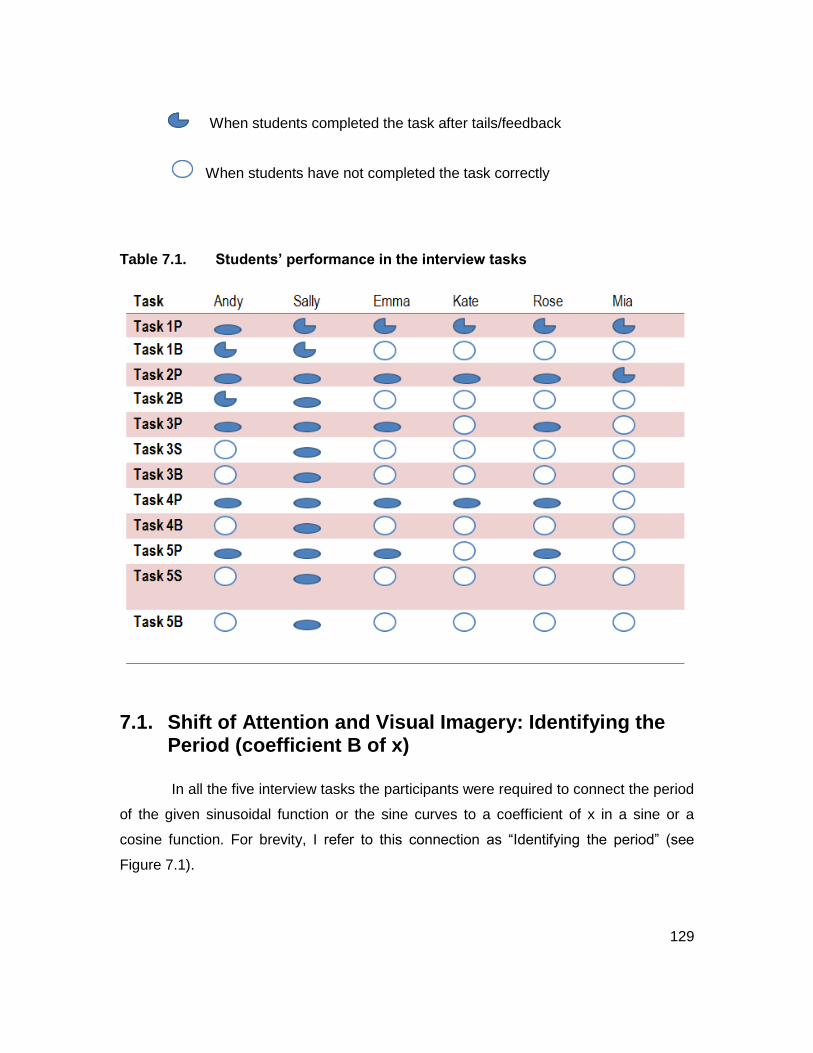
129
When students completed the task after tails/feedback
When students have not completed the task correctly
Table 7.1. Students’ performance in the interview tasks
7.1. Shift of Attention and Visual Imagery: Identifying the Period (coefficient B of x)
In all the five interview tasks the participants were required to connect the period
of the given sinusoidal function or the sine curves to a coefficient of x in a sine or a
cosine function. For brevity, I refer to this connection as “Identifying the period” (see
Figure 7.1).

130
Figure 7.1. Period of a canonical function
7.1.1. Identifying Period in Task 1
7.1.1.1. Initial Confusion
Among all six students who were interviewed in this study, almost everybody
(except Andy) identified the period (B) unsuccessfully at the first attempt. While Andy in
Task 1 realized that the given curve represented the function 𝑓(𝑥) = 𝑠𝑖𝑛(2𝑥), Rose, for
example, stated:
“It is 𝑓(𝑥) = 𝑠𝑖𝑛(1
2𝑥). It is sine graph because it starts at 0 and it should be
𝑠𝑖𝑛(1
2𝑥). The sine graph start at 0 and then π and 2𝜋 but this one is o, ,
2𝜋
3. This is
half of sine graph. Because the period here is 𝜋 while it is 2𝜋 in the original sine
curve.”
Kate and Emma initially made similar errors. The above statement indicates that
these three participants recognized incorrectly the function for the given graph,
determining it to be 𝑓(𝑥) = 𝑠𝑖𝑛(1
2𝑥). Analyzing the situation using Mason’s (2008))
framework it can be concluded that Rose, Kate and Emma reasoned on the perceived
properties of the sinusoidal functions and from there they determined (incorrectly)
relationships between the visual representation and the symbolic representation. This is
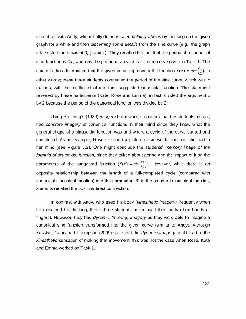
131
in contrast with Andy, who initially demonstrated holding wholes by focusing on the given
graph for a while and then discerning some details from the sine curve (e.g., the graph
intersected the x-axis at 0, 𝜋
2, and 𝜋). They recalled the fact that the period of a canonical
sine function is 2𝜋, whereas the period of a cycle is 𝜋 in the curve given in Task 1. The
students thus determined that the given curve represents the function 𝑓(𝑥) = 𝑠𝑖𝑛 (𝑥
2). In
other words; these three students connected the period of the sine curve, which was 𝜋
radians, with the coefficient of x in their suggested sinusoidal function. The statement
revealed by these participants (Kate, Rose and Emma), in fact, divided the argument x
by 2 because the period of the canonical function was divided by 2.
Using Presmeg’s (1989) imagery framework, it appears that the students, in fact,
had concrete imagery of canonical functions in their mind since they knew what the
general shape of a sinusoidal function was and where a cycle of the curve started and
completed. As an example, Rose sketched a picture of sinusoidal function she had in
her mind (see Figure 7.2). One might conclude the students’ memory image of the
formula of sinusoidal function, since they talked about period and the impact of it on the
parameters of the suggested function (𝑓(𝑥) = 𝑠𝑖𝑛 (𝑥
2)). However, while there is an
opposite relationship between the length of a full-completed cycle (compared with
canonical sinusoidal function) and the parameter “B” in the standard sinusoidal function,
students recalled the positive/direct connection.
In contrast with Andy, who used his body (kinesthetic imagery) frequently when
he explained his thinking, these three students never used their body (their hands or
fingers). However, they had dynamic (moving) imagery as they were able to imagine a
canonical sine function transformed into the given curve (similar to Andy). Although
Kosslyn, Ganis and Thompson (2009) state that the dynamic imagery could lead to the
kinesthetic sensation of making that movement, this was not the case when Rose, Kate
and Emma worked on Task 1.
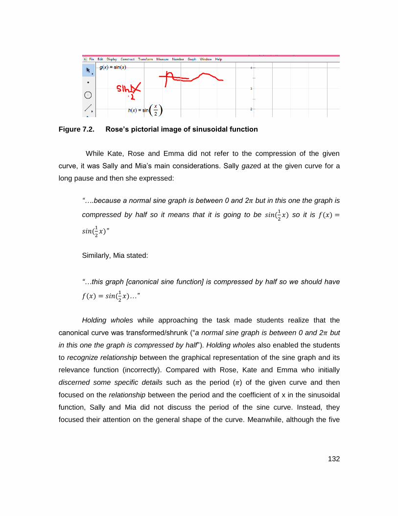
132
Figure 7.2. Rose’s pictorial image of sinusoidal function
While Kate, Rose and Emma did not refer to the compression of the given
curve, it was Sally and Mia’s main considerations. Sally gazed at the given curve for a
long pause and then she expressed:
“….because a normal sine graph is between 0 and 2𝜋 but in this one the graph is
compressed by half so it means that it is going to be 𝑠𝑖𝑛(1
2𝑥) so it is 𝑓(𝑥) =
𝑠𝑖𝑛(1
2𝑥)”
Similarly, Mia stated:
“…this graph [canonical sine function] is compressed by half so we should have
𝑓(𝑥) = 𝑠𝑖𝑛(1
2𝑥)…”
Holding wholes while approaching the task made students realize that the
canonical curve was transformed/shrunk (“a normal sine graph is between 0 and 2𝜋 but
in this one the graph is compressed by half”). Holding wholes also enabled the students
to recognize relationship between the graphical representation of the sine graph and its
relevance function (incorrectly). Compared with Rose, Kate and Emma who initially
discerned some specific details such as the period (𝜋) of the given curve and then
focused on the relationship between the period and the coefficient of x in the sinusoidal
function, Sally and Mia did not discuss the period of the sine curve. Instead, they
focused their attention on the general shape of the curve. Meanwhile, although the five

133
students looked at the given graph from different perspectives, they proposed the same
incorrect function (𝑓(𝑥) = 𝑠𝑖𝑛(1
2𝑥)).
Similar to the other participants, Sally and Mia had pictorial imagery since they
had concrete descriptions of canonical functions in their mind (…this graph [canonical
sine function] is compressed). When comparing the given curve with the graph of a
canonical function, the students had, in fact, dynamic imagery because they were able to
transform a canonical function into the given curve in their mind. This imagery led Sally
and Mia (similar to Andy) to use their body when completing Task 1. As an example,
Sally moved her two fingers (from her right hand) to illustrate the compression of the
given curve (see Figure 7.3). Sally’s action shows her kinesthetic imagery of sinusoidal
functions. Mia used exactly the same gesture.
Figure 7.3. Sally’s usage of her two fingers to show that the curve was shrunk
As it appears from the students’ discussions that while 𝑥
2 and
1
2 𝑥 are the same,
they often tended to express their suggested function for Task 1 as sine of 1
2 𝑥. This
shows that the students attempted to establish the relationship between the period and
the coefficient of x in the sinusoidal function. Since the period of the given curve (π) was
half of the period of a canonical sine function (2π), the coefficient of x should be 1
2. In

134
other words, the participants’ language was often in direct correspondence with the
resulting algebraic expression.
The phenomenon is also reminiscent of “same A – same B” intuitive rule, as
described by Stavy and Tirosh (2000). For example, “Same area – same perimeter” is a
frequent confusion of learners explained by this intuitive rule. In the case of Task 1,
“same A – same B” was interpreted as “half of (canonical) cycle – half of argument”.
As evident from the data, the majority of students in this study had initial
confusion when completing Task 1; however, they successfully found the correct
function for the given curve after the graph of their suggested function was sketched. In
the following section, the participants’ approaches are described.
7.1.1.2. Importance of Computer Feedback
Observing the graph of the function 𝑓(𝑥) = 𝑠𝑖𝑛(1
2𝑥) made participants realize that
the graph of their suggested function did not correspond to the given curve. The
participants, then, used different methods to correct their initial suggestion. In the
following, the students’ responses are described. If a student’s solution was different
from others, it is described in a separate section; otherwise similar students’ responses
are explained in the same section.
Kate, after gazing at the screen for two minutes and holding both graphs as
whole, began to compare the two sinusoidal graphs respectively (see Figure 7.4)
through discerning detail from both curves. She stated that:
“….this one [#1] is half of 𝑓(𝑥) = 𝑠𝑖𝑛(𝑥) at 2𝜋, but this one [#2] has one, two
complete sine graphs between 0 and 2𝜋. So, my answer was wrong. It is
𝑓(𝑥) = 𝑠𝑖𝑛(2𝑥). "
As it appears from the above statement, and consistent with Mason (2008)
observation, identifying details from the curves directed Kate to recognize relationship
between the given curve (#2 in Figure 7.4) and its appropriate sinusoidal function

135
(𝑓(𝑥) = 𝑠𝑖𝑛(2𝑥)). The above quote from Kate also illustrates her pattern imagery of
sinusoidal function, since she was able to realize the repeated outline (“one, two
complete sine graphs between 0 and 2π”) embedded in the given curve (#2). Moreover,
Kate used concrete imagery because she had a visual image of a canonical function
when she explained her thinking (“this one [#1] is half of 𝑓(𝑥) = 𝑠𝑖𝑛(𝑥) at 2𝜋”).
Figure 7.4. Graph of 𝒇(𝒙) = 𝒔𝒊𝒏(𝟏
𝟐𝒙) and 𝒇(𝒙) = 𝒔𝒊𝒏(𝟐𝒙)
Similarly, getting feedback from the graph of her suggested function (see Figure
7.4) shifted Sally’s attention to the connection between the graph #2 (see Figure 7.4)
and its represented function as she expressed:
“….I made a little error when I was calculating my B value which is the
compression of the x-values, if it is compressed by a half…., so if it is
compressed by half it is 1 over half is 2[ it means 11
2
= 2]. I think the function
should be 𝑓(𝑥) = 𝑠𝑖𝑛(2𝑥).”
The above excerpt also indicates that Sally attempted to reason on the perceived
properties of the sinusoidal functions (“… if it is compressed by a half, so if it is
compressed by half it is 1 over half is…”). This justification led her to change her initial
suggestion successfully from 𝑓(𝑥) = 𝑠𝑖𝑛(1
2𝑥) into 𝑓(𝑥) = 𝑠𝑖𝑛(2𝑥). In other words, she

136
recognized the inverse relationship between the period of the given graph and the
coefficient of x in the sine function.
While describing her answer, Sally used the sketchpad’s pointer to refer to the
coefficient of x in the sinusoidal function 𝑓(𝑥) = 𝑠𝑖𝑛(1
2𝑥) (see Figure 7.5) and she stated:
“…we actually we should calculate by going 1 over B…”
The aforementioned statements indicate that Sally had the memory image of
formula of the canonical function because she acknowledged the coefficient of the
argument x as “B.” She, moreover, had concrete imagery of sinusoidal functions as she
expressed that the graph (the canonical function) was compressed (the canonical sine
curve shrunk into two full sine curves). One might also conclude that Sally had the
dynamic imagery since she was able to move the given curve in her mind to compare it
with the canonic curves.
Figure 7.5. Sally’s pointing to the B value in the suggested function
When she saw the graph of 𝑓(𝑥) = 𝑠𝑖𝑛(1
2𝑥), Emma, similar to Sally, attempted to
find connection between the period and the coefficient of x in the sinusoidal function as
she stated:
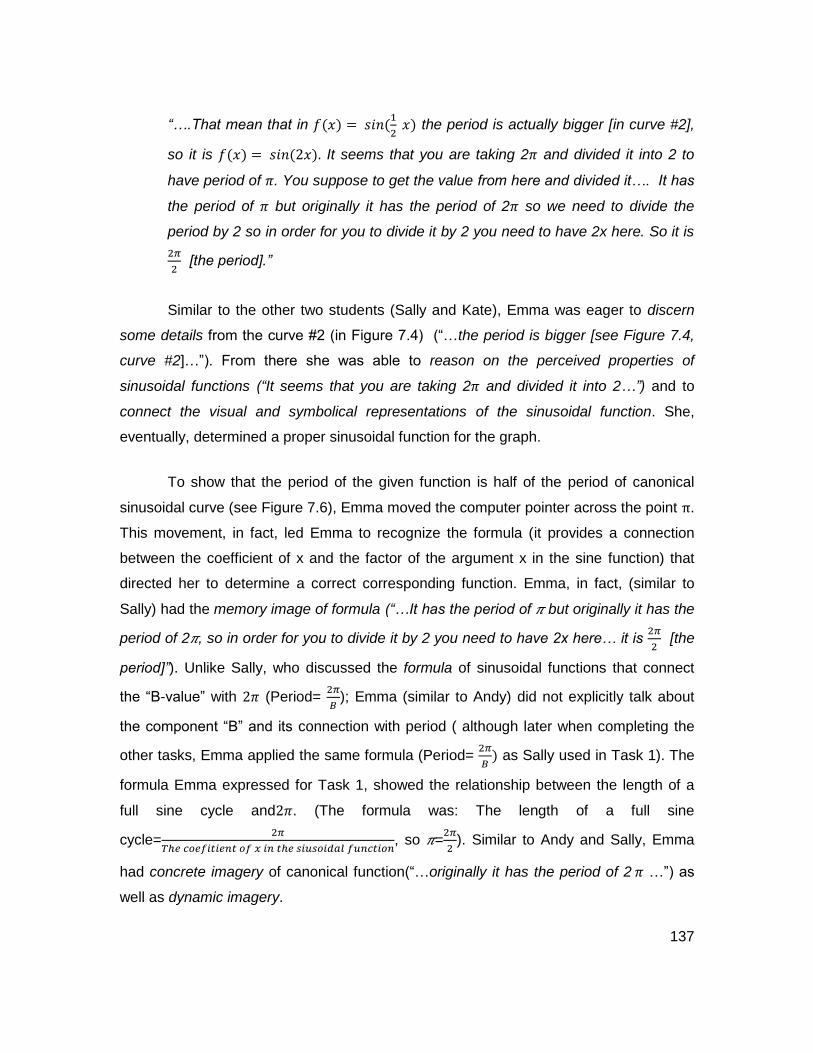
137
“….That mean that in 𝑓(𝑥) = 𝑠𝑖𝑛(1
2 𝑥) the period is actually bigger [in curve #2],
so it is 𝑓(𝑥) = 𝑠𝑖𝑛(2𝑥). It seems that you are taking 2𝜋 and divided it into 2 to
have period of 𝜋. You suppose to get the value from here and divided it…. It has
the period of 𝜋 but originally it has the period of 2𝜋 so we need to divide the
period by 2 so in order for you to divide it by 2 you need to have 2x here. So it is
2𝜋
2 [the period].”
Similar to the other two students (Sally and Kate), Emma was eager to discern
some details from the curve #2 (in Figure 7.4) (“…the period is bigger [see Figure 7.4,
curve #2]…”). From there she was able to reason on the perceived properties of
sinusoidal functions (“It seems that you are taking 2𝜋 and divided it into 2…”) and to
connect the visual and symbolical representations of the sinusoidal function. She,
eventually, determined a proper sinusoidal function for the graph.
To show that the period of the given function is half of the period of canonical
sinusoidal curve (see Figure 7.6), Emma moved the computer pointer across the point π.
This movement, in fact, led Emma to recognize the formula (it provides a connection
between the coefficient of x and the factor of the argument x in the sine function) that
directed her to determine a correct corresponding function. Emma, in fact, (similar to
Sally) had the memory image of formula (“…It has the period of 𝜋 but originally it has the
period of 2𝜋, so in order for you to divide it by 2 you need to have 2x here… it is 2𝜋
2 [the
period]”). Unlike Sally, who discussed the formula of sinusoidal functions that connect
the “B-value” with 2𝜋 (Period= 2𝜋
𝐵); Emma (similar to Andy) did not explicitly talk about
the component “B” and its connection with period ( although later when completing the
other tasks, Emma applied the same formula (Period= 2𝜋
𝐵) as Sally used in Task 1). The
formula Emma expressed for Task 1, showed the relationship between the length of a
full sine cycle and2𝜋. (The formula was: The length of a full sine
cycle=2𝜋
𝑇ℎ𝑒 𝑐𝑜𝑒𝑓𝑖𝑡𝑖𝑒𝑛𝑡 𝑜𝑓 𝑥 𝑖𝑛 𝑡ℎ𝑒 𝑠𝑖𝑢𝑠𝑜𝑖𝑑𝑎𝑙 𝑓𝑢𝑛𝑐𝑡𝑖𝑜𝑛, so 𝜋=
2𝜋
2). Similar to Andy and Sally, Emma
had concrete imagery of canonical function(“…originally it has the period of 2 𝜋 …”) as
well as dynamic imagery.
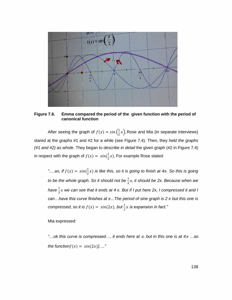
138
Figure 7.6. Emma compared the period of the given function with the period of canonical function
After seeing the graph of 𝑓(𝑥) = 𝑠𝑖𝑛 (1
2𝑥), Rose and Mia (in separate interviews)
stared at the graphs #1 and #2 for a while (see Figure 7.4). Then, they held the graphs
(#1 and #2) as whole. They began to describe in detail the given graph (#2 in Figure 7.4)
in respect with the graph of 𝑓(𝑥) = 𝑠𝑖𝑛(1
2𝑥). For example Rose stated:
“….so, if 𝑓(𝑥) = 𝑠𝑖𝑛(1
2𝑥) is like this, so it is going to finish at 4𝜋. So this is going
to be the whole graph. So it should not be 1
2𝑥, it should be 2x. Because when we
have 1
2𝑥 we can see that it ends at 4 𝜋. But if I put here 2x, I compressed it and I
can…have this curve finishes at 𝜋...The period of sine graph is 2 𝜋 but this one is
compressed, so it is 𝑓(𝑥) = 𝑠𝑖𝑛(2𝑥), but 1
2𝑥 is expansion in fact.”
Mia expressed:
“…ok this curve is compressed…, it ends here at 𝜋, but in this one is at 4𝜋 …so
the function𝑓(𝑥) = 𝑠𝑖𝑛(2𝑥)]….”
139
As mentioned previously, in order to describe that her suggested function
(𝑓(𝑥) = 𝑠𝑖𝑛(1
2𝑥)) was not a proper function for the represented curve (#1, see Figure
7.4), Emma was looking for the ended points of the full sine cycles in the given graph as
well as in the canonical sinusoidal graph. Meanwhile, Kate paid her attention to the
number of completed cycles in the graph, while Rose and Mia compared the end point
of a cycle curve #2 with that of curve #1, considering the origin as a beginning of a cycle
(“….1
2𝑥 we can see that it ends at 4 𝜋. But…I can…have this curve finishes at 𝜋...”). Mia
used the computer pointer to show the end point of a cycle in the curve #1 (see Figure
7.7); the end point of the cycle in curve #2 (𝑓(𝑥) = 𝑠𝑖𝑛(2 𝑥)) was displayed through the
same manner (see Figure 7.8). In other words, Rose and Mia by linking the ended points
of the full cycles (in the both curves and compared it with the curve of the canonical
function), they connected the visual representations with the symbolic representations.
They recalled that since a full sine cycle finished at 4𝜋 in curve #1, therefore the
coefficient of x is 1
2 (as
4
2= 2 so the inverse of 2 is
1
2 which is the factor of x in the
sinusoidal function). Similarly, because a sine cycle completed at 𝜋 in the given curve
#2, the coefficient for x in the sinusoidal function should be the number 2 (the coefficient
of 𝜋 is 1. So 1 divided by 2 equals 1
2 and then the inverse of
1
2 is 2 which is the coefficient
of x). In other words, similar to Emma and Andy, Mia and Rose applied their memory
image of formula of sinusoidal functions when completing the task.
To illustrate their thinking, they also applied their kinesthetic imagery. For
example, when Rose described the period of a canonical function, she used her right
index finger to point at 2𝜋 (see Figure 7.9). As it was also described in the previous
section (section 7.1.1), Rose and Mia had concrete imagery of sinusoidal function since
they have a picture of a canonical function in their mind. The participants’ descriptions
indicate that concrete imagery was the most common imagery among the five categories
of imagery.
As demonstrated, all the participants noticed their errors after considering the
graph of the function 𝑓(𝑥) = 𝑠𝑖𝑛(1
2𝑥) and they indicated the correct function for the given

140
curve. The students’ work on Task 1 provided them with an opportunity to experience
further success in the rest of the interview tasks.
Figure 7.7. The end point of the curve #1 displaced by the computer pointer
Figure 7.8. Mia used the pointer to show the end point of the given curve #2 and the compression of the canonical function
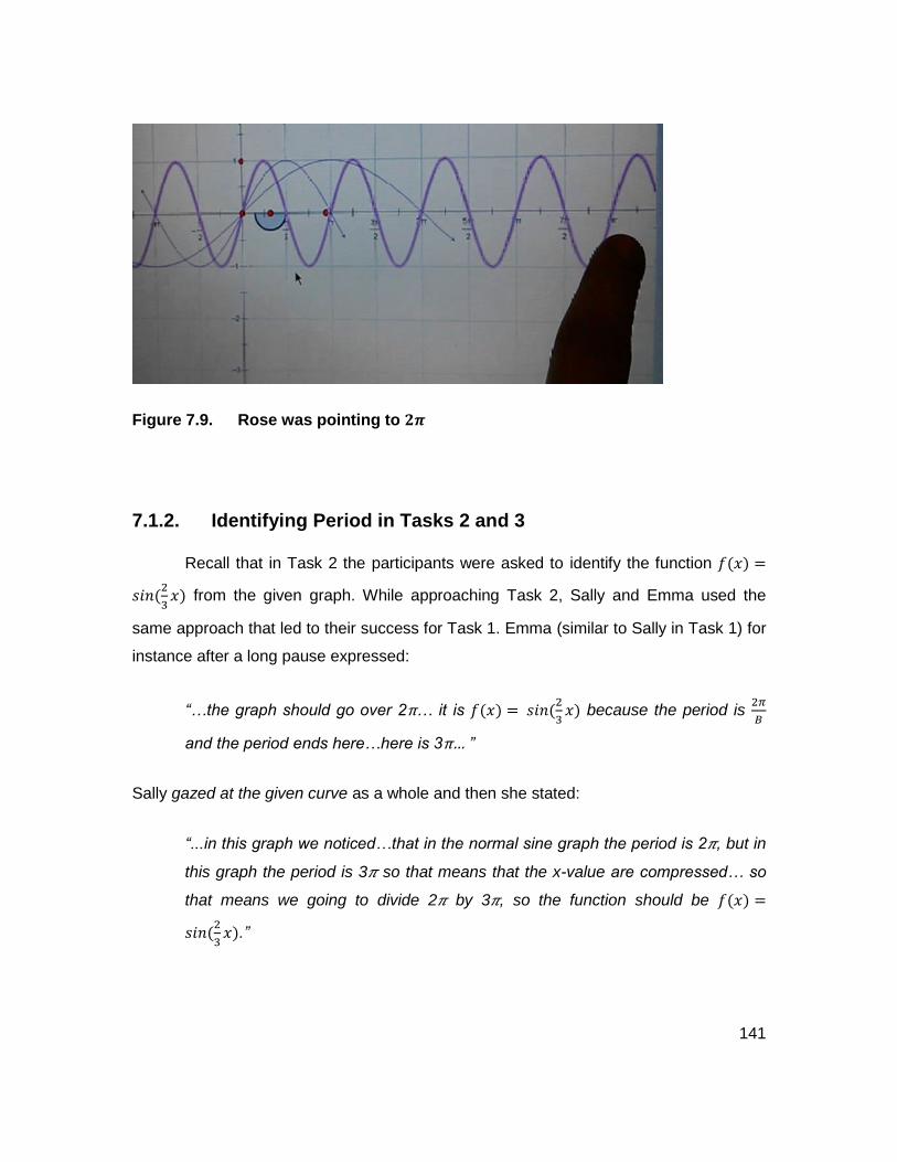
141
Figure 7.9. Rose was pointing to 𝟐𝝅
7.1.2. Identifying Period in Tasks 2 and 3
Recall that in Task 2 the participants were asked to identify the function 𝑓(𝑥) =
𝑠𝑖𝑛(2
3𝑥) from the given graph. While approaching Task 2, Sally and Emma used the
same approach that led to their success for Task 1. Emma (similar to Sally in Task 1) for
instance after a long pause expressed:
“…the graph should go over 2π… it is 𝑓(𝑥) = 𝑠𝑖𝑛(2
3𝑥) because the period is
2𝜋
𝐵
and the period ends here…here is 3π… ”
Sally gazed at the given curve as a whole and then she stated:
“...in this graph we noticed…that in the normal sine graph the period is 2𝜋, but in
this graph the period is 3𝜋 so that means that the x-value are compressed… so
that means we going to divide 2𝜋 by 3𝜋, so the function should be 𝑓(𝑥) =
𝑠𝑖𝑛(2
3𝑥).”

142
It is evident from the above quotations that Emma and Sally’s attention shifted
from holding whole to discerning details from the given curve. Finding the period of the
given curve and comparing it with the period of a canonical function shows that they
perceived properties of a sinusoidal function. To interconnect the graphical
representation to the numerical depiction, they used their previous experience gained
from Task 1. They first found the point in which a full cycle (starting from the origin)
completed (here at 3𝜋) and then they divided the period of a canonical function (2π) by
it. This illustrates that they recalled the memory image of formula of sinusoidal function.
They also had concrete imagery and therefore dynamic imagery of sinusoidal functions
since they were able to move the given graph to visualize a canonical function in their
mind.
Contrary to her approach to Task 1, where Kate applied her pattern imagery to
realize the period of the given curve (“…one and two cycles are in the interval [0, 2𝜋]”),
she did not use the same method for Task 2. Similar to Andy, Sally and Emma; Kate
also attempted to apply her memory image of formula of sinusoidal functions when
approaching Task 2 (she expressed that the period in a sinusoidal function is2π
B).
However, after a short pause and gazing at the given graph, Kate eventually noticed that
a full cycle finished at the point 3𝜋. She, therefore, suggested the function 𝑓(𝑥) =
𝑠𝑖𝑛(3𝑥) without paying attention to her mentioned formula. Apparently, observing of the
graphical representation in Task 2 led Kate to identify the function inappropriately.
Recall that in Task 3 the students were asked the function of 𝑓(𝑥) = 𝑐𝑜𝑠(2
5𝑥 −
π
5)
from the given graph. Emma and Sally consistently applied for Task 3 the same method
they used for Tasks 1 and 2. In other words, they were able to realize a correct period
for the given curve using their memory image of formula of sinusoidal functions.
However, none of the previous approaches (pattern imagery and memory image of
formula) supported Kate to determine the period of the given curve in completing Task 3
(she expressed “I have no idea for this graph… It is a cosine function”). Approaching
Task 3, Rose applied the same method she used for Tasks 1 and 2. After gazing at the
given curve, Rose noticed that a full cycle of a cosine curve, was completed at the point

143
5π. She then suggested 2
5 as the coefficient of x in the sinusoidal function (because
according to her method, ended- point of a full sinusoidal cycle (5π in this task) should
be divided in to 2 and then the results should be flipped). Similar strategy also helped
Rose to realize a correct period for the Task 2.
Mia’s approach to Task 2 was different from her approach to Task 1. After
holding the graph as whole for a long pause, she did discern some details from the x-
axis. She then stated:
“…It is sine of x over something because if it is sine of x it would end here [at
2π]…ok, it is 𝑓(𝑥) = 𝑠𝑖𝑛(𝑥
3) because there are one, two three spaces here
between 0 and this point and again one, two, three here…(see Figure 7.10)”
As it appears from the above statement, Mia counted the number of “blocks”
between 0 (the point A in Figure 7.10) and the point in which the curve intersected the x-
axis point B) and again from the point B to another one in which the graph intersected
the x-axis (point C). Because the distance between the points A and B, and B and C was
3 blocks, Mia put the fraction 1
3 for the coefficient of x in the suggested sinusoidal
function. This illustrates that Mia used her pictorial imagery of canonical function in her
mind when suggesting the incorrect function (“…if it is sine of x it would end here [at
2π]…”). Observing the graph of the function 𝑓(𝑥) = 𝑠𝑖𝑛(1
3𝑥) led her to suggest the
functions 𝑓(𝑥) = 𝑠𝑖𝑛 (1
2𝑥) and 𝑓(𝑥) = 𝑠𝑖𝑛(
1
2𝑥 +
𝜋
2) as possible solutions to Task 2.
Considering the visual feedback from the graphs of these suggestions, then indicated
that the function should be 𝑓(𝑥) = 𝑠𝑖𝑛( 𝑥
1.5), which is in fact correct but unconventional
notation. When she was asked to explain her thinking, she indicated:
“…this one was too stretched [referring to the graph of 𝑓(𝑥) = 𝑠𝑖𝑛(1
3𝑥)] and this
one was not stretched enough [referring to the graph of the previous suggested
function 𝑓(𝑥) = 𝑠𝑖𝑛(1
2 𝑥 +
𝜋
2)], so I though it should be 𝑓(𝑥) = 𝑠𝑖𝑛(
𝑥
1.5) to be fitted
in this curve.”
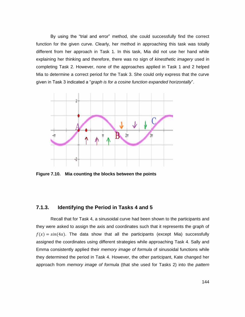
144
By using the “trial and error” method, she could successfully find the correct
function for the given curve. Clearly, her method in approaching this task was totally
different from her approach in Task 1. In this task, Mia did not use her hand while
explaining her thinking and therefore, there was no sign of kinesthetic imagery used in
completing Task 2. However, none of the approaches applied in Task 1 and 2 helped
Mia to determine a correct period for the Task 3. She could only express that the curve
given in Task 3 indicated a “graph is for a cosine function expanded horizontally”.
Figure 7.10. Mia counting the blocks between the points
7.1.3. Identifying the Period in Tasks 4 and 5
Recall that for Task 4, a sinusoidal curve had been shown to the participants and
they were asked to assign the axis and coordinates such that it represents the graph of
𝑓(𝑥) = 𝑠𝑖𝑛(4𝑥). The data show that all the participants (except Mia) successfully
assigned the coordinates using different strategies while approaching Task 4. Sally and
Emma consistently applied their memory image of formula of sinusoidal functions while
they determined the period in Task 4. However, the other participant, Kate changed her
approach from memory image of formula (that she used for Tasks 2) into the pattern

145
imagery (as she applied previously for Task 1) when completing Task 4(see Figure
7.11). She expressed:
“…I know that 2π is here because 1, 2, 3, 4 periods between 0,2π and
here 1 and -1…”
The above statement demonstrates that Kate also had concrete imagery of
sinusoidal function because she knew that a canonical sine function completes one
cycle in the interval [0, 2π] and the amplitude is 1. This also illustrates that Kate
perceived properties of sinusoidal functions and she used them to recognize relationship
between the symbolic representation and the graphical representation.
While, none of the previously used strategies helped Kate to complete
successfully Task 5, in which she was asked to assign coordinates to represent 𝑓(𝑥) =
𝑐𝑜𝑠(3𝑥 − 𝜋
4), the pattern imagery led Rose to realize the period correctly for Task 5
(similar to Task 4). The memory imagery ability also supported Sally and Emma to
realize correctly the period in Task 5 (similar to other interview tasks)
Figure 7.11. Kate placed the 4 cycles in the interval [0, 2π]
As mentioned earlier, all the participants were able to complete Task 4
successfully except Mia. When completing this task she stated:
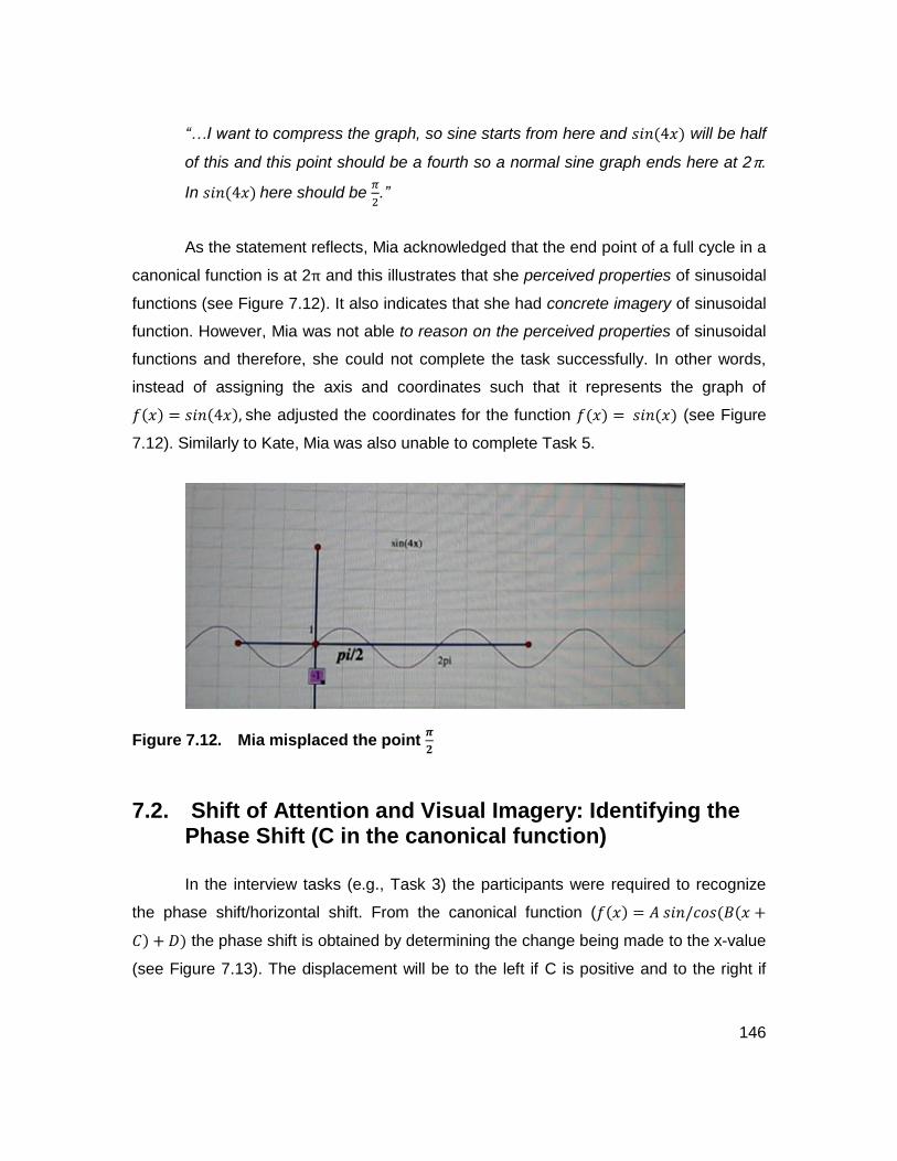
146
“…I want to compress the graph, so sine starts from here and 𝑠𝑖𝑛(4𝑥) will be half
of this and this point should be a fourth so a normal sine graph ends here at 2π.
In 𝑠𝑖𝑛(4𝑥) here should be 𝜋
2.”
As the statement reflects, Mia acknowledged that the end point of a full cycle in a
canonical function is at 2π and this illustrates that she perceived properties of sinusoidal
functions (see Figure 7.12). It also indicates that she had concrete imagery of sinusoidal
function. However, Mia was not able to reason on the perceived properties of sinusoidal
functions and therefore, she could not complete the task successfully. In other words,
instead of assigning the axis and coordinates such that it represents the graph of
𝑓(𝑥) = 𝑠𝑖𝑛(4𝑥), she adjusted the coordinates for the function 𝑓(𝑥) = 𝑠𝑖𝑛(𝑥) (see Figure
7.12). Similarly to Kate, Mia was also unable to complete Task 5.
Figure 7.12. Mia misplaced the point 𝝅
𝟐
7.2. Shift of Attention and Visual Imagery: Identifying the Phase Shift (C in the canonical function)
In the interview tasks (e.g., Task 3) the participants were required to recognize
the phase shift/horizontal shift. From the canonical function (𝑓(𝑥) = 𝐴 𝑠𝑖𝑛/𝑐𝑜𝑠(𝐵(𝑥 +
𝐶) + 𝐷) the phase shift is obtained by determining the change being made to the x-value
(see Figure 7.13). The displacement will be to the left if C is positive and to the right if

147
the phase shift is negative. For brevity, I refer to this connection as “Identifying the phase
shift”.
Figure 7.13. Identifying phase shift/horizontal shift
The data show that few students were able to identify the horizontal shift/phase
shift when changing the sine function into the cosine functions and vice versa in the
interview tasks. After successfully identifying the correct sine function (𝑓(𝑥) = 𝑠𝑖𝑛(2𝑥))
from the given curve in Task 1, the participants were asked to determine a cosine
function for the given curve. As evident from data, the majority of participants chose the
same strategy. When approaching the task, most students attempted to establish a
relationship between a sine and a cosine function by adding up 𝜋
2 to the argument 2𝑥.
For instance, Mia expressed:
“…cosine function is a flip version of sine function…it has horizontal translation
to the right, so it is 𝑓(𝑥) = 𝑐𝑜𝑠 (2𝑥 + 𝜋
2).”
From the above student’s statement one may conclude that the participants had
memory image of formula of shifting a sine function into a cosine function because she
realized that the sine and cosine functions always relate to each other by a difference of
𝜋
2. However, Mia (and similarly most other participants) identified incorrectly the sign of
horizontal shift. In other words, while the graph shifted to the right by 𝜋
2, she added
𝜋
2 to
the argument 2𝑥 (instead of subtracting it). The students’ discussions indicate that they
148
have not perceived properties of sinusoidal functions and also have not successfully
recognized relationship between the symbolic and the graphical representation of the
cosine function.
The participants, then, were asked to describe the cosine function from the given
curve (instead of focusing on the formula correctly or incorrectly). As evident from data,
none of the students (except Sally) was able to determine the proper horizontal shift
from the given graph. For instance after 5 minutes pausing, Rose expressed:
“…I know the differences between them are 𝜋
2….I do not know…it is shifted to the
right by 𝜋
2…. I try to match something to match this 𝑓(𝑥) = 𝑐𝑜𝑠(2𝑥 +
𝜋
2)….”
As it is indicated from Rose’s reply, she attempted to determine a horizontal shift
that represents her suggested function (𝑓(𝑥) = 𝑐𝑜𝑠(2𝑥 + 𝜋
2)). However, her suggested
horizontal shift again was incorrect. Even Emma, who was able to change correctly the
formula of the function 𝑓(𝑥) = 𝑠𝑖𝑛(2𝑥) into the cosine function 𝑓(𝑥) = 𝑐𝑜𝑠 (2𝑥 − 𝜋
2), was
not able to identify a cosine function from the given graph. Sally, on the other hand,
completed this part of Task 1 successfully focusing on the given graph.
Unlike the other participants who relied on the formula (correctly or incorrectly)
and the point 𝜋
2 when connecting the sine function into a cosine function, Sally focused
only on the given curve in Task 1. After holding the given curve as a whole, Sally
attempted to discern some details from the curve by stretching it horizontally. From
there, she zoomed on the point𝜋
4 on the x-axis. She stated that the curve was shifted
horizontally by 𝜋
4, because its y-value was 1. Sally then subtracted
𝜋
4 from the argument
(2x). She, then, considered the cosine function 𝑓(𝑥) = 𝑐𝑜𝑠( 2𝑥 − 𝜋
4 ) for the given curve.
Observing the graph of her suggested function (𝑓(𝑥) = 𝑐𝑜𝑠( 2𝑥 −𝜋
4 )) made Sally
realize that the function did not fit the given curve (from Task 1). Sally expressed:
149
“… Ok, I think I know where my mistake was. It was that I forgot to put bracket
around here…”
Recognizing her mistake led Sally to suggest successfully the function 𝑓(𝑥) =
𝑐𝑜𝑠(2(𝑥 −𝜋
4)). Sally’s success illustrates that she applied her memory image of formula
of sinusoidal function (𝑓(𝑥) = 𝐴 𝑐𝑜𝑠(𝐵(𝑋 + 𝐶) + 𝐷)). It also shows that she was able to
establish a link between the visual representation of sinusoidal function and the symbolic
representation. Sally used the same approach for the rest of interview tasks when she
was asked to determine alternative sinusoidal function. However, other participants
consistently found difficulties in realizing the horizontal shift in the other tasks.
Similar to their initial mistakes in Task 1, the majority of
students could only add up or subtract 𝜋
2 from the function 𝑓(𝑥) = 𝑠𝑖𝑛(
2
3𝑥) in Task 2
without reflective thinking about the given graph. When asked them to focus on the given
graph, participants were not able to realize the amount of radian by which the graph
shifted horizontally. Kate for instance, focused her attention on the point (3𝜋
4, 1) and
expressed that:
“…𝑓(𝑥) = 𝑐𝑜𝑠( 2
3𝑥 +
3𝜋
4), because here is
3𝜋
4 . It is shifted to the to the right…
After extending the graph, Kate zoomed on the point 3𝜋
4 in which the y-value was
1. The details she discerned from the graph led her to connect the graphical
representation with the incorrect symbolic representation when focusing on the
horizontal shift. The data show that Kate did not apply properly her memory image of
formula of transformation of sinusoidal functions, because she misplaced the bracket in
the suggested function (although she found a correct point from the graph). Besides, she
added up the point (3𝜋
4) to the argument x instead of subtracting it. The proper cosine
function for the given graph was 𝑓(𝑥) = 𝑐𝑜𝑠( 2
3(𝑥 −
3𝜋
4)). Similarly, other students either
focused on the point 3𝜋
4 or
𝜋
2 and then added them up to the argument of the function.

150
The students encountered the same difficulties when attempting to determine the
alternative functions in the Tasks 3, 4 and 5. To complete Task 3, for example, Rose
after gazing at the graph and stretching the graph horizontally stated:
“….there is a transformation in x direction….the transformation… the x where
starts is at ( 𝜋
2 , 1)…we should subtract this …”
The above statement indicates that Rose focused on the point ( 𝜋
2 , 1) which did
not exist in the given graph. However because she had a pictorial imagery of the
canonical cosine in her mind and she knew that a sine and a cosine function connecting
each other with 𝜋
2, she subtracted
𝜋
2 from the arguments of the function. She, in fact, used
her memory image of formula of sinusoidal function along with her knowledge of
properties of sinusoidal functions without focusing on the appropriate point of given
graph. The majority of students made the same error as Rose did. They just focused on
the point 𝜋
2 and they subtracted it from the argument of the function. Meanwhile some
other students extended the given graph, but they did discern the incorrect detail from
the graph. However, they did not suggest proper phase shift and therefore a correct
alternative function for Task 3. For example, Emma stated:
“…I think it moves this way by 𝜋
4….”
Emma unsuccessfully found a point in which the graph had the y-value=1(the
proper point is (−3𝜋
4, 0)). Afterward, she made the same error as Rose and most other
participants did; she subtracted the incorrect point from the argument BX in the function
instead of adding it to the argument x in the cosine function (because the graph shifted
to the left). As evident from the data most students participated in this study mixed up
both standard formula related to the transformations of sinusoidal functions together
(𝑓(𝑥) = 𝐴 𝑠𝑖𝑛/𝑐𝑜𝑠(𝐵(𝑋 + 𝐶) + 𝐷) and 𝑓(𝑥) = 𝐴 𝑠𝑖𝑛/𝑐𝑜𝑠 (𝐵𝑋 + 𝐵𝐶) + 𝐷)), when asking
to find the alternative functions for the tasks. The students’ replies indicate that, in fact,
the majority of participants were unable to apply their memory image of formula of
transformation of sinusoidal functions properly. However, amongst the participants, Sally

151
was able to determine proper alternative function for Task 3 by applying the same
approach (memory image of formula, discerning proper details and reasoning on the
perceived properties of sinusoidal functions) as the previous tasks.
Not only Sally was the only student who successfully found the alternative
functions in all five-interview tasks, she determined the proper phase shifts in Tasks 3
and 5. Sally’s reliance on her memory image of formula of sinusoidal functions
supported her to discern proper details from the given function, for example in Task 5
(𝑓(𝑥) = 𝑐𝑜𝑠(3𝑥 −π
4)), she stated:
“… we first need to take out the 3 so it become 𝜋
12. we know it is shifted to the
right by 𝜋
12…. So this is my normal cosine function we need to shift the graph
𝜋
12
to the right because that is given by formula 𝑓(𝑥) = 𝑐𝑜𝑠(𝐵(𝑥 − 𝐶)) and C is the
positive number and is 𝜋
12. Here is 1 and -1….”
Identifying the amount of phase shift led Sally to assign axes and coordinates in
the proper place (in order to identify phase shift in Task 3 (𝑓(𝑥) = 𝑐𝑜𝑠(2
5𝑥 −
π
5)), Sally
followed the same strategy). However, all other students were unsuccessful in identifying
phase shift in Tasks 3 and 5. As an example, the memory image of formula (she used in
previous tasks) did not help Emma to determine the horizontal shift correctly in Tasks 3
and 5. For instance when completing Task 5, she expressed:
“……because the amplitude is not changing so here is 1 and -1. Because the
original period is 2π but here we have 3x so the period should be 2𝜋
3 but then we
have transformation on x on the right direction. So we move the graph over by
𝜋
4…”
As the above quote illustrates, Emma became confused by mixing up again
conventional representations𝑓(𝑥) = 𝐴 𝑠𝑖𝑛/𝑐𝑜𝑠 (𝐵(𝑥 + 𝐶) + 𝐷 (1) and 𝑓(𝑥) = 𝐴 𝑠𝑖𝑛/
𝑐𝑜𝑠(𝐵𝑥 + 𝐵𝐶) + 𝐷 (2). While C is the horizontal shift in the function (1) and (2), Emma
152
made a common error as the other participants did in this task, considering BC as the
shift. Whereas the phase shift was 𝜋
12 for the function 𝑓(𝑥) = 𝑐𝑜𝑠(3𝑥 −
𝜋
4) according to
the function (2) (since 𝜋
4= 𝐵𝐶 and 𝐵 = 3 therefore 𝐶 =
𝜋
12), Emma determined incorrectly
𝜋
4 = 𝐶 as the amount by which the graph should be shifted horizontally. In other words,
although she had pictorial imagery on sinusoidal functions (as she expressed “because
the amplitude is not changing so here is 1 and -1… original period is 2π…”), she did not
perceive properties of sinusoidal function and therefore she did not recognize the phase
shift correctly. As mentioned, all the other participants made the same error as Emma
did when attempting to determine phase shift in Task 3 and 5.
7.3. Covariational Reasoning ability: Identifying Period and Phase Shift
According to Carlson et. al. (2002), a students’ covariational reasoning ability is
said to reach a certain level when it supports not only the mental action associated with
that given level, but also with all mental actions associated with lower levels. As
explained Chapter 5, section 5.3, students’ developmental level related to covariation
could vary from L1 (Coordination) to L5 (Instantaneous rate). Carlson et. al. stated that
at the coordination level (L1), the images of covariation support the mental action of
coordinating the change of one variable with changes in the other variable (MA1). At the
direction level (L2), the images of covariation support the mental actions of coordinating
the direction of change of one variable with changes in the other variable. The mental
actions MA1 and MA2 are BOTH supported by Level 2 image. L3 includes the collection
of mental actions from M1 (coordinating the value of one variable with changes in the
other) to M3 (Coordinating the amount of change of one variable with changes in the
other variable). Table 7.2 present a summary of the participants’ convariation reasoning
ability
B Changing a sinusoidal function into a cosine function and vice versa
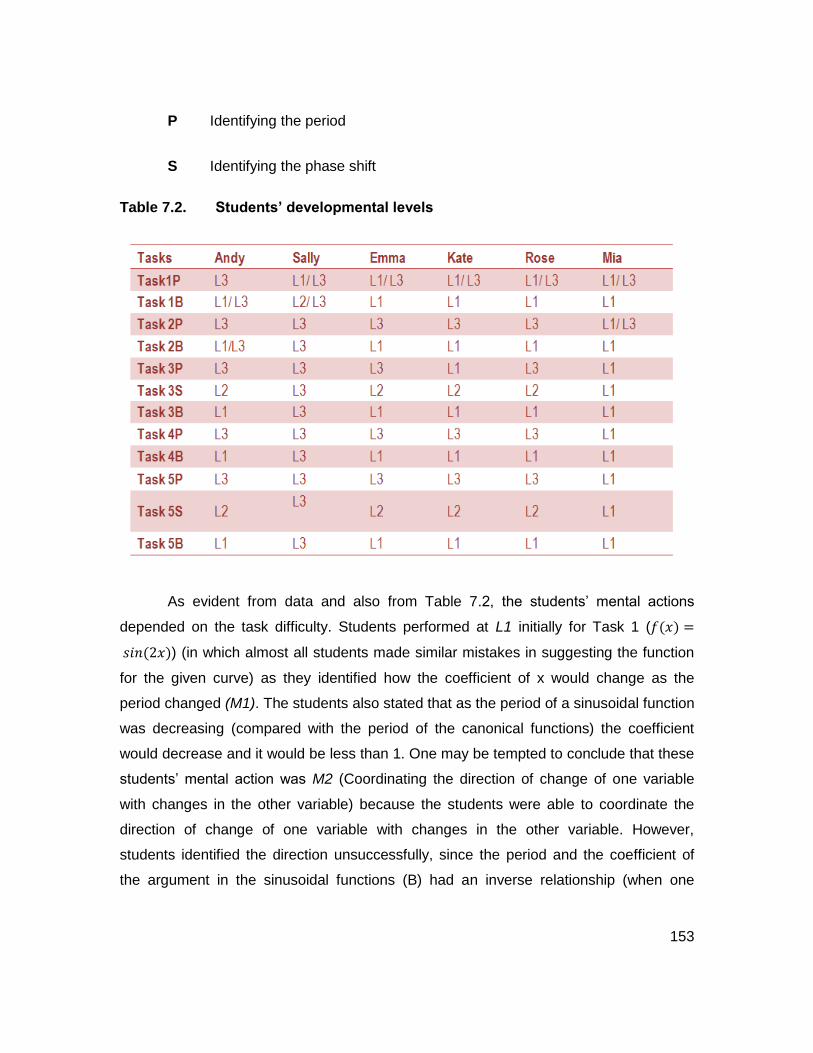
153
P Identifying the period
S Identifying the phase shift
Table 7.2. Students’ developmental levels
As evident from data and also from Table 7.2, the students’ mental actions
depended on the task difficulty. Students performed at L1 initially for Task 1 (𝑓(𝑥) =
𝑠𝑖𝑛(2𝑥)) (in which almost all students made similar mistakes in suggesting the function
for the given curve) as they identified how the coefficient of x would change as the
period changed (M1). The students also stated that as the period of a sinusoidal function
was decreasing (compared with the period of the canonical functions) the coefficient
would decrease and it would be less than 1. One may be tempted to conclude that these
students’ mental action was M2 (Coordinating the direction of change of one variable
with changes in the other variable) because the students were able to coordinate the
direction of change of one variable with changes in the other variable. However,
students identified the direction unsuccessfully, since the period and the coefficient of
the argument in the sinusoidal functions (B) had an inverse relationship (when one

154
increases the other decreases). The same applies for M3. Although the students
attempted to establish a connection between the amount of period and the factor of x in
the sinusoidal function (M3), their proposed numbers for the coefficient of x were
incorrect. As a result, their demonstrated developmental level was L1 (Coordination).
Getting feedback from the graph of their suggested function (𝑓(𝑥) = 𝑠𝑖𝑛(1
2 𝑥))
made the students realize that there is an inverse relationship between the period of the
curve and the coefficient of x in the sinusoidal functions (when the period is decreasing,
the coefficient of x would be greater than 1 (M2)). They could also identify the amount of
periods and the coefficient of x correctly (M3). As such, upon prompting and computer
feedback, they operated at L3.
As it has been shown in the Table 7.2, the developmental level of some
participants, such as Andy and Sally, stayed consistently at L3 (as in Task 1), while it
varied for the other participants when they struggled to determine periodicity for the rest
of the tasks. In other words, the students’ developmental level varied from L1 to L3 when
the participants attempted to identify the connection between the coefficient of x and the
length of the period in the given curve (Tasks 2 and 3) or the given sinusoidal function
(Tasks 4 and 5).
As described in the section 7.2 and Table 7.2, only Sally determined correctly the
amount of phase shift and its influence on the function as well as its graph (L3) in Tasks
3 and 5. The other students (Emma, Kate and Rose) acknowledged that the curve
shifted horizontally if it did not intersect the origin (0,0) and y=1 in Task 3, and if a certain
amount of radian subtracted from the given function in Task 5 (M1). They knew that if
the graph shifted to the right, a certain amount of radian should be subtracted from the
argument x and vice versa in both Tasks 3 and 5 (M2). As such, the covatiation
reasoning ability of Emma, Kate and Rose was at L2 level because they could not
determine the amount of phase shift correctly. However, Mia’s covariation reasoning
stayed at L1 because not only she could not determine the direction of shifting of the
curve as result of horizontal transformation, but also she could not identify the proper
amount of phase shift for the Tasks 3 and 5. The majority of students did the same
155
mistake as Mia did in Task 3 and 5, when they were required to assign the alternative
sine/cosine functions for the Tasks 1-5. In fact, most participants shifted the curve
incorrectly to the right when the sign of the horizontal shift was positive (If they could
shift the graph correctly, their covariation reasoning was at L2). They also did not identify
the amount of phase shift correctly (If they determined the amount of phase shift
successfully, their covariation reasoning was at L3). As such, the developmental level of
the majority of students in identifying the phase shift was L1.
A shown in the Chapters 6 and 7, the presented tasks were challenging to the
participants. They were successful to some degree, occasionally relying on a computer
feedback, in identifying the periodicity of the presented functions (mostly at L3 level).
However, the success with identifying the phase shift was rather limited (often at L1 or
L2 level). This main difficulty can be attributed to the inability to connect the visual
representations to graphical representations of sinusoidal functions.

156
Chapter 8. Discussion
In this chapter, I restate the research questions and I address the questions with
respect to the findings of my study. The limitations and the difficulties I encountered
during this dissertation are also described. Students’ strengths and weaknesses that
were revealed when completing the interview tasks support my recommendations for
teaching transformations of sinusoidal functions. These recommendations are presented
in the last section of this chapter.
8.1. Research Findings and Comments
In chapter 3, I reviewed the findings of prior research related to trigonometry and
students’ difficulties in grasping trigonometric functions. In order to deal with students’
misconceptions and to help them understand the concept of trigonometric functions
more efficiently, some researchers such as Tuna (2013) recommended teaching
trigonometric functions in the context of graphs of functions. In accord with Tuna’s
suggestion, I think students would be able to sketch trigonometric functions, if they
comprehend the properties of transformations of functions. Despite the significant role
transformations of trigonometric functions play in grasping trigonometric functions (as
Tuna (2013) proposed), there have been only sporadic research studies concentrating
on this topic. Therefore, my study has shed some light on the way undergraduate
students deal with transformations of sinusoidal functions.
In this research study I investigated students’ shifts of attention as well as their
forms of visual imageries when they attempted to match the graphical representation of

157
functions with their analytical representations in the context of trigonometry. I was also
interested in studying students’ covational reasoning as they determined sinusoidal
functions representing given graphs, and when they adjusted coordinates to match the
given graphs with the presented sinusoidal functions. The difficulties students
encountered when working on the tasks involving transformations of sinusoidal functions
are of interest in this study. As such, the particular research questions addressed in this
study are:
1) How do undergraduate students complete mathematics tasks involving the
transformations of sinusoidal functions?
2) What is undergraduate students’ covational reasoning and visual imagery of
the transformations of sinusoidal functions?
3) How do students shift their attention when completing interview tasks?
4) What are the common mistakes students often encounter when they work with
transformations of sinusoidal functions?
In the following section I address the research questions as I concentrate on the
main themes extracted from the participants’ responses to the presented tasks.
The data analysis in Chapters 6 and 7 illustrates that eventually all six
undergraduate students were able to complete successfully only Task 1 (𝑓(𝑥) =
𝑠𝑖𝑛(2𝑥)) amongst five interview tasks. In order to complete this task, they often shifted
their attention to discerning details of the given graph and then focused on the reasoning
on the perceived properties of sinusoidal functions. Meanwhile, they applied their
memory image of formula, the pattern as well as concrete imagery, when completing the
task. At the first glance, one might consider students’ mental action in grasping
periodicity at advanced level, L3 (according to Carlson’s et al., (2002) covariational
reasoning classification), since they were able to identify the period in Task 1 correctly.
However, students performed differently on the other interview tasks involving periodicity
(with whole number or fraction for the arguments of x).
158
The data show that the students’ covaritional reasoning fluctuated when
determining the periodicity of the interview tasks. Some students’ mental development
related to identifying periodicity was at the beginning level (L1), because the students
acknowledged that there is a close relationship between the length of a full sine cycle
and the periodicity of the function (M1). However, they were unsuccessful in realizing
that the period and the coefficient of the argument in the sinusoidal functions (B) had an
inverse relationship (when one increases the other decreases, M2). Moreover, they were
unable in determining the amount of periodicity (if they could identify periodicity, their
mental action would be M3). However, the covariational reasoning of the same students
shifted to the advanced level, L3, when completing some other tasks.
In general, the data illustrate that participants were more successful in identifying
periodicity when the coefficient of x was a whole number, than when it was a fraction. As
seen in Chapter 6 and 7, some students were able to determine periodicity in Task 1 and
4 (where coefficient of x was a whole number), but they encountered difficulties in
completing Task 2 (𝑓(𝑥) = 𝑠𝑖𝑛(2
3 𝑥)) and Task 3 (𝑓(𝑥) = 𝑐𝑜𝑠(
2
5 𝑥 −
𝜋
5)). For example,
Kate looked at the graph in Task 2 and at the first glance she realized a full sine cycle
appeared between 0 and the point 3π (discerning details from the given graph). Using
her experience in Task 1, getting feedback from the computer and relying on the
concrete and memory image of formula, however, did not support Kate to suggest the
proper function for the graph in Task 2 with the fraction coefficient. Kate also hesitated to
offer a function for the given graph in Task 3. She simply stated:“…I have no idea for this
graph.”
As data illustrate, according to Carlson’s et al. (2002) framework, only one
student’s developmental level was at the advanced level (L3) in determining the
alternative sine/cosine functions for all five interview tasks. In other words, most students
were not able to identify the alternative functions for the given interview tasks and their
performance was at L1 level. As an example in Task 1 when students were asked to
suggest a cosine function for the given graph, most students unsuccessfully wrote the
function of 𝑓(𝑥) = 𝑐𝑜𝑠(2𝑥 + 𝜋
2). They knew that a cosine graph is a sine graph shifted
159
horizontally; however, they were unable to recognize the direction of horizontal
movement as well as the proper amount of the shift. The students’ mistakes in the task
illustrate that they were unable to determine a phase shift from the given graph. It is
interesting that even some students, who applied their memory image of the formula of
the sinusoidal functions when completing other tasks, did not use the formula to identify
the phase shift in the given graph in Task 1 (when attempting to find the alternative
function for the task). Even discerning details, perceiving properties of sinusoidal
functions, and reasoning on the properties did not support them to find the correct link
between the graph and the analytical representations and vice versa in Task 1. Similarly,
the students’ covariational reasoning stayed at L1 level in the rest of interview tasks
(Tasks 2-5), when identified the alternative functions for the tasks. Only Andy’s
covariational reasoning stayed unchanged in Task 2 (at L3 level as in Task 1), although
it moved back to L1 from L3 for Tasks 3, 4 and 5 (when he was asked to find the
alternative functions).
Sally was the only student who identified the phase shift in Tasks 3 and 5
correctly (Recall that she also correctly found the alternative cosine/sine functions for all
interview tasks). Sally, in fact, applied her memory image of formula as well as dynamic
and kinesthetic imagery in order to match the given graph with the proper function
shifted horizontally in Task 3 and 5. She performed at developmental level, L3. Even
Andy, who determined proper alternative functions for the given graph in Task 1 and 2
(but not in the rest of tasks), did not determine phase shift in Tasks 3 and 5 successfully.
As was described in Chapter 7, students often incorrectly identified 𝜋
5 for Task 3 (instead
of 𝜋
2), and
𝜋
4 for Task 5 (instead of
𝜋
12). In other words, students performed poorly in both
types of tasks; “Identifying sinusoidal functions” and “Assigning coordinate” tasks when
completing tasks involved identifying the phase shift. In fact, the majority of participants’
mental development related to realizing a phase shift is at the beginning/surface level,
L1 (according to Carlson’s et al. (2002) mental action classification). One might conclude
that this is the case because the majority of students, in fact, did not have a proper
memory image of formula of transformations of sinusoidal functions in their mind. As
such, they did not focus their attention on discerning appropriate details from the given
160
tasks, although they perceived properties of sinusoidal functions. In accord with the
findings of Chiu et al.,(2001) in the interview tasks involving the phase shift students,
mostly misunderstood the connections between the graphical and algebraic
representations.
Moreover, the students’ misconceptions of recognizing phase shift affected their
identification of periodicity. As mentioned previously in this chapter as well as chapters 6
and 7, determining periodicity when the coefficient of x was a fraction was a difficult task
for some students. This problem is further highlighted when phase shifts are involved in
the tasks. When completing Task 2 (𝑓(𝑥) = 𝑠𝑖𝑛(2
3𝑥)) in which the coefficient of x was
2
3,
there were some students who successfully determined periodicity, using their memory
image of formula. However, those students became confused in identifying periodicity in
Task 3 (𝑓(𝑥) = 𝑐𝑜𝑠(2
5𝑥 −
π
5)) in which similar to Task 2, the coefficient of x was a fraction
(2
5 ), but the amount of
π
5 radian was subtracted from the argument x. In other words,
while some students realized the given curve intersected the x-axis at the point 3π and
therefore identified periodicity correctly in Task 2, determining the full length of one full
cycle (the beginning and end point of a full curve) was not easy for them in Task 3 in
which the sinusoid was shifted horizontally.
The results of this study in regarding identifying horizontal shift are consistent
with the findings of other studies such as Oliveira (2011) and Zazkis et al., (2003).
Besides students’ difficulties in identifying the amount of horizontal shift, identifying the
direction of the phase shift and then moving the graph to left or right accordingly was a
problem for the majority of students. While the findings of previous studies indicate that
participants mixed up the positive (negative) sign of the argument in a quadratic function
with shifting the graph to the right (left), this problem becomes more significant in the
context of sinusoidal functions. It is the case because identifying left and right shifts in a
periodic sinusoidal function depends on the placement of the axes. In a periodic
functions there are multiple ways of assigning coordinates on the axes to accommodate
the given phase shift.
161
Considering students’ performance on both types of interview tasks, it is evident
that participants performed better in “Identifying sinusoidal functions” tasks compared
with “Assigning coordinate” tasks, when students were required to determine periodicity.
In other words, more students recognized period properly in the tasks a graph given and
students required to identify sinusoidal function represented the graph, than in tasks in
which the sinusoidal functions given and students should adjust coordinates on the given
sinusoidal curve. As an example, Mia (who completed successfully Task 1, for example)
assigned the axes on the given sinusoidal curve in a way that represented the graph of
the function 𝑓(𝑥) = 𝑠𝑖𝑛(𝑥) rather than 𝑓(𝑥) = 𝑠𝑖𝑛(4𝑥) in Task 4. Her response to this
task illustrates that she did not pay attention to the particular details could be discerned
from the given function. However, due to having concrete imagery of a sinusoidal
function in her mind, she situated the coordinates exactly at the same place as for the
graph of 𝑓(𝑥) = 𝑠𝑖𝑛(𝑥).
In accord with the findings of Gagatsis, Elia, and Kyriakides (2003) and Lage and
Gaisman (2006), it appears from the data that sometimes the task in graphical
representation creates cognitive difficulties that hinder students’ ability to make
connections between the algebraic and the graphical representations. Meanwhile, the
discrepancy in students’ performance in identifying period vs. identifying phase shift
illustrates that they had difficulty when considering graphs of sinusoidal functions
transformed horizontally. These findings are consistent with the results of other studies
by Chiu, Kessel, Moschkovich, and Munoz-Nunezby (2001) Eisenberg and Dreyfus
(1994); Baker, Hemenway, and Trigueros (2000); and Consciência and Oliveira (2011)
who found students' misconceptions of function transformations in general, and
horizontal transformations in particular.
8.2. Contributions of the Study
As was discussed in this chapter and also previous chapters, the main focus of
this dissertation is on sinusoidal functions. While some limited previous studies focused
on students’ difficulty in applying sine and cosine functions defined over the domain of

162
real numbers (Challenger, 2009; Moore, 2010), on the influence of teaching
trigonometric functions in context of unit circle and triangle (Brown, 2005 and Weber,
2005), on the students and teachers’ difficulties in realizing angle measure (Akkoç &
Akbaş Gül, 2010) and on the recognizing real numbers as radians (Orhun, 2001), this
dissertation (to my knowledge) is the first research focused on students’ work on the
tasks involving transformations of sinusoidal functions. There are studies, such as Duval
(1999) and Eisenberg and Dreyfus (1994), which examine students’ difficulties in the
transformation of cubic and quartic functions, however, I have not come across prior
research studies that consider how students deal with tasks that require their knowledge
in transforming sinusoidal functions.
In this research I focused on participants’ ability to identify periodicity and phase
shift in sinusoidal functions, while connecting algebraic and graphical representation of
functions. There is a small number of studies, (e.g. Shama,1998 and Van Dormolen and
Zaslavsky, 2003) that discuss definitions of periodicity in general. In the study by Demir
(2012), students’ conceptual understanding of definition of periodicity of canonical
functions in the graph, and of the periodicity of a sine function (𝑠𝑖𝑛(−𝜋
2)) in the unit circle
were investigated. However, my research investigated how undergraduate students
completed tasks that required them to identify periodicity and phase shift from the
graphs of given sinusoidal functions and to assign coordinates on the given sinusoid
graph in order to match a given functions and its corresponding graph. As such, the
focus and the findings of this dissertation are unique and provide a significant
contribution to research in the area of trigonometry and well as in the area of function
transformations.
Furthermore, my research contributed to task design. In this study I designed two
types of tasks (type A and type B). While some of the prior research studies used tasks
of type A, the design of tasks of type B (Assigning Coordinates) was novel and unique.
None of the previous researchers required students to assign axes and coordinates so
that the given sinusoidal curve would represent the given function. However, the effect
of the novelty of the task on students’ difficulties has to explore in further research.

163
8.3. Research Limitations
I recognize some limitations of my study in terms of the interview tasks,
participants’ familiarity with using sketchpad, as well as the number of participants.
The interview tasks I used for my research were all comprised of sinusoidal
functions having fractions or whole numbers for arguments of x. However, three tasks
had whole numbers for the coefficients of x and two tasks had fractions. I might have
more accurate results, if I had designed more of tasks in which the sinusoidal functions
comprised of fraction coefficients. This is significant since the results of this study show
that students encountered more difficulties in the tasks with fraction of coefficients.
Furthermore, only two tasks included a phase shift, which were challenging for the
participants, when compared with the tasks involving periodicity only. These two tasks
.combined phase shift and periodicity. Lack of tasks that involved a phase shift without
the change in the period of the conventional sinusoid weakens the conclusions on
students’ difficulties in identifying a phase shift.
The use of Sketchpad gave students an opportunity to manipulate the given
graphs and also to receive immediate feedback on their initial answers and therefore to
correct their initial suggestions. However, it seems that the majority of students were
unfamiliar with applying sketchpad in order to adjust coordinates. Task 4 and 5, in which
students were required to assign the axes and place coordinates were presented at the
end of interviews, when most students were tired. If I mixed the order of tasks from
“Identifying sinusoidal functions” and “Assigning coordinates” students might have
performed differently. I could have obtained more reliable findings if I also asked a few of
the “Assigning coordinates” tasks to be completed using paper and pencil. Furthermore,
although the study was done in the present of sketchpad, the specific interaction of
students with sketchpad was not explored deeply in this study.
Another limitation of this study is associated with the duration of interviews. Since
the interviews were one hour long, some students grew tired and they wanted to finish
the interview as soon as possible no matter how appropriate their answers were.

164
Therefore, more accurate results could have been obtained if the interviews were
conducted in two separate thirty minute sessions on two different days.
Six students from Calculus courses volunteered their time to participate in this
study. Among them three were enrolled in Calculus I, where students have opportunities
to refresh their knowledge about transformations of sinusoidal functions by reviewing the
concepts of trigonometric functions and transformation of functions (after High School
Calculus). The rest of students were from Calculus II, where they had no further chance
of revising the concepts of trigonometry and transformation of trigonometric functions.
The data show that the participants enrolled in Calculus I completed the interview tasks
more successfully than the Calculus II students. Although it is unclear whether the
stronger performance of students in Calculus I can be attributed to the more recent
review of transformations of sinusoidal functions or to students’ general knowledge and
ability, I could have had different results if all data came from students enrolled in
Calculus I.
8.4. Pedagogical Implications and Suggestions
Drawing on my findings and the fact that some of the participants in this study
encountered difficulties in identifying transformations of sinusoidal functions, this concept
needs to be emphasized more in the Calculus textbooks. Reviewing the Calculus
textbook that has been used at this university (e.g., Barnett, Ziegler & Byleen, 2003), I
noticed that there is a section in the “Functions” chapter in which horizontal and vertical
transformations of functions are described, without mentioning or exemplifying
transformations of trigonometric functions. In another chapter, trigonometric concepts
are explained. However only the canonical sinusoidal functions are sketched. In other
words, since students had limited opportunities to learn about the transformation of
sinusoidal functions, their difficulties in completing the interview tasks in this study is not
a surprising result (students learn transforming sinusoidal functions briefly in High
School pre-Calculus). Teachers and curriculum designers need to focus on this
important concept, because transformations of sinusoidal functions have application in

165
other undergraduate courses, such as physics. Students’ inability to deal with
transformations of sinusoidal functions may hinder their success in other courses.
Students in my study experienced difficulties identifying phase shifts and
periodicity in the given trigonometric functions. Although participants in this research
were able to successfully identify some sinusoidal functions from the given graphs, they
were not able to adjust coordinates on the sinusoidal curve to represent some of the
given functions. This problem was highlighted even more when the coefficient of x in a
given function was a fraction. However, reviewing the Calculus textbooks revealed that
the authors focused mostly on whole number coefficients when included tasks on
identifying functions from the given graphs. Teachers should take note of this and focus
on sketching of sinusoidal functions with fractional coefficients. While the initial focus on
whole number coefficients is appropriate, teachers need to enrich the repertoire of task
presented to students by including fractional coefficients. This will enhance students’
understanding of the connections between algebraic and graphical representation of
sinusoidal functions.
After teaching periodicity, teachers can move on to the phase shift. The initial
consideration of the phase shift should be for sinusoidal functions with a periodicity of
2π, if the coefficient of x is 1. That is, initial consideration of horizontal transformation
should not be conflated with that of expansion or compression. Only then combined
transformations should be approached.
When interview tasks in my study involved phase shift and periodicity other than
2π, the majority of students completed them unsuccessfully. This result is consistent
with the prior research studies on transforming quadratic functions horizontally. This
result is not surprising since, the textbook practice questions concentrate mostly on the
phase shift tasks for functions having the argument of x 1 (periodicity is 2π). In these
tasks students identify the phase shift more easily. Thus, teachers need to focus on the
phase shift tasks in functions with periodicity other than 2π, and involving students with
more practice questions in which phase shift is connected to both analytical and
graphical representations.

166
To improve students’ conceptual understanding of the transformations of
sinusoidal functions, it is very important that teachers pay attention to the students’ shifts
of attention. Relying on the findings of this study, students are often able to discern
details from the given function of a graph, they perceive properties of a sinusoidal
function, but they are not able to reason on the properties. Teachers might shift students’
attention from details to reasoning about properties of sinusoidal functions by asking
students to describe their thinking. Using this skill would help teachers evaluate
students’ understanding of the transformation concept and try to improve students’
learning.
8.5. Reflection of this Journey
This research journey greatly influenced the way I was thinking about teaching
and learning of mathematics, and in particular transformations of sinusoidal functions.
Before doing this research, I have never thought about the influence of students’
imagery on their learning of mathematics. I now recognize that the students’ visual
imagery plays an important role in their conceptual understanding of transformations of
functions. In other words, I find it important to pay attention to the students’ body
movements and their mental images, which might be sketched in a paper or in the
computer screen when completing the mathematics tasks.
Applying Carlson’s et al. (2002) covariational reasoning framework in this study
made me realize that it significant to get insight into undergraduate students’ verbal
expressions related to sinusoidal functions. I note that providing students with
opportunities to participate in class conversations would let me as a teacher to identify
the level of their mental actions and therefore to modify my instructional approaches
accordingly, where needed.
Conducting this study also changed my research approach significantly. In my
previous research I relied on a single theoretical framework. I first found it a difficult task
to analyze data collected for this study with respect to three different theoretical

167
frameworks. However, I became more and more comfortable to interpret data according
to each framework and this gives me richer results and a broader view about
undergraduate students’ grasping of the topic. This research provided me an opportunity
to enjoy doing research in one of the most difficult topics in Calculus. This motivates me
to engage in future studies focusing on undergraduate mathematics topics.

168
References
Adamek T., Penkalski K., & Valentine G., (2005). The history of trigonometry,
history of mathematics. Retrieved from
ttp://math.rutgers.edu/~mjraman/History_Of_Trig.pdf.
Aguirre, J. M., Turner, E., Bartell, T. G., Drake, C., Foote, M. Q., & Roth
McDuffie, A. (2012). Analyzing effective mathematics lessons for English learners: A
multiple mathematical lens approach. In S. Celedón-Pattichis & N. Ramirez (Eds.),
Beyond good teaching: Advancing mathematics education for ELLs (pp. 207-222).
Reston, VA: National Council of Teachers of Mathematics.
Ainley, J., Barton, B., Jones, K., Pfannkuch, M., & Thomas, M. O. J. (2001). Is
What You See What You Get? Representations, Metaphors and Tools in Mathematics,
Proceedings of the Second Conference of the European Society for Research in
Mathematics Education, Mariánské Lázne, Czech Republic, to appear.
Akkoc, H. (2008). Pre-service mathematics teachers’ concept image of radian.
International Journal of Mathematical Education in Science and Technology, 39(7), 857–
878.
Akkoç, H. & Akbaş Gül, N. (2010). Analysis of a teaching approach aiming at eliminating
student difficulties with radian. Ankara University Journal of Faculty of Educational
Sciences, 43(1), 97-129.
Army, P. D. (1991). An approach to teaching a college course in trigonometry
using applications and a graphing calculator. Dissertation Abstracts International, 54.
Bayazit, I. (2005). The Relationship Between Teaching and Learning Through the

169
Context of Functions. (Unpublished PhD Dissertation), Mathematics Education Research
Centre: University of Warwick.
Baker, B., Hemenway, C., & Trigueros, M. (2000). On transformations of basic
functions. In: H. Chick, K. Stacey, & J. Vincent (Eds.), Proceedings of the 12th ICMI
Study Conference on the Future of the Teaching and Learning of Algebra (1), 41–47.
University of Melbourne.
Baki, A., & Kutluca, T. (2009). Student teachers and teachers about difficult
subjects in 10th grade mathematics class. Journal of Kastomonu Egitim, 17(2), 609–624.
Barnes, J. A. (1999). Creative writing in trigonometry. Mathematics Teacher,
92(6), 498–503.
Blackett, N., & Tall, D. (1991). Gender and the versatile learning of trigonometry
using computer software. In F. Furinghetti (Ed.), Proceedings of the Fifteenth
Conference of the International Group for the Psychology of Mathematics Education (1),
pp. 144-151. Assisi, Italy: PME.
Bressoud, D.M. (2010). Historical reflections on teaching trigonometry.
Mathematics Teacher, 104(2), 106-112
Breslich, E. R. (1928): Developing functional thinking in secondary school
mathematics. In: National Council of Teachers of Mathematics (NCTM) (Ed.) The Third
Yearbook (42–56). New York, NY: National Council of Teachers of Mathematics,
Teachers College, Columbia University.
Brown, S. A. (2005). The trigonometric connection: Students' understanding of sine and
cosine. (Unpublished Ph.D. Dissertation), Illinois State University: USA.
Brown, S.A. (2006). The trigonometric connection: Students’ understanding of
sine and cosine. In Proceedings of the 30th conference of the international group for the
psychology of mathematics education (pp. 228). Prague: PME.

170
Burch, J. (1981). The development interview, testing, and generalization of a
theory based model of conceptual structures for solving routine trigonometry
problems.(Unpublished doctoral dissertation), Virginia Polytechnic Institute and State
University, Blacksburg, VA.
Byers, P. (2010). Investigating trigonometric representations in the transition to
college mathematics. College Quarterly, 13(2), 1-10.
Challenger, M. (2009). From triangles to a concept: a phenomenographic study of A-
level students' development of the concept of trigonometry. (Unpublished doctoral
dissertation), University of Warwick.
Carlson, M. P. (1998). A cross-sectional investigation of the development of the
function concept. In A. H. Schoenfeld, J. Kaput, & E. Dubinsky (Eds.), CBMS Issues in
Mathematics Education: Research in Collegiate Mathematics Education III, 7, 114–162
Carlson, M., Jacobs, S., Coe, E., Larsen, S., & Hsu, E. (2002). Applying
covariational reasoning while modeling dynamic events: A framework and a study.
Journal for Research in Mathematics Education, 33(5), 352–378.
Carlson, M., & Oehrtman, M. (2004). Key aspects of knowing and learning the
concept of function. Research Sampler Series, MAA Notes Online(invited).
Chiu, M. M., Kessel, C., Moschkovich, J., & Munoz-Nunez, A. (2001). Learning to
graph linear functions: A case study of conceptual change. Cognition & Instruction, 2,
215-252.
Choi-koh, S. S. (2003). Effect of a graphing calculator on a 10th-grade student’s
study of trigonometry. The Journal of Educational Research, 96(6), 359-368.
Čižmešija, A. & Šipuš, M.(2013). The trigonometric functions- concept image of
pre-service mathematics teachers. Retrieved from
http://cerme8.metu.edu.tr/wgpapers/WG17/WG17Posters/WG17_P_Cizmesija.pdf.

171
Colgan, L. (1992). Graphing tools in mathematics classrooms: Some factors
affecting successful use. Unpublished doctoral dissertation. (Unpublished doctoral
dissertation),University of Toronto Canada.
Consciência, M. & Oliveira, H. (2011). Function concept and functions'
transformations: The role of the graphic calculator. CERME7, Rzeszów, Poland.
Demir, O, (2011). Students’ concept development and understanding of sine and
cosine functions. (Unpublished doctoral dissertation), University of Van Amsterdam.
Delice, A. and Monaghan,J. (2005). Tool use in trigonometry in two countries.
Fourth congress of the European society for research in Mathematics Education, Snat
Feliu de Guixols,Spain, 17-21.
Delice, A., and Roper, T. (2006). Implications of a comparative study for
mathematics education in the English education system. Teaching Mathematics and Its
Applications, 25(2), 64-72.
Duval, R. (1999). Representation, vision and visualization: Cognitive functions in
mathematical thinking. Basic issues for learning. In F. Hitt, & M. Santos (Eds.),
Proceedings of the Twenty First Annual Meeting of the North American Chapter of the
23 International Group for the Psychology of Mathematics Education. Columbus, OH:
ERIC.
Eisenberg, T. and Dreyfus, T. (1994). On understanding how students learn to
visualize function transformations. Issues in Mathematics Education, 4, 45-68.
Elliott, S. (1998).Visualization and using technology in A Level mathematics. In E.
Bills (ed.) Proceedings of the BSRLM Day Conference at the University of Birmingham
(pp. 45-50).Coventry: University of Warwick

172
Fi, C. (2003). Preservice secondary school mathematics teachers' knowledge of
trigonometry: Subject matter content knowledge, pedagogical content knowledge and
envisioned pedagogy.
(Unpublished Ph.D. Dissertation), University of Iowa: USA.
Fi, C. (2006). Preservice secondary school mathematics teachers' knowledge of
trigonometry: Cofunctions. In S. Alatorre, J. L. Cortina, M. Sáiz & A. Méndez (Eds.),
Proceedings of the 28th annual meeting of the North American Chapter of the
International Group for the Psychology of Mathematics Education. Mérida, México:
Universidad Pedagogical National.
Gagatsis, A., Elia, I,. & Kyriakides,L. (2003). The nature of multiple
representations in developing mathematical relationships. In N, Pateman.B., Dougherty&
J. Ziliox (Eds), proceeding of 2003 joint meeting of PME and PMENA, 1.p.287.Honolulu,
Hawaii:USA.
Garofalo, J., Drier, H., Harper, S., Timmerman, M. A., & Shockey, T. (2000).
Promoting appropriate uses of technology in mathematics teacher preparation.
Contemporary Issues in Technology and Teacher Education, 1(1), 66-88.
Gould, D. & Schmidt, D., (2010). Trigonometry comes alive through digital
storytelling. Mathematics Teacher, 104 (4), 296-301.
Gray, E.M. and Tall, D. (1994). Duality, Ambiguity and Flexibility: A perceptual
view of Simple Arithmetic. Journal of Research in Mathematics Education, 25 (2), 115-
141.
Gür, H. (2009). Trigonometry Learning. New Horizons in Education, 57(1), 67-80
Hirsch, C. R., Weinhold, M., & Nichols, C. (1991). Trigonometry today.
Mathematics Teacher, 84(2), 98–106.
173
Kang, O. (2003). A new way to teach trigonometric functions. Sungkyunkwan
University, Republic of Korea. Retrieved from http://www.icme-
organisers.dk/tsg09/OkKiKang.pdf.
Kendal, M., & Stacey, K. (1997). Teaching trigonometry. Vinculum, 34(1), 4–8.
Kissane, B., & Kemp, M. (2009). Teaching and learning trigonometry with
technology. Electronic Proceedings of the 14th Asian Technology Conference in
Mathematics. Beijing Normal University, Beijing, China: ACTM.
Knuth, E. (2000). Understanding connections between equations and graphs.
The Mathematics Teacher, 93(1), 48-53. Lage, A., & Gaisman,M. (2006). An analysis of
students’ ideas about transformations of functions. Advanced Mathematical Thinking
(2)23.
Lambertus, A. (2007). Students' understanding of the function concept: Concept
images and concept definitions. (Unpublished master’s thesis), NCSU, Raleigh, NC
Leinhardt, G., Zaslavsky, O., & Stein, M. K. (1990). Functions, graphs, and
graphing: Tasks, learning, and teaching. Review of Educational Research, 60, 1-64.
Marchi, D., (2012). A study of student understanding of the sine function through
representations and the process and object perspectives. (Unpublished Doctoral
Dissertation), Ohio State University.
Mariotti, M. A. and Pesci. A. (1994) Visualization in Teaching - Learning
Situations. Proceedings of PME 18, 1, P 22.
Martinez-Sierra, G. (2008). On the transit from trigonometry to calculus: the case
of the conceptual breaks in the construction of the trigonometric functions in school. 11th
International Congress on Mathematical Education. Retrieved from
http://tsg.icme11.org/document/get/667.

174
Mason, J. (1992). Doing and Construing Mathematics in Screenspace,
Proceedings of the 15th Annual Conference of the Mathematics Education Research
Group of Australasia, Sydney, 1–17.
Mason, J. (2008). Being mathematical with and in front of learners: attention,
awareness, and attitude as sources of differences between teacher educators, teachers
and learners. In T. Wood and B. Jaworski, International handbook of mathematics
teacher education: vol. 4. Rotterdam, the Netherlands: Sense Publishers, pp. 31-56.
Maor, E. 1998. Trigonometric delights. Princeton University Press, Princeton, N.J
Moore. K. C. (2010). The Role of Quantitative Reasoning in Precalculus Students
Learning Central Concepts of Trigonometry. (Unpublished Doctoral Dissertation),
Arizona State University.
Moore, K. C., & Bowling, S. A. (2008). Covariational reasoning and quantification
in a college algebra course. In Proceedings for the eleventh special interest group of the
mathematical association of america on research in undergraduate mathematics
education conference on research in undergraduate mathematics education. San Diego
- Mission Valley, California.
Moore, K. C., LaForest, K., & Kim, H. J. (2012). The unit circle and unit
conversions. In (Eds.) S. Brown, S. Larsen, K. Marrongelle, and M. Oehrtman,
Proceedings of the Fifteenth Annual Conference on Research in Undergraduate
Mathematics Education (pp. 16–31). Portland, OR: Portland State University.
Ng, K., and Hu, C. (2006). Use web-based simulation to learn trigonometric
curves. Retrieved from http://www.cimt.plymouth.ac.uk/journal/chunhu.pdf.
Oehrtman, M. C., Carlson, M. P., & Thompson, P. W. (2008). Foundational
reasoning abilities that promote coherence in students’ function understanding. In M. P.
Carlson & C. Rasmussen (Eds.), Making the connection: Research and practice in

175
undergraduate mathematics (pp. 27-42). Washington, DC: Mathematical Association of
America.
Orhun, N. (2001). Students’ mistakes and misconceptions on teaching of
trigonometry. Mathematics Education Into The 21st Century Project Proceedings of the
International Conference New Ideas in Mathematics Education International Conference
on New Ideas in Mathematics Education, Palm Cove: Australia.
Palmer, E. (1980). Trigonometry instruction: an aptitude treatment interaction
study.(Unpublished Doctoral Dissertation), The Ohio State University.
Pesek, D. D., & Kirshner, D. (2000). Interference of instrumental instruction in
subsequent relational learning. Journal for Research in Mathematics Education 31(5),
524-540.
Piaget, J. (1981). Intelligence and offectivity: Their relationship during child
development (T. A. Brown & C. E. Kaegi, Trans.) Palo Alto, CA: Annual Reviews, Inc.
(Original work published 1954). Piaget, J., & Inhelder, B. (1969). The psychology of the
child. New York: Basic Books.
Presmeg, N.C. (1986a). Visualization in high school mathematics. For the
learning ofMathematics, 6(3), pp. 42-46.
Presmeg, N. C. (1986b). Visualization in high school mathematics. For the
Learning of Mathematics, 6(3), 42-46.
Presmeg, N. (1989). Visualization in multicultural mathematics classrooms.
Focus on Learning Problems in Mathematics, 11(1 & 2), 17-24.
Presmeg, N. C. (1992). Prototypes, metaphors, metonymies, and imaginative
rationality in high school mathematics. Educational Studies in Mathematics, 23, 595-610.
176
Presmeg, N. (1997). Generalization using imagery in mathematics. In English, L.
(Ed.) Mathematical reasoning. Analogies, metaphors and images (pp. 299-312).
Mahwah, NJ: Erlbaum.
Presmeg, N. C. (2006). Research on visualization in learning and teaching
mathematics. In A. Gutiérrez & P. Boero (Eds.), Handbook of research on the
psychology of mathematics education: Past, present and future (pp. 205-235).
Rotterdam, The Netherlands: Sense Publishers.
Robinson, S.A. (1996). The effects of computer animated instruction in college
trigonometry on student achievement, conceptual understanding, and student attitudes.
(Unpublished Doctoral Dissertation), The University of Nebraska.
Ross, J., Bruce, C., and Sibbald, T. (2011). Sequencing computer-assisted
learning of transformations of trigonometric functions. Teaching Mathematics
Applications 30(3), 120-137.
Shama, G. (1998). Understanding periodicity as a process with a gestalt
structure. Educational Studies in Mathematics, 35, 255-281
Stacey, K., & Ball, L. (2001). How might computer algebra change senior
mathematics: The case of trigonometry. In B. Lee (Ed.), Mathematics Shaping
Australia.Proceedings of the 18th Biennial Conference of the Australian Association of
Mathematics Teachers (CD-ROM). Adelaide: AAMT.
Stavy, R., & Tirosh, D. (2000). How students (mis)understand science and
mathematics: Intuitive rules. New York: Teachers College Press.
Steckroth, J.J. (2007). Technology-enhanced mathematics instruction: Effects of
visualization on student understanding of trigonometry. (Unpublished PhD Dissertation),
University of Virginia, Virginia, USA.

177
Tall, D. (1986). Using the computer as an environment for building and testing
mathematical concepts: A tribute to Richard Skemp, In Papers in Honor of Richard
Skemp, 21-36, Warwick.
Tatar, E., Okur, M., & Tuna, A., (2008). Ortaöğretim matematiğinde öğrenme
güçlüklerinin saptanmasına yönelik bir çalışma. Kastamonu Eğitim Dergisi, 16 (2), 507-
516.
Thompson, P. W. (1994). Images of rate and operational understanding of the
Fundamental Theorem of Calculus. Educational Studies in Mathematics, 26(2-3), 229–
274.
Topçu, T., Kertil, M., Akkoç, H., Yilmaz, K., & Önder, O. (2006). Pre-service and
in-service mathematics teachers’ concept images of radian. In J. Novotná, H. Moraová,
M. Krátká, & N. Stehlíková (Eds.). Proceedings 30th Conference of the International
Groups for the Psychology of Mathematics Education. Prague: PME.
Tuna, A. (2013). A conceptual analysis of the knowledge of prospective
mathematics teachers about degree and radian. World Journal of Education, 3(4), 1 – 9.
Vinner S. (1983).Conflicts between definitions and intuitions: the case of the tangent.
Proceedings of the 6th annual meeting of the North American Chapter of the
International Group for the Psychology of Mathematics Education. Antwerp:PME.
Van Dormolen, J., & Zaslavsky, O. (2009). The many facets of a definition: The
case of periodicity. Journal of Mathematical Behavior, 22(1), 91–106.
Van Sickle, J. (2011). History of trigonometry education in united states,1776-
1900.PhD dissertation, Columbia university.
Wheatley, G. & Brown, D. (1994) The Construction and Re-presentation of
Images in Mathematical Activity. Proceedings of the 18th annual meeting of the North
American Chapter of the International Group for the Psychology of Mathematics
Education, PME 18, 1, P 81.

178
Weber, K. (2005), Students’ understanding of trigonometric functions.
Mathematics Education Research Journal, 17(3), 91-112.
Yerushalmy, M. (1988). Formation of algebraic concepts using multiple
representation software environments. Unpublished PhD Dissertation), University of
Haifa, Israel.
Yenitepe, M.E. (2002). Application of computer aided mathematics teaching in a
secondary school. The Turkish Online Journal of Educational Technology (1)1.
Yerushalmy, M. & Schwartz, J.L. (1993).Seizing the Opportunity to Make Algebra
Mathematically and Pedagogically Interesting In : T.A. Romberg, E. Fennema, and T.
Carpenter (Eds.) Integrating Research on Graphical Representations of Functions. pp.
41-68. Erlbaum Inc. NJ.
Zandieh, M. J. (2000).A theoretical framework for analyzing student
understanding of the concept of derivative. In E. Dubinsky, A. Schoenfeld, & J. Kaput
(Eds.), CBMS Issues in Mathematics: Research in Collegiate Mathematics Education,
IV(8), 103–127
Zazkis, R., Liljedahl, P. & Gadowsky, K. (2003). Students’ conceptions of function
translation: Obstacles, intuitions and rerouting. Journal of Mathematical Behavior, 22,
437-450.
Zengin, Y., Furkan, H., & Kutluca, T. (2012). The effect of dynamic software
geogebra on student achievement in teaching of trigonometry. Procedia – Social and
Behavioral Sciences, 31, 183-187.