Students Today, Teachers Tomorrow: Identifying

constraints on the provision of education

Tahir Andrabi Jishnu Das Asim Ijaz Khwaja∗

November 2012

Abstract

With an estimated one hundred and �fteen million children not attending primary

school in the developing world, increasing access to education is critical. This paper

highlights a supply-side factor - the availability of low-cost teachers - and the resulting

ability of the market to o�er a�ordable education. We �rst show that private schools are

three times more likely to emerge in villages with government girls' secondary schools

(GSSs). Identi�cation is obtained by using o�cial school construction guidelines as

an instrument for the presence of GSSs. In contrast, private school presence shows

little or no relationship with girls' primary or boys' primary and secondary government

schools. In support of a supply-channel, we then show that, villages which received a

GSS have over twice as many educated women, and private school teachers' wages are

27 percent lower in these villages. In an environment with low female education and

mobility, GSSs substantially increase the local supply of skilled women lowering wages

locally and allowing the market to o�er a�ordable education. These �ndings highlight

the prominent role of women as teachers in facilitating educational access and resonate

with similar historical evidence from developed economies. The students of today are

the teachers of tomorrow.

∗Pomona College, Development Research Group, World Bank, and Kennedy School of Government, Harvard University.

Email: tandrabi@pomona.edu; jdas1@worldbank.org; akhwaja@hks.harvard.edu. This paper was funded through grants from

the PSIA and KCP trust-funds and the South Asia Human Development Group at the World Bank. We thank the editor Amy

Finkelstein, two anonymous referees, Abhijit Banerjee, Esther Du�o, Karla Ho�, Rema Hanna, Caroline Hoxby, Hanan Jacoby,

Brian Jacob, Ghazala Mansuri, Sendhil Mullainathan, Rohini Pande, Juan Saavedra, Tara Vishwanath, and seminar participants

at BREAD (Yale), Lahore University of Management Sciences, LSE, NBER Education meetings, Harvard University, IUPUI,

The World Bank, University of Michigan, University of Maryland, and Wharton for comments. We are grateful to Nirvana

Abou-Gabal, Alexandra Cirone, Sean Lewis-Faupel, Niharika Singh, and Tristan Zajonc for research assistance. Assistance

from the Project Monitoring and Implementation Unit in Lahore is also acknowledged. All errors are our own. The �ndings,

interpretations, and conclusions expressed in this paper are entirely those of the authors. They do not necessarily represent the

view of the World Bank, its Executive Directors, or the countries they represent.

1 Introduction

Despite the powerful global consensus created through the Millennium Development

Goals, over a third of developing countries are unlikely to achieve universal primary en-

rollment by 2015. While low demand for education is one likely explanation for this poor

performance, a key supply-side constraint is the availability of a�ordable teachers. The

potential pool of teachers is limited in many parts of the developing world - less than 12

percent of the population in Sub-Saharan Africa complete secondary education and even less

so in rural areas. Educationists increasingly argue that there are severe teacher �shortages,�

a concern that resonates with the challenges faced in designing incentives for teachers to

move to rural areas and to exert greater e�ort (UNESCO 2004, Urquiola and Vegas 2005,

Chaudhury et al. 2006). Given this stress on teacher supply in low-income countries, it is

therefore surprising that there is little micro-economic evidence relating a higher supply of

potential teachers to better educational provision.

In this paper, we provide the �rst evidence that public investments in secondary education

facilitates future educational provision by increasing the local pool of potential teachers and

therefore decreasing the cost of providing education. In other words, the students of today

become the teachers of tomorrow.

There are two steps to our argument. First, we show that the construction of government

girls' secondary schools (henceforth GSS) in Pakistan had a large impact on the education

market: Instrumental variable estimates suggest that villages where such schools were con-

structed are 27 percentage points or three times more likely to see private primary schools

emerge in the following years.1 The instrument, an indicator for whether a village has the

largest population amongst all its neighbors (�local top-rank�), is based on o�cial population

based guidelines for GSS construction from a Social Action Program in the 1980s. Since two

1The vast majority of private schools operate in a free and relatively unregulated market as for-pro�t,co-educational, English-medium schools that o�er secular education (contrary to popular views, non-pro�tand religious schools play a small role in Pakistan, with at most a 3 percent enrollment share (Andrabi et al.2006)) and hire teachers from the local market. This is in contrast to the government sector where teacherhiring is governed by teachers' unions, state-wide hiring regulations, and non-transparent processes.

2

villages with equal populations may di�er in whether they are locally top-ranked or not,

the instrument provides substantial variation even after controlling for polynomials in vil-

lage population. A series of robustness tests, in the spirit of Altonji et al. (2005), provide

additional support for the exclusion restriction.

In the second step, we argue that GSS construction impacts private primary school loca-

tion because it augments local teacher supply in an environment with low female geographical

and occupational mobility. In support of a �women as teachers� supply channel, we document

that: (a) private provision is a�ected only by GSS construction (girls' primary or boys' pri-

mary/secondary schools have little e�ect); (b) having a GSS more than doubles the number

of women in the (median) village with secondary or higher education and; (c) the fraction of

secondary educated females in a village has a large impact on private educational provision,

while the fraction of similarly educated men does not. These facts could be reconciled with

solely demand-side explanations if the demand for education is primarily driven by mothers

with secondary education (as opposed to mothers with primary education or fathers with

any level of education). A more conclusive test is based on observing the e�ect of GSS con-

struction on private school teachers' wages: Whereas demand-side explanations suggest that

teacher wages should increase in villages with a GSS, supply-side explanations suggest the

opposite. In support of the latter, we show that private school teachers' wages are 27 percent

lower in villages with a GSS. With teacher wages accounting for close to 90 percent of the

operational costs of private schools, this lower wage in GSS villages o�ers a substantial cost

advantage. Moreover, consistent with the hypothesized mechanism, we �nd that this wage

drop is higher in villages with more restricted female labor markets as proxied by village

development indicators and sex-ratios.

Our results illustrate how investments that increase the supply of teachers in rural areas

of low-income countries can boost educational provision. As in the United States (Rivkin

et al. 2005), a �nding from observational and experimental studies in low-income countries

is that augmenting teacher resources leads to better outcomes, whether through reducing

3

class-sizes (Case and Deaton 1999, Urquiola 2006), reducing teacher absenteeism (Du�o et

al. 2012), or providing additional teachers for poorly performing students (Banerjee et al.

2007). This naturally raises the question of where the additional teachers are going to come

from, and therefore the structure of the broader labor market for teachers. For instance,

work on the decline in teaching quality in the United States highlights the link between

teacher supply and female labor force participation (Corcoran et al. 2004, Hoxby and Leigh

2004). The only randomized intervention, to our knowledge, that tried to increase the supply

of schools through the private educational market failed precisely because teachers could not

be found (Alderman et al. 2003). In this paper we provide the �rst evidence of the tight

link between the teacher labor market and educational markets in a low-income setting, thus

highlighting the initial role of the public sector in bolstering the supply of teachers.

The remainder of the paper is structured as follows: Section II is a brief guide to the

institutional context and data, Sections III and IV present the empirical methodology,and

the results, respectively, and Section V concludes.

2 Institutional Background and Data

2.1 The Context

Pakistan, as other South Asian and African countries, has seen an explosion in the private

sector share of primary education. Private school numbers have increased over ten-fold, from

3,800 in 1983 to 47,000 by 2005, and currently, over a third of primary enrollment is in the

private sector with the fastest growth in rural areas (Andrabi et al. 2008).2

While this private school growth is impressive, it has generated more cross-sectional than

time-series variation with growth mostly bunched in the 1990s. Hence, our paper exploits

2 Contrary to popular belief and media reporting, these changes have little to do with religious education.

Andrabi et al. (2006) show that enrollment in religious schools, or madrassas is low (roughly 1 percent) and

has remained constant since the mid-80s.

4

the cross-sectional variation in private school location to identify constraints to education

provision. One of the key observations for the purposes of this paper is that since these

private schools represent for-pro�t enterprises operating in a largely unrestricted market

(there are no public subsidies and little regulation), their locational decisions are informative

about supply and demand factors in the educational market rather than public priorities or

ideology (which may in�uence the location of public, NGO, or religious schools). Central to

this argument is the importance of human capital, and speci�cally women as teachers in the

provision of private education, together with the limited availability of secondary-educated

women in a restricted geographical labor market and the resulting impact on skilled female

wages.

In fact, the majority of private schools are driven by a low-cost, low-price business model.

Andrabi et al. (2008) show that the median annual fee in a Pakistani rural private school

in 2000 was Rs. 600, so that a month's fee was somewhat less than the daily unskilled

wage.3 The data show that there are few �xed costs in running a private school in Pakistan

(private schools are often setup initially in the owner's house) with teachers' wages forming

the bulk,90 percent, of the overall operational costs. Typical schools employ four teachers,

mostly locally-resident women with at least a secondary education, and enroll around 100

children.

These low fees are sustained through the reliance on female teachers.4 In the context

of a patriarchal society, limited geographical and occupational mobility for women implies

that locally-resident women o�er a cheaper (�captured�) supply of teachers. Female wages

are indeed 30 percent lower than male wages after controlling for educational quali�cations

and experience (World Bank 2005). More than 70 percent of all women live in the village

where they were born; less than 3 percent are engaged in o�-farm work; and among those

3In contrast, private schools (elementary and secondary) in the United States charged $3,524 in 1991. At14 percent of GDP per capita, the relative cost of private schooling is 3.5 times higher in the US.

4In comparison, wages for public sector teachers are �ve times higher for both men and women. As aresult, per-child spending in rural private schools (Rs. 1012 annually) is half of that in rural public schools(Rs. 2039 annually), although available facilities are comparable across the two.

5

with secondary education and a wage-earning job, 87 percent are teachers or health workers.

Safety concerns and a patriarchal society restrict the ability of women to �nd wage work

outside the village where they live or in occupations other than teaching and publicly-

provided health care (World Bank 2005). Consequently, public investments in human capital

for women likely boost the local supply for teachers.

However, the supply of potential female teachers is low and varies across villages based

on the availability of nearby schooling options. In 1981, there were 4 literate adult women

(out of 242) in the median village in Punjab, the largest and most dynamic province in the

country. Over sixty percent of villages in the province had three or fewer secondary-school

educated women, and 41 percent had no such women. This was driven in part by a shortage

of local secondary schooling options for rural women. In our sample, the presence of a GSS

is associated with an increase of over 50 percent (compared to the median village without a

GSS) in the percentage of women with a secondary education (from 3 to 4.6 percent).

These two features of the market for female skilled labor�low wages and limited supply�

combined with the unrestricted and unsubsidized market for private schooling inform our

empirical strategy. The presence of a GSS should generate cross-sectional variation in the

availability of locally resident women with secondary education. If the availability of human

capital constrains private education provision and there is limited mobility, this in turn

should a�ect the likelihood of a private school existing in a village.

2.2 Data

We employ three data sources: (a) a complete census of private schools carried out by

the Federal Bureau of Statistics in 2000; (b) administrative data on the location and date

of construction of public schools in the Punjab province available from the province's Edu-

cational Management and Information Systems (EMIS 2001) augmented with the National

Educational Census (NEC 2005); and (c) data on village-level demographics and educa-

tional pro�les from the 1981 and the 1998 population censuses of Punjab, which provide

6

both baseline and contemporaneous information on village-level characteristics.

We restrict our analysis to rural areas in the province of Punjab, the largest province

in the country which hosts 60 percent of the population, two-thirds of whom live in rural

areas.5 Since the EMIS and the other datasets do not employ a common village coding

scheme, we had to match villages in the di�erent databases on the basis of their names.

Using a combination of a phonetic algorithm and manual post-match, we were able to match

over 90 percent of the villages across databases (23,064 of the 25,266 unique Punjabi villages

in the 1981 census).

In our �nal estimation sample, we restrict attention to villages that did not receive

a girls' or boys' secondary school prior to 1981 and did not have such secondary schools

in their neighboring villages. This reduces our sample to 9,333 villages, but a�ords two

advantages. First, it allows for cleaner econometric identi�cation and interpretation of the

results as our instrument utilizes public school construction guidelines that were applied

for GSSs constructed after the 1980s. This also alleviates exclusion restriction concerns

that arise if our instrument were to predict other public goods. Second, focusing on the

shorter exposure (to GSS) periods is likely to better isolate supply-side e�ects since GSS

construction probably impacts a range of demand factors over a longer time span. It is

nevertheless reassuring to note that all of our main results hold in the full sample of villages,

both in terms of statistical and economic signi�cance, and several of these results are in fact

stronger (Appendix Table II).6

Table I presents summary statistics for the �nal sample. Two and a half percent, or 232

5Not all data sets (e.g., EMIS, 1981 Census) were readily accessible for other provinces, and urban areascould not be matched at the granular level necessary to exploit the cross-sectional variation in private schoollocation and GSS presence that we utilize in the paper.

6Interestingly, while our restricted sample result shows that GSS presence leads to a lower wage (Table V),in the full sample although initial exposure to GSS is indeed associated with lower wages, prolonged exposure(more than 26 years) is associated with higher wages. This is consistent with a net supply impact within ashorter time-frame (20 years) but suggests that, in the longer term, the demand e�ect may dominate: Asmore and more educated girls become mothers and grand-mothers, they impact educational demand. Ittherefore o�ers another important consideration for why restricting our analysis to the reduced sample isappropriate in identifying the (initially dominant) supply channel.

7

villages, in this sample received a GSS between 1981 and 2001.7 Conditional on existence,

the median age of a GSS is fourteen years; therefore, most were constructed early on in

the twenty-year period. There is a private school in one out of every eight villages, and

the majority of these villages already had or received a primary public school. Finally, the

number of women reporting secondary or higher education,eight or more years of schooling,

increased from one in the median village in 1981 to nine by 1998.

3 Methodology and Empirical Framework

There are two broad empirical challenges. The �rst is to identify the causal impact

of GSSs on subsequent private school existence. The second is to argue that the driving

force is a teacher supply channel rather than an increase in the demand for education from

secondary-educated women.

A simple framework outlines the entrepreneur's problem, highlighting the role of the

public sector and the econometric and interpretational issues in identifying the impact of a

GSS. An entrepreneur opens a school in village i if the net return is positive.8 Given that

school fees and teachers' salaries account for 98.4 percent and 89 percent of total revenues

and costs, respectively (Andrabi et al. 2008), NetReturni = Feei ∗Ni −Wagei ∗ Ti, where

Feei is the average private school fee for a single student in village i, Wagei is the average

private school teacher's salary, and Ni and Ti are the number of students enrolled and

teachers employed. Since the schooling market may be geographically segregated, wages and

fees may di�er across villages. GSS construction both increases the supply of teachers in

the village, thus a�ecting Wagei, and may increase schooling demand, re�ected in Feei. A

7This number is quite low relative to what the school construction guidelines would have suggested. Whilethis is not surprising given that these guidelines were constrained by budgetary limitations, it may lead toconcerns about the power of the instrument and the external validity of our results. We therefore addressthese in detail later in the paper.

8This assumes that there is no shortage of entrepreneurs (otherwise, not every positive NPV project willbe undertaken). Incorporating such shortages does not change the qualitative results. The qualitative resultsalso extend to a dynamic framework provided that the �xed costs of setting up schools is small.

8

reduced form expression for net return can then be written as:

NetReturni = α + (β1 + γ1)GSSi + β′XDi + γ′XS

i (1)

where XDi and XS

i are village demographics and characteristics that respectively a�ect the

demand for private schooling and the costs of running such schools. The demand and supply

impact of GSS construction are captured by β1 and γ1 respectively. We are interested both

in the joint estimation of (β1 + γ1) and in arguing that the there is a supply channel (i.e., γ1

is positive and signi�cant).

Since the net return a private school earns is not observed, we treat net return in Equation

(1) as a latent variable in a probability model such that Prob(PrivateSchoolExists) =

Prob(NetReturni > 0), and estimate:

Privateit = α + (β1 + γ1)GSSit + β′Xit +∑r

γ′rSirt + (vi + εit) (2)

where Privateit is a binary variable that takes the value 1 if a private school exists in village

i at time t and GSSit is a binary variable that takes the value 1 if a GSS exists in village i

at time t. Xit are observed characteristics village characteristics at time t and Sirt are other

government schooling options (primary boys/girls schools and boys secondary school) at time

t, where each option is indexed by r. The error term, (vi + εit), consists of a time-invariant

unobserved component, vi, and a random component, εit. The main identi�cation challenge

is that the presence of a GSS in village i in time period t is likely a function of (unobserved)

village/region attributes and hence the OLS estimate of (β1 + γ1) in Equation (2) is biased

and inconsistent. While �rst di�erencing Equation (2) helps, the estimated (β1 +γ1) in such

a speci�cation would still be biased due to time-varying covariates that determine receiving

a GSS and a�ect private school presence. Therefore, we instrument for GSS construction

using program guidelines for a school expansion program undertaken in the 1980s.

9

3.1 Identi�cation Strategy

Our instrumental variables strategy exploits the fact that the regressor of interest, the

construction of a GSS, is partly based on whether the village has the largest population

locally. To the extent that this local top-rank generates a relationship with village pop-

ulation that is highly discontinuous/nonsmooth (two village with arbitrarily close/similar

populations may di�er in whether they are top-ranked), it can be used as an instrument

while directly controlling for linear and polynomial functions of the underlying covariate

itself (Campbell 1969, Angrist and Lavy 1999).

GSS construction after 1981 was a consequence of the 1980 Pakistan Social Action Pro-

gram (SAP). Speci�c guidelines a�ected where these schools could be built. In particular,

the recommended guidelines for opening a new GSS speci�ed a preference for higher village

(student) populations and stipulated that there be no other GSS within a ten-kilometer

radius. We capture this guideline through a �local top-rank� indicator variable, Rulei, that

takes the value 1 if village i is the largest village (in terms of population9) amongst nearby

villages (the set PCi) and 0 otherwise:

Rulei =

1 if Populationi = max

j∈PCi

(Populationj)

0 if Populationi < maxj∈PCi

(Populationj)

In the absence of precise village location data, we use the next highest administrative

classi�cation, the �Patwar-Circle� (PC), which typically covers four villages, to approximate

the radius rule. In terms of actual land area, this is a reasonable approximation; dividing the

size of the province by the number of PCs shows that one school in every PC would satisfy the

radius requirements of the rule. We should note though that this is a proxy measure for the

9Since GSSs could have been built in any year between 1981 and 1998, we assign a value of one to Ruleiif it was the largest village in its PC based either on its 1981 or 1998 population. In addition, for the 4.5percent of villages in our sample that are alone in their PC, we assign a value of 0 to the instrument. Ourresults are robust to the using either 1981 or 1998 population exclusively or assigning the value 1 to Ruleifor single-village PCs.

10

10km distance radius guideline and it likely results in us obtaining a weaker �rst stage. Since

there are no village-level GIS databases available, this is the only feasible strategy and we

deal with a potentially weaker �rst stage by using bivariate probit estimation to obtain more

plausible second stage estimates. Figure 1 shows that this local top-rank indicator indeed

displays a relationship with village population that is highly discontinuous and nonsmooth

(i.e. not only do similar/equal-sized village di�er in the indicator value but also larger-sized

villages may have a lower indicator value).

Our �nal empirical speci�cation is :

Privatei = αPCi+ (β1 + γ1)GSSit + β′1Popi81 + β′2Pop

2i81 + β′3Popi98 + β′4Pop

2i98+

β′Xit +∑

γ′rSirt + (vi + εit) (3)

where the Xit controls also include indicators of village wealth and area. We estimate

Equation (3) using Rulei as an instrument for GSSit. By including a full set of PC �xed

e�ects, αPCi, and polynomials in village population, the remaining variation that theRulei

exploits is likely uncorrelated with the demand for private schooling. Nevertheless, in Section

4, we present several robustness tests to check for the validity of the exclusion restriction.

Speci�cally, we show: (a) our instrument does not predict the construction of other public

goods, and (b) it is the local (within-PC) population rank that matters rather than the

population rank of a village in the next larger administrative unit above a PC, where the

radius rule would less likely apply.

3.2 Isolating the Supply-Side

To identify the existence of a supply-side e�ect, we employ two strategies. First, on

the quantity margin, a supply-side channel suggests several patterns. In particular, we

expect: (a) since 98 percent of teachers in private schools report at least secondary education,

secondary schools should have a larger impact on private school existence than primary

11

schools; (b) the e�ect of GSS should be larger than that of boys' secondary schools; (c)

villages with a GSS should report a larger stock of educated women;10 and (d) private school

existence should respond more to the stock of women with higher education than men.

Second, and more conclusive evidence for the presence of the supply-side channel comes

from the price margin. If private schools locate in villages with a GSS due to increases in

demand, we should see higher teachers' wages in such villages. Conversely, if the GSS e�ect

works in part through the supply channel, we should observe lower wages. Therefore, one

should test for di�erences in skilled women's wages in villages with and without a GSS. Since

the only available village-level data that captures skilled women's wages is the private school

census which records average teacher wages in all private schools, a simple correlation of

wages and GSS may be biased, with the bias depending both on how GSS were placed and

on the truncation of the wage distribution due to missing wages in villages without private

schools. We address this selection problem using both a Heckman selection model and the

�control-function� approach (Angrist 1995). Details of both approaches are in Appendix I.

4 Results

4.1 IV Strategy: First Stage and Speci�cation Checks

To clarify the identifying assumptions needed for our Instrumental variable strategy,

Figure I plots both the relationship between the instrument, Rulei, and village population

and the non-parametric relationship between private school existence and village population.

For the former, it is noteworthy that there are both �eligible� (Rulei = 1) and �ineligible�

(Rulei = 0) villages at all population levels. We can thus compare two villages with the

same population but di�erent eligibility status, allowing us to exclude the direct e�ect of

population on private school existence. Further, given that the non-parametric relationship

10This test relies on there being limited migration. To the extent that educated women migrate out (in),the estimates could be attenuated (overestimated). With female migration rates around 15% (Hamid 2010),we don't perceive this as a substantial concern.

12

between private school existence and village population is approximately linear, linear and

quadratic population terms in the regression speci�cation likely su�ciently control for the

underlying relationship between village population and private school existence.

Table II presents the �rst stage results. Column (1) runs a probit speci�cation with linear

and quadratic controls for population, and shows that an eligible village was 1.24 percentage

points more likely to receive a GSS. Column (2) augments the �rst stage with other village-

level public goods and PC �xed e�ects (there are 2875 separate PCs in the sample), resulting

in similar point estimates that are signi�cant at the 1 percent level of con�dence: Villages

with Rulei = 1 were 1.6 percentage points more likely to receive a GSS. Although the point

estimate seems small, this is because few GSSs were constructed. In fact, this estimate

represents an almost 100 percent increase over the fraction of ineligible (instrument = 0)

villages that had received a GSS by 2001. Both the basic and more demanding �rst stage

are at or above the proposed critical thresholds for detecting weak instruments (Stock et al.

2002).

IV Strategy: Exclusion Restriction

We �rst con�rm that there are neither statistically signi�cant baseline di�erences in

educational levels for women or men nor in their age distribution between eligible (instrument

= 1) and ineligible (instrument = 0) villages (Appendix Table I). The only di�erences are in

the initial population and area, which arise directly from the construction of the instrument

and are controlled for in the IV speci�cations. Moreover, there are no di�erences in other

village socio-economic attributes, such as the extent of permanent housing, media access

(TV and radio), men/women with national identi�cation cards, or sex-ratios.

The exclusion restriction could also fail if the government used the same village population-

rank criteria for allocating other investments. The PC classi�cation was used in the colonial

times as a land revenue assessment and recording unit and continues to be used as such

and is an explicit classi�cation used in the population census. However, it is not used as

a jurisdiction for policy making purposes such as the delivery of public services or political

13

representation. The smallest administrative political unit is instead the Union Council (UC),

with little overlap between the two (GOP 1967 & 1979, Ali & Nasir 2010). Columns (3)

through (8) in Table II directly assess this by demonstrating that our instrument does not

predict any other government investments, ranging from others types of schooling to other

public goods such as potable water and electri�cation. While the point estimates for pri-

mary schools appear similar to that of the GSS, they represent less than a 2 percent increase

relative to the comparison group as compared to the 100 percent increase for GSSs between

eligible and ineligible villages.

A third possible concern is that being a top-ranked village in a region is important in itself

and that our instrument does not re�ect the ten-kilometer-radius rule but a more general rank

e�ect. If local rank is important in general, one would still expect that being the top-ranked

village in the next largest administrative unit after the PC, a Qannongoh Halqa (QH), would

also predict having a GSS. Columns (9) and (10) run this �placebo test� and demonstrate

that it is local rank in PC and not local rank in QH that matters. This lends further support

that our instrument predicts GSS placement because of the ten-kilometer-radius rule rather

than some inherent characteristic about top-ranked villages within administrative units.

Moreover, as we detail in the next section, PC-rank only matters in regions where we would

expect it to (i.e., where a GSS was provided). 11

GSS impact on Private Schools

Table III �rst presents OLS results based on Equation(3).12 The construction of a GSS

increases the probability of a private school in the village by 9.5 percentage points [Column

(1)]. Note that the speci�cation includes a full set of village-level controls, including exposure

11An additional placebo experiment groups villages into �fake� PCs and estimates the reduced form re-lationship, cov(Privateit, GSSit|Pop), �ve thousand times. Our actual reduced form coe�cient lies withinthe top 1 percentile of the distribution of reduced form coe�cients generated by the fake PC simulations,demonstrating that it is extremely unlikely that the coe�cient we obtain is an artifact of a village beinglarge; what matters is the speci�c assignment of villages to PCs.

12We focus on the existence of private schools rather than their enrollment share. Most variations inthe number of children enrolled in private schools is driven by the extensive (whether or not there is aprivate school in the village) rather than the intensive (variation in private school enrollment conditional onexistence) margin. Our results are similar if we look at private school enrollment. We prefer the extensivemargin since the data on enrollment is noisier.

14

to other types of public schools and PC �xed e�ects. Column (2) addresses any selection

concerns arising from time-invariant village e�ects by �rst-di�erencing (1998 less 1981 values)

the data at the village level. The e�ect of receiving a GSS on change in private school

existence increases slightly to 9.7 percentage points.

Figure II provides a simple illustration of our instrumental variable estimates by dividing

villages into four population quartiles (averaged over 1981 and 1998 populations). The top

panel compares the percentage of villages with a GSS in the �eligible� (Rulei = 1) group

compared to �ineligible� (Rulei = 0) group. This di�erence represents the �rst-stage of the

instrumental variables (IV) estimate, cov(GSSit, Rulei). The bottom panel illustrates the

reduced form regression by comparing, over the same population quartiles, the percentage

of villages with a private school in the �eligible� and �ineligible� groups. Given that the

instrument varies in every population quartile, our results are not driven by variation in a

single population group. For all population quartiles, the �rst-stage indicates that eligible

villages were more likely to receive a GSS. In addition, the reduced form suggests that,

controlling for population, villages that were eligible to receive a GSS were also more likely

to see private schools arise at a later date.

Columns (3) to (5) of Table III present the IV regression coe�cients. Column (3),

the linear IV speci�cation, shows that the estimated coe�cient of GSS on private school

existence increases from the OLS and �rst di�erence speci�cations to 1.50 in the linear

IV speci�cation. Given that both the existence of a GSS and the presence of a private

school are binary variables, Columns (4) and (5) present estimates of the Average Treatment

E�ect (ATE) and Treatment on Treated (ATT) using a bivariate probit speci�cation; the

marginal e�ects are reported only for variable of interest (�xx� indicates other variables

included in the speci�cation) and we report analytical standard-errors computed using the

delta method. The point-estimate from the bivariate probit is still large but less than a

�fth that of the linear IV and signi�cant at the 10 percent level of con�dence for the ATE

and the 1 percent level for the ATT. The biprobit estimates suggest that private schools

15

are 25 to 27 percentage points more likely to locate in villages with a GSS�more than

a 200 percent increase over the comparison group (villages without a GSS) probability of

12.3 percent. Given con�dence intervals obtained from linear IV estimates are particularly

large when treatment probabilities are low and the model includes additional covariates (see

Chiburis et al. [2011] and Appendix II), our preferred estimates are from the bivariate probit

speci�cation.

The larger IV estimates suggest that time-varying omitted variables that increase the

likelihood of private schools are in fact negatively correlated with GSS construction. There

are several reasons why one may expect this. Governments may act altruistically, trying to

equalize di�erences between villages by allocating GSSs to villages with lower educational

demand. However, less altruistically, schools are often also provided in villages with power-

ful/feudal local landlords and o�cials as political rents. These villages in turn likely have

lower development/educational demand levels. Moreover, given the requirement to give land

for free for school construction, these schools were constructed in areas where land prices

were also low. To the extent that low land prices are associated with poor educational

returns, we would expect similar results to those documented here.

A Further Check of the Exclusion Restriction

Columns (6) and (7) present an additional check by showing that the reduced form only

holds where one would expect (i.e., regions where at least a GSS was provided). We divide

villages into two sub-groups, �program regions,� where at least one village in a broadly

de�ned area (we use QH, the unit larger than a PC) received a GSS and �non-program

regions,� where no village in the QH received a GSS. Note, in particular, that even if we

do not know how regions were selected, comparisons across program and non-program areas

are instructive. In particular, if population rank within the PC has no independent e�ect on

the probability of setting up a private school, we should �nd a strong relationship between

private school existence and eligibility for villages in program regions but not in non-program

regions. A contrary result in non-program areas would suggest a violation of the exclusion

16

restriction. Our results con�rm that population rank with the PC has an e�ect on private

school location only in program areas, providing further support for the instrument. Column

(6) shows that for program regions, eligibility increases the probability of a private school

by 3.8 percentage points; conversely, in non-program regions, eligibility has no impact on

private school existence [Column (7)].13

4.2 Potential Channels: Evidence for Supply-Side E�ects

As described in Section 3, we now examine whether the impact of GSS on private schools

operates through a supply-side channel by looking at the quantity and price margins.

Quantity Margin

We �rst examine whether, consistent with a women-as-teachers channel, GSSs have a

larger impact on private school existence relative to other types of public schooling (Table

4). Column (1) shows that the coe�cient for years of exposure to a GSS is almost four

times as large as that of the next most important public school type. Column (2), the

�rst-di�erence speci�cation, shows that by better addressing time-invariant village selection

factors, the importance of GSS is further magni�ed: no other (than GSS) public schooling

type a�ects the likelihood of a private school setting up in the village.

Columns (3) to (6) show that, as expected, GSSs are indeed associated with more ed-

ucated women in the village. In both the OLS and �rst-di�erence speci�cations, a GSS

increases the number of adult women with higher levels of education (equal to eight or more

years of schooling) to 10.8 more women, a more than doubling of the stock of educated

women in the village. Column (5) utilizes a similar IV strategy and, as before, shows that

while the IV estimate is signi�cant, it is substantially larger than the OLS estimate. This is

due to the relatively small �rst stage coe�cient (see Table II). Column (6) makes this clear

by presenting the reduced form estimate. While the large magnitude of the IV estimate is

13Replicating the �rst-stage, linear IV, and biprobit estimates for program regions also produces similarresults and with more statistical signi�cance given a stronger �rst-stage (not surprising, since identi�cationis achieved only o� the variation in program regions).

17

di�cult to take literally and we believe the OLS/�rst di�erence estimates are more realistic,

the point is that GSS existence substantially increases the number of educated women in the

village even when potential selection concerns are taken into account.14

Finally, Columns (7) and (8) examine the importance of secondary school educated

women directly on the existence of a private school. In both the OLS and �rst-di�erence

speci�cations, the impact of women with eight or more years of schooling is large and very

signi�cant, while the percentage of similarly educated males has no impact on the existence

of a private school.

Another potential approach to isolating the supply-side is to use variation in the timing

of the public school construction since supply-side channels suggest that private schools will

emerge �ve to eight years after the construction of a GSS (or three years if there was a

preexisting primary school). Although there is suggestive evidence that this is indeed the

case as the impact of GSSs on private schools is primarily driven by 5 or more years of

exposure to GSSs, the data are too limited to further exploit this source of variation.

Price Margin

Table V provides further evidence for the existence of a supply channel. Recall, that a fall

in private school teacher (i.e. skilled women) wages would suggest the existence of a supply-

side channel, since demand-side factors should lead to increases in such wages. We compare

the average (log) teacher salary in private schools in villages with and without a GSS using

data from the private school census. Column (1) presents the OLS results in the sample of

villages for which we have teacher wage data. We include PC FEs in all speci�cations. The

results are large and signi�cant: Private schools in villages with a GSS report an 27 percent

lower average teaching wage.

Since we only observe wage data where a private school exists, Columns (2) through (5)

14We should note that the OLS/�rst-di�erence are large enough to generate (the few) teachers one wouldneed for the supply channel, but not enough to produce su�cient educated mothers that one would expect ifthe demand channel were the primary driver. While the IV estimates could generate such a demand channel,they are implausibly large: The median village in our sample has only 9 women with higher education in1998, with a mean of 26 and, with a typical GSS only graduating around 5 or so girls per year. Even by2005, an increase of 220 women is therefore quite implausible.

18

correct for selection into the sample. Columns (2) and (3) present results using Heckman's

selection model, and Columns (4) and (5) use the �control function� approach (see Appendix

I). In both approaches, identi�cation is based on the non-linearity of the selection equation

(see Du�o [2001] as an example). Augmenting the instrument set with potential candidates

that are correlated to the probability of having a private school but uncorrelated to the

wage-bill can further help with the identi�cation and the e�ciency of the estimator. Fol-

lowing Downes and Greenstein (1996), we propose using the number of public boys' primary

schools as an additional instrument in the selection equation. In the presence of competitive

schooling e�ects, private schools should be less likely to set up in villages where there are

public boys' primary schools. Additionally, such schools are unlikely to a�ect the wage-bill

of the entrepreneur directly since public school teachers are rarely, if ever, hired locally and

because their wages are �xed and centrally determined. While we remain cautious in using

this instrument since primary schools for boys may be endogenously placed, it does serve as

a robustness check on the identi�cation based on non-linearities in the selection equation.

Columns (2) and (4) use the functional form of the selection equation to achieve identi�ca-

tion, and Columns (3) and (5) introduce the additional instrument. The results are similar

to the OLS estimates, with estimates of 27 to 28 percent suggesting that selection into the

non-zero wage sample is of limited importance.

Columns (6) and (7) present tentative evidence that wage declines due to a GSS are

larger in villages where labor markets for women are more restricted and localized. In both

cases, we have standardized the interaction variable so as to allow for the GSS coe�cient

itself to be interpretable/comparable to the previous speci�cations. Column (6) considers

the di�erential e�ect of GSS construction on wages for villages that vary in progressivity as

proxied by the (standardized) female/male ratio for children under the age of 14. Villages

at the 25th percentile of the distribution (actual female/male ratio of 0.86) see a wage

decline of 58 percent due to GSS construction, compared to essentially no decline for villages

at the 75th percentile of the distribution (actual female/male ratio of almost 1). Column

19

(7) uses (standardized) household's per capita access to radios as an indicator of village-

level development. While the results for the interaction term are only signi�cant at the

26 percent level in this case, the signs are in the expected direction. Wages decline by

46 percent in villages where no houses have access to radios (6 percent of the sample),

compared to a 26 percent decline in villages which are at the 75th percentile of the radio

access distribution. While encouraging, these results are, at best, tentative. Endogenous

variation (these variables are only available in the 1998 and not baseline, i.e. 1981, census),

as well as the suitability of these two indicators as proxies for the restrictiveness of the female

labor market, requires that they be viewed with some caution.

Interestingly, the wage estimates obtained are broadly consistent with arbitrage condi-

tions that should hold in equilibrium under a supply-side explanation. First, assuming that

men have fewer or no occupational and geographic mobility restrictions, (equivalent) men

must command at least 27% higher wages than women since otherwise private schools could

setup in villages without a GSS by hiring (local/non-local) men rather than women. An-

drabi et al. (2008) show that men, with the same observed characteristics, earn 33 percent

more than women. Second, neither larger class-sizes nor higher fees are feasible in order

to o�-set the higher male teacher cost. Our estimates suggest that the required class-size

increase would lead to an educational quality drop that would no longer make the private

school competitive relative to the (free) public sector.15 Similarly, given the relatively high

price-elasticity estimated from data in Pakistan (Carneiro et al.[2010] �nd that a 1 percent

increase in prices reduces the market share per private school by 1.2 percent), fee increases

are also not feasible.

15Andrabi et al. (2011a) shows that the yearly value-added of private schooling is around 0.25 standard-deviations. Although the estimates from the experimental literature on class-size reductions vary somewhat,a number of studies suggest gains of 0.2 to 0.3 standard deviations due to a reduction of four to ten students(Angrist and Lavy 1999, Krueger 1999, Muralidharan and Sundararaman 2011). Given median wages andschool fees in Punjab, this translates into seven more children per class to generate enough revenue to coverthe 33 percent higher wages of a male teacher. Such an increase would however almost entirely o�set theprivate school quality advantage.

20

5 Conclusion

This paper highlights a potential virtuous cycle of human capital accumulation. In an

environment with low educational levels, teacher shortages can pose severe and persistent

constraints by raising the cost of educational provision. When credit markets are imperfect

or long-term commitments are not credible, this can lead to poverty traps (Ljungqvist 1993,

Banerjee 2004). In such cases, public funds may address the inter-temporal externalities

generated through the link between consuming schooling today and providing schooling

tomorrow. This speaks to a broader public �nance literature that concerns itself with crowd-

out (Cutler and Gruber 1996). If public capital reduces the cost of production for private

capital, it is possible that over time public investments crowd-in subsequent private capital

(Aschaeur 1989a and 1989b). This likely holds for public infrastructure investments such

as transportation and basic research. Whether this is the case in education is particularly

important to know given the historically large public investments that countries make in

human capital. Our paper provides evidence for such crowd-in.

The evidence of crowd-in and supply-side constraints cautions against over-optimism

regarding market educational provision and, in doing so, provides a clearer rationale for the

public sector's role. This is particularly important given a new round of pessimism about

public sector provision. In South Asia for instance, the public sector is widely regarded as

broken. With teacher absenteeism exceeding 40 percent in some areas (Chaudhury et al.

2006) and political imperatives making reform di�cult (Grindle 2004), the private sector is

increasingly viewed as a viable alternative (Tooley 2005, Tooley and Dixon 2005).

This paper shows that private sector schools do not arise in a vacuum. Previous public

investments crowd-in the private sector so that government schools are not only contempo-

raneous substitutes but also temporal complements with private sector provision (Tilak and

Sudarshan [2001] con�rm a similar complementary relation in India). Moreover, analogous

supply-side constraints likely exist at higher education levels. The fact that the private

21

sector hasn't made as much in-roads in secondary schooling suggests that teaching supply

constraints have yet to be alleviated at that level.

To the extent that the public sector can alleviate binding supply constraints, the longer-

term impacts likely represent more than a sectoral realignment of children from public to

private schools. There are several reasons to think that the emergence of private schools

has had a positive impact on educational outcomes in terms of enrollment and learning

outcomes. A randomly allocated subsidy for the creation of private schools in rural Pakistan

led to increases of 14.6 and 22.1 percentage points in female enrollment for two of three

program districts, likely by reducing average distance to schools (Kim et. al. 1999). In

our sample, overall enrollment rates in villages with private schools are 13 percentage points

higher even after controlling for other schooling options and village/regional characteristics.

In addition, test scores of children in rural private schools are almost a standard deviation

higher than those of their government counterparts even after accounting for possible child

selection through IV and dynamic panel data methods (Andrabi et al. 2011a, Andrabi et al.

2011b). Evidence from other countries also suggests that private sector growth represents an

improvement in overall education (West and Woessmann 2010). Moreover, private schools

appear to o�er higher-quality education at far lower costs. The unionization and pay-grade

of public teachers implies that per-child costs of private schools is half that of public schools

(Jimenez et al. 1991, Kim et al. 1999, Alderman et al. 2003, Hoxby and Leigh 2004).

The public sector is then left with a tricky task in these environments. If the private

sector is to play a role in educational provision, initial investments from the public sector

help build up the necessary supply of teachers. However, once the private sector enters the

local market, the public sector becomes a direct competitor for students and, to an extent,

teachers. This direct competition coupled with poor accountability in the government sector

now hurts educational provision. If, as we suggest, private schools represent an increase

in the quality of education and raise overall enrollment levels, the public sector has to do

enough, but not too much.

22

Appendix I

Selection Issues in the Wage Bill

Since we only observe the wage bill in villages where there is a private school, a concern

described in the main text is that simple OLS estimates may be biased if such selection is

not accounted for. Here, we provide details on two approaches that we use in the paper

to address such concerns. Following Angrist (1995), the problem can be formally stated as

follows. The wage-bill is determined through a linear equation conditional on the existence

of a private school

WBi = α + βGSSi + εi (4)

and a censoring equation (denoting WBi = I as the indicator for whether WBi is non-

missing)

WBi = I{δGSSi − νi > 0}. (5)

The instrument, Zi, determines a �rst stage

GSSi = γ + µZi + τi. (6)

Given the validity of the instrument, Zi, we assume that cov(τi, Zi) = 0. Then,

E(εi|Zi,WBi = 1) = E(εi|Zi, (δγ + δµZi > νi − δτi)

so that cov(εi, Zi) 6= 0 in Equation (4) above. Thus, although Zi is a valid instrument

for the decision to setup a private school, it is not a valid instrument in Equation (4). There

are two potential solutions.

Following Heckman (1979), if we assume that (εi, νi, τi) are jointly normally distributed,

homoskedastic, and independent of Zi, we obtain the familiar �Mills ratio� as the relevant

23

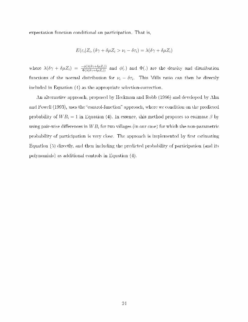
expectation function conditional on participation. That is,

E(εi|Zi, (δγ + δµZi > νi − δτi) = λ(δγ + δµZi)

where λ(δγ + δµZi) = −φ(λ(δγ+δµZi))Φ(λ(δγ+δµZi))

and φ(.) and Φ(.) are the density and distribution

functions of the normal distribution for νi − δτi. This Mills ratio can then be directly

included in Equation (4) as the appropriate selection-correction.

An alternative approach, proposed by Heckman and Robb (1986) and developed by Ahn

and Powell (1993), uses the �control-function� approach, where we condition on the predicted

probability of WBi = 1 in Equation (4). In essence, this method proposes to estimate β by

using pair-wise di�erences inWBi for two villages (in our case) for which the non-parametric

probability of participation is very close. The approach is implemented by �rst estimating

Equation (5) directly, and then including the predicted probability of participation (and its

polynomials) as additional controls in Equation (4).

24

Appendix II

Comparing Linear IV and Biprobit estimates

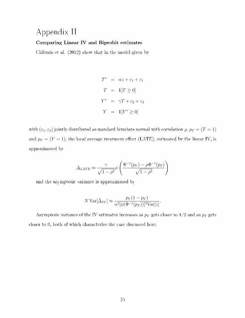
Chiburis et al. (2012) show that in the model given by

T ∗ = αz + c1 + ε1

T = 1[T ≥ 0]

Y ∗ = γT + c2 + ε2

Y = 1[Y ∗ ≥ 0]

with (ε1, ε2) jointly distributed as standard bivariate normal with correlation ρ, pT = (T = 1)

and pY = (Y = 1), the local average treatment e�ect (LATE), estimated by the linear IV, is

approximated by

∆LATE ≈γ√

1− ρ2φ

(Φ−1(pY )− ρΦ−1(pT )√

1− ρ2

)and the asymptotic variance is approximated by

N Var[∆̂IV ] ≈ pY (1− pY )

α2[φ(Φ−1(pT ))]2Var[z].

Asymptotic variance of the IV estimator increases as pY gets closer to 1/2 and as pT gets

closer to 0, both of which characterize the case discussed here.

25

References

[1] Ahn, Hyungtaik, and James Powell. 1993. �Semiparametric Estimation of Censored

Selection Models with a Nonparametric Selection Mechanism.� Journal of Econometrics.

58 (1-2): 3-29.

[2] Alderman, Harold, Jooseop Kim, and Peter F. Orazem. 2003. �Design, Evaluation, and

Sustainability of Private Schools for the Poor: The Pakistan Urban and Rural Fellowship

School Experiments.� Economics of Education Review. 22 (3): 265-274.

[3] Altonji, Joseph G., Todd E. Elder, and Christoper R. Taber. 2005. �An Evaluation of

Instrumental Variable Strategies for Estimating the E�ects of Catholic Schools.� Journal

of Human Resources. 40 (4): 791-821

[4] . Ali, Zahir and Abdul Nasir. 2010. �Land Administration System in Pakistan � Current

Situation and Stakeholders' Perception.� A paper presented at FIG Congress 2010,

Facing the Challenges � Building the Capacity. Sydney, Australia, 11� 16 April 2010

[5] Andrabi, Tahir, Jishnu Das, Asim Ijaz Khwaja, and Tristan Zajonc. 2006. �Religious

Education in Pakistan: A Look at the Data.� Comparative Education Review. 50 (3):

446-477.

[6] Andrabi, Tahir, Jishnu Das, and Asim Ijaz Khwaja. 2008. �A Dime a Day: The Pos-

sibilities and Limits of Private Schooling in Pakistan.� Comparative Education Review.

52 (3): 329-355.

[7] Andrabi, Tahir, Jishnu Das, Asim Ijaz Khwaja, and Tristan Zajonc. 2011a.�Do Value

Added Estimates Add Value? Accounting for Learning Dynamics.� American Economic

Journal: Applied Economics. 3(3): 29-54.

[8] Andrabi, Tahir, Natalie Bau, Jishnu Das, and Asim Ijaz Khwaja. 2011b. �Are bad public

schools public bads? Test Scores and Civic Values in private and public schools.� In

Progress.

[9] Angrist, Joshua David. 1995. �Conditioning on the Probability of Selection to Con-

trol Selection Bias�. Technical Working Paper No. 181, National Bureau of Economic

Research, Cambridge, MA.

[10] Angrist, Joshua, and Victor Lavy. 1999. �Using Maimonedes' Rule to Estimate the

E�ect of Class Size on Scholastic Achievement.� Quarterly Journal of Economics. 114

(2): 533-575.

26

[11] Aschauer, D. 1989a. "Is Public Expenditure Productive?" Journal of Monetary Eco-

nomics. 23 (2): 177- 200.

[12] Aschauer, D. 1989b. "Does Public Capital Crowd Out Private Capital?" Journal of

Monetary Economics. 24 (2): 171-188.

[13] Banerjee, Abhijit V. 2004. �Educational Policy and the Economics of the Family.� Jour-

nal of Development Economics. 74 (1): 3-32.

[14] Banerjee, Abhijit V., Shawn Cole, Esther Du�o, and Leigh Linden. 2007. �Remedying

Education: Evidence from Two Randomized Experiments in India.� Quarterly Journal

of Economics. 122 (3): 1235-1264.

[15] Campbell, D. T. 1969. �Reforms as Experiments.� American Psychologist. 24 (4): 409�

429.

[16] Carneiro, Pedro, Jishnu Das, and Hugo Reis. 2010. �Estimating The Demand for School

Attributes in Pakistan.� In Progress.

[17] Case, Anne, and Angus Deaton. 1999. �School Inputs and Educational Outcomes in

South Africa.� Quarterly Journal of Economics. 114 (3): 1047-1084.

[18] Chaudhury, Nazmul, Je� Hammer, Michael Kremer, Karthik Muralidharan, and F.

Halsey Rogers. 2006. �Missing in Action: Teacher and Health Worker Absence in De-

veloping Countries.� Journal of Economic Perspectives. 20 (1): 91-116.

[19] Chiburis, Richard, Jishnu Das, and Misha Lokshin. 2012. �A Practical Comparison of

the Bivariate Probit and Linear IV Estimators.� Economics Letters. 117 (3): 762-766.

[20] Corcoran, Sean P., William N. Evans, and Robert M. Schwab. 2004. �Changing Labor

Market Opportunities for Women and the Quality of Teachers, 1957-2000.� American

Economic Review. 94 (2): 230-235.

[21] Cutler, David M & Gruber, Jonathan. 1996. "Does Public Insurance Crowd Out Private

Insurance?" The Quarterly Journal of Economics. 111(2): 391-430.

[22] Downes, Thomas A., and Shane M. Greenstein. 1996. �Understanding the Supply Deci-

sions of Nonpro�ts: Modeling the Location of Private Schools.� Rand Journal of Eco-

nomics. 27 (2): 365-390.

27

[23] Du�o, Esther. 2001. �Schooling and Labor Market Consequences of School Construc-

tion in Indonesia: Evidence from an Unusual Policy Experiment.� American Economic

Review. 91 (4): 795-813.

[24] Du�o, Esther, Rema Hanna, and Stephen Ryan. 2012. �Incentives Work: Getting Teach-

ers to Come to School.� American Economic Review, 102(4): 1241-1278.

[25] Government of Pakistan. 1967. �The Punjab Land Revenue Act 1967.�

[26] Government of Pakistan. 1979. Chapter VII: Function of Rural Local Councils. Punjab

Local Government Ordinance 1979.

[27] Grindle, Merilee Serrill. 2004. Despite the Odds: The Contentious Politics of Education

Reform. Princeton, NJ: Princeton University Press.

[28] Hamid, Shahnaz. 2010. �Rural to Urban Migration in Pakistan: The Gender Perspec-

tive.� PIDE Working paper 2010: 56.

[29] Heckman, James J., and Richard Robb. 1986. �Alternative Methods for Solving the

Problem of Selection Bias in Evaluating the Impact of Treatments on Outcomes.�

In Howard Wainer (Ed.), Drawing Inferences from Self-Selected Samples. New York:

Springer-Verlag.

[30] Hoxby, Caroline M., and Andrew Leigh. 2004. �Pulled Away or Pushed Out? Explaining

the Decline of Teacher Aptitude in the United States.� American Economic Review. 94

(2): 236-240.

[31] Jimenez, Emmanuel, Marlaine E. Lockheed, and Vicente Paqueo. 1991. �The Relative

E�ciency of Private and Public Schools in Developing Countries.� World Bank Research

Observer. 6 (2): 205-218.

[32] Kim, Jooseop, Harold Alderman, and Peter F. Orazem. 1999. �Can Private School

Subsidies Increase Schooling for the Poor? The Quetta Urban Fellowship Program.�

World Bank Economic Review. 13 (3): 443-465.

[33] Krueger, Alan B. 1999. �Experimental Estimates of Education Production Functions.�

Quarterly Journal of Economics. 114 (2): 497-532.

[34] Ljungqvist, Lars. 1993. �Economic Underdevelopment: The Case of a Missing Market

for Human Capital.� Journal of Development Economics. 40 (2): 219-239.

28

[35] Muralidharan, Karthik, and Venkatesh Sundararaman. 2011.�Teacher Performance Pay:

Experimental Evidence from India.� Journal of Political Economy. 119(1) 39-77.

[36] Rivkin, Steven G., Eric A. Hanushek, and John F. Kain. 2005. �Teachers, Schools, and

Academic Achievement.� Econometrica. 73 (2): 417-458.

[37] Stock, James H., Jonathon H. Wright, and Motohiro Yogo. 2002. �A Survey of Weak

Instruments and Weak Identi�cation in Generalized Method of Moments.� Journal of

Business and Economic Statistics. 20 (4): 518-529.

[38] Tilak, Jandhyala B. G., and Ratna M. Sudarshan. 2001. �Private Schooling in Rural

India.� Working Paper #WP010009, National Council of Applied Economic Research,

New Delhi, India.

[39] Tooley, James. 2005. �Private Schools for the Poor: Education Where No One Expects

It.� Education Next. 5 (4): 22-32.

[40] Tooley, James, and Pauline Dixon. 2005. Private Education is Good for the Poor: A

study of private schools serving the poor in low-income countries. Washington, DC:

CATO Institute.

[41] UNESCO. 2004. Initiative for Teacher Education in Sub-Saharan Africa. New York:

United Nations Educational, Scienti�c and Cultural Organization.

[42] Urquiola, Miguel. 2006. �Identifying Class Size E�ects in Developing Countries: Evi-

dence from Rural Bolivia.� The Review of Economics and Statistics. 88 (1): 171-177.

[43] Urquiola, Miguel, and Emiliana Vegas. 2005. �Arbitrary Variation in Teacher Salaries:

An Analysis of Teacher Pay in Bolivia.� In Emiliana Vegas (Ed.), Incentives to Improve

Teaching . Washington, DC: The World Bank.

[44] West, M and Ludger Woessmann. 2010. � `Every Catholic child in a Catholic school':

Historical resistance to state schooling, contemporary school competition and student

achievement across countries.� Economic Journal 120 (546): F229-F255.

[45] World Bank. 2005. Improving Gender Outcomes: The Promise for Pakistan. Washing-

ton, DC: The World Bank.

29

Variable Mean 50 th Percentile S.D. N

1981 Number of Women with Middle+ Education 4.28 1 17.94 9333

1998 Number of Women with Middle+ Education 26.74 9 92.80 9333

1981 Percent Women with Middle+ Education 0.01 0 0.03 8882

1998 Percent Women with Middle+ Education 0.06 0.03 0.07 8915

Households Per Capita With Radio Access (1998) 0.03 0.02 0.03 8952Ratio of Females to Males, Under Age 14 (1998) 0.94 0.93 0.24 8892Area (Acres, 1998) 1550.34 1042 2520.51 9091

Percent of Houses Permanent (1998) 0.06 0.06 0.05 8935

Households with Water Access (1998) 0.01 0.001 0.02 8935

Households with Electricity Access (1998) 0.07 0.07 0.06 8935

1981 Total Population 1020.36 667.00 1247.91 9333

1998 Total Population 1537.70 961.00 2053.87 93331981 Population of Largest Village in PC  1670.04 1375.00 1310.46 9333

Number of Villages in PC (1998) 4.57 4 2.28 9333Girls' Secondary School Exists 0.02 0 0.16 9333

Girls' Primary School Exists 0.56 1 0.50 9330

Boys' Secondary School Exists 0.01 0 0.12 9333

Boys' Primary School Exists 0.70 1 0.46 9330

Girls' Secondary School Exposure (if one exists) 13.15 14 5.47 232

Girls' Primary School Exposure (if one exists) 21.43 18 11.80 4967

Boys' Secondary School Exposure (if one exists) 12.62 13.50 5.16 138

Boys' Primary School Exposure (if one exists) 35.21 31 19.66 6475Private School Exists 0.13 0 0.33 9258

Number of Private Schools 0.22 0 0.87 9258

Average Teaching Wage (Annual‐ log Rs) 9.04 9.10 0.70 1131

Private School Enrollment Rate (if one exists) 0.12 0.06 0.37 1165

Table I ‐ Summary Statistics (Village Level)

This table presents summary statistics for various variables of interest. The years for which the above data are 

given varies by source: All 1981/1998 variables are from the 1981/1998 Population Censuses while all schooling 

data is from the EMIS, NEC, or Private School Census.

30

(1) (2) (3) (4) (5) (6) (7) (8) (9) (10)

Dependent VariableGirls' Secondary 

School

Girls' Secondary 

School

Girls' Primary 

School

Boys' Primary 

School

Boys' Secondary 

SchoolWater Electricity

Permanent 

Houses

Girls' Secondary 

School

Girls' Secondary 

School

Instrument 0.0124*** 0.016*** 0.011 0.011 0.0008 ‐0.0002 0.002 0.002 0.012***

(0.004) (0.005) (0.015) (0.014) (0.0037) (0.0008) (0.001) (0.001) (0.004)‐0.005 ‐0.003

(‐0.008) (0.008)

Girls' Primary School Exists ‐0.052***

(0.004)

Boys' Secondary School Exists 0.232***

(0.017)

Boys' Primary School Exists 0.003

(0.005)

Area (000s of Acres) 0.001

(0.002)

% Houses Permanent 0.076

(0.053)

1981 Population (000s) 0.0059* 0.014 0.293*** 0.374*** ‐0.002 0.002 0.018*** ‐0.002 0.0087** 0.006*

(0.004) (0.010) (0.027) (0.025) (0.007) (0.001) (0.002) (0.002) (0.0035) (0.004)

1981 Population (000s)2 ‐0.0003 (0.001) ‐0.033*** ‐0.041*** 0.002* ‐0.0003* ‐0.002*** 0.0001 ‐0.0005** ‐0.0003

(0.0002) (0.001) (0.003) (0.003) (0.001) (0.0002) (0.0003) (0.0003) (0.0002) (0.0002)

1998 Population (000s) 0.003 0.003 ‐0.019 ‐0.054*** 0.008** 0.0001 ‐0.002 0.001 0.0029 0.003

(0.002) (0.005) (0.014) (0.013) (0.003) (0.0007) (0.001) (0.001) (0.0020) (0.002)

1998 Population (000s)2 ‐2x10‐5 0.0002 0.002*** 0.003*** 3x10‐5 2x10‐5 1x10‐4*** ‐1x10‐5 ‐2x10‐5 ‐2x10‐5

(5x10‐5) (0.0001) (0.0004) (0.0004) (10x10

‐5) (2x10

‐5) (0.1x10

‐4) (3x10

‐5) (5x10

‐5) (5x10

‐5)

PC Fixed Effects Y Y Y Y Y Y Y

R‐Squared 0.48 0.46 0.48 0.42 0.70 0.69

Adjusted R‐Squared 0.17

Pseudo R‐Squared 0.05 0.05 0.05

Chi‐Square Stat (Instrument = 13.04

F‐Stat (Instrument = 0) 8.9Observations 9333 8705 9330 9330 9333 8935 8935 8935 9333 9333

Table II ‐ First Stage and Falsification Tests

OLS Falsification Tests ‐ Other Public GoodsFalsification Test  ‐  Probit with QH 

Top Rank

Standard errors in parentheses with * indicating significance at 10%, ** at 5%, and *** at 1%. Columns (1)‐(2)  present first stage regressions using the eligibility rule as a predictor for the location of GSS. Column (1) 

gives the increased probability of finding a GSS in an eligible village (with basic population controls). Column (2) presents a linear first stage that includes controls for the village's population in 1981 and 1998, other 

village level public goods, and PC fixed effects. Columns (3)‐(8) check that the instrument does not predict other public goods. Columns (9)‐(10) show that a village having the highest population within a QH does not 

predict GSS construction.

First Stage ‐ Probit and OLS

Has Highest Population 

   in QH, 1981

31

(1) (2) (3) (4) (5) (6) (7)

OLSFirst 

Difference

Linear, Second 

Stage

Bivariate 

Probit ‐ ATE

Bivariate Probit ‐ 

Average ToT Effect

Reduced 

Form ‐ 

Program QHs

Reduced Form ‐ 

Non‐Program 

QHs

Instrument 0.038*** ‐0.0017

(0.014) (0.016)

0.095*** 0.097*** 1.505* 0.266* 0.246***

(0.025) (0.025) (0.802) (0.151) (0.092)

Girls' Primary School Exists 0.016* 0.089** xx xx 0.007 0.017

(0.0080) (0.043) (0.011) (0.014)

Boys' Secondary School Exists ‐0.005 ‐0.333* xx xx ‐0.030 0.112*

(0.034) (0.191) (0.040) (0.063)

Boys' Primary School Exists ‐0.005 ‐0.009 xx xx ‐0.009 0.001

(0.009) (0.012) (0.012) (0.014)

0.0190

(0.035)

‐0.011

(0.008)

‐0.026***

(0.010)

Area (000s of Acres) ‐0.008** ‐0.009** xx xx ‐0.029*** ‐0.002

(0.003) (0.004) (0.007) (0.004)

% Houses Permanent 0.194* 0.083 xx xx 0.184 0.208

(0.103) (0.142) (0.133) (0.163)

1981 Population (000s) 0.046*** 0.013 xx xx 0.035 0.054*

(0.017) (0.028) (0.027) (0.028)

1981 Population (000s)2 ‐0.0030 ‐0.0002 xx xx 0.004 ‐0.007**

(0.002) (0.003) (0.004) (0.003)

1998 Population (000s) 0.064*** 0.059*** xx xx 0.060*** 0.067***

(0.009) (0.012) (0.012) (0.014)

1998 Population (000s)2 ‐0.001*** ‐0.001*** xx xx ‐0.002*** ‐0.002***

(0.0003) (0.0004) (0.0005) (0.0004)

∆ Population (000s) 0.075***

(0.005)

PC Fixed Effects Y Y Y Y Y

R‐Squared 0.51 0.57

Adjusted R‐Squared 0.31 0.28

Prob > F 37.81 24.71

Prob > Chi‐Square 0.00

Observations 8705 8900 8705 8705 8705 5191 3514Number of PCs (1998) 2784

Table III ‐ GSS Impact on Private School Existence

Standard errors in parentheses with * indicating significance at 10%, ** at 5%, and *** at 1%. This table presents regression results for which the 

dependent variable is a dummy indicating the presence of at least one private school in a village (or the change in this variable for the first difference 

specification). Column (1)  gives OLS results for the impact of GSS on private school existence. Column (2) shows a first‐differenced specification.  (First‐

differencing Girls' Secondary School Exists does not change the variable because our sample contains no villages which had a GSS prior to 1981. That is, 

having a GSS in our sample is equivalent to receiving one after 1981.) Columns (3)‐(5) present the IV specifications. Column (3) gives the second stage 

results from a linear specification. Columns (4)‐(5) implement the bivariate probit specification and report, respectively, the average treatment effect and 

the treatment on the treated effect of a GSS on the existence of a private school with analytical standard‐errors computed using the delta method. 

Controls are present in these two regressions where marked with an "xx", but coefficients and standard errors are not given. These regressions also 

include (in the absence of PC fixed effects) linear and quadratic controls for the population of the largest village in the PC as well as a control for the 

number of villages in the PC. Columns (6)‐(7) present an additional check of the instrument by showing that the reduced form only holds in broad areas 

where at least one GSS was provided. Villages are divided into two sub‐groups: "program regions," where at least one village in the QH received a GSS 

[Column(6)]; and "non‐program regions," where no village in the QH received a GSS [Column (7)].

Received Girls' Primary 

   School After 1981Received Boys' Secondary 

   School After 1981Received Boys' Primary 

   School After 1981

Girls' Secondary School Exists 

( = Received GSS After 1981)

32

(1) (2) (3) (4) (5) (6) (7) (8)

Dependent Variable

OLSFirst 

DifferenceOLS

First 

Difference

Second 

Stage

Reduced 

FormOLS

First 

Difference

Instrument 3.46***

(1.19)

0.006***

(0.002)

0.0015***

(0.000)

0.001

(0.003)

0.0004**

(0.0002)

Girls' Secondary School Exists 0.097*** 10.81*** 9.52*** 219.32**

(0.025) (2.93) (3.55) (103.06)

Girls' Primary School Exists 2.37** 13.08** 1.79*

(0.99) (5.46) (0.98)

Boys' Secondary School Exists 7.51* ‐40.96* 9.98**

(3.98) (24.55) (3.93)

Boys' Primary School Exists 1.28 0.59 1.27

(1.06) (1.49) (1.06)

‐0.011 ‐4.32***

(0.008) (1.17)

0.019 14.25***

(0.035) (4.91)

‐0.026*** ‐0.65

(0.010) (1.36)

% Women with Middle+ Education 0.376***

(0.084)

% Men with Middle+ Education 0.033

(0.049)

∆ % Women w/ Middle+ Education 0.414***

(0.086)

∆ % Men w/ Middle+ Education ‐0.047

(0.050)

Area (000s of Acres) ‐0.008** ‐2.03*** ‐2.15*** ‐2.03*** ‐0.008**

(0.003) (0.39) (0.53) (0.39) (0.003)

% Houses Permanent 0.187* 44.83*** 28.43 45.14*** 0.276**

(0.104) (12.05) (18.30) (12.06) (0.128)

1981 Population (000s) 0.028 ‐1.61 ‐6.36* ‐3.35 0.046***

(0.018) (2.04) (3.63) (2.15) (0.017)

1981 Population (000s)2 ‐0.001 ‐0.32 0.07 ‐0.16 ‐0.003

(0.002) (0.24) (0.38) (0.25) (0.002)

1998 Population (000s) 0.065*** 9.71*** 8.91*** 9.45*** 0.064***

(0.009) (1.05) (1.49) (1.06) (0.009)

1998 Population (000s)2 ‐0.0012*** 1.79*** 1.76*** 1.79*** ‐0.0012***

(0.0003) (0.03) (0.05) (0.03) (0.0003)

∆ Population (000s) 0.075*** 60.39*** 0.072***

(0.005) (0.71) (0.005)

PC Fixed Effects Y Y Y Y Y Y Y Y

Adjusted R‐Squared 0.32 0.28 0.88 0.77 0.88 0.32 0.27

Prob > F 4.08Observations 8355 8900 8705 8975 8705 8705 8685 8711

Received Boys' Primary 

   School After 1981

Table IV ‐ Private School Existence: The Female Teacher Channel

Standard errors in parentheses with * indicating significance at 10%, ** at 5%, and *** at 1%. Columns (1)‐(2) present estimates for the effects of 

school exposure on private school existance from a linear probability model and a first difference specification. (First‐differencing Girls' Seconary 

School Exists does not change the variable because our sample contains no villages which had a GSS prior to 1981. That is, having a GSS in our 

sample is equivalent to receiving one after 1981.) Using the same approach, Columns (3)‐(4) assess the correlation between educated women and 

the presence of a GSS. Columns (5)‐(6) examine this relationship through an instrumental variable specification and present the second stage and 

reduced form. Finally, columns (7)‐(8) show the extent to which the extent of secondary‐school‐educated women in the village are associated with 

private school existence.

Private School Exists Number of Women with Middle+ Education Private School Exists

Years Exposure to Girls' 

   Secondary SchoolYears Exposure to Girls' 

   Primary SchoolYears Exposure to Boys' 

   Secondary SchoolYears Exposure to Boys' 

   Primary School

Received Girls' Primary 

   School After 1981Received Boys' Secondary 

   School After 1981

33

(1) (2) (3) (4) (5) (6) (7)

OLS HeckmanHeckman 

(Expanded First 

Stage)

Control 

Function

Control Function  

(Expanded First Stage)OLS OLS

Girls' Secondary School Exists ‐0.318* ‐0.321*** ‐0.321*** ‐0.324* ‐0.325* ‐0.356* ‐0.365**(0.186) (0.091) (0.092) (0.191) (0.187) (0.187) (0.188)

Girls' Primary School Exists 0.075 0.061 0.061 0.069 0.068 0.057 0.074(0.087) (0.042) (0.043) (0.099) (0.088) (0.087) (0.087)

Boys' Secondary School Exists 0.295 0.282** 0.285** 0.269 0.269 0.333 0.299(0.220) (0.111) (0.112) (0.226) (0.225) (0.221) (0.220)

Boys' Primary School Exists 0.019 0.015 0.0001 0.013 0.010 0.036 0.011(0.087) (0.042) (0.044) (0.096) (0.091) (0.087) (0.087)

0.028(0.085)1.567*(0.854)

0.051(0.467)0.305(0.266)

Area (000s of Acres) ‐0.058 ‐0.056*** ‐0.058*** ‐0.058 ‐0.058 ‐0.061 ‐0.061(0.039) (0.021) (0.021) (0.040) (0.039) (0.039) (0.039)

% Houses Permanent 0.006 0.055 0.046 0.016 0.003 ‐0.058 ‐0.238(1.320) (0.635) (0.644) (1.329) (1.327) (1.318) (1.333)

1981 Population (000s) 0.122 0.274** 0.253** 0.198 0.186 0.138 0.136(0.104) (0.110) (0.105) (0.185) (0.182) (0.105) (0.105)

1981 Population (000s)2 ‐0.021* ‐0.039*** ‐0.037*** (0.031) (0.030) ‐0.021* ‐0.022*(0.012) (0.014) (0.013) (0.021) (0.021) (0.012) (0.012)

1998 Population (000s) 0.028 0.097* 0.088* 0.033 0.027 0.016 0.027(0.053) (0.052) (0.049) (0.093) (0.092) (0.053) (0.053)

1998 Population (000s)2 0.001 ‐0.001 ‐0.001 0.0002 0.0003 0.001 0.001(0.001) (0.001) (0.001) (0.002) (0.002) (0.001) (0.001)

PC Fixed Effects Y Y Y Y Y Y Y

Adjusted R‐Squared 0.46 0.45 0.46 0.46 0.46Observations 1090 9292 9292 1090 1090 1090 1090

Table V ‐ Supply Side Impact: Average Teaching Wage in Private Schools

Standard errors in parentheses with * indicating significance at 10%, ** at 5%, and *** at 1%. This table examines the impact of GSS on skilled women wages. The dependent variable 

is the (logarithm of the) average salary of a private school teacher in the village. Since private school teachers are almost entirely women and educated women are mostly employed 

as teachers, this measure is a reasonable proxy for skilled women wages. Column (1) presents the OLS results. The sample is slightly smaller than the number of villages where there is 

a private school since, in a few cases in the PEIP data, private schools did not report wages. Columns (2)‐(5) correct for selection into the wage sample. Columns (2)‐(3) present results 

using Heckman's selection model. Columns (4)‐(5) use the "control function" approach. Columns (3) and (5) include the presence of a government boys primary school in the village as 

an additional instrument in the selection stage. Finally, columns (6)‐(7) present tentative evidence that wage declines are larger in villages where labor markets for women are more 

restricted. In both cases we have standardized the interaction variable so as to allow for the GSS coefficient itself to be interpretable/comparable to the previous specifications.  

Column (6) examines the differential effect of GSS construction on wages for more and less progressive villages using the (standardized) female/male ratio for children under the age 

of 14 as an indicator of gender bias. Column (7) presents similar results using (standardized) households per capita with access to radios as an indicator of village‐level development.

Std. Ratio of Females to Males, Under

   Age 14 × Girls' Secondary School Exists

Std. Households Per Capita With Radio 

   Access × Girls' Secondary School Exists

Std. Ratio of Females to Males, Under 

   Age 14

Std. Households Per Capita With Radio 

   Access

34

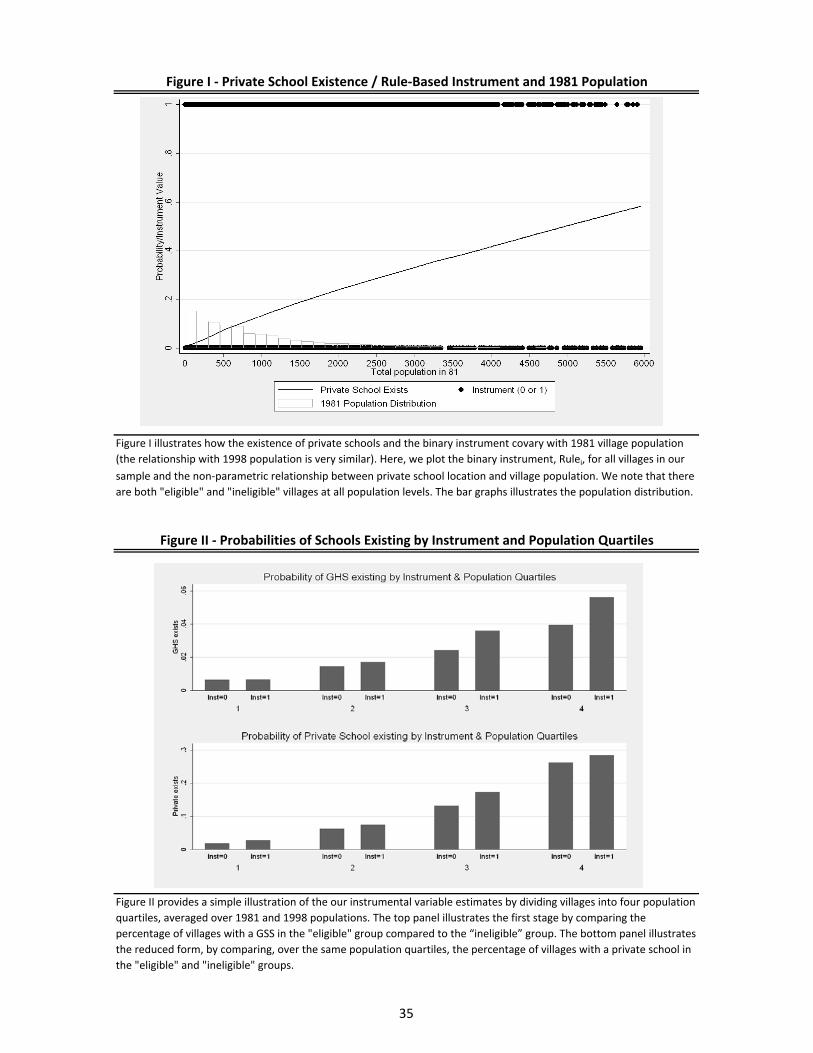
Figure I ‐ Private School Existence / Rule‐Based Instrument and 1981 Population

Fi I ill t t h th i t f i t h l d th bi i t t ith 1981 ill l ti

Figure II ‐ Probabilities of Schools Existing by Instrument and Population Quartiles

Figure I illustrates how the existence of private schools and the binary instrument covary with 1981 village population 

(the relationship with 1998 population is very similar). Here, we plot the binary instrument, Rulei, for all villages in our 

sample and the non‐parametric relationship between private school location and village population. We note that there 

are both "eligible" and "ineligible" villages at all population levels. The bar graphs illustrates the population distribution. 

Figure II provides a simple illustration of the our instrumental variable estimates by dividing villages into four population 

quartiles, averaged over 1981 and 1998 populations. The top panel illustrates the first stage by comparing the 

percentage of villages with a GSS in the "eligible" group compared to the “ineligible” group The bottom panel illustratespercentage of villages with a GSS in the  eligible  group compared to the  ineligible  group. The bottom panel illustrates 

the reduced form, by comparing, over the same population quartiles, the percentage of villages with a private school in 

the "eligible" and "ineligible" groups.

35

Variable Instrument=1 Instrument=0 Difference P‐Value

Area in Acres (1998) 2084.61 1326.88 757.73 0.00

44.58 32.12 57.43

Total Population (1981) 1644.75 759.79 884.96 0.00

22.78 14.48 26.82

Total Population (1998) 2516.91 1129.06 1387.85 0.00

43.42 22.22 44.38

% ∆ Population (1981 to 1998) 0.62 0.69 ‐0.07 0.24

0.030 0.037 0.059

Ratio of Females to Males (1981) 0.904 0.904 0.000 0.99

0.006 0.004 0.007

Ratio of Females to Males (1998) 0.938 0.946 ‐0.007 0.16

0.005 0.003 0.005

% Women Aged 4 and Below (1981) 0.158 0.154 0.004 0.63

0.007 0.005 0.008

% Women Aged 5‐14 (1981) 0.285 0.284 0.001 0.92

0.009 0.006 0.010

% Women with ID Card (1998) 0.490 0.478 0.012 0.30

0.010 0.006 0.012

% Literate Women, Aged 15+ (1981) 0.016 0.017 ‐0.001 0.74

0.002 0.002 0.003

% Women with Middle+ Education, Aged 15+  0.014 0.014 0.000 0.91

0.002 0.001 0.003

% Men Aged 4 and Below (1981) 0.144 0.141 0.004 0.65

0.007 0.004 0.008

% Men Aged 5‐14 (1981) 0.293 0.291 0.003 0.81

0.009 0.006 0.010

% Men with ID Card (1998) 0.691 0.684 0.007 0.50

0.009 0.006 0.011

% Literate Men, Aged 15+ (1981) 0.169 0.166 0.003 0.73

0.007 0.005 0.009

% Men with Middle+ Education, Aged 15+ (1981) 0.120 0.119 0.001 0.95

0.006 0.004 0.007

% Houses Permanent (1998) 0.063 0.065 ‐0.002 0.76

0.005 0.003 0.006

% Households with Water (1998) 0.011 0.010 0.001 0.61

0.002 0.001 0.002

% Households with Electricity (1998) 0.075 0.068 0.006 0.27

0.005 0.003 0.006

% Households with TV (1998) 0.029 0.028 0.001 0.82

0.003 0.002 0.004

% Household with Radio (1998) 0.025 0.028 ‐0.003 0.380.003 0.002 0.004

Appendix Table I ‐ Differences in Means

Standard errors in parentheses. This tables gives evidence that there are no unexpected baseline differences in observables 

between eligible (Instrument = 1) and ineligible (Instrument = 0) villages. The only significant differences are in population 

and area, which arise directly from the construction of the instrument. Several 1998 variables of interest are included when 

1981 numbers are not available, though these are not, strictly speaking, baseline measurements.

36

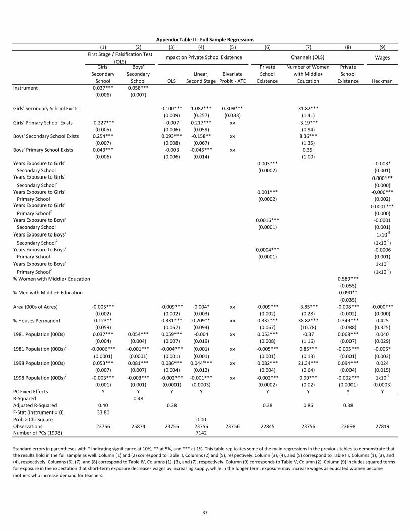
(1) (2) (3) (4) (5) (6) (7) (8) (9)

Wages

Girls' 

Secondary 

School

Boys' 

Secondary 

School OLS

Linear, 

Second Stage 

Bivariate 

Probit ‐ ATE

Private 

School 

Existence

Number of Women 

with Middle+ 

Education

Private 

School 

Existence Heckman

Instrument 0.037*** 0.058***

(0.006) (0.007)

Girls' Secondary School Exists 0.100*** 1.082*** 0.309*** 31.82***

(0.009) (0.257) (0.033) (1.41)

Girls' Primary School Exists ‐0.227*** ‐0.007 0.217*** xx ‐3.19***

(0.005) (0.006) (0.059) (0.94)Boys' Secondary School Exists 0.254*** 0.093*** ‐0.158** xx 8.36***

(0.007) (0.008) (0.067) (1.35)

Boys' Primary School Exists 0.043*** ‐0.003 ‐0.045*** xx 0.35

(0.006) (0.006) (0.014) (1.00)

0.003*** ‐0.003*

(0.0002) (0.001)

0.0001**

(0.000)

0.001*** ‐0.006***

(0.0002) (0.002)

0.0001***

(0.000)

0.0016*** ‐0.0001

(0.0001) (0.001)

‐1x10‐9

(1x10‐9)

0.0004*** ‐0.0006

(0.0001) (0.001)

1x10‐9

(1x10‐9)

% Women with Middle+ Education 0.589***

(0.055)

% Men with Middle+ Education 0.090**

(0.035)

Area (000s of Acres) ‐0.005*** ‐0.009*** ‐0.004* xx ‐0.009*** ‐3.85*** ‐0.008*** ‐0.000***

(0.002) (0.002) (0.003) (0.002) (0.28) (0.002) (0.000)

% Houses Permanent 0.123** 0.331*** 0.209** xx 0.332*** 38.82*** 0.349*** 0.425

(0.059) (0.067) (0.094) (0.067) (10.78) (0.088) (0.325)

1981 Population (000s) 0.037*** 0.054*** 0.059*** ‐0.004 xx 0.053*** ‐0.37 0.068*** 0.040

(0.004) (0.004) (0.007) (0.019) (0.008) (1.16) (0.007) (0.029)

1981 Population (000s)2 ‐0.0006*** ‐0.001*** ‐0.004*** (0.001) xx ‐0.005*** 0.85*** ‐0.005*** ‐0.005*

(0.0001) (0.0001) (0.001) (0.001) (0.001) (0.13) (0.001) (0.003)

1998 Population (000s) 0.053*** 0.081*** 0.086*** 0.044'*** xx 0.082*** 21.34*** 0.094*** 0.024

(0.007) (0.007) (0.004) (0.012) (0.004) (0.64) (0.004) (0.015)

1998 Population (000s)2 ‐0.003*** ‐0.003*** ‐0.002*** ‐0.001*** xx ‐0.002*** 0.99*** ‐0.002*** 1x10‐9

(0.001) (0.001) (0.0001) (0.0003) (0.0002) (0.02) (0.0001) (0.0003)

PC Fixed Effects Y Y Y Y Y Y Y Y

R‐Squared 0.48

Adjusted R‐Squared 0.40 0.38 0.38 0.86 0.38

F‐Stat (Instrument = 0) 33.80

Prob > Chi‐Square 0.00

Observations 23756 25874 23756 23756 23756  22845 23756 23698 27819Number of PCs (1998) 7142

Appendix Table II ‐ Full Sample Regressions

Years Exposure to Girls' 

   Secondary SchoolYears Exposure to Girls' 

   Secondary School2

Years Exposure to Girls' 

   Primary School

First Stage / Falsification Test 

(OLS)Impact on Private School Existence Channels (OLS)

Standard errors in parentheses with * indicating significance at 10%, ** at 5%, and *** at 1%. This table replicates some of the main regressions in the previous tables to demonstrate that 

the results hold in the full sample as well. Column (1) and (2) correspond to Table II, Columns (2) and (5), respectively. Column (3), (4), and (5) correspond to Table III, Columns (1), (3), and 

(4), respectively. Columns (6), (7), and (8) correspond to Table IV, Columns (1), (3), and (7), respectively. Column (9) corresponds to Table V, Column (2). Column (9) includes squared terms 

for exposure in the expectation that short‐term exposure decreases wages by increasing supply, while in the longer term, exposure may increase wages as educated women become 

mothers who increase demand for teachers.

Years Exposure to Girls' 

   Primary School2

Years Exposure to Boys' 

   Secondary School

Years Exposure to Boys' 

   Secondary School2

Years Exposure to Boys' 

   Primary School

Years Exposure to Boys' 

   Primary School2

37