STUDENT JOURNAL OF PHYSICS - iopb.res.insjp/sjp_past_issues/sjp632017/full.pdf · Departament d’Estructura i Constituents de la Mat`eria and ... Nucleons are composed of three valence

Volume 6 Number 3 Jul - Sep 2017

STUDENT JOURNAL OF PHYSICS

INTERNATIONAL EDITION

INDIAN ASSOCIATION OF PHYSICS TEACHERS

ISSN – 2319-3166


This is a quarterly journal published by Indian Association Of Physics Teachers. It publishes research articlescontributed by Under Graduate and Post Graduate students of colleges, universities and similar teachinginstitutions, as principal authors.

INTERNATIONAL EDITORIAL BOARD

Editor-in-Chief

L. SatpathyInstitute of Physics, Bhubaneswar, IndiaE-mail: [email protected]

Chief Editors

Mahanti, S. D.Physics and Astronomy Department, Michigan State University, East Lansing, Mi 48824, USAE-mail: [email protected], A.M.Institute of Physics, Bhubaneswar, IndiaE-mail: [email protected]

EDITORS

Caballero, DannyDepartment of Physics, Michigan State University, U.S.A.E-mail: [email protected], GerdJoint Professor in Physics & Lyman Briggs College, Michigan State University, U.S.A.E-mail: [email protected] Mohanty, BedangaNISER, Bhubaneswar, IndiaE-mail: [email protected], PrasantaIISER, Kolkata, IndiaE-mail: [email protected] Prasad, K.C.Mahatma Gandhi College, Thiruvananthapuram, IndiaE-mail: [email protected], RalphPhysics Department, University of Uppsala, SwedenE-mail: [email protected], Vijay A.Homi Bhabha Centre for Science Education (TIFR), Mumbai, IndiaE-mail: [email protected], AllisonDepartment of Physics, University of Bath Bath BA2 7AY, UKE-mail: [email protected]

INTERNATIONAL ADVISORY BOARD

Mani, H.S.CMI, Chennai, India ([email protected]) Moszkowski, S. M.UCLA, USA ([email protected]) Pati, Jogesh C.SLAC, Stanford, USA ([email protected]) Prakash, SatyaPanjab University, Chandigarh, India ([email protected]) Ramakrishnan, T.V.BHU, Varanasi, India ([email protected]) Rajasekaran, G.The Institute of Mathematical Sciences, Chennai, India ([email protected])Sen, AshokeHRI, Allahabad, India ([email protected]) Vinas, X.Departament d’Estructura i Constituents de la Mat`eria and Institut de Ci`encies del Cosmos, Facultat de F´ısica, Universitat de Barcelona, Barcelona, Spain ([email protected])

TECHNICAL EDITOR

Pradhan, D.ILS, Bhubaneswar, India([email protected])

WEB MANAGEMENT

Ghosh, Aditya PrasadIOP, Bhubaneswar, India([email protected])

Registered Office

Editor-in-Chief, SJP, Institute of Physics, Sainik School, Bhubaneswar, Odisha, India – 751005(www.iopb.res.in/~sjp/)


Scope of the Journal

The journal is devoted to research carried out by students at undergraduate level. It provides a platform for the youngstudents to explore their creativity, originality, and independence in terms of research articles which may be written in

collaboration with senior scientist(s), but with a very significant contribution from the student. The articles will be judgedfor suitability of publication in the following two broad categories:

1. Project based articles

These articles are based on research projects assigned and guided by senior scientist(s) and carried out predominantly or entirely by the student.

2. Articles based on original ideas of student

These articles are originated by the student and developed by him/ her with possible help from senior advisor.Very often an undergraduate student producing original idea is unable to find a venue for its expression where it

can get due attention. SJP, with its primary goal of encouraging original research at the undergraduate level provides a platform for bringing out such research works.

It is an online journal with no cost to the author.Since SJP is concerned with undergraduate physics education, it will occasionally also publish articles on science education

written by senior physicists.

Information for Authors

• Check the accuracy of your references.• Include the complete source information for any references cited in the abstract. (Do not cite reference numbers in

the abstract.)• Number references in text consecutively, starting with [1].

• Language: Papers should have a clear presentation written in good English. Use a spell checker.

Submission

1. Use the link "Submit" of Website to submit all files (manuscript and figures) together in the submission (either as a single .tar file or as multiple files)

2. Choose one of the Editors in the link "Submit" of Website as communicating editor while submitting your manuscript.

Preparation for Submission

Use the template available at "Submit" section of Website for preparation of the manuscript.

Re-Submission

• For re-submission, please respond to the major points of the criticism raised by the referees.• If your paper is accepted, please check the proofs carefully.

Scope

• SJP covers all areas of applied, fundamental, and interdisciplinary physics research.

http://www.iopb.res.in/~sjp/submit.php




Studying the Puzzle of the Pion Nucleon Sigma Term

Christopher Kane1∗1Senior Undergraduate Student, Department of Paper and Bioprocess Engineering, SUNY ESF, Syracuse, NewYork, USA.

Abstract. In this paper I investigate the flavor dependence of the pion nucleon sigma term (σπN ) for theNf = 2, Nf = 2 + 1, and Nf = 2 + 1 + 1 cases, where Nf is the number of flavors. I calculate σπNusing the Hellmann-Feynman method which uses results of lattice quantum chromodynamics (LQCD). I usethe expansion from Baryon Chiral Perturbation Theory as my nucleon mass fitting equation. I extrapolate thedata to a → 0, where a is the spacing of the lattice in LQCD, and apply the constraint that data must meet thecondition MπL > 3.8 to avoid finite volume effects, where Mπ is the pion mass and L is the length of thelattice in LQCD. My results shed light on the recent disparity between values of σπN calculated using differentmethods.

1. INTRODUCTION

The search for dark matter has seen a surge of interest in recent years with the hope of findingphysics beyond the standard model. All current experimental searches rely on dark matter particlesinteracting with nucleonic matter, i.e. protons and neutrons. One leading candidate for a darkmatter particle is the neutralino, which is predicted by the theory of super-symmetry [1]. In orderto constrain experiments searching for the neutralino, the cross section of interaction with nucleonsmust be known. The pion-nucleon sigma term (σπN ), which is a fundamental parameter in the theoryof quantum chromodynamics (QCD), is used to calculate this cross section [2]. It was originallycalculated by phenomenological methods but recently has been calculated using methods involvingLQCD. There is a disparity between the two methods however, with σπN being significantly lowerusing the latter method [3]. This disparity is large enough to cause concern in the dark mattercommunity as experiments would need to be changed accordingly.

One method of calculating σπN using LQCD data is called the Hellman-Feynman (HF) method.The HF theorem relates σπN to the nucleon mass (MN ) dependence on the quark mass (mq) [4].The HF theorem can also relate σπN to the nucleon mass dependence on the pion mass (Mπ) asM2π = mq . From this point on, Mπ and mq will be used interchangeably with this understanding.

The HF theorem is defined in Eq. 1.

σπN = mq∂

∂mqMN (mq) = M2

π

∂

∂M2π

MN (M2π) (1)

∗Summer REU student at the Department of Physics and Astronomy, Michigan State University, East Lansing, Michigan48823, USA. Email: [email protected]

122


LQCD is used to calculate the nucleon mass from a given quark mass (quark masses need not bephysical). These data points are in turn used to determine the nucleon mass dependence on thequark mass the HF theorem requires to calculate σπN . It does so by simulating the dynamics insidethe nucleon. Nucleons are composed of three valence quarks, but from the Heisenberg UncertaintyPrinciple, ∆E∆t ≥ ~2, we know that quark-antiquark pairs can be created and annihilated from thevacuum. Heavier quarks will be created for shorter periods of time and therefore will have a smallereffect on the internal dynamics of the nucleon. It is common in LQCD simulations to assume thatonly the two and three lightest flavors (up, down, strange) of quarks contribute to the dynamics andthat contributions from the heavier flavors (charmed, top, and bottom) can be ignored. In this paperI present results of σπN calculated from data that included the two lightest flavors (Nf = 2), threelightest flavors (Nf = 2 + 1), and four lightest flavors (Nf = 2 + 1 + 1) to see if the heavier quarkshave a significant contribution or if they can be safely ignored in further simulations.

2. LATTICE QCD

2.1 Overview

QCD is the theory that describes how quarks and gluons interact via the strong force. At highenergies, i.e. particle accelerators, perturbation theory can be used to perform precise calculations.At low energies however, i.e. inside a nucleon, perturbation theory fails and calculations can nolonger be done. Lattice QCD is a fully non-perturbative formulation of QCD that can performcalculations at any energy [5].

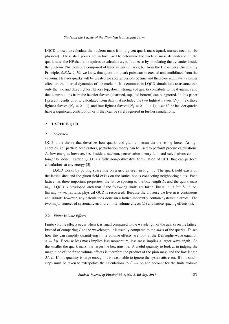
LQCD works by putting spacetime on a grid as seen in Fig. 1. The quark field exists onthe lattice sites and the gluon field exists on the lattice bonds connecting neighboring sites. Eachlattice has three important properties, the lattice spacing a, the box length L, and the quark massmq . LQCD is developed such that if the following limits are taken, lim a → 0, limL → ∞,limmq → mq,physical, physical QCD is recovered. Because the universe we live in is continuousand infinite however, any calculations done on a lattice inherently contain systematic errors. Thetwo major sources of systematic error are finite volume effects (L) and lattice spacing effects (a).

2.2 Finite Volume Effects

Finite volume effects occur when L is small compared to the wavelength of the quarks on the lattice.Instead of comparing L to the wavelength, it is usually compared to the mass of the quarks. To seehow this can simplify quantifying finite volume effects, we look at the DeBroglie wave equationλ = hp. Because less mass implies less momentum, less mass implies a larger wavelength. Sothe smaller the quark mass, the larger the box must be. A useful quantity to look at in judging themagnitude of the finite volume effects is therefore the product of the pion mass and the box lengthMπL. If this quantity is large enough, it is reasonable to ignore the systematic error. If it is small,steps must be taken to extrapolate the calculations to L → ∞ and account for the finite volume

Student Journal of Physics,Vol. 6, No. 3, Jul-Sep. 2017 123

Christopher Kane

Figure 1. Image of a proton on a typical lattice in LQCD. The lattice spacing a is ingreen and the box length L is in red. The image is reproduced with the permission ofProfessor H. Lin.

effects.

2.3 Lattice Spacing Effects

Finite lattice spacing effects occur when a is too large to properly simulate strong force dynamics.The value of a necessary is less dependent on mq than L. A standard value of a generally acceptedto limit the size of finite lattice spacing effects is a < 0.1 fm. The leading corrections in thelattice spacing effects that remain are typically O(a2) [5]. As systematic errors are unique to eachsimulation, results can be extrapolated to a→ 0 by adding a term cja

2 to the fitting equation wherej indicates what collaboration each data point was calculated by. The cj terms are then treated asfitting parameters.

3. METHOD OF CALCULATION

3.1 Applying the Hellmann-Feynman Theorem

The HF methods requires a functional relationship between the nucleon mass and quark mass. Toachieve the necessary functional relationship, I use the expansion taken from Baryon Chiral Pertur-bation Theory (BχPT) [6]. The first several terms of the expansion in the pion mass can be seen inEq. 2.

MN (M2π) = M0 − 4C1M

2π +

1

2αM4

π +C1

8π2f2πM4π ln

M2π

M0(2)

124 Student Journal of Physics,Vol. 6, No. 3, Jul-Sep. 2017


The terms M0, C1, and α are low energy constants (LECs) that must be determined beforecalculating σπN . Once they are known, the HF theorem allows for a straightforward calculation ofσπN through a simple analytic derivative given by Eq. 3.

σπN = −4C1M2π + αM4

π +C1

4π2f2πM4π ln

M2π

M20

+C1

8π2f2πM4π (3)

3.2 Determining the Low Energy Constants

The LECs are determined by fitting Eq. 2 to the nucleon mass data generated by LQCD using vary-ing pion masses. All sources of error are small enough compared to the error in the values of MN

and are therefore deemed negligible. Additionally, errors in MN are assumed to be uncorrelated.To ensure that finite volume effects were negligible, points that did not satisfy MπL > 3.8 did notenter the fit. Points were extrapolated to a → 0 by including a term of the form cja

2 in the fit foreach collaboration data was taken from. Three cj terms were added in the Nf = 2 case and two cjterms were added in both the Nf = 2 + 1 and Nf = 2 + 1 + 1 case. The final χ2 function that Iminimize is

χ2 =∑i=1

MN (M2π) + cja

2 − di(M2π)

σi, (4)

where di(M2π) are the LQCD data points for MN with associated uncertainties σi. The common

fitting parameters for all three fits include M0, C1, and α. A good fit will have χ2/dof ∼= 1, wheredof is short for the degrees of freedom in the fit and is defined as the number of data points (di)minus the number of fitting parameters (i.e. M0, C1, α, cj). Uncertainties in the fit parameters,nucleon mass, and σπN were determined using the standard jackknife procedure described in [7].All values will be given in the form mean(stdev). As an example, 7.92(13) shows that the meanvalue is 7.92 with an associated standard deviation is 0.13.

4. RESULTS

For the fit usingNf = 2 LQCD collaboration data, seven points were taken from the Mainz collabo-ration [8], six points were taken from the RQCD collaboration [9], and seven points were taken fromthe ETM collaboration [10]. The three extrapolation parameters (cj of Eq. 4), can be found in Table1. The cLQCD and cRQCD terms are consistent with zero while the cMainz term is not. This showsthat the systematic error introduced in the ETM and RQCD collaborations were similar in magnitudeand thus a non-zero extrapolation was necessary for the Mainz data points. For the Nf = 2 + 1 fit,nine points were taken from the LHP collaboration [11] and five points were taken from the NMEcollaboration [12]. The extrapolation parameters cLHP and cNME are not consistent with zero asseen in Table 1. For the Nf = 2 + 1 + 1 fit, fifteen points were taken from the ETM collaboration


Christopher Kane

[13] and six points were taken from the PNDME collaboration [14]. Like the Nf = 2 + 1 case, theextrapolation parameters cETMC and cPNDME are not consistent with zero as seen in Table 1.

2*Nf = 2 cRQCD −0.12(15)

cETMC 0.15(14)cMainz 0.55(19)

2*Nf = 2+1 cLHP 0.124(9)cNME −0.166(4)

2*Nf = 2+1+1 cETMC 0.136(4)cPNDME −0.042(25)

Table 1. Extrapolation parameter values (a→ 0) for the Nf = 2, 2+1, 2+1+1 fits.

The fit for the Nf = 2 case can be seen in Fig. 2. The large χ2/dof can be explained byanalyzing the contribution of each individual data point to the total value. In this fit, three datapoints contributed to more than 50% of the total value. From this it is seen that using Eq. 2 asthe fitting equation is appropriate, and the systematic error in the three data points in question wasunderestimated. The fit for the Nf = 2 + 1 case can be found in Fig. 3. Although the χ2/dofis smaller than in the Nf = 2 case, it is still not low enough to be considered a good fit. Similarto the previous case however, three data points accounted for over 50% of the value. This leadsto the same conclusion that the systematic error in those data points were underestimated. Thefit for the Nf = 2 + 1 + 1 case can be seen in Fig. 4. The χ2/dof is within the range to indi-cate a good fit. This shows that errors in all data points have appropriate errors associated withthem.

Nf M0 [GeV] C1 [GeV-1] α [GeV-3] σπN [MeV] χ2dof

2 0.908(4) −0.55(6) −5.4(1.8) 40(4) 4.762+1 0.901(23) −0.26(18) 11(10) 25(11) 2.04

2+1+1 0.916(18) −0.56(4) −7.5(9) 40(3) 1.31

Table 2. Results for BχPT fits to Nf = 2, 2+1, 2+1+1 nucleon mass data.

The values of σπN for the Nf = 2 and Nf = 2 + 1 cases, seen in Table 2, agree with valuesproduced by [6] within errorbars. Comparing the values of σπN for all three cases, we see that themean values for the Nf = 2 and Nf = 2 + 1 + 1 cases are equal with similar error bars. The meanvalue for the Nf = 2 + 1 case is significantly smaller comparatively, but has a standard deviation of40% the mean value. Because of this large error, the value still agrees with the Nf = 2 case withinerror bars and is just over one standard deviation away from agreeing with the Nf = 2 + 1 + 1

case within error bars. Furthermore, comparing the values of the fitting parameters it is seen that thevalues ofM0 for the three cases are not statistically different. The values ofC1 and α for theNf = 2

and Nf = 2 + 1 + 1 cases are indistinguishable while the values for the Nf = 2 + 1 case disagree.



0.9

1

1.1

1.2

1.3

1.4

1.5

0 0.05 0.1 0.15 0.2 0.25 0.3 0.35

Nf=2

M N[G

eV]

Mπ2[GeV2]

RQCDMainzETMC

Figure 2. Nf=2 flavor fit of nucleon mass vs. pion mass squared. Data points fromRQCD are in green, from Mainz are in red, and from ETMC are in blue. The shadedblue region is the uncertainty in the MN calculations while the solid dark blue line isthe mean value of MN .

0.9

1

1.1

1.2

1.3

1.4

1.5

0 0.05 0.1 0.15 0.2 0.25 0.3 0.35

Nf=2+1+1

M N[G

eV]

Mπ2[GeV2]

LHPCNME

Figure 3. Nf = 2 + 1 flavor fit of nucleon mass vs. pion mass squared. Data pointsfrom NME are in blue and points from LHPC are in green.

0.9

1

1.1

1.2

1.3

1.4

1.5

0 0.05 0.1 0.15 0.2 0.25 0.3 0.35

Nf=2+1+1

M N[G

eV]

Mπ2[GeV2]

ETMCPNDME

Figure 4. Nf = 2 + 1 + 1 flavor fit of nucleon mass vs. pion mass squared. Datapoints from ETMC are in red and points from PNDME are in green.


Christopher Kane

However, the error in C1 and α for the Nf = 2 + 1 case are, again large, with values of 70% and90% of the mean respectively. One possibility for the large error in the Nf = 2 + 1 case is the smallnumber of available data points compared to the other cases. The Nf = 2 and Nf = 2 + 1 + 1 hadtwenty data points that met the fit requirements while the Nf = 2 + 1 case had only fourteen pointsthat met the fit requirements. Because of the large error in the parameters for the three flavor case,I cannot conclude the value of σπN is statistically different from the two and four flavor case. Thefits therefore show that the values of σπN for the three cases are not statistically different and thereis no apparent flavor dependence.

5. SUMMARY AND CONCLUSION

In this work I collected data from various collaborations generated using lattice QCD for the twoflavor, three flavor, and four flavor cases. The data needed to meet the requirement that MπL > 3.8

to assure finite volume effects could be safely ignored. Terms of the form cja2 were added to the

fitting equation to account for lattice spacing effects. This data was fitted to an expansion of thenucleon mass in terms of the pion mass developed from Baryon Chiral Perturbation Theory. Oncethe low energy constants were determined, I applied the Hellmann-Feynman theorem to the fittingequation in order to calculate σπN . Comparing the values of σπN for the three cases, it is seen thatthey are not statistically different. This shows that after a first level analysis, σπN has no significantdependence on the number of flavors included in the LQCD simulations. The inclusion of heavierquarks can therefore not account for the disparity in values calculated by phenomenological methodsand LQCD methods.

6. ACKNOWLEDGEMENTS

I would like to thank Michigan State University and the NSF for the opportunity to participate in thiswork. I would also like to thank Professor Huey-Wen Lin for her guidance throughout the project.

References

[1] Y. Shadmi, Introduction to Supersymmetry, in Proceedings, 2014 European School of High-EnergyPhysics (ESHEP 2014): Garderen, The Netherlands, June 18 - July 01 2014, pp. 95123, 2016.

[2] J. Giedt, A. W. Thomas, and R. D. Young, Dark matter, the CMSSM and lattice QCD, Phys. Rev. Lett.,vol. 103, p. 201802, 2009.

[3] Y.-B. Yang, A. Alexandru, T. Draper, J. Liang, and K.-F. Liu, N and strangeness sigma terms at thephysical point with chiral fermions, Phys. Rev., vol. D94, no. 5, p. 054503, 2016.

[4] R. P. Feynman, Forces in molecules, Phys. Rev., vol. 56, pp. 340343, Aug 1939.[5] R. Gupta, Introduction to lattice QCD: Course, in Probing the standard model of particle interactions.

Proceedings, Summer School in Theoretical Physics, NATO Advanced Study Institute, 68th session, LesHouches, France, July 28-September 5, 1997. Pt. 1, 2, pp. 83219, 1997.



[6] L. Alvarez-Ruso, T. Ledwig, J. Martin Camalich, and M. J. Vicente-Vacas, Nucleon mass and pion-nucleon sigma term from a chiral analysis of lattice QCD data, Phys. Rev., vol. D88, no. 5, p. 054507,2013.

[7] B. Efron, The jackknife, the bootstrap and other resampling plans. SIAM, 1982.[8] G. von Hippel, T. D. Rae, E. Shintani, and H. Wittig, Nucleon matrix elements from lattice QCD with

all-mode-averaging and a domain-decomposed solver: an exploratory study, Nucl. Phys., vol. B914, pp.138159, 2017.

[9] G. S. Bali, S. Collins, B. Gl assle, M. G ockeler, J. Najjar, R. H. R odl, A. Sch afer, R. W. Schiel, W. Soldner, and A. Sternbeck, Nucleon isovector couplings from N f = 2 lattice QCD, Phys. Rev., vol. D91,no. 5, p. 054501, 2015.

[10] C. Alexandrou, M. Brinet, J. Carbonell, M. Constantinou, P. A. Harraud, P. Guichon, K. Jansen, T. Korzec,and M. Papinutto, Axial Nucleon form factors from lattice QCD, Phys. Rev., vol. D83, p. 045010, 2011.

[11] J. R. Green, J. W. Negele, A. V. Pochinsky, S. N. Syritsyn, M. Engelhardt, and S. Krieg, Nucleon elec-tromagnetic form factors from lattice QCD using a nearly physical pion mass, Phys. Rev., vol. D90, p.074507, 2014.

[12] B. Yoon et al., Isovector charges of the nucleon from 2+1-flavor QCD with clover fermions, Phys. Rev.,vol. D95, no. 7, p. 074508, 2017.

[13] C. Alexandrou, V. Drach, K. Jansen, C. Kallidonis, and G. Koutsou, Baryon spectrum with N f = 2 + 1 +1 twisted mass fermions, Phys. Rev., vol. D90, no. 7, p. 074501, 2014.

[14] G. Rajan, J. Yong-Chull, L. Huey-Wen, Y. Boram, and B. Tanmoy, Axial Vector Form Factors of theNucleon from Lattice QCD, 2017.



One-Dimensional Chain Collisions for Different Intermediate MassSystems

Renu Raman Sahu1∗, Ayush Amitabh2 and Vijay A. Singh3†1Second Year, Int. M.Sc., School of Physical Sciences, National Institute of Science Education and Research,Jatani -752050, Odisha, India.2Second Year, B.Sc., Physics Department, Patna Science College, Ashok Rajpath, Patna, Bihar-800 006, India.3Centre for Excellence in Basic Sciences, Mumbai University, Kalina, Santa-Kruz East, Mumbai 400 093,India.

Abstract. It is known that one can transfer the bulk of the kinetic energy of a body to another body ofsmaller mass by arranging a large number of collisions with intermediate masses. In this project we explorethe transfer of kinetic energy for masses arranged in arithmetic and harmonic progression. We also take intoaccount inelastic collisions and find that there is an optimum number of intermediate masses which will ensuremaximal transfer of kinetic energy. We have discovered interesting duality relations. Irrespective of the factthat the collisions are elastic or inelastic, we find that the results of arithmetic progression map onto that of theharmonic progression.

1. INTRODUCTION

Collision is one of the simplest mechanical interaction between two bodies and in the process energyand momentum are exchanged. One-dimensional collision as a means of transferring energy andensuring velocity amplification is of interest because it provides a simple model for understandingnatural phenomena where sequential collisions come into play. For example supernova explosioncan be understood with the help of one-dimensional chain collision of vertically stacked masses [1].Kerwin has explained the phenomena of super-ball collisions using an analytical method [2]. Thedynamics of a queue, chain accidents in traffic, systems with narrow passage to allow for a singleparticle etc. can be modelled as one-dimensional chain collision systems.

The quantity of interest in studying such systems is the fraction of energy or momentum thatis transferred. The exchange of kinetic energy and momentum depends mainly on the coefficientof restitution e and the ratios of colliding masses. The coefficient of restitution is a property of thecolliding masses and for masses made of similar material we shall assume that it is a constant. Whatone can manipulate is ‘mass’ because one can extract a particular amount of mass from the bulk.Brilliantov and Poschel considered viscoelastic particles where e is a function of colliding massesand their relative velocity [3]. Recently, Ricardo and Lee showed that the maximum transfer of

∗[email protected]†[email protected]

130

One-Dimensional Chain Collisions for Different Intermediate Mass Systems

kinetic energy takes place if the intermediate masses are geometric means of final and initial mass[4]. They have also considered the case of inelastic collision with fixed coefficient of restitution e.

In our work, we take two different intermediate mass systems and compare the numerical valuesof kinetic energy and velocity transfer ratios for a given value of initial and final mass. UnlikeRicardo and Lee, we take masses in arithmetic and harmonic progression. We consider the generalcase of inelastic collision.

2. BASIC EQUATIONS

We assume that the two colliding masses are spheres placed on the x- axis in such a way that thedistance between their centres is greater than the sum of their radii. Let a mass M moving withvelocity V , collide with a mass m which was intially at rest and due to which it’s velocity changesto V ′ while the mass m gains a velocity v. This is shown in Fig. 1.

M

V

m

0

MassBefore Collision

Velocity

M

V ′

m

v

After Collision

Figure 1. Collision of two masses

We define the velocity transfer ratio rv as

rv =v

V

Similarly kinetic energy transfer ratio is defined as

rK =12mv2

12MV 2

Since the momentum is conserved we have

MV = MV ′ +mv (1)

The coefficient of restitution is

e = (v − V ′)/V (2)

Using eqns. (1) and (2) we get the expression for velocity transfer ratio

rv =(e+ 1)M

(M +m)(3)


Renu Raman Sahu, Ayush Amitabh and Vijay A. Singh

M m1 m2 mn m

1st 2nd (n+ 1)thCollision

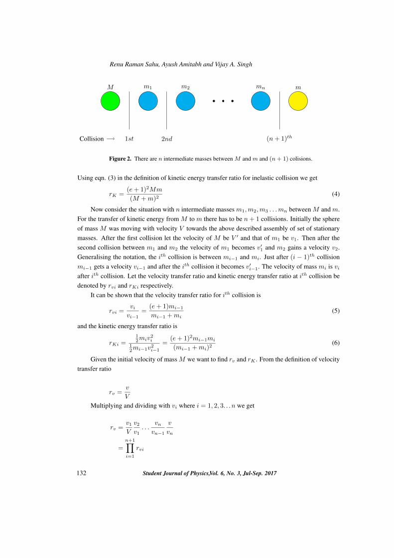
Figure 2. There are n intermediate masses between M and m and (n+ 1) colisions.

Using eqn. (3) in the definition of kinetic energy transfer ratio for inelastic collision we get

rK =(e+ 1)2Mm

(M +m)2(4)

Now consider the situation with n intermediate masses m1,m2,m3 . . .mn between M and m.For the transfer of kinetic energy from M to m there has to be n+ 1 collisions. Initially the sphereof mass M was moving with velocity V towards the above described assembly of set of stationarymasses. After the first collision let the velocity of M be V ′ and that of m1 be v1. Then after thesecond collision between m1 and m2 the velocity of m1 becomes v′1 and m2 gains a velocity v2.Generalising the notation, the ith collision is between mi−1 and mi. Just after (i − 1)th collisionmi−1 gets a velocity vi−1 and after the ith collision it becomes v′i−1. The velocity of mass mi is viafter ith collision. Let the velocity transfer ratio and kinetic energy transfer ratio at ith collision bedenoted by rvi and rKi respectively.

It can be shown that the velocity transfer ratio for ith collision is

rvi =vi

vi−1=

(e+ 1)mi−1

mi−1 +mi(5)

and the kinetic energy transfer ratio is

rKi =12miv

2i

12mi−1v2i−1

=(e+ 1)2mi−1mi

(mi−1 +mi)2(6)

Given the initial velocity of mass M we want to find rv and rK . From the definition of velocitytransfer ratio

rv =v

V

Multiplying and dividing with vi where i = 1, 2, 3. . .n we get

rv =v1V

v2v1

. . .vn

vn−1

v

vn

=

n+1∏i=1

rvi



Similarly

rK =

n+1∏i=1

rKi (7)

Next we consider two intermediate mass systems, arithmetic and harmonic.

3. INTERMEDIATE MASS SYSTEMS

3.1 Intermediate Masses in Arithmetic Progression

In this case the intermediate masses mi are such that M > m1 > m2 . . .mn > m and the magnitudeof difference of any two consecutive masses is a constant for the system. That is

M −m1 = mi−1 −mi = mn −m

where i = 2, 3 . . . n Let the common difference be denoted by d.

d =M −m

n+ 1(8)

Mass of ith intermediate sphere is mi = M − id. Substituting the value of d from eqn. (8) weget

mi =(n+ 1− i)M + im

n+ 1(9)

Similarly

mi−1 =(n+ 2− i)M + (i− 1)m

n+ 1

Using eqns. (5), (7) and (9), the velocity transfer ratio is

rv =

n+1∏i=1

(e+ 1)[(n+ 2− i)M + (i− 1)m]

[2(n− i) + 3]M + (2i− 1)m(10)

The momentum transfer ratio rpi for the ith collision is obtained by multiplying the mass ratiomi/mi−1 with rvi. So, the momentum transfer ratio is

rp =

n+1∏i=1

((e+ 1)[(n+ 1− i)M + im]

[2(n− i) + 3]M + (2i− 1)m

)(11)

Similarly, using eqns. (6), (7) and (9), the kinetic energy transfer ratio is



n e = 1 e = 0.99 e = 0.95 e = 0.90

0 0.7462 0.7388 0.7094 0.67351 0.8508 0.8361 0.7688 0.69292 0.8953 0.8705 0.7691 0.65813 0.9196 0.8835 0.7510 0.61014 0.9348 0.8891 0.7257 0.55975 0.9453 0.8901 0.6976 0.51086 0.9528 0.8882 0.6685 0.46477 0.9585 0.8847 0.6393 0.42198 0.9630 0.8799 0.6106 0.38259 0.9666 0.8784 0.5826 0.3465

Table 1. The energy transfer rK for varying number (n) of intermediate masses isdepicted in this table. Here the mass ratio x = m/M = 0.33. See text for discussion.

x e = 1 e = 0.99 e = 0.95 e = 0.90

nopt rK nopt rK nopt rK nopt rK

0.10 ∞ 1 13 0.7539 5 0.5394 3 0.42610.33 ∞ 1 5 0.8901 2 0.7691 1 0.69290.50 ∞ 1 3 0.9313 1 0.8498 0 0.8022

Table 2. Optimum number of intermediate masses (nopt) and corresponding energytransfer (rK ) for various mass ratios (x) and coefficient of restitution (e).



rK =

n+1∏i=1

(e+ 1)2[(n+ 1− i)M + im][(n+ 2− i)M + (i− 1)m]

[(2(n− i) + 3)M + (2i− 1)m]2(12)

The above expression for kinetic energy transfer is displayed for x = 0.33 in Table 1. Fornearly elastic collision (e.g. e = 0.99), the optimum number of collisions is nopt = 5. As thecollision becomes increasingly inelastic, nopt shifts to lower values. In fact for e = 0.9, nopt is 1.For realistic scenarios, the exercise of introducing intermediate masses is counter-productive.

In Table 2 we display the optimum number of collisions for varying mass ratios. Even for analmost elastic collision (e = 0.99), the kinetic energy transfer is sub-optimal varying from 93% to75%. For a realistic case like e = 0.90 we find that the exercise of introducing intermediate massesis not beneficial.

3.2 Intermediate Masses in Harmonic Progression

For the intermediate masses to be the harmonic means of M and m, their reciprocals have to be thearithmetic means of 1/M and 1/m. Let us denote the common difference by d′. So,

d′ =

( 1m −

1M

n+ 1

)(13)

The reciprocal of ith mass is

1

mi=

1

M+ id′

On simplifying further we get

mi =Mm(n+ 1)

(n+ 1− i)m+ iM(14)

Similarly the mass of (i− 1)th sphere will be

mi−1 =Mm(n+ 1)

(n+ 2− i)m+ (i− 1)M

Using eqns. (5), (7) and (14) the velocity transfer ratio is

rv =

n+1∏i=1

((e+ 1)[(n+ 1− i)m+ iM ]

[2(n− i) + 3]m+ (2i− 1)M

)(15)

The momentum transfer ratio in this case is

rp =

n+1∏i=1

(e+ 1)[(n+ 2− i)m+ (i− 1)M ]

[2(n− i) + 3]m+ (2i− 1)M(16)

Now, using eqns. (6), (7) and (14) the kinetic energy transfer ratio is

rK =

n+1∏i=1

((e+ 1)2[(n+ 2− i)m+ (i− 1)M ][(n+ 1− i)m+ iM ]

[(2(n− i) + 3)m+ (2i− 1)M ]2

)(17)



3.3 Symmetry

A numerical exercise for the mass ratio m/M=0.33 in the harmonic case yields results identical tothe arithmetic case of Table 2. This is not surprising since an interesting symmetry relation can bediscerned by examining the relevant expressions. For a system with n intermediate masses, it is seenthat the velocity transfer ratio in the (n + 2 − i)th collision for the arithmetic mean system is thesame as that in ith collision of the harmonic mean system. Replacing i by (n + 2 − i) we get theself-same expression for the velocity transfer ratio of ith collision in harmonic mean system.

(rvi)AP =(e+ 1)[(n+ 2− i)M + (i− 1)m]

[2(n− i) + 3]M + (2i− 1)m(18)

Replacing i→ n+ 2− i in eqn. 18

(rv(n+2−i)

)AP

=(e+ 1)[(n+ 2− (n+ 2− i))M + ((n+ 2− i)− 1)m]

[2(n− (n+ 2− i)) + 3]M + (2(n+ 2− i)− 1)m

This simplifies and we get(rv(n+2−i)

)AP

=(e+ 1)[iM + (n+ 1− i)m]

[(2i− 1)M + (2(n− i) + 3)m]= (rvi)HP (19)

Now it immediately follows that the kinetic energy transfer ratio will be same for (n + 2 − i)th

collision in arithmetic mean system and ith collision in harmonic mean system.(rK(n+2−i)

)AP

= (rKi)HP (20)

It is easy to see that the final velocity transfer ratio and kinetic energy transfer ratio will be same forboth progressions.

Consider the expression for momentum transfer for ith collision in the harmonic case.

(rpi)HP =(e+ 1)[(n+ 2− i)m+ (i− 1)M ]

[2(n− i) + 3]m+ (2i− 1)M(21)

An interesting relation exists. If we switch the masses M ↔ m for the velocity gain (eqn. (18)),we obtain the corresponding momentum gain for the harmonic case (eqn. (21)). The reverse is alsotrue.

4. CONCLUSION

We began by discussing that full transfer of kinetic energy from one body to another is not possible,if their masses are unequal. However, a judicious introduction of intermediate masses may ensureoptimum transfer of kinetic energy. We have taken two different intermediate mass systems, arith-metic and harmonic. An interesting duality relation between arithmetic and harmonic was observed(section 3.3). We find that for realistic scenarios the exercise of introducing intermediate massesyields limited benefit. This scheme is a paradigm for similar exercises, such as impedance matchingin electrical circuits. We hope to explore such connections in the near future.



5. ACKNOWLEDGEMENTS

One of us (VAS) acknowledges support from the Raja Ramanna Fellowship by the DAE. We thankthe NIUS Physics Programme, HBCSE-TIFR, Mumbai-400088 for valuable support.

References

[1] Mellen W R, 1968, Superball rebound projectiles, Am. J. Phys. pp–845[2] Kerwin J D, 1972, Velocity Momentum and Energy Transmissions in Chain Collisions, Am. J. Phys

1152–7[3] Thorsten Poschel and Nikolai V. Brilliantov, 2001, Extremal collision sequences of particles on a line:

Optimal transmission of kinetic energy, PhysRevE.63.021505 1–9[4] Bernard Ricardo and Paul Lee, 2015, Maximizing Kinetic Energy transfer in one-dimensional many-body

collisions, Eur. J. Phys. 36 205013



The Jaggery (Gud) Mounds of Bijnor

Lakshya P. S. Kaura1 and Praveen Pathak2∗1Class 12, Delhi Public School, Sector 19, Faridabad, Haryana, India 1210022Homi Bhabha Center for Science Education,Tata Institute of Fundamental Research, Mankhurd, Mumbai, India 400088

Abstract. Jaggery (unrefined sugar) is locally made during the sugarcane harvesting season in Bijnor, a majorsugarcan growing area in India. As the hot semisolid heaps of jaggery are poured on the workfloor they acquirepredictable shapes. We analyse the formation of one such shape employing elementary hydrodynamics. Weobtain an interesting relation between the shear stress and the height of the jaggery mound. Using the equationof continuity and plausible assumptions we attempt to explain why the shape of the mound remains invariant.A similar approach can be used to understand a variety of shapes from porous sugar candy to glaciers.

1. INTRODUCTION

Bijnor in western Uttar Pradesh (UP) is arguably the jaggery capital of India. On the bus route fromMoradabad to Meerut one can catch sight of huge mounds of jaggery (called gur or gud in Hindi andpanella in Cental and South America) during the peak sugarcane harvesting season as one passesby this town. Indeed, the production of jaggery is a cottage industry in almost all areas of the worldwhere sugarcane is grown in abundance.

Sugarcane is crushed and its juice is boiled and evaporated in large shallow pans. Often limeor a chemical is added so that the impurities rise to the top in a frothy mixture and are removed. Thesemi-solid mixture is yellow to dark brown in colour. It is scooped using small buckets and pouredon to a clean floor. The shape acquired by these jaggery mounds are varied but at times one can seethe shape as shown in Fig. 1. Two wooden planks or metal sheets are placed at two ends (y = 0and 2L) and the hot jaggery is poured close to the meridian defined by the y axis at a more or lesssteady rate. The hot viscous jaggery spreads symmetrically from the centre to the sides (x = −L/2to x = L/2). In this article we try to understand the profile of this mound using our knowledge ofelementary fluid mechanics.

2. THE PROFILE OF THE MOUND

We can consider the jaggery mound to be an incompressible viscous fluid system. Over short timescales we take the height profile H(x, y) to be fixed and independent of y. In this paper we attempt

∗[email protected]

138

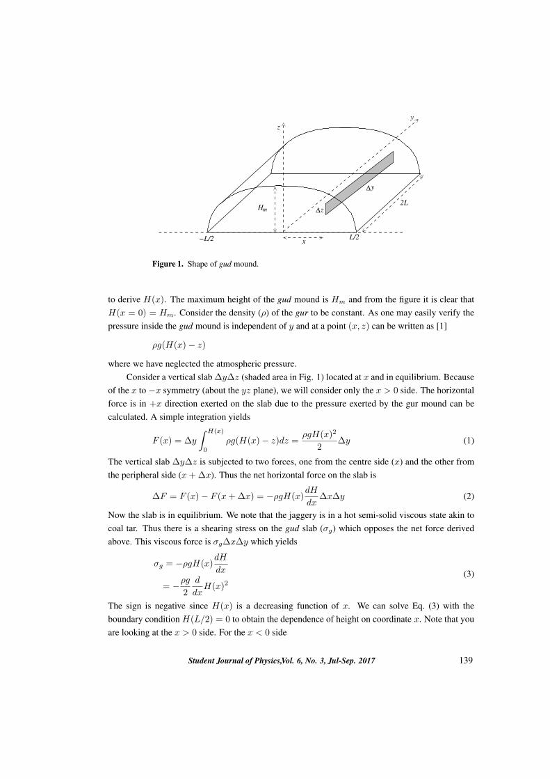
Hm ∆z

∆y

z

x

y

2L

L/2−L/2

Figure 1. Shape of gud mound.

to derive H(x). The maximum height of the gud mound is Hm and from the figure it is clear thatH(x = 0) = Hm. Consider the density (ρ) of the gur to be constant. As one may easily verify thepressure inside the gud mound is independent of y and at a point (x, z) can be written as [1]

ρg(H(x)− z)

where we have neglected the atmospheric pressure.Consider a vertical slab ∆y∆z (shaded area in Fig. 1) located at x and in equilibrium. Because

of the x to −x symmetry (about the yz plane), we will consider only the x > 0 side. The horizontalforce is in +x direction exerted on the slab due to the pressure exerted by the gur mound can becalculated. A simple integration yields

F (x) = ∆y

∫ H(x)

0

ρg(H(x)− z)dz =ρgH(x)2

2∆y (1)

The vertical slab ∆y∆z is subjected to two forces, one from the centre side (x) and the other fromthe peripheral side (x+ ∆x). Thus the net horizontal force on the slab is

∆F = F (x)− F (x+ ∆x) = −ρgH(x)dH

dx∆x∆y (2)

Now the slab is in equilibrium. We note that the jaggery is in a hot semi-solid viscous state akin tocoal tar. Thus there is a shearing stress on the gud slab (σg) which opposes the net force derivedabove. This viscous force is σg∆x∆y which yields

σg = −ρgH(x)dH

dx

= −ρg2

d

dxH(x)2

(3)

The sign is negative since H(x) is a decreasing function of x. We can solve Eq. (3) with theboundary condition H(L/2) = 0 to obtain the dependence of height on coordinate x. Note that youare looking at the x > 0 side. For the x < 0 side


H(x) =

√σgL

ρg

(1− 2x

L

)and the maximum height by inserting x = 0 in the above equation. Thus

Hm =

√σgL

ρg(4)

The total volume (V ) of the (gur) mound can be calculated by integrating Eq. (5) and multi-plying by the constant factor along the y-axis, namely 2L. Keeping in mind the symmetry of themound on either side of the yz plane yields an additional factor of two.

V = 4L

∫ L/2

0

H(x)dx

= 4L

√σgL

ρg

∫ L/2

0

√1− 2x

Ldx

=4

3L5/2

√σgρg

=4

3L2Hm

(5)

3. DISCUSSION

The Equation (4) for the maximum height could also be derived by dimensional analysis. The shapeof viscous fluids is determined by two opposing forces: gravity and the force of viscosity and/orsurface tension. In the current case we are in the happy situation that the dimensionless factor isunity, hence the dimensional analysis yields the exact result.

The base area A ' L2, so the volume as evidenced in Eq. (5) scales as V ' A5/4. This scalingrelation for the spread of a viscous fluid is perhaps general. For a viscous system with given densityand shear stress it is a consequence of the fact that the height decreases parabolically with the spreadalong the x direction.

A related question is why the shape of the mound remains invariant as the semi-solid jag-gery is poured periodically and gently over a span of several hours. This appears to be a case ofself-organized criticality (SOC). Additionally the shapes of several viscous substances may also besusceptible to similar analysis. We plan to examine these issues in detail in the future.

The density of the jaggery gur found in our house hold is around 1300 kg/m3 [2]. TakingL = 4 m and Hm = 1 m, the total mass of a gur mound will be roughly equal to 28 tonnes. Thisgives σg ≈ 3.25 kPa. We urge the reader to buy jaggery, verify our model and experiment further.Physics is sweet, physics is fun!


4. ACKNOWLEDGMENTS

One of us (LPSK) gratefully acknowledges discussions with B. S. Sharma and Dr. H. S. Vashistha ofhis school. PP acknowledges the support of National Initiative on Undergraduate Sciences (NIUS)programme undertaken by the Homi Bhabha Centre for Science Education (HBCSE-TIFR), Mum-bai, India and some unpublished notes of Siddharth Singh on hydrodynamics.

References

[1] Halliday D., Resnick R., and Walker J. 1994 Fundamentals of Physics (New Delhi: Asian Books Pvt.Ltd.)

[2] Supriya D Patil and S V Anekar, 2014, “Effect of Different Parameters and Storage Conditions on LiquidJaggery Without Adding Preservatives”, Intnl J of Res in Engg and Tech, 12, 280 - 283


T. Saxton1*, J. Slivka2 and M. J. Comstock3

1 Third year, B. Sc, Department of Physics, Illinois State University, Normal, Illinois

2 Second year, B.S. Department of Physics and Astronomy, M ichigan State University, East Lansing, Michigan3 Department of Physics and Astronomy, Michigan State University, East Lansing, Michigan

*Email: [email protected]

Abstract: As the structure of the protein is essential to its function, a better understanding of protein folding

is fundamental to understanding protein function. [1] This comprehension of the function and folding ofproteins will enable medicine to synthesize proteins in a way currently not possible. One of the majorhurdles is that the protein has the capability of folding in different ways and speeds. The goal of our experiment is the examination of the hYAP protein, and to see the different speeds offolding that it undergoes. Our specific goal was to find instances of fast folding of the protein - foldingoccurring within less than a millisecond. The methodology behind this experimentation is presented,along with results for fast folding of the protein, and slow folding of the protein.

1. INTRODUCTION

Current engineering of proteins is difficult, because of the direct relationship offunction and folding. Furthermore, a greater understanding of protein folding canprovide a possible method of combating prions - proteins that have folded in a mannerdifferent than their native structure. At times a function detrimental in comparison to thestandard function will arise as a result of this abnormal folding. This abnormal foldingcan result in other proteins folding abnormally as well, leading to diseases such as bovinespongiform encephalopathy in certain animals, Creutzfeldt-Jakob disease, Alzheimer’sdisease or Gerstmann-Straussler syndrome in humans for example. [2] [3] Byunderstanding how proteins fold, the possibilities of chemical synthesis of proteins forindividuals with unique dietary needs becomes possible. [4] Consequently, a greaterunderstanding of diseases thought to be caused by prions will lead towards more efficienttreatment of these diseases. In this paper, we use the single molecule trapping techniqueto study protein folding. This technique is useful in this matter as it allows us to build astochastic model of the protein, one molecule at a time. This is in contrast to othermethods that result in building a model of the protein that is an average of the behavior.In this experiment, we utilize an optical trapping method in which we capture two“beads” that when placed in the optical traps form a DNA tether with each other.

Unfolding Proteins: Fast versus Slow



2. EXPERIMENTAL

2.1 Overview of Trapping Method

The sample chamber and experimental set up is contained in a room of its own,with baffling on the walls to prevent noise pollution, and the lights off to prevent lightpollution from affecting the experiment. With the beads captured in the optical trap, themotion of the beads can be controlled to a certain degree. The trap itself is conical inshape and creates a restoring force upon the bead trapped within it. If the trap is movedto the left, the bead will be pulled to the left as well as it re-centers itself in the trap. Thisis what allows us to directly apply a force to an individual protein. A calibration is foundfor every bead pair that tells us the trap stiffness and the conversion constant fordetermining the position of the beads. Once this is done, the beads begin fishing for atether. This entails one of the optical traps remaining stationary, while the other oscillatescloser and further from the stationary optical trap. The streptavidin beads have a DNAstrand on them, followed by the protein, followed by another strand of DNA. The strandof DNA not directly on the streptavidin bead forms a digoxygenin with anti-digoxygeninbond with the anti-digoxygenin bead. The successful formation of this bond is what iscalled a tether. Once a peak force is measured during the movement further from thestationary trap, this is indicative that the DNA from the streptavidin bead has formed atether with the anti-digoxygenin bead. At this point, the bead pair is able to be used toexert force on the protein such that it will unfold, as seen in Figure 1.

Figure 1: Starting from the top, the beads are tethered together by the DNA. Left to right, it is ananti-digoxygenin bead, DNA, the protein under examination, DNA, and finally the streptavidinbead. As the beads are moved further apart, the protein experiences a force and eventuallyunfolds.

The beads are caught in the optical trap by the platform the sample chamber ismounted on being moved. This movement is controlled outside of the room the samplechamber is contained in.


2.2 Optical Trap Set-up

The laser used in this experiment is in the infrared spectrum at 1064 nm and is a5W laser. One of the objectives is held fixed, while the other is allowed to be movedperpendicularly towards and away from the sample chamber (see figure 2). Thismovement changes the diameter of the laser beam, and provides better collimation ofthe laser. The accuracy of the collimation is checked with the aid of an infraredfluorescent card. The camera focused on the experiment has two lenses in front of it, anultraviolet lens and an infrared lens. When the infrared lens is filtering light, the lasercan be seen on a monitor. This allows a visual check of the laser to be conducted. Theexperimentalist looks for a shape that is as near a uniform circle as can be obtainedvisually. If the circle appears to be more elliptical, this is indicative that the samplechamber itself is not presenting a vertical surface for the laser to pass through, and assuch the laser is coming out angled rather than straight. This is adjusted by physicallyrotating the chamber to achieve a uniform circle rather than an ellipse. This is ameasure taken to ensure that before the sample is being experimented with, the opticaltrap will successfully capture the beads. If the chamber is not presenting a verticalsurface for the laser to pass through, this can lead to issues during the experiment. Asthe sample chamber is moved, the angling can result in the captured bead being removedfrom the optical trap. This occurs because if the sample chamber is angled, as it ismoved the odds of the optical trap causing a bead to collide with the surface of thesample chamber increase.

PD: Photodetector D: Dichroic Mirror F: FilterO: Objective P: Pin Hole PM: Piezo MirrorS: Sample Chamber T: Telescope *: Conjugate Planes

Figure 2: The experimental setup. [5]


2.3 Preparation of Sample Chamber

Figure 3: The sample chamber. Syringes are connected to the connectors, which have a needle onthem attaching them to a tube. Through these tubes, the buffer, streptavidin and anti-digoxygenin beads flow through the channels. The capillaries allow the beads in the top andbottom channels to flow into the middle channel where the optical trap is then used to capturethe beads and perform the experiment. The fluids then leave the chamber through the tubes onthe left. Image is not to scale. Image credit: Fallyn Stieglitz

Before the experiment can be conducted, the sample chamber must be preparedfor the optical trap. The chamber used in this experiment is constructed out of coverglass and parafilm (see figure 3). The parafilm is used to create three separate channelson the cover glass: the bottom channel is where the streptavidin beads with the proteinconstruct flow through, the middle channel is where the buffer solution flows through,and the top channel is where the anti-digoxygenin beads flow through. On the middlechannel there are two capillaries connecting the channel to the top and bottom channels.These capillaries are what allow the beads to flow through to the middle channel and becaptured by the optical trap. The chamber is initially prepared for a trapping session byfirst pushing milli-Q water (filtered 0.2 microns) through the channels using syringes.This is done to ensure that no excess of experimental materials is wasted. The purpose ofpushing the milli-Q through the channels is to ensure that there are no air bubblescovering, or in, the capillaries before the experimental materials are added. The beads are


on the order of a micron in size and would not be able to flow into or through thecapillary if an air bubble is blocking the capillary in any way. The chamber is thenplaced between the objectives of the experimental setup and visually verified for the clearopenings on the capillaries by the experimentalist. These syringes containing the milli-Qare left connected to the sample chamber until the syringes containing the sample to beused are connected to the chamber. This is another step taken to ensure that no air getsinto the chamber and causes bubbles that might interfere with a capillary.

2.4 Sample Preparation

The preparation of the sample involves making the buffer solution. The buffersolution is a combination of Triss-HCl, Glucose, NaCl, and water in a centrifuge tube.Three separate centrifuge tubes are then used to portion out the buffer solution. Afterthe buffer has been portioned, the beads are then added to the tubes. Before adding theanti-digoxygenin beads to a tube, the beads are first vortexed. This is to ensure thatupon pipetting the beads, the container has a uniform concentration of beads as overtime the beads will settle at the bottom of the container. The streptavidin beads are thenadded to a separate tube, after being mixed by inverting or flicking the container. As thestreptavidin beads have DNA attached to them, they cannot be vortexed as this wouldshred the DNA. Finally, pyranose oxidase (poxy) is added to all three tubes. Thepurpose of the addition of the poxy is to prevent oxygen from interacting with thesolution as best as possible. Oxygen in solution can get converted into “radicaloxygen”. Radical oxygen is highly reactive and will react with the molecules, possiblybreaking the DNA tethers or damaging the protein under study. The poxy is an oxygenscavenger, and will keep the radical oxygen from reacting within the solution. The threeseparate mixtures are then transferred into separate airtight syringes. The airtightsyringes and the poxy are implementations put into place to mitigate waste of materialand ensure that oxygen is not a reason for lack of success during the experiment.However, at some point the poxy will become saturated with oxygen, and unable toscavenge any more oxygen from the solution. This will typically end the experiment, asthe oxygen will now be able to interact with the DNA and prevent tethers from beingformed successfully. To begin the experiment, the airtight syringes replace the syringescurrently attached to the sample chamber. During this replacement, it is imperative thatair not be able to enter the tubes of the sample chamber. To prevent this, theexperimentalist adds milli-Q to the connection location, to ensure that once the airtightsyringe is connected, there is no air between the solution contained within the syringeand the milli-Q currently in the tubes of the sample chamber. The airtight syringes arethen placed in specific positions that correspond to controls used by the setup to controlthe flow of the beads (anti-dixoxygenin or streptavidin) and the buffer. There are


motorized syringe pumps at these positions that push the solution out of the syringes atspeeds ranging in the hundreds of nanoliters per second.

2.5 Application of Force to Protein Construct

Once this is done, the goal is to trap an anti-digoxygenin bead in one optical trap,a streptavidin bead in the other optical trap, and then form a tether between the two beadsusing the DNA. Once the beads are both successfully caught in the optical trap, acalibration of the trap for this bead pair is done. This will determine the trap stiffnessconstant and a conversion constant that gives the bead position from the optical method.[5] The calibration also gives the experimentalist a control over data collection. For beadpairs of a sample protein, the calibration for a bead pair should not be vastly different incomparison to other bead pairs of the same sample protein. If a bead pair presents acalibration that is outside of the standard calibration for a sample protein, it isimmediately apparent to the experimentalist that this bead pair cannot be used for datacollection. This can happen for a variety of reasons: the beads vary in size, there could bemore than one bead in the optical trap, there could be multiple tethers formed between thebeads, the sample protein could possibly be bad. If the calibration is within the standardcalibration for the sample, the beads then form the tether. Once the tether has beenformed, a force can be applied to the protein. This is done quickly at first, to test whetheror not the tether is stable. One of the optical traps is held stationary, and the other trapmoves away from it (see figure 1) which cause the force to be applied to the protein. At acertain force the protein will unfold, and this force is measurable. After this fast scan hasbeen performed, a slow scan is performed. The slow scan involves the trap moving indiscrete jumps as it moves away from the stationary trap. The slow scan is performed inorder to see the fast folding occur. The fast folding occurs rapidly, in times less than amillisecond; scanning too quickly risks missing these fast folding occurrences. Byscanning slowly, we keep the protein at a certain force for a longer time. Due to thestatistical mechanical nature of folding, at certain forces the unfolded state will be just aslikely to occur as the folded state. This slow scan allows us to see this happen, as shownin the following results.


3. RESULTS AND DISCUSSION

3.1 Slow Folding Proteins

Figure 4: An example of slow folding. In comparison to fast folding, slow folding takes place inhalf to full seconds.

Shown in figure 4 is an example of slow folding. There are two different modelsto describe the dependence of the tether extension on the force applied: a model forthe protein folded, and a model for the protein unfolded. The molecules are modelledusing the statistical mechanics of polymers. One of these models includes the unfoldedprotein polymer, the other does not. At low forces, the models are indistinguishablefrom one another, but as the force increases, the models separate. This separationbetween models is used to identify when and where the protein unfolds. In the examplepresented, the protein extended slightly less than 1550 nm, at which point the proteinthen unfolded (indicated by the arrow), at a force of approximately 10 pN. The data isinterpreted as a representation of slow folding because as can be seen at the point ofunfolding, there is a single distinct jump; the blue line moves from the folded model to

Force vs. Extension

---- Folded Model

---- Unfolded Model

Data

Unfolding


the unfolded model and stays there.

3.2 Fast Folding Proteins

Shown in figure 5 is an example of fast folding. The difference here being thatrather than there being a single distinct jump, there is more of a smooth transitionbetween the folded and unfolded models that occurs over an extension range. This is dueto how the data is taken; as the data is being taken, it is being averaged to avoid files ofan excessive data size. The above is said to be fast folding because it is not folding justonce, but jumping between models rapidly. The result is that as the protein is jumpingbetween the models, at the lower force it spends a greater amount of time folded than itdoes unfolded. As the force increases, the time spent folded lessens and it is more likely

Figure 5: An example of fast folding. The expected time for fast folding to occur is in the millisecond time range. As seen in the circled area, the data is not just following one model. The data points, if followed sequentially, would alternate between the folded model and the unfolded model as the protein switches between the two states rapidly.

Force vs. Extension

---- Folded Model

---- Unfolded Model

Data


to find the protein in an unfolded state, until finally the protein is unfolded and followingthe unfolded model.

3.3 ConclusionBased upon the data taken during these experiments it was determined that fast

folding was possible for the protein construct. However, these instances of this differentfolding were few and far between. Over the course of 8 weeks of experimentation, wefound 4 instances that were believed to be indicative of fast folding. However, we haveshown that the methodology presented is useful for examining different foldingprocedures for a given protein. As a result of this, future studies will be made involving aprotein construct Protein G, as it has also shown possibilities of there being differenttypes of folding occurring. Whereas before it seemed to have two distinct states, thefolded and unfolded state, through the use of this method there is evidence to suggest thatthere might be a state in between the folded and unfolded states. This in between state ofProtein G is the focus of future studies using this method. ACKNOWLEDGEMENTS

T.S. and J.S. would like to acknowledge the Comstock Laboratory and Dr.Matthew Comstock for his mentorship at Michigan State University. T.S. receivedsupport from a Research Experience for Undergraduates (REU) supported by the NSF(1559776). The work was also supported by a grant from the NSF to the Comstock lab(MCB-1514706).

REFERENCES[1] Collinge, J. (2001). Prion diseases of humans and animals: their causes and

molecular basis. London, England.

[2] Hartl, U. (2010). Protein Folding: mechanisms and role in disease.

[3] James A. Olzmann, K. B.-S. (2003, December 9). Familial Parkinson's Disease-associated L166P Mutation Disrupts DJ-1 Protein Folding and Function. Atlanta, Georgia, United States of America.

[4] Nilsson, B. L., Soellner, M. B., & Raines, R. T. (2005). Chemical Synthesis of Proteins. Annual Review of Biophysics and Biomolecular Structure, 34, 91–118. http://doi.org/10.1146/annurev.biophys.34.040204.144700

[5] Comstock, M. J., Ha, T., & Chemla, Y. R. (2011). Ultrahigh-resolution optical trap with single-fluorophore sensitivity. Nature Methods, 8(4), 335-340. DOI: 10.1038/nmeth.1574


http://dx.doi.org/10.1038/nmeth.1574


Study of low energy proton capture resonances in 14N Rajan Paul1, Sathi Sharma2, Sangeeta Das2, M. Saha Sarkar2*

1Second year, M.Sc., Department of Physics, VIT University, Vellore-632014, India 2Nuclear Physics Division, Saha Institute of Nuclear Physics, Kolkata-700064, India *[email protected]

Abstract: Several proton capture resonances in 14N have been studied theoretically using partial waveanalysis technique. Most of the results agree well with available experimental data. The analysis hasbeen extended to indicate that one of the resonances with uncertain spin may need a change in theassignment.

1. INTRODUCTIONStudy of radiative low energy proton capture reactions has several important implicationsin nuclear astrophysics. Experimental data on the capture cross sections at stellarenergies are essential for studying primordial nucleosynthesis. The measurements atstellar energies are difficult as the direct capture cross-sections are very low. Usuallydata measured at higher energies are extrapolated to lower energies, which may fail ifthere are low energy resonances. The astrophysical capture reaction rate is thus greatlyaffected by the capture resonances at the stellar energies.

The partial wave analysis technique for studying nuclear radiative capture resonances iswell-established. This analysis is also useful to search for new resonances and to predicttheir quantum numbers. In the present work, various experimentally observed resonances[1] in 14N are reproduced reasonably well using this theory. Spectroscopic factors forthese states have also been estimated. Some of the deviations of the theoretical resultsfrom data are discussed for future scopes.


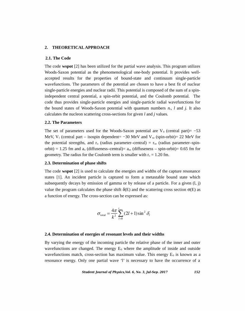
2. THEORETICAL APPROACH

2.1. The Code

The code wspot [2] has been utilized for the partial wave analysis. This program utilizesWoods-Saxon potential as the phenomenological one-body potential. It provides well-accepted results for the properties of bound-state and continuum single-particlewavefunctions. The parameters of the potential are chosen to have a best fit of nuclearsingle-particle energies and nuclear radii. This potential is composed of the sum of a spin-independent central potential, a spin-orbit potential, and the Coulomb potential. Thecode thus provides single-particle energies and single-particle radial wavefunctions forthe bound states of Woods-Saxon potential with quantum numbers nr, l and j. It alsocalculates the nucleon scattering cross-sections for given l and j values.

2.2. The Parameters

The set of parameters used for the Woods-Saxon potential are V0 (central part)= −53MeV, V1 (central part – isospin dependent= −30 MeV and V so (spin-orbit)= 22 MeV forthe potential strengths, and ro (radius parameter–central) = rso (radius parameter–spin-orbit) = 1.25 fm and ao (diffuseness–central)= aso (diffuseness – spin-orbit)= 0.65 fm forgeometry. The radius for the Coulomb term is smaller with rc = 1.20 fm.

2.3. Determination of phase shifts

The code wspot [2] is used to calculate the energies and widths of the capture resonancestates [1]. An incident particle is captured to form a metastable bound state whichsubsequently decays by emission of gamma or by release of a particle. For a given (l, j)

value the program calculates the phase shift (E) and the scattering cross section (E) as

a function of energy. The cross-section can be expressed as:

2.4. Determination of energies of resonant levels and their widths

By varying the energy of the incoming particle the relative phase of the inner and outerwavefunctions are changed. The energy E0 where the amplitude of inside and outsidewavefunctions match, cross-section has maximum value. This energy E0 is known as aresonance energy. Only one partial wave ‘l’ is necessary to have the occurrence of a


resonance state corresponding to the energy E0 where l = / 2. The width of the resonance(Г) is determined from the energy (E), where cross-section reduces to half of a centralvalue (E-E0) = ±Г/2.

Ex

(MeV)

ER

(MeV)

VN

factor

Width ()

(keV)

Spectro-scopic

Factor (expt

/theo)

Single Particle Orbital

Expt [1] Theo Expt [1] Theo

7.966 (2¯)

0.416 0.411 0.933 <0.37 0.212 1.74 1d5/2 (l=2)

8.062 (1¯)

0.512 0.515 0.972 23 (1) 66.8 0.34 2s1/2 (l=0)

8.620 (0+)

1.07 1.07 0.703 3.8 (3) 124 0.03 1p1/2 (l=1)

8.776 (0¯)

1.226 1.074 0.914 410 (20) 475 0.86 2s1/2

(l=0)

Table 1: Comparison of experimental and theoretical features of the low energyresonance states at different excitation energies (Ex) in 14N.

2.5. Inputs needed to identify a resonance

The energy range that could be populated in the compound nucleus by capture of theincoming projectile by the target nucleus is determined by the energy given in the inputand the Q value of the reaction. The incoming particle energy necessary to populate aresonant state is known as resonance energy (Er).

The resonances which are already identified in a particular nucleus can be reproduced toget an idea of the spectroscopic purity of the state. For a particular choice of l and j, thedepth of the central potential is varied (normalized) by a factor such that the resonanceenergy is determined correctly. The ratio of widths of the resonance obtained inexperiment over theory provides a measure of the spectroscopic factor of that particularstate.

By fixing a particular depth of the potential as estimated from reproducing knownresonances – unknown resonances can be also identified which corresponds to a specificsingle particle orbit (l,j).


3. RESULTS AND DISCUSSION

3.1. Study of known proton capture resonances in 14N

The Q value for the reaction 13C+p14N+ is 7550 keV. The ground state spin of 13C is

1/2¯. The known resonances [1] have been reproduced by varying the potential depths.The single particle orbits are chosen keeping in mind the spin assignment in 14N, as wellas the earlier information of the l value. The results are shown in Figure 1 and Table 1.Figure 1 shows the features of different resonances in 14N. In Fig 1a, the variation of thenormalization factor of the potential to choose the best value for reproducing theexperimental resonance energy is demonstrated for a particular case. In Fig 1b, theresonance at 8062 keV (1¯), reported to be originated from l=0, has been shown to bereproduced by the l=2 contribution. However in Table 1, the spectroscopic factor hasbeen calculated for l=0 contribution only. Figs 1c and d show the features for otherresonances.

The results show quite good agreement with the experimental data. However, except forthe 0- state at 8776 keV, the spectroscopic factors for the other states do not appear to berealistic. The normalization factors for the potential corresponding to different shells andl values are consistent. For d5/2 and s1/2 orbitals, the normalization is less than 1 (~0.91-0.97), whereas for p1/2, it needs 30% reduction (~0.7), indicating that the resonanceenergies are under predicted with full strength of the potential. However, in Fig.1 b, whilereproducing the resonance (1¯) with d3/2, the resonance energy is over predicted resultingin a normalization value > 1 (~1.35).


0.4 0.6 0.8 1.0 1.2 1.4 1.6

0

50

100

150

200

250

0.5175 0.5180 0.5185

500

1000

1500

2000

2500

0.4110 0.4112 0.4114

1000

2000

3000

0.5 1.0 1.5 2.0

0

200

400

600

800

(b)

Normalisation factor of Vn

(a) 1d3/2

: 1-

VN=1.359

Width= 0.5215 keV

Energy (proton) MeV

(d)(c)Width : 0.1922 keV

1d5/2

: 2-

VN=0.933

Cro

ss-s

ection (arb

itra

ry u

nits)

Energy (proton) MeV

1p1/2

: 0+

VN=0.703

Figure 1: Theoretical results for different resonances. See text for details.

3.2. Comments on resonance states with relatively higher spins

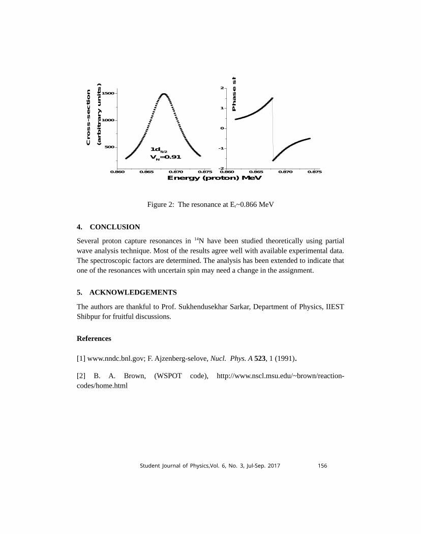
In the present work, no excitation of the target has been considered. With thisassumption, having a resonance with spin >3 (4) with negative (positive) parity at lowenergies (Er< 1000 keV) is unlikely as those will need coupling with l=4 (5) partial wave,i.e g (h) orbitals. However, such states have been reported in literature [1].

Thereafter, with normalization around 0.91 as obtained for d5/2 for known resonances, theenergies are varied and a resonance is obtained at ER~0.8 MeV (Fig. 2). The energyalmost matches with an observed state at 8490 keV with a tentatively assigned spin of(4¯). However, having two close-by resonances with same l is also doubtful. This spinassignment therefore needs to be revalidated experimentally.


0.860 0.865 0.870 0.875-2

-1

0

1

2

0.860 0.865 0.870 0.875

500

1000

1500

Phase s

hift

1d5/2

VN=0.91

Energy (proton) MeV

Cross-sectio

n

(arbitrary u

nits)

Figure 2: The resonance at Er~0.866 MeV

4. CONCLUSION

Several proton capture resonances in 14N have been studied theoretically using partialwave analysis technique. Most of the results agree well with available experimental data.The spectroscopic factors are determined. The analysis has been extended to indicate thatone of the resonances with uncertain spin may need a change in the assignment.

5. ACKNOWLEDGEMENTS

The authors are thankful to Prof. Sukhendusekhar Sarkar, Department of Physics, IIESTShibpur for fruitful discussions.

References

[1] www.nndc.bnl.gov; F. Ajzenberg-selove, Nucl. Phys. A 523, 1 (1991).

[2] B. A. Brown, (WSPOT code), http://www.nscl.msu.edu/~brown/reaction-codes/home.html



Volume 6 Number 3 Jul - Sep 2017

CONTENTS

ARTICLES

Studying the Puzzle of the Pion Nucleon Sigma Term 122

Christopher Kane

One-Dimensional Chain Collisions for Different Intermediate Mass Systems 130


The jaggery (Gud) mounds of Bijnor 138

Lakshya P. S. Kaura and Praveen Pathak

Unfolding Proteins: Fast versus Slow 142

T. Saxton, J. Slivka and M. J. Comstock

Study of low energy proton capture resonances in 14N 151

Rajan Paul, Sathi Sharma, Sangeeta Das, M. Saha Sarkar

Documents

STUDENT JOURNAL OF PHYSICS - iopb.res.insjp/sjp_past_issues/sjp632017/full.pdf · Departament d’Estructura i Constituents de la Mat`eria and ... Nucleons are composed of three valence