Stuart-Landau oscillators

arX

iv:2

111.

1444

4v1

[nl

in.C

D]

29

Nov

202

1

EPJ manuscript No.(will be inserted by the editor)

High-order synchronization in a system of nonlinearly coupledStuart-Landau oscillators

Nissi Thomas1, S. Karthiga1 and M. Senthilvelan1, a

Department of Nonlinear Dynamics, School of Physics, Bharathidasan University, Tiruchirappalli 620024, Tamil Nadu, India.

the date of receipt and acceptance should be inserted later

Abstract. The high-order synchronization was studied in systems driven by external force and in au-tonomous systems with proper frequency mismatch. Differing from the literature, in this article, we demon-strate the occurrence of high-order (1 : 2) synchronization in an autonomous nonlinearly coupled (Stuart-Landau) oscillators which admit a particular form of rotational symmetry. Interestingly, the observed 1 : 2synchronization happens not only for a particular choice of natural frequencies but for all possible choicesof frequencies. We have observed such a behaviour in the case of 1 : 1 synchronization, where we haveseen a variety of couplings in the literature that forces the oscillators to have almost equal frequencies andmakes the system to oscillate with a common frequency independent of whether the oscillators are identicalor non-identical. Similarly, in this article we observe that, whether the initial choice of frequencies is ofthe ratio 1 : 2 or not, the given nonlinear coupling forces the system to oscillate with the frequency ratio1 : 2. Further, we present synchronization and other dynamical behaviours of the system by considereingdifferent choices of natural frequencies.

PACS. XX.XX.XX No PACS code given

1 Introduction

Synchronization, one of the fascinating phenomena ob-served in coupled systems where this subject has seena very wide literature [1]. Various types of entrainmentbehaviour [2,3,4,5] and various forms of synchrony pat-terns [6,7,8,9,10,11,12] have been studied in different sys-tems with different coupling topologies. When two or moreoscillators are coupled, they may start to oscillate withthe same frequency and their amplitudes and phases mayalso get related. Such oscillations with equalized frequencywith suitable coupling is known as 1 : 1 synchronization[1] and there are variety of physical systems which exhibit1 : 1 synchronization. Besides this, high-order synchro-nization, in which the frequencies of the oscillators arerelated by a particular ratio (n : m), may also occur [1].Comparing the literatures of 1 : 1 and n : m synchroniza-tion, the latter is less studied but still the occurence ofsuch synchronization is observed in physical and biolog-ical systems including cardiorespiratory system [13], thejosephson junction based electrical rotator [14], a ruby nu-clear magnetic resonance laser with delayed feedback [15]and in the circuit of thermally coupled VO2 (vanadiumdioxide) oscillators [16]. Besides this, the possibility of us-ing high-order synchronized states in reservior computingis also demonstrated recently in the Refs. [16,17,18,19,20].

a e-mail:[email protected]

It is evident from the literature that the high-ordersynchronization has been explored much in the case offorced or non-autonomous systems. In the case of au-tonomous systems, this n : m synchronization is achievedthrough frequency mismatch only when the natural fre-quency of the oscillators is said to have the ratio ω1 :ω2= n : m [1]. In this article we report the occurrence ofn : m synchronization in an autonomous system of cou-pled Stuart-Landau oscillators where the nonlinear cou-pling among the oscillators is shown to induce 1 : 2 syn-chronization. A symmetry admitted by this nonlinear cou-pled system is responsible for the occurence of this high-order (1 : 2) synchronization. Because of this symmetry,there is no restriction imposed on the natural frequenciesof the oscillators. In other words, whatever be the naturalfrequencies of the two oscillators (whether they are iden-tical or non-identical or their natural frequencies have theratio 1 : 2) the symmetry admitted by the system onlyallows 1 : 2 synchronization and no other type of synchro-nization. By considering the dynamical behaviours of thesystem for different cases of ω1 and ω2, we illustrate bothanalytically and numerically that all the stationary statesof the system represent 1 : 2 synchronized state alone andno stationary states representing any other synchronizedstate do exist. We also bring out few other interesting dy-namical aspects of the system under this nonlinear cou-pling. The first and foremost is that the system shows amultistable behaviour when the coupling strength is var-ied. Due to this, the system exhibits oscillations in both

http://arxiv.org/abs/2111.14444v1

2 Nissi Thomas et al.: High-order synchronization in a system of nonlinearly coupled Stuart-Landau oscillators

clockwise and anticlockwise direction. We also present aninteresting case in which the multistable clockwise and an-ticlockwise states have the same periodic orbit with sameamplitude but different frequencies of oscillation.

We organize our work as follows. In Sec. 2, we presentthe considered model and discuss briefly the possibility ofpractical realization of the model. In Sec. 3, we discussthe dynamics for the case ω2 6= 2ω1 where we elucidatethe results with two different cases, namely (i) ω1 = ω2

and (ii) ω2 6= ω1. We also analyze the stationary statescorresponding to these two cases and discuss their stabili-ties in this section. In Sec. 4, we investigate the dynamicsof the system when the natural frequencies of the uncou-pled oscillators have the frequency relation ω1 : ω2 = 1 : 2.Finally, we summarize our results in Sec. 5.

2 Model

We consider two Stuart-Landau oscillators interacting witheach other through an asymmetric quadratic coupling inthe following manner,

α = (γ1 − γ2|α|2)α− iω1α− 2iζα∗β,

β = (γ1 − γ2|β|2)β − iω2β − iζα2, (1)

where α = x1 + iy1 ∈ C and β = x2 + iy2 ∈ C are thestate variables corresponding to the two Stuart-Landauoscillators. α∗ and β∗ represent their complex conjugates.The parameters γ1 ∈ R+ and γ2 ∈ R+ respectively repre-sent the negative linear damping (linear gain) and positivenonlinear damping (nonlinear loss) strengths. The damp-ing rate γ1 is also known as Hopf bifurcation parameteras the system executes steady state dynamics for γ1 < 0,supercritical Hopf bifurcation at γ1 = 0 and oscillatory dy-namics for γ1 > 0. The parameters ω1 and ω2 respectivelydenote natural frequencies of the two uncoupled Stuart-Landau oscillators and ζ represents the strength of theasymmetric nonlinear coupling. As the oscillators α andβ are coupled to each other in an assimilar way (vide Eq.(1)), we call the coupling as asymmetric coupling.

This type of coupling may be achieved in different con-texts. In a very recent work [21], two of the present au-thors have shown the possibility of observing the abovesystem (1) (or the nonlinear coupling) in the context oftrapped ions. In this recent article, the Lindblad masterequation corresponding to a system of two quantum vander Pol oscillators coupled via a nonlinear cross-Kerr in-teraction has been considered. This nonlinear interactioncan be achieved by considering the strong coulombic inter-action between two trapped-ions [22]. The classical ampli-tude equations obtained from the Lindbland master equa-tion of the coupled system is similar to the one given inEq.(1).

3 Dynamics of the system

(Case: ω2 6= 2ω1)

3.1 Stationary periodic orbits

Now we unveil the dynamical features that come out dueto the nonlinear coupling. We recall here that in the ab-sence of coupling, the two Stuart-Landau oscillators exe-cute oscillatory dynamics along clockwise direction withamplitude

√

γ1/γ2 with respective frequencies ω1 and ω2.In the presence of coupling, we can study the dynamics ofthe system qualitatively by examining the stability of theirstationary states or modes. For this purpose, by consider-ing α = R1 exp (iθ1) and β = R2 exp (iθ2), we can obtainthe dynamical equations for amplitudes Ri and phases θi(i = 1 and 2) corresponding to Eq. (1) and they are givenby

R1 = (γ1 − γ2R21)R1 + 2ζR1R2 sin(θ2 − 2θ1),

R2 = (γ1 − γ2R22)R2 − ζR2

1 sin(θ2 − 2θ1),

θ1 = −ω1 − 2ζR2 cos(θ2 − 2θ1),

θ2 = −ω2 − ζR2

1

R2

cos(θ2 − 2θ1). (2)

A closer observation on Eq. (2) reveals that the systemremains same with repect to the transformation θ2 → θ2+2ψ and θ1 → θ1 + ψ. Further discussion will make clearthat this symmetric nature is responsible for the 1 : 2 typesynchronization in the system (in the original Eq. (1), thissymmetry can be seen as the invariance of the system withrespect to the transformation α → αeiψ and β → βe2iψ).We can reduce the above Eq. (2) to

R1 = (γ1 − γ2R21)R1 + 2ζR1R2 sin δ,

R2 = (γ1 − γ2R22)R2 − ζR2

1 sin δ,

δ = −∆− ζ(R2

1 − 4R22

R2

)

cos δ, (3)

where δ = θ2 − 2θ1 is a form of phase difference and∆ = ω2 − 2ω1 represents the frequency detuning amongthe two Stuart-Landau oscillators. The stationary oscilla-tory states or limit cycles of the system can be found bysetting R1 = R2 = δ = 0. In the following, we presentthe form of the stationary periodic orbits correspondingto all the cases excluding ω2 = 2ω1. The dynamics and thepossible stable and unstable periodic orbits or limit cyclescorresponding to the limiting case ω2 = 2ω1 are discussedseparately in Sec. 4. For the case ω2 6= 2ω1, the systemsupports five possible periodic states which are given by

R∗

1 =√χR∗

2, R∗

2 =

√

γ1γ2

(χ+ 2)

(χ2 + 2),

δ∗ = tan−1

[

−γ2R∗22

∆

(χ− 1)(χ− 4)

(χ+ 2)

]

, (4)

where χ can be determined by solving the quintic polyno-mial equation

γ1

γ2ζ2(χ+2)(χ2+2)(χ−4)2−γ

21(χ−1)2(χ−4)2−∆

2(χ2+2)2 = 0.

(5)

Nissi Thomas et al.: High-order synchronization in a system of nonlinearly coupled Stuart-Landau oscillators 3

J =

γ1 − 3γ1R∗21 + 2ζR∗

2 sin δ∗ 2ζR∗

1 sin δ∗ 2ζR∗

1R∗

2 cos δ∗

−2ζR∗

1 sin δ∗ γ1 − 3γ2R

∗22 −ζR∗2

1 cos δ∗

−2ζR∗

1

R∗

2

cos δ∗ ζ(

R∗2

1+4R∗2

2

R∗2

2

)

cos δ∗ ζ(

R∗2

1−4R∗2

2

R∗

2

)

sin δ∗

. (6)

We have analyzed all five cases. Our results indicatethat there exists two possible periodic orbits which be-come stable in different parametric regions. Before we dis-cuss the results of the linear stability analysis correspond-ing to different cases, we wish to indicate certain impor-tant inferences that we can observe from the form of theabove stationary states.

The first observation one can make from Eq. (4) is thatin none of the stationary states (mentioned in Eq. (4) and(5)), the amplitude of the two oscillators match with eachother (R∗

1 6= R∗

2) and their ratio is found to be equal to√χ

(where χ takes the value 1 only at a particular parametricvalue and not for a range of parametric values (or for arange of values of ζ)). Similarly, considering the frequencyof the oscillators α and β in these stationary states (theunderlying expressions can be deduced by substituting thevalues of R∗

1, R∗

2, and δ∗ corresponding to the stationary

states (Eq. (4) and (5)) in the expressions of θ1 and θ2 ofEq. (2)), we observe that they take the values,

θ∗1 = −ω1 − 2ζR∗

2 cos δ∗ = −ω1 + 2∆

1

χ− 4,

θ∗2 = −ω2 − ζR∗2

1

R∗

2

cos δ∗ = −ω2 +∆χ

χ− 4. (7)

Equation (7) clearly indicates that

θ∗1 6= θ∗2 , (8)

and so none of the states mentioned in Eq. (4) show am-plitude as well as frequency matching among the two os-cillators (α and β). It is a well known fact that at theasymptotic time limit, the dynamical system approaches(or settles into) one of its stable stationary configurations.In this regard, the above discussion says that none of thestationary states (including unstable and stable states)correspond to first order or 1 : 1 synchronized state. Thismimics that the introduced nonlinear coupling (1) maynot induce first order synchronization in the consideredsystem. A closer look on Eq. (7) (and use ∆ = ω2 − 2ω1)further reveals the role of coupling where all the stationarystates satisfy

θ∗2

θ∗1= 2. (9)

Thus, the stationary states of the system represent thestate of 1 : 2 synchronization where the angular frequencyof the second oscillator is twice the angular frequencyof the first oscillator. Hence the introduced coupling fa-cilitates higher-order (or 1 : 2) synchronization rather

than first order synchronization. Note that the relation(9) holds for all choices of ω1 and ω2 and so only 1 : 2 syn-chronization is observed in all the cases. Thus, the relation(9) clearly indicates the usefulness of the considered asym-metric coupling in inducing high order synchronization. Toillustrate it more clearly, we discuss two important casesin the following sub-sections.

3.2 Case (i): ω1 = ω2

As a first case, we consider a simple situation in whichtwo identical oscillators (that is, ω1 = ω2 = ω = 1.0)are coupled. In the absence of coupling, due to the iden-tical nature, the two oscillators oscillate with the samefrequency and amplitude. However, this is not possible inthe presence of asymmetric coupling and the system willno longer support stationary periodic orbits with identicalfrequency and amplitude. The dynamical characteristicsof this case is illustrated in Fig. 1 where the informationof the amplitude, frequency and relative phase of the twooscillators are given with respect to ζ. The maxima andminima values of x1 and x2 (corresponding to differentstable or unstable stationary periodic orbits) are obtainedusing Eqs. (4) and (5) and are presented in Figs. 1(a) and1(b). Similarly, the angular frequency of the first oscilla-

tor, θ∗1 , (the frequency of the second oscillator, θ∗2 = 2θ∗1)and the relative phase difference δ∗ corresponding to dif-ferent stable and unstable orbits are shown respectively inFigs. 1(c) and 1(d).

From Figs. 1(a)-1(d), we can see that there are fourdifferent dynamical regions (I-IV). In region-I, there areno stable periodic states as seen in Fig. 1(a) or 1(b) andthe numerical studies show the existence of stable quasi-periodic or torus type oscillations in this region. The stabi-lization of periodic states are found only at ζ ≡ 0.54, thatis in region-II where the green curve (colour online) withfilled triangles represent a stable periodic state. We havelabeled the latter periodic states as PS−1. We can observefrom Fig. 1(a) and Fig. 1(b) that even in the region-II, thetorus oscillations are found to be stable and so there ex-ists multi-stability between PS−1 state and quasi-periodicstates in the region-II. The phase portraits of the coexist-ing torus oscillation and PS−1 periodic orbit at ζ = 0.56are shown respectively in Figs. 2(a) and 2(b). For ζ > 0.59,the torus oscillations are no more stable and PS−1 statealone is stable in region-III as observed in Figs. 1(a) and1(b). The latter figures also show the stabilization of onemore periodic state, namely PS−2, in region-IV (that isfor ζ > 2.05) and so there will be a multi-stability in the


ζ

x∗ 1

Torus PS-2

PS-1

ζ0

IVIIIIII

4.02.00

0.7

0.0

-0.7

ζ

x∗ 2

ζ0

IVIIIIII

4.02.00

0.7

0.0

-0.7

ζ

θ∗ 1

ζ0

IVIIIIII

5.02.50

4.00

0

-4.00

(b)

(c) (d)

(a)

ζ

δ∗

ζ0

IVIIIIII

5.02.50

π10

π25

0

-π25

Fig. 1. Maxima and minima values of the variables x1 and x2 in different stable and unstable stationary states of the system inEq. (1) for ω1 = ω2 = 1.0 are shown respectively in Figs. 1(a) and 1(b) for different values of ζ. Similarly, the angular frequency

θ1∗

and the relative phase difference δ∗ corresponding to different stable and unstable states are shown with respect to ζ in Figs.1(c) and 1(d). In all the above figures, we represent the unstable states with dashed lines and the stable states with continuousline with some filled attributes like filled circles or filled triangles. In all these figures, we consider γ1 = 0.25, γ2 = 1.0 andω1 = ω2 = 1.0.

region-IV. Both PS-1 and PS-2 states are found to be sta-ble for all higher values of ζ > 2.05.

Being discussed the stabilization of different periodicand quasi-periodic states, let us now have a closer lookat their dynamical characteristics with respect to ζ. It isclear from Eq. (9) that in the presence of coupling, all theperiodic states including stable and unstable ones men-tioned in Figs. 1(a)-1(d) correspond to second order syn-

chronized state (where θ∗2 = 2θ∗1). However, in the isolatedcase ζ = 0, the two oscillators are found to oscillate withidentical amplitude and frequency. So, the system does notstabilize in any second order synchronized periodic stateas soon as the coupling is introduced and quasi-periodicoscillations appear in the initial transition region. For aslightly higher value of ζ (ζ = 0.54), the stabilization of asecond order synchronized state, namely PS−1 occurs andthis state is found to be stable for all values of ζ > 0.54. Acloser look at Figs. 1(a) and 1(b) tells us that the ampli-tude of the second oscillator is higher than the amplitudeof the first oscillator near ζ = 0.54 and with the increaseof ζ, an opposite behaviour is observed where the am-plitude of the first oscillator becomes higher. From Eq.(9), it is clear that the frequency of the second oscilla-tor is (two times) higher than the first one. We infer here

that the amplitude of the second oscillator is quickly ad-justed to have a smaller value than the first oscillator sothat it can have higher frequency of oscillations than thefirst oscillator. Now considering the frequency of oscilla-tion corresponding to the state PS−1, Fig. 1(c) shows an

interesting phenomenon where the angular frequency θ∗1

(or equivalentlyθ∗22) changes its sign at the point ζ0.

For ζ < ζ0, θ∗

1 (also θ∗2) is found to be negative and sowe observe oscillations in the clockwise direction as shownin Fig. 2(b) (we recall that even in the uncoupled situation

the angular frequencies θ∗1 and θ∗2 (= −ω) of the oscillatorsare negative which represent clockwise evolution). At the

point ζ = ζ0, θ1∗

and θ2∗

becomes zero and the value ofζ0 is given by

ζ0 =

[(

1

4k

)

×

(

γ1γ2(2ω2 − ω1)2 +

γ2

γ1ω1(ω

21 + 2ω2

2)2

)]1/2

,

(10)

where k = (ω1 + ω2)(ω21 + 2ω2

2). The dynamics at theconsidered parametric values γ1 = 0.25, γ2 = 1.0 withω1 = ω2 = 1.0 and ζ0 = 1.22899 is shown in Fig. 2(c). Dueto the zero frequency nature, non-oscillatory or steady


xi

y i

0.70.0-0.7

0.7

0.0

-0.7

PS-1 (ζ < ζ0)

xi

y i

0.70.0-0.7

0.7

0.0

-0.7

t

xi

100500

0.8

0.4

0.0

-0.4

PS-1 (ζ = ζ0)

xi

y i

0.70.0-0.7

0.7

0.0

-0.7

PS-1 (ζ > ζ0)

xi

y i

0.80.0-0.8

0.8

0.0

-0.8

PS-2

xi

y i

0.80.0-0.8

0.8

0.0

-0.8

(a)

(b)

(c)

(d)

(f)

(e)

Fig. 2. Dynamics of the system for different ζ values and for γ1 = 0.25, γ2 = 1.0 and ω1 = ω2 = 1.0 are shown in the abovefigures. Figs. 2(a) and 2(b) are plotted respectively for two different initial conditions with ζ = 0.56 and they provide the phaseportraits of the first and second oscillator. Figs. 2(c) and 2(d) are plotted for ζ = ζ0 = 1.22899. In Fig. 2(d), we have consideredthree different initial conditions and have given the final asymptotic state corresponding to these initial conditions by filledcircle, square and triangle. The dashed circles in Fig. 2(d) represent the circles in which the steady states or fixed points of thesystem are distributed at ζ = ζ0. Figs. 2(e) and 2(f) are plotted at ζ = 2.1 to illustrate the multistability between clockwiseand anti-clockwise oscillations. These figures are plotted for two different initial conditions through which stabilization of thesystem toward PS−1 and PS−2 states is illustrated. In all these figures, red curve (or red coloured attributes) represents thestates of the first oscillator and black curve (or attributes in black colour) represents the state of the second oscillator. Thearrows in the phase potraits (Figs. 2(b), 2(e) and 2(f)) represent the direction of oscillation.

state dynamics is observed in the latter figure. Secondly,the stabilization does not occur at a particular point. In-stead of that the system stabilizes towards one of the fixedpoints distributed over a circular orbit. In other words, fora particular initial condition, the first oscillator will stabi-lize to any one of the points that lie over a circular orbitof radius

R∗

1 =

√

γ1γ2

2ω2(ω1 + ω2)

(ω21 + 2ω2

2)(11)

and the second oscillator will stabilize towards a point inthe circular orbit of radius

R∗

2 =

√

γ1γ2

ω1(ω1 + ω2)

(ω21 + 2ω2

2), (12)

where the positions of the two oscillators in these circularorbits are restricted to have the phase difference

δ∗ = θ∗2 − 2θ∗1 = − ω1

2ζR∗

2

. (13)

To illustrate the above, we consider a different initial con-dition say ζ0 = 1.22899. In this case, the stabilization ofthe system towards different points along the circular or-bits of radius R∗

1 and R∗

2 is illustrated in Fig. 2(d). In thisfigure, we have considered three different initial conditionsand represent the final asymptotic states of the two oscil-lators by the filled circle, square and triangle.

Upon increasing the value of ζ beyond ζ0, one mayobserve from Fig. 1(c) that the frequency starts increas-

ing and once θ∗1 (and θ∗2) become positive then the sys-tem execute oscillations in the anticlockwise direction. Forinstance, for ζ = 2.1, the existence of anticlockwise os-cillation is shown in Fig. 2(e). Thus, on the whole, theFigs. 2(b), 2(d) and 2(e) clearly illustrate the change ofclockwise rotation in the PS−1 oscillatory state to anti-clockwise direction upon increasing the value of ζ. Fromthese three figures, we can also observe that initially theorbit of the second oscillator is higher than the first oscil-lator - see Fig. 2(b) (which is plotted for ζ = 0.56). Nowupon increasing the value of ζ, the periodic orbit of thefirst oscillator becomes larger than the second one whichcan be noticed from Figs. 2(d) and 2(e) as we have men-tioned in subsection 3.1.

As far as PS−2 state is concerned, Figs. 1(a) and 1(b)tell us that throughout its stable regime, the amplitudeof the second oscillator is smaller than the first oscillatorand Fig. 1(c) indicates that θ∗1 (also θ∗2) remain negativethroughout its stable regime so that the two oscillatorsevolve in clockwise direction. As we noted earlier, in thestable region of PS−2 state (that is, in the region-IV),PS−1 state is stable but here PS−1 state executes os-cillations in the anti-clockwise direction and PS−2 stateexecutes oscillations in the clockwise direction. Hence wecan observe a multistability in region-IV due to the co-existence of clockwise and anticlockwise oscillations. Thishas also been illustrated in the Figs. 2(e) and 2(f) where


ζ

x∗ 1

PS-2

PS-1

ζ0

IVIIIIII

10.05.00

0.7

0.0

-0.7

ζ

x∗ 2

ζ0

IVIIIIII

10.05.00

0.7

0.0

-0.7

ζ

θ∗ 1

ζ0

IVIIIIII

10.05.00

8.00

0

-8.00

(a)

(c) (d)

(b)

ζ

δ∗

ζ0

IVIIIIII

10.05.00

π20

π40

0.0

-π40

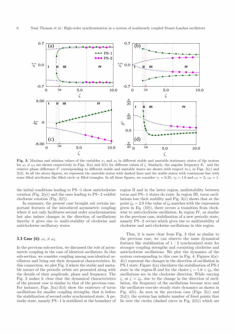
Fig. 3. Maxima and minima values of the variables x1 and x2 in different stable and unstable stationary states of the systemfor ω1 6= ω2 are shown respectively in Figs. 3(a) and 3(b) for different values of ζ. Similarly, the angular frequency θ1

∗

and therelative phase difference δ∗ corresponding to different stable and unstable states are shown with respect to ζ in Figs. 3(c) and3(d). In all the above figures, we represent the unstable states with dashed lines and the stable states with continuous line withsome filled attributes like filled circle or filled triangles. In all these figures, we consider γ1 = 0.25, γ2 = 1.0 and ω1 = 2, ω2 = 1.

the initial conditions leading to PS−1 show anticlockwiserotation (Fig. 2(e)) and the ones leading to PS−2 exhibitclockwise rotation (Fig. 2(f)).

In summary, the present case brought out certain im-portant features of the introduced asymmetric couplingwhere it not only facilitates second order synchronizationbut also induce changes in the direction of oscillationsthereby it gives rise to multi-stability of clockwise andanticlockwise oscillatory states.

3.3 Case (ii): ω1 6= ω2

In the previous sub-section, we discussed the role of asym-metric coupling in the case of identical oscillators. In thissub-section, we consider coupling among non-identical os-cillators and bring out their dynamical characteristics. Inthis connection, we plot Fig. 3 where the stable and unsta-ble nature of the periodic orbits are presented along withthe details of their amplitude, phase and frequency. TheFig. 3 makes it clear that the dynamical characteristicsof the present case is similar to that of the previous case.For instance, Figs. 3(a)-3(d) show the existence of torusoscillations for smaller coupling strengths, that is beforethe stabilization of second order synchronized state. A pe-riodic state, namely PS−1 is stabilized at the boundary of

region II and in the latter region, multistability betweentorus and PS−1 states do exist. In region III, torus oscil-lations lose their stability and Fig. 3(c) shows that at thepoint ζ0 = 2.0 (the value of ζ0 matches with the expressiongiven in Eq. (10)), there occurs a transition from clock-wise to anti-clockwise oscillation. In region IV, as similarto the previous case, stabilization of a new periodic state,namely PS−2 occurs which gives rise to multistability ofclockwise and anti-clockwise oscillations in this region.

Thus, it is more clear from Fig. 3 that as similar tothe previous case, we can observe the same dynamicalfeatures like stabilization of 1 : 2 synchronized state forstronger coupling strengths and coexisting clockwise andanticlockwise oscillations. We plot the dynamics of thesystem corresponding to this case in Fig. 4. Figures 4(a)-4(c) represent the changes in the direction of oscillation inPS-1 state. Figure 4(a) elucidates the stabilization of PS-1state in the region-II and for the choice ζ = 1.6 < ζ0, theoscillations are in the clockwise direction. While varyingζ, at ζ = ζ0, due to the change in the direction of oscil-lation, the frequency of the oscillations become zero andthe oscillators execute steady state dynamics as shown inFig. 4(b). As seen in the previous case (Figs. 2(c) and2(d)), the system has infinite number of fixed points thatlie over the circles (dashed curve in Fig. 2(b)) which are


PS-1 (ζ < ζ0)

xi

y i

0.70.0-0.7

0.7

0.0

-0.7

PS-1 (ζ = ζ0)

xi

y i

0.70.0-0.7

0.7

0.0

-0.7

PS-1 (ζ > ζ0)

xi

y i

0.80.0-0.8

0.8

0.0

-0.8

PS-2

xi

y i

0.80.0-0.8

0.8

0.0

-0.8

PS-1

t

xi

110105100

0.8

0.0

-0.8

PS-2

t

xi

110105100

0.8

0.0

-0.8

(a) (b) (c)

(f) (e) (d)

Fig. 4. Dynamics of the system for different ζ values and for γ1 = 0.25, γ2 = 1.0 and ω1 = 2, ω2 = 1.0. Figs. 4(a)-4(d) are thephase portraits for first and second oscillators for different values of ζ with (a) ζ = 1.6 < ζ0 (in region-2), (b) ζ = ζ0 = 2.0(region-3) and (c) and (d) ζ = 8.1 > ζ0 (region-4) respectively. Figs. 4(a)-4(c) illustrate the change in direction of oscillation inPS-1 state. To illustrate steady state dynamics at critical value, we considered three different initial conditions in Fig. 4(b) andhave given final asymptotic states respectively by circle, square and triangle. In this, the final asymptotic states of the first andsecond oscillators lie respectively over the red and black (dashed) circles. Figs. 4(c)-4(f) illustrates the multistability of PS-1and PS-2 states in region-4 (ζ = 8.1) where Figs. 4(c) and 4(e) (Figs. 4(d) and 4(f)) represent the phase portrait and temporaldynamics of PS-1 (PS-2) state in region-4. In all these figures, red curve (or red coloured attributes) represents the states of thefirst oscillator and black curve (or attributes in black colour) represents the state of the second oscillator. The arrows in thephase potraits (Figs. 4(a), 4(c) and 4(d)) represent the direction of oscillation.

defined by the radii (R∗

1 and R∗

2) and phase difference(δ∗) as given in Eqs. (11)-(13). To elucidate the above, weconsider three different initial conditions in Fig. 4(b) andthe final asymptotic states are represented by filled circle,square and triangle. For ζ = 8.1 > ζ0 (which lies in theregion-4), the multistability of PS-1 (anticlockwise) andPS-2 (clockwise) oscillations are shown in Figs. 4(c) and4(d) respectively. The corresponding temporal dynamicsin PS-1 and PS-2 states are given in Figs. 4(e) and 4(f)and these two figures make clear that in both PS-1 andPS-2 states, the frequencies of the two oscillators are notsame and from Eq. (9) we can confirm that these periodicstates (PS-1 and PS-2) are in 1 : 2 synchronized state. Inthe following, we consider the case where the natural fre-quencies of the uncoupled oscillators have the frequencyrelation ω1 : ω2 = 1 : 2 and investigate the role of asym-metric coupling in such a case.

4 Case (iii): ω2 = 2ω1

As we did earlier, in this interesting limiting case also,we first analytically study the dynamics of the system.For this purpose, we consider α = R1 exp (iθ1) and β =R2 exp (iθ2), where we take θ1 = −ω1t + φ1 and θ2 =−ω2t + φ2. The resultant amplitude and phase equations

are turned out to be

R1 = (γ1 − γ2R21)R1 + 2ζR1R2 sin(φ2 − 2φ1),

R2 = (γ1 − γ2R22)R2 − ζR2

1 sin(φ2 − 2φ1),

φ1 = −2ζR2 cos(φ2 − 2φ1),

φ2 = −ζ R21

R2

cos(φ2 − 2φ1). (14)

We reduce the above equations to the form

R1 = (γ1 − γ2R21)R1 + 2ζR1R2 sin δ,

R2 = (γ1 − γ2R22)R2 − ζR2

1 sin δ,

δ = −ζ(R2

1 − 4R22

R2

)

cos δ, (15)

with δ = θ2 − 2θ1 = φ2 − 2φ1. We now trace out thepossible stationary states or periodic orbits correspondingto this case. From the stability analysis we found thatthere exists two regions where the system exhibits differentdynamical behaviours. The dynamics of the stable andunstable periodic orbits in these dynamical regions aregiven below.

(i) For lower values of ζ we find that periodic orbitscorresponding to δ = π/2 and δ = 3π/2 do exist.When δ = π/2, the amplitude of the corresponding


ζ

x∗ 1 ps-III

ps-II

ps-I

ζ0

III

2.01.00

0.8

0.0

-0.8

ζ

x∗ 2

ζ0

III

2.01.00

0.8

0.0

-0.8

ζ

θ∗ 1

ζ0

III

2.01.00

0.5

-0.5

-1.5

-2.5

ζ

δ∗

ζ0

III

2.01.00

π

π2

0.0

(a)(b)

(c)(d)

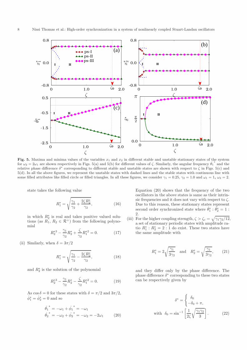
Fig. 5. Maxima and minima values of the variables x1 and x2 in different stable and unstable stationary states of the systemfor ω2 = 2ω1 are shown respectively in Figs. 5(a) and 5(b) for different values of ζ. Similarly, the angular frequency θ1

∗

and therelative phase difference δ∗ corresponding to different stable and unstable states are shown with respect to ζ in Figs. 5(c) and5(d). In all the above figures, we represent the unstable states with dashed lines and the stable states with continuous line withsome filled attributes like filled circle or filled triangles. In all these figures, we consider γ1 = 0.25, γ2 = 1.0 and ω1 = 1, ω2 = 2.

state takes the following value

R∗

1 =

√

γ1γ2

+2ζR∗

2

γ2, (16)

in which R∗

2 is real and takes positive valued solu-tions (as R1, R2 ∈ R+) from the following polyno-mial

R∗32 − γ1

γ2R∗

2 +ζ

γ2R∗2

1 = 0. (17)

(ii) Similarly, when δ = 3π/2

R∗

1 =

√

γ1γ2

− 2ζR∗

2

γ2, (18)

and R∗

2 is the solution of the polynomial

R∗32 − γ1

γ2R∗

2 −ζ

γ2R∗2

1 = 0. (19)

As cos δ = 0 for these states with δ = π/2 and 3π/2,

φ∗1 = φ∗2 = 0 and so

θ1∗

= −ω1 + φ1∗

= −ω1

θ2∗

= −ω2 + φ2∗

= −ω2 = −2ω1 (20)

Equation (20) shows that the frequency of the twooscillators in the above states is same as their intrin-sic frequencies and it does not vary with respect to ζ.Due to this reason, these stationary states representsecond order synchronized state where θ∗1 : θ∗2 = 1 :2.

(iii) For the higher coupling strength, ζ > ζc =√

γ1γ2/12,a set of stationary periodic states with amplitude ra-tio R∗

1 : R∗

2 = 2 : 1 do exist. These two states havethe same amplitude with

R∗

1 = 2

√

γ13γ2

and R∗

2 =

√

γ13γ2

, (21)

and they differ only by the phase difference. Thephase difference δ∗ corresponding to these two statescan be respectively given by

δ∗ =

{

δ0−δ0 + π,

with δ0 = sin−1

[

1

2ζ

√

γ1γ23

]

. (22)


Considering the frequencies of the two oscillators inthese states, we find that in the state with δ∗ = δ0,

θ1∗

= −ω1 − 2ζ

√

γ13γ2

cos δ0,

θ2∗

= −2ω1 − 4ζ

√

γ13γ2

cos δ0, (23)

and in the state with δ∗ = −δ0 + π

θ∗1 = −ω1 + 2ζ

√

γ13γ2

cos δ0,

θ∗2 = −2ω1 + 4ζ

√

γ13γ2

cos δ0. (24)

Thus the two states mentioned by δ∗ = δ0 and −δ0+πdo posses the same amplitudes but have different frequen-cies as given in Eqs. (23) and (24). Importantly, the lat-ter two equations indicate that these two states also havethe frequency ratio in the order θ∗1 : θ∗2 = 1 : 2 and sothey also represent the second order synchronized state.Yet another important observation that we can have fromEqs. (23) and (24) is that in the case δ∗ = δ0, θ

∗

1,2 remainnegative (representing clockwise oscillations) for ζ < ζ0,where ζ0 can be obtained from the expression (10) andthey take positive values (representing anti-clockwise os-cillations) when ζ > ζ0. But in the case δ∗ = −δ0 + π,

Eq. (24) shows that θ∗1,2 remain negative for all values ofζ and so they represent clockwise oscillations.

In the above, we discussed different stationary periodicorbits of the system. Now we turn our attention to the sta-bility nature of the periodic states. In this connection, weplot Fig. 5 by analyzing the existence and stability natureof the above stationary periodic orbits for ω1 = 1.0 andω2 = 2.0. As mentioned earlier there are two different dy-namical regions (I-II) as illustrated in Figs. 5(a)-(d) andfor smaller values of ζ (that is, for ζ < ζc), the states cor-responding to δ∗ = π/2 and 3π/2 (given in Eqs. (17) and(19)) only do exist. For the considered case (ω1 = 1.0 andω2 = 2.0), the polynomial in Eq. (17) corresponding toδ∗ = π/2 yields two positive real roots while Eq. (19) cor-responding to δ∗ = 3π/2 yields only one root. Thus, threestationary periodic orbits are possible for the lower valuesof ζ. Among the three, only one of the states correspond-ing to δ∗ = π/2 is found to be stable which is representedby the brown curve (colour online) with filled squares andthe other two unstable periodic states are represented bydashed blue curves (colour online) in Figs. 5(a)-(d). In-creasing the ζ value beyond ζc (that is, in the region-II),the stable branch of δ∗ = π/2 becomes unstable and thestates corresponding to δ∗ = δ0 and −δ0 + π comes toexistence. The stability of the latter two states are stud-ied and their stable region is obtained with the use ofRouth-Hurwitz criterion [23]. The result shows that thesetwo states become stable as soon as they come into exis-tence (that is, for ζ > ζc =

√

γ1γ2/12 = 0.14). The stablebranches of these two states are respectively indicated bygreen curve (color online) with filled triangles (ps-II state)

and magenta curve (color online) with filled circles (ps-IIIstate) in Figs. 5(a)-5(d).

With this knowledge on the stable states of the sys-tem for different values of ζ, in the following, we proceedto discuss the dynamical characteristics of the system. Thefirst difference which we notice in this case (from Fig. 5)in comparison to the previous cases is that the missing oftorus oscillation. As the intrinsic frequency itself has therelation ω1 : ω2 = 1 : 2, there is no need for torus os-cillation to mediate the stabilization of second order syn-chronized periodic state. Thus the periodic state ps-I isstable for lower coupling strengths (ζ < ζc, region-I). Bylooking at the branch corresponding to this ps-I state inFigs. 5(a) and 5(b), we understand that while we increasethe value of ζ from zero (in region-I), the amplitude ofthe first oscillator increases while the counterpart of thesecond oscillator decreases. We note that in the absence ofcoupling, the two oscillators oscillate with the same am-plitude. Correspondingly, Figs. 5(c) and 5(d) indicate thatfor all values of ζ < ζc (in region-I), the frequency of thetwo oscillators remains the same as that of the naturalfrequency (also shown by Eq. (20)) and the δ value alsoremains the same as π/2. The dynamics of the two oscil-lators in this region-I are presented respectively in Figs.6(a) and 6(b) for ζ = 0.0, 0.05 and 0.12. From these fig-ures, we observe that the amplitude of oscillations alonechanges with respect to ζ and frequencies remain the sameas that of the ζ = 0.0 case.

As mentioned earlier, while ζ < ζc, the amplitude ofthe two oscillators varies with respect to ζ and it reaches

the value R∗

1 = 2R∗

2 = 2

√

γ13γ2

at ζ = ζc. At this critical

point (ζ = ζc), Fig. 5 indicates the occurence of pitch-fork like bifurcation where the two new states, namelyps-II and ps-III gain stability and ps-I loses its stable na-ture. Beyond this critical point, the amplitudes of boththe oscillators do not vary and it remains the same as

R∗

1 = 2R∗

2 = 2

√

γ13γ2

(vide Eq. (21)) which can be seen

from the stable branches of ps-II and ps-III in Figs. 5(a)and the 5(b). The amplitude of oscillations in both thestates ps-II and ps-III are found to be same and so thebranches of ps-II and ps-III lie over each other in Figs.5(a) and 5(b). But considering the frequencies in ps-II andps-III states, Eqs. (23) and (24) and Fig. 5(c) indicatethat they are different and they vary with respect to ζ.Secondly, Eqs. (23) and (24) indicate that both the statesrepresent second order synchronized state. Thus for all val-ues of ζ, frequency of the two oscillators (in both ps-II andps-III states) are in the ratio 1 : 2. Comparing the ampli-tude and frequency ratios of these states (R∗

1 : R∗

2 = 2 : 1,

θ∗1 : θ∗2 = 1 : 2 ) we find that the periodic orbit of the firstoscillator is two times larger than the one correspondingto the second oscillator and the frequency of the secondoscillator is two times than that of the first oscillator.

From Fig. 5(d), it is clear that the value of δ corre-sponding to these two states are different and they varywith respect to ζ. It is important to note that δ value of theps-II state changes from positive to negative at the point


ζ = 0.12ζ = 0.05ζ = 0.00

t

x1

302010

0.8

0.0

-0.75

ζ = 0.12ζ = 0.08ζ = 0.00

t

x2

302010

0.8

0.0

-0.8

IC − 2IC − 1

t

x1

605040

0.8

0.0

-0.8

IC − 2IC − 1

t

x2

605040

0.8

0.0

-0.8

IC − 1

xi

y i

0.70.0-0.7

0.7

0.0

-0.7

IC − 2

xi

y i

0.70.0-0.7

0.7

0.0

-0.7

(a) (c) (e)

(b) (d) (f)

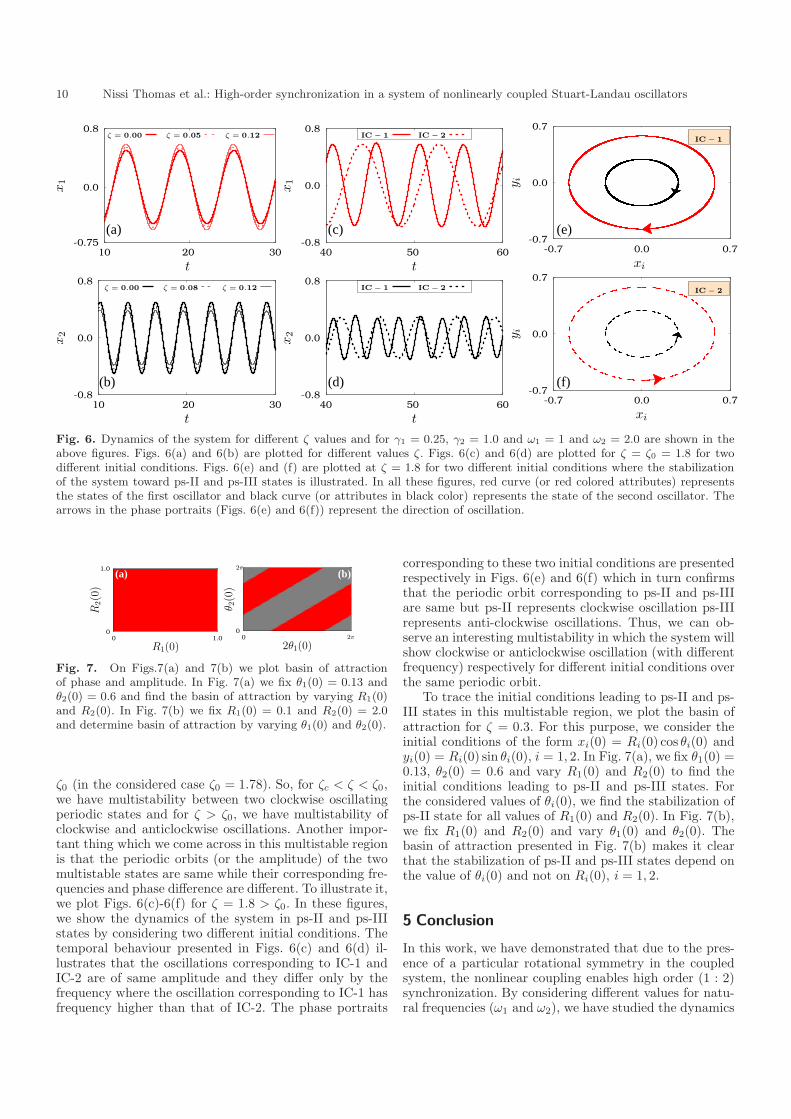
Fig. 6. Dynamics of the system for different ζ values and for γ1 = 0.25, γ2 = 1.0 and ω1 = 1 and ω2 = 2.0 are shown in theabove figures. Figs. 6(a) and 6(b) are plotted for different values ζ. Figs. 6(c) and 6(d) are plotted for ζ = ζ0 = 1.8 for twodifferent initial conditions. Figs. 6(e) and (f) are plotted at ζ = 1.8 for two different initial conditions where the stabilizationof the system toward ps-II and ps-III states is illustrated. In all these figures, red curve (or red colored attributes) representsthe states of the first oscillator and black curve (or attributes in black color) represents the state of the second oscillator. Thearrows in the phase portraits (Figs. 6(e) and 6(f)) represent the direction of oscillation.

2θ1(0)

θ2(0)

2π0

2π

0

R1(0)

R2(0)

1.00

1.0

0

(a) (b)

Fig. 7. On Figs.7(a) and 7(b) we plot basin of attractionof phase and amplitude. In Fig. 7(a) we fix θ1(0) = 0.13 andθ2(0) = 0.6 and find the basin of attraction by varying R1(0)and R2(0). In Fig. 7(b) we fix R1(0) = 0.1 and R2(0) = 2.0and determine basin of attraction by varying θ1(0) and θ2(0).

ζ0 (in the considered case ζ0 = 1.78). So, for ζc < ζ < ζ0,we have multistability between two clockwise oscillatingperiodic states and for ζ > ζ0, we have multistability ofclockwise and anticlockwise oscillations. Another impor-tant thing which we come across in this multistable regionis that the periodic orbits (or the amplitude) of the twomultistable states are same while their corresponding fre-quencies and phase difference are different. To illustrate it,we plot Figs. 6(c)-6(f) for ζ = 1.8 > ζ0. In these figures,we show the dynamics of the system in ps-II and ps-IIIstates by considering two different initial conditions. Thetemporal behaviour presented in Figs. 6(c) and 6(d) il-lustrates that the oscillations corresponding to IC-1 andIC-2 are of same amplitude and they differ only by thefrequency where the oscillation corresponding to IC-1 hasfrequency higher than that of IC-2. The phase portraits

corresponding to these two initial conditions are presentedrespectively in Figs. 6(e) and 6(f) which in turn confirmsthat the periodic orbit corresponding to ps-II and ps-IIIare same but ps-II represents clockwise oscillation ps-IIIrepresents anti-clockwise oscillations. Thus, we can ob-serve an interesting multistability in which the system willshow clockwise or anticlockwise oscillation (with differentfrequency) respectively for different initial conditions overthe same periodic orbit.

To trace the initial conditions leading to ps-II and ps-III states in this multistable region, we plot the basin ofattraction for ζ = 0.3. For this purpose, we consider theinitial conditions of the form xi(0) = Ri(0) cos θi(0) andyi(0) = Ri(0) sin θi(0), i = 1, 2. In Fig. 7(a), we fix θ1(0) =0.13, θ2(0) = 0.6 and vary R1(0) and R2(0) to find theinitial conditions leading to ps-II and ps-III states. Forthe considered values of θi(0), we find the stabilization ofps-II state for all values of R1(0) and R2(0). In Fig. 7(b),we fix R1(0) and R2(0) and vary θ1(0) and θ2(0). Thebasin of attraction presented in Fig. 7(b) makes it clearthat the stabilization of ps-II and ps-III states depend onthe value of θi(0) and not on Ri(0), i = 1, 2.

5 Conclusion

In this work, we have demonstrated that due to the pres-ence of a particular rotational symmetry in the coupledsystem, the nonlinear coupling enables high order (1 : 2)synchronization. By considering different values for natu-ral frequencies (ω1 and ω2), we have studied the dynamics


in different cases. In the ω2 6= 2ω1 case, we have shownthat the system tries to adjust itself towards 1 : 2 synchro-nized state and so torus type oscillations can be observedin weak coupling regime. In the strong coupling regime,we have observed that 1 : 2 type synchronous periodicoscillations appear. We have also identified the multista-bility of clockwise and anticlockwise periodic states in thisregime. In the limiting case (ω2 = 2ω1) 1 : 2 synchronousstates are observed in all the parametric regions. In thiscase, we have demonstrated that the periodic orbit cor-responding to clockwise and anticlockwise periodic statesare the same and they differ only in phase and frequency.

The higher order synchronization has been observedand applied in various biological and/or physical mod-els [13,16,17,18,19,20,24,25]. Hence we expect that theabove mentioned possibility to induce high order synchorniza-tion may have interesting practical applications.

Acknowledgements

NT wishes to thank National Board for Higher Math-ematics, Government of India, for providing the JuniorResearch Fellowship under the Grant No. 02011/20/2018NBHM (R.P)/R&D II/15064. The work of MS forms partof a research project sponsored by Council of Scientificand Industrial Research, Government of India, under theGrant No. 03/1397/17/EMR-II.

Author contributions

All the authors contributed equally to the preparation ofthis manuscript.

Data Availability Statement

All datas generated or analyzed during this study are in-cluded in this article.

References

1. A. Pikovsky, M. Rosenblum and J. Kurths, Synchronization:A Universal Concept in Nonlinear Sciences, (Cambridge Uni-versity Press, Cambridge, 2003).

2. S. -Y. Ha, H. K. Kim, S. W. Ryoo, Commun. Math. Sci.14, 1073 (2016).

3. E. Um, M. Kim, H. Kim, J. H. Kang, H. A. Stone and J.Jeong, Nat. Commun. 11 , 5221 (2020).

4. A. A. Koronovskii, O. I. Moskalenko, A. A. Pivovarov andE. V. Evstifeev, Chaos 30 , 083133 (2020).

5. S. H. Park, J. D. Griffiths, A. Longtin and J. Lefebvre,Front. Appl. Math. Stat. 4, 31 (2018).

6. S. Krishnagopal, J. Lehnert, W. Poel, A. Zhakharova andE. Scholl, Phil. Trans. R. Soc. A. 375, 20160216 (2017).

7. Y. Kuramoto, D. Battogtokh, Nonlin. Phenom. ComplexSys. 5, 380 (2002).

8. M. J. Panaggio, D. M. Abrams, Nonlinearity 28, R67(2015).

9. K. Premalatha, V. K. Chandrasekar, M. Senthilvelan andM. Lakshmanan, Phys. Rev. E. 95, 022208 (2017).

10. Y. Maistrenko, B. Penkovsky and M. Rosenblum, Phys.Rev. E. 89, 060901(R) (2014).

11. E. Rybalova, V. S. Anishchenko, G. I. Strelkova and A.Zakharova, Chaos 29, 071106 (2019).

12. L. Kang, Z. Wang, S. Huo, C. Tian and Z. Liu, NonlinearDyn. 99, 1577 (2020).

13. C. Schafer, M. G. Rosenblum, H-H Abel, J. Kurths, Phys.Rev. E 60, 857 (1999).

14. A. K. Jain, K. K. Likharev, J. E. Lukens and J. E.Sauvagean, Phys. Rep. 109, 309 (1984).

15. J. Simonet, M. Warden and E. Brun, Phys. Rev. E 50,3383 (1994).

16. A. Velichko, V. Putrolaynen, M. Belyaev, Neural Comput& Appl. 33, 3113 (2021).

17. A. Velichko, M. Belyaev, V. Putrolaynen, V. Perminov, A.Pergament, Solid State Electron. 141, 40 (2018).

18. A. Velichko, M. Belyaev, P.Boriskov, Electronics 8(1), 75(2019).

19. A. Velichko, Electronics 8(7), 756 (2019).20. A. Velichko, D. Ryabokom, S. Khanin, A. Sidorenko andA. Rikkiev, IOP Conf. Ser.: Mater. Sci. Eng. 862, 052062(2020).

21. Nissi Thomas, M. Senthilvelan, Quantum Synchronizationof Quantum van der Pol oscillators via cross-Kerr Interaction(Submitted for publication (2021)).

22. S. Ding, G. Maslennikov, R. Hablutzel, H. Loh and D.Matsukevich, Phys. Rev. Lett. 119, 150404 (2017) .

23. M. Lakshmanan and S. Rajasekar, Nonlinear Dynamics:

Integrability, Chaos and Patterns, (Springer, Berlin, 2003).24. D. C. Michaels, E. P. Matyas, J. Jalife, Circ. Res. 58 , 706(1986).

25. R. Bychkov, M. Juhaszova, K. Tsutsui, C. Coletta, M. D.Stern, V. A. Maltsev, E. G. Lakatta, J AM Coll Cardiol EP.6(8), 907-931 (2020).

Documents

Stuart-Landau oscillators