DRAFT

STRUTTURE AERONAUTICHE1

course notes - Part 1 (P1)

Theoretical Fundation of F.E.M.

Structural Dynamics of space-discretized and space-continuous systems

Luigi Morino c⃝ Franco Mastroddi c⃝ Luigi Balis Crema c⃝

September 2017

1Realizzazione di parte delle figure a cura di Valerio Farano, Alessandro Settimi, Sabino Loiodice, Sara DiMario

Contents

I Theoretical Foundation of F.E.M. 1

1 Kinematics 3

1.1 Lagrangian and Eulerian Formulations. Referential description for solid continuum. 3

1.1.1 Material Derivative, Velocity . . . . . . . . . . . . . . . . . . . . . . . . . 6

1.1.2 Derivative of Jacobian . . . . . . . . . . . . . . . . . . . . . . . . . . . . . 8

1.2 Conservation of Mass; Transport Theorems . . . . . . . . . . . . . . . . . . . . . 8

1.2.1 Material Volumes and First Reynolds Transport Theorem . . . . . . . . . 8

1.2.2 Continuity Equation . . . . . . . . . . . . . . . . . . . . . . . . . . . . . . 11

1.2.3 Second Reynolds Transport Theorem . . . . . . . . . . . . . . . . . . . . . 12

1.3 Strain Tensor . . . . . . . . . . . . . . . . . . . . . . . . . . . . . . . . . . . . . . 12

1.4 APPENDIX: Finite Deformation and Strain Tensor∗ . . . . . . . . . . . . . . . . 15

1.4.1 Deformation and Deformation Gradient∗ . . . . . . . . . . . . . . . . . . 15

1.4.2 Stretch Tensors and Cauchy–Green Tensors∗ . . . . . . . . . . . . . . . . 16

1.4.3 Strain Tensor∗ . . . . . . . . . . . . . . . . . . . . . . . . . . . . . . . . . 17

1.4.4 Time Derivative of Strain Tensor∗ . . . . . . . . . . . . . . . . . . . . . . 18

2 Momentum and Energy 21

2.1 Conservation Principles . . . . . . . . . . . . . . . . . . . . . . . . . . . . . . . . 21

2.2 Dynamics . . . . . . . . . . . . . . . . . . . . . . . . . . . . . . . . . . . . . . . . 22

2.2.1 Stress Tensor . . . . . . . . . . . . . . . . . . . . . . . . . . . . . . . . . . 22

2.2.2 Cauchy Equations of Motion . . . . . . . . . . . . . . . . . . . . . . . . . 24

i

2.2.3 Symmetry of Stress Tensor . . . . . . . . . . . . . . . . . . . . . . . . . . 24

2.2.4 Conservation of Mechanical Energy . . . . . . . . . . . . . . . . . . . . . . 25

2.3 Energy . . . . . . . . . . . . . . . . . . . . . . . . . . . . . . . . . . . . . . . . . 26

2.3.1 Conservation of Thermodynamic Energy . . . . . . . . . . . . . . . . . . . 26

2.3.2 Heat Flux Vector . . . . . . . . . . . . . . . . . . . . . . . . . . . . . . . 26

2.3.3 Conservation of Thermodynamic Energy – Differential Form . . . . . . . 28

2.4 Alternative Axioms – Galilean Relativity∗ . . . . . . . . . . . . . . . . . . . . . . 28

3 Thermodynamics 31

3.1 Second Principle of Thermodynamics . . . . . . . . . . . . . . . . . . . . . . . . 31

3.2 Thermodynamics of Solids . . . . . . . . . . . . . . . . . . . . . . . . . . . . . . . 32

3.2.1 Entropy Evolution Equation . . . . . . . . . . . . . . . . . . . . . . . . . 33

3.2.2 Elastic Solids . . . . . . . . . . . . . . . . . . . . . . . . . . . . . . . . . . 34

3.2.3 Alternative Formulation – Free Energy * . . . . . . . . . . . . . . . . . . . 35

3.3 Constitutive equations for isotropic solids . . . . . . . . . . . . . . . . . . . . . . 37

3.3.1 Linearly-elastic and Hookean solids . . . . . . . . . . . . . . . . . . . . . . 37

4 Lagrange equations of motion 45

4.1 Virtual Work Law (weak formulation) . . . . . . . . . . . . . . . . . . . . . . . . 45

4.2 Restricted formulation . . . . . . . . . . . . . . . . . . . . . . . . . . . . . . . . . 46

4.3 Galerkin Equations of Motion . . . . . . . . . . . . . . . . . . . . . . . . . . . . 48

4.4 Lagrange Equations of Motion: general formulation∗ . . . . . . . . . . . . . . . . 51

5 Some issues on Finite Element Method 55

5.1 General characterization of the Finite Element . . . . . . . . . . . . . . . . . . . 55

5.1.1 Displacement field description inside the Finite Element . . . . . . . . . . 55

5.1.2 Constitutive law for the Finite Element . . . . . . . . . . . . . . . . . . . 56

5.1.3 Kinematic law for the Finite Element . . . . . . . . . . . . . . . . . . . . 57

5.1.4 Basic (Lagrange) equations for a generic Finite Element . . . . . . . . . . 58

ii

5.2 1D Finite Elements . . . . . . . . . . . . . . . . . . . . . . . . . . . . . . . . . . . 59

5.2.1 1D axial and torsional beam element . . . . . . . . . . . . . . . . . . . . . 59

5.2.2 1D bending beam element . . . . . . . . . . . . . . . . . . . . . . . . . . . 61

5.2.3 General case of 1D element . . . . . . . . . . . . . . . . . . . . . . . . . . 65

5.3 2D Finite Elements . . . . . . . . . . . . . . . . . . . . . . . . . . . . . . . . . . . 66

5.3.1 2D triangular planar element with in-plane stress . . . . . . . . . . . . . . 66

5.3.2 2D rectangular planar element with in plane stress . . . . . . . . . . . . . 69

5.3.3 2D rectangular planar bending Finite Element . . . . . . . . . . . . . . . 71

5.4 3D Finite Elements . . . . . . . . . . . . . . . . . . . . . . . . . . . . . . . . . . . 72

5.4.1 3D tetrahedral Finite Element . . . . . . . . . . . . . . . . . . . . . . . . 72

5.4.2 Some brief comment on 3D hexahedral Finite Element . . . . . . . . . . . 74

5.5 Final problem assembled: global matrices and global loads . . . . . . . . . . . . . 74

5.5.1 Assembly example . . . . . . . . . . . . . . . . . . . . . . . . . . . . . . . 76

5.5.2 Assignment of the boundary conditions . . . . . . . . . . . . . . . . . . . 78

5.6 Some essential properties of Finite Elements . . . . . . . . . . . . . . . . . . . . . 78

5.6.1 Completeness . . . . . . . . . . . . . . . . . . . . . . . . . . . . . . . . . . 78

5.6.2 Compatibility . . . . . . . . . . . . . . . . . . . . . . . . . . . . . . . . . . 79

5.6.3 Convergence . . . . . . . . . . . . . . . . . . . . . . . . . . . . . . . . . . 79

5.6.4 Geometric invariance . . . . . . . . . . . . . . . . . . . . . . . . . . . . . . 80

II Structural Dynamics of Space-Discretized and Space-Continuous Sys-

tems 81

6 Dynamics of Space-Discret(-ized) Structures- Eigenvectors method 83

6.1 First order systems of linear ODE: free response∗ . . . . . . . . . . . . . . . . . . 83

6.2 First order systems of linear ODE: driven response∗ . . . . . . . . . . . . . . . . 86

6.3 Second order systems of linear ODE for structural problems: associated eigen-

problem and free undamped response . . . . . . . . . . . . . . . . . . . . . . . . . 88

iii

6.3.1 Associated eigenproblem . . . . . . . . . . . . . . . . . . . . . . . . . . . . 88

6.3.2 Free response problem and normal modes of vibrations . . . . . . . . . . . 91

6.3.3 Another Lagrangean-coordinate change∗ . . . . . . . . . . . . . . . . . . . 94

6.4 Second order systems of linear ODE for structural problems: driven undamped

response . . . . . . . . . . . . . . . . . . . . . . . . . . . . . . . . . . . . . . . . . 96

6.4.1 Time Domain (TD) solution . . . . . . . . . . . . . . . . . . . . . . . . . . 96

6.4.2 Laplace Domain (LD) solution (Transfer Function Matrix) . . . . . . . . . 97

6.4.3 Fourier Domain (FD) solution (Frequency Response Function Matrix):

resonance conditions . . . . . . . . . . . . . . . . . . . . . . . . . . . . . . 98

6.4.3.1 Resonance conditions . . . . . . . . . . . . . . . . . . . . . . . . 100

6.5 Eigenproblems associated to Structural problem written as system of first order

ODE . . . . . . . . . . . . . . . . . . . . . . . . . . . . . . . . . . . . . . . . . . . 102

6.6 Co-ordinate Transformations∗ . . . . . . . . . . . . . . . . . . . . . . . . . . . . . 103

6.6.1 Finite Elements vs Modes of Vibration . . . . . . . . . . . . . . . . . . . . 104

6.6.2 Comments . . . . . . . . . . . . . . . . . . . . . . . . . . . . . . . . . . . 106

6.6.3 General Change in Lagrangian Co-ordinates∗ . . . . . . . . . . . . . . . . 107

7 Dynamics of Space-Continuous Structures

- Eigenfunctions method 109

7.1 Eigenfunctions Method – Linear Differential Operators Theory . . . . . . . . . . 109

7.1.1 Definition of Linear Differential Operator . . . . . . . . . . . . . . . . . . 110

7.1.2 Eigenvalues and Eigenfunctions of a Linear Operator . . . . . . . . . . . . 110

7.1.2.1 Example of eigenvalues and eigenfunctions . . . . . . . . . . . . 111

7.1.3 Inner Product, Orthogonality and Set of Orthogonal Functions . . . . . . 112

7.1.4 Adjoint and Self-Adjoint Operators – Betti-Castigliano Theorem for Struc-

tural Operators . . . . . . . . . . . . . . . . . . . . . . . . . . . . . . . . . 113

7.1.4.1 Examples of Self-Adjoint Operators . . . . . . . . . . . . . . . . 114

7.1.4.2 Theorems on self-adjointness . . . . . . . . . . . . . . . . . . . . 115

iv

7.1.5 Eigenvalues and eigenfunction of structural operator v.s. natural frequen-

cies and modes of a structure – Free response . . . . . . . . . . . . . . . . 116

7.1.5.1 Natural modes and frequencies of a homogeneous beam . . . . . 117

7.1.6 Static and Dynamic structural problems using the eigenfunction method

and influence function method – Static and Dynamic responses . . . . . . 121

7.1.6.1 Static problems using the eigenfunction method (Navier’s ap-

proach) . . . . . . . . . . . . . . . . . . . . . . . . . . . . . . . . 122

7.1.6.2 Static problems using the Green function method∗ . . . . . . . . 123

7.1.6.3 Dynamic problems using the eigenfunction method . . . . . . . . 124

7.1.6.4 Dynamic problems using the Green function method∗ . . . . . . 127

7.2 Discretized Eigenfunction methods: comparisons with other standard discretiza-

tion methods . . . . . . . . . . . . . . . . . . . . . . . . . . . . . . . . . . . . . . 132

7.2.1 Eigenfunction method v.s. Galerkin method . . . . . . . . . . . . . . . . . 132

7.2.1.1 An example . . . . . . . . . . . . . . . . . . . . . . . . . . . . . . 133

7.2.2 Galerkin method v.s. Rayleigh-Ritz method . . . . . . . . . . . . . . . . . 136

7.2.2.1 Examples . . . . . . . . . . . . . . . . . . . . . . . . . . . . . . . 138

7.2.3 Some issues on approximated-Eigenfunctions∗ . . . . . . . . . . . . . . . . 145

7.2.4 Fredholm Alternative in the Eigenfunctions/Eigenvectors Method∗ . . . . 148

7.3 Linear operators in three-dimensional linear elasticity . . . . . . . . . . . . . . . 150

7.3.1 Linear dynamic equations for elasticity . . . . . . . . . . . . . . . . . . . . 150

7.3.2 Adjoint and selfadjoint operators . . . . . . . . . . . . . . . . . . . . . . . 151

7.3.3 Selfadjointness of structural operators . . . . . . . . . . . . . . . . . . . . 152

7.3.4 Green’s function (or influence function) for static problems* . . . . . . . . 152

7.3.4.1 Symmetry of G(x,x∗)(p)i . . . . . . . . . . . . . . . . . . . . . . . 153

7.3.5 Green’s integral representation using free-space Green influence function:

BEM in elastostatics∗ . . . . . . . . . . . . . . . . . . . . . . . . . . . . . 153

8 Some Issues on Vibration Damping 155

v

8.1 Highly-Damped linear structures: time-frequency independent and dependent

damping . . . . . . . . . . . . . . . . . . . . . . . . . . . . . . . . . . . . . . . . . 155

8.1.1 Time-frequency independent visco-elastic linear models . . . . . . . . . . 156

8.1.2 Generalized time-frequency dependent visco-elastic linear models . . . . . 157

8.2 Weakly damped linear structures: Reyleigh-Basile hypothesis . . . . . . . . . . . 160

9 Reduction/Condensation Techniques 167

9.1 Static condensation (Guyan-Iron method) . . . . . . . . . . . . . . . . . . . . . . 169

9.2 Dynamic condensation (Craig-Bambton method) . . . . . . . . . . . . . . . . . . 170

9.3 System Equivalent Reduction Expansion Process (SEREP)∗ . . . . . . . . . . . . 173

Bibliography . . . . . . . . . . . . . . . . . . . . . . . . . . . . . . . . . . . . . . . . . 174

A Some issues on Laplace Transform and convolution product 177

A.1 Very basic concepts on Laplace transforms . . . . . . . . . . . . . . . . . . . . . . 177

A.2 General solution for a forced oscillator∗ . . . . . . . . . . . . . . . . . . . . . . . 179

B Some Issues on Fourier Series and Integral 181

B.1 From the Fourier series to the Fourier Integral . . . . . . . . . . . . . . . . . . . . 181

B.1.1 Real Fourier series . . . . . . . . . . . . . . . . . . . . . . . . . . . . . . . 181

B.1.2 Complex Fourier series . . . . . . . . . . . . . . . . . . . . . . . . . . . . . 182

B.1.3 Fourier integral . . . . . . . . . . . . . . . . . . . . . . . . . . . . . . . . . 184

B.2 Discrete Fourier transform and its inverse∗ . . . . . . . . . . . . . . . . . . . . . . 186

vi

Part I

Theoretical Foundation of F.E.M.

1

Chapter 1

Kinematics

In this chapter we discuss some basic concepts regarding the kinematics of deformable continua.

We start with Lagrangian and Eulerian formulations which are discussed in terms of material

coordinates. Next, we examine the principle of conservation of mass for a continuum and some

important consequence (transport theorem) and finally some remarks on strain tensor for solid

continua.

1.1 Lagrangian and Eulerian Formulations. Referential descrip-tion for solid continuum.

In studying the motion of a continuum, one may adopt two points of view. In the first, one

observes the motion of the material points, i.e., the locations of the particles of the continuum

as functions of time. The alternate point of view consists in studying the velocity field at a fixed

point in space. The first approach is known as the Lagrangian point of view, the second as the

Eulerian one.1

In order to formulate these concepts in mathematical terms, let us introduce two different

coordinate systems. The first one is based upon an orthonormal, right-handed Cartesian frame

of reference, with base vectors ih, such that ih · ik = δhk. In this frame of reference, the location

of a point P is determined by the vector

x = x1i1 + x2i2 + x3i3 (1.1)

connecting the origin O to the point P ; x1, x2, and x3 are the Cartesian coordinates of P . In

1The Lagrangian approach is typically used to study solids (i.e., to evaluate the location of each materialpoint as a function of time), whereas the Eulerian approach is typically used to analyze fluids (i.e., to evaluatethe velocity field as a function of x and t). However, for the analysis of the vorticity transport, in particular forstudying wakes, it may be more convenient to use the Lagrangian formulation; this approach is used here.

3

4

the following, we typically identify the point P with its location x.

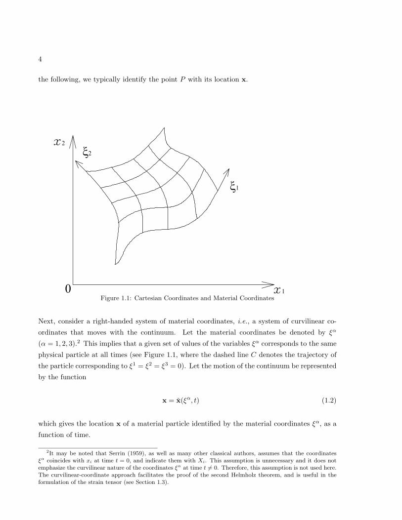
Figure 1.1: Cartesian Coordinates and Material Coordinates

Next, consider a right-handed system of material coordinates, i.e., a system of curvilinear co-

ordinates that moves with the continuum. Let the material coordinates be denoted by ξα

(α = 1, 2, 3).2 This implies that a given set of values of the variables ξα corresponds to the same

physical particle at all times (see Figure 1.1, where the dashed line C denotes the trajectory of

the particle corresponding to ξ1 = ξ2 = ξ3 = 0). Let the motion of the continuum be represented

by the function

x = x(ξα, t) (1.2)

which gives the location x of a material particle identified by the material coordinates ξα, as a

function of time.

2It may be noted that Serrin (1959), as well as many other classical authors, assumes that the coordinatesξα coincides with xi at time t = 0, and indicate them with Xi. This assumption is unnecessary and it does notemphasize the curvilinear nature of the coordinates ξα at time t = 0. Therefore, this assumption is not used here.The curvilinear-coordinate approach facilitates the proof of the second Helmholz theorem, and is useful in theformulation of the strain tensor (see Section 1.3).

5

Next, we assume that the Jacobian of the transformation

J =∂(x1, x2, x3)

∂(ξ1, ξ2, ξ3)(1.3)

is non-zero and finite, i.e., that Eq. 1.2 represents a one-to-one transformation. Thus, Eq. 1.2

may be inverted to give

ξα = ξα(x, t) (1.4)

Also, recall that both systems of coordinates were assumed to be right-handed: hence, we have

that the Jacobian of the transformation is positive: J > 0.

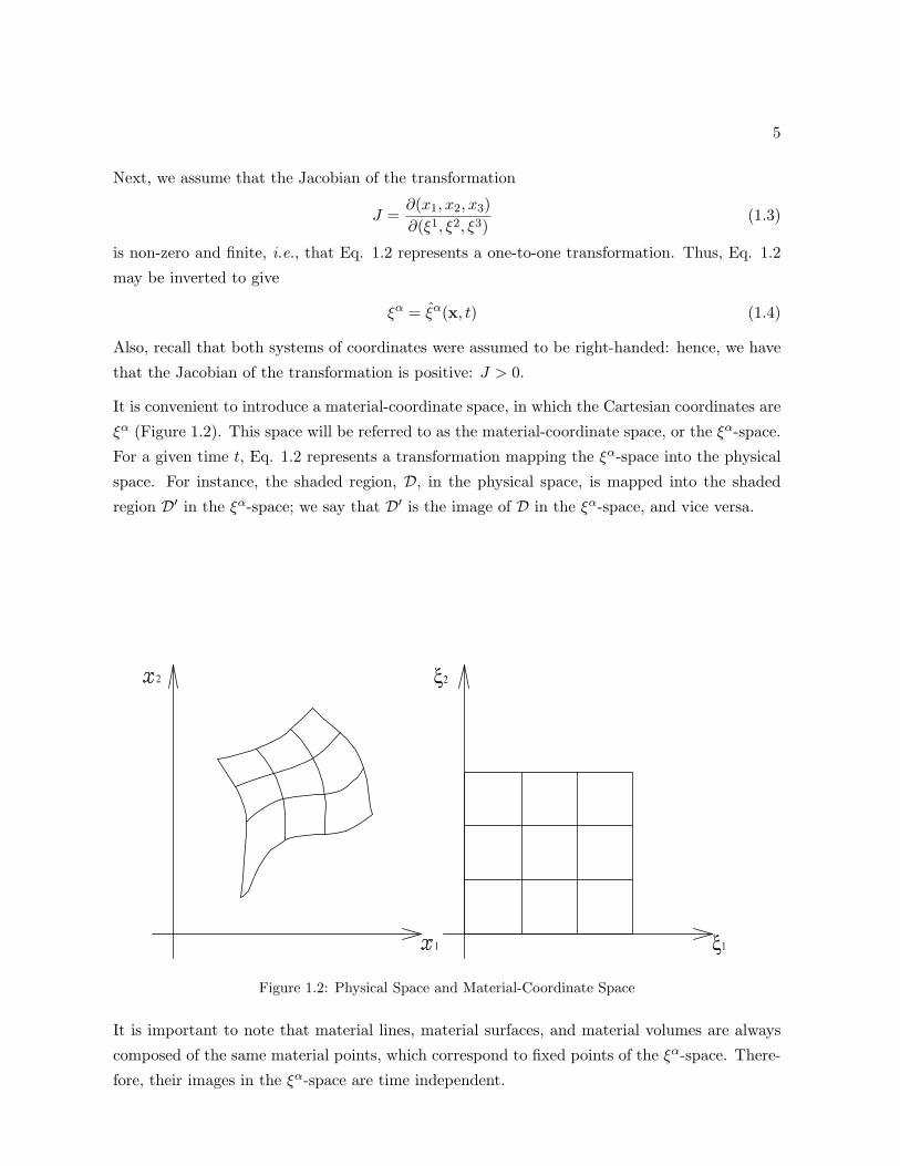
It is convenient to introduce a material-coordinate space, in which the Cartesian coordinates are

ξα (Figure 1.2). This space will be referred to as the material-coordinate space, or the ξα-space.

For a given time t, Eq. 1.2 represents a transformation mapping the ξα-space into the physical

space. For instance, the shaded region, D, in the physical space, is mapped into the shaded

region D′ in the ξα-space; we say that D′ is the image of D in the ξα-space, and vice versa.

Figure 1.2: Physical Space and Material-Coordinate Space

It is important to note that material lines, material surfaces, and material volumes are always

composed of the same material points, which correspond to fixed points of the ξα-space. There-

fore, their images in the ξα-space are time independent.

6

Next, note that we may study a continuum by following the material particles, i.e., by keeping the

coordinates ξα fixed as time varies; as mentioned above, this point of view is called Lagrangian.

In this approach, the density, for instance, is studied as a function of ξα and t. In general, for

any quantity f , we have

f = f(ξα, t) (1.5)

The alternate point of view is the Eulerian, in which the motion is analyzed by studying its

properties at a given point in space during the course of time. In this case, for any function f ,

combining Eqs. 1.4 and 1.5 and setting f(ξα(x, t), t) = f(x, t), we obtain

f = f(x, t) (1.6)

Vice versa, Eq. 1.5 can be obtained from Eq. 1.6 by using Eq. 1.2 and setting f(x(ξα, t), t) =

f(ξα, t).

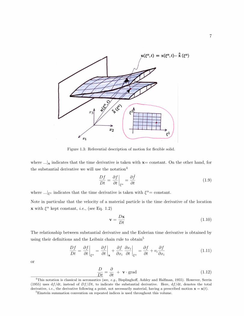
As final remarks in this Section, let us observe that for solid continua it is tipical to refer the

motion to a special or specific reference position here denoted by the vector field◦x (ξα) such

that one can decompose the motion x(ξα, t) as in the following (see Fig. 1.3)

x(ξα, t) =◦x (ξα) + u(ξα, t) (1.7)

This kind of description typical for solid mechanics is also known as referential description.

When this description is adopted, the motion of the continuum is determined by the vector

field u(ξα, t) denoted as displacement field. Note also that in most of the applications in solid

mechanics of deformable bodies the undeformed configurations are often assumed as reference

configurations for the motion of flexible solid bodies (see Section 1.3).

1.1.1 Material Derivative, Velocity

It is important to emphasize the difference between the time derivatives with spatial coordinates

kept constant (i.e., in a fixed point in space, Eulerian derivative) and that with material coordi-

nates kept constant. The latter is the time derivative performed by an observer travelling with

a material particle, and is referred to as the material or substantial derivative of f . In order

to keep notational complexity to a mininum, we will use the following classical convention of

retaining the partial-derivative notations for the Eulerian derivative3

∂f

∂t=∂f

∂t

∣∣∣∣x

=∂f

∂t(1.8)

3See, e.g., Serrin (1959).

7

Figure 1.3: Referential description of motion for flexible solid.

where ...|x indicates that the time derivative is taken with x= constant. On the other hand, for

the substantial derivative we will use the notation4

Df

Dt=∂f

∂t

∣∣∣∣ξα

=∂f

∂t(1.9)

where ...|ξα indicates that the time derivative is taken with ξα= constant.

Note in particular that the velocity of a material particle is the time derivative of the location

x with ξα kept constant, i.e., (see Eq. 1.2)

v =Dx

Dt(1.10)

The relationship between substantial derivative and the Eulerian time derivative is obtained by

using their definitions and the Leibniz chain rule to obtain5

Df

Dt=∂f

∂t

∣∣∣∣ξα

=∂f

∂t

∣∣∣∣x

+∂f

∂xi

∂xi∂t

∣∣∣∣ξα

=∂f

∂t+ vi

∂f

∂xi(1.11)

or

D

Dt=

∂

∂t+ v · grad (1.12)

4This notation is classical in aeronautics (see, e.g., Bisplinghoff, Ashley and Halfman, 1955). However, Serrin(1955) uses df/dt, instead of Df/Dt, to indicate the substantial derivative. Here, df/dt, denotes the totalderivative, i.e., the derivative following a point, not necessarily material, having a prescribed motion x = x(t).

5Einstein summation convention on repeated indices is used throughout this volume.

8

1.1.2 Derivative of Jacobian

In closing this section, we introduce an elegant formula that relates divv to material derivative

of J as

DJ

Dt= Jdivv (1.13)

In order to prove Eq. 1.13, let Jαi be the cofactor of ∂xi/∂ξ

α so that

∑α

∂xi∂ξα

Jαk = Jδik = J if i = k

= 0 if i = k (1.14)

Then, recalling the rule for derivatives of determinants,

DJ

Dt=

∑α,i

D

Dt

(∂xi∂ξα

)Jαi =

∑α,i

∂vi∂ξα

Jαi

=∑α,i,j

∂vi∂xj

∂xj∂ξα

Jαi =

∑i,j

∂vi∂xj

Jδji = J∑i

∂vi∂xi

= J divv (1.15)

in agreement with Equation 1.13.

1.2 Conservation of Mass; Transport Theorems

1.2.1 Material Volumes and First Reynolds Transport Theorem

In this section we use the concept of a material volume, i.e., a volume that is composed of the

same material point, at all time. We will denote this volume with VM and with V0 its image in

the ξα-space. Hence, a volume integral may be expressed as

FM =

∫∫∫VM

fdV =

∫∫∫V0

fJdV0 (1.16)

where dV0 = dξ1dξ2dξ3 is a volume element in the ξα-space. Note that, by definition, V0, and

hence its boundaries in the ξα-space, are time independent. This facilitates the differentiation

of integrals over the volume VM , and this is the main reason for their use in the following.

Consider a material volume VM (t) which deforms in time with the motion law. Then, the volume

integral of an arbitrary but prescribed function f(x, t),

F =

∫∫∫VM (t)

f(x, t) dV (1.17)

is a function only of t.

9

Its derivative with respect to t is given by

d

dt

∫∫∫VM (t)

f dV =

∫∫∫VM (t)

∂f

∂tdV +⃝

∫∫SM (t)

f v · n dS (1.18)

where v is the speed of the continuum on the material boundary ⃝∫∫SM (t) and n its outward unit

normal. Note that in the case of a surface moving in space, the tangential component of the

velocity cannot be defined, as it is apparent in the case of a rotating sphere.

In order to prove Eq. 1.18 (avoiding, for the sake of notation coincisness, the subscript M ), recall

the definition of derivative

dF

dt= lim

t′→t

1

∆t

(∫∫∫V(t′)

f(x, t′) dV −∫∫∫

V(t)f(x, t) dV

)(1.19)

where ∆t = t′ − t.

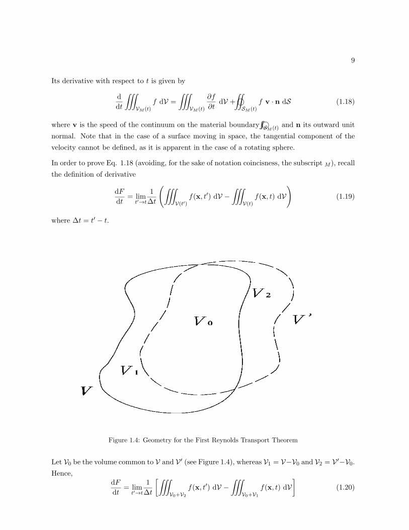
Figure 1.4: Geometry for the First Reynolds Transport Theorem

Let V0 be the volume common to V and V ′ (see Figure 1.4), whereas V1 = V−V0 and V2 = V ′−V0.

Hence,dF

dt= lim

t′→t

1

∆t

[∫∫∫V0+V2

f(x, t′) dV −∫∫∫

V0+V1

f(x, t) dV]

(1.20)

10

Note that the right hand side may be divided into a volume contribution given by

JV = limt′→t

1

∆t

[∫∫∫V0

f(x, t′)dV −∫∫∫

V0

f(x, t)dV]

= limt→′

t1

∆t

∫∫∫V0

[f(x, t′)− f(x, t)

]dV =

∫∫∫V

∂f

∂tdV (1.21)

plus a boundary contribution given by

JB = limt′→t

1

∆t

[∫∫∫V2

f(x, t′)dV −∫∫∫

V1

f(x, t)dV]

= limt′→t

1

∆t

[⃝∫∫

S2

f(x, t′)τ1dS −⃝∫∫

S1

f(x, t)τ2dS]

(1.22)

where Sk is the material boundary between V0 and Vk (k = 1, 2) whereas τk is the thickness of

the volume Vk, given by (recall that v · n is positive if the surface moves in the direction of the

outer normal n, i.e., on S2)

τ1 = −v · n∆t (1.23)

τ2 = v · n∆t (1.24)

Hence

JB = limt′→t

(1

∆t⃝∫∫

S1∪S2

f(x, t)v · n∆tdS)

= ⃝∫∫

Sf(x, t)v · ndS (1.25)

and finally noting that dF/dt = JV + JB, one obtains the First Reynolds Transport Theorem,

Eq. 1.18, for the derivative of the volume integral given by Eq. 1.17. This is an extension to

volume integrals of the Leibnitz formula for the derivative of an integral in which the limits of

integration as well as the integrand are functions of the variable of differentiation.

Equation 1.18 may be rewritten as

d

dt

∫∫∫VM

f dV =

∫∫∫VM

(∂f

∂t+ div f v

)dV (1.26)

or

d

dt

∫∫∫VM

f dV =

∫∫∫VM

(Df

Dt+ f divv

)dV (1.27)

since

∂f

∂t+ div (fv) =

∂f

∂t+ v · grad f + fdivv =

Df

Dt+ fdivv (1.28)

11

1.2.2 Continuity Equation

The first fundamental principle used in this volume is the principle of conservation of mass

which states that the mass of an arbitrary material volume remains constant in time, i.e., in

mathematical terms,

d

dt

∫∫∫VM

ρdV = 0 (1.29)

Using Reynolds transport theorem in the form given by Eqs. 1.26 and 1.27, Eq. 1.29 may be

rewritten as ∫∫∫VM

(∂ρ

∂t+ div ρv

)dV = 0 (1.30)

or, because of the arbitrariness of VM ,

∂ρ

∂t+ div (ρv) = 0 (1.31)

andDρ

Dt+ ρ divv = 0 (1.32)

Eqs. 1.31 and 1.32 are equivalent forms of the continuity equation.

An alternative expression may be obtained using the results of Subsection 1.2.1. Using Eq. 1.16

with f = ρ, the principle of conservation of mass, Eq. 1.29, may be written as∫∫∫V0

D(ρJ)

DtdV0 = 0 (1.33)

or because of the arbitrariness of V0,D

Dt(ρJ) = 0 (1.34)

or

ρJ = constant = ρ0J0 (1.35)

following a particle.6

The equivalence between the last two forms of the continuity equations, Eqs. 1.32 and 1.34,

may be shown by noting that Equation 1.34, using Eq. 1.13, may be written as

JDρ

Dt+ ρ

DJ

Dt= J

(Dρ

Dt+ ρdivv

)= 0 (1.36)

in agreement with Eq. 1.32.

6Noting that for an infinitesimal volume V = JV0, and that V0 is constant for material volumes, Eq. 1.34 maybe interpreted as saying that the mass ρVM of an infinitesimal material volume VM remains constant.

12

1.2.3 Second Reynolds Transport Theorem

The Reynolds transport theorem assumes a very interesting form if f = ρg, where g denotes an

arbitrary function. In this case, Eq. 1.27 yields

d

dt

∫∫∫VM

ρg dV =

∫∫∫VM

(ρDg

Dt+ g

Dρ

Dt+ ρgdivv

)dV (1.37)

or, using Eq. 1.32,d

dt

∫∫∫VM

ρg dV =

∫∫∫VM

ρDg

DtdV (1.38)

This equation is known as the second Reynolds transport theorem.

An alternate, more direct and more physically intuitive proof of the second transport theorem

may be obtained by noting that, using Eq. 1.35, one has

d

dt

∫∫∫VM

ρg dV =d

dt

∫∫∫V0

ρgJ dV0 =

∫∫∫V0

D

Dt(ρgJ)dV0 =

∫∫∫V0

ρDg

DtJdV0 =

∫∫∫VM

ρDg

DtdV

(1.39)

in agreement with Eq. 1.38. This derivation shows that ρ and J compensate each other. In

physical terms, ρdV = ρJdV0 (mass of a material-volume element) is kept constant during the

process of differentiation.

1.3 Strain Tensor

The objective of this Section is to introduce some remarks on the definition of the strain tensor.

The elementary definition of this tensor, in terms of its Cartesian components,

ϵij =1

2

(∂ui∂xj

+∂uj∂xi

)(1.40)

is not satisfactory, except for infinitesimal displacement. A limited formulation of classical

results (see Refs. [1, 3]) is presented in Appendix 1.4 (see Truesdell and Noll, 1965, for a more

general presentation).

Let x indicate the location of a point with respect to an inertial frame of reference. Let ξα

indicate a system of material coordinates, i.e., a system of curvilinear coordinates that deforms

with continuum, so that, at any time, a given value of ξα (α = 1, 2, 3) corresponds to the same

material point. Then,

x = x(ξα, t) (1.41)

13

represents the motion of the continuum. Let

◦x(ξα) = x(ξα, 0) (1.42)

indicate the configuration at time t = 0, which will be referred to as the reference (undeformed)

configuration.

The displacement

u(ξα, t) = x(ξα, t)− ◦x(ξα) (1.43)

represents the deformation from the reference configuration (‘deformation’ is here use in a general

sense, to include in particular the displacement corresponding to rigid-body motion).

Consider an infinitesimal segment that is composed of the same points at all times (i.e., a

material segment) with infinitesimal material coordinates (dξα1, dξα2, dξα3). At time t = 0

(undeformed configuration) we have for the corrisponding infinitesimal position

d◦x =

∂◦x

∂ξαdξα =

◦gαdξ

α (1.44)

where◦gα =

∂◦x

∂ξα(1.45)

are the material base vectors in the reference (undeformed) configuration. At the generic instant

of time one has

dx =∂x

∂ξαdξα = gαdξ

α (1.46)

where

gα =∂x

∂ξα(1.47)

are the material base vectors, i.e., base vectors locally tangent to the material co-ordinate ξα at

the generic instant of time t of the motion.

The strain tensor is defined as

E =1

2(C−

◦C) =

1

2(C− I) (1.48)

where, in terms of components,

Cαβ := gα · gβ

and7

◦Cαβ:=

◦gα·

◦gβ

7Note that◦C≡ I if the material co-ordinate coincides with the carthesian ones at time t = 0, see later.

14

Considering the position given by Eq. 1.43, the strain components are given terms of displace-

ment as

ϵαβ =1

2(Cαβ−

◦Cαβ) =

1

2(gα · gβ−

◦gα·

◦gβ) =

1

2

[(◦gα +

∂u

∂ξα

)·(

◦gβ +

∂u

∂ξβ

)−

◦gα·

◦gβ

]or,

ϵαβ =1

2

[◦gα · ∂u

∂ξβ+

◦gβ · ∂u

∂ξα+∂u

∂ξα· ∂u∂ξβ

](1.49)

Note that this tensor is symmetric. Note also that if◦x i(ξ

α) = δiαξα, i.e., if ξα coincides with

xi at time t = 0, then◦gα = iα and

◦g iα = δiα, and hence

∂u

∂ξβ·◦gα =

∂ui∂ξβ

δiα =∂uα∂ξβ

(1.50)

and

ϵαβ =1

2

(∂uα∂xβ

+∂uβ∂xα

+∂uγ∂xα

∂uγ∂xβ

)(1.51)

The linearized expression for the strain tensor is

ϵαβ =1

2(uα,β + uβ,α) (1.52)

Note that the familiar expressions given for the non-linear stress tensor

ϵij =1

2

(∂ui∂xj

+∂uj∂xi

+∂uk∂xi

∂uk∂xj

)(1.53)

and for the linear one

ϵij =1

2

(∂ui∂xj

+∂uj∂xi

)(1.54)

are misleading in that they do not emphasize that the coordinates are material coordinates, not

Eulerian coordinates.

We have with the above definitions specialized to the linearized case (Eq. 1.54)

2DϵijDt

=D

Dt

(∂ui∂xj

+∂uj∂xi

)=∂vi∂xj

+∂vj∂xi

(1.55)

or, in absolute notation,DE

Dt= D (1.56)

where

D = Sym (∇v) (1.57)

is the so-called strain-rate tensor that is, for that is demonstrated, the symmetric part of the

gradient of the velocity.

It is worth pointing out that this result is quite general and valid also for finite (not-linearized)

deformation (see Appendix 1.4).

15

1.4 APPENDIX: Finite Deformation and Strain Tensor∗

The objective of this Appendix is to introduce a definition of the finite strain tensor. The

elementary definition of this tensor, in terms of its Cartesian components,

ϵij =1

2

(∂ui∂xj

+∂uj∂xi

)(1.58)

is not satisfactory, except for infinitesimal displacement, because if the displacement corresponds

to a rigid–body rotation, the use of Eq. 1.58 yields a non-zero strain tensor. The formulation

presented here is a limited presentation of classical results (see Truesdell and Noll, 1965, for a

more general presentation).

1.4.1 Deformation and Deformation Gradient∗

Let x indicate the location of a point with respect to an inertial frame of reference. Let ξα

indicate a system of material coordinates, i.e., a system of curvilinear coordinates that deforms

with continuum, so that, at any time, a given value of ξα (α = 1, 2, 3) corresponds to the same

material point. Then,

x = x(ξα, t) (1.59)

represents the motion of the continuum. Let

◦x(ξα) = x(ξα, 0) (1.60)

indicate the configuration at time t = 0, which will be referred to as the reference configuration.

The displacement

u(ξα, t) = x(ξα, t)− ◦x(ξα) (1.61)

represents the deformation from the reference configuration (‘deformation’ is here use in a general

sense, to include in particular the displacement corresponding to rigid-body motion).

Consider an infinitesimal segment that is composed of the same points at all times (i.e., a

material segment)

dx =∂x

∂ξαdξα = gαdξ

α (1.62)

where

gα =∂x

∂ξα(1.63)

are the material covariant base vectors. In Cartesian components we have

dxi = giαdξα (1.64)

16

At time t = 0 we have

d◦x =

∂◦x

∂ξαdξα =

◦gαdξ

α (1.65)

where◦gα =

∂◦x

∂ξα(1.66)

are the covariant base vectors in the reference configuration. In Cartesian components we have

d◦x i =

◦g iαdξ

α (1.67)

Dotting Eq. 1.65 with the contravariant base vector◦gα and recalling that

◦gα·

◦gβ = δβα (1.68)

we have

dξα =◦gα · d ◦

x =◦gαid

◦x i (1.69)

Combining with Eq. 1.64 we have

dxi = giα◦gαj d

◦x j (1.70)

or

dxi = Fijd◦x j (1.71)

where

Fij = giα◦gαj (1.72)

are the components of deformation gradient defined as

F = gα◦gα (1.73)

1.4.2 Stretch Tensors and Cauchy–Green Tensors∗

The formulation for the strain tensor is based on a linear algebra theorem (see Sect. 41 of the

Appendix in Tuesdell and Toupin (1960)).

Polar Decomposition Theorem: ‘Any invertible linear transformation F has two unique multi-

plicative decompositions

F = RU (1.74)

F = VR (1.75)

in which R is orthogonal and U and V are symmetric and positive-definite’.

17

If F is the deformation gradient, R is called the rotation tensor, U the right stretch tensor and

V the left stretch tensor. The square of the right stretch tensor

C = U2 = FTF (1.76)

is called the right Cauchy–Green tensor and the square of the left stretch tensor

B = V2 = FFT = RCRT (1.77)

is called the left Cauchy–Green tensor.

Combining Eqs. 1.72 and 1.76 one obtains

Cij = FkiFkj = gkα◦gαi gkβ

◦g βj =

◦gαi gαβ

◦g βj (1.78)

or

C =◦gαgαβ

◦gβ (1.79)

Similarly,

Bij = FikFjk = giα◦gαkgjβ

◦g βk = giα

◦gαβgjβ (1.80)

or

B = gα◦gαβgβ (1.81)

Note that◦Cαβ= gαβ (1.82)

i.e., C and the metric tensor have both components gαβ. However, they have different base

vectors, and therefore they have different contravariant components, since gαβ is used to raise

the indices of the metric tensor, whereas◦gαβ is used to raise the indices of C8

◦C

αβ

=◦gαβgβγ

◦g γδ (1.83)

1.4.3 Strain Tensor∗

The strain tensor is defined as

E =1

2(C−

◦C) =

1

2(C− I)

or, setting x− ◦x= u,

ϵαβ =1

2(gαβ−

◦gαβ) =

1

2(gα · gβ−

◦gα·

◦gβ) =

1

2

[(◦gα +

∂u

∂ξα

)·(

◦gβ +

∂u

∂ξβ

)−

◦gα·

◦gβ

](1.84)

8This is why here the strain tensor is typically given in terms of its covariant components, and consequentlythe stress tensor is given in terms of its contravariant components.

18

or,

ϵαβ =1

2

[◦gα · ∂u

∂ξβ+

◦gβ · ∂u

∂ξα+∂u

∂ξα· ∂u∂ξβ

](1.85)

Note that this tensor is symmetric. Note also that if◦x i(ξ

α) = δiαξα, i.e., if ξα coincides with

xi at time t = 0, then◦gα = iα and

◦g iα = δiα, and hence

∂u

∂ξβ·◦gα =

∂ui∂ξβ

δiα =∂uα∂ξβ

(1.86)

and

ϵαβ =1

2

(∂uα∂xβ

+∂uβ∂xα

+∂uγ∂xα

∂uγ∂xβ

)(1.87)

The linearized expression for the strain tensor is

ϵαβ =1

2(uα,β + uβ,α) (1.88)

Note that the familiar expressions given for the non-linear stress tensor

ϵij =1

2

(∂ui∂xj

+∂uj∂xi

+∂uk∂xi

∂uk∂xj

)(1.89)

and for the linear one

ϵij =1

2

(∂ui∂xj

+∂uj∂xi

)(1.90)

are misleading in that they do not emphasize that the coordinates are material coordinates, not

Eulerian coordinates.

1.4.4 Time Derivative of Strain Tensor∗

Recalling that (Eq. 1.10)DgαDt

=∂v

∂ξα(1.91)

we have

2DE

Dt=

DC

Dt=

D

Dt

[◦gαgαβ

◦gβ]=

◦gα D

Dt(gα · gβ)

◦gβ

=◦gα

(DgαDt

· gβ + gα ·DgβDt

)◦gβ =

◦gα

(∂v

∂ξα· gβ + gα · ∂v

∂ξα

)◦gβ (1.92)

orDE

Dt=

◦gα vα/β + vβ/α

2

◦gβ (1.93)

In other words, the covariant components of E = DE/Dt in the reference base vectors are

Eαβ =vα/β + vβ/α

2(1.94)

Bibliography

[1] Serrin, J., “Mathematical Principles of Classical Fluid Mechanics”, in Ed.: S. Fluegge,

Encyclopedia of Physics, Vol. VIII/1, pp.125–263, 1959.

[2] Truesdell, C., and Toupin, R. A., “The Classical Field Theories”, in ed.: S. Fluegge, Ency-

clopedia of Physics, Vol. III/1, (1960)

[3] Truesdell, C., and Noll, W., “The Non–linear Field Theories of Mechanics”, in ed.: S.

Fluegge, Encyclopedia of Physics, Vol. III/3, (1965)

[4] Morino, L. Mastroddi, F., “Introduction to Theoretical Aeroelasticity for Aircraft Design”,

in preparation.

19

20