Embed Size (px)
Citation preview
Structured Quantum Programming
Bernhard Omer
first version26th May 2003
last revision2nd September 2009
Institute for Theoretical Physics
Vienna University of Technology
E-mail: [email protected]
Homepage: http://www.itp.tuwien.ac.at/~oemer/
Contents
Preface iii
1 Quantum Computing 11.1 The Way to Quantum Computing . . . . . . . . . . . . . . . . 1
1.1.1 From Huygens to Planck . . . . . . . . . . . . . . . . . 11.1.2 The Century of Quantum Physics . . . . . . . . . . . . 21.1.3 Beyond the Church-Turing Thesis . . . . . . . . . . . . 3
1.2 Quantum Mechanics . . . . . . . . . . . . . . . . . . . . . . . 41.2.1 Quantum Computation as Quantum Mechanical Theory 41.2.2 Linear Algebra . . . . . . . . . . . . . . . . . . . . . . 51.2.3 The Postulates of Quantum Mechanics . . . . . . . . . 9
1.3 Classical Computing . . . . . . . . . . . . . . . . . . . . . . . 131.3.1 The Church-Turing Thesis . . . . . . . . . . . . . . . . 131.3.2 Machines . . . . . . . . . . . . . . . . . . . . . . . . . 141.3.3 Programs . . . . . . . . . . . . . . . . . . . . . . . . . 17
1.4 Elements of Quantum Computing . . . . . . . . . . . . . . . . 201.4.1 Quantum Memory . . . . . . . . . . . . . . . . . . . . 201.4.2 Quantum Operations . . . . . . . . . . . . . . . . . . . 241.4.3 Input and Output . . . . . . . . . . . . . . . . . . . . . 31
1.5 Concepts of Quantum Computation . . . . . . . . . . . . . . . 341.5.1 Models and Formalisms . . . . . . . . . . . . . . . . . 341.5.2 Quantum Algorithms . . . . . . . . . . . . . . . . . . . 38
2 Structured Quantum Programming 452.1 Introduction . . . . . . . . . . . . . . . . . . . . . . . . . . . . 45
2.1.1 Motivation . . . . . . . . . . . . . . . . . . . . . . . . . 452.1.2 Quantum Programming Languages . . . . . . . . . . . 452.1.3 Classification of Programming Languages . . . . . . . . 462.1.4 Goals . . . . . . . . . . . . . . . . . . . . . . . . . . . . 492.1.5 State-of-the-Art . . . . . . . . . . . . . . . . . . . . . . 49
2.2 The Computational Model of Quantum Programming . . . . . 50
i
2.2.1 Quantum Circuits . . . . . . . . . . . . . . . . . . . . . 512.2.2 Finite Quantum Programs . . . . . . . . . . . . . . . . 512.2.3 Hybrid Architecture . . . . . . . . . . . . . . . . . . . 56
2.3 Structured Programming . . . . . . . . . . . . . . . . . . . . . 592.3.1 Program Structure . . . . . . . . . . . . . . . . . . . . 592.3.2 Expressions and Variables . . . . . . . . . . . . . . . . 602.3.3 Subroutines . . . . . . . . . . . . . . . . . . . . . . . . 612.3.4 Statements . . . . . . . . . . . . . . . . . . . . . . . . 62
2.4 Elementary Quantum Operations . . . . . . . . . . . . . . . . 642.4.1 Quantum Registers . . . . . . . . . . . . . . . . . . . . 652.4.2 Elementary Gates . . . . . . . . . . . . . . . . . . . . . 692.4.3 Measurements . . . . . . . . . . . . . . . . . . . . . . . 73
2.5 Operators . . . . . . . . . . . . . . . . . . . . . . . . . . . . . 742.5.1 Quantum Subroutines . . . . . . . . . . . . . . . . . . 742.5.2 General Operators . . . . . . . . . . . . . . . . . . . . 782.5.3 Basis Permutations . . . . . . . . . . . . . . . . . . . . 85
2.6 Quantum Flow Control . . . . . . . . . . . . . . . . . . . . . . 922.6.1 Conditional Operators . . . . . . . . . . . . . . . . . . 922.6.2 Conditional Branching . . . . . . . . . . . . . . . . . . 972.6.3 Quantum Conditions . . . . . . . . . . . . . . . . . . . 102
A QCL Quick Reference 108A.1 Syntax . . . . . . . . . . . . . . . . . . . . . . . . . . . . . . . 108
A.1.1 Expressions . . . . . . . . . . . . . . . . . . . . . . . . 109A.1.2 Statements . . . . . . . . . . . . . . . . . . . . . . . . 110A.1.3 Definitions . . . . . . . . . . . . . . . . . . . . . . . . . 110
A.2 Expressions . . . . . . . . . . . . . . . . . . . . . . . . . . . . 111A.2.1 Data Types . . . . . . . . . . . . . . . . . . . . . . . . 111A.2.2 Operators . . . . . . . . . . . . . . . . . . . . . . . . . 113A.2.3 Elementary Functions . . . . . . . . . . . . . . . . . . 114
A.3 Statements . . . . . . . . . . . . . . . . . . . . . . . . . . . . . 114A.3.1 Simple Statements . . . . . . . . . . . . . . . . . . . . 114A.3.2 Flow Control . . . . . . . . . . . . . . . . . . . . . . . 115A.3.3 Interactive Commands . . . . . . . . . . . . . . . . . . 116
A.4 Interpreter Options . . . . . . . . . . . . . . . . . . . . . . . . 118
References 119
ii
Preface
In contrast to quantum circuits, quantum Turing machines or the algebraicdefinition of unitary transformations, programming languages allow the com-plete and constructive description of quantum algorithms including their clas-sical control structure for arbitrary input sizes and hardware architectures.
This thesis investigates how the classical formalism of structured pro-gramming can be adapted to the field of quantum computing, based on themachine model of a universal computer with a quantum oracle allowing theapplication of unitary gates and the measurement of single qubits. Startingwith the abstract notion of programs as finite automatons (finite programs)and in analogy to classical programming languages, the concept of structuredquantum programming languages (QPLs) is developed and illustrated by theexperimental language QCL.
A QPL is called imperative if it provides quantum registers (quantumvariables), elementary gates and single qubit measurements. A proceduralQPL additionally supports unitary subroutines and non-classical conceptslike the reverse execution of code to derive the adjoint operator or the unitary“uncomputing” of temporary quantum registers (scratch space management).A procedural QPL is called structured it also allows the use of qubits andboolean expression of qubits (quantum conditions) in structured flow-controlstatements (quantum if-statement).
A QCL interpreter for the Linux operating system as well as a numericalsimulator for arbitrary quantum oracles are available as free software from
http://www.itp.tuwien.ac.at/~oemer/qcl.html
Overview
Chapter 1 gives a general introduction to quantum computing and describesthe key concepts and formalism necessary for the discussion of QPLs.
After a short historical overview (1.1), the formalism and the postulatesof quantum mechanics are presented in section 1.2. Section 1.3 introducesthe key concepts of classical computation and develops a formal notion of
iii
machines and programs which differs from the usual formalizations by treat-ing machines and programs as separate entities. In section 1.4 the abstractmachine concept is applied to quantum computing and the main componentsof a quantum computer, namely qubit-registers, unitary gates and qubit mea-surements, are discussed using a new formalism called register notation whichallows the compact and abstract description of quantum circuits. Finally,section 1.5 discusses the formal description and the design of quantum algo-rithms.
Chapter 2 presents the concept of structured quantum programming lan-guages as a new formalism for quantum computing.
After a general introduction to classical and quantum programming lan-guages (2.1), section 2.2 discusses universal quantum computers and intro-duces the hybrid quantum architecture as the computational model of quan-tum programming. After an introduction to the key elements of classicalstructured programming languages (2.3), the remainder of chapter 2 demon-strates how these concepts can be adapted to quantum computing: Sec-tion 2.4 discusses the minimal requirements for a universal QPL (imperativequantum programming), section 2.5 introduces unitary subroutine (proceduralquantum programming) and, finally, section 2.6 demonstrates how conditionaloperators can be used to realize the semantics of conditional branching onqubits and quantum conditions (structured quantum programming).
iv
Chapter 1
Quantum Computing
1.1 The Way to Quantum Computing
1.1.1 From Huygens to Planck
Before the adoption of quantum theory, one of the main problems of whatnow is referred to as classical physics was the dual nature of light. Whileits linear propagation and the lack of a physical medium seemed to suggesta particle-like behavior, phenomena like interference and diffraction are wellknown properties of waves.
In 1690, Christiaan Huygens explained optical birefringence in his Traitede la lumiere where he developed a comprehensive wave-theory of light. [35]14 years later, Isaac Newton published his Opticks in which he explainedphenomena like reflection, dispersion, color and polarization by interpretinglight as a stream of differently sized particles.
The corpuscular-theory of light dominated the scientific discussion untilthe beginning of the 19th century when Young and Fresnel demonstrated sev-eral shortcomings of the theory which can be resolved assuming transversallight-waves in a universal medium called Ether. In 1873 in his Treatise onElectricity and Magnetism, Maxwell published a set of 4 partial differentialequations which lay the foundation to classical electrodynamics and elegantlyexplains light as electromagnetic waves. Maxwell’s theory however was stillunable to explain the radiation of black bodies as well the the discrete energyspectra of atoms. Both shortcomings would prove crucial in the developmentof quantum theory.
1
CHAPTER 1. QUANTUM COMPUTING 2
1.1.2 The Century of Quantum Physics
Classical electodynamics predict that the energy distribution in a cavity –and therefore the spectrum of a black body – is proportional to the numberof vibrational modes, which leads to an energy density of
Uλ(T ) = 8πkTλ−4,
known as Rayleigh-Jeans Law, which is not integrable. [14]In the year 1900, Max Planck found a way to avoid this contradiction,
which is also known as ultraviolet catastrophe, by the ad-hoc assumption, thatthe possible energy states are restricted to E = nhν, where n is an integer,ν the frequency and h the Planck constant, the fundamental constant ofquantum physics, with a value of
h = 2πh = 6.626075 · 10−34Js
This restriction causes the probability of frequencies ν À kT/h to de-crease exponentially and leads to the integrable distribution
Uν(T ) =8πν2
c3hν
ehν/kT − 1
which is also in exact accordance with the experimental data.Five years later, Albert Einstein explained the photo-electric effect by
postulating the existence of light particles, later called photons, with theenergy E = hν.
In 1913, Niels Bohr calculated the value of the Rydberg constant, byassuming that the angular momentum of electrons orbiting the nucleus sat-isfies the quantization condition L = nh = nh/2π. This restriction could bejustified by attributing wave properties to the electron and demanding thattheir corresponding wave functions form a standing wave; however this kindof hybrid theory remained unsatisfactory.
A complete solution for the problem came in 1923 from Werner Heisen-berg who used a matrix-based formalism; two years later Erwin Schrodingerpublished an equivalent solution using complex wave functions.
In 1927, Heisenberg formulated the uncertainty principle, which formal-ized the complementarity of the wave and the particle picture, claimed byBohr which, while being mutually exclusive, are both essential for a completedescription of quantum events. Together with a statistical interpretationof Schrodinger’s wave function, they lay the theoretical foundation for theCopenhagen interpretation of quantum mechanics. [17]
CHAPTER 1. QUANTUM COMPUTING 3
“We regard quantum mechanics as a complete theory for whichthe fundamental physical and mathematical hypotheses are nolonger susceptible of modification.”
Werner Heisenberg and Max Born, Solvay Congress of 1927
While its explanation of quantum phenomena like entanglement or mea-surement still seems somewhat unsatisfactory, even after 75 years, the Copen-hagen interpretation can still be regarded as the mainstream in quantumphysics. Apparent contradictions like the famous EPR paradox [29] have notonly been verified by experiment, but also serve as fundamental principles fornew fields of research like quantum cryptography and quantum computing.
1.1.3 Beyond the Church-Turing Thesis
The basic idea of modern computing science is the view of computationas a mechanical, rather than a purely mental process. In 1936, Alan Tur-ing formalized this concept by constructing an abstract device, now calledTuring-Machine, which he proved to be capable of performing any effective(i.e. mechanical, algorithmic) computation. At about the same time, AlonzoChurch showed that any function of positive integers is effectively calculableonly if recursive. Both findings are, in fact, equivalent and are commonlyreferred to as the Church-Turing Thesis. In its strong form, it can be sum-marized as
Any algorithmic process can be simulated efficiently using aTuring machine
This means that, no matter what type of machine is actually used fora certain computation, an equivalent Turing Machine can be found whichsolves the same problem with only polynomial overhead.
The strong Church-Turing Thesis came under attack when in 1977 RobertSolovay and Volker Strassen published a fast Monte-Carlo test for primality[55, 43], a problem for which no efficient deterministic algorithm was knownat that time.1 While this challenge could easily be resolved by using a prob-abilistic Turing Machine, it raises the question whether even more powerfulmodels of computation exists.
In 1985, David Deutsch adopted a more general approach and tried todevelop an abstract machine, the Universal Quantum Computer, which isnot targeted at some formal notion of computability, but should be capable
1In 2002, Manindra Agrawal, Neeraj Kayal and Nitin Saxena eventually found a deter-ministic primality test [40] with a worst case time complexity of O(n12).
CHAPTER 1. QUANTUM COMPUTING 4
of effectively simulating an arbitrary physical system and consequently anyrealizable computational device [24, 56]. Deutsch also described a simplequantum algorithm which would be capable of determining in a single stepwhether a given one-bit oracle function f : B → B is either constant orbalanced. The algorithm was later generalized for n-bit functions f : Bn → B(Deutsch-Jozsa problem [26]) and demonstrates that a quantum computer isindeed more powerful than a probabilistic Turing machine.
At the same time, Richard Feynman showed how local Hamiltonians canbe constructed to perform arbitrary classical computations [31].
In 1994, Peter Shor demonstrated how prime factorization and the cal-culation of the discrete logarithm could be efficiently performed on a quan-tum computer [54]. The immense practical importance of these problemsfor cryptography made Shor’s algorithm the “killer-application” of quantumcomputing.
One year later, Lov Grover designed a quantum algorithm for findinga unique solution to Q(x) = 1 in an unstructured search space of size n,requiring only O(
√n) evaluations of the black-box oracle function Q [32].
At this time, Peter Zoller and Ignacio Cirac demonstrated how a linearion trap can be used to store qubits and perform quantum computations[19]. In 2001, a team at IBM succeeded to implement Shor’s algorithm onan NMR based 7-qubit quantum computer to factorize the number 15 [18].
1.2 Quantum Mechanics
1.2.1 Quantum Computation as Quantum MechanicalTheory
Strictly spoken, the algebraic formulation of quantum mechanics, which shallbe introduced in this section, is not a physical theory in its own right, butrather provides a framework to formulate physical theories within. Depend-ing on how exactly the Hilbert spaces and Hamiltonians are constructed,different theories emerge, from non-relativistic quantum electrodynamics,which still maintains many formal analogies to classical physics, to quan-tum chromodynamics which introduces entities like quarks and gluons whichare completely meaningless outside the scope of quantum mechanics.
Quantum computing is yet another theory on top of the abstract quantummechanical formalism. It is, however, not a physical theory in the sense thatit tries to accurately describe natural processes, but is built on abstractconcepts like qubits and quantum gates, without regard to the underlyingphysical quantum-dynamical model.
CHAPTER 1. QUANTUM COMPUTING 5
This top-down approach is at the same time the greatest strength andthe greatest weakness of quantum computation. While it guarantees that itscomputational model is in fact the most general which is physically realiz-able in a quantum mechanical universe, the lack of a concrete and scalable“reference implementation”, like the Turing machine is for classical comput-ing, leaves open the question whether quantum computers with more than ahandful of qubits are in fact possible, under realistic assumptions for noiseand experimental accuracy.
1.2.2 Linear Algebra
1.2.2.1 Braket Notation
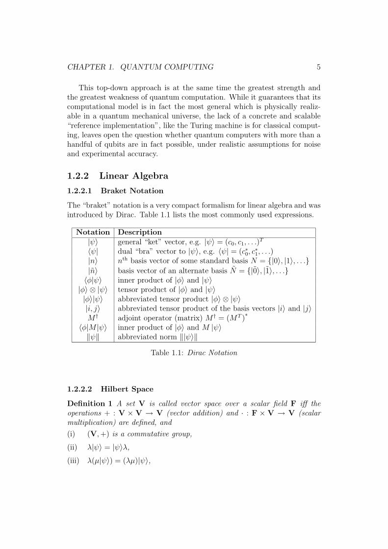
The “braket” notation is a very compact formalism for linear algebra and wasintroduced by Dirac. Table 1.1 lists the most commonly used expressions.
Notation Description|ψ〉 general “ket” vector, e.g. |ψ〉 = (c0, c1, . . .)
T
〈ψ| dual “bra” vector to |ψ〉, e.g. 〈ψ| = (c∗0, c∗1, . . .)
|n〉 nth basis vector of some standard basis N = {|0〉, |1〉, . . .}|n〉 basis vector of an alternate basis N = {|0〉, |1〉, . . .}〈φ|ψ〉 inner product of |φ〉 and |ψ〉|φ〉 ⊗ |ψ〉 tensor product of |φ〉 and |ψ〉|φ〉|ψ〉 abbreviated tensor product |φ〉 ⊗ |ψ〉|i, j〉 abbreviated tensor product of the basis vectors |i〉 and |j〉M † adjoint operator (matrix) M † = (MT )
∗
〈φ|M |ψ〉 inner product of |φ〉 and M |ψ〉‖ψ‖ abbreviated norm ‖|ψ〉‖
Table 1.1: Dirac Notation
1.2.2.2 Hilbert Space
Definition 1 A set V is called vector space over a scalar field F iff theoperations + : V × V → V (vector addition) and · : F × V → V (scalarmultiplication) are defined, and
(i) (V,+) is a commutative group,
(ii) λ|ψ〉 = |ψ〉λ,(iii) λ(µ|ψ〉) = (λµ)|ψ〉,
CHAPTER 1. QUANTUM COMPUTING 6
(iv) (λ+ µ)|ψ〉 = λ|ψ〉+ µ|ψ〉,(v) λ(|ψ〉+ |φ〉) = λ|ψ〉+ λ|φ〉.
From now on, we will only consider complex vector spaces, i.e. F = C.
Definition 2 Let V be a complex vector space. A function 〈·|·〉 : V×V→ Cis called inner product iff
(i) 〈ψ|(λ|φ〉+ µ|χ〉) = λ〈ψ|φ〉+ µ〈ψ|φ〉,(ii) 〈ψ|φ〉 = 〈φ|ψ〉∗,(iii) 〈ψ|ψ〉 ∈ R, 〈ψ|ψ〉 ≥ 0, 〈ψ|ψ〉 = 0⇔ |ψ〉 = o.
An inner product also defines the norm ‖|ψ〉‖ =√〈ψ|ψ〉 (also written as
‖ψ‖). The following inequalities apply:
|〈ψ|φ〉| ≤ ‖ψ‖‖φ‖ (Schwarz inequality) (1.1)
‖|ψ〉+ |φ〉‖ ≤ ‖ψ‖+ ‖φ‖ (triangle inequality) (1.2)
Definition 3 (Completeness) Let V be a vector space with the norm ‖ · ‖and |ψn〉 ∈ V a sequence of vectors.
(i) |ψn〉 is a Cauchy sequence iff ∀ε > 0 ∃N > 0 such that
∀n,m > N, ‖|ψn〉 − |ψm〉‖ < ε (1.3)
(ii) |ψn〉 is convergent iff there is a |ψ〉 ∈ V such that
∀ε > 0 ∃N > 0 ∀n > N, ‖|ψn〉 − |ψ〉‖ < ε (1.4)
V is complete iff every Cauchy sequence converges.
Definition 4 A complete vector space H with an inner product 〈·|·〉 and the
corresponding norm ‖ψ‖ =√〈ψ|ψ〉 is called Hilbert space.
A Hilbert space H is separable if there exists an enumerable set S ⊆ Hwhich is dense in H, i.e. for any |ψ〉 ∈ H and ε > 0 there exists a |σ〉 ∈ Swith ‖|ψ〉 − |σ〉‖ < ε. From now on, we will only consider separable Hilbertspaces.
A vector |ψ〉 ∈ H is normalized or a unit-vector iff ‖ψ‖ = 1. An enu-merable set of normalized vectors B = {|ψ0〉, |ψ0〉, . . .} is called orthonormal
CHAPTER 1. QUANTUM COMPUTING 7
system iff 〈ψi|ψj〉 = δij. An orthonormal system B is an (orthonormal) basisof H iff any vector |ψ〉 ∈ H can be written as
|ψ〉 =∑
i
λi|ψi〉 with |ψi〉 ∈ B
Since Hilbert spaces are complete by definition, any separable, complexHilbert space H with some basis B is algebraically isomorphic and isometricto either
(i) Cn with the basis {|0〉, |1〉, . . . |n− 1〉} with |k〉 = (δ0k, δ1k, . . . δn−1,k)T
if dimH = |B| = n or
(ii) l2 (i.e. the space of complex sequences 〈ξn〉 for which∑k |ξk|2 is defined)
with the basis vectors |k〉 = (δ0k, δ1k, . . .)T if dimH = |B| = ℵ0
In quantum computing we usually deal with finite dimensional Hilbertspaces, so unless otherwise noted we will always assume H = Cn. In Cn, a“ket” vector |ψ〉 can be written as column vector and the dual “bra” vector〈ψ| can be written as row vector 〈ψ| = (|ψ〉∗)T , which allows the innerproduct 〈·|·〉 to be formally expressed as ordinary matrix multiplication.
Definition 5 Let H1 and H2 be Hilbert spaces with the bases B1 and B2,then the tensor product
H = H1 ⊗H2 ={ ∑
|i〉∈B1
∑
|j〉∈B2
cij|i, j〉∣∣∣ cij ∈ C
}(1.5)
is also a Hilbert space with the basis B = B1 ×B2 and the inner product
〈i, j|i′, j′〉 = 〈i|i′〉〈j|j′〉 = δii′δjj′ with |i〉, |i′〉 ∈ B1 and |i〉, |i′〉 ∈ B2
.
1.2.2.3 Linear Operators
Definition 6 Let V be a vector space and A be function A : V → V. A iscalled linear operator on V iff
A(λ|ψ〉+ µ|φ〉) = λA(|ψ〉) + µA(|φ〉) = λA|ψ〉+ µA|φ〉. (1.6)
In Cn, a linear operator A can be written as a n × n matrix with thematrix elements aij = 〈i|A|j〉
A =
a0,0 · · · a0,n−1...
. . ....
an−1,0 · · · an−1,n−1
=
∑
i,j
aij|i〉〈j| (1.7)
CHAPTER 1. QUANTUM COMPUTING 8
Because of (1.6), a linear operator on a vector space V with the basis Bis completely defined by its effect on the basis vectors, so the above operatorA could also be written as
A : |n〉 →∑
k
akn|k〉 with |k〉 ∈ B (1.8)
Definition 7 The operator A† = (AT )∗
=∑i,j aji
∗|i〉〈j| is called adjointoperator of A.
Definition 8 A linear operator A is called
(i) normal iff A†A = AA†,
(ii) self-adjoint or Hermitian iff A† = A,
(iii) positive iff 〈ψ|A|ψ〉 ∈ R+0 ∀ |ψ〉 ∈ H,
(iv) unitary iff A†A = I, with I being the identity operator,
(v) idempotent iff A2 = A,
(vi) self-inverse iff A2 = I,
(vii) an (orthogonal) projection iff A is self-adjoint and idempotent.
SU(n) is the group of unitary operators on Cn with determinant 1. Sincefor each unitary U on Cn there exists a physically equivalent U ′ = eiϕU ∈SU(n) (see 1.2.3.1), we will also use SU(n) to denote any set of operatorsphysically equivalent to SU(n).
Definition 9 An a ∈ C with at least one non-zero solution |a〉 of the equa-tion A|a〉 = a|a〉 is called eigenvalue of A, with |a〉 being an eigenvector fora. The set {|ψ〉 ∈ H|A|ψ〉 = a|ψ〉} is known as the eigenspace of A for theeigenvalue a.
Any linear operator A can be written in terms of its eigenvectors as
A =∑
i
ai |ı〉〈ı| with 〈ı|〉 = δij. (1.9)
This form is called spectral decomposition of A.
Definition 10 Let A be a linear operator on H1 and B a linear operator onH2, then the tensor product
A⊗B =∑
i,j
∑
i′,j′|i, j〉〈i|A|i′〉〈j|B|j′〉〈i′, j′| (1.10)
is a linear operator on H1 ⊗H2.
Definition 11 Let A and B be linear operators on H. The operator [A,B] =AB − BA is called commutator and {A,B} = AB + BA is called anti-commutator of A and B.
CHAPTER 1. QUANTUM COMPUTING 9
1.2.3 The Postulates of Quantum Mechanics
1.2.3.1 Quantum States
Postulate 1 Associated to any physical system S is a complex Hilbert spaceH known as the state space of S. The state of S is completely described by aunit vector |ψ〉 ∈ H with ‖ψ‖ = 1, which is called the state vector of S. Twostate vectors |ψ〉 and |ψ′〉 are equivalent (|ψ〉 ' |ψ′〉) iff |ψ′〉 = eiϕ|ψ〉 withreal ϕ.
How exactly the state space of for a given physical system is constructed,is beyond the scope of this postulate.
Qubits The simplest non-trivial quantum mechanical system is the quan-tum bit or qubit with a state space B = C2. The state |ψ〉 of a qubit canbe described by a linear combination (also called superposition) of just twobasis states labeled |0〉 and |1〉
|ψ〉 = α|0〉+ β|1〉 with α, β ∈ C and |α|2 + |β|2 = 1 (1.11)
1.2.3.2 Evolution
Postulate 2 The temporal evolution of the state of a closed quantum systemis described by the Schrodinger equation
ih∂
∂t|ψ〉 = H|ψ〉 (1.12)
with the (experimental) Planck constant h ≈ 1.05457 · 10−34Js and a fixedself-adjoint operator H on the state space H known as the Hamiltonian ofthe system.
In quantum physics, it is common to use a system of measurement whereh = 1, so that (1.12) can be written in the dimensionless form i|ψ〉 = H|ψ〉.
The Hamiltonian H completely describes the dynamics of a closed quan-tum system. As with the state space, the concrete form of H (or an approxi-mation thereof) must be determined by the physical theory used to describethe system.
Unitary Evolution If we know the system to be in some initial state |ψ0〉at the time t = 0, we can define an operator U(t) such that
HU(t) |ψ0〉 = i∂
∂tU(t) |ψ0〉 and U(0)|ψ〉 = |ψ〉 (1.13)
CHAPTER 1. QUANTUM COMPUTING 10
and get the operator equation
H U(t) = i∂
∂tU(t) (1.14)
with the solution
U(t) = e−iHt =∞∑
n=0
1
n!(−i)ntnHn (1.15)
U(t) is the operator of temporal evolution and satisfies the criterion
U(t) |ψ(t0)〉 = |ψ(t0 + t)〉 (1.16)
U(t) is unitary because H = H† and therefore
U(t)U †(t) = e−iHte+iHt = I, (1.17)
In fact, U(t) and the Hamiltonian are equivalent descriptions of a system’sdynamics. Since any unitary operator U can be expressed as the exponentialof a self-adjoint operator H such that U = e−iH , we can reformulate the 2nd
postulate in a non-continuous, discrete-time version:
The temporal evolution of a closed quantum system from the state |ψ〉at time t1 to state |ψ′〉 at time t2 can be described by a unitary operatorU = U(t2 − t1) such that |ψ′〉 = U |ψ〉.
In either formulation, the postulate only applies to closed systems, soH or U(t) are fixed operators. It is however often possible to interact witha quantum system in such a manner that it can still be treated as isolated,while the effect of the interaction can mathematically be described by a time-varying Hamiltonian. Even in that case, the discrete evolution of the systembetween two points in time t1 and t2 can still be described by a unitaryoperator U = U(t1, t2). In this context, we would speak of applying theoperator U to a quantum state |ψ〉.
1.2.3.3 Measurements
Postulate 3 A (projective) measurement2 is described by a self-adjoint op-erator M , called observable, with the spectral decomposition M =
∑mmPm,
where Pm is the projector onto the eigenspace of the eigenvalue m.The eigenvalues m of M correspond to the possible outcomes of the mea-
surement. Measuring |ψ〉 will give the result m with probability p(m) =
2There is also a more general formulation of quantum measurement allowing non-projective measurement operators. See [43] for details.
CHAPTER 1. QUANTUM COMPUTING 11
〈ψ|Pm|ψ〉, thereby reducing |ψ〉 to the post-measurement state
|ψ′〉 =1√p(m)
Pm|ψ〉 (1.18)
For a qubit state, the self-adjoint operator N
N =
(0 00 1
)= 0 · |0〉〈0|+ 1 · |1〉〈1| (1.19)
is known as the standard observable. Generally, for a system with the statespace H = Cn, the standard observable N can be defined as N =
∑i i|i〉〈i|.
Definition 12 The weighted average 〈M〉 over all possible outcomes of ameasurement of M is called expectation value and is defined as
〈M〉 =∑m
p(m)m =∑m
〈ψ|mPm|ψ〉 = 〈ψ|M |ψ〉 (1.20)
Definition 13 The standard deviation ∆M of all possible outcomes of ameasurement is defined as
∆M =√〈(M − 〈M〉)2〉 =
√〈M2〉 − 〈M〉2 (1.21)
The Heisenberg Uncertainty Principle The destructive nature of mea-surement raises the question whether 2 observables A and B can be measuredsimultaneously. This can only be the case if the post-measurement state |ψ′〉is an eigenvector of A and B
A|ψ′〉 = a|ψ′〉 and B|ψ′〉 = b|ψ′〉 (1.22)
This is equivalent to the condition [A,B] = 0. If A and B do not commute,then the uncertainty product (∆A)(∆B) > 0.
To find a lower limit for (∆A)(∆B) we introduce the operators δA =A−〈A〉 and δB = B−〈B〉 and can express the squared uncertainty productas
(∆A)2(∆B)2 = 〈(δA)2〉〈(δB)2〉 = 〈ψ|(δA)(δA)|ψ〉〈ψ|(δB)(δB)|ψ〉 (1.23)
Since δA and δB are self adjoint, we can express the above as
(∆A)2(∆B)2 = ‖δA|ψ〉‖2‖δB|ψ〉‖2. (1.24)
Using (1.1) and [A,B] = [δA, δB] we get
(∆A)(∆B) ≥ 1
2
∣∣∣〈[A,B]〉∣∣∣ (1.25)
CHAPTER 1. QUANTUM COMPUTING 12
1.2.3.4 Composite Systems
Postulate 4 The state space H of a composite physical system is the tensorproduct of the state spaces Hi of its components. Moreover, if the subsystemsare in the states |ψi〉 ∈ Hi, then the joint state |Ψ〉 ∈ H of the compositesystem is |Ψ〉 = |ψ1〉 ⊗ |ψ2〉 ⊗ . . .⊗ |ψn〉.
Let S be a composite system of S1 and S2 with the state space H =H1⊗H2. A measurement of the observable M : H1 → H1 in S1, is equivalentto measuring the observable M (1) = M ⊗ I in S with I being the identityoperator on H2. Equivalently, a unitary transformation U : H1 → H1 of S1
is described by the padded operator U (1) = U ⊗ I on H.A joint state of the form |Ψ〉 = |ψ1〉 ⊗ |ψ2〉 is called product state, which
can be expanded to
|Ψ〉 =∑
i
∑
j
aibj|i, j〉 with∑
i
|ai|2 = 1 and∑
j
|bj|2 = 1 (1.26)
In product states, unitary transformations or measurements performed onone system, do not affect the state of the other system.
Entanglement Not any joint state is a product state. A state
|Ψ〉 =∑
i
∑
j
cij|i, j〉 with∑
i,j
|cij|2 = 1 (1.27)
where the coefficients cij cannot be written as cij = aibj is called entangled.Consider the following joint states of two qubits
|ΨA〉 =1
2|0, 0〉+ 1
2|1, 0〉+ 1
2|0, 1〉+ 1
2|1, 1〉 and (1.28)
|ΨB〉 =1√2|0, 0〉+ 1√
2|1, 1〉 (1.29)
A single measurement of either qubit (using the standard observable asdefined in (1.19)) will give 0 or 1 with equal probability p = 1/2. Assumingthat a measurement of the first qubit gave the result m, the respective postmeasurement states are
|Ψ′A〉 =
1√2|m, 0〉+ 1√
2|m, 1〉 and (1.30)
|Ψ′B〉 = |m,m〉 (1.31)
A measurement of the second qubit of |Ψ′A〉 will still give a random re-
sult, while in the case of |Ψ′B〉, the outcome is correlated to the previous
measurement and will always produce m. |ΨB〉 is also known as Bell state.
CHAPTER 1. QUANTUM COMPUTING 13
1.3 Classical Computing
1.3.1 The Church-Turing Thesis
As already mentioned in 1.1.3, computing science is based on the paradigmof computation being a mechanical, rather than a purely mental process. Amethod, or procedure P for achieving some desired result is called effectiveor mechanical if [21]
1. P is set out in terms of a finite number of exact instructions (eachinstruction being expressed by means of a finite number of symbols);
2. P will, if carried out without error, always produce the desired resultin a finite number of steps;
3. P can (in practice or in principle) be carried out by a human beingunaided by any machinery save paper and pencil;
4. P demands no insight or ingenuity on the part of the human beingcarrying it out.
Alan Turing and Alonzo Church both formalized the above definition byintroducing the concept of computability by Turing machine and the math-ematically equivalent concept of recursive functions with the following con-clusions:
Turing’s Thesis LCMs [logical computing machines i.e. Turing machines]can do anything that could be described as “rule of thumb” or “purely me-chanical”. [58]
Church’s Thesis A function of positive integers is effectively calculableonly if recursive. [50]
As the above statements are equivalent, they are commonly referred to asthe Church-Turing Thesis which defines the scope of classical computing.
1.3.1.1 Partial Recursive Functions
The class P of partial recursive functions mathematically captures the con-cept of “effective” functions f : Nn → Nm. P can be constructed fromsimpler classes in the following way: [39]
CHAPTER 1. QUANTUM COMPUTING 14
1. A basic function f : Nn → Nm is a function f : x → y where yi iseither a constant yi = ci, ci ∈ N or an element of the input vectoryi = xσ(i). The class BF of basic function is closed under the basicoperators BO = {◦,×}, where “◦” denotes function composition and“×” the usual cross-product.
2. The class PR of primitive recursive functions is generated from BF∪{S}by closure under BO ∪ {Pr} where
(i) S : N→ N is the successor function S(n) = n+ 1 and
(ii) Pr denotes the primitive recursion h = Pr[f, g]
h(x, 0) = f(x), h(x, n+ 1) = g(x, n, h(x, n)) (1.32)
3. P is generated from PR by closure under BO ∪ {µ0}. The operator µ0
is called µ0-recursion (minimization) and defined as
µ0[f ] : x→ mink∈N
[f(x, k) = 0] with f ∈ PR (1.33)
As µ0[f ](x) is only defined if ∃k ∈ N, f(x, k) = 0, P is a class of par-tial functions. The class R ⊂ P of total functions in P is called recursivefunctions.
1.3.2 Machines
1.3.2.1 General Machines
Definition 14 A machine M is a 5-tuple (S, O, T, δ, β) where [39]
(i) S is a set of of computational states
(ii) O = {fi : S → S} is an enumerable set of operations on S (memorycommands)
(iii) T = {ti : S → B} is an enumerable set of predicates on S (test com-mands)
(iv) δ : I → S is an input function for the enumerable input set I(v) β : S→ O is an output function for the enumerable output set O
By providing a set of (simple) elementary operations and predicates, amachine defines a framework for the description of effective procedures. Theenumerability of O and T guarantees that such a description, called program,can be finite and represented as a string over a finite set of symbols.
CHAPTER 1. QUANTUM COMPUTING 15
1.3.2.2 Discrete Machines
A more rigid interpretation of effectivity also requires S to be enumerable, sothat not only the program but also the computational state can be expressed“by finite means” and the whole computation can in fact be carried out bymanipulating symbols “on paper”. Such machines are known as discrete.For any machineM = (S, O, T, δ, β) with O = {f1, f2, . . .} and the input setI = {x1, x2, . . .} an equivalent discrete machine M′ = (S′, O, T, δ, β) can beconstructed by the diagonalization
S′ =∞⋃
n=1
{(g1 ◦ g2 ◦ . . . ◦ gn)(δ(x)) | g ∈ Onn, x ∈ In} (1.34)
where O0 = {I}, On+1 = On ∪ {fn} and In = {x0, . . . xn}.
Turing Machines A Turing Machine (TM) consists of a head operatingon an infinite tape of memory cells. In the simplest case, each cell can onlyadopt one of two possible states labeled 0 (also called blank) and 1.
If we index the cells by their relative position to the head, we can describethe content of the tape content as a function s : Z→ B and write
s = (. . . s−2s−1|s0s1s2 . . .). (1.35)
The state space T is the set of all tapes containing only a finite numberof 1s.3
T ={s : Z→ B
∣∣∣∞∑
i=−∞si <∞
}(1.36)
We can now define a TM as a machine M = (T, {S,E,L,R}, {T}, δ, β)with the commands
(i) S(. . . s−1|s0s1s2 . . .) = (. . . s−1|1s1s2 . . .) (set)
(ii) E(. . . s−1|s0s1s2 . . .) = (. . . s−1|0s1s2 . . .) (erase)
(iii) L(s) = s′ where s′i = si+1 (move left)
(iv) R(s) = s′ where s′i = si−1 (move right)
(v) T(s) = s0 (test)
For I = Nm and O = Nn we can define a Turing machine TMmn =
(T, {S,E,L,R}, {T}, δm, βn) with the unary encoding
δm(x1, x2, . . . xn) = (0ω|1x101x20 . . . 01xm0ω) and (1.37)
βn(. . . |1y101y20 . . . 01yn0 . . .) = (y1, y2, . . . yn) (1.38)
3This zero tails state condition is necessary as the set T′ = {s : Z→ B} would not beenumerable.
CHAPTER 1. QUANTUM COMPUTING 16
1.3.2.3 Finite Machines
For a discrete machineM with an infinite S, the number of symbols to rep-resent a computational state s ∈ S can get arbitrarily large so any realizationofM would require unlimited memory. If the amount of memory is limited,so is the number of computational states. A discrete machineM with limitedmemory is called finite.
The memory capacity of a finite machineM with the finite state space Sis S = log2 |S| bit.
1.3.2.4 Oracles
If a machine M1 = (S1, O1, T1, δ1, β2) is extended to allow computationson another machine M2 = (S2, O2, T2, δ2, β2), then the resulting machineM =M1 ./M2 is referred to as anM1-machine with anM2-oracle.
The interaction between M1 and M2 is described by oracle commandsof the form
fO : S1 × S2 → S1 × S2 or tO : S1 × S2 → B (1.39)
andM can be written as
M = (S1 × S2, O1 × {I1} ∪ {fO}, T1 ∪ {tO}, δ, β) (1.40)
with I2 being the identity on S2.Depending on the definition of fO and tO, oracle calls can correspond to
single M2-commands up to the execution of complete finite programs (see1.3.3.2) on M2. Still, with regard to time complexity, an oracle-call countsas a single computational step.
1.3.2.5 Probabilistic Machines
A machine M = (S, O, T, δ, β) is probabilistic if it provides at least onerandom test command c ∈ T . A random predicate c : S 7→ B can bemathematically described by the probability distribution p(c|s) where s ∈ S,so
c : s 7→{
true with p = p(c|s)false with p = 1− p(c|s) (1.41)
We can generalize this definition by also allowing for random memorycommands f : S 7→ S
f : s 7→ s′ with p = pf (s′|s) where ∀s ∈ S,
∑
s′∈S
pf (s′|s) = 1 (1.42)
CHAPTER 1. QUANTUM COMPUTING 17
and output functions β : S 7→ O. In the latter case, pβ(y|s) with y ∈ O isalso called (probability) spectrum of s.
For any probabilistic machine M it is possible to formally construct acorresponding deterministic machine M operating on the distribution space
S ={ps : S→ [0, 1]
∣∣∣∑
s∈S
ps(s) = 1}
(1.43)
A state s ∈ S has the (Shannon) entropy
H(s) = −∑
s∈S
p(s|s) log2 p(s|s), p(s|s) = ps(s). (1.44)
Probabilistic Turing Machine A probabilistic Turing Machine (PTM)can be constructed from a deterministic TM by adding a stateless randomoracle which provides a “fair coin toss” test command C with p(C) = p(¬C) =1/2.
1.3.3 Programs
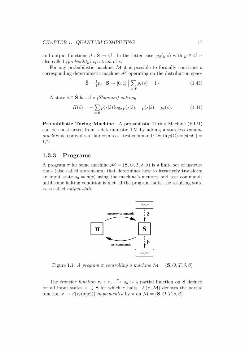
A program π for some machine M = (S, O, T, δ, β) is a finite set of instruc-tions (also called statements) that determines how to iteratively transforman input state s0 = δ(x) using the machine’s memory and test commandsuntil some halting condition is met. If the program halts, the resulting statesh is called output state.
π
δ
β
input
output
test commands
memory commands
S
Figure 1.1: A program π controlling a machine M = (S, O, T, δ, β)
The transfer function τπ : s0π−→ sh is a partial function on S defined
for all input states s0 ∈ S for which π halts. F (π,M) denotes the partialfunction x→ β(τπ(δ(x))) implemented by π onM = (S, O, T, δ, β).
CHAPTER 1. QUANTUM COMPUTING 18
The interpretation of a program π of a program class Π is specified bya step function ρ : Π × P × S → P × S. P = P(π) is the set of possiblecontrol-states with a unique p0 ∈ P called initial state and a subset Ph ⊆ Pcalled halting states.
A pair (p, s) ∈ P× S is called a configuration. ρ has the general form
ρπ(p, s) =
(ν(π, p), fµ(π,p)(s)
)if p ∈ Pf(
ν(π, p, tµ(π,p)(s)), s)
if p ∈ Pt
(p, s) if p ∈ Ph
(1.45)
where P = Pf ∪Pt ∪Ph, fµ(π,p) ∈ O and tµ(π,p) ∈ T .For an input state s0 = δ(x), (p0, s0) = (p0, δ(x)) is called initial configu-
ration. The transfer function τ is defined as
(ph, τπ(s0)) = ρn(p0, s0) with n = minkρk(p0, s0) ∈ Ph × S (1.46)
If π halts for a given input x ∈ I, n is called the (time) complexity of thecomputation.
1.3.3.1 Sequences
Definition 15 A program σ ∈ On for a machine M = (S, O, T, δ, β) con-sisting of a static list of n memory commands is called a sequence. Thetransfer function τσ : s→ (σ1 ◦ σ2 ◦ . . . ◦ σn)(s) is a total function.
Definition 16 Let S be composed of identical indexed memory cells Mi withthe state space S, such that S = S1 ⊕ S2 ⊕ . . . for some suitable composition⊕ and g a function g : Sn → Sn. The class of functions Γ(g) = {gi1i2...in :S → S} where gi1i2...in denotes the application of g to a permutation of nmutually different cells Mi1 ,Mi2 . . .Min is called an n-ary gate.
If O is a union of gates, then a sequence σ ∈ O? can be interpreted as afeed forward network and is also called a circuit.
A set of operations O is universal if for any function f : I ′ → O definedfor a finite subset I ′ ⊆ I there exists a sequence σ ∈ O? such that f(x) =β(τσ(δ(x))) for all x ∈ I ′.
While generally, more powerful programming concepts are required tofully exploit the computational potential of a machine M = (S, O, T, δ, β),sequences are sufficient to implement any function that can possibly be im-plemented if either
(i) O is universal and (a)M is finite or (b) I is a finite set
(ii) M provides no test-commands, i.e. T = ∅
CHAPTER 1. QUANTUM COMPUTING 19
1.3.3.2 Finite Programs
Definition 17 LetM be a machine (S, O, T, δ, β) and L an enumerable setof labels with an element l0 ∈ L called start-label.
(i) A triple (l, f, p) ∈ L×O × L is called function-statement
(ii) A 4-tuple (l, t, p, q) ∈ L× T × L× L is called test-statement
The labels l are called statement-, p and q are called jump-labels. A finiteprogram π ∈ Π for M is a finite set of statements with unique labels l.
Function- and test-statements are also written as
l: f then p
l: if t then p else q
A program π ∈ Π describes a finite automaton operating onM with thestep function
ρπ(l, s) =
(p, f(s)) if πl = (l, f, p)(p, s) if πl = (l, t, p, q) ∧ t(s)(q, s) if πl = (l, t, p, q) ∧ ¬t(s)(l, s) if l /∈ Lπ
(1.47)
where Lπ denotes the set of statement-labels in π and πl : Lπ → π thestatement with the label l.
According to the Church-Turing thesis, any effective function f : Nn →Nm can be implemented as a finite program π for TMm
n and the set of Turing-computable functions
F (TM) = {F (π, TMmn ) |π ∈ Π, n,m ∈ N} (1.48)
is identical to P.
Definition 18 (Universal Computer) A machineM = (S, O, T, δ, β) withthe encodings δ : N? → S and β : S → N? is a universal computer iff forany f ∈ P, there exists a finite program π for M such that f = F (π,M).
1.3.3.3 Programming Languages
Definition 19 A programming language L ⊆ Σ? for a machine M is aclass of algorithm descriptions p ∈ Σ? over some alphabet Σ, which can beefficiently translated into a finite program π ∈ Π for M by another programπL for a machine
ML = (S, O, T, δ : Σ? → S, β : S→ Π) (1.49)
CHAPTER 1. QUANTUM COMPUTING 20
The pair (πL,ML) is called a compiler for L. It is usually required thatthe compilation is efficient, i.e. has polynomial time and space complexity.
A programming language L is universal, if M is a universal computerand for any f ∈ P there exists a program p ∈ L such that f = F (p,M) =F (F (πL,ML),M).
1.4 Elements of Quantum Computing
Just like a classical machine, a quantum computer, essentially consists ofthree parts: a memory, which holds the current machine state, a processor,which performs elementary operations on the machine state, and some sortof input/output which allows to set the initial state and extract the finalstate of the computation.
Formally, we can describe a quantum computer as a probabilistic machineM = (H, O, T, δ, β) where
• H is the state space of the quantum system operated on,
• O a set of (deterministic) unitary transformations,
• T a set of (probabilistic) measurement commands,
• δ is the initialization operator and
• β describes the final measurement.
1.4.1 Quantum Memory
1.4.1.1 Qubits
The quantum analogue to the classical bit is the quantum bit or qubit (see1.2.3.1).
Definition 20 A qubit or quantum bit is a quantum system whose state canbe fully described by a superposition of two orthonormal basis states labeled|0〉 and |1〉.
The state space of a qubit is the Hilbert space B = C2. The orthonormalsystem {|0〉, |1〉} is called computational basis.
The classical value of a qubit is described by the standard observableN = |1〉〈1| (1.19). 〈N〉 gives the probability to find the system in state |1〉 ifa measurement is performed on the qubit.
CHAPTER 1. QUANTUM COMPUTING 21
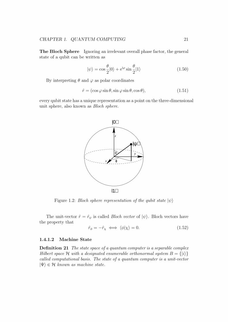
The Bloch Sphere Ignoring an irrelevant overall phase factor, the generalstate of a qubit can be written as
|ψ〉 = cosθ
2|0〉+ eiϕ sin
θ
2|1〉 (1.50)
By interpreting θ and ϕ as polar coordinates
r = (cosϕ sin θ, sinϕ sin θ, cos θ), (1.51)
every qubit state has a unique representation as a point on the three-dimensionalunit sphere, also known as Bloch sphere.
ϕ
|0⟩
|1⟩
|ψ⟩
y
z
x
θ
Figure 1.2: Bloch sphere representation of the qubit state |ψ〉
The unit-vector r = rψ is called Bloch vector of |ψ〉. Bloch vectors havethe property that
rφ = −rχ ⇐⇒ 〈φ|χ〉 = 0. (1.52)
1.4.1.2 Machine State
Definition 21 The state space of a quantum computer is a separable complexHilbert space H with a designated enumerable orthonormal system B = {|i〉}called computational basis. The state of a quantum computer is a unit-vector|Ψ〉 ∈ H known as machine state.
CHAPTER 1. QUANTUM COMPUTING 22
Classically, the common state space S of a composite system consistingof n memory cells with the state spaces Si is given by the cross-productS = S1× S2× . . .× Sn. In quantum mechanics, this is only true for productstates (see 1.2.3.4).
The state space H of a quantum computer composed of n identical sub-systems with the state space S is given as the tensor product
H = S⊗n =
n times︷ ︸︸ ︷S ⊗ . . .⊗ S (1.53)
The machine state |Ψ〉 of an n-qubit quantum computer is therefore aunit vector in H = B⊗n = C2n
|Ψ〉 =∑
(d0...dn−1)∈Bn
cd0...dn−1|d0 . . . dn−1〉 with∑ |cd0...dn−1|2 = 1 (1.54)
The basis vectors |d0 . . . dn−1〉 can be interpreted as binary numbers andrelabeled as |k〉 with k =
∑n−1i=0 2idi so B can be written as B = {|k〉|k ∈ Z2n}.
A quantum computer M = (H, O, T, δ, β) is finite if dimH < ∞. Thememory capacity of a finite quantum computer is log2 dimH qubit.
Unlimited Memory As the state space of a quantum computer is a sep-arable Hilbert space, it is isomorphic to either Cn or l2 (see 1.2.2.2).
The Hilbert space B⊗ω resulting from a composition of an infinite numberof qubits is non-separable. We can however construct a separable subspaceB? ⊂ B⊗ω which is isomorphic to l2 by introducing a zero tail state condition.
B? ={|ψ〉 ⊗ |0〉⊗ω
∣∣∣ |ψ〉 ∈ B⊗n, n ∈ N}
(1.55)
1.4.1.3 Quantum Registers
Definition 22 Let H be the state space of a quantum computerM with thecomputational basis B = {|i〉}. A quantum register s is a sub-system of Mwith a finite dimensional state space Hs and a basis Bs = {|i〉s} such thatH = Hs ⊗ Hs and B = Bs × Bs. If M is finite, then s is known as thecomplimentary register to s.
A register s defines a decomposition for the computational basis B, soany basis vector |k〉 ∈ B can be written as the product state |k〉 = |ik〉s|jk〉swith |ik〉s ∈ Bs and |jk〉s ∈ Bs.
In H the classical value of a register s is described by the register observ-able N(s)
N(s) ≡ Ns ⊗ Is =∑
i,j
i |i〉s|j〉s〈i|s〈j|s (1.56)
CHAPTER 1. QUANTUM COMPUTING 23
whereNs is the standard observable onHs and Is the identity operator onHs.Likewise, a unitary transformation U on Hs can be expressed as a registeroperator U(s) on H
U(s) ≡ U ⊗ Is =∑
i,i′,jui,i′ |i〉s|j〉s〈i′|s〈j|s (1.57)
where ui,i′ is the matrix element ui,i′ = 〈i|U |i′〉.
Qubit Registers When H is the state space of a composition of the qubitsqi, i.e. H = B⊗m or H = B?, then any qi defines a register qi with thedecomposition
|d0 . . . di−1didi+1 . . .〉 = |di〉qi|d0 . . . di−1di+1 . . .〉qi
(1.58)
Likewise, any permutation (s0s1 . . . sn−1) = (qk0qk1 . . . qkn−1) of mutuallydifferent qubits sj ∈ {qi} defines an n-qubit register s = qk0 ◦qk1 ◦ . . . ◦qkn−1
with the decomposition
|d0d1 . . .〉 =
(n−1⊗
i=0
|dki〉qki
)⊗ | . . .〉s = |dk0dk1 . . . dkn−1〉s| . . .〉s (1.59)
The order of qubits is important, so while a ◦ b and b ◦ a refer to thesame 2-qubit subsystem, they are two different registers.
If s is a n-qubit register and U an operator on B⊗n, then the registeroperator U(s) is also referred to as a quantum gate.
Register States Strictly speaking, the state of a register s is only definedif the machine state |Ψ〉 is of the form |Ψ〉 = |ψ〉s|χ〉s. In that case, we saythat s is in the pure state |ψ〉 ∈ Hs. Alternatively, the state of s can bedescribed by the (reduced) density operator ρs.
Definition 23 Let H = Ha ⊗ Hb be the state space of a composite systema ◦ b. For a machine state
|Ψ〉 =∑
i,j
cij|i〉a|j〉b with∑
i,j
|cij|2 = 1 (1.60)
the reduced density operator ρa : Ha → Ha is defined as
ρa = trb (|Ψ〉〈Ψ|) =∑
i,i′|i〉a〈i′|a
∑
j
cijc∗i′j (1.61)
CHAPTER 1. QUANTUM COMPUTING 24
If a register s is in a pure state then ρs = |ψ〉〈ψ| and tr(ρ2s) = trρs = 1. If
s is entangled then ρs is a positive operator with the spectral decomposition
ρs =∑
k
pk|ψk〉〈ψk| with pk ∈ [0, 1) and∑
k
pk = 1 (1.62)
and tr(ρ2s) < 1. In that case, s is also said to be in the mixed state ρs.
4
The density operator allows to treat s as an isolated system with re-gard to unitary evolution and measurements as long as no operation on s isperformed:
(i) Let U be a unitary operator on Hs, then
|Ψ′〉 = U(s)|Ψ〉 =⇒ ρ′s = UρsU†. (1.63)
(ii) Let M be a Hermitian operator on Hs with the spectral decompositionM =
∑mmPm, then p(m) = 〈Ψ|Pm(s)|Ψ〉 = tr(Pmρs) and
|Ψ′〉 =Pm|Ψ〉√p(m)
=⇒ ρ′s =PmρsP
†m
p(m). (1.64)
Schmidt Decomposition If s and s are entangled, the machine state canalways be written as
|Ψ〉 =∑
i
λi|ψi〉s|χi〉s with λi ∈ R+ and∑
i
λ2 = 1 (1.65)
such that |ψi〉 ∈ Hs and |χi〉 ∈ Hs are orthonormal states i.e. 〈ψi|ψj〉 = δijand 〈χi|χj〉 = δij. This representation is known as Schmidt decomposition.
1.4.2 Quantum Operations
1.4.2.1 Unitary Operators
According to the 2nd postulate of quantum mechanics (see 1.2.3.2), the evo-lution of a closed quantum system is unitary and can be described by theoperator U(t) = e−iHt. Therefore, the memory commands O of a quantumcomputerM = (H, O, T, δ, β) are unitary transformations on the state spaceH.
A unitary transformations U is a linear operator of the form UU † =
I and describes a basis transformation BU−→ B. From a computational
point of view, these mathematical properties account for three fundamentaldifferences between classical and quantum computing:
4The term “mixed state” refers to the fact that ρ exhibits the same measurementstatistics as a system which is known to be in the state |ψk〉 with probability pk.
CHAPTER 1. QUANTUM COMPUTING 25
• Reversibility: Since unitary operators, by definition, match the con-dition UU † = I, for every transformation U there exists the inversetransformation U (−1) = U †. As a consequence, quantum computationis restricted to reversible functions.5
• Superposition: A “classical” state |Ψ〉 = |k〉 ∈ B can be transformedinto a superposition of several basis vectors
|Ψ′〉 = U |k〉 = |k〉 =∑
k′uk′k|k′〉 (1.66)
and vice versa.
• Parallelism: If the machine state |Ψ〉 already is a superposition ofseveral basis vectors, then a transformation U is applied to all basisstates simultaneously.
U∑
k
ck|k〉 =∑
k
ckU |k〉 (1.67)
This feature of quantum computing is called quantum parallelism andis a consequence of the linearity of unitary transformations.
1.4.2.2 Qubit Operators
The simplest case of unitary transformations are operators which work on asingle qubit. A general 2-dimensional complex unitary matrix U ∈ SU(2)can be written as
U = eiϕ
(e
i2(−α−β) cos θ
2−e
i2(−α+β) sin θ
2
ei2(α−β) sin θ
2e
i2(α+β) cos θ
2
)(1.68)
As we have shown in 1.4.1.1, every qubit state |ψ〉 ∈ B can be representedby a Bloch vector rψ. Rotations about the x, y and z-axes in the Bloch spherecorrespond to the operators
Rx(θ) =
(cos θ
2−i sin θ
2
−i sin θ2
cos θ2
)(1.69)
Ry(θ) =
(cos θ
2− sin θ
2
sin θ2
cos θ2
)(1.70)
Rz(θ) =
(e−iθ/2 0
0 eiθ/2
)(1.71)
5A classical analogue would be the class of bijective functions on Bn.
CHAPTER 1. QUANTUM COMPUTING 26
on B. It is easy to verify that R†i (θ) = Ri(−θ), so all Ri are unitary operators.Using the self-inverse Pauli matrices
σx =
(0 11 0
), σy =
(0 −ii 0
), σz =
(1 00 −1
)(1.72)
a general rotation6 about a unit vector n can be written as
Rn(θ) = e−i2θn·~σ = cos
θ
2I − i sin
θ
2(nxσx + nyσy + nzσz) (1.73)
Let U ∈ SU(2) have the orthonormal eigenvectors |u〉 and |v〉 and theeigenvalues u and v, then U can be written as
U = u|u〉〈u|+ v|v〉〈v| = eiϕRn(δ) (1.74)
where n is the Bloch vector of |u〉 and δ is the phase difference between uand v, i.e. v = eiδu.
1.4.2.3 Universal Qubit Operations
As qubit operators correspond to rotations in the Bloch sphere, any unitaryU on B can implemented as a composition of three rotations about twoorthogonal axes and a (physically irrelevant) overall phase factor.7 e.g.
U = eiϕRz(α)Ry(β)Rz(γ) (Z-Y decomposition) or (1.75)
U = eiϕRx(α)Ry(β)Rx(γ) (X-Y decomposition) (1.76)
This means, for symmetry reasons, that for any two orthogonal unit vec-tors u and v, the operator set Ouv = {Ru(θ) | θ ∈ R} ∪ {Rv(θ) | θ ∈ R} isuniversal for single qubit operations.
Definition 24 (Universality of operator sets) LetH be a separable Hilbertspace and O a set of unitary operators on H. O is universal on H if for anyunitary operator U : H → H and for any ε ∈ R+, there exists a compositionσ = U1 ◦ U2 ◦ . . . ◦ Uk with Ui ∈ O and an overall phase eiϕ such that
∣∣∣〈φ|(U − eiϕσ)|χ〉∣∣∣ < ε ∀ |φ〉, |χ〉 ∈ H. (1.77)
6Note that despite the mathematical period of 4π, Rn(θ) and Rn(θ + 2π) = −Rn(θ)describe the same physical operation.
7Note that expanding (1.75) directly leads to (1.68).
CHAPTER 1. QUANTUM COMPUTING 27
Let O = {Rn(θ) | θ ∈ R} be the class of rotations about some axis vectorn. Since
Rn(α+ β) = Rn(α)Rn(β) and Rn(θ + 2kπ) = (−1)kRn(θ), (1.78)
the set {Rkn(ξ) | k ∈ N} ⊂ O is dense in O iff ξ 6= 0 and ξ/π is irrational.
So any pair {Ru(qπ), Rv(pπ)} of orthogonal qubit rotations where u ⊥ v andp, q ∈ I+ already constitutes a universal set of qubit operators.
The above result can be generalized to non-orthogonal rotations: LetV = Rv(β) andW = Rw(γ) be unitary qubit operators where 0 < |(v, w)| < 1and let u be an axis vector orthonormal to v. Since W can be written asW = Rv(β1)Ru(α)Rv(β2), we can construct a qubit rotation
U = Ru(α) = Rv(−β1)W Rv(−β2) (1.79)
orthogonal to V . Provided that β/π, γ/π ∈ I+, there exist k1, k2 ∈ N suchthat Rv(−βi) ≈ V ki to arbitrary precision and the operator pair {V,W} isuniversal.
1.4.2.4 Quantum Gates
Definition 25 Let H = B⊗n or H = B? be the state space of a compositesystem of the qubits S = {qi} and Rk(S) = {s ⊆ S | |s| = k} denote theordered k-qubit subsets of S i.e. the set of k-qubit registers. The class
Γ(U) = {U(s) | s ∈ Rk(S)} (1.80)
of register operators on H for some unitary k-qubit operator on B⊗k is calleda k-qubit quantum gate.
Informally, we can describe a k-qubit gate as a unitary operator whichcan be equally applied to any k-qubit register of a quantum computer. Inthat case, the term “gate” is also used to refer to a single register operatorU(s) ∈ Γ(U) as well as to the operator U itself.
Common Elementary Gates
Single Qubit Gates
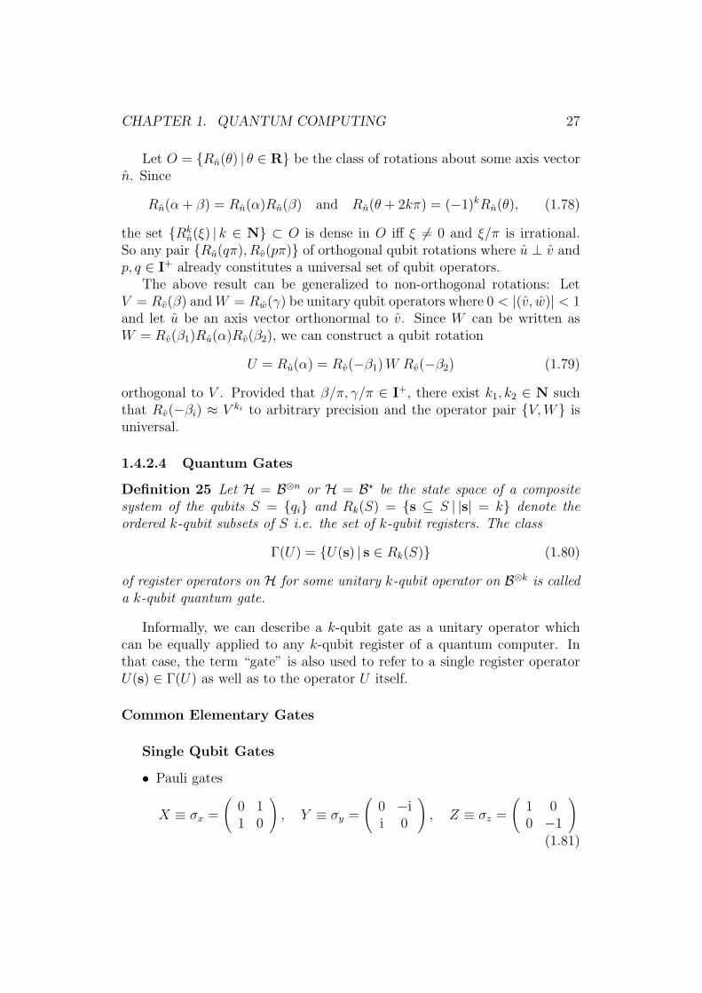
• Pauli gates
X ≡ σx =
(0 11 0
), Y ≡ σy =
(0 −ii 0
), Z ≡ σz =
(1 00 −1
)
(1.81)

CHAPTER 1. QUANTUM COMPUTING 28
• Hadamard gate
H ≡ 1√2
(1 11 −1
)(1.82)
• Phase- and π/8-gate8
S ≡√Z =
(1 00 i
), T ≡
√S =
(1 00 eiπ/4
)(1.83)
Two Qubit Gates
• controlled-not gate
CNot : |x, y〉 → |x⊕ y, y〉 (1.84)
• swap-gateSwap : |x, y〉 → |y, x〉 (1.85)
• controlled-phase-gate
CPhase : |x, y〉 → ixy|x, y〉 (1.86)
Three Qubit Gates
• Toffoli-gate (controlled-controlled-not)
CCNot : |x, y, z〉 → |x⊕ (y ∧ z), y, z〉 (1.87)
• Fredkin-gate (controlled-swap)
CSwap : |x, y, z〉 →{|y, x, z〉 if z = 1|x, y, z〉 if z = 0
(1.88)
1.4.2.5 Controlled Gates
The single most important 2-qubit gate is the controlled-not-gate. The CNot-gate operates on a target qubit t and a control (or enable) qubit e and can bedefined using the X-gate, as matrix
CNot = C[X] =
(I 00 X
)=
1 0 0 00 1 0 00 0 0 10 0 1 0
(1.89)
8T is named π/8-gate as T ' eiπσx/8.
CHAPTER 1. QUANTUM COMPUTING 29
or as the register operator
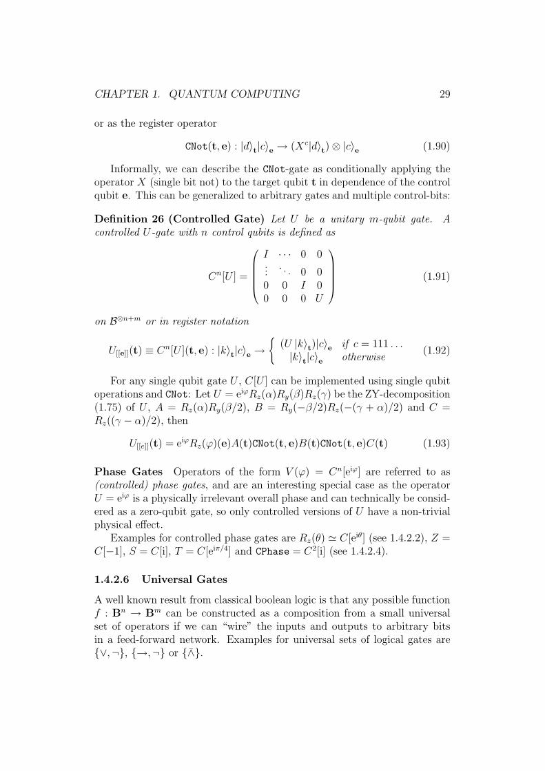
CNot(t, e) : |d〉t|c〉e → (Xc|d〉t)⊗ |c〉e (1.90)
Informally, we can describe the CNot-gate as conditionally applying theoperator X (single bit not) to the target qubit t in dependence of the controlqubit e. This can be generalized to arbitrary gates and multiple control-bits:
Definition 26 (Controlled Gate) Let U be a unitary m-qubit gate. Acontrolled U-gate with n control qubits is defined as
Cn[U ] =
I · · · 0 0...
. . . 0 00 0 I 00 0 0 U
(1.91)
on B⊗n+m or in register notation
U[[e]](t) ≡ Cn[U ](t, e) : |k〉t|c〉e →{
(U |k〉t)|c〉e if c = 111 . . .|k〉t|c〉e otherwise
(1.92)
For any single qubit gate U , C[U ] can be implemented using single qubitoperations and CNot: Let U = eiϕRz(α)Ry(β)Rz(γ) be the ZY-decomposition(1.75) of U , A = Rz(α)Ry(β/2), B = Ry(−β/2)Rz(−(γ + α)/2) and C =Rz((γ − α)/2), then
U[[e]](t) = eiϕRz(ϕ)(e)A(t)CNot(t, e)B(t)CNot(t, e)C(t) (1.93)
Phase Gates Operators of the form V (ϕ) = Cn[eiϕ] are referred to as(controlled) phase gates, and are an interesting special case as the operatorU = eiϕ is a physically irrelevant overall phase and can technically be consid-ered as a zero-qubit gate, so only controlled versions of U have a non-trivialphysical effect.
Examples for controlled phase gates are Rz(θ) ' C[eiθ] (see 1.4.2.2), Z =C[−1], S = C[i], T = C[eiπ/4] and CPhase = C2[i] (see 1.4.2.4).
1.4.2.6 Universal Gates
A well known result from classical boolean logic is that any possible functionf : Bn → Bm can be constructed as a composition from a small universalset of operators if we can “wire” the inputs and outputs to arbitrary bitsin a feed-forward network. Examples for universal sets of logical gates are{∨,¬}, {→,¬} or {∧}.
CHAPTER 1. QUANTUM COMPUTING 30
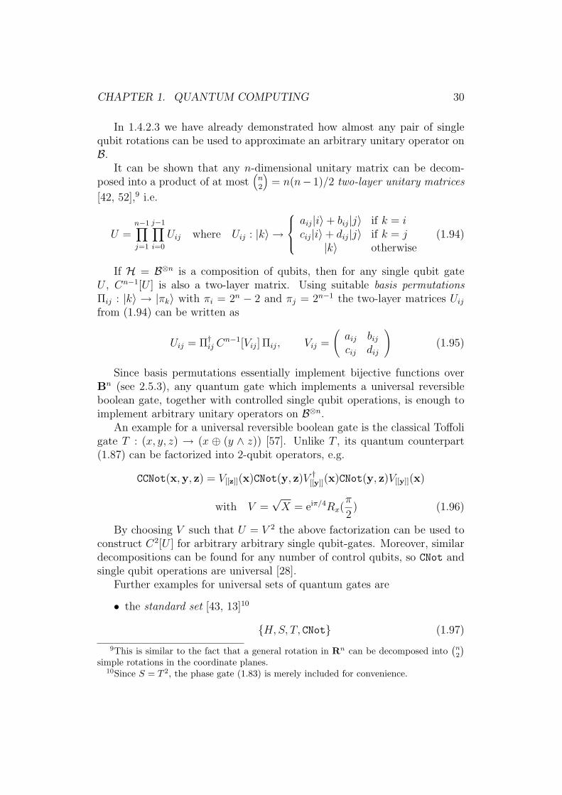
In 1.4.2.3 we have already demonstrated how almost any pair of singlequbit rotations can be used to approximate an arbitrary unitary operator onB.
It can be shown that any n-dimensional unitary matrix can be decom-posed into a product of at most
(n2
)= n(n− 1)/2 two-layer unitary matrices
[42, 52],9 i.e.
U =n−1∏
j=1
j−1∏
i=0
Uij where Uij : |k〉 →
aij|i〉+ bij|j〉 if k = icij|i〉+ dij|j〉 if k = j
|k〉 otherwise(1.94)
If H = B⊗n is a composition of qubits, then for any single qubit gateU , Cn−1[U ] is also a two-layer matrix. Using suitable basis permutationsΠij : |k〉 → |πk〉 with πi = 2n − 2 and πj = 2n−1 the two-layer matrices Uijfrom (1.94) can be written as
Uij = Π†ij C
n−1[Vij] Πij, Vij =
(aij bijcij dij
)(1.95)
Since basis permutations essentially implement bijective functions overBn (see 2.5.3), any quantum gate which implements a universal reversibleboolean gate, together with controlled single qubit operations, is enough toimplement arbitrary unitary operators on B⊗n.
An example for a universal reversible boolean gate is the classical Toffoligate T : (x, y, z) → (x ⊕ (y ∧ z)) [57]. Unlike T , its quantum counterpart(1.87) can be factorized into 2-qubit operators, e.g.
CCNot(x,y, z) = V[[z]](x)CNot(y, z)V †[[y]](x)CNot(y, z)V[[y]](x)
with V =√X = eiπ/4Rx(
π
2) (1.96)
By choosing V such that U = V 2 the above factorization can be used toconstruct C2[U ] for arbitrary arbitrary single qubit-gates. Moreover, similardecompositions can be found for any number of control qubits, so CNot andsingle qubit operations are universal [28].
Further examples for universal sets of quantum gates are
• the standard set [43, 13]10
{H,S, T, CNot} (1.97)
9This is similar to the fact that a general rotation in Rn can be decomposed into(n2
)simple rotations in the coordinate planes.
10Since S = T 2, the phase gate (1.83) is merely included for convenience.
CHAPTER 1. QUANTUM COMPUTING 31
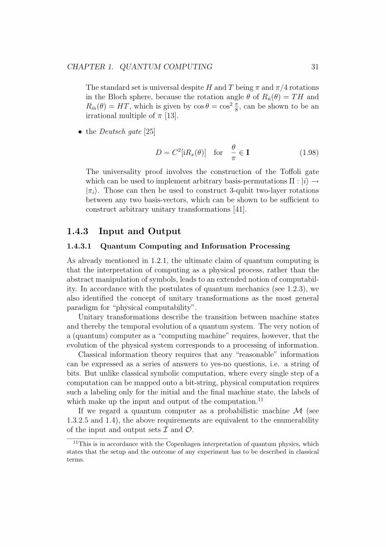
The standard set is universal despiteH and T being π and π/4 rotationsin the Bloch sphere, because the rotation angle θ of Rn(θ) = TH andRm(θ) = HT , which is given by cos θ = cos2 π
8, can be shown to be an
irrational multiple of π [13].
• the Deutsch gate [25]
D = C2[iRx(θ)] forθ
π∈ I (1.98)
The universality proof involves the construction of the Toffoli gatewhich can be used to implement arbitrary basis-permutations Π : |i〉 →|πi〉. Those can then be used to construct 3-qubit two-layer rotationsbetween any two basis-vectors, which can be shown to be sufficient toconstruct arbitrary unitary transformations [41].
1.4.3 Input and Output
1.4.3.1 Quantum Computing and Information Processing
As already mentioned in 1.2.1, the ultimate claim of quantum computing isthat the interpretation of computing as a physical process, rather than theabstract manipulation of symbols, leads to an extended notion of computabil-ity. In accordance with the postulates of quantum mechanics (see 1.2.3), wealso identified the concept of unitary transformations as the most generalparadigm for “physical computability”.
Unitary transformations describe the transition between machine statesand thereby the temporal evolution of a quantum system. The very notion ofa (quantum) computer as a “computing machine” requires, however, that theevolution of the physical system corresponds to a processing of information.
Classical information theory requires that any “reasonable” informationcan be expressed as a series of answers to yes-no questions, i.e. a string ofbits. But unlike classical symbolic computation, where every single step of acomputation can be mapped onto a bit-string, physical computation requiressuch a labeling only for the initial and the final machine state, the labels ofwhich make up the input and output of the computation.11
If we regard a quantum computer as a probabilistic machine M (see1.3.2.5 and 1.4), the above requirements are equivalent to the enumerabilityof the input and output sets I and O.
11This is in accordance with the Copenhagen interpretation of quantum physics, whichstates that the setup and the outcome of any experiment has to be described in classicalterms.
CHAPTER 1. QUANTUM COMPUTING 32
1.4.3.2 Measurement Operators
In the classical machine definition (see 1.3.2), a test command t ∈ T is afunction t : S→ B. In the case of a quantum computerM = (H, O, T, δ, β),however, the machine state |Ψ〉 ∈ H is not directly accessible and any phys-ically realizable test-command will have to amount to the measurement ofsome observable M .
According to the 3rd postulate of quantum mechanics (see 1.2.3.3), themeasurement of M on |Ψ〉 is only deterministic and invariant to |Ψ〉 iff |Ψ〉happens to be an eigenstate ofM , so the test commands are no longer booleanpredicates on S but probabilistic measurement operators, i.e.
T = {µi : H 7→ H×B} (1.99)
Definition 27 Let M be a self-adjoint operator on H with the spectral de-composition M =
∑m λmPm, then the measurement operator µ[M ] is a prob-
abilistic mapping µ[M ] : H 7→ H×R defined as
µ[M ] : |Ψ〉 7→(
1√pmPm|Ψ〉, λm
)with probability pm = 〈Ψ|Pm|Ψ〉
(1.100)
Since test commands are supposed to deliver boolean results, each µicorresponds to a projection operator Pi i.e. a Hermitian with the eigen-values 0 and 1. So µi = µi[Pi] and
µ[P ] : |Ψ〉 7→
( 1√pP |Ψ〉, 1) with p = 〈Ψ|P |Ψ〉
( 1√p(I − P )|Ψ〉, 0) with p = 〈Ψ|I − P |Ψ〉 (1.101)
If P = N(s) we also write µ(s) ≡ µ[N(s)]. Also, we will occasionallyignore one of the function values if this is convenient and can be done withoutambiguity.
Single Qubit Measurements If H = B⊗n, then a natural choice for Piare the standard observable
N(qi) = I⊗i ⊗ |1〉〈1| ⊗ I⊗n−i−1 (1.102)
for each qubit qi. IfM provides a universal set O of unitary operators, singlequbit measurements in the computational basis are sufficient to measure anarbitrary P :
CHAPTER 1. QUANTUM COMPUTING 33
A general projection P has the form
P =∑n
λn|n〉〈n| with λn ∈ B and |n〉 ∈ B (1.103)
where B is an arbitrary orthonormal basis of H. If O is universal, then itis possible to implement the unitary operator U =
∑n |n〉〈n| and P can be
expressed as P = U †P ′U with P ′ =∑n λ
′n|n〉〈n|.
To measure P ′, we can use an additional scratch qubit s in state |0〉s anduse the unitary operator
U ′ : |k〉s|n〉s → |k ⊕ λ′n〉s|n〉s (1.104)
to prepare the entangled machine state
|Ψ′〉 =∑n
cn|λ′n〉s|n〉s where cn = 〈n|Ψ〉 (1.105)
A measurement of N(s) on |Ψ′〉 is now equivalent to to measuring P ′ on|Ψ〉. If the result is 1 and therefore s is left in the state |1〉s, the previousstate can be restored by applying X(s).
Output Function To retrieve the classical result of the computation, afinal measurement is required. Using the standard observable N on H, wecan define the probabilistic output function β : H 7→ N as β = µ[N ].12
1.4.3.3 State Preparation
To set or reset a quantum computer M to desired initial state |Ψ0〉, noadditional operations besides unitary transformations and measurements arenecessary. Assuming H = B⊗n, it suffices to measure all qubits to bringM into a known state |Ψ〉 = |m〉 and then to apply an arbitrary unitaryoperator Um which satisfies the condition 〈Ψ0|Um|m〉 = 1.
If |Ψ0〉 = |d0d1 . . . dn−1〉 then at most n X-gates are required for thepreparation.13 It is also convenient to include a special non-unitary memorycommand
reset : |Ψ〉 → |0〉 (1.106)
for the initialization of the machine state.
12This notation is actually a shorthand for β(|Ψ〉) = m ⇐⇒ µ[N ]|Ψ〉 = (|Ψm〉,m).13For arbitrary |Ψ0〉, the number of necessary gates generally increases exponentially.
CHAPTER 1. QUANTUM COMPUTING 34
Input Function To allow the preparation of “classical” input states wecan define the input function δ(s) : N → H as δ(s) = |s〉. For quantumalgorithms which take their input in the form of oracle operators14 and con-sequently do not require any classical input, it is common to assume an initialstate |Ψ0〉 = δ(s) = |0〉.
1.5 Concepts of Quantum Computation
1.5.1 Models and Formalisms
As we demonstrated in 1.3 the concept of the universal computer can berepresented by several equivalent models, corresponding to different scientificapproaches. From a mathematical point of view, a universal computer is amachine capable of calculating partial recursive functions (1.3.1.1), computerscientists often use the Turing machine (1.3.2.2) as their favorite model, anelectronic engineer would possibly speak of logic circuits while a programmerprobably will prefer a universal programming language (1.3.3.2).
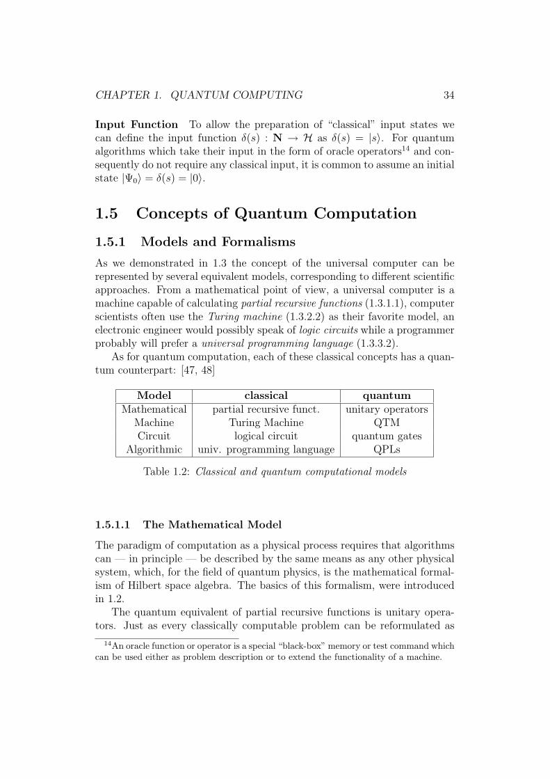
As for quantum computation, each of these classical concepts has a quan-tum counterpart: [47, 48]
Model classical quantumMathematical partial recursive funct. unitary operators
Machine Turing Machine QTMCircuit logical circuit quantum gates
Algorithmic univ. programming language QPLs
Table 1.2: Classical and quantum computational models
1.5.1.1 The Mathematical Model
The paradigm of computation as a physical process requires that algorithmscan — in principle — be described by the same means as any other physicalsystem, which, for the field of quantum physics, is the mathematical formal-ism of Hilbert space algebra. The basics of this formalism, were introducedin 1.2.
The quantum equivalent of partial recursive functions is unitary opera-tors. Just as every classically computable problem can be reformulated as
14An oracle function or operator is a special “black-box” memory or test command whichcan be used either as problem description or to extend the functionality of a machine.
CHAPTER 1. QUANTUM COMPUTING 35
calculating the value of a partial recursive function, every quantum compu-tation can be described by a unitary operator.15
The mathematical description of an operator is inherently declarative;the actual implementation for a certain quantum architecture i.e. the al-gorithmic decomposition into elementary operations, is beyond the scope ofthis formalism. Also, since the mathematical model treats unitary operatorsas black boxes, no complexity measure is provided.
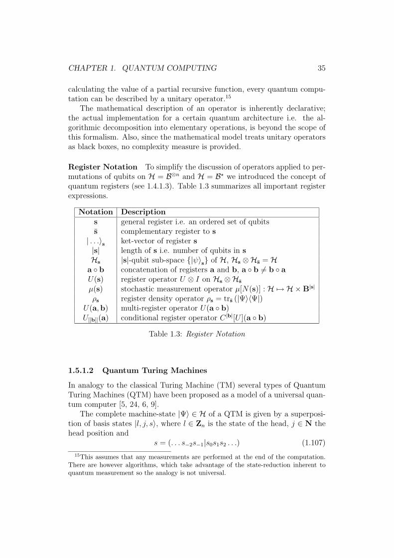
Register Notation To simplify the discussion of operators applied to per-mutations of qubits on H = B⊗n and H = B? we introduced the concept ofquantum registers (see 1.4.1.3). Table 1.3 summarizes all important registerexpressions.
Notation Descriptions general register i.e. an ordered set of qubitss complementary register to s| . . .〉s ket-vector of register s|s| length of s i.e. number of qubits in sHs |s|-qubit sub-space {|ψ〉s} of H, Hs ⊗Hs = H
a ◦ b concatenation of registers a and b, a ◦ b 6= b ◦ aU(s) register operator U ⊗ I on Hs ⊗Hs
µ(s) stochastic measurement operator µ[N(s)] : H 7→ H×B|s|
ρs register density operator ρs = trs (|Ψ〉〈Ψ|)U(a,b) multi-register operator U(a ◦ b)U[[b]](a) conditional register operator C |b|[U ](a ◦ b)
Table 1.3: Register Notation
1.5.1.2 Quantum Turing Machines
In analogy to the classical Turing Machine (TM) several types of QuantumTuring Machines (QTM) have been proposed as a model of a universal quan-tum computer [5, 24, 6, 9].
The complete machine-state |Ψ〉 ∈ H of a QTM is given by a superposi-tion of basis states |l, j, s〉, where l ∈ Zn is the state of the head, j ∈ N thehead position and
s = (. . . s−2s−1|s0s1s2 . . .) (1.107)
15This assumes that any measurements are performed at the end of the computation.There are however algorithms, which take advantage of the state-reduction inherent toquantum measurement so the analogy is not universal.
CHAPTER 1. QUANTUM COMPUTING 36
the binary representation of the tape-content. To keep H separable, s hasto meet the zero tail state condition (see 1.3.2.2) i.e. only a finite number ofbits with sm 6= 0 are allowed, so s ∈ B? and H = Cn ⊗ l2 ⊗ B?
The quantum analogue of the transition function of a classical probabilis-tic TM is the unitary step operator T , which has to meet locality conditionsfor the affected tape-qubit, as well as for head movement.16
QTMs provide a measure for execution times, but — as with the classicalTM — finding an appropriate step operator can be very hard.
1.5.1.3 Quantum Circuits
Quantum circuits are the quantum equivalent to classical boolean feed-forwardnetworks, with one major difference: since all quantum computations have tobe unitary, quantum circuits can be evaluated in both directions (as in clas-sical reversible logic). Quantum circuits are composed of elementary gatesand operate on qubits.17 The “wiring” between the gates defines the registeron which the gates operate, so an m-qubit gate U in an n-qubit circuit candescribe up to n!
(n−m)!different unitary transformations U(s).
As opposed to the mathematical formalism, the gate-notation is an in-herently constructive method and the complexity of the problem is directlyreflected in the number of gates necessary to implement it. However, sincequantum circuits describe static sequences, the size of the input as well asthe number of qubits is fixed, so without additional assumptions, quantumcircuits cannot be used to analyze the complexity depending on the size ofthe problem. For the same reason, quantum circuits are also inadequate formachines with unlimited memory.
Restrictions In comparison with classical boolean feed-forward networks,this imposes the following restrictions:
• Only n-to-n networks are allowed i.e. the total number of inputs hasto match the total number of outputs.
• Only n-to-n gates are allowed.
16Instead of a unitary step-operator T , it is also possible to directly construct a (local)Hamiltonian H (see 1.2.3.2) [5, 6]. In this case, the computation does not need to bediscrete and T ′ = U(t0) = e−iHt0 is not required to conform to locality conditions.
17There also exist extentions to cover measurements and classical bits [43]. In that case,quantum circuits can also be used to describe irreversible computations.
CHAPTER 1. QUANTUM COMPUTING 37
• No forking of inputs is allowed. This is directly related to the fact thatqubits cannot be copied, i.e. that there exists no unitary operation
Copy |ψ〉|0〉 → |ψ〉|ψ〉 with |ψ〉 ∈ C2 (1.108)
which can turn a general qubit-state into a product state of itself.
• No “dead ends” are allowed. Again, this is because the erasure of aqubit
Erase |ψ〉 → |0〉 with |ψ〉 ∈ C2 (1.109)
is not a unitary operation.
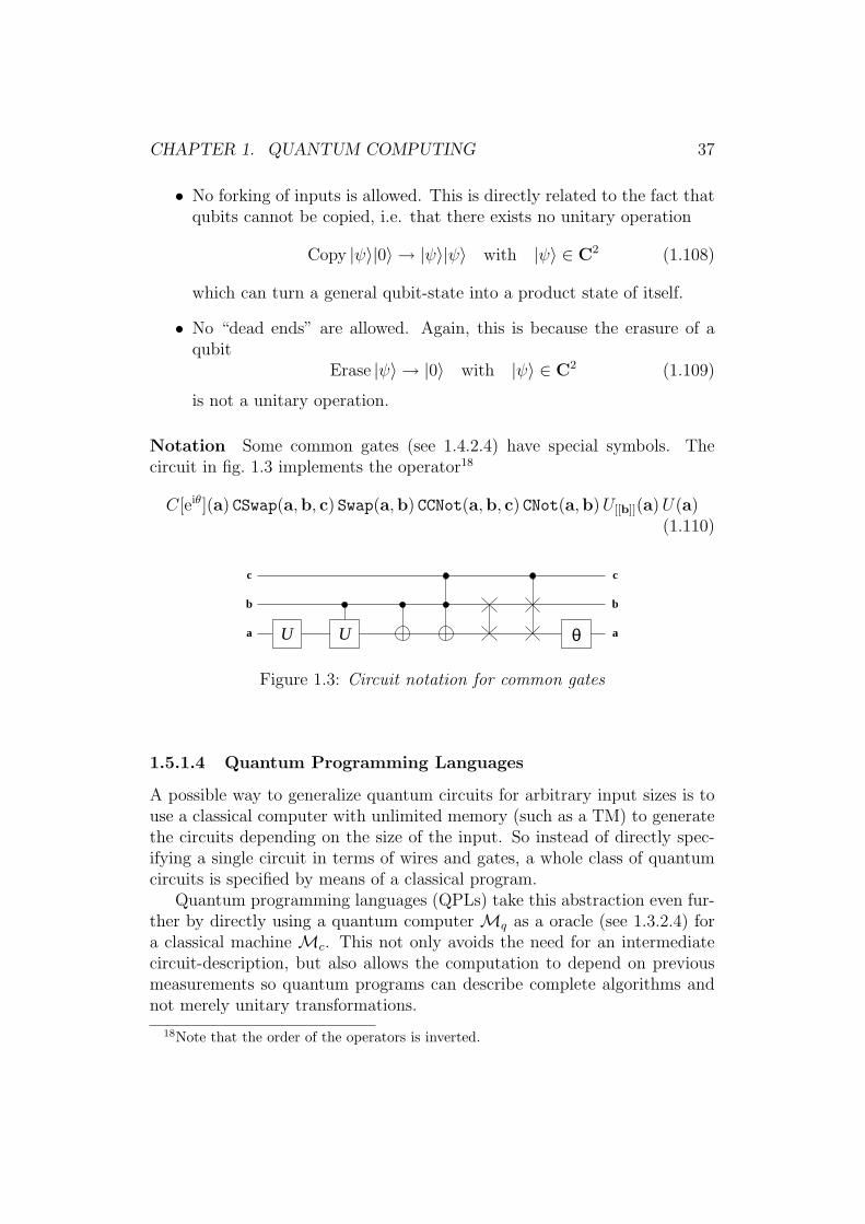
Notation Some common gates (see 1.4.2.4) have special symbols. Thecircuit in fig. 1.3 implements the operator18
C[eiθ](a) CSwap(a,b, c) Swap(a,b) CCNot(a,b, c) CNot(a,b)U[[b]](a)U(a)(1.110)
a
b
c
a
b
c
U θU
Figure 1.3: Circuit notation for common gates
1.5.1.4 Quantum Programming Languages
A possible way to generalize quantum circuits for arbitrary input sizes is touse a classical computer with unlimited memory (such as a TM) to generatethe circuits depending on the size of the input. So instead of directly spec-ifying a single circuit in terms of wires and gates, a whole class of quantumcircuits is specified by means of a classical program.
Quantum programming languages (QPLs) take this abstraction even fur-ther by directly using a quantum computer Mq as a oracle (see 1.3.2.4) fora classical machine Mc. This not only avoids the need for an intermediatecircuit-description, but also allows the computation to depend on previousmeasurements so quantum programs can describe complete algorithms andnot merely unitary transformations.
18Note that the order of the operators is inverted.
CHAPTER 1. QUANTUM COMPUTING 38
1.5.2 Quantum Algorithms
1.5.2.1 Classical and Quantum Computability
If we consider a finite quantum computer with the Toffoli gate (see 1.4.2.4) asthe only available instruction, then any transformation of the machine statehas to be of the form
|Ψ〉 = |i〉 −→ |g(i)〉 = |Ψ′〉 with g : Bn → Bn (1.111)
Since the Toffoli gate is universal for reversible boolean logic, any bijectivebinary function g can directly be implemented on a quantum computer.
A general binary function f on Bn, can be implemented by an arbitraryunitary operator F which satisfies the condition F |i, 0〉 = |i, f(i)〉.
So any function f computable on a (finite) classical machine can also beimplemented on a quantum computer with a universal set of gates. Moreover,C. H. Bennet has shown that a reversible implementation of f can be madewith a maximal overhead of O(2) in time and O(
√n) in space complexity
[7].On the other hand, a general n-qubit quantum state consists of maximally
2n basis-vectors with a non-zero amplitude and can consequently be describedby an array of 2n complex numbers. Also, any m-qubit quantum gate can bedescribed by a complex 2n × 2n matrix with the elements uij = 〈i|U |j〉.
By encoding the complex amplitudes as a pair of floating point binarynumbers a classical computer can simulate any unitary operator to arbitraryprecision.19 This will generally require an overhead of O(en) in time as well asin space complexity. Due to the stochastic nature of quantum measurements,the emulating computer will also need a source of true randomness (like e.g.the probabilistic Turing machine).
So classical and quantum computers are computationally equivalent, butwhile it is possible to efficiently simulate a classical computer on a quantumcomputer, the opposite case can involve an exponential overhead. Therefore,while not extending our notion of computability, for certain tasks quantumalgorithms might provide a more efficient solutions than classical implemen-tations.
1.5.2.2 Deutsch’s Algorithm
In 1985, Deutsch proposed a probabilistic algorithm [24] which for someoracle function g : B→ B allows to compute g(0)⊕ g(1) with a probabilityof 1/2 using only 1 application of G:
19The linearity of unitary transformations assures that small errors will not escalate.
CHAPTER 1. QUANTUM COMPUTING 39
Let G : |x, y〉 → |x, y ⊕ g(x)〉 be a 2-qubit oracle-operator implementingthe boolean oracle function g : B→ B.
1. Prepare an empty initial state |Ψ0〉 = |0〉x|0〉y.
2. Apply H(x)
|Ψ1〉 = (H |0〉x) |0〉y =1√2
(|0〉x|0〉y + |1〉x|0〉y
)(1.112)
3. Apply the oracle operator G, giving
|Ψ2〉 =1√2
(|0〉x|g(0)〉y + |1〉x|g(1)〉y
)(1.113)
4. Apply H(x ◦ y), resulting in
|Ψ3〉 =1
2√
2
∑
x∈B
∑
y∈B
((−1)yg(0) + (−1)x+yg(1)
)|x〉x|y〉y (1.114)
5. Measure x and y.
As (1.114) can be simplified to
|Ψ3〉 =1√2
(|0〉x|0〉y + (−1)g(0)|g(0)⊕ g(1)〉x|1〉y
)(1.115)
the register x will contain the value g(0)⊕g(1) whenever 1 has been measuredin y which will happen in 50% of the cases.
While strictly speaking, this does not provide any speedup over the clas-sical case, if we take into account that, on average, two tries are required toactually measure g(0) ⊕ g(1), Deutsch’s algorithm was the first proof thatquantum computers are capable of performing computations in ways thatare impossible on a classical computer.20
Generally, in order to achieve any speedup over classical algorithms, it isnecessary to take advantage of the unique features of quantum computing,namely
• Superposition (step 2)
• Quantum Parallelism (step 3)
• Interference (step 4)
20There exist several improvements and generalizations to the original version ofDeutsch’s algorithm [26, 20], one of which — the Deutsch-Jozsa Algorithm — is describedin 1.5.2.6.
CHAPTER 1. QUANTUM COMPUTING 40
1.5.2.3 Superposition
A key element in any universal programming language is conditional branch-ing. Any classical program (see 1.3.3) can be modeled as a decision tree whereeach node corresponds to a binary state sn and leads to one or more succes-sor states s
(i)n+1. On a deterministic Turing machine (TM), only one of those
transitions sn → s(k)n+1 is possible, so the computational path 〈s0, s1, . . . sn〉 is
predetermined.On a probabilistic TM (see 1.3.2.5), the transitions are characterized by
probabilities pi with∑i pi = 1 and one of the possible successor states s
(i)n+1
is chosen accordingly at random.Since the basis-vectors |i〉 directly correspond to classical binary states,
we might interpret a unitary transformation
U : |s〉 →∑
s′uss′|s′〉 with s, s′ ∈ Bn and uss′ ∈ C (1.116)
as a probabilistic transition form the classical state s to the successor statess′ with the transition probabilities ps′ = |uss′|2, but unless we perform ameasurement, the resulting machine state remains in a superposition of allpossible classical successor states
|Ψ〉 = |sn〉 U−→ |Ψ′〉 =∑
i
usns
(i)n+1|s(i)n+1〉 (1.117)
So from a classical point of view, we can consider a unitary operator whichtransforms an eigenstate into a superposition of n eigenstates with nonzeroamplitudes as a 1–n fork-operation, which enables a quantum computer tofollow several classical computational paths at once.
Hadamard-Transform Most non-classical algorithms take advantage ofthis feature by bringing a register into a even superposition of all basis-statesto serve as search space. In Deutsch’s algorithm, this is achieved by applyingthe Hadamard-gate on the first qubit-register.
The H-gate can be generalized to n-qubit registers, by applying H toeach individual qubit. The resulting unitary operator is called Hadamardtransform and defined as:
H : |x〉 → 2n2
∑
y∈Bn
(−1)x·y|y〉 (1.118)
where x · y =∑i xiyi denotes the binary inner product. The transformed
basis
B = {H|x〉 | x ∈ Bn} = {|+〉, |−〉}n with |±〉 =1√2
(|0〉 ± |1〉) (1.119)
CHAPTER 1. QUANTUM COMPUTING 41
is sometimes referred to as the dual basis.Classically, the Hadamard transform of |Ψ〉 = |0〉 can be viewed as a
binary decision tree with a 50% chance for each bit to flip. For an n-qubitregister, this leads to 2n classical computational paths all of which are fol-lowed simultaneously resulting in a superposition of 2n eigenvectors.
1.5.2.4 Quantum Parallelism
If we restrict unitary transformations to basis-permutations (i.e. operatorsof the form |i〉 → |πi〉 then the classical decision tree degenerates into a listand we end up with the functionality of a classical deterministic reversiblecomputer i.e. for any bijective binary function f : Bn → Bn there is acorresponding unitary operator
F : |s〉 → |f(s)〉 with s ∈ Bn. (1.120)
The restriction to bijective functions is not a severe as it seems, since forany general binary function g : Bn → Bm a corresponding quantum function
G : |s, 0〉 → |s, g(s)〉 with s ∈ Bn (1.121)
can be constructed, which implements g with a maximum overhead of O(√n)
in space- and O(2) time-complexity.However, if we use a quantum function on an superposition of eigenstates,
the same classical computation is performed on all bit-strings simultaneously.
G∑s
cs|s, 0〉 =∑s
csG|s, 0〉 =∑s
cs|s, g(s)〉 (1.122)
In classical terms, this can be described as a SIMD (single instruction,multiple data) vector operation, in quantum terms this feature is referred toas quantum parallelism.
In Deutsch’s algorithms, quantum parallelism is exploited by applying Gon the superposition |Ψ1〉 = (|00〉+ |10〉)/√2.
1.5.2.5 Interference
While superpositions and quantum parallelism allow us to perform an expo-nentially large number of classical computations in parallel, the only way toread out any results is by performing a measurement whereby all but one ofthe superpositioned eigenstates get discarded. Since it does not make anydifference if the computational path is determined during the calculation (aswith the probabilistic TM) or a-posteriori (by quantum measurement), the

CHAPTER 1. QUANTUM COMPUTING 42
use of quantum computers would not provide any advantage over probabilis-tic classical computers.
Quantum states, however, are not merely a probability distribution ofbinary values but complex vectors i.e. each basis-state in a superposition isnot characterized by a real probability, but a complex amplitude, so
|ψ1〉 =1√2(|0〉+ |1〉) and |ψ2〉 =
1√2(|0〉 − |1〉) (1.123)
describe different states, even if they have the same probability spectrum.So, while on a probabilistic TM, the probabilities of two different com-
putational paths leading to the same final state s simply add up, this is notnecessarily the case on a quantum computer since generally
|α + β|2 6= |α|2 + |β|2 for α, β ∈ C. (1.124)
To illustrate this concept, consider the three states
|ψ1〉 = |0〉, |ψ2〉 = |1〉 and |ψ3〉 =1√2(|0〉+ |1〉). (1.125)
If we apply the Hadamard-transform H to the basis states |ψ1〉 and |ψ2〉 weget
|ψ′1〉 = H |ψ1〉 =1√2(|0〉+ |1〉) and |ψ′2〉 = H |ψ2〉 =
1√2(|0〉 − |1〉).
(1.126)Since |ψ′1〉 and |ψ′2〉 have the same probability distribution and |ψ3〉 is
merely a superposition of |ψ1〉 and |ψ2〉, classically we would assume that|ψ′3〉 also shows the same probability spectrum, however
|ψ′3〉 = H |ψ3〉 =1√2(|ψ′1〉+ |ψ′2〉) = |0〉 (1.127)
so in case of |0〉 the probabilities added up while in case of |1〉, the complexamplitudes had opposing signs leading to a partial probability of 0. Thisphenomenon is referred to as positive or negative interference.
So while the computational paths on a probabilistic TM are independent,interference allows computations on superposition states to interact and it isthis interaction which allows a quantum computer to solve certain problemsmore efficiently than classical computers. The foremost design principle forany quantum algorithm therefore is to use interference to increase the prob-ability of “interesting” basis states while trying to reduce the probability of“uninteresting” states, in order to improve the chance that a measurementwill pick one of the former.
CHAPTER 1. QUANTUM COMPUTING 43
Basis Transformations Since any unitary operator U can also be re-garded as a basis transformation, the above problem can also be reformulatedas finding an appropriate observable for the measurement, thereby effectivelyreplacing the standard observable N by the Hermitian operator
M = N = U N U † =∑n
n|n〉〈n|. (1.128)
This view is especially useful, if global properties of classical functionssuch as periodicy are of interest for the problem.
In Deutsch’s algorithms, the final measurement is performed in the dualbasis (1.119), which allows g(0) ⊕ g(1) to be extracted in a single measure-ment.
1.5.2.6 Deutsch-Jozsa Algorithm
The Deutsch-Jozsa algorithm [26] is an improved and generalized versionof the original algorithm described in (see 1.5.2.2). For n = 1 it gives adeterministic solution to Deutsch’s problem:
Let F : |x, y〉 → |x, y ⊕ f(x)〉 be an (n + 1)-qubit oracle-operator im-plementing a boolean function f : Bn → B. Let us further assume thatwe know that f is either constant ((∀x)f(x) = b where b ∈ B) or balanced(∑f(x) = 2n−1). Classically, 2n−1 +1 evaluations of f would be necessary to
find out which of the possibilities applies. The following quantum algorithmcan solve this decision problem with a single application of F :
1. Prepare initial state |Ψ0〉 = |0〉x|1〉y.
2. Apply H(x ◦ y) to set up the search space superposition
|Ψ1〉 = 2−n+1
2
∑
x∈Bn
|x〉x(|0〉y − |1〉y
). (1.129)
3. Apply the oracle operator, giving quantum parallelism
|Ψ2〉 = 2−n+1
2
∑
x∈Bn
(−1)f(x)|x〉x(|0〉y − |1〉y
). (1.130)
4. Apply H(x), which results in interference
|Ψ3〉 =∑
z∈Bn
cz|z〉x ⊗1√2
(|0〉y − |1〉y
), cz = 2−n
∑
x∈Bn
(−1)x·z+f(x)
(1.131)
CHAPTER 1. QUANTUM COMPUTING 44
5. Measure x.
The probability to measure 0 in x is |c0|2 where
c0 = 2−n∑
x∈Bn
(−1)f(x) (1.132)
If f is constant c0 = ±1, if f is balanced, the summands cancel out andc0 = 0, so µ(x)|Ψ3〉 = 0 ⇐⇒ f is constant.
Chapter 2
Structured QuantumProgramming
2.1 Introduction
2.1.1 Motivation
As quantum computing is on its way to becoming an established disciplineof computing science, much effort is being put into the development of newquantum algorithms. This research has usually not got much in common withthe experimental work on quantum computers and is rarely tied to a specifichardware, but instead employs an abstract notion of a quantum computerwith qubits, registers, and a small set of suitable elementary operations [3],which allows one to concentrate on the problem at hand.
A programming language which integrates these abstractions by designshould be a useful tool in situations where the much more general physicalformalism of Hilbert space algebra gets unnecessarily complex.
The possibility to formulate and simulate an algorithm in a program-ming language should also make it easier to optimize the implementationwith regard to different quantum architectures and allow for more accurateestimates of time and memory complexity.
2.1.2 Quantum Programming Languages
From a software engineering point of view, we can regard the algebraic for-malism as a specification language, as the mathematical description of aquantum algorithm is inherently declarative and provides no means to de-rive a unique decomposition into elementary operations for a given quantumhardware.
45
CHAPTER 2. STRUCTURED QUANTUM PROGRAMMING 46
Low level formalisms as e.g. quantum circuits [25], on the other hand,are usually restricted to specific tasks, such as the description of unitarytransformations, and thus lack the generality to express all aspects of non-classical algorithms.
The purpose of programming languages is therefore twofold, as they allowthe expression of a computation’s semantics in an abstract manner, as well asthe automated generation of a sequence of elementary operations to controlthe computing device. Any useful quantum programming language (QPL)therefore needs to be
• constructive
• hardware independent
• provide arbitrary levels of abstraction
• integrate non-classical features at a semantic level
While the first three requirements equally apply to classical and quan-tum programming languages, QPLs also have to reflect the peculiarities ofquantum computing, as e.g.
• reversibility of unitary operations
• non-locality of qubits
• non-observability of states
• destructive nature of measurement
• lack of an erase operation
at a design level and consequently have to provide the means to take advan-tage of these features (e.g. by allowing to run code “in reverse”).1
2.1.3 Classification of Programming Languages
In traditional CS, programming languages can be categorized as either logical(e.g. Prolog), functional (e.g. LISP) or imperative (e.g. Assembler, Fortran,Pascal, C), the latter being the most widely used, for the description ofalgorithms, as well as for the actual implementation of real world programs.
1Classical languages with additional quantum directives (like e.g.. a C++ simulationor device driver API) are therefore not considered to be QPLs, as they do not genericallysupport these non-classical concepts [61].
CHAPTER 2. STRUCTURED QUANTUM PROGRAMMING 47
2.1.3.1 Imperative Programming Languages
Imperative programming is centered around the concept of a computationalstate, and commands modifying the state [1]. The state is an abstraction forthe modifiable storage of the underlying machine model and is semanticallyexpressed in terms of symbolic variables of various data types and the currentstate of control (instruction counter, stack pointer, etc.), which may or maynot have a direct representation within the language.
During its execution, a program generates a sequence of states. Thetransition from one state to the next is determined by
• assignment commands, which modify the state of variables, and
• sequencing commands, which modify the state of control.
The direct correspondence between state chances and program statementsleads to the concept of flow of control, i.e. a computation can be characterizedby the actual sequence of commands. This allows an imperative program tobe traced by following the current state of control and introduces a notionof locality of execution.
Examples of imperative programming languages are assembly languageor BASIC. Concepts of imperative programming are reflected in the hybridquantum architecture (2.2.3) and the concept of symbolic quantum registers(2.4.1).
2.1.3.2 Procedural Programming Languages
Imperative programming combined with parameterized subroutines (proce-dures, functions) it is called procedural programming. The availability ofsubroutines allows for
• Functional Abstraction: Code of similar or identical functionalitycan be generalized to reusable parameterized procedures.
• Hierarchical Program Structure: Subroutines can contain calls toother subroutines which provides arbitrary levels of abstraction andsupports a top-down approach in software design.
• Recursion: Subroutines can also contain calls to themselves whichallows for an elegant and efficient implementation of otherwise compli-cated control structures and directly supports the classical “divide andconquer” approach in software design.
CHAPTER 2. STRUCTURED QUANTUM PROGRAMMING 48
• Private Scopes: Subroutines provide their own namespace which re-duces interdependencies within the program.
• Local Variables: Local namespaces also allow the use of temporaryvariables of limited lifetime which leads to more efficient usage of theavailable storage and allows details of the implementation to be hiddenfrom the procedure’s calling interface.
Examples of procedural programming languages are Fortran and C. Con-cepts of procedural programming are reflected in quantum data types (2.4.1.3,2.5.2.2), quantum subroutines (2.5.1) and scratch space management (2.5.3.5)[47].
2.1.3.3 Structured Programming Languages
An mentioned in 2.1.3.1, imperative programs consist of assignment andsequencing commands. A simple way to provide flow-control is by means ofa goto command which explicitly transfers control to a labeled commandwhich is to be executed next.
goto label;
if condition then goto label;
This approach is problematic as it implies a flat control structure where anylabeled command can be jumped to from anywhere within the program (or,in the case of procedural languages, the current subroutine). This tends tomake larger programs unreadable (“spaghetti code”).
In 1966, Corrado Bohm and Guiseppe Jacopini showed [11] that the gotocommand can be replaced by the nesting and stacking (sequencing) of threebasic control statements
• sequence (block-statements),
• selection (if-statements) and
• iteration (conditional loops),
with well defined entry- and exit-points. This approach, called structuredprogramming [27, 23], implies a strictly hierarchical control-structure whichnot only makes programs easier to understand, but also provides useful meta-information for the compiler.
Examples of structured programming languages are Pascal and Modula,but almost any procedural language supports the necessary control state-ments, even if their exclusive use is not enforced. Concepts of structuredprogramming are reflected in quantum conditions (2.6.3), conditional opera-tors (2.6.1) and quantum if-statements (2.6.2.1).
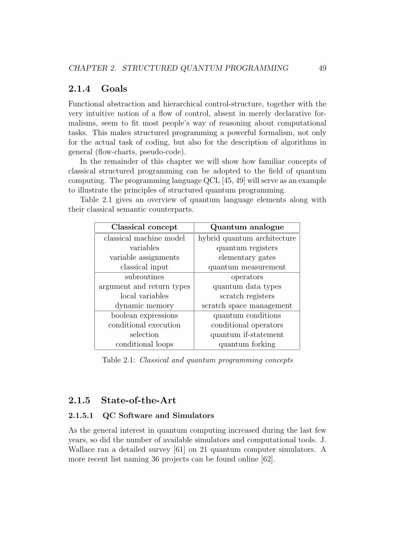
CHAPTER 2. STRUCTURED QUANTUM PROGRAMMING 49
2.1.4 Goals
Functional abstraction and hierarchical control-structure, together with thevery intuitive notion of a flow of control, absent in merely declarative for-malisms, seem to fit most people’s way of reasoning about computationaltasks. This makes structured programming a powerful formalism, not onlyfor the actual task of coding, but also for the description of algorithms ingeneral (flow-charts, pseudo-code).
In the remainder of this chapter we will show how familiar concepts ofclassical structured programming can be adopted to the field of quantumcomputing. The programming language QCL [45, 49] will serve as an exampleto illustrate the principles of structured quantum programming.
Table 2.1 gives an overview of quantum language elements along withtheir classical semantic counterparts.
Classical concept Quantum analogue
classical machine model hybrid quantum architecturevariables quantum registers
variable assignments elementary gatesclassical input quantum measurementsubroutines operators
argument and return types quantum data typeslocal variables scratch registers
dynamic memory scratch space managementboolean expressions quantum conditions
conditional execution conditional operatorsselection quantum if-statement
conditional loops quantum forking
Table 2.1: Classical and quantum programming concepts
2.1.5 State-of-the-Art
2.1.5.1 QC Software and Simulators
As the general interest in quantum computing increased during the last fewyears, so did the number of available simulators and computational tools. J.Wallace ran a detailed survey [61] on 21 quantum computer simulators. Amore recent list naming 36 projects can be found online [62].
CHAPTER 2. STRUCTURED QUANTUM PROGRAMMING 50
The available software can be roughly categorized as
• class libraries for existing classical languages
• packages for computer algebra systems
• quantum circuit simulators
• simulations of specific quantum hardware
• simulations of specific algorithms
• other quantum simulations (QTMs, quantum Bayesian nets, etc.)
2.1.5.2 Quantum Programming Languages
Besides QCL [49], there have been at least 3 attempts to design a quantumprogramming language
• 1996 Q-gol by Greg Baker [2]
• 2000 qGCL by Paolo Zuliani [63]
• 2002 Quantum C Language by Stephen Blaha [10]
From those, the most evolved project is probably Zuliani’s qGCL. In histhesis [63] Zuliani proposes an abstract formalism with rigorous semanticsand an associated refinement calculus which allows for program derivationand strict proof of correctness. There is, however, no interpreter or compileravailable.
2.2 The Computational Model of Quantum
Programming
In this section we will demonstrate why quantum circuits and finite programsare insufficient for universal quantum computation and introduce the hybridquantum architecture as the computational model of quantum programming.
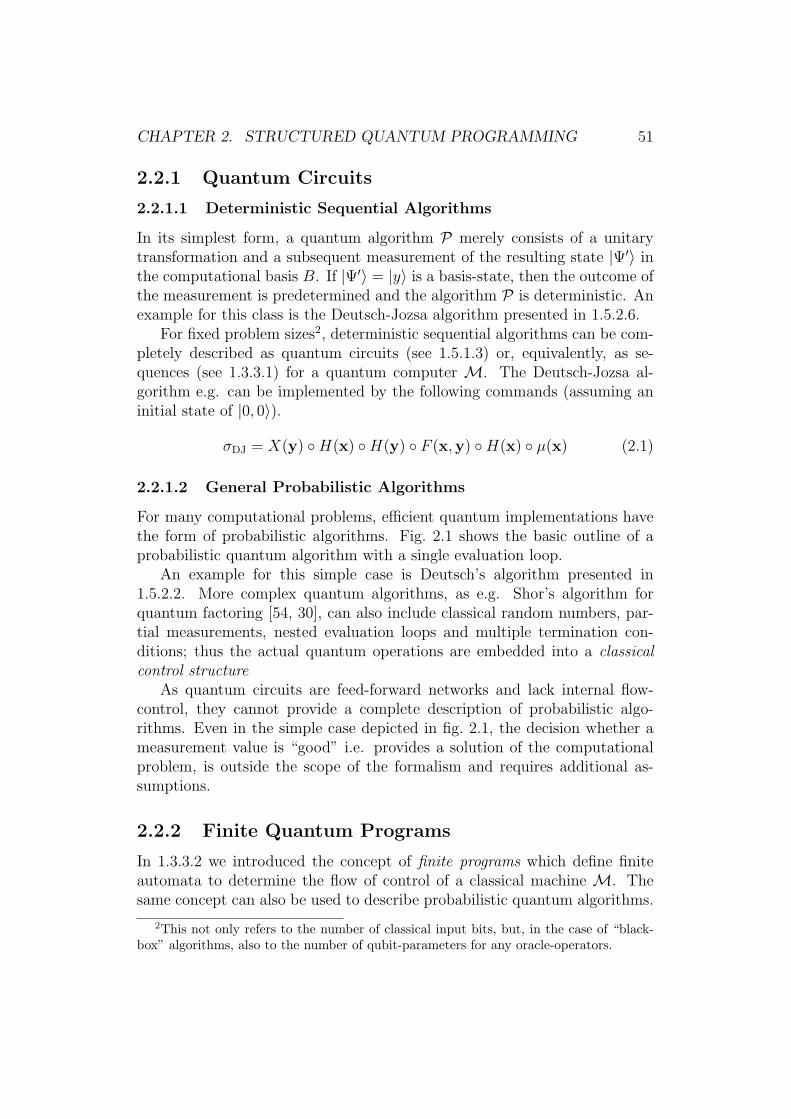
CHAPTER 2. STRUCTURED QUANTUM PROGRAMMING 51
2.2.1 Quantum Circuits
2.2.1.1 Deterministic Sequential Algorithms
In its simplest form, a quantum algorithm P merely consists of a unitarytransformation and a subsequent measurement of the resulting state |Ψ′〉 inthe computational basis B. If |Ψ′〉 = |y〉 is a basis-state, then the outcome ofthe measurement is predetermined and the algorithm P is deterministic. Anexample for this class is the Deutsch-Jozsa algorithm presented in 1.5.2.6.
For fixed problem sizes2, deterministic sequential algorithms can be com-pletely described as quantum circuits (see 1.5.1.3) or, equivalently, as se-quences (see 1.3.3.1) for a quantum computer M. The Deutsch-Jozsa al-gorithm e.g. can be implemented by the following commands (assuming aninitial state of |0, 0〉).
σDJ = X(y) ◦H(x) ◦H(y) ◦ F (x,y) ◦H(x) ◦ µ(x) (2.1)
2.2.1.2 General Probabilistic Algorithms
For many computational problems, efficient quantum implementations havethe form of probabilistic algorithms. Fig. 2.1 shows the basic outline of aprobabilistic quantum algorithm with a single evaluation loop.
An example for this simple case is Deutsch’s algorithm presented in1.5.2.2. More complex quantum algorithms, as e.g. Shor’s algorithm forquantum factoring [54, 30], can also include classical random numbers, par-tial measurements, nested evaluation loops and multiple termination con-ditions; thus the actual quantum operations are embedded into a classicalcontrol structure
As quantum circuits are feed-forward networks and lack internal flow-control, they cannot provide a complete description of probabilistic algo-rithms. Even in the simple case depicted in fig. 2.1, the decision whether ameasurement value is “good” i.e. provides a solution of the computationalproblem, is outside the scope of the formalism and requires additional as-sumptions.
2.2.2 Finite Quantum Programs
In 1.3.3.2 we introduced the concept of finite programs which define finiteautomata to determine the flow of control of a classical machine M. Thesame concept can also be used to describe probabilistic quantum algorithms.
2This not only refers to the number of classical input bits, but, in the case of “black-box” algorithms, also to the number of qubit-parameters for any oracle-operators.
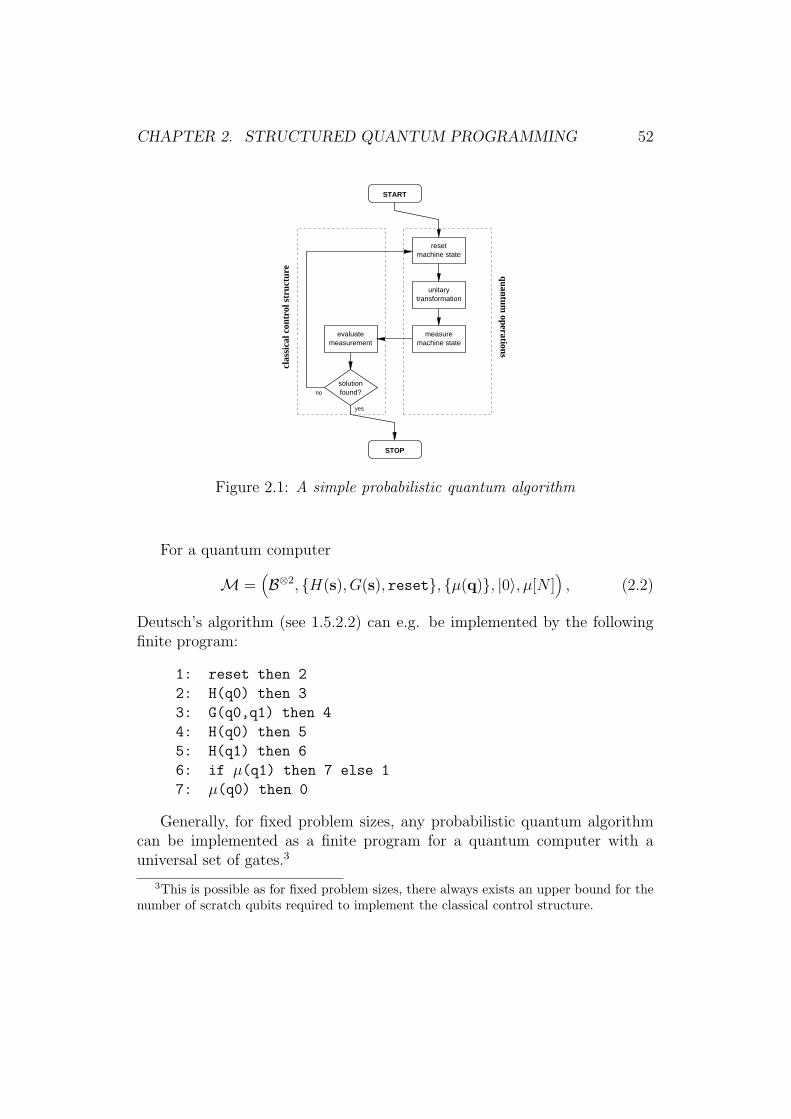
CHAPTER 2. STRUCTURED QUANTUM PROGRAMMING 52
clas
sica
l con
trol
str
uctu
re quantum operations
resetmachine state
unitarytransformation
measuremachine state
evaluatemeasurement
solutionfound?
START
STOP
no
yes
Figure 2.1: A simple probabilistic quantum algorithm
For a quantum computer
M =(B⊗2, {H(s), G(s), reset}, {µ(q)}, |0〉, µ[N ]
), (2.2)
Deutsch’s algorithm (see 1.5.2.2) can e.g. be implemented by the followingfinite program:
1: reset then 2
2: H(q0) then 3
3: G(q0,q1) then 4
4: H(q0) then 5
5: H(q1) then 6
6: if µ(q1) then 7 else 1
7: µ(q0) then 0
Generally, for fixed problem sizes, any probabilistic quantum algorithmcan be implemented as a finite program for a quantum computer with auniversal set of gates.3
3This is possible as for fixed problem sizes, there always exists an upper bound for thenumber of scratch qubits required to implement the classical control structure.
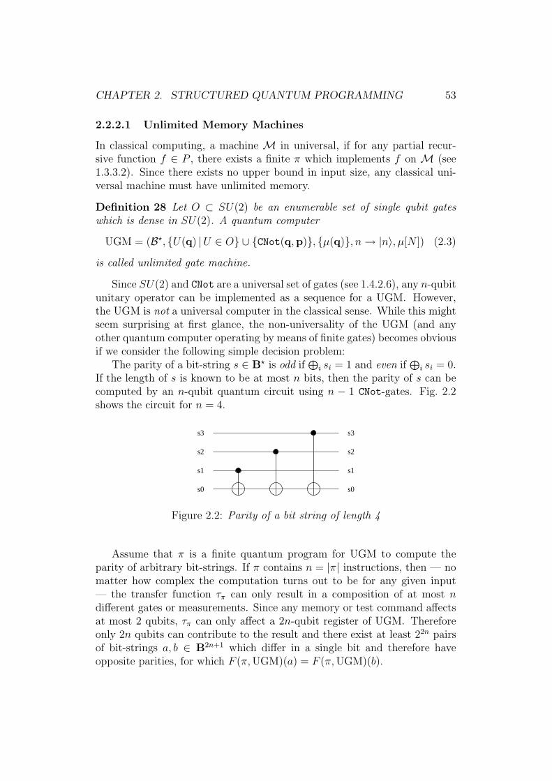
CHAPTER 2. STRUCTURED QUANTUM PROGRAMMING 53
2.2.2.1 Unlimited Memory Machines
In classical computing, a machine M in universal, if for any partial recur-sive function f ∈ P , there exists a finite π which implements f on M (see1.3.3.2). Since there exists no upper bound in input size, any classical uni-versal machine must have unlimited memory.
Definition 28 Let O ⊂ SU(2) be an enumerable set of single qubit gateswhich is dense in SU(2). A quantum computer
UGM = (B?, {U(q) |U ∈ O} ∪ {CNot(q,p)}, {µ(q)}, n→ |n〉, µ[N ]) (2.3)
is called unlimited gate machine.
Since SU(2) and CNot are a universal set of gates (see 1.4.2.6), any n-qubitunitary operator can be implemented as a sequence for a UGM. However,the UGM is not a universal computer in the classical sense. While this mightseem surprising at first glance, the non-universality of the UGM (and anyother quantum computer operating by means of finite gates) becomes obviousif we consider the following simple decision problem:
The parity of a bit-string s ∈ B? is odd if⊕
i si = 1 and even if⊕i si = 0.
If the length of s is known to be at most n bits, then the parity of s can becomputed by an n-qubit quantum circuit using n − 1 CNot-gates. Fig. 2.2shows the circuit for n = 4.
s0
s2
s1
s3
s0
s2
s1
s3
Figure 2.2: Parity of a bit string of length 4
Assume that π is a finite quantum program for UGM to compute theparity of arbitrary bit-strings. If π contains n = |π| instructions, then — nomatter how complex the computation turns out to be for any given input— the transfer function τπ can only result in a composition of at most ndifferent gates or measurements. Since any memory or test command affectsat most 2 qubits, τπ can only affect a 2n-qubit register of UGM. Thereforeonly 2n qubits can contribute to the result and there exist at least 22n pairsof bit-strings a, b ∈ B2n+1 which differ in a single bit and therefore haveopposite parities, for which F (π,UGM)(a) = F (π,UGM)(b).
CHAPTER 2. STRUCTURED QUANTUM PROGRAMMING 54
2.2.2.2 Universal Quantum Computers
The above results shows that for finite programs to be universal, a quantumcomputer M = (H, O, T, δ, β) has to provide at least one global operatorU ∈ O which acts non-trivially on l2 subspaces of H.4
Let H = T = B? ⊗B? be the Hilbert space of a double infinite “tape” ofqubits with zero tail states i.e.
T ={|0〉⊗ω ⊗ |ψ〉 ⊗ |0〉⊗ω
∣∣∣ |ψ〉 ∈ B⊗n, n ∈ N}
(2.4)
and B be the computational basis of T with the single qubit registers l,hand r
B ={| . . . s−3s−2〉|s−1〉l|s0〉h|s1〉r|s2s3 . . .〉
∣∣∣ s : Z→ B,∞∑
i=−∞si <∞
}(2.5)
We can now define a unitary shift operator S on T as
S : | . . . s−2s−1〉|s0〉h|s1s2s3 . . .〉 → | . . . s−2s−1s0〉|s1〉h|s2s3 . . .〉 (2.6)
Classical Quantum Turing Machine Let’s consider the following quan-tum computer
M =(T , {X(h), S, S†}, {µ(h)}, s→ |0〉|s〉, µ[N ]
). (2.7)
It is obvious thatM does not provide a complete set of unitary operators aseach of the three memory commands operates within B, so no superpositioncan be created. However,M is a universal computer; in factM is a TuringMachine (see 1.3.2.2) in disguise. Table 2.2 gives the homomorphisms totranslate finite programs betweenM and a TM.
Because of this equivalence, we call M a classical quantum Turing ma-chine or CQTM.
Semi-classical Quantum Turing Machine The CQTM can be extendedby adding a universal set of unitary transformations. Because of the avail-ability of the shift operator, those operations can be localized and may berestricted to a small number of fixed qubit positions.5
4An example would be the step-operator of a QTM (see 1.5.1.2).5This is an important feature and several proposed ion-trap based hardware architec-
tures for quantum computers take advantage of this [37, 53].
CHAPTER 2. STRUCTURED QUANTUM PROGRAMMING 55
TM CQTM
L (left) SR (right) S†
T (test) µ(h)S (set) 1: if µ(h) then 0 else 2
2: X(h) then 0
E (erase) 1: if µ(h) then 2 else 0
2: X(h) then 0
1: if T then 2 else 3 X(h)2: E then 0
3: S then 0
Table 2.2: Equivalent TM and CQTM commands
Definition 29 The quantum computer
SQTM = (T , O, {µ(h)}, s→ |0〉|s〉, µ[N ]) (2.8)
with the memory commands
O = {H(h), T (h), CNot(h, l), CNot(h, r), S, S†} (2.9)
is called semi-classical (or simple) quantum Turing machine.
Since X = HT 4H, the SQTM is capable of emulating a CQTM and isalso a universal computer.
Let qk denote the kth qubit relative to h and let U be an arbitrary singlequbit operator U ∈ SU(2). Since H and T are universal for single qubitoperations (see 1.4.2.6), there exists a composition U ′ = H
∏i T
niH to ap-proximate U to arbitrary precision. 6 The register operator U(qk) can thenbe realized by
U(qk) ≈ (S†)kH(h)
(∏
i
T ni(h)H(h)
)Sk. (2.10)
Moreover, since
Swap(qk,qk+1) = (S†)kCNot(h, r)CNot(r,h)CNot(h, r)Sk and (2.11)
Swap(qk,qk+l+1) = Swap(qk,qk+l)Swap(qk + l,qk+l+1)Swap(qk,qk+l) (2.12)
any permutation of qubits can be realized and the controlled-not can beapplied to arbitrary registers. This means that a SQTM can emulate a UGMand allows to implement arbitrary unitary transformations.
6Note, that H is self-inverse, so the factorization of U ′ does not contain higher powersof H as Hk+2 = Hk. By the same reasoning ni < 8 as T k+8 = T k.
CHAPTER 2. STRUCTURED QUANTUM PROGRAMMING 56
General Quantum Algorithms Non-classical algorithms usually requirethe creation of quantum circuits depending on classical parameters such asthe problem-size. In the most general case, this description is given by arecursive function (see 1.3.1.1), so the actual gate-sequence can be determinedby a finite-program on a universal computer.
To demonstrate that the SQTM is able to run general quantum algo-rithms, we need to show how tape-qubits can be addressed as the result ofa classical computation. A possible way to achieve this, is to treat all eventape-qubits as classical bit and use them to emulate a TM while using all oddqubits to carry out the actual quantum computation (memory interleaving).
The example below shows how to apply a Hadamard gate to the kth oddqubit (q2k+1), whose position k is unary encoded (see 1.3.2.2) into the evenqubits which are used classically.
1: if µ(h) then 2 else 4 end mark (0) reached?2: S then 3 move to the next classical bit3: S then 1 and reiterate4: S then 5 move head over qubit5: H(h) then 6 apply Hadamard gate6: S† then 7 move back to end mark7: S† then 8 move to the previous8: S† then 9 classical bit9: if µ(h) then 7 else 10 begin mark (0) reached?
10: S then 11 move head to original11: S then 0 position
2.2.3 Hybrid Architecture
In 2.2.2.1 we showed that gate-based quantum computers are not universal.On the other hand, global unitary operations like the shift operator (see2.2.2.2) cannot be expressed within the circuit model, cannot be equally ap-plied to machines with unlimited and limited memory and cannot be assumedto be equally available on different quantum hardware architectures.
To overcome the above restrictions, quantum programming uses a classi-cal universal language to define the actual sequence of elementary instructionsfor a quantum computer, so a program is not intended to run on a quantumcomputer itself, but on a (probabilistic) classical computer, which in turncontrols a quantum computer and processes the results of measurements.
From the perspective of the user, a quantum program behaves exactly likeany other classical program, in the sense that it takes classical input, suchas startup parameters or interactive data, and produces classical output.
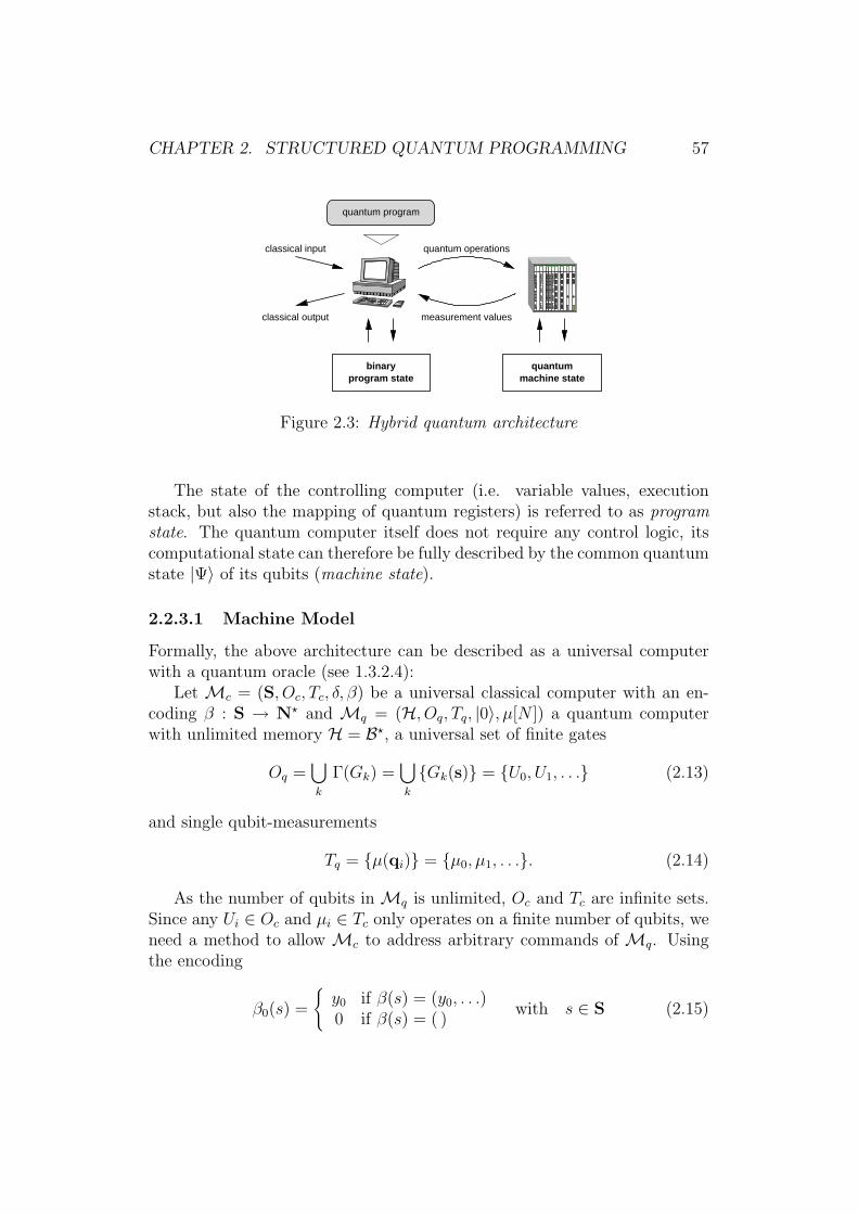
CHAPTER 2. STRUCTURED QUANTUM PROGRAMMING 57
program statequantum
machine state
measurement values
quantum operations
binary
classical input
classical output
quantum program
����
����
����������������������������
����������������
Figure 2.3: Hybrid quantum architecture
The state of the controlling computer (i.e. variable values, executionstack, but also the mapping of quantum registers) is referred to as programstate. The quantum computer itself does not require any control logic, itscomputational state can therefore be fully described by the common quantumstate |Ψ〉 of its qubits (machine state).
2.2.3.1 Machine Model
Formally, the above architecture can be described as a universal computerwith a quantum oracle (see 1.3.2.4):
Let Mc = (S, Oc, Tc, δ, β) be a universal classical computer with an en-coding β : S → N? and Mq = (H, Oq, Tq, |0〉, µ[N ]) a quantum computerwith unlimited memory H = B?, a universal set of finite gates
Oq =⋃
k
Γ(Gk) =⋃
k
{Gk(s)} = {U0, U1, . . .} (2.13)
and single qubit-measurements
Tq = {µ(qi)} = {µ0, µ1, . . .}. (2.14)
As the number of qubits in Mq is unlimited, Oc and Tc are infinite sets.Since any Ui ∈ Oc and µi ∈ Tc only operates on a finite number of qubits, weneed a method to allow Mc to address arbitrary commands of Mq. Usingthe encoding
β0(s) =
{y0 if β(s) = (y0, . . .)0 if β(s) = ( )
with s ∈ S (2.15)
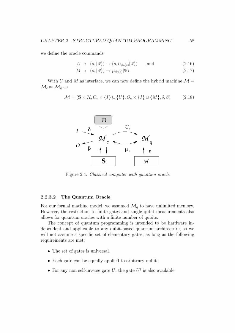
CHAPTER 2. STRUCTURED QUANTUM PROGRAMMING 58
we define the oracle commands
U : (s, |Ψ〉)→ (s, Uβ0(s)|Ψ〉) and (2.16)
M : (s, |Ψ〉)→ µβ0(s)|Ψ〉 (2.17)
With U and M as interface, we can now define the hybrid machineM =Mc ./Mq as
M = (S×H, Oc × {I} ∪ {U}, Oc × {I} ∪ {M}, δ, β) (2.18)
M M
µO
δ
β
IU
i
i
c q
S H
π
Figure 2.4: Classical computer with quantum oracle
2.2.3.2 The Quantum Oracle
For our formal machine model, we assumed Mq to have unlimited memory.However, the restriction to finite gates and single qubit measurements alsoallows for quantum oracles with a finite number of qubits.
The concept of quantum programming is intended to be hardware in-dependent and applicable to any qubit-based quantum architecture, so wewill not assume a specific set of elementary gates, as long as the followingrequirements are met:
• The set of gates is universal.
• Each gate can be equally applied to arbitrary qubits.
• For any non self-inverse gate U , the gate U † is also available.
CHAPTER 2. STRUCTURED QUANTUM PROGRAMMING 59
Elementary gates may take any number of classical parameters and mayor may not be restricted in the number of qubits they operate on.
Some concepts of structured quantum programming will require certainoperators to be available either as elementary gates or as user-defined op-erators i.e. procedural compositions of gates which can be defined in theprogramming language itself. Those operators are
• a Fanout operation i.e. an arbitrary unitary operator which matchesthe condition
Fanout : |n〉x|0〉y → |n〉x|n〉y where |x| = |y| (2.19)
Fanout is usually implemented as |a, b〉 → |a, a⊕ b〉 using CNot-gatesand is required for the transparent use of local scratch registers (see2.5.3.5).
• the Not- (or X-) gate and the controlled-not gate Cn[X] with an arbi-trary number of control qubits. The implementation of Cn[X] may usescratch qubits. X and Cn[X] are required for quantum conditions (see2.6.3) and the quantum if-statement (see 2.6.2.1).
2.3 Structured Programming
Since the computational model of QPLs is that of a classical computer with aquantum oracle, any QPL is also a universal classical programming language.In this section, we will summarize the key elements of classical structuredprogramming languages.
2.3.1 Program Structure
A structured program is a sequence (block) of statements and definitions,which are processed top-down and may contain blocks themselves (control-statements, subroutine-definitions).
2.3.1.1 Statements
Statements range from simple commands, through subroutine calls to nestedcontrol-statements and are executed when they are encountered.
qcl> if random()>=0.5 { print "red"; } else { print "black"; }: red

CHAPTER 2. STRUCTURED QUANTUM PROGRAMMING 60
2.3.1.2 Definitions
Definitions are not executed but bind a value (variable- or constant-definition)or a block of code (subroutine-definition) to a symbol (identifier).
qcl> int counter=5;qcl> int fac(int n) { if n<=0 {return 1;} else {return n*fac(n-1);} }
Each symbol has an associated type, which can either be a data type or asubroutine type.
2.3.1.3 Expressions
Statements and subroutine-calls can take arguments of certain data types.Expressions can be composed of literals, variables and constants combinedby operators and function calls.
qcl> print "5 out of 10:",fac(10)/fac(5)^2,"combinations.": 5 out of 10: 252 combinations.
2.3.2 Expressions and Variables
Unlike untyped formalisms like finite programs or circuits, in programminglanguages, an expression is usually associated with a data type T . A valuev ∈ T is called an instance of T .
2.3.2.1 Atomic Expressions
The direct symbolic representation of an instance v ∈ T is called a literal.
Type Description Examplesint integer 1234, -1
real real number 3.14, -0.001
complex complex number (0,-1), (0.5, 0.866)
Table 2.3: Scalar arithmetic types and literals in QCL
A symbol which is permanently bound to a value v ∈ T is called a (sym-bolic) constant of type T . A symbol which can be bound to arbitrary in-stances of T is called a variable of type T .
CHAPTER 2. STRUCTURED QUANTUM PROGRAMMING 61
2.3.2.2 Definitions
Constants and variables have to be defined (i.e. declared and initialized)before they can be used. To assure deterministic behaviour (see 2.5.1.2) werequire that a variable is bound to a type dependent default value if no initialvalue is provided.
qcl> const pi = 3.141592653589793238462643383279502884197;qcl> const I = (0,1);qcl> complex z=exp(I*pi/4);qcl> string msg="Hello World";qcl> real vector v[3]; // v is initialized with [0,0,0]
After its definition, a constant or variable is visible and can be used in anysubsequent statements and definitions until the end of the current subroutine(local symbol) or the end of the program (global symbol).7
2.3.2.3 Composite Expressions
Literals, constants and variables are atomic expressions. General expressionscan be recursively constructed from atomic expression by operators and func-tion calls.
expr ← atomic-expression
← function ( expr , . . .)
← unary-operator expr
← expr binary-operator expr
← n-ary-operator ( expr , . . .)
So general expressions can be described as trees with literals, constantsand variables as leaf-nodes and operators and functions as inner nodes.
qcl> print (3^2+4^2)*sin(log(z)/I);: 17.6777
2.3.3 Subroutines
A subroutine S is a named block (also referred to as body of S) preceded bya list of parameter-declarations. The body of a subroutine may contain callsto itself (recursion).
Classical procedural languages usually provide two types of subroutines:
7There also exist languages with finer grained scoping rules, e.g. C++, where variablescan be local to a block.
CHAPTER 2. STRUCTURED QUANTUM PROGRAMMING 62
2.3.3.1 Procedures
A procedure is a general subroutine with arbitrary dependencies and side-effects on the program state. This means that besides its declared arguments,a procedure can also depend on hidden parameters, external input and ran-dom events. Moreover, procedures can also change the binding of globalvariables.
int cash;procedure roulette(int bet) {int n;input "pick a number:",n;cash=cash-bet;if n==floor(37*random()) { cash=cash+36*bet; };
}
In procedural quantum programming, procedures, being the most gen-eral subroutine type (see 2.5), are used to implement the classical controlstructure of quantum algorithms (see 2.2.1.2).
2.3.3.2 Functions
A function is a subroutine which returns a value v ∈ T of a certain data-typeT .
In procedural quantum programming, functions have strict mathematicalsemantics, which means that v must exclusively and deterministically dependon the declared arguments and that the computation of v must not exhibitany side-effects on the program state.8 This implies that neither global vari-ables nor calls of less restricted subroutine types may appear within the bodyof a function.
int fibonacci(int n) {if n<2 {
return 1;} else {
return fibonacci(n-1)+fibonacci(n-2);}
}
2.3.4 Statements
2.3.4.1 Assignment
An assignment binds a variable (or an element of a data structure such asan array) of type T to a value specified by an expression of the same type.
8Many classical procedural languages (e.g. C) are less strict and treat functions asprocedures with a return value.
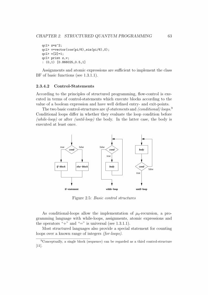
CHAPTER 2. STRUCTURED QUANTUM PROGRAMMING 63
qcl> z=z^2;qcl> v=vector(cos(pi/6),sin(pi/6),0);qcl> v[2]=1;qcl> print z,v;: (0,1) [0.866025,0.5,1]
Assignments and atomic expressions are sufficient to implement the classBF of basic functions (see 1.3.1.1).
2.3.4.2 Control-Statements
According to the principles of structured programming, flow-control is exe-cuted in terms of control-statements which execute blocks according to thevalue of a boolean expression and have well defined entry- and exit-points.
The two basic control-structures are if-statements and (conditional) loops.9
Conditional loops differ in whether they evaluate the loop condition before(while-loop) or after (until-loop) the body. In the latter case, the body isexecuted at least once.
true
true
false
falsetrue false
if−statement while−loop until−loop
bodycondcond
if−block else−block body cond
Figure 2.5: Basic control structures
As conditional-loops allow the implementation of µ0-recursion, a pro-gramming language with while-loops, assignments, atomic expressions andthe operators “+” and “=” is universal (see 1.3.1.1).
Most structured languages also provide a special statement for countingloops over a known range of integers (for-loops).
9Conceptually, a single block (sequence) can be regarded as a third control-structure[11].

CHAPTER 2. STRUCTURED QUANTUM PROGRAMMING 64
qcl> for i=a to b { body(i); }; // for-loop and equivalentqcl> i=a; while i<=b { body(i); i=i+1; } // while-loop
As counting loops allow the implementation of primitive recursion, a pro-gramming language with for-loops, assignments, atomic expressions and ad-dition is sufficient to implement the class PR of primitive recursive functions(see 1.3.1.1).
Break Statements A break-statement allows the innermost loop to beimmediately exited, regardless of the loop condition. While the possibility toexit a loop from any point within the body can be considered to be againstthe spirit of structured programming as it compromises the concept of welldefined exit points, most structured languages do provide a break-statement(as does QCL).
2.3.4.3 Calls
A call of a procedure S binds a list of arguments to the parameters of Sand executes the body of S. The parameter bindings as well as any symboldefinitions within S are local.
2.3.4.4 Input and Output
Any programming language has to provide means to communicate with theoutside world. This can be realized by designated input- and output-variablesat the start and termination of the program or at runtime via I/O-commands.
qcl> input "length in cm:",x;? length in cm: 192qcl> print x,"cm =",x/2.54,"inches";: 192 cm = 75.5906 inches
2.4 Elementary Quantum Operations
As introduced in 2.2.3, the computational model of quantum programming isa universal computer with a quantum oracle. Formally, the interface betweenthe classical front-end and the quantum backend can be described by oraclecommands which allow elementary gates to be applied to and measurementsto be performed on arbitrary target qubits.
In this section, we will show how this interface can be represented withinthe scope of an imperative (see 2.1.3.1) programming language (imperativequantum programming).10
10Even if the classical language provides subroutines and structured flow-control, the
CHAPTER 2. STRUCTURED QUANTUM PROGRAMMING 65
2.4.1 Quantum Registers
In 1.4.1.3, we defined a quantum register s as an arbitrary sub-system witha finite dimensional state space Hs and a well-defined computational basisBs. We will also make the following assumptions about the quantum oracleMq (see 2.2.3.2):
• The state spaceH ofMq is a composition of identical qubit subsystems,i.e. H = B⊗n or H = B?.• Elementary gates and measurements operate on a finite number of
qubits.11
• All operations ofMq can be equally applied to arbitrary qubits.
• The qubits ofMq are numbered in ascending order starting with zero.
The restriction to qubits implies that any register s is either a single qubit(s = qi), a composition of single qubit registers (s = qk0 ◦ qk1 ◦ . . . ◦ qkn−1)or the null-register (s = o). An n-qubit quantum computer thus allows for
n∑
k=0
n!
(n− k)! = n!n∑
k=0
1
k!= ben!c (2.20)
different registers.
Notation We write Rnk to denote the set of k-qubit registers for an n-qubit
quantum computer. As Rnk is equivalent to the set of possible k-permutations
of n elements,
|Rkn| = P n
k =n!
(n− k)! . (2.21)
Further, we define
Rk =⋃∞n=1R
nk (set of k-qubit registers) (2.22)
Rn =⋃nk=0R
nk (set of registers over n qubits) (2.23)
R =⋃∞n=1R
n (set of general registers) (2.24)
resulting QPL would still be regarded as imperative as it lacks semantic support for op-erators and quantum if-statements.
11For convenience, QCL also supports a (global) reset-command (see 1.4.3.3).
CHAPTER 2. STRUCTURED QUANTUM PROGRAMMING 66
2.4.1.1 Language Representation of Registers
Within a structured QPL, quantum registers are instances of a quantumdata type (see 2.4.1.3) Q.12 Semantically, an n-qubit register s ∈ Q is a finitesequence of mutually different qubit positions s = (s0, s1 . . . sn−1), so s doesnot denote the physical register itself, but serves as a pointer (logical register)to the actual n-qubit sub-system qs0 ◦ . . . ◦ qsn−1 ofMq (physical register).
This distinction allows registers to be treated just like any other classicaldata type, so register variables can be declared, printed and combined toexpressions, just like classical variables.13
qcl> qureg q[1]; // allocate single qubit registerqcl> qureg p[4]; // allocate 4-qubit registerqcl> qureg qp = q & p; // declare combined register qpqcl> print q,p,qp; // print register mappings: <0> <1,2,3,4> <0,1,2,3,4>qcl> print p[0..2] & q; // registers can be combined to expressions: <1,2,3,0>
Registers are the formal interface between the classical front-end and thequantum oracle. All operations on the machine state take quantum registersas operands14 and are restricted to their corresponding sub-spaces.
qcl> H(q); // apply Hadamard gate to register q[5/32] 0.70711 |0,0> + 0.70711 |1,0>qcl> Not(p); // invert qubits in register p[5/32] 0.70711 |0,15> + 0.70711 |1,15>qcl> measure q; // measure register q[5/32] 1 |1,15>
2.4.1.2 The Quantum Heap
The mapping between logical registers and physical qubits is handled trans-parently by allocation and deallocation of registers from the set of all availablequbits, also referred to as the quantum heap [46].15 Quantum registers areexplicitely allocated, when a register variable is defined, but also implicitly
12Since quantum data types are only used to restrict the possible operations on registers,mathematically, any quantum data type Q denotes the same set of qubit permutations,i.e. Q = R.
13To allow for the static allocation of qubits, QCL does not allow register assignments,so in QCL, registers variables are treated as symbolic constants.
14Depending on our point of view, registers can be thought of being passed by value(logical registers) or reference (physical registers).
15In classical programming, the section of memory reserved for dynamic variables iscalled the heap.
CHAPTER 2. STRUCTURED QUANTUM PROGRAMMING 67
for scratch space management (see 2.5.3.5) and for the evaluation of quantumconditions (see 2.6.3).
Just as classical variables are initialized with type-dependent default val-ues, newly allocated registers and consequently all free (i.e. unallocated)quantum memory has to be empty.
Definition 30 (Empty Registers) A quantum register e is empty iff themachine state |Ψ〉 is of the form |Ψ〉 = |0〉e|ψ〉e or, equivalently, ρe = |0〉〈0|.
Also, temporary registers must be emptied before deallocation, which, inthe case of local register variables, takes place when the symbol leaves scope.This can be achieved either by measurement or by uncomputing (see 2.5.3.5).
At startup, the whole machine state is empty, thus |Ψ〉 = |0〉.qcl> dump;: STATE: 0 / 32 qubits allocated, 32 / 32 qubits free1 |0>
The concept of the quantum heap allows for two important abstractions:
• Since the allocation of registers is transparent, no qubit positions needto be specified and no register literals need to be defined. This alsoleaves room for architecture-dependent optimizations.
• Since allocated and unallocated qubits are in a product state, the def-inition of quantum algorithms is independent of the total number ofqubits.
2.4.1.3 Quantum Data Types
Different quantum data-types can be used to restrict the way unitary oper-ators may affect quantum registers. This is not only done to prevent pro-gramming errors and to make the code more readable, but also to provideinformation to the compiler or interpreter to allow for more efficient opti-mizations and to designate the argument-, target- and scratch-registers ofquantum functions (see 2.5.3.3), to allow for transparent scratch space man-agement.
General Registers impose no restrictions and can be used as argumentsto arbitrary operators.
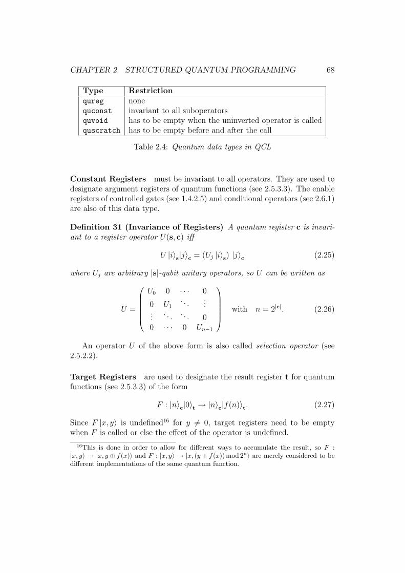
CHAPTER 2. STRUCTURED QUANTUM PROGRAMMING 68
Type Restrictionqureg nonequconst invariant to all suboperatorsquvoid has to be empty when the uninverted operator is calledquscratch has to be empty before and after the call
Table 2.4: Quantum data types in QCL
Constant Registers must be invariant to all operators. They are used todesignate argument registers of quantum functions (see 2.5.3.3). The enableregisters of controlled gates (see 1.4.2.5) and conditional operators (see 2.6.1)are also of this data type.
Definition 31 (Invariance of Registers) A quantum register c is invari-ant to a register operator U(s, c) iff
U |i〉s|j〉c = (Uj |i〉s) |j〉c (2.25)
where Uj are arbitrary |s|-qubit unitary operators, so U can be written as
U =
U0 0 · · · 0
0 U1. . .
......
. . . . . . 00 · · · 0 Un−1
with n = 2|c|. (2.26)
An operator U of the above form is also called selection operator (see2.5.2.2).
Target Registers are used to designate the result register t for quantumfunctions (see 2.5.3.3) of the form
F : |n〉c|0〉t → |n〉c|f(n)〉t. (2.27)
Since F |x, y〉 is undefined16 for y 6= 0, target registers need to be emptywhen F is called or else the effect of the operator is undefined.
16This is done in order to allow for different ways to accumulate the result, so F :|x, y〉 → |x, y ⊕ f(x)〉 and F : |x, y〉 → |x, (y + f(x))mod 2n〉 are merely considered to bedifferent implementations of the same quantum function.

CHAPTER 2. STRUCTURED QUANTUM PROGRAMMING 69
Scratch Registers are temporary registers which can be used within theimplementation of an operator but are required to be empty before and afterthe call.17
2.4.1.4 Register Expressions
On an n-qubit quantum computer, a single k-qubit gate U can be used toimplement up to n!
(n−k)! different unitary transformation U(s) by applying Uto different registers. In order to realize all possible qubit permutations, aQPL has to provide means to extract subregisters and to combine disjointregisters.
Definition 32 A register a = (a0 . . . an−1) ∈ Rn is a subregister a ⊆ b ofb = (b0 . . . bm−1) ∈ Rm iff
n−1∧
i=0
m−1∨
j=0
ai = bj. (2.28)
Definition 33 Two registers a = (a0 . . . an−1) ∈ Rn and b = (b0 . . . bm−1) ∈Rm are disjoint iff
n−1∧
i=0
m−1∧
j=0
ai 6= bj. (2.29)
Table 2.5 shows the available operators in QCL to manipulate quantumregisters.
Expr. Description Registera reference 〈a0, a1 . . . an〉
a[i] qubit 〈ai〉a[i..j] sub-register 〈ai, ai+1 . . . aj〉a[i::l] sub-register 〈ai, ai+1 . . . ai+l−1〉a & b concatenation 〈a0, a1 . . . an, b0, b1 . . . bm〉
Table 2.5: Register expressions in QCL
2.4.2 Elementary Gates
Just as assignments (see 2.3.4.1) represent atomic changes of the programstate, elementary gates are the fundamental primitives to manipulate thequantum machine state.
17In QCL, the type quscratch, when used for a local register, denotes managed scratchregisters (see 2.5.3.5) which are uncomputed automatically, while a local qureg is anunmanaged scratch (see 2.5.2.4) register which has to be emptied by the operator itself.
CHAPTER 2. STRUCTURED QUANTUM PROGRAMMING 70
2.4.2.1 Register Operators
A k-qubit (elementary) gate (see 1.4.2.4) is an atomic unitary transformationU which can be applied to arbitrary k-qubit registers s ∈ Rk of the quantumoracle (see 2.2.3.2). The resulting transformation of the machine state isformally described by the register operator (see 1.4.1.3)
U(s) = U ⊗ Is =∑
i,j,k
uij |i〉s|k〉s〈j|s〈k|s with uij = 〈i|U |j〉. (2.30)
In the circuit model, a register operator describes a gate which is wiredto operate on certain qubits. In (2.30), the “wiring” is hidden in the ba-sis decomposition | . . .〉s ⊗ | . . .〉s, however it can be made explicit, by theintroduction of a register-dependent reordering operator.
Definition 34 (Reordering Operator) Let H = B⊗n (or H = B?) ands = (s0 . . . sk−1) ∈ Rn
k (or Rk) be a k-qubit register of H. A qubit permutation
Πs |d0, d1 . . . dn−1〉 = |dπ0 , dπ1 . . . dπn−1〉 (2.31)
on H with π being a bijective function on Zn (or N) and πi = si for i < k iscalled reordering operator for s.
The definition of Πs is not unique; for H = B⊗n, there exist (n − k)!different Π(i)
s and infinitely many for H = B?.Functionally, the reordering operator can be compared to the shift- and
swap-operations used to address arbitrary tape-qubits on the SQTM (see2.2.2.2).
Definition 35 (Register Operator) The register operator U(s) for a k-qubit operator U and a k-qubit quantum register s ∈ Rn
k of H = B⊗n (ors ∈ Rk of H = B?) is defined as
U(s) = Π†s (U ⊗ I) Πs on H. (2.32)
Fig. 2.6 shows a quantum circuit for U(s) on a 5-qubit machine with Ubeing a 3-qubit gate and s = (0, 2, 3).
2.4.2.2 Language Representation of Gates
Since quantum programming is supposed to be a hardware independent for-malism, besides the three basic requirements named in 2.2.3.2 (universality,functional equivalence of qubits, availability of adjoint gates), no assump-tions can be made on the operators provided by the quantum oracle andthere is no specific set of elementary gates.
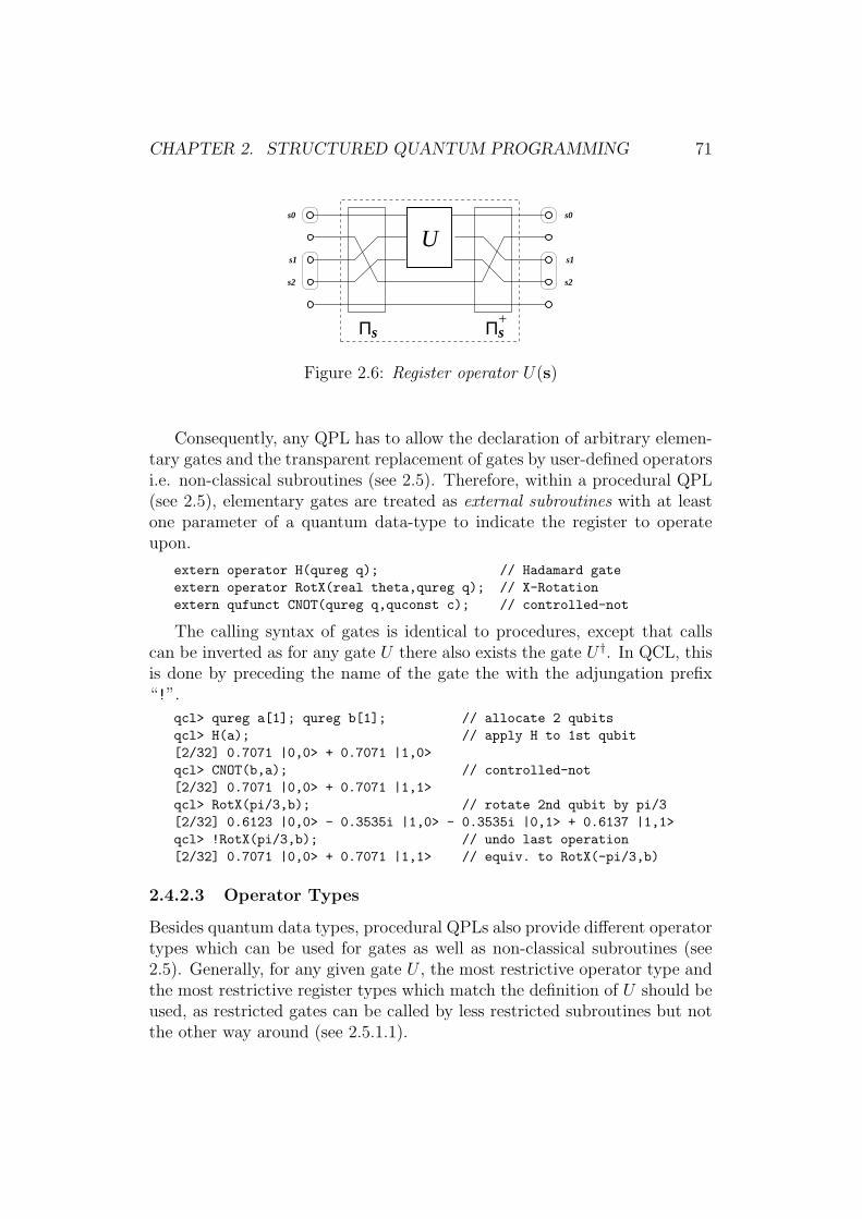
CHAPTER 2. STRUCTURED QUANTUM PROGRAMMING 71
s0
s1
s2
s0
s1
s2
Π Πs s+
U
Figure 2.6: Register operator U(s)
Consequently, any QPL has to allow the declaration of arbitrary elemen-tary gates and the transparent replacement of gates by user-defined operatorsi.e. non-classical subroutines (see 2.5). Therefore, within a procedural QPL(see 2.5), elementary gates are treated as external subroutines with at leastone parameter of a quantum data-type to indicate the register to operateupon.
extern operator H(qureg q); // Hadamard gateextern operator RotX(real theta,qureg q); // X-Rotationextern qufunct CNOT(qureg q,quconst c); // controlled-not
The calling syntax of gates is identical to procedures, except that callscan be inverted as for any gate U there also exists the gate U †. In QCL, thisis done by preceding the name of the gate the with the adjungation prefix“!”.
qcl> qureg a[1]; qureg b[1]; // allocate 2 qubitsqcl> H(a); // apply H to 1st qubit[2/32] 0.7071 |0,0> + 0.7071 |1,0>qcl> CNOT(b,a); // controlled-not[2/32] 0.7071 |0,0> + 0.7071 |1,1>qcl> RotX(pi/3,b); // rotate 2nd qubit by pi/3[2/32] 0.6123 |0,0> - 0.3535i |1,0> - 0.3535i |0,1> + 0.6137 |1,1>qcl> !RotX(pi/3,b); // undo last operation[2/32] 0.7071 |0,0> + 0.7071 |1,1> // equiv. to RotX(-pi/3,b)
2.4.2.3 Operator Types
Besides quantum data types, procedural QPLs also provide different operatortypes which can be used for gates as well as non-classical subroutines (see2.5). Generally, for any given gate U , the most restrictive operator type andthe most restrictive register types which match the definition of U should beused, as restricted gates can be called by less restricted subroutines but notthe other way around (see 2.5.1.1).
CHAPTER 2. STRUCTURED QUANTUM PROGRAMMING 72
General Operators allow arbitrary unitary transformations on the argu-ment registers.
extern operator RotX(real theta,qureg q); // X-Rotation
Basis Permutations are operators of the form F : |n〉 → |f(n)〉 with fbeing a bijective boolean function.
extern qufunct CNOT(qureg q,quconst c); // controlled-not
Conditional Operators are a generalization of controlled gates (see 1.4.2.5)for enable registers of arbitrary size (including the null-register i.e. the un-controlled operator).
Definition 36 Let s, e ∈ R be disjoint registers and U(s) be a register oper-ator, then the operator
U[[e]](s) : |k〉s|c〉e →{
(U |k〉s)|c〉e if c = 111 . . .|k〉s|c〉e otherwise
(2.33)
is called conditional operator with the enable (or control) register e
General operators as well as basis permutations can be declared condi-tional.
extern cond operator Phase(real phi); // conditional phase gateextern cond qufunct Not(qureg q); // conditional not gate
The enable register is passed as an implicit parameter if the operator isused within the body of a quantum if-statement (see 2.6.2.1), so operatorswithout an explicit argument register can be useful (conditional phase gates).
qcl> qureg s[1]; qureg e[2]; // allocate 2 registersqcl> H(e); // create test state in e[3/32] 0.5 |0,0> + 0.5 |0,1> + 0.5 |0,2> + 0.5 |0,3>qcl> if e[0] { Phase(pi); } // flip sign if LSB of e is set[3/32] 0.5 |0,0> - 0.5 |0,1> + 0.5 |0,2> - 0.5 |0,3>qcl> if e { Not(s); } // invert target qubit s for e=11[3/32] 0.5 |0,0> - 0.5 |0,1> + 0.5 |0,2> - 0.5 |1,3>
CHAPTER 2. STRUCTURED QUANTUM PROGRAMMING 73
2.4.3 Measurements
2.4.3.1 Register Observable
In quantum mechanics, classical physical quantities (observables) are de-scribed by Hermitian operators (see 1.2.3.3). In quantum programming, werestrict measurements to the computational basis B = {|n〉}, expressed bythe standard observable N =
∑n n|n〉〈n|. Using the register basis Bs = {|k〉s}
the register observable N(s) can be defined as (see 1.4.1.3)
N(s) = Ns ⊗ Is =∑
i,j
i |i〉s|j〉s〈i|s〈j|s. (2.34)
Again, we can avoid the use of the register basis Bs by defining N(s) bymeans of a reordering operator Πs (see 2.4.2.1).
Definition 37 (Register Observable) The register observable N(s) for ak-qubit quantum register s ∈ Rn
k on H = B⊗n (or s ∈ Rk on H = B?) isdefined as
N(s) = Π†s (N ⊗ I) Πs with N =
2k−1∑
i=0
i|i〉〈i|. (2.35)
Further, we assume the basis-vectors are labeled as little-endian binarynumbers (i.e. LSB first), so for two disjoint registers a ∈ Rn and b ∈ Rm
N(a ◦ b) = N(a) + 2nN(b). (2.36)
2.4.3.2 Language Representation of Measurements
Since QPLs are intended to control a classical computer which serves asa front-end between the user and the quantum oracle (see 2.2.3), quantummeasurements are treated analogously to external classical input (see 2.3.4.4)and are implemented as a quantum input command with the side effect thatthe machine state gets reduced (see 1.2.3.3).
qcl> qureg q[8]; // allocate an 8-qubit register qqcl> int m; // declare a classical input variableqcl> H(q); // prepare an even superposition in q[8/32] 0.0625 |0> + ... + 0.0625 |255> (256 terms)qcl> measure q[0..5],m; // measure the first 6 qubits of q[8/32] 0.5 |50> + 0.5 |114> + 0.5 |178> + 0.5 |242>qcl> print m; // print measurement result: 50
CHAPTER 2. STRUCTURED QUANTUM PROGRAMMING 74
2.4.3.3 Initialization
Since many quantum algorithms are probabilistic (see 2.2.1.2) and involveiterating over the same computation until a solution is found, it is convenientto provide a command to reset the machine state |Ψ〉 to the initial state |0〉and empty all allocated registers, while not affecting the program state, sothat variable bindings and register mappings remain valid.
[8/32] 0.5 |50> + 0.5 |114> + 0.5 |178> + 0.5 |242>qcl> reset; // reset quantum state as generated above[8/32] 1 |0>qcl> print q,m; // variables q and m are not affected: <0,1,2,3,4,5,6,7> 50
Since the initialization of |Ψ〉 can be implemented by measuring all allo-cated registers and inverting qubits qi found in state ρqi
= |1〉〈1| to zero byapplying the not-gate X(qi), it is not necessary for the quantum oracle toprovide a generic reset-command (see 1.4.3.3).
procedure resetregister(qureg q) {int i;int m;for i=0 to #q-1 { // iterate over qubits
measure q[i],m; // measure i-th qubitif m==1 { Not(q[i]); } // invert if measured 1
}}
2.5 Operators
While registers, elementary gates and measurements are already sufficient toimplement arbitrary quantum algorithms, a programming language restrictedto those concepts would not be much different from a classical language witha quantum device driver as it would lack a semantic representation for unitaryoperators, which are the essence of all quantum algorithms.
In this section, we will demonstrate how unitary operators can be inte-grated into the framework of a procedural programming language (proceduralquantum programming).
2.5.1 Quantum Subroutines
Procedural programming languages provide arbitrary levels of abstraction byallowing to group simple computational tasks into parameterized subroutineswhich can be used recursively as primitives for the definition of more complexsubroutines.
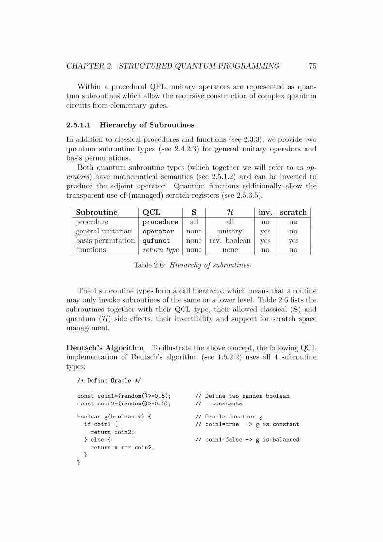
CHAPTER 2. STRUCTURED QUANTUM PROGRAMMING 75
Within a procedural QPL, unitary operators are represented as quan-tum subroutines which allow the recursive construction of complex quantumcircuits from elementary gates.
2.5.1.1 Hierarchy of Subroutines
In addition to classical procedures and functions (see 2.3.3), we provide twoquantum subroutine types (see 2.4.2.3) for general unitary operators andbasis permutations.
Both quantum subroutine types (which together we will refer to as op-erators) have mathematical semantics (see 2.5.1.2) and can be inverted toproduce the adjoint operator. Quantum functions additionally allow thetransparent use of (managed) scratch registers (see 2.5.3.5).
Subroutine QCL S H inv. scratchprocedure procedure all all no nogeneral unitarian operator none unitary yes nobasis permutation qufunct none rev. boolean yes yesfunctions return type none none no no
Table 2.6: Hierarchy of subroutines
The 4 subroutine types form a call hierarchy, which means that a routinemay only invoke subroutines of the same or a lower level. Table 2.6 lists thesubroutines together with their QCL type, their allowed classical (S) andquantum (H) side effects, their invertibility and support for scratch spacemanagement.
Deutsch’s Algorithm To illustrate the above concept, the following QCLimplementation of Deutsch’s algorithm (see 1.5.2.2) uses all 4 subroutinetypes:
/* Define Oracle */
const coin1=(random()>=0.5); // Define two random booleanconst coin2=(random()>=0.5); // constants
boolean g(boolean x) { // Oracle function gif coin1 { // coin1=true -> g is constant
return coin2;} else { // coin1=false -> g is balanced
return x xor coin2;}
}
CHAPTER 2. STRUCTURED QUANTUM PROGRAMMING 76
qufunct G(quconst x,quvoid y) { // Construct oracle op. G from gif g(false) xor g(true) { CNot(y,x); }if g(false) { Not(y); }
}
/* Deutsch’s Algorithm */
operator U(qureg x,qureg y) { // Bundle all unitary operationsH(x); // of the algorithm into oneG(x,y); // operator UH(x & y);
}
procedure deutsch() { // Classical control structurequreg x[1]; // allocate 2 qubitsqureg y[1];int m;{ // evaluation loop
reset; // initialize machine stateU(x,y); // do unitary computationmeasure y,m; // measure 2nd register
} until m==1; // value in 1st register valid?measure x,m; // measure 1st register whichprint "g(0) xor g(1) =",m; // contains g(0) xor g(1)reset; // clean up
}
2.5.1.2 Mathematical Semantics
In classical routines, subroutines are executed when they are called (lin-ear execution) i.e. when control reaches the corresponding call-statement(see 2.3.4.3). Operators, however, support non-classical concepts like invert-ibility (see 2.5.2.3), scratch space management (see 2.5.3.5) and quantumif-statements (see 2.6.2.1) with the result that neither the number nor theexecution order of suboperators necessarily corresponds to the classical flowof control (non-linear execution).
Therefore operators have mathematical semantics i.e. their effect is com-pletely described by the unitary transformation they implement as a func-tion of their declared parameters; so they must be reproduceable and neitherdepend on nor exhibit side-effects on the program state. This specificallyexcludes
• the use of global variables
• user input and classical random numbers
• measurements and resetting of the machine state
• calls of procedures

CHAPTER 2. STRUCTURED QUANTUM PROGRAMMING 77
2.5.1.3 Language Representation of Operators
Formally, just like a classical procedure, an operator is a named block (see2.3.1) with a list of symbolic parameters of classical or quantum types. Thelatter are used to indicate the registers the operator is applied to.
The QCL operator below implements the basis permutation
xregb(a) : |x〉a → |x⊕ b〉a (2.37)
qufunct xreg(qureg a,int b) { // xor reg. a with binary number bint i;for i=0 to #a-1 { // iterate over qubits of a
if bit(b,i) { Not(a[i]); } // invert i-th qubit of a if} // i-th bit of b is set
}
The calling syntax of operators is identical to gates, including the abilityto call the adjoint operator. Since operators have mathematical semantics,an operator is completely equivalent to an elementary gate with the samedeclaration and functionality. So it makes e.g. no difference whether theZ-gate (see 1.4.2.4) is provided by the quantum oracle
extern operator Z(qureg q); // pi-rotation about the Z-axis
or implemented as the sequence Z = HXH by the operator
operator Z(qureg q) { H(q); Not(q); H(q); }
2.5.1.4 Polymorphism
On an n-qubit quantum computer, an k-qubit gate can implement up ton!
(n−k)! unitary transformations U(s) with s ∈ Rnk . In procedural quantum
programming, this polymorphism is further extended by additional abstrac-tions:
• Register Size: Argument registers can be of different sizes, so forevery quantum parameter s, the register size |s| is passed as an implicitclassical parameter. In QCL, the size of a register is given by the size-operator “#”, so #s = |s|. An operator with a single argument registers ∈ Rn can implement up to ben!c different unitary transformations.
• Multiple Registers: Operators can take multiple argument regis-ters. Since for any s ∈ Rk, there exist
(k+q−1q−1
)possible decompositions
s = s1 ◦ . . . ◦ sq (including null-registers), an operator with p registerarguments si with the total size k =
∑qi=1 |si| can implement up to(
k+q−1q−1
)different unitary gates.
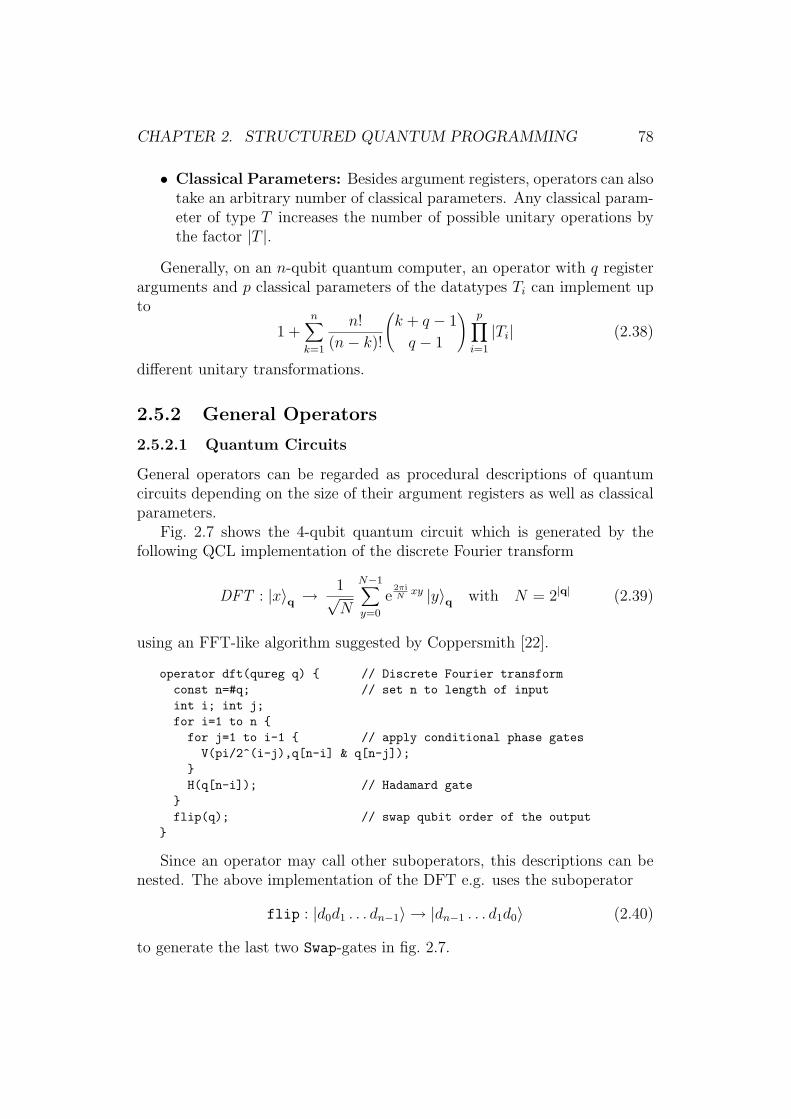
CHAPTER 2. STRUCTURED QUANTUM PROGRAMMING 78
• Classical Parameters: Besides argument registers, operators can alsotake an arbitrary number of classical parameters. Any classical param-eter of type T increases the number of possible unitary operations bythe factor |T |.
Generally, on an n-qubit quantum computer, an operator with q registerarguments and p classical parameters of the datatypes Ti can implement upto
1 +n∑
k=1
n!
(n− k)!
(k + q − 1
q − 1
) p∏
i=1
|Ti| (2.38)
different unitary transformations.
2.5.2 General Operators
2.5.2.1 Quantum Circuits
General operators can be regarded as procedural descriptions of quantumcircuits depending on the size of their argument registers as well as classicalparameters.
Fig. 2.7 shows the 4-qubit quantum circuit which is generated by thefollowing QCL implementation of the discrete Fourier transform
DFT : |x〉q →1√N
N−1∑
y=0
e2πiNxy |y〉q with N = 2|q| (2.39)
using an FFT-like algorithm suggested by Coppersmith [22].
operator dft(qureg q) { // Discrete Fourier transformconst n=#q; // set n to length of inputint i; int j;for i=1 to n {
for j=1 to i-1 { // apply conditional phase gatesV(pi/2^(i-j),q[n-i] & q[n-j]);
}H(q[n-i]); // Hadamard gate
}flip(q); // swap qubit order of the output
}
Since an operator may call other suboperators, this descriptions can benested. The above implementation of the DFT e.g. uses the suboperator
flip : |d0d1 . . . dn−1〉 → |dn−1 . . . d1d0〉 (2.40)
to generate the last two Swap-gates in fig. 2.7.
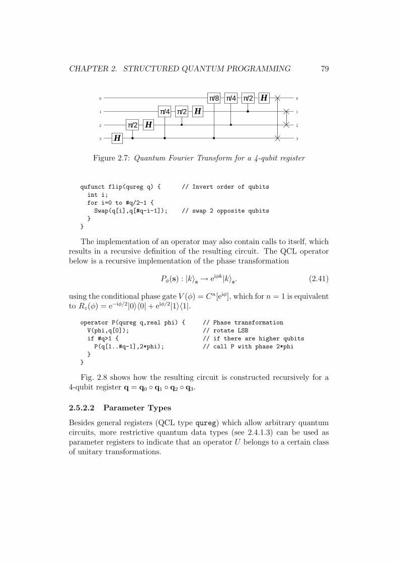
CHAPTER 2. STRUCTURED QUANTUM PROGRAMMING 79
0
1
2
3
0
1
2
3H
Hπ/2
π/4 H
π/8 π/4 π/2 H
π/2
Figure 2.7: Quantum Fourier Transform for a 4-qubit register
qufunct flip(qureg q) { // Invert order of qubitsint i;for i=0 to #q/2-1 {
Swap(q[i],q[#q-i-1]); // swap 2 opposite qubits}
}
The implementation of an operator may also contain calls to itself, whichresults in a recursive definition of the resulting circuit. The QCL operatorbelow is a recursive implementation of the phase transformation
Pφ(s) : |k〉s → eiφk|k〉s. (2.41)
using the conditional phase gate V (φ) = Cn[eiφ], which for n = 1 is equivalentto Rz(φ) = e−iφ/2|0〉〈0|+ eiφ/2|1〉〈1|.
operator P(qureg q,real phi) { // Phase transformationV(phi,q[0]); // rotate LSBif #q>1 { // if there are higher qubits
P(q[1..#q-1],2*phi); // call P with phase 2*phi}
}
Fig. 2.8 shows how the resulting circuit is constructed recursively for a4-qubit register q = q0 ◦ q1 ◦ q2 ◦ q3.
2.5.2.2 Parameter Types
Besides general registers (QCL type qureg) which allow arbitrary quantumcircuits, more restrictive quantum data types (see 2.4.1.3) can be used asparameter registers to indicate that an operator U belongs to a certain classof unitary transformations.
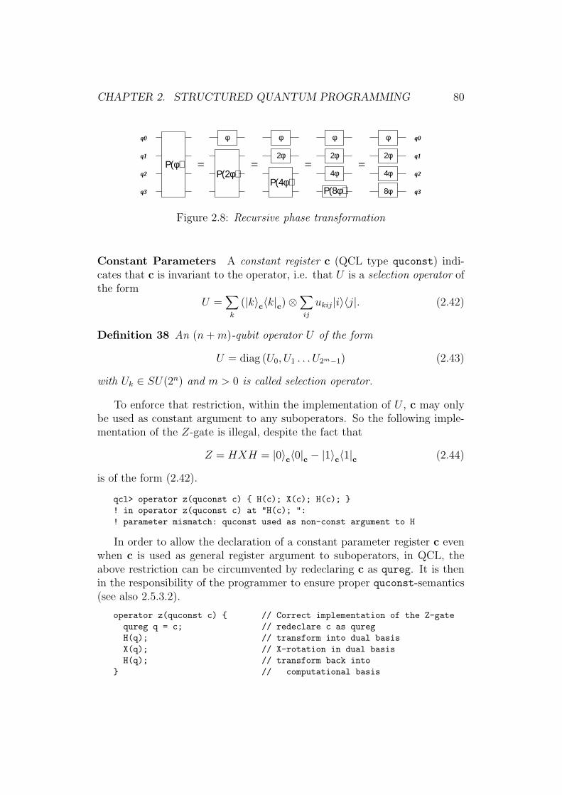
CHAPTER 2. STRUCTURED QUANTUM PROGRAMMING 80
Ρ(φ)Ρ(2φ)
Ρ(4φ)Ρ(8φ)
φ φ φ φ
2φ 2φ 2φ
4φ 4φ
8φ
= = ==
q0
q1
q2
q3
q0
q1
q2
q3
Figure 2.8: Recursive phase transformation
Constant Parameters A constant register c (QCL type quconst) indi-cates that c is invariant to the operator, i.e. that U is a selection operator ofthe form
U =∑
k
(|k〉c〈k|c)⊗∑
ij
ukij|i〉〈j|. (2.42)
Definition 38 An (n+m)-qubit operator U of the form
U = diag (U0, U1 . . . U2m−1) (2.43)
with Uk ∈ SU(2n) and m > 0 is called selection operator.
To enforce that restriction, within the implementation of U , c may onlybe used as constant argument to any suboperators. So the following imple-mentation of the Z-gate is illegal, despite the fact that
Z = HXH = |0〉c〈0|c − |1〉c〈1|c (2.44)
is of the form (2.42).
qcl> operator z(quconst c) { H(c); X(c); H(c); }! in operator z(quconst c) at "H(c); ":! parameter mismatch: quconst used as non-const argument to H
In order to allow the declaration of a constant parameter register c evenwhen c is used as general register argument to suboperators, in QCL, theabove restriction can be circumvented by redeclaring c as qureg. It is thenin the responsibility of the programmer to ensure proper quconst-semantics(see also 2.5.3.2).
operator z(quconst c) { // Correct implementation of the Z-gatequreg q = c; // redeclare c as quregH(q); // transform into dual basisX(q); // X-rotation in dual basisH(q); // transform back into
} // computational basis
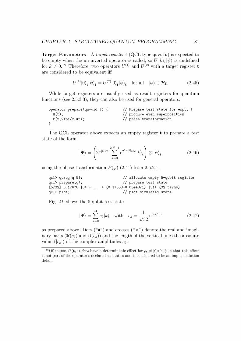
CHAPTER 2. STRUCTURED QUANTUM PROGRAMMING 81
Target Parameters A target register t (QCL type quvoid) is expected tobe empty when the un-inverted operator is called, so U |k〉t|ψ〉 is undefinedfor k 6= 0.18 Therefore, two operators U (1) and U (2) with a target register tare considered to be equivalent iff
U (1)|0〉t|ψ〉t = U (2)|0〉t|ψ〉t for all |ψ〉 ∈ Ht. (2.45)
While target registers are usually used as result registers for quantumfunctions (see 2.5.3.3), they can also be used for general operators:
operator prepare(quvoid t) { // Prepare test state for empty tH(t); // produce even superpositionP(t,2*pi/2^#t); // phase transformation
}
The QCL operator above expects an empty register t to prepare a teststate of the form
|Ψ〉 =
2−|t|/2
2|t|−1∑
k=0
e21−|t|iπk|k〉t⊗ |ψ〉t (2.46)
using the phase transformation P (ϕ) (2.41) from 2.5.2.1.
qcl> qureg q[5]; // allocate empty 5-qubit registerqcl> prepare(q); // prepare test state[5/32] 0.17678 |0> + ... + (0.17338-0.034487i) |31> (32 terms)qcl> plot; // plot simulated state
Fig. 2.9 shows the 5-qubit test state
|Ψ〉 =31∑
k=0
ck|k〉 with ck =1√32
eiπk/16 (2.47)
as prepared above. Dots (“•”) and crosses (“×”) denote the real and imagi-nary parts (<(ck) and =(ck)) and the length of the vertical lines the absolutevalue (|ck|) of the complex amplitudes ck.
18Of course, U(t, s) does have a deterministic effect for ρt 6= |0〉〈0|, just that this effectis not part of the operator’s declared semantics and is considered to be an implementationdetail.

CHAPTER 2. STRUCTURED QUANTUM PROGRAMMING 82
5 used qubits, 32 basevectors
Figure 2.9: 5-qubit test state
Scratch Parameters A scratch register s (QCL type quscratch) is ex-pected to be empty before and after the operator is called, so U has has tobe of the form
U = (|0〉s〈0|s)⊗∑
ij
uij|i〉〈j|+2|s|−1∑
k,l=1
∑
ij
uklij|k〉s|i〉〈l|s〈j| (2.48)
Scratch parameters (also called explicit scratch registers), have the samesemantics as unmanaged (see 2.5.2.4) local scratch variables (QCL-type qureg),except that they are provided as parameters instead of getting allocated fromthe quantum heap (see 2.4.1.2). Explicit scratch parameters can be usefulfor suboperators as they allow to temporarily use target registers, or otherregisters that are known to be empty at some point during a computation,as scratch to save quantum memory.
2.5.2.3 Inverse Operators
Unlike procedures, operator calls can be inverted. In QCL, this is done bypreceding the operator name with the adjungation prefix “!”. The adjointoperator of a composition of unitary operators is19
(n∏
i=1
Ui
)†=
n∏
i=1
U †n+1−i (2.49)
19To avoid ambiguities with non-commutative matrix products, we use the convention∏ni=1 fi = fnfn−1 . . . f1
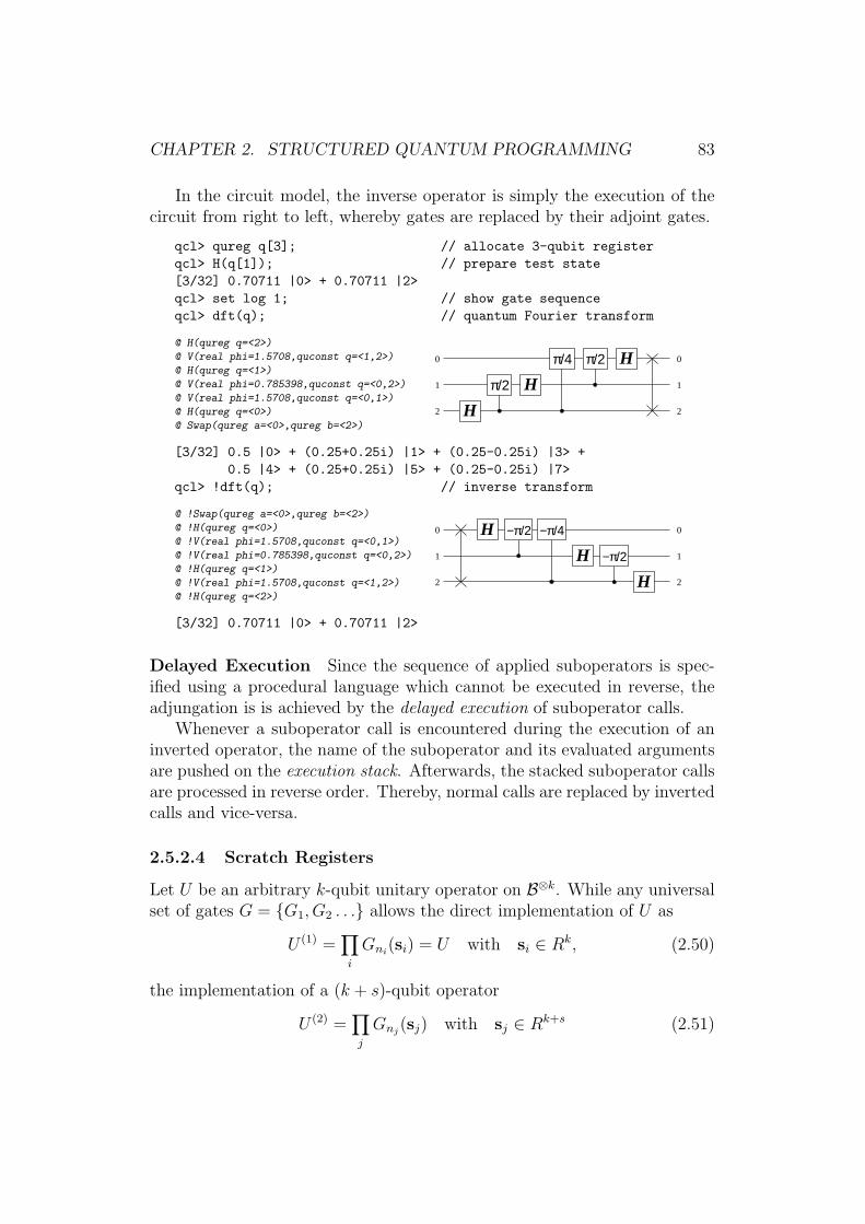
CHAPTER 2. STRUCTURED QUANTUM PROGRAMMING 83
In the circuit model, the inverse operator is simply the execution of thecircuit from right to left, whereby gates are replaced by their adjoint gates.
qcl> qureg q[3]; // allocate 3-qubit registerqcl> H(q[1]); // prepare test state[3/32] 0.70711 |0> + 0.70711 |2>qcl> set log 1; // show gate sequenceqcl> dft(q); // quantum Fourier transform
@ H(qureg q=<2>)
@ V(real phi=1.5708,quconst q=<1,2>)
@ H(qureg q=<1>)
@ V(real phi=0.785398,quconst q=<0,2>)
@ V(real phi=1.5708,quconst q=<0,1>)
@ H(qureg q=<0>)
@ Swap(qureg a=<0>,qureg b=<2>)
0
11
0
22 H
Hπ/2
π/4 Hπ/2
[3/32] 0.5 |0> + (0.25+0.25i) |1> + (0.25-0.25i) |3> +0.5 |4> + (0.25+0.25i) |5> + (0.25-0.25i) |7>
qcl> !dft(q); // inverse transform
@ !Swap(qureg a=<0>,qureg b=<2>)
@ !H(qureg q=<0>)
@ !V(real phi=1.5708,quconst q=<0,1>)
@ !V(real phi=0.785398,quconst q=<0,2>)
@ !H(qureg q=<1>)
@ !V(real phi=1.5708,quconst q=<1,2>)
@ !H(qureg q=<2>)
0
11
0
22
H
H
H −π/2
−π/2
−π/4
[3/32] 0.70711 |0> + 0.70711 |2>
Delayed Execution Since the sequence of applied suboperators is spec-ified using a procedural language which cannot be executed in reverse, theadjungation is is achieved by the delayed execution of suboperator calls.
Whenever a suboperator call is encountered during the execution of aninverted operator, the name of the suboperator and its evaluated argumentsare pushed on the execution stack. Afterwards, the stacked suboperator callsare processed in reverse order. Thereby, normal calls are replaced by invertedcalls and vice-versa.
2.5.2.4 Scratch Registers
Let U be an arbitrary k-qubit unitary operator on B⊗k. While any universalset of gates G = {G1, G2 . . .} allows the direct implementation of U as
U (1) =∏
i
Gni(si) = U with si ∈ Rk, (2.50)
the implementation of a (k + s)-qubit operator
U (2) =∏
j
Gnj(sj) with sj ∈ Rk+s (2.51)
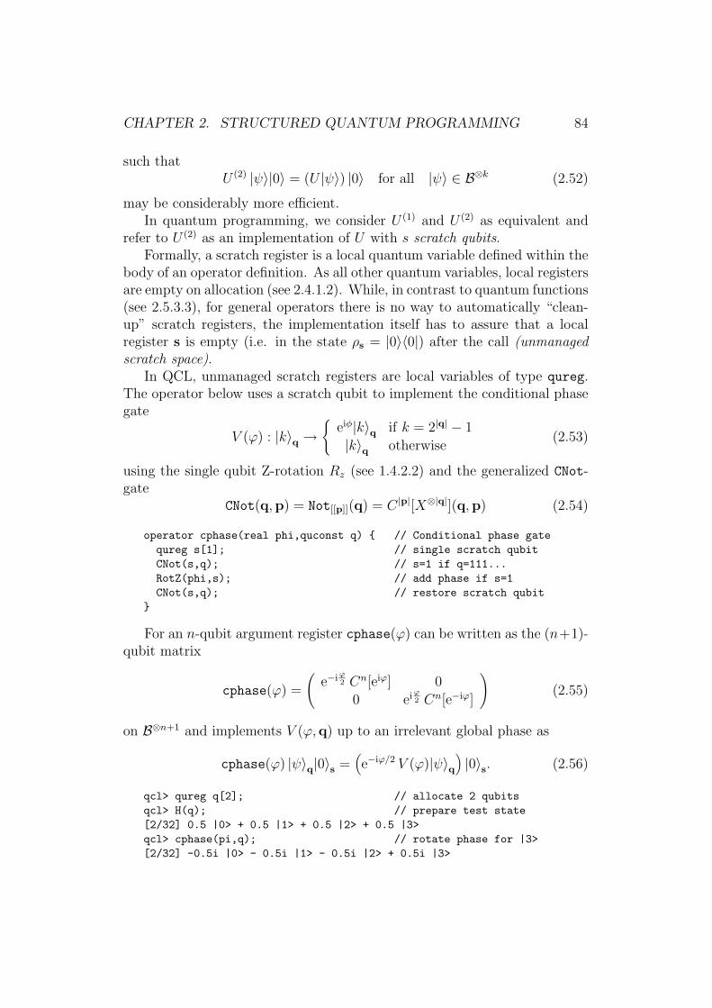
CHAPTER 2. STRUCTURED QUANTUM PROGRAMMING 84
such thatU (2) |ψ〉|0〉 = (U |ψ〉) |0〉 for all |ψ〉 ∈ B⊗k (2.52)
may be considerably more efficient.In quantum programming, we consider U (1) and U (2) as equivalent and
refer to U (2) as an implementation of U with s scratch qubits.Formally, a scratch register is a local quantum variable defined within the
body of an operator definition. As all other quantum variables, local registersare empty on allocation (see 2.4.1.2). While, in contrast to quantum functions(see 2.5.3.3), for general operators there is no way to automatically “clean-up” scratch registers, the implementation itself has to assure that a localregister s is empty (i.e. in the state ρs = |0〉〈0|) after the call (unmanagedscratch space).
In QCL, unmanaged scratch registers are local variables of type qureg.The operator below uses a scratch qubit to implement the conditional phasegate
V (ϕ) : |k〉q →{
eiφ|k〉q if k = 2|q| − 1
|k〉q otherwise(2.53)
using the single qubit Z-rotation Rz (see 1.4.2.2) and the generalized CNot-gate
CNot(q,p) = Not[[p]](q) = C |p|[X⊗|q|](q,p) (2.54)
operator cphase(real phi,quconst q) { // Conditional phase gatequreg s[1]; // single scratch qubitCNot(s,q); // s=1 if q=111...RotZ(phi,s); // add phase if s=1CNot(s,q); // restore scratch qubit
}
For an n-qubit argument register cphase(ϕ) can be written as the (n+1)-qubit matrix
cphase(ϕ) =
(e−iϕ
2 Cn[eiϕ] 0
0 eiϕ2 Cn[e−iϕ]
)(2.55)
on B⊗n+1 and implements V (ϕ,q) up to an irrelevant global phase as
cphase(ϕ) |ψ〉q|0〉s =(e−iϕ/2 V (ϕ)|ψ〉q
)|0〉s. (2.56)
qcl> qureg q[2]; // allocate 2 qubitsqcl> H(q); // prepare test state[2/32] 0.5 |0> + 0.5 |1> + 0.5 |2> + 0.5 |3>qcl> cphase(pi,q); // rotate phase for |3>[2/32] -0.5i |0> - 0.5i |1> - 0.5i |2> + 0.5i |3>
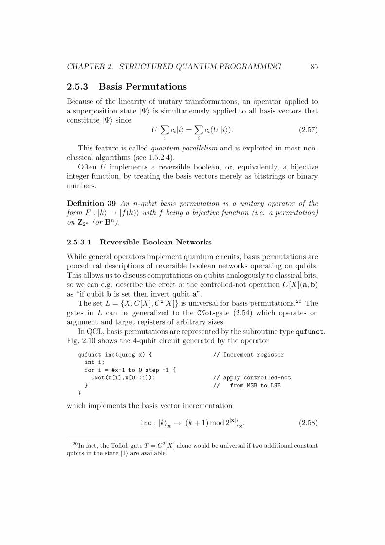
CHAPTER 2. STRUCTURED QUANTUM PROGRAMMING 85
2.5.3 Basis Permutations
Because of the linearity of unitary transformations, an operator applied toa superposition state |Ψ〉 is simultaneously applied to all basis vectors thatconstitute |Ψ〉 since
U∑
i
ci|i〉 =∑
i
ci(U |i〉). (2.57)
This feature is called quantum parallelism and is exploited in most non-classical algorithms (see 1.5.2.4).
Often U implements a reversible boolean, or, equivalently, a bijectiveinteger function, by treating the basis vectors merely as bitstrings or binarynumbers.
Definition 39 An n-qubit basis permutation is a unitary operator of theform F : |k〉 → |f(k)〉 with f being a bijective function (i.e. a permutation)on Z2n (or Bn).
2.5.3.1 Reversible Boolean Networks
While general operators implement quantum circuits, basis permutations areprocedural descriptions of reversible boolean networks operating on qubits.This allows us to discuss computations on qubits analogously to classical bits,so we can e.g. describe the effect of the controlled-not operation C[X](a,b)as “if qubit b is set then invert qubit a”.
The set L = {X,C[X], C2[X]} is universal for basis permutations.20 Thegates in L can be generalized to the CNot-gate (2.54) which operates onargument and target registers of arbitrary sizes.
In QCL, basis permutations are represented by the subroutine type qufunct.Fig. 2.10 shows the 4-qubit circuit generated by the operator
qufunct inc(qureg x) { // Increment registerint i;for i = #x-1 to 0 step -1 {
CNot(x[i],x[0::i]); // apply controlled-not} // from MSB to LSB
}
which implements the basis vector incrementation
inc : |k〉x → |(k + 1) mod 2|x|〉x. (2.58)
20In fact, the Toffoli gate T = C2[X] alone would be universal if two additional constantqubits in the state |1〉 are available.
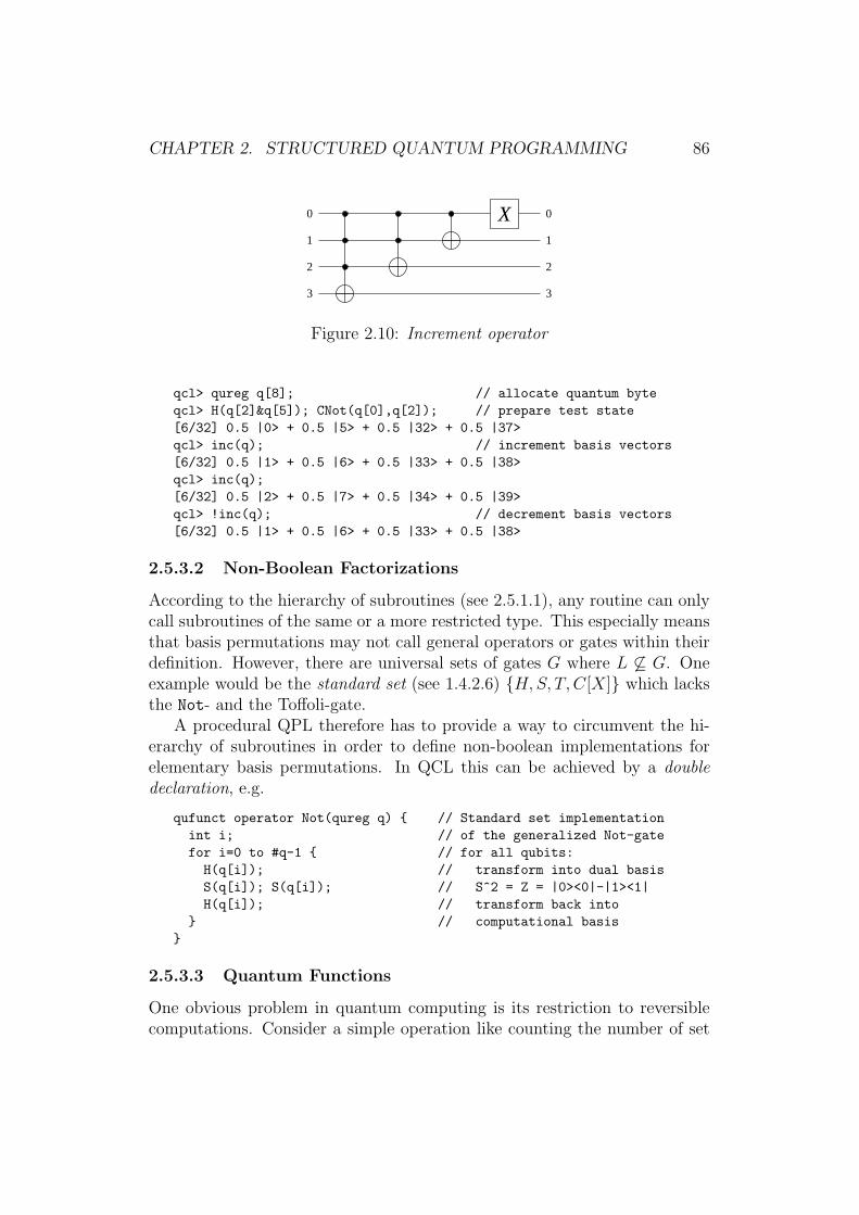
CHAPTER 2. STRUCTURED QUANTUM PROGRAMMING 86
0
1
2
3
0
1
2
3
X
Figure 2.10: Increment operator
qcl> qureg q[8]; // allocate quantum byteqcl> H(q[2]&q[5]); CNot(q[0],q[2]); // prepare test state[6/32] 0.5 |0> + 0.5 |5> + 0.5 |32> + 0.5 |37>qcl> inc(q); // increment basis vectors[6/32] 0.5 |1> + 0.5 |6> + 0.5 |33> + 0.5 |38>qcl> inc(q);[6/32] 0.5 |2> + 0.5 |7> + 0.5 |34> + 0.5 |39>qcl> !inc(q); // decrement basis vectors[6/32] 0.5 |1> + 0.5 |6> + 0.5 |33> + 0.5 |38>
2.5.3.2 Non-Boolean Factorizations
According to the hierarchy of subroutines (see 2.5.1.1), any routine can onlycall subroutines of the same or a more restricted type. This especially meansthat basis permutations may not call general operators or gates within theirdefinition. However, there are universal sets of gates G where L 6⊆ G. Oneexample would be the standard set (see 1.4.2.6) {H,S, T, C[X]} which lacksthe Not- and the Toffoli-gate.
A procedural QPL therefore has to provide a way to circumvent the hi-erarchy of subroutines in order to define non-boolean implementations forelementary basis permutations. In QCL this can be achieved by a doubledeclaration, e.g.
qufunct operator Not(qureg q) { // Standard set implementationint i; // of the generalized Not-gatefor i=0 to #q-1 { // for all qubits:
H(q[i]); // transform into dual basisS(q[i]); S(q[i]); // S^2 = Z = |0><0|-|1><1|H(q[i]); // transform back into
} // computational basis}
2.5.3.3 Quantum Functions
One obvious problem in quantum computing is its restriction to reversiblecomputations. Consider a simple operation like counting the number of set
CHAPTER 2. STRUCTURED QUANTUM PROGRAMMING 87
qubits in a register q
bitcount′ : |k〉q → |b(k)〉q with (2.59)
b(n) = nmod 2 + b(bn/2c) and b(0) = 0. (2.60)
Clearly, this operation is non-reversible since bitcount′ |2n〉 = 1 for alln < |q|, so bitcount′ is not an unitary operator. However, if we use anadditional register p with 2|p| > |q|, then we can always find a unitaryoperator bitcount such that
bitcount : |k〉q|0〉p → |k〉q|b(k)〉p (2.61)
Definition 40 Let c ∈ Rn and t ∈ Rm be disjoint registers and f be anarbitrary function f : Z2n → Z2m (or f : Bn → Bm). A unitary operator Fof the form
F : |x〉c|y〉t → |x〉c|g(f(x), y)〉t with g(z, 0) = z (2.62)
is referred to as quantum function implementing f with the accumulationfunction g.
Since F is required to be unitary, each hz : y → g(z, y) must be a 2m-permutation with hz(0) = z. So for any given function f : Z2n → Z2m thereexist 2n(2m − 1)! different quantum functions F (k) which implement f .
In procedural quantum programming, two quantum functions F (1) andF (2) are considered equivalent when they implement the same function, soF |x〉t|y〉t is undefined for y 6= 0 which makes the actual definition of g anirrelevant implementation detail.21
The above notion of equivalence implies that t is a target register (see2.5.2.2). Also, from the form of (2.62) it follows that c is a constant regis-ter. Using the QCL register types quconst and quvoid, we can implementbitcount as the quantum function
qufunct bitcount(quconst q,quvoid p) { // count set bits in qint i; int j;if #q>=2^#p { // make sure that p is wide
exit "target register too small"; // enough}for i=0 to #q-1 { // iterate over qubits in q
for j=#p-1 to 0 step -1 { // increment p if q[i]CNot(p[j],p[0::j] & q[i]); // is set
}}
}
21This abstraction is necessary as the use of scratch registers (see 2.5.3.5) can affect g.
CHAPTER 2. STRUCTURED QUANTUM PROGRAMMING 88
with the accumulation function g(z, y) = (z + y) mod 2|p|, so
bitcount : |x〉q|y〉p → |x〉q|(y + b(k)) mod 2|p|〉p. (2.63)
qcl> qureg q[3]; qureg p[2]; // allocate argument and target reg.qcl> H(q); // prepare superposition[5/32] 0.3535 |0,0> + 0.3535 |1,0> + 0.3535 |2,0> + 0.3535 |3,0> +
0.3535 |4,0> + 0.3535 |5,0> + 0.3535 |6,0> + 0.3535 |7,0>qcl> bitcount(q,p); // count set qubits[5/32] 0.3535 |0,0> + 0.3535 |1,1> + 0.3535 |2,1> + 0.3535 |4,1> +
0.3535 |3,2> + 0.3535 |5,2> + 0.3535 |6,2> + 0.3535 |7,3>
2.5.3.4 Junk Registers
While quantum functions can be used to work around the reversible natureof quantum computing, the necessity to keep a copy of the argument is aproblem, as longer computations will leave registers filled with intermediateresults.
Suppose we want to compare the number of set qubits in two registers aand b, i.e. find a quantum function to implement the predicate
c(x, y) =
{1 if b(x) = b(y)0 otherwise .
(2.64)
Using an auxiliary register s and B = bitcount from (2.63), the operator
bitcmp0(a,b, t, s) = CNot(t, s) Not(s)B†(b, s)B(a, s) (2.65)
implements c but leaves the register s in a “dirty” state:
|x, y, 0, 0〉 B(a,s)−→ |x, y, b(x), 0〉 B†(b,s)−→ |x, y, b(x)− b(y), 0〉 Not(s)−→ (2.66)
|x, y, 11...1⊕ (b(x)− b(y)), 0〉 CNot(t,s)−→ |x, y, 11...1⊕ (b(x)− b(y)), c(x, y)〉qufunct bitcmp0(quconst a,quconst b,quvoid t,quvoid s) {bitcount(a,s); // write #bits(a) to s!bitcount(b,s); // subtract b(b) from sNot(s); // invert sCNot(t,s); // t=1 if #bits(a)-#bits(b)=0
}
Since s does not contain useful information and is usually entangled (i.e.tr(ρ2
s) < 1) so that it cannot be reset by measurement (see 2.4.3.3) withoutaffecting other registers, s is called a junk register. A quantum function
F : |x, 0〉|0〉s → |x, f(x)〉|j(x)〉s (2.67)
with a junk parameter s is called a dirty implementation of f .
CHAPTER 2. STRUCTURED QUANTUM PROGRAMMING 89
qcl> qureg a[3];qureg b[3]; // allocate registers a,b,s,tqcl> qureg s[2];qureg t[1];qcl> H(a[0]); Not(a[2]); // prepare test state for a[9/32] 0.70711 |4,0,0,0> + 0.70711 |5,0,0,0>qcl> H(b[1]); Not(b[0]); // prepare test state for b[9/32] 0.5 |4,1,0,0> + 0.5 |5,1,0,0> + 0.5 |4,3,0,0> + 0.5 |5,3,0,0>qcl> bitcmp(a,b,t,s); // compare number of bits[9/32] 0.5 |4,3,0,0> + 0.5 |5,1,2,0> + 0.5 |4,1,3,1> + 0.5 |5,3,3,1>
2.5.3.5 Scratch Space Management
Let F be a a dirty implementation of a classical function f with the argumentregister x, the target register y and the junk register s
F : |k〉x|0〉y|0〉s → |k〉x|f(k)〉y|j(k)〉s (2.68)
While computing f(k), F also fills s with the temporary junk bits j(k).To reclaim s, Bennett proposed the following method [7], which is known asuncomputing:
1. Allocate an (empty) auxiliary register t of the same size as y.
2. Replace F (x,y, s) by the operator
F ′(x,y, s, t) = F †(x, t, s) Fanout(t,y)F (x, t, s). (2.69)
The above procedure restores both the junk and the auxiliary register sos and t are scratch parameters (see 2.5.2.2) of F ′ so F ′ is a clean implemen-tation of f with |s|+ |t| scratch qubits (see 2.5.2.4):
|k, 0, 0, 0〉 F (x,t,s)−→ |k, 0, j(k), f(k)〉 Fanout(t,y)−→
|k, f(k), j(k), f(k)〉 F†(x,t,s)−→ |k, f(k), 0, 0〉 (2.70)
The Fanout Operator The Fanout operator is a quantum function im-plementing the identity i.e.
Fanout : |x〉a|0〉b → |x〉a|x〉b with |a| = |b| (2.71)
and is usually realized using |x| controlled-not gates with the accumulationfunction gF (x, y) = x⊕ y.
cond qufunct Fanout(quconst a,quvoid b) {int i;if #a!=#b { exit "fanout arguments must be of equal size"; }for i=0 to #a-1 { CNot(b[i],a[i]); }
}
CHAPTER 2. STRUCTURED QUANTUM PROGRAMMING 90
Let F be a dirty implementation of f with the accumulation function gand a junk register s, so
F : |x〉x|y〉y|0〉s → |x〉x|g(f(x), y)〉y|j(x, y)〉s. (2.72)
The clean version F ′ according to (2.69) with the scratch registers s andt is given as
F ′ : |x〉x|y〉y|0〉s|0〉t → |x〉x|gF (f(x), y)〉y|0〉s|0〉t. (2.73)
So in F ′ the original accumulation function g is replaced by the accumu-lation function gF of the Fanout operator.
Scratch Registers In procedural quantum programming, the method ofuncomputing (2.69) allows the automatically reclaiming of local registerswhich are left in a non-empty state after the body of the operator has beenexecuted (managed scratch registers). In QCL managed scratch registers arelocal variables of type quscratch.
Since the method of uncomputing only works for quantum functions,managed scratch registers are restricted to basis permutations with constantand target registers as quantum parameters.
For bitcmp0 from (see 2.5.3.4), a clean version can be constructed bymaking s a managed local scratch register
qufunct bitcmp(quconst a,quconst b,quvoid t) {quscratch s[ceil(log(max(#a,#b)+0.5,2))];bitcmp0 (a,b,t,s);
}
which is not only equivalent to but also implements the same unitary trans-formation22 as the following operator using two unmanaged scratch registers(see 2.5.2.4).
qufunct bitcmp(quconst a,quconst b,quvoid t) {qureg s[ceil(log(max(#a,#b)+0.5,2))];qureg u[#t];bitcmp0 (a,b,u,s);CNot(t,u);!bitcmp0 (a,b,u,s);
}
22Note that for single qubits, every possible implementation of the Fanout operator isidentical to a CNot gate.
CHAPTER 2. STRUCTURED QUANTUM PROGRAMMING 91
2.5.3.6 Calling Semantics
The potential use of managed scratch registers extends the calling seman-tics of basis permutations as compared to general operators. Consider thequantum functions
qufunct U1(quconst x,quvoid y,quvoid s) { // s is junk registerA(x,y,s);B(x,y,s)
}
qufunct U2(quconst x,quvoid y) { // s is scratch registerquscratch s;A(x,y,s);B(x,y,s)
}
While the calls U1(x,y,s) and !U1(x,y,s) are analogous to general op-erator calls i.e.
U1(x,y, s) = B(x,y, s)A(x,y, s) and U †1(x,y, s) = A†(x,y, s)B†(x,y, s)(2.74)
the calls U2(x,y,s) and !U2(x,y,s) cause the transparent allocation of aregister t, with |t| = |y| and results in the transformations
U2(x,y, s, t) = U †1(x, t, s) Fanout(t,y)U1(x, t, s) and (2.75)
U †2(x,y, s, t) = U †1(x, t, s) Fanout†(t,y)U1(x, t, s). (2.76)
Note that U2 and U †2 are almost identical and that U2 = U †2 if a Hermitianimplementation of the Fanout operator is used.
Double Execution When a general operator or basis permutation with-out managed scratch registers is executed, calls of suboperators are eitherprocessed immediately (linear execution) or pushed on the execution stack(delayed execution), depending on whether the normal or the inverse opera-tor has been called (see 2.5.2.3).
In the case of a quantum function with managed scratch registers, afterthe initial remapping of the target registers, suboperator calls always getexecuted and pushed on the execution stack (double execution). After thebody of the subroutine has been processed, the appropriate Fanout (normalcall) or Fanout† (inverted call) operation is executed and then the stackedcalls get executed again in reverse order with their adjungation flags inverted.

CHAPTER 2. STRUCTURED QUANTUM PROGRAMMING 92
2.6 Quantum Flow Control
All classical programming languages, in one way or another, allow the condi-tional execution of code depending on a boolean variable or logical expression(conditional branching). In structured languages conditional branching is re-alized by if-statements with well defined entry and exit points.
While the unobservability of qubits forbids a direct implementation, wewill show how conditional operators can be used to emulate conditionalbranching on qubits (quantum if-statement) as well as (bounded) conditionalloops with quantum termination conditions to the effect that, with regardto flow-control, qubits can be treated almost equivalently to classical bits(structured quantum programming).
We will further demonstrate how qubits and registers can be combined toarbitrary boolean expressions and complex predicates (quantum conditions).
2.6.1 Conditional Operators
As already mentioned in 2.4.2.3, for a unitary register operator U(s) andan enable (or control) register e ∈ R disjoint to s, the conditional operatorU[[e]](s) is defined as
U[[e]](s) : |k〉s|c〉e →{
(U |k〉s)|c〉e if c = 111 . . .|k〉s|c〉e otherwise .
(2.77)
If e is a qubit so |e| = 1, then informally, we can describe the effect ofU[[e]](s) as “if e is set then apply U(s)” which relates to the fact that
U[[e]]
2|s|−1∑
k=0
∑
b∈B
ckb|k〉s|b〉e =2|s|−1∑
k=0
ckb|k〉s|0〉e +2|s|−1∑
k=0
ckb (U |k〉s) |1〉e. (2.78)
2.6.1.1 Properties of Conditional Operators
Orthogonal Enable Registers Let U, V ∈ SU(2n) be n-qubit unitaryoperators, s ∈ Rn a n-qubit register and q ∈ R1 a qubit disjoint to s (i.e.q ⊆ s), then [
U[[q]](s)X(q), V[[q]](s)X(q)]
= 0. (2.79)
For arbitrary register operators U(x) and V (y), (2.79) can be generalizedto [
U[[e]](x)Xn(c), V[[e]](y)Xn(c)]
= 0 (2.80)
with c ∈ Rn being an non-empty subregister c ⊆ e and x,y ⊆ e.
CHAPTER 2. STRUCTURED QUANTUM PROGRAMMING 93
Conditional Decomposition Its easy to verify that for an arbitrary U(s)and a qubit q ∈ R1,q ⊆ s
U(s) = U[[q]](s)X(q)U[[q]](s)X(q). (2.81)
Definition 41 An n-qubit basis permutation P : |k〉 → |p(k)〉 is called cycliciff it generates the computational basis B such that for any |k〉 ∈ B
2n−1⋃
i=0
P i|k〉 = {|j〉 | j ∈ Z2n} = B (2.82)
p is therefore a permutation on Z2n with the cycle length 2n. If P is cyclic,then A† P A is also cyclic for an arbitrary basis permutations A. An examplefor a cyclic basis permutation is the operator inc (2.58) from 2.5.3.1.
We can now generalize the identity (2.81) for enable registers e ∈ Rn, e ⊆s to
U(s) =(U[[e]](s)P (e)
)2n
(2.83)
with P being an arbitrary n-qubit cyclic basis permutation.
Conditional Composition Let V,W ∈ SU(2n) be n-qubit unitary oper-ators, then the selection operator
U =
(V 00 W
)(2.84)
can be implemented as
U(s, c) = X(c)V[[c]](s)X(c)W[[c]](s) (2.85)
Likewise, for any (n+m)-qubit selection operator
U = diag (U0, U1 . . . U2m−1) (2.86)
there exists an cyclic m-qubit basis permutation P such that
U(s, c) =2m−1∏
i=0
Ui [[c]](s)P (c) (2.87)
CHAPTER 2. STRUCTURED QUANTUM PROGRAMMING 94
2.6.1.2 Conditional Subroutines
As conditional operators are just a special case of selection operators (see2.5.2.2), they can be implemented as quantum subroutines with a constantenable register.
The operator below implements a conditional version cinc of the registerincrement operator (2.58) defined as
cinc : |k〉x|c〉e →{|(k + 1) mod 2|x|〉x|c〉e if c = 11...1
|(k〉x|c〉e otherwise(2.88)
qufunct cinc(qureg x,quconst e) { // Conditional incrementint i; // as selectionfor i = #x-1 to 0 step -1 { // operator
CNot(x[i],x[0::i] & e);}
}
The above operator is a conditional version of (2.58)
cinc : |k〉x|c〉e →{|(k + 1) mod 2|x|〉x|c〉e if c = 11...1
|(k〉x|c〉e otherwise(2.89)
Structured QPLs directly support conditional execution, i.e. the auto-matic construction of U[[e]] from a given implementation of U , by allowingthe explicit declaration of conditional subroutines.
In QCL, conditional operators can be defined by prefixing the subroutinedeclaration with the keyword cond.
cond qufunct inc(qureg x) { // Conditional increment registerint i; // as conditionalfor i = #x-1 to 0 step -1 { // subroutine
CNot(x[i],x[0::i]);}
}
Conditional Calls The enable register e is an implicit constant param-eter and not part of the parameter declaration of a conditional subroutine.Instead, e is set by a quantum if-statement (see 2.6.2.1) and transparentlypassed on to all suboperators, which therefore are also required to be eitherconditional operators or conditional elementary gates (see 2.4.2.3).
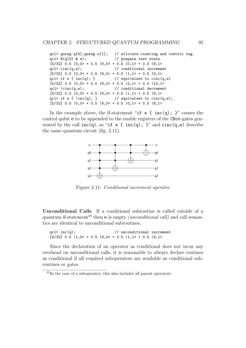
CHAPTER 2. STRUCTURED QUANTUM PROGRAMMING 95
qcl> qureg q[4];qureg e[1]; // allocate counting and control reg.qcl> H(q[3] & e); // prepare test state[5/32] 0.5 |0,0> + 0.5 |8,0> + 0.5 |0,1> + 0.5 |8,1>qcl> cinc(q,e); // conditional increment[5/32] 0.5 |0,0> + 0.5 |8,0> + 0.5 |1,1> + 0.5 |9,1>qcl> if e { inc(q); } // equivalent to cinc(q,e)[5/32] 0.5 |0,0> + 0.5 |8,0> + 0.5 |2,1> + 0.5 |10,1>qcl> !cinc(q,e); // conditional decrement[5/32] 0.5 |0,0> + 0.5 |8,0> + 0.5 |1,1> + 0.5 |9,1>qcl> if e { !inc(q); } // equivalent to cinc(q,e);[5/32] 0.5 |0,0> + 0.5 |8,0> + 0.5 |0,1> + 0.5 |8,1>
In the example above, the if-statement “if e { inc(q); }” causes thecontrol qubit e to be appended to the enable registers of the CNot-gates gen-erated by the call inc(q), so “if e { inc(q); }” and cinc(q,e) describethe same quantum circuit (fig. 2.11).
q0
q1
q2
q3
e
q0
q1
q2
q3
e
Figure 2.11: Conditional increment operator
Unconditional Calls If a conditional subroutine is called outside of aquantum if-statement23 then e is empty (unconditional call) and call seman-tics are identical to unconditional subroutines.
qcl> inc(q); // unconditional increment[4/32] 0.5 |1,0> + 0.5 |9,0> + 0.5 |1,1> + 0.5 |9,1>
Since the declaration of an operator as conditional does not incur anyoverhead on unconditional calls, it is reasonable to always declare routinesas conditional if all required suboperators are available as conditional sub-routines or gates.
23In the case of a suboperator, this also includes all parent operators
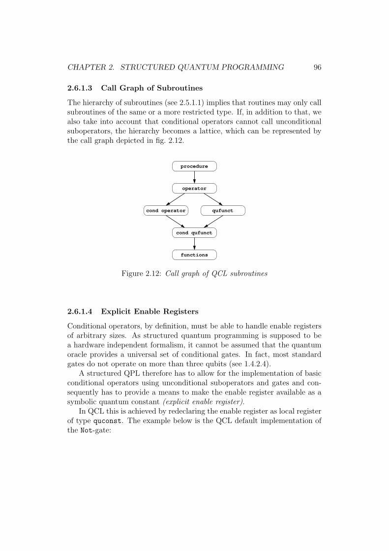
CHAPTER 2. STRUCTURED QUANTUM PROGRAMMING 96
2.6.1.3 Call Graph of Subroutines
The hierarchy of subroutines (see 2.5.1.1) implies that routines may only callsubroutines of the same or a more restricted type. If, in addition to that, wealso take into account that conditional operators cannot call unconditionalsuboperators, the hierarchy becomes a lattice, which can be represented bythe call graph depicted in fig. 2.12.
procedure
operator
cond qufunct
functions
cond operator qufunct
Figure 2.12: Call graph of QCL subroutines
2.6.1.4 Explicit Enable Registers
Conditional operators, by definition, must be able to handle enable registersof arbitrary sizes. As structured quantum programming is supposed to bea hardware independent formalism, it cannot be assumed that the quantumoracle provides a universal set of conditional gates. In fact, most standardgates do not operate on more than three qubits (see 1.4.2.4).
A structured QPL therefore has to allow for the implementation of basicconditional operators using unconditional suboperators and gates and con-sequently has to provide a means to make the enable register available as asymbolic quantum constant (explicit enable register).
In QCL this is achieved by redeclaring the enable register as local registerof type quconst. The example below is the QCL default implementation ofthe Not-gate:
CHAPTER 2. STRUCTURED QUANTUM PROGRAMMING 97
extern qufunct NOT(qureg q); // unconditional Notextern qufunct CNOT(qureg q,quconst c); // unconditional CNot
cond qufunct Not(qureg q) { // conditional Notquconst e = cond; // e=enable registerif #e>0 { CNOT(q,e); } else { NOT(q); } //
}
2.6.2 Conditional Branching
2.6.2.1 Quantum If-Statements
In classical structured programming languages, the conditional execution ofa statement sequence (block) σ depending on the value of a boolean variablep is expressed by an if-statement S of the form
if p then σ1, σ2 . . . σn endif
or, if one of two blocks σ and τ should be executed,
if p then σ1, σ2 . . . σn else τ1, τ2 . . . τm endif
If the instead of a classical boolean variable, the if-condition is a qubit p
if p then σ1, σ2 . . . σn else τ1, τ2 . . . τm endif
then S is referred to as quantum if-statement (QIS). S is called
(i) invalid iff σ or τ contain24 procedure calls, measurements, reset orinput commands or use random numbers.
(ii) nested iff σ or τ contain other quantum if-statements.
(iii) dirty iff σ or τ contain assignments or break-statements.
(iv) clean iff S is valid and not dirty.
(v) simple iff S is clean and τ = () i.e. no else-branch is defined.
Block and Tail Operators Like the body of an operator subroutine,the if- and else-branches σ and τ are basically procedural descriptions ofquantum circuits, or more precisely, of sequences of suboperators which getgenerated by linear execution. However, unlike a subroutine, σ (τ) has nodeclared interface, so its “parameters” are all classical and quantum variablesthat are visible in the current scope. Also, σ (τ) is not guaranteed to havemathematical semantics (dirty QIS).
24This also includes any sub-statements in control structures.

CHAPTER 2. STRUCTURED QUANTUM PROGRAMMING 98
We will write σ (τ) to denote the composition of suboperators (blockoperator)which would be generated if σ (τ) is executed in place of S25 and σ (τ) todenote the circuit that is generated when the execution is continued until theend of the current subroutine (tail operator).26 In global scope σ and τ areundefined.
In the following example σ, τ , σ and τ would evaluate to
σ = B(x), τ = C(x), σ = D(x,y)B(x) and τ = D(x,y)C(x). (2.90)
operator U(qureg x,qureg y) {A(x);if y { B(x); } else { C(x); } // quantum if-statementD(x,y);
}
2.6.2.2 Conditional Execution
A simple QIS S is of the form
if p then σ1, σ2 . . . σn endif
and implements the transformation US = σ[[p]]. So simple QISs can be usedto set the enable registers of conditional operators (conditional calls, see2.6.1.2).
Since p is already passed as an implicit parameter σ must not operate onp i.e. σ = σ(p), so the QIS below is not a miraculous implementation of aunitary erase operation, but simply triggers an error
qcl> if q { Not(q); }! at "Not(q); ":! runtime error: arguments overlap with quantum condition
Global Control Register Internally, the passing of enable registers toconditional subroutines is handled by a global control register g.
Whenever a simple QIS is encountered, the following happens:
1. The appropriate enable register p is appended to g.
2. The if-branch σ is executed.
3. p is removed from g.
Whenever a call to a conditional gate is encountered, the current valueof g is passed as enable register to the quantum oracle.
25i.e. the circuit that would be generated if S were a classical if-statement with p = true(p = false)
26Note that therefore, even if no else-branch is defined and consequently τ = (), thisdoes not imply that τ = I.
CHAPTER 2. STRUCTURED QUANTUM PROGRAMMING 99
2.6.2.3 Quantum Selection
A clean QIS S with τ 6= () is of the form
if p then σ1, σ2 . . . σn else τ1, τ2 . . . τm endif
The semantics of S (i.e. the corresponding unitary transformation) aredefined as the selection operator
US : |k〉|c〉p →{
(σ|k〉)|c〉p if c = 1
(τ |k〉)|c〉p if c = 0.(2.91)
As US contains σ and τ as suboperators, this means that, unlike a classicalif-statement, both branches of S get executed. As we assumed that neitherσ nor τ contain assignments or other statements which would change theprogram state, both branches cannot exhibit mutual side effects and this canbe done without being inconsistent with classical semantics.27
US is realized as the conditional composition (2.85)
US = Not(p) τ[[p]] Not(p) σ[[p]] =
(τ 00 σ
)(2.92)
so the QIS on the left corresponds to the right sequence (see 2.6.1.2)
if p {inc(x); // cinc(x,p); conditional increment
} else { // Not(p); invert enable qubit!inc(x); // !cinc(x,p); conditional decrement
} // Not(p); restore enable qubit
2.6.2.4 Quantum Forking
If the body of a classical if-statement S contains changes to the program state(e.g. assignments to local variables), then subsequent operator calls maydiffer, depending on whether the if- or the else-branch has been executed. Ifhowever, S is a (dirty) QIS, then both paths need to be executed in orderto determine the corresponding conditional operator US, which allows fornon-classical side-effects and can lead to classically inconsistent states.
To illustrate the problem, consider the operator
27An example for inconsistent code would be e.g.
boolean v := trueif p then v := ¬v else v := ¬v endifif v then error “classically unreachable code” endif

CHAPTER 2. STRUCTURED QUANTUM PROGRAMMING 100
operator U(qureg s,quconst p) {int n;if p { n=1; } else { n=0; } // dirty QISV(n,s); // n=0 or n=1?
}
At first glance it seems impossible to come up with semantics U(s,p) thatare both, classically consistent and also provide a reasonable interpretationas quantum control statement because there is no reason to prefer one of the“obvious” candidates V0(s) and V1(s) over the other.
As a quantum analogy, we might say that the QIS brought p and theclassical variable n into a correlated state, which would suggest the interpre-tation that V0(s) is applied to all basis vectors |k〉s|0〉e and V1(s) to all basisvectors |k〉s|1〉e i.e.
U : |k〉s|n〉p → (Vn|k〉s)|n〉p (2.93)
While these semantics are symmetric28 and have a reasonable quantuminterpretation, they are not classically consistent as they leave the binding ofn undefined. But here, the mathematical semantics of operators (see 2.5.1.2)come to the rescue, as they state that operators are defined by their unitaryeffect and may not change the program state. Since n is a local variableabout to leave scope, we might as well leave it undefined. However, thesesemantics also imply that dirty QISs cannot be used in global scope or withinprocedures.
The above interpretation could also be described as extending the QIS toinclude the remainder of the operator, so U is considered to be equivalent to
operator U(qureg s,quconst p) {int n;if p { n=1; V(n,s); } else { n=0; V(n,s); }
}
As this can only be done explicitly if the QIS in question is not part ofa control statement (like, e.g. a while-loop), a more general notion of whatexactly constitutes the “remainder of a subroutine” is necessary. This isprovided by the the tail operators σ and τ (see 2.6.2.1).
Using σ and τ , the above method can be formalized so that for a dirtyQIS S of the form
if p then σ1, σ2 . . . σn else τ1, τ2 . . . τm endif
the transformation US implemented by S can be defined as
US : |k〉|c〉p →{
(σ|k〉)|c〉p if c = 11..1
(τ |k〉)|c〉p otherwise .(2.94)
28i.e. treat both branches of the QIS equally.
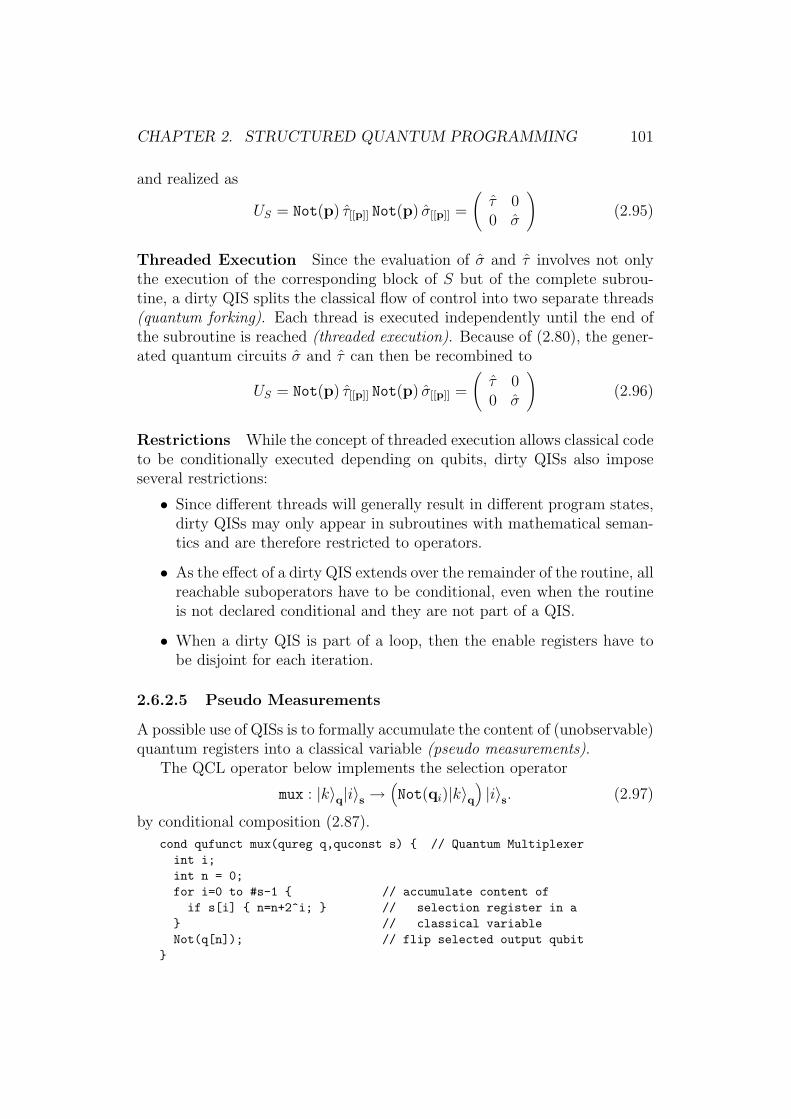
CHAPTER 2. STRUCTURED QUANTUM PROGRAMMING 101
and realized as
US = Not(p) τ[[p]] Not(p) σ[[p]] =
(τ 00 σ
)(2.95)
Threaded Execution Since the evaluation of σ and τ involves not onlythe execution of the corresponding block of S but of the complete subrou-tine, a dirty QIS splits the classical flow of control into two separate threads(quantum forking). Each thread is executed independently until the end ofthe subroutine is reached (threaded execution). Because of (2.80), the gener-ated quantum circuits σ and τ can then be recombined to
US = Not(p) τ[[p]] Not(p) σ[[p]] =
(τ 00 σ
)(2.96)
Restrictions While the concept of threaded execution allows classical codeto be conditionally executed depending on qubits, dirty QISs also imposeseveral restrictions:
• Since different threads will generally result in different program states,dirty QISs may only appear in subroutines with mathematical seman-tics and are therefore restricted to operators.
• As the effect of a dirty QIS extends over the remainder of the routine, allreachable suboperators have to be conditional, even when the routineis not declared conditional and they are not part of a QIS.
• When a dirty QIS is part of a loop, then the enable registers have tobe disjoint for each iteration.
2.6.2.5 Pseudo Measurements
A possible use of QISs is to formally accumulate the content of (unobservable)quantum registers into a classical variable (pseudo measurements).
The QCL operator below implements the selection operator
mux : |k〉q|i〉s →(Not(qi)|k〉q
)|i〉s. (2.97)
by conditional composition (2.87).
cond qufunct mux(qureg q,quconst s) { // Quantum Multiplexerint i;int n = 0;for i=0 to #s-1 { // accumulate content of
if s[i] { n=n+2^i; } // selection register in a} // classical variableNot(q[n]); // flip selected output qubit
}
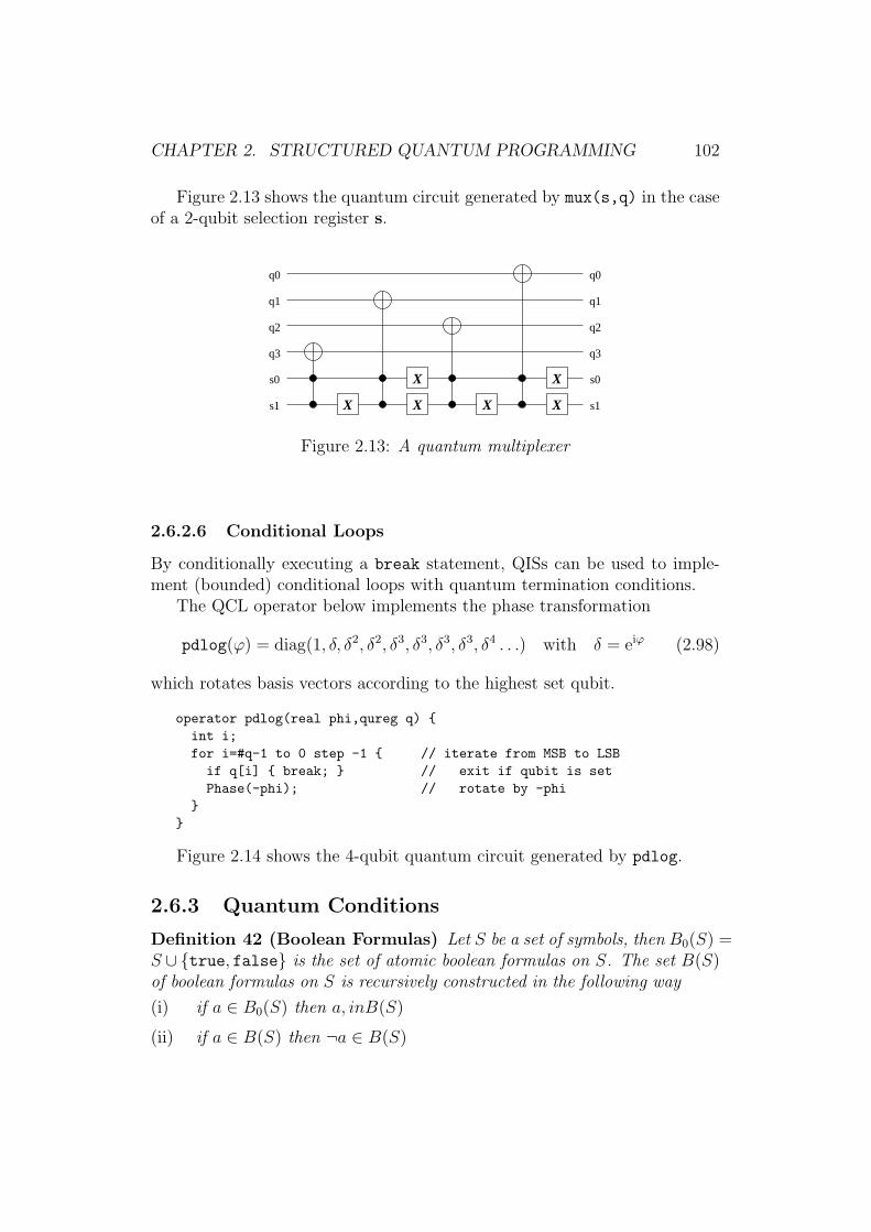
CHAPTER 2. STRUCTURED QUANTUM PROGRAMMING 102
Figure 2.13 shows the quantum circuit generated by mux(s,q) in the caseof a 2-qubit selection register s.
q0
q1
q2
q3
s0
s1
q0
q1
q2
q3
s0
s1 X X
X
X X
X
Figure 2.13: A quantum multiplexer
2.6.2.6 Conditional Loops
By conditionally executing a break statement, QISs can be used to imple-ment (bounded) conditional loops with quantum termination conditions.
The QCL operator below implements the phase transformation
pdlog(ϕ) = diag(1, δ, δ2, δ2, δ3, δ3, δ3, δ3, δ4 . . .) with δ = eiϕ (2.98)
which rotates basis vectors according to the highest set qubit.
operator pdlog(real phi,qureg q) {int i;for i=#q-1 to 0 step -1 { // iterate from MSB to LSB
if q[i] { break; } // exit if qubit is setPhase(-phi); // rotate by -phi
}}
Figure 2.14 shows the 4-qubit quantum circuit generated by pdlog.
2.6.3 Quantum Conditions
Definition 42 (Boolean Formulas) Let S be a set of symbols, then B0(S) =S ∪ {true, false} is the set of atomic boolean formulas on S. The set B(S)of boolean formulas on S is recursively constructed in the following way
(i) if a ∈ B0(S) then a, inB(S)
(ii) if a ∈ B(S) then ¬a ∈ B(S)
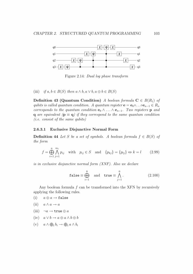
CHAPTER 2. STRUCTURED QUANTUM PROGRAMMING 103
q0
q1
q2
q3
q0
q1
q2
q3X φ
X φ
X φ
X φ X
X
X
X
Figure 2.14: Dual log phase transform
(iii) if a, b ∈ B(S) then a ∧ b, a ∨ b, a⊕ b ∈ B(S)
Definition 43 (Quantum Condition) A boolean formula C ∈ B(R1) ofqubits is called quantum condition. A quantum register e = e0◦. . .◦en−1 ∈ Rn
corresponds to the quantum condition e0 ∧ . . . ∧ en−1. Two registers p andq are equivalent (p ≡ q) if they correspond to the same quantum condition(i.e. consist of the same qubits)
2.6.3.1 Exclusive Disjunctive Normal Form
Definition 44 Let S be a set of symbols. A boolean formula f ∈ B(S) ofthe form
f =n⊕
i=1
mi∧
j=1
pij with pij ∈ S and {pkj} = {plj} ⇔ k = l (2.99)
is in exclusive disjunctive normal form (XNF). Also we declare
false ≡0⊕
i=1
and true ≡0∧
j=1
. (2.100)
Any boolean formula f can be transformed into the XFN by recursivelyapplying the following rules.
(i) a⊕ a→ false
(ii) a ∧ a→ a
(iii) ¬a→ true⊕ a(iv) a ∨ b→ a⊕ a ∧ b⊕ b(v) a ∧⊕
i bi →⊕
i a ∧ bi
CHAPTER 2. STRUCTURED QUANTUM PROGRAMMING 104
From now on, we will assume that quantum conditions are provided inXNF. Further, we will use the notation
C = {pi} ⇐⇒ C =⊕
i
|pi|−1∧
j=0
pij. (2.101)
Definition 45 Let p,q ∈ R be registers and P = {pi}, Q = {qi} be the setof qubits in p,q. The registers p ∪ q and p ∩ q are defined as
p ∪ q = r0 ◦ . . . ◦ rk−1, ri ∈ P ∪Q, ri < rj ⇔ i < j (2.102)
p ∩ q = s0 ◦ . . . ◦ sl−1, ri ∈ P ∩Q, ri < rj ⇔ i < j (2.103)
Definition 46 Let C = {pi} be a quantum condition. The register
c = reg C =⋃
i
pi (2.104)
is called condition register of C.
2.6.3.2 Quantum Predicates
Definition 47 Let C = {pi} be a quantum condition with the conditionregister c = reg C and t ∈ R1. The operator
PC(c, t) = X[[C]](t) =∏
i
CNot(t,pi) (2.105)
is called quantum predicate of C with the target register t.
Definition 48 Let C = {pi} be a quantum condition with the conditionregister c = reg C, c : B|c| → B such that PC|x〉c|0〉 = |x〉c|c(x)〉 and U be aunitary operator. The (extended) conditional operator U[[C]] is defined as
U[[C]] : |k〉|x〉c →{
(U |k〉)|x〉c if c(k)|k〉|x〉c if ¬c(k) . (2.106)
By using an empty scratch qubit s, U[[C]] can be implemented as
U[[C]] = PC(c, s)U[[s]] PC(c, s) (2.107)
Boolean Operations Let p,q be qubits, s be an empty scratch qubit andU a unitary operator. The extended conditional operators for the booleanoperations not, and, xor and or can be implemented as
U[[¬p]] = X(p)U[[p]]X(p) (2.108)
U[[p∧q]] = U[[p◦q]] (2.109)
U[[p⊕q]] = X[[p]](s)X[[q]](s)U[[s]]X[[q]](s)X[[p]](s) (2.110)
U[[p∨q]] = X[[p◦q]](s)U[[p⊕q]]X[[p◦q]](s) (2.111)

CHAPTER 2. STRUCTURED QUANTUM PROGRAMMING 105
2.6.3.3 Language Representation of Quantum Conditions
In structured quantum programming, quantum conditions are representedas a special datatype (QCL type qucond) that represents a list of constantquantum registers. Boolean operators can be used to combine registers,quantum conditions and even classical boolean expressions:
qcl> qureg a[1]; qureg b[1]; // allocate 2 qubitsqcl> print a and b, a or b, a xor b; // basic boolean operators: <0,1> <0; 1; 0,1> <0; 1>qcl> qucond c; // qucond variableqcl> c=not (a or b); // qucond assignmentqcl> print c, #c, c[3]; // print c, the number of: <*; 0; 1; 0,1> 4 <0,1> // clauses, the last registerqcl> print c xor true, c and (1==2); // mixed quantum/boolean: <0; 1; 0,1> <> // expressionsqcl> c=(pi > 3); // boolean expressions getqcl> print c; // cast to qucond if: <*> // necessary
QCL even defines a comparison operator to compare registers to otherregisters or integers.
qcl> qureg q[4];qcl> print q==15,q==7;: <0,1,2,3> <0,1,2; 0,1,2,3>
2.6.3.4 Quantum Conditions and If-Statements
The main use of quantum conditions is as arguments to quantum if-statements.
if C then σ1, σ2 . . . σn else τ1, τ2 . . . τm endif
Depending on C, there are 5 possible cases:
1. If C = {} = false, the else-branch is executed.
2. If C = {o} = true, the if-branch is executed.
3. If C = {p} and |p| = 1 then the QIS is executed normally.
4. If C = {q} and |q| > 1 and the QIS is simple, then the QIS is executednormally.
5. Otherwise,
(a) an empty scratch qubit s is allocated,
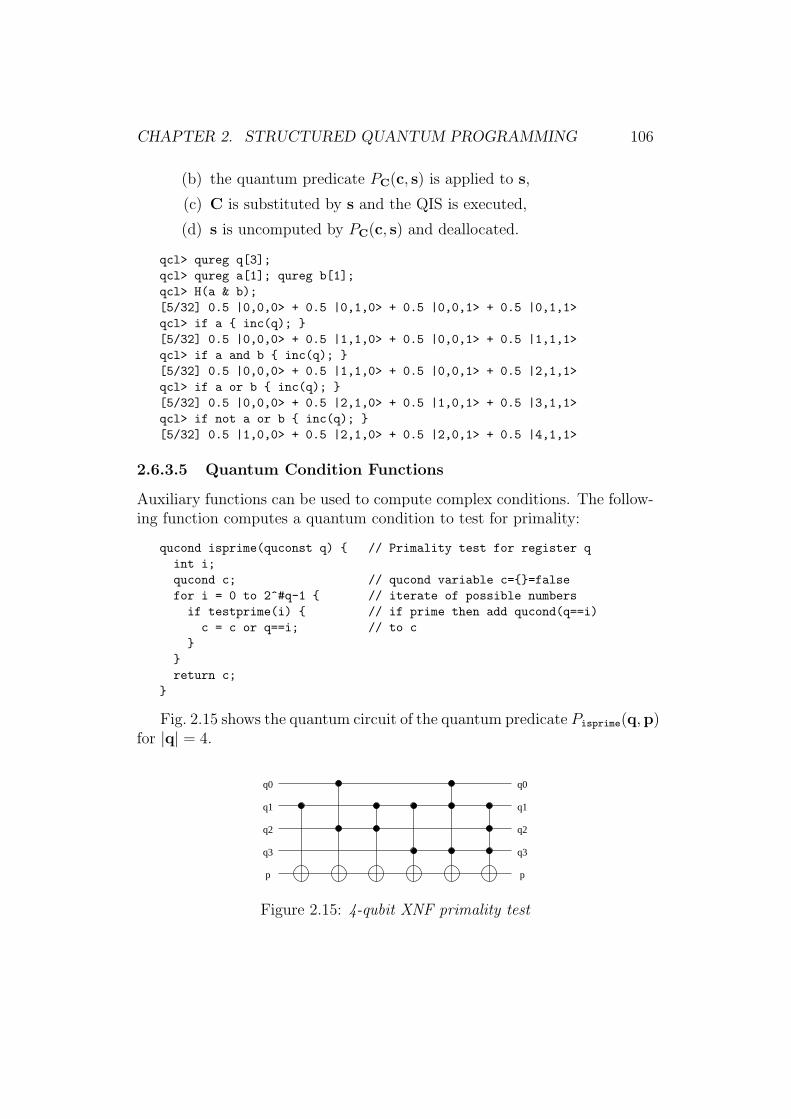
CHAPTER 2. STRUCTURED QUANTUM PROGRAMMING 106
(b) the quantum predicate PC(c, s) is applied to s,
(c) C is substituted by s and the QIS is executed,
(d) s is uncomputed by PC(c, s) and deallocated.
qcl> qureg q[3];qcl> qureg a[1]; qureg b[1];qcl> H(a & b);[5/32] 0.5 |0,0,0> + 0.5 |0,1,0> + 0.5 |0,0,1> + 0.5 |0,1,1>qcl> if a { inc(q); }[5/32] 0.5 |0,0,0> + 0.5 |1,1,0> + 0.5 |0,0,1> + 0.5 |1,1,1>qcl> if a and b { inc(q); }[5/32] 0.5 |0,0,0> + 0.5 |1,1,0> + 0.5 |0,0,1> + 0.5 |2,1,1>qcl> if a or b { inc(q); }[5/32] 0.5 |0,0,0> + 0.5 |2,1,0> + 0.5 |1,0,1> + 0.5 |3,1,1>qcl> if not a or b { inc(q); }[5/32] 0.5 |1,0,0> + 0.5 |2,1,0> + 0.5 |2,0,1> + 0.5 |4,1,1>
2.6.3.5 Quantum Condition Functions
Auxiliary functions can be used to compute complex conditions. The follow-ing function computes a quantum condition to test for primality:
qucond isprime(quconst q) { // Primality test for register qint i;qucond c; // qucond variable c={}=falsefor i = 0 to 2^#q-1 { // iterate of possible numbers
if testprime(i) { // if prime then add qucond(q==i)c = c or q==i; // to c
}}return c;
}
Fig. 2.15 shows the quantum circuit of the quantum predicate Pisprime(q,p)for |q| = 4.
q0
q1
q2
q3
p
q0
q1
q2
q3
p
Figure 2.15: 4-qubit XNF primality test
CHAPTER 2. STRUCTURED QUANTUM PROGRAMMING 107
qcl> qureg q[4];qcl> H(q);[4/32] 0.25 |0> + 0.25 |1> + 0.25 |2> + 0.25 |3> + 0.25 |4> +0.25 |5> + 0.25 |6> + 0.25 |7> + 0.25 |8> + 0.25 |9> + 0.25 |10> +0.25 |11> + 0.25 |12> + 0.25 |13> + 0.25 |14> + 0.25 |15>
qcl> if isprime(q) { Phase(pi); } // swap sign if prime[4/32] 0.25 |0> + 0.25 |1> - 0.25 |2> - 0.25 |3> + 0.25 |4> -0.25 |5> + 0.25 |6> - 0.25 |7> + 0.25 |8> + 0.25 |9> + 0.25 |10> -0.25 |11> + 0.25 |12> - 0.25 |13> + 0.25 |14> + 0.25 |15>
Appendix A
QCL Quick Reference
A.1 Syntax
The syntactic structure of a QCL program is described by a context freeLALR(1) grammar. For the formal syntax definition the following notationis used:
expression-name ← expression-def 1
← expression-def 2
· · · · · ·
Within syntax definitions, the following conventions apply
• Keywords and other literal text is set in courier
• Subexpressions are set in italic
• Optional expressions are put in [ square brackets ]. Optional expres-sions can be repeated 0 or 1 times.
• Multiple expressions are put in { braces }. Multiple expression canbe repeated 0, 1 or n times.
• Alternatives are written as alt 1| alt 2| . . . Exactly one alternative hasto be chosen.
• Grouping of expressions can be forced by ( round brackets ).
To simplify the notation of literals, the following character classes aredefined:
108
APPENDIX A. QCL QUICK REFERENCE 109
• digit ← decimal digit from 0 to 9.
• letter ← alphabetic letter form a to z or A to Z. Case is significant.
• char ← printable character except ‘"’.
A QCL Program is a sequence of statements and definitions so
qcl-input ← { stmt | def }
Comments Like C++, QCL supports two ways of commenting code. Allcomments are simply discarded by the scanner.
Line comments are started with // and last until the end of the currentline
C-style comments are started with /* and terminated with */ and maycontinue over several lines. C-style comments may not be nested.
A.1.1 Expressions
complex-coord ← [ + | - ] digit { digit } [ . { digit }]const ← digit { digit } [ . { digit }]
← ( complex-coord , complex-coord )
← true | false← " { char } "
subscript ← identifier [ expr { , expr } ]expr ← const | subscript
← identifier [ [ expr [( : | .. ) expr ] ] ]
← identifier ( [ expr { , expr }] )← ( expr )
← # expr
← expr ^ expr
← - expr
← expr ( * | / ) expr
← expr mod expr
← expr ( + | - | & ) expr

APPENDIX A. QCL QUICK REFERENCE 110
← expr ( == | != | < | <= | > | >= ) expr
← not expr
← expr and expr
← expr ( or | xor ) expr
A.1.2 Statements
block ← { stmt { stmt } }option ← letter { letter | - }
stmt ← [ ! ] identifier ( [ expr { , expr }] ) ;
← ( identifier | subscript ) = expr ;
← expr ( -> | <- | <-> ) expr ;
← for identifier = expr to expr [ step expr ] block
← while expr block
← block until expr ;
← if expr block [ else block ]
← return expr ;
← input [ expr , ] identifier ;
← print expr [ , expr ] ;
← exit [ expr ] ;
← measure expr [ , identifier ] ;
← reset ;
← dump [ expr ] ;
← list [ identifier { , identifier }] ;← ( load | save ) [ expr ] ;
← shell ;
← set option [ , expr ] ;
← stmt ;
A.1.3 Definitions
scalartype ← int | real | complexquantumtype ← qureg | quvoid | quconst | quscratch
tensortype ← ( vector | matrix | tensor digit ) scalartype
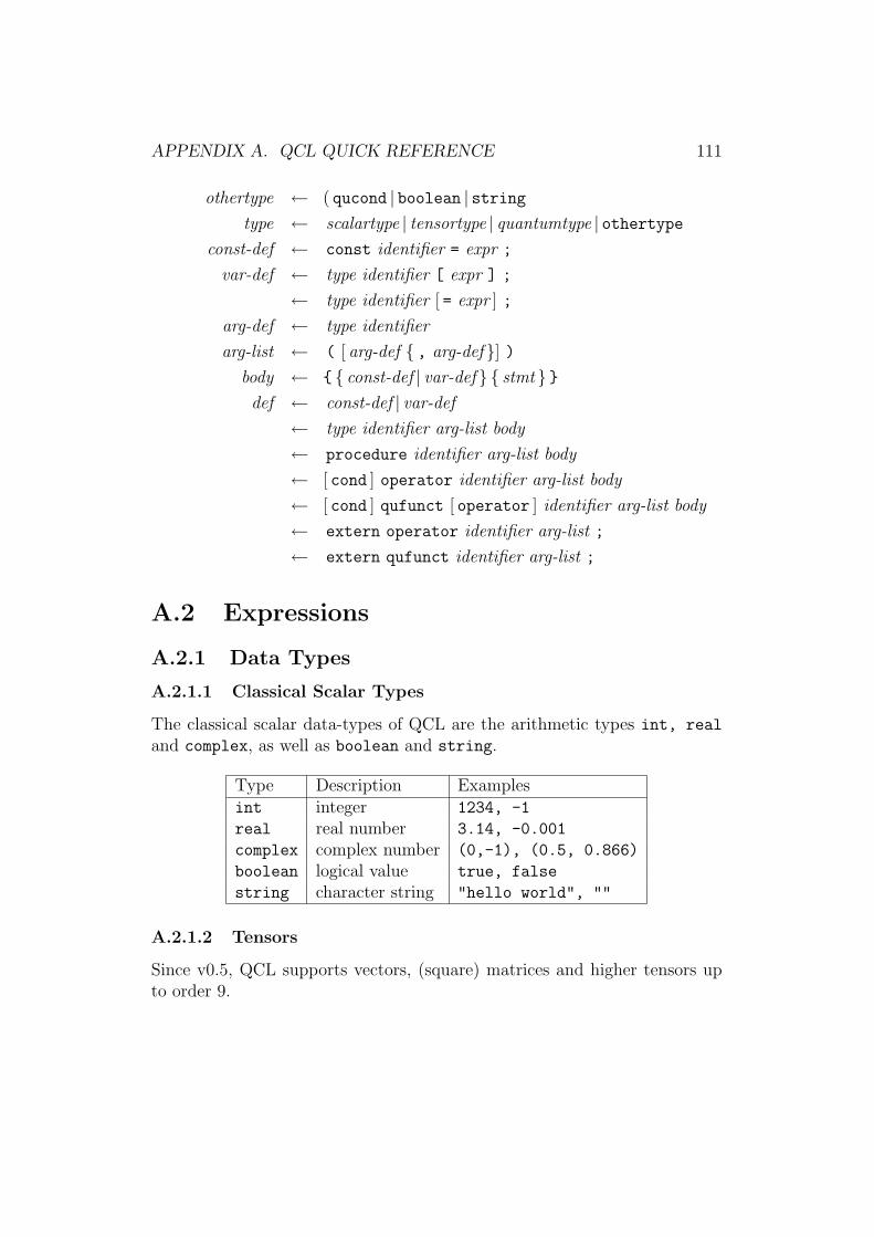
APPENDIX A. QCL QUICK REFERENCE 111
othertype ← ( qucond | boolean | stringtype ← scalartype | tensortype | quantumtype | othertype
const-def ← const identifier = expr ;
var-def ← type identifier [ expr ] ;
← type identifier [ = expr ] ;
arg-def ← type identifier
arg-list ← ( [ arg-def { , arg-def }] )body ← { { const-def | var-def } { stmt } }def ← const-def | var-def
← type identifier arg-list body
← procedure identifier arg-list body
← [ cond ] operator identifier arg-list body
← [ cond ] qufunct [ operator ] identifier arg-list body
← extern operator identifier arg-list ;
← extern qufunct identifier arg-list ;
A.2 Expressions
A.2.1 Data Types
A.2.1.1 Classical Scalar Types
The classical scalar data-types of QCL are the arithmetic types int, real
and complex, as well as boolean and string.
Type Description Examplesint integer 1234, -1
real real number 3.14, -0.001
complex complex number (0,-1), (0.5, 0.866)
boolean logical value true, false
string character string "hello world", ""
A.2.1.2 Tensors
Since v0.5, QCL supports vectors, (square) matrices and higher tensors upto order 9.

APPENDIX A. QCL QUICK REFERENCE 112
Type Description Examplesvector vector vector(0,0.5,0.866)
matrix square matrix matrix(0,(0,-1),(0,1),0)
tensorn tensor of order n tensor3(1,0,0,0,0,0,0,1)
Tensors can be defined for the arithmetic scalar types int, real andcomplex. A tensor variable v of order n and dimension dim is declared bythe syntax
scalartype tensorn v[dim];
For tensors of order 1 and 2 the keywords vector and matrix can be used.The subscript operator v[coord] is used to access tensor elements with
coord being a comma separated list of n zero-based integer indices.There are no tensor literals; instead a tensor object of order n and di-
mension d is created by the constructor function tensorn(elem), with elem
being a comma separated list of dn scalar expressions ordered in ascendingorder of their indices with the leftmost index being the most significant.
Tensors of equal order and dimension can be added, subtracted and as-signed to. Tensors can be multiplied by scalars or by tensors of equal dimen-sion. In the latter case, multiplication is defined as generalized dot-product,i.e. contraction by summing over the innermost indices
ai1...in−1in ∗ bj1j2...jm =∑
k
ai1...in−1kbkj2...jm
A.2.1.3 Register Types
For local variables or parameters of the types quvoid and quscratch let Ube the corresponding unitary operator.
Type Function Restrictionqureg general register nonequconst quantum constant invariant to all operatorsquvoid target register empty when U is calledquscratch scratch register empty when U or U † are called
A.2.1.4 Quantum Conditions
Boolean expressions of qubits are represented by the QCL type qucond. LetC be a variable of type qucond and
C = {pi} =n−1⊕
i=0
|pi|−1∧
j=0
pij
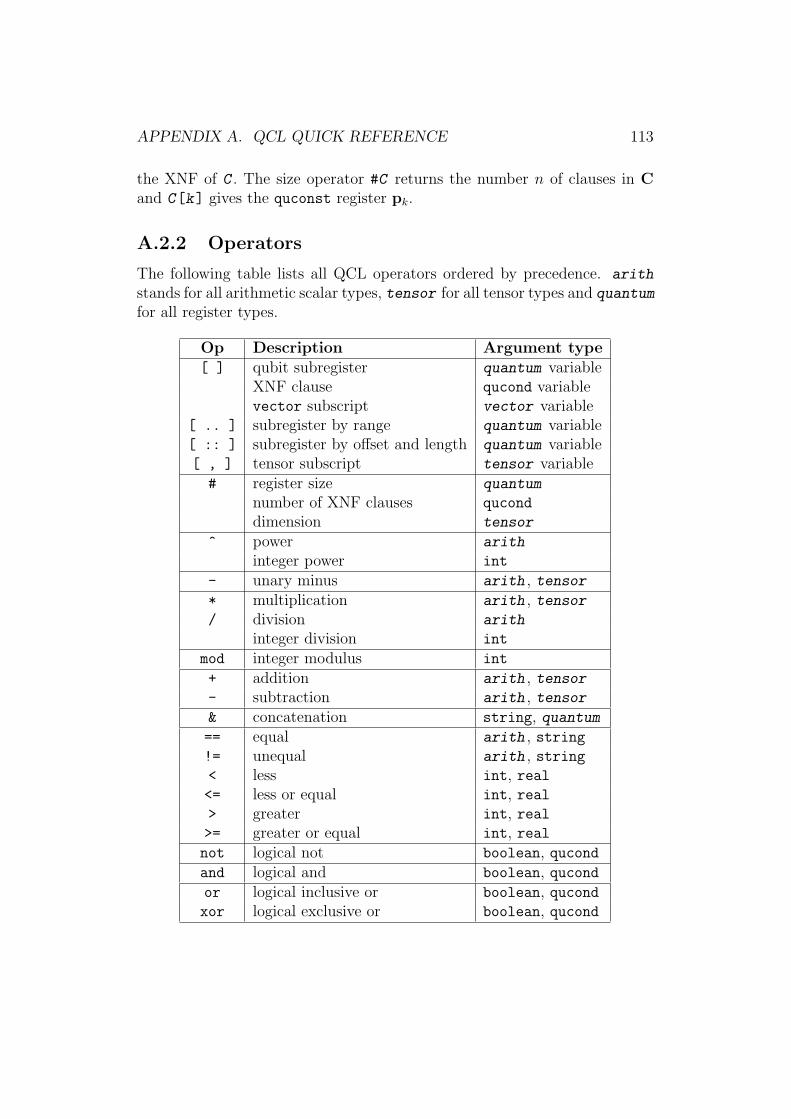
APPENDIX A. QCL QUICK REFERENCE 113
the XNF of C . The size operator #C returns the number n of clauses in Cand C[k] gives the quconst register pk.
A.2.2 Operators
The following table lists all QCL operators ordered by precedence. arith
stands for all arithmetic scalar types, tensor for all tensor types and quantum
for all register types.
Op Description Argument type[ ] qubit subregister quantum variable
XNF clause qucond variablevector subscript vector variable
[ .. ] subregister by range quantum variable[ :: ] subregister by offset and length quantum variable[ , ] tensor subscript tensor variable
# register size quantum
number of XNF clauses qucond
dimension tensor
^ power arith
integer power int
- unary minus arith , tensor* multiplication arith , tensor/ division arith
integer division int
mod integer modulus int
+ addition arith , tensor- subtraction arith , tensor& concatenation string, quantum== equal arith , string!= unequal arith , string< less int, real<= less or equal int, real> greater int, real>= greater or equal int, realnot logical not boolean, qucondand logical and boolean, qucondor logical inclusive or boolean, qucondxor logical exclusive or boolean, qucond
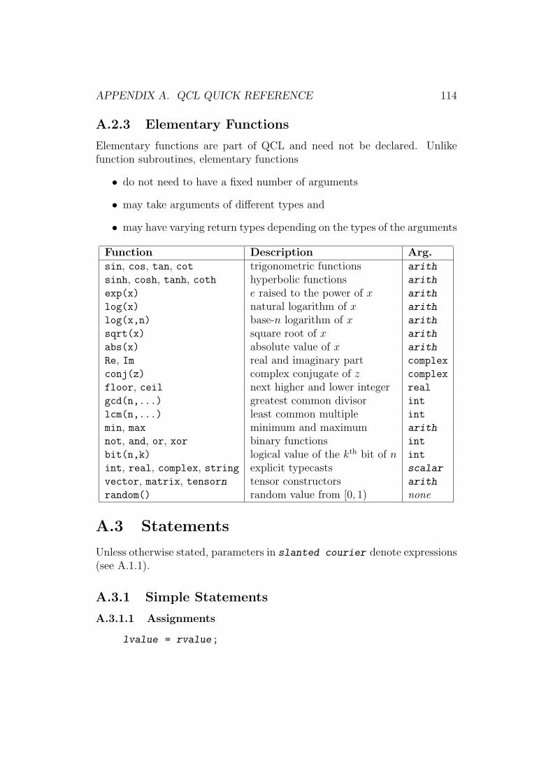
APPENDIX A. QCL QUICK REFERENCE 114
A.2.3 Elementary Functions
Elementary functions are part of QCL and need not be declared. Unlikefunction subroutines, elementary functions
• do not need to have a fixed number of arguments
• may take arguments of different types and
• may have varying return types depending on the types of the arguments
Function Description Arg.sin, cos, tan, cot trigonometric functions arith
sinh, cosh, tanh, coth hyperbolic functions arith
exp(x) e raised to the power of x arith
log(x) natural logarithm of x arith
log(x,n) base-n logarithm of x arith
sqrt(x) square root of x arith
abs(x) absolute value of x arith
Re, Im real and imaginary part complex
conj(z) complex conjugate of z complex
floor, ceil next higher and lower integer real
gcd(n,...) greatest common divisor int
lcm(n,...) least common multiple int
min, max minimum and maximum arith
not, and, or, xor binary functions int
bit(n,k) logical value of the kth bit of n int
int, real, complex, string explicit typecasts scalar
vector, matrix, tensorn tensor constructors arith
random() random value from [0, 1) none
A.3 Statements
Unless otherwise stated, parameters in slanted courier denote expressions(see A.1.1).
A.3.1 Simple Statements
A.3.1.1 Assignments
lvalue = rvalue;
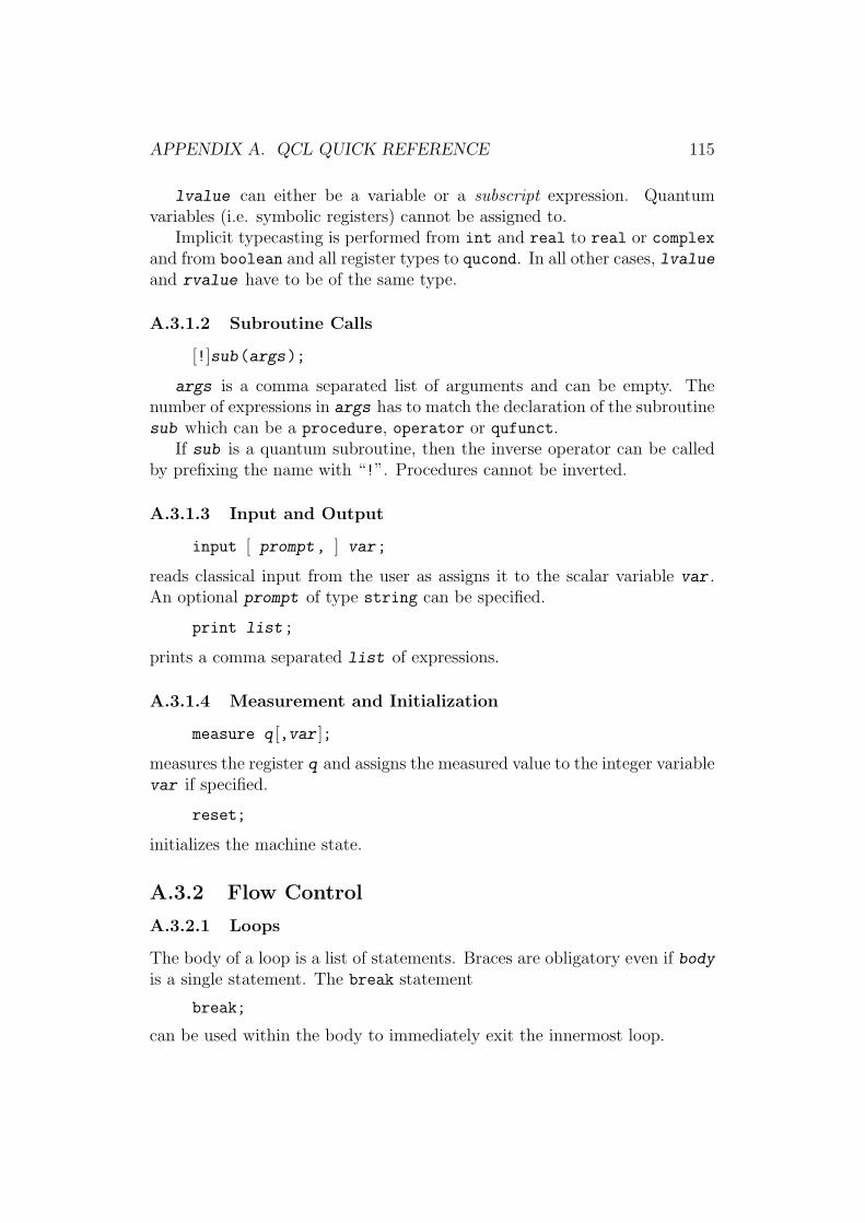
APPENDIX A. QCL QUICK REFERENCE 115
lvalue can either be a variable or a subscript expression. Quantumvariables (i.e. symbolic registers) cannot be assigned to.
Implicit typecasting is performed from int and real to real or complexand from boolean and all register types to qucond. In all other cases, lvalueand rvalue have to be of the same type.
A.3.1.2 Subroutine Calls
[!]sub(args);
args is a comma separated list of arguments and can be empty. Thenumber of expressions in args has to match the declaration of the subroutinesub which can be a procedure, operator or qufunct.
If sub is a quantum subroutine, then the inverse operator can be calledby prefixing the name with “!”. Procedures cannot be inverted.
A.3.1.3 Input and Output
input [ prompt, ] var;
reads classical input from the user as assigns it to the scalar variable var .An optional prompt of type string can be specified.
print list;
prints a comma separated list of expressions.
A.3.1.4 Measurement and Initialization
measure q [,var ];
measures the register q and assigns the measured value to the integer variablevar if specified.
reset;
initializes the machine state.
A.3.2 Flow Control
A.3.2.1 Loops
The body of a loop is a list of statements. Braces are obligatory even if bodyis a single statement. The break statement
break;
can be used within the body to immediately exit the innermost loop.
APPENDIX A. QCL QUICK REFERENCE 116
Conditional Loops
while cond { body }
{ body } until cond;
cond is a boolean expression. The body of an until-loop is executed atleast once.
Counting Loops
for i = a to b [ step s ] { body }
The range a , b and the optional step size s are integer expressions. Theloop variable i is also of type int and is redeclared as symbolic constantwithin the body.
A.3.2.2 If-statement
if cond { sigma } [ else { tau }]
The if-branch sigma and the optional else-branch tau are list of state-ments; braces are obligatory even for single statements.
The if-condition cond is either a boolean expression (classical if-statement)or a quantum condition (quantum if-statement).
A.3.2.3 Abnormal Termination
exit msg;
prints out the error message msg and terminates the QCL program.
A.3.3 Interactive Commands
The QCL interpreter qcl defines additional commands which are mainlyintended for interactive use and debugging and not considered to be core-parts of QCL.
A.3.3.1 Simulation Commands
The following commands are only available if QCL is used together with anumerical simulator.
dump [ q ];

APPENDIX A. QCL QUICK REFERENCE 117
prints the probability spectrum of the register q . If no register is specified,the current machine state is printed.
plot [ q ];
plots the probability spectrum of the register q . If no register is specified,the current machine state is plotted.
plot q, p ;
plots the probability spectrum of q ◦ p as two-dimensional density graph.
save file;
saves the current machine state to file .
load file;
loads the current machine state from file .
A.3.3.2 Other Commands
set opt val;
sets the interpreter option opt (without the leading “--”) to the value val .Please refer to appendix A.4 for a complete list of options.
list [sym ];
lists the definition of the symbol sym in the current scope. If no symbol isspecified, all currently defined symbols are listed.
shell;
opens a subshell which can be closed again with the exit command. Sub-shells can also be opened in response to keyboard interrupts and runtimeerrors (see A.4). Symbols defined in a subshell are local and leave scopewhen the shell is left again.
exit;
closes the current shell. Closing the top-level shell terminates the session.
APPENDIX A. QCL QUICK REFERENCE 118
A.4 Interpreter Options
The QCL interpreter qcl has the following options:
Startup Options Those can only be set on the command line.
-h, --help display this message-V, --version display version information-i, --interactive force interactive mode-x, --exec<commands> execute ¡commands¿ on startup-q, --quiet skip startup message--color color xterm interface--texmacs TeXmacs interface (experimental)-n, --no-default-include don’t read default.qcl on startup-o, --logfile specify a logfile-b, --bits=n: set number of qubits (32)
Dynamic Options Those can be set on the command line or via the set
command (see above). Default values are given in brackets.
-s, --seed=<seed-value> set random seed value (system time)-I, --include-path=<path> QCL include path (/usr/local/lib/qcl)--library=<y|n> ignore redefinitions of existing symbols (n)-d, --dump-file=<file> send output of dump-command to file (none)-p, --plot-file=<file> Postscript file created by plot-command (none)-f, --dump-format=x,d,b list base vectors as hex, decimal or binary (d)-r, --show-regs=<y|n> show global registers in dumped states (y)-D, --dump-precision=<d> shown d digits in dumped states (5)-P, --precision=<digits> shown digits for real and complex values (6)-Z, --trunc-zeros=<y|n> truncate zeros for real and complex values (y)-T, --truc-states=<y|n> truncate non-allocated qubits (y)--plot-paper=<format> Set paper-format for Postscript output (b5)--plot-size=<pixel> Set maximum window size for X11 plots (600)-Q, --qureg-mask=<y|n> list registers as masks instead of lists (n)-g, --debug=<y|n> open debug-shell on error (n)-a, --auto-dump=<max> dump states up to max terms in shell mode (8)-l, --log==<y|n> log external operator calls (n)-L, --log-state==<y|n> log state after each transformation (n)-c, --check==<y|n> check consistency of quantum heap (n)--trace==<y|n> trace mode (very verbose) (n)-S, --syntax=<y|n> check only the syntax, no interpretation (n)-E, --echo=<y|n> echo parsed input (n)-t, --test=<y|n> test program, ignore quantum operations (n)-e, --shell-escape=<y|n> honor shell-escapes (y)--irq=<y|n> allow user interrupts if supported (y)
Bibliography
[1] Anthony A. Aaby: Introduction to Programming Languages (1996).http://cs.wwc.edu/~aabyan/221_2/PLBOOK/
[2] G. Baker: Qgol (1996). project-thesis, Macquarie University,http://www.ifost.org.au/~gregb/q-gol/
[3] A. Barenco et al.: Elementary Gates for Quantum Computation(1995). Phys. Rev. A 52, pp. 3457-3467
[4] D. Beckman et al.: Efficient networks for quantum factoring (1996).Phys. Rev. A 54, pp. 1034-1063
[5] P.A. Benioff: The computer as a physical system: A microscopicquantum mechanical Hamiltonian model of computers as representedby Turing machines (1980). J. Stat. Phys., 22(5), pp. 563-591
[6] P.A. Benioff: Models of Quantum Turing Machines (1997). LANLquant-ph/9708054
[7] C.H. Bennet: Logical Reversibility of Computation (1973). IBM J.Res. Develop. 17, 525
[8] C.H. Bennet: Time-space trade-offs for reversible computation (1989).SIAM J. Comput. 18, p. 766
[9] E. Bernstein, U. Vazirani: Quantum complexity theory (1997). SIAMJ. Comput., 26(5), pp. 1411-1473
[10] S. Blaha: Quantum Computers and Quantum Computer Languages:Quantum Assembly Language and Quantum C Language (2002).LANL quant-ph/0201082
[11] C. Bohm and G. Jacopini: Flow Diagrams, Turing Machines, andLanguages with Only Two Formation Rules (1966). Communicationsof the ACM, Vol. 9, No. 5, pp. 336-371
119
BIBLIOGRAPHY 120
[12] M. Boyer, G. Brassard, P. Hoyer, A. Tapp: Tight bounds on quantumsearching (1998). Fortschritte der Physik, vol. 46(4-5), pp. 493-505
[13] P.O, Boykin et al.: On universal and fault-tolerant quantumcomputing (1999). LANL quant-ph/9906054
[14] J. Branson: Quantum Physics 130A (2001). lecture notes,http://heppc16.ucsd.edu/ph130a/130a_notes/node15.html
[15] J. Buchmann: Faktorisierung großer Zahlen (1996). Spektrum derWissenschaft 9/96, pp. 80-88
[16] S.L. Braunstein: Quantum computation: a tutorial (1995).http://www.informatics.bangor.ac.uk/~schmuel/comp/comp.html
[17] D.C. Cassidy: Exhibit on Werner Heisenberg (1998). AmericanInstitute of Physicshttp://www.aip.org/history/heisenberg/p09_text.htm
[18] I.L. Chuang et al.: NMR quantum computing: Realizing Shor’salgorithm (2001). Nature 414, pp. 883-887
[19] J.I. Cirac, P. Zoller: Quantum Computations with Cold trapped Ions(1995). Phys. Rev. Lett. 74, p. 4091
[20] R. Cleve, A.Ekert, C. Macchiavello, M. Mosca: Quantum algorithmsrevisited (1998). Proc. R. Soc., London A 454, pp. 339-354
[21] B.J. Copeland: The Church-Turing Thesis (1996). StanfordEncyclopedia of Philosophy ISSN, pp. 1095-5054
[22] D. Coppersmith: An Approximate Fourier Transform Useful inQuantum Factoring (1994). IBM Research Report No. RC19642
[23] O.J. Dahl, E.W. Dijkstra, C.A.R. Hoare: Structured Programming(1972). Academic Press, London, UK
[24] D. Deutsch,: Quantum theory, the Church-Turing principle and theuniversal quantum computer (1985). Proc. R. Soc., London, A 400, pp.97-117
[25] D. Deutsch: Quantum computational networks (1989). Proc. R. Soc.,London, A 439, pp. 553-558
BIBLIOGRAPHY 121
[26] D. Deutsch and R. Jozsa: Rapid solution of problems by quantumcomputer (1992). Proc. Roy. Soc. London, Ser. A, vol. 439, pp.553-558
[27] E.W. Dijkstra: Structured Programming (1969). Software EngineeringTechniques, Buxton, J. N., and Randell, B., eds. Brussels, Belgium,NATO Science Committee
[28] D.P. DiVincenzo: Two bit gates are universal for quantumcomputation (1995). Phys. Rev. A, 51(2), pp. 1015-1022
[29] A. Einstein, B. Podolsky, N. Rosen: Can quantum-mechanicaldescription of physical reality be considered complete? (1935). PhysicalReview 47, pp. 777-780
[30] A. Ekert, R. Jozsa: Shor’s Quantum Algorithm for Factoring Numbers(1996). Rev. Modern Physics 68 (3), pp. 733-753
[31] R.P. Feynman: Quantum mechanical computers (1985). Optics News11, pp 11-20
[32] Lov K. Grover: A fast quantum mechanical algorithm for databasesearch (1996). Proceeding of the 28th Annual ACM Symposium onTheory of Computing
[33] J. Gruska,: Foundations of Computing (1998). chap. 12: “Frontiers -Quantum Computing”
[34] G.H. Hardy, E.M. Wright: An Introduction to the Theory of NumbersOxford (1938). U.K.: Oxford Univ. Press
[35] A. Hermann: Lexikon - Geschichte der Physik A-Z (1978). Aulis-VerlagDeubner & Co KG
[36] R.W. Keyes: Miniaturization of electronics and its limits (1988). IBMJ. Res. Develop. 32(1), pp. 24-28
[37] D. Kielpinski, C. Monroe and D.J. Wineland: Architecture for alarge-scale ion-trap quantum computer (2002). Nature 417, pp. 709-711
[38] W. Kummer and R. Trausmuth: Quantentheorie (1988). Skriptum zurVorlesung 131.869
[39] A. Leitsch: Skriptum zur Vorlesung “Algorithmen-, Rekursions undKomplexitatstheorie” (1994). Technical University Vienna

BIBLIOGRAPHY 122
[40] M. Agrawal, N. Kayal, N. Saxena: PRIMES is in P (2002). preprint,http://www.cse.iitk.ac.in/users/manindra/primality.ps
[41] Z. Meglicki: Introduction to Quantum Computing (M743) (2002).http://beige.ucs.indiana.edu/B679/M743.html
[42] F.D. Murnaghan: The Unitary and Rotation Groups (1962). SpartanBooks, Washington
[43] M.A. Nielsen and I.L. Chuang: Quantum Computation and QuantumInformation (2000). Cambridge University Press
[44] B. Omer: Simulation of Quantum Computers (1996).http://www.itp.tuwien.ac.at/~oemer/papers.html
[45] B. Omer: A Procedural Formalism for Quantum Computing (1998).master-thesis, Technical University of Vienna
[46] B. Omer: Quantum Programming in QCL (2000). master-thesis,Technical University of Vienna
[47] B. Omer: Procedural Quantum Programming (2002). Proc. of the 5thInt. Conference CASYS 2001, D. M. Dubois (Ed.), AIP ConferenceProceedings 627, pp. 276-285
[48] B. Omer: Classical Concepts in Quantum Programming (2003).accepted for publication in the QS2002 Conference Proceedings, LANLquant-ph/0211100
[49] B. Omer: QCL homepage (2003).http://www.itp.tuwien.ac.at/~oemer/qcl.html
[50] E.L. Post: Finite Combinatory Processes - Formulation 1 (1936).Journal of Symbolic Logic, 1, pp. 103-105
[51] H. Putnam: A philosopher looks at quantum mechanics (1965). R.Colodny (ed.), Beyond the Edge of Certainty: Essays in ContemporaryScience and Philosophy, Englewood Cliffs, New Jersey: Prentice Hall,pp. 130-158.
[52] M. Reck, A. Zeilinger, H.J. Bernstein, P. Bertani: Experimentalrealization of any discrete unitary operator (1994). Phys. Rev. Lett.,73(1), pp. 58-61
BIBLIOGRAPHY 123
[53] M.A. Rowe et al.: Transport of quantum states and separation of ionsin a dual rf ion trap (2002). Quantum Information and Computation 2,pp. 257-271
[54] P.W. Shor.: Algorithms for quantum computation: Discrete logarithmsand factoring (1994). Proc. 35th Annual Symposium on Foundations ofComputer Science, IEEE Press, Los Alamitos, CA
[55] R. Solovay and V. Strassen: A Fast Monte-Carlo Test for Primality(1977). SIAM Journal on Computing, 1977, pp. 84-85
[56] K. Svozil: Quantum algorithmic information theory (1996). Journal ofUniversal Computer Science 2, pp. 311-346
[57] T. Toffoli: Bicontinuous extension of reversible combinatorial functions(1981). Math. Syst. Theory 14, pp. 13-23
[58] A.M. Turing: On computable numbers, with an application to theEntscheidungsproblem (1936). Proc. of the London MathematicalSociety, ser. 2. vol. 42, pp. 230-265,http://www.abelard.org/turpap2/tp2-ie.asp
[59] A.M. Turing: Intelligent Machinery (1948). National PhysicalLaboratory Report. In Meltzer, B., Michie, D. (eds) 1969. MachineIntelligence 5. Edinburgh: Edinburgh University Press., 7
[60] B. VanHoy: Structured Programming, Control Structures, if-elseStatements, Pseudocode (1998). APCS-C++, Lesson 8, ICThttp://www.mvhs.fuhsd.org/bob_vanhoy/pdfs/lesson08.pdf
[61] J. Wallace: Quantum Computer Simulators (2001). Partial Proc. of the4th Int. Conference CASYS 2000, D. M. Dubois (Ed.), InternationalJournal of Computing Anticipatory Systems, volume 10, 2001, pp.230-245
[62] J. Wallace: Quantum Computer Simulators (2002). online survey,http://www.dcs.ex.ac.uk/~jwallace/simtable.htm
[63] P. Zuliani: Quantum Programming (2001). PhD thesis, University ofOxford,http://web.comlab.ox.ac.uk/oucl/work/paolo.zuliani/pzthesis.ps.gz
List of Figures
1.1 A program π controlling a machine M = (S, O, T, δ, β) . . . . 171.2 Bloch sphere representation of the qubit state |ψ〉 . . . . . . . . 211.3 Circuit notation for common gates . . . . . . . . . . . . . . . . 37
2.1 A simple probabilistic quantum algorithm . . . . . . . . . . . . 522.2 Parity of a bit string of length 4 . . . . . . . . . . . . . . . . . 532.3 Hybrid quantum architecture . . . . . . . . . . . . . . . . . . . 572.4 Classical computer with quantum oracle . . . . . . . . . . . . . 582.5 Basic control structures . . . . . . . . . . . . . . . . . . . . . . 632.6 Register operator U(s) . . . . . . . . . . . . . . . . . . . . . . 712.7 Quantum Fourier Transform for a 4-qubit register . . . . . . . 792.8 Recursive phase transformation . . . . . . . . . . . . . . . . . 802.9 5-qubit test state . . . . . . . . . . . . . . . . . . . . . . . . . 822.10 Increment operator . . . . . . . . . . . . . . . . . . . . . . . . 862.11 Conditional increment operator . . . . . . . . . . . . . . . . . 952.12 Call graph of QCL subroutines . . . . . . . . . . . . . . . . . . 962.13 A quantum multiplexer . . . . . . . . . . . . . . . . . . . . . . 1022.14 Dual log phase transform . . . . . . . . . . . . . . . . . . . . . 1032.15 4-qubit XNF primality test . . . . . . . . . . . . . . . . . . . . 106
124
List of Tables
1.1 Dirac Notation . . . . . . . . . . . . . . . . . . . . . . . . . . 51.2 Classical and quantum computational models . . . . . . . . . . 341.3 Register Notation . . . . . . . . . . . . . . . . . . . . . . . . . 35
2.1 Classical and quantum programming concepts . . . . . . . . . . 492.2 Equivalent TM and CQTM commands . . . . . . . . . . . . . 552.3 Scalar arithmetic types and literals in QCL . . . . . . . . . . . 602.4 Quantum data types in QCL . . . . . . . . . . . . . . . . . . . 682.5 Register expressions in QCL . . . . . . . . . . . . . . . . . . . 692.6 Hierarchy of subroutines . . . . . . . . . . . . . . . . . . . . . 75
125
![Feyerabend and physics - TU Wientph.tuwien.ac.at/~svozil/publ/2004-fey.doc · Web viewLater, Feyerabend wrote several papers [55, 56] on physics-related topics, in particular on](https://img.pdfslide.us/doc/110x75/5f06f95b7e708231d41aaa71/feyerabend-and-physics-tu-svozilpubl2004-feydoc-web-view-later-feyerabend.jpg)