Embed Size (px)
Citation preview
PhD Thesis
Structured Hidden Markov Model:
A General Tool for Modeling Process Behavior
Ugo Galassi
Dipartimento di Informatica
Universita degli Studi di Torino
Advisors:
Prof. Attilio Giordana
Prof.ssa Lorenza Saitta
PhD Coordinator:
Prof. Pietro Torasso

2

I would like to dedicate this thesis to my mother
for her support, love and encouragement.
Abstract
Core of this thesis is the Structured Hidden Markov Model (S-HMM), a
variant of Hierarchical Hidden Markov Model, which shows interesting in-
teresting properties for modeling the generative process behind complex
events hidden in symbolic sequences. On the one hand, S-HMM exhibits
a quasi-linear computational complexity, which can be exploited in order
to construct very large models, as it may be required in many real time
critical applications. On the other hand, it may be constructed and trained
incrementally. Owing to this second property, it is possible to combine a
variety of machine learning and data-mining algorithms in order to learn
different components of a S-HMM from different knowledge sources. Fi-
nally, the S-HMM structure provides an abstraction mechanism allowing a
high level symbolic description of the knowledge embedded in S-HMM to
be easily obtained.
In the first part of the thesis, S-HMM is formally defined starting from the
framework provided by the graphical model approach, and its properties are
investigated. Afterwards, a new unsupervised learning algorithm it will be
presented, EDY (Event DiscoverY), which is capable of inferring a S-HMM
from a database of sequences. The algorithm is incremental and constructs
a complex S-HMM by assembling partial models, which can be mined from
the data or proposed by a human expert. EDY is validated on a suite of
artificial datasets, where the challenge for the algorithm is to reconstruct
the model that generated the data. Finally, an application to a real problem
of user profiling is described.
Contents
1 Introduction 1
1.1 The problem . . . . . . . . . . . . . . . . . . . . . . . . . . . . . . . . . 1
1.2 Existing Approaches . . . . . . . . . . . . . . . . . . . . . . . . . . . . . 4
1.3 Contributions and Outline of the Thesis . . . . . . . . . . . . . . . . . . 5
1.4 Citations to previously published work . . . . . . . . . . . . . . . . . . . 6
2 Process modeling 9
2.1 Modeling stochastic processes . . . . . . . . . . . . . . . . . . . . . . . . 10
2.1.1 What is a model? . . . . . . . . . . . . . . . . . . . . . . . . . . . 10
2.1.2 Stochastic models . . . . . . . . . . . . . . . . . . . . . . . . . . 11
2.1.3 Generative and Discriminative Models . . . . . . . . . . . . . . . 12
2.1.4 Probabilistic Graphical Models . . . . . . . . . . . . . . . . . . . 14
2.1.4.1 Directed and undirected models . . . . . . . . . . . . . 14
2.1.4.2 Considerations . . . . . . . . . . . . . . . . . . . . . . . 16
2.2 Markov Processes . . . . . . . . . . . . . . . . . . . . . . . . . . . . . . . 19
2.3 Observable Markov Models . . . . . . . . . . . . . . . . . . . . . . . . . 20
2.3.1 An example: the weather model . . . . . . . . . . . . . . . . . . 21
2.4 Hidden Markov Models . . . . . . . . . . . . . . . . . . . . . . . . . . . 23
2.4.1 From observable to hidden states . . . . . . . . . . . . . . . . . . 24
2.4.2 A formal definition of Hidden Markov Models . . . . . . . . . . . 27
2.5 Computing probabilities with HMMs . . . . . . . . . . . . . . . . . . . . 29
2.5.1 Forward algorithm . . . . . . . . . . . . . . . . . . . . . . . . . . 29
2.5.2 Viterbi algorithm . . . . . . . . . . . . . . . . . . . . . . . . . . . 31
2.5.3 The most probable state and the backward algorithm . . . . . . 32
2.5.4 Parameter estimation for HMMs . . . . . . . . . . . . . . . . . . 33
iii
CONTENTS
2.6 Hierarchical approach to HMMs . . . . . . . . . . . . . . . . . . . . . . . 35
2.7 Modeling Temporal Dynamics . . . . . . . . . . . . . . . . . . . . . . . . 38
2.7.1 Bayesian Networks . . . . . . . . . . . . . . . . . . . . . . . . . . 38
2.7.1.1 Factorization and Conditional Independence . . . . . . 40
2.7.1.2 Inference . . . . . . . . . . . . . . . . . . . . . . . . . . 41
2.7.2 Dynamic Bayesian Networks . . . . . . . . . . . . . . . . . . . . 43
2.7.2.1 First-order Markov Models from the DBN perspective . 44
2.7.2.2 Hidden Markov Models . . . . . . . . . . . . . . . . . . 45
2.7.2.3 Auto-Regressive Hidden Markov Models . . . . . . . . 46
2.7.2.4 Factorial Hidden Markov Models . . . . . . . . . . . . . 46
3 A new approach: the Structured Hidden Markov Model 49
3.1 The Structured Hidden Markov Model . . . . . . . . . . . . . . . . . . . 51
3.1.1 Structure of a Block . . . . . . . . . . . . . . . . . . . . . . . . . 51
3.1.2 Estimating Probabilities in S-HMM . . . . . . . . . . . . . . . . 53
3.2 S-HMMs are locally trainable . . . . . . . . . . . . . . . . . . . . . . . . 55
4 Applying S-HMMs to Real World Tasks 57
4.1 Sub-Models structure . . . . . . . . . . . . . . . . . . . . . . . . . . . . . 59
4.1.1 Left-to-Right HMMs . . . . . . . . . . . . . . . . . . . . . . . . . 60
4.2 Modeling duration and gaps . . . . . . . . . . . . . . . . . . . . . . . . . 62
4.3 Modeling motifs . . . . . . . . . . . . . . . . . . . . . . . . . . . . . . . 65
4.3.1 String Alignment and Multiple Alignment . . . . . . . . . . . . . 65
4.3.2 Building models from multiple alignments . . . . . . . . . . . . . 67
4.3.3 Another approach to motifs modeling . . . . . . . . . . . . . . . 69
4.4 Matching complexity . . . . . . . . . . . . . . . . . . . . . . . . . . . . . 70
4.5 Sequence Segmentation . . . . . . . . . . . . . . . . . . . . . . . . . . . 72
4.6 Knowledge Transfer . . . . . . . . . . . . . . . . . . . . . . . . . . . . . 74
5 Edy: a tool for unsupervised learning of SHMMs 77
5.1 Edy’s discovery strategy . . . . . . . . . . . . . . . . . . . . . . . . . . . 78
5.2 Learning algorithm . . . . . . . . . . . . . . . . . . . . . . . . . . . . . . 80
5.3 Model extension . . . . . . . . . . . . . . . . . . . . . . . . . . . . . . . 81
5.3.1 Searching for regularities . . . . . . . . . . . . . . . . . . . . . . 82
iv

CONTENTS
5.3.2 The extension procedure . . . . . . . . . . . . . . . . . . . . . . . 84
5.4 Model refinement . . . . . . . . . . . . . . . . . . . . . . . . . . . . . . . 85
5.5 Comparing EDY to other approaches . . . . . . . . . . . . . . . . . . . . 87
5.5.1 Inducing HMM by Bayesian model merging . . . . . . . . . . . . 87
5.5.2 Learning Hidden Markov Model for Information Extraction . . . 89
5.5.3 Meta-MEME . . . . . . . . . . . . . . . . . . . . . . . . . . . . . 90
5.5.4 A task specific learner for inferring structured cis-regulatory mod-
ules . . . . . . . . . . . . . . . . . . . . . . . . . . . . . . . . . . 91
6 Analysis on Artificial Traces 93
6.1 Artificial Datasets . . . . . . . . . . . . . . . . . . . . . . . . . . . . . . 94
6.1.1 ”Cities” Datasets . . . . . . . . . . . . . . . . . . . . . . . . . . . 95
6.1.2 ”Sequential” Datasets . . . . . . . . . . . . . . . . . . . . . . . . 95
6.1.3 ”Structured” Datasets . . . . . . . . . . . . . . . . . . . . . . . . 98
6.2 Comparing HMMs . . . . . . . . . . . . . . . . . . . . . . . . . . . . . . 99
6.3 Motif reconstruction in presence of noise . . . . . . . . . . . . . . . . . . 102
6.4 Discovering Sequential S-HMMs . . . . . . . . . . . . . . . . . . . . . . . 104
6.5 Discovering graph structured patterns . . . . . . . . . . . . . . . . . . . 113
6.6 Discussion . . . . . . . . . . . . . . . . . . . . . . . . . . . . . . . . . . . 118
7 An Application to Keystroking Dynamics for a Human Agent 121
7.1 The Experimental Setting . . . . . . . . . . . . . . . . . . . . . . . . . . 122
7.1.1 Input information . . . . . . . . . . . . . . . . . . . . . . . . . . 122
7.1.2 Modeling user behavior . . . . . . . . . . . . . . . . . . . . . . . 123
7.1.3 Model construction . . . . . . . . . . . . . . . . . . . . . . . . . . 124
7.2 User Profiling . . . . . . . . . . . . . . . . . . . . . . . . . . . . . . . . . 124
7.3 User Authentication . . . . . . . . . . . . . . . . . . . . . . . . . . . . . 125
8 Conclusions and future work 129
A Basic algorithms in presence of silent nodes 133
A.1 Forward algorithm . . . . . . . . . . . . . . . . . . . . . . . . . . . . . . 133
A.2 Backward algorithm . . . . . . . . . . . . . . . . . . . . . . . . . . . . . 134
A.3 Viterbi algorithm . . . . . . . . . . . . . . . . . . . . . . . . . . . . . . . 134
A.4 Bahum-Welch algorithm . . . . . . . . . . . . . . . . . . . . . . . . . . . 135
v

CONTENTS
Bibliography 143
vi

List of Figures
2.1 An example of directed (a) graph that cannot be re-expressed as an
undirected graph and vice versa (b) . . . . . . . . . . . . . . . . . . . . 16
2.2 An example of directed (a) graph G and the corresponding moralized
graph Gm (b) . . . . . . . . . . . . . . . . . . . . . . . . . . . . . . . . . 17
2.3 Moralization could suppress some of the conditional independences in a
graph. (a) A directed acyclic graph. (b) The correspondent moral graph
in which E is become part of the conditioning set of F . (c) The revisited
moral graph. . . . . . . . . . . . . . . . . . . . . . . . . . . . . . . . . . 18
2.4 An Observable Markov Model describing the weather evolution . . . . . 22
2.5 An Hidden Markov Model for the weather scenario . . . . . . . . . . . . 24
2.6 Models designed for the problem of dishonest gambler: (a) a six-state
Observable Markov Model, (b) a corresponding degenerated HMM, (c)
a two state HMM . . . . . . . . . . . . . . . . . . . . . . . . . . . . . . . 26
2.7 Algorithm for generating a sequence of observations by an HMM λ. . . . 28
2.8 Given a model and set of training sequences it is possible to compute the
observations probabilities in each state, computing the relative frequencies 34
2.9 Example of Hierarchical Hidden Markov Model. . . . . . . . . . . . . . . 36
2.10 A Bayesian Net. Nodes represent binary random variables. A represent
the condition ”it is cloudy”, B represent the condition ”the sprinkler is
on”, C is ”it is raining” and D correspond to ”the grass is wet”. . . . . . 39
2.11 A Bayesian Net. X and Y are indepent but given Z they are conditional
dependent. . . . . . . . . . . . . . . . . . . . . . . . . . . . . . . . . . . 41
vii
LIST OF FIGURES
2.12 The bayes ball algorithm: (a),(c),(f) the ball cannot pass from A to C
and vice versa that are conditionally independent; (b),(d),(e) the ball
could pass, A and C are conditionally dependent. . . . . . . . . . . . . . 42
2.13 (a) An unrolled Temporal Bayesian Networks in which occur only extra-
slice connections. (b) An unrolled Dynamic Bayesian Networks allowing
also for intra-slice connections. Gray areas represents time slices. It is
evident that temporal models are sub-classes of dynamic models. . . . . 45
2.14 A Bayesian Net representing a first-order Markov Model . . . . . . . . . 45
2.15 A Bayesian Net representing an Hidden Markov Model.Gray nodes rep-
resent observable nodes . . . . . . . . . . . . . . . . . . . . . . . . . . . 46
2.16 An Auto-Regressive Hidden Markov Model.Gray nodes represent observ-
able nodes . . . . . . . . . . . . . . . . . . . . . . . . . . . . . . . . . . . 47
2.17 A Factorial Hidden Markov Model with three chains. Gray nodes repre-
sent observable nodes. . . . . . . . . . . . . . . . . . . . . . . . . . . . . 48
3.1 Example of Structured Hidden Markov Model composed of three inter-
connected blocks, plus two null blocks, λ0 and λ4, providing the start
and end states. Distribution A is non-null only for explicitly represented
arcs. . . . . . . . . . . . . . . . . . . . . . . . . . . . . . . . . . . . . . 53
4.1 Four topologies of HMMs. (a) A 4-states ergodic model. (b) A 1st-
order LR-HMM with 5 states. (c) A 5-states 2nd-order LR-HMM. (d)
A 6-state LR-HMM with two parallel path. . . . . . . . . . . . . . . . . 61
4.2 A single state HMM for modelling exponentially decaying distributions
of durations . . . . . . . . . . . . . . . . . . . . . . . . . . . . . . . . . . 62
4.3 Possible HMMs for modeling duration . . . . . . . . . . . . . . . . . . . 64
4.4 Examples of string alignments between several deformations of the word
”PARIS”, originated from insertion, deletion and substitution errors: (a)
Global alignment; (b) Local Alignment; (c) Multiple alignment. . . . . . 66
4.5 An Hidden Markov Model equivalent to a position specific score matrix.
Alignment is trivial because there is no choice of transitions. . . . . . . 67
4.6 An Hidden Markov Model with match and insert states denoted respec-
tively with squares and diamonds. . . . . . . . . . . . . . . . . . . . . . 68
viii

LIST OF FIGURES
4.7 An Hidden Markov Model with match and delete states denoted respec-
tively with squares and circle. Delete states are silent state introduced
in order to allow long gap keeping low the number of transitions. . . . . 69
4.8 Example of Profile Hidden Markov Model. Circles denote states with no-
observable emission, rectangles denote match states, and diamond denote
insert states. . . . . . . . . . . . . . . . . . . . . . . . . . . . . . . . . . 69
4.9 Complexity for a sequence interpretation task: (a) cpu time versus the
string length. Different curves correspond to different number of states. 72
4.10 Structured HMMs are easy to translate into an approximate logic de-
scription. . . . . . . . . . . . . . . . . . . . . . . . . . . . . . . . . . . . 76
5.1 Edy Algorithm; HALT denotes the variable that controls the overall
cycle execution. . . . . . . . . . . . . . . . . . . . . . . . . . . . . . . . . 82
5.2 Example of cluster hierarchy. Leaves corresponds to the states of the
level γ, whereas second level nodes correspond to models µ of motifs and
gaps . . . . . . . . . . . . . . . . . . . . . . . . . . . . . . . . . . . . . . 85
6.1 Model A2: it is composed by a chain of three motifs separated by alter-
native gap of varying length. Each one of the observable state is mapped
to one low-level automata . . . . . . . . . . . . . . . . . . . . . . . . . . 96
6.2 Model A3: it is composed by a chain of six motifs separated by alterna-
tive gap of varying length . . . . . . . . . . . . . . . . . . . . . . . . . . 96
6.3 Model A4: Like models A2 and A3 it is composed by a chain of motifs
separated by alternative gap of varying length. In this model we have 9
motifs . . . . . . . . . . . . . . . . . . . . . . . . . . . . . . . . . . . . . 97
6.4 Model B3: it is composed by a chain with forward jumps that allow
generating sequences with a varying number of motifs (varying from two
to six) that, when presents, they appear always in the same order . . . 97
6.5 Model C3: it is composed by a sequence of constant and alternative
motifs, separated by gaps . . . . . . . . . . . . . . . . . . . . . . . . . . 98
6.6 Model D3: it is a complex model with alternative motif (that could also
be optionals), alternated with gaps . . . . . . . . . . . . . . . . . . . . . 99
ix

LIST OF FIGURES
6.7 Algorithms performances on the sequences generated by models in Group
A2. The plot reports ǫ(λO, λD) on the test set versus the motif length
ML ∈ {5, 8, 11, 15}. . . . . . . . . . . . . . . . . . . . . . . . . . . . . . . 109
6.8 Algorithms performances on the sequences generated by models in Group
A2. The plot reports ǫ(λO, λD) on the test set versus the alphabet
cardinality |A| ∈ {4, 7, 14, 25}. . . . . . . . . . . . . . . . . . . . . . . . . 109
6.9 Algorithms performances on the sequences generated by models in Group
A3. The plot reports ǫ(λO, λD) on the test set versus the motif length
ML ∈ {5, 8, 11, 15}. . . . . . . . . . . . . . . . . . . . . . . . . . . . . . . 110
6.10 Algorithms performances on the sequences generated by models in Group
A3. The plot reports ǫ(λO, λD) on the test set versus the alphabet
cardinality |A| ∈ {4, 7, 14, 25}. . . . . . . . . . . . . . . . . . . . . . . . . 110
6.11 Algorithms performances on the sequences generated by models in Group
A4. The plot reports ǫ(λO, λD) on the test set versus the motif length
ML ∈ {5, 8, 11, 15}. . . . . . . . . . . . . . . . . . . . . . . . . . . . . . . 111
6.12 Algorithms performances on the sequences generated by models in Group
A4. The plot reports the error ǫ(λO, λD) on the test set versus the
alphabet cardinality |A| ∈ {4, 7, 14, 25}. . . . . . . . . . . . . . . . . . . 111
6.13 Algorithms performances on the sequences generated by models in Group
B3. The plot reports the ǫ(λO, λD) on the test set versus the motif length
ML ∈ {5, 8, 11, 15}. . . . . . . . . . . . . . . . . . . . . . . . . . . . . . . 112
6.14 Algorithms performances on the sequences generated by models in Group
B3. The plot reports ǫ(λO, λD) on the test set versus the alphabet car-
dinality |A| ∈ {4, 7, 14, 25}. . . . . . . . . . . . . . . . . . . . . . . . . . 112
6.15 Algorithms performances on the sequences generated by models in Group
C3. The plot reports the error Err = Err(λD) on the test set versus
the motif length ML ∈ {5, 8, 11, 15}. . . . . . . . . . . . . . . . . . . . . 116
6.16 Algorithms performances on the sequences generated by models in Group
C3. The plot reports the error Err = Err(λD) on the test set versus
the alphabet cardinality |A| ∈ {4, 7, 14, 25}. . . . . . . . . . . . . . . . . 116
6.17 Algorithms performances on the sequences generated by models in Group
D3. The plot reports the error Err = Err(λD) on the test set versus
the motif length ML ∈ {5, 8, 11, 15}. . . . . . . . . . . . . . . . . . . . . 117
x

LIST OF FIGURES
6.18 Algorithms performances on the sequences generated by models in Group
D3. The plot reports the error Err = Err(λD) on the test set versus
the alphabet cardinality |A| ∈ {4, 7, 14, 25}. . . . . . . . . . . . . . . . . 117
7.1 Example of string set obtained by expansion of a word. Typical typing
errors are evident, such as the exchange of the A with the I, or double
key strokes (S and D pressed simultaneosly). . . . . . . . . . . . . . . . 122
7.2 Time evolution, of the logarithm of P (uj). (a) for a single user profile;
(b) for all user profiles. Circles describe P (uj) when the performer was
uj . Crosses correspond to P (uj) when the performer was another user. . 126
7.3 Results produced by the pair of models learned for the name and the
surname of a user. The x axis reports the probability assigned to a se-
quence by the name model. The y axis reports the probability assigned
by the surname model. Circles denote sequences belonging to the learn-
ing set. Black squares denote sequences belonging to the positive testing
set, and ’+’ denotes sequences typed by other users. . . . . . . . . . . . 127
7.4 Example of the S-HMM learned for the name of a user. Circles represent
basic blocks encoding models of strokes (thick line) and of gaps between
one stroke and another (thin line). . . . . . . . . . . . . . . . . . . . . . 128
xi

LIST OF FIGURES
xii

Chapter 1
Introduction
Since many years, temporal and spatial sequences have been the subject of investigation
in many fields, such as statistics [36], signal processing, pattern recognition, economy,
network monitoring, and molecular biology. In fact, many kinds of data from the real
world naturally come in this form. In the general case, a temporal sequence is the
observable manifestation (the trace) of a process, or of a set of processes, which evolve
during time. This is, for instance, the case of sequential signals [6, 21, 55] coming from
sensors, of the log generated by a demon running on a server [7, 11, 35, 38, 39], or a
stock market index.
On the other hand, spatial sequences can be frequently seen as a kind of “program”
planning the activity of a process, which will be executed in a second time generating
a related temporal sequence. The most well known instance of this case is the DNA
[16, 64], which plans the process executed by proteins in order to reproduce a living
creature.
This view, which sets a strict relation between temporal and spatial sequences,
makes it frequently possible to apply the same methodologies to both temporal and
spatial sequences.
1.1 The problem
Most research work developed for the analysis, classification, or interpretation of tem-
poral and/or spatial sequences can be seen as an attempt to construct a more or less
accurate model of the process underlying the observed data. However, on the one hand
1

1. INTRODUCTION
it is universally accepted that reconstructing the complete model is not feasible (except
for trivial cases), and, on the other hand, it is not even interesting for the kind of
applications commonly addressed.
Therefore, only task-specific approximations are usually built up. Considering the
relationship between the tasks and the corresponding models developed in the litera-
ture, two major model families can be distinguished: discriminative models and gener-
ative models.
Discriminative models are typically used in classification tasks, where it is required
to distinguish the process generating a sequence from a set of other known processes.
When this set is small, in general it is not necessary to reconstruct the behavior of the
process behind the sequence, but it may be sufficient to identify some typical features
able to single out the correct process. A good example of this kind of task is provided
by one of the early problems faced in speech recognition: the recognition of isolated
words in small vocabularies. In simple cases, gross features, like the total energy in the
different regions of the signals, may be sufficient to solve this classification task without
requiring to model the acoustic and phonetic events actually producing the observed
signal. Pattern recognition and machine learning literature show plenty of examples
where purely discriminative models are applied to sequence classification tasks.
On the opposite, a generative model tries to describe the logic behind the observed
sequences with an accuracy which depends on the task. In the case of a temporal
sequence, the aim is modeling the behavior of the process that produces the observed
data, whereas in the case of a spatial sequence the aim is to model the control flow of
the program encoded in the sequence itself.
The approach and the effort for building a generative model strongly depends on
the required accuracy, and on the possible availability of domain knowledge. In general,
constructing a generative model is considered a more ambitious and difficult task than
building a discriminative one.
Typical tasks, where a generative model is required, are the ones where an inter-
pretation of a sequence must be provided. An example of it can be the well known
problem of sequence tagging with a set of semantic categories. Another example can
be that of predicting the future events of a temporal sequence on the basis of the past
history. Nevertheless, even in classification tasks, where the set of alternative processes
to distinguish from is very large, a purely discriminative model can be not sufficient.
2
1.1 The problem
For instance, considering again the isolated word recognition task, when the vocabulary
becomes very large, a model accounting for the single actions producing the phonemes
composing the spoken word (i.e., a generative model) becomes necessary [56].
Most methods proposed for constructing the generative model of a process can be
cast in the statistical framework provided by the Markov chains and by the graphical
models. Following this approach, a statistical approximation of a process is built;
then, the process’s behavior is described as a path in a state space governed by a set
of probability distributions. The advantages of this approach are several. Firstly, it
is not necessary to reconstruct the control algorithm in details, because they can be
hidden into probability distributions. Secondly, at least in principle, the statistical
distributions governing the transitions between states can be estimated from a learning
set of sequences collected from the past history. Finally, increasing the size of the state
space, the accuracy of the model can be arbitrarily increased.
On the other hand, the entire approach suffers from the limitations due to the
expressiveness of the language provided by graphical models, which in many cases
correspond to finite state machines. Moreover, developing the structure of a graphical
model is not trivial, as we will discuss in the following, and may require a considerable
amount of work. Therefore, it will be very important to havef algorithms able to
infer from a database of sequences not only the probability distributions but also the
structure of the model, i.e., the number of states and the transitions interconnecting
them. Unfortunately, this task is very difficult and only partial solutions are today
available.
Aim of this thesis is to contribute a new method for automatizing the construction
of a statistical generative model of a database of temporal (spatial) sequences. In
order to simplify the task, the scope has been restricted to symbolic sequences (i.e.,
strings). Symbolic sequences are per se representative of a large class of data found in
real applications. Moreover, in many cases, non symbolic sequences can be transformed
into strings preserving a reasonable accuracy, as it will be discussed in Section 7.
Let us get a closer look to the problem of inferring a statistical (approximate)
generative model from a database of symbolic sequences. The problem of inferring a
precise generative model has been faced in the domain of formal languages [30], where
the problem is to reconstruct a formal grammar capable of generating all the strings in
the given database. As this approach constructs a precise model, it requires a learning
3

1. INTRODUCTION
database containing all or almost all the strings that can occur in practice; however,
this is rarely the case, because such database would be too large to be tractable.
On the contrary, the statistical approach tends to produce a model capturing only
the regularities occurring in the sequences, while unfrequent patterns are considered as
noise. This approach has the advantage that from a relatively small set of strings it is
already possible to infer a model.
In order to clarify this point consider the problem of building a model of the be-
havior of a computer user, starting from the traces extracted from a log of his/her
activity. Typically, any user exhibits periods of activity, which are repeated with high
frequency, like registering on the mail server, browsing the pages of the news, and so
on. Nevertheless, there are other activity phases where his/her behavior is erratic and
unpredictable: for instance, the sequence of pages he/she will visit when is looking for a
Christmas gift on the Web. Regular phases will occur frequently in the logs with minor
changes, whereas erratic phases will probably not resemble to any other occurring in
the log.
Therefore, a statistical model will try to capture only the regularities, while non-
repetitive phases will be left undefined and accounted for as random subsequences.
Following a terminology originated in the domain of bio-informatics, where this
kind of problem has been extensively investigated, we will call motifs the substrings
corresponding to regularities, and gaps the substrings corresponding to noise or to
erratic behavior.
Therefore, any string can be seen as a structured sequence of motifs, possibly in-
terleaved with gaps. In the following we will some time refer to this kind of pattern
as a Complex Event (CE), as it corresponds to a complex phase of the activity of the
generative process.
1.2 Existing Approaches
The problem of inferring a generative model from this kind of data has been previously
investigated by many authors proposing approaches ranging from computational learn-
ing theory [2, 14, 50, 51, 53] to neural networks [17], from syntactic pattern recognition
[25] to probabilistic automata [20].
4
1.3 Contributions and Outline of the Thesis
One of the main problems of those approaches is that they perform poorly on
sequences with very long gaps. On one hand, statistical correlations among distant
episodes are difficult to detect. In fact, short motifs have a high probability of oc-
curring in a long random sequences. Then, by considering motifs in isolation, short
subsequences corresponding to true regularities are easily missed, as they cannot be
distinguished from random ones. On the other hand, the complexity of the mining
algorithm increases with the length of the portion of sequence to be searched in order
to detect such kind of correlations.
A few works [57, 58], principally related to DNA analysis, addressed the problem
of discovering rare events; however these events are single motifs and the approaches
fail to discover correlations among motifs that are far apart.
An approach that proved to be effective for solving this kind of real world pattern
recognition problem is the one based on Hidden Markov Models [16, 56]. However,
despite their potential, being stochastic models, they include a possibly high number of
parameters; hence, many research efforts have been devoted to constrain their structure
in such a way to reduce the complexity of the parameter estimation task. To this aim
the hierarchical HMM [18, 45] and the factorial HMM [26] have been proposed.
Promising results have been obtained from the use of HMMs and their modifications
in several applications. However, the number of problems in which HMMs have indeed
been applied is small if compared with the number of problems where they could be
theoretically applied. HMMs are a conceptually clear framework and have well-defined
and easy-to-use statistical properties, so the main reason for the lack of a wider diffusion
in concrete applications if to be found in their low capacity of accounting for long-range
dependencies, which requires structural information [15].
1.3 Contributions and Outline of the Thesis
In this thesis we propose a new methodology that extends standard HMMs. This new
paradigm, called Structured HMM (S-HMM) [24], benefits from interesting composi-
tional properties, which allow a hierarchical representations of complex events to be
constructed. These representations can be built up incrementally, by integrating mod-
els of motifs discovered via statistical techniques and knowledge of the domain provided
by an expert.
5

1. INTRODUCTION
The approach presented here aims at keeping low the computational complexity of
the models and of their usage and learning, by reducing the generality of the HMM’s
structure, at the same time accounting for structural information. A S-HMM is in
fact a graphical model, built up according to precise composition rules aggregating
sub-graphs (in turn, S-HMM as well), independent from one another.
A S-HMM provides a global model of the dynamics of a process; it is composed of
a number of different kinds of blocks, specialized in modeling gaps or motifs. This is a
major feature of S-HMM, because it offers flexibility in the representation while being
still able to capture long-range correlations. The different blocks can be learned sep-
arately, and also successively re-trained independently from the other ones, providing
thus a natural sub-problem decomposition.
In this way, not only parameter estimation can be efficiently performed, but also the
model itself offers a high level, interpretable description of the knowledge it encodes, in
a way understandable by a human user. In several application domains (e.g., Molecular
Biology [16]), this requirement is of primary concern when evaluation of the model has
to be done by humans. Moreover, in this way, domain knowledge provided by an expert
could be easily integrated, as well.
1.4 Citations to previously published work
The work described in this thesis systematizes and extends the content of several pre-
vious publications, reported in the following.
• Journals
– U.Galassi, M.Botta, A.Giordana (2006) ”Hierarchical Hidden Markov Mod-
els for User/Process Profile Learning” In Fundamenta Informaticae, Vol.
78(4), pp 487 - 505, 2007.
• Lecture Notes
– U.Galassi, A.Giordana, L.Saitta, M.Botta. ”Learning Profiles based on Hier-
archical Hidden Markov Model”. In Proc. of 15th International Symposium
on Methodologies for Intelligent Systems (ISMIS 2005), pp. 47-55, May
2005.
6

1.4 Citations to previously published work
– U.Galassi, A.Giordana. ”Learning Regular Expressions from Noisy Sequences”.
In Proc of 6th International Symposium on Abstraction, Reformulation and
Approximation (SARA 2005), pp. 92-107, July 2005.
– A.Giordana, U.Galassi, L.Saitta. ”Experimental Evaluation of Hierarchical
Hidden Markov Model”. In Proc. of 9th Congress of the Italian Association
for Artificial Intelligence (AI*IA 2005), pp. 249-257, September 2005.
– U.Galassi, A.Giordana, L.Saitta. ”Structured Hidden Markov Model: a
General Framework for Modeling Complex Sequences”. In Proc. of 10th
Congress of the Italian Association for Artificial Intelligence (AI*IA 2007),
pp. 290-301, September 2007.
• Peer Reviewed Conferences Proceedings
– M.Botta, U.Galassi, A.Giordana. ”Learning Complex and Sparse Events in
Long Sequences”. In Proc. of the 16th European Conference on Artificial
Intelligence (ECAI2004), pp. 425-429, August 2004.
– U.Galassi, A.Giordana, D.Mendola. ”Learning User Profiles From Traces”.
In Proc. of the 2005 Symposium on Applications and the Internet Workshops
(SAINT-W05), pp. 166-169, January 2005.
– U.Galassi, A.Giordana, L.Saitta, M.Botta (2005) ”Learning Complex Event
Description by Abstraction”. In Proc. of 19th International Joint Confer-
ence on Artificial Intelligence (IJCAI-05), pp. 1600-1601, August 2005.
– U.Galassi, A.Giordana, L.Saitta (2006) ”EDY: an Algorithm for Discovering
Complex Events in Symbolic Sequences”. In Proc. LISOS Workshop , June
2006.
– U.Galassi, A.Giordana, L.Saitta, M.Botta. ”Incremental Construction of
Structured Hidden Markov Models”. In Proc. of 20th International Joint
Conference on Artificial Intelligence (IJCAI-07), pp 798 - 803, January 2007.
– U.Galassi, A.Giordana, L.Saitta ”Modeling Temporal Behavior via Struc-
tured Hidden Markov Models: an Application to Keystroking Dynamics”.
In Proc. of 3rd Indian International Conference on Artificial Intelligence
(IICAI-07).
7

1. INTRODUCTION
8
Chapter 2
Process modeling
In this chapter we discuss the foundations of the stochastic approach to the problem
of modeling a process. The basic idea behind this approach is to construct a model of
a process starting from a set of sequences of events typically generated by the process
itself. Subsequently, the model could be also used to discover properties of the process,
or to predict future events on the basis of the past history.
In a typical scenario, there is no deterministic relation among the observations; in
addition, there is added uncertainty resulting from the limited size of our data sets and
from any mismatch between the model and the true process. Probability theory is the
primary tool that permits us to cope with these kinds of uncertainty and randomness.
To build a model totally truthful to a process is usually impossible, apart from very
simple cases, both because of noise and because of the inherent complexity of real-world
processes, which hinderns perfect estimation from a limited number of observations. On
the other hand, a perfect model may not even be useful, as usually we are interested
only in some aspects of the process under analysis. Then, a stochastic approach allows
an approximate model to be built, yet sufficient to investigate the characteristics of
interest.
In next sections we will introduce in more details the concept of stochastic modeling
and its applications to temporal data, such as the traces generated by a process. We
will also introduce the concept of probabilistic graphical model, a tool that allows
dependencies among variables of be expressed in a graphical way. After that we will
focus our attention on the concept of Markovian processes and on Hidden Markov
Models. In the end we will provide a basic survey of other kinds of probabilistic models.
9
2. PROCESS MODELING
2.1 Modeling stochastic processes
2.1.1 What is a model?
Before enter into the details of how a model works, it is important to define what a
model is. There are two typical (and rather different) views about the meaning of
model. One view is a mechanistic one, in which models elucidate the mechanism by
which something happens. These models are very powerful but are also very difficult
to create, often requiring years of experimental work and difficult intellectual insights.
A different view of models considers them as black boxes and makes no claims that
the mechanism of the model matches anything in the real world. In this approach a
model is evaluated on the basis of his accuracy in prediction, not by the mechanism
used. Making numerically accurate and fully mechanistic models is rarely possible in
real world task.
When there is the need of analyzing and modelling a database of sequences, the
predictions that can be obtained by a black-box model are somewhat limited. The
models we will focus on, namely Hidden Markov Models, fall somewhere between the
extremes of mechanistic models and pure black-box models. They do not provide
mechanistic explanations but they have an internal structure that can provide an insight
into the characteristic dynamics of the modeled process. We will also see that this kind
of structure can be easily modified, according to domain knowledge, in order to improve
the model performances.
From a general point of view, a model can be used for three main purposes: de-
scribing the details of a process, predicting its outcomes, or for classification purposes,
i.e., predicting a single variable k which takes values in a finite unordered set, given
some input data x = (x1, · · · , xn). It is easy to understand that not all the models
could perform well on all three kinds of tasks. When there is the need of modelling
processes characterized by great complexity and affected by randomness, usually the
main approach is to focus only on the aspects required for solving the task; in this
way the computational complexity of the models can be controlled, in such a way to
obtain practically useful ones. This idea led to different families of specialized models,
for example models designed for classification, like the Support Vector Machines [60].
Now we will introduce the concept of Stochastic Models and, after that, we will
spend some time discussing the differences between Discriminative and Generative
10
2.1 Modeling stochastic processes
models, differences that ly at the core of our work.
2.1.2 Stochastic models
Stochastic models describe the evolution of systems that are characterized by inherent
randomness, or operate in an unpredictable environment. Probability provides princi-
pled means for analyzing random outcomes. But in modeling stochastic processes the
key role is played by time. A stochastic model is a tool for predicting probability dis-
tributions of potential outcomes by allowing a random variation in its inputs over time.
Then, this kind of process can be expressed by means of a family of random variables
Xt, which model their evolution over time. Stochastic models that use discrete time
t ∈ {0, 1, ...} are the most common ones. In fact, by choosing arbitrarily small time
intervals, many real-word phenomena can be represented.
Before talking about the problem of explicitly modeling randomness in a process
evolution, it is important to consider that also a deterministic evolutionary process can
be described as a random one. Consider, for instance, a generic equation of the form
xt+1 = f(xt) with x0 ∈ [0, 1]. There is no randomness in the evolution itself, but since
it is possible to choose any initial condition, it is possible to consider this starting value
as random.
Now we could formally introduce the concept of stochastic model.
Definition 1 A stochastic model Λ is a family of probability distributions
Λ = {P (θ) | θ ∈ Θ} (2.1)
where θ is a parameter vector, Θ is the parameter space and P (θ) is a probability
distribution function defined on the probability space Θ.
The basic assumption is that the sequences of traces generated by a process are
generated according to a probability distribution. For this reason, training a model
corresponds to finding which of the P (θ) most likely produced the observations. Model
training is usually defined as parameter estimation because it requires finding the best
estimates of the parameters θ. In a modeling task we need to assign to each entity
a random variable so the P (θ) represents the joint probability distribution over all
the random variables. From basic probability theory we know the we can factor the
joint probability as a product of conditional probabilities. We need to consider that
11
2. PROCESS MODELING
each variable can potentially depend on every other variable, and, hence, the joint
probability distribution may require a number of parameters that grows exponentially
with the number of random variables in the model. For this reason, in order to maintain
the complexity affordable, it becomes necessary to make assumptions of independence
between variables. But the independence assumption is too restrictive. So we make
assumptions of conditional independence instead.
Definition 2 (Conditional independence) We define two (set of) variables XA
and XB conditionally independent given a third (set of) variable XC if P (XA,XB |
XC) = P (XA | XC)P (XB | XC) for all XA,XB and XC such that P (XC) 6= 0.
We will denote the conditional independence assumption with the following notation:
XA ⊥ XB | XC
Asserting conditional independence among variables means reducing the computa-
tional complexity of computing the joint probability over all variables. For example, in
Markov Models it is assumed the Markov property. This property will be introduced in
details in section 2.2 but, from an intuitive point of view, we could say that it states that
a future state in a process evolution is independent from all the past states assumed
by the process except from its immediate predecessor (or in other cases it depends on
its last nth predecessors). In some cases those assumptions can be reductive, but they
are a great improvement in keeping the complexity tractable.
2.1.3 Generative and Discriminative Models
After having introduced in a general way the concept of stochastic models we could
think of dividing them in two groups: discriminative and generative models. Given a
vector of features x and a finite set K of classes to which this vector may belong, a
discriminative model describes the conditional probability p(k | x), where k ∈ K, while
a generative model represents the joint probability p(k,x). In other words, generative
models fully describe the data, while discriminative models describe only the differences
between classes without considering the classes themselves.
To understand the difference between those two categories it could be helpful con-
sidering a scenario in which we are collecting different set of sequences of system calls
generated by k different processes. Each sequence is represented by means of a fea-
tures vector x and it is labelled according to its class. If our objective is, for a new
12
2.1 Modeling stochastic processes
sequence xi, to determine which process it belongs to (which process most probably
generated it under certain assumptions), the natural choice is to use a discriminative
model. In a discriminative approach we introduce a parametric model for the posterior
probabilities, and we infer the values of the parameters from a set of labelled training
data. From basic decision theory [6] we know that the most complete characterization
of the solution can be expressed in terms of the set of posterior probabilities p(k | xi).
Once we know these probabilities, it is easy to assign the new sequence to a particular
process. In a generative approach we model the joint distribution p(k,xi) of sequences
and labels. This can be done by learning the class prior probabilities p(k) and the con-
ditional densities for each class p(xi | k) and, afterward, applying the Bayes theorem
in order to compute the posterior probabilities:
p(k | xi) =p(xi | k)p(k)
∑
j∈K p(xi | j)p(j)(2.2)
Obviously it is always possible to compute p(k | xi), given p(k) and p(xi | k), using
the Bayes theorem, but the discriminative approach is typically better if our objective
is to only discriminate among classes. In fact, modeling the full joint distribution of a
class could be difficult when the data is highly structured; in this case we need a lot
of examples in order to characterize them. Apart from this drawback, discriminative
models are typically very fast at assigning new data to a class, while generative models
often require iterative solutions.
On the other hand, generative models can take into account complicated inter-
dependencies between input variables and can handle compositionality, i.e., pieces of
structural information that can be learned separately and combined later, whereas stan-
dard discriminative models need to see all combinations of possibilities during training.
They can easily handle missing or partially labelled data and a new class k + 1 can be
added incrementally by learning its class conditional density p(xi | k+1) independently
of all previous classes.
We will focus our attention on the nerative kind of models, namely the family which
Hidden Markov models belong to. The reason is that, despite the major difficulty in
training them, they are more flexible and highly adaptable to different kinds of complex
tasks.
13
2. PROCESS MODELING
2.1.4 Probabilistic Graphical Models
After having introduced discriminative and generative models, we need to take another
step, and to introduce a concept that will be really useful for analyzing stochastic
models.
We need to introduce the so called probabilistic graphical models, a tool that allows
the problems of uncertainty and complexity to be dealt with in a natural way. These
models can be seen as a merge between probability theory and graph theory. They
are playing an increasing role in Machine Learning, because they are based on well
studied classical multivariate probabilistic systems, and, at the same time, the graph
theoretic side of graphical models provides both an interface by which humans can
model highly interacting set of variables, as well as a data structure that is well suited
to design general-purpose algorithms. Besides, they provide a convenient and useful
way of representing and exploiting the assumptions of independence described in section
2.1.2 (e.g. the Markov Property). Hidden Markov Model, which are the core of our
work, can be seen as a special kind of graphical models.
From an abstract point of view, a graphical model is a statistical model, where
the joint distribution pθ is expressed by means of an underlying graph, whose nodes
represent random variables and whose edges (directed or undirected) represent proba-
bilistic relationships between variables. The idea is to represent a complex distribution
involving a (possibly) large number of random variables as a product of local functions,
where each variable depends only on a small number of related variables, according to
the specific independence assumptions that have been done.
2.1.4.1 Directed and undirected models
When Graphical Models are used to represent a family of joint (or conditional) distribu-
tions, directed graphs are called Bayesian Networks, and undirected graphs are called
Markov Random Fields. They have different properties with different advantages, but
the crucial difference is in the definition of conditional independence as we will discuss
below.
Consider a a family of random variables X associated with a set of nodes in a graph
G = (V,E), where xi denote the random variable associated with node i (i ∈ V ).
14

2.1 Modeling stochastic processes
The family of joint probability distributions associated with a given graph can
be expressed in term of product over probability functions (we will refer to them as
potential functions) defined on subsetsXC for any C ⊆ V . For directed graphs the basic
subset is defined on every node i and all of his parents as the conditional probability of
the node given its parents. Then a Bayesian Network is a family of distributions that
factorize as:
p(x) =∏
i
p(xi | parents(xi)) (2.3)
where parents(xi) is the set of parents of xi in the graph. It is important to note that
also the functions p(xi | parents(xi)) are themselves conditional probability distribu-
tions.
Under this assumption it becomes easy to give the conditional independence defi-
nition for Bayesian Networks:
Definition 3 (Conditional independence for Bayesian Networks) A node xi is
conditionally independent of its non-descendants, given its parents.
For undirected graphs, the basic subsets on which the potential functions are defined
are cliques, i.e., subsets C of nodes that are completely connected. For a given clique we
could define a general potential function ψ that assigns a positive real number to each
clique. In other word, given XC , that is the sub-family of random variables associated
with nodes C ⊆ V , we could define the potential function ψC(XC) in V n → R+.
Then a Markov Random Field is a family of distributions that factorize as:
p(x) =1
Z
∏
c∈C
ψc(Xc) (2.4)
where C is the set of cliques in the graph and Z is the partition function, a global
normalization constant ensuring that∑
x p(x) = 1. Formally:
Z =∑
x
∏
c∈C
ψc(Xc) (2.5)
Now we can give also a formal definition for conditional independence in Markov
Random Fields:
Definition 4 (Conditional independence for Markov Random Fields) A node
xi is conditionally independent of all other nodes in the network given its Markov Blan-
ket, that is the set of all the neighbors of xi.
15
2. PROCESS MODELING
2.1.4.2 Considerations
Directed graphs are a natural choice when there is the need of modeling successions of
events that are characterized by some temporal causality, or, in general, for modeling
those data in which there is a conditional relationship between entities. Undirected
models are appropriate in modeling those data in which such directionality does not
exists.
Undirected graphs are really flexible because they allow potential functions that
are not probability distributions, but they are also difficult to be applied to big-sized
task. The reason is due to the high computational cost in computing the normalizing
constant Z. Actually, the only algorithms that could be used efficiently to perform this
task are approximate ones.
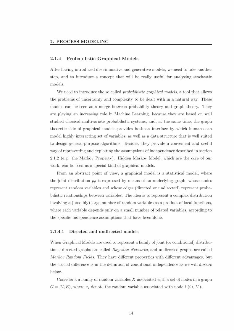
In general, directed and undirected graphs make different assertions of conditional
independence; then we have families of probability distributions captured by a directed
graph which are not captured by undirected graphs and vice versa [52]. Two examples
are given in figure 2.1.
B
C
A
C
A
B
D
(a) (b)
Figure 2.1: An example of directed (a) graph that cannot be re-expressed as an undi-
rected graph and vice versa (b)
It is important to note that recent work on graphical models are trying to offer a
general framework in which to unify a large class of statistical models. Many of the
classical multivariate probabilistic systems studied in fields such as statistics, systems
engineering, information theory, pattern recognition and statistical mechanics, could
be treated as special cases of the general graphical model formalism. The idea is to
exploit the graph algorithms in order to define general algorithms to perform learning
16
2.1 Modeling stochastic processes
and inference task on such models. Moreover, specialized techniques that have been
developed in one of these fields could be transferred to others.
Also if, in general, we can not unify directed and undirected graphs, we can observe
that undirected graphs can be seen, in a typical case, as a generalization of directed
ones. We have to observe that equation (2.3) could be viewed as special case of (2.4).
In fact we do not need to add a normalizing factor Z because it sums over a probability
distribution so thet Z = 1. A second observation is that p(xi | Xparents(i)) can be
considered a potential functions but it is defined on a set of nodes that may not be a
clique.
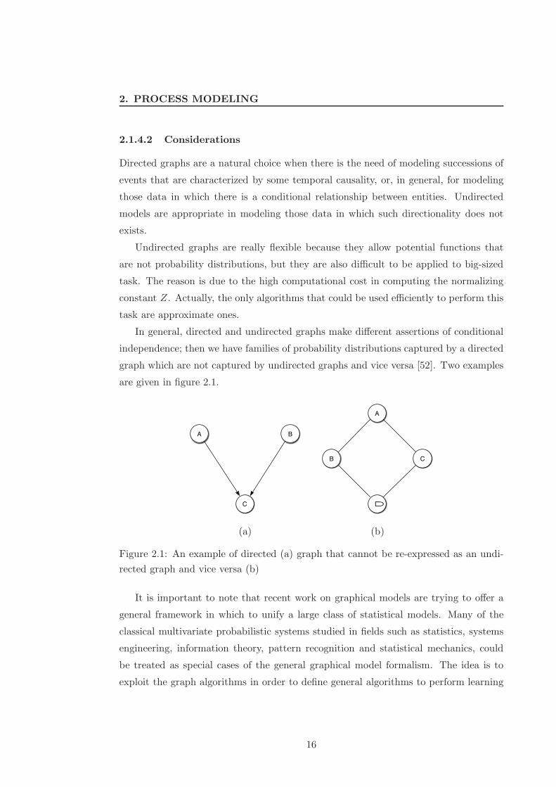
In order to allow unification between directed and undirected graphs it has been
introduced the concept of moral graph associated with a directed graph G. The moral
graph Gm is an undirected graph obtained by connecting, for each node in G, all
of its parent and transforming the directed arcs in undirected ones. The conditional
probability p(xi | Xparents(i)) applied to Gm is now a potential function reducing (2.3)
to a special case of (2.4). In Figure 2.2 is given an example of a directed graph and its
equivalent moralized undirected graph.
C
F
D
E
A B
C
F
D
E
A B
(a) (b)
Figure 2.2: An example of directed (a) graph G and the corresponding moralized graph
Gm (b)
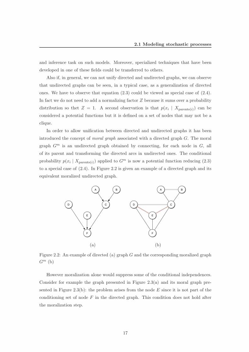
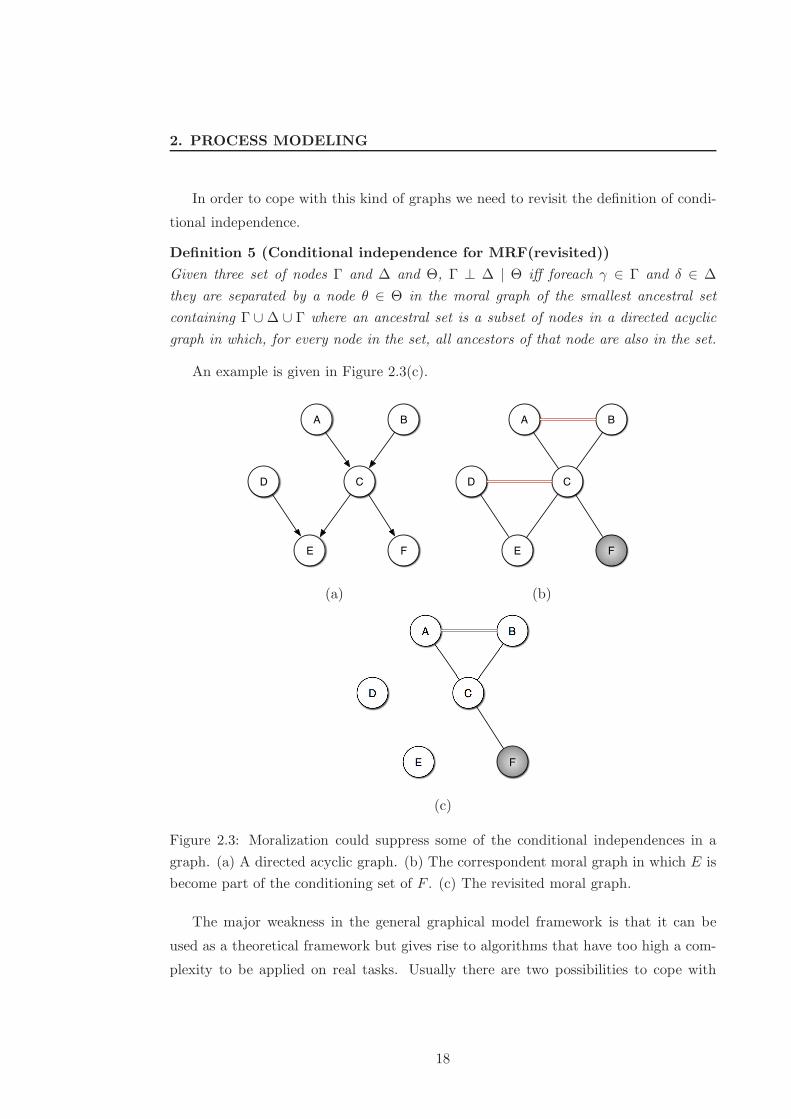
However moralization alone would suppress some of the conditional independences.
Consider for example the graph presented in Figure 2.3(a) and its moral graph pre-
sented in Figure 2.3(b): the problem arises from the node E since it is not part of the
conditioning set of node F in the directed graph. This condition does not hold after
the moralization step.
17
2. PROCESS MODELING
In order to cope with this kind of graphs we need to revisit the definition of condi-
tional independence.
Definition 5 (Conditional independence for MRF(revisited))
Given three set of nodes Γ and ∆ and Θ, Γ ⊥ ∆ | Θ iff foreach γ ∈ Γ and δ ∈ ∆
they are separated by a node θ ∈ Θ in the moral graph of the smallest ancestral set
containing Γ ∪ ∆ ∪ Γ where an ancestral set is a subset of nodes in a directed acyclic
graph in which, for every node in the set, all ancestors of that node are also in the set.
An example is given in Figure 2.3(c).
C
E
D
A B
F F
C
E
D
A B
(a) (b)
C
E
D
A B
F
(c)
Figure 2.3: Moralization could suppress some of the conditional independences in a
graph. (a) A directed acyclic graph. (b) The correspondent moral graph in which E is
become part of the conditioning set of F . (c) The revisited moral graph.
The major weakness in the general graphical model framework is that it can be
used as a theoretical framework but gives rise to algorithms that have too high a com-
plexity to be applied on real tasks. Usually there are two possibilities to cope with
18
2.2 Markov Processes
this drawback: either to use the graphical model paradigm as a formal paradigm and
use traditional algorithms in practice, or to develop sub-classes of the general algo-
rithms that only offer approximate solutions or, when they have the same complexity
of traditional ones, are totally equivalent to these last.
In the following we will make use of the graphical models paradigm to introduce
the general context in which we can insert the Hidden Markov Model formalism, and to
compare this model with others. The reader interested in generalizations of this type
of models is referred to [32, 33]
2.2 Markov Processes
When there is the need of modeling discrete processes in which future evolution of
the system depends only on the actual state of the system itself and does not rely on
its past conditions, Markov processes are the more natural choice, being perhaps the
simplest model of a random evolution without long-term memory.
Definition 6 (Markov Property) A family of discrete random variables
{Xt | t ∈ Z+} has the Markov property if
P (Xt+1 ∈ U | X0,X1, ...,Xt) = P (Xt+1 ∈ U | Xt,Xt−1, · · · ,Xt−n) (2.6)
where U is a discrete uniform distribution and n < t.
The above definition states that a stochastic process has the Markov property if the
conditional probability distribution of future states of the process, given the present
state and all past ones, only depends upon the last n states. Under this condition the
sequence Xt is said to form a Markov chain of order n.
At this point we can formally define a Markov process:
Definition 7 (Markov process) A Markov process of order n is a sequence Xt of
random variables indexed by discrete time t ∈ Z+ , or continuous time t ≥ 0 that
satisfies the Markov property.
Even though it is theoretically possible to consider any process order, in practice
it is typical to reduce to first order Markov chains, i.e., the probability of being in
a specific state at time t depend only upon the previous state at time t − 1. More
formally:
19

2. PROCESS MODELING
Definition 8 (First Order Markov Process) A first order Markov process is a se-
quence Xt of random variables indexed by discrete time t ∈ Z+ , or continuous time
t ≥ 0 that satisfies the following property:
P (Xt+1 ∈ U | X0,X1, ...,Xt) = P (Xt+1 ∈ U | Xt) (2.7)
where U is a discrete uniform distribution.
2.3 Observable Markov Models
We will restrict our attention to Markov chain whose state space is finite and consists
of a set S of N distinct states, S = {s1, s2, · · · , sN}. We can re-write eq. (2.7) as
follows:
P (Xt+1 = sk | X0,X1, ...,Xt) = P (Xt+1 = sk | Xt) (2.8)
We will also consider only Markov chains with stationary transition probabilities,
i.e., transitions in which the probability of going from a states to another does not
depend upon time. Such Markov chains are called homogeneous.
Definition 9 (Homogeneous Markov chains) A Markov chains is defined homo-
geneous if:
P (Xt+1 = sk | Xt = sj) = P (Xn+1 = sk | Xn = sj) ∀t, n > 0 (2.9)
The homogeneity assumption is not realistic in many real world processes, but it
is a good approximation that introduces an interesting property: as time evolves, the
probability of being in a given state becomes more and more independent of the initial
state.
Another advantage of homogeneity is that it allows a process to be modeled in an
easy and convenient way: a stationary Markov chain, whose state space is finite and of
size N , can be fully described by the initial states distribution Π:
Π = {πi} = P (X0 = si) 1 ≤ i ≤ N (2.10)
and by the state transition probability distribution A:
A = {aij} = [P (Xt+1 = sj | Xt = si)]N×N1 ≤ i, j ≤ N (2.11a)
20
2.3 Observable Markov Models
with the state transition coefficients obeying to the standard stochastic constraints:
aij ≥ 0 (2.11b)
N∑
i=1
aij = 1 (2.11c)
The stochastic process we have defined is called Observable Markov Model, since the
output of the process is the set of states, at each time instant, corresponding to physical
(observable) events. Markov Models are generally represented as a graph, where nodes
represent the state space and edges represent the transition probabilities.
2.3.1 An example: the weather model
For the sake of a better understanding, it would be useful to try and model a simple
process. If our objective is to build a (simple) model of the weather evolution, we could
assume that (1) the weather is observed once a day, and (2) we would consider only
one of this three possible states: sunny(S), cloudy(C) and rain(R). Another important
assumption is that the state of the model depends only upon the previous state (Markov
property).
Observing the evolution of weather for a sufficient number of days it is possible to
compute the probability of moving from one state to each of the others. Below there
is a possible state transition matrix A :
A = (aij) =
0.5 0.3 0.20.3 0.4 0.30.2 0.3 0.4
i, j ∈ {S,C,R}
and the corresponding vector Π of initial probabilities:
Π = (πi) =(1.0 0.0 0.0
)i ∈ {S,C,R}
that is, we know it was sunny on day 0.
A first easy question, which we may want to answer just by looking at the transition
matrix, is: if we are in a specific state (e.g., sunny) what is the probability of observing
another specific state (e.g., sunny, again) the day after? In this case: P (aSS) = 0.5
A second question, which we may want to answer, is to find out the probability
of observing a precise sequences of events (e.g., S,S,C,R,C ). More formally, given the
21
2. PROCESS MODELING
Sunny
Sunny
Sunny
0.2
0.5
0.3
0.2
0.3
0.3
0.4
0.4
0.4
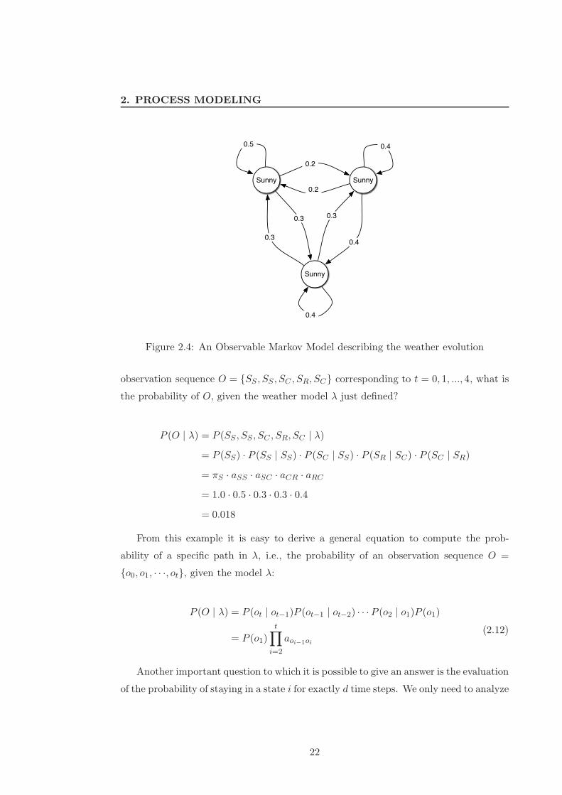
Figure 2.4: An Observable Markov Model describing the weather evolution
observation sequence O = {SS , SS , SC , SR, SC} corresponding to t = 0, 1, ..., 4, what is
the probability of O, given the weather model λ just defined?
P (O | λ) = P (SS , SS , SC , SR, SC | λ)
= P (SS) · P (SS | SS) · P (SC | SS) · P (SR | SC) · P (SC | SR)
= πS · aSS · aSC · aCR · aRC
= 1.0 · 0.5 · 0.3 · 0.3 · 0.4
= 0.018
From this example it is easy to derive a general equation to compute the prob-
ability of a specific path in λ, i.e., the probability of an observation sequence O =
{o0, o1, · · ·, ot}, given the model λ:
P (O | λ) = P (ot | ot−1)P (ot−1 | ot−2) · · ·P (o2 | o1)P (o1)
= P (o1)
t∏
i=2
aoi−1oi
(2.12)
Another important question to which it is possible to give an answer is the evaluation
of the probability of staying in a state i for exactly d time steps. We only need to analyze
22
2.4 Hidden Markov Models
the probability of the observation sequence:
O = {si, si, si, · · · , si︸ ︷︷ ︸
d times
, sj} si, sj ∈ S i 6= j (2.13)
given the model λ, which is:
P (O | λ, o0 = si) = (aii)d−1(1 − aii) (2.14)
This probability function over the stay duration follows an exponential law, and it
is characteristic of a Markov chain. According to this function, it is easy to calculate
the expected number of times in which the system will remain in the same state i,
conditioned on starting in that state:
di =
∞∑
d=0
d · P (O | λ, o0 = si)
=
∞∑
d=0
d(aii)d−1(1 − aii)
=1
1 − aii
(2.15)
According to the example, the expected number of consecutive (e.g.) sunny day,
would be
di =1
1 − 0.5= 2
2.4 Hidden Markov Models
Having a state for each observation could be a too strong assumption in many real-
world problems. Modeling a process in this way means to compute the probability of
transition from each state to the others and this is not always possible, because the
amount of data required to estimate all the transition probabilities could be impractical.
Hidden Markov Models (HMMs) are the most well-known and practically used ex-
tension of Markov chains. They offer a solution to this problem introducing, for each
state, an underlying stochastic process that is not known (it is hidden) but could be
inferred through the observations it generates.
23
2. PROCESS MODELING
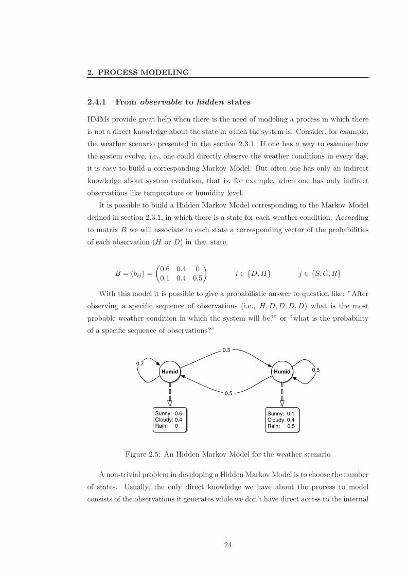
2.4.1 From observable to hidden states
HMMs provide great help when there is the need of modeling a process in which there
is not a direct knowledge about the state in which the system is. Consider, for example,
the weather scenario presented in the section 2.3.1. If one has a way to esamine how
the system evolve, i.e., one could directly observe the weather conditions in every day,
it is easy to build a corresponding Markov Model. But often one has only an indirect
knowledge about system evolution, that is, for example, when one has only indirect
observations like temperature or humidity level.
It is possible to build a Hidden Markov Model corresponding to the Markov Model
defined in section 2.3.1, in which there is a state for each weather condition. According
to matrix B we will associate to each state a corresponding vector of the probabilities
of each observation (H or D) in that state.
B = (bij) =
(0.6 0.4 00.1 0.4 0.5
)
i ∈ {D,H} j ∈ {S,C,R}
With this model it is possible to give a probabilistic answer to question like: ”After
observing a specific sequence of observations (i.e., H,D,D,D,D) what is the most
probable weather condition in which the system will be?” or ”what is the probability
of a specific sequence of observations?”
Humid
Sunny: 0.6Cloudy: 0.4Rain: 0
Sunny: 0.1Cloudy: 0.4Rain: 0.5
Humid
0.7
0.3
0.5
0.5
Figure 2.5: An Hidden Markov Model for the weather scenario
A non-trivial problem in developing a Hidden Markov Model is to choose the number
of states. Usually, the only direct knowledge we have about the process to model
consists of the observations it generates while we don’t have direct access to the internal
24

2.4 Hidden Markov Models
structure of the process. When a specific knowledge of the domains is available it is
easier to build a model that gives a good approximation of the process, but, in many
cases, it is a problem of not easy solution and can be strongly task-dependent. This is
a reason for which the literature on HMMs focused more on the problem of learning
the probabilities governing the model than on the one of determining its structure.
To understand the question, it could be helpful to consider the following scenario:
Suppose you are playing dice with a dishonest gambler. At every round a six-head die
is rolled and your objective is to predict the value that will come out. The gambler has
a second die with some bias and, before every roll, there is a certain probability that
he exchange the dices. It is impossible for the player to see if the change happens and
the only events that is observable is the result of the roll of the die. Given the above
scenario, the problem of interest is how do we build an HMM to model the observed
sequence of roll.
A first choice, if we do not know that the gambler has two dice and is exchanging
them, is to build a model with a state for each one of the six possible values of the die. In
that case the model is a fully Observable Markov Model and the only issue for complete
specification of the model would be to decide the best value that has to be assigned to
each transition, according to the observed values of the previous rolls. (Figure 2.6(a))
An equivalent HMM to this Observable Markov Model would be a degenerate 1-state
model with the observations corresponding to the six possible values of the die (Figure
2.6(b)).
Another choice, for explaining the observed sequence of dice rolled is to build a
model with two states, each one corresponding to a different die. Each state is char-
acterized by a probability distribution of outcomes and transitions between states are
characterized by a state transition matrix(Figure 2.6(c)).
It is interesting to notice that the physical mechanism which determine how the dice
are exchanged could itself be another probabilistic events (for example the gambler toss
a coin to decide if exchange the dice or not). It is possible to build a more complex
model to taking into account all this kind of information, but when a model grows,
the number of parameters to be estimated increases accordingly. A larger HMM would
seem to inherently be more capable of modeling a series of events than would do an
equivalent, smallest, model. Althought this is theoretically true, we will see later that
25

2. PROCESS MODELING
1
1 1
1
1
1
(a)
SingleDie
a11
1: b11
2: b12
3: b13
4: b14
5: b15
6: b16
(b)
Die 1 Die 2
1: b21
2: b22
3: b23
4: b24
5: b25
6: b26
1: b11
2: b12
3: b13
4: b14
5: b15
6: b16
a12
a11
a21
a22
(c)
Figure 2.6: Models designed for the problem of dishonest gambler: (a) a six-state
Observable Markov Model, (b) a corresponding degenerated HMM, (c) a two state
HMM
26
2.4 Hidden Markov Models
practical considerations impose strong limitations on the size of models that can be
effectively considered.
2.4.2 A formal definition of Hidden Markov Models
An Hidden Markov Model is a stochastic finite automaton defined by a tuple λ =
〈S, V,A,B,Π〉 where:
1. S is the set of states and its cardinality is N . We will denote the individual states
with S = {s1, s2, · · · , sN} and we will use si(t) to indicate the state si at time t.
We also introduce the notation qt to denote the generic state at time t.
2. V is the set of distinct events that can be generated by the modeled process. It
is intersting to notice that in some states could happens that only a subset of V
could be emitted. Consider, for example, the matrix B described in section 2.4.1
: in the state R (rain) the probability of observation D is null. The cardinality
of the set is M and we will denote individual symbols with V = {v1, v2, · · · , vM}.
We will refer to the symbol vk at time t with the notation vk(t)
3. A is a probability distribution governing the transitions from one state to another.
Specifically, any member aij of A defines the probability of transition from state
si to state sj. According to the definitions of A introduced in the section 2.3 we
will rewrite the equation (2.11) as:
A = {aij} = [P (sj(t+ 1) | si(t))]N×N 1 ≤ i, j ≤ N (2.16a)
with:
aij ≥ 0 (2.16b)
N∑
i=1
aij = 1 (2.16c)
4. B is a probability distribution governing the emission of observable events depend-
ing on the state. Specifically, an item bik belonging to B defines the probability of
observing event vk when the process is in the state si. For having clearer formulas
we will rewrite bik as bi(vk). Formally we have:
bi(vk) = P (vk(t) | si(t)) 1 ≤ i ≤ N 1 ≤ k ≤M (2.17a)
27

2. PROCESS MODELING
with:
bi(vk) ≥ 0 (2.17b)
M∑
k=1
bi(vk) = 1 (2.17c)
5. Π = {π1, π2, · · · , πN} is a distribution on S defining, for every si ∈ S, the prob-
ability that Si is the initial state of the process. Analogously with previous
definitions we have:
Π = πi = P (si(t) | t = 1) 1 ≤ i ≤ N (2.18a)
with:
πi ≥ 0 (2.18b)
N∑
k=1
πi = 1 (2.18c)
We talk about emission of observable events because we can think of HMMs as
generative models that can be used to generate observation sequences. Algorithmically,
a sequence of observations O = o1, o2, · · · , oT , with ot ∈ V can be generated by an HMM
λ as described in 2.7.
GEN (λ)
Set t = 1
Choose si(t) according to Π
while t ≤ T doEmit the symbol Ot = Vk according to B
if t ≤ T thenTransit to a new state sj(t+ 1) according to A
Set si = sj
end
Set t = t+ 1end
Figure 2.7: Algorithm for generating a sequence of observations by an HMM λ.
28
2.5 Computing probabilities with HMMs
2.5 Computing probabilities with HMMs
From the previous definitions it is easy to derive the formula for computing the joint
probability of observing a succession of events O = o1, o2, · · · , oT generated from a
sequence of states σ = si1 , si2, · · · , siT given an HMM λ, under the assumption that
the observations are statistically independent:
P (O,σ | λ) = P (O | σ, λ)P (σ | λ) (2.19a)
where:
P (O | σ, λ) =
T∏
t=1
P (ot | sit, λ) = bi1(o1)bi2(o2) · · · biT (oT ) (2.19b)
and
P (σ | λ) = πi1asi1si2asi2
si3· · · asi(T−1)
siT(2.19c)
Thus we could rewrite the equation (2.19):
P (O,σ | λ) = (πi1bi1(o1))
T∏
t=2
asi(t−1)sitbit(ot) (2.20)
Equation (2.20) is not really useful, because the sequence of states is unknown. It
may exist more than one (typically many) sequences of states σ that lead to the gener-
ation of a specific sequence of observations. So we could be interested in determining
the most probable sequence of states (σ∗) that generated a sequence O, or we could be
interested in determining the probability of observing O given all the possible paths in
λ that could generate it, i.e., the probability of O given λ.
2.5.1 Forward algorithm
We will start facing the problem of computing the probability that a given sequence
of observations O is generated by a model λ. To found a way to compute this value is
apparently easy; we only need to recall the equations (2.19a) and (2.20) and consider
that they could be used in order to compute the probability of O on a given path in
29
2. PROCESS MODELING
λ. In order to compute the probability P (O | λ) we need to sum the probability of O
over all the possible paths in λ. Formally:
P (O | λ) =∑
All S
[P (O | σ, λ)P (σ | λ)] (2.21)
This solution is not useful in practice because the number of possible paths grows
exponentially with the length of the sequence. A possible approximation could be to
ignore all the paths beside the most probable one, defining:
P (O | λ) ≃ P (σ∗) (2.22)
Even though this approximation gives good results in practice, we do not need to
use it, because, taking advantage of the Markov property, it is possible to develop a
dynamic programming algorithm (called forward) similar to the Viterbi algorithm. In
order to describe the algorithm we need to define a forward variable α defined as follow:
αi(t) = P (o1 · · · ot, si(t) | λ) (2.23)
This variable represent the probability of observing the subsequence o1 · · · ot being in
state si at time t, given λ. We will describe how to compute this probability inductively
(forward algorithm):
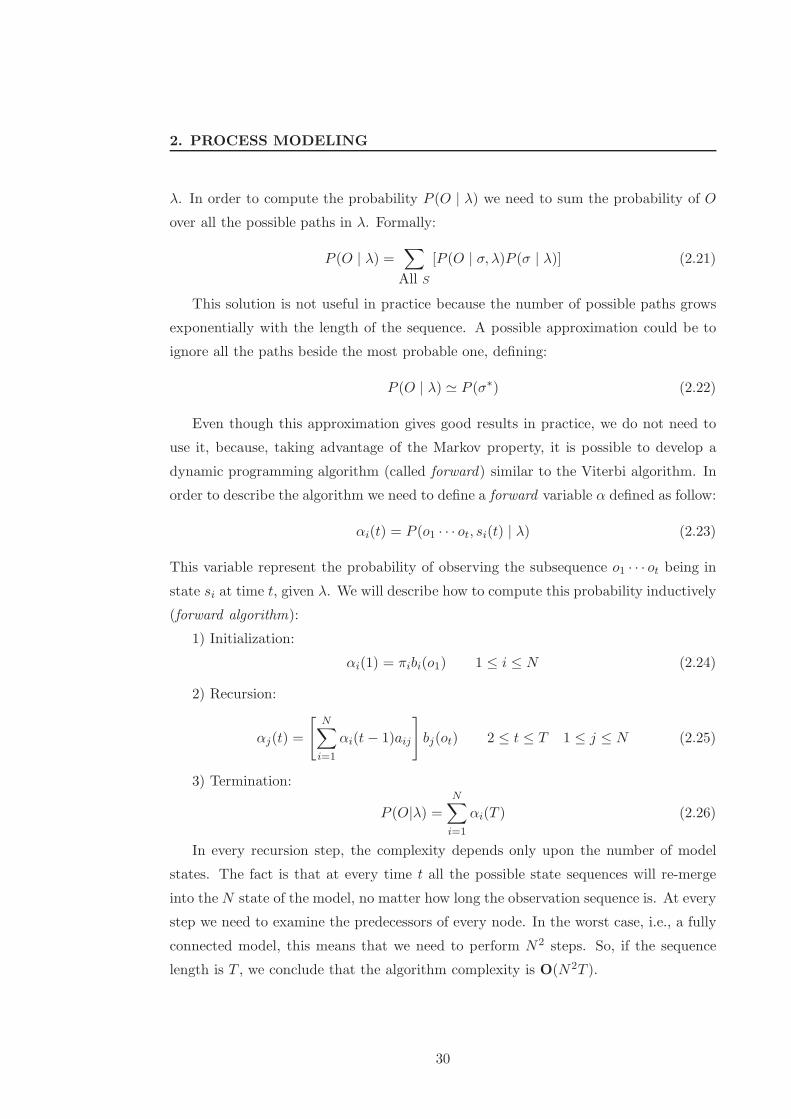
1) Initialization:
αi(1) = πibi(o1) 1 ≤ i ≤ N (2.24)
2) Recursion:
αj(t) =
[N∑
i=1
αi(t− 1)aij
]
bj(ot) 2 ≤ t ≤ T 1 ≤ j ≤ N (2.25)
3) Termination:
P (O|λ) =
N∑
i=1
αi(T ) (2.26)
In every recursion step, the complexity depends only upon the number of model
states. The fact is that at every time t all the possible state sequences will re-merge
into the N state of the model, no matter how long the observation sequence is. At every
step we need to examine the predecessors of every node. In the worst case, i.e., a fully
connected model, this means that we need to perform N2 steps. So, if the sequence
length is T , we conclude that the algorithm complexity is O(N2T ).
30
2.5 Computing probabilities with HMMs
2.5.2 Viterbi algorithm
Another question to which we want to answer is: how could we infer a state sequence
that is optimal, in some meaningful sense, given an observation sequence O and a model
λ? There are several possible ways of solving this problem. The difficulty lies with the
definition of the optimal state sequence. The most widely used criterion is to find the
single best state sequence (path), i.e. to find the single path σ∗ that maximize the
probability P (σ | O,λ) which is equivalent to maximize
We can perform this computations through a dynamic programming algorithm
called Viterbi algorithm. The key idea, based on the Markov property, is that at
every step the probability of being in a state depend only upon the previous state. So,
if we are interested in the path with the maximum probability, we need to choose, for
every state sj at time t+ 1, the best among all paths leading to it at time t. In order
to backtrace the full path we only need to maintain, for every state and for every slice
of time, a pointer to the previous state.
Defining with δj(t + 1) the probability of the most probable path ending in state
sj at time t+ 1 and with ψj(t+ 1) the index of the state si from which come the best
path leading to sj, it is possible, now, give a formal description of the algorithm.
1) Initialization:
δi(1) = πibi(o1) 1 ≤ i ≤ N (2.27a)
ψi(1) = 0 (2.27b)
2) Recursion:
δj(t) = max1≤i≤N
[δi(t− 1)aij ] bj(ot) 2 ≤ t ≤ T 1 ≤ j ≤ N (2.28a)
ψj(t) = arg max1≤i≤N
[δi(t− 1)aij ] 2 ≤ t ≤ T 1 ≤ j ≤ N (2.28b)
3) Termination:
P (σ∗) = max1≤i≤N
[δi(T )] (2.29a)
Pathσ∗(T ) = arg max1≤i≤N
[δi(T )] (2.29b)
4) Backtracking:
Pathσ∗(t) = ψ[Pathσ∗(t+1)](t+ 1) (2.30a)
31

2. PROCESS MODELING
Again, as for the calculus of Viterbi algorithm, the order of complexity of the Viterbi
method is O(N2T )
2.5.3 The most probable state and the backward algorithm
Another question that could be of interest is determining the most probable state in
which we will observe the event ot. More generally the question is: how could we
compute the probability P (si(t) | O,λ), i.e., the probability of being in state i at time
t, given the sequence O and the model λ? Also this value can be recursively computed.
We can start from the joint probability P (si(t), O | λ), i.e. the probability of observing
the full sequence with the tth symbol produced by state i:
P (si(t), O | λ) = P (o1 · · · ot, si(t) | λ)P (ot+1 · · · oT | o1 · · · ot, si(t), λ)
= P (o1 · · · ot, si(t) | λ)P (ot+1 · · · oT | si(t), λ)
= αi(t)βi(t)
(2.31)
where βi(t) = P (ot+1 · · · oT | si(t), λ). With βi(t) we are able to compute P (si(t) | O,λ).
In fact, being P (si(t), O | λ) = αi(t)βi(t), using the formula for conditional probability
we obtain:
γi(t) = P (si(t) | O,λ) =αi(t)βi(t)
P (O | λ)(2.32)
The probability P (O | λ) can be computed with the forward algorithm. The way of
computing βi(t) is analogous to the one for computing the forward variable, but instead
obtained by a backward recursion starting at the end of the sequence:
1) Initialization:
βi(T ) = 1 1 ≤ i ≤ N (2.33)
2) Recursion:
βi(t) =N∑
j=1
aijbj(ot+1)βj(t+ 1) 1 ≤ t ≤ T − 1 1 ≤ i ≤ N (2.34)
3) Termination:
P (O|λ) =
N∑
i=1
πibi(o1)βi(1) (2.35)
The complexity analysis of this algorithm is analogous to the one performed in
subsection 2.5.1 for the Forward algorithm.
32
2.5 Computing probabilities with HMMs
It is interesting to observe that we can use the equation (2.32) to perform a decoding
alternative to the one performed by the Viterbi algorithm. We can use it in order to
determine the path in λ in which every node is the individually most likely state at
time t. These can be particularly useful when many different paths have almost the
same probability of being the most probable one. This mean that in place of choosing
σ∗ we could choose a state sequence σ∗ defined as follow:
σ∗ = σt = arg maxiP (si(t) | O,λ) 1 ≤ t ≤ T (2.36)
This state sequence is more interesting in order to analyze the state assignment at
time t rather determining a complete path. In fact the state sequence so defined may
not be a legal path through the model if some transitions are not permitted, which is
normally the case.
2.5.4 Parameter estimation for HMMs
Two of the most difficult problems that arise when using HMMs are (1) determining
the model topology, i.e., to find the number of states of the model and which ones
of them are connected, and (2) to find the correct values for emission and transition
probabilities. For now we will assume that a domain expert has given us the right
number of states and that they could be fully connected, and we will examine the
second problem starting from a set of training sequences that are independent from
one another.
If we would know the state sequence, we could use a maximum likelihood method
for estimating the probabilities for A and B. We denote with aij the number of times in
which we have the state si followed by the state sj, and with bi(vk) the number of times
in which we observe the emission of symbol vk in the state si. Under this assumptions
we could express the formula for estimating aij and bi(vk):
aij =aij
∑
j′∈S aij′(2.37a)
bi(vk) =bi(vk)
∑
vk′∈V bi(vk′)(2.37b)
This kind of method is obviously vulnerable to overfitting if there are insufficient
data. Another problem is that if there is a state that is never used because there are
33
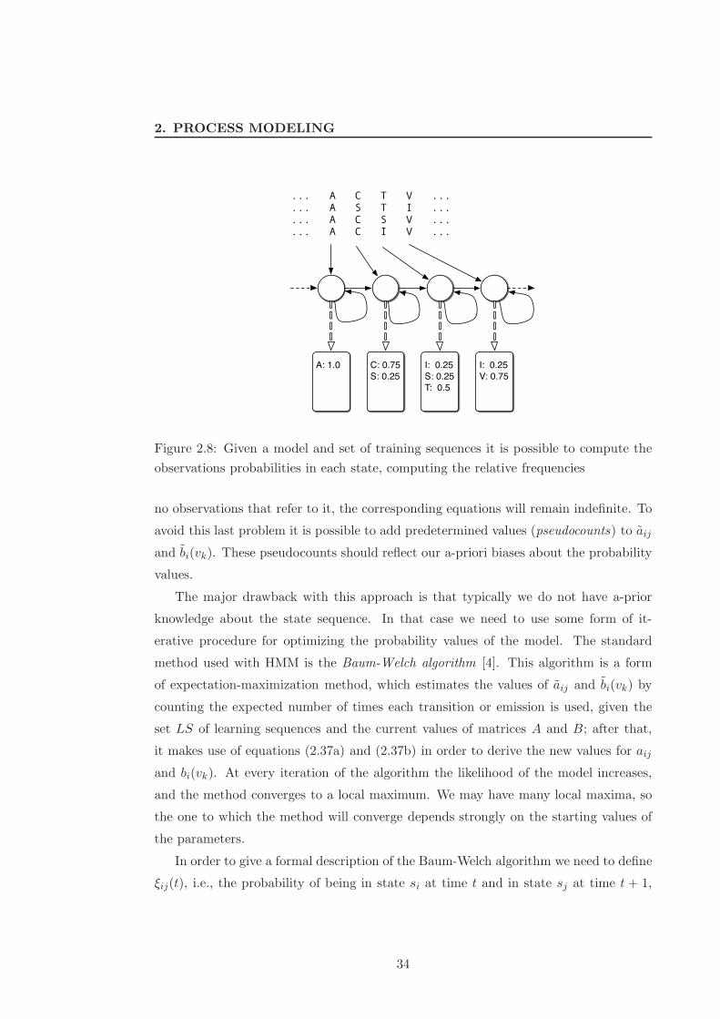
2. PROCESS MODELING
... A C T V ...
... A S T I ...
... A C S V ...
... A C I V ...
A: 1.0 C: 0.75
S: 0.25
I: 0.25
S: 0.25
T: 0.5
I: 0.25
V: 0.75
Figure 2.8: Given a model and set of training sequences it is possible to compute the
observations probabilities in each state, computing the relative frequencies
no observations that refer to it, the corresponding equations will remain indefinite. To
avoid this last problem it is possible to add predetermined values (pseudocounts) to aij
and bi(vk). These pseudocounts should reflect our a-priori biases about the probability
values.
The major drawback with this approach is that typically we do not have a-prior
knowledge about the state sequence. In that case we need to use some form of it-
erative procedure for optimizing the probability values of the model. The standard
method used with HMM is the Baum-Welch algorithm [4]. This algorithm is a form
of expectation-maximization method, which estimates the values of aij and bi(vk) by
counting the expected number of times each transition or emission is used, given the
set LS of learning sequences and the current values of matrices A and B; after that,
it makes use of equations (2.37a) and (2.37b) in order to derive the new values for aij
and bi(vk). At every iteration of the algorithm the likelihood of the model increases,
and the method converges to a local maximum. We may have many local maxima, so
the one to which the method will converge depends strongly on the starting values of
the parameters.
In order to give a formal description of the Baum-Welch algorithm we need to define
ξij(t), i.e., the probability of being in state si at time t and in state sj at time t + 1,
34
2.6 Hierarchical approach to HMMs
given the model and the observation sequence. This formula descends directly from
(2.32):
ξij(t) = P (si(t), sj(t+ 1) | O,λ) =αi(t)aijbj(o(t+1))βj(t+ 1)
P (O | λ)(2.38)
At this point we are able to introduce the Baum-Welch algorithm:
1) Initialization:
Assign some starting values to the parameters of the model λ
2) Recursion:
Compute aij and bi(v) according to (2.37) with:
aij =∑
O∈LS
∑
1≤t≤TT=length(O)
ξOij(t)
(2.39a)
bi(v) =∑
O∈LS
∑
1≤t≤TT=length(O)
v=ot
γOi (t)
(2.39b)
where ξOij (t) and γO
i (t) are, respectively, the values of ξij(t) and γi(t) com-
puted on sequence O.
3) Termination:
Terminate when the likelihood of the model on LS doesn’t improve better
than a predetermined threshold, or when the maximum number of recur-
sions step is reached.
2.6 Hierarchical approach to HMMs
The Hierarchical Hidden Markov Model has been introduced by Fine, Singer and Thisby
[18] as an extension of HMMs. The extension immediately follows from the regular
languages property of being closed under substitution, which allows a large finite state
35
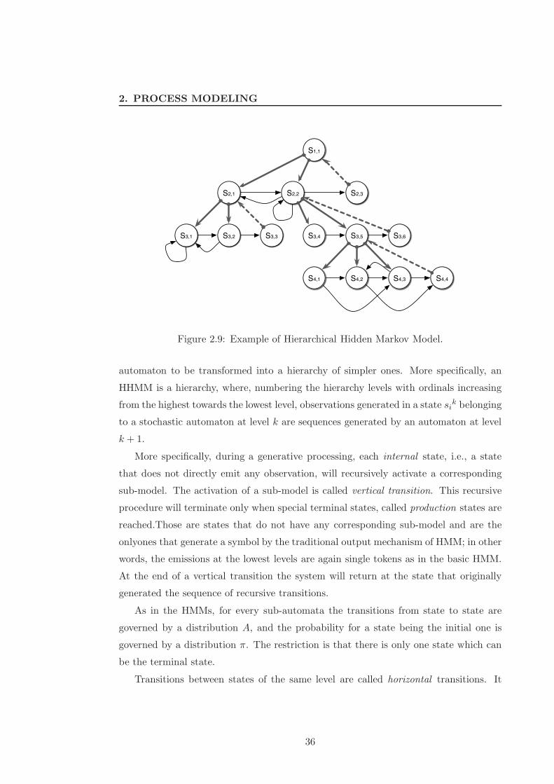
2. PROCESS MODELING
S1,1
S2,1 S2,2 S2,3
S3,3S3,2 S3,4 S3,5 S3,6S3,1
S4,1 S4,2 S4,3 S4,4
Figure 2.9: Example of Hierarchical Hidden Markov Model.
automaton to be transformed into a hierarchy of simpler ones. More specifically, an
HHMM is a hierarchy, where, numbering the hierarchy levels with ordinals increasing
from the highest towards the lowest level, observations generated in a state sik belonging
to a stochastic automaton at level k are sequences generated by an automaton at level
k + 1.
More specifically, during a generative processing, each internal state, i.e., a state
that does not directly emit any observation, will recursively activate a corresponding
sub-model. The activation of a sub-model is called vertical transition. This recursive
procedure will terminate only when special terminal states, called production states are
reached.Those are states that do not have any corresponding sub-model and are the
onlyones that generate a symbol by the traditional output mechanism of HMM; in other
words, the emissions at the lowest levels are again single tokens as in the basic HMM.
At the end of a vertical transition the system will return at the state that originally
generated the sequence of recursive transitions.
As in the HMMs, for every sub-automata the transitions from state to state are
governed by a distribution A, and the probability for a state being the initial one is
governed by a distribution π. The restriction is that there is only one state which can
be the terminal state.
Transitions between states of the same level are called horizontal transitions. It
36
2.6 Hierarchical approach to HMMs
is important to put in evidence that the only horizontal transitions allowed are those
between states of the same sub-automata, i.e., no direct transition may occur between
the states of different automata in the hierarchy. Figure 2.6 shows an example of
HHMM.
We will give a formal description of a Hierarchical Hidden Markov Model. We will
denote a generic state of an HHMM with sdi ( d ∈ {1, · · · ,D} ) where i is the state
index and d the level in the hierarchy, that is numbered from 1 (the root) to D (the
production states). The internal states may have different numbers of sub-states, so
that this number will be denoted with∣∣sd
i
∣∣. Moreover, an HHMM is characterized by
the state transition probability between the internal state and the output distribution
vector of the production states, i.e., for each internal state sd there is a state transition
probability matrix Asddetermining the probabilities of a horizontal transition:
Asd
= asd
ij = P (sd+1j | sd+1
i ) (2.40)
We also need to define the initial distribution vector Πsd
over the sub-states of sd,
i.e. the probability for each state sd+1i of being activated from sd:
Πsd
= πsd
(s(d+1)i ) = P (sd+1
i | sd) (2.41)
Every production state sD will be solely characterized by its output probability
vector Bsdthat define, for each symbol vk ∈ V , the probability of being emitted by sD
:
BsD
= bsD
(vk) = P (vk | sd) (2.42)
The full set of parameters is denoted by:
λ ={
λsd
|d ∈ {1, · · · ,D}}
={{
Asd
|d ∈ {1, · · · ,D − 1}}
,{
Πsd
|d ∈ {1, · · · ,D − 1}}
, BsD} (2.43)
The major advantage provided by the hierarchical structure is a strong reduction
of the number of parameters to estimate. In fact, automata at the same level in the
hierarchy do not share interconnections: every interaction through them is governed
by transitions at the higher levels. This means that for two automata λskl , λsk
m at level
k the probability of moving from the terminal state of λskl to one state of λsk
m is stated
by a single parameter associated to a transition at level k − 1.
37
2. PROCESS MODELING
A second advantage is that the modularization enforced by the hierarchical structure
allows the different automata to be modified and trained individually, thus providing
a natural subproblem decomposition. Examples of such approaches could be found in
[8, 63]
On the other hand, HHMM has the drawback of a greater algorithmic complexity.
In the seminal paper by Fine et al. [18], the classical algorithms Forward-Backward,
Viterbi and EM were extended to the HHMM, but the complexity increased by one
order of magnitude, in fact it runs in O(T 3).
Flattening an HHMM, by compiling it into an equivalent HMM, is always possible,
but it will multiply the number of transitions and the number of parameters to estimate
because we will obtain a corresponding HMM. If the original HHMM has a sub-model
that is shared between many highest level states, i.e. λskl = λsk
m , this structure must be
multiplicated in the flattened HMM, so the resulting model is generally larger. It is the
ability to reuse sub-models in different contexts that makes HHMMs more appealing
than standard HMMs.
In a more recent work, Murphy and Paskin [45] propose a linear (approximated)
algorithm by mapping a HHMM into a Dynamic Bayesian Network; nevertheless the
method is complex and not easy to apply.
2.7 Modeling Temporal Dynamics
Until now we introduced Hidden Markov Models as a way for modeling temporal and
sequencial data, but they can be seen as a special cases of the Dynamic Bayesian Net-
works (DBNs) a sub-class of directed graphical models oriented to time series modeling.
In order to understand better what Dynamic Bayesian Networks are, we need to
expand briefly the introduction to Bayesian Networks that as been provided in section
2.1.4.1.
2.7.1 Bayesian Networks
A Bayesian network is a directed acyclic graph for representing conditional indepen-
dences between a set of random variables. In figure 2.10 it is possible to observe an
example of Bayesian Net that represents a particular factorization involving the random
variables A,B,C,D. The nodes in a Bayesian Network represent propositional variables
38
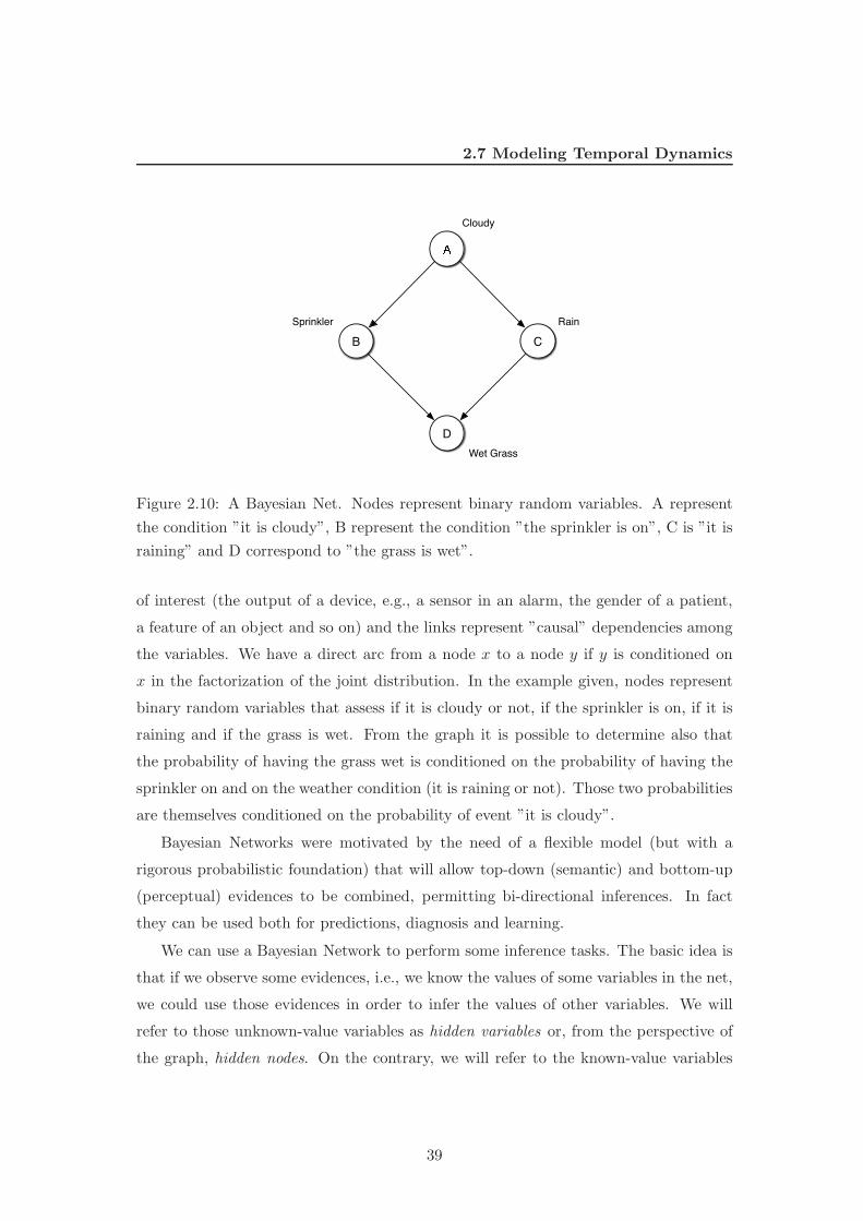
2.7 Modeling Temporal Dynamics
�B C
D
Cloudy
Sprinkler Rain
Wet Grass
Figure 2.10: A Bayesian Net. Nodes represent binary random variables. A represent
the condition ”it is cloudy”, B represent the condition ”the sprinkler is on”, C is ”it is
raining” and D correspond to ”the grass is wet”.
of interest (the output of a device, e.g., a sensor in an alarm, the gender of a patient,
a feature of an object and so on) and the links represent ”causal” dependencies among
the variables. We have a direct arc from a node x to a node y if y is conditioned on
x in the factorization of the joint distribution. In the example given, nodes represent
binary random variables that assess if it is cloudy or not, if the sprinkler is on, if it is
raining and if the grass is wet. From the graph it is possible to determine also that
the probability of having the grass wet is conditioned on the probability of having the
sprinkler on and on the weather condition (it is raining or not). Those two probabilities
are themselves conditioned on the probability of event ”it is cloudy”.
Bayesian Networks were motivated by the need of a flexible model (but with a
rigorous probabilistic foundation) that will allow top-down (semantic) and bottom-up
(perceptual) evidences to be combined, permitting bi-directional inferences. In fact
they can be used both for predictions, diagnosis and learning.
We can use a Bayesian Network to perform some inference tasks. The basic idea is
that if we observe some evidences, i.e., we know the values of some variables in the net,
we could use those evidences in order to infer the values of other variables. We will
refer to those unknown-value variables as hidden variables or, from the perspective of
the graph, hidden nodes. On the contrary, we will refer to the known-value variables
39

2. PROCESS MODELING
as observable variables or observable nodes.
In an intuitive way, we can think about a Bayesian Net as a knowledge bas, which
explicitly represents some beliefs about the elements in the system and the relationships
between them. The main purpose of such knowledge is to infer some belief or make
conclusions about some events in the system. Bayesian Network operate by propagating
beliefs throughout the network once some evidences are become availables.
2.7.1.1 Factorization and Conditional Independence
The basic factorization property in a Bayes network was introduced in section 2.1.4.1.
In few words, we can say that in a Bayes Network each variable is conditionally indepen-
dent of its non-descendants given its parents. For example, if we consider the network
provided in figure 2.10 the parent of D are B and C and they render D independent
of the remaining non-descendant, A. That is:
P (D | A,B,C) = P (D | B,C) (2.44)
The complete factorization of the graph in figure 2.10 can be expressed as follow:
P (A,B,C,D) = P (A)P (B | A)P (C | A)P (D | B,C) (2.45)
Selecting as parents the direct causes of a given variable automatically satisfies the
local conditional (in)dependence conditions and is really useful in constructing Bayesian
Networks, but, once the basic conditional (in)dependence has been set there are other
ones that follow from those. Consider for example the Network presented in figure 2.11.
X and Y are marginally independent but, given Z, they become conditional dependent.
This important effect is called explaining away and is easy to explain: flip two coins
independently, and let X = coin 1 and Y = coin 2. Let Y = 1 if the coins come up the
same and y = 0 if different. X and Y are independent, but if you know that Y = 1
they become coupled.
In general, it is a hard problem to say which extra conditional independence state-
ments follow from a basic set. By the way, there exist an efficient algorithm for gener-
ating all the conditional independence statements that must be true, given the connec-
tivity of the graph. This algorithm is called Bayes Ball algorithm [62] and allows one
to check whether two (sets of) variables (X and Y ) may or may not be conditional in-
dependent, given a third (set of) variables Z. In those case we talk about D-separation.
40
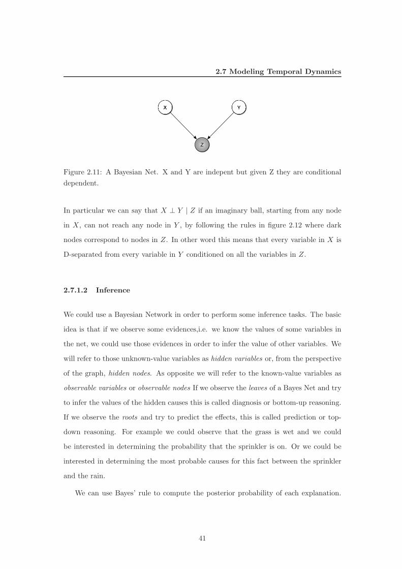
2.7 Modeling Temporal Dynamics�Y
Z
Figure 2.11: A Bayesian Net. X and Y are indepent but given Z they are conditional
dependent.
In particular we can say that X ⊥ Y | Z if an imaginary ball, starting from any node
in X, can not reach any node in Y , by following the rules in figure 2.12 where dark
nodes correspond to nodes in Z. In other word this means that every variable in X is
D-separated from every variable in Y conditioned on all the variables in Z.
2.7.1.2 Inference
We could use a Bayesian Network in order to perform some inference tasks. The basic
idea is that if we observe some evidences,i.e. we know the values of some variables in
the net, we could use those evidences in order to infer the value of other variables. We
will refer to those unknown-value variables as hidden variables or, from the perspective
of the graph, hidden nodes. As opposite we will refer to the known-value variables as
observable variables or observable nodes If we observe the leaves of a Bayes Net and try
to infer the values of the hidden causes this is called diagnosis or bottom-up reasoning.
If we observe the roots and try to predict the effects, this is called prediction or top-
down reasoning. For example we could observe that the grass is wet and we could
be interested in determining the probability that the sprinkler is on. Or we could be
interested in determining the most probable causes for this fact between the sprinkler
and the rain.
We can use Bayes’ rule to compute the posterior probability of each explanation.
41

2. PROCESS MODELING�B C
�B C
(a) (b)
�B
C�
B
C
(c) (d)�B
C�
B
C
(e) (f)
Figure 2.12: The bayes ball algorithm: (a),(c),(f) the ball cannot pass from A to C and
vice versa that are conditionally independent; (b),(d),(e) the ball could pass, A and C
are conditionally dependent.
The probability of having the sprinkler on, given that the grass is wet, is:
P (B = on | D = true) =
=P (B = on,D = true)
P (D = true)
=
∑
A,C P (A,B = on, C,D = true)∑
A,B,C P (A,B,C,D = on)
=
∑
A,C P (A)P (B = on | A), P (C | A), P (D = true | B = on, C)∑
A,B,C P (A)P (B | A), P (C | A), P (D = true | B,C)
(2.46)
In general computing posterior estimates using Bayes’ rule is computationally in-
tractable but we can use the conditional independence assumptions encoded in the
graph in order to speed up the whole process. For singly connected networks, i.e.
networks in which the underlying undirected graph has no loops, there is a general
42
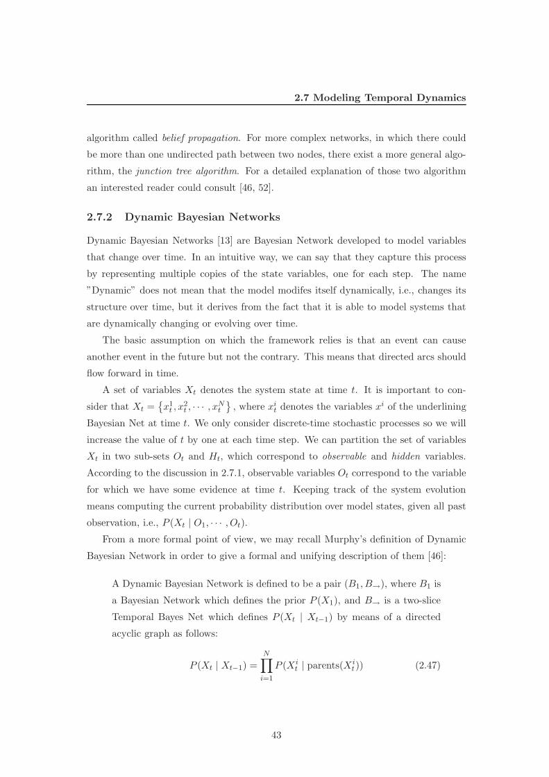
2.7 Modeling Temporal Dynamics
algorithm called belief propagation. For more complex networks, in which there could
be more than one undirected path between two nodes, there exist a more general algo-
rithm, the junction tree algorithm. For a detailed explanation of those two algorithm
an interested reader could consult [46, 52].
2.7.2 Dynamic Bayesian Networks
Dynamic Bayesian Networks [13] are Bayesian Network developed to model variables
that change over time. In an intuitive way, we can say that they capture this process
by representing multiple copies of the state variables, one for each step. The name
”Dynamic” does not mean that the model modifes itself dynamically, i.e., changes its
structure over time, but it derives from the fact that it is able to model systems that
are dynamically changing or evolving over time.
The basic assumption on which the framework relies is that an event can cause
another event in the future but not the contrary. This means that directed arcs should
flow forward in time.
A set of variables Xt denotes the system state at time t. It is important to con-
sider that Xt ={x1
t , x2t , · · · , x
Nt
}, where xi
t denotes the variables xi of the underlining
Bayesian Net at time t. We only consider discrete-time stochastic processes so we will
increase the value of t by one at each time step. We can partition the set of variables
Xt in two sub-sets Ot and Ht, which correspond to observable and hidden variables.
According to the discussion in 2.7.1, observable variables Ot correspond to the variable
for which we have some evidence at time t. Keeping track of the system evolution
means computing the current probability distribution over model states, given all past
observation, i.e., P (Xt | O1, · · · , Ot).
From a more formal point of view, we may recall Murphy’s definition of Dynamic
Bayesian Network in order to give a formal and unifying description of them [46]:
A Dynamic Bayesian Network is defined to be a pair (B1, B→), where B1 is
a Bayesian Network which defines the prior P (X1), and B→ is a two-slice
Temporal Bayes Net which defines P (Xt | Xt−1) by means of a directed
acyclic graph as follows:
P (Xt | Xt−1) =
N∏
i=1
P (Xit | parents(Xi
t)) (2.47)
43
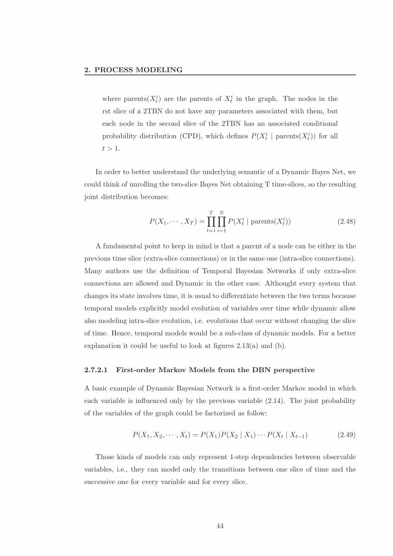
2. PROCESS MODELING
where parents(Xit) are the parents of Xi
t in the graph. The nodes in the
rst slice of a 2TBN do not have any parameters associated with them, but
each node in the second slice of the 2TBN has an associated conditional
probability distribution (CPD), which defines P (Xit | parents(Xi
t)) for all
t > 1.
In order to better understand the underlying semantic of a Dynamic Bayes Net, we
could think of unrolling the two-slice Bayes Net obtaining T time-slices, so the resulting
joint distribution becomes:
P (X1, · · · ,XT ) =
T∏
t=1
N∏
i=1
P (Xit | parents(Xi
t)) (2.48)
A fundamental point to keep in mind is that a parent of a node can be either in the
previous time slice (extra-slice connections) or in the same one (intra-slice connections).
Many authors use the definition of Temporal Bayesian Networks if only extra-slice
connections are allowed and Dynamic in the other case. Althought every system that
changes its state involves time, it is usual to differentiate between the two terms because
temporal models explicitly model evolution of variables over time while dynamic allow
also modeling intra-slice evolution, i.e. evolutions that occur without changing the slice
of time. Hence, temporal models would be a sub-class of dynamic models. For a better
explanation it could be useful to look at figures 2.13(a) and (b).
2.7.2.1 First-order Markov Models from the DBN perspective
A basic example of Dynamic Bayesian Network is a first-order Markov model in which
each variable is influenced only by the previous variable (2.14). The joint probability
of the variables of the graph could be factorized as follow:
P (X1,X2, · · · ,Xt) = P (X1)P (X2 | X1) · · ·P (Xt | Xt−1) (2.49)
Those kinds of models can only represent 1-step dependencies between observable
variables, i.e., they can model only the transitions between one slice of time and the
successive one for every variable and for every slice.
44
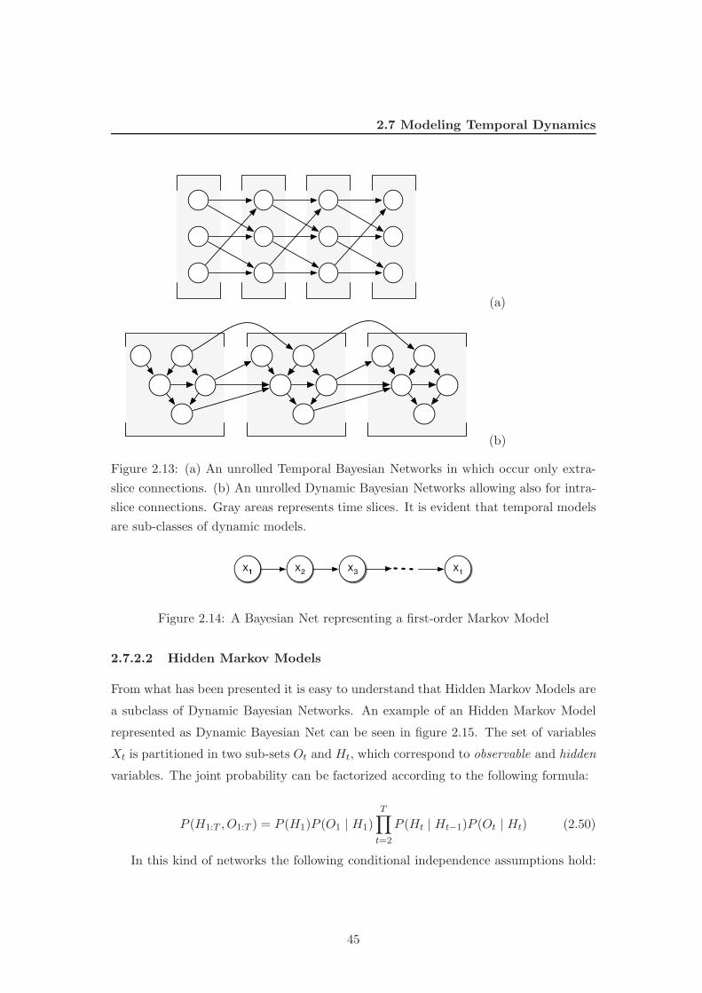
2.7 Modeling Temporal Dynamics
(a)
(b)
Figure 2.13: (a) An unrolled Temporal Bayesian Networks in which occur only extra-
slice connections. (b) An unrolled Dynamic Bayesian Networks allowing also for intra-
slice connections. Gray areas represents time slices. It is evident that temporal models
are sub-classes of dynamic models.�X 2X
3X
tX
Figure 2.14: A Bayesian Net representing a first-order Markov Model
2.7.2.2 Hidden Markov Models
From what has been presented it is easy to understand that Hidden Markov Models are
a subclass of Dynamic Bayesian Networks. An example of an Hidden Markov Model
represented as Dynamic Bayesian Net can be seen in figure 2.15. The set of variables
Xt is partitioned in two sub-sets Ot and Ht, which correspond to observable and hidden
variables. The joint probability can be factorized according to the following formula:
P (H1:T , O1:T ) = P (H1)P (O1 | H1)
T∏
t=2
P (Ht | Ht−1)P (Ot | Ht) (2.50)
In this kind of networks the following conditional independence assumptions hold:
45
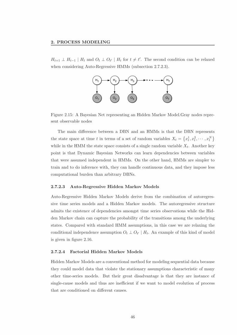
2. PROCESS MODELING
Ht+1 ⊥ Ht−1 | Ht and Ot ⊥ Ot′ | Ht for t 6= t′. The second condition can be relaxed
when considering Auto-Regressive HMMs (subsection 2.7.2.3).H 2H
3H
TH
1O
2O
3O
TO
Figure 2.15: A Bayesian Net representing an Hidden Markov Model.Gray nodes repre-
sent observable nodes
The main difference between a DBN and an HMMs is that the DBN represents
the state space at time t in terms of a set of random variables Xt ={x1
t , x2t , · · · , x
Nt
}
while in the HMM the state space consists of a single random variable Xt. Another key
point is that Dynamic Bayesian Networks can learn dependencies between variables
that were assumed independent in HMMs. On the other hand, HMMs are simpler to
train and to do inference with, they can handle continuous data, and they impose less
computational burden than arbitrary DBNs.
2.7.2.3 Auto-Regressive Hidden Markov Models
Auto-Regressive Hidden Markov Models derive from the combination of autoregres-
sive time series models and a Hidden Markov models. The autoregressive structure
admits the existence of dependencies amongst time series observations while the Hid-
den Markov chain can capture the probability of the transitions among the underlying
states. Compared with standard HMM assumptions, in this case we are relaxing the
conditional independence assumption Ot ⊥ Ot′ | Ht. An example of this kind of model
is given in figure 2.16.
2.7.2.4 Factorial Hidden Markov Models
Hidden Markov Models are a conventional method for modeling sequential data because
they could model data that violate the stationary assumptions characteristic of many
other time-series models. But their great disadvantage is that they are instance of
single-cause models and thus are inefficient if we want to model evolution of process
that are conditioned on different causes.
46
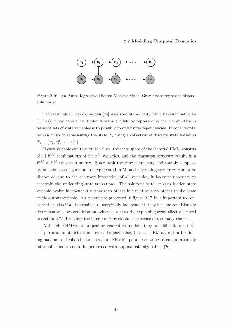
2.7 Modeling Temporal Dynamics
H 2H
3H
TH
1O
2O
3O
TO
Figure 2.16: An Auto-Regressive Hidden Markov Model.Gray nodes represent observ-
able nodes
Factorial hidden Markov models [26] are a special case of dynamic Bayesian networks
(DBNs). They generalize Hidden Markov Models by representing the hidden state in
terms of sets of state variables with possibly complex interdependencies. In other words,
we can think of representing the state Xt using a collection of discrete state variables
Xt ={x1
t , x2t , · · · , x
Mt
}.
If each variable can take on K values, the state space of the factorial HMM consists
of all KM combinations of the xMt variables, and the transition structure results in a
KM × KM transition matrix. Since both the time complexity and sample complex-
ity of estimation algorithm are exponential in M, and interesting structures cannot be
discovered due to the arbitrary interaction of all variables, it becomes necessary to
constrain the underlying state transitions. The solutions is to let each hidden state
variable evolve independently from each others but relating each others to the same
single output variable. An example is presented in figure 2.17 It is important to con-
sider that, also if all the chains are marginally independent, they become conditionally
dependent once we condition on evidence, due to the explaining away effect discussed
in section 2.7.1.1 making the inference intractable in presence of too many chains.
Although FHMMs are appealing generative models, they are difficult to use for
the purposes of statistical inference. In particular, the exact EM algorithm for find-
ing maximum likelihood estimates of an FHMMs parameter values is computationally
intractable and needs to be performed with approximate algorithms [26].
47
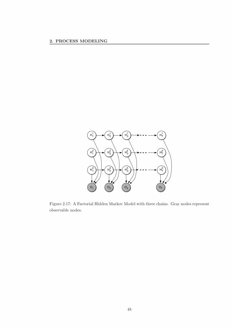
2. PROCESS MODELING
�H 2H
3H
TH
1O
2O
3O
TO
3 3 3 3
1H
2H
3H
TH
2 2 2 2
1H
2H
3H
TH
1 1 1 1
Figure 2.17: A Factorial Hidden Markov Model with three chains. Gray nodes represent
observable nodes.
48
Chapter 3
A new approach: the Structured
Hidden Markov Model
What we researched for it is a tool that permit of automatically discover complex events
in long sequences and, at the same time, offers an efficient way for modeling them.
The problem of analyzing long sequences arise in many challenging applications of
data mining, ranging from DNA analysis to user profiling and anti-intrusion systems.
Those kind of sequences are, typically,characterized by sparseness, i.e. short consecutive
chains of atomic events that are characteristic of analyzed event (we will refer to them
as episodes or motif ) and that are interleaved with long sequences of atomic events
(gap) where irrelevant facts, or facts related to spurious activities, may occur. To learn
a model for those kind of processes means to learn the episodes that characterize them
and also learn the correlations between the episodes.
Assuming that possible instances of a sparse pattern can be represented by a first or-
der Markov chain, an approach which reported impressive records of successes in speech
recognition [55] and DNA analysis [16], is based on Hidden Markov Model (HMM) [56]).
However, developing applications based on HMM does not reduce to running a learn-
ing algorithm but it may be a very costly process. In general, complex applications
require to construct an ad-hoc system, where several partial HMMs are developed and
integrated with procedural knowledge obtained from experts of the domain.
Hierarchical Hidden Markov Model, as seen in the chapter 2 introduce the possi-
bility of having a hierarchical structure in the model permitting to model recursive
or repetitive structure very well. This means that a long chain of elementary events
49
3. A NEW APPROACH: THE STRUCTURED HIDDEN MARKOVMODEL
belonging to the same episode could be abstracted in to a single event corresponding
to a state at the higher level of the hierarchy. This is obtained by exploiting the reg-
ular languages property of being closed under substitution, which allows a large finite
automaton to be transformed into a hierarchy of simpler ones. Moreover the number
of parameters to estimate is strongly reduced by assigning a null probability to many
transitions in distribution A and to many observations in distribution B (recall section
2.4.2 for a formal definition of A and B).
A first problem about using effectively HMM and HHMM is that, while the problem
of estimation parameters has been widely investigated, little has been done in order to
learn their structure. Only a few proposals can be found in the literature in order to
learn the structure of HMM but almost nothing has been done with respect to HHMM.
Another problem strictly related to HHMM is that the inference algorithm runs in
O(T 3) time, where T is the length of sequence analyzed. The make the use of HHMM
infeasible on long sequences.
What we developed is a variant of HMMs that inherits the major advantages related
to the structural property of HHMMs but that still could be make use of standard
inference algorithms developed for HMMs. This model has been called structured HMM
(S-HMM) [24]. An S-HMM is a graph built up, according to precise composition
rules, with several ”independent” sub-graphs (sub-models). It will be demonstrated
that a major feature of S-HMM is that they could be locally trained using classical
Baum-Welch algorithm, considering only a subset of the sub-models occurring in the
compound one. A nice consequence of this property is that a S-HMM can be constructed
and trained incrementally, by adding new sub-models or revising existing ones as new
information comes in. Newly added sub-model could be produced by an independent
learning process or may be provided by an expert as a-priori knowledge. Different
models could be learned and successively re-trained independently one from the other
providing a natural subproblems decomposition.
In order to model complex temporal dynamics not only the order in which motifs
could appear need to be taken in to account. Typically also the gaps between motifs
could be significant. They need to be explicitly taken into account and, so, we need a
way to explicitly model them.
The compositional property of S-HMMs allow to have a global model, describing
the dynamics of a process, that is a composition of different kinds of blocks especially
50

3.1 The Structured Hidden Markov Model
developed for modeling gaps or motifs. This is another major feature of S-HMM because
it permit mixing different kinds of blocks well-suited for specific tasks and at the same
time it allows to detect the interdependencies between blocks (motifs and/or gaps).
3.1 The Structured Hidden Markov Model
The basic assumption underlying an S-HMM (see Bouchaffra and Tan [9]) is that a
sequence O = {O1, O2, O3, ..., Ot} of observations could be segmented into a set of
subsequences O(1), O(2), ..., O(N), each one generated by a sub-process with only weak
interactions with its neighbors. This assumption is realistic in many practical ap-
plications, such as, for instance, speech recognition [55, 56], and DNA analysis [16].
In speech recognition, regions are phonetic segments, like syllables, corresponding to
recurrent structures in the language. In DNA, they may be biologically significant
segments (motifs) interleaved with non-coding segments (such as junk-DNA). S-HMMs
aim exactly at modeling such kind of processes, and, hence, they are represented as
directed graphs, structured into sub-graphs (blocks), each one modeling a specific kind
of sub-sequences.
Informally, a block consists of a set of states, only two of which (the initial and the
end state) are allowed to be connected to other blocks. As an S-HMM is itself a block,
a nesting mechanism is immediate to define.
3.1.1 Structure of a Block
In this section, a formal definition of S-HMM will be provided. O will denote a sequence
of observations {O1, O2, . . . , Ot}, where every observation Ot is a symbol Vk chosen from
an alphabet of possible events V . Remember from subsection 2.4.2 that an HMM is a
stochastic automaton characterized by a set of states S, an alphabet V , and a triple
λ = 〈A,B,Π〉, being:
• A : S × S → [0, 1] a probability distribution, aij, governing the transition from
state Si to state Sj;
• B : S × V → [0, 1] a probability distribution, bi(Vk), governing the emission of
symbols in each state Si ∈ S;
51

3. A NEW APPROACH: THE STRUCTURED HIDDEN MARKOVMODEL
• Π : S → [0, 1] a distribution assigning to each state Si ∈ S the probability of
being the start state.
A state Si will be said a silent state if ∀Vk ∈ V : bi(Vk) = 0, i.e., Si does not emit
any observable symbol. When entering a silent state, the time counter must not be
incremented.
Definition 10 A basic block of an S-HMM is a 4-tuple λ = 〈A,B, I,E〉, where I,E ∈
Q are silent states such that: π(I) = 1, ∀Si ∈ S : aiI = 0, and ∀Si ∈ S : aEi = 0.
In other words, I and E are the input and the output states, respectively. Therefore,
a composite block can be defined by connecting, through a transition network, the input
and output states of a set of blocks.
Definition 11 Given an ordered set of blocks Λ = {λi|1 ≤ i ≤ N}, a composite block
is a 4-tuple λ = 〈AI , AE , I, E〉, where:
• AI : E × I → [0, 1], AE : I × E → [0, 1] are probability distributions governing
the transitions from the output states E to the input states I, and from the input
states I to the output states E of the component blocks Λ, respectively.
• For all pairs 〈Ei, Ij〉 the transition probability aEiIj= 0 if j ≤ i.
• I ≡ I1 and E ≡ EN are the input and output states of the composite block,
respectively.
According to Definition 11 the components of a composite block can be either basic
blocks or, in turn, composite blocks. In other words, composite blocks can be arbitrarily
nested. Moreover, we will keep the notation S-HMM to designate non-basic blocks only.
As a special case, a block can degenerate to the null block, which consists of the
start and end states only, connected by an edge with probability aIE = 1. The null
block is useful to provide a dummy input state I or a dummy output state E, when no
one of the component block is suited to this purpose.
An example of S-HMM structured into three blocks λ1, λ2, λ3, and two null blocks
λ0, λ4, providing the start and the end states, is described in Figure 3.1.
52

3.1 The Structured Hidden Markov Model
λ
λ
λ
2
3
I1
I2
E1
E2
I3 E3
211 1
4131
1 2
22
32
1 3
33
23
E0I 0 I4 E4
λ1
λ0 λ4
Figure 3.1: Example of Structured Hidden Markov Model composed of three inter-
connected blocks, plus two null blocks, λ0 and λ4, providing the start and end states.
Distribution A is non-null only for explicitly represented arcs.
3.1.2 Estimating Probabilities in S-HMM
As formally stated in [56], three problems are associated with the HMM approach:
1. given a model λ and a sequence of observations O, compute the probability
P (O|λ);
2. given a model λ and a sequence of observations O, assumed to be generated by
λ, compute the most likely sequence of states in λ;
3. given a model λ and a sequence of observations O (or a set of sequences [55]),
estimate the parameters in λ in order to maximize P (O|λ).
The classical solution to Problem 1 and 3 relies on two functions α and β, plus other
auxiliary functions γ and ξ, defined on α and β. The classical solution to Problem 2
relies on Viterbi algorithm [19], which implements a function computationally analogous
to α. In the following we will extend α and β to S-HMMs in order to prove some
properties to be exploited by an incremental learning algorithm.
Given a sequence of observations O = {O1, O2, ..., Ot, .., OT } and a model λ, the
function αi(t) computes, for every time t (1 ≤ t ≤ T ), the joint probability of being in
state Si and observing the symbols from O1 to Ot.
Let us consider an S-HMM λ containing N blocks. We want to define the recursive
equations allowing α to be computed. In order to do this, we have to extend the
standard definition in order to include silent states: when leaving a silent state, the
53

3. A NEW APPROACH: THE STRUCTURED HIDDEN MARKOVMODEL
time counter is not incremented. When entering the block λk = 〈Ak, Bk, Ik, Ek〉 with
Nk states, at time r(1 ≤ r < t ≤ T ), the following equations are to be used:
αIk(r) = P (O1, ..., Or, Si(r) = Ik) (3.1a)
αj(t) = αIk(t− 1)a
(k)Ikjb
(k)j (Ot) +
Nk∑
i=1
αi(t− 1)a(k)ij b
(k)j (Ot)
(r + 1 6 t 6 T, 1 6 j 6 Nk, Sj 6= Ik, Sj 6= Ek)
(3.1b)
αEk(t) = αIk
(t) +
Nk∑
i=1
αi(t)a(k)jEk
(3.1c)
Notice that the above equations only depends upon external states through the values
of αIk(r) (1 6 r 6 T ) computed for the input state; moreover, the block propagates
αEk(t) (1 6 t 6 T ) to the following blocks only through the output state. Finally,
αI1(1) = 1 and αEN(T ) = P (O|λ).
Function βi(t) is complementary to αi(t), and computes the probability of observing
the symbols ot+1, ot+2, ... , oT , given that Si is the state at time t. For β a backward
recursive definition can be given:
βEk(r) = P (or+1, ..., oT |Si(r) = Ek) (3.2a)
βi(t) = βEk(t+ 1)a
(k)iEk
+
Nk∑
j=1
βj(t+ 1)b(k)j (ot+1)a
(k)ij
(1 6 t 6 r − 1, 1 6 i 6 Nk, Si 6= Ek, Si 6= Ik)
(3.2b)
βIk(t) = βEk
(t) +
Nk∑
j=1
βj(t)a(k)Ikj (3.2c)
From equations (3.2), it follows that P (O|λ) = βI1(1).
Definition 12 An S-HMM is said a forward S-HMM when for all non-basic blocks the
matrix AI and AE define a directed acyclic graph.
For a forward S-HMM it is easy to prove the following theorem.
Theorem 1 In a forward S-HMM, the complexity of computing functions α and β is:
C ≤ T (∑NC
h=1N2h +M
∑Nk=1N
2k )
being Nh the dimension of matrix A(h)I of the h − th block, M the cardinality of the
alphabet, NC the number of composite blocks, and N the number of basic blocks.
54
3.2 S-HMMs are locally trainable
Proof 1 Notice that the second summation in the right-hand side of the formula cor-
responds to the computation of α and β inside the basic blocks, whereas the first sum-
mation is due to the block interconnection. Following the block recursive nesting and
starting from the basic blocks, we observe that, in absence of any hypothesis on dis-
tribution A, each basic block is an HMM, whose complexity for computing α and β is
upperbounded by N2kMT [56]. As the global network interconnecting the basic blocks is
a directed forward graph, every basic block needs to be evaluated only once.
Let us consider now a composite block; the interconnecting structure is an oriented
forward graph, by definition, and, then, equations (3.1) and (3.2) must be evaluated
only once on the input (output) of every internal block S-HMMh. As a conclusion, the
complexity for this step is upperbounded by TN2h.
This is an upper bound on the calculation of functions α and β on a generic S-
HMM. In the next chapther we will introduce some special kind of basic blocs expecially
developed in order to model motif a gap in an efficent way. It will be demonstred that
adopting those ad-hoc basic blocks, the complexity will become quasi-linear in the
number of states.
3.2 S-HMMs are locally trainable
The classical algorithm for estimating the probability distributions governing state
transitions and observations are estimated by means of the Baum-Welch algorithm
[4, 56], which relies on the functions α and β defined in the previous section. In the
following we will briefly review the algorithm in order to adapt it to S-HMMs. The
algorithm uses two functions, ξ and γ, defined through α and β. Function ξi,j(t)
computes the probability of the transition between states Si (at time t) and Sj (at time
t+ 1), assuming that the observation O has been generated by model λ:
ξi,j(t) =αi(t)aijbj(Ot+1)βj(t+ 1)
P (O|λ)(3.3)
Function γi(t) computes the probability of being in state Si at time t, assuming that
the observation O has been generated by model λ, and can be written as:
γi(t) =αi(t)βi(t)
P (O|λ)(3.4)
The sum of ξi,j(t) over t estimates the number of times transition Si → Sj occurs
when λ generates the sequence O. In an analogous way, by summing γi(t) over t, an
55
3. A NEW APPROACH: THE STRUCTURED HIDDEN MARKOVMODEL
estimate of the number of times state Si has been visited is obtained. Then aij can be
re-estimated (a-posteriori, after seeing O) as the ratio of the sum over time of ξi,j(t)
and γi(t):
aij =
∑T−1t=1 αi(t)aijbj(Ot+1)βj(t+ 1)
∑T−1t=1 αi(t)βi(t)
(3.5)
With a similar reasoning it is possible to obtain an a-posteriori estimate of the prob-
ability of observing o = vk when the model is in state qj. The estimate is provided
by the ratio between the number of times state qj has been visited and symbol vk has
been observed, and the total number of times qj has been visited:
bj(k) =
∑T−1t=1
ot=vk
αj(t)βj(t)
∑T−1t=1 αj(t)βj(t)
(3.6)
From (3.1) and (3.2) it appears that, inside basic block λk, equations (3.5) and (3.6)
are immediately applicable. Then the Baum-Welch algorithm can be used without any
change to learn the probability distributions inside basic blocks.
On the contrary, equation (3.5) must be modified in order to adapt it to re-estimate
transition probabilities between output and input states of the blocks, which are silent
states. As there is no emission, α and β propagate through transitions without time
change; then, equation (3.5) must be modified as in the following:
aEiIj=
∑T−1t=1 αEi
(t)aEiIjβIj
(t)∑T−1
t=1 αEi(t)βIj
(t)(3.7)
It is worth noticing that functions α and β depend upon the states in other blocks
only through the value of αIk(t) and βEk
(t), respectively. This means that, in block
λk, given the vectors
αIk(1), αIk
(2), ...αIk(T )
and
βEk(1), βEk
(2), ...βEk(T )
Baum-Welch algorithm can be iterated inside a block without the need of recomputing
α and β in the external blocks. We will call this a locality property. The practical
implication of the locality property is that a block can be modified and trained without
any impact on the other components of an S-HMM.
56

Chapter 4
Applying S-HMMs to Real
World Tasks
Most HMM applications can be reduced to classification (instances of Problem 1 de-
scribed in section 3.1.2 ) or interpretation (instances of Problem 2 also described in
section 3.1.2) tasks. Word recognition and user/process profiling are typical classifica-
tion tasks.Sequence tagging and knowledge extraction, as done in DNA analysis, are
typical interpretation tasks. In this chapter we will focus on the problem of knowledge
extraction, but most of the proposed solutions also hold for classification tasks.
A model for interpreting a sequence is a global model, able to identify interesting
patterns (i.e., motifs, adopting Bio-Informatics terminology), which occur with signifi-
cant regularity, as well as gaps, i.e., regions where no regularities are found. Having a
global model of the sequence is important, because it allows inter-dependencies among
motifs to be detected. Nevertheless, a global model must account for the distribution
of the observations on the entire sequence, and hence it could become intractable.
We tame this problem by introducing special basic blocks, designed to take advance
of the natural sub-problems decompositions made possible by S-HMMs. When we need
to model motifs or gaps we will adopt different kinds of basic blocks that are especially
developed for the event that is needed to be modelled.
In previous chapter we assumed that inside a basic block transitions are possible
from any state to any other state. An example of this kind of structure could be seen
in figure 4.1(a). Althought it is easy to think of starting with a fully connected model,
i.e. one in which all transitions are allowed and let to the learning algorithm the task
57
4. APPLYING S-HMMS TO REAL WORLD TASKS
of discovering which transitions to use, it is infeasible in practice. For problems of
any realistic size it will usually lead to very bad models, even with plenty of training
data. And we need to take into account that to suppose of having large learning sets
is a quite optimistic assumption in many real world problems. Here the problem is
not over fitting but local maxima [16]. The less constrained the model is, the more
severe the local maximum problem becomes. There are methods that attempt to adapt
the model topology based on the data by adding and removing transitions and states
[22, 65]. However, in practice, successful HMMs are constructed by carefully deciding
which transitions are to be allowed in the model, based on the knowledge about the
problem under investigation.
In our approach it is possible having different kind of HMMs structures according to
the kind of event that we need to model, i.e. structures in which the allowed transitions
are constrained on the basis of the kind of events that are to be modelled. Disabling
transition from a state to another means to set the corresponding transition to zero.
The classical algorithm for estimating probability on HMMs (like Baum-Welch) are not
affected by this constraints. A transition set to zero, after a re-estimation step, will be
still set to zero because when the probability is null the expected number of transitions
will also be null. Therefore all the mathematics is unchanged even if not all transitions
are possible.
Disallowing some transitions is helpful not only in avoiding local maxima. Another
advantage of constraining the structure of sub-models is that reducing the number of
possible transitions in a basic S-HMM block will also reduce the computational cost
of learning algorithms. Since the amount of free parameters and the amount of com-
putations are directly dependent on the number of non-zero transitions probabilities,
keeping low the number of possible transitions is an help in keeping low the computa-
tional cost of algorithms on HMMs.
In the following sections we’ll address the following issues: (a) how to construct
basic blocks for modeling motifs and the gaps between them; (b) how to segment a
sequence detecting the instances of the basic blocks; (c) how to extract a readable
interpretation from a sequence.
58
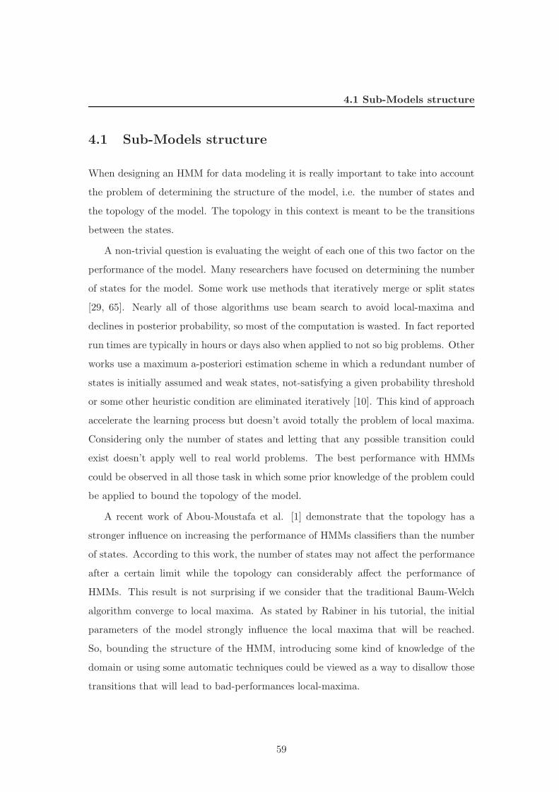
4.1 Sub-Models structure
4.1 Sub-Models structure
When designing an HMM for data modeling it is really important to take into account
the problem of determining the structure of the model, i.e. the number of states and
the topology of the model. The topology in this context is meant to be the transitions
between the states.
A non-trivial question is evaluating the weight of each one of this two factor on the
performance of the model. Many researchers have focused on determining the number
of states for the model. Some work use methods that iteratively merge or split states
[29, 65]. Nearly all of those algorithms use beam search to avoid local-maxima and
declines in posterior probability, so most of the computation is wasted. In fact reported
run times are typically in hours or days also when applied to not so big problems. Other
works use a maximum a-posteriori estimation scheme in which a redundant number of
states is initially assumed and weak states, not-satisfying a given probability threshold
or some other heuristic condition are eliminated iteratively [10]. This kind of approach
accelerate the learning process but doesn’t avoid totally the problem of local maxima.
Considering only the number of states and letting that any possible transition could
exist doesn’t apply well to real world problems. The best performance with HMMs
could be observed in all those task in which some prior knowledge of the problem could
be applied to bound the topology of the model.
A recent work of Abou-Moustafa et al. [1] demonstrate that the topology has a
stronger influence on increasing the performance of HMMs classifiers than the number
of states. According to this work, the number of states may not affect the performance
after a certain limit while the topology can considerably affect the performance of
HMMs. This result is not surprising if we consider that the traditional Baum-Welch
algorithm converge to local maxima. As stated by Rabiner in his tutorial, the initial
parameters of the model strongly influence the local maxima that will be reached.
So, bounding the structure of the HMM, introducing some kind of knowledge of the
domain or using some automatic techniques could be viewed as a way to disallow those
transitions that will lead to bad-performances local-maxima.
59
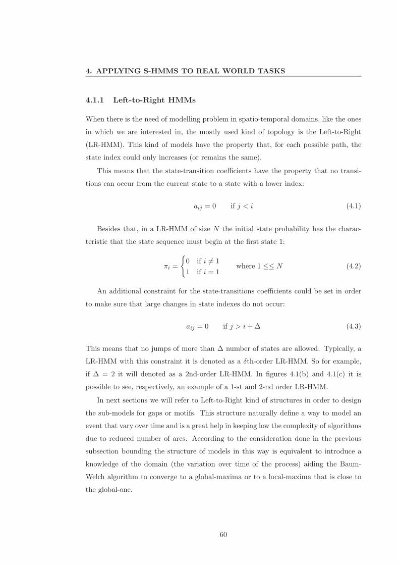
4. APPLYING S-HMMS TO REAL WORLD TASKS
4.1.1 Left-to-Right HMMs
When there is the need of modelling problem in spatio-temporal domains, like the ones
in which we are interested in, the mostly used kind of topology is the Left-to-Right
(LR-HMM). This kind of models have the property that, for each possible path, the
state index could only increases (or remains the same).
This means that the state-transition coefficients have the property that no transi-
tions can occur from the current state to a state with a lower index:
aij = 0 if j < i (4.1)
Besides that, in a LR-HMM of size N the initial state probability has the charac-
teristic that the state sequence must begin at the first state 1:
πi =
{
0 if i 6= 1
1 if i = 1where 1 ≤≤ N (4.2)
An additional constraint for the state-transitions coefficients could be set in order
to make sure that large changes in state indexes do not occur:
aij = 0 if j > i+ ∆ (4.3)
This means that no jumps of more than ∆ number of states are allowed. Typically, a
LR-HMM with this constraint it is denoted as a δth-order LR-HMM. So for example,
if ∆ = 2 it will denoted as a 2nd-order LR-HMM. In figures 4.1(b) and 4.1(c) it is
possible to see, respectively, an example of a 1-st and 2-nd order LR-HMM.
In next sections we will refer to Left-to-Right kind of structures in order to design
the sub-models for gaps or motifs. This structure naturally define a way to model an
event that vary over time and is a great help in keeping low the complexity of algorithms
due to reduced number of arcs. According to the consideration done in the previous
subsection bounding the structure of models in this way is equivalent to introduce a
knowledge of the domain (the variation over time of the process) aiding the Baum-
Welch algorithm to converge to a global-maxima or to a local-maxima that is close to
the global-one.
60
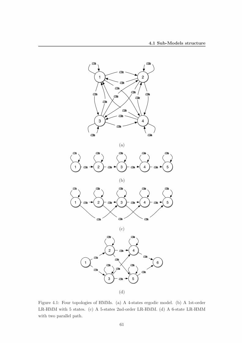
4.1 Sub-Models structure
1
43
2
a11
a12
a13
a14
a21
a23a24
a31
a32
a34
a42
a41
a43
a22
a33 a44
(a)
1
a11
2
a22
3
a33
4
a44
a12 a23 a34 5
a55
a45
(b)
1
a11
2
a22
3
a33
4
a44
a12 a23 a34 5
a55
a45
a13 a24 a35
(c)
1
2
a22
4
a44
6
a12
a24
a46
3
a33
5
a55
a35
a13a56
a25
a34
(d)
Figure 4.1: Four topologies of HMMs. (a) A 4-states ergodic model. (b) A 1st-order
LR-HMM with 5 states. (c) A 5-states 2nd-order LR-HMM. (d) A 6-state LR-HMM
with two parallel path.
61
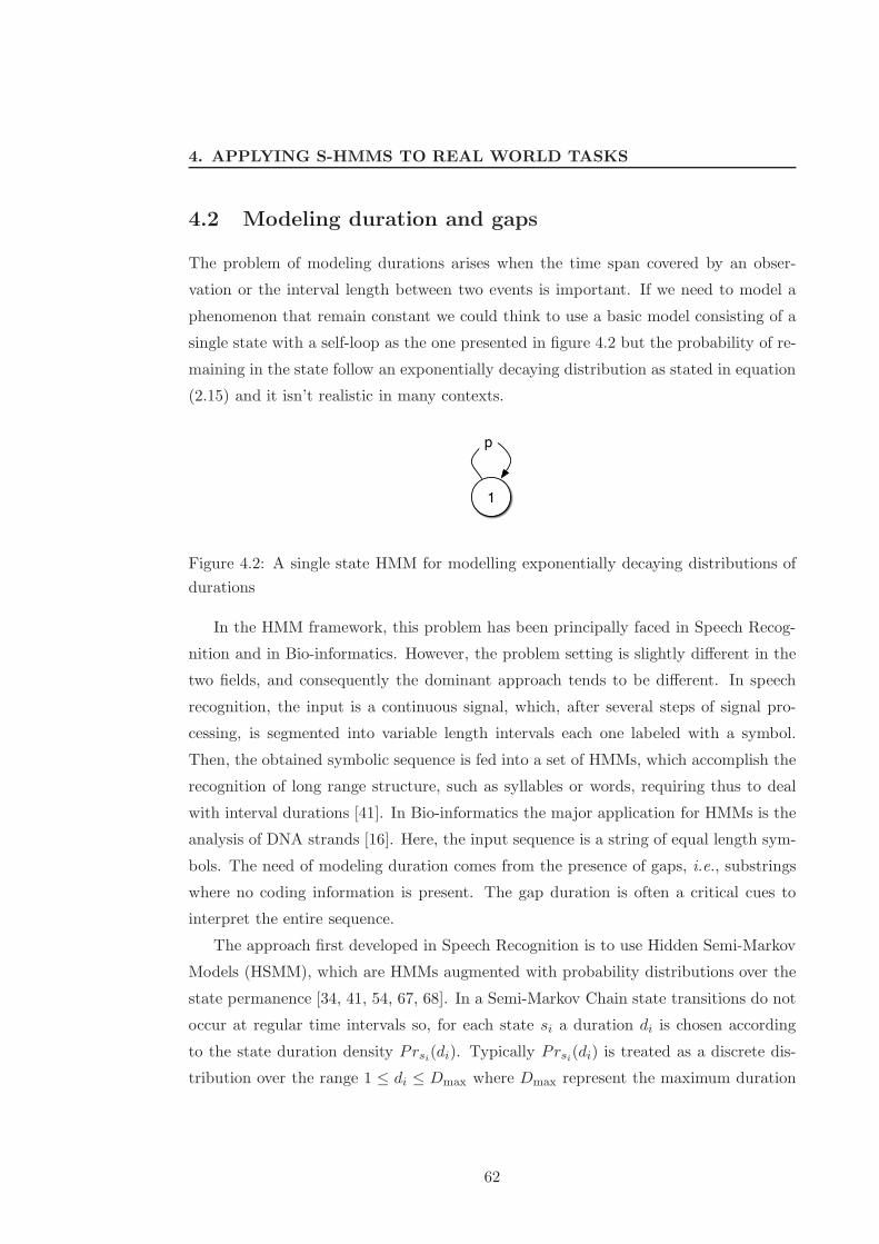
4. APPLYING S-HMMS TO REAL WORLD TASKS
4.2 Modeling duration and gaps
The problem of modeling durations arises when the time span covered by an obser-
vation or the interval length between two events is important. If we need to model a
phenomenon that remain constant we could think to use a basic model consisting of a
single state with a self-loop as the one presented in figure 4.2 but the probability of re-
maining in the state follow an exponentially decaying distribution as stated in equation
(2.15) and it isn’t realistic in many contexts.
1
p
Figure 4.2: A single state HMM for modelling exponentially decaying distributions of
durations
In the HMM framework, this problem has been principally faced in Speech Recog-
nition and in Bio-informatics. However, the problem setting is slightly different in the
two fields, and consequently the dominant approach tends to be different. In speech
recognition, the input is a continuous signal, which, after several steps of signal pro-
cessing, is segmented into variable length intervals each one labeled with a symbol.
Then, the obtained symbolic sequence is fed into a set of HMMs, which accomplish the
recognition of long range structure, such as syllables or words, requiring thus to deal
with interval durations [41]. In Bio-informatics the major application for HMMs is the
analysis of DNA strands [16]. Here, the input sequence is a string of equal length sym-
bols. The need of modeling duration comes from the presence of gaps, i.e., substrings
where no coding information is present. The gap duration is often a critical cues to
interpret the entire sequence.
The approach first developed in Speech Recognition is to use Hidden Semi-Markov
Models (HSMM), which are HMMs augmented with probability distributions over the
state permanence [34, 41, 54, 67, 68]. In a Semi-Markov Chain state transitions do not
occur at regular time intervals so, for each state si a duration di is chosen according
to the state duration density Prsi(di). Typically Prsi
(di) is treated as a discrete dis-
tribution over the range 1 ≤ di ≤ Dmax where Dmax represent the maximum duration
62
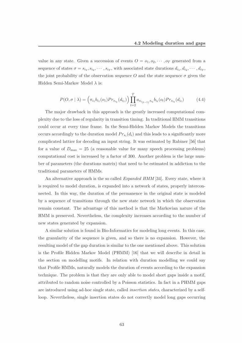
4.2 Modeling duration and gaps
value in any state. Given a succession of events O = o1, o2, · · · , oT generated from a
sequence of states σ = si1 , si2, · · · , siT , with associated state durations di1 , di2 , · · · , diT ,
the joint probability of the observation sequence O and the state sequence σ given the
Hidden Semi-Markov Model λ is:
P (O,σ | λ) =(
πi1bi1(o1)Prsi1(di1)
) T∏
t=2
asi(t−1)sitbit(ot)Prsit
(dit) (4.4)
The major drawback in this approach is the greatly increased computational com-
plexity due to the loss of regularity in transition timing. In traditional HMM transitions
could occur at every time frame. In the Semi-Hidden Markov Models the transitions
occurs accordingly to the duration model Prsi(di) and this leads to a significantly more
complicated lattice for decoding an input string. It was estimated by Rabiner [56] that
for a value of Dmax = 25 (a reasonable value for many speech processing problems)
computational cost is increased by a factor of 300. Another problem is the large num-
ber of parameters (the durations matrix) that need to be estimated in addiction to the
traditional parameters of HMMs.
An alternative approach is the so called Expanded HMM [34]. Every state, where it
is required to model duration, is expanded into a network of states, properly intercon-
nected. In this way, the duration of the permanence in the original state is modeled
by a sequence of transitions through the new state network in which the observation
remain constant. The advantage of this method is that the Markovian nature of the
HMM is preserved. Nevertheless, the complexity increases according to the number of
new states generated by expansion.
A similar solution is found in Bio-Informatics for modeling long events. In this case,
the granularity of the sequence is given, and so there is no expansion. However, the
resulting model of the gap duration is similar to the one mentioned above. This solution
is the Profile Hidden Markov Model (PHMM) [16] that we will describe in detail in
the section on modelling motifs. In relation with duration modelling we could say
that Profile HMMs, naturally models the duration of events according to the expansion
technique. The problem is that they are only able to model short gaps inside a motif,
attributed to random noise controlled by a Poisson statistics. In fact in a PHMM gaps
are introduced using ad-hoc single state, called insertion states, characterized by a self-
loop. Nevertheless, single insertion states do not correctly model long gaps occurring
63

4. APPLYING S-HMMS TO REAL WORLD TASKS
� 3 4 51.0 0.8 0.5 61.0
0.3
0.2
1 1.0
(a) 3
� �� ��1-p 1-p 1-p 61-p1 1.0
p
(b)
Figure 4.3: Possible HMMs for modeling duration
between two motifs. The most appropriate probability distribution for this kind of gaps
may vary from case to case, but it is never the exponential decay defined by an insert
state with a self-loop.
In our framework we adopted well defined topologies of LR-HMMs in order to model
gap duration. In all cases, the observation is supposed to be produced by random
noise so in every state of a gap sub-model we will observe the same distribution over
observations. This limitations is very effective in reducing the number of parameters
that need to be estimated because all the states of a gap sub-model share the same
observation distribution, independently from the number of states in the model. After
having defined, statistically, the length of a gap it is easy to model it using one of the
possible topologies. The chosen topologies are characterized by constant number of
arcs exiting from each node. This value is very low, usually 2 or 3, depending on the
topologies.
Two HMM topologies, suitable for modeling gaps, are reported in Figure 4.3. The
architecture in Figure 4.3(a) can be used to model any duration distribution over a
finite and discrete interval. However, the drawback of this model is the potentially
large number of parameters to estimate. In all cases, the observation is supposed to be
produced by random noise. Model in Figure 4.3(b) exhibits an Erlang’s distribution,
when the Forward-Backward algorithm is used. Unfortunately, the distribution of the
most likely duration computed by Viterbi algorithm still follows an exponential law.
Therefore, this model, which is more compact with respect to the previous one, is not
64

4.3 Modeling motifs
useful for the task of segmenting and tagging sequences by means of Viterbi algorithm.
4.3 Modeling motifs
A more complex analysis as to be done in order to find a way to model motifs. A motif
is a subsequence frequently occurring in a reference sequences set. Motif occurrences
may be different from one to another, provided that an assigned equivalence relation
has to be satisfied. In the specific case, the equivalence relation is encoded through a
basic block of an S-HMM.
Many proposals exist for HMM architectures oriented to capture specific patterns.
One of the widely used approach is the Profile HMM (PHMM), a model developed in
Bio-Informatics [16], which well fits the needs of providing a readable interpretation of
a sequence, i.e. a profile. The basic assumption underlying PHMM is that the different
instances of a motif originate from a canonical form, but are subject to insertion,
deletion and substitution errors.
Now we need to introduce briefly the concepts of pairwise and multiple alignment.
After that introduction we could describe how it is possible building motifs models
starting from multiple alignments.
4.3.1 String Alignment and Multiple Alignment
A key role in the order to learn and to model motifs is represented by approximate
matching and it is based on string alignment. String alignment has been deeply inves-
tigated in Machine Learning and a wide collection of effective algorithms are available.
Here, we will recall some basic concepts, but an exhaustive introduction to the topic
could be find in [16, 28].
Definition 13 Given two strings s1 and s2, let s′1 and s′2 be two strings obtained
from s1 and s2, respectively, by inserting an arbitrary number of spaces such that
the symbols in the two strings can be put in a one-to-one correspondence. The pair
A(s1, s2) = 〈s′1, s′2〉, is said a global alignment between s1 and s2.
From global alignment, local alignment and multi-alignment can be defined.
65
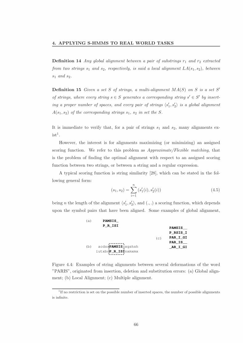
4. APPLYING S-HMMS TO REAL WORLD TASKS
Definition 14 Any global alignment between a pair of substrings r1 and r2 extracted
from two strings s1 and s2, respectively, is said a local alignment LA(s1, s2), between
s1 and s2.
Definition 15 Given a set S of strings, a multi-alignment MA(S) on S is a set S′
of strings, where every string s ∈ S generates a corresponding string s′ ∈ S′ by insert-
ing a proper number of spaces, and every pair of strings 〈s′1, s′2〉 is a global alignment
A(s1, s2) of the corresponding strings s1, s2 in set the S.
It is immediate to verify that, for a pair of strings s1 and s2, many alignments ex-
ist1.
However, the interest is for alignments maximizing (or minimizing) an assigned
scoring function. We refer to this problem as Approximate/Flexible matching, that
is the problem of finding the optimal alignment with respect to an assigned scoring
function between two strings, or between a string and a regular expression.
A typical scoring function is string similarity [28], which can be stated in the fol-
lowing general form:
(s1, s2) =
n∑
i=1
(s′1(i), s′2(i)) (4.5)
being n the length of the alignment 〈s′1, s′2〉, and (., .) a scoring function, which depends
upon the symbol pairs that have been aligned. Some examples of global alignment,
PAMSIS_P_R_ISI
acdssPAMSIS_xgshshiutxboP_R_ISInxmxmx
(a)
(b)
(c)
PAMSIS__P_RSIS_IPAR_I_GIPAR_IS___AR_I_GI
Figure 4.4: Examples of string alignments between several deformations of the word
”PARIS”, originated from insertion, deletion and substitution errors: (a) Global align-
ment; (b) Local Alignment; (c) Multiple alignment.
1If no restriction is set on the possible number of inserted spaces, the number of possible alignments
is infinite.
66
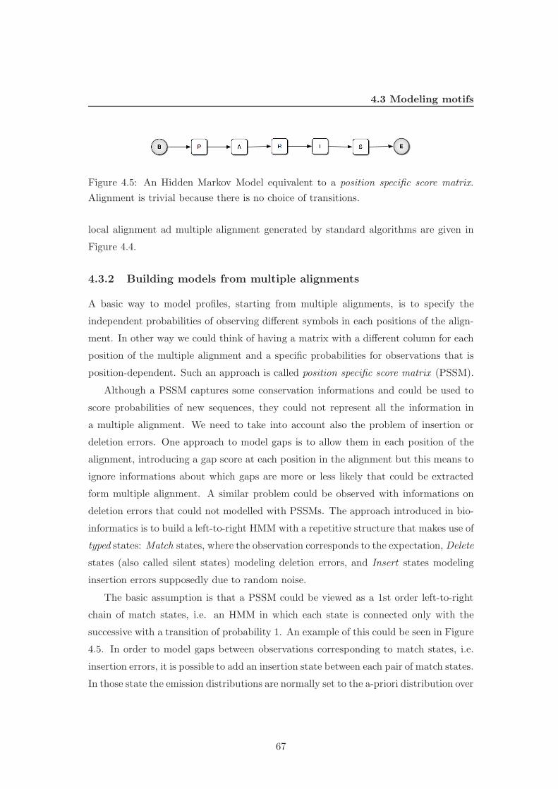
4.3 Modeling motifs
B � A R I S E
Figure 4.5: An Hidden Markov Model equivalent to a position specific score matrix.
Alignment is trivial because there is no choice of transitions.
local alignment ad multiple alignment generated by standard algorithms are given in
Figure 4.4.
4.3.2 Building models from multiple alignments
A basic way to model profiles, starting from multiple alignments, is to specify the
independent probabilities of observing different symbols in each positions of the align-
ment. In other way we could think of having a matrix with a different column for each
position of the multiple alignment and a specific probabilities for observations that is
position-dependent. Such an approach is called position specific score matrix (PSSM).
Although a PSSM captures some conservation informations and could be used to
score probabilities of new sequences, they could not represent all the information in
a multiple alignment. We need to take into account also the problem of insertion or
deletion errors. One approach to model gaps is to allow them in each position of the
alignment, introducing a gap score at each position in the alignment but this means to
ignore informations about which gaps are more or less likely that could be extracted
form multiple alignment. A similar problem could be observed with informations on
deletion errors that could not modelled with PSSMs. The approach introduced in bio-
informatics is to build a left-to-right HMM with a repetitive structure that makes use of
typed states: Match states, where the observation corresponds to the expectation, Delete
states (also called silent states) modeling deletion errors, and Insert states modeling
insertion errors supposedly due to random noise.
The basic assumption is that a PSSM could be viewed as a 1st order left-to-right
chain of match states, i.e. an HMM in which each state is connected only with the
successive with a transition of probability 1. An example of this could be seen in Figure
4.5. In order to model gaps between observations corresponding to match states, i.e.
insertion errors, it is possible to add an insertion state between each pair of match states.
In those state the emission distributions are normally set to the a-priori distribution over
67
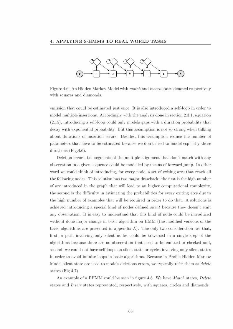
4. APPLYING S-HMMS TO REAL WORLD TASKS
B � A R I S E
Figure 4.6: An Hidden Markov Model with match and insert states denoted respectively
with squares and diamonds.
emission that could be estimated just once. It is also introduced a self-loop in order to
model multiple insertions. Accordingly with the analysis done in section 2.3.1, equation
(2.15), introducing a self-loop could only models gaps with a duration probability that
decay with exponential probability. But this assumption is not so strong when talking
about durations of insertion errors. Besides, this assumption reduce the number of
parameters that have to be estimated because we don’t need to model esplicitly those
durations (Fig.4.6).
Deletion errors, i.e. segments of the multiple alignment that don’t match with any
observation in a given sequence could be modelled by means of forward jump. In other
word we could think of introducing, for every node, a set of exiting arcs that reach all
the following nodes. This solution has two major drawback: the first is the high number
of arc introduced in the graph that will lead to an higher computational complexity,
the second is the difficulty in estimating the probabilities for every exiting arcs due to
the high number of examples that will be required in order to do that. A solutions is
achieved introducing a special kind of nodes defined silent because they doesn’t emit
any observation. It is easy to understand that this kind of node could be introduced
without done major change in basic algorithm on HMM (the modified versions of the
basic algorithms are presented in appendix A). The only two consideration are that,
first, a path involving only silent nodes could be traversed in a single step of the
algorithms because there are no observation that need to be emitted or checked and,
second, we could not have self loops on silent state or cycles involving only silent states
in order to avoid infinite loops in basic algorithms. Because in Profile Hidden Markov
Model silent state are used to models deletions errors, we typically refer them as delete
states (Fig.4.7).
An example of a PHMM could be seen in figure 4.8. We have Match states, Delete
states and Insert states represented, respectively, with squares, circles and diamonds.
68

4.3 Modeling motifs
B � A R I S E
Figure 4.7: An Hidden Markov Model with match and delete states denoted respectively
with squares and circle. Delete states are silent state introduced in order to allow long
gap keeping low the number of transitions.
B � A R I S E
Figure 4.8: Example of Profile Hidden Markov Model. Circles denote states with no-
observable emission, rectangles denote match states, and diamond denote insert states.
4.3.3 Another approach to motifs modeling
Profile Hidden Markov Model are very useful in bio-informatics task because they
could be learned by using only a few sequences set and doesn’t require to be refined by
using Baum-Welch training step because all the probabilities are learned in a statistical
way. Beside this, the repetitive and easy-to-understand PHMM structure easily allow
domain expert to adjust the model in order to fit the required task. We need to take
into account that in Biological domain could be very hard find large learning set on
which apply totally unsupervised techniques.
A problem that arises in order to use Profile Hidden Markov Models on some kind
of real-word tasks is that if we *want* to use Baum-Welch algorithm, for example to
adjust the probabilities of the model because a new set of sequences have just been
added to the learning set, we could lose the knowledge connected with the structure.
To understand this point we need to do a little consideration: we could use the
Viterbi algorithm in order to find the most probable path on a PHMM. The concep-
tual differentiation between match and insert states permit us to tell that observations
emitted by an insert state are correspondent to insertion error and that observations
69
4. APPLYING S-HMMS TO REAL WORLD TASKS
emitted by a match state belong to the profile. Baum-Welch algorithm doesn’t distin-
guish between different kind of emitting states so it could happen that the algorithm
increase the probability of observing profile symbols in insertion states, or could change
the transitions probabilities making possible that different profile symbols are read in
the same (insert) state. In other word applying Baum-Welch algorithm on a PHMM
could lead at loosing the conceptual correlation between insertion state and insertion
error. Another problem is that long chain of delete state could lead the baum-welch
algorithm towards local maxima because they permit to go through the full chain of
states in a single step theoretically permitting of by-passing also all the match states.
For this reasons we modelled profile also by using a k-order Bakis topology , i.e. a
Left-to-Right model in which in every state the only allowed transition are self loops
and jump towards the k following states. This a topology largely used in speech-
recognition because typically utterances begins and ends at well-identified time instants
and because speech could be well modelled by sequential HMM. From a conceptual point
of view this means merging insert and match state in a same state and using forward
jump in order to model deletion errors. We limit the number of forward jump to a well
defined value k in order to limit to a constant value the branching factor of the model.
Usually we impose k = 8. It is important to note that this is not a crucial parameters
under the condition of not choosing value too low; it is obvious that the value of k
determine the number of consecutive deletion error, i.e. the consecutive emitting state
that could be ignored in a single step, that could be modelled. But if we choose a value
for k that is too large we will have no drawbacks because during the refining step the
unused arc probabilities will be set to zero by the Bahum-Welch algorithm. The only
effect will be a slightly increase in the computational cost. Using k = 7 it could be a
good choice in majority of task since we could easily understand that having more than
seven consecutive deletion error on a profile it is quite improbable. An example of this
topology could be seen in figure 4.1 (c) (in this case k = 2).
4.4 Matching complexity
In the section 3.1.2 the upper bound on the calculation of functions α and β has
been reported. However, adopting the basic block structures suggested in the previous
70
4.4 Matching complexity
sections for modeling motifs and gaps, this complexity becomes quasi-linear in the
number of states.
If we recall the theorem 1 we could see that in a forward S-HMM, the complexity
of computing functions α and β is:
C ≤ T (∑NC
h=1N2h +M
∑Nl=1N
2l )
being Nh the dimension of matrix A(h)I of the h − th block, M the cardinality of the
alphabet, i.e. a constant term, NC the number of composite blocks, and N the number
of basic blocks.
For shake of brevity we will denote the product in the first term of equation (N2h)
as P1 and the product in the second term of equation (N2l ) as P2 thus the equations
will be rewrited as:
C ≤ T (∑NC
h=1 P1 +M∑N
l=1 P2)
We could start remembering that the second summation in the right-hand side of
the formula corresponds to the computation of α and β inside the basic blocks, whereas
the first summation is due to the block interconnection. Examining the basic-blocks
complexity we need also to remember that in each node we need to check the alpha
(beta) values only for each node that is directly connected with this one. In presence
of a constant branching factor f we could rewrite P2 as: P2 = fNl. Because P2 is
the only term affecting the worst-case complexity of basic-blocks we could state that
in presence of a constant branching factor the complexity of a single step of algorithms
become O(fNl), i.e., being f a constant term, a linear complexity.
Considering Profile HMMs (see Figure 4.8), it is immediate to verify that their
branching factor is 3 so we obtain O(3Nl). If we model profiles by means a k − order
Bakis topology we still a number of exiting arcs from every node that is bounded to
a constant (and quite-small) value of k + 1 (the forward jumps and the self loop).
Supposing k = 7 we have eight exiting arcs so the complexity will become O(8Nl). If
we consider both the gap models in Figure 4.3(a) and 4.3(b) the complexity decreases
to O(2Nl).
Let us consider now a composite block; as stated in proof of theorem 1 the intercon-
necting structure is an oriented forward graph, by definition, and, then, equations (3.1)
and (3.2) must be evaluated only once on the input (output) of every internal block
S-HMMh so the complexity for this step is upperbounded by O(N2h) because P1 = N2
h
So the only nonlinear term can be due to the matrix interconnecting the blocks. We
71
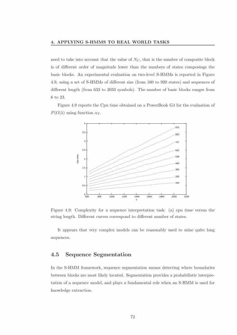
4. APPLYING S-HMMS TO REAL WORLD TASKS
need to take into account that the value of NC , that is the number of composite block
is of different order of magnitude lower than the numbers of states composings the
basic blocks. An experimental evaluation on two-level S-HMMs is reported in Figure
4.9, using a set of S-HMMs of different size (from 160 to 920 states) and sequences of
different length (from 633 to 2033 symbols). The number of basic blocks ranges from
6 to 23.
Figure 4.9 reports the Cpu time obtained on a PowerBook G4 for the evaluation of
P (O|λ) using function αT .
0
0.5
1
1.5
2
2.5
3
3.5
4
600 800 1000 1200 1400 1600 1800 2000 2200
Cpu
tim
e
T
160
255
350
443
538
632
727
820
915
Figure 4.9: Complexity for a sequence interpretation task: (a) cpu time versus the
string length. Different curves correspond to different number of states.
It appears that very complex models can be reasonably used to mine quite long
sequences.
4.5 Sequence Segmentation
In the S-HMM framework, sequence segmentation means detecting where boundaries
between blocks are most likely located. Segmentation provides a probabilistic interpre-
tation of a sequence model, and plays a fundamental role when an S-HMM is used for
knowledge extraction.
72
4.5 Sequence Segmentation
Imposing a Left-to-Right structure is very useful because it could be effectively
useful in answering to one of the most difficult questions in constructing HMM: What
should the hidden state represent? For each basic-block states the segmentations is
bounded by the topology of the model that avoid for the same state to occur in different
part of the same sequence tagging. In other word, in presence of a Left-to-Right
topology, the segmentation permit to assign a particular meaning to each block, defining
the most probable lattice of sub-sequences that could be assigned to it.
In many context could be really important having the possibility to attach knowledge-
driven meaning to a particular blocks of the S-HMM. For example in a speech recog-
nition problem could be easy to associate a phoneme or a word to a basic-block; this
fact could be a great help for domain experts that need to identify and to generalize
similar speech unit (representing a particular linguistic meaning and the associated
distribution on acoustic subsequences) which can be re-used or shared between models.
Two methods exist for accomplishing this segmentation task. The classical one is
based on Viterbi algorithm in order to find the most likely path in the state space of the
model. Then, for every pair of blocks λr, λs on the path, the most likely time instant
for the transition from the output state of λr to the input state of λs is chosen as the
boundary between the two blocks. In this way a unique, non ambiguous segmentation
is obtained, with a complexity which is the same as for computing α and β.
The second method, also described in [56], consists in finding the maximum likeli-
hood time for the transition from λr to λs by computing:
τrs = argmaxt
(ξEr,Is(t)
γEr(t)
)
(4.6)
Computing boundaries by means of (4.6) requires a complexity O(T ) for every boundary
that has to be located, in addition to the complexity for computing one α and β.
The advantage of this method is that it can provide alternative segmentations by
considering also blocks that do not lie on the maximum likelihood path. Moreover, it is
compatible with the use of gap models of the type described in Figure 4.3(b), because
it does not use Viterbi algorithm.
73

4. APPLYING S-HMMS TO REAL WORLD TASKS
4.6 Knowledge Transfer
When a tool is used in a knowledge extraction task, two important features are desir-
able: (a) the extracted knowledge should be readable for a human user; (b) a human
user should be able to elicit chunks of knowledge, which the tool will exploit during the
extraction process.
The basic HMM does not have such properties, whereas task oriented HMMs, such
as Profile HMM, may provide such properties to a limited extent. On the contrary, the
S-HMM structure naturally supports high level logical descriptions.
An example of how an S-HMM can be described in symbolic form is provided in
Figure 4.10. Basic blocks and composite blocks must be described in different ways.
Basic blocks are either HMMs (modeling subsequences), or gap models. In both cases,
a precise description of the underlying automaton will be complex, without providing
readable information to the user. Instead, an approximate description, characterizing
at an abstract level the knowledge captured by a block, is more useful. For instance,
blocks corresponding to regularities like motifs can be characterized by providing the
maximum likelihood sequence (MLS) as the nominal form of the sequence, and the
average deviation (AvDv) from the nominal form. Instead, gaps can be characterized
by suppling the average duration (AvDr), and the minimum (MnDr) and maximum
(MxDr) duration.
On the contrary, the model’s composite structure is easy to describe by means of
a logic language. As an example, Figure 4.10(c) provides the translation into Horn
clauses, whereas Figure 4.10(d) provides the translation into regular expressions. In
both cases, richer representations can be obtained by annotating the expressions with
numeric attributes.
By using a logic description language, or regular expressions, a user can also provide
the specification of an S-HMM structure, or part of it, which will be completed and
trained by a learning algorithm. Logic formulas as in Figure 4.10(c) can be immediately
translated into the structure of composite blocks. Nevertheless, also an approximate
specification for basic blocks, as described in Figure 4.10, can be mapped to block mod-
els when the model scheme is given. For instance, suppose that motifs are described
by Profile HMMs, and gaps by the scheme of Figure 4.3(a) or (b). Then, the maxi-
mum likelihood sequence provided in the logic description implicitly sets the number
74

4.6 Knowledge Transfer
of match states and, together with the average deviation, provides the prior for an
initial distribution on the observations. In an analogous way, minimum, maximum and
average values specified for the gap duration can be used to set the number of states
and a prior on the initial probability distribution. Then, a training algorithm can tune
the model parameters.
75
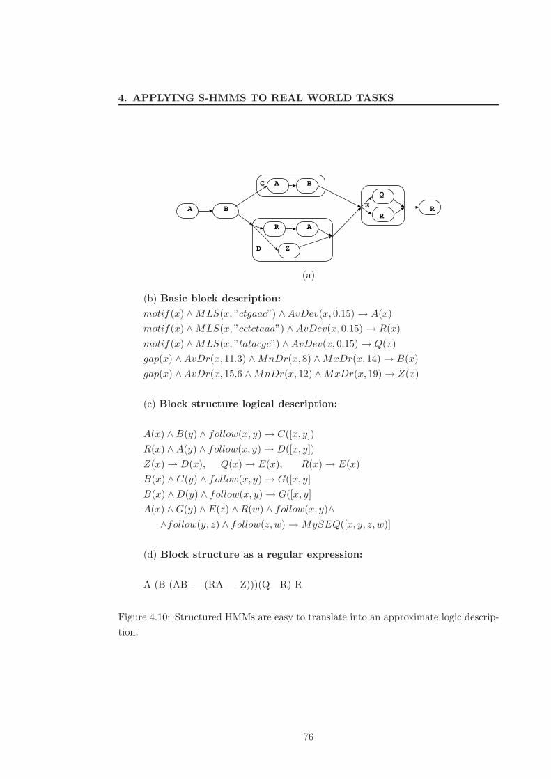
4. APPLYING S-HMMS TO REAL WORLD TASKS
A B
C
D
E R
A B
R A
Z
Q
R
(a)
(b) Basic block description:
motif(x) ∧MLS(x, ”ctgaac”) ∧AvDev(x, 0.15) → A(x)
motif(x) ∧MLS(x, ”cctctaaa”) ∧AvDev(x, 0.15) → R(x)
motif(x) ∧MLS(x, ”tatacgc”) ∧AvDev(x, 0.15) → Q(x)
gap(x) ∧AvDr(x, 11.3) ∧MnDr(x, 8) ∧MxDr(x, 14) → B(x)
gap(x) ∧AvDr(x, 15.6 ∧MnDr(x, 12) ∧MxDr(x, 19) → Z(x)
(c) Block structure logical description:
A(x) ∧B(y) ∧ follow(x, y) → C([x, y])
R(x) ∧A(y) ∧ follow(x, y) → D([x, y])
Z(x) → D(x), Q(x) → E(x), R(x) → E(x)
B(x) ∧C(y) ∧ follow(x, y) → G([x, y]
B(x) ∧D(y) ∧ follow(x, y) → G([x, y]
A(x) ∧G(y) ∧ E(z) ∧R(w) ∧ follow(x, y)∧
∧follow(y, z) ∧ follow(z,w) →MySEQ([x, y, z, w)]
(d) Block structure as a regular expression:
A (B (AB — (RA — Z)))(Q—R) R
Figure 4.10: Structured HMMs are easy to translate into an approximate logic descrip-
tion.
76

Chapter 5
Edy: a tool for unsupervised
learning of SHMMs
In this chapter, we present an unsupervised algorithm, called EDY (Event DiscoverY),
for inferring a S-HMM from a database of sequences. This algorithm is the major
contribution of this thesis, and addresses a very difficult task that up to now has seen
very few solution proposals in the literature.
However, the algorithm, in the present form show two strong limitations:
• The generated S-HMMs has only two levels of block nesting;
• The structure of the blocks is limited to forward graphs, which at most can contain
self loops.
The first limitation, may become sensible only in cases of very complex HMMs, and
in practice it didn’t become evident in all the cases, in which EDY has been applied.
The second limitation, instead, is more relevant and becomes evident when the
learning sequences have been generated by an iterative process. In this case, EDY can
be applied in order to learn a model which generate a single cycle, or, alternatively, it
can try to learn a forward model for a full sequence of cycles. Nevertheless it is not
capable of learning the iterative structure.
Not withstanding such limitations we will show, in the following, that EDY is
already a powerful induction algorithm, which solves non trivial tasks.
EDY constructs a S-HMM incrementally going through a learning cycle in which
a model is progressively extended and refined, by repeatedly incorporating new basic
77
5. EDY: A TOOL FOR UNSUPERVISED LEARNING OF SHMMS
blocks modeling motifs or gaps. The cycle may initiate with an empty model or with
a partial model supplied by an expert of the domain, and terminates when there is no
more evidence of new motifs to incorporate.
The rational behind this architecture is that regularities due to the presence of
motifs may be difficult (or impossible) to distinguish from randomness when considered
in isolation, but may become evident in the context established by a partial model.
Therefore the algorithm tries to discover first the motifs, which are evident in absence
of any a priori information. Then using such motifs it builds up a first model which is
augmented cycle after cycles by adding new motifs as long as they become detectable.
The core of all the learning process is made up by two steps: the extension and the
refinement step. The first it is responsible for discovering new motifs looking inside the
learning sequences (as we just mentioned) and integrating them in the current model,
while the second one refine the structure of the current model. In the following, EDY’s
algorithm will be described into details.
5.1 Edy’s discovery strategy
The EDY algorithm exploits co-occurrence of regularities in bounded regions of a se-
quence in order to detect short motifs. The S-HMM λ of a sparse pattern is constructed
incrementally, starting from a learning set LS of sequences, going through a learning
cycle in which a model is progressively extended and refined, by repeatedly incorpo-
rating new motifs and gaps. The cycle initiate with a model λ that could be supplied
by an expert of the domain or could be an empty model,i.e. a model that considers
the whole sequences as an unique gap, if there is no knowledge of the domain. The
algorithm terminates when there is no more evidence of new motifs to incorporate.
At every step of the learning cycle EDY receive in input the model λ generated in
the previous step and the whole learning set LS. Abstract states in the upper level γ of
λ are associated to motifs and gaps that have been found in corresponding subsequences
of the sequences in LS. In general, motifs and gaps are interleaved but this is not a
necessary conditions. In the first step of the cycle, if there is no knowledge of domain
the model λ will have a single abstract state considering the whole sequences in the
learning set as a single gap.
78

5.1 Edy’s discovery strategy
In order to extend λ, EDY analyzes any gap searching for new motifs. Good can-
didates are:
1. pairs of motifs whose inter-distance follows a peaked distribution.
2. motifs that occur at approximately constant distance from one of the gap bound-
aries;
3. motifs that show a high frequency of occurrence;
It is important to consider that at every step we start searching for the most evident
motifs and only in successive steps we progressively search for less evident ones. When
searching in long sequences with a low alphabet cardinality it is easy to observe ran-
dom subsequences occurring with an high frequency. This is typical in many task like
DNA analysis. A way to overcome this difficulty is to consider not only the frequency
but also the spatial position of motifs. For this reason motifs occurring always in (ap-
proximately) the same position will be preferred to others characterized by an higher
frequency but that occur randomly. In order to distinguish motifs from random noise
another way that we could follow is not to consider motifs in isolation but examine how
they co-occur. Pair, or more in general, group of motifs that co-occur regularly and
whose inter-distance follow some non-casual distribution, are easier to distinguish from
random noise.
After candidate motifs are generated (with any of the strategies), the problem arises
of evaluating their likelihood, distinguishing true motifs from apparent motifs due to
randomness. The key idea is that a S-HMM λ generated by a motif (or a group of motifs)
that is truly an expression of the underlying process that generated the sequences of
the learning set LS, will have better performance on the sequences of the learning set
in comparison with the performance that it will obtain on random sequences. On the
other hand if the (group of) motif(s) has been due to randomness the performance
obtained on the sequences of the learning set or on random ones will be quite the same.
When talking about performance of a model λ on a set of sequencesX = {x1, ..., xn}
we are referring to the average probability P (xi | λ) w.r.t. X. As discussed in section 2.5
we could use the forward-backward algorithm for calculating the probability P (xi | λ)
that a sequence xi is generated by λ. One could argue that what we are searching for
is not the likelihood P (xi|λ) but the a-posteriori probability P (λ | xi).
79
5. EDY: A TOOL FOR UNSUPERVISED LEARNING OF SHMMS
Using Bayes theorem, we get: P (xi | λ)P (λ) = P (λ|xi)P (xi). Given the set S of
the subsequences of sequences in LS and another set R of random sequences, whose
lengths follow the same distribution as those in S, the following relation:
ρ(λ, S) =ES [P (s|λ)]
ER[P (r|λ)]=ES [P (λ|s)P (s)]
ER[P (λ|r)P (r)], s ∈ S, r ∈ R. (5.1)
where ES [.] and ER[.] is the mean computed with respect to the sequences in S
and R respectively, can be considered as an estimate of the reliability of accepting
the hypothesis that model λ has been generated from occurrences of a true (group of)
motif(s) rather from an apparent one(s). In order to understand the meaning of ρ(λ, S),
we have to remember that the (group of) motif(s) must be found in most sequences of
S to become a candidate (group of) motif(s). Then, the probability value computed
by the forward-backward algorithm may differ from one sequence s from another. For
comparing ES[P (s|λ)] and ER[P (r|λ)] we use the Wilcoxon’s test (with p > 0.99) . It
is also interesting to put in evidence that the value of the ratio ρ(λ, S) between the two
performance could be used also in order to compare competing motif models.
There are two points that need to be taken in consideration about the generation of
the sequences of the random set. The first is quite obvious and it is that the stochastic
process generating the random sequences has got to emit symbols that belong to the
same alphabet observed in the learning set. Those symbol shall occur independently,
according to the apriori occurrence probabilities observed in LS. The second is that, in
order to compare the performance of a model λ on a sequence s belonging to LS and
on a random sequence r it is necessary that the two sequence share the same length
because, as it is easy to verify, given two sequences r and r′ where length(r′) > length(r)
the probability P (r′|λ) is usually less (or almost equal) to the probability P (r|λ). The
reason it is easy: as stated when describing the factorization property for computing
probabilities in HMMs (recall section 2.5 ) depend on the length of sequence. So being
a product of probabilities its values could only decrease (or almost remain the same)
for each term added.
5.2 Learning algorithm
The main learning algorithm iteratively performs a cycle in which two operators can
be applied: the Extend and the Refine operators. The model λ given in input to the
80
5.3 Model extension
algorithm is progressively refined according to a learning set LS. When it converges to a
stable condition in which no ulterior refinement could be performed it try to extend the
model adding new motifs. The algorithm terminates when new motifs could be added.
Before describing in details the learning algorithm, we need to describe sequence tagging
and sequence abstraction, which are the basic procedures of the learning strategy.
Sequence tagging. Let λt denote the current version of the S-HMM, constructed by
EDY after t iterations from a learning set LS. Sequence tagging is accomplished by
using the Viterbi algorithm to find, in each sequence s ∈ LS, the most likely instances
of λt. From these instances it is easy to determine the regions where most likely the
motifs and gaps described by λt occur. Such regions are tagged with the id of the
corresponding motif and gap models. In the following LS(λt) will denote the set of
learning sequences tagged using λt.
Sequence abstraction. After sequence tagging has been done, an abstract description
s′(λt) can be generated, for each sequence s ∈ LS, by replacing the tagged regions with
the corresponding motif or tag id. In the following, LS′(λt) will denote the set of all
sequences abstracted using λt.
The abstract scheme of the learning algorithm is presented in 5.1.
In the next sections we will illustrate the Extend and the Refine operators.
5.3 Model extension
Given the current model λ = λt, the algorithm applies the Refine operator until (ap-
proximately) no difference exists, in the tagged sequences in LS(λt), between two con-
secutive cycles. When this happens, EDY tries to extend the current model, by adding
some motif discovered inside a gap. However, a candidate motif is not substituted to
the gap, but both are kept in parallel, waiting for the Refine operator to decide. Notice
that at most one candidate motif is added in an extension step, with the only exception
in the first cycle, where a more complex initial model, containing a chain of n motifs
(with n ≥ 1), may be constructed.
The extension phase is made by three major step. In a first step the algorithm
search for regularities exploiting classical techniques developed in Molecular Biology
[16]. After those hypotheses for motifs in gaps have been discovered, candidates S-
81

5. EDY: A TOOL FOR UNSUPERVISED LEARNING OF SHMMS
EDY (λ)
STABLE = False, HALT = False
while ¬ HALT do
while ¬ STABLE doλnew = Refine(λ)
if LS(λnew) ≃ LS(λ) thenSTABLE = True
end
λ = λnew
end
λnew = Extend(λ)
if λnew 6= λ thenλ = λnew
STABLE = Falseelse
HALT = True;
end
end
Figure 5.1: Edy Algorithm; HALT denotes the variable that controls the overall
cycle execution.
HMM are generated according to sections 4.2 and 4.3. Finally, after candidates are
generated their likelihood is estimated according to (5.1) discussed in 5.1
In the following we will briefly overview Before presenting the algorithm exploiting
the model extension phase In the following we will briefly overview the heuristic pro-
cedure used for generating hypotheses for motifs in gaps, and for building an S-HMM,
to be validated according to the formula (5.1). In order to find motifs, EDY searches
for regularities exploiting techniques developed in Molecular Biology .
5.3.1 Searching for regularities
A basic problem that arise when analyzing sequences is to find if two sequences are
related. This is done by aligning the sequences (or part of them) and then deciding if
this alignment could be considered as due to relationships between sequences or it is
just due to randomness. Intuitively the concept of alignment involve associating pair
82
5.3 Model extension
of symbols of the two sequences in such a way to maximize the number of identical
symbols that could be aligned together and minimize the numbers of gaps, i.e. the
symbols of a sequence that does not align to symbols of the other sequence. In general
what we search for is the best alignment according to some optimization criterion.
When comparing sequence we need to have a way for asserting how similar they
are. In order to compute how much two sequences are similar we need to have a way
to compute the distance between them. Distance and similarity are dual notions; So if
x1 and x2 are highly similar sequences, than intuitively they have small distance. We
can replace sequence similarity by distance and obtain qualitatively similar results for
pairwise global sequence alignment. A criterion widely used to compute this distance
it is the Levenstein distance. In an intuitive way we could say that the Levenstein
distance between two strings is given by the minimum number of operations needed
to transform one string into the other, where an operation is an insertion, deletion, or
substitution of a single character.
A typical algorithm for performing a global alignment between two sequences, i.e.
an alignment that interest the whole sequences, is the Needlman-Wunsch algorithm [47].
This is a dynamic programming algorithm that find the minimum distance alignment
in time O(nm) where n and m are the lengths of the two sequences.
However what we are interested on is local similarity. Usually when comparing
long sequences global alignments are very poor but could exist regions (presumably
the functional parts) that are very similar. In other words, while there may be little
global similarity between related sequences, there are usually one or more strong local
similarities. A simple approach to this problem was proposed by Smith and Waterman
[64]. The main problem with this algorithm is that it found only the best single local
match between two sequences. In most of cases we are interested in all the possible
local alignments with a significant score. Another problem is that algorithm like that
proposed by Smith and Waterman perform in O(nm) that it is not efficient enough for
real task like searching in huge database of sequences (like those of human genome).
For solve those problems many researchers proposed very fast heuristic procedures that
are ”nearly” correct with respect to a formally stated optimization criterion.
One of the most popular that we implemented in our system it is FASTA, originally
developed by Lipman and Pearson in 1985 [42]. FASTA reports most of the alignments
that would be produced by an equivalent dynamic programming algorithm but it misses
83
5. EDY: A TOOL FOR UNSUPERVISED LEARNING OF SHMMS
some matches and also reports some spurious ones with respect to an optimal compu-
tation. On the other hand it is very fast and it permit to easily perform search on
large databases. The basic intuition on which resides the algorithm is that a good local
alignment between two sequences usually contain intervals with perfect matches. The
algorithm perform a search of all the identical words of length ktup, shared between
the two examined sentences and after that search for local alignments starting from
those perfect matches. There is a tradeoff between speed and sensitivity in the choice
of the parameter ktup: with higher values of ktup the algorithm becomes faster but it
is also easiest that it misses significant matches.
We used FASTA in order to search possible group of subsequences that are clus-
tered together in order to generate the multiple alignments used to build sub-models
according 4.2 and 4.3. This step naturally lead to generate an high number of possible
candidates, many of them could be due to false regularities that occur more frequently
when the cardinality of alphabet decrease and the sequence length increase. We have
not to be worried about this because also if FASTA will propose a large number of
candidates their likelihood will be easily analyzed by the aposteriori analysis exploited
by means the Bayesian equation (5.1). This probabilistic value will provide a way for
ranking candidates in order to choose the better one.
5.3.2 The extension procedure
After having introduced all the basic aspect on which resides the extension procedure
we are now able to provide an abstract version of the algorithm:
1. For every pair of sequences (s1, s2) in LS, or pairs of subsequences where a gap
has been found, EDY finds all local, statistically significant alignments between
them, and collects the aligned subsequences into a set A. Subsequences in A are
the candidate motif instances.
2. Subsequences in A are then grouped, forming three kinds of clusters: (a) clus-
ters of highly frequent (disregarding the position) subsequences, bearing a strong
similarity among them; (b) clusters of similar subsequences that occur at an al-
most constant distance from one of the boundaries of the sequence; (c) pairs of
clusters of similar subsequences that frequently occur at a regular distance from
one another. Levenstein’s distance [40] is used between sequences.
84

5.4 Model refinement
3. Every cluster Ci from the previous step is used to construct a corresponding S-
HMM µi, using the algorithm described in 4.3. The algorithm first constructs a
multiple alignment among all subsequences in Ci, and then it builds a model µi
from the aligned subsequences.
4. Gap models are then constructed, on the basis of their length distribution.
5. From every motif model µi and the models of the adjacent gaps a partial S-
HMM λi is constructed and evaluated, as explained in Section 5.1. Among all
the discovered motif models, the one which obtains the best evaluation is selected
for actually extending the model.
5.4 Model refinement
As the mechanism exploited by the model extension procedure is rather primitive,
at every step only a single motif model is added to the S-HMM. Then, the model
refinement procedure reconstructs motif and gap models , until convergence on stable
models is achieved.
µ1 µ2 µ3 µ4
M3 M4 G0 G1 G2 G3 G4M1M0 M2
Merge
Split
µ12 µ1 µ2
M3 M4 G0 G1 G2 G3 G4M1M0 M2
µ3µ1
Figure 5.2: Example of cluster hierarchy. Leaves corresponds to the states of the level
γ, whereas second level nodes correspond to models µ of motifs and gaps
85
5. EDY: A TOOL FOR UNSUPERVISED LEARNING OF SHMMS
The starting point is the tagged dataset LS(λt) constructed before calling the refine-
ment operator. All sequence segments corresponding to motif and gap instances, which
have been detected by the Viterbi algorithm, are collected into a two level hierarchical
clustering. The clusters associated to the leaves correspond to states at the level γ of
the model. Each leaf contains all the subsequences which have been emitted by the
model µ (motif or gap) when the S-HMM was in the corresponding state. However,
emissions in different states can be generated by the same motif/gap model. Then,
the clusters at the second level group together the leaves whose elements are generated
by the same model µ, but in different states. The root node of the tree is a dummy
node, representing the whole set of segments. During the refinement process, second
level clusters can be split or merged (see right part of Figure 5.2), thus increasing or
decreasing the set of existing motif/gap models. Given a distance measure between
instances (the edit distance in the specific case), two clusters of motif/gap instances
are merged if the distance between their centers is not greater than their average intra-
cluster distance. Alternatively, a cluster, whose children have an intra-cluster distance
much smaller than the inter-cluster distance, may be split.
The specific operators, which are applied in a refinement step, are briefly described
in the following.
Boundary refinement - This operator is meant to correct possible segmentation
errors performed during the initial learning phase. Before trying to refine a motif
model, the algorithm for searching local alignments is run on the new set of instances,
but allowing the alignments to possibly extend into the adjoining gap regions for one or
two positions. Instances of the motif can thus be extended (or reduced) if the original
segmentation is found inaccurate. However, this operator is only applied a few times
when a new motif is constructed, because, in the long term, it can cause instability.
Model diversification - If µ is a model associated to two different states Mj, Mk of
level γ, and the two associated instance clusters Cj and Ck significantly differ, then µ
is split into µj and µk, which are trained on Cj and Ck, respectively.
Model unification - When two models µj and µk have children that cannot be
distinguished among themselves according to the distance criterion, the models can
be merge into a single one, µ, whose parameters can be estimated from the cluster
obtained as union of µj and µk’s children. The procedure for merging gap models is
analogous, but based on a different criterion. More precisely, considering two clusters
86
5.5 Comparing EDY to other approaches
Cj and Ck of gap instances, the histograms hj and hk of the corresponding gap lengths
are constructed. Histograms are compared among each other, and ”similar” ones are
merged. This operator is only activated optionally, as it may slow down convergence
to a stable hierarchy.
Parameter refinement - As the instances of a model may be currently different from
those used to initially learn it, the model’s parameters are re-estimated from the new
set of instances.
Gap model refinement - This operator is similar to the preceding one, except that the
parameters to be estimated are those appearing in the distribution of the gap lengths.
Hierarchy Revision. The algorithm for the construction/reconstruction of the level
γ of the S-HMM is very similar to the one that constructs the motif models. The
difference is that it works on the abstracted sequences belonging to LS′.
As the above algorithm is computationally inexpensive, it is repeated at every
refinement step, in order to propagate to the upper level changes in the structure at
the lower level.
5.5 Comparing EDY to other approaches
In literature it is possible to find a large group of works related to the problem of
learning probabilities on Hidden Markov Models but very few of them address the
problem of discovering their structure.
In the follow we will briefly overview and compare to EDY the works related to the
problem of discovering HMM’s structure in an unsupervised way.
5.5.1 Inducing HMM by Bayesian model merging
One of the first methods, for learning from data the HMM structure, has been presented
by Stolcke and Omohundro [65, 66]. Also in this case the model’s structure is learned
incrementally by adjusting it while new evidence emerges.
As in the case of EDY, the basic idea is to construct a model by assembling several
basic submodels. The difference with respect to EDY consists in the way the models are
integrated. In this case the block structure is not preserved in order to achieve a more
compact model. The merging algorithm works by iteratively merging pair of states
87
5. EDY: A TOOL FOR UNSUPERVISED LEARNING OF SHMMS
guided by an induction mechanism. The merge step gives back a new state with emis-
sion and transition probabilities which are the weighted averages of the corresponding
distributions for the states which have been merged. When new data become available
it is possible to build new sub-models and reiterate the same procedure.
The initial Hidden Markov Model is constructed as a disjunction of all observed
sequences. Each observation is represented as a sub-model with one state for each
observation. In the merging step the system tries to merge each pair of states in the
whole HMM generating a model Mi for each pair. The algorithm retains, among all
the generated models the one that maximize P (Mi|LS(X)), being LS(X) the learning
set.
The core idea behind this framework is that learning from sample data means per-
forming a generalization process from them. This implies trading off model likelihood
against some sort of of bias towards a more general model expressed by a prior proba-
bility distribution over all possible HMMs.
The Bayesian framework provides a formal basis for this tradeoff. Bayes rules
express the probability P (Mi|LS(X)) as
P (Mi|LS(X)) =P (Mi)P (LS(X)|Mi)
P (LS(X))(5.2)
Since the data LS(X) are fixed the algorithm maximizes P (Mi)P (LS(X)|Mi) where
P (LS(X)|Mi) is the likelihood computed by applying the Forward or the Viterbi algo-
rithm. This form of Bayesian inference is therefore a generalization of the Maximum
Likelihood estimation method, where the prior P (MI) is added to the expression be-
ing maximized. It is evident that the choice of the right prior is crucial in the kind
of performed generalization. This choice is done by on the basis of an experimental
analysis. A possible prior could be derived from the complexity of the model, i.e. the
number of states and transitions. This mean adding a bias toward ”simplest models”,
i.e. models with fewer states and transitions. Another choice could be the Dirichlet
conjugate prior [5]. This is possible because both transition and emission probabili-
ties are given by multinomial distributions. Using this prior is equal to adding a bias
towards uniform transition and emission probabilities.
It is evident that a major limitation of this technique is due to the complexity of
testing all possible merges between pair of states. In large models the computational
complexity will be too high to be applied in practice. Nevertheless, it is a solution that
88

5.5 Comparing EDY to other approaches
could be accounted for, in future releases of Edy, in order to build the models at higher
levels of the hierarchy.
5.5.2 Learning Hidden Markov Model for Information Extraction
A framework, similar to the previous one, has been proposed by Andrew McCallum et
al. [43, 61]. In this case Hidden Markov Models are used in order to extract information
from the headers of computer science research papers. They put in evidence how the
use of a fully connected HMM, with one state per class (e.g. title, author, note, etc.),
could lead to poor performance. A better solution can be obtained by having a model
with multiple states per class, with only few transitions out of each state. Such kind of
model can better estimate the likelihood of finding the instance of a specific class in a
given position the document and can model specific emissions from states corresponding
to the same class.
The proposed algorithm starts from sequences labeled with class information. From
this sequences it is built a maximally-specific model that is a model in which each
sequence is modelled as a chain of states and all the chains are connected to the same
begin and end state. This lead to a disjunctive model expressing all (and only) the
sequences of the learning set. Each word int learning data is associated to a single
state and the state is labeled with the class corresponding to that word.
Similarly to the approach of Stolcke and Omohundro 5.5.1 the obtained model is
used as a start point for model merging in order to obtain a model that generalize the
learning set. McCallum et al. proposed two main types of model merging techniques
called neighbor-merging and V-merging. The first technique merges all states, which
share a same transition and have the same class label. When multiple neighbor states
with the same class label are merged into a single one, a self-loop transition is introduced
in order to model the state duration for that class. This technique allows merging
subsequences of consecutive states into a single state, reducing so the length of the
whole chain. The second technique, V-merging, merges any two states that have the
same label and share transitions from or to a common states. V-merging permit of
reducing the branching factor in the maximally-specified model. in an iterative cycle.
Besides this two techniques McCallum et al. implemented also the bayesian model
merging described in 5.5.1 using a prior designed in order to reflect a preference for
smaller models.
89

5. EDY: A TOOL FOR UNSUPERVISED LEARNING OF SHMMS
5.5.3 Meta-MEME
An interesting tool that needs to be discussed is Meta-MEME [27]. It is a tool for
building complex Hidden Markov Models in a totally unsupervised way. The learned
models are focused on highly conserved regions discovered in a learning set made up
of biological sequences. Meta-MEME generates a model for the whole sequences, also
when they are very long and contain gaps. It operates in two steps. In the first step
it searches for motifs and builds up a sub-model for each one of them. In the second
step it merges the sub-models into a single left-to-right HMM.
Meta-MEME relies on MEME[3] in order to discover common-motifs in the se-
quences of the learning set. MEME is a tool, which uses expectation-maximization to
discover highly conserved region in sequences of DNA or protein sequences. Given a
set of sequences it outputs one or more probabilistic position specific score matrix of
motifs found in data.
The Hidden Markov Models constructed are a simplified form of standard Profile
HMM. Each motif sub-model is modeled by a sequence of match states in which neither
insert state nor delete state are allowed. Thus the match states form a chain in which
the only transitions allowed are toward the following match state. The gap between
motifs are modeled by only a single state with a self-loop, in which the probability of
remaining in that state is equal to the length of the corresponding gap in the canonical
motif occurrence schema. The probability distribution of the possible emission is set
equal to the uniform distribution. It is important to remember (as described in section
4.2) that long gaps could be poorly modelled by a single state with a self-loop because
it can models only exponentially decaying distributions of durations. So the resulting
model will be fairly resilient to insertions and deletions within the gap regions.
In order to build multi-motif models from MEME output, Meta-MEME has to
decide how many motifs to use and in which order to connect them. The used heuristic
is quite simple. Meta-MEME discovers up to n different motif (where n is an input of
the program). Those motif are the more significant ones, i.e. the motifs occurring in the
majority of the sequences. In constructing the HMM, Meta-MEME uses information
about the order and spacing of motifs within the family. By default, Meta-MEME
builds a model with a linear topology. It is also possible to request that Meta-MEME
build a model in which every motif is connected to every other motif. This completely
90
5.5 Comparing EDY to other approaches
connected topology allows for the accurate modeling of families containing repeated or
shuffled elements. An important aspect is that motifs sub-models doesn’t share intra-
model connection but are only connected through the gap states previously described.
By comparing Meta-MEME to EDY, the strong similarity between the model struc-
ture they construct immediately appears. Nevertheless, the model built by meta-
MEME is less accurate than the one built by EDY(see for instance the gap model).
Moreover, Meta-MEME is one step only. Then, motifs, which are not evident enough
in absence of the constraints due to a partial model, cannot be reliably discovered.
5.5.4 A task specific learner for inferring structured cis-regulatory
modules
A more recent approach that faces the problem of automatically inferring the structure
of Hidden Markov Models, able at modeling complex events, has been proposed by
Noto and Craven [48, 49]. Their work was motivated by the necessity of inferring the
model the regulatory mechanism, called cis-regulatory modules (CRM), which binds
transcription factors to DNA in gene’s promoter regions. Such modules are charac-
terized not only by specific nucleotide sequences (motifs) but also by the logical and
spatial relationship between them.
In Noto and Craven approach, motifs are represented as probabilistic position spe-
cific score matrices put in relationship by logical operators. A first observation about
this approach it is that in this framework not only conjunctions or disjunctions of mo-
tifs are considered but also the negation, permitting of modeling also binding sites that
must not appear in a promoter sequence. As well as for EDY algorithm, the system
proposed by Noto and Craven easily allows accounting for apriori knowledge coming
from an expert of domain. A major motivation for this necessity is that in biological
domain the disposability of learning data is typically very limited. Another reason
is that relevant motifs may appear anywhere in promoter regions, usually quite long.
Besides logical relationships also strand preferences, i.e. the probability of binding to
the template DNA strand, and distance distributions between consecutive motifs are
addressed.
The strategy, which guides the unsupervised learning of the the global model, uses
a beast-first beam search [44] that starts with a null model that is extended iteratively
91

5. EDY: A TOOL FOR UNSUPERVISED LEARNING OF SHMMS
by adding new motif models. At each step, the possible model changes can be obtained
by applying one of the following operator:
• adding a new binding site (AND);
• adding an alternative motif for a previously discovered binding site (OR);
• adding a repressor motif, i.e. a motif that should not appear in the CRM;
• setting constraints on strand or motif distances, or on motif order.
At each step in the search process all possible operators, compatible with the current
state of the model, are applied. For each operator a new model is learned and eval-
uated. The k best solutions are then retained for the next cycle. Different solutions
are evaluated by a χ2 test in order to detect the presence of equivalent solutions. In
this case only one is kept. In its worth noticing that the system learns using not only
positive instances of the target CRM but also negative instances in order to learn about
negative motifs.
Comparing to EDY Noto and Craven method, it appears a strong similarity in the
underlying approach. However, the model learned by this one exceeds the expression
power of HMM, and can account for knowledge, which cannot be properly modeled in
the HMM framework. On the other hand, the incremental learning strategy used by
EDY seems to be more sophisticated and flexible. A direct comparison between the
two systems would be interesting.
92

Chapter 6
Analysis on Artificial Traces
This chapter provides an extensive evaluation of the learning algorithm using artificial
traces. Artificial data are a suitable tool to evaluate learning algorithms, because they
can be constructed on purpose to put in evidence both strong and weak points. In
order to fully analyze the real potentiality of the algorithm we needed to test it on
sequences in which we really know the patterns hidden inside. More specifically, the
algorithm has been validated using artificial sequence sets, where known patterns have
been hidden. The challenge for the algorithm was to reconstruct the original model
from the data.
In order to perform this analysis we have designed different kind of datasets of
growing difficulty, aimed at testing different aspect of the algorithm. These datasets
are available, for the Machine Learning community, on the web 1. They are a proposal
benchmark for deep-testing and comparing of tools developed for analysis of temporal
(spatial) sequences in which the objective is to reconstruct the generative model from
which originated the sequences.
In the following of this chapter we will firstly discuss into detail the characteristics
of the proposed datasets. Then we will use then in order to provide an extensive
analysis of EDY’s performances. An experimental evaluation on a real-world task will
be presented in the following chapter.
1http://www.edygroup.di.unipmn.it
93

6. ANALYSIS ON ARTIFICIAL TRACES
6.1 Artificial Datasets
In order to understand why we use artificial traces to test EDY performances, we must
remember that goal of EDY is to reconstruct the generative model of a process, and not
a classification model as it is done by most existing learning algorithms as, for instance,
SVMs [60].
In Machine Learning literature a large number of datasets have been proposed,
related to temporal or spatial learning. Many of them are also available on the WEB.
Typically they originate from real-world processes, e.g. traces of the activity of a
process, DNA sequences, etc. For this reason it is difficult to have a precise knowledge
of the generative process, which originated the sequences.
This kind of data are suitable for testing the ability of an algorithm at learning a
classification model, but are not suitable for testing the ability of EDY at inferring the
generative model.
The fundamental problem is that it is not possible to decide a priori if a HMM is
the appropriate formal tool for modeling the generative process we want to reconstruct.
We remember that HMMs are based on regular languages, which have a quite limited
expressiveness. Then, any process, which cannot be described in this framework will not
be modeled with good approximation by a HMM. In this case, even an excellent learning
algorithm would exhibit poor performances. A second aspect, which is difficult to test
using real sequences, concerns the EDY’s ability at distinguishing from relevant the
information (motifs) in the dataset and the noise (gaps). The question, which naturally
arises is: how many regularities discovered by EDY correspond to real regularities
produced by the generative process and how many of them are only apparent regularities
due to a wrong statistical inference. Again this question cannot be answered using a
dataset where the true generative mechanism is unknown.
Therefore, the solution we adopted is to test EDY with traces generated by means
of known S-HMMs constructed by means of a semi-automatic procedure. The task for
EDY is then to reconstruct, as closely as possible, the original model starting from the
traces. As the target model is a S-HMM, the task should be solvable with very good
approximation. Then, the only sources of inaccuracy can be due to weaknesses of the
algorithm strategies or to a dataset size insufficient to detect all existing regularities.
94
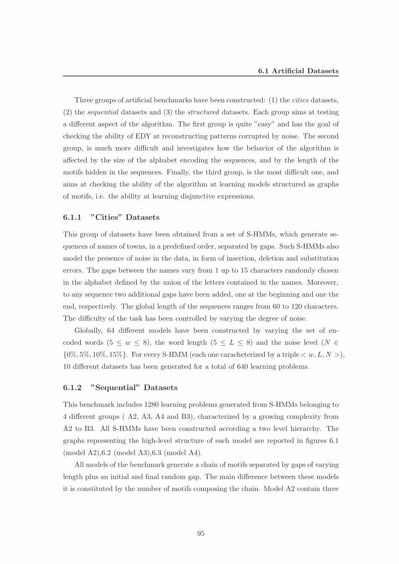
6.1 Artificial Datasets
Three groups of artificial benchmarks have been constructed: (1) the cities datasets,
(2) the sequential datasets and (3) the structured datasets. Each group aims at testing
a different aspect of the algorithm. The first group is quite ”easy” and has the goal of
checking the ability of EDY at reconstructing patterns corrupted by noise. The second
group, is much more difficult and investigates how the behavior of the algorithm is
affected by the size of the alphabet encoding the sequences, and by the length of the
motifs hidden in the sequences. Finally, the third group, is the most difficult one, and
aims at checking the ability of the algorithm at learning models structured as graphs
of motifs, i.e. the ability at learning disjunctive expressions.
6.1.1 ”Cities” Datasets
This group of datasets have been obtained from a set of S-HMMs, which generate se-
quences of names of towns, in a predefined order, separated by gaps. Such S-HMMs also
model the presence of noise in the data, in form of insertion, deletion and substitution
errors. The gaps between the names vary from 1 up to 15 characters randomly chosen
in the alphabet defined by the union of the letters contained in the names. Moreover,
to any sequence two additional gaps have been added, one at the beginning and one the
end, respectively. The global length of the sequences ranges from 60 to 120 characters.
The difficulty of the task has been controlled by varying the degree of noise.
Globally, 64 different models have been constructed by varying the set of en-
coded words (5 ≤ w ≤ 8), the word length (5 ≤ L ≤ 8) and the noise level (N ∈
{0%, 5%, 10%, 15%}. For every S-HMM (each one caracheterized by a triple< w,L,N >),
10 different datasets has been generated for a total of 640 learning problems.
6.1.2 ”Sequential” Datasets
This benchmark includes 1280 learning problems generated from S-HMMs belonging to
4 different groups ( A2, A3, A4 and B3), characterized by a growing complexity from
A2 to B3. All S-HMMs have been constructed according a two level hierarchy. The
graphs representing the high-level structure of each model are reported in figures 6.1
(model A2),6.2 (model A3),6.3 (model A4).
All models of the benchmark generate a chain of motifs separated by gaps of varying
length plus an initial and final random gap. The main difference between these models
it is constituted by the number of motifs composing the chain. Model A2 contain three
95
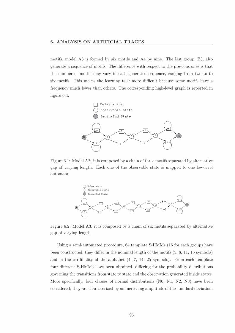
6. ANALYSIS ON ARTIFICIAL TRACES
motifs, model A3 is formed by six motifs and A4 by nine. The last group, B3, also
generate a sequence of motifs. The difference with respect to the previous ones is that
the number of motifs may vary in each generated sequence, ranging from two to to
six motifs. This makes the learning task more difficult because some motifs have a
frequency much lower than others. The corresponding high-level graph is reported in
figure 6.4.
Figure 6.1: Model A2: it is composed by a chain of three motifs separated by alternative
gap of varying length. Each one of the observable state is mapped to one low-level
automata
Figure 6.2: Model A3: it is composed by a chain of six motifs separated by alternative
gap of varying length
Using a semi-automated procedure, 64 template S-HMMs (16 for each group) have
been constructed; they differ in the nominal length of the motifs (5, 8, 11, 15 symbols)
and in the cardinality of the alphabet (4, 7, 14, 25 symbols). From each template
four different S-HMMs have been obtained, differing for the probability distributions
governing the transitions from state to state and the observation generated inside states.
More specifically, four classes of normal distributions (N0, N1, N2, N3) have been
considered; they are characterized by an increasing amplitude of the standard deviation.
96
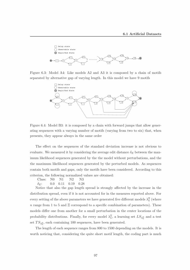
6.1 Artificial Datasets
Figure 6.3: Model A4: Like models A2 and A3 it is composed by a chain of motifs
separated by alternative gap of varying length. In this model we have 9 motifs
Figure 6.4: Model B3: it is composed by a chain with forward jumps that allow gener-
ating sequences with a varying number of motifs (varying from two to six) that, when
presents, they appear always in the same order
The effect on the sequences of the standard deviation increase is not obvious to
evaluate. We measured it by considering the average edit distance δE between the max-
imum likelihood sequences generated by the the model without perturbations, and the
the maximum likelihood sequences generated by the perturbed models. As sequences
contain both motifs and gaps, only the motifs have been considered. According to this
criterion, the following normalized values are obtained:Class: N0 N1 N2 N3δE : 0.0 0.11 0.19 0.28
Notice that also the gap length spread is strongly affected by the increase in the
distribution spread, even if it is not accounted for in the measures reported above. For
every setting of the above parameters we have generated five different models λΞn (where
n range from 1 to 5 and Ξ correspond to a specific combination of parameters). These
models differ one from another for a small perturbation in the center locations of the
probability distributions. Finally, for every model λΞn , a learning set LSλΞ
nand a test
set TSλΞn, each containing 100 sequences, have been generated.
The length of each sequence ranges from 800 to 1500 depending on the models. It is
worth noticing that, considering the quite short motif length, the coding part is much
97
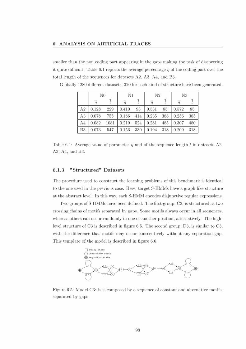
6. ANALYSIS ON ARTIFICIAL TRACES
smaller than the non coding part appearing in the gaps making the task of discovering
it quite difficult. Table 6.1 reports the average percentage η of the coding part over the
total length of the sequences for datasets A2, A3, A4, and B3.
Globally 1280 different datasets, 320 for each kind of structure have been generated.
N0 N1 N2 N3
η l η l η l η l
A2 0.128 229 0.410 93 0.531 85 0.572 85
A3 0.078 755 0.186 414 0.235 388 0.256 385
A4 0.082 1081 0.219 524 0.281 485 0.307 480
B3 0.073 547 0.156 330 0.194 318 0.209 318
Table 6.1: Average value of parameter η and of the sequence length l in datasets A2,
A3, A4, and B3.
6.1.3 ”Structured” Datasets
The procedure used to construct the learning problems of this benchmark is identical
to the one used in the previous case. Here, target S-HMMs have a graph like structure
at the abstract level. In this way, each S-HMM encodes disjunctive regular expressions.
Two groups of S-HMMs have been defined. The first group, C3, is structured as two
crossing chains of motifs separated by gaps. Some motifs always occur in all sequences,
whereas others can occur randomly in one or another position, alternatively. The high-
level structure of C3 is described in figure 6.5. The second group, D3, is similar to C3,
with the difference that motifs may occur consecutively without any separation gap.
This template of the model is described in figure 6.6.
Figure 6.5: Model C3: it is composed by a sequence of constant and alternative motifs,
separated by gaps
98

6.2 Comparing HMMs
Figure 6.6: Model D3: it is a complex model with alternative motif (that could also be
optionals), alternated with gaps
According to the procedure described in section 6.1.2, 32 template S-HMMs (16 for
each group) have been generated, which differ in the nominal length of the motifs (5,
8, 11, 15 symbols), in the cardinality of the alphabet (4, 7, 14, 25 symbols), and in the
level of noise affecting their emission (N0, N1, N2, N3).
For every setting of the above parameters five different models λΞn have been gen-
erated, each one used for generating a learning problem. The length of generated
sequences ranges from 800 to 1500 depending on models, and also in this case the por-
tion of string containing motifs is a small fraction of the entire string (see Figure 6.2.
A set of 640 different datasets, 320 for each kind of structure has been generated.
N0 N1 N2 N3
η l η l η l η l
C3 0.076 773 0.184 414 0.230 390 0.248 389
D3 0.158 328 0.231 291 0.265 300 0.280 306
Table 6.2: Average value of parameter η and of the sequence length l in datasets C3
and D3.
Table 6.2 reports the ratio between the coding and the average length of the se-
quences of datasets C3 and D3.
6.2 Comparing HMMs
The target for EDY is to reconstruct the original model from a sample of the sequences it
generates. Therefore, EDY’s performances can be evaluated by comparing the original
99
6. ANALYSIS ON ARTIFICIAL TRACES
model to the learned one. However, in order to do this comparison we need some sort
of similarity measure, which is not obvious, at all.
In the following we will discuss this problem and we will select some similar-
ity/distance measures, related to specific aspects of EDY’s performances we want to
test.
The first choice we have to face is between what we call direct measures and indirect
measures for evaluating the similarity of the HMMs. As direct measures we intend
measures, which directly compare the structure of the weighted graphs describing the
HMMs. However, we ruled out this approach. On the one hand, even if the problem
of comparing graphs has been addressed in the literature, there is not yet a universal
agreement on a specific measure method. On the other hand, a direct comparison
between the structure of two HMMs can be not meaningful. In fact, quite different
structures can be absolutely equivalent with respect to the probability distribution
induced on the sequences they can generate, whereas small differences in the structure
can lead to dramatic differences in the observed behavior.
As indirect measures we intend the ones, which compare HMMs through the be-
havior they exhibit with respect to specific tasks. A first criterion is to compare two
models on the base of the sequence distribution they generate. Two models can be
considered equivalent when the corresponding distributions are identical.
Several measures can be found in the literature [37, 56, 59], which can be used for
this purpose. We selected the one proposed by Rabiner [56], which has the advantage
of being simple to compute, truly compare the (dis)similarity between pair of Hidden
Markov Models and is meaningful in the probabilistic framework of the HMM. Given
two models λO and λD and a string s generated by model λO (denoted with sO), the
distance between λD and λO with respect to sO is measured as:
d(sO, λD, λO) =1
T[log(p(sO|λD)) − log(p(sO|λO))] (6.1)
being T the length of string sD. The distance expressed in (6.1) could be viewed as
a measure of how well model λD matches sequences generated by model λO. Because
this distance measure is the difference in log probabilities of the observation sequence
conditioned on the models being compared, it will sometimes referred to as divergence
distance. By summing the value obtained by expression (6.1) on all sequences belonging
to the distributions to compare, we obtain the average similarity between d(λD, λO).
100

6.2 Comparing HMMs
Therefore two models are equivalent when d(λD, λO) = 0 and the standard deviation
σ(d(λD, λO)) = 0.
A problem with this distance is that it is non-symmetric but for our purpose there
is no particular requirement that the distance be symmetric because we are interested
in analyzing how much the model learned by the induction algorithm differs from the
original one and we have no assumptions on the opposite assertion. It is important to
consider that the induced model is built on observed evidence of the original model.
So, in presence of non-trivial generative models, a model induced from a limited num-
ber of observations will necessary models only a subset of the probability distribution
expressed by the original one.
Distance (6.1) holds for any kind of HMM and then also for a S-HMM. However,
the probability assigned by a HMM to a sequence is the most important aspect in all
the applications which can be set as classification tasks or as prediction tasks (the First
Problem connected to HMM [56]).
In other kinds of application, the model is used in order to provide an explanation
for the patterns observed in a sequence (the Second Problem connected to HMM [56]).
Usually, this is done by applying Viterbi algorithm in order to find the maximum
likelihood path on the model, which can generate the observed string. In this case, the
structure of the model becomes really important, because the explanation will be given
in terms of a sequence of transitions on the model. Nevertheless, pretending to infer a
model closely resembling to the original one in all details, in order to obtain a detailed
and correct interpretation of a string, is absolutely beyond the reach of EDY, as well
as of any other existing algorithm. Nevertheless, in applications such as signal tagging,
or DNA mining, only a macro-interpretation of the sequence is desired, while the fine
grain structure can be irrelevant. Referring to the case of DNA, the main goal, in the
tasks where HMMs are applied, is to discover related groups of motifs in a sequence
database. The detailed interpretation of the different nucleotides inside a motif is left
to other kinds of analysis.
Under this assumption, the hierarchical block structure of a S-HMM can be ex-
ploited in order to build models preserving not the fine grain structure of the genera-
tive model but its macro structure, useful in order to correctly segment a sequence into
motifs and gaps. This can be achieved if the blocks of the S-HMM hierarchy are prop-
erly chosen by the induction algorithm. Then will introduce a distance measure aimed
101
6. ANALYSIS ON ARTIFICIAL TRACES
at testing EDY’s ability at discovering the macro structure of the generative model.
More specifically, the measure ρ(sO, λD, λO) accounts for EDY’s ability at segmenting
a string s into motifs and gaps corresponding to the ones defined by the original model.
Following the previously introduced notation, model λO is assumed to be the original
model, while λD is the model discovered by the induction algorithm.
Informally, ρ is computed by means of the following algorithm. String sO generated
by λO is segmented into a sequence of motifs and gaps using both λD and λO. Let sλD,
sλOdenote the segmentations obtained from λD and λO, respectively; sλD
, sλOare
aligned by putting into correspondence the pair of segments tagged as motifs, which
show the greatest similarity between them. This step is carried on by a dynamic pro-
gramming algorithm derived from the ones described in the previous sections. Finally,
ρ(sO, λD, λO) is computed as the ratio:
ρ(sO, λD, λO) =A(sλD
, sλO)
L(sλO)
(6.2)
In (6.2) A(sλD, sλO
) is sum of the the edit distance computed for all segment pairs,
which have been aligned. Possible segments on both sides, which have not found any
correspondence are accounted by computing the edit distance from the null string. The
denominator L(sλO), is the sum of length of all motifs occurring in the segmentation
sλO.
A second measure ǫ(s, λD, λO) has also been introduced, which simply accounts for
EDY’s ability at correctly distinguishing the meaningful information in the learning
set from the non meaningful one inside the gaps. The algorithm for computing ǫ is
a obtained as a simplification of the previous one. Again segmentation sλD, sλO
are
computed. Then, two substrings mλD, mλO
are extracted from sλD, sλO
, by collecting
all motifs defined by λD, λO, respectively. Finally, ǫ(sO, λD, λO) is computed as the
ratio:
ǫ(sO, λD, λO) =D(mλD
,mλO)
L(sλO)
(6.3)
being D(mλD,mλO
) the edit distance between mλDand mλO
.
6.3 Motif reconstruction in presence of noise
This case study has the goal of evaluating the ability of the algorithm at correctly
generalizing the nominal form of motives in presence of noise. It is based on the cities
102
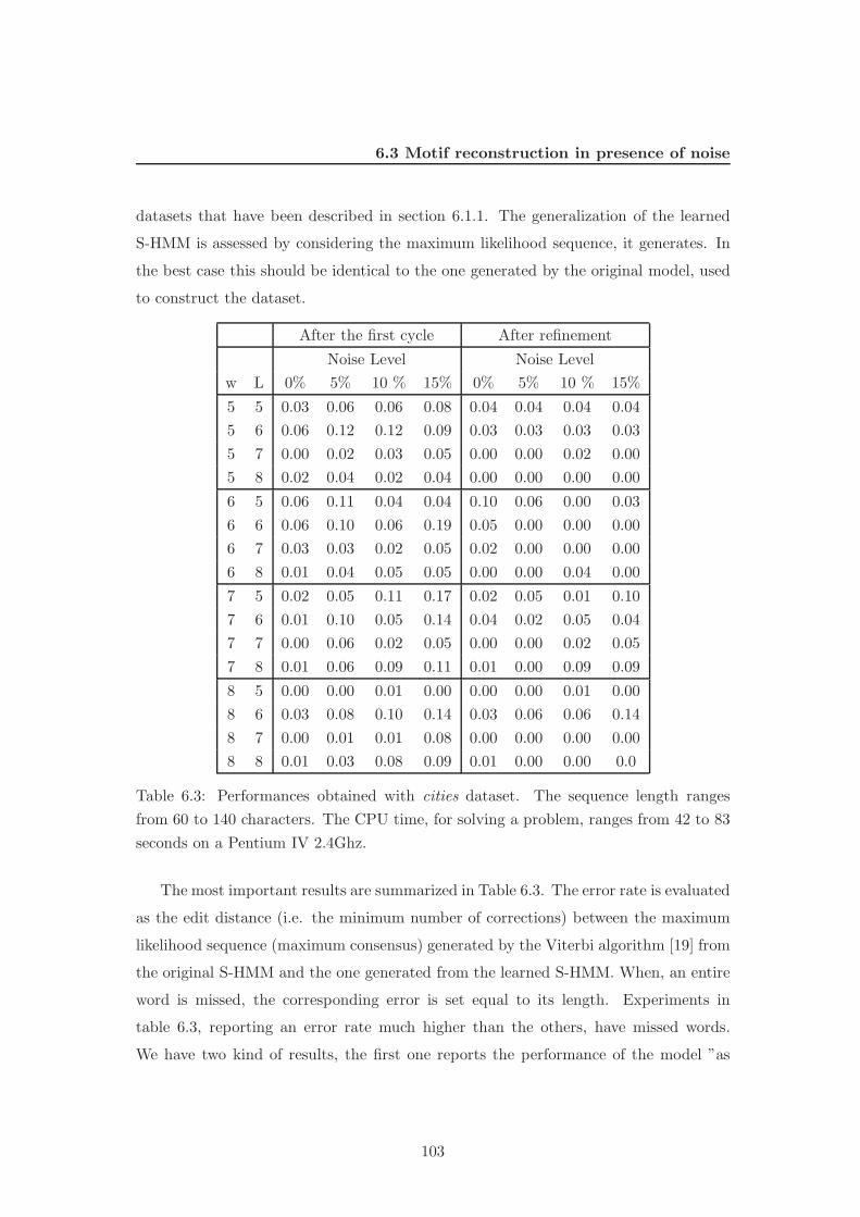
6.3 Motif reconstruction in presence of noise
datasets that have been described in section 6.1.1. The generalization of the learned
S-HMM is assessed by considering the maximum likelihood sequence, it generates. In
the best case this should be identical to the one generated by the original model, used
to construct the dataset.
After the first cycle After refinement
Noise Level Noise Level
w L 0% 5% 10 % 15% 0% 5% 10 % 15%
5 5 0.03 0.06 0.06 0.08 0.04 0.04 0.04 0.04
5 6 0.06 0.12 0.12 0.09 0.03 0.03 0.03 0.03
5 7 0.00 0.02 0.03 0.05 0.00 0.00 0.02 0.00
5 8 0.02 0.04 0.02 0.04 0.00 0.00 0.00 0.00
6 5 0.06 0.11 0.04 0.04 0.10 0.06 0.00 0.03
6 6 0.06 0.10 0.06 0.19 0.05 0.00 0.00 0.00
6 7 0.03 0.03 0.02 0.05 0.02 0.00 0.00 0.00
6 8 0.01 0.04 0.05 0.05 0.00 0.00 0.04 0.00
7 5 0.02 0.05 0.11 0.17 0.02 0.05 0.01 0.10
7 6 0.01 0.10 0.05 0.14 0.04 0.02 0.05 0.04
7 7 0.00 0.06 0.02 0.05 0.00 0.00 0.02 0.05
7 8 0.01 0.06 0.09 0.11 0.01 0.00 0.09 0.09
8 5 0.00 0.00 0.01 0.00 0.00 0.00 0.01 0.00
8 6 0.03 0.08 0.10 0.14 0.03 0.06 0.06 0.14
8 7 0.00 0.01 0.01 0.08 0.00 0.00 0.00 0.00
8 8 0.01 0.03 0.08 0.09 0.01 0.00 0.00 0.0
Table 6.3: Performances obtained with cities dataset. The sequence length ranges
from 60 to 140 characters. The CPU time, for solving a problem, ranges from 42 to 83
seconds on a Pentium IV 2.4Ghz.
The most important results are summarized in Table 6.3. The error rate is evaluated
as the edit distance (i.e. the minimum number of corrections) between the maximum
likelihood sequence (maximum consensus) generated by the Viterbi algorithm [19] from
the original S-HMM and the one generated from the learned S-HMM. When, an entire
word is missed, the corresponding error is set equal to its length. Experiments in
table 6.3, reporting an error rate much higher than the others, have missed words.
We have two kind of results, the first one reports the performance of the model ”as
103
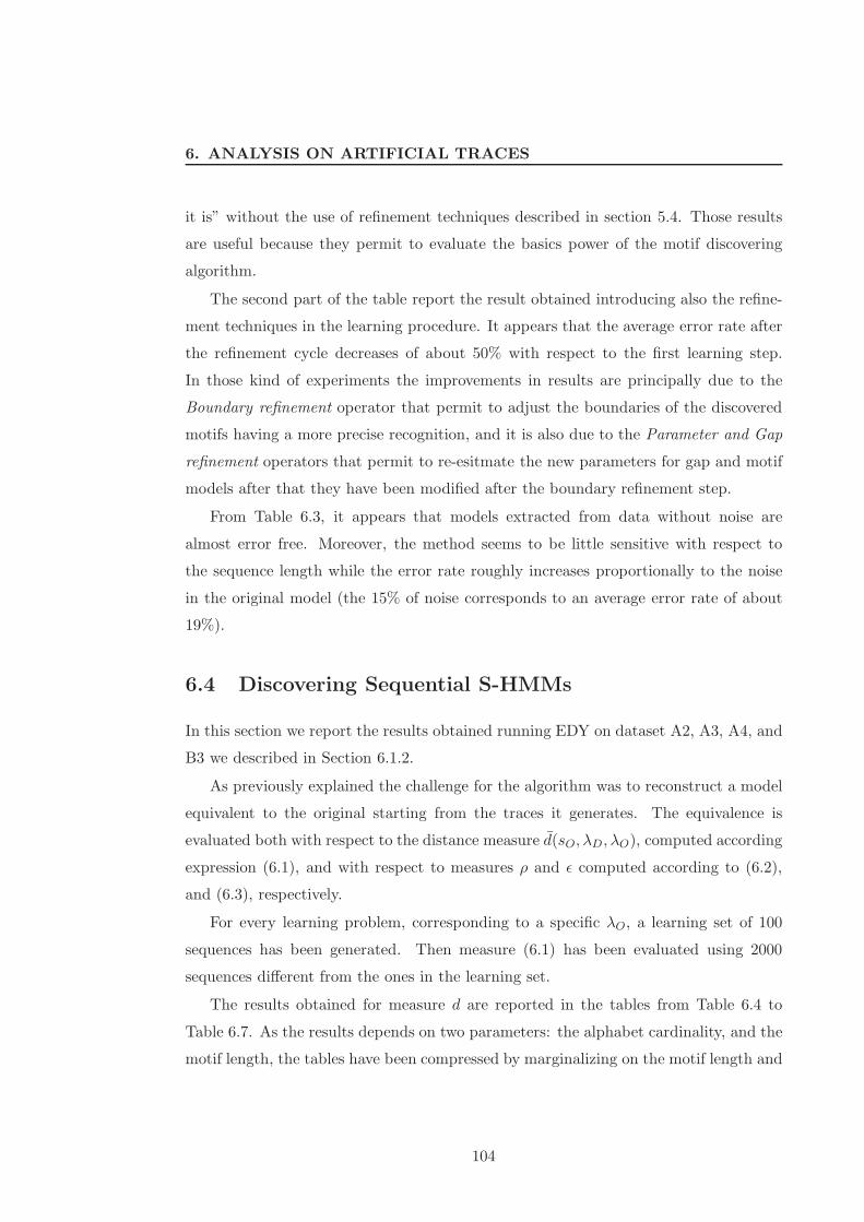
6. ANALYSIS ON ARTIFICIAL TRACES
it is” without the use of refinement techniques described in section 5.4. Those results
are useful because they permit to evaluate the basics power of the motif discovering
algorithm.
The second part of the table report the result obtained introducing also the refine-
ment techniques in the learning procedure. It appears that the average error rate after
the refinement cycle decreases of about 50% with respect to the first learning step.
In those kind of experiments the improvements in results are principally due to the
Boundary refinement operator that permit to adjust the boundaries of the discovered
motifs having a more precise recognition, and it is also due to the Parameter and Gap
refinement operators that permit to re-esitmate the new parameters for gap and motif
models after that they have been modified after the boundary refinement step.
From Table 6.3, it appears that models extracted from data without noise are
almost error free. Moreover, the method seems to be little sensitive with respect to
the sequence length while the error rate roughly increases proportionally to the noise
in the original model (the 15% of noise corresponds to an average error rate of about
19%).
6.4 Discovering Sequential S-HMMs
In this section we report the results obtained running EDY on dataset A2, A3, A4, and
B3 we described in Section 6.1.2.
As previously explained the challenge for the algorithm was to reconstruct a model
equivalent to the original starting from the traces it generates. The equivalence is
evaluated both with respect to the distance measure d(sO, λD, λO), computed according
expression (6.1), and with respect to measures ρ and ǫ computed according to (6.2),
and (6.3), respectively.
For every learning problem, corresponding to a specific λO, a learning set of 100
sequences has been generated. Then measure (6.1) has been evaluated using 2000
sequences different from the ones in the learning set.
The results obtained for measure d are reported in the tables from Table 6.4 to
Table 6.7. As the results depends on two parameters: the alphabet cardinality, and the
motif length, the tables have been compressed by marginalizing on the motif length and
104
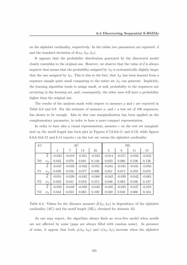
6.4 Discovering Sequential S-HMMs
on the alphabet cardinality, respectively. In the tables two parameters are reported: d
and the standard deviation of d(sO, λD, λO).
It appears that the probability distribution generated by the discovered model
closely resembles to the original one. However, we observe that the value of d is always
negative that means that the probability assigned by λD is systematically slightly larger
that the one assigned by λO. This is due to the fact, that λD has been learned from a
sequence sample quite small comparing to the entire set λO can generate. Implicitly,
the learning algorithm tends to assign small, or null, probability to the sequences not
occurring in the learning set, and, consequently, the other ones will have a probability
higher than the original one.
The results of the analysis made with respect to measure ρ and ǫ are reported in
Table 6.8 and 6.9. For the estimate of measure ρ, and ǫ a test set of 100 sequences,
has shown to be enough. Also in this case marginalization has been applied on the
complementary parameter, in order to have a more compact representation.
In order to have also a visual representation, measure ǫ on the test set marginal-
ized on the motif length has been plot in Figures 6.7,6.9,6.11 and 6.13) while figures
6.8,6.10,6.12 and 6.14 reports ǫ on the test set versus the alphabet cardinality.
A2 AC ML
4 7 14 25 5 8 11 15
d -0.023 -0.019 -0.021 -0.043 -0.014 -0.017 -0.033 -0.042
N0 σd 0.042 0.070 0.081 0.148 0.033 0.066 0.106 0.136
d -0.047 -0.033 -0.042 -0.051 -0.041 -0.041 -0.041 -0.050
N1 σd 0.039 0.056 0.077 0.090 0.051 0.074 0.059 0.078
d -0.051 -0.028 -0.042 -0.068 -0.042 -0.039 -0.042 -0.065
N2 σd 0.033 0.041 0.053 0.215 0.046 0.064 0.046 0.187
d -0.059 -0.049 -0.038 -0.042 -0.035 -0.035 -0.047 -0.070
N3 σd 0.043 0.053 0.065 0.100 0.049 0.048 0.060 0.104
Table 6.4: Values for the distance measure d(λO, λD) in dependency of the alphabet
cardinality (AC) and the motif length (ML), obtained for datasets A2
As one may expect, the algorithm always finds an error-free model when motifs
are not affected by noise (gaps are always filled with random noise). In presence
of noise, it appear that both ρ(λO, λD) and ǫ(λO, λD) increase when the alphabet
105
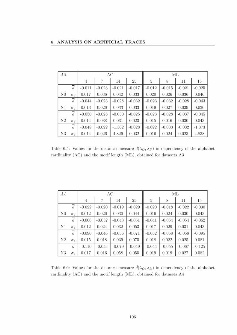
6. ANALYSIS ON ARTIFICIAL TRACES
A3 AC ML
4 7 14 25 5 8 11 15
d -0.011 -0.023 -0.021 -0.017 -0.012 -0.015 -0.021 -0.025
N0 σd 0.017 0.036 0.042 0.033 0.020 0.026 0.036 0.046
d -0.044 -0.023 -0.028 -0.032 -0.023 -0.032 -0.028 -0.043
N1 σd 0.013 0.026 0.033 0.033 0.019 0.027 0.029 0.030
d -0.050 -0.028 -0.030 -0.025 -0.023 -0.028 -0.037 -0.045
N2 σd 0.014 0.038 0.031 0.023 0.015 0.016 0.030 0.043
d -0.048 -0.022 -1.362 -0.028 -0.022 -0.033 -0.032 -1.373
N3 σd 0.014 0.026 4.829 0.032 0.016 0.024 0.023 4.838
Table 6.5: Values for the distance measure d(λO, λD) in dependency of the alphabet
cardinality (AC) and the motif length (ML), obtained for datasets A3
A4 AC ML
4 7 14 25 5 8 11 15
d -0.022 -0.020 -0.019 -0.029 -0.020 -0.018 -0.022 -0.030
N0 σd 0.012 0.026 0.030 0.044 0.016 0.024 0.030 0.043
d -0.066 -0.052 -0.043 -0.051 -0.041 -0.054 -0.054 -0.062
N1 σd 0.012 0.024 0.032 0.053 0.017 0.029 0.031 0.043
d -0.090 -0.046 -0.036 -0.071 -0.032 -0.058 -0.058 -0.095
N2 σd 0.015 0.018 0.039 0.075 0.018 0.022 0.025 0.081
d -0.110 -0.053 -0.079 -0.049 -0.044 -0.055 -0.067 -0.125
N3 σd 0.017 0.016 0.058 0.055 0.019 0.019 0.027 0.082
Table 6.6: Values for the distance measure d(λO, λD) in dependency of the alphabet
cardinality (AC) and the motif length (ML), obtained for datasets A4
106
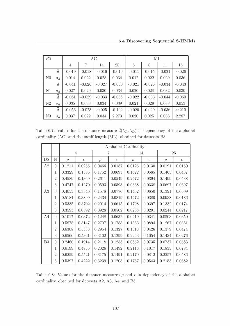
6.4 Discovering Sequential S-HMMs
B3 AC ML
4 7 14 25 5 8 11 15
d -0.019 -0.018 -0.016 -0.019 -0.011 -0.015 -0.021 -0.026
N0 σd 0.014 0.022 0.028 0.034 0.012 0.022 0.029 0.036
d -0.041 -0.026 -0.027 -0.030 -0.021 -0.026 -0.034 -0.043
N1 σd 0.027 0.029 0.030 0.034 0.020 0.028 0.032 0.039
d -0.061 -0.029 -0.033 -0.035 -0.022 -0.033 -0.044 -0.060
N2 σd 0.035 0.033 0.034 0.039 0.021 0.029 0.038 0.053
d -0.056 -0.023 -0.025 -0.192 -0.020 -0.029 -0.036 -0.210
N3 σd 0.037 0.022 0.034 2.273 0.020 0.025 0.033 2.287
Table 6.7: Values for the distance measure d(λO, λD) in dependency of the alphabet
cardinality (AC) and the motif length (ML), obtained for datasets B3
Alphabet Cardinality
4 7 14 25
DS N ρ ǫ ρ ǫ ρ ǫ ρ ǫ
A2 0 0.1211 0.0255 0.0466 0.0187 0.0126 0.0130 0.0191 0.0160
1 0.3329 0.1385 0.1752 0.0693 0.1622 0.0585 0.1465 0.0437
2 0.4589 0.1369 0.2611 0.0549 0.2472 0.0394 0.1499 0.0538
3 0.4747 0.1270 0.0593 0.0593 0.0338 0.0338 0.0697 0.0697
A3 0 0.4053 0.3346 0.1578 0.0776 0.1452 0.0650 0.1391 0.0509
1 0.5184 0.3899 0.2434 0.0819 0.1472 0.0380 0.0938 0.0186
2 0.5335 0.3702 0.2014 0.0615 0.1798 0.0397 0.1332 0.0174
3 0.3593 0.0592 0.0928 0.0502 0.0288 0.0291 0.0244 0.0217
A4 0 0.1017 0.0372 0.1248 0.0632 0.0419 0.0341 0.0503 0.0350
1 0.5875 0.5147 0.2707 0.1788 0.1363 0.0894 0.1267 0.0561
2 0.6308 0.5333 0.2954 0.1327 0.1318 0.0426 0.1379 0.0474
3 0.6566 0.5361 0.3102 0.1299 0.2243 0.1054 0.1434 0.0276
B3 0 0.2460 0.1914 0.2118 0.1253 0.0852 0.0735 0.0737 0.0583
1 0.6199 0.4835 0.2026 0.1492 0.2113 0.1017 0.1833 0.0784
2 0.6259 0.5521 0.3175 0.1491 0.2179 0.0812 0.2257 0.0586
3 0.5397 0.4222 0.3239 0.1205 0.1737 0.0543 0.2153 0.0382
Table 6.8: Values for the distance measures ρ and ǫ in dependency of the alphabet
cardinality, obtained for datasets A2, A3, A4, and B3
107
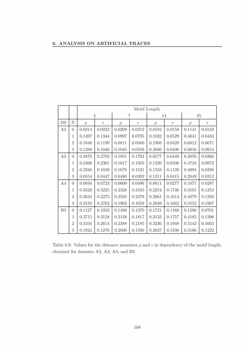
6. ANALYSIS ON ARTIFICIAL TRACES
Motif Length
4 7 14 25
DS N ρ ǫ ρ ǫ ρ ǫ ρ ǫ
A2 0 0.0214 0.0222 0.0209 0.0212 0.0182 0.0158 0.1141 0.0133
1 0.1497 0.1344 0.0997 0.0795 0.1032 0.0529 0.4641 0.0434
2 0.1640 0.1199 0.0811 0.0560 0.1908 0.0420 0.6812 0.0671
3 0.1288 0.1046 0.1045 0.0503 0.2686 0.0436 0.6916 0.0913
A3 0 0.2870 0.2703 0.1951 0.1762 0.0577 0.0449 0.3076 0.0366
1 0.2466 0.2301 0.1617 0.1505 0.1220 0.0508 0.4724 0.0972
2 0.2348 0.1839 0.1678 0.1531 0.1558 0.1120 0.4894 0.0398
3 0.0554 0.0447 0.0480 0.0392 0.1211 0.0415 0.2049 0.0312
A4 0 0.0856 0.0723 0.0609 0.0496 0.0611 0.0277 0.1071 0.0287
1 0.3528 0.3225 0.2328 0.2165 0.2254 0.1746 0.3101 0.1253
2 0.2634 0.2275 0.2585 0.2378 0.2661 0.1614 0.4079 0.1293
3 0.3182 0.2762 0.1963 0.1659 0.2649 0.1662 0.5552 0.1907
B3 0 0.1127 0.1023 0.1486 0.1370 0.1721 0.1168 0.1500 0.0701
1 0.3715 0.3158 0.2138 0.1817 0.2133 0.1757 0.4185 0.1396
2 0.3104 0.2614 0.2388 0.2185 0.3236 0.1948 0.5143 0.1663
3 0.1824 0.1276 0.2006 0.1580 0.2637 0.1538 0.5166 0.1222
Table 6.9: Values for the distance measures ρ and ǫ in dependency of the motif length,
obtained for datasets A2, A3, A4, and B3
108
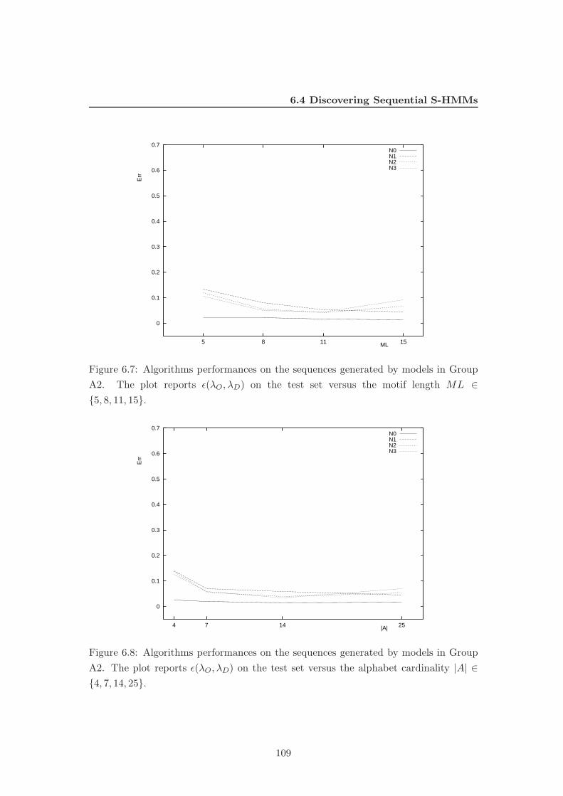
6.4 Discovering Sequential S-HMMs
0
0.1
0.2
0.3
0.4
0.5
0.6
0.7
151185
Err
ML
N0N1N2N3
Figure 6.7: Algorithms performances on the sequences generated by models in Group
A2. The plot reports ǫ(λO, λD) on the test set versus the motif length ML ∈
{5, 8, 11, 15}.
0
0.1
0.2
0.3
0.4
0.5
0.6
0.7
251474
Err
|A|
N0N1N2N3
Figure 6.8: Algorithms performances on the sequences generated by models in Group
A2. The plot reports ǫ(λO, λD) on the test set versus the alphabet cardinality |A| ∈
{4, 7, 14, 25}.
109
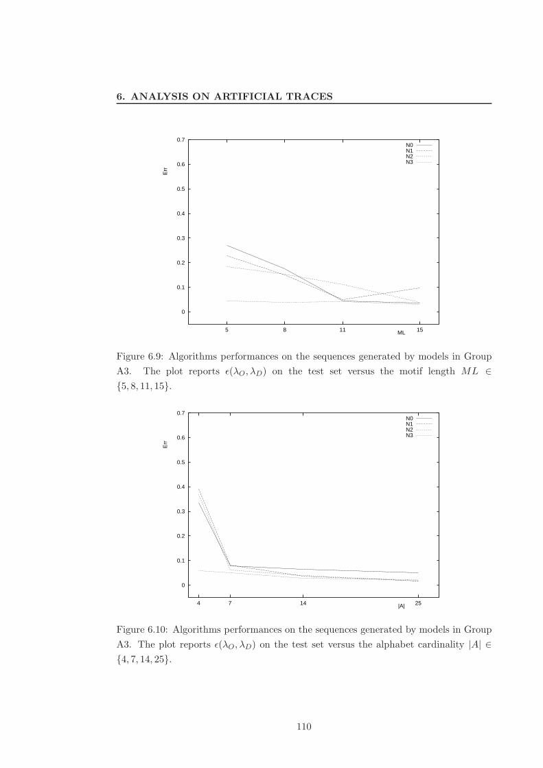
6. ANALYSIS ON ARTIFICIAL TRACES
0
0.1
0.2
0.3
0.4
0.5
0.6
0.7
151185
Err
ML
N0N1N2N3
Figure 6.9: Algorithms performances on the sequences generated by models in Group
A3. The plot reports ǫ(λO, λD) on the test set versus the motif length ML ∈
{5, 8, 11, 15}.
0
0.1
0.2
0.3
0.4
0.5
0.6
0.7
251474
Err
|A|
N0N1N2N3
Figure 6.10: Algorithms performances on the sequences generated by models in Group
A3. The plot reports ǫ(λO, λD) on the test set versus the alphabet cardinality |A| ∈
{4, 7, 14, 25}.
110
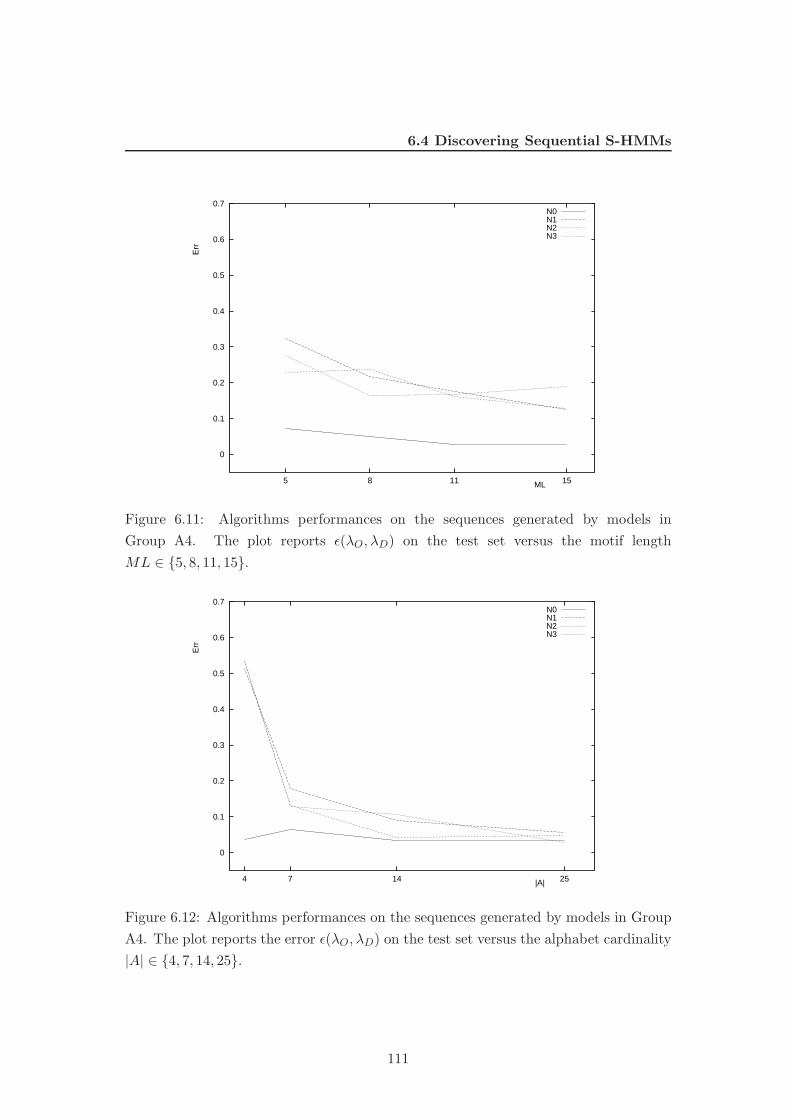
6.4 Discovering Sequential S-HMMs
0
0.1
0.2
0.3
0.4
0.5
0.6
0.7
151185
Err
ML
N0N1N2N3
Figure 6.11: Algorithms performances on the sequences generated by models in
Group A4. The plot reports ǫ(λO, λD) on the test set versus the motif length
ML ∈ {5, 8, 11, 15}.
0
0.1
0.2
0.3
0.4
0.5
0.6
0.7
251474
Err
|A|
N0N1N2N3
Figure 6.12: Algorithms performances on the sequences generated by models in Group
A4. The plot reports the error ǫ(λO, λD) on the test set versus the alphabet cardinality
|A| ∈ {4, 7, 14, 25}.
111

6. ANALYSIS ON ARTIFICIAL TRACES
0
0.1
0.2
0.3
0.4
0.5
0.6
0.7
151185
Err
ML
N0N1N2N3
Figure 6.13: Algorithms performances on the sequences generated by models in Group
B3. The plot reports the ǫ(λO, λD) on the test set versus the motif length ML ∈
{5, 8, 11, 15}.
0
0.1
0.2
0.3
0.4
0.5
0.6
0.7
251474
Err
|A|
N0N1N2N3
Figure 6.14: Algorithms performances on the sequences generated by models in Group
B3. The plot reports ǫ(λO, λD) on the test set versus the alphabet cardinality |A| ∈
{4, 7, 14, 25}.
112

6.5 Discovering graph structured patterns
cardinality and the motif length decrease, as well as when the standard deviation of
the target model increases, as it is reasonable to expect. In fact, when the alphabet
is small, it is more difficult to distinguish real motifs from apparent regularities due
to randomness. For the same reason, short motifs are more difficult to detect. Then,
the performance degradation is due, in general, to the failure of the algorithm, which
searches for new motifs without finding the correct ones. However, it is surprising that
the accuracy in some cases, like 6.9, decreases again when motifs become longer than
11 symbols. A possible explanation is the following: when the average length of a motif
instances increases in presence of noise, the number of alternative sequences, among
which the correct instances of the motif are to be identified, increases, smoothing thus
the similarity among strings and increasing confusion.
The decrease in the similarity between the target model and the discovered model,
when the probability distributions have long tails, is also in agreement with what one
expects. Nevertheless, it is interesting that the error rate remains comparable to the
level of noise of the dataset. It is also worth noticing that the performances evaluated
on the test sets and on the learning sets are almost identical, as their differences are
not statistically significant.
Finally, the system always converged to a stable model in a number of steps ranging
from 11 to 35. The computational complexity for solving a single problem of the second
group corresponds to a cpu time ranging from 30 to 40 minutes on a Opteron.
6.5 Discovering graph structured patterns
Aims of this case study is to check the ability of the algorithm at reconstructing patterns
described by disjunctive expressions. We used the structured datasets (C3 and D3) in
order to perform this analysis. As discussed in section 6.1.3 this group of datasets
is very similar to the sequential datasets but characterized by a more complex graph
structure.
As in the previous section the results are described by means of a set of tables,
reporting the values obtained for measure d (Table 6.10 and 6.11), and for measure ρ
and ǫ (Table 6.12, 6.13). Moreover, also in this case the results for measure ǫ have been
represented in graphical form in Figure 6.15, 6.16, 6.18, and 6.18.
113

6. ANALYSIS ON ARTIFICIAL TRACES
C3 AC ML
4 7 14 25 5 8 11 15
d -0.018 -0.024 -0.028 -0.028 -0.014 -0.024 -0.027 -0.032
N0 σd 0.015 0.030 0.045 0.052 0.022 0.033 0.039 0.049
d -0.049 -0.035 -0.033 -0.043 -0.030 -0.033 -0.044 -0.053
N1 σd 0.016 0.032 0.039 0.048 0.020 0.034 0.038 0.042
d -0.044 -0.036 -0.037 -0.040 -0.031 -0.032 -0.044 -0.049
N2 σd 0.015 0.038 0.035 0.045 0.021 0.025 0.036 0.050
d -0.067 -0.036 -0.039 -0.036 -0.039 -0.033 -0.037 -0.069
N3 σd 0.017 0.031 0.046 0.029 0.024 0.026 0.039 0.035
Table 6.10: Values for the distance measure d(λO, λD) in dependency of the alphabet
cardinality (AC) and the motif length (ML), obtained for datasets C3
D3 AC ML
4 7 14 25 5 8 11 15
d -0.067 -0.076 -0.074 -0.086 -0.051 -0.070 -0.081 -0.102
N0 σd 0.029 0.048 0.087 0.116 0.043 0.060 0.078 0.097
d -0.084 -0.088 -0.093 -0.083 -0.064 -0.093 -0.082 -0.108
N1 σd 0.027 0.052 0.051 0.063 0.032 0.045 0.042 0.073
d -0.080 -0.073 -0.085 -0.081 -0.073 -0.073 -0.092 -0.081
N2 σd 0.025 0.038 0.045 0.052 0.035 0.034 0.043 0.049
d -0.088 -0.086 -0.094 -0.107 -0.076 -0.084 -0.098 -0.117
N3 σd 0.028 0.050 0.051 0.061 0.039 0.041 0.054 0.056
Table 6.11: Values for the distance measure d(λO, λD) in dependency of the alphabet
cardinality (AC) and the motif length (ML), obtained for datasets D3
114

6.5 Discovering graph structured patterns
Alphabet Cardinality
4 7 14 25
DS N ρ ǫ ρ ǫ ρ ǫ ρ ǫ
C3 0 0.3694 0.2608 0.1923 0.1168 0.1573 0.0768 0.1510 0.0711
1 0.6157 0.3738 0.2542 0.1060 0.2303 0.0663 0.1447 0.0400
2 0.5626 0.2794 0.3698 0.1069 0.2026 0.0469 0.1812 0.0482
3 0.4471 0.2737 0.1125 0.0596 0.0483 0.0303 0.0322 0.0193
D3 0 0.6692 0.2434 0.4604 0.1832 0.2300 0.0888 0.2118 0.0779
1 0.7789 0.3645 0.5491 0.2252 0.3980 0.1446 0.3102 0.0925
2 0.6618 0.3236 0.5388 0.1403 0.4034 0.1164 0.3653 0.0774
3 0.7231 0.3625 0.5370 0.1775 0.3789 0.1266 0.4161 0.1072
Table 6.12: Values for the distance measures ρ and ǫ in dependency of the alphabet
cardinality, obtained for datasets C3 and D3
Motif Length
4 7 14 25
DS N ρ ǫ ρ ǫ ρ ǫ ρ ǫ
C3 0 0.3416 0.1995 0.1549 0.1579 0.1192 0.1117 0.2543 0.1242
1 0.3209 0.2562 0.1506 0.2416 0.2687 0.1926 0.5047 0.1364
2 0.3280 0.2513 0.1545 0.1624 0.2978 0.14979 0.5360 0.0943
3 0.0658 0.0549 0.0703 0.0601 0.1572 0.0421 0.2516 0.1711
D3 0 0.4678 0.1995 0.4065 0.1579 0.3287 0.1117 0.3685 0.1242
1 0.6045 0.2562 0.3852 0.2416 0.3852 0.1926 0.5079 0.1364
2 0.5907 0.2513 0.4324 0.1624 0.406 0.1497 0.5401 0.0943
3 0.6031 0.2564 0.3882 0.2013 0.4239 0.1596 0.6399 0.1565
Table 6.13: Values for the distance measures ρ and ǫ in dependency of the motif length,
obtained for datasets C3 and D3
115

6. ANALYSIS ON ARTIFICIAL TRACES
0
0.1
0.2
0.3
0.4
0.5
0.6
0.7
151185
Err
ML
N0N1N2N3
Figure 6.15: Algorithms performances on the sequences generated by models in Group
C3. The plot reports the error Err = Err(λD) on the test set versus the motif length
ML ∈ {5, 8, 11, 15}.
0
0.1
0.2
0.3
0.4
0.5
0.6
0.7
251474
Err
|A|
N0N1N2N3
Figure 6.16: Algorithms performances on the sequences generated by models in Group
C3. The plot reports the error Err = Err(λD) on the test set versus the alphabet
cardinality |A| ∈ {4, 7, 14, 25}.
116
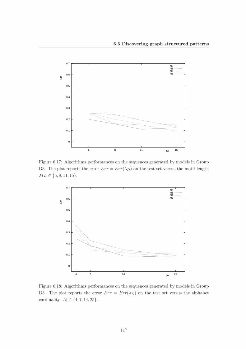
6.5 Discovering graph structured patterns
0
0.1
0.2
0.3
0.4
0.5
0.6
0.7
151185
Err
ML
N0N1N2N3
Figure 6.17: Algorithms performances on the sequences generated by models in Group
D3. The plot reports the error Err = Err(λD) on the test set versus the motif length
ML ∈ {5, 8, 11, 15}.
0
0.1
0.2
0.3
0.4
0.5
0.6
0.7
251474
Err
|A|
N0N1N2N3
Figure 6.18: Algorithms performances on the sequences generated by models in Group
D3. The plot reports the error Err = Err(λD) on the test set versus the alphabet
cardinality |A| ∈ {4, 7, 14, 25}.
117

6. ANALYSIS ON ARTIFICIAL TRACES
Also in this case, we obtain performances, which, even if worst that in the previous
one, are good for what concerns d and ǫ measures. Instead, parameter ρ hows that the
learned structure tends to be significantly different from the original one.
It is important to evidence how the performances improve when the cardinality of
alphabet grow up. As stated in previous section this is a quite obvious result because
when the cardinality of alphabet grows apparent regularities due to randomness are
more rare. The accuracy in some cases, like 6.15, decreases again when motif length
increases. This phenomenon is particularly evident when motifs are characterized by
a low alphabet cardinality and a high noise level. We observed this behavior also in
the test reported in the previous section. Again a possible explanation is that, when
the average length of a motif instances increases in presence of noise, the number
of alternative sequences, among which the correct instances of the motif are to be
identified, increases, smoothing thus the similarity among strings and increasing the
entropy.
Despite the complexity of the task the algorithm reached systematically perfor-
mance comparable to the level of noise of the dataset and the system always converged
to a stable model in a number of steps not greater than 40. Finally the average time
for performing each one of those task was about 1 hour on an Opteron.
6.6 Discussion
The analysis reported in the previous sections investigates the capabilities of EDY at
reconstructing a generative model starting from a sample of the sequences it generated.
A first aspect we analyzed is its ability at discovering motifs in presence of noise. This
preliminary analysis on a relatively easy datasets shows really good performance. It is
worth noticing the increment in performance we observed after the introduction of the
refinement step.
In fact, the first step for discovering motifs is based FASTA (see section 5.3.1), which
is very fast in discovering local alignments but is strongly depending on the value of its
control parameters (ktup parameter, in particular). When a motif is strongly perturbed,
the algorithm tends to identify only the most conservative regions while tends to miss
the less conservative on the boundaries. The operator that perform the boundary
extension together with those performing parameters and gaps refinement shown to be
118
6.6 Discussion
capable of reconstructing the nominal form of the motifs, most times without errors,
as it could be seen in table 6.3.
However, EDY’s ability at discovering motifs has challenged on much harder datasets,
i.e, sequential and structured datasets, where the performances are not always so satis-
factory.
The first feature emerging from the tables, and the figures we reported in the pre-
vious sections, is the strong influence of the alphabet cardinality on the algorithm
performances. With small alphabets, the performances remarkably decay. Moreover,
this effect is amplified by the presence of noise. According to our explanation, the
phenomenon depends on the probability of finding apparent regularities, due to ran-
domness, which increases as long as the alphabet becomes small. Consequently, on the
one hand, apparent motifs are confused with the real ones making harder the task for
the discovery procedure. On the other hand, the statistical test we use for selecting
the motifs to include in the model, tends to reject also good motifs, because they have
a high probability of occurring also in a random sequence.
The second feature, which emerges, is the divergence between ρ and ǫ in many learn-
ing problems, which appears to depend upon both the motif length and the alphabet
cardinality. The cause of this divergence is due to the fact that the some of original
motifs are segmented into several smaller ones.
If motifs are short this happens when the cardinality of the alphabet is small as
an effect of the phenomenon we discussed above. As true motifs can be confused with
false motifs, the discovery procedure can distinguish only one part of a motif, i.e. the
one which by chance appears to be more stable in the learning set. Afterwards, it may
happens that in a later step, searching inside a gap the missed part be discovered and
included in the model as an independent motif. However, a similar problem it may
happen also with alphabet of large cardinality when the motifs are very long. This is
due to the weakness of FASTA we already discussed: When a long motif is corrupted
in the central part it may be split into two or more fragments that the refinement
procedures are no more able to recover. This problem could solved using a algorithm
for merging contiguous motifs. Unfortunately, at the moment such algorithm has not
yet been implemented.
In conclusion, the motif fragmentation effect let ρ and ǫ exhibit values quite different
in several learning problems. In this case most relevant information has been discovered,
119

6. ANALYSIS ON ARTIFICIAL TRACES
while the macro-structure of the original S-HMM has not preserved with good accuracy.
Then, the discovered model is suitable for classification or for prediction tasks (as
confirmed by d distance measure), but it not suitable for interpretation (segmentation)
tasks.
120

Chapter 7
An Application to Keystroking
Dynamics for a Human Agent
The problem of modeling the behavior of an agent may have a very different setting,
depending on the kind of agent and on the type of features available for building the
model. Here, we will focus on the problem of modeling the behavior of a human agent
interacting with a computer system through a keyboard. In other words, the goal is to
construct a model capturing the dynamics of a user typing on a keyboard.
This task has been widely investigated in the past, in order to develop biometric
authentication methods (see, for instance [11, 23]), which led to patented solutions [12].
Our purpose is not to provide a new challenging solution to this task, but simply to
show how easy it is to generate user models based on S-HMMs, which are performing
quite well.
Two case studies have been investigated, characterized by two different targets. The
first one addresses the problem of building a discriminant profile of a user, during the
activity of typing a free text. This kind of task plays an important role when the goal
is to build a monitoring system, which checks on typical behavior of a group of agents
and rises an alarm signal when someone of them is not behaving according to its profile.
The second case study aims at producing an authentication procedure based on
keystroke dynamics during the login phase, which can be used in order to make more
difficult to break into a system in case of password theft.
Not withstanding the deep difference in the targets, the two experiments share the
problem setting, i.e, the input information to match against the behavior model, and
121
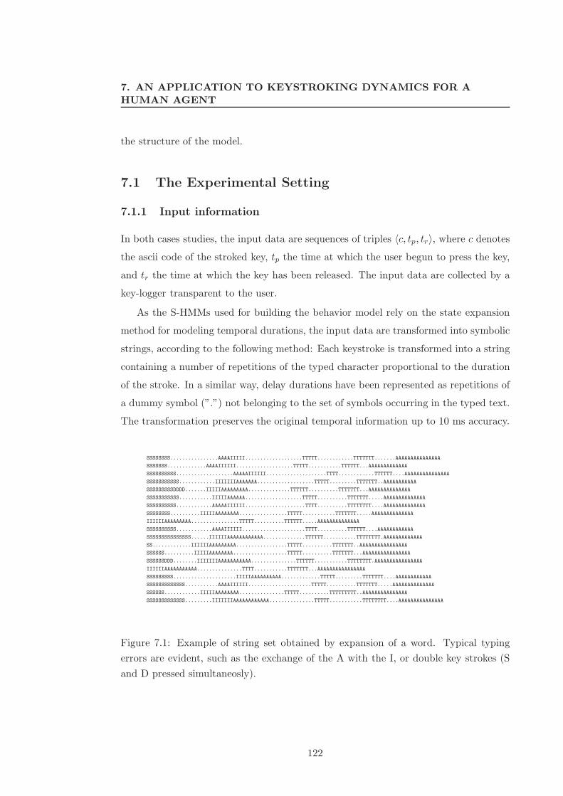
7. AN APPLICATION TO KEYSTROKING DYNAMICS FOR AHUMAN AGENT
the structure of the model.
7.1 The Experimental Setting
7.1.1 Input information
In both cases studies, the input data are sequences of triples 〈c, tp, tr〉, where c denotes
the ascii code of the stroked key, tp the time at which the user begun to press the key,
and tr the time at which the key has been released. The input data are collected by a
key-logger transparent to the user.
As the S-HMMs used for building the behavior model rely on the state expansion
method for modeling temporal durations, the input data are transformed into symbolic
strings, according to the following method: Each keystroke is transformed into a string
containing a number of repetitions of the typed character proportional to the duration
of the stroke. In a similar way, delay durations have been represented as repetitions of
a dummy symbol (”.”) not belonging to the set of symbols occurring in the typed text.
The transformation preserves the original temporal information up to 10 ms accuracy.
SSSSSSSS................AAAAIIIII...................TTTTT............TTTTTTT.......AAAAAAAAAAAAAAA
SSSSSSS.............AAAAIIIIII...................TTTTT...........TTTTTT...AAAAAAAAAAAAA
SSSSSSSSSS...................AAAAAIIIIII....................TTTT............TTTTTT....AAAAAAAAAAAAAAA
SSSSSSSSSSS............IIIIIIIAAAAAAA...................TTTTT.........TTTTTTT..AAAAAAAAAAA
SSSSSSSSSDDDD.......IIIIIAAAAAAAAA..............TTTTTT..........TTTTTTT...AAAAAAAAAAAAAA
SSSSSSSSSSS...........IIIIIAAAAAA...................TTTTT..........TTTTTTT.....AAAAAAAAAAAAAA
SSSSSSSSSS............AAAAAIIIIII....................TTTT..........TTTTTTTT....AAAAAAAAAAAAAA
SSSSSSSS..........IIIIIAAAAAAAA................TTTTT...........TTTTTTT.....AAAAAAAAAAAAAA
IIIIIIAAAAAAAAA................TTTTT..........TTTTTT.....AAAAAAAAAAAAAA
SSSSSSSSSS............AAAAIIIIII.....................TTTT..........TTTTTT....AAAAAAAAAAAA
SSSSSSSSSSSSSSS......IIIIIIAAAAAAAAAAAA..............TTTTTT...........TTTTTTTT.AAAAAAAAAAAAA
SS.............IIIIIIAAAAAAAAA.................TTTTT..........TTTTTTT..AAAAAAAAAAAAAAAA
SSSSSS..........IIIIIAAAAAAAA..................TTTTT..........TTTTTTT...AAAAAAAAAAAAAAAA
SSSSSSDDD........IIIIIIIAAAAAAAAAAA...............TTTTTT...........TTTTTTTT.AAAAAAAAAAAAAAAA
IIIIIIAAAAAAAAAAA...............TTTT...........TTTTTTT...AAAAAAAAAAAAAAAA
SSSSSSSSS.....................IIIIIAAAAAAAAAA.............TTTTT.........TTTTTTT....AAAAAAAAAAAA
SSSSSSSSSSSSS...........AAAAIIIIII.....................TTTTT..........TTTTTTT.....AAAAAAAAAAAAAA
SSSSSS............IIIIIAAAAAAAA...............TTTTT..........TTTTTTTTT..AAAAAAAAAAAAAAA
SSSSSSSSSSSSS.........IIIIIIIAAAAAAAAAAAA...............TTTTT...........TTTTTTTT....AAAAAAAAAAAAAAA
Figure 7.1: Example of string set obtained by expansion of a word. Typical typing
errors are evident, such as the exchange of the A with the I, or double key strokes (S
and D pressed simultaneosly).
122
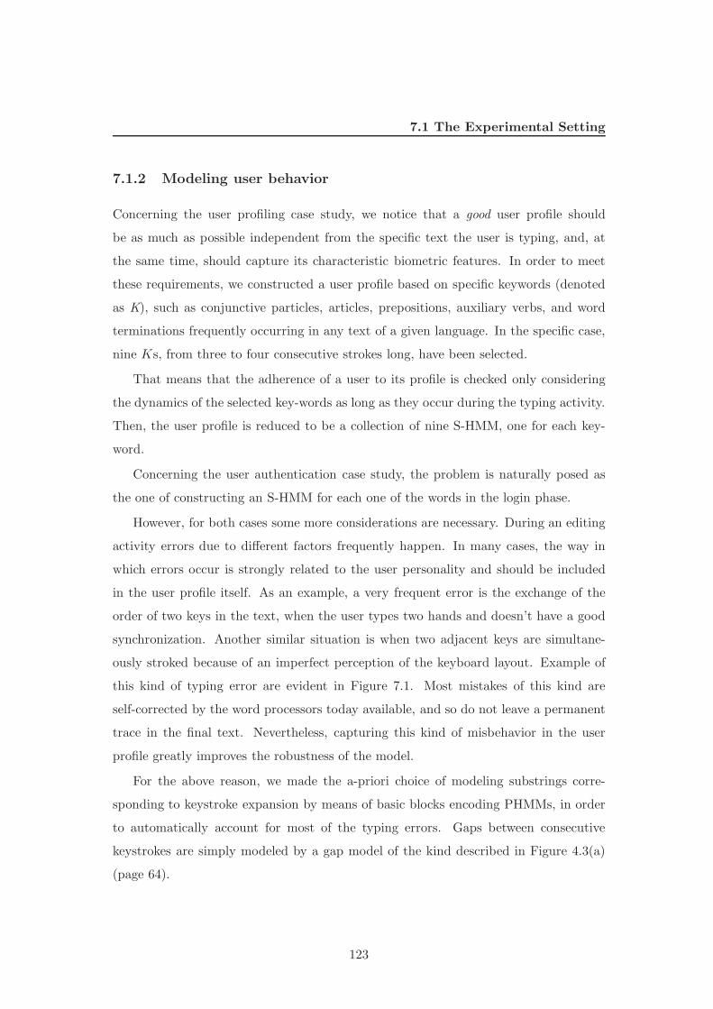
7.1 The Experimental Setting
7.1.2 Modeling user behavior
Concerning the user profiling case study, we notice that a good user profile should
be as much as possible independent from the specific text the user is typing, and, at
the same time, should capture its characteristic biometric features. In order to meet
these requirements, we constructed a user profile based on specific keywords (denoted
as K), such as conjunctive particles, articles, prepositions, auxiliary verbs, and word
terminations frequently occurring in any text of a given language. In the specific case,
nine Ks, from three to four consecutive strokes long, have been selected.
That means that the adherence of a user to its profile is checked only considering
the dynamics of the selected key-words as long as they occur during the typing activity.
Then, the user profile is reduced to be a collection of nine S-HMM, one for each key-
word.
Concerning the user authentication case study, the problem is naturally posed as
the one of constructing an S-HMM for each one of the words in the login phase.
However, for both cases some more considerations are necessary. During an editing
activity errors due to different factors frequently happen. In many cases, the way in
which errors occur is strongly related to the user personality and should be included
in the user profile itself. As an example, a very frequent error is the exchange of the
order of two keys in the text, when the user types two hands and doesn’t have a good
synchronization. Another similar situation is when two adjacent keys are simultane-
ously stroked because of an imperfect perception of the keyboard layout. Example of
this kind of typing error are evident in Figure 7.1. Most mistakes of this kind are
self-corrected by the word processors today available, and so do not leave a permanent
trace in the final text. Nevertheless, capturing this kind of misbehavior in the user
profile greatly improves the robustness of the model.
For the above reason, we made the a-priori choice of modeling substrings corre-
sponding to keystroke expansion by means of basic blocks encoding PHMMs, in order
to automatically account for most of the typing errors. Gaps between consecutive
keystrokes are simply modeled by a gap model of the kind described in Figure 4.3(a)
(page 64).
123
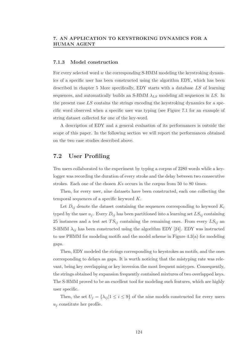
7. AN APPLICATION TO KEYSTROKING DYNAMICS FOR AHUMAN AGENT
7.1.3 Model construction
For every selected word w the corresponding S-HMM modeling the keystroking dynam-
ics of a specific user has been constructed using the algorithm EDY, which has been
described in chapter 5 More specifically, EDY starts with a database LS of learning
sequences, and automatically builds an S-HMM λLS modeling all sequences in LS. In
the present case LS contains the strings encoding the keystroking dynamics for a spe-
cific word observed when a specific user was typing (see Figure 7.1 for an example of
string dataset collected for one of the key-word.
A description of EDY and a general evaluation of its performances is outside the
scope of this paper. In the following section we will report the performances obtained
on the two case studies described above.
7.2 User Profiling
Ten users collaborated to the experiment by typing a corpus of 2280 words while a key-
logger was recording the duration of every stroke and the delay between two consecutive
strokes. Each one of the chosen Ks occurs in the corpus from 50 to 80 times.
Then, for every user, nine datasets have been constructed, each one collecting the
temporal sequences of a specific keyword K.
Let Dij denote the dataset containing the sequences corresponding to keyword Ki
typed by the user uj . Every Dij has been partitioned into a learning set LSij containing
25 instances and a test set TSij containing the remaining ones. From every LSij an
S-HMM λij has been constructed using the algorithm EDY [24]. EDY was instructed
to use PHMM for modeling motifs and the model scheme in Figure 4.3(a) for modeling
gaps.
Then, EDY modeled the strings corresponding to keystrokes as motifs, and the ones
corresponding to delays as gaps. It is worth noticing that the mistyping rate was rele-
vant, being key overlapping or key inversion the most frequent mistypes. Consequently,
the strings obtained by expansion frequently contained mixtures of two overlapped keys.
The S-HMM proved to be an excellent tool for modeling such features, which are highly
user specific.
Then, the set Uj = {λij |1 ≤ i ≤ 9} of the nine models constructed for every users
uj constitute her profile.
124
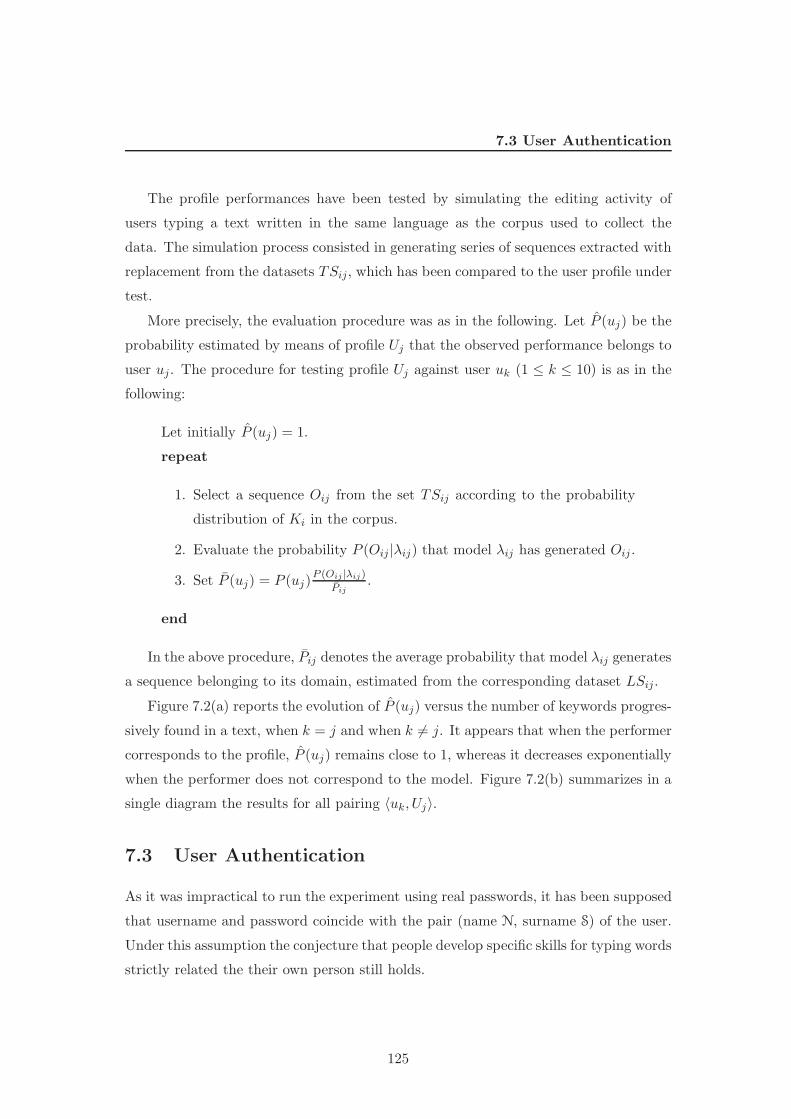
7.3 User Authentication
The profile performances have been tested by simulating the editing activity of
users typing a text written in the same language as the corpus used to collect the
data. The simulation process consisted in generating series of sequences extracted with
replacement from the datasets TSij, which has been compared to the user profile under
test.
More precisely, the evaluation procedure was as in the following. Let P (uj) be the
probability estimated by means of profile Uj that the observed performance belongs to
user uj. The procedure for testing profile Uj against user uk (1 ≤ k ≤ 10) is as in the
following:
Let initially P (uj) = 1.
repeat
1. Select a sequence Oij from the set TSij according to the probability
distribution of Ki in the corpus.
2. Evaluate the probability P (Oij |λij) that model λij has generated Oij .
3. Set P (uj) = P (uj)P (Oij |λij)
Pij.
end
In the above procedure, Pij denotes the average probability that model λij generates
a sequence belonging to its domain, estimated from the corresponding dataset LSij.
Figure 7.2(a) reports the evolution of P (uj) versus the number of keywords progres-
sively found in a text, when k = j and when k 6= j. It appears that when the performer
corresponds to the profile, P (uj) remains close to 1, whereas it decreases exponentially
when the performer does not correspond to the model. Figure 7.2(b) summarizes in a
single diagram the results for all pairing 〈uk, Uj〉.
7.3 User Authentication
As it was impractical to run the experiment using real passwords, it has been supposed
that username and password coincide with the pair (name N, surname S) of the user.
Under this assumption the conjecture that people develop specific skills for typing words
strictly related the their own person still holds.
125
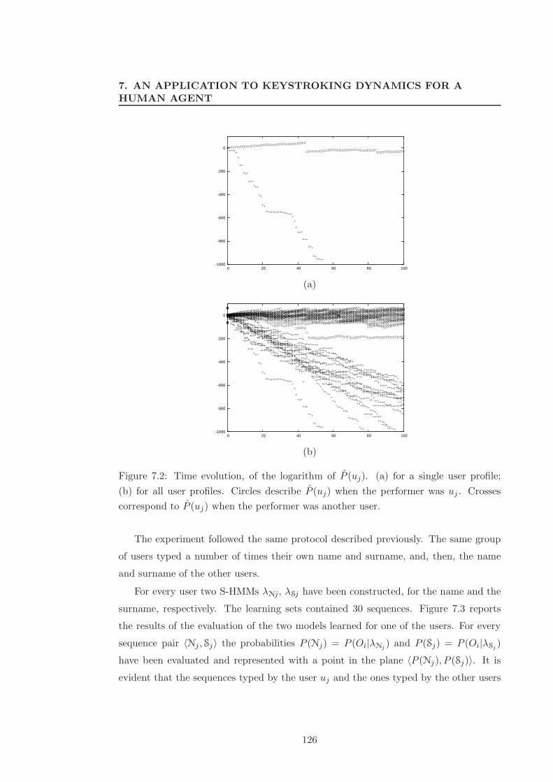
7. AN APPLICATION TO KEYSTROKING DYNAMICS FOR AHUMAN AGENT
-1000
-800
-600
-400
-200
0
0 20 40 60 80 100
(a)
-1000
-800
-600
-400
-200
0
0 20 40 60 80 100
(b)
Figure 7.2: Time evolution, of the logarithm of P (uj). (a) for a single user profile;
(b) for all user profiles. Circles describe P (uj) when the performer was uj . Crosses
correspond to P (uj) when the performer was another user.
The experiment followed the same protocol described previously. The same group
of users typed a number of times their own name and surname, and, then, the name
and surname of the other users.
For every user two S-HMMs λNj, λSj have been constructed, for the name and the
surname, respectively. The learning sets contained 30 sequences. Figure 7.3 reports
the results of the evaluation of the two models learned for one of the users. For every
sequence pair 〈Nj ,Sj〉 the probabilities P (Nj) = P (Oi|λNj) and P (Sj) = P (Oi|λSj
)
have been evaluated and represented with a point in the plane 〈P (Nj), P (Sj)〉. It is
evident that the sequences typed by the user uj and the ones typed by the other users
126
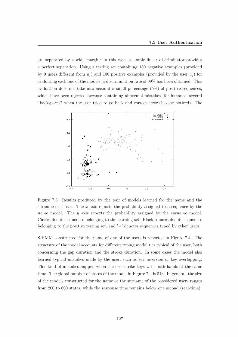
7.3 User Authentication
are separated by a wide margin: in this case, a simple linear discriminator provides
a perfect separation. Using a testing set containing 150 negative examples (provided
by 9 users different from uj) and 100 positive examples (provided by the user uj) for
evaluating each one of the models, a discrimination rate of 99% has been obtained. This
evaluation does not take into account a small percentage (5%) of positive sequences,
which have been rejected because containing abnormal mistakes (for instance, several
”backspaces” when the user tried to go back and correct errors he/she noticed). The
-1.4
-1.2
-1
-0.8
-0.6
-0.4-1.4-1.2-1-0.8-0.6-0.4
LS-USERTS-USER
TS-OTHERS
Figure 7.3: Results produced by the pair of models learned for the name and the
surname of a user. The x axis reports the probability assigned to a sequence by the
name model. The y axis reports the probability assigned by the surname model.
Circles denote sequences belonging to the learning set. Black squares denote sequences
belonging to the positive testing set, and ’+’ denotes sequences typed by other users.
S-HMM constructed for the name of one of the users is reported in Figure 7.4. The
structure of the model accounts for different typing modalities typical of the user, both
concerning the gap duration and the stroke duration. In some cases the model also
learned typical mistakes made by the user, such as key inversion or key overlapping.
This kind of mistakes happen when the user strike keys with both hands at the same
time. The global number of states of the model in Figure 7.4 is 513. In general, the size
of the models constructed for the name or the surname of the considered users ranges
from 200 to 600 states, while the response time remains below one second (real-time).
127
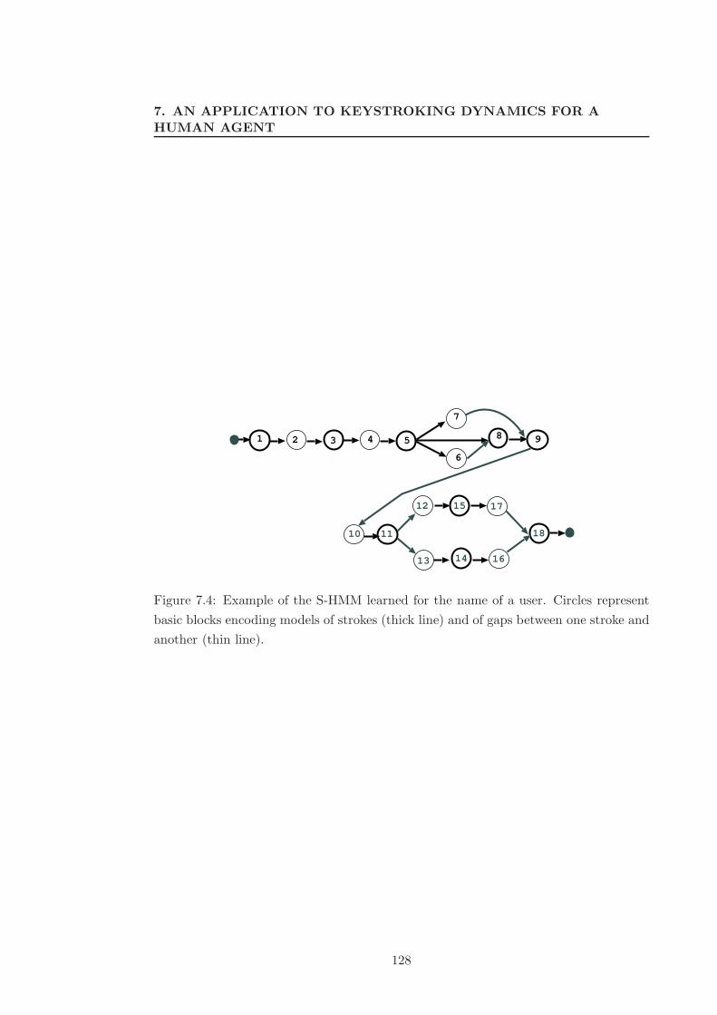
7. AN APPLICATION TO KEYSTROKING DYNAMICS FOR AHUMAN AGENT
1 2 3 4 5 9
7
6
8
10 11
12
13
15 17
14 16
18
Figure 7.4: Example of the S-HMM learned for the name of a user. Circles represent
basic blocks encoding models of strokes (thick line) and of gaps between one stroke and
another (thin line).
128
Chapter 8
Conclusions and future work
Stochastic generative models have been largely proposed has a suitable tool for analyz-
ing temporal or spatial sequences, such sequential signals coming from sensor or log of
system usage [43, 56]. While discriminative models are only suited for discriminative
task, generative models could be used also for providing an interpretation of a sequence
or to predict the future events of a temporal sequence on the basis of its past history.
Probability theory offers a framework for modeling the evolution of processes char-
acterized by inherent randomness or operating in environments too complex for a pre-
cise analysis. In this framework the statistical distributions governing the evolution
of a system can be estimated from a learning set of traces describing its past history.
However, the basic method originating from this approach doesn’t scale up to complex
models, and then a variety of methods have been proposed in the literature in order to
circumvent this problem.
Most of them can be casted in the graphical model framework, where a process
is modelled as a path in a state space governed by a set of probability distributions.
These models can be seen as a merge between probability theory and graph theory.
They are based on a well studied probabilistic framework and at the same time they
offer an interface by which humans can model highly interacting set of variables. [32]
Despite the advantages of this framework, developing the structure of a graphical
models is not trivial and most works proposed in the past only deal with the problem
of inferring the probability distribution governing that structure.
The main contributions of this thesis are mainly two: in the first place has been
proposed an unsupervised method, that we called EDY, for automatically synthesizing
129
8. CONCLUSIONS AND FUTURE WORK
complex profiles from traces which, even if exploits existing techniques, developed in
bio-informatics [16, 31], is absolutely novel.
In second place a great novelty consist in the design of the Structured Hidden
Markov Model architecture, a variant of Hidden Markov Models that inherits the major
advantages related to the structural property of Hierarchical Hidden Markov Models,
i.e. the possibility of modelling recursive or repetitive structure very well, reducing
at the same time the number of parameters to estimate, but that still could be make
use of standard inference algorithm developed for HMMs. They exhibit a really low
computational complexity allowing them to be applied to very long sequences in an
affordable time. Computing the Viterbi-path of a sentence 1000 characters long with
a model of 600 states will takes less than 2 second on a Intel CoreDuo @ 2,16Ghz.
A S-HMM is a graph built up, according to precise composition rules, with several
independent sub-graph (that are still S-HMMs). The compositional property of S-
HMMs allow to have a global model that is a composition of different kinds of blocks
especially developed for modeling gaps or motifs. The major feature of S-HMMs is that
they could be locally trained, considering only a sub-set of the whole model. For this
reason they can be constructed and trained incrementally taming the complexity of the
learning procedures.
The EDY algorithm that we proposed in chapter 5 has been successfully applied
for inferring S-HMMs from databases of sequences. It present two major limitations:
it generates S-HMMs with only two levels of block nesting and models blocks with a
left-to-right structure, which at most may contain self-loops. Despite those limitations
it demonstrated to be a powerful induction algorithm able at solving non trivial tasks
like the one of user profiling.
EDY constructs a S-HMM incrementally going through a learning cycle in which a
model is progressively extended and refined. It exploits co-occurrence of regularities in
bounded regions of a sequence in order to detect short motifs used to built new basic
blocks that will be nested in the model and successively refined.
The system has been tested both on artificial traces and on a task of user-profiling
in which the objective was to construct a model capturing the dynamics of a user typing
on a keyboard. The analysis on artificial traces makes evident the strong points and
the weaknesses of the induction algorithm. It exhibits good results on complex task
but it is also biased by the discovering motifs procedures that despite its velocity tend
130

to loose the less conservative boundaries of motifs it searches for. A second problem is
that, under some conditions, described in section 6.6, it tends to model a single motif as
a chain of shorter motifs. This is not a problem in discriminative tasks or when we are
interested in modeling the probability distribution observed in the learning sequences.
nevertheless, it becomes a serious inconvenient when the goal is to interpret a sequence
in a data mining task.
Therefore, there is space left for an incredible number of improvements. The next
steps, we are planning in order to obtain a more powerful EDY version, will be to
improve the motif discovery algorithms and to implement an operator for merging
consecutive motifs in order to obtain a better description of the modeled process.
131

8. CONCLUSIONS AND FUTURE WORK
132
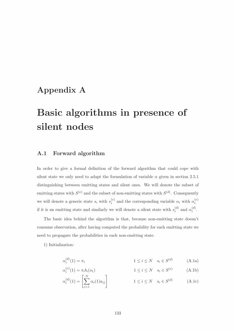
Appendix A
Basic algorithms in presence of
silent nodes
A.1 Forward algorithm
In order to give a formal definition of the forward algorithm that could cope with
silent state we only need to adapt the formulation of variable α given in section 2.5.1
distinguishing between emitting states and silent ones. We will denote the subset of
emitting states with S(e) and the subset of non-emitting states with S(d). Conseguently
we will denote a generic state si with s(e)i and the corresponding variable αi with α
(e)i
if it is an emitting state and similarly we will denote a silent state with s(d)i and α
(d)i .
The basic idea behind the algorithm is that, because non-emitting state doesn’t
consume observation, after having computed the probability for each emitting state we
need to propagate the probabilities in each non-emitting state.
1) Initialization:
α(d)i (1) = πi 1 ≤ i ≤ N si ∈ S(d) (A.1a)
α(e)i (1) = πibi(o1) 1 ≤ i ≤ N si ∈ S(e) (A.1b)
α(d)i (1) =
[N∑
i=1
αi(1)aij
]
1 ≤ i ≤ N si ∈ S(d) (A.1c)
133
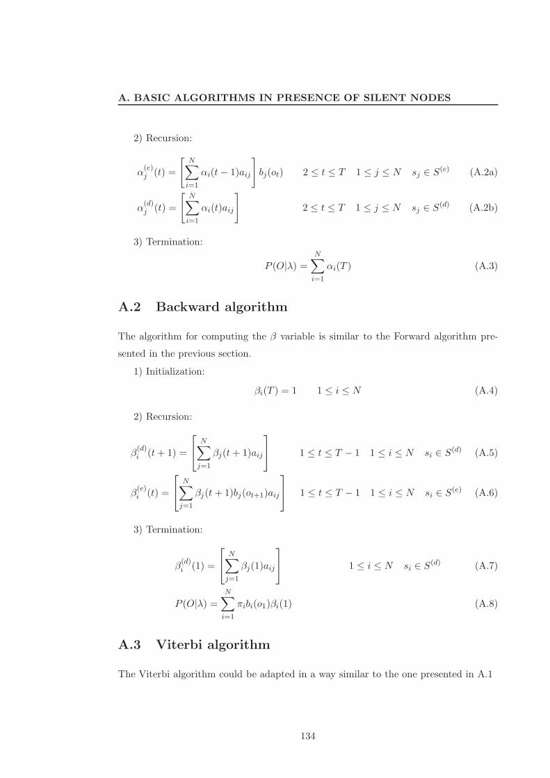
A. BASIC ALGORITHMS IN PRESENCE OF SILENT NODES
2) Recursion:
α(e)j (t) =
[N∑
i=1
αi(t− 1)aij
]
bj(ot) 2 ≤ t ≤ T 1 ≤ j ≤ N sj ∈ S(e) (A.2a)
α(d)j (t) =
[N∑
i=1
αi(t)aij
]
2 ≤ t ≤ T 1 ≤ j ≤ N sj ∈ S(d) (A.2b)
3) Termination:
P (O|λ) =
N∑
i=1
αi(T ) (A.3)
A.2 Backward algorithm
The algorithm for computing the β variable is similar to the Forward algorithm pre-
sented in the previous section.
1) Initialization:
βi(T ) = 1 1 ≤ i ≤ N (A.4)
2) Recursion:
β(d)i (t+ 1) =
N∑
j=1
βj(t+ 1)aij
1 ≤ t ≤ T − 1 1 ≤ i ≤ N si ∈ S(d) (A.5)
β(e)i (t) =
N∑
j=1
βj(t+ 1)bj(ot+1)aij
1 ≤ t ≤ T − 1 1 ≤ i ≤ N si ∈ S(e) (A.6)
3) Termination:
β(d)i (1) =
N∑
j=1
βj(1)aij
1 ≤ i ≤ N si ∈ S(d) (A.7)
P (O|λ) =
N∑
i=1
πibi(o1)βi(1) (A.8)
A.3 Viterbi algorithm
The Viterbi algorithm could be adapted in a way similar to the one presented in A.1
134

A.4 Bahum-Welch algorithm
1) Initialization:
δ(d)i (1) = πi 1 ≤ i ≤ N si ∈ S(d) (A.9a)
δ(e)i (1) = πibi(o1) 1 ≤ i ≤ N si ∈ S(e) (A.9b)
ψ(e)i (1) = 0 1 ≤ i ≤ N si ∈ S(e) (A.9c)
δ(d)i (1) =
[N∑
i=1
δi(1)aij
]
1 ≤ i ≤ N si ∈ S(d) (A.9d)
ψ(d)i (1) = arg max
1≤i≤N[δi(t− 1)aij ] 1 ≤ i ≤ N si ∈ S(d) (A.9e)
2) Recursion:
δ(e)j (t) = max
1≤i≤N[δi(t− 1)aij] bj(ot) 2 ≤ t ≤ T 1 ≤ j ≤ N sj ∈ S
(e) (A.10a)
δ(d)j (t) = max
1≤i≤N[δi(t)aij] 2 ≤ t ≤ T 1 ≤ j ≤ N sj ∈ S(d) (A.10b)
ψj(t) = arg max1≤i≤N
[δi(t− 1)aij ] 2 ≤ t ≤ T 1 ≤ j ≤ N (A.10c)
3) Termination:
P (σ∗) = max1≤i≤N
[δi(T )] (A.11a)
Pathσ∗(T ) = arg max1≤i≤N
[δi(T )] (A.11b)
4) Backtracking:
Pathσ∗(t) = ψ[Pathσ∗(t+1)](t+ 1) (A.12a)
A.4 Bahum-Welch algorithm
According with section 2.5.4, in order to give a formal description of the Baum-Welch
algorithm we need to define ξij(t), i.e. the probability of being in state si at time t and
in state sj at time t+ 1, given the model and the observation sequence. Again we need
to treat explicitly silent and emitting states.
ξij(t) = P (si(t), sj(t+ 1) | O,λ) =αi(t)aijbj(o(t+1))βj(t+ 1)
P (O | λ)
where bj(o(t+1)) = 0 if sj ∈ S(d)
(A.13)
At this point we are able to introduce the Baum-Welch algorithm:
135
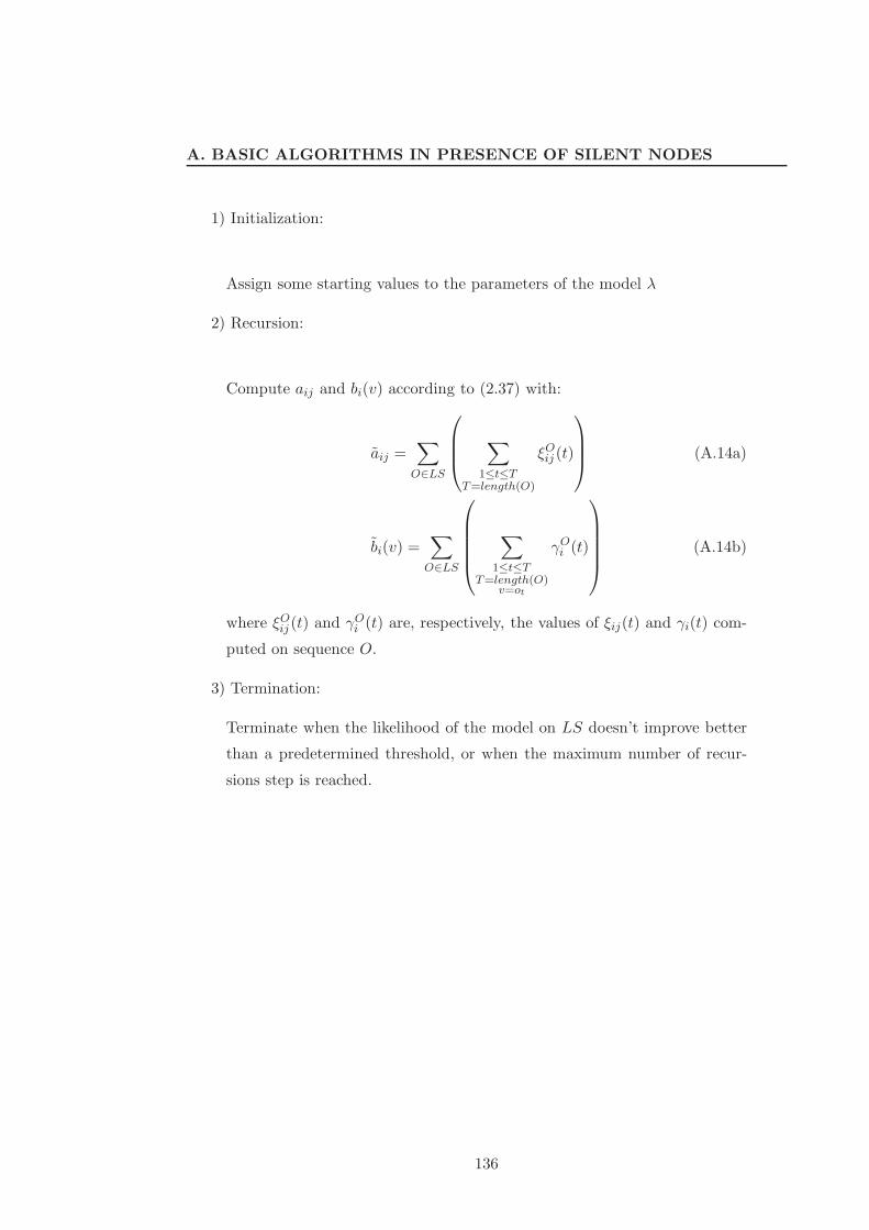
A. BASIC ALGORITHMS IN PRESENCE OF SILENT NODES
1) Initialization:
Assign some starting values to the parameters of the model λ
2) Recursion:
Compute aij and bi(v) according to (2.37) with:
aij =∑
O∈LS
∑
1≤t≤TT=length(O)
ξOij (t)
(A.14a)
bi(v) =∑
O∈LS
∑
1≤t≤TT=length(O)
v=ot
γOi (t)
(A.14b)
where ξOij (t) and γO
i (t) are, respectively, the values of ξij(t) and γi(t) com-
puted on sequence O.
3) Termination:
Terminate when the likelihood of the model on LS doesn’t improve better
than a predetermined threshold, or when the maximum number of recur-
sions step is reached.
136

Bibliography
[1] K. T. Abou-Moustafa, M. Cheriet, and C. Y. Suen. On the structure of hidden
markov models. Pattern Recogn. Lett., 25(8):923–931, 2004. 59
[2] Dana Angluin. Queries and concept learning. Machine Learning, 2(4):319–342,
1987. 4
[3] Timothy L. Bailey, Nadya Williams, Chris Misleh, and Wilfred W. Li. Meme: dis-
covering and analyzing dna and protein sequence motifs. Nucleic Acids Research,
34(Web-Server-Issue):369–373, 2006. 90
[4] L. E. Baum, T. Petrie, G. Soules, and N. Weiss. A maximisation techniques
occurring in the statistical analysis of probabilistic functions of markov chains.
The Annals of Mathematical Statistics, 41(1):164 – 171, 1970. 34, 55
[5] J. O. Berger. Statistical Decision Theory and Bayesian Analysis. Springer-Verlag,
New York, 1985. 88
[6] Christopher M. Bishop. Neural Networks for Pattern Recognition. Oxford Univer-
sity Press, November 1995. 1, 13
[7] S. Bleha, C. Slivinsky, and B. Hussein. Computer-access security systems using
keystroke dynamics. IEEE Transactions on Pattern Analysis and Machine Intel-
ligence, PAMI-12(12):1217–1222, 1990. 1
[8] M. Botta, U. Galassi, and A.Giordana. Learning complex and sparse events in long
sequences. In Proceedings of the European Conference on Artificial Intelligence,
ECAI-04, Valencia, Spain, August 2004. 38
137
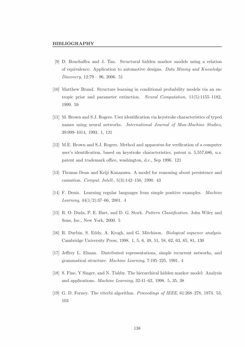
BIBLIOGRAPHY
[9] D. Bouchaffra and J. Tan. Structural hidden markov models using a relation
of equivalence: Application to automotive designs. Data Mining and Knowledge
Discovery, 12:79 – 96, 2006. 51
[10] Matthew Brand. Structure learning in conditional probability models via an en-
tropic prior and parameter extinction. Neural Computation, 11(5):1155–1182,
1999. 59
[11] M. Brown and S.J. Rogers. User identification via keystroke characteristics of typed
names using neural networks. International Journal of Man-Machine Studies,
39:999–1014, 1993. 1, 121
[12] M.E. Brown and S.J. Rogers. Method and apparatus for verification of a computer
user’s identification, based on keystroke characteristics, patent n. 5,557,686, u.s.
patent and trademark office, washington, d.c., Sep 1996. 121
[13] Thomas Dean and Keiji Kanazawa. A model for reasoning about persistence and
causation. Comput. Intell., 5(3):142–150, 1990. 43
[14] F. Denis. Learning regular languages from simple positive examples. Machine
Learning, 44(1/2):37–66, 2001. 4
[15] R. O. Duda, P. E. Hart, and D. G. Stork. Pattern Classification. John Wiley and
Sons, Inc., New York, 2000. 5
[16] R. Durbin, S. Eddy, A. Krogh, and G. Mitchison. Biological sequence analysis.
Cambridge University Press, 1998. 1, 5, 6, 49, 51, 58, 62, 63, 65, 81, 130
[17] Jeffrey L. Elman. Distributed representations, simple recurrent networks, and
grammatical structure. Machine Learning, 7:195–225, 1991. 4
[18] S. Fine, Y Singer, and N. Tishby. The hierarchical hidden markov model: Analysis
and applications. Machine Learning, 32:41–62, 1998. 5, 35, 38
[19] G. D. Forney. The viterbi algorithm. Proceedings of IEEE, 61:268–278, 1973. 53,
103
138
BIBLIOGRAPHY
[20] P. Frasconi, M. Gori, M. Maggini, and G. Soda. Representation of finite state
automata in recurrent radial basis function networks. Machine Learning, 23:5–32,
1996. 4
[21] K. S. Fu. Syntactic pattern recognition and applications. Prentice Hall, 1982. 1
[22] Yukiko Fujiwara, Minoru Asogawa, and Akihiko Konagaya. Stochastic motif ex-
traction using hidden markov model. In Russ B. Altman, Douglas L. Brutlag,
Peter D. Karp, Richard H. Lathrop, and David B. Searls, editors, ISMB, vol-
ume Proceedings of the Second International Conference on Intelligent Systems
for Molecular Biology, pages 121–129. AAAI, 1994. 58
[23] S. Furnell, J. M. Orrissey, P. Sanders, and C. Stockel. Applications of keystroke
analysis for improved login security and continuous user authentication. In Pro-
ceedings of the Information and System Security Conference, pages 283–294, 1996.
121
[24] U. Galassi, A. Giordana, and L. Saitta. Incremental construction of structured
hidden markov models. In proceedings IJCAI-2007, pages 2222–2227, 2007. 5, 50,
124
[25] Pedro Garcia and Enrique Vidal. Inference of k-testable languages in the strict
sense and application to syntactic pattern recognition. IEEE Trans. Pattern Anal.
Mach. Intell., 12(9):920–925, 1990. 4
[26] Z. Ghahramani and M. Jordan. Factorial hidden markov models. Machine Learn-
ing, 2:1–31, 1997. 5, 47
[27] N. W. Grundy, T.L. Bailey, C.P. Elkan, and M.E. Baker. Meta-meme: Motif-
based hidden markov models of biological sequences. Computer Applications in
the Biosciences, 13(4):397–406, 1997. 90
[28] D. Gussfield. Algorithms on Strings, Trees, and Sequences. Cambridge University
Press, 1997. 65, 66
[29] Singer H. Hmm topology design using maximum likelihood successive state split-
ting. Computer Speech and Language, 11:17–41(25), 1997. 59
139
BIBLIOGRAPHY
[30] J.E. Hopcroft and J.D. Ullman. Formal languages and their relation to automata.
Addison-Wesley, 1969. 3
[31] Richard Hughey and Anders Krogh. Hidden markov models for sequence anal-
ysis: extension and analysis of the basic method. Computer Applications in the
Biosciences, 12(2):95–107, 1996. 130
[32] Jordan. Graphical models. Statistical Science (Special Issue on Bayesian Statis-
tics), 19:140–155, 2004. 19, 129
[33] Michael I. Jordan and Terrence J. Sejnowski. Graphical models: Foundations of
neural computation. Pattern Anal. Appl., 5(4):401–402, 2002. 19
[34] Antonio Bonafonte Josep. Duration modeling with expanded hmm applied to
speech recognition. 62, 63
[35] R. Joyce and G. Gupta. User authorization based on keystroke latencies. Com-
munications of the ACM, 33(2):168–176, 1990. 1
[36] M. G. Kendall, A. Stuart, and J. K. Ord, editors. Kendall’s advanced theory of
statistics. Oxford University Press, Inc., New York, NY, USA, 1987. 1
[37] S. Kullback and R. A. Leibler. On information and sufficiency. Annals of Mathe-
matical Statistics, 22:79–86, 1951. 100
[38] W. Lee, W. Fan, M. Miller, S.J. Stolfo, and E. Zadok. Toward cost-sensitive
modeling for intrusion detection and response. Journal of Computer Security, 10:5
– 22, 2002. 1
[39] W. Lee and S.J Stolfo. Data mining approaches for intrusion detection. In Proceed-
ings of the Seventh USENIX Security Symposium (SECURITY ’98), San Antonio,
TX, 1998. 1
[40] V.I. Levenstein. Binary codes capable of correcting insertions and reversals. Soviet.
Phys. Dokl., 10:707–717, 1966. 84
[41] S.E. Levinson. Continuous variable duration hidden markov models for automatic
speech recognition. Computer Speech and Language, 1:29 – 45, 1986. 62
140

BIBLIOGRAPHY
[42] D.J. Lipman and W.R. Pearson. Rapid and sensitive protein similarity searches.
Science, 227:1435–1476, 1985. 83
[43] A. McCallum, K. Nigam, J. Rennie, and K. Seymore. Automating the construction
of internet portals with machine learning. Information Retrieval Journal, 3:127–
163, 2000. 89, 129
[44] T.M. Mitchell. Machine Learning. McGraw Hill, 1997. 91
[45] K. Murphy and M. Paskin. Linear time inference in hierarchical hmms. In Advances
in Neural Information Processing Systems (NIPS-01), volume 14, 2001. 5, 38
[46] K.P. Murphy. Dynamic Bayesian Networks: Representation, Inference and Learn-
ing. Ph.D thesis, Dpt. of Computer Science, UC, Berkeley, 2002. 43
[47] S. B. Needleman and C. D. Wunsch. A general method applicable to the search for
similarities in the amino acid sequence of two proteins. J. Mol. Biol., 48:443–53,
1970. 83
[48] K. Noto and M. Craven. Learning probabilistic models of cis-regulatory modules
that represent logical and spatial aspects. Bioinformatics, 23(2):e156–e162, 2006.
91
[49] K. Noto and M. Craven. A specialized learner for inferring structured cis-regulatory
modules. BMC Bioinformatics, 7:528, 2006. 91
[50] R. G. Parekh and V. G. Honavar. Learning DFA from simple examples. In
Proceedings of the 8th International Workshop on Algorithmic Learning Theory
(ALT’97), Lecture Notes in Artificial Intelligence, volume 1316, pages 116 –131,
Sendai, Japan, 1997. Springer. 4
[51] Rajesh Parekh, Codrin Nichitiu, and Vasant Honavar. A polynomial time incre-
mental algorithm for learning DFA. Lecture Notes in Computer Science, 1433:37–
50, 1998. 4
[52] Judea Pearl. Probabilistic reasoning in intelligent systems: networks of plausible
inference. Morgan Kaufmann Publishers Inc., San Francisco, CA, USA, 1988. 16,
43
141
BIBLIOGRAPHY
[53] Sara Porat and Jerome A. Feldman. Learning automata from ordered examples.
Machine Learning, 7:109–138, 1991. 4
[54] Janne Pylkkonen and Mikko Kurimo. Using phone durations in finnish large vo-
cabulary continuous speech recognition, 2004. 62
[55] L. Rabiner and B. Juang. Fundamentals of Speech Recognition. Prentice Hall,
Englewood Cliffs, NY, 1993. 1, 49, 51, 53
[56] L.R. Rabiner. A tutorial on hidden markov models and selected applications in
speech recognition. Proceedings of IEEE, 77(2):257–286, 1989. 3, 5, 49, 51, 53, 55,
63, 73, 100, 101, 129
[57] Mireille Regnier. Mathematical tools for regulatory signals extraction. In
N. Kolchanov and R. Hofestaedt, editors, Bioinformatics of Genome Regulation
and Structure, pages 61–70. Kluwer Academic Publisher, 2004. Preliminary version
at BGRS’02. 5
[58] Mireille Regnier and Alain Denise. Rare events and conditional events on random
strings. DMTCS, 6(2):191–214, 2004. 5
[59] Y. Rubner, C. Tomasi, and L. J. Guibas. The earth mover’s distance as a metric
for image retrieval. International Journal of Computer Vision, 40(2):99–121, 2000.
100
[60] B. Scholkopf, C. Burgess, and A. Smola. Advances in Kernel Methods. MIP Press,
1998. 10, 94
[61] Kristie Seymore, Andrew McCallum, and Roni Rosenfeld. Learning hidden Markov
model structure for information extraction. In AAAI 99 Workshop on Machine
Learning for Information Extraction, 1999. 89
[62] R. Shachter. Bayes-ball: The rational pastime (for determining irrelevance and
requisite information in belief networks and influence diagrams, 1998. 40
[63] M. Skounakis, M. Craven, and S. Ray. Hierarchical hidden markov models for
information extraction. In Proceedings of the 18th International Joint Conference
on Artificial Intelligence IJCAI-03, pages x–x. Morgan Kaufmann, 2003. 38
142

BIBLIOGRAPHY
[64] T.F. Smith and M.S. Waterman. Identification of common molecular subsequences.
Journal of Molecular Biology, 147:195–292, 1981. 1, 83
[65] A. Stolcke and S. Omohundro. Hidden markov model induction by bayesian model
merging. Advances in Neural Information Processing Systems, 5:11–18, 1993. 58,
59, 87
[66] A. Stolcke and S. M. Omohundro. Best-first model merging for hidden Markov
model induction. Technical Report TR-94-003, 1947 Center Street, Berkeley, CA,
1994. 87
[67] D. Tweed, R. Fisher, J. Bins, and T. List. Efficient hidden semi-markov model
inference for structured video sequences. In Proc. 2nd Joint IEEE Int. Workshop
on VSPETS, pages 247–254, Beijing, China, 2005. 62
[68] S-Z Yu and H. Kobashi. An efficient forward-backward algorithm for an explicit
duration hidden markov model. IEEE Signal Processing Letters, 10(1), 2003. 62
143