1

Supporting Information

Structure, Thermodynamics, and Dynamics of Thin

Brine Films in Oil-Brine-Rock Systems

Chao Fang,1 Shuyu Sun,2 Rui Qiao1,*

1 Department of Mechanical Engineering, Virginia Tech, Blacksburg, VA 24061 2 Division of Physical Science and Engineering, King Abdullah University of Science and

Technology, Thuwal 23955-6900, Saudi Arabia

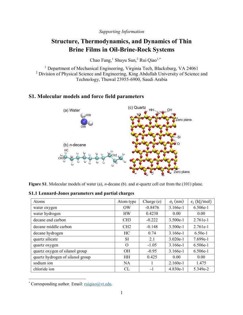
S1. Molecular models and force field parameters

Figure S1. Molecular models of water (a), n-decane (b). and 𝛼-quartz cell cut from the (101) plane.

S1.1 Lennard-Jones parameters and partial charges

Atoms Atom type Charge (e) 𝜎𝑖 (nm) 𝜖𝑖 (kJ/mol)

water oxygen OW -0.8476 3.166e-1 6.506e-1

water hydrogen HW 0.4238 0.00 0.00

decane end carbon CH3 -0.222 3.500e-1 2.761e-1

decane middle carbon CH2 -0.148 3.500e-1 2.761e-1

decane hydrogen HC 0.74 3.166e-1 6.50e-1

quartz silicate SI 2.1 3.020e-1 7.699e-1

quartz oxygen O -1.05 3.166e-1 6.506e-1

quartz oxygen of silanol group OH -0.95 3.166e-1 6.506e-1

quartz hydrogen of silanol group HH 0.425 0.00 0.00

sodium ion NA 1 2.160e-1 1.475

chloride ion CL -1 4.830e-1 5.349e-2

* Corresponding author. Email: ruiqiao@vt.edu.

2

S1.2 Boned parameters

(a) The bond stretching between two boned atoms i and j is represented by a harmonic potential,

𝑉𝑏(𝑟𝑖𝑗) =1

2𝑘𝑖𝑗

𝑏 (𝑟𝑖𝑗 − 𝑏𝑖𝑗)2

. (s1)

The bond parameters are

Bond type 𝑏 (nm) 𝑘𝑏 (kJ/mol/nm2)

OW-HW 9.572e-1 5.021e5

CH3(CH2)-CH2 1.529e-1 2.243e5

CH3(CH2)-CH 1.09e-1 2.845e5

OH-HH 1.0 4.637e5

(b) The angle vibration between three atoms i, j, and k is represented by a harmonic potential,

𝑉𝑎(𝜃𝑖𝑗𝑘) =1

2𝑘𝑖𝑗𝑘

𝑎 (𝜃𝑖𝑗𝑘 − 𝜃𝑖𝑗𝑘0 )

2. (s2)

The angle parameters are

Angle type 𝑘𝑎 (kJ/mol/rad2) 𝜃0 (degree)

HW-OW-HW 6.276000e+02 109.5

CH2 -CH2-CH2 (CH3) 4.882730e+02 112.7

CH2(CH3)-CH2(CH3)-HC 3.138000e+02 110.7

HC-CH2(CH3)-HC 2.761440e+02 107.8

SI-OH-HH 5.271840e+02 109.47

(c) The Ryckaert-Bellemans proper dihedral is used,

𝑉𝑟𝑏(𝜙𝑖𝑗𝑘𝑙) = ∑ 𝐶𝑛(𝑐𝑜𝑠(𝜙𝑖𝑗𝑘𝑙 − 180𝑜))𝑛5

𝑛=0 . (s3)

The dihedral parameters are

Dihedral type 𝑐0 (𝑘𝐽/𝑚𝑜𝑙) 𝑐1 (𝑘𝐽/𝑚𝑜𝑙) 𝑐2 (𝑘𝐽/𝑚𝑜𝑙) 𝑐3 (𝑘𝐽/𝑚𝑜𝑙) 𝑐4 (𝑘𝐽/𝑚𝑜𝑙) 𝑐5 (𝑘𝐽/𝑚𝑜𝑙)

CH2(CH3)-

CH2-CH2-

CH2(CH3)

5.1879e-01 -2.3019e-01 8.9681e-01 1.4913e+00 0 0

HC-CH2-CH2-

CH2(CH3, HC) 6.2760e-01 -1.8828e+00 0 2.5104e+00 0 0

3

S2. Thin brine films during last 100ns of simulation

Figure S2. The number of water and ions in thin brine films during the last 100ns of equilibrium simulation.

The number is computed within the red dashed box shown in Fig. 1a. The number is averaged every 2.5ns.

Figure S3. The pressure on the top piston during the last 100ns of simulation. The pressure at each time

step is shown in lines (orange) and the running average with a window of 2.5ns is shown in symbols (blue).

4

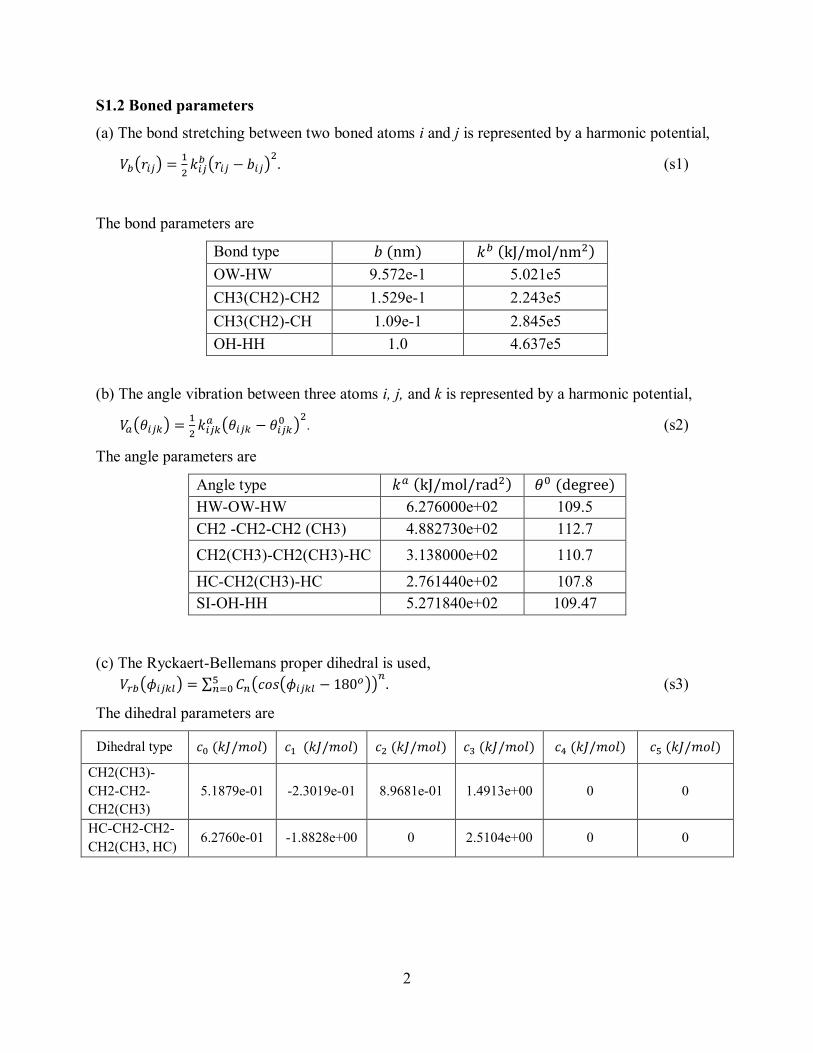
S3. Water-oil interface at 1M thin brine film

Figure S4. The water-oil interface of 1M thin brine films. The density profiles of water and oil near quartz

surface for two different film thickness: (a) h=0.90nm and (b) h=0.72nm.

S4. Geometry of the decane molecules

We introduce a gyration tensor for each decane molecule:

𝑆𝑚𝑛 = ∑ (𝑟𝑚(𝑖)

− 𝑟𝑚(𝑗)

)(𝑟𝑛(𝑖)

− 𝑟𝑛(𝑗)

)𝑖,𝑗 , (s4)

where 𝑟𝑚(𝑖)

is the mth Cartesian coordinate of the position vector 𝒓(𝑖) of the ith atom. Diagonalizing

𝑆𝑚𝑛 effectively fits the decane molecule to an ellipsoid. 𝑆𝑚𝑛’s eigenvalues 𝜎𝑘 (k=1, 2, 3 from the

largest to smallest eigenvalues) are the principal moments of the gyration tensor. The radius of

gyration of a decane molecule is given by 𝑅𝑔2 = 𝜎1

2 + 𝜎22 + 𝜎3

2. The eigenvectors 𝑺𝑘 of the gyration

tensor are the decane molecule’s principal axes.

5

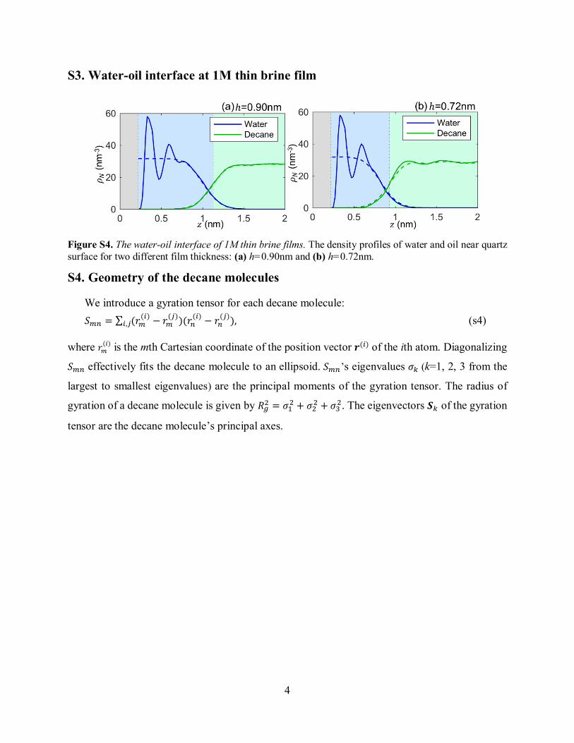
S5. Static dielectric constant of SPC/E water

Figure S5. The static dielectric constant of SPC/E water. 900 water molecules are included inside a periodic

simulation box. The convergence of dielectric constant, 휀, during four independent simulations done at

T=298.15 K (a) and T=350 K (b). 휀 is obtained by computing the total dipole moment fluctuation in the system.1-2 The averages are taken from the last 5ns and the error bars are obtained from four cases. At

T=298.15 K, 휀 = 70.14 ± 2.63, in agreement with that reported in previous simulations with the same water

model.3 At T=350 K, 휀 = 56.83 ± 1.31.

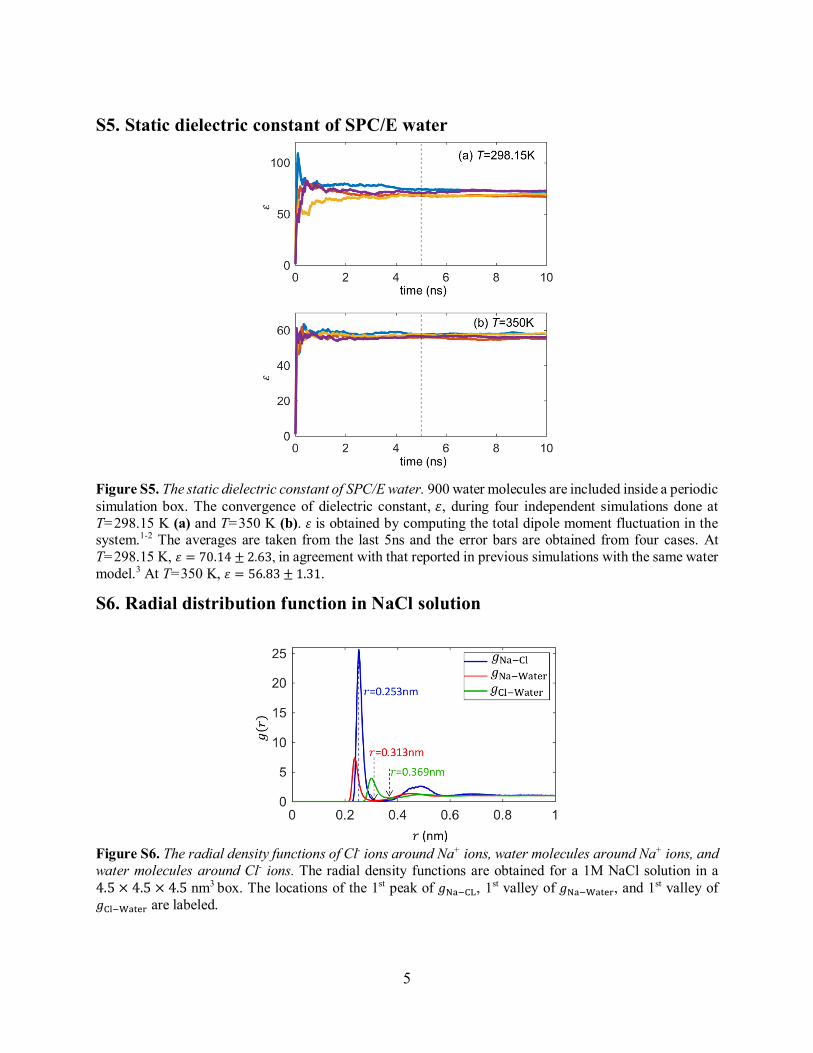
S6. Radial distribution function in NaCl solution

Figure S6. The radial density functions of Cl- ions around Na+ ions, water molecules around Na+ ions, and

water molecules around Cl- ions. The radial density functions are obtained for a 1M NaCl solution in a

4.5 × 4.5 × 4.5 nm3 box. The locations of the 1st peak of 𝑔Na−CL, 1st valley of 𝑔Na−Water, and 1st valley of

𝑔Cl−Water are labeled.

6

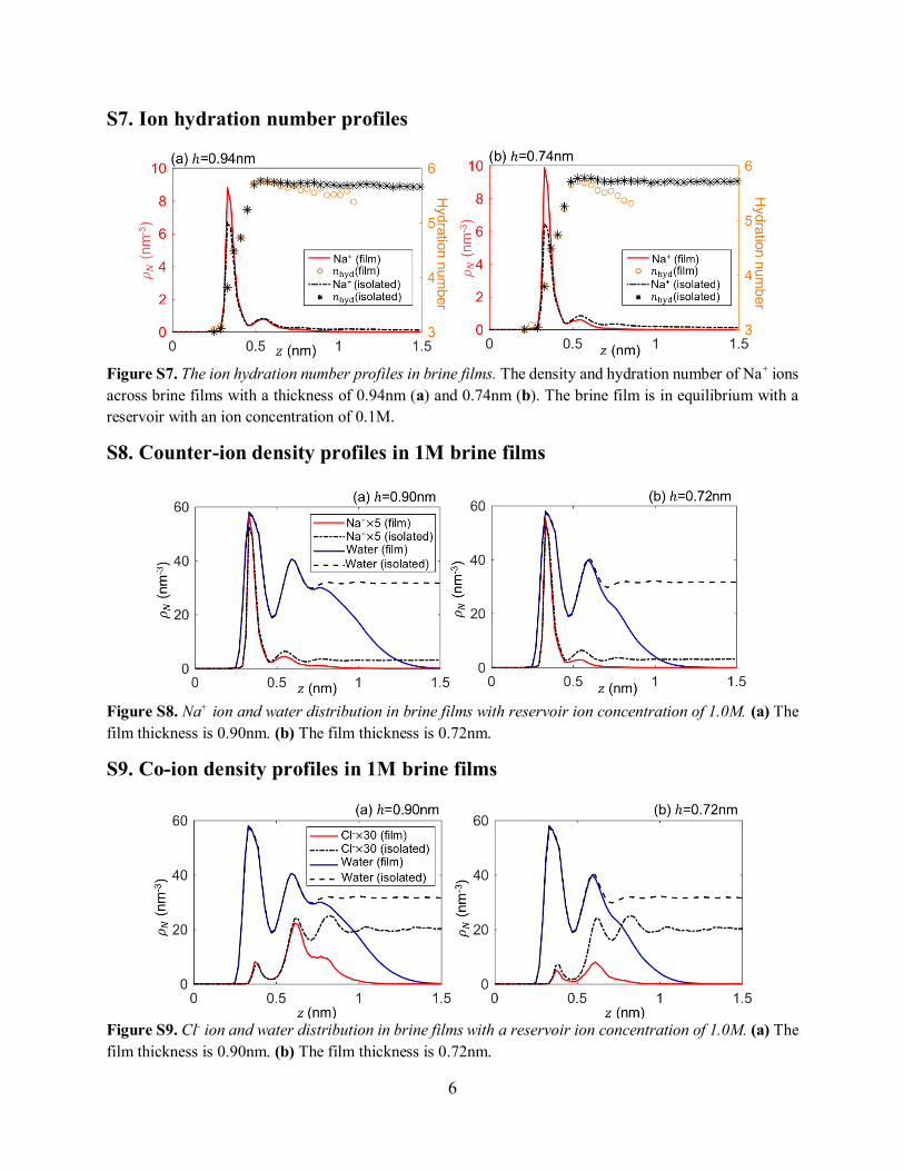
S7. Ion hydration number profiles

Figure S7. The ion hydration number profiles in brine films. The density and hydration number of Na+ ions

across brine films with a thickness of 0.94nm (a) and 0.74nm (b). The brine film is in equilibrium with a

reservoir with an ion concentration of 0.1M.

S8. Counter-ion density profiles in 1M brine films

Figure S8. Na+ ion and water distribution in brine films with reservoir ion concentration of 1.0M. (a) The

film thickness is 0.90nm. (b) The film thickness is 0.72nm.

S9. Co-ion density profiles in 1M brine films

Figure S9. Cl- ion and water distribution in brine films with a reservoir ion concentration of 1.0M. (a) The

film thickness is 0.90nm. (b) The film thickness is 0.72nm.

7

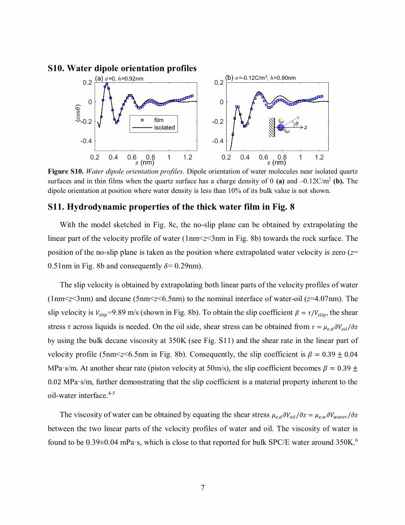
S10. Water dipole orientation profiles

Figure S10. Water dipole orientation profiles. Dipole orientation of water molecules near isolated quartz

surfaces and in thin films when the quartz surface has a charge density of 0 (a) and –0.12C/m2 (b). The

dipole orientation at position where water density is less than 10% of its bulk value is not shown.

S11. Hydrodynamic properties of the thick water film in Fig. 8

With the model sketched in Fig. 8c, the no-slip plane can be obtained by extrapolating the

linear part of the velocity profile of water (1nm<z<3nm in Fig. 8b) towards the rock surface. The

position of the no-slip plane is taken as the position where extrapolated water velocity is zero (z=

0.51nm in Fig. 8b and consequently 𝛿= 0.29nm).

The slip velocity is obtained by extrapolating both linear parts of the velocity profiles of water

(1nm<z<3nm) and decane (5nm<z<6.5nm) to the nominal interface of water-oil (z=4.07nm). The

slip velocity is 𝑉𝑠𝑙𝑖𝑝=9.89 m/s (shown in Fig. 8b). To obtain the slip coefficient 𝛽 = 𝜏/𝑉𝑠𝑙𝑖𝑝, the shear

stress 𝜏 across liquids is needed. On the oil side, shear stress can be obtained from 𝜏 = 𝜇𝑒,𝑑𝜕𝑉𝑜𝑖𝑙/𝜕𝑧

by using the bulk decane viscosity at 350K (see Fig. S11) and the shear rate in the linear part of

velocity profile (5nm<z<6.5nm in Fig. 8b). Consequently, the slip coefficient is 𝛽 = 0.39 ± 0.04

MPa·s/m. At another shear rate (piston velocity at 50m/s), the slip coefficient becomes 𝛽 = 0.39 ±

0.02 MPa·s/m, further demonstrating that the slip coefficient is a material property inherent to the

oil-water interface.4-5

The viscosity of water can be obtained by equating the shear stress 𝜇𝑒,𝑑𝜕𝑉𝑜𝑖𝑙/𝜕𝑧 = 𝜇𝑒,𝑤𝜕𝑉𝑤𝑎𝑡𝑒𝑟/𝜕𝑧

between the two linear parts of the velocity profiles of water and oil. The viscosity of water is

found to be 0.39±0.04 mPa·s, which is close to that reported for bulk SPC/E water around 350K.6

8

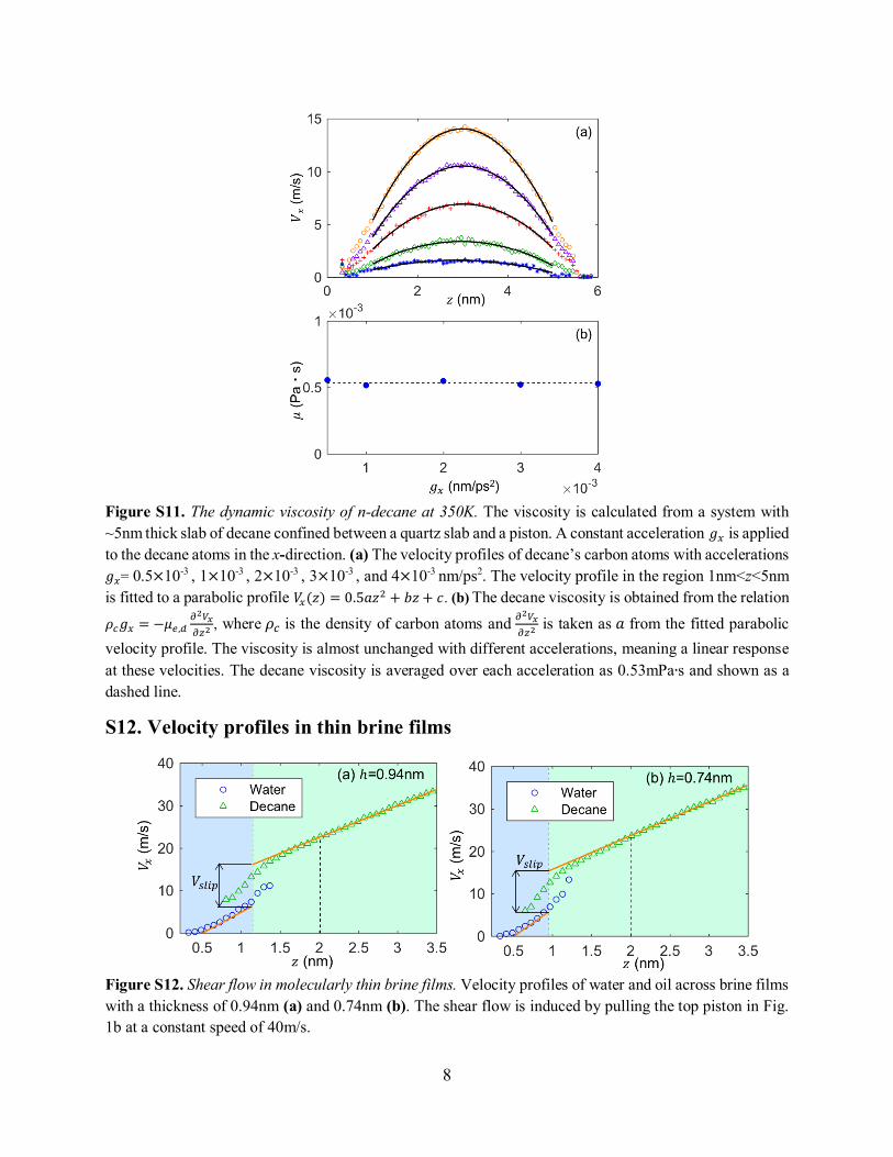
Figure S11. The dynamic viscosity of n-decane at 350K. The viscosity is calculated from a system with

~5nm thick slab of decane confined between a quartz slab and a piston. A constant acceleration 𝑔𝑥 is applied

to the decane atoms in the x-direction. (a) The velocity profiles of decane’s carbon atoms with accelerations

𝑔𝑥= 0.5×10-3 , 1×10-3 , 2×10-3 , 3×10-3 , and 4×10-3 nm/ps2. The velocity profile in the region 1nm<z<5nm

is fitted to a parabolic profile 𝑉𝑥(𝑧) = 0.5𝑎𝑧2 + 𝑏𝑧 + 𝑐. (b) The decane viscosity is obtained from the relation

𝜌𝑐𝑔𝑥 = −𝜇𝑒,𝑑𝜕2𝑉𝑥

𝜕𝑧2 , where 𝜌𝑐 is the density of carbon atoms and 𝜕2𝑉𝑥

𝜕𝑧2 is taken as 𝑎 from the fitted parabolic

velocity profile. The viscosity is almost unchanged with different accelerations, meaning a linear response

at these velocities. The decane viscosity is averaged over each acceleration as 0.53mPa∙s and shown as a

dashed line.

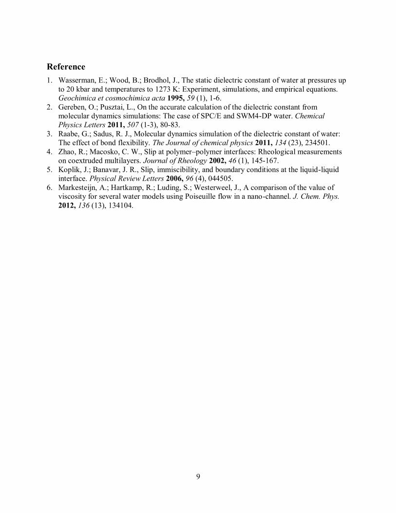
S12. Velocity profiles in thin brine films

Figure S12. Shear flow in molecularly thin brine films. Velocity profiles of water and oil across brine films

with a thickness of 0.94nm (a) and 0.74nm (b). The shear flow is induced by pulling the top piston in Fig.

1b at a constant speed of 40m/s.

9

Reference

1. Wasserman, E.; Wood, B.; Brodhol, J., The static dielectric constant of water at pressures up

to 20 kbar and temperatures to 1273 K: Experiment, simulations, and empirical equations.

Geochimica et cosmochimica acta 1995, 59 (1), 1-6.

2. Gereben, O.; Pusztai, L., On the accurate calculation of the dielectric constant from

molecular dynamics simulations: The case of SPC/E and SWM4-DP water. Chemical

Physics Letters 2011, 507 (1-3), 80-83.

3. Raabe, G.; Sadus, R. J., Molecular dynamics simulation of the dielectric constant of water:

The effect of bond flexibility. The Journal of chemical physics 2011, 134 (23), 234501.

4. Zhao, R.; Macosko, C. W., Slip at polymer–polymer interfaces: Rheological measurements

on coextruded multilayers. Journal of Rheology 2002, 46 (1), 145-167.

5. Koplik, J.; Banavar, J. R., Slip, immiscibility, and boundary conditions at the liquid-liquid

interface. Physical Review Letters 2006, 96 (4), 044505.

6. Markesteijn, A.; Hartkamp, R.; Luding, S.; Westerweel, J., A comparison of the value of

viscosity for several water models using Poiseuille flow in a nano-channel. J. Chem. Phys.

2012, 136 (13), 134104.