Structure of bifurcated solutions of two-dimensional infinite Prandtl number convection with no-slip boundary conditions

Applied Mathematics and Computation 218 (2012) 10586–10601

Contents lists available at SciVerse ScienceDirect

Applied Mathematics and Computation

journal homepage: www.elsevier .com/ locate /amc

Structure of bifurcated solutions of two-dimensional infinite Prandtlnumber convection with no-slip boundary conditions

Jungho ParkDepartment of Mathematics, New York Institute of Technology, Old Westbury, NY 11568, United States

a r t i c l e i n f o

Keywords:Rayleigh–Bénard convectionBifurcationStructure of solutionsStructural stabilityInfinite Prandtl numberNo-slip boundary conditions

0096-3003/$ - see front matter � 2012 Elsevier Inchttp://dx.doi.org/10.1016/j.amc.2012.04.021

E-mail address: [email protected]

a b s t r a c t

We consider the two-dimensional infinite Prandtl number convection problem with no-slip boundary conditions. The existence of a bifurcation from the trivial solution to anattractor RR was proved by Park [13]. The no-stress case has been examined in [14]. Weprove in this paper that the bifurcated attractor RR consists of only one cycle of steady statesolutions and it is homeomorphic to S1. By thoroughly investigating the structure and tran-sitions the solutions of the infinite Prandtl number convection problem in physical space,we confirm that the bifurcated solutions are indeed structurally stable. We show what theasymptotic structure of the bifurcated solutions looks like. This bifurcation analysis isbased on a new notion of bifurcation, called attractor bifurcation, and structural stabilityis derived using geometric theories of incompressible flows.

� 2012 Elsevier Inc. All rights reserved.

1. Introduction

In this paper we explore the structure of bifurcated solutions of the Bénard convection with no-slip boundary conditionswhich mean that the fluid flow does not move on the top and bottom boundaries. The same problem has been studied underno-stress boundary conditions [14] and much of the work in this paper is similar to the no-stress case. However, no-slip con-ditions require new ideas because no-slip boundary conditions do not allow for an explicit solution of the linearized eigen-value problem.

Rayleigh–Bénard convection, that is, a buoyancy-driven convection in a fluid layer heated from below and cooled fromabove, is one of the prime examples of bifurcating high-dimensional systems. It has long been a subject of intense theoreticaland experimental study and has been applied to many different areas of study such as meteorology, geophysics, and astro-physics. The governing equations are the following Boussinesq equations:

@u@tþ ðu � rÞuþ q�1

0 rp� mDu ¼ �gk 1� aðT � T0Þ� �

; ð1:1Þ

@T@tþ ðu � rÞT � jDT ¼ 0; ð1:2Þ

r � u ¼ 0; ð1:3Þ

where m is the kinematic viscosity, q0 is the fluid density at the lower surface, j is the thermal diffusivity, a is the coefficientof thermal expansion of the fluid, g is the acceleration due to gravity, u ¼ ðu1;u2Þ is the velocity field, p is the pressurefunction, T is the temperature field, T0 is a constant temperature at the lower boundary, and k ¼ ð0;1Þ is the unit vectorin x2-direction.

. All rights reserved.

http://dx.doi.org/10.1016/j.amc.2012.04.021

mailto:[email protected]

http://dx.doi.org/10.1016/j.amc.2012.04.021

http://www.sciencedirect.com/science/journal/00963003

http://www.elsevier.com/locate/amc

J. Park / Applied Mathematics and Computation 218 (2012) 10586–10601 10587

To make the equations non-dimensional, let

x ¼ hx0;

t ¼ h2t0=j;u ¼ ju0=h;

T ¼ bhðT 0=ffiffiffiRpÞ þ T0 � bhx02;

p ¼ q0k2p0=h2 þ p0 � gq0ðhx02 þ abh2ðx02Þ2=2Þ;

Pr ¼ m=j:

where, p0 is a constant. Omitting the primes, the Eqs. (1.1)–(1.3) can be rewritten as follows:

1Pr

@u@tþ ðu � rÞu

� �þrp� Du� RTk ¼ 0; ð1:4Þ

@T@tþ ðu � rÞT � DT ¼ 0; ð1:5Þ

r � u ¼ 0: ð1:6Þ

In the Boussinesq equations, we have two important numbers: the Rayleigh number,

R ¼ gaðT2 � T1Þh3

mj;

which measures the ratio of overall buoyancy force to the damping coefficients, and the Prandtl number,

Pr ¼mj;

which measures the relative importance of kinematic viscosity over thermal diffusivity. Here, h is the distance between twoplates confining the fluid and T2 � T1 is the temperature difference between the bottom and top plates.

Due to the fact that mathematical information is very limited, even the issue of the existence of regular solutions is notknown, it is highly required to simplify the complicated equations. For example, the infinite Prandtl number limit of theBoussinesq equations has been used as the standard model for the convection of earth’s mantle, where it is argued thatPr could be of the order 1024, as well as for many gasses under high pressure. A broader rationale for investigating the infinitePrandtl number convection is based on the observation of both the linear and weakly nonlinear theories; that fluids withPr > 1 convect in a similar fashion. Moreover, the infinite Prandtl number model of convection can also be justified as thelimit of the Boussinesq approximation to the Rayleigh–Bénard convection as the Prandtl number approaches infinity [20,21].

In the limit of the infinite Prandtl number, the inertial terms in the momentum equation can be dropped, thus we are leftwith a linear dependence of the velocity field on temperature:

rp� Du� RTk ¼ 0; ð1:7Þ@T@tþ ðu � rÞT � DT ¼ 0; ð1:8Þ

r � u ¼ 0: ð1:9Þ

The basic linear profiles of (1.7)–(1.9) are steady state solutions given by

u ¼ 0;T ¼ 1� x2;

p ¼ p0 þ R x2 �x2

2

2

� �k:

Let q be the difference between p and the steady state solutions, and let h be the difference between T and the steady statessolutions, i.e, p ¼ p0 þ Rðx2 �

x22

2 Þkþ q and T ¼ ð1� x2Þ þ h. Then the equations for the perturbation of these trivial solutionsare derived as

rq� Du� Rhk ¼ 0;@h@tþ ðu � rÞh� Dh� u2 ¼ 0;

r � u ¼ 0:

Let T ¼ffiffiffiRp

h and p ¼ q. Then we have

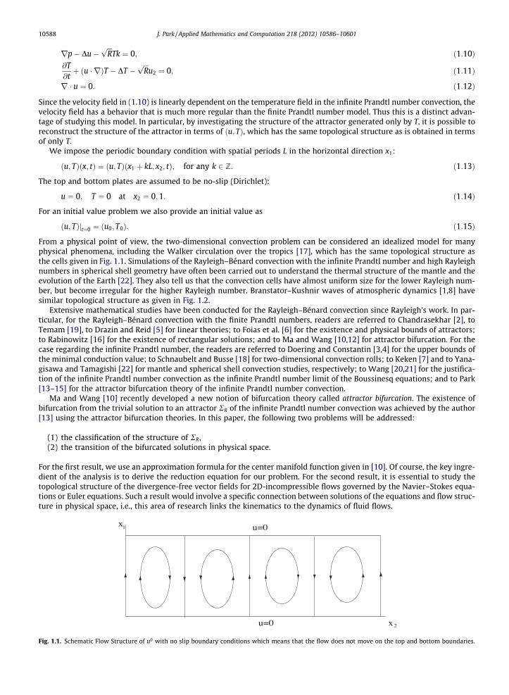
Fig. 1.1

10588 J. Park / Applied Mathematics and Computation 218 (2012) 10586–10601

rp� Du�ffiffiffiRp

Tk ¼ 0; ð1:10Þ@T@tþ ðu � rÞT � DT �

ffiffiffiRp

u2 ¼ 0; ð1:11Þ

r � u ¼ 0: ð1:12Þ

Since the velocity field in (1.10) is linearly dependent on the temperature field in the infinite Prandtl number convection, thevelocity field has a behavior that is much more regular than the finite Prandtl number model. Thus this is a distinct advan-tage of studying this model. In particular, by investigating the structure of the attractor generated only by T, it is possible toreconstruct the structure of the attractor in terms of ðu; TÞ, which has the same topological structure as is obtained in termsof only T.

We impose the periodic boundary condition with spatial periods L in the horizontal direction x1:

ðu; TÞðx; tÞ ¼ ðu; TÞðx1 þ kL; x2; tÞ; for any k 2 Z: ð1:13Þ

The top and bottom plates are assumed to be no-slip (Dirichlet):

u ¼ 0; T ¼ 0 at x2 ¼ 0;1: ð1:14Þ

For an initial value problem we also provide an initial value as

ðu; TÞjt¼0 ¼ ðu0; T0Þ: ð1:15Þ

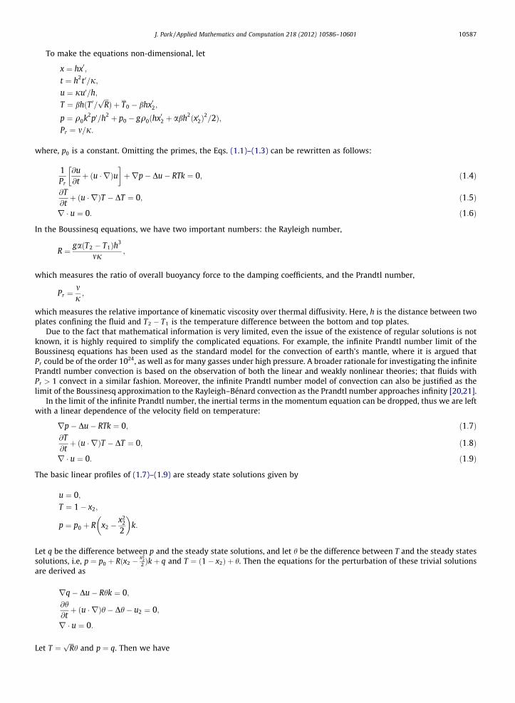
From a physical point of view, the two-dimensional convection problem can be considered an idealized model for manyphysical phenomena, including the Walker circulation over the tropics [17], which has the same topological structure asthe cells given in Fig. 1.1. Simulations of the Rayleigh–Bénard convection with the infinite Prandtl number and high Rayleighnumbers in spherical shell geometry have often been carried out to understand the thermal structure of the mantle and theevolution of the Earth [22]. They also tell us that the convection cells have almost uniform size for the lower Rayleigh num-ber, but become irregular for the higher Rayleigh number. Branstator–Kushnir waves of atmospheric dynamics [1,8] havesimilar topological structure as given in Fig. 1.2.

Extensive mathematical studies have been conducted for the Rayleigh–Bénard convection since Rayleigh’s work. In par-ticular, for the Rayleigh–Bénard convection with the finite Prandtl numbers, readers are referred to Chandrasekhar [2], toTemam [19], to Drazin and Reid [5] for linear theories; to Foias et al. [6] for the existence and physical bounds of attractors;to Rabinowitz [16] for the existence of rectangular solutions; and to Ma and Wang [10,12] for attractor bifurcation. For thecase regarding the infinite Prandtl number, the readers are referred to Doering and Constantin [3,4] for the upper bounds ofthe minimal conduction value; to Schnaubelt and Busse [18] for two-dimensional convection rolls; to Keken [7] and to Yana-gisawa and Tamagishi [22] for mantle and spherical shell convection studies, respectively; to Wang [20,21] for the justifica-tion of the infinite Prandtl number convection as the infinite Prandtl number limit of the Boussinesq equations; and to Park[13–15] for the attractor bifurcation theory of the infinite Prandtl number convection.

Ma and Wang [10] recently developed a new notion of bifurcation theory called attractor bifurcation. The existence ofbifurcation from the trivial solution to an attractor RR of the infinite Prandtl number convection was achieved by the author[13] using the attractor bifurcation theories. In this paper, the following two problems will be addressed:

(1) the classification of the structure of RR,(2) the transition of the bifurcated solutions in physical space.

For the first result, we use an approximation formula for the center manifold function given in [10]. Of course, the key ingre-dient of the analysis is to derive the reduction equation for our problem. For the second result, it is essential to study thetopological structure of the divergence-free vector fields for 2D-incompressible flows governed by the Navier–Stokes equa-tions or Euler equations. Such a result would involve a specific connection between solutions of the equations and flow struc-ture in physical space, i.e., this area of research links the kinematics to the dynamics of fluid flows.

x

x1

2

u=0

u=0

. Schematic Flow Structure of u0 with no slip boundary conditions which means that the flow does not move on the top and bottom boundaries.

Fig. 1.2. Zonally moving meandering structure of flow uðt;W0Þ with no-slip boundary conditions, which means that the flow does not move on the top andbottom boundaries.


As a result, we have a bifurcation from the trivial state to an attractor RR as R crosses the critical Rayleigh number Rc , thefirst eigenvalue of the eigenvalue problem of linearized equations [13]. Next, we prove that RR is homeomorphic to S1 andthat RR consists of steady state solutions for Rc < R < Rc þ e for some e > 0. These results can be obtained by analyzing eigen-vectors in terms of the temperature field T and later on, the velocity field uðTÞ associated with the temperature T can bereconstructed by the eigenvectors of T. Thanks to the geometric theory of 2D incompressible flows [11], the structure andits transitions between the convection states in physical space is analyzed. Through this, we prove that the associated veloc-ity field is structurally stable and show what the asymptotic structure looks like. This leads us, in particular, to a rigorousjustification of the structure as the cells given in Fig. 1.1 and the structure as the zonally moving meandering flows inFig. 1.2. The main results of this paper are the followings.

Theorem 1.1. For the problem ((1.10)–(1.12)) with ((1.13)–(1.15)), we have the following assertions: for R > Rc, the equationbifurcates from the trivial solution ðT;RÞ ¼ ð0;RcÞ to an attractor RR which is homeomorphic to S1. RR consists of exactly one cycleof steady state solutions whose structure in physical space is shown as in Fig. 1.1.

Theorem 1.2. For any ðu0ðT0Þ; T0Þ 2 eH � H n ðC [ EÞ, there exists a time t0 P 0 such that for any t P t0, the associated vector fielduðt;W0Þ is structurally stable and is topologically equivalent to the structure as shown in Fig. 1.2, where W ¼ ðuðt;W0Þ; Tðt;W0ÞÞ isthe solution of ((1.10)–(1.14)) with initial data W0 ¼ ðu0ðT0Þ; T0Þand C is the stable manifold of ðuðTÞ; TÞ ¼ 0 with co-dimension 2in eH � H and
eH ¼ fu 2 L2ðXÞ2jr � u ¼ 0; u1is periodic in x1 direction and u2 ¼ 0 at x2 ¼ 0;1g;
E ¼ fðu; TÞ 2 eH � HjR 1

0 u1 dx2 ¼ 0g:
The above two theorems will be proved in Section 3 and Section 4, respectively.
It is worthwhile to mention that the above results can only be obtained by the attractor bifurcation theories. The classicalbifurcation theory including symmetry arguments implies that the bifurcated attractor contains a circle of steady states. Weneed, however, the new bifurcated theory to prove in particular that the bifurcated attractors are exactly of type S1.

The paper is organized as follows. After introducing the infinite Prandtl number convection and its mathematical settingsin Section 2, we describe the center manifold approximation and bifurcation theories for the infinite Prandtl number con-vection in Section 3, followed by a topological structure of the bifurcated solutions. Then we study the structural stabilityand the asymptotic structure of the bifurcated solutions in Section 4.

2. Bénard problem and its mathematical setting

In this paper we deal with the Boussinesq equations on the non-dimensional domain X ¼ R� ð0;1Þ � R2. Since (1.10) to-gether with (1.12) is a Stokes equation, we have the solution u ¼ uðTÞ under the above boundary condition. Replacing u andits second component u2 in (1.11) by the solution which depends on T, we obtain the following equation

@T@tþ ðuðTÞ � rÞT � DT �

ffiffiffiRp

u2ðTÞ ¼ 0; ð2:1Þ

where uðTÞ and u2ðTÞ satisfy (1.10).Adjusting boundary and initial conditions yields

T ¼ 0 at x2 ¼ 0;1;Tðx; tÞ ¼ Tðx1 þ kL; x2; tÞ; for x 2 X;

ð2:2Þ


Tjt¼0 ¼ T0: ð2:3Þ

Instead of considering the bifurcation problem (1.10)–(1.12) with (1.13)–(1.15), we consider only (2.1) with (2.2) and (2.3),which depends only on T. The velocity field uðTÞ associated with T will be reconstructed later on.

We shall recall here the functional setting of the Eq. (2.1) with the boundary and initial conditions (2.2) and (2.3). Let

H ¼ L2ðXÞ and H1 ¼ H10ðXÞ \ H2ðXÞ;

where H10ðXÞ is the space of functions in H1ðXÞ, which vanish at x2 ¼ 0;1 and are periodic in x1-direction.

Thanks to the existence result, we can define a semi-group

SðtÞ : T0 ! TðtÞ;

which enjoys the semi-group properties.In the bifurcation theory for the infinite Prandtl number convection, the critical Rayleigh number, denoted by Rc , plays a

key role. We consider the linearized equations of (2.1) with the boundary conditions (2.2),

�DT �ffiffiffiRp

u2ðTÞ ¼ 0; ð2:4Þ

where u2ðTÞ satisfies (1.10).Since this eigenvalue problem for the Rayleigh number R is symmetric, all eigenvalues Rk with multiplicities mk of (2.4)

with (2.2) are real numbers, and

0 < R1 < � � � < Rk < Rkþ1 < � � � ð2:5Þ

in the sense that

�Duþrp� kTk ¼ 0;�DT � ku2 ¼ 0;r � u ¼ 0;

8><>:
is equivalent to Z
Xru � reu þrT � reTh i

dx ¼ kZ

XTeu2 þ u2

eTh idx;

where k ¼ffiffiffiRp

.The first eigenvalue R1 depends on periods L. It is known that there is a period Lc which minimizes R1ðLÞ. We denote the

critical Rayleigh number by Rc . Let the multiplicity of Rc be m1 ¼ m ðm P 1Þ and the first eigenvectors T1; . . . ; Tm of (2.4) beorthonormal, such that

hTi; TjiH ¼Z

XTi � Tjdx ¼ dij:

Then E0, the first eigenspace of (2.4) with (2.2) is

E0 ¼Xm

k¼1

akTkjak 2 R;1 6 k 6 m

( ): ð2:6Þ

Let H and H1 be defined as above. Define Lk ¼ �Aþ Bk : H1 ! H and G : H1 ! H by8
AðTÞ ¼ �DT;
BkðTÞ ¼ ku2ðTÞ;GðTÞ ¼ �ðuðTÞ � rÞT;

><>: ð2:7Þ


. Then we have an operator equation, which is equivalent to the Boussinesq Eq. (2.1):

dTdt¼ LkT þ GðTÞ: ð2:8Þ

3. Center manifold and attractor bifurcation theory

3.1. Center manifold approximation

The purpose of this section is to recall some results of the center manifold theory under general settings, i.e., general func-tion spaces and general functional equations. It is a powerful tool for the reduction method and for the dynamic bifurcationof abstract nonlinear evolution equations developed in [10].

Let H and H1 be two arbitrary Hilbert spaces, and H1,!H be a dense and compact inclusion. Consider the following non-linear evolution equations


dvdt¼ Lkv þ Gðv; kÞ; ð3:1Þ

vð0Þ ¼ v0; ð3:2Þ

where v : H � ½0;1Þ ! H is the unknown function, k 2 R is the system parameter, and Lk : H1 ! H are the parameterized lin-ear completely continuous fields continuously depending on k 2 R, which satisfy

Lk ¼ �Aþ Bk a sectorial operator;A : H1 ! H a linear homeomorphism;

Bk : H1 ! H the parameterized linear compact operators:

8><>: ð3:3Þ

We can see that Lk generates an analytic semi-group fe�tLkgtP0 and then we can define fractional power operators Lak for any

0 6 a 6 1 with the domain Ha ¼ DðLak Þ such that Ha1 � Ha2 if a2 < a1, and H0 ¼ H.

We now assume that the nonlinear terms Gð�; kÞ : Ha ! H for some 0 6 a < 1 are a family of parameterized Cr boundedoperators (r P 1) continuously depending on the parameter k 2 R, such that

Gðv; kÞ ¼ oðkvkHaÞ; 8k 2 R: ð3:4Þ

For the linear operator A, we assume that there exists a real eigenvalue sequence fqkg � R and an eigenvector sequencefekg � H1 such that

Aek ¼ qkek;

0 < q1 6 q2 6 � � � ;qk !1 ðk!1Þ;

8><>: ð3:5Þ

where fekg is an orthogonal basis of H.For the compact operator Bk : H1 ! H, we also assume that there is a constant 0 < h < 1 such that

Bk : Hh ! H bounded; 8k 2 R: ð3:6Þ

We know that the operator L ¼ �Aþ Bk satisfying (3.5) and (3.6) is a sectorial operator. It generates an analytic semigroupfSkðtÞgtP0. Then the solution of (3.1) and (3.2) can be expressed as

vðt;v0Þ ¼ SkðtÞv0; t P 0:

We assume that the spaces H1 and H can be decomposed into

H1 ¼ Ek1 � Ek

2; dimEk1 <1; near k0 2 R1;

H ¼ eEk1 � eEk

2;eEk

1 ¼ Ek1;

eEk2 ¼ closure of Ek

2 in H;

(ð3:7Þ

where Ek1 and Ek

2 are two invariant subspaces of Lk, i.e., Lk can be decomposed into Lk ¼ Lk1 � L

k2 such that for any k near k0,

Lk1 ¼ LkjEk

1: Ek

1 ! eEk1;

Lk2 ¼ LkjEk

2: Ek

2 ! eEk2;

8<: ð3:8Þ

where all eigenvalues of Lk2 possess negative real parts, and all eigenvalues of Lk

1 possess nonnegative real parts at k ¼ k0.Thus, for k near k0, (3.1) can be rewritten as

dxdt ¼ L

k1xþ G1ðx; y; kÞ;

dydt ¼ L

k2yþ G2ðx; y; kÞ;

(ð3:9Þ

where v ¼ xþ y 2 H1; x 2 Ek1; y 2 Ek

2, Giðx; y; kÞ ¼ PiGðv ; kÞ, and Pi : H ! eEi are canonical projections. Furthermore, we let

Ek2ðaÞ ¼ Ek

2 \ Ha;

with a given by (3.4).

Theorem 3.1 (Center Manifold Theorem). Assume ((3.4)–(3.8)). Then there exists a neighborhood of k0 given by jk� k0j < dfor some d > 0, a neighborhood Bk � Ek

1 of x ¼ 0, and a C1 function Uð�; kÞ : Bk ! Ek2ðaÞ, depending continuously on k, such that

(1) Uð0; kÞ ¼ 0; DxUð0; kÞ ¼ 0.(2) The set

Mk ¼ ðx; yÞ 2 H1jx 2 Bk; y ¼ Uðx; kÞ 2 Ek2ðaÞ

n o;

called the center manifold, is locally invariant for (3.1), i.e., for any v0 2 Mk,


vkðt;v0Þ 2 Mk; 80 6 t < tv0 ;

for some tv0 > 0, where vkðt;v0Þ is the solution of (3.1).

(3) If ðxkðtÞ; ykðtÞÞ is a solution of (3.9), then there are bk > 0 and kk > 0 with kk depending on ðxkð0Þ; ykð0ÞÞ, such that

kykðtÞ �UðxkðtÞ; kÞkH 6 kke�bkt :

By the help of the Center Manifold Theorem, we obtain the following bifurcation equation reduced to the finite dimen-sional system

dxdt¼ Lk

1xþ G1ðxþUðxÞ; kÞ;

for x 2 Bk � Ek1.

Now we recall an approximation of the center manifold function which will be used in the proof of Theorem 1.1; see [10]for details. Let the nonlinear operator G be given by

Gðv; kÞ ¼ Gkðv ; kÞ þ oðjvjkÞ; ð3:10Þ

where Gkðv ; kÞ is a k-multilinear operator(k P 2).

Theorem 3.2 [10]. Under the conditions in Theorem 3.1 and (3.10), we have the following center manifold functionapproximation:

Uðv ; kÞ ¼ ð�Lk2Þ�1P2Gkðv ; kÞ þ OðjRebðkÞj � jjv jjkÞ þ oðjjv jjkÞ;

where bðkÞ ¼ ðb1ðkÞ; . . . ; bmðkÞÞ are the eigenvalues of Lk1.

Consider the case where Lk : H1 ! H is symmetric. Then the eigenvalues are real, and the eigenvectors form an orthogonalbasis of H. Therefore, we have

v ¼ xþ y 2 Ek1 � Ek

2;

x ¼Xm

i¼1

xiei 2 Ek1;

y ¼X1

i¼mþ1

xiei 2 Ek2:

Then near k ¼ k0, the formula in Theorem 3.2, can be expressed as follows:

Uðx; kÞ ¼X1

j¼mþ1

Ujðx; kÞej þ OðjRebðkÞj � jjxjjkÞ þ oðjjxjjkÞ; ð3:11Þ

where

Ujðx; kÞ ¼ � 1bjðkÞ

X16j1 ;...;jk6m

ajj1 ��jk

xj1 � � � xjk ;

ajj1 ��jk¼< Gkðej1 ; . . . ; ejk ; kÞ; ej>H:

3.2. Attractor bifurcation theory for the infinite Prandtl number convection

In this subsection, we shall recall the attractor bifurcation theory of the infinite Prandtl number convection [13] and pro-vide a sufficient condition which implies that the bifurcated attractor of the system (3.1) is homeomorphic to S1.

Definition 3.3. A set R � H is called an invariant set of (3.1) if SðtÞR ¼ R for any t P 0. An invariant set R � H of (3.1) is saidto be an attractor if R is compact and there exists a neighborhood U � H of R such that for any u 2 U we have

limt!1

distHðvðt;uÞ;RÞ ¼ 0: ð3:12Þ

The largest open set U satisfying (3.12) is called the basin of attraction of R.

Definition 3.4

(1) We say that the Eq. (3.1) bifurcates from ðv ; kÞ ¼ ð0; k0Þ to an invariant set Xk, if there exists a sequence of invariantsets fXkng of (3.1), 0 R Xkn , such that


limn!1

kn ¼ k0;

limn!1

maxx2Xkn

jxj ¼ 0:

(2) If the invariant set Xk is an attractor of (3.1), then the bifurcation is called attractor bifurcation.(3) If Xk is an attractor and is homotopy equivalent to an m-dimensional sphere Sm, then the bifurcation is called Sm-

attractor bifurcation.

Let the eigenvalues (counting multiplicity) of Lk be given by

bkðkÞ 2 C ðk P 1Þ:

Suppose that

RebiðkÞ< 0 if k < k0;

¼ 0 if k ¼ k0

> 0 if k > k0;

8><>: ð1 6 i 6 mÞ; ð3:13Þ

Rebjðk0Þ < 0 ðmþ 1 6 jÞ: ð3:14Þ

Let the eigenspace of Lk at k0 be

E0 ¼[mi¼1

v 2 H1jðLk0 � biðk0ÞÞkv ¼ 0; k ¼ 1;2; . . .n o

:

The following dynamic bifurcation theorem for (2.1) was proved based on the principle of exchange of stabilities and asymp-totic stability of trivial solution [13].

Theorem 3.5 [13]. For the problem (2.1) with (2.2), we have the following assertions:

(1) If R 6 Rc, the steady state T ¼ 0 is a globally asymptotically stable equilibrium point of the equation.(2) The Eq. (2.1) bifurcates from ðT;RÞ ¼ ð0;RcÞ to an attractor RR for R > Rc, with m� 1 6 dimRR 6 m, which is connected

when m > 0.(3) For any T 2 RR, the associated velocity field u ¼ uðTÞ, which is achieved from a given T, can be expressed as

u ¼Xm

k¼1

akek þ oXm

k¼1

akek

!; ð3:15Þ

where ek are eigenvectors of (2.1) corresponding to each Tk.
(4) The attractor RR has the homotopy type of an ðm� 1Þ-dimensional sphere Sm�1 provided RR is a finite simplicial complex.(5) For any bounded open set U � L2ðXÞ with 0 2 U there is an e > 0 such that as Rc < R < Rc þ e, the attractor RR attracts U=C
in L2ðXÞ, where C is the stable manifold of T ¼ 0 with co-dimension m.

Remark 3.6. We can easily see that Theorem 3.5 is true for the 2D-Bénard problem as well as for the 3D-Bénard problem. Itis also true under any combination of two boundary conditions, no-slip and no-stress, on top or bottom plates.

So far, we have introduced some crucial definitions and theorems which have established the existence of bifurcation. Wenow introduce another theorem related to the structure of the bifurcated solutions.

Let v be a two-dimensional Crðr P 1Þ vector field given by

vkðxÞ ¼ kx� Gðx; kÞ; ð3:16Þ

for x 2 R2. Here, Gðx; kÞ is defined as in (3.10) and satisfies an inequality

C1jxjkþ16< Gkðx; kÞ; x>H 6 C2jxjkþ1

; ð3:17Þ

for some constants 0 < C1 < C2 and k ¼ 2mþ 1; m P 1.

Theorem 3.7 [10]. Under the condition (3.17), the vector field (3.16) bifurcates from ðx; kÞ ¼ ð0; k0Þ to an attractor Rk for k > k0,which is homeomorphic to S1. Moreover, one and only one of the following is true.

(1) Rk is a periodic orbit,(2) Rk consists of infinitely many singular points, or(3) Rk contains at most 2ðkþ 1Þ ¼ 4ðmþ 1Þ singular points, and has 4N þ nðN þ n P 1Þ singular points, 2N of which are saddle

points, 2N of which are stable node points (possibly degenerate), and n of which have index zero.


3.3. Proof of Theorem 1.1

In this subsection, we shall prove the first result which is related to the classification of the structure of RR.Step 1. We divide the proof into several steps. In the first step, we shall consider the eigenvalue problem of the linearized

equation of (2.1) and shall find the eigenvectors and the critical Rayleigh number Rc .Let’s consider the eigenvalue problem of the linear equation,

LkT ¼ bðkÞT: ð3:18Þ

It is equivalent to

�DT � ku2ðTÞ þ bðkÞT ¼ 0;


. Because uðTÞ satisfies

�DuðTÞ þ rp� kTk ¼ 0;

we can put two equations together as follows:

�DuðTÞ þ rp� kTk ¼ 0;�DT � ku2ðTÞ þ bðkÞT ¼ 0;r � u ¼ 0:

8><>: ð3:19Þ

For the no-slip boundary conditions, the following separation of variables is appropriate: for T 2 H1,

ðu; TÞ ¼ ðu1;u2; TÞ ¼ � sin2kp

Lx1H0ðx2Þ;

2kpL

cos2kp

Lx1Hðx2Þ; cos

2kpL

x1Hðx2Þ� �

;

or,

ðu; TÞ ¼ ðu1;u2; TÞ ¼ cos2kp

Lx1H0ðx2Þ;

2kpL

sin2kp

Lx1Hðx2Þ; sin

2kpL

x1Hðx2Þ� �

:

Then, from (3.19) we can derive a system of ODEs

ðD2 � a2kÞ

2H ¼ kakH;

ðD2 � a2kÞH ¼ �kakH þ bðkÞH;

(ð3:20Þ

supplemented with the boundary conditions

H ¼ DH ¼ H ¼ 0 at x2 ¼ 0;1; ð3:21Þ

where D ¼ ddx2

and ak ¼ 2kpL .

It is worthwhile to mention that the technical difference between the no-slip boundary conditions and the stress freeboundary conditions is due to (3.21). We can get H ¼ D2H ¼ 0 from the stress free boundary conditions which allows usan explicit sequence of eigenvalues and eigenvectors(see [14,15] for details). However, the no-slip boundary conditionsdo not allows for an explicit solution of (3.20) and (3.21).

The eigenvalue problem (3.20) with boundary conditions (3.21) is symmetric, and has complete sequence of eigenvaluesand eigenvectors for given k P 0 and k:

bk;jðkÞP bk;jþ1ðkÞ; bk;j ! �1 as j!1;Hk;j 2 H4ð0;1Þ \ H2

0ð0;1Þ;Hk;j 2 H2ð0;1Þ \ H1

0ð0;1Þ;

8><>: ð3:22Þ

for j ¼ 1;2; . . . Moreover,

fHk;j;Hk;jjj ¼ 1;2; . . .g

forms an orthogonal basis of L2ð0;1Þ � L2ð0;1Þ.From the above arguments, it can be seen that the following sequences are the set of eigenvectors of (3.19):

ðuk;2j�1; Tk;2j�1Þ ¼ � sin2kp

Lx1H0k;2j�1ðx2Þ;

2kpL

cos2kp

Lx1Hk;2j�1ðx2Þ; cos

2kpL

x1Hk;2j�1ðx2Þ� �

; ð3:23Þ

ðuk;2j; Tk;2jÞ ¼ cos2kp

Lx1H0k;2jðx2Þ;

2kpL

sin2kp

Lx1Hk;2jðx2Þ; sin

2kpL

x1Hk;2jðx2Þ� �

; ð3:24Þ

where k P 0 and j P 1.


We know that

b11ðkÞ ¼ b12ðkÞ< 0 if k < kc;

¼ 0 if k ¼ kc;

> 0 if k > kc;

8><>:b11 > bkjðkcÞ if ðk; jÞ – ð1;1Þ;

so that bk;jðkcÞ < 0 for ðk; jÞ– ð1;1Þ and the first eigenvectors of (3.19) corresponding to b11 are

ðu11; T11Þ and ðu12; T12Þ:

We remark here that we can derive from (3.19), (3.23) and (3.24) that for k ¼ 0

ðu0;2j�1; T0;2j�1Þ ¼ ð0; 0; sin jpx2Þ;ðu0;2j; T0;2jÞ ¼ ðH00;2jðx2Þ;0; 0Þ:

Step 2. We shall show that the bifurcated attractor of (2.1) and (2.2) contains a singularity cycle and it can be shown in theexactly same way which has been used in [14]. We omit the details.

Step 3. In the third step, we shall investigate the topological structure of RR. Let Ek1 ¼ E0 ¼ spanfT11; T12g and Ek

2 ¼ E?0 . ForT 2 H, we have the Furier expansion

T ¼X

kP0;jP1

ykjTk;j:

Then the reduction equations of (2.8) are as follows:

dy11dt ¼ b11ðkÞy11 þ 1

<T11 ;T11>H< G2ðT; TÞ; T11>H;

dy12dt ¼ b11ðkÞy12 þ 1

<T12 ;T12>H< G2ðT; TÞ; T12>H;

8<: ð3:25Þ

where G2 is the bilinear operator of G such that

G2ðT; TÞ ¼ �ðuðTÞ � rÞT;

< G2ðT1; T2Þ; T3>H ¼ �Z

XðuðT1Þ � rT2ÞT3 dx:

Let U be the center manifold function. Then

T ¼ y11T11 þ y12T12 þU:

We note here that for T11 and T12,

< G2ðT1; T2Þ; T3>H ¼ �Z

XuðT1Þ � rT2ð ÞT3 dx ¼ � < G2ðT1; T3Þ; T2>H:

In particular,

< G2ðT1; T2Þ; T2>H ¼ 0:

Therefore, we have

< G2ðT; TÞ; T11>H ¼< G2ðT11; T12Þ; T11>Hy11y12þ < G2ðT11;UÞ; T11>Hy11þ < G2ðT12; T12Þ; T11>Hy212þ

< G2ðT12;UÞ; T11>Hy12þ < G2ðU; T12Þ; T11>Hy12þ < G2ðU;UÞ; T11>H; ð3:26Þ

and

< G2ðT; TÞ; T12>H ¼< G2ðT11; T11Þ; T12>Hy211þ < G2ðT11;UÞ; T12>Hy11þ < G2ðT12; T11Þ; T12>Hy11y12þ

< G2ðT12;UÞ; T12>Hy12þ < G2ðU; T11Þ; T12>Hy11þ < G2ðU;UÞ; T12>H: ð3:27Þ

It is easy to check that the following inner products vanish for k P 0; j P 1 :

< G2ðT11; T12Þ; Tk;2j�1>H ¼2pL

Z L

0

Z 1

0H011ðx2ÞH12ðx2ÞHk;2j�1ðx2Þ � H11ðx2ÞH012ðx2ÞHk;2j�1ðx2Þ� �

sin2pL

x1 cos2pL

x1

� cos2kp

Lx1 dx ¼ 0;

< G2ðT12; T11Þ; Tk;2j�1>H ¼2pL

Z L

0

Z 1

0H012ðx2ÞH11ðx2ÞHk;2j�1ðx2Þ � H12ðx2ÞH011ðx2ÞHk;2j�1ðx2Þ� �

sin2pL

x1

� cos2pL

x1 cos2kp

Lx1 dx ¼ 0;


< G2ðT11; T11Þ; Tk;2j>H ¼ �2pL

Z L

0

Z 1

0sin

2pL

x1

� �2

sin2kp

Lx1H011ðx2ÞH11ðx2ÞHk;2jðx2Þ þ cos

2pL

x1

� �2

� sin2kp

Lx1H11ðx2ÞH011ðx2ÞHk;2jðx2Þdx ¼ 0;

< G2ðT12; T12Þ; Tk;2j>H ¼ �2pL

Z L

0

Z 1

0cos

2pL

x1

� �2

sin2kp

Lx1H012ðx2ÞH12ðx2ÞHk;2jðx2Þ þ sin

2pL

x1

� �2

� sin2kp

Lx1H12ðx2ÞH012ðx2ÞHk;2jðx2Þdx ¼ 0;

< G2ðTk;2j�1; T12Þ; T11>H ¼Z L

0

Z 1

0

2pL

sin2kp

Lx1 cos

2pL

x1

� �2

H0k;2j�1ðx2ÞH12ðx2ÞH11ðx2Þ �2kp

Lcos

2kpL

x1

� sin2pL

x1 cos2pL

x1Hk;2j�1ðx2ÞH012ðx2ÞH11ðx2Þdx ¼ 0:

We also have

< G2ðT11; T11Þ; Tk;2j�1>H ¼ �2pL

Z L

0

Z 1

0sin

2pL

x1

� �2

cos2kp

Lx1H011ðx2ÞH11ðx2ÞHk;2j�1ðx2Þ

þ cos2pL

x1

� �2

cos2kp

Lx1H11ðx2ÞH011ðx2ÞHk;2j�1ðx2Þdx ¼

– 0 if k ¼ 0;2;

¼ 0 otherwise;

8<:< G2ðT12; T12Þ; Tk;2j�1>H ¼ �

2pL

Z L

0

Z 1

0cos

2pL

x1

� �2

cos2kp

Lx1H012ðx2ÞH12ðx2ÞHk;2j�1ðx2Þ

þ sin2pL

x1

� �2

cos2kp

Lx1H12ðx2ÞH012ðx2ÞHk;2j�1ðx2Þdx ¼

– 0 if k ¼ 0;2;

¼ 0 otherwise;

(

< G2ðT11; T12Þ; Tk;2j>H ¼2pL

Z L

0

Z 1

0sin

2pL

x1 cos2pL

x1 sin2kp

Lx1H011ðx2ÞH12ðx2ÞHk;2jðx2Þ

� cos2pL

x1 sin2pL

x1 sin2kp

Lx1H11ðx2ÞH012ðx2ÞHk;2jðx2Þdx ¼

– 0 if k ¼ 2;¼ 0 otherwise;

< G2ðT12; T11Þ; Tk;2j>H ¼2pL

Z L

0

Z 1

0sin

2pL

x1 cos2pL

x1 sin2kp

Lx1H012ðx2ÞH11ðx2ÞHk;2jðx2Þ

� cos2pL

x1 sin2pL

x1 sin2kp

Lx1H12ðx2ÞH011ðx2ÞHk;2jðx2Þdx ¼

– 0 if k ¼ 2;¼ 0 otherwise;

< G2ðTk;2j; T12Þ; T11>H ¼ �Z L

0

Z 1

0

2pL

cos2kp

Lx1 cos

2pL

x1

� �2

H0k;2jðx2ÞH12ðx2ÞH11ðx2Þ

þ 2kpL

sin2kp

Lx1 sin

2pL

x1 cos2pL

x1Hk;2jðx2ÞH012ðx2ÞH11ðx2Þdx ¼– 0 if k ¼ 0;2;¼ 0 otherwise:

By Theorem 3.2, it is seen that the center manifold function U, near k ¼ kc , can be expressed as

UðyÞ ¼X

ðk;jÞ – ð1;1Þ;ð1;2ÞUk;jðyÞTk;j þ oðjyj2Þ; ð3:28Þ

where

Uk;jðyÞ ¼ �1

bkjðkÞX

16p;q62

akjpqy1py1q;

akjpq ¼< G2ðT1p; T1qÞ; Tk;j>H:


Due to the above inner products and (3.28), (3.26) and (3.27) become

< G2ðT; TÞ; T11>H ¼ �X1j¼2

½< G2ðT11; T11Þ; T0;2j�1>HU0;2j�1þ < G2ðT11; T11Þ; T2;2j�1>HU2;2j�1�y11

�X1j¼2

< G2ðT12; T11Þ; T2;2j>HU2;2j� �

y12 þX1j¼2

½< G2ðT0;2j; T12Þ; T11>HU0;2j

þ < G2ðT2;2j; T12Þ; T11>HU2;2j�y12þ < G2ðU;UÞ; T11>H; ð3:29Þ

and

< G2ðT; TÞ; T12>H ¼ �X1j¼2

½< G2ðT12; T12Þ; T0;2j�1>HU0;2j�1þ < G2ðT12; T12Þ; T2;2j�1>HU2;2j�1�y12

�X1j¼2

< G2ðT11; T12Þ; T2;2j>HU2;2j� �

y11 þX1j¼2

½< G2ðT0;2j; T11Þ; T12>HU0;2j

þ < G2ðT2;2j; T11Þ; T12>HU2;2j�y11þ < G2ðU;UÞ; T12>H: ð3:30Þ

Direct calculations yield

< G2ðT2;2j; T12Þ; T11>H ¼ �Z

XðuðT2;2j � rT12ÞT11dx ¼ �p

2

Z 1

0ðH02;2jH12H11 þ 2H2;2jH

012H11Þdx2

¼ �p2

Z 1

0

ddx2ðH2;2jH

211Þdx2 ¼ 0;

and some identities

< G2ðT11; T11Þ; T0;2j�1>H ¼< G2ðT12; T12Þ; T0;2j�1>H;

< G2ðT11; T12Þ; T2;2j>H ¼< G2ðT12; T11Þ; T2;2j>H;

< G2ðT11; T11Þ; T2;2j�1>H ¼ � < G2ðT12; T12Þ; T2;2j�1>H:

By (3.28), near k ¼ kc we can calculate coefficients of the center manifold function explicitly:

U0;2j�1 ¼ �1

b0;2j�1ðkÞX

16p;q62

a0;2j�1pq y1py1q ¼ �

1b0;2j�1ðkÞ

< G2ðT11; T11Þ; T0;2j�1>Hðy211 þ y2

12Þ þ oðjy11j2 þ jy12j

2Þ

U2;2j�1 ¼ �1

b2;2j�1ðkÞX

16p;q62

a2;2j�1pq y1py1q ¼ �

1b2;2j�1ðkÞ

< G2ðT11; T11Þ; T2;2j�1>Hðy211 � y2

12Þ þ oðjy11j2 þ jy12j

2Þ

U0;2j ¼ �1

b0;2jðkÞX

16p;q62

a0;2jpq y1py1q ¼ 0

U2;2j ¼ �1

b2;2jðkÞX

16p;q62

a2;2jpq y1py1q ¼ �

2b2;2jðkÞ

< G2ðT11; T12Þ; T2;2j>Hy11y12 þ oðjy11j2 þ jy12j

2Þ:

ð3:31Þ

Replacing (3.29) and (3.30) with (3.31), we obtain

< G2ðT; TÞ; T11>H ¼ �X1j¼2

1b0;2j�1ðkÞ

< G2ðT11; T11Þ; T0;2j�1>2H

!y11ðy2

11 þ y212Þ

�X1j¼2

1b2;2j�1ðkÞ

< G2ðT11; T11Þ; T2;2j�1>2H

!y11ðy2

11 þ y212Þ

þ < G2ðU;UÞ; T11>H þ oðjy11j3 þ jy12j

3Þ; ð3:32Þ

and

< G2ðT; TÞ; T12>H ¼ �X1j¼2

1b0;2j�1ðkÞ

< G2ðT11; T11Þ; T0;2j�1>2H

!y12ðy2

11 þ y212Þ

�X1j¼2

1b2;2j�1ðkÞ

< G2ðT11; T11Þ; T2;2j�1>2H

!y12ðy2

11 þ y212Þ

þ < G2ðU;UÞ; T12>H þ oðjy11j3 þ jy12j

3Þ: ð3:33Þ

We know that the center manifold function involves only higher order terms

UðyÞ ¼ Oðjy11j2 þ jy12j

2Þ;


which implies that

< G2ðU;UÞ; T1i>H ¼ oðjy11j3; jy12j

3Þ; ði ¼ 1;2Þ: ð3:34Þ

Let

a ¼X1j¼2

< G2ðT11; T11Þ; T0;2j�1>2H

b0;2j�1ðkÞþ< G2ðT11; T11Þ; T2;2j�1>

2H

b2;2j�1ðkÞ

!:

Then a < 0 for kc < k < kc þ e. Note that for k P 0 and j P 1,

jjTk;2j�1jj2H ¼ jjTk;2jjj2H:

Then, from (3.34) we get the bifurcation equations reduced on the center manifold:

dy11dt ¼ b11ðkÞy11 þ a

jjTk;2j�1 jj2Hy11ðy2

11 þ y212Þ þ oðjy11j

3; jy12j

3Þ;dy12

dt ¼ b11ðkÞy12 þ ajjTk;2j jj2H

y12ðy211 þ y2

12Þ þ oðjy11j3; jy12j

3Þ:ð3:35Þ

It can be easily verified that (3.35) satisfies conditions of Theorem 3.7 so that we can conclude that RR is homeomorphic to S1.This completes the proof. h

4. Structural stability theorems

4.1. Basic settings

In this section we shall recall some results on structural stability for two-dimensional divergence free vector fields gov-erned by the Navier-Stokes equations or the Euler equations. See [9,11] for details.

Let CrðX;R2Þ be the space of all Crðr P 1Þ vector fields on X, which are periodic in x1 direction with periods L, and let

DrðX;R2Þ ¼ fv 2 CrðX;R2Þjr � v ¼ 0;v2 ¼ 0 at x2 ¼ 0;1g;Br

0ðX;R2Þ ¼ fv 2 DrðX;R2Þjv ¼ 0 at x2 ¼ 0;1g:

Definition 4.1. Two vector fields u;v 2 CrðX;R2Þ are called topologically equivalent if there exists a homeomorphism ofu : X! X, which takes the orbits of u to that of v and preserves their orientations.

Definition 4.2. Let X ¼ DrðX;R2Þ. A vector field v 2 X is called structurally stable in X if there exists a neighborhood U � X ofv such that for any u 2 U;u and v are topologically equivalent.

Let v 2 DrðX;R2Þ. We recall some basic definitions and properties on divergence free vector fields.

1. A point p 2 X is called a singular point of v if vðpÞ ¼ 0; a singular point p of v is called non-degenerate if the Jacobianmatrix DvðpÞ is invertible; v is called regular if all singular points of v are non-degenerate.

2. An interior non-degenerate singular point of v can be either a center or a saddle, and a non-degenerate boundary singularpoint must be a saddle.

3. Saddles of v must be connected to saddles. An interior saddle p 2 X is called self connected if p is connected to itself. i.e., poccurs in a graph whose topological form is that of the ‘1’.

Let v 2 Br0ðX;R2Þ. Then, it is obvious that each point on x2 ¼ 0;1 is a singular point of v. Now, we need to classify the bound-

ary points of X.

Definition 4.3. Let u 2 Br0ðX;RÞ (r P 2).

1. A point p 2 @X is called a @-regular point of u if @usðpÞ@n – 0; otherwise, p is called a @-singular point of u.

2. A @-singular point p 2 @X of u is called non-degenerate if

det@2usðpÞ@s@n

@2usðpÞ@n2

@2unðpÞ@s@n

@2unðpÞ@n2

0@ 1A– 0:

A non-degenerate @-singular point of u is also called a @-saddle point of u.3. u is called D-regular if u is regular in int X, and all @-singular points of u on @X are non-degenerate.


Lemma 4.4 (Connection Lemma, [11]). Let u;v 2 DrðX;R2Þ with v sufficiently small, and L � X be an extended orbit of u startingat p. Then an extended orbit c of uþ v starting at p passes through a point q 2 L if and only if
Z
L½p;q�v � d‘ ¼ 0;

where L½p; q� is the curve segment on L from p and q.

Theorem 4.5 ([9,11]). Let u 2 Br0ðX;R2Þ (r P 2). Then u is structurally stable if and only if

(1) u is D-regular,(2) all interior saddle points of u are self-connected, and(3) each @-saddle point of u on @X is connected to a @-saddle points on the same connected component of @X.

Remark 4.6. The difference between two boundary conditions, no-slip and no-stress, is due to the zero-average condition.Since ðða;0Þ;0Þ is a solution of (1.10)–(1.12) for any constant a under no-stress boundary condition, the velocity field in thefunction space must satisfy

RX udx ¼ 0. Hence, an orbit connecting two saddles on different components of the boundary can

not be broken with a perturbation into orbits connecting only saddles on the same connected component of the boundary.See [14] for details.

Now, we prove the structural stability theorem.

4.2. Proof of Theorem 1.2

We infer from (3.35) that for any T 2 RR, the associated steady state velocity field u ¼ ðu1;u2Þ can be expressed as

u ¼X2

k¼1

y1ku1k þ oX2

k¼1

y1ku1k

!;

which implies that

u1 ¼ y11 � sin2pL

x1H011

� �þ y12 cos

2pL

x1H011

� �þ v1ðy11; y12;b11Þ;

u2 ¼ y112pL

cos2pL

x1H11

� �þ y12

2pL

sin2pL

x1H11

� �þ v2ðy11; y12;b11Þ:

ð4:1Þ

Now, note that the above expansion were done in terms of the eigenvectors. Thus, they must hold not only on H, but also onhigher dimensional Sobolev spaces Hm ðm P 0Þ. Simple modifications yield

u1 ¼ r sin 2pL ðh� x1ÞH011 þ v1ðy11; y12; b11Þ;

u2 ¼ 2prL cos 2p

L ðh� x1ÞH11 þ v2ðy11; y12;b11Þ;ð4:2Þ

for some 0 6 h 6 2p. Here,

r2 ¼ y211 þ y2

12 ¼b11ðkÞ�a

jjT11jj2H þ obðkÞ�a

� �; for k > k11;

v iðy11; y12;b11Þ ¼ oðrÞ ði ¼ 1;2Þ:

Let

E ¼ ðu; TÞ 2 eH � HjZ

Xu1 dx ¼ 0

�:

Then, E is invariant for the Eqs. (1.10)–(1.12), which implies that
Z 1
0v1 dx2 ¼ 0:

Therefore, in the Fourier expansion of u in (3.23) and (3.24), the coefficients of ðu0;2j; T0;2jÞ ¼ ðH00;2jðx2Þ; 0;0Þ are zero. By theConnection Lemma, it follows that u ¼ ðu1;u2Þ is topologically equivalent to the velocity field

u0 ¼ ðu01;u

02Þ ¼ r sin

2pL

x1H011ðx2Þ;2pL

cos2pL

x1H11ðx2Þ� �

:

It is known that the first eigenvector H11ðx2Þ at k ¼ kc is given by


H11ðx2Þ ¼ cos q0 x2 �12

� �� 0:06151664 cosh q1 x2 �

12

� �cos q2 x� 1

2

� �þ 0:103887

� sinh q1 x2 �12

� �sin q2 x2 �

12

� �; ð4:3Þ

where q0 ¼ 3:973639; q1 ¼ 5:095214; q2 ¼ 2:126096; see [2] for details. The structure of u0, the steady state solution, ispure roll structure whose flow, on the top and bottom plates, does not move and is as shown in Fig. 1.1. Now it sufficesto show that u0 is structurally stable.

From

@u01

@x2¼ r sin

2pL

x1H00ðx2Þ ¼ 0;

the @-singular points of u are

ðx1; x2Þ ¼kL2;0

� �;

kL2;1

� �;

and we can see that

det

@2u01

@x1@x2

@2u01

@x22

@2u02

@x1@x2

@2u02

@x22

264375 ¼ det

2prL cos 2p

L x1H0011ðx2Þ r sin 2pL x1Hð3Þ11 ðx2Þ

� 2prL

� 2r sin 2p

L x1H0011ðx2Þ 2prL cos 2p

L x1H0011ðx2Þ

" #– 0;

at ðx1; x2Þ ¼ ðkL2 ;0Þ and ðkL

2 ;1Þ. Therefore, every @-singular point of u0 is non-degenerate. For interior singular points of u0,

ðx1; x2Þ ¼ð2kþ 1Þ

4L;

12

� �;

det Du0 ¼ det2pr

L cos 2pL x1H011ðx2Þ r sin 2p

L x1H0011ðx2Þ

� 2prL

� 2r sin 2pL x1H11ðx2Þ 2pr

L cos 2pL x1H011ðx2Þ

" #– 0:

Therefore, the velocity field u0 is D-regular, which means that u is D-regular for kc < k < kc þ e. By Theorem 4.5, u is struc-turally stable.

The rest part of the proof will be dedicated to show the structure of the velocity field u in physical space.For some initial value W0 ¼ ðu0; T0Þ 2 ðeH � HÞ=E,

W0 ¼X

k

akWk þU0;

where U0 2 E and Wk ¼ ðsin kpL x2;0;0Þ, k ¼ 2mþ 1; ðm ¼ 0;1; � � �Þ. Since

< G2ðT; TÞ;Wk>H ¼ 0;

the solution W ¼ ðuðt;W0Þ; Tðt;W0ÞÞ of (1.10)–(1.12) is

Wðt;W0Þ ¼X

k

akeb0kðkÞtWk þ eU0ðt;W0Þ:

By Foias [6], we know that the solution ðu; TÞ is analytic in time and all Hm norms of ðuðt;W0Þ; Tðt;W0ÞÞ remains uniformlybounded in time for t P d > 0. Therefore by Theorem 3.5, we have

limt!1

min/2RR

jjWðt;W0Þ � /jjCr ¼ 0:

Thus, uðt;W0Þ is topologically equivalent to a velocity field defined by

vðt;W0Þ ¼ u0 þ aK eb0K ðkÞtðsinðKp=LÞx2;0Þ;

where K ¼ minfkjak – 0; k is oddg, and t is sufficiently large. It follows from the method for breaking saddle connections[9,11] that the topological structure of vðt;W0Þ is as shown in Fig. 1.2.

This completes the proof. h

Acknowledgement

The work was supported by NYIT Institutional Support of Research and Creativity Grants.


References

[1] G.W. Branstator, A striding example of the atmosphere’s leading traveling pattern, J. Atmos. sci. 44 (1987) 2310–2323.[2] S. Chandrasekhar, Hydrodynamic and Hydromagnetic Stability, Dover Publications, Inc, 1981.[3] C. Doering, P. Constantin, Infinite prandtl number convection, J. Stat. Phys. 94 (1999) 159–172.[4] C. Doering, P. Constantin, On upper bounds for infinite Prandtl number convection with or without rotation, J. Math. Phys. 42 (2) (2001) 784–795.[5] P. Drazin, W. Reid, Hydrodynamic Stability, second ed., Cambridge University Press, 2004.[6] C. Foias, O. Manley, R. Temam, Attractors for the Bénard problem: existence and physical bounds on their fractal dimension, Nonlinear Anal. 11 (1987)

939–967.[7] P.E. Van Keken, Evolution of starting mantle plumes: a comparison between numerical and laboratory models, Earth. Planet. Sci. Lett. 148 (1997) 1–11.[8] K. Kushnir, Retrograding wintertime low-frequency disturbances over the north pacific ocean, J. Atmos. sci. 44 (1987) 2727–2742.[9] T. Ma, S. Wang, Structural classification and stability of divergence-free vector fields, Physica D 171 (2002) 107–126.

[10] T. Ma, S. Wang, Bifurcation Theory and Applications, World Scientific, 2005.[11] T. Ma, S. Wang, Geometric Theory of Incompressible Flows with Applications to Fluid Dynamics, vol. 119 of Mathematical Surveys and Monographs,

Americal Mathematical Society, Providence, RI, 2005.[12] T. Ma, S. Wang, Rayleigh–Benard convection: dynamics and structure in the physical space, Comm. Math. Sci. 5 (3) (2007) 553–574.[13] J. Park, Dynamic bifurcation theory of Rayleigh–Bénard convection with infinite prandtl number, Disc. Cont. Dyn. Sys.B 6 (3) (2005) 591–604.[14] J. Park, Two-dimensional infinite Prandtl number convection: structure of bifurcated solutions, J. Nonlinear Sci. 17 (2007) 199–220.[15] J. Park, Thermosolutal convection at infinite Prandtl number with or without rotation: bifurcation and stability in physical space, J. Math. Phys. 52

(2011) 053701.[16] P.H. Rabinowitz, Existence and nonuniqueness of rectangular solutions of the Bénard problem, Arch. Rational Mech. Anal. 29 (1968) 32–57.[17] M. Salby, Fundamentals of Atmospheric Physics, Academic Press, 1996.[18] M. Schnaubelt, F. Busse, On the stability of two-dimensional convection rolls in an infinite Prandtl number fluid with stress-free boundaries, J. Appl.

Math. Phys. 40 (1989) 153–162.[19] R. Temam, Infinite-dimensional dynamical systems in mechanics physics, Applied Mathematical Sciences, second ed., vol. 68, Springer, Verlag, New

York, 1997.[20] X. Wang, Infinite Prandtl number limit of Rayleigh–Bénard convection, Commun. Pure Appl. Math. 57 (2004) 1265–1282.[21] X. Wang, A note on long time behavior of solutions to the Boussinesq system at large Prandtl number, Contemp. Math. (2005) 315–323.[22] T. Yanagisawa, Y. Yamagishi, Rayleigh–Bénard convection in spherical shell with infinite Prandtl number at high Rayleigh number, J. Earth Simulator 4

(2005) 11–17.

Documents

Structure of bifurcated solutions of two-dimensional infinite Prandtl number convection with no-slip boundary conditions