Embed Size (px)
Citation preview
Mon. Not. R. Astron. Soc. 417, 762–784 (2011) doi:10.1111/j.1365-2966.2011.19349.x
Structure in phase space associated with spiral and bar density wavesin an N-body hybrid galactic disc
Alice C. Quillen,1� Jamie Dougherty,1 Micaela B. Bagley,1,2 Ivan Minchev3,4
and Justin Comparetta1
1Department of Physics and Astronomy, University of Rochester, Rochester, NY 14627, USA2Steward Observatory, 933 N. Cherry Street, University of Arizona, AZ 85721, USA3Observatoire Astronomique, Universite de Strasbourg, CNRS UMR 7550, 67000 Strasbourg, France4Astrophysikalisches Institut Potsdam, An der Sternwarte 16, D-14482, Potsdam, Germany
Accepted 2011 June 23. Received 2011 May 24; in original form 2010 October 25
ABSTRACTAn N-body hybrid simulation, integrating both massive and tracer particles, of a Galacticdisc is used to study the stellar phase-space distribution or velocity distributions in differentlocal neighbourhoods. Pattern speeds identified in Fourier spectrograms suggest that two- andthree-armed spiral density waves, a bar and a lopsided motion are coupled in this simulation,with resonances of one pattern lying near resonances of other patterns. We construct radial andtangential (uv) velocity distributions from particles in different local neighbourhoods. Morethan one clump is common in these local velocity distributions regardless of the position inthe disc. Features in the velocity distribution observed at one galactic radius are also seenin nearby neighbourhoods (at larger and smaller radii) but with shifted mean v values. Thisis expected if the v velocity component of a clump sets the mean orbital galactic radius ofits stars. We find that gaps in the velocity distribution are associated with the radii of kinksor discontinuities in the spiral arms. These gaps also seem to be associated with Lindbladresonances with spiral density waves and so denote boundaries between different dominantpatterns in the disc. We discuss implications for interpretations of the Milky Way disc based onlocal velocity distributions. Velocity distributions created from regions just outside the bar’souter Lindblad resonance and with the bar oriented at 45◦ from the Sun-Galactic centre linemore closely resemble that seen in the solar neighbourhood (triangular in shape at lower uv
and with a Hercules-like stream) when there is a strong nearby spiral arm, consistent with theobserved Centaurus Arm tangent, just interior to the solar neighbourhood.
Key words: Galaxy: kinematics and dynamics – galaxies: kinematics and dynamics –galaxies: spiral.
1 IN T RO D U C T I O N
The velocity distribution of stars in the solar neighbourhood con-tains structure that has been particularly clearly revealed fromHipparcos observations (Dehnen & Binney 1998; Famaey et al.2005). Much of this structure was previously associated with mov-ing groups (Eggen 1996). Moving groups are associations of starsthat are kinematically similar or have similar space motions. Young,early-type stars can be moving together because they carry the kine-matic signature of their birth (Eggen 1996). However, a numberof the kinematic clumps identified through the kinematic studiesalso contain later type and older stars (Dehnen & Binney 1998;
�E-mail: [email protected]
Nordstrom et al. 2004; Arifyanto & Fuchs 2006; Famaey, Siebert& Jorissen 2008).
In a small region or neighbourhood of a galaxy, structure inthe stellar velocity distribution can be caused by different dynam-ical processes. Bar or spiral patterns can induce structure in thephase-space distribution, particularly in the vicinity of Lindbladresonances (LRs; Yuan & Kuo 1997; Dehnen 1999; Fux 2001;Quillen & Minchev 2005; Minchev & Quillen 2006; Antoja et al.2009; Gardner et al. 2010; Lepine et al. 2011). Mergers and orbitingsatellite subhaloes can leave behind stellar streams (e.g. Bekki &Freeman 2003; Meza et al. 2005; Helmi et al. 2006; Gomez et al.2010). In a local neighbourhood, these could be seen as increasesin the stellar number density at a particular velocity.
The velocity vector of a star in the solar neighbourhood can bedescribed in Galactocentric coordinates with components (u, v, w).Here u is the radial component with positive u for motion towards
C© 2011 The AuthorsMonthly Notices of the Royal Astronomical Society C© 2011 RAS
Phase space structure of an N-body disc 763
the Galactic centre. The v component is the tangential velocitycomponent subtracted by the velocity of a particle in a circular orbitcomputed from the azimuthally averaged mid-plane gravitationalpotential. The v component is positive for a particle with tangentialcomponent larger than the circular velocity that is moving in thesame direction as disc rotation. The w component is the velocity inthe z direction.
Quillen & Minchev (2005) showed that LRs associated with aspiral pattern, given by their approximate v velocity component,were likely locations for deficits in the velocity distribution in thesolar neighbourhood (also see Fux 2001; Lepine et al. 2011). Oneither side of the resonance the shape of orbits changes. For exampleclosed or periodic orbits can shift orientation so they are parallelto a bar on one side of the resonance and perpendicular on theother side. On resonance there may be no nearly circular orbits.As a consequence in a specific local neighbourhood there can be aparticular velocity associated with resonance that corresponds onlyto orbits with high epicyclic variations. These may not be wellpopulated by stars leading to a deficit of stars in the local velocitydistribution at this particular velocity. This picture is also consistentwith the division between the Hercules stream and the thin disc starsthat is likely caused by the m = 2 outer Lindblad resonance (OLR)with the Galactic bar (Dehnen 2000; Minchev, Nordhaus & Quillen2007; Gardner et al. 2010).
Structure seen in the velocity distribution can also be caused byrecent large-scale perturbations. Perturbations on the Galactic disccaused by bar formation or a galactic encounter can perturb theaction angle distribution. Subsequent phase wrapping can inducestructure in the velocity distribution (Minchev et al. 2009; Quillenet al. 2009). Transient spiral density waves can also leave behindstructure in the local phase-space distribution (De Simone, Wu &Tremaine 2004). The local velocity distributions can be particu-larly complex when both spiral and bar perturbations are present orwhen multiple spiral patterns are present (Quillen 2003; Minchev& Quillen 2006; Chakrabarty & Sideris 2008; Antoja et al. 2009;Minchev & Famaey 2010; Minchev et al. 2010, 2011).
The variety of explanations for structure in the regional phase-space distribution presents a challenge for interpretation of currentand forthcoming radial velocity and proper motion surveys. Wemay better understand the imprint of different dynamical structuresin the phase-space distribution by probing simplified numericalmodels. Most numerical studies of structure in localized regionsof the galactic disc phase-space distribution have been done us-ing test particle integrations (e.g. Dehnen 2000; De Simone et al.2004; Quillen & Minchev 2005; Chakrabarty & Sideris 2008;Antoja et al. 2009; Minchev et al. 2009; Quillen et al. 2009; Gardneret al. 2010). Few studies have probed the local phase-space distri-bution in an N-body simulation of a galactic disc (but see Fux2000) because of the large number of particles required to resolvestructure in both physical and velocity space. In this paper we usean N-body hybrid simulation, integrating both massive and tracerparticles, that exhibits both spiral and bar structures to probe thevelocity distribution in different regions of a simulated disc galaxy.Our goal is to relate structure in the local phase-space distribu-tion to bar and spiral patterns that we can directly measure in thesimulation.
2 SI M U L AT I O N S
In this section we describe our N-body hybrid simulations andtheir initial conditions. We also describe our procedure for making
spectrograms of the Fourier components so that we can identifypattern speeds in the simulations.
2.1 The N-body hybrid code
The N-body integrator used is a direct-summation code calledφ-GRAPE (Harfst et al. 2007) that employs a fourth-order Hermiteintegration scheme with hierarchical commensurate block timessteps (Makino & Aarseth 1992). Instead of using special-purposeGRAPE hardware we use the Sapporo subroutine library (Gaburov,Harfst & Portegies Zwart 2009) that closely matches the GRAPE-6subroutine library (Makino et al. 2003) but allows the force compu-tations to be done on graphics processing units (GPUs). The integra-tor has been modified so that massless tracer particles can simulta-neously be integrated along with the massive particles (Comparetta& Quillen 2011). The tracer particles help us resolve structure inphase space without compromising on the capability of carrying outa self-consistent N-body simulation. The simulations were run on anode with 2 NVIDIA Quadro FX 5800 GPUs. The cards are capableof performing double-precision floating point computations; how-ever the computations were optimized on these GPUs to achievedouble-precision accuracy with single-precision computations us-ing a corrector (Gaburov et al. 2009). The Quadro FX cards weredesigned to target the Computer-Aided Design and Digital Con-tent Creation audience and so were slower but more accurate thanother similar video cards even though they did not implement errorcorrection code.
2.2 Initial conditions for the integration
The initial conditions for a model Milky Way galaxy were gener-ated using numerical phase-phase distribution functions using themethod discussed by Widrow, Pym & Dubinski (2008) and theirnumerical routines which are described by Widrow et al. (2008),Kuijken & Dubinski (1995) and Widrow & Dubinski (2005). Thiscode, called GalacticICS, computes a gravitational potential forbulge, disc and halo components, and then computes the distribu-tion function for each component. Particle initial conditions are thencomputed for each component. The galactic bulge is consistent witha Sercic law for the projected density. The halo density profile isdescribed by five parameters, a halo scalelength, a cusp exponent,a velocity dispersion, and an inner truncation radius and truncationsmoothness, so it is more general than an NFW profile. The disc fallsoff exponentially with radius and as a sech2 with vertical height.We have adopted the parameters for the Milky Way model listed intable 2 in Widrow et al. (2008). A suite of observational constraintsare used to constrain the parameters of this model, including theOort constants, the bulge dispersion, the local velocity ellipsoid,the outer rotation curve, vertical forces above the disc and the discsurface brightness profile.
The number of massive particles we simulated for the halo, bulgeand disc is 50 000, 150 000 and 800 000, respectively. The halo islive. The number of test (massless) particles in the disc is 3 millionand exceeds the number of massive particles by a factor of 3. Thetotal mass in disc, bulge and halo is 5.3 × 10¹⁰, 8.3 × 10⁹ and 4.6 ×10¹¹ M�, respectively. The mass of halo, bulge and disc particlesis 9.2 × 10⁶, 5.5 × 10⁴ and 6.6 × 10⁴ M�, respectively. Snapshotswere output every 5 Myr and our simulation ran for 1.3 Gyr.
The smoothing length is 10 pc and is similar to the mean discinterparticle spacing. We have checked that the centre of mass ofthe simulation drifts a distance shorter than the smoothing length
C© 2011 The Authors, MNRAS 417, 762–784Monthly Notices of the Royal Astronomical Society C© 2011 RAS
764 A. C. Quillen et al.
during the entire simulation. The parameters used to choose time-steps in the Hermite integrator were η = 0.1 and ηs = 0.01 (seeMakino & Aarseth 1992; Harfst et al. 2007). The minimum time-step is proportional to
√η and is estimated from the ratio of the
acceleration to the jerk. Our value places the minimum possibletime-step near the boundary of recommended practice.1 The totalenergy drops by 0.2 per cent during the simulation, at the boundaryof recommended practice that suggests a maximum energy error2
δE/E � 1/√
N (see Quinlan & Tremaine 1992 on how the shadowdistance depends on noise and softening).
In our goal to well resolve the galactic disc we have purposelyundersampled both halo and bulge, and so have introduced spuriousnumerical noise into the simulation from these populations. Theproduct of the mass of halo particles and the halo density exceedsthat of the same product for the disc implying that numerical heatingfrom the massive particles in the disc is lower than that inducedby the live halo particles. The large time-steps, relatively smallsmoothing length and large halo particles imply that this simulationis noisier than many discussed in the literature.
We first discuss the morphology of the simulated galaxy and thenuse the spectrograms constructed from the disc density as a functionof time to identify patterns.
3 MO R P H O L O G Y
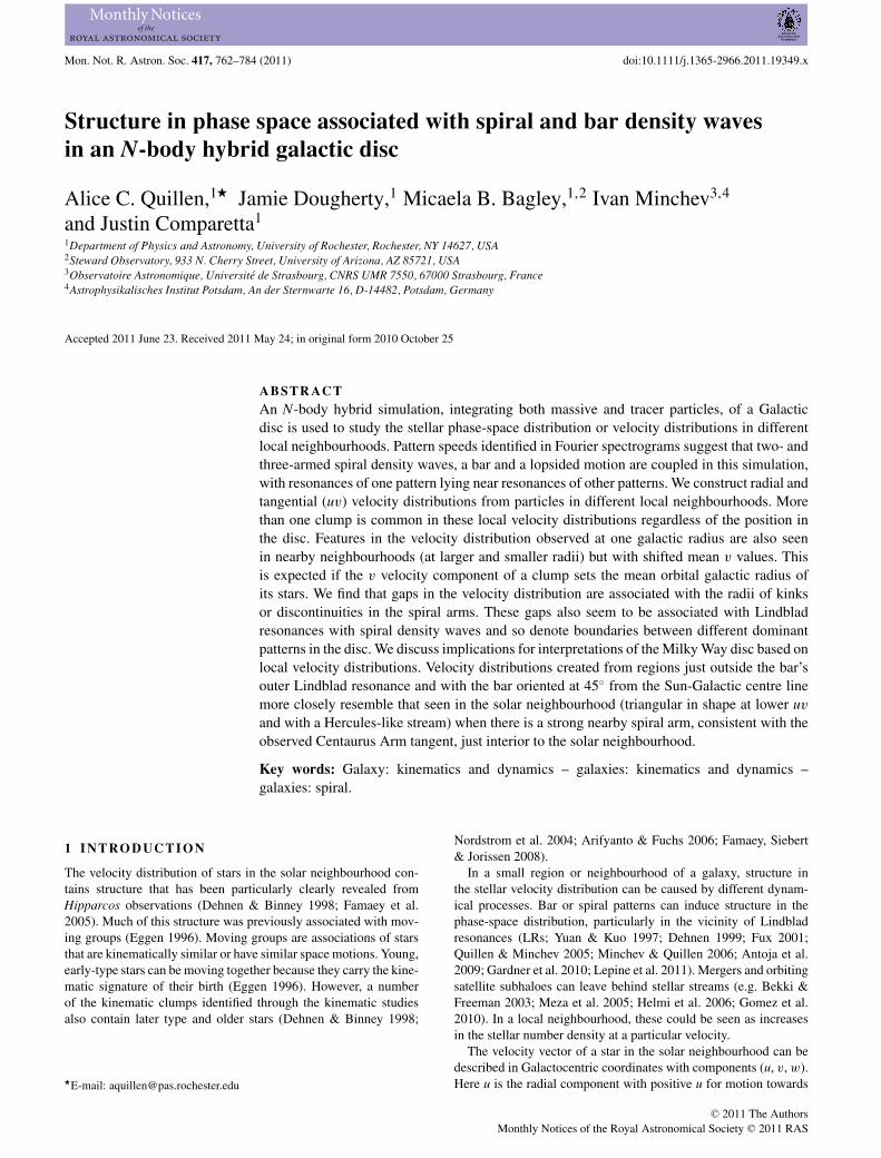
In Fig. 1 we show the disc density projected on to the mid-planein Cartesian coordinates for a few of the simulation outputs (snap-shots). Disc particles are used to create these density histograms,but bulge and halo particles are neglected. In Figs 1(a) and (b)both massive and tracer particles are shown. Fig. 1(c) is similarto Fig. 1(b) except only massive disc particles are shown. We findno significant differences between the distribution of massive andtracer disc particles, consistent with the previous study using thesame hybrid code (Comparetta & Quillen 2011).
The numbers of massive particles are sufficiently low that nu-merical noise is present and amplified to become spiral structure.During the initial 40 snapshots (over a total time of 200 Myr) (shownin Fig. 1a) two- and three-armed spiral armed waves grow inthe region with radius 5–12 kpc. At around a time T ∼ 225 Myran open and somewhat lopsided axisymmetric structure growswithin a radius of 4 kpc that becomes the bar. At later times bothtwo- and three-armed structure exists outside the bar (shown inFig. 1b).
As our halo is live (and not fixed) lopsided motions are notprevented in the simulation. Lopsided motions and three-armedstructure have previously been observed in N-body simulations ofisolated discs (e.g. see the simulations by Chilingarian et al. 2010).The bulge does not remain fixed during the simulation as a lop-sided perturbation develops that moves its centre slowly up to adistance of 0.5 kpc away from the initial origin. This distance islarger than the distance our centre of mass drifts during the simu-lation (less than 10 pc). The lopsided motion may be related to thedevelopment of three-armed structures in the disc and asymmetriesin the bar. Lopsidedness is common in spiral galaxies (see Jog &Combes 2009 for a review), and can spontaneously grow in N-bodysimulations of discs (Revaz & Pfenniger 2004; Saha, Combes &Jog 2007). If the pattern speed is slow, a lopsided mode can be
1 N-Body Simulation Techniques: There is a right way and a wrong way, byKatz N., http://supernova.lbl.gov/∼evlinder/umass/sumold/com8lx.ps2 http://www.ifa.hawaii.edu/∼barnes/ast626_09/NBody.pdf
long lasting (Ideta 2002). There is no single strong frequency oramplitude associated with the lopsided motion in our simulation,though the motion is primarily counter-clockwise and moving withthe direction of galactic rotation. We have checked that the centreof mass of the simulation drifts less than the smoothing length of10 pc so the lopsided motion is not due to an unphysical drift inthe total momentum in the simulation. However, the growth of thelopsided motion could be due to noise associated with our smallsmoothing length and large halo mass particles. Simulations of adisc residing in a rigid halo would not exhibit lopsided motions.However, as most galaxies display lopsidedness we can considerit a realistic characteristic of a galactic disc. We will discuss thismotion later on when we discuss the m = 1 Fourier componentspectrograms.
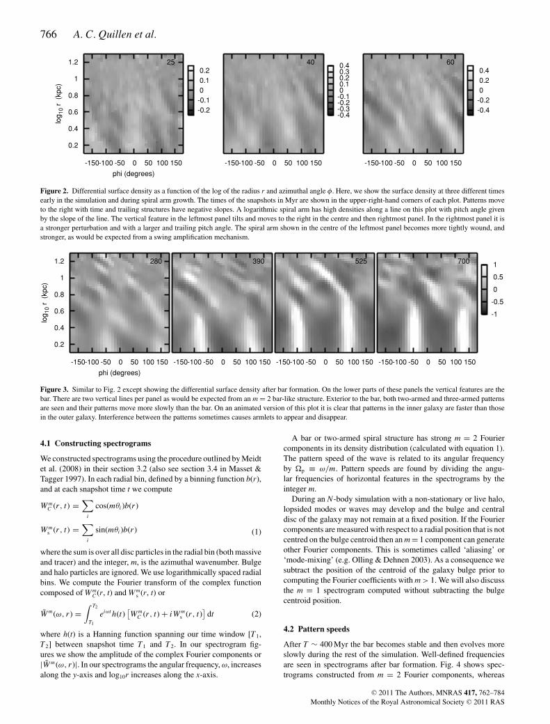
We also show the disc density in polar coordinates in Figs 2 and 3.These figures show differential density histograms as a function ofradius and azimuthal angle (r, φ) (or in cylindrical coordinates againprojected on to the mid-plane). The bins to create these two plots arelogarithmically spaced in radius. The disc density �(r, φ) in thesetwo plots has been normalized at each radius. These histogram show(�(r, φ) − �(r))�(r)−1 where �(r) is the mean density at radiusr averaged over the angle φ. A logarithmic spiral would give highdensities along a straight line in these plots, with slope set by thespiral arm pitch angle. Two-armed structures would correspond totwo linear but sloped features, each separated by 180◦. Trailingspiral structures have negative slopes. A bar on these diagramswould correspond to two vertical features separated by 180◦. Thecentroid of the galaxy bulge is subtracted prior to computing thedensity histograms shown in Figs 2 and 3 in polar coordinates butnot in Fig. 1 that is in Cartesian coordinates. The times of thesnapshots in Myr are shown in the upper-right corners of each panelshown in Figs 1–3.
In Fig. 2 the differential surface density in polar coordinates isshown at three different times early in the simulation and duringthe early phase of spiral arm growth. The nearly vertical strip inthe leftmost panel tilts and moves to the right at later times. In therightmost panel it is a stronger perturbation and with a larger, trailingpitch angle. The spiral arm shown in the centre of the leftmost panelbecomes more tightly wound, and stronger (as seen on the right) aswould be expected from a swing amplification mechanism. Afterabout 50 Myr the spiral patterns are more slowly evolving. Otherthan during bar formation at about 330 Myr, and in the beginningof the simulation before 50 Myr, the spiral pitch angles do not seemto vary significantly.
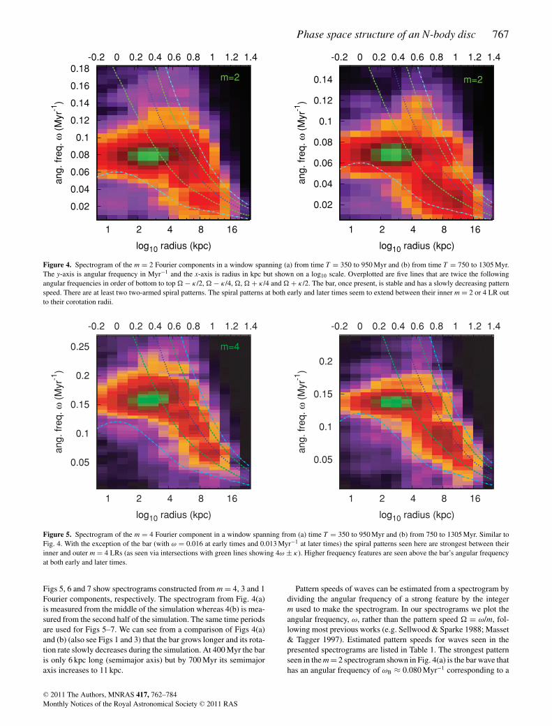
In Fig. 3 the differential surface density is also shown at threedifferent times but after bar formation. On the lower parts of thepanels the bar is seen as a pair of vertical strips. We can see that thebar length increases later in the simulation. Exterior to the bar, bothtwo- and three-armed patterns are seen and their patterns move moreslowly than the bar. The winding or pitch angle of spiral featuresis about 24◦ and α ≡ dφ/dln r ∼ 2.3. This pitch angle exceedsmany but not all estimates for spiral arm pitch angles near thesolar neighbourhood (see table 1 in Vallee 2008; most pitch angleestimates are ∼13◦). Other than during bar formation and before50 Myr, the spiral pitch angles do not seem to vary significantly.
When animated the two- and three-armed features appear to con-structively and destructively add with density peaks occurring attimes and positions when two patterns lie on top of one another(e.g. as discussed by Henry, Quillen & Gutermuth 2003; Meidt,Rand & Merrifield 2009). The sum of two different patterns cancause individual arm peaks to shift position and temporarily appearmore or less tightly wound.
C© 2011 The Authors, MNRAS 417, 762–784Monthly Notices of the Royal Astronomical Society C© 2011 RAS
Phase space structure of an N-body disc 765
Figure 1. Disc stellar densities projected into the xy plane during early spiral arm and bar growth. The time of each snapshot is shown in Myr on the lowerright of each panel. (a) Here we show the earlier part of the simulation. During this time we see initial stochastic spiral arm growth followed by the onset ofbar instability. (b) Here we show snapshots from the later part of the simulation. We can see that the bar is not symmetrical; it can be lopsided. At times thegalaxy appears to have three arms (e.g. at T = 750 Myr). Kinks and discontinuities are commonly seen in the spiral structure. (c) The same as (b) except onlymassive disc particles are shown. There is no significant difference between the distributions of massive and massless disc particles.
Kinks or changes in pitch angle of the spiral arms seen in thedensity images in Cartesian coordinates (in Fig. 1b) correspond toplaces where the spiral arms are discontinuous or change slope inthe density distribution as seen in the polar plots (e.g. Fig. 3). Forexample, the spiral pattern just outside the bar has a lower patternspeed than the bar. Consequently, the phase of the spiral arms varieswith respect to the bar. At times spiral arms appear to be linked withthe bar and at other times they appear separated from the bar. Spiralarms in the outer galaxy have slower pattern speeds than those in
the inner galaxy. At times the spiral arms appear to be connected,and at other times, armlets or kinks are seen.
4 SP I R A L A N D BA R PAT T E R N SI N THE SI MULATI ON
Before we discuss velocity distributions extracted from local neigh-bourhoods we first discuss patterns of waves measured from thesimulations.
C© 2011 The Authors, MNRAS 417, 762–784Monthly Notices of the Royal Astronomical Society C© 2011 RAS
766 A. C. Quillen et al.
Figure 2. Differential surface density as a function of the log of the radius r and azimuthal angle φ. Here, we show the surface density at three different timesearly in the simulation and during spiral arm growth. The times of the snapshots in Myr are shown in the upper-right-hand corners of each plot. Patterns moveto the right with time and trailing structures have negative slopes. A logarithmic spiral arm has high densities along a line on this plot with pitch angle givenby the slope of the line. The vertical feature in the leftmost panel tilts and moves to the right in the centre and then rightmost panel. In the rightmost panel it isa stronger perturbation and with a larger and trailing pitch angle. The spiral arm shown in the centre of the leftmost panel becomes more tightly wound, andstronger, as would be expected from a swing amplification mechanism.
Figure 3. Similar to Fig. 2 except showing the differential surface density after bar formation. On the lower parts of these panels the vertical features are thebar. There are two vertical lines per panel as would be expected from an m = 2 bar-like structure. Exterior to the bar, both two-armed and three-armed patternsare seen and their patterns move more slowly than the bar. On an animated version of this plot it is clear that patterns in the inner galaxy are faster than thosein the outer galaxy. Interference between the patterns sometimes causes armlets to appear and disappear.
4.1 Constructing spectrograms
We constructed spectrograms using the procedure outlined by Meidtet al. (2008) in their section 3.2 (also see section 3.4 in Masset &Tagger 1997). In each radial bin, defined by a binning function b(r),and at each snapshot time t we compute
WmC (r, t) =
∑i
cos(mθi)b(r)
Wms (r, t) =
∑i
sin(mθi)b(r) (1)
where the sum is over all disc particles in the radial bin (both massiveand tracer) and the integer, m, is the azimuthal wavenumber. Bulgeand halo particles are ignored. We use logarithmically spaced radialbins. We compute the Fourier transform of the complex functioncomposed of Wm
C(r, t) and Wms (r, t) or
Wm(ω, r) =∫ T2
T1
eiωth(t)[Wm
C (r, t) + iWms (r, t)
]dt (2)
where h(t) is a Hanning function spanning our time window [T1,T2] between snapshot time T1 and T2. In our spectrogram fig-ures we show the amplitude of the complex Fourier components or|Wm(ω, r)|. In our spectrograms the angular frequency, ω, increasesalong the y-axis and log10r increases along the x-axis.
A bar or two-armed spiral structure has strong m = 2 Fouriercomponents in its density distribution (calculated with equation 1).The pattern speed of the wave is related to its angular frequencyby p ≡ ω/m. Pattern speeds are found by dividing the angu-lar frequencies of horizontal features in the spectrograms by theinteger m.
During an N-body simulation with a non-stationary or live halo,lopsided modes or waves may develop and the bulge and centraldisc of the galaxy may not remain at a fixed position. If the Fouriercomponents are measured with respect to a radial position that is notcentred on the bulge centroid then an m = 1 component can generateother Fourier components. This is sometimes called ‘aliasing’ or‘mode-mixing’ (e.g. Olling & Dehnen 2003). As a consequence wesubtract the position of the centroid of the galaxy bulge prior tocomputing the Fourier coefficients with m > 1. We will also discussthe m = 1 spectrogram computed without subtracting the bulgecentroid position.
4.2 Pattern speeds
After T ∼ 400 Myr the bar becomes stable and then evolves moreslowly during the rest of the simulation. Well-defined frequenciesare seen in spectrograms after bar formation. Fig. 4 shows spec-trograms constructed from m = 2 Fourier components, whereas
C© 2011 The Authors, MNRAS 417, 762–784Monthly Notices of the Royal Astronomical Society C© 2011 RAS
Phase space structure of an N-body disc 767
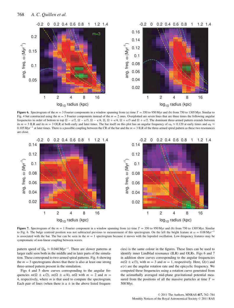
Figure 4. Spectrogram of the m = 2 Fourier components in a window spanning (a) from time T = 350 to 950 Myr and (b) from time T = 750 to 1305 Myr.The y-axis is angular frequency in Myr−1 and the x-axis is radius in kpc but shown on a log10 scale. Overplotted are five lines that are twice the followingangular frequencies in order of bottom to top − κ/2, − κ/4, , + κ/4 and + κ/2. The bar, once present, is stable and has a slowly decreasing patternspeed. There are at least two two-armed spiral patterns. The spiral patterns at both early and later times seem to extend between their inner m = 2 or 4 LR outto their corotation radii.
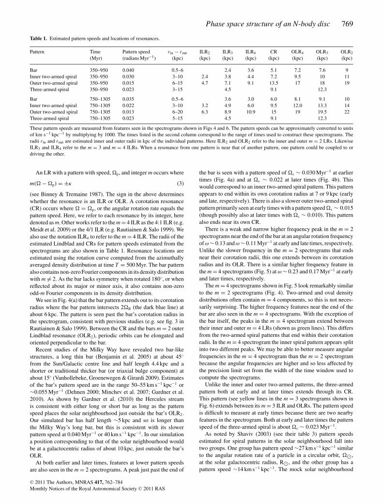
Figure 5. Spectrogram of the m = 4 Fourier component in a window spanning from (a) time T = 350 to 950 Myr and (b) from 750 to 1305 Myr. Similar toFig. 4. With the exception of the bar (with ω = 0.016 at early times and 0.013 Myr−1 at later times) the spiral patterns seen here are strongest between theirinner and outer m = 4 LRs (as seen via intersections with green lines showing 4ω ± κ). Higher frequency features are seen above the bar’s angular frequencyat both early and later times.
Figs 5, 6 and 7 show spectrograms constructed from m = 4, 3 and 1Fourier components, respectively. The spectrogram from Fig. 4(a)is measured from the middle of the simulation whereas 4(b) is mea-sured from the second half of the simulation. The same time periodsare used for Figs 5–7. We can see from a comparison of Figs 4(a)and (b) (also see Figs 1 and 3) that the bar grows longer and its rota-tion rate slowly decreases during the simulation. At 400 Myr the baris only 6 kpc long (semimajor axis) but by 700 Myr its semimajoraxis increases to 11 kpc.
Pattern speeds of waves can be estimated from a spectrogram bydividing the angular frequency of a strong feature by the integerm used to make the spectrogram. In our spectrograms we plot theangular frequency, ω, rather than the pattern speed = ω/m, fol-lowing most previous works (e.g. Sellwood & Sparke 1988; Masset& Tagger 1997). Estimated pattern speeds for waves seen in thepresented spectrograms are listed in Table 1. The strongest patternseen in the m = 2 spectrogram shown in Fig. 4(a) is the bar wave thathas an angular frequency of ωB ≈ 0.080 Myr−1 corresponding to a
C© 2011 The Authors, MNRAS 417, 762–784Monthly Notices of the Royal Astronomical Society C© 2011 RAS
768 A. C. Quillen et al.
Figure 6. Spectrogram of the m = 3 Fourier components in a window spanning from (a) time T = 350 to 950 Myr and (b) from 750 to 1305 Myr. Similar toFig. 4 but constructed using the m = 3 Fourier components instead of the m = 2 ones. Overplotted are seven lines that are three times the following angularfrequencies in order of bottom to top − κ/2, − κ/3, − κ/4, , + κ/4, + κ/3 and + κ/2. The dominant three-armed pattern extends betweenits m = 3 ILR and its m = 3 OLR at both early and later times. The bar itself on this plot has an angular frequency of ωb ≈ 0.120 at early times and ωb ≈0.105 Myr−1 at later times. There is a possible coupling between the CR of the bar and the m = 3 ILR of the three-armed spiral pattern as these two resonancesare close.
Figure 7. Spectrogram of the m = 1 Fourier component in a window spanning from (a) time T = 350 to 950 Myr and (b) from 750 to 1305 Myr. Similarto Fig. 6. The bulge centroid position was not subtracted previous to measurement of this spectrogram. On the left the bright feature at ω = 0.08 Myr−1
is associated with the bar. The bar can be seen in the m = 1 spectrogram because it moves with the lopsided oscillation. Low-frequency features may besymptomatic of non-linear coupling between waves.
pattern speed of B ≈ 0.040 Myr−1. There are slower patterns atlarger radii seen both in the middle and in later parts of the simula-tion. These correspond to two-armed spiral patterns. Fig. 6 showingthe m = 3 spectrograms shows that there is also at least one strongthree-armed pattern present in the simulation.
Figs 4 and 5 show curves corresponding to the angular fre-quencies m( ± κ/2), m( ± κ/4), m with m = 2 and m =4, respectively, where m is that used to compute the spectrogram.Each pair of lines (when there is a ± in the above listed frequen-
cies) is the same colour in the figures. These lines can be used toidentify inner Lindblad resonance (ILR) and OLRs. Figs 6 and 7in addition show curves corresponding to the angular frequenciesm( ± κ/3), with m = 3 and m = 1, respectively. Here, (r) andκ(r) are the angular rotation rate and the epicyclic frequency. Wecomputed these frequencies using a rotation curve generated fromthe azimuthally averaged mid-plane gravitational potential mea-sured from the positions of all the massive particles at time T =500 Myr.
C© 2011 The Authors, MNRAS 417, 762–784Monthly Notices of the Royal Astronomical Society C© 2011 RAS
Phase space structure of an N-body disc 769
Table 1. Estimated pattern speeds and locations of resonances.
Pattern Time Pattern speed rin − rout ILR2 ILR3 ILR4 CR OLR4 OLR3 OLR2
(Myr) (radians Myr−1) (kpc) (kpc) (kpc) (kpc) (kpc) (kpc) (kpc) (kpc)
Bar 350–950 0.040 0.5–6 2.4 3.6 5.1 7.2 7.6 9Inner two-armed spiral 350–950 0.030 3–10 2.4 3.8 4.4 7.2 9.5 10 11Outer two-armed spiral 350–950 0.015 6–15 4.7 7.1 9.1 13.5 17 18 19Three-armed spiral 350–950 0.023 3–15 4.5 9.1 12.3
Bar 750–1305 0.035 0.5–6 3.6 3.0 6.0 8.1 9.1 10Inner two-armed spiral 750–1305 0.022 3–10 3.2 4.9 6.0 9.5 12.0 13.3 14Outer two-armed spiral 750–1305 0.013 6–20 6.3 8.9 10.9 15 19 19.5 22Three-armed spiral 750–1305 0.023 5–15 4.5 9.1 12.3
These pattern speeds are measured from features seen in the spectrograms shown in Figs 4 and 6. The pattern speeds can be approximately converted to unitsof km s−1 kpc−1 by multiplying by 1000. The times listed in the second column correspond to the range of times used to construct these spectrograms. Theradii rin and rout are estimated inner and outer radii in kpc of the individual patterns. Here ILR2 and OLR2 refer to the inner and outer m = 2 LRs. LikewiseILR3 and ILR4 refer to the m = 3 and m = 4 ILRs. When a resonance from one pattern is near that of another pattern, one pattern could be coupled to ordriving the other.
An LR with a pattern with speed, p, and integer m occurs where
m( − p) = ±κ (3)
(see Binney & Tremaine 1987). The sign in the above determineswhether the resonance is an ILR or OLR. A corotation resonance(CR) occurs where = p, or the angular rotation rate equals thepattern speed. Here, we refer to each resonance by its integer, heredenoted as m. Other works refer to the m = 4 ILR as the 4:1 ILR (e.g.Meidt et al. 2009) or the 4/1 ILR (e.g. Rautiainen & Salo 1999). Wealso use the notation ILR4 to refer to the m = 4 ILR. The radii of theestimated Lindblad and CRs for pattern speeds estimated from thespectrograms are also shown in Table 1. Resonance locations areestimated using the rotation curve computed from the azimuthallyaveraged density distribution at time T = 500 Myr. The bar patternalso contains non-zero Fourier components in its density distributionwith m = 2. As the bar lacks symmetry when rotated 180◦, or whenreflected about its major or minor axis, it also contains non-zeroodd-m Fourier components in its density distribution.
We see in Fig. 4(a) that the bar pattern extends out to its corotationradius where the bar pattern intersects 2B (the dark blue line) atabout 6 kpc. The pattern is seen past the bar’s corotation radius inthe spectrogram, consistent with previous studies (e.g. see fig. 3 inRautiainen & Salo 1999). Between the CR and the bars m = 2 outerLindblad resonance (OLR2), periodic orbits can be elongated andoriented perpendicular to the bar.
Recent studies of the Milky Way have revealed two bar-likestructures, a long thin bar (Benjamin et al. 2005) at about 45◦
from the Sun/Galactic centre line and half length 4.4 kpc and ashorter or traditional thicker bar (or triaxial bulge component) atabout 15◦ (Vanhollebeke, Groenewegen & Girardi 2009). Estimatesof the bar’s pattern speed are in the range 50–55 km s−1 kpc−1 or∼0.055 Myr−1 (Dehnen 2000; Minchev et al. 2007; Gardner et al.2010). As shown by Gardner et al. (2010) the Hercules streamis consistent with either long or short bar as long as the patternspeed places the solar neighbourhood just outside the bar’s OLR2.Our simulated bar has half length ∼5 kpc and so is longer thanthe Milky Way’s long bar, but this is consistent with its slowerpattern speed at 0.040 Myr−1 or 40 km s−1 kpc−1. In our simulationa position corresponding to that of the solar neighbourhood wouldbe at a galactocentric radius of about 10 kpc, just outside the bar’sOLR.
At both earlier and later times, features at lower pattern speedsare also seen in the m = 2 spectrograms. A peak just past the end of
the bar is seen with a pattern speed of s ∼ 0.030 Myr−1 at earliertimes (Fig. 4a) and at s ∼ 0.022 at later times (Fig. 4b). Thiswould correspond to an inner two-armed spiral pattern. This patternappears to end within its own corotation radius at 7 or 9 kpc (earlyand late, respectively). There is also a slower outer two-armed spiralpattern primarily seen at early times with a pattern speed s ∼ 0.015(though possibly also at later times with s ∼ 0.010). This patternalso ends near its own CR.
There is a weak and narrow higher frequency peak in the m = 2spectrograms near the end of the bar at an angular rotation frequencyof ω ∼ 0.13 and ω ∼ 0.11 Myr−1 at early and late times, respectively.Unlike the slower frequency in the m = 2 spectrograms that endsnear their corotation radii, this one extends between its corotationradius and its OLR. There is a similar higher frequency feature inthe m = 4 spectrograms (Fig. 5) at ω ∼ 0.23 and 0.17 Myr−1 at earlyand later times, respectively.
The m = 4 spectrograms shown in Fig. 5 look remarkably similarto the m = 2 spectrograms (Fig. 4). Two-armed and oval densitydistributions often contain m = 4 components, so this is not neces-sarily surprising. The higher frequency features near the end of thebar are also seen in the m = 4 spectrograms. With the exception ofthe bar itself, the peaks in the m = 4 spectrogram extend betweentheir inner and outer m = 4 LRs (shown as green lines). This differsfrom the two-armed spiral patterns that end within their corotationradii. In the m = 4 spectrogram the inner spiral pattern appears splitinto two different peaks. We may be able to better measure angularfrequencies in the m = 4 spectrogram than the m = 2 spectrogrambecause the angular frequencies are higher and so less affected bythe precision limit set from the width of the time window used tocompute the spectrograms.
Unlike the inner and outer two-armed patterns, the three-armedpattern both at early and at later times extends through its CR.This pattern (see yellow lines in the m = 3 spectrograms shown inFig. 6) extends between its m = 3 ILR and OLRs. The pattern speedis difficult to measure at early times because there are two nearbyfeatures in the spectrogram. Both at early and later times the patternspeed of the three-armed spiral is about s ∼ 0.023 Myr−1.
As noted by Shaviv (2003) (see their table 3) pattern speedsestimated for spiral patterns in the solar neighbourhood fall intotwo groups. One group has pattern speed ∼27 km s−1 kpc−1 similarto the angular rotation rate of a particle in a circular orbit, �,at the solar galactocentric radius, R�, and the other group has apattern speed ∼14 km s−1 kpc−1. The mock solar neighbourhood
C© 2011 The Authors, MNRAS 417, 762–784Monthly Notices of the Royal Astronomical Society C© 2011 RAS
770 A. C. Quillen et al.
position in our simulation lies outside the inner two-armed spi-ral pattern at 0.030 Myr−1, but is affected by the three-armed spi-ral wave with pattern speed 0.023 Myr−1 or ∼23 km s−1 kpc−1 andthe outer two-armed spiral with a pattern speed of 0.015 Myr−1 or∼15 km s−1 kpc−1. If the spiral waves present in the solar neighbour-hood are driven by the Galactic bar then it might be interesting tomatch the faster pattern speed measured in the solar neighbourhoodwith a three-armed pattern driven by the bar and the slower pat-tern speed with a two-armed pattern also possibly linked to the bar.However, with the exception of Naoz & Shaviv (2007), few studieshave considered the interpretation of the solar neighbourhood interms of two or more patterns.
Previous works have seen spiral structure in N-body or par-ticle mesh simulations at pattern speeds that differ from that ofthe bar (e.g. Sellwood & Sparke 1988; Patsis & Kaufmann 1999;Rautiainen & Salo 1999; Voglis, Stavropoulos & Kalapotharakos2006). Masset & Tagger (1997) interpreted this behaviour in termsof non-linear mode coupling (Tagger et al. 1987; Sygnet et al. 1988),whereas Sellwood & Lin (1989) interpret the differences in patternspeeds in terms of transient behaviour and a groove instability. Thespiral patterns in the simulations by Sellwood & Sparke (1988)extend from their m = 2 ILRs to their OLRs (see their fig. 1). How-ever, the patterns of the two spiral density waves seen by Patsis &Kaufmann (1999) in a simulation lacking a bar extend from theirm = 2 inner to their outer m = 4 LRs. Both of these situations differfrom the two-armed structures in our simulations that end withintheir corotation radii. The simulations by Rautiainen & Salo (1999)are closest in behaviour to ours, showing multiple spiral patternsextending past the bar, with some patterns ending near or withintheir corotation radii.
As the spiral and bar patterns in our simulations are moderatelylong lived, the spiral patterns could be driven by the bar (Yuan& Kuo 1997; Masset & Tagger 1997; Rautiainen & Salo 1999).Rautiainen & Salo (1999) accounted for the ranges and speeds ofspiral patterns using the non-linear wave-coupling scenario. Theyfound that they could often associate the beginning of a slowerouter pattern with the location of one of its resonances that is also aresonance with an inner faster bar or other spiral pattern. The overlapbetween the resonances relates one pattern speed to the other andcouples one perturbation to the other. Rautiainen & Salo (1999)found examples of CR/ILR4, CR/ILR2, OLR2/CR and OLR2/ILR2
couplings between spiral and bar waves and between two differentspiral density waves.
For our system there is a possible connection between the bar’sCR and the m = 3 ILR of the three-armed spiral armed wave.A comparison of resonance locations (see Table 1) shows that thebar’s CR lies close to the three-armed spiral’s m = 3 ILR. The radialdistance between these resonances is small compared to the errorfrom measurement in the spectrogram. There is also a possiblecoupling between other resonances. It is difficult to differentiatebetween possibilities by resonance locations alone as driving couldoccur in a spatially broad region near a resonance. As suggested byMasset & Tagger (1997) we can test for mode or wave coupling bysearching for waves at beat frequencies though Rautiainen & Salo(1999) found that expected beat waves are not always detectable.
4.3 Non-linear coupling of waves
The scenario introduced by Tagger et al. (1987) suggests that thereare strong non-linearities in the stellar response when resonancescoincide. Two waves (e.g. bar and spiral) couple to a third one ata beat frequency. For example, we consider azimuthal wavenum-
ber mB associated with a bar perturbation at pattern speed B andso frequency ωB = mBB. We consider azimuthal wavenumberms associated with a spiral pattern at pattern speed s and so an-gular frequency ωs = mss. A third wave can be excited withan azimuthal wavenumber m = mB + ms and angular frequencyω = ωB + ωs or with wavenumber m = mB − ms and ω =ωB − ωs.
An example explored by Tagger et al. (1987) is a bar and spiralmode, both with m = 2, coupled to a slow axisymmetric modewith m = 0 and a faster four-armed one with m = 4 (Masset &Tagger 1997). Like Masset & Tagger (1997) we see features inthe m = 4 spectrograms at frequencies above that of the bar, andthese can be considered predictions of the wave-coupling scenario.Unfortunately, the number of features present in the m = 2 and m =4 spectrograms is high and the imprecision of measured frequenciesmakes it difficult to definitively determine whether there is couplingbetween m = 2, 4 waves and a slow axisymmetric mode.
As our simulation contains a bar (m = 2), a lopsided m = 1motion and a three-armed wave we can consider coupling betweenthese three waves. To create the m = 2, 3 and 4 spectrogram wefirst subtracted the bulge centroid; however the galaxy centre movesduring the simulation. In Fig. 7, showing the m = 1 spectrograms butconstructed in the inertial frame, we see features associated with themajor patterns identified in the other spectrograms. For example wesee a peak at ω = 0.08 Myr−1 that coincides with the bar’s angularfrequency. One interesting peak is at an angular rotation rate of ω ∼0.010 that is also seen in the m = 3 spectrogram at a radius of about8 kpc (log10r = 0.9). At earlier times there is power at ω ∼ 0.03in the m = 1 spectrogram that is broader than the similar featureseen in the m = 2 spectrogram. This suggests that there is sufficientpower at low frequencies in the lopsided wave that it could coupleto other waves.
Since there is power at low frequencies in lopsided motion, wecan consider the possibility of a coupling between a slow lopsidedmode and the bar. Here, the index and pattern speed of the lopsidedwave are mL = 1, L and that of the bar is mB = 2, B. Thesum leads to a three-armed spiral pattern with angular frequencyωs = L +2B or pattern speed s = 1
3 (L + 2B). If we assumethat this corresponds to the three-armed pattern with s ∼ 0.028then we can solve for the angular frequency of the lopsided modeL ∼ 0.01. There may be power at this frequency as there are low-frequency features in the m = 1 spectrogram. Thus, a lopsided slowmode could be coupling the bar and the three-armed spiral waves.
A variety of resonant overlaps or non-linear wave couplings arepossible and may account for the driving of the patterns presentin the simulation. If we could more precisely measure frequenciesof the patterns then we would better determine which associationsare most important or likely. Unfortunately, peaks in the spectro-grams are sensitive to the range (in time) of simulation data usedto construct the spectrogram (e.g. compare Figs 4a to b). Longertime series are required to make more accurate frequency measure-ments. Since the pattern speeds are not fixed, increasing the sizeof the time window does not increase the precision of a frequencymeasurement. This is particularly the case for slow patterns thatmight be important for the non-linear coupling models.
In summary, we find that the spectrograms are rich in small fea-tures. The shape of the spectrograms seen at early times resemblesthat at later times implying that the frequencies of these smallerfeatures are slowing along with the bar pattern. Even though thereare many waves present, they are not stochastically appearing anddisappearing but slowly evolving. LRs associated with one waveare likely to be coincident with resonances of another wave present
C© 2011 The Authors, MNRAS 417, 762–784Monthly Notices of the Royal Astronomical Society C© 2011 RAS
Phase space structure of an N-body disc 771
in the simulation. Together these findings suggest that the wavespresent in the simulation are coupled due to non-linear interactions.The most convincing and strongest coupling is that between thebar, the lopsided wave and the three-armed spiral wave. The mul-titude of small features present in the spectrograms suggest thatadditional couplings are present. The presence of features in thespectrograms at frequencies above that of the bar is consistent withthe wave-coupling scenario.
5 ST RU C T U R E I N T H E UV PLANE
We first describe how we construct velocity distributions in localneighbourhoods. We then discuss possible relations between fea-tures seen in these velocity distribution and the spiral or bar patterns.
5.1 Velocity uv distribution histograms in localneighbourhoods
We construct velocity distribution histograms in different localneighbourhoods in the following manner. Consider a neighbour-hood centred about a point in the disc plane with coordinates (x0,y0, 0) or in cylindrical coordinates (r0, φ0, 0). We will refer to neigh-bourhoods by the cylindrical coordinates of their centres; (r0, φ0).We consider a star or simulated particle in the neighbourhood of thiscentre point if its coordinates (x, y, z) have distance in the plane,R = √
(x − x0)2 + (y − y0)2 < r0f where f is a dimensionlessscaling factor setting the size of the neighbourhood. We computethe radial and tangential components of the velocity of each starwith respect to the vector to the galactic centre defined by the cen-tral coordinates of the neighbourhood, (x0, y0, 0). The u componentis −1 times the radial velocity component in this galactic coordi-nate system. The v component is the tangential component in thiscoordinate system minus the circular velocity estimated from theazimuthally averaged mid-plane rotation curve computed at timeT = 500 Myr.
Histograms showing the uv velocity distribution are computedfrom the disc particles in each neighbourhood. The computed his-tograms are effectively coarse-grained phase-space distributions.The larger the neighbourhood, the larger is number of stars in theneighbourhood. If there are too few stars in the neighbourhoodthen the velocity distribution is noisy. If the neighbourhood is largethen structure present on small spatial scales may be masked orsmoothed by the coarse graining. An extreme example would be ifthe neighbourhood were so large that it contained two spiral armdensity peaks.
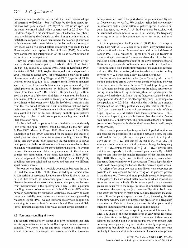
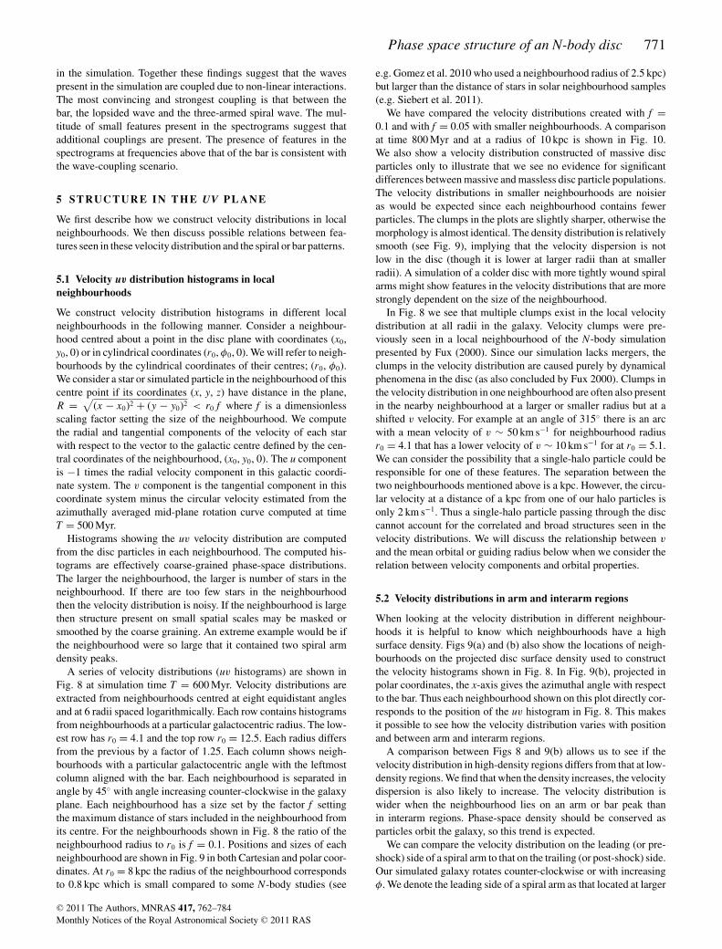
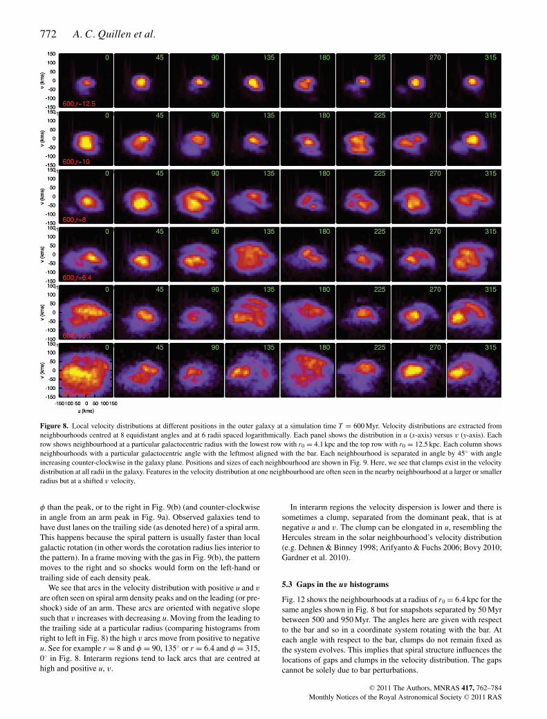
A series of velocity distributions (uv histograms) are shown inFig. 8 at simulation time T = 600 Myr. Velocity distributions areextracted from neighbourhoods centred at eight equidistant anglesand at 6 radii spaced logarithmically. Each row contains histogramsfrom neighbourhoods at a particular galactocentric radius. The low-est row has r0 = 4.1 and the top row r0 = 12.5. Each radius differsfrom the previous by a factor of 1.25. Each column shows neigh-bourhoods with a particular galactocentric angle with the leftmostcolumn aligned with the bar. Each neighbourhood is separated inangle by 45◦ with angle increasing counter-clockwise in the galaxyplane. Each neighbourhood has a size set by the factor f settingthe maximum distance of stars included in the neighbourhood fromits centre. For the neighbourhoods shown in Fig. 8 the ratio of theneighbourhood radius to r0 is f = 0.1. Positions and sizes of eachneighbourhood are shown in Fig. 9 in both Cartesian and polar coor-dinates. At r0 = 8 kpc the radius of the neighbourhood correspondsto 0.8 kpc which is small compared to some N-body studies (see
e.g. Gomez et al. 2010 who used a neighbourhood radius of 2.5 kpc)but larger than the distance of stars in solar neighbourhood samples(e.g. Siebert et al. 2011).
We have compared the velocity distributions created with f =0.1 and with f = 0.05 with smaller neighbourhoods. A comparisonat time 800 Myr and at a radius of 10 kpc is shown in Fig. 10.We also show a velocity distribution constructed of massive discparticles only to illustrate that we see no evidence for significantdifferences between massive and massless disc particle populations.The velocity distributions in smaller neighbourhoods are noisieras would be expected since each neighbourhood contains fewerparticles. The clumps in the plots are slightly sharper, otherwise themorphology is almost identical. The density distribution is relativelysmooth (see Fig. 9), implying that the velocity dispersion is notlow in the disc (though it is lower at larger radii than at smallerradii). A simulation of a colder disc with more tightly wound spiralarms might show features in the velocity distributions that are morestrongly dependent on the size of the neighbourhood.
In Fig. 8 we see that multiple clumps exist in the local velocitydistribution at all radii in the galaxy. Velocity clumps were pre-viously seen in a local neighbourhood of the N-body simulationpresented by Fux (2000). Since our simulation lacks mergers, theclumps in the velocity distribution are caused purely by dynamicalphenomena in the disc (as also concluded by Fux 2000). Clumps inthe velocity distribution in one neighbourhood are often also presentin the nearby neighbourhood at a larger or smaller radius but at ashifted v velocity. For example at an angle of 315◦ there is an arcwith a mean velocity of v ∼ 50 km s−1 for neighbourhood radiusr0 = 4.1 that has a lower velocity of v ∼ 10 km s−1 for at r0 = 5.1.We can consider the possibility that a single-halo particle could beresponsible for one of these features. The separation between thetwo neighbourhoods mentioned above is a kpc. However, the circu-lar velocity at a distance of a kpc from one of our halo particles isonly 2 km s−1. Thus a single-halo particle passing through the disccannot account for the correlated and broad structures seen in thevelocity distributions. We will discuss the relationship between v
and the mean orbital or guiding radius below when we consider therelation between velocity components and orbital properties.
5.2 Velocity distributions in arm and interarm regions
When looking at the velocity distribution in different neighbour-hoods it is helpful to know which neighbourhoods have a highsurface density. Figs 9(a) and (b) also show the locations of neigh-bourhoods on the projected disc surface density used to constructthe velocity histograms shown in Fig. 8. In Fig. 9(b), projected inpolar coordinates, the x-axis gives the azimuthal angle with respectto the bar. Thus each neighbourhood shown on this plot directly cor-responds to the position of the uv histogram in Fig. 8. This makesit possible to see how the velocity distribution varies with positionand between arm and interarm regions.
A comparison between Figs 8 and 9(b) allows us to see if thevelocity distribution in high-density regions differs from that at low-density regions. We find that when the density increases, the velocitydispersion is also likely to increase. The velocity distribution iswider when the neighbourhood lies on an arm or bar peak thanin interarm regions. Phase-space density should be conserved asparticles orbit the galaxy, so this trend is expected.
We can compare the velocity distribution on the leading (or pre-shock) side of a spiral arm to that on the trailing (or post-shock) side.Our simulated galaxy rotates counter-clockwise or with increasingφ. We denote the leading side of a spiral arm as that located at larger
C© 2011 The Authors, MNRAS 417, 762–784Monthly Notices of the Royal Astronomical Society C© 2011 RAS
772 A. C. Quillen et al.
Figure 8. Local velocity distributions at different positions in the outer galaxy at a simulation time T = 600 Myr. Velocity distributions are extracted fromneighbourhoods centred at 8 equidistant angles and at 6 radii spaced logarithmically. Each panel shows the distribution in u (x-axis) versus v (y-axis). Eachrow shows neighbourhood at a particular galactocentric radius with the lowest row with r0 = 4.1 kpc and the top row with r0 = 12.5 kpc. Each column showsneighbourhoods with a particular galactocentric angle with the leftmost aligned with the bar. Each neighbourhood is separated in angle by 45◦ with angleincreasing counter-clockwise in the galaxy plane. Positions and sizes of each neighbourhood are shown in Fig. 9. Here, we see that clumps exist in the velocitydistribution at all radii in the galaxy. Features in the velocity distribution at one neighbourhood are often seen in the nearby neighbourhood at a larger or smallerradius but at a shifted v velocity.
φ than the peak, or to the right in Fig. 9(b) (and counter-clockwisein angle from an arm peak in Fig. 9a). Observed galaxies tend tohave dust lanes on the trailing side (as denoted here) of a spiral arm.This happens because the spiral pattern is usually faster than localgalactic rotation (in other words the corotation radius lies interior tothe pattern). In a frame moving with the gas in Fig. 9(b), the patternmoves to the right and so shocks would form on the left-hand ortrailing side of each density peak.
We see that arcs in the velocity distribution with positive u and v
are often seen on spiral arm density peaks and on the leading (or pre-shock) side of an arm. These arcs are oriented with negative slopesuch that v increases with decreasing u. Moving from the leading tothe trailing side at a particular radius (comparing histograms fromright to left in Fig. 8) the high v arcs move from positive to negativeu. See for example r = 8 and φ = 90, 135◦ or r = 6.4 and φ = 315,0◦ in Fig. 8. Interarm regions tend to lack arcs that are centred athigh and positive u, v.
In interarm regions the velocity dispersion is lower and there issometimes a clump, separated from the dominant peak, that is atnegative u and v. The clump can be elongated in u, resembling theHercules stream in the solar neighbourhood’s velocity distribution(e.g. Dehnen & Binney 1998; Arifyanto & Fuchs 2006; Bovy 2010;Gardner et al. 2010).
5.3 Gaps in the uv histograms
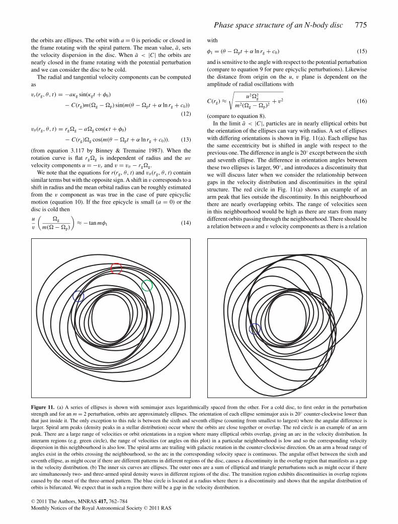
Fig. 12 shows the neighbourhoods at a radius of r0 = 6.4 kpc for thesame angles shown in Fig. 8 but for snapshots separated by 50 Myrbetween 500 and 950 Myr. The angles here are given with respectto the bar and so in a coordinate system rotating with the bar. Ateach angle with respect to the bar, clumps do not remain fixed asthe system evolves. This implies that spiral structure influences thelocations of gaps and clumps in the velocity distribution. The gapscannot be solely due to bar perturbations.
C© 2011 The Authors, MNRAS 417, 762–784Monthly Notices of the Royal Astronomical Society C© 2011 RAS
Phase space structure of an N-body disc 773
Figure 9. The positions of the neighbourhoods used to construct velocity distribution histograms shown in Fig. 8. (a) The neighbourhoods are shown in aCartesian coordinate system. The green circles show the angle of the neighbourhoods oriented along the bar and referred to as angle zero (with respect to thebar) and are shown in the leftmost column of Fig. 8. In Fig. 8 the angles of each column, from left to right, correspond to positions with angle increasing by 45◦in the anti-clockwise direction on this plot. Radii of changes in spiral arm pitch angle or discontinuities in spiral structure estimated from the polar plots areshown as dotted black circles. (b) The approximate locations of the neighbourhoods shown on a projection of angle versus logarithmic radius (the differentialdensity distribution is constructed as in Fig. 3). The positions of the neighbourhoods on this plot are in the same order as the velocity distribution panels shownin Fig. 8. Black dotted horizontal lines are shown at radii where there are changes in spiral arm pitch angle or there are discontinuities in the spiral arms. Manyof these lines correspond to resonances with patterns seen in the spectrogram.
Figure 10. A comparison between velocity distributions extracted at a radius of r0 = 10 kpc using neighbourhoods with radius with 500 pc (f = 0.05; toppanels) and 1000 pc (f = 0.1; middle row of panels). The simulation time was arbitrarily chosen and is 800 Myr. The bottom row is similar to the middle panelbut shows only massive disc particles whereas the distributions in the top two rows are constructed from both massive and tracer particles. The neighbourhoodshave the same angles as in Fig. 8 and are arranged in the same way. When the neighbourhoods are larger the velocity distributions are smoother and less grainyas would be expected because more particles are found in each neighbourhood.
A stream similar to the Hercules stream at v ∼ −50 km s−1 ispresent in the velocity distribution at early times at angle 0 (alignedwith the bar) at r0 = 6.4 kpc. Like the Hercules stream (e.g. Dehnen1999) this arc or clump has a wide u distribution, has a narrow v
distribution and is centred at a negative u value. However, the bar’sm = 2 OLR (at about 9 kpc) lies outside these neighbourhoods,so this clump cannot be associated with this resonance, Similarfeature low u, v clumps in the velocity distribution are also seen
at other radii such as r0 = 8 and 10 kpc but appearing at differenttimes in the simulation and at different angles with respect to thebar, consequently the bar and resonances associated with it cannotprovide the only explanation for these features.
The spiral density waves have slower patterns than the bar, hencedensity peaks associated with them move to the left (or to a smallerφ) as a function of time or moving downward in Fig. 12. At oneposition as a wave peak passes through the neighbourhood first a
C© 2011 The Authors, MNRAS 417, 762–784Monthly Notices of the Royal Astronomical Society C© 2011 RAS
774 A. C. Quillen et al.
velocity distribution typical of a leading side of an arm is seen. Ata later time in the same location a velocity distribution typical of atrailing side is seen. The velocity distribution contains a positive uand v feature when on the leading side of a spiral feature. The featureis centred at progressively lower u values as the arm passes by andthe neighbourhood moves to the trailing side. See for example therightmost column and at an angle of 315◦ between times 500 to700 Myr (top five rows).
While clumps come and go in time, we find that the gaps be-tween the clumps tend to remain at the same v values. For exampleconsider the rightmost column of Fig. 12. Two gaps are seen withdifferent degrees of prominence at differ times. We recall from Fig. 8that gaps at one neighbourhood radius were often seen at anotherneighbourhood radius but shifted in v. To compare a gap seen ina neighbourhood at one radius to that seen in a neighbourhood atanother radius we can consider motions of particle orbits.
6 INTERPRETING STRUCTUREIN THE UV PLANE
To relate structure in local velocity distributions it is helpful to recallmodels for orbits. We first consider epicyclic motion in the absenceof perturbations, then review the orbital dynamics to the first orderin the perturbation strength in the presence of perturbations. Inboth case we consider the relation between uv velocities in a localneighbourhood and quantities describing the orbit such as a meanor guiding radius and an epicyclic amplitude.
In the absence of perturbations from spiral arms, the motion ofstars in the disc of a galaxy can be described in terms of radialor epicyclic oscillations about a circular orbit (Kalnajs 1979). It isuseful to specify the relation between the observed velocity compo-nents u, v and the parameters describing the epicyclic motion (e.g.Fux 2000, 2001; Quillen & Minchev 2005) or the mean radius orguiding radius, rg, and the epicyclic amplitude. The energy of an or-bit in the plane of an axisymmetric system (neglecting perturbationsfrom spiral structure) with a flat rotation curve is
E(u, v) = (vc + v)2
2+ u2
2+ v2
c ln r + constant, (4)
where the potential energy, ln r, is that appropriate for a flat rotationcurve, r is the Galactocentric radius and vc is the circular velocity.
With an epicyclic approximation we can write the energy
E = v2c
[1
2+ ln rg
]+ Eepi (5)
where the term on the left is the energy of a star in a circular orbitabout a guiding radius rg and Eepi is the energy from the epicyclicmotion,
Eepi = u2
2+ κ2(r − rg)2
2= κ2a2
2. (6)
Here a is the epicyclic amplitude and κ is the epicyclic frequencyat the guiding radius rg.
We now consider stars specifically in a neighbourhood of galac-tocentric radius r0, restricting us to a specific location in the galaxy.Setting the energy equal to that written in terms of the epicyclicmotion using equations (5, 6), we solve for the guiding radius, rg.It is convenient to define the distance between the guiding or meanradius and the neighbourhood’s galactocentric radius, s = rg − r0.To the first order in v and s we find that a star in the neighbourhoodwith velocity components u, v has a guiding radius withs
r0≈ v
vc(7)
and epicyclic amplitude a
a
r0≈ v−1
c
√u2
2+ v2. (8)
The factor of a half is from κ2/2 equivalent to 2 when the rotationcurve is flat. An angle describing the phase in the epicycle is
φ ∼ atan
( −u√2v
)(9)
(consistent with equations 2–4, Quillen 2003, for a flat rotationcurve). The epicyclic phase angle φ = 0 at apocentre.
The above three relations allow us to relate the velocity compo-nents u, v for stars in the solar neighbourhood, and to quantitiesused to describe the epicyclic motion: the guiding radius, epicyclicamplitude and phase angle. Particles with positive v have s > 0 andso guiding radii that are larger than the radius of the neighbourhood,r0. Particles with negative v have s < 0 and so are expected to spendmost of their orbits inside r0. The distance from the origin, u = v =0, determines the epicyclic amplitude.
It may also be useful to writev
vc= rg
r0− 1, (10)
where we have used our definition for s in equation (7). This equa-tion shows that to the first order v sets the guiding radius of aparticle. This is useful because the guiding radius sets the approx-imate angular rotation rate and rotation period of the orbit. Theguiding radius also sets the approximate epicyclic frequency (orperiod) of the particle’s orbit. Resonances occur where sums of in-teger multiples of these periods are equal to an integer multiple ofa pattern speed. Thus the v value of clumps or gaps in the velocitydistribution may also allow us to locate resonances.
6.1 Spiral perturbations to first order in the uv plane
The above approximation neglects the effect of bar or spiral per-turbations. Spiral waves give a time-dependent perturbation tothe gravitational potential that can be approximated by a sin-gle Fourier component depending on a single frequency. Fora logarithmic spiral perturbation with m arms we can considerV (r, θ, t) = Vm cos(m(θ − pt + α ln r)) where the pitch angleα = −dθ /dr. To the first order in the perturbation strength Vm
the orbit of a star in the galactic mid-plane with mean or guidingradius rg
r(rg, θ, t) = rg + a cos(κgt + φ0)
+ C(rg) cos(m(θ − pt + α ln rg + c0)) (11)
(Binney & Tremaine 1987; equation 3– 119a) where a is an epicyclicamplitude, and c0, φ0 are phase angles. The forced epicyclicamplitude in the WKB approximation |C(rg)| ≈ | αVm
rg�g| where
�g = κ2g − m2(g − p)2 represents the distance to an LR and
is evaluated at the guiding or mean radius, rg and κg and g are theepicyclic frequency and angular rotation rate at rg. The denominator�g becomes small near the LR and the first-order approximationbreaks down. A higher order approximation can be used to showthat closed orbits exist on both sides of resonance and that epicyclicamplitudes do not become infinite on resonance (e.g. Contopoulos1975).
The orbital motion (equation 11) consists of an epicyclic motionwith amplitude a and a phase φ0 and a forced motion aligned withthe potential perturbation and moving with it. A population of starswould have a distribution in both a and φ0. When a = 0 and m = 2
C© 2011 The Authors, MNRAS 417, 762–784Monthly Notices of the Royal Astronomical Society C© 2011 RAS
Phase space structure of an N-body disc 775
the orbits are ellipses. The orbit with a = 0 is periodic or closed inthe frame rotating with the spiral pattern. The mean value, a, setsthe velocity dispersion in the disc. When a < |C| the orbits arenearly closed in the frame rotating with the potential perturbationand we can consider the disc to be cold.
The radial and tangential velocity components can be computedas
vr (rg, θ, t) = −aκg sin(κgt + φ0)
− C(rg)m(g − p) sin(m(θ − pt + α ln rg + c0))
(12)
vθ (rg, θ, t) = rgg − ag cos(κt + φ0)
− C(rg)g cos(m(θ − pt + α ln rg + c0)). (13)
(from equation 3.117 by Binney & Tremaine 1987). When therotation curve is flat rgg is independent of radius and the uv
velocity components u = −vr and v = vθ − rgg.We note that the equations for r(rg, θ , t) and vθ (rg, θ , t) contain
similar terms but with the opposite sign. A shift in v corresponds to ashift in radius and the mean orbital radius can be roughly estimatedfrom the v component as was true in the case of pure epicyclicmotion (equation 10). If the free epicycle is small (a = 0) or thedisc is cold then
u
v
(g
m( − p)
)≈ − tan mφ1 (14)
with
φ1 = (θ − pt + α ln rg + c0) (15)
and is sensitive to the angle with respect to the potential perturbation(compare to equation 9 for pure epicyclic perturbations). Likewisethe distance from origin on the u, v plane is dependent on theamplitude of radial oscillations with
C(rg) ≈√
u22g
m2(g − p)2+ v2 (16)
(compare to equation 8).In the limit a < |C|, particles are in nearly elliptical orbits but
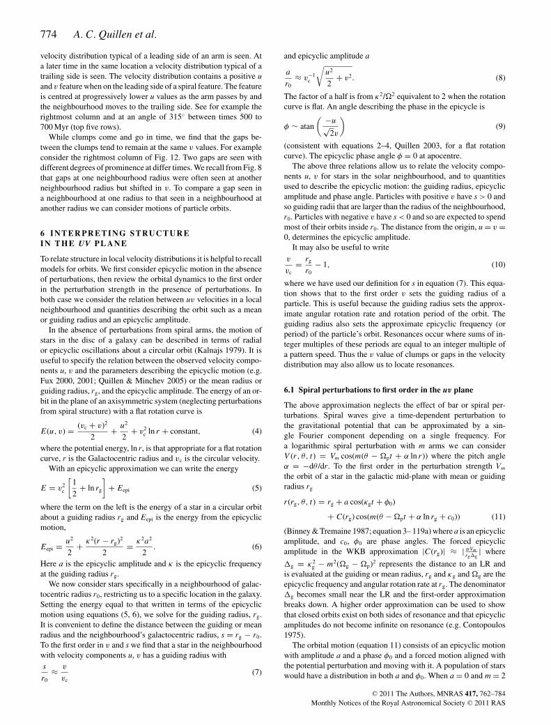
the orientation of the ellipses can vary with radius. A set of ellipseswith differing orientations is shown in Fig. 11(a). Each ellipse hasthe same eccentricity but is shifted in angle with respect to theprevious one. The difference in angle is 20◦ except between the sixthand seventh ellipse. The difference in orientation angles betweenthese two ellipses is larger, 90◦, and introduces a discontinuity thatwe will discuss later when we consider the relationship betweengaps in the velocity distribution and discontinuities in the spiralstructure. The red circle in Fig. 11(a) shows an example of anarm peak that lies outside the discontinuity. In this neighbourhoodthere are nearly overlapping orbits. The range of velocities seenin this neighbourhood would be high as there are stars from manydifferent orbits passing through the neighbourhood. There should bea relation between u and v velocity components as there is a relation
Figure 11. (a) A series of ellipses is shown with semimajor axes logarithmically spaced from the other. For a cold disc, to first order in the perturbationstrength and for an m = 2 perturbation, orbits are approximately ellipses. The orientation of each ellipse semimajor axis is 20◦ counter-clockwise lower thanthat just inside it. The only exception to this rule is between the sixth and seventh ellipse (counting from smallest to largest) where the angular difference islarger. Spiral arm peaks (density peaks in a stellar distribution) occur where the orbits are close together or overlap. The red circle is an example of an armpeak. There are a large range of velocities or orbit orientations in a region where many elliptical orbits overlap, giving an arc in the velocity distribution. Ininterarm regions (e.g. green circle), the range of velocities (or angles on this plot) in a particular neighbourhood is low and so the corresponding velocitydispersion in this neighbourhood is also low. The spiral arms are trailing with galactic rotation in the counter-clockwise direction. On an arm a broad range ofangles exist in the orbits crossing the neighbourhood, so the arc in the corresponding velocity space is continuous. The angular offset between the sixth andseventh ellipse, as might occur if there are different patterns in different regions of the disc, causes a discontinuity in the overlap region that manifests as a gapin the velocity distribution. (b) The inner six curves are ellipses. The outer ones are a sum of elliptical and triangle perturbations such as might occur if thereare simultaneously two- and three-armed spiral density waves in different regions of the disc. The transition region exhibits discontinuities in overlap regionscaused by the onset of the three-armed pattern. The blue circle is located at a radius where there is a discontinuity and shows that the angular distribution oforbits is bifurcated. We expect that in such a region there will be a gap in the velocity distribution.
C© 2011 The Authors, MNRAS 417, 762–784Monthly Notices of the Royal Astronomical Society C© 2011 RAS
776 A. C. Quillen et al.
between mean galactic radius of the ellipse and orbital angle in theneighbourhood. Thus the velocity distribution would exhibit an arc.
The green circle in Fig. 11(a) shows an interarm region wherethe angles of orbits only vary slightly compared to that in the redneighbourhood. In the green interarm neighbourhood we expect anarrow velocity distribution. This illustrates why we see, or expectto see, arcs in the velocity distributions on spiral arm peaks andlower velocity dispersions in interarm regions.
An arc in a local velocity distribution that has u decreasing asv increases can be interpreted in terms of orbital properties as afunction of rg (approximately set by v). The positive v orbits havelarger guiding radii. The change in angle or v/u slope on the velocitydistribution plots implies that the epicyclic angle φ1 (equation 15)decreases with increasing rg. Thus these arcs correspond to a relationbetween epicyclic angle and guiding radius. Consider our cartoon(Fig. 11a) showing concentric ellipses with different orientationangles. A neighbourhood on top of a spiral arm peak (such as the redone) intersects orbits with a range of epicyclic angles, correspondingon this figure to a smooth change in orientation of the ellipse. Thuswe expect that an arc would be observed in a velocity distributionat the position of a spiral arm peak. The angle of the arc in thevelocity distribution is likely to be affected by the winding angleof the spiral structure with a more open spiral corresponding toan arc with steeper slope. However, a neighbourhood may containorbits with a smaller range of guiding radii if the spiral structure isless tightly wound. Model orbital distributions would be needed touse the slopes and ranges of velocities of clumps seen in velocitydistributions, and their gradients, to place constraints on the spiralstructure (pattern speed, pitch angle and strength) from observationsof the velocity distribution alone.
We now consider the type of arc that would be seen on a trailingspiral arm. The red neighbourhood in Fig. 11(a) intersects orbitsnear apocentre with small guiding radii (and so negative v) andorbits that are near pericentre that have larger guiding radii (and sopositive v). In between and in the neighbourhood are orbits that aremoving towards the Galactic centre and so have positive u values.For trailing spiral structure we expect the arc to progress from lowv to high v passing through the top-right quadrant of the uv plane,as we seen in arm peaks in Figs 8, 12 and 13. Thus, our illustrationFig. 11(a) provides an explanation consistent with spiral structurefor the arcs seen in the velocity distribution.
We can use our first-order perturbation model (equations 11–13) to consider particles with nearby guiding radii. We expandequation (11) for closed orbits (a = 0)
r(rg + x, θ, t) ≈ rg + x
+ C(rg) cos(m(θ − pt + α ln rg + c0))
− C(rg) sin(m(θ − pt + α ln rg + c0))mαx
rg
(17)
where we have used the WKB approximation by neglectingdC(rg)/dr. The derivative of the above equation
dr
drg≈ 1 − C(rg) sin(m(θ − pt + α ln rg + c0))
mα
rg. (18)
Consider two closed orbits separated by a small difference inguiding radius. The radial distance between these closed orbits at aparticle angular location is the smallest when the above derivativeis minimum. A small difference in current radius is possible whenthe sine term is negative. This happens midway between pericen-tre and apocentre. Thus the closed orbits are nearest to each otherwhen this sine term is negative (mφ1 = π /2). The radial velocity is
also proportional to the sine of the angle. For α > 0, correspondingto trailing arms, we find that the orbits are closest together whenthe radial velocity component is negative and the particles are ap-proaching pericentre (positive u, zero v), as shown by the red circlein Fig. 11(a). Orbits are maximally distant when the radial velocityis positive or 90◦ away from the red circle in Fig. 11(a) that showsa two-armed structure. At locations and corresponding velocitieswhere the above derivative is high, the phase-space density wouldbe higher and so there would be features seen in a local velocity dis-tribution. Inclusion of the derivative dC(rg)/dr when estimating thederivative dr/drg would shift the estimated angle of the minimumof the derivative. This shift may explain why arcs in the velocitydistribution are primarily located in the upper-right-hand quadrant(positive u, v) and not centred at u > 0, v = 0.
The above discussion has neglected the dispersion of orbits aboutthe closed or periodic ones shown in our cartoons (Fig. 11); howeverif the dispersion is neglected then the predicted velocity distributioncontains particles at only a few velocities. The stellar dispersion hasbeen used in constructing weights for orbits to populate the velocityhistograms and predict velocity distributions from test particle inte-grations (e.g. Dehnen 2000; Quillen & Minchev 2005). We shouldremember that Fig. 11 only qualitatively gives us a relation be-tween orbital and velocity distribution, however the properties ofclosed orbits are relevant for interpretation of these distributions(e.g. Quillen & Minchev 2005).
The above equations are given in the WKB approximation fora spiral perturbation. For a bar or two-armed open spiral perturba-tion to the first order the orbits are also ellipses, however the WKBapproximation cannot be used. For a bar perturbation an additionalterm in vθ should be taken into account when estimating the guidingradius and the angle m(θ −pt) from u, v (see Binney & Tremaine1987, section 3.3). For a spiral perturbation if the WKB approxima-tion is not used additional terms in both velocity components wouldbe used to estimate the guiding radius, the orbit orientation and theangle with respect to it from u, v (e.g. Contopoulos 1975).
7 G APS AT D I FFERENT RADI I
We now look at the location of gaps in the velocity distributionfor the snapshot shown in Figs 8 and 9 at T = 600 Myr. In Fig. 8at a radius of r0 = 5.1 kpc and an angle of φ0 = 135◦ there aretwo gaps seen in the velocity distribution, one centred at v ∼ 50and the other at v ∼ 0 km s−1. The one at v ∼ 0 has a guidingradius of rg ∼ 5.1 kpc, the same as the neighbourhood radius. Equa-tion (10) can be used to predict the value of this gap observed froma neighbourhood radius of r0 = 4.1 kpc instead of at 5.1 kpc. Weestimate that it should lie at v ∼ 50 km s−1. There is an arc witha gap at about v ∼ 50 km s−1 in the velocity distribution at r0 =4.1 kpc and at φ0 = 135◦, as expected. The other gap in the neigh-bourhood with r0 = 5.1, φ0 = 135◦ at v ∼ 50 km s−1 has a guidingradius rg ∼ 6.3 kpc (again using equation 10). A clump with thisguiding radius would lie at v ∼ 0 km s−1 in a neighbourhood withr0 = 6.4 kpc. We do not see a gap with this v value at r0 = 6.4 kpcand φ0 = 135◦ but we do see one in the neighbouring position atr0 = 6.4 kpc, φ0 = 90◦. Thus we find that the relation between v
and guiding radius is consistent with shifts in individual features inv as a function of neighbourhood radius.
We also find gaps at nearly zero v values in neighbourhoods withr0 ∼ 8 and 10 kpc. In the inner galaxy there is a gap at r0 = 4.1 kpc,φ0 = 45, 90◦ with slightly negative v that is also present at v ∼−50 km s−1 in the neighbourhood with r0 = 5.1 kpc, φ0 = 45◦ and
C© 2011 The Authors, MNRAS 417, 762–784Monthly Notices of the Royal Astronomical Society C© 2011 RAS
Phase space structure of an N-body disc 777
Figure 12. We show uv velocity distribution histograms generated with neighbourhood radii of r0 = 6.4 kpc but at different times. From top to bottom row thehistograms were generated from snapshots at output times 500 to 950 Myr. Each snapshot is separated in time by 50 Myr. As in Fig. 8 the angles are given withrespect to the bar and the same sequence of angles is shown. Gaps in the velocity distribution tend to remain at the same v values. Even though the positionsshown are fixed in the bar’s rotating frame there are variations in the features seen in the velocity distribution that must be due to the spiral waves in the outerdisc.
C© 2011 The Authors, MNRAS 417, 762–784Monthly Notices of the Royal Astronomical Society C© 2011 RAS
778 A. C. Quillen et al.
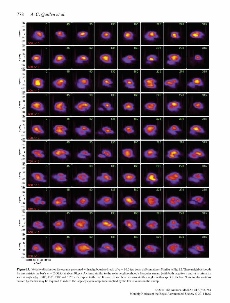
Figure 13. Velocity distribution histograms generated with neighbourhood radii of r0 = 10.0 kpc but at different times. Similar to Fig. 12. These neighbourhoodslie just outside the bar’s m = 2 OLR (at about 9 kpc). A clump similar to the solar neighbourhood’s Hercules stream (with both negative u and v) is primarilyseen at angles φ0 = 90◦, 135◦, 270◦ and 315◦ with respect to the bar. It is rare to see these streams at other angles with respect to the bar. Non-circular motionscaused by the bar may be required to induce the large epicyclic amplitude implied by the low v values in the clump.
C© 2011 The Authors, MNRAS 417, 762–784Monthly Notices of the Royal Astronomical Society C© 2011 RAS
Phase space structure of an N-body disc 779
has rg ∼ 3.9 kpc. Altogether we see gaps at the following guidingradii rg ∼ 3.9, 5.1, 6.3, 8 and 10 kpc at this time in the simulation.
Looking back at Fig. 8 we compare the location of gaps in thevelocity distribution (identified by their guiding radii) and the loca-tions of kinks (changes in winding angle) or discontinuities in thespiral arms. In Fig. 9(b) we have identified radii where there arediscontinuities in the spiral structure, and changes in either wind-ing angle (kinks) or places where spiral arms or armlets appear ordisappear. These radii are shown as black circles in Fig. 9(a) andas horizontal lines in Fig. 9(b). The radii of the discontinuities onthese plots are at rd ∼ 3.5, 5.1, 6.3, 8.7 and 11 kpc. A comparisonbetween the list of discontinuities and our list of gaps identified inthe velocity distributions (identified by their guiding radii) suggeststhat these two lists are related.
A gap in the velocity distribution occurs in a neighbourhood whenthere are two groups of stars each with velocity vectors in similar butdifferent directions, but few stars with velocity vectors in betweenthose of the two groups. In Fig. 11(a) we show concentric ellipsesthat increase in radius and shift in orientation angle. The differencein orientation angle between each ellipse is small and constantexcept between the sixth and seventh ellipse where the differenceis much large and 90◦. There is a discontinuity in the position ofthe spiral arm peak at the radius of the introduced large changein orientation angle that we can see from the shape of the orbitaloverlap regions. The discontinuity introduces regions such as theneighbourhood illustrated with the blue circle. This neighbourhoodcontains orbits with two separate groups of orbit angles. In thisneighbourhood we would expect a corresponding gap in the velocitydistribution. Fig. 11(a) shows that we expect gaps in the velocitydistribution where there are discontinuities in the spiral structure,and suggests that gaps in the velocity distribution only occur at radiiwhere there are discontinuities in spiral structure and at specificangles where there are spiral arm peaks. We do not see gaps inevery velocity distribution in Fig. 8 but do tend to see them wherethe surface density is high. This is expected as density peaks canoccur when multiple pattern peaks coincide.
In the previous section we introduced a first-order perturbativeorbital model containing a single potential perturbation (equations11–13). This model can be extended for multiple patterns givingorbits with radius, radial and tangential velocity as a function ofguiding or mean radius to the first order in the perturbation strengths
r(rg, θ, t) = rg + a cos(κgt + φ0)
+ C1(rg) cos(m1(θ − 1t + α1 ln rg + c1)
+ C2(rg) cos(m2(θ − 2t + α2 ln rg + c2). (19)
When a is smaller compared to |C1| and |C2| the orbits are nearlyclosed as shown in Figs 11(a) and (b).
For a particular neighbourhood with r, θ the above equationsmust be inverted to solve for rg, a and φ0 as a function of thevelocity components. The inversion need not give a unique valueof rg so particles from separated radial regions (in guiding radiusrg) can simultaneously be present in one local neighbourhood. Thesimilarity of terms in r, u, vθ implies that there is a close relationbetween the inverted rg distribution and the velocity components.This situation is illustrated in Figs 11(a) and (b) where transitionsbetween one pattern and another gives neighbourhoods containingorbits from different regions of the galaxy and a bifurcated velocitydistribution in that neighbourhood. Fig. 11(a) shows a transition be-tween an inner and an outer two-armed pattern. Fig. 11(b) illustratesa transition between a two-armed and a three-armed pattern. In thisfigure the inner six curves are ellipses; however the outer ones are
a sum of elliptical and triangle perturbations such as might occur ifthere are simultaneously two-armed and three-armed spiral densitywaves. The elliptical and triangular perturbations vary smoothly inorientation angle from curve to curve. The transition region exhibitsdiscontinuities in overlap regions caused by the onset of the three-armed pattern. The blue circle is located at a radius where there isa discontinuity and shows that the angular distribution of orbits isbifurcated. We expect that in such a region there will be a gap in thevelocity distribution.
A neighbourhood with r, θ is most likely to contain two separatesolutions for rg if the phases of the arguments for each perturba-tion have opposite signs. For example if the angle m1(θ − 1t +α1ln rg + c1) ∼ 0 and C1 > 0 then r > rg and the particles in aneighbourhood at r will have guiding radii interior to r. The orbitswill have u ∼ 0 but v greater than the circular velocity at r (consis-tent with the discussion in Section 5.5). If the angle m2(θ − 2t +α2ln rg + c2) ∼ π then the opposite is true. A neighbourhood at rcan simultaneously contain stars on orbits associated with an inte-rior perturbation near apocentre and stars associated with an outerperturbation near pericentre.
Our spectrograms showed that there are both two-armed andthree-armed patterns present in this simulation. The two-armedand three-armed patterns have different radial extents and differ-ent pattern speeds. Fig. 11(b) shows that the transition between atwo-armed and three-armed pattern can cause a discontinuity in thespiral arm peaks. This type of discontinuity can also give neigh-bourhoods with two sets of orbital orientation angles and so gaps ina velocity distribution, as illustrated by the blue neighbourhood inthis figure.
We now compare the list of radial discontinuities and gaps withestimated resonance locations identified from the pattern speeds inthe simulations. If we only had one strong wave then we wouldbe restricted to a few resonances. However our simulation showsmultiple patterns, each with a different radial range. Keeping this inmind, perhaps it is not surprising that the density distribution showsmultiple spiral arm discontinuities and the velocity distributionsshow multiple gaps.
If the spiral patterns are excited at resonances then we expectthat they will start or/and end near resonances. In Section 4, wediscussed likely ranges for these patterns with likely resonances asboundaries. The innermost discontinuity, seen both as gaps in thevelocity distribution and in the spiral morphology, lies at a radiusof about rg ∼ 4 kpc. This lies near the bar’s m = 4 ILR and isnot distant from the m = 2 ILR of the inner two-armed spiral. Thediscontinuity at a guiding radius, rg ∼ 5 kpc lies near the bar’s CR,the m = 3 ILR of the three-armed spiral and is not distant from them = 4 ILR of the inner two-armed spiral and the m = 2 ILR of theouter two-armed spiral. The discontinuity at a radius rg ∼ 11 is nearthe m = 3 OLR of the three-armed spiral and the m = 2 OLR ofthe inner two-armed spiral. That at rg∼8 kpc is near the bar’s m =2 OLR and the m = 2 ILR of the outer two-armed spiral. It alsomay be the outer boundary of the inner two-armed spiral and nearits m = 4 OLR. The division at rd ∼ 6.3 is not obviously associatedwith a resonance but could be due to a division between the innerand outer two-armed spirals.
The first-order approximation used here has a small divisor prob-lem nearing resonance. To understand the dynamics near resonancea higher order model is required (Contopoulos 1975). Approachingresonance the epicyclic amplitude increases but does not go to infin-ity and closed orbits exist on both sides of resonance. Consequently,a closed orbit approximation (such as illustrated in Fig. 11) may notbe invalid even quite close to resonance. As epicyclic amplitudes
C© 2011 The Authors, MNRAS 417, 762–784Monthly Notices of the Royal Astronomical Society C© 2011 RAS
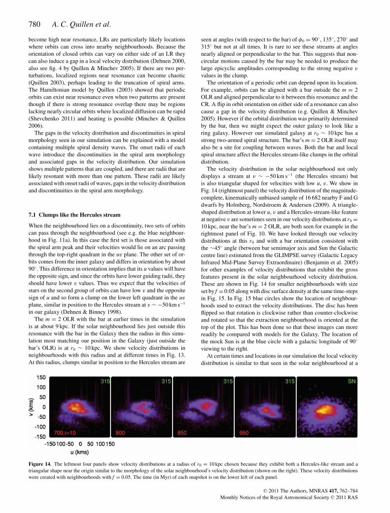
780 A. C. Quillen et al.
become high near resonance, LRs are particularly likely locationswhere orbits can cross into nearby neighbourhoods. Because theorientation of closed orbits can vary on either side of an LR theycan also induce a gap in a local velocity distribution (Dehnen 2000,also see fig. 4 by Quillen & Minchev 2005). If there are two per-turbations, localized regions near resonance can become chaotic(Quillen 2003), perhaps leading to the truncation of spiral arms.The Hamiltonian model by Quillen (2003) showed that periodicorbits can exist near resonance even when two patterns are presentthough if there is strong resonance overlap there may be regionslacking nearly circular orbits where localized diffusion can be rapid(Shevchenko 2011) and heating is possible (Minchev & Quillen2006).
The gaps in the velocity distribution and discontinuities in spiralmorphology seen in our simulation can be explained with a modelcontaining multiple spiral density waves. The onset radii of eachwave introduce the discontinuities in the spiral arm morphologyand associated gaps in the velocity distribution. Our simulationshows multiple patterns that are coupled, and there are radii that arelikely resonant with more than one pattern. These radii are likelyassociated with onset radii of waves, gaps in the velocity distributionand discontinuities in the spiral arm morphology.
7.1 Clumps like the Hercules stream
When the neighbourhood lies on a discontinuity, two sets of orbitscan pass through the neighbourhood (see e.g. the blue neighbour-hood in Fig. 11a). In this case the first set is those associated withthe spiral arm peak and their velocities would lie on an arc passingthrough the top-right quadrant in the uv plane. The other set of or-bits comes from the inner galaxy and differs in orientation by about90◦. This difference in orientation implies that its u values will havethe opposite sign, and since the orbits have lower guiding radii, theyshould have lower v values. Thus we expect that the velocities ofstars on the second group of orbits can have low v and the oppositesign of u and so form a clump on the lower left quadrant in the uv
plane, similar in position to the Hercules stream at v ∼ −50 km s−1
in our galaxy (Dehnen & Binney 1998).The m = 2 OLR with the bar at earlier times in the simulation
is at about 9 kpc. If the solar neighbourhood lies just outside thisresonance with the bar in the Galaxy then the radius in this simu-lation most matching our position in the Galaxy (just outside thebar’s OLR) is at r0 ∼ 10 kpc. We show velocity distributions inneighbourhoods with this radius and at different times in Fig. 13.At this radius, clumps similar in position to the Hercules stream are
seen at angles (with respect to the bar) of φ0 = 90◦, 135◦, 270◦ and315◦ but not at all times. It is rare to see these streams at anglesnearly aligned or perpendicular to the bar. This suggests that non-circular motions caused by the bar may be needed to produce thelarge epicyclic amplitudes corresponding to the strong negative v
values in the clump.The orientation of a periodic orbit can depend upon its location.
For example, orbits can be aligned with a bar outside the m = 2OLR and aligned perpendicular to it between this resonance and theCR. A flip in orbit orientation on either side of a resonance can alsocause a gap in the velocity distribution (e.g. Quillen & Minchev2005). However if the orbital distribution was primarily determinedby the bar, then we might expect the outer galaxy to look like aring galaxy. However our simulated galaxy at r0 ∼ 10 kpc has astrong two-armed spiral structure. The bar’s m = 2 OLR itself mayalso be a site for coupling between waves. Both the bar and localspiral structure affect the Hercules stream-like clumps in the orbitaldistribution.
The velocity distribution in the solar neighbourhood not onlydisplays a stream at v ∼ −50 km s−1 (the Hercules stream) butis also triangular shaped for velocities with low u, v. We show inFig. 14 (rightmost panel) the velocity distribution of the magnitude-complete, kinematically unbiased sample of 16 682 nearby F and Gdwarfs by Holmberg, Nordstroem & Andersen (2009). A triangle-shaped distribution at lower u, v and a Hercules-stream-like featureat negative v are sometimes seen in our velocity distributions at r0 =10 kpc, near the bar’s m = 2 OLR, are both seen for example in therightmost panel of Fig. 10. We have looked through our velocitydistributions at this r0 and with a bar orientation consistent withthe ∼45◦ angle (between bar semimajor axis and Sun the Galacticcentre line) estimated from the GLIMPSE survey (Galactic LegacyInfrared Mid-Plane Survey Extraordinaire) (Benjamin et al. 2005)for other examples of velocity distributions that exhibit the grossfeatures present in the solar neighbourhood velocity distribution.These are shown in Fig. 14 for smaller neighbourhoods with sizeset by f = 0.05 along with disc surface density at the same time-stepsin Fig. 15. In Fig. 15 blue circles show the location of neighbour-hoods used to extract the velocity distributions. The disc has beenflipped so that rotation is clockwise rather than counter-clockwiseand rotated so that the extraction neighbourhood is oriented at thetop of the plot. This has been done so that these images can morereadily be compared with models for the Galaxy. The location ofthe mock Sun is at the blue circle with a galactic longitude of 90◦
viewing to the right.At certain times and locations in our simulation the local velocity
distribution is similar to that seen in the solar neighbourhood at a
Figure 14. The leftmost four panels show velocity distributions at a radius of r0 = 10 kpc chosen because they exhibit both a Hercules-like stream and atriangular shape near the origin similar to the morphology of the solar neighbourhood’s velocity distribution (shown on the right). These velocity distributionswere created with neighbourhoods with f = 0.05. The time (in Myr) of each snapshot is on the lower left of each panel.
C© 2011 The Authors, MNRAS 417, 762–784Monthly Notices of the Royal Astronomical Society C© 2011 RAS
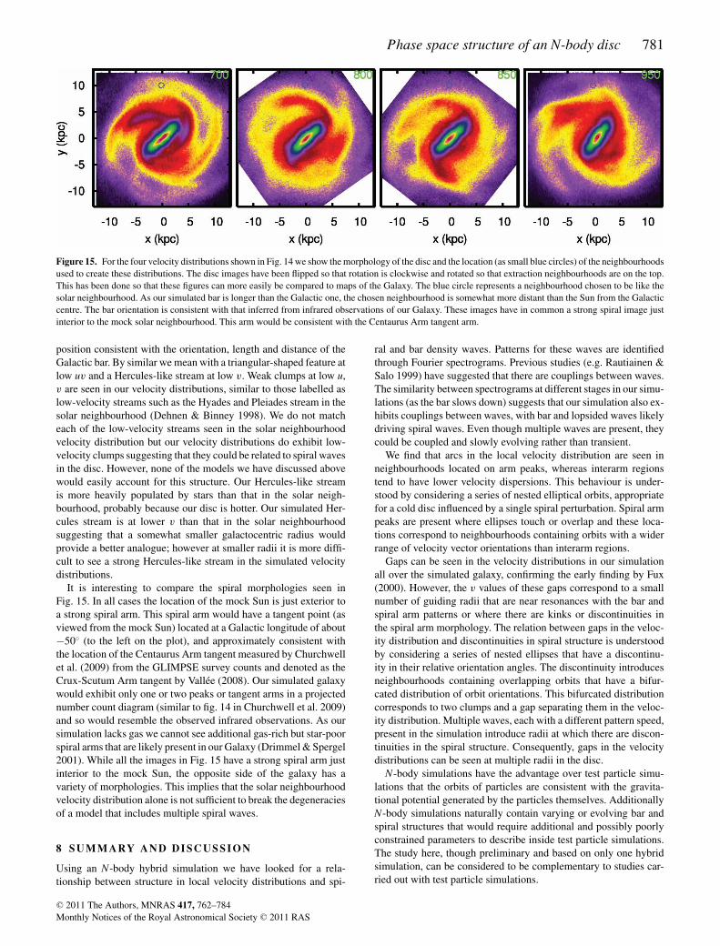
Phase space structure of an N-body disc 781
Figure 15. For the four velocity distributions shown in Fig. 14 we show the morphology of the disc and the location (as small blue circles) of the neighbourhoodsused to create these distributions. The disc images have been flipped so that rotation is clockwise and rotated so that extraction neighbourhoods are on the top.This has been done so that these figures can more easily be compared to maps of the Galaxy. The blue circle represents a neighbourhood chosen to be like thesolar neighbourhood. As our simulated bar is longer than the Galactic one, the chosen neighbourhood is somewhat more distant than the Sun from the Galacticcentre. The bar orientation is consistent with that inferred from infrared observations of our Galaxy. These images have in common a strong spiral image justinterior to the mock solar neighbourhood. This arm would be consistent with the Centaurus Arm tangent arm.
position consistent with the orientation, length and distance of theGalactic bar. By similar we mean with a triangular-shaped feature atlow uv and a Hercules-like stream at low v. Weak clumps at low u,v are seen in our velocity distributions, similar to those labelled aslow-velocity streams such as the Hyades and Pleiades stream in thesolar neighbourhood (Dehnen & Binney 1998). We do not matcheach of the low-velocity streams seen in the solar neighbourhoodvelocity distribution but our velocity distributions do exhibit low-velocity clumps suggesting that they could be related to spiral wavesin the disc. However, none of the models we have discussed abovewould easily account for this structure. Our Hercules-like streamis more heavily populated by stars than that in the solar neigh-bourhood, probably because our disc is hotter. Our simulated Her-cules stream is at lower v than that in the solar neighbourhoodsuggesting that a somewhat smaller galactocentric radius wouldprovide a better analogue; however at smaller radii it is more diffi-cult to see a strong Hercules-like stream in the simulated velocitydistributions.
It is interesting to compare the spiral morphologies seen inFig. 15. In all cases the location of the mock Sun is just exterior toa strong spiral arm. This spiral arm would have a tangent point (asviewed from the mock Sun) located at a Galactic longitude of about−50◦ (to the left on the plot), and approximately consistent withthe location of the Centaurus Arm tangent measured by Churchwellet al. (2009) from the GLIMPSE survey counts and denoted as theCrux-Scutum Arm tangent by Vallee (2008). Our simulated galaxywould exhibit only one or two peaks or tangent arms in a projectednumber count diagram (similar to fig. 14 in Churchwell et al. 2009)and so would resemble the observed infrared observations. As oursimulation lacks gas we cannot see additional gas-rich but star-poorspiral arms that are likely present in our Galaxy (Drimmel & Spergel2001). While all the images in Fig. 15 have a strong spiral arm justinterior to the mock Sun, the opposite side of the galaxy has avariety of morphologies. This implies that the solar neighbourhoodvelocity distribution alone is not sufficient to break the degeneraciesof a model that includes multiple spiral waves.
8 SUMMARY AND DISCUSSION
Using an N-body hybrid simulation we have looked for a rela-tionship between structure in local velocity distributions and spi-
ral and bar density waves. Patterns for these waves are identifiedthrough Fourier spectrograms. Previous studies (e.g. Rautiainen &Salo 1999) have suggested that there are couplings between waves.The similarity between spectrograms at different stages in our simu-lations (as the bar slows down) suggests that our simulation also ex-hibits couplings between waves, with bar and lopsided waves likelydriving spiral waves. Even though multiple waves are present, theycould be coupled and slowly evolving rather than transient.
We find that arcs in the local velocity distribution are seen inneighbourhoods located on arm peaks, whereas interarm regionstend to have lower velocity dispersions. This behaviour is under-stood by considering a series of nested elliptical orbits, appropriatefor a cold disc influenced by a single spiral perturbation. Spiral armpeaks are present where ellipses touch or overlap and these loca-tions correspond to neighbourhoods containing orbits with a widerrange of velocity vector orientations than interarm regions.
Gaps can be seen in the velocity distributions in our simulationall over the simulated galaxy, confirming the early finding by Fux(2000). However, the v values of these gaps correspond to a smallnumber of guiding radii that are near resonances with the bar andspiral arm patterns or where there are kinks or discontinuities inthe spiral arm morphology. The relation between gaps in the veloc-ity distribution and discontinuities in spiral structure is understoodby considering a series of nested ellipses that have a discontinu-ity in their relative orientation angles. The discontinuity introducesneighbourhoods containing overlapping orbits that have a bifur-cated distribution of orbit orientations. This bifurcated distributioncorresponds to two clumps and a gap separating them in the veloc-ity distribution. Multiple waves, each with a different pattern speed,present in the simulation introduce radii at which there are discon-tinuities in the spiral structure. Consequently, gaps in the velocitydistributions can be seen at multiple radii in the disc.
N-body simulations have the advantage over test particle simu-lations that the orbits of particles are consistent with the gravita-tional potential generated by the particles themselves. AdditionallyN-body simulations naturally contain varying or evolving bar andspiral structures that would require additional and possibly poorlyconstrained parameters to describe inside test particle simulations.The study here, though preliminary and based on only one hybridsimulation, can be considered to be complementary to studies car-ried out with test particle simulations.
C© 2011 The Authors, MNRAS 417, 762–784Monthly Notices of the Royal Astronomical Society C© 2011 RAS
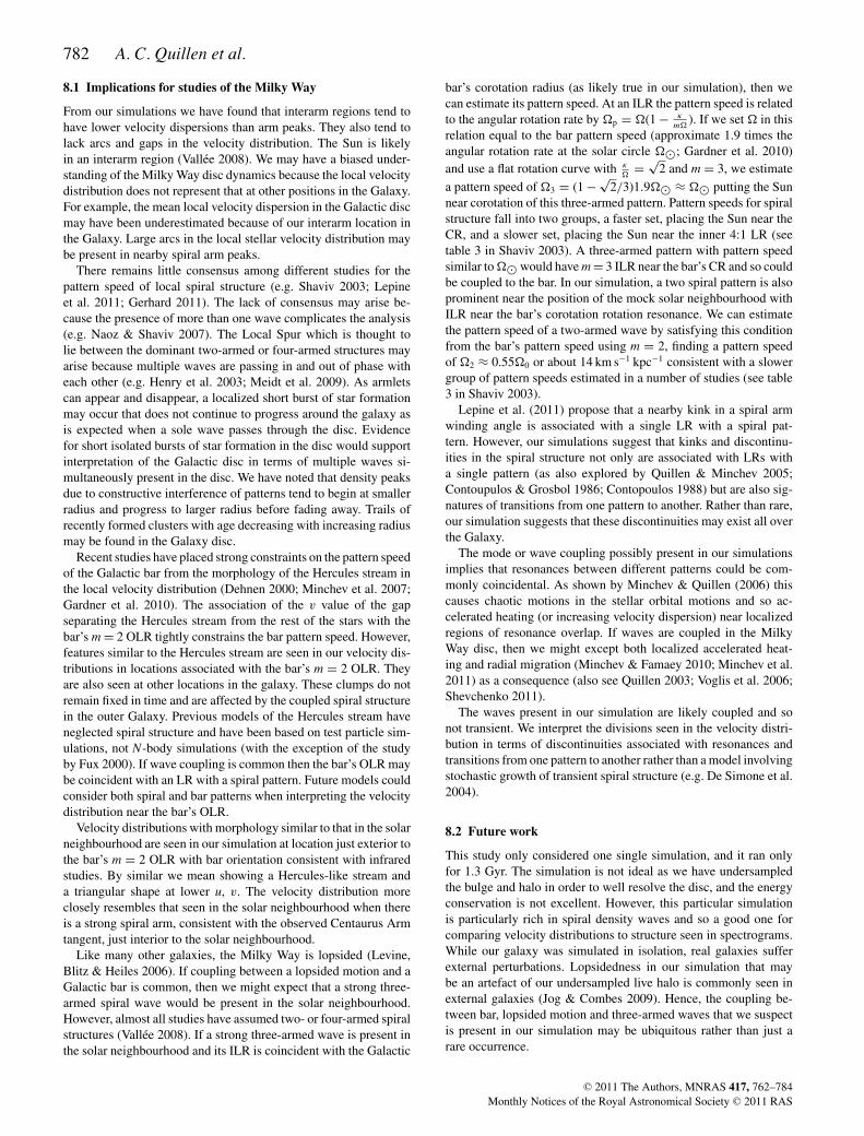
782 A. C. Quillen et al.
8.1 Implications for studies of the Milky Way
From our simulations we have found that interarm regions tend tohave lower velocity dispersions than arm peaks. They also tend tolack arcs and gaps in the velocity distribution. The Sun is likelyin an interarm region (Vallee 2008). We may have a biased under-standing of the Milky Way disc dynamics because the local velocitydistribution does not represent that at other positions in the Galaxy.For example, the mean local velocity dispersion in the Galactic discmay have been underestimated because of our interarm location inthe Galaxy. Large arcs in the local stellar velocity distribution maybe present in nearby spiral arm peaks.
There remains little consensus among different studies for thepattern speed of local spiral structure (e.g. Shaviv 2003; Lepineet al. 2011; Gerhard 2011). The lack of consensus may arise be-cause the presence of more than one wave complicates the analysis(e.g. Naoz & Shaviv 2007). The Local Spur which is thought tolie between the dominant two-armed or four-armed structures mayarise because multiple waves are passing in and out of phase witheach other (e.g. Henry et al. 2003; Meidt et al. 2009). As armletscan appear and disappear, a localized short burst of star formationmay occur that does not continue to progress around the galaxy asis expected when a sole wave passes through the disc. Evidencefor short isolated bursts of star formation in the disc would supportinterpretation of the Galactic disc in terms of multiple waves si-multaneously present in the disc. We have noted that density peaksdue to constructive interference of patterns tend to begin at smallerradius and progress to larger radius before fading away. Trails ofrecently formed clusters with age decreasing with increasing radiusmay be found in the Galaxy disc.
Recent studies have placed strong constraints on the pattern speedof the Galactic bar from the morphology of the Hercules stream inthe local velocity distribution (Dehnen 2000; Minchev et al. 2007;Gardner et al. 2010). The association of the v value of the gapseparating the Hercules stream from the rest of the stars with thebar’s m = 2 OLR tightly constrains the bar pattern speed. However,features similar to the Hercules stream are seen in our velocity dis-tributions in locations associated with the bar’s m = 2 OLR. Theyare also seen at other locations in the galaxy. These clumps do notremain fixed in time and are affected by the coupled spiral structurein the outer Galaxy. Previous models of the Hercules stream haveneglected spiral structure and have been based on test particle sim-ulations, not N-body simulations (with the exception of the studyby Fux 2000). If wave coupling is common then the bar’s OLR maybe coincident with an LR with a spiral pattern. Future models couldconsider both spiral and bar patterns when interpreting the velocitydistribution near the bar’s OLR.
Velocity distributions with morphology similar to that in the solarneighbourhood are seen in our simulation at location just exterior tothe bar’s m = 2 OLR with bar orientation consistent with infraredstudies. By similar we mean showing a Hercules-like stream anda triangular shape at lower u, v. The velocity distribution moreclosely resembles that seen in the solar neighbourhood when thereis a strong spiral arm, consistent with the observed Centaurus Armtangent, just interior to the solar neighbourhood.
Like many other galaxies, the Milky Way is lopsided (Levine,Blitz & Heiles 2006). If coupling between a lopsided motion and aGalactic bar is common, then we might expect that a strong three-armed spiral wave would be present in the solar neighbourhood.However, almost all studies have assumed two- or four-armed spiralstructures (Vallee 2008). If a strong three-armed wave is present inthe solar neighbourhood and its ILR is coincident with the Galactic
bar’s corotation radius (as likely true in our simulation), then wecan estimate its pattern speed. At an ILR the pattern speed is relatedto the angular rotation rate by p = (1 − κ
m). If we set in this
relation equal to the bar pattern speed (approximate 1.9 times theangular rotation rate at the solar circle �; Gardner et al. 2010)and use a flat rotation curve with κ
= √
2 and m = 3, we estimate
a pattern speed of 3 = (1 − √2/3)1.9� ≈ � putting the Sun
near corotation of this three-armed pattern. Pattern speeds for spiralstructure fall into two groups, a faster set, placing the Sun near theCR, and a slower set, placing the Sun near the inner 4:1 LR (seetable 3 in Shaviv 2003). A three-armed pattern with pattern speedsimilar to � would have m = 3 ILR near the bar’s CR and so couldbe coupled to the bar. In our simulation, a two spiral pattern is alsoprominent near the position of the mock solar neighbourhood withILR near the bar’s corotation rotation resonance. We can estimatethe pattern speed of a two-armed wave by satisfying this conditionfrom the bar’s pattern speed using m = 2, finding a pattern speedof 2 ≈ 0.550 or about 14 km s−1 kpc−1 consistent with a slowergroup of pattern speeds estimated in a number of studies (see table3 in Shaviv 2003).
Lepine et al. (2011) propose that a nearby kink in a spiral armwinding angle is associated with a single LR with a spiral pat-tern. However, our simulations suggest that kinks and discontinu-ities in the spiral structure not only are associated with LRs witha single pattern (as also explored by Quillen & Minchev 2005;Contoupulos & Grosbol 1986; Contopoulos 1988) but are also sig-natures of transitions from one pattern to another. Rather than rare,our simulation suggests that these discontinuities may exist all overthe Galaxy.
The mode or wave coupling possibly present in our simulationsimplies that resonances between different patterns could be com-monly coincidental. As shown by Minchev & Quillen (2006) thiscauses chaotic motions in the stellar orbital motions and so ac-celerated heating (or increasing velocity dispersion) near localizedregions of resonance overlap. If waves are coupled in the MilkyWay disc, then we might except both localized accelerated heat-ing and radial migration (Minchev & Famaey 2010; Minchev et al.2011) as a consequence (also see Quillen 2003; Voglis et al. 2006;Shevchenko 2011).
The waves present in our simulation are likely coupled and sonot transient. We interpret the divisions seen in the velocity distri-bution in terms of discontinuities associated with resonances andtransitions from one pattern to another rather than a model involvingstochastic growth of transient spiral structure (e.g. De Simone et al.2004).
8.2 Future work
This study only considered one single simulation, and it ran onlyfor 1.3 Gyr. The simulation is not ideal as we have undersampledthe bulge and halo in order to well resolve the disc, and the energyconservation is not excellent. However, this particular simulationis particularly rich in spiral density waves and so a good one forcomparing velocity distributions to structure seen in spectrograms.While our galaxy was simulated in isolation, real galaxies sufferexternal perturbations. Lopsidedness in our simulation that maybe an artefact of our undersampled live halo is commonly seen inexternal galaxies (Jog & Combes 2009). Hence, the coupling be-tween bar, lopsided motion and three-armed waves that we suspectis present in our simulation may be ubiquitous rather than just arare occurrence.
C© 2011 The Authors, MNRAS 417, 762–784Monthly Notices of the Royal Astronomical Society C© 2011 RAS
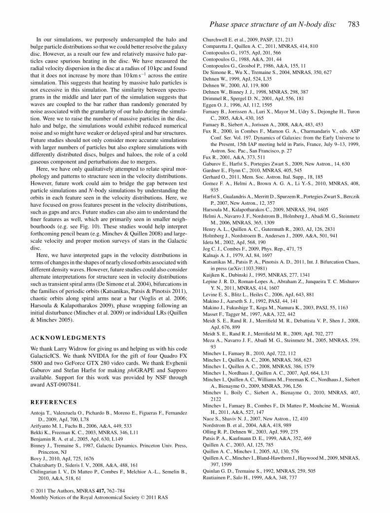
Phase space structure of an N-body disc 783
In our simulations, we purposely undersampled the halo andbulge particle distributions so that we could better resolve the galaxydisc. However, as a result our few and relatively massive halo par-ticles cause spurious heating in the disc. We have measured theradial velocity dispersion in the disc at a radius of 10 kpc and foundthat it does not increase by more than 10 km s−1 across the entiresimulation. This suggests that heating by massive halo particles isnot excessive in this simulation. The similarity between spectro-grams in the middle and later part of the simulation suggests thatwaves are coupled to the bar rather than randomly generated bynoise associated with the granularity of our halo during the simula-tion. Were we to raise the number of massive particles in the disc,halo and bulge, the simulations would exhibit reduced numericalnoise and so might have weaker or delayed spiral and bar structures.Future studies should not only consider more accurate simulationswith larger numbers of particles but also explore simulations withdifferently distributed discs, bulges and haloes, the role of a coldgaseous component and perturbations due to mergers.
Here, we have only qualitatively attempted to relate spiral mor-phology and patterns to structure seen in the velocity distributions.However, future work could aim to bridge the gap between testparticle simulations and N-body simulations by understanding theorbits in each feature seen in the velocity distributions. Here, wehave focused on gross features present in the velocity distributions,such as gaps and arcs. Future studies can also aim to understand thefiner features as well, which are primarily seen in smaller neigh-bourhoods (e.g. see Fig. 10). These studies would help interpretforthcoming pencil beam (e.g. Minchev & Quillen 2008) and large-scale velocity and proper motion surveys of stars in the Galacticdisc.
Here, we have interpreted gaps in the velocity distributions interms of changes in the shapes of nearly closed orbits associated withdifferent density waves. However, future studies could also consideralternate interpretations for structure seen in velocity distributionssuch as transient spiral arms (De Simone et al. 2004), bifurcations inthe families of periodic orbits (Katsanikas, Patsis & Pinotsis 2011),chaotic orbits along spiral arms near a bar (Voglis et al. 2006;Harsoula & Kalapotharakos 2009), phase wrapping following aninitial disturbance (Minchev et al. 2009) or individual LRs (Quillen& Minchev 2005).
AC K N OW L E D G M E N T S
We thank Larry Widrow for giving us and helping us with his codeGalacticICS. We thank NVIDIA for the gift of four Quadro FX5800 and two GeForce GTX 280 video cards. We thank EvgheniiGaburov and Stefan Harfst for making phiGRAPE and Sapporoavailable. Support for this work was provided by NSF throughaward AST-0907841.
REFERENCES
Antoja T., Valenzuela O., Pichardo B., Moreno E., Figueras F., FernandezD., 2009, ApJ, 700, L78
Arifyanto M. I., Fuchs B., 2006, A&A, 449, 533Bekki K., Freeman K. C., 2003, MNRAS, 346, L11Benjamin R. A. et al., 2005, ApJ, 630, L149Binney J., Tremaine S., 1987, Galactic Dynamics. Princeton Univ. Press,
Princeton, NJBovy J., 2010, ApJ, 725, 1676Chakrabarty D., Sideris I. V., 2008, A&A, 488, 161Chilingarian I. V., Di Matteo P., Combes F., Melchior A.-L., Semelin B.,
2010, A&A, 518, 61
Churchwell E. et al., 2009, PASP, 121, 213Comparetta J., Quillen A. C., 2011, MNRAS, 414, 810Contopoulos G., 1975, ApJ, 201, 566Contopoulos G., 1988, A&A, 201, 44Contopoulos G., Grosbol P., 1986, A&A, 155, 11De Simone R., Wu X., Tremaine S., 2004, MNRAS, 350, 627Dehnen W., 1999, ApJ, 524, L35Dehnen W., 2000, AJ, 119, 800Dehnen W., Binney J. J., 1998, MNRAS, 298, 387Drimmel R., Spergel D. N., 2001, ApJ, 556, 181Eggen O. J., 1996, AJ, 112, 1595Famaey B., Jorrissen A., Luri X., Mayor M., Udry S., Dejonghe H., Turon
C., 2005, A&A, 430, 165Famaey B., Siebert A., Jorissen A., 2008, A&A, 483, 453Fux R., 2000, in Combes F., Mamon G. A., Charmandaris V., eds. ASP
Conf. Ser. Vol. 197. Dynamics of Galaxies: from the Early Universe tothe Present, 15th IAP meeting held in Paris, France, July 9–13, 1999,Astron. Soc. Pac., San Francisco, p. 27
Fux R., 2001, A&A, 373, 511Gaburov E., Harfst S., Portegies Zwart S., 2009, New Astron., 14, 630Gardner E., Flynn C., 2010, MNRAS, 405, 545Gerhard O., 2011, Mem. Soc. Astron. Ital. Supp., 18, 185Gomez F. A., Helmi A., Brown A. G. A., Li Y.-S., 2010, MNRAS, 408,
935Harfst S., Gualandris A., Merritt D., Spurzem R., Portegies Zwart S., Berczik
P., 2007, New Astron., 12, 357Harsoula M., Kalapotharakos C., 2009, MNRAS, 394, 1605Helmi A., Navarro J. F., Nordstrom B., Holmberg J., Abadi M. G., Steinmetz
M., 2006, MNRAS, 365, 1309Henry A. L., Quillen A. C., Gutermuth R., 2003, AJ, 126, 2831Holmberg J., Nordstroem B., Andersen J., 2009, A&A, 501, 941Ideta M., 2002, ApJ, 568, 190Jog C. J., Combes F., 2009, Phys. Rep., 471, 75Kalnajs A. J., 1979, AJ, 84, 1697Katsanikas M., Patsis P. A., Pinotsis A. D., 2011, Int. J. Bifurcation Chaos,
in press (arXiv:1103.3981)Kuijken K., Dubinski J., 1995, MNRAS, 277, 1341Lepine J. R. D., Roman-Lopes A., Abraham Z., Junqueira T. C. Mishurov
Y. N., 2011, MNRAS, 414, 1607Levine E. S., Blitz L., Heiles C., 2006, ApJ, 643, 881Makino J., Aarseth S. J., 1992, PASJ, 44, 141Makino J., Fukushige T., Koga M., Namura K., 2003, PASJ, 55, 1163Masset F., Tagger M., 1997, A&A, 322, 442Meidt S. E., Rand R. J., Merrifield M. R., Debattista V. P., Shen J., 2008,
ApJ, 676, 899Meidt S. E., Rand R. J., Merrifield M. R., 2009, ApJ, 702, 277Meza A., Navarro J. F., Abadi M. G., Steinmetz M., 2005, MNRAS, 359,
93Minchev I., Famaey B., 2010, ApJ, 722, 112Minchev I., Quillen A. C., 2006, MNRAS, 368, 623Minchev I., Quillen A. C., 2008, MNRAS, 386, 1579Minchev I., Nordhaus J., Quillen A. C., 2007, ApJ, 664, L31Minchev I., Quillen A. C., Williams M., Freeman K. C., Nordhaus J., Siebert
A., Bienayme O., 2009, MNRAS, 396, L56Minchev I., Boily C., Siebert A., Bienayme O., 2010, MNRAS, 407,
2122Minchev I., Famaey B., Combes F., Di Matteo P., Mouhcine M., Wozniak
H., 2011, A&A, 527, 147Naoz S., Shaviv N. J., 2007, New Astron., 12, 410Nordstrom B. et al., 2004, A&A, 418, 989Olling R. P., Dehnen W., 2003, ApJ, 599, 275Patsis P. A., Kaufmann D. E., 1999, A&A, 352, 469Quillen A. C., 2003, AJ, 125, 785Quillen A. C., Minchev I., 2005, AJ, 130, 576Quillen A. C., Minchev I., Bland-Hawthorn J., Haywood M., 2009, MNRAS,
397, 1599Quinlan G. D., Tremaine S., 1992, MNRAS, 259, 505Rautiainen P., Salo H., 1999, A&A, 348, 737
C© 2011 The Authors, MNRAS 417, 762–784Monthly Notices of the Royal Astronomical Society C© 2011 RAS
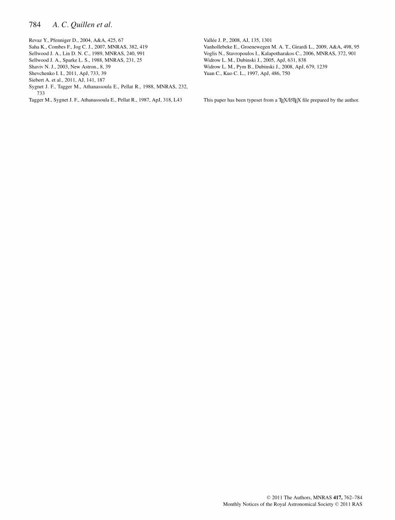
784 A. C. Quillen et al.
Revaz Y., Pfenniger D., 2004, A&A, 425, 67Saha K., Combes F., Jog C. J., 2007, MNRAS, 382, 419Sellwood J. A., Lin D. N. C., 1989, MNRAS, 240, 991Sellwood J. A., Sparke L. S., 1988, MNRAS, 231, 25Shaviv N. J., 2003, New Astron., 8, 39Shevchenko I. I., 2011, ApJ, 733, 39Siebert A. et al., 2011, AJ, 141, 187Sygnet J. F., Tagger M., Athanassoula E., Pellat R., 1988, MNRAS, 232,
733Tagger M., Sygnet J. F., Athanassoula E., Pellat R., 1987, ApJ, 318, L43
Vallee J. P., 2008, AJ, 135, 1301Vanhollebeke E., Groenewegen M. A. T., Girardi L., 2009, A&A, 498, 95Voglis N., Stavropoulos I., Kalapotharakos C., 2006, MNRAS, 372, 901Widrow L. M., Dubinski J., 2005, ApJ, 631, 838Widrow L. M., Pym B., Dubinski J., 2008, ApJ, 679, 1239Yuan C., Kuo C. L., 1997, ApJ, 486, 750
This paper has been typeset from a TEX/LATEX file prepared by the author.
C© 2011 The Authors, MNRAS 417, 762–784Monthly Notices of the Royal Astronomical Society C© 2011 RAS