Embed Size (px)
Citation preview

STRUCTURE IN LIQUID TRIGLYCERIDES
by
Liangle Lin
Submitted in partial fulfilment of the requirements for the degree of Master of Science
at
Dalhousie University Halifax, Nova Scotia
October 2014
© Copyright by Liangle Lin, 2014

TABLE OF CONTENTS
TABLE OF CONTENTS .................................................................................................... ii
LIST OF TABLES ............................................................................................................. iv
LIST OF FIGURES ............................................................................................................ v
ABSTRACT ...................................................................................................................... vii
LIST OF ABBREVIATIONS AND SYMBOLS USED ................................................. viii
ACKNOWLEGEMENTS ................................................................................................... x
CHAPTER 1 INTRODUCTION ........................................................................................ 1
CHAPTER 2 LITERATURE REVIEW ............................................................................. 3
2.1. Triglycerides ............................................................................................................ 3
2.1.1. Polymorphism ................................................................................................... 4
2.1.2. Liquid Structure of TAGs ................................................................................. 6
2.2. X-ray Scattering ..................................................................................................... 11
CHAPTER 3 EXPERIMENTAL METHODS AND MATERIALS ................................ 14
3.1. Materials ................................................................................................................ 14
3.2. X-ray Scattering Measurements ............................................................................. 14
3.2.1.Equipment Used ............................................................................................... 15
3.2.2. Sample Treatment ........................................................................................... 18
3.3 Image Processing .................................................................................................... 19
3.4. Electron Density Function ..................................................................................... 20
CHAPTER 4 RESULTS OF THE X-RAY SCATTERING DATA .............................. 22

4.1. Wide-Angle X-ray Scattering Measurements ........................................................ 23
4.1.1. WAXS FWHM ............................................................................................... 23
4.1.2. WAXS R-spacing Values ............................................................................... 24
4.2 Small-angle X-ray Scattering Measurements ......................................................... 26
4.2.1. SAXS FWHM ................................................................................................. 27
4.2.2. SAXS R-spacing Values ................................................................................. 28
CHAPTER 5 DISCUSSIONS OF THE X-RAY SCATTERING DATA ........................ 31
5.1 Discussions of WAXS R-spacing Values ............................................................... 32
5.2 Discussions of SAXS R-spacing Values................................................................. 36
5.3 The Loose Multimer Model .................................................................................... 37
5.3.1. Spatial Distribution of the Molecules of Liquid TAGs .................................. 37
5.3.2. Function to Estimate the Density of Liquid TAGs ......................................... 38
5.3.3. Prediction of Characteristic Distance Between Molecules of Liquid TAGs .. 39
5.3.4. Loose Multimer Model Calculations .............................................................. 40
5.3.5. NLM Results ..................................................................................................... 43
CHAPTER 6 SUMMARY AND CONCLUSION ........................................................ 47
REFERENCES ................................................................................................................. 50

LIST OF TABLES
Table 2-1 Fatty acids in TAG samples used in our research. ............................................. 4 Table 2-2 Melting point (˚C) of the three polymorphic forms for LLL, MMM, PPP, SSS
(Takeuchi et al., 2003). ............................................................................................... 4 Table 3-1 Temperature profiles for X-ray scattering measurements in the NSLS beamline
X10A.Temperatures are chosen at an increment of every 5°C between the temperatures. 18
Table 3-2 Numbers of images for each sample at corresponding temperatures, from the SAXS measurements in the Dunn building...............................................................19
Table 4-1 WAXS d-spacing values (nm) of TAG samples from the experiment done at
the NSLS beamline X10A. ....................................................................................... 23
Table 4-2 FWHM values ( of TAG samples from the experiment done at the NSLS beamline X10A. ........................................................................................................ 24
Table 4-3 Peak type of the liquid TAG samples from the results of peak fitting in IgorPro.
................................................................................................................................... 24 Table 4-4 SAXS d-spacing values (nm) of TAG samples from the experiment done at the
NSLS beamline X10A. ............................................................................................. 26 Table 4-5 SAXS d-spacing values (nm) of TAG samples from the experiment done in the
Dunn building. .......................................................................................................... 27
Table 4-6 FWHM values ( of LLL, MMM, PPP and SSS from SAXS measurements at the NSLS beamline X10A. .................................................................................... 27
Table 4-7 FWHM values ( of TAG samples from the experiment done in the Dunn building. .................................................................................................................... 28
Table 5-1 Molecular weight of TAG molecules (g/mol). ................................................. 37 Table 5-2 Carbon numbers of each aliphatic chain in TAG molecules ............................ 38 Table 5-3 Density values (kg/m3) for the three selected TAGs at 80 and 100 ˚C calculated
using equation 15. ..................................................................................................... 39

LIST OF FIGURES
Figure 2-1(a) A general TAG molecule structure, (b) the subcell structures of three most
common polymorphisms in TAGs, (c) unit cell structure of tricaprin ß form and (d) chain length structure in TAGs (Sato, 2001). ............................................................. 3
Figure 2-2 The relation between Gibbs energy and temperature for the three main polymorphic forms of TAGs (Himawan et al., 2006). ................................................ 6
Figure 2-3 a (left) proposed structure of TAGs in liquid by Larsson (1972); b (middle) proposed structure of TAGs in liquid by Cebula et al., (1992); c (right) proposed “Y”-conformation within each “disc”, where TAG fatty acid chains spread out at ~120˚ to each other in a single, though diffuse, plane (Corkery et al., 2007). ........... 7
Figure 2-4 Chain segment AB in dense rubber. ................................................................ 10
Figure 2-5 A schematic drawing of the molecular organization of n-octanol that accounts for the observed X-ray diffraction patterns. .............................................................. 11
Figure 2-6 Schematic representation of X-ray scattering from a crystalline material (Bragg, 1913). ........................................................................................................... 12
Figure 3-1 Image of the Brookhaven National Laboratory National Synchrotron Light
Source (NSLS I) showing the beam line status (BNLWebsite). ............................... 16
Figure 3-2 Setup of X-ray scattering experiments performed at National Synchrotron Light Source.. ............................................................................................................ 16
Figure 3-3 The NanoSTAR SAXS machine with components labeled. Taken from the Bruker-AXS NanoSTAR manual. ............................................................................ 17
Figure 3-4 (left) An Image from Laue camera, indicating SAXS (inner circle) and WAXS (outer circle) peak. .................................................................................................... 19
Figure 3-5 Gauss peak was fitted into radial plot of LLL at 140 ˚C from the experiment done in the Dunn building.. ....................................................................................... 20
Figure 4-1 Example of electron density ratio plots. .......................................................... 22
Figure 4-2 Wide-angle R-spacing values of TAG samples from the experiment done at the NSLS beamline X10A as a function of temperature. .......................................... 25
Figure 4-3 Small-angle R-spacing values of TAG samples from the experiment done in the NSLS beamline X10A as a function of temperature. .......................................... 29

Figure 4-4 Small-angle R-spacing values of TAG samples from the experiment done in the Dunn building as a function of temperature ........................................................ 29
Figure 5-1 Simple schematic of an idealized liquid made of evenly distributed space-
filling molecules occupying equal volumes. ............................................................. 31
Figure 5-2 Plots of the predicted wide-angle R-spacing value from the density of TAGs and the dotted lines are the predicted WA R-spacing values based on equation (12a)................................................................................................................................... 32
Figure 5-3 Plots of the predicted wide-angle R-spacing values from density of alkanes with carbon numbers of 10–16. ................................................................................ 34
Figure 5-4 Angle of maximum scattering 2θmax as a function of the temperature for unbranched alkanes CnH2n+2 with even n and polyethylene (Ovchinnikov et al., 1976) ......................................................................................................................... 35
Figure 5-5 Wide-angle R-spacing values of the unbranched alkanes (Ovchinnikov et al.,
1976) compared with our TAG samples. .................................................................. 35 Figure 5-6 Plots of the predicted small-angle R-spacing values from density of alkanes
and the dotted lines are the predicted SA R-spacing values using equation 12b..............................................................................................................................36
Figure 5-7 Schematic arrangement of LM in space. ......................................................... 41 Figure 5-8 On the left: snapshot of LLL bilayer at 160 ˚C(Hsu & Violi, 2009); on the
right: snapshot of PPP at 350K at 300ns (Hall et al., 2008).. ................................... 42 Figure 5-9 Average NLM of TAG samples from the experiment done in the NSLS
beamline X10A as a function of temperature. .......................................................... 44 Figure 5-10 Average NLM of TAG samples from the experiment done in the Dunn
building as a function of temperature. ...................................................................... 44

ABSTRACT
The structure and distribution of triglycerides (TAGs) in fats affects the properties of
the final products, in terms of texture, appearance and mouth feel. A few debates and
models have been developed on the distribution of TAG molecules in the liquid, but they
are not consistent with the actual density of oils or our X-ray scattering (XRS) data.
Four pure liquid TAG samples were examined by XRS at temperatures up to 210 °C.
WAXS data are consistent with the liquid phase of alkanes and other aliphatic molecules.
SAXS data are similar to those produced by alcohols and fatty acids, whose molecules
associate via polar groups. Therefore, we developed a new conceptual model to describe
the clustering of liquid TAGs as “Loose Multimers” and from it estimated that they
consist approximately of 5 to 9 molecules. The average number of molecules decreases
with temperature and increases with molecular weight.
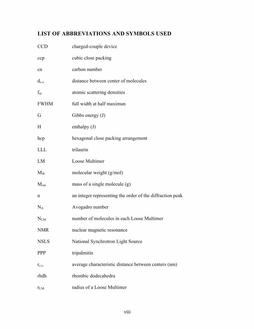
LIST OF ABBREVIATIONS AND SYMBOLS USED
CCD charged-couple device
ccp cubic close packing
cn carbon number
dc-c distance between center of molecules
fm atomic scattering densities
FWHM full width at half maximun
G Gibbs energy (J)
H enthalpy (J)
hcp hexagonal close packing arrangement
LLL trilaurin
LM Loose Multimer
MW molecular weight (g/mol)
Msm mass of a single molecule (g)
n an integer representing the order of the diffraction peak
NA Avogadro number
NLM number of molecules in each Loose Multimer
NMR nuclear magnetic resonance
NSLS National Synchrotron Light Source
PPP tripalmitin
rc-c average characteristic distance between centers (nm)
rhdh rhombic dodecahedra
rLM radius of a Loose Multimer

rzk, rtk, rck coefficients used to determine the density of TAG molecules
S entropy (J/K)
SAXS small-angle X-ray scattering
SSS tristearin
T temperature (˚C)
TAG triglyceride or triacylglycerol
Tm melting temperature (˚C)
V volume of the molecule (nm3)
VLM volume of each Loose Multimer (nm3)
Vsm volume occupied by a single molecule (nm3)
WAXS wide-angle X-ray scattering
XRD X-ray diffraction
XRS X-ray scattering
wavelength of the X-ray beam (Å)
the Bragg angle (˚)
density (g/cm3)
electron density per unit volume at a distance r from the reference atom
average electron density in the sample
full width at half maximum of the scattered peak (Å-1)

ACKNOWLEGEMENTS
I would first like to thank my supervisor, Dr. Gianfranco Mazzanti, for his support,
patience, encouragement, helpfulness and willingness to teach. I have learned a lot during
my time here and I consider it to have been a very great opportunity for me to come to
Halifax and do research with the Mazzanti group. I am indebted to the deep insights of
Dr. David Pink, and the feedback from Dr. Jan Haelssig. The use of the Nanostar
instrument was kindly granted by Dr. Jeff Dahn, with the technical support from Dr.
Robbie Sanderson. Technical assistance at the synchrotron was provided by Steve
Bennett.
I would also like to thank all my research colleagues: Omar Al-Qatami, Pavan
Karthik Batchu, Amro Alkhudair, Rong Liu, Mohit Kalaria, Pranav Arora, Xiyan Deng
and Yujing Wang. Thanks for making this time a very pleasant one.
Finally, I'd like to express gratitude to my family and friends, whose encouragement
and support has helped me all the way.

CHAPTER 1 INTRODUCTION
Fats or lipids, mainly made of triglycerides (TAGs), are the key ingredients in many
very popular foods, like ice cream, chocolate, margarine, etc. The structure and
distribution of TAGs affects the properties of the final products, in terms of texture,
appearance and mouth feel (Himawan, Starov & Stapley, 2006; Metin & Hartel, 2005).
A few models have been proposed to describe the distribution of TAGs molecules in
their liquid state. Larsson (1972) proposed a popular lamellar model, but it turned out to
be inconsistent with the small angle neutron scattering data from Cebula et al. (1992). On
the other hand, molecular modeling by Sum et al. (2003) supported the lamellar
hypothesis. The recent discotic model proposal by Corkery et al. (2007) is not consistent
with the actual density of oils or with our observations of SAXS from liquid TAGs X-ray
scattering (XRS) data obtained as collateral data prior to hundreds of time-resolved
crystallization experiments. Limited molecular association was predicted by simulation
studies on liquid alkanes (Fujiwara & Sato, 1999; Takeuchi, 1998). Some degree of
transient clustering was also observed, though not quantified, in simulations on TAGs
conducted by Hall, Repakova, & Vattulainen (2008); Hsu & Violi (2009) and Pink et al.
(2010)
X-rays have been used for a very long time in studying TAGs crystalline phases. X-
ray diffraction (XRD) and XRS are fundamentally similar because both methods use
intense beams of X-ray to obtain structural information of the sample. Differences arise
from making measurements of target molecules in solutions or liquid state (XRS) or
embedded in a crystal (diffraction). Both are forms of elastic scattering that provide
information on spatial distribution of electron densities. TAGs produce two regions of
XRS patterns: small-angle (SAXS) and wide-angle (WAXS). WAXS comes from the
short distance between the aliphatic chains, and is essentially similar to that of alkanes.
SAXS probably arise from the long distance between the glycerol cores, since the
differences in electron density between cores and chains produce scattering
As derived by Debye (1947), the scattering intensity is the product of the scattering
amplitude by a noncrystalline array of atoms at a given reciprocal scattering vector “q” as
a function of scattering angles (Klug & Alexander, 1974). Since Bragg’s law cannot
apply strictly to XRS in liquid, Klug & Alexander (1974) introduced the “R-spacing” and
described its relationship to Bragg’s “d”. These concepts will be used in this Thesis to
interpret the scattering data.
This research aims to find out how TAGs molecules are distributed in the liquid and
develop a model to better describe their distribution, based on our XRS observations and
modeling or experimental literature reports.
Our hypothesis is that, in their liquid melt, TAGs molecules associate to form
clusters, that have on average 5 to 9 molecules.
Four pure TAG samples were used: trilaurin (LLL), trimyristin (MMM), tripalmitin
(PPP) and tristearin (SSS). A series of XRS experiments were performed on the X10A
beamline (wavelength 1.0889 Å) in the National Synchrotron Light Source at
Brookhaven National Laboratory, and in the Dunn building of the Physics Department at
Dalhousie University (wavelength 1.541 Å). Each sample was kept in a capillary at high
temperature while SAXS and WAXS data were being collected.
CHAPTER 2 LITERATURE REVIEW
2.1. Triglycerides
Fats and lipids are widely used in food, cosmetics, pharmaceuticals, etc. (Gunstone
& Padley, 1997). They are heavily present in commercial fat products, such as chocolate,
margarine, butter, and baked goods. Both processing and storage conditions are important
determinants in food quality, texture, and shelf-life (Himawan, Starov & Stapley, 2006;
Metin & Hartel, 2005). TAGs are the main component of edible fats constituting from
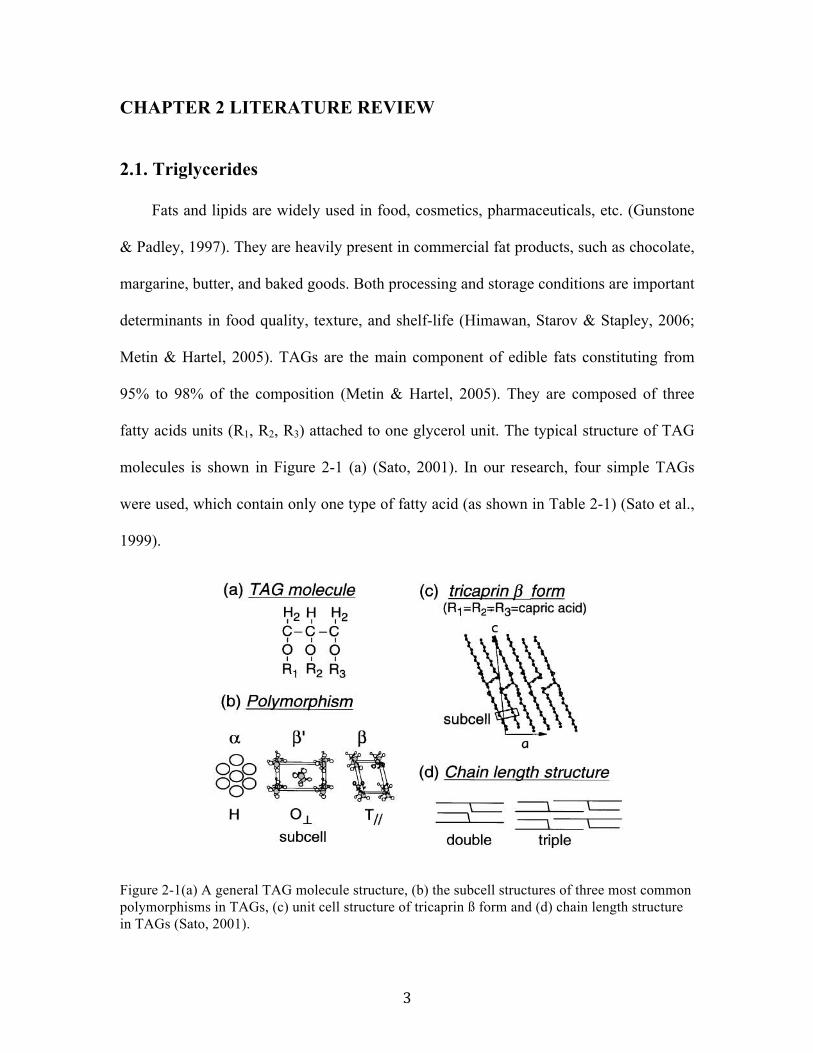
95% to 98% of the composition (Metin & Hartel, 2005). They are composed of three
fatty acids units (R1, R2, R3) attached to one glycerol unit. The typical structure of TAG
molecules is shown in Figure 2-1 (a) (Sato, 2001). In our research, four simple TAGs
were used, which contain only one type of fatty acid (as shown in Table 2-1) (Sato et al.,
1999).
Figure 2-1(a) A general TAG molecule structure, (b) the subcell structures of three most common polymorphisms in TAGs, (c) unit cell structure of tricaprin ß form and (d) chain length structure in TAGs (Sato, 2001).

Table 2-1 Fatty acids in TAG samples used in our research. Code Fatty acid Chain Length
L lauric acid (dodecanoic acid) 12 M myristic acid (tetradecanoic acid) 14 P palmitic acid (hexadecanoic acid) 16 S stearic acid (octadecanoic acid) 18
2.1.1. Polymorphism
The polymorphic crystalline structure of fats was studied long before any interest
arose in their liquid state, and seems to have influenced the initial ideas of possible
structure in the liquid. Polymorphism is the ability of a molecule to form more than one
crystalline structure depending on its arrangement within the crystal lattice (Metin and
Hartel, 2005). The crystallization behavior of the TAGs are directly influenced by
polymorphism, which is influenced by molecular structure itself, and by several external
factors such as temperature, pressure, solvent, rate of crystallization, impurities (Sato,
2001). TAG molecules packed in different crystalline arrangements exhibit significantly
different melting temperature, shown in Table 2-2 (M. Takeuchi, Ueno, & Sato, 2003).
Table 2-2 Melting point (˚C) of the three polymorphic forms for LLL, MMM, PPP, SSS (M. Takeuchi et al., 2003).
α β β ’
LLL 15 35 46.5
MMM 33 46.5 57
PPP 44.7 56.6 66.4
SSS 54.9 64 73.1
There are three common polymorphs of fats: α ,β and β ’ (Larsson, 1966). The
differences between polymorphs come from their subcell structure and are apparent from
a top view of these planes, as seen in Figure 2-1 (b). α is an unstable form in which the

hydrocarbon chains are packed in a hexagonal (H) type subcell. β ’ is a metastable form
that has an orthorhombic perpendicular (O⊥ ) subcell. β is the most stable form and has
a triclinic parallel (T ⁄⁄) subcell (Takeuchi et al., 2003). Subcell structures are defined as
cross-sectional packaging of the zigzag aliphatic chains (Sato, 2001). The chain length
structure produces a repetitive sequence of the acyl chains involved in a unit cell lamella
along the long-chain axis. The stacking of these chains can be in either a double or triple
chain length structure, shown in Figure 2-1 (d). A double chain length structure usually
occurs when the chemical properties of the three acid moieties are the same or very
similar, as shown in Figure 2-1 (c) of tricaprin β form (Jensen & Mabis, 1966).
The Gibbs energy (G) determines the thermodynamic stability of the polymorphic
forms of TAGs; the polymorph that has the lowest G is the most stable. G-Temperature
(T) diagram is shown in Figure 2-2 for the three basic polymorphs of TAGs. The plot
follows the equation for G as a function of enthalpy (H), entropy (S) and T, which is:
(1)
The G values are the largest for the α form, intermediate for the β ’ form and
smallest for the β form. Each polymorphic form has its own melting temperature, Tm,
shown as the intersection points of the G-T curves of the polymorphs and the liquid
phase.

Figure 2-2 The relation between Gibbs energy and temperature for the three main polymorphic forms of TAGs (Himawan et al., 2006).
2.1.2. Liquid Structure of TAGs
Initial attempts to ascribe a liquid structure to the TAG melts seem to have stemmed
from an extension of the polymorphic concept towards the next level of disorder, e.g. at
energy contents above the α polymorph. Thus, it has been proposed that a liquid
crystalline phase exists in some fat systems before the crystallization of TAGs, unless the
temperature is far enough above the melting point to totally destroy this ordering
(Hernqvist, 1984; Larsson, 1972; Ueno et al., 1997). Below the melting point, the
molecules in the liquid phase would spontaneously organize themselves into these liquid
crystals, prior to the formation of actual crystals. This hypothetical liquid crystal structure
may also explain the “crystal memory”, a phenomenon where fat tends to form the same

crystal structure before melting as the ordering of the liquid phase at the beginning of
crystallization (Hernqvist, 1984).
Figure 2-3 a (left) proposed structure of TAGs in liquid by Larsson (1972); b (middle) proposed structure of TAGs in liquid by Cebula et al., (1992); c (right) proposed “Y”-conformation within each “disc”, where TAG fatty acid chains spread out at ~120˚ to each other in a single, though diffuse, plane (Corkery et al., 2007).
Since Larsson first proposed the lamellar model based on XRD measurements, as
seen in Figure 2-3 (a), a few debates and models were brought up. By incorporating
Raman spectroscopy into the methods, Hernqvist (1984) showed that the order of TAGs
melt was quite constant and the order of different segments in the hydrocarbon chains
varied with different chain length. This smectic structure was also supported by
Callaghan & Jolley (1977) through 13C Nuclear Magnetic Reasonance (NMR)
measurements. However, Cebula, et al. (1992) claimed that a nematic phase of liquid
crystals was more consistent with their observation from SANS experiments, shown in
Figure 2-3 (b), instead of the organized molecular aggregates of the smectic liquid
crystals in Larsson’s model. On the other hand, molecular modeling by Sum et al. (2003)
supported the lamellar hypothesis. More recently, an alternative discotic model has been
proposed by Corkery, et al. (2007) that triglyceride molecules exist in the liquid state
with fully splayed chains (“Y” shape), forming discs structure, shown in Figure 2-3 (c).

These discs then stacked into flexible short cylindrical rods-packing order. However, the
discotic model is not consistent with the actual density of oils or with our vast database of
liquid TAGs XRS data. Molecular dynamics simulations done by Hsu & Violi (2009) and
Hall, Repakova, & Vattulainen (2008) do not support Sum's (2003) proposal of layered
structure in liquid TAGs. Hall (2008) pointed out that the liquid system is different from
the crystalline-like system and shows a random conformation. In addition, Hsu (2009)
reported that liquid TAG molecules with longer aliphatic chains present a higher degree
of recoil and hence a greater entanglement between molecules. With Raman
Spectroscopy measurements and computer simulations of LLL in the liquid phase, Pink
et al. (2010) studied the transition between h-Y conformations, and denied the lamellar
model (Larsson, 1972), the discotic packing (Corkery et al., 2007) and the nematic model
(Cebula et al., 1992). The idea of a “soft” solid-liquid transition was supported by Da
Silva & Rousseau (2008) by studying the ß polymorph to liquid phase transition of five
monosaturated TAGs using Raman spectroscopy. Besides, Pink et al. (2010) found in the
simulations that the liquid phase exhibits the formation of clusters due to nonzero
attractive dipole-dipole interactions via the C=O group, which they thought may give rise
to the observed peak in the scattering function at d ≈ 4.6 Å in the WAXS region. The
scattering at that “d” value, however, is also largely produced by the alkyl chains, and is
therefore not a proof of proximity between glycerol cores of different molecules. This
WAXS prediction is in agreement with the work of Stewart & Morrow (1927) on
alcohols and Ovchinnikov et al. (1976) on unbranched alkanes. However, numbers of
molecules in each cluster was not looked into either in simulations or experimentally in
previous studies.

In order to understand what is the distribution of TAGs in their liquid state, apart
from the glycerol cores, it is important to understand the distribution of the aliphatic
chains. De Gennes (1971) discussed possible motion for one polymer molecule
performing wormlike displacements in a strongly cross-linked polymer gel (reptation)
and first predicted that the overall mobility and diffusion coefficients of the primitive
chain depend strongly on molecular weight. With the help of De Gennes’s results, Doi &
Edwards (1978a, 1978b, 1979) studied the dynamics of polymers in melts and presented
a mathematical model to describe the Brownian motion of polymers. The chains are
entangled and cannot pass through each other, which confines each chain inside a tube-
like region (figure 2-4), along which it displaces itself. The center line of such a tube-like
region was called the primitive path, and can be regarded as the shortest curve which has
the same topology as the real chain relative to the other polymer molecules. The primitive
chain was characterized by the step length and a diffusion coefficient. The motion inside
the tube is thus some kind of reptation. The step length of the primitive chain may be
thought as a mean intermolecular distance.(Doi & Edwards, 1978b; Doi, 1975).

Figure 2-4 Chain segment AB in dense rubber. The points A and B denote the cross-linked points, and the dots represent other chains which, in this drawing, are assumed to be perpendicular to the paper. Due to entanglements the chain is confined to the tube-like region denoted by the broken line. The bold line shows the primitive path (Doi & Edwards, 1978b).
Many experiments and modeling have been done on liquid alcohols (Chapman et al.,
1990; Franks et al., 1993; Stewart & Morrow, 1927; Stewart, 1927), alkanes (Christenson
et al., 1987; Goodsaid-Zalduondo & Engelman, 1981; Ovchinnikov et al., 1976; Venturi
et al., 2009), fatty acids (Iwahashi et al., 2004) and paraffins (Stewart, 1927, 1928).
Iwahashi (2004) found that fatty acids exist mostly as dimers and the dimers aggregate to
form clusters possessing a “quasi-smectic” liquid crystal. In all these molecular liquids
the hydrocarbon chains produce a WAXS scattering peak consistent with an average
inter-chain distance of about 4.6 Å. Frank et al. (1993) recorded XRD patterns from n-
octanol and then analyzed the SAXS patterns using a modified version of the Percus-
Yevick hard-sphere theory for liquids. This theory was also tested by Chapman et al.
(1990). Figure 2-5 shows the schematic drawing of the molecular organization of n-
octanol. The n-octanol molecules are associated in aggregates, with their hydroxyl groups
forming roughly spherical clusters and their hydrocarbon chains pointing outwards,
almost fully extended (Franks et al., 1993).

Figure 2- 5 A schematic drawing of the molecular organization of n-octanol that accounts for the observed X-ray diffraction patterns. The alcohol molecules are grouped in clusters with their hydroxyl groups approximated by either a sphere of diameter of 8.78 Å in pure n-octanol and 9.98 Å in hydrated N-octanol or a Gaussian with a FWHM of 6.22 Å in pure n-octanol and 7.08 Å in hydrated n-octanol (Franks et al., 1993).
2.2. X-ray Scattering
X-ray has long been used in studying TAGs (Clarkson & Malkin, 1948; Mazzanti et
al. 2003; Metin & Hartel, 2005; Ueno et al., 1997). XRD and XRS are fundamentally
similar because both methods use intense beams of X-ray to obtain structural information
of the sample (Williams & Carter, 2009). Differences arise from making measurements
of target molecules in solutions (XRS) or embedded in a crystal (XRD). Elastic scattering
provides information on spatial distribution of electrons.
According to Bragg’s law (Bragg, 1913), for a given set of lattice planes with an
inter-plane distance of d (Figure 2-4), the condition for a diffraction peak to occur can be
written as:

(2)
where is the wavelength of the X-ray, is the scattering angle and n is an integer
representing the order of the diffraction peak.
Figure 2-6 Schematic representation of X-ray scattering from a crystalline material (Bragg, 1913).
The scattering intensity is the product of the scattering amplitude by a noncrystalline
array of atoms at a given reciprocal scattering vector “q” as a function of the scattering
angle (Debye 1947). As presented by Klug (1974) it can be written as
(3)
Where
(4)
The vector is an inner distance vector, pointing from the mth scattering center to
the nth scattering center. The are the atomic scattering densities and depend on the
number of electrons of the atom and the heavier an atom the greater the . Since

Bragg’s law (Bragg, 1913) cannot apply strictly to XRS in liquid, Klug & Alexander
(1974) came up with a general “R-spacing” corresponding to the average physical
distance between scatterers:
with (5)
corresponds to a strong maximum in the diffraction pattern at angle and is equal
to 1.25 times the d-spacing calculated with the aid of the Bragg equation, for a diffraction
peak centered around a value of q0 for the scattering vector. Klug however points out that
the real value is likely smaller e.g. 1.22. For polymer chains, this factor was estimated to
be 1.11. Klug recommended determining the value experimentally if possible.
There are two regions of XRS patterns produced by TAGs: SAXS and WAXS.
WAXS shows the short distance between the aliphatic chains, and is due to the variations
of electron density between atoms of neighboring molecules (or adjacent molecule
branches) and the background vacuum. SAXS indicates the long distance between the
glycerol cores and it is produced likely by the differences in electron density between
cores and chains. Forward scattering from a single particle (Roess & Shull, 1947) is
different from the inter-particle scattering (Lund & Vineyard, 1949). What we are seeing
in our small angle scattering is not the forward scattering, but the inter-particle scattering.
A wider angle scattering exists that is related to intramolecular electron density
variations, but that is not discussed in this thesis. It corresponds to distances of less than 2
Å.

CHAPTER 3 EXPERIMENTAL METHODS AND MATERIALS
3.1. Materials
Pure LLL, MMM, PPP and SSS were chosen for this work. These TAGs are
extensively distributed in nature and widely studied. Moreover, they have consecutive
chain length carbon numbers (from 12 to 18), which makes easier to observe and
interpret the results.
LLL, MMM, SSS and PPP samples were obtained from Sigma-Aldrich Chemical
Co. with more than 99% purity and were used without further purification. Thin wall X-
ray glass capillaries of 1.5 mm diameter from Charles Supper Company were used to
hold the samples.
3.2. X-ray Scattering Measurements
A series of XRS experiments were performed at the beamline X10A in the National
Synchrotron Light Source (NSLS, Brookhaven National Laboratory, Upton, NY, US)
(Figure 3-1), and in the Dunn building of the Physics Department at Dalhousie
University. Each sample was kept in a capillary at high temperature while SAXS and
WAXS data were being collected.

3.2.1. Equipment
3.2.1.1. Synchrotron Radiation XRS
The beam line has energy that can be adjusted from 8 to 17 KeV. The exact energy
is selected using a monochromator with two parallel crystal surfaces. A set of mirrors
aligns the beam, and then it is collimated by a set of slits. The beam is further defined
downstream with two more sets of slits so that when it reaches the sample it has a size of
0.5 mm x 0.5 mm. Its wavelength during our experiments was 1.0889 Å. Images of the
SAXS patterns were collected to a computer by Bruker-AXS SMART software, which
controls the SMART 1500 2D CCD detector camera. Meanwhile, a Laue camera
manufactured by Photonic Science was used to collect the WAXS patterns. The image
data were then analyzed to study the nanostructures of the liquid samples.
Figure 3-2 shows a schematic of the setup of XRS experiments performed. A
temperature controller was used to monitor and control the temperature of the sample
capillaries via a Labview user interface developed in our research group. WA and SA
detectors were both used and a flypath full of Helium was assembled to provide a weak
background. In this particular setup, both cameras were centered in a line with the
flypath. Hence, the Photonic Science camera was used for capture of WAXS patterns
simultaneously with SAXS patterns. The pixel size of this camera is 0.3387 mm and it
was placed at a distance of 636.5 mm from the sample. The wavelength was calibrated
using aluminum oxide (Al2O3) in a capillary and a point detector on a rotating arm
centered at the crossing between the beam and the capillary. The distance was calibrated
using the same capillary and capturing the WAXD pattern of the Al2O3 on the Laue
camera. The exposure time of a WAXS pattern was set to be 4 minutes.

Figure 3-1 Image of the Brookhaven National Laboratory National Synchrotron Light Source (NSLS I) showing the beam line status (BNLWebsite).
Figure 3-2 Setup of X-ray scattering experiments performed at National Synchrotron Light Source. Drawing by Dr. Gianfranco Mazzanti.

3.2.1.2. In-house XRS
The beam time in the synchrotron is limited, so in order to get more data at higher
temperatures to verify our hypotheses, SAXS measurements were performed in Dr. Jeff
Dahn’s lab, located in the Dunn building of the Physics Department at Dalhousie
University (Figure 3-3).
Figure 3-3 The NanoSTAR SAXS machine with components labeled. Taken from the Bruker-AXS NanoSTAR manual.
A pinhole collimated Bruker-AXS NanoSTAR equipped with a 30 W microfocus
Incoatec IμSCu source and Vantec-2000 area detector was used to collect SAXS data and
is shown in Figure 3-3. The generator operated at 40 kV and 650 μA, and a 400 μm
diameter beam of Cu-Kα (1.541 Å) radiation was selected using pinholes and a set of
Göbel mirrors. Scattering angles ranged from 0.23 to 5.00˚. The distance from the sample
to the detector was 771.78 mm calibrated with silver behenate (Ag-Beh). The exposure
time of a SAXS pattern was set to be 2 hours in order to acquire satisfactory intensity.
This also ensured thermal equilibrium in the capillary.
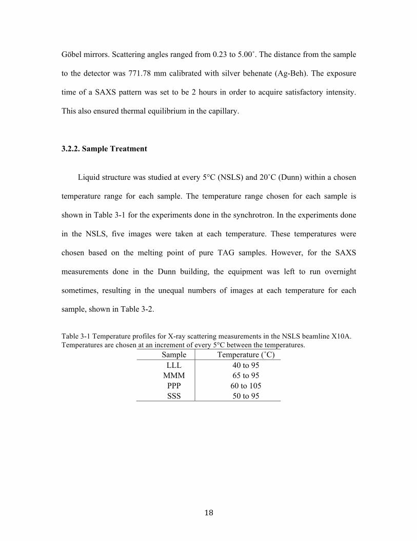
3.2.2. Sample Treatment
Liquid structure was studied at every 5°C (NSLS) and 20˚C (Dunn) within a chosen
temperature range for each sample. The temperature range chosen for each sample is
shown in Table 3-1 for the experiments done in the synchrotron. In the experiments done
in the NSLS, five images were taken at each temperature. These temperatures were
chosen based on the melting point of pure TAG samples. However, for the SAXS
measurements done in the Dunn building, the equipment was left to run overnight
sometimes, resulting in the unequal numbers of images at each temperature for each
sample, shown in Table 3-2.
Table 3-1 Temperature profiles for X-ray scattering measurements in the NSLS beamline X10A. Temperatures are chosen at an increment of every 5°C between the temperatures.
Sample Temperature (˚C)
LLL 40 to 95 MMM 65 to 95
PPP 60 to 105 SSS 50 to 95

Table 3-2 Numbers of images for each sample at corresponding temperatures, from the SAXS measurements in the Dunn building.
Temperature (˚C) LLL PPP SSS
60 2 2
80 2 8 3 100 8 9 1
120 1 9 6 140 10 5 3
160 1 4 2 180 5 11 8
200 8 5 3
3.3 Image Processing
X-ray scattering images were filtered using a macro developed in ImageJ to remove
‘bad pixels’ which were the abnormal pixels appearing in every single image due to
imperfections in the detector. Then radial plots were created after the images were
filtered and centered, a sample of PPP at 60˚C is shown in Figure 3-4.
Figure 3-4 (left) An Image from Laue camera, indicating SAXS (inner circle) and WAXS (outer circle) peak. q is the scattering vector and I is the intensity of X-ray beam in arbitrary unit (a.u.). (right) Corresponding radial plot of intensity as a function of q value of PPP at 60˚C, the peak at a smaller q value is the SAXS peak and the one at a larger q value is the WAXS peak.
q value (Å-1)
I (a
.u.)

Figure 3-5 Gauss peak was fitted into radial plot of LLL at 140 ˚C from the experiment done in the Dunn building. The green line is the background, the blue line shows the experimental data, the red line is the Gauss function, and upper part shows the residuals of the curve fitting.
Then different functions were fitted into peaks using IgorPro6. Figure 3-5 shows an
example of the fitted radial plot of LLL at 40 ˚C.
3.4. Electron Density Function
By means of the Fourier integral theorem, Klug (1974) simplified the scattering
intensity equation and the transformation of the scattering function for identical spherical
particles yields:
(6)
where is the electron density per unit volume at a distance r from the reference
atom. The number of atoms contained in spherical shell of radius is , and
is the average electron density in the sample.
Typical scattering functions are Gaussian (G) and Lorentzian (L), or a convolution
900800700600500400
4321
15
-15
400360320
0
q value (Å-1)
I (a
.u.)

of both, i.e. Voigt. The G and L functions normalized to an area of 1 are:
(7)
(8)
where the constant term Kg for the Gaussian function is:
(9)
and is the full width at half maximum (FWHM) of the scattered peak, is the
scattering vector and is the center value of the scattering vector of the peak. Although
in a logarithmic scale the functions tend to zero in a very different way, most of the
scattering information needed to characterize the structures is contained in the first two
orders of magnitude of the peak. Therefore the contribution of the “tails” is of little
consequence. The shape may contain some information about the structure, but it is
beyond the scope of this work to interpret its meaning.
The ratio between / can be expressed as (Habenschuss & Narten, 1989,
1990):
(10)
(11)
From these electron density function ratios one can obtain the correction factor for
R-spacing of the liquid samples for our specific experimental conditions.
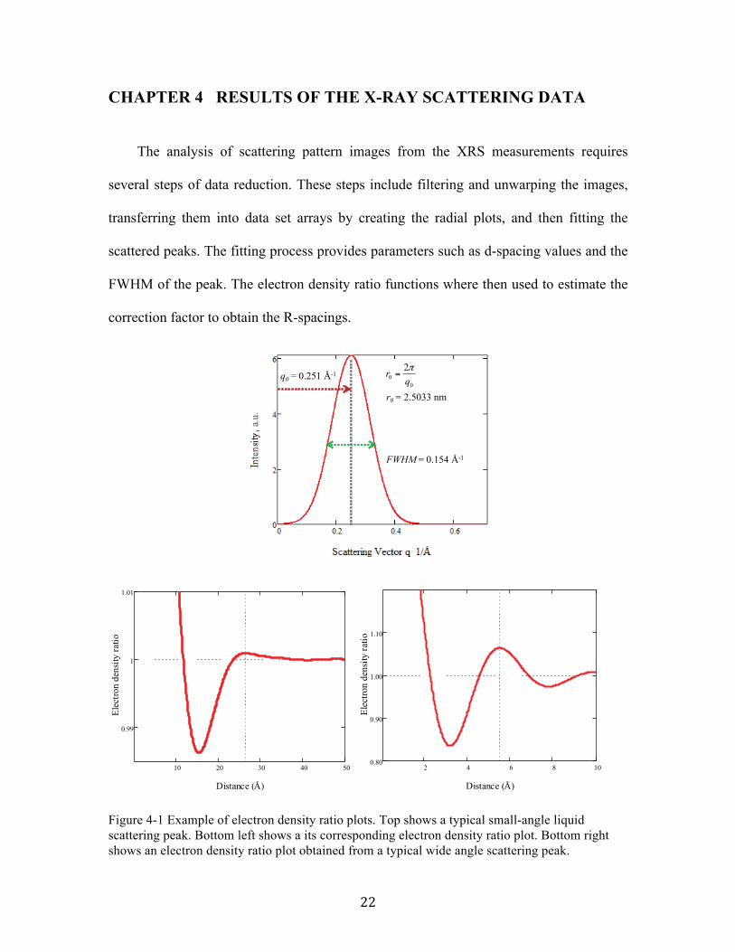
CHAPTER 4 RESULTS OF THE X-RAY SCATTERING DATA
The analysis of scattering pattern images from the XRS measurements requires
several steps of data reduction. These steps include filtering and unwarping the images,
transferring them into data set arrays by creating the radial plots, and then fitting the
scattered peaks. The fitting process provides parameters such as d-spacing values and the
FWHM of the peak. The electron density ratio functions where then used to estimate the
correction factor to obtain the R-spacings.
Figure 4-1 Example of electron density ratio plots. Top shows a typical small-angle liquid scattering peak. Bottom left shows a its corresponding electron density ratio plot. Bottom right shows an electron density ratio plot obtained from a typical wide angle scattering peak.
r0 = 2.5033 nm
FWHM = 0.154 Å-1
q0 = 0.251 Å-10
02q
r π=
10 20 30 40 50
0.99
1
1.01
Distance (Å)
Elec
tron
dens
ity ra
tio
2 4 6 8 100.80
0.90
1.00
1.10
Distance (Å)
Elec
tron
dens
ity ra
tio

4.1. Wide-Angle X-ray Scattering Measurements
The WAXS measurements reveal short distance between atoms that either belong to
different alkane chains or more frequently atoms from two different molecules (Venturi
et al., 2009). Table 4-1 shows the WAXS d-spacing values of all the WAXS
measurements done in the Synchrotron.
Table 4-1 WAXS d-spacing values (nm) of TAG samples from the experiment done at the NSLS beamline X10A.
Temperature (˚C)
Sample
LLL MMM PPP SSS
40 0.4577 45 0.4585 50 0.4598 0.4586 55 0.4609 0.4597 60 0.4618 0.4607 0.4615 65 0.4628 0.4617 0.4627 0.4620 70 0.4639 0.4627 0.4636 0.4630 75 0.4649 0.4636 0.4648 0.4641 80 0.4658 0.4647 0.4657 0.4649 85 0.4670 0.4660 0.4669 0.4661 90 0.4678 0.4667 0.4677 0.4669 95 0.4686 0.4674 0.4690 0.4678 100 0.4697 105 0.4697
The standard error of the d-spacing values is less than ±0.001
4.1.1. WAXS FWHM
FWHM (Table 4-2) of the liquid peaks and the type of the peaks (Table 4-3) were
given by peak fitting using IgorPro.

Table 4-2 FWHM values ( of TAG samples from the experiment done at the NSLS beamline X10A.
Temperature (˚C)
Sample
LLL MMM PPP SSS
40 0.4423
45 0.4457
50 0.4509 0.3704
55 0.4542 0.3735
60 0.4574 0.3707 0.3534
65 0.4603 0.3729 0.3559 0.4001
70 0.4636 0.3759 0.3565 0.4016
75 0.4665 0.3863 0.3582 0.4004
80 0.4697 0.4175 0.3585 0.4011
85 0.4733 0.4151 0.3599 0.4005
90 0.4749 0.4125 0.3614 0.3973
95 0.4776 0.4365 0.3605 0.3960
100 0.3591
105 0.3586
The standard error of the FWHM values is less than ±0.001.
Table 4-3 Peak type of the liquid TAG samples from the results of peak fitting in IgorPro. Sample WA_X10A SA_X10A SA_Dunn
LLL Lorentzian Voigt Gauss
PPP Voigt Gauss Gauss
MMM Voigt Gauss Gauss
SSS Voigt Gauss Gauss
4.1.2. WAXS R-spacing Values
Example calculation:
Wide-angle liquid scattering Gaussian peak (Figure 3-4) at d = 4.620 Å, which
agrees with Pink et al. (2010) on the scattering peaks laid under the cluster formation,
with FWHM = 1.23 Å-1. The electron density ratio function has its first maximum at dmax
= 5.527 Å. Ratio = 5.527/4.688 = 1.18.

The ratio was calculated for every sample at each temperature. Then we took
average of the ratios and obtained , which is the correction factor for WAXS
R-spacing, not too different from the value of 1.11 estimated by Klug (1974). Calculated
R-spacing values are plotted against temperature in Figure 4-2.
Figure 4-2 Wide-angle R-spacing values of TAG samples from the experiment done at the NSLS beamline X10A as a function of temperature.
It is clear that the R-spacing values of liquid TAGs increase almost linearly as the
temperature increases, which means that the short distances between the aliphatic chains
of TAGs increase with temperature. For a given Van der Waals force field, the average
distances at which the attracting forces (Van der Waals) and the “repulsive forces”
(thermal vibrations) equilibrate are larger at higher temperatures. Furthermore, the Van
der Waals forces decrease with distance non-linearly. The linear trend in the data may be

due to the small temperature range, since the density (which changes with R3) has been
measured and is linear with temperature.
There is not much difference in R-spacing values between the samples with different
carbon numbers, probably because the forces are averaged over the CH2 groups, and
hence are not very sensitive to their numbers.
4.2 Small-angle X-ray Scattering Measurements
The SAXS measurements reveal long distances between glycerol cores of TAGs.
The SAXS d-spacing values of all the SAXS measurements done in the Synchrotron and
the Dunn building are shown in Table 4-4 and 4-5. For the peak types, refer to Table 4-3.
Table 4-4 SAXS d-spacing values (nm) of TAG samples from the experiment done at the NSLS beamline X10A.
Temperature (˚C)
Sample
LLL MMM PPP SSS
40 2.1090 45 2.1004 50 2.0861 2.3644 55 2.0765 2.3549 60 2.0688 2.3473 2.4478 65 2.0604 2.3373 2.4351 2.6205 70 2.0540 2.3318 2.4259 2.6093 75 2.0484 2.3278 2.4149 2.5943 80 2.0409 2.3114 2.4081 2.5864 85 2.0347 2.2989 2.3987 2.5830 90 2.0304 2.2932 2.3927 2.5695 95 2.0252 2.2998 2.3850 2.5562
100 2.3790 105 2.3784
The standard error of the d-spacing values is less than ±0.01.

Table 4-5 SAXS d-spacing values (nm) of TAG samples from the experiment done in the Dunn building.
The standard error of the d-spacing values is less than ±0.01.
4.2.1. SAXS FWHM
FWHM of the liquid peaks from Synchrotron and the Dunn building are shown in
Table 4-6 and 4-7.
Table 4-6 FWHM values ( of LLL, MMM, PPP and SSS from SAXS measurements at the NSLS beamline X10A.
Temperature (˚C)
Sample
LLL MMM PPP SSS
40 0.2165 45 0.2113 50 0.2071 0.1298 55 0.2046 0.1308 60 0.2026 0.1305 0.1225 65 0.2005 0.1310 0.1223 0.1356 70 0.2021 0.1306 0.1220 0.1369 75 0.2019 0.1320 0.1218 0.1355 80 0.1996 0.1318 0.1212 0.1354 85 0.1967 0.1348 0.1211 0.1349 90 0.1967 0.1348 0.1203 0.1354 95 0.1972 0.1303 0.1203 0.1323
100 0.1219 105 0.1209
The standard error of the FWHM values is less than ±0.01.
Temperature (˚C)
Sample
LLL PPP SSS
60 2.0922 2.4174
80 2.0781 2.4022 2.5287
100 2.0578 2.3790 2.5397
120 2.0393 2.3625 2.5105
140 2.0192 2.3666 2.5084
160 2.0088 2.3569 2.5045
180 2.0023 2.3571 2.5013
200 2.0090 2.3638 2.4938

Table 4-7 FWHM values ( of TAG samples from the experiment done in the Dunn building.
Temperature (˚C)
Sample
LLL PPP SSS
60 0.1989 0.1470
80 0.2069 0.1593 0.1524
100 0.2099 0.1597 0.1507
120 0.2183 0.1666 0.1671
140 0.2255 0.1661 0.1778
160 0.2327 0.1706 0.1552
180 0.2384 0.1719 0.1550
200 0.2364 0.1731 0.1518 The standard error of the FWHM values is less than ±0.01.
4.2.2. SAXS R-spacing Values
The electron density function ratio for SA R-spacing was calculated in the same way
as shown for the WA, and its average value is 1.050. This value at smaller angles is not
too different from 1.22 (Klug, 1974). The SA R-spacing values were calculated and
plotted in Figure 4-3 and 4-4 for the synchrotron and the Dunn data, respectively.

Figure 4-3 Small-angle R-spacing values of TAG samples from the experiment done in the NSLS beamline X10A as a function of temperature.
Figure 4-4 Small-angle R-spacing values of TAG samples from the experiment done in the Dunn building as a function of temperature

SAXS R-spacing values are in an inverse relation to temperature, and this means
that the long distance between glycerol cores of TAGs shortens when they are heated up.
With the increasing carbon number in TAGs, the R-spacing values become larger.
The SAXS R-spacing values of both measurements are not exactly the same. This is
likely due to the uncertainty of the peak fitting of the SAXS data from the Dunn building.
We were not able to capture the whole liquid peak (as shown in Figure 3-5) of the TAGs
samples because it was difficult to adjust the distance between the sample and the
detector. The SAXS R-spacing values are, however, in the same range, and the
conclusions derived from both data sets turned out to be in the same range as well.
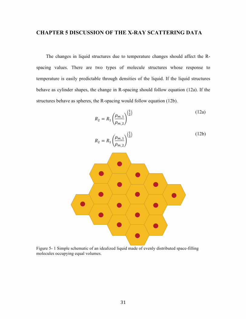
CHAPTER 5 DISCUSSION OF THE X-RAY SCATTERING DATA
The changes in liquid structures due to temperature changes should affect the R-
spacing values. There are two types of molecule structures whose response to
temperature is easily predictable through densities of the liquid. If the liquid structures
behave as cylinder shapes, the change in R-spacing should follow equation (12a). If the
structures behave as spheres, the R-spacing would follow equation (12b).
(12a)
(12b)
Figure 5- 1 Simple schematic of an idealized liquid made of evenly distributed space-filling molecules occupying equal volumes.

5.1 Discussion of WAXS R-spacing Values
In agreement with the cylinder structure of hydrocarbon chains suggested in the
literature (Doi & Edwards, 1978a, 1978b, 1979), the average distance between primitive
chains is expected to increase as the temperature increases. This happens because the
volume occupied by the flexible cylinder that encloses the polymer increases. However,
given this cylinder shape, the increase in cross-sectional area is proportional to R2.
Therefore, the change in distance R with T should follow equation (12a). If liquid TAGs
are evenly distributed as individual molecules, and each molecule occupies equal volume
(Figure 5-1), the changes in R should follow equation (12b).
Figure 5- 2 Plots of the predicted wide-angle R-spacing value from the density of TAGs and the dotted lines are the predicted WA R-spacing values based on equation (12a), each letter corresponds to our TAG samples.

The predicted WA R-spacing values using this expression are exactly the same as
the experimental ones. The simulations by Hsu & Violi (2009) indicate that there may be
a recoil of up to 70% in the chains, where the average distance between the carbonyl
carbon in the polar group and the last carbon of the TAG chains in the liquid is 30% less
than the distance in the crystal form. This result is also consistent with the flexible
cylinder concept of Doi & Edwards (1978). The aliphatic chains will thus not be fully
extended radially as depicted in the concept by Franks et al. (1993) for n-octanol, but will
have a higher degree of entanglement. This does not preclude that the distances between
axes of the cylinders (primitive chains) depend on temperature as described above. The
same situation should apply to the WA R-spacing values of unbranched alkanes
(Ovchinnikov et al., 1976) with the estimated WA R-spacing values from density
(Assael, Dymond, & Exadaktilou, 1994). If we were to consider that the WA R-pacing
values were affected only by the “alkane behavior” of the alkyl chains, their change with
temperature could be also calculated using the ratios of the densities of alkanes of the
same number of carbons. It turns out that the WA R-spacing values do not follow the
trend in equation (12a) when the alkanes densities are used, as shown in Figure 5-3. The
interpretation of this difference is beyond the scope of this thesis.

Figure 5- 3 Plots of the predicted wide-angle R-spacing values from density of alkanes with carbon numbers of 10–16, and the dotted lines are the predicted WA R-spacing values using equation 12b, each number corresponds to the carbon number of the alkane sample.
Ovchinnikov et al. (1976) investigated short-range order in liquid unbranched
alkanes and polyethylene using XRS and plotted the relationship between the maximum
scattering angle and the temperature, shown in Figure 5-4. Converting the scattering
angle to WA R-spacing values, we compared the R-spacing values of unbranched alkanes
with our TAG samples in Figure 5-5. The values of both R-spacing are in the same range.

Figure 5- 4 Angle of maximum scattering 2θmax as a function of the temperature for unbranched
alkanes CnH2n+2 with even n and polyethylene (Ovchinnikov et al., 1976).
Figure 5- 5 Wide-angle R-spacing values of the unbranched alkanes (Ovchinnikov et al., 1976) compared with our TAG samples.

5.2 Discussion of SAXS R-spacing Values
Estimated from equation (12b), SA R-spacing values should follow the dotted line in
Figure 5-6. It is clear that the actual SA R-spacing data we acquired from the SAXS in
the Dunn building differ from the estimated values. The same applies to the data from the
synchrotron.
Figure 5- 6 Plots of the predicted small-angle R-spacing value from the density of TAGs and the dotted lines are the predicted SA R-spacing values using equation 12b, each letter corresponds to our TAG samples.

5.3 The Loose Multimer Model
5.3.1. Spatial Distribution of the Molecules of Liquid TAGs
The most efficient space filling packing of monodisperse (single sized) solid spheres
are the hexagonal close packing arrangement (hcp) and the cubic close packing (ccp).
The spheres will occupy of the space. If the spheres are allowed to fill
the rest of the space by growing equally, they will form rhombic dodecahedra (rhdh),
because in the hcp, each sphere is equivalent to any other one, and each one has a
coordination number of 12, i.e, touches 12 other spheres. The diameter of the sphere
inscribed in the rhdh is equal to the distance between the centers of two adjacent rhdhs.
If the edge length of an rhdh is a, the radius of an inscribed sphere ( ) is =
and the volume V is If the volume of the space filling rhdh is known,
the distance between centers ( ) can be calculated as:
(13)
where is the volume of the average rhdh that encloses the molecules.
From the Avogadro number, (molecule/mol), it is possible to
determine the mass of a single molecule (Msm):
(14)
where is the mass weight of TAG molecules per mole (g/mol), shown in Table
5-1.
Table 5-1 Molecular weight of TAG molecules (g/mol).
LLL MMM PPP SSS
639.01 723.16 807.43 891.48

Taking PPP at 60˚C as an example, . Then:
(g/PPP molecule) (15)
Combining Msm with the density ( ), we are able to find the volume occupied by a
single molecule (Vsm). The density depends on the composition, temperature ( ), and the
number of carbons in TAG molecules can characterize the composition.
5.3.2. Function to Estimate the Density of Liquid TAGs
A function to estimate the density of liquid saturated TAGs as a function of carbon
number ( ) of the saturated fatty acid and temperature in °C was fitted to data from the
literature (Joglekar & Watson, 1928), and the following equation was obtained:
(16)
where coefficients There is a good
agreement between calculated and experimental values, shown in Table 5-3.
For example, the density of PPP at 60˚C is:
(17)
Table 5-2 Carbon numbers of each aliphatic chain in TAG molecules.
LLL MMM PPP SSS
12 14 16 18

Table 5-3 Density values (kg/m3) for the three selected TAGs at 80 and 100 ˚C calculated using equation 15; last two columns report data available in the literature. a-(Gunstone & Padley, 1997; Kishore, Shobha, & Mattamal, 1990; Phillips & Mattamal, 1978; Rabelo, et al., 2000). b-(Sum et al., 2003).
TAG T (˚C) Calculated Experimenta Simulationb
LLL 80 880.44 882 918
100 866.78 866 909 PPP 80 866.49 868 902
100 852.83 854 890 SSS 80 862.72 862 895
100 849.06 852 883
5.3.3. Prediction of Characteristic Distance Between Molecules of Liquid TAGs
If the “unit blocks” of the liquid where single TAG molecules in which the alkyl
chains were crumpled around the glycerol core, we would have a simple, space filling
average concept of the liquid, with individual glycerol cores separated equally (on
average). To calculate the distance between these cores, we first calculate the volume of a
single molecule (Vsm), in nm3, by:
(18)
For PPP at 60 °C:
(19)
Assuming that the averaged distribution is space filling, the average characteristic
distance between centers (rc-c) in nm is:
(20)
and, again for PPP at 60 °C this distance would be:
(21)
which is much less than the typical experimental R-spacing value 2.448 nm.

It is thus evident from the experimental results that the molecules of the TAGs
cannot be individually dispersed in their liquid state. It follows then that they must form
some kind of clusters where several glycerol cores are very close, surrounded by their
alkyl chains.
5.3.4. Loose Multimer Model Calculations
This solution to the centre-to-centre distance discrepancy is based on the often-
remarked difference in polarity between the glycerol core of the TAGs and their aliphatic
chains. The oxygen atoms at the core are permanent dipoles, especially the one with the
double bond, and therefore they make this part of the molecule hydrophilic. The aliphatic
chains, on the other hand, only have very weak dipoles, and are therefore hydrophobic. It
has been postulated in previous research that the hydrophilic cores have stronger
attraction forces between them than the aliphatic chains (Iwahashi & Kasahara, 2001).
Thus some degree of association between these cores is not unlikely. In fact, many
simulations show that this association is likely the case (Sum et al., 2003; Pink et al.,
2010), though these simulations did not calculate the statistics of the associations. It is
clear that this association determines very strongly the formation of crystalline phases.
Two main defined types of associative behaviour have been previously postulated in the
literature: lamellar (Larsson, 1992) and discotic (Corkery et al., 2007). We propose an
alternative association, that we call the Loose Multimer model. This model is consistent
with SAXS and WAXS data, and also seems to explain satisfactorily many observed
properties of liquid TAGs as well as some peculiarities of their crystallization behaviour.
It is also qualitatively consistent with the results of the simulations (Sum et al., 2003;

Pink et al., 2010). Since the scattering has to be produced by space zones (volumes) of
different electronic density, it is reasonable to think that the hydrophilic cores have
different scattering density than the space occupied by the hydrophobic chains, which are
essentially an aliphatic “sea”. With this in mind, we can extend the concept of the rhdh so
that more than one molecule is in each rhdh, but arranged in such way that the cores are
very close together, with the folded aliphatic chains wrapped around them. We call these
entities Loose Multimers (LM).
They are loose because there is no strong chemical bonding between the molecules
in the unit, and molecules can be exchanged between units. It is also a flexible unit,
spatially speaking. They are called multimers because they have several molecules, but
the numbers are not too big, as would be the case of a polymer.
The shapes of the LM do not have to be, of course, perfectly dodecahedral, but they
will be some kind of squeezed deformed spheres (Figure 5-7), that change dynamically in
time. They keep, however, a space filling arrangement consistent with the measured
density of the liquid.
Figure 5- 7 Schematic arrangement of LM in space. R1, R2, R3 represent the distance between glycerol cores of neighboring LMs.
R1
R2 R3
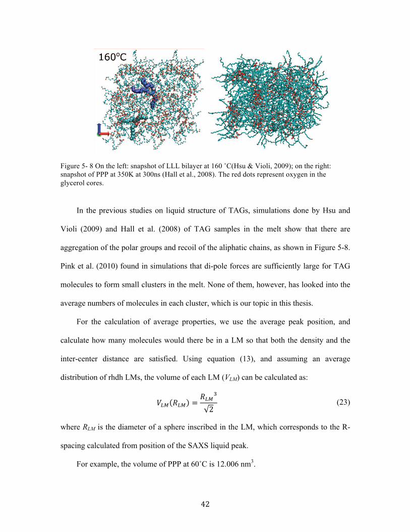
Figure 5- 8 On the left: snapshot of LLL bilayer at 160 ˚C(Hsu & Violi, 2009); on the right: snapshot of PPP at 350K at 300ns (Hall et al., 2008). The red dots represent oxygen in the glycerol cores.
In the previous studies on liquid structure of TAGs, simulations done by Hsu and
Violi (2009) and Hall et al. (2008) of TAG samples in the melt show that there are
aggregation of the polar groups and recoil of the aliphatic chains, as shown in Figure 5-8.
Pink et al. (2010) found in simulations that di-pole forces are sufficiently large for TAG
molecules to form small clusters in the melt. None of them, however, has looked into the
average numbers of molecules in each cluster, which is our topic in this thesis.
For the calculation of average properties, we use the average peak position, and
calculate how many molecules would there be in a LM so that both the density and the
inter-center distance are satisfied. Using equation (13), and assuming an average
distribution of rhdh LMs, the volume of each LM (VLM) can be calculated as:
(23)
where RLM is the diameter of a sphere inscribed in the LM, which corresponds to the R-
spacing calculated from position of the SAXS liquid peak.
For example, the volume of PPP at 60˚C is 12.006 nm3.

By dividing the total volume of the cluster over the volume of each molecule we
calculate the average number of molecules in each LM (NLM):
(24)
and:
(25)
5.3.5. Average number of molecules in each LM: NLM Results
NLM were calculated from the q0 and R computed from the data collected for each
sample at each temperature, and plotted against temperature, as shown in Figure 5-9 and
5-10. The uncertainties in the q0 and density values are very small, but the accuracy of the
R-spacing value conversion, and of the q0 values is not well defined, though it will not
change the general range of the calculated results. For instance, for PPP at 80 ˚C the
average NLM is 7.51 from the NSLS data, and 7.45 from the Dunn data.

Figure 5- 9 Average NLM of TAG samples from the experiment done in the NSLS beamline X10A as a function of temperature.
Figure 5- 10 Average NLM of TAG samples from the experiment done in the Dunn building as a function of temperature.

The NLM are in a range of 5 to 9. It is clearly shown in Figure 5-9 and 5-10 that with
the increase of temperature, the number of molecules in each LM is reduced. The
increasing temperature means that each molecule has more kinetic energy, therefore
fewer molecules will stay together in a cluster, and there will be more clusters of smaller
sizes. The exact distribution of cluster sizes at each temperature has not been estimated
from our data, only the average value. Higher energy contents also means that a TAG
molecule can move more freely from one cluster to another, and therefore the number of
unattached molecules would increase with temperature. There surely is density
fluctuation in the fluid at the length scale of the cluster, both inside the clusters and
between clusters. However what is being observed here is the overall averaged effect of
those fluctuations in both time and space. Therefore, NLM represents the average number
of molecules per cluster, not the exact number in every entity. The reduction of NLM with
increasing temperature provides a very consistent explanation for the counter-intuitive
reduction of the SA R-spacing values with increasing temperature. When the temperature
is increased, more clusters of smaller sizes are formed, resulting in shorter distances
between the glycerol cores of TAGs.
The clustering explains why it is so difficult to form a glass, given that the clusters
provide a lowered Gibbs energy barrier for crystallization nucleation to occur. This,
however, does not explain so easily why these materials require such degree of
undercooling before they start to crystallize. In our PPP experiments, for instance, the
liquid persisted easily at 60˚C, 7.4˚C below the Tm of β PPP. On the other hand, this
indicates that the energy barrier for the glass transition is higher than that for the
crystallization process. This experimental observation is in agreement with the

experimental and simulation results of Pink et al. (2010), who reported that there is a
discontinuous phase transition that possesses a broad metastable region. The explanation
for this provided by Pink et al. (2010): even though the molecules may be clustered
around glycerol groups, the methylene groups of the alkyl chains have random rotations
(trans-gauche) and it takes considerable time for them to align in the all-trans
configuration needed for crystallization.

CHAPTER 6 SUMMARY AND CONCLUSION
The goal of this work was to discover and model the distribution of TAG molecules
in their liquid state, and more specifically to estimate the average number of molecules
that would be found in clusters. Four pure liquid TAG samples were kept at high
temperatures and examined with XRS.
The TAG molecules should fill the space of the liquid in such way that the average
density of the smaller entities is equal to the density of the bulk fluid, be these entities
molecules or groups of attached molecules. The simplest space filling packing of
monodisperse (single sized) solid spheres are the hexagonal close packing arrangement
and the cubic close packing, but the actual space filling solids are the rhdh that
circumscribe the spheres. If we assume that the TAG molecules are distributed
individually in the liquid, the characteristic average distance between each pair of
molecules would be much smaller than the actual distance we measured from SAXS.
Therefore, based on the clustering suggested by Pink et al. (2010), we developed a
“Loose Multimer” model to estimate the average spatial distribution of molecules. We
assume that the liquid TAGs are clustered together and arranged in such way that the
cores are very close together, wrapped in the folded aliphatic chains. We call these
entities “Loose Multimers”. The average volume occupied by a cluster corresponds then
to that of a rhombic dodecahedron. They are loose because there is no strong chemical
bonding between the molecules in the unit, and molecules can be exchanged between
units. Spatially speaking, it is also a flexible unit. It might not be strictly as rhombic
dodecahedron, in extreme cases, the TAG molecules might lie as cylinders and cluster in

layers forming cross-like shapes. However, the forces between molecules and the exact
shape still needs further discussion and advanced simulations.
By dividing the total volume of the cluster over the volume of each molecule, the
numbers of molecules per cluster were calculated. These are scatterers distributed
spatially that are consistent with clustering of molecules in loose multimers of 5 to 9
molecules.
The number of molecules per multimer is reduced as temperature increases, and are
increased as carbon number in TAG is increased. This is the behavior expected in a fluid
made of ‘sticky’ entities.
From WAXS, the aliphatic chains were found to behave very similarly to those of
other alkyl compounds, e.g. like long flexible cylinders.
Nuclear Magnetic Resonance (NMR) experiments done by Maclean (2008) with
pure and mixture samples of LLL and MMM show that there are two different diffusing
species in liquid TAGs, one is fast and the other is slow. The estimated radius sizes of the
slow diffusing species of LLL and MMM are around 1 nm, so the dameter would be 2
nm, which is very close to the R-spacing values obtained from our SAXS measurements.
Therefore, the slow diffusing species are likely representative of clusters, while the fast
diffusing species correspond probably to intra-cluster movement of the hydrocarbon
chains of TAGs. The results agree generally with our model and provide a future work
possibility.
This thesis sets the stage for understanding a crystallization process at the nano-
level that is different from that of a homogeneous liquid. The clustering should produce a
deviation in the temperature dependency of the viscosity liquid and the diffusivity of the
molecules, when compared to a single molecule fluid. This may be very difficult to verify

experimentally, unless the time of formation of stable clusters is much longer than the
time needed to change the temperature and perform measurements.

REFERENCES
Assael, M., Dymond, J., & Exadaktilou, D. (1994). An improved representation forn-alkane liquid densities. International Journal of Thermophyscis, 15(1). Retrieved from http://link.springer.com/article/10.1007/BF01439252
Bragg, W. L. (1913). The Structure of Some Crystals as Indicated by Their Diffraction of X-rays. Proceedings of the Royal Society A: Mathematical, Physical and Engineering Sciences, 89(610), 248–277. doi:10.1098/rspa.1913.0083
Callaghan, P. T., & Jolley, K. W. (1977). An irreversible liquid–liquid phase transition in tristearin. The Journal of Chemical Physics, 67(10), 4773. doi:10.1063/1.434607
Cebula, D., McClements, D., Povey, M., & Smith, P. (1992). Neutron Diffraction Studies of Liquid and Crystalline Trilaurin. Journal of the American Oil Chemist Scoiety, 69(2), 130–136. Retrieved from http://link.springer.com/article/10.1007/BF02540562
Chapman, W., Gubbins, K., Jackson, G., & Radosa, M. (1990). New reference equation of state for associating liquids. Industrial & Engineering Chemistry Research, 29, 1709–1721. Retrieved from http://pubs.acs.org/doi/abs/10.1021/ie00104a021
Christenson, H. K., Gruen, D. W. R., Horn, R. G., & Israelachvili, J. N. (1987). Structuring in liquid alkanes between solid surfaces: Force measurements and mean-field theory. The Journal of Chemical Physics, 87(3), 1834. doi:10.1063/1.453196
Clarkson, C. E., & Malkin, T. (1948). An X-ray and thermal examination of the glycerides. Part IX. The polymorphism of simple triglycerides. Journal of the Chemical Society (Resumed), 985. doi:10.1039/jr9480000985
Corkery, R. W., Rousseau, D., Smith, P., Pink, D. A., & Hanna, C. B. (2007). A case for discotic liquid crystals in molten triglycerides. Langmuir : The ACS Journal of Surfaces and Colloids, 23(13), 7241–6. doi:10.1021/la0634140
Da Silva, E., & Rousseau, D. (2008). Molecular order and thermodynamics of the solid-liquid transition in triglycerides via Raman spectroscopy. Physical Chemistry Chemical Physics : PCCP, 10(31), 4606–4613. doi:10.1039/b717412h
De Gennes, P. (1971). Reptation of a Polymer Chain in the Presence of Fixed Obstacles. The Journal of Chemical Physics, 572(1971). doi:10.1063/1.1675789
Debye, P. (1947). Molecular-weight Determination by Light Scattering. The Journal of Physical Chemistry, 18(8), 18–32. Retrieved from http://pubs.acs.org/doi/abs/10.1021/j150451a002

Doi, M. (1975). An estimation of the tube radius in the entanglement effect of concentrated polymer solutions. Journal of Physics A: Mathematical and General, 8(6), 959–965. doi:10.1088/0305-4470/8/6/014
Doi, M., & Edwards, S. (1978a). Dynamic of Concentrated Polymer Systems Part 3.-The Constitutive Equation. Journal of the Chemical Society, Faraday Transactions 2, 74, 1818–1832. doi:10.1039/f29787401818
Doi, M., & Edwards, S. (1978b). Dynamics of Concentrated Polymer Systems Part 1.-Brownian Motion in the Equilibrium State. Journal of the Chemical Society, Faraday Transactions 2, 1789–1801. Retrieved from http://pubs.rsc.org/en/content/articlehtml/1978/f2/f29787401789
Doi, M., & Edwards, S. (1979). Dynamics of Concentrated Polymer Systems Part 4.-Rheological Properties. Journal of the Chemical Society, Faraday Transactions 2, 38–54. Retrieved from http://pubs.rsc.org/en/content/articlehtml/1979/f2/f29797500038
Franks, N., Abraham, M., & Lieb, W. (1993). Molecular Organization of Liquid n-Octanol: An X-ray Diffraction Analysis. Journal of Pharmaceutical …, 82(5), 466–470. Retrieved from http://onlinelibrary.wiley.com/doi/10.1002/jps.2600820507/abstract
Fujiwara, S., & Sato, T. (1999). Molecular dynamics simulation of structure formation of short chain molecules. The Journal of Chemical Physics, 110(19), 9757. doi:10.1063/1.478941
Goodsaid-Zalduondo, F., & Engelman, D. M. (1981). Conformation of liquid N-alkanes. Biophysical Journal, 35(3), 587–94. doi:10.1016/S0006-3495(81)84814-X
Gunstone, F., & Padley, F. (1997). Lipid Technologies and Applications. CRC press. Retrieved from http://books.google.com/books?hl=en&lr=&id=MccA-I5PgIsC&oi=fnd&pg=PR9&dq=Lipid+Technologies+and+Applications&ots=LzM361KLoz&sig=o4AaUo-v9QmI8eh5sdRRxPJXiAo
Habenschuss, A., & Narten, A. H. (1989). X-ray diffraction study of liquid n-butane at 140 and 267 K. The Journal of Chemical Physics, 91(7), 4299. doi:10.1063/1.456810
Habenschuss, A., & Narten, A. H. (1990). X-ray diffraction study of some liquid alkanes. The Journal of Chemical Physics, 92(9), 5692. doi:10.1063/1.458500
Hall, A., Repakova, J., & Vattulainen, I. (2008). Modeling of the triglyceride-rich core in lipoprotein particles. The Journal of Physical Chemistry. B, 112(44), 13772–82. doi:10.1021/jp803950w

Hernqvist, L. (1984). On the Structure of Triglycerides in the Liquid State and Fat Crystallization. Fette, Seifen, Anstrichmittel, 86(8), 297–300. doi:10.1002/lipi.19840860802
Himawan, C., Starov, V. M., & Stapley, A. G. F. (2006). Thermodynamic and kinetic aspects of fat crystallization. Advances in Colloid and Interface Science, 122(1-3), 3–33. doi:10.1016/j.cis.2006.06.016
Hsu, W.-D., & Violi, A. (2009). Order-disorder phase transformation of triacylglycerols: effect of the structure of the aliphatic chains. The Journal of Physical Chemistry. B, 113(4), 887–93. doi:10.1021/jp806440d
Iwahashi, M., Takebayashi, S., Umehara, A., Kasahara, Y., Minami, H., Matsuzawa, H., … Takahashi, H. (2004). Dynamical dimer structure and liquid structure of fatty acids in their binary liquid mixture: dodecanoic and 3-phenylpropionic acids system. Chemistry and Physics of Lipids, 129(2), 195–208. doi:10.1016/j.chemphyslip.2004.01.005
Jensen, L. H., & Mabis, A. J. (1966). Refinement of the structure of β-tricaprin. Acta Crystallographica, 21(5), 770–781. doi:10.1107/S0365110X66003839
Joglekar, R., & Watson, H. (1928). The Physical Properties of Pure Triglycerides. Journal of the Society of Chemical Industry, 47, 365–368. Retrieved from http://journal.iisc.ernet.in/index.php/iisc/article/viewFile/1868/1934
Kishore, K., Shobha, H. K., & Mattamal, G. J. (1990). Structural effects on the vaporization of high molecular weight esters. The Journal of Physical Chemistry, 94(4), 1642–1648. doi:10.1021/j100367a077
Klug, H., & Alexander, L. (1974). X-ray Diffraction Procedures: For Polycrystalline and Amorphous Materials, 2nd Edition. Willey, New York, EUA (p. 992). Retrieved from http://scholar.google.com/scholar?hl=en&btnG=Search&q=intitle:X-ray+diffraction+procedures#2
Larsson, K. (1966). Classification of Glyceride Crystal Forms. Acta Chemica Scandinavica, 20, 2255–2260.
Larsson, K. (1972). Molecular Arrangement in Glycerides. Fette, Seifen, Anstrichmittel, 74(3), 136–142. doi:10.1002/lipi.19720740302
Larsson, K. (1992). On the structure of the liquid state of triglycerides. Journal of the American Oil Chemists Society, 69(8), 835–836. Retrieved from http://link.springer.com/article/10.1007/BF02635928

Lund, L. H., & Vineyard, G. H. (1949). Inter-Particle Interference Effects in the Small Angle X-Ray Scattering from Fine Powders. Journal of Applied Physics, 20(6), 593. doi:10.1063/1.1698433
MacLean, D. (2008). An NMR study of diffusion in surfactant-free emulsions and molten triglyceride mixtures. Retrieved from http://adsabs.harvard.edu/abs/2012PhDT.......432M
Mazzanti, G., Guthrie, S. E., Sirota, E. B., Marangoni, A. G., & Idziak, S. H. J. (2003). Orientation and Phase Transitions of Fat Crystals under Shear. Crystal Growth & Design, 3(5), 721–725. doi:10.1021/cg034048a
Metin, S., & Hartel, R. W. (2005). Crystallization of Fats and Oils. In Bailey’s Industrial Oil and Fat Products. John Wiley & Sons, Inc. doi:10.1002/047167849X.bio021
Ovchinnikov, Y. k., Antipov, E. M., Markova, G. S., & Bakeev, N. F. (1976). Comparative Investigation of Short-range Order in Unbranched Alkanes and Polyethylene. Die Makromolekulare Chemie, 177(5), 1567–1581. doi:10.1002/macp.1976.021770524
Phillips, J. C., & Mattamal, G. J. (1978). Effect of number of carboxyl groups on liquid density of esters of alkylcarboxylic acids. Journal of Chemical & Engineering Data, 23(1), 1–6. doi:10.1021/je60076a031
Pink, D. A., Hanna, C. B., Sandt, C., MacDonald, A. J., MacEachern, R., Corkery, R., & Rousseau, D. (2010). Modeling the solid-liquid phase transition in saturated triglycerides. The Journal of Chemical Physics, 132(5), 054502. doi:10.1063/1.3276108
Rabelo, J., Batista, E., Cavaleri, F. vio W., & Meirelles, A. J. A. (2000). Viscosity prediction for fatty systems. Journal of the American Oil Chemists’ Society, 77(12), 1255–1262. doi:10.1007/s11746-000-0197-z
Roess, L. C., & Shull, C. G. (1947). XRay Scattering at Small Angles by FinelyDivided Solids. II. Exact Theory for Random Distributions of Spheroidal Particles. Journal of Applied Physics, 308(1947), 308–313. doi:10.1063/1.1697651
Sato, K. (2001). Crystallization behaviour of fats and lipids — a review. Chemical Engineering Science, 56(7), 2255–2265. doi:10.1016/S0009-2509(00)00458-9
Stewart, G. (1927). X-ray Diffraction in Liquids: Saturated Normal Fatty Acids, Isomers of Primary Normal Alcohols, and Normal Paraffins. Proceedings of the National Academy of Sciences of …, 13(12), 787–789. Retrieved from http://www.ncbi.nlm.nih.gov/pmc/articles/PMC1085245/

Stewart, G. (1928). X-ray Diffraction in Liquid mormal Paraffins. Physical Review, 31, 174–179. Retrieved from http://journals.aps.org/pr/abstract/10.1103/PhysRev.31.174
Stewart, G., & Morrow, R. (1927). X-ray Diffraction in Liquid: Primary Normal Alcohols. Physical Review, 30, 232–244. Retrieved from http://journals.aps.org/pr/abstract/10.1103/PhysRev.30.232
Sum, A. K., Biddy, M. J., de Pablo, J. J., & Tupy, M. J. (2003). Predictive Molecular Model for the Thermodynamic and Transport Properties of Triacylglycerols. The Journal of Physical Chemistry B, 107(51), 14443–14451. doi:10.1021/jp035906g
Takeuchi, H. (1998). Structure formation during the crystallization induction period of a short chain-molecule system: A molecular dynamics study. The Journal of Chemical Physics, 109(13), 5614. doi:10.1063/1.477179
Takeuchi, M., Ueno, S., & Sato, K. (2003). Synchrotron Radiation SAXS/WAXS Study of Polymorph-Dependent Phase Behavior of Binary Mixtures of Saturated Monoacid Triacylglycerols. Crystal Growth & Design, 3(3), 369–374. doi:10.1021/cg025594r
Ueno, S., Minato, A., Seto, H., Amemiya, Y., & Sato, K. (1997). Synchrotron Radiation X-ray Diffraction Study of Liquid Crystal Formation and Polymorphic Crystallization of SOS (sn-1,3-Distearoyl-2-oleoyl Glycerol). The Journal of Physical Chemistry B, 101(35), 6847–6854. doi:10.1021/jp9715639
Van Malssen, K., Peschar, R., Brito C, & Schenk, H. (1996). Real-Time X-Ray Powder Diffraction Investigations on Cocoa Butter . III . Direct 13-Crystallization of Cocoa Butter : Occurrence of a Memory Effect. Journal of the American Oil …, 73(10), 1225–1230. Retrieved from http://link.springer.com/article/10.1007/BF02525450
Venturi, G., Formisano, F., Cuello, G. J., Johnson, M. R., Pellegrini, E., Bafile, U., & Guarini, E. (2009). Structure of liquid n-hexane. The Journal of Chemical Physics, 131(3), 034508. doi:10.1063/1.3176413
Williams, D., & Carter, C. (2009). Scattering and Diffraction. Transmission Electron Microscopy, 23–39. Retrieved from http://link.springer.com/chapter/10.1007/978-0-387-76501-3_2