Structurally aware discretisation for Bayesian networks

Helen Mayfield a, Edoardo Bertone b, Oz Sahin b,c, Carl Smith d

a Cities Research Institute, Griffith University, Queensland, Australia b School of Engineering and Cities Research Institute, Griffith University, Queensland, Australia

c Griffith Climate Change Response Program, Griffith University, Queensland, Australia d UQ Business School, The University of Queensland, Queensland, Australia

email: helenmayfield@warpmail.net

Abstract: Bayesian networks represent a versatile probabilistic modelling technique widely used to tackle a range of problems in many different domains. However, they are discrete models, and a significant decision when designing a BN is how to split the continuous variables into discrete bins. Default options offered in most BN packages include assigning an equal number of cases to each bin or assigning equal sized bins. However, these methods discretise nodes independently of each other. When learning probabilities from data, this can result in conditional probability tables (CPTs) with missing or uninformed probabilities because data for particular bin combinations (scenarios) is either missing or scarce. This can result in poor model performance.

We propose that the structure of the network is an important determinant in node discretisation, and that the best bin allocations for a simple naïve network will be different to those for more complicated networks that attempt to model relationships between the predictor variables. Furthermore, a good discretisation algorithm should not require the model designer to specify the exact number of bins as a target for discretisation. Rather, it should be flexible in determining bin allocations within limits specified by the model designer. BN performance can be improved if discretisation results in CPTs that contain fewer combinations with insufficient evidence to confidently estimate probabilities. We have developed a structure aware discretisation (SAD) algorithm that minimises the number of missing probabilities in CPTs by taking into account network structure. The algorithm requires some parameters to be set, such as the minimum number of cases in each bin, but determines the exact number of bins and their limits based on the data. It consists of two stages: a structurally unaware discretisation stage (SUD) that distributes the cases into bins until each bin has a minimum number of cases, followed by a structure aware discretisation stage (SAD) that further reduces the number of bins to account for incomplete CPTs.

The algorithm was tested on a real life water quality case study, using three different network structures (naïve network, tree augmented network and expert designed network). The results show that both the SUD and SAD stages of the algorithm have potential to improve the discretisation process over equal case discretisation by selecting an appropriate number of bins and their limits. Improvement in performance (area under the receiver operating curve and the true skill statistic) was greatest in non-naïve network structures. A major benefit of SAD is that model designers are not required to specify the exact number of bins, with the algorithm instead balancing the parsimony and precision of the network.

Keywords: Bayesian networks, structure aware discretisation, water treatment optimisation

22nd International Congress on Modelling and Simulation, Hobart, Tasmania, Australia, 3 to 8 December 2017 mssanz.org.au/modsim2017

1420

Mayfield et al., Structurally aware discretisation for Bayesian networks

1. INTRODUCTION

Bayesian Networks (BNs) are causal probability models (Fenton and Neil, 2013). Their graphical nature, ability to incorporate expert knowledge and their inherent representation of uncertainty, make them a popular tool for participatory model building. A BN consists of a Directed Acyclic Graph (DAG) for showing dependencies among variables and conditional probability tables (CPTs) for specifying the probabilistic relationships among variables that are causally linked. Variables in a BN, which can be discrete or continuous, are represented as nodes. Nodes within a BN, whether discrete or continuous, are often discretised (or binned) to form states. Links between nodes are directed from the parent node (independent variable) to the child node (dependent variable). For each child node, the network contains a CPT that stores the probability of the node being in a particular state for each possible combination of parent node states. Discretisation of variables is not a requirement of BNs (Pearl, 2014), however, it is one of the known shortcomings of most commercial packages.

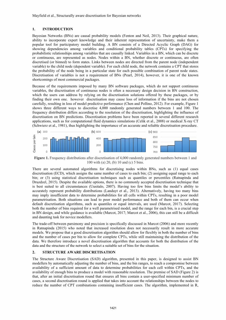
Because of the requirements imposed by many BN software packages, which do not support continuous variables, the discretisation of continuous nodes is often a necessary design decision in BN construction, which the users can address by relying on the discretisation solutions offered by these packages, or by finding their own one. however discretisation may cause loss of information if the bins are not chosen carefully, resulting in loss of model predictive performance (Chen and Pollino, 2012). For example, Figure 1 shows three different ways to discretise 4,000 randomly generated numbers between 1 and 100. The frequency distribution differs according to the resolution of the discretisation, highlighting the influence of discretisation on BN predictions. Discretisation problems have been reported in several different research applications, such as for computational fluid dynamics simulations (Celik et al., 2008) or medical X-ray CT (Schwierz et al., 1981), thus highlighting the importance of an accurate and reliable discretisation procedure.

Figure 1. Frequency distributions after discretisation of 4,000 randomly generated numbers between 1 and 100 with (a) 20, (b) 10 and (c) 5 bins.

There are several automated algorithms for discretising nodes within BNs, such as (1) equal cases discretisation (ECD), which assigns the same number of cases to each bin; (2) assigning equal range to each bin; or (3) using statistical discretisation techniques such as quantiles or percentiles (Ratnapinda and Druzdzel, 2015). Despite the available options, there is no commonly accepted discretisation technique that is best suited to all circumstances (Uusitalo, 2007). Having too few bins limits the model’s ability to accurately represent probability distributions (Landuyt et al., 2013). Alternatively, having too many bins may imply insufficient data to determine probabilities for all cells within CPTs, resulting in a poor model parametrisation. Both situations can lead to poor model performance and both of them can occur when default discretisation algorithms, such as quantiles or equal intervals, are used (Marcot, 2017). Selecting both the number of bins required for a well parametrised model, and the range for each bin, is a crucial step in BN design, and while guidance is available (Marcot, 2017; Marcot et al., 2006), this can still be a difficult and daunting task for novice modellers.

The trade-off between parsimony and precision is specifically discussed in Marcot (2006) and more recently in Ratnapinda (2015) who noted that increased resolution does not necessarily result in more accurate models. We propose that a good discretisation algorithm should allow for flexibly in both the number of bins and the number of cases per bin to allow for complete CPTs, while still maintaining the distribution of the data. We therefore introduce a novel discretisation algorithm that accounts for both the distribution of the data and the structure of the network to select a suitable set of bins for the situation.

2. STRUCTURE AWARE DISCRETISATION

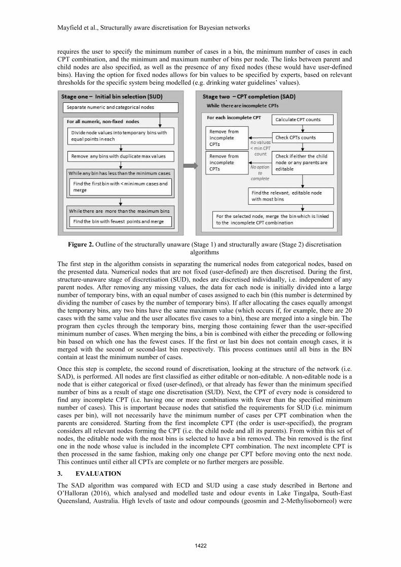
The Structure Aware Discretisation (SAD) algorithm, presented in this paper, is designed to assist BN modellers by automatically adjusting the number of bins, and the bin ranges, to reach a compromise between availability of a sufficient amount of data to determine probabilities for each cell within CPTs, and the availability of enough bins to produce a model with reasonable resolution. The premise of SAD (Figure 2) is that, after an initial discretisation round that ensures all bins contain a user-specified minimum number of cases, a second discretisation round is applied that takes into account the relationships between the nodes to reduce the number of CPT combinations containing insufficient cases. The algorithm, implemented in R,

1421

Mayfield et al., Structurally aware discretisation for Bayesian networks

requires the user to specify the minimum number of cases in a bin, the minimum number of cases in each CPT combination, and the minimum and maximum number of bins per node. The links between parent and child nodes are also specified, as well as the presence of any fixed nodes (these would have user-defined bins). Having the option for fixed nodes allows for bin values to be specified by experts, based on relevant thresholds for the specific system being modelled (e.g. drinking water guidelines’ values).

Figure 2. Outline of the structurally unaware (Stage 1) and structurally aware (Stage 2) discretisation algorithms

The first step in the algorithm consists in separating the numerical nodes from categorical nodes, based on the presented data. Numerical nodes that are not fixed (user-defined) are then discretised. During the first, structure-unaware stage of discretisation (SUD), nodes are discretised individually, i.e. independent of any parent nodes. After removing any missing values, the data for each node is initially divided into a large number of temporary bins, with an equal number of cases assigned to each bin (this number is determined by dividing the number of cases by the number of temporary bins). If after allocating the cases equally amongst the temporary bins, any two bins have the same maximum value (which occurs if, for example, there are 20 cases with the same value and the user allocates five cases to a bin), these are merged into a single bin. The program then cycles through the temporary bins, merging those containing fewer than the user-specified minimum number of cases. When merging the bins, a bin is combined with either the preceding or following bin based on which one has the fewest cases. If the first or last bin does not contain enough cases, it is merged with the second or second-last bin respectively. This process continues until all bins in the BN contain at least the minimum number of cases.

Once this step is complete, the second round of discretisation, looking at the structure of the network (i.e. SAD), is performed. All nodes are first classified as either editable or non-editable. A non-editable node is a node that is either categorical or fixed (user-defined), or that already has fewer than the minimum specified number of bins as a result of stage one discretisation (SUD). Next, the CPT of every node is considered to find any incomplete CPT (i.e. having one or more combinations with fewer than the specified minimum number of cases). This is important because nodes that satisfied the requirements for SUD (i.e. minimum cases per bin), will not necessarily have the minimum number of cases per CPT combination when the parents are considered. Starting from the first incomplete CPT (the order is user-specified), the program considers all relevant nodes forming the CPT (i.e. the child node and all its parents). From within this set of nodes, the editable node with the most bins is selected to have a bin removed. The bin removed is the first one in the node whose value is included in the incomplete CPT combination. The next incomplete CPT is then processed in the same fashion, making only one change per CPT before moving onto the next node. This continues until either all CPTs are complete or no further mergers are possible.

3. EVALUATION

The SAD algorithm was compared with ECD and SUD using a case study described in Bertone and O’Halloran (2016), which analysed and modelled taste and odour events in Lake Tingalpa, South-East Queensland, Australia. High levels of taste and odour compounds (geosmin and 2-Methylisoborneol) were

1422

Mayfield et al., Structurally aware discretisation for Bayesian networks

recorded in recent years at the Capalaba drinking water treatment plant (withdrawing raw water from Lake Tingalpa), managed by Seqwater. The ability to predict such events in advance, based on lake’s water quality, would greatly enhance the capacity of the treatment plant of proactively managing them and ensuring that safe and aesthetically pleasing water is delivered to the consumers. Data-driven prediction models have been developed in recent years in other Seqwater reservoirs/treatment plants (Bertone et al., 2017; Bertone et al., 2015), leading to increased operational proactivity and lower treatment costs. For this case study, the response variable (i.e. target node in the BN) was geosmin concentration; specifically, whether or not the geosmin levels were over 10 ng/L, i.e. what it was defined as the detection threshold. Among the predictors considered in this BN were cyanobacteria concentrations, nutrients (e.g. nitrogen, iron), turbidity and dam volume. These parameters were typically monitored on a weekly, up to daily, basis. The data sample contained 189 records.

Three network structures were tested: a naïve BN in which all nodes have only the target node as a parent; a tree augmented BN (TAN) in which all nodes have the target node and at most one other node, as a parent; and an expert-structured BN where links between nodes were determined by experts. The structure for the TAN networks was learnt from the data using Netica (Norsys Software Corp, 2013).

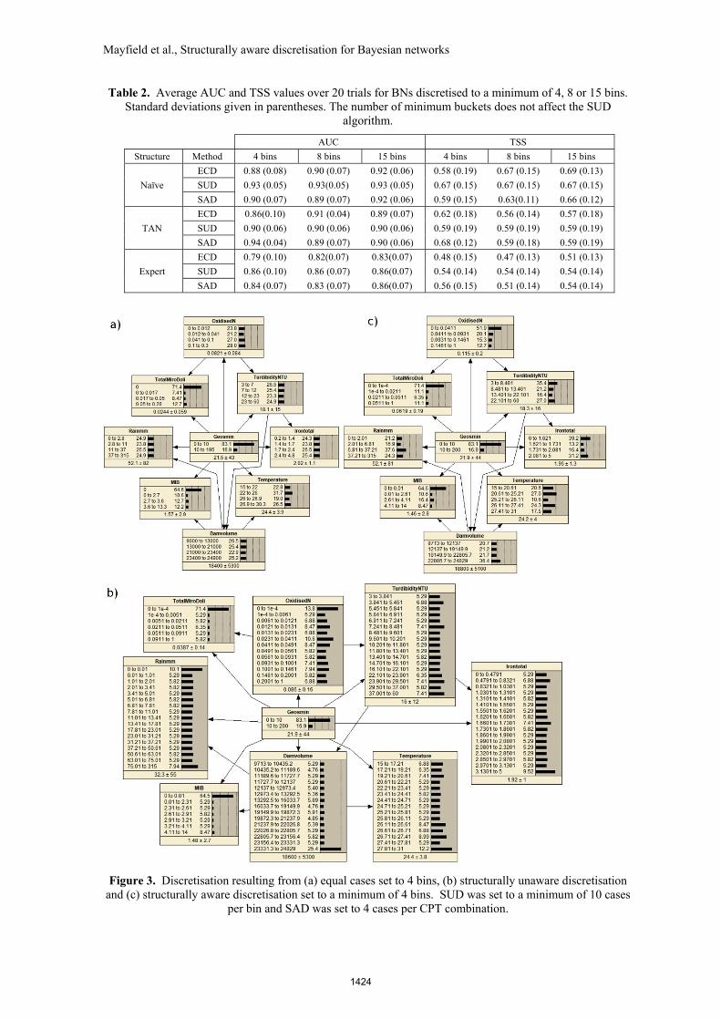
To test the effect of changing the parameters passed to the algorithm, each structure was discretised to have either 4, 8 or 15 bins. For ECD, this represented the exact number of bins generated. For SUD (stage one of SAD), this number is not used, as the minimum number of bins is instead determined by the distribution of the data and the minimum number of cases required in each bin. For SAD, this represented the minimum number of bins allowed before stage two merging is stopped (fewer bins may be generated in stage one, in which case no further modifications are made to the node in stage two). The SUD models were generated for a minimum of 10 cases per bin and the SAD models further required a minimum of 4 cases per CPT combination. The number of bins generated by SAD for each structure is given in Table 1.

Table 1. Average number of bins per node generated by the SAD algorithm when set to a minimum of 4, 8 or 15 bins. SUD BNs contained an average of 13.38 (min = 6, max = 17) bins per node

Minimum bins

Naïve TAN Expert

4 4.25 (min =4, max = 5) 4.13 (min = 4, max = 5) 4.00 (min= 4, max = 4)

8 8.625 (min = 6, max = 16) 8.88 (min = 6, max = 15) 7.63 (min = 6, max = 8)

15 12.75 (min = 6, max = 16) 12.75 (min = 6, max = 16) 12.75 (min = 6, max = 16)

All models were evaluated using the area under the receiver operating curve - AUC (Bradley, 1997) and the true skill statistic – TSS (Allouche et al., 2006). For TSS, the most probable outcome was selected (i.e. cases with a greater than 50% chance of having a geosmin value greater than 10 ng/L were considered as a positive result). Trial datasets were created using repeated random subsampling to create a series of 20 training-testing data pairs. In each pair 75% of the data was used for training and 25% for testing. Results are given in Table 2.

While differences in model performance were generally small, ECD models were the worst performing in seven out of nine model designs based on AUC results and six out of nine based on TSS results. The SUD algorithm was the best performing model in five of the nine model designs (based on AUC) and equal best with SAD in two further designs. SUD was also the best (or equal best) performing model in six of the nine designs based on TSS results. SAD was most likely to improve model performance in the TAN and expert structured models as opposed to the naïve models.

Sample bins derived from each algorithm for the four bins case are shown in Figure 3.

1423

Mayfield et al., Structurally aware discretisation for Bayesian networks

Table 2. Average AUC and TSS values over 20 trials for BNs discretised to a minimum of 4, 8 or 15 bins. Standard deviations given in parentheses. The number of minimum buckets does not affect the SUD

algorithm.

AUC TSS

Structure Method 4 bins 8 bins 15 bins 4 bins 8 bins 15 bins

Naïve

ECD 0.88 (0.08) 0.90 (0.07) 0.92 (0.06) 0.58 (0.19) 0.67 (0.15) 0.69 (0.13)

SUD 0.93 (0.05) 0.93(0.05) 0.93 (0.05) 0.67 (0.15) 0.67 (0.15) 0.67 (0.15)

SAD 0.90 (0.07) 0.89 (0.07) 0.92 (0.06) 0.59 (0.15) 0.63(0.11) 0.66 (0.12)

TAN

ECD 0.86(0.10) 0.91 (0.04) 0.89 (0.07) 0.62 (0.18) 0.56 (0.14) 0.57 (0.18)

SUD 0.90 (0.06) 0.90 (0.06) 0.90 (0.06) 0.59 (0.19) 0.59 (0.19) 0.59 (0.19)

SAD 0.94 (0.04) 0.89 (0.07) 0.90 (0.06) 0.68 (0.12) 0.59 (0.18) 0.59 (0.19)

Expert

ECD 0.79 (0.10) 0.82(0.07) 0.83(0.07) 0.48 (0.15) 0.47 (0.13) 0.51 (0.13)

SUD 0.86 (0.10) 0.86 (0.07) 0.86(0.07) 0.54 (0.14) 0.54 (0.14) 0.54 (0.14)

SAD 0.84 (0.07) 0.83 (0.07) 0.86(0.07) 0.56 (0.15) 0.51 (0.14) 0.54 (0.14)

Figure 3. Discretisation resulting from (a) equal cases set to 4 bins, (b) structurally unaware discretisation and (c) structurally aware discretisation set to a minimum of 4 bins. SUD was set to a minimum of 10 cases

per bin and SAD was set to 4 cases per CPT combination.

1424

Mayfield et al., Structurally aware discretisation for Bayesian networks

4. DISCUSSION

Both the SAD and SUD algorithms generally improved the model performance over ECD, particularly for model designs such as TAN and expert structured that attempt to explicitly model relationships between the predictors. The lower than expected improvement from stage two of the algorithm (SAD) is possibly as a result of the small sample size of the dataset (189 cases). This may have inhibited SAD in two ways. Firstly, few cases meant that fewer bins were generated in stage one (SUD), leaving limited potential improvement for round two. Secondly, fewer cases mean that CPTs are less likely to be completed early on, resulting in many nodes being reduced to the minimum number of bins.

While both SUD and SAD algorithms avoid the need for the user to define a set number of bins for each node, users still need to specify the minimum number of cases in each bin for SUD and the minimum cases per CPT combination for SAD. There are several different ways for deciding these values, such as specifying the number of cases needed for 95% confidence based on the sample size, or basing it on the prevalence rate of the data (e.g. a dataset with a 10% prevalence rate would need at least 10 cases in each bin to be able to represent this rate). Future work will focus on providing guidance on how to select the minimum number of cases based on the characteristics of the dataset. As the SAD algorithm currently outputs only a template listing the discretisation for each node, other planned work includes directly creating a .dne file as output, which can be read by either Netica (Norsys Software Corp, 2013) or Genie (Druzdzel., 1999), and linking the program to the “bnlearn” package in R (Scutari, 2010) to increase the software options available to the user.

In some instances, SAD will continue to merge nodes without improving model parametrisation. For example, if two parent nodes are fixed, and some combination of these two nodes have insufficient cases, SAD will continue to compress the child node until the minimum number of bins is reached, despite not being possible to complete the CPT. Several improvements are also planned in order to contain this effect, including ignoring CPT combinations for fixed nodes where completing the CPTs would be impossible, and allowing a small percentage of each CPT to remain incomplete.

5. CONCLUSIONS AND RECOMMENDATIONS

In this paper, we present a new approach for automated discretisation of continuous nodes with Bayesian networks, i.e. Structure Aware Discretisation (SAD). SAD considers the states of parent nodes while discretising a child node. SAD was compared to both the Equal Cases Discretisation (ECD) and Structure Unaware Discretisation (SUD) using a real life water quality case study. The three different structures tested (Naïve, TAN and expert) each had different levels of complexity, allowing the discretisation algorithm to be evaluated across a range of situations. For the majority of the BNs evaluated, those discretised using SAD performed as well as, or better than, ECD; however the distinction was less clear when compared to BNs discretised using SUD (Table 2).

The results show that the SAD algorithm has the potential to maintain BN performance compared to default algorithms such as ECD, whilst avoiding the need for the user to specify the exact number of bins. This flexibility is major advantage of the SAD and SUD algorithms over the ECD algorithm in that the user does not need to know a priori how many bins are required to represent the distribution of the data or how few bins are needed to ensure the network has sufficient data to learn from. Although some parameters are required, the algorithms themselves determine the number of bins needed to meet these criteria, or to get as close as possible to them. SAD generally produces fewer bins to ensure that all of them have sufficient cases. Conversely, the SUD algorithm generally produces more bins (Table 1, Figure 3), resulting in better model resolution. By taking the structure of the network into account, SAD is able to suggest bins that more closely match the data than ECD (by allowing more bins when data permits), while maintaining a compromise with the number of incomplete CPTs. This overcomes one of the major challenges faced by novice designers and helps to prevent their BNs from generating spurious predictions.

ACKNOWLEDGMENTS

The Authors would like to thank the Griffith University Cities Research Institute for funding this project and Seqwater for sharing the data for the case study presented in this paper.

1425

Mayfield et al., Structurally aware discretisation for Bayesian networks

REFERENCES

Allouche, O., Tsoar, A., Kadmon, R. (2006). Assessing the accuracy of species distribution models: prevalence, kappa and the true skill statistic (TSS). Journal of Applied Ecology 43, 1223–1232.

Bertone, E., O' Halloran, K., Stewart, R.A., de Oliveira, G.F. (2017). Medium-term storage volume prediction for optimum reservoir management: A hybrid data-driven approach. Journal of Cleaner Production 154, 353-365.

Bertone, E., O’Halloran, K. (2016). Analysis and Modelling of Taste and Odour Events in a Shallow Subtropical Reservoir. Environments 3, 22.

Bertone, E., Stewart, R.A., Zhang, H., Bartkow, M., Hacker, C. (2015). An autonomous decision support system for manganese forecasting in subtropical water reservoirs. Environmental Modelling & Software 73, 133-147.

Bradley, A.P. (1997). The use of the area under the ROC curve in the evaluation of machine learning algorithms. Pattern Recognition 30, 1145-1159.

Celik, I., Ghia, U., Roache, P.J., Freitas, C.J., Coleman, H., Raad, P.E. (2008). Procedure for estimation and reporting of uncertainty due to discretization in CFD applications. Journal of Fluids Engineering-Transactions of the ASME 130.

Chen, S.H., Pollino, C.A. (2012). Good practice in Bayesian network modelling. Environmental Modelling & Software 37, 134-145.

Druzdzel., M. (1999). SMILE: Structural Modeling, Inference, and Learning Engine and GeNIe: A development environment for graphical decision-theoretic models (Intelligent Systems Demonstration), Proceedings of the Sixteenth National Conference on Artificial Intelligence. Orlando, Florida: Decision Systems Laboratory of the University of Pittsburgh, pp. 342-343.

Fenton, N., Neil, M. (2013). Risk Assessment and Decision analysis with Bayesian Networks. New York: CRC Press.

Landuyt, D., Broekx, S., D'Hondt, R., Engelen, G., Aertsens, J., Goethals, P.L.M. (2013). A review of Bayesian belief networks in ecosystem service modelling. Environmental Modelling & Software 46, 1-11.

Marcot, B.G. (2017). Common quandaries and their practical solutions in Bayesian network modeling. Ecological Modelling 358, 1-9.

Marcot, B.G., Steventon, J.D., Sutherland, G.D., McCann, R.K. (2006). Guidelines for developing and updating Bayesian belief networks applied to ecological modeling and conservation. Canadian Journal of Forest Research 36, 3063-3074.

Norsys Software Corp. (2013). Netica Bayesian Belief Network software. https://www.norsys.com.

Pearl, J. (2014). Probabilistic reasoning in intelligent systems: networks of plausible inference: Morgan Kaufmann.

Ratnapinda, P., Druzdzel, M.J. (2015). Learning discrete Bayesian network parameters from continuous data streams: What is the best strategy? Journal of Applied Logic 13, 628-642.

Schwierz, G., Härer, W., Wiesent, K. (1981). Sampling and Discretization Problems in X-ray-CT, in: Herman, G.T., Natterer, F. (Eds.), Mathematical Aspects of Computerized Tomography: Proceedings, Oberwolfach, February 10–16, 1980. Berlin, Heidelberg: Springer Berlin Heidelberg, pp. 292-309.

Scutari, M. (2010). Learning Bayesian Networks with the bnlearn R Package. 2010 35, 22.

Uusitalo, L. (2007). Advantages and challenges of Bayesian networks in environmental modelling. Ecological Modelling 203, 312-318.

1426