Structural, thermal, and optical performance (STOP ... · The James Webb Space Telescope includes t he Integrated Science Instrument Module ... The final results from the STOP analysis

*[email protected]; phone 303-939-5446; ballaerospace.com

Structural, thermal, and optical performance (STOP) modeling and results for the James Webb Space Telescope integrated science

instrument module Renee Graceya*, Andrew Bartoszykb, Emmanuel Cofiec, Brian Comberd, George Hartige,

Joseph Howardb, Derek Sabatkea, Greg Wenzelf, Raymond Ohlb

aBall Aerospace, 1600 Commerce St, Boulder, CO, USA 80301; bNASA Goddard Space Flight Center, Greenbelt Rd., Greenbelt, MD USA 20771; cSGT, Inc., 7515 Mission Dr., Suite 300,

Seabrook, MD USA 20706; dComber Thermal Solutions, 8367 Silver Trumpet Drive, Columbia, MD USA 21045; eSpace Telescope Science Institute, 3700 San Martin Dr., Baltimore, MD USA

21218; fSierra Lobo, Inc., 6301 Ivy Lane, Suite 620, Greenbelt, MD USA 20770

ABSTRACT

The James Webb Space Telescope includes the Integrated Science Instrument Module (ISIM) element that contains four science instruments (SI) including a Guider. We performed extensive structural, thermal, and optical performance (STOP) modeling in support of all phases of ISIM development. In this paper, we focus on modeling and results associated with test and verification. ISIM’s test program is bound by ground environments, mostly notably the 1g and test chamber thermal environments. This paper describes STOP modeling used to predict ISIM system performance in 0g and at various on-orbit temperature environments. The predictions are used to project results obtained during testing to on-orbit performance.

Keywords: STOP, ISIM, structural, thermal, optical, gravity, jitter

1. INTRODUCTION

The James Webb Space Telescope (JWST) [1] is a general astrophysics observatory which consists of a 6.6m diameter, segmented, deployable telescope for cryogenic IR space astronomy (~40K). The JWST Observatory architecture includes the Optical Telescope Element (OTE) and the Integrated Science Instrument Module (ISIM) element. ISIM contains four science instruments (SI) and a Guider mounted to a composite metering structure [2].

Figure 1: The James Webb Space Telescope

ISIM

Modeling, Systems Engineering, and Project Management for Astronomy VII, edited by George Z. Angeli, Philippe Dierickx, Proc. of SPIE Vol. 9911, 99111A

© 2016 SPIE · CCC code: 0277-786X/16/$18 · doi: 10.1117/12.2233641

Proc. of SPIE Vol. 9911 99111A-1

Downloaded From: http://proceedings.spiedigitallibrary.org/ on 02/10/2017 Terms of Use: http://spiedigitallibrary.org/ss/termsofuse.aspx

https://ntrs.nasa.gov/search.jsp?R=20170003434 2018-06-20T21:17:12+00:00Z

Oit focal surface

point source:

SESChamberShell

SES N2Shroud

SES HeShroud

OSIM SourceCold Box

IEC - inside IEC He Shroud

- Harness Radiator

OSIM -insideOSIMN2 Shroud

Vibration Isolators

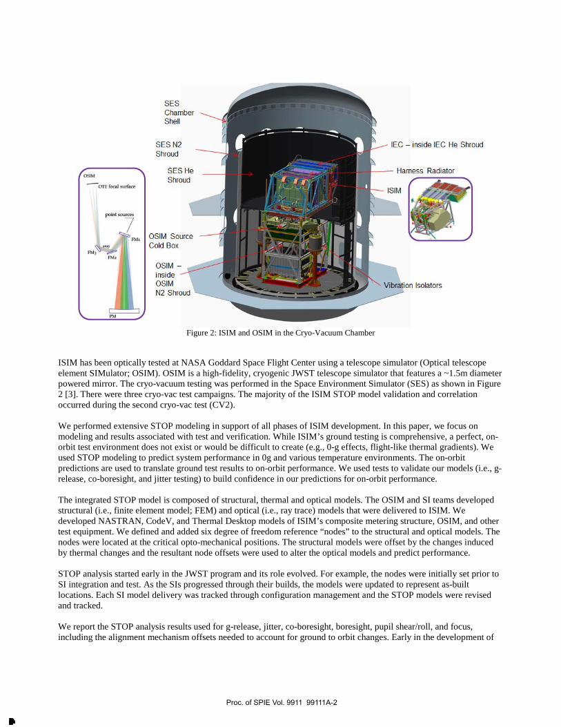
Figure 2: ISIM and OSIM in the Cryo-Vacuum Chamber

ISIM has been optically tested at NASA Goddard Space Flight Center using a telescope simulator (Optical telescope element SIMulator; OSIM). OSIM is a high-fidelity, cryogenic JWST telescope simulator that features a ~1.5m diameter powered mirror. The cryo-vacuum testing was performed in the Space Environment Simulator (SES) as shown in Figure 2 [3]. There were three cryo-vac test campaigns. The majority of the ISIM STOP model validation and correlation occurred during the second cryo-vac test (CV2).

We performed extensive STOP modeling in support of all phases of ISIM development. In this paper, we focus on modeling and results associated with test and verification. While ISIM’s ground testing is comprehensive, a perfect, on-orbit test environment does not exist or would be difficult to create (e.g., 0-g effects, flight-like thermal gradients). We used STOP modeling to predict system performance in 0g and various temperature environments. The on-orbit predictions are used to translate ground test results to on-orbit performance. We used tests to validate our models (i.e., g-release, co-boresight, and jitter testing) to build confidence in our predictions for on-orbit performance.

The integrated STOP model is composed of structural, thermal and optical models. The OSIM and SI teams developed structural (i.e., finite element model; FEM) and optical (i.e., ray trace) models that were delivered to ISIM. We developed NASTRAN, CodeV, and Thermal Desktop models of ISIM’s composite metering structure, OSIM, and other test equipment. We defined and added six degree of freedom reference “nodes” to the structural and optical models. The nodes were located at the critical opto-mechanical positions. The structural models were offset by the changes induced by thermal changes and the resultant node offsets were used to alter the optical models and predict performance.

STOP analysis started early in the JWST program and its role evolved. For example, the nodes were initially set prior to SI integration and test. As the SIs progressed through their builds, the models were updated to represent as-built locations. Each SI model delivery was tracked through configuration management and the STOP models were revised and tracked.

We report the STOP analysis results used for g-release, jitter, co-boresight, boresight, pupil shear/roll, and focus, including the alignment mechanism offsets needed to account for ground to orbit changes. Early in the development of



the ISIM ground test program, we used this analysis to understand the impact of the cryogenic test environment on these parameters. For example, ISIM has a co-boresight alignment requirement that is challenging to measure via test. We used STOP analysis to design the co-boresight test and predict the output. After the test was complete, we used the results to validate the STOP model. Similarly, an ambient g-release test was performed on ISIM using metrology, validating the structural model. These validation tests were a check against possible modeling errors that might contribute to systematic error in our on-orbit performance predictions.

2. STOP INTEGRATED MODEL AND ANALYSIS DESCRIPTION

The ISIM system integrated STOP model is used to perform multi-disciplinary analysis to predict science instrument optical performance changes resulting from mechanical distortions induced by thermal and gravity loading on the system. The STOP analysis is a necessary step for on-orbit requirements verification and instrument optical calibration since the ISIM cryo-vacuum tests include gravity loading and a different temperature environment than predicted for on-orbit operations. In other words, STOP analysis bridges the difference between CV and on-orbit environments. The ISIM system integrated STOP model includes thermal, structural, and optical models that are maintained and exercised by different discipline experts; and the STOP analysis process includes data handoffs between the different discipline experts. Intermediate steps in the STOP analysis process include predicting temperatures and motions at discreet locations in the system. The final results from the STOP analysis are in the form of changes to SI optical performance parameters (shown in Table 1). STOP analyses were completed for the CV2 test and On-orbit configurations. The analysis objectives were:

1. Provide predictions to assess performance with respect to CV test budgets.2. Provide verification support for on-orbit instrument co-boresight stability requirements.3. Provide predictions for supporting ambient ISIM alignment and metrology.4. Provide input for SI on-orbit optical performance parameter predictions (the final results are presented as

gravity and thermal back-outs for ground to on-orbit analysis).

2.1 STOP ANALYSIS PROCESS

The ISIM STOP analysis process includes the use of and coordination between three different discipline (thermal, structural, and optical) models and analyses. The thermal model and analysis predicts temperatures in the on-orbit and on-ground test environments. The structural model and analysis predicts distortions under the predicted temperatures and gravity. The optical model and analysis predicts instrument optical performance under the predicted distortions. Each model and analysis requires a discipline expert and the overall process and coordination between the discipline analyses requires a systems manager. Figure 3 shows the models used by each discipline. Figure 4 illustrates the STOP analysis process flow including the model and analysis boundary for each discipline and data handoffs between disciplines.

Table 1: Science Instrument Optical Performance Parameters and Reported by STOP

Optical Performance Parameter Units Description

Delta Focus millimeters Given in OTE focal space. Defined as minimum rms WFE for analysis field point. Determines focus mechanism movements.

Pupil Shear in V2 and V3 millimeters, % Change from nominal location; mm converted to % of nominal

pupil diameter.

Wave Front Error nanometers (rms) Wave Front Error after focus mechanism compensation.

Pupil Roll degrees Change from nominal location (of +/− orthogonal reference rays).

Boresight Shift in V2 and V3

milliarcseconds Change in field angle (on the sky) to get to the nominal detector (sub-pixel) location.

millimeters Given in OTE focal space. Defined as minimum rms WFE for analysis field point.



ooao

IntegratedThermal Model

ThermalAnalysis

Thermal Desktop Thermal Desktop

IntegratedStructural

Temperatures(thermal)

StructuralAnalysis

NASTRAN NASTRAN

InstrumentOptical Model

Code V, Linear OpticalModel (LOM).Spreadsheet Math Models

OpticalAnalysis

Code V. Linear OpticalIvtodel (LONI).Spreadsheet Math Models

Temperatures(structural)

Map Temps toStructure FEM

Displacementsof Tracking

Perturbati(optical)

GeneratePerturbations

for OpticalModel

OpticalPerformance(WFE: Focus:Pupil Shear:

LOS)

Ideas/TMG.Python

EXCEL

DiscipliMode

Analysis /'Process

IntermediateResults

Thermal ModelModel Format : Thermal Desktop

Structural ModelModel Format: NASTRAN

Optical ModelsModel Format: Code V, LOM*

NIRCam ShortWavelength Channel

MIRI ImagerMode

.!NIRSpec CameraImaging Mode

Fine GuiderChannel A

OSIM

*LOM - Linear Optical Model developedin -house by GSFC optical analysis team.

Figure 3: Models used for STOP analysis

Figure 4: STOP Analysis Process Flow

ISIM STOP analysis also provides ground to on-orbit back-outs for predicting on-orbit performance, calibrating instruments on the ground for on-orbit operations, and verifying that the instruments meet on-orbit performance



CV SI Performance Parameters:From 'SIM Test Measurements

SI Performance Parameter Changes(CV2 Test to On- orbit):

From GSFC STOP Analysis Predictions

STOP Analysis: Gravity Sag Release forCV2 SES Test

( -1.1G in +V1)

STOP Analysis: Thermal /MechEnvironment Variation(On- Orbit- CV2 Test)

SI Performance Parameter Changes:From Changes to KMs After Testing

Inputs from Test

Inputs from SI(JPAn.Jysis

On -Orbit SIPerformance

ParameterPredictions

requirements. The analysis flow for adding ground to orbit STOP back-outs to measured SI performance during ground testing is shown in Figure 5.

Figure 5: Predicting On-orbit Performance Using STOP Ground to On-orbit Back-outs

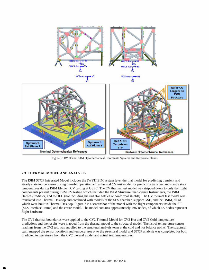
2.2 COORDINATE SYSTEMS

Well defined and understood coordinate systems were essential to the success of the STOP model validation and analysis. Two ISIM optomechanical coordinate systems were defined: Optomechanical Coordinate System A (OMCS-A) and Optomechanical Coordinate System B (OMCS-B). The two coordinate systems are nominally parallel to and offset from the JWST V-coordinate system (see Figure 6). OMCS-A is located at and moves with the OTE/ISIM interface. OMCS-B is located at and moves with the KM (kinematic mount) to ISIM structure interface (+V1 side of the ISIM structure). The relative motion of OMCS-B with respect to OMCS-A represents the rigid body motion of the ISIM Structure with respect to the OTE/ISIM interface plane. For every STOP analysis load case, nodal displacements and SI optical performance parameters are processed with respect to both the perturbed OMCS-A (the OTE/ISIM interface) and the perturbed OMCS-B (the KM to ISIM structure interface). Reference B-CG (or BCG) is a surrogate for OMCS-B and is the average of the targets shown is Figure 6.



OptomechRef Plane A

OptomechRef Plane B

Nominal Optomechanical References

VCS.oll c V7

V1

Ref B -CGTargets on

ISIMStructure

Hardware Optomechanical References

Figure 6: JWST and ISIM Optomechanical Coordinate Systems and Reference Planes

2.3 THERMAL MODEL AND ANALYSIS

The ISIM STOP Integrated Model includes the JWST/ISIM system level thermal model for predicting transient and steady state temperatures during on-orbit operation and a thermal CV test model for predicting transient and steady state temperatures during ISIM Element CV testing at GSFC. The CV thermal test model was stripped down to only the flight components present during ISIM CV testing which included the ISIM Structure, the Science Instruments, the ISIM Harness Radiator, and the IEC (not including the radiator baffles or conformal shields). The CV thermal test model was translated into Thermal Desktop and combined with models of the SES chamber, support GSE, and the OSIM, all of which were built in Thermal Desktop. Figure 7 is a screenshot of the model with the flight components inside the SIF (SES Interface Frame) and the entire model. The model contains approximately 19K nodes, of which 6K nodes represent flight hardware.

The CV2 thermal boundaries were applied to the CV2 Thermal Model for CV2 Hot and CV2 Cold temperature predictions and the results were mapped from the thermal model to the structural model. The list of temperature sensor readings from the CV2 test was supplied to the structural analysis team at the cold and hot balance points. The structural team mapped the sensor locations and temperatures onto the structural model and STOP analysis was completed for both predicted temperatures from the CV2 thermal model and actual test temperatures.



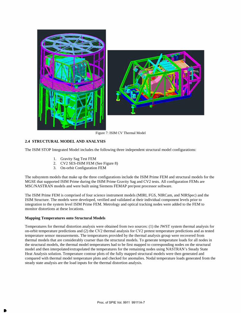
Figure 7: ISIM CV Thermal Model

2.4 STRUCTURAL MODEL AND ANALYSIS

The ISIM STOP Integrated Model includes the following three independent structural model configurations:

1. Gravity Sag Test FEM2. CV2 SES-ISIM FEM (See Figure 8)3. On-orbit Configuration FEM

The subsystem models that make up the three configurations include the ISIM Prime FEM and structural models for the MGSE that supported ISIM Prime during the ISIM Prime Gravity Sag and CV2 tests. All configuration FEMs are MSC/NASTRAN models and were built using Siemens FEMAP pre/post processor software.

The ISIM Prime FEM is comprised of four science instrument models (MIRI, FGS, NIRCam, and NIRSpec) and the ISIM Structure. The models were developed, verified and validated at their individual component levels prior to integration to the system level ISIM Prime FEM. Metrology and optical tracking nodes were added to the FEM to monitor distortions at these locations.

Mapping Temperatures onto Structural Models

Temperatures for thermal distortion analysis were obtained from two sources: (1) the JWST system thermal analysis for on-orbit temperature predictions and (2) the CV2 thermal analysis for CV2 pretest temperature predictions and as tested temperature sensor measurements. The temperatures provided by the thermal analysis group were recovered from thermal models that are considerably coarser than the structural models. To generate temperature loads for all nodes in the structural models, the thermal model temperatures had to be first mapped to corresponding nodes on the structural model and then interpolated/extrapolated the temperatures for the remaining nodes using NASTRAN’s Steady State Heat Analysis solution. Temperature contour plots of the fully mapped structural models were then generated and compared with thermal model temperature plots and checked for anomalies. Nodal temperature loads generated from the steady state analysis are the load inputs for the thermal distortion analysis.



Figure 8: ISIM Prime in CV2 Test Configuration

Structural Model Displacements

Nodal displacements were tracked at locations defined by the optics model and by the metrology group. All locations and displacements are in the JWST V-coordinate system. Several local coordinate systems, all parallel to the JWST V-coordinate system, were defined in the FEM to allow for the removal of rigid body motions and the reporting of final distortion results relative to these local systems.

Nominal Model Verses Stochastic Model

There are two analysis approaches used to determine nodal displacements. The first is the nominal model approach, and the second is a stochastic model approach. The stochastic model assumes a design space that accounts for variation in parameters and is used to predict the model uncertainty due to factors such as material property (e.g. variability and uncertainty in material property values) and geometric (e.g. bond line thickness) variability. The stochastic model provides a mean prediction and an uncertainty band (2-sigma results from a Monte Carlo simulation). As per project guidelines, modeling uncertainty factors (MUF) are used to provide conservatism and margin in thermal distortion predictions. The nominal model assumes a single point in design space where all parameters (material properties and dimensions) are at their nominal values. Nominal model predictions are multiplied by a nominal MUF of 1.6, while stochastic model predictions use of MUF of 1.4. Model validation criteria are tied to these analysis approaches and their associated modeling uncertainty factors. For nominal model predictions, the model validation goal is for predictions multiplied by the 1.6 MUF to bound the measured performance. For stochastic model predictions, the model validation goal is for the predicted uncertainty bandwidth to envelop measured performance including measurement error.



WRY ; : ,(6....e«..>...I.C,

2.5 OPTICAL MODEL AND ANALYSIS

The ISIM STOP optical models were built up from the science instrument optical models delivered by the SI teams. Figure 3 shows the CodeV optical ray traces for each of the science instruments. STOP optical analysis was performed using the optical models constructed in CodeV. Cross checks on the CodeV results were additionally completed using a LOM (Linear Optical Model) developed by the GSFC ISIM Optical Analysis group.

The optical STOP models contain “nodes” that are located at the centers of each optical element and some of the key mechanical interfaces. The structural models include corresponding nodes for tracking 6-DOF motions of the optical elements. The structural analyst supplies nodal displacements (based upon gravity or thermal impacts) to the optical analyst. The optical analyst applies the offsets to the nodes in the models and calculates the impacts to boresight, focus, pupil shear, and pupil roll for each instrument. The models use one field angle per SI optical path. In addition to the CodeV optical SI “node” models, many other models and macros (CodeV command scripts) were used during the analysis. An Excel spreadsheet was used to call up the files and compile the results for each case that was run.

3. STOP AND INTEGRATED MODEL CORRELATION AND VALIDATION

3.1 THERMAL MODEL CORRELATION AND VALIDATION

Thermal Model Validation for Temperature Predictions

Figure 9 is the predicted temperature map for ISIM Prime at CV2 Cold and Figure 10 is the actual temperature map based on temperature sensor measurements on ISIM Prime during the CV2 cold balance test. The predicted verses test max/min temperatures are within +/− 1K and the temperature gradient shapes are nearly identical.

Figure 9: ISIM Prime CV2 Cold Temperature Map (CV2 Thermal Model Prediction)

Figure 10: ISIM Prime CV2 Cold Temperature Map (Test Temperature Measurements)



Load Case: CV2 Test Temperatures - CV2 Predicted Temperatures

Relative to FGS Guider Channel 1

SI

Motion in the sky from Chief RayData

OTE FocalSurface

dXAN =RV3 dYAN =RV2 RSS RSS

(mas) (mas) (mas) (microns)

FGSG1 - - - -

FGSG2 -0.18 0.11 0.21 0.13

NIRISS 0.89 0.12 0.90 0.57

NCSWA 0.20 -1.45 1.47 0.94

NCSWB 0.42 -1.58 1.63 1.04

NS 1.94 -2.88 3.47 2.22

MIRI 0.77 2.25 2.38 1.52

NCLWA 0.41 -1.61 1.66 1.06

NCLWB 0.21 -1.55 1.56 1.00

Relative to Reference A

SI

Motion on the Detector from ChiefRay Data

Motion in the sky from Chief RayData

OTE FocalSurface

dX dY RSS dXAN =RV3 dYAN =RV2 RSS RSS

(microns) (microns) (microns) (mas) (mas) (mas) (microns)

FGSG1 0.36 1.03 1.09 1.46 4.01 4.27 2.72

FGSG2 0.34 1.07 1.12 1.28 4.12 4.32 2.76

NIRISS 0.66 1.13 1.30 2.35 4.13 4.75 3.04

NCSWA 0.94 1.50 1.77 1.66 2.56 3.05 1.95

NCSWB 1.11 1.39 1.78 1.87 2.43 3.07 1.96

NS 0.32 0.53 0.62 3.40 1.13 3.58 2.29

MIRI -0.62 -1.36 1.50 2.23 6.26 6.64 4.24

NCLWA 0.52 0.69 0.86 1.87 2.40 3.04 1.94

NCLWB 0.48 0.69 0.84 1.66 2.46 2.97 1.90

Thermal Model Validation for Optical Performance

The ambient temperature to CV2 Cold temperature is a large change, but the delta between the test vs predicted temperature maps leads to a small boresight shift (as seen in Table 2). These small shifts further validated the CV2 Thermal Model for STOP analysis.

Table 2: SI Boresight Shifts using Thermal Maps (Delta between CV2 Test Measurements and Predictions)

3.2 STRUCTURAL MODEL CORRELATION AND VALIDATION

The ISIM Prime Structural Model is validated by comparing predicted motions from the nominal model1 to test measurements for the ISIM Prime Gravity Sag test. Per section 2.4, the nominal model is validated if the test measurements, including measurement errors, are enveloped by the nominal model predictions multiplied by +/− the nominal MUF or the 95% uncertainty bandwidth multiplied by the MUF (1.4).

The metrology target points tracked for the gravity sag test are separated into two sets: targets on the SI benches and targets on the ISIM Structure. Correlation of target motions on the instruments is critical for validating the structural model since the final ISIM STOP results are directly affected by motions of the instruments relative to Reference B-CG. Correlation of target motions on the ISIM Structure is considered secondary and not needed to validate the ISIM structural model for STOP analysis since motions at these locations do not directly affect instrument performance predictions. Figure 11 (NIRCam is shown as an example) compares FEM predictions with +/− 1.4 MUF error bars to test measurements with +/− 2-sigma error bars for motions at the SI bench metrology points. All predicted motions and measurements are relative to Reference B-CG. Note that motions are relatively large in the V1 direction due to gravity loading in this direction and the fact that the SIs are cantilevered off from the ISIM Structure. The nominal model predictions agree very well with test measurements for all significant motions (> 50 microns) for the SI bench motions. Measurements under 50 microns are under the measurement noise floor. All nominal predictions above 50 microns with their corresponding MUF error bars envelope the test measurements with their corresponding 2-sigma error bars, with the exception of Mod A (-V1 hole) . The measurement error bars for these two target points are uncharacteristically high, thus preventing the prediction error bars from enveloping the measurement error bars; however the nominal predictions at the two locations are within 50 microns of the nominal measurements. The nominal ISIM structural model can therefore be considered validated for STOP analysis.

1 A stochastic model was not validated for gravity sag



o

-50

-100

-150

200

-250

300

-350

MODA +V11 MODA +V13 MODA +V14 MODA +V34 ModA +V3 hole ModA -V1 hole ModB +V3 hole ModB -V1 hole

Test+ Error Bar FEM + Error Bar(40 %)

g.cv>

200

150

100

50

0

50

100

-150

MODA +V11 MODA +V13 MODA +V14 4 ModA +V3 hole M le Mod +V3 hole M. e

Test + Error Bar FEM +Error Bar(40%)

150

100

50

50

100

150

-200

Test + Error Bar FEM + Error Bar(40%)

f1 13I

MODA +V34 ModA +V3 hole ModA -V1 hole Mod +V3 hole ModB -V1 hole

Figure 11: ISIM Gravity Sag Test NIRCam Target Motions (Prediction vs Measurement)



3.3 JITTER MEASUREMENTS AND MODEL CORRELATION

A dynamics study of the OSIM+ISIM system was performed to estimate the magnitude of the image line of sight jitter that would be experienced during the ISIM CV test series. The initial study used input from accelerometer measurements of the vacuum chamber environment and OSIM made during the OSIM CV test program and an OSIM/BIA (Beam Image Analyzer) NASTRAN model. It was correlated with the optical measurements made during the same testing with the BIA camera, with some damping adjustments. Figure 12 shows the resulting jitter estimates and the Power Spectral Density (PSD). The model was subsequently used to predict the jitter expected at each of the SI focal planes, incorporating the ISIM NASTRAN model in place of the BIA. Figure 13 shows the predictions, which indicate near compliance with the stated goal of <0.25 pixel RMS jitter for each SI; the slight exceedance was not deemed an issue, since this was not a requirement, but a goal.

0.0

0.5

1.0

1.5

2.0

2.5

3.0

3.5

4.0

4.5

5.0

1 10 100

micron2/Hz&

microns rms

Frequency (Hz)

OSIM/BIA PhaRet Detector Image Motion Test vs. Analysis(Free vs. Fixed Rollers)

Free PSD Free Rollers Cumulative RMS (4.0 microns rms)Fixed PSD Fixed Rollers Cumulative RMS (4.0 microns rms)Envelope of Fixed & Free PSD Envelope of Fixed & Free: Cumulative RMS (4.6 microns rms)Test Measurement Total RMS (3.6 microns rms)

Analysis≈ 35% > Test

OSIM/BIA PhaRet Predictions: Envelope of Fixed and Free Rollers PSDs

(4.6 microns rms)

OSIM/BIA PhaRetTest Measurement(3.4 microns rms)

OSIM/BIA PhaRet Predictions: Fixed and Free Rollers PSDs

(4.0 microns rms)

Analysis≈ 18% > Test

Figure 12: OSIM/BIA STOP Modeling LOS Jitter Results



0.0

1.0

2.0

3.0

4.0

5.0

6.0

7.0

1 10 100

microns rms

Frequency (Hz)

Detector Image Motion Analysis Predictions: ISIM CV2 vs. OSIM/BIA PhaRetCumulative RMS (Free vs. Fixed Rollers)

SI: Free Rollers PSDs (3.2 microns rms) SI Fixed Rollers PSDs (4.7 microns rms)

SI: Envelope of Fixed & Free Roller PSDs (4.8 microns rms) OSIM/BIA PhaRet: Envelope of Fixed & Free Roller PSDs (4.6 microns rms)

MIRI Requirement (6.3 microns rms) SI Requirement (4.5 microns rms)

MIRI Requirement (6.3 microns rms)

FGS, NIRCam & NIRSpecRequirement

(4.5 microns rms)

SI: Free Rollers (3.2 microns rms)

OSIM/BIA PhaRetEnv. Fixed & Free

Rollers (4.6 microns rms)

SI: Fixed Rollers (4.7 microns rms)

SI: Envelope Fixed & Free Rollers (4.8 microns rms)

Figure 13: OSIM/ISIM STOP Modeling LOS Jitter Predictions

An assessment of the image jitter was made as part of the OSIM+SI checkout phase of CV2 (Figure 14). Over a two day period, jitter was measured with NIRSpec, NIRCam A & B (SW), NIRISS and the two Guiders, but not with MIRI. NIRCam jitter measured slightly above the 0.25 pixel goal, but did not significantly affect the optical performance measurements. Variability was investigated by repeating measurements for the three SIs as shown in the plot. Measurements were made with the OSIM source pulsed at 10 milliseconds (ms), to enable measurement of jitter due to vibration frequencies below ~100 Hz, with ~200 samples. Image sequences were analyzed by fitting subsampled 2-D Gaussians to determine image center and width. Figure 15 shows analysis results from a representative pulsed source data set, showing image center in X and Y detector pixel coordinates vs. time and the image location, in mas projected to the sky, in V2/V3 coordinates with measured RMS jitter indicated.

Instrument milliarcsec pixelsmicrons at OTE

focal surfaceNIRISS 11.6 0.18 7.41NIRSpec 11.8 0.11 7.54NIRSpec (2) 15.2 0.15 9.71Guider 1 12.0 0.18 7.67NIRCam A 9.5 0.30 6.07NIRCam A (2) 10.4 0.33 6.65NIRCam B 9.8 0.31 6.26NIRCam B (2) 9.4 0.30 6.01

Jitter

02468

10121416

NIR

ISS

NIR

Spec

NIR

Spec

(2)

Gui

der 1

NIR

Cam

A

NIR

Cam

A (2

)

NIR

Cam

B

NIR

Cam

B (2

)

Jitte

r (m

as)

Figure 14: Summary of ISIM CV2 Image LOS Jitter Results



05

0.0

.4

-0.5

-15100 200 ]W

Elapsed time (t)X05 X Fur.: 0207 p

400

L

0.0

g

E '05

I

10903

1090.0

m

1089.5

1069.0

c .s mas RMD

10D 100 300 400Elapsedr.(a)

1645 Y per: 0.179 pe

1041-0 1041.5 102.090 (p)

XMS jtilen 0.312 pe

10425

Figure 15: NIRCam A Pulsed Source Analysis Results

Guider measurements were also made with the source in continuous illumination mode, in order to assess the frequency content of the jitter and as a demonstration of a capability to use FGS to assist with tuning of the MIRI Cryo-cooler compressor frequency (to minimize its image jitter contribution). Guider 2 was continuously illuminated with the OSIM source and 8x8 subarrays read out at a cadence of 1.25 ms in CAL mode, while “guiding” with Guider 1. The resulting 50,000 frame observation was subsampled every 10 frames to yield 5000 samples averaged over ~12.6 ms intervals and analyzed by fitting a 2D Gaussian. Total jitter was measured at ~10.7 mas, similar to what is seen in the (10 ms) pulsed illumination measurements. The data were sampled at other intervals, yielding different results and an indication of the jitter power spectrum (Figure 16). Finally, a time-series analysis was performed, sampling at 5-frame (6.3 ms) intervals, indicating the dominant frequency and several other strong contributors (Figure 17). This result is in general agreement with the STOP modeling (See Figure 12, above).



Guider2 Jitter CV2 LD155 Continuous OTP0252NR_cv2c 2014 -08 -1930

20

10

0

b

-10

-20

-30-30 -20 -10 0 10 20

dr2 (silos)FOSFCAL -EXPOSURE -2- 4231032358

30


-20 -10 0 10 20ev2 (mn)

FG3FGIL-EIDPOSVRE-7-4231032358

30


20

10

E 0

b

-10

-20

-30-30 -20 -10 0 10 20

OV2 (man)FOSFCAL -EXPOSURE -2- 4231032358

30

Guider2 Jitter CV2 L0155 Continuous OTP0252NR_cv2c 2014 -08 -1930

20

10

0

b

-10

-20

-30-30 -20 -10 0 10 20

002 (mos)F2511001. -EXPOSURE- 2- 4231032358

30

Guider 2 Jitter LD155 Continuous OTP0252NR_cv2c 2014 -08 -19 Guider 2 Jitter LD155 Continuous OTP0252NR_cv2c 2014 -08 -192.5

2.0

0.5

0 20 40 60 80 100Frequency (Hz)

0.8

c 0.6

3Oa

'14 0.4

0.2

0.0 ll....1 .Lt .

120 0 20 40 60 80 100 120Frequency (Hz)

Figure 16: Guider 2 continuous illumination jitter results with various temporal resampling

Figure 17: Continuous Illumination Jitter Results for Guider 2



43

42

41

40

39

38

37

36

__...

_.__

1. 6 7 11 16 21 26

Measurement Set

+F652 NIRSpec

0.005

0.000

c -0.005

.-0.010

Sé

-0.015

WF -0.020

5 -0.025

1 -0.030

I-0.035pá°

-----l-_,_(A\p--..._ kt..."4_a-- _ /

-0.0406 7 11 16 21 26

Measurement Set

FGR +MROm -tNIRSpK

3.4 INTEGRATED MODEL CORRELATION AND VALIDATION

The ISIM STOP Integrated Model is validated through a comparison of instrument boresight shift predictions and test measurements for the CV2 Overdrive test (CV2 Hot and CV2 Cold). Predictions and measurements for other optical performance parameter shifts (pupil shear, pupil roll, pupil focus, etc.) during the CV2 Overdrive are not included in the comparison for validation since the shifts were too small to measure. The analytical model is considered validated if the test measurements, including measurement errors, are enveloped by the analytical predictions multiplied by the appropriate MUFs.

Instrument boresight orientations and the test system temperatures were measured during CV2 Cold and CV2 Hot. For CV2 Cold, a set of boresight orientations and temperatures were collected for the CV2 Overdrive baseline Set 0. For CV2 Hot, 30 sets of boresight shifts (from CV2 Cold) and temperatures were collected over a period of several days. Temperatures and shifts did not reach steady state until after Set 6 (see temperature and co-boresight shift plots in Figures 18 and 19).

Figure 18: Measured SI Temperatures during CV2 Hot

Figure 19: Measured V2 Boresight Shifts (from CV2 Cold) during CV2 Hot



That Measwemert wth 2 -Sigma Erri Nominal Prediction( MUF =1.6) Prediction with 2-Sigma Error

c9

re

m

so

o

o

FGS-G1 FGS -G2 NIRISS MIRI NRS2 NCSWA NCSWB NCLWA NCLWB

Measured shifts for Sets 13 through 30, excluding Sets 12, 18, and 292, were then averaged for a single value shift in boresight from CV2 Cold to CV2 Hot for each instrument. The measured temperatures for Sets 13 through 30 were also combined for an average CV2 Hot temperature map. STOP analysis was then completed for the measured CV2 Overdrive temperature load (CV2 Hot – CV2 Cold) using the LOM for the optical analysis portion (see Figure 4). Boresight shifts relative to Reference A and co-boresight shifts relative to FGS-1 were recovered for each instrument. Additionally, stochastic analysis was completed to determine 2-sigma error bounds on structural model distortion predictions and carried through the optical analysis for 2-sigma error bars on the optical performance results. Figures 20 and 21 show instrument co-boresight shifts relative to FGS-1. The nominal predictions include a 1.6 MUF and the stochastic predictions include +/− 1.4 x 2-sigma error bars. The test measurements include +/− 2-sigma error bars processed from the measured data in Sets 13 through 30 (excluding Set 12, 18, and 29). The test errors determined at the CV2 Hot temperatures were also multiplied by √2 to account for CV2 cold baseline measurement errors. As can readily be seen in the plots, analytical predictions and measurements agree well for motions relative to FGS-1 and Reference A. With the exception of predictions from the nominal model for instrument V3 shifts relative to FGS-1, the test measurements with error bars are generally enveloped by the analytical predictions. Temporal drifts in V3 shifts were observed in the CV2 Hot measurement sets. It is believed that these drifts are not due to temperature drifts during CV2 Hot and prevent correlation of the STOP model for V3 shifts with respect to FGS-1. Note also that the analytical error bars are different between co-boresight shifts relative to FGS-1 and boresight shifts relative to Reference A for each instrument. This is due to ISIM KM and OSIM error contributions included in the shifts relative to Reference A and the propagation of FGS-1 error bars in all of instrument shifts relative to FGS-1.

Preliminary Verification of On-orbit Co-boresight Shift Requirements

There are various requirements for ISIM co-boresight stability, but the driving requirements during on-orbit operations require pointing stability to be < 30 mas/K. Scaling the derived on-orbit 30 mas/K pointing stability requirement by the average temperature change across ISIM Prime during CV2 Overdrive (4.3 K), a test co-boresight stability limit is determined to be 130 mas (= 4.3 K x 30 mas/K). As can readily be seen in Figures 20 and 21, the co-boresight shifts for the CV2 Overdrive are well inside the limits (+/−130 mas limits in the plots).

Figure 20: CV2 Overdrive Co-boresight Shift in V2 Relative to FGS-1

2 These sets were excluded because of loss/bad data.



Test Measurement wth 2 -Sigma Error Nominal Prediction( MUFTI 6) Prediction with 2 -Sgma Error

130

110

fo

-10

IIINRS2 NCSWA NCSWB NCLWA NCLWB

i IiFGS-G1 FGS-G2 NIRISS MIRI

CV -Hot

Avg Temp

On -orbit Hot (EOL)

Hot Attitude

On-orbit Ho : OL) Col Attitude

$CV-Cold

delta -T = 10K

ñ -orbit Cold (EOL)

On -orbit Cold (BOL)

BOL Mission Life EOL

* CV2 Cold z CV3 Cold z On -Orbit Cold BOL

STOP Thermal Backout is determined by using the node changes betweenthe average temp of CV -Cold and On -Orbit Hot (BOL)

Figure 21: CV2 Overdrive Co-boresight Shift in V3 Relative to FGS-1

4. GROUND TO ON-ORBIT BACKOUTS

4.1 OPTICAL STOP RESULTS

The two cases that make up the ground (CV test environment) to on-orbit back-outs are gravity and thermal. The gravity case was created by applying a 1g load in the +V1 direction to the ISIM in SES model. The thermal case was created (in general) by using the On-orbit Hot BOL (beginning of life) thermal map and subtracting the CV2 Cold thermal map. Figure 22 shows the general relationship of the thermal cases and how the thermal back-out is generated. Results for the gravity cases are given in Figures 23. The results for each SI include motion on the sky (boresight change) with respect to Guider 1 and with respect to Reference BCG. Other results listed in the figures are focus, pupil shear, and pupil roll. All results except “pre-opt” focus values are after focus optimization using the focus mechanisms. The pupil values for NIRCam are after the focus mechanism optimization for focus and pupil shear (since the NIRCam focus mechanism can tip/tilt to correct pupil misalignments).

Figure 22: Understanding Thermal Cases for Ground to On-orbit Thermal Back-out



SIdXAN=dRV3

(mas)dYAN=dRV2

(mas)dXAN=dRV3

(mas)dYAN=dRV2

(mas)Radial (mm)

Radial (%)

FGSG1 - - -66.83 83.82 -0.41 0.78 0.51 0.00FGSG2 0.6 11.1 -66.2 94.9 -0.39 0.79 0.52 0.04NIRISS -51.9 -180.7 -118.7 -96.9 -0.34 0.72 0.47 -0.21NCSWA 180.7 202.8 113.8 286.6 -0.36 0.00 0.00 -0.02NCSWB 184.8 205.4 117.9 289.2 -0.35 0.00 0.00 0.16NS -243.2 80.5 -310.1 164.3 -0.18 0.89 0.59 0.03MIRI 122.5 -196.2 55.7 -112.4 -0.15 0.07 0.05 -0.02NCLWA 180.1 124.2 113.3 208.0 -0.36 1.34 0.89 -0.02NCLWB 211.1 200.9 144.2 284.7 -0.35 1.08 0.71 0.22

1with tricontagon mask

Boresight Changewith respect to Guider 1 Motion in the sky (mas)

Focus1

Pre-Opt Delta (mm, at OTE focal plane)

Pupil Roll (amin)

Pupil Shear (at OSIM Exit Pupil)

Figure 23: Optical Performance STOP Results for +V1 Gravity in SES (MUF = 1.4)

Analysis back-outs are used to translate optical performance CV (SES chamber) test results to on-orbit values (no gravity and different thermal environments). The back-outs are used for on-orbit predictions (no MUF applied) and comparison to on-orbit requirements (MUF applied). For the gravity case, the structural analysis offsets provided to the optical analyst are for the gravity condition during CV. To generate gravity back-outs, the optical analysis results require a sign change for gravity release from CV to On-orbit. For the thermal case, the structural analysis offsets provided to the optical analyst is the thermal environment change from CV to On-orbit. The thermal case therefore does not require a sign change. Figure 5 shows the process for translating CV2 performance measurements to on-orbit predictions. The optical results for the gravity and thermal cases (no MUF) are combined to generate ground to on-orbit back-outs (see Figure 24). The back-outs are deltas from the best focus locations determined during CV testing. As mentioned above, the NIRCam focus mechanisms have a tip/tilt capability that is used to realign the pupil. The NIRCam shortwave (SW) and longwave (LW) share a focus mechanism. Locations were determined by optimizing the SW channel. For the back-out analysis, there is no MUF added because the intent is to accurately predict the performance. In other analyses, a more bounding approach is necessary. To confirm that requirements are met, a MUF is used.

Boresight Change with respect to BCG

Motion in the sky (mas)

SI XAN (mas) YAN (mas)Radial (mm)

Radial (%)

FGSG1 26.1 -99.8 0.56 0.37FGSG2 24.5 -104.3 0.57 0.37NIRISS 52.1 35.0 0.52 0.34NCSWA -74.7 -191.2

-0.03-0.03-0.13-0.12 0.00 0.00

-0.03-0.040.120.01

NCSWB -76.0 -192.9 - 0.00 0.00 -NS 198.6 -115.7 - 0.63 0.41 -MIRI 116.5 186.5

0.110.05NA 0.25 0.17

0.110.010.22

NCLWA -56.0 -185.6 0.94 0.62NCLWB -94.5 -187.5

-0.12-0.11 0.76 0.50

-0.01-0.19

Pupil Shear (at OSIM Exit Pupil)

BoresightMotion in the sky (mas) Pupil

Roll (amin)

Focus mech movement to minimum rms

at SI focal plane1 (mm)

1with tricontagon mask

Figure 24: Back-outs/offsets for Translating CV Performance to On-orbit Predictions (No MUF)



5. CONCLUSIONS

This paper shows a summary of the ISIM STOP Analysis work done on the JWST. The modeling and analysis have been validated by correlating analytical predictions to test results from the CV2 Overdrive and the ISIM Prime Gravity Sag tests. Both the CV2 test results and the validated STOP analysis demonstrate verification for a number of SI optical performance requirements levied on ISIM. STOP analysis was also completed for ground to on-orbit back-outs. The back-outs are used for instrument calibration for on-orbit operation and for verification of additional SI optical performance requirements.

ACKNOWLEDGEMENTS

The work presented in this paper is based on results from various ISIM test campaigns, conducted at the NASA Goddard Space Flight Center (GSFC). We are indebted to the ISIM test personnel for test planning & execution, real-time data review, Science Instrument support, facilities maintenance, and overall support during the tests. More generally, the collective effort and dedication of a much larger group of people made this work possible. The authors gratefully acknowledge the contributions of optical, mechanical, electrical, and systems engineers, managers, and scientists associated with the James Webb Space Telescope project as a whole, and the Integrated Science Instrument Module element, the Science Instruments within ISIM [namely the FGS Guider and NIRISS, provided by the Canadian Space Agency (CSA) and COM DEV; MIRI, provided by the European Consortium with the European Space Agency (ESA), and by the NASA Jet Propulsion Laboratory (JPL); NIRCam, provided by the University of Arizona and Lockheed Martin; and NIRSpec, provided by ESA, with components provided by NASA GSFC], and the OSIM OGSE in specific. Without the early and continuous modeling efforts and support from the Science Instrument teams, none of this work would have been possible. Broadly, JWST is led by NASA and we acknowledge the leadership from the JWST Project Office at GSFC and the valuable contributions from all NASA centers and Headquarters. JWST is also an international collaboration and we acknowledge the contributions of Science Instruments and personnel by CSA & ESA, along with their supporting contractors and partner universities. While the list of contributors is long, we would be remiss if we did not explicitly acknowledge the early and significant contributors from the optics side including Mark Wilson, Philip Young, and Brent Bos. John Johnston was critical to the early understanding of the STOP analysis with regards to the system requirements and performance. Scott Rohrbach’s optical system knowledge was essential for understanding the ISIM requirements and how they correlated to the STOP results.

This work is supported by the James Webb Space Telescope project at NASA Goddard Space Flight Center.

REFERENCES

[1] P. A. Lightsey, C. Atkinson, M. Clampin, and L.D. Feinberg, “James Webb Space Telescope: large deployablecryogenic telescope in space,” Optical Engineering 51, 011,003-1-011,003-19 (2012).

[2] M. A. Greenhouse, V Balzano, P. Davila, M. P. Drury, J. L. Dunn, S. D. Glazer, E. Greville, G. Henegar, E. L.Johnson, R. Lundquist, J. McCloskey, R. G. Ohl IV, R. A. Rashford, M. F. Voynton, “Status of the James WebbSpace Telescope Integrated Science Instrument Module System,” Proc. SPIE 8146, 814606 (2011).

[3] D. Sabatke, J. Sullivan, S. Rohrbach, D. Kubalak, “Ray-tracing for coordinate knowledge in the JWST IntegratedScience Instrument Module,” Proc. SPIE 9293, 929306-3 (2014).



Documents

Structural, thermal, and optical performance (STOP ... · The James Webb Space Telescope includes t he Integrated Science Instrument Module ... The final results from the STOP analysis