Embed Size (px)
Citation preview

The University of MaineDigitalCommons@UMaine
Electronic Theses and Dissertations Fogler Library
2006
Structural Testing and Analysis of HybridComposite/Metal Joints for High-Speed MarineStructuresJean Paul Kabche
Follow this and additional works at: http://digitalcommons.library.umaine.edu/etd
Part of the Mechanical Engineering Commons
This Open-Access Dissertation is brought to you for free and open access by DigitalCommons@UMaine. It has been accepted for inclusion inElectronic Theses and Dissertations by an authorized administrator of DigitalCommons@UMaine.
Recommended CitationKabche, Jean Paul, "Structural Testing and Analysis of Hybrid Composite/Metal Joints for High-Speed Marine Structures" (2006).Electronic Theses and Dissertations. 274.http://digitalcommons.library.umaine.edu/etd/274
STRUCTURAL TESTING AND ANALYSIS OF HYBRID
COMPOSITE/METAL JOINTS FOR HIGH-SPEED
MARINE STRUCTURES
BY
Jean Paul Kabche
B.S. University of Maine, 1999
M.S. University of Maine, 200 1
A THESIS
Submitted in Partial Fulfillment of the
Requirements for the Degree of
Doctor of Philosophy
(in Mechanical Engineering)
The Graduate School
The University of Maine
May, 2006
Advisory Committee:
Vincent Caccese, Associate Professor of Mechanical Engineering, Advisor
Donald Grant, R. C. Hill Professor and Chairman of Mechanical Engineering
Senthil Vel, Assistant Professor of Mechanical Engineering
William Davids, Associate Professor of Civil Engineering
Larry Thompson, Principal Research Engineer, Applied Thermal Sciences
STRUCTURAL TESTING AND ANALYSIS OF HYBRID
COMPOSITEJMETAL JOINTS FOR HIGH-SPEED
MARINE STRUCTURES
By Jean Paul Kabche
Thesis Advisor: Dr. Vincent Caccese
An Abstract of the Thesis Presented in Partial Fulfillment of the Requirements for the
Degree of Doctor of Philosophy (in Mechanical Engineering)
May 2006
The implementation of composite materials in engineering applications has
observed a rapid increase over the last few decades. The U.S. Navy currently has an
objective to enhance its future naval capabilities by developing hull-forms with advanced
materials, including composites. Speed can be increased by reduction in weight and by
incorporating innovative shaping of the hull-form, which can potentially be achieved with
composites. Any naval vessel using composite materials for structural components will
require hybrid connections of some sort, where composite sections are joined to metallic
sub-structures. Joints are critical regions in the design of hybrid systems, as failures
typically occur at joints and interfaces and rarely within the bulk of the structure.
Accordingly, this effort presents the development of a watertight, hybrid composite/metal
bolted joint, for cases where the panels are removable.

An experimental study was conducted to quantify the performance of numerous
hybrid joints with various geometries, loaded in flexure. The test results showed that, for
resisting bending loads, joints with doubler plates can be made stronger and rotationally
stiffer than standard bolted joints while also mitigating opening of the joint, thereby
improving the ability to seal the connection for watertight integrity. Based on these
results, a joint geometry was selected and incorporated into the hydrostatic testing of a
large-scale, four-panel assembly. A linear response of the system was observed up to its
design pressure load of 82.74 kPa. Damage initiated as stiffener delamination at 1.4
times the design load. After failure of several stiffeners, the hybrid assembly withstood
up to 3 times its design load without leakage. Hence, the response of the hybrid joint
employed was deemed successful.
Numerical analysis of the joints and the hybrid assembly are also presented.
Simplified shell finite element models were developed at both local and global levels.
These models were used to estimate the joint stiffness and good correlation with the test
results was observed. To study the local stresses at the joint region and to provide an
estimate of failure initiation, detailed generalized plane strain contact models were
created to capture the three-dimensional effects of the connection.

DEDICATION
For my family. . .

ACKNOWLEDGEMENTS
Upon completion of this work, I would like to thank my thesis advisor, Dr. Vince
Caccese, for his constant help and guidance throughout the research and dissertation
writing process. I would also like to acknowledge the help of the Advisory Committee
for taking the time to thoroughly read and critique this dissertation. In addition, I would
like to thank all of the undergraduate students who contributed to this project, in
particular, Marilyn Nichols, Mike Robinson, Dave Cote and Ethan Brush. Special thanks
to Keith Berube for his guidance in many research aspects, Josh Walls for his assistance
during the testing process, Randy Bragg and Ryan Beaumont for their invaluable
laboratory assistance.
I gratefully acknowledge the financial support provided by the Office of Naval
Research under grant number NO00 14-0 1 - 1-09 16, as well as additional funding provided
by the University of Maine Summer Graduate Research Fellowship and the Association
of Graduate Students.
My endless thanks go to Laurita "Little Bird" Azevedo, for her sincere support,
encouragement and caring during this long process.
Finally, I would like to thank my family, for always being a source of love,
encouragement and motivation in all aspects of my life. Their constant support and
understanding during these years has been fundamental in furthering my education. I
certainly hope that their efforts are partially reflected through the completion of this
work.

TABLE OF CONTENTS
. . DEDICATION ........................................................................................................... 11
... ACKNOWLEDGEMENTS .................................................................. 111
LIST OF TABLES ............................................................................ ix
LIST OF FIGURES ........................................................................... xi
................................................................... 1 . INTRODUCTION 1
1.1. Overview ......................................................................... 1
1.2. Project Background and Objectives .......................................... 3
1.3. Objectives, Organization and Scope ......................................... 7
2 . LITERATURE REVIEW ........................................................... 9
............................................. 2.1. Naval Structures and Composites 9
2.2. Material Systems and Manufacturing Methods ............................. 10
2.3. Hybrid Structures for Marine Applications ................................. 12
2.4. Bolted Joints ..................................................................... 15
2.4.1. Hybrid Compositehfetal Bolted Joints ............................. 18
2.4.2. Failure Modes in Composite Bolted Joints ....................... 18
2.4.3. Composite Bolted Joints Subjected to Axial and Flexure
............................................................... Loading 22
2.4.4. Composite Bolted Joints Subjected to Fatigue Loading ........ 25
2.5. Summary of the Literature Findings and Research Significance ........... 28

3 . STRUCTURAL TESTING OF HYBRID JOINTS UNDER
............................................................ FLEXURAL LOADING 30
......................................................... 3.1. Joint Testing Rationale 30
........................................................ 3.2. Joint Testing Objectives 30
.................................. 3.3. Hybrid Joint Configuration and Geometry 32
......................................................... 3.3.1. Bolted Joints 32
3.3.2. Bolted Joints with Doubler Plates ................................ -35
....................................... 3.4. Materials and Test Article Fabrication 42
....................................................... 3.5. Joint Testing Procedures 45
3.5.1. Test Setup ............................................................. 45
...................................................... 3.5.2. Testing Method 48
...................................................... 3.5.3. Instrumentation 50
3.5.4. Data-Acquisition Configuration .................................... 54
3.6. Joint Testing Results ............................................................ 55
3.6.1. Cyclic Response: Load versus Displacement Curves ........... 56
3.6.2. Cyclic Response: Load versus Strain Curves .................... 62
3.6.3. Load versus Displacement Envelopes ............................ 66
3.6.3.1. Load versus Displacement Envelopes for
.............................................. Bolted Joints 66
3.6.3.2. Load versus Displacement Envelopes for
Bolted Joints with Doubler Plates ...................... 68
........................................................ 3.6.4. Failure Modes 7 1

................................. 3.6.5. Damage Load and Ultimate Load 76
................................. 3.6.6. Initial Joint Rotational Stiffness, J 79
..................... 3.7. Hybrid Joint Selection for Large-Scale Panel Testing 82
4 . STRUCTURAL TESTING OF A LARGE-SCALE, HYBRID PANEL
ASSEMBLY UNDER HYDROSTATIC PRESSURE LOADING .............. 84
......................................................... 4.1. Panel Testing Rationale 84
........................................................ 4.2. Panel Testing Objectives 84
........................................... 4.3. Geometry of the Hybrid Panel Assembly 85
......................... 4.3.1. Component Panel Design and Geometry 87
........................... 4.3.2. Description of the Hybrid Joint Region 91
....................................... 4.4. Materials and Test Article Fabrication 94
....................................................... 4.5. Panel Testing Procedures 98
............................................................. 4.5.1. Test Setup 98
...................................................... 4.5.2. Testing Method 103
...................................................... 4.5.3. Instrumentation 105
.................................... 4.5.4. Data-Acquisition Configuration 116
........................................................... 4.6. Panel Testing Results 118
................................. 4.6.1. Load versus Displacement Curves 118
............................................. 4.6.2. Displaced Panel Shapes 123
4.6.3. Correlation of Displaced Panel Shapes to
....................................................................... Photogrammetry 124
.......................................... 4.6.4. Load versus Strain Curves 128
........................................................ 4.6.5. Failure Modes 135

5 . FINlTE ELEMENT ANALYSIS OF HYBRlD BOLTED
................................................................................................. ASSEMBLY 138
......................................................................... 5.1. Rationale 138
........................................................ 5.2. Finite Element Analysis Objectives 140
................................. 5.3. Local Finite Element Model (Shell Model) 141
.................................... 5.3.1. Finite Element Model Description 142
...... 5.3.2. Computing the Effective Properties of the Hybrid Region 146
............................................... 5.3.3. Local Shell Model Verification 150
.................... 5.4. Global Finite Element Model of Isolated Stiffened Panels 155
................................ 5.5. Global Finite Element Model of Hybrid Assembly 163
............................... 5.5.1. Global Finite Element Model Description 163
...................................... 5.5.2. Modeling of the Hybrid Joint Region 166
........................................ 5.5.3. Global Shell Model Verification 1 6 8
..................... 5.5.4. Parametric Study of Global Structural Response 178
...................... 5.5.4.1. Effect of the Doubler Plate Thickness 179
5.5.4.2. Effect of the Composite Thickness ........................... 182
5.5.4.3. Effect of the Flange Thickness (W8x31 and
W14x53 I-Beams) ..................................................... 185
........... 5.6. Generalized Plane Strain Finite Element Model of Hybrid Joint 191
........................... 5.6.1. Generalized Plane Strain Model Description 191
............................................................... 5.6.2. Contact Modeling 1 9 5
.................................................................... 5.6.3. Modeling the Bolt 198
................................................................... 5.6.4. Model Verification 202

5.6.5. Generalized Plane Strain Modeling Results ............................ 204
5.6.6. Damage Initiation Prediction ................................................... 217
6 . CONCLUSIONS AND RECOMMENDATIONS ............................... 222
6.1. Sub-component Joint Testing ........................................................... 222
6.2. Hybrid Panel Assembly Testing ........................................................ 224
.......................................... 6.3. Finite Element Analysis of Hybrid Joints 225
REFERENCES ................................................................................ 227
APPENDICES ................................................................................. 231
Appendix A . Material Specifications ....................................................... 231
Appendix B . Instrumentation Specifications ..................................... 237
Appendix C . Load versus Outer Displacement Plots of Hybrid Joints ......... 239
Appendix D . Load versus Middle Displacement Plots of Hybrid Joints ...... 267
Appendix E . Load versus Inner Displacement Plots of Hybrid Joints ......... 295
Appendix F . Load versus Strain Plots of Hybrid Joints ................................ 323
Appendix G . Assembly of Stiffened Panels and Doubler Plates onto
the Hydrostatic Test Tank ........................................................ 351
Appendix H . Load versus Displacement Plots of Stiffened Panels .............. 362
BIOGRAPHY OF THE AUTHOR ............................................................................ 368
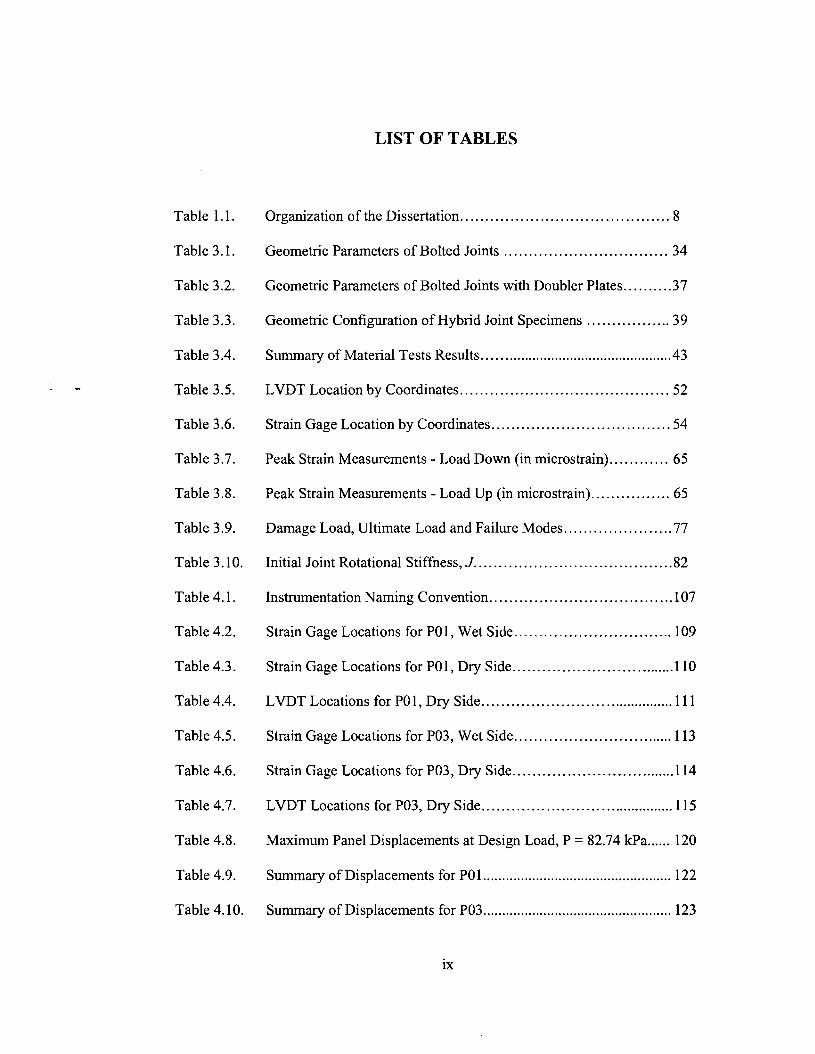
LIST OF TABLES
Table 1.1.
Table 3.1.
Table 3.2.
Table 3.3.
Table 3.4.
Table 3.5.
Table 3.6.
Table 3.7.
Table 3.8.
Table 3.9.
Table 3.10.
Table 4.1.
Table 4.2.
Table 4.3.
Table 4.4.
Table 4.5.
Table 4.6.
Table 4.7.
Table 4.8.
Table 4.9.
Table 4.10.
.......................................... Organization of the Dissertation 8
................................. Geometric Parameters of Bolted Joints 34
.......... Geometric Parameters of Bolted Joints with Doubler Plates 37
Geometric Configuration of Hybrid Joint Specimens ................. 39
................................................. Summary of Material Tests Results 43
LVDT Location by Coordinates .......................................... 52
Strain Gage Location by Coordinates ................................... -54
Peak Strain Measurements - Load Down (in microstrain) ............ 65
Peak Strain Measurements - Load Up (in microstrain) ................ 65
Damage Load, Ultimate Load and Failure Modes ...................... 77
Initial Joint Rotational Stiffness, J ........................................ 82
Instrumentation Naming Convention ..................................... 107
Strain Gage Locations for POI, Wet Side ................................ 109
Strain Gage Locations for POI, Dry Side .................................. 110
LVDT Locations for POI, Dry Side .......................................... I l l
Strain Gage Locations for P03, Wet Side ................................. 113
Strain Gage Locations for P03, Dry Side .................................. 114
.......................................... LVDT Locations for P03, Dry Side 115
Maximum Panel Displacements at Design Load, P = 82.74 kPa ...... 120
.................................................. Summary of Displacements for PO1 122
Summary of Displacements for PO3 .................................................. 123

Table 4.1 1 .
Table 4.12.
Table 4.13.
Table 4.14.
Table 4.15.
Table 4.16.
Table 4.17.
Table 4.18.
Table 5.1.
Table 5.2.
Table 5.3.
Table 5.4.
Table 5.5.
Table 5.6.
Table 5.7.
Table 5.8.
Table A . 1 .
Table A.2.
Table A.3.
Table B . 1 .
Table B.2.
Summary of Displacements for P02. PO4 and I-beams ..................... 123
Strain Readings for Pol. Dry Side. (in microstrain) .......................... 130
Strain Readings for PO 1. Dry Side. Joint Region (in microstrain) ..... 131
Strain Readings for PO 1. Dry Side. I-beam Flanges (in ps) ............... 131
Strain Readings for P03. Dry Side (in microstrain) ........................... 134
Strain Readings for P03. Dry Side. Joint Region (in microstrain) ..... 134
Strain Readings for P03. Dry Side. I-beam Flanges (in ps) .............. 134
Strain Readings at the I-beam Intersection (in microstrain) .............. 134
Vertical Displacement of Joint Models at P = 4.45 KN .................... 153
Strain Results for Joint Models (E, ) at P = 4.45 KIV .......................... 154
Orthotropic Lamina Properties for an EGNE System ....................... 156
Lamination Scheme for Stiffened Panels ........................................... 156
Vertical Displacements of Isolated Panels at P = 82.74 kPa ............. 160
Approximate Geometry of the I-Beam Sections in the
Hybrid Assembly ............................................................................... 168
Orthotropic Lamina Properties for a 55% v.f. EGNE System .......... 194
Orthotropic Material Properties in Terms of the Elastic
Stiffness Mah-ix. C. in GPa ................................................................ 195
DIAB Divinycell H80 Foam .............................................................. 231
DERAKANE 8084 Vinyl Ester Resin ............................................... 233
Brunswick Technologies. Inc . E-Glass Fibers ................................... 235
Lebow 3 174 Load Cells ..................................................................... 237
Macrosensors Linear Variable Displacement Transducers ................ 238

LIST OF FIGURES
Figure 1.1.
Figure 1.2.
Figure 1.3.
Figure 1.4.
Figure 2.1.
Figure 2.2.
Figure 2.3.
Figure 2.4.
Figure 2.5.
Figure 2.6.
Figure 2.7.
Figure 2.8.
Figure 2.9.
Figure 2.10.
Figure 3.1.
Figure 3.2.
................................... Hybrid High-speed Vessel. MIDFOIL 2
The MACH Concept: Blending of Marine and Space
................................................................. Technologies 4
...................................... Monolithic Composite Construction 5
............................................... MACH Concept Schematic -7
Applications of Composite Materials for Naval Structures
.................................................................................. [Mouritz, 200 11 10
Composite Panels Attached to a Metallic Sub-Frame [Berube
............................................................................. and Caccese, 1 9991 13
Composite Sections Attached to Metallic Sections [Berube and
................................................................................... Caccese, 19991 14
.................................. Bolted Joint: Single-Lap Configuration 17
................................. Bolted Joint: Double-Lap Configuration 17
.................................................. Net Section Failure Mode 19
...................................................... Bearing Failure Mode 20
................................................... Shear-Out Failure Mode 20
........................................................... Bolt Failure Mode 21
Average Joint Load Capacities for Different Bolt
............................................ Pre-Loads [Cooper and Turvey, 19951 22
................................... Schematic of the Bolted Joint Concept 33
........................................ Baseline Geometry of Bolted Joints 33
Figure 3.3.
Figure 3.4.
Figure 3.5.
Figure 3.6.
Figure 3.7.
Figure 3.8.
Figure 3.9.
Figure 3.10.
Figure 3.1 1 .
Figure 3.12.
Figure 3.13.
Figure 3.14.
Figure 3.15.
Figure 3.16.
Figure 3.17.
Figure 3.18.
Figure 3.19.
Figure 3.20.
Figure 3.2 1 .
Figure 3.22.
Figure 3.23.
Figure 3.24.
Bolted Joint Specimens with Steel Gussets .............................. 35
Schematic of the Bolted Joint with Doubler Plate Concept ............ 36
Baseline Geometry of Bolted Joints with Doubler Plates .............. 36
Bolted Joints with Doubler Plates ........................................ 38
Photographs of Bolted Joint Specimens .................................... 40
.......... Photographs of Bolted Joint Specimens with Doubler Plates 41
VARTM Fabrication Setup ................................................ 44
Tapered EGNE Composite Specimens .................................. 45
................................................... Experimental Test Setup 46
Dimensions of the W 12 Load Beam and Load Heads
(in meters) .......................................................................................... 47
Connection of Test Article to Reaction Frame and Load Heads ...... 47
Schematic of the Testing Method .......................................... 48
Typical Reversed Cyclic Loading History .............................. 49
........................... Load Cell Setup Schematic (Exploded View) 50
....................................................... LVDT Configuration 51
LVDT Setup on Reaction Frame .......................................... 52
Strain Gage Configuration ................................................. 53
Data-Acquisition System Schematic ...................................... 55
Typical Load versus Displacement Curve ............................... 56
.......... Load versus Displacement Curves for BT-6 (Outer LVDTs) 58
Load versus Displacement Curves for DS-4 (Outer LVDTs) .......... 58
Load versus Displacement Curves for BT-6 (Middle LVDTs) ........ 60

Figure 3.25.
Figure 3.26.
Figure 3.27.
Figure 3.28.
Figure 3.29.
Figure 3.30.
Figure 3.3 1 .
Figure 3.32.
Figure 3.33.
Figure 3.34.
Figure 3.35.
Figure 3.36.
Figure 3.37.
Figure 3.38.
Figure 3.39.
Figure 3.40.
Figure 3.4 1 .
Figure 3.42.
Figure 3.43.
Load versus Displacement Curves for DS-4 (Middle LVDTs) ........ 60
Load versus Displacement Curves for BT-6 (Inner LVDTs) .......... 61
......... Load versus Displacement Curves for DS-4 (Inner LVDTs) 62
Load versus Strain Curves for BT.6 ...................................... 63
Load versus Strain Curves for DS.4 ...................................... 63
Load versus Displacement Envelopes for Protruding-head
Bolted Joints ................................................................. 67
Load versus Displacement Envelopes for Tapered-head
Bolted Joints ................................................................. 67
Specimen BP-1 Displaced Downward at Cycle Set 10 ................ 68
Load versus Displacement Envelopes for Bolted Joints with
Short and Medium Doubler Plates ................................................. 69
Load versus Displacement Envelopes for Bolted Joints with
Long Doubler Plates ........................................................ 70
Specimen DM- 1 Displaced Downward at Cycle Set 10 .................. 71
Failure Modes BLSC and BUDE .......................................... 72
Failure Mode NSBL ......................................................... 73
Failure Mode GSDE ........................................................ 73
Failure Mode FFIB ......................................................... 74
Failure Mode DUEC ........................................................ 74
Failure Mode DLEC ........................................................ 75
Failure Mode DACB ................................................................ 75
Damage Load and Ultimate Load ......................................... 77

Figure 3.44.
Figure 3.45.
Figure 4.1.
Figure 4.2.
Figure 4.3.
Figure 4.4.
Figure 4.5.
Figure 4.6.
Figure 4.7.
Figure 4.8.
Figure 4.9.
Figure 4.10.
Figure 4.1 1 .
Figure 4.12.
Figure 4.13.
Figure 4.14.
Figure 4.15.
Figure 4.16.
Figure 4.17.
Figure 4.18.
Typical Moment versus Rotation Curve for Cycle Set 1 ............... 80
Loading of Test Article in Flexure ........................................ 81
Hybrid LiRing Body Schematic ........................................... 85
Hybrid Panel Assembly and Hydrostatic Test Tank
Configuration ................................................................. 86
Geometry of Hybrid Panel Assembly (in meters) ....................... 86
Geometry of the Small Panels - POI, Top View (in meters) .......... 87
Geometry of the Small Panels - POI, Cross-Sectional View
(in mm) ......................................................................... 88
Hat-Stiffener Geometry for Small Panels (in mm) ..................... 88
Geometry of the Large Panels - P03, Top View (in meters) ............ 89
Geometry of the Large Panels - P03, Cross-Sectional View (in
mm) ............................................................................. 90
Hat-Stiffener Geometry of Large Panels (in mm) ....................... 90
Hybrid Assembly Schematic (Exploded View) ............................. 91
Photograph of Short Doubler and Foam Insert Joint (DS-4) .......... 92
Schematic of Hybrid Joint Details and Geometry (in mm) ............ 93
Fabrication of Small Panels ............................................... -95
Lamination Sequence for Hat-Stiffener Fabrication ................... 95
Large Panel Fabrication, Stage 1 : Flat Panels ........................... 96
Large Panel Fabrication, Stage 2: Hat-Stiffeners ...................... 97
Schematic of Hydrostatic Test Setup ..................................... 98
Geometry of the Hydrostatic Test Tank (in meters) .................... 99
Figure 4.19.
Figure 4.20.
Figure 4.21.
Figure 4.22.
Figure 4.23.
Figure 4.24.
Figure 4.25.
Figure 4.26.
Figure 4.27.
Figure 4.28.
Figure 4.29.
Figure 4.30.
Figure 4.3 1 .
Figure 4.32.
Figure 4.33.
Figure 4.34.
Figure 4.35.
Figure 4.36.
Figure 4.37.
Figure 4.38.
Figure 4.39.
Typical Laser Welded Channel with Stiffeners ......................... 100
Laser Welded Channel at ATS Processing Facility ..................... 100
Cross-Sectional Dimensions of a Laser Welded Channel (in mm) .... 101
Connection of Laser Welded Channel to the W36x300 Grillage ..... 102
Connection of a Composite Panel to a Laser Welded Channel
Using a Steel Backing Plate ..................................................... 102
Schematic of Hydrostatic Pressure Test Setup .......................... 104
Pressure Cycle History ...................................................... 105
Naming Conventions and Coordinate Systems for Hybrid
Assembly Components ...................................................................... 107
Strain Gage Configuration for POI, Wet Side .............................. 108
Strain Gage Configuration for Pol, Dry Side ........................... 109
LVDT Configuration for POI. Top View ......................................... 110
LVDT Configuration for POI. Side View ................................ 111
Strain Gage Configuration for P03. Wet Side ........................... 112
Strain Gage Configuration for P03. Dry Side .................................... 112
................................. LVDT Configuration for P03. Top View 115
LVDT Configuration for P03. Side View ................................ 115
Data-Acquisition System Schematic ...................................... 117
Load versus Displacement Curves for PO 1 (DP 1 - 1) .......................... 119
Load versus Displacement Curves for PO3 (DP3-1) .................... 119
Onset of Damage at the StiffenerIPanel Interface (P03) ............... 121
Displaced Shapes for PO 1 ........................................................... 124

Figure 4.40.
Figure 4.41.
Figure 4.42.
Figure 4.43.
Figure 4.44.
Figure 4.45.
Figure 4.46.
Figure 4.47.
Figure 4.48.
Figure 4.49.
Figure 4.50.
Figure 4.5 1 .
Figure 4.52.
Figure 5.1.
Figure 5.2.
Figure 5.3.
Figure 5.4.
Figure 5.5.
Figure 5.6.
Figure 5.7.
Displaced Shapes for PO3 ........................................................... 124
..................................... Displaced Shapes for POI at 124 kPa 125
Displaced Shapes for PO3 at 124 kPa ..................................... 125
..................................... Displaced Shapes for PO1 at 248 kPa 126
...................................... Displaced Shapes for PO3 at 248kPa 126
Surface Plot of Displaced Panel Assembly at 124 kPa Using
Photogrammetry (in mm) ............................................................... 127
Surface Plot of Displaced Panel Assembly at 248 kPa Using
Photogrammetry (in mm) ................................................................. 1 2 8
Load versus Strain Curves for PO1 ....................................... 129
Load versus Strain Curves for PO3 ....................................... 132
Stiffener Failure on PO3 .................................................... 135
Close-up of Stiffener Failure on PO3 .................................... 136
Stiffener Failure on PO4 ....................................................... 137
.................................... Close-up of Stiffener Failure on PO4 137
Hybrid Lifting Body, Component and Sub-component
Structures ..................................................................... 139
................................................... Schematic of the FEA Approach 141
Photograph of the DS-4 Joint Configuration .................................... 143
Baseline Geometry of the DS-4 Joint Configuration (in mm) ........... 144
Baseline Geometry of the DS-4 Joint Shell Model (in mm) ............ 144
Mesh, Loading and Boundary Conditions of DS-4 Shell Model ...... 145
Schematic of the DS-4 Joint Configuration .................................. 146

Figure 5.8.
Figure 5.9.
Figure 5.10.
Figure 5.11.
Figure 5.12.
Figure 5.13.
Figure 5.14.
Figure 5.15.
Figure 5.16.
Figure 5.17.
Figure 5.18.
Figure 5.19.
Figure 5.20.
Figure 5.2 1 .
Figure 5.22.
Figure 5.23.
Schematic of Hybrid Shell Section A .......................................... 147
Schematic of Hybrid Shell Section B ........................................ 148
Schematic of Hybrid Shell Section C ......................................... 148
Displacement Contour (U, ) of DS-4 Joint, P = 4.45 KN (in mm) ...... 151
Strain Contour (E, ) of DS-4 Joint at P = 4.45 KN .............................. 151
Deflected Shape of DS-4 Joint at P = 4.45 KN ................................. 152
Strain Profile (E, ) of DS-4 Joint at P = 4.45 KN ................................ 154
Various Sections of EGNE Stiffened Panels .................................... 156
Boundary Conditions of Isolated Panel FE Model ............................ 157
Displacement Contour of Isolated Small Panel, Pin-Fixed BC
at P = 82.74 Wa (in mm) .................................................................. 158
Displacement Contour of Isolated Small Panel, Fixed BC
at P = 82.74 kPa (in mm) ................................................................... 159
Displacement Contour of Isolated Large Panel. Pin-Fixed BC
at P = 82.74 Wa (inmm) .................................................................. 159
Displacement Contour of Isolated Large Panel. Fixed BC
atP = 82.74kPa (inmm) .................................................................. 160
Displaced Shapes of Small Panel in the xl direction at
P = 82.74 kPa ..................................................................................... 161
Displaced Shapes of Small Panel in the y, direction at
P = 82.74 kPa ..................................................................................... 161
Displaced Shapes of Large Panel in the x3 direction at
P = 82.74 kPa .................................................................................... 162

Figure 5.24.
Figure 5.25.
Figure 5.26.
Figure 5.27.
Figure 5.28.
Figure 5.29.
Figure 5.30.
Figure 5.3 1 .
Figure 5.32.
Figure 5.33.
Figure 5.34.
Figure 5.35.
Figure 5.36.
Displaced Shapes of Large Panel in the y3 direction at
P = 82.74 kPa ..................................................................................... 162
Hybrid Assembly and Panel Geometry (in meters) ........................... 164
Loading and Boundary Conditions of Hybrid Assembly Model ....... 165
Meshed Model of Hybrid Assembly .................................................. 165
Schematic of the Hybrid Joint Regions in the Global Model ............ 167
Baseline Geometry of the DS-4 Joint in the Hybrid Assembly
(in mm) .............................................................................................. -168
Displacement Contour of Hybrid Assembly at P = 82.74 kPa
(in mm) .............................................................................................. -169
Vertical Displacement Contour of a Small Panel at P = 82.74
kPa (in mm) ........................................................................................ 170
Vertical Displacement Contour of a Large Panel at P = 82.74
kPa (in mm) ....................................................................................... 1 7 0
Displaced Shape of a Small Panel in the xl direction at
P = 82.74 kPa .................................................................................... 171
Displaced Shape of a Small Panel in the yl direction at
P = 82.74 kPa ..................................................................................... 171
Displaced Shape of a Large Panel in the x3 direction at
P = 82.74 kPa ................................................................................. 172
Displaced Shape of a Large Panel in the y3 direction at
P = 82.74 kPa ..................................................................................... 172
Figure 5.37. Strain Contour (E, ) for a Small Panel at P = 82.74 kPa ..................... 173
Figure 5.38.
Figure 5.39.
Figure 5.40.
Figure 5.4 1 .
Figure 5.42.
Figure 5.43.
Figure 5.44.
Figure 5.45.
Figure 5.46.
Figure 5.47.
Figure 5.48.
Figure 5.49.
Figure 5.50.
Strain Contour (9) for a Small Panel at P = 82.74 kPa ..................... 174
Strain Profile of a Small Panel in the xl direction at
P = 82.74 kPa ...... . . . . .. . .. . ..... .. . ..... . ....... . . . . . . . . . . . . . . . . . 174
Strain Profile of a Small Panel in the yl direction at
P = 82.74 @a ................................................................................... 175
Strain Contour (E,) for a Large Panel at P = 82.74 kPa ..................... 176
Strain Contour (5) for a Large Panel at P = 82.74 kPa ..................... 177
Strain Profile of a Large Panel in the x3 direction at
P = 82.74 kPa ..................................................................................... 177
Strain Profile of a Large Panel in the y3 direction at
P = 82.74 kPa ..................................................................................... 178
Effect of td on the Displaced Shapes of a Small Panel in the
xl direction at P = 82.74 kPa .............................................................. 180
Effect of td on the Displaced Shapes of a Small Panel in the
yl direction at P = 82.74 kPa .............................................................. 180
Effect of td on the Displaced Shapes of a Large Panel in the
x3 direction at P = 82.74 kPa .............................................................. 18 1
Effect of td on the Displaced Shapes of a Large Panel in the
. . y3 direction at P = 82.74 kPa ......................................................... 18 1
Effect of tc on the Displaced Shapes of a Small Panel in the
xl direction at P = 82.74 kPa .............................................................. 183
Effect of tc on the Displaced Shapes of a Small Panel in the
yl direction at P = 82.74 kPa .............................................................. 183
Figure 5.51.
Figure 5.52.
Figure 5.53.
Figure 5.54.
Figure 5.55.
Figure 5.56.
Figure 5.57.
Figure 5.58.
Figure 5.59.
Figure 5.60.
Figure 5.61.
Figure 5.62.
Figure 5.63.
Effect of tc on the Displaced Shapes of a Large Panel in the
x 3 direction at P = 82.74 kPa .............................................................. 184
Effect of tc on the Displaced Shapes of a Large Panel in the
y 3 direction at P = 82.74 kPa .............................................................. 184
Effect of tfCsx3] on the Displaced Shapes of a Small Panel in the
X I direction at P = 82.74 kPa ............................................................. 186
Effect of tfr_sx31 on the Displaced Shapes of a Small Panel in the
yl direction at P = 82.74 kPa .............................................................. 186
Effect of tfl-sx3] on the Displaced Shapes of a Large Panel in the
xl direction at P = 82.74 kPa .............................................................. 187
Effect of tfl-sx3/ on the Displaced Shapes of a Large Panel in the
yl direction at P = 82.74 kPa .............................................................. 187
Effect of tf1_14x53 on the Displaced Shapes of a Small Panel in the
xl direction at P = 82.74 kPa .............................................................. 188
Effect of ~j7-14~53 on the Displaced Shapes of a Small Panel in the
y, direction at P = 82.74 kPa ............................................................. 189
Effect of tf l -14~53 on the Displaced Shapes of a Large Panel in the
x 3 direction at P = 82.74 kPa .............................................................. 189
Effect of tf1_14xj3 on the Displaced Shapes of a Large Panel in the
y 3 direction at P = 82.74 kPa .............................................................. 190
Schematic of Plane Strain Model (DS-4) .......................................... -192
DS-4 Joint Geometry (in rnm) .......................................................... 192
....................................................... Meshed Model of the DS-4 Joint 193

Figure 5.64.
Figure 5.65.
Figure 5.66.
Figure 5.67.
Figure 5.68.
Figure 5.69.
Figure 5.70.
Figure 5.7 1 .
Figure 5.72.
Figure 5.73.
Figure 5.74.
Figure 5.75.
Figure 5.76.
Figure 5.77.
Figure 5.78.
Contact Surface Definitions for DS-4 Joint Model ............................ 196
Constrained Nodes along the Bolt-line .............................................. 198
Joint Model using a Spring Element .................................................. 200
Effect of the Spring Stiffness on the End Displacement
(x = 381 mm) ...................................................................................... 201
Effect of the Spring Stiffness on the Joint Displacement
(x = 133 mm) ...................................................................................... 202
Deflected Shape of DS-4 Joint Model (P = 4.45 KN. Down) ........... 203
Deflected Shape of DS-4 Joint Model (P = 4.45 KN. Up) ................ 203
Displacement Contour. Load Down (P = 4.45 KN) .......................... 205
Displacement Contour. Load Up (P = 4.45 KN) ............................... 205
Contact Pressure at the Doubler/Composite Interface.
Load Down (P = 4.45 KN) ................................................................ -206
Contact Pressure at the Doubler/Composite Interface.
Load Up (P = 4.45 KN) .................................................................... 207
Contact Pressure at the Composite/Flange Interface.
Load Down (P = 4.45 KN) ................................................................. 208
Contact Pressure at the Composite/Flange Interface.
Load Up (P = 4.45 KN) ..................................................................... 208
Contact Gap at the Doubler/Composite Interface. Load Down
(P = 4.45 KN) ................................................................................... 209
Contact Gap at the Doubler/Composite Interface. Load Up
(P = 4.45 KN) ................................................................................. 210

Figure 5.79.
Figure 5.80.
Figure 5.81.
Figure 5.82.
Figure 5.83.
Figure 5.84.
Figure 5.85.
Figure 5.86.
Figure 5.87.
Figure 5.88.
Figure C.1.
Figure C.2.
Figure C.3.
Figure C.4.
Figure C.5.
Figure C.6.
Figure C.7.
Figure C.8.
Contact Gap at the Composite/Flange Interface. Load Down
(P = 4.45 KN) ..................................................................................... 210
Contact Gap at the Composite/Flange Interface, Load Up
(P = 4.45 KN) ..................................................................................... 211
Normal Stress Contour, o,, Load Down (P = 4.45 KN) ................... 212
Normal Stress Contour, o,, Load Up (P = 4.45 KN) ........................ 213
Shear Stress Contour, z,, Load Down (P = 4.45 KN) ....................... 215
Shear Stress Contour, z,, Load Up (P = 4.45 KN) ............................ 216
Load versus Displacement Envelope for DS-4 Joint ......................... 218
Stress Contour (on) at P = 26 KN, Load Down, Showing First
Ply Failure of a O-deg Layer (in MPa) ............................................. 2 1 9
Stress Contour (o-) at P = 13 KN, Load Down, Showing
Crushing of the Matrix by the Steel Flange (in MPa) ........................ 219
Experimental Load versus Displacement Curve of DS-4 Joint
for Cycle Sets 1 and 8 (Inner LVDTs) .............................................. 220
Load-Displacement Curves for Specimen BP-1, Cycle Sets 1-6 ....... 239
Load-Displacement Curves for Specimen BP-1, Cycle Sets 7- 12 ..... 240
Load-Displacement Curves for Specimen BT-2, Cycle Sets 1-6 ...... 241
Load-Displacement Curves for Specimen BT-2, Cycle Sets 7-1 1 .... 242
Load-Displacement Curves for Specimen BP-3, Cycle Sets 1-6 ....... 243
Load-Displacement Curves for Specimen BP-3, Cycle Sets 7-12 ..... 244
Load-Displacement Curves for Specimen BT-4, Cycle Sets 1-6 ...... 245
Load-Displacement Curves for Specimen BT-4, Cycle Sets 7-1 1 .... 246

Figure C.9.
Figure C . 10 .
Figure C . 1 1 .
Figure C . 12 .
Figure C . 13 .
Figure C . 14 .
Figure C.15.
Figure C . 16 .
Figure C . 17 .
Figure C . 18 .
Figure C . 19 .
Figure C.20.
Figure C.2 1 .
Figure C.22.
Figure C.23.
Figure C.24.
Figure C.25.
Figure C.26.
Figure C.27.
Figure C.28.
Figure D . 1 .
Figure D.2.
Figure D.3.
Load-Displacement Curves for Specimen BP.5. Cycle Sets 1-6 ....... 247
Load-Displacement Curves for Specimen BP.5. Cycle Sets 7-12 ..... 248
Load-Displacement Curves for Specimen BT.6. Cycle Sets 1 .6 ...... 249
Load-Displacement Curves for Specimen BT.6. Cycle Sets 7-12 .... 250
Load-Displacement Curves for Specimen BT.7. Cycle Sets 1 .6 ...... 251
Load-Displacement Curves for Specimen BT.7, Cycle Sets 7-12 .... 252
Load-Displacement Curves for Specimen DM.1, Cycle Sets 1 .6 ..... 253
Load-Displacement Curves for Specimen DM- 1, Cycle Sets 7-1 2 ... 254
Load-Displacement Curves for Specimen DL.2, Cycle Sets 1-6 ...... 255
Load-Displacement Curves for Specimen DL.2, Cycle Sets 7-12 .... 256
Load-Displacement Curves for Specimen DL.3. Cycle Sets 1-6 ...... 257
.... Load-Displacement Curves for Specimen DL.3, Cycle Sets 6-12 258
Load-Displacement Curves for Specimen DS.4, Cycle Sets 1-6 ...... 259
Load-Displacement Curves for Specimen DS.4, Cycle Sets 7-12 .... 260
Load-Displacement Curves for Specimen DL.5, Cycle Sets 1 .6 ...... 261
Load-Displacement Curves for Specimen DL.5, Cycle Sets 7-12 .... 262
Load-Displacement Curves for Specimen DM.6, Cycle Sets 1-6 ..... 263
Load-Displacement Curves for Specimen DM.6, Cycle Sets 7-12 ... 264
Load-Displacement Curves for Specimen DL.7, Cycle Sets 1-6 ...... 265
Load-Displacement Curves for Specimen DL.7, Cycle Sets 7- 12 .... 266
Load-Displacement Curves for Specimen BP- 1, Cycle Sets 1 .6 ....... 267
Load-Displacement Curves for Specimen BP- 1, Cycle Sets 7- 12 ..... 268
Load-Displacement Curves for Specimen BT.2, Cycle Sets 1-6 ...... 269
Figure D.4.
Figure D.5.
Figure D.6.
Figure D.7.
Figure D.8.
Figure D.9.
Figure D . 10 .
Figure D . 1 1 .
Figure D . 12 .
Figure D . 13 .
Figure D . 14 .
Figure D . 1 5 .
Figure D . 16 .
Figure D . 17 .
Figure D . 18 .
Figure D . 19 .
Figure D.20.
Figure D.2 1 .
Figure D.22.
Figure D.23.
Figure D.24.
Figure D.25.
Figure D.26.
Load-Displacement Curves for Specimen BT.2. Cycle Sets 7-1 1 .... 270
Load-Displacement Curves for Specimen BP.3. Cycle Sets 1-6 ....... 271
Load-Displacement Curves for Specimen BP.3. Cycle Sets 7-12 ..... 272
Load-Displacement Curves for Specimen BT-4. Cycle Sets 1-6 ...... 273
Load-Displacement Curves for Specimen BT.4. Cycle Sets 7-1 1 .... 274
Load-Displacement Curves for Specimen BP.5. Cycle Sets 1-6 ....... 275
Load-Displacement Curves for Specimen BP.5. Cycle Sets 7- 12 ..... 276
Load-Displacement Curves for Specimen BT.6. Cycle Sets 1-6 ...... 277
Load-Displacement Curves for Specimen BT.6. Cycle Sets 7-12 .... 278
Load-Displacement Curves for Specimen BT.7. Cycle Sets 1-6 ...... 279
Load-Displacement Curves for Specimen BT.7. Cycle Sets 7-12 .... 280
Load-Displacement Curves for Specimen DM.1. Cycle Sets 1 .6 ..... 281
Load-Displacement Curves for Specimen DM- 1. Cycle Sets 7- 12 ... 282
Load-Displacement Curves for Specimen DL.2. Cycle Sets 1-6 ...... 283
Load-Displacement Curves for Specimen DL.2. Cycle Sets 7-12 .... 284
Load-Displacement Curves for Specimen DL.3. Cycle Sets 1-6 ...... 285
Load-Displacement Curves for Specimen DL.3. Cycle Sets 6-12 .... 286
Load-Displacement Curves for Specimen DS-4. Cycle Sets 1-6 ...... 287
Load-Displacement Curves for Specimen DS-4. Cycle Sets 7-1 2 .... 288
Load-Displacement Curves for Specimen DL.5. Cycle Sets 1-6 ...... 289
Load-Displacement Curves for Specimen DL.5. Cycle Sets 7-12 .... 290
Load-Displacement Curves for Specimen DM.6. Cycle Sets 1-6 ..... 291
Load-Displacement Curves for Specimen DM.6. Cycle Sets 7-12 ... 292
Figure D.27.
Figure D.28.
Figure E . 1 .
Figure E.2.
Figure E.3.
Figure E.4.
Figure E.5.
Figure E.6.
Figure E.7.
Figure E.8.
Figure E.9.
Figure E . 10 .
Figure E . 1 1 .
Figure E . 12 .
Figure E . 1 3 .
Figure E . 14 .
Figure E . 15 .
Figure E . 16 .
Figure E . 17 .
Figure E . 18 .
Figure E . 19 .
Figure E.20.
Figure E.2 1 .
Load-Displacement Curves for Specimen DL.7. Cycle Sets 1 .6 ...... 293
Load-Displacement Curves for Specimen DL.7. Cycle Sets 7-12 .... 294
Load-Displacement Curves for Specimen BP- 1. Cycle Sets 1-6 ....... 295
Load-Displacement Curves for Specimen BP-1, Cycle Sets 7-12 ..... 296
Load-Displacement Curves for Specimen BT-2, Cycle Sets 1-6 ...... 297
Load-Displacement Curves for Specimen BT.2, Cycle Sets 7-1 1 .... 298
Load-Displacement Curves for Specimen BP-3, Cycle Sets 1-6 ...... 299
Load-Displacement Curves for Specimen BP-3, Cycle Sets 7-12 ..... 300
Load-Displacement Curves for Specimen BT-4, Cycle Sets 1-6 ...... 301
Load-Displacement Curves for Specimen BT-4, Cycle Sets 7-1 1 .... 302
Load-Displacement Curves for Specimen BP.5, Cycle Sets 1-6 ....... 303
Load-Displacement Curves for Specimen BP-5, Cycle Sets 7-1 2 ..... 304
Load-Displacement Curves for Specimen BT.6, Cycle Sets 1-6 ...... 305
Load-Displacement Curves for Specimen BT.6, Cycle Sets 7-12 .... 306
Load-Displacement Curves for Specimen BT-7, Cycle Sets 1 .6 ...... 307
Load-Displacement Curves for Specimen BT-7, Cycle Sets 7-12 .... 308
Load-Displacement Curves for Specimen DM.1, Cycle Sets 1-6 ..... 309
Load-Displacement Curves for Specimen DM- 1, Cycle Sets 7-12 ... 3 10
Load-Displacement Curves for Specimen DL-2, Cycle Sets 1-6 ...... 311
Load-Displacement Curves for Specimen DL.2, Cycle Sets 7-12 .... 312
Load-Displacement Curves for Specimen DL-3, Cycle Sets 1-6 ...... 313
Load-Displacement Curves for Specimen DL-3, Cycle Sets 6- 12 .... 314
Load-Displacement Curves for Specimen DS.4, Cycle Sets 1-6 ...... 315
Figure E.22.
Figure E.23.
Figure E.24.
Figure E.25.
Figure E.26.
Figure E.27.
Figure E.28.
Figure F . 1 .
Figure F.2.
Figure F.3.
Figure F.4.
Figure F.5.
Figure F.6.
Figure F.7.
Figure F.8.
Figure F.9.
Figure F . 10 .
Figure F . 1 1 .
Figure F . 12 .
Figure F.13.
Figure F.14.
Figure F.15.
Figure F . 16 .
Load-Displacement Curves for Specimen DS.4. Cycle Sets 7-12 .... 316
Load-Displacement Curves for Specimen DL.5. Cycle Sets 1-6 ...... 317
Load-Displacement Curves for Specimen DL.5. Cycle Sets 7-12 .... 318
Load-Displacement Curves for Specimen DM.6. Cycle Sets 1-6 ..... 319
Load-Displacement Curves for Specimen DM.6. Cycle Sets 7-12 ... 320
Load-Displacement Curves for Specimen DL.7. Cycle Sets 1-6 ...... 321
Load-Displacement Curves for Specimen DL.7. Cycle Sets 7-12 .... 322
................... Load-Strain Curves for Specimen BP.1. Cycle Sets 1-6 323
................. Load-Strain Curves for Specimen BP.1. Cycle Sets 7-12 324
................... Load-Strain Curves for Specimen BT.2. Cycle Sets 1-6 325
................. Load-Strain Curves for Specimen BT.2. Cycle Sets 7-1 1 326
................... Load-Strain Curves for Specimen BP.3. Cycle Sets 1-6 327
................. Load-Strain Curves for Specimen BP.3. Cycle Sets 7-12 328
................... Load-Strain Curves for Specimen BT.4. Cycle Sets 1-6 329
................. Load-Strain Curves for Specimen BT.4. Cycle Sets 7-12 330
................... Load-Strain Curves for Specimen BP.5. Cycle Sets 1.6 331
................. Load-Strain Curves for Specimen BP.5. Cycle Sets 7-12 332
................... Load-Strain Curves for Specimen BT.6. Cycle Sets 1-6 333
................. Load-Strain Curves for Specimen BT.6. Cycle Sets 7-12 334
................... Load-Strain Curves for Specimen BT.7. Cycle Sets 1-6 335
................. Load-Strain Curves for Specimen BT.7. Cycle Sets 7-12 336
.................. Load-Strain Curves for Specimen DM.1. Cycle Sets 1-6 337
................ Load-Strain Curves for Specimen DM.1. Cycle Sets 7-12 338

Figure F . 17 .
Figure F.18.
Figure F . 19 .
Figure F.20.
Figure F.2 1 .
Figure F.22.
Figure F.23.
Figure F.24.
Figure F.25.
Figure F.26.
Figure F.27.
Figure F.28.
Figure G . 1 .
Figure G.2.
Figure G.3.
Figure G.4.
Figure G.5.
Figure G.6.
Figure G.7.
Figure G.8.
Load-Strain Curves for Specimen DL.2. Cycle Sets 1-6 ................... 339
Load-Strain Curves for Specimen DL.2. Cycle Sets 7-12 ................. 340
Load-Strain Curves for Specimen DL.3. Cycle Sets 1-6 ................... 341
Load-Strain Curves for Specimen DL.3. Cycle Sets 6-12 ................. 342
Load-Strain Curves for Specimen DS.4. Cycle Sets 1-6 ................... 343
Load-Strain Curves for Specimen DS.4. Cycle Sets 7-12 ................. 344
................... Load-Strain Curves for Specimen DL.5. Cycle Sets 1-6 345
Load-Strain Curves for Specimen DL.5. Cycle Sets 7-12 ................. 346
Load-Strain Curves for Specimen DM.6. Cycle Sets 1-6 .................. 347
Load-Strain Curves for Specimen DM.6. Cycle Sets 7-12 ................ 348
Load-Strain Curves for Specimen DL.7. Cycle Sets 1-6 ................... 349
Load-Strain Curves for Specimen DL.7. Cycle Sets 7-12 ................. 350
Small Panel Suspended off the Hydrostatic Test Tank ...................... 351
Steel I-beam and Small Panel Interfaces ........................................... 352
Application of Silicon Sealant at I-beandpanel Interfaces ................ 352
Alignment and Installation of Small Panels onto Steel I-Beams ....... 353
Clamped Outer Edge of the Composite Panel to the Steel
I-Beam ............................................................................................... 354
Small Panel with Cured Silicone Seal along the Composite1
.................................................................................... Steel Interface 354
Application of the Silicone Sealant at the Panel Seams .................... 355
Alignment of Doubler Centerpiece and Composite Panels ............... 356

Figure G.9.
Figure G . 10 .
Figure G . 1 1 .
Figure G . 12 .
Figure G.13.
Figure G . 14 .
Figure H . 1 .
Figure H.2.
Figure H.3.
Figure H.4.
Figure H.5.
Figure H.6.
Application of the Silicone Sealant to the Top Surfaces of the
............................................................................... Composite Panels 357
Bolt Torque Pattern Used for Installation of the Doubler
Centerpiece ........................................................................................ 358
Application of Silicone Sealant at the CompositeDoubler
Interfaces ........................................................................................... -359
Application of Silicone Sealant at the CompositeDoubler
Interfaces ........................................................................................... -359
Torque Direction for Installation of Doubler Plates .......................... 360
Wet Side of Hybrid Panel Assembly after Sealing and
Installation of the Doubler Plates ....................................................... 361
................... Load versus Displacement Curves for PO1 at 82.74 kPa 362
Load versus Displacement Curves for PO1 at 124 Wa ...................... 363
...................... Load versus Displacement Curves for PO1 at 248 Wa 364
Load versus Displacement Curves for PO3 at 82.74 kPa ................... 365
...................... Load versus Displacement Curves for PO3 at 124 Wa 366
...................... Load versus Displacement Curves for PO3 at 248 Wa 367
Chapter 1
INTRODUCTION
1.1. Overview
The implementation of composite materials in conjunction with metals into hybrid
structural systems is currently being developed in several key applications. For instance,
the aircraft industry has manufactured some of their recent commercial airplanes by
combining carbon fiberlpolymer matrix composites and aluminum. Another example can
be found in ship structures, where the U.S. Navy is developing E-Glass vinyl esterlsteel
(EGNE) hybrid structural systems, in order to enhance their future naval capabilities.
Hybrid systems, where metals are used as the backbone of the structure and composites
are used for the bulk of the system, are of particular interest. These systems can
potentially be more advantageous than a single material system when cost, maintenance,
weight, and structural performance are considered simultaneously.
During the last few decades, the shipbuilding industry has been investigating
innovative manufacturing methods as a way to achieve greater performance and to reduce
maintenance costs. For example, Navatek, Ltd., of Honolulu, HI, has successfully built
experimental ships that incorporate lifting bodies, in order to provide enhanced sea-
keeping through reduction in motions, higher lift-to-drag ratios, and greater compatibility
with multiple hull types. The MIDFOIL, shown in Figure 1.1, is one example of these
ships.

Figure 1.1. Hybrid High-Speed Vessel, MIDFOIL
Traditional hull-forms, however, have been constructed using aluminum and steel.
Using metals for hull-form construction has made it difficult and costly to achieve the
desired and relatively complex hydrodynamic shapes, which in turn has led to higher
structural weight and limited access to the inside of the lifting body and the ship hull. For
instance, carbon steel is dense and is highly susceptible to corrosion when at sea, which
translates into higher maintenance costs. Aluminum, although lightweight, is prone to
fatigue failures. In light of these disadvantages, advanced composite materials have
emerged as a viable alternative to the conventional hull construction methods. EGNE
systems are of particular interest for large ship structures, provided that they can lead to
superior hydrodynamic shapes, weight reduction and higher speeds. Additionally, using
composites for the bulk of the structure could help achieve a more stealthy and corrosion-
resistant structure.

As a way to solve the issues that have slowed the development of the next
generation of hull forms, the University of Maine (UMaine) teamed up with Industry and
Navy partners, in order to develop innovative, modular hull construction techniques for
naval and civilian applications. This effort involved Navatek, Ltd., of Honolulu, Hawaii,
Applied Thermal Sciences, Inc., of Sanford, Maine (ATS), the NAVSEA Surface
Warfare Center, of Bethesda, of Maryland (NSWC-CD), and the University of Maine, in
Orono, Maine. The multi-year effort was named the Modular Advanced Composite Hull-
form project (MACH). The collective project goal was to develop modular hull
construction techniques for fast surface ship and hybrid hull applications.
1.2. Project Background and Objectives
The MACH concept was developed as a blending of marine and space
technologies, as illustrated in Figure 1.2. Conventional composite ship construction was
being used at the inception of the MACH project in 1999, as demonstrated in Figure 1.2a.
The composite MIDFOIL displacement pod was constructed in a monolithic fashion, as
shown in Figure 1.3. This method has led to optimal hydrodynamic shapes, but has made
internal access to the lifting body and ship hull a difficult task. Also, these vessels were
designed for proof-of-concept testing and improvements are required if they are to be
scaled up in size and deployed for long-term military or commercial use.
The panelized construction concept with removable panels was inspired by work
conducted by the University of Maine in support of NASA's X-38 crew return vehicle
project (Figure 1.2b). The highly complex outer shape of this spacecraft was attained by
a system of high-temperature resistant composite panels over a metallic structural frame.
The success of the X-38 project inspired the University of Maine and Navatek to propose
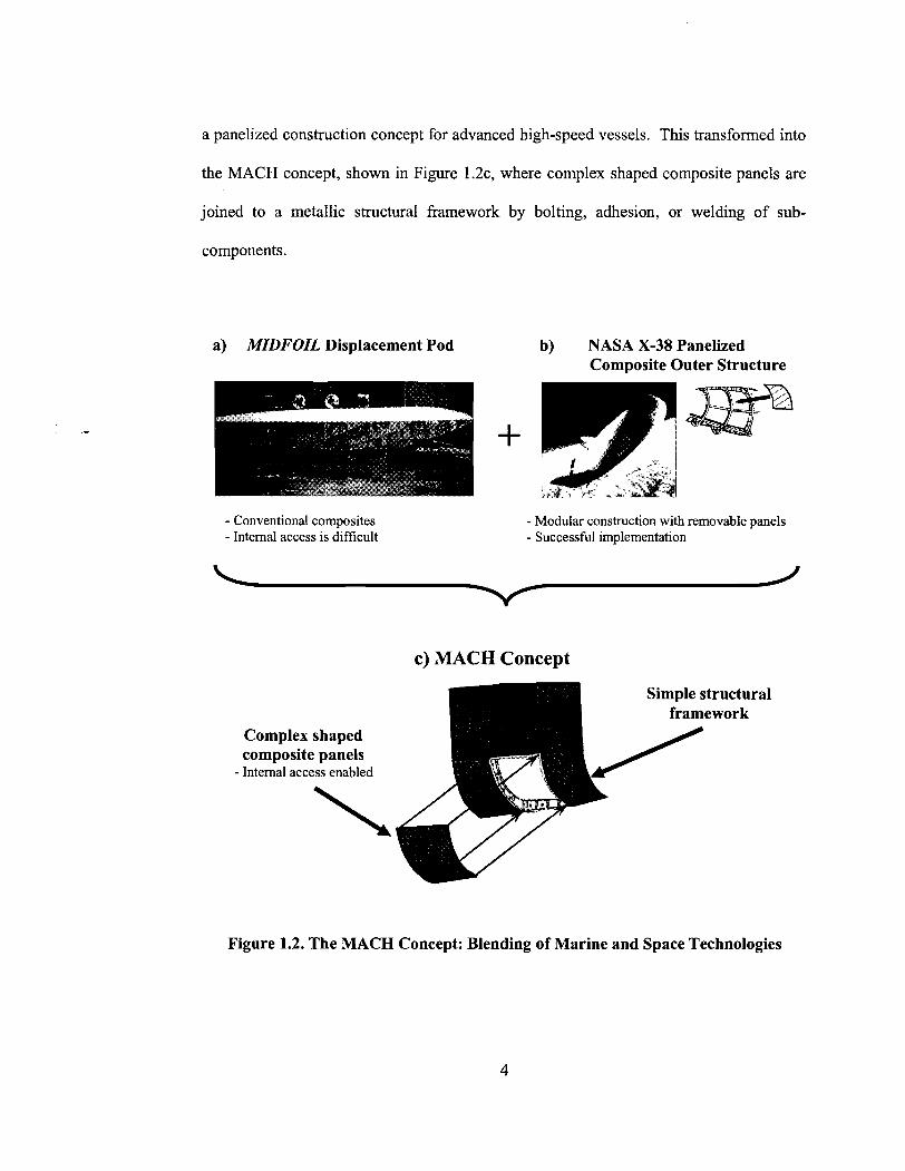
a panelized construction concept for advanced high-speed vessels. This transformed into
the MACH concept, shown in Figure 1.2c, where complex shaped composite panels are
joined to a metallic structural framework by bolting, adhesion, or welding of sub-
component~.
a) MIDFOIL Displacement Pod b) NASA X-38 Panelized Composite Outer Structure
- Conventional composites - Internal access is difficult
- Modular construction with removable panels - Successful implementation
c) MACH Concept
Complex shaped composite panels Internal access enabled
Simple structural framework
Figure 1.2. The MACH Concept: Blending of Marine and Space Technologies

Figure 1.3. Monolithic Composite Construction
The overall objective of the proposed MACH effort was to develop and
demonstrate hybrid composite/metal joining concepts for naval ship hull applications.
The core of the project aimed at developing hybrid systems consisting of composite
structural sections attached to a metallic supporting structure. By combining composite
and metallic components, it is possible to take advantage of the beneficial properties of
each material. In general, the complex shapes required for advanced ship designs will
benefit from the use of composite materials in construction. Accordingly, the emphasis
of the MACH project is on the development of hybrid construction and joining systems.
This technology was demonstrated at both the joint sub-component level and at the
hybrid system level.

A schematic of the proposed MACH method for construction of a hybrid
composite/metal version of an underwater lifting body with removable panels is shown in
Figure 1.4. The concept consists of modular panels, made of composite materials,
attached to a metallic sub-frame, by means of a bolted connection. The composite panel
designs can be monocoque (unstiffened), rib-stiffened or sandwich construction,
depending upon the geometry and loading requirements. The panels must be able to
withstand the applied loads, while maintaining watertight integrity. The primary
advantages of the MACH concept are as follows:
1) Advanced hull shapes can be achieved due to the extensive use of
composite materials for the bulk of the structure,
2) Use of composite panels instead of metallic skins is expected to decrease
the overall weight of the system, which would make high-speed surface ships
faster and more efficient for a given payload
3) Modularity of the system (use of removable panels) would improve access to
the hull and lifting body, which in turn would allow for ease of maintenance of
equipment housed inside the lifting body, and
4) Use of a stiff metallic skeleton will facilitate the attachment of propulsion
equipment. while providing structural integrity.

Composite panel
Metallic sub- frame
Bolted connection to 7 metallic sub-frame
1
Figure 1.4. MACH Concept Schematic
1.3. Objectives, Organization and Scope
The main research goals of the work presented herein are as follows:
1) Structural testing of hybrid composite/metal joints. The current effort
includes testing of various joint configurations at the sub-component level.
2) Hydrostatic testing of a large-scale, hybrid panel assembly to demonstrate the
applicability and watertight integrity of hybrid joints at the component level.
3) Develop a simplified approach to model hybrid joints in large-scale structures,
by using finite element analysis.
The organization of the dissertation is summarized in Table 1.1. During Phase 1
of the research, presented in Chapter 3, a comprehensive experimental study was
performed to quantify the performance of hybrid joints with different bolted geometries,
by using beams as sub-components of the modular panels. Connection details were
chosen for their potential to be watertight and cost effective. A relative assessment of the
structural response of these joints, loaded in flexure, is provided. This laboratory study

served as a precursor to more complex and costly component panel studies, and as a
verification tool for local finite element models of hybrid joints.
Table 1.1. Organization of the Dissertation
Phase 2 deals with the hydrostatic testing of a large-scale, four-panel assembly, as
presented in Chapter 4. The modular panel assembly incorporated a hybrid joint, which
was selected based on the sub-component joint test results. The assembly was loaded to
failure, using uniform water pressure. This test served as verification of the design of the
hybrid panel assembly, as well as proof of the joint concept and demonstration of the
fabrication details and techniques using a VARTM process. Additionally, these results
are used to verify the global finite element models.
In Phase 3, finite element analysis was conducted in order to devise a simplified
shell model for hybrid joints in large-scale structures, as presented in Chapter 5. Models
were validated using the experimental data available for both local and global systems. A
local plane strain model is also presented to study the local stresses at the joint and to
predict the initiation of failure.
CHAPTER
1
2
3
4
5
6
CONTENTS
Project overview, background and objectives -
Literature review
Structural testing of hybrid joints under flexural loading
Structural testing of a four-panel hybrid assembly under hydrostatic loading
Finite element analysis of hybrid bolted assembly
Conclusions and recommendations

Chapter 2
LITERATURE REVIEW
2.1. Naval Structures and Composites
The use of advanced composite materials in structural applications has been
increasing during the past several decades. In marine structures, composites have been
used in small vessels and are potentially feasible for superstructures, decks, bulkheads,
propellers, and other equipment on large ships. For large vessels, however, the
implementation of composites for ship hull structural components is currently at the
developmental stage. Increased use of composites has arisen with the intention to
improve the structural performance of ships, while reducing manufacturing and
maintenance costs. The numerous potential applications of composite materials for naval
structures are outlined by Mouritz et al. [2001], and are illustrated in Figure 2.1.
According to Black [2003] and Kimpara [1991], recent naval ship designs have
been primarily concerned with achieving lighter, faster, lower maintenance and more
stealthy structures. Speed can be increased by reducing structural weight and by
implementing innovative complex shaping of the hull-form. Advanced materials and
structural systems are required to achieve these goals. In turn, a departure from
traditional hull construction methods, which primarily use aluminum and steel, is
necessary. Mouritz [200:1.] stated that replacing metallic naval vessels and components
with composites is a difficult and slow process, given that metals perform very well in
most applications. Currently, complete composite hull sections can be found in relatively
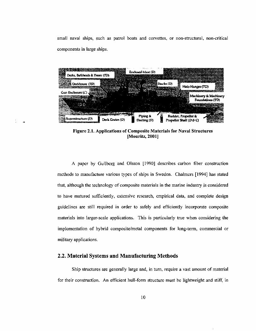
small naval ships, such as patrol boats and corvettes, or non-structural, non-critical
components in large ships.
Figure 2.1. Applications of Composite Materials for Naval Structures [Mouritz, 200:1]
A paper by Gullberg and Olsson [I9901 describes carbon fiber construction
methods to manufacture various types of ships in Sweden. Chalmers [I9941 has stated
that, although the technology of composite materials in the marine industry is considered
to have matured sufficiently, extensive research, empirical data, and complete design
guidelines are still required in order to safely and efficiently incorporate composite
materials into larger-scale applications. This is particularly true when considering the
implementation of hybrid composite/metal components for long-term, commercial or
military applications.
2.2. Material Systems and Manufacturing Methods
Ship structures are generally large and, in turn, require a vast amount of material
for their construction. An efficient hull-form structure must be lightweight and stiff, in

order to maintain its shape while resisting the applied loads. In addition, the structure
must be fatigue, impact and shock resistant. To achieve these goals, it is essential to
choose a low cost-per-pound material system and a manufacturing process that performs
to requirements. One of the primary cost drivers in developing advanced hull-forms with
conventional techniques is the metal forming of complex shapes. Using metals for the
bulk of the structure has made it difficult to achieve complex hydrodynamic shapes.
Hybrid composite/metal systems have emerged as a viable alternative to conventional
construction and manufacturing methods, due to the ease of manufacturing complex
shapes at relatively little incremental cost, when compared to fabrication with metals.
E-Glass/vinyl ester (EGNE) systems are of particular interest for large ship
structures, since they can lead to weight reduction and complex curvatures. Some of the
major advantages of EGNE systems, as outlined by Chu et al. [2004], are: 1) corrosion
resistance; 2) relatively high ultimate failure strains; and 3) damage tolerance. Recently,
much emphasis has been placed on the use of EGIVE systems, manufactured using a
vacuum-assisted resin transfer molding process (VARTM). This process offers good
strength characteristics which can be achieved at a much lower cost than, for example,
aerospace grade carbon fiber composites. As discussed by Critchfield and Judy [1994],
the U.S. Navy has demonstrated the applicability of VARTM as a low-cost process for
fabricating high-performance composite ship structures, including monocoque, single-
skin stiffened, and sandwich configurations. Using composites for the bulk of the vessel
could help achieve a more stealthy and corrosion-resistant structure, especially when used
in combination with corrosion-resistant metals, such as stainless steel and aluminum.

In spite of their apparent advantages, Barsoum [2003] stated that composites
alone lack the stiffness and strength to adequately withstand the loads of a large ship
structure. Furthermore, in a quasi-isotropic lay-up, the elastic modulus of EGNE
systems is nearly one order of magnitude less than steel. The stiffness mismatch between
composites and metals poses a great challenge when joining these dissimilar materials.
These observations will potentially cause designs that are typically performed on a
strength basis, to become stiffness-driven, particularly when equipment requirements set
a lower bound on the natural frequencies of the structure. For instance, a study by Alm
[I9831 estimated that a 50-m composite naval ship was 2.4 times less stiff than its steel
counterpart. Similarly, an article by Boyd [2004] states that an all composite ship
structure greater than 150 meters is currently unfeasible, and that the application of
hybrid composite/metal construction needs to be explored further.
2.3. Hybrid Structures for Marine Applications
To alleviate the lack of stiffness of composite materials alone, the hybrid structure
concept has arisen as a potential solution, where composites are used for stealth, weight
savings and reduced maintenance purposes, and metals are used to achieve structural
integrity. Barsoum [2003] discusses one example of this concept, where non-magnetic
stainless steel is used in combination with composites in order to create hybrid hull-forms
with low electromagnetic signatures.
Berube and Caccese [I9991 identified a major type of hybrid structural system,
which incorporates composite panels as skins attached to a metallic sub-frame, as shown
in Figure 2.2. The composite panels can be monocoque (unstiffened), rib-stiffened or
sandwich construction, depending on the geometry and loading requirements. Recently,
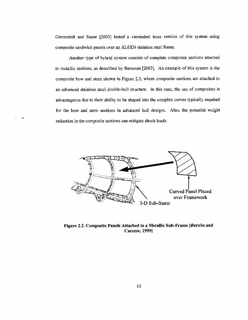
Grenestedt and Sause [2005] tested a vierendeel truss version of this system using
composite sandwich panels over an AL6XN stainless steel frame.
Another type of hybrid system consists of complete composite sections attached
to metallic sections, as described by Barsoum [2003]. An example of this system is the
composite bow and stern shown in Figure 2.3, where composite sections are attached to
an advanced stainless steel double-hull structure. In this case, the use of composites is
advantageous due to their ability to be shaped into the complex curves typically required
for the bow and stem sections in advanced hull designs. Also, the potential weight
reduction in the composite sections can mitigate shock loads.
Curved Panel Placed over Framework
Figure 2.2. Composite Panels Attached to a Metallic Sub-Frame [Berube and Caccese, 19991
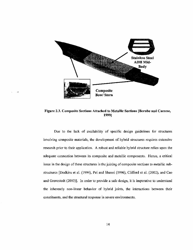
Figure 2.3. Composite Sections Attached to Metallic Sections [Berube and Caccese, 19991
Due to the lack of availability of specific design guidelines for structures
involving composite materials, the development of hybrid structures requires extensive
research prior to their application. A robust and reliable hybrid structure relies upon the
adequate connection between its composite and metallic components. Hence, a critical
issue in the design of these structures is the joining of composite sections to metallic sub-
structures [Dodkins et al. (1994), Pei and Shenoi (1996), Clifford et al. (2002), and Cao
and Grenestedt (2003)l. In order to provide a safe design, it is imperative to understand
the inherently non-linear behavior of hybrid joints, the interactions between their
constituents, and the structural response in severe environments.

The application of hybrid composite/metal structures has been gaining momentum
over the past several years. Accordingly, hybrid composite/metal connections which can
withstand the applied loads and other environmental effects are required. Connection
details are application specific, especially for cases where composites need to be attached
to metal structures. Several studies have recently emerged with regards to ship
applications of composite/metal joints. Cao and Grenestedt [2003] describe the testing of
a sandwich panel to metal interface, where they investigated the change in structural
response with embedment depth of the interface. It was concluded that placement of the
steel has a significant effect on the strength and should be moved away from the point of
stress concentrations. Boyd et al. [2004a, 2004bl describe an embedded metal joint
connecting a composite sandwich panel to a steel deck for a helicopter hangar. In this
application, a steel plate was embedded at the end of a tapered composite sandwich
section panel made from FRP skins and a balsa core. The fatigue life and residual
strength were evaluated for this joint.
2.4. Bolted Joints
Mechanical joints are the preferred method to assemble structural members for
cases where removable sections are required. Their main advantage over other
techniques is that it is easy to disassemble the structure, which facilitates maintenance
and allows for replacement of damaged parts. Researchers have conducted numerous
studies on composite bolted joints to identi@ the key parameters affecting joint
efficiency. In particular, it is necessary to understand the mechanisms that induce
damage and the loads at which failure occurs.

Bolted joints are critical structural regions and must be properly designed so that
the desired performance from the overall structure is obtained. Because of large stress
concentrations, joints can become a source of weakness if proper design practice is not
followed. Accordingly, failures typically occur at connections and interfaces, rather than
within the bulk of the system. To provide a safe and cost-effective joint design, it is
typical to configure the joint with respect to the geometry and the constituent materials,
which affect both strength and failure modes.
The simplest type of mechanical joint is the single-lap joint, shown in Figure 2.4,
in which two members are joined together by using a bolt or rivet. The key geometric
variables used in design are: hole size (h), bolt diameter (4, end distance (e), width of the
member (w) and member thickness (t) . While this joint scheme may be the most weight
efficient due the few parts involved when loaded in-plane, the eccentric load path induces
undesirable bending moments, commonly known as secondary bending. According to
Vangrimde and Boukhili [2003], secondary bending typically leads to lower strength
values. In order to mitigate the moment caused by the load eccentricity, the double-lap
joint configuration, shown in Figure 2.5, was introduced. This connection requires at
least two fasteners and two doubler plates, but bending moments will not occur under in-
plane loading. The single-bolt configuration, regardless of the type of lap joint, is the
most commonly used configuration for experimental and analytical studies found in the
literature. However, in the majority of practical engineering applications, multi-row
bolted joints are used to transfer loads between components.

Figure 2.4. Bolted Joint: Single-Lap Configuration
Figure 2.5. Bolted Joint: Double-Lap Configuration

2.4.1. Hybrid CompositeIMetal Bolted Joints
Joining composite materials and metals is more complex than joining isotropic
materials, due to the interfaces, material property mismatch, large number of possible
lamination configurations and the difficulty to accurately predict failure loads. Since
most isotropic metals exhibit plastic behavior, yielding may occur in regions of high
stress and shift some of the load resistance to lower stress regions. On the other hand,
composites are generally elastic until failure occurs, and stress concentrations may give
rise to catastrophic and unexpected failures.
The apparent difficulties in composite joint designs and the potential
consequences of in-service joint failures result in the use of large factors of safety. There
is a constant need for more detailed information about the behavior of these joints in
order to improve the design methods. A comprehensive report on joint design for naval
vessels was compiled by Bonanni et al. [2001], in which joint design guidelines for naval
ship construction and multiple examples of hybrid connections are presented.
2.4.2. Failure Modes in Composite Bolted Joints
Failure modes in composite bolted joints have been well documented in the
literature. Vangrimde and Boukhili [2003], Persson and Eriksson [1999], Camanho and
Matthews [2000], and Ireman et al. [2000], are some examples. Failure is typically
divided into two categories: macroscopic and microscopic failure. Macroscopic failure
refers to a damage state at which a structure is no longer able to withstand an increase in
the applied loads. This type of failure is readily observable and indicates a significant
loss of stiffness. In other words, macroscopic failure is considered to be the final stage in

the damage development process. In bolted composite laminates, the prominent
macroscopic failure modes are: net-section, bearing, shear-out and bolt failure.
The net-section mode, depicted in Figure 2.6, refers to failure transverse to the
direction of the bolt load and is mainly initiated by tangential and compressive stresses
acting at the edge of the hole. For a joint subjected to uniaxial loading, net-section failure
typically occurs when the ratio of the by-pass load (load applied to the plate) to the
bearing load (load going through the bolt) is high, or when the ratio dlw (bolt size to plate
width) is high.
Figure 2.6. Net Section Failure Mode
Bearing failure, shown in Figure 2.7, consists of damage to the area near the
contact region between the laminate and the bolt, and is a direct result of the compressive
stresses acting on the surface of the hole. The bolt pre-load (lateral constraint) strongly
affects this mode, since lateral constraint prevents delamination and buckling of the
fibers. Bearing occurs when either the ratio of the bearing load to the by-pass load is
high or when the wld ratio is high.
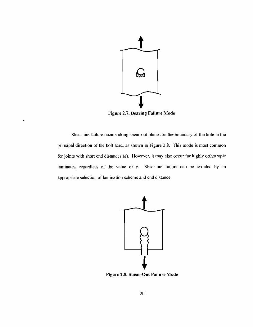
Figure 2.7. Bearing Failure Mode
Shear-out failure occurs along shear-out planes on the boundary of the hole in the
principal direction of the bolt load, as shown in Figure 2.8. This mode is most common
for joints with short end distances (e). However, it may also occur for highly orthotropic
laminates, regardless of the value of e. Shear-out failure can be avoided by an
appropriate selection of lamination scheme and end distance.
Figure 2.8. Shear-Out Failure Mode

The bolt failure mode, shown in Figure 2.9, occurs as a consequence of high shear
stresses in combination with bending stresses in the bolt. This mode typically occurs as a
secondary failure, following the onset of bearing failure.
Figure 2.9. Bolt Failure Mode
In joint design, all failure modes should be considered. Bearing failure is the
preferred mode in composite bolted joints, as the joint can continue to withstand loads
beyond the onset of failure. The other failure modes are usually catastrophic and do not
provide the opportunity to resolve the onset of damage before ultimate failure occurs. A
study by Vangrimde and Boukhili [2003] found that the development of bearing failure
assures the highest strength for a single-bolt joint. Hart-Smith [I9911 stated that high-
strength joints with multiple bolt rows are often critical in tension due to high by-pass
loads in the innermost bolt row.
Design charts for composite bolted joints loaded in tension, for both single-bolt
and multi-bolt configurations, are often found in the literature [Hart-Smith (1978),
Cooper and Turvey (1995), and Collings (1977)l. These charts relate the geometric
ratios, eld and wld, to specific failure modes and are geared towards helping the design
engineer avoid the aforementioned macroscopic failure modes. An example of these
charts, as presented by Cooper and Turvey [1995], is shown in Figure 2.1 0.

a) As a function of eld b) As a function of wld
Figure 2.10. Average Joint Load Capacities for Different Bolt Pre-Loads [Cooper and Turvey, 19951
Microscopic failure refers to damage that occurs near the edge of the holes in
bolted laminated composite materials. Damage of the structure initiates at the
microscopic level, becomes macroscopic damage and consequently leads to final rupture
of the structure. Microscopic failure modes include: tensile, compressive and shear fiber
and matrix failure, debonding and delamination between plies. For example, hole
machining is a clear source of microscopic damage. Improper drilling techniques may
lead to delamination and fiber fracture, which will ultimately have an influence on the
strength and fatigue resistance of the structure.
2.4.3. Composite Bolted Joints Subjected to Axial and Flexure Loading
An experimental study by Collings [1977] investigated the factors affecting the
strength of bolted joints in multi-directional carbon fiber reinforced polymer (CFRP)
laminates. For single-hole joints loaded in tension, the ultimate strength was found to be
strongly dependent on ply orientation, bolt size (4 and specimen width (w). It was also
observed that the best overall performance was exhibited by * 45" laminates. In multi-
hole joints, no adverse interaction was observed between holes. In other words,
22

increasing the number of holes did not cause a discernable loss in joint efficiency, for the
set of parameters investigated.
Ireman et al. [2000] conducted an experimental investigation to characterize the
damage development around holes in bolted graphitelepoxy single-lap joints, subjected to
quasi-static tension. The laminates were fabricated from the unidirectional pre-preg
system HTAl6376, and quasi-isotropic and zero-dominated lamination schemes were
investigated. It was found that, in general, specimens with tapered-head bolts have a
lower strength than those specimens with protruding-head bolts. The difference in joint
strength between tapered-head and protruding-head joints decreases as the diameter of
the tapered-head bolt increases. Secondary bending was observed to occur as a
consequence of significant joint damage. The failure sequence was determined to initiate
as matrix cracking at 25 percent of the failure load, fiber fracture at 35 percent of ultimate
failure, and delamination at 70 percent of final rupture. Joints with quasi-isotropic lay-
ups exhibited higher strength and slower failure sequences than those joints with zero-
dominated lay-ups.
Cooper and Tumey [I9951 conducted an experimental investigation for double-
lap, single-bolt joints, loaded in tension. The laminates were manufactured from a
pultruded fiberglass reinforced polyester (FRP) flat sheet material. Eighty-one specimens
were tested to determine the effects of the geometric ratios, eld and wld, and bolt
clamping torque on the strength of the joint. Their results showed that filly clamped
joints increased in strength by as much as 80 percent. It was also found that the initial
joint stiffness was mainly affected by the wld ratio, while the effect of the e/d ratio and
the bolt clamping torque was small.

Smith et al. [I9861 conducted a similar investigation on the strength of CFRP
single-lap bolted joints loaded in flexure, as a function of plate width (w) and edge
distance (e). The results of the study revealed that the effect of overall joint bending was
a likely factor in the reduced strength observed in single-lap joints, when compared to
double-lap joints. Also, larger values of wle (plate width to edge distance ratio) led to
higher strength values.
A study by Oh et al. [I9971 investigated the influence of ply angle, lamination
sequence, ratio of constituent materials, and clamping force, on the strength of double-
lap, bolted joints loaded in tension. Glasslepoxy and carbonlepoxy laminates were tested.
It was found that the bearing strength increased as the * 45" plies were distributed evenly
in the thickness direction, regardless of the ratio of the constituent materials. It was also
observed that higher bearing strength values could be attained as the bolt clamping force
was increased.
A study by Cohen et al. [I9951 provides a strength comparison of multi-row
bolted composite joints under axial loading, as a function of the number of holes (3, 5, 7
and 9 holes) and the lamination sequence. The laminates were fabricated using Hercules
IM7Gl3501-6 graphitelepoxy pre-impregnated tape and cured in an autoclave. The
lamination sequence used represents a typical lay-up for joint regions of a composite
rocket booster. With a total of 168 plies and a laminate thickness of 26.04 mm, the
sequence was as follows: [{(*I 5)3/902/0/*9/0/*9/0/* 9IOlf 9101* 9101902]) d(l* 1 5)3], where
9 = 30, 45, and 60 degrees. The test results showed higher strength values for the joint
specimens with 9 holes. For a given number of holes, joint configurations with * 45"
reinforcing plies attained the highest strength values, when compared to joints with

reinforcing fibers oriented at 30 and 60 degrees. When compared to 3-hole specimens, 9-
hole joints only resulted in a 4 percent strength increase. Hence, for experimental
purposes, the three-hole joint configuration was recommended as the most affordable and
not overly conservative joint, when considering joint strength.
Starikov and Schon [2002] conducted an experimental investigation on the quasi-
static behavior of single-lap and double-lap, protruding-head, bolted joints loaded in
tension and compression. The composite plates were made of carbon fiberlepoxy
(HTA716376) using two lamination sequences: 1) quasi-isotropic [(*45/0/90)~],, and 2)
(*45/0/90/04~9010~) ,. The plates were joined by two (single-bolt row), four (double-bolt
row), and six (triple-bolt row) titanium, protruding-head bolts. The results of these tests
showed that the specimens joined with three bolt rows (either single-lap or double-lap
joints) exhibited the highest quasi-static tensile and compressive strengths. It was also
observed that, for the same specimen type, the ultimate strength and strain values were
higher for the compressive loading case. The lowest resistance to quasi-static loading
was observed for specimens with a single row of bolts. However, multi-row joints failed
catastrophically in net-section, while single-row joints failed in bearing. Load-transfer
measurements between different bolt rows showed that, in general, the first bolt row
transfers the largest amount of load.
2.4.4. Composite Bolted Joints Subjected to Fatigue Loading
The relationships between material properties, geometric variables, lamination
sequence, failure loads and failure modes in composite bolted joints have been the subject
of much of the research found in the literature. Persson and Eriksson [1999] conducted
an experimental investigation with the objective of ranking the factors that most
25

significantly affect strength and fatigue life in multi-row, carbon-epoxy bolted joints,
using a linear regression analysis. For static loading, it was found that the most
influential factors were the bolt diameter to laminate thickness ratio (dlt), the bolt pre-
load, and the bolt-head type. Use of protruding-head bolts increased the gross section
strength, when compared to tapered-head bolts. Variation in pre-preg type for a given
fiber type and environmental conditions were found to have a lesser effect on the
strength.
In the same study, Persson and Eriksson [I9951 also investigated the joint
response when subjected to fatigue loading of constant amplitude, with initial deflections
varying no more than 0.05 mm. In the latter part (from 90 percent) of the fatigue life,
deflections increased catastrophically due to the addition of the local stiffness loss. It
was concluded that damage may have been growing without affecting the overall
structural response of the specimen, until a critical point was reached. At this point, the
significant stiffness loss caused large deflections which resulted in sudden and
catastrophic failure of the laminate.
Herrington and Sabbaghian [I9931 studied the effects of the load magnitude,
orientation of the reinforcing fibers, and bolt pre-load, on the fatigue life of composite
bolted joints. Their results showed that the outer ply angle had a small effect on the joint
strength. The most influential factor was found to be the bolt pre-load, which increased
the joint strength. It was also suggested that the pre-load could increase the fatigue life of
the joint.
Starikov and Schon [2002] performed experimental studies on the fatigue
resistance of single-row and multi-row, composite bolted joints with protruding-head

bolts. Quasi-isotropic and highly orthotropic lay-ups were investigated. The results of
the protruding-head bolted joint tests indicated that a multi-row configuration with a
quasi-isotropic lay-up displayed the highest fatigue resistance. Bolt failure was the
dominant mode. For all lay-ups, the fatigue behavior of the composite joints was
observed to vary linearly with the number of bolts.
Starikov and Schon [2001] performed a similar fatigue study for joints with
tapered-head bolts. Three types of bolts were used: all-composite fasteners (ACF),
titanium torque-set bolts, and titanium Huck-comp bolts. The results showed that joints
using titanium bolts attained a higher fatigue life than those using composite bolts. At
high load levels, the fatigue resistance of specimens with Huck-comp bolts was
comparable to that of joints with protruding-head bolts. It was concluded that failure of
the joints with composite bolts was due to the low ability of the bolts to carry cyclic shear
loading. The dominant failure mode observed was bolt fracture.
Benchekchou and White [1995a] conducted both theoretical and experimental
studies to determine the stresses around bolts in composite joints subjected to fatigue
loading. The cantilever-type specimens, made of CFRP and XASI914 CUD material,
were subjected to cyclic loading. Three different quasi-isotropic lamination sequences
were investigated. Three-dimensional finite element analysis was used to determine the
highest normal and shear stress regions. The experimental results showed that the greater
the flexural amplitude, the more quickly damage initiated in the plates. Damage
developed earlier for plates with smaller holes, when compared to those with larger
diameter holes. For a given applied load, the reduced area between the bolt and the
laminate lead to higher stresses, which resulted in delamination. It was also observed

that, for all bolt diameters and flexural amplitudes considered, [(*45/0/90)2], was the
most fatigue-resistant lamination sequence. Finite element results showed that the
maximum stresses occurred near the holes, where the bolt-head is positioned, when the
structure was loaded away from the fixed support. When loaded towards the support,
some of the maximum and minimum normal and shear stresses occurred near the holes,
while other stresses occurred at the edge of the plate. For a given end displacement,
stress values around the holes were lower for bending towards the clamp than away from
the clamp. Analytical data was compared with the experimental results, with an 8 percent
difference.
Benchekchou and White [1995b] conducted the same type of fatigue study for
joints with tapered-head bolts. Higher shear stresses were observed for joints with
tapered-head bolts than those with protruding-head bolts, as fewer fatigue cycles were
needed to initiate damage. A direct correlation between high normal and shear stresses
from the models and initiation of delamination and shear cracks in the experiments was
observed. High normal and shear stresses occurred in the regions around the holes, with
maximum stresses occurring in the first and last * 45O plies. Changing the bolt pre-load
did not affect the maximum normal and shear stresses. Both the finite element models
and the test results showed that the [(*45/0/90)2], lay-up was the most resistant to fatigue
loading.
2.5. Summary of the Literature Findings and Research Significance
The summary of the literature shows that considerable research has been
conducted on composite bolted joints subjected to in-plane and fatigue loads. For the
most part, researchers have outlined the major factors affecting the joint capacity and the

types of failures that may occur under various loading conditions. The geometric ratios,
the bolt pre-load, and the lamination sequence have been ranked as the most influential
factors affecting the structural integrity of the joint. Because of the inherent difficulty of
predicting failure in composite bolted joints, these investigations have typically involved
comprehensive experimental programs.
A few papers have stated that hybrid joints are considered to have great potential
for future engineering applications, but are currently at the developmental stage. A
limited number of major investigations on hybrid systems were found in the literature and
this is an area that requires further research. In order to characterize the structural
behavior of hybrid joints, the response of these systems needs to be investigated
experimentally and their applicability for large-scale structures needs to be demonstrated
at the sub-component and component levels. An extensive experimental investigation,
including in-plane, flexural, and fatigue loading, is required to achieve these goals.
Accordingly, the study presented herein aims at providing a comparative study of the
performance of various hybrid bolted joint configurations loaded in flexure. Also, this
study provides a basis for assessing the applicability of hybrid joints to underwater
marine structures.
Chapter 3
STRUCTURAL TESTING OF HYBRTD JOINTS UNDER
FLEXURAL LOADING
3.1. Joint Testing Rationale
In marine applications, any vessel using composite materials for the bulk of the
system will require hybrid connections of some sort, where composite components are
attached to metallic sub-structures. The structural integrity and performance of a ship
will be strongly influenced by the performance of attachments and internal connections.
Therefore, assessing the structural integrity of a hybrid system must include detailed
studies of the connection behavior. An accurate appraisal of structural integrity depends
primarily on proper assessment of the structural response of the connections and
interfaces and a sound estimate of the loads that induce failure. Accordingly, a thorough
investigation of the hybrid connection mechanics is an essential part of this research.
3.2. Joint Testing Objectives
One of the primary objectives of the MACH project is to develop a watertight,
hybrid composite/metal joint for lifting body structures. In doing so, it is desired to
attach removable, modular composite panels to the metallic lifting body sub-structures.
Because dissimilar materials are being joined, the connection of composite sections to
metallic components is a critical issue in the design of hybrid systems. Hybrid joint
design is more complex than conventional metallic joints, because of the dissimilar
interfaces and the numerous failure modes that can be induced by the use of composite

materials. Hybrid joints are inherently non-linear and characterization of their behavior
requires complex analytical models that need experimental verification. In order to
provide a reliable design, it is imperative to investigate the non-linear connection
mechanics, the interactions between the constituents, and the response of the system
under severe environmental conditions.
Marine structures are subjected to in-plane and out-of-plane loads, and are
therefore susceptible to both through-the-thickness and bending failure modes. The
experimental study presented in this section is aimed at assessing the structural response
of hybrid joint specimens subjected to primarily flexural loading. For this investigation,
hybrid joint test articles were isolated as sub-components of the large-scale panel
assembly. Test articles were configured with representative panel cross-sections and
representative interface attachment conditions. The primary goal was to develop a
watertight joint that would maintain a hydrodynamic profile when implemented into a
modular, panel assembly of the lifting body structure. The relative performance of
various joint designs was assessed on the basis of: initial joint rotational stiffness,
strength, and the types of failure modes observed.
Sub-component testing was conducted to evaluate critical panel configuration
parameters, such as panel attachments, tapering, and use of stiffening doubler plates and
foam inserts. This testing phase is a precursor to the more costly and geometrically
complex testing of a large-scale, modular panel assembly, presented in Chapter 4.
Additionally, the experimental data obtained from these tests can be used to verify
analytical models and to develop design guidelines for hybrid joints.

3.3. Hybrid Joint Configuration and Geometry
Potential hybrid joint configurations were judged and selected based upon their
ability to be made watertight, smooth shaped, and cost effective. A total of fifteen joint
specimens were tested. Specimens were grouped into two main categories: bolted joints
and bolted joints with doubler plates. The major geometric parameters investigated were:
bolt type, bolt diameter, and doubler plate geometry.
3.3.1. Bolted Joints
The bolted joint sub-component, presented in Figure 3.1, was selected as the
baseline for the experimental investigation, as this configuration is common in practice
and is relatively inexpensive to manufacture and assemble. The joint consists of two
composite beams attached to a steel I-beam member by using two rows of bolts, with
three bolts per row. Both protruding-head and tapered-head, grade 8, steel bolts, were
used for this study. Tapered-head bolts entail more work during installation, but provide
a smooth top surface, when compared to protruding-head bolts. To better distribute the
clamping force through the thickness of the joint, steel washers were used at the top and
bottom surfaces of the specimens with protruding-head bolts, and at the underside of the
steel I-beam member for specimens with tapered-head bolts. The baseline geometry of
the bolted joint sub-component is presented in Figure 3.2 and Table 3.1 provides a
description of the geometric parameters used.

Composite beams
- Steel I-beam member
Figure 3.1. Schematic of the Bolted Joint Sub-component
Figure 3.2. Baseline Geometry of the Bolted Joint Sub-component
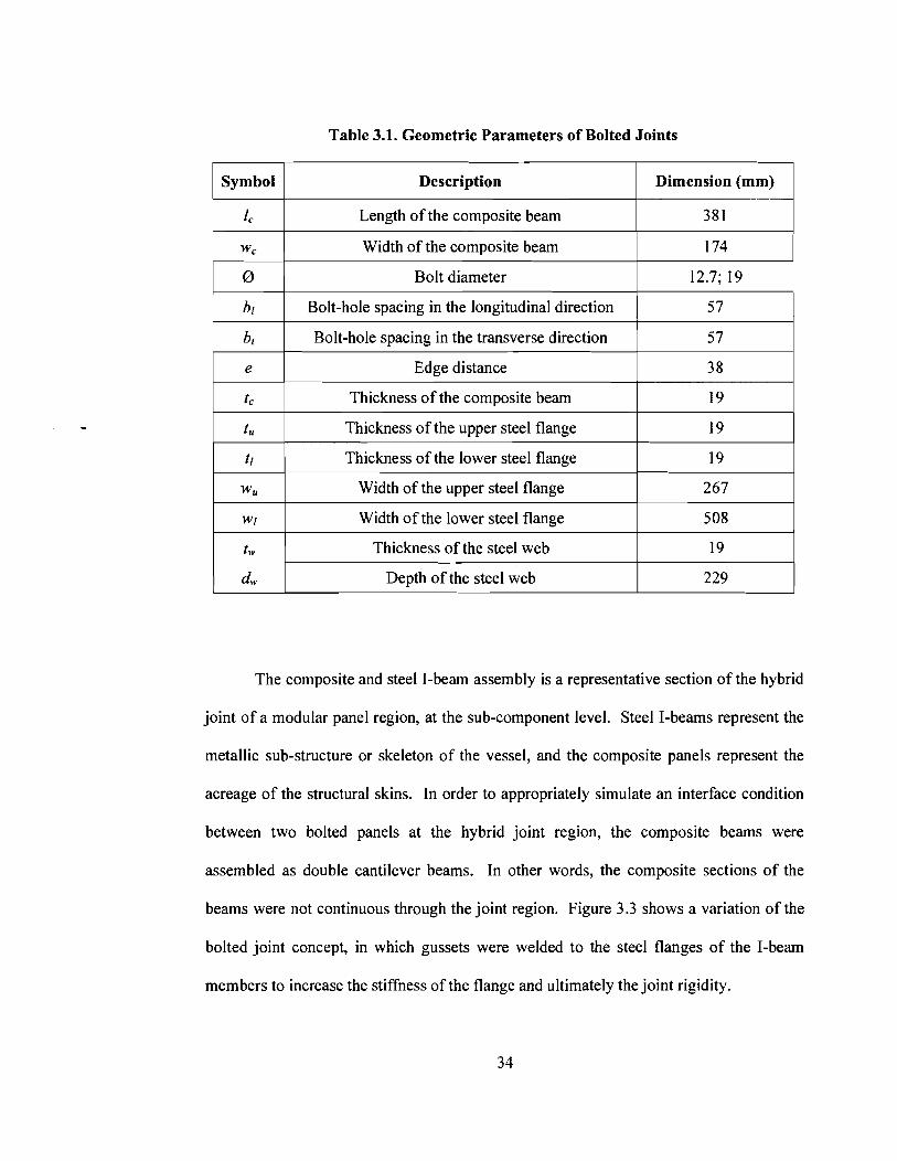
Table 3.1. Geometric Parameters of Bolted Joints
The composite and steel I-beam assembly is a representative section of the hybrid
joint of a modular panel region, at the sub-component level. Steel I-beams represent the
metallic sub-structure or skeleton of the vessel, and the composite panels represent the
acreage of the structural skins. In order to appropriately simulate an interface condition
between two bolted panels at the hybrid joint region, the composite beams were
assembled as double cantilever beams. In other words, the composite sections of the
beams were not continuous through the joint region. Figure 3.3 shows a variation of the
bolted joint concept, in which gussets were welded to the steel flanges of the I-beam
members to increase the stiffness of the flange and ultimately the joint rigidity.
Symbol
Ic
w c
0
br
b,
e
tc
t I,
tr
wu
W I
tw
dw
Description
Length of the composite beam
Width of the composite beam
Bolt diameter
Bolt-hole spacing in the longitudinal direction
Bolt-hole spacing in the transverse direction
Edge distance
Thickness of the composite beam
Thickness of the upper steel flange
Thickness of the lower steel flange
Width of the upper steel flange
Width of the lower steel flange
Thickness of the steel web
Depth of the steel web
Dimension (mm)
381
1 74
12.7; 19
57
57
38
19
19
19
267
508
19
229
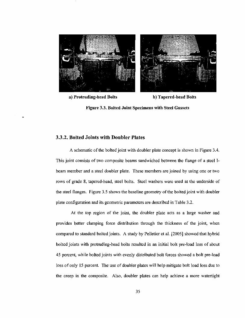
a) Protruding-head Bolts b) Tapered-head Bolts
Figure 3.3. Bolted Joint Specimens with Steel Gussets
3.3.2. Bolted Joints with Doubler Plates
A schematic of the bolted joint with doubler plate concept is shown in Figure 3.4.
This joint consists of two composite beams sandwiched between the flange of a steel I-
beam member and a steel doubler plate. These members are joined by using one or two
rows of grade 8, tapered-head, steel bolts. Steel washers were used at the underside of
the steel flanges. Figure 3.5 shows the baseline geometry of the bolted joint with doubler
plate configuration and its geometric parameters are described in Table 3.2.
At the top region of the joint, the doubler plate acts as a large washer and
provides better clamping force distribution through the thickness of the joint, when
compared to standard bolted joints. A study by Pelletier et al. [2005] showed that hybrid
bolted joints with protruding-head bolts resulted in an initial bolt pre-load loss of about
45 percent, while bolted joints with evenly distributed bolt forces showed a bolt pre-load
loss of only 15 percent. The use of doubler plates will help mitigate bolt load loss due to
the creep in the composite. Also, doubler plates can help achieve a more watertight
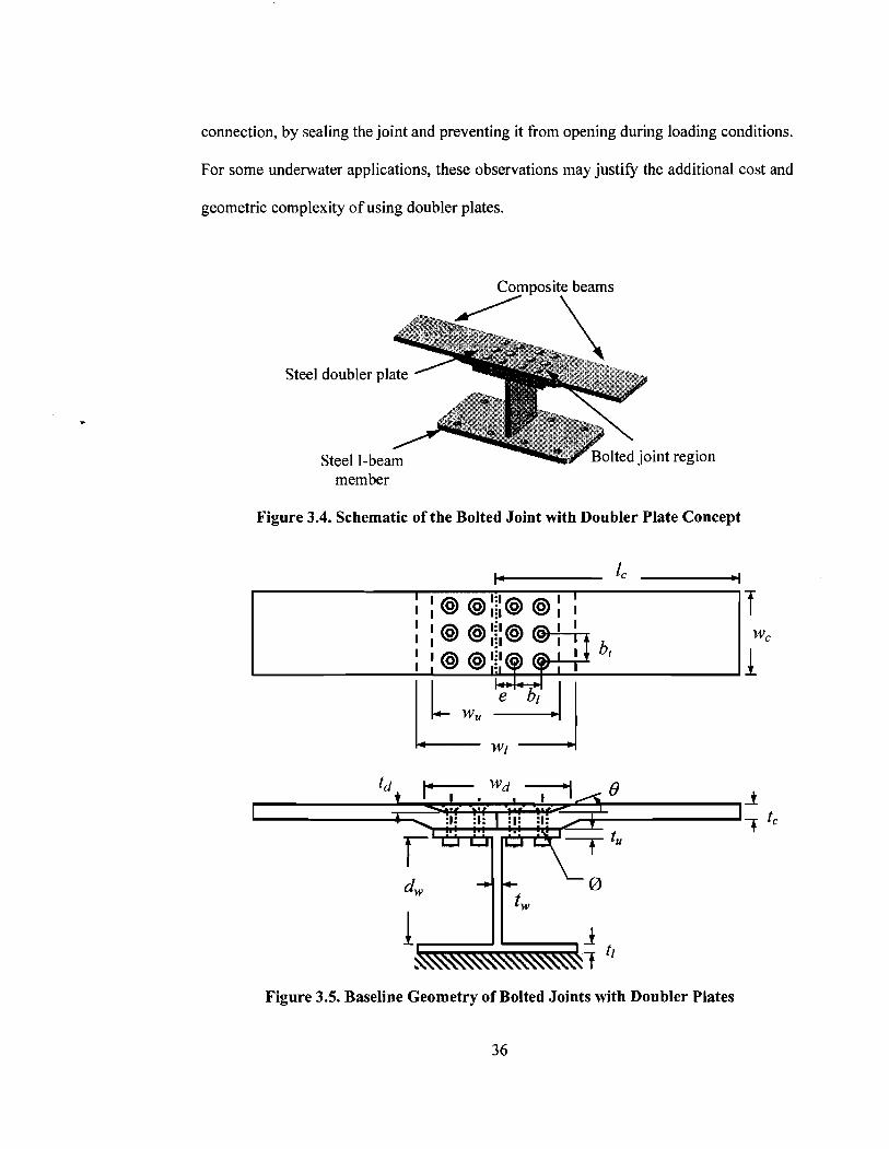
connection, by sealing the joint and preventing it from opening during loading conditions.
For some underwater applications, these observations may justify the additional cost and
geometric complexity of using doubler plates.
Composite beams
Steel doubler plate
Steel I-bea Bolted joint region member
Figure 3.4. Schematic of the Bolted Joint with Doubler Plate Concept
Figure 3.5. Baseline Geometry of Bolted Joints with Doubler Plates
3 6

Table 3.2. Geometric Parameters of Bolted Joints with Doubler Plates
Figure 3.6 shows photographs of bolted joints with doubler plates, for specimens
with and without a foam insert. Foam inserts were used at the tapered region of the
composite beam to increase the strength and stiffness of the joint, and to align the start of
the taper with the edge of the steel flange. Using foam inserts required modifications to
the thickness of the composite beam at the joint region. In order to accommodate the
insert and align the start of the taper with the edge of the steel flange, the thickness of the
composite beam was tapered from 25.4 mm at the joint region, to 19 mm at the free end
of the beam.
Symbol
lc
w c
0
br
b,
e
tc
tu
tr
w u
W I
tw
dw
wd
td
B
Description
Length of the composite beam, mm
Width of the composite beam, mm
Bolt diameter, mm
Bolt-hole spacing in the longitudinal direction, mm
Bolt-hole spacing in the transverse direction, mm
Edge distance, mm
Thickness of the composite beam, mm
Thickness of the upper steel flange, mm
Thickness ofthe lower steel flange, mm
Width of the upper steel flange, mm
Width of the lower steel flange, mm
Thickness of the steel web, mm
Depth of the steel web, mm
Width of the doubler plate, mm
Thickness of doubler plate, mm
Taper angle, degrees
Dimension
38 1
174
12.7; 19
5 7
5 7
38
19
19
19
267
508
19
22 9
146; 267; 324
6.35; 12.7
24
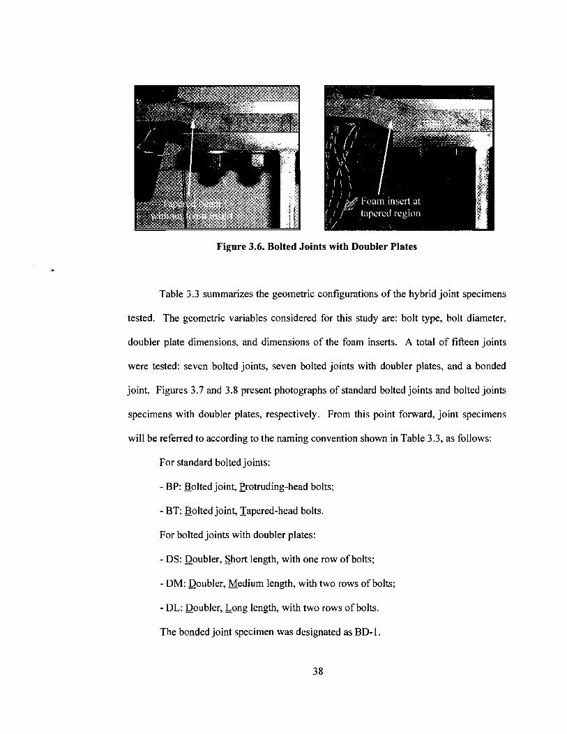
Figure 3.6. Bolted Joints with Doubler Plates
Table 3.3 summarizes the geometric configurations of the hybrid joint specimens
tested. The geometric variables considered for this study are: bolt type, bolt diameter,
doubler plate dimensions, and dimensions of the foam inserts. A total of fifteen joints
were tested: seven bolted joints, seven bolted joints with doubler plates, and a bonded
joint. Figures 3.7 and 3.8 present photographs of standard bolted joints and bolted joints
specimens with doubler plates, respectively. From this point forward, joint specimens
will be referred to according to the naming convention shown in Table 3.3, as follows:
For standard bolted joints:
- BP: Bolted joint, Protruding-head bolts;
- BT: Bolted joint, Tapered-head bolts.
For bolted joints with doubler plates:
- DS: Doubler, Short length, with one row of bolts;
- DM: Doubler, Medium length, with two rows of bolts;
- DL: Doubler, Long length, with two rows of bolts.
The bonded joint specimen was designated as BD-1.
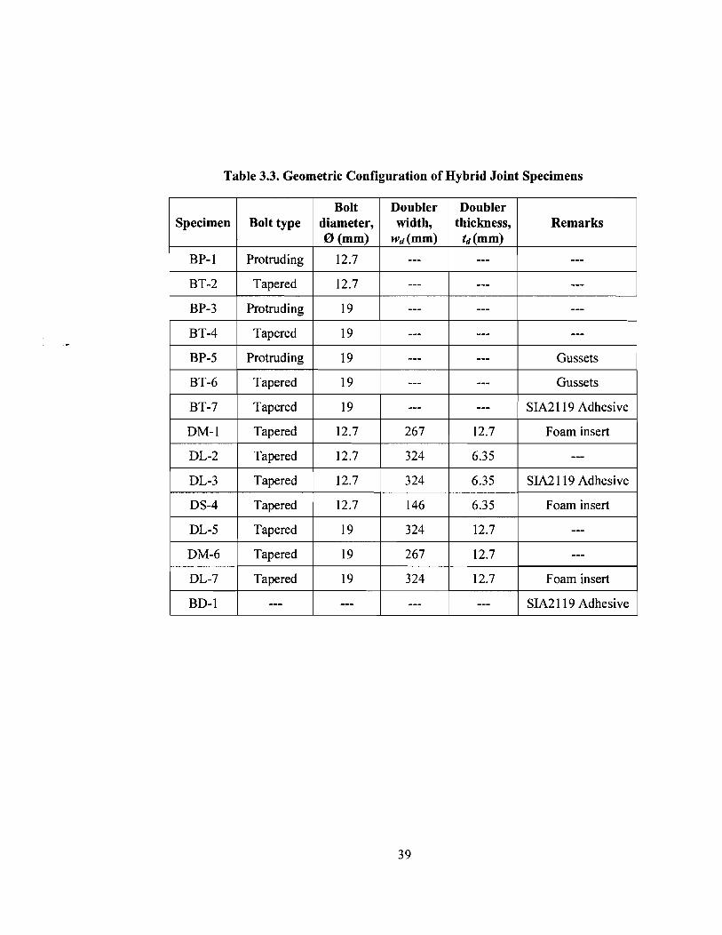
Table 3.3. Geometric Configuration of Hybrid Joint Specimens
Specimen
BP-1
BT-2
BP-3
BT-4
BP-5
BT-6
BT-7
DM- 1
DL-2
DL-3
DS-4
DL-5
DM-6
DL-7
BD-1
Doubler thickness,
f,l(~flm) --- --- ---
---
---
--- ---
12.7
6.35
6.35
6.35
12.7
12.7
12.7
---
Bolt type
Protruding
Tapered
Protruding
Tapered
Protruding
Tapered
Tapered
Tapered
Tapered
Tapered
Tapered
Tapered
Tapered
Tapered
---
Remarks
--- --- ---
---
Gussets
Gussets
SIA2 1 19 Adhesive
Foam insert
---
SIA2 1 19 Adhesive
Foam insert
--- ---
Foam insert
SIA2 1 19 Adhesive
Bolt diameter, 0 (mm)
12.7
12.7
19
19
19
19
19
12.7
12.7
12.7
12.7
19
19
19
---
Doubler width,
w,l(mm) ---
---
---
---
--- ---
---
267
324
324
146
324
267
324
---
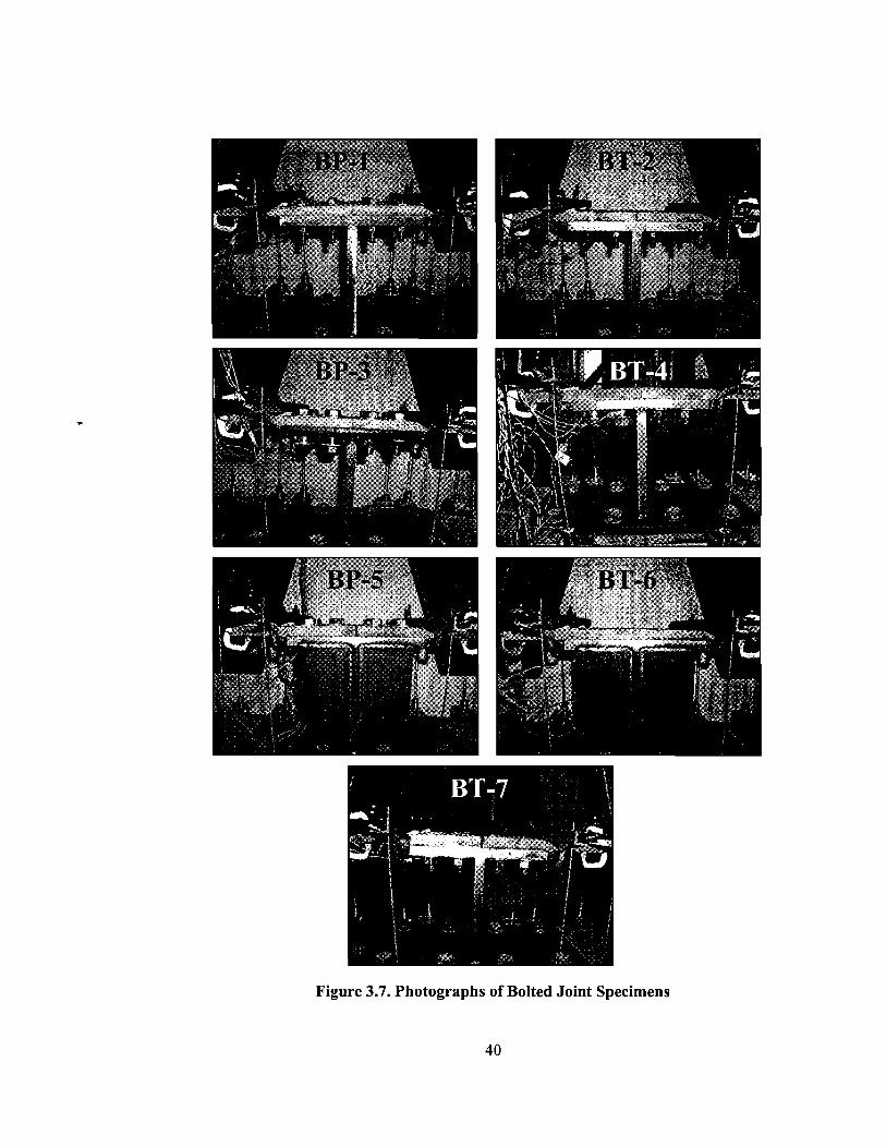
Figure 3.7. Photographs of Bolted Joint Specimens

Figure 3.8. Photographs of Bolted Joint Specimens with Doubler Plates

3.4. Materials and Test Article Fabrication
Another objective of the MACH project was to use innovative material systems
and processes to reduce structural weight, achieve complex shapes of the hull-form, and
improve the corrosion resistance of the structure. Using composite materials for the bulk
of the system can help achieve these goals in a cost-effective manner. EGNE systems,
manufactured using a vacuum-assisted resin transfer molding process (VARTM), offer an
attractive approach, as this process can be carried out in the laboratory at a lower cost
than, for instance, fabrication with metals. Additionally, the U.S. Navy is currently
investigating EGNE systems and VARTM processes as preferred choices for fabrication
of marine structures. Hence, these were selected for manufacturing the composite beams.
DOW Derakane 8084 vinyl ester resin and E-Glass fibers were used as the
composite specimen constituents. The reinforcing fibers were 680-gm 0-90" and 680-gm
* 45" knit fabric, manufactured by Brunswick Technologies, Inc. The 0" and 90" fibers
are stitched together, as well as the +45" and -45" fibers. The foam inserts were
fabricated using DIAB ~ i v i n ~ c e l l @ H80 foam. Steel components were fabricated by
Alexander's Welding & Machine, Inc., of Greenfield, Maine. Steel I-beam members
were made from 19-mm thick, A36 grade, plates. The steel doublers were made from
12.7-mm and 6.35-mm thick, A36 grade, plates. Material specifications are presented in
Appendix A.
Fabrication of the composite specimens was carried out in the Hybrid Structures
Laboratory, at the University of Maine, using a VARTM process. A forty-eight layer,
quasi-isotropic, [(f45, 0/90)6]s configuration was used as the baseline laminate
architecture. The nominal thickness of each layer was 0.397 mm, and the total laminate
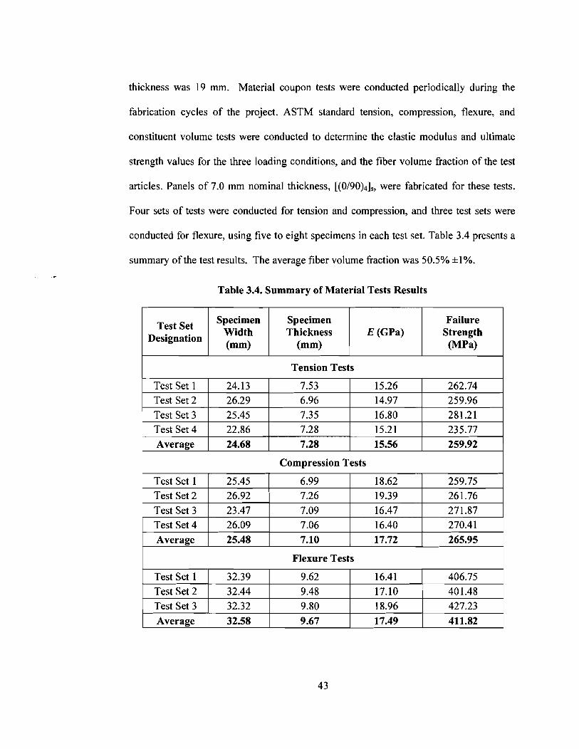
thickness was 19 mm. Material coupon tests were conducted periodically during the
fabrication cycles of the project. ASTM standard tension, compression, flexure, and
constituent volume tests were conducted to determine the elastic modulus and ultimate
strength values for the three loading conditions, and the fiber volume fraction of the test
articles. Panels of 7.0 mm nominal thickness, [(0/90)4],, were fabricated for these tests.
Four sets of tests were conducted for tension and compression, and three test sets were
conducted for flexure, using five to eight specimens in each test set. Table 3.4 presents a
summary of the test results. The average fiber volume fraction was 50.5% *I%.
Table 3.4. Summary of Material Tests Results
Failure Strength (MPa)
Test Set Designation
Specimen Width (mm)
Tension Tests
Test Set 1 Test Set 2 Test Set 3 Test Set 4 Average
Specimen Thickness
(mm) E (GPa)
24.13 26.29 25.45 22.86 24.68
Compression Tests
15.26 14.97 16.80 15.21 15.56
7.53 6.96 7.35 7.28 7.28
Test Set 1 Test Set 2 Test Set 3 Test Set 4 Average
262.74 259.96 281.21 235.77 259.92
25.45 26.92 23.47 26.09 25.48
Flexure Tests
6.99 7.26 7.09 7.06 7.10
Test Set 1 Test Set 2 Test Set 3 Average
18.62 19.39 16.47 16.40 17.72
32.39 32.44 32.32 32.58
259.75 26 1.76 271.87 270.41 265.95
9.62 9.48 9.80 9.67
16.41 17.10 18.96 17.49
406.75 40 1.48 427.23 411.82
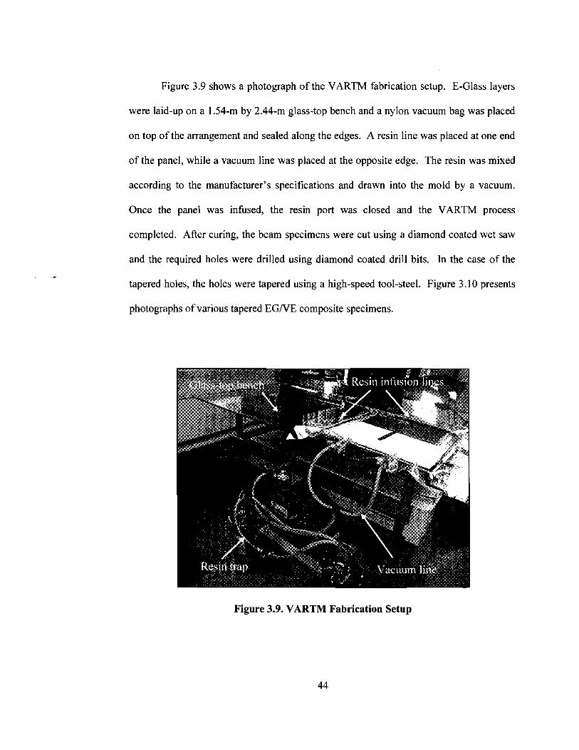
Figure 3.9 shows a photograph of the VARTM fabrication setup. E-Glass layers
were laid-up on a 1.54-m by 2.44-m glass-top bench and a nylon vacuum bag was placed
on top of the arrangement and sealed along the edges. A resin line was placed at one end
of the panel, while a vacuum line was placed at the opposite edge. The resin was mixed
according to the manufacturer's specifications and drawn into the mold by a vacuum.
Once the panel was infused, the resin port was closed and the VARTM process
completed. After curing, the beam specimens were cut using a diamond coated wet saw
and the required holes were drilled using diamond coated drill bits. In the case of the
tapered holes, the holes were tapered using a high-speed tool-steel. Figure 3.10 presents
photographs of various tapered EGNE composite specimens.
Figure 3.9. VARTM Fabrication Setup

Figure 3.10. Tapered EGNE Composite Specimens
3.5. Joint Testing Procedures
3.5.1. Test Setup
Testing of the hybrid joint specimens was conducted at the Hybrid Structures
Laboratory, at the University of Maine. A photograph of the experimental test setup is
shown in Figure 3.1 1. It consists of a 245-KN, f 254-mm, MTS@ actuator, mounted on a
1335-KN+ modular, reaction frame. The end of the actuator was attached to the upper
surface of a 2.82-m long, guided, W12 load beam, using four grade 8, 25.4-mm, steel
bolts. Load heads were attached to the lower surface of the load beam, in order to
transfer the applied MTS@ load to the test article. Rollers were attached to the ends of the
load beam to achieve a tight fit with the side plates, in order to avoid rotation of the W12
beam. Figure 3.12 shows the dimensions of the W 12 load beam and the load heads.
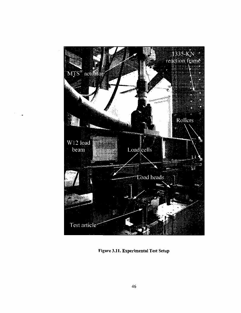
Figure 3.11. Experimental Test Setup

Figure 3.12. Dimensions of the W12 Load Beam and Load Heads (in meters)
Figure 3.13 depicts the connection of the test article to the reaction frame and the
load heads. The bottom flange of the steel I-beam member was attached to the reaction
frame by using eight, grade 5, 22.22-mm, steel bolts. The free ends of the composite
beams were secured between the two roller pins of the load heads using the large, 25.4-
mm, setscrews.
lller pins
.22-mm bolts -
' W12 load beam
-@Roller pins
Figure 3.13. Connection of the Test Article to the Reaction Frame and Load Heads
47
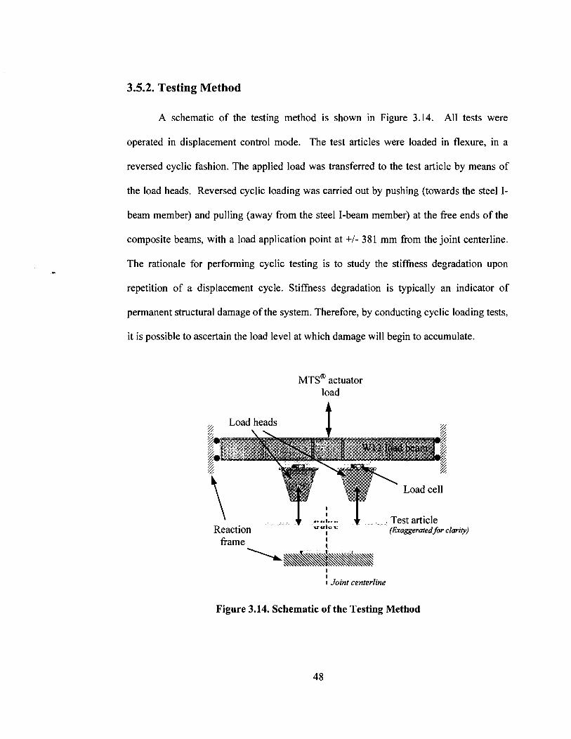
3.5.2. Testing Method
A schematic of the testing method is shown in Figure 3.14. All tests were
operated in displacement control mode. The test articles were loaded in flexure, in a
reversed cyclic fashion. The applied load was transferred to the test article by means of
the load heads. Reversed cyclic loading was carried out by pushing (towards the steel I-
beam member) and pulling (away from the steel I-beam member) at the free ends of the
composite beams, with a load application point at +I- 381 mm from the joint centerline.
The rationale for performing cyclic testing is to study the stiffness degradation upon
repetition of a displacement cycle. Stiffness degradation is typically an indicator of
permanent structural damage of the system. Therefore, by conducting cyclic loading tests,
it is possible to ascertain the load level at which damage will begin to accumulate.
MTS@ actuator load
,, Load heads t
\ + - .. I 4 .* .- w u l w w
Test article Reaction I (Exaggeratedfor clmiv)
frame
I
Joint centerline
Figure 3.14. Schematic of the Testing Method
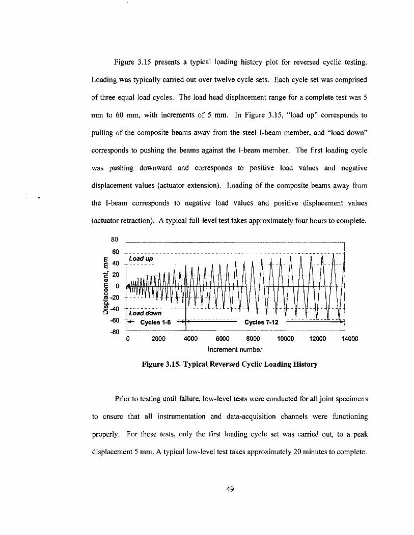
Figure 3.15 presents a typical loading history plot for reversed cyclic testing.
Loading was typically carried out over twelve cycle sets. Each cycle set was comprised
of three equal load cycles. The load head displacement range for a complete test was 5
mm to 60 mm, with increments of 5 mm. In Figure 3.15, "load up" corresponds to
pulling of the composite beams away from the steel I-beam member, and "load down"
corresponds to pushing the beams against the I-beam member. The first loading cycle
was pushing downward and corresponds to positive load values and negative
displacement values (actuator extension). Loading of the composite beams away from
the I-beam corresponds to negative load values and positive displacement values
(actuator retraction). A typical full-level test takes approximately four hours to complete.
I Load down I - - - - - - - - - - - - - - -
. . - - - - - - - - ti; Cycles 1-6 Cycles 7-12
0 2000 4000 6000 8000 10000 12000 14000
Increment number
Figure 3.15. Typical Reversed Cyclic Loading History
Prior to testing until failure, low-level tests were conducted for all joint specimens
to ensure that all instrumentation and data-acquisition channels were functioning
properly. For these tests, only the first loading cycle set was carried out, to a peak
displacement 5 mm. A typical low-level test takes approximately 20 minutes to complete.
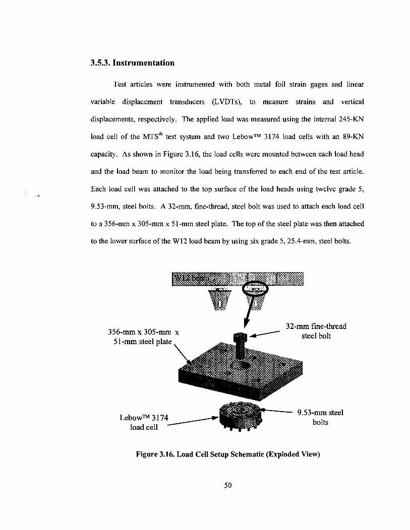
3.5.3. Instrumentation
Test articles were instrumented with both metal foil strain gages and linear
variable displacement transducers (LVDTs), to measure strains and vertical
displacements, respectively. The applied load was measured using the internal 245-KN
load cell of the MTS@ test system and two LebowTM 3174 load cells with an 89-KN
capacity. As shown in Figure 3.16, the load cells were mounted between each load head
and the load beam to monitor the load being transferred to each end of the test article.
Each load cell was attached to the top surface of the load heads using twelve grade 5,
9.53-mm, steel bolts. A 32-mm, fine-thread, steel bolt was used to attach each load cell
to a 356-mm x 305-mm x 51-mm steel plate. The top of the steel plate was then attached
to the lower surface of the W12 load beam by using six grade 5,25.4-mm, steel bolts.
32-mm fine-thread 356-mm x 305-mm x
5 1 -mm steel plate
9.53-mm steel LebowTM 3 174 / bolts load cell
Figure 3.16. Load Cell Setup Schematic (Exploded View)
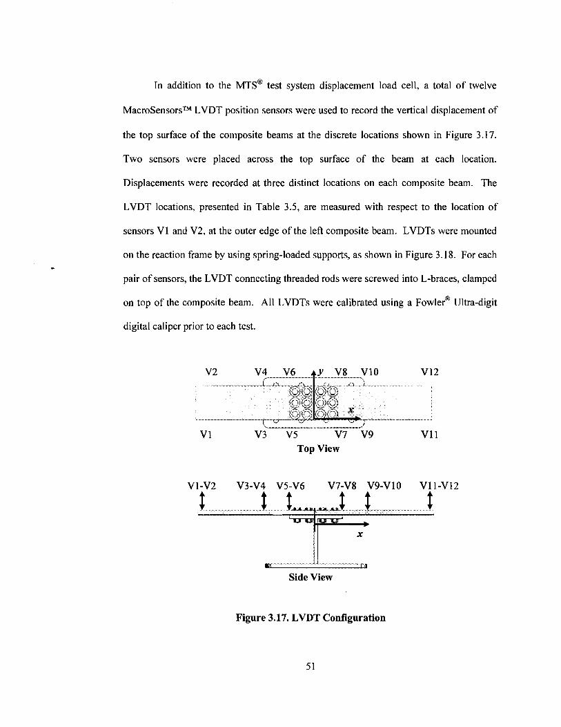
In addition to the MTS@ test system displacement load cell, a total of twelve
MacroSensorsm LVDT position sensors were used to record the vertical displacement of
the top surface of the composite beams at the discrete locations shown in Figure 3.17.
Two sensors were placed across the top surface of the beam at each location.
Displacements were recorded at three distinct locations on each composite beam. The
LVDT locations, presented in Table 3.5, are measured with respect to the location of
sensors V1 and V2, at the outer edge of the left composite beam. LVDTs were mounted
on the reaction frame by using spring-loaded supports, as shown in Figure 3.18. For each
pair of sensors, the LVDT connecting threaded rods were screwed into L-braces, clamped
on top of the composite beam. All LVDTs were calibrated using a ~owler@ Ultra-digit
digital caliper prior to each test.
v 1 v 3 v 5 v 7 v 9 v11 Top View
Side View
Figure 3.17. LVDT Configuration

Table 3.5. LVDT Location by Coordinates
Reaction frame
V9 (middle)
V10 (middle)
V 1 1 (outer)
V 1 2 (outer)
Connecting threaded rods
LVDT spring- oaded supports
+I- 25.4
+I- 25.4
+I- 50.8
+I- 50.8
Figure 3.18. LVDT Setup on Reaction Frame
203
203
381
381
0
1 72
0
1 72

Figure 3.19 shows a schematic of the strain gage configuration. Strain gages and
adhesives were procured from Micro-Measurements Group, Inc. Four uniaxial strain
gages, type CEA-00-125UW-350, were mounted on one of the composite beams, using
AE-10 adhesive. A CEA-13-250UW-350 strain gage was bonded to the underside of the
steel flange. Gages SG1 and SG2 were used to monitor strains in the composite beam,
SG3 and SG4 were used to monitor strains on the composite at the joint region, and SG5
was used to monitor yielding of the steel I-beam member. SG-1 was bonded to the
bottom surface of the composite beam, while SG2, SG3 and SG4 were bonded to the top
surface. Prior to each test, strain channels were calibrated using a 3 5 0 4 strain calibrator.
Table 3.6 presents the strain gage locations, measured from the bottom left corner of the
composite beam. VishayTM 2120 multi-channel signal conditioners were used for load
and strain data-acquisition. Instrumentation specifications are presented in Appendix B.
Top View
Side View
Figure 3.19. Strain Gage Configuration
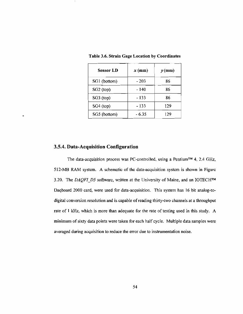
Table 3.6. Strain Gage Location by Coordinates
3.5.4. Data-Acquisition Configuration
Sensor 1.D
SGI (bottom)
SG2 (top)
SG3 (top)
SG4 (top)
SG5 (bottom)
The data-acquisition process was PC-controlled, using a PentiumTM 4, 2.4 GHz,
512-MB RAM system. A schematic of the data-acquisition system is shown in Figure
3.20. The DAQFI-D5 software, written at the University of Maine, and an IOTECHTM
Daqboard 2000 card, were used for data-acquisition. This system has 16 bit analog-to-
digital conversion resolution and is capable of reading thirty-two channels at a throughput
rate of 1 kHz, which is more than adequate for the rate of testing used in this study. A
minimum of sixty data points were taken for each half cycle. Multiple data samples were
averaged during acquisition to reduce the error due to instrumentation noise.
x (mm)
- 203
- 140
- 133
- 133
- 6.35
Y (mm)
8 6
86
8 6
129
129
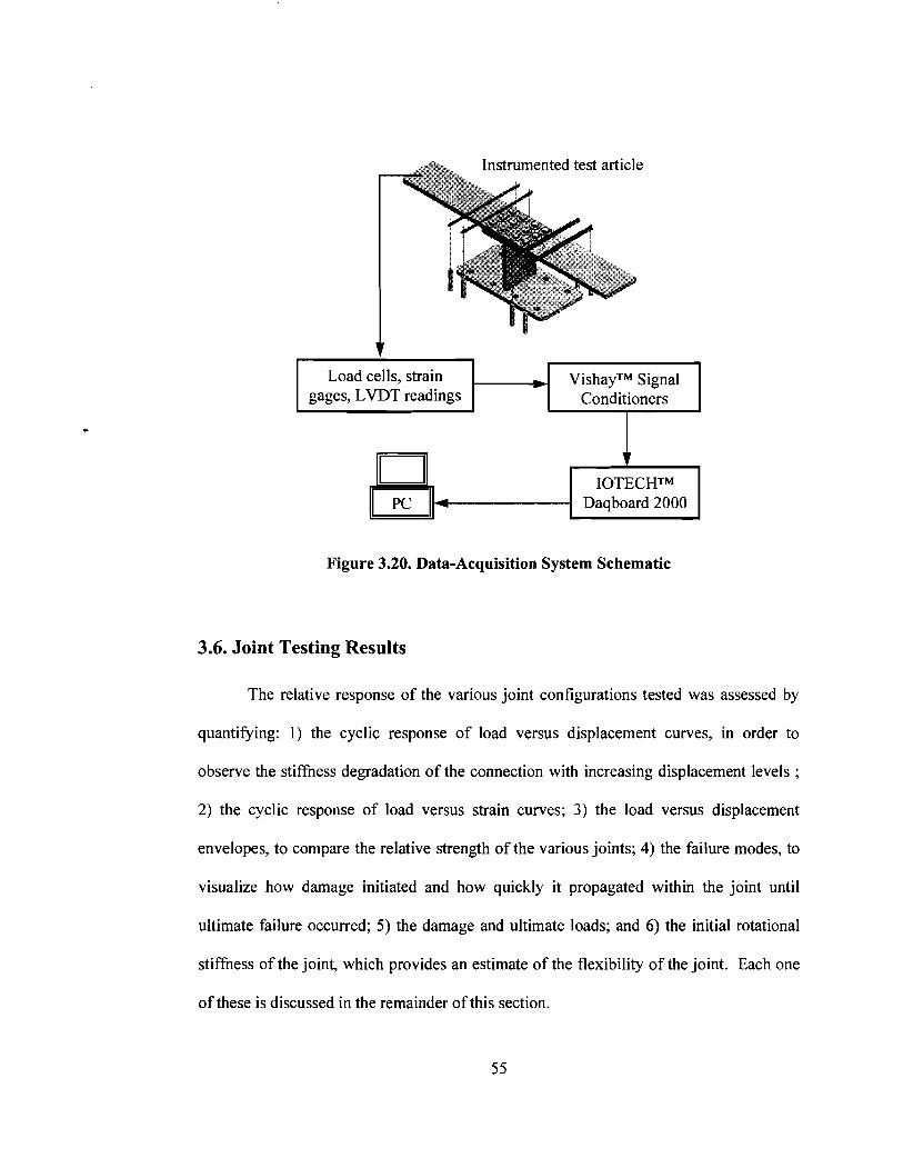
1
IOTECHTM Daqboard 2000
Figure 3.20. Data-Acquisition System Schematic
3.6. Joint Testing Results
The relative response of the various joint configurations tested was assessed by
quantifying: 1) the cyclic response of load versus displacement curves, in order to
observe the stiffness degradation of the connection with increasing displacement levels ;
2) the cyclic response of load versus strain curves; 3) the load versus displacement
envelopes, to compare the relative strength of the various joints; 4) the failure modes, to
visualize how damage initiated and how quickly it propagated within the joint until
ultimate failure occurred; 5) the damage and ultimate loads; and 6 ) the initial rotational
stiffness of the joint, which provides an estimate of the flexibility of the joint. Each one
of these is discussed in the remainder of this section.
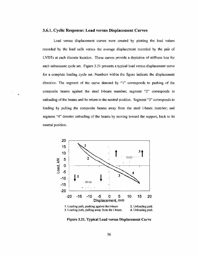
3.6.1. Cyclic Response: Load versus Displacement Curves
Load versus displacement curves were created by plotting the load values
recorded by the load cells versus the average displacement recorded by the pair of
LVDTs at each discrete location. These curves provide a depiction of stiffness loss for
each subsequent cycle set. Figure 3.21 presents a typical load versus displacement curve
for a complete loading cycle set. Numbers within the figure indicate the displacement
direction. The segment of the curve denoted by "1" corresponds to pushing of the
composite beams against the steel I-beam member; segment "2" corresponds to
unloading of the beams and its return to the neutral position. Segment "3" corresponds to
loading by pulling the composite beams away from the steel I-beam member; and
segment "4" denotes unloading of the beams by moving toward the support, back to its
neutral position.
-20 -15 -10 -5 0 5 10 15 20 Displacement, mm
1. Loading path, pushing against the I-beam 2. Unloading path 3. Loading path, pulling away from the I-beam 4. Unloading path
Figure 3.21. Typical Load versus Displacement Curve

Load versus displacement curves for specimens BT-6 and DS-4 are presented in
Figures 3.22 through 3.27, as examples of the cyclic behavior of the joints. Each figure
presents three different sets of load versus displacement cycles, as well as the complete
hysteresis loop. As described in Section 3.3, specimen BT-6 is a tapered-head bolted
joint, with gussets welded to the steel I-beam member. This configuration represents a
case of a very stiff sub-structure. Specimen DS-4 uses a short doubler plate with tapered-
head bolts and a foam insert at the tapered region of the composite. Curves are presented
for displacements recorded at the LVDT locations shown in Figure 3.17. Appendix C
presents the complete load versus outer displacement curves for all specimens.
Figures 3.22 and 3.23 present the load versus displacement curves for specimens
BT-6 and DS-4, respectively, using the displacement values recorded at the free ends of
the composite beams (outer LVDTs). The first of twelve displacement cycle sets, with a
peak displacement of 5.08 mm, is shown in Figures 3.22a and 3.23a, where it is observed
that the response of the joint is stiffer when displaced against the steel I-beam, due to the
additional bending resistance of the steel flange. The three cycles plotted in these figures
loop upon themselves, indicating a stable hysteresis response. The slight opening of the
hysteresis loops is a typical non-linearity observed in bolted joints. This behavior is
attributed to opening and closing of the gap between the joint components as the
displacement direction changes. For instance, when moved against the I-beam member,
the gap between the composite and the flange is already closed at the neutral position. On
the other hand, when moving upwardly, a gap opens up between these two components
before the steel member begins to take load. Friction between the joint components also
contributes to the opening of the load versus displacement loops.
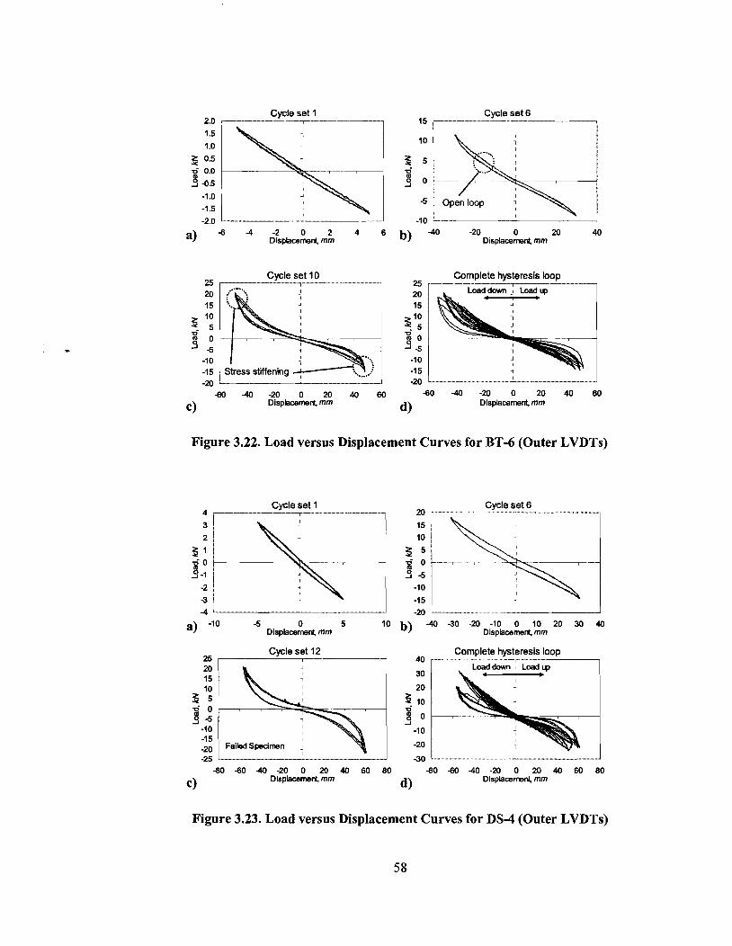
Cycle set 1 Cycle set 6 2.0
: : 1 i I
8 A 4.5
-2.0 -1 0
Cycle set 10 25 20 15
5 u- rn 0 3 - 5
-1 0 -1 5 -20
6 0 -40 -20 0 20 40 60 -60 -40 -20 0 20 40 60
c) ~ ispkcemnt , mm d)
Dlspbcement, mm
Figure 3.22. Load versus Displacement Curves for BT-6 (Outer LVDTs)
Cycle set 1 4 ---- Cycle set 6 20 , . . . . . . "
i
- - 7-- rn
-2 / -1 0
3 i , -1 5 I I I
4 - -20 ... . ...
a) -lo -5 0 5 10 b) 4 0 -30 -20 -10 0 10 20 30 40 Dispbcemr& mm Dispbcernent. mm
Cycle set 12 Complete hysteresis loop 25 --.- 20 15 10
5 5
1: -1 0 -1 5 -20 -25
-80 -60 40 -20 0 20 40 60 80 -80 -60 4 0 -20 0 20 40 60 80
c) D~spbcemnt, mm
d) Dlspbcemr& mm
Figure 3.23. Load versus Displacement Curves for DS-4 (Outer LVDTs)

Figures 3.22b and 3.23b show the load versus displacement curves for the sixth
set of cycles, with a peak displacement of 30.48 mm. Opening of the loops became more
pronounced with increasing cycle sets. Non-linear behavior in the form of stress-
stiffening was observed toward the end of this set of cycles, and is depicted in these
figures. For DS-4, the initiation of this behavior was observed toward the end of the fifth
set of cycles. Stress-stiffening was attributed to large deformation of the structure, given
that the end displacement-to-thickness ratio was approximately 1.6 at this loading stage.
Figures 3 . 2 2 ~ and 3 . 2 3 ~ present the load versus displacement curves for the tenth
set of cycles (BT-6) and the twelfth set of cycles (DS-4), respectively, after the specimens
had undergone severe damage. For BT-6, the loading and unloading paths began to differ
significantly at the beginning of the tenth set of cycles. At the end of this cycle set, the
specimen had reached ultimate failure and further data were not available. For DS-4,
significant loadinglunloading path discrepancies were observed at the beginning of the
twelfth cycle set and permanent damage resulted in a significant drop in load during
subsequent cycles. The complete hysteresis loops are presented in Figures 3.22d and
3.23d, where stiffness degradation is indicated by the drastic drop in load, which also
accounted for ultimate failure of the specimens.
Figures 3.24 and 3.25 present the load versus displacement curves for BT-6 and
DS-4, using the displacements recorded by the middle LVDTs. Significant load drops
were observed after the ninth cycle set for BT-6 and at the twelfth cycle set for DS-4.
When displaced downward, the rigidity of the steel flange accounts for the slightly
steeper slope of the curves, when compared to displacing upward. Appendix D presents
the complete load versus middle displacement curves for all specimens.

Cycle set 6
d 4 0 .-
-5 1
............................. -1 0
-1.50 -1.00 4.50 0.00 0.50 1.00 1.50 -10 d 0 5 10
a) Displacement, mm b) Displacement, mm
-15 1 -20 1 - -
-20 -10 0 10 20 -20 -1 0 0 10 20 Displacement, mm ~lsplacement, mm
c) d)
Figure 3.24. Load versus Displacement Curves for BT-6 (Middle LVDTs)
Cycle set 1 4 , ....................................................... ..7.. ..................................................................... Cycle set 6
2 1 B
m . 7-
3 - 1 i -2 i -1 0
I
-3 / 4 -1 5 l a ! . J -20
-1.50 -1.00 -0.50 0.00 0.50 I .DO -10 6 0 5 10 a) Displacement, mm ~ l s p b m e n t , mm
Cycle set 12 Complete hysteresis loop 25 I 40 20 1 15 !
30
10 i j 20 s 5 ;
0 . o t - - 7 . , .; . . . . i q 1 0
0
4 6 ) i i J 8 0 -10 1 -1 0 -15 ; 1 -20 -20 ; ! -25 i I J -30
3 0 -20 -10 0 10 20 30 3 0 -20 -10 0 10 20 30 ~ ~ s p b m e n f mm Displacement, mm
c) d)
Figure 3.25. Load versus Displacement Curves for DS-4 (Middle LVDTs)

Figures 3.26 and 3.27 present the load versus displacement curves for
displacements recorded at the joint region (inner LVDTs). Because these LVDTs are
aligned with the edge of the steel flange, the data in these figures indicate the actual joint
response. In Figures 3.26a and 3.27a, opening of the loops is more clearly captured by
this set of LVDTs than by the middle or outer LVDTs. For the sixth set of cycles
presented in Figures 3.26b and 3.27b, the added rigidity of the steel gussets (BT-6) is
observed when the specimen is displaced against the I-beam, as the curves have a steeper
slope, when compared to displacing upward. In Figure 3.26c, failure of specimen BT-6 is
depicted by the different loading and unloading paths, particularly for displacing away
from the steel I-beam. Imminent failure is depicted in Figures 3.26d and 3.27d, where
DS-4 shows a more dramatic load drop during the final loading cycle sets. Appendix E
presents the complete load versus inner displacement curves for all specimens.
Cycle set 1 1
Cycle set 6 2.00 15 r
1.50
1 .oo r 0.50
3- 0.00
94 .50
-1 .oo
-1.50
-2.00 -0.10 -0.05 0.00 0.05 0.10 0.15
a) Displacement, mm -0.50 0.00 0.50 1.00
Displacement, mm
Cycle set 10 Complete hysteresis loop 25
-1 0 1 2 3 4 -2 0 2 4 6 ~lsp~acemed, mm Dlsplacemed, mm
c) d)
Figure 3.26. Load versus Displacement Curves for BT-6 (Inner LVDTs)

-10 -5 0 5 10 15 -10 d 0 5 10 15
c) Displacement, mm d) Displacement, mm
Cycle se t 1 Cycle se t 6
Figure 3.27. Load versus Displacement Curves for DS-4 (Inner LVDTs)
4
3
2
$ 3 3 -1 0
-2
3
4
3.6.2. Cyclic Response: Load versus Strain Curves
Selected load versus strain curves for specimens BT-6 and DS-4 are presented in
Figures 3.28 and 3.29, respectively. Each figure contains four different sets of cycles for
each specimen. When the specimen is displaced against the steel I-beam, the gages on
the top surface of the composite beam are in tension (SG2, SG3, and SG4) and the gages
at the underside of the composite beam (SG 1) and at the bottom of the steel I-beam (SG5)
are in compression. When the specimen is displaced away from the steel I-beam, SG2,
SG3 and SG4 are in compression and SGl and SG5 are in tension. The complete load
versus strain plots, for all cycle sets, are presented in Appendix F.
a) -0.60 -0.40 -0.20 0.00 020 0.40 0.60 b) 4 -2 0 2 4 6 ~isphcement, mm Displacemen!, mm
\\- i -. - 7- d A -5 0 ;'I[-\\ J -7- - 1 I
4 , I I
-10 -1
-1 5 ,, i " 1 " . . . . . .
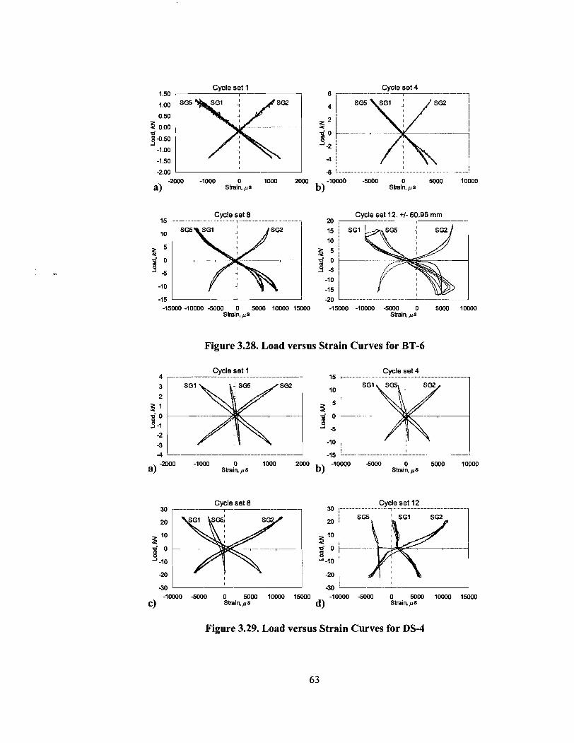
Cycle set 1 Cycle set 4 1.50 6 r---.----.---...--.-...-.
1 .OO i ;
0.50
s 0.00 I - - -. .. - - - - 6 7---
0.50 -
-I I
-1 .oo 1 i -1.50
-2.00 1 I . . . . . . . . -. .....................................................................
-2000 -1000 0 -5000 0 5000 IOOW S h i ~ ps Shin, p s
Cycle set 12. +I- 60.96 mm
-15000 -10000 -5000 0 5000 I0000 15000 -15000 -10000 -5000 0 5000 I0000 Shin. p s Strain, ps
Figure 3.28. Load versus Strain Curves for BT-6
Cycle set 1 Cycle set 4 I I 15 I 7 - e l
-1 000 0 I000 2000 b) -10000 6000 0 5000 10000 Strain. p s Strain. p s
Cycle set 8 30
20
s lo 6 0 $. -'-lo
-20
-30 -10000 -5000 0 5000 10000 15000 -10000 -5000 0 5000 I0000 15000
c) Straln, p s d) Strain,ps
Figure 3.29. Load versus Strain Curves for DS4
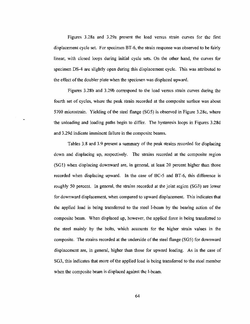
Figures 3.28a and 3.29a present the load versus strain curves for the first
displacement cycle set. For specimen BT-6, the strain response was observed to be fairly
linear, with closed loops during initial cycle sets. On the other hand, the curves for
specimen DS-4 are slightly open during this displacement cycle. This was attributed to
the effect of the doubler plate when the specimen was displaced upward.
Figures 3.28b and 3.29b correspond to the load versus strain curves during the
fourth set of cycles, where the peak strain recorded at the composite surface was about
5700 microstrain. Yielding of the steel flange (SG5) is observed in Figure 3.28c, where
the unloading and loading paths begin to differ. The hysteresis loops in Figures 3.28d
and 3.29d indicate imminent failure in the composite beams.
Tables 3.8 and 3.9 present a summary of the peak strains recorded for displacing
down and displacing up, respectively. The strains recorded at the composite region
(SG1) when displacing downward are, in general, at least 20 percent higher than those
recorded when displacing upward. In the case of BC-5 and BT-6, this difference is
roughly 50 percent. In general, the strains recorded at the joint region (SG3) are lower
for downward displacement, when compared to upward displacement. This indicates that
the applied load is being transferred to the steel I-beam by the bearing action of the
composite beam. When displaced up, however, the applied force is being transferred to
the steel mainly by the bolts, which accounts for the higher strain values in the
composite. The strains recorded at the underside of the steel flange (SG5) for downward
displacement are, in general, higher than those for upward loading. As in the case of
SG3, this indicates that more of the applied load is being transferred to the steel member
when the composite beam is displaced against the I-beam.

Table 3.7. Peak Strain Measurements - Load Down (in microstrain)
Table 3.8. Peak Strain Measurements - Load Up (in microstrain)
Specimen
BP-1 BT-2 BP-3 BT-4 BC-5 BT-6
SG1
9670 95 10 8310 8266 12790 12050
Specimen
BP-1 BT-2 BP-3 BT-4 BC-5 BT-6 BT-7
SG1
5890 6060 7550 6357 6030 6600 6260
SG2
8850 8590 11100 8590 9610 8310
SG3
8970 6350 10789 6579 12766 8990
SG4
12450 9900 7430 9967 12854 12309
SG2
7710 8290 9780 7510 9850 7550 7000
SG5
13245 12367 9690 1 1682 10877 1 1745
SG3
1 1290 1 1005 12098 9788 1 1890 12349 12390
SG4
1 1567 12356 12589 1 1678 1 1223 1 1890 12390
SG5
9982 9220 1 1066 10456 8690 9630 9010
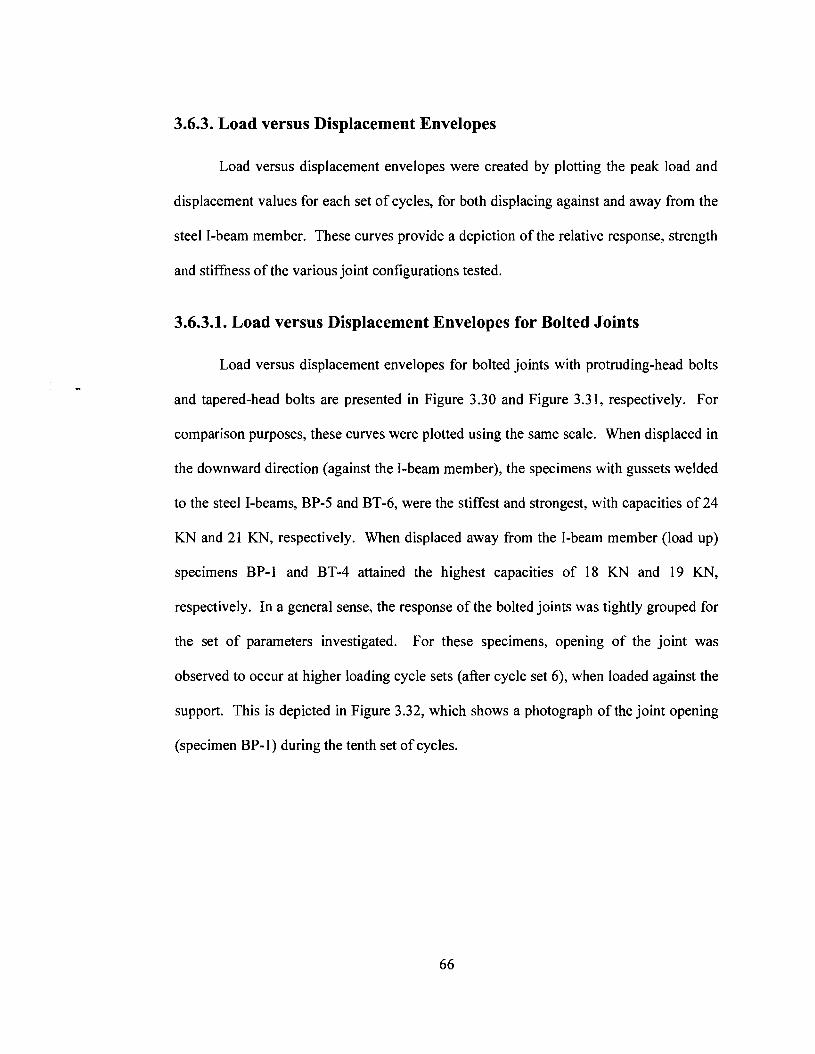
3.6.3. Load versus Displacement Envelopes
Load versus displacement envelopes were created by plotting the peak load and
displacement values for each set of cycles, for both displacing against and away from the
steel I-beam member. These curves provide a depiction of the relative response, strength
and stiffness of the various joint configurations tested.
3.6.3.1. Load versus Displacement Envelopes for Bolted Joints
Load versus displacement envelopes for bolted joints with protruding-head bolts
and tapered-head bolts are presented in Figure 3.30 and Figure 3.31, respectively. For
comparison purposes, these curves were plotted using the same scale. When displaced in
the downward direction (against the I-beam member), the specimens with gussets welded
to the steel I-beams, BP-5 and BT-6, were the stiffest and strongest, with capacities of 24
KN and 21 KN, respectively. When displaced away from the I-beam member (load up)
specimens BP-1 and BT-4 attained the highest capacities of 18 KN and 19 KN,
respectively. In a general sense, the response of the bolted joints was tightly grouped for
the set of parameters investigated. For these specimens, opening of the joint was
observed to occur at higher loading cycle sets (after cycle set 6), when loaded against the
support. This is depicted in Figure 3.32, which shows a photograph of the joint opening
(specimen BP-1) during the tenth set of cycles.
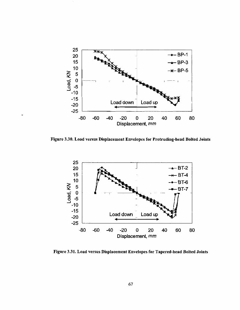
Load down 4 Load up \ A L
-25 I I
-80 -60 -40 -20 0 20 40 60 80 Displacement, mm
Figure 3.30. Load versus Displacement Envelopes for Protruding-head Bolted Joints
Load down 1 Load UD .\
-60 -40 -20 0 20 40 60 80 Displacement, mm
Figure 3.31. Load versus Displacement Envelopes for Tapered-head Bolted Joints
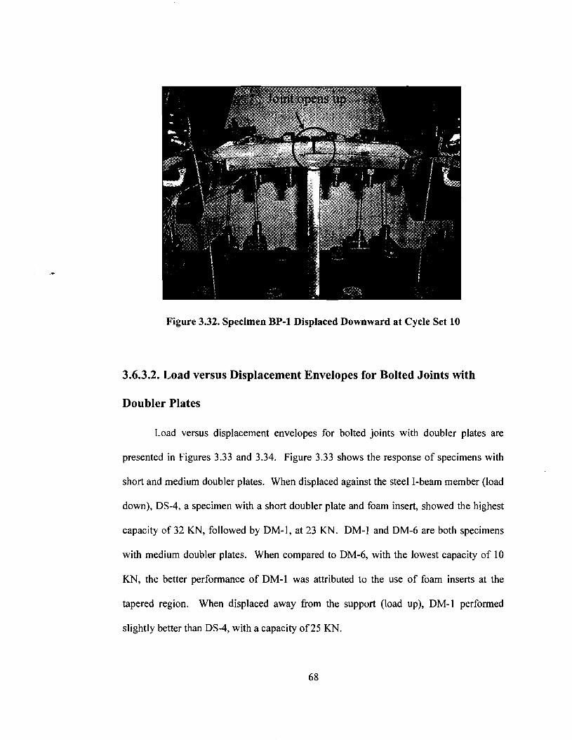
Figure 3.32. Specimen BP-1 Displaced Downward at Cycle Set 10
3.6.3.2. Load versus Displacement Envelopes for Bolted Joints with
Doubler Plates
Load versus displacement envelopes for bolted joints with doubler plates are
presented in Figures 3.33 and 3.34. Figure 3.33 shows the response of specimens with
short and medium doubler plates. When displaced against the steel I-beam member (load
down), DS-4, a specimen with a short doubler plate and foam insert, showed the highest
capacity of 32 KN, followed by DM-1, at 23 KN. DM-1 and DM-6 are both specimens
with medium doubler plates. When compared to DM-6, with the lowest capacity of 10
KN, the better performance of DM-1 was attributed to the use of foam inserts at the
tapered region. When displaced away from the support (load up), DM-1 performed
slightly better than DS-4, with a capacity of 25 KN.

-80 -60 -40 -20 0 20 40 60 80 Displacement, mm
-30
Figure 3.33. Load versus Displacement Envelopes for Bolted Joints with Short and Medium Doubler Plates
Figure 3.34 presents the load versus displacement envelopes for joints with long
doubler plates. When displaced against the steel I-beam (load down), specimens DL-2
and DL-3 attained the highest capacities of 34 KN and 31 KN, respectively. Both of
-40 -
Load down -
4
these specimens use 6.35-mm thick, long doubler plates. The same was true for the case
Load up b
of displacing away from the support. DL-7, a specimen with a 12.70-mm thick, long
doubler plate and foam insert, attained peak loads comparable to DL-2 and DL-3, up until
the sixth cycle set (displaced down, 30 mm) and the eighth cycle set (displaced up, 40
mm). After these cycle sets, the drop in peak loads for DL-7 is suspected to be a
consequence of the doubler geometry, which led to premature failure by bearing of the
steel at the top surface of the composite. DL-5 attained the lowest capacity of about 9.91
KN .
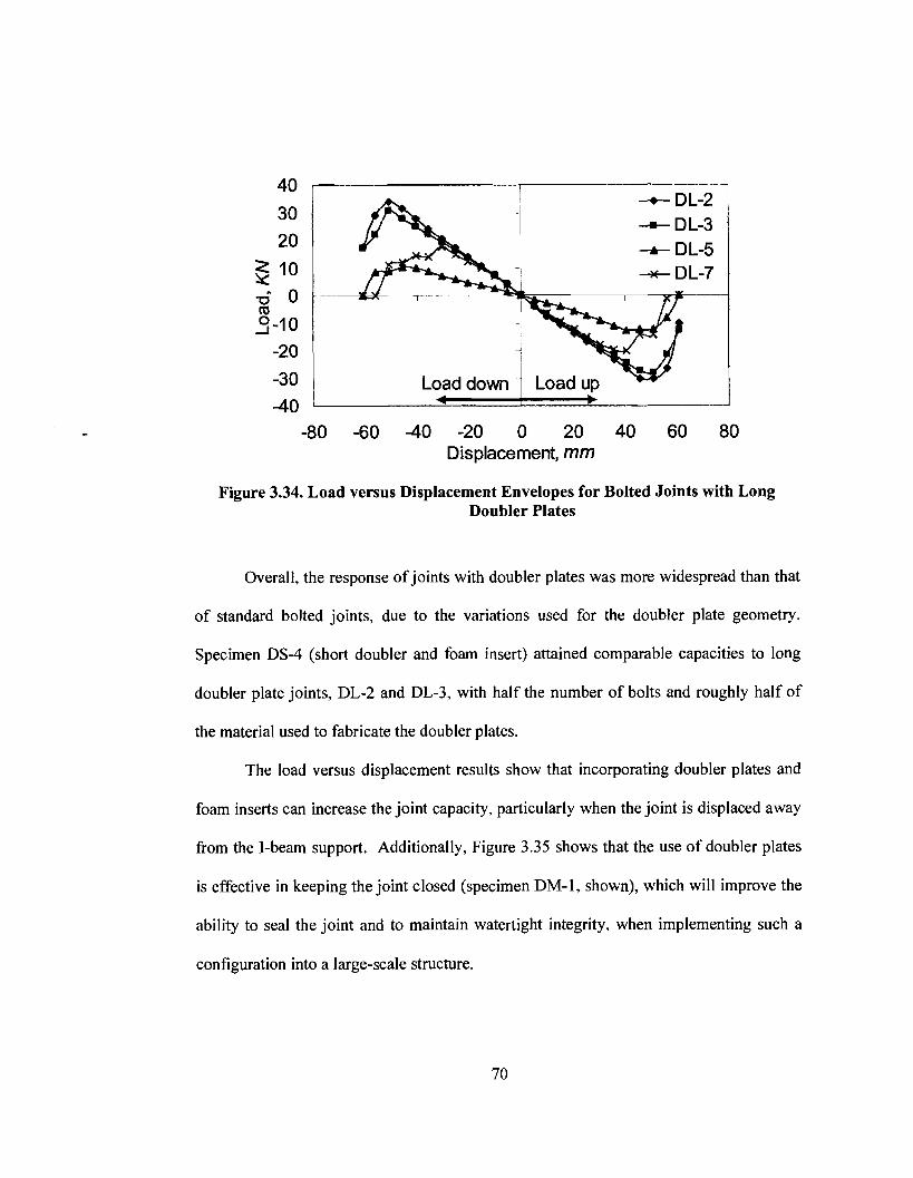
Load
-80 -60 -40 -20 0 20 40 60 80 Displacement, mm
Figure 3.34. Load versus Displacement Envelopes for Bolted Joints with Long Doubler Plates
Overall, the response of joints with doubler plates was more widespread than that
of standard bolted joints, due to the variations used for the doubler plate geometry.
Specimen DS-4 (short doubler and foam insert) attained comparable capacities to long
doubler plate joints, DL-2 and DL-3, with half the number of bolts and roughly half of
the material used to fabricate the doubler plates.
The load versus displacement results show that incorporating doubler plates and
foam inserts can increase the joint capacity, particularly when the joint is displaced away
from the I-beam support. Additionally, Figure 3.35 shows that the use of doubler plates
is effective in keeping the joint closed (specimen DM-1, shown), which will improve the
ability to seal the joint and to maintain watertight integrity, when implementing such a
configuration into a large-scale structure.

Figure 3.35. Specimen DM-1 Displaced Downward at Cycle Set 10
3.6.4. Failure Modes
Initiation of damage in composite bolted joints typically occurs as a combination
of delamination, fiber fracture, and bearing, which can take place either at the net section
or the gross section of the connection, depending upon the geometry and loading
conditions. For the tests presented in this chapter, the non-linear behavior observed in the
steel members was primarily due to yielding, which is typical for a structural steel, such
as A36.
Macroscopic damage in the composite was monitored by visual inspection and by
the behavior of the load versus displacement curves and the load versus strain curves.
Photographs of the joint specimens were taken at the beginning and the end of each
displacement cycle set, in order to document the onset of damage and correlate its
occurrence with the recorded load, displacement and strain data.
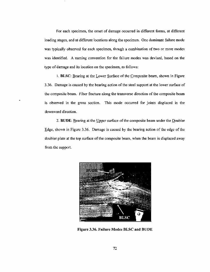
For each specimen, the onset of damage occurred in different forms, at different
loading stages, and at different locations along the specimen. One dominant failure mode
was typically observed for each specimen, though a combination of two or more modes
was identified. A naming convention for the failure modes was devised, based on the
type of damage and its location on the specimen, as follows:
1. BLSC: Bearing at the Lower Surface of the Composite beam, shown in Figure
3.36. Damage is caused by the bearing action of the steel support at the lower surface of
the composite beam. Fiber fracture along the transverse direction of the composite beam
is observed in the gross section. This mode occurred for joints displaced in the
downward direction.
2. BUDE: Bearing at the Upper surface of the composite beam under the Doubler
Edge, shown in Figure 3.36. Damage is caused by the bearing action of the edge of the
doubler plate at the top surface of the composite beam, when the beam is displaced away
from the support.
Figure 3.36. Failure Modes BLSC and BUDE
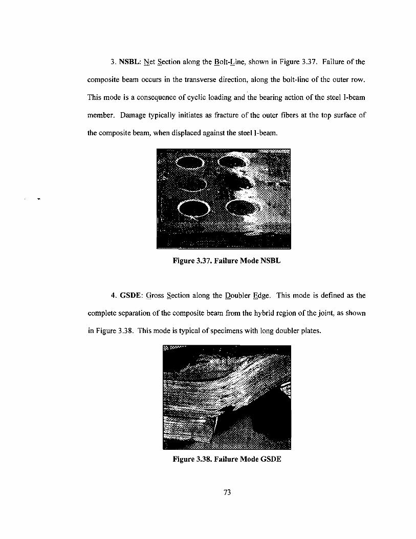
3. NSBL: Net Section along the Bolt-Line, shown in Figure 3.37. Failure of the
composite beam occurs in the transverse direction, along the bolt-line of the outer row.
This mode is a consequence of cyclic loading and the bearing action of the steel I-beam
member. Damage typically initiates as fracture of the outer fibers at the top surface of
the composite beam, when displaced against the steel I-beam.
Figure 3.37. Failure Mode NSBL
4. GSDE: B o s s Section along the Doubler Edge. This mode is defined as the
complete separation of the composite beam from the hybrid region of the joint, as shown
in Figure 3.38. This mode is typical of specimens with long doubler plates.
Figure 3.38. Failure Mode GSDE
73
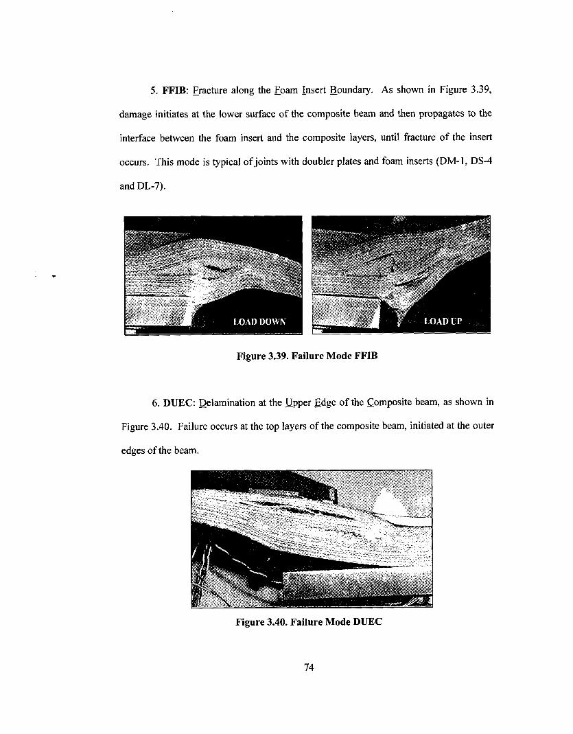
5. FFIB: Fracture along the Foam insert Boundary. As shown in Figure 3.39,
damage initiates at the lower surface of the composite beam and then propagates to the
interface between the foam insert and the composite layers, until fracture of the insert
occurs. This mode is typical of joints with doubler plates and foam inserts (DM-1, DS-4
and DL-7).
Figure 3.39. Failure Mode FFIB
6. DUEC: Delamination at the upper Edge of the Composite beam, as shown in
Figure 3.40. Failure occurs at the top layers of the composite beam, initiated at the outer
edges of the beam.
Figure 3.40. Failure Mode DUEC
74

7. DLEC: Delamination at the Lower Edge of the Composite beam. As shown in
Figure 3.41, failure occurs as separation of the bottom layers of the composite beam, and
initiates at the outer edges of the beam.
Figure 3.41. Failure Mode DLEC
8. DACB: Debonding at the Adhesive and Composite Beam interface. This mode
occurred for specimen BD-1, as shown in Figure 3.42. In this case, complete separation
of the composite beams from the steel flanges occurred as a consequence of the stresses
acting at the interface between the adhesive and the lower surface of the composite beam.
Figure 3.42. Failure Mode DACB

3.6.5. Damage Load and Ultimate Load
The damage load, Pdmg, was defined as the load magnitude at which discrepancies
in the loading/unloading curves and/or macroscopic damage were first observed. This
load value represents the onset of macroscopic damage, though microscopic damage may
have been developing prior to this load. The ultimate load, Purl, was taken to be the
maximum force that the joint was able to withstand (joint capacity).
Figure 3.43 presents a bar plot of the damage and ultimate loads for all joint
specimens. These values are summarized in Table 3.9. Arrows within the table are used
to indicate the displacement direction when the onset of a particular mode was recorded.
The failure modes are listed in the sequence in which they were observed to occur. The
performance of standard bolted joints was tightly grouped, while a more widespread
performance was observed for bolted joints with doubler plates.
For downward displacement of joints without doubler plates, the peak ultimate
loads were observed for the gusseted specimens, BP-5 and BT-6, at 23.74 KN and 20.94
KN, respectively. Specimen BT-2 showed the lowest capacity, at 16.99 KN. The peak
capacity of specimens with protruding-head bolts showed a 5 percent increase, when
compared with specimens with tapered-head bolts. The gusseted steel I-beam members
produced a 24 percent strength increase for the protruding-head bolt configurations (BP-3
versus BP-5), and a 10 percent increase for the tapered-head bolt configurations (BT-4
versus BT-6).
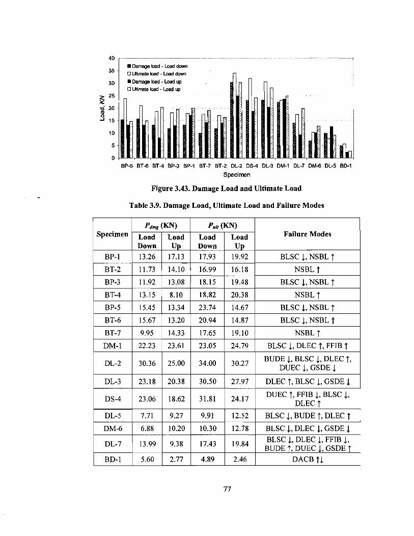
fa Damage load - Load d m Ubimte bad - Load d m
Damageload-Loadup Outimtebad-Loadup
BP-5 BT-6 BT-4 BP-3 BP-1 BT-7 BT-2 DL-2 DS-4 DL-3 DM-1 DL-7 DM-6 DL-5 BD-1
Specimen
Figure 3.43. Damage Load and Ultimate Load
Table 3.9. Damage Load, Ultimate Load and Failure Modes
'pecimen
BP-1
BT-2
BP-3
BT-4
BP-5
BT-6
BT-7
DM-1
DL-2
DL-3
DS-4
DL-5
DM-6
DL-7
BD- 1
Failure Modes
BLSC J, NSBL T NSBL T
BLSC J, NSBL T NSBL T
BLSC J, NSBL T BLSC J, NSBL T
NSBL T BLSC J, DLEC T, FFIB T
BUDE J, BLSC J, DLEC T, DUEC J, GSDE J
DLEC T, BLSC J, GSDE J
DUEC T, FFIB J, BLSC J, DLEC T
BLSC J, BUDE T, DLEC t BLSC J, DLEC J, GSDE 5. BLSC J, DLEC 4, FFIB J,
BUDE , DUEC J, GSDE DACB TJ
Pdmg
Load Down 13.26
11.73
11.92
13.15
15.45
15.67
9.95
22.23
30.36
23.18
23.06
7.71
6.88
13.99
5.60
(m) Load Up
17.13
14.10
13.08
8.10
13.34
13.20
14.33
23.61
25.00
20.38
18.62
9.27
10.20
9.38
2.77
Pul,
Load Down 17.93
16.99
18.15
18.82
23.74
20.94
17.65
23.05
34.00
30.50
31.81
9.91
10.30
17.43
4.89
(m) Load Up
19.92
16.18
19.48
20.38
14.67
14.87
19.10
24.79
30.27
27.97
24.17
12.52
12.78
19.84
2.46

When subjected to upward displacement, the peak ultimate loads were recorded
for specimens BT-4 and BP-1, with magnitudes of 20.38 KN and 19.92 KN, respectively.
The lowest capacity was observed for specimen BP-5, at 14.67 KN. The use of
protruding-head bolts and steel washers resulted in larger bending rigidity and joint
capacity, when compared to tapered-head bolted joints. For specimens BP-5 and BT-6,
the use of gussets led to failure by BLSC, which resulted in higher capacities when
displaced downward, but did not lead to ultimate failure.
In specimens with gusseted I-beam supports, for both protruding-head and
tapered-head bolts, damage first occurred in the form of BLSC and ultimate failure
occurred by NSBL, when displaced downward. NSBL developed at the upper surface of
the composite beam, particularly in specimens with tapered-head bolts, due to the lower
bending resistance of the section when displaced upward. NSBL was the dominant
failure mode for specimens with tapered-head bolts and typically occurred during upward
loading. BLSC and NSBL were the dominant failure modes for specimens with
protruding-head bolts and ultimate failure occurred when loaded upward. It was apparent
that the gussets substantially increased the stiffness of the steel I-beam member, and to
some degree, they also increased the strength of the joint. Also, by using gussets,
damage initiated as BLSC, which is a less catastrophic mode than, for instance, net-
section failure (NSBL). Specimens without gussets were prone to failure initiation in the
upward direction.
In joints with doubler plates subjected to downward displacement, the peak
ultimate load was observed for specimen DL-2, at 34 KN, followed by specimen DS-4, at
31.81 KN. Specimen DL-5 attained the lowest capacity of 9.91 KN. When displaced in

the upward direction, the peak ultimate load was attained by specimen DL-2, at 30.27
KN, followed by specimen DL-3, at 27.97 KN. Due to the complex geometry of the
joint, combinations of failure modes were observed for these specimens. BLSC was
identified as the only common mode for all specimens and it occurred when displacing
the beams in the downward direction.
For specimens with foam inserts, delamination at the upper and lower surfaces of
the composite (DUEC, DLEC) was typically observed, followed by FFIB, in which
fracture along the foam insert occurred as a consequence of delamination and later
expanded to the center of the foam insert. Specimen DL-7, using a long doubler, showed
a combination of virtually all of the failure modes, including BUDE and GSDE, the latter
being the more catastrophic type of failure. This observation suggested that reducing the
width of the doubler plates (and thereby altering the geometry of the foam inserts)
resulted in a more gradual and less catastrophic sequence of failure modes, which was the
case for DM-1 and DS-4, where GSDE was not present and larger joint capacities were
achieved (23 KN and 32 KN, respectively). For the specimens without foam inserts,
ultimate failure by GSDE was observed, as well as delamination and bearing modes. Of
all the joints tested, DL-2 achieved the peak capacity, but ultimate failure occurred by
GSDE.
3.6.6. Initial Joint Rotational Stiffness, J
The initial joint rotational stiffness, J , is defined as the initial slope of the moment
versus rotation curve, during the first loading cycle, where the displacement ranges from
0 to 5.08 mm. A typical moment versus rotation curve for the first loading cycle set is
presented in Figure 3.44, where Jd is the slope of the curve for downward loading and J u
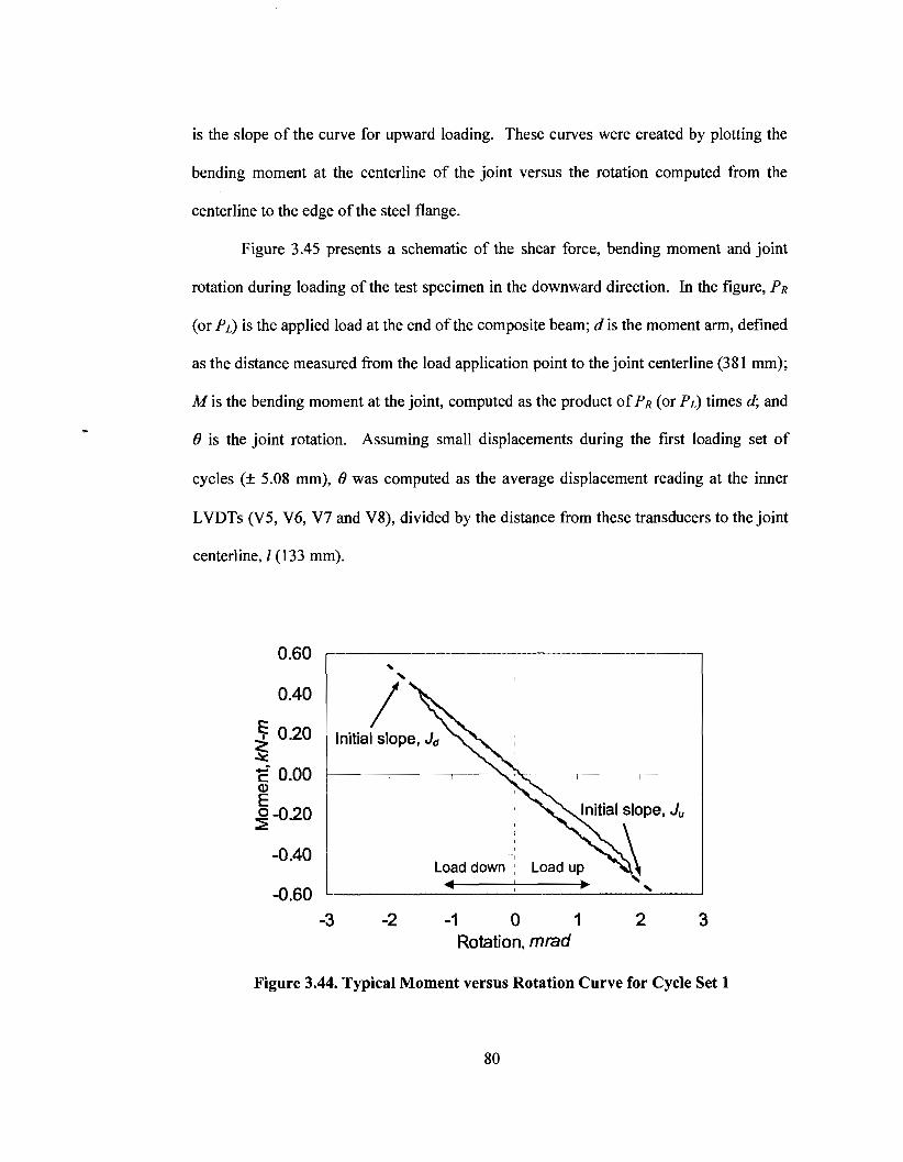
is the slope of the curve for upward loading. These curves were created by plotting the
bending moment at the centerline of the joint versus the rotation computed from the
centerline to the edge of the steel flange.
Figure 3.45 presents a schematic of the shear force, bending moment and joint
rotation during loading of the test specimen in the downward direction. In the figure, PR
(or PL) is the applied load at the end of the composite beam; d is the moment arm, defined
as the distance measured from the load application point to the joint centerline (381 mm);
M is the bending moment at the joint, computed as the product of PR (or PL) times d; and
0 is the joint rotation. Assuming small displacements during the first loading set of
cycles (+ 5.08 mm), 0 was computed as the average displacement reading at the inner
LVDTs (V5, V6, V7 and V8), divided by the distance from these transducers to the joint
centerline, l(133 mm).
Rotation, mrad
Figure 3.44. Typical Moment versus Rotation Curve for Cycle Set 1

Joint Centerline
Figure 3.45. Loading of Test Article in Flexure
Table 3.10 presents a summary of the computed values for J d and Ju. For standard
bolted joints, specimens BP-5 and BT-6 are the stiffest due to the additional resistance of
the steel gussets. When compared to specimen BT-2 (bolted joint with two rows of bolts),
specimen DS-4, with a single row of the same diameter bolts, is 30 percent stiffer when
displaced downward, and 34 percent stiffer when displaced upward. In general, these
results show that bolted joints with doubler plates and foam inserts can be made
rotationally stiffer than standard bolted joints, when loaded in bending.

Table 3.10. Initial Joint Rotational Stiffness, J
3.7. Hybrid Joint Selection for Large-Scale Panel Testing
The primary goal of the sub-component joint testing study presented in this
chapter was to develop a watertight, hybrid connection, which could be implemented into
the hydrostatic testing of a large-scale, four-panel assembly. Selection of an acceptable
joint configuration was based upon the relative performance of potential concepts with
regards to joint capacity, rotational stiffness, failure mode sequence, and the ability to
seal the joint for watertight integrity.
The results of this study have shown that, for resisting bending loads, joints with
doubler plates can be made stronger and rotationally stiffer than standard bolted joints.
328.54
182.1 1
322.68
187.34
DL-5
DM-6
DL-7
BD- 1
348.27
212.32
371.55
221.33

For example, when compared to its standard bolted joint counterpart (BT-2, two rows of
the same diameter bolts), a joint using a short doubler plate, a foam insert, and a single
row of bolts (DS-4), was found to be at least 46 percent stronger and 29 percent stiffer
when displaced downward, and 33 percent stronger and 34 percent stiffer when displaced
upward. Doubler plates proved effective in mitigating opening of the joint, which will
improve the ability to seal the joint and maintain watertight integrity. Hence, the
additional expense and geometric complexity of bolted joints with doubler plates and
foam inserts may be justified for some underwater applications.
When comparing the performance of all joint configurations with doubler plates,
it was observed that a joint with a short doubler plate, such as DS-4, can attain capacities
comparable to those of joints with long doubler plates (DL-2, DL-3). When compared to
DS-4, the use of long doublers induced more catastrophic failure sequences, which
ultimately led to complete separation of the composite beam from the joint region
(GSDE). Moreover, DS-4 requires roughly half of the material for fabrication of the
doubler plates and half the number of bolts than those joints with medium and long
doubler plates. This may be a significant factor when considering installation andlor
maintenance of large-scale structures that require multi-panel assemblies using bolted
connections. In light of these observations, the short doubler and foam insert joint
configuration (DS-4) was selected for implementation into the hybrid, four-panel
assembly presented in Chapter 4.

Chapter 4
STRUCTURAL TESTING OF A LARGE-SCALE, HYBRID
PANEL ASSEMBLY UNDER HYDROSTATIC
PRESSURE LOADING
4.1. Panel Testing Rationale
This section presents the structural testing of a large-scale, modular panel
assembly, which incorporates the DS-4 joint configuration described in Chapter 3. Four
modular panels were assembled using this joint scheme, and loaded with uniform
hydrostatic pressure, until failure was attained. A novel hydrostatic test system was
developed and implemented for this study. The results obtained from this test serve as
verification of the design of the hybrid panel assembly, proof of the hybrid joint concept,
and demonstration of the fabrication details and techniques using a VARTM process.
Additionally, the test results are used to validate global finite element models of the panel
assembly response.
4.2. Panel Testing Objectives
The main goal of testing a large-scale region of the hybrid lifting body was to
assess the structural performance of the MACH concept, when applied to a modular,
multi-panel assembly. The region selected for testing consists of four panels, located at
the lower, aft section of an existing hybrid lifting body design, as shown in Figure 4.1.
This region represents a highly stressed area on the lifting body, where the actual panels
had a slight curvature. Flat panels were used to simplify the test system and the

manufacturing process, as well as to reduce test cost. In an effort to accurately represent
the panel assembly and hybrid joint regions, a testing scheme using four stiffened panels
was chosen for this study. This configuration encompassed the testing of multiple panels,
as well as an assessment of the watertight integrity of the hybrid joint region.
MACH panel testing 7
Figure 4.1. Hybrid Lifting Body Schematic
4.3. Geometry of the Hybrid Panel Assembly
The hybrid panel assembly consists of four EGNE composite panels, attached to
steel I-beam members by means of the DS-4 joint configuration, and bolted down to the
boundaries of a test tank. As shown in Figure 4.2, the hybrid panel assembly was
attached as the top element in a hydrostatic pressure tank test system, by using bolts at
the tank boundaries. An O-ring gasket was used to create a watertight seal between the
test tank and the outer edges of the assembly. Figure 4.3 presents the geometry of the
hybrid panel assembly, where the small panels were labeled as PO1 and P02, while the
large panels were labeled as PO3 and P04. The I-beam arrangement, representing the
bulkheads of the lifting body structure, was composed of one 3.14-meter W14x53 beam,

and two, 1.74-meter W8x31, beams. As described by Thompson et al. [2005], these I-
beams were chosen to attain panel displacements that are as close as practical to the
displacements computed for the actual lifting body, using a global finite element analysis.
Steel I-beams
boundaries test tank
Figure 4.2. Hybrid Panel Assembly and Hydrostatic Test Tank Configuration
/ Stiffener 14x53
(@.I beam
' 1.74
E W E 1- W8x3 1 beam 3;;1 Stiffener (@.) ) panels
Figure 4.3. Geometry of the Hybrid Panel Assembly (in meters)
/ Hybrid region joint
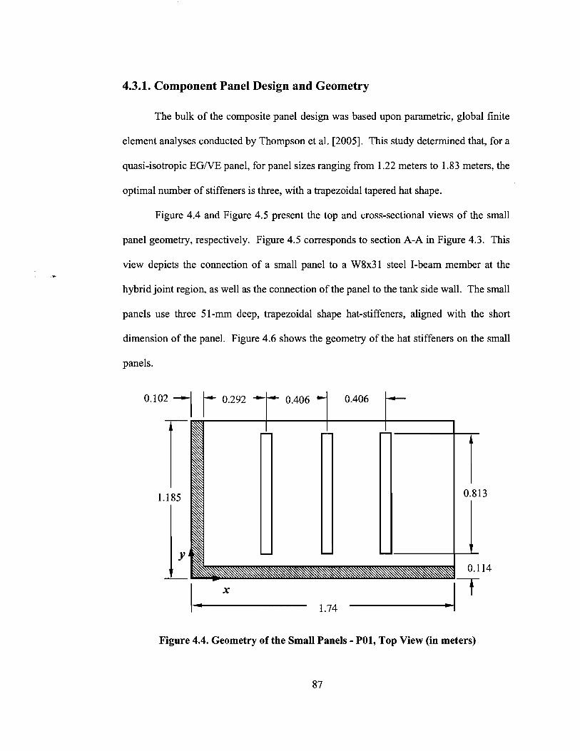
4.3.1. Component Panel Design and Geometry
The bulk of the composite panel design was based upon parametric, global finite
element analyses conducted by Thompson et al. [2005]. This study determined that, for a
quasi-isotropic EGNE panel, for panel sizes ranging from 1.22 meters to 1.83 meters, the
optimal number of stiffeners is three, with a trapezoidal tapered hat shape.
Figure 4.4 and Figure 4.5 present the top and cross-sectional views of the small
panel geometry, respectively. Figure 4.5 corresponds to section A-A in Figure 4.3. This
view depicts the connection of a small panel to a W8x31 steel I-beam member at the
hybrid joint region, as well as the connection of the panel to the tank side wall. The small
panels use three 51-mm deep, trapezoidal shape hat-stiffeners, aligned with the short
dimension of the panel. Figure 4.6 shows the geometry of the hat stiffeners on the small
panels.
Figure 4.4. Geometry of the Small Panels - POI, Top View (in meters)

Small panel
Tank side wall
Figure 4.5. Geometry of the Small Panels - POI, Cross-Sectional View (in mm)
Figure 4.6. Section C-C: Hat-Stiffener Geometry for Small Panels (in mm)

Figure 4.7 and Figure 4.8 present the top and cross-sectional views of the large
panel geometry, respectively. Figure 4.8 corresponds to section B-B (Figure 4.3), which
depicts the connection of a large panel to a W14x53 steel I-beam member and the
connection of the panel to the tank side wall. These panels use three 152-mm deep,
trapezoidal shape hat-stiffeners, aligned with the short dimension of the panel. A
sectioned view of the hat-stiffener geometry of the large panels is shown in Figure 4.9.
For both small and large panels, the laminate thickness was tapered from 25.4 mm at the
edges, to 12.7 mm at the center of the panels.
Figure 4.7. Geometry of the Large Panels - P03, Top View (in meters)
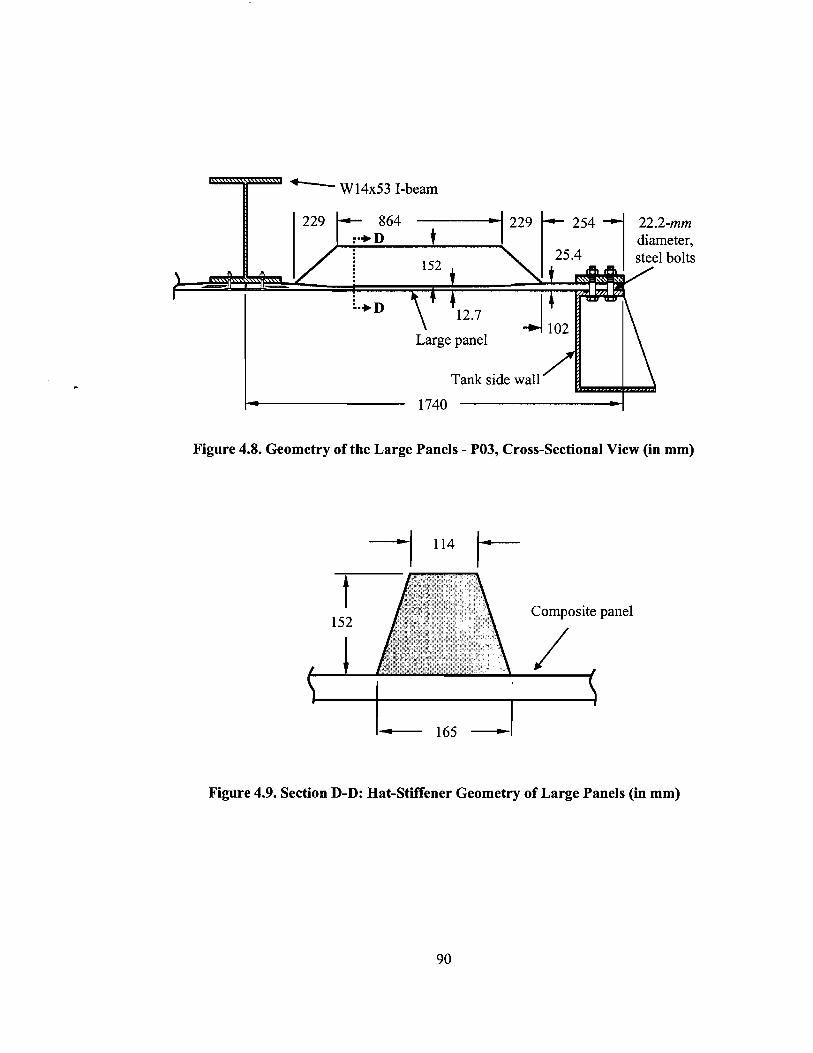
Tank side wall
Figure 4.8. Geometry of the Large Panels - P03, Cross-Sectional View (in mm)
Composite panel
Figure 4.9. Section D-D: Hat-Stiffener Geometry of Large Panels (in mm)

4.3.2. Description of the Hybrid Joint Region
Based on the sub-component test results presented in Chapter 3, a hybrid joint
with a short doubler plate and a foam insert (DS-4) was selected to connect the composite
panels to the steel I-beam members. An exploded view of the hybrid assembly schematic
is shown in Figure 4.10. The panel assembly consists of four hat-stiffened panels, bolted
onto the boundaries of the hydrostatic test tank. The hybrid joint region is composed of
four doubler plate sections (with two rows of bolts), a centerpiece doubler plate, the
edges of the composite panels, and two steel I-beams. For clarity, the steel I-beams are
not shown in this figure. It is noted that the surfaces with doubler plates represent the wet
side of the actual hybrid lifting body. Doubler plates are designated as "D##," where "D"
stands for "doubler," and the digits represent the panels that the doubler plate connects.
For instance, D34 is the doubler plate connecting the large panels, PO3 and P04.
Doubler plate, D 12
Figure 4.10. Hybrid Assembly Schematic (Exploded View)

A photograph of the short doubler with foam insert joint (DS-4) is shown in
Figure 4.1 1 and Figure 4.12 shows a schematic of the joint details and dimensions. As
described in Chapter 3, the joint consists of a composite panel sandwiched between a
steel I-beam member and a 146-mm wide by 6.35-mm thick, steel doubler plate. Foam
inserts were used to increase the strength and rigidity of the joint and to fix the start of the
tapered region with the edge of the steel flange. These members were joined together by
two rows of 12.7-mm, grade 5 tapered-head bolts, spaced at 38.1 rnrn on each side of the
steel web. A total of 206 bolts were used at the hybrid joint region. For watertight
integrity, a layer of RTV, clear silicone was applied at the interfaces between the steel
members and the composite panels. The hybrid joint and panel assembly procedures are
summarized in Appendix G.
Figure 4.11. Photograph of Short Doubler and Foam Insert Joint (DS-4)
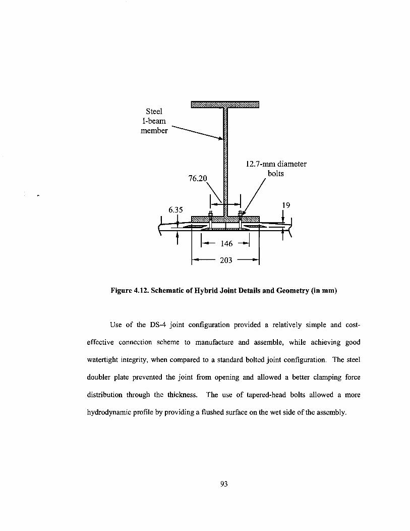
S tee1 I-beam member
N bolts
Figure 4.12. Schematic of Hybrid Joint Details and Geometry (in mm)
Use of the DS-4 joint configuration provided a relatively simple and cost-
effective connection scheme to manufacture and assemble, while achieving good
watertight integrity, when compared to a standard bolted joint configuration. The steel
doubler plate prevented the joint from opening and allowed a better clamping force
distribution through the thickness. The use of tapered-head bolts allowed a more
hydrodynamic profile by providing a flushed surface on the wet side of the assembly.

4.4. Materials and Test Article Fabrication
Fabrication of the composite panels was carried out at the Hybrid Structures
Laboratory, at the University of Maine, using a vacuum assisted resin transfer molding
process (VARTM). DOW Derakane 8084 Vinyl Ester resin and E-Glass fibers were used
as the panel constituents. The reinforcing fibers were 680-gm, 0190, and 680-gm, + 45,
knit fabric, and were provided by Brunswick Technologies, Inc. (BTI). DIAB Divinycell
H-80 foam was used to fabricate the foam inserts and the hat-stiffener sections.
A 12.7-mm thick, [(*45)f (0/90)f]4s quasi-isotropic lay-up was used as the
laminate architecture. The tapered region of the composite panels was created by
interleaving * 45 and 0190 full-panel sheets with 0190 drop ply strips at the boundaries.
This arrangement provided a total laminate thickness of 25.4 mm at the edges, tapering
down to 12.7 mm at the center of the panels. In order to account for the doubler plate
region, fabrication of the panels was performed on a 3-m by 3-m table, with a pre-
fabricated steel mold.
The small panels and the hat-stiffeners were co-infused and photographs of their
fabrication stages are shown in Figure 4.13. Resin infusion lines were placed on top of
the stiffeners and vacuum lines were located at the edges of the fabrication table. To
manufacture the stiffeners, the foam sections were positioned at the desired stiffener
locations and a total of eight E-Glass layers were placed on top of each foam
arrangement. A schematic of the lamination sequence for the hat-stiffener fabrication is
shown in Figure 4.14.

a) Panel and Hat-Stiffener Lay-Up
b) Panel Infusion
Figure 4.13. Fabrication of Small Panels
Side View Front View
Figure 4.14. Lamination Sequence for Hat-Stiffener Fabrication
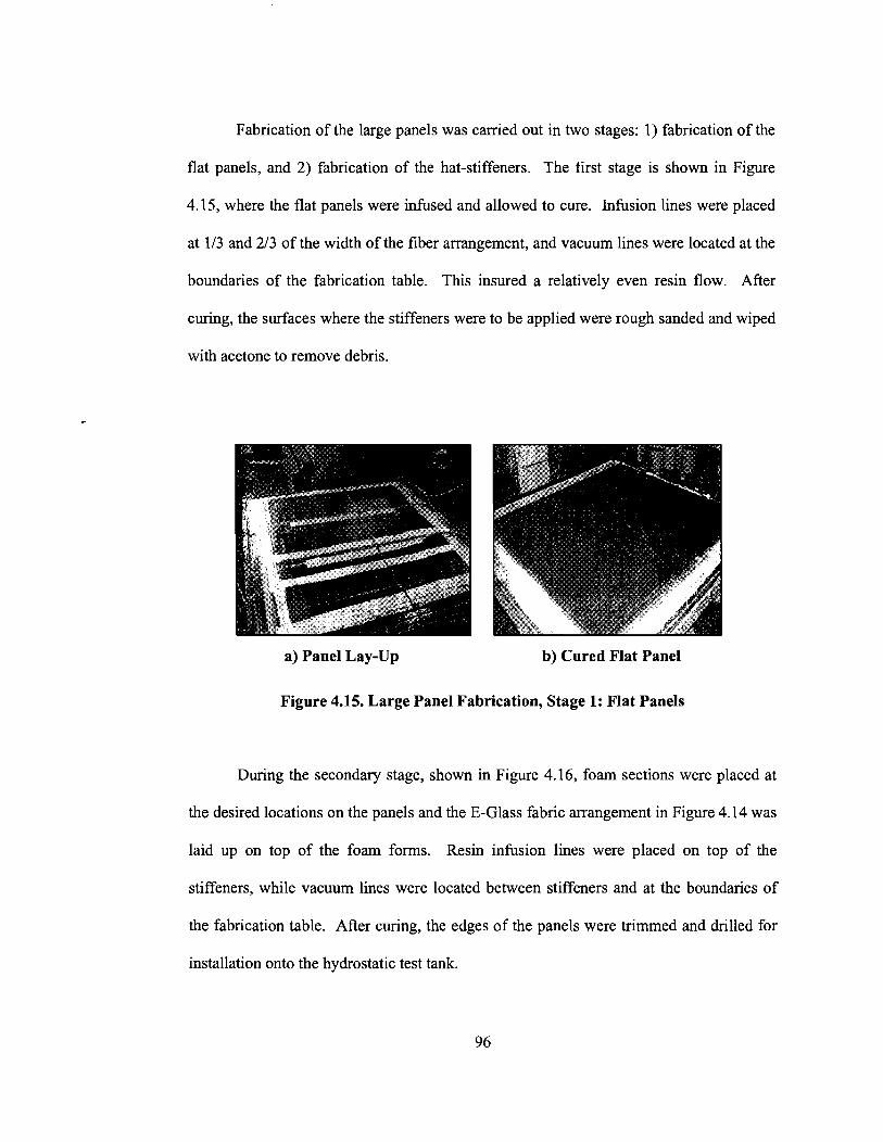
Fabrication of the large panels was carried out in two stages: 1) fabrication of the
flat panels, and 2) fabrication of the hat-stiffeners. The first stage is shown in Figure
4.15, where the flat panels were infused and allowed to cure. Infusion lines were placed
at 113 and 213 of the width of the fiber arrangement, and vacuum lines were located at the
boundaries of the fabrication table. This insured a relatively even resin flow. After
curing, the surfaces where the stiffeners were to be applied were rough sanded and wiped
with acetone to remove debris.
a) Panel Lay-Up b) Cured Flat Panel
Figure 4.15. Large Panel Fabrication, Stage 1: Flat Panels
During the secondary stage, shown in Figure 4.16, foam sections were placed at
the desired locations on the panels and the E-Glass fabric arrangement in Figure 4.14 was
laid up on top of the foam forms. Resin infusion lines were placed on top of the
stiffeners, while vacuum lines were located between stiffeners and at the boundaries of
the fabrication table. After curing, the edges of the panels were trimmed and drilled for
installation onto the hydrostatic test tank.
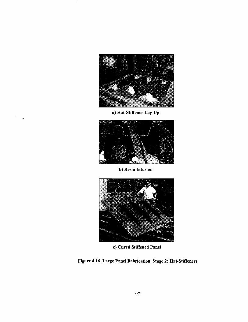
a) Hat-Stiffener Lay-Up
b) Resin Infusion
c) Cured Stiffened Panel
Figure 4.16. Large Panel Fabrication, Stage 2: Hat-Stiffeners
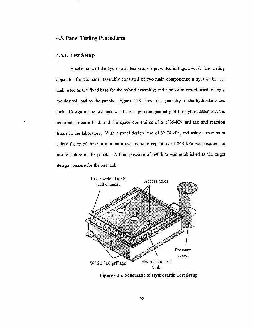
4.5. Panel Testing Procedures
4.5.1. Test Setup
A schematic of the hydrostatic test setup is presented in Figure 4.17. The testing
apparatus for the panel assembly consisted of two main components: a hydrostatic test
tank, used as the fixed base for the hybrid assembly; and a pressure vessel, used to apply
the desired load to the panels. Figure 4.18 shows the geometry of the hydrostatic test
tank. Design of the test tank was based upon the geometry of the hybrid assembly, the
required pressure load, and the space constraints of a 1335-KN grillage and reaction
frame in the laboratory. With a panel design load of 82.74 H a , and using a maximum
safety factor of three, a minimum test pressure capability of 248 kPa was required to
insure failure of the panels. A final pressure of 690 kPa was established as the target
design pressure for the test tank.
Laser welded tank
tank
Figure 4.17. Schematic of Hydrostatic Test Setup

1- 2.832 -i Figure 4.18. Geometry of the Hydrostatic Test Tank (in meters)
The hydrostatic test tank was comprised of four, custom laser welded, 337-mm
deep, steel channel sections to form the walls, and a 38-mm thick steel plate to form the
bottom of the tank. Figure 4.19 shows a typical laser welded channel. To provide
adequate stiffness to the top and bottom flanges, 12.7-mm thick web stiffeners were
welded to the channels, on 381-mm centers. A photograph of a welded channel, prior to
welding of the stiffeners, is shown in Figure 4.20, and its cross-sectional dimensions are
shown in Figure 4.2 1. The steel channel sections were fabricated at the Applied Thermal
Sciences, Inc. Laser Processing Facility, in Sanford, Maine. Use of laser welding made it
possible to create custom channel sections, while minimizing welding distortion and
insuring watertight integrity at the tank and composite panel interfaces.

O-ring groove
stiffeners
Figure 4.19. Typical Laser Welded Channel with Stiffeners
Figure 4-20. Laser Welded Channel at ATS Processing Faci]iQ

12.7-mm thick stiffeners at
3 8 1 -mm centers
Figure 4.21. Cross-Sectional Dimensions of a Laser Welded Channel (in mm)
Figure 4.22 depicts the connection of a laser welded channel to the test tank base
plate and the W36x300 grillage. As illustrated in Figure 4.23, the composite test panels
were connected to the hydrostatic test tank by sandwiching the panels between the top
flange of the tank channels and a 25.4-mm thick, steel backing plate. The panels were
bolted to the tank using 22.2-mm, grade 8 steel bolts, arranged in a pattern shown in
Figure 4.18. A watertight seal was created by using a 9.53-mm, square rubber O-ring,
located in a 15.88-mm x 6.68-mm deep gland, on the top flange of the tank, inside the
first bolt row. The bottom flanges of the laser welded channels were bolted to the 38-mm
thick, steel bottom plate. The bottom plate was then attached to the top flange of the
W36x300 grillage, by using 25.4-mm, grade 8, steel bolts.
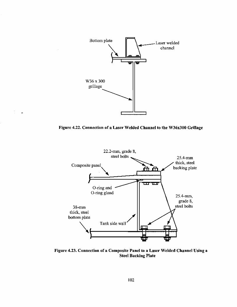
W36 x 300 grillage
\ I 1
Laser welded channel
Figure 4.22. Connection of a Laser Welded Channel to the W36x300 Grillage
22.2-mm, grade 8, 25.4-mm
38-mm thick, steel
bottom plate Tank side wall
Figure 4.23. Connection of a Composite Panel to a Laser Welded Channel Using a Steel Backing Plate

4.5.2. Testing Method
Testing of the panel assembly was conducted at the Hybrid Structures Laboratory,
at the University of Maine. A critical aspect of the hydrostatic testing procedure was to
devise a method to accurately regulate the tank pressure. Researchers have utilized
various methods for simulating hydrostatic and aerodynamic loads for testing of panels.
Some of these approaches were reviewed for their potential application to the MACH
concept panel testing.
Among the methods considered for loading of the hybrid assembly was a pressure
bladder approach, in which a distributed flexural load is applied in conjunction with a
traditional load frame [ASTM D6416-99, 20041. Though this method could be adapted
for large-scale panel testing, the watertight integrity of the joint could not be adequately
evaluated. Another approach considered was the D-Box test fixture, developed by
Lockheed Aeronautical Systems and later applied by NASA Langley Research center
[Arbur et al., 19951, which utilizes a sealed box pressurized with air or other inert gas to
generate flexural loading on full-scale curved panels. Due to the complexity and cost
associated with the test fixture, this technique was not well suited for panel testing.
Another technique used is multiple point loading, where pads are bonded to a plate or
outer skin. The nature of this technique makes it difficult to evaluate watertight integrity
and to achieve a realistic distributed panel load.
In light of the apparent inadequacies of the aforementioned techniques for panel
testing and their application to the MACH concept, devising a hydrostatichydrodynamic
test system was essential. By utilizing water as the testing medium, it is possible to
evaluate both the structural response of the panel assembly and the watertight integrity of
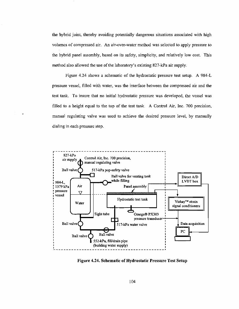
the hybrid joint, thereby avoiding potentially dangerous situations associated with high
volumes of compressed air. An air-over-water method was selected to apply pressure to
the hybrid panel assembly, based on its safety, simplicity, and relatively low cost. This
method also allowed the use of the laboratory's existing 827-kPa air supply.
Figure 4.24 shows a schematic of the hydrostatic pressure test setup. A 984-L
pressure vessel, filled with water, was the interface between the compressed air and the
test tank. To insure that no initial hydrostatic pressure was developed, the vessel was
filled to a height equal to the top of the test tank. A Control Air, Inc. 700 precision,
manual regulating valve was used to achieve the desired pressure level, by manually
dialing in each pressure step.
I 827-kPa I I I
manual regulating valve I I
I
valve for venting tank
pressure transducer
17-kPa water valve
I
I I 552-kPa, filVdrain pipe I (building water supply) I I I - - - - - - - - - - - - - - - - - - - - - - - - - - - - - - - - - - - - - - - - - - - a
Figure 4.24. Schematic of Hydrostatic Pressure Test Setup
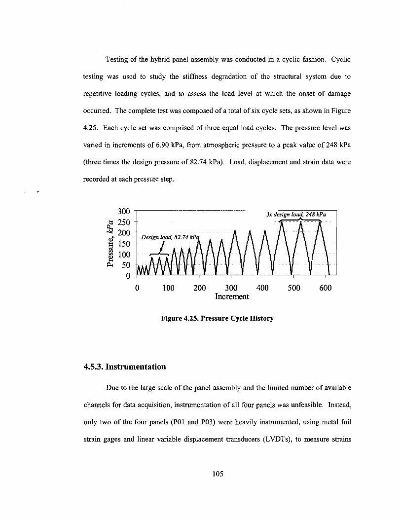
Testing of the hybrid panel assembly was conducted in a cyclic fashion. Cyclic
testing was used to study the stiffness degradation of the structural system due to
repetitive loading cycles, and to assess the load level at which the onset of damage
occurred. The complete test was composed of a total of six cycle sets, as shown in Figure
4.25. Each cycle set was comprised of three equal load cycles. The pressure level was
varied in increments of 6.90 kPa, from atmospheric pressure to a peak value of 248 kPa
(three times the design pressure of 82.74 Ha) . Load, displacement and strain data were
recorded at each pressure step.
I I I
100 200 300 400 500 600 Increment
Figure 4.25. Pressure Cycle History
4.5.3. Instrumentation
Due to the large scale of the panel assembly and the limited number of available
channels for data acquisition, instrumentation of all four panels was unfeasible. Instead,
only two of the four panels (PO1 and P03) were heavily instrumented, using metal foil
strain gages and linear variable displacement transducers (LVDTs), to measure strains

and vertical displacements at discrete locations on the panels and the steel I-beam
members. The applied pressure was measured using an omegam PX303 pressure
transducer, mounted on one of the side walls of the test tank. In addition,
photogrammetry targets were used to monitor the displacement field.
Strain gages were procured from Micro-Measurements Group, Inc. A total of
forty-eight uniaxial gages, type CEA-00-250UW-350, and four rosette gages, type CEA-
00-250UR-350, were installed on the composite panel surfaces. A total of fourteen
uniaxial gages, type CEA-06-250UW-350, were mounted on the steel members. A total
of fifteen MacroSensorsTM LVDTs were used to measure the vertical displacement of the
panels and the I-beam members. Six LVDTs were placed on each panel, PO1 and P03,
and one LVDT was placed at the crossing point of the I-beams to monitor the global
displacement of the assembly. For PO2 and P04, one LVDT was placed at the center of
each panel.
Figure 4.26 shows a schematic of the hybrid panel assembly and the naming
conventions used to identify its various components. The small panels are identified as
PO1 and P02, while the large panels are identified as PO3 and P04. Doubler plate
designations are shown in the figure, where the centerpiece doubler is designated as CP.
A local coordinate system is used for each panel and labeled according to the panel
number, i.e. XI, yl, for small panel 1 (POI), etc. The origin of the coordinate systems is
located at the center of CP. Strain gages and LVDTs were designated according to the
instrumentation naming convention presented in Table 4.1.
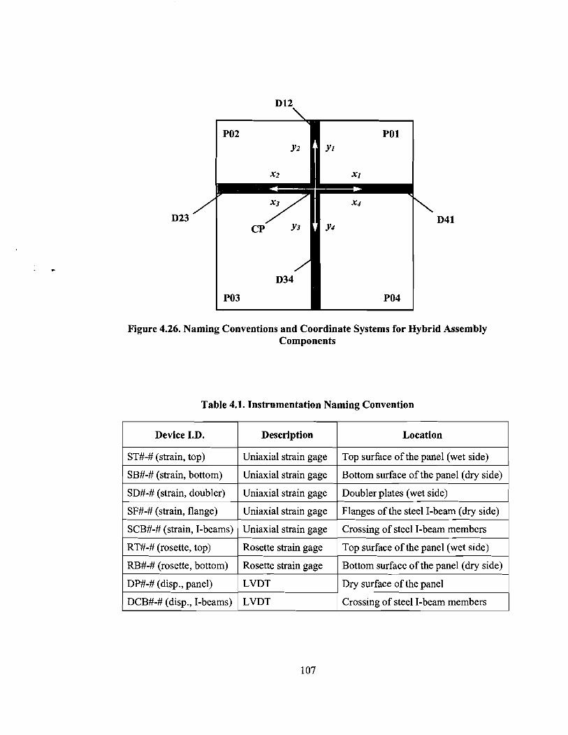
Figure 4.26. Naming Conventions and Coordinate Systems for Hybrid Assembly Components
Table 4.1. Instrumentation Naming Convention
Device I.D.
ST#-# (strain, top)
SB#-# (strain, bottom)
SD#-# (strain, doubler)
SF#-# (strain, flange)
SCB#-# (strain, I-beams)
RT#-# (rosette, top)
RB#-# (rosette, bottom)
DP#-# (disp., panel)
DCB#-# (disp., I-beams)
Description
Uniaxial strain gage
Uniaxial strain gage
Uniaxial strain gage
Uniaxial strain gage
Uniaxial strain gage
Rosette strain gage
Rosette strain gage
LVDT
LVDT
Location
Top surface of the panel (wet side)
Bottom surface of the panel (dry side)
Doubler plates (wet side)
Flanges of the steel I-beam (dry side)
Crossing of steel I-beam members
Top surface of the panel (wet side)
Bottom surface of the panel (dry side)
Dry surface of the panel
Crossing of steel I-beam members

In Table 4.1, the first number following the letters corresponds to the panel
number on which the device was installed, and the second number corresponds to the
device number. For instance, STl-1 stands for "Strain gage on the Top surface, panel 1,
gage number 1." Similarly, DP1-1 stands for "Displacement sensor, Panel 1, LVDT
number 1 ."
Figure 4.27 shows a schematic of the strain gage configuration for the wet side of
Pol, while Figure 4.28 shows that of the dry side. The geometric locations of the strain
gages on the wet and dry surfaces of the panel are presented in Tables 4.2 and 4.3,
respectively. The LVDT configuration for PO1 is depicted in Figures 4.29 and 4.30. The
geometric locations of the LVDTs are summarized in Table 4.4.
Figure 4.27. Strain Gage Configuration for POI, Wet Side

Figure 4.28. Strain Gage Configuration for Pol, Dry Side
Table 4.2. Strain Gage Locations for POI, Wet Side

Table 4.3. Strain Gage Locations for POI, Dry Side
X I
Figure 4.29. LVDT Configuration for POI, Plan View
Gage I.D.
SBl-1 SB 1-2 SB 1-3 SBl-4
RB 1 -5A RB 1 -5B RB 1 -5C SB 1-6 SB 1-7 SB 1-8 SB 1-9
SB1-10 SB1-11 SF1-1 SF 1-2 SF 1-3 SF 1-4 SF 1-5 SF 1-6
Gage type
Uniaxial Uniaxial Uniaxial Uniaxial Rosette Rosette Rosette Uniaxial Uniaxial Uniaxial Uniaxial Uniaxial Uniaxial Uniaxial Uniaxial Uniaxial Uniaxial Uniaxial Uniaxial
yl (mm)
719 71 1 522 522 144 144 144 522 522 127 117 524 524 524 524 48 4 1 52 4 1
xl (mm)
8 13 8 13 82 1 8 13 8 13 8 13 8 13 586 606 606 606 127 117 48 38 58 1 58 1 813 8 13
Location
Panel, Bottom Panel, Bottom Panel, Bottom Panel, Bottom Panel, Bottom Panel, Bottom Panel, Bottom Panel, Bottom Panel, Bottom Panel, Bottom Panel, Bottom Panel, Bottom Panel, Bottom
FY FY FX FX FX FX
Gage direction
X I
Y I X I
y I Y I Y I X I
X I
y I Y I X I
X I
Y I X I
y I Y I X I
y I X I

Figure 4.30. LVDT Configuration for POI, Side View
Table 4.4. LVDT Locations for POI, Dry Side
Schematics of the strain gage configuration for the wet and dry sides of PO3 are
shown in Figures 4.3 1 and 4.32, respectively. Strain gage locations are summarized in
Tables 4.5 and 4.6. LVDT configuration schematics for PO3 are presented in Figures
4.33 and 4.34 and their geometric locations are presented in Table 4.7.

Figure 4.31. Strain Gage Configuration for P03, Wet Side
Figure 4.32. Strain Gage Configuration for P03, Dry Side
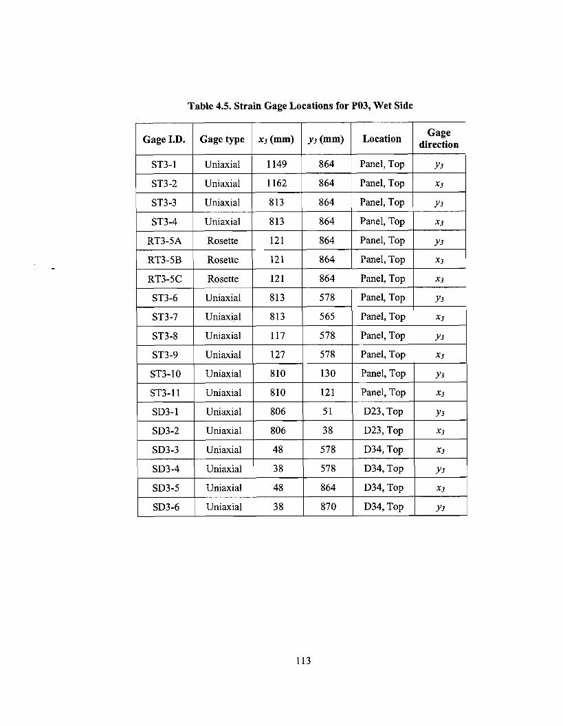
Table 4.5. Strain Gage Locations for P03, Wet Side
Gage direction
Y3
X3
Y3
x3
Y3
X 3
x3
Y3
X 3
Y3
X 3
Y3
x3
Y3
x3
x3
Y3
x3
Y3
Location
Panel, Top
Panel, Top
Panel, Top
Panel, Top
Panel, Top
Panel, Top
Panel, Top
Panel, Top
Panel, Top
Panel, Top
Panel, Top
Panel, Top
Panel, Top
D23, Top
D23, Top
D34, Top
D34, Top
D34, Top
D34, Top
y3 (mm)
864
864
864
864
864
864
864
578
565
578
578
130
121
5 1
38
578
578
864
870
Gage I.D.
ST3-1
ST3-2
ST3-3
ST3-4
RT3-5A
RT3-5B
RT3-5C
ST3-6
ST3-7
ST3-8
ST3-9
ST3-10
ST3-11
SD3-1
SD3-2
SD3-3
SD3-4
SD3-5
SD3-6
Gage type
Uniaxial
Uniaxial
Uniaxial
Uniaxial
Rosette
Rosette
Rosette
Uniaxial
Uniaxial
Uniaxial
Uniaxial
Uniaxial
Uniaxial
Uniaxial
Uniaxial
Uniaxial
Uniaxial
Uniaxial
Uniaxial
x3 (mm)
1149
1162
813
813
121
121
121
813
813
117
127
810
810
806
806
48
3 8
48
3 8
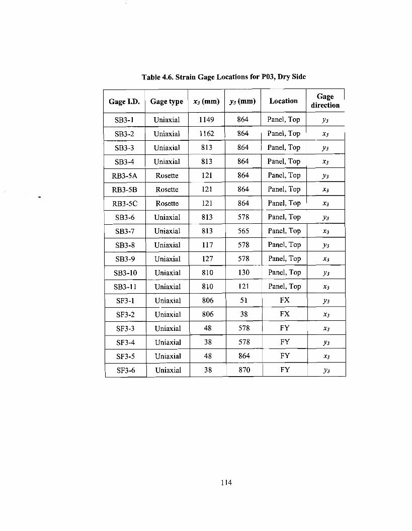
Table 4.6. Strain Gage Locations for P03, Dry Side
y 3 (mm)
864
864
864
864
864
864
864
578
565
578
578
130
121
5 1
38
578
578
864
870
x 3 (mm)
1149
1162
8 13
8 13
121
121
121
8 13
813
117
127
810
810
8 06
8 06
48
38
48
3 8
Gage I.D.
SB3-1
SB3-2
SB3-3
SB3-4
RB3-5A
RB3-5B
RB3-5C
SB3-6
SB3-7
SB3-8
SB3-9
SB3-10
SB3-11
SF3-1
SF3-2
SF3-3
SF3-4
SF3-5
SF3-6
Gage type
Uniaxial
Uniaxial
Uniaxial
Uniaxial
Rosette
Rosette
Rosette
Uniaxial
Uniaxial
Uniaxial
Uniaxial
Uniaxial
Uniaxial
Uniaxial
Uniaxial
Uniaxial
Uniaxial
Uniaxial
Uniaxial
Location
Panel, Top
Panel, Top
Panel, Top
Panel, Top
Panel, Top
Panel, Top
Panel, Top
Panel, Top
Panel, Top
Panel, Top
Panel, Top
Panel, Top
Panel, Top
FX
FX
FY
FY
FY
FY
Gage direction
Y 3
X 3
Y 3
X 3
Y 3
X 3
X 3
Y 3
x3
Y 3
X 3
Y 3
X 3
Y 3
X 3
X 3
Y 3
X 3
Y 3

Figure 4.33. LVDT Configuration for P03, Plan View
y3 c--l Figure 4.34. LVDT Configuration for P03, Side View
Table 4.7. LVDT Locations for P03, Dry Side

4.5.4. Data-Acquisition Configuration
Figure 4.35 shows a schematic of the data-acquisition system. Data-acquisition
was carried out using two PentiumTM 4, 2.4 GHz, 512-MB RAM systems, two
IOTECHTM Daqboard 2000 cards, and nine VishayTM 2120 multi-channel strain signal
conditioners. These systems have 16 bit analog-to-digital conversion resolution and are
capable of reading a total of forty-eight channels at a throughput rate of 1 kHz, which
was appropriate for the rate of testing used in this study.
The data-acquisition process was controlled using the DAQFI-D5 software,
written at the University of Maine. Load, displacement and strain values were recorded
at every load step. A timed data taking routine was used to trigger the system every three
minutes, which was found to be an adequate time interval to allow pressure stabilization
inside of the test tank. Strain readings from seven signal conditioners were multiplexed
in order to accommodate all strain gages and the available number of channels. To
reduce the errors due to instrumentation noise, multiple samples were averaged during
data acquisition. Photogrammetry data was taken during the initial stage, prior to loading
of the assembly, and at the peak pressure values of 124 kPa and 248 kPa.
Test data were recorded using two IOTECH data acquisition systems. The
systems were labeled as DAQ-A and DAQ-B. DAQ-A was equipped with two
DAQboard 2000 boards, capable of reading 32 channels, while DAQ-B was configured
to read 16 channels. The multiplexed strain values were recorded using the DAQ-B
system. Pressure transducer values were recorded with both systems. For data-
acquisition purposes, the DAQ-A system acted as the master system, which triggered
DAQ-B to record data every three minutes.
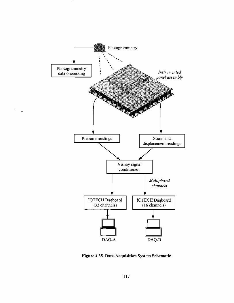
Photogrammetry
1 \\ --.
Instrumented
Pressure readings Strain and displacement readings
Vishay signal conditioners
I I Multiplexed
channels
IOTECH Daqboard IOTECH Daqboard (32 channels)
I
DAQ-A DAQ-B
Figure 4.35. Data-Acquisition System Schematic
4.6. Panel Testing Results
The panel testing results were subdivided into four distinct sections: 1) load
versus displacement curves; 2) displaced panel shapes; 3) load versus strain curves; and
4) failure modes. Testing of the panels to failure allowed the verification of the panel
design and the manufacturing techniques. Additionally, it allowed an assessment of the
feasibility of implementing the DS-4 joint configuration into a large-scale panel
assembly. Correlation of the displacements recorded with LVDTs and photogrammetry is
also presented in this section.
4.6.1. Load versus Displacement Curves
Load versus displacement curves at various load steps are used to provide an
indication of stiffness degradation and to observe the onset of damage and ultimate
structural failure. The load versus displacement curves for panels PO1 and PO3 are
presented in Figures 4.36 and 4.37, respectively. These curves correspond to the vertical
displacement values recorded at the center of the middle stiffeners (DP1-1, DP3-I). Each
figure presents curves for the first three load cycle sets and the loops for the entire test.
Figures 4.36a and 4.37a show the load versus displacement curves for the initial
loading cycle set, with a peak pressure value of 41.37 kPa, one half of the panel design
load. For this case, the pressure was increased in steps of 3.45 kPa for the 0-21 kPa
range, and 6.90 kPa for the 21-41.37 kPa range. The curves for PO1 and PO3 exhibit a
stable, linear response, as the loading and unloading paths are nearly identical. For this
load cycle set, the maximum displacement values recorded for PO1 and PO3 were 3.26
rnrn and 3.47 mm, respectively.
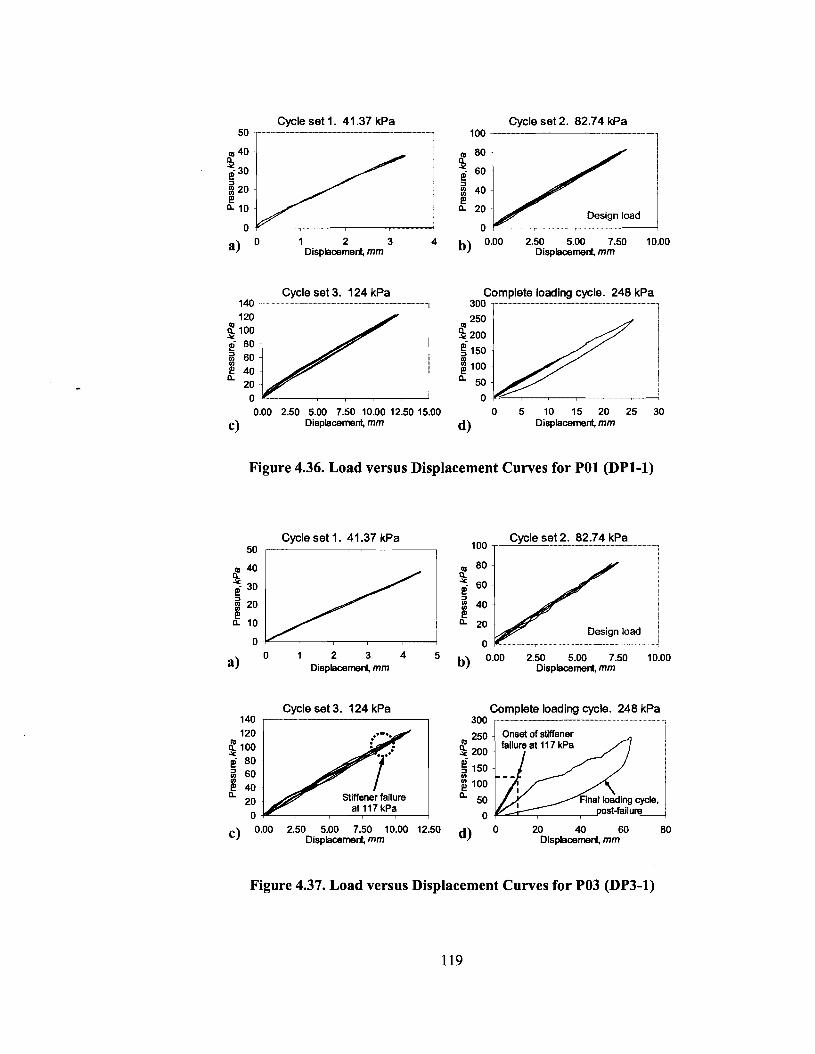
Cycle set I . 41.37 kPa Cycle set 2. 82.74 kPa 50 .
I- , '00 TI._I" 1
1 2 3 4 b) 0.00 2.50 5.00 7.50 10.00 Displacement, mm Displacement, mm
Cycle set 3. 124 kPa Complete loading cycle. 248 kPa ............... ...... ....
0.00 2.50 5.00 7.50 10.00 12.50 15.00 0 5 10 15 20 25 30
c) Displacement, mm d) Displacement, mm
Figure 4.36. Load versus Displacement Curves for PO1 (DP1-1)
Cycle set 1. 41.37 kPa Cycle set 2. 82.74 kPa 50 1 I
l o o T' .-
a) 0 1 2 3 4 5 b) 0.00 2.50 5.00 7.50 10.00
Displacemet-& mm Displacement, mm
Cycle set 3. 124 kPa Complete loading cycle. 248 kPa . ...... 140 1 1 300 ,
120 C l 0 0
250 1 * 200 failure at 11 7 kPa
2 so 60
$ 150 - - $100 ! @ 40
0 20 Stiffener failure n.
50 I Final loading cycle, ,
0 0 ost-failure 1
C) 0.00 2.50 5.00 7.50 10.00 12.50 d) O 20 40 60 80
Displacement, mm Displacement, mm
Figure 4.37. Load versus Displacement Curves for PO3 (DP3-1)

Figures 4.36b and 4.37b show the load versus displacement curves of panels PO1
and P03, when loaded to the design pressure of 82.74 kPa. Linear behavior of the system
was observed and visual inspection of the panel assembly indicated no apparent damage.
The design load was reached without damage to the joint or the composite panels. For
this load cycle set, the maximum displacement values recorded for PO1 and PO3 were
8.70 mrn (DP1-6) and 8.42 mm (DP3-6), respectively, which correspond to the
displacements recorded between stiffeners.
As described by Thompson et al. [2005], the peak deflection of the panels, A,,,
was established according to Equation (4. I), where L is the span of the panel and b is the
design factor. The panels were designed with a target value of bdesig,, = 200. Table 4.8
summarizes the maximum panel displacements at the design load, along with the values
of b,, computed using the experimental results. For both small and large panels, this
ratio is very close to the design target, with a peak difference of 9.14 percent for the large
panel.
Table 4.8. Maximum Panel Displacements at Design Load, P = 82.74 kPa
Panel
PO 1
PO3
L (mm)
1638
1838
a (
8.70
8.42
b, = L 1 Amax
193.45
2 18.29
bdesign
200
200
Yo Difference
3.28
9.14

Figures 4 .36~ and 4 . 3 7 ~ show the load versus displacement curves for the third set
of cycles, where the hybrid assembly was loaded to a pressure of 124 kPa. A slight
opening of the curves was observed for this loading step. At 1 17 kPa, failure was visibly
observed at the stiffenerlpanel interface, on the outer stiffener of P03, but was not
observable fiom the curves in Figure 4.37c, since damage was localized at the tapered
region of the stiffener (Figure 4.38) and was not captured by the LVDT located at the
center of the stiffener (DP3-1). The onset of damage produced load redistribution fiom
the outer stiffener to the middle and inner stiffeners, until failure of all stiffeners occurred
during the last loading cycle set. For this set of loading cycles, the peak displacements
recorded for PO 1 and PO3 were 13.47 mm (DPl-6) and 12.84 mm (DP3-6), respectively.
Figure 4.38. Onset of Damage at the StiffenerIPanel Interface (P03)
Load versus displacement curves for the entire test are shown in Figures 4.36d
and 4.37d. In both cases, the unloading path was different from the loading path, which
indicated permanent stiffness degradation within the composite panels. For the small
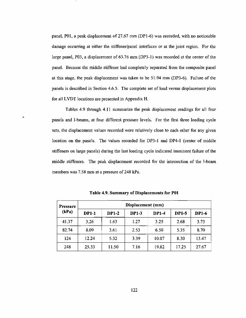
panel, Pol, a peak displacement of 27.67 mm (DP1-6) was recorded, with no noticeable
damage occurring at either the stiffenerlpanel interfaces or at the joint region. For the
large panel, P03, a displacement of 63.76 mm (DP3-1) was recorded at the center of the
panel. Because the middle stiffener had completely separated from the composite panel
at this stage, the peak displacement was taken to be 51.94 mm (DP3-6). Failure of the
panels is described in Section 4.6.5. The complete set of load versus displacement plots
for all LVDT locations are presented in Appendix H.
Tables 4.9 through 4.1 1 summarize the peak displacement readings for all four
panels and I-beams, at four different pressure levels. For the first three loading cycle
sets, the displacement values recorded were relatively close to each other for any given
location on the panels. The values recorded for DP3-1 and DP4-1 (center of middle
stiffeners on large panels) during the last loading cycle indicated imminent failure of the
middle stiffeners. The peak displacement recorded for the intersection of the I-beam
members was 7.58 mm at a pressure of 248 kPa.
Table 4.9. Summary of Displacements for PO1
Pressure (kPa)
41.37
82.74
124
248
Displacement (mm)
DPl-1
3.26
8.09
12.24
25.33
DP1-2
1.63
3.61
5.32
11.50
DP1-3
1.27
2.53
3.39
7.16
DP1-4
3.25
6.50
10.07
19.82
DP1-5
2.68
5.35
8.30
17.25
DP1-6
3.73
8.70
13.47
27.67

Table 4.10. Summary of Displacements for PO3
Table 4.11. Summary of Displacements for P02, PO4 and I-beams
Pressure (*a)
41.37
82.74
124
248
4.6.2. Displaced Panel Shapes
Displacement (mm)
Pressure (*a)
41.37
82.74
124
248
Figures 4.39 and 4.40 present the displaced shapes for panels POI and PO3 at
various pressure load levels, respectively. These shapes were plotted using displacement
values recorded at discrete LVDT locations, along the x and y directions for PO1 and P03,
versus the LVDT location. In a qualitative sense, the curves for the first three pressure
level values indicate a nearly proportional increase of displacement with increasing
pressure.
DP3-1
3.47
7.53
11.16
63.76
Displacement (mm)
DP3-5
2.18
4.35
6.58
28.56
DP2-1
3.72
7.44
11.15
23.73
DP3-2
3.31
6.63
10.07
49.26
DP3-6
3.75
8.42
12.84 -
51.94
DP4-1
3.37
6.74
10.69
74.99
DP3-3
1.28
2.67
3.80
14.09
DCB-1
1.28
2.56
3.39
7.58
DP3-4
1.72
3.44
4.97
11.94

Figure 4.39. Displaced Shapes for PO1
Figure 4.40. Displaced Shapes for PO3
4.6.3. Correlation of Displaced Panel Shapes to Photogrammetry
Figures 4.41 and 4.42 present the displaced shapes for PO1 and P03, for a pressure
of 124 H a . These curves were plotted using displacement values recorded at discrete
locations, from LVDTs and photogrammetry targets. As depicted in Figure 4.26, the X I
axis is aligned transversely to the stiffener direction and y, is in the stiffener direction, for
POI. For P03, the xj axis is aligned with the direction of the stiffeners and y3 is transverse
to the stiffeners. In general terms, and for a pressure load level of 124 H a , good
agreement was observed between the values recorded from the LVDTs and those from
the photogrammetry targets, with a peak discrepancy of 7 percent.

Figure 4.41. Displaced Shapes for PO1 at 124 kPa
Figure 4.42. Displaced Shapes for PO3 at 124 kPa
Figures 4.43 and 4.44 present the displaced shapes for PO1 and P03, respectively,
for a pressure load of 248 kPa, after failure of the stiffeners had occurred on the large
panels. Good agreement was observed between the LVDT and photogrammetry target
readings for Pol. In the case of PO3 along the x3 direction, the curves in Figure 4.44
show a clear discrepancy between the recorded values at the middle stiffener. This was
attributed to severe bending of the LVDT rods at this load level, which in turn under
predicted the deflection values on the large panels, particularly at the region where the
stiffeners had completely separated from the composite panel. For the curves plotted
along the y3 direction, the LVDT and photogrammetry curves showed good agreement,
except for the readings at the center of the middle stiffener, which differed by 13 percent.

Figure 4.43. Displaced Shapes for PO1 at 248 kPa
100 .-
90 I +LMIT~ .-rn- Actual
Figure 4.44. Displaced Shapes for PO3 at 248kPa
Readings from the photogrammetry targets were used to create surface plots of
the displaced panel assembly, as shown in Figures 4.45 and 4.46. The use of
photogrammetry aided in visualizing the global behavior of the panel assembly, which
would have not been attainable using the few, discrete displacement LVDT readings.
Figure 4.45 shows a surface plot of the displaced panel assembly when loaded to 124
kPa. The valley-shaped regions in PO3 and PO4 display the effect of the stiffeners, while
the sufaces in red represent the regions between stiffeners, which show the peak
displacement values recorded, at 12.84 mm (DP3-6).

Figure 4.45. Surface Plot of Displaced Panel Assembly at 124 kPa Using Photogrammetry (in mm)
Figure 4.46 presents the surface plot of the displaced panel assembly loaded to
248 kPa, after failure of all stiffeners on the large panels had occurred. Prominent peaks
are observed at the stiffener locations on PO3 and P04, which depict the separation of the
middle stiffeners from the composite panels. At this stage, the stiffeners were no longer
effective, and peak displacements are observed on the stiffener regions closer to the fixed
boundary of the test tank.
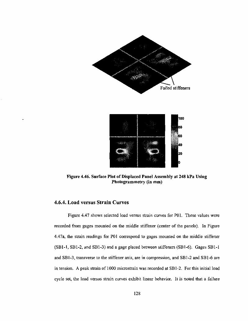
Figure 4.46. Surface Plot of Displaced Panel Assembly at 248 kPa Using Photogrammetry (in mm)
4.6.4. Load versus Strain Curves
Figure 4.47 shows selected load versus strain curves for Pol. These values were
recorded from gages mounted on the middle stiffener (center of the panels). In Figure
4.47a7 the strain readings for PO1 correspond to gages mounted on the middle stiffener
(SB1-1, SB 1-2, and SB1-3) and a gage placed between stiffeners (SB 1-6). Gages SB1- 1
and SB 1-3, transverse to the stiffener axis, are in compression, and SB 1-2 and SB 1 -6 are
in tension. A peak strain of 1000 microstrain was recorded at SB1-2. For this initial load
cycle set, the load versus strain curves exhibit linear behavior. It is noted that a failure
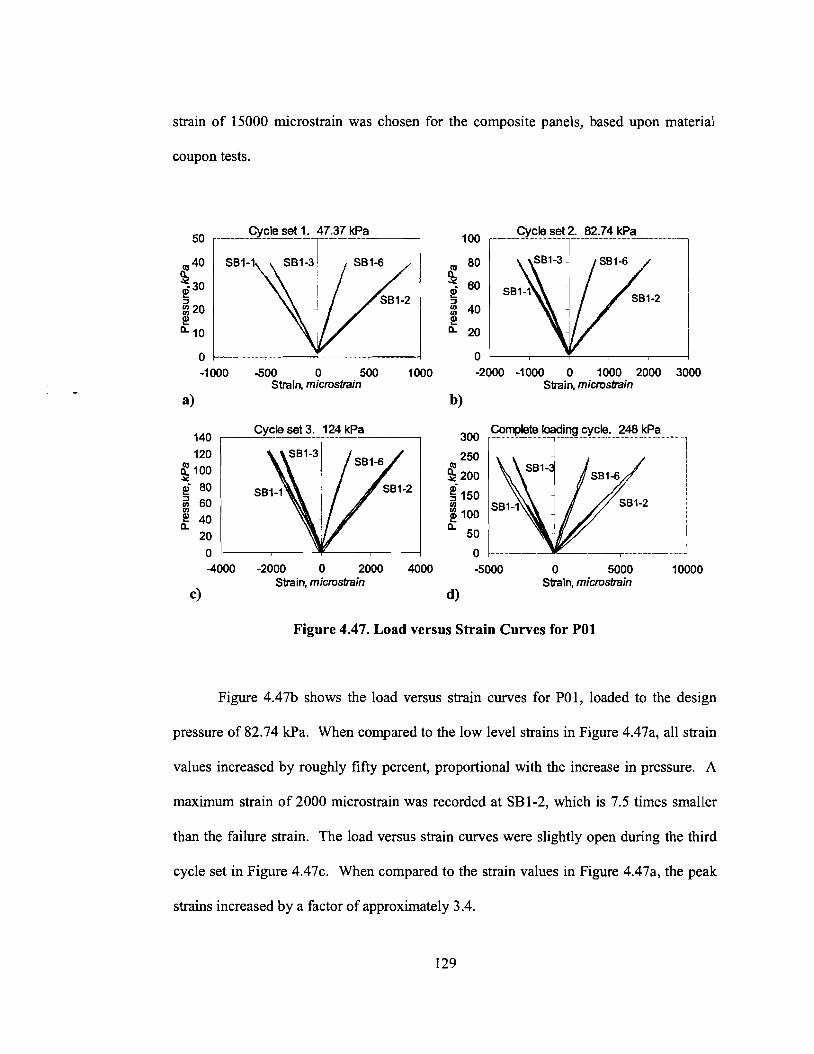
strain of 15000 microstrain was chosen for the composite panels, based upon material
coupon tests.
Cycle set 1. 47.37 kPa 50 r-.-lll--..-...-l-r_.._ 100 II1._.__-i_________. Cycle set 2. 82.74 kPa
-1000 -500 0 500 1000 -2000 -1000 0 1000 2000 3000 Strain, microstrain Strain, mimstrain
a) b)
140 1 Cycle set 3. 124 kPa Complete loading cycle. 248 kPa
I I 300
1
-4000 -2000 0 2000 4000 -5000 0 5000 10000 Strain, microshin Strain, microstrain
c) d)
Figure 4.47. Load versus Strain Curves for PO1
Figure 4.47b shows the load versus strain curves for Pol, loaded to the design
pressure of 82.74 kPa. When compared to the low level strains in Figure 4.47a, all strain
values increased by roughly fifty percent, proportional with the increase in pressure. A
maximum strain of 2000 microstrain was recorded at SBl-2, which is 7.5 times smaller
than the failure strain. The load versus strain curves were slightly open during the third
cycle set in Figure 4 .47~. When compared to the strain values in Figure 4.47a, the peak
strains increased by a factor of approximately 3.4.
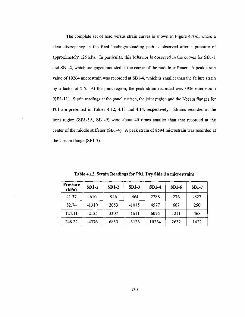
The complete set of load versus strain curves is shown in Figure 4.47d, where a
clear discrepancy in the final loadinglunloading path is observed after a pressure of
approximately 125 kPa. In particular, this behavior is observed in the curves for SB1-1
and SBl-2, which are gages mounted at the center of the middle stiffener. A peak strain
value of 10264 microstrain was recorded at SB1-4, which is smaller than the failure strain
by a factor of 2.5. At the joint region, the peak strain recorded was 3936 microstrain
(SBl-11). Strain readings at the panel surface, the joint region and the I-beam flanges for
PO1 are presented in Tables 4.12, 4.13 and 4.14, respectively. Strains recorded at the
joint region (SB1-5A, SB1-9) were about 40 times smaller than that recorded at the
center of the middle stiffener (SB1-4). A peak strain of 8594 microstrain was recorded at
the I-beam flange (SF 1-5).
Table 4.12. Strain Readings for POI, Dry Side (in microstrain)
Pressure (Wa) 41.37
82.74
124.11
248.22
SB1-1
-610
-1310
-2125
-4376
SB1-2
946
2053
3307
6833
SB1-3
-464
-1015
-161 1
-3 126
SB1-4
2288
4577
6076
10264
SB1-6
276
667
121 1
2632
SB1-7
-827
250
468
1422
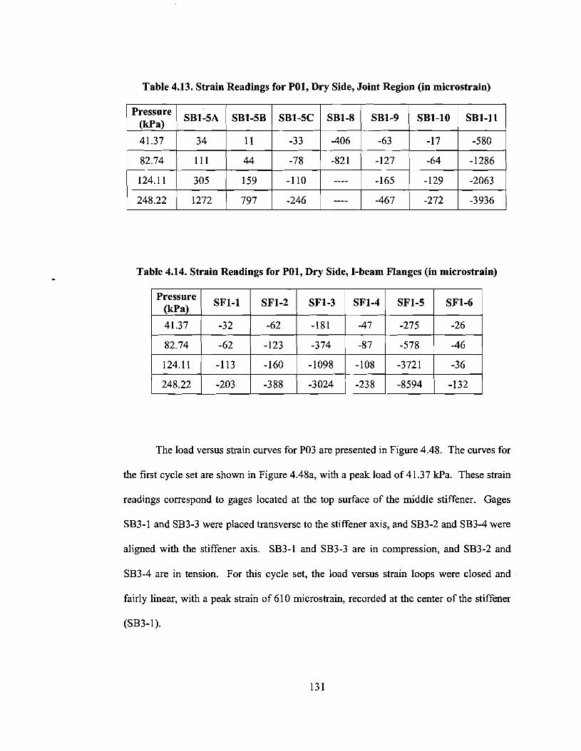
Table 4.13. Strain Readings for Pol, Dry Side, Joint Region (in microstrain)
Table 4.14. Strain Readings for POI, Dry Side, I-beam Flanges (in microstrain)
Pressure
41.37
82.74
124.1 1
248.22
The load versus strain curves for PO3 are presented in Figure 4.48. The curves for
the first cycle set are shown in Figure 4.48a, with a peak load of 41.37 kPa. These strain
readings correspond to gages located at the top surface of the middle stiffener. Gages
SB3-1 and SB3-3 were placed transverse to the stiffener axis, and SB3-2 and SB3-4 were
aligned with the stiffener axis. SB3-1 and SB3-3 are in compression, and SB3-2 and
SB3-4 are in tension. For this cycle set, the load versus strain loops were closed and
fairly linear, with a peak strain of 61 0 microstrain, recorded at the center of the stiffener
(SB3-I).
SB1-5A
34
11 1
305
1272
SB1-5C
-33
-78
-1 10
-246
SB1-5B
11
44
159
797
SB1-8
-406
-82 1
---- ----
SB1-9
-63
-127
-165
-467
SB1-10
-17
-64
-129
-272
SB1-11
-580
- 1286
-2063
-3936

--.-- Cycle set 2. 82.74 kPa 100
8 80
*- 60 ; $ 40 g! Q 20
0 -500 0 500 1000 -1 000 0 1000 2000 3000
Strain, microshin b)
Strain, microshin a)
Cycle set 3. 124 kPa
-2000 0 2000 4000 6000
c) Shin, microshin
Corr~lete loading cycle. 248 kPa
-2000 0 2000 4000 6000
d) Strain, microstrain
Figure 4.48. Load versus Strain Curves for PO3
Figure 4.48b shows the load versus strain curves for PO3 when the assembly was
loaded to the design pressure of 82.74 kPa. When compared to the initial loading cycle
strains in Figure 4.48a, the magnitudes increased by a factor of approximately 6. A
maximum strain of 2700 microstrain was recorded at SB3-2, which is 5.5 times smaller
than the failure strain. The panel response was observed to be linear up to its design load,
with closed loops and no visible damage either on the surface of the panels or at the joint
region.
As with Pol, open loops were observed during the third cycle set shown in Figure
4 .48~. Though difficult to differentiate in this figure, the unloading curves for SB3-1 and
SB3-3 did not follow the loading path during the third cycle set. When compared to the
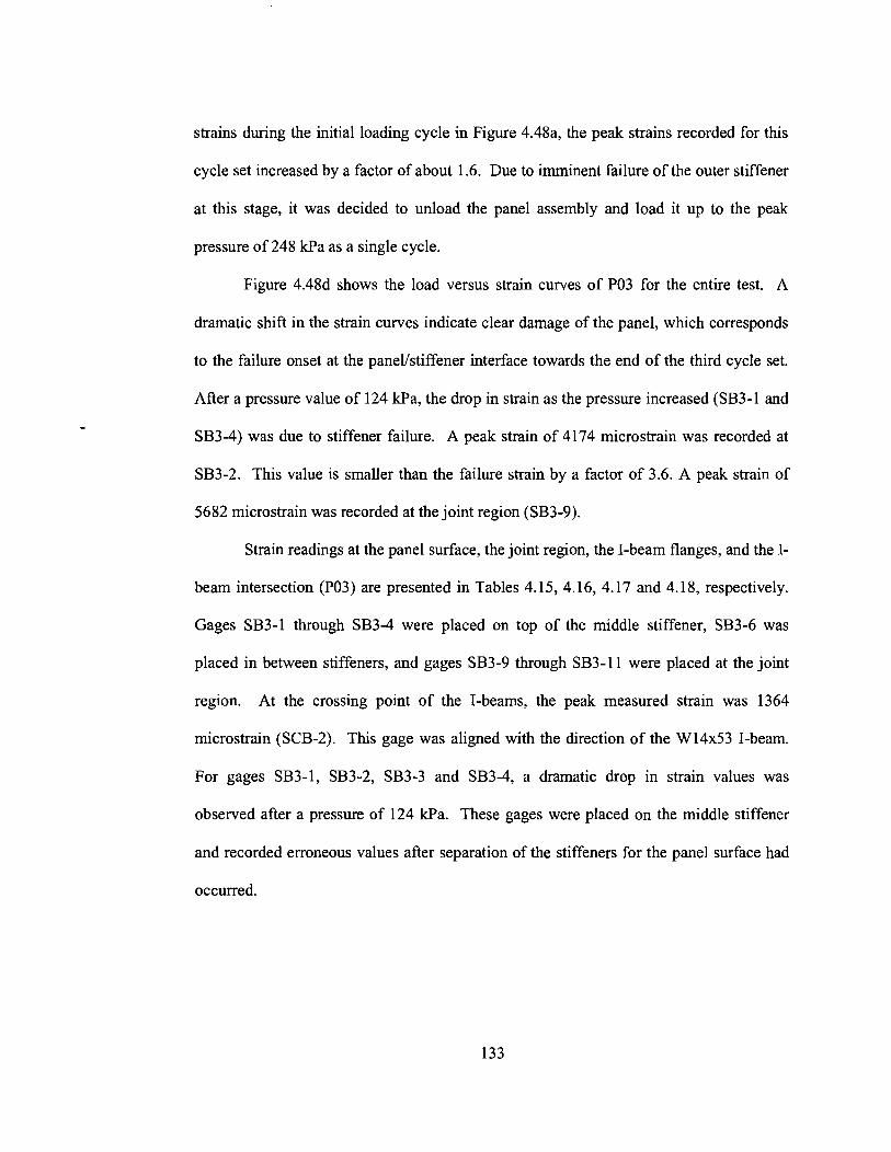
strains during the initial loading cycle in Figure 4.48a, the peak strains recorded for this
cycle set increased by a factor of about 1.6. Due to imminent failure of the outer stiffener
at this stage, it was decided to unload the panel assembly and load it up to the peak
pressure of 248 @a as a single cycle.
Figure 4.48d shows the load versus strain curves of PO3 for the entire test. A
dramatic shift in the strain curves indicate clear damage of the panel, which corresponds
to the failure onset at the panewstiffener interface towards the end of the third cycle set.
After a pressure value of 124 @a, the drop in strain as the pressure increased (SB3-1 and
SB3-4) was due to stiffener failure. A peak strain of 4174 microstrain was recorded at
SB3-2. This value is smaller than the failure strain by a factor of 3.6. A peak strain of
5682 microstrain was recorded at the joint region (SB3-9).
Strain readings at the panel surface, the joint region, the I-beam flanges, and the I-
beam intersection (P03) are presented in Tables 4.15, 4.16, 4.17 and 4.18, respectively.
Gages SB3-1 through SB3-4 were placed on top of the middle stiffener, SB3-6 was
placed in between stiffeners, and gages SB3-9 through SB3-11 were placed at the joint
region. At the crossing point of the I-beams, the peak measured strain was 1364
microstrain (SCB-2). This gage was aligned with the direction of the W14x53 I-beam.
For gages SB3-1, SB3-2, SB3-3 and SB3-4, a dramatic drop in strain values was
observed after a pressure of 124 Wa. These gages were placed on the middle stiffener
and recorded erroneous values after separation of the stiffeners for the panel surface had
occurred.
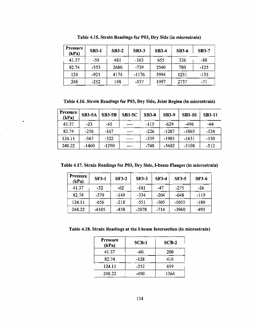
Table 4.15. Strain Readings for P03, Dry Side (in microstrain)
Table 4.16. Strain Readings for P03, Dry Side, Joint Region (in microstrain)
Pressure (ma) 41.37
82.74
124
248
Table 4.17. Strain Readings for P03, Dry Side, I-beam Flanges (in microstrain)
SB3-1
-50
-553
-92 1
-252
Pressure (kPa) 41.37
82.74
124.1 1
248.22
Table 4.18. Strain Readings at the I-beam Intersection (in microstrain)
SB3-2
48 1
2686
4174
148
SB3-5A
-23
-256
-567
-1460
Pressure (ma) , ,
SCB-1 SCB-2
SB3-5B
-45
-167
-522
-1290
I
SB3-3
-163
-739
-1 176
-537
SB3-6
326
780
1251
2737
SB3-4
655
2540
3994
1997
SB3-5C
---- ---- ---- ----
SB3-7
-88
-125
-155
-71
SB3-8
-1 15
-226
-339
-748
SB3-9
-629
-1287
-1983
-5682
SB3-10
-496
-1065
-1631
-3108
SB3-11
-64
-124
-130
-512

4.6.5. Failure Modes
Failure of the hybrid assembly occurred as delamination of the stiffeners on the
large panels, PO3 and P04, while the small panels withstood the peak applied pressure
without observable damage at the stiffener or joint regions. The onset of failure was
observed during the last cycle of the third cycle set, at 117 kPa, at the stiffenerlpanel
interface of the outer stiffener on P03.
Figure 4.49 shows a photograph of a failed large panel (P03) at the conclusion of
the test. The numbers in the figure are used to indicate the failure sequence. Failure of
the outer stiffener began near the tank boundary (1) and propagated towards the center of
the stiffener. After the outer stiffener had become ineffective, load was redistributed to
the other stiffeners, and subsequent damage began to occur at the middle (2) and inner
stiffeners (3). Delamination of the stiffeners then began to occur near the hybrid joint
region (4, 5). The outer sections of the stiffeners on P03, near the tank boundary, failed
before damage was observed to initiate on P04. A close-up of the delaminated middle
stiffener is shown in Figure 4.50.
Figure 4.49. Stiffener Failure on PO3
135

Figure 4.50. Close-Up of Stiffener Failure on PO3
Figure 4.51 shows a photograph of PO4 after failure. Damage initiated at the
inner stiffener near the hybrid joint region (I), at 152 kPa, and propagated to the outer
stiffener (2). The inner and outer stiffener sections near the tank boundary then began to
delaminate (3, 4), until the middle stiffener section completely separated from the panel
( 9 , as seen in Figure 4.52. At a pressure value of 234 H a , even though all stiffeners on
both large panels had failed, the panels continued to withstand the applied pressure up to
248 kPa (three times the design load). At this point, it was decided to bring the test to an
end. Complete separation of the stiffeners from the composite shell was observed at this
stage. No leaks were observed at the joint region, which indicated that watertight
integrity of the joint was maintained.
Delamination of the stiffeners indicated that failure of the composite panels was
due to the stiffenerlpanel interface. This type of failure resulted from a combination of
stiffener geometry and techniques for bonding of the stiffeners to the flat surface of the

panels. Providing more shear resistance at the interface, by interleaving fabric or by
improved adhesion, would delay the initiation of this failure mode. Improvements of the
manufacturing techniques should result in stronger panels.
Figure 4.51. Stiffener Failure on PO4
Figure 4.52. Close-Up of Stiffener Failure on PO4

Chapter 5
FINITE ELEMENT ANALYSIS OF HYBRID BOLTED ASSEMBLY
5.1. Rationale
This chapter presents the finite element analysis (FEA) procedures used to study
the local behavior of the hybrid joint and the global response of the panel assembly. The
study was subdivided into two main phases: 1) finite element analysis of the sub-
component joint region (local models); and 2) finite element analysis of the hybrid panel
assembly (global models). All finite element models are developed using the commercial
software package ANSYS, Version 10.0. The modeling techniques are verified with the
available experimental data presented in Chapters 3 and 4.
Analysis of mechanical joints cannot be conducted without considering the
behavior of the global structure, since the mechanical response of joints is coupled to that
of the structures which they connect. In other words, the geometry, materials and loading
of the global structure will have a direct influence on the forces being transferred to the
joint. Similarly, the stiffness of the joint will have an impact on the global response of
the structure. Understanding the relationship between the response of both local and
global systems is imperative in the design of structures being joined with mechanical
connections.
In general, when modeling large structures, it is not be feasible to include all of
the small-scale features of the joint. As described by Bonnani [2001], the usual approach
for analyzing mechanical joints is to perform a global analysis of the large-scale structure
using an approximate joint stiffness, in order to determine the loads being transferred to

the joint. A detailed joint configuration is then developed and its stiffness can be
calculated and input back into the global model to verify design criteria. This process
may be repeated if fbrther refinement of the joint is needed. For a new joint design,
experimental validation is required.
For the FEA work presented in this chapter, the global structure (component)
consists of a four-panel assembly of the hybrid lifting body, and the local structure (sub-
component) is the hybrid joint, as shown in Figure 5.1. Based on the strength test results
presented in Chapter 3, a short doubler joint configuration (DS-4) was selected for the
hybrid connection. The experimental data for this connection scheme is used as the
baseline for validation of local and global modeling techniques.
Region selected for
Hybrid Panel Assembly (Component)
Hybrid Lifting Body \
Hybrid Joint (Sub-component)
Figure 5.1. Hybrid Lifting Body, Component and Sub-component Structures

5.2. Finite Element Analysis Objectives
The main objective of this study is to provide a simplified approach for modeling
hybrid joints in large-scale structures. Figure 5.2 presents a schematic of the proposed
FEA approach. First, a simplified local shell model was developed to estimate the joint
stiffness, by computing the approximate rigidity of each of the hybrid joint regions. This
approach was then incorporated into a global model of the hybrid panel assembly to
estimate the global deflections. Lastly, a detailed 2D plane strain model was used to
estimate the local stresses of the joint. Accordingly, the objectives of the FEA study are
as follows:
1. To develop a simplified shell model to analyze joint structures, by
modifying the shell element properties at the hybrid region;
2. To validate the finite element models using the available experimental data
from both sub-component (local) and component (global) tests. These data are
presented in Chapters 3 and 4, respectively.
3. To perform parametric studies of the effect of joint geometry on the global
response of the panel assembly (sensitivity study).
4. To develop a detailed, plane strain model of the hybrid joint, which includes
the contact interactions between the joint constituents and the effect of the bolt, to
provide predictions of critical stresses and failure initiation.

b
Global Shell Model
Input forces into Estimate global deflections
Estimate local stresses
Local Plane Strain Model Local Shell Model
Figure 5.2. Schematic of the FEA Approach
5.3. Local Finite Element Model (Shell Model)
The purpose of the local shell model is to provide a simplified approach for
estimating the joint stiffness by computing the approximate rigidities of the sections at
the hybrid region. While using shells elements will limit the extent of the details that can

be incorporated into the local model, the end objective is to implement this approach into
a global model of the hybrid panel assembly, where extensive detailing of the joint
geometry would be unfeasible. The criterion is that the shell elements capture the local
stiffness of the connection.
Initially, connection elements (rotational springs) were considered to model the
joint behavior, i.e. the connection of the hybrid joint region to the acreage of the
composite panel. This approach may be feasible, for example, for a local model of a
component or sub-component, where only three degrees of freedom (two displacements
and one rotation) are considered. However, modeling the joint region of a large-scale
structure such as the hybrid four-panel assembly will require a large number of
connection elements, whose rotational properties need to be prescribed for all degrees of
freedom involved. In a three dimensional model, such an approach would be impractical.
A more feasible approach to this problem is to modify the properties of the elements at
the hybrid joint region, by using effective section properties. This approach is a
precursor to modeling of the joint at the global level and is the main focus of this section.
5.3.1. Finite Element Model Description
A photograph of the DS-4 sub-component joint specimen is shown in Figure 5.3.
This connection scheme consists of a composite beam sandwiched between a steel flange
and a steel doubler plate. A foam insert is used to align the tapered region of the
composite with the edge of the steel flange. A schematic of the baseline geometry of the
DS-4 joint configuration is presented in Figure 5.4. For purposes of property designation
in the analysis, the joint has been sub-divided into six distinct sections: A, B, C, D, E, and
F. Section A represents the region composed of the steel doubler, the composite beam
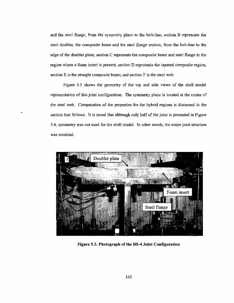
and the steel flange, from the symmetry plane to the bolt-line; section B represents the
steel doubler, the composite beam and the steel flange section, from the bolt-line to the
edge of the doubler plate; section C represents the composite beam and steel flange in the
region where a foam insert is present; section D represents the tapered composite region;
section E is the straight composite beam; and section F is the steel web.
Figure 5.5 shows the geometry of the top and side views of the shell model
representation of this joint configuration. The symmetry plane is located at the center of
the steel web. Computation of the properties for the hybrid regions is discussed in the
section that follows. It is noted that although only half of the joint is presented in Figure
5.4, symmetry was not used for the shell model. In other words, the entire joint structure
was modeled.
Figure 5.3. Photograph of the DS-4 Joint Configuration

;/ Symmetry plane
Figure 5.4. Baseline Geometry of the DS-4 Joint Configuration (in mm)
-/ Symmetry plane I I Top View
Side View
Figure 5.5. Baseline Geometry of the DS-4 Joint Shell Model (in mm)

The meshed model, loading and boundary conditions are shown in Figure 5.6.
Element type SHELL1 8 1, which is a 4-node element with six degrees of freedom at each
node and includes the effects of shear deformation, was chosen for this study. This
element is suitable for modeling thin to moderately-thick shell structures [ANSYS Online
Manual, 20041. Based on a preliminary convergence study, a mesh of 1785 elements was
found appropriate. A nominal load of 4.45-KN was applied at free ends of the composite
beams, which represents the force applied by the load heads. Model verification was
conducted at this load magnitude, since linear response of the experimental load versus
displacement and load versus strain curves was observed. To simulate a fixed base
condition, all degrees of freedom at the bottom edge of section F (steel web) were
constrained.
P = 4.45 KN at free ends of composite beams
Fixed displacements and rotations
Element size = 6.35 mm Mesh size = 1765 elements
Figure 5.6. Mesh, Loading and Boundary Conditions of DS-4 Shell Model

5.3.2. Computing the Effective Properties of the Hybrid Region
A schematic of the side view of the DS-4 joint is shown in Figure 5.7a, which
shows the reference plane used in the analysis. This joint configuration is used as a case
study for validation of the modeling approach. Figure 5.7b presents the shell model
representation of the joint. The main objective of this approach is to compute the
properties of each of the hybrid joint sections for implementation into the shell finite
element model. These calculations are performed using the mid-plane of the composite
beam section (E) as the reference plane. This plane was chosen as a reference for
property calculations, provided that the end objective of this approach is to extend this
method to a global shell model. In a global model, it is often convenient to compute the
properties with respect to the mid-plane of the panel sections, as these regions constitute
the acreage of the structure. It is noted that since the properties for sections D and E are
input as layered shell sections, the effective properties are computed for sections A, B
and C.
a) Actual Joint Configuration b) Shell Model Representation
Figure 5.7. Schematic of the DS-4 Joint Configuration
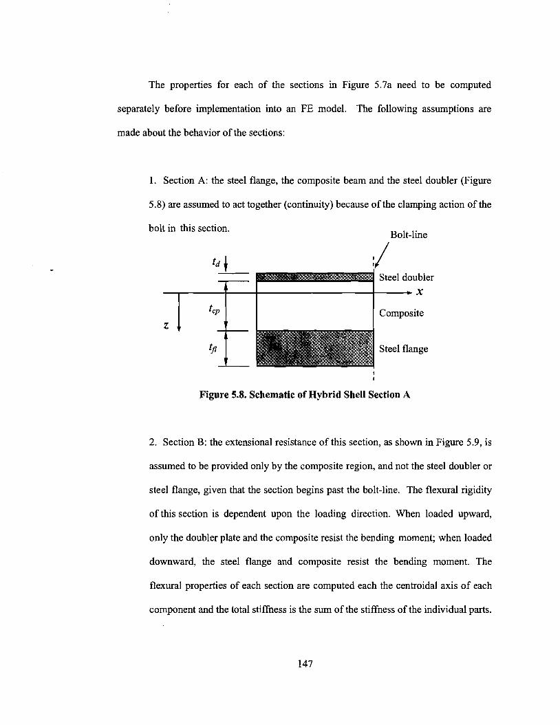
The properties for each of the sections in Figure 5.7a need to be computed
separately before implementation into an FE model. The following assumptions are
made about the behavior of the sections:
1. Section A: the steel flange, the composite beam and the steel doubler (Figure
5.8) are assumed to act together (continuity) because of the clamping action of the
bolt in this section.
I
Steel doubler
C Steel flange
I
t c ~
Figure 5.8. Schematic of Hybrid Shell Section A
b X
Composite
2. Section B: the extensional resistance of this section, as shown in Figure 5.9, is
assumed to be provided only by the composite region, and not the steel doubler or
steel flange, given that the section begins past the bolt-line. The flexural rigidity
ofthis section is dependent upon the loading direction. When loaded upward,
only the doubler plate and the composite resist the bending moment; when loaded
downward, the steel flange and composite resist the bending moment. The
flexural properties of each section are computed each the centroidal axis of each
component and the total stiffness is the sum of the stiffness of the individual parts.

Steel doubler
X
Figure 5.9. Schematic of Hybrid Shell Section B
3. Section C: the extensional resistance of this section, as shown in Figure 5.10,
is assumed to be provided only by the composite region. When loaded up, only
the composite (with the foam insert) resists the bending moment, while the steel
flange and composite resist a downward acting moment. The flexural properties
of each section are computed about each component's own centroidal axis, as
expressed in Equation (5.1).
I Comoosite
I.
Figure 5.10. Schematic of Hybrid Shell Section C
barn , ~ C P
\ I - Composite
,X Foam

The bending rigidity of the individual sub-sections, (El)i, can be added in order to
calculate the effective bending rigidity of the section, (Elefl), as follows:
For instance, the effective bending rigidity of section B when loaded downward is
computed as follows:
= ECPICP + ES I,,
Where Ecp is the modulus of elasticity of the composite beam, Es is the modulus
of elasticity of steel, and Icp and I jr are the moment of inertia of the composite beam and
the steel flange, respectively. This assumption is made on the basis that the bolt preload
compresses the components sufficiently such that the curvatures are approximately the
same.
The effective section thickness, tefi can then be computed from as shown in
Equation (5.3). This yields an effective thickness for the modified hybrid joint section.
These values of t e ~ are then input into the finite element model as the thicknesses of the
shell sections, using the SHELL SECTION LAY-UP OPTION in the ANSYS Main
Menu. The properties for section E are input on a layer-by-layer basis by specifying the
thickness and orientation of each lamina. The tapered section was approximated as a
rectangular section of average thickness (thickness at the center of the tapered section).

5.3.3. Local Shell Model Verification
The local shell modeling approach was validated using the results obtained from
the DS-4 joint specimen testing. Models with all-steel and all-composite joint sections
were also created. For an all-steel joint model, all sub-sections of sections A, B and C
were considered to be steel. For an all-composite case, these sections were considered to
be EGNE. These models represent the stiffest case and the most flexible case for a given
joint configuration, respectively, and are used to determine the upper and lower bounds
of the response of the joint.
A load of 4.45 KN was applied at the free ends of the composite beams.
Displacement and strain contour plots for the model using hybrid section properties (DS-
4) are shown in Figures 5.1 1 and 5.12, respectively. The composite beams bend in the
regular shape of cantilever beams, as expected. A maximum displacement of 7.28 mm
was obtained at the free end of the composite beam. A peak strain of 2881 microstrain
was recorded at 203 mm from the joint centerline, which corresponds to the straight
composite beam section (E).
Vertical displacement values (U,) were recorded along the length of the FE model
and compared with the experimental values recorded at the three LVDT locations
outlined in Chapter 3 (Figure 3.17): I ) the end of the steel flange (V5-V6, V7-V8); 2) 203
mm from the joint centerline (V3-V4, V9-VIO); and 3) the free end of the composite
beam (Vl-V2, Vll-V12). The strain values (E,) recorded at these locations corresponds
to gages SG5, SG3 and SGl , respectively, as shown in Figure 3.19.
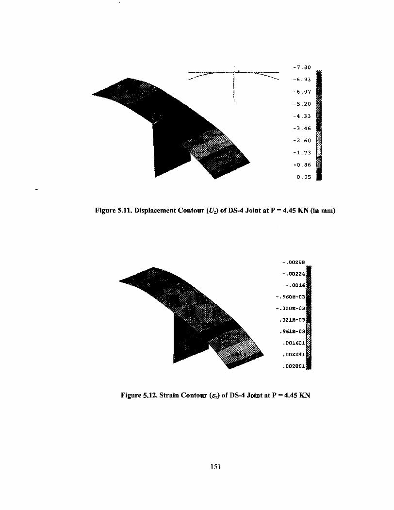
Figure 5.11. Displacement Contour (U,) of DS-4 Joint at P = 4.45 KN (in mm)
Figure 5.12. Strain Contour (E,) of DS-4 Joint at P = 4.45 KN

Figure 5.13 shows the deflected shape for the DS-4 joint for the three modeling
cases and the experimental results and Table 5.1 summarizes the discrete vertical
displacement values recorded. The deflected shapes show that using an all-steel section
under predicts the joint deflection by 22 percent at the free end of the composite beam (x
= 381 rnm) and by 85 percent at the end of the steel flange (x = 133 mm). The use of an
all-composite joint over estimates the peak deflection by 21 percent and the deflection at
the end of the flange (x = 133 mm) by 71 percent. Using hybrid joint properties yielded
fairly accurate displacement predictions, within 10 percent difference of the test results.
Deflected shape, DS-4 (P = 4.45 KN) 2
Figure 5.13. Deflected Shape of DS-4 Joint at P = 4.45 KN
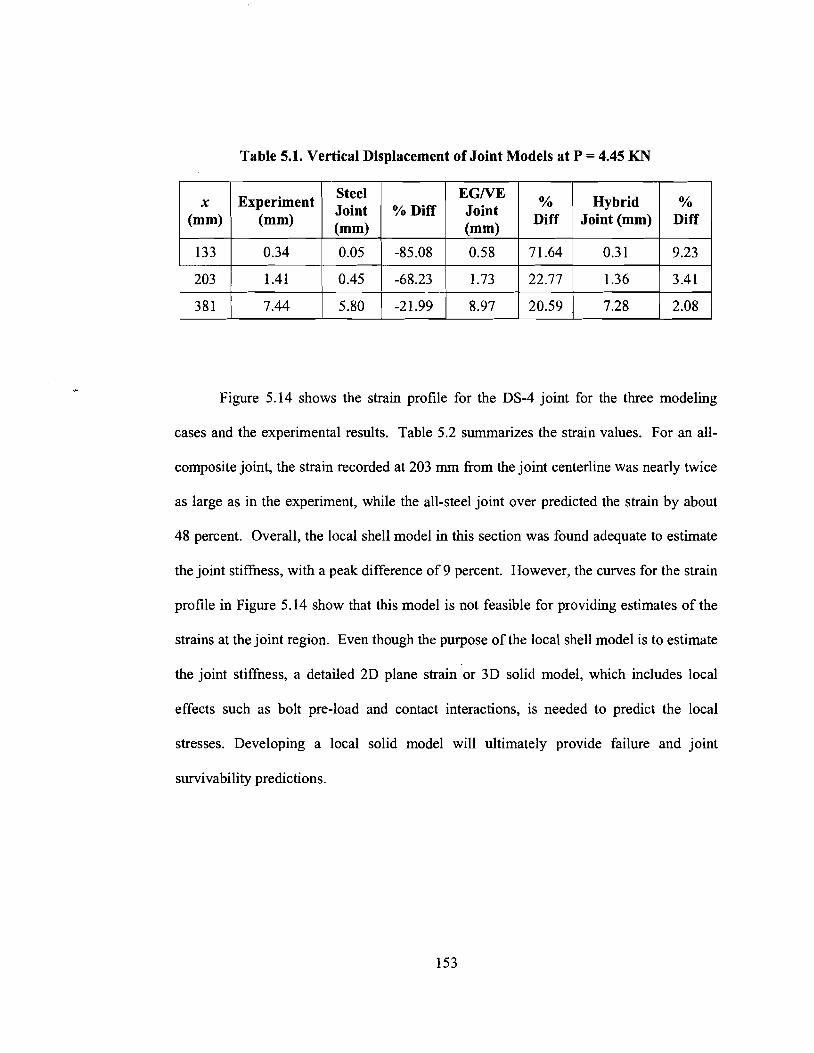
Table 5.1. Vertical Displacement of Joint Models at P = 4.45 KN
Figure 5.14 shows the strain profile for the DS-4 joint for the three modeling
cases and the experimental results. Table 5.2 summarizes the strain values. For an all-
composite joint, the strain recorded at 203 mrn from the joint centerline was nearly twice
as large as in the experiment, while the all-steel joint over predicted the strain by about
48 percent. Overall, the local shell model in this section was found adequate to estimate
the joint stiffness, with a peak difference of 9 percent. However, the curves for the strain
profile in Figure 5.14 show that this model is not feasible for providing estimates of the
strains at the joint region. Even though the purpose of the local shell model is to estimate
the joint stiffness, a detailed 2D plane strain or 3D solid model, which includes local
effects such as bolt pre-load and contact interactions, is needed to predict the local
stresses. Developing a local solid model will ultimately provide failure and joint
survivability predictions.
x (mm)
133
203
381
Experiment (mm)
0.34
1.41
7.44
Steel Joint (mm) 0.05
0.45
5.80
% Diff
-85.08
-68.23
-21.99
EGNE Joint (mm) 0.58
1.73
8.97
% Diff
71.64
22.77
20.59
Hybrid Joint (mm)
0.3 1
1.36
7.28
YO Diff
9.23
3.41
2.08
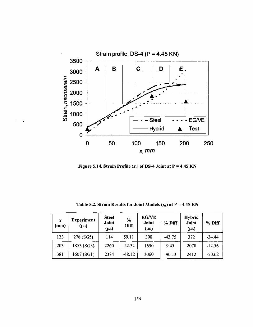
Strain profile, DS-4 (P = 4.45 KN) 3500
Figure 5.14. Strain Profile (E,) of DS-4 Joint at P = 4.45 KN
Table 5.2. Strain Results for Joint Models (E,) at P = 4.45 KN
x (mm)
133
203
381
Experiment (PI
278 (SGS)
1853 (SG3)
1607 (SGl)
Steel Joint (PI
114
2260
2384
% Di ff
59.1 1
-22.32
-48.12
EGNE Joint (CLE)
398
1690
3060
Hybrid Joint (PC)
372
2070
2412
% Diff
-43.75
9.45
-90.13
% Diff
-34.44
-12.56
-50.62

5.4. Global Finite Element Model of Isolated Stiffened Panels
Prior to modeling the entire hybrid assembly and incorporating the modified shell
approach for the hybrid region, a study was conducted to investigate the response of
isolated panels with ideal boundary conditions. In other words, instead of modeling the
hybrid region, the panel boundaries corresponding to the hybrid region are modeled as
pinned and fixed boundaries. Hence, the contribution of the I-beam movement to the
panel deflections is not accounted for in this model. This study is an attempt to
investigate the bounds of the individual panel response and to compare these to the
experimentally obtained displaced shapes.
Figure 5.15 depicts the various sections of a small stiffened panel (Pol). Region
1 corresponds to the thickened boundaries of the panel; region 2 corresponds to the
stiffened region of the panel; region 3 corresponds to the top section of the stiffeners; and
region 4 corresponds to the side sections of the stiffeners. The structure is modeled as a
layered shell. The material properties are input by specifying the layer thickness and
orientation using the SHELL SECTION LAY-UP OPTION. Table 5.3 presents the
orthotropic lamina properties for the EGNE system used for each lamina. A detailed
summary of the lamination scheme for each panel section in Figure 5.15 is presented in
Table 5.4. It is noted that the same lamination scheme was used for the large panels.

1) 25.4-mm thick boundary 2) 12.7-mm panel region 3) 6.35-mm stiffener top 4) 3.175-mm stiffener side
Figure 5.15. Various Sections of EGNE Stiffened Panels
Table 5.3. Orthotropic Lamina Properties for an EGNE System
Table 5.4. Lamination Scheme for Stiffened Panels
Ell
(GPa)
37.93
E22
(GPa)
10.56
Section
1
2
3
4
E33
(GPa)
10.56
Description
Thick boundary
Stiffened panel
Stiffener top
Stiffened side
G12
(GPa)
3.192
Thickness (mm)
25.4
12.7
6.35
3.1 75
Lamination Sequence
64 layers: [{*45/(0/90)3)4],
32 layers: [{*45/(0/90))4],
16 layers: [(0/90)3/*45]2
8 layers: [(0/90)/(*45)12
G13
(GPa)
3.192
G23
(GPa)
2.258
012
0.29
013
0.29
023
0.439
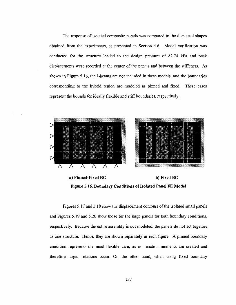
The response of isolated composite panels was compared to the displaced shapes
obtained from the experiments, as presented in Section 4.6. Model verification was
conducted for the structure loaded to the design pressure of 82.74 kPa and peak
displacements were recorded at the center of the panels and between the stiffeners. As
shown in Figure 5.16, the I-beams are not included in these models, and the boundaries
corresponding to the hybrid region are modeled as pinned and fixed. These cases
represent the bounds for ideally flexible and stiff boundaries, respectively.
a) Pinned-Fixed BC b) Fixed BC
Figure 5.16. Boundary Conditions of Isolated Panel WE Model
Figures 5.17 and 5.18 show the displacement contours of the isolated small panels
and Figures 5.19 and 5.20 show those for the large panels for both boundary conditions,
respectively. Because the entire assembly is not modeled, the panels do not act together
as one structure. Hence, they are shown separately in each figure. A pinned boundary
condition represents the most flexible case, as no reaction moments are created and
therefore larger rotations occur. On the other hand, when using fixed boundary
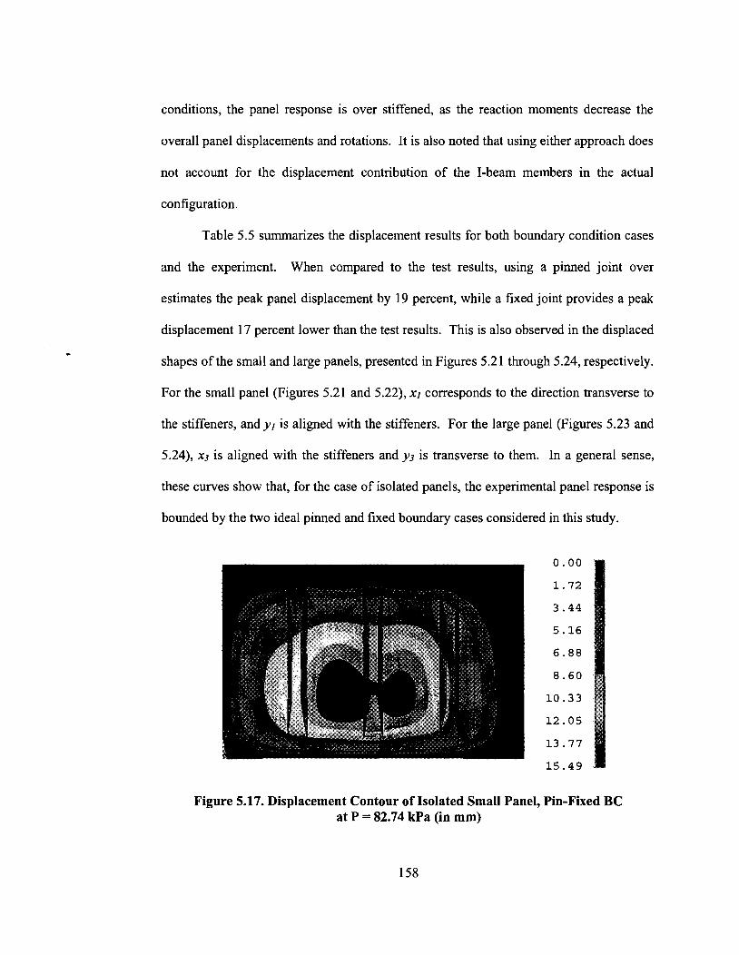
conditions, the panel response is over stiffened, as the reaction moments decrease the
overall panel displacements and rotations. It is also noted that using either approach does
not account for the displacement contribution of the I-beam members in the actual
configuration.
Table 5.5 summarizes the displacement results for both boundary condition cases
and the experiment. When compared to the test results, using a pinned joint over
estimates the peak panel displacement by 19 percent, while a fixed joint provides a peak
displacement 17 percent lower than the test results. This is also observed in the displaced
shapes of the small and large panels, presented in Figures 5.21 through 5.24, respectively.
For the small panel (Figures 5.21 and 5.22), X I corresponds to the direction transverse to
the stiffeners, and y, is aligned with the stiffeners. For the large panel (Figures 5.23 and
5.24), x j is aligned with the stiffeners and y3 is transverse to them. In a general sense,
these curves show that, for the case of isolated panels, the experimental panel response is
bounded by the two ideal pinned and fixed boundary cases considered in this study.
Figure 5.17. Displacement Contour of Isolated Small Panel, Pin-Fixed BC at P = 82.74 kPa (in mm)

Figure 5.18. Displacement Contour of Isolated Small Panel, Fixed BC at P = 82.74 kPa (in mm)
Figure 5.19. Displacement Contour of Isolated Large Panel, Pin-Fixed BC at P = 82.74 kPa (in mm)

Figure 5.20. Displacement Contour of Isolated Large Panel, Fixed BC at P = 82.74 kPa (in mm)
Table 5.5. Vertical Displacements of Isolated Panels at P = 82.74 kPa
Boundary Condition
Pinned
Fixed
Test
Displacement (mm)
Small Panel (POI, P02)
Center
8.94
5.12
7.65
Large Panel (P03, P04)
Between Stiffeners
9.63
7.41
8.60
Center
8.28
6.58
7.35
Between Stiffeners
9.70
8.18
8.34
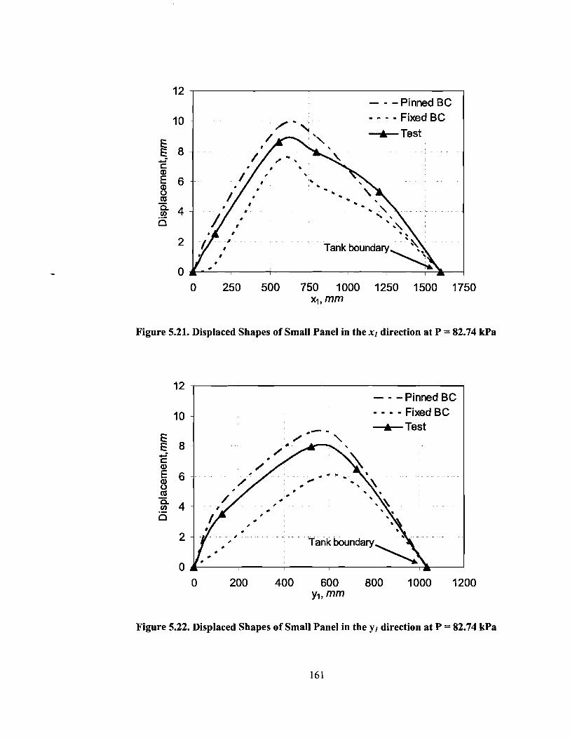
Figure 5.21. Displaced Shapes of Small Panel in the xl direction at P = 82.74 kPa
-
- - - Pinned BC - - - - Fixed BC
Figure 5.22. Displaced Shapes of Small Panel in the y, direction at P = 82.74 kPa
--t- Test
-
- - -Pinned BC - - - - Fixed BC
+Test 0 *- - \ -

Figure 5.23. Displaced Shapes of Large Panel in the x3 direction at P = 82.74 kPa
-
- - - Pinned BC - - - - Fixed BC
,-t- Test
- - - Pinned BC - - - - Fixed BC .+ Test
Figure 5.24. Displaced Shapes of Large Panel in the y3 direction at P = 82.74 kPa
/ - 0 \

5.5. Global Finite Element Model of Hybrid Assembly
The main objective of the global modeling approach is to extend the simplified
shell approach described in Section 5.3.1 to the case of a multi-panel structure that is
joined together by a hybrid joint. In this model, the four panels and the I-beams are
included, in order to account for the contribution of the beams to the panel displacements.
After validation of the approach, studies are conducted to investigate the sensitivity of the
panel response to varying geometric parameters at the joint region. As an end objective,
this study will provide a global interpretation of the variables that most strongly affect the
structural response of the assembly.
When considering large-scale FE models with stiffened panels, using beam
elements instead of shell elements is an attractive option for modeling the stiffeners. This
is particularly true when the number of stiffeners and the geometric complexity of the
model are significant. Initially, it was attempted to model the stiffeners using a single
row of beam elements for each stiffener, but little success was achieved due to the actual
breadth of the hat-stiffener arrangement. For the study presented in this section, all of the
panels, stiffeners and I-beam members are modeled using shell elements.
5.5.1. Global Finite Element Model Description
Figure 5.25 presents the hybrid assembly and panel geometry. Details of the
panel and stiffener geometries are presented in Figures 4.4 through 4.9, of Chapter 4.
Figure 5.26 presents a top view of the FE model of the hybrid assembly. A pressure load
of 82.74 kPa (design load) was applied to the flat surfaces of the panels, as indicated by
the red dots. These surfaces represent the wet side of the actual assembly configuration.
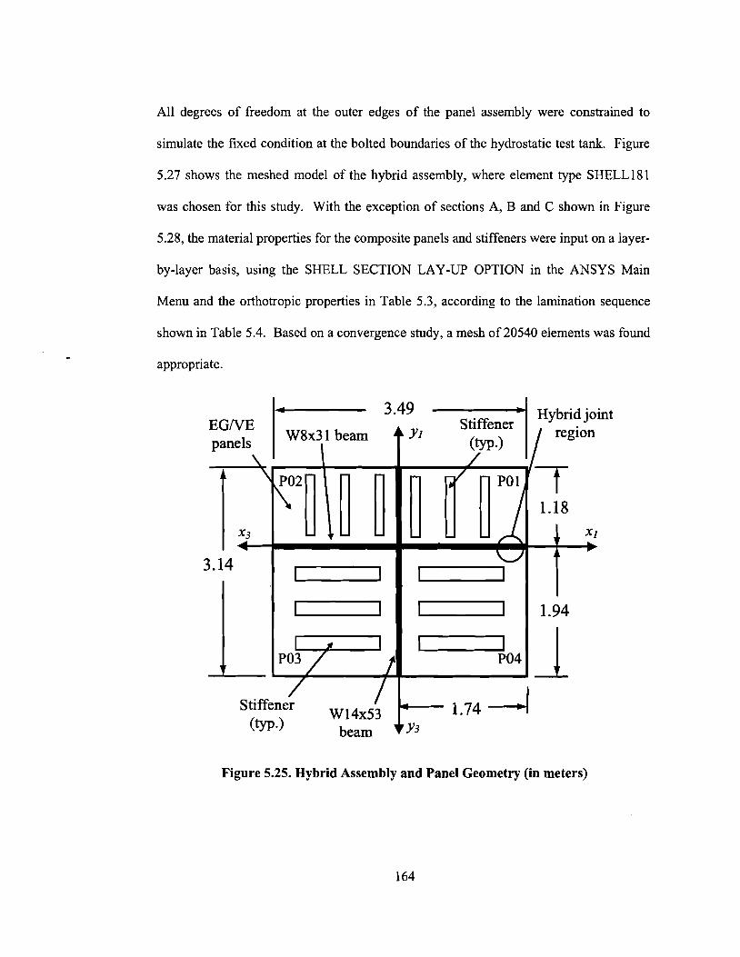
All degrees of freedom at the outer edges of the panel assembly were constrained to
simulate the fixed condition at the bolted boundaries of the hydrostatic test tank. Figure
5.27 shows the meshed model of the hybrid assembly, where element type SHELL 18 1
was chosen for this study. With the exception of sections A, B and C shown in Figure
5.28, the material properties for the composite panels and stiffeners were input on a layer-
by-layer basis, using the SHELL SECTION LAY-UP OPTION in the ANSYS Main
Menu and the orthotropic properties in Table 5.3, according to the lamination sequence
shown in Table 5.4. Based on a convergence study, a mesh of 20540 elements was found
appropriate.
Figure 5.25. Hybrid Assembly and Panel Geometry (in meters)
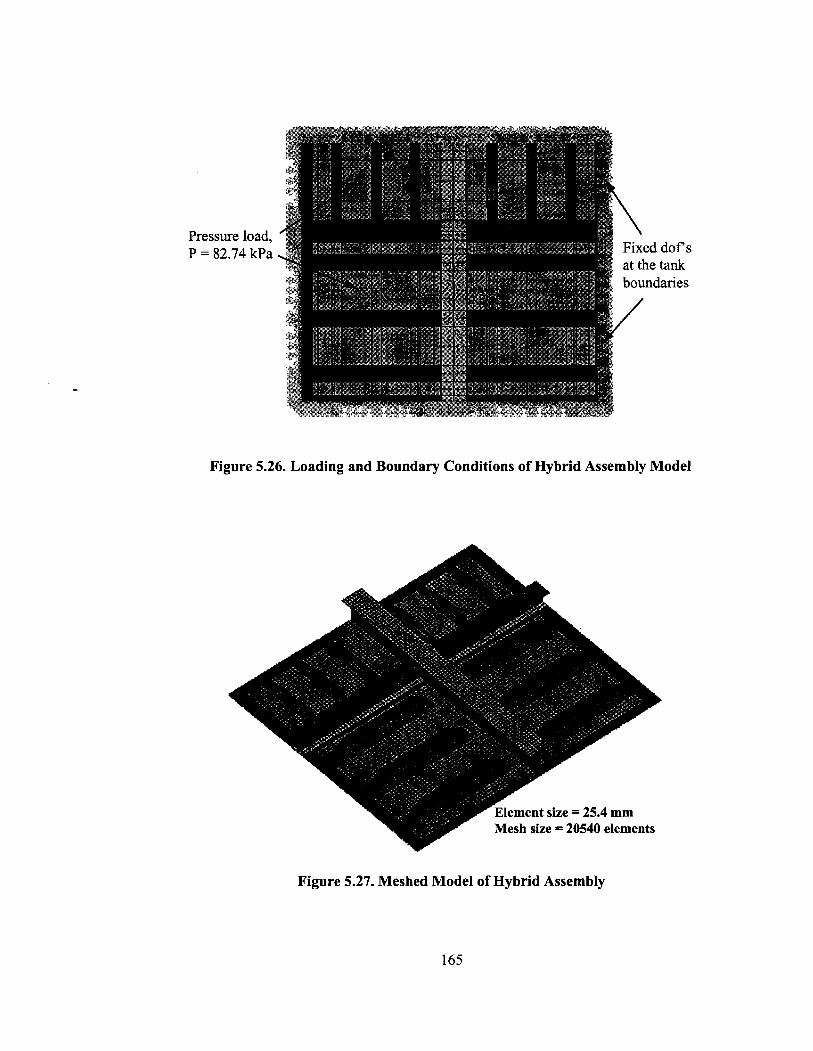
Pressur P = 82.
:e load, 74 kPa Fixed
at the bounc
dof s tank
h i e s
Figure 5.26. Loading and Boundary Conditions of Hybrid Assembly Model
Figure 5.27. Meshed Model of Hybrid Assembly

5.5.2. Modeling of the Hybrid Joint Region
The global model presented in this section includes the full, four panel hybrid
assembly and it accounts for the contribution of the hybrid region and the contribution of
the I-beam members to the panel deflections. Using a similar approach to that presented
in Section 5.3.1 for the local shell model, the joint in the global assembly was modeled
by computing the approximate section properties for the elements composing the hybrid
region. By using this approach, the entire structure can be built using shell elements and
only those sections that represent the joint region are modified and assigned effective
properties.
Figure 5.28a presents a top view of the FE model of the four panel hybrid
assembly. Figures 5.28b and 5 . 2 8 ~ show detailed schematics of the hybrid joint region of
the W8x31 I-beam and the W14x53 I-beam, respectively. Figure 5.282, depicts the
connection of a small and large panel (POl-P04) with the W8x31 I-beam. Similarly,
Figure 5 .28~ depicts the connection of the two large panels (P03-P04) with the W14x53
I-beam. In each figure, the hybrid joint regions (sections A, B and C), as well as the
tapered and straight panel regions (sections D and E), are indicated.
A cross-sectional view of these regions and the baseline geometry for this model
are shown in Figure 5.29. The approximate geometry of the I-beam member shown in
this figure is summarized in Table 5.6. For this global model, the tapered region (D)
extends a distance of 203.20 mm from the edge of the steel flange to the start of the
stiffener region. Section E represents the flat region of the composite panel. In the local
shell model, this region corresponds to the free end of the composite beam. As was done
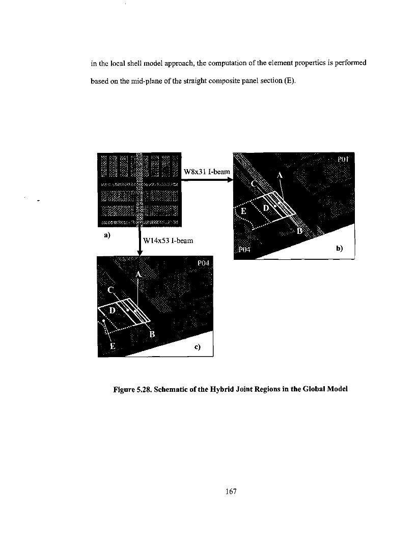
in the local shell model approach, the computation of the element properties is performed
based on the mid-plane of the straight composite panel section (E).
Figure 5.28. Schematic of the Hybrid Joint Regions in the Global Model
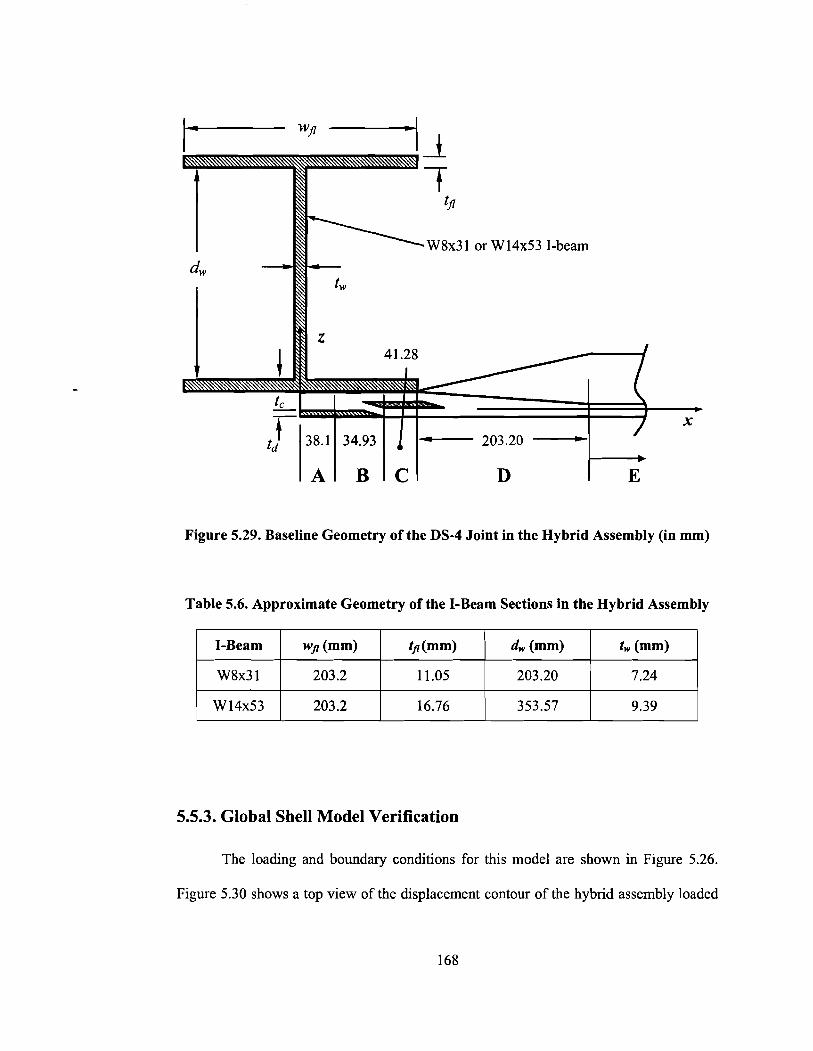
rB 38.1 34.93 1 A B C D
Figure 5.29. Baseline Geometry of the DS-4 Joint in the Hybrid Assembly (in mm)
Table 5.6. Approximate Geometry of the I-Beam Sections in the Hybrid Assembly
5.5.3. Global Shell Model Verification
The loading and boundary conditions for this model are shown in Figure 5.26.
Figure 5.30 shows a top view of the displacement contour of the hybrid assembly loaded

to the design pressure of 82.74 kPa. Figures 5.31 and 5.32 present the individual
displacement contours for the small and large panels, respectively. These plots show that
the peak panel displacements occur at the regions between the stiffeners, as was observed
in the experiments. As presented in Figures 5.33 through 5.36, the displaced shapes
obtained from the FE models and the test results, for both small and large panels, show
good agreement, with a peak difference of 10 percent. In a general sense, the shapes
obtained from the FE model slightly under predict the experimental displacements. This
discrepancy is mainly attributed to: 1) the differences in the assumed material properties
and the as-built geometry; 2) the idealized joint condition in the FE model, which does
not include the contact interaction between the various joint components (doubler plate,
edge of the composite beam and steel flange) and the effect of the bolts in the actual
structure; and, 3) the assumed fixed boundary condition at the tank boundaries, which
may not be a completely rigid condition in the actual test configuration.
Figure 5.30. Displacement Contour of Hybrid Assembly at P = 82.74 kPa (in mm)
169

0 .00
0 .94
1 . 8 7
2 . 8 1
3 .75
4 . 6 8
5 .62
6 .56
7 .50
8.43
Figure 5.31. Vertical Displacement Contour of a Small Panel at P = 82.74 kPa (in mm)
Figure 5.32. Vertical Displacement Contour of a Large Panel at P = 82.74 kPa (in mm)

Figure 5.33. Displaced Shape of a Small Panel in the XI direction at P = 82.74 kPa
10 - - - - FEA
Figure 5.34. Displaced Shape of a Small Panel in the yl direction at P = 82.74 kPa
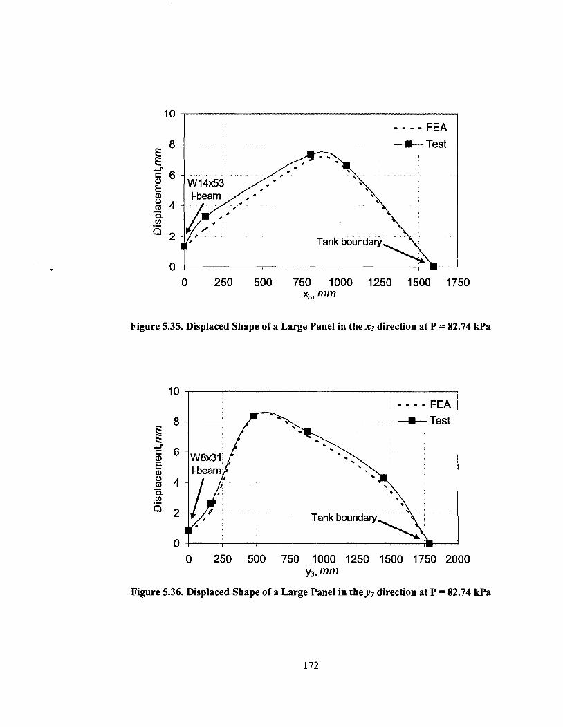
- - - - FEA - --t- Test
-
Figure 5.35. Displaced Shape of a Large Panel in the x3 direction at P = 82.74 kPa
- - - - FEA
--t- Test
Figure 5.36. Displaced Shape of a Large Panel in the y3 direction at P = 82.74 kPa
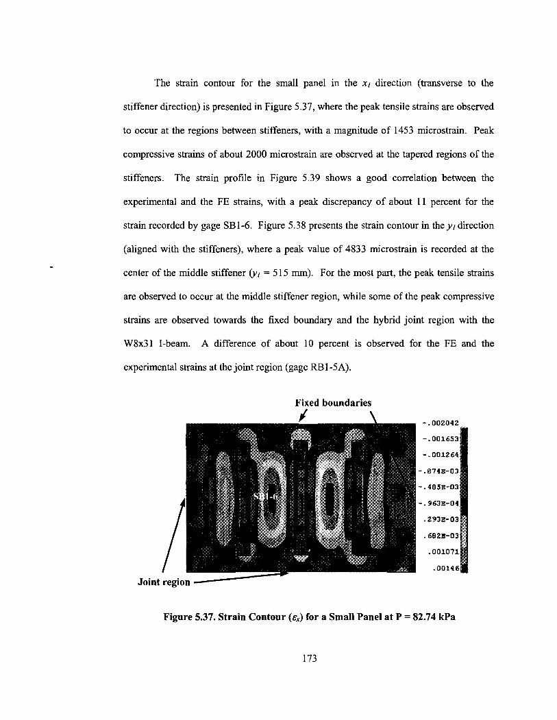
The strain contour for the small panel in the XI direction (transverse to the
stiffener direction) is presented in Figure 5.37, where the peak tensile strains are observed
to occur at the regions between stiffeners, with a magnitude of 1453 microstrain. Peak
compressive strains of about 2000 microstrain are observed at the tapered regions of the
stiffeners. The strain profile in Figure 5.39 shows a good correlation between the
experimental and the FE strains, with a peak discrepancy of about 11 percent for the
strain recorded by gage SB1-6. Figure 5.38 presents the strain contour in the yl direction
(aligned with the stiffeners), where a peak value of 4833 microstrain is recorded at the
center of the middle stiffener (yI = 5 15 mm). For the most part, the peak tensile strains
are observed to occur at the middle stiffener region, while some of the peak compressive
strains are observed towards the fixed boundary and the hybrid joint region with the
W8x31 I-beam. A difference of about 10 percent is observed for the FE and the
experimental strains at the joint region (gage RE3 1 -5A).
Fixed boundaries
Joint
Figure 5.37. Strain Contour (E,) for a Small Panel at P = 82.74 kPa
173
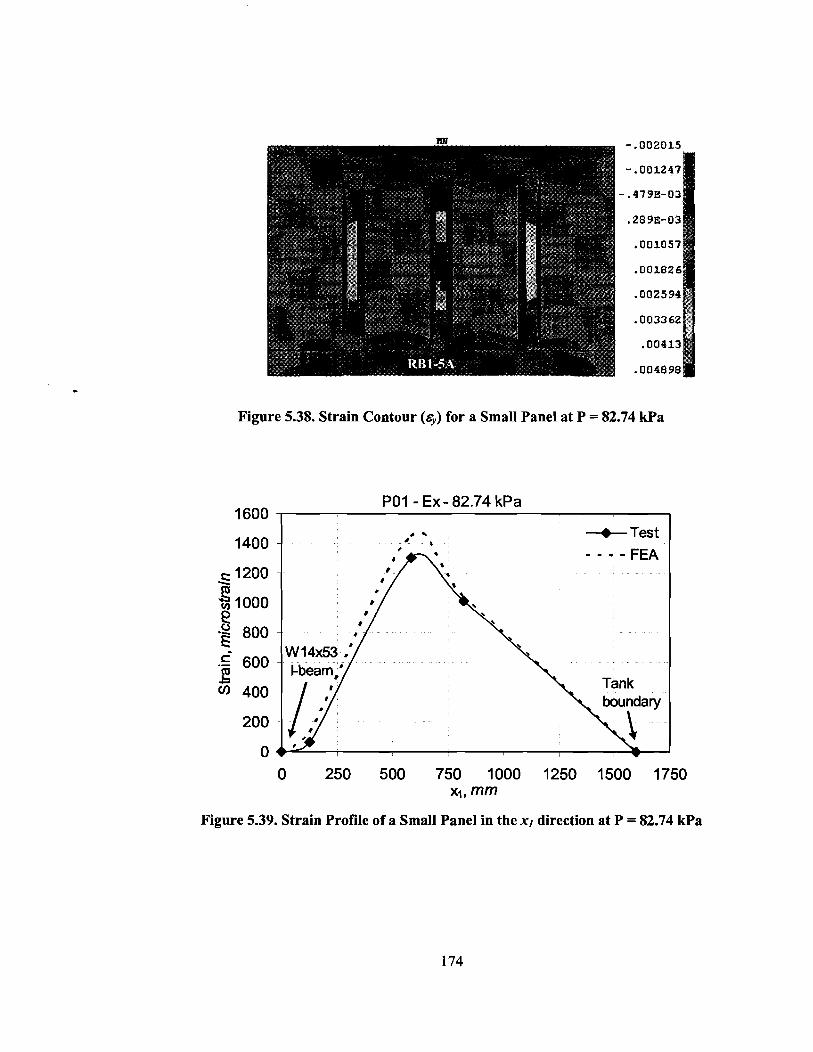
Figure 5.38. Strain Contour (5) for a Small Panel at P = 82.74 kPa
4 ' L -+- Test - - - - FEA
-
Figure 5.39. Strain Profile of a Small Panel in the XI direction at P = 82.74 kPa

Figure 5.40. Strain Profile of a Small Panel in the yl direction at P = 82.74 kPa
The strain contour for the large panel in the x3 direction (stiffener direction) is
presented in Figure 5.41, where a peak tensile strain of 3080 microstrain is observed at
the center of the middle stiffener. Peak compressive strains of about 2781 microstrain are
observed towards the fixed tank boundary. The strain profile in Figure 5.43 shows a peak
discrepancy of about 25 percent for the strain recorded at the joint region by gage RB3-
5C. Figure 5.42 shows the strain contour for the large panel in the y3 direction
(transverse to the stiffeners), where a peak compressive strain of 2622 microstrain is
recorded at the start of the tapered region of the middle stiffener. When compared to the
strain profile in Figure 5.44, the results from the FE results agree with the experimental
strains, with a difference of 11 percent for the strain recorded at the region between

stiffeners (gage SB3-6). Overall, the global model presented in this section is adequate
for estimating the global panel deflections and the strains within the bulk of the panels.
Some of the discrepancies between the numerical and the experimental strains were
observed near the joint region, given that this simplified approach does not account for
the three dimensional effects and contact interactions at the joint, and therefore is not
expected to provide an accurate appraisal of the local stress or strain state near the joint.
Fixed bou
,, Joint r
ndaries 1
egion
- .a0367
Figure 5.41. Strain Contour (E . ) for a Large Panel at P = 82.74 kPa

Figure 5.42. Strain Contour (E-) for a Large Panel at P = 82.74 kPa
c - - 5 #
-+ Test
I 1 I I I
Figure 5.43. Strain Profile of a Large Panel in the x3 direction at P = 82.74 kPa
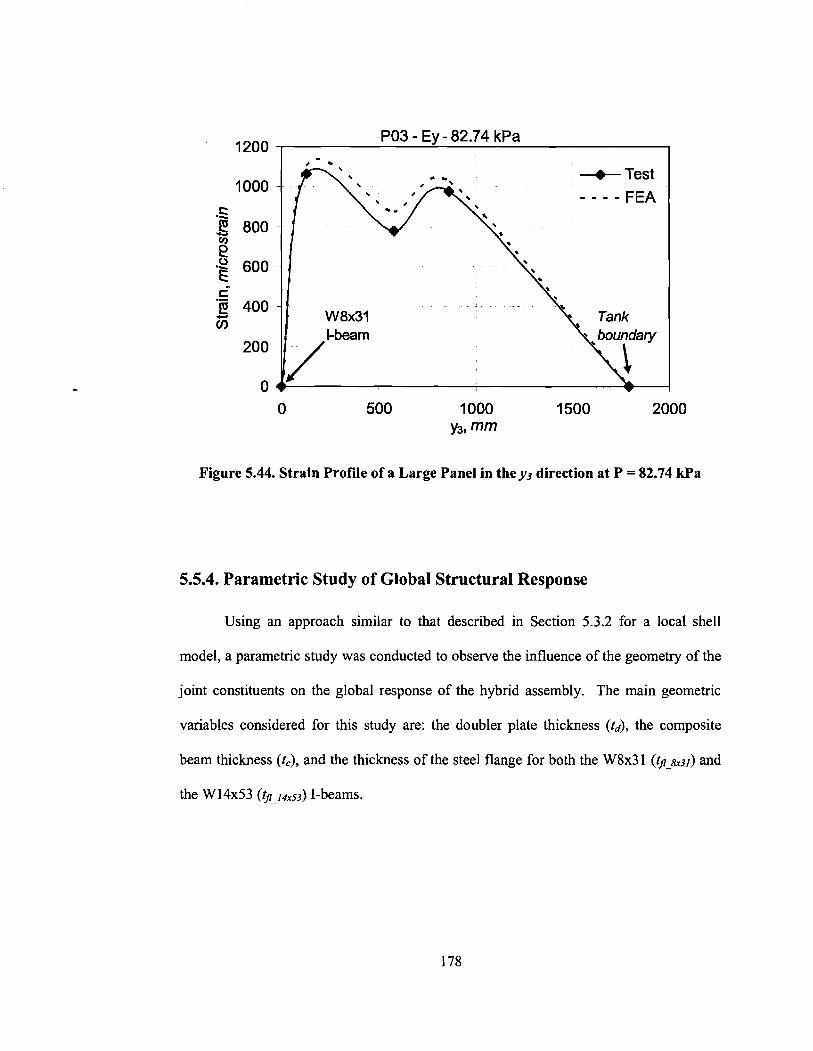
Figure 5.44. Strain Profile of a Large Panel in the y3 direction at P = 82.74 kPa
5.5.4. Parametric Study of Global Structural Response
Using an approach similar to that described in Section 5.3.2 for a local shell
model, a parametric study was conducted to observe the influence of the geometry of the
joint constituents on the global response of the hybrid assembly. The main geometric
variables considered for this study are: the doubler plate thickness (td), the composite
beam thickness (t,), and the thickness of the steel flange for both the W8x3 1 (9 - sx3~) and
the W14x53 (9-Idxs3) I-beams.

5.5.4.1. Effect of the Doubler Plate Thickness
The effect of the doubler plate thickness on the global panel response was studied
for the assembly loaded to the design pressure of 82.74 H a . According to the approach
presented in Section 5.3.2, the properties of each joint section were computed for a given
doubler plate thickness value, td, while holding the steel flange thicknesses (tfr - gx3/,
tfr - 14~53) and the composite thickness (t,), constant (Figure 5.29). A doubler plate thickness
range of 0.5 td to 4 td was used, with td being the baseline thickness of 6.35 mm.
A comparison of the displaced shapes for a small panel in the xl and y, direction
are presented in Figures 5.45 and 5.46, respectively. In a qualitative sense, these curves
show that varying the doubler plate thickness affects the small panel displacements near
the hybrid joint region (y~ = 120 mm), particularly for the displaced shapes along the
stiffener direction ( y ~ direction). The effect of the td decreases as yl increases, for the
region between the outer stiffener and the tank boundary, which indicates that the
response of this region is mostly affected by the clamped boundary conditions at the outer
edges of the panel. Transverse to the stiffeners (XI direction), the doubler plate thickness
affects the displacements at the center of the panel. These results also suggest that that
W8x3 1 I-beam has a large influence on the response of the small panels.
Figures 5.47 and 5.48 show the displaced shapes for the large panel in the x3 and
y3 directions, respectively. In the x3 direction, these curves show that the effect of the
doubler thickness is significant towards the joint region (x3 = 120 mm). Transverse to the
stiffeners, the effect of the doubler is observed at y3 = 1425 mm, towards the tank
boundary. Increasing the doubler thickness provides a modest additional moment
resistance in bending, when compared to the baseline case of td= 6.35 mm. For example,

it is estimated that using a doubler thickness twice as large as the baseline thickness
reduces the peak panel deflection by about 7 percent.
Figure 5.45. Effect of t d on the Displaced Shapes of a Small Panel in the xl direction at P = 82.74 kPa
Figure 5.46. Effect of t d on the Displaced Shapes of a Small Panel in they, direction at P = 82.74 kPa

Figure 5.47. Effect of td on the Displaced Shapes of a Large Panel in the x3 direction at P = 82.74 kPa
Figure 5.48. Effect of td on the Displaced Shapes of a Large Panel in the yj direction at P = 82.74 kPa
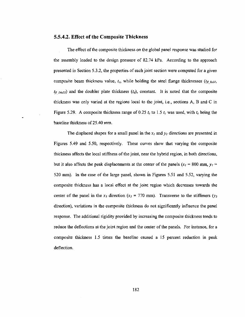
5.5.4.2. Effect of the Composite Thickness
The effect of the composite thickness on the global panel response was studied for
the assembly loaded to the design pressure of 82.74 kPa. According to the approach
presented in Section 5.3.2, the properties of each joint section were computed for a given
composite beam thickness value, t,, while holding the steel flange thicknesses (9 - 8~31,
fj1_14x53) and the doubler plate thickness (td), constant. It is noted that the composite
thickness was only varied at the regions local to the joint, i.e., sections A, B and C in
Figure 5.29. A composite thickness range of 0.25 t, to 1.5 t, was used, with t, being the
baseline thickness of 25.40 mm.
The displaced shapes for a small panel in the x, and yl directions are presented in
Figures 5.49 and 5.50, respectively. These curves show that varying the composite
thickness affects the local stiffness of the joint, near the hybrid region, in both directions,
but it also affects the peak displacements at the center of the panels (XI = 800 mm, yl =
520 mm). In the case of the large panel, shown in Figures 5.51 and 5.52, varying the
composite thickness has a local effect at the joint region which decreases towards the
center of the panel in the x3 direction (x3 = 770 mm). Transverse to the stiffeners (y3
direction), variations in the composite thickness do not significantly influence the panel
response. The additional rigidity provided by increasing the composite thickness tends to
reduce the deflections at the joint region and the center of the panels. For instance, for a
composite thickness 1.5 times the baseline caused a 15 percent reduction in peak
deflection.
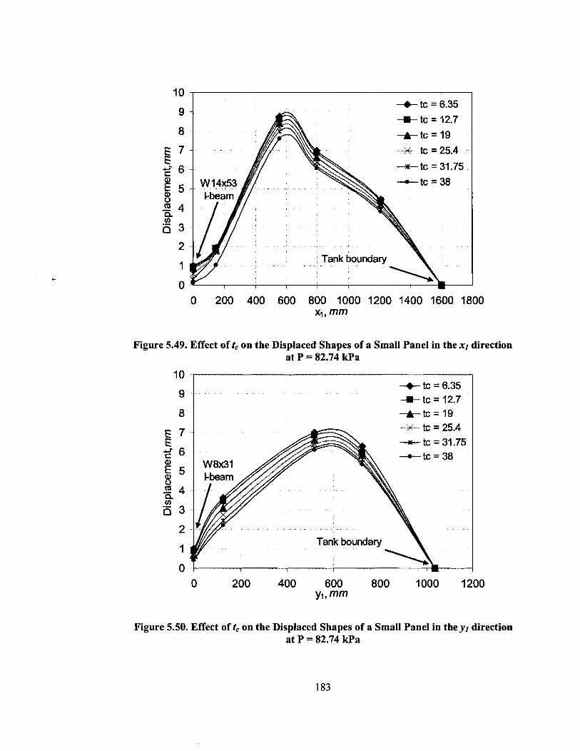
Figure 5.49. Effect of tc on the Displaced Shapes of a Small Panel in the xl direction at P = 82.74 kPa
Figure 5.50. Effect of tc on the Displaced Shapes of a Small Panel in the yl direction at P = 82.74 kPa
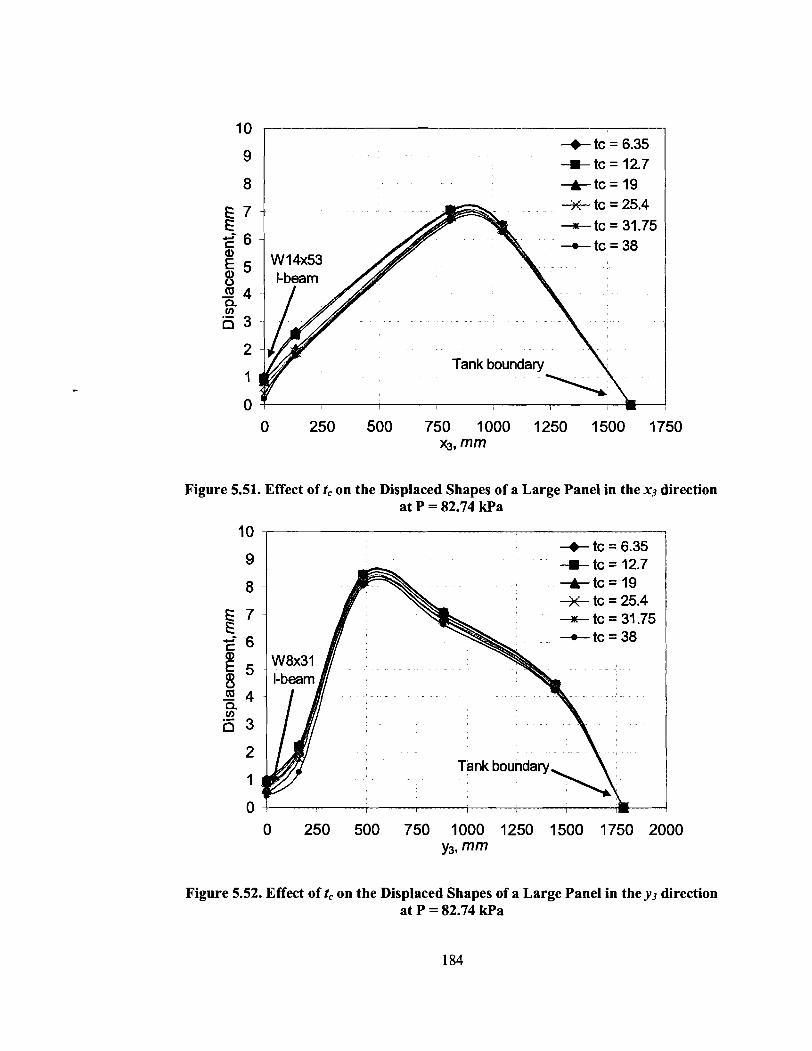
Figure 5.51. Effect oft, on the Displaced Shapes of a Large Panel in the x3 direction at P = 82.74 kPa
Figure 5.52. Effect of t, on the Displaced Shapes of a Large Panel in the y3 direction at P = 82.74 kPa

5.5.4.3. Effect of Flange Thickness (W8x31 and W14x53 I-Beams)
The effect of the steel flange thickness on the global panel response was studied
for the assembly loaded to the design pressure of 82.74 kPa, for both I-beams. According
to the approach presented in Section 5.3.2, the properties of each joint section were
computed for a given flange thickness value, ty, while holding the doubler plate thickness
(td) and the composite beam thickness (t,), constant. The flange thickness was modified
for one I-beam at a time. For the W8x31 I-beam, a flange thickness range of 0.50 tJI-gx31
to 2.5 ~JI-8x3, was used, with 98x31 - being the baseline thickness of 11.05 mm. For the
W14x53 I-beam, a flange thickness range of 0.25 tJI - 14~53 to 2 ~ J I - 14~53 was used, with
t~1_14~53 being the baseline thickness of 16.76 mm. The approximate I-beam dimensions
are summarized in Table 5.6.
Figure 5.53 and 5.54 present the displaced shapes of the small panel for varying
flange thickness values of the W8x31 I-beam. In the XI direction, transverse to the
stiffener direction, the flange effect is more pronounced for the middle regions of the
panel (600 mm < XI < 800 mm), but not as significant at the joint region (XI, yl = 0). In
the yl direction, aligned with the stiffeners, the flange thickness has a more significant
effect on the panel response, particularly towards the joint region 011 = 130 mm). Again,
this suggests that the W8x31 I-beam has a large influence on the behavior of the small
panels, particularly in the stiffener direction. In the case of the large panel in Figures
5.55 and 5.56, changing the thickness of the W8x31 I-beam does not have an effect on
the displacement, particularly in the direction transverse to the stiffeners.

Figure 5.53. Effect of f/l_Bx31 on the Displaced Shapes of a Small Panel in the XI
direction at P = 82.74 kPa
Figure 5.54. Effect of on the Displaced Shapes of a Small Panel in the yl direction at P = 82.74 kPa

+ ffl = 5.53 ffl= 11.05
Figure
1
--x- ffl= 22.10 ++ ffl = 27.63
5.55. Effect of t/l_adl on the Displaced Shapes of a Large Panel in the direction at P = 82.74 kPa
0
9
8 t ffl = 16.58
7 -x- ffl = 22.10
6 ++ ffl = 27.63
5
4
3
2
1
0
0 250 500 750 1000 1250 1500 1750 2000 Y3r mm
Figure 5.56. Effect of t/l_adl on the Displaced Shapes of a Large Panel in the y3
direction at P = 82.74 kPa
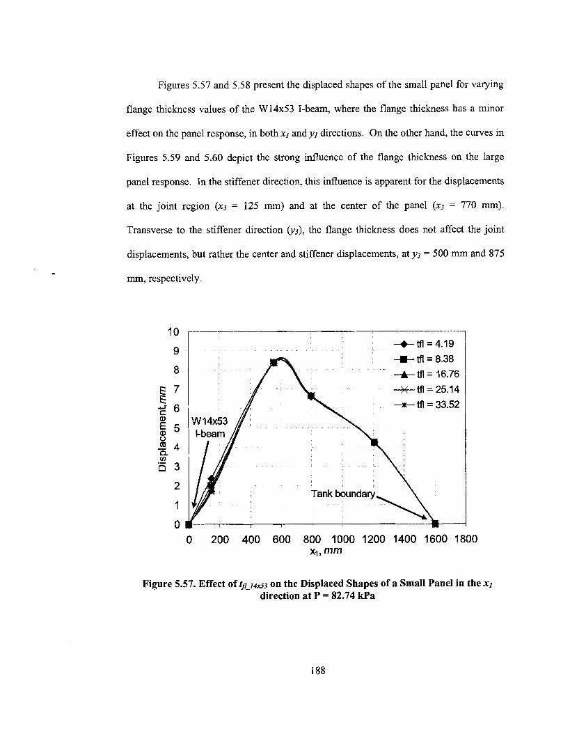
Figures 5.57 and 5.58 present the displaced shapes of the small panel for varying
flange thickness values of the W14x53 I-beam, where the flange thickness has a minor
effect on the panel response, in both xl and yl directions. On the other hand, the curves in
Figures 5.59 and 5.60 depict the strong influence of the flange thickness on the large
panel response. In the stiffener direction, this influence is apparent for the displacements
at the joint region (x3 = 125 rnm) and at the center of the panel (x3 = 770 mrn).
Transverse to the stiffener direction (y3), the flange thickness does not affect the joint
displacements, but rather the center and stiffener displacements, at y3 = 500 mm and 875
mm, respectively.
-t- tfl = 8.38 +ffl = 16.76
ffl = 25.14
-+ ffl = 33.52
Figure 5.57. Effect of l/r - 1 4 f l on the Displaced Shapes of a Small Panel in the XI
direction at P = 82.74 kPa
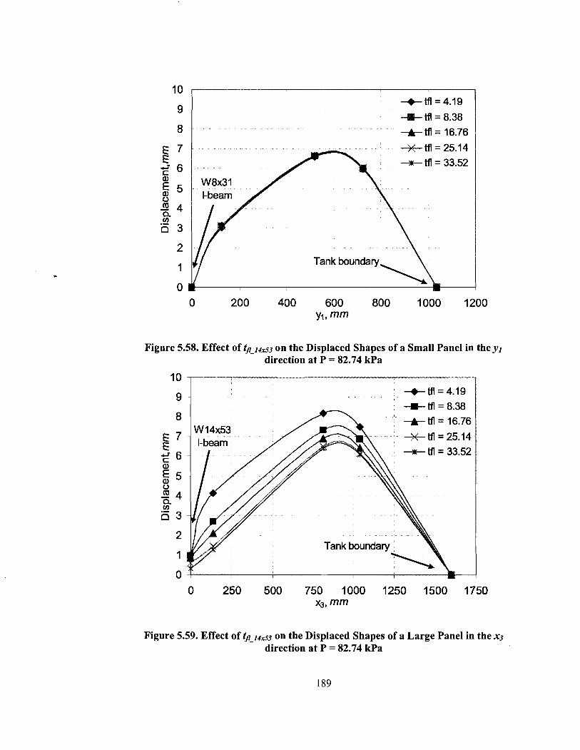
Figure 5.58. Effect of fj1_14x53 on the Displaced Shapes of a Small Panel in the yl direction at P = 82.74 kPa
-t- ffl = 8.38
Tank boundary \
Figure 5.59. Effect of fj1_14x53 on the Displaced Shapes of a Large Panel in the x3 direction at P = 82.74 kPa

Figure 5.60. Effect of k 1 d x s 3 on the Displaced Shapes of a Large Panel in the y3 direction at P = 82.74 kPa
The parametric study presented in this section shows that the global response of
the hybrid assembly is most sensitive to changes in the steel component geometries,
particularly the steel flange. Changes in the doubler geometry most strongly affect the
local response of the small panels at the joint region, in the stiffener direction. Increasing
the thickness of the composite has a modest localized effect in the joint region, but does
not significantly contribute to reduction in global panel deflections, especially for the
large panels. As expected, the steel flange thickness has a strong effect on the moment
resistance of the connection and on the global panel deflections. The study also shows
that the W8x3 1 I-beam drives the response of the small panels, but does not significantly
affect the response of the large panels. Conversely, the W14x53 I-beam drives the
response of the large panels, but not that of the small panels.

5.6. Generalized Plane Strain Finite Element Model of Hybrid Joint
The shell models presented in the previous sections were found appropriate to
estimate the joint stiffness. Furthermore, these models are usehl for studying the global
response of large-scale structures where extensive detailing of the small-scale features is
not feasible. However, since details of the bolted connection are not included, shell
models do not provide an accurate appraisal of the local stresses at the joint. The plane
strain model presented in this section is used to investigate the local joint response in
bending, by modeling the contact interactions between the joint constituents and the bolt.
Though a three dimensional solid model is more appropriate to compute the local
stresses, the computational cost and modeling complexity would be very large and
impractical for application into a large-scale structural model.
The initial approach presented is to model the joint as a "glued" entity, where all
the joint components act together as one piece and the contact interactions are not
included. In the second approach, contact modeling is prescribed by specifying the
surfaces that will interact as the joint is loaded. Lastly, a contact model that incorporates
the net effect of the bolt is presented. Included in this last model are the use of nodal
constraints and the use of a spring element along the bolt-line. Model verification is
conducted for the case of the DS-4 joint configuration, which was the connection type
used for the hybrid panel assembly described in Chapter 4.
5.6.1. Generalized Plane Strain Model Description
Figure 5.61 presents a schematic of a plane strain model of the DS-4 joint
configuration. The joint geometry is shown in Figure 5.62. The composite laminate
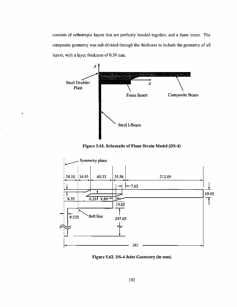
consists of orthotropic layers that are perfectly bonded together, and a foam insert. The
composite geometry was sub-divided through the thickness to include the geometry of all
layers, with a layer thickness of 0.39 mrn.
Figure 5.61. Schematic of Plane Strain Model (DS-4)
! / Symmetry plane
Figure 5.62. DS-4 Joint Geometry (in mm)
212.09 A - C
-7.62
I
I I
1 38.10 34.93 - - w - . I
I --
60.33 -
I 19.05 I
I
35.56 - b4 -
19.05
f - ''\~olt line 1 9.525
7- 247.65
I

Figure 5.63 shows the meshed model of the joint, where element type PLANE1 83
is used. PLANE183 is a higher order 2-D, 8-node element with quadratic displacement
behavior. This element is defined by 8 nodes having two degrees of fi-eedom at each
node: translations in the nodal x and y directions. Higher order elements are generally
well suited for bending dominated problems. To save computational time, only one half
of the joint is modeled. A mesh of approximately 18500 elements is used. Three
elements are used through the thickness of each layer to ensure accurate stress results.
All degrees of freedom at the bottom of the steel flange are constrained to simulate a
fixed base condition, and symmetry boundary conditions are applied about the joint
centerline. Nodal forces are input per unit of depth. For a total load of 4.45 KN and a
specimen width of 171.45 mrn, a concentrated load of 25.92 N per unit depth is applied to
the free end of the composite beam. This represents a total force of 4.45 KN on the
17 1.45-mm deep joint specimen.
Figure 5.63. Meshed Model of the DS-4 Joint

The steel doubler plate and steel I-beam members are assigned an elastic modulus
of 203 GPa, a Poisson's ratio of 0.30 and a yield strength of 248 MPa. The foam insert is
modeled as an isotropic material, having an elastic modulus of 80 MPa and a Poisson's
ratio of 0.29. The orthotropic material properties for a single EGNE lamina (55% v.f.) in
the principal material coordinates are presented in Table 5.7. The material properties and
strengths were obtained analytically using the ~ o m ~ o s i t e ~ r o @ software. For input into a
plane strain model, the orthotropic material properties in terms of the elastic stiffness
matrix, [q, are used. [C] is the inverse of the compliance matrix, [A, which is computed
in terms of the engineering constants: the elastic moduli EI, E2, E3, Poisson's ratios 012,
013, 023, the shear moduli, G12, G23, G13, and the fiber orientation, 8 [Hyer, 19981.
Table 5.8 summarizes the computed non-zero coefficients for the various ply
orientations comprising the laminated beam. In ANSYS, this input is done by using the
ANISOTROPIC ELASTICITY MATERIAL MODEL option, in STIFFNESS FORM.
The laminate architecture consists of a [(k 45, 0/90)6]s configuration at the free end of the
composite and a [(k 45, 0/90)8]s at the joint region. Four different material definitions are
created for the four layer orientations. Two local coordinate systems are created for the
layers in tapered regions of the composite, as shown in Figure 5.64.
Table 5.7. Orthotropic Lamina Properties for a 55% v.f. EGNE System
EII (GPa)
37.93
SI+
(MPa)
1021
4522
(GPa)
10.56
s 2 +
(MPa)
62
4533
(GPa)
10.56
s12+
(MPa)
39
GI2 (GPa)
3.192
Si (MPa)
- 607
GI3 (GPa)
3.192
Si (MPa)
- 305
G23 (GPa)
2.258
s12-
(MPa)
- 39
012
0.29
013
0.29
023
0.439
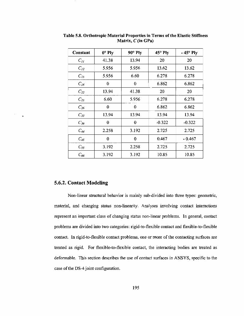
Table 5.8. Orthotropic Material Properties in Terms of the Elastic Stiffness Matrix, C (in GPa)
5.6.2. Contact Modeling
Non-linear structural behavior is mainly sub-divided into three types: geometric,
material, and changing status non-linearity. Analyses involving contact interactions
represent an important class of changing status non-linear problems. In general, contact
problems are divided into two categories: rigid-to-flexible contact and flexible-to-flexible
contact. In rigid-to-flexible contact problems, one or more of the contacting surfaces are
treated as rigid. For flexible-to-flexible contact, the interacting bodies are treated as
deformable. This section describes the use of contact surfaces in ANSYS, specific to the
case of the DS-4 joint configuration.
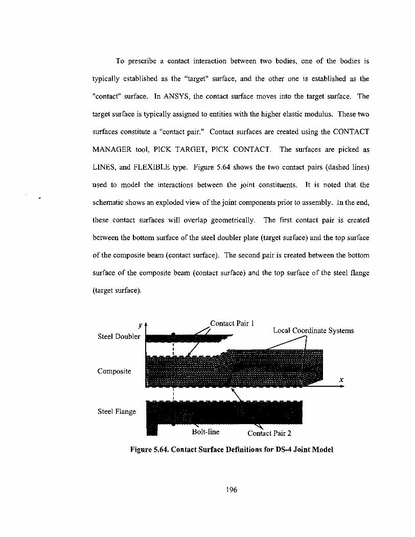
To prescribe a contact interaction between two bodies, one of the bodies is
typically established as the "target" surface, and the other one is established as the
"contact" surface. In ANSYS, the contact surface moves into the target surface. The
target surface is typically assigned to entities with the higher elastic modulus. These two
surfaces constitute a "contact pair." Contact surfaces are created using the CONTACT
MANAGER tool, PICK TARGET, PICK CONTACT. The surfaces are picked as
LINES, and FLEXIBLE type. Figure 5.64 shows the two contact pairs (dashed lines)
used to model the interactions between the joint constituents. It is noted that the
schematic shows an exploded view of the joint components prior to assembly. In the end,
these contact surfaces will overlap geometrically. The first contact pair is created
between the bottom surface of the steel doubler plate (target surface) and the top surface
of the composite beam (contact surface). The second pair is created between the bottom
surface of the composite beam (contact surface) and the top surface of the steel flange
(target surface).
Y Local Coordinate Systems Steel Doubler / I
Figure 5.64. Contact Surface Definitions for DS-4 Joint Model

The contact elements are automatically assigned by ANSYS based on the type of
solid element used. In this case, PLANE183 (second order) elements are used and
contact elements are automatically created as having mid-side nodes. To define target
contact surfaces, TARGET169 elements are used. These elements overlay the solid
elements (PLANE 183) describing the boundary of the deformable body. CONTAC 172
elements are used to represent contact and sliding between 2-D target surfaces and a
deformable surface. This element is located on the surfaces of 2-D solid elements with
mid-side nodes for compatibility.
Because of the non-linear nature of contact modeling, loading of the structure is
performed in steps. For most problems, at least two load steps are required. After the
boundary conditions have been defined, the first load step is created in the ANSYS Main
Menu, with the SOLUTION, DEFINE LOAD, LOAD STEP OPTIONS, WRITE LOAD
STEP FILE command. The load step file number is assigned as "1 ." This initial step is a
"neutral" step where the program identifies the surfaces that will come into contact. For
the models presented in this section, the contacting surfaces are coincident (i.e., their
edges occupy the same geometric space) and these are recognized as surfaces that will
interact in subsequent steps. Once contact has been established, the second (or higher)
steps are used to define structural loads. At this point, loads are applied to the structure,
and a second step (loading step) is created using the same commands, this time assigning
the load step number as "2." This may be repeated if further loading steps are necessary.
To run the job, use the SOLUTION, SOLVE, FROM LS FILES and specify the starting
load step as 1 and the ending load step as 2.

5.6.3. Modeling the Bolt
This section presents two approaches for modeling the bolt in conjunction with
contact modeling. The first approach consists of coupling the nodal displacements of the
different joint sections (doubler, composite and steel flange) along the bolt-line in they
direction, as shown in the schematic of Figure 5.65. This is done by using the COUPLE
DOFs option and manually picking the nodes to constrain. Nodal constraints are also
enforced in the x direction at the coincident nodes between the steel and composite
interfaces, to prevent rigid body motion of the composite beam.
Coincident nodes constrained in the x direction at interfaces
\ Nodes coupled in the
y direction along bolt-line
Figure 5.65. Constrained Nodes along the Bolt-line
The second approach consists of using a spring element to model the bolt
stiffness. A schematic of this model is presented in Figure 5.66, where the spring
element is depicted by a solid line attached to the upper node of the steel doubler and the

lower node of the steel flange. The spring connects the top node of the steel doubler plate
to the bottom node of the steel flange. To do this, an additional line is created along the
bolt-line and overlaid on top of the existing bolt-line. Element COMBIN14 is used to
define the spring and a real constant defines the spring stiffness, k. The spring element
needs to be meshed separately, after the joint regions have been meshed and the contact
surfaces defined. To create a single spring, assign the number of divisions to be 1.
For the DS-4 joint configuration, the stiffness of the linear spring can be
calculated by smearing the axial stiffness of the three bolts across the width of the model.
For a single bolt in axial loading, the bolt stiffness is computed as follows:
EA k =- bolt
Lbolr
For a grade 8, tapered-head bolt with a diameter of 12.7 mm, used in the joint
specimens, E = 203 GPa, Lbolt = 50.8 mm, and A = 126.70 mm2. From Eq. (5.4), the
stiffness of a single bolt, kbolt, is found to be 506.2 KNImm. The smeared bolt stiffness
across the width of the joint is computed using Eq. (5.5) for the joint test model, and Eq.
(5.6) for the global model, as follows:
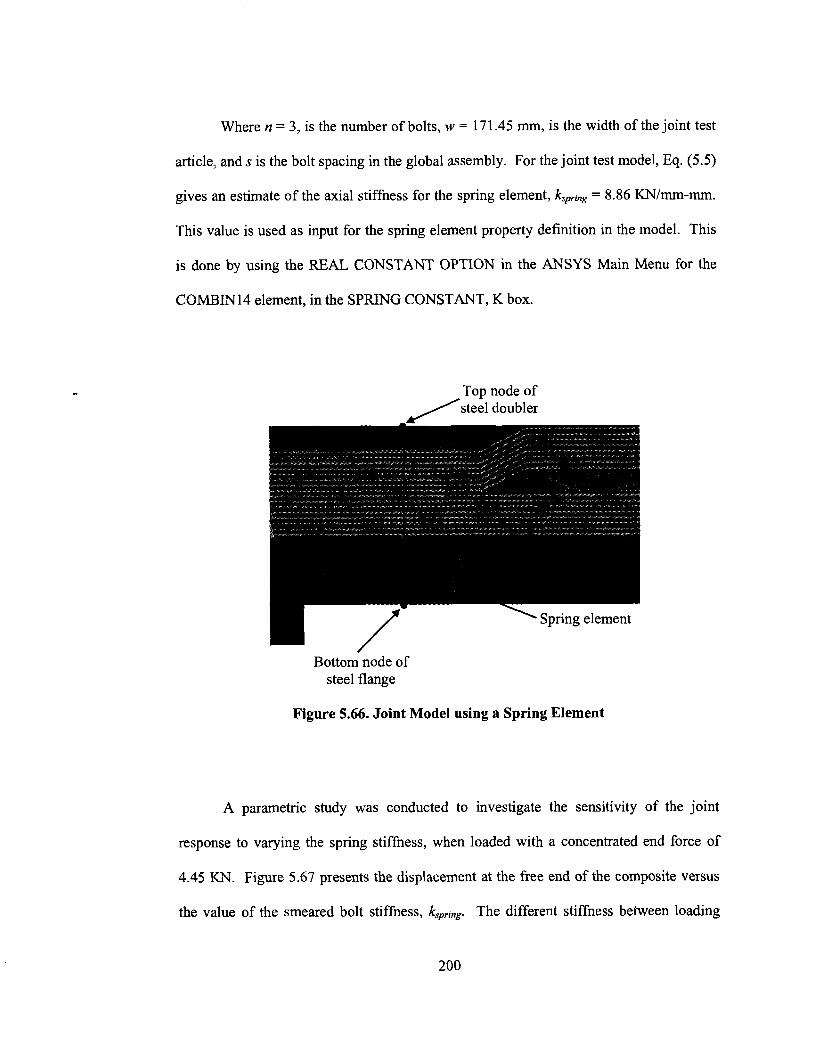
Where n = 3, is the number of bolts, w = 171.45 rnm, is the width of the joint test
article, and s is the bolt spacing in the global assembly. For the joint test model, Eq. (5.5)
gives an estimate of the axial stiffness for the spring element, kSPring = 8.86 KNImm-mm.
This value is used as input for the spring element property definition in the model. This
is done by using the REAL CONSTANT OPTION in the ANSYS Main Menu for the
COMBIN14 element, in the SPRING CONSTANT, K box.
Bottom node of steel flange
Figure 5.66. Joint Model using a Spring Element
A parametric study was conducted to investigate the sensitivity of the joint
response to varying the spring stiffness, when loaded with a concentrated end force of
4.45 KN. Figure 5.67 presents the displacement at the free end of the composite versus
the value of the smeared bolt stiffness, ksprinr The different stiffness between loading
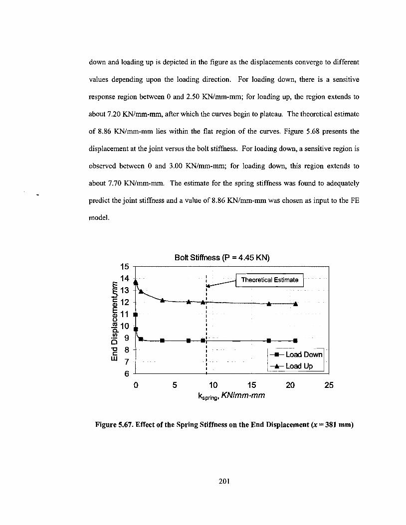
down and loading up is depicted in the figure as the displacements converge to different
values depending upon the loading direction. For loading down, there is a sensitive
response region between 0 and 2.50 KN/mm-mm; for loading up, the region extends to
about 7.20 KN/mm-mm, after which the curves begin to plateau. The theoretical estimate
of 8.86 KN/mm-mm lies within the flat region of the curves. Figure 5.68 presents the
displacement at the joint versus the bolt stiffness. For loading down, a sensitive region is
observed between 0 and 3.00 KN/mm-mm; for loading down, this region extends to
about 7.70 Wmm-mm. The estimate for the spring stiffness was found to adequately
predict the joint stiffness and a value of 8.86 KN/mm-mm was chosen as input to the FE
model.
Bolt Stiffness (P = 4.45 KN)
I I
.I ..I I
I I A
1 . I I
$10 i I I
I
I I I w I w
2 8 - I I I
7 - I I I I -A- Load Up
6 1
I
Figure 5.67. Effect of the Spring Stiffness on the End Displacement (x = 381 mm)
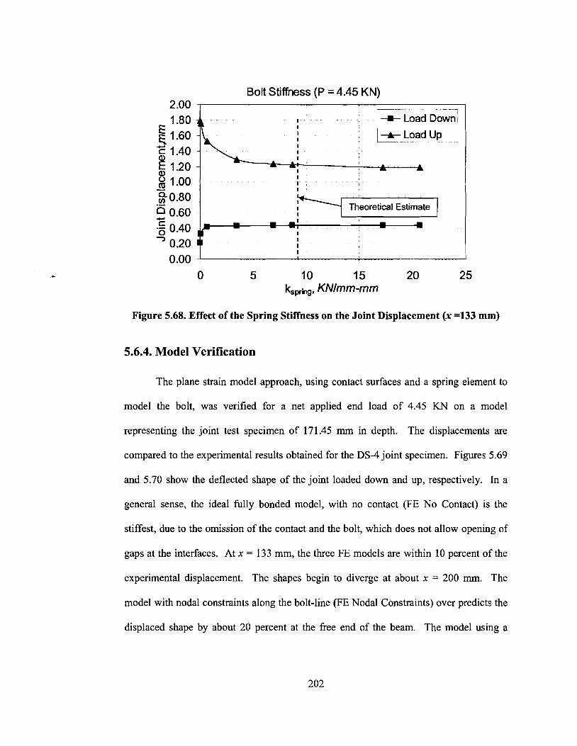
Bolt Stiffness (P = 4.45 KN)
I I
Theoretical Estimate
Figure 5.68. Effect of the Spring Stiffness on the Joint Displacement (x =I33 mm)
5.6.4. Model Verification
The plane strain model approach, using contact surfaces and a spring element to
model the bolt, was verified for a net applied end load of 4.45 KN on a model
representing the joint test specimen of 171.45 mm in depth. The displacements are
compared to the experimental results obtained for the DS-4 joint specimen. Figures 5.69
and 5.70 show the deflected shape of the joint loaded down and up, respectively. In a
general sense, the ideal fully bonded model, with no contact (FE No Contact) is the
stiffest, due to the omission of the contact and the bolt, which does not allow opening of
gaps at the interfaces. At x = 133 mm, the three FE models are within 10 percent of the
experimental displacement. The shapes begin to diverge at about x = 200 mm. The
model with nodal constraints along the bolt-line (FE Nodal Constraints) over predicts the
displaced shape by about 20 percent at the free end of the beam. The model using a

spring element (FE Spring) provides a good depiction of the deflected shape of the joint,
with a difference of under 10 percent.
P = 4.45 KN, Down
-
- . - - FE No Contact
I -FE Spring \
\ -1 0
Figure 5.69. Deflected Shape of DS-4 Joint Models (P = 4.45 KN, Down)
P = 4.45 KN, UP
- FE Nodal Constraints
-
Figure 5.70. Deflected Shape of DS-4 Joint Models (P = 4.45 KN, Up)

5.6.5. Generalized Plane Strain Modeling Results Using Spring and
Contact Elements
The results presented in this section correspond to the model using a spring
element to account for the bolt. The structure is loaded to 4.45 KN at the free end of the
beam. It is desired to study the contact pressure at the interfaces between the steel and
composite components, the magnitude of the contact gap and the normal and shear
stresses on the composite. The experiments showed that damage initiated at the top and
bottom layers of the composite due to the bearing action of the steel doubler and flange
on the composite beam. Hence, the stresses at these locations are of interest.
Figure 5.71 presents the displacement contour of the joint loaded downward. As
expected, a gap opens up at the tapered interface between the steel doubler and the
composite beam. Another gap is observed at the bottom left interface between the
composite and the steel flange. This gap occurs due to the action of the spring and the
symmetry boundary condition applied to the doubler plate, which allows movement of
the composite beam in they direction.
Figure 5.72 shows the displacement contour of the joint loaded upward. In this
case, the gap between the doubler and the composite at the tapered region is closed. A
gap opens up at the steel flange and composite beam interface, after the bolt-line (x > 38
rnm). The larger displacement at the end of the beam is due to the lower bending
resistance provided by the steel doubler during upward loading, when compared to the
steel flange during downward loading. When compared to the results in Figure 5.13, the
generalized plane strain model is less stiff than the shell model by 6 percent (load down)
and by 12 percent (load up), due to the inclusion of the bolt and contact interactions.

Figure 5.71. Displacement Contour, Load Down (P = 4.45 KN)
Figure 5.72. Displacement Contour, Load Up (P = 4.45 KN)
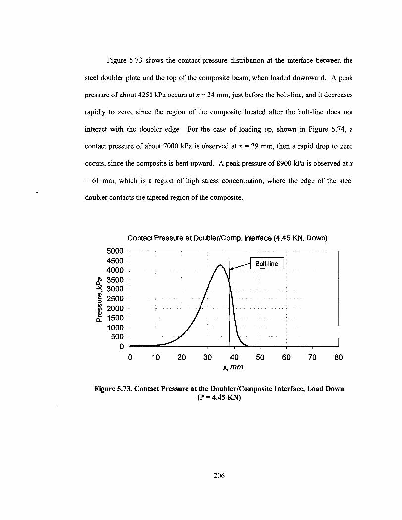
Figure 5.73 shows the contact pressure distribution at the interface between the
steel doubler plate and the top of the composite beam, when loaded downward. A peak
pressure of about 4250 kPa occurs at x = 34 mm, just before the bolt-line, and it decreases
rapidly to zero, since the region of the composite located after the bolt-line does not
interact with the doubler edge. For the case of loading up, shown in Figure 5.74, a
contact pressure of about 7000 kPa is observed at x = 29 mm, then a rapid drop to zero
occurs, since the composite is bent upward. A peak pressure of 8900 kPa is observed at x
= 61 mm, which is a region of high stress concentration, where the edge of the steel
doubler contacts the tapered region of the composite.
Contact Pressure at DoublerlComp. Interface (4.45 KN, Down)
Figure 5.73. Contact Pressure at the Doubler/Composite Interface, Load Down (P = 4.45 KN)

Contact Pressure at DoublerIComp. Interface (4.45 KN, Up)
Figure 5.74. Contact Pressure at the Doubler/Composite Interface, Load Up (P = 4.45 KN)
Figure 5.75 presents the contact pressure distribution at the interface between the
steel flange and the bottom of the.composite beam, when loaded downward. An initial
pressure of about 200 kPa is observed from x = 0 to 18 mm, after which the pressure dies
down and reaches a peak of 42000 Wa, which is due to the localized contact between the
composite and the edge of the steel flange at 138 mm. For the case of loading up in
Figure 5.76, a peak pressure of 9900 kPa occurs at x = 0, where the composite
compresses against the steel flange as the joint is loaded. The pressure drops to zero just
before the bolt-line (x = 27 mm), due to opening of the gap at the interface.
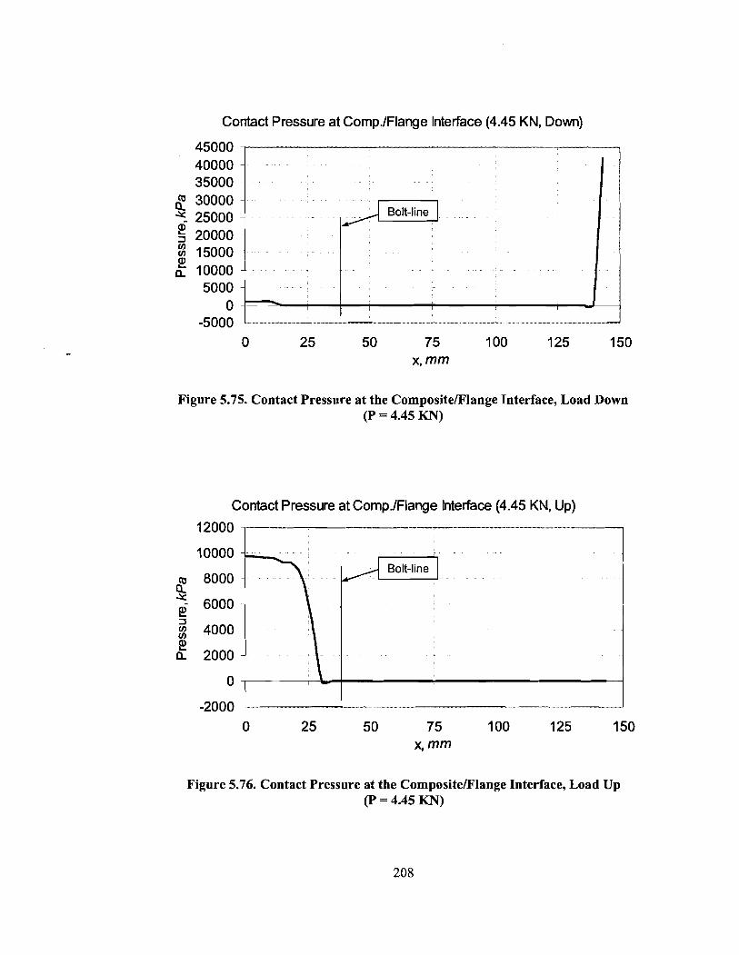
Contact Pressure at Comp./Flange Interface (4.45 KN, Down)
Figure 5.75. Contact Pressure at the Composite/Flange Interface, Load Down (P = 4.45 KN)
Figure 5.76. Contact Pressure at the Composite/Flange Interface, Load Up (P = 4.45 KN)
Contact Pressure at Comp./Flange Interface (4.45 KN, Up)
12000 --- ---v - - -" " - -
10000 - Bolt-line
(p 8000 -
I 1 I I
3 er 6000 - 3
4000 - V)
t 2000 -
0
-2000 - 0 25 50 75 100 125 150
K mm
- I -
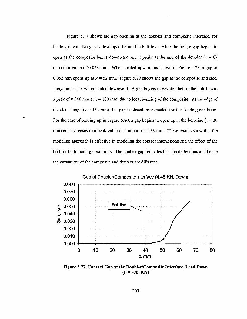
Figure 5.77 shows the gap opening at the doubler and composite interface, for
loading down. No gap is developed before the bolt-line. After the bolt, a gap begins to
open as the composite bends downward and it peaks at the end of the doubler (x = 67
mm) to a value of 0.058 mm. When loaded upward, as shown in Figure 5.78, a gap of
0.052 mm opens up at x = 52 mm. Figure 5.79 shows the gap at the composite and steel
flange interface, when loaded downward. A gap begins to develop before the bolt-line to
a peak of 0.040 rnrn at x = 100 mm, due to local bending of the composite. At the edge of
the steel flange (x = 133 mm), the gap is closed, as expected for this loading condition.
For the case of loading up in Figure 5.80, a gap begins to open up at the bolt-line (x = 38
mm) and increases to a peak value of 1 mm at x = 133 mm. These results show that the
modeling approach is effective in modeling the contact interactions and the effect of the
bolt for both loading conditions. The contact gap indicates that the deflections and hence
the curvatures of the composite and doubler are different.
Gap at Doubler/Composite Interface (4.45 KN, Down)
:::;: ;
Figure 5.77. Contact Gap at the Doubler/Composite Interface, Load Down (P = 4.45 KN)

Figure 5.78. Contact Gap at the Doubler/Composite Interface, Load Up (P = 4.45 KN)
Figure 5.79. Contact Gap at the Composite/Flange Interface, Load Down (P = 4.45 KN)
Gap at CompositeIFlange Interface (4.45 KN, Down)
0.070 -
0.060 -
0.050
-".. --.-.-.-
Bolt-line
0.040 -
$ 0.030 - a ,
0.020
0.010 -
0.000 1 I I I

Figure 5.80. Contact Gap at the CompositeIFlange Interface, Load Up (P = 4.45 KN)
Figure 5.81 presents the normal stress contour for the case of downward loading.
In a general sense, it is observed that the peak stresses (-134 MPa, 120 MPa) occur at the
outer layers of the top and bottom surfaces of the composite, particularly at the tapered
region of the composite beam. In the case of loading up in Figure 5.82, the peak stresses
recorded (-264 MPa, 221 MPa) occur in the steel doubler plate, as a result of the
compressive action of the composite beam. A peak tensile stress of 113 MPa is recorded
at the end of the tapered region of the composite beam.

Figure 5.81. Normal Stress Contour, a,, Load Down at P = 4.45 KN (in MPa)

-264.75
-210.71
-156.68
-102.63
-48.59
5.45
59.50
113.53
167.58
221.62
-264 MPa 221 MPa
Figure 5.82. Normal Stress Contour, on, Load Up at P = 4.45 KN (in MPa)
Figure 5.83 presents the shear stress contour when the joint is loaded downward.
A peak stress of 16 MPa is observed at the contact region between the lower edge of the
doubler plate and the tapered section of the composite. At the bottom tapered section of
the composite, a peak stress of -12 MPa is recorded. Figure 5.84 shows the shear stress
contour when the joint is loaded upward. In this case, a peak stress of 54 MPa is
observed at the lower edge of the steel doubler plate and a peak stress of -43 MPa is
observed at the tapered composite region in contact with the doubler. At the lower
tapered region of the composite, a stress of 38 MPa was recorded. The high shear
stresses observed in the tapered regions of the composite beam will lead to delamination
and eventually failure along the interfaces between the composite and the foam. As
observed in the experiments for joints with doubler plates and foam inserts, damage
initiated at the tapered regions, due to the bearing action of the steel members, and then
propagated to the foam insert and eventually caused final rupture.

Figure 5.83. Shear Stress Contour, r,, Load Down at P = 4.45 KN (in MPa)
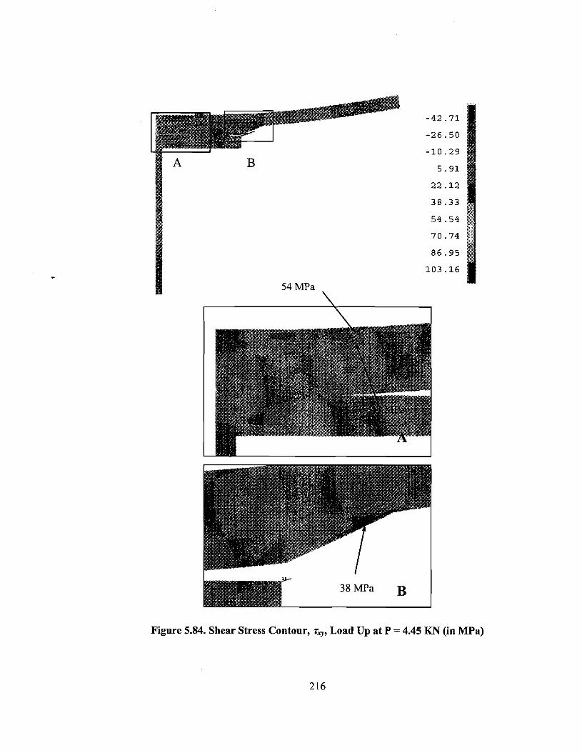
54 MPa
Figure 5.84. Shear Stress Contour, z,, Load Up at P = 4.45 KN (in MPa)

5.6.6. Damage Initiation Prediction
This section presents the complete load versus displacement response of the DS-4
joint and an estimate of damage initiation. The load versus displacement response is
shown for both loading directions. Initiation of failure is used as the strength estimate
for this connection because after this load significant damage will begin to accumulate.
Failure initiation is estimated by comparing the peak normal stresses obtained from the
model with the strength values of each lamina, as given in Table 5.7. In this analysis, the
joint is loaded in flexure, by applying a concentrated end load at x = 38 1 mm, as shown in
Figure 5.63. A load of 40 KN is applied in steps (increments) of 4.45 KN, for a total of
1 1 load steps (note that the initial step is for gap closure during initial contact, so a total
of 10 steps are actually used for loading).
Figure 5.85 presents a comparison of the experimental and numerical load versus
displacement envelopes for the DS-4 joint. It is noted that the response of the system is
stiffer when loading down than when loading up. For loading down, the response of the
model closely follows the experimental results until a load of about 8 KN, after which
slight stiffness degradation is observed in the experimental data. It is suspected that this
stiffness decrease is due to the cyclic loading that causes minor material damage at this
load level. For loading up, the experimental and numerical results agree well up until a
load value of about 8 KN. The discrepancies between the numerical and experimental
results are attributed to the material model used for the composite layers and other
differences between the model and the as-built geometry. The layers are modeled using
orthotropic material property definitions, which do not account for stiffness degradation
due to progressive failure that occurs in the actual joint specimen during testing.
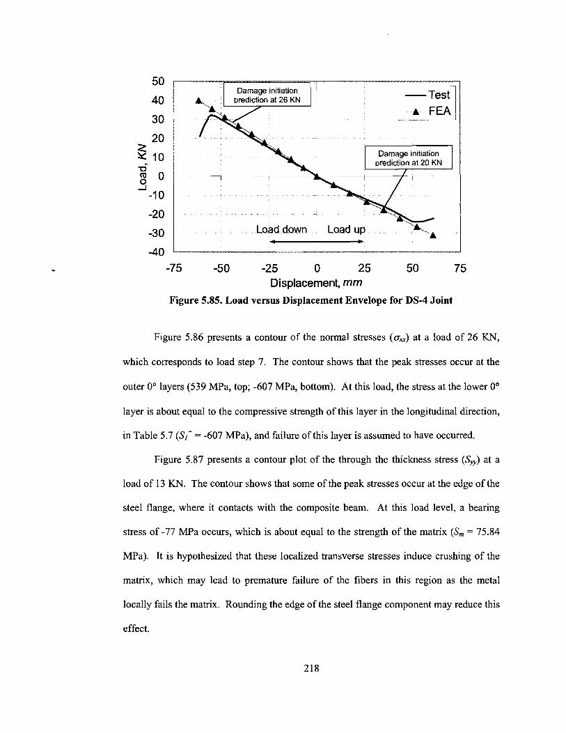
-40 -75 -50 -25 0 25 50 75
Displacement, mm
I--
- -'% -\
Load down _ Load up A- ..A 4 F
Figure 5.85. Load versus Displacement Envelope for DS-4 Joint
Figure 5.86 presents a contour of the normal stresses (0,) at a load of 26 KN,
which corresponds to load step 7. The contour shows that the peak stresses occur at the
outer 0" layers (539 MPa, top; -607 MPa, bottom). At this load, the stress at the lower 0"
layer is about equal to the compressive strength of this layer in the longitudinal direction,
in Table 5.7 (SI+ = -607 MPa), and failure of this layer is assumed to have occurred.
Figure 5.87 presents a contour plot of the through the thickness stress (S,) at a
load of 13 KN. The contour shows that some of the peak stresses occur at the edge of the
steel flange, where it contacts with the composite beam. At this load level, a bearing
stress of -77 MPa occurs, which is about equal to the strength of the matrix (S, = 75.84
MPa). It is hypothesized that these localized transverse stresses induce crushing of the
matrix, which may lead to premature failure of the fibers in this region as the metal
locally fails the matrix. Rounding the edge of the steel flange component may reduce this
effect.

-609
-482
-354
-227
-99
29
156
2 84
4 12
53 9
at on = - 607 MPa
Figure 5.86. Stress Contour (0,) at P = 26 KN, Load Down, Showing First Ply Failure of a 0-deg Layer (in MPa)
Figure 5.87. Stress Contour (o,) at P = 13 KN, Load Down, Showing Crushing of the Matrix by the Steel Flange (in MPa)

Figure 5.88 presents the load versus displacement curve of the joint for cycle sets
1 and 8, for displacements recorded with the inner LVDTs ('joint region). The first
significant drop in load occurred when loading in the downward direction, where the
experimental peak load attained is about 23 KN. This drop in load may be attributed to
fiber failure and is an indication of damage initiation. The predicted peak load based on
the FE model is 26 KN. Loading up resulted in a similar phenomenon with a predicted
damage initiation load of 20 KN, compared to the load observed in the experiment of
-0.60 -0.40 -0.20 0.00 0.20 0.40 0.60 Displacement, mm
18.6 KN. Cycle set 1
Cycle set 8 30 I I I
4 ,
3
2
8 8 0 0 J -1
-2
-3
4
-5 0 5 10 Displacement, mm
1
I
1
J I I I
Figure 5.88. Experimental Load versus Displacement Curve of DS-4 Joint for Cycle Sets 1 and 8 (Inner LVDTs)

The generalized plane strain model presented in this section provides a good
estimate of failure initiation, but does not account for progressive material non-linearity
due to the decrease in stifhess with increasing load. In order to appropriately predict the
strength of the joint, a progressive damage model is required, where the stiffness of the
failed elements is reduced once the layers containing these elements reach any of the
failure criteria. Such an approach is beyond the scope of this work, but it is recommended
for future hybrid joint analyses.

Chapter 6
CONCLUSIONS AND RECOMMENDATIONS
6.1. Sub-component Joint Testing
An experimental investigation was conducted to assess the relative structural
performance of hybrid composite/metal bolted connections, subjected to flexural loading.
Two types of hybrid connections were investigated as part of this study, namely, standard
bolted joints and bolted joints with doubler plates. Overall, the goal was to develop a
watertight, hybrid connection, to resist bending loads and to reduce the bolt load loss due
to the viscoelastic creep effects typically observed in a composite material. This was
accomplished by using tapered-head bolts in lieu of protruding-head bolts and by
implementing a doubler plate, which prevents the joint from opening and decreases the
bolt load loss due to creep by spreading the bolt pre-load over a wider area.
The response of fifteen different joint configurations was studied experimentally.
Evaluation was based upon the relative performance of potential concepts with regards to
joint capacity, rotational stiffness, failure mode sequence, and the ability to seal the joint
for watertight integrity. The results of this study have shown that, for resisting bending
loads, joints with doubler plates can be made stronger and rotationally stiffer than
standard bolted joints. For example, when compared to its standard bolted joint
counterpart with two rows of the same diameter bolts (BT-2), a joint using a short
doubler plate, a foam insert, and a single row of bolts (DS-4), was found to be at least 46
percent stronger and 29 percent stiffer when displaced downward, and 33 percent
stronger and 34 percent stiffer when displaced upward. Doubler plates proved effective

in mitigating opening of the joint, which will improve the ability to seal the joint and
maintain watertight integrity. Hence, the additional expense and geometric complexity of
bolted joints with doubler plates and foam inserts may be justified for some underwater
applications.
When comparing the performance of all joint configurations with doubler plates
to each other, it was observed that a joint with a short doubler plate and one row of bolts
(such as DS-4) can attain capacities comparable to those of joints with long doubler
plates and two rows of bolts (such as DL-2 and DL-3). When compared to DS-4, the use
of long doublers induced more catastrophic failure sequences, which ultimately led to
complete separation of the composite beam from the joint region. Moreover, DS-4
requires roughly half of the material for fabrication of the doubler plates and half the
number of bolts than those joints with medium and long doubler plates. This may be a
significant factor when considering installation andlor maintenance of large-scale
structures that require multi-panel assemblies using bolted connections. In light of these
test results, the short doubler and foam insert joint configuration (DS-4) was selected for
implementation into hydrostatic testing of a hybrid, four-panel assembly.
It is recommended that future hybrid joint work focuses on: 1) repeat testing to
study the variability in joint performance; 2) possible ways to fabricate joints with
doubler plates and foam inserts more economically; 3) testing of joints subjected to in-
plane tension and compression; 4) developing hybrid joints that may be welded, as
opposed to bolted; and 5) studying the fatigue resistance of hybrid connections.

6.2. Hybrid Panel Assembly Testing
Testing of a large-scale region of the hybrid lifting body was conducted to assess
the structural performance of the MACH concept, when applied to a modular, multi-panel
assembly. A hydrostatic test system and test procedure were successfully developed and
implemented for this study. The hybrid joint was assembled by attaching four E-
glasslvinyl ester composite, hat-stiffened panels to steel I-beam members, acting as
bulkheads. The panels were loaded to a target peak pressure of 248 kPa, until failure was
imminent. Test results showed a linear response of the system when loaded to the design
pressure of 82.74 kPa. Non-linear behavior of the load-strain curves and the load-
displacement curves was observed at the beginning of the third loading cycle set, with a
peak pressure of 1.5 times the design pressure. Non-linearity of these curves indicated
imminent damage, which occurred as delamination of the stiffeners on the large panels at
1.4 times the design load. No damage was observed in the small panels. After failure of
several stiffeners, the hybrid panel assembly withstood 3 times the design load without
leakage. Hence, the response of the hybrid joint was deemed successful, as watertight
integrity was achieved. Delamination of the stiffeners indicated that failure of the
composite panels was due to the stiffenerlpanel interface. This type of failure resulted
from a combination of stiffener geometry and techniques for bonding of the stiffeners to
the flat surface of the panels. Providing more shear resistance at the interface, by
interleaving fabric or by improved adhesion, would delay the initiation of this failure
mode. Improvements of the manufacturing techniques should result in stronger panels.
It is recommended that future work focuses on investigating the structural
response of hybrid systems which use other types of metals, such as aluminum, and

systems which implement other types of joint geometries, including a weldable joint
configuration. It is also recommended to study the fatigue life of the hybrid assembly
using various joint configurations. Finally, composite stiffener manufacturing techniques
should be improved, while also conducting stiffener geometry optimization studies.
6.3. Finite Element Analysis of Hybrid Joints
Global finite element analysis (FEA) was accomplished using shell element
models. In so doing, a local model of the joint was used to develop a modeling
methodology that was ultimately implemented on a global shell model of the four-panel
assembly. The local shell model divided the hybrid joint into five regions. Properties for
each region were prescribed according to assumptions made. The predicted response was
compared to the experimental results for the DS-4 joint. Results show that the hybrid FE
model gives a good prediction of the joint stiffness, with displacement results within 10
percent of the experimental values. Predictions of stress, strain and strength of the joint
region were not accomplished with the shell model and require detailed local models.
Shell finite element models of the global four-panel assembly show good agreement with
experiments with a difference in peak displacements of less than 10 percent. Parametric
studies using the global shell model show that the steel flange and steel doubler plate
thickness have a significant impact on the connection rigidity.
Detailed joint modeling was carried out using a generalized plane strain finite
element model. This model included contact between the composite and steel
components, and a spring to represent the bolts. Different stiffness was demonstrated in
pulling and pushing of the composite, due to the variation in joint gap opening caused by
the connection geometry. The detailed model gave a good prediction of the DS-4 joint

response. Local contact pressures were shown to be high at the end of the steel flange
and the edge of the steel doubler plate, which are regions where failure initiated during
testing. Details to reduce this stress riser may improve the strength of the connection.

REFERENCES
Alm, F. (1983). GRP versus steel in ship construction. Naval Forces; 5; 82-86.
ANSYS (2004). ANSYS reference manual. ANSYS Inc. Houston, PA.
Arbur, D. R., Gerro, J. A., Dickson, J. (1 995). D-box fixture for testing stiffened panels in compression and pressure. Journal of Aircraft; 32-6.
ASTM Standard D6416-99 (2004). Standard test method for two-dimensional flexural properties of simply supported sandwich composite plates subjected to a distributed load. Annual book of ASTM standards.
Barsoum, R.G. S. (2003). Best of both worlds: hybrid ship hulls use composites and steel. AMPTIAC 2003; 7-3 : 52-61.
Benchekchou, B., White, R. G. (1995a). Stresses around fasteners in composite structures in flexure and effects on fatigue damage initiation part 1: cheese-head bolts. Composite Structures 1995; 33; 95-108.
Benchekchou, B., White, R. G. (1995b). Stresses around fasteners in composite structures in flexure and effects on fatigue damage initiation part 2: countersunk bolts. Composite Structures 1995; 33; 109-1 19.
Berube, K. A., Caccese, V. (1999). Construction and connection concepts for a modular advanced composite hull-form, University of Maine Department of Mechanical Engineering, Report No. C-99 14, December 1999,33 pp.
Black, S. (2003). Fighting ships augment combat readiness with advanced composites. High Performance Composites 2003 ; 30-33.
Bonanni, D. L., Caiazzo, A., Flanagan, G. (2001). Design guide for joints in marine composite structures - part 1, concept development. Report No. NSWCCD-65-TR- 2000101. NSWC Carderock, January 2001.
Boone, M. J., Caccese, V., Bragg, R., Berube, K. A. (2003). Mechanical testing of Epoxy adhesives for naval applications, UM-MACH-RPT-0 1-03, April 2003.
Boyd, S. W., Blake, J. I. R., Shenoi, R. A., Mawella, J. (2004a). Fatigue life and residual strength analysis of steel-composite joints. Applied Mechanics and Materials; 1-2; 81-86.
Boyd, S. W., Blake, J. I. R., Shenoi, R. A., Kapadia, A. (2004b). Integrity of hybrid steel- to-composite joints for marine application. J. Engrg for the Maritime Environment, V218. Part M, 235-246.

Camanho, P. P., Matthews, F. L. (2000). Bonded metallic inserts for bolted joints in composite laminates. Proc Instn Mech Engrs February 2000, V214; N1, pp 33-40 (8).
Cao, J., Grenestedt, J. L. (2003). Test of a redesigned glass-fiber reinforced vinyl ester to steel joint for use between a naval GRP superstructure and a steel hull. Composite Structures 2003; 60-4; 439-445.
Chalmers, D. W. (1994). The potential for the use of composite materials in marine structures. Marine Structures 1994; 2-5; 441 -456.
Chu, W., Wu, L., Kharbari, V. (2004). Durability evaluation of moderate temperature cured E-Glass/vinylester systems. Composite Structures 2004; 66; 367-376.
Clifford, S. M., Manger, C. I. C., Clyne, T. W. (2002). Characterisation of a glass-fibre reinforced vinylester to steel joint for use between a naval GRP superstructure and a steel hull. Composite Structures 2002; 57; 59-66.
Cohen, D., Hyer, M. W., Shuart, M. J., Griffin, 0 . H., Prasad, C., Yalamanchili, S. R. (1995). Failure criterion for thick multifastener graphite-epoxy composite joints. American Society of Testing and Materials.
Collings, T. A. (1977). The strength of bolted joints in multi-directional cfrp laminates. Composites 1977; 43-55.
Collings, T. A. (1982). On the bearing strength of CFRP laminates. Composites 1982; 13; 241-252.
Cooper, C., Turvey, G. J. (1995). Effects of joint geometry and bolt torque on the structural performance of single bolt tension joints in pultruded GRP sheet material. Composite Structures 1995; 32; 2 17-226.
Critchfield, M. O., Judy, T. D. (1994). Low-cost design and fabrication of composite ship structures. Marine Structures 1994; 2-5; 475-494.
Dodkins, A. R., Shenoi, R. A., Hawkins, G. L. (1994). Design of joints and attachments in FRP ship structures. Marine Structures 1994; 7; 229-238.
Gullberg, O., Olsson, K. A. (1990). Design and construction of GRP sandwich ship hulls. Marine Structures 1990; 3; 93-109.
Grenestedt, J. L., Suase, R. (2005). Vierendeel steel truss/composite skin hull test, ATLSS report No. 05-19. Lehigh University, Bethlehem, PA, August, 13 pp.
Hart-Smith, L. (1978). Mechanically-fastened joints for advanced composites - phenomenological considerations and simple analyses. Fourth Conference on Fibrous Composites in Structural Design 1978; 14-17.

Hart-Smith, L. (1991). An engineer's viewpoint on design and analysis of aircraft structural joints. International Conference on Aircraft Damage Assessment and Repair 1991;
Herrington, P. D., Sabbaghian, M. (1993). Fatigue failure of bolted joints. Composite Materials 1993; 27; 491-512.
Hyer, M.W. (1998). Stress analysis of fiber-reinforced composite materials, McGraw Hill, Boston, MA. 627 pp. w
Ireman, T., Ranvik, T., Eriksson, I. (2000). On damage development in mechanically fastened composite laminates. Composite Structures 2000: 49; 15 1-1 7 1.
Kimpara, I. Use of advanced composite materials in marine vehicles. Marine Structures 1991; 4-2; 117-127.
Mouritz, A. P., Gellert, E., Burchill, P., Challis, K. (2001). Review of advanced composite structures for naval ships and submarines. Composite Structures 2001; 53; 21- 41.
Oh, J. H., Kim, Y. G., Lee, D. G. (1997). Optimum bolted joints for hybrid composite materials. Composite Structures 1997; 1-4; 329-33 1.
Pei, J., Shenoi, R. A. (1996). An examination of key aspects defining performance characteristics of out-of-plane joints in FRP marine structures. Composites A 1996; 27; 89- 103.
Pelletier, K., Caccese, V., Berube, K. A. (2005). Influence of stress relaxation in hybrid composite/metal bolted connections. Report No. UM-MACH-RPT-01-02, University of Maine, Department of Mechanical Engineering, , 87 pp.
Persson, E., Eriksson, I. (1999). Fatigue of multiple-row bolted joints in carbonlepoxy laminates: ranking of factors affecting strength and fatigue life. International Journal of Fatigue 1999; 21; 337-353.
Smith, P. A., Pascoe, J., Polak, C., Stroud, D.O. (1986). The behaviour of single-lap bolted joints in CFRP laminates. Composite Structures 1986; 1-3; 41 -55.
Starikov, R., Schon, J. (2001). Quasi-static behaviour of composite joints with protruding-head bolts. Composite Structures 200 1 ; 5 1 ; 4 1 1-425.
Starikov, R., Schon, J. (2002a). Experimental study on fatigue resistance on composite joints with protruding-head bolts. Composite Structures 2002; 55; 1 - 1 1.
Starikov, R., Schon, J. (2002b). Fatigue resistance on composite joints with countersunk composite and metal fasteners. International Journal of Fatigue 2002; 21; 39-47.

Thompson, L., Walls, J., Caccese, V. (2005). Design and analysis of a hybrid composite/metal structural system for underwater lifting bodies. Report No. UM-MACH- RPT-01-08, University of Maine Department of Mechanical Engineering, 95 pp.
Vangrimde, B., Boukhili, R. (2003). Descriptive relationships between bearing response and macroscopic damage in GRP bolted joints. Composite Part B: Engineering 2003; 34; 593-605.
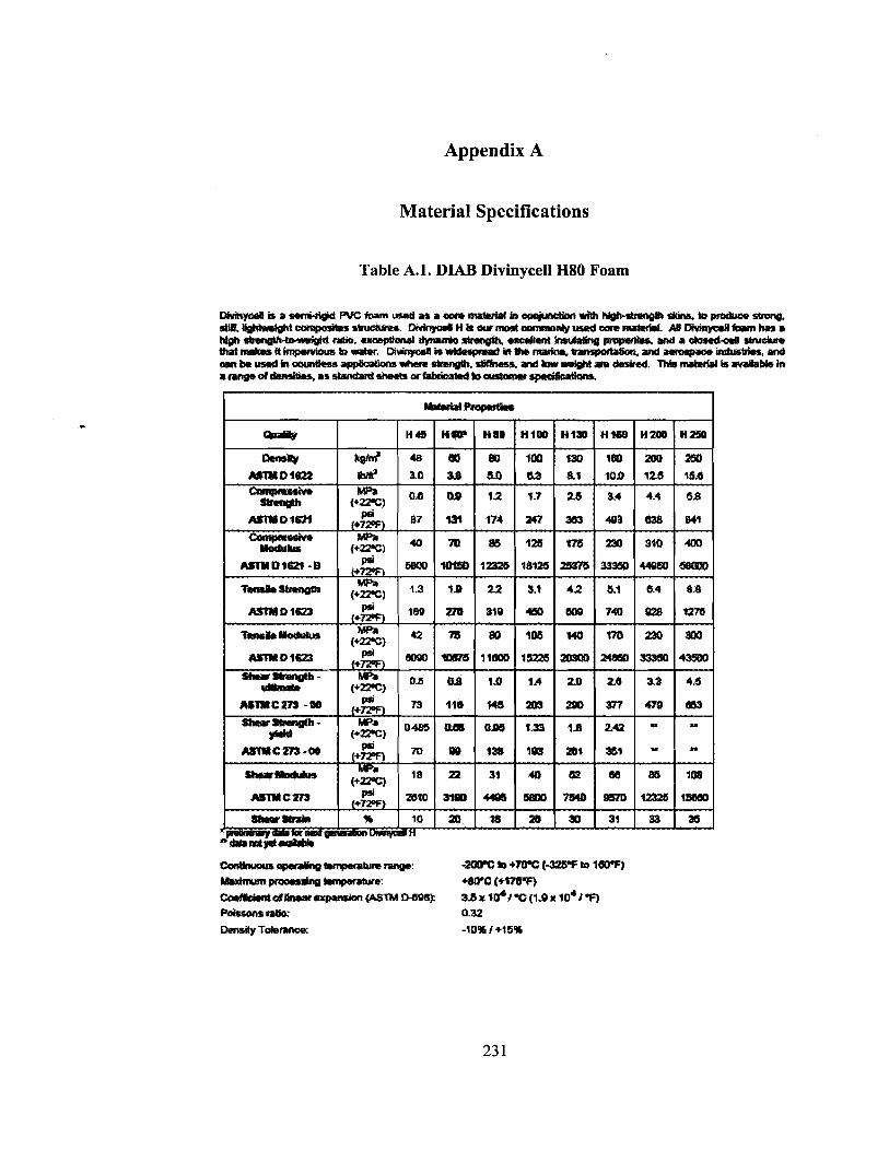
Appendix A
Material Specifications
Table A.1. DIAB Divinycell H80 Foam

Table A.1. cont'd
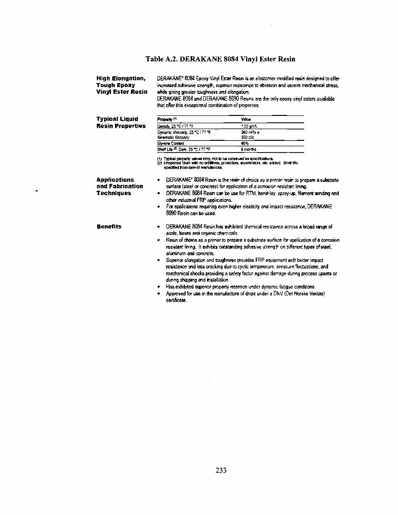
Table A.2. DERAKANE 8084 Vinyl Ester Resin
High Elongation, D E R M E * eC6B4 Epwy Vmyl Esrw R m is an elasmer mdified resin designed b & Tough Epoxy 1 w e 4 a&- sWmgtb, stpermr rsmtance to a b r ~ m a d oevefe mectaanrcal stress, Vinyl Ester Resin vvhb gi* j ~ & r toughness a& I n q w f i .
DERMNE @!M a d D E W E 80% Rwm ate 'he only e m rmyi &m mailable ha! d e r this exceptmal cwnb'mahn af propeaerttes
Typical Liquid RI Y ~ U C
Resin Properties o e ~ ~ , 2s -c I 7 .F I 72 &L T & w m i b ~ & 2SnCln'F 3% rPa s K i n e Wscmr# 35Ct&t
(1) ~ y p w ppmp~y -my, nee iv IS anrsuadarrpeclllcallona p) urqww aun wm ~ ~ Q R R M ~ , ponatbm toxwer:ts. & aodaa m%r IIE
Applications DEWEQW Resin is the *esira of choice w a palmer vsir rn piw~epte a &crate and Fabrication w h c e (sted or mmrete) appkshlwi of a mm:m reastan: linang. Techniques * D E W E BW Resin can k use dcr R n f , hmeh-kt$ .spray-up. f d l a m
dhe~ tndustml FRP sppkatiwas. For a ~ l i c a h s requiring wen bighw elasticity m d imgtact resistam, DE
Resin can k used.
Benefits E M W E R m has &~btted & m l ressbnce amss a broad ran* d ads, bases md mgmic &emals Rem cd &coce as a p m r to prepare a stibstraae surface br a p p l a o n of a c m i m reslsta~ linng. It exhi's o~stanrj~ng a&wue s?rmg;S. on dtferere types of steel, a l m m snd ccncrete.
w Superior efongat~m and ~~~ p~~vides mP equipment wt:h k & r impact resistance and ksg cracking duem cyclic tempraw, cres6Jre ~ u w a t i i , and me&micat shxks pmdlnq a safety %GW aganst dmage dumg W* Qt dunng sbpcng and ins@ldon Has exhibited -or propee etentrsn under dyrrarn~c fahue cond-. Appmved for use In !he maraubcture at ships u r k r a DkV lDel N w h Vm~hs] cSt&ate.
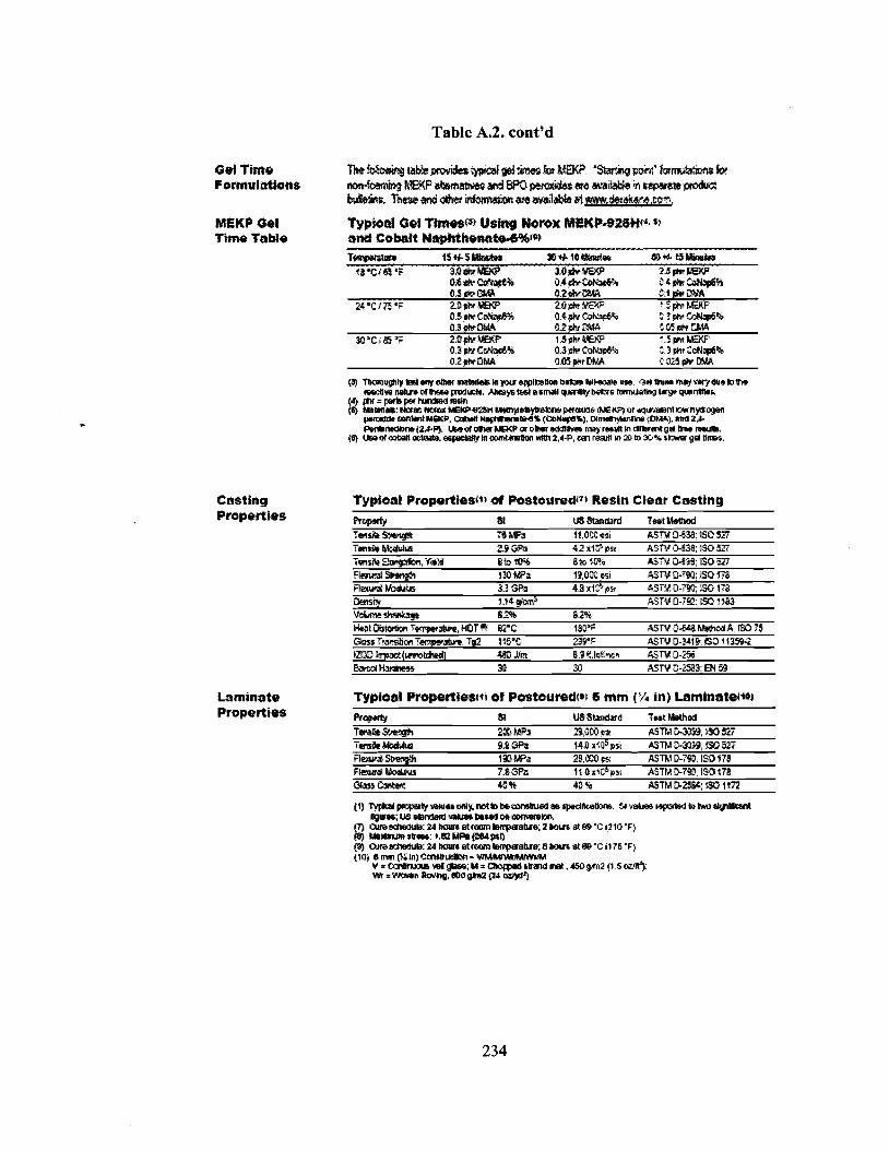
Table A.2. cont'd
Gel Time Pormul#tions
MEKP Gel Time Table
Casting Properties
Laminate Properties
(3) TholougMy ka e q ohof mMaki m you awllaaon aetm r u l w l e we Od ttnm rney vefy due Lo tR Redlrre nabrs dlssbe pmmtc. AAWS test e amall qlm~tf a/me mw~l)np lags prenlDas.
te) ~ r a o t ~ ~ m ~ ~ l n a * n t t m l l o n v r t m 2 i ~ ~ , e 4 n r ~ l n a ) b ~ ~ % i b f f p ~ 1 l m r .
Typical Propeaiesr*s of Pcrstcuredc4r Resin CIear Casting
Bm 83 US Standard Tmt Methad TMS& s%xim 76 MR 11 EC a i &SIX 063: 10 3a Tmsb W u r 2.9 GP3 4 2 x j C5 psi ASM 04%; IS0 SZT TM& ilph, Y ~ M ~b $046 810 ~ 0 % ~ S T V 0-638: SO 527 =l%aPsl SbetmJh l3GtdPa 10,P:O wi ASW 0-393; #SO i7@ RPXYO~ h&k 3.3 @a 4 8 rtZkprt A9TV 0-79$ iW 178
0mltV 1.14gkd an4 a-7%. &so 1d8a V 0 l ~ 82% 8 2% Hmt Oistcmm Ter*perJhrP, HOT @ 82°C 181P: ASTW 3648 Aiechcd A ISO T5 @as Tmdkn 7 ~ # u b r r . Tg2 l XghC t 3 W ASW D-3419 1% 11393-2 ecLa krp~ci am 480 JM 9(1 t .~~&wl ASTV 9-23 W H a w m % 33 33 ASW 0-2583, EN 59
Typical Prepertiesfrl ot Postcured49k 5 mm ['/a in) Laminatetla)
-r- -, -. - - .
Tensib Sm?&h 2-rn WJ B,OCO ASTM D-3236, B5 327 Tensik Wdla 9.8 G h 14fJ x105 pn ASM &303g, Sf2 527
(7j hschsaub: 2d howr MtoMn bpgalre; 2 k1u6 at 88 'C !21G'F, (8) Waicnrm reew: 1.m MW (284prl) (g ~le~b:2dhowrMturnIsnpgalrd:8kIUr&RO'Ci176'Fj (lo) 6 mm 0; In) p r n m - v!Wwvi~mwvrsM
v = mtinae m~ gtaw; M = rbcnd r n t .4sogrn~ (1 s ozan3. m mng. eoogmz (24 -9
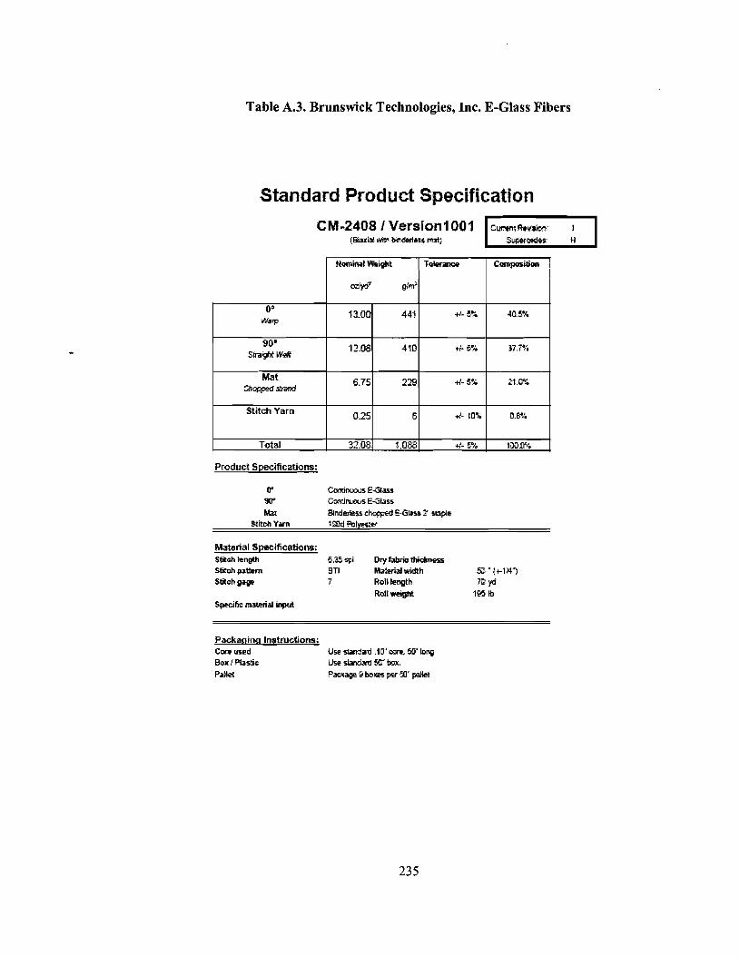
Table A.3. Brunswick Technologies, Inc. E-Glass Fibers
Standard Product Specification
Product Specifications:
Material Specifications: Stitah length B.35spi D r y f ~ c f ~ Stttch pattern BTI Material width B .{t-l."q Stiioh ~ q e ? Roll k @ h 76 yd
Roll weight ID5 Ib Specific mtetial krput
Packaaine Instn~ctiona: Cwe used USE standad .lD"crrecrre W lag Box l Pbsdic IktstandadE:'. Pdld p~4age boxes gar 50" @let

Table A.3. cont'd
Standard Product Specification
XM-2408 I Version ? O W Btxral wth btnchd mat
Product Specification%:
*W Ca-truous E-Glass # Gmt@bows E-Olasr
Bindewd kaat Bm&red chpe:! s:r& E-Glass Stit& Yam 15% payester
Material Specifications: Stitches Por inch 5 C&' +I- 1 sit!( Dly tabnc thickness Stitch pagem G-din Material width ba " (+-I 43 Various Stitch !3qc 3 C Rdl length %a fl
Rdl WPI*~ 233 b FalU w q h t a 3 1 Specik material inpat
Peckaninn Imtructions: Care used Sendm tube f l o x l ~ Sundao bx Pdkt Smndar5 pale!

Appendix B
Instrumentation Specifications
Table B.1. Lebow 3174 Load Cells
Tenston and comprwlan 5,600 br. to 4 50,000 ibs.
S f M S O R C H A R A C T E R I S T I C S : B l ? 4 , l ' l ? S A M D 9 ~ T ? l J
YGQa WbwkLCDID PTUlcoaQlb cl&'czqoF R I I I C T X I M H m OwlCmnN trcQw uwm ~sanwp*cmc, WKINS cs ~ ~ 1 4 WTL KW*L~S*O ~ W W I C I ~ NO?d.UMON HOU W K m Wf lWCUi%
M U F IBOHliMIM lOROUCllll us, n m onkib ~ k i a r n a ~ ~ mtwncs
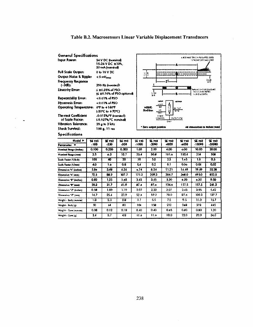
Table B.2. Macrosensors Linear Variable Displacement Transducers
C~nsmf S p s e # @ d m lnpur Pcrwac?
hr(l Scale Outpv~:
250 Ho. Lineatlty Esrsr: f rn.PSkJ# sC
@ *O.lU% c4 a4PSOqW Repbawbiliy Etwx @??.~Jl% of W3
sls Enm <Q.QIX ol px,
'v OQF k +1Wf I.zQQ1: k + 7 W q
T h traal Cogffldsn -0.0 1 W F km;hd) of Saak Farm? I.Q.OZ?%PC IWB*
me ZOgfolkHz loo@# 11 nn
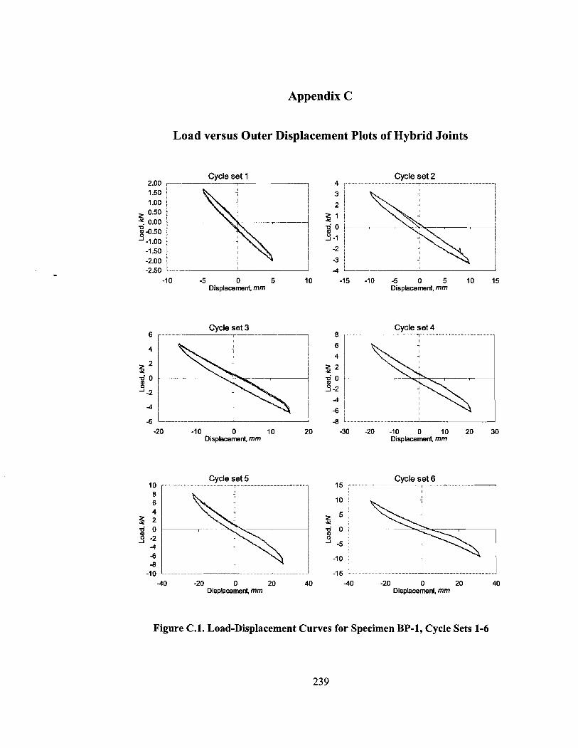
Appendix C
Load versus Outer Displacement Plots of Hybrid Joints
Cycle set 1 2.00 I
-1 0 -5 0 5 10 Displacement, mm
Cycle set 2 4 ......................................................... "" ....T " ........................ " ................
-15 -10 -5 0 5 10 15 Displacement, mm
Cycle set 3 Cycle set 4 6
4
5 6 0
-2
4
-20 -1 0 0 10 20 -30 -20 -10 0 10 20 30 Displacement, mm Displacement, mm
Figure C.1. Load-Displacement Curves for Specimen BP-1, Cycle Sets 1-6
Cycle set 5 10 8 6 4
5 2 d 0 3 -2
4 S -8
-1 0 4 0 -20 0 20 40 4 0 -20 0 20 40
Displacement, mm Displacement, mm
................. " .................................................................... " " ..........
\ ..
.... .-
1
I
1 I
..... - "
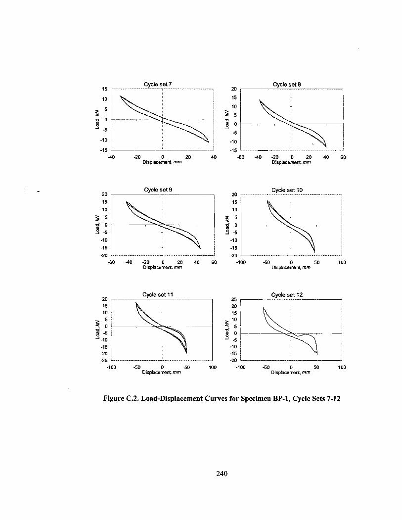
Cycle set 7 15 , .............. ... 1
-40 -20 0 20 40 Displacement, mm
Cycle set 9 20 1 I
-60 -40 -20 0 20 40 60 Displacement, mm
Cycle set 11 20 I ,
-1 00 -50 0 50 100 Displacement, mm
Cycle set 8 , I
-60 -40 -20 0 20 40 60 Displacement, mm
Cycle set 10 20 1...... ........................................ ................ I
-100 -50 0 50 100 Displacement, mm
Cycle set 12 . 25 .....r-....---
5 7- r--
4 -5 -1 0 -1 5
-1 00 -50 0 50 100 Displacement, mm
Figure C.2. Load-Displacement Curves for Specimen BP-1, Cycle Sets 7-12
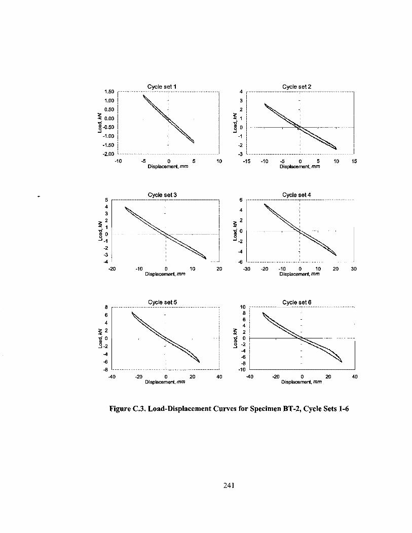
Cycle set 1 1.50 , .............................. ........................................................................
-2.00 1 ' i -1 0 5 0 5 10
Displacement, mm
-3 i " ........................... 2 ....................................................... . . I -15 -10 5 0 5 10 15
Displacement, mrn
Cycle set 3 5 ----" Cycle set 4
............... 1
6 1
-20 -1 0 0 10 20 -30 -20 -10 0 10 20 30 Displacement, rnrn Displacement, mm
Figure C.3. Load-Displacement Cuwes for Specimen BT-2, Cycle Sets 1-6
Cycle set 5 ................... ..... .- ................
Cycle set 6 10 8 6 4
j $ 2 G O
7- -.- 1 m d 0 m 4 -2 ; 2 -2
-4 -4 I -6 -6 1
I -0 1
-0 I ..... . ................. I -1 0
-40 -20 0 20 40 -40 -20 0 20 40 Displacement, mm Displacement, mm

Cycle set 9 Cycle set 10 ............ I 20 ,. -
1 I I 1 15 1
, 10 I
-10 , I
-15 1
Cycle set 7
6 0 4 0 -20 0 20 40 60 -1 00 -50 0 50 D~splacement mm Displacement. mm
15
-1 00 -50 0 50 100 Displacement, mm
--- .................................................................................................... ......................
Figure C.4. Load-Displacement Curves for Specimen BT-2, Cycle Sets 7-11
Cycle set 8
\ Y i 1 1
10
2
; -I 0 -5 0
-1 0
. j 15
I I I
i 10
I i s 5
I I 1 d J - 5 $ 0
j i -1 0
-15 I 1
. -15 -- 4 0 -20 0 20 40 6 0 4 0 -20 0 20 40 60
Displacement, mm Displacement. mm
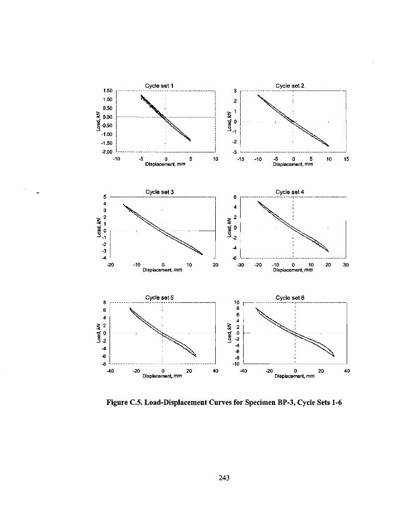
Cycle set 2
1
!
i !
-2 I
i i -2.00 i .... ........... L.." 2 -3 ,- ........ . L-.""""."" . -10 -5 0 5 10 -15 -10 -5 0 5 10 15
Displacement, mm Dispbcernent, mm
Cycle set 3 5 Cycle set 4
............ 7-.- I 6 - T-.-.--.--...--..--.-.-
-20 -10 0 10 20 -30 -20 -10 0 10 20 30 Displacement. mm Displacement, mm
Cycle set 6
r-- - - - 1 - - -
I
d 0
J -2 8 -2 1 J
1
I -- - - -10 4 0 -20 0 20 40 4 0 -20 0 20 40
D~spbcement, mm D~sptacement, mm
Figure C.5. Load-Displacement Curves for Specimen BP-3, Cycle Sets 1-6

Cycle set 8 ..... ....................... .......... ...... 15 --
i -
-5 -5 i
-1 0 I 1 -10 i i
-15 -- I 4 -1 5
I
4 0 -20 0 20 40 6 0 4 0 -20 0 20 40 60 Displacement, mm Displacement, mm
Cycle set 9 . 20 .............................................
3 -5
-1 0
i . .
-1 00 -50 0
-20 1..
6 0 4 0 -20 0 20 40 60 50 Displacement, mm Displacement, mm
Cycle set 11 Cycle set 12 20 r" -.--.pp--.
I I -15 / I
-20 i I
-1 00 5 0 0 50 -1 00 5 0 0 50 Displacement, mm Dlsphcement, mm
Figure C.6. Load-Displacement Curves for Specimen BP-3, Cycle Sets 7-12
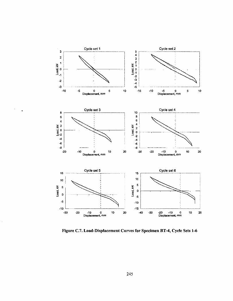
Cycle set 1 3 ............................................................... " " ......... " ... \ 5 r--. Cycle set 2
-1 0 -5 0 5 10 -15 -10 -5 0 5 10 Displacement, mm Displacement, mm
8 Cycle set 3 10 Cycle set 4
6
4
5 < 0 - ..
....... 8 T--
-1 -2 I
4 J I 4 1 1
-6 I
I -6 .......... -8 I -8 i
-20 -10 0 10 20 -30 -20 -10 0 10 20 Displacement, mm Displacemenf mm
15 Cycle set 5 -- ......
Cycle set 6 15 7--
-
-5 I -10 I
1
-10 I ........... I -15 ' -30 -20 -10 0 10 20 4 0 3 0 -20 -10 0 10 20
Displacement, mm Displacement, mm
Figure C.7. Load-Displacement Curves for Specimen BT-4, Cycle Sets 1-6
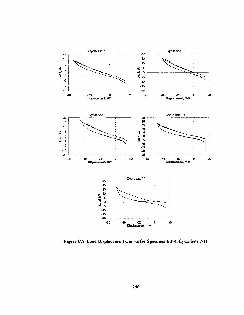
Cycle set 8
- r - -- - ---
"
-40 -20 0 20 -60 4 0 -20 0 20 Displacement, mm Disphcement, mm
Cycle set 9 20 15
10
s u- 0 8 -1 -5
-1 0
-1 5
-20 -60 -40 -20 0 20 -60 -40 -20 0 20
Disphcement, mm Displacement mm
Cycle set 11 25 I
- -.
6 0 -40 -20 0 20 Disphcement, mm
Figure C.8. Load-Displacement Curves for Specimen BT-4, Cycle Sets 7-11
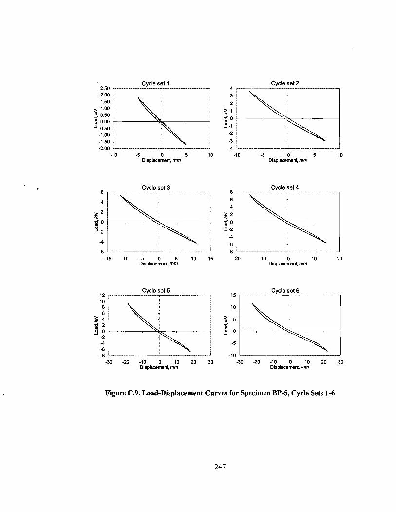
Cycle set 1 2.50 ! ............................................................................................... ... ....,
2.00 / I I
-1 0 -5 0 5 10 Displacement, mm
Cycle set 3
Cycle set 2 4
-1 0 -5 0 5 10 Displacement, mm
Cvcle set 4
-15 -10 -5 0 5 10 15 -20 -10 0 10 20 Displacement, mm Displacement, mm
Cycle set 5 - -- Cycle set 6 l2 I"-- lo I 6
v- - , z 0 -- - -
-I
I
-5 I 1
8 L---.-_____ ' "-- - -1 0
3 0 -20 -10 0 10 20 30 -30 -20 -10 0 10 20 30 Dlsphcement, mm Displacement, mm
Figure C.9. Load-Displacement Curves for Specimen BP-5, Cycle Sets 1-6

Cycle set 7 20 Cycle set 8
. . ................... ..................... 20
15 J i
10 I
2 ; 5
0 .-.
J J
-5 5
-1 0 i
-1 0 I I
-1 5 --.A -15 L L - - . . . - - -~
-40 -20 0 20 40 -40 -20 0 20 40 Displacement, mm Displacement mm
-40 -20 0 20 40 -60 -40 -20 0 20 40 Displacement mm Displacement, mm
Cycle set 11 30 1 I
Cycle set 12 30 ,
25 1 , I 1
Figure C.lO. Load-Displacement Curves for Specimen BP-5, Cycle Sets 7-12

Cycle set 1 2.00 .......................................................... .. ............................. ........... " ......
Cycle set 2 4 . -- - ...
-15 -10 -5 0 5 10 15 Displacement, mm
Cycle set 3 6 ....... 8 Cycle set 4
6 0
-2
4 I
-20 -1 0 0 10 20 -30 -20 -10 0 10 20 30 Displacement, mm Displacement, mm
Cycle set 5 lo ... ...-....... 15 ......................... Cycle set 6 . .,
d 0 4 -2 4 -6 -5
I
-8 I I
-10 ........ -1 0 I i
-40 -20 0 20 40 -40 -20 0 20 40 Displacement, mm Displacement, mm
Figure C.l l . Load-Displacement Curves for Specimen BT-6, Cycle Sets 1-6

Cycle set 7 20 ............................................. .- ...............................................................................................
-40 -20 0 20 40 Displacement, mm
Cycle set 9 25 !
! -20 i .................................................................... J -60 -40 -20 0 20 40 60
Dispbcement, mm
Cycle set 8 , I
-60 -40 -20 0 20 40 60 Displacement, mm
Cycle set 10 25 , ................................ ................................................................
-20 I ........................... 1 J -100 -50 0 50 100
Displacement, mm
Cycle set 11 25 1 I
-1 00 -50 0 50 100 Displacement, mm
Figure C.12. Load-Displacement Curves for Specimen BT-6, Cycle Sets 7-12

Cycle set 1 Cycle set 2 6 ;------.---.-- 5 i A
4 1 3 !
2 2 1 2 1 m O ' 3.1 I
-2 / -3 i 4 j -5
-10 -5 0 5 10 -15 -10 -5 0 5 10 15 Displacement, mm Displacement, mm
Cycle set 3 8 r..' Cycle set 4
... v
..... . . - 7 ---7 -
1
4 I 4 6 '
6 L-- I I -8 i -!--
-20 -1 0 0 10 20 -30 -20 -10 0 10 20 30 Displacement, mm Dispbcement, mm
Cycle set 5 .............
' -7- -.
I
I
i -1 0 1
I
i -1 5 I
4 0 -20 0 20 40 4 0 -20 0 20 40 Displacement, mm Displacement, mm
Figure C.13. Load-Displacement Curves for Specimen BT-7, Cycle Sets 1-6
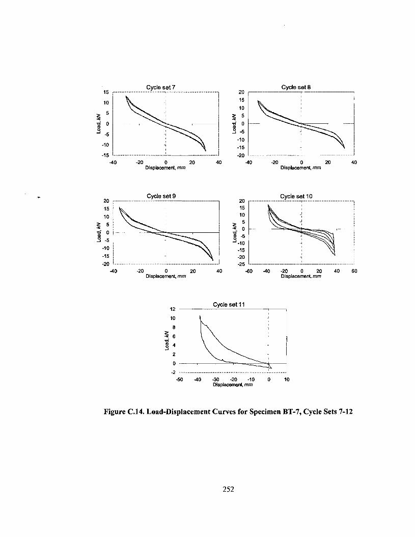
4 0 -20 0 20 40 4 0 -20 0 20 40 Displacement, mm Displacement, mm
Cycle set 9 Cycle set 10 ........ 20 r I 20 , -
4 0 -20 0 20 40 -60 4 0 -20 0 20 40 60 Displacement, mm Displacemerd. mm
Cycle set 11 12 I -- -
5 0 4 0 3 0 -20 -10 0 10 Displacement mm
Figure C.14. Load-Displacement Curves for Specimen BT-7, Cycle Sets 7-12
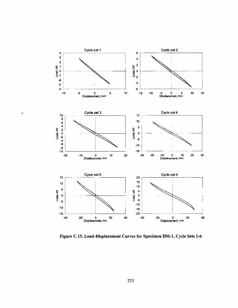
Cycle set 2 -- ,\\ . , . . 1 1 1
, ...-..-I 1
i I
I r I
1 j
I I i -6 ! .- > "- 1
-1 0 -5 0 5 10 -15 -10 5 0 5 10 15 Displacement mm Displacement, mm
Cycle set 4 ............... -----r----.---- 15 -.
1
7
-1 0 -8 . 1
-1 0 .. I I / -1 5 - -20 -10 0 10 20 -30 -20 -10 0 10 20 30
Displacement, mm Displacement mm
Cycle set 5 Cycle set 6 20 ..........
7 - -- --
1
i 1
-10 i I
I -15 ( I
-15 [ I I
4 0 -20 0 20 40 4 0 -20 0 20 40 Displacemenf mm Displacement, mm
Figure C.15. Load-Displacement Curves for Specimen DM-1, Cycle Sets 1-6

-40 -20 0 20 40 6 0 -40 -20 0 20 40 60 Displacement mm Displacement mm
30
20
5 lo
A a o -1 0
-20
-30 6 0 -40 -20 0 20 40 60 -100 -50 0 50
Displacement mm Displacement, mm
Cycle set 11 25 I I
-100 -50 0 50 100 Displacement, mm
Figure C.16. Load-Displacement Curves for Specimen DM-1, Cycle Sets 7-12
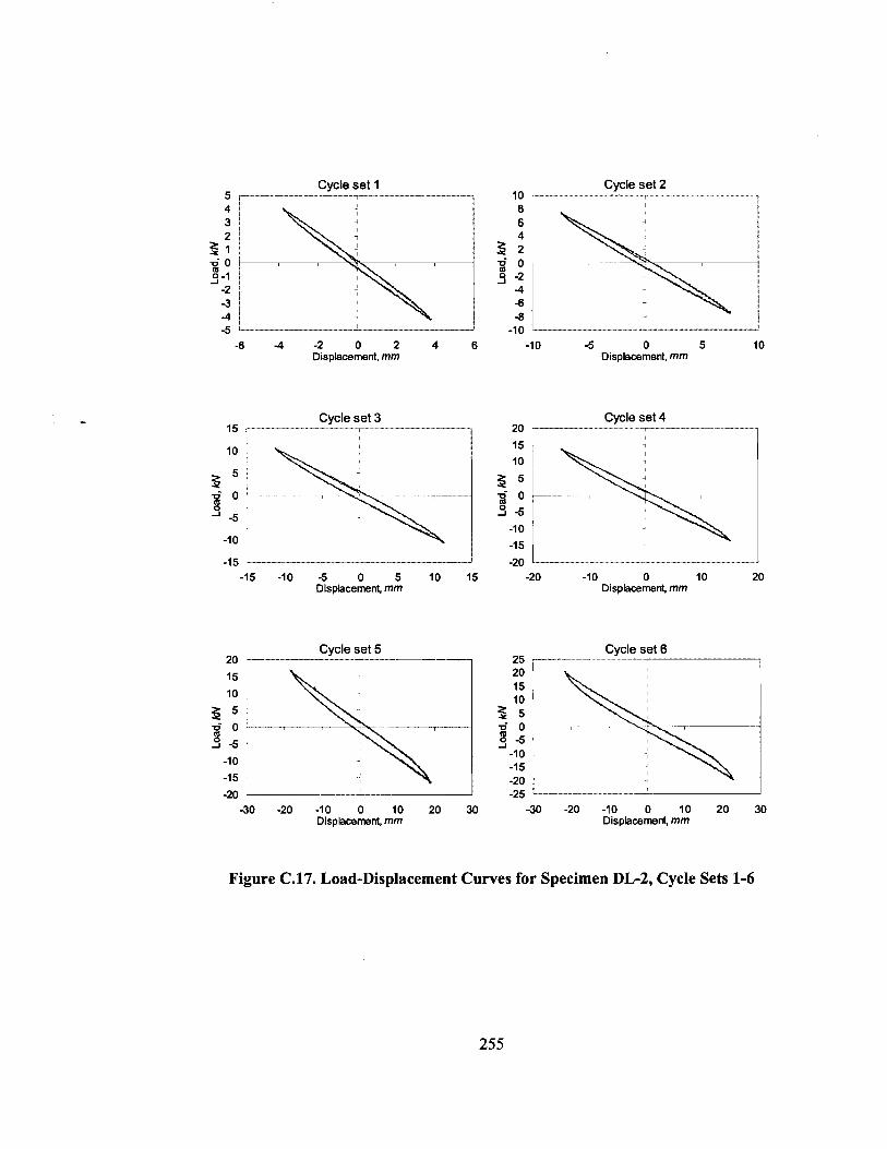
Cycle set 1 5 ?- ......... "--" . ..T. . ...
i 4 1 3 / 2 1
$ 1 $ 0 1 0 -1 [ J i -2 j
3 1 -4 3 -5 '-"-" . ............ "..L ....-...........
-6 -4 -2 0 2 4 6 -1 0 -5 0 5 10 Displacement mm Displacement, mm
Cycle set 3 15
Cycle set 4 ............ 20 r.-.--.." 7-- -'I
-15 -10 -5 0 5 10 15 -20 -1 0 0 10 20 Displacement, mm Displacement, mm
Cycle set 5 20 r..-.-...
Cycle set 6 ........................ . 7------- 1
3 0 -20 -10 0 10 20 30 -30 -20 -10 0 10 20 30 Displacement mm Displacement, mm
Figure C.17. Load-Displacement Curves for Specimen DL-2, Cycle Sets 1-6

Cycle set 7 30 , . ................................................ ,..... ........ ........
-40 -20 0 20 40 Displacemenf mm
Cycle set 9 40 I I
-40 -20 0 20 40 Displacemenf mm
Cycle set 8 40 / I 1
Cycle set 10 40 , ............. .- ....................................... ...$
I 1
......................
-60 -40 -20 0 20 40 -60 -40 -20 0 20 40 Displacemenf mm Displacement, mm
Figure C.18. Load-Displacement Curves for Specimen DL-2, Cycle Sets 7-12

- 6 4 - 2 0 2 4 6 -1 0 -5 0 5 10 Displacement, rnrn Displacement mrn
Cycle set 4 15 1
5 s d 0 1
8 -5 i
1
-1 0 -1 0 I
I I
-1 5 1 --
-15 -10 -5 0 5 10 15 -20 -1 0 0 10 20 Displacement, mm Displacement, mm
Figure C.19. Load-Displacement Curves for Specimen DL-3, Cycle Sets 1-6
20
15
10
s u- 0 8 -5
-10 -1 5
-20 ----------- -30 -20 -10 0 10 20 30 -30 -20 -10 0 10 20 30
~lsplacement mm Displacement, mrn
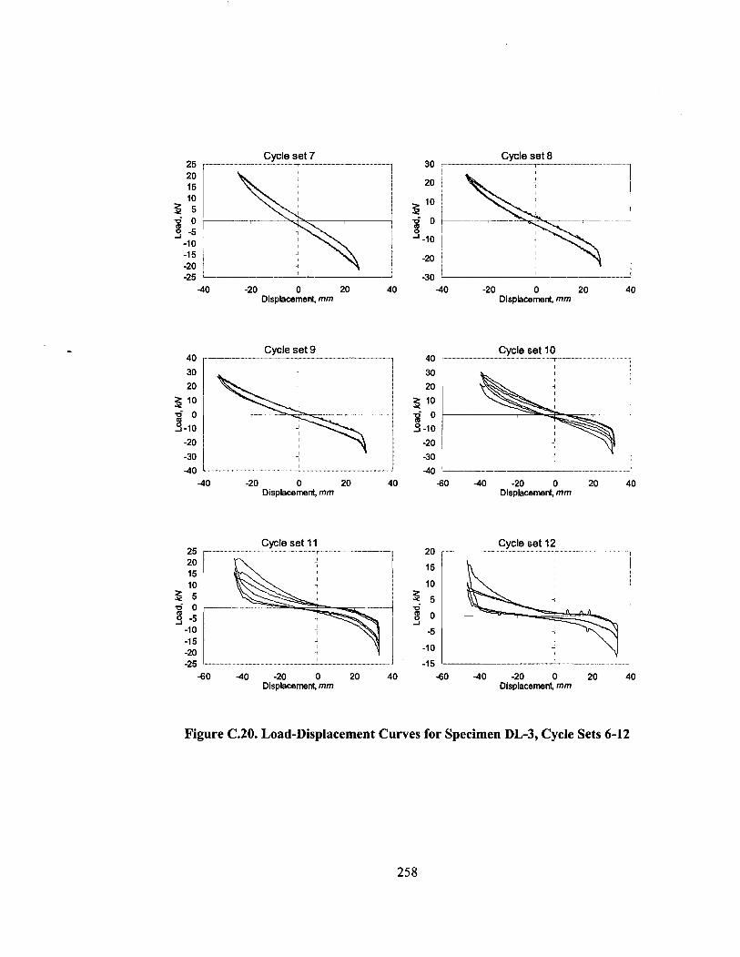
Cycle set 7 25 ...................................................................................................................................... 20 I
15 1
-1 5 -20 -25
-40 -20 0 20 40 -40 -20 0 20 40 Displacement, mm Displacement, mm
Cycle set 9 Cycle set 10 .............. 40 1 1 40 -. . . .,
-40 -20 0 20 40 -60 -40 -20 0 20 40 Displacement, mm Displacement, mm
Cycle set 11 .. . .......... 25
20 15 10
z 5 : 0 4 . -1 0 -1 5 -20 -25
S O -40 -20 0 20 40 -60 -40 -20 0 20 40 Dispbcemenf mm Displacement, mm
Figure C.20. Load-Displacement Curves for Specimen DL-3, Cycle Sets 6-12
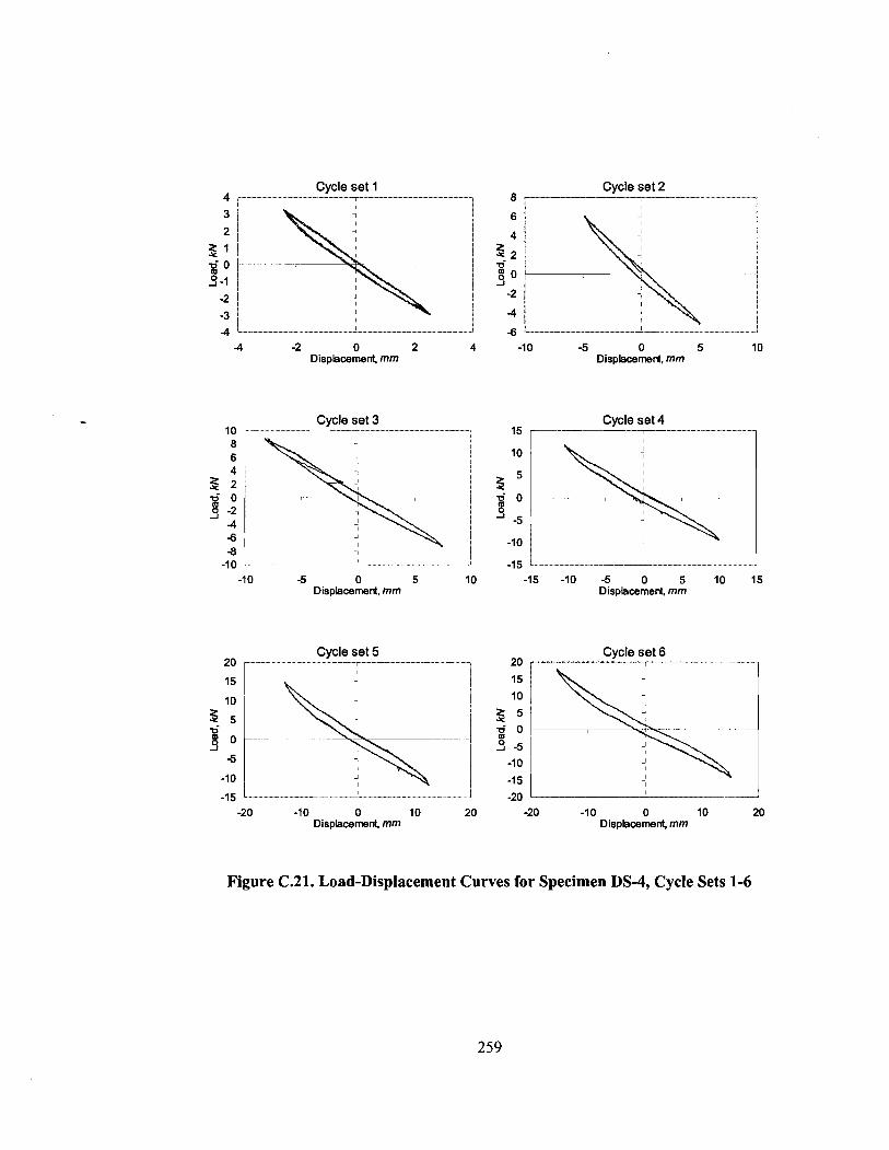
Cycle set 1 4 .................. ..........T.........-.. ............... ............................................... Cycle set 2
... 8 : "-
-4 -2 0 2 4 -1 0 -5 0 5 10 Dispbcement, mm Displacement, mm
Cycle set 4 ..........-. ........... 15 --.. .-
4 1
-4 I
6 I
-8 1 ! 1
I
-10 . -1 5 I .......................... "-
-1 0 -5 0 5 10 -15 -10 -5 0 5 10 15 Displacement, mm Dispbcernent, mm
Cycle set 5 .......... -- ........
1 I
-20 -10 0 10 20 Dispbcement, mm
Cycle set 6 20 7 - -- - --I
-20 -1 0 0 10 20 Displacement, mm
Figure C.21. Load-Displacement Curves for Specimen DS-4, Cycle Sets 1-6
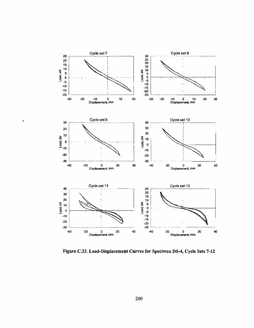
Cycle set 7 25 7. ........................................................................................
Cycle set 8 30 I I
-30 -20 -10 0 10 20 -30 -20 -10 0 10 20 30 Displacemenf mm Displacement, mm
4 0 -20 0 20 40 Displacement, mm
Cycle set 10 40 , ...................
-30 i .- 2 A 4 0 -20 0 20 40
Displacement, mm
Cycle set 11 Cycle set 12 25 20 15
5 6 0 3 -5
-1 0 -1 5 -20 -25
-40 -2 0 0 20 40 4 0 -20 0 20 40 Displacement, mm Displacement, mm
Figure C.22. Load-Displacement Curves for Specimen DS-4, Cycle Sets 7-12

- 6 4 - 2 0 2 4 6 -1 0 -5 0 5 10 Displacement, mm Dispbcement, mm
Cycle set 3 6
Cycle set 4
4
2 2
y' - 1
,m -2 A
4 1 1
-6 1 I -8 ! I
-8 -10 . . . . . . 1
-15 -10 -5 0 5 10 15 -20 -1 0 0 10 20 Displacement mm Displacement mm
Cycle set 5 10 -- Cycle set 6
1 15 r- -
Figure C.23. Load-Displacement Curves for Specimen DL-5, Cycle Sets 1-6
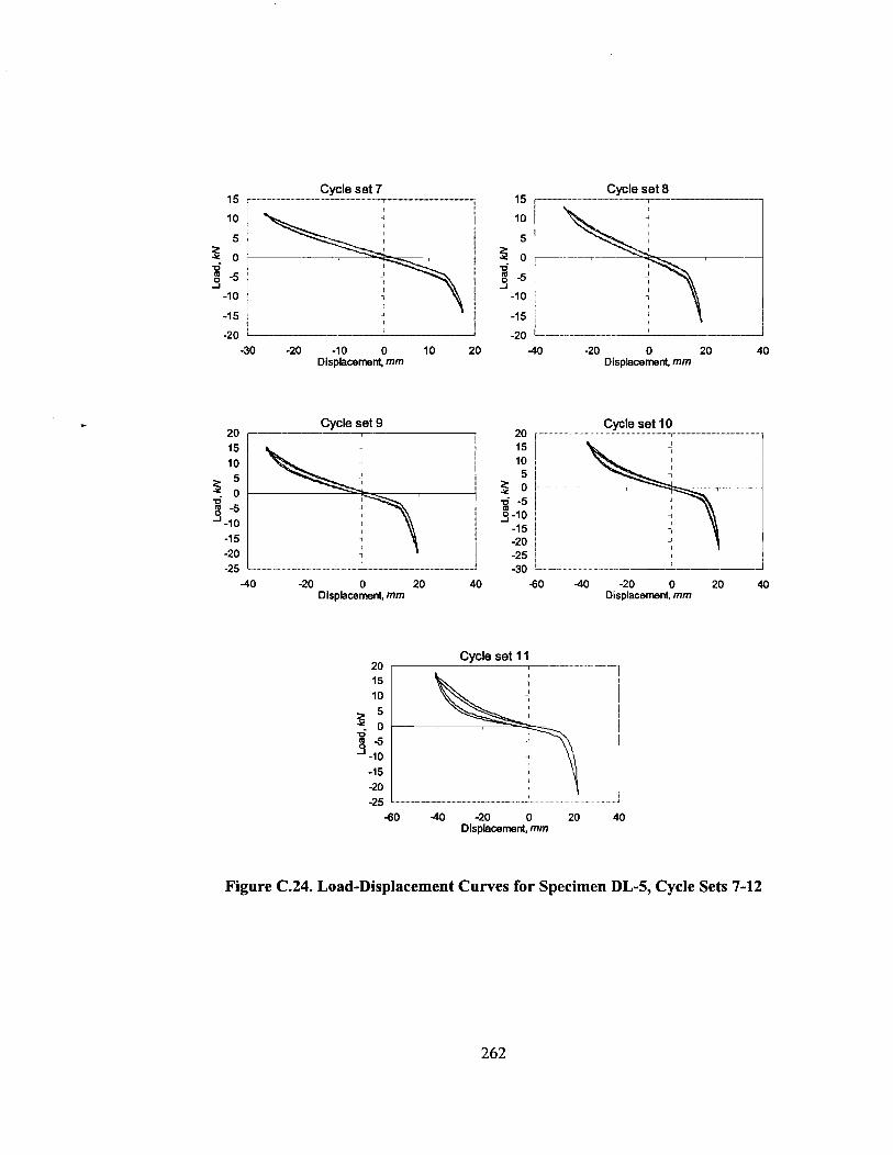
Cycle set 7 ................. "" ................................ ................................ ..............................
-30 -20 -10 0 10 20 Displacement, mm
Cycle set 9
Cycle se t 8 15 1 1
-40 -20 Displacement, 0 mm 20 40
Cycle se t 10 20 , ................ I
-40 -20 0 20 40 6 0 -40 -20 0 20 40 Displacement, mm Displacement, mm
Cycle set 11 20 I
-60 -40 -20 0 20 40 Displacement, mm
Figure C.24. Load-Displacement Curves for Specimen DL-5, Cycle Sets 7-12
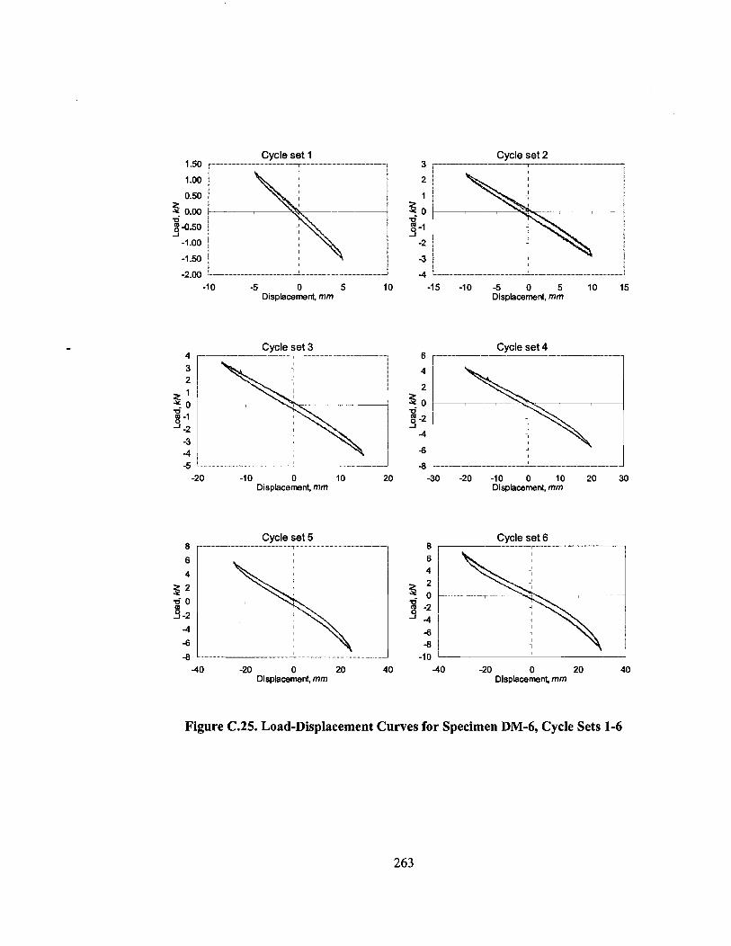
Cycle set 1 1 .50
-1 0 -5 0 5 10 Displacement, mm
Cycle set 2 3 :
-15 -10 -5 0 5 10 15 Displacement, mm
Cycle set 3 4 --
Cycle set 4 . ....... ....... 6
3 2
2 0
8 -l -2 -4 -3
I
-4 -5
-20 -1 0 0 10 20 -30 -20 -10 0 10 20 30 Displacement, mm Displacement, mm
Cycle set 5 8 1-.--.7....-.. ..................
I
-40 -20 0 20 40 Dlsplacement, mm
4 0 -20 0 20 40 Displacement, mm
Figure C.25. Load-Displacement Curves for Specimen DM-6, Cycle Sets 1-6
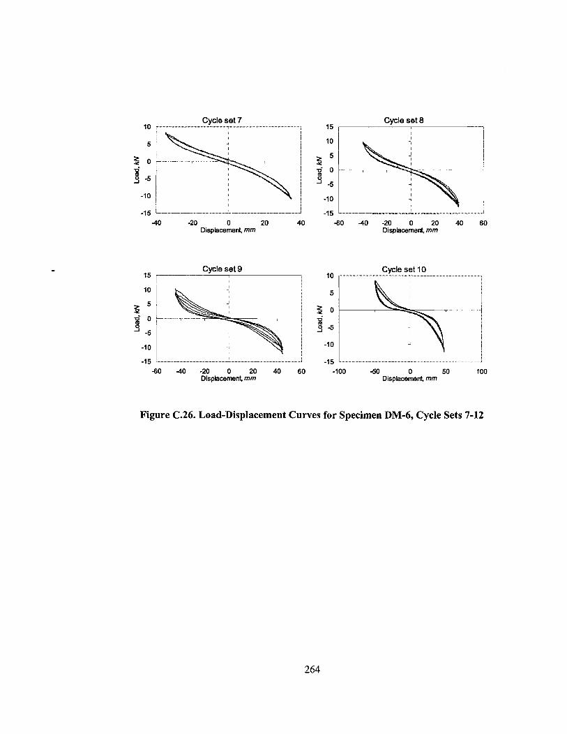
Cycle set 7 10 " ...... " ....T" " " :
Cycle set 8 15
j I
I 10 5 1 5 S 0 i 5
d m i 6 0 I ; 9 -5 I J -5
I -1 0
i -1 0
-15 - "... -15 - 4 0 -20 0 20 40 -60 4 0 -20 0 20 40 60
Displacement mm Displacement, mm
-60 4 0 -20 0 20 40 60 -100 -50 0 50 100 Displacement, mm Displacement, mm
Figure C.26. Load-Displacement Curves for Specimen DM-6, Cycle Sets 7-12
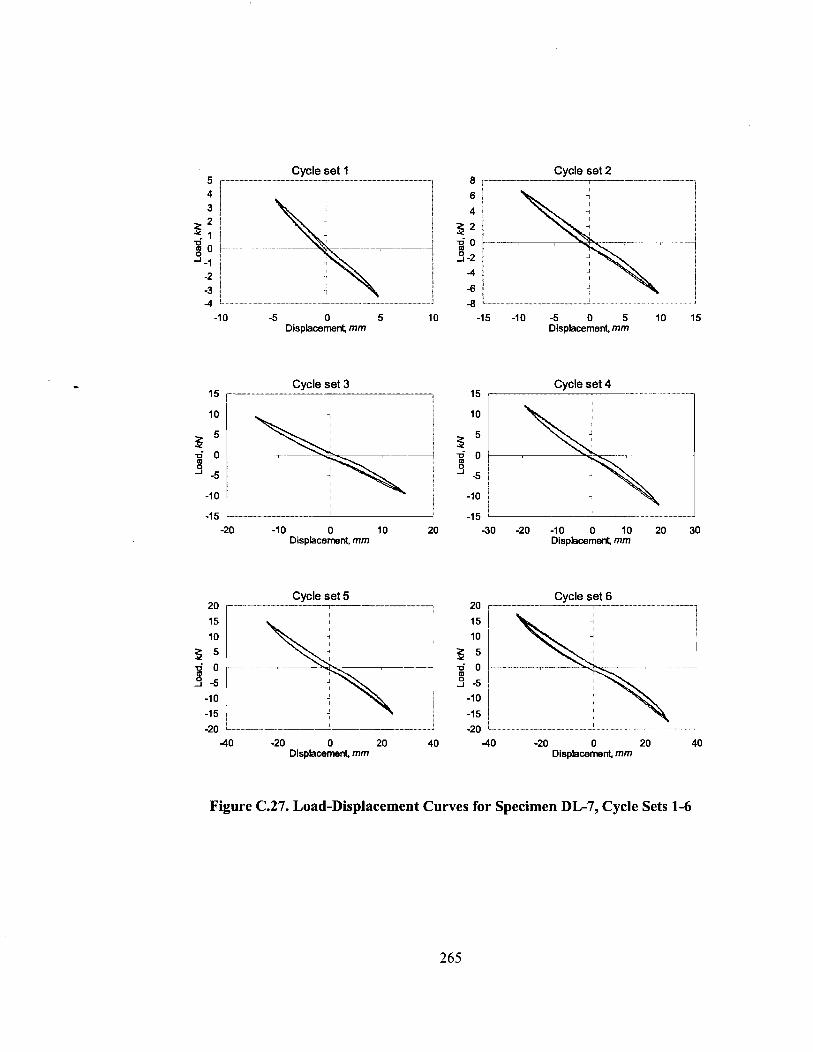
Cycle set 1 5 , .................................... ............................................. .- ............................................... 1
A I I
-1 0 3 0 5 10 Displacement, mm
Cycle set 2 8 ..- .. -. ... - .......
- 8 ' - - -i
-15 -10 -5 0 5 10 15 Displacernent, mm
Cycle set 3 15
Cycle set 4 .............. 15
I ? i
10 i 10 I \\ 1 % s 5
3 O - - - 7 - - - i g o
2 -, -5 1 -5
-1 0 1 -10 I i
-1 5 I -1 5 -20 -1 0 0 10 20 -30 -20 -10 0 10 20 30
Displacement, mm Displacement, mm
Cycle set 5 20 .................... ... ,
Cycle set 6 20 i----.---.-T-.--.--.. .................
4 0 -20 0 20 40 Displacement, mm
Figure C.27. Load-Displacement Curves for Specimen DL-7, Cycle Sets 1-6

Cycle set 8
4 0 -20 0 20 40 -60 4 0 -20 0 20 40 60 Displacement, mm Displacement, mm
Cycle set 9
-60 4 0 -20 0 20 40 60 -60 4 0 -20 0 20 40 60 Displacement, mm Displacement, mm
Figure C.28. Load-Displacement Curves for Specimen DL-7, Cycle Sets 7-12

Appendix D
Load versus Middle Displacement Plots of Hybrid Joints
Cycle set 1 2 00 i..-.............. ................ " ........................................................................................... .
Cycle set 2 4 1
4 -2 0 2 4 Displacement, mm
Cycle set 3 Cycle set 4 -
3 -2 4
I
4 -2 0 2 4 6 -5 0 5 10 Displacement, mm Displacement, mm
Cycle set 5 Cycle set 6 ................ 15
--
i J -5 1
-10 I J -15
-1 0 -5 0 5 10 -10 -5 0 5 10 Displacement, mm Displacement, mm
Figure D.1. Load-Displacement Curves for Specimen BP-1, Cycle Sets 1-6

Cycle set 7 15 r--- 7m
........................................ ...........
-15 L L ....... -10 -5 0 5 10 15
Displacement, mm
Cycle set 9 20 I T - ' " " I
-20 -1 0 0 10 20 Dispbcement, mm
Cycle set 11 20 ,I--.----. .
Cycle set 8 20 7 I -1
-15 -10 -5 0 5 10 15 Displacement, mm
Cycle set 10 20 r -
-20 -1 0 0 10 20 Displacement, mm
25 Cycle set 12
.....
Figure D.2. Load-Displacement Curves for Specimen BP-1, Cycle Sets 7-12
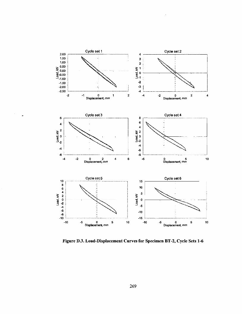
Cycle set 1 2.00
5 -2.50 : . .- I J -2 -1 0 1 2
Displacement mm
Cycle set 2 4 r I
-4 -2 0 2 4 Displacement, mm
Cycle set 3 6 T--- -- .................................
Cycle set 4
...... 7--
1 -6 4 : ....... : ........... - .........................................
-4 -2 0 2 4 6 -5 0 5 10 Displacement, mm Displacement, mm
. . . .
J -5 I
-1 0 1 I
........ .................. -1 5 i ......... ._.
-1 0 -5 0 5 10 -1 0 -5 0 5 10 Displacement, mm Displacement, mm
Figure D.3. Load-Displacement Curves for Specimen BT-2, Cycle Sets 1-6
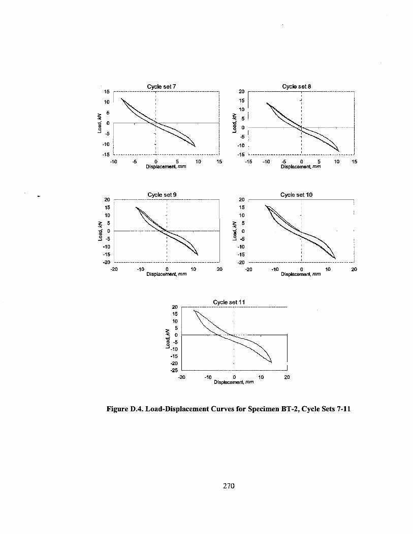
Cycle set 7 ............................................ "--" .
...... .... J -10 -5 0 5 10 15
Displacement, mm
Cycle set 9 20 1
-20 -1 0 0 10 20 Displacement, mm
Cycle set 8 20 1 , I
Cycle set 10 20 , 1
-20 -1 0 0 10 20 Displacement, mm
Cycle set 11 20 , .......
-20 -1 0 0 10 20 Displacement, mm
Figure D.4. Load-Displacement Curves for Specimen BT-2, Cycle Sets 7-1 1

Cycle set 2 1-- -.. 3
j 2
i 1 1 .... , ... i 5 1 d o I $ I -I -1
-2 I
........ ..... -2.00 i ALL. i -3 1
-1.50 -1.00 -0.50 0.00 0.50 1.00 1.50 -3 -2 -1 0 1 2 3 Displacement, mm Displacement, mm
Cycle set 3 5 r...-.-.-.--....y..---....- ............ , 6 .......................
Cycle set 4 T---..----. 1
-4 -2 0 2 4 -5 0 5 10 Displacement, mm Displacement, mm
Figure D.5. Load-Displacement Curves for Specimen BP-3, Cycle Sets 1-6
Cycle set 6
-10
\ ~ - -~~ -~
.. -1 0 -5 0 5 10 -10 -5 0 5 10
Displacement, mm Displacement, mm

Cycle set 7 .....................................
55 5
... T --
i -5 I
-1 0 -1 0
2 -1s i " "l..
-10 -5 0 5 10 15 -15 -10 -5 0 5 10 15 Displacement, mm Displacement, mm
Cycle set 9 I
-20 I - I 1 -20 -1 0 0 10 20
Displacement, mm
Cycle set 11 20 , .. -
Cycle set 10
-1 0 0 10 20 Displacement, mm
Cycle set 12 20 !.-.--. ..... --T..------.---.---,
-20 -1 0 0 10 20 -20 -10 0 10 20 30 Dlspbcernent, mm Displacement, mm
Figure D.6. Load-Displacement Curves for Specimen BP-3, Cycle Sets 7-12

Cycle set 1 3 7---...-.-.p.-- Cycle set 2
2
1 s 6 0 2!
-1
-2
-3 .......... ' ................. -2 -1 0 1 2 4 -2 0 2 4
Displacement, mm Displacement mm
Cycle set 3 8 ! I
4 -2 0 2 4 6 Displacement. mm
Cycle set 4 10 -- .---"
-1 0 -5 0 5 10 Displacement, mm
Cycle set 6 ..................................................................... 15 I
I I
10
K i 4 0 -5
! i
-1 0 i I
-10 L .... 1 ; -15 . I
-1 0 -5 0 5 10 -1 0 -5 0 5 10 Displacement, mm Displacement, mm
Figure D.7. Load-Displacement Curves for Specimen BT-4, Cycle Sets 1-6
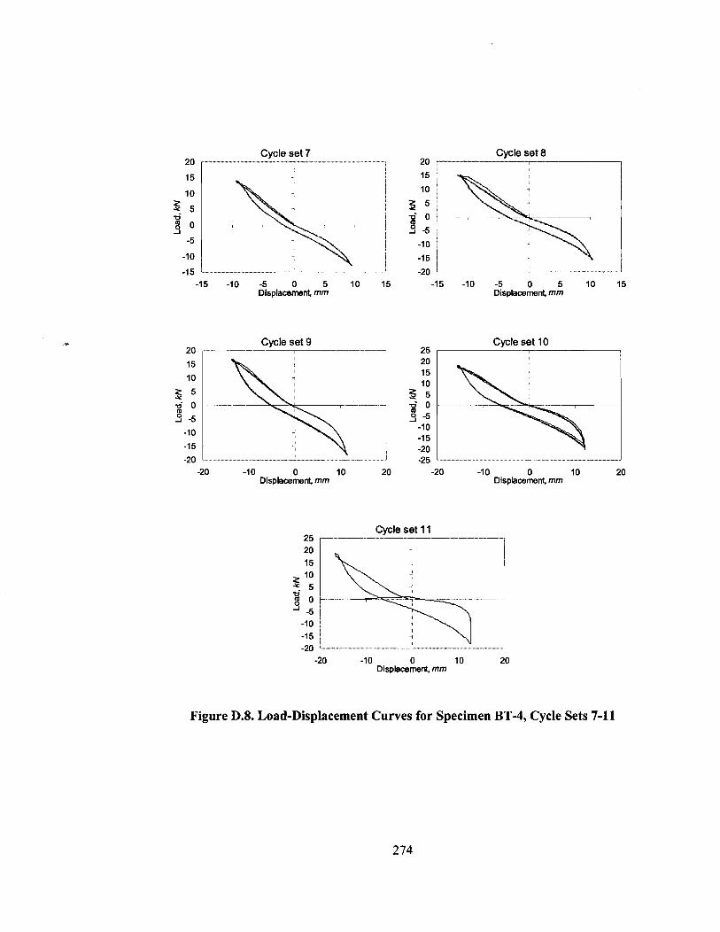
Cycle set 7 20 , . . ............... .
I 1
-15 -10 -5 0 5 10 15 Displacement, mm
Cycle set 8 20 i 1
-15 -10 -5 0 5 10 15 Displacement, mm
Cycle set 11 ....................
I
Cycle set 9 20
Cycle set 10
-20 -10 0 10 20 Displacement, mm
15 10
5 0
m 3 -5
-10
-15
-20
Figure D.8. Load-Displacement Curves for Specimen BT-4, Cycle Sets 7-11
\<----": -~ ~-
I I I I
' ........
-20 -1 0 0 10 20 -20 -1 0 0 10 20 Displacement, mm Displacement, mm
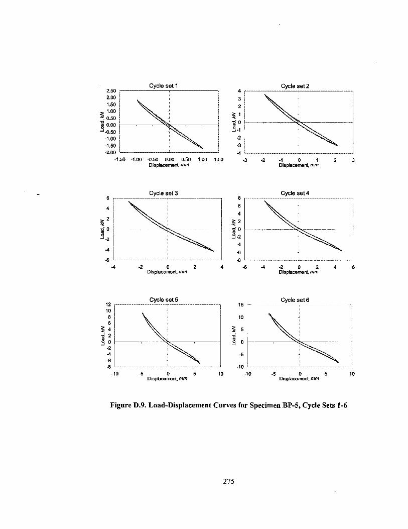
Cycle set 1 2.50
I "."---T
2.00 1 I
! -2.00 i ..........
-1.50 -1.00 4.50 0.00 0.50 1.00 1.50 Displacement, mm
4 r--- Cycle set 2
4 I 1
3 -2 -1 0 1 2 3 Displacement, mm
Cycle set 4 -.----."
I I ......
4 -2 0 2 4 - 6 4 - 2 0 2 4 6 Displacement, mm Displacement, mm
-10 -5 0 5 10 -1 0 -5 0 5 10 Displacement, mm Displacement, mm
Cycle set 6
Figure D.9. Load-Displacement Cuwes for Specimen BP-5, Cycle Sets 1-6
15
lo
5 5 d
4 0
-5
-1 0 \ , ,- --- - i
J
I -._I_ ..:

Cycle set 8
............ ....... ....................... 1 ........ 1 -1 0 -5 0 5 10 -1 0 -5 0 5 10 15
~lsplacement, mm Displacement, mm
Cycle set 9 25 r- 25 I Cycle set 10
-15 -10 -5 0 5 10 15 -20 -1 0 0 10 20 Displacement, mm Displacement, mm
Cycle set 12
-20 -1 0 0 10 20 -20 -1 0 0 10 20 Displacement, mm Displacement, mm
Figure D.lO. Load-Displacement Curves for Specimen BP-5, Cycle Sets 7-12
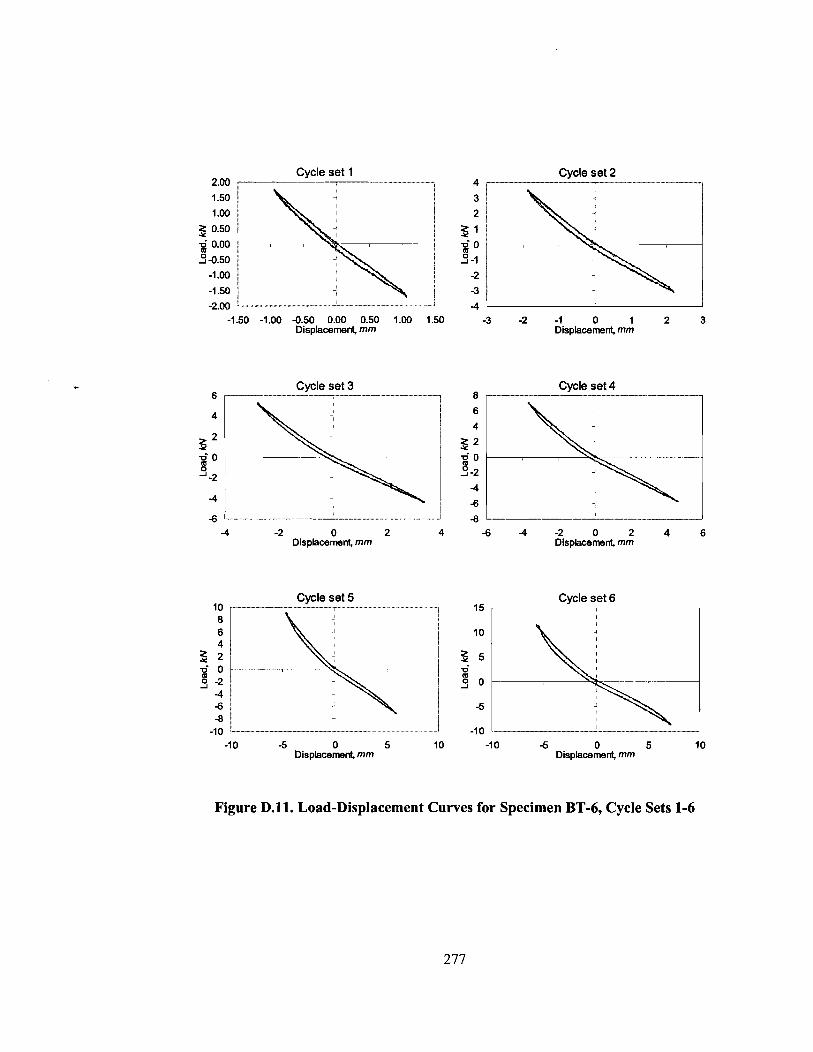
Cycle set 1 2.00 --->
-1.50 -1.00 -0.50 0.00 0.50 1.00 1.50 Displacement. mm
Cycle set 2 4 T-------"
-3 -2 1 0 1 2 3 Displacement, mm
Cycle set 3 .---.-T-.---..--.-.
Cycle set 4 . . 6
2 s ....... . .. d 0 -, , - -
8 -I -2
-I -2 -4
-4 1
.........................
-4 -2 0 2 4 8 - 4 - 2 0 2 4 6 Displacement, mm Displacement, mm
Cycle set 5 ....................................................................................... ...........
I
I
j 1
Cycle set 6 15 I
I
-1 0 -5 0 5 10 -1 0 -5 0 5 10 Displacement, mm Displacement, mm
Figure D.l l . Load-Displacement Curves for Specimen BT-6, Cycle Sets 1-6
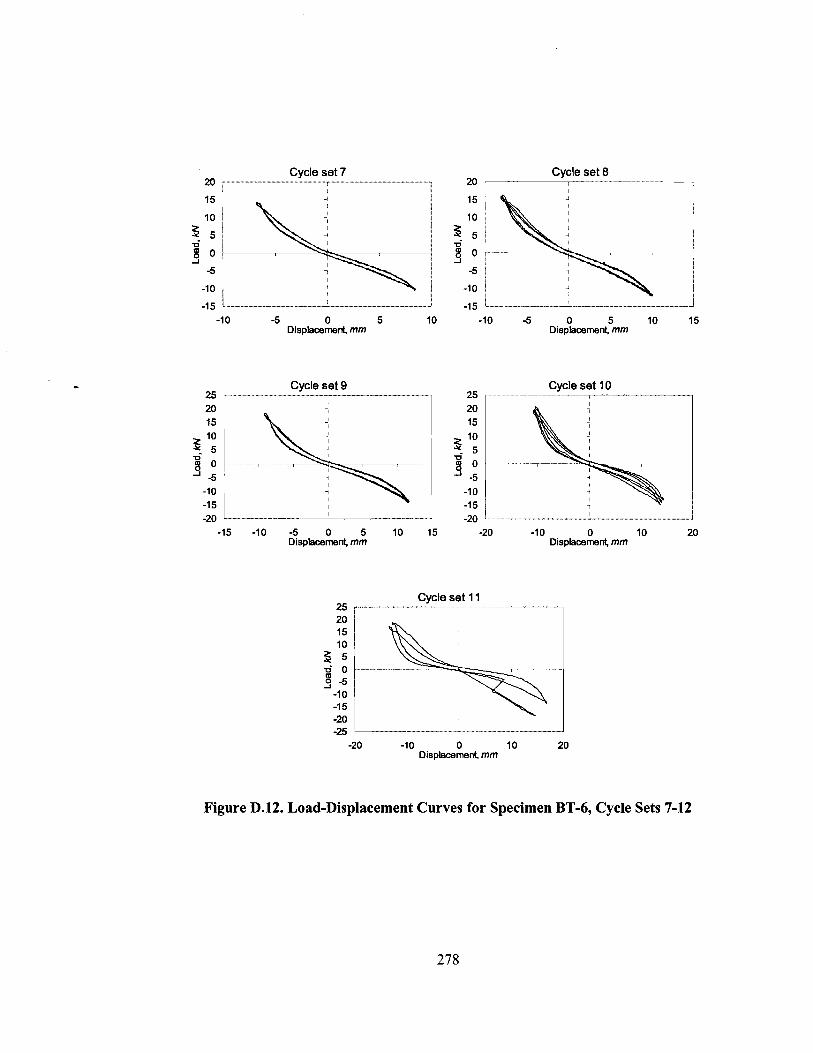
20
15
10
5 d 8 0 J
-5
-10
-1 5 -10 -5 0 5 10 -10 -5 0 5 10 15
Dlsplacemenf mm Displacement, mm
Cycle set 9 Cycle set 10 25 r--- -------.-..I 25 1 I
-15 -10 -5 0 5 10 15 -20 -1 0 0 10 20 Displacement, mm Displacement mm
Cycle set 11 25 ....... .... 7
Figure D.12. Load-Displacement Curves for Specimen BT-6, Cycle Sets 7-12
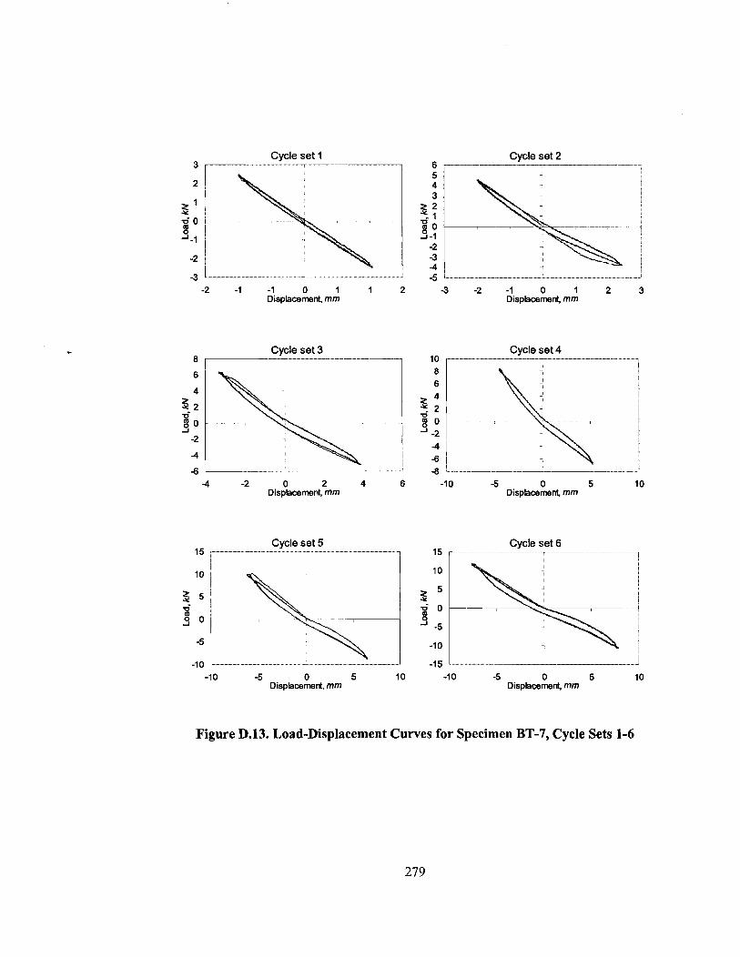
Cycle set 1 3 - .. Cycle set 2
6
0 -1-1 i
I -2 -3 -2 ; 4 -5 d
-2 -1 -1 0 1 1 2 3 -2 -1 0 1 2 3 Displacement, mm Displacement, mm
!
4 I I
-2 1
4 1
6 -. . ... . . . .. . . .. ..
4 -2 0 2 4 6 -1 0 -5 0 5 10 Displacement, mm Displacement, mm
Cycle set 6
____--...-.... J
-10 -5 0 5 10 -1 0 -5 0 5 10 Displacement, mm Displacement, mm
Figure D.13. Load-Displacement Curves for Specimen BT-7, Cycle Sets 1-6

Cycle set 8
-10 -5 0 5 10 15 -15 -10 -5 0 5 10 15 Displacement, mm Displacement, mm
Cycle set 9 Cycle set 10 ............... T--- 1 1
-20 -10 0 10 20 -20 -1 0 0 10 20 Displacement, mm Displacement, mm
Cycle set 11 l2 1
-20 -1 5 -10 -5 0 Displacement, mm
Figure D.14. Load-Displacement Curves for Specimen BT-7, Cycle Sets 7-12

Cycle set 1 4 r. Cycle set 2
6 --- 7.- I i
3 1 4
2 1 5 1 j
i 6 0
s 6 0 -- .-
4 - 1 1 A -2 I
-2 1 I 4 1 3 1
4 i..." ... .-. 8 J
4 -2 0 2 4 -10 -5 0 5 10 Displacement, mm Displacement, mm
-10 -5 0 5 10 -15 -10 5 0 5 10 15 Displacement, mm Displacement, mm
Cycle set 5 Cycle set 6 15 20
10
2 2 5 . . . . . . .
-I z 8 -I -5 o o - 3 -I :Fsq -5 o o
-15 ............. -1 5 -20
-20 -10 0 10 20 -20 -1 0 0 10 20 Displacement, mm Displacement, mm
Figure D.15. Load-Displacement Curves for Specimen DM-1, Cycle Sets 1-6

Cycle set 7 20 " " ..... "
Cycle set 8 25 r-- t I
3 0 -20 -10 0 10 20 30 -30 -20 -10 0 10 20 30 Displacement, mm Displacement mm
-20
4 0 -20 0 20 40 4 0 -20 0 20 40 Displacement mm Displacement mm
Cycle set 11 25 7--- - - T - -
4 0 -20 0 20 40 Displacement mm
Figure D.16. Load-Displacement Curves for Specimen DM-1, Cycle Sets 7-12
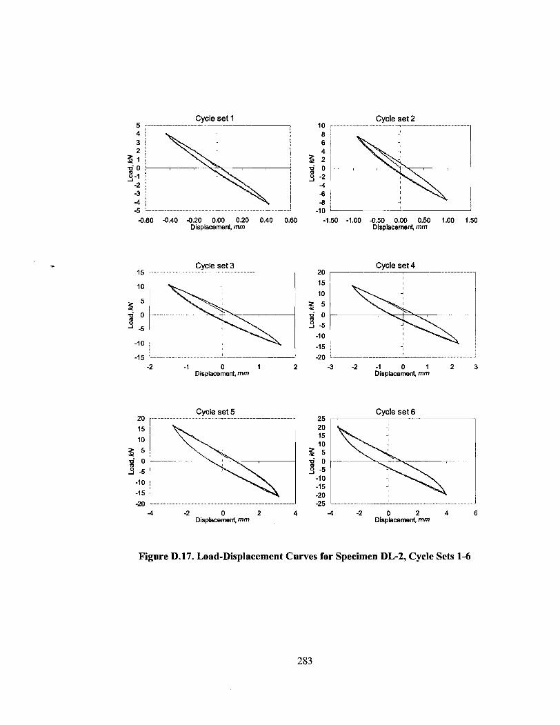
Cycle set 2
-0.60 -0.40 -0.20 0.00 0.20 0.40 0.60 -1.50 -1.00 -0.50 0.00 0.50 1.00 1.50 Displacement, mm Displacement. mm
Cycle set 6
-4 -2 0 2 4 -4 -2 0 2 4 6 Dispbcemenf mm Displacemenf mm
Cycle set 3
Figure D.17. Load-Displacement Curves for Specimen DL-2, Cycle Sets 1-6
15 .- . . - .......... Cycle set 4
10
h 5
6 0
-5
..........
...............
2o I_.__
I
15
$ " m 3 -5
-1 0
- lo I -15
-15 1 I
.. ........... -20 -!.- -2 -1 0 I 2 -3 -2 -1 0 I 2 3
Displacement, mm Displacement, mm

Cycle set 7
-5 0 5 10 Displacement, rnrn
Cycle set 9 40 r. ....... 7- 1
-1 0 -5 0 5 10 Displacement, rnrn
Cycle set 8 40
-10 -5 0 5 10 Displacement, rnrn
Cycle set 10 40 - -
-10 -5 0 5 10 Displacement. rnrn
Cycle set 12 -- --
d 8 -r 0
-5
-1 5 - - -- -- --
-10 -5 0 5 10 15 -30 -20 -10 0 10 20 Displacement, rnrn D~splacement, rnrn
Figure D.18. Load-Displacement Curves for Specimen DL-2, Cycle Sets 7-12
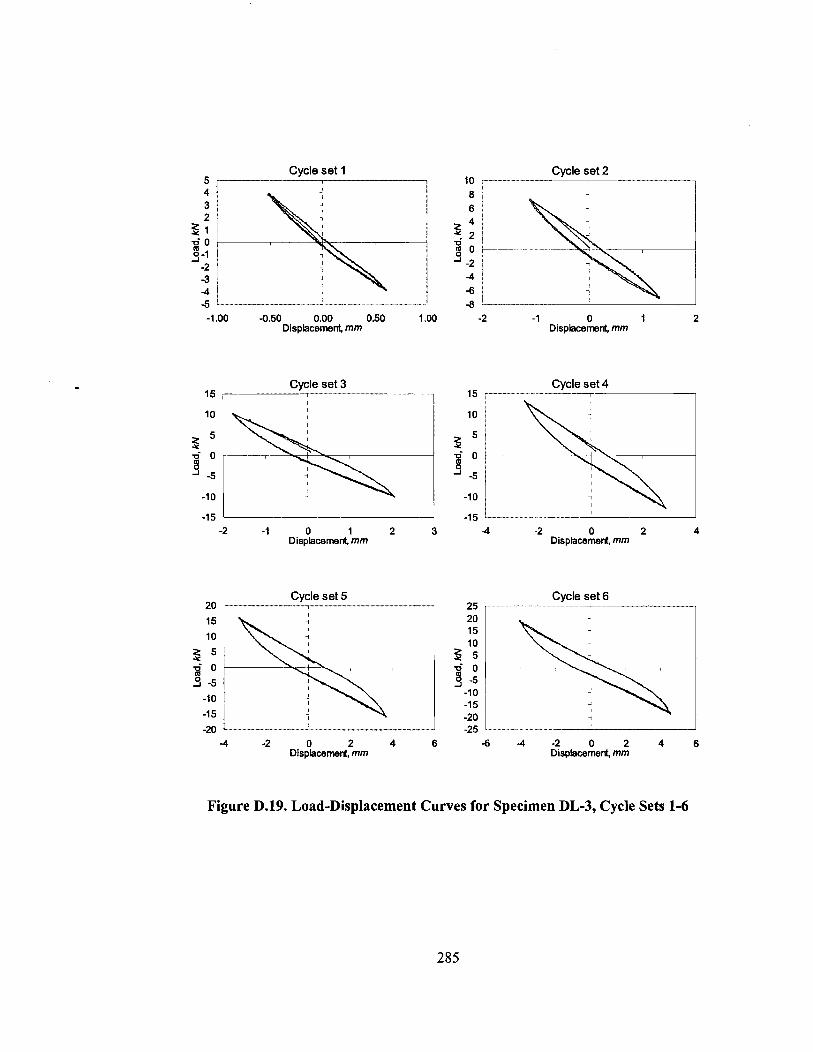
5 Cycle set I
-1.00 -0.50 0.00 0.50 1 .OO Displacement, mm
Cycle set 2 10 -
-2 -1 0 1 2 Displacement, mm
Cycle set 4 ..................
5 s 6 0 T
8 -5 -5
I
-1 0 1
...................
-2 -1 0 1 2 3 4 -2 0 2 4 Displacemerd, mm Displacement, mm
Cycle set 5 20 .- ..............................................................................................
Cycle set 6 25 7--- I I
20 15 10 10
2 5 : 0
-1 0
-5 i -15 1 I
-20 1 2 ................
-4 -2 0 2 4 6 - 6 - 4 - 2 0 2 4 6 Displacement, mm Displacement, mm
Figure D.19. Load-Displacement Curves for Specimen DL-3, Cycle Sets 1-6
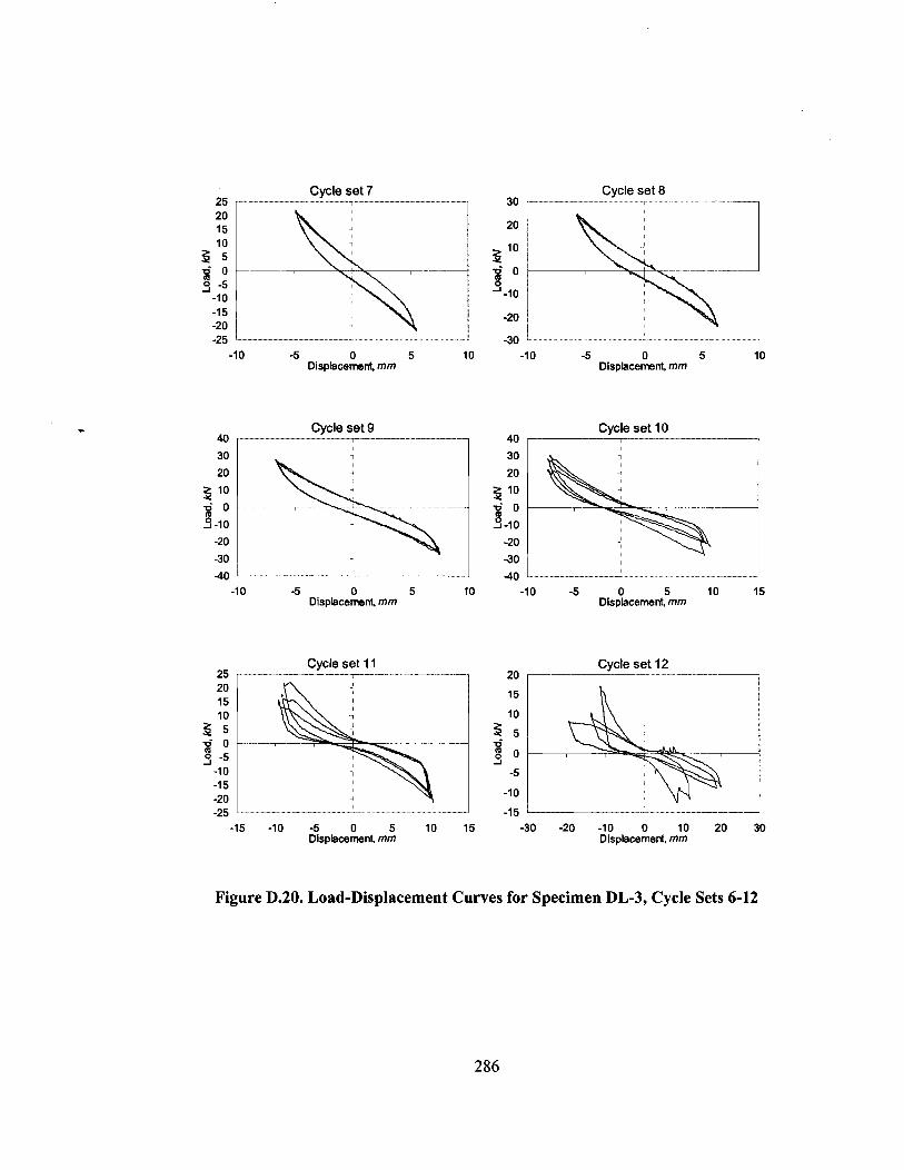
Cycle set 8
-10 -5 0 5 10 -1 0 -5 0 5 10 Displacement, mm Displacement mm
Cycle set 9 40 ........
Cycle set 10 40 I
-10 -5 0 5 10 -10 -5 0 5 10 15 Displacement mm Displacement, mm
-15 -10 -5 0 5 10 15 -30 -20 -10 0 10 20 30 Displacement mm Displacement, mm
Figure D.20. Load-Displacement Curves for Specimen DL-3, Cycle Sets 6-12

Cycle set 1 4 Cycle set 2 I 8 r" - 'l---p---'l
-1.50 -1.00 -0.50 0.00 0.50 1.00 1.50 -3 -2 -1 0 1 2 3 Displacement, mm Displacement, mm
Cycle set 4
......
4 -5
-1 0
... -15
4 -2 0 2 4 6 -5 0 5 10 Displacement, mm Displacement, mm
Cycle set 5 20 -" ............................ - ............ "
I Cycle
10 :: r--L set 6
-1 0 -5 0 5 10 Displacement. mm
Figure D.21. Load-Displacement Curves for Specimen DS-4, Cycle Sets 1-6
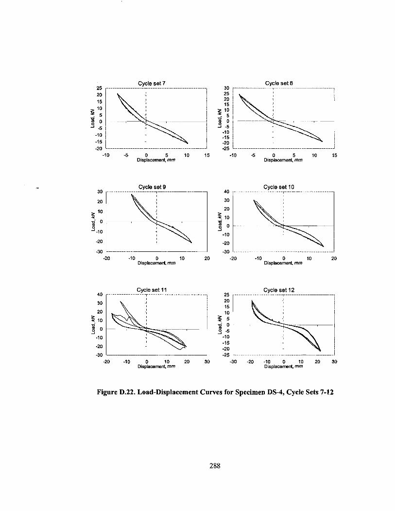
-10 -5 0 5 10 15 -10 -5 0 5 10 15 Displacement, mm Displacement, mm
Cycle set 9
-20 -1 0 0 10 20 Displacement mm
Cycle set 10 1
-1 0 Displacement 0 mm 10 20
-20 -10 0 10 20 30 -30 -20 -10 0 10 20 30 Displacement, mm Displacemed. mm
Figure D.22. Load-Displacement Curves for Specimen DS-4, Cycle Sets 7-12
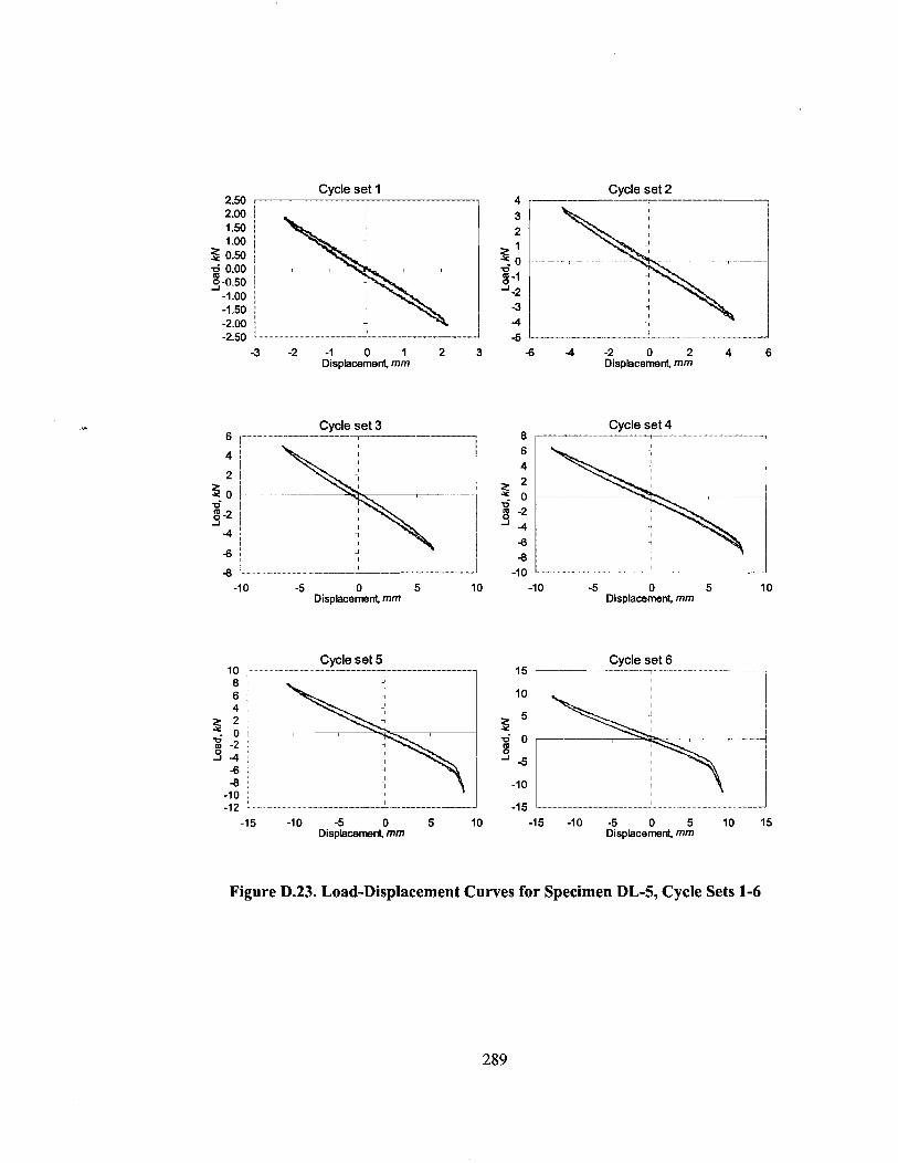
Cycle set 1 2 50 I
-3 -2 -1 0 1 2 3 Displacement mm
Cycle set 2 4 r.-------------
- 6 - 4 - 2 0 2 4 6 Displacement, mm
-1 0 -5 0 5 10 -1 0 -5 0 5 10 Displacement, mm Displacement, mm
Cycle set 5 ....................... ................. 10 "
Cycle set 6 15 1
-15 -10 -5 0 5 10 -15 -10 -5 0 5 10 15 Displacemert, mm Displacement mm
Figure D.23. Load-Displacement Curves for Specimen DL-5, Cycle Sets 1-6

Cycle set 7 Cycle set 8
d 8 -5 4
-1 0
-1 5
-20 -1 0 0 10 20 -20 -1 0 0 10 20 Displacement, mm Displacement, mm
Cycle set 10
1 - -
-30 -20 -10 0 10 20 -30 -20 -10 0 10 20 Displacement, mm Displacement, mm
Cycle set 11 20 .... "" .....
Figure D.24. Load-Displacement Curves for Specimen DL-5, Cycle Sets 7-12

Cycle set 1 Cycle set 2 1.50 I---'
1.00 1 0.50 1
s 0.00 I d i g-0.50 i -1
-1.00 1 -1.50 / -2.00 i .. "A ..
-2.00 -1.00 0.00 1.00 2.00 -4 -2 0 2 4 Displacement, mm Displacement, mm
4 ;
Cycle set 3 --"-- Cycle set 4 ......... -17- I
3 / 2 1 s ;
6 i m-1 j 4, 1
-3 1
4 : -5 ... - ---L . .
- 6 - 4 - 2 0 2 4 6 -1 0 -5 0 5 10 Displacement, mm Displacement, mm
Cycle set 6 B
6 4
s $ 0
4 -2
4
-6
8 -1 0 -5 0 5 10 -1 0 -5 0 5 10
Displacement mm Displacement, mm
Figure D.25. Load-Displacement Cuwes for Specimen DM-6, Cycle Sets 1-6

7' i 15 i I lo I i s 5 I d o i 1 4 I
-5
j -10
-15 -15 -10 -5 0 5 10 -20 -10 0 10 20
Displacement, mm Displacement, mm
Cycle set 9 15
Cycle set 10 10
10 5
5 2 5 0
m d
-I 4 -5 -5
-1 0 -1 0
-20 -1 0 0 10 20 -30 -20 -10 0 10 20 Displacement, mm Displacement, mm
Cycle set 11 - . . ..
3 0 -20 -10 0 10 20 Displacement, mm
Figure D.26. Load-Displacement Curves for Specimen DM-6, Cycle Sets 7-12

Cycle set 1 Cycle set 2 .. 8 I -7
4 -2 0 2 4 -1 0 -5 0 5 10 Displacement mm Displacement, mm
-10 -5 0 5 10 Displacement, mm
-15 -10 -5 0 5 10 15 Displacement, mm
Cycle set 5 20 ...........................
I
-20 -1 0 0 10 20 Displacement mm
Cycle set 6 20 , -- I
-20 -1 0 0 10 20 Displacement, mm
Figure D.27. Load-Displacement Curves for Specimen DL-7, Cycle Sets 1-6

Cycle se t 8
3 0 -20 -10 0 10 20 30 -30 -20 -10 0 10 20 30 Displacement, mm Displacement, mm
Cycle se t 9 15
Cycle se t 10
10
5
5 0 6 g -5 -I
-10
-15 -20 I
4 0 -20 0 20 40 4 0 -20 0 20 40 Displacement, mm Displacement, mm
Figure D.28. Load-Displacement Curves for Specimen DL-7, Cycle Sets 7-12

Appendix E
Load versus Inner Displacement Plots of Hybrid Joints
Cycle set 1 2-00 ; .-
1.00 j 0.50 j
g4.50 1 -1 -1.00 1
-1.50 I -2.00 1
4.40 4.20 0.00 0.20 0.40 Displacement, mm
Cycle set 2 4 1
4.60 4.40 4.20 0.00 0.20 0.40 0.60 Displacement, mm
Cycle set 5
.. . . -15 1 ..I -2.00 -1.00 0.00 1.00 2.00 -2 -1 0 1 2
Displacement, mm Displacement, mm
Cycle set 4 6 4r\21 ::.\\
Figure E.1. Load-Displacement Curves for Specimen BP-1, Cycle Sets 1-6
s d o ..... -- u - 0
-I -2 -I -2
-4
-6 -8
- i - - 7 I
,
-1.00 4.50 0.00 0.50 1 .OO -1.00 4.50 0.00 0.50 1.00 1.50 Displacement, mm Displacement, mm
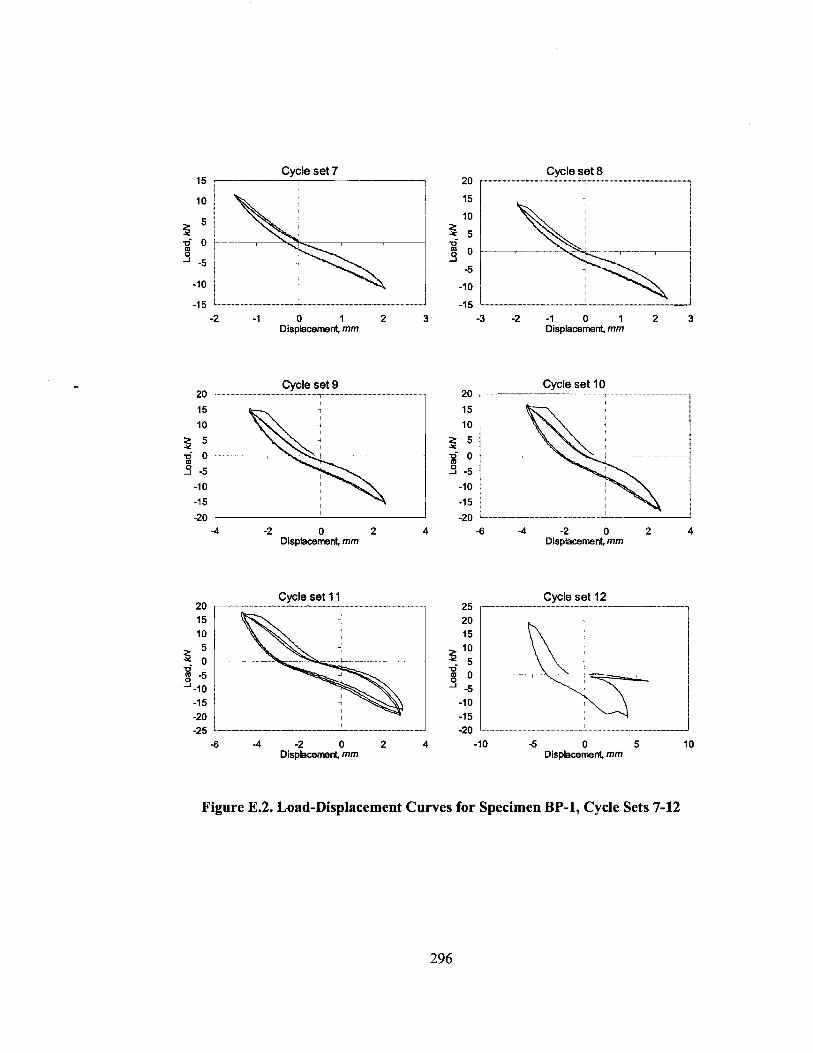
Cycle set 7 Cycle set 8 ................................................. ..................... ..... .............. " " - .......................... ....... 15 i ,
2 I i 5 I
r------i
-5 I i
-1 0 I
I -1 5 .- " .....-i -...-~...,""""4 -15 -2 -1 0 I 2 3 -3 -2 -1 0 I 2 3
Displacement, mm Displacement, mm
-4 -2 0 2 4 -6 -4 -2 0 2 4 Displacement, mm Displacement, mm
Cycle set 11
-25 I
-6 -4 -2 0 2 4 Displacement, mm
Cycle set 12 25 ........ .-
1
-1 0 -5 0 5 10 Displacement, mm
Figure E.2. Load-Displacement Curves for Specimen BP-1, Cycle Sets 7-12

" Cycle set 2
4
7-
1
I
-2.50 i .....- _L I
-0.40 -0.20 0.00 0.20 0.40 4.60 -0.40 -0.20 0.00 0.20 0.40 0.60 Displacement, mm Displacement mm
.-.... ............-.. -15 L----------. -
-2.00 -1.00 0.00 1 .oo 2.00 -2 -1 0 1 2 Dispbcemeri, mm Displacement mm
Cycle set 3 6 r..---.-.- ............................ 8
Figure E.3. Load-Displacement Curves for Specimen BT-2, Cycle Sets 1-6
4 1 ! s 2 1
-- 0 t~p - ~. ~
8 i -I-2 4 ] 1 ! \ 6
4
;: S -6 -2 4
-6 i ........... ... -8 -1.00 -0.50 0.00 0.50 1 .OO -1.00 -0.50 0.00 0.50 1.00 1.50
Displacement mm Displacement, mm
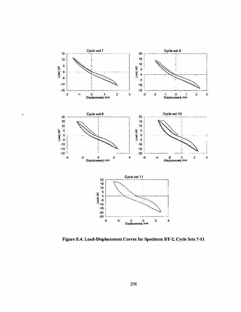
Cycle set 7 I I
Cycle set 8 20 , . . . .................. .....r....... . .
I
i -15 L -? .. 8
-2 -1 0 1 2 3 Displacement mm
3 - 2 - 1 0 1 2 3 Displacement, mm
Cycle set 9 20 ...............................
m 3 -5
-1 0 -1 5
-20 1
-4 -2 0 2 4 -6 -4 -2 0 2 4 Displacement, mm Displacement, mm
Cycle set 11
-15 1
-20 1 -25 L
-6 -4 -2 0 2 4 D~splacement, mm
Figure E.4. Load-Displacement Curves for Specimen BT-2, Cycle Sets 7-11
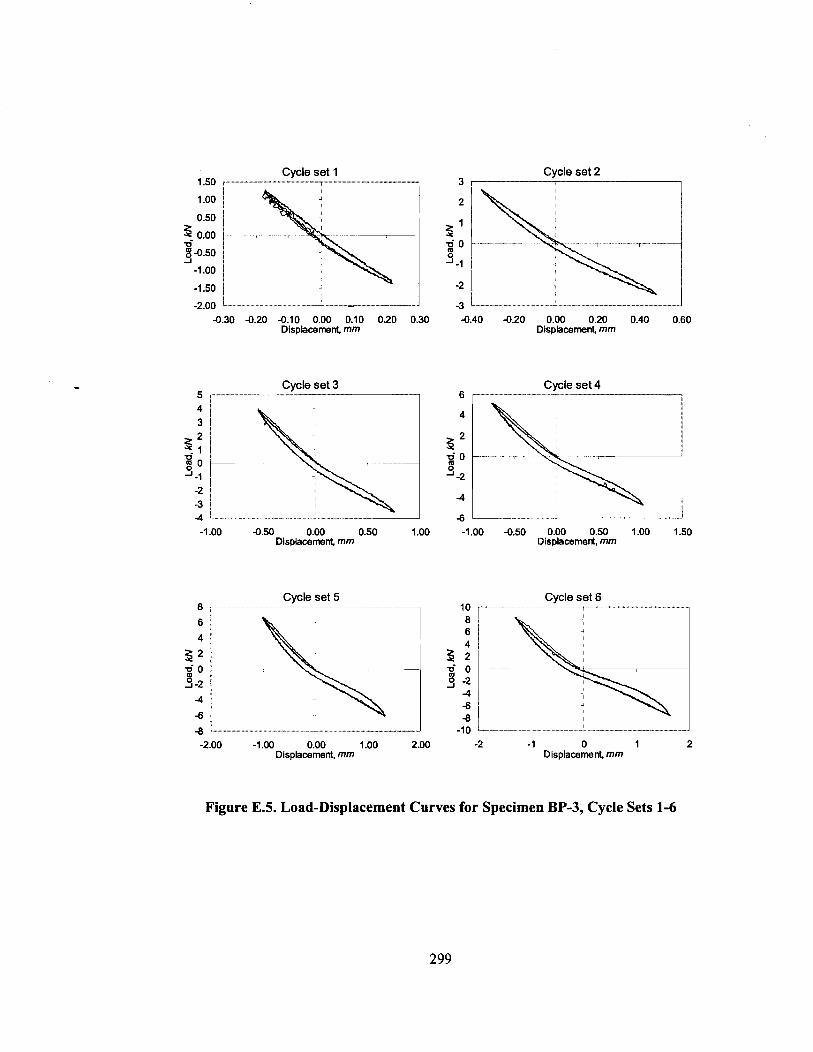
Cycle set 2
0
-2.00 '
4.30 4.20 4.10 0.00 0.10 0.20 0.30 4.40 4.20 0.00 0.20 0.40 0.60 Displacement, mm Displacement, mm
Cycle set 3 5 i----------
Cycle set 4 6 ----- - - - . - --
-1.00 4.50 0.00 0.50 1 .OO -1.00 4.50 0.00 0.50 1.00 1.50 Displacement mm Displacement, mm
Cycle set 5
-2.00 -1.00 0.00 1 .oo 2.00 -2 -1 0 1 2 Displacement, mm Displacement, mm
Figure E.5. Load-Displacement Curves for Specimen BP-3, Cycle Sets 1-6

Cycle set 7
-2 -1 0 1 2 3 3 - 2 - 1 0 1 2 3 Displacement, mm Displacement, mm
4 -2 0 2 4 -6 4 -2 0 2 4 Displacement, mm Displacement, mm
Cycle set 11 Cycle set 12 20 20 - - ---- -- - - - 15 10
2 0 (: 6 0 1.- \I
z! -5 J-lo
8 J -5
-15 -1 0
-20 -1 5 -25 -20 - -
-6 4 -2 0 2 4 -1 0 -5 0 5 Displacement, mm Displacement, mm
Figure E.6. Load-Displacement Curves for Specimen BP-3, Cycle Sets 7-12

7.- --- . - -- -
I
4.40 4.20 0.00 0.20 0.40 -1.00 4.50 0.00 0.50 1 .OO Displacement, mm Displacement mm
Cycle set 3 8 --" ......... ___ Cycle set 4 10
1
-1.00 4.50 0.00 0.50 1 .OO Displacement mm
Cycle set 5 15
I 1
-2.00 -1.00 0.00 1 .oo 2.00 Displacement, mm
Cycle set 6 r- ................................................. .... I
-2.00 -1.00 0.00 1 .oo 2.00 -2 -1 0 1 2 3 Displacement, mm Displacement mm
Figure E.7. Load-Displacement Curves for Specimen BT-4, Cycle Sets 1-6
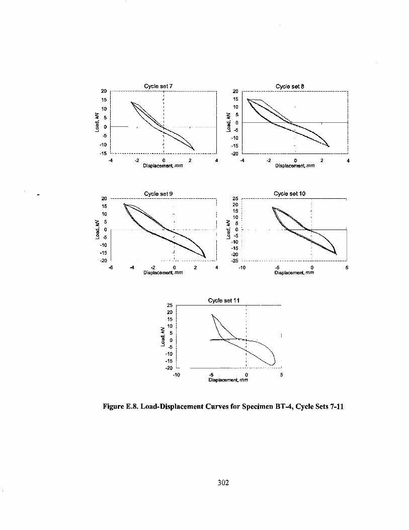
Cycle set 7 20 1
i I
4 -2 0 2 4 4 -2 0 2 4 Displacement mm Displacement, mm
-1 5
8 4 -2 0 2 4 -1 0 -5 0 5 Displacement mm Displacement, mm
Cycle set 11 25 i
20 1 15 / 10 !
-5 -10 / -15 -20 - - -
-10 -5 0 5 Displacement, mm
Figure E.8. Load-Displacement Curves for Specimen BT-4, Cycle Sets 7-11
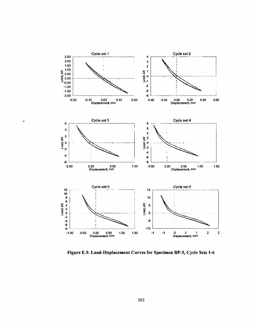
Cycle set 1 2.50 ....................................................................................................................
2.00 1 1.50 1 1.00
3 0.50 1 u-
-0.50 1 -1.00 j -1.50 I -2.00 I A-
-0.20 -0.10 0.00 0.10 0.20 Displacement mm
Cycle set 2 4 1
4 1 -0.40 -0.20 0.00 0.20 0.40 0.60
Displacement, mm
-0.50 0.00 0.50 1 .OO -0.50 0.00 0.50 1 .OO 1 .SO Displacement, mm Displacement, mm
-1.00 -0.50 0.00 0.50 1.00 1.50 -1 -1 0 1 1 2 2 Displacement, mm Displacement, mm
Figure E.9. Load-Displacement Curves for Specimen BP-5, Cycle Sets 1-6

Cycle set 7 ..... .". " """ ..............
1 -5
-10 j J
-15 : .-i ...... -15 : -1 -1 0 1 2 3 -2 -1 0 1 2 3
Displacement, mm Displacement, mm
I
-2 -1 0 1 2 3 -2 0 2 4 Displacement, mm Displacement. mm
Cycle set 11 Cycle set 12 30 - 1 25 I
20 ! I
15 g 10
I !
6 5 i
3 O r A -5
-10 -15 -20 - -
-2 0 2 4 6 -2 0 2 4 6 DispiacemenL mm Disptacement, mm
Figure E.lO. Load-Displacement Curves for Specimen BP-5, Cycle Sets 7-12
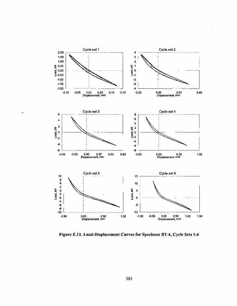
Cycle s e t 1 2.00 !.-....- .......................................................................................................... ".
-2.00 L
4.10 4.05 0.00 0.05 0.10 0.15 Displacement, mm
Cycle s e t 2 4 1
4.20 0.00 0.20 0.40 Displacement. mm
Cycle s e t 3 6 T--.----.." .-.- - ..- . .. . . .-
2 / s i - . . r. ... ---
I~
0 J-2 ;
1 I
1
-4 3 1
6 i 1 ! -0.40 -0.20 0.00 0.20 0.40 0.60 -0.50 0.00 0.50 1.00
Displacement mm Displacement, mm
Cycle s e t 5
-0.50 0.00 0.50 1 .OO -1.00 4.50 0.00 0.50 1.00 1.50 Displacement, mm Displacement, mm
Figure E.ll . Load-Displacement Curves for Specimen BT-6, Cycle Sets 1-6
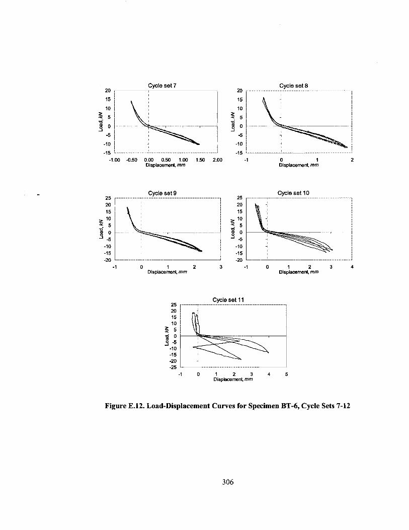
Cycle set 7 Cycle set 8 20
-15 L....--- . . 2 -
-1.00 -0.50 0.00 0.50 1.00 1.50 2.00 -1 0 1 2 Displacement, mm Displacement, mm
Cycle set 10 25 20 15
2 lo ; 5
4 ," -1 0 -1 5 -20
-1 0 1 2 3 -1 0 1 2 3 4 Dispbcement, mm Displacement, mm
Cycle set 11 25 1
-1 0 1 2 3 4 5 Displacement. mm
Figure E.12. Load-Displacement Curves for Specimen BT-6, Cycle Sets 7-12
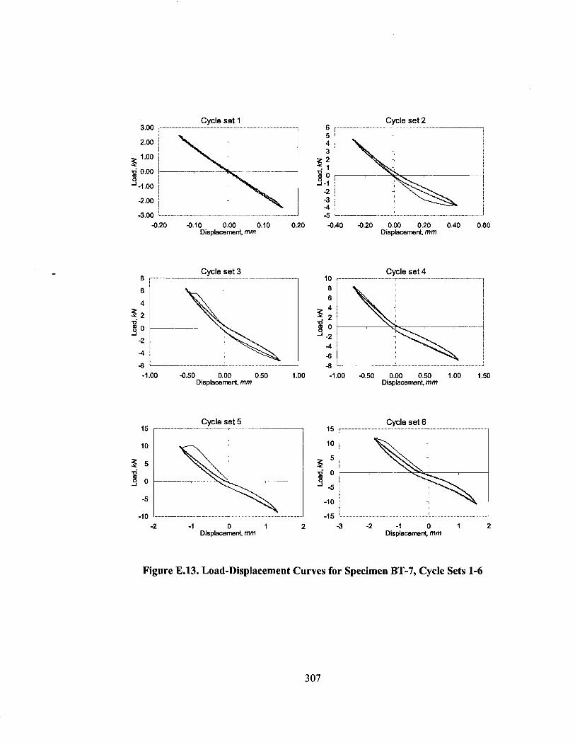
Cycle set 2 6 5 4 3
s; d m 0 3 -1
-2 -3 -4 -5 - d
-0.20 -0.10 0.00 0.10 0.20 -0.40 -0.20 0.00 0.20 0.40 0.60 Displacement, mm Displacement mm
Cycle set 3 Cycle set 4
$ 2 7--- --
-
-2
- 4 1 4 :
-1 .OO -0.50 0.00 0.50 1.00 -1.00 -0.50 0.00 0.50 1.00 1.50 Displacement, mm Displacement, mm
- . . - . - . -- Cycle set 6
-2 -1 0 1 2 3 -2 -1 0 1 2 Displacement, mm Displacement, mm
Figure E.13. Load-Displacement Curves for Specimen BT-7, Cycle Sets 1-6

15
10
5 5 d 0 8 1 -5
-10
-15 -3 -2 -1 0 1 2 3 4 -2 0 2 4
Displacement, mm Displacement, mm
Cycle se t 9 20 , .................................................. " -- ......... " ..........-r-..... ..............
I
8 4 -2 0 2 4 Displacement, mm
Cycle se t 10 20 1 7
-10 -5 0 5 10 Displacement. mm
Cycle se t 11 12 1 I I
-2 L ..
8 4 -2 0 2 Displacement, mm
Figure E.14. Load-Displacement Curves for Specimen BT-7, Cycle Sets 7-12

Cycle set 1 4 .......................................... 7.. ...... .-
Cycle set 2 6
d 0 8 4 -1
-2 I !
1 I
-3 I
I -6 L-.-.- -4 -1.50 -1.00 -0.50 0.00 0.50 1.00 1.50 3 -2 -1 0 1 2 3
Displacement, mm Displacement, mm
Cycle set 3 10
Cycle set 4 .............................. ......... -"'? 15 ;---
8 6 4
s 2 6 0 - ; 7--- 0 4 -2
-4 -6 -0
1
i I
-10 .................................... i -15 L . ........................
-4 -2 0 2 4
i - 6 - 4 - 2 0 2 4 6
Displacement, mm Displacement, mm
Cycle set 5 Cycle set 6 15
10
5 5 6 0 8 A -5
-1 0
-1 5 -1 0 -5 0 5 10 -1 0 -5 0 5 10
Displacement, mm Displacement, mm
Figure E.15. Load-Displacement Curves for Specimen DM-1, Cycle Sets 1-6
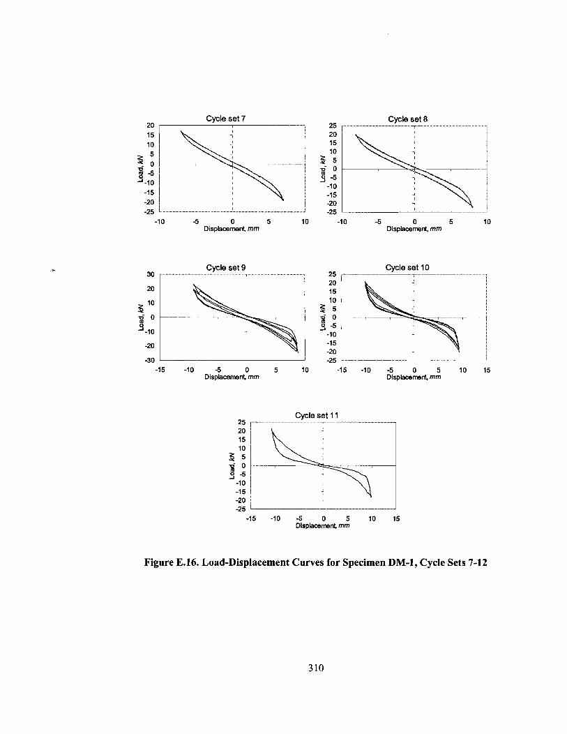
Cycle set 8
-25 i J -25
-1 0 -5 0 5 10 -1 0 -5 0 5 10 Displacement mm Displacement, mm
Cycle set 9 30 r-,... .... ,....... . ... . ......... . . ... . - ....,...-.-..-----..-..-.-..... ..... . ....... . .. ............. ..... .. Cycle set 10
!
-15 -10 -5 0 5 10 -15 -10 -5 0 5 10 15 Displacement mm Displacement mm
Cycle set 1 1
-20 i -25 L--------- "-
-15 -10 -5 0 5 10 15 ~ispbcement, mm
Figure E.16. Load-Displacement Curves for Specimen DM-1, Cycle Sets 7-12

Cycle set 1 5 .................. " ...... .- "
Cycle set 2 10
4 I I 8 3 6
4 s: s 2 6 0 u- 0
4 -1 4 -2 -2 4 3 6 4 -8 i
5 " ........... " " L-.-."". . -1 0
I ---
-1.00 -0.50 0.00 0.50 1 .DO -2 -1 0 1 2 Displacemerd, mm Displacement, mm
Cycle set 3 15
Cycle set 4 20 r.p-.--T.
10
2
% 0 . m m :
i I 3-51 -5 I 1 -101 1 -1 0 I 1 -151
-4 -2 0 2 4 4 -2 0 2 4 Displacemerd, mm Displacement, mm
Cycle set 5 Cycle set 6 20
15
10
2 5 ; 0
3 -5
-1 0
-1 5
-20 8 - 4 - 2 0 2 4 6 5 0 5 10
~lspbcement, mm Displacement, mm
Figure E.17. Load-Displacement Curves for Specimen DL-2, Cycle Sets 1-6

Cycle set 7 30 7 I I
-1 0 -5 0 5 10 Displacement, mm
Cycle set 9 40 .......................................................... ..................... , . ..... ............................. ..,.,
-10 -5 0 5 10 Displacement, mm
Cycle set 8 40 , ................................................. . , ....... ...........
I
-1 0 -5 0 5 10 Displacement, mm
Cycle set 10 40 ---- I
-10 -5 0 5 10 Displacement, mm
Cycle set 1 1 Cycle set 12 40 25
30 20
20 15
4 10 u
s lo z 0 J
-1 0 $ ",
-5 -20 -10
........................ .... . -30 -15 -
-1 0 -5 0 5 10 -1 0 -5 0 5 10 Displacement, mm Displacement, mm
Figure E.18. Load-Displacement Curves for Specimen DL-2, Cycle Sets 7-12
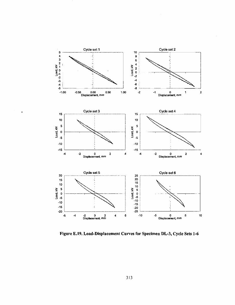
Cycle set 1 5 .....-.*...-......................................II-............... " ............... " ............... Cycle set 2
10 ; ,
-1.00 4.50 0.00 0.50 1 .OO -2 -1 0 1 2 Displacement, mm Displacement, mm
..... ,
4 -2 0 2 4 4 -2 0 2 4 Displacement, mm Displacement, mm
Cycle set 5 20 25
15
10
m 3 -5
I -1 0 -10 I -1 5 -15 I
I j -20 -20 - .............. 1 1 -25
- 6 4 - 2 0 2 4 6 -1 0 -5 0 5 10 Dlsplacement, mm Displacement, mm
Figure E.19. Load-Displacement Curves for Specimen DL-3, Cycle Sets 1-6

Cycle set 7 .............. -
I
-1 0 -5 0 5 10 -10 -5 0 5 10 Displacement, mm Displacement, mm
m
-20
-30
-1 0 -5 0 5 10 -1 0 -5 0 5 10 Displacement, mm Displacement, mm
Cycle set 11
-1 0 -5 0 5 10 -15 -10 -5 0 5 10 Displacement, mm Displacement, mm
Figure E.20. Load-Displacement Curves for Specimen DL-3, Cycle Sets 6-12

Cycle set 1 4 .. " . . ... " ....................................................
Cycle set 2 8
I I
3 6
2 4
5 5 2 3- 0
3 -1 t! 0 J
-2 -2
3 4
4 0.60 0.40 0.20 0.00 0.20 0.40 0.60 -1.00 0.50 0.00 0.50 1.00 1.50
Displacement mm Dispbcement, mm
Cycle set 3 I
- -. Cycle set 4 .... 10
8 6 4
s 2 d 0 4 -2
4 -6 -8 I
1 I
-10 I ........................... ., -15 i "-
-2 -1 0 1 2 3 -2 -1 0 1 2 3 Displacement mm Displacement, mm
Cycle set 5 I
Cycle set 6 20
-2 0 2 4 4 -2 0 2 4 6 Dispbcement, mm Displacement, mm
Figure E.21. Load-Displacement Curves for Specimen DS-4, Cycle Sets 1-6
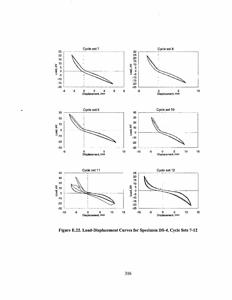
Cycle set 7 Cycle set 8 ............................................................................ 25 I I 30 ......................
- 4 - 2 0 2 4 6 8 -5 0 5 10 Displacement, mm Displacement, mm
30 ...................................................................................................................................... Cycle set 10
m u 0 ' 1
J -10 i J
-10 -20 7 -20
I
-5 0 5 10 -10 -5 0 5 10 15 Displacement, mm Displacement, mm
Cycle set 11 Cycle set 12 ............................................. 25
20 15 10
s 5 d 0 -
4 6 -10 -15 -20 -25
-10 -5 0 5 10 15 -10 -5 0 5 10 15 Displacement mm Displacement, mm
Figure E.22. Load-Displacement Curves for Specimen DS-4, Cycle Sets 7-12

Cycle set 1 2 50 .- ............................................................. . t
-1.00 -0.50 0.00 0.50 1 .OO Displacement, mm
Cycle set 2 A I
-2 -1 0 I 2 Displacemenf mm
Cycle set 4
- . - . ...
-4 -2 0 2 4 -4 -2 0 2 4 Displacement, mm Displacement, mm
Cycle set 5 Cycle set 6
8 -8
8 -4 -2 0 2 4 8 -4 -2 0 2 4 Displacement, mm Displacemenf mm
Figure E.23. Load-Displacement Curves for Specimen DL-5, Cycle Sets 1-6

Cycle set 7 15 8 i
-20 ".- . ...... ;
-1 0 -5 0 5 Displacement, mm
Cycle set 8 15 7- ................................... ............ ....
'I -1 0 -5 0 5
Displacement, mm
-1 0 -5 0 Displacement, mm
,lo -5 0 5 Displacement, mm
Cycle set 11 20 r-- -- -.
-1 0 4 0 5 10 Displacement, mm
Figure E.24. Load-Displacement Curves for Specimen DE5, Cycle Sets 7-12

Cycle set 1 1 .50 i.... - "
1" ...l....l.....ll....l..-...... Cycle set 2
......... ............................. 3
-i---
d 8-0.50 !
-I
-1 .oo -2
-1.50 , -3 9.00 L p--.--.-.-..--..---.-.-.-. -4
-1.50 -1.00 -0.50 0.00 0.50 1.00 1.50 -3 -2 -1 0 1 2 3 Displacement, mm Displacement mm
Cycle set 4 6 .
-i . -. .................
-4 -2 0 2 4 - 6 - 4 - 2 0 2 4 6 Displacement mm Displacement mm
Cycle set 5 - -. - -- - . - 8
6
4
2 2 x- 0 3 -2
-4
-6
-8 -10 ' -1 0 -5 0 5 10 -1 0 -5 0 5 10
Dlspbcernent, mm Displacement, mm
Figure E.25. Load-Displacement Curves for Specimen DM-6, Cycle Sets 1-6

Cycle set 7 I
5 1 i 9 0 1
I 4.1 i
-10 1 -15 i : ... ........ i
-10 -5 0 5 10 -10 -5 0 5 10 Displacement, mm Displacement, mm
Cycle set 9 15 , Cycle set 10
...................................... ...... I I
-15 -10 -5 0 5 10 15 -15 -10 -5 0 5 10 15 Displacement, mm Displacement, mm
Cycle set I I 10 , .- --
I
-15 i ..................... : . J -15 -10 -5 0 5 10 15
Displacement, mm
Figure E.26. Load-Displacement Curves for Specimen DM-6, Cycle Sets 7-12

Cycle set 1 5 r.- ........................ . -. ................ .......
Cycle set 2 8 3
I , ".",
-3 -2 -1 0 1 2 3 Displacement, mm
........................
4 -2 0 2 4 - 6 4 - 2 0 2 4 6 Displacement. mm Displacement mm
Cycle set 5 20 --------T-----------------
-10 -5 0 5 10 Displacement mm
Cycle set 6 20 ! .......... ...................
-1 0 -5 0 5 10 Displacement mm
Figure E.27. Load-Displacement Cuwes for Specimen DL-7, Cycle Sets 1-6
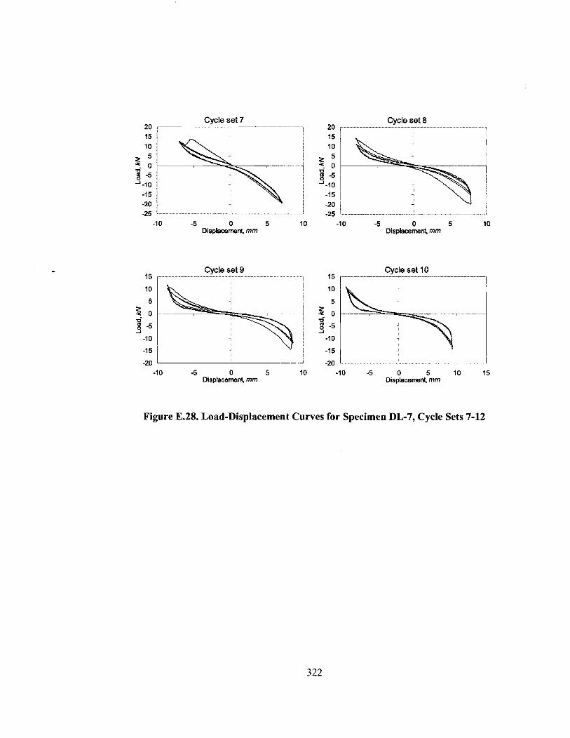
Cycle set 7
-1 0 -5 0 5 10 -1 0 -5 0 5 10 Displacement mm Displacement, mm
-
-10 -5 0 5 10 -10 -5 0 5 10 15 Displacement, mm Displacement, mm
Figure E.28. Load-Displacement Curves for Specimen DL-7, Cycle Sets 7-12

Appendix F
Load versus Strain Plots of Hybrid Joints
Cycle set 1 Cycle set 2
-2000 -1000 0 1000 2000 3000 -4000 -2000 0 2000 4000 Shin, p s Strain, p s
Cycle set 3 6.00
Cycle set 4 ...........................
I ..........7......
1
-10000 -5000 0 5000 10000 -10000 -5000 0 5000 10000 Strain, p s Strain, p s
Cycle set 5 Cycle set 6
.............................. " ......... .
-15000 -10000 -5000 0 5000 10000 -15000 -10000 -5000 0 5000 l o o ~ ~ Strain, p s Strain, ,us
Figure F.1. Load-Strain Curves for Specimen BP-1, Cycle Sets 1-6

Cycle set 7 "" "
Cycle set 8 ............. ................... .. I I
Strain, p s Strain, p s -15000 -10000 -5000 0 5000 10000 -15000 -10000 -5000 0 5000 10000 15000
... 20
15
10
s d 0
3 -5
-10
-1 5
-20 -1 5000 -10000 -5000 0 5000 10000 15000 -1 5000 -10000 -5000 0 5000 10000 15000
Strain. p s Strain,ps
Cycle set 11 I
Figure F.2. Load-Strain Curves for Specimen BP-1, Cycle Sets 7-12
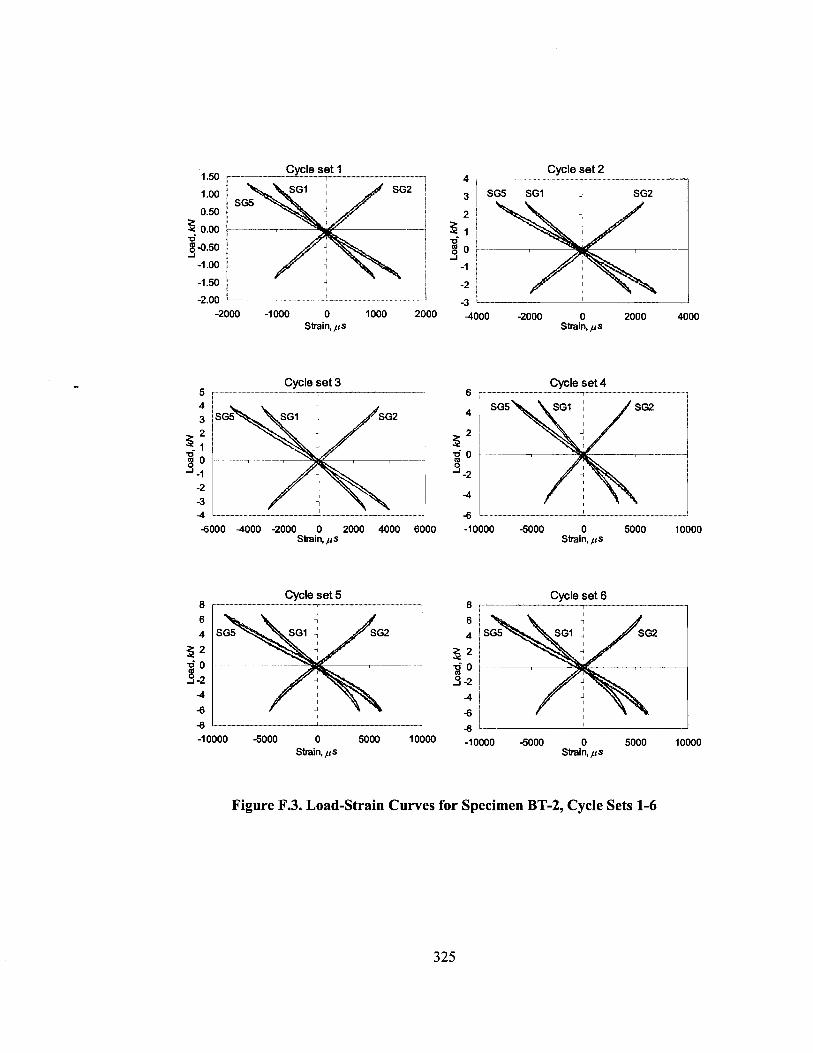
Cycle set 2 4
3 SG5 SGl A SG2 I
I
-2000 -1000 0 1000 2000 4000 -2000 0 2000 4000 Strain. ps Strain, ps
Cycle set 3 Cycle set 4 5 ! I 6 , ........ . .--.....T-.......-.- :
-6000 4000 -2000 0 2000 4000 6000 -10000 -5000 0 5000 10000 Strain. ps Strain. ps
Cycle set 5 Cycle set 6
-10000 -5000 0 10000 -10000 5000 0 5000 10000 Strain, ps Shin, ps
Figure F.3. Load-Strain Curves for Specimen BT-2, Cycle Sets 1-6

Cycle set 7 Cycle set 8 1 5 1 - - 7 I I 15 , 1
-15000 -10000 -5000 0 5000 10000 -15000 -10000 -5000 0 5000 10000 Strain. ps Strain, p s
Cycle set 9 - Cycle set 10 ........................ ........ .. - ........ -
-15000 -10000 -5000 0 5000 I0000 -15000 -10000 -5000 0 5000 10000 15000 Strain, p s Strain, p s
20 ................... Cycle set 1 1
-25 L I .J -15000 -10000 5000 0 5000 10000
Strain. ps
Figure F.4. Load-Strain Curves for Specimen BT-2, Cycle Sets 7-11

Cycle se t 2
-2000 -1000 0 1000 2000 400,3 -2000 0 2000 4000 Strain, ps Strain, ps
-5000 -2500 0 2500 5000 -10000 -5000 0 5000 10000 Strain, ps Strain, ps
Cycle se t 5 Cycle se t 6 8 1 8 ......................................................................................................... 1
431 1
-15000 -10000 5000 0 5000 ~0000 -15000 -10000 -5000 0 5000 ~0000 Strain, ps Strain, ps
Figure F.5. Load-Strain Curves for Specimen BP-3, Cycle Sets 1-6

-15000 -10000 -5000 0 5000 10000 -15000 -10000 -5000 0 5000 10000 15000 Strain, ps Strain, p s
Cycle set 9 Cycle set 10
-15000 -10000 -5000 0 5000 10000 15000 -15000 -10000 -5000 0 5000 10000 15000 Strain. p s Strain, ps
Cycle set 11 20 . 7-- 1
-15000 -10000 -5000 0 5000 10000 15000 Strain, p s
20 - Cycle set 12
-15000 -10000 -5000 0 5000 Strain, ps
Figure F.6. Load-Strain Curves for Specimen BP-3, Cycle Sets 7-12
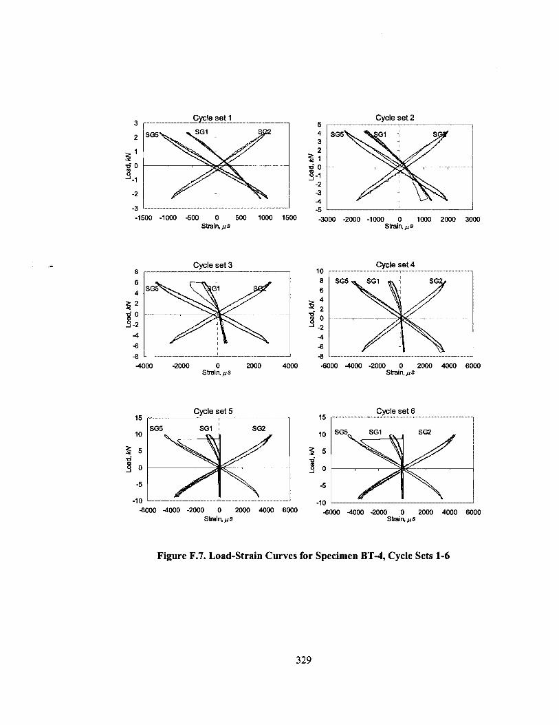
Cycle set 2
-1500 -1000 5 0 0 0 500 1000 1500 -3000 -2000 -1000 0 1000 2000 3000 Strain, ps Shin, ps
Cycle set 3 Cycle set 4 ... " ......... I
4000 -2000 0 2000 4000 -6000 4000 -2000 0 2000 4000 6000 Strain. ps Strain. ps
Cycle set 5 Cycle set 6 ................. ... 1
15 ,
-6000 4000 -2000 0 2000 4000 6000 -6000 4000 -2000 0 2000 4000 6000 Shin, ps Shin, ps
Figure F.7. Load-Strain Curves for Specimen BT-4, Cycle Sets 1-6

Cycle set 7 20 i-.- 1
-5000 -3000 -1000 1000 3000 5000 Strain, p s
Cycle set 8 20
-10000 -5000 0 5000 10000 Strain, p s
Cycle set 9 Cycle set 10 20 I
-5000 0 5000 10000 -6000 -4000 -2000 0 2000 4000 6000 Strain. p s Strain, ps
Cycle set 11 25 ..............................................................
-15000 -10000 -5000 0 5000 10000 Strain, ps
Figure F.8. Load-Strain Curves for Specimen BT-4, Cycle Sets 7-12
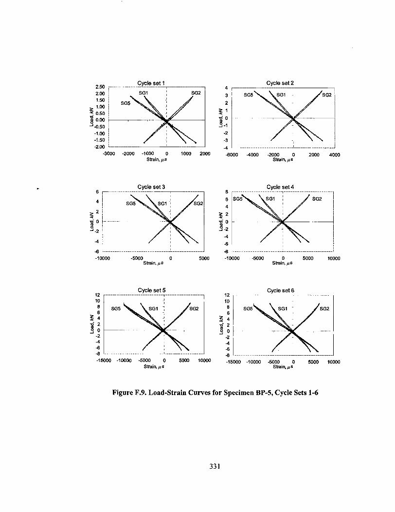
Cycle set 1 2 50 --. . .
-3000 -2000 -1000 0 1000 2000 Strain, ps
Cycle set 2
-4000 -2000 0 2000 4000 Strain. ps
-1 0000 -5000 0 5000 -10000 -5000 0 5000 10000 Strain. ps Strain, ps
Cycle set 5 12 ,. ................ ................................................... "
Cycle set 6 1 I
- -15000 -10000 -5000 0 5000 10000 -15000 -10000 5000 0 5000 10000
Strain, p s Strain, ps
Figure F.9. Load-Strain Curves for Specimen BP-5, Cycle Sets 1-6

Cycle set 7 - Cycle set 8 ....................... ................. 20 , 1
-15000 -10000 5000 0 5000 10000 Strain, p s
-15000 -10000 -5000 0 5000 10000 15000 Strain, p s
Cycle set 9 25 r-..----.--.----.-- --r----- Cycle set 10 . 25 I---.-----------T--..
-15000 -10000 -5000 0 5000 10000 15000 -15000 -10000 5000 0 5000 10000 15000 Strain, p s Shin,ps
Cycle set 12 .-
-15000 -10000 -5000 0 5000 10000 -15000 -10000 -5000 0 5000 10000 Shin. p s Shin, p s
Figure F.lO. Load-Strain Curves for Specimen BP-5, Cycle Sets 7-12
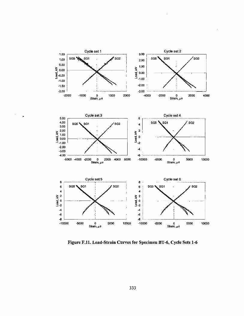
-2000 -1000 0 1000 2000 4000 -2000 0 2000 4000 Strain, p s Strain, p s
Cycle set 3 Cycle set 4 ............................ 5.00 1 1 6 , 1
-6000 4000 -2000 0 2000 4000 6000 -10000 -5000 0 5000 10000 Strain, p s Strain,,&
Cycle set 5 8 1...-...-...............................-...........T-................................. " - ................... ..... 8 ,. - . . . - - -
Cycle set 6 1 I
-10000 -5000 0 5000 10000 -10000 -5000 0 5000 10000 Strain, p s Strain, p s
Figure F. l l . Load-Strain Curves for Specimen BT-6, Cycle Sets 1-6

Cycle set 7 15 --.. ............ ... ..r-...... - .................................. - .--,.,.--...t Cycle set 8
15 1
-1 0000 -5000 0 5000 10000 -15000 -10000 -5000 0 5000 10000 15000 Shin, p s Shin, ps
Cycle set 10 ............ ...T" ..
-15000 -10000 -5000 0 5000 10000 15000 -15000 -10000 -5000 0 5000 10000 Shin, ps Strain. p s
Cycle set 11 Cycle set 12 ... ... .. .......................
-15000 -10000 -5000 0 5000 10000 15000 -15000 -10000 -5000 0 5000 10000 Shin. ps Strain. p s
Figure F.12. Load-Strain Curves for Specimen BT-6, Cycle Sets 7-12
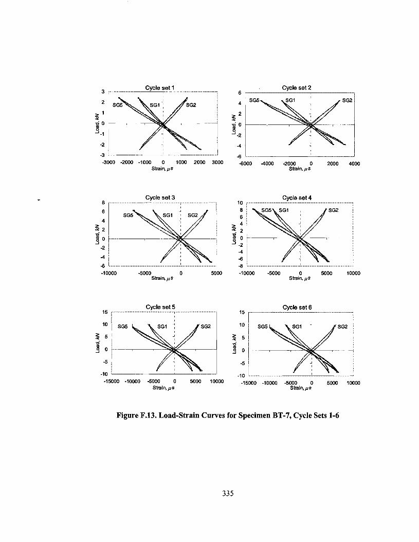
, Cycle set 2
' -3000 -2000 -1000 0 1000 2000 3000 BOO0 4000 -2000 0 2000 4000
Shin, p s Strain, p s
Cycle set 3 Cycle set 4 .. ............... ............................................. 8 r r I ........................................ :
-10000 -5000 0 5000 -10000 -5000 0 5000 10000 Strain, p s Strain. ps
Cycle set 5 15 , ........................................................................................................................... Cycle set 6
15 i
-15000 -10000 -5000 0 5000 10000 -15000 -10000 -5000 0 5000 10000 Strain, p s Strain, p s
Figure F.13. Load-Strain Curves for Specimen BT-7, Cycle Sets 1-6

Cycle set 7 15 .......................................................................... "
Cycle set 8 20 7-- I 1
-15000 -10000 -5000 0 5000 10000 -15000 -10000 -5000 0 5000 10000 Strain. p s Strain, p s
-1 5000 -10000 -5000 0 5000 10000 15000 -15000 -10000 -5000 0 5000 10000 Strain. p s Strainrrrs
-15000 -10000 -5000 0 5000 10000 15000 -15000 -10000 -5000 0 5000 10000 Strain, p s Strain, p s
Figure F.14. Load-Strain Curves for Specimen BT-7, Cycle Sets 7-12
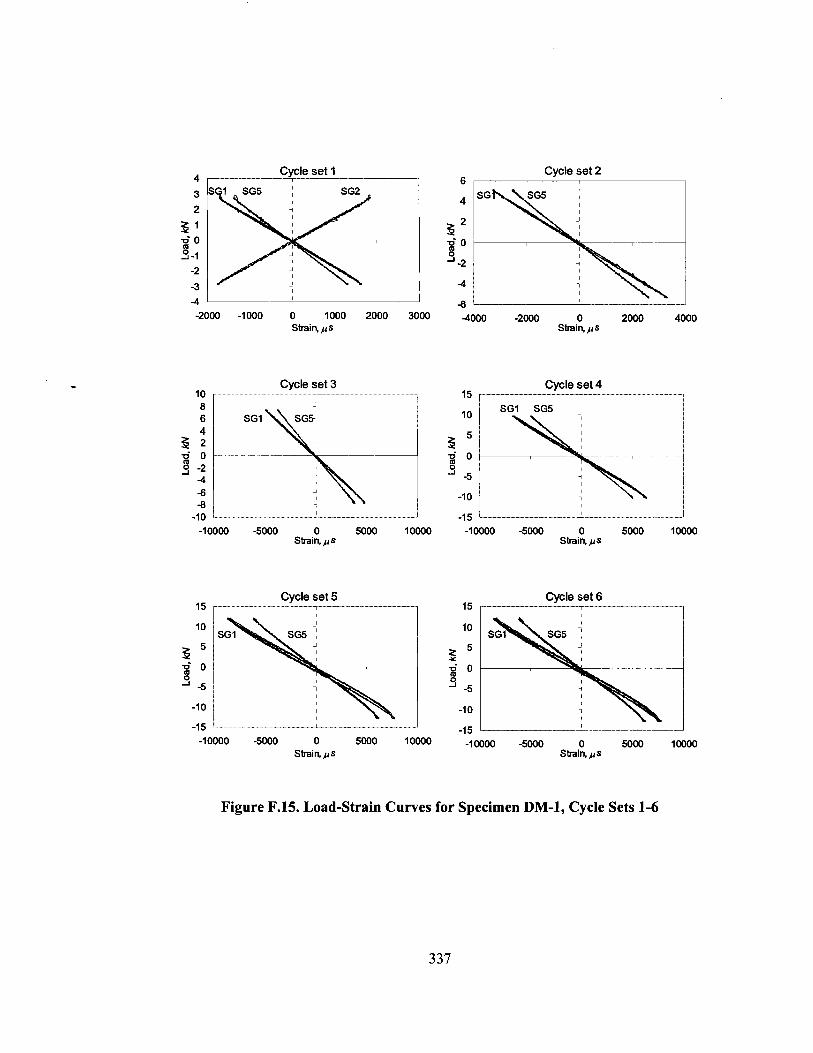
Cycle set 1 Cycle set 2 4 6
3 4 2
s s z- 0 3- 0
4 -1 A 0 -2
-2 4 3
4 -6 -2000 -1000 0 1000 2000 3000 4000 -2000 0 2000 4000
Shin, ps Strain. ps
Cycle set 3
-10000 -5000 0 5000 10000 -10000 -5000 0 5000 10000 Shin, ps Strain, ps
15
10
2
2 0 m
3-5
-1 0
-1 5 -10000 -5000 0 5000 10000 -10000 -5000 0 5000 10000
Shin, ps Shin, ps
Figure F.15. Load-Strain Curves for Specimen DM-1, Cycle Sets 1-6
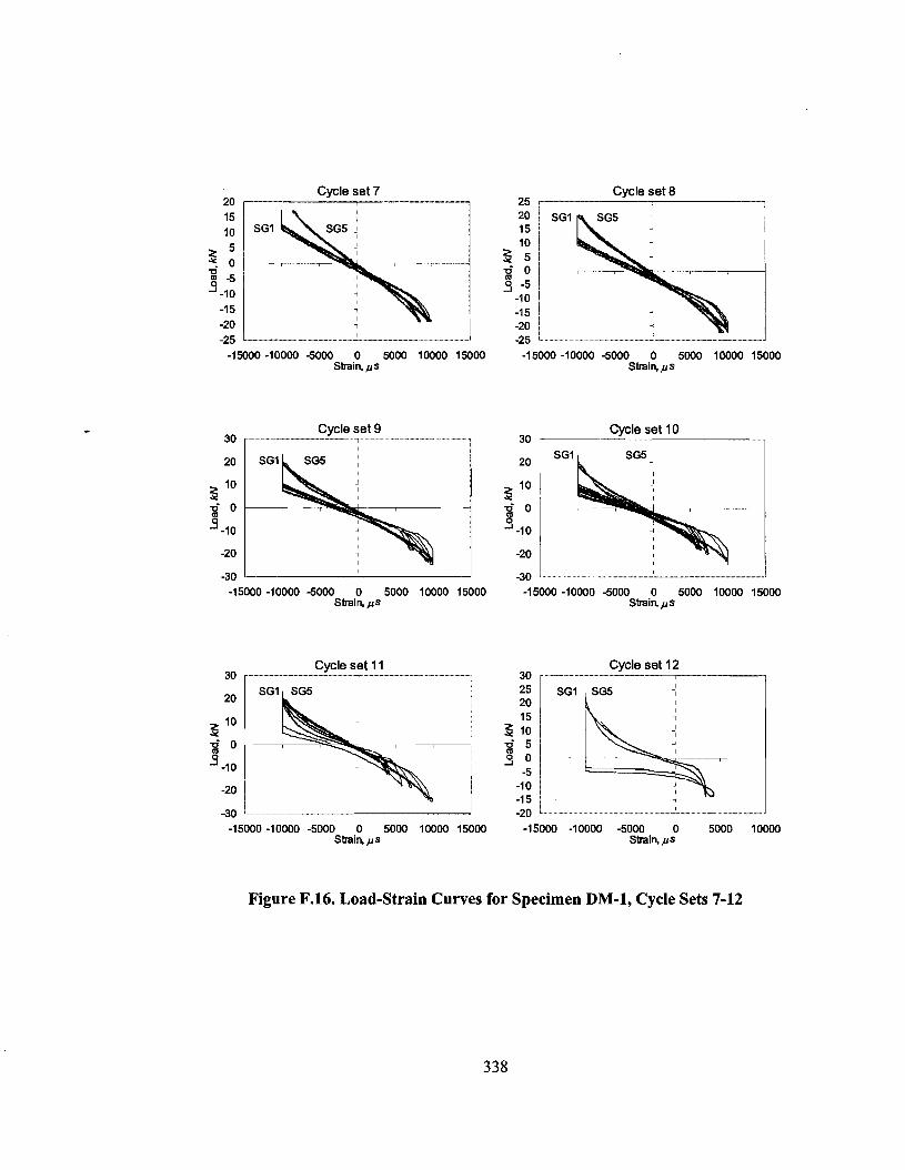
Cycle set 7 Cycle set 8 20 7-- I
-15000 -10000 -5000 0 5000 10000 15000 -15000 -10000 -5000 0 5000 10000 15000 Shin. ,US Strain,ps
Cycle set 9 Cycle set 10
-15000 -10000 5000 0 5000 10000 15000 -15000 -10000 5000 0 5000 10000 15000 Shin. ,US Strain. ,U s
Cycle set 1 1 30 ............................................................................................................ Cycle set 12
30 I
-15000 -10000 -5000 0 5000 10000 15000 -15000 -10000 -5000 0 5000 10000 Strain, ,US Shin. ,US
Figure F.16. Load-Strain Curves for Specimen DM-1, Cycle Sets 7-12
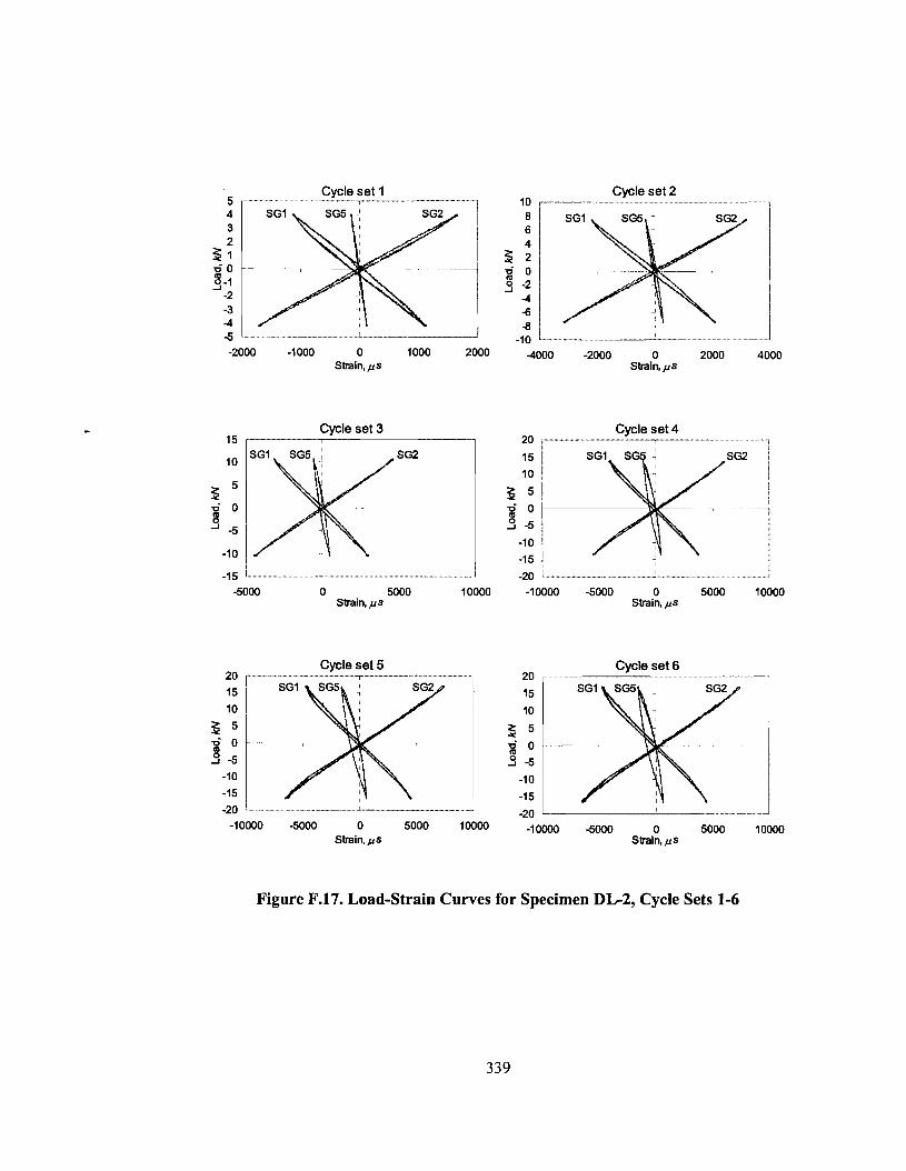
Cycle set 1 5 , 7..........." " ... Cycle set 2 ................................... ..... 10 i
..
-2000 -1000 0 1000 2000 4000 -2000 0 2000 4000 Strain, p s Strain, p s
Cycle set 3
7--- -
-5000 0 5000 10000 -10000 -5000 0 5000 10000 Strain, p s Strain, ps
Cycle set 5 ........................................................................ ..
-5000 0 5000 Strain, p s
Cycle set 6
-10000 -5000 0 5000 10000 Strain, p s
Figure F.17. Load-Strain Curves for Specimen DL-2, Cycle Sets 1-6
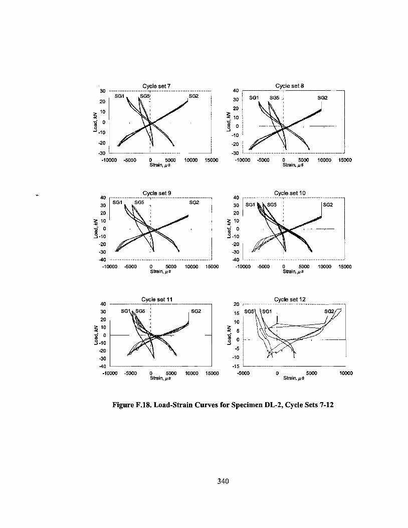
Cycle set 8
v- --.
......... ....
-10000 -5000 0 5000 I0000 15000 -10000 -5000 0 5000 I0000 15000 Shin, rS Strain, ,US
Cycle set 9 40
30
20
5 10
d 0 m S -10
-20
-30
Cycle set 11 Cycle set 12 40 r------ 20 ,-..
-10000 -5000 0 5000 I0000 15000 -5000 0 5000 I0000 Strain, ,US Strain. ,US
Figure F.18. Load-Strain Curves for Specimen DL-2, Cycle Sets 7-12
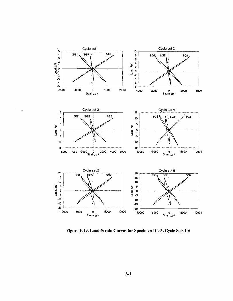
Cycle set 1 5 r......................................." ............-.-..-...-.r-.............................-........................w....., Cycle set 2
10 .
-2000 -1000 0 1000 2000 4000 -2000 0 2000 4000 Shin, ps Shin. ps
15
10
5 i5 i O
-5
-1 0
-1 5 SO00 4000 -2000 0 2000 4000 6000 -10000 -5000 0 5000 10000
Shin, ps Strain, ps
. -.7.-. .. .- .....
1
-20 - -'-- -20 / I i
-10000 -5000 0 5000 10000 -10000 -5000 0 5000 10000 Strain, ps Shin, pS
Figure F.19. Load-Strain Curves for Specimen DL-3, Cycle Sets 1-6
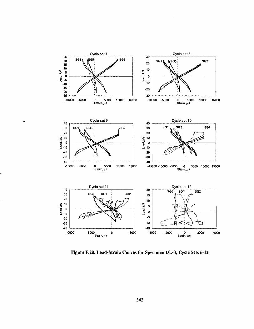
25 20 15 10
s 5 u- 0 4 4
-1 0 -15 -20 -25
-10000 -5000 0 5000 10000 15000 -10000 -5000 0 5000 10000 15000 Strain, ps Strain, ps
Cycle set 9 40 l--...---.-..--.-,.. Cycle set 10
I 40
-40 I -40 1 -10000 -5000 0 5000 10000 15000 -15000 -10000 -5000 0 5000 10000 15000
Strain. ps Strain. ps
Cycle set 11 40 T I Cycle set 12
-10000 -5000 0 5000 -4000 -2000 0 2000 4000 Strain, ps Strain. ps
Figure F.20. Load-Strain Curves for Specimen DL-3, Cycle Sets 6-12

Cycle set 1 4 r------------
Cycle set 2 8 I - 1
-2000 -1000 0 1000 2000 4000 -2000 0 2000 4000 Strain, ps Strain, ps
Cycle set 3 10 .. ... .. .. . . .. .. Cycle set 4
15 i-----.7-....-.---.---..-.--.-- "
SG2
~-
I
4000 -2000 0 2000 4000 6000 -10000 -5000 0 5000 lo000 Strain, ps Strain. ps
Cycle set 6 20
15
J -5 , -10
I -1 5
-10000 -5000 0 5000 10000 -10000 -5000 0 5000 10000 Strain, ps Strain, ps
Figure F.21. Load-Strain Curves for Specimen DS-4, Cycle Sets 1-6

Cycle set 7 25 r.. ....................................................................................................... --- 30 ;-----
Cycle set 8
-10000 -5000 0 5000 10000 15000 -10000 -5000 0 5000 10000 15000 Strain, ps Strain, p s
............... 40 Cycle set 10 T-.--
--
3 0 1 1 3 0 ; .... -10000 -5000 0 5000 10000 15000 -10000 -5000 0 5000 10000 15000 20000
Strain, ps Strain, p s
40 30
30 20
20
9 10 u
3-i lo d 0
0 -I
8 -I -10
-1 0
-20 -20
-30 -30
4 -20000 -1 0000 0 10OOO 20000 -10000 -5000 0 5000 10000 15000
Strain. ps Strain, p s
Figure F.22. Load-Strain Curves for Specimen DS-4, Cycle Sets 7-12

Cycle set 2 4 3 2
h :, d m -1 3 -2
-3 4 -5 .
-2000 -1000 0 1000 2000 4000 -2000 0 2000 4000 Shin. f i s Straln, f i s
Cycle set 3 Cycle set 4
6000 4000 -2000 0 2000 4000 6000 -10000 -5000 0 5000 10000 Strain, f i s Strain, f i s
Cycle set 5 Cycle set 6 10 8 6 4
2 2 -*. 0 x -2 9 4
-6 -8
-1 0 -12 .
-10000 -5000 0 5000 10000 -10000 -5000 0 5000 10000 Strain, f i s Strain, p s
Figure F.23. Load-Strain Curves for Specimen DL-5, Cycle Sets 1-6

Cycle set 7 .. ..-.. " Cycle set 8 . .... . ........................ 15 ,
j -20 i . .... "...l--." ..................... J -15000 -10000 -5000 0 5000 10000 15000 -1 5000 -10000 -5000 0 5000 10000 15000
Stiain, p s Strain, p s
Cycle set 9 20 y------+. Cycle set 10 ................ .. r - - - - - . . 7 7- -'l
-25 -30 -1 5000 -10000 -5000 0 5000 I0000 15000 -15000 -10000 -5000 0 5000 10000 15000
Strain. p s Strain, p s
-15000 -10000 -5000 0 5000 10000 15000 4000 -2000 0 2000 4000 Strain, p s Strain.ps
Figure F.24. Load-Strain Curves for Specimen DL-5, Cycle Sets 7-12
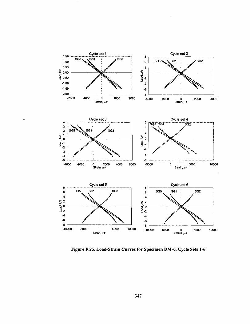
.... ..., ... ... , Cycle set 2
- - . - - - . - .- .- -2000 -1000 0 1000 2000 4)oo -2000 0 2000 4000
S t r a i ~ ps Straln, p s
Cycle set 3 Cycle set 4
4000 -2000 0 2000 4000 6000 -5000 0 5000 10000 Strain, p s Strain, p s
Cycle set 5 8 .. ... Cycle set 6
8 --.- --- 1
-10000 -5000 0 5000 10000 -10000 -5000 0 5000 10000 Strain, pS Strain. pS
Figure F.25. Load-Strain Cuwes for Specimen DM-6, Cycle Sets 1-6

Cycle set 7 10 ......................................................................................... "
Cycle set 8 I 1
-10000 -5000 0 5000 10000 15000 -10000 -5000 0 5000 10000 15000 Shin, ps Shin, ps
Cycle set 9 15 r.---.-.....--------.---7--.--.--...-., Cycle set 10 15 -. "I
-15000 -10000 -5000 0 5000 10000 15000 -10000 5000 0 5000 10000 15000 Shin. ps Strain, ps
Figure F.26. Load-Strain Curves for Specimen DM-6, Cycle Sets 7-12

Cycle set 1 5 .- . - ?"
4 SG5 SGl
3
A -1 -2 -3 -4 3000 -2000 -1000 0 1000 2000 3000
Strain, p s
Cycle set 2 1
-6000 4000 -2000 0 2000 4000 6000 Strain, p s
Cycle set 3 Cycle set 4 . . . . . . . . 15 I 1 - ....,
-10000 -5000 0 5000 10000 -10000 -5000 0 5000 10000 Strain, p s Strain. ps
Cycle set 5 20 , . Cycle set 6
................................................................................. ............................................... 1 20 ,
-20 L -'.-A -15000 -10000 -5000 0 5000 10000 -15000 -10000 -5000 0 5000 10000
Strain, ps Strain, ps
Figure F.27. Load-Strain Curves for Specimen DL-7, Cycle Sets 1-6
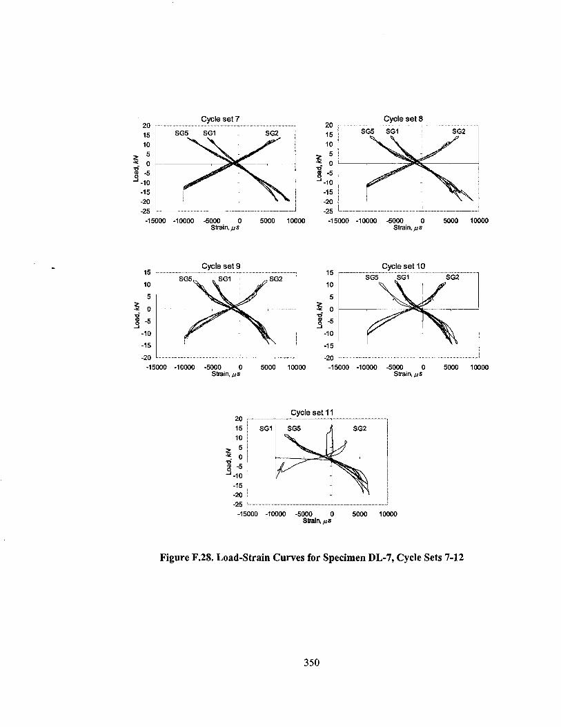
Cycle set 7 Cycle set 8 I
SG5 SG1 SG2
-15000 -10000 5000 0 5000 I0000 -15000 -10000 5000 0 5000 I0000 Strain, ps Strain, ps
Cycle set 9 Cycle set 10
-20 I -20 -15000 -10000 -5000 0 5000 10000 -15000 -10000 -5000 0 5000 I0000
Strain, ps Shin, ps
Cycle set I I
-15000 -10000 -5000 0 5000 I0000 Shin, ps
Figure F.28. Load-Strain Curves for Specimen DL-7, Cycle Sets 7-12

Appendix G
Assembly of Stiffened Panels and Doubler Plates onto the Hydrostatic
Test Tank
Appendix G.1. Phase 1: Sealing of the Steel Flange/Composite Panel Interfaces
1. Using jacks, raise the desired panel off the steel I-beam, with enough clearance to
clean the surfaces and apply the sealant, as shown in Figure G. 1.
Figure G.1. Small Panel Suspended off the Hydrostatic Test Tank
2. Using aerosol parts cleaner, thoroughly clean the bottom surfaces of the panels, where
they will interface with the steel flanges (Figure G.2).
3. Clean the top surfaces of the steel flanges, with aerosol parts cleaner (Figure G.2).

Figure G.2. Steel I-beam and Small Panel Interfaces
4. Apply the silicone sealant to the upper surface of the steel flanges, where it will
interface with the bottom surface of the panels, as shown in Figure G.3. Two beads of
sealant along the depth of the steel beam are recommended, to insure a uniform and
continuous seal along the interfaces.
Figure G.3. Application of Silicon Sealant at I-beam/Panel Interfaces
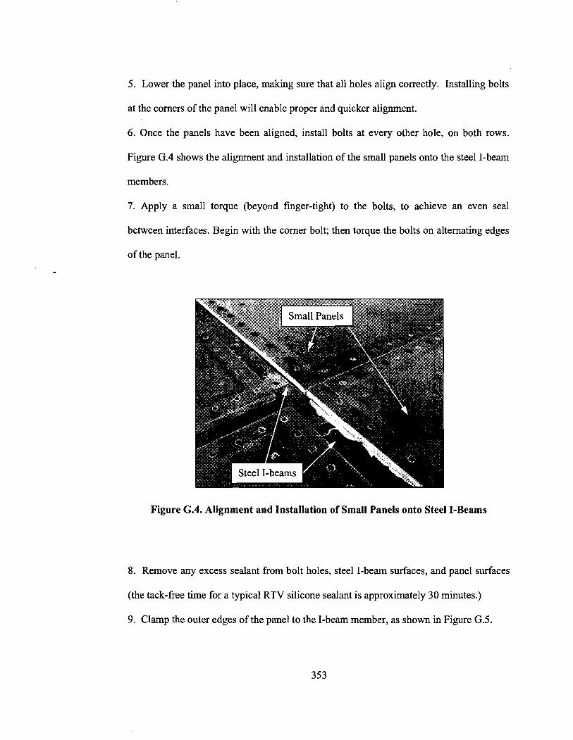
5. Lower the panel into place, making sure that all holes align correctly. Installing bolts
at the comers of the panel will enable proper and quicker alignment.
6. Once the panels have been aligned, install bolts at every other hole, on both rows.
Figure G.4 shows the alignment and installation of the small panels onto the steel I-beam
members.
7. Apply a small torque (beyond finger-tight) to the bolts, to achieve an even seal
between interfaces. Begin with the comer bolt; then torque the bolts on alternating edges
of the panel.
Figure G.4. Alignment and Installation of Small Panels onto Steel I-Beams
8. Remove any excess sealant fi-om bolt holes, steel I-beam surfaces, and panel surfaces
(the tack-free time for a typical RTV silicone sealant is approximately 30 minutes.)
9. Clamp the outer edges of the panel to the I-beam member, as shown in Figure G.5.
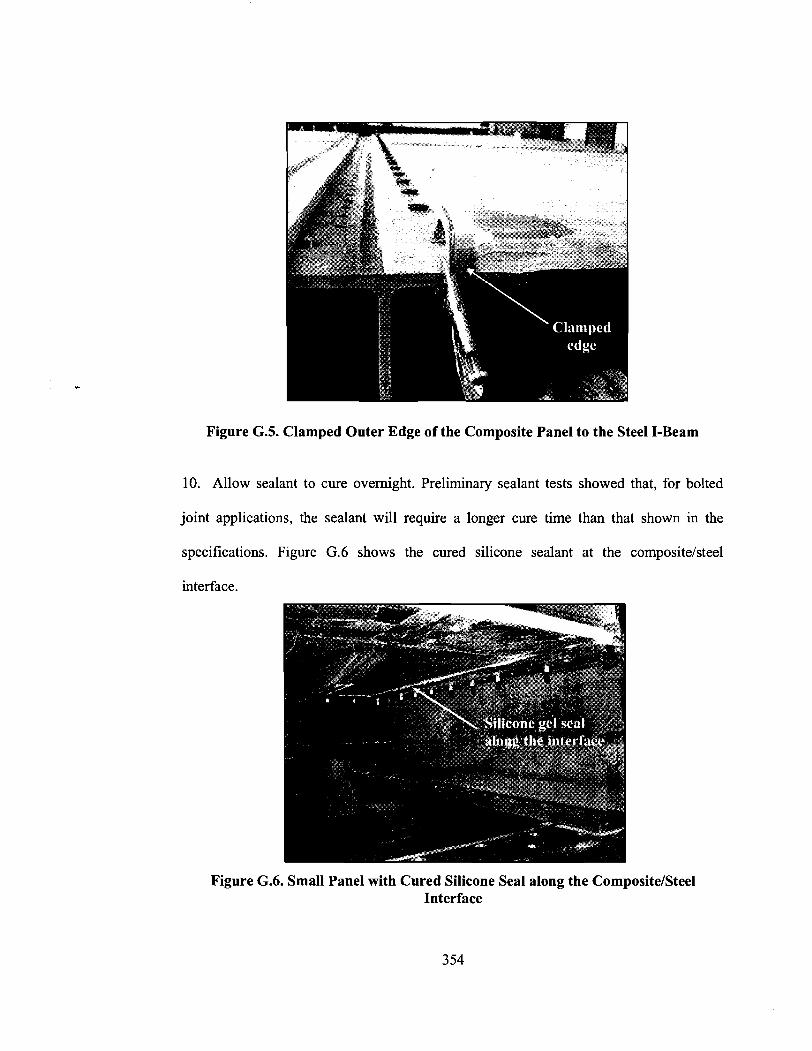
Figure G.5. Clamped Outer Edge of the Composite Panel to the Steel I-Beam
10. Allow sealant to cure overnight. Preliminary sealant tests showed that, for bolted
joint applications, the sealant will require a longer cure time than that shown in the
specifications. Figure G.6 shows the cured silicone sealant at the composite/steel
interface.
Figure G.6. Small Panel with Cured Silicone Seal along the CompositeISteel Interface

11. Repeat steps 1 through 10 for panels 2 ,3 and 4. [Note: the interfaces between panels
1 and 2 and the steel I-beam were sealed on the same day (07-18-04) and allowed to cure
for over 48 hours. The large panels (3 and 4) were sealed at a later date (07-25-04)].
12. Fill the seams between the edges of the panels with silicone sealant and smooth-flush
with panels. Begin at the center of the panel, working the silicone gel outwardly, as
shown in Figure G.7.
Figure G.7. Application of the Silicone Sealant at the Panel Seams
13. Allow the sealant to cure for a period of at least 48 hours.
355
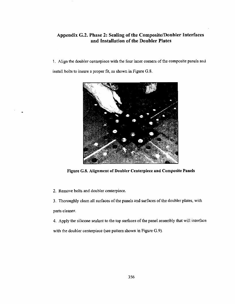
Appendix G.2. Phase 2: Sealing of the Composite/Doubler Interfaces and Installation of the Doubler Plates
1. Align the doubler centerpiece with the four inner comers of the composite panels and
install bolts to insure a proper fit, as shown in Figure G.8.
Figure G.8. Alignment of Doubler Centerpiece and Composite Panels
2. Remove bolts and doubler centerpiece.
3. Thoroughly clean all surfaces of the panels and surfaces of the doubler plates, with
parts cleaner.
4. Apply the silicone sealant to the top surfaces of the panel assembly that will interface
with the doubler centerpiece (see pattern shown in Figure G.9).

Figure G.9. Application of the Silicone Sealant to the Top Surfaces of the Composite Panels
5. Set doubler centerpiece on top of the composite panel comers, making sure that all
holes align properly.
6. Install all bolts, without applying any torque.
7. Spray all bolts with anti-seize lubricant and install washers and nuts.
8. Apply a finger-tight torque to all bolts.
9. Apply 50 percent of the specified torque (25 ft-lb) using the torque pattern shown in
Figure G.lO. Begin with the bolts at the center of the doubler centerpiece and then move
to the outside bolts.
10. Using the same torque pattern, apply 100 percent of the specified torque to the bolts.

Figure G.lO. Bolt Torque Pattern Used for Installation of the Doubler Centerpiece
11. Align the doubler plate with the edges of the composite panels and install comer
bolts, to insure a proper fit.
12. Remove bolts and doubler plate.
13. Thoroughly clean all surfaces of the panels and surfaces of the doubler plates, using
parts cleaner.
14. Apply the silicone sealant to the top surfaces of the panel assembly that will interface
with the doubler plates, shown in Figure G.ll . Using four beads of sealant is
recommended for a proper sealant distribution at the interfaces.

Figure G.ll . Application of Silicone Sealant at the Composite/Doubler Interfaces
15. Set the doubler piece in place, installing two corner bolts, to insure proper alignment,
as shown in Figure G. 12.
Figure G.12. Application of Silicone Sealant at the Composite/Doubler Interfaces
359

16. Install all bolts.
17. Spray all bolts with anti-seize lubricant and install washers and nuts.
18. Apply a finger-tight torque.
19. Starting with the bolts closest to the doubler centerpiece, apply 50 percent of the
specified torque (25 ft-lb). Apply torque to the remaining bolts, working towards the
outside edge, in the direction of the arrows shown in Figure G.13.
Figure G.13. Torque Direction for Installation of Doubler Plates
20. Using the same torque pattern in Figure G.13, apply 100 percent of the specified
torque to the bolts. Clamp the outer edges of the doubler (towards the tank boundary) to
achieve a uniform clamping pressure along the length of the doubler plate.
21. Repeat steps 11 through 20 for the remaining doubler plates, D23, D34, and D41.
The assembled panel and doubler plate arrangement, after it sealing at the interfaces and
after all bolts have been torqued to specifications, is shown in Figure G.14.

Figure G.14. Wet Side of Hybrid Panel Assembly after Sealing and Installation of the Doubler Plates
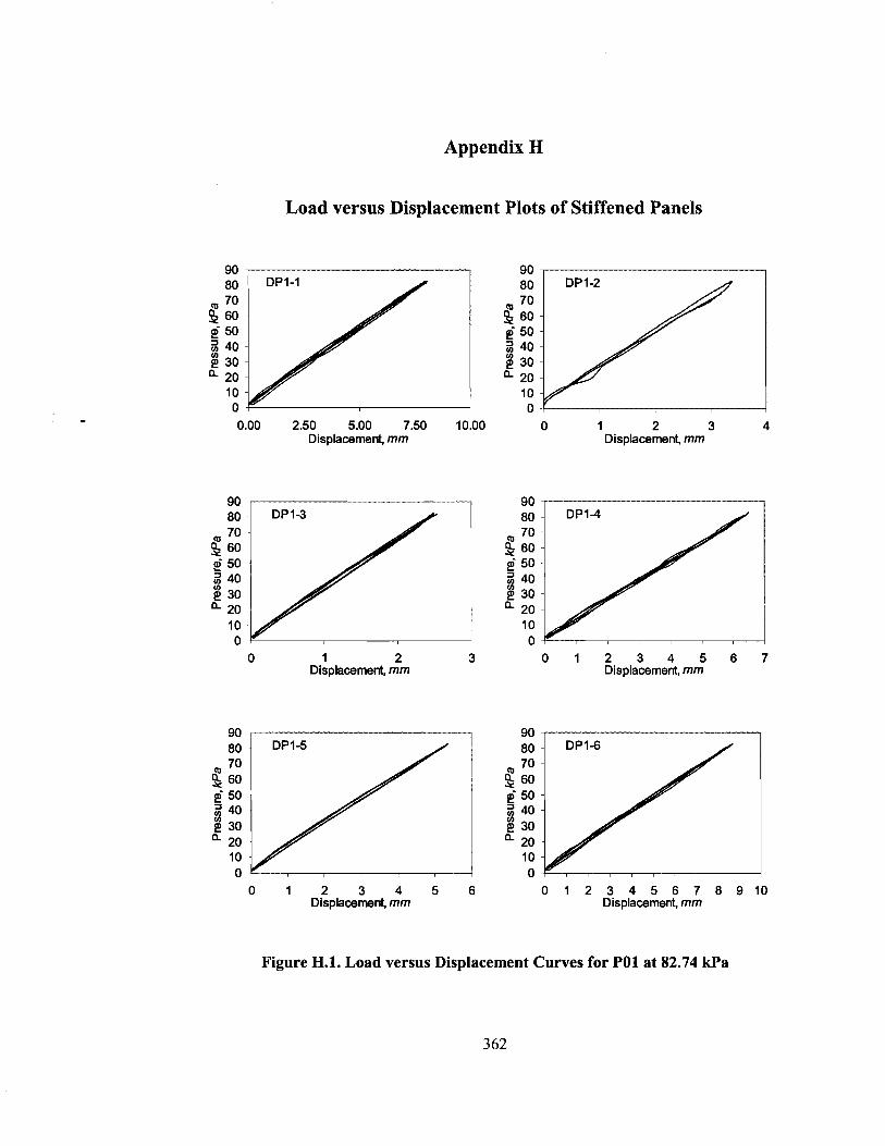
Appendix H
Load versus Displacement Plots of Stiffened Panels
90 80
([I 70
'& 60 @ 50
40 30
a 20 10 0
0.00 2.50 5.00 7.50 10.00 0 1 2 3 4 Displacement, mm Displacement, mm
0 1 2 Displacement, mm
0 1 2 3 4 5 6 7 Displacement, mm
0 1 2 3 4 5 6 0 1 2 3 4 5 6 7 8 9 1 0 Displacement, mm Displacement, mm
Figure H.1. Load versus Displacement Curves for PO1 at 82.74 kPa

0 5 10 15 0 1 2 3 4 5 6 Displacement, mm Displacement, mm
0 1 2 3 4 0 5 10 15 Displacement, mm Displacement, mm
0.00 2.50 5.00 7.50 10.00 0 5 10 15 Displacement, mm Displacement, mm
Figure H.2. Load versus Displacement Curves for PO1 at 124 kPa

0 10 20 30 0 5 10 15 Displacement, mm Displacement, mm
0 5 10 15 20 0 10 20 30 Displacement, mm Displacement, mm
300 1 300
Figure H.3. Load versus Displacement Curves for PO1 at 248 kPa
DPl-3 DPl-4 250 - I
250 - I
(II i
#200 - 2 200 - a-
$150 - V)
g 150 V)
t loo - L
t l o o a
I 50 - 1 50 -
I 0 0
0 2 4 6 8 0 10 20 30 Displacement, mm Displacement, mm

0.00 2.50 5.00 7.50 10.00 0.00 2.50 5.00 7.50 Displacement, mm Displacement, mm
0 1 2 3 Displacement, mm
0 1 2 3 Displacement, mm
0 2 4 6 0 5 Displacement, mm Displacement, mm
Figure H.4. Load versus Displacement Curves for PO3 at 82.74 kPa
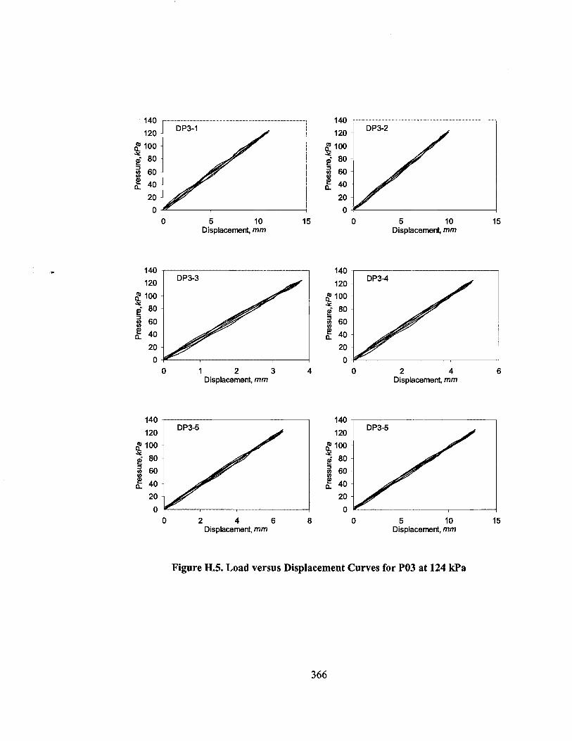
0 5 10 15 0 5 10 15 Displacement, mm Displacement, mm
0 1 2 3 4 0 2 4 6 Displacement, mm Displacement, mm
0 2 4 6 8 0 5 10 15 Displacement, mm Displacement, mm
Figure H.5. Load versus Displacement Cuwes for PO3 at 124 kPa
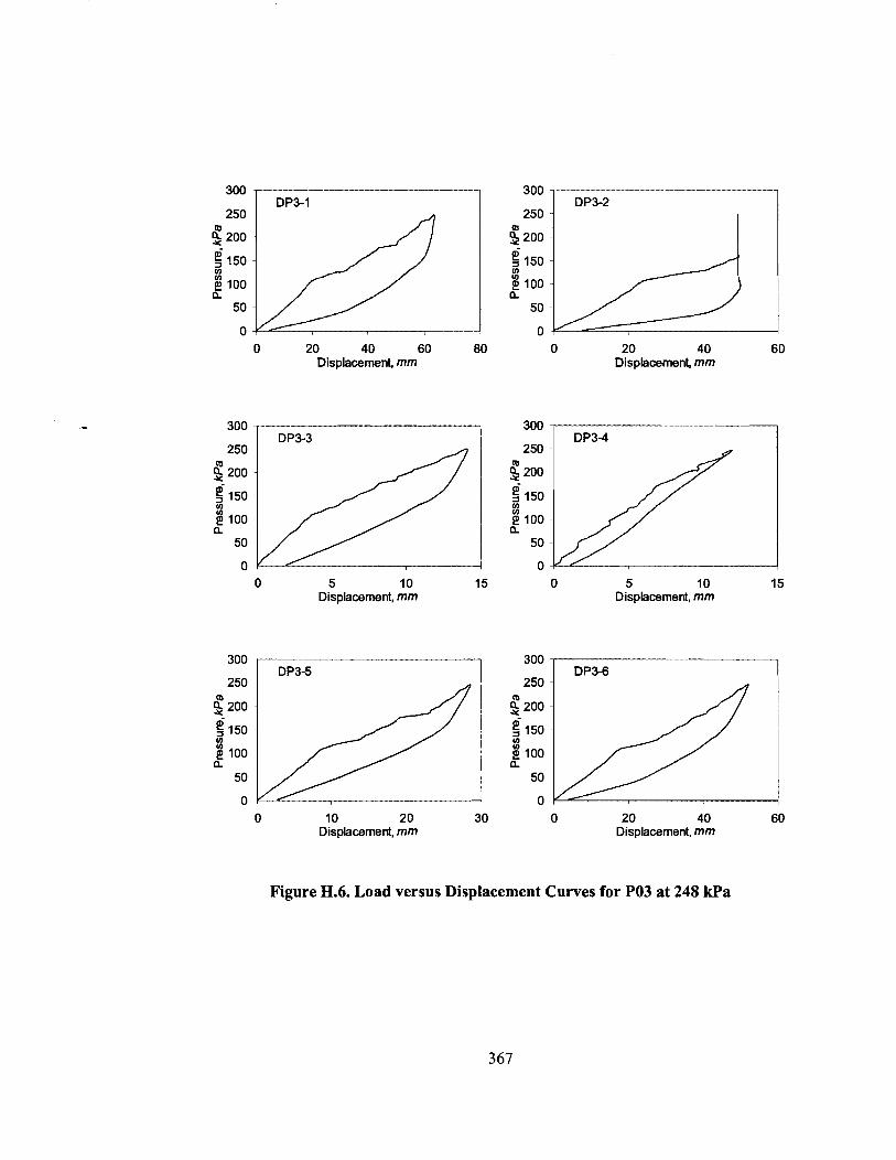
0 20 40 60 80 0 20 40 60 Displacement, mm Displacement, mm
0 5 10 15 0 5 10 15 Displacement, mm Displacement, mm
0 10 20 30 0 20 40 60 Displacement, mm Displacement, mm
Figure H.6. Load versus Displacement Curves for PO3 at 248 kPa

BIOGRAPHY OF THE ALTTHOR
Jean Paul Kabche was born in Caracas, Venezuela on June 27, 1978. He spent
most of his young years between the cities of Caracas and Puerto Ordaz. In June 1995,
he graduated from Colegio Sun Luis, in Caracas. Upon accepting a full international
student tuition waiver, he came to the University of Maine in August 1995 and received a
Bachelor of Science degree in Mechanical Engineering in May 1999 and a Master of
Science degree in Mechanical Engineering in August 2001.
After receiving his degree, Jean Paul will continue his computational and
experimental research work in the academic environment as a Post-Doctoral Research
Associate at the University of Maine. He is a candidate for the Doctor of Philosophy
degree in Mechanical Engineering from the University of Maine in May, 2006.