Embed Size (px)
Citation preview

Pier Luca Maffettone - Nonlinear Dynamical Systems I AA 2008/09
Lezione 5
Structural stability and bifurcations
Structural stability and bifurcations /61Lezione 5
AA 2008/2009 Pier Luca Maffettone Nonlinear Dynamical Systems I AA 2008/09
References
2
Strogatz, S. H., Nonlinear dynamics and chaos: with application to physics, biology, chemistry and engineering, Addison Wesley, New York 1994.
Very instructive with simple approach
Wiggins S., Introduction to applied nonlinear dynamical systems and chaos, Springer Verlag, New York 1990 (2nd Ed. 2003)
Kuznetsov Y. A., Elements of applied bifurcation theory, Springer Verlag, New York 2004 (3rd Rev. Ed.)
A complete overview of the problems
Carr J., Applications of centre manifold theory, Springer Verlag, New York, 1981
Very detailed on some aspects
Structural stability and bifurcations /61Lezione 5
AA 2008/2009 Pier Luca Maffettone Nonlinear Dynamical Systems I AA 2008/09
Previous lectures - Nonlinear dynamical systems
Stability of hyperbolic equilibrium points and periodic orbits
Stability of nonhyperbolic situations
Center manifold theorem
Dynamics on the center manifold
The linearized dynamics does not give information on stability
3
Structural stability and bifurcations /61Lezione 5
AA 2008/2009 Pier Luca Maffettone Nonlinear Dynamical Systems I AA 2008/09
Motivations - Theory
Models contain parameters
What happens to the geometry of the phase space when a parameter changes?
Quantitative changes
Qualitative changes
Implication on the safety
Qualitative changes will be called bifurcations.
When can we observe qualitative changes?
Can we a priori know the possible scenarios for different dynamical systems?
Dynamical systems can be quite “large”: do we need to account for details of their “largeness” or we can limit to something simpler?
4
Structural stability and bifurcations /61Lezione 5
AA 2008/2009 Pier Luca Maffettone Nonlinear Dynamical Systems I AA 2008/09
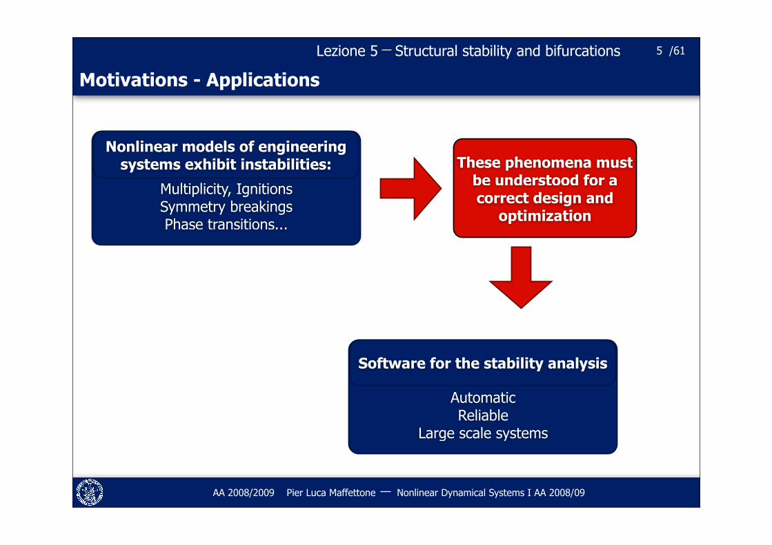
Motivations - Applications
5
Multiplicity, IgnitionsSymmetry breakingsPhase transitions...
Nonlinear models of engineering systems exhibit instabilities:
Automatic Reliable
Large scale systems
Software for the stability analysis
These phenomena must be understood for a correct design and
optimization
Structural stability and bifurcations /61Lezione 5
AA 2008/2009 Pier Luca Maffettone Nonlinear Dynamical Systems I AA 2008/09
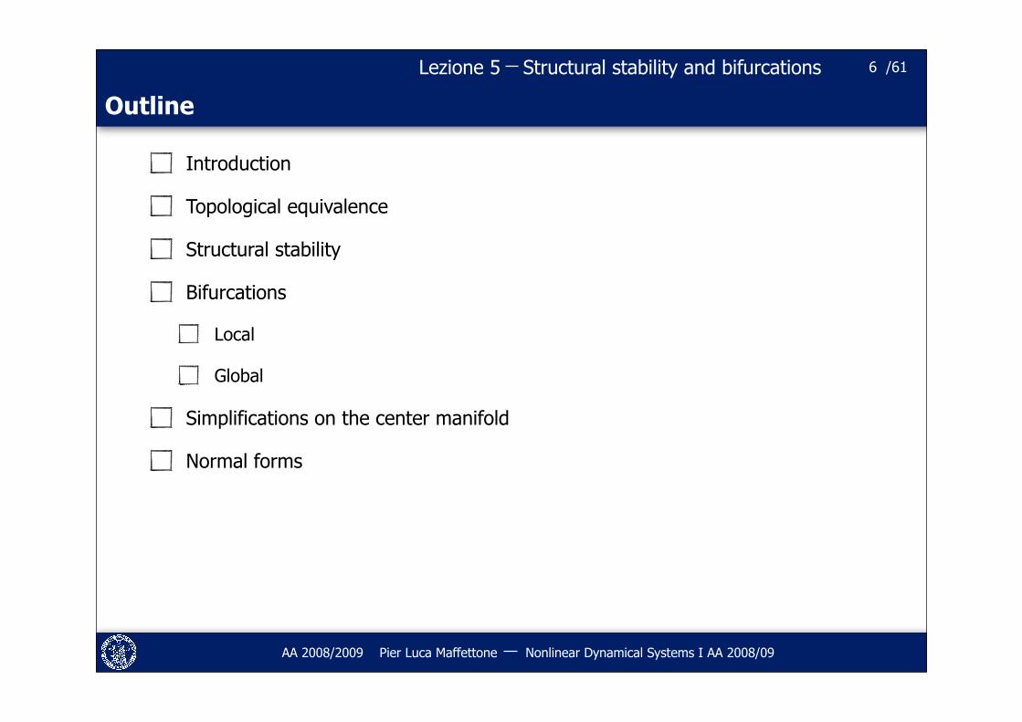
Outline
Introduction
Topological equivalence
Structural stability
Bifurcations
Local
Global
Simplifications on the center manifold
Normal forms
6
Structural stability and bifurcations /61Lezione 5
AA 2008/2009 Pier Luca Maffettone Nonlinear Dynamical Systems I AA 2008/09
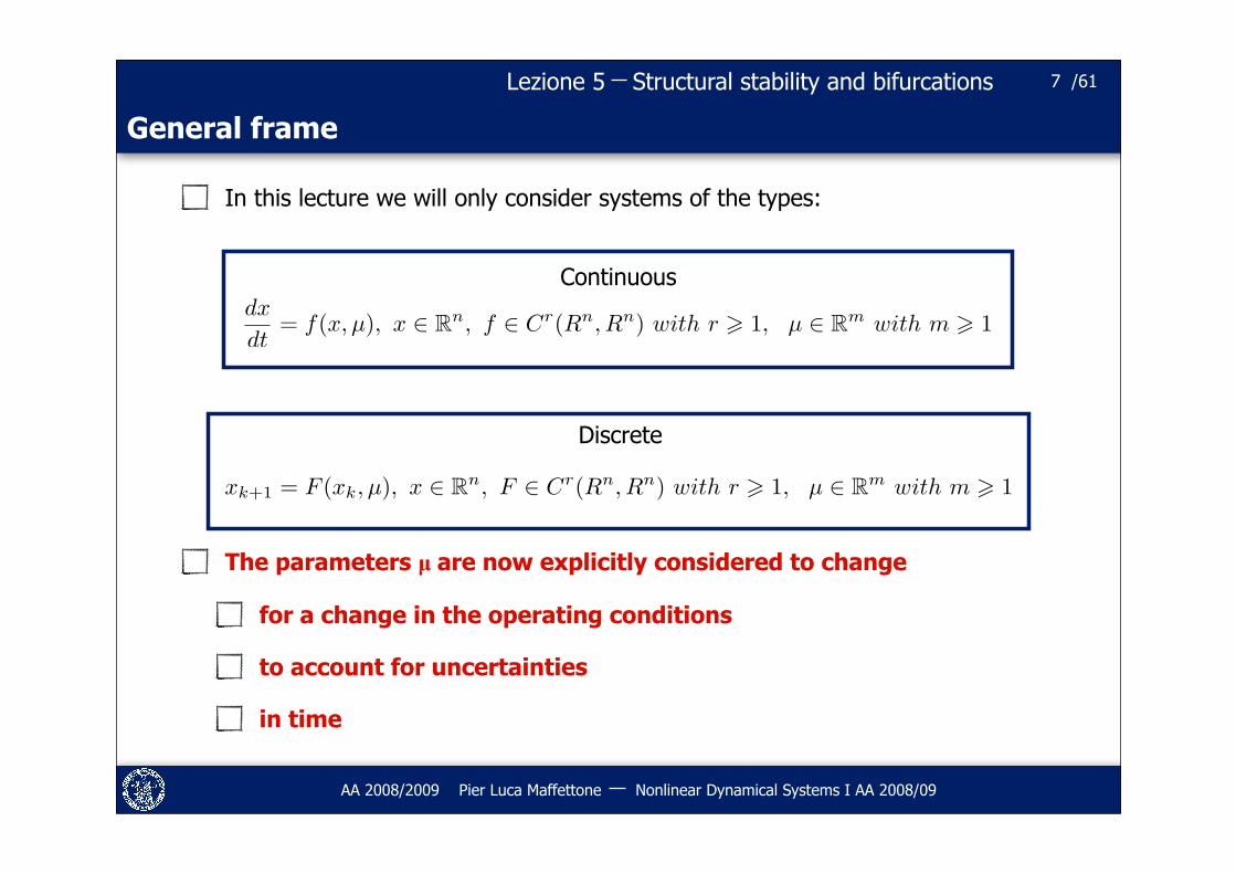
General frame
In this lecture we will only consider systems of the types:
The parameters µ are now explicitly considered to change
for a change in the operating conditions
to account for uncertainties
in time
7
Continuous
Discrete
dx
dt= f(x, µ), x ! Rn, f ! Cr(Rn, Rn) with r ! 1, µ ! Rm with m ! 1
xk+1 = F (xk, µ), x ! Rn, F ! Cr(Rn, Rn) with r ! 1, µ ! Rm with m ! 1
Structural stability and bifurcations /61Lezione 5
AA 2008/2009 Pier Luca Maffettone Nonlinear Dynamical Systems I AA 2008/09
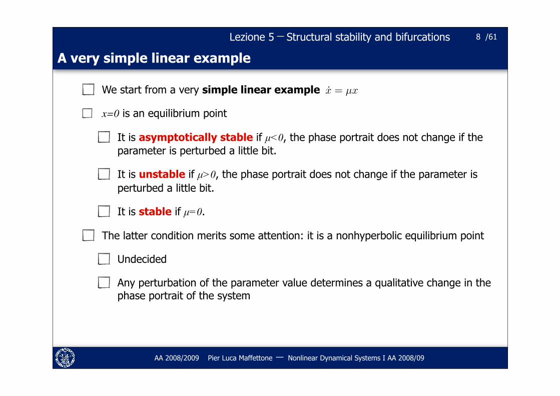
A very simple linear example
We start from a very simple linear example
x=0 is an equilibrium point
It is asymptotically stable if µ<0, the phase portrait does not change if the parameter is perturbed a little bit.
It is unstable if µ>0, the phase portrait does not change if the parameter is perturbed a little bit.
It is stable if µ=0.
The latter condition merits some attention: it is a nonhyperbolic equilibrium point
Undecided
Any perturbation of the parameter value determines a qualitative change in the phase portrait of the system
8
x = µx
Structural stability and bifurcations /61Lezione 5
AA 2008/2009 Pier Luca Maffettone Nonlinear Dynamical Systems I AA 2008/09
Motivation
Two important considerations:
Hyperbolic points seems to be “indifferent” to small parameter changes, while the nonhyperbolic point is strongly affected from them
Is this a kind of stability with respect to parameter changes?
NB: the stability we know was related to changes in the state of the system.
It seems that a qualitative change occurs when the system passes through a nonhyperbolic point: Bifurcations?
These two aspects will be addressed in detail in this lecture.
9

Structural stability and bifurcations /61Lezione 5
AA 2008/2009 Pier Luca Maffettone Nonlinear Dynamical Systems I AA 2008/09
10
Topological equivalence
Structural stability and bifurcations /61Lezione 5
AA 2008/2009 Pier Luca Maffettone Nonlinear Dynamical Systems I AA 2008/09
Topological equivalence of linear systems
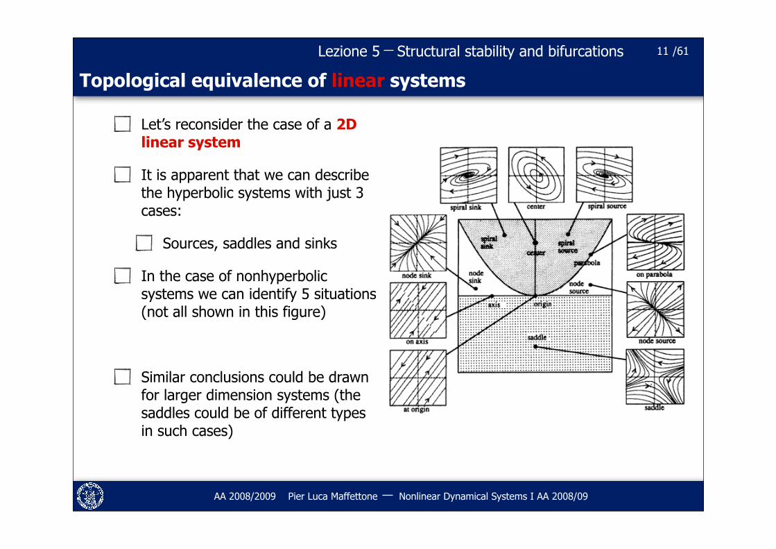
Let’s reconsider the case of a 2D linear system
It is apparent that we can describe the hyperbolic systems with just 3 cases:
Sources, saddles and sinks
In the case of nonhyperbolic systems we can identify 5 situations (not all shown in this figure)
Similar conclusions could be drawn for larger dimension systems (the saddles could be of different types in such cases)
11
Structural stability and bifurcations /61Lezione 5
AA 2008/2009 Pier Luca Maffettone Nonlinear Dynamical Systems I AA 2008/09
Topological equivalence of linear systems
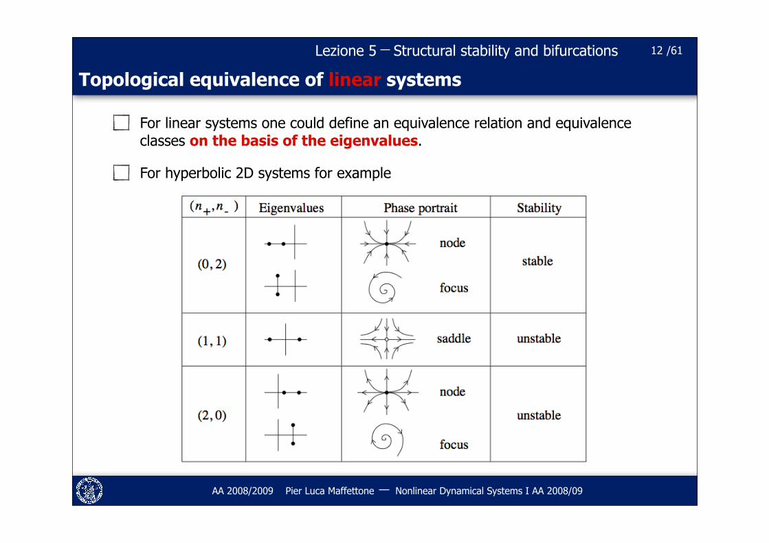
For linear systems one could define an equivalence relation and equivalence classes on the basis of the eigenvalues.
For hyperbolic 2D systems for example
12
Structural stability and bifurcations /61Lezione 5
AA 2008/2009 Pier Luca Maffettone Nonlinear Dynamical Systems I AA 2008/09
Topological equivalence of linear systems
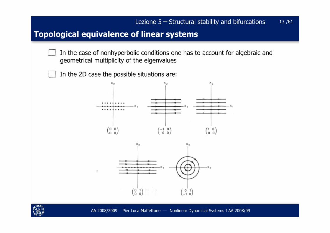
In the case of nonhyperbolic conditions one has to account for algebraic and geometrical multiplicity of the eigenvalues
In the 2D case the possible situations are:
13
Structural stability and bifurcations /61Lezione 5
AA 2008/2009 Pier Luca Maffettone Nonlinear Dynamical Systems I AA 2008/09
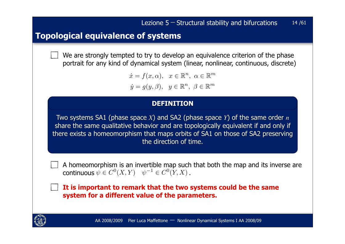
Topological equivalence of systems
We are strongly tempted to try to develop an equivalence criterion of the phase portrait for any kind of dynamical system (linear, nonlinear, continuous, discrete)
A homeomorphism is an invertible map such that both the map and its inverse are continuous .
It is important to remark that the two systems could be the same system for a different value of the parameters.
14
Two systems SA1 (phase space X) and SA2 (phase space Y) of the same order n share the same qualitative behavior and are topologically equivalent if and only if
there exists a homeomorphism that maps orbits of SA1 on those of SA2 preserving the direction of time.
DEFINITION
x = f(x, !), x ! Rn, ! ! Rm
y = g(y,!), y ! Rn, ! ! Rm
! ! C0(X, Y ) !!1 ! C0(Y,X)
Structural stability and bifurcations /61Lezione 5
AA 2008/2009 Pier Luca Maffettone Nonlinear Dynamical Systems I AA 2008/09
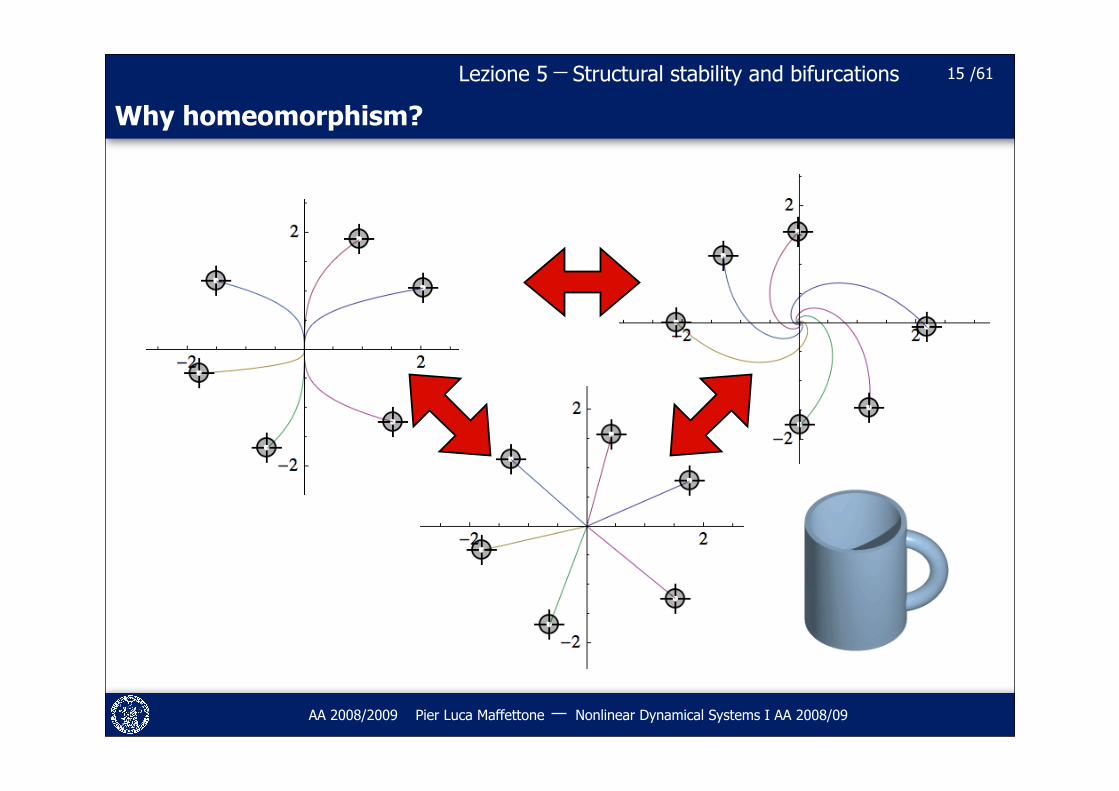
Why homeomorphism?
15
Structural stability and bifurcations /61Lezione 5
AA 2008/2009 Pier Luca Maffettone Nonlinear Dynamical Systems I AA 2008/09
Topological equivalence of systems
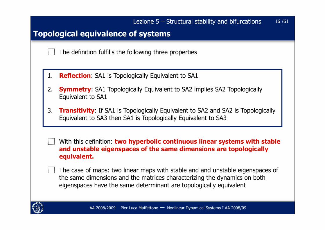
The definition fulfills the following three properties
1. Reflection: SA1 is Topologically Equivalent to SA1
2. Symmetry: SA1 Topologically Equivalent to SA2 implies SA2 Topologically Equivalent to SA1
3. Transitivity: If SA1 is Topologically Equivalent to SA2 and SA2 is Topologically Equivalent to SA3 then SA1 is Topologically Equivalent to SA3
With this definition: two hyperbolic continuous linear systems with stable and unstable eigenspaces of the same dimensions are topologically equivalent.
The case of maps: two linear maps with stable and and unstable eigenspaces of the same dimensions and the matrices characterizing the dynamics on both eigenspaces have the same determinant are topologically equivalent
16
Structural stability and bifurcations /61Lezione 5
AA 2008/2009 Pier Luca Maffettone Nonlinear Dynamical Systems I AA 2008/09
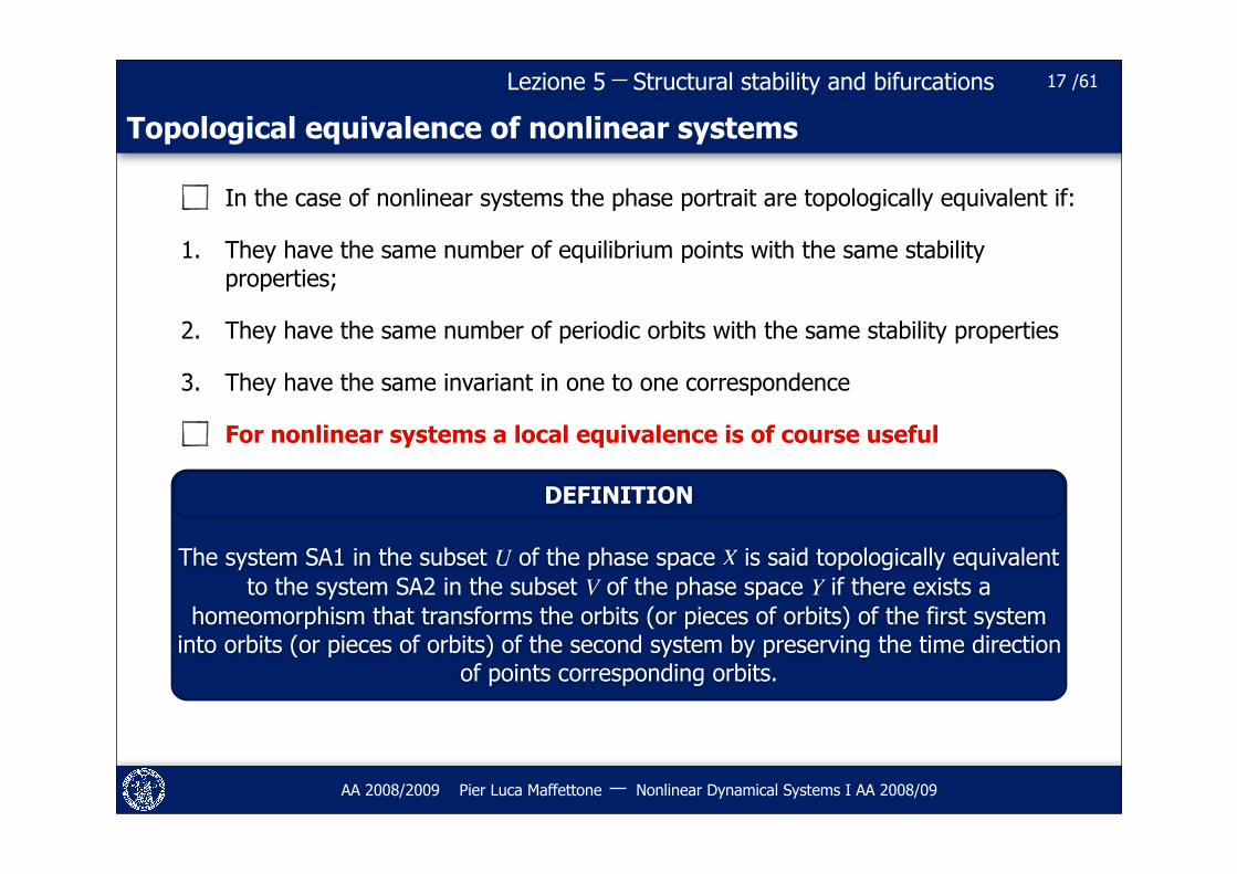
Topological equivalence of nonlinear systems
In the case of nonlinear systems the phase portrait are topologically equivalent if:
1. They have the same number of equilibrium points with the same stability properties;
2. They have the same number of periodic orbits with the same stability properties
3. They have the same invariant in one to one correspondence
For nonlinear systems a local equivalence is of course useful
17
The system SA1 in the subset U of the phase space X is said topologically equivalent to the system SA2 in the subset V of the phase space Y if there exists a
homeomorphism that transforms the orbits (or pieces of orbits) of the first system into orbits (or pieces of orbits) of the second system by preserving the time direction
of points corresponding orbits.
DEFINITION
Structural stability and bifurcations /61Lezione 5
AA 2008/2009 Pier Luca Maffettone Nonlinear Dynamical Systems I AA 2008/09
Topological equivalence of systems
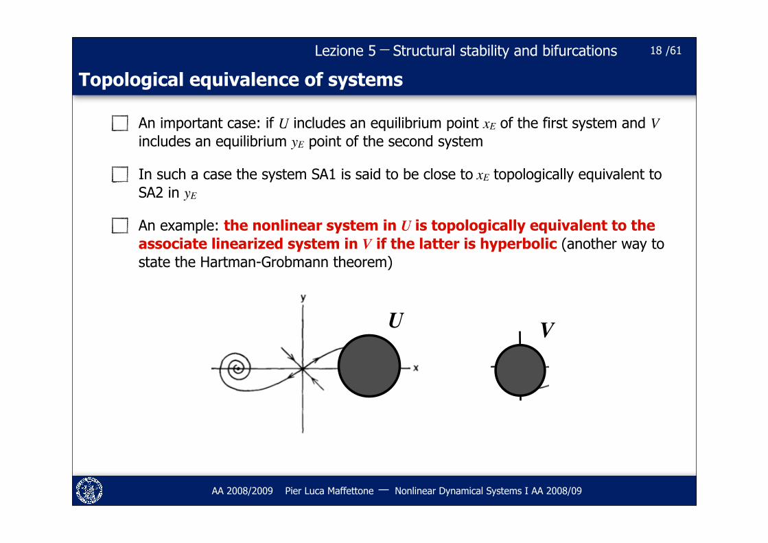
An important case: if U includes an equilibrium point xE of the first system and V includes an equilibrium yE point of the second system
In such a case the system SA1 is said to be close to xE topologically equivalent to SA2 in yE
An example: the nonlinear system in U is topologically equivalent to the associate linearized system in V if the latter is hyperbolic (another way to state the Hartman-Grobmann theorem)
18
U V

Structural stability and bifurcations /61Lezione 5
AA 2008/2009 Pier Luca Maffettone Nonlinear Dynamical Systems I AA 2008/09
19
Bifurcation conditions
Structural stability and bifurcations /61Lezione 5
AA 2008/2009 Pier Luca Maffettone Nonlinear Dynamical Systems I AA 2008/09
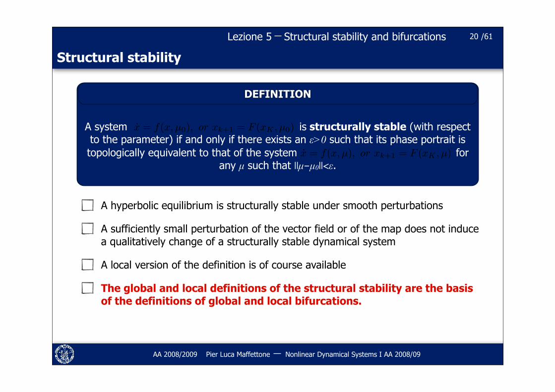
Structural stability
A hyperbolic equilibrium is structurally stable under smooth perturbations
A sufficiently small perturbation of the vector field or of the map does not induce a qualitatively change of a structurally stable dynamical system
A local version of the definition is of course available
The global and local definitions of the structural stability are the basis of the definitions of global and local bifurcations.
20
A system is structurally stable (with respect to the parameter) if and only if there exists an ε>0 such that its phase portrait is topologically equivalent to that of the system for
any µ such that ||µ-µ0||<ε.
x = f(x, µ0), or xk+1 = F (xK , µ0)
x = f(x, µ), or xk+1 = F (xK , µ)
DEFINITION
Structural stability and bifurcations /61Lezione 5
AA 2008/2009 Pier Luca Maffettone Nonlinear Dynamical Systems I AA 2008/09
Bifurcation conditions
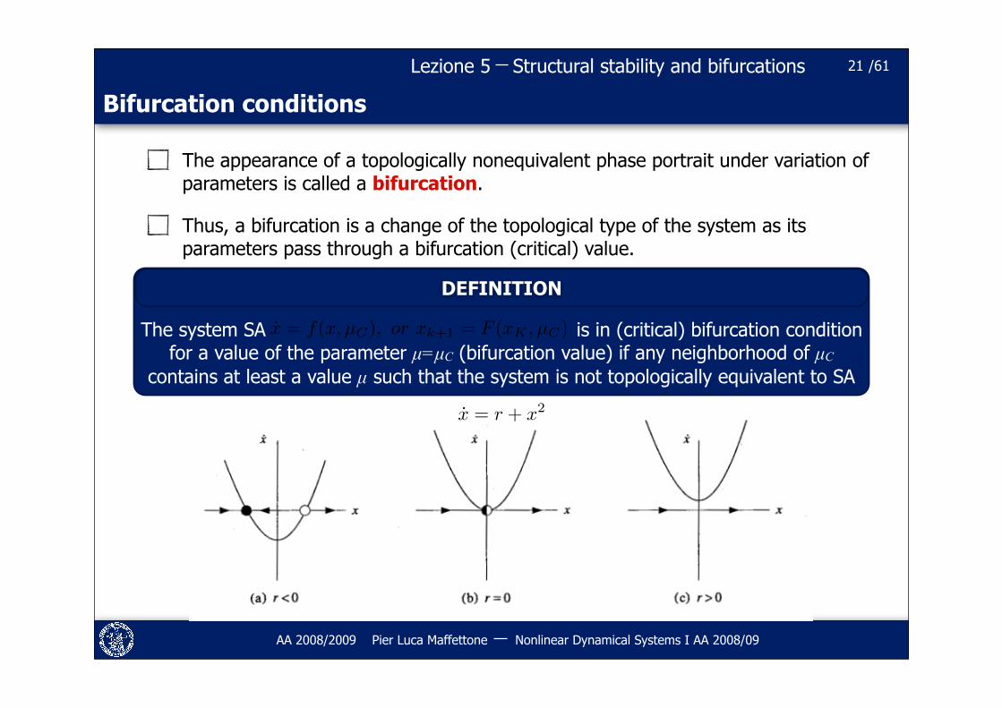
The appearance of a topologically nonequivalent phase portrait under variation of parameters is called a bifurcation.
Thus, a bifurcation is a change of the topological type of the system as its parameters pass through a bifurcation (critical) value.
21
The system SA is in (critical) bifurcation condition for a value of the parameter µ=µC (bifurcation value) if any neighborhood of µC
contains at least a value µ such that the system is not topologically equivalent to SA
DEFINITION
x = f(x, µC), or xk+1 = F (xK , µC)
x = r + x2
Structural stability and bifurcations /61Lezione 5
AA 2008/2009 Pier Luca Maffettone Nonlinear Dynamical Systems I AA 2008/09
Bifurcations
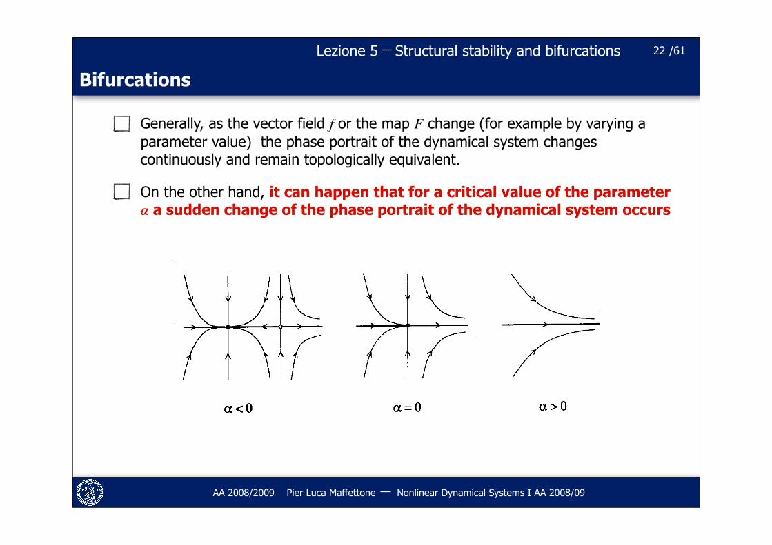
Generally, as the vector field f or the map F change (for example by varying a parameter value) the phase portrait of the dynamical system changes continuously and remain topologically equivalent.
On the other hand, it can happen that for a critical value of the parameter α a sudden change of the phase portrait of the dynamical system occurs
22
Structural stability and bifurcations /61Lezione 5
AA 2008/2009 Pier Luca Maffettone Nonlinear Dynamical Systems I AA 2008/09
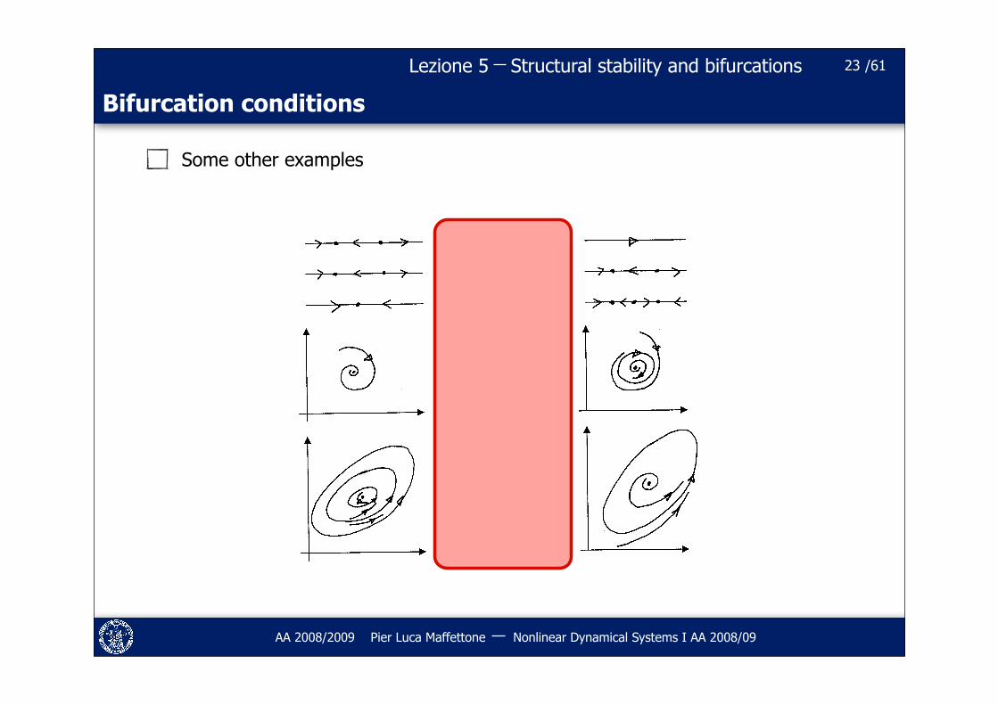
Bifurcation conditions
Some other examples
23
Structural stability and bifurcations /61Lezione 5
AA 2008/2009 Pier Luca Maffettone Nonlinear Dynamical Systems I AA 2008/09
Local and global bifurcations
Bifurcations are classified as local or global
Continuous systems
We will examine bifurcations of both equilibrium points and limit cycles
The latter will be studied as bifurcation of fixed points of maps (Poincaré map)
Discrete systems
We will examine bifurcations of fixed points and of m-periodic points (fixed points of iterated maps)
More on bifurcations in NDSII
24
Structural stability and bifurcations /61Lezione 5
AA 2008/2009 Pier Luca Maffettone Nonlinear Dynamical Systems I AA 2008/09
Bifurcation of equilibrium points
With xE an equilibrium point of a nonlinear dynamical system:
Hartman-Grobman theorems states that any nonlinear system in a neighborhood of xE
is locally topologically equivalent to the associate linearized system if such linearized system is hyperbolic. Bifurcations of hyperbolic equilibrium points are not possible.
Nonhyperbolicity of xE is necessary condition for the occurrence of local bifurcations and the critical conditions of local bifurcations have to be searched for among nonhyperbolic equilibrium points
Local bifurcation of equilibrium points are signaled by the nonhyperbolicity: eigenvalues with zero real parts (continuous systems) or unit magnitude Floquet multipliers (discrete systems)
25
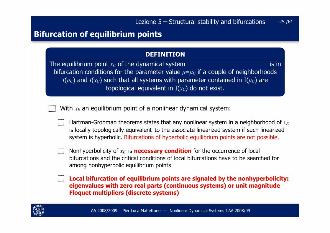
x = f(x, µ) (xk+1 = F (xk, µ)The equilibrium point xC of the dynamical system is in bifurcation conditions for the parameter value µ=µC if a couple of neighborhoods
I(µC) and I(xC) such that all systems with parameter contained in I(µC) are topological equivalent in I(xC) do not exist.
DEFINITION
Structural stability and bifurcations /61Lezione 5
AA 2008/2009 Pier Luca Maffettone Nonlinear Dynamical Systems I AA 2008/09
Bifurcation of equilibrium points
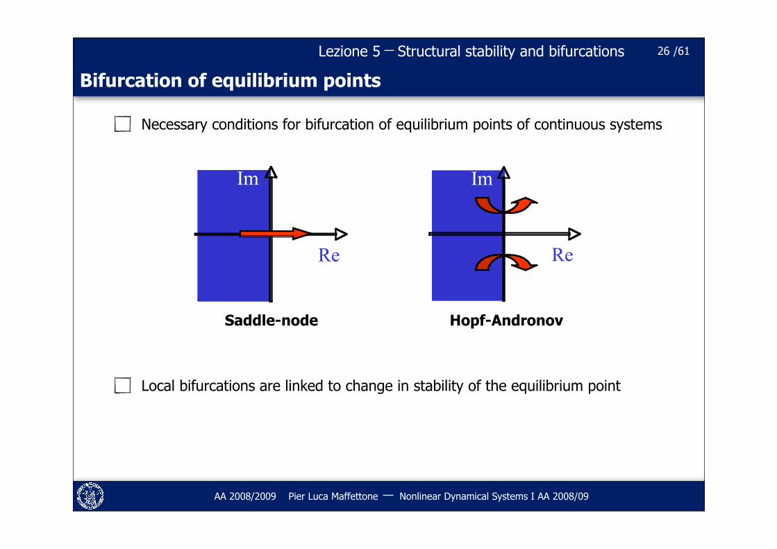
Necessary conditions for bifurcation of equilibrium points of continuous systems
Local bifurcations are linked to change in stability of the equilibrium point
26
Re
Im
Re
Im
Saddle-node Hopf-Andronov
Structural stability and bifurcations /61Lezione 5
AA 2008/2009 Pier Luca Maffettone Nonlinear Dynamical Systems I AA 2008/09
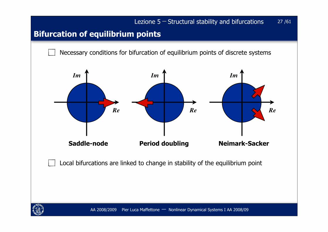
Bifurcation of equilibrium points
Necessary conditions for bifurcation of equilibrium points of discrete systems
Local bifurcations are linked to change in stability of the equilibrium point
27
Saddle-node
Im Im Im
Re Re Re
Period doubling Neimark-Sacker
Structural stability and bifurcations /61Lezione 5
AA 2008/2009 Pier Luca Maffettone Nonlinear Dynamical Systems I AA 2008/09
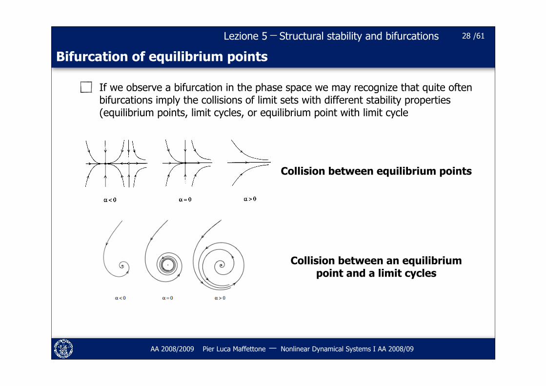
Bifurcation of equilibrium points
If we observe a bifurcation in the phase space we may recognize that quite often bifurcations imply the collisions of limit sets with different stability properties (equilibrium points, limit cycles, or equilibrium point with limit cycle
28
Collision between equilibrium points
Collision between an equilibrium point and a limit cycles
Structural stability and bifurcations /61Lezione 5
AA 2008/2009 Pier Luca Maffettone Nonlinear Dynamical Systems I AA 2008/09
Global bifurcations
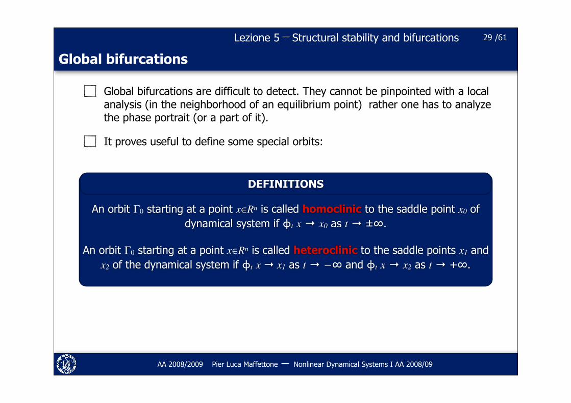
Global bifurcations are difficult to detect. They cannot be pinpointed with a local analysis (in the neighborhood of an equilibrium point) rather one has to analyze the phase portrait (or a part of it).
It proves useful to define some special orbits:
29
An orbit Γ0 starting at a point x∈Rn is called homoclinic to the saddle point x0 of dynamical system if ϕt x → x0 as t → ±∞.
An orbit Γ0 starting at a point x∈Rn is called heteroclinic to the saddle points x1 and x2 of the dynamical system if ϕt x → x1 as t → −∞ and ϕt x → x2 as t → +∞.
DEFINITIONS
Structural stability and bifurcations /61Lezione 5
AA 2008/2009 Pier Luca Maffettone Nonlinear Dynamical Systems I AA 2008/09
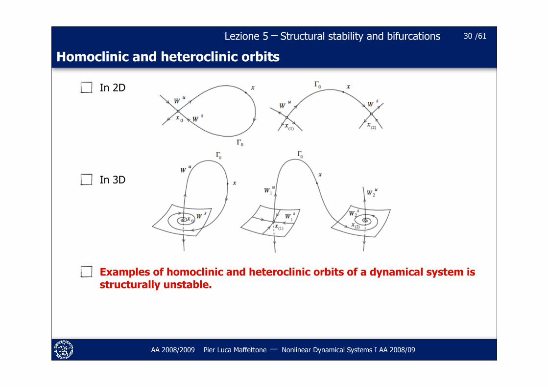
Homoclinic and heteroclinic orbits
In 2D
In 3D
Examples of homoclinic and heteroclinic orbits of a dynamical system is structurally unstable.
30
Structural stability and bifurcations /61Lezione 5
AA 2008/2009 Pier Luca Maffettone Nonlinear Dynamical Systems I AA 2008/09
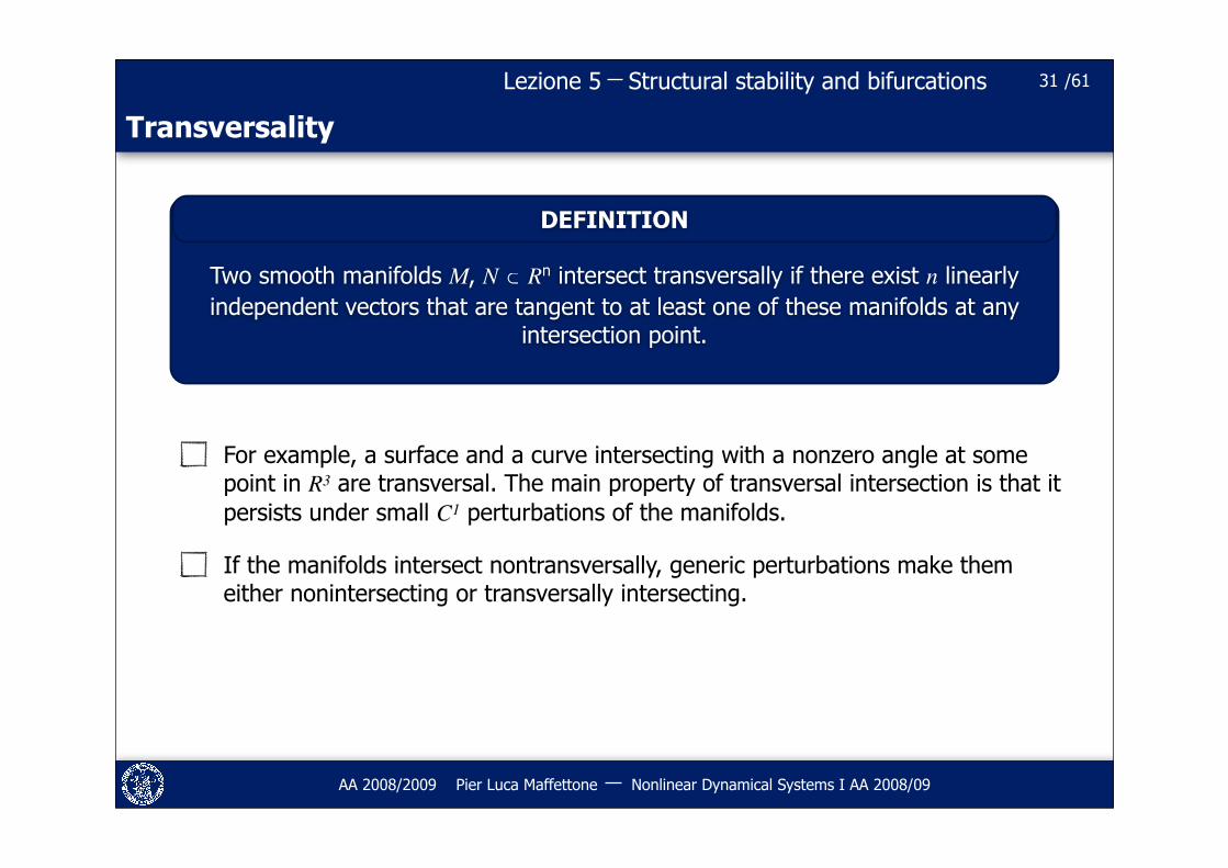
Transversality
For example, a surface and a curve intersecting with a nonzero angle at some point in R3 are transversal. The main property of transversal intersection is that it persists under small C1 perturbations of the manifolds.
If the manifolds intersect nontransversally, generic perturbations make them either nonintersecting or transversally intersecting.
31
Two smooth manifolds M, N ⊂ Rn intersect transversally if there exist n linearly independent vectors that are tangent to at least one of these manifolds at any
intersection point.
DEFINITION
Structural stability and bifurcations /61Lezione 5
AA 2008/2009 Pier Luca Maffettone Nonlinear Dynamical Systems I AA 2008/09
Global bifurcation
32
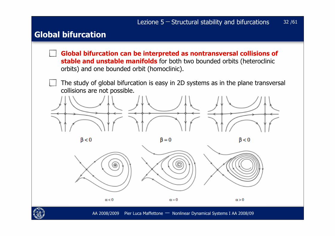
Global bifurcation can be interpreted as nontransversal collisions of stable and unstable manifolds for both two bounded orbits (heteroclinic orbits) and one bounded orbit (homoclinic).
The study of global bifurcation is easy in 2D systems as in the plane transversal collisions are not possible.

Structural stability and bifurcations /61Lezione 5
AA 2008/2009 Pier Luca Maffettone Nonlinear Dynamical Systems I AA 2008/09
33
USEFUL TOOLS
Structural stability and bifurcations /61Lezione 5
AA 2008/2009 Pier Luca Maffettone Nonlinear Dynamical Systems I AA 2008/09
Solution diagrams
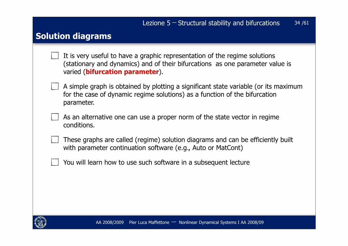
It is very useful to have a graphic representation of the regime solutions (stationary and dynamics) and of their bifurcations as one parameter value is varied (bifurcation parameter).
A simple graph is obtained by plotting a significant state variable (or its maximum for the case of dynamic regime solutions) as a function of the bifurcation parameter.
As an alternative one can use a proper norm of the state vector in regime conditions.
These graphs are called (regime) solution diagrams and can be efficiently built with parameter continuation software (e.g., Auto or MatCont)
You will learn how to use such software in a subsequent lecture
34
Structural stability and bifurcations /61Lezione 5
AA 2008/2009 Pier Luca Maffettone Nonlinear Dynamical Systems I AA 2008/09
Solution diagrams
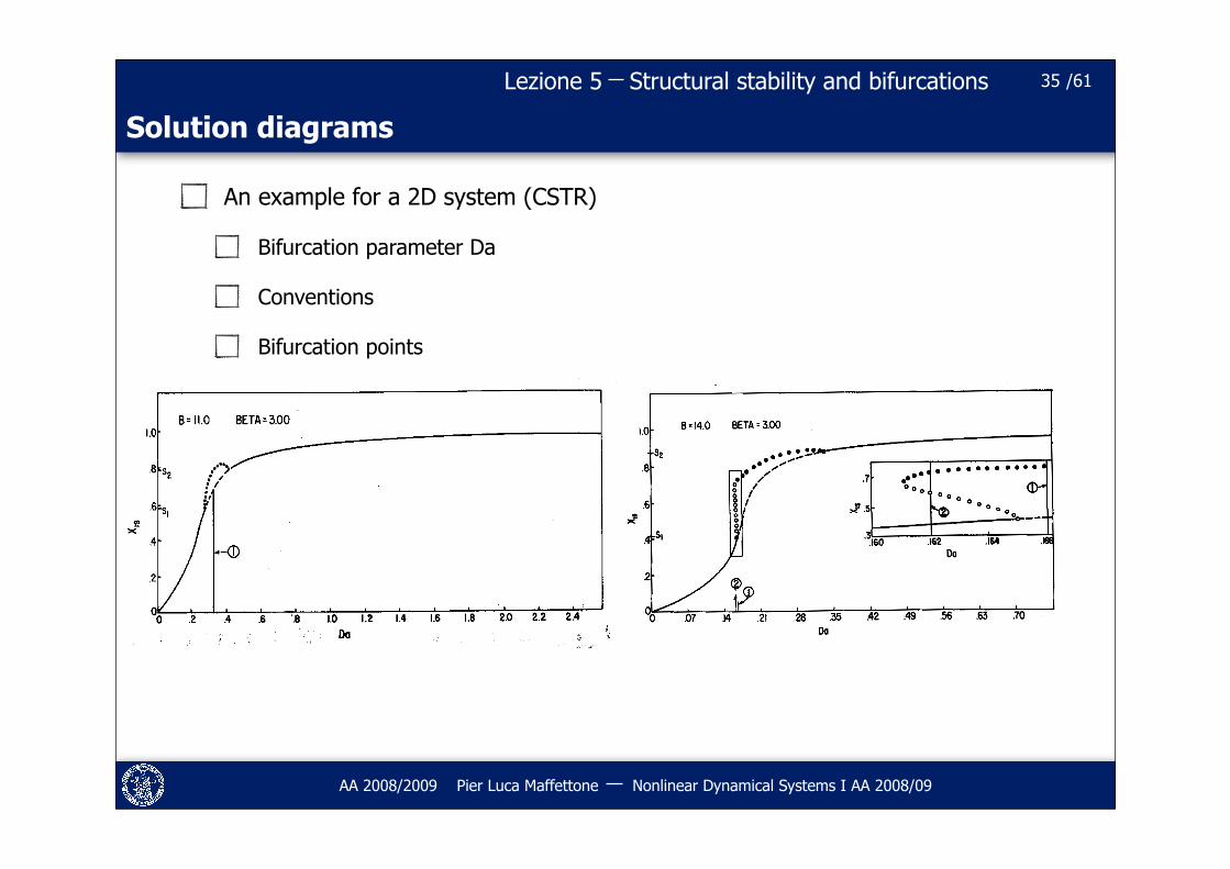
An example for a 2D system (CSTR)
Bifurcation parameter Da
Conventions
Bifurcation points
35
Structural stability and bifurcations /61Lezione 5
AA 2008/2009 Pier Luca Maffettone Nonlinear Dynamical Systems I AA 2008/09
Bifurcation diagrams
If the model contains more than one single parameter, i.e., if μ is a vector with more than one component, the critical values for a parameter depend on the other parameter values.
One can than build a diagram in the parameter space where bifurcation values are reported. The plot of the manifolds corresponding to bifurcation conditions in the parameter space of interest.
When a parameter value is varied one moves in this space
If no bifurcation line is crossed the systems are all topologically equivalent
If a bifurcation line is crossed the system show a qualitative change in its properties.
36
Structural stability and bifurcations /61Lezione 5
AA 2008/2009 Pier Luca Maffettone Nonlinear Dynamical Systems I AA 2008/09
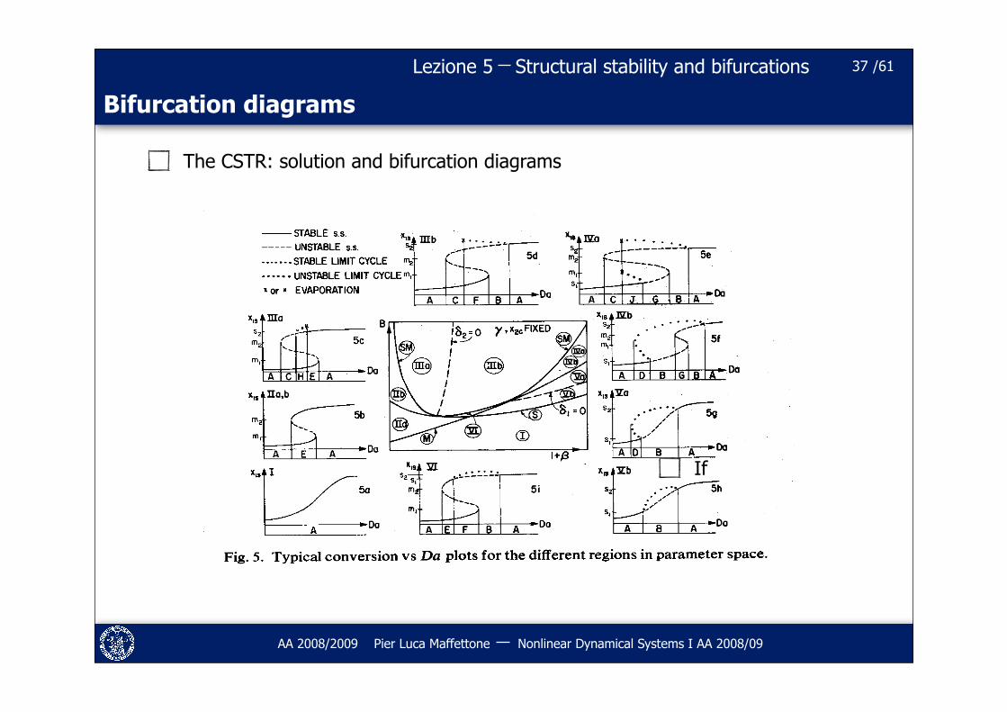
Bifurcation diagrams
The CSTR: solution and bifurcation diagrams
37
If
Structural stability and bifurcations /61Lezione 5
AA 2008/2009 Pier Luca Maffettone Nonlinear Dynamical Systems I AA 2008/09
Catastrophic bifurcations
Parameters may change in time. If such variations are slow (with respect to the characteristic times of the dynamical system) the system will remain in regime conditions by attaining the new (with respect to the parameter value) stable states.
One would observe a qualitative change of the regime solution if the (slowly changing) parameter crosses a bifurcation value.
A change of regime would then be observed: for example from a steady state to a periodic solution.
We are not guaranteed that when crossing a bifurcation value the state of the system would experience a “small” change when attaining the new stable solution (if any!)
When the change is not small we say that the corresponding bifurcation is catastrophic (in the sense that the change might have strong consequences)i: explosions, ignitions, extinctions, runaway, …., static failures (Tacoma Narrows bridge), ….
38
Structural stability and bifurcations /61Lezione 5
AA 2008/2009 Pier Luca Maffettone Nonlinear Dynamical Systems I AA 2008/09
Catastrophic bifurcations (Wikipedia)
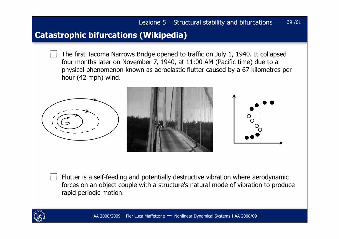
The first Tacoma Narrows Bridge opened to traffic on July 1, 1940. It collapsed four months later on November 7, 1940, at 11:00 AM (Pacific time) due to a physical phenomenon known as aeroelastic flutter caused by a 67 kilometres per hour (42 mph) wind.
Flutter is a self-feeding and potentially destructive vibration where aerodynamic forces on an object couple with a structure's natural mode of vibration to produce rapid periodic motion.
39
Structural stability and bifurcations /61Lezione 5
AA 2008/2009 Pier Luca Maffettone Nonlinear Dynamical Systems I AA 2008/09
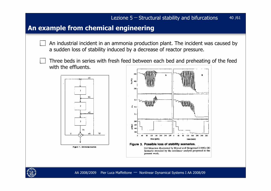
An example from chemical engineering
An industrial incident in an ammonia production plant. The incident was caused by a sudden loss of stability induced by a decrease of reactor pressure.
Three beds in series with fresh feed between each bed and preheating of the feed with the effluents.
40
Structural stability and bifurcations /61Lezione 5
AA 2008/2009 Pier Luca Maffettone Nonlinear Dynamical Systems I AA 2008/09
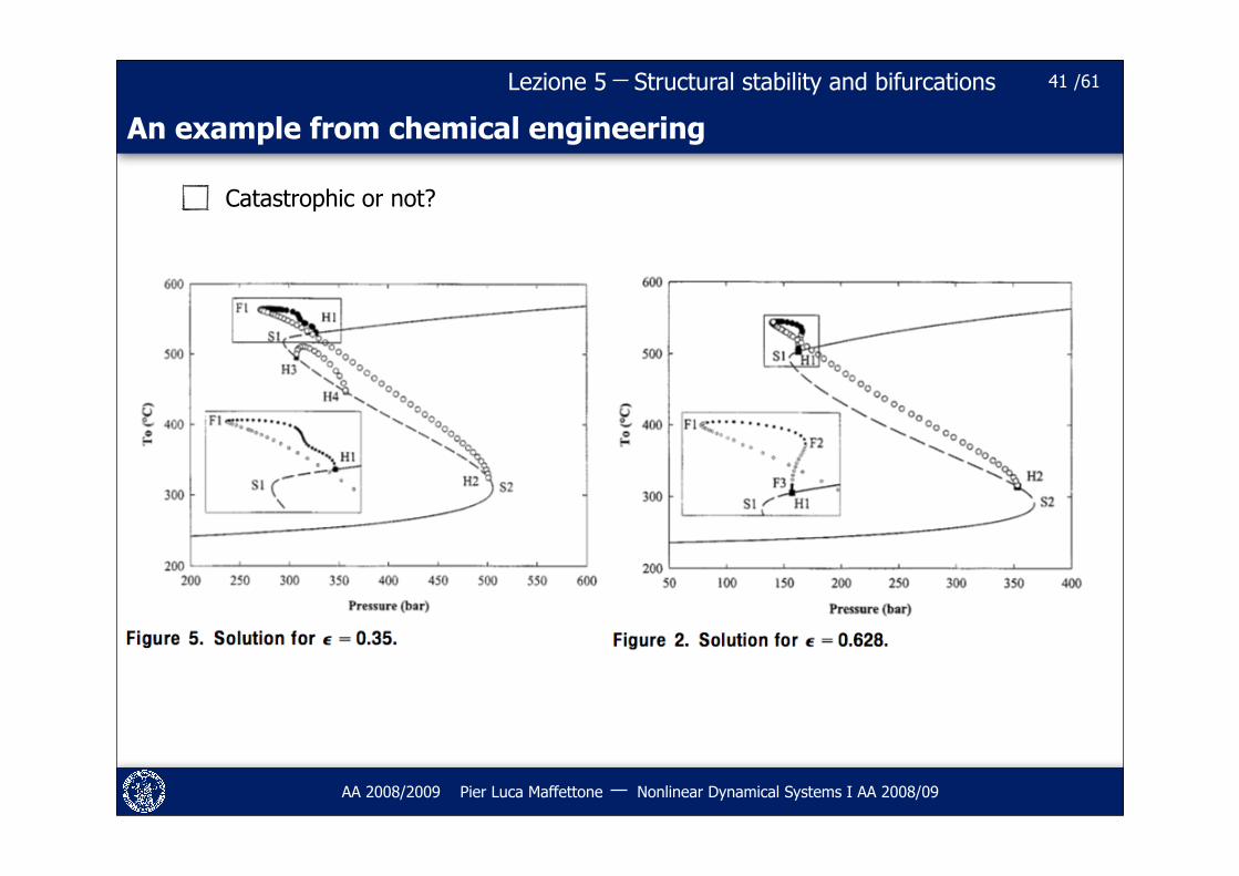
An example from chemical engineering
Catastrophic or not?
41

Structural stability and bifurcations /61Lezione 5
AA 2008/2009 Pier Luca Maffettone Nonlinear Dynamical Systems I AA 2008/09
42
ANALYSIS OF LOCAL BIFURCATIONSCENTER MANIFOLD THEOREM
Structural stability and bifurcations /61Lezione 5
AA 2008/2009 Pier Luca Maffettone Nonlinear Dynamical Systems I AA 2008/09
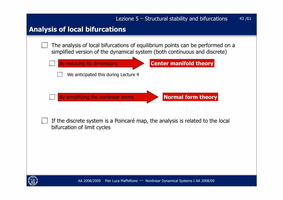
Analysis of local bifurcations
The analysis of local bifurcations of equilibrium points can be performed on a simplified version of the dynamical system (both continuous and discrete)
By reducing its dimensions
We anticipated this during Lecture 4
By simplifying the nonlinear terms
If the discrete system is a Poincaré map, the analysis is related to the local bifurcation of limit cycles
43
Center manifold theory
Normal form theory
Structural stability and bifurcations /61Lezione 5
AA 2008/2009 Pier Luca Maffettone Nonlinear Dynamical Systems I AA 2008/09
Center manifolds and local bifurcations of continuous systems
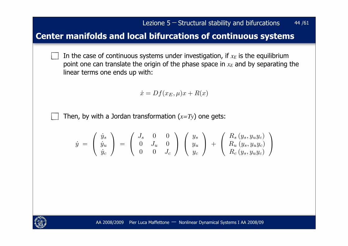
In the case of continuous systems under investigation, if xE is the equilibrium point one can translate the origin of the phase space in xE and by separating the linear terms one ends up with:
Then, by with a Jordan transformation (x=Ty) one gets:
44
x = Df(xE , µ)x + R(x)
y =
!
"ys
yu
yc
#
$ =
!
"Js 0 00 Ju 00 0 Jc
#
$
!
"ys
yu
yc
#
$ +
!
"Rs (ys, yuyc)Ru (ys, yuyc)Rc (ys, yuyc)
#
$
Structural stability and bifurcations /61Lezione 5
AA 2008/2009 Pier Luca Maffettone Nonlinear Dynamical Systems I AA 2008/09
Center manifolds and local bifurcations of continuous systems
If xE is a nonhyperbolic equilibrium point
1. There exists at least one center manifold WC(0) with the same dimensions of EC of the associate linearized system
2. There exists one and only one stable manifold WS(0) with the same dimensions of ES of the associate linearized system
3. There exists one and only one unstable manifold WU(0) with the same dimensions of EU of the associate linearized system
4. The three manifolds crosses at the origin and are there tangent to the eigenspaces of the associate linearized system.
The (possible) bifurcation of the nonhyperbolic equilibrium point xE can be studied on a system with lower dimensions (those of the center eigenspace).
45
Structural stability and bifurcations /61Lezione 5
AA 2008/2009 Pier Luca Maffettone Nonlinear Dynamical Systems I AA 2008/09
Center manifolds and local bifurcations of continuous systems
Indeed, it can be demonstrated that local bifurcations take place on the center manifold (which is locally attracting).
As we have already learned the center manifold close to the origin is described by the equation:
Thus, the local bifurcations can be studied on a center manifold on the reduced system:
Where are the parameters? We want to study the local bifurcation on the center manifold, so it must exist in a neighborhood of the critical parameter value.
46
W cloc :
!ys = hs(yc)yu = hu(yc)
yc = Jc yc + Rc(hs(yc), hu(yc), yc)
Structural stability and bifurcations /61Lezione 5
AA 2008/2009 Pier Luca Maffettone Nonlinear Dynamical Systems I AA 2008/09
Center manifolds in parameter-dependent systems
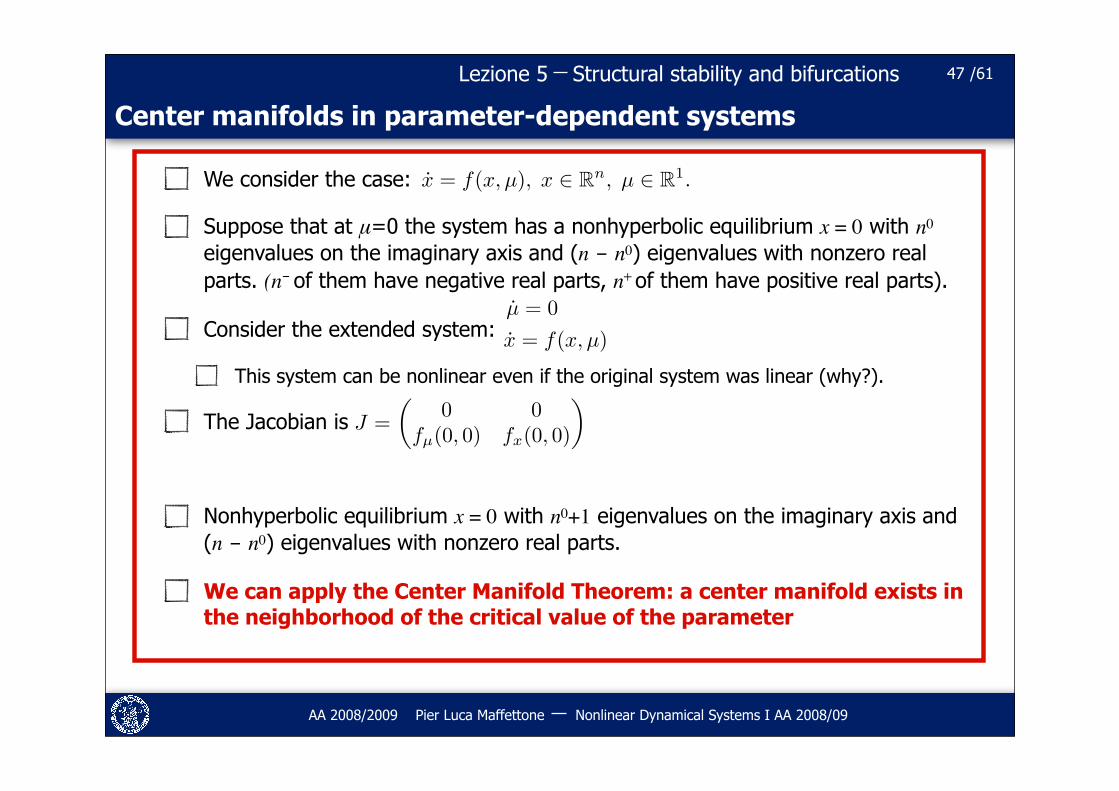
We consider the case:
Suppose that at μ=0 the system has a nonhyperbolic equilibrium x = 0 with n0 eigenvalues on the imaginary axis and (n - n0) eigenvalues with nonzero real parts. (n- of them have negative real parts, n+ of them have positive real parts).
Consider the extended system:
This system can be nonlinear even if the original system was linear (why?).
The Jacobian is
Nonhyperbolic equilibrium x = 0 with n0+1 eigenvalues on the imaginary axis and (n - n0) eigenvalues with nonzero real parts.
We can apply the Center Manifold Theorem: a center manifold exists in the neighborhood of the critical value of the parameter
47
x = f(x, µ), x ! Rn, µ ! R1.
µ = 0x = f(x, µ)
J =!
0 0fµ(0, 0) fx(0, 0)
"
Structural stability and bifurcations /61Lezione 5
AA 2008/2009 Pier Luca Maffettone Nonlinear Dynamical Systems I AA 2008/09
Center manifolds in parameter-dependent systems
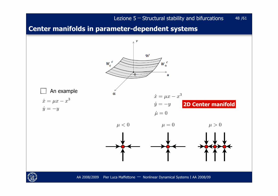
An example
48
x = µx! x3
y = !yµ = 0
x = µx! x3
y = !y 2D Center manifold
µ < 0 µ = 0 µ > 0
Structural stability and bifurcations /61Lezione 5
AA 2008/2009 Pier Luca Maffettone Nonlinear Dynamical Systems I AA 2008/09
Center manifolds in parameter-dependent systems
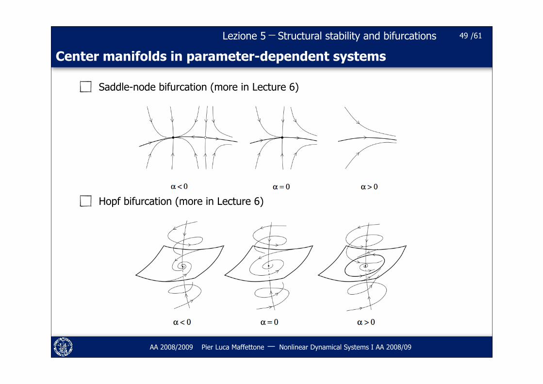
Saddle-node bifurcation (more in Lecture 6)
Hopf bifurcation (more in Lecture 6)
49
Structural stability and bifurcations /61Lezione 5
AA 2008/2009 Pier Luca Maffettone Nonlinear Dynamical Systems I AA 2008/09
Center manifolds in parameter-dependent systems
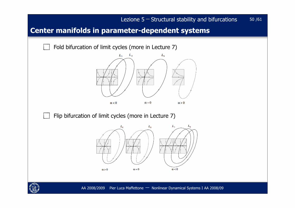
Fold bifurcation of limit cycles (more in Lecture 7)
Flip bifurcation of limit cycles (more in Lecture 7)
50
Structural stability and bifurcations /61Lezione 5
AA 2008/2009 Pier Luca Maffettone Nonlinear Dynamical Systems I AA 2008/09
Center manifolds in parameter-dependent systems
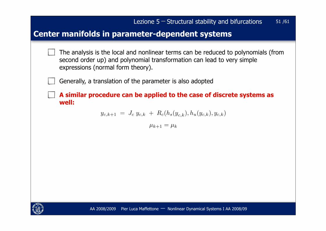
The analysis is the local and nonlinear terms can be reduced to polynomials (from second order up) and polynomial transformation can lead to very simple expressions (normal form theory).
Generally, a translation of the parameter is also adopted
A similar procedure can be applied to the case of discrete systems as well:
51
yc,k+1 = Jc yc,k + Rc(hs(yc,k), hu(yc,k), yc,k)
µk+1 = µk
Structural stability and bifurcations /61Lezione 5
AA 2008/2009 Pier Luca Maffettone Nonlinear Dynamical Systems I AA 2008/09
52
ANALYSIS OF LOCAL BIFURCATIONSNORMAL FORMS
Structural stability and bifurcations /61Lezione 5
AA 2008/2009 Pier Luca Maffettone Nonlinear Dynamical Systems I AA 2008/09
Normal forms
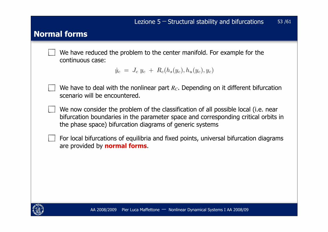
We have reduced the problem to the center manifold. For example for the continuous case:
We have to deal with the nonlinear part RC. Depending on it different bifurcation scenario will be encountered.
We now consider the problem of the classification of all possible local (i.e. near bifurcation boundaries in the parameter space and corresponding critical orbits in the phase space) bifurcation diagrams of generic systems
For local bifurcations of equilibria and fixed points, universal bifurcation diagrams are provided by normal forms.
53
yc = Jc yc + Rc(hs(yc), hu(yc), yc)
Structural stability and bifurcations /61Lezione 5
AA 2008/2009 Pier Luca Maffettone Nonlinear Dynamical Systems I AA 2008/09
Normal forms
A normal form of a mathematical object, broadly speaking, is a simplified form of the object obtained by applying a transformation (often a change of coordinates) that is considered to preserve the essential features of the object.
For instance, a matrix can be brought into Jordan normal form by applying a similarity transformation.
Now we consider normal forms for autonomous systems of differential equations (vector fields or flows) near an equilibrium point.
Similar ideas can be used for discrete-time dynamical systems near a fixed point, or for flows near a periodic orbit.
54
Structural stability and bifurcations /61Lezione 5
AA 2008/2009 Pier Luca Maffettone Nonlinear Dynamical Systems I AA 2008/09
Normal forms
The idea of a normal form is to find a polynomial which would be topologically equivalent to a given system around a bifurcation point.
Questions
1. Can an equivalent polynomial be found, i.e., does it exist?
2. Is the normal form unique?
3. Which properties of the bifurcation determine the minimal degree of such a polynomial?
55
Given a bifurcation, a polynomial dynamical system is called a normal form of the bifurcation at (λ,x)=(λ0,x0) if it satisfies the generic bifurcation conditions,
and is topologically equivalent to any system satisfying the same bifurcation conditions
DEFINITION
x = f(x, !)
Structural stability and bifurcations /61Lezione 5
AA 2008/2009 Pier Luca Maffettone Nonlinear Dynamical Systems I AA 2008/09
Normal forms
The method is local: the coordinate transformations are generated in the neighborhood of a known solution
The coordinate transformation will in general be nonlinear functions of the dependent variables
Solution of a series of linear problems
The structure of the normal form is determined entirely by the nature of the linear part of the vector field
56
Structural stability and bifurcations /61Lezione 5
AA 2008/2009 Pier Luca Maffettone Nonlinear Dynamical Systems I AA 2008/09
Normal forms
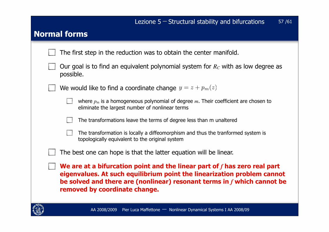
The first step in the reduction was to obtain the center manifold.
Our goal is to find an equivalent polynomial system for RC with as low degree as possible.
We would like to find a coordinate change
where pm is a homogeneous polynomial of degree m. Their coefficient are chosen to eliminate the largest number of nonlinear terms
The transformations leave the terms of degree less than m unaltered
The transformation is locally a diffeomorphism and thus the tranformed system is topologically equivalent to the original system
The best one can hope is that the latter equation will be linear.
We are at a bifurcation point and the linear part of f has zero real part eigenvalues. At such equilibrium point the linearization problem cannot be solved and there are (nonlinear) resonant terms in f which cannot be removed by coordinate change.
57
y = z + pm(z)
Structural stability and bifurcations /61Lezione 5
AA 2008/2009 Pier Luca Maffettone Nonlinear Dynamical Systems I AA 2008/09
Normal forms - Technicalities
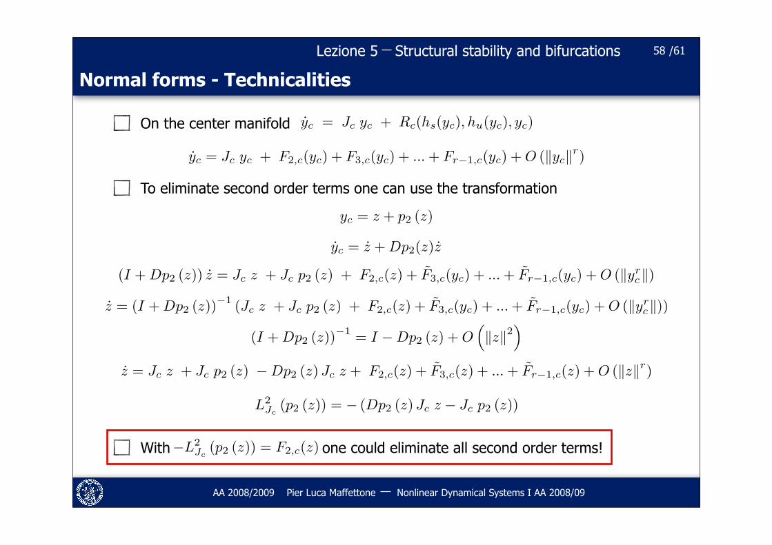
On the center manifold
To eliminate second order terms one can use the transformation
With one could eliminate all second order terms!
58
yc = Jc yc + Rc(hs(yc), hu(yc), yc)
yc = Jc yc + F2,c(yc) + F3,c(yc) + ... + Fr!1,c(yc) + O (!yc!r)
yc = z + p2 (z)
yc = z + Dp2(z)z
(I + Dp2 (z)) z = Jc z + Jc p2 (z) + F2,c(z) + F3,c(yc) + ... + Fr!1,c(yc) + O (!yrc!)
z = (I + Dp2 (z))!1 (Jc z + Jc p2 (z) + F2,c(z) + F3,c(yc) + ... + Fr!1,c(yc) + O (!yrc!))
(I + Dp2 (z))!1 = I !Dp2 (z) + O!"z"2
"
z = Jc z + Jc p2 (z) !Dp2 (z)Jc z + F2,c(z) + F3,c(z) + ... + Fr!1,c(z) + O ("z"r)
L2Jc
(p2 (z)) = ! (Dp2 (z)Jc z ! Jc p2 (z))
!L2Jc
(p2 (z)) = F2,c(z)
Structural stability and bifurcations /61Lezione 5
AA 2008/2009 Pier Luca Maffettone Nonlinear Dynamical Systems I AA 2008/09
Normal forms - Technicalities
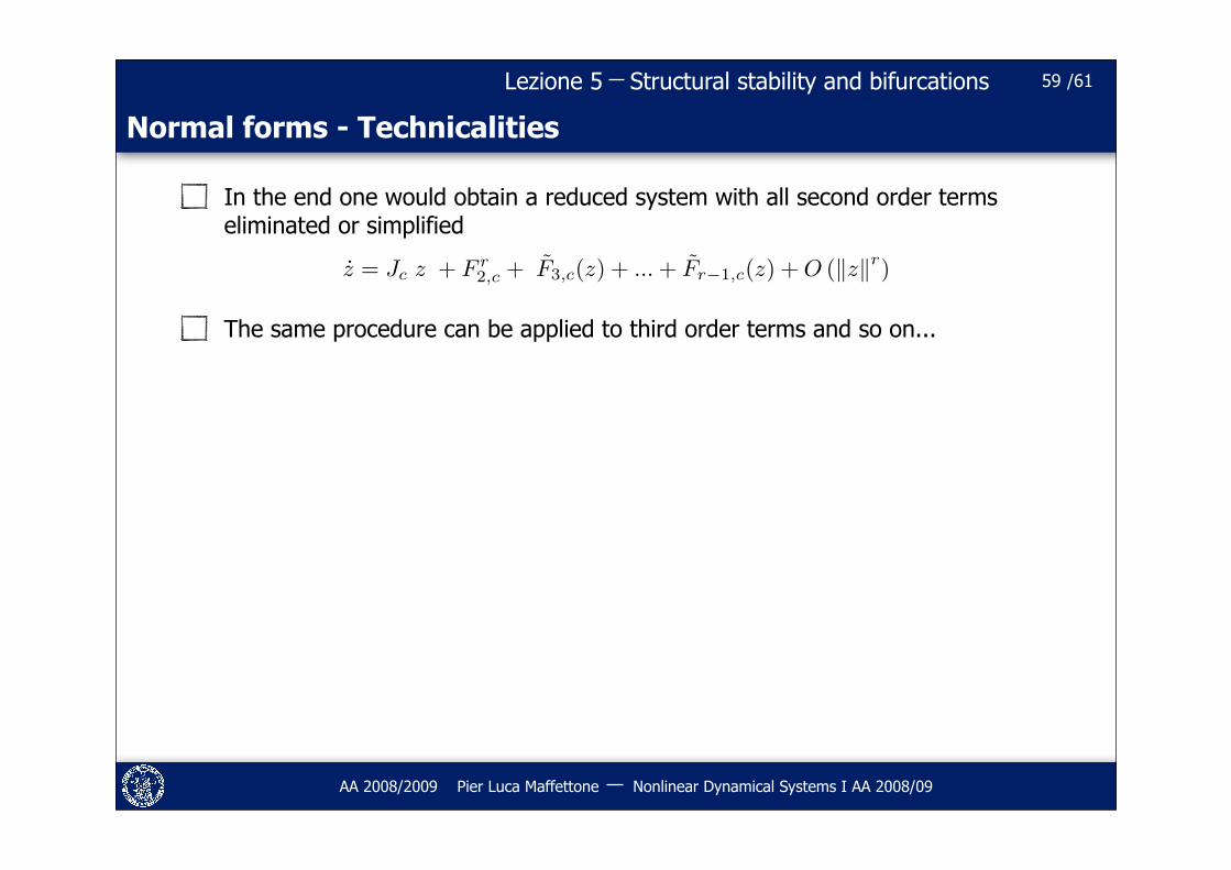
In the end one would obtain a reduced system with all second order terms eliminated or simplified
The same procedure can be applied to third order terms and so on...
59
z = Jc z + F r2,c + F3,c(z) + ... + Fr!1,c(z) + O (!z!r)
Structural stability and bifurcations /61Lezione 5
AA 2008/2009 Pier Luca Maffettone Nonlinear Dynamical Systems I AA 2008/09
Normal forms
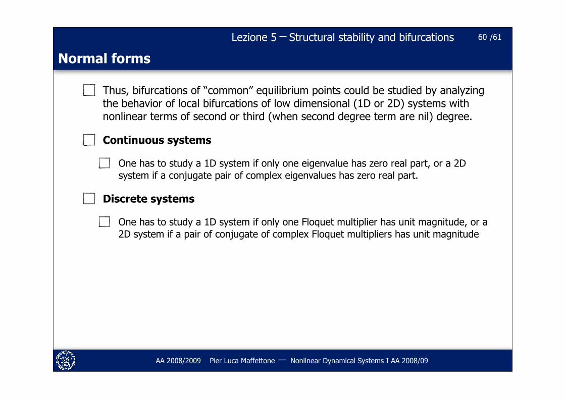
Thus, bifurcations of “common” equilibrium points could be studied by analyzing the behavior of local bifurcations of low dimensional (1D or 2D) systems with nonlinear terms of second or third (when second degree term are nil) degree.
Continuous systems
One has to study a 1D system if only one eigenvalue has zero real part, or a 2D system if a conjugate pair of complex eigenvalues has zero real part.
Discrete systems
One has to study a 1D system if only one Floquet multiplier has unit magnitude, or a 2D system if a pair of conjugate of complex Floquet multipliers has unit magnitude
60
Structural stability and bifurcations /61Lezione 5
AA 2008/2009 Pier Luca Maffettone Nonlinear Dynamical Systems I AA 2008/09
Final remarks
The concept of topological equivalence
Structural stability: another kind of stability
Effect of parameter changes
Bifurcations as passage through structural instability
Catastrophic bifurcations
Center manifold theory to describe bifurcation in low dimensions
Normal forms: a way to classify bifurcations
61