Embed Size (px)
Citation preview
STRUCTURAL RESPONSE OF A 45° SKEW
PRESTRESSED. CONCRETE BOX~GIRDER
HIGHWAY BRIDGE SUBJECTED TO
VEHICULAR LOADING
BROOKVILLE BRIDGE
by
Thomas Schaffer
FRITZ ENGINEERINGLABORATORY LIBRARY

STRUCTURAL RESPONSE OF A
45~ SKEW PRESTRESSED CONCRETE
BOX-GIRDER HIGHWAY BRIDGE
SUBJECTED TO VEHICULAR LOADING
BROOKVILLE BRIDGE
by
Thomas Schaffer
A THESIS
Presented to the Graduate Faculty
of Lehigh University
in Candidacy for the Degree of
Master of Science
FRITZ Ej\JGlr~EERIj\JG
LABORfiTOR'y' LJBR/~fr(
Lehigh University
1967

CERTIFICATE OF APPROVAL
This thesis is accepted and approved in partial
fulfillment of the requirements for the degree of Master of
Science in Civil Engineering.
(Date)
Professor D. A. VanHornProfessor in Charg~, and Chairman,Department of Civil Engineering
i
STRUCTURAL RESPONSE OF A 45° SKEW PRESTRESSED CONCRETE i-~ tpBOX-GIRDER HIGHWAY BRIDGE SUBJECTED TO VEHICULAR LOADING
BROOKVILLE BRIDGE
by Thomas Schaffer
.Durirlg t11e sumrners of 196 L)" 1965, a:nd .1'966, a series of
field tests were conducted on five prestressed concre'te box-beam
11:Lg-llVJtS,y bridg'es located ill the Cornm011tJJealth of Pen11sylvania_
Four of the bridges were right bridges while one, located at
Brookville, was constructed on a 45° skeWQ In the field tests,
each bridge was subjected to vehicular loading consisting of a
3-axle truel\. vvhich was a close sirnulatioll of tIle AASHO f"lS20 de-
sign vellicle.
This report, based on the test of the Brookville Bridge,
cO!1taiI1S (1) cl det'a:Lled deSC1~iptiorl of tile ld test procedure
c!nd equipfnent, (2) ;;1 cOJnplete outline and flow CflcU:,t of tr\6 eOl'n-
puter prog'rarH used iXl the pl"oCessirig arlel arlalysis of t:he data,
( 3) a s u-mmary of tlle rnea.sured s'tructural I"es pons e the
, irlc~luding a, cornpa,risori witll aright bridge having ne~lrly
identiccil overall dimensions and member sizes"
Initially, separate reports are being prepared on the
behavior of each of the test structures. The primary intent of
reports is to present a detailed ption of the
havior each of all se
:t:1eport vvill

ABSTRACT
During the summers of 1964, 1965, and 1966, a series of
field tests were conducted on five prestressed concrete box-beam
highway bridges located in the Commonwealth of Pennsylvania.
Four of the bridges were right bridges while one, located at
Brookville, was constructed on a 45° skew. In the field tests,
each bridge was subjected to vehicular loading consisting of a
3-axle truck which was a close simulation of the AASHO HS20 de
sign vehicle.
This report, based on the test of the Brookville Bridge,
contains (1) a detailed description of the field test procedure
and equipment, (2) a complete outline and flow chart of the com
puter program used in the processing and analysis of the data,
and (3) a summary of the measured structural response of the
bridge, including a comparison with a right bridge having nearly
identical overall 'dimensions and member sizes.
Initially, separate reports are being prepared on the
behavior of each of the test structures. The primary intent of
these reports is to present a detailed description of the be
havior of each of the bridges. After all of the separate reports
have been completed, a summary report will be prepared.
ii
1.
2.
3.
TABLE OF CONTENTS
INTRODUCTION
1.1 Background
1.2 Object and Scope
1.3 Previous Research
TESTING
2.1 Test Bridge and Site
2.2 Gage Sections and Locations
2.3 Instrumentation
2.4 Test Vehicle
2.5 Test Runs
2.6 Loading Lanes
2.7 Longitudinal Position and Timing
DATA REDUCTION AND EVALUATION
1
1
3
4
6
6
7
8
9
10
10
11
12
3.1 Oscillograph Trace. Reading 12
3.2 Evaluation of Oscillograph Data 13
3.2.1 Strain Calculation l3
3.2.2 Strain Tabulation and Plotting 15
3.2.3 Moment Calculations 15
4. PRESENTATION OF TEST RESULTS 19
4.1 Maximum Moment Coefficients 19
4.2 Deflections at Midspan 20
4.3 Maximum Strain at Bottom Girder Surfaces 20
4.4 Effective Width of Slab, Curb., and 21Parapet Wall
4.5 Neutral Axis Location 21
iii

5. DISCUSSION OF TEST RESULTS 22
5.1 Vehicle Position at Maximum Response 22
5.2 Maximum Moment Coefficients 22
5.3 Deflection and Rotation at Midspan 24
5.4 Maximum Strain at Bottom Girder Surfaces 26
5.5 Effective Width of Slab, Curb, and 27Parapet Wall
6. SUMMARY AND CONCLUSIONS· 28
6.1 Sununary 28
6.2 Conclusions 30
7., ACKNONLEDGMENTS 34
8. APPENDIX 35
9. TABLES 59
10. .FIGURES 80
11. REFERENCES 113
12. VITA lIS
iv

LIST OF TABLES
Table
1 Test Bridge Characteristics 60
2 Maximum Moment Coefficients, Crawl Run Loading 61
3 Maximum Moment Coefficients at Midspan for 62Berwick Bridge, Crawl Run Loading
4 Comparison of Maximum Moment Coefficients 63at Midspan
5 Comparison of Maximum Moment Coefficients 64at Midspan
6 Comparison of Maximum Moment Coefficients 65at Midspan
7 Effect of Skew on Maximum Moments at Midspan 66of Beams
8 Midspan Girder Deflections - Brookville Bridge 67
9 Girder Deflections at Midspan in Berwick Bridge 68
10 Comparison of Girder Deflections 69
11 Comparison of Girder Deflections 70
12 Comparison of Girder Deflections 71
13 Maximum Strain at Bottom Surface of Girder - 72Brookville Bridge
14 Maximum Strain at Bottom Surface of Girder - 73Berwick Bridge
15 Maximum Strain at Bottom Surface of Girder - 74Brookville Bridge
16 Maximum Strain at Bottom Surface of Girder - 75Brookville Bridge
17 Maximum Strain at Bottom Sllrface of Girder - 76Berwick Bridge
18 Comparison of Averaged Maximum Strains at 77Bottom Surface of Girder
19 Effective Slab Width 78
20 Neutral Axis Location 79
v
Figure
1
2
3
4
.5
6
7
8a
8b
9
10
11
12
13
14
15
16
17
18
19
20
21
LIST OF FIGURES
Test Bridge
Cross-Section of Brookville Bridge
Plan View of Bridge Deck
Composite Girder Cross-Section
Underside Detail Showing Gaged Sections
Cross-Section Showing SR-4 Gages Consideredin Evaluation for Moment Coefficients
Instrumentation Flow Chart
. Underside of Test Bridge, Showing Skewand Instrumentation
Detail of Instrumentation, Showing ·SR-4Gages and Deflectometer
Test Vehicle
Typical Strain Data Tabulation
Maximum Moment Coefficients at Section El
Maximum Moment Coefficients at Section E2
Maximum Moment Coefficients at Section I
Superimposed Moment Coefficients (Average)
Vehicle Location in Each Lane to ProduceMaximum Response at Section £1
Vehicle Location in Each Lane to ProduceMaximum Response at Section El
Vehicle Location in Each Lane to ProduceMaximum Response at Section E1
Vehicle Location in Each Lane to ProduceMaximum Response at Section E1
Vehicle Location in Each Lane to ProduceMaximum Response at Section £2
Vehicle Location in Each Lane to ProduceMaximum Response at Section E2.
Vehicle Location in Each Lane to ProduceMaximum Response at Section E2
vi-
81
82
83
84
85
86
87
88
88
89
90
91
92
93
94
95
96
97
98
99
100
101

Figure
22
23
24
25
26
27
28
29
30
31
32
Vehicle Location in Each Lane to ProduceMaximum Response at Section E2
Vehicle Location in Each Lane to ProduceMaximum Response at Section I
Vehicle Location in Each Lane to ProduceMaximum Response at Section I
Vehicle Location in Each Lane to ProduceMaximum Response at Section I
Vehicle Location in Each Lane to ProduceMaximum Response at Section I
Deflection Due to Indicated Lane Loading
Deflection Due to Indicated Lane Loading
Deflections With Two Lanes Loaded
Deflections With Two Lanes Loaded
Maximum Strain at Bottom of Beam
Maximum Bottom Strain With Two Load Vehicles
vii
102
103
104
105
106
107
108
109
110
III
112

1. INTRODUCTION
1.1 Background
Early prestressed concrete highway bridges in the
United States were generally constructed either with the longi
tudinal girders in direct contact, or with very small lateral
spacing. This adjacent girder configuration was utilized as a
means of gaining positive interaction between beams in the lat
eral distribution of live load. Transverse post-tensioning was
often employed, along with shear keys between the beams, to pro
vide significant resistance to bending in the lateral direction.
As a result, the adjacent girder bridge could be analyzed as an
orthotropic plate structure, since longitudinal bending resist
ance was greater in magnitude than that in the lateral direction. 1
A number of girder cross-sections were used, including I-shaped,
box-shaped, upright or inverted tee, and channel-shaped, with
most forms having some means of developing positive lateral in
teraction. 2
In Pennsylvania, most of the adjacent -girder bridges
have used the box-shaped cross-section. In these bridges, the
girders are placed with their faces nearly touching, and the
small space between is occupied by a cast-in-place concrete shear
key. With this configuration, there is no need to depend on a
rigid deck slab for any structural purpose, and the tops of the

beams provide an unbroken surface. Therefore, only a thin wear
ing course need be applied for the structure to be ready for
traffic.
Recent design practice has led to the use of prestressed
concrete girders in a spread configuration, parallel to that in'
a beam-slab bridge utilizing steel stringers. Load transmission
between beams is accomplished by means of a reinforced concrete
deck slab cast to act compositely with the beams. Diaphragms are
normally cast-in-place between beams at intervals along the span
to aid in a more uniform distribution of live load to the beams.
Both I-shaped and box-shaped cross-sections have been used 'in the
spread beam configuration, with the utilization of the box-section
being the most recent development in Pennsylvania. The box girder
differs in structural behavior over the I-shape in that it has
more resistance to torsion. It is believed that the box section,
by virtue of this torsional stiffness, may be superior. to the
other shapes in developing a·more uniform lateral distribution of
applied loads. Since this additional rigidity has not been taken
into account, it is felt that previous designs may be somewhat
conservative.
As a result, in 1964, the Structural Concrete Division.
of the Department of Civil Engineering initiated a research project
with the purpose of evaluating the structural behavior of spread
prestressed concrete box girder bridges. The foremost purpose of
-2-

the project is to determine the actual lateral distribution of
vehicular loads in this type of bridge.
Initial tests were conducted on an existing highway
bridge near Drehersville, Pennsylvania. This test series served
as a pilot for following tests, and provided insight into the
effects of certain design factors on the behavior of the bridge.
Two load vehicles, closely simulating AASHO H20-S16-44 loading,
were run across the test span, both singly and in combinatione
Instrumentation was arranged to measure strains in beams, slab,
curb,. and parapet, and to measure deflections. The pilot tests
indicated principally t~at~ (1) positive composite action ~xists
between the beams and deck, including the curb and parapet wall,
(2) that the effect of multiple vehicle loads can be evaluated
by superimposing single vehicle effects, (3) that only half of
the beams in a bridge need be gaged to evaluate the behavior of
the entire bridge, and (4) that actual ~ive load distribution is
significantly different from that assumed in present design. 3
It was decided that subsequent tests be planned to
evaluate the effects of several f~ctors on live load distribution
in the spread-box bridge type. These are primarily (1) degree of
skew angle between the crossing routes, (2) width of beam section,
and (3) the effect of midspan diaphragms~ One bridge, having no
significant degree of skew, was selected as the standard for the
tests, and three others of similar dimensions, but with desired
-3-

variations from the standard, were chosen for the purpose of com
parison. The characteristics of the four bridges are given in
Table 1.
1.2 Object and Scope
In the phase of the project reported herein, the pri
mary purpose is to evaluate the effect of a 45° skew on the lat
eral distribution of live load in one of the bridges tested.
Spread-box girder bridges existing at present in Pennsylvania
have been designed using a live load distribution factor of 8/5.5
for interior girders, where S is the lateral girder spacing,
center-to-center. The distribution factor determines the portion
of the standard design wheel load to be applied to each interior
girder in design. The factor in use is equal to the largest fac
tor specified for any beam-slab bridge type currently listed in
the design standards of either the Pennsylvania Department of
Highways4 or American Association of State Highway Officials. 6
It is believed that, due to the torsional characteristic of the
box section, this factor could be changed to more accurately re
flect the behavior of the section. Data gathered from the test
ing of a right bridge at Berwick, Pennsylvania, which is the
standard bridge for these tests, indicated maximum loads for in
terior and exterior girders which differed significantly from the
design loads. 6 In this report, data is analyzed to compare the
distribution in the skew bridge with that of the ~ight bridge.
-3-

The analysis performed in this phase of the project is
of experimental strain data only. In the processing of data from
the bridges tested which had no appreciable skew, the determina
tion of externally applied moments was a simple matter. However,
with a skewed bridge, the analysis is considerably more complex.
The skew has the .effect of creating an eccentric distribution of
beam end reactions which cannot be accurately determined.
1.3 Previous Research
In March of 1946, the University of Illinois published
the first of a series of reports on the extensive testing of slab
and beam bridge models. 7 The models utilized steel stringers of
I-shaped.section, with five beams in each model. The first re
port covers simple span right bridges which were thoroughly in
strumented to observe behavior in the beams and slab. Later tests
included studies of models with 30° and 60° skew angles. a Speci
mens were loaded to failure, and influence charts compiled for
beam strain, beam deflection, and slab reinforcement strain.
The study considered the effect of skew on beam strain and deflec
tion, slab reinforcement strain, ultimate strength, and dead load
moments in the test bridges. A later report published as part of
this same series presents a theoretic~l analysis of the same type
of bridge, comparing the behavior of bridges with 30°, 45°; and
60° skew to that of a right bridge. 9 The analysis consists basi
cally of the simultaneous solution of difference equations, using
-4-
symmetrical and anti-symmetrical load components on a grid con
forming to the skew of the slab. The principal parameters used
in the analysis are beam spacing-span ratio, and the ratio of
slab stiffness to beam stiffness. Tables of coefficients are
compiled whi.ch may be used to compute quantitatively the effects
of single concentrated loads, or AASHO standard H-loading. A
formula is given for approximate conversion to H-S type loading,
so that-the effects of this ·configuration may be evaluated.
Little published material is available on field test
ing of skew bridges. A recent report from the University of
California10 describes the experimental evaluation of a theoret-'
ical solution performed on a steel orthotropic plate skew struc
ture. Tests were run on a bridge constructed for experimental
purposes on a California highway, with the main objective being
to determine the accuracy of the analysis. No comparison is
made of the behavior of the skew structure to a similar right
structure.
-5-

2. TESTING
2.1 Test Bridge and Site
The test bridge, details of which are shown in Figs. 1
through 4, carries Legislative Route 701 over the eastbound lanes
of Int~rstate Route 80 (L.R. 1009-3) two miles north of Brook
ville, Jefferson County, Pennsylvania. Dimensions closely match
those of the Berwick Bridge, with a simply-supporte~ span of
64 feet 10-1/2 inches, and a roadway width of 28 feet. The four
identical longitudinal girders are of precast, . pre-tensioned con
crete, with a hollow box cross-section nominally 48 inches wide
and 36 inches deep, and laterally spaced at 8 feet 10 inches
center-tb-center. The bridge was chosen because its only signif
icant difference from the Berwick Bridge is the skew angle of 45° .
Interaction between the slab and beams is provided by extending
the girder shear reinforcement through the top of the girder into
the slab. The curbs and parapet walls are linked to the s~ab by
reinforcing steel in much the sam~ manner, but are not assumed in
design to form part of the load-bearing structure.
The bridge is located on a section of tangent roadway,
with a 3.1% grade falling toward the south. The approach from
either end of the bridge is clear, with slight curvatur~ and rising
grade on the road to the south, while a similar bridge spanning the
-6-

westbound lanes of Interstate Route 80, slight curvature, and
gently rising ,grade lie to the north. There is no super-elevation
or extreme crown in the immediate vicinity of the test span.
2.2 Gage Sections and Locations
It was concluded in Fritz Engineering Laboratory Report
No. 315.1 that only half of the beams in a bridge of this type
need be gaged thoroughly to give an accurate picture of its be
havior. Therefore, only the two girders toward the east side of
the bridge were extensively instrumented. Gaged sections were
located at midspan on Girders A (exterior) and B (interior), and
a third section was located on Girder A on a line running perpen
dicular to the girders from the interior gage section, as shown
in Fig. 5.
The two gaged sections on the exterior girder have been
designated as El (midspan) and E2, and the interior section is re
ferred to as Section I·. Each section was mounted with four strain
gages per girder face; two gages were mounted on the bottom sur-.
face of the girder, with others placed nominally at 6 inches, 15
in~hes, and 34 inches.above the bottom surface, for a total of
eight gages per girder. Single gages were placed on the bottom
surfaces of Girders C and D in locations corresponding antisymrnet
rically to the main sections on Girders A and B to serve as a check
system. Single deflection gages were placed at midspan of each
-7-
girder. These gages are a type devised by ~he Bureau of Public
Roads, called a deflectometer. The deflectometer is described in
the following section.
2.3 Instrumentation
All strain gages used in testing were of the SR-4 elec
trical resistance type manufactured by the Baldwin-Lima-Hamilton
Corporation. The gages were mounted using a cement supplied by
Baldwin for the purpose, after the gage locations were ground
smooth and sealed with a prior coat of cement. Gages exposed to
weather were proteqted with Gagekote, an epoxy compound which is
applied after the gage cement has cured.
Following mounting, each gage was wired into a conven
tional Wheatstone bridge circuit with three inactive gages placed
nearby such that all were at ambient temperature conditions.
Strain data was recorded using a mobile instrument unit owned by
the U. S. Bureau of Public Roads. The equipment is housed in a
trailer and consists mainly of an oscillator, 48 gage circuit am
plification·channels, and three variable speed recording oscillo
graphs. The oscillator transmits a reference signal to the bank
of amplifiers, where each amplifier is connected into a gage cir
cuit as described above. During a 'test run, the transmitted sig
nal will be altered by gage activity, magnified by the amplifier,
and transmitted to an oscillograph galvanometer, where the
-8-

galvanometer movement is permanently recorded on photographic
paper. A flow-chart diagram of the circuitry in the testing
trailer is shown in Fig. 7.
Deflections are measured with the BPR deflectometer,
shown in Fig. Sb. The deflectometer is essentially a small can
tilever beam of rectangular cross-section in which the width
tapers uniformly from the support end to the tip. The depth of
the small beam remains constant through its length, so that the
cross-section has a uniform, linear decrease in moment of in
ertia from the support end to the free end. Four SR-4 strain
gages are bonded to the beam near -the support'end, which is
clamped rigidly to the bridge girder at the point where deflec
tion is to be measured. A wire is connected between the free
end of the cantilever and a weight resting on the ground, in or
der to impose a downward deflection on the cantilever. When the
bridge girder deflects under load, the forced deflection in the
cantilever decreases, and the change is registered by the record
ing equipment in the same manner as with the other strain gages •.
The deflectometer is calibrated when it is fabricated, so that
the bridge girder deflection is easily evaluated.
2.4 Test Vehicle
The vehicle used for testing is a diesel-powered trac
tor and.semi-trailer owned by the Bureau of Public Roads. The
-9-

dimensions of the vehicle conform well to AASHO H20-Sl6-44 de
sign loading,5 measuring 13.0 feet from the front axle to the
drive aXle, and 20.4 feet from the drive axle to the trailer
axle. The trailer was loaded with gravel distributed to produce
axle loads quite close to those ~pecified in the design code, as
shown in Fig. 9. Between the start and finish of testing, there
was some change in the loads, due to change in the moisture con
tent of the gravel.
2.5 Test Runs
Runs stud.ied in preparati..on for this 'report are of a
static nature, with the vehicle moving across the span at a crawl
speed of two to three miles per hour. Hand signals were used to
guide the vehicle in the desired lateral position during all runs.
A total of twenty static runs were made, with two runs in each of
five northbound lanes, and two runs in ~ach southbound" lane. Ex
tensive dynamic testing was conducted, and is being evaluated by
the· Bureau of Public Roads.
2.6 Loading Lanes
The loading lanes, shown in Fig. 2, were laid Ollt so
that the load vehicle is laterally. positioned either over a gir
der centerline or over a line midway between girder centerlines.
On the Brookville Bridge, this scheme give? five loading lanes,
-10-
spaced uniformly at 53 inches. When the vehicle is in the out
side lanes, numbered 1 and 5, the centerline of the outside wheel
is 17.5 inches from the curb face, which meets the AASHO specifi
cation calling for placement 24 inches or less from the curb in
design.5
2.7 Longitudinal Position and Timing
Vehicle position was indicated on oscillograph records
through the use of air hoses placed transversely across the road
way in the path of the vehicle. As each axle crossed an air hose,
a pressure switc~ was activated, causing a sharp break in a ref
erence trace on the oscillograph records. One hose was placed at
midspan, with two others 50 feet to the north and south of the
midspan hose, as shown in Fig. 3.
In addition to the air hoses indicating longitudinal
position, hoses were employed to determine vehi~le speed during
dynamic runs. These hoses were placed 165 feet apart, and served
to actuate a digital timing device, which allowed easy computa
tion of average vehicle speed across the span.
-11-
3. DATA REDUCTION AND EVALUATION
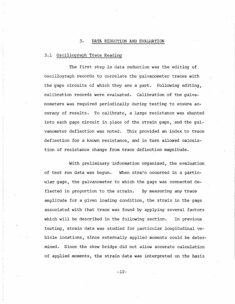
3.1 Oscillograph Trace Reading
The first step in data reduction was the editing of
oscillograph records to correlate the galvanometer traces with
the gage circuits of which they are a part. Following editi~g,
calibration records were evaluated~ Calibration of the galva
nometers was required periodically during testing to ensure ac
curacy of results. To calibrate, a large resistance was shunted
into each gage circuit in place of the strain gage, and the gal
vanometer deflection was noted. This provided an index to trace
deflection for a known, resistance, and in turn allowed calcula
tion of resistance change from trace deflection magnitude.
With preliminary information organized, the evaluation
of test run data was begun. When stra~.n occurred in a partic
ular gage, the galvanometer to which the gage was connected de
flected in proportion to the strain. By measuring any-trace
amplitude for.a given loading condition, the· strain- in the gage
associated with that trace was found by applying several factors
which will be described in the following section·. In previous
testing, strain data was studied for particular longitudinal ve
hicle locations, since externally applied moments could be deter
mined. Since the skew bridge did not allow accurate calculation
of applied moments, the strain data was interpreted on the basis
-12-

of maximum response. Noting the gages which reflected bending
at a particular section, the maximum trace ~mplitudes for those
gages were found on a test run record. At this location on the
record, the amplitudes of the traces under consideration were
measured to an accuracy of 0.01 inch, and the longitudinal posi
tion of the load vehicle, was determined by proportioning the
distance between axles on the vehicle to the distance between
reference marks on the oscillograph. record (see Sec. 2.7). In
most ·cases, the maximum amplitude was located easily by eye.
However, when the vehicle was placed in the westerly lanes on
the span, gage activity in the beams on the east side of the
structure was slight, making the location of the maximum ampli
tude' more difficult.
3.2 Evaluation of Oscillograph Data
3.2.1 Strain Calculation
After load trace amplitudes were measured and tabUlated,
they were entered as input in a computer program which calculated
strains and beam deflections in the test ~tructure" The conversion
of oscillogr~ph trace amplitudes to strain and deflection values
was a relatively simple matter, involving multiplication of the
load trace amplitude measurement by one variable and several con
stant quantities which were dependent on electrical resistances.
-13-

The apparent strain in any gage is given by
where R = gag~ resistanceg
R = calibrating resistancec
F = gage factor
The only variation from normal calculations involving
electric resistance strain gages is CL, which is a resistance
correction factor for the length of cable from the amplifier ,to
the gages. These lengths sometimes ranged as high as 300 feet.
The other values for Rg , Rc ' and F are known prior to testing,
and are constant. Calibrating attenuation and operating attenu-
ation, which are resistance adjustments in the amplifiers which
control the sensitivity of the oscillograph galvanometers, are
held constant for the static test series. For each gage circuit,
all constant factors can be combined as
K = tiLL
operating attenuationX'ca~ibrating attenuation
.Finally, the experimental values, which are the load
trace amplitude and the calibration trace deflection, are combined
-14-

with K as
e = K x load trace amplitudecalibration trace deflection
where e = experimental value for strain at a given location
on the structure
3.2.2 Strain Tabulation and Plotting
After strain values were obtained in the form of corn-
puter output, they were tabulated on a schematic· cross-sectiqn
view of the test bridge, with each ~train value written, in micro
inches per inch, at the approximate location where the strain was
measured. A typical strain tabulation is found in Fig. 10.
Following tabulation, girder web strain values were
plotted by the computer, permitting easy location of unreasonable
values which did not fall within approximately 5% of a straight
line strain distribution through the depth of the girder. Strain
values which seemed unr~asonable were dropped from consideration-
in subsequent calculations.
3.2.3 Moment Calculations
It was not possible to calculate moments directly from
the test data, because a dependable modulus of elasticity value
for the'girder concrete was not available. Instead, bending was
-15~

evaluated on the basis of a quantity termed the moment coeffi
clent. The moment coefficient is simply the experimental moment
value as a function of the modulus of elasticity, having a unit
of ft-in2 if the moment is to be expressed in ft-lb and the modu
lus in psi. Multiplication of the moment coefficient by the mod
ulus of elasticity, if known, would give the experimental moment
value.
After unreasonable girder strain values were eliminated
from the initial data, the remaining values were used as input for
the principal computer program. The program begins by determin
ing the most probable straight line strain distribution by the
method of least squares, and calculates the distance from the bot
tom surface of the girder to the experimental neutral axis for
each girder face. Taking the neutral axis location as determined,
along with various properties of the girder cross-section, the
program then calculates effective area of deck slab, and, for the
exterior girder, effective curb and parapet wall area by balancing
area-moments of concrete above and below the neutral axis. With
the effective concrete area known, it is possible to compute the
properties of the composite cross-section in bending, and by
utilizing the previously computed strains, the moment coefficient
can be determined. For an exterior girder, the computer output
lists the following:
1. effective width of slab
2. effective width of curb
3. effective width of parapet wall
-16-

4. x-x moment of inertia (composite section)
5. y-y moment of inertia (composite section)
6. 'product of inertia (composite section)
7 •. moment coefficient
Output from interior beam calculations contains the same informa
tion except for curb and parapet figures. In calculating slab
widths, the program limits the width of slab available to the ex
terior girder to half the distance between girder centerlines.
This condition is not imposed on the interior girder calculations,
in order that sufficient slab will be available in any case to
balance the area-moments.
When the program was first used, calculations were per
formed giving consideration to transformed reinforcing steel area
in the deck slab, assuming a modular ratio of 6. In the bridges
studied, the deck reinforcement does not follow a dimensionally
consistent pattern, and it was nece~sary to devote considerable
time and attention to altering the·program for each bridge studied.
,Therefore, it was decided to evaluate the effect of neglecting .slab
steel on the moment. coefficient value, and found that the computed
value varies by less than· 1%. From that ,time, therefore, calcula
tions have been made without considering deck slab reinforcement.
A more detailed description of the computer program is
included as an appendix to th~s report. The program was written
in the General Electric-Lehigh University LEWIZ compiler language.11
A flow chart is included, so that the program logic may be studied
-l7-

in detail. Other contents in the append,ix are a printout of the
LEWIZ program, a sample of the program input format·, and a sample
output sheet.
-18-
4. PRESENTATION OF TEST RESULTS
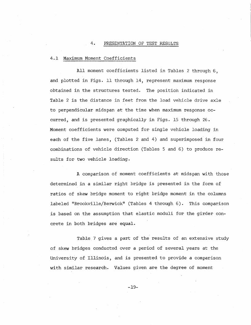
4.1 Maximum Moment Coefficients
All moment coefficients listed in Tables 2 through 6,
and plotted in Figs. 11 through 14, represent maximum response
obtained in the structures tested. The positiori indicated in
Table 2 is the distance in feet from the load vehicle drive axle
to perpendicular midspan at the time when maximum response oc
curred, and is presented graphically in Figs. 15 through 26.
Moment coefficients were computed for single vehicle loading in
each of the five l~nes, (Tables 2 and 4) and superimposed in four
combinations of vehicle direction (Tables 5 and 6) to produce re
sults for two vehicle loading.
A comparis.on of moment coefficients at midspan with those
determined in a similar right bridge is presented in the form of
ratios of skew bridge moment to right bridge moment in the columns
labeled ttBrookville/~erwickn (Tables 4 through 6). This comparison
is based on the assumption that elastic moduli for .the gi'rder con
crete in both bridges .are equal.
Table. 7 gives a. part of the results of an extensive study
of skew bridges conducted over a period of several years at the
University of Illinois, and is present~d to provide a comparison
with similar research. Values given are the degree of moment
-l9-

reduction in a variety of skew bridges when compared with a right
bridge of similar characteristics. The reduction percentages will
be discussed and compared with results obtained on this pr9ject in
Chapter 5.
4.2 Deflections at Midspan
In the calculation of deflections at midspan, longitu
dinal vehicle position has been given primary consideration, with
deflections computed when the vehicle drive axle is located at skew
mid~pan on the structure. This condition was imposed in o'rder to
provide a qualitative comparisQn of behavior as vehicle position
varies~ In Tables 8 through 12, deflection values for all four
girders have been compiled in a.manner similar to that in the case
of moment coefficients, including values listed for both one and
two vehicle loads, and a numerical comparison between skew and
right bridges. Graphic presentation of deflection data. is given
in Figs. 27 through 30.
4.3 Maximum Strain at Bottom Girder Surfaces
Strain data is compiled for one and two vehicle loadings,
with comparison of midspan strain magnitude, in Tables 13 through
18. The strain values were computed at the same identical load
vehicle positions as were the moment coefficients. Strain data is
plotted in Figs. 31 and 32, to provide observation of strain trends
at the gaged sections.
-20-

4.4 Effective Width of Slab, Curb, and Parapet Wall
In Table 19 are listed the effective widths of slab,
curb, and parapet walls for exterior sections, and the effective
width of slab for interior sections. These widths were calcu
lated to balance area-moments about the experimentally determined
location of the neutral axis. For the interior girder, as much
slab width as was theoretically required was made available. For
the exterior girder, the available sla~ width was terminated at
95 inches, the midway point to·the adjacent interior girder. More
concrete area was often required in exterior girder bending, and
was allotted as necessary from the curb and parapet wall. The
data given is 'for single vehicle loading only.
4.5 Neutral Axis Location
The calculated height of the experimentally determined
neutral axis above the bottom surface for left· and right girder
faces is listed in Table 20. The values listed are for 'single
vehicle loading, and provide for a qualitative look at girder ro
tation. In calculating ~oment coefficients, neutral axis heights
were averaged for each section, and composite beam section proper
ties were computed with respect to the horizontal axis. Neutral
axis locations are included for each gage section, considering
all test runs, for single vehicle loading.
-21-

5. DISCUSSION OF TEST RESULTS
5.l Vehicle Position at Maximum Response
In ,general, the test structure responded predictably
to lateral variation in load vehicle position. The largest mo
ment in any gaged section occurred when the load vehicle passed
in the loading lane closest to the section, and the moment de
creased as the vehicle was run in lanes at greater lateral dis
tances from the section under consideration.
Response was not so predicta.ble, however, with respect
to longitudinal'vehicle position. In all cases, the vehicle was
placed so that skew midspan was within its length when maximum
occurred, but otherwise no general statement can be made. The
drive axle fell within 10 feet of skew midspan in almost all in
stances, and considerably closer in sOhthbound runs. The general
trend of position shown in Figs. 15 through 26 follows the skew
midspan line, and seems to indicate that positioning with the
vehicle drive wheels at midspan would have yielded response very
close to maximum at the sections considered.
5.2 Maximum Moment Coefficients
It is notable that moment coefficients determined at
sections El and E2 are very close in magnitude. This is a probable
-"22-
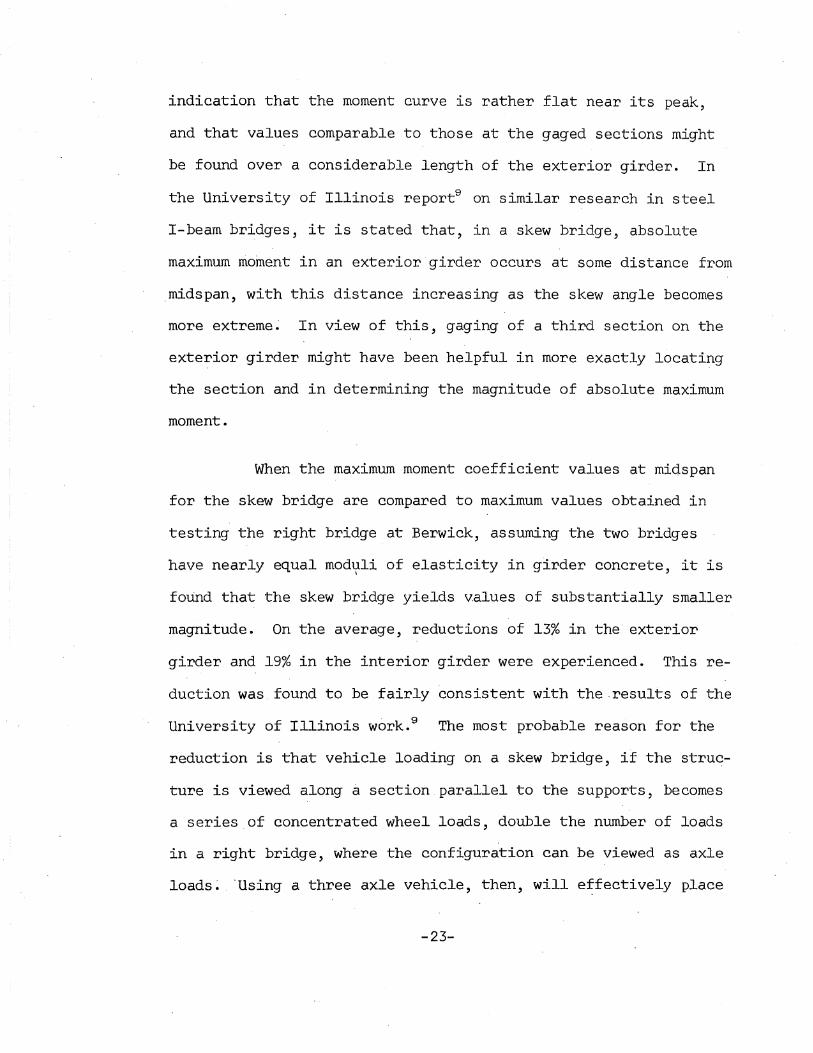
indication that the moment curve is rather flat near its peak,
and that values comparable to those at the gaged sections might
be found over a considerable length of the exterior girder. In
the University of Illinois report9 on similar research in steel
I-beam bridges, it is stated that, in a skew bridge, absolute
maximum moment in an exterior girder occurs at some distance from
.midspan, with this distance increasing as the skew angle becomes
more extreme~ In view of this, gaging of a third section on the
exterior girder might have been helpfUl in more exactly locating
the section and in determining the magnitude of absolute maximum
moment.
When the maximum moment coefficient values at midspan
for the skew bridge are compared to maximum values obtained in
testing the right bridge at Berwick, assuming the two bridges
have nearly equal mod~li of elasticity in girder concrete, it is
found that the skew bridge yields values of substantially smaller
magnitude. On the average, reductions of 13% in the exterior
girder and 19% in the interior girder were experienced. This re
duction was found to be fairly consistent with the.results of the
University of Illinois work. 9 The most probable reason for the
reduction is that vehicle loading on a skew bridge, if the struq
ture is viewed along a section parallel to the supports, becomes
a series_of concentrated wheel loads, double the number of loads
in a right bridge, where the configuration can be viewed as axle
loads~ 'Using a three axle vehicle, then, will effectively place
-23-

six individual concentrated loads on, a skew bridge, and three
concentrated loads on a right bridge. It can be seen that, on
the skew bridge, some wheel loads will lie closer to the end
supports than on a comparable right bridge, resulting in a re
duction in the moment at any section. Data from this project
shows an overall average moment reduction of 16% for single vehicle loading. In a rough comparison, figures from University
of Illinois data, converted to use with AASHO H-S loading, show
an average reduction of 21% for a bridge of 45° skew. Disagree
ment in the reduction figures could indicate some effect of the
difference in bending properties between the concrete box-shaped
section and the steel I-shaped section studied in Illinois r~
search. This cannot be discussed at present as there has been
no work done specifically in this area. The Illinois reportsS,s
have provided conclusive evidence that I-beam bridges of up to
30° skew show no appreciable reduction in moment, but that the
reduction becomes considerable, and increases with degree of
skew, in bridges with skew greater than 30°. In view of these
findings, it appears that valuable information might be gained
by investigating box girder bridges of other than 45° skew in
future testing, in,order to- determine the magn~tude of moment re
duction with varying skew in box girder bridges.
5.3 Deflection and Rotation at Midspan
Deflections experienced in this phase of testing are
quite consistent in magnitude with those in bridges tested
-24-
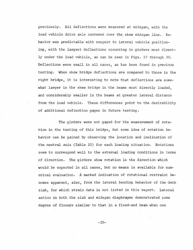
previously. "All deflections were measured at midspan, with the
load vehicle drive axle centered over the skew midspan line. Be
havior was predictable with respect to lateral vehicle position
ing, with the largest deflections occurring in girders most direct
ly under the load vehicle, as can be seen in Figs. 27 through 30.
Deflections were small in all cases, as has been found in previous
testing. When skew bridge deflections are compared to those in the
right bridge, it is interesting to note that deflections are some
what "larger in the skew bridge in the beams most directly loaded,
and considerably smaller in the beams "at greater lateral distance
from the load vehicle. These differences point to the desirability
of additional deflection gages in future testing.
The girders were not gaged for the measurement of rota
tion in the testing of this bridge, but some idea of rotation be
havior c'an be gained lJy observing the location and inclination of
the neutral axis (Table 20) for each loading situation. Rotations
seem to correspond well to the external loading conditions in terms
of direction. The girders show rotation in the direction which
would be expected in all cases, but no means is ava"ilable for num
erical evaluation. A marked indication of rotational restraint be
comes apparent, also, from the lateral bending behavior of the deck
slab, for which strain data is not listed in this report. Lateral
action in both the slab and midspan diaphragms demonstrated some
degree of flexure similar to that in a fixed-end beam when one
-25-
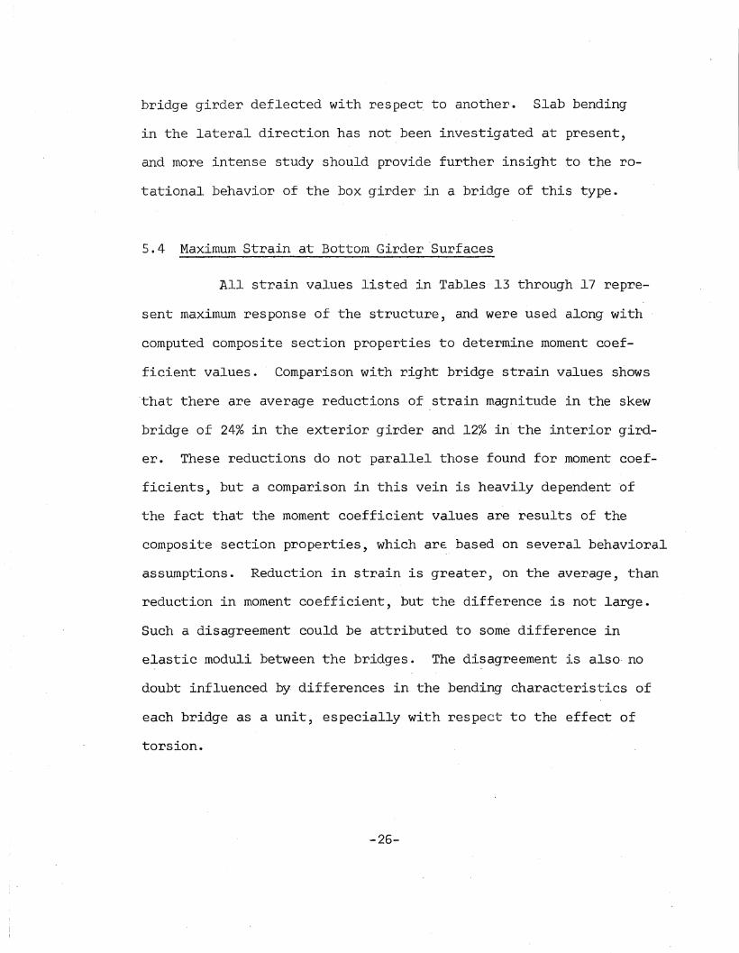
bridge girder deflected with respec~ to another. Slab bending
in the lateral direction has not been investigated at present,
and more intense study sho~ld provide further insight to the ro
tational behavior of the box girder in a bridge of this type.
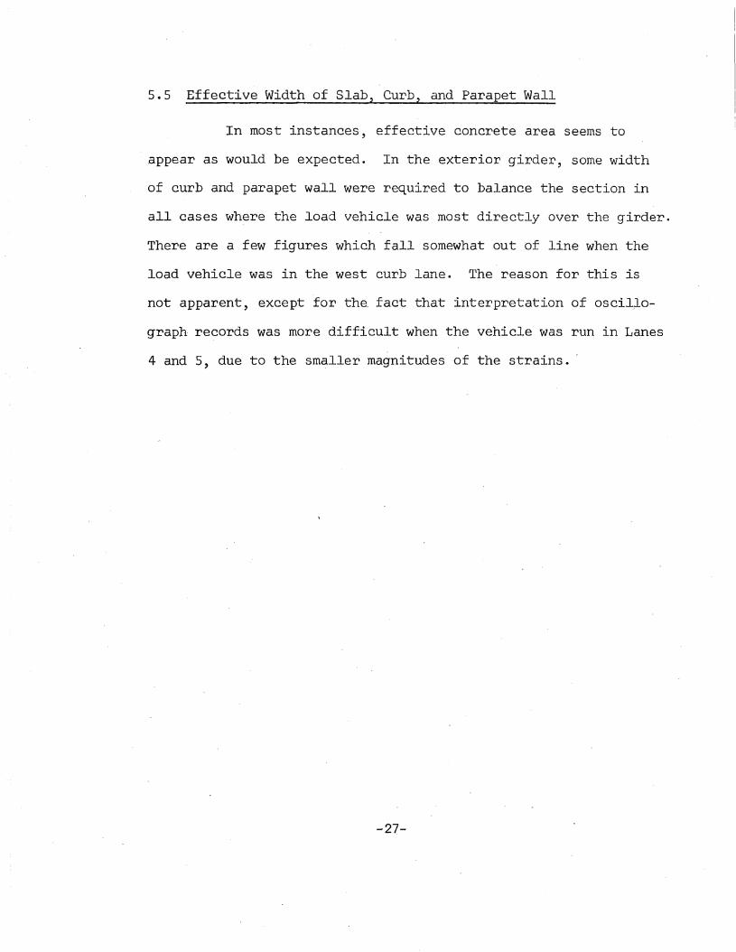
5.4 Maximum Strain at Bottom Girder 'Surfaces
All strain values listed in Tables 13 through 17 repre
sent maximum response of the structure, and were used along with
computed composite section properties to determine moment coef
ficient values. Comparison with right bridge strain values shows
'that there are average reductions of strain magnitude in the skew
bridge of 24% in the exterior girder and 12% in" the interior gird
er. These reductions do not parallel those found for .moment coef
ficients, but a comparison in this vein is heavily dependent 'of
the fact that the moment coefficient values are results of the
composi~e section properties, which art based on several behavioral
assumptions. Reduction in strain is greater, on the average, than
reduction in moment coefficient, but the difference is not large.
Such a disagreement could be attributed to some difference in
elastic moduli between the bridges. The disagreement is also, no
doubt influenced by differences in the bending characteristics of
each bridge as a unit, especially with respect to the effect of
torsion.
-26-
5.5 Effective Width of Slab, Curb, and Parapet Wall
In most instances, effective concrete area seems to
appear as would be expected. In the exterior girder, some width
of curb and parapet wall were required to balance the section in
all cases where the load vehicle was most directly over the girder.
There are a few figures which fall somewhat out of line when the
load vehicle was in the west curb lane. The reason for this is
not apparent, except for the, fact that interpretation of oscil~o
graph records was more difficult when the vehicle was run in Lanes
4 and 5, due to the smaller magnitudes of the strains ..
-27-
6. SUMMARY AND CONCLUSIONS
6.1 Summary
The main objective in this report is the evaluation
of data collected in the field testing of a prestressed con-
crete box girder highway bridge of 45° skew, and the comparison
of its structural behavior with that of a right bridge of simi
lar characteristics. The bridge tested was a beam-slab structure
utilizing four precast, pre-tensioned girders of hollow box cross
section, topped by a composite reinforced concrete deck slab.
The main instrumentation for field testing was devoted
to the measurement of fiber strains at three girder cross-sections $
Two of the sections were located on one of the exterior gird~rs,
and one on the adjacent interior girder, for the evaluation of in
ternal bending moments produced by the rest loading. Additional
instrumentation was arranged to measure girder deflections, slab
strains, and midspan diaphragm strains.
Tests were conducted using a load vehicle closely con
forming to AASHO HS20-44 loading, along with a mobile instrumen
tation unit owned by the U. S. Bureau of Public Roads. All test
runs were made with the load vehicle moving at crawl speed, in
five loading lanes established for testing purposes.
-28-
The measured bending moments are presented as moment
coefficients, which take the dimensional form of bending moments
divided by the modulus of elasticity of the girder concrete, and
are expressed in the units ft-in. 2 This was done because no re
liable value was available for the modulus of elasticity in this
bridge. A comparison of the internal bending moments produced in
the skew bridge with those in the right bridge is, therefore, based
on the assumption that the elastic moduli in both bridges are equal,
and d~als solely with maximum response of the structure.
Moment coefficients were determined with the aid of a
computer program designed to perform calculations for any girder
,cross-section. The program calculates the area of the composite
section from strain data by balancing area moments about the neu
tral axis determined for a specific loading situation, and calcu
lates properties for tpe section which, when combined with ideal
ized strai~ values for the bottom girder surface, yield the mo
ment coefficient value. The logic of the program is described in
an appendix to this report.
In comparing moment coefficient values for the skew
bridge· to those for the right bridge, it was found that the values
for the skew bridge were generally lower. This reduction in mo
ment is probably due to the geometry of the skew bridge, in that
the effect of the skew is to more uniformly distribute the six
wheel loads over the span length.
-29-

Previous research conducted at the University of Ill
inois established that the degree of moment ,reduction in a skew
bridge varies with the degree of skew, increasing as the skew
becomes more extreme. The Illinois report is discussed in this
text, with a rough comparison made between moment reductions in
a 45° skew steel I-beam bridge, and those in the structure upon
which this report is based.
The girder deflection data for the Brookville "Bridge
shows a reduction of similar magnitud~ to that experienced with
"moment coefficients, but without the same pattern in reductions.
The reason' for the difference cannot be determined at present
because deflection instrumentation was not "sufficient to allow
a thorough analysis.
Also considered to a lesser degree were strains at the
bottom girder surface, calculated effective concrete areas in the
composite beam sections, and calculated locations of the neutral
axis in each section for all test runs.
6.2 Conclusions
From the crawl-run testing of the skew bridge 'at Brook
ville, the following conclusions can be drawn:
1. There was a reduction in moment coeffi
cients in the skew bridge in all cases
-30-

compared with similar values from the
right bridge. The magnitude of the re
duction, however, can be assumed to apply
only to a structure of 45° skew, as it was·
previously established that the moment re
duction varies with the degree of skew.s,s
This suggests that consideration of bridges
with different skew angles is in order, if
a relationship between skew angle and mo
ment reduction is to be established. There
fore, it is apparent that girders in a skew
bridge, designed on the basis of provisions
specified for right bridges, will actually
be stressed to lower levels than their right
bri~ge counterparts.
2. On the basis of the data ana~yzed, it appears
that the maximum live-load moment-envelope
in the exterior girder has a nearly constant
v~lue near absolute maximum over a consider
able length of girder. The exact location
and value of the maximum moment coefficient
cannot be estimated from available data, but
it is likely that the maximum occurs at some
distance from midspan, as was found in earlier
-31-
studies at the University _of Illinois.8,~
Additional girder instrumentation in future
testing would help to provide useful infor
mation toward this end.
3. For maximum response in either exterior or
interior girders, the longitudinal vehicle
was usually with the drive axle in close
proximity to the skew midspan line. It is
felt that·.data ~valuation with the drive
wheels located at skew midspan would yield
nearly the same experimental results as were
found with the more exact location of the
positions which' produced absolute maximum
responses.
4. Deflections in the skew bridge were generally
smaller than those in the right bridge, but
there was a marked tendency for the girder
most directly loaded to deflect considerably
more than the other girders, and in some
cases, more than the corresponding girder in
the right bridge. The reason for this dif
ferent distribution of deflections is not
apparent, and additional instrume~tation
would be required for a more complete evalu
ation.
-32-

5. The magnitudes and distributions of
strains in the skew bridge 'were quite
compa~able to those in the right bridge,
and in. general, the magnitudes were
sl'ightly smaller. The differences in
magnitude can be attributed primarily
to the more uniform longitudinal dis
tribution of load in the skew bridge,
and to some difference in the effective
modulus of elasticity.
-33-

7. ACKNOWLEDGMENTS
This study, which forms a part of an overall investi
gation of load distribution in prestressed concrete box-beam
bridges, was conducted in the Department of Civil Engineering at
Lehigh University, under the auspices of the Lehigh University
Institute of Research. The program is being sponsored by the
Pennsylvania Department of Highways, the U. S. Bureau of Public
Roads, and the Reinforced Concrete Research Council.
The field testing was accomplished with equipment owned
by the U. S. Bureau of Public Roads, and made available through
the cooperation of Mr. C. F. Scheffey, Chief, Structures and
Applied Mechanics Division, Office of Research and Development.
The instrumentation and operation of test equipment were under
the supervision of Mr. R. F. Varney, assisted by Messrs. W~ Arm
strong, C. Ballinger, and H. Laatz, of the Bureau of Public Roads.
The Lehigh University staff was represented in testing
by Mr. A. A. Guilford, Principal Investigator, and- by Messrs. W. J.
Douglas and R. J. Dietz. Data reduction and computer programming
were accomplished with the aid of Messrs. Guilford, R. H. Kilmer,
and C. S. Lin. The efforts of Mr. R. Sopko, Miss Sharon Gubich,
and Mr. J. Gera in drafting, and Mrs. Carol Kostenbader in typing
the manuscript are appreciated.
-34a-

The author wishes to extend gratitude to Professor D. A.
VanHorn for guidance and assistance rendered during all phases of
work leading up to, and particularly including, preparation of this
thesis.
-34b-

8. APPENDIX
The computer program used- ~n the major portion of
data reduction is a combination of four independent programs,
each of which, with small modifications, can be used separately
when expedient. The program contains (1) a least squares fit
ting routine which idealizes strain distribution through the
depth of the girder, (2) a program to calculate moment coe-ffi
cients in interior girders, (3) a similar program for exterio~
girders, and (4) a routine to calculate lateral distribution
coefficients, not used in data reduction for the skew bridge.
The LEWIZ compiler language, unlike the more common
FORTRAN, requires no input format. Input data is entered in a
pre-determined sequential order as specified by· "card read"
(CRD) statements in the program. All LEWIZ arithmetic is carried
out in floating point form, unless otherwise specified. All al
gebraic statements are written in exactly the same form used with
FORTRAN, and should be readily understood by "anyone with- a general
knowledge of programming.
In the following pages are (1) a program flow chart "in
verbal form, (2) a list of all program variable names, each with
a description of the quantity it represents, and (3) a printout
of the program as written, with a sample output. The LEWIZ program
-35-

may be used by entering the values called for in CRD statements,
in exactly the order given in the printout. The only format re
quired in input data is a space left after each value on the
punched cards.
-36-

Least Squares Fit Program
Start
Dimension for values1. NA location 4. Interior moments2. Strain 5. Exterior3, Effective slab width
Initialize valuesrequire.d for least ~....- .....
squares fit
Read (N) numberof good strain
values, runnumber
-37-
Read coordinatesof next strain
loc.ation
Add coordinatesof point in
L8 series
compute fittedvalues for
NA location,strain at bottom
es
no

1
Read bridge constants, number of
~-----------......... sections to beconsidered
Initialize ·subscriptsstrains left and right,
and moment valuestorage location
Print column headingsfor interior beam
moment values
Interior Beam Program
-38-
. Take appropriate strainandNA values from L8 fit
storage and compute moment ........---arms to area segments
Compute ef activeslab width by
bal.ancing areasabout NA
Compute Ix ofsegments, thencombine to get
total Ix
Compute I y ofsegmentS' and
combine to gettotal I y-
symmetrical section
Rl
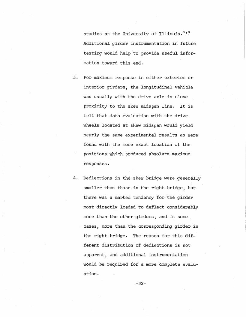
compute I aboutinclined axis (1M)
Produc t (IMN),angle of loadapplication ct'
compute verticalmoment component
MX
R2
-39-
Increase subscriptsfor strain, NA,moment values
to denote nextinterior storage
location
Initialize subscriptswhich denote exterior
beam locations
no
no
Exterior Beam Program
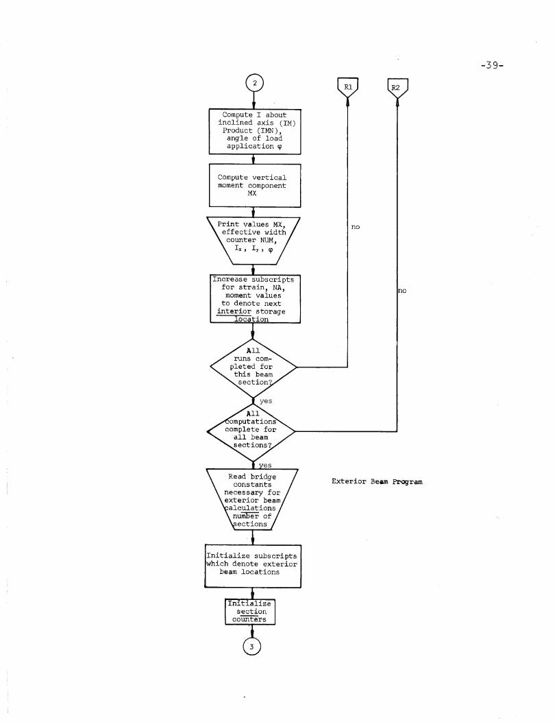
ApprOX~lHate slabwidth taken to betrue effective width
Reaq. sectionvalues--beam depth,
slab thicknessnumber-r'Uns forthis section
Print columnheadings forexterior beam
values
Take NA and strainvalues from
appropriate locations in L8 fit
Initialize curband parapet width
to zero
ompute moment armsto area segments for
Ix--compute maximumslab width allowed~adjacent beam
compute approximateslab width by balancingarea moments about NAx
Isapproximateslab width
greater thanmaximumllowed?
Maximum slab widthtaken to be trueeffective width
R3
-40-
R4

L1
Curb widthcalculatedtaken to beeffectivecurb width
Compute curbwidth, ,using slab
width determined, bybalancing area moments
Iscurb width
greater thanmaximum
llowed?
yes
Maximum allowablecurb widthtaken to be
effective curb width
Compute effectiveparapet widthby balancingarea moments
about NAx
Taking effectivewidths computed,
find Ix for all areasegments and combineto get Ix of section
Compute areas,moment anns,
area moments, I yfor all segmentsinvolved--combine
to get' I y for entiresection, and location
of NAy
compute I xy for allsegments and combineto get I xy for entire
section
Compute I aboutinclined axis M,(1M), Product, (IMN)and angle of loadapplication (qJ)
. R3
R3
R4
R4
-41-

compute verticalmoment component
MXE
Print valueseffective slab, curb,
arapet width MXE,
Increase subscriptsfor strain, NA,
moment values todenote next exterior
storage location
Read number of setsf runs to be combined
for distributioncoefficients
Print explanatoryinformation
Read number runswithin followinget--Print colu
headings
R3
no
Distribution CoefficientProgram
RS
R4
no
-42-
-43-
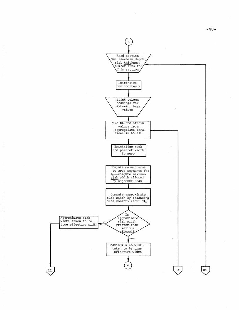
Read Lane, Speed,Position, and
locations of valuesto be combined ~-------..
Locate necessarymoments and combineto get percentage
values
no
noPrint values forane, speed, position
and momentpercentages
END

NOTATION IN DISTRIBUTION COEFFICIENTS PROGRAM
Least Squares Program
NAS
T,0T
sx,sxxSY,SXyD,A,BN
RXyS(J)
NA(J)
neutral axis--averaged horizontalstrain determined by least squares fit at bottom
of beam ,total number of sets of strain readings to be
considered in-Ieast squares routine--amUltiple of 4 since there are four beamsides (two exterior.and two interior) for anyone run
intermediate values in least squares fit procedure
number of strain values to be considered for onebeam side
run numberstrain valuestrain gage location; inches from bottom of beamstrain at bottom of beam as calculated in least
squares routineneutral axis location as calculated in least
squares routine
Interior Beam Moment Program
ABMYBM
HBMIBMX
IBMY
WSEC
DL,DR
TL,TR
area of nominal box girder section (ina)centroidal distance from bottom of beam for box
girder section (in.)nominal depth of box girder (in.)moment of inertia of box girder about its
centroidal axis x-x (in4)-
moment of inertia of box girder about itscentroidal axis y-y (centerline of section)(in4
)
nominal width of box girder (in.)number of beam sections to be considered in a
set of computations (composite section variesdue to change in slab thickness)
measured depth of beam with slab in place, leftand right, respectively (in.)
measured slab thickness to ~eft and right of boxgirder (in.)
-44-

NUM
NAL , NAR
SL,SR
YNA
,T~D
IlliEG
NEGA
DNEG
DSLAB
DBM
EW(J)
ISLAB
INEG
JBM
IX
IY
BETA1M
IMNSTRAINIILAM
PHIMX(J)
number of computation runs for"a given beamsection
neutral axis location, left and right, for a'given loading case
strain at bottom of beam, left and right, for agiven loading case
distance from bottom of beam to horizontalneutral axis
average slab thicknessaverage beam depth with slab in placeheight of tToverlapu i.e. distance which girder
protrudes into slabarea of overlapdistance from horizontal neutral axis to bottom
of slabdistance from horizontal neutral axis to centroid
of overlapdistance from horizontal neutral axis to centroid
of slabdistance from horizontal neutral axis to centroid
of box girdercalculated effective width of slab for a given
loading case (in.)moment of inertia of effective slab about
horizontal neutral axismoment of inertia of overlap about horizontal
neutral axismoment of inertia of box girder section about
horizontal neutral axismoment of inertia of composite section about
neutral horizontal neutral axis~oment of inertia of composite section about
girder centerlineangle of inclination of experimental neutral axismoment of inertia of composite section about
experimental'neutral axisproduct of inertia of composite sectionaverage strain at bottom of beamdirected "moment of .inertiaangle between plane of loading and experimental
neutral axisangle between plane of loading and verticalmoment coefficient value in interior beam for a
given loading case
-45-

Exterior Beam Moment Program
weWPHC,HP¢H
DXC
DXP
CWPiiJHNDN
DYS
Dye
DYP
MSW
BSASW
swCWPiiJISLX
IBEX
lex
IPX
IX
ASWNDXN
WPA
DXPA
width of curb on the bridge (from edge ofroadway to outside of parapet) (in.)
width of parapet wall on the bridge (in.)height of curb and parapet, respectively (in.)width of overhang (from outside of exterior
beam to outside of parapet) (ino)x-distance from centerline of girder to centroid
of curb (in.)x-distance from centerline of girder to centroid
of parapet wall (in.)calculated effective curb widthcalculated effective parapet wall widthheight of overlapy-distance from horizontal neutral axis to
centroid of overlapy-distance from horizontal neutral axis to
centroid of slaby-distance from horizontal neutral axis to
centroid of curby-distance from horizontal neutral axis to
centroid of parapetmaximum width of effective slab--determined by
slab width required by adjacent interior orbeam
c-c girder spacing (in.)approximate effective slab width--intermediate
valuecalculated effective slab widthcalculated effective curb widthcalculated effective parapet wall widthmoment of inertia of effective slab about
horizontal neutral axismoment of inertia of girder about horizontal
neutral axismoment of inertia of effective curb about
- horizontal neutral axismoment of inertia of effective parapet wall
about horizontal neutral· axismoment of inertia of composite section about
horizontal neutral axisarea of effective slabwidth of overlapx-distance from centerline of girder to centroid
of overlapwidth of additional slab thickness outside of
exterior beamx-distance from centerline of-girder to centroid
of additional slab thickness area
-46-

DXS
ANACAPAT¢TMA
DX
IY
IY
DXDXSDXNDXPADCXDPXIXY
MXE(J)
x-distance from centerline of girder to centroidof effective slab
area of overlaparea of effective curbarea of effective parapet wallarea of effective composite sectionarea-moment of all segments about girder
centerlinex-distance from girder centerline to y-y centroidal
axis of composite sectionmoment of inertia of effective composite section
'about girder centerlinere-defined as moment of inertia of effective
composite section about its y-y centroidalaxis
re-defined to comply with transfer of referencefrom centerline of girder to y-y centroidalaxis of composite section
product of inertia of effective composite sectionwith reference to its own centroidal axesx-x and y-y
vertical component of moment for a given loadingcase
Distribution Coefficients Program
MPA , MPB ,MPC,MPD
Note:
N
MLANE8PDA,B,C,D
POGSMD,MC
MT
number of sets of runs to be considered (varieswith position, section, speed, direction:set consists of sufficient runs to describeeIfect of anyone position, section, speed,direction combination)
number of runs within set to follow instructionlane in which test run took placespeed of test vehiclestorage locations of proper moment values to
be combinedcombined expression for position and sectionmoments in beams D,C,B,A respectively for a
given loading casesum of internal moment in all beams for a given
loading casepercentage of total moment carried by beams
A,B,C,D respectively
where variable names in interior beam program areused again in exterior beam program, they are described in the explanation of interior beam namesonly. Variable names not described here are thoseof index counters and subscripts.
-47-
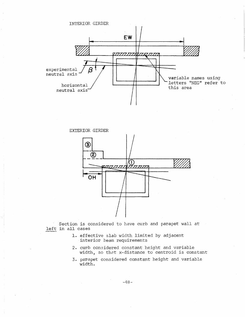
INTERIOR GIRDER
EW
experimentalneutral axis
horizontalneutral axis
EXTERIOR GIRDER
variable names usingletters TtNEGn refer tothis area
@
®- ---~----+-~-------~........"""""""'-
OH
Section is considered to have curb and parapet wall atleft in all cases
1. effective slab width limited by adjacent-interior beam requirements
2. curb considered constant height and variablewidth, so that x-distance to centroid is constant
3. parapet considered constant height and variablewidth.
-48-

OU5 2095 SCHAFFER--SOLUTION rOR LOAD DISTRI8UTION FACTORSS~p 1( 67 12 02.0
PAGE 1. SEP 12 67
SEQ LA8L TYP ST4TeHENT C ZERO NOT 0 PI.US MINUS ELSE:
U~l. 1J N4[16D].S[160J,ewt40].~X(20J,HXE[20] [
002. J:sl [
OU3. C~DTOT [U04. 51- COUNTER RUN NEUTRAL,. AXIS C
STRESS AT BOTTOH FIBER [ ] [ ) ( ) t J I005. 1 S(IlSXX~SY=SXYJIlO [ ] ( ) t i [ ) t0\16. fIXN.R.P"K [ ] ( J t J [ 1 [007. CRDN.R SNUM Of DATA POINTS AND RUN NUM [ ] [ ] [ ] [ ] [008. N~.N [ J t ] [ i [ ] [OQ9. 010 2 N'l=NN.1 [ ] [ J [ ] [99 1 tO~O. CRDX,Y $ ON~ DATA flOOINT [ ] t ] ( J [ ) [all. Sl(·SX.X,SY=SY·Y [ J [ ] [ i [ 1 [Ui2. S(X.SXX+X-X,SXY.SXY+X-Y [ ] [ J [ ] ( ] [2013, 99 O"SXX*N.SX*SX [ ] t 1 ( ] [ ] [Oi4, A:S[SXY*N~SY*SX]/D [ ] t ) [ ] ( J [U15. B~[SXX·SY·SXY*SX]/D ( ] t J [ ) ( ] [01,6. StJ]=C"'BJ/A [ ] t J [ J t J t01.7. N~[JJ=8 ( ) [ ) [ ] ( , tU~8, PV JiR,NAtJJ,SrJl ( ] [ ] [ ] t ] [019, PL ( ] t 1 ( 1 [ 1 [U20. [)-J+1)·TOT {1 ] [ ] ( 1 (1 ] t021. 001 CRDA~M.YBM.H8M,I8MX.IBMy,W.SEC { ] ( ] [ J ( ] [022, 00.5 C:a1 [ ] [ 1 ( J t J tOc3, r I XN'jM [ ] t ] [ 1 t 1 r0,4. 47 CRDD~.DR,TL,TR,N ( 1 [ J [ J t ] [0,5. 30 NIJM:1 { ] t ] [ ] [ ] [0~6. R"3,rc4,J~2 [ 1 t ] ( J [ ] [
Ot7. s~ I~TERI0R BEAM CALCU~AT!ON~ ( ] t ] [ 1 [ J [028. PI. EFr, WIDTH HOMENT/E.10**~6 LB.FT R-RUN C
. IX ty PHI { ] t J [ ] [ J [O~9. 55 N~L.NA[R"NAR.NA[r, ( ] [ ] [ j t ] [030. SLastR],SRl;s[r] [ ] t 1 [ ] [ l [O~l. 70 S COMPUTE EFFECTIVe WIoTH BY AREA MOMENTS [ ] [ 1 [ 1 ( 1 t032. 80 Yl\fA.CNAL+NARl/2 [ 1 t ] ( i t ) tO~3. 90 T;t[TL·TR]/2 ( ) [ 1 [ i [ ] [0~4. :;00 D~[DL+DR]/2 [ ] [ ] [ J [ , [O~5. 110 H~EG~HBH·D [ ] t ] [ ) [ ] [036. 120 NSG.HNEG*W [ ] [ ] t J [ 1 (
O~7. 130 A~D.YNA [ ) [ J [ ) [ ] [0~8. 140 D'iEGaA"HNEG/2 [ ] [ . 1 r ] [ J [O~9. 150 D3LA8~A+T/2 [ 1 t ) ( J [ J [O~O. ~60 D9M.VNA.YBM [ ] [ ] t i [ ] [041. E~[Jl~[ABM*DBM"NEG.DNE&J/t'.DSLABJ [ ] [ 1 [ J [ J [042. 210 S COMPUTE MOMENTS Of t~eRTIA ABOUT x, V, AND ( ] [ 1 [ ] [ J [043. 220 S INC~lNED M AXES [ ] [ 1 [ J t 1 [044. ISLAB.tEW[J].T••3J/12·EW[~'·T.DSLA8.*2 [ ] [ J ( J [ ] t045. 240 I~EG~rW*HNEG.HNeG.HNEG!/la.. W.HNEG*ONEG*DNeG [ ) [ ] ( J [ ] r046. 250 J9M_XBMX·ABM*08H*OBH [ ] [ ] [ ] t , [
047. 290 13 IX·IS~AB·INEG·JBM [ ] t ] 1 J [ J [O.8~ 300 K:t2 [ ] [ ] t i t 1 -r049. IY~18MY.[T·EwtJ]·*3]/12·{HNEG*W••3'/12 [ 1 t ] ( ] [ ] [
0'0. 8E~cATAN.t[NAL~NAR]/W' [ ] t ] t j [48 1 [49O~l. 48 BETAIJ.SETA [ ] r J ( j [ ] [
i . I0'2. 49 I~.[tX·IYJ/2·t[IX·IY]/2J.COS.[2.8ETAJ [ ] [ ) [ ] [ ] [
~O!)3-. .50 I~N=[[lX·IY]/2J*SIN.t2.BET·J ( J [ l [ J [ J [ ]
LOI

PAGE 2, SriP 12 67
SEQ LABL TYP STATEMENT C ZERO NOT 0 PLUS MINUS ELSE
054. 460 STRAIN;:rSL"'SR~/2 [ ] [ ] [ 1 ( ] [055. 470 IIaSQRT,[IMN*IMN+IM*IM' [ ] [ ] [ i [ ] [056. 510 L4M8ATAN,tIH/IMN] [ ) t 1 [ ] [50 1 [51057, 50 L~M •• \..AH ( ) t ] [ ] [ ] (
0;8, 51 P~I.BETA·LAH-J,1415927/2 [ ) [ ] [ ] t52 ] [530~9, 52 P~l.~P,",I [ ] t ] [ ) [ ] [060, 53 M~[Jl~[Il*STRAlN·COS,[PHI)'/[YNA.12.COS,[ C
BETA) ) [ ) [ ] [ ] ( ] (Obl, PI. [ ] [ J t j t ] [U62, PV E~(J,,~X[JJ,NUM.IX~Iy,PHI [ ] ( ] [ J [ ) [063. R~R ... 4,F"=F'+4 r ] [ ) [ 1 [ ] [064, [J:rJ·2J [ ) [ J [ j [ ] [065. 600 r~UMcNUM*1'-N [ ) [ ) [54 1 ( ) [55O~6, 54 [C=C+1J·SEC [ ] ( ] [854 i ( ] [47O~7. 000010854 CRDA~M,YBM,HBH.I8MX,I8MY,W,WC,WP,HC,HP,OH,DXC.C
, 020 D~~,BS,SEC [
Ob8, R=1,K=2 [
069, J21 [
DID, 000030 5=1 [
071, A49 CRDD~,OR.TL,TR,NUM [
072. OOOD50 N:;1 [
073, S~ EXTeRIOR BEAM CALCULATIONS [
0/4, 000051 P1.. ErF, SLAB I ErF", CURs I EFF, PARAPET/ C000052 ~OMENT/E.10.'.6, ~B·rT / N IX C
IV IXV [ ] ( ] [ 1 t J C ]
075, 001660 Pi.. [ ] [ ) t J t 1 [ J076, A50 N4~aNA(R].NAR.NA(K' r J [ J ( 1 1 J t ]
077, P01J.1 [ ] [ ] [ ) t ) ( )
078, Sl.=SCRJ .. SRpSrKl [ ] ( ] t ) t J [ ]
079, 000061 C·~;:PW~O [ ] [ ] [ ] t ] [ )
060, 000070 NJ\Jl[NAL+NAR]/2 [ ] [ J ( j t l [ JU81, 000080 T2[TL·TRJ/2 [ ) [ ) [ ] t ) [ )
062, 000090 D~tDL·DRJ/2 [ ) [ ] [ j t J ( ]
083, 000100 H\jaHBM"D [ ] [ ) [ J t J ( ]
U~4, 000110 A~D-NA l ] [ ) [ ) t 1 [ ]
O~5, 000+20 D-3M:NA-yBH [ ) t J t J t , [ ]
Oa6. 000130 D~wA·HN/2 [ ) [ J [ j t ] [ ]
067, 000140 DYSaA.T/2 [ ] t ) [ ] t ] [ ']
068. 000150 D'(C:A*T.HC/2 '[ 1 [ ] [ J [ J [ J089, 000160 DYP:zA.T.HC"HP/2 [ ] [ ) [ 1 t ] [ )
O~O, MSW.OH·W/2·8S·EW[P]/2,~SW·tO~+W/2·9S/2] [ ) ( J lA99 J t 1 tA98 IU~l, A99 HSW.OI-l*W/2*BS/2 r ] [ ] [ J t ] [ ]
O~2, A98 ASW.CABM*DBM1/[T*DYS-HN*QNf [ J [ ) ( J [ ] [ )
Oii3. 000231 ASW-MSW r ) [ ) [ A!5] t ] [ A97)O~4, 000240 A97 ASW-W/2 [ ] [ ] [Ai 1 t ] tA04 JO~5, 000250 A1 ASWs(ABM.OBM+(W/2J*tHN*ON*A ft O,5])1 C
, 000260 tT·OYS"A-0,51 [ 1 [ I ( ) ( J [6, 000270 ASW.tW/2·0H) [ ) [ ] [A2 i [ ] [.047. 000280 .2 ASW.tA8M·DBM-OH.[HN.DN*A-O.~))/[T*OYS.HN·ON) [ l t ] [ l [ ] [
8, 000300 ASW-CW·O,,",] r l [ ] rA3 t ( 1 [A49. 43 ASWatABM*OBM+W*CHN*ON).OH*lA.O,51JI C
000320 rT*OYS, t ] [ 1 [ ] t .1 t ]
100, A4 S,"ASW [ ] [ ] [ j [ J t ]
101. 000340 S';·HSW [ ] [ ] [A5 J [ , [A18 ].102. A5 Sii~M5W [ ) [ J [ l [ J t r103, 000360 S"'-rW/2.0HJ [ ] [ ) [ J tA6 J lA' ] I
Ul0I

PAGE 3, SEP 12 67
11 SEQ LABL TYP ST4TEMENT C ZERO NOT 0 PLUS MINUS ELS~--,
lU4. A6 C~.[A8M*D8M~S~.T.OY~+[~/2].HN*DN+[SW-W/2J. COOO~BO [~·o,5J]/{HC*OYC] [ ] [ J [ J [ J [,6,10 J
105. 147 Sol/.[W .. OHl [ 1 [ J [ J [048 ] [A9 ]
106. 400 AS C~=[ABM*D8M.SW.[T·DVS~~N*ON'-O~.[HN*DN+A·a.5]C
410 J/[HC*DVCJ [ J [ J [ J [ ] r Al~}107. A9 C~=[A8M.08M.SW.T.OYS+W.~N·ON-OH.[A~O.5]l/ C
000440 {..,C.OYC] [ ] [ 1 [ ] [ J [A10 ]1P8. 1410 C.oj-..wc [ 1 t 1 [A11 1 ( ] tA18 J1U9. All C..j·WC ( ) [ } [ J [ J [ ]
110. 000470 S.oj-rw/2.0Hl ( ] t 1 [ J [A12 f [ Al,jJ111. A12 P~=[A8M*D8M-CW.HC.DYC·S~.[A~O.5}+t~/2J.[A·O.5C
000500 +~N.ON)]/rMp.OYP) [ ] t 1 [ ] [ ] [.416112. A13 S~,[W~OHJ [ 1 [ ] [ j (0414 J [A1S11.3. A14 P~c[A8M.DBM·Cw·HC*DYC·SW*(T*DYS~HN*DN1-OH. C
000540 [~·o.5·HN.DNJJ/[HP.DYPJ [ ] [ ] r J [ ] [A16114. 1415 P~3[ABM.DBM.Cw*HC*OYC-SW·r·DYS.W*HN*DN-OH. C
000570 {~·O.5l1/[HP*DYP] ( ] [ ) [ J t 1 [ ]115. A16 p·~·wP [ ] r ) (A17 J t 1 rA18 1116. 1417 p~ P4RAPET WIDTH EXCEEDS. ~AXIMUM ( ) [ ] [ J [ ) r ]117. AlB S"'''[~/2+0HJ [ 1 r ) [ J (.19 1 [.42D . J118. A19 I5LX=Sw*[T**3/12+T.DYS··2J+tSW~W/2'*(1/12· C
000630 [~·O.5J.·2J·[W/2J.fH~··3/12+HN*DN*·2J [ ) [ ) [ ) [ , tA23119. A20 S..j-rW+OHl [ ] t ) [ J [.421 ) CA22120. A21 ISLX=sw·tT··3/12+T*DYS·*2J+o~·r1/12+[A-D.'j C
000670 **2j-C SW·OH1*(HN**3/1Z.HN*ON*.21 [ J t J [ J [ , [A23 ]121. A22 ISLX=SW.(T··3/12+T*OYS·*21+0H*[1/12+(A-Q,5] C
, 000700 **2]~w·[HN**3/12+HN*DN.·2l [ ] t ] [ J [ 1 [122. A23 I3EX=IBHX+ABM*OBM·.2 [ ] [ J [ j [ ] [lc3. 720 ICX=C~*[HC·.3/12+HC·OVC.*21 [ ] [ J [ J [ ] [124. 730 IPX=P~·[HP·.3/12+HP·DYP·.2J [ 1 [ J [ ] ( 1 [1.::5. 000740 IX=IBEX.ISLX+!CX+IPX t J t 1 [ J [ ) (1~6. 000750 AS=SW*T t ] [ ] [ ]- [ J t1e7. 000760 S.o/-[W/2+0H] [ ] t ] [ ) [042<4 J [A251,a. A24 W\j:W/2 [ ] t ] [ ) [ ) [1~9. 000780 D(N:-\ol / 4 [ ] t ] r J ( ] [
1~0. WPA=S~"W/2 ( ] t ] t 1 [ , [1~1. D~PA="'(SW+\ll/2J/2 ( ] t ] [ 1 ( ) tlS2. 000810 D:<Sr:;-S\ol/2 [ ) [ ] [ j t ) [A29133. A25 S"j .. rW+OHl [ ] [ 1 [ J [.426 ] [A271~4. A26 ~P'4I1SW.OH r ] [ ] [ J t ] [lJ5. 000840 DXN-[wN.Wl/2 r 1 [ ] [ ] t J [A28136. A27 W'I='" [ ] [ J [ ) [ J [1~7. 000860 D)(N=O [ ) t ) [ ] [ ) r1~8. A28 WPA.OH r ) r ) [ J ( ] t1~9. 0008BO O)(PAD,.[W+OH]/2 [ ) [ } ( ] [ ) (
140. 000890 D:<S=[SW-Wl/2-0H [ ] t ] [ ) [ ) [141. A29 o4-4-HN.WN [ 1 r J [ J [ ) [
1.2. 001200 ACaCW*HC [ ] [ ] [ J t ] t143. 001270 AP-PW*HP [ ] [ ] [ J [ ] [14 .... A40 ATOTaA8M+AS-AN·WPA.AC·AP [ ] [ } t J [ ] r145. 1~20 H~·AS*DXS.AN·OXN+WPA.DXPA• .4q.DXC.AP.DXP ( ] t J [ j [ ] t146. 001340 DXilMA/ArOT [ J r ) ( J t ] [
147. 001350 I1 D IBMV.T*SW*·3/12.4S-0XS*.Z·HN*WN**3/12 C1360 -4N*OXN.*2+WPA·tWPA••2/~2·0XPA C1370 .*2].HC*CW.*3/12+o4C.DXC.*2.~P*PW.*3 C I1380 112+AP*OXP**2 [ ] t ) t J t ] t J V1
-> --~---~.~~-~------,
__ ~____ r .~. ~ ~ _ r _.~ ... _~ .. _ ~ ~J--II

PAGE 4. SEP 12 61
II SEQ LABL TYP, STATEMENT C ZERO NOT 0 p~US MINUS ELSt:
·1~8. 001390 IYc!YI'ATOT*OX··2 [ ] [ ] [
149, 001400 D~II-DX [ ) t ] [150. 001410 Dl(SaDXS.OX ( ] [ J [
1~1. 001420 O(N=DXN ... OX [ ] t ] [
152. 001430 O"PA=DXPA+OX [ ] r ) [
1'3. 001450 DCX:rOXC.OX [ ] [ ] r1'4. 00146U DPXcDXP.OX ( ] [ ] [
1'5, 001480 Il(YaABM.DX·[·08M]·AS*OXS*DYS~AN*DXN.DN·WPA*C001500 O<PA*r A·O,5]+AC*DCX*DYC+AP*OPX*DYP [
1,6. 001510 BETAsATAN.[[NAL-NAR1/W' [
1~7, 001530 A42 I~·[lX·IY]/2·t(IX-IY]/2l*CoS.t2·BE'A]·IXY. C001540 SIN.[2*BETA] [ ] [ ] [ J [ J [
1'8. 001550 I~Nc[{lX·IY]/21*SJN,[2*BETAl+IXY·COS.[2.BeTAl[ J [ ] [ ] [ ] [159. 001551 It=SCRT,CIMN*IMN+IM*IH, [ ] [ J r J [ ) [
1~0. 00156U STRAIN!;[SL+SRJ/2 [ ] t ] [ J [ J [
1~1. 001610 L~MI:ATAN,[IM/IMNJ [ ) [ J [ J [A43 1 [A44162. 001620 A43 L~M."LAH [ 1 [ J [ ] [ J (
lb3. 001630 A44 P~1=8ETA+LAH·3.1415927/2 [ ] [ J [ j [ ••5 ] [A46164. 001640 A45 P~I ... PHI [ J [ 1 [ 1 [ ] [
165. A46 MXE[Jl~[II*STRAIN.COS.fPHlJ'/~NA.12.COS,[ C03ETAJ] [ ] [ ) ( 1 [ ] [
166. Pv S~,CW,PW,MXE[J],N.IX,I~'IXY ( ] [ ] ( J [ ] [
1~7. PL [ ] [ ] t J [ J [
158. J;lJ+2 [ ] t ] [ ] t ) [
169. R2R.4 f K:cK"'4 [ J [ J [ ] [ 1 t170. 001700 [~=N+l]-NUM ( ] { 1 [A47 J [ 1 (A50111. 001710 A47 ('SJlS·1)·SEC [ ] [ ] [A48 ] [ ) 1A49112. A48 F'IXLl\NE,SPD,POOS [ 1 [ ] t J [ 1 [
1/3. 00002U CRDN SNUM8ER Or SETS OF RUNS [ ] [ ] [ ] [ ) [
114. 000030 K21 [ ] [ ) [ 1 [ ] t11'5. 000040Cl S~PERCENTAGE OF TOTA~ MOMENT C~RRIED BY EACH BEC
000050 A~ [ ] { ) [ 1 "[
1/6, 000060 PL [ ] [ ] [ J [
177, 000070 PLIIl ~ANE COLUMN f SEcOND DIGIT INDICATES DIREC000080 eTION, 1 VoR ~, OR E., AND 2 FOR S. OR W. [
178. p~ I~ POSITION AND seCTIO~ CO~U~N, 1~~OSITION oReSECTIO~ A, 2=POSITIO~ OR SECTION 8, ETC. [
179. 000090 CRDM SNuMBER OF RUNS WIT~lN rUL~OWING SeT [
leO. 000100 PL (
ltsl. PL LANE/DIR, SPEEO pOS./SEC, CBEAM D BEAM C BEAM B C
BEAM A TOTAL MOME:NT ( 1 ( 1182. 000140 PL [ 1 [ ]
183. 000150 L=1 t ] [ ]
184. C2 CRDL~NE.SPD.A,B.C,D,POOS [ ] [ 1185. M1.MXE[AJ [ ) [ ]
186. MC-MX[B] [ ] [ 1lB7. MIi-MXtCl ( ] [ ]
188. M4crMXE[Ol [ ] [ ]
169. MTsHO.MC·MB+HA [ ] t ]
190. 000190 MPA. (t'1A/HT] -100 [ 1 [ ).
191. 000200 MFB&:[HB/MT1*lQO ( ] t ]
192. 000210 MPCc(MC/MT1*100 [ J [ )
1~3. 000220 MFJOarMD/HT1*100 ( ] [ l194. PV L4NE,SPD,POOS.MPD,MPC,~PB,MP~,MT [ ] [ ] \ . \ , \ ,li5. 000250 PI. [ ] t ] [ J t J t ]
U1I\)
I

PAGE 5. SiP 12 67
~ SeQ LABL TVP STATEMENT C ZERO NOT 0 -PLus MINUS ELSE-. + _ •• ~
1~6. 000260 [L.IL+S.J·H [ ] r 1 [ C3J [ ] [ C2l1~7. C:5 [1<.K·11~N-- [ ] [ J [END J t 1 rei J"~~8. OOD28~ END END [ ) t J t i [ J [ )
*~.**SYMBOL TABLE•••••A AeM ATAN••9 'A50 199B BETA B5-4BS '98 ASWC COS CWA5 A97 AtD DL DRDNea DSLA8 DB"EW DXC DXPON Dys DyeF DYP ••A2 A3 A18A6 ., Al0A8 .9 A11HBM WNEG HeHP ~N A12I8MX IBMY ISLASINE13 IX ty1M IMN ItA13 '-16 A14Ai5 A17 419A20 ISLX A43A21 '22 IBexlex tPX ASA24 A25 DXNDX'" DXS A29A26 '-27 JJ8f't" A28 ANAC AP K
*A40 ATOT DXLAM DCX DPXIXY MX "XEHSW MA *.. -42A4~ NA- NNN NUM NAL.NAR NEG OM
"4" ... 5 ••6A47 p PHIPW ...8 L.ANEpoos C1
'" IL C2 MD Ln--He ----- R JIl8 LN
I
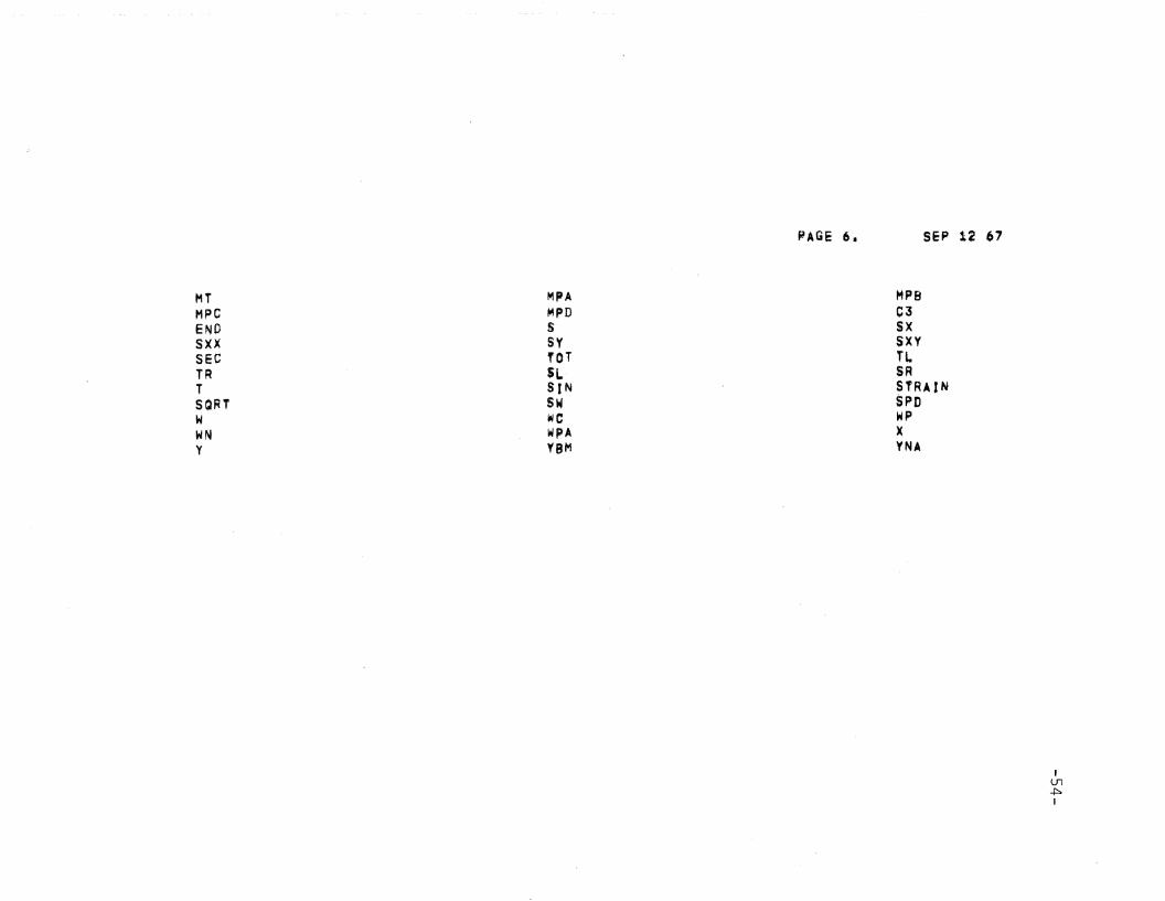
MTMPCENDSXXSECTRTSQRiWWNY
MPAMPDSSVfOTSLSINswweWPAYBM
PAGE 6. SEP 12 61
MPBC3sxSXyTLSRSTRAINSPDWPXYNA
IlJl..j::::=.I


INTERIOR SEAM CALCULATIONSEFF. WleTH MOMENT/E.10·.~6 L8~rT R~RUN I~ IV P~I
1. 09694~4+02· 4.02.331 5 9*04 1 4.1912-182.05 8.7978574+05 6,41673BO~04
1-.15261:>5+02 4.62730;9·04 2 4.2534247+0!J 1..0013044.06 1.5724450-04
1,1501127.02 3.7771754·04 3 4.2506968+05 9.9558097+05 3.9798543-03
9,1439003+01 2 -. 7 8161 02" 0 4 4 J.9632e01+0fS 5.6042555+05 6.-797~780;O2
5.1443512+-01 1,930185 5*04 5 3.2808153+05 !.9910248+05 6 e- 6816 46 0; 02
IUl(J)
I
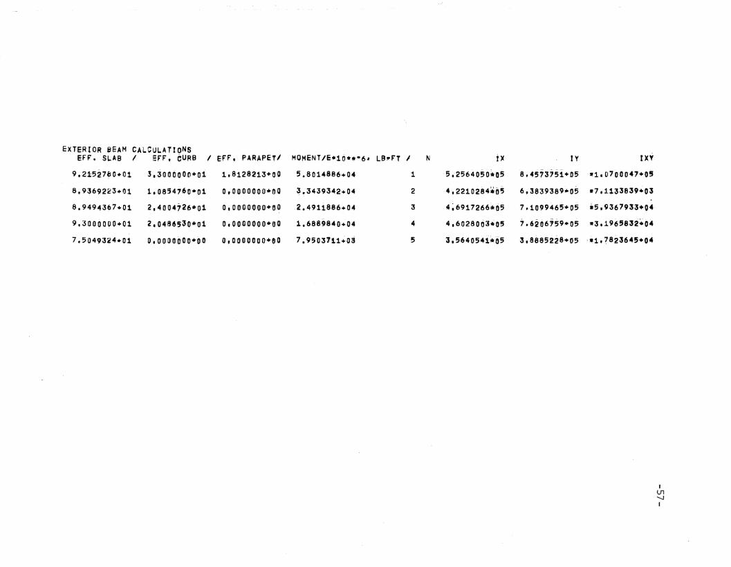
EXTERIOR SEAM CALCULATIONSEFF. SLAB I EFF, ~URB I EFP. PARAPETI MOMENT/E-l0*.-6. LB~rT I N t~ tv IXY
9.215~7~O.01 3~~OOOOOO.Ol 1,8128213+00 5.8014886+04 1 5i25640~O~05 8.45j3j~i.05 '1.0'00047.0~
8.93692~3.01 1.0854160*01 0.0000000.00 ~.3439342+0~ 2 .-,2210284'05 6.3839389.05 -7.1133839.03
8.9494367+01 2.4004726*01 0,0000000+00 -2.4911886.04 3 4~6917266.ri5 7,1099465+05 .5.,9367933+0.
9.3000000+01 ,.04865~O.01 O.OOOOOOO.OQ 1.6889840+04 4 4,6028003.05 7.6206159.05 -3,196'832.04
7,5049324.01 O.oooOtiOO.OD 0.0000000.00 7.95037l1+0~ 5 3.5640541~ri5 !,8~852~8.05 '.1t?8~3645.0.
IlJl-....j
I
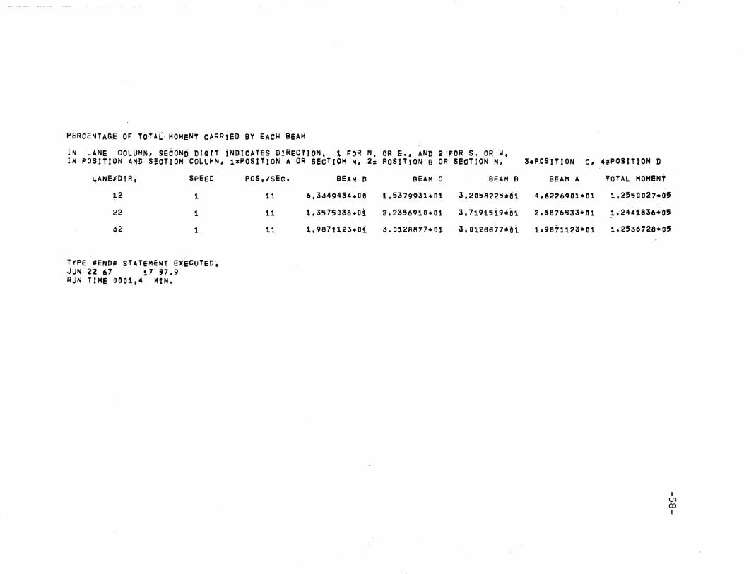
PERCENTAGi or TOTAL; MOMeNT CARRIED BY EACH BEAM
IN LANE COLUMN, ~E~ONti OIGlT iNDICATES Dl~E9TIONJ _, '~R ~t OR ~.~. AND ~ ",OR_S, OR_W,IN POSITION AND SiCTION COLUMN, 1~POSfTION A :QR SECTtOM M, .2: POSITIONs OR -SiOTION N, 3~PDSifjbN ~. 4,posrT10~ b
L.ANE/DIR. SpEeD POS,/sEc, BEAM D
12 1 11 6.3J494~4... 0e
22 1 11 1.3575038:"01
32 1 11 1.9871123+01.
BiAM C -BEAM B BeAM A 'OTA~ MOMENT-
!~5379931.01 3,2058225~ril 4,6226901.01 1,2550021.0'
2.2356910.01 3.71915i9.~1 2.'8j6~J3.01 ~i24~1836~OB
S.0128e".Cl !,01288~7.~i ~.98t1123.oi li2536728~OS
TYPE #ENO' STAffMi~T ExeCUTED.JUN 22- 67 i'- 51~9
RUN TIME 0001.4 ~lN.
IUlOJI

9. TABLES
-59-

Table 1 Test Bridge Characteristics
Test Span C-C Clear Beam Size Skew MidspanSpacing Spacing Diaphragms
Pilot 61 f 6 TT 7 f 2 TT 3 f 2 Tf 48 TT X 33 TT 90° yes
Berwick 65 f 3TT 8 f 9-3/8 TT 4 f 9-3/8 TT 48 ft X 39 TT 90° yes
Brookville 64 f lO-1/2 TT 8 f Ion 4 f lOTT 48 TT X 36 ft 45° yes
White Haven 64' 8 TT 9 ' on 6 f OTT 36 TT X 42 ft 82° yes
Philadelphia 71 f 9 ft 9' 6 TT 5' 6 TT 48" x 42" 87° yes
Philadelphia 71' 9 TT 9 f 6 TT 5 f 6 TT 48 TT X 42 TT 87° no
IOJoI
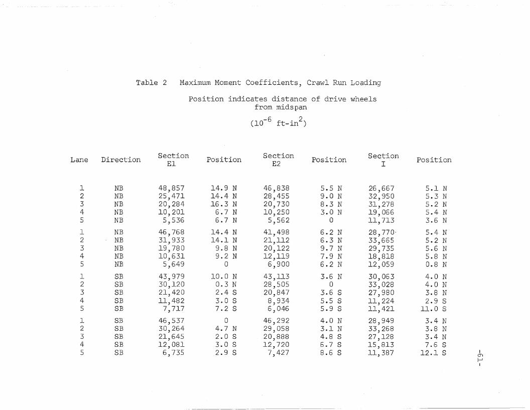
Table 2 Maximum Moment Coefficients, Crawl Run Loading
Position indica~es distance of drive wheelsfrom midspan
(lO-6 ft-in2 )
Lane Direction Section Position Section Position Section PositionE1 E2 I
1 NB 48,857 14.9 N 46,838 5.5 N 26,667 5.1 N2 NB 25,471 14.4 N 28,455 9.0 N 32,950 5.3 N3 NB 20,284 16.3 N 20,730 8.3 N 31,278 5.2 N4 NB 10,201 6.7 N 10,250 3.0 N 19,066 5.4 N5 NB 5,536 6.7 N 5,562 0 11,713 3.6 N
1 NB 46,768 14.4 N 41,498 6.2 N 28,770- 5.4 N2 NB 31,933 14.1 N 21,112 6.3 N 33,665 5.2 N3 NB 19,780 9.8 N 20,122 9.7 N 29,735 5.6 N4 NB 10,631 9.2 N 12,119 7.9 N 18,818 5.8 N5 NB 5,649 0 6,900 6.2 N 12,059 0.8 N
1 BE 43,979 10.0 N 43,113 3.6 N 30, 063 4.0 N2 SB 30,120 0.3 N 28,505 0 33,028 4.0 N3 BE 21,420 2.4 S 20,847 3.6 S 27,980 3.8 N4 SE 11,482 3.0 S 8,934 5.5 S 11,224 2.9 S5 BE 7,717 7.2 S 6,046 5.9 S 11,421 11.0 S
1 BB 46,537 0 46,292 4.0 N 28,949 3.4 N2 BE 30,264 4.7 N 29,058 3.1 N 33,268 3.8 N3 BB 21,645 2.0 S 20,888 4.8 S 27,128 3.4 N4 BB 12,081 3.0 S 12,720 6.7 S 15,813 7.6 S5 BE 6,735 2.9 B 7,427 8.6 S 11,387 12.1 S I
ml-JI

Table 3 Maximum Moment Coefficients at Midspanfor Berwick Bridge, Crawl Run Loading
(lO-6 ft-in2 )
Lane
1
2
3
1
2
3
Dire·ction
North
North
North
South
South
South
A
49,512
37,997
23,373
49,337
34,922
24,304
Girder
B
34,970
35,776
31,900
35,329
35,987
30,429
-c
16,982
24, 036
31,900
14,578
20,770
30,429
D
11,539
17,410
23,373
14,570
16,206
24,304
Ienf\..)
I
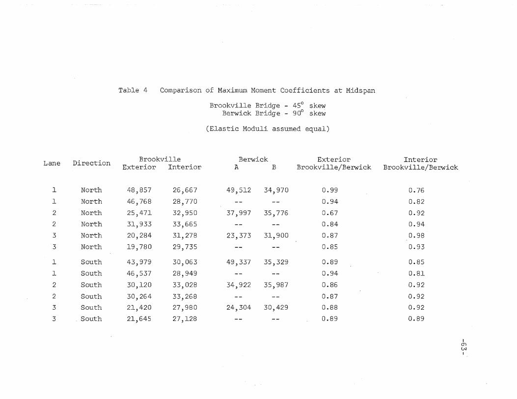
Table 4 Comparison of Maximum Moment Coefficients at Midspan
Brookville Bridge - 45° skewBerwick Bridge - 90° skew
(Elastic Moduli assumed equal)
Lane Direction Brookville Berwick Exterior InteriorExterior Interior A B Brookville/Berwick Brookville/Berwick
1 North 48,857 26,667 49,512 34,970 0.99 0.76
1 North 46,768 28,770 -- -- 0.94 0.82
2 North 25,471 32,950 37,997 35,776 0.67 0.92
2 North 31,933 33,665 -- -- 0.84 0.94
3 North 20,284 31,278 23,373 31,900 0.87 0.98
3 North 19,780 29,735 -- -- 0.85 0.93
1 South 43,979 30,063 49,337 35,329 0.89 0.85
1 South 46,537 28,949 -- -- 0.94 0.81
2 South 30,120 33,028 34,922 35,987 0.86 .0.92
2 South 30,264 33,268 -- -- 0.87 0.92
3 South 21,420 27,980 24,304 30,429 0.88 0.92
3 South 21,645 27,128 -- -- 0.89 0.89
IOJLNI
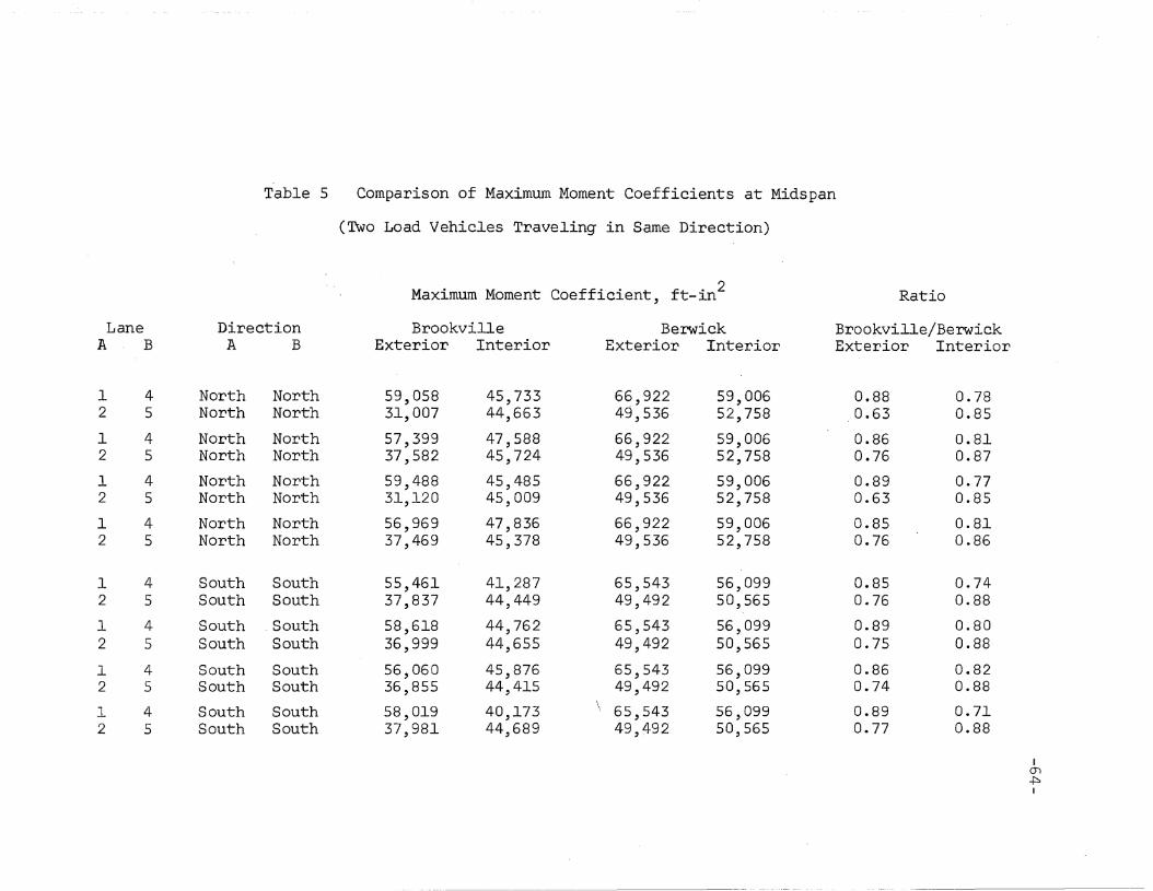
Table 5 Comparison of Maximum Moment Coefficients at Midspan
(Two Load Vehicles Traveling in Same Direction)

Table 6 Comparison of Maximum Moment Coefficients at Midspan
(Two Load Vehicles Traveling in Opposite Directions)
Maximum Moment Coefficient, ft-in2Ratio
Lane Direction Brookville Berwick Brookville/BerwickA B A B Exterior Interior Exterior Interior Exterior Interior
1 4 North South 60,339 37,891 65,718 55,740 0.77 0.682 5 North South 33,188 44,371 52,567 50,354 0.63 0.88
1 4 North South 60,938 42,480 65,718 55,740 0.93 0.762 5 North South 32,206 44,337 52,567 50,354 0.61 0.88
1 4 North South 58,250 39,994 65,718 55,740 0.89 0.722 5 North South 39,650 45,086 52,567 50,354 0.75 0.90
1 4 North South 58,849 44,583 65,718 55,740 0.90 0.802 5 North South 38,668 45,052 52,567 50,354 0.74 0.89
1 4 South North 54,180 49,129 66,747 59,365 0.81 0.832 5 South North 35,656 44,741 46,461 52,969 0.77 0.84
1 4 South North 54,610 48,881 66,747 59,365 0.8.2 0.822 5 South North 35,769 45,087 46,461 52,969 0.77 0.85
1 4 South North 56,738 48,015 66,747 59,365 0.85 0.812 5 South North 35,800 44,981 46,461 52,969 0.77 0.85
1 4 South North 57,168 47,767 66,747 59,365 0.86 0.812 5 South North 35,913 45,327 46,461 52,969 0.77 0.86
ImUlI
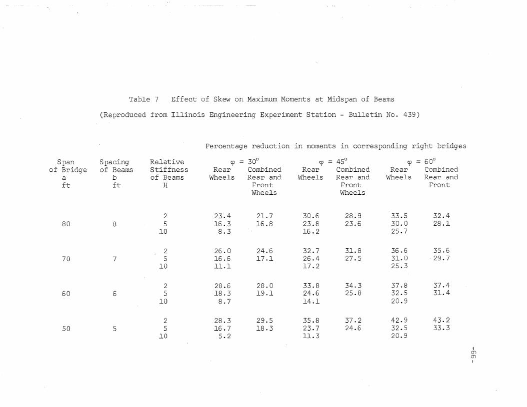
Table 7 Effect of Skew on Maximum Moments at Midspan of Beams
(Reproduced from Illinois Engineering Experiment Station - Bulletin No. 439)
Percentage reduction in moments in corresponding right bridges
Span Spacing Relative cp = 30° ep = 45° cp = 60°of Bridge of Beams Stiffness Rear Combined Rear Combined Rear Combined
a b of Beams Wheels Rear and Wheels Rear and Wheels Rear andft ft H Front Front Front
Wheels Wheels
2 23.4 21.7 30.6 28.9 33.5 32.480 8 5 16.3 16.8 23.8 23.6 30.0 28.1
10 8.3 16.2 25.7
2 26.0 24.6 32.7 31.8 36.6 35.670 7 5 16.6 17.1 26.4 27.5 31.0 ·29.7
10 11.1 17.2 25.3
2 28.6 28.0 33.8 34.3 37.8 37.460 6 5 18.3 19.1 24.6 25.8 32.5 31.4
10 8.7 14.1 20.9
2 28.3 29.5 35.8 37.2 42.9 43.250 5 5 16.7 18.3 23.7 24.6 32.5 33.3
10 5.2 11.3 20.9
I01OJI

Table 8 Midspan Girder Deflections - Brookville Bridge
Load vehicle positioned ~ith drive wheelson midspan line
(Deflection in inches)
Girder
Lane Direction A B C D
1 NB 0.075 0.073 0.035 0.014
2 NB 0.048 0.078 0.047 0.020
3 NB 0.032 0.066 0.064 0.040
4 NB 0.017 0.046 0.070 0.062
5 NB 0.009 0.030 0.062 0.089
1 NB 0.077 0.075 0.035 0.012
2 NB 0.049 0.080 0.050 0.022
3 NB 0.032 0.066 0.062 0.036
4 NB 0.017 0.046 0.070 0.065
5 NE 0.009 0.030 0.061 0.092
1 BE 0.084 0.071 0.030 0.009
2 SB 0.058 0.082 0.044 0.015
3 BB 0.037 0.073 0.060 0.033
4 SB 0.020 0.051 0.070 0.056
5 BB 0.011 0.036 0.066 0.084
1 8B 0.084 0.072 0.030 0.009
2 BB 0.059 0.084 0.046 0.019
3 BB 0.036 0.072 0.060 0.033
4 SB 0.018 0.042 0.052 0.040
5 8E 0.010 0.033 0.063 0.080
-67-

Table 9 Girder Deflections at Midspan in Berwick Bridge
(Deflections in inches)
GirderLane Direction
A B C D
1 North 0.0800 0.0710 0.0504 0.0273
2 North 0.0612 0.0718 0.0529 0.0291
3 North 0.0461 0.0682 0.0715 0.0455
4 North 0.0331 0.0538 0.0752 0.0609
5 North 0.0243 0.0428 0.0723 0.0810
1 South 0.0728 0.0649 0.0610 0.0204
2 South 0.0546 0.0677 0.0800 0.0296
3 South 0.0381 0.0617 0.1114 0.0398
4 South 0.0258 0.0478 0.1016 0.0524
5 South 0.0188 0.0372 0.0974 0.0745
IOJ0)
I

Table 10 Comparison of Girder Deflections
(Load vehicle positioned with drive wheels at midspan)
Deflection, lO-3 inches Ratio
Lane Direction Brookville Berwick Brookville/BerwickA B C D A B C D A B C D
1 North 075 073 035 014 080 071 050 027 0.94 1.03 0.70 0.521 North 077 075 035 012 -- -- -- -- 0.96 1.06 0.70 0.442 North 048 078 047 020 061 072 053 029 0.79 1.08 0.89 0.692 North 049 080 050 022 -- -- -- -- 0.80 1.11 0.94 0.763 North 032 066 064 040 046 068 072 046 0.70 0.97 0.89 0.873 North 032 066 062 036 -- -- -- -- 0.70 0.97 0.86 0.784 North 017 046 070 062 033 054 075 061 0.52 0.85 0.93 1.024 North 017 046 070 065 -- -- -- -- 0.52 0.85 0.93 1.065 North 009 030 062 089 024 043 072 081 0.38 0.70 0.86 1.105 North 009 030 061 092 -- -- -- -- 0.38 0.70 0.85 1.14
1 South 084 071 030 009 073 065 061 020 1.15 1.09 0·.49 0.451 South 084 072 030 009 -- -- -- -- 1.15 1.11 0.49 0.452 South 058 082 044 015 055 068 080 030 1.05 1.20 0.55 0.502 South 059 084 046 019 -- -- -- -- 1.07 1.23 0.58 0.633 South 037 073 060 033 038 062 III 040 0.97 1.18 0.54 0.823 South 036 072 060 033 -- -- -- -- 0.95 1.16 0.54 0.824 South 020 051 070 056 026 048 102 052 0.77 1.06 0.69 1.084 South 018 042 052 040 -- -- -- -- 0.69 0.88 O.5l 0.775 South 011 036 066 084 019 037 097 074 0.58 0.97 0.68 1.145 South 010 033 063 080 -- -- -- -- 0.53 0.89 0.65 1.08 I
01LDI
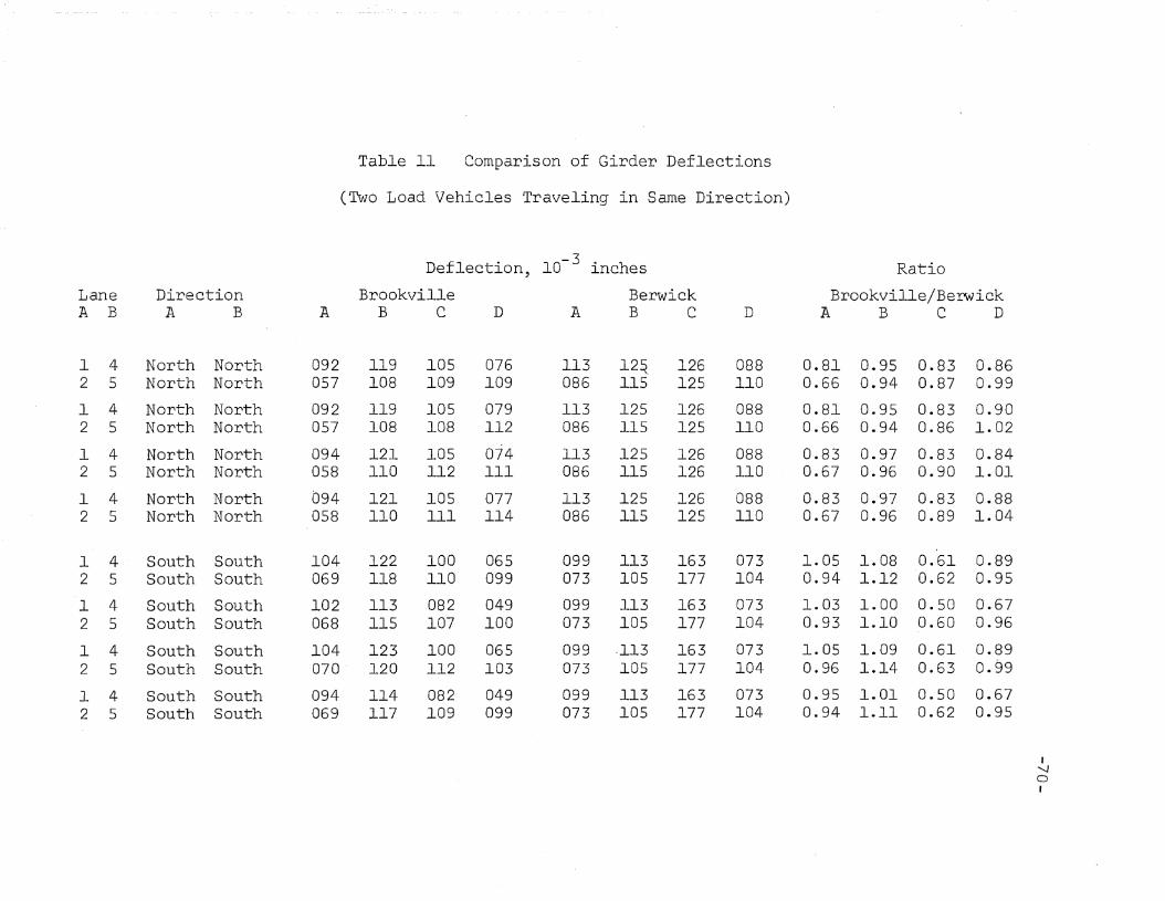
Table 11 Comparison of Girder Deflections
(Two Load Vehicles Traveling in Same Direction)
Deflection, lO-3 inches Ratio
Lane Direction Brookville Berwick Brookville/BerwickA B A B A B C D A B C D A B C D
1 4 North North 092 119 105 076 113 12~ l26 088 0.81 0.95 0.83 0.862 5 North North 057 108 109 109 086 115 125 110 0.66 0.94 0.87 0.99
1 4 North North 092 119 105 079 113 125 126 088 0.81 0.95 0.83 0.902 5 North North 057 108 108 112 086 115 125 110 0.66 0.94 0.86 1.02
1 4 North North 094 121 105 074 113 125 126 088 0.83 0.97 0.83 0.842 5 North North 058 110 112 III 086 115 126 110 0.67 0.96 0.90 1.01
1 4 North 'North 094 121 105 077 113 125 126 088 0.83 0.97 0.83 0.882 5 North North 058 110 III 114 086 115 125 110 0.67 0.96 0.89 1.04
1 4 South South 104 122 100 065 099 113 163 073 1.05 1.08 0.61 0.892 5 South South 069 118 110 099 073 105 177 104 0.94 1.12 0.62 0.95
1 4 South South 102 113 082 049 099 113 163 073 1.03 1.00 0.50 0.672 5 South South 068 115 107 100 073 105 177 104 0.93 1.10 0.60 0.96
1 4 South South 104 123 100 065 099 -113 163 073 1.05 1.09 0.61 0.892 5 South South 070 120 112 103 073 105 177 104 0.96 1.14 0.63 0.99
1 4 South South 094 114 082 049 099 113 163 073 0.95 1.01 0.50 0.672 5 South South 069 117 109 099 073 105 177 104 0.94 1.11 0.62 0.95
J'-J0I

Table 12 Comparison of Girder Deflections
(Two Load Vehicles Traveling in Opposite Directions)
f · -3 RatioDe lectlon, 10 inches
Lane Direction Brookville Berwick Brookville/BerwickA B A B A B C D A B C D A B C D
1 4 North South 095 124 105 070 106 119 152 080 0.90 1.04 0.69 0.882 5 North South 059 114 113 104 080 109 150 104 0.74 1.04 0.75 1.00
1 4 North South 093 115 087 054 106 119 152 080 0.88 0.97 0.57 0.682 5 North South 058 III 110 100 080 109 150 104 0.72 1.02 0.73 0.96
1 4 North South 097 126 105 068 106 119 152 080 0.92 1.06 0.69 0.852 5 North South 060 116 116 106 080 109 150 104 0.75 1.06 0.77 1.02
1 4 North South 095 117 087 052 106 119 152 080 0.90 0.98 0.57 0.652 5 North South 059 113 113 102 080 109 150 104 0.74 1.04 0.75 0.98
1 4 South North 101 117 100 071 106 119 136 081 0.95 0.98 0.74 0.882 5 South North 067 112 114 077 079 110 152 III 0.85 1.02 0.75 0.69
1 4 South North 101 117 100 074 106 119 136 081 0.95 0.98 0.74 0.912 5 South North 067 112 105 107 079 110 152 III 0.85 1.02 0.69 0.96
1 4 South North 101 118 100 071 106 119 136 081 0.95 0.99 0.74 0.882 5 South North 068 114 108 108 079 110 152 III 0.86 1.04 0.71 0.97
1 4 South North 10l 118 100 074 lO6 119 l36 081 0.95 0.99 0.74 O.9l2 5 South North 068 114 107 III 079 110 152 III 0.86 1.04 0.70 l.OO
I-....j
f---JI

Table 13 Maximum Strain at Bottom Surface of Girder - Brookville Bridge
(One Load Vehicle)
(lO-6 in/in)
Section El Section E2 Se.ction ILane Direction Left Right Left Right Left Right
1 North 36.7 43.7 33.9 40.2 31.0 25.82 North 28.5 28.3 26.6- 27.5 36.3 32.73 North 18.4 15.8 19.7 19.1 27.8 34.84 North -11.7 9.2 12.7 12.0 20.0 19.-65 North 6.0 5.5 9.2 7.0 13.7 11.9
1 North 35.4 43.1 33.5 40.5 33.9 25.52 North 26.2 28.5 30.1 28.4 37.2 35.03 North 18.4 15.4 19.6 17.2 26.2 33.44 North 11.0 8.7 12.3 10.4 19.8 19.25 North 6.9 4.3 7.4 4.6 14.0 11.9
1 South 37.2 41.5 35.8 43.6 36.0 27.22 South 26.8 24.6 26.9 28.6 36.5 34.73 South 18.-2 16.9 19.3 19.7 25.1 30.04 South 10.0 8.9 13.8 9.5 10.9 15.45 South 8.0 4.1 7.9 6.0 13.4 11.6
1 South 37.1 37.0 36.9 45.6 34.6 27.52 South 24.8 23.1 '26.5 27.7 38.4 34.23 South 19.3 15.5 19.5 19.4 24.4 31.54 South 11.1 8.0 12.3 11.3 19.0 15.75 South 7.9 5.0 7.0 7.1 12.1 11.8 I
-......J1'0I

Table l4 Maximum Strain at Bottom Surfaceof Girder - Berwick Bridge
(lO-6 in/in)
Exterior InteriorTruck Location Left Right Left Right
Lane l 3.8.9 42.0 34.8 30.9
Lane 2 3l.4 30.l 34.0 34.2
Lane 3 23.2 19.5 29.5 32.2
Lane 4 l7.9 lS.O 23.6 23.7
Lane 5 ll.7 9.2 18.9 15.8
I-......Jl.NI

Table lS Maximum Strain at Bottom Surface of Girder - Brookville Bridge
(Two Load Vehicles Traveling in Same Direction)
(10- 6 in/in)

Table 16 Maximum Strain at Bottom Surface of Girder - Brookville Bridge
(Two Load Vehicles Traveling in Opposite Directions)
(10- 6 in/in)
Lane Direction Section El Section E2 Section I
A B A B Left Right Left Right Left Right
1 4 North South 46.7 52.6 47.7 49.7 41.9 41.22 5 North South 36.5 32.5 34.6 33.4 49.7 48.1
1 4 North South 47.8 51.6 46.2 51.5 49.9 41.52 5 North South 36.4 33.4 33.7 34.5 48.4 44.6
1 4 North South 45.4 52.0 47.3 50.0 44.8 40.92 5 North South 34.3 ,32.6 38.0 34.4 50.6 46.7
1 4 North South 46.4 51.1 45.8 51.8 52.8 41.22 5 North 'South 34.2 33.6 37.1 35.5 49.3 46.9
1 4 South North 48.9 5·0.7 48.6 55.6 56.0 46.82 5 South North 32.7 30.1 36.0 35.5 50.2 46.6
1 4 South North 48.2 50.2 48.2 54.0 55.8 46.52 5 South North 33.7 28.9 34.3 33.1 50.6 46.6
1 4 South North 48.8 46.2 49.7 57.7 54.6 47.12 5 South North 30.8 28.6 35.7 34.7 52.1 46.1
1 4 South North 48.1 45.7 49.3 56.0 54.4 46.82 5 South North 31.7 27.4 33.9 32.3 52.5 46.1
I-JUl1
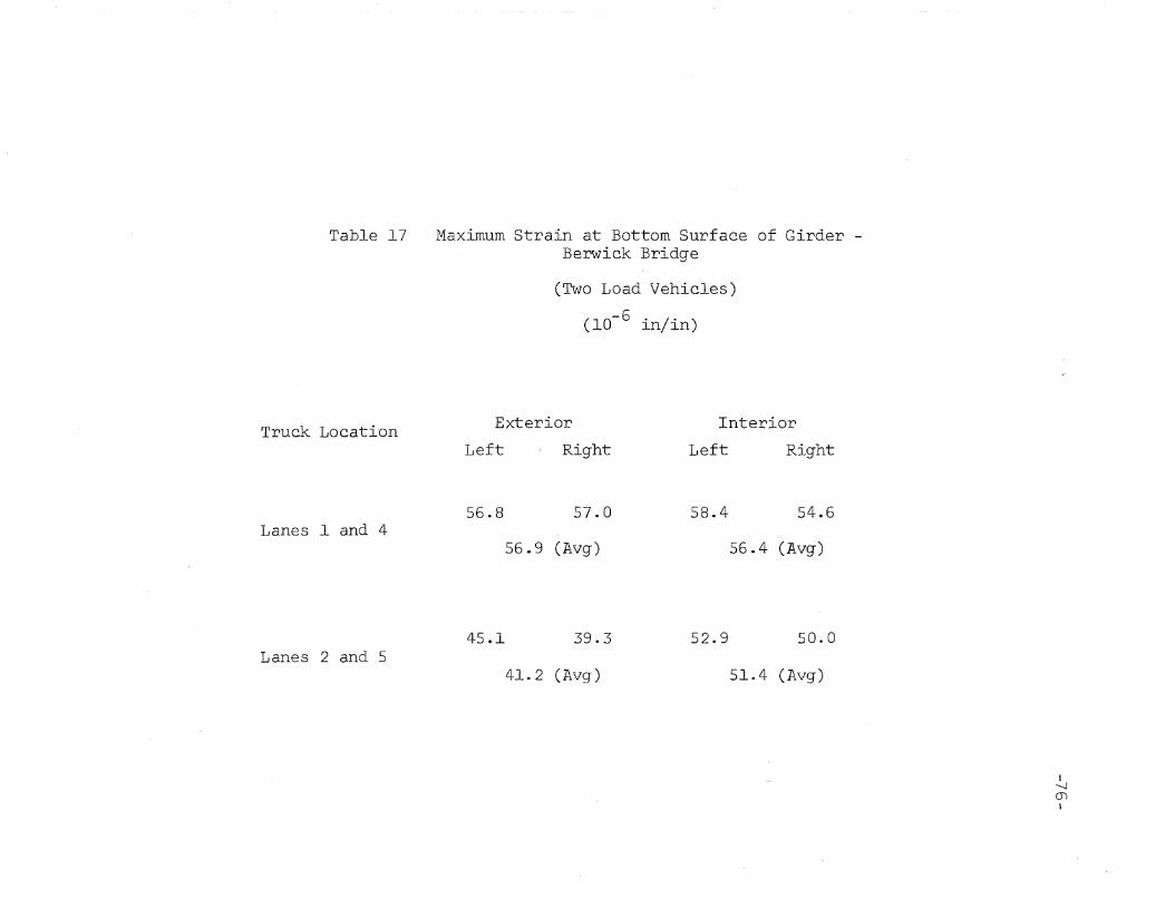
Table l7 Maximum Strain at Bottom Surface of Girder Berwick Bridge
(Two Load Vehicles)
(lO-6 in/in)
Exterior InteriorTruck LocationLeft Right Left Right
56.4 (Avg)Lanes land 4
56.8 57.0
56.9 (Avg)
58.4 54.6
45.1 39.3 52.9 50.0Lanes 2 and 5
41.2 (Avg) 51.4 (Avg)
I-......j
mI

Table 18 Comparison of Averaged Maximum Strainsat Bottom Surface of Girder
-77 -
(Ratio of value from Brookville Bridge to value from Berwick Bridge)
One Vehicle
Lane Direction Exterior InteriorLeft Right Left Right
1 North 0.92 1.03 0.93 0.832 North 0.87 0.94 1.08 0.993 North 0.79 0.80 0.92 1.064 North 0.63 0.60 0.84 0.825 North 0.55 0.53 0.73 0.75
1 South 0.95 0.94 1.02 0.882 South 0.82 0.79 1.10 1.013 South 0.81 0.83 0.84 0.964 South 0.59 0.56 0.63 -0.665 South 0.68 0.50 0.68 0.74
Two Vehicles
Lane Direction Exterior InteriorA B A B Left Right Left Right
1 4 North North 0.84 0.92 0.90 0.822 5 North North 0.78 0.85 0.96 0.92
1 4 South South 0.84 0.84 0.86 0.782 5 South South 0.78 0.72 0.95 0.92
1 4 North South 0.82 0.91 0.81 0.752 5 North South 0.82 0.84 0.94 0.93
1 4 South North 0.85 0.84 0.94 0.862 5 South North 0.75 0.73 0.97 0.93

Table 19 Effective Slab Width
(inches)
Section El Section E2 Section ILane Direction Slab Curb Parapet Slab Curb Parapet Slab
1 North 95.00 33.00 2.51 95.00 33.00 4.66 87.182 North 95.00 24.50 0 95.00 15.45 0 99.143 North 95.00 14.93 0 95.00 16.86 a 110.824 North 95.00 0.75 0 6.18 0 0 111.685 North 61.57 0 0 12.49 0 0 69.13
1 North 95.00 33.00 2.98 95.00 25.69 0 111.952 North 95.00 24.76 0 49.28 0 0 84.353 North 95.00 25.53 0 95.00 17.97 0 106.414 North 95.00 9.25 0 95.00 11.15 0 90.845 North 83.26 0 0 95.00 31.99 0 74.26
1 South 95.00 24.38 a 95.00 24.37 a 97.532 South 95.00 33.00 0.12 95.00 14.36 0 81,.013 South 95.00 26.08 0 95.00 19.06 0 120.104 South 95.00 15.72 0 35.21 0 0 41.635 South 95.00 33.00 8.93 6.04 0 0 64.73
1 South 95.00 33.00 2.43 95.00 30.38 a 82.512 South 95.00 33.00 3.60 95.00 16.48 0 72.763 South 95.00 33.00 0.73 95.00 16.62 0 101.104 South 95.00 27.21 0 95.00 15'.18 0 65.515 South 73.71 0 0 95.00 7.15 0 82.09
I.....JOJI

Table 20 Neutral Axis Location
[Location given as distance (inches) above bottom girder surface]
Section E1 Section E2 Section ILane Direction Left Right Left Right Left Right
1 North 31.69 28-. 98 32.02 29.80 24.53 27.112 North 26.24 24.95 29.93 25.78 25.28 27.863 North 32.99 22.61 30.21 25.81 29.70 24.744 North 31.11 20.97 21.89 25.15 28.09 26.445 North 26.08 20.92 16.00 19.59 26.86 22.17
1 North 31.15 29.78 30.92 26.96 26.06 28.492 North 31.89 25.80 . 18.79 26.26 25.99 25.283 North 31.96 25.88 30.81 25.46 29.74 24.224 North 31.66 22.60 31.04 23.68 28.78 23.355 North 30.56 19.77 31.40 27.67 27.51 22.32
1 South 30.89 26.72 30.12 27.49 25.48 27.472 South 31.72 27.61 29.27 26.20 25.42 25.393 South 32.79 25.16 30.06 26.44 30.13 25.254 South 33.44 22.33 19.40 22.62 23-. 03 20.825 South 31.68 32.29 23.27 23.55 27.06 21.25
1 South 32.34 28.28 30.77 28.00 24.49 26.532 South 32.18 29.07 30.37 25.57 24.80 24.803 So'uth 32.64 27.04 30.46 25.52 28.72 24.644 South 33.47 24.70 30.71 24.94 26.96 21.485 South 29.86 19.05 . 31.43 22.32 28.51 22.45 I
'-JLOI

10. FIGURES
-80-
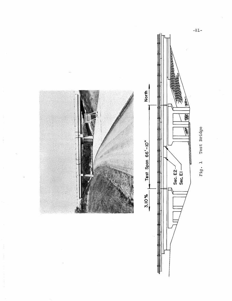
-81-

East
33' - 6 11
2'--9'~ 28'-0" 2'-9 11
5
I234
I ~Iope ~41~Ft.~SIOpe Y4''112: I=(.\J-,o.N
3 1-6 11 3 Spaces @ al-IO" = 26 1-6" 3 1-611
Scole:II II 1 a../4 =1 -
Fig. 2 Cross-Section of Brookville BridgeI
OJf\..)
I
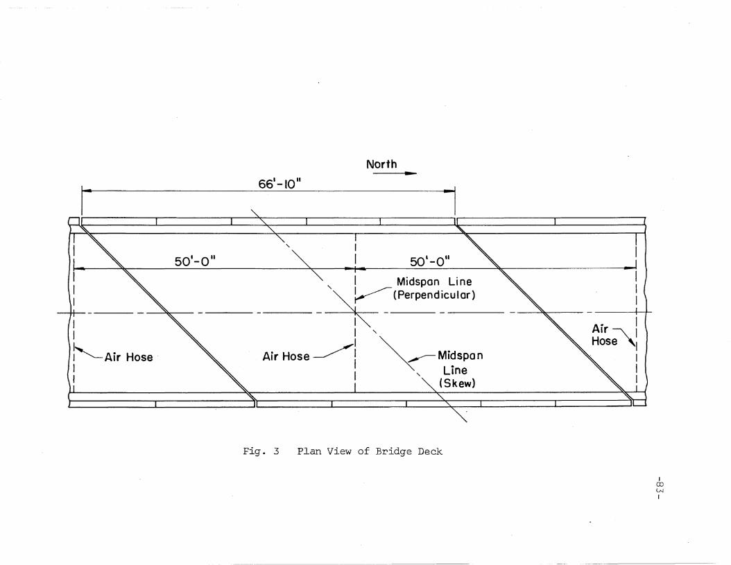
661-10" North
"50' -0"
~ ~Midspan~, Line
(Skew)
'\.
I Midspan Li ne~ (Perpendicular)"
II
AirHose~1II
50'-0"
II
~Air HoseII
Fig. 3 Plan View of Bridge Deck
IOJWI
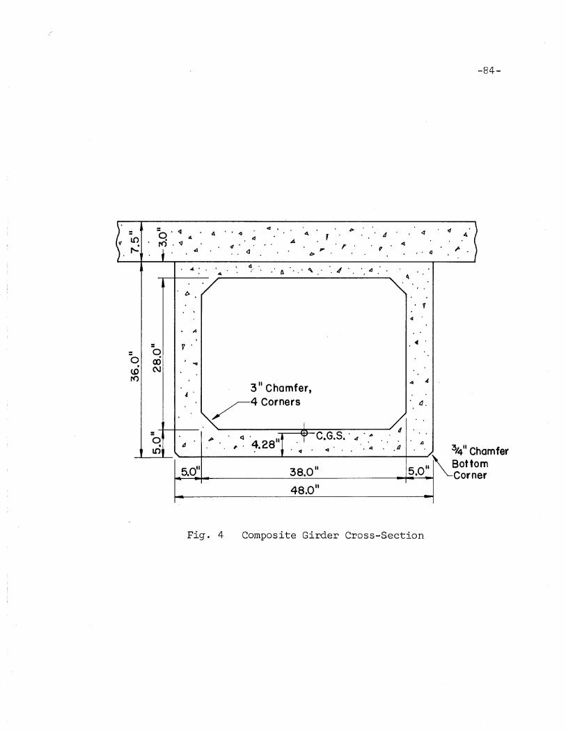
-84-
hamferomer
~.<J
<f J> <1= 0' 4 <Q &\ , is 4 4LO 4 4 ArO -q 4r-: .(/ ,
" ;.f .a (]
, .. 4b
~",. ~~
~ ~ ./ A4.
~
I>
V
04
.. ,4
Vtf
q0 CO ,
~. (\JCDro
3 11 Chamfer,4 4
.4 /4Corners d.
~II"'-
C.G.S. . 4<t·~.28111 .r ~ iA
0 "'"d .0.• ,. • 4 JJ .. ~ 3/411 ClOt 4 "4
\..
5.0" 38.0" 501l~Bott- · Corn
48.0" - I
Fig. 4 Composite Girder Cross-Section

Legend:
o Def~ection GageI
: Fully Gaged SectionI
x Single SR-4 Gage
D', (18,36)
c
,
(17 ,35)
x (118)
North
.....
B, K ,Sec.I(goges9-16) '\: ;::::==~ ',II '
A
Sec. E2 (gages 101-108)
Sec. EI (gages 1-8) --
Fig. 5 Underside Detail Showing Gaged Sections
(viewed from top)
IcoV1I
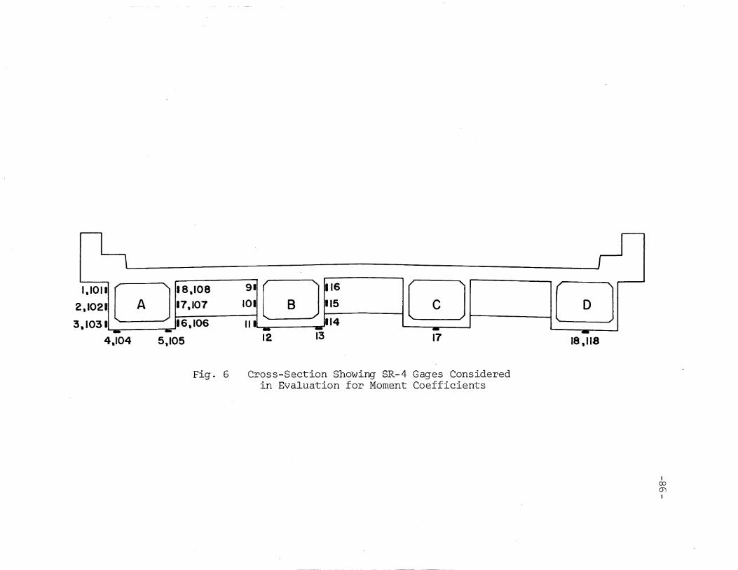
1,1011 18,108 91 116
2,1021 A 17,107 101 B 115
3.1031 16,106 III 14
4,104 5,105 12 13 17
D
18,118
Fig. 6 Cross-Section Showing SR-4 Gages Consideredin Evaluation for Moment Coefficients
IOJOJI

"
VOLTAGE REGULATOR
95 - 130 v. INPUT
I 10 v. OUTPUT
"
OSCILLATOR
REFERENCE SIGNAL
-87 -
"-- SR-4
AMPLIFIER ---- AND-~GAGE CIRCUIT
1SIGNAL ALTERED .BY
GAG E ACTIVITY
+OSCILLOGRAPHGALVANOMETER
Fig. 7 Instrumentation Flow Chart
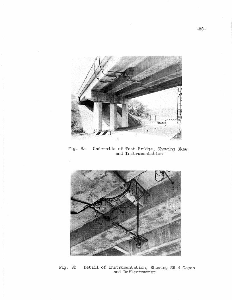
-88-
Fig. Sa Underside of Test Bridge, Showing Skewand Instrumentation
Fig. Sb Detail of Instrumentation, Showing SR-4 Gagesand Deflectometer
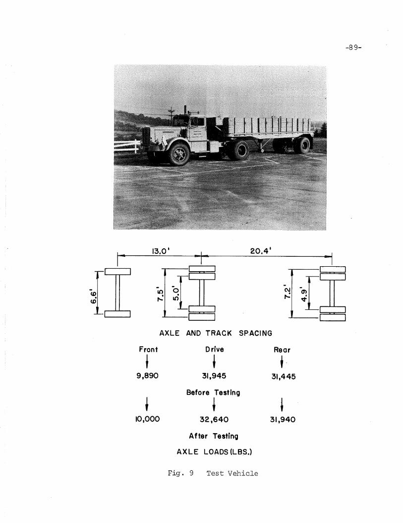
-89-
I. 13.0' .1_ 20.4'
-1I I
- -- C\Jto . en• r-- •,... V
I
AXLE AND TRACK SP.ACING
Front Drrve Rear
J t t·9,890 31,945 31,445
Before Testing
t t ~10,000 32,640 31,940
Aft.er Testing
AXLE LOADS (LBS.)
Fig. 9 Test Vehicle
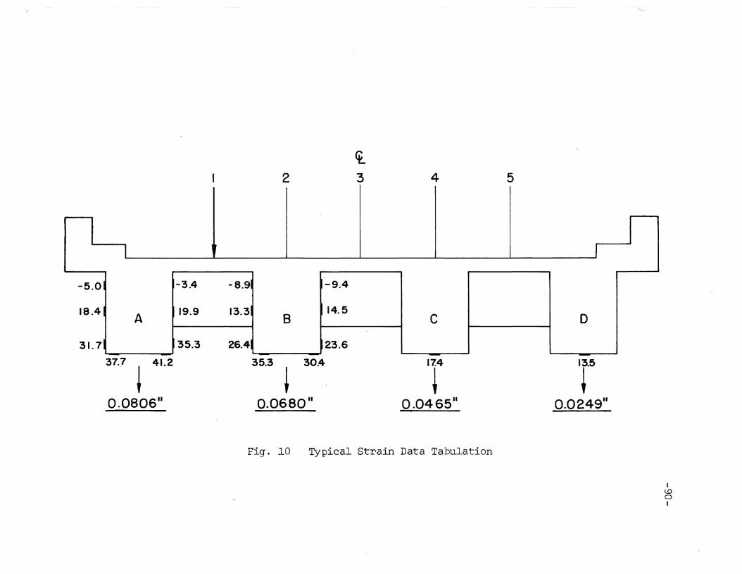
2
i3 4 5
I ', I
-5.01 -3.4 -8.91 1-9.4
18.41A
19.9 13.31 t 14.5B C D
31.71 35.3 26.41 123.6- - -
37.7 l 41.2
0.0806 11
35.3 30.4
~0.0680"
114
~0.0465"
13.5
+0.0249"
Fig. 10 Typical Strain Data Tabulation
ILOoI

50,000
40,000
MOMENTCOEFFICIENT 30,000( FT. - IN. 2 )
20,000
10,000
--Northbound
--- Southbound
2 3
LANE
4 5
Fig. 11 Maximum Moment Coefficients at Section ElI
1Dj--JI

50,000
40,000
MOMENTCOEFFICIENT 30,000(FT.-IN.2)
20,000
10,000
- Northbound
--- Southbound
2 3
LANE
4 5
Fig. l2 Maximum Moment Coefficients at Section E2-Jto1'0I
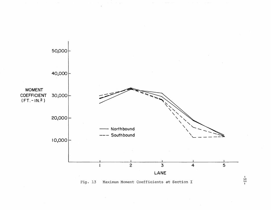
50,000
401000
MOMENTCOEFFICIENT 30,000(FT.-IN.2 )
20,000
1-0,000
-- Northboun-d
--- Southbound
~~
....... ~"'''''~,
",'\'\.'
""'\ '---.. .........
" --.;:'\. ----'- -
2 3
LANE
4 5
Fig. l3 Maximum Moment Coefficients at Section I
ILOLNI

Sec. EI
-94~
0"'--------1...---------------......---Sec. I
Fig. 14 Superimposed Moment Coefficients (Average)
Load vehicles traveling in lanes anddirections indicated on plot
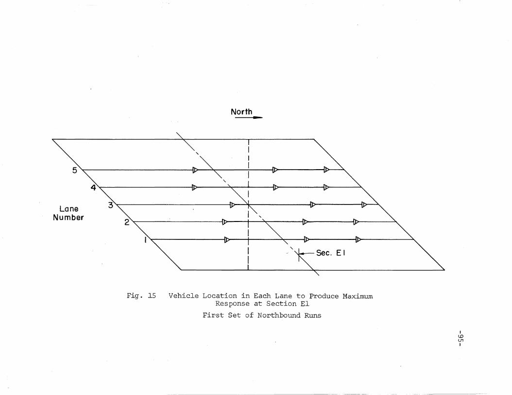
North
,
5 '\: I'b '< . 11' ~
,2 '< Il> I >( II> ID "
3'< I'b 'k 11' It>---"
4'< It: At I ID tD "
LaneNumber
......
Sec. EI
Fig. lS Vehicle Location in Each Lane to Produce MaximumResponse at Section El
First Set of Northbound Runs
ILOV1I

North
,
5 ' rb > Ib Il> '< < -
"
"
2 '< ['b I)< I'b Ib '
3 '< Il> >l [l) It> '\
4 '< rt >, I It> If:) ' ..
LaneNumber
" Sec. E I
Fig. l6 Vehicle Location in Each Lane to Produce MaximumResponse at Section El
Second Set of Northbound Runs
IlO0)
I

North
"
5 " <1J > <U I <II '>< < ,
'\.
4 '\: <1.1 >«11 I c1l ",
LaneNumber
3 "\: <1.l Q.1 'h: dl '"
"2 " <lI <II ) d1 "< < ""
,,-·~Sec. EI
Fig. l7 Vehicle Location in Each Lane to Produce MaximumResponse at Section El
First Set of Southbound Runs
I1.O-.......JI

/
North
5 '< <II > ( <Ill <.11 >
4 " ([]) c:n I <1' "< < ....
, I
LaneNumber
3 '< <11 (1\ >L <II >,.
2 '< <II I <0 en "'..
,Sec. EI
Fig. 18 Vehicle Location in Each Lane to Produce MaximumResponse at Section El
Second Set of Southbound Runs
IlDcoI

North
"
5 '< ~),< ID lD >,
"4 '< 1D > < I II)' IV' >,
LaneNumber
3 '< ID'k ID ID >,
"2'"'<---------.:.- I'D I'(ID ID-------~",
(--sec. E2
Fig. 19 Vehicle Location in Each Lane to Produce MaximumResponse at Section E2
First Set of Northbound Runs
ILD1.OI
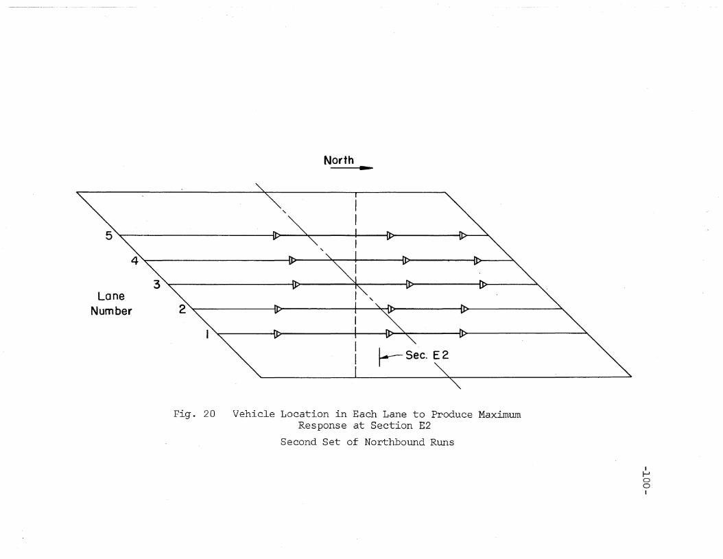
North
....
5 '" ID >< I ID I~
"-2 '< ID I >< II' ID >,
....
3 '" ID 1< ID 1D >,
4 '< It> >< I ID ID >,
LaneNumber
rsec. E2
Fig. 20 Vehicle Location in Each Lane to Produce MaximumResponse at Section E2
Second Set of Northbound Runs
IJ--IooI

North
,
5 "< <II > < a I I (II ' ..
,4 '< <11 (II >( I 01 ' ...
3 '"< <11 (II 1 en '
LaneNumber 2' <f1 'c: d1 >( dl '
I--- Sec. E2
Fig. 21 Vehicle Location in Each Lane to Produce MaximumResponse at Section E2
First Set of Southbound Runs
I}--JoJ---II

North
"
5 '< <l1 aJ <11 ' ..
"4 ' ~ ~> ~ ,
< < "
LoneNumber
3 '< QJ QI 1< Ct., "...
"2 "< (JJ I C(J'{ OJ J\,
I---sec. E2
Fig. 22 Vehicle Location in Each Lane to Produce MaximumResponse at Section E2
Second Set of Southbound Runs
IJ--lol'0I

North
"
"4' In > I ID ID >
5 ....< ID >c I ID ID >
LaneNumber
3 ....< 10 'C::: tD ID > ...
Sec. I2 ' ID I YID ID > ..
"
Fig. 23 Vehicle Location in Each Lane to Produce MaximumResponse at Section I
First Set of Northbound Runs
II--'ol1'J1

North
"
,
4 >< In) 1 ID ID "'...
5 ' 10 '( ID ID >,.
Sec. 1
,2' ID----------II--=:~'D ID--------~\.
3 "'c ID II ID ID >
LaneNumber
Fig. 24 Vehicle Location in Each Lane to Produce MaximumResponse at Section I
Second Set of Northbound Runs
If--!o~I
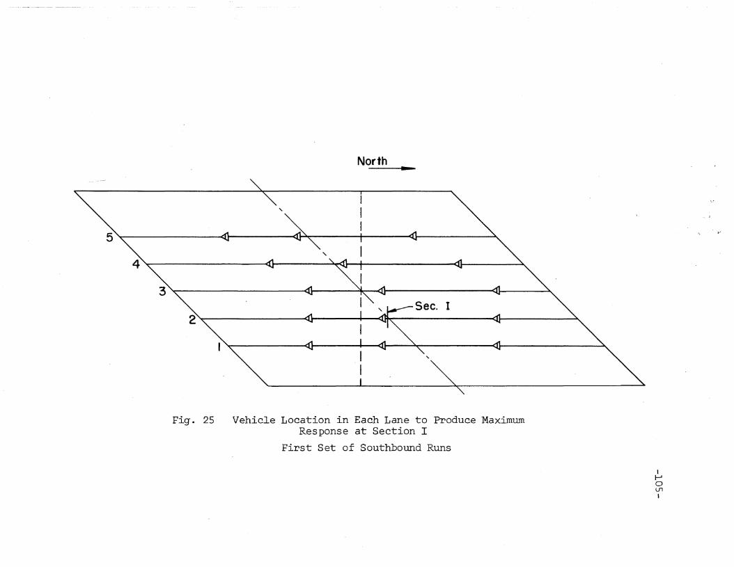
North
"
5 'c (J I Q I ] < I QJ ' ...
,4 'c a, 'c <I, 1 01 '
3 '( aJ 1< 01 '11 ' ..
Sec. I2 'c (l' I 011< 01 >
"
Fig. 25 Vehicle Location in Each Lane to Produce MaximumResponse at Section I
First Set of Southbound Runs
1f--..JolJlI

North
"5 '\L «J eu >< I r:ll >,
4 >< (JJ ell >< I OJ >,
Sec. I2 '< ell I <U>k <.11 >
" I3 "\L <tJ >k <l.J a:I "
LaneNumber
"
Fig. 26 Vehicle Location in Each Lane to Produce MaximumResponse at Section I
Second Set of Southbound Runs
Ir-'omI

A
2
B
3 4
c
5
-107-
o
0.076 0.074 0.035 0.013
0.048 0.079 0.048 0.021
I!
I II
0.032 0.066 0.063 0.038
0.017 0.046 0.070 0.064
0.009 0.030 0.062 0.090
Fig. 27 Deflection Due to Indicated Lane Loading (inches)
Northbound runs
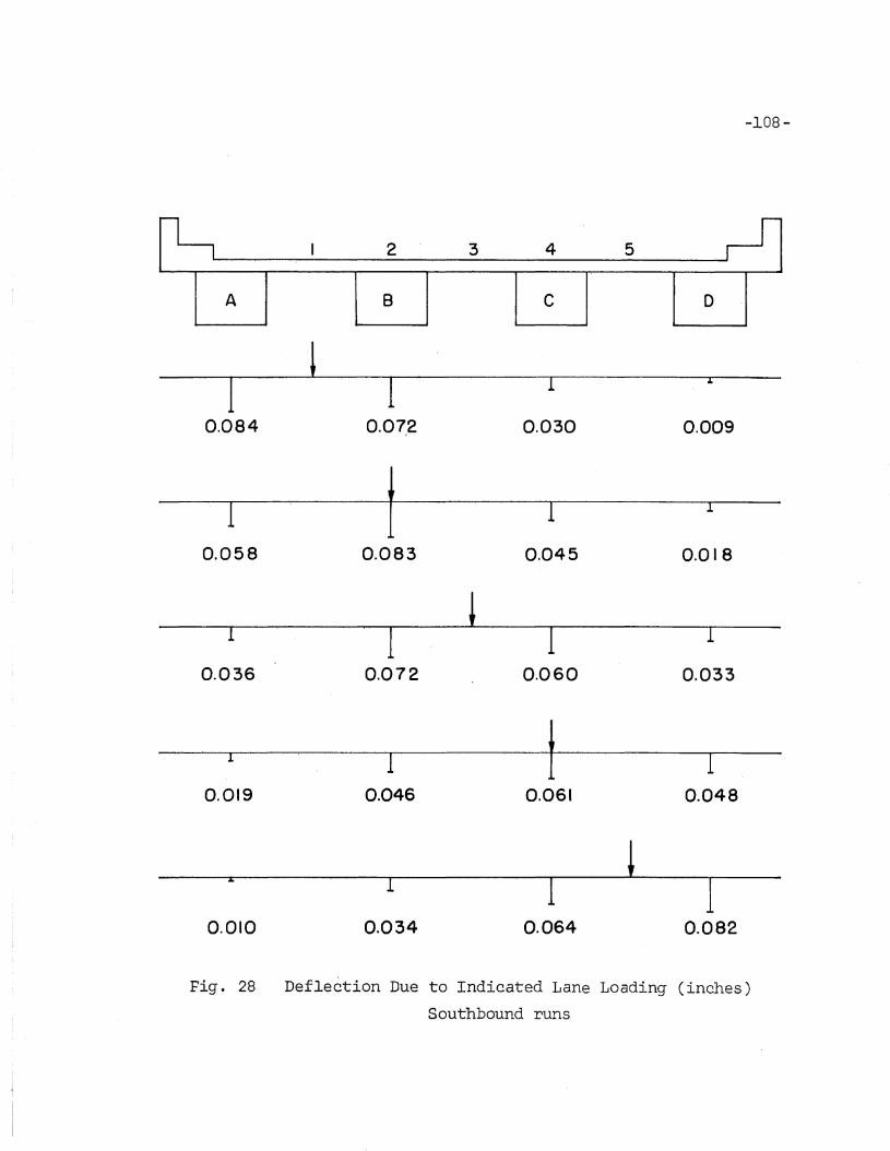
-108-
Il-r I 2 3 4 5 ~A B C 0
0.084 0.07,2 0.030 0.009
0.058 0.083 0.045 0.018
lI I I I
0.036 0.072 0.060 0.033
I1 ' I I0.019 0.046 0.061 0.048
0.010 0.034 0.064 0.082
Fig. 28 Deflection Due to Indicated Lane Loading (inches)
Southbound runs

-109-
~ I 2 3 4 5 ~A B C 0
N N
0.093 0.120
N
0.105
N
0.076
0.058
S
0.109 0.110
S
0.112
0.101
0.069
0.118
S
0.091
O.tlO
s0.057
0.100
Fig. 29 Deflections With Two Lanes Loaded
Vehicles superimposed in same direction
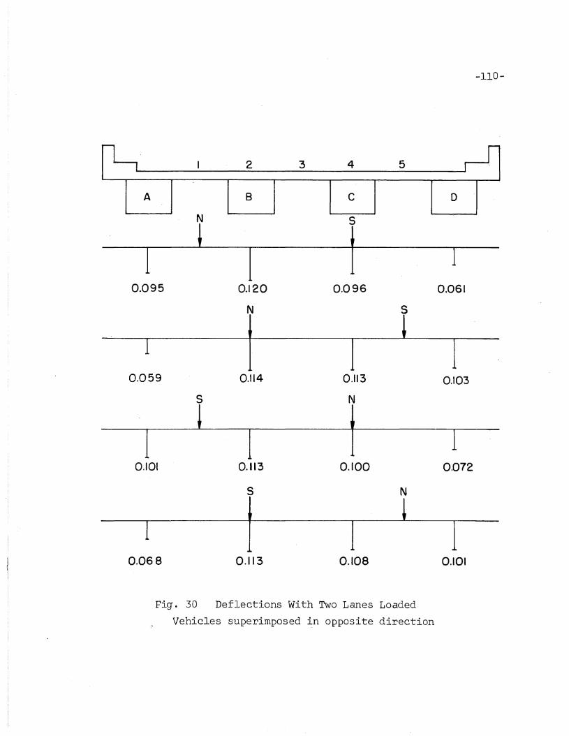
A
N
2
B
3 4
c
s
5
-110-
o
0.095 0.120
N
0.096
s0.061
0.059
s
0.114 0.113
N
0.103
0.101 0.113
s
0.100
N
0.072
0.068 0.113 0.108 0.101
Fig. 30 Deflections With Two Lanes Loaded
Vehicles superimposed ~n opposite direction

-lll-
IS-25
-----.. 3S..-
...... 45I---........ -
55 -----
50
40
30
20
10
°L RSECTION EI
Q fJ50
40
30 25
20 35
4510 55
°L RSECTION E2
~ !J50
40
30
20 45
10 55
L- RSECTION I
[\ ~50
40
30 2N
20 3N
104N
N
o L RSECTION EI
,....J:
~ J]uz""-(J)LLJ 50J:U
40zI
0 30 2Na:~ 20 3N:t 4N-........
z 10<t 5Na:: o L.... R(J)
SECTION E2
[' J]50
40 2NIN
30
204N
5N
10
L RSECTION I
Fig. 31 Maximum Strain at Bottom of Beam
Single vehicle loading - vehicle travelingin indicated lane ,and direction
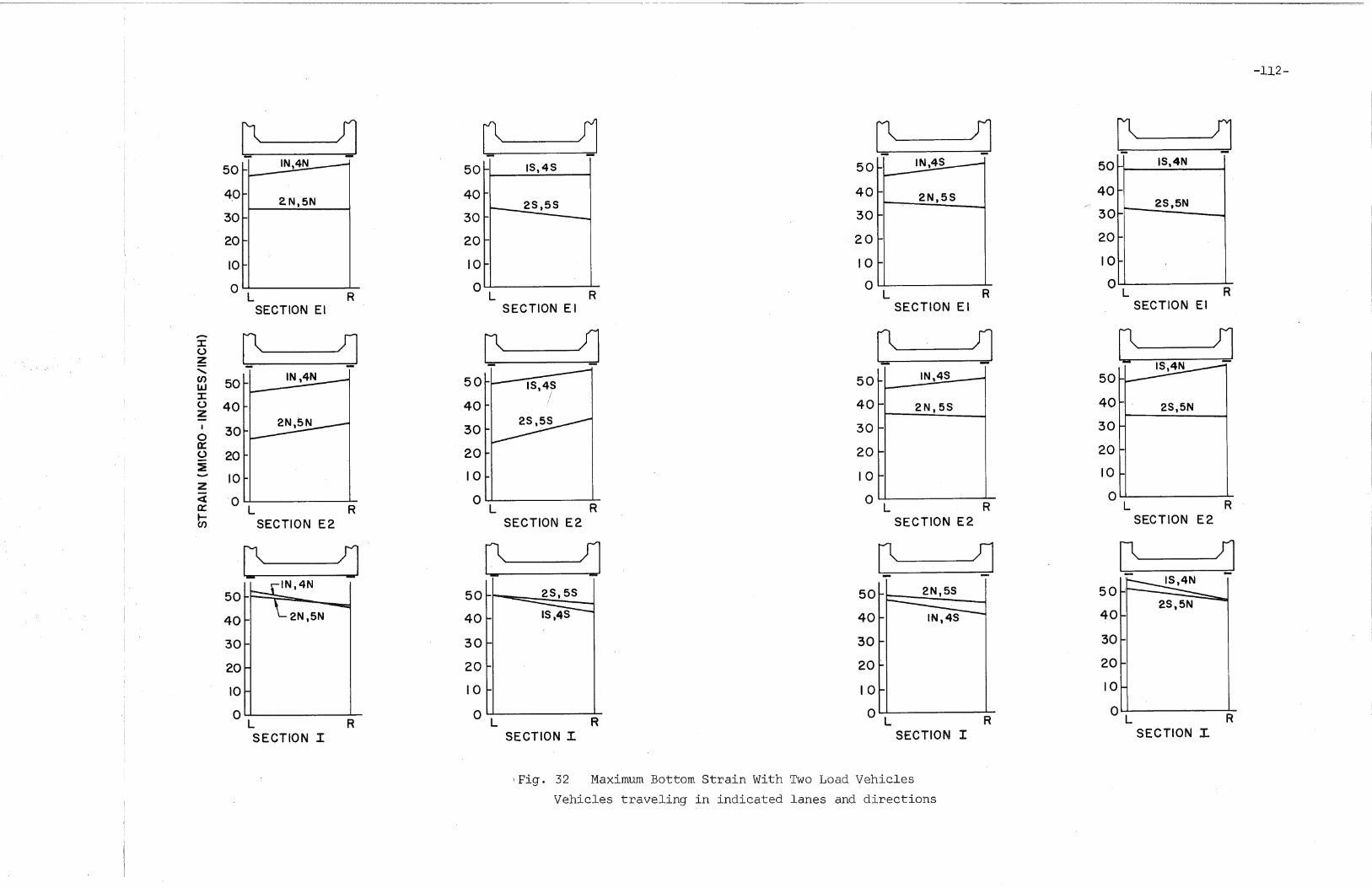
-112-
2S.5N
C' ~
I
~ !J
50
40
30
20
10
o L RSECTION I
20 ....
10 ....
aL
SECTION EI
40
30
20
10
0 " I
L RSECTION E2
:~tl 15,4N I
2N,5S
2N.5S
l; !J
[' . ~
~ ~
50
40
30
201
10
a L RSECTION I
50 L1 IN,4S~
40rlN 55
30
20
10
oL
SECTION E2
50
40
30
. 20
10
o L RSECTION EI
IS,4S
~ f]
Q Jj
[' !J50 ~r- 2S.55
40
30
20
10
o L RSECTION I
50
40
30
20
10
o L RSECTION EI
50
40
30
20
10
oL
SECTION E2
R
2N,5N
50 t-r-- 7=>
40
30
20
10
oLSECTION I
~ JI I
50
4°11 2. N. 5N
30
20
10
o L RSECTION EI
,-.
~ ~J:UZ"-(/) 50w:J:U 40z
I 3000::0 20:E
z 10
4 o La:: Rt-SECTION E2en
\Fig. 32 Maximum Bottom Strain With Two Load Vehicles
Vehicles traveling in indicated lanes and directions
11. REFERENCES
1 Walther, R. E.INVESTIGATION OF MULTI~BEAM BRIDGES, Fritz EngineeringLaboratory Report 223.14, August 1956
2 Ruudlett, J. C.PRESTRESSING PRACTICE IN BRIDGE BUILDING, ASCE Proceedings,July 1955, Vol. 81, No. 733
3 Douglas , W. J. and VanHorn, D. A.LATERAL DISTRIBUTION OF STATIC LOADS IN A PRESTRESSED CONCRETE BOX-BEAM BRIDGE, Fritz Engineering Laboratory Report315.1, August 1966
4Pennsy1vania Department of Highways, Bridge DivisionSTANDARDS FOR PRESTRESSED CONCRETE BRIDGES, 1960
5 American Association of State Highway OfficialsSTANDARD SPECIFICATIONS FOR HIGHWAY BRIDGES, Washington,D. C., 1961
6 Guilford, A. A. and VanHorn, D. A.LATERAL DISTRIBUTION OF VEHICULAR LOADS IN A PRESTRESSEDCONCRETE BOX-BEAM BRIDGE - BERWICK BRIDGE
7 Newmark, N". M., Siess, C. P., and Penman, R. R.STUDIES OF SLAB AND BEAM HIGHWAY BRIDGES, PART I - TESTSOF SIMPLE-SPAN RIGHT I-BEAM BRIDGES, University of IllinoisEngine~ring Experiment Station, Bulletin No. 363, March 1946
8 Newmark, N. M., Siess, C. P., and Peckham, W. M.STUDIES OF SLAB AND BEAM HIGHWAY BRIDGES, PART II - TESTSOF SIMPLE-SPAN SKEW I-BEAM BRIDGES, University of IllinoisEngineering Experiment Station, Bulletin No. 375, January1948
9 Chen, T. Y., Siess, C. P., and Newmark, N. M.STUDIES OF SLAB AND BEAM HIGHWAY BRIDGES, PART VI - MOMENTSIN SIMPLY-SUPPORTED SKEW I-BEAM BRIDGES, University ofIllinois Engineering Experiment Station, Bulletin No. 439,Janqary 1957
-113-

10 Bouwkamp, J. G.BEHAVIOR OF A SKEW STEEL-DECK BRIDGE UNDER STATIC ANDDYNAMIC LOADS, Report No. SESM-65-2, College of Engineering,Office of Research Services, University of California,Berkeley, April 1965
11Lehigh University, Computing LabWIZ COMPILER MANUAL, Bethlehem, Pennsylvania, September 1964
-114-

12. VITA
The author was born on June 3, 1942, the son of
William and Isabelle Tait Schaffer, in Philadelphia, Pennsyl
vania.
Basic education was taken in Philadelphia public
schools to graduation from Germantown High School in January of
1960. The author was enrolled at the Pennsylvania State Univer
sity from September 1960 to December 1964 at which time he re
ceived the Bachelor of Science Degree in Civil Engineering.
Following employment for a short time with Gannett,
Fleming, Corddry and Carpenter, Consulting Engineers, the author
joined the staff of the Department of Civil Engineering, Lehigh
University, as a research assistant in the Structural Concrete
Division of the Fritz Engineering Laboratory in July of 1965.
-115-