A11107 3101^3

NBSIR 84-2921

Structural Reliability Fundamentalsand Their Application to OffshoreStructures

Emil Simiu

U.S. DEPARTMENT OF COMMERCENational Bureau of Standards

Center for Building Technology

Gaithersburg, MD 20899

and

Charles E. Smith

Technology Assessment and Research Branch

Minerals Management Service

U.S. Department of the Interior

Reston, VA 22091

September 1984

-QC-130

,156

Prepared for:

inerals Management Service

I.S. Department of the Interior

eston, VA 22091

34-2921

1934C . 3 . „

NBSIR 84-2921

STRUCTURAL RELIABILITY FUNDAMENTALSAND THEIR APPLICATION TO OFFSHORESTRUCTURES

Emil Simiu

U.S. DEPARTMENT OF COMMERCENational Bureau of Standards

Center for Building Technology

Gaithersburg, MD 20899

and

Charles E. Smith

Technology Assessment and Research Branch

Minerals Management Service

U.S. Department of the Interior

Reston, VA 22091

September 1984

Prepared for:

Minerals Management Service

U.S. Department of the Interior

Reston, VA 22091

U.S. DEPARTMENT OF COMMERCE, Malcolm Baldrige. Secretary

NATIONAL BUREAU OF STANDARDS. Ernest Ambler. Director

TABLE OF CONTENTS

Page

1. INTRODUCTION 1

2. NOMINAL FAILURE PROBABILITIES, SAFETY INDICES, AND LOAD ANDRESISTANCE FACTORS 4

3. SUMMARY AND CONCLUSIONS 19

4. REFERENCES 20

iii

LIST OF TABLES

Page

Table 1. Probabilities of Failure of Four Members Corresponding to

Various Distributions of the Variables 14

LIST OF FIGURES

Figure 1. Index 3 for member with random load and deterministicresistance 23

Figure 2. Index 3 for member with random load and random resistance . 24

Figure 3. Index 3 in space of variables r r ,ur 25

Figure 4. Failure boundaries for members I and II 26

Figure 5. Probability density function fp(rr ) 27

iv

1 . INTRODUCTION

The objective of structural reliability is to develop design criteria and

verification procedures aimed at ensuring that structures built according to

specifications will perform acceptably from a safety and serviceability view-point. This objective could in principle be achieved by meeting the followingrequirement: failure probabilities (i.e., probabilities that structures or

members will fail to satisfy certain performance criteria) must be equal to or

less than some benchmark values referred to as target failure probabilities .0

Such an approach would require [2, 13]:

1. The probabilistic description of the loads expected to act on the

structure

.

2. The probabilistic description of the physical properties of the

structure which affect its behavior under loads.

3. The physical description of the limit states, i.e., the states in

which the structure is unserviceable (serviceability limit states) orunsafe (ultimate limit states). Examples of limit states include:excessive deformations (determined from functional considerations);excessive accelerations (determined from studies of equipment perfor-mance, or from ergonomic studies on user discomfort in structuresexperiencing dynamic loads); specified levels of nonstructural damage;structural collapse.

4. Load-structural response relationships covering the range of responsesfrom zero up to the limit state being considered.

5. The estimation of the probabilities of occurrence of the various limitstates (i.e., of the failure probabilities), based on the elements listedin items 1 through 4 above and on the use of appropriate probabilisticand statistical tools.

6. The specification of maximum acceptable probabilities of occurrence ofthe various limit states (i.e., of target failure probabilities).

The performance of a structure would be judged acceptable from a safety orserviceability viewpoint if the differences between the target and the failureprobabilities were either positive (in which case the structure would beoverdesigned) or equal to zero.

a An alternative statement of this requirement is that the reliabilitiescorresponding to the various limit states must be equal to or exceed the

respective target reliabilities (reliability being defined as the differencebetween unity and the failure probability).

1

The approach just described is seldom applicable in practice. Owing to physicaland probabilistic modeling difficulties and to the absence of sufficient statis-tical data it seldom is possible to provide confident probabilistic descriptionsof the loads, particularly within the loading range corresponding to ultimatelimit states. Comprehensive probabilistic descriptions of the relevant physicalproperties of the structure are frequently not available. In some cases limitstates are difficult to define quantitatively, particularly with regard to

serviceability. Difficulties may also arise in attempting to describe relation-ships between loading and structural response that involve material and/orgeometric nonlinearities or contributions by nonstructural elements to the

total structural capacity. For many realistic structures (e.g., redundant off-shore structures subjected to wind and wave effects) the estimation of failureprobabilities can be analytically unfeasible or computationally prohibitive,at least in the present state of the art. A further difficulty is due to the

iterative nature of the design process and the consequent need to perform a

reliability check after each step of the iterative design. Finally, there arefew agreed upon values of target failure probabilities, particularly forlimit states involving loss of life, as opposed to mere economic loss.*

The reliability analyst is therefore forced to accept various compromises. In

practice, in the absence of sufficient data and of proved probabilistic andphysical models, it may be necessary to use conservative models, or models basedat least in part on subjective belief. In addition, definitions of limit statesmay have to be adopted on the basis of computational convenience, rather thanon physical grounds. (For example, ultimate limit states are defined in mostcases as the collapse of individual members, rather than as the collapse of thestructure as a whole;** member collapse is in certain cases conventionally definedas the attainment of the yield stress at the most highly stressed section of

the member, even though this does not usually entail physical collapse.) Finally,to simplify the computations, various approximations concerning the mechanicaland probabilistic behavior of the structure may have to be used.

Estimates of nominal (or "notional") failure probabilities are thus obtainedthat can differ—in certain instances significantly—from the "true" probabili-ties. However, if there are grounds to believe that the ratios of nominal to

"true" probabilities for two given designs do not differ significantly, the

two designs may be compared from a reliability viewpoint on the basis of therespective nominal, rather than "true", probabilities. It would, of course,be desirable to establish target (i.e., maximum acceptable) nominal failureprobabilities. Attempts are made to infer target nominal failure probabilities

For questions pertaining to safety goals for the operation of nuclear powerplants, see reference 1.

In recent years a number of studies concerned with structural systems havebeen reported [ 2 ,3 ,4 , 5 ,6 , 7 ]

.

However the practical usefulness of such studiesremains limited, particularly as far as ocean engineering applications areconcerned

.

2

from the reliability analysis of exemplary designs, i.e., designs that are

regarded by professional consensus as acceptably but not overly safe. Such

inferences are part of the process referred to as safety calibration against

accepted practice.

While there are instances where such a process can be carried out successfully,difficulties arise in many practical situations. For example, structural reli-ability calculations suggest that current design practice as embodied in the

American National Standard A58.1 [8] and other building standards and codesis not risk-consistent. In particular, estimated reliabilities of membersdesigned in accordance with current practice are considerably lower for memberssubjected to dead, live, and wind loads than for members subjected only to deadand live loads [9, 13, 17], especially when the effect of wind is large comparedto the effect of dead and live loads. Whether these differences are real oronly apparent, i.e., due to shortcomings of current structural and reliabilityanalyses, remains to be established. Thus, it is not possible in the presentstate of the art to determine whether it is the lower or the higher estimatedreliabilities that should be adopted as target values.

In spite of both theoretical and practical difficulties, structural reliabilitytools can in a number of cases be used to advantage in design and for codedevelopment purposes. The objective of this report is to present a review offundamental topics in structural reliability as applied to individual members,which are potentially applicable to ocean engineering problems. These topicsinclude: the estimation of failure probabilities; safety indices; and safety(or load and resistance) factors.

The earliest justification of current design practice with respect to windloading was traced by the authors to Fleming's 1913 monograph Wind Stresses[10], which states: "Maximum wind loading comes seldom and lasts but a

short time. The working stresses used for the loading may therefore be

increased by 50% above those used for ordinary live- and dead-loads."

3

2. NOMINAL FAILURE PROBABILITIES, SAFETY INDICES, AND LOAD AND RESISTANCEFACTORS

The estimation of nominal failure probabilities3 is an essential task ofstructural reliability,, Safety indices are, at least in theory, measures of

failure probabilities. The use of load and resistance factors in designcriteria is intended to ensure that the members to which the criteria areapplied have acceptable failure probabilities within any specified period ofinterest (e.g. one year, or the lifetime of a structure).

Modeling of Loads as Random Processes and Random Variables

Quantities that vary continuously and randomly with time (e.g., the wind speed,the wind velocity vector, or the wave height at a given location) can be modeledas random processes. Quantities that are constant in time, (e.g., the deadweight), or whose variation in time follows a deterministic law, can be modeledmore simply as random variables.

In problems involving combinations of two or more randomly time-dependent loads,it is in general necessary to estimate failure probabilities by resorting to

models and techniques drawn from the theory of random processes. If the systembeing considered depends, in addition to the randomly time-dependent loads,

upon the random variables, Xi , X2 , ... Xm ,estimates of failure probabilities

P(failure |X]_, X2 , ... Xm ) are obtained which are conditional upon the values

Xi, X2 , ... Xfjj taken on by these variables. The probability of failure of the

structure, Pf ,is then estimated by applying the theorem of total probability

as follows:

Pf = / P(failure|x 1 ,x2,...xk)fx1> x2,“’Xk ( x l> x2»**‘xk) dx

1dx

2•••dx

k

where fx^, Xp, ... Xk

( x l> x 2> ••• xk)= joint probability density function of

Xf ,X2 , ... Ak . For treatments of load combination problems based on random

process representations see references 11 and 12.

In problems involving only one randomly time-dependent parameter, £(t), the

question of combining time-dependent random processes no longer arises. It is

therefore convenient in applications to use, in lieu of the random process, C(t),its largest value during the lifetime of the structure, denoted by X^ n ^ . Bysubstituting the random variable, x( n ), for the random process, ?(t), the treat-ment of the reliability problem is simplified considerably. The largestlifetime value, X^ n ), can be characterized probabilistically as follows:

Fx(n)

(») “( \( 1 )

Cx>!n

a For brevity, nominal failure probabilities are henceforth referred to simplyas failure probabilities.

4

where = extreme value of c(t) during a time interval t^ = T/n, T = lifetimeof structure, n = integer and F = cumulative distribution function of X^ n '.

The cumulative distribution function of XVAy ,F is referred to as the

parent distribution of x( n ). Equation 2 holds if successive values of X^Dare identically distributed and statistically independent. An application of

equation 2 is presented in the following example.

Example . Let X^^ = Ua denote the largest yearly wind speed at a givenlocation. Then x( n ) = U denotes the largest wind speed occurring at

that location during an n-year period (equal to the lifetime of the structure) .

It is assumed that the largest yearly wind speed, Ua has an ExtremeValue Type I distribution, i.e.,

fti

(u ) = exp [-exp(--^)] (3)ua d o

It can be shown that

M = Ua - 0.45 ou (4)a

o - 0.78 0y ( 5

)

a

where Ua and oy = sample mean and sample standard deviation of thea

largest annual wind speed data, Ua . From Eqs. 2 through 5 it followsthat the probability distribution of the largest lifetime wind speed, U,

is

:

Fy(u) = exp [-exp(- -) ] (6)an

where

Un - U - 0.45 ay (7)

an = 0.78 ay (7a)

U = Ua + 0.78 0y in n (8)a

°U = aU (9)a

and n = lifetime of structure in years.

5

Finally, we consider the case where the structure is acted upon by two randomlytime-dependent loads with the following properties: (1) their extreme valueshave negligible probability of simultaneous occurrence, (2) their most unfavor-able combination occurs when one of the loads reaches its largest lifetimevalue, while the other has an "ordinary" (also termed "arbitrary-point-in time"),rather than an extreme, value3 . Since the "arbitrary-point-in-time" loadingcan be modeled by an appropriately chosen time-independent probabilitydistribution [13], the reliability problem can in this case also be reducedto one involving only random variables.

Failure and Safe Regions, Failure Boundary

Consider a structure or member subjected to a load Q, and let the value of the

loading that induces a certain limit state in the structure (e.g., the yieldstress) be denoted by R. It is assumed that both Q and R are random variables.The space defined by these variables is referred to as the load space . Bydefinition, failure occurs for any pair of values, Q, R, satisfying the relation

R - 0 < 0 (10)

Equation 10 defines the failure region in the load space. The survival region,

or safe region,

is defined by the relation

R - Q > 0 (11)

The failure boundary, which separates the failure and safe regions, is defined

by the equation

R - 0 = 0 (12)

Relations similar to equations 10, 11, and 12 can be written inspace

, defined by the variables Qe , Re, where Qe is the effect,induced in the structure by the load Q (e.g., a state of stressand Re is the corresponding capacity (e.g., the yield stress ordeformation) . The equation of the failure boundary in the load

the load effector state,or deformation)

,

a specifiedeffect space is

Re - Qe = 0 (13)

In general, Q and R are functions of random variables , X2 , ... Xn (e.g.,aerodynamic coefficients, terrain roughness, cross-sectional area, modulus of

a For example, it may be assumed that these properties characterize the windload and the live load acting on members of high-rise building frames.

6

elasticity, breaking strength) 3,i.e.,

0 II 0 X (—

•

X2 > • • • Xn ) (14)

R = R(XX ,

x2 , ... xn ) (15)

Substitution of equations 14 and 15 into equations 10, 11, and 12 yields the

mapping of the failure region, safe region, and failure boundary onto the

space of the variables, X2 , . .., Xn . The equation of the failure boundary

thus can be written as

g(Xi, X2 , ...» Xn ) = 0 (16)

The well-behaved nature of structural mechanics relations generally ensuresthat equation 13 is the mapping of equation 12 onto the load effect space.Equation 16 is thus the mapping onto the space X]_

,X2 , . . • , Xn not only of

equation 12, but of equation 13 as well. Therefore, once it is made clear atthe outset that the problem is formulated in the load, or in the load effect,space, it is permissible to refer generically to 0 and Ge as "loads” and toR and Re as "resistances", and to omit the index "e" in equation 13.

The important case is noted where relations between loads and/or resistancesand more fundamental variables of the problem, Xi, X2 , ... Xn , can only beobtained numerically. In that case, equation 16 cannot, in general, bewritten in closed form.

It is useful in various applications to map the failure region, the safe region,and the failure boundary onto the space of the variables Yj, Y2 , ..., Yr ,

defined by transformations

Yi = YiCXi, X2 , ..., Xn ) (i = 1, 2, ..., r) (17)

For example, if in equation 16 Xj. = p, and X2 = U, where p = air densityand U = wind speed, a variable representing the dynamic pressure may be definedby the transformation Y^ = 1/2 pU

,and equation 16 may be mapped onto the

space of the variables Y]_, X3 ,X4 , ..., Xn . Another example is the frequently

used set of transformations

*1 = £nR (18)

y2 = JcnQ (19)

a These are sometimes referred to as basic variables. We will use here simplythe term "variables", since what constitutes a basic variable is in -

.

instances a matter of convention. For example, the hourly wind speedabove ground in open terrain, which is regarded in most applications as a

basic variable, depends in turn upon various random storm character 1 sti s,

such as the difference between atmospheric pressures at the center and t <•

periphery of the storm, the radius of maximum storm winds, and so forth.

7

It follows immediately from equations 12, 18, and 19 that the mapping of the

failure boundary onto the space Yj_, Y2 , is

YX

- Y2 = 0 (20)

or

SinR - £nQ = 0 (21)

The failure boundary is a point, a curve, a surface, or a hypersurface accordingto whether the problems at hand is formulated in a space of one, two, three,or more than three random variables.

General Expression for Estimation of Failure Probability

Let the failure region in the space of reduced variables3 x, ,X2

r rdenoted by ft. The probability of failure Pf, can be written as:

xn » ber

p f=

Ia fL

1 9 Z 9

r r

(xi ,Xo

, . . . xn ) dxi dxo ... dxn (22)r r r r r r

where the integrand is the joint probability density function of the reducedvariables

.

In most cases the estimation of failure probabilities by equation 22 is

computationally unwieldy, if not prohibitive, and the use of alternative methodsis attempted instead. Various such methods, whose applicability depends uponthe characteristics of the problem at hand, are described following theintroduction in the next section of the useful notion of safety index.

Safety Indices

The safety index is a statistic which, under certain conditions that will be

illustrated subsequently, can provide a simple and convenient means of assessingstructural reliability.

a The reduced (or standardized variable, xr ,

corresponding to a variable, X, is

defined as

X - X

where X and ox are the mean and standard deviation of X, respectively ._The coefficient of variation (c.o.v.) of X is defined as the ratio ax/Xand is denoted by Vy.

8

We consider a failure boundary in the space of a given set of variables, and

denote by S its mapping in the space of the corresponding reduced variables.

The safety index, 3, is defined as the shortest distance in this space between

the origin and the boundary S [I4] a. The point on the boundary S that is

closest to the origin, as well as its mapping in the space of the originalvariables, is referred to as the checking point . For any given structuralproblem, the numerical value of the safety index depends upon the set of vari-

ables in which the problem is formulated. The examples that follow illustratethe meaning of the safety index and the dependence of its numerical value upon

the set of variables being used.

Example 1 . It is assumed that the only random variable of the problem is

the load (effect) Q. The resistance— a deterministic quantity—is denotedby R. The mapping of the failure boundary

0 - R = 0 (23)

onto the space of the reduced variable q r = (Q - Q)/oq (i.e., onto theaxis 0q r

—see figure 1) is a point, q ,whose distance from the origin

0 is 3 = (R - Q)/<Jq. The safety index represents in this case the dif-ference between the values R and Q measured in terms of standard deviations,oq. It is clear that the larger the safety index 3 (i.e., the largerthe difference R - Q for any given Oq, or the smaller Oq for any givendifference R - Q) , the smaller the probability that Q > R.

Example 2 . Consider the failure boundary in the load space (equation

10), and assume that both R and Q are random variables. The mappingof equation 12 onto the space of the reduced variables q r = (Q - 0) oqand r r = (R - R)/oq is the line [13]

0Q<lr + Q " GRrr “ R = 0 (24)

(figure 2). The distance between the origin and this line is

3 =R - Q

+ a1/2

(25)

a This definition is applicable to statistically independent variables. If

the variables of the problem are correlated, they can be transformed by a

linear operator into a set of independent variables [14], Note that an

alternative, generalized safety index was proposed in reference 15, whcseperformance is superior in situations where the failure boundaries 3re r.

(see also Chapter 9 of reference 16).

9

This definition of the safety index was suggested in [20]

Example 3 . Instead of operating in the load space R, Q, we considerequation 20, i.e., the failure boundary in the space ,

Y£ , defined byequations 18 and 19. Following exactly the same steps as in the pre-ceding example, but applying them to the variables Yj and Y2 ,

the safetyindex is in this case

3 =

)

172(26)

Expansion in a Taylor series yields

- 1 , - 9 1

Yl

= Sin R + (R -R) — - ± (R - R) z — + ...

R 2 R2

and a similar expression for Y£. It then follows that if R and Q areuncorrelated

,

(27)

Jin R - _L V2 - (£n Q - _L V2 )

3 «

(V2 + v2 )1 / 2

R 0

(28)

where Vr and Vq denote the coefficient of variation of R and 0, respectively,If higher order terms in the numerator of equation 28 are neglected, whichis reasonable provided that Vr and Vq are less than 0.3, say,

3 *An(R/Q)

(V? + v 2 )

1/2

'r1

’ey

This definition of the safety index was used, e.g., in [22].

(29)

Example 4 . Consider a linearly elastic member whose stresses, 0, can be

written as

0 = aU2 (30)

where a = deterministic influence coefficient and U = wind speed. We

assume that a = 0.00267 ksi/(mph) 2; the mean and standard deviation of

the largest annual wind speed are Ua = 43.73 mph and ajj = 8.61 mph; themean and standard deviation of the resistance are R = 35.3 ksi and

or = 3.39 ksi; and that the lifetime of the member is n = 50 years. Fromequations 8 and 9, it follows that the mean and standard deviation of the

10

largest lifetime wind speed are U = 70 mph, ay = 8.61 mph. An expansionof equation 30 in a Taylor series about the mean, U, yields

0 = aU2 (l + Vy) (31)

and

Vq « 2Vy (32)

i.e., 0 * 13.3 ksi and Oq - 3.27 ksi. The equation of the failuresurface in the space of the variables U, R is

aU2 - R = 0 (33)

and its mapping in the space of the reduced variables ur ,rr is

(ur + ^-) 2 =-^- (r r + *-) (34)

°U ao 2 aR

The value of the safety jndex is 0 =^4.31 (figure 3). The coordinates of

the checking point are r r= -2.51, ur = 3.50, to which there corre-

spond in the U, R space the coordinates U* = 100.14 mph, R* = 26.76 ksi.

It can be verified that the values of the safety index corresponding to

the variables 0, R (equation 25) and £nQ, &nR (equation 29) are

0 - 4.66 and 0 - 3.69, respectively.

Note that the mean and standard deviation of the largest lifetime wind speed or

of the largest lifetime load, which are needed for the calculation of the safetyindex, cannot be estimated directly from measured data, but must be obtainedfrom the probability distribution of the lifetime extreme. This distributionis estimated from the parent distribution that best fits the measured annualextreme data. Knowledge of, or an assumption concerning, the parent proba-bility distribution is required for the estimation of the safety index in allcases involving a random variable that represents a lifetime extreme.

Safety Indices and Failure Probabilities: The Case of Normal VariablesConsider the space of the variables Q and R, and assume that both variables arenormally distributed. Note that the failure boundary (equation 12) is lin-ear. Since the variate R - Q is normally distributed, the probability offailure can be written as

Pf = F(R - Q < 0)

/2Fgr_ q/ exp [-*(— -

2

A )2

] dx—00 4 aR-Q

= 1 - $ (_JL_=_n_)/a 2 + a 2

R 0

(35)

11

where $ = standardized normal cumulative distribution function, and the quantitybetween parentheses is the safety index, 3, corresponding to the space of the

variables R, Q (equation 25).

More generally, it can similarly be shown that the relationship

P f = 1 - $(0) (36)

is valid if all the independent variables, Xj, X2 , ... Xn are normally distri-buted, the failure boundary (equation 16) is a linear function, and 3 is the

safety index in the space of the reduced variables x^ ,X2 , . . . ,

xn .

r r r

Equation 36, of which equation 35 is a particular case, can be used evenif the variables Xj ,

X2 , . .., Xn are not normally distributed and the failureboundary g(Xj, X2 , ..., Xn ) = 0 is nonlinear, provided that a transformation of

variables Yi = f^X^) (i = 1, 2, . .., n) can be found such that are normallydistributed and the failure boundary in the space Y^ , Y2 , ..., Yn is linear.For example, assume that R and 0 have lognormal distributions. Then Yj = In

Q

and Y2 = &nR are normally distributed, and the equation of the failure boundaryis Yj - Y2 = 0 (equation 20). Applying equation 36 to the variables Yj

and Y2 ,

P f = 1

« 1

£nR - &nQ

SZ 2 , _ 2°£nR + a£nQ

&n(R/"0)

V 2 + V 2R Q

(37)

The quantities between parentheses in equation 37 may be recognized,respectively, as the exact and approximate expression for the safety index, 3,

corresponding to the space of the variables £nR, JlnQ (equations 26 and 29).

Safety Indices and Failure Probabilities: The Case of Non-normal Variables

If the variables Xj, X 2 , ... Xn , are non-normal, or functions thereof are non-linear, equation 36 is not applicable. The fact that equation 36 does not hold

means that members having the same safety index will, in general, have differentfailure probabilities. To illustrate the relationship between safety indexand failure probability we consider the four members for which the means andstandard deviations of the load and resistance are listed in table 1. MembersI and II have the same value of 3 in the space of the reduced variables y]_ ,

y2 (corresponding to equations 18 and 19); their failure boundaries in

that space are shown in figure 4. Members II, III, and IV have the same valueof 3 in the space of the reduced variables r r , q r ,

representing the resistanceand the load, respectively. The probabilities of failure of the four membersbased on the assumption that all the variables are normal are shown in column

8, Table 1. Those corresponding to the assumption that all the variables are

12

Table

I.

Probabilities

of

Failure

of

Four

Members

Corresponding

to

Various

Distributions

of

the

Variables

rsi

hux

•o

si-

oc

-~

T3

X

o

-ooXXsc

X

rHu

X

-u

=

XXX

o

•oCi

X

si

JZ

m

Si

u

•j ic.

c ^c

4J Cc. z£ —X >XX o

e

cc

•X X

X XX Xsc _x

u

13

lognormally distributed are listed in column 9. Column 10 shows the failureprobabilities based on the assumptions that (a) the load is given by equation30, (b) the distribution of the wind speed is Extreme Value Type I, and (c)

the reduced variable representing the resistance has the probability densityfunction f

p(r

r ),shown in figure 5

a. (From equations 6 and 22 it follows

that the failure probability based on these assumptions has the expression

Pf -1

, . u r + 0.45 u r + 0.45,

0.78 lvjxp he*Pt- —, 78 1

- - 0.78|dUf

°u

a°n2fu r + JL)

2 -iOn CJtj Or,

X / _ fp(rr )dr r (38)

- JL

°R

in which U and Vjj are related to Q and Vq as shown by equations 31 and 32.)The probabilities of column 10 were obtained by evaluating the integrals of

equation 38.

It is seen from table 1 that to equal values of the safety index, 8, calculatedby equation 25 (which is based on the assumption that the probability distri-butions of 0 and R are normal), there correspond failure probabilities calculatedby quadrature (column 10) that vary by as much as one order of magnitude (membersII, III, and IV). On the other hand, results of numerical studies reported inreference 17 showed that, for values of 0 comparable to these of column 9,

equation 38 can be fitted to within a factor smaller than two by the curve

Pf

exp [- (.

8 + 0.45 ^

0.835

1/0.85,(39)

where 8 is calculated by equation 29; that is, the probability of failure, Pf

,

is, at least approximately, determined uniquely by the safety index 0 calculatedby equation 29, regardless of the relative values of Q, Vq, R, and Vr. Thisinteresting conclusion - which, as was just pointed out, does not hold for

the safety index, 8, calculated by equation 25 - is explained by the approximatesimilarity between the shapes of the lognormal distribution on the one hand,and the distributions used in equation 38 on the other hand.

Note, however, that while this conclusion is valid in the particular case justexamined, it does not necessarily hold in other situations. For example, it

a This shape corresponds approximately to published data on the yield stress of

A33 steel, for which the nominal value, the mean value, and the coefficientof variation arep. 237].

Fy = 33 ksi, R * 1.07 Fy ,and VR » 0.096 [17; 18,

14

is possible that two members, one subjected to gravity loads and the other to

wind or wave loads, will have widely different failure probabilities even if

their safety indices calculated by equation 29 are nearly equal. In this

case, or in similar cases, a comparative reliability analysis would requirethe estimation of the failure probability by equation 22 or by alternative,approximate methods. A few such methods are briefly described in the followingsection

.

Approximate Methods for Estimating Failure Probabilities

We first describe the method referred to as normalization at the checking point[19]. The principle of the method is to transform the variables,

,into a

set of approximately equivalent normal variables, x!?, having the followingproperty:

Px^(X* ) = f( X;*)

=_J_ <Kx?*) (40)oxn r

PX.

(Xi>= F < xi*)

= <D(x. n*)

r(41)

where i = 1, 2, ..., m, the asterisk denotes the checking point, px and Pxare the probability density function and cumulative distribution function of X^

,

respectively, f and <}> are the normal and standardized normal probability densityfunction, respectively, F and $ are the normal and standardized normal cumula-tive distribution function, respectively, x? is the reduced variable corre-

rsponding to X^, and a

xn is the standard deviation of Xj. From equations

40 and 41 it follows that

axn=

4>(*1

[ P (X*

) ]

px.(x*)

X? = xi" $

1[P

Xi(X*)]axn

(42)

(43)

where the bar denotes mean value. Once X? and axn are obtained from

equations 42 and 43, the problem can be restated in the space of the reducedvariables, x^ . The safety index, 3, is the distance in this space between

rthe origin and the failure boundary. A computer program for calculating this

15

distance, based on an algorithm proposed in reference 19, is presented in

reference 13. Following the calculation of 3, the probability of failureis estimated by equation 36.

The procedure just described is approximate because equation 36 does not holdif the failure boundary is nonlinear.

A method for reducing the errors due to the nonlinearity of the failure boundarywas proposed in reference 21. Following normalization at the checking point,relations similar in principle to equation 36 are used that correspond to the

case where the failure boundary is a quadric, rather than a (hyper) plane.The failure probability depends upon the safety index corresponding to the

space of the coordinates X? and upon the characteristics of the quadric.The latter are determined from the condition that the quadric approximatesthe nonlinear failure boundary as closely as possible at the checking point.

An alternative procedure was proposed in reference 22, in which the failureboundary in the space of the original, non-normal variables is written in the

form

The functions Y^X-^) can be determined by approximate methods briefly describedin reference 17. Equation 44 is in effect a linearization of the failureboundary in the space of the variables Y^. The probability distributions ofthe variables Y-^ are estimated from the distributions of X^. An approximatemethod for carrying out such estimates, which usually involves elementaryalgebraic operations, is described in references 23 and 24. The probabi-lity distributions of Y-^ can also be estimated by Monte Carlo simulations.Once these distributions are known, the method of normalization at the checkingpoint is applied to the variables Y^. The safety index, 3, is then calculatedin the space of the reduced equivalent normal variables, and equation 36 canbe applied to obtain the failure probability.

Safety Factors

Consider a structure characterized by a set of variables with means and standarddeviations X- and aY ,

and checking points with coordinates X^ and Xj (i =1 A

i1 1

r1, 2, ... n) in the space of the original and the reduced variables, respectively.

By definition:

n

g(Xi, X2 , ..., Xn ) = E Yi(Xi) (44)i=l

( 45 )

16

Equation 47 can be written as

Xi

" YX;L

Xi

where

V 1 + VXi

( 46 )

(47)

The quantity Yy is termed the partial safety factor applicable to the mean ofi

the variable X^.

In design applications the means, Xj_, are seldom used, and nominal designvalues, such as the 100-year wave, the allowable steel stress, Fa ,

or the nominalyield stress, Fy, are employed instead. Let these nominal values be denoted by

. Equation 46 can be rewritten as [13]

xi - Vi

where

(i — 1, 2, . < • , n) (48)

The factor Yy is the partial safety factor applicable to the nominal design

value of the variable X^.

In the particular case in which the variables of concern are the load, 0, and the

resistance, R, the partial safety factors are referred to as the load andresistance factor. For the resistance factor the notation <?£ or pR is usedin lieu of Y£ or y^»

From the definition of the partial safety factor (equation 47) and the definitionof the checking point in the space of the reduced variables corresponding to

Yi = &nR and Y2 = inQ, it follows that if higher order terms (see equation27) are neglected

* exp(-aRavR ) (50)

y~ = exp(a0av

Q) (51)

= cos[tan_1 (VQ/VR )

]

(52)

cxq = sin[ tan- l (Vq/Vr ) ] (53)

17

where B = safety index given by equation 29.

Care must be exercised in using simplified approximate expressions for partialsafety factors. To show this, we_consider below an application of the followingexpression for the load factor, Yq> proposed in reference 23 as an approximationto equation 51 for members subjected to wind loads:

Yq = 1 + 0.55 B VQ (54)

where B is calculated by equation 29.

Example . For members I and II of table 1, it would follow from equation54 that Yn = 1»50 and Yn = 1«31, respectively. However, if equation

gI _

WII _51 is used, Yn “ 2.32 and y n = 1.63. It is concluded that equation 4

uI

UIImay result in misleading estimates of the load factor Yq»

Equations 50 and 51 show that load and resistance factors depend not onlyon the safety index, B, but on the coefficients of variation Vq, Vr as well.For this reason, to members having the same safety index B there cancorrespond widely different sets of load and resistance factors as calculatedby equations 50 and 51. This is illustrated in the following example.

Example . Members I and II of table 1 have the same safety indexcalculated by equation 29 (as well as approximately the same failureprobabilities — see column 10 of table 1). The values of Vr for thetwo members are also the same; however the respective values of Vq differ(table 1). It can be verified that, owing to this difference, the

load and resistance factors for the two members (given by equations 50

through 53) are <f>p- 0.88 versus <)>p - 0.83 and, as indicated earlier,K

IKII

Yn = 2.32 versus Yn = 1*63.^1 WII

Conversely, the use in the design of various members of the same set of loadand resistance factors does not necessarily ensure that those members will havethe same probabilities of failure. This creates difficulties in the development of

risk-consistent load and resistance factors for codified design. These difficulties,and proposed approaches for dealing with them, are discussed in reference 13

and 15. Problems related to codes of practice are also discussed in reference24.

18

3. SUMMARY AND CONCLUSIONS

A review was presented of fundamental topics in structural reliability that are

potentially applicable to ocean engineering problems. As mentioned in the

report, although a number of studies concerned with structural systems have

been reported (e.g., references 2 to 7), the practical usefulness of suchstudies remains limited, particularly as far as ocean engineering applicationsare concerned. The present report is concerned with applications to individualmembers

.

Some of the potential advantages of reliability methods in the context of

offshore platform analysis and design have been outlined in reference 25. In

the present report such methods have been subjected to an independent criticalreview aimed at highlighting possible difficulties and pitfalls in theirapplication. Principal conclusions of the review are:

1. Uncertainties with respect to structural behavior and to probabilisticcharacterizations of relevant parameters can render difficult, if notimpossible, meaningful comparisons between estimated safety levels of

members belonging to different types of structure or to structures subjectedto different types of load. These difficulties are compounded by the

failure of most current reliability methods to account adequately for the

complexities of systems reliability behavior, particularly in casesinvolving time dependent loads such as wind or waves.

2. Reliability methods based on the use of safety indices cannot be appliedin cases involving a random variable that represents a lifetime extremeunless an explicit assumption is made with regard to the parent probabilitydistribution of that variable.

3. Reliability methods based on the use of safety indices or load andresistance factors can in certain instances provide useful comparisonsbetween the safety levels of certain types of members. This is the caseonly if it can be determined that the relation between the safety indexand the failure probability for those members is independent of, or weaklydependent upon, the relative values of the mean and coefficients of varia-tion of the resistances and of the loads.

4. Simplified approximate expressions for partial safety factors should beused with caution, and their range of applicability should be carefullychecked against the "exact" expressions from which they are derived.

The writers believe that the observations presented in this report can be

helpful in ensuring that reliability analyses conducted for offshorestructures can be used prudently and confidently by both practitioners and

regulatory bodies.

19

4.

REFERENCES

1. Safety Goals for Nuclear Power Plant Operation . NUREG-0880, Revision 1,

U.S. Nuclear Regulation Commission Office of Policy Evaluation, Washington,D.C., May 1893.

2. P. Thoft - Christensen, and M. J. Baker, Structural Reliability Theoryand Applications

,Springer-Verlag

,Berlin, 1982.

3. F. Moses, Utilization of a Reliability-Bases API RP2A Format on PlatformDesign, API PRAC Project 81-22, American Petroleum Institute, Dallas, TX,Nov. 1982.

4. R. M. Bennett and A. H.-S. Ang, Investigation of Methods for StructuralSystem Reliability

, UILU-ENG-83-201 4 , Dept, of Civil Engineering, Universityof Illinois, Urbana, Illinois, Sept. 1983

5. C. A. Cornell, R. Rackwitz, Y. Guenard, and R. Bea, ReliabiltiyEvaluation of Tension Leg Platforms, in Proceedings of the 4th ASCE SpecialtyConference on Probablistic Mechanics and Structural Reliability

,Y.-K. Wen,

ed., January 11-13, 1984, Berkeley, Calif.

6. F. Moses, "Reliability of Structural Systems," Journal of the StructuralDivision ," ASCE, Sept. 1974, pp. 1813-1820.

7. E. Vanmarcke and D. Angelides, "Risk Assessment for Offshore Structures:A Review," Journal of Structural Engineering, Feb. 1983, pp. 555-571.

8. American National Standard Minimum Design Loads for Buildings and OtherStructures

,ANSI A58. 1-1982, American National Standards Institute, New

York, N.Y., 1982.

9. T. V. Galambos, et al., "Probability Based Load Criteria: Assessmentof Current Design Practice," Journal of the Structural Division

,ASCE,

May 1982, pp. 959-977.

10. R. Fleming, Wind Stresses,Engineering News, New York, 1915 (Reprints from

Engineering News , 1915).

11. Y. K. Wen, "Statistical Combination of Extreme Loads," Journal of the

Structural Division , ASCE, May 1977, pp. 1079-1095.

12. R. D. Larrabee, and C. A. Cornell, "Combination of Various Load Processes,"Journal of the Structural Division

,ASCE, January 1981, pp. 223-239.

13. B. Ellingwood et al., Development of a Probability Based LoadCriterion for American National Standard A58

,NBS Special Publication

577, National Bureau of Standards, Washington, D.C., June 1980.

20

14. A. M. Hasofer, and N. C. Lind, "Exact and Invariant Second-Moment Code

Format," Journal of the Engineering Mechanics Division, ASCE, February

1978, pp. 829-844.

15. 0. Ditlevsen, "Generalized Second Moment Reliability Index," Journal of

Structural Mechanics,Vol. 7 (1979) pp. 435-451.

16. 0. Ditlevsen, Uncertainty Modeling, McGraw-Hill International Book Company,New York, N.Y., 1981.

17. E. Simiu, and J. R. Shaver, "Wind Loading and Reliability-Based Design,"in Wind Engineering

,Proceedings of the Fifth International Conference,

Fort Collins, Colorado, USA, July 1979, Vol. 2, Pergamon Press, Oxford-New York, 1980.

18. W. McGuire, Steel Structures,Prentice Hall, Inc., Englewood Cliffs,

N.J., 1968.

19. R. Rackwitz, and B. Fiessler, Non-normal Distributions in StructuralReliability

,SFB 96, Technical University of Munich, Ber. zur

Sicherheitstheorie der Bauwerke, No. 29, 1978, pp. 1-22.

20. C. A. Cornell, "A Probability-Based Structural Code," ACI Journal,

Dec. 1969.

21. B. Fiessler, H.-J Newmann, and R. Rackwitz, "Quadratic Limit Statesin Structural Reliability," Journal of the Engineering MechanicsDivision

,ASCE, August 1979, pp. 661-676.

22. T. V. Galambos,and M. K. Ravindra, Tentative Load and Resistance Factor

Design Criteria for Steel Buildings, Research Report No. 18, Civil

Engineering Department, Washington University, St. Louis, MO, Sept. 1973.

23. M. K. Ravindra, C. A. Cornell, and T. V. Galambos, "Wind and Snow LoadFactors for Use in LRFD," Journal of the Stuctural Division, ASCE, Sept.

1978, pp. 1443-1457.

24. F. Casciati and L. Faravelli, "Load Combination by Partial Safety Factors,"Nuclear Engineering and Design , Vol. 75 (1982) pp. 432-452.

25. "Application of Reliability Methods in Design and Analysis of OffshorePlatforms," Journal of Structural Engineering

, Oct. 1983, pp. 2265-2291.

21

.

23

figure

1.

Safety

index

0in

space

of

variable

qr.

The

cu^vt

p

(qr)

represents

the

probability

density

24

Figure

2.

Failure

boundary

in

space

of

coordinates

qr

and

rr.

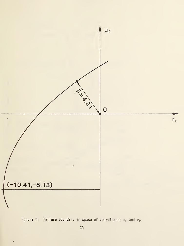
Figure 3. Failure boundary in space of coordinates u r and r r

25

>

26

Figure

4.

Failure

boundaries

for

members

I

and

II

Figure 5. Probability distribution of steel yield stress

27

NBS-114A (REV. 2-80

U.S. DEPT. OF COMM.

BIBLIOGRAPHIC DATASHEET (See instructions)

1„ PUBLICATION ORREPORT NO.

NBSIR 84-2921

2. Performing Organ. Report No 3. Publication Date

September 1984

4. TITLE AND SUBTITLE

Structural Reliability Fundamentals and Their Application to Offshore Structures

5. AUTHOR(S)

Emil Simiu and Charles E. Smith6. PERFORMING ORGANIZATION (If joint or other than NBS, see instructions) 7. Contract/Grant No.

national bureau of standardsDEPARTMENT OF COMMERCE 8. Type of Report & Period Covered

WASHINGTON, D.C. 20234

9. SPONSORING ORGANIZATION NAME AND COMPLETE ADDRESS (Street, City . Stole, ZIP)

Minerals Management ServiceDepartment of the InteriorRoom IP-119 USGS National Ctr. Bldg., 12203 Sunrise Valley DriveReston, VA 22091

10. SUPPLEMENTARY NOTES

Document describes a computer program; SF-185, FIPS Software Summary, is attached.

11.

ABSTRACT (A 200-word or less factual summary of most significant information. If document includes a significantbibliography or literature survey, mention it here)

The objective of this report is to present an overview of fundamental topics in

structural reliability as applied to individual members, which are potentially

applicable to ocean engineering problems. These topics include: the estimation

of failure probabilities; safety indices; and safety (or load and resistance)

factors. Some of the theoretical and practical difficulties in the application

of structural reliability tools are mentioned and/or discussed.

12. KEY WORDS f Si x to twelve entries; alphabetical order; capitalize only proper names; and separate key words by serm'co/onsj

Failure; probability theory; reliability; risk; statistics; structural engineering.

13. AVAILABILITY 14. NO. OFPRINTED PAGES

[x] Uni imited

For Official Distribution. Do Not Release to NTIS

1 1 Order From Superintendent of Documents, U.S. Government Printing Office, Washington, D.C.31

15. Price20402.

[X] Order From National Technical Information Service (NTIS), Springfield, VA. 22161 $8.50

U S COMM- D C 6043-P80