Structural relations, cointegration and identification: some simple results and their application

Journal of Econometrics 87 (1998) 87—113

Structural relations, cointegration and identification:some simple results and their application

James Davidson!,*! Cardiff Business School, Colum Drive, Cardiff CF1 3EU, UK

Received 1 June 1995; received in revised form 1 October 1997

Abstract

This paper presents and applies some results on the interpretation of cointegratingregressions. The key concept is the irreducible cointegrating (IC) relation, one from whichno variable can be omitted without loss of the cointegration property. Extending earlierresults, it is shown that under certain circumstances, IC relations are identified structuralforms. It is possible, at least in principle, to learn about the structure of simultaneouslong-run relations directly from cointegration analyses, in contrast with the well-knownfact that no such knowledge can be obtained from the correlations between stationaryvariables. IC relations can also be estimated by asymptotically mixed Gaussian andmedian unbiased estimators, permitting standard inference. MINIMAL, an algorithm forextracting the IC subsets of a data set, is applied to variety of artificial and actualdata. ( 1998 Elsevier Science S.A. All rights reserved.

JEL classification: C32

Keywords: Structural; Identification; Cointegration; Irreducible cointegrating vector

1. Introduction

Considerable interest has recently been shown in the problem of identifyingthe long-run relationships in a linear cointegrating model with I(1) variables; seefor example Pesaran and Shin (1994), Johansen (1995), Boswijk (1995), and

*Corresponding author. E-mail: [email protected]

0304-4076/98/$— see front matter ( 1998 Elsevier Science S.A. All rights reserved.PII S 0 3 0 4 - 4 0 7 6 ( 9 8 ) 0 0 0 0 7 - 4

Hsiao (1997). These papers focus on the problem of imposing and testingrestrictions on the space of the cointegrating vectors in the context of a vectorerror correction model (VECM), so as to determine long-run behaviouralparameters such as supply and demand elasticities, propensities to consume orsave, etc. We will call such parameters, and the relations containing them,structural. Following on from a recent note (Davidson, 1994) this paper ad-dresses the structural identification issue from a slightly different perspectivecompared to the above-mentioned work. One feature of our analysis is that itprovides an interpretation of single cointegrating regressions of the familiarEngle—Granger (1987) type, although as we subsequently show, it is relevant tothe system estimation problem too.

There is a risk of confusion in the use of the word structure, because of themany different uses to which it has been put by different authors. We note forexample that Hendry (1995) invokes the properties of constancy across interven-tions and regime shifts in his definition of structural, and these are implicit here,but our analysis does not consider such shifts explicitly. We use the term tomean, simply, parameters/relations which have a direct economic interpretation,and may therefore satisfy restrictions based on economic theory. In the contextof simultaneous equations, our usage is the same as in the familiar CowlesCommission analysis (see e.g. Johnston, 1984, Chapter 11). This warns us, forexample, that a regression involving jointly determined variables typicallyestimates a hybrid of different structural relations; for example, the regression ofprice on quantity and other variables will in general estimate a mixture of thedemand and supply schedules. However, a different estimation method (e.g.instrumental variables) can yield consistent estimates of a structural equationprovided the well-known conditions for identification are satisfied. If we focuson the ‘cointegrating structure’ (cointegrating relations between I(1) variables)and ignore the short-run dynamics of the system (involving differences of the I(1)variables and other I(0) variables), the identification problem is formally similarto the Cowles Commission case.1 The main differences are, first, that thedistinction between endogenous and exogenous variables disappears and nor-malisations are arbitrary; and second, as we show, the characterisation ofconsistent estimators is notably different in the I(1) case.

Section 2 of the paper gives a number of simple, non-technical results on theinterpretation of cointegrating regressions. The basic idea is to show that it maybe possible to deduce features of the long-run structure direct from the dataanalysis. Thus, we show that least squares consistently estimates an identified

1 As Johansen (1995) argues, the identification of the dynamic components may be consideredseparately. Ignoring these is appropriate to single-equation cointegration analysis, but even in thecontext of system estimation, a priori restrictions on the dynamics which might aid identification ofthe cointegrating structure are rare, and we lose little by neglecting this possibility.

88 J. Davidson / Journal of Econometrics 87 (1998) 87–113

structural equation, but also that in certain favourable circumstances, it ispossible to establish the status of the equation from the data alone. The keyconcept, developed in Section 2.1, is the irreducible cointegrating (IC) relation;that is to say, a cointegrating relation, which ceases to be so if any of thevariables it contains are suppressed. Section 2.2 gives some additional resultsconcerning IC relations, and Section 2.3 illustrates the results by means ofa simple example. A closely related question concerns the feasibility of efficientestimation and standard inference. The standard errors and t-ratios in an OLScointegrating regression do not generally have the conventional interpretation,but procedures such as the fully modified least squares estimator of Phillips andHansen (1990) are available. Under certain circumstances these are asymp-totically mixed normal, median unbiased to order ¹~1, and allow standardinference. Section 2.4 gives a theorem showing that the Phillips—Hansen type ofestimator is always appropriate for the estimation of IC equations.

Section 3 of the paper considers the problem of detecting and estimating theIC vectors for a data set. Section 3.1 describes MINIMAL, an algorithmimplemented in the GAUSS language which tests sequentially for the ICproperty in every subset of variables, employing a Wald test of restrictions onthe Johansen (1988, 1991) estimator of the cointegrating space. Section 3.2summarises some simulation findings on MINIMAL. Section 3.3 reportsapplications of the method to two economic data sets, a collection of quarter-ly series of UK interest rates and related variables, and the data on theUS economy used in the study of King et al. (1991). Section 4 concludes thepaper.

2. Structure and cointegration

2.1. The background

The starting point for the analysis is the pair of results proved in Davidson(1994). However, to provide the necessary background, we first briefly review thetextbook theory of the identification of simultaneous equations. Suppose

b@xt"z

t(s]1) (2.1)

is a vector of equations connecting a vector of variables xt(m]1) where b is

a m]s matrix of coefficients. In the usual Cowles Commission type of simulta-neous equations model, z

t&iid(0, R). At most s of the variables in x

tare thought

of as being determined by this system, the remaining m!s being givenexogenously. If we know nothing about the correlation of the disturbances, thesystem

db@xt"dz

t(2.2)

J. Davidson / Journal of Econometrics 87 (1998) 87–113 89

where d(s]s) is any non-singular matrix, is observationally equivalent to theoriginal one. For consistent estimation, enough restrictions on the columns ofb must be known to rule out all possibilities except d"I

s.2 Suppose we are

interested in estimating the first column of b, say b1, normalised on the first

element, given the prior information that the last m!g1

elements are zero; inother words,

b1"(1, b

21,2,b

g11, 0,2,0)@. (2.3)

Let b be row-partitioned conformably with b1

as

b"Cba

bbD"C

b1a

b2a

0 b2bD

(g1

rows)

(m!g1

rows)(2.4)

where b2b

has dimension (m!g1)](s!1). If and only if rank(b

2b)"s!1, the

only choice of r (s]1) such that the vector br satisfies the known priorrestrictions on b

1is r"e

1"(1,0,2,0)@. This is the well-known rank condition

for identification, and in the usual analysis, it is normally a necessary conditionfor consistent estimation of the equation by instrumental variable or maximumlikelihood methods.3

Now consider the cointegrating VAR, the system of reduced-rank dynamicequations which has been analysed by Johansen (1988, 1991) inter alia:

A(¸)xt"ab@x

t#A*(¸)Dx

t"u

t(m]1), (2.5)

where ¸ is the lag operator, A(¸)"ab@#A*(¸)(1!¸) such that A(1)"ab@,and a and b are m]s matrices, the loadings matrix and the matrix of cointeg-rating vectors, respectively.4 When s(m it can be shown that x

t&I(1), and

the system embodies a set of long-run equilibrium relations of the form (2.1)where

zt"(a@a)~1a@(u

t!A*(¸)Dx

t)&I(0). (2.6)

2For simplicity we confine attention to the case of zero restrictions on the coefficients.

3 Johansen (1995) points out that the test of this condition is not strictly operational becauseelements of b are unknown a priori, and presents a version of the rank test in terms solely of therestrictions being imposed. Note however that the usual test yields a valid result for all possiblevalues of b except for a set of Lebesgue measure zero.

4 It is customary to write this representation with the maximum order of lag on the ‘levels’ term,which merely redefines A*(¸). Eq. (2.5) is more convenient for the present analysis. The representa-tion also assumes that the variables have zero mean, and that there are no deterministic trends. Theelaborations required to relax these assumptions are straightforward and do not alter the essentialsof the problem. For simplicity of exposition, they are omitted here.


In this model, there are s distinct linearly independent cointegrating vectors, thecolumns of b. As in the static model, without restrictions on b the long run of thesystem is observationally equivalent to Eq. (2.2) with loadings matrix ad~1.Johansen’s methodology does not attempt to solve this problem and estimatesa collection of orthonormalised vectors spanning the same space as b.

However, the usual considerations apply in identifying the cointegratingvectors. The simplest result is the following, which, although it directly relates tosingle equation estimation, has wider implications.

¹heorem 1 (Davidson, 1994). If a column of b (say, b1) is identified by the rank

condition, the O¸S regression which includes just the variables having unrestricted(non-zero) coefficients in b

1is consistent for b

1.

Note that if another variable is added to this cointegrating regression, itscoefficient does not converge to zero and the other coefficients to the same limitsas before, as we would expect of an ‘irrelevant’ variable in a stationary regres-sion. The regression coefficients will generally converge to some other element ofthe cointegrating space. The situation is loosely analogous to what happens if aninstrument whose exclusion from a simultaneous structural equation is helpingto identify it is added to the equation. The resulting IV estimator is of courseinconsistent. Theorem 1 is given in terms of OLS, but it holds in respect of anyestimator that has been shown consistent for b

1when OLS is consistent, such as

2-stage least squares, or the Phillips—Hansen (1990) fully modified estimator. Wesay more about this in Section 2.4.

If a collection of I(1) variables is found to be cointegrated, it does not followthat the estimated vector can be interpreted as structural. However, the follow-ing concept is relevant in this connection.

Definition 1. A set of I(1) variables will be called irreducibly cointegrated (IC) ifthey are cointegrated, but dropping any of the variables leaves a set that is notcointegrated.

We will also speak of an IC relation, or IC vector, to refer to the correspond-ing cointegrating coefficients for these variables. We immediately note thefollowing important property of these vectors.

¹heorem 2. An IC vector is unique, up to the choice of normalisation.

Proof. This is by contradiction. Suppose there exists for the IC variables a set ofcointegrating vectors of rank at least two. Any linear combination of thesevectors lies in the cointegrating space, and by choosing the weights appropriate-ly, we can always generate such a combination having a zero element. Since thevariable in question can therefore be dropped from the set without losingcointegration, the IC assumption is contradicted. h


The following is the result that explains our interest in IC relations.

¹heorem 3 (Davidson, 1994). If and only if a structural cointegrating relation isidentified by the rank condition, it is irreducible. h

This tells us that at least some IC vectors are structural. Theorem 3 does noteliminate all ambiguity in the interpretation of a particular cointegrating regres-sion, but it has a number of useful implications. In fact, it is easy to see onreflection that an IC vector must have a certain status with regard to theunderlying cointegrating structure. When the cointegrating rank of the system iss, an IC relation can contain at most m!s#1 variables. There are betweens and ( m

m~s`1) of these vectors in total, the actual number depending on the

degrees of overidentification of the relations of the system. But in addition to upto s identified structural relations, which are among the IC vectors by Theorem3, there are also generally a number of solved relations (or equivalently, solvedvectors).

Definition 2. A solved vector is a linear combination of structural vectors fromwhich one or more common variables are eliminated by choice of offsettingweights such that the included variables are not a superset of any of thecomponent relations.

A solved vector lies in the cointegrating space by construction, and if itscomponents are identified structural vectors, it may also be irreducible.5 Thelargest number of solved relations arises with a just-identified system. There arenone at all under maximal overidentification, such that each variable appears inone and only one structural relation. In the sense of being solved from thestructure, these relations are comparable to the reduced form equations of theconventional simultaneous equations analysis, and may indeed coincide withthem (see the example in Section 2.3). However, the reduced forms are definedwith respect to a particular normalisation, based on the endogenous—exogenousdistinction, which is irrelevant here. Moreover, the reduced forms with respectto a given normalisation all contain m!s#1 variables by definition. Theyneed not be irreducible even if the model is identified.

2.2. Implications of irreducible cointegration

A common research methodology is to construct a putative cointegratingregression in the light of some economic theory, the theory being deemed to

5 Indeed, it seems to be necessarily irreducible, but we do not need to prove this, simply to notethat IC vectors can be of this form.


receive support if the hypothesis of non-cointegration is rejected in this equa-tion. However, according to Theorem 3, a cointegrating vector that containsredundant elements can be of no interest to us. The theory could be wrong, inwhich case this is just an arbitrary element of the cointegrating space. If thetheory is correct, the relation is revealed to be underidentified, and the estimateis inconsistent, representing a hybrid of different structural equations, just as inthe conventional analysis of simultaneity. Irreducibility is therefore an impor-tant diagnostic property of a cointegrating regression. Although simple consid-erations of parsimony would often lead to IC vectors being reported in practice,no one, to the author’s knowledge, has previously considered the implications oftesting for irreducibility.

If an IC relation is found, interest focuses on the problem of distinguishingbetween structural and solved forms. Of course, the theoretical model mightanswer this question for us, as the example below will illustrate. However,important clues may also be provided by the data themselves. The followinglemma has inherent interest, and is also useful in proving our first main result.(All proofs for this section are given in Appendix A).

¸emma 1. Provided b is restricted only by zero and normalisation restrictions,a solved IC relation contains at least as many variables as each of the identifiedstructural relations from which it derives.

An example of an additional restriction on b which would invalidate the resultof Lemma 1 is where two rows of the matrix are the same, such that twovariables take the same coefficients in every cointegrating relation. Such restric-tions are clearly not impossible since the economics of the model might implythem. However, we can rule them out from arising “by chance” in the same wayas we are willing to rule out a failure of identification from the same cause. (Seefootnote 3.)

In general, therefore, the fewer variables an IC relation contains, and the fewerit shares with other IC relations, the better the chance that it is structural andnot a solved form. In the extreme cases, we can actually draw definite con-clusions, as the following pair of results show.

¹heorem 4. If an IC relation contains strictly fewer variables than all those othershaving variables in common with it then, subject to the condition of ¸emma 1, it isan overidentified structural relation.

¹heorem 5. If an IC relation contains a variable which appears in no other ICrelation, it is structural.

Thus, it is possible, in the context of simultaneous cointegrating relations, todiscover structural economic relationships directly from a data analysis, without


the use of any theory. To take a very simple example, suppose our system(assumed complete) consists of four I(1) variables, x, y, z and w. If the pairs (x, y)and (z, w) are found to be cointegrated (but not the pairs (x, z) or (y, w)) these twocointegrating relations, necessarily irreducible of course, are also necessarilystructural. Neither can have arisen as a result of solving out some morefundamental relationships. This is a case of maximal overidentification. If, onthe other hand, the pairs (x, y) and (x, z) are cointegrated, it follows necessarilythat the pair (y, z) is also cointegrated. The cointegrating rank of these threevariables is 2, and one of these three IC relations necessarily exists by beingsolved from the other two; but it is not possible to know which, without a priortheory.6

It needs to be emphasised that Theorems 4 and 5 are no more than possibilitytheorems. There is no guarantee that the conditions will be satisfied in anyparticular case. Nonetheless, the mere possibility of a ‘free lunch’, of gainingsome direct knowledge of the cointegrating structure without any prior theory,may be found surprising and counter-intuitive, given our strong preconceptionsabout structural modelling derived from the stationary data case. The funda-mental implication of the present results is that models with stochastic trendsare different in this respect.

2.3. An example

The results can be illustrated in more depth with reference to the standardmarket model discussed in Davidson (1994), that we write here as

qt!b

21pt!b

31wt!b

41rt&I(0) (demand),

qt!b

22pt!b

32wt!b

42rt&I(0) (supply),

wt&I(0),

rt&I(0), (2.7)

where ptdenotes price, q

tquantity, and w

tand r

tare autonomous variables.7

Both schedules are cointegrating but wtand r

tare not cointegrated with each

6The empirical example of US output, consumption and investment discussed in Section 3.3below is a case in point. The consumption and investment functions are commonly thought of asstructural, directly reflecting the economic activities generating the data. They jointly imply a coin-tegrating relationship between consumption and investment. Of course, a theory which says theconsumption/investment relation is ‘structural’ cannot be contradicted by the data. The point wemake here is that in the maximally overidentified case (pairwise cointegration) no such ambiguityexists. The structure is explicit in the data.

7The notation ‘&I(0)’ indicates the possible existence of short-run dynamics in these relation-ships which, however, are explicitly excluded from consideration. It is only the cointegratingstructure which concerns us here.


other, otherwise we would have to augment the system with this extra relation.Here, m"4 and s"2. If there are no restrictions on the system (so that it isunderidentified by the usual criteria) there are four IC relations each involvingthree variables, obtained by dropping the variables p

t, q

t, w

t, r

tfrom the set one

at a time. Of course, none of these corresponds to the structural relations. If

b41"b

32"0

so that both schedules satisfy the rank condition, the demand schedule isconsistently estimated by regressing q

ton p

tand w

t, and the supply schedule is

consistently estimated by regressing qton p

tand r

t. There are two other IC

relations, what we usually call the reduced forms, containing respectively(q

t, w

t, r

t) and (p

t, w

t, r

t). To distinguish the reduced (i.e. solved) forms from the

structural relations we can use our economic knowledge that only the demandand supply schedules contain both p

tand q

t. We do not even need to know in

advance which schedule contains wtand which r

t, since the theoretical signs of

the slopes, b21(0 and b

22'0, are sufficient prior knowledge to distinguish

them.8If the restrictions are b

31"b

41"0, the supply relation is underidentified and

the demand relation is overidentified. In this case ptand q

tare cointegrated so

there are three IC relations, of which one is uniquely smallest. We thereby knowfrom Theorem 4 (without any economic knowledge being required) that this isan identified structural relation. There are also the same two solved forms asbefore. Of course, the supply relation is not IC.

If the restrictions are b22"b

41"b

32"0, so that supply is determined

exogenously, the whole system is again identified, but qtand r

tare a cointegrated

pair. There are again only three IC relations, of which only one is a solved form.The supply relation is known to be structural, independent of theory, byTheorem 4 and similarly the demand relation, being the only relation containingptis known to be structural by Theorem 5. We could actually learn about the

existence of the supply and demand functions empirically, without having anyeconomic theory to structure the investigation! A similar argument would applyin the c ase of inelastic demand.9

8Of course, we need to know that the system is identified to make this interpretation, anda situation in which we know that each schedule contains at most one autonomous variable, but notwhich one, is arguably unlikely! Nonetheless the point of principle remains valid, that suchinformation could not suffice to reveal the correct specification in the stationary data case, but coulddo so here.

9Note that this analysis assumes, crucially, that all relevant variables are included in the data setbeing analysed. If any are omitted the application of the results could lead to incorrect conclusions.This case is explored more fully in the working version of the paper, see Davidson (1996).


2.4. Estimation of IC vectors

We showed in Theorem 2 that if a set of variables have the IC property, the ICvector is unique. This fact is of some practical importance, because it means thatsingle equation estimators are available for IC vectors which are asymptoticallymixed Gaussian and median unbiased to O(¹~1), so that standard tests ofhypotheses are available asymptotically. This is true whether or not the vectorsare structural, but it obviously has special relevance in the structural case,because it implies that identification by the rank condition is a sufficientcondition for these properties to hold. This result follows from the fact that anyIC vector can be embedded in a closed dynamic system for the relevant subset ofincluded variables, solved out of Eq. (2.5). By construction, this system hascointegrating rank 1, and after a suitable transformation, it can be rearranged intothe triangular form assumed in Phillips (1991) and Phillips and Hansen (1990).

These authors work with systems having the form (apart from possibledeterministic trends that we omit here)

x1t"c@x

2t#u

1t,

Dx2t"u

2t, (2.8)

where x1t

is s]1, x2t

is (m!s)]1, c is (m!s)]s, and u1t, u

2tare vectors of

stationary processes. This structure implies the partition b@"[Is: !c@], such

that the regressions of the elements of x1t

onto x2t

yield consistent estimates ofthe structural coefficients. The marginal submodel for x

2tnecessarily carries the

full complement of m!s unit roots. The ‘reduced form’ structure of the condi-tional submodel in Eq. (2.8) is highly restrictive for cases with s'1, but if s"1,every b(m]1) satisfies the requirement after merely being normalised on its firstelement. The following theorem shows that a solved model having this structurecan always be invoked for an IC vector.

¹heorem 6. ¸et xt"(x@

at, x@

bt)@ define a partition of the variables into subsets of

dimension g1

and m!g1

respectively. If xat

is an IC subset, the closed dynamicsubsystem for x

atsolved out from Eq. (2.5), having the form

B(¸)xat"v

t&I(0) (g

1]1) (2.9)

has cointegrating rank 1.

(See Appendix A for the proof.)10 Given Eq. (2.9), it is straightforward toreparameterise the dynamics of the subsystem into the form of Eq. (2.8). Letting

10The condition of Theorem 6 is sufficient but not necessary. A non-IC vector having a solveddynamic form of rank 1 would arise if the ‘droppable’ variable(s) do not appear in any cointegratingrelations, which is not ruled out (i.e., rows of b can be zero).


B(1)"a1!

b@1!

(see the proof of Theorem 6 for details of the notation) constructa full-rank matrix G(g

1]g

1) with a partition into the first column,

G1"(a@

1aa@1a

)~1a1a

, and the remaining g1!1 columns G

2orthogonal to a

1a,

with the property G@2a1a"0. Then define the partition

G@2B*(z)"[C

1(z),C

2(z)] (2.10)

where C1(z) is (g

1!1)]1 and C

2(z) ((g

1!1)](g

1!1)) has all its roots outside

the unit circle by assumption. It is now easy to see that after transforming system(2.9) by premultiplication by G@, it has the partition

xa,1t

"c@1xa,2t

#w1t,

Dxa,2t

"w2t, (2.11)

where (1, !c@1)"b@

1!,

w1t"v

1t!(a@

1aa1a

)~1a1a

B*(¸)Dxat&I(0) (2.12)

and

w2t"C

2(¸)~1(v

2t!C

1(¸)Dx

a,1t)&I(0). (2.13)

While model (2.11) is not a finite-order VAR in general, the short-run dynamicsmay (for example) be approximated non-parametrically by the estimationmethods cited.

3. Testing for irreducibly cointegrated subsets

3.1. The MINIMAL Algorithm

The analysis of Section 2 suggests that a good starting point for an empiricalinvestigation of a set of I(1) variables might be to catalogue the IC subsets. Toknow whether the long-run structural equilibrium relations suggested by eco-nomic theory actually belong to this collection, in the available data, could oftenbe useful in, for example, pointing to potentially fruitful avenues of research andruling out others. There are 2m!m!1 possible subsets of two or more out ofm variables, and even with a moderate value of m, an ad hoc data explorationcould not be relied on to examine every one of these. Except in the smallest datasets, a systematic search procedure is required to be sure of detecting all therelevant subsets.

One could, in principle, perform cointegration tests on all the possible subsetssystematically, and merely study the full printout. Once a set is judged on the


evidence to be cointegrated, all supersets of this set can be excluded from theanalysis on the basis that only IC vectors are interesting. Once all non-cointegrated sets, and cointegrated supersets, have been eliminated, the remain-ing sets of variables can be categorised as IC and subjected to further study.Pursuing this approach leads naturally to the idea of automating the elimina-tion procedure. MINIMAL is an algorithm that performs this task, imple-mented in the GAUSS language.

The essential component of MINIMAL is a self-calling procedure whose codeis listed in Appendix B. The procedure takes as its input a set of 3 or more I(1)variables, which at the initial call is the complete data set. It returns the value ofa logical variable set to ‘True’ if the input set contains a cointegrated subset,according to the test criteria set by the user. The procedure itself consists ofa loop that drops each variable in turn. If more than two then remain, theprocedure calls itself with the remaining variables as input, and if ‘True’ isreturned, the loop is incremented directly. Otherwise, the cointegration test isperformed on the subset,11 and if cointegration is found this subset is necessarilyIC on the criteria, and is printed out. When execution of the loop is complete,the procedure returns with the value ‘True’ unless none of the subsets was foundcointegrated, in which case ‘False’ is returned.

Thus, in effect, sequences of tests are conducted as follows. Start with a pair ofvariables, test these for cointegration, and then add variables one at a time to theset until a cointegrated subset is found; repeat this sequence of operations inevery possible way. When the program terminates, every subset of the variableswill have been tested for cointegration unless a subset of the subset has pre-viously been found cointegrated. The output lists all the sets of cointegratedvariables that have no cointegrated subset. The ‘bottom-up’ structure of thealgorithm ensures that all such sets are detected with the smallest number oftests. It interesting to draw a comparison here with the more usual type ofspecification search in econometrics. The ‘general-to-particular’ mode of search,starting with a general model and specialising it until a rejection is obtained ona test for correct specification, is often preferred to the ‘particular-to-general’method. MINIMAL may appear to belong in the latter category, but it shouldbe noted that since every subset is tested, the ordering of the tests does not affectthe outcome. It is easy to verify that unless one or more cointegrating vectors arefound (which eliminates the corresponding supersets from the search), every oneof the possible 2m!m!1 subsets are tested by the algorithm. The critical ruleis that every superset of a cointegrated set (on the chosen criterion) is treatedas cointegrated. A ‘top-down’ search would require many more tests to be

11To avoid multiple reporting, the test subset is first checked against the list of IC sets previouslyfound.


performed, but if the superset rule is adopted, could not lead to a differentoutcome.12

The test used to implement MINIMAL could take either non-cointegrationor cointegration as the null hypothesis. This only makes a difference when wehave to take into account the effect of false inferences, to which differentprobabilities are then implicitly assigned. The procedure was implementedinitially using the usual Engle—Granger (1987) methodology, of running a re-gression and testing the hypothesis of non-cointegration of the residuals. How-ever, residual-based tests introduce a number of well-known problems. Onemust choose a normalisation for the regression, and the outcome of the tests isnot invariant to this choice. In addition, these methods are known to suffer lowpower, see for example the study of Kremers et al. (1992).

An alternative approach, assuming the cointegrating rank of the system isknown, is to perform Wald tests of the relevant restrictions on the estimates ofb in Eq. (2.5) yielded by the Johansen (1988, 1991) maximum likelihood proced-ure. The hypothesis to be tested takes the form that the cointegrating spacecontains a vector satisfying certain exclusion restrictions, such that the includedvariables form a cointegrated subset. The hypothesis of p exclusions can beexpressed in the form

Hba"0 (p]1) (3.1)

where (after suitable ordering of the variables) H"[0 : Ip] (p]m), and a repres-

ents the eigenvector corresponding to the smallest eigenvalue of the matrixb@H@Hb. In Davidson (1998) it is shown that a suitably constructed quadraticform in the vector HbK aL , where bK is the Johansen MLE, and a the samplecounterpart of a corresponding to bK , is asymptotically chi-squared withmin(p, m!s) degrees of freedom under the null hypothesis.13 The test can beimplemented in practice following a preliminary estimation of the cointegratingrank using (for example) the Johansen trace test. Subject to the null being true,a consistent, asymptotically mixed normal estimator of the restricted cointegrat-ing vector is provided by

bK "GbK aL ((m!p)]1) (3.2)

12The alternative rule, that if a test on a particular set rejects cointegration, then all subsets aredeemed without further testing to be non-cointegrating, could of course yield a different outcome.For consistency one must impose one rule or the other, and the present choice is viewed as the bestone for this problem.

13We cannot test more than m!s restrictions on a column of b because of the way the Johansenb matrix is normalised for estimation. If p'm!s we can test m!s linear combinations of therestrictions, which in general will hold only if the restrictions themselves do. In practice this is doneby taking the Moore—Penrose inverse of the singular covariance matrix. See Davidson (1998) fordetails.


where G"[Im~p

: 0]. Moreover, if this vector is IC by virtue of being anidentified structural relation, then bK consistently estimates the structural para-meters up to the choice of normalisation. This last result reflects the fact thatTheorem 1 is also relevant to system estimators. A vector that is both cointegrat-ing and satisfies the identifying restrictions must be the identified structuralform. Illustrative output from MINIMAL applied to artificial data is reported inAppendix C.

3.2. Simulation experiments

This section reports some Monte Carlo replications of MINIMAL. Artificialdata were generated from four different long-run models, each containing fivevariables. Three have cointegrating rank of 2, with differing amounts ofoveridentification (i.e., sparseness of the b matrix) since preliminary experimentssuggested that this is a crucial factor in the exercise. The fourth has cointegratingrank 3. The values of the b matrices are as follows:

C1 00 10 !1

!1 00 !1 D C

1 1!1 1

0 1!1 0

0 !1 D C1 12 21.5 !1

!1 00 !1 D C

1 1 11 0 !1

!1 0 00 !1 00 0 !1 D (3.3)

Model 1 Model 2 Model 3 Model 4

Model 1 is maximally overidentified, having disjoint cointegrated subsets, andhas just the two structural IC vectors. It can also be verified by inspection thatModel 2 has four IC vectors, Model 3 (which is just-identified) has five, andModel 4 has six.

For each of the long-run models, alternative dynamic structures were speci-fied, having the triangular form of Eq. (2.9), but with different amounts of noiseand short-run dependence. First, five independent AR processes were generated,of the form u

it"cu

i,t~1#e

itwhere e

it&NI(0,1), i"1,2,5. Of these, the cases

i"1, 2, 3 in Models 1—3, and i"1, 2 in Model 4, were cumulated to produceARIMA(1,1,0) processes. The remaining variables were then generated by theequations defined in Eq. (3.3), with additive errors pu

it. (See Appendix C for an

example, corresponding to Model 2). The parameters c and r were variedbetween experiments, the former being assigned the values 0, 0.3, 0.6 and 0.9, andthe latter, 0.5, 1, 2 and 4. All the experiments were conducted with 100 observa-tions. The Johansen maximum likelihood estimates were calculated, with deter-ministic trends being fitted (although not present in the data) and with the orderof the VAR set first to 1, and then to 2. The latter corresponds to the actualmaximum lag implicit in the structure, although the Johansen method implies


some over-parameterisation, and the former was usually the value recommen-ded by the Schwarz information criterion. The full set of experiments wasconducted for both cases. Although technically misspecified, the more par-simonious model often gave the better results, especially in the trace tests.

Figs. 1 and 2 report a selection of the test results in graphical form.14 Theseplots show the proportion of ‘successes’ in 1000 Monte Carlo replications, asa function of c and p. By a ‘success’ is meant (except in Fig. 1b) that MINIMALcorrectly reported all the true IC vectors for the model, and no false ones. Theshading in the figures distinguishes those regions of the response surface wherethe success rate lies in the different bands of width 0.2, ranging from better than0.8 (white) down to 0.2 or worse (darkest).

Fig. 1 shows the results of four experiments (in the rows) on models 1, 2 and3 respectively (shown in the columns). Row (a) shows the proportion of ‘suc-cesses’ in the application of MINIMAL using the Wald test where the truecointegrating rank is treated as known. Row (b) shows the proportion ofsuccesses in the sequential application of the Johansen trace test15 to determinethe cointegrating rank, starting with null hypothesis s)m!1, and reducings until a rejection is obtained. Row (c) shows the results of treating the cointeg-rating rank as unknown, and running MINIMAL after choosing s according tothe outcome of the trace test sequence. Finally, row (d) shows the results ofrunning MINIMAL using a residual-based test for cointegration, the Phillips(1987) nonparametric ZK

ttest.16 All of the tests in these experiments were carried

out at the nominal 1% significance level.To return a ‘success’ in these experiments, MINIMAL must make correct

decisions in all of between 14 and 25 tests. By contrast, to determine thecointegrating rank in this instance requires correct decisions in just three tests.In view of this, the relative performance of MINIMAL revealed in Fig. 1a isnoteworthy. Moreover, Fig. 1c shows that the penalty attached to not knowings, although not negligible, is smaller than we would expect if the two sets of testoutcomes were independent of each other. In data sets whose cointegrating rankcan be determined, there is a relatively high probability that we can alsocorrectly discover the IC vectors. These findings should not surprise us too

14 In Fig. 1 the results reported are the VAR(1) estimates, while in Fig. 2 they are for the VAR(2).For the full set of results, in tabular form, see the working version of the paper, Davidson (1996).

15The trace test is implemented using the critical values given by Osterwald-Lenum (1992), andalso the degrees of freedom correction of Reimers (1991) cited in Banerjee et al. (1993). In otherexperiments the maximal eigenvalue test was tried, but proved less successful in finding the correctrank.

16See Phillips and Ouliaris (1990) for details of this test. The Newey-West (1987) varianceestimator was adopted. To overcome the problem of choice of normalisation, the residuals werecalculated for every normalisation, and the test statistics averaged. Since no estimate of b is used,there is no need for a prior estimate of s in this implementation of MINIMAL.


Fig. 1. (a) MINIMAL with known cointegrating rank; (b) cointegrating rank determination by thetrace test; (c) MINIMAL with estimated cointegrating rank; (d) MINIMAL implemented withresidual-based cointegration test.

much if we note that once s is set correctly the Wald test should be relativelypowerful, exploiting the ¹~1-consistency of the ML estimator. By contrast,MINIMAL implemented with the residual-based test (Fig. 1d) performs poorly.


Fig. 2. Model 4: MINIMAL with different Wald test rejection criteria.

Fig. 2 shows the application of MINIMAL to Model 4 (with s treatedas known) where in this case the three plots show the effect of changingthe rejection criterion of the Wald test. The first two plots show the resultof using 5% and 1% nominal significance levels respectively. Note that a‘success’ is obtained by both rejecting and not rejecting certain hypothesesin combination, and therefore the probability of success is controlled by ad-justing the size of the tests to match the available power. In favourable cases,it was found that choosing a nominal significance level substantially lowerthan 1% gave the best results. Various rules of thumb for varying the rejec-tion criterion were tried, and the third plot in Fig. 2 shows the result of oneof these. The rule of thumb used here is as follows: set the critical value equalto four times the 1% nominal value from the chi-squared tabulationwhen p"m!2 (the hypothesis of a cointegrated pair), at twice the 1% nominalvalue for p"m!3, and use the standard 1% test otherwise. This rule isspectacularly successful in favourable cases (low p and c) with near 100%success.17

For reasons of space we do not report here the corresponding results forModels 1—3, but can summarise the overall finding that there is no ‘best’significance level to cover all cases. In general, the low significance levels do bestwith a high degree of overidentification. On the other hand, in just-identifiedcases such as Model 3, the test statistics for all the valid ( just-identifying)restrictions are identically zero. Since we want to reject all the overidentifyingrestrictions in these cases, a smaller critical value will necessarily out-performa larger one. In short, some experimentation with different rejection criteriawould seem advisable in practical modelling situations.

17A point to note about this model is that when p"m!2"3, the limiting null distribution hasat most m!s"2 degrees of freedom. See footnote 13.


Table 1

bK 1 2

2.5% Consols rate 0.29 0.19 0.282(0.095)

[10.23]3 month Local !0.32 !5.02 — !4.9Authorities rate (0.036)3 months uncovered !0.65 0.034 !0.648Eurodollar rate (0.122)

[37.32]Inter-bank rate 0.19 4.91 — 5

(0.038)$/£ exchange rate 3.38 0.18 3.37

(0.0615)[3021]

U.S. Govt. long bond yield 0.98 !0.013 0.98(0.143)

[48.95]

Wald 1.48 6.36Phillips—Perron !4.325 !6.77

3.3. MINIMAL analysis in practice

In this section, we apply the methodology to two sets of quarterly economictime series. The first is a collection of UK interest rates and related variables forthe period 1963(4)—1984(2) (Table 1). The second consists of five US macroeco-nomic series, the logs of real output (y), consumption (c), investment (i), and realmoney balances (m!p), and the interest rate (R), for 1951(1)—1985(4) (Table 2).The latter are the variables analysed in the well-known study of King et al.(1991) (KPSW), and also by Pesaran and Shin (1994), among others. KPSW alsoinclude the rate of inflation in their study, but it is excluded here in view of doubtthat it is truly I(1).

The tables show the bK matrices from the Johansen MLE, and then theestimates of the IC vectors, computed as bK in Eq. (3.2), with ‘standard errors’ inparentheses.18 These vectors are not normalised on any variable, but inherittheir normalisation from that of bK . The numbers in square brackets, for vectorswith more than two elements only, are the values of the Wald statistic obtainedif the corresponding variable is dropped, as confirmation that the subset is

18As noted, these standard errors are stochastic asymptotically, but provide approximate confi-dence intervals in the sense that the ratios with the deviations of the point estimates from their truevalues are asymptotically N(0,1).


Tab

le2

bK1

23

45

6

y!

11.3

!63

.3!

5.56

—!

9.27

—14

.7!

48.5

—(5

.23)

(6.2

4)(2

.2)

[43.

5]c

!15

.317

.522

——

!18

.8!

25.3

—!

21.6

(5.9

4)(2

.22)

(1.2

7)[4

3.49

]i

!2.

063.

63!

14.2

!11

.512

.414

.6—

——

(1.4

)(1

.39)

(1.3

)[4

3.49

]m!

p17

.540

.62.

736.

92—

——

39.1

10.1

(2.3

6)(2

.74)

(2.7

7)[4

.05]

[110

][5

.33]

R0.

860.

22!

0.15

0.48

6—

——

0.80

30.

826

(0.4

64)

(0.5

39)

(0.5

45)

[1.9

6][2

.73]

3.01

]

Wal

d0

0.85

70.

041

1.94

00

Phill

ips—

Per

ron

!4.

44!

4.48

!4.

52!

4.83

!5.

98!

4.48


indeed IC. At the foot of each column there appears both the Wald statistic forthe vector itself and the Phillips—Perron test (1988) statistic for non-cointegra-tion, computed from the residuals generated by bK . Note that bK converges toa fixed limit at rate ¹~1 under both null and alternative hypotheses. Asymp-totically the test can be treated as a simple test for a unit root, without the usualcomplications associated with residual-based tests where the regression coeffi-cients converge to random limits under the null. This statistic provides anindependent check that the estimated relation is in fact cointegrating.19 Failureto reject would point to the possibility that the cointegrating rank is incorrectlychosen, or simply that the sample evidence is weak.

For the interest rate data (Table 1) the maximum lag of the VAR was set to1 on the basis of the Schwarz information criterion, taking note of the simula-tion evidence cited above, which cautions against over-parameterisation. A de-terministic trend is assumed. The maximal eigenvalue and trace tests bothindicate a cointegrating rank of 2. Two IC vectors were found, implyinga maximally overidentified structure with two disjoint IC subsets, so that nosolved vectors exist. The results shown were obtained by setting the significancelevel of the Wald tests to 5%. Setting the significance level to 1% results in theexclusion of the Consols rate in vector 1. (The frailty of its role is also indicatedby the exclusion test statistic, which is only 10.2.) Vector 1 explains the Euro-dollar rate as a weighted average of US and UK government bond rates, alsodepending positively on the strength of sterling against the dollar. Vector 2 tellsthe simple story of a close co-movement between two UK short rates.20

In the US data, the Akaike and Schwarz criteria both indicate a maximum lagof 2. The sample evidence is equivocal here, since for two of the variables, i andR, the unit root hypothesis is rejected once a deterministic trend is allowed for. Itis also not possible to reject the hypothesis that the cointegrating rank is 2.However, in the spirit of attempting to reproduce previous results we over-ridethis result, and assume a five-variable model with a cointegrating rank of 3.Perhaps because b is not so well determined in this instance, the Wald test doesnot reject various theoretically implausible restrictions at the conventionalsignificance levels. However, if we rank the vectors according to the value of theWald statistic, we find that the six IC vectors which the evidence most favoursare precisely those suggested by the KPSW model. Table 2 shows the result ofrunning MINIMAL with (in effect) the nominal significance level set somewhatover 10%. According to the KPSW analysis, the three ‘structural’ vectors are 2,4 and 5. Vectors 1, 3 and 6 can be interpreted as solved from 2 and 5, 2 and 4, and

19The 5% critical value for n+100, and allowing for a deterministic trend, is !3.46.

20The gap between these two series rarely exceeds 0.5% but is quite highly autocorrelated, whichexplains why the cointegration between them is strong but not overwhelming.


4 and 5, respectively. This is the complete set of IC vectors for the model.However, note the fragility of the inclusion of R in all the vectors containing it,especially vector 1, and also the fact that these coefficients are all within twostandard errors of zero.

Finally, we note in passing that other structural restrictions on b could easilybe tested by the Wald procedure, for example, the unit elasticity restrictions onthe (y, i) and (c, y) relations. This avoids the need for iterative estimation underthe null hypothesis, but it is more important to note how it would allow suchhypotheses to be tested without fully specifying the structural model. We could,for example, test the hypothesis: ‘the cointegrating space contains a vector(1, !1, 0, 0, 0)@, up to a normalising constant’ without specifying anything else,other than the cointegrating rank of the system.

4. Conclusion

In this paper we have defined the notion of an irreducible cointegratingrelation, or vector. We show that such vectors have a special relationship withthe long-run structural relations of the data generation process, when the latterare subject to identifying exclusion restrictions. This is a feature of cointegrationanalysis that appears not to have been noted explicitly before. Sequential testsfor cointegration can determine whether the IC property holds for a given set oftime series. In principle only single equation methods are needed for theanalysis, but working with a system estimator proves much more efficient inpractice. We show in Monte Carlo experiments that sequential testing using theMINIMAL algorithm to determine the IC relations can have a success fre-quency comparable to the correct determination of the cointegrating rank bythe usual sequential testing. The method may therefore prove useful as anadjunct to conventional methods of analysis, particularly if it is difficult tospecify the long-run structure completely on the basis of prior theory.

We show that in certain circumstances, when there is overidentification of thelong-run structure, we might be able to learn something about that structurethrough nothing more than inspection of the irreducible cointegrating regres-sions associated with a set of data. Such an outcome is by no means guaranteedin practice, since only overidentified models can have this property, and max-imum overidentification (no overlap of the cointegrated subsets) is necessary tolearn the complete structure in this way. Nevertheless, the result runs counter tothe popular intuition about simultaneous structural models, drawing as it doeson our experience of the standard stationary-data case, and is of some interestfor this reason alone. The possibility that ‘incredible assumptions’ (in theoft-quoted words of Christopher Sims, 1980) need not always be the price ofobtaining structural estimates turns out to be a distinctive feature of modelswith stochastic trends.


Acknowledgements

I am grateful to Jan Magnus for advice, and to Peter Boswijk, LaurenceCopeland, Russel Davidson, Jurgen Doornik, David Hendry, Cheng Hsiao,David Peel, Tom Rothenberg, two anonymous referees, and associate editorfor their comments on earlier versions of the paper. The usual disclaimerapplies.

Appendix A. Proofs

Proof of ¸emma 1. Let a solved IC relation d@xtbe defined by d"br, where

r (s]1) is a vector of weights which, for irreducibility, must equate at least s!1elements of d to zero. With no loss of generality, consider the first structuralcointegrating relation, having coefficients b

1(m]1). Let this be identified and

hence IC by Theorem 3, and assume r1O0, so that d depends on it. Next, let r*

(s]1) to be equal to r except for its first element, which is 0, and define d*"br*such that

d"r1b1#d*.

By the assumption of identification, there exists no r, as defined, such that d* hasthe same zero restrictions as b

1. In the absence of linear restrictions across the

columns of b, r1

can be chosen to equate at most one element of d to zero. Itfollows that d contains at least as many nonzero elements as b

1. h

Proof of ¹heorem 4. First, consider the case where each relation in the system iseither just-identified or underidentified. Then every identified structural relation,and every solved relation, contains exactly m!s#1 variables, and there is nouniquely smallest IC relation. Next, suppose there are overidentified structuralrelations. These contain fewer than m!s#1 variables, and Lemma 1 showsthat they never contain more variables than the solved relations containingthem. If there exists a uniquely smallest IC relation, such that all the otherscontain more variables, it follows that this must be structural.

Next consider an arbitrary subset of the variables, denoted S. The set A(S) ofall the IC relations containing at least one member of subset S consists of all theidentified structural relations containing elements of S, plus all the solved ICrelations derived, in part or wholly, from these. Note that each IC relation that issolved from a particular structural relation must, by construction, have one ormore variables in common with it. Suppose A(S) contains a relation, R, which isstrictly the smallest (has fewest variables) in A(S). R cannot be a solved relationaccording to Lemma 1, and hence must be structural. Note that this is true evenif there are equally small or smaller IC relations not belonging to A(S), sinceR cannot be solved from any of these by definition. h


Proof of ¹heorem 5. Suppose there is a structural relation, Equation (1) (say),containing a variable x

15(say) which appears in no other structural relation.

First, let equation (1) be identified, and hence IC by Theorem 3. Sincex15

appears in only the one equation, any solved relation involving equation (1)must contain x

1tby definition. Given the existence of such a relation, x

1twould

appear in at least two IC relations, contrary to supposition.Second, suppose equation (1) is underidentified. This means there is a linear

combination of equations (2)—(5) that satisfies the same zero restrictions asequation (1). This vector lies in the cointegrating space, and by the suppositionthat x

1tappears uniquely in equation (1), its first element must be zero. It follows

that x1t

can be dropped from equation (1) without losing cointegration, andhence, that x

1tis not cointegrated with any combination of x

2t,2,x

.t. It

therefore cannot appear in any IC relation, whether structural or solved. h

Proof of ¹heorem 6. Assume initially that the vector in question is structural andidentified. Re-order the system such that the coefficients are b

1a"

(1,b21

,2,bg11

)@ as in Eqs. (2.3) and (2.4), and such that after partitioning Eq. (2.5) as

Aaa(¸)x

at#A

ab(¸)x

bt"u

at(g

1]1)

Aab(¸)x

at#A

bb(¸)x

bt"u

bt((m!g

1)]1) (A.1)

the polynomial matrix Abb

(z) has full rank. That is to say, Abb

(z) is non-singularat all points z3C other than the solutions of DA

bb(z)D"0. The second block in

Eq. (A.1) may be solved for xbt

as

xbt"A

bb(¸)~1u

bt!A

bb(¸)~1A

ba(¸)x

at. (A.2)

Since b spans the cointegrating space we must have, from Eqs. (2.4) and (A.2),

b@axat"!b@

bxbt#I(0)"!D(¸)x

at#I(0) (A.3)

where D(z)"b@bA

bb(z)~1A

ba(z) (s]g

1). We cannot assume that A

bb(1)~1 exists,

but the top row of D(z) is zero since the top row of bb@ is zero from Eq. (2.4). If

D2(z) denotes the remaining rows, the decomposition D

2(z)"D

2(1)#

D*2(z)(1!z) exists by construction. By the irreducibility hypothesis and The-

orem 3, rank(b2b

)"s!1, and hence none of the columns of b2a

are indepen-dently cointegrating for x

at. It is therefore clear from Eq. (A.3) that b@

2a"D

2(1).


Substituting for xbt

in the first block of Eq. (A.1) we obtain Eq. (2.9), whereB(z)"A

aa(z)!A

ab(z)A

bb(z)~1A

ba(z) and v

t"u

at!A

ab(¸)A

bb(¸)~1u

bt. Using

Aaa(1)"a

ab@a

and Aab

(1)"a!b@b, where a

ais g

1]s, we find

B(1)"aa(b@

a!D(1))"a

aCb@1a

0 D"a1a

b@1a

, (A.4)

where a1a

(g1]1) is the first column of a

a. Two conclusions may be drawn from

this. First, applying the usual decomposition B(z)"a1a

b@1a#B*(z)(1!z) as in

Eq. (2.5), we have

vt"B(¸)x

at"a

1ab@1a

xat#B*(¸)Dx

at&I(0) (A.5)

so that Eq. (2.9) holds. Second, B(1) has rank 1, and b1a

is the unique cointegrat-ing vector of this system.

This completes the proof for the identified structural case. If the vector inquestion is a solved form, let b* denote the ‘true’ structure, and assume thatEq. (2.5) represents a reparameterised structure with b"b*d where d is s]snon-singular, of which the first column b

1"b*d

1is the solved form in question.

Since by assumption the cointegrating vector b1a

is irreducible, it must be‘identified’ in the reparameterised model, in the sense that rank (b

2b)"s!1, by

Theorem 3. The previous analysis can now be performed on this case, complet-ing the proof. h

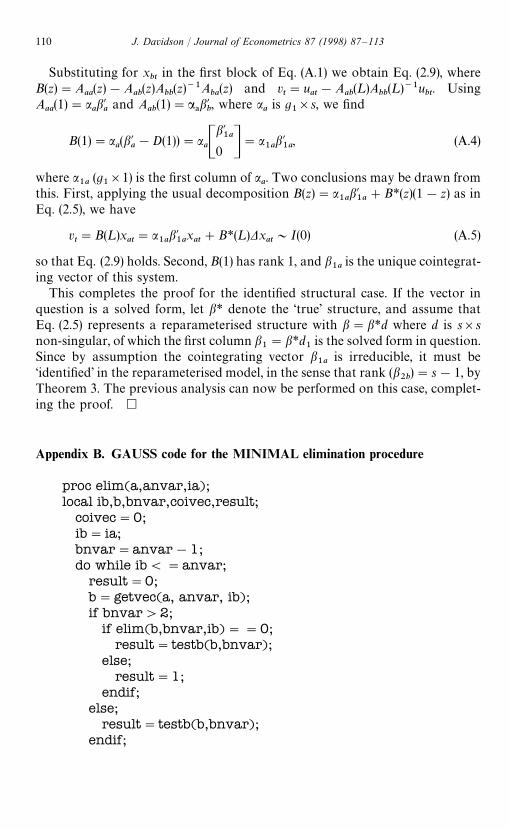
Appendix B. GAUSS code for the MINIMAL elimination procedure

proc elim(a,anvar,ia);local ib,b,bnvar,coivec,result;

coivec"0;ib"ia;bnvar"anvar!1;do while ib("anvar;

result"0;b"getvec(a, anvar, ib);if bnvar'2;

if elim(b,bnvar,ib)""0;result"testb(b,bnvar);

else;result"1;

endif;else;

result"testb(b,bnvar);endif;


if result""1;coivec"1;

endif;ib"ib#1;

endo;retp(coivec);endp;

Notes:

1. ia is a scalar, set to 1 when procedure elim is called from the main program.anvar is a scalar set initially to m, the number of variables in the data set. a isa vector of dimension anvar, containing the storage locations of variables inthe data set. On the initial call, a"M1,2,mN.

2. Procedure getvec removes the ibth element from a, returning a vector ofdimension anvar!1.

3. Procedure testb returns the result of the cointegration test. Before doing thetest it checks if the current set has been found to be IC at a previous stage, inwhich case a positive result is returned directly. Otherwise, if the test result ispositive the set is added to the list of IC subsets, and printed out.

Appendix C. An example of MINIMAL output, with simulated data

Let variables X1t, X

2t, X

3tbe generated by X

it"X

i,t~1#º

it, with X

i0"0,

and then X4t

and X5t

be generated by

X4t"X

1t#X

2t#X

3t#º

4t, (C.1)

X5t"X

1t!X

2t#º

5t, (C.2)

where ºit&NID(0,1) for i "1,2,5. In this model, the cointegrating rank (s) is

2, and the number of IC vectors is 4. These are the ‘structures’ (C.1) and (C.2),and two solved relations obtained as the sum and difference of (C.1) and (C.2),respectively.

Table 3 shows the output from MINIMAL applied to a sample of size 100generated from this DGP, following Johansen estimation and using the tracetest to set the cointegrating rank (correctly) at 2. The nominal 5% significancelevel was used in the Wald tests. The first two columns of the table contain thecointegrating vectors estimated by the Johansen MLE, and the next four are thereported IC vectors, obtained with the formula in Eq. (3.2), with standard errorsin parentheses. The vectors a are shown, transposed, in the top row. Thenumbers in the bottom row are the Wald statistics. Note that these equal0 identically for fewer than s"2 restrictions. The third and fourth columns maybe recognised as estimates of Eqs. (C.1) and (C.2) respectively (with arbitrary


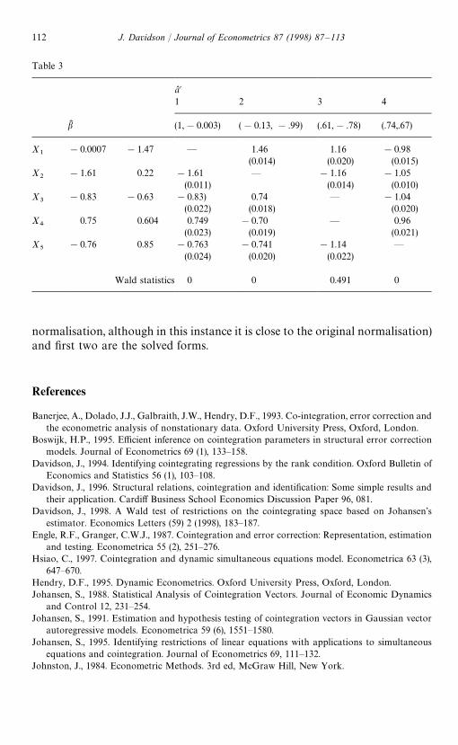
Table 3

aL @1 2 3 4

bK (1,!0.003) (!0.13, !.99) (.61,!.78) (.74,.67)

X1

!0.0007 !1.47 — 1.46 1.16 !0.98(0.014) (0.020) (0.015)

X2

!1.61 0.22 !1.61 — !1.16 !1.05(0.011) (0.014) (0.010)

X3

!0.83 !0.63 !0.83) 0.74 — !1.04(0.022) (0.018) (0.020)

X4

0.75 0.604 0.749 !0.70 — 0.96(0.023) (0.019) (0.021)

X5

!0.76 0.85 !0.763 !0.741 !1.14 —(0.024) (0.020) (0.022)

Wald statistics 0 0 0.491 0

normalisation, although in this instance it is close to the original normalisation)and first two are the solved forms.

References

Banerjee, A., Dolado, J.J., Galbraith, J.W., Hendry, D.F., 1993. Co-integration, error correction andthe econometric analysis of nonstationary data. Oxford University Press, Oxford, London.

Boswijk, H.P., 1995. Efficient inference on cointegration parameters in structural error correctionmodels. Journal of Econometrics 69 (1), 133—158.

Davidson, J., 1994. Identifying cointegrating regressions by the rank condition. Oxford Bulletin ofEconomics and Statistics 56 (1), 103—108.

Davidson, J., 1996. Structural relations, cointegration and identification: Some simple results andtheir application. Cardiff Business School Economics Discussion Paper 96, 081.

Davidson, J., 1998. A Wald test of restrictions on the cointegrating space based on Johansen’sestimator. Economics Letters (59) 2 (1998), 183—187.

Engle, R.F., Granger, C.W.J., 1987. Cointegration and error correction: Representation, estimationand testing. Econometrica 55 (2), 251—276.

Hsiao, C., 1997. Cointegration and dynamic simultaneous equations model. Econometrica 63 (3),647—670.

Hendry, D.F., 1995. Dynamic Econometrics. Oxford University Press, Oxford, London.Johansen, S., 1988. Statistical Analysis of Cointegration Vectors. Journal of Economic Dynamics

and Control 12, 231—254.Johansen, S., 1991. Estimation and hypothesis testing of cointegration vectors in Gaussian vector

autoregressive models. Econometrica 59 (6), 1551—1580.Johansen, S., 1995. Identifying restrictions of linear equations with applications to simultaneous

equations and cointegration. Journal of Econometrics 69, 111—132.Johnston, J., 1984. Econometric Methods. 3rd ed, McGraw Hill, New York.


King, R.G., Plosser, C.I., Stock, J.H., Watson, M.W., 1991. Stochastic Trends and EconomicFluctuations. American Economic Review 81 (4), 819—840.

Kremers, J.J.M., Ericsson, N.R., Dolado, J.J., 1992. The power of cointegration tests. Oxford Bulletinof Economics and Statistics 54 (3), 325—348.

Newey, W.K., West, K., 1987. A simple positive definite heteroskedasticity and correlation consis-tent covariance matrix. Econometrica 55, 703—708.

Osterwald-Lenum, M., 1992. A note with fractiles of the asymptotic distribution of the maximumlikelihood cointegration rank test statistics: Four cases. Oxford Bulletin of Economics andStatistics 54, 461—472.

Pesaran, M.H., Shin, Y., 1994. Long-run structural modelling. Working Paper. Department ofApplied Economics. University of Cambridge (September).

Phillips, P.C.B., 1987. Time series regression with a unit root. Econometrica 55 (2), 277—301.Phillips, P.C.B., 1991. Optimal inference in cointegrated systems. Econometrica 59(2) (March),

283—306.Phillips, P.C.B., Hansen, B.E., 1990. Statistical Inference in Instrumental Variables Regression with

I(1) Processes. Review of Economic Studies 57, 99—125.Phillips, P.C.B., Ouliaris, S., 1990. Asymptotic Properties of residual based tests for cointegration.

Econometrica 58 (1), 165—193.Phillips, P.C.B., Perron, P., 1988. Testing for a unit root in time series regression. Biometrika 75,

335—346.Reimers, H.E., 1991. Comparisons of tests of multivariate cointegration. Discussion Paper 58.

Christian-Albrechts University, Kiel.Sims, C., 1980. Macroeconomics and Reality. Econometrica 48 (1), 1—48.


Documents

Structural relations, cointegration and identification: some simple results and their application