Embed Size (px)
Citation preview

Polytypic Functional Programming
and
Data Abstraction
by Pablo Nogueira Iglesias, MSc
Thesis submitted to the University of Nottingham for the degree
of Doctor of Philosophy. September 2005

abstract
Structural polymorphism is a generic programming technique known within the func-
tional programming community under the names of polytypic or datatype-generic pro-
gramming. In this thesis we show that such a technique conflicts with the principle of
data abstraction and propose a solution for reconciliation. More concretely, we show
that popular polytypic extensions of the functional programming language Haskell,
namely, Generic Haskell and Scrap your Boilerplate have their genericity limited by
data abstraction. We propose an extension to the Generic Haskell language where the
‘structure’ in ‘structural polymorphism’ is defined around the concept of interface and
not the representation of a type.
More precisely, polytypic functions capture families of polymorphic functions in one
single template definition. Instances of a polytypic function for specific algebraic types
can be generated automatically by a compiler following the definitional structure of the
types. However, the definitional structure of an abstract type is, for maintainability
reasons, logically hidden and, sometimes, even physically unavailable (e.g., precompiled
libraries). Even if the representation is known, the semantic gap between an abstract
type and its representation type makes automatic generation difficult, if not impossible.
Furthermore, if it were possible it would nevertheless be impractical: the code generated
from the definitional structure of the internal representation is rendered obsolete when
the representation changes. The purpose of an abstract type is to minimise the impact
of representation changes on client code.
Data abstraction is upheld by client code, whether polytypic or not, when it works
with abstract types through their public interfaces. Fortunately, interfaces can provide
enough description of ‘structure’ to guide the automatic construction of two polytypic
functions that extract and insert data from abstract types to concrete types and vice
versa. Polytypic functions can be defined in this setting in terms of polytypic inser-
tion, polytypic extraction, and ordinary polytypic functions on concrete types. We
propose the extension of the Generic Haskell language with mechanisms that enable
programmers to supply the necessary information. The scheme relies on another pro-
posed extension to support polytypic programming with type-class constrained types,
which we show are not supported by Generic Haskell.

Contents
1 Introduction 1
1.1 General theme and contribution . . . . . . . . . . . . . . . . . . . . . . . 1
1.2 Notes to the reader . . . . . . . . . . . . . . . . . . . . . . . . . . . . . . 1
1.3 The problem in a nutshell . . . . . . . . . . . . . . . . . . . . . . . . . . 5
1.4 Contributions . . . . . . . . . . . . . . . . . . . . . . . . . . . . . . . . . 8
1.5 Structure and organisation . . . . . . . . . . . . . . . . . . . . . . . . . . 9
I Prerequisites 15
2 Language Games 16
2.1 Object versus meta . . . . . . . . . . . . . . . . . . . . . . . . . . . . . . 16
2.2 Definitions and equality . . . . . . . . . . . . . . . . . . . . . . . . . . . 16
2.3 Grammatical conventions . . . . . . . . . . . . . . . . . . . . . . . . . . 17
2.4 Quantification . . . . . . . . . . . . . . . . . . . . . . . . . . . . . . . . . 17
2.5 The importance of types . . . . . . . . . . . . . . . . . . . . . . . . . . . 17
2.6 Denoting functions . . . . . . . . . . . . . . . . . . . . . . . . . . . . . . 22
2.7 Lambda Calculi . . . . . . . . . . . . . . . . . . . . . . . . . . . . . . . . 22
2.7.1 Pure Simply Typed Lambda Calculus . . . . . . . . . . . . . . . 23
2.7.2 Adding primitive types and values. . . . . . . . . . . . . . . . . . 27
2.7.3 Adding parametric polymorphism: System F . . . . . . . . . . . 28
2.7.4 Adding type operators: System Fω . . . . . . . . . . . . . . . . . 30
2.7.5 Adding general recursion . . . . . . . . . . . . . . . . . . . . . . 34
3 Bits of Category Theory 38
3.1 Categories and abstraction . . . . . . . . . . . . . . . . . . . . . . . . . . 38
3.2 Direction of arrows . . . . . . . . . . . . . . . . . . . . . . . . . . . . . . 39
3.3 Definition of category . . . . . . . . . . . . . . . . . . . . . . . . . . . . 41
3.4 Example categories . . . . . . . . . . . . . . . . . . . . . . . . . . . . . . 42
3.5 Duality . . . . . . . . . . . . . . . . . . . . . . . . . . . . . . . . . . . . 43
3.6 Initial and final objects . . . . . . . . . . . . . . . . . . . . . . . . . . . 43
3

3.7 Isomorphisms . . . . . . . . . . . . . . . . . . . . . . . . . . . . . . . . . 44
3.8 Functors . . . . . . . . . . . . . . . . . . . . . . . . . . . . . . . . . . . . 44
3.9 (Co)Limits . . . . . . . . . . . . . . . . . . . . . . . . . . . . . . . . . . 46
3.9.1 (Co)Products . . . . . . . . . . . . . . . . . . . . . . . . . . . . . 47
3.9.2 (Co)Products and abstraction . . . . . . . . . . . . . . . . . . . . 49
3.10 Arrow functor . . . . . . . . . . . . . . . . . . . . . . . . . . . . . . . . . 51
3.11 Algebra of functors . . . . . . . . . . . . . . . . . . . . . . . . . . . . . . 52
3.12 Natural transformations . . . . . . . . . . . . . . . . . . . . . . . . . . . 55
4 Generic Programming 59
4.1 Genericity and the two uses of abstraction . . . . . . . . . . . . . . . . . 59
4.2 Data abstraction . . . . . . . . . . . . . . . . . . . . . . . . . . . . . . . 62
4.3 Generic Programming and Software Engineering . . . . . . . . . . . . . 63
4.4 Generic Programming and Generative Programming . . . . . . . . . . . 66
4.5 Types and Generic Programming . . . . . . . . . . . . . . . . . . . . . . 67
4.6 Types and program generators . . . . . . . . . . . . . . . . . . . . . . . 68
4.7 The Generic Programming zoo . . . . . . . . . . . . . . . . . . . . . . . 69
4.7.1 Varieties of instantiation . . . . . . . . . . . . . . . . . . . . . . . 70
4.7.2 Varieties of polymorphism . . . . . . . . . . . . . . . . . . . . . . 71
4.8 Where does this work fall? . . . . . . . . . . . . . . . . . . . . . . . . . . 79
5 Data Abstraction 80
5.1 Benefits of data abstraction . . . . . . . . . . . . . . . . . . . . . . . . . 81
5.2 Pitfalls of data abstraction . . . . . . . . . . . . . . . . . . . . . . . . . . 81
5.3 Algebraic specification of data types . . . . . . . . . . . . . . . . . . . . 83
5.4 The basic specification formalism, by example . . . . . . . . . . . . . . . 86
5.5 Partial specifications with conditional equations. . . . . . . . . . . . . . 90
5.6 Constraints on parametricity, reloaded . . . . . . . . . . . . . . . . . . . 92
5.7 Concrete types are bigger . . . . . . . . . . . . . . . . . . . . . . . . . . 94
5.8 Embodiments in functional languages . . . . . . . . . . . . . . . . . . . 95
5.8.1 ADTs in Haskell . . . . . . . . . . . . . . . . . . . . . . . . . . . 95
5.8.2 On constrained algebraic types . . . . . . . . . . . . . . . . . . . 97
5.8.3 The SML module system . . . . . . . . . . . . . . . . . . . . . . 99
5.9 Classification of operators . . . . . . . . . . . . . . . . . . . . . . . . . . 101

5.10 Classification of ADTs . . . . . . . . . . . . . . . . . . . . . . . . . . . . 103
II Functional Polytypic Programming and Data Abstraction 106
6 Structural Polymorphism in Haskell 107
6.1 Generic Haskell . . . . . . . . . . . . . . . . . . . . . . . . . . . . . . . . 107
6.1.1 Algebraic data types in Haskell . . . . . . . . . . . . . . . . . . . 108
6.1.2 From parametric to structural polymorphism . . . . . . . . . . . 112
6.1.3 Generic Haskell and System Fω . . . . . . . . . . . . . . . . . . . 124
6.1.4 Nominal type equivalence and embedding-projection pairs . . . . 126
6.1.5 The expressibility of polykinded type definitions . . . . . . . . . 130
6.1.6 Polytypic abstraction . . . . . . . . . . . . . . . . . . . . . . . . 131
6.1.7 The expressibility of polytypic definitions . . . . . . . . . . . . . 132
6.1.8 Summary of instantiation process . . . . . . . . . . . . . . . . . . 133
6.1.9 Polytypic functions are not first-class . . . . . . . . . . . . . . . . 134
6.1.10 Type-class constraints and constrained algebraic types . . . . . . 135
6.1.11 Polykinded types as context abstractions . . . . . . . . . . . . . 137
6.1.12 Parameterisation on base types . . . . . . . . . . . . . . . . . . . 148
6.1.13 Generic Haskell, categorially . . . . . . . . . . . . . . . . . . . . 149
6.2 Scrap your Boilerplate . . . . . . . . . . . . . . . . . . . . . . . . . . . . 152
6.2.1 Strategic Programming . . . . . . . . . . . . . . . . . . . . . . . 152
6.2.2 SyB tour . . . . . . . . . . . . . . . . . . . . . . . . . . . . . . . 155
6.3 Generic Haskell vs SyB . . . . . . . . . . . . . . . . . . . . . . . . . . . 164
6.4 Lightweight approaches . . . . . . . . . . . . . . . . . . . . . . . . . . . 167
7 Polytypism and Data Abstraction 168
7.1 Polytypism conflicts with data abstraction . . . . . . . . . . . . . . . . . 169
7.1.1 Foraging clutter . . . . . . . . . . . . . . . . . . . . . . . . . . . 171
7.1.2 Breaking the law . . . . . . . . . . . . . . . . . . . . . . . . . . . 175
7.1.3 On mapping over abstract types . . . . . . . . . . . . . . . . . . 179
7.2 Don’t abstract, export. . . . . . . . . . . . . . . . . . . . . . . . . . . . . 182
7.3 Buck the representations! . . . . . . . . . . . . . . . . . . . . . . . . . . 184

8 Pattern Matching and Data Abstraction 186
8.1 Conclusions first . . . . . . . . . . . . . . . . . . . . . . . . . . . . . . . 187
8.2 An overview of pattern matching . . . . . . . . . . . . . . . . . . . . . . 187
8.3 Proposals for reconciliation . . . . . . . . . . . . . . . . . . . . . . . . . 191
8.3.1 SML’s abstract value constructors . . . . . . . . . . . . . . . . . 192
8.3.2 Miranda’s lawful concrete types . . . . . . . . . . . . . . . . . . . 193
8.3.3 Wadler’s views . . . . . . . . . . . . . . . . . . . . . . . . . . . . 195
8.3.4 Palao’s Active Patterns . . . . . . . . . . . . . . . . . . . . . . . 198
8.3.5 Other proposals . . . . . . . . . . . . . . . . . . . . . . . . . . . . 204
9 F-views and Polytypic Extensional Programming 205
9.1 An examination of possible approaches . . . . . . . . . . . . . . . . . . . 205
9.2 Extensional Programming: design goals . . . . . . . . . . . . . . . . . . 207
9.3 Preliminaries: F -algebras and linear ADTs . . . . . . . . . . . . . . . . 208
9.4 Construction vs Observation . . . . . . . . . . . . . . . . . . . . . . . . . 213
9.4.1 Finding dual operators in lists . . . . . . . . . . . . . . . . . . . 217
9.4.2 Finding dual operators in linear ADTs . . . . . . . . . . . . . . . 218
9.5 Insertion and extraction for unbounded linear ADTs . . . . . . . . . . . 219
9.5.1 Choosing the concrete type and the operators . . . . . . . . . . . 219
9.5.2 Parameterising on signature morphisms . . . . . . . . . . . . . . 221
9.6 Insertion and extraction for bounded linear ADTs . . . . . . . . . . . . . 224
9.7 Extensional equality . . . . . . . . . . . . . . . . . . . . . . . . . . . . . 226
9.8 Encoding generic functions on linear ADTs in Haskell . . . . . . . . . . 226
9.9 Extensional Programming = EC[I] . . . . . . . . . . . . . . . . . . . . . 236
9.10 Polytypic extraction and insertion . . . . . . . . . . . . . . . . . . . . . 238
9.10.1 F -views . . . . . . . . . . . . . . . . . . . . . . . . . . . . . . . . 238
9.10.2 Named signature morphisms . . . . . . . . . . . . . . . . . . . . 239
9.10.3 Implementing F -views and named signature morphisms . . . . . 241
9.10.4 Polyaric types and instance generation . . . . . . . . . . . . . . . 242
9.10.5 Generation examples . . . . . . . . . . . . . . . . . . . . . . . . . 244
9.11 Defining polytypic functions . . . . . . . . . . . . . . . . . . . . . . . . . 246
9.12 Polytypic extension . . . . . . . . . . . . . . . . . . . . . . . . . . . . . . 249
9.13 Exporting . . . . . . . . . . . . . . . . . . . . . . . . . . . . . . . . . . . 250
9.14 Forgetful extraction . . . . . . . . . . . . . . . . . . . . . . . . . . . . . 253

9.15 Passing and comparing payload between ADTs . . . . . . . . . . . . . . 254
10 Future Work 255
III Appendix 259
A Details from Chapter 5 260
A.1 Our specification formalism, set-theoretically . . . . . . . . . . . . . . . 260
A.1.1 Signatures and sorts . . . . . . . . . . . . . . . . . . . . . . . . . 262
A.1.2 Terms, sort-assignments and substitution . . . . . . . . . . . . . 264
A.1.3 Algebras . . . . . . . . . . . . . . . . . . . . . . . . . . . . . . . . 267
A.1.4 Substitution lemma . . . . . . . . . . . . . . . . . . . . . . . . . 270
A.1.5 Signature morphisms . . . . . . . . . . . . . . . . . . . . . . . . . 273
A.1.6 Theories and homomorphisms . . . . . . . . . . . . . . . . . . . . 274
A.1.7 Initial models . . . . . . . . . . . . . . . . . . . . . . . . . . . . . 279
A.2 Our partial formalism, set-theoretically . . . . . . . . . . . . . . . . . . . 281
A.3 Our formalism, categorially . . . . . . . . . . . . . . . . . . . . . . . . . 285
A.3.1 F -Algebras . . . . . . . . . . . . . . . . . . . . . . . . . . . . . . 287
Acknowledgments 291
Bibliography 293

List of Figures
1.1 Equality for Nats and Lists. . . . . . . . . . . . . . . . . . . . . . . . . 6
2.1 The Pure Simply Typed Lambda Calculus. . . . . . . . . . . . . . . . . 23
2.2 Meta-variable conventions for Lambda Calculi. . . . . . . . . . . . . . . 24
2.3 The (Extended) Simply Typed Lambda Calculus. The base type ∗ is
removed from the language of types and new productions are added for
terms and type-terms to those in Figure 2.1. Only a small sample of
type and reduction rules are shown. . . . . . . . . . . . . . . . . . . . . 29
2.4 System F extensions. . . . . . . . . . . . . . . . . . . . . . . . . . . . . . 31
2.5 System Fω adds type operators, a reduction relation (I), and an equi-
valence relation (≡) on type-terms. . . . . . . . . . . . . . . . . . . . . . 33
2.6 Extension of System Fω with fixed-point operators. . . . . . . . . . . . . 36
3.1 Arrows and composition. . . . . . . . . . . . . . . . . . . . . . . . . . . . 40
3.2 A functor F diagrammatically. . . . . . . . . . . . . . . . . . . . . . . . 45
3.3 Type Prod stands for a product type and CoProd for a coproduct type. 49
3.4 An ‘implementation’ of Figure 3.3 which describes the internal structure
of the objects and arrows. . . . . . . . . . . . . . . . . . . . . . . . . . . 50
3.5 η is a natural transformation when ηA;G(f) = F (f); ηB for every pair
of objects A and B in C. . . . . . . . . . . . . . . . . . . . . . . . . . . 56
4.1 Classic polymorphism with instantiation based on substitution [CW85,
p4] [CE00, chp. 6] [Pie02, part v] [Mit96, chp. 9]. . . . . . . . . . . . . . 72
5.1 Signature NAT. . . . . . . . . . . . . . . . . . . . . . . . . . . . . . . . . 86
5.2 Signatures STRING and CHAR. . . . . . . . . . . . . . . . . . . . . . . . . 87
5.3 Theory NAT2. . . . . . . . . . . . . . . . . . . . . . . . . . . . . . . . . . 88
5.4 STACK with error terms. . . . . . . . . . . . . . . . . . . . . . . . . . . . 91
5.5 Partial specification of stacks. . . . . . . . . . . . . . . . . . . . . . . . . 92
5.6 Specification of FIFO queues. . . . . . . . . . . . . . . . . . . . . . . . . 93
5.7 A possible specification of Sets. . . . . . . . . . . . . . . . . . . . . . . . 94
8

5.8 ADTs in Haskell using type classes. . . . . . . . . . . . . . . . . . . . . . 96
5.9 Signature Stack and structure S1 implementing Stack. . . . . . . . . . 100
5.10 SML Functor example. . . . . . . . . . . . . . . . . . . . . . . . . . . . . 102
6.1 Some data types and their kinds in Haskell. . . . . . . . . . . . . . . . . 111
6.2 List vs BList. . . . . . . . . . . . . . . . . . . . . . . . . . . . . . . . . 112
6.3 Specialisation of polykinded type Size〈k〉 t where t is GTree and there-
fore k is (*->*)->*->*. . . . . . . . . . . . . . . . . . . . . . . . . . . . 115
6.4 Some type operators and their respective representation type operators.
These definitions are not legal Haskell 98: type synonyms cannot be
recursive. . . . . . . . . . . . . . . . . . . . . . . . . . . . . . . . . . . . 117
6.5 Polytypic gsize with implicit and explicit recursion. . . . . . . . . . . . 118
6.6 Instantiations of gsize. . . . . . . . . . . . . . . . . . . . . . . . . . . . 119
6.7 Type signatures of the functions in Figure 6.6 written in terms of a type
synonym. . . . . . . . . . . . . . . . . . . . . . . . . . . . . . . . . . . . 120
6.8 Examples of usage of polytypic gsize. . . . . . . . . . . . . . . . . . . . 121
6.9 Polytypic map, polytypic equality, and examples of usage. . . . . . . . . 122
6.10 Writing and using instances of gsize for lists in System Fω. Type-terms
in universal type applications are shown in square brackets. . . . . . . . 125
6.11 Generic Haskell’s representation types for lists and binary trees, together
with their embedding and projection functions. . . . . . . . . . . . . . . 127
6.12 Embedding-projection pairs and polytypic mapEP. . . . . . . . . . . . . . 129
6.13 Polytypic reductions. . . . . . . . . . . . . . . . . . . . . . . . . . . . . . 131
6.14 Grammar of constraints and constraint lists. . . . . . . . . . . . . . . . . 138
6.15 A polykinded type and its context-parametric version. . . . . . . . . . . 140
6.16 Context-parametric polykinded types Size’ and Map’. . . . . . . . . . . 141
6.17 Type-reduction rules for context-parametric types. . . . . . . . . . . . . 141
6.18 Parameterising gsize on the values of base types and units. . . . . . . . 149
6.19 Polytypic gsize, gmap, and geq in terms of products and coproducts. . 150
6.20 Some functors and their polytypic function instances. Notice that map×’s
definition has been expanded. . . . . . . . . . . . . . . . . . . . . . . . 150
6.21 General pattern of a polytypic function definition expressed categorially.
B ranges over base types. . . . . . . . . . . . . . . . . . . . . . . . . . . 151

7.1 CSet implemented in terms of ordered lists or binary search trees with
respective implementation of insertion. . . . . . . . . . . . . . . . . . . . 173
7.2 Queue interface and some possible implementations. . . . . . . . . . . . 174
7.3 Mapping negation over a binary search tree representing a priority queue
yields an illegal queue value. . . . . . . . . . . . . . . . . . . . . . . . . . 176
7.4 A MemoList implementation. . . . . . . . . . . . . . . . . . . . . . . . . 177
8.1 A simple language of patterns consisting of variables, value constructors
applied to patterns, and n-ary tuples of patterns. . . . . . . . . . . . . . 188
9.1 Signature and Haskell class definition of linear ADTs. . . . . . . . . . . 209
9.2 Lists, stacks, and FIFO queues are examples of linear ADTs. . . . . . . 209
9.3 Explicit dictionaries and Sat proxy. . . . . . . . . . . . . . . . . . . . . 227
9.4 Type classes LinearADT and LinearCDT. . . . . . . . . . . . . . . . . . 228
9.5 Generic functions extracT and inserT. . . . . . . . . . . . . . . . . . . 228
9.6 List type and functions mapList and sizeList. . . . . . . . . . . . . . 230
9.7 FIFO-queue interface and a possible implementation. . . . . . . . . . . . 230
9.8 Stack interface and a possible implementation . . . . . . . . . . . . . . . 231
9.9 Ordered-set interface and a possible implementation. . . . . . . . . . . . 232
9.10 Ordered sets, FIFO queues, and stacks are linear ADTs. . . . . . . . . . 233
9.11 Map, size, and equality as generic functions on LinearADTs. . . . . . . . 234
9.12 Computing with ordered sets. . . . . . . . . . . . . . . . . . . . . . . . . 234
9.13 Computing with FIFO queues and stacks. . . . . . . . . . . . . . . . . . 235
9.14 Examples of F -view declarations and their implicitly-defined operators. 239
9.15 Possible implementation of F -views and named signature morphisms. . 241
9.16 Meta-function genCopro generates the body of extracT at compile-time
following the structure specified by its second argument. . . . . . . . . . 243
9.17 Polytypic gsize, gmap, geq defined in terms of inserT and extracT. . 248
A.1 Strings and characters in a given sort-assignment. . . . . . . . . . . . . . 266
A.2 Two possible algebraic semantics for the specification of Figure A.1. . . 271
A.3 Diagram describing operator names, sources, and targets. The coproduct
is the limit. . . . . . . . . . . . . . . . . . . . . . . . . . . . . . . . . . . 288

List of Tables
2.1 Differences in notation at meta- and object level. Type annotations are
provided separately from terms in Haskell. . . . . . . . . . . . . . . . . . 24
6.1 Examples of Strategic Programming combinators. . . . . . . . . . . . . . 154
11

Chapter 1
Introduction
In order to get to where I want to be from here, I would not start from
here. [Moo02]
1.1 General theme and contribution
Structural polymorphism is a Generic Programming technique known within the func-
tional programming community under the names of polytypic or datatype-generic pro-
gramming. In this thesis we show that such a technique conflicts with the prin-
ciple of data abstraction and propose a solution for reconciliation. More concretely,
we show that popular polytypic extensions of the functional programming language
Haskell, namely, Generic Haskell [HJ02, Hin02, Hin00, Loh04] and Scrap your Boil-
erplate [LP03, LP04, LP05] have their genericity limited by data abstraction. We
propose a solution for Generic Haskell where the ‘structure’ in ‘structural polymorph-
ism’ is defined around the concept of interface and not the representation of a type.
Section 1.3 describes the research problem in more detail. Section 1.4 lists the thesis’
contributions. Section 1.5 provides a detailed list of contents.
1.2 Notes to the reader
Style of presentation. The present thesis has been written in a discursive and
‘reader-friendly’ style where the tension between rigour and readability has been eased
often in favour of the latter. Naturally, doctoral theses are not textbooks and a dis-
cursive style could fall into an excess of verbosity. However, theses should be meant to
be read by someone other than the author and the examiners. Communicating ideas
to a wide audience is also an essential aspect of scholarship and research.
I have had several types of reader in mind during the writing. I hope to have been able
to balance their dissenting expectations. The first type is that of graduate students, like
myself, who would like to make use of this work but may not be entirely familiar with
the background material and cannot indulge in fetching and studying the cited papers,
1

1.2 Notes to the reader 2
often less recommended as a first exposure and by their very nature less comprehensive.
I have tried to spell out the prerequisites for understanding and to be as self-contained
as possible. Inexorably, the organisation and exposition of background material is
personal. I hope the reader finds it useful and interesting.
The second type of reader is an stereotyped practitioner for whom C++ is the only lan-
guage supporting expressive Generic Programming features. Such a reader praises the
language for its ‘efficiency’ and backward-compatibility while neglecting its theoretical
and practical flaws. It may strike that a work concerned with functional program-
ming should care about those who mistakenly regard functional programming as “toy
recursive programming with lists”. Certainly, by comparison functional programming
is practiced by a minority, and functional polytypic programming by an even smaller
minority. Consequently, I have described Generic Haskell and Scrap your Boilerplate
in considerable detail in Chapter 6, so we can thereafter explore whether there is life
beyond the C++ Standard Template Library that may be of interest to programmers
for whom data abstraction is a sine qua non.
The last type of reader is the functional programmer for whom the world of algebraic
types is not deemed low-level. To my surprise, during a workshop discussion I found
amusing that the Haskell type:
data Ord a ⇒ Tree a = Empty | Node a (Tree a) (Tree a)
was considered as defining an ordered bag. Why not an ordered set, or a priority queue,
or what have you? Some functional programmers despise object-oriented languages
because of orthogonal unsafe features such as downcasting. But object-orientation is
not only about objects passing messages, but also about programming with first-class,
re-usable, and extensible abstractions, an aspect which is found wanting in Haskell.
Chapters 7 and 8, as well as parts of Chapter 4, have been written with this reader in
mind.
Floating boxes will appear scattered throughout the text following a sequential
numbering within each chapter. Boxes 1.1 and 1.2 on the next pages are two examples.
Boxes expand on particular topics or discuss issues cross-cutting several sections.
Cited work. I have made an effort to cite original authors and papers but, in some
cases, instead of standard or ‘classic’ references I have opted for references that I have
1.2 Notes to the reader 3
'
&
$
%
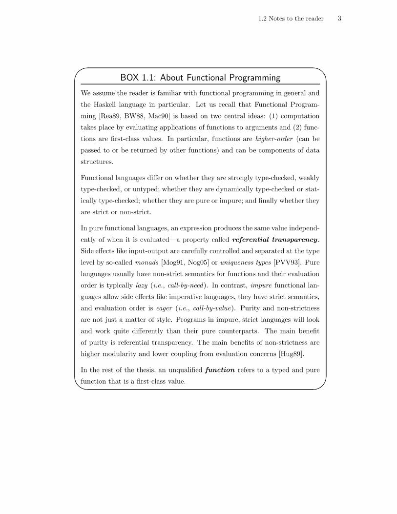
BOX 1.1: About Functional Programming
We assume the reader is familiar with functional programming in general and
the Haskell language in particular. Let us recall that Functional Program-
ming [Rea89, BW88, Mac90] is based on two central ideas: (1) computation
takes place by evaluating applications of functions to arguments and (2) func-
tions are first-class values. In particular, functions are higher-order (can be
passed to or be returned by other functions) and can be components of data
structures.
Functional languages differ on whether they are strongly type-checked, weakly
type-checked, or untyped; whether they are dynamically type-checked or stat-
ically type-checked; whether they are pure or impure; and finally whether they
are strict or non-strict.
In pure functional languages, an expression produces the same value independ-
ently of when it is evaluated—a property called referential transparency .
Side effects like input-output are carefully controlled and separated at the type
level by so-called monads [Mog91, Nog05] or uniqueness types [PVV93]. Pure
languages usually have non-strict semantics for functions and their evaluation
order is typically lazy (i.e., call-by-need). In contrast, impure functional lan-
guages allow side effects like imperative languages, they have strict semantics,
and evaluation order is eager (i.e., call-by-value). Purity and non-strictness
are not just a matter of style. Programs in impure, strict languages will look
and work quite differently than their pure counterparts. The main benefit
of purity is referential transparency. The main benefits of non-strictness are
higher modularity and lower coupling from evaluation concerns [Hug89].
In the rest of the thesis, an unqualified function refers to a typed and pure
function that is a first-class value.

1.2 Notes to the reader 4
'
&
$
%
BOX 1.2: The Haskell Language
Haskell is a strongly type-checked, pure, and non-strict functional language
which has become pretty much the de facto standard lazy language. The
reader will find information about the Haskell language in www.haskell.org.
Haskell’s syntax is sugar for a core language similar to System Fω with type
classes and nominal type equivalence. It supports rank-n polymorphism with
the help of type annotations [OL96, SP04]. (We explain what all this means
in Chapters 2 and 4.)
In Haskell, types and values are separated and its designers deliberately over-
loaded notation at both levels. Examples are expressions like (a,b) or [a]
which can be interpreted as value or type expressions. At the value level the
expressions denote, respectively, a pair of values and a singleton list value,
where the values are given by variables a and b. At the type level the ex-
pressions denote, respectively, the type of pairs with elements of type a and
elements of type b, and the type of lists with elements of type a. The over-
loading of parentheses for products and bracketing can also lead to confusion.
Since we cannot redesign Haskell, we have to stick to its actual syntax and
common conventions.

1.3 The problem in a nutshell 5
studied in more detail or that may be of better help to unacquainted readers.
1.3 The problem in a nutshell
This section explains the research problem in a nutshell. Part II of the thesis provides
all the details.
The state-of-the-art. Generic Programming is often associated with varieties of
polymorphism (parametric, subtype, etc). Structural polymorphism or polytypism is
one such variety in which programs (functions) can be obtained automatically from the
definitional structure of the types on which they work.
Equality is an archetypical example of polytypic function: it can be defined automatic-
ally for algebraic data types that lack function components (recall that function equality
is, in general, not computable [Cut80]). Some Haskell examples:
data Nat = Zero | Succ Nat
data List a = Nil | Cons a (List a)
Type Nat is the hoary type of natural numbers with its well-known value constructor
Zero and the rather rude Succ. Type List is the hoary type of lists.1 It is a parametric
type, i.e., List takes a non-parametric type through type variable a and yields the type
of lists with data of type a.
Polytypic programming is founded on the idea that the structure of a function is de-
termined by the structure of its input type. Look at Figure 1.1. The equality function
for natural numbers takes two natural-number arguments and returns a boolean value.
Because List is parametric, the equality function for lists needs the function that com-
putes equality on list elements as an extra argument. The body of equality for Nat and
List is defined by pattern-matching on the value constructors. Differing value con-
structors are unequal. Identical value constructors are equal only if their components
are all equal. The structure of the functions clearly follows the structure of the types.
Because of this, it is possible for a compiler to generate the types and bodies of equality
functions automatically. The fact that equality’s function name is overloaded is a
somewhat orthogonal, yet important, issue: the type-class mechanism employed in
resolving overloading [Blo91, WB89, Jon92, Jon95b, MJP97] has several limitations
1Admittedly, looking at its constructors the type List is really the type of stacks.

1.3 The problem in a nutshell 6
eqNat :: Nat → Nat → BooleqNat Zero Zero = TrueeqNat Zero _ = FalseeqNat _ Zero = FalseeqNat (Succ n) (Succ m) = eqNat n m
eqList :: ∀ a. (a → a → Bool) → (List a → List a → Bool)eqList eqa Nil Nil = TrueeqList eqa Nil _ = FalseeqList eqa _ Nil = FalseeqList eqa (Cons x xs) (Cons y ys) = (eqa x y) && (eqList eqa xs ys)
Figure 1.1: Equality for Nats and Lists.
which restrict the sort of types for which equality can be automatically derived.
Generic Haskell is a language extension in which programmers can define a polytypic
function (a generic template) which is used by the Generic Haskell compiler in the auto-
matic generation of instances of the polytypic function for every type in the program
(Section 6.1). Equality is one such example.
Scrap your Boilerplate combines polytypic programming and strategic programming
techniques. The Glasgow Haskell Compiler supports the necessary extensions to gen-
erate instances of special functions, called one-layer traversals, following the structure
of types. Programmers can define generic functions in terms of one-layer traversals
(Section 6.2)
Conflict with data abstraction. Functions on abstract data types cannot be ob-
tained automatically following the definitional structure of a type. For one thing, the
definitional structure (i.e., the internal representation) of an abstract type is, for main-
tainability reasons, logically hidden and, sometimes, even physically unavailable (e.g.,
precompiled libraries). Even if the representation is known, the semantic gap between
an abstract type and its representation type makes automatic generation difficult, if
not impossible. Furthermore, if it were possible it would nevertheless be impractical:
the code generated from the definitional structure of the internal representation is
rendered obsolete when the representation changes. The purpose of an abstract type
is to minimise the impact of representation changes on client code.
Let us illustrate this point with a particular example of abstract type: ordered sets

1.3 The problem in a nutshell 7
implemented as ordered lists:
data Ord a ⇒ Set a = MkSet (List a)
An equality function can be obtained from the definitional structure of the type:
eqSet :: ∀ a. Ord a ⇒ (a → a → Bool) → (Set a → Set a → Bool)
eqSet eqa (MkSet xs) (MkSet ys) = eqList eqa xs ys
However, this definition would consider MkSet [1] and MkSet [1,1] unequal sets,
which is not the case.
The ordered-set type is more restricted than the ordered-list type, i.e., it is subject
to more laws: no repetition. Consequently, its equality function has to reflect that
restriction somehow. If we change the representation from lists to binary search trees,
say, a new definition of eqSet has to be generated.
Ordinary functions on abstract types typically access the latter’s information content
via an interface of operators that enable the observation and construction of values of
the type. In this setting, equality for sets would be programmed thus:
eqSet :: ∀ a. Ord a ⇒ (a → a → Bool) → (Set a → Set a → Bool)
eqSet eqa s1 s2
| isEmpty s1 && isEmpty s2 = True
| isEmpty s1 && not (isEmpty s2) = False
| not (isEmpty s1) && isEmpty s2 = False
| otherwise = let m1 = smallest s1
m2 = smallest s2
r1 = remove m1 s1
r2 = remove m2 s2
in (eqa m1 m2) && (eqSet eqa r1 r2)
This definition uses interface operators and, therefore, is not affected by changes of
representation. The question to address is whether we can generate such definitions
following the ‘structure’ provided by an interface, and how to put it to work. This is
the topic of this thesis.

1.4 Contributions 8
1.4 Contributions
1. We provide a survey of Generic Programming in general (Chapter 4) and of Gen-
eric Haskell and Scrap your Boilerplate in particular (Chapter 6), discussing their
features, expressibility, limitations, differences, and similarities.
2. We show that polytypism conflicts with data abstraction (Chapter 7). This should
not be surprising: a function that is defined in terms of the definitional structure of
the type implementing an abstract type can wreak havoc, whether it is an ordinary
function or the instance of a polytypic function. However, it is important to drive
home the point for those lured by the ‘generic’ adjective, and there are also conflicts
specific to the nature of Generic Haskell and Scrap your Boilerplate. We also explain
why polytypic extension is an unsatisfactory solution.
3. Abstract types are often implemented in terms of type-class constrained types, i.e.,
parametric algebraic data types with some or all of their argument types constrained
by type classes (Sections 5.6 and 5.8.2). We show that Generic Haskell does not sup-
port constrained types (Section 6.1.10) and propose a solution in which polykinded
types are made context-parametric (Section 6.1.11). The proposal entails an ex-
tension to the Generic Haskell compiler, not the language. We discuss the wider
implications of constraints in abstraction in Chapter 5.
4. We provide a formal introduction to the syntax and semantics of algebraic specific-
ations with partial operators and conditional equations, which for us provide the
meaning to the word ‘abstract type’. Algebraic specifications have equational laws
which are important to us because they specify a type and, more relevantly, are
needed in our approach to polytypic programming with abstract types (Chapter 5
and Appendix A).
5. We define the concept of unbounded and bounded abstract types and explain the
conditions that both classes of types must satisfy to be functors, i.e., to have a map
function (Section 5.10).
6. Polytypic functions and their instances are defined by pattern matching, and pattern
matching conflicts with data abstraction. There are several proposals for reconciling
pattern matching with data abstraction and the first thing that comes to mind is
to investigate whether they can be of any use in reconciling polytypic programming

1.5 Structure and organisation 9
with data abstraction. We survey the most popular and promising proposals and
argue that their applicability to polytypic programming is unsatisfactory and limited
(Chapter 8).
7. We propose an extension to the Generic Haskell language for supporting polytypic
programming with abstract types. The key idea is to provide ‘definitional structure’
in terms of interfaces (algebraic specifications), not type representations. Working
with interfaces leads to a form of Extensional Programming . We show that Generic
Extensional Programming is possible (Chapter 9).
More precisely, we introduce functorial views or F -views, which specify the func-
torial structure of operator interfaces, and named signature morphisms, which spe-
cify the conformance of particular abstract types or concrete types to particular
F -views. Equational laws have to be used by the programmer when declaring sig-
nature morphisms.
Observation and construction in abstract types may not be inverses. Polytypic
functions on abstract types cannot be programmed without the help of insertion
and extraction functions from/to the abstract type to/from some concrete type. We
show that these functions can be defined polytypically, i.e., instances for particular
abstract and concrete types can be obtained automatically following the structure
of F -views and using the operators provided by signature morphisms. We show that
polytypic functions on abstract types can be defined in terms of polytypic insertion,
polytypic extraction, and ordinary polytypic functions on concrete types. We show
that polytypic extension is supported. Finally, we introduce the notion of exporting
in order to support polytypic programming with non-parametric abstract types.
1.5 Structure and organisation
This thesis is organised in three parts. Part I explains background material used by later
chapters. Part II surveys polytypic functional programming, describes the conflict with
data abstraction, and proposes a solution for reconciliation. Part III is an appendix
with technical details from Chapter 5.

1.5 Structure and organisation 10
Part I. Background
Chapter 2: Language Games introduces conceptual terminology and notational
conventions. It also contains a brief account of types and typed programming, pin-
pointing their relevance to Generic Programming. Several families of Lambda Calculi
are then overviewed which are necessary for a full understanding of Chapters 4 and 6.
The overview is not meant to be a tutorial but a brushing up. Bibliographic references
are provided in the relevant sections.
Chapter 3: Bits of Category Theory. Category Theory provides a general, ab-
stract, and uniform meta-language in which to express many ideas that have different
concrete manifestations. This chapter spells out several category-theoretical concepts
that are used in Chapters 6, 5, and 9.
Chapter 4: Generic Programming overviews the manifestations of genericity in
programming. Section 4.1 opens the chapter with a discussion on the two variants
of abstraction (control and data) and defines Generic Programming as the judicious
integration of parametrisation, instantiation and encapsulation. Section 4.2 overviews
the concept of data abstraction, which is expanded and formalised in Chapter 5. Sec-
tion 4.3 discusses the role of Generic Programming in the wider context of Software
Engineering. Section 4.4 talks briefly about the role of Generic Programming in Gen-
erative Programming and vice versa. Sections 4.5 and 4.6 discuss the importance of
typed programming in Generic Programming, a topic resumed from Chapter 2. Sec-
tion 4.7 provides a coarse classification of genericity and its different manifestations in
programming. Finally, Section 4.8 winds up discussing where the present thesis stands
in the described setting.
Chapter 5: Data Abstraction. Data abstraction corresponds with the principle
of representation independence. But what are abstract types, really? How should we
formalise them?
We believe algebraic specifications are the best route to the formalisation and under-
standing of abstract types. Algebraic specifications have several advantages beyond the
mere specification of a formal object; in particular, they provide an interface for client
code, they can be used in the formal construction and verification of client code, there
1.5 Structure and organisation 11
is a formal relation between the specification and the implementation, and prototype
implementations can be obtained automatically [LEW96, Mar98, GWM+93].
Mainstream languages do not support algebraic specifications or equational laws for
operators. However, we assume that algebraic specifications have been used in the
design and implementation of abstract types. In particular, the presence of equational
laws is important to motivate and describe our approach to Generic Programming.
The chapter starts discussing the advantages and disadvantages of data abstraction in
Sections 5.1 and 5.2 respectively, underlining the impact of parametricity constraints
on maintainability, a recurring issue whose import to Generic Programming is discussed
in Chapter 6.
Sections 5.3, 5.4, and 5.5 introduce algebraic specifications with partial operators and
conditional equations. Partial operators are those that may produce run-time errors.
They are common in strongly-typed languages that separate values from types (a simple
example is the list function head). Conditional equations are needed to cope with parti-
ality. For readability, the formal and technical details have been moved to Appendix A.
The formalism presented is first order. Our aim is to explore Generic Programming
on classic abstract types which can be described perfectly well in a first-order setting.
Higher-order functions such as catamorphisms will be written as generic programs
outside the type using the latter’s first-order operators (Chapter 9).
The chapter presents several examples of algebraic specifications that are used by sub-
sequent chapters (e.g., Chapters 7 and 9). Section 5.6 illustrates with an algebraic
specification example the problems of constrained abstract types, which were discussed
in the context of the Haskell language in Section 5.8.
The mechanisms available in Haskell and Standard ML for supporting abstract data
types are described in Section 5.8.
The chapter concludes with a classification of abstract types and their operators that
is assumed by subsequent chapters (Sections 5.9 and 5.10).

1.5 Structure and organisation 12
Part II. Functional Polytypic Programming and Data Abstraction
Chapter 6: Structural Polymorphism in Haskell examines the two most pop-
ular polytypic language extensions of Haskell: Generic Haskell [Hin00, Hin02, HJ02]
and Scrap your Boilerplate [LP03, LP04, LP05]. The latter combines polytypic and
Strategic Programming techniques [VS04, LVV02], which are also examined.
The version of Generic Haskell studied is the so-called classic one supported by the
Beryl release of the Generic Haskell compiler (version 1.23, Linux build). However, its
syntax has been sugared to fit some of the notational conventions of Chapter 2. The
differences with Dependency-style Generic Haskell [Loh04] are also outlined. We do not
go into much detail concerning Dependency-style Generic Haskell because there is an
excellent presentation [Loh04] and, more importantly, because it is based on the same
idea (structural polymorphism) as classic Generic Haskell and is therefore subject to
the same problems we study in Chapter 7.
Section 6.2 describes the Scrap your Boilerplate approach paper by paper after an initial
exposure to the ideas of Strategic Programming.
The material for this chapter has been used in several talks. It is self-contained and
follows a tutorial style. The following topics are of special interest:
• The impact of nominal versus structural type systems (Sections 6.1.3 and 6.1.4),
and the question of expressibility (Section 6.1.5). It is also not clear what the
most general polykinded type of a function is (Section 6.1.2). There are polytypic
functions that are not expressible in Generic Haskell (Section 6.1.7). Finally, we
argue in favour of parameterising polytypic functions on the cases for manifest types
(Section 6.1.12).
• Section 6.1.10 shows that Generic Haskell does not support constrained data types,
which play a major role in the implementation of abstract data types. (The reader
may want to read Sections 5.2, 5.6, 5.7, and 5.8.1 in order to put the problem in
context.) Section 6.1.11 proposes a solution based on making polykinded types para-
metric on type-class constraints. The moral of this contribution is that “polytypic
functions possess constrained-parametric polykinded types”.
1.5 Structure and organisation 13
• Polytypic function definitions are described categorially2 in Section 6.1.13. The
categorial rendition is used later in Chapter 9 to justify that it is not possible to
express polytypic functions on abstract types in the same way as on concrete types.
Chapter 7: Polytypism and Data Abstraction shows that data abstraction
limits polytypism’s genericity because polytypic functions manipulate concrete repres-
entations. The problems are outlined at the beginning of Section 7.1 and the rest of the
chapter elaborates with examples. Section 7.1.3 explains when a map function can be
programmed for an abstract type and discusses the obstacles involved in programming
it polytypically in terms of concrete representations. Section 7.2 argues that abstract-
ing over data contents is not a satisfactory way of dealing with manifest abstract types,
making the case for ‘exporting’, a mechanism to be introduced in Chapter 9. Section 7.3
summarises: buck the representations.
Chapter 8: Pattern Matching and Data Abstraction. Pattern matching is an-
other language feature that conflicts with data abstraction. There are several proposals
for reconciling pattern matching and data abstraction. This chapter overviews them
and argues that their application to reconciling polytypic programming and data ab-
straction is unsatisfactory and limited. Resistance to bucking the representations is
futile.
Chapter 9: F -views and Extensional Programming begins with an examina-
tion of some possible ways of reconciling polytypic programming with data abstraction,
and narrows down the list after analysing the pros and cons. The remaining sections
introduce and develop our proposal in detail.
Bucking the representations means programming with abstract types has to be done
through their interfaces. This leads to a form of Extensional Programming where client
functions are concerned with the data contents of a type and ignore its representation.
Some notion of structure is needed for polytypism to be possible. The clients of an ab-
stract type can provide a definition of structure in terms of F -views. Observation and
construction must be separated. Observation is performed by a polytypic extraction
function that extracts payload from an abstract type into a concrete type that con-
forms to the same F -view. Correspondingly, construction is performed by a polytypic
2Following [Gol79] we use categorial instead of categorical in order to distinguish the technical fromthe ordinary use of the adjective.

1.5 Structure and organisation 14
insertion function that inserts payload from the concrete type to the abstract type.
In Section 9.8 we demonstrate that many of the ideas can be encoded in Haskell for
particular families of abstract types. From Section 9.9, we generalise and show how
insertion and extraction can be defined polytypically: their types are polytypic on the
structure provided by an F -view and the signature morphisms are used in the gener-
ation of their bodies by a compiler. Section 9.11 shows how polytypic functions on
abstract types can be defined in terms of polytypic insertion and extraction. Sec-
tion 9.12 shows how polytypic extension or specialisation can be done in our system.
Section 9.13 introduces the idea of exporting in order to support polytypic program-
ming with manifest abstract types. Sections 9.14 and 9.15 discuss some applications of
polytypic extension.
Chapter 10: Future Work discusses future lines of research and other design
choices and the challenges they present.
Appendix
Details from Chapter 5. The appendix contains the technical details of the formal
syntax and semantics of the algebraic specification formalism of Chapter 5. Of particu-
lar importance is the concept of Σ-Algebra (Definition A.1.7) which involves the notion
of symbol-mapping. This is an important but often obviated ingredient that is also
present in the definition of signature morphisms, Σ-homomorphisms , and partiality.
Signature morphisms and F -algebras (Section A.3.1) are essential for understanding
and justifying our approach to Generic Programming (Chapter 9).
Part I
Prerequisites
15

Chapter 2
Language Games
“In order to recognise the symbol in the sign we must consider the sig-
nificant use.” Ludwig Wittgenstein. Tratactus Logico-Philosophicus,
Proposition 3.326
This chapter presents some concepts, terminology, and notational conventions used
throughout the thesis. It is not meant as an introductory exposition but as a brushing
up. Bibliographic references are provided in the relevant sections. The treatment of
Category Theory is postponed to Chapter 3.
2.1 Object versus meta
We assume familiarity with the distinction between object language , a particular
formal language under study, and meta-language , the notation used when talking
about the object language.
2.2 Definitions and equality
It is common practice in mathematics to use equality as a definitional device. Since
equality is also used as a relation on already defined entities, we distinguish equality
from definitional equality and use the symboldef= for the latter. A definition induces an
equality in the sense that if Xdef= Y then X = Y ; the converse need not be true.
In some chapters we make heavy use of inductive definitions expressed as natural de-
duction rules and rule schemas which have the following shape:
antecedent1 . . . antecedentn
consequent1 . . . consequentn
where n ≥ 0. Rules can be read forwards (when all antecedents are the case then
all the consequents are the case) or backwards (all the consequents are the case if all
the antecedents are the case). Inductive rules will be used for expressing conditional
16

2.3 Grammatical conventions 17
definitions and inference rules of formal deduction systems. Variables in antecedents
and consequents are assumed universally quantified unless indicated otherwise.
2.3 Grammatical conventions
We use EBNF notation to express the syntax of several formal languages. Non-terminals
are written in capitalised slanted. Any other symbol stands for a terminal with the
exception of the postfix meta-operators ?, +, and ∗. Their meaning is as follows: X?,
X∗, and X+ denote, respectively, zero or one X, zero or more X, and one or more X, where
X can be a terminal or non-terminal. Parentheses are also used as meta-notation for
grouping, e.g., (X Y)∗.
The following EBNF example is a snippet of C++’s grammar [Str92]:
CondOp ::= if Cond Block (else Block)?
Cond ::= ( Expression )
Block ::= Stmt | Stmt+
In the first production parentheses are meta-notation. In the second they are object-
level symbols because they are not followed by a postfix meta-operator.
2.4 Quantification
We follow the widely used and well-known ‘quantifier-dot’ convention when denoting
quantification in logical formulae. For example, in ∀x.P the scope of bound variable x
starts from the dot to the end of the expression P . Also,
∀x∈S. P abbreviates ∀x. x∈S ⇒ P
2.5 The importance of types
We deliberately use term to refer to English terms (for instance, ‘overloading’ is a
term) and to program terms. Following the convention of most strongly type-checked
programming languages, we distinguish between value-level terms and type-level terms,
called type-terms or just types. Originally types were introduced as a mechanism for
optimising storage in early programming languages like fortran [CW85, p7ff]. Types

2.5 The importance of types 18
classify syntactically well-formed terms.1 Every well-formed term is associated with
one or perhaps more type-terms. Thus, types introduce a new level of description
that is reflected grammatically and semantically. This has important repercussions on
language design:
• The classification of terms by type-terms provides a syntactic method for proving
the absence of particular classes of execution (run-time) errors, generically called
type errors. A type system is a precise specification of such a method and a type
checker a feasible and hopefully efficient implementation.
Type errors typically include incompatibility errors—which arise when operators
are applied to terms of the wrong type—and those related to enforcing abstraction,
e.g., scoping, visibility, etc. A precise definition of what constitutes a type error
is determined, amongst other factors, by the expressibility of the type language
(Box 2.1).
Type systems usually come in the guise of logical proof systems, and type checkers
in the guise of specialised proof-checking algorithms. Type systems must be able to
decidably prove or disprove propositions, here called judgements, which assert that
a well-formed term t has a particular type-term σ in a type-assignment Γ, the whole
judgement typically written as Γ ` t : σ. A type-assignment contains the type-terms
of the term’s free variables that are in scope. Terms with no free variables are called
closed terms.
Type-terms and terms are defined by means of context-free grammars, but their
association is established in a context-sensitive fashion by inference rules, usu-
ally written in natural deduction style, which establish compositional implications
between judgements. Compositionality means that the type of a term can be de-
termined from the types of its constituent subterms and associated type-assignments.
Type checking is the process of proving a judgement by deduction, i.e., of provid-
ing a derivation of the judgement from some axioms by the application of the type
inference rules.
We define some type languages and systems in Section 2.7. The following refer-
ences are excellent introductions to types and type systems in relation to program-
1This sentence is deliberately ambiguous; both interpretations are true: types classify terms syn-tactically and these terms are syntactically well-formed.

2.5 The importance of types 19
ming: [Car97, CW85, Mit96, Pie02, Pie05, Sch94].'
&
$
%
BOX 2.1: Type Soundness Can Be Deceptive
A type system comes with a definition of what constitutes a type error. A pro-
gram is well-typed if it passes the type checker. Type soundness means well-
typed programs are well-behaved, where well-behaved programs are those
that don’t crash because of a type error. A formal semantics is needed to
prove type soundness [Car97, Pie02].
Type soundness can be deceptive: a well-behaved program may still crash if the
source of the error is not included in the type system’s definition of type error.
One must be careful when spouting the old chestnut ‘well-typed programs
cannot go wrong’. In many popular type systems it is disproved at the first
counterexample—like computing the head of an empty list in languages of the
ML family or downcasting to the wrong class in C++ or Java.
• Type checking may influence term-language design; for instance, its feasibility may
restrict the permitted recursion schemes (e.g., structural, generative, polymorphic,
general, etc). In practice, the language of types is designed with a particular type-
checking algorithm in mind [CW85, p11]. However, type reconstruction,2 also known
as type inference, need not restrict the language of types, for disambiguating annota-
tions can always be given by the programmer, e.g. [OL96]
• Value-level terms are evaluated at run time; type-level terms are usually evaluated at
compile time (Box 2.2). A powerful and sophisticated language of types can become
pretty much a static (compile-time) mini-programming language, with more effort
and computation performed by the type checker. By ‘effort’ we not only mean
that type checking or type reconstruction may require substantial computation, but
that some form of compile-time ‘execution’ of type-level terms is also taking place.
How involved this execution is depends on the complexity of the type language.
(Section 2.7.4 shows a trivial example.)
Type-level computation has an impact not only on software development (i.e., being
able to widen the definition of type error and catch more correctness errors stat-
2The process of finding automatically the most general type of a term that has no type annotations.

2.5 The importance of types 20
'
&
$
%
BOX 2.2: Strong/Weak, Static/Dynamic
Static type-checking is typically distinguished from dynamic type-
checking in that programs are type checked without evaluating them, whereas
in the latter they are type checked while evaluating them. With modern lan-
guages this account of static type-checking is somewhat imprecise; we should
rather say that programs are type checked without evaluating the whole of
them.
The difference between strong and weak type-checking hinges upon the
definition of type error or, in other words, on whether the language of types
is sophisticated enough to guarantee that well-typed terms don’t crash.
Strong/Weak is orthogonal to Static/Dynamic. For instance, Lisp† is strongly
and dynamically type-checked. C is statically and weakly type-checked.
From the standpoint of program development, the advantages of strong and
static type-checking should be clear after reading the previous definitions in
a different light: dynamic type-checking puts run-time errors and type errors
at the same level. Weak type-checking is about being happy with narrower
notions of type error and passing the hot potato to the programmer. Pro-
grammers of the C era revel on their bestowed responsibility, but “the price
of freedom is hours spent hunting errors that might have been caught auto-
matically” [Pau96, p7].
In this thesis we take strong, static type-checking for granted.
†Lots of Insidious and Silly Parenthesis.

2.5 The importance of types 21
ically), but also on aspects related to Generic Programming such as the ability to
define typed language extensions within the language itself, automatic program gen-
eration, and meta-programming, e.g., [CE00, LP03, KLS04, Lau95, MS00]. Types
are also essential for Generic Programming for other reasons that not only have to
do with typed programming: they are a necessary precondition for genericity in a
typed world (Chapter 4).
• Type-level languages vary in complexity according to their term language. For
instance, Haskell has some sort of ‘prologish’ language at the type level due to
its type class mechanism [HHPW92, Blo91, Jon92]. C++ Templates are Turing-
complete: it is possible to write programs that ‘run’ at compile time [VJ03, CE00]. In
dependently-typed languages like Epigram [MM04], there is no separation between
type-terms and terms and the type checker also deals with (normalising) values of
computations. In Epigram, the semantic properties of programs are encoded in the
language directly as types, which express relationships between values and other
types—for example, one can define the type List a n, that is, the type of lists of
payload a and length n.
Of course, not all semantic properties are decidable statically, for they may depend
on dynamic information. After all, we have to run programs in order to compute;
compiling them is not enough. However, many ‘interesting’ properties can be ap-
proximated by types. To the author’s knowledge, a sort of Rice’s Theorem on type-
language expressibility has not been enunciated; the range of semantic properties
that are decidable and feasible via type approximations is still a matter of research
in type languages, the theoretical limit being the halting problem. However, it has
yet to be elucidated whether programming in that fashion is more convenient. What
is certain is that Generic Programming techniques will be essential [AMM05].
• Since types provide a conservative, static, and decidable approximation of program
semantics, they also play an important role in program specification and construc-
tion. Of course, program values are not fully understood just by looking at their
types, but the more sophisticated the type language, the more properties captured
by them. For instance, many properties of functions can be obtained from just their
types, e.g. [Wad89], and function construction can be interactively guided by type
information in languages with rich type systems, e.g. [MM04].

2.6 Denoting functions 22
• Finally, types are useful in documentation, security, efficient compilation, and op-
timisation, e.g.: [HM95, Wei02] [DDMM03, GP03]
2.6 Denoting functions
In mathematics, the application of unary function f to x is written f(x) and f ’s defin-
ition is expressed as f(x)def= E. Here E abbreviates an expression where x may occur
free. The notation generalises naturally to n-ary functions. We follow this convention
at the meta-level. For us, variables may be strings, not just characters, and therefore
notations such as fx or FX are deemed confusing. In functional languages supporting
currying, function application is denoted by whitespace, with parentheses breaking the
convention. For example, f(x), f x, and f (x) are all valid applications. Inexorably,
we follow this convention at the object-level.
2.7 Lambda Calculi
The Lambda Calculus [Chu41, Mit96, Bar84] introduces a uniform and convenient
notation for manipulating unnamed first-class functions. Initially a formal (i.e., sym-
bolic) language of untyped functions that was part of a proof system of functional
equality, it has developed into a family of systems that model different aspects of com-
putation. Typed extensions with polymorphism, recursion, built-in primitives, plus
naming and definitional facilities at value and type level make up the core languages of
functional languages [Lan66, Pie02, Mit96, Rea89]; in fact, many functional language
constructs are syntactic sugar or derived forms [Pie02, p51]. Improvements to the core
language’s operational aspects form the basis of functional language implementations.
We assume the reader is familiar with the Lambda Calculus. In the following pages
we gloss over the syntactic, context-dependent, and operational aspects of the family
of calculi that make up most of Haskell’s core language. These are necessary for a full
understanding of Chapter 4 and Chapter 6. For axiomatic and denotational semantic
aspects the reader is referred to [Mit96, Sch94, Sto77, Ten76]. We only mention in
passing that, commonly, types and functional programs are taken to be objects and
arrows in the category of Complete Partial Orders [Mit96], but such interpretation is
slightly inaccurate [DJ04]. Category Theory (Chapter 3) provides, among other things,
a uniform meta-language for talking and moving about semantic universes.

2.7 Lambda Calculi 23
2.7.1 Pure Simply Typed Lambda Calculus
Type ::= ∗ −− base type| Type → Type −− function type| (Type) −− grouping
Term ::= TermVar −− term variable| Term Term −− term application| λ TermVar : Type . Term −− term abstraction| (Term) −− grouping
Γ(x) = τ
Γ ` x : τ
Γ ` t1 : σ → τ Γ ` t2 : σ
Γ ` (t1 t2) : τ
Γ, x : σ ` t : τ
Γ ` (λx :σ . t) : σ → τ
(λx :τ . t) t′ B t[t′/x]β
t1 B t′1
t1 t2 B t′1 t2li1
t2 B t′2
x t2 B x t′2li2
t B tref
t1 B t2 t2 B t3
t1 B t3trs
Figure 2.1: The Pure Simply Typed Lambda Calculus.
Figure 2.1 shows the syntax, type rules, and operational semantics of the Pure Simply
Typed Lambda Calculus (PSTLC). There are terms carrying type annotations and for
that reason it is dubbed ‘explicitly typed’—or a la Church, who first proposed it [HS86].
The following paragraphs elaborate.
Terms and types. The PSTLC has a language of types (non terminal Type) for
expressing the types of functions inductively from a unique base or ground type ∗, and
a language of terms (non-terminal Term) which consists of variables, lambda abstrac-
tions (unnamed functions), and applications of terms to other terms.3 Variables
stand for formal parameters or yet-to-be-defined primitive values when not bound by
any λ. In a lambda abstraction λx :τ.t, the λ symbol indicates that x is a bound
3That application is denoted by whitespace is not quite deducible from the grammar alone. Inorder for the two terms to be distinguished there must be some separator token between them whichis assumed to be whitespace.

2.7 Lambda Calculi 24
variable (i.e., a formal parameter), τ is the type of x, and t abbreviates an expression
where x may occur free.
In the rest of the chapter, we stick to the meta-variable conventions shown in Table 2.2.
Table 2.1 lists the symbols whose notation at the meta-level and object level (i.e.,
Haskell) differ. An exception is the ‘has kind’ symbol (Sections 2.7.3 and 2.7.4) which
is not standard Haskell 98. (The Glasgow Haskell Compiler supports ‘has kind’, written
‘::’, but we use ‘:’ instead to differentiate kind from type signatures.)
σ, τ , . . . range over types.x, y, . . . range over term variables.t, t′, . . . range over terms.Γ ranges over type-assignments.α, β, . . . range over type variables (Section 2.7.3).κ, ν range over kinds (Section 2.7.3).
Figure 2.2: Meta-variable conventions for Lambda Calculi.
Notion Meta-level symbol Haskell symbol
Definitiondef= =
Equality = ==
‘Has type’ : ::
‘Has kind’ : :
Type variable α, β, . . . a, b, . . .Lambda abstraction λx :τ . x λx→ x
Table 2.1: Differences in notation at meta- and object level. Type annotations areprovided separately from terms in Haskell.
Types and terms are separated with the only exception that types can appear as annota-
tions in lambda abstractions. The type of a function is also called its type signature .
It describes the function’s arity, order, and the type of its arguments. The arity is
the number of arguments it takes. The order is determined from its type signature as
follows:
order(∗)def= 0
order(σ → τ)def= max ( 1 + order(σ), order(τ) )
Let τ be the type of a lambda abstraction and suppose order(τ) = n. If n = 1 then
the lambda abstraction may either return a manifest (non-function) value of type ∗ or
another lambda abstraction of order 1 as result. If n > 1, then it is a higher-order
2.7 Lambda Calculi 25
abstraction that either takes or returns a lambda abstraction of order n.
Occasionally we blur the conceptual distinction between manifest values and function
values by considering the former as nullary functions and the latter as proper func-
tions.
The fixity of a function is an independent concept. It determines the syntactical
denotation of the application of the function to its arguments. In some functional
languages, functions can be infix, prefix, postfix, mixfix, and have their precedence and
associativity defined by programmers. In the PSTLC, lambda abstractions are prefix,
application associates to the left—for example, t1 t2 t3 is parsed as (t1 t2) t3—and
consequently arrows in type signatures associate to the right—for example, ∗ → ∗ → ∗
is parsed as ∗ → (∗ → ∗).
Multiple-argument functions are represented as curried higher-order functions that
take one argument but return another function as result. For example, the term:
λx :∗ . λy :∗ → ∗ . y x
is a higher-order function that takes a manifest value x and returns a function that
takes a function y as argument and applies it to x.
Related terminology. An operator is a term whose value is a function (a precise
definition of ‘value’ is given on page 26). It also has a more specific use in relation
to abstract data types and algebra (Chapter 5). Sometimes operation is used inter-
changeably with operator. The term method has wider connotations than operation
and is used in its object-oriented sense [Bud02]. A call site is another name for an
application of an operator to an operand.
An operand is a term that plays the role of a parameter or argument . A formal
parameter or argument appears in a definition whereas an actual parameter or argu-
ment appears in an application. The following are synonyms: X is a parameter of Y
(or Y is parameterised by X), Y is indexed by X (or Y is X-indexed), Y is dependent
on X (or Y is X-dependent).
We use the word ‘type’ not only in reference to type-terms but also in reference to data
types, i.e., a concrete realisation of the type in an implementation design or actual
code. We use data structure for data of more elaborate structural complexity, usually

2.7 Lambda Calculi 26
involving not only type operators but perhaps other linguistic constructs (e.g., mod-
ules). In a purely functional setting, data-type values are immutable and persistent :
operations on values of the type produce new values. Occasionally, however, it is con-
venient to treat all these values as a “unique identity invariant under changes” [Oka98a,
p3]. This figure of speech is the persistent identity .
Type rules. The type rules listed in Figure 2.1 can be employed to check the type
of a term compositionally from the type of its subterms. The type of a term depends
on the type of its free variables. This context-dependent information is captured by a
type-assignment function Γ : TypeVar → Type which acts as a symbol table of sorts
that stores the types of free variables in scope. The operation Γ, x : τ denotes the
construction of a new type-assignment and has the following definition:
(Γ, x : τ)(y)def= if x = y then τ else Γ(y)
The type rules are rather intuitive. Notice only that Γ is enlarged in the last rule
because x may occur free in t.
Operational semantics. The call-by-name operational semantics is shown in the
last box of Figure 2.1. A reduction relation B is defined between terms. Briefly, Rule β
captures the reduction of an application of a lambda abstraction to an argument. The
free occurrences of the parameter variable are substituted (avoiding variable capture)
by the argument in the lambda abstraction’s body. This is what the operation t[t ′/x]
means, which reads “t where t′ is substituted for free x” [Bar84]. Rule li1 specifies
that an application t1 t2 can be reduced to the term t′1 t2 when t1 can be reduced
to t′1. Rule li2 specifies that reduction must proceed to the argument of an applic-
ation when the term being applied is a free variable. Together, these rules specify a
leftmost-outermost reduction order. Rules ref and trs specify that B is a reflexive
and transitive relation.
A value is a program term of central importance. Operationally, the set of values V
is a subset of the set of normal forms N , which is in turn a subset of the set of terms
T , that is, V ⊆ N ⊆ T . These sets are to be fixed by definition. A term is in normal
form if no reduction rule, other than reflexivity, is applicable to it. In the PSTLC, all
normal forms are values and they are defined by the following grammar:
NF ::= TermVar | λ TermVar : Type . Term

2.7 Lambda Calculi 27
That is: variables and lambda abstractions are normal forms, which means that func-
tion bodies are evaluated only after the function is applied to an argument. This is
reflected in the operational semantics by the deliberate omission of the following rule:
t B t′
λx :τ . t B λx :τ . t′
It can be the case in other languages that there are normal forms that are not values.
Examples are stuck terms which denote run-time errors.
Example. The following derivation proves a reduction:
(λx :∗ → ∗ . x) (λx :∗ . x) B (λx :∗ . x)β
(λx :∗ → ∗ . x) (λx :∗ . x) y B (λx :∗ . x) yli1
(λx :∗ . x) y B yβ
(λx :∗ → ∗ . x) (λx :∗ . x) y B ytrs
The following is an example reduction of a well-typed PSTLC term to its normal form.
The subterm being reduced at each reduction step is shown underlined.
(λy :∗ → ∗ . y z) ((λy :∗ → ∗ . y) (λx :∗ . x))
B ((λy :∗ → ∗ . y) (λx :∗ . x)) z
B (λx :∗ . x) z
B z
2.7.2 Adding primitive types and values.
The PSTLC is impractical as a programming language. Given a term t, its free variables
have no meanings. The PSTLC extended with various primitives has been given specific
names. In particular, the language PCF (Programming Computable Functions) is
a PSTLC extended with natural numbers, booleans, cartesian products, and fixed
points [Sto77, Mit96].
In Figure 2.3 we extend the grammar of terms and types of Figure 2.1 to include
some primitive types. The base type ∗ is now removed from the language of types.
Of particular interest are cartesian product and disjoint sum types that endow the
Extended STLC (referred to as STLC from now on) with algebraic types roughly similar
2.7 Lambda Calculi 28
to those supported by functional languages.
We only show a tiny sample of type and reduction rules for primitives, the latter called
δ-rules in the jargon, to illustrate how the extension goes. Consult [Car97, CW85,
Pie02, Mit96] for more detail. Primitive types are all manifest and therefore their order
is 0.
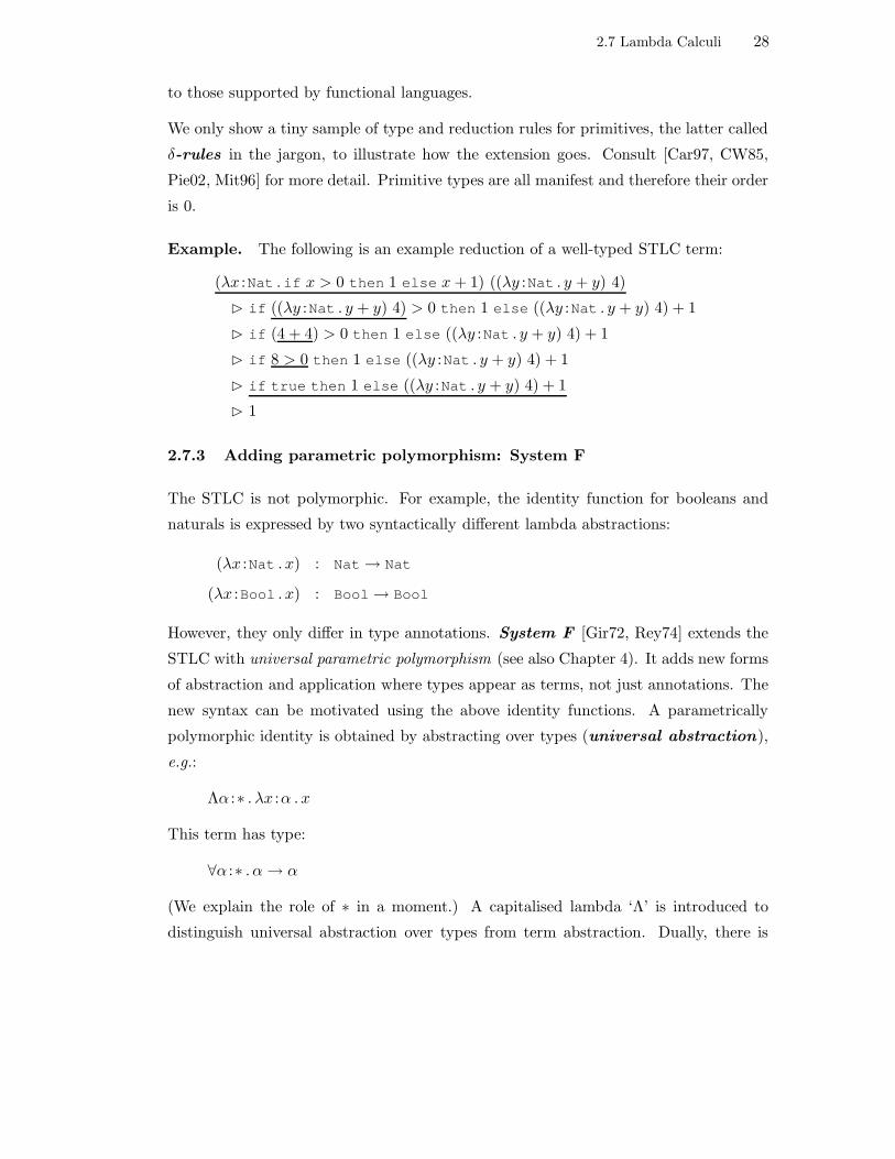
Example. The following is an example reduction of a well-typed STLC term:
(λx :Nat . if x > 0 then 1 else x + 1) ((λy :Nat . y + y) 4)
B if ((λy :Nat . y + y) 4) > 0 then 1 else ((λy :Nat . y + y) 4) + 1
B if (4 + 4) > 0 then 1 else ((λy :Nat . y + y) 4) + 1
B if 8 > 0 then 1 else ((λy :Nat . y + y) 4) + 1
B if true then 1 else ((λy :Nat . y + y) 4) + 1
B 1
2.7.3 Adding parametric polymorphism: System F
The STLC is not polymorphic. For example, the identity function for booleans and
naturals is expressed by two syntactically different lambda abstractions:
(λx :Nat . x) : Nat→ Nat
(λx :Bool . x) : Bool→ Bool
However, they only differ in type annotations. System F [Gir72, Rey74] extends the
STLC with universal parametric polymorphism (see also Chapter 4). It adds new forms
of abstraction and application where types appear as terms, not just annotations. The
new syntax can be motivated using the above identity functions. A parametrically
polymorphic identity is obtained by abstracting over types (universal abstraction),
e.g.:
Λα :∗ . λx :α . x
This term has type:
∀α :∗ . α→ α
(We explain the role of ∗ in a moment.) A capitalised lambda ‘Λ’ is introduced to
distinguish universal abstraction over types from term abstraction. Dually, there is
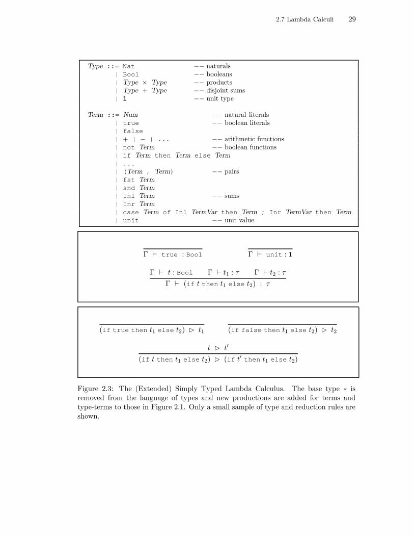
2.7 Lambda Calculi 29
Type ::= Nat −− naturals| Bool −− booleans| Type × Type −− products| Type + Type −− disjoint sums| 1 −− unit type
Term ::= Num −− natural literals| true −− boolean literals| false| + | − | ... −− arithmetic functions| not Term −− boolean functions| if Term then Term else Term
| ...| (Term , Term) −− pairs| fst Term
| snd Term
| Inl Term −− sums| Inr Term
| case Term of Inl TermVar then Term ; Inr TermVar then Term
| unit −− unit value
Γ ` true : Bool Γ ` unit : 1
Γ ` t : Bool Γ ` t1 : τ Γ ` t2 : τ
Γ ` (if t then t1 else t2) : τ
(if true then t1 else t2) B t1 (if false then t1 else t2) B t2
t B t′
(if t then t1 else t2) B (if t′ then t1 else t2)
Figure 2.3: The (Extended) Simply Typed Lambda Calculus. The base type ∗ isremoved from the language of types and new productions are added for terms andtype-terms to those in Figure 2.1. Only a small sample of type and reduction rules areshown.

2.7 Lambda Calculi 30
universal application , e.g.:
(Λα :∗ . λx :α . x) Nat B (λx :Nat . x)
A universal application is evaluated by substituting the type-term argument for the
free occurrences of the bound type-variable in the body of the universal abstraction.
Another example:
(Λβ :∗ . (Λα :∗ . λx :α . x) β) Nat B (Λα :∗ . λx :α . x) Nat
Figure 2.4 shows the additions to the grammar, to the type rules, and to the operational
semantics. Because of the introduction of type variables, rules for type-term well-
formedness are provided (a few are shown in the first row of the second box).
We reintroduce ∗ at a new level and call it a base or ground kind . Kinds classify types
and are explained in detail in Section 2.7.4; for the moment, type variables in universal
abstractions always have kind ∗, for they can only be substituted for base types which
are all manifest, but we use in advance the kind meta-variable κ because the language
of kinds is extended in Section 2.7.4. Type-assignments now also store the kinds of
type variables.
The type rules for universal abstraction and application are shown in the second row
of the second box. Notice that a type-level, capture-avoiding substitution operation is
assumed which replaces type variables for types in terms. The last box in Figure 2.4
enlarges the reduction relation to account for universal applications. Universal abstrac-
tions are normal forms like regular term abstractions.
2.7.4 Adding type operators: System Fω
System Fω extends System F with type operators, i.e., functions at the type level.
They are also called type constructors, but we prefer to use ‘constructor’ at the
value level when referring to the terms associated with type operators, called value
constructors. (For personal reasons, we deprecate the term data constructor .) An
example of type operator is List which when applied to a manifest type τ returns the
type of lists of type τ . Its associated value constructors are:
Nil :: ∀ a:∗. List a
Cons :: ∀ a:∗. a → List a → List a

2.7 Lambda Calculi 31
Kind ::= ∗
Type ::= TypeVar
| ∀ TypeVar : Kind . Type → Type
Term ::= Λ TypeVar : Kind . Term −− universal abstraction| Term Type −− universal application
Γ(α) = κ
Γ ` α : κ
Γ ` σ Γ ` τ
Γ ` σ → τ
Γ, α : κ ` σ
Γ ` ∀α :κ . σ. . .
Γ, α : κ ` t : τ
Γ ` (Λα :κ . t) : (∀α :κ . τ)
Γ ` t : (∀α :κ . τ) Γ ` σ
Γ ` t σ : τ [σ/α]
(Λα :κ . t) σ B t[σ/α]
Figure 2.4: System F extensions.

2.7 Lambda Calculi 32
which are names for primitive constants without δ-rules—e.g., a term like Cons t Nil is
in normal form, whatever the t (Section 6.1.1). Manifest types such as Nat or Bool are
‘values’ at the type level. A fully applied (i.e., closed) type operator also constitutes a
manifest type, e.g.: List Nat. Occasionally, we blur the distinction between manifest
types and type operators by considering the former as nullary type operators and
the latter as proper type operators.
To model type-level functions, the PSTLC of Figure 2.1 is lifted to the type level as
shown in the first box of Figure 2.5, so that terms such as α, λα :κ . τ , and τ σ (that is,
type variables, type-level abstractions, and type-level applications) are defined
as legal type-terms.
The kind of a type-term is somewhat inaccurately described as the ‘type’ of a type-
term. But kinds only describe the arity and order of type operators. The kind of a
nullary type operator (a manifest type) is ∗. The kind of a proper type operator is
denoted as κ→ ν, where κ is the kind of its argument and ν the kind of its result. The
order of a type operator is determined from its kind signature as follows:
order(∗)def= 0
order(κ→ ν)def= max ( 1 + order(κ), order(ν) )
Kinds do not have a status as the ‘types’ of types when there are orthogonal features
in the type language (e.g. qualified types [Jon92]) that render them inaccurate as such.
For instance, the following two Haskell definitions of the type operator List have the
same kind, but the second is constrained on the range of type arguments:
data List a = Nil | Cons a (List a)
data Ord a ⇒ List a = Nil | Cons a (List a)
Type checkers kind-check applications of type operators to arguments to make sure
the latter have the right expected kind. Kind-checking rules are shown in the second
box of Figure 2.5. The first three lines establish the kinds of manifest types and also
depict the kind-checking rules for primitive type operators such as + and ×, etc. The
last line contains the type rules of the PSTLC but lifted as kind rules (compare with
Figure 2.1).
The third box in Figure 2.5 shows a type-level reduction relation I between type-terms
that is reflexive, transitive, and compatible with all ways of constructing type-terms.

2.7 Lambda Calculi 33
Kind ::= ∗| Kind → Kind
Type ::= Type Type −− type application| λ TypeVar : Kind . Type −− type abstraction
Γ ` Nat : ∗ Γ ` Bool : ∗
Γ ` τ1 : ∗ Γ ` τ2 : ∗
Γ ` (τ1 → τ2) : ∗
Γ ` τ1 : ∗ Γ ` τ2 : ∗
Γ ` (τ1 × τ2) : ∗
Γ ` τ1 : ∗ Γ ` τ2 : ∗
Γ ` (τ1 + τ2) : ∗
Γ, α : κ ` τ : ∗
Γ ` ∀α :κ . τ : ∗
Γ(α) = κ
Γ ` α : κ
Γ ` τ1 : κ→ ν Γ ` τ2 : κ
Γ ` (τ1 τ2) : ν
Γ, α : κ ` τ : ν
Γ ` (λα :κ . τ) : κ→ ν
(λα :κ . τ) τ ′I τ [τ ′/α]
τ1 I τ ′1
τ1 τ2 I τ ′1 τ2
τ2 I τ ′2
P τ2 I P τ ′2
τ1 I τ ′1 τ2 I τ ′
2
τ1 + τ2 I τ ′1 + τ ′
2
τ1 I τ ′1 τ2 I τ ′
2
τ1 × τ2 I τ ′1 × τ ′
2
τ1 I τ ′1 τ2 I τ ′
2
τ1 → τ2 I τ ′1 → τ ′
2
τ I τ ′
∀α :κ . τ I ∀α :κ . τ ′ τ I τ
τ1 I τ2 τ2 I τ3
τ1 I τ3
τ ≡ τ
τ1 ≡ τ2
τ2 ≡ τ1
τ1 ≡ τ2 τ2 ≡ τ3
τ1 ≡ τ3
τ1 ≡ σ1 τ2 ≡ σ2
τ1 → τ2 ≡ σ1 → σ2
τ ≡ σ
∀x :κ . τ ≡ ∀x :κ . σ
τ ≡ σ
λα :κ . τ ≡ λα :κ . σ
τ1 ≡ σ1 τ2 ≡ σ2
τ1 τ2 ≡ σ1 σ2 (λα :κ . τ) τ ′ ≡ τ [τ ′/α]
Figure 2.5: System Fω adds type operators, a reduction relation (I), and an equivalencerelation (≡) on type-terms.

2.7 Lambda Calculi 34
The symbol P stands for a primitive type, i.e., Bool, Nat, or 1, which is in normal form.
The reduction relation is static: type-level applications are reduced by the type-checker
at compile time. This relation is a trivial example of type-level computation.
The last box in Figure 2.5 defines a relation of structural type equivalence which
specifies that two type-terms are equal when their structure is equal. The relation is
reflexive, symmetric, transitive, and compatible with all ways of constructing types.
Normal forms of type-terms are type variables, primitive types, type-level abstractions,
and type-terms of the form τ1 × τ2, ∀α :κ . τ1, τ1 + τ2, and τ1 → τ2, when τ1 and τ2 are
themselves in normal form.
Notice that there are three sorts of substitutions, two at the term level (one replacing
term variables for terms in term abstractions and another replacing type variables for
type-terms in universal abstractions) plus one at the type level (replacing type variables
for type-terms in type-level abstractions).
2.7.5 Adding general recursion
All the languages described so far are strongly normalising, i.e., terms and type-terms
always reduce to normal form [Pie02, Mit96]. However, in order to use System Fω
for real programming we need to introduce some form of recursion. In this section
we extend the language of terms and types to cater for general recursive functions
and type operators. In functional languages, functions (term-level or type-level) are
recursive when the function name is applied to another term within its own body.
For instance, the recursive definition of the list type and the factorial function can be
written in Haskell as follows:
data List a = Nil | Cons a (List a)
factorial n = if n==0 then 1 else n ∗ factorial(n-1)
Which can be translated to the lambda notation of System Fω as follows:
List = λa:∗. 1 + (a × (List a))
factorial = λn:Nat. if n==0 then 1 else n ∗ factorial (n-1)
But term and type lambda abstractions are unnamed; the naming mechanism above is
meta-notation. Recursion must be achieved indirectly. Let us abstract in both cases
over the name of the function to remove the recursion:

2.7 Lambda Calculi 35
List = λf:∗ → ∗. λa:∗. 1 + (a × f a)
factorial = λf:Nat→Nat. λn:Nat. if n==0 then 1 else n ∗ f (n-1)
It is typical at this point to resort to meta-level arguments or denotational semantics
to explain that the equations:
List = List List
factorial = factorial factorial
have a least solution in some semantic domain that gives meaning to System Fω syntax.
Such solution is the least fixed point of the equation. Fortunately, there is no need
to resort to meta-level arguments. Operationally, recursive functions are reduced by
unfolding their body at each recursive call. This unfolding can be carried out at the
object level by two new primitive term and type constants fix and Fix respectively.
They are called fixed-point operators because, semantically, they return the least
fixed point of their argument.4 Their type- and kind-signatures are respectively:
fix : ∀τ :κ. (τ → τ)→ τ
Fix : ∀κ. (κ→ κ)→ κ
Their type-checking and reduction rules are shown in Figure 2.6. The intuition is that
at the meta-level, the following equations must hold:
(fix f) = f (fix f)
(Fix F) = F (Fix F)
which turned into reduction rules give:
(fix f) B f (fix f)
(Fix F) I F (Fix F)
but since F and f abbreviate respectively type and term lambda abstractions, we
have:
(fix (λx :α . t)) B (λx :α . t) (fix (λx :α . t))
B t[x/(fix (λx :α . t))]
(Fix (λα :κ . τ)) I (λα :κ . τ) (Fix (λα :κ . τ))
I τ[α/(Fix (λα :κ . τ))]
4Fixed-point operators are also denoted Y and µ in the literature.
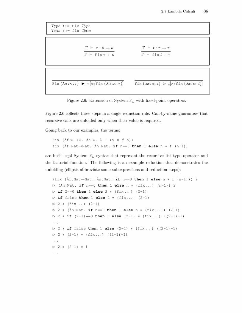
2.7 Lambda Calculi 36
Type ::= Fix Type
Term ::= fix Term
Γ ` τ : κ→ κ
Γ ` Fix τ : κ
Γ ` t : τ → τ
Γ ` fix t : τ
Fix (λα :κ . τ) I τ [α/Fix (λα :κ . τ)] fix (λx :α . t) B t[x/fix (λx :α . t)]
Figure 2.6: Extension of System Fω with fixed-point operators.
Figure 2.6 collects these steps in a single reduction rule. Call-by-name guarantees that
recursive calls are unfolded only when their value is required.
Going back to our examples, the terms:
Fix (λf:∗ → ∗. λa:∗. 1 + (a × f a))
fix (λf:Nat→Nat. λn:Nat. if n==0 then 1 else n ∗ f (n-1))
are both legal System Fω syntax that represent the recursive list type operator and
the factorial function. The following is an example reduction that demonstrates the
unfolding (ellipsis abbreviate some subexpressions and reduction steps):
(fix (λf:Nat→Nat. λn:Nat. if n==0 then 1 else n ∗ f (n-1))) 2
B (λn:Nat. if n==0 then 1 else n ∗ (fix . . . ) (n-1)) 2
B if 2==0 then 1 else 2 ∗ (fix . . . ) (2-1)
B if false then 1 else 2 ∗ (fix . . . ) (2-1)
B 2 ∗ (fix . . . ) (2-1)
B 2 ∗ (λn:Nat. if n==0 then 1 else n ∗ (fix . . . )) (2-1)
B 2 ∗ if (2-1)==0 then 1 else (2-1) ∗ (fix . . . ) ((2-1)-1)
. . .
B 2 ∗ if false then 1 else (2-1) ∗ (fix . . . ) ((2-1)-1)
B 2 ∗ (2-1) ∗ (fix . . . ) ((2-1)-1)
. . .
B 2 ∗ (2-1) ∗ 1
. . .

2.7 Lambda Calculi 37
B 2
Et Voila.

Chapter 3
Bits of Category Theory
[C]ategory theory is not specialised to a particular setting. It is a basic
conceptual and notational framework in the same sense as set theory . . .
though it deals with more abstract constructions. [Pie91, p.xi]
Category Theory is heavily used in programming language theory, especially in de-
notational semantics, algebraic specification, and program construction. The central
concepts of these disciplines are usually wielded in their categorial formulation because
Category Theory provides a general, abstract, and uniform meta-language in which to
express many ideas that have different concrete manifestations.
Abstraction is of special interest to us and certain category-theoretical concepts will be
used when talking about polytypic programs and abstract data types in Chapters 6, 5,
and 9. More precisely, the categories of particular interest to us are the category of
types and the category of algebras and partial algebras. Further references on category
theory are [SS03, Fok92, BBvv98, BW99, Pie91].
3.1 Categories and abstraction
For mathematical structures to constitute categories one needs to identify ‘entities with
structure’, called objects, and ‘structure-preserving’ mappings between them, called
arrows. Preserving structure means preserving the property of being a valid object of
the category. Due to their often graphical presentation, a collection of objects and a
collection of arrows is called a diagram . (We use the word ‘collection’ in a technical
sense: a collection is an homogeneous set.)
The axioms describing what constitutes a category are rather general and wildly dif-
ferent mathematical structures can be ‘categorised as categories’. Only arrows need
satisfy minimal requirements: there must be an arrow composition operation that is
partial, closed, associative, and has unique neutral element—the identity arrow, which
must exist for every object.
38

3.2 Direction of arrows 39
Category Theory is constructive in the sense that witnesses (arrows) are always con-
structed in terms of compositions of other arrows rather than have their existence
posited. Category Theory is coherent in the sense that such arrows must satisfy uni-
versal properties (also known as naturality properties) expressed as equations involving
universally-quantified arrows and their compositions. More precisely, many properties
of diagrams do not depend on the internal structure of the particular objects under
consideration and can be studied abstractly and independently of them. These uni-
versal properties are expressible externally, that is, purely in terms of composition of
arrows.
As a contrasting illustration, Set Theory is concerned with the internal structure of
sets and mappings. For instance, injective functions are characterised in terms of a
property held by the elements of their domain and codomain sets:
f : A→ B a ∈ A a′ ∈ A f(a) = f(a′)⇒ a = a′
f is injective
The categorial approach abstracts away from this detail and concentrates on the ex-
ternal relationships between arrows. Sets considered as objects and set-theoretic total
functions considered as arrows make up a category where arrow composition is func-
tion composition. The equivalent concept of injective function, namely, monic arrow,
is defined in terms of its properties under composition:
f : A→ B g : C → A h : C → A f g = f h ⇒ g = h
f is monic
This definition is a generalisation that applies in all categories and therefore a monic
arrow in some categories may have nothing to do with the notion of injective function
(Section 3.4).
3.2 Direction of arrows
Arrows will be written forwards, whether in type signatures or categorial diagrams.
That is, we will write f : A → B and not f : B ← A. Good reasons have been given
in favour of the latter style. In particular, the type of an applied function composition
reads swiftly from the types of the functions involved when read from right to left—i.e.,

3.2 Direction of arrows 40
in the same direction as that of the arrows—as shown in Figure 3.1(1). This is not the
case when arrows and types are read from left to right, as shown in Figure 3.1(2)(3),
for composition applies its right argument first.
g : C ← B f : B ← A
g f : C ← A(1)
g : B → C f : A→ B
g f : A→ C(2)
f : A→ B g : B → C
g f : A→ C(3)
f : A→ B g : B → C
f ; g : A→ C(4)
Figure 3.1: Arrows and composition.
Furthermore, writing the target type on the left and the source type on the right
is consistent with the normal notation for function application, where the arguments
appear to the right of the function name, i.e.: (g f) x = g (f x). “[In] the alternative,
so-called diagrammatical forms, one writes x f for application and f ; g for composition,
where x (f ; g) = (x f) g” [BdM97, p2]. Nonetheless, there are also good reasons for
writing arrows forwards:
1. It is the standard notation in mathematics and functional programming languages.
It requires practice to get used to the backwards notation and we risk confusing read-
ers unfamiliar with it. The choice is between flipping some compositions around in
order to read types naturally versus flipping all arrows in order to make composition
read naturally.
2. Only aesthetics or rigidity proscribes the use of a diagrammatical notation for com-
position alongside the normal notation for function application. There is no reason
why composition cannot be used at will both in its diagrammatical or traditional
form.
3. Only in the diagrammatical form does the type of composition itself read naturally,
as it is only there that f is the first argument:
Figure 3.1(1), : (C ← A)← (B ← A)← (C ← B)
Figure 3.1(2)(3), : (B → C)→ (A→ B)→ (A→ C)

3.3 Definition of category 41
Figure 3.1(4), ; : (A→ B)→ (B → C)→ (A→ C)
Unless, of course, one defines g f as the infix way of writing (f, g) instead of the
expected (g, f).
3.3 Definition of category
A category is identified by defining the objects, the arrows, what is composition, what
is an identity arrow, and checking that categorial axioms are satisfied.
Definition 3.3.1 A category C is a collection of objects Obj (C) and a collection of
arrows Arr(C), such that:
1. For every pair of objects A and B there might be zero or more arrows from A to
B. These arrows can be collected into a set which we denote by Arr(A,B). Notice
that Arr(C) denotes the collection of all arrows of C whereas Arr(A,B) denotes the
collection of arrows from A to B. It is common practice to write f : A → B when
f∈Arr(A,B). It is also common practice to call A the source of f and B the target
of f . Arrows have unique sources and targets. This is usually represented neatly in
a diagram:
Af - B
2. There is an arrow-composition operation (denoted by ; or by as shown in Figure 3.1)
with the following properties:
(a) It is partial: two arrows f and g compose if the target of f equals the source
of g.
(b) It is closed: the resulting arrow is in Arr(C):f : A→ B g : B → C
f ; g : A→ C
(c) It is associative:f : A→ B g : B → C h : C → D
f ; (g;h) = (f ; g);h

3.4 Example categories 42
(d) It has a left and right identity arrow for every object:
f : A→ B idA : A→ A idB : B → B
idA; f = f f ; idB = f
Identities are unique:
u; f = f ⇒ u = idA
f ;u = f ⇒ u = idB
Category Theory is an algebra of ‘typed’ arrows. By composing arrows we obtain new
arrows; but arrows with the same source and target need not be equal. It is only when
h = f ; g that we say the following diagram commutes:
Af - B
@@
@@
@h
RC
g
?
Universal properties are equations involving arrows expressible in terms of diagrams
that commute.
3.4 Example categories
Categories are named after their objects. A typical category is Set, where objects are
sets, arrows are total set-theoretic functions, and composition is function composition,
which satisfies the categorial requirements for arrow composition. Another typical
category is Pre, where objects are the members of a pre-ordered set (A,≤), arrows are
pairs (x, y) : x → y such that x∈A, y∈A, x ≤ y, and arrow composition is defined as
follows:
(x, y) : x→ y (y, z) : y → z
(x, y) ; (y, z) : x→ z (x, y) ; (y, z)def= (x, z)

3.5 Duality 43
This example shows that arrows need not be functions.
A category of particular interest to us is Type, the category of types where objects
are monomorphic types, arrows are functional programs between these types, and ar-
row composition is function composition. In Chapter 5 we introduce the category of
algebras and partial algebras, where arrows are, respectively, algebra homomorphisms
and partial homomorphisms.
3.5 Duality
For every categorial notion involving diagrams there is always a dual one in which the
direction of the arrows is reversed. If C is a category, the dual or opposite category
Cop has the same objects and arrows as C only that the direction of the arrows is
reversed:
A ∈ Obj (C)
A ∈ Obj (Cop)
f ∈ Arr(C) f : A→ B
f ∈ Arr(Cop) f : B → A
3.6 Initial and final objects
Definition 3.6.1 Given a category C, 0∈Obj (C) is an initial object iff for every
object A there is a unique arrow !A : 0 → A. Accordingly, !0 = id0. Dually, given a
category C, 1∈Obj (C) is a terminal object iff for every object A there is a unique
arrow !A : A→ 1. Accordingly, !1 = id1.
Arrows x : 1 → A from terminal objects are called constants of A [Pie91, p17]. The
motivation is that, for example, in the category of types, functional programs from the
terminal type 1 (called unit type) to any other type A can be put into one-to-one
correspondence with the values in A. In other words, there is an injective function
i : A→ (1→ A) such that if x is a value of type A then i(x) is a value of type 1→ A,
i.e., a function. For instance, given the type of natural numbers:
data Nat = Zero | Succ Nat
the nullary value constructor Zero : Nat is a constant which can be lifted to a function
Zero : 1 → Nat. We use this device for other categories in Section A.3.1.

3.7 Isomorphisms 44
3.7 Isomorphisms
Definition 3.7.1 Two objects A and B in a category are isomorphic when there are
arrows f : A → B and g : B → A whose composition is the identity. In other words,
f ; g = idA and g; f = idB .
3.8 Functors
Categories are themselves mathematical structures. Functors are maps between cat-
egories which preserve the categorial structure.
Definition 3.8.1 A functor F : C → D is an overloaded total map1 between cat-
egories C and D mapping objects to objects and arrows to arrows while preserving
composition and identities. More precisely,
F : Obj (C)→ Obj (D)
F : Arr(C)→ Arr(D)
such that:
1. ∀A∈Obj (C). F (A) ∈ Obj (D)
2. If the functor is covariant in its arrow argument then:
f ∈ Arr(C) f : A→ B
F (f) ∈ Arr(D) F (f) : F (A)→ F (B)
3. If the functor is contravariant in its arrow argument then:
f ∈ Arr(C) f : B → A
F (f) ∈ Arr(D) F (f) : F (A)→ F (B)
However, a functor is just ‘contravariant’ when f : A→ B but F (f) : F (B)→ F (A).
1Or if the reader prefers, two maps with overloaded name.

3.8 Functors 45
4. Finally, and more importantly, the functor preserves the categorial structure:
f ∈ Arr(C) g ∈ Arr(C)
F (f ; g) = F (f) ; F (g)
A ∈ Obj (C)
F (idA) = idF (A)
Figure 3.2 characterises a functor diagrammatically. If F is a functor and the diagram
in C commutes, the diagram in D also commutes.
Af - B
@@
@@
@f ; g
RC
g
?
AidA - A
F -
F (A)F (f)- F (B)
@@
@@
@F (f ; g)
RF (C)
F (g)
?
F (A)F (idA)- F (A)
Figure 3.2: A functor F diagrammatically.
For simplicity, Definition 3.8.1 defines a unary functor. Functors of any arity are defined
in terms of cartesian products of categories.
Definition 3.8.2 The product category of two categories C and D, denoted C×D,
is a category where:
Obj (C×D)def= Obj (C)×Obj (D)
Arr(C×D)def= Arr(C)×Arr(D)
such that:
f ∈ Arr(C) f : A→ C g ∈ Arr(D) g : B → D
(f, g) ∈ Arr(C×D) (f, g) : (A,B)→ (C,D)

3.9 (Co)Limits 46
The previous definition can be trivially extended to n-tuples; we talk then about n-
product categories. For instance, a binary functor (or bifunctor) is a functor from a
product category to another category, e.g., F : C×D→ E, and similarly for n-functors.
We will be mostly interested in endofunctors, that is, in functors from Cn to C, where
Cn is the n-product of C. For the sake of clarity, let us illustrate how Definition 3.8.1
is adapted for a binary covariant functor F : C2 → C:
(A,B) ∈ Obj (C2)
F (A,B) ∈ Obj (C)
(f, g) ∈ Arr(C2)
F (f, g) ∈ Arr(C)
(f, g) : (A,B)→ (C,D)
F (f, g) : F (A,B)→ F (C,D)
In the category of types, a functor F : Type → Type at the object level is a type
operator that maps types to types: if F is a type operator and A is a manifest type
then F (A) is a manifest type. At the arrow level, i.e., functional programs, F must
satisfy the following:
F (f) : F (A)→ F (B)
F (f ; g) = F (f);F (g)
F (idA) = idF (A)
Which means that at the arrow level F is the map function for the type operator. For
example, in the case of type operator List:
map f :: List a → List b
map (f ‘;‘ g) == map f ‘;‘ map g
map (id :: a → a) == (id :: List a → List a)
where f ‘;‘ g = g f. We have used explicit type annotations to illustrate the types
of each id instance.
Sections 3.9.1 and 3.10 present examples of binary functors.
3.9 (Co)Limits
A limit is a solution to a diagram, i.e., another diagram consisting of an object and a
collection of arrows that satisfies the universal property that any other solution factors
uniquely, i.e., there is a unique arrow from the other solution to the object in the limit
diagram which makes the combined diagrams commute. The colimit is the solution in

3.9 (Co)Limits 47
the dual diagram. Limits and colimits can be studied bottom-up from empty diagrams
by adding objects and arrows. In the next sections we only present (co)limits for
diagrams that are used later on.
3.9.1 (Co)Products
A (co)product is the (co)limit of a diagram involving two objects A and B and no
arrows. Following [SS03] we present both notions simultaneously. The product is an
object A×B and two arrows exl and exr. The coproduct is an object A + B and two
arrows inl and inr:
A A
exl
@@
@@
@inl
RA×B A + B
@@
@@
@
exr
R
inr
B B
such that for any other similar solution (object S with arrows f and g), there is a unique
mediating arrow from it to the product (or from the coproduct to it) that makes the
following diagrams commute:
A A
exl
f
*@
@@
@@
inlR
HHHHHHHHHHH
f
jS ................
m- A×B A + B ................
m′
- SHHHHHHHHHHH
g
j
@@
@@
@
exr
R
inr
g
*
B B
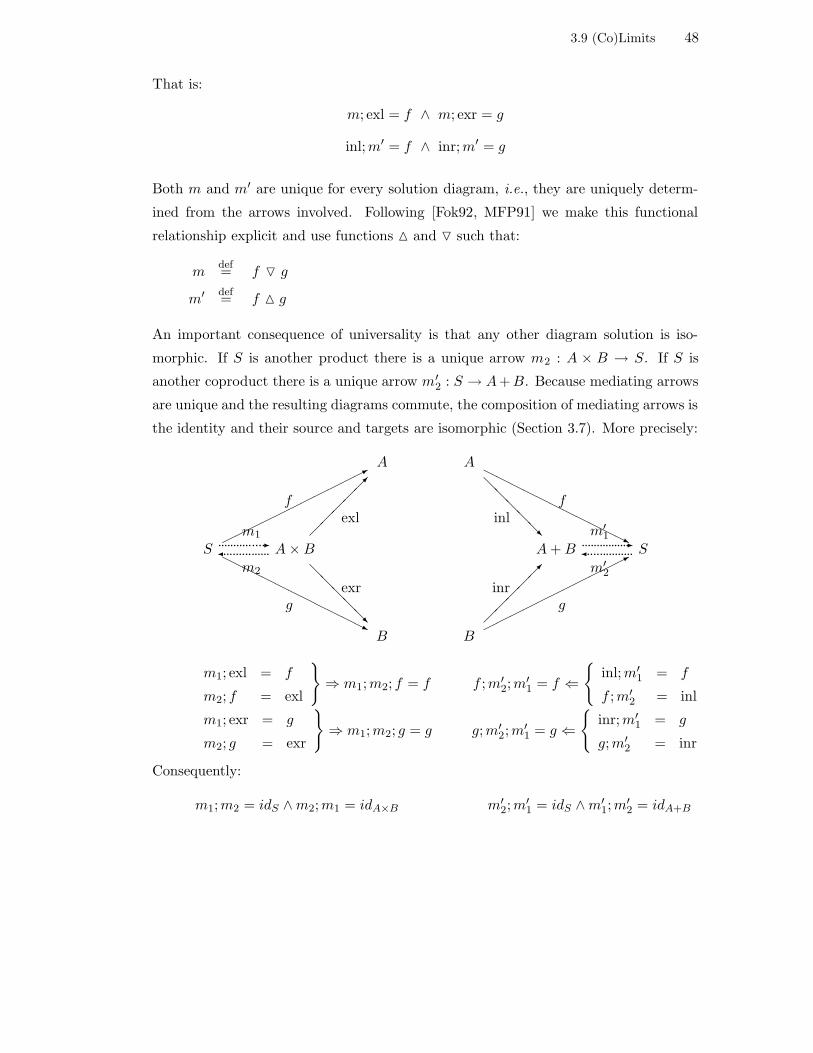
3.9 (Co)Limits 48
That is:
m; exl = f ∧ m; exr = g
inl;m′ = f ∧ inr;m′ = g
Both m and m′ are unique for every solution diagram, i.e., they are uniquely determ-
ined from the arrows involved. Following [Fok92, MFP91] we make this functional
relationship explicit and use functions M and O such that:
mdef= f O g
m′ def= f M g
An important consequence of universality is that any other diagram solution is iso-
morphic. If S is another product there is a unique arrow m2 : A × B → S. If S is
another coproduct there is a unique arrow m′2 : S → A+B. Because mediating arrows
are unique and the resulting diagrams commute, the composition of mediating arrows is
the identity and their source and targets are isomorphic (Section 3.7). More precisely:
A A
exl
f
*@
@@
@@
inlR
HHHHHHHHHHH
f
jS ...........
m1....-
.........m2
...... A×B A + B ......m′
1..........-
....m′
2
........... SHHHHHHHHHHH
g
j
@@
@@
@
exr
R
inr
g
*
B B
m1; exl = f
m2; f = exl
⇒ m1;m2; f = f f ;m′2;m
′1 = f ⇐
inl;m′1 = f
f ;m′2 = inl
m1; exr = g
m2; g = exr
⇒ m1;m2; g = g g;m′2;m
′1 = g ⇐
inr;m′1 = g
g;m′2 = inr
Consequently:
m1;m2 = idS ∧m2;m1 = idA×B m′2;m
′1 = idS ∧m′
1;m′2 = idA+B

3.9 (Co)Limits 49
3.9.2 (Co)Products and abstraction
The definition of product captures the general notion of an object that is uniquely
formed by combining two objects such that we can recover them via arrows exl and
exr irrespective of the internal structure of that composite object. For example, in the
category of sets, the categorial product is the cartesian product, which can be defined
internally in many ways:
A×Bdef= a, a, b | a∈A ∧ b∈B
A×Bdef= b, a, b | a∈A ∧ b∈B
A×Bdef= a, 0, b, 1 | a∈A ∧ b∈B
The product object is a generalisation, i.e., an abstract set with operations for construc-
tion and observation. In the category of types, A×B is an abstract type (a composite
of A and B with two selector operators) which abstracts from the internal structure
(representation) of the object.
A coproduct is a type into which we can inject two types using the two arrows. The
mediating arrow f M g provides lifted construction in products and f O g provides
lifted discrimination plus selection in coproducts as shown in Figure 3.3, where lifting
refers to the process of turning values into functions.
exl :: Prod a b → aexr :: Prod a b → bM :: (c → a) → (c → b) → (c → Prod a b)
(f M g) x = prod (f x) (g x)prod :: a → b → Prod a b
inl :: a → CoProd a binr :: b → CoProd a bO :: (a → c) → (b → c) → (CoProd a b → c)
(f O g) x = if isl x then (f asl) x else (f asr) xasl :: CoProd a b → aasr :: CoProd a b → bisl :: CoProd a b → Bool
Figure 3.3: Type Prod stands for a product type and CoProd for a coproduct type.
Notice that types Prod and CoProd are abstract, we have not provided their definition

3.9 (Co)Limits 50
in terms of concrete types. In a functional language (i.e., Haskell), binary products
and coproducts are manipulated through concrete representations introduced in type
definitions, i.e., cartesian products and disjoint sums (Figure 3.4).
type Prod a b = (a,b)data CoProd a b = Inl a | Inr b
exl = fstexr = sndinl = Inlinr = Inrisl (Inl _) = trueisl (Inr _) = falseasl (Inl x) = xasl (Inr _) = undefinedasr (Inl _) = undefinedasr (Inr y) = y
Figure 3.4: An ‘implementation’ of Figure 3.3 which describes the internal structure ofthe objects and arrows.
Binary (co)products are generalised to n-ary (co)products trivially: the (co)product is
an object and n arrows [Pie91].
Interestingly, product and coproduct construction, i.e., × and +, are both endofunctors
from C2 to C. It is standard to deviate from the prefix functor application notation
and write A×B instead of ×(A,B) and similarly for +. More precisely:
(A,B) ∈ Obj (C2)
A×B ∈ Obj (C)
(f, g) ∈ Arr(C2)
f × g ∈ Arr(C)
f : A→ C g : B → D
f × g : A×B → C ×D
In the category of types, at the arrow level × corresponds to the function:
map_Prod :: (a → c) → (b → d) → Prod a b → Prod c d
map_Prod f g = (f exl) M (g exr)
In the case of concrete tuple types (Figure 3.4), the function can be written more
familiarly:
map× :: (a → c) → (b → d) → Prod a b → Prod c d
map× f g (x,y) = (f x, g y)
Similarly, for coproducts:

3.10 Arrow functor 51
map_CoProd :: (a → c) → (b → d) → CoProd a b → CoProd c d
map_CoProd f g = (inl f) O (inr g)
map+ :: (a → c) → (b → d) → CoProd a b → CoProd c d
map+ f g (Inl x) = Inl (f x)
map+ f g (Inr y) = Inr (g y)
3.10 Arrow functor
In Section 3.3 we introduced the notation Arr(A,B) to express the collection of arrows
from A to B in a given category C. Interestingly, Arr can be understood as an endo-
functor from C2 to C. In the category of types, for any (A,B)∈Obj (Type2), Arr(A,B)
is another type: the type of functions (arrows in Type) from A to B. This functor has
the peculiar characteristic that it is contravariant on its first argument. Why this is so
becomes apparent by looking at the following diagram:
Af - C
B
h
?
g- D
?
?
At the arrow level, we cannot define Arr(f, g) : Arr(A,B)→ Arr(C,D) by composing
f and g with arrows h∈Arr(A,B) to yield an arrow in Arr(C,D). We can do it if Arr
is contravariant on its first argument:
A fC
B
h
?
g- D
f ;h; g
?

3.11 Algebra of functors 52
Definition 3.10.1 Given a category C, the arrow functor Arr : C2 → C is defined
as follows:
(A,B) ∈ Obj (C2)
Arr(A,B) ∈ Obj (C)
f : C → A g : B → D h ∈ Arr(A,B)
Arr(f, g) : Arr(A,B)→ Arr(C,D) (Arr(f, g))(h)def= f ;h; g
In the category of types, Arr(A,B) is the function space A → B. At the arrow level,
f → g can be written using more familiar Haskell notation:
map→ :: (c → a) → (b → d) → (a → b) → (c → d)
map→ f g h = g h f
3.11 Algebra of functors
Just like there is an algebra of manifest types and type operators which can be combined
to form type-terms, there is an algebra of objects and functors which can be combined
to form object expressions. The following definitions provide the machinery.
Identity functor: The identity functor Id : C→ C is defined as follows:
A ∈ Obj (C)
Id(A) ∈ Obj (C) Id(A)def= A
f ∈ Arr(C) f : A→ B
Id(f) ∈ Arr(C) Id(f)def= f
Constant functor: The constant functor KB : C → C for every object B of C is
defined as follows:
A ∈ Obj (C)
KB(A) ∈ Obj (C) KB(A)def= B
f ∈ Arr(C) f : C → D
KB(f) ∈ Arr(C) KB(f)def= idB
Polynomial functors and pointwise lifting: Objects described by object expres-
sions can be obtained from applications of the constant functor, the identity functor,
and the product and coproduct functors to other objects. For example, if A, B and C

3.11 Algebra of functors 53
are objects of C, so is A + (B × C). The object is not named but written in terms of
applications of functors to objects.
Functors can also be defined in terms of object expressions. In the previous expression
if A stands for a free variable instead of an object, the object turns into a functor
(· + (B × C)) : C → C, where we indicate by · the place were the actual parameter
would go. More commonly, functors are named in definitions:
F (X)def= X + (B × C)
(Inexplicably, Lambda Calculus notation has never caught on in Category Theory or
in maths as a whole.)
It is sometimes convenient to define F only in terms of the functors involved and not
in terms of functors and objects. To do that we define a notion of pointwise lifting
for functors.
Definition 3.11.1 Let F : C2 → C be a functor. The lifting of F , denoted F is
defined as follows:
A ∈ Obj (C) G : C→ C H : C→ C
F (G,H) : C→ C (F (G,H))(A)def= F (G(A),H(A))
With this definition at hand it is not difficult to check that F (X)def= X + (B ×C) can
be defined in terms of functors and pointwise-lifted functors:
Fdef= Id+(KB×KC)
At the object level:
F (A) = (Id +(KB×KC))(A)
= Id(A) + (KB×KC)(A)
= A + (KB(A)×KC(A))
= A + (B × C)

3.11 Algebra of functors 54
At the arrow level:
F (f) = (Id +(KB×KC))(f)
= Id(f) + (KB×KC)(f)
= f + (KB(f)×KC(f))
= f + (idB × idC)
The last expression is more commonly written in Haskell as follows for fixed types C
and B:
map+ f (map× (id :: B → B) (id :: C → C))
Pointwise lifting produces higher-order functors:
F : C2 → C
F : Func(C,C)2 → Func(C,C)
where Func(C,C) is the category of functors from C to C (yep, functors make up a
category, see Section 3.12). It is common to write Func(C,C) as C→ C, making the
‘type signature’ of F more obvious to a functional programmer:
F : (C→ C)→ (C→ C)
The final touch is provided by lifting objects to functors. An object A∈Obj (C) is lifted
to a functor A : 1→ C, where 1 is the initial category (the initial object in the category
of small categories, see Section 3.12). If we drop the notational distinction between
lifted and regular functors, objects, and lifted products, we end up in a ‘language-game’
similar to that of values and (higher-order) functions, or manifest types and (higher-
order) type operators. This facilitates the treatment of type operators as functors.
The last ingredient in this setting is the introduction of fixed points to account for
recursive equations involving functors from Cn to C. Let us state here the definition
for n = 1:
Definition 3.11.2 Let C be a category and F : C→ C a functor. A fixed point of
F is a pair (A,α) where A∈Obj (C) and α : F (A)→ A is an isomorphism.
The technical machinery needed to explain the definition in detail is beyond the scope

3.12 Natural transformations 55
of this presentation. Let us just mention that the fixed points of F form a category
and the least fixed point is the initial object. Such category is a subcategory of the
category of F -algebras, discussed in Chapter 5. The proof of existence of the initial
algebra is basically a categorial generalisation of Tarski’s fixed-point theorem [Pie91,
p61–72].
3.12 Natural transformations
Categories are themselves mathematical structures and can be taken to be objects of
another category where functors are the arrows. To avoid circular notions such as the
category of all categories (whose objects are all categories) that may lead to paradoxes
similar to Russell’s in Set Theory [Ham82], categories are classified into small and
large , where in the former objects are not categories.
It is interesting to consider whether arrows of a category are objects of another category
and what would then be the corresponding notion of arrow in this second category,
called an arrow category . Functors are maps between categories which preserve the
categorial structure. A functor category is an example of an arrow category: objects
are functors between small categories; arrows are called natural transformations.
Definition 3.12.1 Let C and D be categories. Let Func(C,D) be the category of
functors from C to D and F and G two functors (objects) of this category that have
the same variance. A natural transformation η : F→G is an arrow in Func(C,D).
(The notation → is introduced for arrows between functors.) More precisely, η is a
family of D-arrows indexed by objects of C:
η = ηX ∈ Arr(F (X), G(X)) | X ∈ Obj (C)
In words, a natural transformation η : F.→ G assigns to each object A∈Obj (C) an
arrow ηA∈Arr(F (A), G(A)). The arrows must satisfy the following coherence (or nat-
urality) property: depending on whether F and G are both covariant or contravariant,

3.12 Natural transformations 56
nA
nB
A
B
F(A)
F(B)
G(A)
G(B)
D
CG
F
. nf
F(f)
G(f)
Figure 3.5: η is a natural transformation when ηA;G(f) = F (f); ηB for every pair ofobjects A and B in C.
the squared diagrams in D commute respectively:
A F (A)ηA- G(A) F (A)
ηA- G(A)
B
f
?F (B)
F (f)
? ηB- G(B)
G(f)
?F (B)
F (f)
6
ηB- G(B)
G(f)
6
C D D
Figure 3.5 is a more illustrative depiction of the definition when F and G are both
covariant. Given A∈Obj (C), we can draw an arrow ηA from F (A) to G(A), i.e.,
between two objects in Obj (D) arising from the same object A by two different functors.
And this can be done for any object in Obj (C). Furthermore, for any other object
B∈Obj (C), there are two ways of defining an arrow from F (A) to G(B), namely,

3.12 Natural transformations 57
F (f); ηB and ηA;G(f). Both must be equal:
F (f) ; ηB = ηA ; G(f)
In the category of types, natural transformations are polymorphic functions between
type operators. For example:
flatten :: List (List a) → List a
flatten xs = foldr (++) []
is a natural transformation:
flatten : List;List.→ List
as proven by the following equation:
(map ‘;‘ map) f ‘;‘ flattenb == flattena ‘;‘ map f
where flattena and flattenb are instances of flatten at any two types a and b
respectively. The equation can be put in the general form as follows:
Fdef= List;List, which at the arrow level is map ‘;‘ map.
Gdef= List, which at the arrow level is map.
ηAdef= flattena
ηBdef= flattenb
Both sides of the equation are functions of type List (List a) → List b which are
equal. The first function maps f :: a → b over the list of list of as and then flattens
the resulting list of bs. The second function flattens the list of lists of as into a list of
as and then maps f to get a list of bs.
That functors as objects and natural transformations as arrows make up a category
is illustrated by the following diagram. The composition of natural transformations is
associative: given η : F.→ G and µ : G
.→ H, their composition η;µ : F
.→ H defined
by (η;µ)A = ηA;µA for every A∈Obj (C) is natural (i.e., the diagram commutes):
F (A)ηA- G(A)
µA- H(A)
F (B)
F (f)
?
ηB
- G(B)
G(f)
?
µB
- H(B)
H(f)
?

3.12 Natural transformations 58
The identity natural transformation ι : F.→ F is the collection of identities of the
objects in the image of F , i.e., ιA = idF (A).

Chapter 4
Generic Programming
abstraction principle: Each significant piece of functionality in a
program should be implemented in just one place in the source. Where
similar functions are carried out by distinct pieces of code, it is in general
beneficial to combine them into one by abstracting out the varying parts.
[Pie02, p339]
The notion of ‘genericity’ in programming arose independently from within different
paradigms that still exert an influence on its meaning, a meaning connoted by techno-
logical contingencies and theoretical advances. The term ‘generic’ is misused as well as
overused. One is tempted to say it is overloaded, or to take the pun further, that it is
polymorphic. It is certainly not generic.
This chapter provides an introduction to Generic Programming and aims at clarifying
some of the confusion. We begin by relating ‘generic’ to another overused term, namely,
‘abstraction’, and wind up discussing where the present thesis stands in the described
setting.
4.1 Genericity and the two uses of abstraction
Abstraction is the basic mechanism for tackling complexity and excessive detail. It
is central to the top-down or bottom-up hierarchical decomposition or imposition of
structure (a model) on a highly interconnected domain that cannot be completely
understood in isolation. The focus at a particular level of description, highlighting
what is relevant and ignoring or hiding what is irrelevant at that level, is more tellingly
dubbed information hiding .
Abstraction made its early appearance in Mathematics and Engineering in the guise of
functional abstraction where the focus is directed toward the ‘function’, purpose,
or role of components irrespective of how they work internally. It made its debut in
programming in the form of control abstraction with the advent of assembly macros
and subroutines. The first high-level programming languages pushed the notion fur-
59

4.1 Genericity and the two uses of abstraction 60
ther with the introduction of structured programming constructs (loops, conditionals,
etc.), procedures, and synchronisation mechanisms for dealing with concurrency. The
idea is summarised by the (Control) Abstraction Principle quoted at the beginning of
the chapter. Implicit in it are two important notions, namely, parametrisation and
encapsulation.1
Parametrisation is the idea of making something a parameter to something else. For
example, an expression with free variables can be abstracted into a function where the
free variables are understood to be parameters. Many definitions of Generic Program-
ming focus on parametrisation, i.e., on making programs more flexible, adaptable,
and general by “allowing a wider variety of entities as parameters than is available
in more traditional programming languages” [Gib03, p1]. Parametrisation enables a
Single Program on Multiple Data model of computation and is therefore central to code
reuse. In the last decade, code reuse has been mostly popularised and achieved through
extension, inheritance being a conspicuous example.
Encapsulation is information hiding with respect to the behaviour of components:
their interaction is fixed but their internals may change. In programming terms, the
interaction is set down in the specification (the what) of some computation or data struc-
ture and the internals are described by its implementation (the how). A consequence
of encapsulation is the interchangeability of components that satisfy the specification.
Thus, if we view our abstracted function as a black box of which we only care about
its name, type, and semantics, then we have encapsulated it. Another function of the
same type and semantics can be considered equal, irrespective of whether it calculates
its outputs in the same fashion.
Genericity is already present in the notion of parametrisation. Programs whose vary-
ing domain-specific details have been factored out as parameters2 could be considered
generic in that regard. Nonetheless, genericity has wider connotations than paramet-
risation. We provide a definition of Generic Programming in a catch-phrase:
Generic Programming = Parametrisation + Instantiation + Encapsulation
1The reader should not confuse parametrisation with parametricity . The latter has a specific mean-ing in relation to parametric polymorphism [Rey74, Wad89].
2Pedantic remark: factoring out something that can vary justifies the use of the term ‘parametervariable’ even in functional languages where variables are immutable. However, some people prefer themore neutral ‘identifier’.

4.1 Genericity and the two uses of abstraction 61
More precisely, forms of genericity can be classified according to the following criteria:
1. Which entities are parameters to which other entities at a level of description, e.g.,
level of values and types, modules, components, agents, etc. Parameterised entities
acquire a new status as a mapping or relation of sorts but they may live at the
same level as other entities, i.e., may be first-class and therefore parameters to other
entities. The higher the entity is located in the hierarchy, the more general it is (e.g.,
compare modules to functions) and the more possibilities for parametrisation and
independence on entities in levels below—not to mention the possibility of mutual
parametrisation when some of the levels are flattened (e.g., dependent types).
2. How parameters are provided to and manipulated by an entity. Parametrisation is
not necessarily a synonym of uniform behaviour (i.e., uniform semantics); the mech-
anics of instantiation are of central importance. Among other things, it plays a
role in determining whether parameterised entities are first-class or can be com-
piled separately from their instantiations (see Sections 4.5 and 4.7.1). Furthermore,
instantiation itself needs not be uniform: some parameters may be instantiated dif-
ferently than others. Finally, the number of parameters may be variable, they may
depend on each other, or be provided by default, etc.
3. Upholding encapsulation. Some researchers have characterised Generic Program-
ming as the attempt at “finding the abstract representation of efficient algorithms,
data structures, and other software concepts” so as to make them generally applic-
able, interoperable and reusable [CE00, cit. p169]. Key ideas are lifting algorithms
to a general level without loosing efficiency and expressing them with minimal as-
sumptions about data types. In other words, lifting control abstraction to a new
level of generality, usually via parametrisation, but upholding encapsulation in data
types, known as data abstraction .
Encapsulation in control abstraction is achieved by hiding the implementation of an
algorithm behind an interface (e.g., function name, type, and semantics). Encapsula-
tion in data abstraction is also achieved by hiding data types behind an interface, but
unfortunately there is some disagreement about how this should be done (Section 4.2).
At any rate, upholding data abstraction is a necessary condition for Generic Program-
ming (Chapter 7). Sometimes, the two uses of ‘abstraction’, control and data, do not

4.2 Data abstraction 62
come hand by hand. Naturally, the lack of sufficient abstraction at a level of description
makes our programs dependent on specific detail and therefore less generic.
4.2 Data abstraction
Data abstraction, i.e., functional abstraction for data, appeared later than control ab-
straction. Originally, the introduction of base data types and their operations provided
machine independent representation and manipulation of data. More complex data
structures were simulated or represented in terms of combinations of base types, struc-
tured types like arrays and records (also called type operators) and previously defined
types. But the impact of the language of types in correctness was soon to be noticed,
and part of the outcome has been a split of the world of data types into concrete data
types and abstract data types (ADTs). The motivation for this split was threefold:
1. In early computer languages, programmer-defined types were not given the same
status as base types. For instance, a programmer-defined Point represented as a
pair of integers could be manipulated by any function on pairs of integers irrespective
of whether the function maintained the properties of Point (e.g., that its values lie
within a certain range).
2. Many correctness problems, such as safety problems, arose, and still continue to
arise, because the language of types is not expressive enough to capture the semantics
of the programmer’s intended (or imagined) type. Or to replace a negative with a
positive, the representing concrete type can be too big: the ‘values’ of the intended
type are represented by a subset of the values of the representing type(s), those that
fulfil some particular criteria.
3. Software Engineering practice, in particular maintenance and evolution, dictated
the conceptual separation between intended type (specification) and representing
type (implementation). The need to minimise the repercussions of ever changing
implementations led to a solution based on encapsulation where the representing
type was hidden behind an interface.
By the mid 1970s, the notion of an abstract data type was engraved on most program-
mers’ minds, but its theoretical formalisation and its embodiment in programming lan-
guage constructs has taken long to mature, the very idea and variations on the theme

4.3 Generic Programming and Software Engineering 63
(e.g., objects) still a subject of current research [AC96, Cas97, DT88, GWM+93, Mit96,
Mar98, Pie02].
Data abstraction has been one of the contributions of Computing Science to Type
Theory in what is popularly known as the ‘formulas-as-types’ correspondence or Curry-
Howard isomorphism [CF68, How80] which identifies formulas of constructive logics
with types, and proofs with functional programs. Programmers write much larger
‘proofs’ than mathematicians. Advances in program structuring and abstract data
types took place in programming without a foundational theory; in fact, many advances
in programming have taken place independently or without any intervention of Type
Theory or otherwise. Other epitomising examples are object-oriented programming
and the serendipitous re-discovery by John Reynolds in programming of Jean-Yves
Girard’s type-theoretical System F (Section 2.7.3). This cycle of invention followed by
formalisation is not uncommon and to bring it into question is to deny reality:
type checking rules or language ideas are put forth without an underlying model
[formal type theory]. Ad hoc rules are not necessarily less desirable for the lack
of a model; it seems to us that if such rules lead to a consistent and useful
programming methodology, there probably is a satisfactory model. [DT88, p.61]
4.3 Generic Programming and Software Engineering
According to conventional wisdom, software suffers from an endemic crisis of unre-
liability, unmanageability, and unprovability. Because our imagination outstrips our
abilities [Bud02, p2], one way of tackling the crisis is, amongst others, to change the
way we channel our imaginations, i.e., to change the programming model. In this set-
ting, it is natural to expect Generic Programming to help reduce software development
and maintenance costs, as fewer programs are developed, maintained and, so much the
better, they can be re-used for varieties of data.
However, there are hardly any standardised or widely accepted software life cycles, or
development processes, or specification and design formalisms, or program construction
methodologies centred around Generic Programming or taking it into account. Excep-
tions are the minor notational extensions in UML,3 the informal ontology of concepts
and methodological aspects brought forth by the design of the C++ STL [MS96, MS94,
3www.uml.org

4.3 Generic Programming and Software Engineering 64
VJ03], and the work of the squiggol community, e.g., [BJJM99, Hoo97], which includes
polytypism and theories of concrete data types.
It is hard to determine the impact that a discipline of Generic Programming will have
on software development, and whether it will dispense with maintainability. Some
authors are skeptical about the latter:
Because each new problem typically requires a slightly different set of behaviours,
it is often difficult to design a truly useful and general-purpose software compon-
ent the first time. Rather, useful reusable software components evolve slowly over
many projects until they finally reach a stable state. [Bud02, p284]
In terms of programming languages and implementations, there is available technology,
experimental prototypes, and idioms at the level of functions and types, with a bit
less at the level of modules and libraries. So far, the most widespread success story
in Generic Programming is polymorphism in all its varieties, popular examples being
the parametric polymorphism of functional languages and the C++ STL. Hopefully,
the rest of the field will soon expand and encompass the full extent of the software
development process.
Understandability. One aspect of genericity that has an impact on development
and is usually taken for granted is understandability. The more generic a function
is, the more things it can do, supposedly the more effort required to construct it, to
understand what parameters are, in which mode they are instantiated, how they are
manipulated, etc.
Ideally, understandability must not compromise control abstraction, e.g., require know-
ledge of the generic function’s implementation or of the internal mechanics of instanti-
ation, although sometimes this is not entirely possible (Section 4.7.2).
When it comes to program proving, already in a first-order setting proofs require heavy
mathematical machinery and get complicated and lengthy for small programs, let alone
in a higher-order setting where there is the danger that some properties may be unde-
cidable.
An example of the tension between genericity and understandability is found in func-
tional languages, where programmers can capture recursion patterns as higher-order

4.3 Generic Programming and Software Engineering 65
functions which factor out specific behaviour as function parameters. However, an ex-
cessive use of the latter can make programs difficult to read, especially if these function
parameters have to circumvent the higher-order function’s behaviour for specific situ-
ations. More concretely, it is well-known that many programs can be expressed using
only the higher-order function fold [Hut99, GHA01], but programmers rarely try to
write all they can in terms of it. They had better rely on generic traversals written in
terms of combinator libraries [LV02a] or on Generic Programming libraries or language
extensions (Chapter 6).
A careful study on the balance between genericity and specificity at various levels of
description (design, component, module, function, etc.) is yet to be produced. Its study
in design patterns [GHJV95] could perhaps be a useful starting point. Design patters
are high-level specifications in which there is a mixture of genericity and specificity. Is-
sues of abstraction, parametrisation, and encapsulation appear at various levels. There
is already some work in this direction in the functional paradigm [OG05, LV02b]
Efficiency. There is also a tension between genericity and efficiency. Initially, a
generic function would seem to be less efficient than a specialised function for a given set
of parameters, if only because of the extra cost of passing and instantiating parameters
and the risk of code bloating in generative approaches.
However, the same can be said about compiled code being less efficient than handwritten
machine code or about C being ‘faster’ than Java. We don’t want to write our programs
in assembly language unless in critical situations, nor do object-oriented programming
in C. Every time there is a leap in abstraction some degree of efficiency is lost.
Indeed, programming languages are better at their job when designed to provide good
automatic support for tasks otherwise performed by the programmer. Opposition to
this trend in defense of technologically contingent notions of efficiency is striking. Had
the stigma of inefficiency not been ignored in the past we would not have procedures,
functional languages, or automatic garbage collection today. The compromise between
genericity and efficiency is, like the hoary space versus time, one of the inevitable
tradeoffs that arise in Computing Science (Box 4.1).
Standard repartees are: (1) it is the job of research in program transformation and
optimising compilers to obtain reasonable efficiency and, (2) mechanisms for supplying

4.4 Generic Programming and Generative Programming 66
'
&
$
%
BOX 4.1: Genericity vs Efficiency
“Correctness must come first. Clarity must usually come second, and efficiency
third. Any sacrifice of clarity makes the program harder to maintain, and must
be justified by a significant efficiency gain.” [Pau96, p10]
“More computing sins are committed in the name of efficiency (without ne-
cessarily achieving it) than for any other single reason—including blind stu-
pidity.” [Wul72]
efficient specialised code for critical situations can always be provided. An example of
the former can be found in [AS05] where a program transformation technique (fusion)
is enhanced for the optimisation of code generated by the Generic Haskell compiler.
An example of the latter is partial template specialisation in C++ [VJ03] and polytypic
extension in Scrap your Boilerplate (Section 6.2).
Notice the use of the expression ‘reasonable efficiency’. Admittedly, efficiency improve-
ments usually entail a loss of clarity, for the improvements on an originally inefficient
algorithm are obtained after exploiting properties of the problem that are not imme-
diate. Syntactic and semantic program transformation techniques are theoretically
limited and cannot produce fully optimal results:
Program transformations can indeed improve efficiency, but we should regard ex-
ecutable specifications with caution. . . The ideal of declarative programming
is to free us from writing programs—just state the requirements and the computer
will do the rest. Hoare [Hoa87] has explored this ideal in the case of the Greatest
Common Divisor, demonstrating that it is still a dream. A more realistic claim
for declarative programming is to make programs easier to understand. [Pau96,
p10]
The moral of the story is that machines cannot replace programmers.
4.4 Generic Programming and Generative Programming
Generic Programming represents a key implementation technique for Generative Pro-
gramming , a Software Engineering paradigm that aims at manufacturing software

4.5 Types and Generic Programming 67
components in the same ‘automated assembly line’ fashion as most goods are manu-
factured in other industries. More precisely:
Generative Programming focuses on software system families rather than one-of-
a-kind systems. Instead of building single family members from scratch, they can
all be generated based on a common generative domain model . . . that has three
components: a means of specifying family members, the implementation compon-
ents from which each member can be assembled, and the configuration knowledge
mapping between a specification of a member and a finished member. [CE00, p5]
The implementation components must be highly orthogonal, combinable, reusable, and
non-redundant. Not surprisingly, here is where Generic Programming comes into the
picture. However, the view of generic programs as implementation components for
Generative Programming does not alleviate the criticisms of Section 4.3, for even if the
system family specification is lifted to the generative domain model, the specification
and development of generic components still needs to be carried out.
In the other direction, Generative Programming techniques also provide implementa-
tion solutions to Generic Programming. Examples are program generation from gen-
eric specifications, generative compilation, and meta-programming techniques (we have
already touched upon this in Section 2.5). Generative Programming also includes the
possibility of generic program generation, where “the parameters to the [generic] pro-
gram generation process remove unnecessary options of the general model and fill in
some application-specific detail” [CE00, p209].
4.5 Types and Generic Programming
Types are influential in programming and inexorably too in Generic Programming. The
need to type check generic entities is part of the quest for richer type languages and
systems.
For instance, most of the available technology in statically type-checked languages is
based on type parametrisation. Also, in some typed languages, generic function defini-
tions are at most type-checked by the compiler; code is only generated for their applica-
tions to actual arguments. Examples are C++ Templates and Generic Haskell. In C++,
template functions are not type-checked, their instantiations are. In Generic Haskell,

4.6 Types and program generators 68
so-called polytypic functions are only type-checked by the compiler. Code is generated
for their applications. Both language extensions support separate compilation: tem-
plate instantiation is type-checked as late as link time, and applications of polytypic
functions may appear in different modules. However, the compilation of applications
requires reading the module with the definitions.
Generic Programming in untyped or dynamically type-checked languages is not entirely
a non-issue. Types are implicitly present in strongly and dynamically type-checked
languages. At run-time one gets ‘type’ errors even if types are not explicitly included
in the language. Even in untyped languages, generalising certain constructions is not
trivial and types somehow arise naturally [CW85, p3].
The definition and instantiation of generic entities must be well-typed and strong static
type-checking should not be sacrificed for the sake of genericity. For example, in many
languages arrays consist only of pointers to a chunk of memory of a fixed size. Functions
on these arrays have to be given their size as a separate parameter—the source of a
correctness problem—but they can work on arbitrary arrays. Bundling memory and
size in an abstract data type means, for most languages, that functions can only work
on arrays of particular sizes. The solution is not to sacrifice safety for genericity but to
design a language of types where genericity can be safely accommodated.
4.6 Types and program generators
Sometimes the language of types is expressive enough to allow typed generic programs
and data to be directly or indirectly defined within the language itself, or via lib-
raries or reflection. When the existing language of types is not powerful enough,
type and term language extensions are proposed which are either incorporated as part
of the language, with occasional unexpected interactions with existing features (e.g.,
C++ Templates [Str92]), or implemented using program generators (e.g., Generic
Haskell [HJ02]):
[A generator] produces ‘code’ in some language which is already implemented
[and is] used to extend the power of the base language . . . This process should
be compared with that of functional abstraction. The difference lies in [that]
manipulation is performed before the final compiling [where the semantic checks
of the whole program take place]. Macrogeneration seems to be particularly
4.7 The Generic Programming zoo 69
valuable when a semantic extension of the language is required [and the] only
alternative to trickery with macros is to rewrite the compiler—in effect, to design
a new language. . . In a more sophisticated language the need for macrogenerator
diminishes. [Str00]
Another important aspect of generic entities that may cause confusion is the relation-
ship between being first-class, typed, part of language extensions, or implemented in
terms of program generators. All these possibilities are orthogonal:
• An entity at a particular level (e.g., agents, modules, types, terms) is first-class if
it plays the role of a “value” at that level. Amongst other things, it can be a part
of other entities and a parameter or result of other entities. In a typed language, a
first-class value has a type; but having a type does not grant first-class status. (e.g.,
functions in C). Haskell modules are examples of entities that are not first-class and
don’t have types.
• Typed generic entities implemented using generators may not be first-class because
of particular design decisions regarding generator or compiler implementation, not
because of theoretical limitations. Some Draconian restrictions on C++ Templates,
like forbidding virtual member template functions, are examples of this. On the
contrary, generic functions are not first-class in Generic Haskell because their types
are parametric on attributes of actual type-operator arguments, which are not known
until instantiation (Section 6.1).
4.7 The Generic Programming zoo
Generic Programming is better characterised by a classification of its particular mani-
festations which account for the differences in the usage of the term. As discussed in
Section 4.1, genericity qualifies parametrisation by describing what are parameters, how
and when they are instantiated, and whether abstraction is upheld. The inhabitants of
the Generic Programming zoo can be classified according to this criteria.
Most general-purpose typed programming languages usually have three explicit levels
of values, types, and modules (which may contain types and values) plus two more
possible implicit or explicit levels, namely, one of kinds (Chapter 2) and another one
for checking the correct use of abstractions when they are not checked at the type

4.7 The Generic Programming zoo 70
level (e.g., Standard ML modules). In some languages abstractions are checked at the
type level (e.g., existential types, higher-order records, classes, etc). Special-purpose
languages may have other levels.
Most mainstream languages keep values and types apart, i.e., values can only be para-
meters to values or functions and similarly for types and type operators. It is natural
to explore what happens when an entity in a higher level is a parameter to an entity in
a lower level (e.g., values parameterised by types) or when the levels are interconnected
(Box 4.2). It is also natural to explore the different possibilities of instantiation.'
&
$
%
BOX 4.2: Varieties of Parametrisation
The following table lists some possibilities of parametrisation at value, type,
and kind level (adapted from [HJ02, p17]).
Instantiation
Entity Parameter Based on substitution Based on structure
Value Value Ordinary functions
Value Type Polymorphic functions Polytypic functions
Value Kind
Type Value Dependent types
Type Type Ordinary type operators Polytypic types
Type Kind Polykinded types
Kind Value Dependent kinds
Kind Type Dependent kinds
Kind Kind Kind operators Kind-indexed kind
This table does not consider binding time (Section 4.7.1). Ordinary functions
have types. Ordinary type operators have kinds. Polytypic functions have
polykinded types. Polytypic types have kind-indexed kinds.
4.7.1 Varieties of instantiation
Different varieties of instantiation can be entertained depending on how and when
actual arguments are provided.
Concerning the how, the typical method of instantiation is the substitution of the ac-

4.7 The Generic Programming zoo 71
tual argument for the formal parameter. This kind of ‘syntactical replacement’ is not
trivial to implement and is qualified by evaluation order; typically call-by-X, where X
is value, push-value, reference, need, name, etc. All these modes of evaluation assume
that function definitions are not evaluated but just optimally compiled. It is the typ-
ical method of instantiation in function and type application in classical varieties of
polymorphism and dependent types.
Instantiation could also involve some sort of examination of the argument that guides
the instantiation. This is the case in structural polymorphism, where types and func-
tions are dependent on the structure of type arguments and therefore the latter de-
termine the former’s semantics. In statically-typed languages, what is manipulated at
run-time is a value representing the type argument, if at all.
Non-uniform behaviour is possible in all these instantiation schemes (see Section 4.7.2
and Box 4.2).
Concerning the when or the binding time , instantiation can take place at compile
time (static parametrisation), at run time (dynamic parametrisation), or at
both. Static parametrisation rules out run-time variability and may complicate separate
compilation—e.g., template instantiation in C++ is sometimes deferred until link time.
At the value level, the correctness of instantiations that take place dynamically may
usually be checked statically (e.g., type checking function applications).
The notions of open world and closed world are typically used in relation to exten-
sion. Generic entities are open world if they can be extended incrementally without
recompiling already written code. However, the notions can also be used with re-
gards to instantiation and separate compilation: generic entities are open world if their
definitions can be compiled (or at least, type-checked) without their instantiations. In
other words, separate compilation is supported. ‘Openness’ refers here to the fact that
definitions are universal and not determined by how they are used.
4.7.2 Varieties of polymorphism
C++ Templates and the STL are considered examples of Generic Programming. Ada’s
instantiatable modules are actually called ‘generics’. Many of the current uses of gen-
ericity conform to what is technically known as polymorphism , a vocable derived

4.7 The Generic Programming zoo 72
Polymorphism
Universal
OverridingSubtypeSubclass
Ad hoc
Inclusion
ParametricUnbounded
Bounded
F−Bounded
PredicativeImpredicative
Type:Type
Existentials
Overloading
Dependent Types
Coercion
Dipatching:
Multiple/SingleStatic/Dynamic
Figure 4.1: Classic polymorphism with instantiation based on substitution [CW85, p4][CE00, chp. 6] [Pie02, part v] [Mit96, chp. 9].
from the Greek poly morphos, literally meaning ‘many forms’.4 Typically, an entity
(usually a value or a type) is polymorphic if it has many semantic meanings. Ex-
amples of meaning are the value denoted or the type, the latter an approximation of
the semantics.
An early but crude classification of polymorphism was proposed by Strachey [Str00]
and later improved by Cardelli and Wegner [CW85] from a types perspective; or more
precisely, from the perspective of the types of functions, for the type of a polymorphic
function specifies the nature of its polymorphism. Figure 4.7.2 depict and extends their
classification. The remainder of the section elaborates on it.
The original definition of ad-hoc polymorphism was given by Strachey [Str00, p37]:
In ad hoc polymorphism there is no systematic way of determining the type of
the result from the type of the arguments. There may be several rules of limited
extent which reduce the number of cases, but these are themselves ad hoc both
4Morphos is a Greek god who can take any form he wishes, even that of a giant carrot.

4.7 The Generic Programming zoo 73
in scope and content.
Coercion is an example of ad hoc polymorphism. Coercion is automatic or implicit
conversion . A conversion is a transformation of a value from one type to another
type. In the case of coercion, on the surface the value seemingly retains its identity
and is seen as having many types. Behind the surface the compiler inserts calls to con-
versions functions and creates new temporary values. Coercions not involving changes
of representation are called castings.
Overloading is the foremost and most powerful instance of ad hoc polymorphism. It is
basically a mechanism for symbol reuse. A function name, literal value, etc, is used with
different meanings (e.g., types) but what is actually being defined is typically a fixed
set of monomorphic values or functions that are only nominally related.5 The functions
work on different types with unrelated structure and thus have unrelated semantics.
Their use in the program is determined by a process of ‘best-match’ resolution, typically
performed at compile-time, based on the context of instantiation, which in the case of
functions is determined by the types of the actual arguments and the lexical scope.
Overloading is a very powerful feature, especially if combined with other features like
inheritance, redefinition, polyadicity, etc; but it lacks a generality that is often com-
plemented by extension or generative approaches. C++ Templates are an example
(Boxes 4.3 and 4.4).
Whether languages are explicitly or implicitly typed (i.e., require type annotations)
has an impact on the overloading scheme. In explicitly typed object-oriented languages
like Java or C++, overloaded methods may have different type signatures and different
semantics—e.g. myStack.push(), myDoor.push(), etc. In implicitly typed functional
languages of the ML family, overloading is either forbidden or has to be achieved via
type classes [Blo91, WB89, Jon92]. Type classes capture a more uniform form of
overloading that relates types by making them belong to the same type class (Box 4.5).
However, in Haskell the aforementioned push methods cannot be defined as overloaded
functions within the same scope because the type of stacks and the type of doors do
not fall naturally under the same type class. The functions can be overloaded in terms
of scope if the types are defined in different modules and the function names are always
5We are talking about stand-alone overloading. Matters change when overloading is combined withother forms of polymorphism.

4.7 The Generic Programming zoo 74
'
&
$
%
BOX 4.3: C++ Templates (Description)
C++ Templates are a language extension for static parametrisation. More
precisely, templates endow C++ with a restricted form of polymorphism in
its dependent, unbounded parametric, bounded parametric, and F -bounded
parametric variants.
The static parametrisation, the mechanics of instantiation, and the fact that
templates were designed to be backward-compatible with C++’s legacy type
system is what make templates peculiar and restricted. More precisely, tem-
plated functions and classes are compile-time macros for what after instan-
tiation are a set of overloaded functions and classes, with ‘late’ overloading
resolution performed at link time if necessary [VJ03]. This ad hoc modus op-
erandi requires clever compilation tricks and imposes restrictions on what can
be programmed. Also, features that could be present in a uniform treatment
have to be added a posteriori—e.g., member template functions and typedef
templates. Box 4.4 continues with examples.
qualified by module name. In Standard ML overloading is rather Spartan because type
reconstruction cannot disambiguate the context if type annotations are missing.6
Universal polymorphism contrasts with ad hoc polymorphism in the uniformity of
type structure and “behaviour”. Universally polymorphic entities have many types/se-
mantics, even potentially infinite ones, but can be characterised uniformly by a fixed
set of rules, and the range of variability can be expressed syntactically using the ∀
quantifier, whence the ‘universality’.
Parametric polymorphism is the kind of universal polymorphism that is often iden-
tified with Generic Programming because it relies on generic parameters to achieve
uniformity. Generic parameters are type or value parameters to other types. They are
instantiated using substitution and are reflected at the type level by the introduction
of type variables. Entities that “have many types” in reality have one unique, univer-
sally quantified type (e.g., Section 2.7.3). More power is added when type operators
6For many, type reconstruction is more a hurdle than an aid: it is rather strange to let compilersinfer specifications from implementations.

4.7 The Generic Programming zoo 75
'
&
$
%
BOX 4.4: C++ Templates (Example)
The following is a template function that swaps the values of two variables of
the same type:
template<typename T>
void swap(T& a, T& b) T temp = a; a = b; b = temp;
The template keyword instructs the compiler to treat the entity that follows
as a parameterised entity. Within the angle brackets the programmer spe-
cifies the kind of parametrisation. In this example, the parameter is a type
variable T, so ‘template<typename T>’ is similar to ‘λτ : ∗ . ’ in System F
(Section 2.7.3). A type name is either a base type or a class. Unfortunately,
there is no type annotation specifying which methods are to be implemented
by T. One has to look at the code to find out possible constraints or rely on the
compiler, which might issue the error messages at link time. In our example,
T must provide a copy constructor and operator=. There follows an example
of usage:
int x=1, y=2;
Car car1("Ford Fiesta");
Car car2("Nissan Micra");
swap(x,y);
swap(car1,car2);
Behind the scenes, the compiler generates two overloaded instances of swap
for the types to which the function is implicitly applied:†
void swap (int a, int b) int temp = a; . . .
void swap (Car& a, Car& b) Car temp = a; . . .
At each function call, the compiler figures out the implicit type parameter
by a process of type reconstruction based on the types of actual value argu-
ments. In addition to type parametrisation, template functions and classes
can be parametric on values and parameterised classes (so-called template-
templates) [VJ03].
†Generating code for each type produces code bloating .
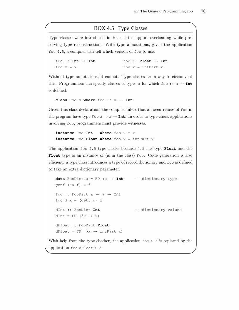
4.7 The Generic Programming zoo 76
'
&
$
%
BOX 4.5: Type Classes
Type classes were introduced in Haskell to support overloading while pre-
serving type reconstruction. With type annotations, given the application
foo 4.5, a compiler can tell which version of foo to use:
foo :: Int → Int foo :: Float → Int
foo x = x foo x = intPart x
Without type annotations, it cannot. Type classes are a way to circumvent
this. Programmers can specify classes of types a for which foo :: a → Int
is defined:
class Foo a where foo :: a → Int
Given this class declaration, the compiler infers that all occurrences of foo in
the program have type Foo a⇒ a→ Int. In order to type-check applications
involving foo, programmers must provide witnesses:
instance Foo Int where foo x = x
instance Foo Float where foo x = intPart x
The application foo 4.5 type-checks because 4.5 has type Float and the
Float type is an instance of (is in the class) Foo. Code generation is also
efficient: a type class introduces a type of record dictionary and foo is defined
to take an extra dictionary parameter:
data FooDict a = FD (a → Int) -- dictionary type
getf (FD f) = f
foo :: FooDict a → a → Int
foo d x = (getf d) x
dInt :: FooDict Int -- dictionary values
dInt = FD (λx → x)
dFloat :: FooDict Float
dFloat = FD (λx → intPart x)
With help from the type checker, the application foo 4.5 is replaced by the
application foo dFloat 4.5.

4.7 The Generic Programming zoo 77
are included as primitives or via type definitions, with type-level execution (reduction)
taking place during type checking in the form of type application (e.g., Section 2.7.4).
One common feature of parametric polymorphism is that type information plays no
computational role,i.e., no computational decision is made in terms of types and they
can be erased by the compiler after type checking. This is something to expect: mono-
morphic instances of polymorphic programs differ only in type annotations; recall
System F (Section 2.7.3). Consequently, unlike overloading, one definition suffices.
Moreover, parametrically polymorphic functions are insensitive to type arguments.
They are either too general, e.g.:
∀ a. a → a
or constant, e.g.:
∀ a. a → Int
or combinators, e.g.:
∀ ab. (a → b) → a → b
or involve type operators, e.g.:
∀ a. List a → b
These last functions are insensitive to the payload type of the type operator, or to the
shape type if the type operator is higher order (Section 6.1.1).
Types with value parameters are called dependent types. In languages supporting
dependent types, type-level reduction includes a restricted (i.e., terminating) form of
value-level reduction if type-checking is to terminate.
Different manifestations of parametric polymorphism are obtained by twiddling various
knobs like the range of the ∀, the instantiation mode, or the interplay with other features
like, say, dispatching. The range of the ∀ can be defined in terms of type universes.
The possibilities are rightly exemplified by the families of typed lambda calculi classified
under the names of predicative, impredicative, and Type:Type. By permitting values
to be types in each family we obtain new families of predicative, impredicative, or
Type:Type dependently-typed polymorphism. Most of the interesting combinations
are depicted in the so-called Lambda Cube [Pie02].

4.7 The Generic Programming zoo 78
In predicative polymorphism, universally quantified types “live” in a separate universe
from other types, a distinction captured syntactically by a separation of types into type
schemes and type-terms, the former including type-terms and universally quantified
type-terms. The foremost example of predicative polymorphism is the Hindley-Damas-
Milner or ML-style of polymorphism (also called let-polymorphism) of functional lan-
guages where type inference is efficiently decided by Milner and Damas’ W algorithm—a
straightforward exposition of W can be found in [FH88] and [PVV93].
In impredicative polymorphism, there is no distinction between type-terms and type
schemes, and parameters themselves may have universally quantified types. The fore-
most example is System F (Section 2.7.3).
In Type:Type polymorphism, the universe of types is also a type, hence the colon
notation. Type checking may not be decidable and types cannot be understood naively
as sets of values (a set of all sets leads to Russell’s paradox [Ham82]). The formalisation
of Type:Type polymorphism requires the machinery of dependent types [Car86]. It has
applications in the implementation of typed module systems, for modules contain values
but also types.
In bounded parametric polymorphism the range of the ∀ can be restricted to sub-
universes within the universe of types [CW85]. It subsumes parametric polymorphism
in the sense that ∀a.τ is ∀a∈Type.τ , where Type is the whole universe of types. The
subtype relation is an example of bound:
registrationNumber :: ∀ a≤Vehicle. a → Int
Type classes are a form of bounded parametric polymorphism where the bound is given
by a class-membership predicate instead of a subtype predicate, i.e.:
sort :: ∀ a. Ord a ⇒ [a] → [a]
is identical to:
sort :: ∀ a∈Ord. [a] →[a]
F-bounded polymorphism is a form of bounded polymorphism in which sub-universes
are parametric and, possibly, recursively defined [Mit96].
In inclusion polymorphism , there is an inclusion relation between sub-universes. It
is especially used in combination with bounded polymorphism. A well-known inclusion

4.8 Where does this work fall? 79
relation is subtyping , where the members of a type (values) are also members of a
supertype. Type classes provide a different kind of inclusion: members of a type class
(types) are also members of its superclass.
Object-oriented languages offer different combinations of polymorphism. Inheritance
(subclassing) is wrongly identified with subtyping [AC96, CW85, Cas97]. The former
is about reusing implementations whereas the latter is about reusing specifications.
Replacement, refinement, dynamic dispatching, and overriding are powerful but ortho-
gonal features [Bud02].
Universal polymorphism is ‘too generic’: functions are insensitive to the possible values
of universally-quantified type variables. Structural polymorphism or polytypism
is a form of polymorphism in which the definitional structure of a type is a parameter
to the function, which thereby does not have unique semantics. Instantiation is not
based on substitution. Polytypic functions can be typed, but their types are para-
metric on attributes of type-operator arguments. Polytypic functions are really meta-
functions that produce code from actual type arguments. Consequently, the mechanics
of instantiation must be known in order to understand how polytypic functions work.
Polytypism captures and generalises overloading and parametric polymorphism.
Polytypism is a form of compile-time reflection. At run time the type of an object can
be inspected using some library extension. At compile time that functionality must
be provided by the types themselves and, therefore, a language extension is needed.
We examine two popular polytypic language extensions to the Haskell language in
Chapter 6
4.8 Where does this work fall?
With structural polymorphism, functions are parametric on the definitional structure
of types. When types are abstract, the definitional structure is hidden. Structural
polymorphism is thus at odds with data abstraction. But in the classic varieties of
polymorphism data abstraction is an orthogonal feature. The present work investigates
what is needed to restore the order.

Chapter 5
Data Abstraction
[The] key problem in the design and implementation of large software
systems is reducing the amount of complexity or detail that must be
considered at any one time. One way to do this is via the process of
abstraction. [Gut77, p397]
The history of programming languages is a history towards higher control abstraction
and higher data abstraction. Data abstraction appeared late in Mathematics and Com-
puting (around the 1970s). Key ideas in control abstraction were already present in
the seminal papers on the theory of computable functions (1930s). The tardiness can
be explained by the fact that aspects which are in theory irrelevant can be in practice
of the utmost importance: real programs reach a size of millions of lines and each may
bring about a failure of the whole program.
When applied to data, ‘abstraction’ corresponds with the principle of representation-
independence. Abstract types are defined by a specification, not by an implementation.
Abstract types are represented or simulated in terms of concrete types using the data
definition mechanisms of programming languages. Abstract types define sets of values
but the interest shifts towards operators that ‘hide’ them; that is, abstract values
are manipulated only through operators. Constant or literal values are understood
as nullary operators. Thus, the separation between abstract types and built-in types
is artificial: the latter are abstract with respect to their machine representation; the
former are as real as a built-in type.
In the early 1970s, the notions of program module and information hiding garnered from
Software Engineering practice converged with the formalisation and understanding of
abstract types in terms of Universal Algebra and its categorial rendition. Examples of
pioneering work are [LG86, Gut77, Mor73, BG82, GTW79].
The specification of an abstract type consists of two parts: (1) A syntactic part that
defines the type’s name and operator symbols. The latter implicitly define the set
of well-formed terms that can be constructed with them. (2) A semantic part or just
80

5.1 Benefits of data abstraction 81
‘semantics’, which inexorably has to be expressed syntactically, that prescribes operator
usage and, consequently, the observable behaviour of the values of the type. Notions
of visibility, scope, and module follow as implementation mechanisms.
5.1 Benefits of data abstraction
Abstract data types (ADTs) enforce representation independence which facilitates soft-
ware evolution and maintainability. Changes to an ADT’s implementation do not affect
client code as long as the specification and the semantics of the operators remain un-
changed. The ADT’s specification is a contract or interface between the designer,
client, and implementor of the ADT. The separation of interface and implementation
allows ADTs to be provided as reusable, portable, and pre-compiled (binary) compon-
ents.
ADTs are ideal for modular design and division of work. They befit the requirements
of high cohesion, low coupling, and reasonable size. ADT interfaces gather collections
of operators and types and provide the only interconnection with client code. For lack
of standardised terminology, let us call the coupling between an ADT’s interface and
its client code interface coupling .
ADTs harmonise with the design methodology of stepwise refinement of programs and
the data they manipulate. Program actions are decomposed into smaller, yet unspe-
cified actions, and the existence of ADTs is postulated. Decisions about representation,
set of operators and their implementation are postponed. Details are discovered as the
requirements and the design are refined.
ADTs have proven their worth in software development. Extensions to the idea (e.g.,
objects) are deemed sine qua non in modern programming. Object-oriented program-
ming itself is about programming with first-class, extensible abstract types where the
notion of operator is replaced by the notion of message. Features like overriding, late
dispatching, etc, are orthogonal.
5.2 Pitfalls of data abstraction
ADTs are less flexible and make programs more verbose. For instance, C/C++ pro-
grammers revel in their cryptic pointer fiddlings and the confusion between strings and
null-terminated arrays of characters. With Java’s String, only string operators are

5.2 Pitfalls of data abstraction 82
applicable to string values; programmers have to use conversion operators and be more
explicit about what they want. Some consider this to be a pitfall; we do not.
Usually, the choice of ADT is driven by a set of desired efficient operators. However,
there is often an efficiency trade-off among them caused by the choice of representation.
A simple example is the ADT of complex numbers. There are two typical represent-
ations: cartesian and polar. Addition in the cartesian representation is more efficient
than in the polar representation whereas for multiplication it is the opposite case. Un-
fortunately, both representations cannot be used at once without losing efficiency in
the translation.
The separation between interface and implementation improves but does not resolve
completely in practice the coupling between client code and ADT implementations. An
implementation change may entail an interface change that in turn may affect already
written client code.
A typical example occurs during maintenance when operators are added, deleted, or
modified. In many cases this situation can be anticipated and cared for during the
design stage; but often it cannot, especially if the changes are elicited during the usage
of the abstract type in a live software system. This problem is intrinsic to the nature
of software: it evolves.
A thornier example of implementation decisions affecting interfaces occurs in the case
of parameterised ADTs when an implementation decision may affect the parametricity,
i.e., may impose or modify parameter constraints which in turn affect client code. As
a realistic scenario, take the case of a data-analysis application for managing numerical
data and producing statistical reports, in particular frequency analysis [Mar98, p163-
164]. A natural choice of abstract type would be a table that provides an abstract
view of the data base. Among the operators, there is an insertion operator that adds
elements to the table (increasing their frequency) and selector operators for returning
the ith element on the table or its frequency (elements can be sorted by frequency).
The efficient implementation of insertion compromises that of selection: hash tables are
more adequate for quickly storing and retrieving large volumes of data by key whereas
ordered structures such as heaps or balanced search trees are more suitable for storing
and retrieving ordered data. The constraints expressing whether the data parameter is
‘hashable’ or ordered differ but anyhow have to be stated in the type’s interface. The

5.3 Algebraic specification of data types 83
choice of implementation could conceivably change as the circumstances of the software
system’s usage change. Going for both constraints from the start may be limiting or
impossible.
There is research on automatic selection of efficient representations based on compile-
time analysis of operator usage guided by programmer annotations (see, [CH96] for a
probabilistic approach to the problem). To the author’s knowledge, there is no univer-
sally accepted way of dealing with the problem, and most specification or programming
languages either ignore it or offer their own custom-made solutions. We come back to
this problem in Section 5.6, which illustrates it with an algebraic specification example,
and in Sections 5.8.1 and 5.8.2, which discuss it in the context of the Haskell language.
In Section 6.1.11 we make Generic Haskell cope with constraints.
5.3 Algebraic specification of data types
Algebraic specifications are axiomatic formal systems for specifying ADTs precisely,
unambiguously, and independently of their implementation. They have several advant-
ages beyond the mere specification of a formal object; in particular, they provide an
interface for client code, they can be used in the formal construction and verification
of client code, there is a formal relation between the specification and the implementa-
tion [Mar98, p221-224], and prototype implementations can be obtained automatically
(e.g., [GWM+93]).
Algebraic specifications are subject to all the issues that arise in the description of
any axiomatic system: the distinction between syntax, semantics, and pragmatics; the
notions of syntactic as well as semantic consistency, soundness, and completeness, etc.
Because we cannot communicate ethereal ideas in our heads without syntax, and cer-
tainly do not want to talk about meanings too informally, endowing an axiomatic sys-
tem with meaning amounts to providing a translation or interpretation of that formal
system in terms of another formal system that is ‘hopefully’ better understood—i.e.,
squiggles to familiar squiggles. One should not get the mistaken impression that se-
mantic universes are already there, waiting to be matched syntactically. As specific-
ations get more and more sophisticated, so are semantic universes discovered (or one
should say, contrived) in order to endow the former with meaning. The reason for
bothering with a translation is non-injectivity: different syntactic entities may have

5.3 Algebraic specification of data types 84
the same semantic meaning.
The meaning of algebraic specifications is provided by the formal system of Universal
Algebra. This is why algebraic specifications are ‘algebraic’. Concretely, in this thesis
the meaning of an algebraic specification is a partial many-sorted algebra , in par-
ticular, the least or initial one. The reasons for choosing this semantic formalism are
fourfold:
1. Algebraic specifications are collections of texts whose meaning is considered simul-
taneously : the meaning of a specification depends on the meaning of the specific-
ations it imports and is therefore convenient to consider all specifications at once.
Many-sorted algebras are algebras with many carriers, i.e., sets of values. (They are
more precisely called many-valued but the terminology has not caught on.)
2. Partial algebras allow us to deal with partial operators in a natural way. Partial
operators are operators that may produce stuck terms, i.e., run-time errors. They
are common in strongly-typed languages that separate values from types. For ex-
ample, the function that returns the head of a list is a partial operator which fails
when the list is empty.
3. Classic algebraic specification formalisms have limitations on expressibility. Firstly,
the behaviour of each type is described by means of equational axioms to be satisfied
by any meaning-providing algebra. Equations form a simple specification language
but many properties cannot be expressed with equations alone. For example, the
axiom of functional extensionality requires a conditional equation:
f x = g x ⇒ f = g
Secondly, operators are first-order functions.1 Equations involving higher-order op-
erators are difficult to wield; in particular higher-order unification is in general
undecidable (not surprising, for function equality is undecidable). However, there
is no reason to worry. On the one hand, Parameterised Programming makes the
case for lifting higher-order programming from operators to specifications [Gog88].
On the other hand, there are algebraic specifications with higher-order partial op-
erators and conditional equations that are complete with respect to the class of all
extensional models [Mei95].
1For some authors, this is what ‘algebraic’ means, e.g. [Mit96, p145].

5.3 Algebraic specification of data types 85
Our specification formalism will permit conditional equations, which are essential
in specifications involving partial operators. As to the order of operators, we remain
in a first-order world. Firstly, our aim is to explore Generic Programming on classic
abstract types which can be described perfectly well in a first-order setting. Higher-
order functions such as maps or folds will be written as generic programs outside
the type using the latter’s first-order operators. Secondly, conditional equations are
important to us for purposes of specification, not deduction.
4. We want our specifications to have a unique meaning (up to isomorphism). Initiality
captures the idea of the least algebra that satisfies the specification, i.e., it does not
satisfy equations that are not syntactically provable from the axioms, and the carriers
contain values that are symbolised by at least one term (i.e., expression involving
operators). There is also another model, the final algebra , which is unique up to
isomorphism. The central notion here is bisimulation, the dual notion of congruence
in initial algebras. A bisimulation establishes an equivalence relation between terms
whose external observable behaviour is equivalent. Such information-hiding overtone
might render the impression of being a better notion of meaning for abstract types,
for the programmer is free to implement a simulation of the type so long as the
terms’ observable behaviour is the same. However, one thing is the semantics of a
specification and another its implementation, of which we care less in this thesis.
Finally, initial algebras have been studied in depth and endow specifications with
an interesting form of induction.
The following sections describe our algebraic specification formalism. For readability,
the technical details about its semantics and set-theoretic formalisation are given in
Appendix A. The formalism is presented in two stages. A basic formalism is presen-
ted first, namely, signatures, theories with equations, and initial algebra semantics.
Section 5.4 presents its syntax and semantics discursively through a few examples.
Section A.1 details its set-theoretic formalisation and algebraic semantics. Section 5.5
describes the extension of the basic formalism with partial operators and conditional
equations. Section A.2 details the semantics of the extended formalism. Section A.3
glides over the categorial rendition of algebra; in particular, Section A.3.1 introduces
the notion of F -Algebra which is essential for a full understanding of Chapter 9.
Partial algebras were first studied in [BW82] and the existence of initial models in

5.4 The basic specification formalism, by example 86
[AC89]. Ordered-sorted algebras are a generalisation that includes a notion of inclusion
(subtyping) among specifications [GM89]. The books [LEW96, Mar98] are excellent
introductions to algebraic specifications.
5.4 The basic specification formalism, by example
Our algebraic specification formalism has a syntactic part or signature and a semantic
part or theory . The syntactic part declares the name of the specification and the name
of the types defined, called sorts in the jargon. A sort is a piece of uninterpreted syntax,
a name, but it is meant to stand for something, i.e., a set of values. A signature also
lists the set of operator names and their sort-signatures which specify the arity and
sort of operator arguments and return values. Nullary operators are called constants.
Figure 5.1 shows a simple example.
signature NATsorts Natopszero : → Natsucc : Nat → Nat
end
Figure 5.1: Signature NAT.
Functional programmers express the same idea with different notation, where only
sorts, called ‘type names’ in this case, and operator names, called ‘value constructors’,
are defined explicitly:
data Nat = Zero | Succ Nat
As shown above, a signature starts with the keyword signature followed by the sig-
nature’s name (in uppercase), the keyword sorts followed by the list of (capitalised)
sort-names, and the keyword ops with the list of (lowercase) operator names and their
sort-signatures. We assume operators are all prefix and written in functional style.
An optional use clause can be included to import other specifications as shown in
Figure 5.2.
Whitespace in sort-signatures separates argument sorts. This notation is consistent
with most algebraic specification languages and has the advantage that it can be in-
terpreted either as cartesian product or as function space (currying). This last inter-

5.4 The basic specification formalism, by example 87
signature STRING signature CHARsorts String sorts Charuse CHAR opsops ch0 : → Charempty : → String . . .pre : Char String → String ch255 : → Char
end end
Figure 5.2: Signatures STRING and CHAR.
pretation conflicts with our previous assertion that operators are first-order. We make
an exception for operators that only return functions because there is an isomorphism
between the types A×B → C and A→ B → C. In some functional languages curry-
ing seems the preference and we want to keep in mind the possibility of working with
algebraic specifications in such languages, even if not currently supported.
There is clearly a shift of emphasis from values to operators: programmers specify the
permitted operators, and terms can be formed out of repeated applications of proper
operators to constants. These terms must satisfy the well-sortedness property that
every proper operator is applied to arguments of the sorts specified by its sort-signature.
The functional style is important as it conveys the notion of referential transparency :
terms are meant to stand for values of the type, and one term represents a unique value.
For example, signature NAT defines the sort Nat, which is meant to stand for the
set of natural numbers. The set of operators generates terms that can be put in
correspondence with natural numbers: zero for 0, succ zero for 1, etc. A natural
number is represented by only one NAT term.
In general specifications may contain laws, that is, relations between terms—e.g.,
equations or conditional equations—that specify the behaviour of operators. More
precisely, relations are semantic constraints: an algebra must satisfy them in order to
be a model. Figure 5.3 shows an example of an algebraic specification with laws.
The signature name has changed because we have added one operator. The semantic
part or theory embeds a signature part by preceding it with the keyword theory and the
name of the theory (in uppercase). A theory adds (1) a list of free-variable declarations
for variables appearing in the laws which are assumed universally quantified, and (2) a
list of laws (equations) which, in this example, specify the behaviour of plus.

5.4 The basic specification formalism, by example 88
theory NAT2
signature NAT2
sorts Natopszero : → Natsucc : Nat → Natplus : Nat Nat → Nat
varsx,y : Nat
lawsplus x zero = xplus x (succ y) = succ (plus x y)
end
Figure 5.3: Theory NAT2.
Equality is an equivalence relation and therefore equations introduce equivalences
among terms. Consequently, countably infinite terms may denote the same value;
for instance:
succ zero
plus zero (succ zero)
plus (succ zero) zero
plus (plus zero zero) (succ zero)
. . .
all represent the natural number 1.
The meaning of an algebraic specification is a many-sorted algebra : broadly, sets of
values, called carriers, and functions on those values, called algebraic operators,
that satisfy the laws. Many different algebras can be models of the specification,
i.e., we can make a correspondence between terms and values, and algebraic operators
satisfy all the axiomatic equations and those derivable (syntactically provable) from
them. The initial algebra approach provides a definition of the most natural model.
The carriers of an initial algebra contain values that are represented by at least one
term, i.e., there are no junk values in the algebra. And the algebraic operators only
satisfy the equations of the specification, i.e., there is no confusion between values;
in other words, the model does not satisfy extra equations between values that are not
reflected as equational axioms between terms, or as equations that can be derived from
the latter.

5.4 The basic specification formalism, by example 89
Take signature NAT, for example. We assume that it specifies the set of natural numbers.
However, we can also make a correspondence between the set of terms and the set of
integers. In this case, negative integers are not represented by any term (junk). We can
also make a correspondence with the set 0, 1, 2, where succ is interpreted as ‘addition
modulo 3’, that is, 2 + 1 = 0, but there are no laws in the specification reflecting this
property (confusion).
The following EBNF grammar describes the syntax of the specification formalism.
Non-terminals Uname, Cname, and Lname stand for upper-case identifier, capitalised
identifier, and lowercase identifier respectively:
Theory ::= theory Uname Signature Vars? Laws
Signature ::= signature Uname UseList? Param? Body
UseList ::= use Uname+
Body ::= sorts Cname+ (ops OpList)?
OpList ::= (Lname : SortSig)+
SortSig ::= Cname∗ → Cname
Vars ::= vars (Lname : Cname)+
Laws ::= (Term = Term)+
Param ::= param Cname (OpList Vars? Laws)∗
We will often drop the vars clause, for free variables are those symbols that are not
declared by other clauses and their sorts can be inferred from the context of use without
effort.
As indicated by non-terminal Param, an algebraic specification can be parametric on an-
other algebraic specification. A formal parameter is declared using the keyword param
followed by the list of capitalised sort names and the set of constraints (laws) that
must be satisfied by the parameter specification. Without constraints, the paramet-
erised specification is (unbounded-)parametrically polymorphic, and with constraints,
bounded-parametrically polymorphic (Chapter 4).
Parameterised specifications are functions on specifications and they could be higher
order, i.e., parametric specifications could take parametric specifications as parameters.
The meaning of parametric specifications can be studied directly in terms of signature
and theory morphisms [BG82, LEW96], which also describe other composition mech-
anisms such as inclusion, derivation, etc. Another possibility is to study the meaning
of actual instantiations, that is, of the specifications resulting from the instantiation of

5.5 Partial specifications with conditional equations. 90
the parameters to non-parametric (or manifest, if you will) specifications. This is the
approach we follow in Appendix A, for it is the simplest.
5.5 Partial specifications with conditional equations.
In strongly and statically type-checked languages that separate types from values, ADT
operators may be partial. Partial operators produce stuck or non-reducible terms (when
equations are directed and turned into reduction rules). Examples of partial operators
are tos and pop, which return or remove respectively the top of a stack. The following
are stuck terms:
tos emptyStack
pop emptyStack
Many people think of stuck terms as being undefined. Specification languages of yore
ignored them for that reason. However, the term ‘undefined’ is also a synonym of non-
termination, this meaning stemming from Partial Recursion Theory. A stuck term is
not the same as a non-terminating term. We can always test whether the argument
of a partial function meets a condition (i.e., whether the stack is empty) at run-time
whereas testing for non-termination is in general undecidable even at run-time.2
Partial functions introduce countably infinite stuck terms if the grammar of terms is
recursive. For example:
empty? (pop emptyStack)
push 1 (pop emptyStack)
push 2 (pop emptyStack)
. . .
Stuck terms do not stand for values in any carrier. Also, they cannot be proven equal to
any other term. They constitute junk and algebraic specifications must somehow deal
with them. A possible solution is to introduce the notion of error terms and axioms for
them which are reminiscent of the use of ⊥ in Complete Partial Orders [Sto77, Ten76].
More precisely, we add to every specification:
1. One constant operator error_s of sort s, for every s.
2This fact is what supports the idea of replacing run-time tests by static ones in richer type systems;we would not expect richer type systems to decide the halting problem.

5.5 Partial specifications with conditional equations. 91
2. An error-testing operator error_s? of sort s → Bool, for every sort s.
3. Equations for the above.
4. BOOL is imported and it has an if-then-else conditional operator.
For example, Figure 5.4 shows part of a specification of stacks.
theory STACKsignature STACKsorts Stackparam Elemuse BOOLops
emptyStack : Stackpush : Elem Stack → Stackpop : Stack → Stacktos : Stack → Elemempty? : Stack → Boolerror_Elem : Elemerror_Stack : Stackerror_Elem? : Elem → Boolerror_Stack? : Stack → Bool
lawstos error_Stack = error_Elemtos emptyStack = error_Elemtos (push x s) = if error_Elem? x then error_Elem
else if error_Stack? s then error_Elemelse x
pop empty_Stack = error_Stack. . .
Figure 5.4: STACK with error terms.
Conditionals are used for testing at the object level whether variables stand for error
terms. Specifications of this kind can be proven consistent, where each carrier of the
initial algebra has one error value [Mit96, p200]. However, they are low level and
difficult to read and write.
Partial specifications with conditional equations provide a higher-level approach that
makes specifications more readable. Partial operators are prefixed by the keyword
partial. An object-level definedness predicate DEF is introduced such that DEF (t)
abbreviates DEF (t) = true and asserts that t is defined, i.e., it is sugar for t = t.

5.6 Constraints on parametricity, reloaded 92
Laws now contain conditional equations of the form:
t1 = t′1 ∧ . . . ∧ tn = t′n ⇒ E
where n ≥ 0 and E is either an equation t = t′ or a partial equation t ' t′ which
is syntactic sugar for DEF (t) ∧ DEF (t′) ⇒ t = t′. Premises in conditional equations
represent preconditions; definedness is only an example. An empty premise (n = 0)
gives rise to an equation E. Figure 5.5 shows the partial specification of stacks.
theory STACKsignature STACKsorts Stackparam Elemuse BOOLops
partial tos : Stack → Elempartial pop : Stack → StackemptyS : Stackpush : Elem Stack → Stackempty? : Stack → Bool
lawsDEF( tos (push x s) )DEF( pop (push x s) )tos (push x s) = xpop (push x s) = sempty? emptyS = trueempty? (push x s) = false
Figure 5.5: Partial specification of stacks.
We will use syntactic sugar for boolean terms and write t instead of t=true and ¬ t
instead of t=false only in the premises of conditional equations. This sugar is used
in Figure 5.6 which shows the specification of FIFO queues.
5.6 Constraints on parametricity, reloaded
ADT implementations are driven by pragmatic concerns. In the case of parameterised
ADTs, some implementations impose constraints on payload types. We have already
touched upon this in Section 5.2. This section illustrates the problem with an algebraic
specification example.
Consider the parametric ADT of sets shown in Figure 5.7. Sets are unordered collections
without repeated elements. Typical expected operators are construction, membership

5.6 Constraints on parametricity, reloaded 93
theory FIFOsignature FIFOsorts Fifoparam Elemuse BOOLops
emptyQ : Fifoenq : Elem Fifo → FifoemptyQ? : Fifo → Boolpartial front : Fifo → Elempartial deq : Fifo → Fifo
lawsDEF( front (enq x q) )DEF( deq (enq x q) )emptyQ? emptyQ = trueemptyQ? (enq x q) = false
(emptyQ? q) ⇒ front (enq x q) = x¬ (emptyQ? q) ⇒ front (enq x q) = front q
(emptyQ? q) ⇒ deq (enq x q) = x¬ (emptyQ? q) ⇒ deq (enq x q) = enq x (deq q)
end
Figure 5.6: Specification of FIFO queues.
test, and cardinality. Other possible operators not included in the figure are union,
intersection, complement, etc.
Unconstrained sets are rather Spartan: payload elements can be put in the set and
the cardinality can be calculated. Set membership, and operators derived from it
such as union and intersection, imposes an equality constraint on payload types. The
implementation of set complement may add another constraint.
Sets can be implemented in various ways. For example, as lists without repeated
elements where insert leaves only one copy of each element in the list and card returns
the length of the list. Sets can also be implemented as lists with repeated elements
where insert inserts unrestrictedly and card skips repeated elements from the total
count. Another possible implementation is in terms of hash tables where either insert
or card skip repeated elements when dealing with collision lists. This implementation
forces a ‘hashable’ constraint on the payload type. Sets can be implemented in terms of
boolean dynamic vectors. In this case payload elements must be indexable, i.e., there
must exist an injective function indexOf : Elem → Nat. The application insert x
sets the position indexOf x in the vector to True.

5.7 Concrete types are bigger 94
theory SETsignature SETsorts Setparam Elem
use BOOLops
equal : Elem Elem → Boollaws
equal x x = trueequal x y = true ⇒ equal y x = trueequal x y = true ∧ equal y z = true ⇒ equal x z = true
use BOOL NATopsemptySet : SetemptySet? : Set → Boolinsert : Elem Set → Setmember? : Elem Set → Boolcard : Set → Nat
lawsemptySet? emptySet = trueemptySet? (insert x s) = Falseinsert x (insert x s) = insert x sinsert x (insert y s) = insert y (insert x s)member? x emptySet = Falsemember? x (insert y s) = equal x y or member? x scard emptySet = Zerocard (insert x s)
= plus (card s) (if member? x s then Zero else Succ Zero)
Figure 5.7: A possible specification of Sets.
5.7 Concrete types are bigger
Concrete types are bigger than abstract types. The reason for this lies partly in the
context-free nature of the language of concrete types. Context-dependent properties
such as repetition or equality of payload elements are not captured by type definitions.
ADTs impose context-dependent constraints on concrete types indirectly by means of
equational laws and payload constraints.
Let’s look at the problem from another angle. Consider the concrete type:
data Ord a ⇒ Tree a = Empty | Node a (Tree a) (Tree a)
This type can be used in the implementation of different abstract types: binary search
trees, priority queues, ordered sets, ordered bags, etc. In each case, the operators

5.8 Embodiments in functional languages 95
available and their laws are different: the maximum element in the left subtree of
a non-empty binary search tree is at most the root, whereas in a priority queue the
ordering in the tree could be different, with smaller values to the right of the root.
Binary search trees, priority queues and bags may contain repeated elements; that
is not the case for ordered sets. In a priority queue there is the choice of inserting
elements with same priority in FIFO fashion or via some collision-resolution function,
etc. Elements are removed from a fixed position (e.g. the front) in a priority queue. For
sets, bags, and binary search trees, the element to remove must be indicated explicitly,
e.g.:
remove : Elem → Set → Set
It is a mistake to think that Tree is the ‘natural’ representation type of any ADT. We
have already touched upon this in Chapter 1. This is the reason why ADTs are encap-
sulated behind an interface of operators that maintain the implementation invariants
of the representation type.
5.8 Embodiments in functional languages
Mainstream functional languages, notably Haskell and SML, are not concerned with
algebraic specifications of data types in any fashion. The following two sections describe
the mechanisms available in Haskell and SML for defining ADTs.
5.8.1 ADTs in Haskell
Haskell supports ADTs poorly, relying on a module concept not dissimilar to C++’s
name-spaces [Str92]. A module is a logical entity that does not necessarily correspond
to a program file, but this is usually the case. Modules are linguistic constructs for
controlling name scope and visibility. They are not first-class entities. ADTs are imple-
mented using modules by means of exporting (making public) type and operator names
while hiding value constructors and operator implementations. There are mechanisms
for controlling the way data and operators are imported such as local or qualified im-
ports and transitivity—e.g., if M imports M’ and M’ imports type A, M cannot see A
unless explicitly imported.
The Set ADT shown in Figure 5.7 can be conveyed to Haskell as shown below. In this
example there is no separation between specification (only syntax) and implementa-

5.8 Embodiments in functional languages 96
tion:
module Set (Set,emptySet,insert,member,card) where
data Eq a ⇒ Set a = MkSet [a]
emptySet :: Eq a ⇒ Set a
emptySet = MkSet []
insert :: Eq a ⇒ a → Set a → Set a
insert x (s@(MkSet l)) = if elem x l then s else MkSet (x:l)
. . .
The module name Set is followed by a parenthesised list in the heading which declares
the exported names. The type name Set is exported but not its value constructor
MkSet. (The overloading of module and type-operator name is legal.) The constraint
on the payload type is not shown in the export clause but must be figured out by looking
at the type definition. It must be included also in the type signatures of operators.
(Changing the implementation to boolean vectors would impose a different type-class
constraint which would affect client code—Section 5.8.2).
Type classes can be employed to separate specification from implementation as shown
in Figure 5.8.
module Set (Set(..)) whereclass Set s whereemptySet :: Eq a ⇒ s ainsert :: Eq a ⇒ a → s a → s a. . .
module Set’ (Set’) whereimport Setdata Eq a ⇒ Set’ a = MkSet [a]
instance Set Set’ whereemptySet = MkSet []insert x (s@(MkSet l)) = if elem x l then s else MkSet (x:l). . .
Figure 5.8: ADTs in Haskell using type classes.
In the first module, the names Set and Set’ are overloaded: Set names a type class and
the module where it is defined. A type s is a member of type class Set if it implements
the required set operators. The type-class constraint Eq a has to be written in the type
signature of every operator. In the second module, Set’ is also overloaded: it names a

5.8 Embodiments in functional languages 97
type operator and the module where it is defined. The Set’ type is made an instance
of Set by providing an implementation for every operator. The module exports only
the type, not the value constructor MkSet.
We conclude with an example of usage. Function addList adds the elements of a list
into a set:
addList :: (Eq a, Set s) ⇒ [a] → s a → s a
addList [] s = s
addList (x:xs) s = insert x (insert xs s)
Notice the Set constraint in the type signature: s must satisfy the Set interface.
5.8.2 On constrained algebraic types
In Haskell, it seems natural to implement constrained ADTs in terms of constrained
type operators. A first-order constrained type operator is type-class constrained on
some or all of its payload.
However, constrained type operators are contentious. Paraphrasing Section 4.2.1 of the
online Haskell Report,3 a declaration such as:
data Eq a ⇒ Set a = MkSet [a]
is equivalent to the following:
data Set a where
MkSet :: Eq a ⇒ [a] → Set a
That is, constrained type operators do not carry constraints, their value constructors
do. Hence, construction or pattern-matching with MkSet gives rise to an Eq constraint.
‘[T]the context in the data declaration has no other effect whatsoever’. The last sen-
tence from the Haskell report is proven by the following snippet:
foo :: Set a → Int
foo _ = 3
foo (undefined :: Set (Int → Int))
> 3
3http://www.haskell.org/onlinereport/decls.html#sect4.2.1

5.8 Embodiments in functional languages 98
The code type-checks and runs despite that integer functions are not instances of class
Eq. This is because MkSet is not involved. On the other hand, function bar below has
a constraint in its type signature because it pattern-matches against MkSet:
bar :: Eq a ⇒ Set a → a
bar (MkSet xs) = . . .
The legality of a type such as Set (Int → Int) can be explained more accurately
using System Fω notation (Section 2.7.4). The constrained definition of Set would give
the impression that at the type level the type application of Set to an argument is legal
only when the latter is in class Eq. However, as already explained in Section 2.7.4, the
kind system accounts for arity and order, not for class membership. Suppose we can
annotate kinds with classes such that, for instance, ∗Eq is the collection of types of kind
∗ in class Eq. The definition of the Set type and its value constructor MkSet would be
expressed in this setting thus:
Set : ∗Eq → ∗
Setdef= λα :∗Eq . [α]
MkSet : ∀α : ∗Eq . [α]→ Set α
MkSetdef= Λα :∗Eq . λx : [α] . x
In Haskell, however, type classes are orthogonal to the kind system. Set retains its
∗ → ∗ kind and MkSet carries the constraint. If constraints were associated with type
operators they would provide more security: writing expressions with illegal types such
as Set (Int → Int) would be impossible.
Many Haskell programmers avoid constrained type operators and prefer to constrain
functions. This is practical from the point of view of type-operator reusability. For
example, there is only one type of lists. Lists with constrained payload are not defined
by a new type, but manipulated by constrained functions such as sort. In other words,
there is no such thing as a constrained list type in the program.
However, there are reasons why constrained types are useful. For once, because they
are constrained, the idea is that they are to be used for specific applications. More
importantly, constraints are useful for documentation purposes. Logically, it makes
more sense to specify constraints in a single place (a type definition) instead of in all
places where the type is used (functions). The fact that constraints in type signatures of
functions can be inferred makes this point stronger. However, explicit type signatures

5.8 Embodiments in functional languages 99
should be written down for documentation purposes (they are part of a function’s
specification) and with higher-rank polymorphism they are unavoidable (Chapter 4).
This brings us to the point about the impact of constraints in maintainability.
When it comes to ADTs, constraints are formally associated with the type operator: in
the case of sets, for example, membership test imposes an Eq constraint on the payload
type. We can also argue that ADT values are manipulated via exported operators and
that it is perfectly possible to remove constraints from implementation type operators
as long as exported operators carry them. For example, in the module-based definition
of sets in Section 5.8.1, MkSet is not exported and we could remove the constraint from
Set’s data declaration. Similarly for the class-based definition.
But putting constraints on operators hinders maintenance [Hug99]. We have touched
upon this in Sections 5.2 and 5.6: payload constraints are fragile with respect to im-
plementation changes. They can be affected by, and therefore disclose, implementation
decisions.
For instance, changing the Set implementation from lists to dynamic boolean vectors
entails changing Eq to Ix (indexable) in the type signatures of set operators. (The
constraint is changed, not added, because Ix is a sub-type-class of Eq.) Client functions
using set operators are affected by constraint propagation if their type signatures are
given explicitly and contain an Eq constraint on set payload. Grappling with this
problem leads to solutions based on constraint or class parametrisation (Section 6.2
and Section 6.1.10).
5.8.3 The SML module system
ADTs are also implemented in Standard ML with the help of modules. SML has a
more sophisticated module system with a sound theoretical basis (which employs the
machinery of dependent types) [Tof96, Pau96, DT88]. An SML module is an abstract
concept in terms of which SML programs can be structured. This section overviews
the linguistic constructs whose manipulation and combination make up the notion of
SML module.
An SML signature bundles a set of type names, type signatures, exceptions, and
SML structure names under the same scope. Signatures play the role of specifications
or interfaces, i.e., a signature is the module-level equivalent of the ‘type’ of an SML

5.8 Embodiments in functional languages 100
structure.
An SML structure bundles a set of type and value definitions under the same scope.
In short, a signature declares a module’s interface whereas the structure declares its
implementation. This model is similar to Ada’s and Modula/2’s.
Figure 5.9 shows the signature Stack and a possible structure S1 implementing Stack.
In SML, whether a function raises an exception is not reflected on its type signature,
hence the comments.
signature Stack = sigtype α texception Emptyval empty : α tval push : α * α t → α tval tos : α t → α (* raises Empty *)val pop : α t → α t (* raises Empty *)
end
structure S1 :> Stack = structtype α t = α listexception Emptyval empty = []fun push (x,s) = x::sfun tos [] = raise Empty| tos (x::xs) = x
fun pop [] = raise Empty| pop (x::xs) = xs
end
Figure 5.9: Signature Stack and structure S1 implementing Stack.
Signatures and structures lack laws. A structure conforms to a signature when it
provides definitions for all the signature’s types, values, and structure names. SML is
an implicitly typed language and the compiler is expected to infer the signature of a
structure. By default, the inferred signature contains the types of all declared items in
the structure. Programmers may impose structure-to-signature conformance explicitly.
This is what :> denotes in Figure 5.9.
Structures do not hide information: ‘declaring a structure hardly differs from declaring
its items separately, except that a structure declaration is taken as a unit and introduces
compound names’ [Pau96]. Information hiding is achieved by omitting private items
from the signature; hence, a structure may contain more items than specified by a

5.9 Classification of operators 101
signature.
Signatures are not type-terms and structures are not values: in SML, type-terms and
terms are separated; therefore, an entity that encompasses both kinds of terms lives at a
different linguistic level. Structure values are created and manipulated at compile/link
time, where ‘type-level computation’ amounts to enforcing scope and visibility plus
type checking of constituent items and signature conformance.
Signatures can be combined in various ways to form new signatures and similarly for
structures. SML’s module system goes a bit further and permits the definition of para-
meterised modules, surprisingly called ‘functors’. An SML functor takes a structure
that conforms to a signature and creates another structure as a result, which conforms
to another signature. Functors can be type-checked and compiled to machine code
before applied to their arguments. Figure 5.10 shows a functor example. The SET
signature declares the interface of a set. The EQ signature declares the interface of a
type with equality. Functor LIST_SET takes a structure conforming to EQ and returns
a structure conforming to SET where sets are implemented as lists.
5.9 Classification of operators
Section 5.7 has already introduced some operator terminology, and we have been using
some of it when calling an operator a ‘constructor’ or a ‘selector’. We now provide a
more detailed classification according to the role operators play in specifications. This
classification is used by subsequent chapters.
There are two major operator groups [Mar98, p189-190]: constructors and observ-
ers. Constructors generate values of the type. They can be free or non-free (i.e., there
are or there are not equations among them). We have already seen some examples to
which we add some more:
emptyS : → Stack
enq : Elem → Fifo → Fifo
insert : Elem → Set → Set
mkTreeNode : Elem → Tree → Tree → Tree
There can be multiple constructors. A typical example is the type of double-ended
queues where we can queue values at the front and at the rear of the queue. Lists can
be constructed using nil and cons, nil and snoc, nil and singleton and concat,

5.9 Classification of operators 102
signature EQ = sigtype tval eq : t * t → bool
end
signature SET = sigtype Settype Elemval empty : Setval isEmpty : Set → boolval insert : Elem * Set → Setval member : Elem * Set → boolval card : Set → int
end
functor LIST_SET (Element : EQ) : SET = structtype Elem = Element.tdatatype ListSet = Nil | Cons of Elem * ListSettype Set = ListSetval empty = Nilfun isEmpty Nil = true| isEmpty _ = false
. . .end
Figure 5.10: SML Functor example.
etc.
The second group of operators is that of observers. Two important subgroups are
(boolean) discriminators, which enquire about which constructor has created the
value, and (partial) selectors which enable the selection (extraction, if you will) of
data components. Examples of discriminators are:
isEmptyS : Stack → Bool
isEmptyQ : Fifo → Bool
isLeaf : Tree → Bool
Examples of selectors are:
head : List → Elem
tail : List → List
tos : Stack → Elem
pop : Stack → Stack
leaf : Tree → Elem

5.10 Classification of ADTs 103
leftTree : Tree → Tree
lookup : Key → Table → Elem
Removal operators are selectors. There are two kinds of removal: implicit and expli-
cit . For example:
implicit : ADT → (Elem, ADT)
explicit : Elem → ADT → ADT
Implicit removals are usually decomposed into as many selector operators as necessary.
For example, one selector returns an element and another returns a new ADT value
with that element removed. The element is not an argument in either case, for its
‘location’ is fixed, e.g.:
front : Fifo → Elem
deq : Fifo → Fifo
Explicit removal consists typically of a single selector that takes the element to remove
as an argument. For example:
remove : Elem → Set → Set
Selectors are also called modifiers by some authors. Others use the term destructor .
We deprecate the latter for it has deallocation connotations that are irrelevant in the
garbage-collected functional world.
Interrogators enquire about properties of the type. Examples are:
member : Elem → Set → Bool
cardinality : Set → Int
Finally, enumerators carry payload contents to a different type, usually a concrete
one. For example:
enumerate : Set → List
5.10 Classification of ADTs
This section provides a classification of ADTs which is used by subsequent chapters.
An ADT is unbounded when the internal arrangement of payload elements is inde-
pendent of any payload property. In other words, the structure of an unbounded ADT

5.10 Classification of ADTs 104
is described by the number and position of payload elements, where by position we
mean the location of an element in the abstract type, not its implementation type.
Examples of unbounded ADTs are stacks, FIFO queues, double-ended queues, lists,
arrays, matrices, etc. Notice that unbounded ADTs may have constrained payload. A
FIFO queue can be constrained to payload with equality but only to make queue equal-
ity decidable. Arrays can be constrained to indexable payload, but in a referentially-
transparent world the position of an element is given by an indexing function and is
therefore constant; new array values are created by providing new indexing functions.
An ADT is bounded when the internal arrangement of payload depends on a property
of the payload. More precisely, there are context-dependent laws such as ordering, lack
of ordering, repetition, etc, which affect the position of payload elements and whose
conformance may impose a constraint on the payload. What is more, the position of
an element may be irrelevant.
Examples of bounded ADTs are sets, bags, ordered sets, ordered bags, binary search
trees, heaps, priority queues, random queues, hash tables, dictionaries, etc. Sets are
constrained on payload with equality not only to decide set equality but to be able
to define the ADT: sets do not have repeated elements and set membership has to
be implemented. (Sets are typical examples of insensitive types where the position
of elements, being irrelevant, cannot be used in their characterisation). Ordered sets
require an order relation on their payload. The payload of hash tables and dictionaries
must be, respectively, ‘hashable’ and ‘keyable’.
Finally, an ADT is mixed when it is both bounded and unbounded. Examples of mixed
ADTs are composites of two ADTs where one is bounded and the other is unbounded.
Such ADTs may have multiple payload types.
In practical programming, unbounded ADTs are general and bounded ADTs are spe-
cific with respect to applications. A very appealing quality of bounded ADTs is that
constructors are ‘smart’: they take care of inserting payload within the abstract struc-
ture.
There are other possible ways of classifying ADTs. For instance, based on their im-
plementation (which is usually the standard classification), on their purpose [Bud02,
p387], on the efficiency of foremost operators (e.g., searching a list takes linear time,

5.10 Classification of ADTs 105
searching a random access list takes constant amortised time, searching a vector takes
constant time. . . ), etc.

Part II
Functional
Polytypic Programming
and
Data Abstraction
106
Chapter 6
Structural Polymorphism in Haskell
Domain Structure Principle: The structure of a function is determined
by the structure of its domain. [Mac90, p202]
Structural polymorphism, or polytypism if you like, pays justice to the dictum “the
structure of the problem immediately suggests the structure of the solution and the
structure of the data type immediately suggests the structure of each function” [FH88,
p41]. In this chapter we examine two popular language extensions for doing polytypic
programming in Haskell: Generic Haskell [Hin00, Loh04, HJ02] and Scrap your Boil-
erplate [LP03, LP04, LP05]. The latter can be understood as a blend of polytypic and
strategic programming techniques [VS04, LVV02], which are also explained.
It is surprising that the Domain Structure Principle quoted above has been around and
uttered ad nauseam, yet nobody has tried to capture the general pattern until recently.
6.1 Generic Haskell
Generic Haskell is a polytypic language extension of Haskell. It comes in two flavours,
classic and dependency-style . In terms of expressibility, dependency-style super-
sedes classic style. The latter’s principles can be summarised in a few paragraphs.
Subsequent sections spell out what these paragraphs mean in more detail:
A polytypic function is structurally polymorphic on one 1 type operator argument
of any kind. It captures a family of polymorphic or overloaded functions on that
type operator.
The type of each member of the family (or instance) depends on the kind of the
type-operator argument. All the instance’s types can be captured in a single
inductive definition which provides a type for the polytypic function. This type
is a polykinded or kind-indexed type because it is parametric on the type
operator’s kind [Hin02].
1Multiple type-operator arguments are a difficult extension [Loh04, p207].
107

6.1 Generic Haskell 108
The body of each member of the family depends on the definitional structure of
the type-operator argument, i.e., its structure in terms of sums of products of
base types, type variables, and applications of type operators. All the instance’s
bodies can be captured in a single inductive definition and, what is more, only
the base case of the induction has to be provided.
A polytypic function is somewhat ambiguously called a type-indexed value . The
name is ambiguous because polymorphic functions are also type-indexed, i.e., para-
metric on a type as made explicit in System F (Section 2.7.3). Moreover, polytypic
functions are not first-class values in Generic Haskell (Section 6.1.9).
Dependency-style Generic Haskell has a type system for keeping track of dependencies
between polytypic functions—other polytypic functions called by a polytypic function
appear on the latter’s type signature (notice the potential impact on maintainability).
However, polykinded types are still used internally by the compiler [Loh04, p104].
Dependency-style also provides more flexible notation and supports polytypic extension,
which endows polytypic functions with non-monotonic behaviour for particular types,
and polytypic types [HJL04], i.e., types that are parametric on the definitional structure
of other types.
Generic Haskell is a language extension with a generative implementation. More pre-
cisely, the Generic Haskell compiler is a pre-processor that generates polymorphic in-
stances of polytypic functions for actual type-operator arguments. In order to generate
the instances, type-operator arguments must be known at compile time (Section 4.7.1).
6.1.1 Algebraic data types in Haskell
In most functional languages, user-defined data types are algebraic. An algebraic
data type definition simultaneously introduces entities at the type and value level. In
Haskell this is done in a data declaration of the form:
data Q⇒ T a1 . . . an = C1 τ11 . . . τ1k1| . . . | Cm τm1 . . . τmkm
where n and k may be 0, m > 0, subscripted a symbols stand for type variables, C
symbols for value constructors, T is a type name, subscripted τ symbols are type-terms,
and Q stands for a qualification or context, i.e., a list of type-class constraints on some
of T ’s type-variable arguments.

6.1 Generic Haskell 109
At the type level, a data definition introduces a new type-operator name T with global
(i.e., module) scope that becomes part of the lexicon of type-terms. Types can be
monomorphic (manifest) or parametrically polymorphic (type-level functions mapping
types to types). Type operators can be higher-order (or higher-kinded). The context
Q restricts the range of type-variable arguments to types belonging to the specified
type classes. Type definitions can be recursive or mutually recursive. Type-terms are
kind-checked and evaluated to manifest types at compile time. Types and values are
separated.
The syntax of a data definition restricts types to be constructed in terms of disjoint
sums2 of cartesian products of primitive types like Int or Bool, type variables, and
other manifest types, i.e., monomorphic or fully applied type operators including the
predefined ‘function space’ type operator ‘→’. Records can also be defined in a data
construct but, at the time of writing, Haskell lacks a universally accepted record system.
In Haskell 98, records are syntactic sugar for products with labelled fields where labels
have global scope. At any rate, records are ignored as data-definition mechanisms by
most polytypic language extensions which assume a world of algebraic data types (i.e.,
sums of products).
At the value level, a data definition introduces a set of value constructors which are
special value-level functions that become part of the lexicon of terms. Value con-
structors are differentiated from ordinary functions syntactically: they have capitalised
names. Value-constructor names within the same module scope must differ. A value
constructor is introduced for each of the sum’s alternatives. Value constructors are
special in the sense that they provide the means for both constructing and representing
values of the type. The application of value constructor C to arguments t11 . . . t1k1of
types τ11 . . . τ1k1respectively does not involve a function call but at most the evaluation
of the arguments themselves. In languages with lazy constructors such as Haskell, the
term C t11 . . . t1k1is a value of the algebraic type; in languages with eager constructors,
the term C v11 . . . v1k1is a value of the algebraic type, where vij is the value of tij.
Because of this representation role and because of the lack of relations (e.g., equations)
between value constructors, the latter can be used in definitions of functions by pattern
matching (Chapter 8). A function defined by pattern matching is defined over the
2‘Disjoint’ is sometimes replaced by ‘discriminated’ and ‘sum’ by ‘union’, but the concept is thesame.
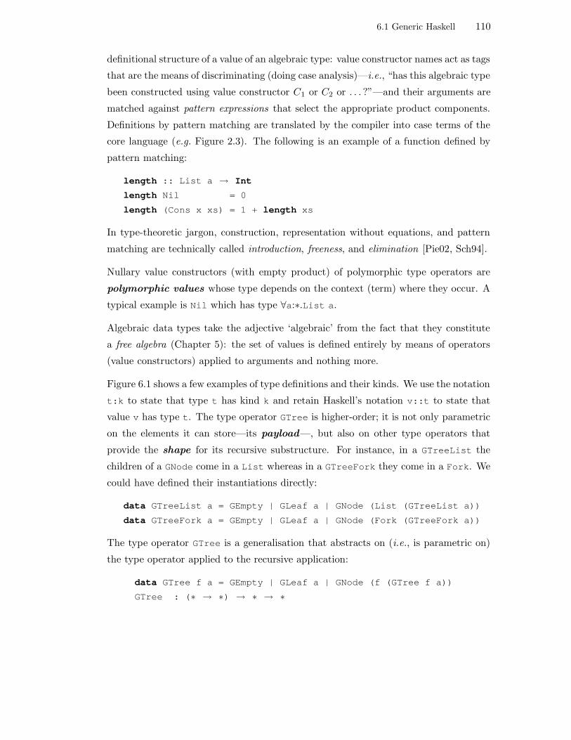
6.1 Generic Haskell 110
definitional structure of a value of an algebraic type: value constructor names act as tags
that are the means of discriminating (doing case analysis)—i.e., “has this algebraic type
been constructed using value constructor C1 or C2 or . . . ?”—and their arguments are
matched against pattern expressions that select the appropriate product components.
Definitions by pattern matching are translated by the compiler into case terms of the
core language (e.g. Figure 2.3). The following is an example of a function defined by
pattern matching:
length :: List a → Int
length Nil = 0
length (Cons x xs) = 1 + length xs
In type-theoretic jargon, construction, representation without equations, and pattern
matching are technically called introduction, freeness, and elimination [Pie02, Sch94].
Nullary value constructors (with empty product) of polymorphic type operators are
polymorphic values whose type depends on the context (term) where they occur. A
typical example is Nil which has type ∀a:∗.List a.
Algebraic data types take the adjective ‘algebraic’ from the fact that they constitute
a free algebra (Chapter 5): the set of values is defined entirely by means of operators
(value constructors) applied to arguments and nothing more.
Figure 6.1 shows a few examples of type definitions and their kinds. We use the notation
t:k to state that type t has kind k and retain Haskell’s notation v::t to state that
value v has type t. The type operator GTree is higher-order; it is not only parametric
on the elements it can store—its payload—, but also on other type operators that
provide the shape for its recursive substructure. For instance, in a GTreeList the
children of a GNode come in a List whereas in a GTreeFork they come in a Fork. We
could have defined their instantiations directly:
data GTreeList a = GEmpty | GLeaf a | GNode (List (GTreeList a))
data GTreeFork a = GEmpty | GLeaf a | GNode (Fork (GTreeFork a))
The type operator GTree is a generalisation that abstracts on (i.e., is parametric on)
the type operator applied to the recursive application:
data GTree f a = GEmpty | GLeaf a | GNode (f (GTree f a))
GTree : (∗ → ∗) → ∗ → ∗

6.1 Generic Haskell 111
data List a = Nil | Cons a (List a)data BTree a b = Empty | Leaf a | Node b (BTree a b) (BTree a b)data GTree f a = GEmpty | GLeaf a | GNode (f (GTree f a))data BGTree f a b = BGEmpty | BGLeaf a | BGNode b (f (BGTree f a b))data Fork a = Fork a adata BList a = BNil | BCons a (BList (Fork a)) -- irregular
-- Instantiationstype TreeCharInt = BTree Char Inttype ArithExp = BTree Int (Int → Int → Int)type GTreeList = GTree Listtype GTreeFork = GTree Fork
t1 :: GTreeList Int -- GTree List Intt1 = GNode [GLeaf 3, GNode [GLeaf 2, GEmpty]]t2 :: GTreeFork Int -- GTree Tree Intt2 = GNode (Fork (GLeaf 3) (GNode (Fork (GLeaf 2) GEmpty)))
Int : ∗List : ∗ → ∗List Int : ∗List Char : ∗BTree : ∗ → ∗ → ∗BTree Char : ∗ → ∗BTree Char Int : ∗GTree : (∗ → ∗) → ∗ → ∗GTree List : ∗ → ∗GTree List Int : ∗BGTree : (∗ → ∗) → ∗ → ∗ → ∗BList : ∗ → ∗
Figure 6.1: Some data types and their kinds in Haskell.
GEmpty :: ∀ f:∗→∗. ∀ a:∗. GTree f a
GLeaf :: ∀ f:∗→∗. ∀ a:∗. a → GTree f a
GNode :: ∀ f:∗→∗. ∀ a:∗. f (GTree f a) → GTree f a
The type operator BList is an example of an irregular type. A recursive type operator
is irregular when it is recursively applied in its definition to arbitrary well-kinded type-
terms, not just type variables. Some authors call these types nested [BM98] and others
non-uniform [Oka98a]. Irregular types are arrived at by a process of data-structural
bootstrapping [Oka98a, Chp10]. They capture structural invariants within the data
type itself that otherwise would have to be maintained by external operations. These
invariants are enforced by the type system when it checks for term well-formedness.

6.1 Generic Haskell 112
Also, irregular types may provide more efficient representations. For example, the type
BList is recursively applied to Fork a instead of a, which means that every recursive
substructure is a pair of BList, thus obtaining the type of balanced trees as shown in
Figure 6.2.
Cons BCons/ \ / \
1 Cons 1 Fork/ \ / \2 Cons BCons BCons
/ \ / \ / \3 Nil 2 BNil 3 BNil
Figure 6.2: List vs BList.
Functions on irregular types must be polymorphically recursive [Myc84, Hen93], i.e.,
each recursive call may have a different type than that of the function. For instance,
the length function for BList has type BList a → Int whereas its recursive call must
have type BList (Fork a) → Int.
6.1.2 From parametric to structural polymorphism
A polytypic function captures a whole family of polymorphic or overloaded functions
in a single definition. Let us recall the function that returns the length of a list:
length :: List a → Int
length Nil = 0
length (Cons x xs) = 1 + length xs
We can think of similar functions for other type operators such as BTree and GTree. All
these functions are instances of a more general, polytypic gsize function that returns
the ‘size’ of an arbitrary type operator. What is the type of gsize?
gsize :: ? → Int
One of the insights behind Generic Haskell is that the type of gsize depends on the
kind of the type operator it works on. Let us write the type signatures and bodies of
gsize instances starting from a kind-∗ type operator and moving all the way up the
kind hierarchy. For a manifest type t, gsize must be a constant function:
∀ t:∗. gsize_t :: t → Int
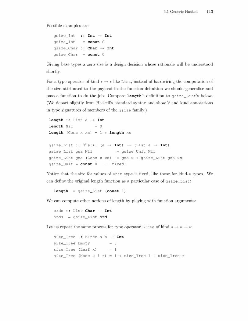
6.1 Generic Haskell 113
Possible examples are:
gsize_Int :: Int → Int
gsize_Int = const 0
gsize_Char :: Char → Int
gsize_Char = const 0
Giving base types a zero size is a design decision whose rationale will be understood
shortly.
For a type operator of kind ∗ → ∗ like List, instead of hardwiring the computation of
the size attributed to the payload in the function definition we should generalise and
pass a function to do the job. Compare length’s definition to gsize_List’s below.
(We depart slightly from Haskell’s standard syntax and show ∀ and kind annotations
in type signatures of members of the gsize family.)
length :: List a → Int
length Nil = 0
length (Cons x xs) = 1 + length xs
gsize_List :: ∀ a:∗. (a → Int) → (List a → Int)
gsize_List gsa Nil = gsize_Unit Nil
gsize_List gsa (Cons x xs) = gsa x + gsize_List gsa xs
gsize_Unit = const 0 -- fixed!
Notice that the size for values of Unit type is fixed, like those for kind-∗ types. We
can define the original length function as a particular case of gsize_List:
length = gsize_List (const 1)
We can compute other notions of length by playing with function arguments:
ords :: List Char → Int
ords = gsize_List ord
Let us repeat the same process for type operator BTree of kind ∗ → ∗ → ∗:
size_Tree :: BTree a b → Int
size_Tree Empty = 0
size_Tree (Leaf x) = 1
size_Tree (Node x l r) = 1 + size_Tree l + size_Tree r

6.1 Generic Haskell 114
gsize_Tree :: ∀ a:∗. (a → Int) →
( ∀ b:∗. (b → Int) → (BTree a b → Int))
gsize_Tree gsa gsb Empty = gsize_Unit Empty
gsize_Tree gsa gsb (Leaf x) = gsa x
gsize_Tree gsa gsb (Node x l r) = gsb x + gsize_Tree gsa gsb l
+ gsize_Tree gsa gsb r
Again, the gsize version takes an argument function for every type variable and the
definition for units is fixed. Let us now write the gsize instance for higher-order
type operator GTree. The argument function gsf associated with type variable f is a
parametrically polymorphic function whose type is that of a gsize for a type operator
of kind ∗ → ∗:
gsize_GTree
:: ∀ f:∗→∗. ( ∀ a:∗. (a → Int) → (f a → Int)) →
( ∀ a:∗. (a → Int) → (GTree f a → Int))
gsize_GTree gsf gsa GEmpty = gsize_Unit GEmpty
gsize_GTree gsf gsa (GLeaf x) = gsa x
gsize_GTree gsf gsa (GNode y) = gsf (gsize_GTree gsf gsa) y
There is an inductive pattern here which can be gleaned by looking carefully at the
type signatures:
∀ t:∗. gsize :: t → Int
∀ t:∗→∗. gsize :: ∀ a:∗. (a → Int) → (t a → Int)
∀ t:∗→∗→∗.
gsize :: ∀ a:∗. (a → Int) → ( ∀ b:∗. (b → Int) → (t a b → Int))
∀ t:(∗→∗)→∗→∗.
gsize :: ∀ t’:∗→∗. ( ∀ a:∗. (a → Int) → (t’ a → Int)) →
( ∀ b:∗. (b → Int) → (t t’ b → Int))
Each version of gsize takes a function for each of the type operator’s type variables.
The number of function arguments is determined by the arity of the type operator and
the type signature of each function argument depends on the kind of the type variable.

6.1 Generic Haskell 115
That is, the type of each gsize is determined by the type operator’s kind inductively
from the type of the kind-∗ case. This is captured by a so-called polykinded type:
type Size〈 ∗ 〉 t = t → Int
type Size〈k→v〉 t = ∀ a. Size〈k〉 a → Size〈v〉 (t a)
The notation Size〈k〉 t indicates that Size is a polykinded type defined by induction
on the kind k of type operator t. The polykinded type is specialised for every actual
type-operator argument to get the types of gsize instances. Figure 6.3 illustrates this
process for t = GTree. (We have renamed type variables in the figure to avoid variable
shadowing.)
Size〈(∗→∗)→∗→∗〉 GTree= ∀ f. Size〈 ∗→∗ 〉 f → Size〈 ∗→∗ 〉 (GTree f)= ∀ f. ( ∀ a. Size〈 ∗ 〉 a → Size〈 ∗ 〉 (f a)) →
( ∀ a. Size〈 ∗ 〉 a → Size〈 ∗ 〉 ((GTree f) a))= ∀ f. ( ∀ a. (a → Int) → f a → Int) →
( ∀ a. (a → Int) → GTree f a → Int)
Figure 6.3: Specialisation of polykinded type Size〈k〉 t where t is GTree and thereforek is (∗→∗)→∗→∗.
Let us move on to the function bodies. In each case, the particular instance of gsize
is defined by pattern matching on the type operator’s definitional structure in terms
of sums of products. There is one line for each sum, i.e., for each value constructor.
Nullary products are considered equivalent to values of Unit type. The total size of a
proper product is calculated by adding the sizes of each product component: the size of
elements whose type is given by a type variable is computed by the function arguments;
the size of recursive substructures is computed by recursive calls. Although not shown
in the examples, components of other types such as base types or user-defined types
would have their particular instances of gsize applied to them.
Consequently, the body of each gsize instance is determined by the type operator’s
definitional structure. (This motivates a pun in ‘poly-typical’: a family of many typical
or expected functions.) There remains to collect all the bodies into a polytypic definition
of a single gsize function. This function would compute the size of an arbitrary type
operator argument of arbitrary kind. For a particular type operator, say List, a call
to polytypic gsize:
gsize〈List〉 (const 1) [1,2,4]

6.1 Generic Haskell 116
where angle brackets denote polytypic application , “should amount” to a call to its
particular instantiation:
gsize_List (const 1) [1,2,4]
Another insight behind Generic Haskell is that polytypic function bodies need not be
defined by a fully-fledged inductive definition; it suffices to define the base case of the
induction, i.e., the behaviour of the function for kind-∗ types, binary sums, and binary
products. The Generic Haskell compiler “automatically takes care of type abstraction,
type application, and type recursion . . . in a type-safe manner” [HJ02, p13]. We should
also add that it automatically takes care of translating n-ary sums and products into
compositions of right-associative binary ones. This translation is a design choice that
plays an important role in understanding the instantiation process and the behaviour
of polytypic functions. Other representations are possible—e.g., left associativity—and
have an effect on the semantics of the function: “most [polytypic] functions are insens-
itive to the translation of sums and products. Two notable exceptions are [encoding
and decoding] for which [another representation] is preferable” [HJ02, p47].
Generic Haskell forces programmers to know the mechanics of the instantiation process,
in particular, the internal way of encoding products and sums, for that determines the
structure and therefore the body and semantics of the instance. At the time of writing,
there are some attempts at letting programmers specify associativity explicitly and to
allow types to be treated (viewed) as other types [HJL05].
In order to define polytypic function bodies, a canonical representation of a type oper-
ator’s definitional structure is needed. It is at this point that representation types,
called structure types in the Generic Haskell literature, are introduced. A represent-
ation type provides a canonical encoding of a type in terms of compositions of binary
sums of binary products of base types and type-operator applications. Representation
types are built on the following base representation types:
data Unit = Unit
data Sum a b = Inl a | Inl b
type Pro a b = (a,b)
type Fun a b = (→) a b
We ignore function space (Fun) in the following examples and defer its discussion until
Section 6.1.4. For readability we will write a+b for Sum a b and a×b for Pro a b. As

6.1 Generic Haskell 117
previously explained, the Generic Haskell compiler follows the convention that + and
× are right associative.
Figure 6.4 shows examples of type operators represented by structurally isomorphic
representation type operators. Let us ignore for the moment the fact that type-synonym
declarations (keyword type) cannot be recursive. We will provide a better definition
of representation types shortly.
data List a = Nil | Cons a (List a)type List’ a = Unit + (a × (List’ a))
data BTree a b = Empty | Leaf a | Node b (BTree a b) (BTree a b)type BTree’ a b = Unit + (a + (b × ((BTree’ a b) × (BTree’ a b))))
data GTree f a = GEmpty | GLeaf a | GNode (f (GTree f a))type GTree’ f a = Unit + (a + (f (GTree’ f a)))
data BList a = BNil | BCons a (BList (Fork a)) -- irregulartype BList’ a = Unit + (a × (BList’ (Fork a)))
Figure 6.4: Some type operators and their respective representation type operators.These definitions are not legal Haskell 98: type synonyms cannot be recursive.
Value-constructor names are dropped but the actual representation type used by the
Generic Haskell compiler includes information about value constructors (names, fixity,
arity, etc.), which is essential for programming polytypic serialisers such as pretty-
printers.
Polytypic functions are defined on base types and base representation types as shown
in the first box of Figure 6.5. The interesting cases are the sum and product ones.
The size of a sum a+b, whatever a and b, within a representation type is computed
by pattern matching on whether the value of the sum type is an Inl or Inr and then
by applying the appropriate argument function to it. The size of a binary product
a×b, whatever a and b, within a representation type is computed by pattern matching
on product components and adding their sizes, which are computed by the argument
functions. The second box in Figure 6.5 is syntactic sugar for the box above where the
recursion is made explicit: the argument functions gsa and gsb are instances of gsize
for the types a and b.

6.1 Generic Haskell 118
gsize〈t:k〉 :: Size〈k〉 tgsize〈Char〉 = const 0gsize〈Int〉 = const 0gsize〈Bool〉 = const 0gsize〈Unit〉 = const 0gsize〈a+b〉 gsa gsb (Inl x) = gsa xgsize〈a+b〉 gsa gsb (Inr y) = gsb ygsize〈a×b〉 gsa gsb (x,y) = gsa x + gsb y
gsize〈t:k〉 :: Size〈k〉 tgsize〈Char〉 = const 0gsize〈Int〉 = const 0gsize〈Bool〉 = const 0gsize〈Unit〉 = const 0gsize〈a+b〉 (Inl x) = gsize〈a〉 xgsize〈a+b〉 (Inr y) = gsize〈b〉 ygsize〈a×b〉 (x,y) = gsize〈a〉 x + gsize〈b〉 y
Figure 6.5: Polytypic gsize with implicit and explicit recursion.
Figure 6.6 illustrates the instantiation process. The first box shows instances of gsize
for base types, units, and binary products and sums. All are generated directly from the
polytypic definition. Their type signatures are obtained by instantiating the polykinded
type Size.
The remaining boxes show the instances of gsize for representation type operators
List’, BTree’, and GTree’. These instances follow the type-operator’s definitional
structure to the letter: an argument function is passed for each of the type-operator’s
type variables; the occurrence of a base type in the representation type translates to
a call to its gsize instance in the body of the function; the occurrence of a sum
translates to a call to gsize_Sum; the occurrence of a product to a call to gsize_Pro;
type-operator application translates to function application.
As an improvement, the type for kind-∗ type operators can be expressed by a type
synonym and the type signatures of all the instances can be written in terms of it as
shown in Figure 6.7.
There are two problems with the scheme presented. First, gsize has been defined on
List’ not List. The generated instantiation is gsize_List’, not gsize_List. And
similarly for the other type operators. Second, the type synonyms in Figure 6.4 are
invalid.

6.1 Generic Haskell 119
gsize_Char :: Char → Intgsize_Char = const 0
gsize_Bool :: Bool → Intgsize_Bool = const 0
gsize_Int :: Int → Intgsize_Int = const 0
gsize_Unit :: Unit → Intgsize_Unit = const 0
gsize_Sum :: ∀ a. (a → Int) → ( ∀ b. (b → Int) → Sum a b → Int)gsize_Sum gsa gsb (Inl x) = gsa xgsize_Sum gsa gsb (Inr y) = gsb y
gsize_Pro :: ∀ a. (a → Int) → ( ∀ b. (b → Int) → Pro a b → Int)gsize_Pro gsa gsb (x,y) = gsa x + gsb y
type List’ a = Unit + a × (List’ a)
gsize_List’ :: ∀ a. (a → Int) → List’ a → Int
gsize_List’ gsa= gsize_Sum gsize_Unit (gsize_Pro gsa (gsize_List’ gsa))
type BTree’ a b = Unit + a + b × (BTree’ a b) × (BTree’ a b)
gsize_BTree’:: ∀ a. (a → Int) → ( ∀ b. (b → Int) → BTree’ a b → Int)
gsize_BTree’ gsa gsb =gsize_Sum gsize_Unit
(gsize_Sum gsa (gsize_Pro gsb(gsize_Pro (gsize_BTree’ gsa gsb) (gsize_BTree’ gsa gsb))))
type GTree’ f a = Unit + (a + (f (GTree’ f a)))
gsize_GTree’:: ∀ f. ( ∀ a. (a → Int) → (f a → Int)) →
( ∀ a. (a → Int) → (GTree f a → Int))
gsize_GTree’ gsf gsa= gsize_Sum gsize_Unit
(gsize_Sum gsa (gsf (gsize_GTree’ gsf gsa)))
Figure 6.6: Instantiations of gsize.

6.1 Generic Haskell 120
type Size t = t → Int
gsize_Int :: Size Intgsize_Unit :: Size Unitgsize_Sum :: ∀ a. Size a → ( ∀ b. Size b → Size (Sum a b))gsize_Pro :: ∀ a. Size a → ( ∀ b. Size b → Size (Pro a b))
gsize_List’ :: ∀ a. Size a → Size (List’ a)
gsize_BTree’ :: ∀ a. Size a → ( ∀ b. Size b → Size (BTree a b))
gsize_GTree’ :: ∀ f. ( ∀ a. Size a → Size (f a)) →( ∀ a. Size a → Size (GTree’ f a))
Figure 6.7: Type signatures of the functions in Figure 6.6 written in terms of a typesynonym.
The type synonym of Figure 6.7 will prove useful in understanding how the Generic
Haskell compiler sorts out this problem. Before delving into that, let us (1) show some
examples of usage, (2) two more examples of polytypic function definitions and (3)
discuss some theoretical aspects of the approach in more detail (Section 6.1.3).
Let us suppose that recursive type synonyms were legal and assume that a call to
gsize on a type operator T is somehow translated to a call on its representation type
T ′. Figure 6.8 shows examples of usage that illustrate the design objectives. Desired
results are shown below each application.
In the figure, type BTree Int Char has kind ∗ and therefore there is no argument
function passed to gsize. The type BTree Int has kind ∗ → ∗ and therefore there is
an argument function passed to gsize. More precisely, the Generic Haskell compiler
replaces the polytypic applications:
gsize〈BTree Int Char〉
gsize〈BTree Int〉
by calls to the instances gsize_BTree_Int_Char and gsize_BTree_Int whose defin-
ition has been generated as follows:
gsize_BTree_Int_Char :: BTree Int Char → Int
gsize_BTree_Int_Char = gsize_BTree gsize_Int gsize_Char
gsize_BTree_Int :: ∀ a. (a → Int) → BTree Int a → Int
gsize_BTree_Int gsa = gsize_BTree gsize_Int gsa

6.1 Generic Haskell 121
aTree :: BTree Int CharaTree = Node ’A’ (Leaf 2) (Leaf 3)
gsize〈BTree Int Char〉 aTree> 0
gsize〈BTree Int〉 (const 1) aTree> 1
gsize〈BTree〉 (const 0) (const 1) aTree> 1
gsize〈BTree〉 (const 1) (const 1) aTree> 3
gsize〈List〉 (const 1) "hello world"> 11
gsize〈List〉 ord "hello world"> 1116
Figure 6.8: Examples of usage of polytypic gsize.
The size computed is zero because that is the size given to integers and characters in
Figure 6.5, which make up the payload of the type. Had we defined gsize differently for
base types then the computed size would differ. We come back to this in Section 6.1.12.
Other examples in Figure 6.8 show how to obtain different sizes (e.g., counting nodes
or counting leaves in BTrees) by playing with function arguments.
Polytypic map and polytypic equality. Figure 6.9 shows the definitions of poly-
typic map and polytypic equality. The latter function shows that overloaded functions
(implemented using type classes in Haskell) are also subject to generalisation in a poly-
typic definition. The polykinded type of polytypic map is at first sight confusing.
According to what has been said so far it might appear to be:
type Map〈 ∗ 〉 t = t → t
type Map〈k→v〉 t = ∀ a. Map〈k〉 a → Map〈v〉 (t a)
However, this polykinded type is not general enough as shown by the following counter-
example:
Map〈 ∗→∗〉 List = ∀ a. Map〈 ∗ 〉 a → Map〈 ∗ 〉 (List a)
= ∀ a. (a → a) → List a → List a

6.1 Generic Haskell 122
type Map〈 ∗ 〉 t1 t2 = t1 → t2type Map〈k→v〉 t1 t2 =∀ a1 a2. Map〈k〉 a1 a2 → Map〈v〉 (t1 a1) (t2 a2)
gmap〈t:k〉 :: Map〈k〉 t tgmap〈Int〉 = idgmap〈Unit〉 = idgmap〈a+b〉 (Inl x) = Inl (gmap〈a〉 x)gmap〈a+b〉 (Inr y) = Inr (gmap〈b〉 y)gmap〈a×b〉 (x,y) = (gmap〈a〉 x, gmap〈b〉 y)
gmap〈List〉 chr [65, 66, 67]> "ABC"
gmap〈BTree〉 ord chr (Node ’A’ (Leaf 66) (Leaf 67))> Node 65 (Leaf ’B’) (Leaf ’C’)
type Eq〈 ∗ 〉 t = t → t → Booltype Eq〈k→v〉 t = ∀ a. Eq〈k〉 a → Eq〈v〉 (t a)
geq〈t:k〉 :: Eq〈k〉 tgeq〈Int〉 = (==)geq〈Unit〉 Unit Unit = Truegeq〈a+b〉 (Inl x) (Inl x’) = geq〈a〉 x x’geq〈a+b〉 (Inl x) (Inr y’) = Falsegeq〈a+b〉 (Inr y) (Inl x’) = Falsegeq〈a+b〉 (Inr y) (Inr y’) = geq〈b〉 y y’geq〈a×b〉 (x,y) (x’,y’) = geq〈a〉 x x’ && geq〈b〉 y y’
geq〈List〉 (==) [1,2,4] [1,2,4]> True
geq〈List〉 (==) [1,2,4] [1,2,3]> False
Figure 6.9: Polytypic map, polytypic equality, and examples of usage.

6.1 Generic Haskell 123
For type operators of higher kinds we need two different universally-quantified variables,
one for the source type and another for the mapped target type:
Map〈 ∗→∗ 〉 List List = ∀ a b. Map〈 ∗ 〉 a b → Map〈 ∗ 〉 (List a) (List b)
= ∀ a b. (a → b) → List a → List b
The polykinded Map type uses two type variables from the start, but the polykinded
type of gmap is restricted to take the same type operator.
Two remarks are in order. First, polytypic map is not defined for function types:
function space is contravariant on its first argument (Section 3.10) and its type signature
therefore breaks the pattern captured by the polykinded type of polytypic map. Second,
as its polykinded type indicates, polytypic map is slightly more general than a map.
For example, the type signature of gmap_GTree is:
map_GTree :: ∀ f g. ( ∀ a b. (a → b) → (f a → g b)) →
( ∀ a b. (a → b) → GTree f a → GTree g b)
Categorially, GTree is a functor if it is functorial in the two arguments. More precisely,
we can define two functions:
hmap :: (Functor f, Functor g) ⇒ Nat f g → Nat (GTree f) (GTree g)
fmap :: Functor f ⇒ (a → b) → GTree f a → GTree f b
where Nat f g is the type of natural transformations from functor f to functor g:
type Nat f g = ∀ a. f a → g a
(The naturality conditions follow from parametricity, i.e., polymorphic functions are
natural transformations in Type.) Functions hmap and fmap must satisfy the functorial
laws:
hmap (µ η) == hmap µ hmap η
hmap (id :: Nat f f) == (id :: Nat (GTree f) (GTree f))
fmap (i j) == fmap i fmap j
fmap (id :: a → a) == (id :: (GTree f) a → (GTree f) a)
where:
µ :: Nat g h i :: b → c
η :: Nat f g j :: a → b

6.1 Generic Haskell 124
Because it is possible to manufacture a function of type f a → g a from a function k
of type (a → b) → f a → g b, namely, k id, map_GTree must satisfy the following
equation:
map_GTree k r == hmap (k id) fmap r
The body of gmap is straightforward. For base types (we only show integers and units)
it is the identity. For sums and products it maps over the components. Examples of
usage are also shown in the figure.
The polykinded type of geq is also straightforward: for kind ∗ it is a binary predicate
on the type t. Regarding the body, equality for base types is standard equality; two
sums are equal if they are both left or right components and their contents are equal;
and two products are equal if their components are equal. Examples of usage are also
shown.
Notice that we could have defined a more general polykinded type for equality following
the spirit of polykinded type Map [HJ02]:
type Eq〈 ∗ 〉 t1 t2 = t1 → t2 → Bool
type Eq〈k→v〉 t1 t2 = ∀ a1 a2. Eq〈k〉 a1 a2 → Eq〈v〉 (t1 a1) (t2 a2)
where now geq would have to have polykinded type Eq〈k〉 t t. The type of its instance
for List’ would be:
geq_List’ :: ∀ a b. (a → b → Bool) → List’ a → List’ b → Bool
Surprisingly, the body of polytypic geq need not change, so one wonders about what
is its most general polykinded type and about the expressibility of polykinded type
definitions. We come back to this in Section 6.1.5.
6.1.3 Generic Haskell and System Fω
If instead of Haskell we were programming in System Fω (Section 2.7.4), our overview
of polytypic programming would have come to a conclusion. In System Fω there is
a structural equivalence relation between types. A type operator and its representa-
tion type are structurally equivalent and we would program with representation types
directly. A polytypic extension of System Fω would translate polykinded types and
polytypic functions following the scheme so far, treating named definitions as sugar for

6.1 Generic Haskell 125
gsize Unitdef= λx :Unit . 0
gsize Intdef= λx :Int . 0
gsize Sumdef= Λα :∗ . λgsa : α→ Int.
Λβ :∗ . λgsb : β → Int.λs :α+β . case s of Inl x then gsa [α] x ; Inr y then gsb [β] y
gsize Prodef= Λα :∗ . λgsa : α→ Int.
Λβ :∗ . λgsb : β → Int.λp :α×β . plus (gsa [α] (fst [α] [β] p)) (gsb [β] (snd [α] [β] p))
Listdef= λα :∗ .1 + α× (List α)
gsize Listdef= Λα :∗ . λgsa :α→ Int .
gsize Sum [Unit] gsize Unit[α× (List α)] (gsize Pro [α] gsa [List α] (gsize List [α] gsa))
Figure 6.10: Writing and using instances of gsize for lists in System Fω. Type-termsin universal type applications are shown in square brackets.
lambda abstractions, with fixed points when there is recursion.
For example, the code in Figure 6.10 shows the instances of gsize for units, integers,
binary sums, products, and lists. For readability, we have used meta-level recursive
names and thus obviated the use of fixed-point operators. Also, to distinguish universal
type applications from term applications more easily, each type argument in a universal
application is written between square brackets.
The following code is an example of usage where xs abbreviates a value of type List Int
which corresponds to the Haskell list value [1,2]:
xsdef= Inr (1, Inr (2, Inl unit))
gsize List [Int] (λx :Int . 1) xs
> 2
The generation of instances like gsize List amounts to producing terms from type-terms,
where the latter are described by a type-level STLC (Chapter 2). The programmer
defines the translation for base types, units, sums, and products. The rest can be

6.1 Generic Haskell 126
taken care of automatically. A polytypic System Fω compiler or interpreter assigns a
System Fω term (an instance of a polytypic function, e.g., gsize List) to a STLC term
(a type-operator, e.g., List) [HJ02, p42ff].
6.1.4 Nominal type equivalence and embedding-projection pairs
Among other things, Haskell differs from System Fω in that type equivalence is nominal,
not structural. In type systems with nominal type equivalence naming is not a
derived form but an explicit and essential language construct. In such systems two
types are equivalent if and only if they have the same name. For several reasons [Pie02,
p251–254] nominal type equivalence is the norm in mainstream programming languages.
It facilitates the treatment of recursion and plays an important role in enforcing data
abstraction. For instance, the types:
data Debit = Debit Int
data Credit = Credit Int
are structurally equivalent but mistaking one for the other can have painful con-
sequences. In Haskell the two types are different, a point underlined by the two different
value constructors. In System Fω, which lacks names, we would only make use of in-
tegers.
A representation type operator is structurally equivalent to many structurally iso-
morphic type operators, but in a nominal type system, programming with, say, a List’
is not programming with a List.
Generic Haskell solves this problem by defining representation types in a different fash-
ion where they only capture the top-level structure of type operators. There is one
embedding function that translates a type operator to its representation type oper-
ator and a projection function that performs the converse. Figure 6.11 shows their
definitions for the case of lists and binary trees. Embedding-projection functions also
follow the structure of the data and their definitions are generated automatically by
the Generic Haskell compiler for arbitrary type operators [HJ02, p46–47].
The instances of gsize have been defined for the illegal representation types of Fig-
ure 6.4. However, for kind-∗ types and binary sums and products these instances need
not change. They will work for the new representation types of Figure 6.11 in the

6.1 Generic Haskell 127
data List a = Nil | Cons a (List a)type List’ a = Unit + (a × (List a))
from_List :: ∀ a. List a → List’ afrom_List Nil = Inl Unitfrom_List (Cons x xs) = Inr (x,xs)
to_List :: ∀ a. List’ a → List ato_List (Inl Unit) = Nilto_List (Inr (x,xs)) = Cons x xs
data BTree a b = Empty | Leaf a | Node b (BTree a b) (BTree a b)type BTree’ a b = Unit + (a + (b × ((BTree a b) × (BTree a b))))
from_BTree :: ∀ a b. Tree a b → Tree’ a bfrom_BTree Empty = Inl (Inl Unit)from_BTree (Leaf x) = Inr (Inl x)from_BTree (Node x l r) = Inr (Inr (x,l,r))
to_BTree :: ∀ a b. Tree’ a b → Tree a bto_BTree (Inl (Inl Unit)) = Emptyto_BTree (Inr (Inl x)) = Leaf xto_BTree (Inr (Inr (x,l,r))) = Node x l r
Figure 6.11: Generic Haskell’s representation types for lists and binary trees, togetherwith their embedding and projection functions.
forthcoming scheme.
The idea is to find out what needs to be modified from the definition of gsize_List’
in order to define gsize_List. First, a new gsize_List’ must be generated for the
new representation type of Figure 6.11 from the polytypic definition. The occurrence
of type operator List in the representation type signals the place in the body where
its gsize instance is to be called:
gsize_List’ :: ∀ a. Size a → Size (List’ a)
gsize_List’ gsa = gsize_Sum gsize_Unit
(gsize_Pro gsa (gsize_List gsa))
Second, looking closely at the types of the functions:
gsize_List’ :: ∀ a. Size a → Size (List’ a)
gsize_List :: ∀ a. Size a → Size (List a)
in order to define gsize_List the remaining ingredient would be a function:

6.1 Generic Haskell 128
foo :: ∀ a. Size (List’ a) → Size (List a)
which would afford to tie the knot:
gsize_List gsa = foo (gsize_List’ gsa)
That is:
gsize_List gsa = foo (gsize_Sum gsize_Unit
(gsize_Pro gsa (gsize_List gsa)))
Fortunately, the embedding-projection functions can help attain this goal:
from_List :: ∀ a. List a → List’ a
to_List :: ∀ a. List’ a → List a
It remains to define lifted versions of types:
bar :: ∀ a. Size (List a) → Size (List’ a)
foo :: ∀ a. Size (List’ a) → Size (List a)
This lifting is performed by a special map function which must be polytypic on the
type synonym, as the process must be repeated for other polytypic functions and type
synonyms like equality:
type Eq a = a → a → Bool
geq_List :: ∀ a. Eq a → Eq (List a)
bar :: ∀ a. Eq (List a) → Eq (List’ a)
foo :: ∀ a. Eq (List’ a) → Eq (List a)
The first box in Figure 6.12 defines a new data type EP and two selector functions
for manipulating embedding-projection pairs conveniently. The second box defines
instances of a special map function mapEP which is the map for EP values: for units and
integers, embedding-projection pairs are identities; for sums and products, embedding-
projection pairs can be obtained by mapping embedding-projection pairs associated
with their components. Notice that the arrow type operator is contravariant on its first
argument (Section 3.10), thus the definition of mapEP_Fun.
As usual, the type of the instance mapEP_Size is obtained from the polykinded type:
MapEP〈 ∗→∗〉 Size =
∀ t t’. MapEP〈 ∗ 〉 t t’ → MapEP〈 ∗ 〉 (Size t) (Size t’)

6.1 Generic Haskell 129
data EP a b = MkEP (a → b) (b → a)
from :: EP a b → (a → b)from (MkEP f t) = f
to :: EP a b → (b → a)to (MkEP f t) = t
mapEP_Int :: EP Int IntmapEP_Int = MkEP id id
mapEP_Unit :: EP Unit UnitmapEP_Unit = MkEP id id
mapEP_Pro :: EP a c → EP b d → EP (a × b) (c × d)mapEP_Pro (MkEP f1 t1) (MkEP f2 t2)= MkEP (map× f1 f2) (map× t1 t2)
mapEP_Sum :: EP a c → EP b d → EP (a + b) (c + d)mapEP_Sum (MkEP f1 t1) (MkEP f2 t2)= MkEP (map+ f1 f2) (map+ t1 t2)
mapEP_Fun :: EP a c → EP b d → EP (a → b) (c → d)mapEP_Fun (MkEP f1 t1) (MkEP f2 t2)= MkEP (map→ t1 f2) (map→ f1 t2)
type MapEP〈 ∗ 〉 t1 t2 = EP t1 t2type MapEP〈k→v〉 t1 t2 =∀ a1 a2. MapEP〈k〉 a1 a2 → MapEP〈v〉 (t1 a1) (t2 a2)
mapEP〈t:k〉 :: MapE〈k〉 t tmapEP〈Int〉 = mapEP_IntmapEP〈Unit〉 = mapEP_UnitmapEP〈a+b〉 = mapEP_SummapEP〈a×b〉 = mapEP_PromapEP〈a→b〉 = mapEP_Fun
Figure 6.12: Embedding-projection pairs and polytypic mapEP.

6.1 Generic Haskell 130
∀ t t’. EP t t’ → EP (Size t) (Size t’)
Letting t=(List a) and t’=(List’ a) would seal off the process. This is achieved by
creating an embedding-projection pair value for lists:
ep_List :: ∀ a. EP (List a) (List’ a)
ep_List = MkEP from_List to_List
and by getting the body of mapEP_Size from its polytypic definition, which follows to
the letter the definitional structure of type synonym Size:
mapEP_Size :: ∀ t t’. EP t t’ → EP (Size t) (Size t’)
mapEP_Size mapEPa = mapEP_Fun mapEPa mapEP_Int
Function mapEP_Size applied to ep_List gives us a value of type:
∀ a. EP (Size (List a)) (Size (List’ a))
whose to component is our sought-after foo:
foo :: ∀ a. Size (List’ a) → Size (List a)
foo = to (mapEP_Size ep_List)
We can now provide the definition of gsize_List:
gsize_List :: ∀ a. Size a → Size (List a)
gsize_List gsa = (to (mapEP_Size ep_List)) (gsize_List’ gsa)
6.1.5 The expressibility of polykinded type definitions
The polykinded type MapEP and the polytypic function mapEP are predefined in the
Generic Haskell prelude. This function in part determines the expressibility of a poly-
kinded type, i.e., what sort of polykinded types can be written. The Generic Haskell
compiler collects all the polykinded type definitions and generates an instance of mapEP
for the type synonyms generated from their kind-∗ cases. As it currently stands, these
synonyms can only contain applications of type operators to arguments. In [HJ02, p51],
the definition of mapEP is extended so that, in general, polykinded types can have the
form:
type T〈 ∗ 〉 t1 . . . tn x . . . z = B
type T〈k→v〉 t1 . . . tn x . . . z =
∀ a1 . . . an. T〈k〉 a1 . . . an x . . . z → T〈v〉 (t1 a1) . . . (tn an) x . . . z

6.1 Generic Haskell 131
where B is a polymorphic type signature where universal quantification is permitted
over type variables of kind ∗ and ∗ → ∗, and where x. . .z are auxiliary type variables
that are passed untouched to the base case. These variables are universally quantified
later when expressing the polykinded type of particular polytypic functions such as
polytypic reduce, shown in Figure 6.13 (notice how a somewhat spurious function has
to be passed to freduce in order to get a more meaningful type.)
type Reduce〈 ∗ 〉 t x = x → (x → x → x) → t → xtype Reduce〈k→v〉 t x = ∀ a. Reduce〈k〉 a x → Reduce〈v〉 (t a) x
reduce〈t:k〉 :: ∀ x. Reduce 〈k〉 t x- body of reduce not shown here
∀ x. Reduce〈 ∗→∗〉 List x=∀ x. ∀ a. Reduce〈 ∗ 〉 a x → Reduce〈 ∗ 〉 (List a x)=∀ x. ∀ a. (x → (x → x → x) → a → x) →
x → (x → x → x) → List a → x-freduce〈t:∗→∗〉 :: ∀ x. x → (x → x → x) → t x → xfreduce〈t〉 = reduce〈t〉 (λx y z → z)
fsum〈t〉 = freduce〈t〉 0 (+)fand〈t〉 = freduce〈t〉 True and
Figure 6.13: Polytypic reductions.
We should also mention that Generic Haskell supports polytypic types, called type-
indexed data types in the literature, i.e., types whose definitional structure depends
on the definitional structure of another type [HJL04]. Polytypic types may appear in
the kind-∗ case of a polykinded type. Instances of polytypic types are generated before
generating the instances of the polykinded type and the polytypic function.
Polykinded types also allow type-class constraints in some situations. We defer this
discussion until Section 6.1.10.
6.1.6 Polytypic abstraction
Figure 6.13 also shows two examples of polytypic abstraction (called ‘generic ab-
straction’ in the Generic Haskell literature) where instances of a polytypic function are
defined for type operators of particular kinds only. Functions fsum and fand work on

6.1 Generic Haskell 132
type operators of kind ∗ → ∗ only. Another example of polytypic abstraction involving
gsize follows:
flength〈t:∗→∗〉 :: t a → Int
flength〈t〉 = gsize〈t〉 (const 1)
length = flength〈List〉
6.1.7 The expressibility of polytypic definitions
Generic Haskell allows us to express catamorphisms such as gsize (Section 6.1.13).
It even allows us to express more generic ones such as freduce, or even more generally,
reduce. Notice that reduce is not quite a polytypic gfoldr. The type signature of
foldr for a given type operator takes one argument per value constructor. The base
case of the polykinded type of a polytypic gfoldr would not only depend on a type
operator’s kind but also on what is to the right of the equals in a data definition.
Also, representation types contain binary products, not n-ary products which are the
arguments taken by the functions that would be passed to gfoldr. For these reasons,
gfoldr is not definable in Generic Haskell.
Let us illustrate the problems in more detail. The following code defines foldr in terms
of a type Alg representing an operator algebra:
data Alg a b = Alg nil :: b, cons :: a → b → b
foldr :: Alg a b → List a → b
foldr alg Nil = nil alg
foldr alg (Cons x xs) = cons x (foldr alg xs)
Particular algebras are values of type Alg:
algSum = Alg nil = 0, cons = (+)
algLen = Alg nil = 0, cons = λx y → 1+y
The following is an example of usage:
foldr algSum [1,2,3]
> 6
foldr algLen [1,2,3]
> 3
It is common practice to write foldr alg as LvOfM where v stands for nil alg and f

6.1 Generic Haskell 133
for cons alg [MFP91].
The instance of gfoldr for List should have the same type signature as foldr. But
Alg not only depends on the kind-signature of List; it also depends on the number
and type signature of List’s value constructors.
Even if we could define a polytypic type Alg〈t〉 of which Alg for lists is an instance,
the representation of n-ary products into associations of binary products becomes an
issue. This is better illustrated in the case of BTree. When it comes to dealing with
the tertiary product of a Node, reduce for BTrees takes two functions, one for each
binary product into which the tertiary product is arranged:
data Alg a b c = Alg empty :: c,
leaf :: a → c,
node :: b → c → c → c
gfoldr_BTree alg Empty = empty alg
gfoldr_BTree alg (Leaf x) = leaf alg x
gfoldr_BTree alg (Node x tl tr) = node alg x (gfoldr_BTree alg tl)
(gfoldr_BTree alg t2)
reduce v l n1 n2 (Inl Unit) = v
reduce v l n1 n2 (Inr (Inl x)) = l x
reduce v l n1 n2 (Inr (Inr (x,(tl, tr)))) = n1 x (n2 t1 tr)
In other words, the gfoldr_BTree generated would not be the one shown above, but
one taking this algebra:
data Alg a b c = Alg v :: c,
l :: a → c,
n1 :: b → c → c,
n2 :: c → c → c
This is what differentiates a fold from a crush. In Figure 6.13, polytypic reduce is a
crush.
6.1.8 Summary of instantiation process
The Generic Haskell compiler collects all the polykinded type definitions P〈∗〉 t and
generates type synonyms P based on that kind-∗ case. It also expands mapEP〈P〉. For

6.1 Generic Haskell 134
each type operator T of kind k passed as an argument to a polytypic function, the
compiler generates its representation type T’ and the relevant machinery for dealing
with its associated embedding-projection pairs. Finally, the compiler generates the
instance of the polytypic function for T. The instance’s type is obtained by expanding
P〈k〉 T and the body follows to the letter the structure of T’ with the exception of the
call to mapEP〈P〉 on the embedding-projection value. The Haskell compiler does the
rest of the job: it type-checks that generated instance bodies have the generated type
signatures and compiles and optimises the code.
6.1.9 Polytypic functions are not first-class
In Generic Haskell, polytypic functions are not first-class, polytypic applications (i.e.,
generated instances) are. To make polytypic functions first class, polykinded types must
be incorporated into Haskell’s type system. However, this would require an extension
of the type system beyond what is needed for type-checking polytypic functions. For
instance, polykinded-type reconstruction is an open question: a polytypic function need
not be associated with a unique polykinded type. (Recall the discussion regarding the
polykinded types of gmap and geq on page 124 and Section 6.1.5.)
First-class status is seldom necessary: type-terms τ in polytypic applications g〈τ〉 must
be known at compile-time unless static type checking is given up. Consequently, they
can be replaced by instances. Take, for example, the following function:
foo :: ∀ t a. ∀ p. p〈 ∗→∗〉 t → (a → c) → t a → c
foo g f = g〈t〉 f
The value of type variable t must be known at compile time and its kind be ∗ → ∗.
Although universally quantified, p cannot be instantiated to Map〈∗ → ∗〉 t1 t2, which
expects two type variable arguments. Finally, the usage of g in the body imposes the
requirement that:
p〈 ∗→∗ 〉 t = (a → c) → t a → c
Let us fix p and t respectively to a particular type-operator and polykinded type:
foo :: ∀ t a. Size〈 ∗→∗ 〉 List → (a → c) → List a → c
foo g f x = g〈List〉 f x
Now foo can only be passed gsize as an argument and c must be Int. There is really

6.1 Generic Haskell 135
no need for parametrisation:
foo :: (a → Int) → List a → Int
foo f x = gsize〈List〉 f x
6.1.10 Type-class constraints and constrained algebraic types
We have not defined polykinded types that involve type-class constraints. It is possible
to include constraints in polytypic abstractions, e.g.:
gsum〈t:∗→∗ 〉 :: Num a ⇒ t a → Int
It is not legal to write constraints in polykinded types. This makes sense: constraints
would appear on nested ∀s due to the recursive nature of the general case. Polytypic
functions would only be applicable to type operators that have those constraints in all
type-variables.
However, type-class constraints introduced in data definitions are ignored by the latest
versions of the Generic Haskell compiler at the time of writing. For example, the
representation type generated for types:
data List a = Nil | Cons a (List a)
data Ord a ⇒ List a = Nil | Cons a (List a)
is exactly the same:
type List’ a = Unit + (a × (List a))
Although the embedding-projection pair ep_List for the unconstrained list has type:
∀ a. EP (List a) (List’ a)
for the constrained list it must have type:
∀ a. Ord a ⇒ EP (List a) (List’ a)
The Haskell compiler complains about the generated code, issuing a type error.
Constraints must also appear in the type signatures of generated instances, e.g., in the
type signature of gsize_List. The reason: ep_List appears in gsize_List’s body
and certainly if List has its type argument constrained so should gsize_List:
gsize_List :: ∀ a. Ord a ⇒ Size a → Size (List a)

6.1 Generic Haskell 136
gsize_List gsa = (to (mapEP_Size ep_List)) (gsize_List’ gsa)
Notice the propagation of constraints:
ep_List :: ∀ a. Ord a ⇒ EP (List a) (List’ a)
gsa :: ∀ a. Ord a ⇒ Size a
(mapEP_Size ep_List) ::
∀ a. Ord a ⇒ EP (Size (List a)) (Size (List’ a))
However, the type signatures of instances are all derived from polykinded types which
cannot accommodate constraints because they are introduced by type-operator argu-
ments in polytypic applications. Indeed, if gsize is applied to the type:
data Eq a ⇒ Set a = . . .
the constraint in the type signature of the instance differs:
gsize_Set :: ∀ a. Eq a ⇒ Size a → Size (Set a)
The polykinded type Size〈k〉 t cannot capture all possible constraints that may appear
in the definition of an arbitrary type operator t. Therefore, Generic Haskell fails to work
with type-class-constrained type operators. It captures an ‘unbounded polymorphism’
kind of polytypism.
Interestingly, polytypic function bodies need not change. The body of gsize_List for
an unconstrained List a is insensitive to the type a. The same polymorphic function
body can compute with a constrained list as long as the constraint is accommodated in
the function’s type signature. The implicit dictionary introduced by the constraint is
ignored:
gsize_List :: ∀ a. Ord a ⇒ Size a → Size (List a)
gsize_List gsa = (to (mapEP_Size ep_List)) (gsize_List’ gsa)
If List had been Eq constrained:
data Eq a ⇒ List a = Nil | Cons a (List a)
only the type signature would be affected:
gsize_List :: ∀ a. Eq a ⇒ Size a → Size (List a)
gsize_List gsa = (to (mapEP_Size ep_List)) (gsize_List’ gsa)

6.1 Generic Haskell 137
We conclude this section mentioning that, in Haskell, parametrically polymorphic func-
tions are often lifted automatically to constrained ones that ignore their dictionary
arguments, e.g.:
silly :: ∀ a. Num a ⇒ ( ∀ a. Num a ⇒ a → a) → a → a
silly f x = f (x + x)
sillyid :: ∀ a. Num a ⇒ a → a
sillyid = silly id
In this example, function silly expects a constrained function but it is passed an
unconstrained id in sillyid. Behind the scenes, what is really passed is a wrapped
identity that discards its dictionary:
id_wrap :: NumD a → a → a
id_wrap dict x = x
6.1.11 Polykinded types as context abstractions
There are two possible ways of coping with constrained type operators in Generic
Haskell. One way is to deal away with them, i.e., never to define constrained type
operators and put constraints on the functions that compute with them. This has
advantages and disadvantages which have been discussed in Section 5.8.2.
Another way is to extend Generic Haskell. However, the extension is surprisingly
simple; in fact, it is possible to leave the language unchanged and to only extend the
Generic Haskell compiler.
The idea is that the constraints for a gsize_T instance, say, are determined from
the constraints of type operator T. Therefore, the polykinded type Size〈k〉 t must
abstract over t’s context (i.e., list of constraints). In other words, polykinded types
must be context-parametric. Fortunately, there is no need to change the Generic Haskell
language. Context-parametric polykinded types and their expansion rules can be hidden
from the programmer and manipulated internally by the Generic Haskell compiler.
Constraint expressions and lists. We introduce the syntax of constraint expres-
sions and constraint lists in Figure 6.14.
Constraint expressions and constraint lists are type-terms. A constraint list can be

6.1 Generic Haskell 138
Type ::= ConstraintList
ConstraintList ::= ε| Constraint # ConstraintList
Constraint ::= ∅| TypeClassName
| λ TypeVar . Body
Body ::= ( TypeClassName Basic ( , TypeClassName Basic )∗ )
Basic ::= TypeVar
| Basic Basic
Figure 6.14: Grammar of constraints and constraint lists.
empty, denoted by ε, or constructed by prefixing a constraint expression (explained
shortly) to a constraint list using the # operator. As expected, # associates to the
right and we allow the following syntactic sugar:
[c1; . . . ; cn]def= c1# . . . #cn#ε
when n > 0.
Given a data declaration of the form:
data ∆ ⇒ T a1 . . . an = . . .
the constraint list ∆T associated with a type operator T contains one constraint expres-
sion for every one of T’s type variables. The constraint expression appears on the list in
the same position from left to right as that of the variable in the data declaration. More
precisely, when n > 0, ∆T = [c1; . . . ; cn] and ci is the constraint expression associated
with ai. When n = 0, ∆T = ε.
A constraint expression can be an empty constraint ∅, a type-class name (e.g.,
Eq), or a new form of lambda-abstraction whose body consists of applications of type-
class names to (applications of) type variables. Lambda-abstractions collect all the
constraints associated with a type variable in a single constraint expression, e.g.:
λx. Eq x
λx. (Eq x, Show x)
λx. Ord (a x)

6.1 Generic Haskell 139
In the last example type variable a is free. We explain the role of free type variables
shortly.
Here are some type operators and their associated constraint lists:
data Eq a ⇒ T1 a = . . .
data (Ix a, Eq b) ⇒ T2 a b = . . .
data (Eq a, Show a) ⇒ T3 a = . . .
data (Eq a, Show a, Num b) ⇒ T4 a b = . . .
data (Functor f, Eq (f a)) ⇒ T5 f a = . . .
data Ord b ⇒ T6 a b = . . .
∆T1 = [ Eq ]
∆T2 = [ Ix ; Eq ]
∆T3 = [ λx.(Eq x, Show x) ]
∆T4 = [ λx.(Eq x, Show x) ; Num ]
∆T5 = [ Functor ; λx.Eq (a x) ]
∆T6 = [ ∅ ; Ord ]
Notice that in ∆T5, type variable a occurs free. Free variables are chosen in alphabetical
order according to positions in constraint lists. For example, in ∆T5, a refers to the type
variable to which the first constraint expression in ∆T5 is to be applied. In contrast, in
a constraint expression of the form λx.Eq (b x), free variable b would refer to the type
variable to which the second constraint expression in the constraint list is to be applied.
Free variables become bound when expanding polykinded types, as shown shortly.
A constraint list ∆T only contains constraints associated with T’s type variables, not
with the type variables of potential type-operator arguments to T, which are unknown.
For instance, T5 List is a legal type, but ∆T5 does not mention constraints associated
with List’s type variables.
Context-parametric polykinded types. A polykinded type P 〈κ〉 t whose general
form is given in the first box of Figure 6.15 can be translated automatically by the
Generic Haskell compiler to a context-parametric polykinded type P ′〈κ〉 t shown
in the second box. The third box explains meta-notation. For simplicity, we ignore aux-
iliary free type variables (Section 6.1.5) which are just carried around when expanding
polykinded types.

6.1 Generic Haskell 140
P 〈∗〉 t = τ
P 〈κ→ ν〉 t = ∀α. P 〈κ〉 α → P 〈ν〉 (t α)
P ′〈∗〉 t = γq. τ
P ′〈κ→ ν〉 t = γq. (∀α. q α⇒ P ′〈κ〉 α ε → P ′〈ν〉 (t α) q)
αdef= α1 . . . αn
tdef= t1 . . . tn
(t α)def= (t1 α1) . . . (tn αn)
q αdef= (q α1, . . . , q αn)
n > 0
Figure 6.15: A polykinded type and its context-parametric version.
We have introduced a new form of abstraction using the symbol γ as binder:3 a
γ-abstraction is a new type-term of the form γq.τ where q may occur free in τ .
(In the P ′〈∗〉 case, however, q must be picked so as not to occur free in τ .)
A γ-application is the application of a γ-abstraction to a constraint list. This is a
type-term of the form (γq.τ) cs, where cs is a type-term whose compile-time value is a
constraint list. The new application is denoted by whitespace but, as we show shortly,
its type-level reduction rules are more complicated than simple substitution. In the
second box of Figure 6.15, there are two γ-applications in the P ′〈κ→ ν〉 case: P ′〈κ〉 α
is γ-applied to ε and P ′〈ν〉 (t α) is γ-applied to q.
The context-parametric versions of Size (Figure 6.5) and Map (Figure 6.9) are shown
in Figure 6.16.
Figure 6.17 shows the type-reduction (or ‘expansion’) rules of context-parametric poly-
kinded types (first box), which includes the type-reduction rules of γ-application (second
box), and the mechanics of constraint-expression application (third box).
Rule c-start shows how the instance of a polykinded type P 〈κ〉 T on an actual
type-operator argument T is to be obtained by reducing its context-parametric ver-
sion P ′〈κ〉 T ∆T which takes T ’s list of constraints into account.
3Capital gamma is often used for denoting contexts, so lowercase gamma makes sense as a binderfor constraint lists.

6.1 Generic Haskell 141
type Size’〈 ∗ 〉 t = γq. t → Inttype Size’〈k→v〉 t
= γq.( ∀a. q a ⇒ (Size’〈k〉 a ε) → (Size’〈v〉 (t a) q ) )
type Map’〈 ∗ 〉 t1 t2 = γq. t1 → t2
type Map’〈k→v〉 t1 t2
= γq.( ∀a1 a2. (q a1, q a2) ⇒(Map’〈k〉 a1 a2 ε) → (Map’〈v〉 (t1 a1) (t2 a2) q ) )
Figure 6.16: Context-parametric polykinded types Size’ and Map’.
P 〈κ〉 T I P ′〈κ〉 T ∆T (c-start)
(γq. (∀α. q α⇒ σ)) ε I ∀α.σ[q/ε] (c-null)(γq. (∀α. q α⇒ σ)) (∅#cs) I ∀α.σ[q/cs] (c-empty)(γq. (∀α. q α⇒ σ)) (c#cs) I ∀α. c α⇒ σ[q/cs] (c-push)(γq. τ) cs I τ if q /∈ FV(τ) (c-drop)
c αdef= (c α1, . . . , c αn)
c αi I
C αi if c = C
(subscript i B)[xi/αi] if c = λx.B
Figure 6.17: Type-reduction rules for context-parametric types.

6.1 Generic Haskell 142
Rule c-null shows the reduction when the constraint list is empty: the context is
removed from the type-term and ε is substituted for q in σ. Rule c-empty shows the
reduction of a list with an empty constraint in the head: the context is removed from
the type-term and q is replaced by the tail of the list. This way other constraints are
pushed down to its associated variables. Rule c-push shows the reduction when the
constraint list is not empty: the constraint expression on the head is applied to the
universally-quantified type variables, and the tail of the constraint list is substituted for
q in σ. Rule c-drop shows the reduction when q /∈ FV(τ): the abstraction is dropped.
Some remarks are in order. In the P ′〈∗〉 case, q /∈ FV(τ) and therefore type reduc-
tion will always proceed by Rule c-drop. In the general case, q is imposed on the
universally-quantified type variables and it is γ-applied to the P ′〈ν〉 case, whereas an
empty constraint list is γ-applied to the P ′〈κ〉 case. This is because ∆T only includes
constraints associated with T’s type variables, as explained above. Finally, notice that
expanding a context-parametric polykinded type with [∅; . . . ; ∅] produces the same res-
ult as expanding it with ε.
The last box in Figure 6.17 indicates how the application of a constraint expression
to a type variable works. The first line explains meta-notation. The second line is a
reduction rule for the application of a constraint expression c to a type variable αi.
The constraint expression c cannot be ∅ because empty constraints are dealt with by
γ-application (c-empty). If c is a type-class name C, constraint application simply
juxtaposes the constraint to the variable. If c is a lambda expression λx.B, first the
auxiliary function subscript i B adds subscripts to B’s free variables (including x),
performing multiple substitution where every free variable µ in B is substituted by µi.
Then, xi is substituted by αi. We omit subscript’s implementation details which are
inessential. Here are a few examples that illustrate how it works:
(γq. (∀a1. q a1 ⇒ . . .)) [C] = ∀a1. C a1 ⇒ . . .
(γq. (∀a1. q a1 ⇒ . . .)) [λx.(C1 x,C2 x)] = ∀a1. (C1 a1,C2 a1) ⇒ . . .
(γq. (∀a1. q a1 ⇒ . . .)) [λx. C (z x)] = ∀a1. C (z1 a1) ⇒ . . .

6.1 Generic Haskell 143
(γq. (∀a1a2. (q a1, q a2) ⇒ . . .)) [C] = ∀a1a2. (C a1,C a2) ⇒ . . .
(γq. (∀a1a2. (q a1, q a2) ⇒ . . .)) [λx.(C1 x,C2 x)]
= ∀a1a2. ((C1 a1,C2 a1), (C1 a2,C2 a2)) ⇒ . . .
(γq. (∀a1a2. (q a1, q a2) ⇒ . . .)) [λx. C (z x)]
= ∀a1a2.(C (z1 a1),C (z2 a2)) ⇒ . . .
Instantiation examples. We conclude this section illustrating the instantiation pro-
cess for the example type-operators given above and for polykinded types Size and
Map. Universally-quantified variables are chosen in order so as to avoid shadowing when
expanding context-parametric polykinded types.
The first example involves T1 which has an Eq constraint on its type variable. For
reasons of space, we omit the details of constraint-expression applications which take
place in rule c-push. We also obviate subscripts when polykinded types have only one
universally-quantified type variable:
Size〈∗→∗〉 T1
I c-start
Size’〈∗→∗〉 T1 [Eq]
I def. of Size’
(γq. (∀a. q a ⇒ Size’〈∗〉 a ε → Size’〈∗〉 (T1 a) q)) [Eq]
I c-push
∀a. Eq a ⇒ Size’〈∗〉 a ε → Size’〈∗〉 (T1 a) ε
I def. of Size’ (twice)
∀a. Eq a ⇒ (γq. a→ Int) ε → (γq. (T1 a)→ Int) ε
I c-drop (twice)
∀a. Eq a ⇒ (a→ Int)→ T1 a→ Int
The second example involves T2 which has two type variables, each with a different
constraint:
Size〈∗→∗→∗〉 T2

6.1 Generic Haskell 144
I c-start
Size’〈∗→∗→∗〉 T2 [Ix;Eq]
I def. of Size’
(γq. (∀a. q a ⇒ Size’〈∗〉 a ε → Size’〈∗→∗〉 (T2 a) q)) [Ix;Eq]
I c-push
∀a. Ix a ⇒ Size’〈∗〉 a ε → Size’〈∗→∗〉 (T2 a) [Eq]
I def. of Size’
∀a. Ix a ⇒ (γq. a→ Int) ε → Size’〈∗→∗〉 (T2 a) [Eq]
I c-drop
∀a. Ix a ⇒ (a→ Int) → Size’〈∗→∗〉 (T2 a) [Eq]
I def. of Size’
∀a. Ix a ⇒ (a→ Int) → (γq. (∀b. q b ⇒ Size’〈∗〉 b ε → Size’〈∗〉 (T2 a b) q)) [Eq]
I c-push
∀a. Ix a ⇒ (a→ Int) → (∀b. Eq b ⇒ Size’〈∗〉 b ε → Size’〈∗〉 (T2 a b) ε)
I def. of Size’
∀a. Ix a ⇒ (a→ Int) → (∀b. Eq b ⇒ (γq. b→ Int) ε → Size’〈∗〉 (T2 a b) ε)
I c-drop
∀a. Ix a ⇒ (a→ Int) → (∀b. Eq b ⇒ (b→ Int) → Size’〈∗〉 (T2 a b) ε)
I def. of Size’
∀a. Ix a ⇒ (a→ Int) → (∀b. Eq b ⇒ (b→ Int) → (γq. (T2 a b)→ Int) ε)
I c-drop
∀a. Ix a ⇒ (a→ Int) → (∀b. Eq b ⇒ (b→ Int) → T2 a b → Int)
The following example involves T3 which has multiple constraints on its only type
variable:
Size〈∗→∗〉 T3
I c-start
Size’〈∗→∗〉 T3 [λx.(Eq x, Show x)]
I def. of Size’
(γq. (∀a. q a ⇒ Size’〈∗〉 a ε → Size’〈∗〉 (T3 a) q)) [λx.(Eq x, Show x)]
I c-push and constraint application
∀a. (Eq a, Show a) ⇒ Size’〈∗〉 a ε → Size’〈∗〉 (T3 a) ε
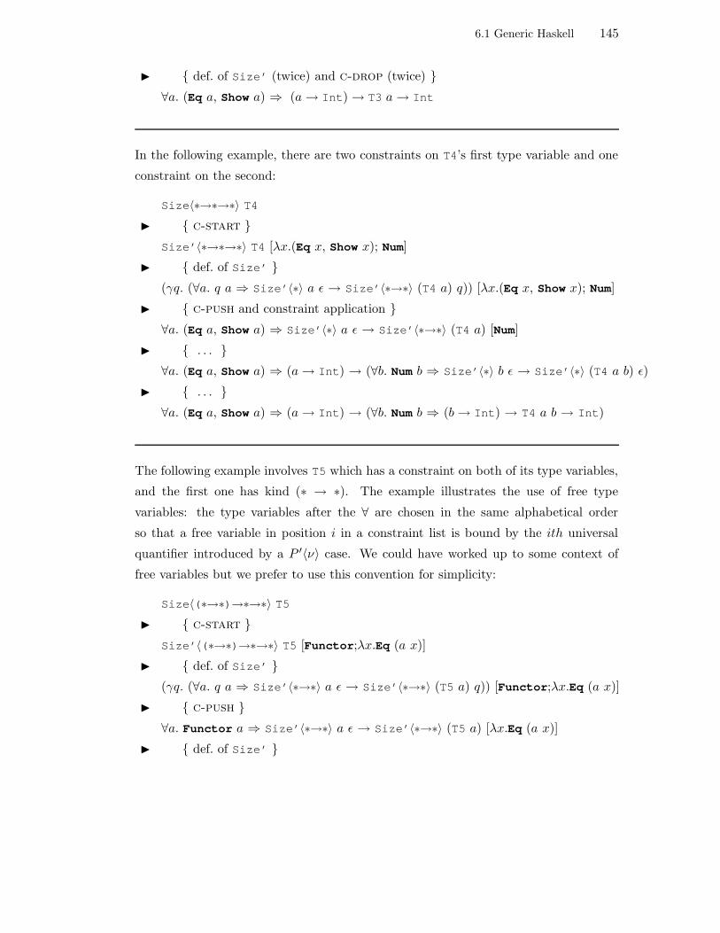
6.1 Generic Haskell 145
I def. of Size’ (twice) and c-drop (twice)
∀a. (Eq a, Show a) ⇒ (a→ Int)→ T3 a→ Int
In the following example, there are two constraints on T4’s first type variable and one
constraint on the second:
Size〈∗→∗→∗〉 T4
I c-start
Size’〈∗→∗→∗〉 T4 [λx.(Eq x, Show x); Num]
I def. of Size’
(γq. (∀a. q a ⇒ Size’〈∗〉 a ε → Size’〈∗→∗〉 (T4 a) q)) [λx.(Eq x, Show x); Num]
I c-push and constraint application
∀a. (Eq a, Show a) ⇒ Size’〈∗〉 a ε → Size’〈∗→∗〉 (T4 a) [Num]
I . . .
∀a. (Eq a, Show a) ⇒ (a→ Int) → (∀b. Num b ⇒ Size’〈∗〉 b ε → Size’〈∗〉 (T4 a b) ε)
I . . .
∀a. (Eq a, Show a) ⇒ (a→ Int) → (∀b. Num b ⇒ (b→ Int) → T4 a b → Int)
The following example involves T5 which has a constraint on both of its type variables,
and the first one has kind (∗ → ∗). The example illustrates the use of free type
variables: the type variables after the ∀ are chosen in the same alphabetical order
so that a free variable in position i in a constraint list is bound by the ith universal
quantifier introduced by a P ′〈ν〉 case. We could have worked up to some context of
free variables but we prefer to use this convention for simplicity:
Size〈(∗→∗)→∗→∗〉 T5
I c-start
Size’〈(∗→∗)→∗→∗〉 T5 [Functor;λx.Eq (a x)]
I def. of Size’
(γq. (∀a. q a ⇒ Size’〈∗→∗〉 a ε → Size’〈∗→∗〉 (T5 a) q)) [Functor;λx.Eq (a x)]
I c-push
∀a. Functor a ⇒ Size’〈∗→∗〉 a ε → Size’〈∗→∗〉 (T5 a) [λx.Eq (a x)]
I def. of Size’

6.1 Generic Haskell 146
∀a. Functor a ⇒ Size’〈∗→∗〉 a ε → (γq. (∀b. q b ⇒ Size’〈∗〉 b ε . . . )) [λx.Eq (a x)]
I c-push
∀a. Functor a ⇒ Size’〈∗→∗〉 a ε → (∀b. Eq (a b) ⇒ Size’〈∗〉 b ε . . . )
I . . .
∀a. Functor a ⇒ Size’〈∗→∗〉 a ε → (∀b. Eq (a b) ⇒ (b→ Int) → . . . )
I . . .
∀a. Functor a ⇒ (∀b. (b→ Int)→ a b→ Int) →
(∀b. Eq (a b) ⇒ (b→ Int) → T5 a b → Int)
We have not shown Rule c-null at work. It has been used in the steps from the penul-
timate equation to the last. For reasons of space, let us use the following abbreviation:
etcdef= (∀b. Eq (a b)⇒ (b→ Int)→ T5 a b→ Int)
These are the details of the derivation:
∀a. Functor a ⇒ Size’〈∗→∗〉 a ε → etc
I def. of Size’
∀a. Functor a ⇒ (γq. (∀b. q b⇒ Size’〈∗〉 b ε → Size’〈∗〉 (a b) q)) ε → etc
I c-null
∀a. Functor a ⇒ (∀b. Size’〈∗〉 b ε → Size’〈∗〉 (a b) ε) → etc
I def. of Size’ and c-drop (twice)
∀a. Functor a ⇒ (∀b. (b→ Int)→ a b→ Int) → etc
The following example involves T6 and shows Rule c-empty at work:
Size〈∗→∗→∗〉 T6
I c-start
Size’〈∗→∗→∗〉 T6 [∅;Ord]
I def. of Size’
(γq. (∀a. q a ⇒ Size’〈∗〉 a ε → Size’〈∗→∗〉 (T6 a) q)) [∅;Ord]
I c-empty
∀a. Size’〈∗〉 a ε → Size’〈∗→∗〉 (T4 a) [Ord]
I . . .
∀a. (a→ Int) → (∀b. Ord b ⇒ (b→ Int) → T4 a b → Int)

6.1 Generic Haskell 147
Lastly, the following example shows the expansion of Map’ which has two universally-
quantified type variables, thus illustrating the use of subscript:
Map’〈(∗→∗)→∗→∗〉 T5 [Functor; λx.Eq (a x)]
I def. of Map
(γq. (∀a1a2. (q a1, q a2) ⇒
(Map’〈∗→∗〉 a1 a2 ε) → (Map’〈∗→∗〉 (T5 a1) (T5 a2) q))) [Functor; λx.Eq (a x)]
I c-push
∀a1a2. (Functor a1, Functor a2) ⇒
(Map’〈∗→∗〉 a1 a2 ε) → (Map’〈∗→∗〉 (T5 a1) (T5 a2) [λx.Eq (a x)])
We abbreviate the result of reducing Map’〈∗ → ∗〉 a2 a2 ε as follows:
Sdef= (∀b1b2. (b1 → b2)→ a1 b1 → a2 b2)
And resume:
∀a1a2. (Functor a1, Functor a2) ⇒ S →
(Map’〈∗→∗〉 (T5 a1) (T5 a2) [λx.Eq (a x)])
I def. of Map’
∀a1a2. (Functor a1, Functor a2) ⇒ S →
((γq. (∀b1b2. (q b1, q b2) ⇒
(Map’〈∗〉 b1 b2 ε) → (Map’〈∗〉 (T5 a1 b1) (T5 a2 b2) q)))
[λx.Eq (a x)])
I c-push (invoking subscript)
∀a1a2. (Functor a1, Functor a2) ⇒ S →
(∀b1b2. (Eq (a1 b1), Eq (a2 b2)) ⇒
(Map’〈∗〉 b1 b2 ε) → (Map’〈∗〉 (T5 a1 b1) (T5 a2 b2) ε))
I ...
∀a1a2. (Functor a1, Functor a2) ⇒ (∀b1b2. (b1 → b2)→ a1 b1 → a2 b2) →
(∀b1b2. (Eq (a1 b1), Eq (a2 b2)) ⇒ (b1 → b2) → (T5 a1 b1) → (T5 a2 b2))
Expansion and instance generation. We conclude the section discussing how the
expansion of context-parametric types fits into the overall generation process. For each
polytypic application g〈T τ1 . . . τn〉 where T is a type operator of kind κ and τi are
well-kinded type applications of kind κi, the Generic Haskell compiler must generate

6.1 Generic Haskell 148
the g T instance whose type is obtained by expanding P ′〈κ〉 T ∆T , where P ′ is the
context-parametric polykinded type of g. The polytypic applications g〈τi〉 must be
compiled to instances g τi whose type is obtained by expanding P ′〈κi〉 τi ε, where the
constraint list is empty. Consequently, constrained type operators cannot be applied
to other constrained type operators. This restriction can be overcome by modifying,
among other things, the definition of constraint lists to account for constraints in τi,
and by γ-applying the P ′〈κ〉 α case in a context-parametric polykinded type to the
constraint list of τi during expansion.
At any rate, we have introduced context-parametric polykinded types in this thesis to
be able to write polytypic functions on first-order ADTs which may be implemented in
terms of constrained types (Chapter 9). First-order type operators cannot be applied
to proper type operators, let alone constrained ones. The solution presented here is
sufficient for our purposes.
6.1.12 Parameterisation on base types
The values for base types and units are fixed in polytypic function definitions. For
example, in the case of gsize, the size for integers is 0 and so is the size computed for
a value of List Int type. It is necessary to abstract over a type-operator’s payload to
compute the size properly:
gsize〈List Int〉 [1,2,3]
> 0
gsize〈List〉 (const 1) [1,2,3]
> 3
Fixing the value for base types can be limiting. For instance, the size for units is
0 and it is therefore impossible to count things such as the number of empty trees
hanging from leaves in a BTree. Serialisation functions (e.g., encoders) take into ac-
count units and base type values; their definition must be changed and recompiled if
their encoding needs to be changed. Furthermore, every time a base type is added
to the system (for example by linking with a library), the polytypic definition has to
be modified and recompiled unless the new case is added by extending the polytypic
function (dependency-style supports ‘polytypic extension’ [Loh04]).
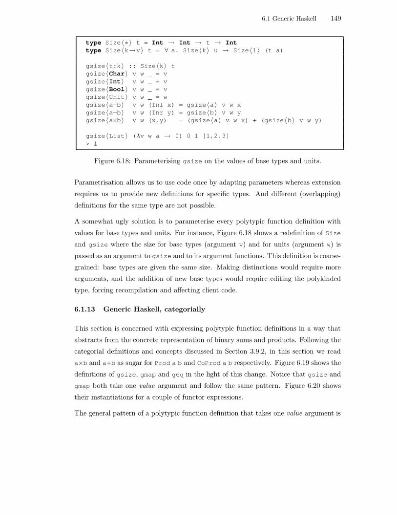
6.1 Generic Haskell 149
type Size〈 ∗ 〉 t = Int → Int → t → Inttype Size〈k→v〉 t = ∀ a. Size〈k〉 u → Size〈l〉 (t a)
gsize〈t:k〉 :: Size〈k〉 tgsize〈Char〉 v w _ = vgsize〈Int〉 v w _ = vgsize〈Bool〉 v w _ = vgsize〈Unit〉 v w _ = wgsize〈a+b〉 v w (Inl x) = gsize〈a〉 v w xgsize〈a+b〉 v w (Inr y) = gsize〈b〉 v w ygsize〈a×b〉 v w (x,y) = (gsize〈a〉 v w x) + (gsize〈b〉 v w y)
gsize〈List〉 (λv w a → 0) 0 1 [1,2,3]> 1
Figure 6.18: Parameterising gsize on the values of base types and units.
Parametrisation allows us to use code once by adapting parameters whereas extension
requires us to provide new definitions for specific types. And different (overlapping)
definitions for the same type are not possible.
A somewhat ugly solution is to parameterise every polytypic function definition with
values for base types and units. For instance, Figure 6.18 shows a redefinition of Size
and gsize where the size for base types (argument v) and for units (argument w) is
passed as an argument to gsize and to its argument functions. This definition is coarse-
grained: base types are given the same size. Making distinctions would require more
arguments, and the addition of new base types would require editing the polykinded
type, forcing recompilation and affecting client code.
6.1.13 Generic Haskell, categorially
This section is concerned with expressing polytypic function definitions in a way that
abstracts from the concrete representation of binary sums and products. Following the
categorial definitions and concepts discussed in Section 3.9.2, in this section we read
a×b and a+b as sugar for Prod a b and CoProd a b respectively. Figure 6.19 shows the
definitions of gsize, gmap and geq in the light of this change. Notice that gsize and
gmap both take one value argument and follow the same pattern. Figure 6.20 shows
their instantiations for a couple of functor expressions.
The general pattern of a polytypic function definition that takes one value argument is

6.1 Generic Haskell 150
gsize〈1〉 = const 0gsize〈Int〉 = const 0gsize〈a+b〉 = gsize〈a〉 O gsize〈b〉gsize〈a×b〉 = plus map× gsize〈a〉 gsize〈b〉
where plus p = exl p + exr p
gmap〈1〉 = idgmap〈Int〉 = idgmap〈a+b〉 = (asLeft gmap〈a〉) O (asRight gmap〈b〉)gmap〈a×b〉 = id map× gmap〈a〉 gmap〈b〉
geq〈1〉 = const (const true)geq〈Int〉 = (==)geq〈a+b〉 c1 c2 = if (isLeft c1 && isLeft c2) then
g〈a〉 (asLeft c1) (asLeft c2)else if (isRight c1 && isRight c2) then
g〈b〉 (asRight c1) (asRight c2)else False
geq〈a×b〉 p1 p2 = geq〈a〉 (exl p1) (exl p2) &&geq〈b〉 (exr p1) (exr p2)
Figure 6.19: Polytypic gsize, gmap, and geq in terms of products and coproducts.
F a = 1 + a × (F a)G f a = 1 + a × f (G f a)
gsize_F gsa = gsize_Unit O (gsa ‘plus‘ (gsize_F gsa))gsize_G gsf gsa = gsize_Unit O (gsa ‘plus‘ (gsf (gsize_G gsf gsa)))
gmap_F gma = (asLeft gmap_Unit) O
(asRight (gma ‘prod‘ (gmap_F gma)))
gmap_G gmf gma = (asLeft gmap_Unit) O
(asRight (gma ‘prod‘ gmf (gmap_F gmf gma)))
Figure 6.20: Some functors and their polytypic function instances. Notice that map×’sdefinition has been expanded.

6.1 Generic Haskell 151
1 B Ainl- A + B inr
B
@@
@@
@cA g〈A〉
R
cB g〈B〉
C?
C?
C?
A exlA×B
exr - B
C
pA g〈A〉
? exl
C × C? exr - C
pB g〈B〉
?
C
θ
?
g〈1〉 = g1g〈B〉 = gB
g〈A+B〉 = (cA g〈A〉) O (cB g〈B〉)where cA g = cafterA g cbeforeA
cB g = cafterB g cbeforeB
g〈A×B〉 = θ (pA g〈A〉) × (pB g〈B〉)where l × r = (l exl) M (r exr)
pA g = pafterA g pbeforeA
pB g = pafterB g pbeforeB
Figure 6.21: General pattern of a polytypic function definition expressed categorially.B ranges over base types.

6.2 Scrap your Boilerplate 152
shown in Figure 6.21. The first box depicts each case as a diagram. The programmer
defines cA, cB , pA, pB and θ. The latter function specifies what is to be done with each
product member after the (possibly) recursive application of the polytypic function.
The cases for units and base types are fixed.
Notice that geq takes two value arguments and follows a different pattern. In order to
express its definition in point-free fashion, like gsize, we would have to define a sort
of zipping pairwise extension of O, M, and θ.
Figure 6.21 illustrates more clearly the fact that a polytypic function definition has
the recursive structure of a catamorphism [MFP91, BdM97]. We come back to this
figure in Chapter 9 when exploring its adaptability in the presence of data abstraction.
6.2 Scrap your Boilerplate
The Scrap your Boilerplate (SyB) approach to generic programming [LP03, LP04,
LP05] is a blend of polytypic and strategic programming ideas. Section 6.2.1 explains
Strategic Programming and Section 6.2.2 provides a paper-by-paper tour of SyB.
6.2.1 Strategic Programming
Data structures are heterogeneous trees of sorts. Computing with them entails travers-
ing them (recursion scheme) and performing actions at every node in the structure.
Some actions may involve combining results of other actions into a value (so-called
type-unifying computations such as catamorphisms), or transforming a value (so-
called type-preserving computations such as maps).4
Given a set of data types, programming by hand functions on them by pattern match-
ing is non-generic, laborious, fragile with respect to changes in the type’s definitions,
and rigid with respect to the recursion scheme and traversal control. Functions are not
parametric on “the ability to determine which parts of the representation are visited in
which order and under which conditions” [VS04, p16]. This problem becomes partic-
ularly annoying when functions only work on some parts of the structure, making the
rest of the code which traverses it (i.e., which recurses in order to get to those parts)
boilerplate code .
4The terminology has been borrowed from [LVK00].

6.2 Scrap your Boilerplate 153
The use of higher-order functions capturing recursion schemes is of little help. Ex-
amples of such functions are generalised folds [Hut99, GHA01, SF93, BP99, MH95]. In
particular:
• The fold function for every type has to be programmed explicitly and so is each par-
ticular fold algebra (operators that replace value constructors) with which we want
to compute. An exception is the programming language Charity,5 where folds are
automatically generated by the compiler for first-order type operators. Program-
mers may assume the existence of these folds when writing their programs.
• Folds are rigid with respect to traversal control: the recursion scheme is fixed and
control refinement has to be hardwired in algebraic operators. For example, to
‘stop folding’ over a binary tree upon a certain condition we need to hardwire the
stop condition in algebraic operators (fold would not ‘stop’ but simply collapse the
pruned subtree into a default value) :
fold_until p :: (a → Bool) → Alg a c → List a → c
fold_until p alg l = foldr alg’ l
where
alg’ = Alg nil = nil alg,
cons = λx y → if p x then nil alg else cons alg x y
In [LVK00] a solution is proposed for reusing algebras by extension and overriding
which is implemented in terms of extensible records.
Strategic Programming [VS04, LVV02] is a more general, paradigm independent solu-
tion to generic traversal (computation) with heterogenous structures. It is based on
the following key ideas: action at a node and traversal must be separated, and tra-
versals must be decomposed into one-layer traversals on the one side and recursion
schemes given by an explicit fixed-point definition on the other side. This separation
of concerns permits composition and parametrisation: actions can be composed and
one-layer traversals and recursion schemes can be provided as action-parametric generic
combinators.
In order for an action at a node to be generic, Strategic Programming assumes the
possibility of type-based dispatch, usually implemented in terms of a dynamic type-case,
5http://www.cpsc.ucalgary.ca/Research/charity/home.html
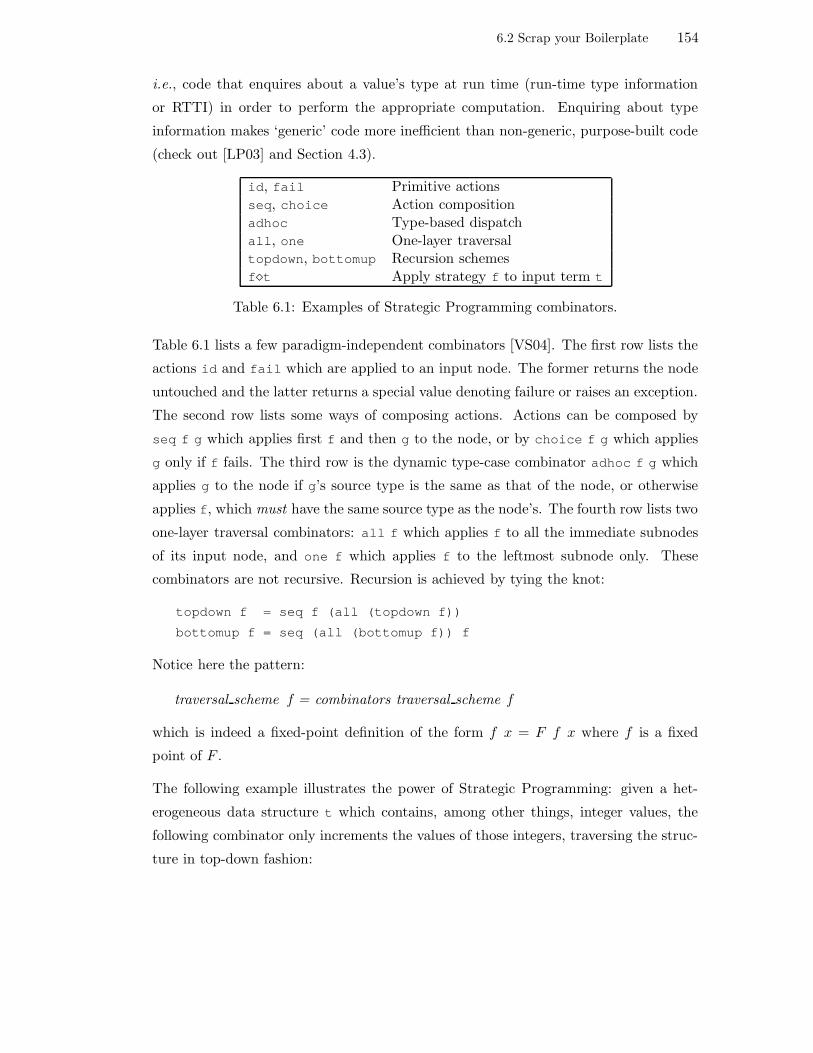
6.2 Scrap your Boilerplate 154
i.e., code that enquires about a value’s type at run time (run-time type information
or RTTI) in order to perform the appropriate computation. Enquiring about type
information makes ‘generic’ code more inefficient than non-generic, purpose-built code
(check out [LP03] and Section 4.3).
id, fail Primitive actionsseq, choice Action compositionadhoc Type-based dispatchall, one One-layer traversaltopdown, bottomup Recursion schemesft Apply strategy f to input term t
Table 6.1: Examples of Strategic Programming combinators.
Table 6.1 lists a few paradigm-independent combinators [VS04]. The first row lists the
actions id and fail which are applied to an input node. The former returns the node
untouched and the latter returns a special value denoting failure or raises an exception.
The second row lists some ways of composing actions. Actions can be composed by
seq f g which applies first f and then g to the node, or by choice f g which applies
g only if f fails. The third row is the dynamic type-case combinator adhoc f g which
applies g to the node if g’s source type is the same as that of the node, or otherwise
applies f, which must have the same source type as the node’s. The fourth row lists two
one-layer traversal combinators: all f which applies f to all the immediate subnodes
of its input node, and one f which applies f to the leftmost subnode only. These
combinators are not recursive. Recursion is achieved by tying the knot:
topdown f = seq f (all (topdown f))
bottomup f = seq (all (bottomup f)) f
Notice here the pattern:
traversal scheme f = combinators traversal scheme f
which is indeed a fixed-point definition of the form f x = F f x where f is a fixed
point of F .
The following example illustrates the power of Strategic Programming: given a het-
erogeneous data structure t which contains, among other things, integer values, the
following combinator only increments the values of those integers, traversing the struc-
ture in top-down fashion:

6.2 Scrap your Boilerplate 155
incInts t = (topdown (adhoc id (+1))) t
Notice the separation between genericity (traversal scheme with identity) and specificity
(action at specific nodes only).
Combinators are composable and have nice algebraic properties. This permits the
definition of new combinators for particular purposes. Theoretically, it seems that two
combinators suffice to express all strategic programs [LV02c].
Strategic Programming combinators are paradigm independent. There are incarnations
with running applications for term-rewrite systems and attribute grammars [VS04],
for object-oriented systems as improvements of the Visitor pattern [Vis01] and, in
the functional paradigm, there is the Strafunski bundle which includes a functional
combinator library and tool support for doing Strategic Programming in Haskell.6
6.2.2 SyB tour
This section describes SyB paper by paper.
The first paper [LP03] begins by presenting a dynamic nominal type-case oper-
ator. It is called type-safe cast in the paper for historical reasons and because it is
implemented using a cast operator that cannot cause run-time errors.
The implementation of cast relies on clever type-class and reflection tricks that enable
it to determine the type of a value at run time by means of applying the instance for
that type of an overloaded function typeOf that has been figured out at compile time
by the type-checker.
More precisely, the cast operator has type:
cast :: (Typeable a, Typeable b) ⇒ a → Maybe b
where the Typeable type class declares the aforementioned typeOf function. The
definition of typeOf is derived automatically by the compiler for a data type using
Haskell’s deriving clause. The function returns a value that makes for the represent-
ation of a manifest type.
Operationally, the application cast x within a context of manifest type Maybe T returns
6Strafunski comes from Strategic and Functional programming resembles the music of Igor Stravinski(http://www.cs.vu.nl/Strafunski).

6.2 Scrap your Boilerplate 156
Just x if x has type T; otherwise returns Nothing:
(cast 1) :: Maybe Int
> Just 1
(cast 1) :: Maybe Char
> Nothing
In other words, we get a Just value when, at run-time, a=b. The name ‘cast’ is
justified in that a value of type Maybe b is obtained from a value of type a. However,
the behaviour of cast x is that of a type-case that checks at run time whether the value
x is of type T, returning Just x of type Maybe T if the answer is positive or returning
Nothing of type Maybe T’ if the answer is negative, where T’ is the actual type of x.
The paper goes on to introduce several operators that can be seen as versions of adhoc
implemented in terms of cast: mkT for type-preserving actions, mkM for monadic type-
preserving actions, and mkQ for type-unifying actions. For example, given a function
f of type a → a, mkT f x applies f to x only if x has type a, returning x otherwise.
Clearly, mkT f corresponds to adhoc id f. Function mkT (or ‘make transformation’)
lifts a transformation (action in Strategic Programming jargon) on a value of a fixed
type into a transformation on a value of type ∀a. Typeable a ⇒ a. It is therefore
called a generic transformation by the authors.
There are three one-layer traversals called gmapT (type-preserving), gmapM (monadic
type-preserving) and gmapQ (type-unifying) defined in type class Data:
class Typeable a ⇒ Data a where
gmapT :: ( ∀ b. Data b ⇒ b → b) → a → a
gmapM :: Monad m ⇒ ( ∀ b. Data b ⇒ b → m b) → a → m a
gmapQ :: ( ∀ b. Data b ⇒ b → r) → a → [r]
Their behaviour is sketched below for an arbitrary n-ary value constructor C. One-layer
traversals are polytypic, i.e., defined on the structure of the node:
gmapT mt (C t1 . . . tn) = C (mt t1) . . . (mt tn)
gmapM mt (C t1 . . . tn) = do t1’ ← mt t1
. . .
tn’ ← mt tn
return C t1’ . . . tn’
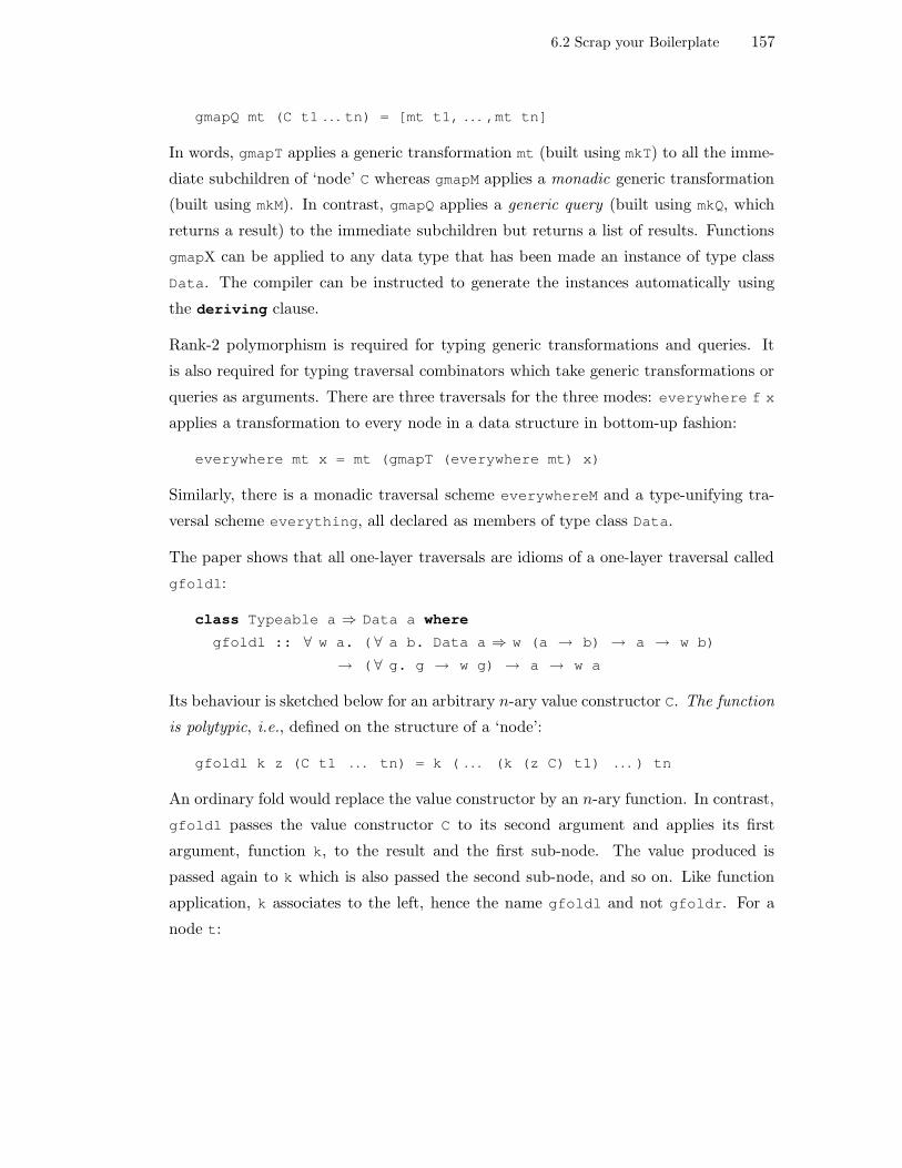
6.2 Scrap your Boilerplate 157
gmapQ mt (C t1 . . . tn) = [mt t1, . . . ,mt tn]
In words, gmapT applies a generic transformation mt (built using mkT) to all the imme-
diate subchildren of ‘node’ C whereas gmapM applies a monadic generic transformation
(built using mkM). In contrast, gmapQ applies a generic query (built using mkQ, which
returns a result) to the immediate subchildren but returns a list of results. Functions
gmapX can be applied to any data type that has been made an instance of type class
Data. The compiler can be instructed to generate the instances automatically using
the deriving clause.
Rank-2 polymorphism is required for typing generic transformations and queries. It
is also required for typing traversal combinators which take generic transformations or
queries as arguments. There are three traversals for the three modes: everywhere f x
applies a transformation to every node in a data structure in bottom-up fashion:
everywhere mt x = mt (gmapT (everywhere mt) x)
Similarly, there is a monadic traversal scheme everywhereM and a type-unifying tra-
versal scheme everything, all declared as members of type class Data.
The paper shows that all one-layer traversals are idioms of a one-layer traversal called
gfoldl:
class Typeable a ⇒ Data a where
gfoldl :: ∀ w a. ( ∀ a b. Data a ⇒ w (a → b) → a → w b)
→ ( ∀ g. g → w g) → a → w a
Its behaviour is sketched below for an arbitrary n-ary value constructor C. The function
is polytypic, i.e., defined on the structure of a ‘node’:
gfoldl k z (C t1 . . . tn) = k ( . . . (k (z C) t1) . . . ) tn
An ordinary fold would replace the value constructor by an n-ary function. In contrast,
gfoldl passes the value constructor C to its second argument and applies its first
argument, function k, to the result and the first sub-node. The value produced is
passed again to k which is also passed the second sub-node, and so on. Like function
application, k associates to the left, hence the name gfoldl and not gfoldr. For a
node t:

6.2 Scrap your Boilerplate 158
gfoldl ($) id t == t
where ($) is prefix function application.
The one-layer traversal gmapT can be defined in terms of gfoldl approximately as
follows:
gmapT mt = gfoldl k id
where k x y = x (mt y)
For instance, given a binary value constructor C:
gmapT mt (C t1 t2) = gfoldl k id (C t1 t2)
= k (k (id C) t1) t2
= k (C (mt t1)) t2
= (C (mt t1)) (mt t2)
= C (mt t1) (mt t2)
The definition is an approximation because it does not type-check: the value returned
by gmapT has type a, not w a. The authors show how to fix the definition of gfoldl
so that w is an identity type, i.e., w a = a.
The paper also introduces combinators for action composition and other traversal
schemes. It uses as a running example a set of heterogeneous kind-∗ data types but
argues that instances of Data can be generated automatically for irregular and para-
metric type-operators. However, Haskell’s type-class mechanism imposes limits with
respect to the kind of type-operators, and the dynamic nominal type-case is performed
on manifest types, not parametric type-operators.
A gsize function can be implemented in SyB as follows:
gsize :: Data a ⇒ a → Int
gsize x = 1 + sum (gmapQ gsize x)
The type-unifying one-layer traversal gmapQ applies gsize recursively to the immediate
subchildren of x, adds up the list of results, and adds one to account for the size of the
present node.
We have already seen some examples of gsize in Generic Haskell:
gsize〈List〉 (const 1) (Cons 1 (Cons 2 Nil))
> 2

6.2 Scrap your Boilerplate 159
gsize〈List Int〉 (Cons 1 (Cons 2 Nil))
> 0
In SyB, however:
xs :: List Int
xs = (Cons 1 (Cons 2 Nil))
gsize xs
> 5
First, we have to provide the type of xs explicitly in an annotation, the application:
gsize (Cons 1 (Cons 2 Nil))
will confuse the type checker which cannot decide whether type variable a in gsize’s
type signature is constrained by Data or Num. The culprit is Haskell’s monomorph-
ism restriction. Second, gsize counts every value constructor into the final size, as
illustrated by the evaluation trace:
gsize (Cons 1 (Cons 2 Nil))
= 1 + sum (gmapQ gsize (Cons 1 (Cons 2 Nil)))
= 1 + sum ([gsize 1, gsize (Cons 2 Nil)])
= 1 + sum ([1 + sum (gmapQ gsize 1), gsize (Cons 2 Nil)])
= 1 + sum ([1, 1 + sum (gmapQ gsize (Cons 2 Nil))])
= 1 + sum ([1, 1 + sum ([gsize 2, gsize Nil])])
= 1 + sum ([1, 1 + sum ([1,1])])
= 5
The trace also illustrates that every recursive call to gsize adds one to the sum of the
size of the subnodes. In contrast:
gsize x = sum (gmapQ gsize x)
gsize xs
> 0
No size! Finally, notice that gsize is applied to a manifest type of type class Data
and, so far, we cannot be parametric on the size of its payload.
Another important feature presented in [LP03] is polytypic function extension or
specialisation, i.e., the ability to override the polytypic function’s behaviour for specific
monomorphic types. As expected, there are three extension combinators: extT, extM,

6.2 Scrap your Boilerplate 160
and extQ. An application extX g f x applies the specialised monomorphic function f
to x if at run time x’s type matches f’s source type; otherwise it applies the polytypic
function g. Certainly, these operators are another manifestation of adhoc, only that
the default behaviour is now provided by a polytypic function. An example involving
gsize:
f :: Company → Int -- provides size for Company values
gsize = gsize_default ‘extQ‘ f
where gsize_default x = 1 + sum (gmapQ gsize x)
The original definition of gsize is rewritten into a default case, gsize_default, and
a specialised case, f, for values of type Company. Notice the fixed-point nature of the
definition: gsize passes gsize_default to extQ and gsize_default calls gsize.
Notice also that the type-specific behaviour, f, is fixed in gsize’s definition. Adding
new type-specific behaviour entails the recompilation of gsize:
h :: Client → Int -- provides size for Client values.
gsize = gsize_default ‘extQ‘ f ‘extQ‘ h
where . . .
Providing the extension in a new function will not avoid recompilation: gsize_default
has to call the new function:
gsize’ = gsize ‘extQ‘ h
gsize . . .
where gsize_default x = 1 + sum (gmapQ gsize’ x)
Finally, notice there are no checks for overlapping extensions; the following is possible:
gsize = gsize_default ‘extQ‘ f ‘extQ‘ f ‘extQ‘ f
The second paper [LP04] extends the original approach endowing the classes
Typeable and Data with reflection operators that allow programmers to dynamically
enquire about a value’s type, its value constructor names, their fixity, etc. Reflection
operators can be derived automatically by the Haskell compiler. Their implementation
follows much of the type-class trickery used in the implementation of cast.
The paper shows how to program serialisers such as pretty-printers and encoders, de-
serialisers that illustrate the benefits of lazy evaluation, and test-data generators. It
also adds new one-layer, zip-like combinators for traversing two data structures at the
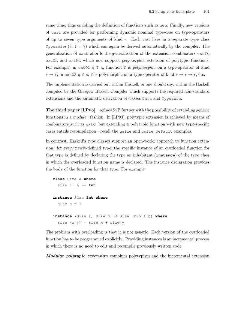
6.2 Scrap your Boilerplate 161
same time, thus enabling the definition of functions such as geq. Finally, new versions
of cast are provided for performing dynamic nominal type-case on type-operators
of up to seven type arguments of kind ∗. Each cast lives in a separate type class
Typeablei (i : 1 . . . 7) which can again be derived automatically by the compiler. The
generalisation of cast affords the generalisation of the extension combinators extTi,
extQi, and extMi, which now support polymorphic extension of polytypic functions.
For example, in extQ1 g f x, function f is polymorphic on a type-operator of kind
∗ → ∗; in extQ2 g f x, f is polymorphic on a type-operator of kind ∗ → ∗ → ∗, etc.
The implementation is carried out within Haskell, or one should say, within the Haskell
compiled by the Glasgow Haskell Compiler which supports the required non-standard
extensions and the automatic derivation of classes Data and Typeable.
The third paper [LP05] refines SyB further with the possibility of extending generic
functions in a modular fashion. In [LP03], polytypic extension is achieved by means of
combinators such as extQ, but extending a polytypic function with new type-specific
cases entails recompilation—recall the gsize and gsize_default examples.
In contrast, Haskell’s type classes support an open-world approach to function exten-
sion: for every newly-defined type, the specific instance of an overloaded function for
that type is defined by declaring the type an inhabitant (instance) of the type class
in which the overloaded function name is declared. The instance declaration provides
the body of the function for that type. For example:
class Size a where
size :: a → Int
instance Size Int where
size x = 1
instance (Size a, Size b) ⇒ Size (Pro a b) where
size (x,y) = size x + size y
The problem with overloading is that it is not generic. Each version of the overloaded
function has to be programmed explicitly. Providing instances is an incremental process
in which there is no need to edit and recompile previously written code.
Modular polytypic extension combines polytypism and the incremental extension

6.2 Scrap your Boilerplate 162
provided by the type-class mechanism. The idea is to get at something like:
-- Pseudo-code
class Size a where
gsize :: a → Int
instance Size a where
gsize x = 1 + sum (gmapQ gsize x)
instance Size Company where
gsize = f
A polytypic function name is now a type-class operation. Its code and extensions are
provided in instances. The first instance above specifies gsize’s default behaviour for
all types a. The second specifies the behaviour for Company values. Unfortunately, the
code does not type-check: type variable a is constrained by type class Data in gsize’s
type signature, and this constraint must appear in the instance heading:
instance Data a ⇒ Size a where
gsize x = 1 + sum (gmapQ gsize x)
Furthermore, gmapQ expects a first argument of type:
Data a ⇒ a → r
but it is passed gsize, whose type is less general and has a different type-class con-
straint:
Size a ⇒ a → Int
The authors argue that making Size a superclass of Data would solve the problem, but
the type-class mechanism works by extending superclasses with subclasses and not the
opposite. The authors propose to extend the type-class mechanism with type-class ab-
straction and type-class application in type-class and instance declarations. They
show how to encode the extension directly in Haskell using some of the ideas in [Hug99].
The rest of the paper is devoted to developing the necessary machinery. The most
problematic point is the definition of recursive instance declarations such as:
instance Data Size t ⇒ Size t where
gsize x = 1 + sum (gmapQ|Size,t| gsize x)

6.2 Scrap your Boilerplate 163
There is a fixed-point ‘equation’ in the instance heading which may compromise the
decidability of type inference, a problem whose full solution is considered future work
(braces with vertical bars denote type-class application).
Now, the RTTI tests of extX are avoided and which gsize function to call on a value
of a type is decided at compile time: either there is an instance of gsize for that type
or otherwise polytypic gsize is applied. Notice that this means there is no way of
overlapping or extending a polytypic function in different ways for the same data type
unless the compiler supports overlapping instances.
Notice that by making polytypic functions members of type classes, these type classes
will appear in the type signatures of client functions.7 For example [LP05, p4]:
gdensity :: (Size a, Depth a) ⇒ a → Int
gdensity x = gsize x / gdepth x
There is a possible impact on maintainability: changing the implementation of gdensity
may affect type-class constraints and, hence, affect its client functions. In the original
scheme, the type of gdensity was the more general:
Data a ⇒ a → Int
A possible patch that localises the change would consist of hiding classes Size and
Depth behind a Density sub-class with no operators:
class (Size a, Depth a) ⇒ Density a
gdensity :: Density a ⇒ a → Int
gdensity x = gsize x / gdepth x
A change in gdensity may entail a change in Density but client functions are unaf-
fected.
We conclude this section with an example that illustrates the advantages of polytypic
extension. On page 159, we showed how polytypic gsize counts value constructors
when calculating the size of a list. With polytypic extension, we can customise the
gsize for lists to count only payload elements:
7Compare with Dependency-style Generic Haskell, where the type of a polytypic function includesthe names of other polytypic functions it calls.

6.3 Generic Haskell vs SyB 164
instance Size a ⇒ Size (List a) where
gsize Nil = 0
gsize (Cons x xs) = gsize x + gsize xs
We cannot be parametric on the size of the payload type—which is computed by gsize’s
instance for the Int type—, but at least value constructors are avoided in the total
count:
xs :: List Int
xs = (Cons 1 (Cons 2 Nil))
gsize xs
> 2
6.3 Generic Haskell vs SyB
Generic Haskell and SyB differ in approach and style.
In Generic Haskell, polytypic functions have polykinded types. The former are defined
by induction on the structure of representation type operators (where only the beha-
viour for base types and base representation types is required). The latter are defined
by induction on kind signatures. The Generic Haskell compiler replaces polytypic ap-
plications by calls to generated instances. It also generates some internal machinery:
representation type operators, embedding-projection pairs, etc.
In SyB, polytypic functions are defined in terms of generic one-layer traversals that
can be derived automatically by the Haskell compiler for manifest types and type
operators whose kind signature is described by the grammar κ ::= ∗ | ∗ → κ up to
seven expansions.
In SyB representation types are unnecessary: type-based dispatch is nominal and re-
lies on typeOf. In contrast, Generic Haskell has representation types and type-based
dispatch is unnecessary.
SyB employs Strategic Programming ideas to separate specificity (nominal action at a
node) from genericity (traversal based on structure). Generic Haskell is purely struc-
tural and specificity can only be achieved via polytypic extension.
SyB is carried out within Haskell with a (supposedly) minimal extension: instructing
the compiler to generate type classes Typeable and Data. In contrast, Generic Haskell

6.3 Generic Haskell vs SyB 165
is a language extension requiring a pre-processing compiler. But polytypic functions
are not type-checked independently of their instantiations. It is the Haskell compiler
the one that type-checks that generated instance bodies conform to generated type
signatures.
Generic Haskell and SyB differ in the model of computation. In SyB there is a set of
one-layer traversals that are used in the definition of polytypic functions on manifest
types. SyB also supports monadic traversals. In contrast, polytypic functions in Gen-
eric Haskell work on unconstrained type operators of arbitrary kinds. The fact that
SyB’s implementation is type-class based imposes technical limits: there are only seven
Typeablei classes.
In SyB, gfoldl and one-layer traversal idioms perform computations on value con-
structors. In Generic Haskell, polytypic functions can perform computations on value
constructors but seldom do so (contrast the gsize examples in page 159).
Despite the differences, we consider Generic Haskell and SyB polytypic language ex-
tensions of Haskell. Abstractly, polytypic programming is characterised thus: in poly-
morphic languages, functions are ‘separated’ by the types on which they work. Poly-
typic functions must work on values of different types. They are a generalisation of
families of overloaded or polymorphic functions whose types and bodies can be gen-
erated automatically in regular fashion. Polytypic functions are used as if they were
a single function. Interestingly, this ‘single’ function can be given a type. The rest is
implementation detail.
We conclude the section with a short description of the paper [HLO06] which is, in
part, an attempt to explain the dynamic behaviour of gfoldl by means of making the
dynamic type information explicit at compile time. More precisely, the paper defines
a generalised algebraic data type [PWW04] for representing type information as
values in programs:
data Type :: ∗ → ∗ where
TInt :: Type Int
TChar :: Type Char
TPair :: Type a → Type b → Type (a,b)
TSum :: Type a → Type b → Type (Sum a b)
TList :: Type a → Type (List a)

6.3 Generic Haskell vs SyB 166
. . .
For example, the value constructor TInt is a value representation of the type Int;
the value constructor TChar is a value representation of the type Char; the expression
TPair TInt TChar is a value representation of the type (Int,Char).
When types are explicitly represented as values at run-time, generic functions can
simulate type-based dispatch, for instance:
gsize :: Type a → a → Int
gsize TInt i = 0
gsize TChar c = 0
gsize (TPair ta tb) (x,y) = gsize ta x + gsize tb y
gsize (TSum ta tb) (Inl x) = gsize ta x
gsize (TSum ta tb) (Inr y) = gsize tb y
gsize (List ta) xs = sum (map (gsize ta) xs)
. . .
In the paper, a type a is said to be typed if it is represented by a Type a value:
data Typed a = HasType a (Type a)
The authors introduce another generalised algebraic data type, called Spine that plays
the same role as a lisp S-expression. There is a ‘generic’ toSpine function that trans-
lates Typed values to (‘un-Typed’) Spine values:
data Spine :: ∗ → ∗ where
Constr :: a → Spine a
() :: Spine (a → b) → a → Spine b
toSpine :: Type a → a → Spine a
In the definition of Spine, Constr plays the role of z and the role of k in the definition
of gfoldl, which is now expressed thus:
gfoldl :: Type a → ( ∀ a b. w (a → b) → Typed a → w b)
→ ( ∀ a. a → w a)
→ a → w a
gfoldl t k z = foldSpine k z toSpine t
However, the generalised algebraic type Type is not extensible: the translation from
6.4 Lightweight approaches 167
Haskell to lisp (i.e., from Typed values to Spine values) explains gfoldl’s dynamic
behaviour statically within Haskell for one compilation. In SyB, when new types are
added the compiler generates their gfoldl instances. In contrast, extending Type
entails its recompilation.
6.4 Lightweight approaches
There are lightweight approaches for doing polytypic programming within Haskell. The
most notable ones are (1) [CH02] which relies either on existential types8 or on gen-
eralised algebraic data types [PWW04] to enforce the correspondence between a type
and its representation type; (2) [Hin04] that extends the previous approach in order
to define polytypic functions on type-operators of order 1 within Haskell 98; and (3)
[OG05] which generalises and collects the ideas into a programmable design pattern
and considers polytypic functions with polytypic (type-indexed) types.
8Type-terms where universal quantification occurs in contravariant position; not to be confused withother notions of existential types that model data abstraction [Pie02].

Chapter 7
Polytypism and Data Abstraction
If you make a small change to a program, it can result in an enorm-
ous change in what the program does. If nature worked that way, the
universe would crash all the time. (Jaron Lanier)
Successful software always gets changed. (Fred Brooks)
In Generic Haskell, polytypic functions are defined by induction on the concrete defini-
tional structure of a type operator, and their polykinded types by induction on the type
operator’s kind signature. In SyB, polytypic functions are defined in terms of one-layer
traversals whose generated instances are applied to the concrete structure of a ‘node’.
Access to concrete representations conflicts with the principle of data abstraction. More
precisely, data abstraction limits polytypism’s genericity.
The present chapter articulates the previous statement. Some readers may deem this
unnecessary. For them the step from the fact that “functions that access ADT repres-
entations can wreak havoc” to the fact that “polytypic functions [or their instances for
that matter] that access ADT representations can wreak havoc” requires no arguments
nor examples. But it is important to drive home the point for those lured by the ‘gen-
eric’ adjective. There are also conflicts specific to the nature of Generic Haskell and
SyB. Calling a function structurally polymorphic highlights the fact that the function
is dependent on structure and whether structure changes.
The whole issue is bound to spur philosophical disagreement. Access to concrete rep-
resentations is one of the dearest tools of the functional programmer—or at least of
‘non-Lispers’. Think for example of functions defined by pattern matching. Or think
about the fact that complex data-structure definitions such as first-class, extensible
higher-order records, or first-class modules for that matter, are ignored by polytypic
languages which always assume a world of algebraic data types (i.e., sums of products).
In Haskell 98, the standard record and module system is even found wanting.
168

7.1 Polytypism conflicts with data abstraction 169
7.1 Polytypism conflicts with data abstraction
First and foremost, concrete representations are logically hidden and often physically
unavailable (e.g. pre-compiled libraries). Second, if polytypic functions were allowed to
sneakily access an ADT’s representation, or were tipped off by an oracle, they would
not work satisfactorily. Data abstraction brings about a different game. More precisely:
1. A pure function must return the same result when applied to the same argument.
This also applies to functions on ADT values. If the function computes its result
by accessing the ADT’s representation and the representation changes, the value
computed may also change despite that the function is applied to the same ‘abstract’
value. Polytypic functions are subject to this problem just like ordinary, non-generic
ones.
In particular, functions accessing representations can be affected by implement-
ation clutter , i.e., data relevant only to the implementation of the type. More
precisely, an ADT may be implemented using various concrete types, parts of which
may contain data used for efficiency or structuring purposes. The well-known trade-
off between time and space indicates that this is bound to happen often: extra data
will be used in order to improve operator speed. It would be rather difficult, if
not impossible, for a function to ascertain the pertinence of data components in
implementations and to know what to do with them in a semantics-preserving way.
(Notice that clutter is not the same as junk: clutter can be part of a non-junk value
of the concrete type that represents a value of the abstract type.)
2. A function accessing ADT representations may violate the implementation in-
variants which guarantee that concrete values are valid representations of abstract
values. These invariants are maintained by ADT operators and are the raison d’etre
for hiding the representation behind an interface. A violation of the implementation
invariants most certainly entails a violation of the type’s semantics, i.e., the value
computed is not a value of the ADT.
3. Polytypic functions also have problems of their own:
(a) A manifest (kind-∗) ADT has the same status as a base type. Polytypic function
definitions have to provide cases for them like they do for integers or booleans
(Section 6.1.12).

7.1 Polytypism conflicts with data abstraction 170
In Generic Haskell, adding a new base type requires editing and recompiling
polytypic function definitions (except those defined by polytypic abstraction),
unless the new case is added incrementally using polytypic extension. In SyB,
the ADT has to be made an instance of Typeable and Data by the ADT
implementor, who is the only one entitled to the internals of the type.
In both cases, if the ADT implementation changes the definition of the poly-
typic function must be changed accordingly. Client code may be affected if the
results computed by the new definition differ from its previous version.
From the viewpoint of Generic Programming, it is better to rely on paramet-
risation than to rely on extension. Parametrisation allows us to write code once
by adapting parameters whereas extension requires us to provide new defini-
tions for specific types, i.e., there is no ‘generic’ programming here other than
name reuse and, furthermore, providing different (overlapping) definitions for
the same type is currently not possible.
(b) Generic Haskell does not support constrained types (Section 6.1.10) which arise
frequently in ADT implementations: order in binary search trees, equality in
sets, etc. In contrast, SyB supports constrained types when the payload is also
constrained on Data, e.g.:
instance (Data a, Ord a) ⇒ Data (OrdSet a) where
gfoldl k z s = k (z fromList) (toList s)
. . .
With polytypic extension, gsize has a Size constraint instead of a Data con-
straint, so Ord must be declared a superclass of Size. The type-class paramet-
risation framework suggested in [LP05] is undergoing research.
4. Polytypic extension is not a satisfactory solution. Let us illustrate this point using
gsize as a running example.
With polytypic extension it is possible to write a definition of gsize for a given
ADT such that it upholds the implementation invariants and ignores implementation
clutter. But there are two problems with this:
(a) Who writes the definition? It could be written by the polytypic programmer if
granted access to the ADT’s implementation. However, it is disturbing to define
a function that accesses the implementation outside the ADT. The definition

7.1 Polytypism conflicts with data abstraction 171
should be provided by the ADT implementor, who can update the definition if
the implementation changes. However, providing gsize as an ADT operator
amounts to providing the size operator directly. The fact that gsize is an
overloaded operator name and that there exists a polytypic version of it is an
orthogonal issue. The ADT implementor must provide a size operator and
the polytypic programmer must define the polytypic extension of gsize for the
ADT in terms of size.
Unfortunately, it is not possible for an ADT implementor to foresee all possible
operators that can be employed in the polytypic extension of future polytypic
functions. Polytypic extension takes place after a polytypic function has been
defined.
In sum, we end up in a visibility problem: polytypic programmers are ADT
clients and cannot customise their polytypic functions for those ADTs by ac-
cessing their implementation.
(b) Where is the genericity? Of course, polytypic programmers can use ADT
interfaces to define their extensions. However, we would like to have a polytypic
gsize that works for all types, concrete or abstract, not one whose version for
every new ADT has to be explicitly programmed. What is desired is automatic
polytypic extension.
The following sections elaborate and illustrate these points with a few examples. Please
note that this chapter is not meant to be a criticism of Generic Haskell or SyB. That
would be unfair, for coping with ADTs is not a design goal of these language extensions.
We just aim at exposing polytypism’s genericity limitations in order to argue the case
for our solution.
7.1.1 Foraging clutter
It is typical of many ADT implementations to use elaborate concrete types with clutter
of fixed types or payload type.
As a typical example, consider ordered sets supporting the following operators: empty,
isEmpty, insert, member, and remove. An ordered set can be implemented in terms
of Red-Black Trees or in terms of Leftist Heaps which contain, respectively, colour and
height components used for re-balancing the tree during insertion and removal [Oka98a,

7.1 Polytypism conflicts with data abstraction 172
p197,p203]:
data Colour = Red | Black
data RBT a = E | N Colour a (RBT a) (RBT a)
data LHeap a = E | N Int a (LHeap a) (LHeap a)
Polytypic functions take these clutter components into account. In Generic Haskell,
their contribution to the computation depends on the definition for units and integers—
recall Figure 6.5 and Section 6.1.12. Polytypic gsize calculates the size correctly
because the size for integers and units is zero. However, serialisation functions such
as pretty-printers or encoders would print or encode the clutter components. In SyB,
gsize counts all the value constructors in nodes, e.g.:
t :: LHeap Int
t = N 0 5 E E
gsize t
> 5
It is more reasonable to expect the size (cardinality) of the set 5 to be 1, count-
ing only the number of payload elements. ADT clients care less about internal value
constructors. Polytypic extension comes to the rescue:
instance Size a ⇒ Size (LHeap a) where
gsize E = 0
gsize (N i x l r) = gsize x + gsize l + gsize r
but, as argued in Section 7.1, from the viewpoint of Generic Programming this is an
unsatisfactory solution.
Clutter can be of payload type. Let us present a simple example first. Imagine an
ordered cached container CSet a for which the membership test for the last inserted
element takes constant time. It could be implemented in terms of ordered lists or binary
search trees, as shown in Figure 7.1. For brevity, only the implementation of insertion
is shown.
Value constructor CE represents an empty CSet and value constructor C a non-empty
CSet with a cached element and a concrete type with all the payload. In the list
implementation, a value C t Nil, where t is an arbitrary term, does not represent a
CSet value and constitutes junk (Chapter 5). Similarly, a term C t BinTree.empty in

7.1 Polytypism conflicts with data abstraction 173
module CSet (CSet,empty,isEmpty,insert,member) wheredata Ord a ⇒ CSet a = CE | C a (Payload a)
-- List implementationtype Payload a = [a]
insert :: Ord a ⇒ a → CSet a → CSet ainsert x CE = C x [x]insert x (C y ys) = C x (x:ys)
-- BinTree implementationimport BinTreetype Payload a = BinTree.BinTree a
insert :: Ord a ⇒ a → CSet a → CSet ainsert x CE = C x (BinTree.insert x BinTree.empty)insert x (C y ys) = C x (BinTree.insert x ys)
Figure 7.1: CSet implemented in terms of ordered lists or binary search trees withrespective implementation of insertion.
the binary search tree implementation constitutes junk.
Both representations contain clutter: a unit value and a cached value of payload type.
In the list implementation, Generic Haskell’s gsize counts the latter when computing
the size:
c = foldr (λx y → CSet.insert x y) CSet.empty [1,2]
gsize〈CSet〉 (const 1) c
> 3
The result should have been 2. The extra unit is also counted by SyB’s gsize:
c :: CSet Char
c = CSet.insert ’A’ CSet.empty
gsize c
> 5
The results for the binary search tree implementation depend on the concrete type
implementing BinTree. If implemented as a Red-Black Tree then SyB’s gsize will
return a different value than if implemented as an ordinary binary search tree.
FIFO-queue implementations afford many examples of clutter. The FIFO-queue inter-
face is shown in Figure 7.2 (top box). There are many possible implementations [Oka98a,
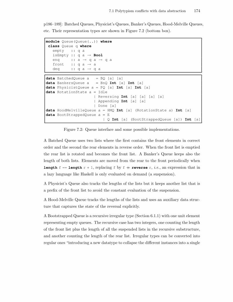
7.1 Polytypism conflicts with data abstraction 174
p186–189]: Batched Queues, Physicist’s Queues, Banker’s Queues, Hood-Melville Queues,
etc. Their representation types are shown in Figure 7.2 (bottom box).
module Queue(Queue(..)) whereclass Queue q where
empty :: q aisEmpty :: q a → Boolenq :: a → q a → q afront :: q a → adeq :: q a → q a
data BatchedQueue a = BQ [a] [a]data BankersQueue a = BnQ Int [a] Int [a]data PhysicistQueue a = PQ [a] Int [a] Int [a]data RotationState a = Idle
| Reversing Int [a] [a] [a] [a]| Appending Int [a] [a]| Done [a]
data HoodMelvilleQueue a = HMQ Int [a] (RotationState a) Int [a]data BootStrappedQueue a = E
| Q Int [a] (BootStrappedQueue [a]) Int [a]
Figure 7.2: Queue interface and some possible implementations.
A Batched Queue uses two lists where the first contains the front elements in correct
order and the second the rear elements in reverse order. When the front list is emptied
the rear list is rotated and becomes the front list. A Banker’s Queue keeps also the
length of both lists. Elements are moved from the rear to the front periodically when
length f == length r + 1, replacing f by f ++ reverse r, i.e., an expression that in
a lazy language like Haskell is only evaluated on demand (a suspension).
A Physicist’s Queue also tracks the lengths of the lists but it keeps another list that is
a prefix of the front list to avoid the constant evaluation of the suspension.
A Hood-Melville Queue tracks the lengths of the lists and uses an auxiliary data struc-
ture that captures the state of the reversal explicitly.
A Bootstrapped Queue is a recursive irregular type (Section 6.1.1) with one unit element
representing empty queues. The recursive case has two integers, one counting the length
of the front list plus the length of all the suspended lists in the recursive substructure,
and another counting the length of the rear list. Irregular types can be converted into
regular ones “introducing a new datatype to collapse the different instances into a single
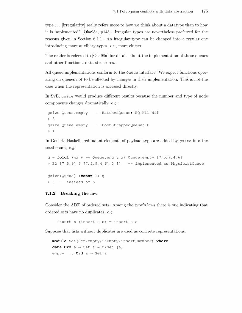
7.1 Polytypism conflicts with data abstraction 175
type . . . [irregularity] really refers more to how we think about a datatype than to how
it is implemented” [Oka98a, p143]. Irregular types are nevertheless preferred for the
reasons given in Section 6.1.1. An irregular type can be changed into a regular one
introducing more auxiliary types, i.e., more clutter.
The reader is referred to [Oka98a] for details about the implementation of these queues
and other functional data structures.
All queue implementations conform to the Queue interface. We expect functions oper-
ating on queues not to be affected by changes in their implementation. This is not the
case when the representation is accessed directly.
In SyB, gsize would produce different results because the number and type of node
components changes dramatically, e.g.:
gsize Queue.empty -- BatchedQueue: BQ Nil Nil
> 3
gsize Queue.empty -- BootStrappedQueue: E
> 1
In Generic Haskell, redundant elements of payload type are added by gsize into the
total count, e.g.:
q = foldl (λx y → Queue.enq y x) Queue.empty [7,5,9,4,6]
> PQ [7,5,9] 5 [7,5,9,4,6] 0 [] -- implemented as PhysicistQueue
gsize〈Queue〉 (const 1) q
> 8 -- instead of 5
7.1.2 Breaking the law
Consider the ADT of ordered sets. Among the type’s laws there is one indicating that
ordered sets have no duplicates, e.g.:
insert x (insert x s) = insert x s
Suppose that lists without duplicates are used as concrete representations:
module Set(Set,empty,isEmpty,insert,member) where
data Ord a ⇒ Set a = MkSet [a]
empty :: Ord a ⇒ Set a

7.1 Polytypism conflicts with data abstraction 176
empty = Set []
insert :: Ord a ⇒ a → Set a → Set a
insert x (MkSet xs) = MkSet ((sort nub) (x:xs))
. . .
Function nub removes duplicates from a list.
The application of gmap may introduce duplicate elements making the result a list that
is no longer a valid representation of a set. For example, mapping const 5 over the set
1, 2, 3 should yield 5. This is not the case:
s = foldr (λx y → Set.insert x y) Set.empty [1,2,3]
gmap〈Set〉 (const 5) s
> MkSet [5,5,5]
Ordered sets can also be implemented in terms of boolean vectors, where payload
elements are indices, or hash tables, where hashed payload elements are indices (Sec-
tion 5.6). However, the map function for a vector maps the elements in the vector, not
the indices, let alone the values to which a (perhaps non-invertible) indexing function
has been applied in order to obtain the indices.
Now consider the type of ordered trees of Section 5.7 which can be used to implement
binary search trees, ordered sets, and priority queues. Again, the application of map
over the implementation can break the structural invariants.
(7,A) (-7,A)/ \ ----> / \
(5,B) (9,C) (-5,B) (-9,C)
Figure 7.3: Mapping negation over a binary search tree representing a priority queueyields an illegal queue value.
Suppose an ordered tree implements a priority queue where the priority is given by an
integer value (Figure 7.3, left tree). If we invert priorities, mapping λ(x,y)→(-x,y),
the resulting tree (Figure 7.3, right tree) is not a valid representation of a priority
queue. The correct representation would be the mirror tree where the element with
highest priority in the left subtree has at most the root’s priority.
Consider a parameterised MemoList ADT supporting the following operators:
nil :: ([a] → a) → MemoList a
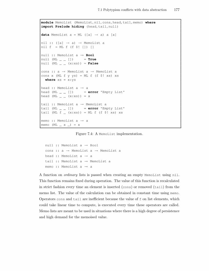
7.1 Polytypism conflicts with data abstraction 177
module MemoList (MemoList,nil,cons,head,tail,memo) whereimport Prelude hiding (head,tail,null)
data MemoList a = ML ([a] → a) a [a]
nil :: ([a] → a) → MemoList anil f = ML f (f $! []) []
null :: MemoList a → Boolnull (ML _ _ []) = Truenull (ML _ _ (x:xs)) = False
cons :: a → MemoList a → MemoList acons x (ML f y ys) = ML f (f $! xs) xs
where xs = x:ys
head :: MemoList a → ahead (ML _ _ []) = error "Empty List"head (ML _ _ (x:xs)) = x
tail :: MemoList a → MemoList atail (ML _ _ []) = error "Empty List"tail (ML f _ (x:xs)) = ML f (f $! xs) xs
memo :: MemoList a → amemo (ML _ x _) = x
Figure 7.4: A MemoList implementation.
null :: MemoList a → Bool
cons :: a → MemoList a → MemoList a
head :: MemoList a → a
tail :: MemoList a → MemoList a
memo :: MemoList a → a
A function on ordinary lists is passed when creating an empty MemoList using nil.
This function remains fixed during operation. The value of this function is recalculated
in strict fashion every time an element is inserted (cons) or removed (tail) from the
memo list. The value of the calculation can be obtained in constant time using memo.
Operators cons and tail are inefficient because the value of f on list elements, which
could take linear time to compute, is executed every time these operators are called.
Memo lists are meant to be used in situations where there is a high degree of persistence
and high demand for the memoised value.

7.1 Polytypism conflicts with data abstraction 178
Figure 7.4 shows an obvious implementation. The infix strict application $! eagerly
evaluates its second argument and then the application of its first argument to the
result. The representation value ML f m xs represents an f-memoised list with the
implementation invariant m = f xs. Ordinary list operators can be readily programmed,
e.g.:
mlength :: MemoList a → Int
mlength ml = if null ml then 0 else 1 + mlength (tail ml)
And we expect typical list equations to hold:
mlength (mconcat xs ys) == mlength xs + mlength ys
(Unfortunately, the type-checker cannot stop mconcat from concatenating memoised
lists built using different memoised functions of the same type, for function equality is
undecidable.)
Generic Haskell’s gsize counts the memoised value.1 But more worryingly, the ap-
plication of gmap can easily break the implementation invariants and produce concrete
values that do not represent values of the ADT:
mlA = cons 1 (cons 1 (cons 1 (nil sum)))
mlB = cons 1 (cons -2 (cons 3 (nil max)))
gsize〈MemoList〉 (const 1) mlA
> 4 -- should have been 3
gmap〈MemoList〉 (+1) mlA
> ML ? 4 [2,2,2] -- sum yields 6 not 4
gmap〈MemoList〉 negate mlB
> ML ? -3 [-1,2,-3] -- max yields 2 not -3
Broadly speaking, the instance of gmap for MemoList behaves thus:
gmap〈MemoList〉 g (ML f m xs) = ML f (g m) (gsize〈List〉 g xs)
The implementation invariant breaks when g m 6= f (gmap〈List〉 g xs).
1In point of fact, gsize (Figure 6.5) must provide a case for the arrow type operator or theapplication would produce a run-time error: memoised lists contain functions as data.
7.1 Polytypism conflicts with data abstraction 179
7.1.3 On mapping over abstract types
Some readers may wonder whether ‘map’ is justified in the case of non-free types.
Categorially, a type is a functor if we can define its map function that satisfies the
functorial laws:
map id = id (7.1)
map (f g) = map f map g (7.2)
The bits of category theory described in Chapter 3 assumed an unboundedly poly-
morphic world. It is because of this parametricity assumption that properties of poly-
morphic programs (natural transformations) can be obtained directly from their types
(functors) [Rey74, Wad89].
The map function for unbounded ADTs (Section 5.10) must respect the number and
position of elements. However, for bounded ADTs this does not have to be the case:
there are context-dependent properties such as ordering, lack of repetition, etc, that
must be preserved by map.
Let us concretise the point. Think of unbounded ADTs such as lists, stacks, FIFO
queues, etc. For these ADTs the following equation is upheld by map:
map f (con x y) == con (f x) (map f y)
Here con stands for the binary constructor. Replace con by cons in the case of lists,
by push in the case of stacks, and by enq in the case of FIFO queues. The fact that
stacks and queues are subject to more equations is an orthogonal issue that relates to
how map is actually defined in terms of the available observers. In particular, FIFO
queues do not satisfy the product law:
con (exl q) (exr q) == q
where con is enq, exl is front, and exr is deq (Section 9.4).
The map equation may not hold for bounded ADTs, as demonstrated by all the ex-
amples in Section 7.1.2. Replace con by insert in ordered sets or enq in priority
queues and the equation only holds when map preserves the order. Consequently, in
the previous examples gmap is not the right function to apply to these ADTs, but a
law-abiding gmap that preserves the semantic properties of the ADTs.

7.1 Polytypism conflicts with data abstraction 180
Is such function really a map? It is if it satisfies the functorial laws. Take ordered
sets, for instance. First, let us make Set an instance of Functor. We use a multi-
parameter type class Functor because Set’s implementation type is constrained by
Ord and therefore we cannot make Set an instance of the Functor class provided by
the Haskell prelude [MJP97]:
class Functor f a b where
map :: (a → b) → f a → f b
instance (Ord a, Ord b) ⇒ Functor Set a b where
map f (MkSet xs) = MkSet ((sort nub map f) xs)
Notice the overloading: map on the right hand side is map on lists.
Set is a functor not because it has been made an instance of Functor but because the
definition of map satisfies the functorial laws. Let us use the following abbreviation:
φ = sort nub
Equation (7.1) is trivial to prove: if the set is empty then map returns another empty
set, and the identity of an empty set is an empty set. If the set is not empty then the
identity is mapped over the list which is not changed.
Equation (7.2) is also trivial to prove for the case of empty sets. For the non-empty
case, let us first expand the left hand side of Equation (7.2):
map (f g) (MkSet xs)
= def. of map for Set
MkSet ((φ map (f g)) xs)
= List is a functor
MkSet ((φ map f map g) xs)
Let us now expand the right hand side:
map f map g (MkSet xs)
= def. of map for Set
map f (MkSet ((φ map g) xs))
= def. of map for Set
MkSet ( (φ map f) ((φ map g) xs) )
= composition

7.1 Polytypism conflicts with data abstraction 181
MkSet ((φ map f φ map g) xs)
Both expansions are equal if the following holds:
φ map f map g = φ map f φ map g
We can prove this is the case using the definition of φ at this point.
However, let us indulge in a more general discussion: What is φ? It is a function
that is applied to a value of the implementation type in order to make it satisfy the
implementation invariants. In the case of ordered sets, it sorts and removes repetitions
from the list.
We can provide a better definition of such repairing functions in terms of the whole
implementation type. For ordered sets:
ϕ (MkSet xs) = MkSet (φ xs)
A map on sets is obtained by mapping over the payload type (list) and then applying
ϕ to re-establish the implementation invariants:
map f (MkSet xs) = ϕ (MkSet (map f xs))
In balanced trees, ϕ performs the balancing. In binary search trees, ϕ turns a BTree
into a binary search BTree, etc.
Recall the implementation type of memo lists from Section 7.1.2:
data MemoList a = ML ([a] → a) a [a]
The map for MemoList is defined as follows:
instance Functor MemoList where
fmap f (ML g x xs) = ML g (g ys) ys
where ys = map f xs
In other words:
fmap f (ML g x xs) = ϕ (ML g x (map f xs))
where ϕ (ML g x xs) = ML g (φ g xs) xs
φ g xs = g xs
Again, the payload part of the concrete type is mapped and the implementation in-

7.2 Don’t abstract, export. 182
variant is maintained by ϕ. Notice that g and x are implementation clutter and g is a
function component that cannot be mapped by Generic Haskell’s gmap (Section 6.1.2).
However, the ADT is a functor, for we can define a map that satisfies the functorial
laws.
Summarising, a map for a bounded ADT may be defined in terms of a function that
maps over the payload parts of the implementation type and another function ϕ that
re-establishes implementation invariants. The ADT is a functor if the functorial laws
are satisfied.
We conclude the section discussing the impact of these issues on Generic Programming.
Set has been made an instance of Functor by defining map in terms of the implement-
ation type. Therefore, it is assumed that the instance declaration has been written
by the ADT implementor. However, our aim is to program a generic map outside the
ADT. If we attempt to define it in terms of the implementation type then we have to
somehow figure out ϕ polytypically for any given ADT. This is not only a Herculean
task; if the representation changes, it is also useless, for ϕ is no longer valid. However,
the reader may have noticed that ϕ’s job is already performed by insert! Interface
operators seem to be part of the solution.
7.2 Don’t abstract, export.
Section 6.1.12 discussed the drawbacks of providing fixed values for units and base types
in polytypic function definitions. Programming with ADTs worsens the situation. It
is impossible to give a meaningful case for all possible non-parametric (kind-∗) ADTs
in polytypic function definitions. It may not be possible physically or logically to turn
them into parameterised ADTs by abstracting over the payload type.
An example: an event-driven GUI system keeps a queue of events. The type has been
defined in a module:
module EventQueue (EventQueue,empty,isEmpty,enq,deq,front) where
import Event
import Queue
data EventQueue = mkEQ (Queue.Queue Event.EventType)
empty = mkEQ Queue.empty
isEmpty (mkEQ q) = Queue.isEmpty q

7.2 Don’t abstract, export. 183
. . .
Type EventQueue is an ADT whose implementation in terms of a Queue ADT is hidden
(the module only exports the type name and the operators). EventQueue is defined as
a new type, not a type synonym, to enforce abstraction further. Programmers writing
other parts of the GUI only know about the interface, and write their code accordingly.
EventQueue is a manifest type. It plays the same role as a kind-∗ basic type. Generic
Haskell’s gsize on an EventQueue value always returns 0 and gmap is the identity.
Let us leave aside the fact that EventQueue could have been bundled by a third-party
provider as part of a pre-compiled library and its representation type would therefore
be unknown (the library is closed source) and physically inaccessible. It makes no sense
to abstract EventQueue into EventQueue a, for a is always Event.EventType; this
is tantamount to using Queue directly. Abstraction is necessary only to use polytypic
functions:
type EventQueue = Queue.Queue Event.EventType
q :: EventQueue
gsize〈Queue.Queue〉 (const 1) q
The type synonym is used everywhere in the program but polytypic function applic-
ations. The situation is rather strange: the programmer uses the type synonym and
thinks in terms of EventQueue but has to use Queue.Queue when calling polytypic
functions.
Now consider this scenario: after some beta testing, EventQueue implementors decide
to use a direct implementation in terms of their own fancy queue type:
data EventQueue = EmptyQueue | Fancy [Event] Int Blah Blahdiblah . . .
Polytypic applications with Queue.Queue become affected by this change.
It would be preferable for polytypic functions to be able to cope with the types in a
software design than to adapt the software design to what polytypic functions can or
cannot do.
Finally, it will be common for manifest ADTs to be used in the implementation of other
manifest ADTs. We are faced with a cascading chain of abstractions which would force
programmers to, pretty much, give up encapsulation:

7.3 Buck the representations! 184
module ProcessQueue(ProcessQueue,empty,isEmpty,enq,deq,front) where
import Process
import Queue
data ProcessQueue = PQ (Queue.Queue Process.ProcessType)
. . .
module ProcessManager(ProcessManager,create,run,kill) where
import Process
import qualified ProcessQueue as ProcQ
data ProcessManager = PM
current :: Process.ProcessType,
sleeping :: ProcQ.ProcessQueue,
running :: ProcQ.ProcessQueue
. . .
Another worrying aspect of abstracting over payload is that it might dredge paramet-
ricity constraints, affecting interfaces and client code. Using EventQueue is simple:
programmers create EventType values and store them in values of EventQueue. Us-
ing Queue requires knowledge of the type’s constraints. If implemented as a binary
search tree, the constraint Ord becomes visible or, worse, other constraints imposed by
the representation type implementing Event.EventType, some of which may be type
classes only known by implementors.
What is needed is a different linguistic mechanism that allows manifest ADTs to in-
dicate or export payload types. It is straightforward to have EventQueue’s interface
specify that its payload is Event.EventType. It is a different thing to have to work
with Queue whose payload we know it always to be Event.EventType. The payload
type remains the same even if the implementation of the container changes, or even if
the interface changes. Exporting is explored in Chapter 9.
7.3 Buck the representations!
The reader only needs to glance through the functional data structures in [Oka98a] to
realise the gap between concrete representation types and abstract types. The former
are bigger. They contain implementation clutter: values that capture properties of the
structure such as size, rank, depth, etc; or parts of the structure itself, or distinguished
payload elements, or even part of the data structure’s state represented as data (e.g.,

7.3 Buck the representations! 185
Hood-Melville queues).
The examples in this chapter are simple. One could provide more complicated examples
of rather obscure representation types but we would have to explain their purpose. Some
ADT implementations are quite a feat of engineering and cleverness, and the systematic
study of efficient functional data structures is still an ongoing field of research.
At any rate, our examples illustrate the hoary point that accessing concrete repres-
entations may produce unintended results and may break implementation invariants
and semantics. This is why concrete representations are hidden behind an interface of
operators that maintain them and enable construction and observation (a view) of the
relevant data.
Polytypic functions are no different from ordinary functions in this regard. Their ‘gen-
ericity’ is due to structural parametrisation alone.
It is perfectly conceivable for future languages to enable compilers to choose ADT
implementations at compile-time based on operator-usage analyses. It is also possible
for a program to manipulate simultaneously different implementations of the same ADT
as long as they are not mixed up in operations. Finally, implementations may change,
but results produced by client code should not.
There are situations in which data seldom changes. A well-designed abstract syntax
tree is rarely changed and compilers usually manipulate its concrete representation dir-
ectly. But more often than not, implementors have to prepare for change. Generic
Programming is about making this preparation unnecessary with respect to code: gen-
eric functions work for all types or, at least, for a big set of types. Polytypic function
definitions should not change when the data changes and should provide accurate and
meaningful results. In short, polytypic functions must not access the concrete defini-
tional structure of ADTs. The reader may wonder how structural polymorphism may
be possible at all. It depends on what we mean by ‘structure’ (Chapter 9).

Chapter 8
Pattern Matching and Data Abstraction
Pattern matching and data abstraction are important concepts. . . but
they do not fit well together. Pattern matching depends on making
public a free data type representation, while data abstraction depends
on hiding the representation. [Wad87]
In Chapter 7, we have argued that polytypic programming conflicts with the principle
of data abstraction. Pattern matching is another language feature that conflicts with
data abstraction, for pattern matching is performed upon unencapsulated, concrete
data types, and therefore its applicability is limited to within the modules implement-
ing ADTs. There are several proposals for reconciling pattern matching with data
abstraction and the first thing that comes to mind is to investigate whether they can
be of any use in reconciling polytypic programming with data abstraction—polytypic
functions pattern-match over concrete definitional structures.
There are two major approaches for reconciling pattern matching and ADTs. The first
approach is based on providing views of the ADT in terms of exported concrete types
together with translation functions from the ADT’s internal concrete representation to
the exported view and vice-versa [Wad87]. The second approach is based on providing
only one translation, keeping constructor operators and turning some discrimination
and selection operators into pattern expressions which, logically, are syntactic sugar for
the former [PPN96, WC93].
In this chapter we review why the first approach is not satisfactory (in fact, it has been
dropped entirely) and why the second approach is of limited help. We also describe
other less well-known, and even less suitable, approaches. We provide the chapter’s
conclusions upfront in the next section and elaborate the details in the remaining
sections.
186

8.1 Conclusions first 187
8.1 Conclusions first
In this chapter we overview the most popular approaches for reconciling pattern match-
ing with data abstraction. These are some of the lessons to be learned from them:
1. Pattern matching is, logically, syntactic sugar for observation.
2. Trying to evolve the value-constructor concept for observation leads to problems.
More precisely, construction and observation may not be inverses and therefore must
be separated. The latter may be provided by some pattern-matching construct. The
former should be performed by ordinary ADT operators.
3. For pattern matching to be effective, it must be possible for computation to take
place at matching time; i.e., effective component selection requires computation.
4. Relying on canonical values is deprecated.
Generic Haskell and SyB are oblivious to the second point in the list. We could embark
on a project to adapt them accordingly, but this is downplayed by the remaining points.
In order to program polytypic functions on ADTs it is necessary to define a uniform
notion of structure. Interfaces may provide such structure. The introduction of elabor-
ated pattern-matching mechanisms and their luggage (e.g., changes to the type system,
possible undecidabilities, etc) is an extra complication, and there is the problem that
construction must take place via operators.
But polytypic functions can be defined in terms of ADT operators. At the end of the
day, ADT operators provide a ‘view’ of an implementation type. In ordinary program-
ming the need for pattern matching is more pressing: there are issues of conciseness,
readability, structural definitions and proofs, etc. In Generic Programming these pres-
sures are localised in the definition of generic functions, which can be provided in two
parts (construction and observation) based on the structure of interfaces (Chapter 9).
8.2 An overview of pattern matching
Conceptually, data types are either concrete or abstract (Section 4.2). In functional
languages, concrete types are either primitive types or algebraic types (Section 6.1.1).
At the value level, algebraic types introduce a free algebra (Chapter 5) generated by a

8.2 An overview of pattern matching 188
Pattern ::= Variable
| ValueConstructor Pattern∗
| ( Pattern, Pattern (, Pattern)∗ )
Figure 8.1: A simple language of patterns consisting of variables, value constructorsapplied to patterns, and n-ary tuples of patterns.
set of value constructors which play several roles. More concretely, given the Haskell
data type definition template introduced in Section 6.1.1:
data Q⇒ T a1 . . . an = C1 τ11 . . . τ1k1| . . . | Cm τm1 . . . τmkm
value constructors Ci play the following roles:
1. Introduction (construction), e.g., a term C1 t11 . . . t1k1introduces (constructs) a
value of the algebraic type, where t1j is an arbitrary term of type τ1j .
2. Representation (freeness), e.g., the term C1 t11 . . . t1k1represents (denotes) a value.
Unlike regular functions, the value computed by an application of a value con-
structor to its arguments is denoted by the application itself. Thus, values carry
their structure explicitly. This is possible because there are no equations between
value constructors that suggest the need of further computation in order to satisfy
them.
3. Elimination, e.g., the pattern C1 p11 . . . p1k1, where p1j are sub-patterns, can be
used for discriminating among sum values of an algebraic type and for selecting the
product components. Patterns are allowed in case expressions of core languages,1
and in top-level function definitions, lambda abstractions, and let-expressions of
most fully-fledged functional languages. A small language of patterns is shown in
Figure 8.1.
Notice that patterns can be nested ; an example would be Cons x (Cons y ys).
Of particular interest are simple patterns of the form C x1 . . . xn where C is a
value constructor and xi are variables. If the variables are all different the pattern
is linear . Writing the same variable in different positions imposes an equality test:
the values matched against the various occurrences must be the same.
1Case expressions for pattern matching are more general than those of Section 2.7.2 which onlypattern-match against values of a sum type.

8.2 An overview of pattern matching 189
4. Value constructors also play the less conspicuous role of aids to the type checker and
of enabling the definition of iso-recursive type operators [Pie02, p275–277,445].
The first three roles are illustrated by the following function definition:
insert :: Eq a ⇒ a → List a → List a
insert x Nil = Cons x Nil
insert x (Cons y ys) = if x == y then Cons y ys
else Cons y (insert x ys)
which is sugar for a definition by case expression:
insert x l = case l of
Nil → Cons x Nil
(Cons y ys) → if x == y then Cons y ys
else Cons y (insert x ys)
The term Cons y ys is used as a pattern in the left hand side of the second arrow and
as a term on the right hand side. As a pattern it discriminates whether the second
argument to insert is constructed using Cons and binds the new variable y to the value
of the first product component, and the new variable ys to the value of the second.
Finally, there is computation with selected values at each discriminated branch.
Technically, the matching process consists of the application of a boolean predicate
(discriminator) followed by an optional process of selection, binding into locally-defined
variables, and computation with selected components. As rightly pointed out in [Pal95,
p4], unification in logic programming languages is a similar but more expressive con-
struct than pattern matching.
Without pattern matching, insert would be written using list operators in a style
familiar to LISP programmers:
insert x l = if null l -- discrimination
then cons x nil -- computation
else let y = head l -- selection and binding
ys = tail l
in cons y (insert x ys) -- computation
This is also the manner in which insert would be written if the list type were abstract.

8.2 An overview of pattern matching 190
With pattern matching, discrimination and selection are expressively combined and
can be compiled effectively. The number of discriminated alternatives (number and
name of value constructors) is fixed and known at compile time so, depending on the
language of patterns, it is possible to check statically whether alternatives overlap or
are exhaustive, i.e., whether patterns in case expressions capture all possible forms of
values. However, partial operators and polymorphic non-terminating terms are allowed
in functional languages, making it possible to write case expressions that produce run-
time errors or do not terminate:2
case l of Nil → head l . . .
But what goes on to the left of the arrow is safe, i.e., discrimination between the
alternatives of a disjoint sum can be exhaustive and selection of product components
into local variables is type-safe.
Another benefit of pattern matching is conciseness and expressiveness. The first defin-
ition of insert is easier to read and understand. It closely follows the structure of the
data it works on. Properties on well-ordered, recursive algebraic types can be proven
by structural induction [Mit96]. Pattern matching can also be used when defining
functions over co-recursive algebraic types and in their proofs [GH05].
However, pattern matching is incompatible with data abstraction, for patterns are
meant to capture the concrete structure of a value. It has also other disadvant-
ages [Tul00, p3]:
1. Pattern matching imposes an evaluation order: patterns in case expressions are
evaluated from left to right and from top to bottom. This has consequences on
the semantics of functions and therefore on how they must be defined. A typical
example is the zip function. The reason for an evaluation order comes from how
nested patterns are decomposed into nested case expressions with simple patterns.
2. Pattern matching “begs for extension upon extension”: there are irrefutable pat-
terns, as patterns, guarded patterns, etc.
3. Patterns can be nested and make it difficult for the eye to determine whether they
2Undefined terms enable the definition of partial operators. The reader should bear in mind thedifference between undefined and non-terminating terms. The former are stuck terms, the latter haveno normal form.

8.3 Proposals for reconciliation 191
overlap or are exhaustive, e.g.:
foo Nil = . . .
foo (Cons 1 Nil) = . . .
foo (Cons _ xs ) = . . .
In fact, testing for exhaustiveness may be toggled off or demoted into a warning:
“partial but total” auxiliary functions are not atypical. For example, although local
function bar is partial, it is always supplied a value on its domain:
foo Nil = 0
foo xs = bar xs
where bar (Cons y ys) = . . .
4. It is important to differentiate between patterns and terms: patterns introduce new
variables and have different semantics, e.g.:
λl → let x = Nil in case l of x → 0 . . .
Pattern matching over sums of products demonstrates how low-level these data defin-
ition mechanisms are and the pitfalls of positional selection. Named records provide
a much better abstraction mechanism as shown below—the example is adapted from
[Pal95, p9]:
data Person = P String String Int . . .
birthday :: Person → Person
birthday (P f s a . . . ) = (P f s (a+1) . . . )
data Person = Pname::String, surname::String, age::Int, . . .
birthday :: Person → Person
birthday (person@Page = a,_) = personage ← a + 1
In the last line, pattern matching only requires the value of the age field, which gets
‘updated’ by the function. Notice also the possibility of record subtyping and the
closeness to ADT programming.
8.3 Proposals for reconciliation
The following sections outline the most important proposals for reconciling pattern
matching with data abstraction.

8.3 Proposals for reconciliation 192
8.3.1 SML’s abstract value constructors
Abstract value constructors are an implemented feature of the ‘Standard ML of
New Jersey’ compiler [AR92]. Strictly speaking, they are not really a proposal for
reconciling pattern matching with data abstraction, but can be used for that purpose
in restricted situations.
An abstract value constructor C is defined as follows:
C x1 . . . xn match P
where to the left of match there is a simple linear pattern and to the right an arbitrary
SML pattern P . The compiler replaces the left hand side by the right hand side, i.e.,
abstract value constructors are macro-substituted by ‘real’ patterns.
Abstract value constructors can be used in pattern matching and in construction. This
double role imposes restrictions on the simple pattern and on P :
• When used in pattern matching, P must be linear and must contain all the variables
of the simple pattern. For example, the following abstract value constructors are
illegal:
C x y match C’ x
C x match C’ x x
In the first line, variable y is defined and, therefore, possibly used on the right hand
side of the arrow in a case expression, but nothing is matched against it when the
abstract value constructor is macro-expanded to C’ x. In the second line, a linear
pattern is macro-expanded into a non-linear one.
• When used in construction, all the variables in P must occur in the simple pattern.
Look at this illegal example:
C x match C’ x y
If the left hand side is macro-expanded to the right-hand side, variable y is not
bound to any value and the term cannot construct anything.
The following is an example of an abstract value constructor that can be used in pattern
matching and construction:

8.3 Proposals for reconciliation 193
data Complex = Complex Real Real
PureReal r match Complex r 0
Functions on complex numbers can be defined by pattern matching over PureReal.
foo (PureReal r) = . . .
foo (Complex r i) = . . .
We can write foo’s body in the second case under the premise that i 6= 0.
Abstract value constructors are not only limited in expressibility because of their use
in patterns and construction, but also because selection does not involve computation.
Recall the FIFO-queue ADT of Chapter 7, in particular the BatchedQueue implement-
ation of Section 7.1.1. It would be very interesting to be able to define two abstract
value constructors Empty and Enq for pattern matching over FIFO-queue values, e.g.:
Empty match BQ [] []
Enq x q match BQ (x::xs) r
Unfortunately, Enq’s definition is illegal and we need some way of specifying computa-
tion:
q = xs @ (reverse r)
8.3.2 Miranda’s lawful concrete types
The functional programming language Miranda supports so-called lawful algebraic
types which are algebraic types with equations between value constructors [Tho86].
These equations are actually rewrite rules for transforming values into canonical ones.
Consequently, rewrite rules must be confluent and terminating.
More precisely, a value of the concrete representation type may not represent a value of
the ADT (junk), and multiple values of the concrete representation type may represent
the same ADT value (confusion). One way of supporting pattern matching and equality
on concrete types is to normalise every constructed value into a canonical value so that
patterns are matched against, and equality is performed on, canonical values that
uniquely represent ADT values.3
There follows an example of a lawful concrete type for sets implemented as lists or,
3Notice that canonical values may still contain implementation clutter.

8.3 Proposals for reconciliation 194
more precisely, as an algebraic type structurally isomorphic to the List type:
data Eq a ⇒ Set a = Empty | Insert a (Set a)
Insert x (Insert y s) == if x == y then Insert y s
else Insert y (Insert x s)
Insert 1 (Insert 1 (Insert 2 Empty))
> Insert 2 (Insert 1 Empty)
Notice the equation involving abstract value constructor Insert. The equation shows
that value constructor Insert plays not only the role of a constructor but also the
role of a normalisation function. More precisely, the lawful type has the following
normalisation function:
insert :: Eq a ⇒ a → Set a → Set a
insert x Empty = Insert x Empty
insert x (Insert y s) = if x == y then Insert y s
else Insert y (insert x s)
The problems with this approach are not difficult to see:
1. Checking that rewrite rules are confluent and normalising requires a lot of effort and
is, in the general case, undecidable.
2. Normalisation into canonical values is inefficient, forces particular representations,
and might not be possible or recommended. Recall the FIFO-queue implementa-
tions of Section 7.1.1 which relied on unevaluated data components to achieve their
amortised efficiency.
3. There is not that much abstraction from the representation: functions working on
values of type Set a are defined by pattern matching on Empty and Insert but we
might want to change the implementation. Wadler’s views (Section 8.3.3) argues for
these two value constructors to be part of a view of the Set type.
4. Selection involving computation is not possible during pattern matching: normal-
isation takes place during construction, not matching.
5. There are serious problems with equational reasoning: the fact that patterns are
matched against values in canonical form is not reflected in the values themselves.
For example, given the following definition:

8.3 Proposals for reconciliation 195
select (Insert x s) = x
the following equations hold:
1
== select’s definition
select (Insert 1 (Insert 2 Empty))
== Insert’s definition
select (Insert 2 (Insert 1 Empty))
== select’s definition
2
In order to reason with values of the concrete type we have to reduce them to normal
form and therefore know the details of the implementation. In particular, the clients
of Set should not be obliged to know details of normalisation.
8.3.3 Wadler’s views
A lawful type in Miranda is a subset of a concrete type: its canonical forms. In con-
trast, Wadler’s views [Wad87] specify an isomorphism between subsets of concrete
types. This becomes particularly useful when dealing with ADTs, for they can be
implemented by many concrete types. ADT designers may choose one of these types
as the implementation type and allow clients to work with (possibly many) view types
isomorphic to (a subset of) the implementation type. Value constructors of the view
type can be used in pattern matching and construction. Because of this double role,
there must be a correspondence between each view type and implementation type, and
vice versa.
An illustrative example is perhaps the type of natural numbers. The Peano represent-
ation in terms of Zero and Succ is handy but inefficient. Programmers usually work
with the base type of positive integers.4 An ADT of natural numbers can be imple-
mented in terms of positive integers but viewed in terms of its Peano representation.
A possible syntax for declaring this follows:
view Int = Zero | Succ Int
4Surprisingly, natural numbers are rarely offered as a base type by most functional programminglanguages.

8.3 Proposals for reconciliation 196
where
in n
| n == 0 = Zero
| n > 0 = Succ (n-1)
| otherwise = error "Negative Integer"
out Zero = 0
out (Succ n) = n + 1
The keyword view declares that Int can be viewed as a recursive algebraic type with
Peano value constructors. Behind the scenes, the compiler translates this view into the
following non-recursive type:
data View = Zero | Succ Int
Functions in and out are translation functions from the implementation type to the
view type and vice versa:
in :: Int → View
out :: View → Int
We need two functions because Peano value constructors may occur in pattern matching
(which requires calls to in) and construction (which requires calls to out).
The factorial function can be defined on the Peano view:
factorial :: Int → Int
factorial Zero = Succ Zero
factorial (Succ n) = (Succ n) ∗ factorial n
The definition can be translated by the compiler to a factorial on integers by inserting
calls to in and out at appropriate places:
factorial :: Int → Int
factorial n = case (in n) of
Zero → out (Succ (out Zero))
Succ n → (out (Succ n)) ∗ factorial n
Functions in and out are similar in spirit to the embedding-projection pairs of Sec-
tion 6.1.4. These functions must be inverses of each other and this cannot be checked
by a compiler.
In particular, out must be total and injective or otherwise it would introduce junk and

8.3 Proposals for reconciliation 197
confusion respectively: there would be values of the view type that are not represented
in the implementation type, and there would be values of the view type that would
have the same representation in the implementation type, thus introducing an implicit
equation between the former values.
Also, in must be injective and its domain must be out’s image. If the domain is a
proper superset, there are implicit equations in the implementation type. If the domain
is a proper subset, there is junk in the implementation type.
Moreover, it might not be possible for a view type and an implementation type to
satisfy them: for instance, it might be the case that a value of the view type is al-
ways representable by multiple values of the implementation type. Palao [Pal95, p32]
illustrates this situation using complex numbers where the implementation type is the
cartesian representation and the view type the polar representation. Multiple repres-
entations introduce implicit equations which hinder equational reasoning. This is the
main reason why Wadler’s views were not included in the Haskell definition. Other
problems with views are [Pal95, Chp4]:
1. The need to take into account the side conditions of functions in and out during
equational reasoning.
2. The fact that seemingly total functions are indeed partial. For example, in the
factorial example, with the Peano representation the function triggers a run-time
error if fed a negative integer. Haskell’s type system cannot check statically whether
Succ is always applied to positive integers during construction.
3. It might be the case that values of the view type should be given in some canonical
form (e.g., complex numbers in polar representation), again introducing implicit
equations.
4. There is a logical separation between pattern matching and construction. Using
value constructors for both makes no sense in many situations. Take for example a
BatchedQueue implementation of queues (Chapter 7):
data BatchedQueue a = BQ [a] [a]
data View a = EmptyQ | Front a (Queue a)
Queue elements must be inserted at the rear of the queue, yet value constructor

8.3 Proposals for reconciliation 198
Front can be used for construction. Notice that introducing an extra value con-
structor:
data View a = EmptyQ | Front a (Queue a) | Enq (Queue a) a
would also introduce an implicit equation: the same queue value can be pattern-
matched against a Front pattern and a Enq pattern. These two value constructors
are not free among themselves. In general, all possible observations cannot be cap-
tured by a single view.
5. However, it is illegal, for implementation reasons, to do pattern matching on different
view types simultaneously. In the BatchedQueue example, we could have provided
the Enq pattern in a different view but we would not be able to pattern match
against Front and Enq simultaneously. This is unproblematic for simple queues but
not so for double-ended queues, where insertion can take place either at the front or
at the rear.
6. Finally, there are many possible ways in which different ADT operations could be
expressed in terms of view types; implementing all of them could be too expensive.
Most problems with Wadler’s views are due to the double role of value constructors
in view types. This is pointed out in [WC93], where view types are restricted to
pattern matching alone, with construction carried out by operators. The out function
disappears and there is no restriction on in. However, pattern matching over different
view types is still illegal because of implementation reasons: the representation type is
transformed into the view type before the matching is performed.
8.3.4 Palao’s Active Patterns
According to Palao et al [PPN96, p112], the limitations of the previous approaches
stem from trying to “evolve the [value] constructor concept instead of starting the
problem from scratch”. For instance, Wadler’s views are a way for programmers to
move across possible implementation types, but observation is performed by means
of a value constructor. In non-free types, construction and observation may not be
inverses. For example, FIFO queues are constructed by inserting elements at the rear
whereas selection from non-empty FIFO queues takes place at the front. Construction
and observation must be separated.

8.3 Proposals for reconciliation 199
As underlined in Section 8.2, observation consists of discrimination followed optionally
by selection and binding of selected values into new local variables. Pattern matching
is just syntactic sugar for this, with added checks for overlapping and exhaustive cases.
Nested patterns only add expressibility to nested observation.
This is the idea behind Palao’s Active Patterns [Pal95, PPN96], which can be
regarded as an extension of SML’s abstract value constructors (Section 8.3.1) where
there can be computation after the matching is performed (hence the ‘active’) and their
use in construction is banned.
The language of Active Patterns is built from ordinary patterns, active destructors,
and compositions of Active Patterns via the @ operator, which is explained shortly:
AP ::= Variable
| ValueConstructor AP∗
| ActiveDestructor AP∗
| AP @ AP
The main advantages of Active Patterns are their expressibility, their support for equa-
tional reasoning, and their smooth integration with algebraic specifications, the latter
an important aspect that is ignored by the previous approaches. ADT operators can be
replaced, expressed, or accompanied by active destructors whose axiomatic semantics
are defined in terms of the operators themselves.
An active destructor consists of a label together with optional positional arguments:
the label denotes an alternative and the positional arguments are expressions that
select components. The translation goes from the implementation type to the active
destructor (the ‘view’), which is not a concrete type, and translation takes place after
matching.
For example, given an ADT of complex numbers:
module Complex(Complex,realPart,imgPart,modulus,argument) where
data Complex = Complex Real Real
. . .
any operator could be provided as an active destructor. For example:
RealPart r match Complex r _
Modulus m match Complex r i where m = sqrt (rˆ2 + iˆ2)

8.3 Proposals for reconciliation 200
The first active destructor, RealPart, is a projection identical to an SML abstract
value constructor. The second, Modulus, is also a projection but the projected value m
involves a computation which is performed after matching. The reader should not be
conned by the notation: if Modulus were an ordinary value constructor then m would
match Modulus’s argument. In contrast, m is an output value and, therefore, the type
of Modulus is not Real → Complex. It is not a function and cannot be used for
construction. (Types for active destructors are mentioned at the end of the section.)
Informally, the operational semantics of the matching process is as follows. Suppose
function foo has one case involving Modulus:
foo (Modulus m’) = E
where E is an expression where m’ may occur free. In the application foo e, the value
of e is pattern-matched against the ordinary pattern Complex r i. If the matching
succeeds, then we have in m’ the modulus of the complex number—the value of m in
the active destructor’s definition.
Pattern matching occurs behind the scenes, respecting data abstraction: the matching
of e’s value against the concrete type and the computation involved in getting the
modulus is hidden from foo’s writer, who only cares about having the value of the
modulus in m’ when the matching succeeds.
In code, foo’s definition involving Modulus is equivalent to:
foo = λe → case e of
Complex r i → E where m’ = sqrt (rˆ2 + iˆ2)
Variables r and i only occur free in the definition of m’, and m’ may occur free in E.
It becomes clear now that Modulus is just an abstract label. It does not play any role
in the compiled code.
We have used a local variable m in the definition of Modulus but the selecting expression
can be written directly in the active destructor:
Modulus (sqrt (rˆ2 + iˆ2)) match Complex r i
FIFO queues illustrate the expressibility of active destructors, which can be provided
by the interface. For example, in a BatchedQueue implementation:

8.3 Proposals for reconciliation 201
EmptyQ match BQ [] []
Front x match BQ (x:_) _
Deq q match BQ [_] r where q = BQ (reverse r) []
Deq q match BQ (_:f) r where q = BQ f r
Because matching takes place over the ordinary patterns after the match keyword, we
can provide multiple definitions of the same active destructor, in this case Deq. We
could have provided a single active destructor Deq’ that selects both the front and the
remaining queue.
The following function uses the previous active destructors:
sizeQ :: Queue a → Int
sizeQ EmptyQ = 0
sizeQ (Deq q) = 1 + sizeQ q
To belabour the point, active destructors EmptyQ and Deq hide the representation type
BQ. A Queue value could be implemented as a physicist’s queue or what have you.
Function sizeQ would not be affected as long as active destructors are defined for the
new implementation.
The following function illustrates the use of @:
showQ :: Show a ⇒ Queue a → String
showQ EmptyQ = ""
showQ (Front x)@(Deq q) = show x ++ showQ q
Here, the @ operator matches showQ’s argument against Front and Queue, obtaining
the appropriate values for x and q if the matching succeeds.
We can define the aforementioned Deq’ active constructor in terms of Front and Deq
using @:
Deq’ x q match (Front x)@(Deq q)
Indeed, the pattern on the right can be an Active Pattern (but active destructors cannot
be directly recursive). Now:
showQ :: Show a ⇒ Queue a → String
showQ EmptyQ = ""
showQ (Deq’ x q) = show x ++ showQ q

8.3 Proposals for reconciliation 202
In functional languages, @ is used for ‘as patterns’ where the ordinary pattern x@p
matches an argument against the ordinary pattern p but binds x to the argument.
Generalising from the fact that variable x is itself a pattern, given two Active Patterns
p1 and p2, the Active Pattern p1@p2 is a conjunction of patterns which succeeds only
if the argument matches both p1 and p2. For ordinary patterns this operator is less
useful: a value matches p1@p2 when both patterns have the same value constructor.
Unlike conventional value constructors, active destructors need not be free among them-
selves, so Enq can be used in conjunction with any other active destructor:
Enq x q match BQ f (x:xs) where q = BQ f xs
extremes :: Queue a → (a,a)
extremes (Front x q)@(Enq y p) = (x,y)
An interesting aspect of Active Patterns is that whether observation is provided in terms
of operators or active destructors is not an irrevocable decision. New active destructors
can be defined in terms of available ones (e.g., Deq’) or in terms of existing operators.
In fact, active destructors could be defined by ADT clients, not implementors, purely
in terms of operators, e.g.:
EmptyQ match q, if isEmpty q
Front x match q, if not (isEmpty q) where x = front q
Deq q’ match q, if not (isEmpty q) where q’ = deq q
Here we have made use of guards. Matching against an active destructor succeeds if
matching against the pattern on the right succeeds and the guard is satisfied. Here the
pattern on the right is a variable, q, and matching against it always succeeds. This
example clearly shows that Active Patterns are sugar for discrimination and selection
operators.
The general form of an active destructor definition is:
C e11 . . . e1n match p1, if G1 where D1
. . .
C em1 . . . emn match pm, if Gm where Dm
where C is the active destructor name, eij are expressions, pi are Active Patterns
(in which C cannot appear at the top level), Gi are guards, and Di are declarations

8.3 Proposals for reconciliation 203
providing bindings for variables in eij . A guard Gi may use variables in Di and pi.
Notice that in all cases the active destructor must have the same ‘arity’. Unlike value
constructors, active destructors cannot be partially applied.
Active Patterns in function definitions must be linear. Nested Active Patterns are
possible because eij are arbitrary expressions. For example, here the queue’s payload
is a binary-tree node:
foo (Front (Node x l r))@(Deq q) = . . .
The value ‘returned to’ Front is pattern-matched against ordinary value constructor
Node.
Active Patterns can be integrated into algebraic specifications: active destructors can
be defined in terms of conditional equations involving ADT operators. Recall the
FIFO-queue example above. The active constructors all follow the pattern:
C v1 . . . vn match v, if G where v1 = s1 v
. . .
vn = sn v
Equational reasoning proceeds by checking guards and substituting selection expres-
sions si, which involve ADT operators, by active destructor variables (see [PPN96,
p118] and [Pal95, Sec5.3] for examples). Using equational reasoning it is possible to
prove, for particular functions, whether Active Patterns are exhaustive and do not
overlap.
Two different compilation algorithms for transforming Active Patterns to case expres-
sions with simple patterns are given in [Pal95, Sec5.5]. It is not clearly specified whether
the algorithms check that Active Patterns are exhaustive and do not overlap. Active
Patterns are exhaustive if ordinary patterns and guards are exhaustive. This is in gen-
eral undecidable: guards are unrestricted boolean expressions. The ability to compose
patterns could make checking for exhaustiveness also difficult to the eye, as Active
Destructors could be conjugated in different fashion via the @ operator. If matching
failure occurs, the run-time system can only provide information about which active de-
structor failed and at which point; it cannot provide information involving the concrete
type without compromising abstraction.
Active destructors can be first-class citizens if the type system provides a type for

8.3 Proposals for reconciliation 204
them. A proposal is given in [Pal95, Sec5.7.1] together with type-checking rules. Type
inference in a Hindley-Damas-Milner type system is only conjectured.
8.3.5 Other proposals
Erwig’s Active Patterns [Erw96] must not be confused with Palao’s. The former
also allow computation at matching time, rearranging the concrete type to some de-
sired pattern, but can be used for construction and functions compute directly with
representations.
First-class patterns [Tul00] are an attempt at providing a combinator language for
patterns, which are now functions of type a→ Maybe b. Case expressions are restricted
to be exhaustive and cannot contain nested patterns. Pattern combinators are built
using some base combinators, operators for composing patterns (e.g., or-match, then-
match, parallel-match, etc.), and an operator for lifting value constructors to pattern
combinators. Syntactic sugar is offered in order to make first-class pattern expressions
more readable.
SML views [Oka98b] carry the ideas in [Wad87] and [WC93] to Standard ML, its
module system, and its call-by-value semantics with effects.

Chapter 9
F-views and Polytypic Extensional Programming
From the practical point of view, not only for economy of implementation
but also for convenience in use, the logically simplest representation is
not always the best [Str00, p38]
In Chapter 6 we have overviewed the two main polytypic language extensions of Haskell.
In Chapter 7 we have argued that the idea in which they are based, structural poly-
morphism, conflicts with data abstraction and is therefore limited in its applicability
and genericity.
Structural polymorphism is founded on a regularity: the structure of a function follows
the structure of the data. Data abstraction destroys the regularity. Abstract values are
represented by a subset of concrete values, those that satisfy implementation invariants.
Data abstraction is upheld by client code, whether polytypic or not, when ADTs are
accessed through a public interface. Interfaces supply operators that satisfy imple-
mentation invariants and deal away with clutter. The question we must ask is whether
ADT interfaces offer a sufficiently regular description of structure that may enable the
definition of polytypic functions. Before trying to answer the question, let us discuss
other alternative solutions.
9.1 An examination of possible approaches
We consider some ways of dealing with the problems raised in Chapter 7 and contrast
their advantages and disadvantages.
1. However tempting, canonical representations are a blind alley. We have already
touched upon their drawbacks in Section 8.3.2.
2. For many, ADTs should provide the relevant functionality, i.e., come equipped with
their own map, foldr, and foldl operators which are expected to be efficient due to
their privileged access to the representation. This approach has several drawbacks.
Firstly, there is no Generic Programming here. Secondly, we have already discussed
205

9.1 An examination of possible approaches 206
fold’s problems with respect to control abstraction (Sections 4.3 and 6.2.1). Thirdly,
ADT implementors cannot anticipate all the possible functionality—recall the ar-
guments against polytypic extension (Section 7.1). Lastly, regarding efficiency, the
implementation of map as an ADT operator may require reshuffling the whole struc-
ture. Think of ordered sets implemented as ordered lists, of heaps implemented as
binary search trees, of dictionaries as hash tables, etc. The folds follow suit, for map
can be programmed in terms of them. The efficient implementation of map may
require a representation tailored for that purpose.
In contrast to providing full functionality, ADTs can provide a minimal or narrow
interface. Control abstraction can be provided in terms of external and generally
applicable (i.e. generic) functions. We consider maps and catamorphisms examples
of such functions. In this sense, we adhere to the philosophy of the C++ STL [MS96,
MS94], but for us genericity means polytypism, not just polymorphism.
3. An intermediate solution is the iterator concept proposed by the C++ STL. An
iterator is an abstraction of a pointer which is manipulated via operators offered by
and implemented within the ADT. Catamorphisms can be defined externally using
iterators.
The iterator approach has its drawbacks. First, iterators are tailored to specific
ADTs and are not polytypic. Second, the pointer abstraction only enables linear
traversals, e.g., top-down breadth-first, bottom-up breadth-first, top-down depth-
first, etc. Third, for type-safety reasons one iterator is needed per payload type.
In a purely functional setting an iterator corresponds to a function that flattens the
ADT into some linear concrete type, for example, a list. Its inverse, a co-iterator
builds an ADT from a list. What is desired is a polytypic iterator that extracts
payload from any ADT to particular concrete types, not just lists. Dually, what
is desired is a coiterator that can build a value of the ADT from values of those
concrete types.
4. It might be possible for a polytypic function to discern automatically whether a
piece of data is clutter and to abstract over clutter without losing information. It
might even be possible for compilers to check, with the help of assertions, whether
polytypic functions break implementation invariants. But even if such a feat were
feasible and decidable in theory, it would be useless in practice. Making changes to

9.2 Extensional Programming: design goals 207
ADT implementations forces the recompilation of client code for clutter and security
checks. And if the checks fail, what should we do?
5. Lastly, we could move into richer type languages where concrete types faithfully
encode abstract types and capture structural properties as data. In other words, we
could move to languages where we can express within a concrete type what otherwise
has to be expressed via operators and their semantics. This path leads to dependent
types [Pie05, Hof97]. Unfortunately, dependent types are designed and tailored to
the structure of the problem at hand, and this hinders their reusability. We have
to rely again on some form of Generic Programming and introduce some notion of
data abstraction to cope with data change [AMM05]. This is a research topic of its
own. In this thesis we content ourselves with making polytypic programming cope
with ADTs in the present state of affairs.
9.2 Extensional Programming: design goals
ADT interfaces provide a view of payload data. A function computing with an ADT
is computing with its payload values alone. How these values are stored internally is
irrelevant and opaque to client code. For lack of better terminology, let us call this
form of programming via interfaces Extensional Programming .
Is Generic Extensional Programming possible? The answer is positive. The following
are our assumptions and goals:
1. We assume ADTs are first order and specified algebraically (Chapter 5). The pro-
gramming language at hand (for us, Haskell) need not support algebraic specifica-
tions, but we assume they have been developed in the design of every ADT. Algebraic
specifications enable programmers to reason about their ADTs and are a contract
for implementors. We will show that algebraic specifications are also needed in the
development of polytypic functions.
2. We assume ADT interfaces are narrow and provide the minimum necessary con-
structors and observers (discriminators and selectors). Polytypic functions will be
written outside the ADT using the first-order operators.
3. ‘Structure’ must be defined in terms of interfaces so that polytypic functions are
9.3 Preliminaries: F -algebras and linear ADTs 208
structurally polymorphic but also uphold encapsulation and respect the ADT’s se-
mantics.
4. Polytypic extension must be supported. Programmers must be able to use specialised
operators when available. There is no need to generate, say, an instance of gmap for
an ADT if it comes equipped with its map operator.
5. It must be possible to define extensional polytypic functions on manifest ADTs.
The map for a queue of integers, say, must not be the identity. The solution must
not rely on abstraction over the payload type (recall Section 7.2).
The functor defined by an ADT’s interface can be put to use as the required notion of
structure that enables the definition of polytypic functions on the ADT. The elaboration
of the details make up the bulk of the chapter. In Section 9.3 we explain some of the
ideas using so-called ‘linear’ ADTs as running examples. From Section 9.9 onwards we
generalise and show how to define typed polytypic functions that work on arbitrary
ADTs. Section 9.12 discusses polytypic extension and Section 9.13 discusses support
for manifest ADTs.
9.3 Preliminaries: F -algebras and linear ADTs
Recall the notion of F -Algebra from Section A.3.1. The polynomial functor F provides
a specification of ‘structure’. However, we have complained in Section A.3.1 that the
mediating S-function is not informative about operator names, and that the same
functor can capture the signature of theories with different equations.
For example, many ADTs are characterised by the signature shown in the first box of
Figure 9.1. The second box shows its rendition as a Haskell type class.
We call an ADT linear if there is a signature morphism (Definition A.1.8) from it to
the LINEAR signature. Linear ADTs are described by the equation:
L(X) = 1 + X × L(X)
and may satisfy various laws. The equation can be expressed as the fixed point of the
functor F (Y ) = 1 + X × Y :
L(X) = F (L(X))

9.3 Preliminaries: F -algebras and linear ADTs 209
signature LINEARsorts Linearuse BOOLparam Elemopscon0 : → Linearcon1 : Elem Linear → Lineardsc0 : Linear → Boolsel10 : Linear → Elemsel11 : Linear → Linear
module Linear(Linear(..)) whereclass Linear l wherecon0 :: l acon1 :: a → l a → l adsc0 :: l a → Boolsel10 :: l a → asel11 :: l a → l a
Figure 9.1: Signature and Haskell class definition of linear ADTs.
1con0- L(X) con1
X × L(X)
sel10
@@
@@
@
sel11
RX Bool
dsc0
?L(X)
List Stack FIFO Queue
dsc0 = null dsc0 = isEmptyS dsc0 = isEmptyQ
con0 = Nil con0 = emptyStack con0 = emptyQ
con1 = Cons con1 = push con1 = enq
sel10 = head sel10 = tos sel10 = front
sel11 = tail sel11 = pop sel11 = deq
Figure 9.2: Lists, stacks, and FIFO queues are examples of linear ADTs.

9.3 Preliminaries: F -algebras and linear ADTs 210
Figure 9.2 (first box) depicts the signature diagrammatically. There are two construct-
ors con0 and con1, two selectors sel10 and sel11, and one discriminator dsc0. Each
constructor takes a product argument: con0 takes a nullary product (Section A.3.1
and 3.6) and con1 takes a binary product.
L(X) is the coproduct of the product types of constructor arguments. The numbers in
constructor names denote the position of their argument’s product type in L(X) from
left to right, starting from 0. In Haskell, operator con1 has a curried type (Section 5.4).
Dually, there are observer operators: a discriminator dsc0 associated with the only
coproduct and two selectors sel10 and sel11 associated with the binary product. There
is nothing to select from a value constructed with con0.
The signatures of several ADTs can be mapped by a signature morphism to the signa-
ture of the diagram. Figure 9.2 (second box) shows the mapping for lists, stacks, and
FIFO queues.1
Perusing [Oka98a], we also find that the signatures of the following ADTs can be
mapped by a signature morphism to the diagram:
• Catenable lists, which have an efficient concatenation operator but its interface sup-
plies all ordinary list operators.
• Priority queues, for they offer the same operators as FIFO queues, only that intern-
ally elements are stored according to priority (a function on elements).
• Ordered sets and ordered bags. In general, these ADTs only provide an interrogator
(membership test) and possibly a removal operator. For the mapping to work we
need operators that may be assigned to sel10 and sel11. The most natural two would
be:
choice :: Set a → a
remove :: a → Set a → Set a
Function choice is a deterministic choice operator that given two equal sets
returns the same element from the set. For ordered sets, it can just return the
minimum element. Function remove removes a given element from the set. We can
assume similar operators for ordered bags. With these operators at hand, ordered
1Signature morphisms are examples of adapters [GHJV95].

9.3 Preliminaries: F -algebras and linear ADTs 211
sets and ordered bags become linear ADTs:
sel10 = choice
sel11 = λs → remove (choice s) s
The choice operator is absent from ordinary sets and bags. These ADTs only
require equality on their payload type and choice is non-deterministic, i.e., it may
be the case that s1 = s2 but (choice s1) 6= (choice s2).
• Sortable collections [Oka98a, p202], if a choice is implemented.
• Heaps, whose Haskell signature follows (adapted from [Oka98a, p197]):
emptyH :: Heap a
isEmptyH :: Heap a → Bool
insert :: a → Heap a → Heap a
merge :: Heap a → Heap a → Heap a
findMin :: Heap a → a
deleteMin :: Heap a → Heap a
with the following mapping of operators:
dsc0 = isEmptyH
con0 = emptyH
con1 = insert
sel10 = findMin
sel11 = deleteMin
Heaps differ from ordered sets in that (1) only the minimum element can be removed
from a heap whereas any element can be removed from an ordered set, and (2) heaps
may contain repeated elements. Heaps can be implemented functionally in many
ways [Oka98a]: leftist heaps, splay heaps, skew binomial heaps, bootstrapped heaps,
pairing heaps, etc.
• Finally, finite maps, tables, and dictionaries can be mapped too but only if they offer
discriminators and selectors. In [Oka98a, p204] we only find the following operators:
emptyT :: Table k a
insert :: k → a → Table k a → Table k a
lookup :: k → Table k a → Maybe a
Function lookup is an interrogator. We need the following operators:

9.3 Preliminaries: F -algebras and linear ADTs 212
isEmptyT :: Table k a → Bool
choice :: Table k a → (k,a)
remove :: (k,a) → Table k a → Table k a
where choice is deterministic. We can then provide the following mapping of op-
erators:
dsc0 = isEmptyT
con0 = emptyT
con1 = curry insert
sel10 = choice
sel11 = λt → remove (choice t) t
Double-ended queues (or ‘deques’) are examples of ADTs with multiple constructors
that have the same argument types. In particular, there are alternative ways of mapping
deque operators to con1, sel10, and sel11. The list of deque operators follows:
isEmptyD :: Deque a → Bool
emptyD :: Deque a
enqfront :: a → Deque a → Deque a
enqrear :: a → Deque a → Deque a
deqfront :: Deque a → Deque a
deqrear :: Deque a → Deque a
front :: Deque a → a
rear :: Deque a → a
The following mappings turn deques into stacks:
dsc0 = isEmptyD dsc0 = isEmptyD
con0 = emptyD con0 = emptyD
con1 = enqfront con1 = enqrear
sel10 = front sel10 = rear
sel11 = deqfront sel11 = deqrear
The following mappings turn deques into FIFO queues:
dsc0 = isEmptyD dsc0 = isEmptyD
con0 = emptyD con0 = emptyD
con1 = enqrear con1 = enqfront
sel10 = front sel10 = rear
sel11 = deqfront sel11 = deqrear

9.4 Construction vs Observation 213
9.4 Construction vs Observation
Construction and observation in ADTs may not be inverses. Consequently, it is not pos-
sible in general to program polytypic functions on them in a single definition following
the pattern given in Figure 6.21.
Let us recall the case for products which involves selection and construction (coproducts
involve discrimination):
g〈A×B〉 = θ (pA g〈A〉) × (pB g〈B〉)
where l × r = (l exl) M (r exr)
pA g = pafterA g pbeforeA
pB g = pafterB g pbeforeB
In linear ADTs, arrows exl and exr correspond to sel10 and sel11 respectively, and con1
corresponds to prod in the definition of O (recall Figure 3.3). When construction and
selection are not inverses in products, the following is the case:
sel10 (con1 x y) 6= x
sel11 (con1 x y) 6= y
That is:
exl (prod x y) 6= x
exr (prod x y) 6= y
However, according to the definitions of Figure 3.3, the equations:
exl (prod x y) = x
exr (prod x y) = y
prod (exl p) (exr p) = p
are product laws. More precisely, the first two equations are equivalent to:
exl (f M g) = f (9.1)
exr (f M g) = g (9.2)
For instance:
exl (f M g) = f
= extensionality

9.4 Construction vs Observation 214
exl (f M g) x = f x
= def. of M
exl prod (f x) (g x) = f x
= generalisation and def. of composition
exl (prod x y) = x
Consequently, when construction and selection in products are not inverses the product
laws are not satisfied.
FIFO queues are examples of ADTs where this occurs. According to Figure 9.2, we
have the following mapping:
prod = enq
exl = front
exr = deq
However, the product law:
enq (front q) (deq q) = q
is only satisfied by empty queues. For non-empty queues what is satisfied is the follow-
ing:
enq (front q) (deq q) = deq (enq (front q) q)
which is derivable from the queue law (Figure 5.6):
¬ (emptyQ? q) ⇒ deq (enq x q) = enq x (deq q)
by working under the assumption that the queue is not empty, by substituting front q
for x on both sides, and by reversing the equation. The equation can be expressed in
point-free style thus:
enq (front M deq) = deq enq (front M id)
Clearly, enq 6= (front M deq)−1.
In Figure 6.21, the case for products g〈A × B〉 assumes the product laws hold. Fig-
ure 6.21 cannot express the map function for FIFO queues. Such function must satisfy:
map_Fifo f (enq x q) = enq (f x) (map_Fifo f q)
There are two natural ways of writing map_Fifo. The first uses queue reversal to

9.4 Construction vs Observation 215
account for the fact that product laws do not hold:
map_Fifo :: (a → b) → Fifo a → Fifo b
map_Fifo f = reverseQ map_Fifo’ f
where map_Fifo’ f q = if (isEmptyQ q) then q
else let fq = front q
dq = deq q
in enq (f fq) (map_Fifo’ f dq)
The second uses an accumulating parameter, performing ‘reversal’ during construction:
map_Fifo :: (a → b) → Fifo a → Fifo b
map_Fifo f q = map_Fifo’ f q emptyQ
where
map_Fifo’ f q = λac → if (isEmptyQ ac) then ac
else let fq = front q
dq = deq q
in map_Fifo’ f dq (enq (f fq) ac)
In the first definition, map_Fifo’ is a catamorphism. However, map_Fifo’ is an aux-
iliary function. Function map_Fifo is not a catamorphism but the composition of
a partially applied catamorphism (reverseQ = map_Fifo’ id) to map_Fifo’. (We
recall that, in general, catamorphisms are not closed under composition [GNP95].)
In the second definition, map_Fifo’ is a catamorphism (we prove this at the end of
the section), but it is also an auxiliary function. The original map_Fifo is not a
catamorphism.
Consequently, polytypic gmap written according to Figure 6.21 cannot express map_Fifo.
Let us illustrate the problem from another angle. Recall the notion of representation
type in Generic Haskell (Section 6.1.2). We can define a representation type for linear
ADTs and concomitant embedding-projection pairs using the operators of the linear
interface:
type Linear’ a = Unit + a × (Linear a)
from_Linear :: ∀ a. Linear a → Linear’ a
from_Linear l = if dsc0 l then Inl Unit
else Inr (sel10 l, sel11 l)

9.4 Construction vs Observation 216
to_Linear :: ∀ a. Linear’ a → Linear a
to_Linear (Inl u) = con0
to_Linear (Inr (l,r)) = con1 l r
Unfortunately, for some linear ADTs, e.g. FIFO queues, the following is not the case:
to_Linear from_Linear == id
(The equation is certainly not the case for most bounded ADTs. Think of ordered sets,
for example. We postpone their discussion until Section 9.6).
We conclude the section with a proof that map_Fifo’ in the second definition of
map_Fifo is a catamorphism. The proof uses the universality property of catamorph-
isms [Hut99]. In what follows, g abbreviates map_Fifo’ f:
g = LcOdM ⇔
isEmptyQ q ⇒ g q = c
¬ isEmptyQ q ⇒ g q = d (front q) (g (deq q))
First, the proof for empty queues:
c = g q
= q empty
c = g emptyQ
= def. of g
c = λac → ac
= polymorphism
c = id
Now the proof for non-empty queues:
d (front q) (g (deq q)) = g q
= q non-empty and def. of g
d (front q) (g (deq q)) = λac → g (deq q) (enq (f (front q)) ac)
= x = front q and y = deq q
d x (g y) = λac → g y (enq (f x) ac)
= generalising z = g y
d x z = λac → z (enq (f x) ac)

9.4 Construction vs Observation 217
Thus:
map_Fifo’ f = L id O (λx z ac → z (enq (f x) ac)) M
9.4.1 Finding dual operators in lists
In mathematics, “often duality is associated with some sort of general operation, where
finding the ‘dual’ of an object twice retrieves the original object”.2 Inspired by the
notion of duality in boolean algebras (e.g., De Morgan principles) it is possible to define
a function dual that when applied to a list operator returns its dual operator [Tur90]:
dual head == last
dual tail == init
dual Cons == snoc
dual Nil == Nil
dual foldl == foldr flip
dual foldr == foldl flip
[Jon95a] shows how to define function dual using type classes. Class Dual is the class
of types with a function that maps values to their duals:
class Dual a where
dual :: a → a
with the proof obligation that:
dual dual == id
Extending duality to function types allows us to find duals of functions:
instance (Dual a, Dual b) ⇒ Dual (a → b) where
dual f = dual f dual
It is easy to prove the following equations:
dual (f x) = dual f dual x
dual (f g) = dual f dual g
Duality in lists involves list reversal:
instance Dual a ⇒ Dual (List a) where
dual = reverse map dual
2Source: Wikipedia.com.
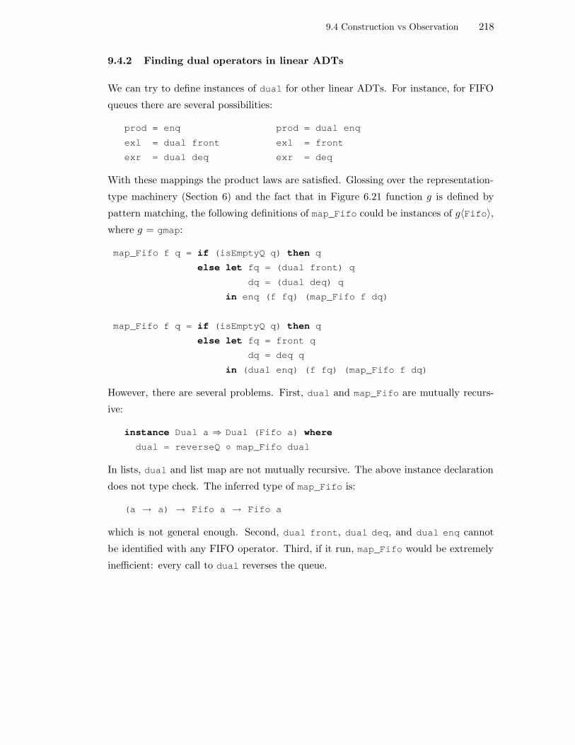
9.4 Construction vs Observation 218
9.4.2 Finding dual operators in linear ADTs
We can try to define instances of dual for other linear ADTs. For instance, for FIFO
queues there are several possibilities:
prod = enq prod = dual enq
exl = dual front exl = front
exr = dual deq exr = deq
With these mappings the product laws are satisfied. Glossing over the representation-
type machinery (Section 6) and the fact that in Figure 6.21 function g is defined by
pattern matching, the following definitions of map_Fifo could be instances of g〈Fifo〉,
where g = gmap:
map_Fifo f q = if (isEmptyQ q) then q
else let fq = (dual front) q
dq = (dual deq) q
in enq (f fq) (map_Fifo f dq)
map_Fifo f q = if (isEmptyQ q) then q
else let fq = front q
dq = deq q
in (dual enq) (f fq) (map_Fifo f dq)
However, there are several problems. First, dual and map_Fifo are mutually recurs-
ive:
instance Dual a ⇒ Dual (Fifo a) where
dual = reverseQ map_Fifo dual
In lists, dual and list map are not mutually recursive. The above instance declaration
does not type check. The inferred type of map_Fifo is:
(a → a) → Fifo a → Fifo a
which is not general enough. Second, dual front, dual deq, and dual enq cannot
be identified with any FIFO operator. Third, if it run, map_Fifo would be extremely
inefficient: every call to dual reverses the queue.

9.5 Insertion and extraction for unbounded linear ADTs 219
9.5 Insertion and extraction for unbounded linear ADTs
In order to define polytypic functions on ADTs, construction and observation must be
separated. In other words, the pattern in Figure 6.21 must be ‘de-fused’. Observation
can be defined as the process of extracting payload into something and construction
as the process of inserting payload from something. There remains to find a something
that affords a uniform and general definition of insertion and extraction, and to study
whether these operations can be defined polytypically. We begin the study focusing on
linear ADTs first.
9.5.1 Choosing the concrete type and the operators
Given an unbounded ADT whose interface can be mapped to LINEAR by a signature
morphism, it is possible to write extraction and insertion functions from/to the ADT
to/from a concrete type with the same interface functor, such that:
1. The extraction function produces a concrete-type replica of the ADT. The value of
the concrete type constructed must mirror the logical positioning of payload in the
ADT. (Observer operators determine the way in which payload is extracted.)
2. The insertion function is the left inverse of the extraction function. However, the
extraction function is not, in general, the left inverse of the insertion function: the
linear ADT satisfies more laws.
For linear ADTs, the obvious choice of concrete type is the list type. Let us call
extraction and insertion functions extracT and inserT respectively:3
extracT :: Linear a → Linear a
extracT t = if dsc0 t then c_con0
else c_con1 (sel10 t) (extracT (sel11 t))
inserT :: Linear a → Linear a
inserT t = if c_dsc0 t then con0
else con1 (c_sel10 t) (inserT (c_sel11 t))
3We have capitalised their last letter to avoid name clashes with ordinary ADT operators. InSection 9.6 we define inserT for ordered sets which already have an insert operator.

9.5 Insertion and extraction for unbounded linear ADTs 220
We have distinguished ADT operators from list operators by prefixing the latter with
the symbol c_, which stands for ‘concrete’. For instance, c_sel10 is the sel10 operator
in the concrete type (lists, for now).
For many linear ADTs (e.g., FIFO queues and stacks) there is only one possible signa-
ture morphism giving values to con0, con1, etc. For ADTs with multiple constructors
(e.g., double-ended queues), there may be more. For concrete types, there are also sev-
eral possible signature morphisms giving values to c_con0, etc. These must be chosen
so that inserT and extracT satisfy the requirements stated at the beginning of the
section. In other words, the following ‘product laws’ must be satisfied:
(c_sel10 extracT) (con1 x y) = x
(c_sel11 extracT) (con1 x y) = y
(sel10 inserT) (c_con1 x y) = x
(sel11 inserT) (c_con1 x y) = y
The laws of the ADT must be used for this task, i.e., programmers must use algebraic
specifications in the definition of inserT and extracT.
Recall the algebraic specifications of FIFO queues and stacks given in Figure 5.6 and
Figure 5.5 respectively. In FIFO queues we dispose of enq, front and deq. We must
find the appropriate c_con1, c_sel10, and c_sel11 in the list type. Functions front,
deq, and enq satisfy, in lists, the same laws as head, tail and snoc, respectively.
Observation and construction are not inverses; queue reversal is needed and this is
captured by dual. Thus, for extraction, the following mapping satisfies the product
laws:
c_con1 = dual snoc
sel10 = front
sel11 = deq
A list replica of the FIFO queue is constructed. For insertion, the following mapping
satisfies the product laws:
con1 = enq
c_sel10 = dual head
c_sel11 = dual tail
Insertion and extraction functions for FIFO queues are shown below:

9.5 Insertion and extraction for unbounded linear ADTs 221
extracT :: Fifo a → List a
extracT q = if isEmptyQ q then Nil
else (dual snoc) (front q) (extracT (deq q))
inserT :: List a → Fifo a
inserT l = if null l then emptyQ
else enq (dual head l) (inserT (dual tail l))
Similarly, we dispose of tos, pop, and push in stacks, which satisfy, in lists, the same
laws as head, tail, and Cons respectively. Fortunately, observation and construction
are inverses. For extraction, the following mapping satisfies the product laws:
c_con1 = Cons
sel10 = tos
sel11 = pop
For insertion, the following mapping satisfies the product laws:
con1 = push
c_sel10 = head
c_sel11 = tail
Insertion and extraction functions for stacks are shown below:
extracT :: Stack a → List a
extracT s = if isEmptyS s then Nil
else Cons (tos s) (extracT (pop s))
inserT :: List a → Stack a
inserT l = if null l then emptyS
else push (head l) (inserT (tail l))
9.5.2 Parameterising on signature morphisms
Calls to dual are terribly inefficient, they involve calls to reverse and map (Sec-
tion 9.4.1). Fortunately, a concrete type is equipped with inverse observers for every
constructor, or they can be programmed for this purpose.
Functions inserT and extracT must be parametric on two signature morphisms, one
mapping ADT operators to linear operators and another mapping concrete-type oper-

9.5 Insertion and extraction for unbounded linear ADTs 222
ators to linear operators.
In this section we show a Haskell implementation and discuss its limitations.
First, we define LinearADT, a type class that describes the operators of the linear
interface:
class LinearADT f where
dsc0 :: f a → Bool
con0 :: f a
con1 :: a → f a → f a
sel10 :: f a → a
sel11 :: f a → f a
We then define LinearCDT, a type class that describes the operators of a concrete type
with a linear interface:
class LinearCDT c_f where
c_dsc0 :: c_f a → Bool
c_con0 :: c_f a
c_con1 :: a → c_f a → c_f a
c_sel10 :: c_f a → a
c_sel11 :: c_f a → c_f a
We re-define inserT and extracT in terms of these type classes:
extracT :: ∀ a. (LinearADT f, LinearCDT c_f) ⇒ f a → c_f a
extracT t = if dsc0 t then c_con0
else c_con1 (sel10 t) (extracT (sel11 t))
inserT :: ∀ a. (LinearADT f, LinearCDT c_f) ⇒ c_f a → f a
inserT t = if c_dsc0 t then con0
else con1 (c_sel10 t) (inserT (c_sel11 t))
Programmers have to provide the appropriate signature morphisms, i.e., to declare
their ADTs instances of LinearADT, and to declare their concrete types instances of
LinearCDT. Programmers must use ADT laws when choosing operators so as to make
inserT the left inverse of extracT:
instance LinearADT Stack where
dsc0 = isEmptyS

9.5 Insertion and extraction for unbounded linear ADTs 223
con0 = emptyS
con1 = push
sel10 = tos
sel11 = pop
instance LinearCDT List where
c_dsc0 = null
c_con0 = Nil
c_con1 = Cons
c_sel10 = head
c_sel11 = tail
instance LinearADT Fifo where
dsc0 = isEmptyQ
con0 = emptyQ
con1 = enq
sel10 = front
sel11 = deq
instance LinearCDT List where
c_dsc0 = null
c_con0 = Nil
c_con1 = Cons
c_sel10 = last
c_sel11 = init
The first List instance is to be used with stacks whereas the second instance is to be
used with FIFO queues. Unfortunately, there are two problems to tackle:
1. There are two overlapping instances of LinearCDT List. Given an application:
(extracT q) :: List Int
where q has type Fifo Int, the compiler cannot determine which instance of
LinearCDT List to use.
2. We have only dealt with unbounded ADTs with unconstrained payload.
The Haskell language does not allow us to name instance declarations and to refer to
them by name. That would enable us to define different instances for the same concrete
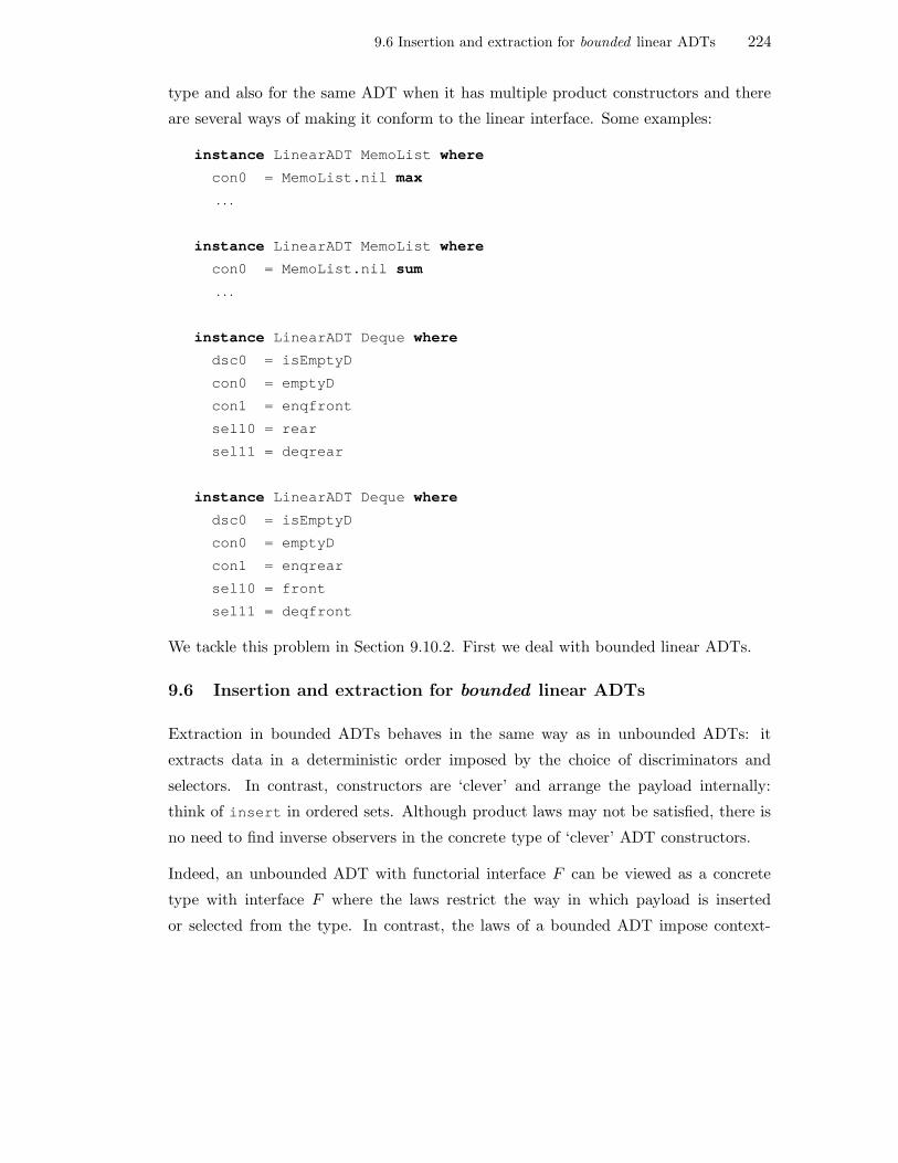
9.6 Insertion and extraction for bounded linear ADTs 224
type and also for the same ADT when it has multiple product constructors and there
are several ways of making it conform to the linear interface. Some examples:
instance LinearADT MemoList where
con0 = MemoList.nil max
. . .
instance LinearADT MemoList where
con0 = MemoList.nil sum
. . .
instance LinearADT Deque where
dsc0 = isEmptyD
con0 = emptyD
con1 = enqfront
sel10 = rear
sel11 = deqrear
instance LinearADT Deque where
dsc0 = isEmptyD
con0 = emptyD
con1 = enqrear
sel10 = front
sel11 = deqfront
We tackle this problem in Section 9.10.2. First we deal with bounded linear ADTs.
9.6 Insertion and extraction for bounded linear ADTs
Extraction in bounded ADTs behaves in the same way as in unbounded ADTs: it
extracts data in a deterministic order imposed by the choice of discriminators and
selectors. In contrast, constructors are ‘clever’ and arrange the payload internally:
think of insert in ordered sets. Although product laws may not be satisfied, there is
no need to find inverse observers in the concrete type of ‘clever’ ADT constructors.
Indeed, an unbounded ADT with functorial interface F can be viewed as a concrete
type with interface F where the laws restrict the way in which payload is inserted
or selected from the type. In contrast, the laws of a bounded ADT impose context-

9.6 Insertion and extraction for bounded linear ADTs 225
dependent restrictions that rely on properties of the payload type. Such restrictions
are taken into account by ‘clever’ constructors.
For example, extraction and insertion for ordered sets can be defined as follows:
extracT :: ∀ a. Ord a ⇒ Set a → List a
extracT s = if isEmptyS s then Nil
else Cons (choice s) (extracT (remove (choice s) s))
inserT :: ∀ a. Ord a ⇒ List a → Set a
inserT l = if null l then emptySet
else insert (head l) (inserT (tail l))
It does not matter whether inserT is defined otherwise as:
inserT :: ∀ a. Ord a ⇒ List a → Set a
inserT l = if null l then emptySet
else insert (last l) (inserT (init l))
Payload elements are arranged internally by insert according to order, and only ele-
ments not already in the set make it. In both cases, inserT is the left inverse of
extracT.
There is an obstacle: the presence of the Ord constraint. It not only appears in the
types of extracT and inserT, but also forces us to define LinearADT and LinearCDT
as multi-parameter type classes (recall the discussion in Section 7.1.3). A possible
solution is to introduce γ-abstraction (Section 6.1.11):
extracT :: γq. ∀a. (q a, LinearADT f, LinearCDT c_f) ⇒ f a → c_f a
inserT :: γq. ∀a. (q a, LinearADT f, LinearCDT c_f) ⇒ c_f a → f a
Fortunately, we can encode these functions in Haskell using a technique proposed
in [Hug99]. The only hurdle remaining is the lack of overlapping instances. In Sec-
tion 9.8 we present the details of the encoding and show how to define generic func-
tions on linear ADTs in terms of inserT and extracT. The section uses extensional
equality as an example of generic function. We first explain what extensional equality
means in the following section.

9.7 Extensional equality 226
9.7 Extensional equality
Extensional equality compares ADTs by comparing their payload contents, not their
internal representation. Extensional equality on two values x and y of the same linear
ADT can be defined as follows:
geqLinear eqa x y = qeq〈List〉 eqa (extracT x) (extracT y)
Function eqLinear is defined under the assumption that the following laws hold:
(dsc0 x) ∧ (dsc0 y) ⇒ x = y
(dsc0 x) ∧ ¬(dsc0 y) ∨ ¬(dsc0 x) ∧ (dsc0 y) ⇒ x 6= y
¬(dsc0 x) ∧ ¬(dsc0 y) ⇒
x = y ⇔ (sel10 x = sel10 y ∧ sel11 x = sel11 y)
For instance, ordered sets with deterministic choice and remove satisfy the conditions.
We can define (extensional) equality for ordered sets provided the payload type supports
ordinary equality:
instance Eq a ⇒ Eq (Set a) where
(==) sx sy = let x = choice sx
y = choice sy
in x == y && (remove x sx) == (remove y sy)
It is possible to test whether two different ADTs that conform to the linear interface are
extensionally equal. For example, it is possible to test whether a stack and an ordered
set are extensionally equal by extracting their payload into two values of the same
concrete type and comparing them for ordinary equality. Unfortunately, this general
notion of extensional equality requires signature morphisms for every ADT involved,
two in this case. We come back to this in Section 9.15.
9.8 Encoding generic functions on linear ADTs in Haskell
This section shows a Haskell implementation4 of inserT, extracT, and of generic size,
map, and equality functions for linear ADTs, whether bounded or unbounded.
To handle constraints we encode both bounded and unbounded ADTs as restricted
types [Hug99]. The key idea is to encode constraints using explicit dictionaries in-
4We have compiled the code using the Glasgow Haskell Compiler v6.2.1, which supports multi-parameter type classes and explicit kind annotations.

9.8 Encoding generic functions on linear ADTs in Haskell 227
stead of the implicit dictionaries created by the compiler, and to define LinearADT
and LinearCDT as multi-parameter type classes where one parameter is an explicit
dictionary. ADTs and concrete types that are instances of these classes are parametric
on constraints, and so are functions defined on them.
data TopD a = TopD my_id :: a → a data EqD a = EqD eq :: a → a → Bool data OrdD a = OrdD lt :: a → a → Bool, eqOrd :: EqD a
class Sat t where dict :: t
instance Sat (TopD a) where -- universal constraintdict = TopD my_id = id
instance Eq a ⇒ Sat (EqD a) wheredict = EqD eq = (==)
instance Ord a ⇒ Sat (OrdD a) wheredict = OrdD lt = (<), eqOrd = dict
Figure 9.3: Explicit dictionaries and Sat proxy.
First, we explain the encoding of explicit dictionaries. The first three lines in Figure 9.3
declare the explicit dictionary types TopD, EqD, and OrdD. The first is a ‘universal’ dic-
tionary which is associated with unbounded ADTs. It has to be provided because
LinearADT and LinearCDT will expect an explicit dictionary argument. However,
unbounded ADTs do not make use of the dictionary’s ‘dummy’ operator. An EqD dic-
tionary has an equality operator eq and an OrdD dictionary ‘extends’ an EqD dictionary
with a comparison operator lt (less than). An Eq constraint is encoded by the explicit
dictionary EqD, and an Ord constraint by the explicit dictionary OrdD.
Class Sat is a proxy, i.e., a type class that is used by programmers to tell the compiler
that an explicit dictionary exists. More precisely, a type a has a dictionary D (or is
D-constrained) if D a is an instance of Sat. Figure 9.3 shows how TopD, EqD, and
OrdD are made instances of Sat. Notice that the last two dictionaries use operators in
implicit dictionaries.
Figure 9.4 shows type classes LinearADT and LinearCDT which now take the expli-
cit dictionary parameter cxt. The dictionary appears as a ‘constraint’ in the type-
signatures of operators.

9.8 Encoding generic functions on linear ADTs in Haskell 228
class LinearADT l cxt wheredsc0 :: Sat (cxt a) ⇒ l cxt a → Boolcon0 :: Sat (cxt a) ⇒ l cxt acon1 :: Sat (cxt a) ⇒ a → l cxt a → l cxt asel10 :: Sat (cxt a) ⇒ l cxt a → asel11 :: Sat (cxt a) ⇒ l cxt a → l cxt a
class LinearCDT l cxt wherec_dsc0 :: Sat (cxt a) ⇒ l cxt a → Boolc_con0 :: Sat (cxt a) ⇒ l cxt ac_con1 :: Sat (cxt a) ⇒ a → l cxt a → l cxt ac_sel10 :: Sat (cxt a) ⇒ l cxt a → ac_sel11 :: Sat (cxt a) ⇒ l cxt a → l cxt a
Figure 9.4: Type classes LinearADT and LinearCDT.
Functions extracT and inserT are shown in Figure 9.5. Function extracT takes an
ADT argument that is an instance of LinearADT and whose payload is constrained on
cxt. It returns a concrete type that is an instance of LinearCDT whose payload is also
constrained on cxt. Function inserT is the left-inverse operation.
extracT :: (LinearADT l cxt, LinearCDT l’ cxt, Sat (cxt a))⇒ l cxt a → l’ cxt a
extracT l = if dsc0 l then c_con0else c_con1 (sel10 l) (extracT (sel11 l))
inserT :: (LinearADT l cxt, LinearCDT l’ cxt, Sat (cxt a))⇒ l’ cxt a → l cxt a
inserT l’ = if c_dsc0 l’ then con0else con1 (c_sel10 l’) (inserT (c_sel11 l’))
Figure 9.5: Generic functions extracT and inserT.
The first box in Figure 9.6 shows the definition of type List. We cannot use ordinary
Haskell lists because an instance of LinearCDT must have the same constraints as the
ADT that is made an instance of LinearADT, and Haskell’s built-in list type is not a
restricted type. Type List is also parametric on an explicit dictionary cxt, whose kind
is written explicitly because it cannot be properly inferred by the compiler (it infers
kind ∗ by default). List operators also have to be programmed from scratch. For each
ordinary list operator we define a List one whose name is prefixed by the letter r (from
‘restricted’). The second box in Figure 9.6 shows two examples. The third box shows

9.8 Encoding generic functions on linear ADTs in Haskell 229
the definitions of map and size for List. The definition of equality has been omitted
for reasons of space.
Figure 9.7 shows the FIFO-queue interface QueueClass and a batched implement-
ation (Chapter 7). The QueueClass interface is defined within a module named
QueueClassM. (ADT operators will be qualified by module name in later figures.)
As with the List type, the implementation type BatchedQueue is parametric on cxt.
Figure 9.8 shows the stack interface StackClass and an implementation in terms of
Haskell’s built-in list type. The StackClass interface is defined within a module named
StackClassM.
Notice that a TopD dictionary is associated with FIFO queues whereas a TopD’ dic-
tionary is associated with stacks. Two dictionaries are needed because overlapping
instances of LinearCDT List TopD are illegal.
Figure 9.9 shows the ordered-set interface SetClass and one possible implementation
in terms of ordered (Haskell) lists. The SetClass interface is defined within a module
named SetClassM. SetList is made an instance of SetClass with constraint OrdD.
Notice how explicit-dictionary operators are used in the implementation of insert and
remove.
Figure 9.10 shows the encoding of signature morphisms. Ordered sets, FIFO queues,
and stacks are made instances of the LinearADT class with the relevant constraints.
There are several LinearCDT List instances associated with these linear ADTs. The
association is established by the shared explicit dictionary.
Finally, Figure 9.11 defines map, size, and equality for linear ADTs. The concrete type
has been fixed to List, which is an instance of class LinearCDT.
It would be preferable to use polytypic functions on the concrete type, that is, to define,
say, sizeLinear as follows:
sizeLinear sa = gsize〈List〉 sa extracT
Unfortunately, Generic Haskell does not support constrained types (Section 6.1.10) and
the instance of gsize generated would be the instance for the restricted List type. In
our encoding, we have to use sizeLinear.
Admittedly, there is no polytypism in the code. From Section 9.9 onwards we show how

9.8 Encoding generic functions on linear ADTs in Haskell 230
data List (cxt :: ∗ → ∗) a = Nil | Cons a (List cxt a)
rNull :: Sat (cxt a) ⇒ List cxt a → BoolrNull Nil = TruerNull (Cons _ _) = False
rHead :: Sat (cxt a) ⇒ List cxt a → arHead Nil = error "rHead: empty list"rHead (Cons x _) = x
mapList :: (Sat (cxt a), Sat (cxt b))⇒ (a → b) → List cxt a → List cxt b
mapList f Nil = NilmapList f (Cons x xs) = Cons (f x) (mapList f xs)--sizeList :: Sat (cxt a) ⇒ (a → Int) → List cxt a → IntsizeList sa Nil = 0sizeList sa (Cons x xs) = sa x + sizeList sa xs
Figure 9.6: List type and functions mapList and sizeList.
class QueueClass q cxt whereempty :: Sat (cxt a) ⇒ q cxt aisEmpty :: Sat (cxt a) ⇒ q cxt a → Boolenq :: Sat (cxt a) ⇒ a → q cxt a → q cxt afront :: Sat (cxt a) ⇒ q cxt a → adeq :: Sat (cxt a) ⇒ q cxt a → q cxt a
data BatchedQueue (cxt :: ∗ → ∗) a = BQ [a] [a]
instance QueueClass BatchedQueue TopD whereempty = BQ [] []
isEmpty (BQ f r) = null f
enq x (BQ f r) = check f (x:r)
front (BQ [] _) = error "Empty Queue"front (BQ (x:f) r) = x
deq (BQ [] _ ) = error "Empty Queue"deq (BQ (x:f) r) = check f r
Figure 9.7: FIFO-queue interface and a possible implementation.

9.8 Encoding generic functions on linear ADTs in Haskell 231
class StackClass s cxt whereempty :: Sat (cxt a) ⇒ s cxt aisEmpty :: Sat (cxt a) ⇒ s cxt a → Boolpush :: Sat (cxt a) ⇒ a → s cxt a → s cxt atos :: Sat (cxt a) ⇒ s cxt a → apop :: Sat (cxt a) ⇒ s cxt a → s cxt a
data Stack (cxt :: ∗ → ∗) a = ST [a]
instance StackClass Stack TopD’ whereempty = ST []isEmpty (ST xs) = null xspush x (ST xs) = ST (x:xs)tos (ST []) = error "tos: empty stack"tos (ST (x:xs)) = xpop (ST []) = error "pop: empty stack"pop (ST (x:xs)) = ST xs
Figure 9.8: Stack interface and a possible implementation
inserT, extracT, and functions on ADTs defined in terms of them can be programmed
polytypically by generalising the solution presented in this Section.
We conclude the section with examples of usage in Figures 9.12 and 9.13. The reader
may want to compare the results with those of Chapter 7. (N.B.: pretty-printing show
functions were defined for every type.)

9.8 Encoding generic functions on linear ADTs in Haskell 232
class SetClass s cxt whereisEmpty :: Sat (cxt a) ⇒ s cxt a → Boolempty :: Sat (cxt a) ⇒ s cxt ainsert :: Sat (cxt a) ⇒ a → s cxt a → s cxt achoice :: Sat (cxt a) ⇒ s cxt a → aremove :: Sat (cxt a) ⇒ a → s cxt a → s cxt amember :: Sat (cxt a) ⇒ a → s cxt a → Bool
data SetList (cxt :: ∗ → ∗) a = SL [a]
instance SetClass SetList OrdD whereempty = SL []
isEmpty (SL xs) = null xs
insert x (SL xs) = SL (insert’ x xs)whereinsert’ x [] = [x]insert’ x (l@(y:ys))
| eq (eqOrd dict) x y = l| (lt dict) x y = (x:y:ys)| otherwise = y : (insert’ x ys)
remove x (SL xs) = SL (remove’ x xs)where remove’ x [] = []
remove’ x (y:ys) = if eq (eqOrd dict) x y then yselse y : (remove’ x ys)
member x (SL xs) = any (eq (eqOrd dict) x) xs
choice (SL []) = error "choice: empty set"choice (SL (x:xs)) = x
Figure 9.9: Ordered-set interface and a possible implementation.

9.8 Encoding generic functions on linear ADTs in Haskell 233
instance LinearADT SetList OrdD wheredsc0 = SetClassM.isEmptycon0 = SetClassM.emptycon1 = SetClassM.insertsel10 = SetClassM.choicesel11 = λs → SetClassM.remove (SetClassM.choice s) s
instance LinearCDT List OrdD wherec_dsc0 = rNullc_con0 = Nilc_con1 = Consc_sel10 = rHeadc_sel11 = rTail
instance LinearADT BatchedQueue TopD wheredsc0 = QueueClassM.isEmptycon0 = QueueClassM.emptycon1 = QueueClassM.enqsel10 = QueueClassM.frontsel11 = QueueClassM.deq
instance LinearCDT List TopD wherec_dsc0 = rNullc_con0 = Nilc_con1 = Consc_sel10 = rLastc_sel11 = rInit
instance LinearADT Stack TopD’ wheredsc0 = StackClassM.isEmptycon0 = StackClassM.emptycon1 = StackClassM.pushsel10 = StackClassM.tossel11 = StackClassM.pop
instance LinearCDT List TopD’ wherec_dsc0 = rNullc_con0 = Nilc_con1 = Consc_sel10 = rHeadc_sel11 = rTail
Figure 9.10: Ordered sets, FIFO queues, and stacks are linear ADTs.

9.8 Encoding generic functions on linear ADTs in Haskell 234
mapLinear :: (LinearADT l cxt, LinearCDT List cxt,Sat (cxt a), Sat (cxt b))
⇒ (a → b) → l cxt a → l cxt b
mapLinear f = inserT mapList f extracT--sizeLinear :: (LinearADT l cxt, LinearCDT List cxt, Sat (cxt a))
⇒ (a → Int) → l cxt a → Int
sizeLinear sa = sizeList sa extracT--eqLinear :: (LinearADT l cxt, LinearCDT List cxt, Sat (cxt a))
⇒ (a → a → Bool) → l cxt a → l cxt a → Bool
eqLinear eqa lx ly = eqList eqa (extracT lx) (extracT ly)
Figure 9.11: Map, size, and equality as generic functions on LinearADTs.
s :: SetList OrdD Int s = foldr (λx y → SetClassM.insert x y)SetClassM.empty [5,1,2,4,3,2,1] > 1,2,3,4,5
s0 = mapLinear (const 0) s> 0
mapLinear negate s> -5,-4,-3,-2,-1
sizeLinear (const 1) s> 5
sizeLinear (const 1) s0> 1
eqLinear (==) s s> True
eqLinear (==) s (remove (choice s) s)> False
eqLinear (==) s (insert (choice s) s)> True
Figure 9.12: Computing with ordered sets.

9.8 Encoding generic functions on linear ADTs in Haskell 235
q :: BatchedQueue TopD Intq = foldl (λx y → QueueClassM.enq y x) QueueClassM.empty [2,5,1,6]> <2,5,1,6>
mapLinear negate q> <-2,-5,-1,-6>
k :: Stack TopD’ Intk = foldr (λx y → StackClassM.push x y) StackClassM.empty [1,2,3]> 1,2,3|
mapLinear negate k> -1,-2,-3|
eqLinear (==) k (pop k)> False
Figure 9.13: Computing with FIFO queues and stacks.
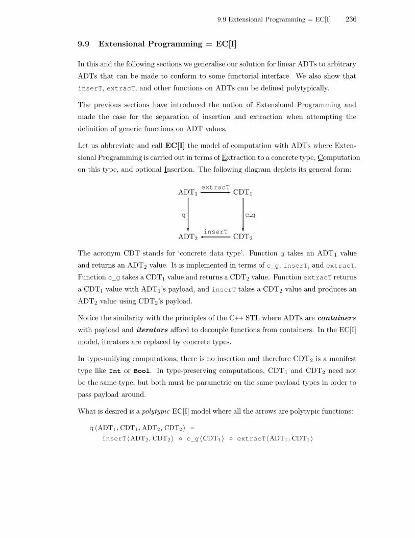
9.9 Extensional Programming = EC[I] 236
9.9 Extensional Programming = EC[I]
In this and the following sections we generalise our solution for linear ADTs to arbitrary
ADTs that can be made to conform to some functorial interface. We also show that
inserT, extracT, and other functions on ADTs can be defined polytypically.
The previous sections have introduced the notion of Extensional Programming and
made the case for the separation of insertion and extraction when attempting the
definition of generic functions on ADT values.
Let us abbreviate and call EC[I] the model of computation with ADTs where Exten-
sional Programming is carried out in terms of Extraction to a concrete type, Computation
on this type, and optional Insertion. The following diagram depicts its general form:
ADT1extracT- CDT1
ADT2
g
?inserT CDT2
c g
?
The acronym CDT stands for ‘concrete data type’. Function g takes an ADT1 value
and returns an ADT2 value. It is implemented in terms of c_g, inserT, and extracT.
Function c_g takes a CDT1 value and returns a CDT2 value. Function extracT returns
a CDT1 value with ADT1’s payload, and inserT takes a CDT2 value and produces an
ADT2 value using CDT2’s payload.
Notice the similarity with the principles of the C++ STL where ADTs are containers
with payload and iterators afford to decouple functions from containers. In the EC[I]
model, iterators are replaced by concrete types.
In type-unifying computations, there is no insertion and therefore CDT2 is a manifest
type like Int or Bool. In type-preserving computations, CDT1 and CDT2 need not
be the same type, but both must be parametric on the same payload types in order to
pass payload around.
What is desired is a polytypic EC[I] model where all the arrows are polytypic functions:
g〈ADT1,CDT1,ADT2,CDT2 〉 =
inserT〈ADT2,CDT2 〉 c_g〈CDT1 〉 extracT〈ADT1,CDT1 〉

9.9 Extensional Programming = EC[I] 237
Every function except c_g is polytypic on more than one argument. This function is
an ordinary Generic Haskell function. Extraction and insertion functions need to know
the functorial structure of their source and target types. Consequently, CDT1 and
CDT2 must be provided as arguments to g or otherwise their values would be fixed in
g’s body. ADTi and CDTi must conform to the same functorial interface. However,
ADT1 and ADT2 need not conform to the same functorial interface.
We will consider a simplified EC[I] model where ADT1 and ADT2 are the same abstract
type and CDT1 and CDT2 are the same concrete type:
ADTextracT- CDT
I@@
@@
@inserT
CDT
c g
?
That is:
g〈ADT,CDT〉 = inserT〈ADT,CDT〉 c_g〈CDT〉 extracT〈ADT,CDT 〉
The reasons are simple:
1. All polytypic functions on ADTs take the same number and type of arguments.
2. Functions inserT and extracT are polytypic on the structure of interface functors,
and choosing a free CDT1 with the same functorial interface as CDT2 is choosing
the same concrete type, names of value constructors and operators notwithstanding.
Function inserT will be a catamorphism, not an anamorphism [MFP91].
3. When CDT and ADT have the same functorial interface then structural inform-
ation cannot be lost. Structural information is lost if extracT is left without a
corresponding inserT, making type-preserving functions undefinable. Furthermore,
inserT must be the left inverse of extracT:
inserT extracT == id
In the case of unbounded ADTs, the CDT must provide all the required operators so
that the above equation can be satisfied. In the case of bounded ADTs, there is no

9.10 Polytypic extraction and insertion 238
need to worry, for there are ‘clever’ constructors that properly reconstruct the ADT
(Section 9.6).
Nonetheless, for some type-unifying computations, such as calculating the size or testing
for equality, loosing the information required for building back the original ADT is not
a problem (Section 9.14).
9.10 Polytypic extraction and insertion
Insertion and extraction functions are structurally polymorphic on the functorial struc-
ture of an interface and, consequently, their definition can be generated automatically
by a compiler. Such functorial structure is declared by the generic programmer in what
we call an F -view .
9.10.1 F -views
An F -view is a language extension for declaring the functorial structure of ADT inter-
faces. We introduce the syntax using some examples. The following F -view is similar
to the type class LinearADT of Section 9.8:
fview Linear a = 1 + a × (Linear a)
The structure of the F -view automatically determines the following operators:
dsc0 :: γq. ∀a. q a ⇒ Linear a → Bool
con0 :: γq. ∀a. q a ⇒ Linear a
con1 :: γq. ∀a. q a ⇒ a → Linear a → Linear a
sel10 :: γq. ∀a. q a ⇒ Linear a → a
sel11 :: γq. ∀a. q a ⇒ Linear a → Linear a
The discriminator dsc0 comes from the presence of the coproduct. There are two
products and hence two constructors con0 and con1. There is no selector for a nullary
product and there are two selectors sel10 and sel11 for the binary product.
Every F -view F automatically determines another F -view c_F where every operator op
in F is named c_op in c_F:
fview c_Linear a = 1 + a × (c_Linear a)
c_dsc0 :: γq. ∀a. q a ⇒ c_Linear a → Bool
c_con0 :: γq. ∀a. q a ⇒ c_Linear a

9.10 Polytypic extraction and insertion 239
c_con1 :: γq. ∀a. q a ⇒ a → c_Linear a → c_Linear a
c_sel10 :: γq. ∀a. q a ⇒ c_Linear a → a
c_sel11 :: γq. ∀a. q a ⇒ c_Linear a → c_Linear a
Other examples of F -views are shown in Figure 9.14. Reading an F -view declaration
from left to right, every ith coproduct has an associated discriminator dsci. Every ith
product has one constructor coni with selectors seli0 to selim, where m is the arity
of the product.
fview Bin1 a = 1 + a × (Bin1 a) × (Bin1 a)dsc0 :: γq. ∀a. q a ⇒ Bin1 a → Boolcon0 :: γq. ∀a. q a ⇒ Bin1 acon1 :: γq. ∀a. q a ⇒ a → Bin1 a → Bin1 a → Bin1 asel10 :: γq. ∀a. q a ⇒ Bin1 a → asel11 :: γq. ∀a. q a ⇒ Bin1 a → Bin1 asel12 :: γq. ∀a. q a ⇒ Bin1 a → Bin1 a
fview Bin2 a b = 1 + a + b × (Bin2 a b) × (Bin2 a b)dsc0 :: γq. ∀a. q a ⇒ Bin2 a b → Booldsc1 :: γq. ∀a. q a ⇒ Bin2 a b → Boolcon0 :: γq. ∀a. q a ⇒ Bin2 a bcon1 :: γq. ∀a. q a ⇒ a → Bin2 a bsel10 :: γq. ∀a. q a ⇒ Bin2 a b → acon2 :: γq. ∀a. q a ⇒ b → Bin2 a b → Bin2 a b → Bin2 a bsel20 :: γq. ∀a. q a ⇒ Bin2 a b → bsel21 :: γq. ∀a. q a ⇒ Bin2 a b → Bin2 a bsel22 :: γq. ∀a. q a ⇒ Bin2 a b → Bin2 a b
fview Composite3 a b c = a × b × ccon0 :: γq. ∀a. q a ⇒ a → b → c → Composite3 a b csel00 :: γq. ∀a. q a ⇒ Composite3 a b c → asel01 :: γq. ∀a. q a ⇒ Composite3 a b c → bsel02 :: γq. ∀a. q a ⇒ Composite3 a b c → c
Figure 9.14: Examples of F -view declarations and their implicitly-defined operators.
9.10.2 Named signature morphisms
ADT interfaces can be made to conform to F -views by providing named signature
morphisms. We have already showed in Section 9.5.2 examples of signature morph-
isms. In this section we explain the new syntax by example.
Set instance Linear by SetL where
dsc0 = isEmptySet

9.10 Polytypic extraction and insertion 240
con0 = emptySet
. . .
The syntax declares that there is a signature morphism SetL from the ADT Set to the
Linear F -view. A signature morphism between a concrete type and c_Linear must
be declared in similar fashion:
List instance c_Linear by L1 where
c_dsc0 = null
c_con0 = Nil
c_con1 = Cons
c_sel10 = head
c_sel11 = tail
List instance c_Linear by L2 where
c_dsc0 = null
c_con0 = Nil
c_con1 = Cons
c_sel10 = last
c_sel11 = init
The two morphisms have different names and therefore can cohabit in a program. In
Section 9.8, F -views were encoded as type classes and signature morphisms were en-
coded as instance declarations. In that setting, overlapping instances were not allowed.
We show a possible implementation of F -views and named signature morphisms in
Section 9.10.3.
To the compiler, every named signature morphism has two associated meta-functions
called type and view. The first returns the type that is made an instance of the F -view,
e.g.:
type SetL = Set
type L2 = List
The second returns a representation of the functorial structure declared by the F -view,
e.g.:
view Linear = 1 + a × (Linear a)
view Composite3 = a × b × c

9.10 Polytypic extraction and insertion 241
9.10.3 Implementing F -views and named signature morphisms
F -views and named signature morphisms are language extensions. In this section we
show that they are reasonable and feasible extensions by indicating a possible imple-
mentation.
An F -view declaration can be translated by the compiler to a multi-parameter type
class where one parameter is an explicit dictionary parameter (Section 9.8) and another
is a name parameter, i.e., a type encoding a signature morphism name. Every function
in the class takes an extra argument of that type.
Named signature morphisms can be translated by the compiler to instances of the type
class that provide actual values for dictionaries and ‘name’ types.
Figure 9.15 shows the translation for F -view c_Linear and named signature morphisms
L1 and L2.
class C_Linear l cxt n wherec_dsc0 :: ∀ a. Sat (cxt a) ⇒ n → l cxt a → Boolc_con0 :: ∀ a. Sat (cxt a) ⇒ n → l cxt ac_con1 :: ∀ a. Sat (cxt a) ⇒ n → a → l cxt a → l cxt ac_sel10 :: ∀ a. Sat (cxt a) ⇒ n → l cxt a → ac_sel11 :: ∀ a. Sat (cxt a) ⇒ n → l cxt a → l cxt a
data L1 = L1data L2 = L2
instance C_Linear List TopD L1 wherec_dsc0 = const nullc_con0 = cons Nilc_con1 = const Consc_sel10 = const headc_sel11 = const tail
instance C_Linear List TopD L2 wherec_dsc0 = const nullc_con0 = cons Nilc_con1 = const Consc_sel10 = const lastc_sel11 = const init
Figure 9.15: Possible implementation of F -views and named signature morphisms.
The F -view is compiled to a type class C_Linear which takes an explicit dictionary

9.10 Polytypic extraction and insertion 242
parameter cxt and a ‘name’ parameter n. Every operator has an extra parameter of
type n.
The signature-morphism names L1 and L2 are compiled to new types with nullary
value constructors of the same name. The signature morphisms are implemented as
instances of C_Linear where operators discard their first argument.
The types L1 and L2 help the compiler resolve the overloading. More precisely, op-
erators c_op only occur in the bodies of inserT and extracT, which take signature-
morphism arguments (we discuss the details of this in the next section). When inserT
or extracT are passed signature morphism L1 as an actual argument, the compiler
generates their bodies writing c_op L1 where a call to c_op would have been expec-
ted. The compiler can deduce from the application that c_op must be of type L1→ τ
for some type τ . The other possibility, L2 → τ does not type-check. Similarly, when
inserT or extracT are passed signature morphism L2 as an actual argument, what
are generated are calls to c_op L2.
9.10.4 Polyaric types and instance generation
We now define inserT and extracT polytypically. Their types are parametric on the
arity of the type component of a signature morphism and their bodies are generated
following the functorial structure provided by the view component. Operator names
are also obtained from signature-morphism arguments.
More precisely, inserT and extracT are parametric on two signature morphisms that
provide all the information. One morphism maps an ADT to an F -view F and another
maps a CDT to the related F -view c F . The bodies are structurally polymorphic
on the functor defined by the F -view. Like Generic Haskell, we follow a generative
approach and generate instances of inserT and extracT for actual signature-morphism
arguments in polytypic applications. Generic programmers do not have to specify
anything. The type-signatures and bodies of instances are generated automatically by
the compiler.
We introduce the notion of polyaric type, i.e., a type that is parametric on the arity
of an ADT, not the kind. The reason for this is that we deal with first-order ADTs

9.10 Polytypic extraction and insertion 243
whose kind is described by the grammar:
κ ::= ∗ | ∗ → κ
Functions extracT and inserT possess polyaric types, and so will polytypic functions
defined in terms of them.
Types ExtracT and InserT are respectively the polyaric types of extracT and inserT:
ExtracT〈n〉 t1 t2 :: γq. ∀ a. q a⇒ t1 a → t2 a
InserT〈n〉 t1 t2 :: γq. ∀ a. q a⇒ t2 a → t1 a
extracT〈f, c f〉 :: ExtracT〈(arity type) f〉 (type f) (type c f) ∆(type f)
insertT〈f, c f〉 :: InserT〈(arity type) c f〉 (type f) (type c f) ∆(type f)
where n > 0 and adef= a1 . . . an. The case n = 0 applies to manifest ADTs and cannot
be explained until we introduce our notion of exporting in Section 9.13.
Let F and C_F be two signature morphisms. The polytypic application extracT〈F,C_F〉
in the program triggers the generation of the instance of extracT for those signature
morphisms, namely, extracT_F_C_F, whose definition is generated by:
genCopro(t, view(F))
where t is a chosen value-parameter name, view(F) = P0 + . . . + Pn for some n ≥ 0
coproducts of products Pi = Xi0 × . . . × Xim for some m ≥ 0, and genCopro is a
compiler meta-function whose definition for extraction is shown in Figure 9.16.
genCopro(t,P0 + . . . + Pn) =if (dsc0 t) then genPro(t,P0). . .else if (dsc(n−1) t) then genPro(t,Pn−1)else genPro(t,Pn)
genPro(t,1i) = c_conigenPro(t,Xi0 × . . .×Xim) = c_coni genTerm(t,Xi0) . . . genTerm(t,Xim)
genTerm(t,aij) = selij tgenTerm(t,(F a)ij) = extracT (selij t)
Figure 9.16: Meta-function genCopro generates the body of extracT at compile-timefollowing the structure specified by its second argument.
An almost identical meta-function is defined for inserT where inserT occurs instead

9.10 Polytypic extraction and insertion 244
of extracT and c op operators occur instead of op operators and vice versa.
9.10.5 Generation examples
We illustrate the generation process for ordered sets and FIFO queues. First, the
signature morphisms:
Set instance Linear by SetF where
dsc0 = isEmptyS
con0 = emptyS
con1 = insert
sel10 = choice
sel11 = λs → remove (choice s) s
Queue instance Linear by QueueF where
dsc0 = isEmptyQ
con0 = emptyQ
con1 = enq
sel10 = front
sel11 = deq
For the concrete type, we use signature morphism L2 from Section 9.10.2. The polytypic
application extracT〈SetF,L2〉 triggers the generation of a extracT_SetF_L2 instance
whose type is given by expanding the polyaric type:
ExtracT〈1〉 Set List [Ord]
The resulting type-signature is:
extracT_SetF_L2 :: ∀ a. Ord a ⇒ Set a → List a
Similarly, the polytypic application inserT〈SetF,L2〉 triggers the generation of an
inserT_SetF_L2 instance whose type is given by expanding the polyaric type:
InserT〈1〉 Set List [Ord]
which yields the type-signature:
inserT_SetF_L2 :: ∀ a. Ord a ⇒ List a → Set a

9.10 Polytypic extraction and insertion 245
The bodies of extracT_SetF_L2 and inserT_SetF_L2 are generated by the compile-
time evaluation of:
genCopro(t, 1 + a× (Linear a))
where F -view operator names are replaced by the actual ones provided by the signature
morphisms:
extracT_SetF_L2 t =
if isEmptyS t then Nil
else Cons (choice t) (extracT ((λs → remove (choice s) s) t)
inserT_SetF_L2 t =
if null t then emptyS
else insert (last t) (inserT (init t))
(If F -views and named signature morphisms are implemented as suggested in Sec-
tion 9.10.3, list and set operators in the previous definitions must be applied to an L2
argument first.)
FIFO queues have no payload constraints. The following polytypic applications:
extracT〈QueueF,L2〉
inserT〈QueueF,L2〉
trigger the generation of the following type-signatures:
extracT_QueueF_L2 :: ExtracT〈1〉 Queue List []
inserT_QueueF_L2 :: InserT〈1〉 Queue List []
and the generation of the bodies using the operators provided by the signature morph-
isms:
extracT_QueueF_L2 :: ∀ a. Queue a → List a
extracT_QueueF_L2 t = if isEmptyQ t then Nil
else Cons (front t) (extracT (deq t))
inserT_QueueF_L2 :: ∀ a. List a → Queue a
inserT_QueueF_L2 t = if null t then emptyQ
else enq (last t) (inserT (init t))

9.11 Defining polytypic functions 246
9.11 Defining polytypic functions
Polytypic functions such as gsize, gmap, or geq can now be programmed in terms of
inserT and extracT. Polytypic functions on first-order ADTs possess polyaric types.
The generic programmer first defines the polyaric type of the function:
G〈0〉 t = τ
G〈n〉 t = ∀ a. G〈0〉 a → G〈n− 1〉 (t a)
which is translated automatically by the compiler into a context-parametric version:
G〈0〉 t = γ q. τ
G〈n〉 t = γ q. ∀ a. q a⇒ G〈0〉 a ε → G〈n− 1〉 (t a) q
A polyaric type can be converted into a polykinded type by mapping arity arguments
to kind arguments:
kindOf (0) = ∗
kindOf (n) = ∗ → KindOf (n− 1)
A polyaric type can be expanded by first transforming it into a polykinded type and
then using the type rules described in Section 6.1.11.
The generic programmer then defines the body of the function:
g〈f, c f〉 :: G〈f〉 f
g〈f, c f〉 πg x = B( x, inserT〈f, c f〉, g〈c f〉 πg, extracT〈f, c f〉 )
Several remarks are in order:
• The polytypic function is parametric on two named signature morphisms, one map-
ping the ADT to an F -view and another mapping the CDT to the implicit F -view
generated by the former. For example, in the polytypic application g〈M1,M2〉, M1
is a signature morphism mapping the operators in type(M1) to view(M1) whereas
signature morphism M2 maps the operators in type(M2) to view(M2), such that
view(M1) is F , for some F -view F , and view(M2) is c F .
• We deprecate the transformation of n-ary (co)products in F -views to associations of
binary ones. In a generative approach, it is possible and reasonable to define poly-
typic functions and their types as templates that are parametric on arity. Thus, func-
tion g takes a vector of function arguments πg = g1 . . . gn, where n = arity(type(f)).

9.11 Defining polytypic functions 247
The special symbol π is a language extension. The type of each gi argument is given
by the polyaric type, that is:
gi :: γq. ∀ a. q a ⇒ G〈0〉 a q
• The body of g〈f, c f〉 is a function B of the argument variables x, of the inserT
and extracT for the same signature morphisms, and also of the ordinary Generic
Haskell function g〈c f〉 applied to the vector πg.
• The polytypic application g〈F,C F 〉 triggers the generation of the instance g F C F
whose type-signature is given by expanding:
G〈(arity type)F 〉 (type F ) ∆(type F )
The generated body is:
B( x, inserT F C F, g〈T 〉 g1 . . . gn, extracT F C F )
where T = type(C F ) and n = arity(T ). For simplicity, generated instances contain
calls to polytypic functions on the concrete type. It would be possible to generate in-
stances for those functions simultaneously, i.e., to generate g T whose type-signature
is given by:
G〈(kindOf arity type)C F 〉 (type C F ) ∆(type C F )
where G is the context-parametric polykinded type of the ordinary Generic Haskell
function.
• Polytypic function definitions can be type-checked. The Generic Haskell compiler
relies on the Haskell compiler to do the job, i.e., it generates the types and bodies of
instances and lets the Haskell compiler check that they match. We also follow this
approach.
Figure 9.17 shows the definition of gsize, gmap, and geq.
We conclude the section with generation examples for ordered sets.
The polytypic application gsize〈SetF,L1〉 triggers the generation of the instance:

9.11 Defining polytypic functions 248
GSIZE〈0〉 t = γq. t → IntGSIZE〈n〉 t = γq. ∀a. q a ⇒ GSIZE〈0〉 a ε → GSIZE〈n-1〉 (t a) q
gsize〈f,c_f〉 :: GSIZE〈f〉 fgsize〈f,c_f〉 πg t = gsize〈c_f〉 πg extracT〈f,c_f〉 t
GMAP〈0〉 t1 t2 = γq. t1 → t2GMAP〈n〉 t1 t2 = γq. ∀a1 a2. q a1 a2 ⇒
GMAP〈0〉 a1 a2 ε → GMAP〈n-1〉 (t1 a1) (t2 a2) q
gmap〈f,c_f〉 :: GMAP〈f〉 fgmap〈f,c_f〉 πg t = inserT〈f,c_f〉 gmap〈c_f〉 πg extracT〈f,c_f〉 t
GEQ〈0〉 t = γq. t → t → IntGEQ〈n〉 t = γq. ∀a. q a ⇒ GEQ〈0〉 a ε → GEQ〈n-1〉 (t a) q
geq〈f,c_f〉 :: GEQ〈f〉 fgeq〈f,c_f〉 πg t1 t2 = geq〈c_f〉 πg (extracT〈f,c_f〉 t1)
(extracT〈f,c_f〉 t2)
Figure 9.17: Polytypic gsize, gmap, geq defined in terms of inserT and extracT.
gsize_SetF_L1 :: GSIZE〈1〉 Set [Ord]
that is:
gsize_SetF_L1 :: ∀ a. Ord a ⇒ (a → Int) → Set a → Int
gsize_SetF_L1 g t = gsize〈List〉 g extracT_SetF_L1 t
Generated instances contain calls to polytypic functions on the concrete type. If in-
stances for them are generated simultaneously then the result is:
gsize_SetF_L1 :: ∀ a. Ord a ⇒ (a → Int) → Set a → Int
gsize_SetF_L1 g t = gsize_List g extracT_SetF_L1 t
The polytypic application gmap〈SetF,L1〉 triggers the generation of the gmap instance:
gmap_SetF_L1 :: GMAP〈1〉 Set [Ord]
that is:
gmap_SetF_L1 :: ∀ a. (Ord a, Ord b) ⇒ (a → b) → Set a → Set b
gmap_SetF_L1 g t = inserT_SetF_L1 gmap〈List〉 g extracT_SetF_L1 t
Finally, the polytypic application geq〈SetF,L1〉 triggers the generation of the geq
instance:

9.12 Polytypic extension 249
geq_SetF_L1 :: GEQ〈1〉 Set [Ord]
that is:
geq_SetF_L1 :: ∀ a. Ord a ⇒ (a → a → Bool) → Set a → Set a → Bool
geq_SetF_L1 g t1 t2 =
geq〈List〉 g (extracT_SetF_L1 t1) (extracT_SetF_F1 t2)
9.12 Polytypic extension
Polytypic extension can be accommodated in our system in a similar way in which
template specialisation is done in C++. Polytypic extension amounts to providing
a definition of specific instances of polytypic functions for specific ADTs. Specialised
functions can be provided for inserT, extracT, and already defined polytypic functions
with polyaric types.
Suppose, for example, that ordered sets come equipped with the following operators:
enumerate :: ∀ a. Ord a ⇒ Set a → List a
fromList :: ∀ a. Ord a ⇒ List a → Set a
cardinality :: ∀ a. Ord a ⇒ Set a → Int
It makes sense to use these operators in the definitions of inserT, extracT, and gsize
for ordered sets. This can be specified by the generic programmer thus:
instance extracT〈type=Set,type=List〉 = enumerate
instance inserT〈type=Set,type=List〉 = fromList
instance gsize〈type=Set,type=List〉 = cardinality
We reuse the keyword instance to avoid multiplication of keywords. The first declara-
tion instructs the compiler to use enumerate instead of generating an extracT instance
when the type attribute of its first signature-morphism argument is Set and the type
attribute of its second signature-morphism argument is List. The declaration only
mentions types, not F -views, because extracT is not generated. The compiler must
make sure that enumerate’s type-signature matches that of an instance of extracT
for sets and lists, that is, it must check that:
ExtracT〈1〉 Set [Ord]
expands to:

9.13 Exporting 250
∀ a. Ord a ⇒ Set a → List a
which is the case.
Similarly, the second declaration instructs the compiler to use fromList instead of
generating an instance of inserT. Finally, the third declaration instructs the compiler
to use cardinality instead of generating an instance of gsize when the types in
the signature morphisms are Set and List. Again, the compiler must check that
type-signatures match, which is the case in these examples.
9.13 Exporting
The difference between exporting and abstracting over payload is somewhat analog-
ous to the difference between lambda abstractions and let-expressions. Exporting in
F -views is based on carrying this difference to the type level.
Recall the EventQueue example of Section 7.2. To make it conform to the Linear
F -view we have to specify that the payload type is fixed. The keyword export is used
for this purpose:
EventQueue instance Linear by EventQL where
export a = Event.EventType
dsc0 = EventQueue.isEmpty
con0 = EventQueue.empty
. . .
The declaration informs the compiler that type variable a in the functorial structure
of Linear will always be Event.EventType.
We can explain now how polyaric types work when the type attribute of a signature
morphism has 0 arity, a discussion that was postponed in Section 9.10.4. These are the
base cases of polyaric types InserT and ExtracT:
ExtracT〈0〉 t1 t2 :: t1 → t2 (payload t1)
InserT〈0〉 t1 t2 :: t2 (payload t1) → t1
Compile-time function payload returns the payload type specified in an export declar-
ation for its type argument.
Let us show some examples of particular instantiations:

9.13 Exporting 251
extracT〈EventQL,L1〉 :: ExtracT〈0〉 EventQueue List []
In this example:
type(EventQL) = EventQueue
arity(EventQueue) = 0
payload (type(EventQL)) = Event.EventType
The result of the expansion is:
extracT_EventQL_L1 :: EventQueue → List Event.EventType
Also:
inserT〈EventQL,L1〉 :: InserT〈0〉 EventQueue List []
after expansion:
inserT_EventQL_L1 :: List Event.EventType → EventQueue
Let us show what should happen with polytypic functions:
gsize〈EventQL,L1〉 :: export (GSIZE〈1〉 EventQueue [])
EventQueue [Event.EventType]
The compile-time meta-function export expands its first argument, the polyaric type
GSIZE, and on the resulting type-signature replaces EventQueue a by EventQueue
and it replaces all remaining occurrences of a by Event.EventType. The resulting
type-signature of the gsize instance is shown below:
gsize_EventQL_L1 ::
(Event.EventType → Int) → EventQueue → Int
In general, let P 〈n〉 T [ ] expand to type-signature S. The evaluation of:
export S T [E1, . . . , En]
where E = payload (T ), yields the type-signature:
[(T a)/T ][a/E]S
Exporting is essential in dealing with composite manifest ADTs. Take for example a
Date ADT whose implementation type is hidden. It comes with the following operat-
ors:

9.13 Exporting 252
mkDate :: Day → Month → Year → Date
getDay :: Date → Dat
getMonth :: Date → Month
getYear :: Date → Year
We can compute with dates by defining a signature morphism using the export facility.
Recall the Composite3 F -view from Section 9.10.1:
Date instance Composite3 by DateC3 where
export a = Day
b = Month
c = Year
con0 = mkDate
sel00 = getDay
sel01 = getMonth
sel02 = getYear
type Tuple3 a b c = (a,b,c)
tuple3 x y z = (x,y,z)
tuple30 (x,y,z) = x
tuple31 (x,y,z) = y
tuple32 (x,y,z) = z
Tuple3 instance c_Composite3 by Tuple3F where
c_con0 = tuple3
c_sel00 = tuple30
c_sel01 = tuple31
c_sel02 = tuple32
mapDate :: (Day → Day) → (Month → Month) → (Year → Year)
→ Date → Date
mapDate = gmap〈DateC3,Tuple3F〉
In Haskell, n-ary tuples are constructed using bracket notation and there are only
predefined selectors for binary tuples, namely, fst and snd. The reader will agree
that concrete types of the form Tuplen for n > 0 could be assumed by the generic
programmer and their type, constructors, and selectors be generated automatically by
the compiler.

9.14 Forgetful extraction 253
Tuple types are also convenient for dealing with random access structures such as arrays
of fixed length. For example:
type Array3 a = Array Int a
Array3 instance Composite3 by ArrayComposite3 where
con0 = λx y z → array (0,2) [(0,x),(1,y),(2,z)]
sel00 = (!0)
sel01 = (!1)
sel02 = (!2)
mapArray3 :: (a → b) → Array3 a → Array3 b
mapArray3 = gmap〈Array3,Tuple3F〉
9.14 Forgetful extraction
In type-unifying computations in which there is no need for insertion, it is possible to
cheat and extract payload from an ADT into a concrete type with different functorial
structure; more precisely, to a concrete type with a polynomial functor of lower coef-
ficient but equal number of payload. For instance, it is possible to extract data from
an ADT conforming to Bin1 (defined in Section 9.10.1) to a list. The trick is to make
List conform to c_Bin1, which is possible because list selectors are not used when
inserT is omitted:
List instance C_Bin1 by ListBin1 where
c_dsc0 = null
c_con0 = Nil
c_con1 = λx y z → Cons x (y ++ z)
c_sel10 = λx → error "attempting to select"
c_sel11 = λx → error "attempting to select"
c_sel12 = λx → error "attempting to select"
Combining ADTs and CDTs with different functorial interfaces entails an exponential
increase in the number of signature-morphism arguments. We come back to this topic
in Chapter 10.

9.15 Passing and comparing payload between ADTs 254
9.15 Passing and comparing payload between ADTs
Because inserT and extracT are parametric on signature morphisms for abstract and
concrete types, it is possible to write non-generic functions that ‘copy’ payload between
different ADTs as long as the functorial structure is the same and the intermediate
concrete type is the same, even if the two signature morphisms for the concrete type
differ. A simple example:
set2queue :: Ord a ⇒ Set a → Queue a
set2queue = inserT〈QueueF,L2〉 extracT〈SetF,L1〉
Notice that type(L1)=type(L2) and that queue selectors in L2 are never used and list
selectors in L1 are never used.
It is not possible however to write payload-copy functions polytypically because inser-
tion, extraction, and polytypic functions with polyaric types are parametric only on
one signature morphism associated with an ADT.
It is also possible to compare payload between ADTs, i.e., to program extensional
equality (Section 9.7):
let x = extracT〈SetF,L1〉
y = extracT〈QueueF,L1〉
in x == y
Notice that the same signature morphism is used for both extraction functions.

Chapter 10
Future Work
I have no illusions about the prospects of the theory I am proposing: it
will suffer the inevitable fate of being proven wrong in many, or most,
details . . . what I am hoping for is that it will be found to contain a
shadowy pattern of truth. . . [Koe89, p18]
Programming with ADTs is programming with their data contents, not their hidden
structure. But for structural polymorphism to be possible we need some notion of
structure.
In this thesis we have shown how polytypic programming can be reconciled with data
abstraction. More precisely, inspired by the concept of F -Algebra and signature morph-
ism, we have proposed a way for generic programmers to define ‘structure’ in terms of
ADT interfaces and to define polytypic functions that are parametric on such structure.
We list some possibilities for future work and research:
1. The language extensions proposed from Section 9.9 onwards have to be implemented.
The reader should bear in mind, however, that the Generic Haskell compiler is not
an open-source project and the inclusion of any extension into an official release
requires the authorisation (and, for practical purposes, the collaboration) with the
design team.
2. Our proposal has focused on first-order ADTs. It would be interesting to investig-
ate ADTs that are higher-order (take parameterised ADTs as parameters) or have
higher-order operators. Polyaric types would have to be ‘upgraded’ to special poly-
kinded types that capture not only the arity but also the order of ADTs. Also, the
reduction rules for context-parametric polykinded types must take into account the
possibility that higher-order ADTs may be passed constrained ADTs as arguments.
Another issue to address is that, with higher-order operators, discriminators and
partial selectors disappear in favour of higher-order eliminators. For instance, partial
selectors null, head, and tail in lists may be replaced by eliminator:
255

256
caseList :: ∀ a b. (Unit → c) → ((a,List a) → c) → List a → c
caseList f g l = if null l then f unit
else g (head l, tail l)
Functions on lists can be programmed in terms of eliminators:
length :: List a → Int
length = caseList (const 0) ((+1) length snd)
And so would polytypic functions be programmed using eliminators. F -views and
named signature morphisms would have to be adapted accordingly.
3. Objects can be seen as first-class ADTs with higher-order operators. We believe
the development of polytypic programming in object-oriented languages like C++
or Java will have to follow an EC[I] model. In this thesis we have not taken into
account the possibility of subtyping. Haskell does not support subtyping but this
may change in the future. Polytypic programming in object-oriented languages is
certainly a path worth investigating and carrying the ideas of polytypic extensional
programming to these languages is an interesting starting point.
4. We would like to carry out the ideas presented here to the SyB approach. First, in-
stances of gfoldl could be generated automatically following the definitional struc-
ture of user-defined F -views. More precisely, in SyB there are instances of gfoldl
for linear ADTs for which there exists an extraction function toList and an inser-
tion function fromList, e.g.:
instance (Data a, Ord a) ⇒ Data (OrdSet a) where
gfoldl k z s = k (z fromList) (toList s)
. . .
If extraction and insertion functions are not offered by the interface they could be
obtained automatically using inserT and extracT:
instance (Data a, Ord a) ⇒ Data (OrdSet a) where
gfoldl k z s = k (z inserT〈SetF,L1〉) (extracT〈SetF,L1〉 s)
. . .
Notice it would be possible to use insertion and extraction functions from/to other
concrete types than lists.
Second, generic functions on ADTs could be generated automatically by the compiler

257
as polytypically-extended versions of ordinary SyB generic functions. More precisely,
the instance:
instance Size a ⇒ Size (OrdSet a) where
gsize = gsize extracT〈SetF,L1〉
could be generated automatically from the polytypic application:
gsize〈SetF,L1〉
provided the programmer has given the definition:
gsize〈f,c_f〉 = gsize〈type(c_f)〉 extract〈f,c_f〉
which tells the compiler that gsize〈type(c_f)〉 is to be the instance of gsize for
the concrete type in c_f.
5. The separation of insertion and extraction calls for code optimisation techniques
in the form of fusion [AS05]. In particular, it is important to investigate whether
insertion and extraction in bounded ADTs can be fused.
6. The possibility of using different F -views in polytypic definitions could be invest-
igated. There are some problems to tackle. For instance, it is possible to extract
payload from a tree into a list in the order imposed by calls to discriminators and
selectors, but there are many ways of constructing a tree from a list, and perhaps
they cannot be captured uniformly.
Furthermore, sometimes it is not possible to define a suitable F -view for an ADT.
A simple example would be a Tree ADT with the following operators:
isEmptyT :: Tree a → Bool
emptyT :: Tree a
insert :: a → Tree a → Tree a
node :: Tree a → a
left :: Tree a → Tree a
right :: Tree a → Tree a
The functor described by constructors is T a = 1+a×(T a) whereas the one described
by discriminators and selectors is T a = 1 + a× (T a)× (T a). We may argue that
it is possible to wrap the Tree interface behind a Heap one (Section 9.3). Or we
may argue that it is possible to define a joinT operator that merges two trees into
a single tree so that Tree’s interface can be mapped to the Linear F -view thus:

258
Tree instance Linear by TreeL where
dsc0 = isEmptyT
con0 = emptyT
con1 = insert
sel10 = node
sel11 = λt → joinT (left t) (right t)
We may also argue that it is possible to rely on polytypic extension:
instance gmap〈type=Tree,type=List〉 g =
inserT〈TreeL,L1〉 flattenT gmap〈BTree〉 g
extracT〈TreeF,BinTreeF〉
where:
flattenT :: BTree a → List a
is a function that flattens the tree into a list.
However, it seems reasonable to investigate the possibility of defining polytypic F -
view transformers that would enable programmers to write polytypic functions on
ADTs using different F -views by means of these transformers.
7. Polytypic functions are not parametric on base types in Generic Haskell, nor in our
scheme (Section 6.1.12).

Part III
Appendix
259

Appendix A
Details from Chapter 5
A.1 Our specification formalism, set-theoretically
Formal or symbolic systems are typically presented (not necessarily contrived or grasped)
in four steps:
1. Define the syntax of terms and the context-dependent information, e.g., sort rules
that inductively define the set of well-formed, well-sorted terms.
2. Define the semantics syntactically by means of relations between terms. An ax-
iomatic semantics defines equations between terms which are axioms in a proof
system of syntactic equality. An axiomatic semantics also provides a specification
of what is wanted: entities conforming to the specification are models. An opera-
tional semantics defines a reduction relation between terms, usually by directing
the equations which become rewrite rules.
3. Investigate the denotational semantics, i.e., provide a translation to another
formal system that provides the semantics: syntactic terms are mapped to se-
mantic values and syntactic relations to semantic relations. This mapping is in-
teresting if more than one syntactic term may stand for the same semantic value.
The translation is provided by an interpreter (poshly called ‘semantic function’)
[Sto77, Sch94, Ten76], which is expressed in a meta-language with care to avoid
circularity [Rey98]. The transformation of interpreters into operational semantics
or abstract machines has been studied recently, e.g. [ABDM03].
4. Make sure the translation works, i.e., that the syntactic and semantic formalisms
are the same. More precisely, prove the syntactic consistency of the proof system
(roughly, it cannot prove all possible equations between terms), the semantic con-
sistency (roughly, there is some equation that is not satisfied by the models), the
soundness (if two terms are related by an equation their meanings are the same),
the semantic completeness (if two meanings are equal, the syntactic equation
260

A.1 Our specification formalism, set-theoretically 261
between their symbolising terms can be proven syntactically), and syntactic com-
pleteness (the set of equations given is enough to prove all desirable equations
between terms).
Consistency and soundness can be proven from properties of the rewrite system. For
instance, if the system of induced rewrite rules is strongly normalising (every term
has a normal form) and confluent (the normal form is unique), then it is consistent
and we can prove an equation between terms by testing whether they have the same
normal form. Also, soundness can be used to prove that an equation is not syntactically
provable by finding a counterexample, i.e., model that satisfies the axioms but not the
equation.
In Chapter 5 we have described our formal system of algebraic specifications by ex-
ample. In this appendix we provide its set-theoretic formalisation. In Section A.3 we
also describe its categorial rendition, which is more concise because the low-level details
provided by the set-theoretic formulation are abstracted away by the concepts wielded.
These details are important for us because we are concerned with the structure of the
objects involved. Moreover, explicit signatures and laws are essential in our approach
to Generic Programming.
The set-theoretic formalisation is presented in painstaking detail for reasons of pre-
cision which inexorably entails a bit of verbosity that might make ‘the obvious seem
impressive’ and might look ‘overly abstract’ [BG82]. Of particular interest is our defin-
ition of Σ-Algebra and F -Algebra. We have borrowed some concepts and notation
from [BG82, Bai89, Ber01, Hei96, Mar98, Mit96]. Our presentation makes heavy use of
inductive definitions in natural-deduction style interspersed with discursive expositions
of the intuitions involved.
Our basic formalism can be described informally in a few sentences: all the elements
present in all specifications are collected into sets: a set of all the defined sorts, a set
of all operator symbols, a set of all equations, a set of well-sorted closed terms that
can be formed from proper and constant operators, a set of well-formed open terms
that can be formed by allowing free variables to be terms, etc. Operators and terms
are classified according to their sort-signature and sort respectively. Equations are
axioms in a proof system of syntactic equality. Issues of consistency, soundness, and
completeness are discussed thereafter. Algebras provide meanings to specifications and

A.1 Our specification formalism, set-theoretically 262
are also described set-theoretically.
A.1.1 Signatures and sorts
It is convenient to use the set of sorts as an indexing device for other sets. Box A.1
(page 263) provides the relevant machinery. The following definition allows us to index
the set of operators conveniently.
Definition A.1.1 Given a set S, we define S∗ as the smallest language (set of strings)
defined by the following inductive rules:
ε ∈ S∗
s ∈ S
quote(s) ∈ S∗
x ∈ S∗ y ∈ S∗
xy ∈ S∗
where ε is the empty string, function quote returns the symbol of its argument as a
string, and string concatenation is denoted by string juxtaposition.
We define S+ as the set S∗× S:
w ∈ S∗ s ∈ S
(w, s) ∈ S+
We write ws as syntactic sugar for (w, s). In what follows w will always range over
strings of S∗ and s over symbols in S. Sort-signatures have the form w → s with
the convention that w is treated as a string and the whitespace separating argument
sorts is ignored. For example, the plus operator in Figure 5.3 has sort-signature
NatNat → Nat .
Definition A.1.2 A signature Σ is a pair (S,Ω) where S is a finite set of sorts and
Ω is an S+-set of operator-symbol sets, i.e., Ω = Ωws | w∈S∗ ∧ s∈S. Operator
symbols are sorted according to their sort-signature, i.e., an operator σ : w → s is in
the set Ωws.
It is assumed that operator symbols have a unique sort-signature (this holds in the
previous definition because Ωws is a set). For simplicity, we also assume that all operator
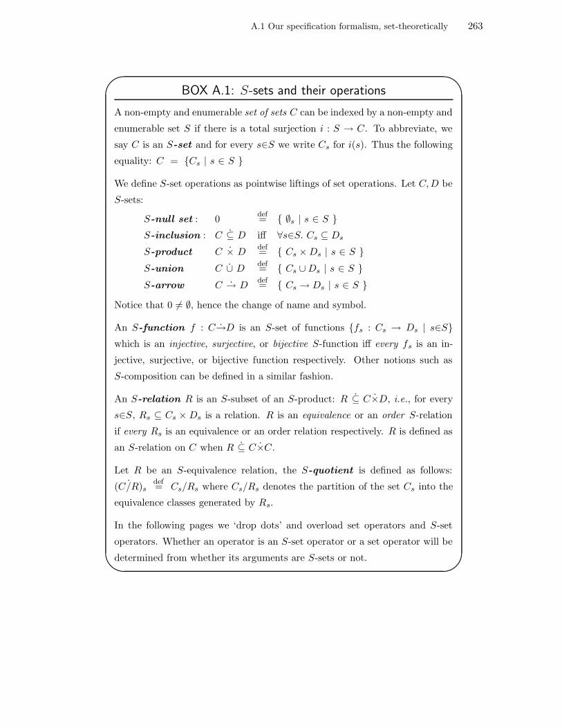
A.1 Our specification formalism, set-theoretically 263
'
&
$
%
BOX A.1: S-sets and their operations
A non-empty and enumerable set of sets C can be indexed by a non-empty and
enumerable set S if there is a total surjection i : S → C. To abbreviate, we
say C is an S-set and for every s∈S we write Cs for i(s). Thus the following
equality: C = Cs | s ∈ S
We define S-set operations as pointwise liftings of set operations. Let C,D be
S-sets:
S-null set : 0def= ∅s | s ∈ S
S-inclusion : C ⊆ D iff ∀s∈S. Cs ⊆ Ds
S-product C × Ddef= Cs ×Ds | s ∈ S
S-union C ∪ Ddef= Cs ∪Ds | s ∈ S
S-arrow C → Ddef= Cs → Ds | s ∈ S
Notice that 0 6= ∅, hence the change of name and symbol.
An S-function f : C→D is an S-set of functions fs : Cs → Ds | s∈S
which is an injective, surjective, or bijective S-function iff every fs is an in-
jective, surjective, or bijective function respectively. Other notions such as
S-composition can be defined in a similar fashion.
An S-relation R is an S-subset of an S-product: R ⊆ C×D, i.e., for every
s∈S, Rs ⊆ Cs ×Ds is a relation. R is an equivalence or an order S-relation
if every Rs is an equivalence or an order relation respectively. R is defined as
an S-relation on C when R ⊆ C×C.
Let R be an S-equivalence relation, the S-quotient is defined as follows:
(C/R)sdef= Cs/Rs where Cs/Rs denotes the partition of the set Cs into the
equivalence classes generated by Rs.
In the following pages we ‘drop dots’ and overload set operators and S-set
operators. Whether an operator is an S-set operator or a set operator will be
determined from whether its arguments are S-sets or not.

A.1 Our specification formalism, set-theoretically 264
symbols are different (not overloaded) but this is not a strict requirement, for sort-
signatures are not inferred (Section 4.7.2). Because the number of operators in a
specification is finite, many sets Ωws will be empty. In subsequent definitions predicates
of the form σ∈Ωws are placed as rule premises.
A.1.2 Terms, sort-assignments and substitution
Given a signature we can define the set of closed terms (with no free variables), but
because equations involve free variables it is better to define the set of open terms from
the start and define the set of closed terms as a special case. Variables are also sorted.
For convenience, instead of assuming the existence of an S-set of variables we make
use of the notion of sort-assignment, i.e., a finite set of pairs that is the extension of a
finite function from variables to sorts.
Definition A.1.3 A sort-assignment Γ : X → S is a finite function from a finite
set of variables to the finite set of sorts.
We use sort-assignments both intensionally (i.e., Γ(x) is a sort) and extensionally as
sets of pairs. Being a set, X has no repetitions.
Definition A.1.4 Given a signature Σ = (S,Ω) and a sort-assignment Γ we define
the S-set of open terms:
Term(Σ,Γ) = Term(Σ,Γ)s | s ∈ S
for every sort s inductively as follows:
Γ(x) = s
x ∈ Term(Σ,Γ)s
σ ∈ Ωs
σ ∈ Term(Σ,Γ)s
σ ∈ Ωs1...sns ti ∈ Term(Σ,Γ)sii ∈ 1 . . . n n > 0
σ t1 . . . tn ∈ Term(Σ,Γ)s
The S-set of closed terms Term(Σ, ∅) is thus defined as a special case. It follows from
the above definition that Term(Σ, ∅) ⊆ Term(Σ,Γ).

A.1 Our specification formalism, set-theoretically 265
Because of the uniform treatment of constant and proper operators, the second induct-
ive rule in Definition A.1.4 could be embedded in the last one by making n ≥ 0, but
it would lose the flavour of a definition by structural induction. Notice that Defini-
tion A.1.4 defines the set of terms by induction on the following recursive grammar of
terms:
t ::= x | σ | σ t1 . . . tn
where x is a meta-variable standing for any object variable, σ is a meta-variable standing
for any constant operator symbol in the second alternative, and for a proper operator
of arity n > 0 in the last alternative. In subsequent definitions or proofs, the phrase
‘by structural induction on terms’ will mean by induction on this grammar.
Figure A.1 (page 266) formally describes the signature of a specification example of
strings and characters in a given sort-assignment.
The S-set of closed terms can also be defined in terms of a substitution of all free
variables in open terms for closed terms. Since terms have no bound variables, the set
of free variables of a term can be defined easily.
Definition A.1.5 Given a term t ∈ Term(Σ,Γ)s, the set FV(t) of free variables of t
is defined inductively on the structure of t as follows:
x ∈ Term(Σ,Γ)s
FV(x)def= x
σ ∈ Term(Σ,Γ)s
FV(σ)def= ∅
σ ∈ Ωs1...sns ti ∈ Term(Σ,Γ)sii ∈ 1 . . . n n > 0
FV(σ t1 . . . tn)def= FV(t1) ∪ . . . ∪ FV(tn)
We first define the substitution of free variables for open terms and then define the
substitution of free variables for closed terms as a special case.
Definition A.1.6 Given term t of sort s in which variable x may occur free, and
another term t′ with the same sort as x, the substitution of t′ for x in t produces
another term of the same sort as t. A substitution is a function from open terms to

A.1 Our specification formalism, set-theoretically 266
signature STRING signature CHARsorts String sorts Charuse CHAR opsops ch0 : → Charempty : → String . . .pre : Char String → String ch255 : → Char
end end
Σdef= (S,Ω) where S
def= Char ,String
Ω = ΩChar ,ΩString ,ΩCharStringString
ΩChardef= ch0, . . . , ch255
ΩStringdef= empty
ΩCharStringStringdef= pre
Γdef= (c,Char ), (s,String)
Term(Σ, ∅)Chardef= ch0, . . . , ch255
Term(Σ,Γ)Char = c ∪ Term(Σ, ∅)Char
Term(Σ,Γ)Stringdef= s, empty, pre c s, pre c empty, pre ch0 empty,
pre ch1 empty, . . . , pre c (pre ch0 empty), . . .
Figure A.1: Strings and characters in a given sort-assignment.

A.1 Our specification formalism, set-theoretically 267
open terms which we denote as [t′/x]t. The following definition provides its ‘type’:
t ∈ Term(Σ,Γ ∪ (x, s′))s t′ ∈ Term(Σ,Γ)s′
[t′/x]t ∈ Term(Σ,Γ)s
Γ is enlarged to guarantee the existence of variable x with sort s′. Notice that Γ is a
function so for the union to yield a valid sort-assignment there cannot be a binding for
x in Γ. This device will be used in subsequent definitions.
The ‘body’ of substitution is defined inductively as follows:
x ∈ Dom(Γ)
[t′/x]xdef= t′
y ∈ Dom(Γ) y 6= x
[t′/x]ydef= y
σ ∈ Term(Σ,Γ)s
[t′/x]σdef= σ
σ ∈ Ωs1...sns ti ∈ Term(Σ,Γ)sii ∈ 1 . . . n n > 0
[t′/x](σ t1 . . . tn)def= σ ([t′/x]t1) . . . ([t′/x]tn)
The substitution of a variable for a closed term is a special case where t′∈Term(Σ, ∅)s′ .
Substituting all remaining free variables in t again for closed terms produces a term
in Term(Σ, ∅)s. Recall that for each s, Term(Σ, ∅)s ⊆ Term(Σ,Γ)s and therefore all
possible substitutions of open-term variables for closed terms will produce closed terms
in Term(Σ, ∅)s. This is consistent with our use of universally quantified variables as
standing for the possibly countably infinite closed terms of the same sort, which enables
us to write a finite set of equations involving variables (perhaps we should call them
equation schemas) instead of a countably infinite number of them involving closed
terms.
A.1.3 Algebras
The semantics of a signature Σ (no equations) is provided by an algebra A. Free
variables for equations are added by a theory. In order to save definitions, let us
define the meaning of a signature in the presence of a sort-assignment (which becomes
necessary when equations are added later on). The semantics is formalised by defining
a ‘symbol-mapping’ S-function that maps sorts to carriers and operator symbols to

A.1 Our specification formalism, set-theoretically 268
algebraic operators, plus a semantic S-function that provides the meaning (value in a
carrier) of a term when given the value-assignment that provides the meanings (values)
of its free variables.
Definition A.1.7 A Σ-Algebra A for a signature Σdef= (S,Ω) and sort-assignment Γ
is a pair (|A|,ΩA) where:
1. |A| is an S-set of carrier sets, each providing values for each sort in S.
2. ΩA is an S+-set of algebraic operators. It is common mathematical practice to
use cartesian products in the carrier-signatures of algebraic operators, i.e.,
σA ∈ ΩAs1...sns
σA : |A|s1× . . . × |A|sn
→ |A|s
3. There is an overloaded symbol-mapping S-function 1, I, that consistently maps
sorts to carriers and operator symbols to algebraic operators. That is, I : S → |A|
and I : Ω→ ΩA such that:
s ∈ S
I(s)def= |A|s
σ ∈ Ωs1...sns n ≥ 0
I(σ) ∈ ΩAs1...sns
In other words:
σ : s1 . . . sn → s n ≥ 0
I(σ) : I(s1) . . . I(sn)→ I(s)
4. There is a value-assignment or finite function ρ : X →⋃
s|A|s from variables to
values of the carriers that conforms to Γ, i.e.: ρ(x) ∈ |A|Γ(x).
5. There is a semantic S-function h where:
hs : Term(Σ,Γ)s → (X →⋃
s
|A|s)→ |A|s
It has become standard practice in denoting semantic functions to use the symbol
of the entity providing the semantics and a double-bracket notation for semantic
1Or if the reader prefers, two S-functions with overloaded name.

A.1 Our specification formalism, set-theoretically 269
function application in order to underline the fact that arguments are syntactic
entities that are interpreted in a particular semantic universe [Mit96, Sto77, Ten76].
In the rest of the chapter we writeAsJ·K instead of hs andAsJtKρ instead of (hs(t))(ρ),
breaking our convention of using explicit parentheses for application at the meta-
level only for this function (Section 2.6).
AsJ·K is inductively defined on the structure of terms as follows:
Γ(x) = s
AsJxKρdef= ρ(x)
sem1σ ∈ Ωs
AsJσKρdef= I(σ)
sem2
σ ∈ Ωs1...sns ti ∈ Term(Σ,Γ)sii ∈ 1 . . . n n > 0
AsJσ t1 . . . tnKρdef= (I(σ))(As1
Jt1Kρ, . . . ,AsnJtnKρ)
sem3
The following property follows from the definition. In words, the property states that
if a term of sort s is in the set of open terms then its meaning with respect to a
value-assignment giving meaning to its free variables is in the carrier giving meaning
to s:
t ∈ Term(Σ,Γ)s
AsJtKρ ∈ |A|s
In some presentations the set of variables X is an S-set, and consequently Γ and ρ
are S-functions; in particular ρs : Xs → |A|s. In this setting, the semantic S-function
can be seen as an extension of value-assignments for variables to value-assignments for
terms (domain extension), and is sometimes denoted as ρ# (see also Section A.3).
Figure A.2 (page 271) shows two possible algebras giving meaning to the algebraic
specification of characters and strings of Figure A.1. The first box defines the S-sets
|A| and ΩA. It also defines that, as required by Definition A.1.7(3), I(s)def= |A|s for
all s∈Char ,String. Finally, the value-assignment ρ is empty because there are no
variables or equations in Figure A.1. These definitions are the same for the two algebras
given in the second and third boxes.

A.1 Our specification formalism, set-theoretically 270
In the second box the carrier for characters is the (extended) ascii table and the carrier
for strings is the set of strings that can be formed with characters from the ascii table.
The reader may want to recall Definition A.1.1 where the star operator, ε, and string
concatenation are defined.
Notice that the definition of ΩAChar is informal. The carrier |A|Char contains constant
values, not algebraic operators. We can consider constants c∈|A|Char as functions
c : |A|1 → |A|Char by positing the existence of an extra sort name 1 with carrier |A|1
which is the carrier of nullary cartesian products (see Sections 3.6 and A.3.1).
There are two algebraic operators with signature |A|Char × |A|String → |A|String called
‘append’ and ‘prepend’ whose description follows:
c ∈ ascii s ∈ ascii∗
append(c, s) ∈ ascii∗ append(c, s)def= s(cε)
c ∈ ascii s ∈ ascii∗
prepend(c, s) ∈ ascii∗ prepend(c, s)def= cs
I maps pre to prepend, but it could have mapped it to append.
In the third box, the carrier for characters is a singleton set with element $. All chi
operators are mapped by I to $. Therefore, if the specification had the equations
ch0 = ch1, . . . , ch254 = ch255, this algebra would satisfy them whereas the algebra
in the second box would not (Section A.1.6). Again, ΩAChar is informally defined to be
|A|Char , but bear in mind that formally there is a lifting of constants to functions. The
meaning for strings is provided by stacks. The empty string is the empty stack [ ], and
pre is mapped to the push operator for stacks. Thus, |A|String contains all the stack
values that can be formed by stacking $s.
A.1.4 Substitution lemma
Each S-indexed semantic function is compositional: the meaning of a term depends
on the meaning of its subterms in a value-assignment. As expected, the substitution
lemma holds: the meaning of [t′/x]t is the same as the meaning of the term t in a
value-assignment that assigns to x the meaning of t′. To state the substitution lemma
we need the notion of value-assignment enlargement denoted ρ〈x 7→ v〉, where ρ is

A.1 Our specification formalism, set-theoretically 271
|A|def= |A|Char , |A|String
ΩA def= ΩA
Char , ΩAString , ΩA
CharStringString
I(Char )def= |A|Char
I(String)def= |A|String
ρdef=
|A|Chardef= ascii
|A|Stringdef= ascii∗
ΩAChar
def= |A|Char
ΩAString
def= ε
ΩACharStringString
def= append, prepend
I(ch0)def= nul
I(ch1)def= soh
...
I(ch255)def=
I(empty)def= ε
I(pre)def= prepend
|A|Chardef= $
|A|Stringdef= [ ], [$], [$$], [$$$], . . . ,
ΩAChar
def= |A|Char
ΩAString
def= [ ]
ΩACharStringString
def= push
I(ch0)def= $
...
I(ch255)def= $
I(empty)def= [ ]
I(pre)def= push
Figure A.2: Two possible algebraic semantics for the specification of Figure A.1.

A.1 Our specification formalism, set-theoretically 272
enlarged with the pair (x, v) such that v∈|A|Γ(x). Context enlargement binds stronger
than application. An enlargement creates a new value-assignment that overlays any
previous binding for x, that is:
ρ〈x 7→ v〉(y)def= if y = x then v else ρ(y)
Lemma A.1.1 (Substitution) Let Γ = Γ′ ∪ (x, s′)
t ∈ Term(Σ,Γ)s t′ ∈ Term(Σ,Γ′)s′ [t′/x]t ∈ Term(Σ,Γ′)s
AsJ [t′/x]t Kρ = AsJtKρ〈x 7→ AsJt′Kρ〉
(Because Γ′ has lower cardinality than Γ, open terms can be turned into closed terms
by repeated substitution.)
Proof: by straightforward induction on t (assuming the preconditions hold):
• t is x:
AsJ [t′/x]x Kρ
= Substitution
AsJ t′ Kρ
= x /∈ FV(t′)
AsJ x Kρ〈x 7→ AsJt′Kρ〉
• t is y and y 6= x:
AsJ [t′/x]y Kρ
= Substitution
AsJ y Kρ
= x /∈ FV(y)
AsJ y Kρ〈x 7→ AsJt′Kρ〉
• t is σ and σ∈Ωs:
AsJ [t′/x]σ Kρ
= Substitution
AsJ σ Kρ
= x /∈ FV(σ)
AsJ σ Kρ〈x 7→ AsJt′Kρ〉
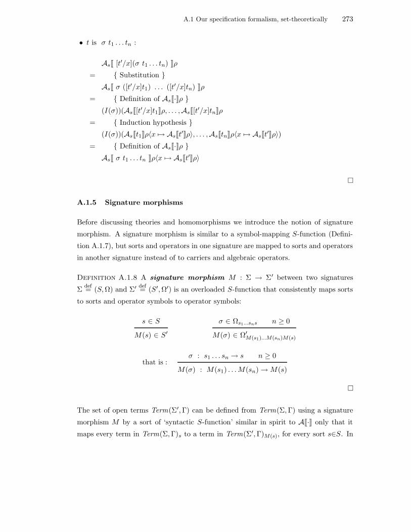
A.1 Our specification formalism, set-theoretically 273
• t is σ t1 . . . tn :
AsJ [t′/x](σ t1 . . . tn) Kρ
= Substitution
AsJ σ ([t′/x]t1) . . . ([t′/x]tn) Kρ
= Definition of AsJ·Kρ
(I(σ))(AsJ[t′/x]t1Kρ, . . . ,AsJ[t
′/x]tnKρ
= Induction hypothesis
(I(σ))(AsJt1Kρ〈x 7→ AsJt′Kρ〉, . . . ,AsJtnKρ〈x 7→ AsJt
′Kρ〉)
= Definition of AsJ·Kρ
AsJ σ t1 . . . tn Kρ〈x 7→ AsJt′Kρ〉
A.1.5 Signature morphisms
Before discussing theories and homomorphisms we introduce the notion of signature
morphism. A signature morphism is similar to a symbol-mapping S-function (Defini-
tion A.1.7), but sorts and operators in one signature are mapped to sorts and operators
in another signature instead of to carriers and algebraic operators.
Definition A.1.8 A signature morphism M : Σ → Σ′ between two signatures
Σdef= (S,Ω) and Σ′ def
= (S′,Ω′) is an overloaded S-function that consistently maps sorts
to sorts and operator symbols to operator symbols:
s ∈ S
M(s) ∈ S′
σ ∈ Ωs1...sns n ≥ 0
M(σ) ∈ Ω′M(s1)...M(sn)M(s)
that is :σ : s1 . . . sn → s n ≥ 0
M(σ) : M(s1) . . . M(sn)→M(s)
The set of open terms Term(Σ′,Γ) can be defined from Term(Σ,Γ) using a signature
morphism M by a sort of ‘syntactic S-function’ similar in spirit to AJ·K only that it
maps every term in Term(Σ,Γ)s to a term in Term(Σ′,Γ)M(s), for every sort s∈S. In

A.1 Our specification formalism, set-theoretically 274
order to be precise about the fact that every variable in Dom(Γ) is mapped to itself,
and to be able to define also the set of open terms Term(Σ′,Γ′) where Γ′ 6= Γ, we need
another device, a variable-assignment ν : Dom(Γ)→ Dom(Γ′) such that if Γ(x) = s
then Γ′(ν(x)) = M(s). We do not use variable-assignments again and only mention
them for the sake of precision.
A.1.6 Theories and homomorphisms
Variables have been taken into account in the previous definitions which assumed the
existence of a sort-assignment Γ. A basic theory adds equations to a signature. Since
we consider conditional equations in Section 5.5, we generalise in advance and speak
about laws instead of equations. Equations are between terms of the same sort and
therefore the laws form an S-set. Equations t1 = t2 are formalised by triples of the
form 〈t1, t2,Γ〉. Mentioning the sort-assignment explicitly is more precise and will be
necessary in order to specify the proof system of which the equations are axioms, in
particular Leibniz’s rule (i.e., substitution of equals for equals) where equality is made
compatible with substitution.
Definition A.1.9 A basic Σ-Theory (or just theory) T is a pair (Σ, L) where Σ is
a signature and L is an S-set of laws (equations) where:
Ls ⊆ 〈t1, t2,Γ〉 | t1∈Term(Σ,Γ)s ∧ t2∈Term(Σ,Γ)s
In what follows we shall use syntactic sugar and write 〈t1 = t2, Γ〉 instead of 〈t1, t2,Γ〉.
The following is an example equation:
〈 pop (push x s) = s , (x,Nat), (s,Stack ) 〉
Equations introduce equivalence relations among terms and constitute axioms in a
proof system of syntactic equality which we now define precisely. (We follow standard
notation and write ` φ if the formula φ can be proven in the proof system from the
axioms by application of rules of inference.)
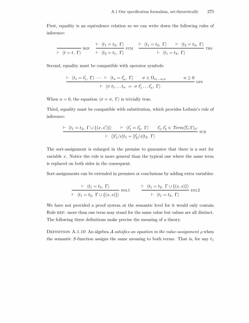
A.1 Our specification formalism, set-theoretically 275
First, equality is an equivalence relation so we can write down the following rules of
inference:
` 〈t = t, Γ〉ref
` 〈t1 = t2, Γ〉
` 〈t2 = t1, Γ〉sym
` 〈t1 = t2, Γ〉 ` 〈t2 = t3, Γ〉
` 〈t1 = t3, Γ〉trs
Second, equality must be compatible with operator symbols:
` 〈t1 = t′1, Γ〉 · · · ` 〈tn = t′n, Γ〉 σ ∈ Ωs1...sns n ≥ 0
` 〈σ t1 . . . tn = σ t′1 . . . t′n, Γ〉ops
When n = 0, the equation 〈σ = σ, Γ〉 is trivially true.
Third, equality must be compatible with substitution, which provides Leibniz’s rule of
inference:
` 〈t1 = t2, Γ ∪ (x, s′)〉 ` 〈t′1 = t′2, Γ〉 t′1, t′2 ∈ Term(Σ,Γ)s′
` 〈[t′1/x]t1 = [t′2/x]t2, Γ〉sub
The sort-assignment is enlarged in the premise to guarantee that there is a sort for
variable x. Notice the rule is more general than the typical one where the same term
is replaced on both sides in the consequent.
Sort-assignments can be extended in premises or conclusions by adding extra variables:
` 〈t1 = t2, Γ〉
` 〈t1 = t2, Γ ∪ (x, s)〉enl1
` 〈t1 = t2, Γ ∪ (x, s)〉
` 〈t1 = t2, Γ〉enl2
We have not provided a proof system at the semantic level for it would only contain
Rule ref: more than one term may stand for the same value but values are all distinct.
The following three definitions make precise the meaning of a theory.
Definition A.1.10 An algebra A satisfies an equation in the value-assignment ρ when
the semantic S-function assigns the same meaning to both terms. That is, for any t1
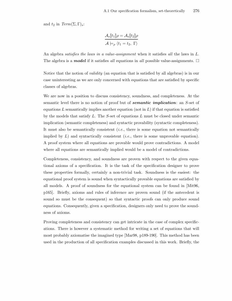
A.1 Our specification formalism, set-theoretically 276
and t2 in Term(Σ,Γ)s:
AsJt1Kρ = AsJt2Kρ
A |=ρ 〈t1 = t2, Γ〉
An algebra satisfies the laws in a value-assignment when it satisfies all the laws in L.
The algebra is a model if it satisfies all equations in all possible value-assignments.
Notice that the notion of validity (an equation that is satisfied by all algebras) is in our
case uninteresting as we are only concerned with equations that are satisfied by specific
classes of algebras.
We are now in a position to discuss consistency, soundness, and completeness. At the
semantic level there is no notion of proof but of semantic implication : an S-set of
equations L semantically implies another equation (not in L) if that equation is satisfied
by the models that satisfy L. The S-set of equations L must be closed under semantic
implication (semantic completeness) and syntactic provability (syntactic completeness).
It must also be semantically consistent (i.e., there is some equation not semantically
implied by L) and syntactically consistent (i.e., there is some unprovable equation).
A proof system where all equations are provable would prove contradictions. A model
where all equations are semantically implied would be a model of contradictions.
Completeness, consistency, and soundness are proven with respect to the given equa-
tional axioms of a specification. It is the task of the specification designer to prove
these properties formally, certainly a non-trivial task. Soundness is the easiest: the
equational proof system is sound when syntactically provable equations are satisfied by
all models. A proof of soundness for the equational system can be found in [Mit96,
p165]. Briefly, axioms and rules of inference are proven sound (if the antecedent is
sound so must be the consequent) so that syntactic proofs can only produce sound
equations. Consequently, given a specification, designers only need to prove the sound-
ness of axioms.
Proving completeness and consistency can get intricate in the case of complex specific-
ations. There is however a systematic method for writing a set of equations that will
most probably axiomatise the imagined type [Mar98, p189-190]. This method has been
used in the production of all specification examples discussed in this work. Briefly, the

A.1 Our specification formalism, set-theoretically 277
method consists in (1) identifying the set of constructor operators that generate all the
terms representing values of the type, (2) writing equations between constructors to
make equal values congruent, and (3) writing equations that specify the behaviour of
the remaining operators on constructor terms.
Completeness is essential to guarantee that we have specified the intended model. How-
ever, we want our specification to be satisfied by a unique model (up to isomorphism).
We are interested in a least-model completeness, namely, that equations satisfied by
the least model are syntactically provable. This form of completeness fails for algebras
with empty carriers2 (which we bar by fiat), or laws with disjunctions (which is not our
case) [Mit96, p157-179]. The least model is unique (up to isomorphism) and in order
to define it we need the notion of homomorphism (literally, ‘same-form-ism’) between
algebras.
In the absence of equations, the S-sets Term(Σ, ∅) and Term(Σ,Γ) are themselves
algebras where the symbol-mapping and semantic S-functions are identities and where
the carrier for sort s is Term(Σ, ∅)s. This construction receives the name of free
algebra from the fact that an algebra is obtained for free only from terms, where
syntactically different terms are taken as semantically different values. This algebra
constitutes a least model.
In the presence of equations and sort-assignment Γ, terms are classified into equivalence
classes. It is common practice to denote by [t] the equivalence class of term t which
contains all those terms equal to t as established by the equations in L or those that
can be proven syntactically from them. Let us denote by ≡L the equivalence relation
on terms generated by the proof system, that is:
t ≡L t′ ⇔ ` 〈t = t′, Γ〉
Inference rule ops states that syntactic equality is compatible with the operators of the
algebra, making ≡L a congruence relation on terms. In this case, the S-set of closed
terms partitioned by equivalence classes constitutes the least model. The following
definitions elaborate the technical scaffolding.
Definition A.1.11 A Σ-homomorphism between two algebras A and B is an over-
2The set of sorts is not empty so if carriers are empty there cannot exist a value-assignment con-forming to any sort-assignment.
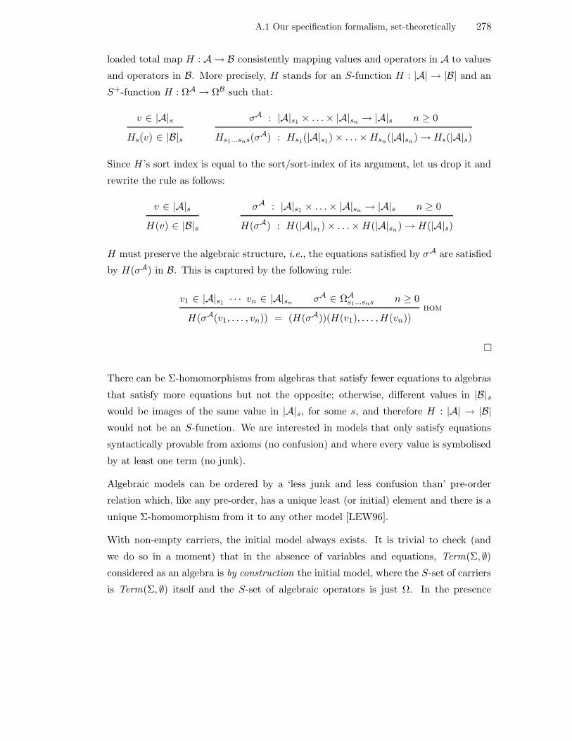
A.1 Our specification formalism, set-theoretically 278
loaded total map H : A → B consistently mapping values and operators in A to values
and operators in B. More precisely, H stands for an S-function H : |A| → |B| and an
S+-function H : ΩA → ΩB such that:
v ∈ |A|s
Hs(v) ∈ |B|s
σA : |A|s1× . . .× |A|sn
→ |A|s n ≥ 0
Hs1...sns(σA) : Hs1
(|A|s1)× . . .×Hsn
(|A|sn)→ Hs(|A|s)
Since H’s sort index is equal to the sort/sort-index of its argument, let us drop it and
rewrite the rule as follows:
v ∈ |A|s
H(v) ∈ |B|s
σA : |A|s1× . . .× |A|sn
→ |A|s n ≥ 0
H(σA) : H(|A|s1)× . . .×H(|A|sn
)→ H(|A|s)
H must preserve the algebraic structure, i.e., the equations satisfied by σA are satisfied
by H(σA) in B. This is captured by the following rule:
v1 ∈ |A|s1· · · vn ∈ |A|sn
σA ∈ ΩAs1...sns n ≥ 0
H(σA(v1, . . . , vn)) = (H(σA))(H(v1), . . . ,H(vn))hom
There can be Σ-homomorphisms from algebras that satisfy fewer equations to algebras
that satisfy more equations but not the opposite; otherwise, different values in |B|s
would be images of the same value in |A|s, for some s, and therefore H : |A| → |B|
would not be an S-function. We are interested in models that only satisfy equations
syntactically provable from axioms (no confusion) and where every value is symbolised
by at least one term (no junk).
Algebraic models can be ordered by a ‘less junk and less confusion than’ pre-order
relation which, like any pre-order, has a unique least (or initial) element and there is a
unique Σ-homomorphism from it to any other model [LEW96].
With non-empty carriers, the initial model always exists. It is trivial to check (and
we do so in a moment) that in the absence of variables and equations, Term(Σ, ∅)
considered as an algebra is by construction the initial model, where the S-set of carriers
is Term(Σ, ∅) itself and the S-set of algebraic operators is just Ω. In the presence

A.1 Our specification formalism, set-theoretically 279
of variables and equations, Γ is not empty and we assume the existence of a value-
assignment ρ that conforms to Γ. However, recall from Definition A.1.6 that under
repeated substitution Term(Σ,Γ) becomes Term(Σ, ∅). Since substitution is compatible
with syntactic equality, the proof system induces a least congruence S-relation ≡L
between closed terms that partitions the set of closed terms into equivalence classes
yielding the S-quotient Term(Σ, ∅)/≡L, which is the initial model.
A.1.7 Initial models
In order to keep the distinction between syntax and semantics, and for consistency with
the use of cartesian products in carrier-signatures, we define the notion of open term
algebra as different from the set of open terms.
Definition A.1.12 The open term algebra is TΣΓdef= (|TΣΓ|,Ω
TΣΓ) where |TΣΓ| is
an S-set of carriers and ΩTΣΓ is an S+-set of algebraic operators such that the carrier
|TΣΓ|s of open term values of sort s is defined inductively as follows:
Γ(x) = s
x ∈ |TΣΓ|s
σ ∈ Ωs
σ ∈ |TΣΓ|s
σ ∈ Ωs1...sns ti ∈ |TΣΓ|sii ∈ 1 . . . n n > 0
σ(t1, . . . , tn) ∈ |TΣΓ|s
The change of notation from Term(Σ,Γ) to TΣΓ and from Ω to ΩTΣΓ is similar to a type
cast where the same entity is considered as having a different meaning. Notationally, Ω
is the set of syntactic symbols whereas ΩTΣΓ has the same elements as Ω now considered
as algebraic operators:
σ : s1 . . . sn → s σ ∈ Ωs1...sns n ≥ 0
σ : |TΣΓ|s1× . . .× |TΣΓ|sn
→ |TΣΓ|s σ ∈ ΩTΣΓ
s1...sns
Sort-signatures have changed to carrier-signatures with cartesian products. The gram-
mar of open terms is now:
t ::= x | σ | σ(t1, . . . , tn)
With closed terms, Γ = ∅ and there is no need for value assignments: the closed term
algebra is TΣdef= TΣ∅.

A.1 Our specification formalism, set-theoretically 280
Now, it is not difficult to glean from Definition A.1.7 that the symbol-mapping and
the semantic S-functions both make up a Σ-homomorphism. The overloaded symbol-
mapping S-function has types I : S → |TΣ| and I : Ω→ ΩTΣ such that:
s ∈ S
I(s)def= |TΣ|s
σ : s1 . . . sn → s n ≥ 0
I(σ) : |TΣ|s1× . . .× |TΣ|sn
→ |TΣ|s
The rightmost consequent follows from the fact that:
σ ∈ Ωs
I(σ)def= σ
inj
where I is an injection, not an identity. In Definition A.1.7, there is already a rule for
I in similar format as that of Definition A.1.11:
σ : s1 . . . sn → s n ≥ 0
I(σ) : I(s1)× . . .× I(sn)→ I(s)
Let us overload I even more and use it to name the semantic S-function in Defini-
tion A.1.7, that is, for all s let us write I for AsJ·K. In Definition A.1.7, Rule sem1 has
to be removed because there are no variables. Rule sem2 holds by Rule inj. Rule sem3
can be rewritten as:
v1 ∈ |TΣ|s1· · · vn ∈ |TΣ|sn
σ ∈ ΩTΣ
s1...sns n ≥ 0
I(σ(v1, . . . , vn))def= (I(σ))(I(v1), . . . , I(vn))
Finally, a definition induces an equality (Chapter 2), making the previous rule an
instance of Rule hom in Definition A.1.11.
In the presence of equations the proof system induces a least congruence S-relation ≡L
between closed terms that partitions the set of closed terms into equivalence classes
yielding the S-quotient Qdef= TΣ/≡L which is defined inductively as follows.
Let [t] denote the equivalence class of term t:
σ ∈ |TΣ|s
[σ] ∈ Qs
σ ∈ ΩTΣ
s1...sns ti ∈ Qsii∈1 . . . n n > 0
[σ(t1, . . . , tn)] ∈ Qs

A.2 Our partial formalism, set-theoretically 281
Because ≡L is a congruence, [σ(t1 . . . tn)] = σ([t1], . . . , [tn]). Furthermore, because the
substitution lemma holds, the meaning of an open term of TΣΓ/≡L can be determined
from the meaning of its free variables, which is given by the equivalence class of value-
assignments [ρ], where [ρ](x)def= [ρ(x)].
By construction, Q is an initial model: all the values of the carrier are represented by at
least one term and Q satisfies all the equations of L closed under syntactic provability.
TΣ constitutes a free algebra that is an initial model of the theory with no equations.
A.2 Our partial formalism, set-theoretically
We now provide a set-theoretical formalisation of partial specifications and their se-
mantics. Only the theory part must change; the definitions of Σ, Term(Σ,Γ), TΣ and
TΣΓ remain. The difference now is that undefined terms are junk and do not symbolise
any algebraic value.
Definition A.2.1 A Partial Σ-Algebra A is a pair (|A|,ΩA) where for σ∈Ωws:
• I(σ)def= σA may be undefined when w = ε, that is, σA /∈ |A|s.
• I(σ)def= σA may be partial when w = s1 . . . sn, that is, for n > 0 and i∈1 . . . n, it
may be the case that vi∈|A|siand σA∈ΩA
s1...sns but σA(v1, . . . , vn) /∈ |A|s.
A Σ-homomorphism between partial algebras is a total S-function and can only map
defined values in carriers to defined values.
Definition A.2.2 A Σ-homomorphism H : A → B between two partial algebras A
and B is a total S-function that satisfies the following:
σA ∈ ΩAs1...sns σA(v1, . . . , vn) ∈ |A|s n ≥ 0
(H(σA))(H(v1), . . . ,H(vn)) ∈ |B|s
σA ∈ ΩAs1...sns σA(v1, . . . , vn) ∈ |A|s n ≥ 0
H(σA(v1, . . . , vn)) = (H(σA))(H(v1), . . . ,H(vn))

A.2 Our partial formalism, set-theoretically 282
The fact that the symbol-mapping S-function I may be undefined for certain constants
means the semantic S-function may also be undefined for some terms. It can also be
undefined for terms involving proper partial operators. Consequently, I and AJ·K no
longer make up a Σ-homomorphism, which must be a total S-function (Section A.1.7).
TΣ is no longer an initial algebra, for it contains junk.
By definition, given a Σ-homomorphism H : A → B between two partial algebras,
|B| may have more defined terms than |A| but not the opposite; otherwise, different
values in |B|s would be images of the same value in |A|s, for some s, and therefore
H : |A| → |B| would not be an S-function.
There is a ‘less partial than’ relation between partial algebras. The initial partial
algebra has a unique Σ-homomorphism from it to any other partial algebra. For a
closed term algebra to be an initial model it must have least junk (contain only those
terms that are defined in all models), least confusion (two defined terms have the
same value only if they do in all models), and there is at least a defined term symbolising
every intended value.
We first revise our definition of theory to account for conditional equations.
Definition A.2.3 A partial theory is a pair (Σ, L) where Σ is a signature and L is a
set of laws involving terms of Term(Σ,Γ) in a context Γ. More precisely, equations in Ls
have the form 〈P ⇒ E, Γ〉 where P is a possibly empty conjunction of preconditions
and E is an equation t = t′ or a partial equation t ' t′. Preconditions consist of
equations. A conditional equation P ⇒ t ' t′ is syntactic sugar for:
P ∧DEF (t) ∧DEF (t′)⇒ t = t′
and predicate DEF (t) is syntactic sugar for t = t.
The proof system does not have to be enlarged with introduction and elimination rules
for conditional equations. Conditional equations can be considered object-level repres-
entations of meta-level inference rules. Every conditional equation 〈E1 ∧ . . . ∧En ⇒
E, Γ〉 where n > 0 introduces an inference rule:
` 〈E1,Γ〉 · · · ` 〈En,Γ〉
` 〈E,Γ〉

A.2 Our partial formalism, set-theoretically 283
An equation between two terms must be satisfied in all models (their interpretation
must produce the same value). For partial equations, if both terms have values (are
defined in the model) then their interpretation must be the same. If one or both terms
are undefined the equation is vacuously satisifed. Consequently, we only have to add
definedness premises in the definition of model.
Definition A.2.4 An algebra A satisfies an equation Edef= 〈t1 = t2, Γ〉 or a partial
equation Edef= 〈t1 ' t2, Γ〉 in the value-assignment ρ when:
AsJt1Kρ ∈ |A|s AsJt2Kρ ∈ |A|s AsJt1Kρ = AsJt2Kρ
A |=ρ E
An algebra A satisfies a conditional equation 〈P ⇒ E, Γ〉 in the value assignment ρ
when:
Pdef= E1 ∧ . . . ∧En A |=ρ E1 · · · A |=ρ En n ≥ 0
A |=ρ E
An algebra satisfies the laws in a value-assignment when it satisfies all the laws in L.
The algebra is a model if it satisfies all equations in all possible value-assignments.
A partial theory has an initial model that is the least defined: it has least junk (a term
is defined if and only if it is defined in all models), it has least confusion (two terms
have the same meaning only if they do in all models), and every value is symbolised by
at least one term. Such a model is defined in terms of the subset of TΣ that contains
all defined terms, which we denote by DomL, and a congruence relation between those
terms induced by the proof system of conditional equations, which we denote by ≡L.
In order to characterise the initial algebra precisely we need to define the notion of
immediate subterm of a term.
Definition A.2.5 The set of immediate subterms Sub(t) of a term t is inductively
defined as follows:
σ ∈ Ω
Sub(σ)def= ∅
σ ∈ Ωs1...sns ti ∈ Term(Σ,Γ)sii ∈ 1 . . . n n > 0
Sub(σ t1 . . . tn)def= t1, . . . , tn

A.2 Our partial formalism, set-theoretically 284
With this set in hand we can define an immediate subterm relation 2 between terms:
t′ 2 t⇔ t′∈Sub(t).
Definition A.2.6 Given a theory (Σ, L), let the set DomL ⊆ TΣ, and the congruence
≡L⊆ DomL × DomL be the smallest set and congruence that satisfy the following
properties:
1. For every equation 〈t1 = t2, Γ〉, every immediate closed term t′ of sort s in Sub(t1)
and Sub(t2) is defined, that is, AsJt′Kρ ∈ |DomL|s.
2. DomL is closed with respect to the immediate subterm relation:
AsJtKρ ∈ |DomL|s t′ ∈ Term(Σ,Γ)s′ t′ 2 t
As′Jt′Kρ ∈ |DomL|s′
3. The congruence is reflexive, symmetric and transitive:
t ∈ |DomL|s
t ≡L t
t1 ≡L t2
t2 ≡L t1
t1 ≡L t2 t2 ≡L t3
t1 ≡L t3
Notice that reflexivity is conditional on definedness.
4. The congruence is compatible with substitution of variables for values: for every
conditional equation 〈E1 . . . En ⇒ E, Γ〉 in L such that Eidef= ti = t′i and E
def= t = t′:
ti, t′i ∈ Term(Σ,Γ)si
AsiJtiKρ ≡L Asi
Jt′iKρ i ∈ 1 . . . n n ≥ 0
AsJtKρ ∈ |DomL|s AsJt′Kρ ∈ |DomL|s AsJtKρ ≡L AsJt
′Kρ
In particular, if n = 0 the consequent becomes an axiom.
5. The congruence is compatible with operators: either applications of operators to
defined and congruent term arguments are defined and congruent, or are undefined.
More precisely, either:
σ ∈ Ωs1...sns ti, t′i ∈ |DomL|si
ti ≡L t′i i ∈ 1 . . . n n > 0
(I(σ))(t1, . . . tn) ∈ |DomL|s
(I(σ))(t′1, . . . t′n) ∈ |DomL|s
(I(σ))(t1, . . . tn) ≡L (I(σ))(t′1, . . . t′n)

A.3 Our formalism, categorially 285
or:
σ ∈ Ωs1...sns ti, t′i ∈ |DomL|si
ti ≡L t′i i ∈ 1 . . . n n > 0
(I(σ))(t1, . . . tn) /∈ |DomL|s (I(σ))(t′1, . . . t′n) /∈ |DomL|s
Theorem A.2.1 The initial algebra of a theory (Σ, L) with partial conditional equa-
tions is the quotient DomL/≡L. The set of carriers is |DomL|/≡L. Let us denote by
[t] the equivalence class of the term t of sort s in |DomL|s. For every operator symbol
σ∈Ωs1...sns where n ≥ 0:
(I(σ))([t1], . . . , [tn])def=
[(I(σ))(t1, . . . , tn)] , if (I(σ))(t1, . . . , tn)∈|DomL|s
undefined , otherwise
A.3 Our formalism, categorially
In the set-theoretical formulation, the same concepts appear again and again, namely,
the existence of objects and structure-preserving arrows between them. The categorial
study of specifications can focus on the syntax or the semantics as long as the categorial
axioms are satisfied by the particular objects and arrows at hand. Furthermore, in some
categories there are distinguished initial objects (e.g., least model, least defined model).
For example, we have the category of sorts, where objects are sorts, arrows are operator
symbols, and signature morphisms are functors (recall Definition A.1.8). We also have
the category of algebras, where objects are carriers, arrows are algebraic operators, and
every Hs is a functor (recall Definition A.1.11).
Σ-Algebras and partial Σ-Algebras with their respective Σ-homomorphisms both con-
stitute categories. In both cases, the identity arrow is the identity Σ-homomorphism
and composition is S-composition of Σ-homomorphisms. The reader can check that
the categorial axioms are satisfied. In both cases, the object of interest is the initial
object of the category.
Recall from Section A.1 that the unique-arrow property of the initial object is satisfied.

A.3 Our formalism, categorially 286
In the category of algebras this property can be depicted as a diagram:
TΣ!A - A
@@
@@
@
!B
RB
H
?
A similar diagram can be written for TΣΓ. Let us denote the initial object as 0. The
following diagram depicts the relationship in any category of algebras:
0!A - A
@@
@@
@
!B
RB
H
?
Recall from page 269 that the semantic S-function can be seen as an extension of value-
assignments considered as S-functions ρ : X → |A|. Let us write TΣ(X) instead of TΣΓ
to underline the role of the, now, S-set of variables X. TΣ(X) is the initial model and
there is a unique Σ-homomorphism from it to any other algebra. At the carrier level
(category Set where objects are carrier sets and arrows are total functions on sets), it is
witnessed by the existence of ρ# which makes the following diagram commute [BG82]:
|TΣ(X)|ρ#
- |A|
ρ
X
ηX
6
That is, ρ# ηX = ρ. Function ηX maps variables to themselves as values (again think
of a cast). The notation gives away the fact that ηX is a natural transformation and
that TΣ(·) is a functor; more precisely, η : Id.→ TΣ, where Id is the identity functor.
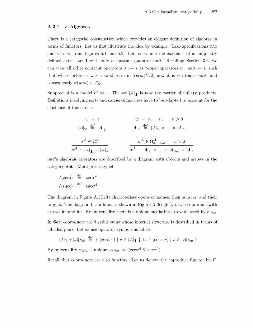
A.3 Our formalism, categorially 287
A.3.1 F -Algebras
There is a categorial construction which provides an elegant definition of algebras in
terms of functors. Let us first illustrate the idea by example. Take specifications NAT
and STRING from Figures 5.1 and 5.2. Let us assume the existence of an implicitly
defined extra sort 1 with only a constant operator unit . Recalling Section 3.6, we
can view all other constant operators σ :→ s as proper operators σ : unit → s, such
that where before σ was a valid term in Term(Σ, ∅) now it is written σ unit , and
consequently σ(unit) ∈ TΣ.
Suppose A is a model of NAT. The set |A|1 is now the carrier of nullary products.
Definitions involving sort- and carrier-signatures have to be adapted to account for the
existence of this carrier:
w = ε
|A|wdef= |A|1
w = s1 . . . sn n > 0
|A|wdef= |A|s1
× . . .× |A|sn
σA ∈ ΩAs
σA : |A|1 → |A|s
σA ∈ ΩAs1...sns n > 0
σA : |A|s1× . . .× |A|sn
→ |A|s
NAT’s algebraic operators are described by a diagram with objects and arrows in the
category Set . More precisely, let
I(zero)def= zeroA
I(succ)def= succA
The diagram in Figure A.3(left) characterises operator names, their sources, and their
targets. The diagram has a limit as shown in Figure A.3(right), i.e., a coproduct with
arrows inl and inr. By universality there is a unique mediating arrow denoted by αNat .
In Set, coproducts are disjoint sums whose internal structure is described in terms of
labelled pairs. Let us use operator symbols as labels:
|A|1 + |A|Natdef= (zero, v) | v ∈ |A|1 ∪ (succ, v) | v ∈ |A|Nat
By universality αNat is unique: αNat = (zeroA O succA)
Recall that coproducts are also functors. Let us denote the coproduct functor by F .
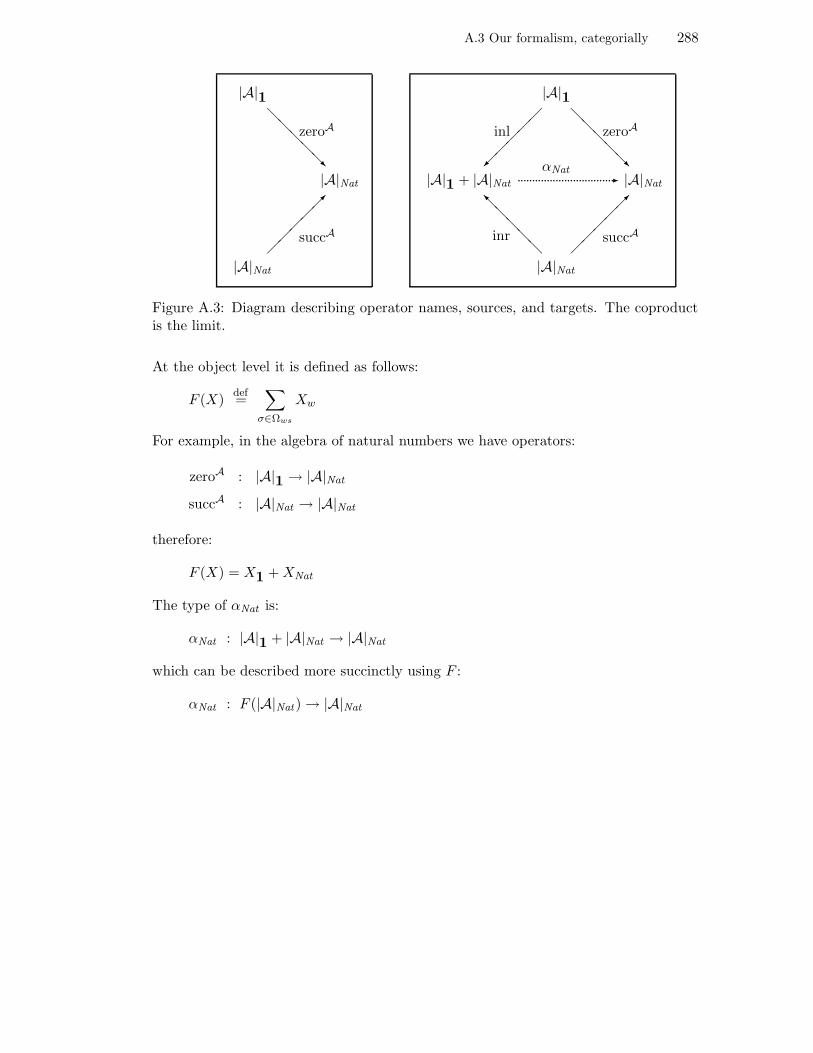
A.3 Our formalism, categorially 288
|A|1
@@
@@
@
zeroA
R|A|Nat
succA
|A|Nat
|A|1
inl
@@
@@
@
zeroA
R|A|1 + |A|Nat
.................................αNat
- |A|Nat
I@@
@@
@inr
succA
|A|Nat
Figure A.3: Diagram describing operator names, sources, and targets. The coproductis the limit.
At the object level it is defined as follows:
F (X)def=
∑
σ∈Ωws
Xw
For example, in the algebra of natural numbers we have operators:
zeroA : |A|1 → |A|Nat
succA : |A|Nat → |A|Nat
therefore:
F (X) = X1 + XNat
The type of αNat is:
αNat : |A|1 + |A|Nat → |A|Nat
which can be described more succinctly using F :
αNat : F (|A|Nat)→ |A|Nat

A.3 Our formalism, categorially 289
At the arrow level F is defined as follows:
h : |A| → |B|
F (h) : F (|A|)→ F (|B|)
hs : |A|s → |B|s s ∈ 1,Nat
Fs(hs) : Fs(|A|s)→ Fs(|B|s)
v ∈ |A|1
(F1(h1))(zero, v)def= (zero, h1(v))
v ∈ |A|Nat
(FNat (hNat ))(succ, v)def= (succ, hNat (v))
If we carry out the same construction for STRING, assuming A is now its model, we
obtain two functions, one for each sort:
αChar : |A|1 + . . . + |A|1 → |A|Char
αChar = (ch0A O . . . O ch255A)
αString : |A|1 + |A|CharString → |A|String
αString = (emptyAO preA)
Clearly, α : F (|A|)→ |A| is an S-function. In general a Σ-Algebra A can be character-
ised in terms of the S-set carrier |A| and the S-function α. This construction receives
the name of F -Algebra. F is the S-functor Fs : Set → Set | s ∈ S where objects
in Set are the carriers |A|s.
We provide a definition of F -Algebras for algebras with one carrier. For many-sorted
algebras, the definition below can be adapted by replacing Set with S-Set (the category
of S-Sets). In that setting, |A| is an S-Set, α is an S-function, and F is an S-functor.
Definition A.3.1 An F -Algebra in Set is a pair (A, α) where |A| is an object in
Set, α : F (|A|) → |A| is an arrow in Set, and F : Set → Set is a functor. An
F -homomorphism h : (|A|, α) → (|B|, β) is an arrow that makes the following dia-
gram commute:
F (|A|)F (h)- F (|B|)
|A|
α
? h - |B|
β
?

A.3 Our formalism, categorially 290
The reader may have realised that α and β are particular instances of the natural
transformation η : F.→ Id (Section 3.12).
The simplicity and conciseness of this definition is due to what it does not say. It only
involves carriers, and the mapping from operators in A to operators in B that is part
of a Σ-homomorphism is not mentioned. Such mapping maps operators to operators
respecting carrier-signatures and constitutes another functor. Finally, mediating arrows
α are not informative about the name of operators nor their carrier-signatures if the
diagram of which the coproduct is a limit is not shown. Providing the diagram amounts
to providing the carrier-signatures of algebraic operators explicitly.
One of the goodies of category theory is that, as expected, the definition of F -Algebra
can be generalised to any category C:
Definition A.3.2 Let C be a category and F : C→ C a functor. An F -Algebra is a
pair (X,α) where X is an object and α : F (X) → X an arrow. An F -homomorphism
h : (X,α) → (Y, β) is an arrow that makes the following diagram commute:
F (X)F (h)- F (Y )
X
α
? h - Y
β
?
It is important to notice that different algebras may be described by the same F , e.g.,
α : F (|A|) → |A| and β : F (|B|) → |B| where α 6= β. In particular, A could be the
algebra giving meaning to an algebraic specification without equations and B the algebra
giving meaning to an algebraic specification with equations. Informally speaking, the
same F may capture the signature of theories with wildly dissimilar equations. We
come back to this point when introducing F -views (Chapter 9).
acknowledgements
My sincere gratitude to:
• My supervisor, Roland Backhouse, for giving me the opportunity to come to Not-
tingham, for finding financial support, for being an absolute gentleman, and for
putting up with my hand-waviness and tardiness. I must apologise for not making
it up to his standards of presentation, notation and spacing (and for using the words
‘dredge’ and ‘buck’).
• The internal examiner, Louise A. Dennis, for accepting the dreadful task of reading,
correcting and, certainly, improving this work, and for giving me the opportunity to
work as a research assistant on a short project which enabled me to pay the bills.
• The internal examiner, Ralf Lammel, for his detailed and incisive criticism without
which this thesis would be worse. I have not come across many researchers that
move so comfortably across programming paradigms and brands of French wine.
• Henrik Nilsson and Fermın Reig for their invaluable help. Many thanks too to the
DGP guys at Oxford, Jeremy Gibbons and Bruno Cesar dos Santos Oliveira, for
their sympathy and constructive criticism on the few, but also invaluable, occasions
in which we met.
• Other FOP members: to inspiring Conor McBride: politics, religion, and type theory
bundled in verbose and gnomic wit. Graham Hutton has a ‘razor’ that enables
him to explain things in a simple and understandable language. Finally, thanks
to discerning, encyclopedic, and mordant Thorsten Altenkirch who perhaps could
express his thoughts with more tact.
On the personal side, I’d like to thank:
• My family, for everything.
• Belen, mi pequeno cuchito, . . . no hay palabras.
• Angel Herranz and Julio Marino, who spur my interest in declarative languages and
programming theory. I am also indebted to Pedro Gomez Arroyo for his encourage-
ment, and to Pilar Herrero for her ‘last-minute’ advice.

A.3 Our formalism, categorially 292
• My friends and acquaintances at the School of Computer Science (ASAP’ers and
MRL’ers, you know who you are) who made my lunches so enjoyable. Special
regards to Martın, Darıo, Jaume, Benji, and Mark Hills. I enjoyed our humorous
and many-sided discussions—but you should make better use of emacs, Mark.
Last, but not at all least, thanks to my office-mates for patiently answering my
English and Haskell questions, for tolerating my eccentricities, and for some lovely
cinema evenings.
Nottingham, April 2006

Bibliography
[ABDM03] Mads Sig Ager, Dariusz Biernacki, Olivier Danvy, and Jan Midtgaard. A
functional correspondence between evaluators and abstract machines. In
Proceedings of the 5th ACM SIGPLAN international conference on Prin-
ciples and Practice of Declarative Programming, pages 8–19. ACM Press,
2003.
[AC89] E. Astesiano and M. Cerioli. On the existence of initial models for partial
(higher-order) conditional specifications. In Proc. Joint Conf. on Theory
and Practice of Software Development, pages 74–88. Springer LNCS 351,
1989.
[AC96] Martın Abadi and Luca Cardelli. A Theory of Objects. Springer-Verlag,
New York, 1996.
[AMM05] Thorsten Altenkirch, Conor McBride, and James McKinna. Why depend-
ent types matter. Manuscript, submitted ICFP’05, April 2005.
[AR92] William E. Aitken and John H. Reppy. Abstract value constructors. In Pro-
ceedings of the 1992 ACM Workshop on ML and its Applications, pages
1–11, San Francisco, USA, June 1992. Association for Computing Ma-
chinery.
[AS05] Artem Alimarine and Sjaak Smetsers. Improved fusion for optimizing gen-
erics. In Proceedings of the 7th Symposium on Practical Aspects of Declar-
ative Programming (PADL’05). ACM Press, January 2005.
[Bai89] Jean Baillie. An introduction to the algebraic specification of abstract data
types. Available online, December 1989.
[Bar84] Henk P. Barendregt. The Lambda Calculus: Its Syntax and Semantics.
North Holland, Amsterdam, revised edition, 1984.
293
BIBLIOGRAPHY 294
[BBvv98] Roland Backhouse, Marcel Bijsterveld, Rik van Geldrop, and Jaap van der
Woude. Category theory as coherently constructive lattice theory. Working
document, 12 June 1998.
[BdM97] Richard Bird and Oege de Moor. Algebra of Programming. International
Series in Computer Science. Prentice-Hall, 1997.
[Ber01] Ulrich Berger. Programming with abstract data types. Lecture Notes
CS376, Department of Computer Science, University of Wales Swansea,
Autumn 2001.
[BG82] Rod Burstall and Joseph Goguen. Algebras, theories, and freeness: An
introduction for computer scientists. In Manfred Wirsing and Gunther
Schmidt, editors, Theoretical Foundations of Programming Methodology,
pages 329–350, Reidel, 1982. Proceedings, 1981 Marktoberdorf NATO
Summer School, NATO Advanced Study Institute Series, Volume C91.
[BJJM99] Roland Backhouse, Patrik Jansson, Johan Jeuring, and Lambert Meertens.
Generic programming – an introduction. In S. Doaitse Swierstra, editor,
3rd International Summer School on Advanced Functional Programming,
Braga, Portugal, LNCS 1608. Springer-Verlag, 1999.
[Blo91] Stephen Blott. Type Classes. PhD thesis, Glasgow University, Glasgow,
Scotland, UK, 1991.
[BM98] Richard Bird and Lambert Meertens. Nested datatypes. In Johan Jeuring,
editor, Proceedings of the Fourth International Conference on Mathematics
of Program Construction (MPC’98), volume 1422 of LNCS, pages 52–67.
Springer Verlag, 1998.
[BP99] Richard Bird and Ross Paterson. Generalised folds for nested datatypes.
Formal Aspects of Computing, 11(2):200–222, 1999.
[Bud02] Timothy Budd. Introduction to Object-Oriented Programming. Addison-
Wesley, 3th edition, 2002.
[BW82] M. Broy and M. Wirsing. Partial abstract types. Acta Informatica,
18(1):47–64, 1982.

BIBLIOGRAPHY 295
[BW88] Richard Bird and Philip Wadler. Introduction to Functional Programming.
International Series in Computer Science. Prentice-Hall, 1988.
[BW99] Michael Barr and Charles Wells. Category theory. Lecture Notes, ESSLLI,
1999.
[Car86] Luca Cardelli. A polymorphic lambda calculus with type:type. Technical
Report SRC Research Report 10, Digital Equipment Corporation, Palo
Alto, California, 1986.
[Car97] Luca Cardelli. Type systems. In Allen B. Tucker, editor, The Computer
Science and Engineering Handbook. CRC Press, Boca Raton, FL, 1997.
Revised 2004.
[Cas97] Giuseppe Castagna. Object-Oriented Programming: A Unified Foundation.
Progress in Theoretical Computer Science. Birkhauser, 1997.
[CE00] Krzysztof Czarnecki and Ulrich Eisenecker. Generative Programming.
Methods, Tools and Applications. Addison-Wesley, 2000.
[CF68] Haskell B. Curry and Robert Feys. Combinatory Logic. North-Holland,
Amsterdam, 2nd edition, 1968.
[CH96] Tyng-Ruey Chuang and Wen L. Hwang. A probabilistic approach to the
problem of automatic selection of data representations. In 1996 ACM SIG-
PLAN International Conference on Functional Programming (ICFP’96),
pages 190–200, Philadephia, Pennsylvania, USA, 1996.
[CH02] James Cheney and Ralf Hinze. A lightweight implementation of gener-
ics and dynamics. In Proceedings of the 2002 ACM SIGPLAN Haskell
Workshop, pages 90–104, New York, October 2002. ACM Press.
[Chu41] Alonzo Church. The Calculi of Lambda Conversion. Princeton University
Press, 1941.
[Cut80] Nigel Cutland. Computability: An Introduction to Recursive Function The-
ory. Cambridge University Press, 1980.

BIBLIOGRAPHY 296
[CW85] Luca Cardelli and Peter Wegner. On understanding types, data abstrac-
tion, and polymorphism. Computer Surveys, 17(4):471–522, December
1985.
[DDMM03] Mourad Debbabi, Nancy Durgin, Mohamed Mejri, and John C. Mitchell.
Security by typing. International Journal on Software Tools for Technology
Transfer (STTT), 4(4):472–495, August 2003.
[DJ04] Nils Anders Danielsson and Patrik Jansson. Chasing bottoms – A case
study in program verification in the presence of partial and infinite values.
In 7th International Conference on Mathematics of Program Construction.
LNCS, Springer-Verlag, 2004.
[DT88] Scott Danforth and Chris Tomlinson. Type theories and object-oriented
programmimg. ACM Comput. Surv., 20(1):29–72, 1988.
[Erw96] Martin Erwig. Active patterns. 1996.
[FH88] Anthony J. Field and Peter G. Harrison. Functional Programming. In-
ternational Series in Computer Science. Addison-Wesley, 1988. (reprinted
1993).
[Fok92] Maarten M. Fokkinga. A gentle introduction to category theory — the
calculational approach. In Lecture Notes of the STOP 1992 Summerschool
on Constructive Algorithmics, pages 1–72 of Part 1. University of Utrecht,
September 1992.
[GH05] Jeremy Gibbons and Graham Hutton. Proof methods for corecursive pro-
grams. Fundamenta Informaticæ, Special Issue on Program Transforma-
tion, IOS Press, 66(4):353–366, April-May 2005.
[GHA01] Jeremy Gibbons, Graham Hutton, and Thorsten Altenkirch. When is a
function a fold or an unfold? Electronic Notes in Theoretical Computer
Science, 44(1), 2001. Proceedings of the 4th International Workshop on
Coalgebraic Methods in Computer Science.
[GHJV95] E. Gamma, R. Helm, R. Johnson, and J. Vlissides. Design Patterns -
Elements of Reusable Object Oriented Software. Addison-Wesley, 1995.

BIBLIOGRAPHY 297
[Gib03] Jeremy Gibbons. Patterns in datatype-generic programming. Declarative
Programming in the Context of Object-Oriented Languages (DPCOOL’03),
2003.
[Gir72] Girard, J.-Y. Interpretation Fonctionnelle et Elimination des Coupures
de l’Arithmetique d’Ordre Superieur. These de doctorat d’etat, Universite
Paris VII, June 1972.
[GM89] Joseph Goguen and Jose Meseguer. Ordered-sorted algebra I: Equational
deduction for multiple inheritance, overloading, exceptions and partial op-
erations. Technical Report SRI-CSL-89-10, Computer Science Lab, SRI
International, July 1989.
[GNP95] Carlos Gregorio Rodriguez, M. Nunez Garcıa, and Pedro Palao-Gostanza.
La potencia expresiva de los catamorfismos. In Proceedings of the Joint
Conference on Declarative Programming, GULP-PRODE’95, pages 477–
484, 1995.
[Gog88] Joseph A. Goguen. Higher order functions considered unnecessary for
higher order programming. Technical Report SRI-CSL-88-1, Computer
Science Lab, SRI International, January 1988.
[Gol79] Robert Goldblatt. Topoi: The Categorial Analysis of Logic. North-Holland,
New York, 1979.
[GP03] Daniele Gorla and Rosario Pugliese. Enforcing security policies via types.
In International Conference on Security in Pervasive Computing, LNCS,
2003.
[GTW79] J. Goguen, J. Thatcher, and E. Wagner. An initial algebra approach to
the specification, correctness, and implementation of abstract data types.
In R. Yeh, editor, Current Trends in Programming Methodology IV, pages
80–149. Prentice-Hall, 1979.
[Gut77] John Guttag. Abstract data types and the development of data structures.
Commun. ACM, 20(6):396–404, 1977.

BIBLIOGRAPHY 298
[GWM+93] Joseph Goguen, Timothy Winkler, Jose Meseguer, Kokichi Futatsugi, and
Jean-Pierre Jouannaud. Introducing OBJ. In Joseph Goguen, editor, Ap-
plications of Algebraic Specification using OBJ. Cambridge, 1993.
[Ham82] A. G. Hamilton. Numbers, Sets and Axioms: The Apparatus of Mathem-
atics. Cambridge University Press, 1982.
[Hei96] James L. Hein. Theory of Computation: An Introduction. Jones and Barlet
Publishers International, London, 1996.
[Hen93] Fritz Henglein. Type inference with polymorphic recursion. ACM Trans-
actions on Programming Languages and Systems, 15(2):253–289, 1993.
[HHPW92] C. Hall, K. Hammond, S. Peyton Jones, and P. Wadler. Type Classes in
Haskell. Technical report, University of Glasgow, Glasgow, Scotland, UK,
1992.
[Hin00] Ralf Hinze. Generic programs and proofs. Habilitationsschrift, Universitat
Bonn, October 2000.
[Hin02] Ralf Hinze. Polytypic values possess polykinded types. Science of Com-
puter Programming, 43(2–3):129–159, June 2002.
[Hin04] Ralf Hinze. Generics for the masses. 9th ACM Sigplan Int. Conf. Func-
tional Programming, pages 236–243, September 2004.
[HJ02] Ralf Hinze and Johan Jeuring. Generic Haskell, Practice and Theory.
In Summer School and Workshop on Generic Programming, Oxford, UK,
LNCS 2297. Springer Verlag, 2002.
[HJL04] Hinze, Jeuring, and Loh. Type-indexed data types. Science of Computer
Programming, 51, 2004.
[HJL05] Stefan Holdermans, Johan Jeuring, and Andres Loh. Generic views on
data types. Technical Report UU-CS-2005-012, Utrecht University, 2005.
[HLO06] Ralf Hinze, Andres Loh, and Bruno C. d. S. Oliveira. ”Scrap Your Boil-
erplate” reloaded. In Eighth International Symposium on Functional and
Logic Programming (FLOPS’06), pages 13–29, 2006.

BIBLIOGRAPHY 299
[HM95] Robert Harper and Greg Morrisett. Compiling polymorphism using inten-
sional type analysis. In Proc. 22nd ACM Symp. on Principles of Program-
ming Languages, January 1995.
[Hoa87] C. A. R. Hoare. An overview of some formal methods for program design.
Computer, September 1987.
[Hof97] Martin Hofmann. Syntax and semantics of dependent types. In A. M. Pitts
and P. Dybjer, editors, Semantics and Logics of Computation, volume 14 of
Publications of the Newton Institute, pages 79–130. Cambridge University
Press, 1997.
[Hoo97] Paul Hoogendijk. A generic theory of data types. PhD thesis, Eindhoven
University of Technology, 1997.
[How80] W. Howard. The formulas-as-types notion of construction. In J. P. Seldin
and J. R. Hindley, editors, To H. B. Curry: Essays on Combinatory Logic,
Lambda-Calculus, and Formalism, pages 479–490. Academic Press, NY,
1980.
[HS86] J. Roger Hindley and Jonathan P. Seldin. Introduction to Combinators and
λ-Calculus. London Mathematical Society, Student Texts 1. Cambridge
University Press, 1986. Reprint 1993.
[Hug89] John Hughes. Why functional programming matters. Computer Journal,
32(2):98–107, 1989.
[Hug99] John Hughes. Restricted data types in Haskell. Haskell Workshop ’99,
September 1999.
[Hut99] Graham Hutton. A tutorial on the universality and expressiveness of fold.
Journal of Functional Programming, 9(4):335–372, July 1999.
[Jon92] Mark P. Jones. Qualified Types: Theory and Practice. PhD thesis, Oxford
University, July 1992.
[Jon95a] Mark P. Jones. Functional programming with overloading and higher-order
polymorphism. Lecture Notes in Computer Science, 925:97ff, 1995.

BIBLIOGRAPHY 300
[Jon95b] Mark P. Jones. A system of constructor classes: overloading and implicit
higher-order polymorphism. Journal of Functional Programming, 5(1):1–
37, January 1995.
[KLS04] Oleg Kiselyov, Ralf Lammel, and Keean Schupke. Strongly typed hetero-
geneous collections. In ACM SIGPLAN Workshop on Haskell. ACM Press,
2004.
[Koe89] Arthur Koestler. The Act of Creation. Penguin Arkana, 1989. First pub-
lished in 1964.
[Lan66] Peter J. Landin. The next 700 programming languages. Communications
of the ACM, 9(3):157–164, March 1966. Originally presented at the Pro-
ceedings of the ACM Programming Language and Pragmatics Conference,
August 8–12, 1965.
[Lau95] Konstantin Laufer. A framework for higher-order functions in C++. In
Proc. Conf. Object-Oriented Technologies (COOTS), Monterey, CA, 1995.
[LEW96] Jacques Loeckx, Hans-Dieter Ehrich, and Markus Wolf. Specification of
Abstract Data Types. John Wiley & Sons Ltd and B. G. Teubner, New
York, NY, 1996.
[LG86] Barbara Liskov and John V. Guttag. Abstraction and Specification in
Program Development. The MIT Electrical Engineering and Computer
Science Series. MIT Press, Cambridge, MA, 1986.
[Loh04] Andres Loh. Exploring Generic Haskell. PhD thesis, Utrecht University,
September 2004.
[LP03] Ralf Lammel and Simon Peyton Jones. Scrap your boilerplate: a prac-
tical design pattern for generic programming. ACM SIGPLAN Notices,
38(3):26–37, March 2003. Proc. of the ACM SIGPLAN Workshop on Types
in Language Design and Implementation (TLDI 2003).
[LP04] Ralf Lammel and Simon Peyton Jones. Scrap more boilerplate: reflection,
zips, and generalised casts. In Proceedings; International Conference on
Functional Programming (ICFP 2004). ACM Press, September 2004.

BIBLIOGRAPHY 301
[LP05] Ralf Lammel and Simon Peyton Jones. Scrap your boilerplate with class:
extensible generic functions. In Proceedings of the ACM SIGPLAN In-
ternational Conference on Functional Programming (ICFP 2005). ACM
Press, September 2005.
[LV02a] R. Lammel and J. Visser. Typed Combinators for Generic Traversal. In
Proc. Practical Aspects of Declarative Programming PADL 2002, volume
2257 of LNCS, pages 137–154. Springer-Verlag, 2002.
[LV02b] Ralf Lammel and Joost Visser. Design Patterns for Functional Strategic
Programming. In Proc. of Third ACM SIGPLAN Workshop on Rule-Based
Programming RULE’02, Pittsburgh, USA, 2002. ACM Press.
[LV02c] Ralf Lammel and Joost Visser. Strategic polymorphism requires just two
combinators! Technical Report cs.PL/0212048, ArXiv, December 2002.
[LVK00] Ralf Lammel, Joost Visser, and Jan Kort. Dealing with large bananas.
In Johan Jeuring, editor, Workshop on Generic Programming, Ponte de
Lima, July 2000. Technical Report UU-CS-2000-19, Universiteit Utrecht.
[LVV02] Ralf Lammel, Eelco Visser, and Joost Visser. The essence of strategic
programming. Draft, 15 October 2002.
[Mac90] Bruce J. MacLennan. Functional Programming, Practice and Theory.
Addison-Wesley, 1990.
[Mar98] Ricardo Pena Marı. Diseno de Programas, Formalismo y Abstraccion.
Prentice-Hall, 1998.
[Mei95] Karl Meinke. A survey of higher-order algebra. Technical Report UUDM
1995:39, ISSN 1101-3591, Department of Mathematics, University of
Uppsala, 1995.
[MFP91] Erik Meijer, Maarten Fokkinga, and Ross Paterson. Functional program-
ming with bananas, lenses, envelopes and barbed wire. In J. Hughes, ed-
itor, Proceedings of the 5th ACM Conference on Functional Programming
Languages and Computer Architecture (FPCA’91), volume 523 of LNCS.
Springer-Verlag, 1991.

BIBLIOGRAPHY 302
[MH95] Erik Meijer and Graham Hutton. Bananas in space: Extending fold and
unfold to exponential types. In Proceedings of the 7th ACM Confer-
ence on Functional Programming Languages and Computer Architecture
(FPCA’95). ACM Press, 1995.
[Mit96] John C. Mitchell. Foundations for Programming Languages. MIT Press,
1996.
[MJP97] Erik Meijer, Mark Jones, and Simon Peyton Jones. Type classes: An
exploration of the design space, May 1997.
[MM04] Connor McBride and James McKinna. The view from the left. Journal of
Functional Programming, 14(1), 2004.
[Mog91] Eugenio Moggi. Notions of computation and monads. Information and
Computation, 93:55–92, 1991.
[Moo02] A. W. Moore. The Infinite. Routledge, London, 2002.
[Mor73] James H. Morris, Jr. Types are not sets. In Proceedings of the 1st an-
nual ACM SIGACT-SIGPLAN symposium on Principles of Programming
Languages, pages 120–124. ACM Press, 1973.
[MS94] David R. Musser and Alexander A. Stepanov. Algorithm-oriented generic
libraries. Software—Practice and Experience, 24(7):623–642, July 1994.
[MS96] David R. Musser and Atul Saini. STL Tutorial and Reference Guide.
Addison-Wesley, Reading, Mass., 1996.
[MS00] Brian McNamara and Yannis Smaragdakis. Functional programming in
C++. In Proceedings of the fifth ACM SIGPLAN International Conference
on Functional Programming, pages 118–129. ACM Press, 2000.
[Myc84] Alan Mycroft. Polymorphic type schemes and recursive definitions. In
M. Paul and B. Robinet, editors, Proceedings of the International Sym-
posium on Programming, volume 167 of LNCS, pages 217–228, Toulouse,
France, April 1984. Springer.
[Nog05] Pablo Nogueira. The gist of side effects in pure functional languages. Tu-
torial, available online, 14th April 2005.

BIBLIOGRAPHY 303
[OG05] Bruno Oliveira and Jeremy Gibbons. Typecase: A design pattern for type-
indexed functions. Submitted to the Haskell Workshop, 2005.
[Oka98a] Chris Okasaki. Purely Functional Data Structures. Cambridge University
Press, 1998.
[Oka98b] Chris Okasaki. Views for Standard ML, 1998.
[OL96] Martin Odersky and Konstantin Laufer. Putting type annotations to work.
In Conference Record of the 23rd ACM SIGPLAN-SIGACT Symposium
on Principles of Programming Languages (POPL’96), pages 54–67, St.
Petersburg, Florida, January 21–24 1996. ACM Press.
[Pal95] Pedro Palao Gostanza. Integracion de Tipos Abstractos de Datos y Ajuste
de Patrones. PhD thesis, Departamento de Informatica y Automatica,
Universidad Complutense de Madrid, 1995.
[Pau96] Lawrence C. Paulson. ML for the Working Programmer. Cambridge Uni-
versity Press, 2nd edition, 1996.
[Pie91] Benjamin C. Pierce. Basic Category Theory for Computer Scientists. The
MIT Press, 1991.
[Pie02] Benjamin C. Pierce. Types and Programming Languages. The MIT Press,
2002.
[Pie05] Benjamin C. Pierce, editor. Advanced Topics in Types and Programming
Languages. The MIT Press, 2005.
[PPN96] Pedro Palao Gostanza, Ricardo Pena, and Manuel Nunez. A new look at
pattern matching in abstract data types. In Proceedings of the first ACM
SIGPLAN international conference on Functional Programming, pages
110–121. ACM Press, 1996.
[PVV93] Rinus Plasmeijer, Marko Van Eekelen, and Marco Van Ekelen. Functional
Programming and Parallel Graph Rewriting. Addison Wesley, 1993.
[PWW04] Simon Peyton Jones, Geoffrey Washburn, and Stephanie Weirich. Wobbly
types: type inference for generalised algebraic data types, July 2004.

BIBLIOGRAPHY 304
[Rea89] Chris Reade. Elements of Functional Programming. International Series
in Computer Science. Addison-Wesley, 1989.
[Rey74] John C. Reynolds. Towards a theory of type structure. In Programming
Symposium, Proceedings Colloque sur la Programmation, pages 408–423.
Springer-Verlag, 1974.
[Rey98] John C. Reynolds. Definitional interpreters for higher-order program-
ming languages. Higher-Order and Symbolic Computation, 11(4):363–397,
December 1998.
[Sch94] David A. Schmidt. The Structure of Typed Programming Languages. MIT
Press, 1994.
[SF93] Tim Sheard and Leonidas Fegaras. A fold for all seasons. In Proceedings of
the 6th Conference on Functional Programming Languages and Computer
Architecture, pages 233–242, 1993.
[SP04] Mark Shields and Simon Peyton Jones. Practical type inference for
arbitrary-rank types. Available online at the authors’ web sites, April
2004.
[SS03] Harold Simmons and Andrea Schalk. Category Theory in Four Easy Move-
ments. Online Book, University of Manchester, October 2003.
[Sto77] Joseph E. Stoy. Denotational Semantics: The Scott-Strachey Approach to
Programming Language Semantics. MIT Press, Cambridge, Massachusetts,
1977.
[Str92] Bjarne Stroustrup. The C++ Programming Language. Addison Wesley,
2nd edition, 1992.
[Str00] Christopher Strachey. Fundamental concepts in programming languages.
Higher Order Symbol. Comput., 13(1-2):11–49, 2000.
[Ten76] R. D. Tennent. The denotational semantics of programming languages.
Commun. ACM, 19(8):437–453, 1976.

BIBLIOGRAPHY 305
[Tho86] Simon Thompson. Laws in miranda. In Richard P. Gabriel, editor, Pro-
ceedings of the ACM Conference on LISP and Functional Programming,
pages 1–12, Cambridge, MA, August 1986. ACM Press.
[Tof96] Mads Tofte. Essentials of Standard ML modules. Lecture Notes, Summer
School in Advanced Functional Programming, August 1996.
[Tul00] Mark Tullsen. First class patterns. 2000.
[Tur90] David A. Turner. Duality and the De Morgan principles for lists. In
W. Feijen, N. van Gasteren, D. Gries, and J. Misra, editors, Beauty is
Our Busines: A Birthday Salute to Edsger W. Dijkstra, pages 390–398.
Springer-Verlag, 1990.
[Vis01] Joost Visser. Visitor combination and traversal control. ACM SIGPLAN
Notices, 36(11):270–282, November 2001. OOPSLA 2001 Conference Pro-
ceedings: Object-Oriented Programming Systems, Languages, and Applic-
ations.
[VJ03] David Vandervoorde and Nicolai Josuttis. C++ Templates. The Complete
Guide. Addison-Wesley, 2003.
[VS04] Joost Visser and Joao Saravia. Tutorial on Strategic Programming Across
Programming Paradigms. Available online at the author’s web sites, 2004.
[Wad87] Philip Wadler. Views: A way for pattern matching to cohabit with data ab-
straction. In Proceedings, 14th Symposium on Principles of Programming
Languages, pages 307–312. ACM Press, 1987.
[Wad89] Philip Wadler. Theorems for free! In Proceedings 4th Int. Conf. on Funct.
Prog. Languages and Computer Arch., FPCA’89, London, UK, 11–13 Sept
1989, pages 347–359. ACM Press, New York, 1989.
[WB89] Philip Wadler and Stephen Blott. How to make ad-hoc polymorphism less
ad hoc. In 16th ACM Symposium on Principles of Programming Languages,
pages 60–76, 1989.
[WC93] F. Warren Burton and Robert D. Cameron. Pattern matching with ab-
stract data types. Journal of Functional Programming, 3(2):171–190, 1993.

BIBLIOGRAPHY 306
[Wei02] Stephanie Weirich. Programming With Types. PhD thesis, Cornell Univer-
sity, August 2002.
[Wul72] W. A. Wulf. A case against the GOTO. SIGPLAN Notices, 11(7):63–69,
nov 1972.

Index
F -Algebra, 14, 85, 289
F -homomorphism, 289
F -view, 9, 13, 238, 290
S-arrow, 263
S-function, 263
S-functor, 289
S-inclusion, 263
S-null set, 263
S-product, 263
S-quotient, 263
S-relation, 263
S-set, 263
S-union, 263def=, 16
Σ-Algebra, 268
partial, 281
Σ-homomorphism, 277
δ-rule, 28
π, 247
abstraction
γ, 140
control, 59
data, 61
encapsulation, 60
functional, 59
polytypic, 131
type class, 162
universal, 28
active destructor, 199
Active Pattern
Erwig’s, 204
Active Patterns
Palao’s, 199
ADT, see type, abstract
bounded, 8, 104, 179, 218, 224
mixed, 104
unbounded, 8, 103, 179, 218, 219,
237
algebra
F -Algebra, 208
Σ-Algebra, 14
carrier, 88, 268
closed term, 279
final, 85
free, 277
initial, 84, 88
partial, 282
many-sorted, 84, 88
model, 88, 276, 283
open term, 279
partial, 84
universal, 84
algebraic specification, 83
anamorphism, 237
application, 23, 25
γ, 140
polytypic, 116
type class, 162
type level, 32
universal, 30
argument, see parameter
307

INDEX 308
arity, 24
boilerplate code, 152
buck, 291
C++, 249
C++ STL, 2, 63, 64, 206, 236
C++ Templates, 21, 68, 69, 71, 73, 74
call site, 25
carrier-signature, 268
casting, 73
catamorphism, 132, 152, 206, 237
categorial, 38
category
S-Set, 289
Pre, 42
Set, 42
Type, 43
Set, 286, 287
Type, 51
arrow, 38
arrow category, 55
constant, 43
definition, 41
diagram, 38
commute, 42
functor, 44
contravariant, 44
covariant, 44
fixed point, 54
higher-order, 54
polynomial, 208
functor category, 55
large, 55
natural transformation, 55
naturality, see universality
object, 38, 41
initial, 43
terminal, 43
opposite, 43
pointwise lifting, 53
product category, 45
small, 55
universality, 39, 42, 48
CDT, 236
closed world, 71
clutter, 169
co-iterator, 206
code bloating, 75
collection, 38
completeness
semantic, 260
syntactic, 261
confusion, 193, 197
least, 282
no confusion, 88, 278
congruence, 277
consistency
semantic, 260
syntactic, 260, 276
constraint expression, 138
constraint list, 137
constructor
eager, 109
lazy, 109
value, 109
container, 236
conversion, 73
crush, 133

INDEX 309
Curry-Howard isomorphism, 63
currying, 25
data constructor, see value constructor
data structure, 25
data type, see type
declarative programming, 66
design pattern, 65
deterministic choice, 210
dispatching, 77
dredge, 184, 291
duality
categorial, 43
DeMorgan, 217
EC[I], 236
polytypic, 236
encapsulation, 10, see abstraction
equality
extensional, 225, 226
equation, 282
conditional, 85
partial, 92, 282
equivalence class, 277
error term, 90
exporting, 9, 14, 243
exporting payload, 184
Extensional Programming, 9, 207
F-bounded, 78
fixed-point operators, 35
fixity, 25
fold, 65, 132, 153
function, 3
nullary, 25
proper, 25
functor
arrow, 52
Generative Programming, 10, 66
generator, 68
Generic Haskell, 107
classic, 12, 107
dependency-style, 12, 107
genericity, 60
implementation invariant, 169
information hiding, see abstraction
instantiation, 10, 61
binding time, 71
substitution, 70
interface, 81
coupling, 81
interpreter, 126, 260
iterator, 206, 236
junk, 169, 172, 193, 196
least, 282
no junk, 88, 278
kind, 30, 32, 69
signature, 32
kind-indexed type, 107
lambda abstraction, 23
type level, 32
Lambda Calculus, 22, 53, 77
Lambda Cube, 77
laws, 87, 274
Leibniz’s rule, 274, see Rule sub
Lisp, 20

INDEX 310
meta-language, 16
method, 25
module
Haskell, 95
normal form
and value, 26
object language, 16
open world, 71, 161
operand, 25
operation, 25
operator, 25
algebraic, 88, 268
classification, 101
constructor, 101, 277
multiple, 101, 212, 220, 224
destructor, 103
discriminator, 102
enumerators, 103
interrogator, 103
modifier, 103
observer, 101, 102
partial, 11, 84
removal
explicit, 103
implicit, 103
selector, 102
symbol, 261, 262
order, 24
parameter
actual, 25
formal, 25
generic, 74
usage, 25
Parameterised Programming, 84
parametricity, 60, 179
parametrisation, 10, 60, see instantiation
dynamic, 71
static, 71
pattern, 188
first-class, 204
linear, 188
nested, 188
simple, 188
pattern matching, 109
payload, 21, 77, 92, 110
persistence, 26
persistent identity, 26
polyaric, 242
polymorphic recursion, 112
polymorphism, 71
ad hoc, 72
ad-hoc
coercion, 73
overloading, 73
impredicative, 78
inclusion, 78
ML-style, 78
parametric, 74
bounded, 78
predicative, 78
structural, 79
Type:Type, 78
universal, 74
polytypic extension, 8, 148, 159, 170,
206, 249
modular, 161

INDEX 311
polytypism, 79
program, see term, value-level
referential transparency, 3, 87
representation type, 116, 215
Rice’s Theorem, 21
RTTI, 154, 163
Rule
β, 23, 26, 27
c-drop, 141
c-empty, 141
c-null, 141
c-push, 141
enl1, 275
enl2, 275
hom, 278, 280
inj, 280
li1, 23, 26, 27
li2, 23, 26
ops, 275, 277
ref, 23, 26, 275
sem1, 269, 280
sem2, 269, 280
sem3, 269, 280
sub, 275
sym, 275
trs, 23, 26, 27, 275
semantic S-function, 268
semantic implication, 276
semantics
axiomatic, 260
denotational, 260
model, 260
operational, 260
shape, 77, 110
signature, 86, 262
morphism, 9, 208, 210, 229, 273,
285
named, 239
type attribute, 240
view attribute, 240
SML functor, 101
SML signature, 99
SML structure, 100
sort, 86, 262
sort-assignment, 264
sort-signature, 86
soundness, 260, 276
Strategic Programming, 152
structure type, see representation type
structured type, see type operator
substitution lemma, 270
subtyping, 79, 256
SyB, 152
symbol-mapping S-function, 268, 273
System F, 28, 63
term, 80, 85
closed, 18
closed set, 264
English, 17
FV function, 265
immediate subterm, 283
open set, 264
stuck, 27
substitution, 265
type-level, see type term
value-level, 17
INDEX 312
well-behaved, 19
well-typed, 19
theory, 86
basic, 274
partial, 282
type, 17, 25
abstract, 62, 187
linear, 208
algebraic, 108
generalised, 165, 167
lawful, 193
assignment, 18
checker, 18
checking
dynamic, 20
static, 20
strong, 20
weak, 20
class, 21, 73
multi-parameter, 180, 225–227
concrete, 62, 187
constructor, see operator
data type, 25
dependent, 21, 61, 77, 207
equivalence
nominal, 126
structural, 34
error, 18
imagined, 62, 276
inference rule, 18
intended, see imagined
irregular, 111
iso-recursive, 189
judgement, 18
manifest, 32
nested, see irregular
non-uniform, see irregular
operator, 30, 62
constrained, 97, 135
nullary, 32
proper, 32
restricted, 226
polykinded, 107, 115
context-parametric, 139
polytypic, 131, 133
scheme, 78
signature, 24
soundness, 19
system, 18
term, 17
type-indexed, see type, polytypic
universe, 77
variable, 32, 74
type-assignment, 26
type-indexed value, 108
type-preserving, 152, 236
type-unifying, 152, 236
types
unit, 43
value, 26
canonical, 193, 205
constructor, 30, 86
manifest, 24, 25
polymorphic, 110
value constructor
abstract, 192
value-assignment, 268

INDEX 313
enlargement, 270
variable-assignment, 274
view
SML, 204
views
Wadler’s, 195


![[5-1] Programming in Java Inheritance and Polymorphism Lecture5](https://img.pdfslide.us/doc/110x75/5697c0121a28abf838ccc271/5-1-programming-in-java-inheritance-and-polymorphism-lecture5.jpg)