Structural Models

Loan and optionality• A firm with risky assets V, which are financed by equity S and

one debt obligation maturing at time T with face value (par value) F.

• The firm’s liabilities are viewed as contingent claims issued against the firm’s asset.

• Default occurs at debt maturity T whenever the firm’s asset valuefalls short of debt value.

ReferenceMerton, R.C., “On the pricing of corporate debt: The risk structureof interest rates,” Journal of Finance vol. 29 (1974) p.449-470.

VT ≤ F VT > F

debt 0 VT − Fequity VT F

value of equity at maturity= max (V − F, 0)which is equivalent to the payoff of a call option with strike F.

total firm assets = total debts + total equity

Payoff received by bondholder at maturity= min(V, F) = F − max(F − V, 0)

corporate loan = Treasury bond + short a put

firm value, V

payoff

face value, F

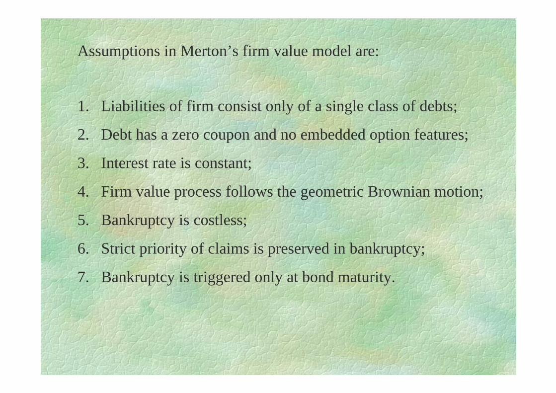
Assumptions in Merton’s firm value model are:

1. Liabilities of firm consist only of a single class of debts;

2. Debt has a zero coupon and no embedded option features;

3. Interest rate is constant;

4. Firm value process follows the geometric Brownian motion;

5. Bankruptcy is costless;

6. Strict priority of claims is preserved in bankruptcy;

7. Bankruptcy is triggered only at bond maturity.

firm value process:

dZdtV

dVVσµ +=

Debt value D(V, t) satisfies the Black-Scholes equation:-

02

2

2

22 =−

∂∂+

∂∂+∂

∂ rDV

DrV

V

DVV

tD

σ

with auxiliary conditions: D(V, T) = min(V, P) and D(0, t) = 0.

),(),( )( tVLFetVD tTr −= −−

where expected loss

−−+−+−−

−−−−+−= −−

tT

tTtTrVN

tT

tTtTrNFetVL

V

FV

V

FV

tTr

V

V

σ

σσ

σ

)()(ln

)()(ln),(

2

2)(

2

2

1st term = present value of par times risk neutral probability of default2nd term = expected recovery in the event of default

Write the expected loss as

,)(

)()(

2

1)(2

−−−− −− V

dN

dNFedN tTr

where is considered as the expected discounted

recovery rate.)(

)(2

1dN

dN−

−

Dt = present value of par − default probability × expected discounted loss given default

where

default probability = N(− d2).

Further, we define loss given default (LGD) by

Expected loss = default probability × loss given default.

Numerical exampleDataVt = 100, σV = 40%, !t = quasi-debt-leverage ratio = 60%,T − t = 1 year and r = ln(1 + 5%).Calculations

1. Given

then F = 100 × 0.6 ×(1 + 5%) = 63.2. Discounted expected recovery value

3. Expected discounted shortfall amounts = 63 − 49.62 = 10.38.4. Cost of default = value of the put

= 14.07% × 10.38 = 1.46;value of credit risky bond is given by 60 − 1.46 = 58.54.

,6.0)(

==−−

V

Fe tTr

t!

.62.49100140726.0

069829.0

)(

)(

2

1 =×=−−= V

dN

dN

Yield,

+−

−−=

−−= )()(

1ln

1ln

121 dNdN

tTr

P

D

tTY

t

tt

!

where quasi-debt ratio.==−−

V

Fe tTr

t

)(

!

Yield spread

+−

−−=−= )()(

1ln

121 dNdN

tTrY

tt

!

Standard deviation, .)()(

)(

21

1V

tD dNdN

dN σσ!+−

−=

Yield spread is an increasing function of !t and σV.

increasing leverage

Terms structures of credit spreads• Downward-sloping for highly leveraged firms.• Humped shape for medium leveraged firms.• Upward-sloping for low leveraged firms.

Possible explanation• For high-quality bonds, credit spreads widen as maturity increases

since the upside potential is limited and the downside risk is substantial.

RemarksMost banking regulations do not recognize the term structure of credit spreads. When allocating capital to cover potential defaults and credit downgrades, a one-year risky bond is treated the same as a ten-yearcounterpart.

Empirical observations on credit spreads• Default premiums are shown to be inversely related to firm size from

empirical studies (not reflected in Merton’s model).

• When maturity is approached, the credit spread either tends to zero(for medium- to low-leveraged firms) or tends to infinity (for high-leveraged firms).

• Observed credit spreads are systematically higher than the model credit spreads (under realistic firm value volatilities).

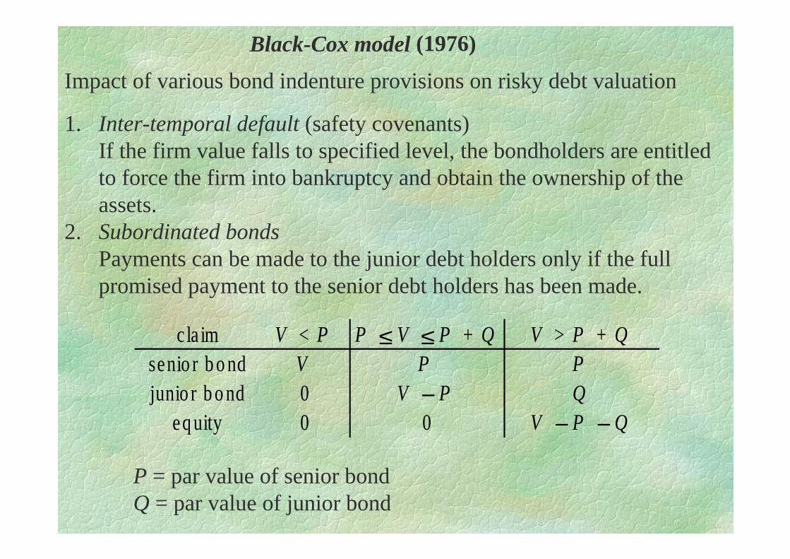
Black-Cox model (1976)

Impact of various bond indenture provisions on risky debt valuation

1. Inter-temporal default (safety covenants)If the firm value falls to specified level, the bondholders are entitledto force the firm into bankruptcy and obtain the ownership of theassets.

2. Subordinated bondsPayments can be made to the junior debt holders only if the fullpromised payment to the senior debt holders has been made.

c la im V < P P ≤ V ≤ P + Q V > P + Qsenio r b o nd V P Pjunio r b o nd 0 V − P Q

eq uity 0 0 V − P − Q

P = par value of senior bondQ = par value of junior bond

Longstaff- Schwartz model (1995)

Interest rate uncertaintyVasicek interest rate process: dr = a(c − r)dt + σrdZr

Bankruptcy-triggering mechanismThreshold value υ(t) for the firm value at which financial distressoccurs: take υ(t) = K = constant.

* If a reorganization occurs during the life of the bond, the bondholder receives (1- ω) times the par value at maturity.

Briys-de Varenne model (1997)

Take υ(t) = αP B(r, t; T)where B(r, t; T) is the default-free zero-coupon bond value, α is a constant

Derivation from the strict priority ruleWrite down of creditor claims

PVTTTPVTTTTt TVTVVVfFPfD <≥≥< ++= ≥ ,2,1 ,,, 111 υυυα

where TV, υ is the first passage time of the firm value process V to the barrier υ.

Zhou model (1997)Jump-diffusion process for the firm value process

dYdZdtmV

dV)1()( −Π++−= σλµ

where dY is a Poisson process with intensity parameter λ;Π > 0 is the jump amplitude with expected value m + 1;µ is the expected instantaneous rate of change of firm value.

• Remedy the unrealistic phenomena of small short-maturity spreadsin pure diffusion firm value process. Default may occur by surprise.

• Allows for a jump process to shock the asset value process.

References

1. Black, F. and J. C. Cox, “Valuing corporate securities: some effectsof bond indenture provision,” Journal of Finance, vol. 31 (1976) p.351-367.

2. Bohn, J. R., “Empirical assessment of a simple contingent claimmodel for the valuation of risky debt,” Working paper of Haas School of Business (1999).

3. Briys E. et al., Option, Futures and Exotic Derivatives, John Wiley(1998), Chap. 9.

4. Longstaff, F. A. and E. S. Schwartz, “A simple approach to valuingrisky fixed and floating rate debts,” Journal of Finance, vol. 50 (1995)p.789-819.

5. Zhou, C., “A jump-diffusion approach to modeling credit risk andvaluing defaultable securities,” Working paper of the Federal Reserve Board (1997).

Dominant factors in structural models for risky debts

1. Issuer’s asset value process.2. Issuer’s capital structure.3. Loss given default.4. Terms and conditions of the debt issue.5. Default-free interest rate process.6. Correlation between the default-free interest rate and asset value.

• Difficult to estimate the parameter values when implementing the models.

Bankruptcy resolutionWeiss analyzed 37 firms (1990, J. of Fin. Econ. p.285-314) for thedirect costs and violation of priority of claims.

1. Direct costs encompass the legal and administrative fees, includingthe costs of lawyers, accountants, etc. They average 3.1% of the book value of debt plus market value of equity at the end of the fiscal year preceding bankruptcy – small impact on debt valuation.

2. Priority of claims is violated for 29 of the 37 firms studied.• The costly valuation hearings may make creditors approve a

plan in which their priority is violated.• Tax-law cooperation of the equity holders is essential to preserve

tax-loss carryforwards.

Strategic debt serviceStrategic debt service may account for 30% to 40% of the premium onrisky debt. Models are constructed to examine the effect on valuationof expanding the strategy space open to equity holders.

• Risk premium prior to bankruptcy may be significantly boosted byexpectation of deviations from absolute priority.

• Debtholders in distressed firms are persuaded to accept concessions.

Indirect bankruptcy costs are the unmeasurable opportunity costs1. Lost sales and a decline in the inventory value.2. Increased operating costs.3. Reduction in the firm’s competitiveness.

Recovery rates (LGD)Findings by E.I. Altman & V.M. Kishore (1996, Fin. Analysts J.)

1. The highest average recoveries came from public utilities (70%)and chemical, petroleum and related products (63%).

2. The original rating of a bond issue as investment grade or belowinvestment grade has virtually no effect on recoveries once seniority is accounted for.

3. Neither the size of the issue nor the time to default from its originaldate of issuance has any association with the recovery rate.

Recovery rates (cont’d)4. Seniority does play the expected role

• Senior secured debt averages about 58% of face value.• Senior unsecured, 48%.• Senior subordinate, 34%.• Junior subordinate, 31%.

Some data

Ind ustry reco very ra teP ub lic utilities 7 0 .4 7 %W ho lesa le and re ta il trad e 4 4 %C asino , ho te l and recrea tio n 4 0 .1 5 %F inancia l institutio ns 3 5 .6 9 %

Seniority recovery rateSenior secured Investment grade 54.80% Non-investment grade 56.42%Senior unsecured Investment grade 48.20% Non-investment grade 48.73%

Discount and zero coupon Investment grade 24.14% Non-investment grade 24.42%