Embed Size (px)
Citation preview
Structural Mechanics
Dr. C. Caprani 1
Structural Mechanics Column Behaviour
2008/9
Dr. Colin Caprani,
Structural Mechanics
Dr. C. Caprani 2
Contents 1. Introduction ......................................................................................................... 3
1.1 Background...................................................................................................... 3
1.2 Stability of Equilibrium................................................................................... 4
2. Buckling Solutions............................................................................................... 6
2.1 Introduction...................................................................................................... 6
2.2 Pinned-Pinned Column.................................................................................... 7
2.3 Column with Initial Displacements ............................................................... 18
2.4 The Effective Length of Columns ................................................................. 30
3. Column Design................................................................................................... 32
3.1 Background to BS5950.................................................................................. 32
3.2 Column Design Examples ............................................................................. 38
4. Appendix ............................................................................................................ 47
4.1 Solutions to Differential Equations ............................................................... 47
4.2 Code Extracts................................................................................................. 51
4.3 Past Exam Questions ..................................................................................... 62
Structural Mechanics
Dr. C. Caprani 3
1. Introduction
1.1 Background
In the linear elastic analysis of structures, we have assumed that compression
members are limited in load capacity in the same way that tension members are, by
ensuring the yield stress of the material is not exceeded. However, as can easily be
checked with a ruler, compression members often fail long before the material yields
due to buckling. So our problem is to identify reduced stress limits that should apply
for compression members so that buckling does not occur.
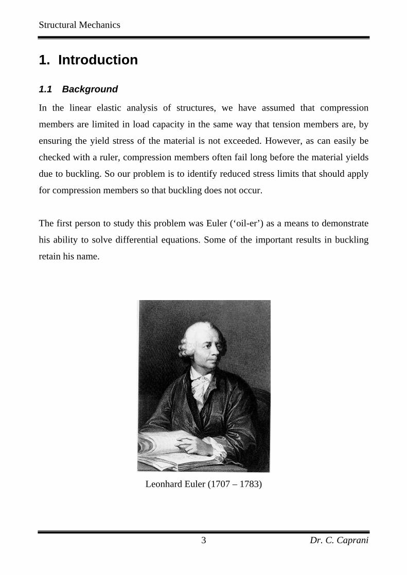
The first person to study this problem was Euler (‘oil-er’) as a means to demonstrate
his ability to solve differential equations. Some of the important results in buckling
retain his name.
Leonhard Euler (1707 – 1783)
Structural Mechanics
Dr. C. Caprani 4
1.2 Stability of Equilibrium
A structure will be in an initial equilibrium position. The stability of its equilibrium
can be assessed by examining the structure’s behaviour in an adjacent position. There
are three states:
• Stable equilibrium: the structure tends to return to its initial position. This is
the best situation to have structures in.
• Neutral (or critical) equilibrium: the structure moves to a displaced
configuration and remains in that position. This does not make for good
structure.
• Unstable equilibrium: any movement from the initial position causes further
movement resulting in a ‘runaway’ failure of the structure.
Structural Mechanics
Dr. C. Caprani 5
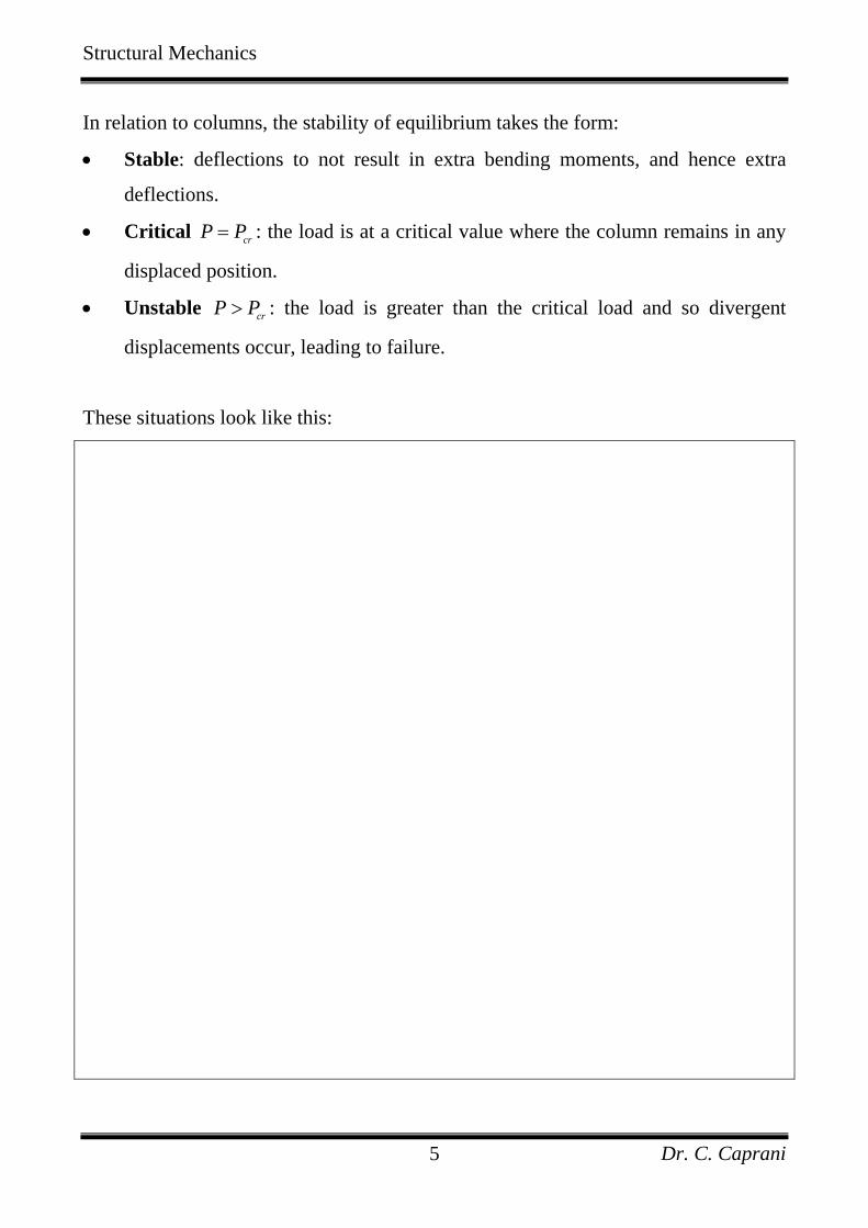
In relation to columns, the stability of equilibrium takes the form:
• Stable: deflections to not result in extra bending moments, and hence extra
deflections.
• Critical crP P= : the load is at a critical value where the column remains in any
displaced position.
• Unstable crP P> : the load is greater than the critical load and so divergent
displacements occur, leading to failure.
These situations look like this:
Structural Mechanics
Dr. C. Caprani 6
2. Buckling Solutions
2.1 Introduction
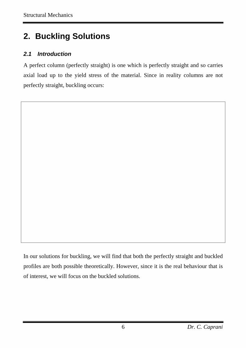
A perfect column (perfectly straight) is one which is perfectly straight and so carries
axial load up to the yield stress of the material. Since in reality columns are not
perfectly straight, buckling occurs:
In our solutions for buckling, we will find that both the perfectly straight and buckled
profiles are both possible theoretically. However, since it is the real behaviour that is
of interest, we will focus on the buckled solutions.
Structural Mechanics
Dr. C. Caprani 7
2.2 Pinned-Pinned Column
Formulation
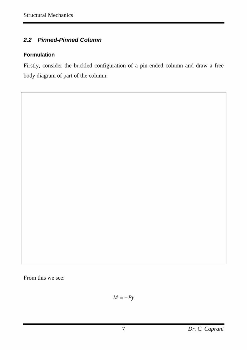
Firstly, consider the buckled configuration of a pin-ended column and draw a free
body diagram of part of the column:
From this we see:
M Py= −
Structural Mechanics
Dr. C. Caprani 8
So for equilibrium:
0M Py+ =
We know from Euler-Bernoulli bending theory that:
2
2
d yM EIdx
=
And so we have:
2
2 0d yEI Pydx
+ = (1)
Dividing across by EI gives:
2
20d y P y
dx EI+ =
If we make the substitution:
2 PkEI
= (2)
We then have:
2
22 0d y k y
dx+ = (3)
Structural Mechanics
Dr. C. Caprani 9
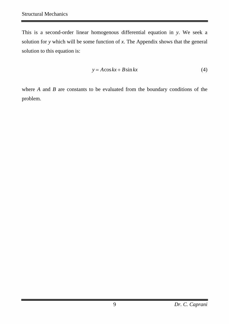
This is a second-order linear homogenous differential equation in y. We seek a
solution for y which will be some function of x. The Appendix shows that the general
solution to this equation is:
cos siny A kx B kx= + (4)
where A and B are constants to be evaluated from the boundary conditions of the
problem.
Structural Mechanics
Dr. C. Caprani 10
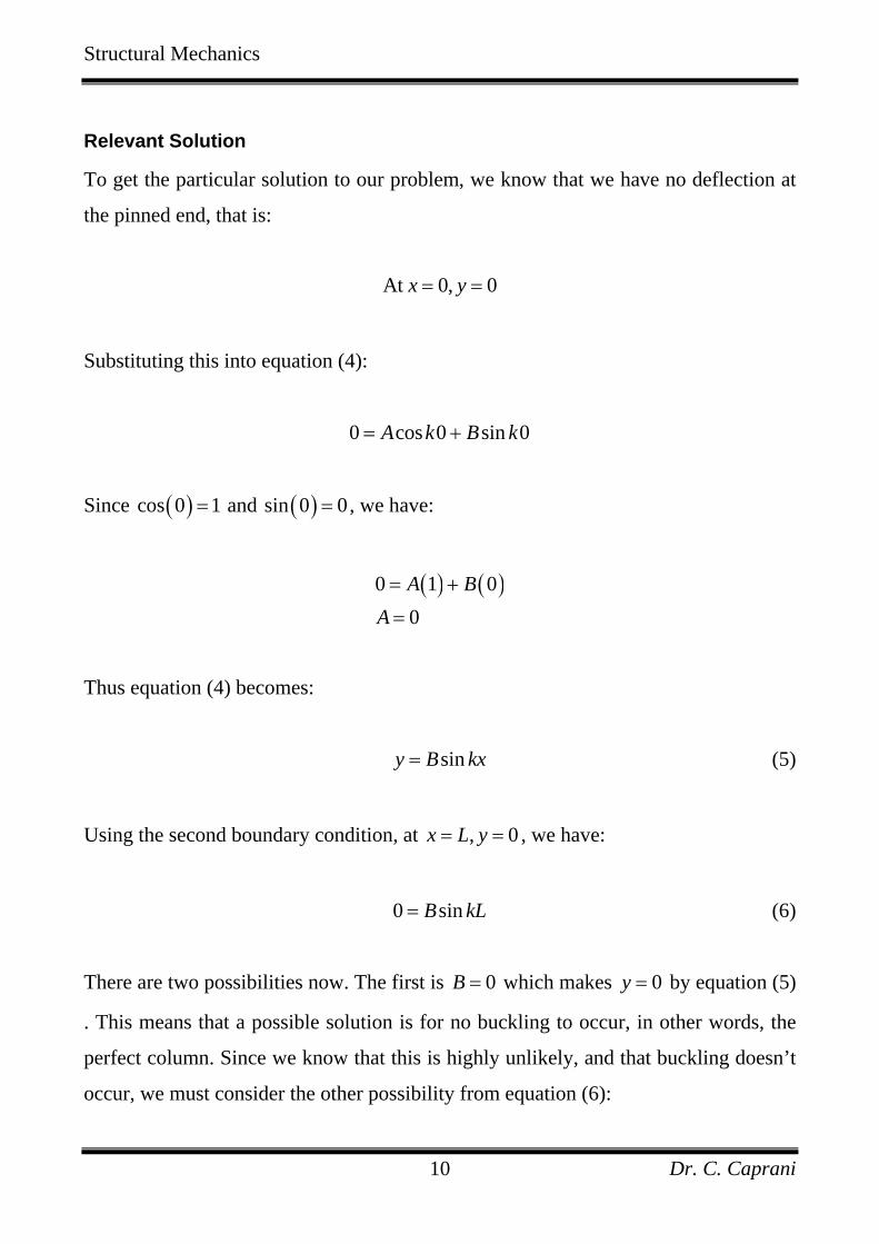
Relevant Solution
To get the particular solution to our problem, we know that we have no deflection at
the pinned end, that is:
At 0, 0x y= =
Substituting this into equation (4):
0 cos 0 sin 0A k B k= +
Since ( )cos 0 1= and ( )sin 0 0= , we have:
( ) ( )0 1 00A B
A= +
=
Thus equation (4) becomes:
siny B kx= (5)
Using the second boundary condition, at , 0x L y= = , we have:
0 sinB kL= (6)
There are two possibilities now. The first is 0B = which makes 0y = by equation (5)
. This means that a possible solution is for no buckling to occur, in other words, the
perfect column. Since we know that this is highly unlikely, and that buckling doesn’t
occur, we must consider the other possibility from equation (6):
Structural Mechanics
Dr. C. Caprani 11
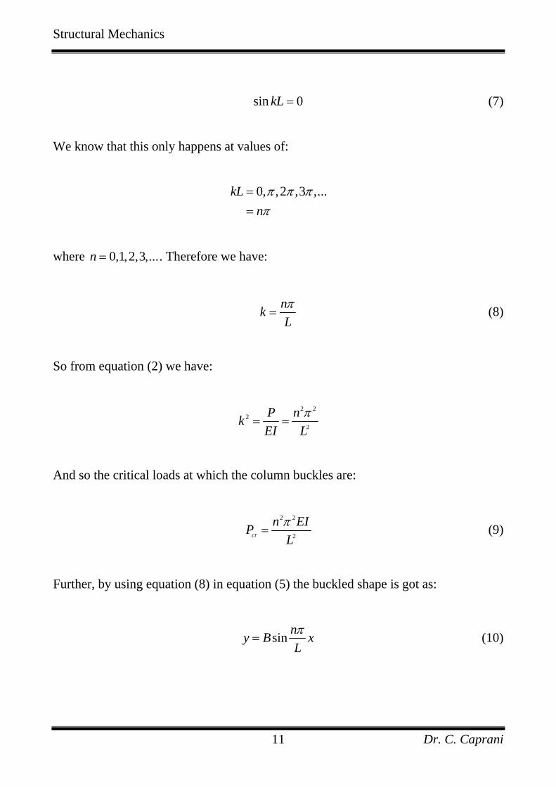
sin 0kL = (7)
We know that this only happens at values of:
0, ,2 ,3 ,...kLnπ π ππ
==
where 0,1,2,3,...n = . Therefore we have:
nkLπ
= (8)
So from equation (2) we have:
2 2
22
P nkEI L
π= =
And so the critical loads at which the column buckles are:
2 2
2cr
n EIPLπ
= (9)
Further, by using equation (8) in equation (5) the buckled shape is got as:
sin ny B xLπ
= (10)
Structural Mechanics
Dr. C. Caprani 12
Euler Buckling Load
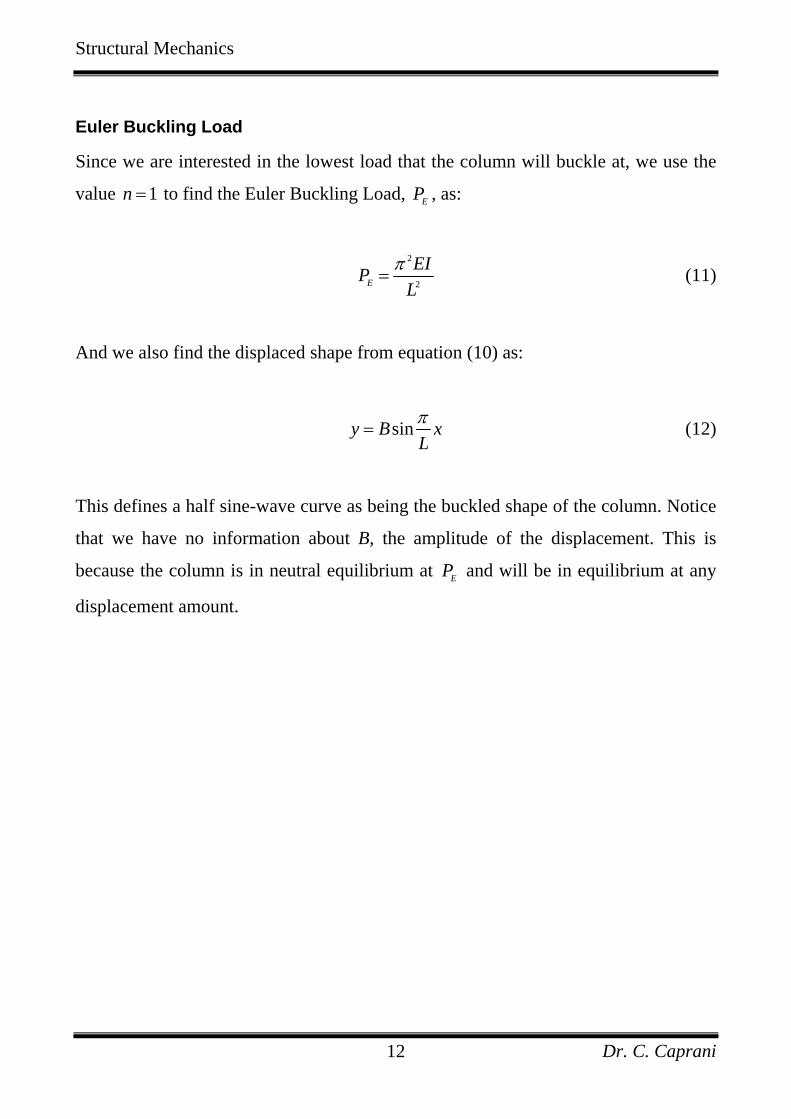
Since we are interested in the lowest load that the column will buckle at, we use the
value 1n = to find the Euler Buckling Load, EP , as:
2
2E
EIPL
π= (11)
And we also find the displaced shape from equation (10) as:
siny B xLπ
= (12)
This defines a half sine-wave curve as being the buckled shape of the column. Notice
that we have no information about B, the amplitude of the displacement. This is
because the column is in neutral equilibrium at EP and will be in equilibrium at any
displacement amount.
Structural Mechanics
Dr. C. Caprani 13
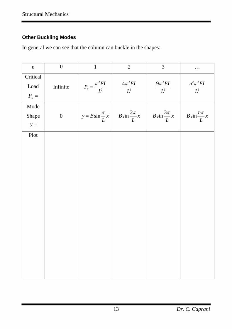
Other Buckling Modes
In general we can see that the column can buckle in the shapes:
n 0 1 2 3 …
Critical
Load
crP = Infinite
2
2E
EIPL
π=
2
2
4 EILπ
2
2
9 EILπ
2 2
2
n EILπ
Mode
Shape y =
0 siny B xLπ
=2sinB xLπ 3sinB x
Lπ sin nB x
Lπ
Plot
Structural Mechanics
Dr. C. Caprani 14
However, to achieve these other buckling loads, the lower modes must be prevented
from occurring by lateral restraints:
Structural Mechanics
Dr. C. Caprani 15
Critical Stress
For design, we are interested in the stress that the material undergoes at the time of
buckling – the critical stress, crσ :
2
2E
cr
P EIA L A
πσ = = (13)
Looking at the factor I A , we see that it is a property of the shape of the cross
section, and is in units of [ ] [ ] [ ]4 2 2length length length= . Therefore, we define a new
geometric property, r, called the Radius of Gyration as:
IrA
= (14)
And so r has units of length. The radius of gyration can be thought of as a distance
from the centroid at which the area of the cross section is concentrated for calculating
the second moment of area, I, since by (14),
2I Ar= (15)
The critical stress can now be expressed as:
2 2
2cr
ErL
πσ =
And we can see that the dimensional properties of the column are summed up by the
factor 2 2r L , which represents a ratio of r to L. Thus we define the Slenderness
Ratio, λ , as:
Structural Mechanics
Dr. C. Caprani 16
Lr
λ = (16)
Finally then, we have the equation for critical stress as:
2
2cr
Eπσλ
= (17)
A plot of the critical stress against slenderness is called a strut curve and looks like:
Structural Mechanics
Dr. C. Caprani 17
As can be seen, at low slendernesses (that is short stocky columns), the critical stress
(to cause bucking) reaches very high values. Since the maximum stress in the
material is the yield stress, me must cap the curve at yσ .
Finally, notice that typical experimental results fall below the Euler strut curve. This
is because the theory examined so far is for perfectly straight columns that have
somehow begun to buckle. In real columns there will be some initial imperfections
which have the effect of reducing the strength of the column. These initial
imperfections can be represented by an initial displacement curve.
Structural Mechanics
Dr. C. Caprani 18
2.3 Column with Initial Displacements
Problem Formulation
The imperfections in the manufacture of real columns mean that an initial
displacement curve exists in the column, prior to loading. Since any curve can be
represented by a Fourier series expansion, we will approximate the initial displaced
shape by the first term of a Fourier series – a sine curve, the equation of which is:
( )0 sin xy x aLπ
= (18)
where, at the midpoint of the column, the initial displacement is a.
Structural Mechanics
Dr. C. Caprani 19
Considering a free-body diagram as before:
gives the equilibrium equation as:
( )2
02 0d yEI P y ydx
+ + =
Thus we have:
2
020d y P Py y
dx EI EI+ + =
Using equation (2) gives:
Structural Mechanics
Dr. C. Caprani 20
2
2 202 0d y k y k y
dx+ + =
And so using equation (18) we have
2
2 22
sind y xk y k adx L
π+ = − (19)
This is a non-homogenous second order differential equation.
Structural Mechanics
Dr. C. Caprani 21
Solution
The solution to non-homogenous differential equations is made up of two parts:
• The complimentary solution (denoted Cy ): this is the solution to the
corresponding homogenous equation. That is, the solution when the right hand
side is zero. We have this from before as equation (4):
cos sinCy A kx B kx= + (20)
• The particular solution (denoted Py ): for the function on the right hand side,
the solution is verified in the Appendix as:
2
22
2
22
2
sin
sin
P
k a xyL
kL
k a xLk
L
ππ
ππ
−=
⎛ ⎞− +⎜ ⎟⎝ ⎠
=−
(21)
Thus the total solution is:
2
22
2
cos sin sin
C Py y yk a xA kx B kx
LkL
ππ
= +
= + +−
(22)
To find the constants, we know that for the pinned-pinned column, 0y = at 0x = :
Structural Mechanics
Dr. C. Caprani 22
( ) ( ) ( ) ( )
2
22
2
0 cos 0 sin 0 sin 0
0
k ay A k B kLk
LA
ππ
= + +−
=
Also, 0y = at x L= , giving:
( ) ( ) ( )
2
22
2
sin sin
0 sin
k ay L B k L LLk
LB kL
ππ
= +−
=
Although this is the same equation as found for the perfectly straight column, we
must consider the implications. If 0B ≠ then sin 0kL = and so kL π= as before. This
yields k Lπ= , or 22 2k Lπ= . Substituting this into equation (22) means that the
third term is infinite and so the deflection is infinite. Since this is impossible for a
stable column with crP P< , we conclude that 0B = and we are left with:
2
22
2
sink a xyLk
L
ππ
=−
(23)
This equation represents the deflections of the column caused by the loading. The
total deflection will be that caused by the loading, in addition to the initial
imperfection deflection curve:
0toty y y= +
And so:
Structural Mechanics
Dr. C. Caprani 23
2
22
2
sin sintot
k x xy a aL Lk
L
π ππ
= +−
Solving out, and dropping the tot subscript on y gives::
2
2 2 2 1 sink xy aL k L
ππ⎛ ⎞
= +⎜ ⎟−⎝ ⎠
And so:
2 2
2 2 2sinL xy a
L k Lπ π
π⎛ ⎞
= ⎜ ⎟−⎝ ⎠ (24)
Now, using the expression for EP (equation (11)), we have:
2
2EP
L EIπ
=
And with the expression for 2k (equation (2)), equation (24) becomes:
sinE
E
P EI xy aP EI P EI L
π=
−
And so we have:
sinE
E
P xy aP P L
π⎡ ⎤= ⎢ ⎥−⎣ ⎦
(25)
Structural Mechanics
Dr. C. Caprani 24
The term in brackets thus amplifies the initial deflection, depending on how close we
are to the critical buckling load. A plot of load against deflection shows:
Structural Mechanics
Dr. C. Caprani 25
Maximum Stress Consideration
At the mid-height of the column, the deflection will be largest, and thus so will the
bending moment. The deflection at the mid-height is got from equation (25), with
2x L= :
sin
2 2E
E
E
E
L P Ly aP P L
P aP P
π⎡ ⎤⎛ ⎞ ⎛ ⎞=⎜ ⎟ ⎜ ⎟⎢ ⎥−⎝ ⎠ ⎝ ⎠⎣ ⎦⎡ ⎤
= ⎢ ⎥−⎣ ⎦
We can equally interpret this equation in terms of stresses by dividing each of the Ps
by A:
2
E
E
Ly aσσ σ⎡ ⎤⎛ ⎞ =⎜ ⎟ ⎢ ⎥−⎝ ⎠ ⎣ ⎦
(26)
where Eσ is the stress associated with the critical Euler load (equation (13)).
Consider again the free-body diagram of the column from mid-height to pin. There
are two sources of stress:
1. The stresses due to the moment alone are:
Moment
MzI
σ =
where z is the distance from the neutral axis of the fibre under consideration.
Structural Mechanics
Dr. C. Caprani 26
2. The stresses due to the axial force are:
Axial
PA
σ =
Thus the stresses at any point are given by:
P MzA I
σ = + (27)
Superposition of the stress diagrams shows this:
The maximum stress is on the outside face and is thus:
max
P McA I
σ = + (28)
where c is the distance from the neutral axis to the inside face of the column.
Structural Mechanics
Dr. C. Caprani 27
Next, into equation (28), we introduce the relevant properties of equation (15) and the
fact that ( )2M Py L= yields:
( )max 2
2Pcy LAr
σ σ= +
But, from equation (26) we know the displacement at mid height, ( )2y L :
max 2E
E
Pc aAr
σσ σσ σ⎡ ⎤
= + ⎢ ⎥−⎣ ⎦
At failure the maximum stress is the yield stress, yσ . The stress associated with the
load P when this occurs is crσ . Hence the governing equation becomes:
2
Ey cr cr
E cr
c ar
σσ σ σσ σ⎡ ⎤
= + ⎢ ⎥−⎣ ⎦
Giving:
2
1 Ey cr
E cr
acr
σσ σσ σ
⎡ ⎤⎛ ⎞= +⎢ ⎥⎜ ⎟−⎝ ⎠⎣ ⎦
(29)
We are looking to find the value of crσ that solves this equation. At the load
corresponding to crσ failure occurs. As can be seen, this failure stress is a function of
the section (through r and c) and the initial imperfection, a, as well as the usual Euler
buckling load for the column (through Eσ ).
Structural Mechanics
Dr. C. Caprani 28
Critical Stress for Buckling
To solve equation (29) for crσ we proceed as follows:
( ) ( )
( ) ( )
2
2 2
2 2 2 2
2 2 2 2
2 2 2 2 2
22
1
0
0
Ey cr
E cr
y E cr cr E cr cr E
y E y cr cr E cr cr cr E
y E y cr cr E cr cr cr E
cr cr y E E y E
cr cr y E E
acr
r r ac
r r r r ac
r r r r ac
r r r ac r
acr
σσ σσ σ
σ σ σ σ σ σ σ σ
σ σ σ σ σ σ σ σ σ σ
σ σ σ σ σ σ σ σ σ σ
σ σ σ σ σ σ σ
σ σ σ σ σ
⎡ ⎤⎛ ⎞= +⎢ ⎥⎜ ⎟−⎝ ⎠⎣ ⎦
− = − +
− = − +
− − + − =
+ − − − + =
⎛+ − − −⎜⎝
0y Eσ σ⎞ + =⎟⎠
We call the parameter that accounts for the initial imperfections called the Perry
Factor:
2
acr
η = (30)
And this gives:
( )2 1 0cr cr y E y Eσ σ σ σ η σ σ⎡ ⎤+ − − + + =⎣ ⎦ (31)
This is a quadratic equation in crσ and so is solved by the usual:
2 4
2b b acx
a− ± −
=
where:
Structural Mechanics
Dr. C. Caprani 29
( )1
1y E
y E
a
b
c
σ σ η
σ σ
=
⎡ ⎤= − − +⎣ ⎦=
And this gives:
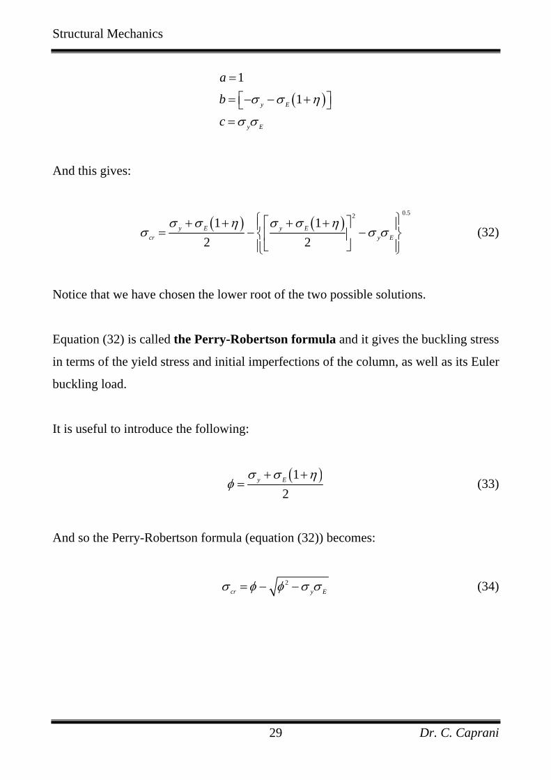
( ) ( )0.52
1 12 2
y E y Ecr y E
σ σ η σ σ ησ σ σ
⎧ ⎫+ + + +⎡ ⎤⎪ ⎪= − −⎨ ⎬⎢ ⎥⎣ ⎦⎪ ⎪⎩ ⎭
(32)
Notice that we have chosen the lower root of the two possible solutions.
Equation (32) is called the Perry-Robertson formula and it gives the buckling stress
in terms of the yield stress and initial imperfections of the column, as well as its Euler
buckling load.
It is useful to introduce the following:
( )1
2y Eσ σ η
φ+ +
= (33)
And so the Perry-Robertson formula (equation (32)) becomes:
2cr y Eσ φ φ σ σ= − − (34)
Structural Mechanics
Dr. C. Caprani 30
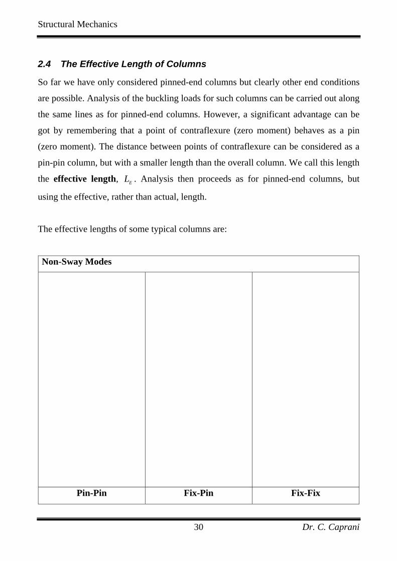
2.4 The Effective Length of Columns
So far we have only considered pinned-end columns but clearly other end conditions
are possible. Analysis of the buckling loads for such columns can be carried out along
the same lines as for pinned-end columns. However, a significant advantage can be
got by remembering that a point of contraflexure (zero moment) behaves as a pin
(zero moment). The distance between points of contraflexure can be considered as a
pin-pin column, but with a smaller length than the overall column. We call this length
the effective length, EL . Analysis then proceeds as for pinned-end columns, but
using the effective, rather than actual, length.
The effective lengths of some typical columns are:
Non-Sway Modes
Pin-Pin Fix-Pin Fix-Fix
Structural Mechanics
Dr. C. Caprani 31
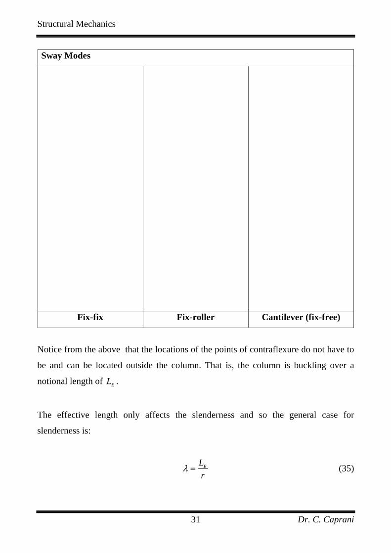
Sway Modes
Fix-fix Fix-roller Cantilever (fix-free)
Notice from the above that the locations of the points of contraflexure do not have to
be and can be located outside the column. That is, the column is buckling over a
notional length of EL .
The effective length only affects the slenderness and so the general case for
slenderness is:
ELr
λ = (35)
Structural Mechanics
Dr. C. Caprani 32
3. Column Design
3.1 Background to BS5950
Initial Imperfections
Robertson performed many tests on struts to arrive at a suitable value for the initial
imperfections in the approach outlined in the previous section. He suggested:
0.003η λ= (36)
where λ is the slenderness of the column, given by equation (16). More recently, the
initial imperfection has been taken as:
2
0.3100λη ⎛ ⎞= ⎜ ⎟
⎝ ⎠ (37)
The idea of linking the initial imperfections to the slenderness is intuitively appealing
– the slimmer a column is, the more likely it is to have imperfections.
The steel design code BS5950 is based on the following:
( )0
1000a λ λ
η−
= (38)
In which:
• a is the Robertson constant (and is not the same as the a we had for the
deflection of the column previously);
• 0λ is called the limiting slenderness as is given by:
Structural Mechanics
Dr. C. Caprani 33
2
0 0.2y
Eπλσ
= (39)
By rearranging equation (17) it can be seen that this is:
0 0.2 crλ λ=
where crλ is the slenderness at which the Euler stress reaches the yield stress of the
material.
As can be seen, the higher the value of a, the more initial imperfection is accounted
for and the compressive strength reduces as a result.
Structural Mechanics
Dr. C. Caprani 34
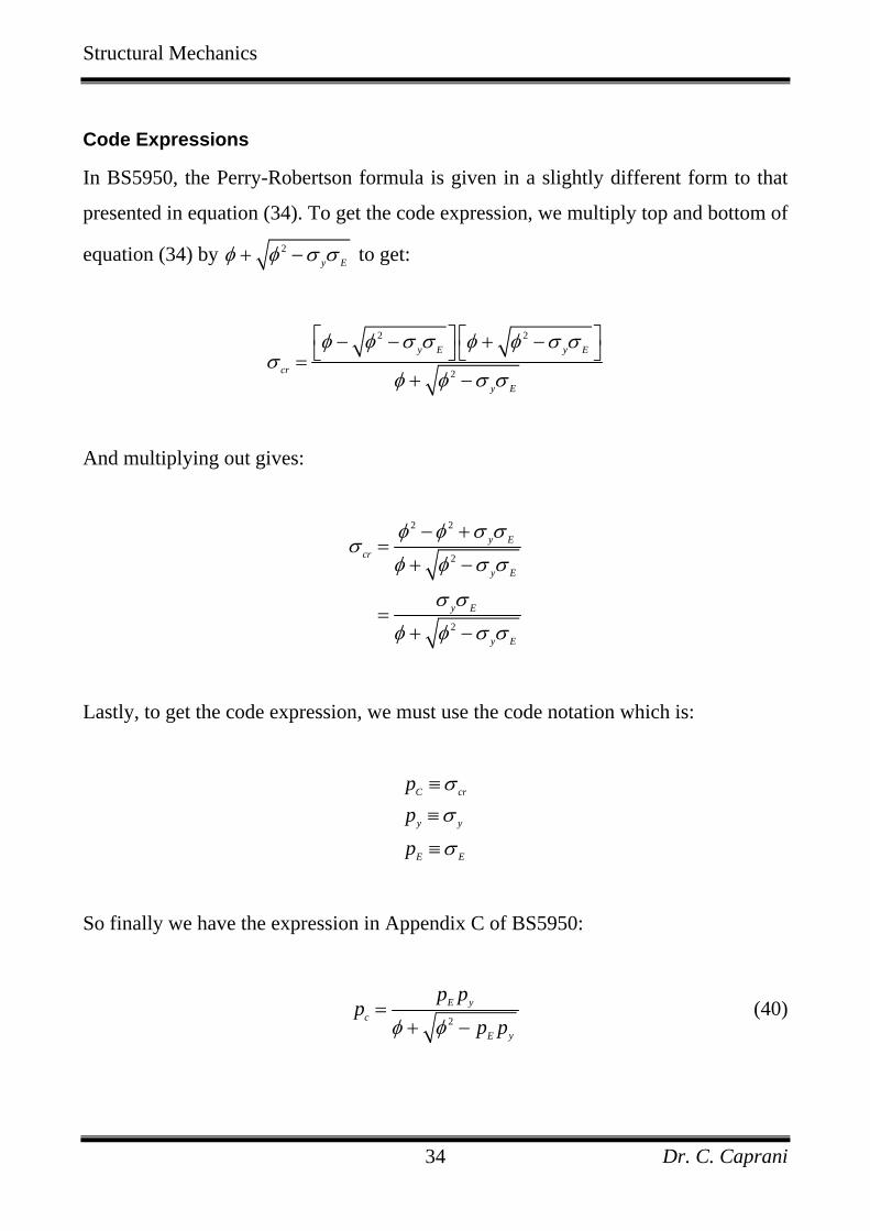
Code Expressions
In BS5950, the Perry-Robertson formula is given in a slightly different form to that
presented in equation (34). To get the code expression, we multiply top and bottom of
equation (34) by 2y Eφ φ σ σ+ − to get:
2 2
2
y E y E
cr
y E
φ φ σ σ φ φ σ σσ
φ φ σ σ
⎡ ⎤ ⎡ ⎤− − + −⎣ ⎦ ⎣ ⎦=+ −
And multiplying out gives:
2 2
2
2
y Ecr
y E
y E
y E
φ φ σ σσ
φ φ σ σ
σ σ
φ φ σ σ
− +=
+ −
=+ −
Lastly, to get the code expression, we must use the code notation which is:
C cr
y y
E E
ppp
σσ
σ
≡≡
≡
So finally we have the expression in Appendix C of BS5950:
2
E yc
E y
p pp
p pφ φ=
+ − (40)
Structural Mechanics
Dr. C. Caprani 35
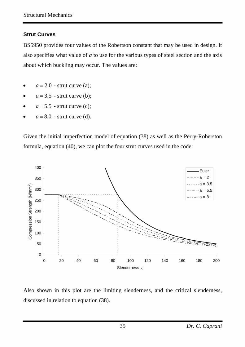
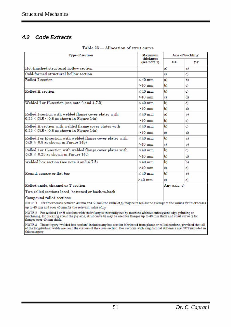
Strut Curves
BS5950 provides four values of the Robertson constant that may be used in design. It
also specifies what value of a to use for the various types of steel section and the axis
about which buckling may occur. The values are:
• 2.0a = - strut curve (a);
• 3.5a = - strut curve (b);
• 5.5a = - strut curve (c);
• 8.0a = - strut curve (d).
Given the initial imperfection model of equation (38) as well as the Perry-Roberston
formula, equation (40), we can plot the four strut curves used in the code:
0
50
100
150
200
250
300
350
400
0 20 40 60 80 100 120 140 160 180 200
Slenderness λ
Com
pres
sion
Stre
ngth
(N/m
m2 )
Eulera = 2a = 3.5a = 5.5a = 8
Also shown in this plot are the limiting slenderness, and the critical slenderness,
discussed in relation to equation (38).
Structural Mechanics
Dr. C. Caprani 36
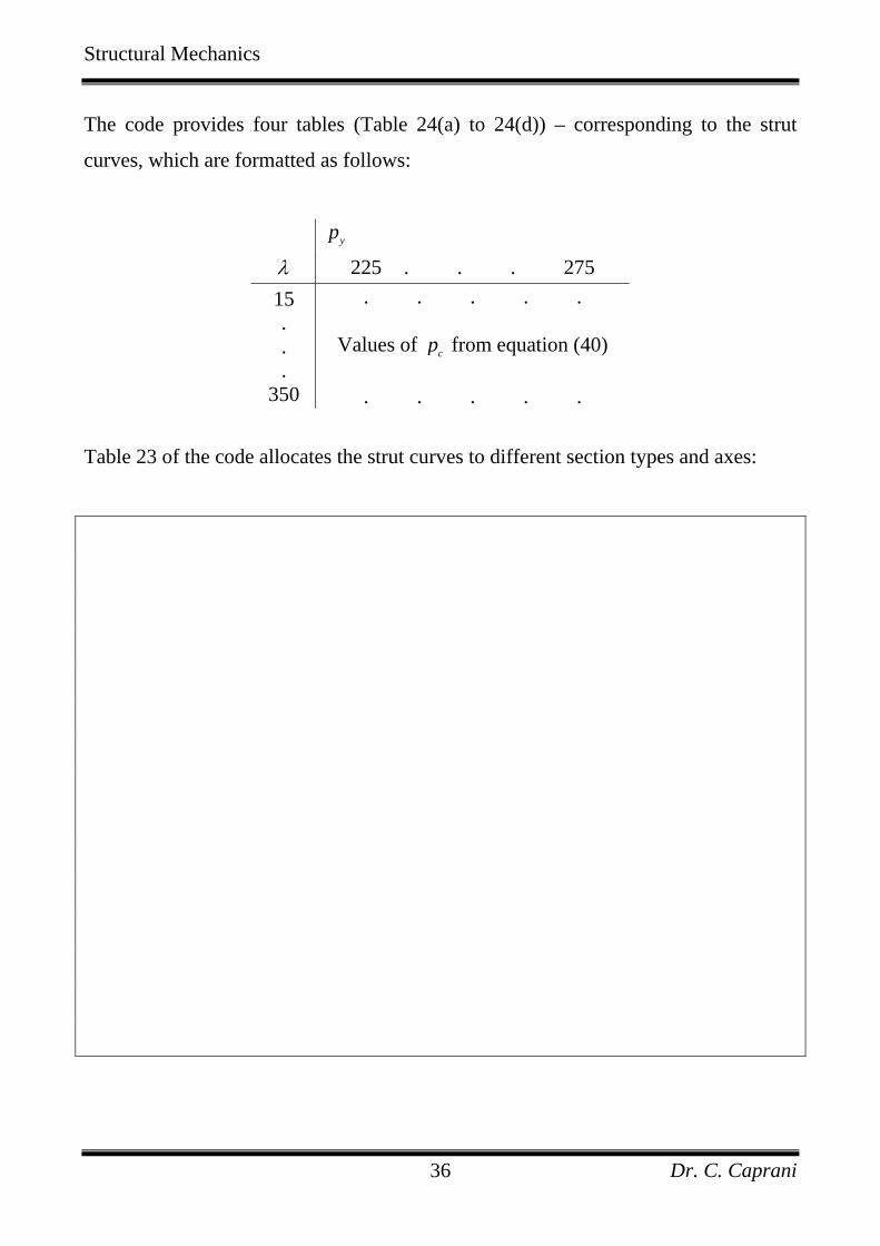
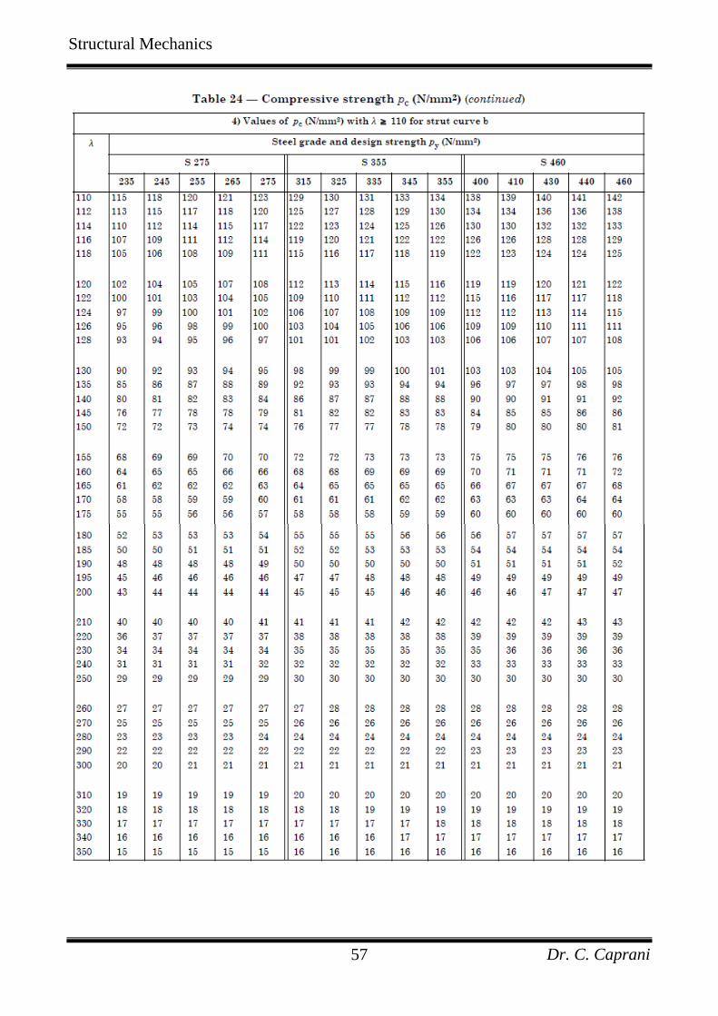
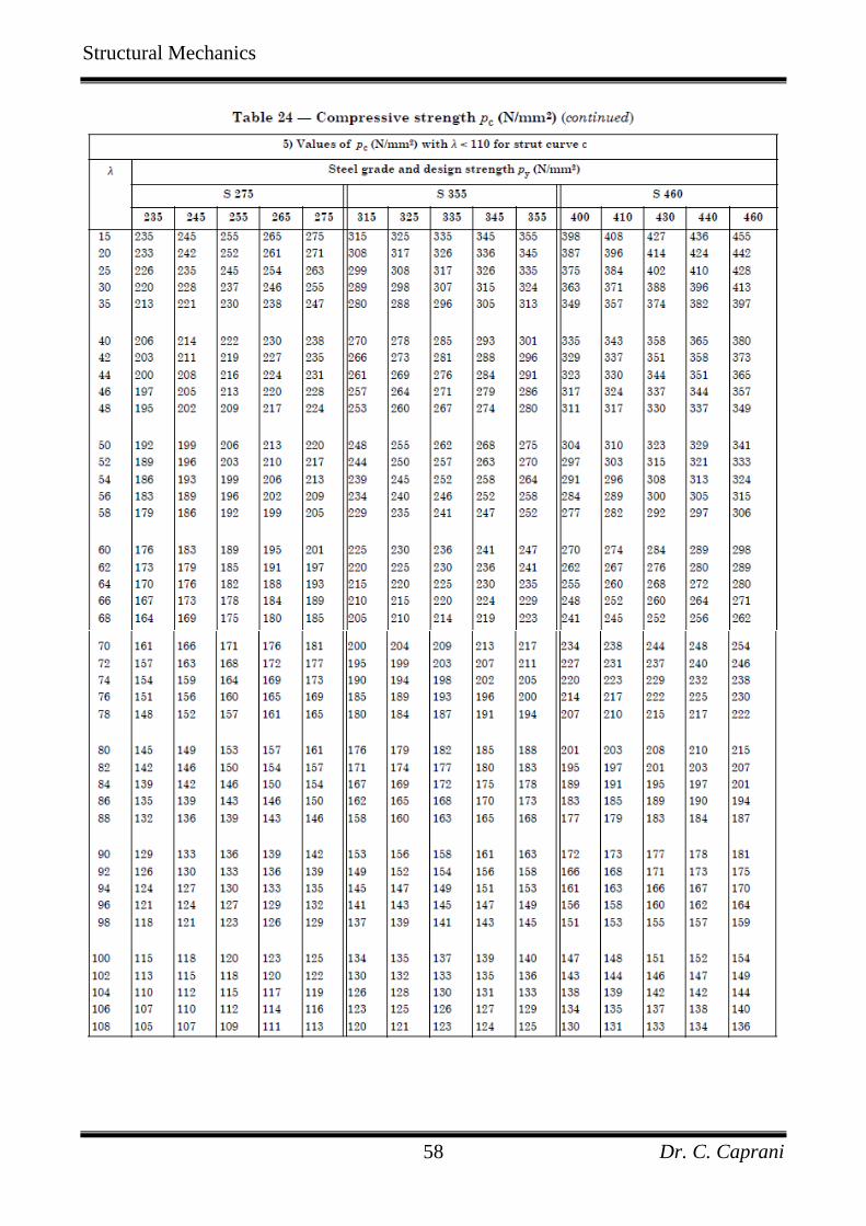
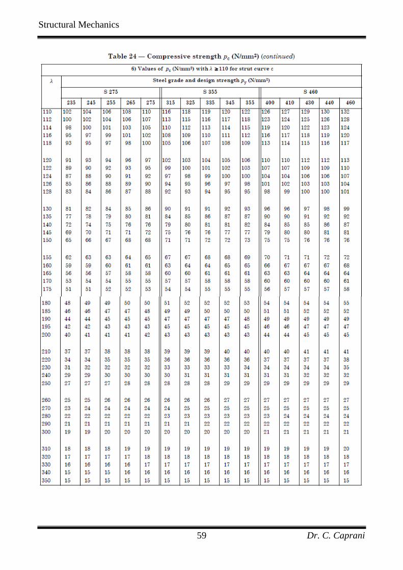
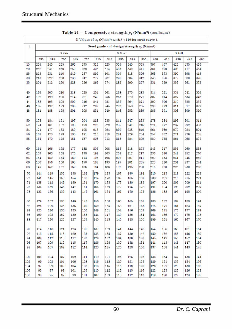
The code provides four tables (Table 24(a) to 24(d)) – corresponding to the strut
curves, which are formatted as follows:
yp
λ 225 . . . 275 15 . . .
350
. . . . .
Values of cp from equation (40)
. . . . .
Table 23 of the code allocates the strut curves to different section types and axes:
Structural Mechanics
Dr. C. Caprani 37
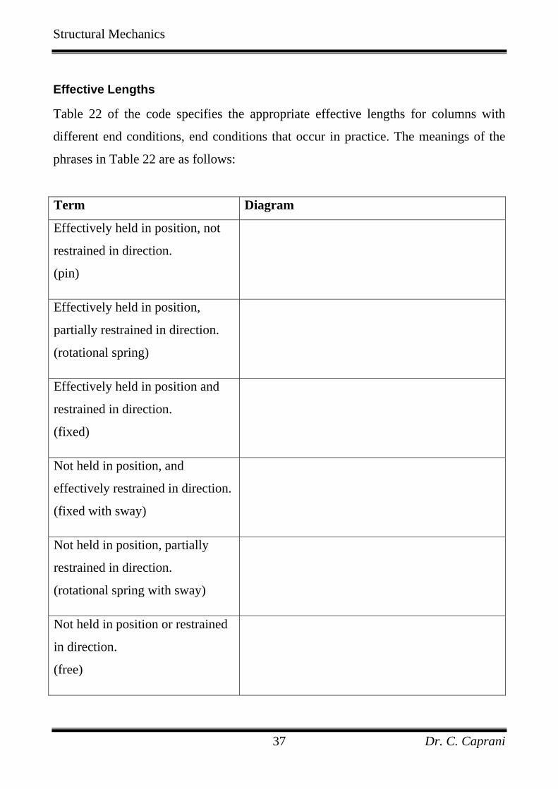
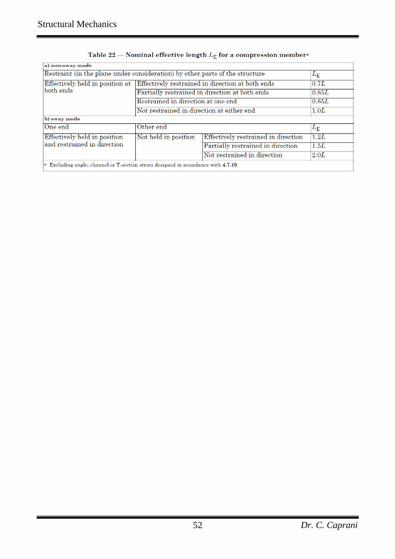
Effective Lengths
Table 22 of the code specifies the appropriate effective lengths for columns with
different end conditions, end conditions that occur in practice. The meanings of the
phrases in Table 22 are as follows:
Term Diagram
Effectively held in position, not
restrained in direction.
(pin)
Effectively held in position,
partially restrained in direction.
(rotational spring)
Effectively held in position and
restrained in direction.
(fixed)
Not held in position, and
effectively restrained in direction.
(fixed with sway)
Not held in position, partially
restrained in direction.
(rotational spring with sway)
Not held in position or restrained
in direction.
(free)
Structural Mechanics
Dr. C. Caprani 38
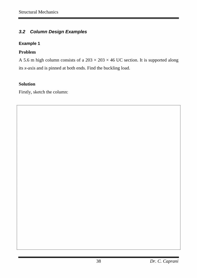
3.2 Column Design Examples
Example 1
Problem
A 5.6 m high column consists of a 203 × 203 × 46 UC section. It is supported along
its x-axis and is pinned at both ends. Find the buckling load.
Solution
Firstly, sketch the column:
Structural Mechanics
Dr. C. Caprani 39
Since the column is supported along its x-x axis, it can only buckle about its y-y axis.
The relevant section properties for a 203 × 203 × 46 UC are:
Cross-Sectional Area 58.8 cm2
Yield stress 275 N/mm2
Modulus of Elasticity 205 kN/mm2
Radius of gyration about the y-y axis 5.12 cm
Robertson Constant for the y-y axis 5.5
Thus:
5600 109.6 11051.1
λ = = ≈
From Table 23 we see that we are using strut curve (c) and so 5.5a = . Also, 2205 kN/mmE = and 2265 N/mmyp = from Table 9. Thus:
The limiting slenderness (equation (39)) is:
2 2 3
0
205 100.2 0.2 17.48265y
Epπ πλ ⋅ ×
= = =
The Perry Factor (equation (38)) is:
( ) ( )0 5.5 110 17.480.509
1000 1000a λ λ
η− −
= = =
The Euler stress (equation (17) is:
Structural Mechanics
Dr. C. Caprani 40
2 2 3
22 2
205 10 168 N/mm110E
Ep π πλ
⋅ ×= = =
The modifying stress (equation (33)) is:
( ) ( ) 21 265 0.509 1 168259 N/mm
2 2y Ep pη
φ+ + + +
= = =
And so the compressive strength (equations (34)or (40)):
2
2 2
168 265 108.6 N/mm259 259 168 265
E yc
E y
p pp
p pφ φ⋅
= = =+ − + − ⋅
Thus the buckling load is:
3
5880 108.6 640.4 kN10g cP A p ⋅
= = =
To check this, use Table 24(c), for 110λ ≥ and 2265 N/mmyp = gives:
2108 N/mmcp = and so the capacity is 3108 5880 10 635 kN⋅ = , which is similar to
the previous calculation.
Structural Mechanics
Dr. C. Caprani 41
Example 2
Problem
For the column of Example 1, the restraint along the x-x axis has to be removed.
Determine the buckling capacity.
Solution
Again, sketch the column:
Structural Mechanics
Dr. C. Caprani 42
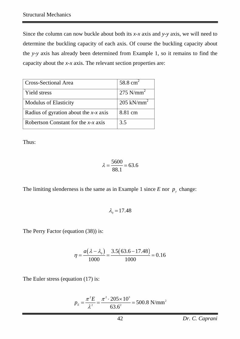
Since the column can now buckle about both its x-x axis and y-y axis, we will need to
determine the buckling capacity of each axis. Of course the buckling capacity about
the y-y axis has already been determined from Example 1, so it remains to find the
capacity about the x-x axis. The relevant section properties are:
Cross-Sectional Area 58.8 cm2
Yield stress 275 N/mm2
Modulus of Elasticity 205 kN/mm2
Radius of gyration about the x-x axis 8.81 cm
Robertson Constant for the x-x axis 3.5
Thus:
5600 63.688.1
λ = =
The limiting slenderness is the same as in Example 1 since E nor yp change:
0 17.48λ =
The Perry Factor (equation (38)) is:
( ) ( )0 3.5 63.6 17.480.16
1000 1000a λ λ
η− −
= = =
The Euler stress (equation (17) is:
2 2 3
22 2
205 10 500.8 N/mm63.6E
Ep π πλ
⋅ ×= = =
Structural Mechanics
Dr. C. Caprani 43
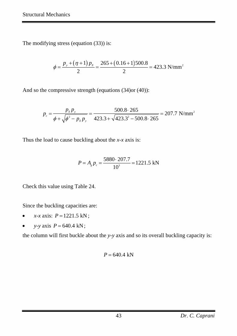
The modifying stress (equation (33)) is:
( ) ( ) 21 265 0.16 1 500.8423.3 N/mm
2 2y Ep pη
φ+ + + +
= = =
And so the compressive strength (equations (34)or (40)):
2
2 2
500.8 265 207.7 N/mm423.3 423.3 500.8 265
E yc
E y
p pp
p pφ φ⋅
= = =+ − + − ⋅
Thus the load to cause buckling about the x-x axis is:
3
5880 207.7 1221.5 kN10g cP A p ⋅
= = =
Check this value using Table 24.
Since the buckling capacities are:
• x-x axis: 1221.5 kNP = ;
• y-y axis 640.4 kNP = ;
the column will first buckle about the y-y axis and so its overall buckling capacity is:
640.4 kNP =
Structural Mechanics
Dr. C. Caprani 44
Example 3
Problem
To increase the capacity of the column of Example 2, the supports in the y-y axis
have been changed to fixed-fixed. Determine the buckling capacity.
Solution
As always, sketch the column:
Structural Mechanics
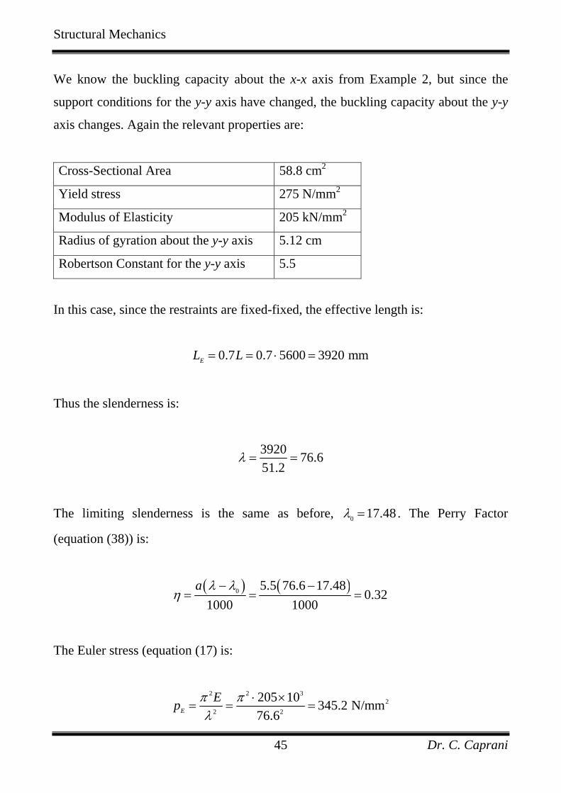
Dr. C. Caprani 45
We know the buckling capacity about the x-x axis from Example 2, but since the
support conditions for the y-y axis have changed, the buckling capacity about the y-y
axis changes. Again the relevant properties are:
Cross-Sectional Area 58.8 cm2
Yield stress 275 N/mm2
Modulus of Elasticity 205 kN/mm2
Radius of gyration about the y-y axis 5.12 cm
Robertson Constant for the y-y axis 5.5
In this case, since the restraints are fixed-fixed, the effective length is:
0.7 0.7 5600 3920 mmEL L= = ⋅ =
Thus the slenderness is:
3920 76.651.2
λ = =
The limiting slenderness is the same as before, 0 17.48λ = . The Perry Factor
(equation (38)) is:
( ) ( )0 5.5 76.6 17.480.32
1000 1000a λ λ
η− −
= = =
The Euler stress (equation (17) is:
2 2 3
22 2
205 10 345.2 N/mm76.6E
Ep π πλ
⋅ ×= = =
Structural Mechanics
Dr. C. Caprani 46
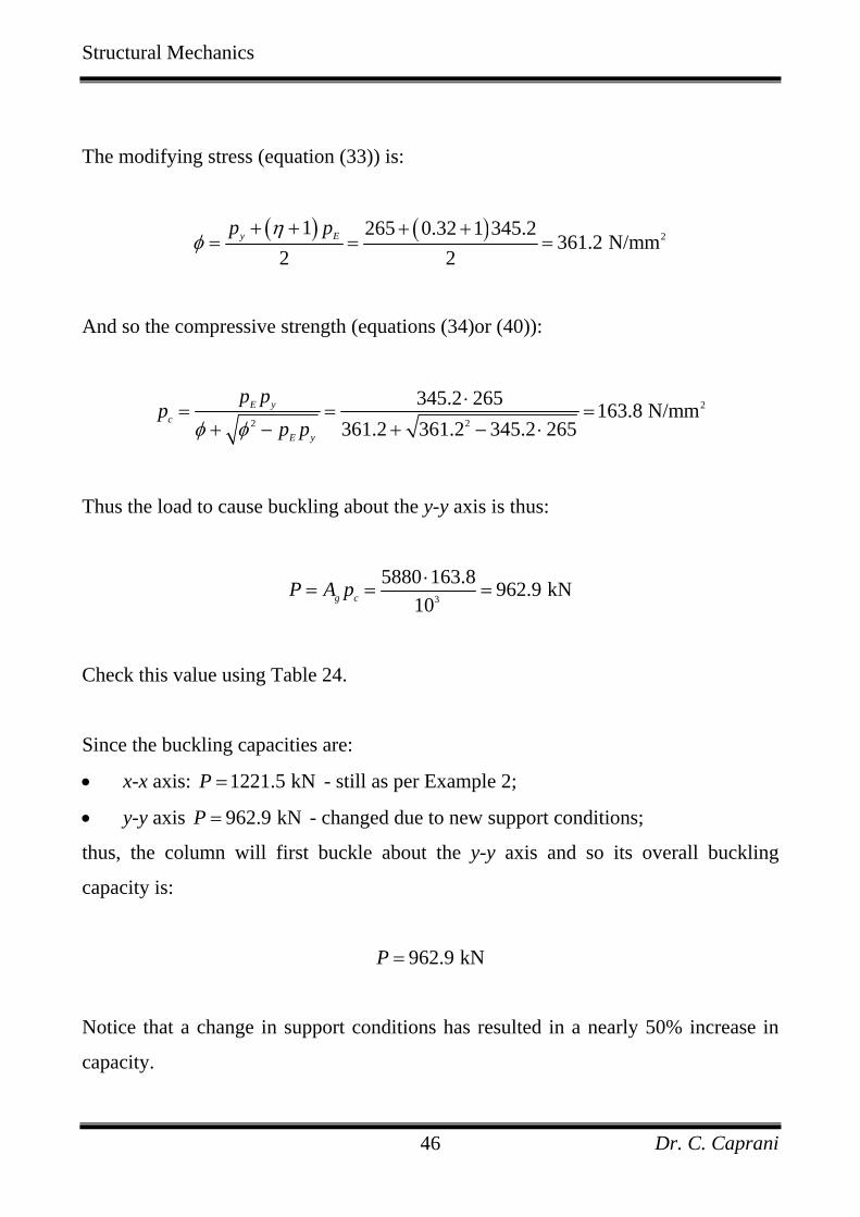
The modifying stress (equation (33)) is:
( ) ( ) 21 265 0.32 1 345.2361.2 N/mm
2 2y Ep pη
φ+ + + +
= = =
And so the compressive strength (equations (34)or (40)):
2
2 2
345.2 265 163.8 N/mm361.2 361.2 345.2 265
E yc
E y
p pp
p pφ φ⋅
= = =+ − + − ⋅
Thus the load to cause buckling about the y-y axis is thus:
3
5880 163.8 962.9 kN10g cP A p ⋅
= = =
Check this value using Table 24.
Since the buckling capacities are:
• x-x axis: 1221.5 kNP = - still as per Example 2;
• y-y axis 962.9 kNP = - changed due to new support conditions;
thus, the column will first buckle about the y-y axis and so its overall buckling
capacity is:
962.9 kNP =
Notice that a change in support conditions has resulted in a nearly 50% increase in
capacity.
Structural Mechanics
Dr. C. Caprani 47
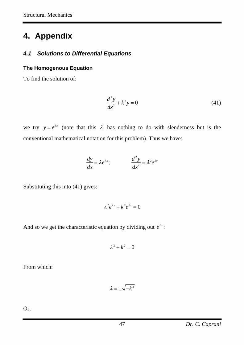
4. Appendix
4.1 Solutions to Differential Equations
The Homogenous Equation
To find the solution of:
2
22 0d y k y
dx+ = (41)
we try xy eλ= (note that this λ has nothing to do with slenderness but is the
conventional mathematical notation for this problem). Thus we have:
2
22;x xdy d ye e
dx dxλ λλ λ= =
Substituting this into (41) gives:
2 2 0x xe k eλ λλ + =
And so we get the characteristic equation by dividing out xeλ :
2 2 0kλ + =
From which:
2kλ = ± −
Or,
Structural Mechanics
Dr. C. Caprani 48
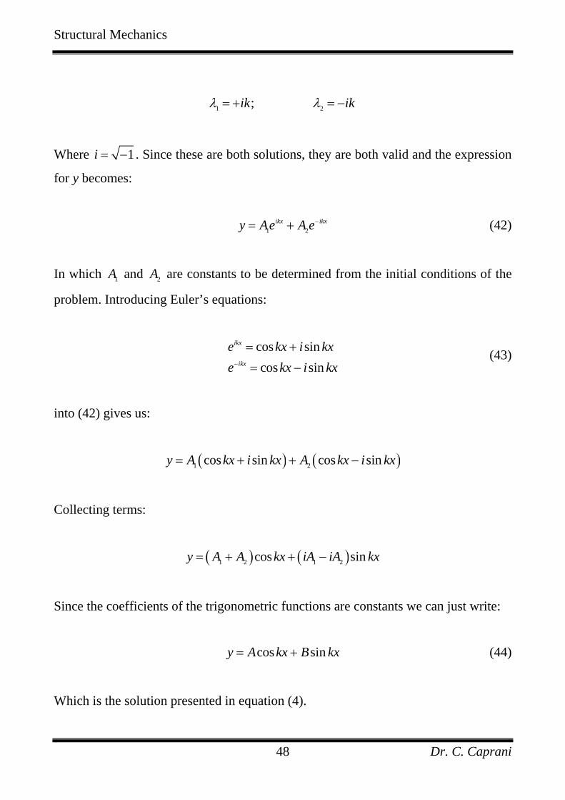
1 2;ik ikλ λ= + = −
Where 1i = − . Since these are both solutions, they are both valid and the expression
for y becomes:
1 2ikx ikxy Ae A e−= + (42)
In which 1A and 2A are constants to be determined from the initial conditions of the
problem. Introducing Euler’s equations:
cos sincos sin
ikx
ikx
e kx i kxe kx i kx−
= +
= − (43)
into (42) gives us:
( ) ( )1 2cos sin cos siny A kx i kx A kx i kx= + + −
Collecting terms:
( ) ( )1 2 1 2cos siny A A kx iA iA kx= + + −
Since the coefficients of the trigonometric functions are constants we can just write:
cos siny A kx B kx= + (44)
Which is the solution presented in equation (4).
Structural Mechanics
Dr. C. Caprani 49
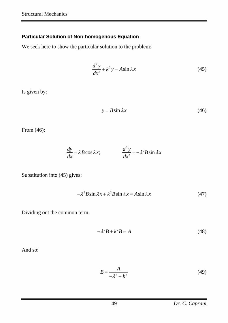
Particular Solution of Non-homogenous Equation
We seek here to show the particular solution to the problem:
2
22
sind y k y A xdx
λ+ = (45)
Is given by:
siny B xλ= (46)
From (46):
2
22cos ; sindy d yB x B x
dx dxλ λ λ λ= = −
Substitution into (45) gives:
2 2sin sin sinB x k B x A xλ λ λ λ− + = (47)
Dividing out the common term:
2 2B k B Aλ− + = (48)
And so:
2 2
ABkλ
=− +
(49)
Structural Mechanics
Dr. C. Caprani 50
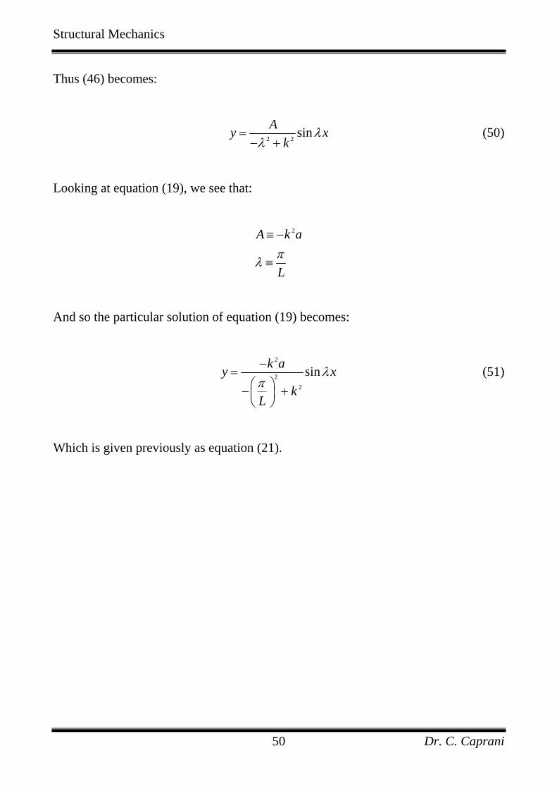
Thus (46) becomes:
2 2 sinAy xk
λλ
=− +
(50)
Looking at equation (19), we see that:
2A k a
Lπλ
≡ −
≡
And so the particular solution of equation (19) becomes:
2
22
sink ay xk
L
λπ−
=⎛ ⎞− +⎜ ⎟⎝ ⎠
(51)
Which is given previously as equation (21).
Structural Mechanics
Dr. C. Caprani 51
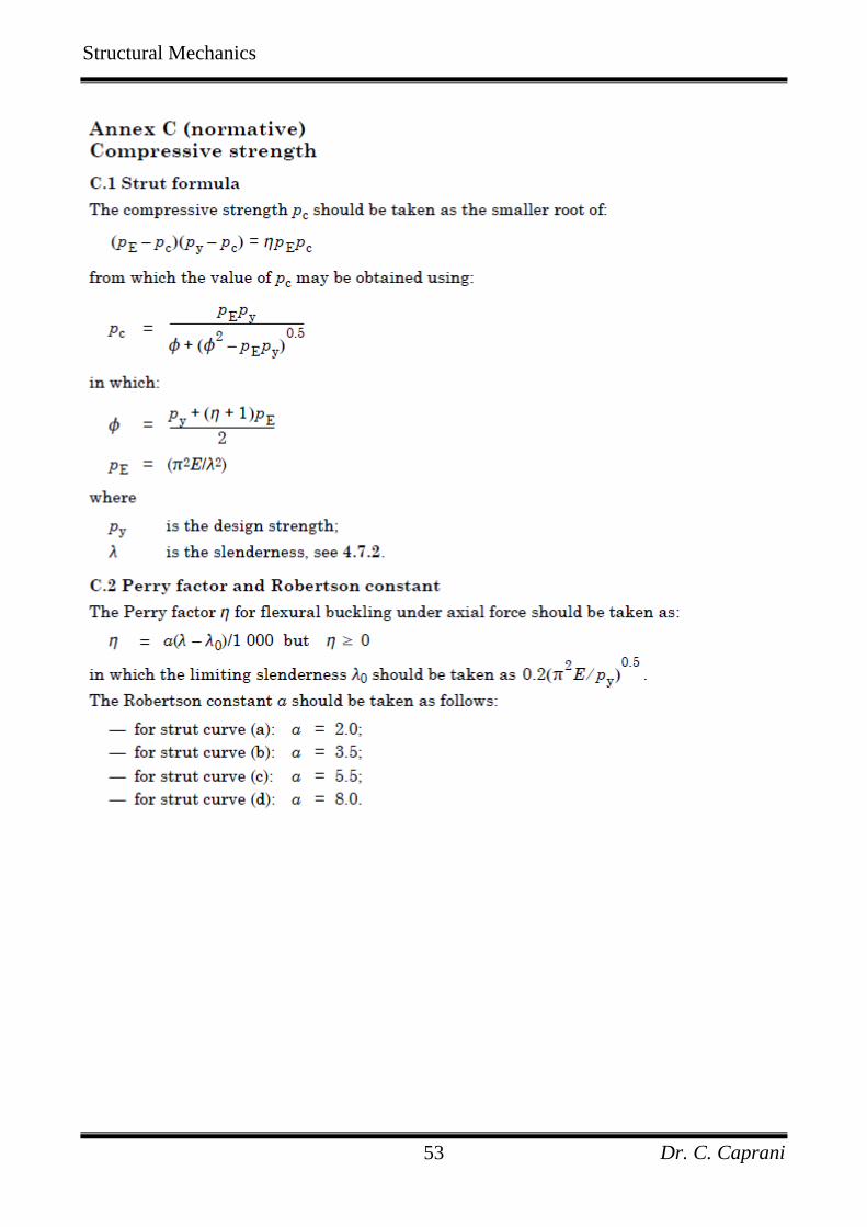
4.2 Code Extracts
Structural Mechanics
Dr. C. Caprani 52
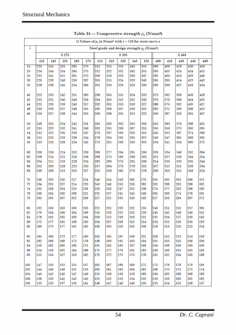
Structural Mechanics
Dr. C. Caprani 53
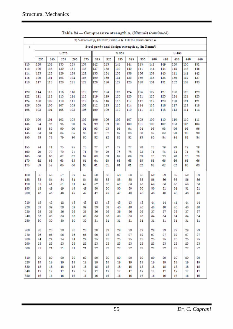
Structural Mechanics
Dr. C. Caprani 54
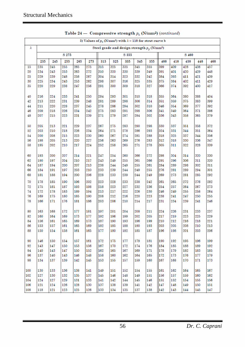
Structural Mechanics
Dr. C. Caprani 55
Structural Mechanics
Dr. C. Caprani 56
Structural Mechanics
Dr. C. Caprani 57
Structural Mechanics
Dr. C. Caprani 58
Structural Mechanics
Dr. C. Caprani 59
Structural Mechanics
Dr. C. Caprani 60
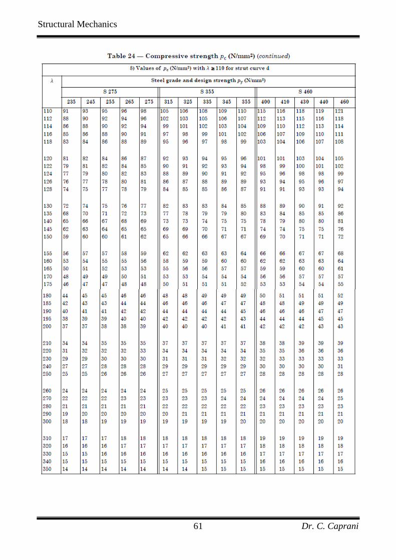
Structural Mechanics
Dr. C. Caprani 61
Structural Mechanics
Dr. C. Caprani 62
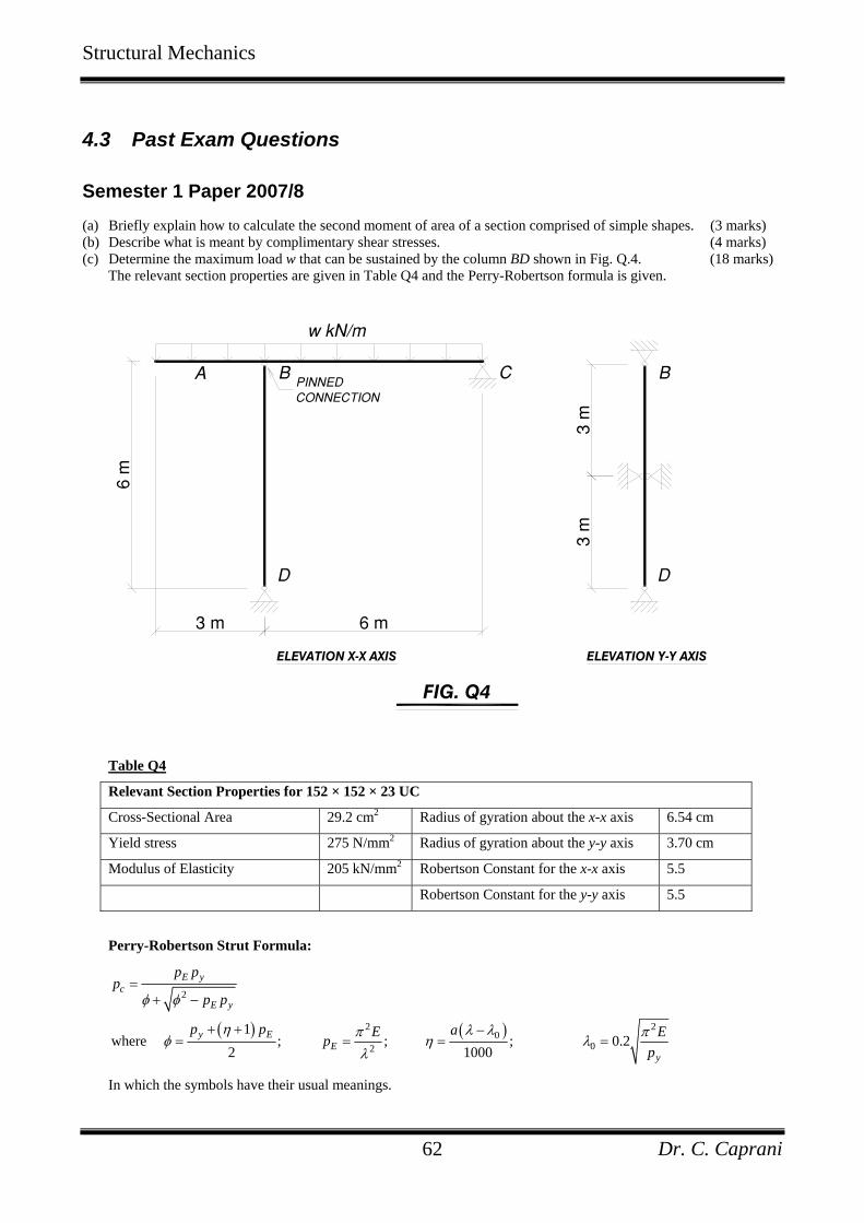
4.3 Past Exam Questions
Semester 1 Paper 2007/8 (a) Briefly explain how to calculate the second moment of area of a section comprised of simple shapes. (3 marks) (b) Describe what is meant by complimentary shear stresses. (4 marks) (c) Determine the maximum load w that can be sustained by the column BD shown in Fig. Q.4. (18 marks)
The relevant section properties are given in Table Q4 and the Perry-Robertson formula is given.
FIG. Q4
C
w kN/m
6 m
B
3 m
APINNEDCONNECTION
D
6 m
ELEVATION X-X AXIS ELEVATION Y-Y AXIS
3 m
3 m
B
D
Table Q4
Relevant Section Properties for 152 × 152 × 23 UC
Cross-Sectional Area 29.2 cm2 Radius of gyration about the x-x axis 6.54 cm
Yield stress 275 N/mm2 Radius of gyration about the y-y axis 3.70 cm
Modulus of Elasticity 205 kN/mm2 Robertson Constant for the x-x axis 5.5
Robertson Constant for the y-y axis 5.5
Perry-Robertson Strut Formula:
( ) ( )
2
2 20
02
1where ; ; ; 0.2
2 1000
E yc
E y
y EE
y
p pp
p p
p p aE Epp
φ φ
η λ λπ πφ η λλ
=+ −
+ + −= = = =
In which the symbols have their usual meanings.