Structural Identification of Mir usingInverse System Dynamics

and Mir/Shuttle Docking Data

Daniel C. Kammer

Associate Professor

and

Adam D. Steltzner

Research Assistant

Department of Engineering Physics

University of Wisconsin

Madison, WI 53706

Abstract

The goal of this work was to determine if it is feasible to use Mir/Shuttle docking data to

perform Mir damage detection. A time-domain technique called a Remote Sensing System was

proposed as an approach. The method uses inverse structural dynamics to identify physical

characteristics of a structure which can subsequently be used for damage detection. The RSS

method was demonstrated for a numerical simulation of Mir/Shuttle docking assuming that sensors

were collocated with Mir docking location. Several fixed interface Mir modes were identified from

the computed RSS pulse responses using the Eigen System Realization Algorithm and then

correlated with ta finite element representation. The method was then applied to the combined set

of docking data from Mir/Shuttle missions STS-81, STS-89, and STS-91. Two modes were

identified that correlated very well with FEM fixed interface modes. Finally, projections of the Mir

and FEM RSS pulse responses onto the individual docking data sets were compared for changes in

the structure. Overall, the results produced by this work appear to indicate that Mir was in an

undamaged state, at least with respect to docking excitation, at the time of STS-91. The

significance of the contribution of the RSS approach is that it is not affected by the nonstationarity

and nonlinearity associated with the Mir/Shuttle docking interface, and docking forces at the

interface do not have to be measured.

2I. Introduction

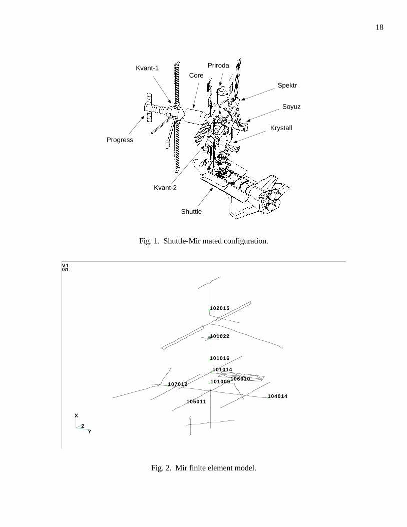
During the course of the Mir-Shuttle program, the structural integrity of Russia's Mir Space

Station, pictured in Fig. 1, was a major concern due to Mir's longevity. The potential problem

was exacerbated when a Progress supply ship collided with Mir during the summer of 1997. Mir

therefore represents a rare opportunity to evaluate methods for detecting damage on an actual

structure in orbit. Currently, modal identification is a very popular approach to damage detection.

Pre- and post-damage vibration experiments are performed and damage is detected by observing

changes in frequencies and shapes of excited modes. Reference [1] presents a comprehensive

review of modal based damage detection techniques. In the case of Mir, there are several possible

sources of excitation, such as Mir and Shuttle thruster firing, intentional crew motion, ambient

noise, and docking events. In general, it was observed that Shuttle docking produced the largest

structural responses in Mir [2].

Modal identification of Mir using docking data represents a formidable challenge for several

reasons. First, modal identification techniques in general work best when there is a sufficient

amount of data available for averaging. In the case of Mir, the short time duration of the docking

events coupled with the availability of a relatively small number of data sets precluded averaging.

In addition, if the measured Mir response to docking is considered as free-decay of a coupled Mir-

Shuttle system, the combined structure is nonlinear due to the docking element, and the system is

time-varying due to non-instantaneous capture. Free-decay identification techniques, such as the

Eigensystem Realization Algorithm (ERA) [3], cannot easily be applied to this problem. In order

to avoid the effects of nonlinearities and the time-varying configuration, Mir docking response can

alternatively be considered as forced response due to the shuttle acting as a large shaker.

Typically, during a modal test, both the force inputs and the response of the system are measured.

Frequency response and pulse response functions are generated and many methods are then

applicable for modal identification. In the case of Mir, the docking forces that excite the space

station are not measured, limiting the number of techniques available for modal identification. Two

output-only approaches that are applicable include the Natural Excitation Technique (NExT) [4]

and subspace identification algorithms [5]. However, these and related methods assume that the

input to the system is white noise. The docking forces applied to Mir clearly do not fit this

criterion.

The objective of the work presented here is to investigate the use of inverse system

identification techniques on Mir/Shuttle docking data to identify Mir vibrational characteristics for

ultimate application to damage detection. This new approach, initially presented by Kammer in

Ref. [6], does not attempt to identify the usual mode shapes and frequencies of a structure. Instead

it identifies the vibrational characteristics of an inverse representation. A system's inverse

representation differs from the usual forward representation in that the roles of the input and output

are reversed. The associated inverse vibrational characteristics consist of frequencies and mode

shapes for the inverse system. In special cases, they represent quantities as closely related to the

forward system as constrained modal parameters. In this situation, inverse frequencies and mode

shapes can be easily related to structural parameters and characteristics. Changes in the inverse

3modal parameters can then be related to corresponding changes in the structure. The main

advantages of using the inverse system identification approach are that the force inputs to the

structure do not have to be known and there are no requirements for the input forces to be random

or stationary.

The paper first gives a brief presentation of the inverse system identification theory. Details

can be found in Ref. [6]. New results involving cases with varying relations between numbers of

reference sensors, inputs, and experimental data sets are discussed. The inverse identification

approach is then applied to a detailed numerically simulated docking example involving a finite

element representation (FEM) of Mir. Finally, the method is applied to actual measured docking

data from STS-81, STS-89, and STS-91. Docking response was recorded using the Russian Mir

Structural Dynamic Measurement System (SDMS) which included 25 piezoelectric accelerometers.

Results are then compared with the FEM and the simulated docking analyses.

II. Theory

The inverse system identification approach is based upon a technique previously developed

by Kammer [7] for measuring the response of an operating structure at discrete locations and

predicting the response at other desired locations on the structure that do not have sensors during

operation. It was shown that an input-output representation called a Remote Sensing System

(RSS) can be derived directly from vibration test data where the input is the measured response at

the sensor locations and the output is the desired remote location response. It is assumed that in

discrete time, the structure can be represented by the difference equation

x k Ax k Bu k+( ) = ( ) + ( )1 (1)

in which x represents an n dimensional state vector, A is the nxn system matrix, B is the nxna

input influence matrix, and u is the na dimensional force vector. The corresponding system output

equation is given by

y k C x k D u ks s s( ) = ( ) + ( ) (2)

where ys is an ns dimensional sensor output vector, Cs is an nsxn output influence matrix, and Ds

is an nsxna direct transmission matrix. Accelerometers are used as sensors such that the direct

transmission matrix is nonzero, however, other types of sensors can be used by appropriately

modifying the derivations using lagged systems. It is also assumed that the structure being

considered is free-free.

An analytical representation of the RSS can be derived by solving Eq. (2) for the force input

at time step k

u k D C x k D y ks s s s( ) = − ( ) + ( )+ + (3)

4in which Ds+ represents the generalized inverse D D D Ds s

Ts s

T+ −= ( ) 1

. Note that the number of

sensors ns must be greater than or equal to the number of inputs na. Equation (4) is then

substituted into the state equation (1) producing

x k Ax k By ks+( ) = ( ) + ( )1 ˆ ˆ (4)

where the new plant and input influence matrices are given by

ˆ ˆA A BD C B BDs s s= − =+ + (5)

Equations (3) and (4) represent an inverse system in which the roles of input and output have been

reversed with respect to the forward system in Eqs. (1) and (2). The forward system output

equation for the response at the desired nd remote locations is analogous to Eq. (2)

y k C x k D u kd d d( ) = ( ) + ( ) (6)

Substituting for the input force from Eq. (3) produces

y k Cx k Dy kd s( ) = ( ) + ( )ˆ ˆ (7)

withˆ ˆC C D D C D D Dd d s s d s= − =+ + (8)

Equations (4) and (6) represent the RSS in which measured response is the input and desired

response is the output. The input force acting on the structure has been completely eliminated from

the system equations. It is important to note that the state equations for both the inverse system

and the RSS are identical.

Alternatively, the RSS can be represented by the convolution

y k Py k id i si

k

( ) = −( )=∑

0

(9)

in which the nd x ns weighting matrices Pi are the RSS Markov parameters. They represent the

free-decay response of the RSS and thus a modal identification technique such as ERA can be used

to identify the corresponding RSS mode shapes and frequencies. Equations (4), (5), (7), and (8)

show that the RSS and its modal parameters depend directly upon the physical parameters of the

actual structure and can be used to detect structural damage.

5A. Inverse System Modal Parameters

In order to be a useful tool, it is important to determine the physical significance of the RSS

or inverse system eigenvalues and corresponding mode shapes when possible. The interpretation

is dependent upon the relationship between the numbers and locations of forward system inputsand outputs. For the special case where there are as many sensors as force inputs, n ns a= , it can

be shown [6] that the inverse system eigenvalues are equivalent to the forward system transmission

zeros. Transmission zeros are defined to be the complex values ψ at which it is possible to apply

a nonzero input,u e t= µ ψ , and get an identically zero output at the sensor locations for suitable

initial conditions x 0( ). Williams [8] can be consulted for more details on transmission zeros and

structures.

Corresponding to the particular case of equal numbers of inputs and outputs, two possible

subcases are considered. In the first subcase, the inputs and outputs are totally noncollocated,

meaning that there are no sensors at any of the input locations. In this situation, the forward

system is in general nonminimum phase [9]. This means that some of the transmission zeros of

the discrete forward system are outside the unit circle, or for the continuous representation, in the

right half plane, which implies that the inverse system has unstable poles. The corresponding RSS

Markov parameters in Eq. (9) grow without bound. The remaining stable inverse system

eigenvalues occur in complex conjugate pairs. It was shown in Ref. [6] that the proposed RSS

identification technique estimates the minimum phase portion of the RSS pulse response

corresponding to the stable transmission zeros and related shapes that are inside the unit circle for

the discrete system.

The second subcase of special interest with respect to identification is one in which sensors

and outputs are collocated. In this situation, every force input location and direction has a

corresponding sensor. In addition, it is assumed that the sensors are just sufficient in number and

location to remove all rigid body modes from the structure if constrained. In this case, Ref. [6]

illustrated that a Craig-Bampton representation [10] of the structure computed relative to the sensor

locations is equivalent to an inverse structural system in which the acceleration at the sensor

locations is the input to a fixed mode state equation and the output is the force applied at the sensor

locations. Therefore, in the rigid body sufficient collocated case, the RSS eigenvalues and mode

shapes correspond to the frequencies and mode shapes of the structure with the sensor degrees of

freedom fixed. This is a strong result in that many techniques exist for relating physical changes in

structures to corresponding changes in the structure's modal parameters.

B . Identification of RSS Markov Parameters

Before modal parameters can be identified, the RSS pulse response must be estimated using

experimental data. The available data is split into the two previously discussed sets, the sensorlocations numbering ns and the desired locations numbering nd . Note that the ns sensor locations

can be considered as references analogous to input locations in a usual vibration test. If there arene experiments, the RSS convolution equation (9) can be expanded into the matrix equation

6PY Ys d= (10)

where

P P P P Y y y yN d d d dnR t

= [ ] = [ ]− −0 1 1 0 1 1L L

Y

y y y

y y

y y

s

s s sn

s sn

s sn N

t

t

t R

=

−

−

−

0 1 1

0 2

0

0

0 0

0

L L

L L

M L M

M M M L M

L L

and ysi is an n ns e× matrix in which the jth column represents the measured sensor response at

time step i for experiment j, ydi is the corresponding response at the desired locations, and nt is

the number of experimental data points. In an application, the data matrices in Ys and Yd are

truncated to NC block columns. Two cases important to RSS modal identification are considered.

1 . Equal Numbers of Sensors and ExperimentsIn this case, the data blocks ysi are assumed to be square and full rank. The corresponding

data matrix Ys theoretically should then be full row rank. If equal numbers of block rows and

block columns are used, i.e. N NR C= , Ys is square and the first NR RSS Markov parameters can

be determined uniquely by inverting Ys in Eq. (10). In practice, the data matrix Ys becomes very

large and ill-conditioned. The usual matrix inverse is replaced by a Moore-Penrose pseudo-inverse

based upon singular value decomposition [11]. In general, for computational stability, the problemis made to be overconstrained by adding block columns such that N NC R> . The solution for the

RSS pulse response is then given by

P Y Y Y Yd sT

s sT= ( )+

(11)

where the superscript + denotes the pseudo-inverse. The normal form of the least-squares solution

is used at the risk of inaccuracy in order to minimize the memory requirements for the pseudo-

inversion of the data matrix. More efficient and accurate solution techniques will be investigated in

future research. Once the RSS pulse response is identified, ERA can be used to extract the

corresponding modal parameters.

2 . More Sensors than Experiments

In Kammer's original development and application [7], identification of the RSS model was

based upon the forward system pulse response measured during a vibration test. In this case, thenumber of experiments is equal to the number of inputs, n ne a= . The goal was to compress the

system information contained in the RSS Markov parameters in the pulse response sequence into a

7much smaller number of equivalent terms or weighting matrices Wi . This was accomplished by

using several more sensors (references) than experiments and many more block columns than

block rows. It is believed that this compression is analogous to that produced by the observerformulation introduced in Refs. [12, 13]. The only requirement is that the product N nR s⋅ must be

greater than the number of observable-controllable modes responding in the data. Due to the

relatively small number of block rows used, the computation of the system equivalent RSS

weighting matrices using Eq. (11) was observed to be very robust to data errors and noise.

Unfortunately, the estimated weighting sequence representation cannot be directly used as free-

decay data in ERA to estimate the RSS modal parameters.

The Mir damage detection problem using docking data represents a case where the number of

sensors is greater than the number of available experiments. During this project, there was only

one set of docking data available from before the Mir/Progress collision, STS-81, and two from

after the collision, STS-89 and STS-91. Damage detection requires the comparison of RSS results

computed using the single data set from STS-81 with results produced from the individual post-

damage data sets. Ideally, there are three forces and three moments acting on Mir through the

docking mechanism. In order to avoid compression when estimating the RSS pulse response in

this case, the number of block rows and columns must be the same. This situation produces a datamatrix Ysi , corresponding to the ith docking data set, that has more rows than columns and the

corresponding matrix Eq. (10) is underdetermined. There are now an infinite number of solutions.

A solution with minimum norm can be obtained using the formulation

P̂ Y Y Y Yi di siT

si siT= ( )+

(12)

If P is the true RSS pulse response, P̂i represents the orthogonal projection [14] of P onto the

column space of data matrix Ysi given by

P̂ PY Y Y Y PHi si siT

si siT

i= ( ) =+

(13)

As in the case of the compressed weighting sequence, the orthogonal projection of the pulse

response cannot be directly used in ERA to estimate the RSS modal parameters. In addition,

estimates of orthogonal projections produced by two different experiments will in general be

different and thus cannot be directly compared for the purpose of detecting structural changes.

Alternatively, it could be assumed that enough docking data sets have been accumulated

during the early life of the structure such that the RSS pulse response of the undamaged structure,

P, can be computed using Eq. (11). A data set from a subsequent docking event can then be used

to detect any damage that may have occurred since the docking event that produced the last data set

used in the identification of the RSS pulse response. Considering only the new docking data set,

Eq. (12) can be used to compute P̂i corresponding to the projection of the RSS pulse response

onto the vector space spanned by the data set. Using the orthogonal projector Hi from Eq. (13),

8the undamaged RSS pulse response P can be projected onto the same vector space to produce Pi .

If P was originally computed using equal numbers of block rows and block columns in its data

matrix Ys and if the structure remains undamaged, then P̂ Pi i= . Lack of agreement indicates

damage. When the conditions mentioned are satisfied, the equality holds in general because the ne

individual data matrices Ysi used to produce Ys in Eqs. (10) and (11) have independent column

spaces. This implies that Pi is due only to the data from the ith docking event and should thus

agree with ̂Pi . For FEM simulated docking data, the equality holds even for the overconstrained

case where the number of block columns is much greater than the number of block rows. In

general, overconstraint is required for computational stability. Unfortunately, real data is not

consistent, therefore the equality P̂ Pi i= does not hold in general in the overconstrained case.

Future work will address this shortcoming of the RSS approach as applied to docking data.

Alternatively, there is an a posteriori approach that can be used to compare individual docking

data sets and search for damage between docking events. The method is not ideal because enough

post-damage data sets must be accumulated to identify a new RSS pulse response using Eq. (11).

The procedure will be demonstrated for real docking data in Section IV.

III. Numerical Example

The use of the RSS identification approach is first demonstrated for a case where there is

sufficient data to perform pulse response identification. A numerical example is presented in which

docking is simulated for Mir using the Russian built FEM supplied by NASA. The FEM shown in

Fig. 2 is an equivalent beam representation containing 2,646 dof and 211 free-free modes with

frequencies below 5.0 Hz. Three independent docking experiments were simulated, each with

three input forces in the x, y, and z directions at the docking node 118009. Moments applied at the

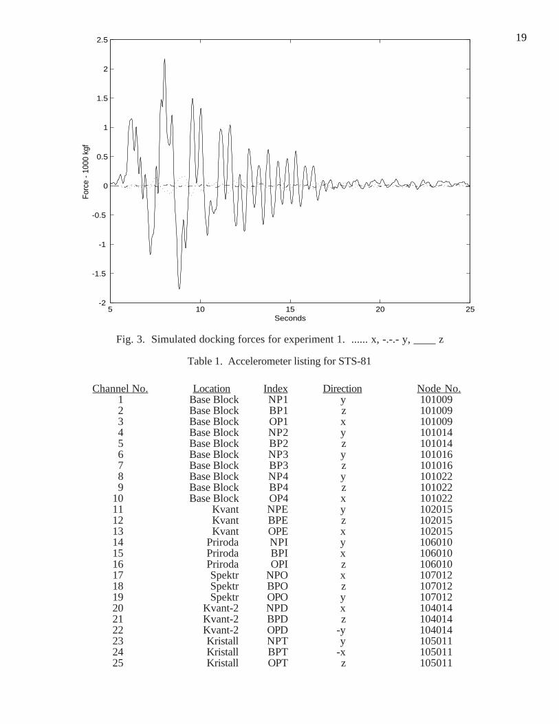
docking node were ignored for computational efficiency. The first set of docking forces was

simulated by scaling the translational response of the accelerometer at node 105011 on the Krystall

module measured during STS-81. The x and y responses were multiplied by 2g, while the z

response was multiplied by 20g. Figure 3 illustrates the corresponding docking forces for

experiment 1. The translational forces analytically reconstructed by NASA for STS-81 were used

in experiment 2 and the translational response measured at node 105011 during STS-89 and scaled

by the same factors as in experiment one were used as docking forces in experiment 3. Two

percent critical damping was assumed for all 211 modes in the simulations.

During the simulated docking experiments, three accelerometers were assumed to be

collocated with the force input locations. Therefore, the numbers of sensors, inputs, and

experiments are all equal to three in this example. The inverse system eigenvalues and mode

shapes will correspond to Mir structural modes with the three translational degrees of freedom at

the sensor locations fixed. Desired response locations were chosen to coincide with the 25

accelerometer locations on Mir. Table 1 lists the locations and corresponding FEM node numbers

in the order in which data channels were measured during STS-81. Figure 2 shows the

corresponding FEM node locations. During the docking experiments, it was assumed that the

9acceleration was also measured at the desired location set just as would be the case during an actual

docking event.

Each experiment was simulated in MATLAB for 1,150 time steps of 0.02 seconds each. In

order to simulate errors and noise in the measured data, normally distributed zero mean random

noise, equivalent to 5.0% of the root-mean-square (rms) response, was added to each of the 3

sensor and 25 desired response channels from each experiment. The RSS pulse response was

computed by generating a sensor data matrix with 650 block rows and 1,100 block columns

producing a 1,950 by 3,300 matrix. Note that the added noise actually helps stabilize the

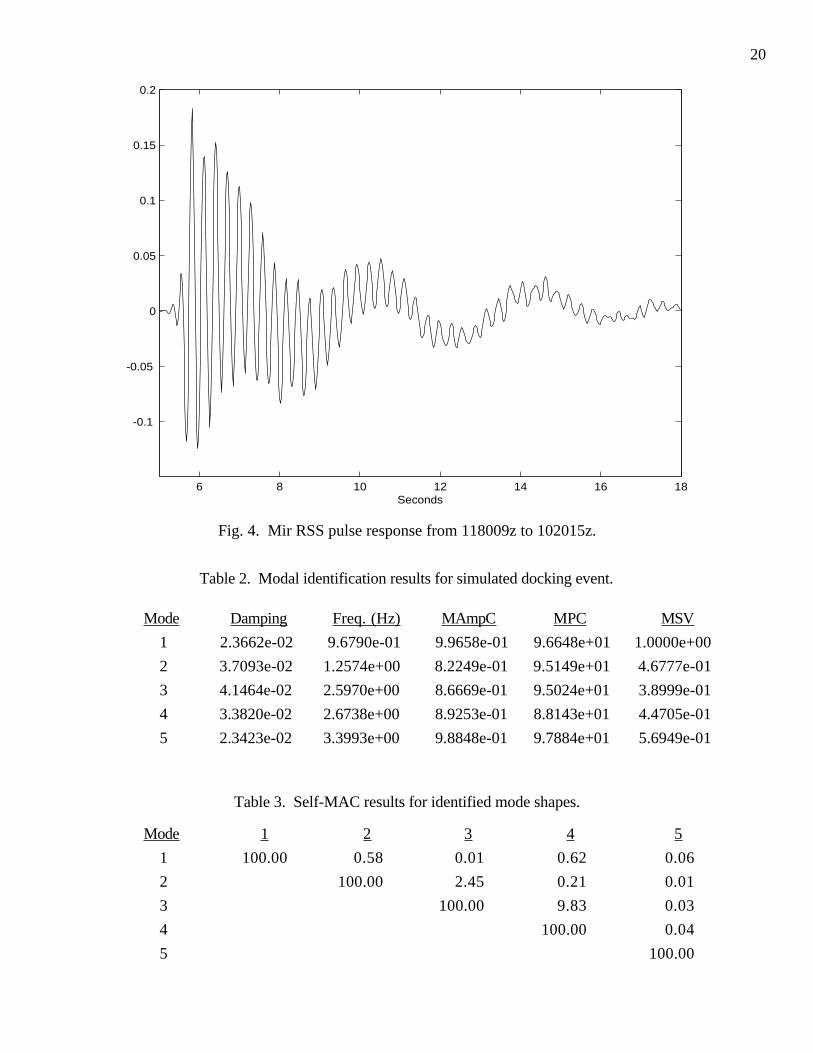
computation of the pulse response in this example. A typical RSS pulse response from sensor

location 118009z to desired response location 102015z is pictured in Fig. 4 after it has been low

pass filtered to 5.0 Hz.

The Eigensystem Realization Algorithm (ERA) was then applied to the estimated noisy RSS

pulse response data. Eighty singular values were retained and 38 mode shapes and frequencies

were computed using a block Hankel matrix with 30 block rows and 500 block columns. Three

indicators of goodness were used to distinguish true modes from noise. The first indicator, Modal

Amplitude Coherence (MAmpC) [11], gives a measure of how well a computed mode shape and

frequency reproduce the measured system response. A value of 1.0 indicates perfect reproduction.

The second indicator, Modal Phase Collinearity (MPC) [15], gives a measure of the degree of

monophase or normal behavior of an extracted mode shape. Its value ranges from 0.0 to 100.0

percent for a perfect normal mode. Finally, the Mode Singular Value (MSV) [11] gives a measure

of the contribution of each mode to the identified pulse response time history. The measure is

normalized such that the strongest responding mode has an MSV value of 1.0.

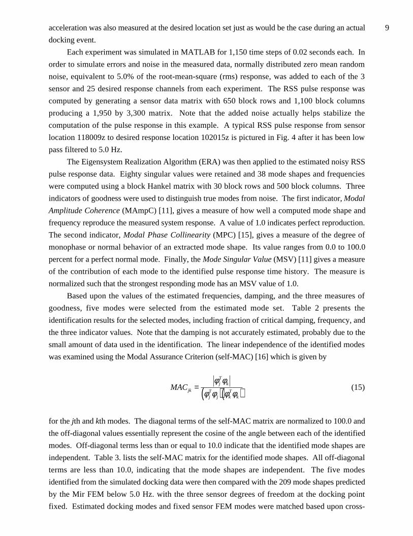
Based upon the values of the estimated frequencies, damping, and the three measures of

goodness, five modes were selected from the estimated mode set. Table 2 presents the

identification results for the selected modes, including fraction of critical damping, frequency, and

the three indicator values. Note that the damping is not accurately estimated, probably due to the

small amount of data used in the identification. The linear independence of the identified modes

was examined using the Modal Assurance Criterion (self-MAC) [16] which is given by

MACjk

jT

k

jT

j kT

k

= ( )( )φ φ

φ φ φ φ(15)

for the jth and kth modes. The diagonal terms of the self-MAC matrix are normalized to 100.0 and

the off-diagonal values essentially represent the cosine of the angle between each of the identified

modes. Off-diagonal terms less than or equal to 10.0 indicate that the identified mode shapes are

independent. Table 3. lists the self-MAC matrix for the identified mode shapes. All off-diagonal

terms are less than 10.0, indicating that the mode shapes are independent. The five modes

identified from the simulated docking data were then compared with the 209 mode shapes predicted

by the Mir FEM below 5.0 Hz. with the three sensor degrees of freedom at the docking point

fixed. Estimated docking modes and fixed sensor FEM modes were matched based upon cross-

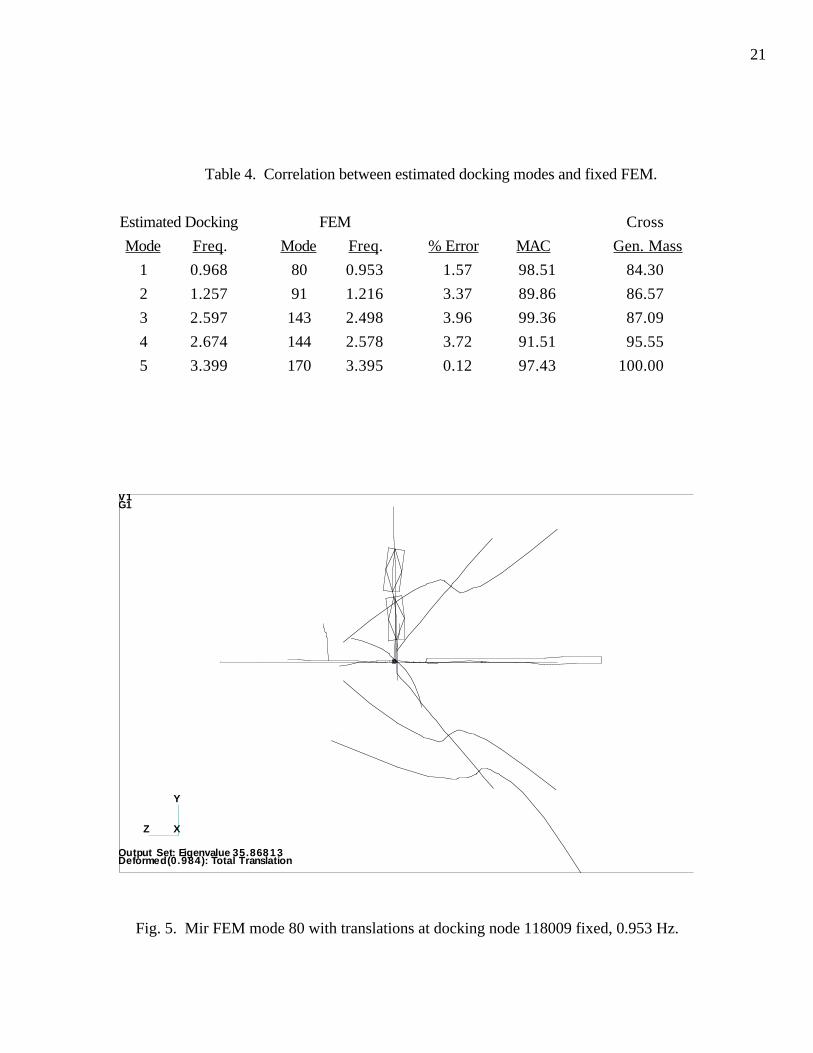
10MAC shape comparison and frequency. Table 4 lists docking/FEM mode pairs with cross-MAC

values and the corresponding frequency errors. Because of the relatively small number of

accelerometers used in the modal identification, the estimated docking modes are highly coupled

with several of the FEM mode shapes.

The simulated test/FEM mode pairing listed in Table 4 was further investigated by computing

a reduced mass matrix, called a Test-Analysis Model (TAM), which possessed only the 25 desired

sensor location degrees of freedom. The very small number of degrees of freedom forced the use

of an advanced technique called Modal reduction [17] to produce the TAM. A Modal TAM was

generated that exactly predicted the five FEM modes that were paired with the simulated test

modes. Cross-orthogonality was then computed between the FEM and test modes using the

relation

CGM MFEMT

TAM Test= φ φ (16)

where φFEM , φTest , and MTAM are the FEM modes, test modes, and TAM mass matrix,

respectively. Table 4 lists the cross-generalized mass values scaled to a perfect value of 100.0 for

each of the simulated test/FEM mode pairs. All values are well above 80.0 indicating good mass

weighted shape agreement. Based upon cross-MAC values that are approximately 90.0 and larger,

frequency errors that are less than 4.0%, and CGM values greater than 80.0, it is believed that the

RSS/ERA approach accurately identifies five sensor fixed FEM modes using docking data with

5.0% noise. Note that Table 2 indicates that simulated test mode 1, which correlates with FEM

mode 80, is the most strongly excited of the test modes identified (MSV = 1.00). This agrees with

the fact that FEM mode 80 possesses the greatest amount (27%) of Effective Mass [18] in the z

direction for the constrained structure. It is expected that the largest docking forces act along the

line of docking or the z axis, therefore mode 80 should be strongly excited. Figure 5 illustrates

FEM mode 80 which can be seen to have a substantial amount of z motion as expected.

An objective of this numerical experiment was to determine if the proposed RSS

identification technique can be used in conjunction with the relatively small amount of data

provided by Mir/Shuttle docking events to detect structural changes or damage in the Mir primary

node, specifically at the Krystall-to-base module interface. One of the major difficulties associated

with using docking data for modal identification is that the excitation due to the docking forces is

neither persistent nor broadband, as evidenced by the identification of only five modes from the

numerical experiment. Each of the identified FEM modes was examined for its strain energy

content within the primary node interfaces. Of the five, mode 80 contains over 80.0% of its modal

strain energy within the primary node interfaces and mode 91 contains 16.8% within the interfaces.

The remaining three modes contain insignificant amounts of strain energy in this area.

Unfortunately, essentially none of the strain energy in modes 80 and 91 corresponds to the

spring elements associated with the Krystall-to-base module interface. Within mode 80, the energy

is evenly divided between the x direction torsional spring element 104400 at the Kvant-2-to-base

module interface and the x direction torsional spring element 107400 at the Spektr-to-base module

11interface. Within mode 91, 11.2% of the strain energy is contained in the z direction torsional

spring element 104600 at the Kvant-2-to-base module interface and 5.5% is contained in the z

direction torsional spring element 107600 at the Spektr-to-base module interface. Inspection of the

remaining sensor fixed FEM modes shows that a significant amount of strain energy does not

appear in the Krystall-to-base module interface until mode 182 at 4.021 Hz., and mode 195 at

4.495 Hz. Neither of these modes was strongly excited and thus not identified from the simulated

docking data. Based upon this example, it appears that damage in the Krystall-to-base module

interface cannot be identified from docking data.

While it isn't possible to detect damage in the Krystall-to-base module interface, it does

appear feasible to identify structural changes in either the Kvant-2-to-base module or Spektr-to-

base module interfaces by monitoring frequency changes in test modes corresponding to FEM

mode 80. The docking simulation and subsequent identification produced an accuracy of 1.57%

for the frequency of mode 80. It has been common practice in modal testing and FEM model

updating to regard a test/FEM frequency difference of less than 5.0% to be very good test-analysis

correlation. It is obvious that the threshold for the existence of damage or correlation depends

strongly on the application, but it would seem that at least a 5.0 to 10.0% change in frequency

would then have to occur to be able to differentiate between a good frequency identification and

actual damage. Design sensitivity analysis using the undamaged FEM indicates that to get the

lower bound 5.0% change in frequency for mode 80 would require approximately a 25% decrease

in the interface stiffness. This is probably an unacceptably high threshold for the detection of

damage in a critical component. It is important to note that the described sensitivity problem for

this particular application is not due to the RSS identification technique presented in this paper.

Any damage detection technique using docking data and subsequent shifts in identified frequencies

would have the same problem.

IV. Application of RSS to Mir/Shuttle Docking Data

The RSS identification technique will now be applied to actual docking data from the STS-

81, STS-89, and STS-91 missions. Docking response was recorded using the Russian Mir

Structural Dynamic Measurement System (SDMS) which included 25 piezoelectric accelerometers.

This measurement system has a fixed frequency range of 0.1 to 5.0 Hz and a fixed dynamic range

of 1.5 to 30.0 milli-g. Analog acceleration is telemetered directly to the ground and then processed

with a sampling rate of 50.0 Hz. Data loss during telemetry can be as high as 15.0% [2]. Further

details can be found in Ref. [2]. All docking data was low-pass filtered to 5.0 Hz prior to being

received from NASA. Unfortunately, only 19 accelerometer locations are common to all three

docking events. The triax on the Spektr module was lost to STS-89 and STS-91 due to the

collision with the Progress spacecraft and data from the triax on Priroda was not included in the

STS-91 data set for unknown reasons. In the subsequent analyses, it is assumed that the docking

forces dominate the response of Mir while the effects of the moments are secondary. This is

consistent with results presented in Ref. [19]. Three RSS reference sensors were selected

corresponding to the triax on the Krystall module. This was an obvious choice due to the

12location's proximity to the actual Mir/Shuttle docking point. Therefore, it assumed that the number

of sensors is equal to the number of inputs, meaning that the inverse system eigenvaluesapproximate the forward system transmission zeros. The number of desired sensor locations, nd ,

is then 16 in the following analyses.

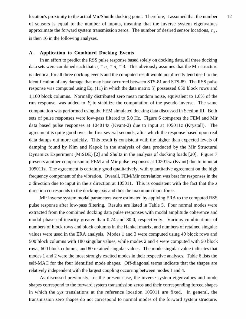
A . Application to Combined Docking Events

In an effort to predict the RSS pulse response based solely on docking data, all three dockingdata sets were combined such that n n ns a e= = = 3. This obviously assumes that the Mir structure

is identical for all three docking events and the computed result would not directly lend itself to the

identification of any damage that may have occurred between STS-81 and STS-89. The RSS pulseresponse was computed using Eq. (11) in which the data matrix Ys possessed 650 block rows and

1,100 block columns. Normally distributed zero mean random noise, equivalent to 1.0% of therms response, was added to Ys to stabilize the computation of the pseudo inverse. The same

computation was performed using the FEM simulated docking data discussed in Section III. Both

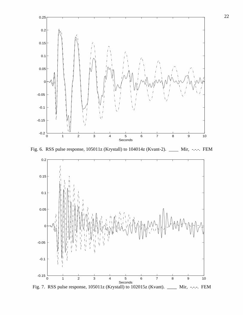
sets of pulse responses were low-pass filtered to 5.0 Hz. Figure 6 compares the FEM and Mir

data based pulse responses at 104014z (Kvant-2) due to input at 105011z (Krystall). The

agreement is quite good over the first several seconds, after which the response based upon real

data damps out more quickly. This result is consistent with the higher than expected levels of

damping found by Kim and Kapok in the analysis of data produced by the Mir Structural

Dynamics Experiment (MiSDE) [2] and Shultz in the analysis of docking loads [20]. Figure 7

presents another comparison of FEM and Mir pulse responses at 102015z (Kvant) due to input at

105011z. The agreement is certainly good qualitatively, with quantitative agreement on the high

frequency component of the vibration. Overall, FEM/Mir correlation was best for responses in the

z direction due to input in the z direction at 105011. This is consistent with the fact that the z

direction corresponds to the docking axis and thus the maximum input force.

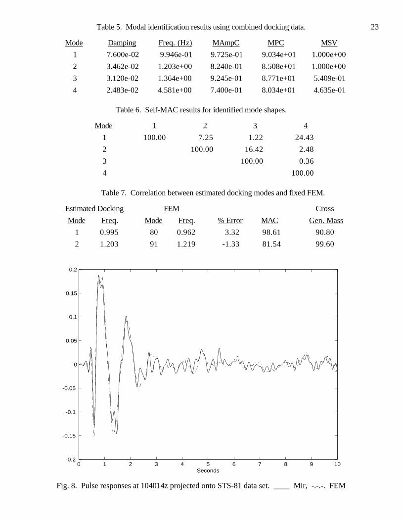
Mir inverse system modal parameters were estimated by applying ERA to the computed RSS

pulse response after low-pass filtering. Results are listed in Table 5. Four normal modes were

extracted from the combined docking data pulse responses with modal amplitude coherence and

modal phase collinearity greater than 0.74 and 80.0, respectively. Various combinations of

numbers of block rows and block columns in the Hankel matrix, and numbers of retained singular

values were used in the ERA analysis. Modes 1 and 3 were computed using 40 block rows and

500 block columns with 180 singular values, while modes 2 and 4 were computed with 50 block

rows, 600 block columns, and 80 retained singular values. The mode singular value indicates that

modes 1 and 2 were the most strongly excited modes in their respective analyses. Table 6 lists the

self-MAC for the four identified mode shapes. Off-diagonal terms indicate that the shapes are

relatively independent with the largest coupling occurring between modes 1 and 4.

As discussed previously, for the present case, the inverse system eigenvalues and mode

shapes correspond to the forward system transmission zeros and their corresponding forced shapes

in which the xyz translations at the reference location 105011 are fixed. In general, the

transmission zero shapes do not correspond to normal modes of the forward system structure.

13However, due to the dominance of the measured response by the input along the z axis and the

high relative stiffness of the structure along this direction, information transmission is very fast

between the docking point 118009 and the reference sensor location on Krystall. It is therefore

believed that the system should behave in many respects as though the input and reference sensor

locations are collocated. At least some of the transmission zero shapes dominated by the z

direction should correspond to normal modes of Mir with 105011xyz fixed.

Test-analysis correlation was performed between the four identified test modes and 208 FEM

modes computed with the translations at 105011 constrained. Based upon frequency and cross-

MAC, the first two test modes were matched with FEM modes 80 and 91, respectively. As in the

numerical simulation, a Modal TAM was generated for FEM modes 80 and 91 and then cross-

orthogonality was computed between the test and corresponding FEM mode shapes. Correlation

results are listed in Table 7. Based upon frequency errors of approximately 3.0% and less, MAC

values greater than 80.0, and cross-generalized mass values greater than 90.0, it is believed that the

FEM accurately predicts the first two modes identified from the combined docking data set. Note

that FEM modes 80 and 91 computed with translations at reference node 105011 fixed are

essentially the same in shape and frequency as FEM modes 80 and 91 computed earlier in the

numerical simulation with the docking node 118009 translations fixed. Therefore, the

identification results produced by the combined docking data sets is very analogous to the results

produced in the simulation in which modes 80 and 91 are predominant and accurately identified.

Noting that over 80.0% of the strain energy in FEM mode 80, and to a much lesser degree in mode

91, is concentrated in the Spektr- and Kvant-2-to-base module interfaces, accurate test-analysis

correlation of these two modes tends to indicate that at least these interfaces in Mir are undamaged

with respect to bending stiffness.

B . Application to Individual Docking Events

A drawback of the approach presented for identifying the RSS pulse response and

subsequent modal identification is the requirement that the number of experiments coincides with

the number of force inputs. This requirement is particularly troublesome in the case of post-

damage modal identification for subsequent damage detection. For the example considered, it

would be very desirable to be able to detect damage after one additional post-damage docking event

rather than waiting for additional docking data sets such that the complete post-damage RSS pulse

response can be detected.

In the previous section, all three docking data sets were combined to produce an estimate of

the RSS pulse response. More block columns than block rows had to be used in the combined

data matrix to stabilize the computation in Eq. (11). Therefore, the projected pulse response P̂i

computed in Eq. (12) using only the ith data set does not coincide with the projection of the pulse

response P onto the column space of the ith data set. A direct comparison of Pi and P̂i cannot be

used to detect damage from one individual data set to the next. However, individual docking data

sets can be used for damage detection in an a posteriori fashion. It is assumed that PFEM , produced

by FEM docking simulations, represents the undamaged structure, and PMir , produced in Section

14IV.A by combining the real docking data, represents the structure identified by the latest three

docking events. Individual docking data sets STS-81, STS-89, and STS-91 can be used to detect

inter-docking event structural damage by comparing the orthogonal projections of each of the pulse

responses onto the corresponding data set. If the projections satisfy

P H P HFEM i Mir i≈ (17)

for the ith data set, then the response produced by the corresponding docking event still reflects the

undamaged structure. If the projected pulse response correlation is poor, this is evidence that a

structural change has occurred. If agreement is good for all three docking data sets, there is strong

evidence that structural damage has not occurred. Of course, another possibility is that damage is

present, but the act of docking doesn't excite it.Equation (17) was applied for all three docking data sets. The orthogonal projectors Hi were

computed using Eq. (13) and a data matrix Ysi with 650 block rows and columns. Figure 8

illustrates the Mir and FEM pulse responses from 105001z to 104014z projected onto data from

STS-81 after low pass filtering to 5.0 Hz. The agreement is quite good, indicating that the

response produced by STS-81 still reflects an undamaged Mir structure. This is consistent with

the results produced by Kim and Kapok [2] and the fact that STS-81 preceded the Progress

collision. This is also consistent with the good test-analysis correlation presented in Section IV.A

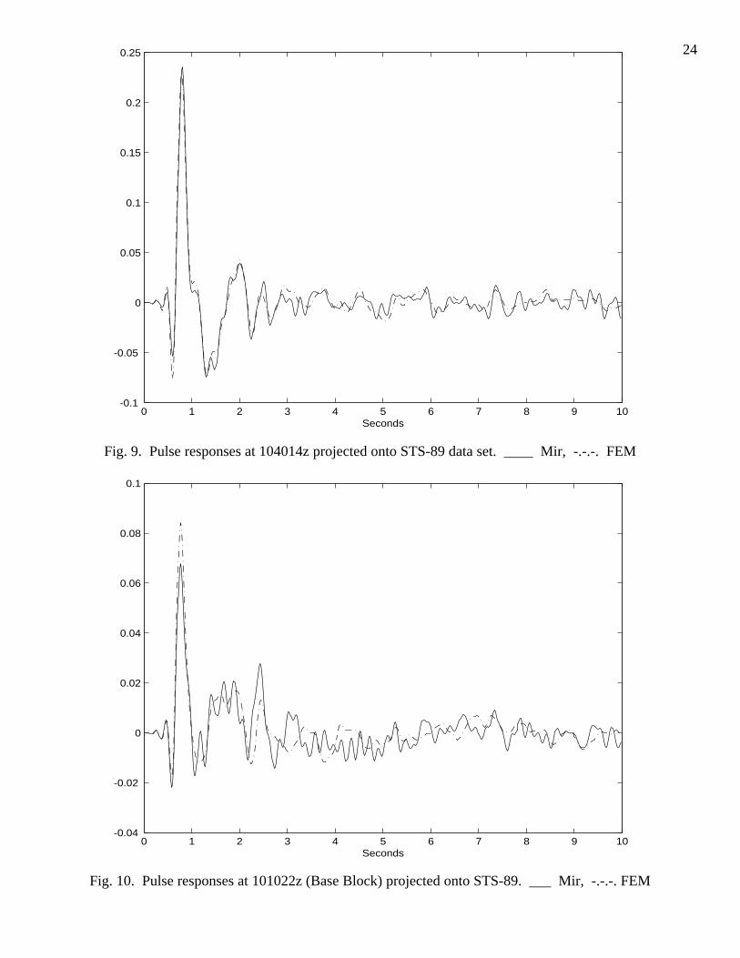
for FEM mode 80 which dominates the response at 104014z. Figure 9 presents the Mir and FEM

pulse responses from 105001z to 104014z projected onto data from STS-89, which took place

after the collision. Once again, the agreement is very good, indicating that response from STS-89

accurately reflects the undamaged Mir structure at least with respect to the x axis torsional springs

at the Spektr and Kvant-2 interfaces to the core module that dominate the strain energy in FEM

mode 80. Mir and FEM pulse responses from 105001z to 101022z (Base Block) projected onto

data from STS-89 are illustrated in Fig. 10. The correlation between projected FEM and Mir

pulses responses at this location is also quite good, again indicating that response from STS-89

reflects the undamaged structure. Comparable agreement between projected Mir and FEM pulse

responses was also found for the other z sensor locations for STS-89.

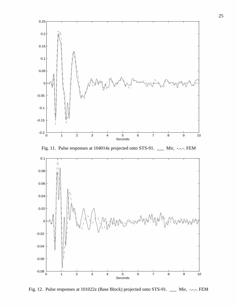
Finally, the pulse responses were projected onto data from STS-91. Figure 11 shows the

projection of the pulse responses from 105001z to 104014z. Agreement is still very good for the

response at 104014z. Figure 12 compares the projected responses at 101022z. The correlation is

not as good for this response, but qualitatively the projections are very comparable. It is believed

that the data from STS-91 also reflects the response of an undamaged Mir structure to docking

loads. Weighing all the results produced by comparing the Mir and FEM pulse responses, their

projections on individual data sets, and modal identification results, it appears that Mir was in an

undamaged state, at least with respect to docking excitation, at the time of STS-91. This

observation is in agreement with the overall results and observations produced by Kim and Kapok

in the Boeing MiSDE analysis [2]. The significance of the contribution of the RSS approach is that

it arrived at the same conclusion using not only a different set of sensor locations, but also a totally

15different type of excitation. The MiSDE work did not consider Mir/Shuttle docking because

capture of the Shuttle is not instantaneous, resulting in a nonstationary system with nonlinear

dynamic behavior. The RSS method is not affected by these problems and therefore compliments

the MiSDE work.

V . Conclusion

The goal of this work was to determine if it is feasible to use Mir/Shuttle docking data to

perform Mir damage detection. A time-domain technique called Remote Sensing was proposed as

an approach. The method uses inverse structural dynamics to identify physical characteristics

which can subsequently be used for damage detection. The term "inverse" refers to the fact that the

roles of input and output are reversed from the usual forward system structural dynamics problem.

If sensors such as accelerometers are placed at the external input locations, modal parameters

corresponding to structural motion with the sensor locations fixed can be identified. If sensors are

not collocated with the inputs, other important structural characteristics can be determined such as

transmission zeros and their corresponding shapes. The RSS method was demonstrated for a

numerical simulation of Mir/Shuttle docking assuming that sensors were collocated with the Mir

docking location. Several fixed interface Mir modes were identified from the computed RSS pulse

responses using ERA, and then correlated with the FEM. The method was then applied to the

combined set of docking data from STS-81, STS-89, and STS-91. Even though there were no

sensors available at the docking point, ERA produced two modes that correlated very well with

FEM fixed interface modes that were also accurately identified in the numerical simulations.

Finally, projections of the Mir and FEM RSS pulse responses onto the individual docking data sets

were compared for changes in the structure. Overall, the results produced by this work appear to

indicate that Mir was in an undamaged state, at least with respect to docking excitation, at the time

of STS-91. There is an especially high level of confidence in the undamaged state of the Spektr-

and Kvant-2-to-base module interfaces. This observation is in agreement with the overall results

and observations produced in the Boeing MiSDE analyses.

The significance of the contribution of the RSS approach is that it was able to produce the

same conclusion using not only a different set of sensor locations, but also a totally different type

of excitation. Mir/Shuttle docking event data was not considered in the MiSDE work because

capture of the Shuttle is not instantaneous, resulting in a nonstationary system with nonlinear

dynamic behavior. The RSS method is not affected by these problems and therefore provides a

strong compliment to the methods and procedures used in the MiSDE work. Another important

advantage of this approach is that it only requires measured response data. The applied external

forces or internal interface forces are not required for modal identification. This characteristic

makes the Remote Sensing System approach applicable in cases where the input forces cannot be

measured. It is believed that RSS provides a valuable new method to identifying characteristics of

structures from measured data without the need for measuring the input.

16

Acknowledgments

This work was supported by NASA Johnson Space Center under Grant NAG9-953. The authors

would like to thank contract monitor Mr. James Dagen for his support and encouragement. They

would also like to express appreciation to Rocket and Space Corporation-Energia (RSC-E) for

providing the Mir FEM and flight data, and Mr. Ken Shultz of Lockheed Martin Corporation.

References

[1] Doebling, S. W., C. R. Farrar, M. B. Prime and D. W. Shevitz, “Damage Detection andHealth Monitoring of Structural and Mechanical Systems from Changes in Their VibrationChracteristics: A Literature Review,” Los Alamos National Laboratory, LA-13070-MS,1996.

[2] Kim, H. and M. Kaouk, “Mir Structural Dynamics Experiment,” The Boeing Company,Contract No. NAS15-10000, 1998.

[3] Juang, J. and R. S. Pappa, “An Eigensystem Realization Algorithm for Modal Identificationand Model Reduction,” Journal of Guidance, Control, and Dynamics, 8(5), 1985, pp. 620-627.

[4] James, G. H., T. G. Carne and J. P. Lauffer, “The Natural Excitation Technique (NExT) forModal Parameter Extraction form Operating Structures,” Modal Analysis, 10(4), 1995, pp.260-277.

[5] Overschee, V. and B. DE Moor, “N4SID: Subspace Algorithms for the Identification ofCombined Deterministic-Stochastic Systems,” Autimatica, 30(1), 1994, pp. 75-93.

[6] Kammer, D. C. and A. D. Steltzner, “Structural Identification using Inverse SystemDynamics,” 17th International Modal Analysis Conference, Kissimmee, FL, SEM, 1999,pp. 1880-1886.

[7] Kammer, D. C., “Estimation of Structural Response Using Remote Sensor Locations,”Journal of Guidance, Control, and Dynamics, 20(3), 1997, pp. 501-508.

[8] Williams, T., “Transmission-Zero Bounds for Large Space Structures, with Applications,”Journal of Guidance, Control, and Dynamics, 12(1), 1989, pp. 33-38.

[9] Cannon, R. H. and D. E. Rosenthal, “Experiments in Control of Flexible Structures withNoncolocated Sensors and Actuators,” Journal of Guidance, Control, and Dynamics, 7(5),1984, pp. 546-553.

[10] Craig, R. R. and M. C. C. Bampton, “Coupling of Substructures for Dynamic Analysis,”6(7), 1968, pp. 1313-1319.

[11] Juang, J. N., Applied System Identification, Prentice Hall, Englewood Cliffs, NJ, 1994.

[12] Juang, J.-N., M. Phan and R. W. Longman, “Identification of Observer/Kalman FilterMarkov Parameters: Theory and Experiments,” Journal of Guidance, Control, andDynamics, 16(2), 1993, pp. 320-329.

[13] Horta, L. G. and C. A. Sandridge, “On-Line Identification of Forward/Inverse Systems forAdaptive Control Applications,” AIAA Guidance, Navigation, and Control Conference, ,1992, pp. 1639-1649.

17[14] Ben-Israel, A. and T. N. E. Greville, Generalized Inverses: Theory and Applications,John Wiley & Sons, New York, 1974.

[15] Pappa, R. S., K. B. Elliot and A. Schenk, “A Consistent-Mode Indicator for theEigensystem Realization Algorithm,” 33rd AIAA/ASME/ASCE/AHS/ASC Structures,Structural Dynamics and Materials Conference, Dallas, TX, 1992, pp. 556-565.

[16] Ewins, D. J., Modal Testing: Theory and Practice, John Wiley & Sons, New York, 1984.

[17] Kammer, D. C., “Test-Analysis Model Development Using an Exact Modal Reduction,”2(4), 1987, pp. 174-179.

[18] Kammer, D. C., and Triller, M. J., "Ranking the Dynamic Importance of Fixed InterfaceModes using a Generalization of Effective Mass," International Journal of Analytical andExperimental Modal Analysis, 9(2), 1994, pp. 77-98.

[19] Steltzner, A. D. and D. C. Kammer, “Input Force Estimation Using an Inverse StructuralFilter,” 17th International Modal Analysis Conference, Kissimmee, FL, SEM, 1999, pp.954-960.

[20] Shultz, K. P., “Loads Analysis for Space Shuttle Docking to Mir,” 30th AIAA Structures,Structural Dynamics, and Materials Conference, Kissimmee, FL, 1997, pp. 555-565.

18

Progress

Kvant-1

Shuttle

Krystall

Kvant-2

Soyuz

Spektr

Priroda

Core

Fig. 1. Shuttle-Mir mated configuration.

X

YZ

101009

101014

101016

101022

102015

104014105011

106010107012

V1G1

Fig. 2. Mir finite element model.

19

5 10 15 20 25-2

-1.5

-1

-0.5

0

0.5

1

1.5

2

2.5

Seconds

Forc

e - 1

000

kgf

Fig. 3. Simulated docking forces for experiment 1. ...... x, -.-.- y, ____ z

Table 1. Accelerometer listing for STS-81

Channel No. Location Index Direction Node No.1 Base Block NP1 y 1010092 Base Block BP1 z 1010093 Base Block OP1 x 1010094 Base Block NP2 y 1010145 Base Block BP2 z 1010146 Base Block NP3 y 1010167 Base Block BP3 z 1010168 Base Block NP4 y 1010229 Base Block BP4 z 101022

10 Base Block OP4 x 10102211 Kvant NPE y 10201512 Kvant BPE z 10201513 Kvant OPE x 10201514 Priroda NPI y 10601015 Priroda BPI x 10601016 Priroda OPI z 10601017 Spektr NPO x 10701218 Spektr BPO z 10701219 Spektr OPO y 10701220 Kvant-2 NPD x 10401421 Kvant-2 BPD z 10401422 Kvant-2 OPD -y 10401423 Kristall NPT y 10501124 Kristall BPT -x 10501125 Kristall OPT z 105011

20

6 8 10 12 14 16 18

-0.1

-0.05

0

0.05

0.1

0.15

0.2

Seconds

Fig. 4. Mir RSS pulse response from 118009z to 102015z.

Table 2. Modal identification results for simulated docking event.

Mode Damping Freq. (Hz) MAmpC MPC MSV

1 2.3662e-02 9.6790e-01 9.9658e-01 9.6648e+01 1.0000e+00

2 3.7093e-02 1.2574e+00 8.2249e-01 9.5149e+01 4.6777e-01

3 4.1464e-02 2.5970e+00 8.6669e-01 9.5024e+01 3.8999e-01

4 3.3820e-02 2.6738e+00 8.9253e-01 8.8143e+01 4.4705e-01

5 2.3423e-02 3.3993e+00 9.8848e-01 9.7884e+01 5.6949e-01

Table 3. Self-MAC results for identified mode shapes.

Mode 1 2 3 4 5

1 100.00 0.58 0.01 0.62 0.06

2 100.00 2.45 0.21 0.01

3 100.00 9.83 0.03

4 100.00 0.04

5 100.00

21

Table 4. Correlation between estimated docking modes and fixed FEM.

Estimated Docking FEM Cross

Mode Freq. Mode Freq. % Error MAC Gen. Mass

1 0.968 80 0.953 1.57 98.51 84.30

2 1.257 91 1.216 3.37 89.86 86.57

3 2.597 143 2.498 3.96 99.36 87.09

4 2.674 144 2.578 3.72 91.51 95.55

5 3.399 170 3.395 0.12 97.43 100.00

X

Y

Z

V1G1

Output Set: Eigenvalue 35.86813Deformed(0.984): Total Translation

Fig. 5. Mir FEM mode 80 with translations at docking node 118009 fixed, 0.953 Hz.

22

0 1 2 3 4 5 6 7 8 9 10-0.2

-0.15

-0.1

-0.05

0

0.05

0.1

0.15

0.2

0.25

Seconds

Fig. 6. RSS pulse response, 105011z (Krystall) to 104014z (Kvant-2). ____ Mir, -.-.-. FEM

0 1 2 3 4 5 6 7 8 9 10-0.15

-0.1

-0.05

0

0.05

0.1

0.15

0.2

Seconds

Fig. 7. RSS pulse response, 105011z (Krystall) to 102015z (Kvant). ____ Mir, -.-.-. FEM

23Table 5. Modal identification results using combined docking data.

Mode Damping Freq. (Hz) MAmpC MPC MSV

1 7.600e-02 9.946e-01 9.725e-01 9.034e+01 1.000e+00

2 3.462e-02 1.203e+00 8.240e-01 8.508e+01 1.000e+00

3 3.120e-02 1.364e+00 9.245e-01 8.771e+01 5.409e-01

4 2.483e-02 4.581e+00 7.400e-01 8.034e+01 4.635e-01

Table 6. Self-MAC results for identified mode shapes.

Mode 1 2 3 4

1 100.00 7.25 1.22 24.43

2 100.00 16.42 2.48

3 100.00 0.36

4 100.00

Table 7. Correlation between estimated docking modes and fixed FEM.

Estimated Docking FEM Cross

Mode Freq. Mode Freq. % Error MAC Gen. Mass

1 0.995 80 0.962 3.32 98.61 90.80

2 1.203 91 1.219 -1.33 81.54 99.60

0 1 2 3 4 5 6 7 8 9 10-0.2

-0.15

-0.1

-0.05

0

0.05

0.1

0.15

0.2

Seconds

Fig. 8. Pulse responses at 104014z projected onto STS-81 data set. ____ Mir, -.-.-. FEM

24

0 1 2 3 4 5 6 7 8 9 10-0.1

-0.05

0

0.05

0.1

0.15

0.2

0.25

Seconds

Fig. 9. Pulse responses at 104014z projected onto STS-89 data set. ____ Mir, -.-.-. FEM

0 1 2 3 4 5 6 7 8 9 10-0.04

-0.02

0

0.02

0.04

0.06

0.08

0.1

Seconds

Fig. 10. Pulse responses at 101022z (Base Block) projected onto STS-89. ___ Mir, -.-.-. FEM

25

0 1 2 3 4 5 6 7 8 9 10-0.2

-0.15

-0.1

-0.05

0

0.05

0.1

0.15

0.2

0.25

Seconds

Fig. 11. Pulse responses at 104014z projected onto STS-91. ___ Mir, -.-.-. FEM

0 1 2 3 4 5 6 7 8 9 10-0.08

-0.06

-0.04

-0.02

0

0.02

0.04

0.06

0.08

0.1

Seconds

Fig. 12. Pulse responses at 101022z (Base Block) projected onto STS-91. ___ Mir, -.-.-. FEM

26