Structural Health Monitoring of Composite Structureswith Piezoelectric-Wafer Active Sensors

Victor Giurgiutiu∗ and Giola Santoni-Bottai†

University of South Carolina, Columbia, South Carolina 29208

DOI: 10.2514/1.J050641

PiezoelectricQ2 wafer active sensors are lightweight and inexpensive enablers for a large class of structural health

monitoring applications such as 1) embedded guided-wave ultrasonics, i.e., pitch–catch, pulse–echo, and phased

arrays; 2) high-frequency modal sensing, i.e., the electromechanical impedance method; and 3) passive detection

(acoustic emission and impact detection). The focus of this paperwill be on the challenges and opportunities posed by

use of piezoelectric-wafer active sensors for structural health monitoring of composite structures as different from

that of themetallic structures onwhich thismethodologywas initially developed.After a brief introduction, thepaper

discusses damage modes in composites. Then it reviews the structural health monitoring principles based on

piezoelectric-wafer active sensors. This is followed by a discussion of guided-wave propagation in composites and

how piezoelectric-wafer active sensor tuning can be achieved. Finally, the paper presents some damage detection

results in composites: 1) hole damage in unidirectional and quasi-isotropic plates and 2) impact damage in quasi-

isotropic plates. The paper ends with conclusions and suggestions for further work.

Nomenclature

A = overall transfer matrix for the compositelaminate

Ak =Q3 transfer matrix for the kth layer in the TMmethod

Ak = amplitude of the partial waves in the kth layer inthe global matrix method

A0, A1, A2 =Q4 antisymmetric Lamb-wave modesa = half-length of the piezoelectric-wafer active

sensors, mC = electrical capacitance, FC = stiffness matrix of the composite layer in global

coordinates, PaC0 = stiffness matrix of the composite layer in local

coordinates, Pac = phase velocity of the wave, m=scE = energy velocity of the wave, m=scg = group velocity of the wave, m=scs = phase velocity of the shear wave, m=s�D� = 4 � 4 field matrix that relates the amplitudes of

partial waves to the displacement and stressfields

Dj = electrical displacement tensor, C=m2

d = half-thickness, mdkij = piezoelectric constant, m=VEk = electrical field tensor, V=mE1 = axial modulus, PaE2 = transverse modulus, Paf = frequency, HzG12, G23 = shear moduli, PaIm = imaginary part of a complex quantity

i =��������1p

k = layer index in a composite layupL = longitudinal directionP = load, NPnn = average power flow in the nth guided-wave

mode, W=m2

P0 = reference load for nondimensionalization, NR = radius, mRe = real part of a complex quantitySij = mechanical strain tensorS0, S1, S2 = symmetric Lamb-wave modesSH0, SH1,SH2

= shear-horizontal guided-wave modes

sEijkl = mechanical compliance under constant electricfield, m2=N

T = transverse directionTkl = stress in tensor notations, k; l� 1; 2; 3, PaTn = stress tensor for the nth guided-wave mode, PaTp = stress in Voigt matrix notations, p� 1; . . . ; 6, PaT1 = coordinate transformation matrix for stressT2 = coordinate transformation matrix for straint = thickness of structure (2d), mta = thickness of actuating piezoelectric-wafer active

sensor, mtb = thickness of bond layer between piezoelectric-

wafer active sensor and structure, mU1, U2, U3 = displacement amplitudes, mU1q, Vq,Wq = displacement amplitudes for the qth eigenvalue

of guided-wave propagation in the compositestructure, m

u1, u2, u3 = displacements, mV1 = excitation voltage at the transmitter, VV2 = detection voltage at the receiver, Vvn = velocity tensor for the nth guided-wave mode

m=sx, y, z = global coordinates, mx1, x2, x3 = global coordinates, mx01, x

02, x03 = local coordinates, m

Y�!� = electromechanical admittance, SZ�!� = electromechanical impedance, �� = ratio between the wave numbers in the x3 and x1

directions� = displacement, m�0 = reference displacement for

nondimensionalization, m"Tjk = dielectric permittivity under constant mechanical

stress, F=m

Presented as Paper 2010-2661 at the 51st AIAA/ASME/ASCE/AHS/ASCStructures, Structural Dynamics, and Materials Conference, Orlando, FL, 12April 2008–15 April 2010; received 10 May 2010; revision received 22October 2010; accepted for publication 26 October 2010. Copyright © 2010by Victor Giurgiutiu. Published by the American Institute of Aeronautics andAstronautics, Inc., with permission. Copies of this paper may be made forpersonal or internal use, on condition that the copier pay the $10.00 per-copyfee to the Copyright Clearance Center, Inc., 222 Rosewood Drive, Danvers,MA 01923; include the code and $10.00 in correspondence with the CCC.

∗Professor, Department ofQ1 Mechanical Engineering, 300 Main StreetSouth. Associate Fellow AIAA.

†Postdoctoral Research Fellow, Department of Mechanical Engineering,300 Main Street South.

AIAA JOURNAL

1

� = wave-propagation angle with respect to the fiberdirection

�31 = electromechanical coupling coefficient�12, �23 = Poisson’s ratios� = wave number, 1=m! = angular frequency, rad=s

I. Introduction

S TRUCTURAL health monitoring (SHM) is an emergingtechnology with multiple applications in the evaluation of

critical structures. The goal of SHM research is to develop amonitoringmethodology that is capable of detecting and identifying,with minimal human intervention, various damage types during theservice life of the structure. Numerous approaches have been used inrecent years to perform structural healthmonitoring [1,2]; they can bebroadly classified into two categories: passive methods and activemethods. Passive SHM methods (such as acoustic emission, impactdetection, strain measurement, etc.) have been studied longer and arerelatively mature; however, they suffer from several drawbacks thatlimit their utility (need for continuous monitoring, indirect inferenceof damage existence, etc.). Active SHM methods are currently ofgreater interest, due to their ability to interrogate a structure at will.One of the promising active SHM methods uses arrays ofpiezoelectric-wafer active sensorsQ5 (PWASs) bonded to a structure forboth transmitting and receiving ultrasonic waves in order to achievedamage detection [3].

There has been a marked increase in recent years in the use ofcomposite materials in numerous types of structures, particularly inair and spacecraft structures. Composites have gained popularity inhigh-performance products that need to be lightweight, yet strongenough to take high loads such as aerospace structures, spacelaunchers, satellites, and racing cars. Their growing use has arisenfrom their high specific strength and stiffness, when compared withmetals, and the ability to shape and tailor their structure to producemore aerodynamically efficient configurations [4].

For this reason, it is important to study how active SHM methods(which were initially developed for isotropic metallic structures) canbe extended to reliably detecting damage in these new types ofmaterials, which are multilayered and anisotropic. One of the mosttroubling forms of damage in laminar composites is low-velocityimpact damage. This type of damage can leave no visual traces, butsubsurface delaminations can significantly reduce the strength of thestructure.

The present paper presents and discusses the challenges andopportunities related to the use of PWASs in generating and sensingultrasonic guided waves in composite materials and how they can be

used to detect damage in composite structures. The paper starts with abrief a presentation of the main composite materials damage types,which are often different from those encountered in metallicstructures. Then, it reviews the principles of PWAS-based SHM.Subsequently, the paper discusses the analytical challenges ofstudying guided waves in composites and shows how the concept ofguided-wave tuning with a PWAS can be applied in the case ofcomposite structures: theoretical predictions and experimentaltuning results are comparatively presented. Finally, the paperpresents experimental results on detecting hole and impact damage incomposite plates with PWAS-based pitch–catch and pulse–echomethods. Hole damage detection experiments were performed onunidirectional and quasi-isotropic plates, and impact damage detec-tion experiments were performed only on quasi-isotropic plates. Thepaper ends with conclusions and suggestions for further work.

II. Damage in Composite Materials

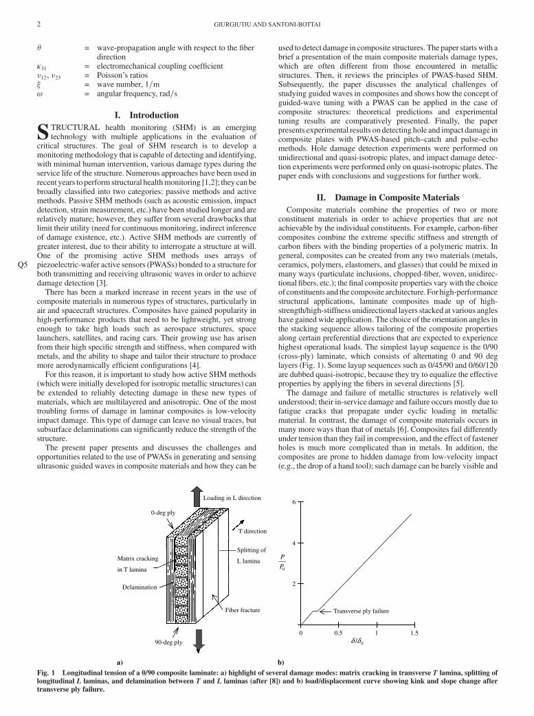
Composite materials combine the properties of two or moreconstituent materials in order to achieve properties that are notachievable by the individual constituents. For example, carbon-fibercomposites combine the extreme specific stiffness and strength ofcarbon fibers with the binding properties of a polymeric matrix. Ingeneral, composites can be created from any two materials (metals,ceramics, polymers, elastomers, and glasses) that could be mixed inmany ways (particulate inclusions, chopped-fiber, woven, unidirec-tional fibers, etc.); the final composite properties varywith the choiceof constituents and the composite architecture. For high-performancestructural applications, laminate composites made up of high-strength/high-stiffness unidirectional layers stacked at various angleshave gained wide application. The choice of the orientation angles inthe stacking sequence allows tailoring of the composite propertiesalong certain preferential directions that are expected to experiencehighest operational loads. The simplest layup sequence is the 0/90(cross-ply) laminate, which consists of alternating 0 and 90 deglayers (Fig. 1). Some layup sequences such as 0/45/90 and 0/60/120are dubbed quasi-isotropic, because they try to equalize the effectiveproperties by applying the fibers in several directions [5].

The damage and failure of metallic structures is relatively wellunderstood; their in-service damage and failure occurs mostly due tofatigue cracks that propagate under cyclic loading in metallicmaterial. In contrast, the damage of composite materials occurs inmany more ways than that of metals [6]. Composites fail differentlyunder tension than they fail in compression, and the effect of fastenerholes is much more complicated than in metals. In addition, thecomposites are prone to hidden damage from low-velocity impact(e.g., the drop of a hand tool); such damage can be barely visible and

Loading in L direction

T direction

Splitting of

L lamina Matrix cracking

in T lamina

0-deg ply

Delamination

90-deg ply

Fiber fracture Transverse ply failure

0 0.5 1 1.5

2

4

6

0

P

P

0/δ δ

a) b)Fig. 1 Longitudinal tension of a 0/90 composite laminate: a) highlight of several damage modes: matrix cracking in transverse T lamina, splitting of

longitudinal L laminas, and delamination between T and L laminas (after [8]) and b) load/displacement curve showing kink and slope change after

transverse ply failure.

2 GIURGIUTIU AND SANTONI-BOTTAI

may go undetected, but its effect on the degradation of the compositestructure strength can be dramatic. These various damage aspectswill be discussed briefly in the next sections.

Current design requirements for composite structures are muchmore stringent than for metallic structures. Military aircraftcomponents have to comply with an Aircraft Structural IntegrityProgram (ASIP) following the JSSG-2006 [7] and MIL-STD-1530[8] guidelines. Preexisting manufacturing flaws and service-inducedcracking are assumed to exist, even if undetected, and the ASIPfunction is tomanage this fact while preventing aircraft accidents anddowntime. In general, metallic structures are allowed to exhibit acertain amount of subcritical crack growth within the design life ofthe component. Detectable cracks are noted and managed as part ofthe maintenance and inspection process. In contrast, no knowndelamination cracks are allowed to exist (much less grow) incomposite structure. However, the composite components aregenerally designed to tolerate a certain size of undetectable damage.Of course, this additional safetymargin comes with aweight penalty,which could be mitigated through better understanding of compositedamage detection and management mechanisms.

To satisfy the damage tolerance requirements, one has todemonstrate that an aircraft structure possesses adequateQ6 residualstrength at the end of service life in the presence of an assumedworst-case damage as, for example, that caused by a low-velocity impact ona composite structure. This may be accomplished by showingpositive margins of safety at the maximum recommended load.Worst-case damage is defined as the damage caused by an impactevent (e.g., a 1 in. hemispherical impactor) at the lesser of thefollowing two energy levels: 100 ft � lb or the energy to cause avisible dent (0.1 in. deep).

A. Tension Damage in Composite Materials

When subjected to axial tension, the composite material displaysprogressive failure throughQ7 several damage mechanisms take placesequentially. Consider, for example, the cross-ply laminate of Fig. 1:as an axial load is applied in the longitudinalL direction, the 0 degplyis loaded along its reinforcing fibers, and the 90 deg ply is loadedacross the fibers. Because the strength of the polymeric matrix ismuch less than that of the fibers, the across-the-fiber strength of thelamina is much lower than the along-the-fiber strength. Hence,matrix cracking of the 90 deg ply occurs at an early stage in theloading cycle (Fig. 1b). As the tension load increases, further damageoccurs in the form of delaminations between the 0 and 90 deg plies,due to 3-D effects at the interface between these two plies with suchradically different properties. The matrix cracks existing in thetransverse ply act as discontinuities generating 3-D disbonding stressthat promotes delaminations. Same 3-D effects will lead to splittingof the 0 deg plies at higher tension loads. If the load continues toincrease, the 0 deg plies will eventually fail due to fiber fracture, atwhich point no load can be supported any longer [9].

This simple 0/90 example indicates that internal damage in acomposite laminate can happen at relatively low stress levels in theform of matrix cracking to be followed, at intermediate levels, by

interply delamination and lamina splitting. If the applied stress iscyclic, as in fatigue loading, then these low-level damage states canincrease and propagate further and further into the composite witheach load cycle. The reinforcing fibers have high strength and goodload-carrying properties, but the matrix cracking, delamination, andlamina splitting mechanisms usually lead to in-service compositestructures becoming operationally unfit and requiring replacement.

B. Compression Damage in Composite Structures

When subjected to axial compression, the composite fails throughloss of elastic stability (buckling). At the global scale, buckling canbe avoided Q8by relative sizing the length and bending stiffness of thecomponent such that loss of elastic stability does not occur for thegiven boundary conditions and operational load levels. At the localscale, the composite material itself can fail under compressionthrough the microbuckling mechanism (Fig. 2). The high-strengthfibers encased in the polymeric matrix can be modeled as beams onan elastic foundation, where the elastic support is provided by thematrix stiffness. Under axial compression, such a beam on an elasticfoundation would eventually buckle and take an undulatory shape(Fig. 2a). The compressive stress values at which this bucklingoccurs are dictated by the fiber bending stiffness and matrixcompression stiffness. For a given fiber/matrix combination, thismicrobuckling compressive strength is fixed and cannot be alteredthrough structural design. (Thicker fibers, e.g., boron fibers, have ahigher compression buckling strength than the thinner carbon fibers;for this reason, boron composites may be preferred in places wherematerial compression strength is critical.) As the compressive load isfurther increased, themicrobuckling is further exacerbated until localfailure occurs in the form of a kink band (Fig. 2b) [10].

C. Fastener Hole Damage in Composite Structures

Mechanical fasteners used in riveted and bolted joints areprevalent in metallic aircraft structures, where they offer a rapid andconvenient method of assembling large structures from smallercomponents. The load-bearing mechanisms of metallic joints arewell understood and easily predicted. The use of mechanicalfasteners Q9in composite structures is also allowed, but this comes withsignificant strength and fatigue penalties. The use of mechanicalfasteners in composite structures somehow clashes with the verynature of composite materials, which carry the load through the high-strength fibers embedded in a relatively-weak polymericmatrix. Thistype of load-carrying capability benefits from a smooth andcontinuous load flow and is adverse to sudden changes in materialproperties and geometries. Ideally, composite joints should be donethrough adhesive bonding with gradual transition from onecomponent into the next. However, when mechanical fasteners areused, they produce sudden discontinuities in the form of holes drilledin the composite structures; these fastener holes act as stressconcentrators. They also act as crack and delamination initiators, dueto microdamage introduced during the hole-drilling process. For thisreason, mechanical fasteners do not seem appropriate for compositeconstruction unless special attention is given to creating stress-free

W

β

φ

a) b) c)Fig. 2 Compression damage of fiber composites through microbuckling: a) undulations of buckled fibers; b) kink band local failure schematic;

c) micrograph of kink band formation in T800/924C carbon-fiber composite (after [8]).

GIURGIUTIU AND SANTONI-BOTTAI 3

holes during design through local reinforcement and damage-freeholes during manufacturing through special tooling. In spite of theseobvious technical issues, current manufacturing practice is such thatmechanical fasteners are still widely used in the construction ofcomposite structures, especially when load transfer has to beachieved between composite and metallic components [11].

A typical example would be one in which the load from acompositewing skin is transferred into an aluminummetallic bracketthrough a bolted junction. When in service, each hole in thecomposite skin would be subjected to both tension and/orcompression loading that may, under certain circumstances, promotedamage initiation and damage progression.

Under tension, the composite joint may fail under three majormodes: tear failure, bearing failure, and shear-out failure. Of these,the tear failure is unlikely to happen, because the fiber reinforcementis strongest in tension. The shear-out failure would happen if thefibers are predominant in the tension direction; shear-out failure canbe counteracted through design by the addition of 45 degreinforcement. The bearing failure is more difficult to prevent,because it is a compression-type loading that has to be taken up by thepolymeric matrix and by the fibers under compression. Bearingfailuremay occur throughmatrix crushing, orfibermicrobuckling, orboth.

Under compression, the composite joint may fail underQ10 threemajor modes: overall buckling of the component, local buckling ofthe regionweaken by the hole, and fibermicrobuckling at the areas ofhighest compression strength. The overall compression buckling canbe prevented by proper component design. Local buckling and fibermicrobuckling may be also prevented by design, but damageaccumulation during cyclic loading would eventually weaken it.

D. Impact Damage in Composite Structures

Composite aerospace structures are prone to a particular type ofdamage that is not critical in metallic aerospace structures: i.e., low-velocity impact damage. Such damage may occur duringmanufacturing or in service, due to, say, a hand tool being droppedonto a thin-wall composite part. When such an impact happens on aconventional metallic structural part, either the part is not damaged atall or, if it is damaged, then it shows clearly as an indent or scratch. Incomposite structures, a similar impact may damage the structurewithout leaving any visible marks on the surface (so-called barelyvisible damage). In this case, the impact result takes the form ofdelaminations in the composite layup. (A more drastic impact mayalso show spalling on the back side, while having no visiblemarks onthe front side [12].)Q11

Delamination due to barely visible impact damage may not have alarge effect on the tension strength of the composite, but it cansignificantly diminish the composite compression strength(delaminated plies have a much weaker buckling resistance thanthe same plies solidly bonded together). Both component bucklingstrength and local buckling strength may be affected; when afastening hole is present, this effect may be even worse. For thisreason, manufacturing companies place a strong emphasis on testingthe open-hole compression and compression after impact strengthsof their composite structures. Detection of delaminations due tobarely visible impact damage is amajor emphasis in composite SHMresearch.

E. Damage Detection in Composite Materials

We have seen that the inherent macroscopic anisotropy andmultimaterial architecture of the composite materials results ininternal damage types that are significantly different from thoseencountered in isotropic metallic materials. Currently, one of themost commonly encountered damage types in compositematerials isthat caused by low-velocity impact; this damage susceptibility(which is not encountered in metallic structures) is mainly due to thelow interlaminar strength of conventional composite layups.Significant degradation of themechanical properties can easily occuras a result of low-velocity impact, even for barely visible damage.Different types of damage may be encountered in the impacted

region, including matrix (resin) cracking, delaminations (inter-laminar cracking), and broken fibers. In the future, as compositestructures accumulate years of service, other damage types related tofatigue effects are also expected to become significant.

To date, much effort has been put into identifying reliablenondestructive evaluation (NDE) techniques for the detection,location, and characterization of composite materials damage, withspecial attention to subsurface delaminations due to manufacturingdefects or to low-velocity impacts. Thermography, shearography,radiography, and ultrasonics are among the most commonly usedNDE techniques [13]. These NDE techniques require stripping theaircraft and even removal of individual components; they employbulky transducers, operate with point scanning, and, in general, aretime-consuming, labor-intensive, and expensive. As a result, thecurrent cost of composite structures inspection is very high: at leastone order of magnitude greater than for metallic structures [14]. Forcomposite structures to be economically viable and to realize theirfull design potential, it is essential that their operation andmaintenance are conducted in a safe and economical manner, on parwith that of existing metallic structures. For this reason, thedevelopment of new composite damage detection methods that canbe applied rapidly and reliably to detect critical composite flaws is anongoing concern. The permanently attached damage-sensingtechnologies developed under the SHM thrust are a promisingresearch direction, because, when implemented, they would permitthe interrogation at will of the composite structures and the reliableand credible detection of internal damage in order to increase flightsafety and reduce operational costs. This technology, thoughpromising, is still in its infancy, and many theoretical andexperimental challenges still have to be resolved, as illustrated next.

III. PWAS for Active SHM

A. PWAS Principles

PWASs are the enabling technology for active SHM systems [15].A PWAS couples the electrical and mechanical effects (mechanicalstrain Sij, mechanical stress Tkl, electrical field Ek, and electricaldisplacement Dj) through the tensorial piezoelectric constitutiveequations:

Sij � sEijklTkl dkijEk Dj � djklTkl "TjkEk (1)

where sEijkl is the mechanical compliance of the material measured at

zero electric field (E� 0), "Tjk is the dielectric permittivity measured

at zero mechanical stress (T � 0), and dkij represents thepiezoelectric coupling effect. In practice, Voigt matrix notationsare often used instead of tensor notation; for example, dkij(i; j; k� 1; 2; 3) is replaced by dqi (q� 1; . . . ; 6 and i� 1, 2, 3). Togenerate guided waves in thin-wall structures, PWASs use the d31coupling between the in-plane strains S1 and S2 and transverseelectric field E3. When used to interrogate thin-wall structures, thePWASs are Q12guided-wave transducers by coupling their in-planemotionwith the guided-wave particle motion on thematerial surface.The in-plane PWAS motion is excited by the applied oscillatoryvoltage through the d31 piezoelectric coupling. Optimum excitationand detection happenswhen the PWAS length is in certain ratioswiththe wavelength of the guided-wave modes. The PWASs action asultrasonic transducers is fundamentally different from that ofconventional ultrasonic transducers. Conventional ultrasonic trans-ducers act through surface tapping: i.e., by applying vibrationpressure to the structural surface. The PWAS transducers act throughsurface pinching, and are strain coupled with the structural surface.This allows the PWAS transducers to have a greater efficiency intransmitting and receiving ultrasonic surface and guidedwaveswhencompared with the conventional ultrasonic transducers. PWASs arelightweight and inexpensive and hence can be deployed in largenumbers on themonitored structure. Just like conventional ultrasonictransducers, PWASs use the piezoelectric effect to generate andreceive ultrasonic waves. However, PWASs are different fromconventional ultrasonic transducers:

4 GIURGIUTIU AND SANTONI-BOTTAI

1) PWASs are firmly coupled with the structure through anadhesive bonding, whereas conventional ultrasonic transducers areweakly coupled through gel, water, or air.

2) PWASs are nonresonant devices that can be tuned selectivelyinto several guided-wave modes, whereas conventional ultrasonictransducers are resonant narrowband devices.

3) PWASs are inexpensive and can be deployed in large quantitieson the structure, whereas conventional ultrasonic transducers areexpensive and used one at a time.

As shown in Fig. 3, PWAS transducers can serve several purposes[15]: high-bandwidth strain sensors, high-bandwidth wave excitersand receivers, resonators, and embedded modal sensors with theelectromechanical impedance method. By application types, PWAStransducers can be used for active sensing of far-field damage usingpulse–echo, pitch–catch, and phased-array methods; active sensingof near-field damage using high-frequency electromechanicalimpedance method and thickness-gauge mode; and passive sensingof damage generating events through detection of low-velocityimpacts and acoustic emission at the tip of advancing cracks.

By using Lamb waves in a thin-wall structure, one can detectstructural anomaly: i.e., cracks, corrosions, delaminations, and otherdamage. Because of the physical, mechanical, and piezoelectricproperties of PWAS transducers, they act as both transmitters andreceivers of Lamb waves traveling through the structure. Uponexcitation with an electric signal, the PWASs generate Lamb wavesin a thin-wall structure. The generated Lamb waves travel throughthe structure and are reflected or diffracted by the structuralboundaries, discontinuities, and damage. The reflected or diffractedwaves arrive at the PWAS, where they are transformed into electricsignals.

B. Traveling-Wave Methods of Damage Detection with PWAS

Transducers

Figure 3a illustrates the pitch–catch method. An electric signalapplied at the transmitter PWAS generates, through piezoelectrictransduction, elastic waves that transverse the structure and arecaptured at the receiver PWAS. As long as the structural regionbetween the transmitter and receiver is in pristine condition, thereceived signalwill be consistently the same; if the structure becomesdamaged, then the received signal will be modified. Comparison

between the historically stored signals and the currently read signalwill indicate when changes (e.g., damage) take place in the structure.The pitch–catch method may be applied to situations in which thedamage is diffuse and/or distributed, such as corrosion in metals ordegradation in composites. By extension of the pitch–catch methodto several pitch–catch pairs in a network of PWASs (sparse array)placed around a structural region of interest, one achieves ultrasonictomography. In such a network, all the PWASs are eventually pairedthrough a round-robin process. The processing of all the collecteddata during the round-robin process yields an image of themonitoredregion indicating the damage area.

Figure 3b illustrates the pulse–echo method. In this case, the samePWAS transducer acts as both transmitter and receiver. A tone-burstsignal applied to the PWAS generates an elastic wave packet thattravels through the structure and reflects at structural boundaries andat cracks and abrupt discontinuities. In a pristine structure, onlyboundary reflections are present, whereas in a damaged structure,reflections from cracks also appear. By comparing historical signalsone can identify when new reflections appear, due to new boundariessuch as cracks and abrupt discontinuities. This comparison may befacilitated by the differential signal method.

Figure 3c illustrates the use of PWAS transducers in thicknessmode. The thickness mode is usually excited at much higherfrequencies than the guided-wave modes discussed in the previoustwo paragraphs. For example, the thickness mode for a 0.2 mmPWAS is excited at around 12MHz,whereas the guided-wavemodesare excited at tens and hundreds of kilohertz. When operating inthickness mode, the PWAS transducer can act as a thickness gauge.In metallic structures, thickness-mode measurements allow thedetection of damage that affects the structural thickness, e.g.,corrosion, which can be detected from that side of the structure,which is outside of the corrosive environment. In compositestructures, thickness-mode measurements may detect cracks that areparallel to the surface, such as delaminations. However, a limitationof the thickness-mode approach is that detection can only be madedirectly under the PWAS location, or in its proximity. In this respect,this method is rather localized, which may be sufficient formonitoring well-defined critical areas, but insufficient for large-areamonitoring.

Figure 3d illustrates the detection of impacts and acousticemission (AE) events. In this case, the PWAS transducer is operating

Fig. 3 Use of a PWAS for damage detection with propagating and standing guided waves in thin-wall structures.

GIURGIUTIU AND SANTONI-BOTTAI 5

as a passive receiver of the elastic waves generated by the impact orby theAE source. By placing several PWAS transducers in a networkconfiguration around a given structural area, one can set up alistening system that would monitor if impact damage or AE eventstake place. Because the PWAS is self-energized through piezo-electric transduction, the listening system can stay in a low-energydormant mode until a triggering by the PWAS wakes it up. Thesignals recorded by the PWAS network can be processed to yield thelocation and amplitude of the impact and/or AE event.

C. Standing-Wave Methods of Damage Detection with PWAS

Transducers

When a structure is excitedwith sustained harmonic excitation of agiven frequency, the waves traveling in the structure undergomultiple boundary reflections and settle down in a standing-wavepattern known as vibration. Structural vibration is characterized byresonance frequencies at which the structural response goes throughpeak values. The structural response measured over a frequencyrange including several resonance frequencies generates a vibrationspectrumor frequency response function.When damage occurring ina structure induces changes in its dynamic properties, the vibrationspectrum also changes. However, the conventional vibration analysismethods are not sensitive enough to detect small incipient damage;they can only measure structural dynamics up to several kilohertz,which is insufficient for the small wavelength needed to discoverincipient damage. An alternative approach that is able to measurestructural spectrum into the hundreds of kilohertz and low-megahertzrange is offered by the electromechanical impedance method [15].The electromechanical impedance method measures the electricalimpedance Z�!� of a PWAS transducer using a an impedanceanalyzer. The real part of the impedance Re�Z� reflects themechanical behavior of the PWAS: i.e., its dynamic spectrum and itsresonances.When the PWAS is attached to a structure, the real part ofthe impedance measured at the PWAS terminals reflects thedynamics of the structure on which the PWAS is attached: i.e., thestructural dynamic spectrum and its resonances. Thus, a PWASattached to a structure can be used as a structural-identification sensorthat measures directly the structural response at very highfrequencies. Figure 3e illustrates the electromechanical impedancespectrum measured in the megahertz range.

D. Phased Arrays and the Embedded Ultrasonics Structural Radar

A natural extension of the PWAS pulse–echo method is thedevelopment of a PWAS phased array (Fig. 3f) that is able to scan alarge area from a single location. Phased arrays were first used inradar applications, because they allowed the replacement of therotating radar dish with a fixed panel equipped with an array oftransmitter-receivers that were energized with prearranged phasedelays. When simultaneous signals are emitted from an array oftransmitters, the constructive interference of the propagating wavescreates a beampositioned broadside to the array. If prearranged phasedelays are introduced in the firing of the signals of individual arrayelements, then the constructive interference beam can be steered todifference angular positions. Thus, an azimuth and elevation sweepcan be achieved without mechanical rotation of the radar platform.The phased-array principle has gained wide use recently inultrasonics, both for medical applications and for nondestructiveevaluation, because ultrasonic phased arrays permit the sweeping ofa large volume from a single location.

The PWAS phased arrays use the phase-array principles to create ainterrogating beamof guidedwaves that travel in a thin-wall structureand can sweep a large area from a single location. The embeddedultrasonics structural radar (EUSR) methodology uses the signalscollected by the PWAS phased array to recreate a virtual sweeping ofthe monitored structural area. The associated image represents thereconstruction of the complete area as if the interrogating beam wasactually sweeping it.When no damage is present, the only echoes arethose arriving from the natural boundaries of the interrogated area; ifdamage is present, its echo reflection is imaged on the EUSR screenindicating its location in �R; �� or �x; y� coordinates. Giurgiutiu et al.

[16] have used PWAS phased arrays to monitor crack growth duringfatigue testing.

IV. Guided Waves in Composites

The evaluation of structural integrity using Lamb-waveultrasonics has long been acknowledged as a very promisingtechnique. Several investigators [17,18] have envisioned theinspection of large metallic plates from a single location usingtransducer arrays, where each element acts as both transmitter andreceiver. Guided signals are generated at different angles around thetransducer positions and the signal reflections from the boundariesare processed for damage detection. This configuration is verypromising for isotropic material but might have some limitations forfibrous composite structures, due to the change in properties withfiber direction. In recent years, numerous investigations haveexplored Lamb-wave techniques for the detection of damage incomposite laminates [6,19,20]. To take full advantage of Lamb-wavetechniques for composite damage detection, one needs to firstunderstand and model how guided waves propagate in compositestructures, which are much more complicated than in isotropicmetallic structures.

The guided waves propagating in composite structures are moredifficult to model than those propagating in isotropic metallicstructures because of the composite material is inherent anisotropyandmultilayered, with each layer having a different orientation. For aplate made of one layer made of unidirectional fibers, thewave speedof the wave propagating in the material depends on the angle �between fibers direction and wave-propagation direction. Hence, foreach angle �, different dispersion curves will be derived. To obtainthe dispersion curves in a plate made of more then one layer, for eachlayer in the plate, we must define a relation between displacementsand stresses at the bottom surface and those at the top surface. Then,through the Snell low, the continuity of displacements, and therelation derived for each layer between stresses and displacements,we relate the stresses and the displacements at the bottom surface ofthe plate to those at the top surface of the plate. By imposing thestress-free boundary surfaces, we obtain the dispersion curves for theplate for a given propagation direction. Two solution approachesexist: the global matrix approach and the transfer matrix approach.

The global matrix method was proposed by Knopoff [21]. In theglobal matrix method, the equations for all the layers are consideredsimultaneously. There is no a priori assumption on theinterdependence between the sets of equations for each interface.This process results in a systemofM� 4�N � 1� equations that has anarrowband M �M matrix. This technique is robust but slow tocompute for many layers, because the matrix is rather large.

The transfer matrix (TM) approach [22–24] was use for layeredcomposites byNayfeh [25]. In theTMmethod, the equations for eachlayer are constructed separately and then linked together through theboundary conditions at the bottom and top surfaces of each layer. Theprocess results in system of six equations for each layer.

Both methods share a common characteristic: a solution of thecharacteristic function does not strictly prove the existence of amodal solution, but only that the system matrix is singular.Furthermore, the calculation of the determinant for the modalsolution needs the use of a good algorithm, because the aim of theproblem is to find the zero of the determinant, whereas the matrix isfrequently close to being singular.

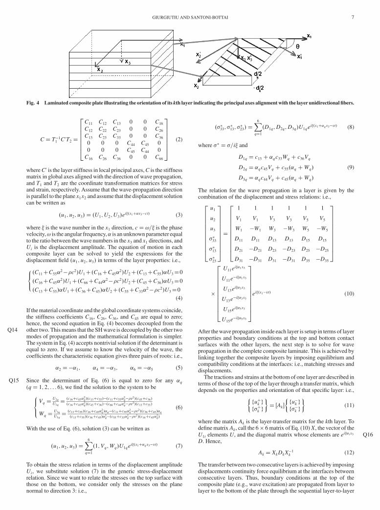
Hereunder, Q13we explain in some detail the procedure for the TMmethod. Figure 4 shows a composite plate made of N layers; eachlayer is made of unidirectional fibers, and they are hence layers oforthotropic properties; however, the layer orientation varies fromlayer to layer [26]. Consider a wave propagating in the material andassume that the angle between the fiber direction and the direction ofwave propagation for the kth layer is �k (see Fig. 4). Define the globalcoordinate system x1, x2, x3 such that x1 is aligned with the directionof wave propagation. Also define a local coordinate system x01, x

02, x03

such that x01 is parallel to the fiber direction (principal axes). Thestiffness matrix of the kth layer can be written as

6 GIURGIUTIU AND SANTONI-BOTTAI

C� T�11 C0T2 �

C11 C12 C13 0 0 C16

C12 C22 C23 0 0 C26

C13 C23 C33 0 0 C36

0 0 0 C44 C45 0

0 0 0 C45 C44 0

C16 C26 C36 0 0 C66

26666664

37777775

(2)

whereC0 is the layer stiffness in local principal axes,C is the stiffnessmatrix in global axes aligned with the direction of wave propagation,and T1 and T2 are the coordinate transformation matrices for stressand strain, respectively. Assume that the wave-propagation directionis parallel to the plane x1x2 and assume that the displacement solutioncan be written as

�u1; u2; u3� � �U1; U2; U3�ei��x1�x3�ct� (3)

where � is the wave number in the x1 direction, c� !=� is the phasevelocity,! is the angular frequency,� is an unknownparameter equalto the ratio between thewave numbers in the x3 and x1 directions, andUi is the displacement amplitude. The equation of motion in eachcomposite layer can be solved to yield the expressions for thedisplacement field �u1; u2; u3� in terms of the layer properties: i.e.,8<:�C11C55�

2��c2�U1�C16C45�2�U2�C13C55��U3�0

�C16C45�2�U1�C66C44�

2��c2�U2�C45C36��U3�0

�C13C55��U1�C36C45��U2�C55C33�2��c2�U3�0

(4)

If thematerial coordinate and the global coordinate systems coincide,the stiffness coefficients C16, C26, C36, and C45 are equal to zero;hence, the second equation in Eq. (4) becomes decoupled from theother two. Thismeans that theQ14 SHwave is decoupled by the other twomodes of propagation and the mathematical formulation is simpler.The system in Eq. (4) accepts nontrivial solution if the determinant isequal to zero. If we assume to know the velocity of the wave, thecoefficients the characteristic equation gives three pairs of roots: i.e.,

�2 ���1; �4 ���3; �6 ���5 (5)

SinceQ15 the determinant of Eq. (6) is equal to zero for any �q(q� 1; 2; . . . 6), we find the solution to the system to be8<:Vq �

U2q

U1q� �c16c45�

2q��c13c55���c11c55�2q��v2��c45c36�

�c16c45�2q��c45c36���c66c44�2q��v2��c13c55�

Wq �U3q

U1q� �c13c55��c16c45�

2q��q��c11c55�2q��v2��c36c45��q

�c13c55��c36c45��2q��c55c33�2q��v2��c16c45�2q�

(6)

With the use of Eq. (6), solution (3) can be written as

�u1; u2; u3� �X6q�1�1; Vq;Wq�U1qe

i��x1�qx3�vt� (7)

To obtain the stress relation in terms of the displacement amplitudeUi, we substitute solution (7) in the generic stress-displacementrelation. Since we want to relate the stresses on the top surface withthose on the bottom, we consider only the stresses on the planenormal to direction 3: i.e.,

��33; �13; �23� �X6q�1�D1q; D2q; D3q�U1qe

i��x1�qx3�vt� (8)

where � � �=i� and

D1q � c13 �qc33Wq c36VqD2q � �qc45Vq c55��q Wq�D3q � �qc44Vq c45��q Wq�

(9)

The relation for the wave propagation in a layer is given by thecombination of the displacement and stress relations: i.e.,

u1

u2

u3

�33

�13

�23

266666666664

377777777775�

1 1 1 1 1 1

V1 V1 V3 V3 V5 V5

W1 �W1 W3 �W3 W5 �W5

D11 D11 D13 D13 D15 D15

D21 �D21 D23 �D23 D25 �D25

D31 �D31 D31 �D31 D35 �D35

266666666664

377777777775

�

U11ei��1x3

U11e�i��1x3

U13ei��3x3

U13e�i��3x3

U15ei��5x3

U15e�i��5x3

266666666664

377777777775ei��x1�vt� (10)

After thewave propagation inside each layer is setup in terms of layerproperties and boundary conditions at the top and bottom contactsurfaces with the other layers, the next step is to solve for wavepropagation in the complete composite laminate. This is achieved bylinking together the composite layers by imposing equilibrium andcompatibility conditions at the interfaces: i.e., matching stresses anddisplacements.

The tractions and strains at the bottom of one layer are described interms of those of the top of the layer through a transfer matrix, whichdepends on the properties and orientation of that specific layer: i.e.,�

fuk gf�k g

�� �Ak�

�fu�k gf��k g

�(11)

where the matrix Ak is the layer-transfer matrix for the kth layer. TodefinematrixAk, call the 6 � 6matrix of Eq. (10)X, the vector of theU1i elements U, and the diagonal matrix whose elements are Q16ei��ix3

D. Hence,

Ak � XkDkX�1k (12)

The transfer between two consecutive layers is achieved by imposingdisplacements continuity force equilibrium at the interfaces betweenconsecutive layers. Thus, boundary conditions at the top of thecomposite plate (e.g., wave excitation) are propagated from layer tolayer to the bottom of the plate through the sequential layer-to-layer

Fig. 4 Laminated composite plate illustrating the orientation of its kth layer indicating the principal axes alignment with the layer unidirectional fibers.

GIURGIUTIU AND SANTONI-BOTTAI 7

transfer. In the end,we relate the displacements and stresses of the topof the layered plate to those at its bottom through the overall transfermatrix A, given by

A�YNk�1Ak (13)

Thus, a small linear system of equation is setup in which theboundary conditions at the top of the plate are related to the boundaryconditions at bottom of the plate. To find the dispersion curves andmode shapes, one assumes traction-free conditions at both top andbottom surfaces and solves the resulting homogenous system interms of unknown top and bottom displacements. The resultingeigenvalue problem yields eigenwave numbers and the associateeigendisplacements at the tops and bottoms of the plates. Theeigenwave numbers yield the phase velocities at the assumedfrequency; the dispersion curves are then obtained by repeating theprocess over a frequency range. The eigendisplacements arepropagated through the matrix transfer process through all the layersin order to determine the thickness-mode shape of that particularguided-wave mode. Though simple in formulation, the TM methodsuffers from numerical instability, because error accumulates in thelayer transfers. To address the numerical instabilities, Rokhlin andWang [27] address this numerical instability issue by introducing thelayer stiffness matrix and using an efficient recursive algorithm tocalculate the global stiffness matrix for the complete laminate. Thelayer stiffness matrix relates the stresses at the top and bottom of thelayer with the corresponding displacements. The terms in the matrixhave only exponentially decaying terms, and hence the transferprocess becomes more stable.

A. Dispersion Curves for Composite Structures

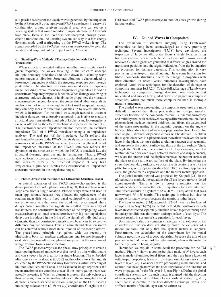
We coded the TM approach following Nayfeh [25].Q17 Figure 6shows the dispersion curves derived for a unidirectional compositeplate made of one layer of 65% graphite 35% epoxy [26]. Thesedispersion curves depend on the propagation direction, �; the cases�� 0, 18, 36, and 90 deg are presented in Fig. 6. It is apparent that for�� 0 deg (i.e., wave propagating along the fiber direction) and for�� 90� (i.e., waves propagating transversely to the fiber direction),the dispersion curves are clearly decoupled into quasi-antisymmetric(Q18 A0, A1, A2; . . .), quasi-symmetric (S0, S1, S2; . . .), and quasi-shear-horizontal (SH0, SH1, SH2; . . .) wavemodes. However, this is not thecase for the offaxis directions �� 18, 36 deg, in which case the threemode types are strongly coupled. The wave velocity is higher whenthe wave propagates along the fiber direction. As the angle of thewave-propagation direction increases, the phase velocity decreasestill reaching a minimum in the direction perpendicular to the fiber.This is due to the fact that along the fiber the material stiffness is

greater than in all the other directions and it decreases, whereas �increases.

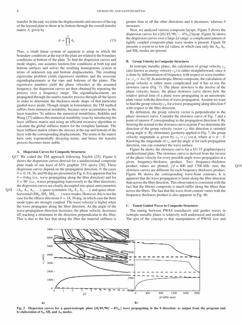
Next, we analyzed various composite layups. Figure 5 shows thedispersion curves for a ��0=45=90= � 45�2s� layup. Figure 5a showsthe dispersion curves over a large �d range: a complicated pattern oftightly coupled composite-plate wave modes is present. Figure 5bpresents a zoom-in to low-�d values, in which case only the A0, S0,and SH0 modes are present.

B. Group Velocity in Composite Structures

In isotropic metallic plates, the calculation of group velocity cg(also known as energy velocity cE) is rather straightforward, since itis done by differentiation of frequency with respect to wave number:i.e., cg � @!=@�. In anisotropic fibrous composite, the calculation ofgroup velocity is rather more complicated and it has to use theslowness curve (Fig. 7). The phase slowness is the inverse of thephase velocity; hence, the phase slowness curve shows how therelative arrival time of a plane wave propagating in an anisotropicplate varies with the direction of wave propagation. Assumewewantto find the group velocity cE for awave propagating along direction �with respect to the fiber direction.

By definition, the group velocity vector is perpendicular to thephase slowness curve. Consider the slowness curve of Fig. 7 and apoint of interest P corresponding to the propagation direction �. Bydrawing the normal to the slowness curve at pointPwe determine thedirection of the group velocity vector cE; this direction is orientedalong angle . By elementary geometry applied to Fig. 7, the groupvelocity magnitude is given by cE � c= cos, where � � �.Knowing the magnitude of cE and the angle for each propagationdirection, one can construct the wave surface.

Figure 8a shows the slowness curve for a 65=35 graphite/epoxyunidirectional plate. The slowness curve is derived from the inverseof the phase velocity for every possible angle wave propagation at agiven frequency-thickness product. Two frequency-thicknessproduct values are plotted: Q19fd� 400 and 1700 kHz �mm; theslowness curves are different for each frequency-thickness product.Figure 8b shows the corresponding wave-front contours. It isapparent that the wave propagation is faster along the fiber directionthan across the fiber direction. This observation is consistent with thefact that the fibrous composite is much stiffer along the fibers thanacross the fibers. The fact that the wave-front contour varies with thefrequency-thickness product is also apparent in Fig. 8b.

C. Tuned Guided Waves in Composite Structures

The tuning between PWAS transducers and guides waves inisotropic metallic plates is relatively well understood and modeled.The gist of the concept is that manipulation of PWAS size and

ξd

b)a)

6000

7000

6000

5000

4000

3000

2000

1000

0

5000

4000

3000

2000

fd (kHz-mm)

4 5 6 70

0 1 2 3400 800 1200 1600 2000

c s (

m/s

)

Fig. 5 Dispersion curves for a quasi-isotropic plate [�0=45=90= � 45�2s] wave propagating in the 0 direction: a) output from the program and

b) elaboration of S0, SH, and A0 modes.

8 GIURGIUTIU AND SANTONI-BOTTAI

frequency allow for selective preferential excitation of certainguided-wave modes and the rejection of other guided-wave modes,as needed by the particular SHM application under consideration. Asimilar tuning effect is also possible in anisotropic composite plates,but the analysis is more complicated, due to the anisotropic wave-propagation characteristics inherent in composite materials [26].

The analysis is performed in two steps:1) Perform the free-response analysis and solve the homogenous

problem to determine the dispersion curves andwavemodes over thefrequency domain of interest.

2) Perform the force-response analysis in which the PWAStransducer is used to excite guided-wave modes in the compositeplate (Fig. 9). The analysis uses the normal mode expansion, since, atany arbitrary frequency, several wave modes can be excited. Somedetails of our approach are given below; further details are availablein [26].

The starting point is the complex reciprocity relation under theassumption of time harmonic waves: i.e.,

�

�y��~v2 � T1 � v1 � ~T2� � �y

�

�x��~v2 � T1 � v1 � ~T2� � �x

� ~v2F1 v1 ~F2 (14)

where v is the particle velocity vector, T is the stress tensor, F is theapplied external force, 1 and 2 are two different solutions due to twodifferent external forces, and the tilde means the complex conjugate.

Consider the case of a PWAS bonded on the top surface of acomposite plate. In this case, the wave guides can be excited at theacoustic boundaries by traction forces only,T � �y.We assume that theexcited field (solution 1) can be represented by mode expansion: i.e.,

v 1 � v1�x; y� �Xn

an�x�vn�y�

T1 � T1�x; y� �Xn

an�x�Tn�y�(15)

where am�x� are the x-dependent modal participation factors thatdepend on the mode under consideration and the excitation used togenerate the field. The modal participation factors are the same forthe all the acoustic fields. The y-dependent terms, vn�y� and Tn�y�,are assumed to be known and depend only on the mode considered.We assume also that solution 2 is of the type

v 2 � v2�x; y� � vn�y�e�i�nx

T2 � T2�x; y� � Tn�y�e�i�nx with F2 � 0(16)

Integrating Eq. (14) with respect to y and through the use of Eqs. (15)and (16) we obtain

��~vn � T1 � v1 � ~Tn� � �yjd�dei~�nx �

�x

�ei

~�nxXm

am�x�Pnm�� 0

(17)

where Pnm is the average power flow of the nth guided mode: i.e.,

ξd ξd

ξd ξd

6000

5000

4000

3000

2000

6000

5000

4000

3000

2000

c s

c s

12000

10000

8000

6000

4000

6000

5000

4000

3000

20000 1 2 3 4 5 6 7 8 0 1 2 3 4 5 6 7 8

0 1 2 3 4 5 6 7 8 0 1 2 3 4 5 6 7 8

Pseudo-A0

Pseudo-S0

Pseudo-A0

Pseudo-S0

Pseudo-A0

Pseudo-S0

Pseudo-A0

Pseudo-S0 Pseudo-SH0

Pseudo-SH0

a) b)

c) d)

Fig. 6 Dispersion curves for unidirectional 65=35 graphite/epoxy plate (only the lower modes are identified): a) �� 0deg (SH0 mode is not displayed),

b) �� 18deg, c) �� 36deg, and d) �� 90deg (SH0 mode is not displayed); � is the wave number and d is the half-thickness.

Ec

φ

θ ψ

1 c

cP

Fig. 7 Slowness curve and notation.

GIURGIUTIU AND SANTONI-BOTTAI 9

Pnm �1

4

Zd

�d��~vn � Tm � vm � ~Tn� � �x dy (18)

According to the orthogonality relation of the wave modes [28], thesummation in Eq. (17) has only one nonzero term. Considering thepropagating mode n (�n real), Eq. (17) can be written as

4Pnn

��

�x i�n

�an�x� � �~vn � T v � ~Tn� � �yjd�d (19)

where

Pnn � Re

�1

4

Zd

�d��~vn � Tn � vn � ~Tn� � �x dy

�

� Re

�� 1

2

Zd

�d~vn � Tn � �x dy

�(20)

Assume that the anisotropic plate is loaded over a finite portion in they direction on the top surface by an infinitewidth traction force in thex direction:

T � �y � t�x�ei!t � �ty�x��y tx�x� �x�ei!t (21)

With the use of the load defined in Eq. (21) and noticing that thesecond term on the left-hand side is zero, because we assumedtraction-free boundary, Eq. (19) becomes

4Pnn

��

�x i�n

�an�x� � ~vn�d� � t�x� (22)

This is a first-order ordinary differential equationQ20 that governs theamplitudes of the general modes. Its solution is

an�x� �e�i�nx

4Pnn~vn�d� �

Zx

c

eixnt�� d (23)

where c is a constant used to satisfy the boundary conditions.Consider a PWAS of length 2a bonded on the top surface of thecomposite plate. The external tractions t are nonzero only in theinterval �a � x � a. We can write the forward-wave solution as

an �x� �~vn�d�4Pnn

� e�i�nxZa

�aei�n �xt� �x� d�x for x > a (24)

The strain (and hence the tuning curves) on the top surface of theplate is given by

"x �@

@x

Xn

an�x�vx�y�Zei!t dt� 1

!

Xn

�nan�x�vx�y�ei!t (25)

or in expanded form using Eq. (23):

"x �~vn�d�4!Pnn

vx�y�ei!tXn

�ne�i�nx

Za

�aei�n �xt� �x� d�x for x > a (26)

This represents the tuning expression of the strain in the compositeplate excited by the PWAS. This derivation is formally equal to thecase of an isotropic plate. The number of modes present depends onthe material properties of the composite plate. For the case of acomposite platemade of one layer of unidirectional fibers, the PWASwill excite only Lamb modes (symmetric and antisymmetric) if weconsider propagation along the fibers or transverse to the fibers. In allother cases, three waves will be present.

The main difficult in solving Eq. (26) lies in the derivation of theaverage power flow. The average power flow is given by the integralover the plate thickness of the velocity by the stress, and it must beperformed numerically. Consider the nth wave mode propagating inthe kth layer of the composite plate (for simplicity of notation, wedrop the subscript n), the integrand of Eq. (20) is given by

�~v � T� � x̂� ~v1T1 ~v2T6 ~v3T4 (27)

Fiber direction

ψ

Fiber direction

θ

1c

-2000

2000

1000

-1000

-2000

0

-1000 0 1000 2000

a) b)

Fig. 8 Directional dependence of wave propagation in unidirectional 65%-graphite/35%-epoxy plate at fd� 400 kHz �mm Q32(solid line) and fd�1700 kHz �mm (dashed line): a) slowness curve (plotted values are 1041=c) and b) wave front.

-a +a

x

( ) i tx e ωτ

ta

t

tb

Bond layer

PWASPWAS, 0.2-mm thick

Substrate structure, 1-mm thick

a) b)

Fig. 9 Model of bond-layer interaction between PWAS and composite structure.

10 GIURGIUTIU AND SANTONI-BOTTAI

where the velocities are derived from the particle displacementsolution (7): i.e.,

�v1; v2; v3� � �i�vX6q�1�1; Vq;Wq�U1qe

i��x1�qx3�vt� (28)

and the stresses are defined as

�T1T4T6

�� i�

Xq

� c11 �qc13Wq c16Vq�qc44Vq c45��q Wq�c16 �qc36Wq c66Vq

�U1qe

i��x1�qx3�vt�

(29)

Once the dispersion curves are known, the stress and the velocity ineach layer for each mode are known, and hence the average powerflow can be computed. It is to be emphasized that the derivation of thetuning curves presented here does not depend on the particularmethod used to derive the dispersion curves.

The integral in Eq. (26) depends on the assumption made on thebond layer between PWAS and structure. For the composite plate, weassume that the thickness of the bond layer is approaching zero; i.e.,we assume ideal bond conditions.

In the case of ideal bonding solution, the shear stress in thebonding layer is concentrated at the ends of the PWAS tips. We canuse the pin-force model to represent the load transferred form thePWAS to the structure: i.e.,

t �x; d� ��a�0���x � a� � ��x a�� �x if jxj � a0 if jxj> a (30)

Substituting Eq. (30) into Eq. (26), after integration we obtain

"x � ia�0~vn�d�2!Pnn

vx�y�ei!tXn

�ne�i�nx sin �na (31)

where a�0 is a constant that depends on the excitation, and~vnx�d�=4Pnn is the excitability function of mode n (depends on themode excited and not on the source used for excitation).

It is apparent from Eq. (31) that as the wave number �n varies, thefunction sin �na goes from maxima and minima in the (�1, 1)interval, and hence the response of the nth mode goes through peaksand valleys. The wave number �n varies with frequency ! and phasevelocities cn: i.e., �n � !=cn. Since the variation of phase velocitywith frequency is different frommode to mode, it is apparent that thepeaks and valleys of one mode will not coincide with those of theothermodes. Hence, one can find frequencies at which certainmodesare rejected (valleys in their response curve), and other modes aretuned in (peaks in their response curves). It is also apparent thatbecause guided-wave propagation in composite plates is direction-ally dependent, the tuning between the PWAS transducer and theguided waves in the composite plate will also depend on thepropagation direction.

To verify these theoretical predictions we performed experimentson a composite plate with PWAS receivers installed at variousdirections from the PWAS transmitter. A 1240 � 1240 mm quasi-isotropic plate with a ��0=45=90= � 45�2�S layup from T300/5208carbon-fiber unidirectional tape was used. The plate had an overallthickness of 2.25 mm. Figure 10 shows the central part of thecomposite plate, where 7 mm round PWAS transducers (0.2-mm-thick, American Piezo Ceramics APC-850) were installed. ThePWAS denoted with the letter T was the transmitter, and thosedenoted with R were the receivers (R1–R5). The distance betweenthe receivers and the transmitter was 250 mm. The step anglebetween sequential receivers was��� 22:5 deg. In addition, a pairof 7mm square PWASswere placed along the fiber direction, with S1

being the transmitter and S2 the receiver.Smoothed three-count tone-burst excitation signals were used.

The signal frequency was swept from 15 to 700 kHz in steps of15 kHz. At each frequency, the wave amplitude and the time of flightfor all the waves present were collected. Since carbon-fiber iselectrically conductive, the composite plate could be used as groundand only a single excitation wire had to be cabled to each PWAStransducer. We found that the ground quality affects the signalstrength; to obtain a strong signal, a good electrical ground wasachieved through bonding a sheet of copper on the compositesurface. In this way the signal was strong and consistent during theexperiments.

Three guided-wave modes were detected: quasi-S0, quasi-A0, andquasi-SH0. The identification of these three guided-wave modes wasdone using wave-packet group velocity compared with theoreticalpredictions. Figure 11a shows the experimentally measured signalamplitudes for the three guided waves for the S1–S2 transducer pair

0º

90º

T

S2

R1

S1

R3

R2

R4 R5

S3

Fig. 10 Experiment setup measuring directional wave speeds in a

��0=45=90= � 45�2�S plate 1240 by 1240mmwith 2.25mm thickness. Theplate was laminated from T300/5208 unidirectional tape.

f (kHz)

V (

mV

)

A0S0

SH

f (kHz)

A0

10

5

12

11

10

9

8

7

6

54

3

2

1

00 100 200 300 400 500 600 700 0 100 200 300

a) b)

Fig. 11 Tuning of PWAS guidedwaves in composites: a) quasi-A0 mode, quasi-S0 mode, and quasi-SH0 mode for PWASs S1—S2 and b) comparison of

theoretical prediction (solid line) vs experimental values for A0 mode.

GIURGIUTIU AND SANTONI-BOTTAI 11

propagating along the 0 deg direction. The quasi-A0 reaches a peakresponse at around 50 kHz and then decreases. In fact, the A0 modedisappears as soon as the quasi-SH0 wave appears. The quasi-S0

mode reaches a peak at 450 kHz and then decreases. The quasi-SH0

mode reaches a peak response at around 325 kHz. Figure 11b shows apreliminary comparison between theoretical prediction derivedthrough Eq. (31) and experimental values for the A0 modepropagating along the 0 deg direction; The vertical scale isnondimensional, since our focus has been on identifying the salientfrequencies. Tuning (maximum response) of the A0 mode has beenpredicted around 60 kHz and experimentally identified around50 kHz, whereasQ21 A0-mode rejection has been predicted around190 kHz, which seems reasonably close to the experimental trend.Examination of Fig. 11b indicates that a reasonable match betweentheory and experiment has been achieved in this initial work;however, further extensive studies are necessary to develop a fulldescription of this tuning and rejection phenomenon for variouscomposite layups and various wave propagation and directions. Inthis work, the theoretical predictions were done in the frequencydomain with single frequency excitation; future work should alsoaddress a comparison between frequency domain and time domainidentification.

V. Experimental Results of Damage Detectionin Composite Plates

We did a series of experiments to detect damage in compositeplates [26]. The first type of damage we used in our experiments wasa small hole of increasing diameter. Holes are generally not arepresentative type of damage for composite structures; however, wedecide to use holes first in our damage detection tests, because thistype of damage can be easily manufactured and reproduced withaccuracy. The second type of damage we considered in ourexperiments was impact damage. This type of damagewas producedusing an inertial impactor. Details of these two types of experimentsare given in the following two sections.

A. Hole Damage Detection in Unidirectional Composite Specimens

We performed experiments to detect small holes of increasing sizein unidirectional composite strips. Two unidirectional strips (41 cmby 5 cm) were used for these experiments. Both strips weinstrumented with two 7 mm round PWASs placed 150 mm apart(Fig. 12). The PWAS transducers were used in pitch–catch mode. Inone experimental setup, the hole damage was placed directly in thepitch–catch path; since this placement is the most favorable fordetection, we used this experiments to determine the detectionthreshold: i.e., the smallest detectable hole size. In the secondexperimental setup, we placed the hole offset by 20 mm from thepitch–catch path. Again, we performed detection experiments withholes of increasing size in order to determine the smallest detectablehole size in this less favorable condition. The hole-size diameters aregiven in Table 1.

The first readings were taken when the strips were undamaged(baselines). Then, we drilled a 0.8 mm hole on both, and we enlargedthem in 11 steps till they reached 6.35mm in diameter. Table 1 reportsthe dimension of the holes for each step and reading. All readings

were recorded at 480 kHz. At this frequency we have a single strongS0 wave packet.

During the pitch–catch experiments, a three-count smoothed tone-burst was applied at the transmitter PWAS-0; the traveling-wavepacket was measured at the receiver PWAS-1. The tone-burstfrequency was 480 kHz; this frequency was selected because, at thisfrequency, we had a strong quasi-S0 wave packet (tuning effect). Thefirst pitch–catch reading was taken with the strip in pristine(undamaged) condition. This reading was used as baseline. Fiveseparate consecutive readings were taken in order to achieve a degreeof statistical variation for our experiment. Then, a 0.8 mm hole wasdrilled and another battery of five pitch–catch readings was taken.The process was repeated with ever increasing hole sizes. Thus, 11reading steps were obtained until the hole reached a 6.35 mmdiameter.

The collected data were analyzed with the damage index (DI)method. The DI value was computed with the root-mean-squaredeviation (RMSD) algorithm: i.e.,

RMSD ������������������������������������������������������������������������������XN

�Re�ui� � Re�u0i ��2�X

N

�Re�u0i ��2s

(32)

where N is the number of points in the analyzing window; ui is thecurrent reading; u0i is the baseline reading.

The resulting DI values were plotted (Fig. 13). The detectionresults for the case when the hole is directly in the pitch–catch pathare given in Fig. 13a,, and the detection results for the hole placedoffside from the pitch–catch path are given in Fig. 13b. The first fivereadings were for the baseline: i.e., for the pristine specimen withoutdamage. The next five readings are for the specimen with the 0.8 mmhole, and so on. If we look at Fig. 13a representing the results for thedamage in the direct pitch–catch path, we note that as soon as damagewas inflicted on the specimen, the DI value changed. This indicatesthat the detection method is very sensitive to small damage. The nextthree groups on the plot in Fig. 13a give theDI values for hole sizes of0.8, 1.5, and 1.6 mm. We note that the change from 0.8 to 1.5 mmdamage size produced a clear jump in the DI value, but the next twochanges were much smaller; this seems to be consistent with the factthat the relative change from1.5 to 1.6mm ismuch smaller than from0.8 to 1.5 mm. The DI values keep increasing with increasing holesize; the only anomaly is that no change was registered by the DIwhen the hole size increased from 2 to 2.4 mm. Note that the biggestjumps in DI values (from reading 20 to reading 21 and from reading45 to reading 46) were achieved for the biggest changes in hole size.

Figure 13b gives the DI results for the hole damage placed offsidefrom the pitch–catch path. The DI value increased as soon as damagewas inflicted. An unexpected fact happened when the hole size wasincreased from 2.0 to 2.4 mm: in this case, the DI increase was muchlarger than before; we suspect that some additional unintendeddamage was produced by the drilling process, or that a threshold inthe interaction between the guided waves and the hole damage wasreached; further investigation of this phenomenon is warranted, but

Fiber direction

PWAS 0 PWAS 1

Hole damage

Hole damage

PWAS 0 PWAS 1

a)

b)

Fig. 12 Unidirectional composite strips with PWASs installed 150 mm

apart. a) hole damage placed on the pitch–catch path; b) hole damaged

placed 20 mm offset from the pitch–catch path.

Table 1 Hole-size diameters used in damage

detection Q34experiments on unidirectional

composite strips

Step Readings Hole size, mm

0 00–04 ——

1 05–09 0.82 10–14 1.53 15–19 1.64 20–25 2.05 26–30 2.46 31–35 3.27 36–40 3.68 41–45 4.09 46–50 4.810 51–55 5.511 56–60 6.4

12 GIURGIUTIU AND SANTONI-BOTTAI

could not be achieved in the time and funding framework of thereported project. It is also interesting and curious to note that inFig. 13, the DI for the smallest offside hole is much larger than thateven for the largest hole directly in the pitch–catch path! This aspectwarrants further investigation, because it is not clear at this stage ifthis reflects a poor metric of if it is a peculiarity of pitch–catchapproach. At first sight, this observation would suggest that themethodology is a poor indicator of damage size, since just a 2 cmoffset in damage location from the direct path could throw the metricoff significantly. It is our intention to investigate this phenomenonfurther and report it in a future publication.

Overall, we can conclude that these initial experiments haveshown that the pitch–catch method can detect hole damage in anunidirectional composite. In addition, these experiments have shownthat the damage detection is also possible when the damage is placedoffside from the pitch–catch path. This latter fact is explainablethrough the fact that guided waves are diffracted by the damage evenwhen the damage is not placed directly in the pitch–catch path.Further work is warranted to continue this investigation and clarifysome of the results.

B. Damage Detection in a Quasi-Isotropic Composite Plate

In this set of experiments, we used a 1240 by 1240 mm quasi-isotropic plate with a ��0=45=90= � 45�2�S layup of T300/5208unidirectional tape; the overall thickness was 2.25 mm. Two damagetypes were considered: drilled holes of increasing diameter and

impact created with an inertial impactor. The experimental setup isshown in Fig. 14. The impact locations aremarked as 1 and 2.A set of12 PWAS transducers were installed in pairs, as shown in Fig. 14.The PWAS pairs were (p0–p1), (p2–p3), (p4–p5), (p8–p9), (p10–p11), and (p12–p13). The distance between the PWAS pairs was300mm. The excitation signal was a three-count 11V smoothed toneburst. The data were collected automatically using an Q22ASCU2 signalswitch (Fig. 14). We collected data from PWASs p0, p1, p5, p8, p12,and p13. Each PWAS was, in turn, the transmitter and the receiver.Three frequency values were used: f� 54 kHz when only the A0

modewas present, f� 225 kHzwhen only theS0 modewas present,and f� 255 kHzwhen the S0 mode had maximum amplitude. Foursequential baseline readings were taken with the plate undamaged.Subsequent readings were taken after each damage type was appliedto the plate.

1. Hole Damage Detection in a Quasi-Isotropic Composite Plate

A hole of increasing size was drilled between PWASs p1 and p12(see Fig. 14). The location of the holewas halfway between these twoPWASs. The diameter of the hole was increased in 14 steps using thedrill sizes shown in Table 2. At each damage step, several readingswere taken. Table 2 shows the step index number, the reading indexnumbers for that step, and the hole drill size. Data processingconsisted in comparing each reading with the baseline (reading 00)and calculating the damage index (DI). The DI value was computed

Reading # Reading #

DI

valu

e

DI

valu

e

0.2

0.15

0.1

3.5

3

2.5

2

1.5

0 5 10 15 20 25 30 35 40 45 500 5 10 15 20 25 30 35 40 45 50

φ=0.8

φ=1.5 φ=1.6

φ=2 φ=2.4

φ=3.2φ=3.6

φ=4

φ=4.8φ=4 φ=3.2

φ=2.4φ=3.6 φ=4.8

φ=1.5 φ=1.6

φ=2 φ=0.8

a) b)Fig. 13 DI analysis of damage detection in an unidirectional composite strip using the pitch–catch method: a) hole damage placed in the pitch–catch

path; b) hole damaged placed offside from the pitch–catch path. Each group of five readings represents five consecutive readings taken at the samedamage level (hole size); the hole-size values are given in Table 1.

y

x

8-channel signal bus

ComputerTektronix TDS210

Digital oscilloscopeGPIB GPIB

8-pin ribbon connector

Parallel Port

ASCU2-PWAS signal

HP 33120

610 mm 610 mm

610

mm

610

mm

1

switch unit

Signal generator

P8P9

P10

P11

P5P4

P0P1

P3P2

PWAS

P12

P13

300 mm

300

mm

hole

2

Fig. 14 Experimental setup for hole-damage detection on quasi-isotropic composite panel. Featured on the plate are 14 PWAS transducers (p0 through

p13), one hole-damage location, and two impact locations (1 and 2).

GIURGIUTIU AND SANTONI-BOTTAI 13

with the RMSD algorithm. We analyzed the DI data with statisticalsoftware (SAS) and stated our conclusions to a significance of 99%.

a. Pitch–Catch Analysis. For pitch–catch analysis, we tookinto consideration only the data coming from the following PWASpairs: 1) PWAS p0 transmitter and PWAS p13 receiver, 2) PWAS p1transmitter and PWAS p12 receiver, and 3) PWAS p5 transmitter andPWAS p8 receiver.

This experiment determined the minimum hole size that twoPWAS pairs (p0–p13, p1–p12) were able to detect. We also usedPWAS pair p5–p8, which was far away from the hole damage andhence nominally insensitive to damage. This allowed us to verify thatour method is consistent and does not give false positives; i.e.,Q23 nodetection comes out when not supposed to do.

Figure 15a shows the 54 kHz detection results; at 54 kHz, onlyA0

modewas present. Thewave velocity is 1580 m=s; thewavelength is29.3mm. Figure 15a shows the box plot of the DI values for the threedifferent PWAS pairs. As the hole diameter increases, the DI valuesfor the two PWAS pairs close to the hole (p0–p13 and p1–p12)increase, whereas the DI values for the PWAS pair p5–p8 remainalmost constant. We analyzed the data with statistical software(SAS), and we observed that with a significance of 99%, PWAS pairp1–p12 can detect the presence of a hole with at least 2.77 mmdiameter. On the other hand, the PWAS pair p0–p13 could detect thepresence of a holewith the same 99% significance onlywhen the holediameter was at least 3.18 mm. The DI for the PWAS pair Q24p05–p08did not show any significant change, as expected.

Figure 15b shows the 225 kHz detection results. At 225 kHz, onlyS0 mode was present. The wave velocity is about 6000 m=s, thewavelength is 26.6 mm. Figure 15b shows the box plot of the DIvalues for the three different PWAS pairs. As the hole diameterincreases, theDI values for the two PWASpairs close to the hole (p0–p13 and p1–p12) increase, whereas the DI value for the PWAS pairp05–p08 remains almost the same.We conclude that the PWAS pairsp0–p13 and p1–p12 could detect the hole damagewith a significanceof 99%when the hole diameter reaches 2.77 mm. On the other hand,the PWAS pair p5–p8 did not detect damage, as expected.

Figure 15c shows the 255 kHzdetection results. At 225 kHz, theS0

mode has maximum amplitude. The wave velocity is about6000 m=s, thewavelength is 23.5mm. Figure 15c shows the box plotof the DI values for the three different PWAS pairs. As the holediameter increases, the DI values for the two PWAS pairs close to thehole (pairs p0–p13 and p1–p12) increases, whereas the DI for thePWAS pair p5–p8 remains almost constant. We conclude that with asignificance of 99%, the PWAS pairs p0–p13 and p1–p12 coulddetect the presence of the hole when its diameter was at least3.18 mm. On the other hand, the PWAS pair p5–p8 did not detectdamage, as expected.

Table 2 Hole diameters for the damage detection

experiments on quasi-isotropic composite panel

Hole size

Step Readings mil mm

1 00–03 0 ——

2 04–07 032 0.813 08–11 059 1.504 12–15 063 1.605 16–19 078 1.986 20–23 109 2.777 24–28 125 3.188 29–32 141 3.589 33–36 156 3.9610 37–40 172 4.3711 41–44 188 4.7812 45–48 203 5.1613 49–52 219 5.5614 53–56 234 5.94

Green: PWAS pair p01–p12 White: PWAS pair p00p–p13

Blue: PWAS pair p05–p08

0.25

0.20

0.15

0.10

1 2 4 5 6 7 8 9 10 11 12 13 14Step

DI

White: PWAS pair p00–p13

Blue: PWAS pair p05–p08

0.25

0.20

0.15

0.10

1 2 4 5 6 7 8 9 10 11 12 13

DI

Step

Green: PWAS pair p01–p12 White: PWAS pair p00–p13

Blue: PWAS pair p05–p08

a) b)

c)

0.25

0.20

0.15

0.10

1 2 4 5 6 7 8 9 10 11 12 13Step

DI

Fig. 15 Pitch–catch hole-detection results showing DI values at different damage step values and different PWAS pairs: a) f � 54 kHz (i.e., when onlyA0 mode is present), b) f � 225 kHz (i.e., when only S0 mode is present), and c) f � 255 kHz (i.e., when the S0 mode has maximum amplitude. Q33

14 GIURGIUTIU AND SANTONI-BOTTAI

b. Pulse–Echo Analysis. Pulse–echo analysis was performedfor PWASs p0–p1. PWAS p0 was used as the transmitter, and PWASp1 was used as the receiver. Here, we report the analysis only forf� 54 kHz when only the A0 mode is present; however, similarresults were obtained at the other two frequencies. Figure 16 showsthe DI box plot at different damage values. Analyzing the data wefind that the first significant difference with respect to step 1(baseline) appears atQ25 step 7, corresponding to a hole of 3.18 mm.Hence, we concluded that with 99% confidence, the pulse–echomethod could detect a hole with a size of at least 3.18 mm.

This set of hole-detection experiments indicated that PWAStransducers used in pitch–catch and pulse–echo modes are able todetect holes in a 2.25-mm-thick isotropic composite plate. Theminimum hole size detected with 99% confidence was 2.77 mm.

2. Impact Damage Detection in a Quasi-Isotropic Composite Plate

The second type of damage considered for detection in the quasi-isotropic composite plate was the damage caused by a low-velocityimpact. This type of damage was produced with the impactorequipment shown in Fig. 17. The impactor had a hemispherical tip of12.7 mm diameter (0.5 in.). Its weight was 391 g (13.79 oz). The

impactor weight could be increased by adding barrels (Fig. 17b) tothe base configuration of Fig. 17a. Each barrel weighed 500 g. (1 lb,1.63 oz); a total of three barrels could be assembled on the impactor.

Two impact damages were produced on the plate with twodifferent impactor configurations (respectively, different weights anddifferent number of barrels). The impactor used for damage A had atotal weight of 1391 g (3 lb, 1.1 oz) andwas dropped through a singlebarrel. Thefirst impact had an energy level of 6 ft � lb and hit the plateat about 3:42 m=s (11:22 ft=s); the second impact had an energylevel of 12 ft � lb and hit the plate at about 4:84 m=s (15:87 ft=s). Theimpactor used for damageB had a total weight of 891 g (1 lb, 15.5 oz)The first impact had an energy level of 6 ft � lb and hit the plate atabout 4:28 m=s (14:03 ft=s); the second impact had an energy levelof 12 ft � lb and hit the plate at about 6 m=s (19:83 ft=s).

Table 3 reports the energy and velocity levels for the two damagecases. For both damage A and damage B we recorded 11 baselinereadings and 10 readings for each energy level. The readings werecollected through the ASCU2 system.

The first impact (damage A) was produced between PWAS 12 andPWAS 11 (marked as 1 in Fig. 14). No visual damage was producedat 6 ft � lb energy level. After the second impact at energy level of12 ft � lb, damage could be seen on the opposite side of the plate. Wetook readings for PWAS pairs p11–p12 and p9–p10. Each PWAStransducer in each pair was used once as the transmitter and once asthe receiver.

The second impact damage (damage B) was produced betweenPWAS p2 and PWAS p11 (marked as 2 in Fig. 14). We collected

1 2 3 4 5 6 7 8 9 10 11 12 Step

2.0

1.5

1.0

DI

Fig. 16 Pulse–echo hole-detection results showing DI values atdifferent damage step values and different PWAS pairs for f �54 kHz (i.e., when only A0 mode is present).

a) b) c)Fig. 17 Impactor equipment used to generate impact damage in the quasi-isotropic specimen: a) impactor with hemispherical tip, b) barrel, and

c) impactor assembly.

1 2 3Step

DI

2 3Step

12 ft-lb 6 ft-lb

12 ft-lb

0.7

0.6

0.5

0.4

0.3

0.2

0.7

0.6

0.5

0.4

0.3

0.2

6 ft-lb

PWAS pair 10 - 09 PWAS pair 12 - 11

1

Fig. 18 A0-mode detection of impact damage A: DI values as a function of the damage level for PWAS pairs p9–p10 and p11–p12 (f � 54 kHz).

Table 3 Synopsis of the impacts applied to

the composite plate of Fig. 14

Energy Velocity

Readings N �m ft � lb m=s ft=s Step

Damage A

00–10 —— —— —— —— 111–20 8 6 3.4 11.2 221–30 16 12 3.4 16.0 3

Damage B

00–10 —— —— —— —— 111–20 8 6 4.2 14.0 221–30 16 12 5.9 19.8 3

GIURGIUTIU AND SANTONI-BOTTAI 15

readings from PWAS pairs p2–p11, p3–p10, and p5–p8. During theexperiment, each PWAS was once the transmitter and once thereceiver. No visible damage was produced after the two impacts.However, the presence of damage in the plate structurewas registeredwith standard ultrasonic methods.

a. Pitch–Catch Analysis. Pitch–catch analysis was done attwo frequencies: f� 54 kHz (with only the A0 mode present) andf� 225 kHz (with only the S0 mode present). Figure 18 shows theA0 DI values for damage A (marked as 1 in Fig. 14). There is notsignificant change between the DI values of the PWAS pair p9–p10,which are far away from the impact damage. However, for the PWASpair p11–p12, which lies on either side of damageA location, there issignificant change after the second impact (energy level 12 ft � lb).Similar results were obtained for damage B with PWAS pairs p2–p10, p3–p10, and p5–p8. This analysis indicates that it is possible todetect the damage after the second stronger impact. Figure 19 showstheS0DI values for damageA.As before, the PWASpair p9–p10 thatis far from the impact damage does not show much change in the DIvalues. The PWAS pair p11–p12 that is placed on either side of theimpact damage shows a DI change after the second impact (energylevel 12 ft � lb), but the change is not as clear as in the case of A0-mode detection. We conclude that the pseudo S0 mode is lesssensitive to impact damage in a quasi-isotropic composite panel.Similar results were obtained for damage B with PWAS pairs p2–p10, p3–p10, and p5–p8.

b. Pulse–Echo Analysis. Pulse–echo analysis was performedfor PWASs p10 and p11 (damage A). PWAS p11 was used as thetransmitter, and PWAS p10 was used as the receiver. We report theanalysis for the A0 mode (54 kHz) and S0 mode (225 kHz). Theresults are shown inFig. 20.Analysis of the data indicates that there issignificant difference between step 1 (baseline) and the damagesteps 2 and 3 for the case of A0 waves (54 kHz). For the case of S0

waves (225 kHz), there is significant difference only between step 1and step 3 (impact at 12 ft � lb). This indicates that, as in the pitch–catch method, the S0 mode is less sensitive to impact damage.

VI. Conclusions

This paper has presented how piezoelectric-wafer active sensors(PWASs) can be used to detect damage in composite structures. Theguided-wave propagation in composites and PWAS tuning effectswere analyzed both theoretically and experimentally. Reasonableagreement was found between the predictive theory presented in thepaper and the tuning experiments on actual composite specimens.Subsequently, the paper presented experimental damage detectionresults in composites: hole damage in unidirectional and quasi-isotropic plates and impact damage in quasi-isotropic plates. Inunidirectional carbon-epoxy composite strips, it was found that theminimum detectable hole size was 0.8 mm. The detection methodused in these experiments was pitch–catch with 480 kHz tuned S0

waves. In quasi-isotropic carbon-epoxy composite plates, it wasfound that the minimum detectable hole size with 99% confidencewas 2.77 mm. In these experiments, we used several tuned guided-wave modes:A0 waves at 54 kHz and S0 waves at 225 and 255 kHz.The detection methods used in these experiments were both pitch–catch and pulse–echo. In the impact damage experiments, it wasfound that tunedA0 guided-wavemodesweremuchmore effective indetecting impact damage in quasi-isotropic carbon-epoxy plates thanS0 modes.

However, the above conclusions about confidence levels andminimum detectable damage size should be interpreted in theappropriate context, since just one specimenwas used for each of thetests, with one set of specific transducer sizes, with damage along oneor two directions at particular distances. In practice, composite platesshow greater manufacturing variability from panel to panel whencompared with metals. It should be borne in mind that theexperimental results presented form a small data set and that these arepreliminary, limited, conclusions. Further research needs to be doneto better understand the interaction of guided waves with damage incomposite materials and how various guided-wave types interactwith various types of damage. An estimation of variability should beachieved by testing of a larger set of specimens in correlation withappropriate predictivemodeling. Of particular interest should also bean estimation of the detection range and directionality effects, whichmake guided-wave methods more difficult to handle in compositesthan in metals, given that composites have nonnegligible internaldamping and present significant steering characteristics.

References

[1] Q26Rose, J. L., and Soley, L., “Ultrasonic Guided Waves for the Detectionof Anomalies in Aircraft Components,”Materials Evaluation, Vol. 50,No. 9, 2000, pp. 1080–1086.

[2] Sohn, H., Farrar, C. R., Hemez, F. M., Shunk, D. D., Stinemates, S. W.,Nadler, B. R., and Czarnecki, J. J., “A Review of Structural HealthMonitoring Literature from 1996–2001,” Los Alamos National Lab.,Rept. LA-13976-MS, Albuquerque, NM, Q272004.

[3] Q28Giurgiutiu, V., Zagrai, A., and Bao, J., “Damage Identification in AgingAircraft Structureswith PiezoelectricWaferActive Sensors,” Journal of

0.6

0.5

0.4

0.3

0.2

1 2 3Step

0.6

0.5

0.4

0.3

0.2

1 2 3Step

DI

6 ft-lb12 ft-lb

6 ft-lb12 ft-lb

PWAS pair 10 - 09 PWAS pair 12 - 11

Fig. 19 S0-mode detection of impact damage A: DI values as a function of the damage level for PWAS pairs p9–p10 and p11–p12 (f � 225 kHz).

A0

S0

6 ft-lb

12 ft-lb

1

0.0

0.5

1.0

1.5

2 3Step

DI

Fig. 20 Damage A DI values at different step values and frequency

54 kHz (white box) and 225 kHz (gray box).

16 GIURGIUTIU AND SANTONI-BOTTAI

Intelligent Material Systems and Structures, Vol. 15, Nos. 9–10, 2004,pp. 673–687.doi:10.1177/1045389X04038051

[4] Soutis, C., and Beaumont, P. W. R., Multi-Scale Modelling of

CompositeMaterial Systems: The Art of Predictive DamageModelling,Woodhead, Sawston, England, U.K., 2005.

[5] Soutis, C., “Recent Advances in Building with Composites,” Plastics,Rubber and Composites: Macromolecular Engineering, Vol. 38,Nos. 9–10, 2009, pp. 359–366.doi:10.1179/146580109X12540995045606

[6] Diamanti, K., Soutis, C., and Hodgkinson, J. M., “Non-DestructiveInspection of Sandwich and Repaired Composite LaminatedStructures,” Composites Science and Technology, Vol. 65, No. 13,2005, pp. 2059–2067.doi:10.1016/j.compscitech.2005.04.010

[7] “Aircraft Structures,”U.S. Dept. of Defense, Joint Service SpecificationGuide JSSG-2006,Q29 30 Oct. 1998.

[8] “Aircraft Structural Integrity Program, General Guidelines for,” U.S.Dept. of Defense MIL-HDBK-1530, 4 Nov. 1996.

[9] Kashtalyan,M., and Soutis, C., “Analysis of Composite Laminates withIntra- and Interlaminar Damage,” Progress in Aerospace Sciences,Vol. 41, No. 2, 2005, pp. 152–173.doi:10.1016/j.paerosci.2005.03.004

[10] Soutis, C., and Guz, I. A., “Fracture of Layered Composites by InternalFibre Instability: Effect of Interlaminar Adhesion,” The Aeronautical

Journal, Vol. 110, No. 1105, 2006, pp. 185–195.[11] Soutis, C., “Modelling the Open Hole Compressive Strength of

Composite Laminates Tested inHot–WetConditions,”Plastics, Rubberand Composites Processing and Applications, Vol. 38, Nos. 2–4, 2009,pp. 55–60.doi:10.1179/174328909X387810

[12] Lee, J. D., Kong, C. D., and Soutis, C., “Modelling of Low VelocityImpact Damage in Laminated Composites,” Journal of Mechanical

Science and Technology, Vol. 19, No. 4, 2005, pp. 947–957.doi:10.1007/BF02919177

[13] Cawley, P., “The Rapid Non-Destructive Inspection of LargeComposite Structures,”Composites, Vol. 25, No. 5, 1994, pp. 351–357.doi:10.1016/S0010-4361(94)80005-7

[14] Bar-Cohen, Y., “In-Service NDE of Aerospace Structures—EmergingTechnologies and Challenges at the End of the 2nd Millennium,”NDT.net [online journal], Vol. 4, No. 9, 1999, pp. 1–21, http://www.ndt.net/article/v04n09/bcohen/bcohen.htm [retrieved 2010]Q30 .

[15] Giurgiutiu, V., Structural Health Monitoring with Piezoelectric Wafer

Active Sensors, Elsevier, New York, 2008, pp. 239–588.[16] Giurgiutiu, V., Yu, L., Kendall, J., and Jenkins, C., “In Situ Imaging of

CrackGrowthwith PiezoelectricWafer Active Sensors,”AIAA Journal,

Vol. 45, No. 11, Nov. 2007, pp. 2758–2769.doi:10.2514/1.30798

[17] Rose, J. L., Ultrasonic Waves in Solid Media, Cambridge Univ. Press,Cambridge, England, U.K., 1999, pp. 177–200.

[18] Wilcox, P., Lowe,M., and Cawley, P., “Lamb and SHWave TransducerArrays for the Inspection of Large Areas of Thick Plates,” Review of

Progress in Quantitative Nondestructive Evaluation, edited by D. O.Thompson, and D. E. Chimenti, Plenum, New York, 2000, pp. 1049–1056.

[19] Birt, E. A., “Damage Detection in Carbon-Fibre Composites UsingUltrasonic Lamb Waves,” Insight, Vol. 40, No. 5, 1998, pp. 335–339.

[20] Diamanti, K., Soutis, C., and Hodgkinson, J. M., “PiezoelectricTransducer Arrangement for the Inspection of Large CompositeStructures,” Composites, Part A: Applied Science and Manufacturing,Vol. 38, No. 4, 2007, pp. 1121–1130.doi:10.1016/j.compositesa.2006.06.011

[21] Knopoff, L., “AMatrixMethod for Elastic Wave Problems,” Bulletin ofthe Seismological Society of America, Vol. 54, No. 1, Feb. 1964,pp. 431–438.

[22] Thomson, W. T., “Transmission of Elastic Waves Through a StratifiedSolid Medium,” Journal of Applied Physics, Vol. 21, 1950, pp. 89–93.doi:10.1063/1.1699629

[23] Haskell, N. A., “Dispersion of Surface Waves on Multilayered Media,”Bulletin of the Seismological Society of America, Vol. 43, 1953, pp. 17–34.

[24] Kausel, E., “Wave Propagation in Anisotropic Layered Media,”International Journal for Numerical Methods in Engineering, Vol. 23,1986, pp. 1567–1578.doi:10.1002/nme.1620230811

[25] Nayfeh, A. H., Wave Propagation in Layered Anisotropic Media with

Application to Composites, Elsevier, New York, 1995, p. 117.[26] Q31Santoni-Bottai, G., “Fundamental Studies in the Lamb-Wave

Interaction Between Piezoelectric Wafer Active Sensor and HostStructure During Structural Health Monitoring,” Ph.D. Dissertation,Univ. of South Carolina, Columbia, SC, April 2010.

[27] Rokhlin, S. I., and Wang, L., “Stable Recursive Algorithm for ElasticWave Propagation in Layered Anisotropic Media: Stiffness MatrixMethod,” Journal of the Acoustical Society of America, Vol. 112, No. 3,June 2002, pp. 822–834.doi:10.1121/1.1497365

[28] Auld, A., Acoustic Fields and Waves in Solids, Vols. 1–2, Wiley, NewYork, 1990, p. 161.

C. CesnikAssociate Editor

GIURGIUTIU AND SANTONI-BOTTAI 17

QueriesIMPORTANT: PLEASE READ CAREFULLY.

When production ofAIAA journal papers begins, the official approved PDF is considered the authoritativemanuscript. Authors are asked to submit source files thatmatch the PDFexactly, to ensure that thefinal published article is theversion thatwas reviewed and accepted by the associate editor.Once a paper has been accepted,any substantial corrections or changes must be approved by the associate editor before they can be incorporated.

If you and the EIC settled on some final changes to yourmanuscript after it was accepted, it is possible that your page proofs do not reflect these final changes. If thatis the case, please submit these changes as itemized corrections to the proofs.

If final changes were made to the figures, please check the figures appearing in the proofs carefully. While it is usual procedure to use the figures that exist in thesource file, if discrepancies are found between figures (manuscript source file vs the approved PDF), the figures from the PDF are inserted in the page proofs, againdeferring to the PDF as the authoritative manuscript. If you find that agreed-upon final changes to your figures are not appearing in your page proofs, please let usknow immediately.

Q1. Please confirm that the above © information is correct.Q2. Numerous adjustments were made throughout for syntax, structure, and journal requirements. Please read closely to ensure that

your meaning was retained, but please do not address changes that did not affect your meaning.Q3. Is it correct that there are two A_k entries or is an accent missing from one?Q4. Ellipses are not permitted in the left column of the Nomenclature and were removed from all affected entries; please add text as

needed.Q5. If you do not like the plural acronym of PWASs, please indicate what noun to uses instead in those uses: e.g., PWAS transducersQ6. Please adjust the wording of “adequate...as...that”; would “adequate...., such as that” or “adequate...., similar to that” suit your

meaning?Q7. Please adjust the wording of “failure through...mechanisms take place”; should it be “failure, though...mechanisms take place” or

“failure through...mechanisms that take place”?Q8. Please adjust the wording of “by relative sizing the”; would “by relatively sizing the” or “by the relative sizing of the” best suit

your meaning?Q9. The word fasters was changed to fasteners here; is that correct?Q10. For compression, the wording of “composite in three” was changed to “composite may fail under three” a) to create a complete

sentence and b) for consistency with the tension wording above. Is that change correct?Q11. The manuscript had “Error! Reference source not found.” here; is there a missing citation/references?Q12. Please adjust the wording of “are...transducers by coupling”; would “become...transducers by coupling” or “act as...transducers by

coupling” suit your meaning?Q13. Please confirm you wish to use the word “Hereunder” here, which is defined as “in accordance with this document” vs Hereafter

or Next.Q14. Please spell out SH at its lone use (or should it be SHM wave)?Q15. a) This citation was changed from (6) to (5); is that correct? b) As discussed by e-mail, Eq. (7) was changed to (6) and all

subsequent citations and equations were renumbered. Please check that all citations are accurate.Q16. Should the space before D here be removed or is there a missing symbol or word?Q17. Please make adjustments to cite Fig. 5 before Fig. 6.Q18. The A0, A1, etc., were styled as A0, A1, etc., for consistency; did that change retain your meaning?Q19. Is fd correct here or should it be f_d? Are there any other uses to be changed?Q20. ODE was spelled out at ordinary differential equation; is that correct?Q21. The use of “A) mode” here was changed to A0 mode; i that correct?Q22. Please supply a definition for ASCU.Q23. Please adjust the wording of “no detection comes out when not supposed to do”; would “no unexpected detection occurs” suit

your meaning?Q24. Are 05 and 08 correct here and below or should they be 5 and 8 as shown above and below?Q25. Steps 01 and 07 were changed to 1 and 7 to match the figure and journal style.Q26. This query was generated by an automatic reference checking system. DOI numbers for references [1, 10, 12, 19, 21, 23] could

not be located in the databases used by the system. While the references may be correct, we ask that you check them so we canprovide as many links to the referenced articles as possible.

Q27. Please check/correct the organization/publisher locations added to various references.Q28. A check of online databases revealed a possible error in Ref. [3]. The date has been changed from ’2003’ to ’2004’. Please

confirm this is correct.Q29. The URLs from everyspec cannot be used and were removed from [7, 8].Q30. Please confirm the URL provided for [14] and note the date you viewed it.Q31. The references have been reordered so that they are cited in the text in numerical order.Q32. AIAA has not indicated color use for your paper and so the color words were removed here. Please confirm that your paper

should be grayscale.Q33. What words should be substituted for green, white, and blue in Fig. 15?Q34. Separation lines and staggered cells are not permitted in tables. In addition, the layouts went top-bottom in Table 1 but left-right in

Table 2. All tables were rearranged and adjusted for journal style and consistency. Please check them for accuracy.

18 GIURGIUTIU AND SANTONI-BOTTAI