Structural Estimation of a Model of School

Choices: the Boston Mechanism vs. Its

Alternatives∗

Caterina Calsamiglia†, Chao Fu‡ and Maia Güell§

1st Version: April 2014, This Version: April 2017

Abstract

We model household choice of schools under the Boston mechanism (BM)

and develop a new method, applicable to a broad class of mechanisms, to fully

solve the choice problem even if it is infeasible via the traditional method. We

estimate the joint distribution of household preferences and sophistication types

using administrative data from Barcelona. Counterfactual policy analyses show

that a change from BM to the Deferred Acceptance mechanism would create

more losers than winners and decrease average welfare by 1,020 euros, while a

change to the top trading cycles mechanism increases average welfare by 460

euros.

∗We thank Yuseob Lee for excellent research assistance. We thank the editor and five anonymousreferees for their suggestions. We thank the staff at IDESCAT, especially Miquel Delgado, for theirhelp in processing the data. We thank Steven Durlauf, Jeremy Fox, Amit Gandhi, John Kennan andChris Taber for insightful discussions. We thank participants at the Cowles conference, BarcelonaGSE summer forum and ASSA 2016, and workshop participants at ASU, Rice, Royal Holloway,Virginia Tech, UChicago and UCL for helpful comments. The authors acknowledge support froma grant from the Institute for New Economic Thinking for the Human Capital and Economic Op-portunity Global Working Group. The views expressed in this paper are those of the authors andnot necessarily those of the funders or persons named here. Calsamiglia acknowledges support fromthe European Research Council through the ERC Grant 638893, and the the Spanish Ministry ofScience and Innovation (ECO2014-53051-P), the Generalitat de Catalunya (2014 SGR 515), andSevero Ochoa. Güell acknowledges support from the Spanish Ministry of Science and Innovation(ECO2011-28965). All errors are ours.†CEMFI and Barcelona GSE.‡Corresponding author: Chao Fu, University of Wisconsin-Madison. cfu@ssc.wisc.edu.§University of Edinburgh, CEP(LSE), CEPR, FEDEA, & IZA.

1

1 Introduction

Designed to broaden households’access to schools beyond their neighborhoods, public

school choice systems have been increasingly adopted in many countries.1 The quality

of schools to which students are assigned can have significant long-term effects for

individual families as well as important implications on effi ciency and equity for a

society.2 How to assign students to schools is of key interest among policy makers

and researchers.

One important debate centers around the popular Boston mechanism (BM), which

is vulnerable to manipulation (Abdulkadiroglu and Sönmez (2003)). Some cities, in-

cluding Boston, have replaced BM with less manipulable mechanisms such as the

student-proposing deferred acceptance mechanism (DA) (Gale and Shapley (1962)).3

However, the effi ciency and equity comparison between BM and its alternatives re-

mains an open question.

To answer this question, one needs to quantify two essential but unobservable

factors underlying households’choices, which is what we do in this paper. The first

factor is household preferences, without which one could not compare welfare across

mechanisms even if household choices were observed under each alternative mecha-

nism. Moreover, as choices are often not observed under counterfactual scenarios,

one needs to predict how households would behave. The knowledge of household

preferences alone is not enough for this purpose. Although BM gives incentives for

households to act strategically, there may exist non-strategic households that simply

rank schools according to their true preferences.4 A switch from BM to DA, for exam-

ple, will induce behavioral changes only among strategic households. The knowledge

about the distribution of household types (strategic or non-strategic) thus becomes a

second essential factor.1Some papers explore changes in families’ school choice sets to study how school choice affect

students’ achievement, e.g., Abdulkadiroglu et al. (2010), Deming et al. (2014), Hastings et al(2009), Lavy (2010), Mehta (2013) and Walters (2013). Other studies focus on how the competitioninduced by school choices affects school performance, e.g., Hoxby (2003) and Rothstein (2006).

2See Heckman and Mosso (2014) for a comprehensive review of the literature on human develop-ment and social mobility.

3See Abdulkadiroglu et al. (2005) for the Boston reform; and Pathak and Sönmez (2013) forswitches in other cities to less-manipulable mechanisms.

4There is direct evidence that both strategic and non-strategic households exist. For example,Abdulkadiroglu et al. (2006) show that some households in Boston obviously failed to strategize.Calsamiglia and Güell (2014) prove that some households obviously behave strategically.

1

We develop a model of school choices under BM by households who differ in both

their preferences for schools and their strategic types. Non-strategic households fill

out application forms according to their true preferences. Strategic households take

admissions risks into account to maximize their expected payoffs. A household’s ex-

pected payoff depends on how it selects and ranks schools on its application list. The

standard way to solve this problem selects the best permutation out of the set of

schools. This method is applicable only when the choice set is small because the

dimensionality grows exponentially with the number of schools. We utilize two unex-

ploited properties of most allocation mechanisms, and show that the full optimization

problem can be effectively solved via backward induction even when the household

faces a large choice set. This solution method is applicable to a wide range of mech-

anisms, covering most mechanisms studied in the literature.

We apply our model to a rich administrative data set from Barcelona, where a BM

system has been used to allocate students across over 300 public schools. Between

2006 and 2007, there was a drastic change in the offi cial definition of school zones

that significantly altered the set of schools a family had priorities for. We estimate

our model using the 2006 pre-reform data via simulated maximum likelihood, and

conduct an out-of-sample validation using the 2007 post-reform data. The model

matches the data in both years.

In counterfactual policy experiments, we assess the performance of two truth-

revealing alternatives to BM: DA and the top trading cycles mechanism (TTC).5 An

average household would lose by an amount equivalent to 1,020 euros in a BM-to-DA

change, and benefit by 460 euros in a BM-to-TTC change. A BM-to-DA change is

more likely to benefit those who live in higher-school-quality zones, hence enlarging

the cross-zone inequality. In a BM-to-TTC change, the quality of the school zone a

household lives in does not impact its chance to win or to lose. While TTC enables

59% of households whose favorite schools are out of their zones to attend such schools,

this fraction is only 47% under BM and 42% under DA.

We contribute to the literature on the design of centralized choice systems initi-

ated by Balinski and Sönmez (1999) for college admissions, and Abdulkadiroglu and

Sönmez (2003) for public school choices, the latter leading to debates on BM. Some

suggest that BM creates an equity problem as non-strategic parents may be disadvan-

5TTC was introduced by Shapley and Scarf (1974) and adapted by Abdulkadiroglu and Sönmez(2003).

2

taged by strategic ones (e.g., Pathak and Sönmez (2008)). Using Boston data under

BM, Abdulkadiroglu et al. (2006) find that households that obviously failed to strate-

gize were disproportionally unassigned. Calsamiglia and Miralles (2014) show that

under certain conditions, the only equilibrium under BM is the one in which families

apply for and are assigned to in-zone schools. Chen and Sönmez (2006) and Ergin

and Sönmez (2006) show that DA is more effi cient than BM in complete information

environments. Abdulkadiroglu et al. (2011), Featherstone and Niederle (2011), and

Miralles (2008) provide examples where BM is more effi cient than DA.6

Empirical studies that quantify the differences between alternative mechanisms

have been sparse.7 He (2014) estimates an equilibrium model under BM. Under

certain assumptions, he estimates household preferences without specifying the dis-

tribution of household sophistication types. This approach imposes fewer presump-

tions on the data, but restricts the model’s ability to compare across mechanisms.

Developed independently at roughly the same time as our paper are Hwang (2015)

and Agarwal and Somaini (2016). Hwang (2015) set-identifies household preferences

assuming certain simple rules on behavior. Assuming all households are strategic,

Agarwal and Somaini (2016) interpret a household’s submitted report as a choice of

a probability distribution over assignments, which naturally corresponds to choosing

the best permutation of schools.8 As in our paper, they also exploit the observed

assignment outcomes and estimate household preferences without having to solve for

the equilibrium. They show that a class of mechanisms can be consistently estimated

and establish conditions under which preferences are non-parametrically identified.

In the application, they estimate a parameteric model using data from Cambridge,

where each household can rank up to 3 programs out of 13. The authors propose an

estimation method based on Gibbs sampling, in which one initiates the procedure by

solving for the best permutation for each household, but avoids having to compute

the likelihood that a report is optimal during the estimation.

Our paper well complements the three papers mentioned above. We develop a

solution method applicable to a wide range of choice mechanisms, which effi ciently

solves household problems that are unmanageable via the standard method. This new

6Some recent studies challenge the robustness of the results from Abdulkadiroglu et al. (2011),e.g., Troyan (2012), Akyol (2014) and Lu (2015).

7With a different focus, Abdulkadiroglu et al. (2014) show the benefits of centralizing schoolchoice procedures.

8In an extension, they allow for the existence of both strategic and non-strategic households.

3

solution method can significantly expand the scope of empirical research on choice

mechanisms. We show evidence suggesting the coexistence of strategic and non-

strategic households, and estimate both household preferences and the distribution

of strategic types in a parametric model. The rich variations in our data allow us

to form a more comprehensive view of the alternative mechanisms in terms of not

only the overall household welfare but also cross-neighborhood inequality. Moreover,

we are able to validate our model using data after a sharp reform, which we view

as a positive message for empirical research that compares different mechanisms via

structural models and counterfactual analyses.

Researchers have used out-of-sample fits for model validation, exploiting random

social experiments (Wise (1985), Lise et al. (2005), Todd and Wolpin (2006)), lab

experiments (Bajari and Hortacsu (2005)), or regime shifts (McFadden and Talvitie

(1977), Pathak and Shi (2014)).9 Some studies, including our paper, deliberately hold

out data for validation purposes, e.g., Lumsdaine et al. (1992), Keane and Moffi tt

(1998) and Keane and Wolpin (2007).

The next section describes the background. Section 3 describes the model. Sec-

tion 4 explains our estimation and identification strategy. Section 5 describes the

data. Section 6 presents the estimation results. Section 7 conducts counterfactual

experiments, followed by the conclusion. The appendix contains further details and

additional tables.

2 Background

2.1 The Public School System in Barcelona

The public school system consists of over 300 public or semi-public schools. Public

schools are fully financed by the government and free to attend. The operation of

public schools follows government rules. All public schools are largely homogenous

in teacher assignment, infrastructure, curricula, and funding per pupil. Semi-public

schools are run privately, have more autonomy, and are allowed to charge service fees.

On average, of the total funding for semi-public schools, 63% is from the government,

34% from service fees, and 3% from private sources. All public and semi-public schools

are subject to the same national limit on class size; and have to unconditionally accept

9See Keane, Todd and Wolpin (2011) for a comprehensive review.

4

and only accept students assigned to them via the centralized procedure. Outside

of the system, there are private schools, accounting for only 4% of all schools in

Barcelona. Private schools receive no public funding, are subject to few restrictions

and do not participate in the centralized school choice program.10

2.2 School Choice within the Public School System

Families get into the public school system via a centralized procedure, in which al-

most all families participate.11 Every April, participating families with a child who

turns 3 in that calendar year submit a ranked list of up to 10 schools.12 Assignment

is via a Boston mechanism. The result is made public between April and May; and

enrollment happens in September. If a school is over-demanded, applicants are pri-

oritized according to government rules. Applicants can get priority points for the

presence of a sibling in the same school (40 points), in-zone schools (30 points), and

some family/child characteristics (e.g., disability (10 points)). Ties in total priority

scores are broken through a fair lottery.

Transferring to a different school within the public system is feasible only if the

receiving school has a free seat, which is nearly impossible for popular schools. In

preschool-to-primary-school transitions, a student has the priority to stay in the same

school she enrolled for preschool. Moreover, students are given priorities to specific

secondary schools based on their primary schools.

2.3 The 2007 Re-Definition of Zones

Before 2007, Barcelona was divided into fixed zones. Families had 30 priority points

for every in-zone school and 0 for out-of-zone schools, regardless of distance.13 In 2007,

a family’s school zone was redefined as the smallest area around its residence that

covered the closest 3 public and 3 semi-public schools.14 The reform was announced

10For this reason, information on private schools is very limited. Given the lack of informationand the small fraction of schools they account for, we treat private schools as part of the (exogenous)outside option.11In 2007, over 95% of families with a 3-year old child in Barcelona participated.12Applications after the deadline can only be considered after all on-time applicants have been

assigned.13Before 2007, a family had priorities for a set of public schools defined by its public-school zone,

and a set of semi-public schools defined by its semi-public-school zone. Throughout the paper,in-zone schools refer to the union of these two sets.14There were over 5,300 zones under this new definition (Calsamiglia and Güell (2014)).

5

abruptly on March 27th, 2007; families were informed via mail by March 30th and

had to submit their lists by April 20th.

3 Model

3.1 Primitives

There are J (public, semi-public) schools distributed across various zones in the city.

There is a continuum of households of measure 1 (we use the words household, appli-

cant, student and parent interchangeably). Each household submits an ordered list

of schools. Then a centralized procedure assigns students according to their appli-

cations, school capacity and a priority structure.15 One can choose either the school

one is assigned to or the outside option.

Each school j has a location lj, a vector wj of observable characteristics, and a

characteristic ζj observable to households but not the researcher.16 No school can

accommodate all students, but each student is guaranteed a seat in the system.

Household i has characteristics xi, a location li, idiosyncratic tastes for schools

εi = εijj, and a type T ∈ 0, 1 (non-strategic or strategic). Households knowtheir tastes and types, which are unobservable to the researcher. The vector εi is

independent of (xi, li) and follows an i.i.d. distribution Fε (ε).17 The fraction of

strategic households varies with household characteristics and locations, λ (xi, li) .

Conditional on observables, the two types differ only in their behaviors, specified

later.

Remark 1 We do not take a stand on why some households are (non)strategic. Thiswould be critical if a policy change may affect the fraction of strategic households.

It’s less concerning for us because we aim at investigating the impact of switching

BM to some truth-revealing mechanisms, under which all households will rank schools

according to their true preferences. Once we recover household preferences and the

15Since almost all families participate in the application procedure in reality, we assume that thecost of application is zero and that all families participate. This is in contrast with the case of thecostly college application, e.g., Fu (2014).16We assume that households have full information about schools. Our data do not allow us to

separate preferences from information frictions. Some examples using experiments to study howinformation affects schooling choices include Hastings and Weinstein (2008) and Jensen (2010).17Each component of εi follows N

(0, σ2ε

).

6

(current) distribution of types, we can compare the current regime with truth-revealing

alternatives without the need to know how household types are determined.

We normalize the ex-ante value of the outside option to 0, so that a household’s

evaluation of each school is relative to its outside option. Let dij be the distance be-

tween household i and school j, and di = dijj . Household i’s utility from attendingschool j is given by,18

uij = U (wj, xi, dij, ζj) + εij.

Between application and enrollment (about 6 months), the value of the outside option

is subject to a shock ηi ∼ i.i.d. N(0, σ2η), e.g., a wage shock that changes one’s

ability to pay for the private school. A household knows the distribution of ηi before

application, and observes ηi afterwards. With ηi, applying for schools in the public

system provides an option value for households. These shocks also rationalize the

data fact that some households opted out despite being assigned to their first choices.

3.2 Priority and Assignment

Priority Scores: Let zl be the zone that contains location l, I(li ∈ zlj

)indicate

whether i lives in school j’s zone, and sibij ∈ 0, 1 indicate whether i has somesibling enrolled in j.19 Household i’s priority score for school j (sij) is given by

sij = x0i a+ b1I

(li ∈ zlj

)+ b2sibij, (1)

where a is the vector of points based on demographics. In Barcelona, a student’s

priority score of her first choice carries over for all schools on her application.20 We

take this feature into account in our analyses. Implied by (1) , multiple households

may tie in their priority scores. If a school is over-demanded, households are ranked

first by their scores, tied households are ranked by random lottery numbers drawn

after applications are submitted.

18A likelihood ratio test does not favor a more complex model with zone characteristics added tothe utility function. Following the literature on choice mechanisms, we abstract from peer effects andsocial interactions (see Epple and Romano (2011) and Blume et. al (2011) for reviews). The majorcomplication is the multiple equilibria problem arising from peer effects and social interactions, evenunder DA or TTC.19Characteristics xi consists of demographics x0i and the vector sibij

Jj=0.

20For example, if a student lists an in-zone sibling school as her first choice, she carries x0i a+b1+b2for all the other schools she listed.

7

The BM Procedure: Schools are gradually filled up over R < J rounds, where

R is the maximum length of an application list.

Round 1: For each school, consider only the students who have listed it as their first

choice and assign seats to them one at a time following their priority scores from high

to low (with random numbers as tie-breakers) until there is either no seat left or no

student left who has listed it as her first choice.

Round r ∈ 2, 3, ..., R: Only the rth choices of the students not previously assignedare considered. For each unfilled-up school, assign the remaining seats to these stu-

dents one at a time following their priority scores and tie-breaking lottery numbers

until there is either no seat left or no student left who has listed it as her rth choice.

The procedure terminates after any step r ≤ R when every student is assigned, or if

the only students who remain unassigned listed no more than r choices. A student

who remains unassigned after the procedure ends can propose a leftover school and

be assigned to it.

Admissions probabilities to each school j can be characterized by a triplet(rj, sj, cutj) , where rj is the round at which j is filled up (rj > R if j is a leftover

school), sj is the priority score for which lottery numbers are used to break ties

for j’s slots, cutj is the cutoff of the lottery number for admission to j. School j

will admit any rth-round applicant before rj, any rthj -round applicant with sij > sj,

and any rthj -round applicant with score sj and random lottery higher than cutj; and

it will reject any other applicant.21 Once the random lottery numbers are drawn,

admissions are fully determined. When making its application decision, a household

knows Si ≡ sijj but not its random number, which makes admissions uncertain

in many school-round cases. The assignment procedure implies that the admissions

probability is (weakly) decreasing in sij in each round, and is (weakly) decreasing

over rounds for all scores. In particular, the admissions probability to a school in

Round r + 1 for the highest priority score is (weakly) lower than that for the lowest

score in Round r.

3.3 Household Problem

We start with the enrollment problem. After seeing the post-application shock ηi and

the assignment result, i chooses between the school it is assigned to and the outside

21In a class of mechanisms, admissions probabilities can be summarized by cutoff rules (Agarwaland Somaini (2016)).

8

option. The expected value of being assigned to school j is

vij = Eηi max uij, ηi . (2)

If rejected by all schools on its list, i can opt for a school that it prefers the most

among the leftover schools (i’s backup). The value (vi0) of being assigned to its

backup school is given by

vi0 = max vijj∈leftovers . (3)

3.3.1 Application: Non-Strategic Households

A non-strategic household lists schools according to its true preferences vijj .With-out further assumptions, any list of length n (1 ≤ n ≤ R) that consists of the ordered

top n schools according to vijj is consistent with non-strategic behavior, whichmakes the prediction of allocation outcomes ambiguous. To avoid such a situation,

we impose the following weak requirement: suppose household i ranks its backup

school as its n∗i -th favorite, then the length of i’s application list ni is such that

ni ≥ min n∗i , R . (4)

That is, when there are still slots left on its application form, a non-strategic household

will list at least up to its backup school.22

Let A0i =

a0

1, ..., a0ni

be an application list for non-strategic (T = 0) household

i, where a0r is the ID of the r

th-listed school and ni satisfies (4) . The elements in A0i

are given by

a01 = arg max

jvijj (5)

a0r = arg max

jvij|j 6= ar′<rj , for 1 < r ≤ min n∗i , ni .

The rth-listed school is one’s rth favorite for the entire list if ni < n∗i , and for the

first n∗i schools if the ni ≥ n∗i .23 Define A0 (xi, εi, li) as the set of lists that satisfy (4)

and (5) for a non-strategic household with (xi, εi, li). If n∗i ≥ R, the set A0 (·) is a22See the online appendix for further discussions about Condition (4).23We do not require that schools listed after one’s backup school be ranked, which is a weaker

assumption than otherwise.

9

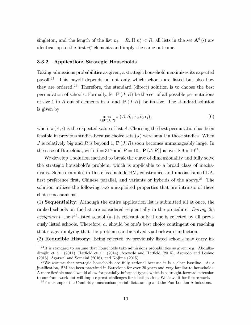
singleton, and the length of the list ni = R. If n∗i < R, all lists in the set A0 (·) areidentical up to the first n∗i elements and imply the same outcome.

3.3.2 Application: Strategic Households

Taking admissions probabilities as given, a strategic household maximizes its expected

payoff.24 This payoff depends on not only which schools are listed but also how

they are ordered.25 Therefore, the standard (direct) solution is to choose the best

permutation of schools. Formally, let P (J ;R) be the set of all possible permutations

of size 1 to R out of elements in J, and |P (J ;R)| be its size. The standard solutionis given by

maxA∈P(J ;R)

π (A, Si, xi, li, εi) , (6)

where π (A, ·) is the expected value of list A. Choosing the best permutation has beenfeasible in previous studies because choice sets (J) were small in those studies. When

J is relatively big and R is beyond 1, P (J ;R) soon becomes unmanageably large. In

the case of Barcelona, with J = 317 and R = 10, |P (J ;R)| is over 8.9× 1024.

We develop a solution method to break the curse of dimensionality and fully solve

the strategic household’s problem, which is applicable to a broad class of mecha-

nisms. Some examples in this class include BM, constrained and unconstrained DA,

first preference first, Chinese parallel, and variants or hybrids of the above.26 The

solution utilizes the following two unexploited properties that are intrinsic of these

choice mechanisms.

(1) Sequentiality: Although the entire application list is submitted all at once, theranked schools on the list are considered sequentially in the procedure. During the

assignment, the rth-listed school (ar) is relevant only if one is rejected by all previ-

ously listed schools. Therefore, ar should be one’s best choice contingent on reaching

that stage, implying that the problem can be solved via backward induction.

(2) Reducible History: Being rejected by previously listed schools may carry in-

24It is standard to assume that households take admissions probabilities as given, e.g., Abdulka-diroglu et al. (2011), Hatfield et al. (2014), Azevedo and Hatfield (2015), Azevedo and Leshno(2015), Agarwal and Somaini (2016), and Kojima (2015).25We assume that strategic households are fully rational because it is a clear baseline. As a

justification, BM has been practiced in Barcelona for over 20 years and very familar to households.A more flexible model would allow for partially-informed types, which is a straight-forward extensionto our framework but will impose great challenges for identification. We leave it for future work.26For example, the Cambridge mechanism, serial dictatorship and the Pan London Admissions.

10

formation about one’s probability of being assigned to ar, but the information can

be fully summarized by objects much simpler than the list (a1, ...ar−1). Therefore,

the problem involves a state space with a dimension much lower than |P (J ;R)|.27 Inparticular, as we show in the online appendix, with some differences in specifics, the

class of mechanisms has the following feature. After being rejected by (a1, ...ar−1) ,

i will be admitted to ar if ar still has seats and if i is ranked high enough among

those being considered. The latter is fully determined by i’s priority and random

lottery number for ar. Among the two factors, i’s priority for ar is determined by

pre-determined characteristics, and, in some instances, the rank position of the school

on i’s list (i.e., r); but it is independent of the other schools on the list.28 One’s lottery

number is drawn after the application, unknown to the applicant when making her

decisions. In the case where a household has a single lottery number across all tie-

breaking cases, correlation arises between the probabilities of being admitted to the

listed schools: being rejected by a1 due to losing the lottery for a1 reveals that one’s

lottery number is below cuta1 , being rejected again by a2 due to losing the lottery for

a2 reveals that one’s lottery number is below min cuta1 , cuta2 , and so on. However,other than this information, (a1, ...ar−1) bears no information that is payoff relevant

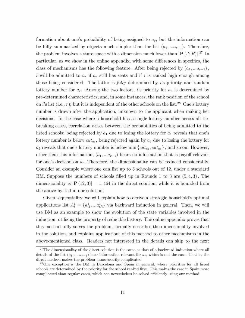
for one’s decision on ar. Therefore, the dimensionality can be reduced considerably.

Consider an example where one can list up to 3 schools out of 12, under a standard

BM. Suppose the numbers of schools filled up in Rounds 1 to 3 are (5, 4, 3) . The

dimensionality is |P (12; 3)| = 1, 464 in the direct solution, while it is bounded from

the above by 150 in our solution.

Given sequentiality, we will explain how to derive a strategic household’s optimal

applications list A1i = a1

i1, ...a1iR via backward induction in general. Then, we will

use BM as an example to show the evolution of the state variables involved in the

induction, utilizing the property of reducible history. The online appendix proves that

this method fully solves the problem, formally describes the dimensionality involved

in the solution, and explains applications of this method to other mechanisms in the

above-mentioned class. Readers not interested in the details can skip to the next

27The dimensionality of the direct solution is the same as that of a backward induction where alldetails of the list (a1, ..., ar−1) bear information relevant for ar, which is not the case. That is, thedirect method makes the problem unnecessarily complicated.28One exception is the BM in Barcelona and Spain in general, where priorities for all listed

schools are determined by the priority for the school ranked first. This makes the case in Spain morecomplicated than regular cases, which can nevertheless be solved effi ciently using our method.

11

section.

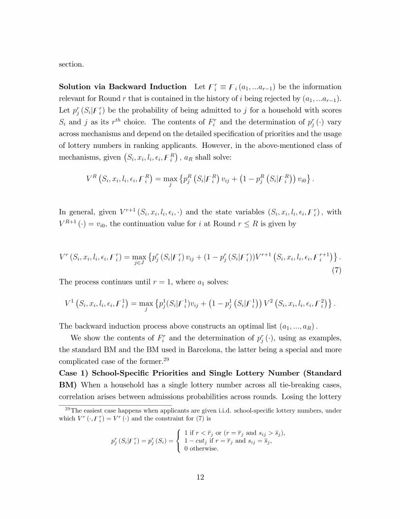
Solution via Backward Induction Let zri ≡ zi (a1, ...ar−1) be the information

relevant for Round r that is contained in the history of i being rejected by (a1, ...ar−1).

Let prj (Si|zri ) be the probability of being admitted to j for a household with scores

Si and j as its rth choice. The contents of F ri and the determination of p

rj (·) vary

across mechanisms and depend on the detailed specification of priorities and the usage

of lottery numbers in ranking applicants. However, in the above-mentioned class of

mechanisms, given(Si, xi, li, εi,zR

i

), aR shall solve:

V R(Si, xi, li, εi,zR

i

)= max

j

pRj(Si|zR

i

)vij +

(1− pRj

(Si|zR

i

))vi0.

In general, given V r+1 (Si, xi, li, εi, ·) and the state variables (Si, xi, li, εi,zri ) , with

V R+1 (·) = vi0, the continuation value for i at Round r ≤ R is given by

V r (Si, xi, li, εi,zri ) = max

j∈J

prj (Si|zr

i ) vij + (1− prj (Si|zri ))V

r+1(Si, xi, li, εi,zr+1

i

).

(7)

The process continues until r = 1, where a1 solves:

V 1(Si, xi, li, εi,z1

i

)= max

j

p1j(Si|z1

i )vij +(1− p1

j

(Si|z1

i

))V 2(Si, xi, li, εi,z2

i

).

The backward induction process above constructs an optimal list (a1, ..., aR) .

We show the contents of F ri and the determination of p

rj (·), using as examples,

the standard BM and the BM used in Barcelona, the latter being a special and more

complicated case of the former.29

Case 1) School-Specific Priorities and Single Lottery Number (StandardBM) When a household has a single lottery number across all tie-breaking cases,correlation arises between admissions probabilities across rounds. Losing the lottery29The easiest case happens when applicants are given i.i.d. school-specific lottery numbers, under

which V r (·,zri ) = V r (·) and the constraint for (7) is

prj (Si|zri ) = prj (Si) =

1 if r < rj or (r = rj and sij > sj),1− cutj if r = rj and sij = sj ,0 otherwise.

12

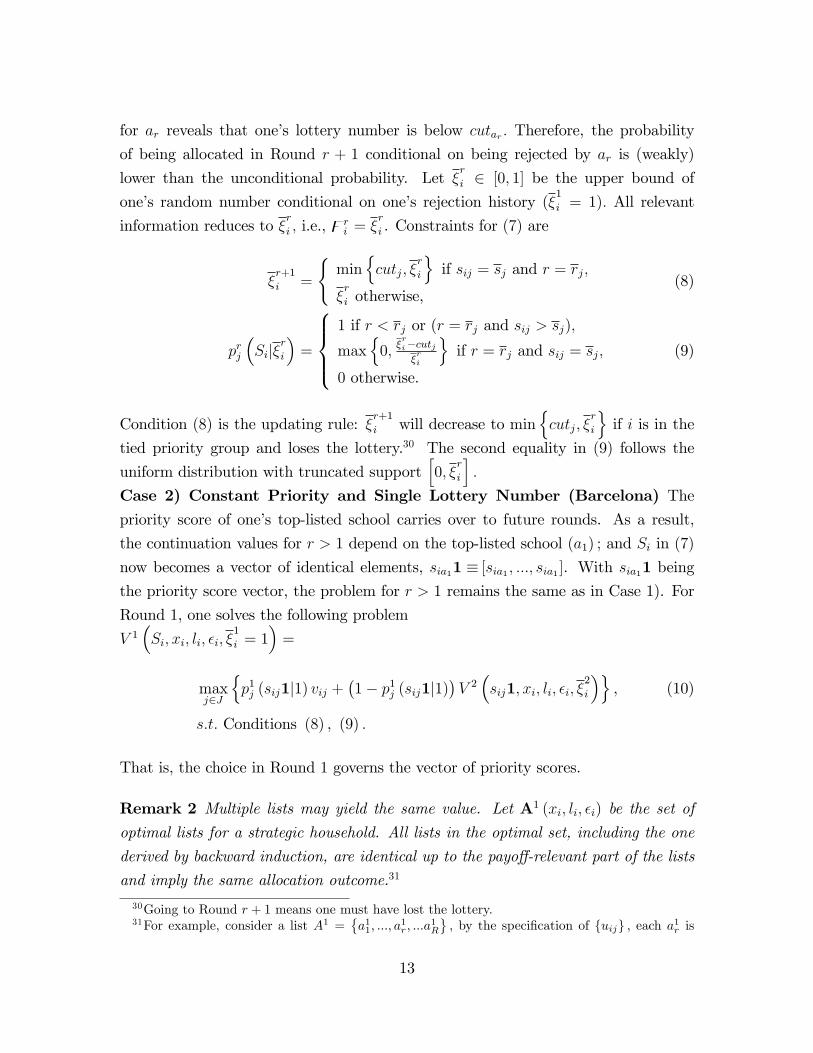
for ar reveals that one’s lottery number is below cutar . Therefore, the probability

of being allocated in Round r + 1 conditional on being rejected by ar is (weakly)

lower than the unconditional probability. Let ξr

i ∈ [0, 1] be the upper bound of

one’s random number conditional on one’s rejection history (ξ1

i = 1). All relevant

information reduces to ξr

i , i.e., zri = ξ

r

i . Constraints for (7) are

ξr+1

i =

min

cutj, ξ

r

i

if sij = sj and r = rj,

ξr

i otherwise,(8)

prj

(Si|ξ

r

i

)=

1 if r < rj or (r = rj and sij > sj),

max

0,ξri−cutjξri

if r = rj and sij = sj,

0 otherwise.

(9)

Condition (8) is the updating rule: ξr+1

i will decrease to mincutj, ξ

r

i

if i is in the

tied priority group and loses the lottery.30 The second equality in (9) follows the

uniform distribution with truncated support[0, ξ

r

i

].

Case 2) Constant Priority and Single Lottery Number (Barcelona) Thepriority score of one’s top-listed school carries over to future rounds. As a result,

the continuation values for r > 1 depend on the top-listed school (a1) ; and Si in (7)

now becomes a vector of identical elements, sia11 ≡ [sia1 , ..., sia1 ]. With sia11 being

the priority score vector, the problem for r > 1 remains the same as in Case 1). For

Round 1, one solves the following problem

V 1(Si, xi, li, εi, ξ

1

i = 1)

=

maxj∈J

p1j (sij1|1) vij +

(1− p1

j (sij1|1))V 2(sij1, xi, li, εi, ξ

2

i

), (10)

s.t. Conditions (8) , (9) .

That is, the choice in Round 1 governs the vector of priority scores.

Remark 2 Multiple lists may yield the same value. Let A1 (xi, li, εi) be the set of

optimal lists for a strategic household. All lists in the optimal set, including the one

derived by backward induction, are identical up to the payoff-relevant part of the lists

and imply the same allocation outcome.31

30Going to Round r + 1 means one must have lost the lottery.31For example, consider a list A1 =

a11, ..., a

1r, ...a

1R

, by the specification of uij , each a1r is

13

4 Estimation

4.1 Further Empirical Specification

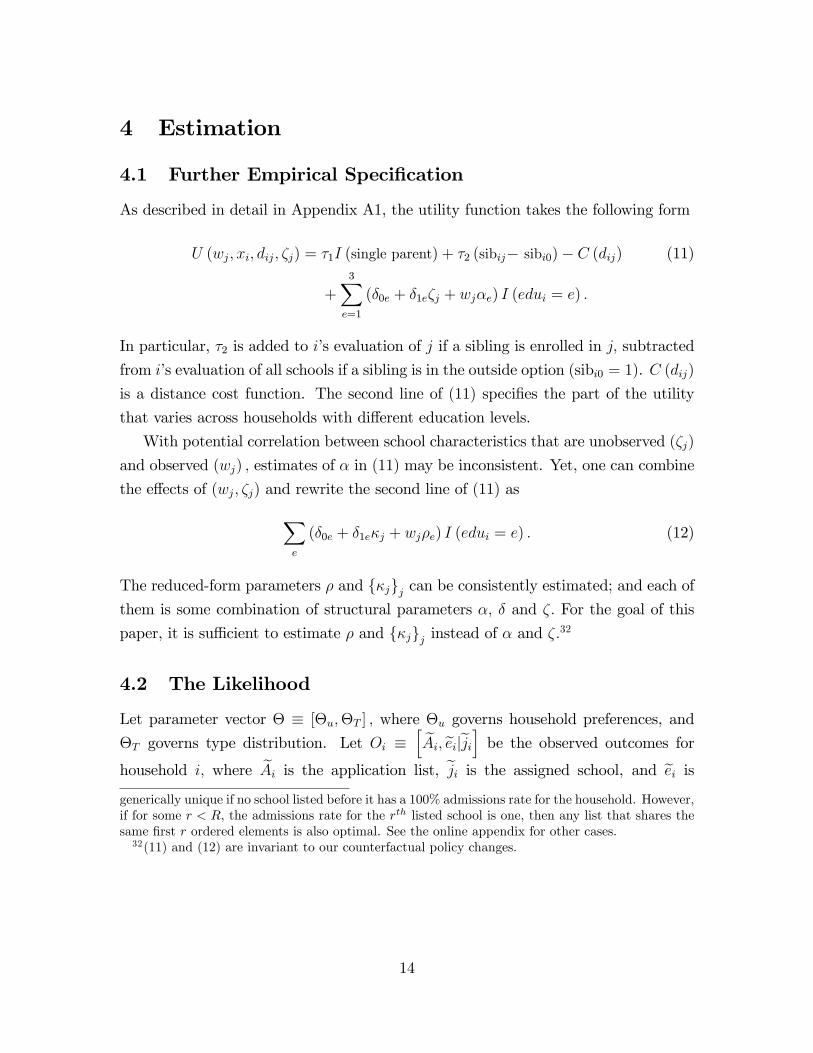
As described in detail in Appendix A1, the utility function takes the following form

U (wj, xi, dij, ζj) = τ1I (single parent) + τ2 (sibij− sibi0)− C (dij) (11)

+3∑e=1

(δ0e + δ1eζj + wjαe) I (edui = e) .

In particular, τ2 is added to i’s evaluation of j if a sibling is enrolled in j, subtracted

from i’s evaluation of all schools if a sibling is in the outside option (sibi0 = 1). C (dij)

is a distance cost function. The second line of (11) specifies the part of the utility

that varies across households with different education levels.

With potential correlation between school characteristics that are unobserved (ζj)

and observed (wj) , estimates of α in (11) may be inconsistent. Yet, one can combine

the effects of (wj, ζj) and rewrite the second line of (11) as∑e

(δ0e + δ1eκj + wjρe) I (edui = e) . (12)

The reduced-form parameters ρ and κjj can be consistently estimated; and each ofthem is some combination of structural parameters α, δ and ζ. For the goal of this

paper, it is suffi cient to estimate ρ and κjj instead of α and ζ.32

4.2 The Likelihood

Let parameter vector Θ ≡ [Θu,ΘT ] , where Θu governs household preferences, and

ΘT governs type distribution. Let Oi ≡[Ai, ei |ji

]be the observed outcomes for

household i, where Ai is the application list, ji is the assigned school, and ei is

generically unique if no school listed before it has a 100% admissions rate for the household. However,if for some r < R, the admissions rate for the rth listed school is one, then any list that shares thesame first r ordered elements is also optimal. See the online appendix for other cases.32(11) and (12) are invariant to our counterfactual policy changes.

14

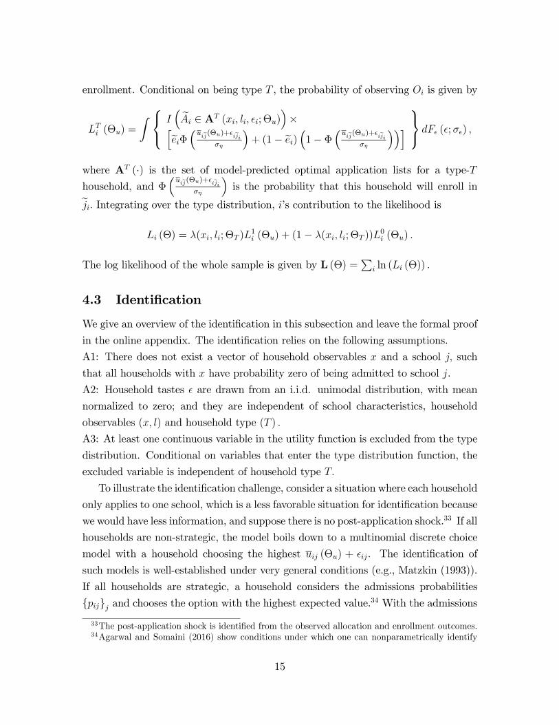
enrollment. Conditional on being type T , the probability of observing Oi is given by

LTi (Θu) =

∫ I(Ai ∈ AT (xi, li, εi; Θu)

)×[

eiΦ(uij(Θu)+εiji

ση

)+ (1− ei)

(1− Φ

(uij(Θu)+εiji

ση

))] dFε (ε;σε) ,

where AT (·) is the set of model-predicted optimal application lists for a type-Thousehold, and Φ

(uij(Θu)+εiji

ση

)is the probability that this household will enroll in

ji. Integrating over the type distribution, i’s contribution to the likelihood is

Li (Θ) = λ(xi, li; ΘT )L1i (Θu) + (1− λ(xi, li; ΘT ))L0

i (Θu) .

The log likelihood of the whole sample is given by L (Θ) =∑

i ln (Li (Θ)) .

4.3 Identification

We give an overview of the identification in this subsection and leave the formal proof

in the online appendix. The identification relies on the following assumptions.

A1: There does not exist a vector of household observables x and a school j, such

that all households with x have probability zero of being admitted to school j.

A2: Household tastes ε are drawn from an i.i.d. unimodal distribution, with mean

normalized to zero; and they are independent of school characteristics, household

observables (x, l) and household type (T ) .

A3: At least one continuous variable in the utility function is excluded from the type

distribution. Conditional on variables that enter the type distribution function, the

excluded variable is independent of household type T.

To illustrate the identification challenge, consider a situation where each household

only applies to one school, which is a less favorable situation for identification because

we would have less information, and suppose there is no post-application shock.33 If all

households are non-strategic, the model boils down to a multinomial discrete choice

model with a household choosing the highest uij (Θu) + εij. The identification of

such models is well-established under very general conditions (e.g., Matzkin (1993)).

If all households are strategic, a household considers the admissions probabilities

pijj and chooses the option with the highest expected value.34 With the admissions33The post-application shock is identified from the observed allocation and enrollment outcomes.34Agarwal and Somaini (2016) show conditions under which one can nonparametrically identify

15

probabilities observed from the data, this model is identified with A1.35 The challenge

exists because we allow for a mixture of both types of households. In the following,

we first explain A2-A3, then give the intuition underlying the identification proof.

4.3.1 A2 and A3 in Our Framework

We observe application lists with different distance-quality-risk combinations with

different frequencies in the data. The model predicts that households of the same

type tend to make similar application lists. Given A2, the distributions of type-

related variables will differ around the modes of the observed choices, which informs

us of the correlation between type T and these variables. A3 guarantees that different

behaviors can arise from exogenous variations within a type. To satisfy A3, we need to

make some restrictions on how household observables (xi, li) enter type distribution

and utility. Conditional on distance, a non-strategic household may not care too

much about living to the left or the right of a school, but a strategic household may

be more likely to have chosen a particular side so as to take advantage of the priority

zone structure.36 However, given that households, strategic or not, share the same

preferences about school characteristics and distances, there is no particular reason

to believe that everything else being equal, the strategic type will live closer to a

particular school than the non-strategic type would just for pure distance concerns.37

In other words, because the only difference between a strategic type and a non-

strategic type is whether or not one considers the admissions probabilities, which are

affected by one’s home location only via the zone to which it belongs to, we assume

that home location li enters the type distribution only via the school zone zli , i.e.,

λ (xi, li) = λ (xi, zli) . In contrast, household utility depends directly on the home-

school distance vector di. Conditional on being in the same school zone, households

with similar characteristics x but different home addresses still face different home-

school distance vectors d, as required in A3.

household preferences when all of them are strategic.35If for all households with x, the admissions probabilities to j are zero, the utility for school j

for these households is unidentifiable, because the expected value of applying to j is zero regardlessof the level of utility.36Without directly modeling households’location choices, we allow household types to be corre-

lated with the characteristics of the school zones they live in. We leave the incorporation of householdlocation choices for future extensions.37See the online appendix for evidence from the data supporting this assumption.

16

4.3.2 The Intuition for Identification

The data contains rich information for identification. First, one can compare a house-

hold’s listed schools with other schools. Due to unobserved school characteristics,

some seemingly good schools may in fact be unattractive, making it not as popular as

it “should have been”among most households. Controlling for such common factors,

as we do in the model, a household may still leave out some seemingly good schools

due to unobserved tastes. A2 implies that tastes are independent of household-school-

specific admissions probabilities, which should not lead to a systematic relationship

between a school being listed and a household’s chances of getting into this school.

However, as will be shown in Section 5, for a large fraction of households, when they

left out schools better than their listed ones in terms of quality, fees and distance, in

most cases, these better schools were ones for which they had lower chances. Such

behavior is highly consistent with strategizing instead of truth-telling.

Second, one can explore the fact that admissions probabilities increase discontin-

uously with in-zone status. Most illustratively, consider households along the border

of two zones. Were all households non-strategic, applications should be very similar

among households along both sides of the border. In contrast, were most households

strategic, applications would be very different across the border.

Finally, conditional on (x, zl) , the variation in d induces different behaviors within

the same type; and conditional on (x, zl, d) , different types behave differently. In par-

ticular, although households share the same preference parameters, different types of

households will behave as if they have different sensitivities to distance. For example,

consider households with the same (x, zl) and a good school j out of their zone zl. As

the distance to j decreases along household addresses, more and more non-strategic

households will apply to j because of the decreasing distance cost. However, the

reactions will be much less obvious among the strategic households, because they

take into account the risk of being rejected, which remains unchanged no matter how

close j is as long as it is out of zl. The different distance-elasticities among house-

holds therefore inform us of the type distribution within (x, zl). This identification

argument does not depend on specific parametric assumptions. For example, Lewbel

(2000) shows that similar models are semiparametrically identified when an A3-like

excluded variable with a large support exists. However, to make the exercise feasible,

17

we have made parametric assumptions.38

4.3.3 Obviously Non-Strategic Households

The identification of our model is further facilitated by the fact that we can partly ob-

serve household type directly from the data: there is one particular type of “mistakes”

that a strategic household will never make, which is a suffi cient (but not necessary)

condition to spot a non-strategic household.39 Intuitively, if a household’s admissions

status is still uncertain for all schools listed so far, and there is another school j it

desires, one should never waste the current slot listing a zero-probability school in-

stead of j because the admissions probabilities decrease over rounds.40 The idea is

formalized in the following claim and proved in the online appendix.41

Claim 1 An application list with the following features is suffi cient but not necessaryevidence that the household must be non-strategic: 1) for some rth element ar on the

list, the household faces zero admissions probability at the rth round, and 2) it faces

admissions probabilities lower than 1 for all schools listed in previous rounds, and 3)

it faces a positive but lower than 100% admissions probability for the school listed in

a later slot r′ ≥ r + 1 and no school listed between ar and ar′ admits the household

with probability 1.

5 Data

We focus on applications among families with children that turned 3 years old in 2006

or 2007 and lived in Barcelona. For each applicant, we observe the application list,

38We have to use parametric assumptions because semiparametric estimation is empirically infea-sible, and because the support of d is bounded by the size of the city, which is not large enoughrelative to the (unbounded) support of household tastes, as required in Lewbel (2000).39If the support of household characteristics is full conditional on being obviously non-strategic,

household preferences can be identified using this subset of households without A1, since ε is inde-pendent of (x, l) . However, our identification does not rely on the existence of obviously non-strategichouseholds.40For example, consider an application list (1, 2, 3, ...) by Household i with Si, where School 1 is

filled up in Round 1 with p11 (Si, ·) < 1, School 2 is filled up in Round 1 hence p22 (·) = 0, and School3 is filled up in Round 3 and 0 < p33 (Si, ·) < 1. This list is irrational, because one has probability 1of getting into School 3 in Round 2 and hence is strictly better off with any list starting with (1, 3)instead of (1, 2) .41Abdulkadiroglu et al. (2006) use a mistake similar to Feature 1) in Claim 1 to spot non-strategic

households, which is to list a school over-demanded in the first round as one’s second choice.

18

the assignment and enrollment outcomes, home address, family background, and the

ID of the school(s) her siblings were enrolled in the year of her application. For each

school, we observe its type (public or semi-public), a measure of quality, capacity and

service fees. The online appendix describes our data sources.

5.1 Admissions Thresholds

Assuming each household is a small player that takes the admissions thresholds as

given, we can recover all parameters by estimating an individual decision model.

Given the observed applications and the priority rules, we make 1,000 copies for each

observed application list and assign each copy a random lottery number. We simulate

the assignment results in this enlarged market to obtain (rj, sj, cutj)j, which aretreated as the ones households expected when they applied. This calculation involves

all participating households (11,871 in 2006).

5.2 Summary Statistics

For estimation, we drop 3,152 observations (obs) whose locations cannot be matched

in the GIS (geographic information system),42 31 obs whose outcomes were incon-

sistent with the offi cial rule, 191 obs with special-need children or post-dealine (and

hence ineligible) applications, and those with missing information.43 The final estima-

tion sample has 6,836 obs. Table 1 summarizes school characteristics.44 Compared to

public schools, semi-public schools have higher quality and larger capacities. Table 2

reports household characteristics in the estimation sample.45 Households had priority

for 22 schools on average but with considerable dispersions depending on their zones.

42We know their priority scores and applications, which enables us to include them in the calcu-lation of admissions thresholds.43In the estimation, we exclude 748 parents who reported their education as “high school or

above.”In policy simulations, we include this subsample so as to make equilibrium assignments. Weestimate the probability of each of them as being college educated as a flexible function of all theother observable characteristics, by comparing them with those who reported exactly high-school orcollege education. The model fit for this subsample is as good as that for the estimation sample,available on request.44School quality is measured by average student test scores on a scale from 0 to 10.45Following the literature on child development, we use mother’s education as the definition of

parental education if the mother is present in the household, otherwise, we use the father’s education.

19

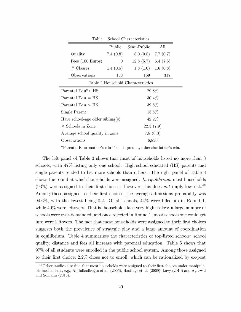
Table 1 School Characteristics

Public Semi-Public All

Quality 7.4 (0.8) 8.0 (0.5) 7.7 (0.7)

Fees (100 Euros) 0 12.8 (5.7) 6.4 (7.5)

# Classes 1.4 (0.5) 1.8 (1.0) 1.6 (0.8)

Observations 158 159 317

Table 2 Household Characteristics

Parental Edua< HS 29.8%

Parental Edu = HS 30.4%

Parental Edu > HS 39.8%

Single Parent 15.8%

Have school-age older sibling(s) 42.2%

# Schools in Zone 22.3 (7.9)

Average school quality in zone 7.8 (0.3)

Observations 6,836aParental Edu: mother’s edu if she is present, otherwise father’s edu.

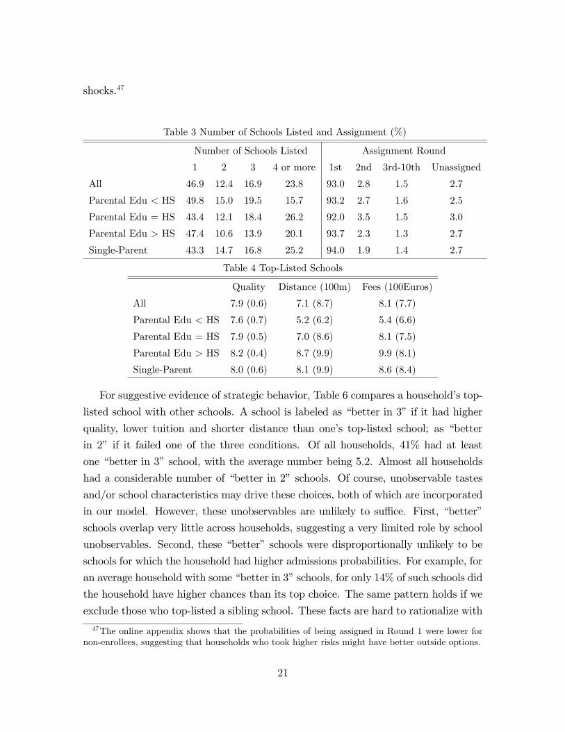
The left panel of Table 3 shows that most of households listed no more than 3

schools, with 47% listing only one school. High-school-educated (HS) parents and

single parents tended to list more schools than others. The right panel of Table 3

shows the round at which households were assigned. In equilibrium, most households

(93%) were assigned to their first choices. However, this does not imply low risk.46

Among those assigned to their first choices, the average admissions probability was

94.6%, with the lowest being 0.2. Of all schools, 44% were filled up in Round 1,

while 40% were leftovers. That is, households face very high stakes: a large number of

schools were over-demanded; and once rejected in Round 1, most schools one could get

into were leftovers. The fact that most households were assigned to their first choices

suggests both the prevalence of strategic play and a large amount of coordination

in equilibrium. Table 4 summarizes the characteristics of top-listed schools: school

quality, distance and fees all increase with parental education. Table 5 shows that

97% of all students were enrolled in the public school system. Among those assigned

to their first choice, 2.2% chose not to enroll, which can be rationalized by ex-post

46Other studies also find that most households were assigned to their first choices under manipula-ble mechanisms, e.g., Abdulkadiroglu et al. (2006), Hastings et al. (2009), Lavy (2010) and Agarwaland Somaini (2016).

20

shocks.47

Table 3 Number of Schools Listed and Assignment (%)

Number of Schools Listed Assignment Round

1 2 3 4 or more 1st 2nd 3rd-10th Unassigned

All 46.9 12.4 16.9 23.8 93.0 2.8 1.5 2.7

Parental Edu < HS 49.8 15.0 19.5 15.7 93.2 2.7 1.6 2.5

Parental Edu = HS 43.4 12.1 18.4 26.2 92.0 3.5 1.5 3.0

Parental Edu > HS 47.4 10.6 13.9 20.1 93.7 2.3 1.3 2.7

Single-Parent 43.3 14.7 16.8 25.2 94.0 1.9 1.4 2.7

Table 4 Top-Listed Schools

Quality Distance (100m) Fees (100Euros)

All 7.9 (0.6) 7.1 (8.7) 8.1 (7.7)

Parental Edu < HS 7.6 (0.7) 5.2 (6.2) 5.4 (6.6)

Parental Edu = HS 7.9 (0.5) 7.0 (8.6) 8.1 (7.5)

Parental Edu > HS 8.2 (0.4) 8.7 (9.9) 9.9 (8.1)

Single-Parent 8.0 (0.6) 8.1 (9.9) 8.6 (8.4)

For suggestive evidence of strategic behavior, Table 6 compares a household’s top-

listed school with other schools. A school is labeled as “better in 3”if it had higher

quality, lower tuition and shorter distance than one’s top-listed school; as “better

in 2” if it failed one of the three conditions. Of all households, 41% had at least

one “better in 3”school, with the average number being 5.2. Almost all households

had a considerable number of “better in 2”schools. Of course, unobservable tastes

and/or school characteristics may drive these choices, both of which are incorporated

in our model. However, these unobservables are unlikely to suffi ce. First, “better”

schools overlap very little across households, suggesting a very limited role by school

unobservables. Second, these “better”schools were disproportionally unlikely to be

schools for which the household had higher admissions probabilities. For example, for

an average household with some “better in 3”schools, for only 14% of such schools did

the household have higher chances than its top choice. The same pattern holds if we

exclude those who top-listed a sibling school. These facts are hard to rationalize with

47The online appendix shows that the probabilities of being assigned in Round 1 were lower fornon-enrollees, suggesting that households who took higher risks might have better outside options.

21

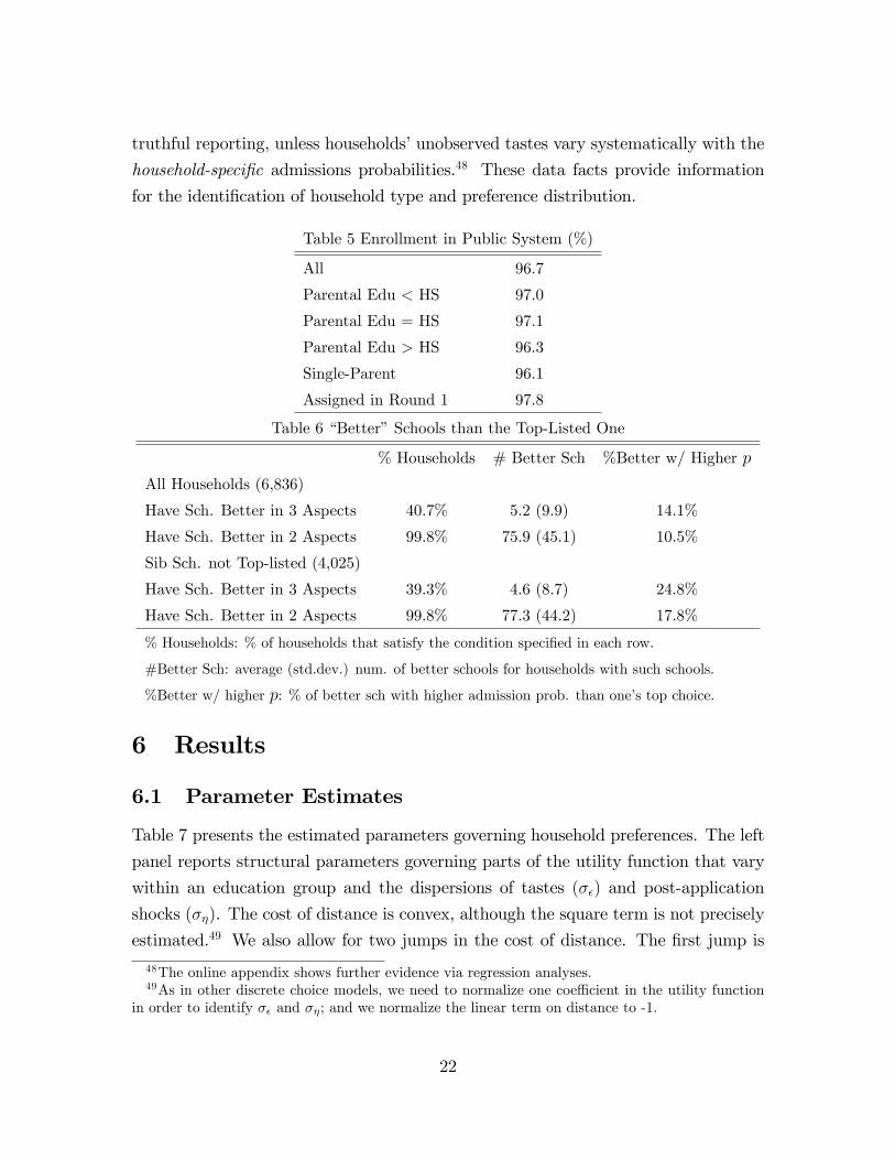
truthful reporting, unless households’unobserved tastes vary systematically with the

household-specific admissions probabilities.48 These data facts provide information

for the identification of household type and preference distribution.

Table 5 Enrollment in Public System (%)

All 96.7

Parental Edu < HS 97.0

Parental Edu = HS 97.1

Parental Edu > HS 96.3

Single-Parent 96.1

Assigned in Round 1 97.8

Table 6 “Better”Schools than the Top-Listed One

% Households # Better Sch %Better w/ Higher p

All Households (6,836)

Have Sch. Better in 3 Aspects 40.7% 5.2 (9.9) 14.1%

Have Sch. Better in 2 Aspects 99.8% 75.9 (45.1) 10.5%

Sib Sch. not Top-listed (4,025)

Have Sch. Better in 3 Aspects 39.3% 4.6 (8.7) 24.8%

Have Sch. Better in 2 Aspects 99.8% 77.3 (44.2) 17.8%

% Households: % of households that satisfy the condition specified in each row.

#Better Sch: average (std.dev.) num. of better schools for households with such schools.

%Better w/ higher p: % of better sch with higher admission prob. than one’s top choice.

6 Results

6.1 Parameter Estimates

Table 7 presents the estimated parameters governing household preferences. The left

panel reports structural parameters governing parts of the utility function that vary

within an education group and the dispersions of tastes (σε) and post-application

shocks (ση). The cost of distance is convex, although the square term is not precisely

estimated.49 We also allow for two jumps in the cost of distance. The first jump is

48The online appendix shows further evidence via regression analyses.49As in other discrete choice models, we need to normalize one coeffi cient in the utility function

in order to identify σε and ση; and we normalize the linear term on distance to -1.

22

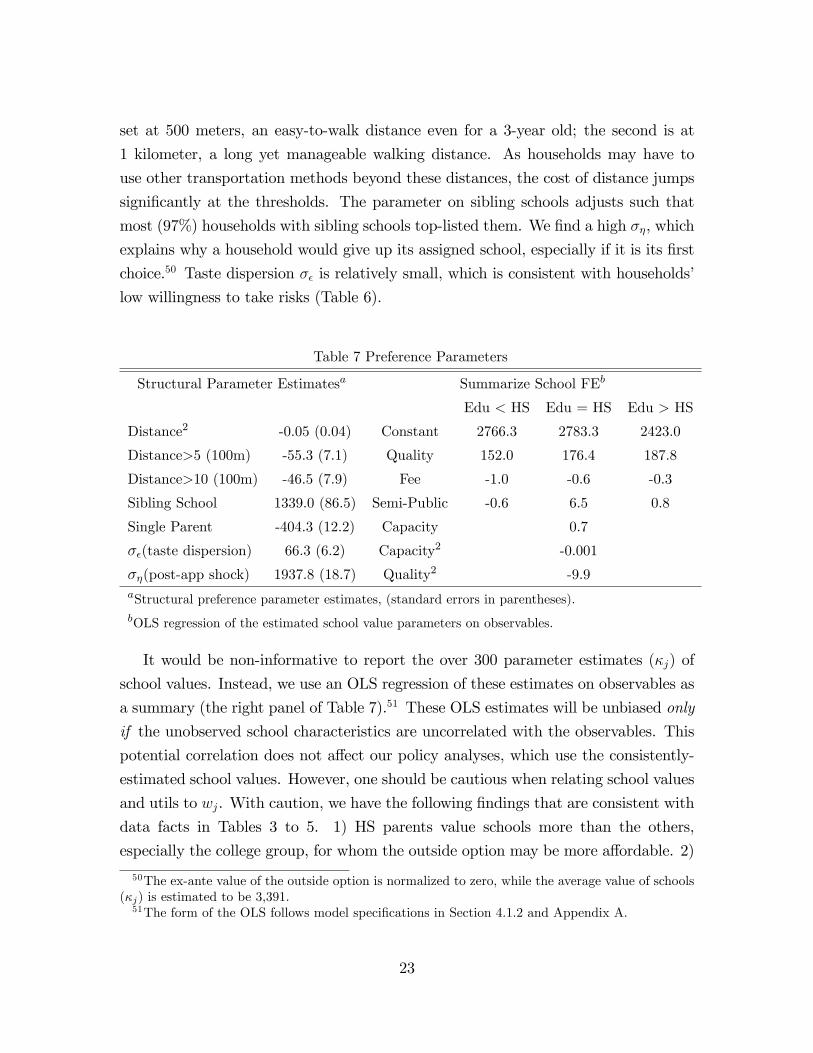
set at 500 meters, an easy-to-walk distance even for a 3-year old; the second is at

1 kilometer, a long yet manageable walking distance. As households may have to

use other transportation methods beyond these distances, the cost of distance jumps

significantly at the thresholds. The parameter on sibling schools adjusts such that

most (97%) households with sibling schools top-listed them. We find a high ση, which

explains why a household would give up its assigned school, especially if it is its first

choice.50 Taste dispersion σε is relatively small, which is consistent with households’

low willingness to take risks (Table 6).

Table 7 Preference Parameters

Structural Parameter Estimatesa Summarize School FEb

Edu < HS Edu = HS Edu > HS

Distance2 -0.05 (0.04) Constant 2766.3 2783.3 2423.0

Distance>5 (100m) -55.3 (7.1) Quality 152.0 176.4 187.8

Distance>10 (100m) -46.5 (7.9) Fee -1.0 -0.6 -0.3

Sibling School 1339.0 (86.5) Semi-Public -0.6 6.5 0.8

Single Parent -404.3 (12.2) Capacity 0.7

σε(taste dispersion) 66.3 (6.2) Capacity2 -0.001

ση(post-app shock) 1937.8 (18.7) Quality2 -9.9aStructural preference parameter estimates, (standard errors in parentheses).bOLS regression of the estimated school value parameters on observables.

It would be non-informative to report the over 300 parameter estimates (κj) of

school values. Instead, we use an OLS regression of these estimates on observables as

a summary (the right panel of Table 7).51 These OLS estimates will be unbiased only

if the unobserved school characteristics are uncorrelated with the observables. This

potential correlation does not affect our policy analyses, which use the consistently-

estimated school values. However, one should be cautious when relating school values

and utils to wj. With caution, we have the following findings that are consistent with

data facts in Tables 3 to 5. 1) HS parents value schools more than the others,

especially the college group, for whom the outside option may be more affordable. 2)

50The ex-ante value of the outside option is normalized to zero, while the average value of schools(κj) is estimated to be 3,391.51The form of the OLS follows model specifications in Section 4.1.2 and Appendix A.

23

Higher educated parents value school quality more and are less sensitive to fees.52 3)

Households prefer schools with larger capacity, which tend to have more resources.

4) Everything else being equal, semi-public schools are more preferable except for the

low-educated group.

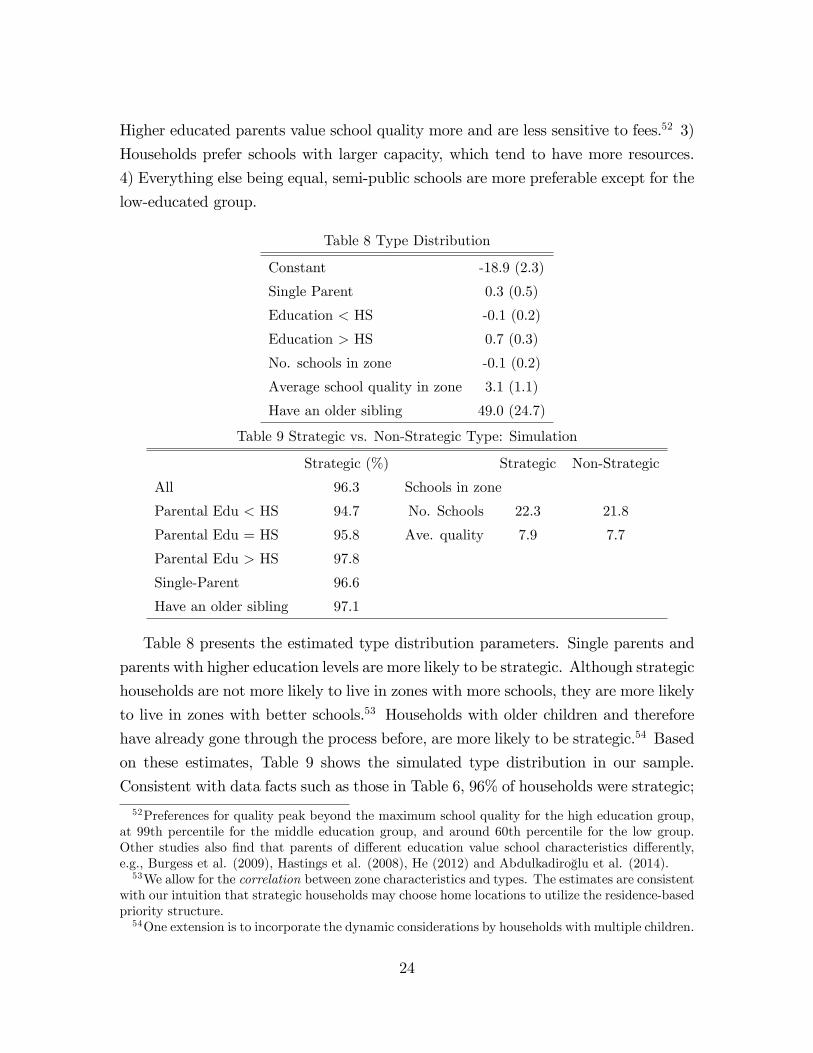
Table 8 Type Distribution

Constant -18.9 (2.3)

Single Parent 0.3 (0.5)

Education < HS -0.1 (0.2)

Education > HS 0.7 (0.3)

No. schools in zone -0.1 (0.2)

Average school quality in zone 3.1 (1.1)

Have an older sibling 49.0 (24.7)

Table 9 Strategic vs. Non-Strategic Type: Simulation

Strategic (%) Strategic Non-Strategic

All 96.3 Schools in zone

Parental Edu < HS 94.7 No. Schools 22.3 21.8

Parental Edu = HS 95.8 Ave. quality 7.9 7.7

Parental Edu > HS 97.8

Single-Parent 96.6

Have an older sibling 97.1

Table 8 presents the estimated type distribution parameters. Single parents and

parents with higher education levels are more likely to be strategic. Although strategic

households are not more likely to live in zones with more schools, they are more likely

to live in zones with better schools.53 Households with older children and therefore

have already gone through the process before, are more likely to be strategic.54 Based

on these estimates, Table 9 shows the simulated type distribution in our sample.

Consistent with data facts such as those in Table 6, 96% of households were strategic;

52Preferences for quality peak beyond the maximum school quality for the high education group,at 99th percentile for the middle education group, and around 60th percentile for the low group.Other studies also find that parents of different education value school characteristics differently,e.g., Burgess et al. (2009), Hastings et al. (2008), He (2012) and Abdulkadiroglu et al. (2014).53We allow for the correlation between zone characteristics and types. The estimates are consistent

with our intuition that strategic households may choose home locations to utilize the residence-basedpriority structure.54One extension is to incorporate the dynamic considerations by households with multiple children.

24

and the fraction increases with education.55 To obtain further insights on our findings,

we have re-estimated our model with the restriction that only 80% of households were

strategic. The fit of this restricted model is significantly worse, as shown in the online

appendix.

6.2 Model Fits and Out-of-Sample Validation

The 2007 re-definition of priority zones abruptly changed the school-household-specific

priorities: priority schools became those that surrounded each home location.56 We

show model fits for both the 2006 and the 2007 samples.57 To simulate the 2007

outcomes, we first calculate the admissions probabilities in 2007 via the same proce-

dure as we do for 2006. Then we use the 2007 sample to conduct an out-of-sample

validation.58 Because the reform came as a surprise and households were unlikely to

relocate before submitting their applications in 2007, we simulate the distribution of

2007 household types using the characteristics of their residential zones according to

the 2006 definition.59

Considered as the most informative test of the model, the first two rows of Table

10 explore the changes in the definition of priority zones. The reform led to situations

where some schools were in the priority zone for a household in one year but not in

the other, which would affect the behavior of a strategic household. In 2006, 24% of

households top-listed a school that was in their priority zone by the 2006 definition

but not by the 2007 definition. In 2007, the fraction of households top-listing these

schools dropped to 12%. On the other hand, the fraction of households that top-listed

schools in their priority zone only by the 2007 definition but not by the 2006 definition

increased from 3% to 12% over the two years. The model is able to replicate such

behaviors and predicts the changes as being from 24% to 14.6% for the first case,

55We find a much smaller fraction of non-strategic households than Abdulkadiroglu et al. (2006).The main reason is our incorporation of the outside option and the leftover schools, which rational-izes the choices by a substantial fraction of households that might be categorized as non-strategicotherwise. Another reason is the long history of BM in Barcelona, where parents have become veryfamiliar with the mechanism.56In 2007, the average (std) number of schools to which a household had priority became 7.0 (1.5).57More fitness tables are in the appendix.58In 2007, 12,335 Barcelona households participated, 7,437 of whom are selected into our validation

sample, using the same selection rule as before.59We also assume that strategic households had rational expectation about admissions probabil-

ities in 2007. As shown below, we can fit the data in both years, suggesting that our assumptionsare not unreasonable.

25

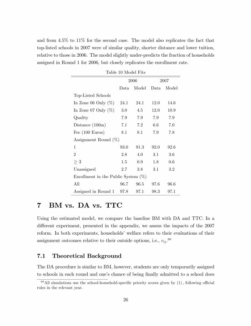
and from 4.5% to 11% for the second case. The model also replicates the fact that

top-listed schools in 2007 were of similar quality, shorter distance and lower tuition,

relative to those in 2006. The model slightly under-predicts the fraction of households

assigned in Round 1 for 2006, but closely replicates the enrollment rate.

Table 10 Model Fits

2006 2007

Data Model Data Model

Top-Listed Schools

In Zone 06 Only (%) 24.1 24.1 12.0 14.6

In Zone 07 Only (%) 3.0 4.5 12.0 10.9

Quality 7.9 7.9 7.9 7.9

Distance (100m) 7.1 7.2 6.6 7.0

Fee (100 Euros) 8.1 8.1 7.9 7.8

Assignment Round (%)

1 93.0 91.3 92.0 92.6

2 2.8 4.0 3.1 3.6

≥ 3 1.5 0.9 1.8 0.6

Unassigned 2.7 3.8 3.1 3.2

Enrollment in the Public System (%)

All 96.7 96.5 97.6 96.6

Assigned in Round 1 97.8 97.1 98.3 97.1

7 BM vs. DA vs. TTC

Using the estimated model, we compare the baseline BM with DA and TTC. In a

different experiment, presented in the appendix, we assess the impacts of the 2007

reform. In both experiments, households’welfare refers to their evaluations of their

assignment outcomes relative to their outside options, i.e., vij.60

7.1 Theoretical Background

The DA procedure is similar to BM, however, students are only temporarily assigned

to schools in each round and one’s chance of being finally admitted to a school does60All simulations use the school-household-specific priority scores given by (1) , following offi cial

rules in the relevant year.

26

not depend on the ranking of the school on her application. TTC creates cycles of

trade between individuals in each round. Each individual in a cycle trades off a seat

in her highest-priority school for a seat in her announced most preferred school among

those with open seats. Whenever such a cycle is formed the allocation is final.

Three properties are considered as desirable but cannot hold simultaneously in a

mechanism: Pareto effi ciency, truth revealing and the elimination of justified envy

(aka stability).61 BM satisfies none of the properties. DA and TTC, with the stan-

dard priority structure, are both truth revealing, which are the cases we consider.62

Between the other two conflicting properties, DA eliminates justified envy, while TTC

achieves Pareto effi ciency. The welfare comparison between BM and its alternatives

is ambiguous because of two competing forces. On the one hand, BM can lead to po-

tential misallocations because households hide their true preferences, which is absent

in DA and TTC. On the other hand, BM may better “respect”households’cardinal

preferences than DA and TTC (Abdulkadiroglu et al. (2011)). BM-induced house-

hold behaviors increase the chance of a “right match”in that a school is matched to

households that value it more. Under a truth-revealing mechanism, households who

share the same ordinal preferences will rank schools the same way and have the same

chance of being allocated to various schools, regardless of who will gain the most

from each school. Given that it is theoretically inconclusive, the welfare comparison

between these mechanisms becomes an empirical question, one that we answer below.

7.2 Results

Under both DA and TTC with the standard priority structure, all households will

list their true preferences.63 We simulate each household’s application list accord-

ingly and assign them using DA and then using TTC, and compare the results with

those from the baseline Barcelona case, i.e., BM with constant priority and single

lottery number.64 We present our results under the more recent (2007) priority zone

61Stability requires that there be no unmatched student-school pair (i, j) where student i prefersschool j to her assignment and she has higher priority at j than some other student who is assigneda seat at school j.62For example, one’s priority score in Round 1 does not carry over to future rounds.63To simulate DA and TTC, it is suffi cient to know household preferences. However, to compare

DA or TTC with the baseline, one needs to know the distribution of household strategic types.64All these mechanisms use random lotteries break ties. For a given set of random lottery numbers,

we simulate the allocation procedure and obtain the outcomes for all students. We repeat this processmany times to obtain the expected (average) outcomes for each simulated student.

27

structure.65

Remark 3 We report total household welfare, the distribution of winners and losersamong different subgroups of households, as well as the assignment outcomes. Total

household welfare is not necessarily the criterion for social welfare, which may involve

different weights across households. Given that we can calculate the welfare at the

household level, our results can be used to calculate any weighted social welfare. Given

a social objective, our results can be easily used for policy-making purposes, although

we do not necessarily recommend one mechanism over another in this paper.

7.2.1 Household Welfare Comparison

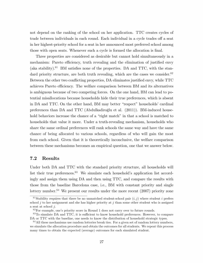
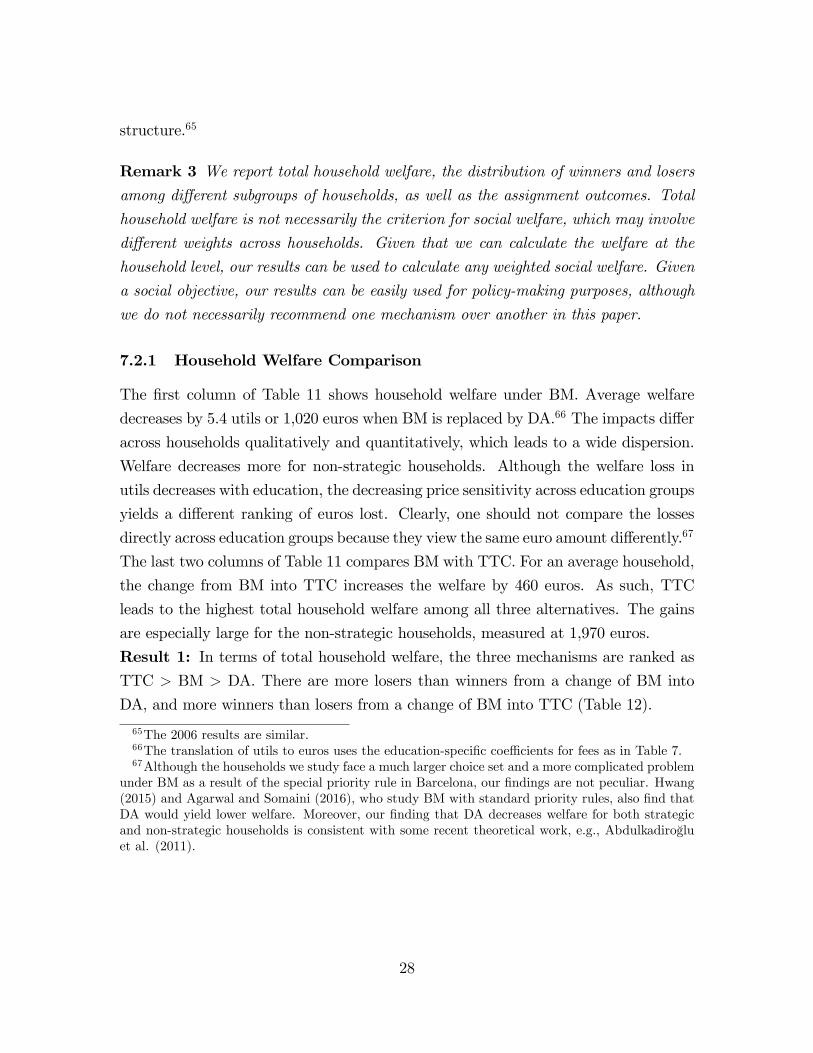
The first column of Table 11 shows household welfare under BM. Average welfare

decreases by 5.4 utils or 1,020 euros when BM is replaced by DA.66 The impacts differ

across households qualitatively and quantitatively, which leads to a wide dispersion.

Welfare decreases more for non-strategic households. Although the welfare loss in

utils decreases with education, the decreasing price sensitivity across education groups

yields a different ranking of euros lost. Clearly, one should not compare the losses

directly across education groups because they view the same euro amount differently.67

The last two columns of Table 11 compares BM with TTC. For an average household,

the change from BM into TTC increases the welfare by 460 euros. As such, TTC

leads to the highest total household welfare among all three alternatives. The gains

are especially large for the non-strategic households, measured at 1,970 euros.

Result 1: In terms of total household welfare, the three mechanisms are ranked asTTC > BM > DA. There are more losers than winners from a change of BM into

DA, and more winners than losers from a change of BM into TTC (Table 12).

65The 2006 results are similar.66The translation of utils to euros uses the education-specific coeffi cients for fees as in Table 7.67Although the households we study face a much larger choice set and a more complicated problem

under BM as a result of the special priority rule in Barcelona, our findings are not peculiar. Hwang(2015) and Agarwal and Somaini (2016), who study BM with standard priority rules, also find thatDA would yield lower welfare. Moreover, our finding that DA decreases welfare for both strategicand non-strategic households is consistent with some recent theoretical work, e.g., Abdulkadirogluet al. (2011).

28

Table 11 Household Welfare: BM vs. DA vs. TTC

% BMa DA-BMb TTC-BMc

∆utils ∆100 euros ∆utils ∆100 euros

All 3,811 (633) -5.4 (30.9) -10.2 (71.8) 1.9 (40.5) 4.6 (96.3)

Strategic 3,810 (633) -5.3 (30.3) -10.2 (69.9) 1.6 (39.9) 3.9 (94.3)

Non-strategic 3,818 (629) -5.7 (41.0) -19.7 (131.8) 8.3 (51.5) 19.7 (131.8)

Edu< HS 3,690 (600) -9.9 (28.3) -10.0 (28.6) 0.1 (31.4) 0.1 (31.7)

Edu= HS 3,934 (619) -5.7 (33.0) -18.3 (106.3) 2.5 (44.1) 8.0 (141.9)

Edu> HS 3,792 (647) -2.1 (30.3) -3.7 (54.6) 2.7 (42.8) 4.8 (77.2)awelfare under BM (std in parentheses), bchange from BM to DA, cchange from BM to TTC

∆utils: welfare change in utils. ∆100 euros: welfare change in 100 euros.

Table 12 Winners and Losers (%)

BM to DA BM to TTC

Winner Loser Winner Loser

All 11.7 33.0 25.0 21.5

Strategic 11.6 32.8 24.6 21.7

Non-strategic 15.3 36.7 32.3 17.5

Edu < HS 7.8 37.0 23.1 22.1

Edu = HS 13.0 35.5 27.4 23.0

Edu > HS 13.3 28.2 24.3 20.0

7.2.2 Cross-Zone Inequality

A household’s welfare can be significantly affected by the school quality within its zone

not only because of the quality-distance trade-off, but also because of the quality-risk

trade-off created by the priority structure. For equity concerns, a replacement of BM

will be more desirable if it is more likely to benefit those living in poor-quality zones.

Table 13 tests whether or not each of the counterfactual reforms meets this goal. In

the change from BM to DA, winners live in better zones than losers, which is against

the equity goal. The difference in zone quality between these two groups is almost

20% of a std of quality across all zones. Changing from BM to TTC, the average

zone quality is similar across winners and losers.

Result 2: Welfare dependence on zone quality increases with a change from BM to

DA, and remains unaffected by a change from BM to TTC.

29

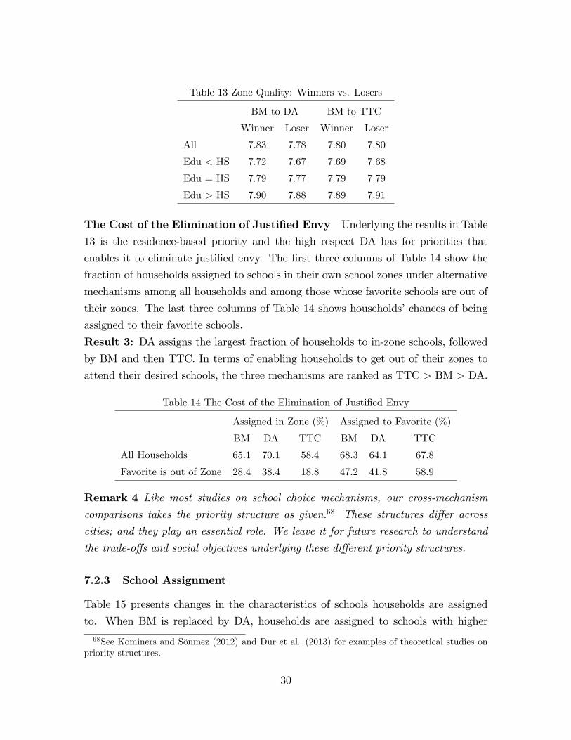
Table 13 Zone Quality: Winners vs. Losers

BM to DA BM to TTC

Winner Loser Winner Loser

All 7.83 7.78 7.80 7.80

Edu < HS 7.72 7.67 7.69 7.68

Edu = HS 7.79 7.77 7.79 7.79

Edu > HS 7.90 7.88 7.89 7.91

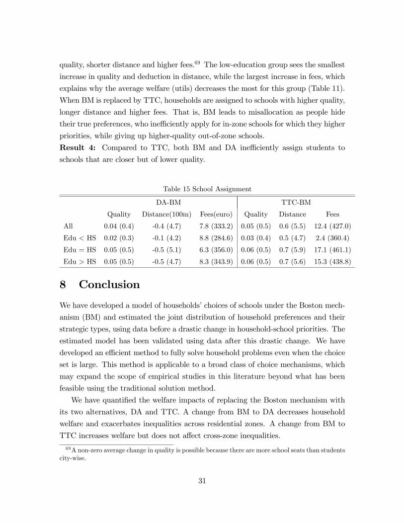
The Cost of the Elimination of Justified Envy Underlying the results in Table

13 is the residence-based priority and the high respect DA has for priorities that

enables it to eliminate justified envy. The first three columns of Table 14 show the

fraction of households assigned to schools in their own school zones under alternative

mechanisms among all households and among those whose favorite schools are out of

their zones. The last three columns of Table 14 shows households’chances of being

assigned to their favorite schools.

Result 3: DA assigns the largest fraction of households to in-zone schools, followedby BM and then TTC. In terms of enabling households to get out of their zones to

attend their desired schools, the three mechanisms are ranked as TTC > BM > DA.

Table 14 The Cost of the Elimination of Justified Envy

Assigned in Zone (%) Assigned to Favorite (%)

BM DA TTC BM DA TTC

All Households 65.1 70.1 58.4 68.3 64.1 67.8

Favorite is out of Zone 28.4 38.4 18.8 47.2 41.8 58.9

Remark 4 Like most studies on school choice mechanisms, our cross-mechanismcomparisons takes the priority structure as given.68 These structures differ across

cities; and they play an essential role. We leave it for future research to understand

the trade-offs and social objectives underlying these different priority structures.

7.2.3 School Assignment

Table 15 presents changes in the characteristics of schools households are assigned

to. When BM is replaced by DA, households are assigned to schools with higher

68See Kominers and Sönmez (2012) and Dur et al. (2013) for examples of theoretical studies onpriority structures.

30

quality, shorter distance and higher fees.69 The low-education group sees the smallest

increase in quality and deduction in distance, while the largest increase in fees, which

explains why the average welfare (utils) decreases the most for this group (Table 11).

When BM is replaced by TTC, households are assigned to schools with higher quality,

longer distance and higher fees. That is, BM leads to misallocation as people hide

their true preferences, who ineffi ciently apply for in-zone schools for which they higher

priorities, while giving up higher-quality out-of-zone schools.

Result 4: Compared to TTC, both BM and DA ineffi ciently assign students to

schools that are closer but of lower quality.

Table 15 School Assignment

DA-BM TTC-BM

Quality Distance(100m) Fees(euro) Quality Distance Fees

All 0.04 (0.4) -0.4 (4.7) 7.8 (333.2) 0.05 (0.5) 0.6 (5.5) 12.4 (427.0)

Edu < HS 0.02 (0.3) -0.1 (4.2) 8.8 (284.6) 0.03 (0.4) 0.5 (4.7) 2.4 (360.4)

Edu = HS 0.05 (0.5) -0.5 (5.1) 6.3 (356.0) 0.06 (0.5) 0.7 (5.9) 17.1 (461.1)

Edu > HS 0.05 (0.5) -0.5 (4.7) 8.3 (343.9) 0.06 (0.5) 0.7 (5.6) 15.3 (438.8)

8 Conclusion

We have developed a model of households’choices of schools under the Boston mech-

anism (BM) and estimated the joint distribution of household preferences and their

strategic types, using data before a drastic change in household-school priorities. The

estimated model has been validated using data after this drastic change. We have

developed an effi cient method to fully solve household problems even when the choice

set is large. This method is applicable to a broad class of choice mechanisms, which

may expand the scope of empirical studies in this literature beyond what has been

feasible using the traditional solution method.

We have quantified the welfare impacts of replacing the Boston mechanism with

its two alternatives, DA and TTC. A change from BM to DA decreases household

welfare and exacerbates inequalities across residential zones. A change from BM to

TTC increases welfare but does not affect cross-zone inequalities.

69A non-zero average change in quality is possible because there are more school seats than studentscity-wise.

31

The methods developed in this paper and the main empirical findings are promis-

ing for future research. One particularly interesting extension is to incorporate house-

hold’s residential choices into the framework of this paper. Individual households may

relocate in order to take advantage of changes in school choice mechanisms and/or in

residence-based priority structures. Such individual incentives will in turn affect the

housing market. There is a large literature on the capitalization of school quality for

housing prices, as reviewed by Black and Machin (2010) and Gibbons and Machin

(2008).70 An important yet challenging research project involves combining this litera-

ture and the framework proposed in our paper, in order to form a more comprehensive

view of the equilibrium impacts of school choice mechanisms on households’choices

of schools and residential areas, and on the housing market.

References

Abdulkadiroglu, A., N. Agarwal and P. Pathak (2014). “The Welfare Effects of Con-

gestion in Uncoordinated Assignment: Evidence from the NYC HS Match,”NBER

working paper.

Abdulkadiroglu, A., J. Angrist, S. Dynarski, T. Kane, and P. Pathak (2011). “Ac-

countability and Flexibility in Public Schools: Evidence from Boston’s Charters and

Pilots,”Quarterly Journal of Economics, 126(2): 699—748.

Abdulkadiroglu, A., Y. Che, and Y. Yasuda (2011). “Resolving Conflicting Prefer-

ences in School Choice: the Boston Mechanism Reconsidered,”American Economic

Review, 101(1): 399-410.

Abdulkadiroglu, A., P. Pathak, and A. Roth (2009). “Strategy-Proofness versus Ef-

ficiency in Matching with Indifferences: Redesigning the NYC High School Match.”

American Economic Review, 99(5): 1954—78.

Abdulkadiroglu, A., P. Pathak, A. Roth and T. Sönmez (2005). “The Boston Public

School Match,”American Economic Review, Papers and Proceedings, 95(2): 368-371.70Ries and Somerville (2010) exploit changes in the catchment areas of public schools in Vancouver

and find significant effects of school performance on housing prices. Epple and Romano (2003)conjecture that school choice systems can eliminate the capitalization of school quality on the housingmarket. Machin and Salvanes (2010) exploit policy reforms in Oslo that allowed students to attendschools without having to live in the school’s catchment area, and find a significant decrease in thecorrelation between a school’s quality and housing prices.

32

Abdulkadiroglu, A., P. Pathak, A. Roth and T. Sönmez (2006). “Changing the Boston

School Choice Mechanism: Strategy-proofness as Equal Access,”National Bureau of

Economic Research Working Paper 11965.

Abdulkadiroglu, A., and T. Sönmez (2003). “School Choice: A Mechanism Design

Approach,”American Economic Review, 93(3): 729-747.

Agarwal, N. and P. Somaini (2015). “Demand Analysis Using Strategic Reports: An

Application to a School Choice Mechanism,”Working Paper MIT.

Akyol, E. (2014). “Welfare Comparison of School Choice Mechanisms under Incom-

plete Information,”Working Paper Pennsylvania State University.

Arcidiacono, P. (2005). “Affi rmative Action in Higher Education: How Do Admission

and Financial Aid Rules Affect Future Earnings?”Econometrica, 73(5): 1477-1524.

Azevedo, E. and J. Hatfield (2015). “Existence of Equilibrium in Large Matching

Markets with Complementarities,”Mimeo, Wharton.

Azevedo, E. and J. Leshno (2015). “A supply and demand framework for two-sided

matching markets”forthcoming, Journal of Political Economy

Bajari, P. and A. Hortacsu (2005) “Are Structural Estimates of Auction Models

Reasonable? Evidence from Experimental Data,”Journal of Political Economy 113,

703—741.

Black, S. and S. Machin (2010) “Housing Valuations of School Performance” in E.

Hanishek, S. Machin and L. Woessmann (eds.), Handbook of the Economics of Edu-

cation, Amsterdam: Elsevier.

Blume, L., W. Brock, S. Durlauf and Y. Ioannides (2011). “Identification of Social

Interactions,”Handbook of Social Economics, ed. by J. Benhabib, A. Bisin and M.

Jackson, North-Holland, Vol 1B: 853-964.

Burgess, S., E. Greaves, A. Vignoles and D. Wilson (2009). “Parental Choice of

primary school in England: what type of schools do parents choose?”CMPOWorking

Paper No. 09/224.

Calsamiglia, C., M. Güell (2014). “The Illusion of Choice: Evidence from Barcelona,”

CEPR Discussion Paper 10011.

33

Calsamiglia, C. and Miralles A. (2014). “All about priorities? Less choice with bad

schools,”mimeo UAB.

Chen, Y., and T. Sönmez (2006). “School Choice: An Experimental Study,”Journal

of Economic Theory, 127(1): 202-231.

Deming, D., J. Hastings, T. Kane, and D. Staiger (2014). “School Choice, School

Quality and Postsecondary Attainment,”American Economic Review, 104(3): 991—

1013.

Epple, D. and R. Romano (2003). “Neighborhood Schools, Choice, and the Distrib-

ution of Educational Benefits,” in C. Hoxby (ed), The Economics of School Choice,

University of Chicago Press.

Epple, D. and R. Romano (2011). “Peer effects in education : a survey of the theory

and evidence,”Handbook of Social Economics, ed. by J. Benhabib, A. Bisin and M.

Jackson, North-Holland, Vol 1B: 1053-1163.

Ergin, H., and T. Sönmez (2006). “Games of School Choice under the Boston Mech-

anism,”Journal of Public Economics, 90(1-2): 215-237.

Dur, U., S. Kominers, P. Pathak and T. Sönmez (2013). "The Demise of Walk Zones

in Boston: Priorities vs. Precedence in School Choice," NBER Working Paper No.

18981.

Featherston, C. and M. Niederle (2008). “Ex Ante Effi ciency in School Choice Mech-

anisms: An Experimental Investigation,”NBER Working Paper 14618.

Fu, C. (2014). “Equilibrium Tuition, Applications, Admissions and Enrollment in the

College Market,”Journal of Political Economy, 122(2): 225-281.

Gibbons, S. and S. Machin (2008) “Valuing School Quality, Better Transport and

Lower Crime,”Oxford Review of Economic Policy, 24: 99-119.

Hastings, J., T. Kane and D. Staiger (2009). “Heterogeneous Preferences and the

Effi cacy of School Choice,”NBER Paper Working Paper 12145.

Hastings, J. and J. Weinstein (2008) “Information, School Choice and Academic

Achievement: Evidence from Two Experiments,”Quarterly Journal of Economics,

1373-1414.

34

Hatfield, J., F. Kojima, and Y. Narita (2014), “Promoting School Competition

through School Choice: A Market Design Approach,”Mimeo, Stanford University.

He, Y. (2014). “Gaming the Boston School Choice Mechanism in Beijing,”Working

Paper, Toulouse School of Economics.

Heckman, J. and S. Mosso (2014). “The Economics of Human Development and Social

Mobility,”Working paper, University of Chicago.

Hoxby, C. (2003): “School Choice and School Productivity (Or, Could School Choice

be a Rising Tide that Lifts All Boats),” in The Economics of School Choice, ed. by

C. Hoxby. Chicago: University of Chicago Press.

Hwang, S. (2015). “A Robust Redesign of High School Match,”Working Paper, UBC.

Jensen, R. (2010). “The (Perceived) Returns to Education and the Demand for

Schooling,”Quarterly Journal of Economics, 125 2, 515-548.

Keane, M. and R. Moffi tt (1998). “A Structural Model of Multiple Welfare Program

Participation and Labor Supply.” International Economic Review 39, 553—590.

Keane, M., P. Todd and K. Wolpin (2011) “The Structural Estimation of Behavioral

Models: Discrete Choice Dynamic Programming Methods and Applications,”in: O.

Ashenfelter and D. Card (Eds.) Handbook of Labor Economics, North-Holland. Vol

4A: 331-461.

Keane, M. and K. Wolpin (2007). “Exploring the Usefulness of a Non-random Holdout

Sample for Model Validation: Welfare Effects on Female Behavior,” International

Economic Review 48, 1351—1378.

Kojima, F. (2015). "Recent Developments in Matching Theory and their Practical

Applications," Manuscript, Stanford University.

Kominers, S. and T. Sönmez (2012). "Designing for Diversity: Matching with Slot-

Specific Priorities," Boston College Working Paper No. 806.

Lavy, V. (2010) “Effects of Free Choice Among Public Schools.”The Review of Eco-

nomic Studies, 77: 1164—1191.

35

Lewbel, A. (2000). “Semiparametric qualitative response model estimation with un-

known heteroscedasticity or instrumental variables,” Journal of Econometrics, 97:

145-177.

Lise, J., S. Seitz, and J. Smith (2005). “Equilibrium Policy Experiments and the

Evaluation of Social Programs,”Mimeo, Queens University.

Lu, J. (2014). “Cardinal Utility and Incomplete Information in School Choice:

Strengthening the Case for the Boston Mechanism,”Undergraduate Thesis, Harvard

University.

Lumsdaine, R., J. Stock, and D. Wise (1992). “Pension Plan Provisions and Retire-

ment: Men and Women, Medicare, and Models,”In: Wise, D.A. (Ed.), Studies in the

Economics of Aging, University of Chicago Press, Chicago.

Machin, S., and K. G. Salvanes (2010). “Valuing School Quality via School Choice

Reform,”IZA Discussion Paper No 4719.

Matzkin, R. (1993). “Nonparametric Identification and Estimation of Polychotomous

Choice Models,”Journal of Econometrics, 58: 137-168.

McFadden, D., and A. Talvitie (1977). “Validation of Disaggregate Travel Demand

Models: Some Tests,”Urban demand forecasting project, final report. Vol. V, Insti-

tute of Transportation Studies, University of California, Berkeley.

Mehta, N. (2013). “Competition in Public School Districts: Charter School Entry,

Student Sorting, and School Input Determination,”Working paper, UWO.

Miralles, A. (2008). “School Choice: The Case for the Boston Mechanism,”Mimeo,

Barcelona Graduate School of Economics.

Pais, J., and A. Pinter (2008). “School Choice and Information: An Experimental

Study on Matching Mechanisms,”Games and Economic Behavior, 64(1): 303-38.

Pathak, P. and P. Shi (2014). “Demand Modeling, Forecasting, and Counterfactuals,”

NBER working paper.

Pathak, P. and T. Sönmez (2008). “Leveling the Playing Field: Sincere and So-

phisticated Players in the Boston Mechanism,”American Economic Review, 98(4):

1636—52.

36

Pathak, P. and T. Sönmez (2013). “School Admissions Reform in Chicago and Eng-

land: Comparing Mechanisms by their Vulnerability to Manipulation,” American

Economic Review, 103(1): 80—106.

Ries, J. and T. Somerville (2010). “School Quality and Residential Property Values:

Evidence from Vancouver Rezoning,”Review of Economics and Statistics, 92(4), 928-

944.

Rothstein, J. (2006). “Good Principals or Good Peers: Parental Valuation of School

Characteristics, Tiebout Equilibrium, and the Incentive Effects of Competition

Among Jurisdictions,”American Economic Review, 96(4): 1333—1350.

Todd, P. and K. Wolpin (2006). “Assessing the Impact of a School Subsidy Program

in Mexico: Using a Social Experiment to Validate a Dynamic Behavioral Model of

Child Schooling and Fertility.”American Economic Review 96, 1384—1417.

Troyan, P. (2012). “Comparing School Choice Mechanisms by Interim and Ex-ante

Welfare,”Games and Economic Behavior, 75(2): 936-947.

Walters, C. (2013). “A Structural Model of Charter School Choice and Academic

Achievement,”Working paper, UC-Berkeley.

Wise, D. (1985). “A Behavioral Model versus Experimentation: the Effects of Housing

Subsidies on Rent.” In: Brucker, P. and R. Pauly (Eds.), Methods of Operations

Research, 50: 441—489.

Appendix

A1. Detailed Functional FormsHousehold: xi = [xi1, ..., xi5] . xi1 = I (edui < High school) , xi2 = I (edui = HS) ,

xi3 = I (edui > HS) , xi4 = I (single parenti = 1) , xi5 = sibling’s school (xi5 = 0 if

outside school, ∈ 1, ...J if non-private school, −9 if no sibling).

School: wj = [wj1, wj2, wj3, wj4]. wj1: school quality, wj2: tuition, wj3: capacity,

wj4 = 1 if semi-public, 0 otherwise.

Zone: Nz: # of schools in zone z, qz: the average school quality in z.

A1.1 Utility: Preference heterogeneity is captured via 3 channels: 1) general schoolvalues relative to the outside option vary with x; 2) trade-offs among distance, quality,

37

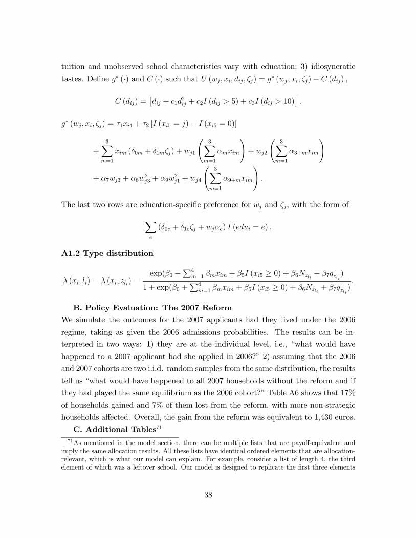
tuition and unobserved school characteristics vary with education; 3) idiosyncratic

tastes. Define g∗ (·) and C (·) such that U (wj, xi, dij, ζj) = g∗ (wj, xi, ζj)− C (dij) ,

C (dij) =[dij + c1d

2ij + c2I (dij > 5) + c3I (dij > 10)

].

g∗ (wj, xi, ζj) = τ1xi4 + τ2 [I (xi5 = j)− I (xi5 = 0)]

+3∑

m=1

xim (δ0m + δ1mζj) + wj1

(3∑

m=1

αmxim

)+ wj2

(3∑

m=1

α3+mxim

)

+ α7wj3 + α8w2j3 + α9w

2j1 + wj4

(3∑

m=1

α9+mxim

).

The last two rows are education-specific preference for wj and ζj, with the form of∑e

(δ0e + δ1eζj + wjαe) I (edui = e) .

A1.2 Type distribution

λ (xi, li) = λ (xi, zli) =exp(β0 +

∑4m=1 βmxim + β5I (xi5 ≥ 0) + β6Nzli

+ β7qzli)

1 + exp(β0 +∑4

m=1 βmxim + β5I (xi5 ≥ 0) + β6Nzli+ β7qzli

).

B. Policy Evaluation: The 2007 ReformWe simulate the outcomes for the 2007 applicants had they lived under the 2006

regime, taking as given the 2006 admissions probabilities. The results can be in-

terpreted in two ways: 1) they are at the individual level, i.e., “what would have

happened to a 2007 applicant had she applied in 2006?”2) assuming that the 2006

and 2007 cohorts are two i.i.d. random samples from the same distribution, the results

tell us “what would have happened to all 2007 households without the reform and if

they had played the same equilibrium as the 2006 cohort?”Table A6 shows that 17%

of households gained and 7% of them lost from the reform, with more non-strategic

households affected. Overall, the gain from the reform was equivalent to 1,430 euros.

C. Additional Tables71

71As mentioned in the model section, there can be multiple lists that are payoff-equivalent andimply the same allocation results. All these lists have identical ordered elements that are allocation-relevant, which is what our model can explain. For example, consider a list of length 4, the thirdelement of which was a leftover school. Our model is designed to replicate the first three elements

38

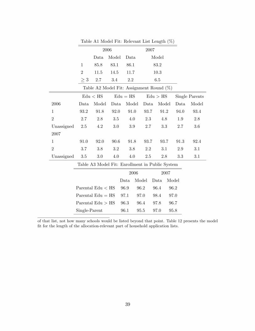
Table A1 Model Fit: Relevant List Length (%)

2006 2007

Data Model Data Model

1 85.8 83.1 86.1 83.2

2 11.5 14.5 11.7 10.3

≥ 3 2.7 3.4 2.2 6.5

Table A2 Model Fit: Assignment Round (%)

Edu < HS Edu = HS Edu > HS Single Parents

2006 Data Model Data Model Data Model Data Model

1 93.2 91.8 92.0 91.0 93.7 91.2 94.0 93.4

2 2.7 2.8 3.5 4.0 2.3 4.8 1.9 2.8

Unassigned 2.5 4.2 3.0 3.9 2.7 3.3 2.7 3.6

2007

1 91.0 92.0 90.6 91.8 93.7 93.7 91.3 92.4

2 3.7 3.8 3.2 3.8 2.2 3.1 2.9 3.1

Unassigned 3.5 3.0 4.0 4.0 2.5 2.8 3.3 3.1

Table A3 Model Fit: Enrollment in Public System

2006 2007

Data Model Data Model

Parental Edu < HS 96.9 96.2 96.4 96.2

Parental Edu = HS 97.1 97.0 98.4 97.0

Parental Edu > HS 96.3 96.4 97.8 96.7

Single-Parent 96.1 95.5 97.0 95.8

of that list, not how many schools would be listed beyond that point. Table 12 presents the modelfit for the length of the allocation-relevant part of household application lists.

39

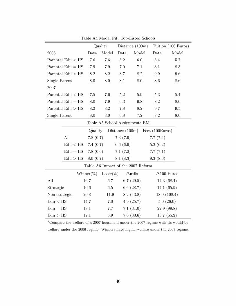
Table A4 Model Fit: Top-Listed Schools

Quality Distance (100m) Tuition (100 Euros)

2006 Data Model Data Model Data Model

Parental Edu < HS 7.6 7.6 5.2 6.0 5.4 5.7

Parental Edu = HS 7.9 7.9 7.0 7.1 8.1 8.3

Parental Edu > HS 8.2 8.2 8.7 8.2 9.9 9.6

Single-Parent 8.0 8.0 8.1 8.0 8.6 8.6

2007

Parental Edu < HS 7.5 7.6 5.2 5.9 5.3 5.4

Parental Edu = HS 8.0 7.9 6.3 6.8 8.2 8.0

Parental Edu > HS 8.2 8.2 7.8 8.2 9.7 9.5

Single-Parent 8.0 8.0 6.8 7.2 8.2 8.0

Table A5 School Assignment: BM

Quality Distance (100m) Fees (100Euros)

All 7.8 (0.7) 7.3 (7.9) 7.7 (7.4)

Edu < HS 7.4 (0.7) 6.6 (6.9) 5.2 (6.2)

Edu = HS 7.8 (0.6) 7.1 (7.2) 7.7 (7.1)

Edu > HS 8.0 (0.7) 8.1 (8.3) 9.3 (8.0)

Table A6 Impact of the 2007 Reform

Winner(%) Loser(%) ∆utils ∆100 Euros

All 16.7 6.7 6.7 (29.5) 14.3 (68.4)

Strategic 16.6 6.5 6.6 (28.7) 14.1 (65.9)

Non-strategic 20.8 11.9 8.2 (43.8) 18.9 (108.4)

Edu < HS 14.7 7.0 4.9 (25.7) 5.0 (26.0)

Edu = HS 18.1 7.7 7.1 (31.0) 22.9 (99.8)

Edu > HS 17.1 5.9 7.6 (30.6) 13.7 (55.2)∗Compare the welfare of a 2007 household under the 2007 regime with its would-be

welfare under the 2006 regime. Winners have higher welfare under the 2007 regime.

40

Structural Estimation of a Model of School Choices: the

Boston Mechanism vs. Its Alternatives (Online Appendix)

Caterina Calsamiglia∗, Chao Fu† and Maia Güell‡

April 16, 2017

1 Backward Induction Solution Method

The backward induction solution method is applicable to a broad class of mechanisms, which

includes BM, constrained and unconstrained DA, first preference first, Chinese parallel, and

variants or hybrids of the above.1 In the following, we refer to this class as the class under

consideration. This section is organized as follows. First, we prove that backward induction

method fully solves the optimization problem for strategic households. Second, we show how

one can apply this method to mechanisms other than BM in the class under consideration.

Then, we formally describe the dimensionality involved in the solution.

1.1 Proof

In the following, we prove that our solution method solves a strategic household’s problem

fully, using the standard BM as an example. The proof is easily adaptable to other mech-

anisms in the class under consideration. Proofs for these other cases are available upon

request.

Proposition 1 Consider a standard Boston Mechanism where a household can choose up

to R schools out of J , who is given a vector of school-specific priorities(Si ≡ sijJj=1

)and

a random lottery number that is used in all rounds. Let vij be the value of being assigned to

School j for Household i, let χi be the vector of preference-related variables (e.g., household

characteristics, location and tastes), let π (Si, χi, A) be the expected payoff from listing A.

∗CEMFI and Barcelona GSE.†Corresponding author: Chao Fu, University of Wisconsin-Madison. cfu@ssc.wisc.edu.‡University of Edinburgh, CEP(LSE), CEPR, FEDEA, & IZA.1Particular variants of the discussed algorithms can be characterized in a similar fashion, e.g., the mech-

anism in Cambridge, serial dictatorship and the Pan London Admissions.

1

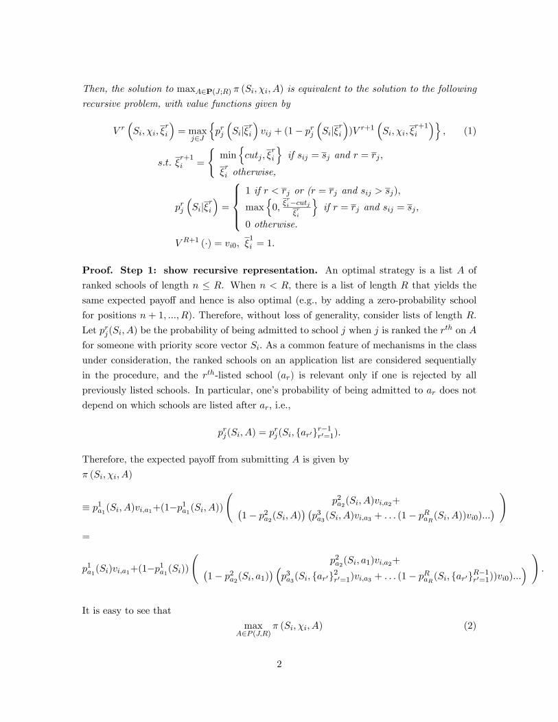
Then, the solution to maxA∈P(J ;R) π (Si, χi, A) is equivalent to the solution to the following

recursive problem, with value functions given by

V r(Si, χi, ξ

ri

)= max

j∈J

prj

(Si|ξ

ri

)vij + (1− prj

(Si|ξ

ri

))V r+1

(Si, χi, ξ

r+1i

), (1)

s.t. ξr+1i =

min

cutj , ξ

ri

if sij = sj and r = rj ,

ξri otherwise,

prj

(Si|ξ

ri

)=

1 if r < rj or (r = rj and sij > sj),

max

0,ξri−cutjξri

if r = rj and sij = sj ,

0 otherwise.

V R+1 (·) = vi0, ξ1i = 1.

Proof. Step 1: show recursive representation. An optimal strategy is a list A of

ranked schools of length n ≤ R. When n < R, there is a list of length R that yields the

same expected payoff and hence is also optimal (e.g., by adding a zero-probability school

for positions n + 1, ..., R). Therefore, without loss of generality, consider lists of length R.

Let prj(Si, A) be the probability of being admitted to school j when j is ranked the rth on A

for someone with priority score vector Si. As a common feature of mechanisms in the class

under consideration, the ranked schools on an application list are considered sequentially

in the procedure, and the rth-listed school (ar) is relevant only if one is rejected by all

previously listed schools. In particular, one’s probability of being admitted to ar does not

depend on which schools are listed after ar, i.e.,

prj(Si, A) = prj(Si, ar′r−1r′=1).

Therefore, the expected payoff from submitting A is given by

π (Si, χi, A)

≡ p1a1(Si, A)vi,a1+(1−p1

a1(Si, A))

(p2a2(Si, A)vi,a2+(

1− p2a2(Si, A)

) (p3a3(Si, A)vi,a3 + . . . (1− pRaR(Si, A))vi0)...

) )=

p1a1(Si)vi,a1+(1−p1

a1(Si))

(p2a2(Si, a1)vi,a2+(

1− p2a2(Si, a1)

) (p3a3(Si, ar′

2r′=1)vi,a3 + . . . (1− pRaR(Si, ar′R−1

r′=1))vi0)...) ) .

It is easy to see that

maxA∈P (J,R)

π (Si, χi, A) (2)

2

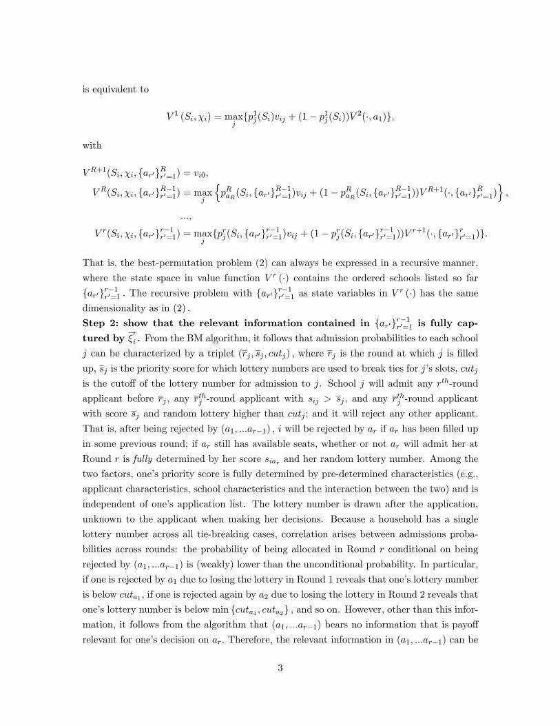
is equivalent to

V 1 (Si, χi) = maxjp1j (Si)vij + (1− p1

j (Si))V2(·, a1),

with

V R+1(Si, χi, ar′Rr′=1) = vi0,

V R(Si, χi, ar′R−1r′=1) = max

j

pRaR(Si, ar′R−1

r′=1)vij + (1− pRaR(Si, ar′R−1r′=1))V R+1(·, ar′Rr′=1)

,

...,

V r(Si, χi, ar′r−1r′=1) = max

jprj(Si, ar′

r−1r′=1)vij + (1− prj(Si, ar′

r−1r′=1))V r+1(·, ar′rr′=1).

That is, the best-permutation problem (2) can always be expressed in a recursive manner,

where the state space in value function V r (·) contains the ordered schools listed so farar′r−1

r′=1 . The recursive problem with ar′r−1r′=1 as state variables in V

r (·) has the samedimensionality as in (2) .

Step 2: show that the relevant information contained in ar′r−1r′=1 is fully cap-

tured by ξri . From the BM algorithm, it follows that admission probabilities to each school

j can be characterized by a triplet (rj , sj , cutj) , where rj is the round at which j is filled

up, sj is the priority score for which lottery numbers are used to break ties for j’s slots, cutjis the cutoff of the lottery number for admission to j. School j will admit any rth-round

applicant before rj , any rthj -round applicant with sij > sj , and any rthj -round applicant

with score sj and random lottery higher than cutj ; and it will reject any other applicant.

That is, after being rejected by (a1, ...ar−1) , i will be rejected by ar if ar has been filled up

in some previous round; if ar still has available seats, whether or not ar will admit her at

Round r is fully determined by her score siar and her random lottery number. Among the

two factors, one’s priority score is fully determined by pre-determined characteristics (e.g.,

applicant characteristics, school characteristics and the interaction between the two) and is

independent of one’s application list. The lottery number is drawn after the application,

unknown to the applicant when making her decisions. Because a household has a single

lottery number across all tie-breaking cases, correlation arises between admissions proba-

bilities across rounds: the probability of being allocated in Round r conditional on being

rejected by (a1, ...ar−1) is (weakly) lower than the unconditional probability. In particular,

if one is rejected by a1 due to losing the lottery in Round 1 reveals that one’s lottery number

is below cuta1 , if one is rejected again by a2 due to losing the lottery in Round 2 reveals that

one’s lottery number is below min cuta1 , cuta2 , and so on. However, other than this infor-mation, it follows from the algorithm that (a1, ...ar−1) bears no information that is payoff

relevant for one’s decision on ar. Therefore, the relevant information in (a1, ...ar−1) can be

3

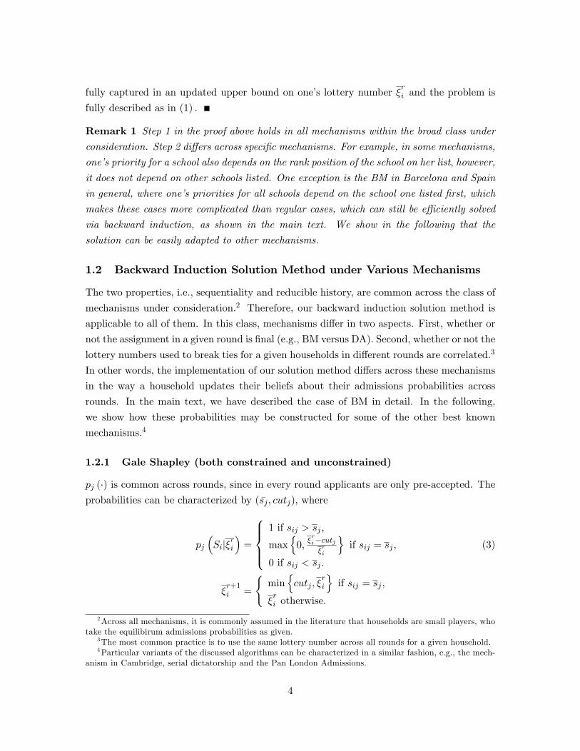
fully captured in an updated upper bound on one’s lottery number ξri and the problem is

fully described as in (1) .

Remark 1 Step 1 in the proof above holds in all mechanisms within the broad class underconsideration. Step 2 differs across specific mechanisms. For example, in some mechanisms,

one’s priority for a school also depends on the rank position of the school on her list, however,

it does not depend on other schools listed. One exception is the BM in Barcelona and Spain

in general, where one’s priorities for all schools depend on the school one listed first, which

makes these cases more complicated than regular cases, which can still be effi ciently solved

via backward induction, as shown in the main text. We show in the following that the

solution can be easily adapted to other mechanisms.

1.2 Backward Induction Solution Method under Various Mechanisms

The two properties, i.e., sequentiality and reducible history, are common across the class of

mechanisms under consideration.2 Therefore, our backward induction solution method is

applicable to all of them. In this class, mechanisms differ in two aspects. First, whether or

not the assignment in a given round is final (e.g., BM versus DA). Second, whether or not the

lottery numbers used to break ties for a given households in different rounds are correlated.3

In other words, the implementation of our solution method differs across these mechanisms

in the way a household updates their beliefs about their admissions probabilities across

rounds. In the main text, we have described the case of BM in detail. In the following,

we show how these probabilities may be constructed for some of the other best known

mechanisms.4

1.2.1 Gale Shapley (both constrained and unconstrained)

pj (·) is common across rounds, since in every round applicants are only pre-accepted. Theprobabilities can be characterized by (sj , cutj), where

pj

(Si|ξ

ri

)=

1 if sij > sj ,

max

0,ξri−cutjξri

if sij = sj ,

0 if sij < sj .

(3)

ξr+1i =

min

cutj , ξ

ri

if sij = sj ,

ξri otherwise.

2Across all mechanisms, it is commonly assumed in the literature that households are small players, whotake the equilibirum admissions probabilities as given.

3The most common practice is to use the same lottery number across all rounds for a given household.4Particular variants of the discussed algorithms can be characterized in a similar fashion, e.g., the mech-

anism in Cambridge, serial dictatorship and the Pan London Admissions.

4

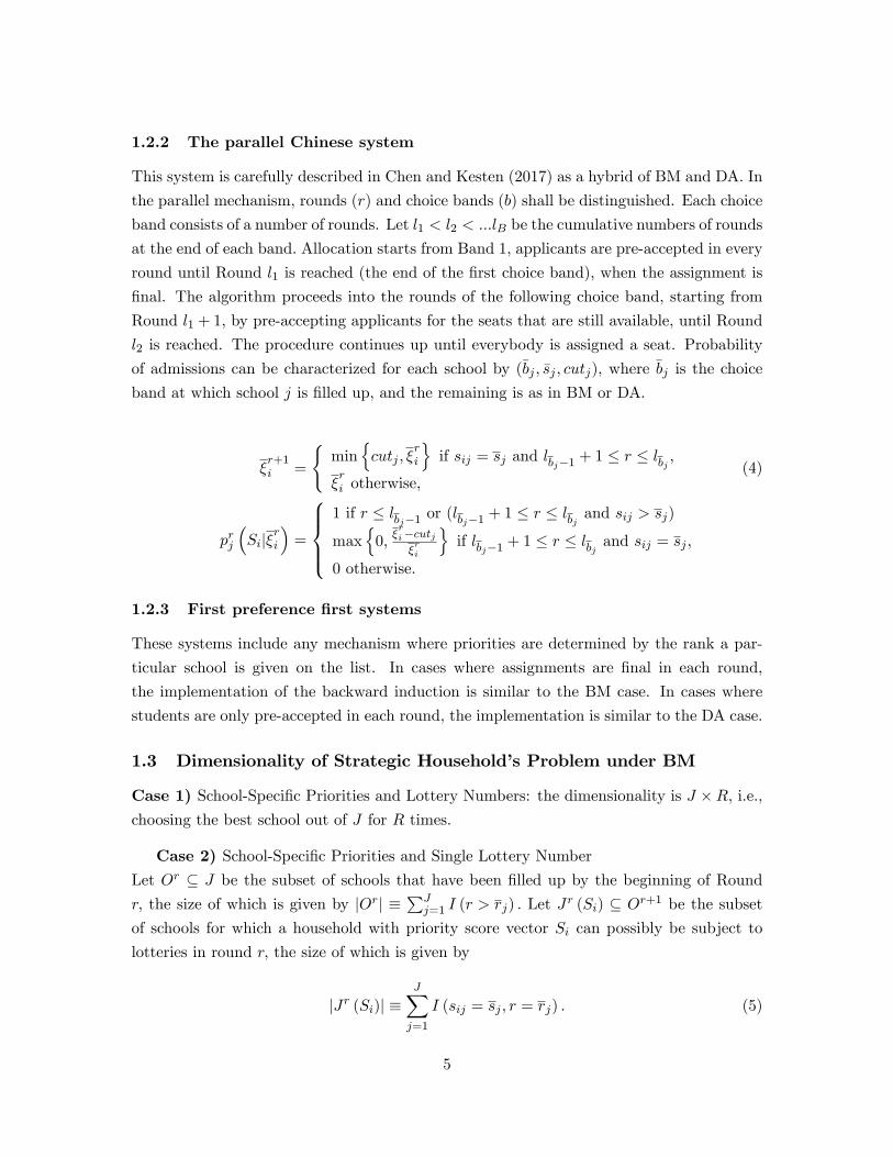
1.2.2 The parallel Chinese system

This system is carefully described in Chen and Kesten (2017) as a hybrid of BM and DA. In

the parallel mechanism, rounds (r) and choice bands (b) shall be distinguished. Each choice

band consists of a number of rounds. Let l1 < l2 < ...lB be the cumulative numbers of rounds

at the end of each band. Allocation starts from Band 1, applicants are pre-accepted in every

round until Round l1 is reached (the end of the first choice band), when the assignment is

final. The algorithm proceeds into the rounds of the following choice band, starting from

Round l1 + 1, by pre-accepting applicants for the seats that are still available, until Round

l2 is reached. The procedure continues up until everybody is assigned a seat. Probability

of admissions can be characterized for each school by (bj , sj , cutj), where bj is the choice

band at which school j is filled up, and the remaining is as in BM or DA.

ξr+1i =

min

cutj , ξ

ri

if sij = sj and lbj−1 + 1 ≤ r ≤ lbj ,

ξri otherwise,

(4)

prj

(Si|ξ

ri

)=

1 if r ≤ lbj−1 or (lbj−1 + 1 ≤ r ≤ lbj and sij > sj)

max

0,ξri−cutjξri

if lbj−1 + 1 ≤ r ≤ lbj and sij = sj ,

0 otherwise.

1.2.3 First preference first systems

These systems include any mechanism where priorities are determined by the rank a par-

ticular school is given on the list. In cases where assignments are final in each round,

the implementation of the backward induction is similar to the BM case. In cases where

students are only pre-accepted in each round, the implementation is similar to the DA case.

1.3 Dimensionality of Strategic Household’s Problem under BM

Case 1) School-Specific Priorities and Lottery Numbers: the dimensionality is J ×R, i.e.,choosing the best school out of J for R times.

Case 2) School-Specific Priorities and Single Lottery NumberLet Or ⊆ J be the subset of schools that have been filled up by the beginning of Round

r, the size of which is given by |Or| ≡∑J

j=1 I (r > rj) . Let Jr (Si) ⊆ Or+1 be the subset

of schools for which a household with priority score vector Si can possibly be subject to

lotteries in round r, the size of which is given by

|Jr (Si)| ≡J∑j=1

I (sij = sj , r = rj) . (5)

5

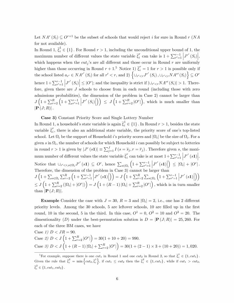
Let NAr (Si) ⊆ Or+1 be the subset of schools that would reject i for sure in Round r (NA

for not available).

In Round 1, ξ1i ∈ 1 . For Round r > 1, including the unconditional upper bound of 1, the

maximum number of different values the state variable ξri can take is 1 +

∑r−1r′=1

∣∣∣Jr′ (Si)∣∣∣,which happens when the cutj’s are all different and those occur in Round r are uniformly

higher than those occurring in Round r + 1.5 Notice 1) ξri = 1 for r > 1 is possible only if

the school listed ar′ ∈ NAr′(Si) for all r′ < r, and 2)

∪r′<rJr

′(Si) ,∪r′<rNAr′ (Si)

⊆ Or

hence 1+∑r−1

r′=1

∣∣∣Jr′ (Si)∣∣∣ ≤ |Or|; and the inequality is strict if |∪r′<rNAr′ (Si)| > 1. There-

fore, given there are J schools to choose from in each round (including those with zero

admissions probabilities), the dimension of the problem in Case 2) cannot be larger than

J(

1 +∑R

r=2

(1 +

∑r−1r′=1

∣∣∣Jr′ (Si)∣∣∣)) ≤ J(

1 +∑R

r=2 |Or|), which is much smaller than

|P (J ;R)| .

Case 3) Constant Priority Score and Single Lottery NumberIn Round 1, a household’s state variable is again ξ

1i ∈ 1 . In Round r > 1, besides the state

variable ξri , there is also an additional state variable, the priority score of one’s top-listed

school. Let Ωi be the support of Household i’s priority scores and |Ωi| be the size of Ωi. For a

given s in Ωi, the number of schools for which Household i can possibly be subject to lotteries

in round r > 1 is given by |Jr (s1)| ≡∑J

j=1 I (s = sj , r = rj) . Therefore given s, the maxi-

mum number of different values the state variable ξri can take is at most 1+

∑r−1r′=1

∣∣∣Jr′ (s1)∣∣∣.

Notice that ∪r′<r,s∈ΩiJr′ (s1) ⊆ Or, hence

∑s∈Ωi

(1 +

∑r−1r′=1

∣∣∣Jr′ (s1)∣∣∣) ≤ |Ωi| + |Or| .

Therefore, the dimension of the problem in Case 3) cannot be larger than

J(

1 +∑

s∈Ωi

∑Rr=2

(1 +

∑r−1r′=1

∣∣∣Jr′ (s1)∣∣∣)) = J

(1 +

∑Rr=2

∑s∈Ωi

(1 +

∑r−1r′=1

∣∣∣Jr′ (s1)∣∣∣))

≤ J(

1 +∑R

r=2 (|Ωi|+ |Or|))

= J(

1 + (R− 1) |Ωi|+∑R

r=2 |Or|), which is in turn smaller

than |P (J ;R)|.

Example Consider the case with J = 30, R = 3 and |Ωi| = 2, i.e., one has 2 different

priority levels. Among the 30 schools, 5 are leftover schools, 10 are filled up in the first

round, 10 in the second, 5 in the third. In this case, O1 = 0, O2 = 10 and O3 = 20. The

dimentionality (D) under the best-permutation solution is D = |P (J ;R)| = 25, 260. For

each of the three BM cases, we have

Case 1) D < JR = 90.

Case 2) D < J(

1 +∑R

r=2 |Or|)

= 30(1 + 10 + 20) = 990.

Case 3) D < J(

1 + (R− 1) |Ωi|+∑R

r=2 |Or|)

= 30(1 + (2− 1)× 3 + (10 + 20)) = 1, 020.

5For example, suppose there is one cut1 in Round 1 and one cut2 in Round 2, so that ξ1

i ∈ 1, cut1 .Given the rule that ξ

2

i = mincut2, ξ

1

i

, if cut1 ≤ cut2 then the ξ

2

i ∈ 1, cut1 , while if cut1 > cut2,

ξ2

i ∈ 1, cut1, cut2 .

6

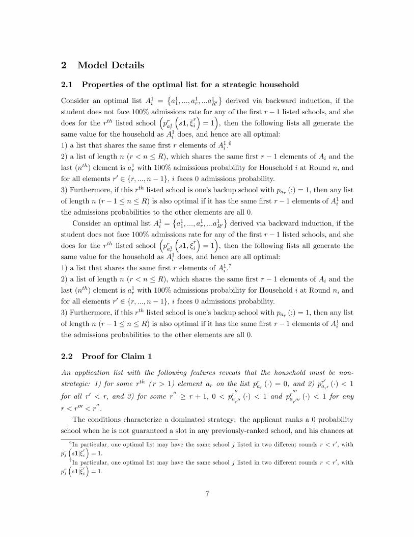
2 Model Details

2.1 Properties of the optimal list for a strategic household

Consider an optimal list A1i =

a1

1, ..., a1r , ...a

1R′derived via backward induction, if the

student does not face 100% admissions rate for any of the first r− 1 listed schools, and she

does for the rth listed school(pra1r

(s1, ξ

ri

)= 1), then the following lists all generate the

same value for the household as A1i does, and hence are all optimal:

1) a list that shares the same first r elements of A1i .6

2) a list of length n (r < n ≤ R), which shares the same first r − 1 elements of Ai and the

last (nth) element is a1r with 100% admissions probability for Household i at Round n, and

for all elements r′ ∈ r, ..., n− 1, i faces 0 admissions probability.

3) Furthermore, if this rth listed school is one’s backup school with par (:) = 1, then any list

of length n (r− 1 ≤ n ≤ R) is also optimal if it has the same first r− 1 elements of A1i and

the admissions probabilities to the other elements are all 0.

Consider an optimal list A1i =

a1

1, ..., a1r , ...a

1R′derived via backward induction, if the

student does not face 100% admissions rate for any of the first r− 1 listed schools, and she

does for the rth listed school(pra1r

(s1, ξ

ri

)= 1), then the following lists all generate the

same value for the household as A1i does, and hence are all optimal:

1) a list that shares the same first r elements of A1i .7

2) a list of length n (r < n ≤ R), which shares the same first r − 1 elements of Ai and the

last (nth) element is a1r with 100% admissions probability for Household i at Round n, and

for all elements r′ ∈ r, ..., n− 1, i faces 0 admissions probability.

3) Furthermore, if this rth listed school is one’s backup school with par (:) = 1, then any list

of length n (r− 1 ≤ n ≤ R) is also optimal if it has the same first r− 1 elements of A1i and

the admissions probabilities to the other elements are all 0.

2.2 Proof for Claim 1

An application list with the following features reveals that the household must be non-

strategic: 1) for some rth ( r > 1) element ar on the list prar (·) = 0, and 2) pr′ar′

(·) < 1

for all r′ < r, and 3) for some r′′ ≥ r + 1, 0 < pr

′′

ar′′ (·) < 1 and pr

′′′

ar′′′ (·) < 1 for any

r < r′′′ < r′′.

The conditions characterize a dominated strategy: the applicant ranks a 0 probability

school when he is not guaranteed a slot in any previously-ranked school, and his chances at

6 In particular, one optimal list may have the same school j listed in two different rounds r < r′, with

prj

(s1|ξri

)= 1.

7 In particular, one optimal list may have the same school j listed in two different rounds r < r′, with

prj

(s1|ξri

)= 1.

7

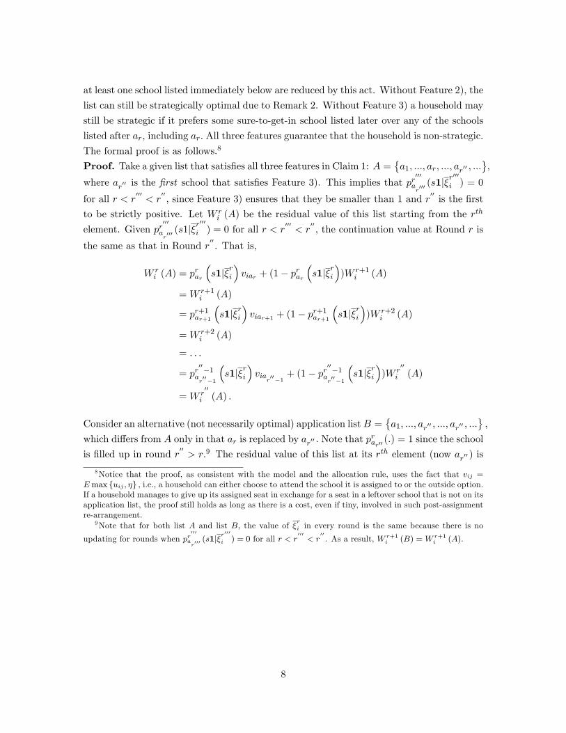
at least one school listed immediately below are reduced by this act. Without Feature 2), the

list can still be strategically optimal due to Remark 2. Without Feature 3) a household may

still be strategic if it prefers some sure-to-get-in school listed later over any of the schools

listed after ar, including ar. All three features guarantee that the household is non-strategic.

The formal proof is as follows.8

Proof. Take a given list that satisfies all three features in Claim 1: A =a1, ..., ar, ..., ar′′ , ...

,

where ar′′ is the first school that satisfies Feature 3). This implies that pr′′′

ar′′′ (s1|ξ

r′′′

i ) = 0

for all r < r′′′< r

′′, since Feature 3) ensures that they be smaller than 1 and r

′′is the first

to be strictly positive. Let W ri (A) be the residual value of this list starting from the rth

element. Given pr′′′

ar′′′ (s1|ξ

r′′′

i ) = 0 for all r < r′′′< r

′′, the continuation value at Round r is

the same as that in Round r′′. That is,

W ri (A) = prar

(s1|ξri

)viar + (1− prar

(s1|ξri

))W r+1

i (A)

= W r+1i (A)

= pr+1ar+1

(s1|ξri

)viar+1 + (1− pr+1

ar+1

(s1|ξri

))W r+2

i (A)

= W r+2i (A)

= . . .

= pr′′−1ar′′−1

(s1|ξri

)via

r′′−1

+ (1− pr′′−1ar′′−1

(s1|ξri

))W r

′′

i (A)

= W r′′

i (A) .

Consider an alternative (not necessarily optimal) application listB =a1, ..., ar′′ , ..., ar′′ , ...

,

which differs from A only in that ar is replaced by ar′′ . Note that prar′′

(.) = 1 since the school

is filled up in round r′′> r.9 The residual value of this list at its rth element (now ar′′ ) is

8Notice that the proof, as consistent with the model and the allocation rule, uses the fact that vij =Emax uij , η , i.e., a household can either choose to attend the school it is assigned to or the outside option.If a household manages to give up its assigned seat in exchange for a seat in a leftover school that is not on itsapplication list, the proof still holds as long as there is a cost, even if tiny, involved in such post-assignmentre-arrangement.

9Note that for both list A and list B, the value of ξr

i in every round is the same because there is no

updating for rounds when pr′′′

ar′′′ (s1|ξ

r′′′

i ) = 0 for all r < r′′′< r

′′. As a result, W r+1

i (B) =W r+1i (A).

8

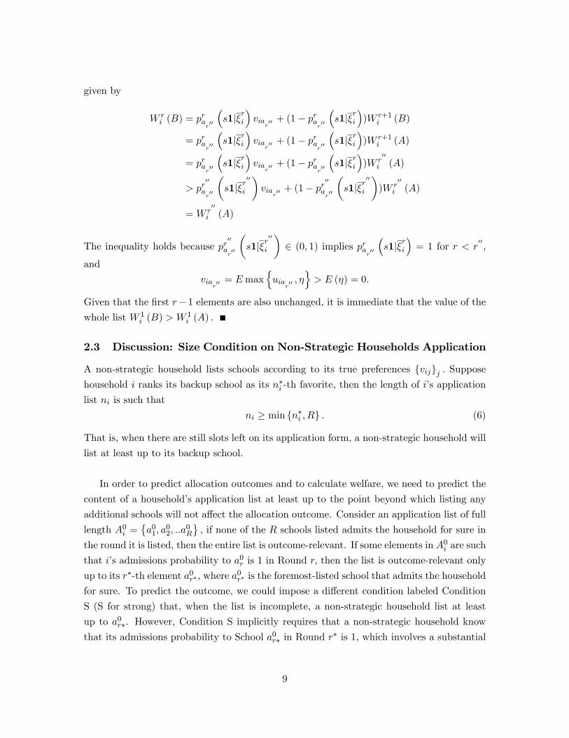
given by

W ri (B) = pra

r′′

(s1|ξri

)via

r′′ + (1− pra

r′′

(s1|ξri

))W r+1

i (B)

= prar′′

(s1|ξri

)via

r′′ + (1− pra

r′′

(s1|ξri

))W r+1

i (A)

= prar′′

(s1|ξri

)via

r′′ + (1− pra

r′′

(s1|ξri

))W r

′′

i (A)

> pr′′

ar′′

(s1|ξr

′′

i

)via

r′′ + (1− pr

′′

ar′′

(s1|ξr

′′

i

))W r

′′

i (A)

= W r′′

i (A)

The inequality holds because pr′′

ar′′

(s1|ξr

′′

i

)∈ (0, 1) implies pra

r′′

(s1|ξri

)= 1 for r < r

′′,

and

viar′′ = Emax

uia

r′′ , η> E (η) = 0.

Given that the first r− 1 elements are also unchanged, it is immediate that the value of the

whole list W 1i (B) > W 1

i (A) .

2.3 Discussion: Size Condition on Non-Strategic Households Application

A non-strategic household lists schools according to its true preferences vijj . Supposehousehold i ranks its backup school as its n∗i -th favorite, then the length of i’s application

list ni is such that

ni ≥ min n∗i , R . (6)

That is, when there are still slots left on its application form, a non-strategic household will

list at least up to its backup school.

In order to predict allocation outcomes and to calculate welfare, we need to predict the

content of a household’s application list at least up to the point beyond which listing any

additional schools will not affect the allocation outcome. Consider an application list of full

length A0i =

a0

1, a02, ..a

0R

, if none of the R schools listed admits the household for sure in

the round it is listed, then the entire list is outcome-relevant. If some elements in A0i are such

that i’s admissions probability to a0r is 1 in Round r, then the list is outcome-relevant only

up to its r∗-th element a0r∗ , where a

0r∗ is the foremost-listed school that admits the household

for sure. To predict the outcome, we could impose a different condition labeled Condition

S (S for strong) that, when the list is incomplete, a non-strategic household list at least

up to a0r∗. However, Condition S implicitly requires that a non-strategic household know

that its admissions probability to School a0r∗ in Round r

∗ is 1, which involves a substantial

9

amount of sophistication. In comparison, Condition (6) is a much weaker requirement that

a non-strategic household know which schools will be leftovers and list at least up to its

backup school. It requires far less sophistication than to know the admissions probabilities

by school and by round.10 One reason is the high persistence in whether or not a school

was left over, which was true even between the two years before and after the drastic re-

definition of priority zones: 265 out of the 317 schools were either left over twice or never left

over in the years of 2006 and 2007. Such high persistence makes it easy to predict the set

of leftover schools. Therefore, it may be reasonable to believe that even the non-strategic

households may have this (minimal) level of sophistication. With this weak requirement,

Condition (6) achieves the same goal as Condition S.11

3 Identification

In this section, we will first prove the identification of our model in its simplified version.

Then, we will give more intuition by contrasting the original model with a re-estimated

model, the latter imposing that a lower fraction of households be strategic. Finally, we will

discuss the exclusion restriction.

3.1 Proof

Since the dispersion of post-application shocks is mainly identified from the enrollment

decisions, to ease the illustration, we show the identification of the model without post-

application shocks. A household has observables (xi, li) and can be one of two types T = 0, 1.

Home-school distance is given by dji = d (li, lj) and zli is the zone that li belongs. Let the

taste for school be εij ∼ i.i.d. N(0, 1).12 In line with (A2) and (A3) in the paper, assume

that d is independent of T conditional on (x, zl) and ε is independent of (x, l, T ) . To give

10 In this model, we have assumed that it is free to fill in the application and, if failing to be assignedwithin R rounds, to propose a leftover school. Given the knowledge of the set of leftover schools and thatleftover schools have 100% admissions probabilities, a non-strategic household would be indifferent betweenadding or not adding its backup school to an incomplete list. Condition (6) specifies that, if indifferent, anon-strategic household will add its backup school. It is also consistent with a situation where the cost ofproposing a leftover school after being rejected in all rounds is higher than listing one more school to one’slist.11To see why Condition (6) achieves the same goal as its much stronger counterpart, consider the following

exhaustive cases. Case 1: None of its R favorite schools admits the household for sure. Both ConditionS and Condition (6) require the same full list of length R. Case 2: At least one of its R favorite schoolsadmits the household for sure. By definition, a backup school admits the student for sure and thereforer∗ ≤ n∗i . If r

∗ < n∗i , i.e., the first sure-to-get school is preferrable to the backup: lengthening the list to n∗i

will not change the outcome, because only the first r∗ elements are outcome-relevant. If r∗ = n∗i , then bothconditions lead to the same list.12Given that the linear distance enters the utility function with coeffi cient of minus one, the standard

deviation of ε is identified from the variation in distance within (x, zl) group. To simplify the notation, wewill present the case where σε is normalized to 1.

10

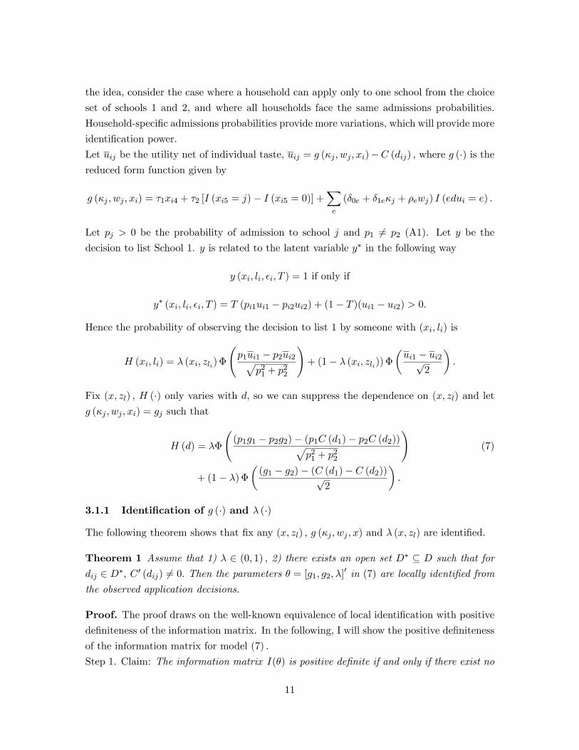
the idea, consider the case where a household can apply only to one school from the choice

set of schools 1 and 2, and where all households face the same admissions probabilities.

Household-specific admissions probabilities provide more variations, which will provide more

identification power.

Let uij be the utility net of individual taste, uij = g (κj , wj , xi)−C (dij) , where g (·) is thereduced form function given by

g (κj , wj , xi) = τ1xi4 + τ2 [I (xi5 = j)− I (xi5 = 0)] +∑e

(δ0e + δ1eκj + ρewj) I (edui = e) .

Let pj > 0 be the probability of admission to school j and p1 6= p2 (A1). Let y be the

decision to list School 1. y is related to the latent variable y∗ in the following way

y (xi, li, εi, T ) = 1 if only if

y∗ (xi, li, εi, T ) = T (pi1ui1 − pi2ui2) + (1− T )(ui1 − ui2) > 0.

Hence the probability of observing the decision to list 1 by someone with (xi, li) is

H (xi, li) = λ (xi, zli) Φ

(p1ui1 − p2ui2√

p21 + p2

2

)+ (1− λ (xi, zli)) Φ

(ui1 − ui2√

2

).

Fix (x, zl) , H (·) only varies with d, so we can suppress the dependence on (x, zl) and let

g (κj , wj , xi) = gj such that

H (d) = λΦ

((p1g1 − p2g2)− (p1C (d1)− p2C (d2))√

p21 + p2

2

)(7)

+ (1− λ) Φ

((g1 − g2)− (C (d1)− C (d2))√

2

).

3.1.1 Identification of g (·) and λ (·)

The following theorem shows that fix any (x, zl) , g (κj , wj , x) and λ (x, zl) are identified.

Theorem 1 Assume that 1) λ ∈ (0, 1) , 2) there exists an open set D∗ ⊆ D such that for

dij ∈ D∗, C ′ (dij) 6= 0. Then the parameters θ = [g1, g2, λ]′ in (7) are locally identified from

the observed application decisions.

Proof. The proof draws on the well-known equivalence of local identification with positivedefiniteness of the information matrix. In the following, I will show the positive definiteness

of the information matrix for model (7) .

Step 1. Claim: The information matrix I(θ) is positive definite if and only if there exist no

11

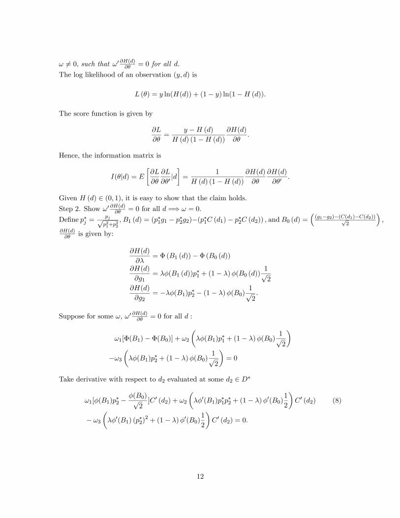
ω 6= 0, such that ω′ ∂H(d)∂θ = 0 for all d.

The log likelihood of an observation (y, d) is

L (θ) = y ln(H(d)) + (1− y) ln(1−H (d)).

The score function is given by

∂L

∂θ=

y −H (d)

H (d) (1−H (d))

∂H(d)

∂θ.

Hence, the information matrix is

I(θ|d) = E

[∂L

∂θ

∂L

∂θ′|d]

=1

H (d) (1−H (d))

∂H(d)

∂θ

∂H(d)

∂θ′.

Given H (d) ∈ (0, 1), it is easy to show that the claim holds.

Step 2. Show ω′ ∂H(d)∂θ = 0 for all d =⇒ ω = 0.

Define p∗j =pj√p21+p22

, B1 (d) = (p∗1g1 − p∗2g2)−(p∗1C (d1)− p∗2C (d2)) , andB0 (d) =(

(g1−g2)−(C(d1)−C(d2))√2

),

∂H(d)∂θ is given by:

∂H(d)

∂λ= Φ (B1 (d))− Φ (B0 (d))

∂H(d)

∂g1= λφ(B1 (d))p∗1 + (1− λ)φ(B0 (d))

1√2

∂H(d)

∂g2= −λφ(B1)p∗2 − (1− λ)φ(B0)

1√2.

Suppose for some ω, ω′ ∂H(d)∂θ = 0 for all d :

ω1[Φ(B1)− Φ(B0)] + ω2

(λφ(B1)p∗1 + (1− λ)φ(B0)

1√2

)−ω3

(λφ(B1)p∗2 + (1− λ)φ(B0)

1√2

)= 0

Take derivative with respect to d2 evaluated at some d2 ∈ D∗

ω1[φ(B1)p∗2 −φ(B0)√

2]C ′ (d2) + ω2

(λφ′(B1)p∗1p

∗2 + (1− λ)φ′(B0)

1

2

)C ′ (d2) (8)

− ω3

(λφ′(B1) (p∗2)2 + (1− λ)φ′(B0)

1

2

)C ′ (d2) = 0.

12

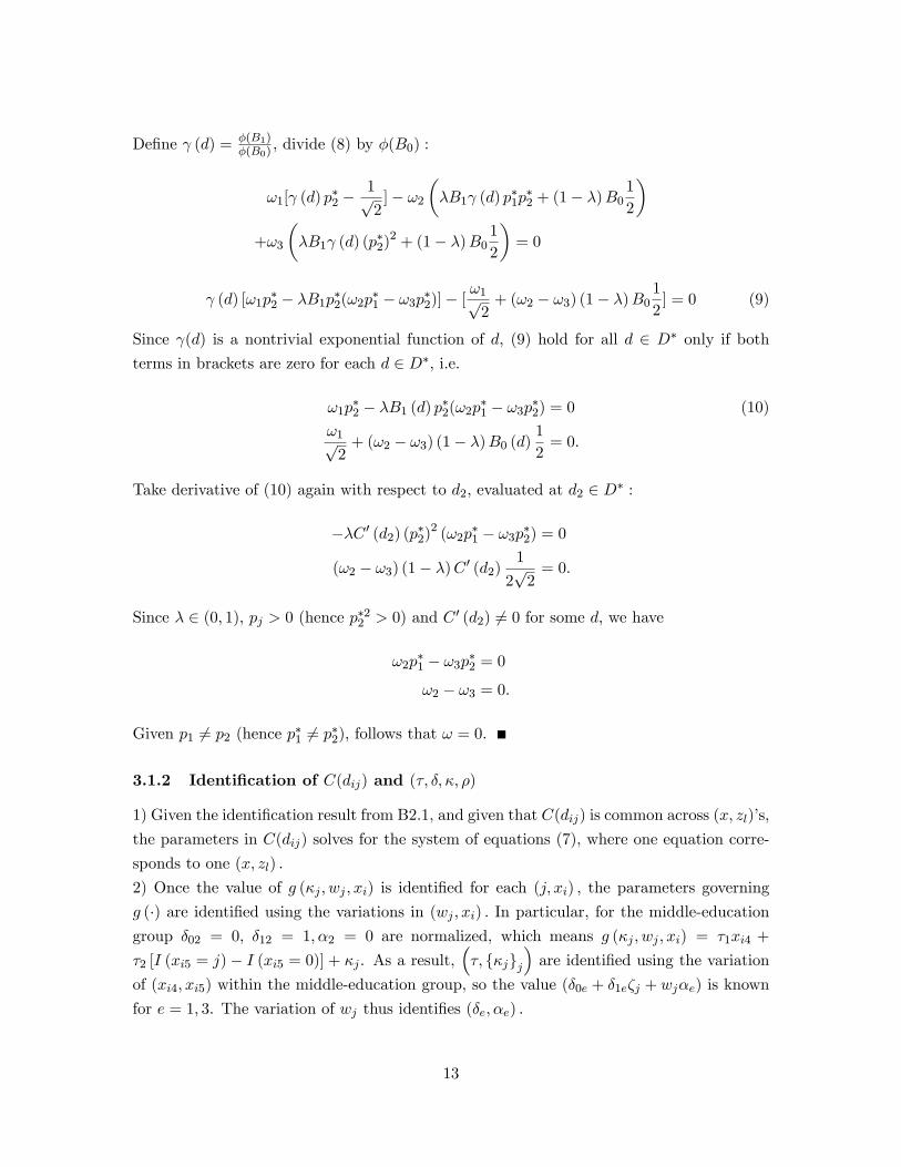
Define γ (d) = φ(B1)φ(B0) , divide (8) by φ(B0) :

ω1[γ (d) p∗2 −1√2

]− ω2

(λB1γ (d) p∗1p

∗2 + (1− λ)B0

1

2

)+ω3

(λB1γ (d) (p∗2)2 + (1− λ)B0

1

2

)= 0

γ (d) [ω1p∗2 − λB1p

∗2(ω2p

∗1 − ω3p

∗2)]− [

ω1√2

+ (ω2 − ω3) (1− λ)B01

2] = 0 (9)

Since γ(d) is a nontrivial exponential function of d, (9) hold for all d ∈ D∗ only if both

terms in brackets are zero for each d ∈ D∗, i.e.

ω1p∗2 − λB1 (d) p∗2(ω2p

∗1 − ω3p

∗2) = 0 (10)

ω1√2

+ (ω2 − ω3) (1− λ)B0 (d)1

2= 0.

Take derivative of (10) again with respect to d2, evaluated at d2 ∈ D∗ :

−λC ′ (d2) (p∗2)2 (ω2p∗1 − ω3p

∗2) = 0

(ω2 − ω3) (1− λ)C ′ (d2)1

2√

2= 0.

Since λ ∈ (0, 1), pj > 0 (hence p∗22 > 0) and C ′ (d2) 6= 0 for some d, we have

ω2p∗1 − ω3p

∗2 = 0

ω2 − ω3 = 0.

Given p1 6= p2 (hence p∗1 6= p∗2), follows that ω = 0.

3.1.2 Identification of C(dij) and (τ, δ, κ, ρ)

1) Given the identification result from B2.1, and given that C(dij) is common across (x, zl)’s,

the parameters in C(dij) solves for the system of equations (7), where one equation corre-

sponds to one (x, zl) .

2) Once the value of g (κj , wj , xi) is identified for each (j, xi) , the parameters governing

g (·) are identified using the variations in (wj , xi) . In particular, for the middle-education

group δ02 = 0, δ12 = 1, α2 = 0 are normalized, which means g (κj , wj , xi) = τ1xi4 +

τ2 [I (xi5 = j)− I (xi5 = 0)] + κj . As a result,(τ, κjj

)are identified using the variation

of (xi4, xi5) within the middle-education group, so the value (δ0e + δ1eζj + wjαe) is known

for e = 1, 3. The variation of wj thus identifies (δe, αe) .

13

3.2 A Model with Fewer Strategic Households

To obtain further insights into our identification, we have re-estimated our model imposing

that a lower fraction of households be strategic. In particular, we have re-estimated all

model parameters other than the type distribution parameters, which are restricted such

that 80% of households are strategic.13 The new estimates are reported in Tables B5 and

B6. The differences between the original parameter estimates and those from this new

model are intuitive. For example, the cost of distance becomes more convex and the taste

dispersion increases. These findings are intuitive, schools with shorter distance are more

likely to be in-zone (high-priority) schools; when fewer households are strategic, preferences

for shorter distance need to be stronger in order to explain why households listed in-zone

schools. Similarly, larger taste dispersion helps explain why they left out schools that look

better than those on their application lists. Table B7 shows the in-sample (2006) fit of this

model alongside with the original model fit. Given that the new model has fewer degrees of

freedom, the fit is naturally worse. However, the comparison reveals some intuition behind

the identification of our model. For example, with fewer strategic households, the new

model over-predicts the fraction of households top-listing schools that are not in their zones

(Row 2); similarly, it underpredicts the fraction of households assigned in Round 1 and

overpredicts the fraction unassigned.

3.3 The Exclusion Restriction

Although types are usually unobservable, they are observed for the group of obviously

naive households. We utilize this data feature to provide some supporting evidence for our

assumption that distance enters preferences but not type distribution (conditional on zone

characterisitics). In particular, we test whether or not obvious naivety is correlated with

distance measures. At least, the two sets of regressions suggest that our exclusion restriction

may not be unreasonable.

First, we run the following regression

naivei = α1dneari + α2q

neari + α3n

500mi + α4n

1kmi + α5n

2kmi + α6d

avei +XiB1 + ZiB2,

where naivei = 1 if i is obviously naive, dneari is the distance to the school that is closest to

i, qneari is the quality of this school. n500mi , n1km

i , n2kmi are the number of schools within 500

meters, 1 km and 2 km, respectively. davei is the average school-home distance across all

in-zone schools for i. Xi is the vector of household observable characteristics, and Zi is the

vector of characteristics of the zone i lives in. As Table B8 shows, none of the α coeffi cients

13 In particular, we adjusted the constant in type distribution λ (xi, li) such that 80% of all households arestrategic. The fractions by education level from low to high are 72%, 77% and 87% respectively.

14

are significant, nor can one reject the hypothesis that they are jointly insignificant (Prob >

F = 0.7825). That is, naive households are not more or less likely to live closer to a school

(α1) or closer to a better school (α2) , to have more schools nearby (α3 to α5), or to have

lower average distance to in-zone schools (α6).

Second, we run three regressions of the following form

yi = β1I (naivei = 1) +XiA1 + ZiA2.

The dependent variables in the three regressions are 1) whether or not i top-listed the

closest school, 2) whether or not i included the closest school in the application list, and

3) whether or not i top-listed an in-zone school. The Results are shown in Table B9 in the

appendix. β1 is insignificant in 1) and 2), but significantly negative in 3). That is, naive

households are less likely to top-list an in-zone school, for which one has higher priorities, as

is consistent with their naive labels. However, they do not seem to exhibit different tastes

for distance.

4 Data Details

4.1 Priority Score Structure

Case 1: Those who do not have a sibling in school have two levels: xia (xia+ b1) for out-

of-zone (in-zone) schools.

Case 2: Those whose sibling(s) is (are) in in-zone schools have 3 levels: xia (xia+ b1) for

out-of-zone (in-zone) non-sibling schools, and xia+ b1 + b2 for sibling schools.

Case 3: Those whose sibling(s) is (are) in out-of-zone schools have 3 levels: xia (xia+ b1)

for out-of-zone (in-zone) non-sibling schools, and xia+ b2 for sibling schools.

Case 4: Those with sibling(s) in some in-zone school and sibling(s) in some out-of-zone

school have 4 levels: xia (xia+ b1) for out-of-zone (in-zone) non-sibling schools, and xia+b2

(xia+ b1 + b2) for out-of-zone (in-zone) sibling schools.

4.2 Data Sources

The final data set consists of merged data sets from five different administrative units:

the Consorci d’Educacio de Barcelona (local authority handling the choice procedure in

Barcelona), Department d’Ensenyament de Catalunya (Department of Education of Catalunya),

the Consell d’Avaluacio de Catalunya (public agency in charge of evaluating the Catalunya

educational system), the Instituto Nacional de Estadistica (national institute of statistics)

15

and the Institut Catala d’Estadistica (statistics institute of Catalunya).14

From the Consorci d’Educacio de Barcelona, we obtain access to every applicant’s appli-

cation form, as well as the information on the school assignment and enrollment outcomes.

An application form contains the entire list of ranked schools a family submitted. In addi-

tion, it records family information that was used to determine the priority the family had

for various schools (e.g., family address, the existence of a sibling in the first-ranked school

and other relevant family and child characteristics). The geocode in this data set allows us

to compute a family’s distance to each school in the city.

From the Census and local register data, we obtain information on the applicant’s family

background, including parental education and whether or not both parents were registered

in the applicant’s household. Since information on siblings who were not enrolled in the

school the family ranked first is irrelevant in the school assignment procedure, it is not

available from the application data. However, such information is relevant for family’s

application decisions. From the Department of Education, we obtained the enrollment data

for children aged 3 to 18 in Catalunya. This data set is then merged with the local register,

which provides us with the ID of the schools enrolled by each of the applicant’s siblings at

the time of the application.

To measure the quality of schools, we use the external evaluation of students conducted

by Consell d’Avaluacio de Catalunya. Since 2009, such external evaluations have been

imposed on all schools in Catalunya, in which students enrolled in the last year of primary

school are tested on math and language subjects.15 From the 2009 test results that we

obtained, we calculated the average test score across subjects for each student, then use

the average across students in each school as a measure of the school’s quality.16 Finally,

to obtain information on the fees charged by semi-public schools (public schools are free to

attend), we use the survey data collected by the Instituto Nacional de Estadistica.17

14These five different data sources were merged and anonimized by the Institut Catala d’Estadistica(IDESCAT).15As mentioned in the background section, a student has the priority to continue her primary-school

education in the same school (with the same capacity) she enrolled for preschool education, which makesit very unlikely that one can transfer to a better school between preschool-primary school transition. Forexample, at least 94% of the 2010 preschool cohort were still enrolled in the same school for primary schooleducation in 2013.16Following the same rule used in Spanish college admissions, we use unweighted average of scores across

subjects for each student.17See http://www.idescat.cat/cat/idescat/publicacions/cataleg/pdfdocs/dossier13.pdf for a summary of

the survey data.

16

4.3 Data Evidence on Strategic Behavior via Regression Analyses

Using each household-school pair as an observation, we run regressions of the following form

yij = Xiα+ sibijβ1 + dijβ2 + d2ijβ3 + d3

ijβ4 + I(li ∈ zlj

)β5 + µj + εij ,

where yij = 1 if j was i’s top choice, Xi are household characteristics, sibij = 1 if i has

a sibling in School j, dij is school-home distance, I(li ∈ zlj

)= 1 if i lives in School j’s

zone, µj is a school fixed effect, and εij is the error term. The results are shown in Table

B3. Conditional on a third-order polynomial of distance, in-zone status still significantly

increases the choice probability.18

5 The DA and TTC Algorithms

5.1 DA

The DA algorithm assigns students as follows.

Round 1: Each school j tentatively assigns its seats to students who top-listed it, one at

a time following their priority order. If school j is over-demanded, lower-ranked applicants

are rejected.

In general, at Round r: Each school j considers the students it has been holding, together

with students who were rejected in the previous round but listed j as their rth choice. Seats

in school j are tentatively assigned to these students, one at a time following their priority

order. If school j is over-demanded, lower-ranked applicants are rejected.

The algorithm terminates when no student is rejected and each student is assigned her final

tentative assignment.

The key differences between DA and BM are 1) in each round, students are only tem-

porarily assigned to a school until the whole procedure ends; and 2) temporarily held

students are considered based only on priorities along with students who were rejected

from their choices in previous rounds and added into a school’s student pool in the current

round. As such, a previously held student can be crowded out by a newly-added student

who has higher priority. That is, top-listing a school does not improve one’s chance of being

finally admitted to this school, which makes truth-telling a (weakly) dominant strategy for

households under DA. Moreover, DA eliminates justified envy. The appealing properties of

DA, however, may conflict with Pareto effi ciency, as shown by Abdulkadiroglu and Sönmez

18There are 317 observations per household in these regressions. The results are robust when we restrictattention to a smaller number of schools for each household (which always include the applied schools), e.g.,the closest N schools, N randomly drawn schools, all in-zone schools plus N randomly drawn out-of-zoneschools (N = 30, 50, 100).

17

(2003).

5.2 TTC

The TTC algorithm assigns students as follows.

Round 1: Assign a counter for each school which keeps track of how many seats are still

available at the school, initially set to equal the school capacity. Each school points to the

student who has the highest priority for the school. Each student points to her favorite

school under her announced preferences.19 This will create ordered lists of distinct schools

(j) and distinct students (i) : (j1, i1, j2, i2, ....), where j1 points at i1, i1 points at j2, and

j2 points at i2, etc. Because there are finite number of schools, at least one cycle will be

formed, where ik (k ≥ 1) points at j1. Although there may be multiple cycles formed in a

round, each school can be part of at most one cycle and each student can be part of at most

one cycle. Every student in a cycle is assigned a seat at the school she points to and is

removed. The counter of each school in a cycle is reduced by one and if it reduces to zero,

the school is also removed. Counters of all schools that are not in any cycle stay put.

In general, at Round r: Each remaining school points to the student with highest priority

among the remaining students and each remaining student points to her favorite school

among the remaining schools. Every student in a cycle is assigned a seat at the school that

she points to and is removed. The counter of each school in a cycle is reduced by one and

if it reduces to zero the school is also removed. Counters of all other schools stay put.

The algorithm terminates when all students are assigned a seat.

Intuitively, in each round TTC creates cycles of trade between individuals. Each individ-

ual in a cycle trades off a seat in her highest-priority school for a seat in her most preferred

school among those that still have seats. Whenever such a cycle is formed the allocation is

final. Hence, the only way for an individual to improve her allocation is through “stealing”

another individual’s school assignment, which will in turn make this other individual worse

off. As such, TTC is Pareto effi cient as shown by Abdulkadiroglu and Sönmez (2003), who

also prove that TTC is truth-revealing. However, TTC does not eliminate justified envy

because student-school priorities are ignored in the TTC trade between individuals

5.3 BMmay respect cardinal preference better than truth-revealing mech-anisms

The intuition can be explained by the following simple example with equal priorities. Con-

sider three schools and a set of households who share the same ordinal but different cardinal19A student announces her entire list of schools before the assignment starts. As such, the “pointing”by

a student is mechanically following her announced list.

18

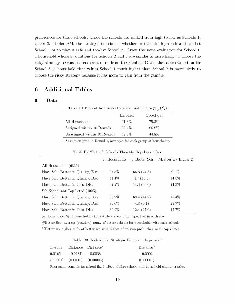
preferences for these schools, where the schools are ranked from high to low as Schools 1,

2 and 3. Under BM, the strategic decision is whether to take the high risk and top-list

School 1 or to play it safe and top-list School 2. Given the same evaluation for School 1,

a household whose evaluations for Schools 2 and 3 are similar is more likely to choose the

risky strategy because it has less to lose from the gamble. Given the same evaluation for

School 3, a household that values School 1 much higher than School 2 is more likely to

choose the risky strategy because it has more to gain from the gamble.

6 Additional Tables

6.1 Data

Table B1 Prob of Admission to one’s First Choice p1ia1

(Si)

Enrolled Opted out

All Households 91.8% 75.3%

Assigned within 10 Rounds 92.7% 86.8%

Unassigned within 10 Rounds 48.5% 44.8%

Admission prob in Round 1, averaged for each group of households.

Table B2 “Better”Schools Than the Top-Listed One

% Households # Better Sch %Better w/ Higher p

All Households (6836)

Have Sch. Better in Quality, Fees 97.5% 66.6 (44.3) 9.1%

Have Sch. Better in Quality, Dist 41.1% 4.7 (10.6) 14.5%

Have Sch. Better in Fees, Dist 62.2% 14.3 (30.6) 24.3%

Sib School not Top-listed (4025)

Have Sch. Better in Quality, Fees 98.2% 69.4 (44.2) 15.4%

Have Sch. Better in Quality, Dist 39.6% 4.3 (9.1) 25.7%

Have Sch. Better in Fees, Dist 60.2% 12.4 (27.0) 42.7%

% Households: % of households that satisfy the condition specified in each row.

#Better Sch: average (std.dev.) num. of better schools for households with such schools.

%Better w/ higher p: % of better sch with higher admission prob. than one’s top choice.

Table B3 Evidence on Strategic Behavior: Regression

In-zone Distance Distance2 Distance3

0.0165 -0.0187 0.0038 -0.0002

(0.0001) (0.0001) (0.00003) (0.00001)

Regression controls for school fixed-effect, sibling school, and household characteristics.

19

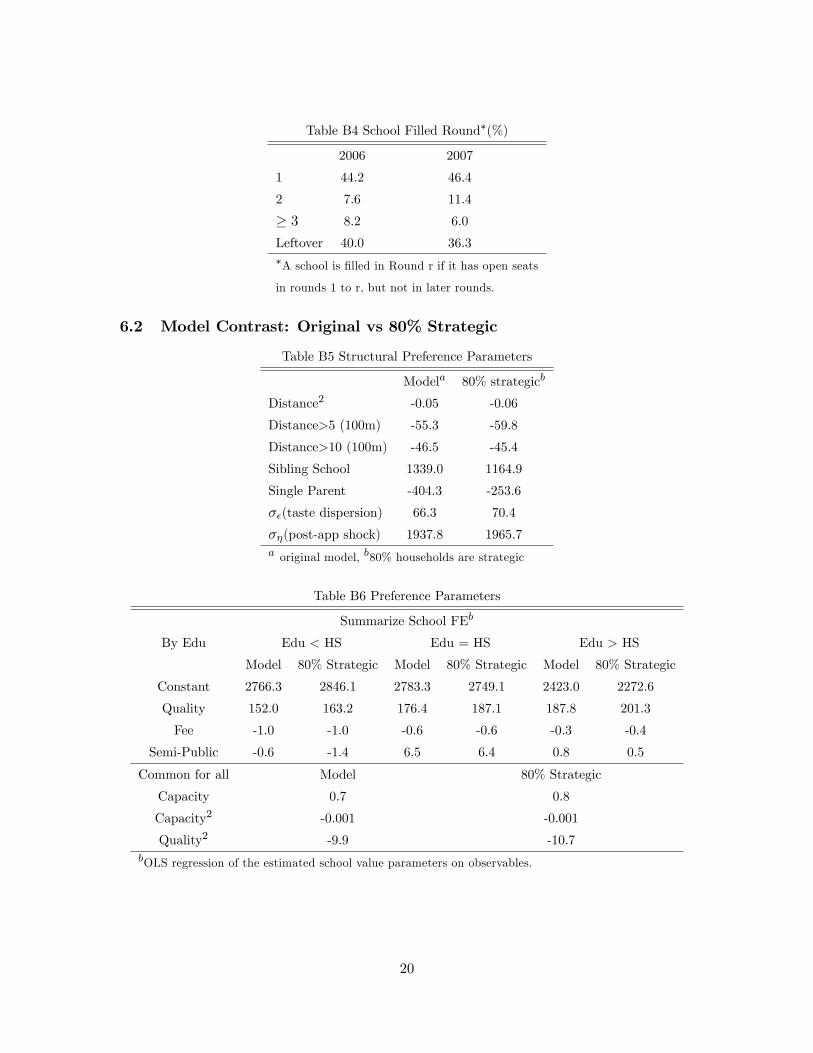
Table B4 School Filled Round∗(%)

2006 2007

1 44.2 46.4

2 7.6 11.4

≥ 3 8.2 6.0

Leftover 40.0 36.3∗A school is filled in Round r if it has open seats

in rounds 1 to r, but not in later rounds.

6.2 Model Contrast: Original vs 80% Strategic

Table B5 Structural Preference Parameters

Modela 80% strategicb

Distance2 -0.05 -0.06

Distance>5 (100m) -55.3 -59.8

Distance>10 (100m) -46.5 -45.4

Sibling School 1339.0 1164.9

Single Parent -404.3 -253.6

σε(taste dispersion) 66.3 70.4

ση(post-app shock) 1937.8 1965.7a original model, b80% households are strategic

Table B6 Preference Parameters

Summarize School FEb

By Edu Edu < HS Edu = HS Edu > HS

Model 80% Strategic Model 80% Strategic Model 80% Strategic

Constant 2766.3 2846.1 2783.3 2749.1 2423.0 2272.6

Quality 152.0 163.2 176.4 187.1 187.8 201.3

Fee -1.0 -1.0 -0.6 -0.6 -0.3 -0.4

Semi-Public -0.6 -1.4 6.5 6.4 0.8 0.5

Common for all Model 80% Strategic

Capacity 0.7 0.8

Capacity2 -0.001 -0.001

Quality2 -9.9 -10.7bOLS regression of the estimated school value parameters on observables.

20

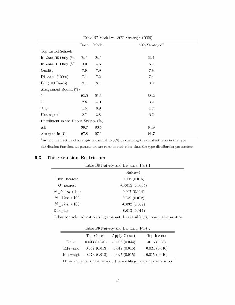
Table B7 Model vs. 80% Strategic (2006)

Data Model 80% Strategic∗

Top-Listed Schools

In Zone 06 Only (%) 24.1 24.1 23.1

In Zone 07 Only (%) 3.0 4.5 5.1

Quality 7.9 7.9 7.9

Distance (100m) 7.1 7.2 7.4

Fee (100 Euros) 8.1 8.1 8.0

Assignment Round (%)

1 93.0 91.3 88.2

2 2.8 4.0 3.9

≥ 3 1.5 0.9 1.2

Unassigned 2.7 3.8 6.7

Enrollment in the Public System (%)

All 96.7 96.5 94.9

Assigned in R1 97.8 97.1 96.7∗Adjust the fraction of strategic household to 80% by changing the constant term in the type

distribution function, all parameters are re-estimated other than the type distribution parameters..

6.3 The Exclusion Restriction

Table B8 Naivety and Distance: Part 1

Naive=1

Dist_nearest 0.006 (0.016)

Q_nearest -0.0015 (0.0035)

N_500m ∗ 100 0.007 (0.114)

N_1km ∗ 100 0.049 (0.072)

N_2km ∗ 100 -0.032 (0.032)

Dist_ave -0.013 (0.011)

Other controls: education, single parent, I(have sibling), zone characteristics

Table B9 Naivety and Distance: Part 2

Top-Closest Apply-Closest Top-Inzone

Naive 0.033 (0.040) -0.003 (0.044) -0.15 (0.03)

Edu=mid -0.047 (0.013) -0.012 (0.015) -0.024 (0.010)

Edu=high -0.073 (0.013) -0.027 (0.015) -0.015 (0.010)

Other controls: single parent, I(have sibling), zone characteristics

21

References

Chen, Y. and O. Kesten (2017) "Chinese College Admissions and School Choice Reforms:

A Theoretical Analysis," Journal of Political Economy, 125 (1): 99-139.

22