Embed Size (px)
Citation preview
Structural Equation Modeling in Stata
Structural Equation Modeling Using the sem
Command and SEM Builder
Kristin MacDonald
Senior StatisticianStataCorp LP
2012 Stata Conference, San Diego
K. L. MacDonald (StataCorp) July 26-27, 2012 1 / 20
Structural Equation Modeling in Stata
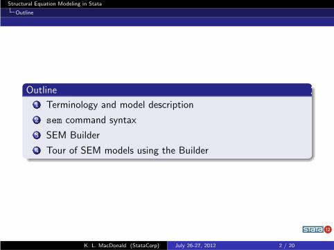
Outline
Outline
1 Terminology and model description
2 sem command syntax
3 SEM Builder
4 Tour of SEM models using the Builder
K. L. MacDonald (StataCorp) July 26-27, 2012 2 / 20
Structural Equation Modeling in Stata
Terminology and model description
What is Structural Equation Modeling?
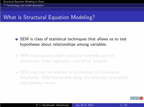
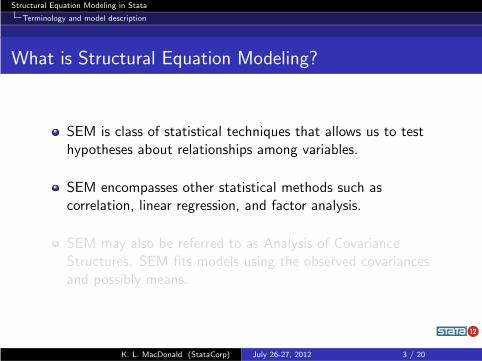
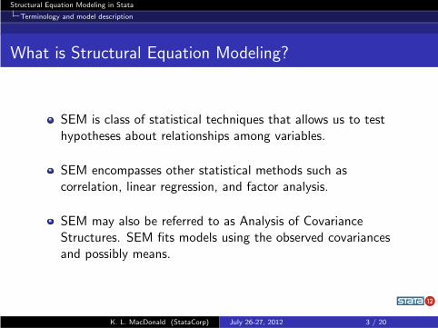
SEM is class of statistical techniques that allows us to testhypotheses about relationships among variables.
SEM encompasses other statistical methods such ascorrelation, linear regression, and factor analysis.
SEM may also be referred to as Analysis of CovarianceStructures. SEM fits models using the observed covariancesand possibly means.
K. L. MacDonald (StataCorp) July 26-27, 2012 3 / 20
Structural Equation Modeling in Stata
Terminology and model description
What is Structural Equation Modeling?
SEM is class of statistical techniques that allows us to testhypotheses about relationships among variables.
SEM encompasses other statistical methods such ascorrelation, linear regression, and factor analysis.
SEM may also be referred to as Analysis of CovarianceStructures. SEM fits models using the observed covariancesand possibly means.
K. L. MacDonald (StataCorp) July 26-27, 2012 3 / 20
Structural Equation Modeling in Stata
Terminology and model description
Types of variables
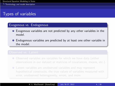
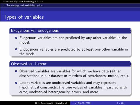
Exogenous vs. Endogenous
Exogenous variables are not predicted by any other variables in themodel.
Endogenous variables are predicted by at least one other variable inthe model.
Observed vs. Latent
Observed variables are variables for which we have data (eitherobservations in our dataset or matrices of covariances, means, etc.).
Latent variables are unobserved variables and may representhypothetical constructs, the true values of variables measured witherror, unobserved heterogeneity, errors, and more.
K. L. MacDonald (StataCorp) July 26-27, 2012 4 / 20
Structural Equation Modeling in Stata
Terminology and model description
Types of variables
Exogenous vs. Endogenous
Exogenous variables are not predicted by any other variables in themodel.
Endogenous variables are predicted by at least one other variable inthe model.
Observed vs. Latent
Observed variables are variables for which we have data (eitherobservations in our dataset or matrices of covariances, means, etc.).
Latent variables are unobserved variables and may representhypothetical constructs, the true values of variables measured witherror, unobserved heterogeneity, errors, and more.
K. L. MacDonald (StataCorp) July 26-27, 2012 4 / 20
Structural Equation Modeling in Stata
Terminology and model description
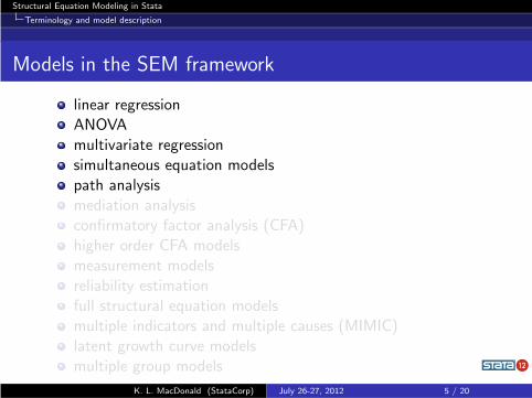
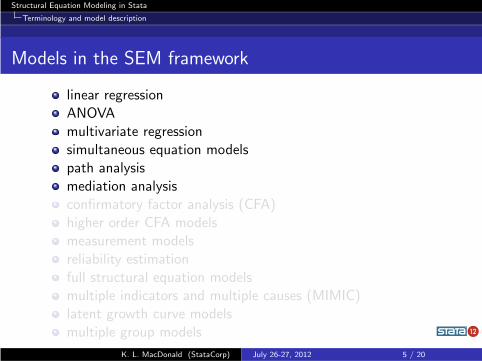
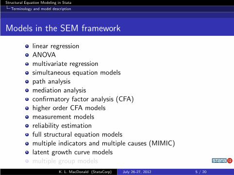
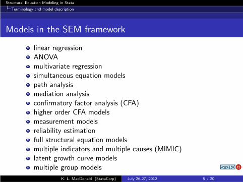
Models in the SEM framework
linear regression
ANOVA
multivariate regression
simultaneous equation models
path analysis
mediation analysis
confirmatory factor analysis (CFA)
higher order CFA models
measurement models
reliability estimation
full structural equation models
multiple indicators and multiple causes (MIMIC)
latent growth curve models
multiple group models
K. L. MacDonald (StataCorp) July 26-27, 2012 5 / 20
Structural Equation Modeling in Stata
Terminology and model description
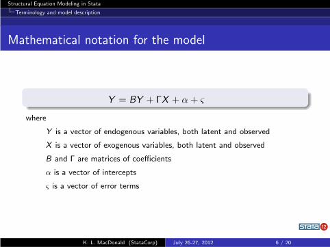
Mathematical notation for the model
Y = BY + ΓX + α+ ς
where
Y is a vector of endogenous variables, both latent and observed
X is a vector of exogenous variables, both latent and observed
B and Γ are matrices of coefficients
α is a vector of intercepts
ς is a vector of error terms
K. L. MacDonald (StataCorp) July 26-27, 2012 6 / 20
Structural Equation Modeling in Stata
Terminology and model description
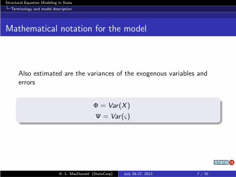
Mathematical notation for the model
Also estimated are the variances of the exogenous variables anderrors
Φ = Var(X )
Ψ = Var(ς)
K. L. MacDonald (StataCorp) July 26-27, 2012 7 / 20

Structural Equation Modeling in Stata
Terminology and model description
Path diagrams
Observed variables represented by rectanglesLatent variables represented by ovalsPaths represented by arrowsCovariances represented by curved lines with arrowsat each end
Multivariate regression Confirmatory factor analysis
y1 ε1
x1
x2
x3
y2 ε2
L1
y1
ε1
y2
ε2
y3
ε3
L2
y4
ε4
y5
ε5
y6
ε6
K. L. MacDonald (StataCorp) July 26-27, 2012 8 / 20
Structural Equation Modeling in Stata
sem command syntax
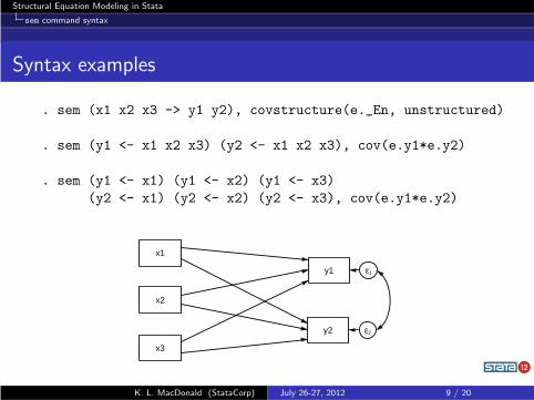
Syntax examples
. sem (x1 x2 x3 -> y1 y2), covstructure(e._En, unstructured)
. sem (y1 <- x1 x2 x3) (y2 <- x1 x2 x3), cov(e.y1*e.y2)
. sem (y1 <- x1) (y1 <- x2) (y1 <- x3)
(y2 <- x1) (y2 <- x2) (y2 <- x3), cov(e.y1*e.y2)
y1 ε1
x1
x2
x3
y2 ε2
K. L. MacDonald (StataCorp) July 26-27, 2012 9 / 20
Structural Equation Modeling in Stata
sem command syntax
Syntax examples
sem syntax mimics path diagrams, using arrows to specifypresumed relationships among variables.
Covariances can be specified using the covariance() orcovstructure() option.
Errors are referred to using the e. prefix with the endogenousvariable’s name.
Arrows are allowed to face either direction. Paths can bespecified individually or many paths can be specified at once.
K. L. MacDonald (StataCorp) July 26-27, 2012 10 / 20
Structural Equation Modeling in Stata
sem command syntax
Syntax examples
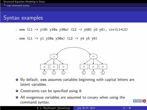
. sem (L1 -> y1@1 y2@a y3@a) (L2 -> y4@1 y5 y6), cov(L1*L2)
. sem (L1 -> y1 y2@a y3@a) (L2 -> y4 y5 y6)
L1
y1
ε1
y2
ε2
y3
ε3
L2
y4
ε4
y5
ε5
y6
ε6
1a
a 1
By default, sem assumes variables beginning with capital letters arelatent variables.
Constraints can be specified using @.
All exogenous variables are assumed to covary when using thecommand syntax.
K. L. MacDonald (StataCorp) July 26-27, 2012 11 / 20
Structural Equation Modeling in Stata
SEM Builder
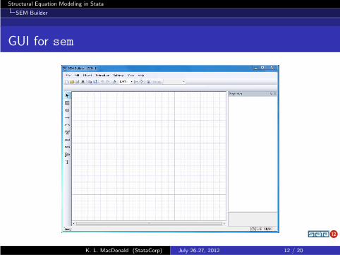
GUI for sem
K. L. MacDonald (StataCorp) July 26-27, 2012 12 / 20
Structural Equation Modeling in Stata
SEM examples
CFA example
Using data from Holzinger and Swineford (1939), we fit a twofactor model. In this example, we have latent variablesrepresenting verbal and spatial abilities. Each are measuredusing results from three tests.
The -sem- command for this model
. sem (Verbal -> paragraph sentence wordc)
(Spatial -> visual cubes paper)
K. L. MacDonald (StataCorp) July 26-27, 2012 13 / 20
Structural Equation Modeling in Stata
SEM examples
Path analysis
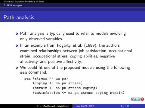
Path analysis is typically used to refer to models involvingonly observed variables.
In an example from Fogarty, et al. (1999), the authorsexamined relationships between job satisfaction, occupationalstrain, occupational stress, coping abilities, negativeaffectivity, and positive affectivity.
We could fit one of the proposed models using the followingsem command.
. sem (stress <- na pa)
(coping <- na pa stress)
(strain <- na pa stress coping)
(satisfaction <- na pa stress coping strain)
K. L. MacDonald (StataCorp) July 26-27, 2012 14 / 20
Structural Equation Modeling in Stata
SEM examples
Full structural equation model
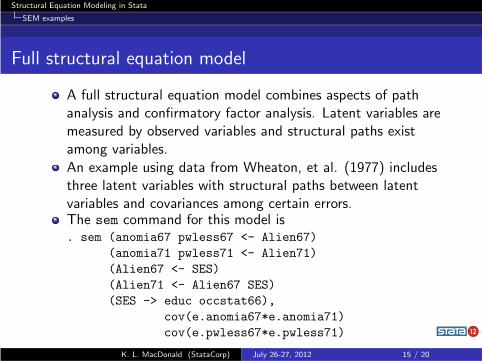
A full structural equation model combines aspects of pathanalysis and confirmatory factor analysis. Latent variables aremeasured by observed variables and structural paths existamong variables.
An example using data from Wheaton, et al. (1977) includesthree latent variables with structural paths between latentvariables and covariances among certain errors.The sem command for this model is. sem (anomia67 pwless67 <- Alien67)
(anomia71 pwless71 <- Alien71)
(Alien67 <- SES)
(Alien71 <- Alien67 SES)
(SES -> educ occstat66),
cov(e.anomia67*e.anomia71)
cov(e.pwless67*e.pwless71)
K. L. MacDonald (StataCorp) July 26-27, 2012 15 / 20
Structural Equation Modeling in Stata
SEM examples
Tips for production quality diagrams
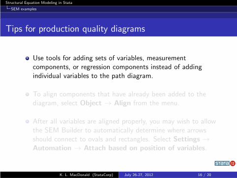
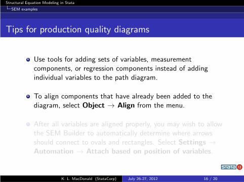
Use tools for adding sets of variables, measurementcomponents, or regression components instead of addingindividual variables to the path diagram.
To align components that have already been added to thediagram, select Object → Align from the menu.
After all variables are aligned properly, you may wish to allowthe SEM Builder to automatically determine where arrowsshould connect to ovals and rectangles. Select Settings →
Automation → Attach based on position of variables.
K. L. MacDonald (StataCorp) July 26-27, 2012 16 / 20
Structural Equation Modeling in Stata
SEM examples
Tips for production quality diagrams
Use the Settings → Variables and Settings →
Connections menu options to make changes globally for theappearance of all variables or paths. It is usually easiest tostart here and then make changes related to individualvariables or paths if you still need to.
Save your .stsem file so that it is easy to make modificationslater. Also save your path diagram in other forms such asPDF, EPS, PNG to easily include in publications.
K. L. MacDonald (StataCorp) July 26-27, 2012 17 / 20

Structural Equation Modeling in Stata
SEM examples
Using tags in the SEM Builder
Tags can be included in labels and results to customize thepath diagram.
To see a list of available tags, type
. help sg tags
In the dialog boxes that are opened through Settings →
Variables and Settings → Connections, the Label andResults tabs show some of these tags in use. If you makechanges in the way labels or results are displayed using thedrop down menus, the corresponding changes using tags willappear in the box next to the menu.
K. L. MacDonald (StataCorp) July 26-27, 2012 18 / 20
Structural Equation Modeling in Stata
SEM examples
We have fit a few classic SEM models using the SEM Builder, butwe have really just scratched the surface the capabilities of sem. Inaddition, we can
obtain robust or cluster-robust standard errors using thevce(robust) and vce(cluster) options
obtain bootstrap or jackknife standard errors
use the svy prefix to take into account complex survey design
instead of listwise deletion, use the method(mlmv) option toperform estimation using maximum likelihood estimation withmissing at random data
perform estimation using asymptotic distribution free (ADF)estimation rather than maximum likelihood estimation
specify a known reliability of an observed variable using thereliability() option
K. L. MacDonald (StataCorp) July 26-27, 2012 19 / 20
Structural Equation Modeling in Stata
References
Bollen, K. A. 1989. Structural Equations with Latent Variables.New York: Wiley.
Fogarty, G., A. M. Machin, M. Albion, L. Sutherland, G. L. Lalor,and S. Revitt. 1999. Predicting occupational strain and jobsatisfaction: The role of stress, coping, and positive and negativeaffectivity. Journal of Vocational Behavior 54:429—452.
Holzinger, K. J. and F. Swineford. 1939. A study in factoranalysis: The stability of a bi-factor solution. Supplementary
Education Monographs, 48. Chicago, IL: University of Chicago.
Kline, R. B. 2011. Principles and Practice of Structural Equation
Modeling. 3rd ed. New York: Guilford Press.
Wheaton, B., B. Muthen, D. F. Alwin, and G. F. Summers. 1977.Assessing reliability and stability in panel models. In Sociological
Methodology 1977, ed. D. R. Heise, 84–136. San Francisco:Jossey-Bass.
K. L. MacDonald (StataCorp) July 26-27, 2012 20 / 20
![Estimating and interpreting structural equation models … · Estimating and interpreting structural equation models in Stata 12 ... and Var [ǫ] = Σ sem (y1 ... Structural equation](https://img.pdfslide.us/doc/110x75/5b286e167f8b9ae8108b4592/estimating-and-interpreting-structural-equation-models-estimating-and-interpreting.jpg)