Embed Size (px)
Citation preview
Structural Equation Modeling
Evangelia Demerouti, PhD
Utrecht UniversityAthens, 18.05.2004
Structure
• Introduction to SEM • Examples• Mediation• Moderation• Longitudinal data
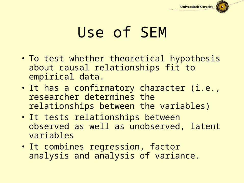
Use of SEM
• To test whether theoretical hypothesis about causal relationships fit to empirical data.
• It has a confirmatory character (i.e., researcher determines the relationships between the variables)
• It tests relationships between observed as well as unobserved, latent variables
• It combines regression, factor analysis and analysis of variance.
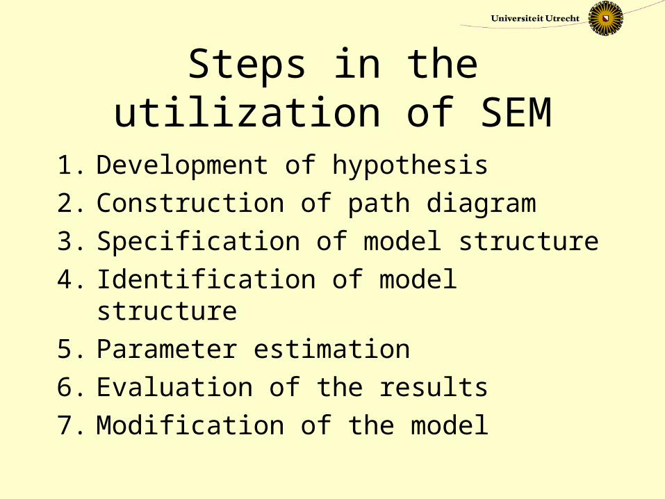
Steps in the utilization of SEM
1. Development of hypothesis2. Construction of path diagram 3. Specification of model structure4. Identification of model structure5. Parameter estimation6. Evaluation of the results7. Modification of the model
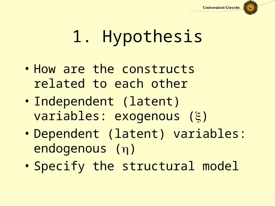
1. Hypothesis
• How are the constructs related to each other
• Independent (latent) variables: exogenous ()
• Dependent (latent) variables: endogenous ()
• Specify the structural model
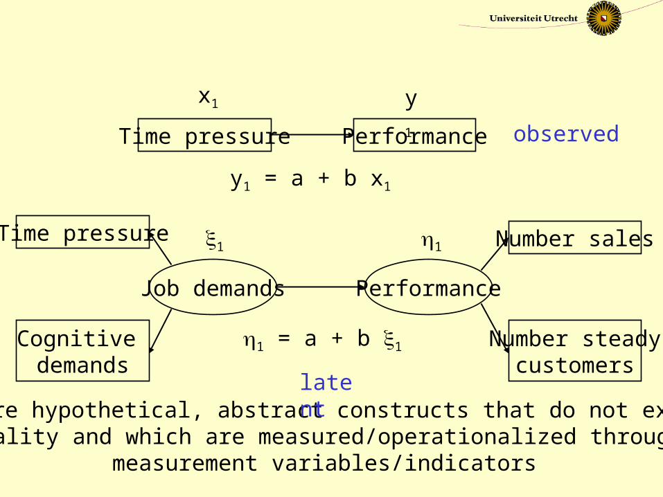
Time pressure Performance
x1 y1
y1 = a + b x1
observed
, are hypothetical, abstract constructs that do not exist inreality and which are measured/operationalized through
measurement variables/indicators
Job demands Performance
Time pressure
Cognitive demands
Number sales
Number steadycustomers
1 1
1 = a + b 1
latent
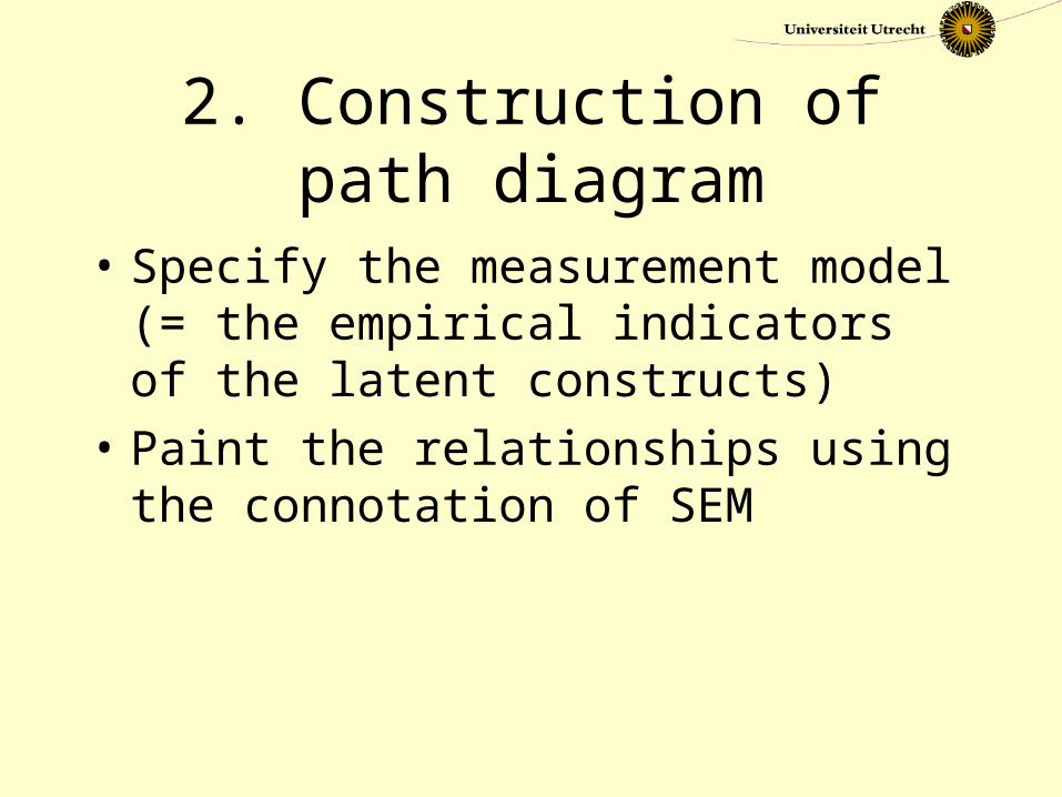
2. Construction of path diagram
• Specify the measurement model (= the empirical indicators of the latent constructs)
• Paint the relationships using the connotation of SEM
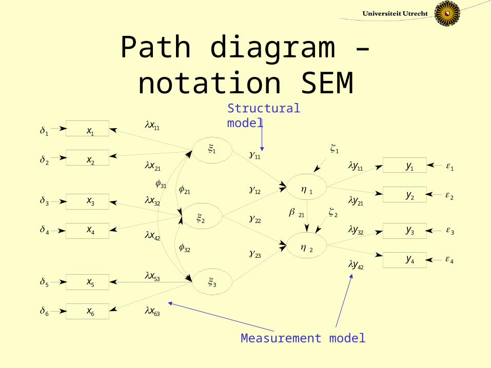
Path diagram – notation SEM
x32
x42
x53
x63
21x
x11
y32
y42
y21
y11
1
2
3
1
2
1
2
11
12
22
23
x1
x2
x3
x4
x5
x6
y1
y2
y3
y4
1
2
3
4
1
2
3
4
5
6
21
21
32
31
Measurement model
Structural model
3. Specification of model structure
• Mathematical specification of the hypotheses using matrices of equities
• Rules1. errors should be uncorrelated with the
latent constructs (otherwise there is another variable which systematically influences the model variable, i.e., incomplete model)
2. errors should be uncorrelated with each other (otherwise there is a systematic error that influence all independent variables, i.e., method factor)
4. Identification of model structure
• Check whether the matrices can be solved, I.e., whether there is enough information from the empirical data to determine the unknown parameters
• If n = number of indicators/observed variables
• s = n (n + 1) / 2 correlation coefficients or number of equities
• If t = number of unknown parameters then t < s (i.e., df > 0)
5. Parameter estimation• The model theoretical correlation matrix (sigma) has the
correlation coefficients which we expect within the data sample if the model is right and the sample is representing the population
• The empirical correlation matrix has the (Pearson product-moment) correlation coefficients (rxy) which indicate in how far the relation between two variables x and y resembles a straight line (if one variable increases, the other does also)
• Iterative estimations of the correlation coefficients in tries to minimize the differences between
and R
Theory Empirical data
The discrepancy between and R expresses whether theoretical model is acceptable
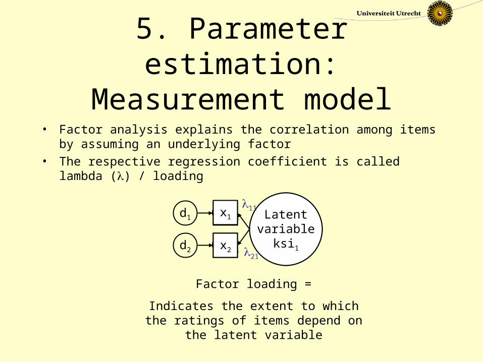
5. Parameter estimation: Measurement model
• Factor analysis explains the correlation among items by assuming an underlying factor
• The respective regression coefficient is called lambda () / loading
Egotisticbusiness
goals
d1 Qebgi1
d2 Qebgc1
Latentvariable
ksi1
x1
x2
Factor loading =
Indicates the extent to which the ratings of items depend on the latent
variable
11
21
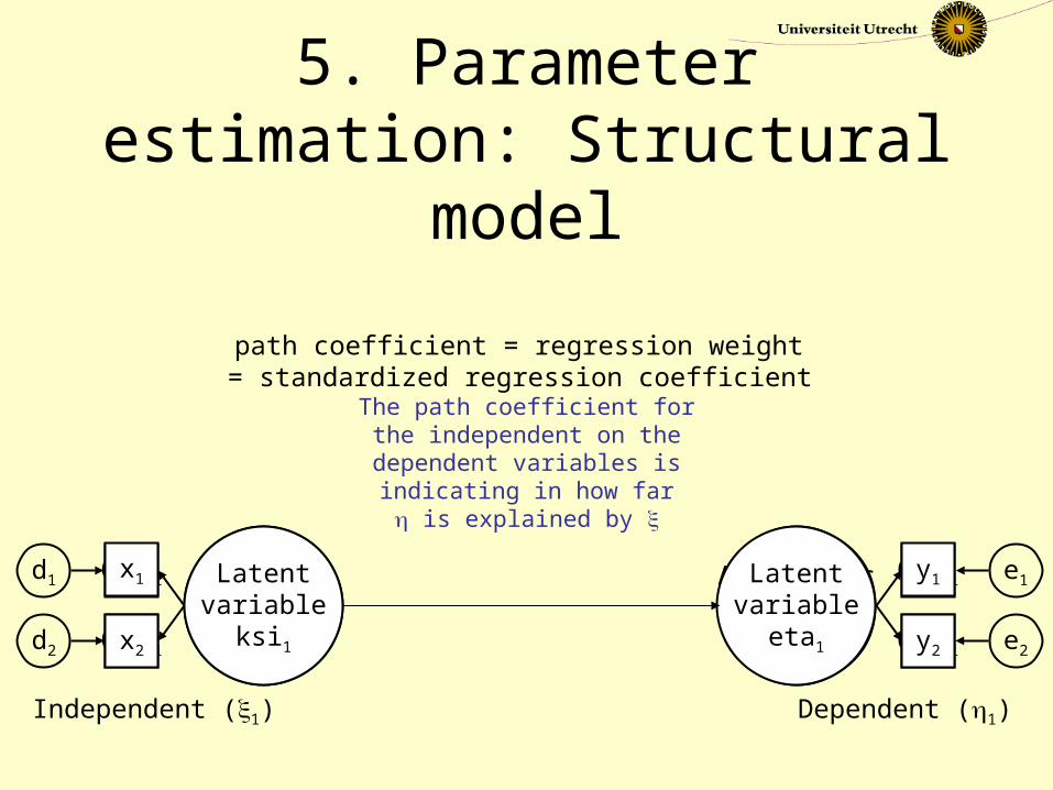
5. Parameter estimation: Structural model
path coefficient = regression weight = standardized regression coefficient
The path coefficient forthe independent on thedependent variables isindicating in how far is explained by
Egotisticbusiness
goals
d1 Qebgi1
d2 Qebgc1
e1Qepgi1
e2Qepgc1
Altruisticbusiness
goals
Latentvariable
ksi1
Latentvariable
eta1
Independent (1) Dependent (1)
x1
x2
y1
y2
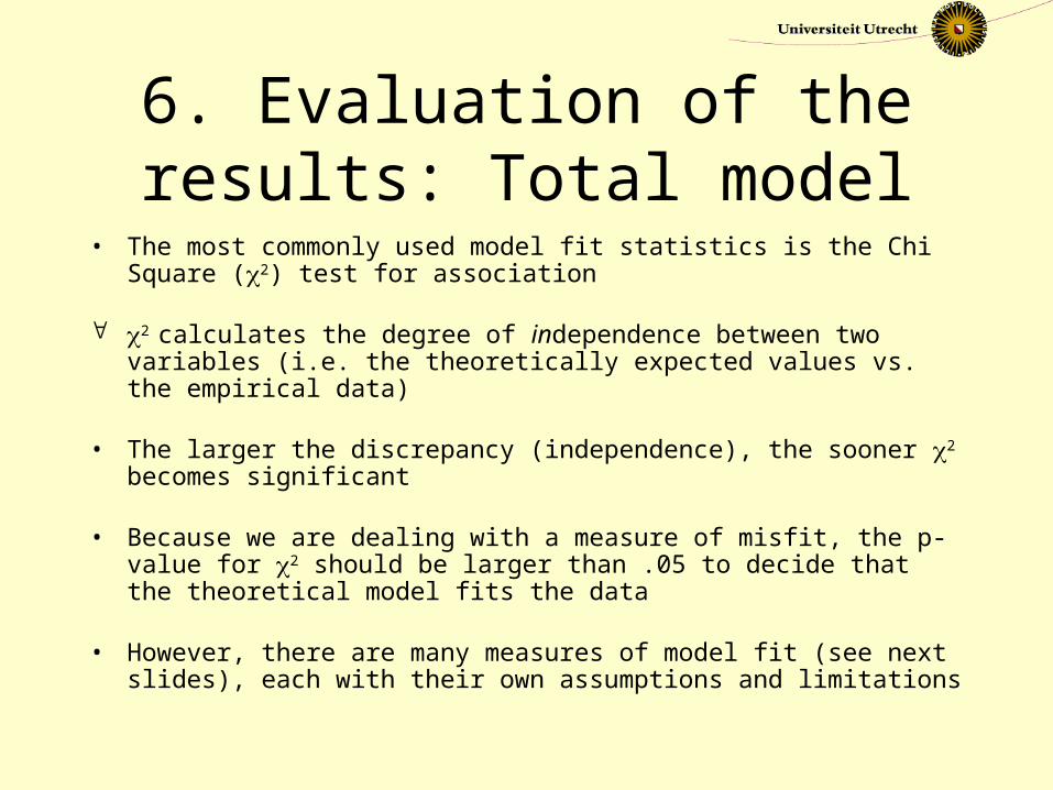
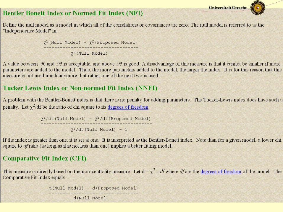
6. Evaluation of the results: Total model
• The most commonly used model fit statistics is the Chi Square (2) test for association
2 calculates the degree of independence between two variables (i.e. the theoretically expected values vs. the empirical data)
• The larger the discrepancy (independence), the sooner 2 becomes significant
• Because we are dealing with a measure of misfit, the p-value for 2 should be larger than .05 to decide that the theoretical model fits the data
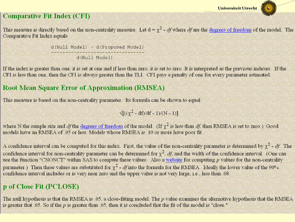
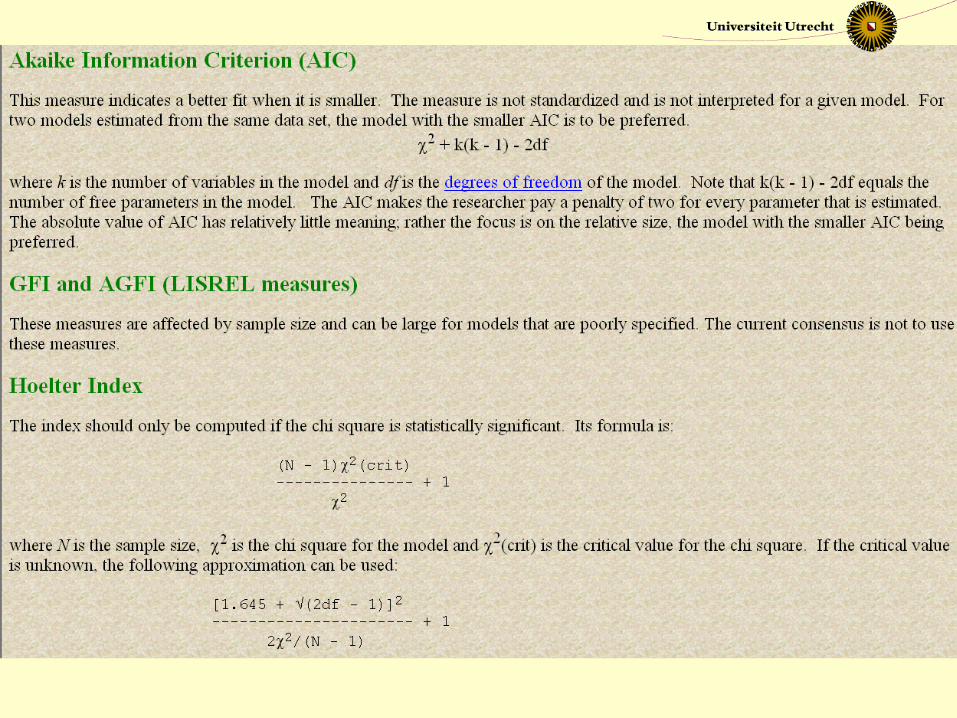
• However, there are many measures of model fit (see next slides), each with their own assumptions and limitations
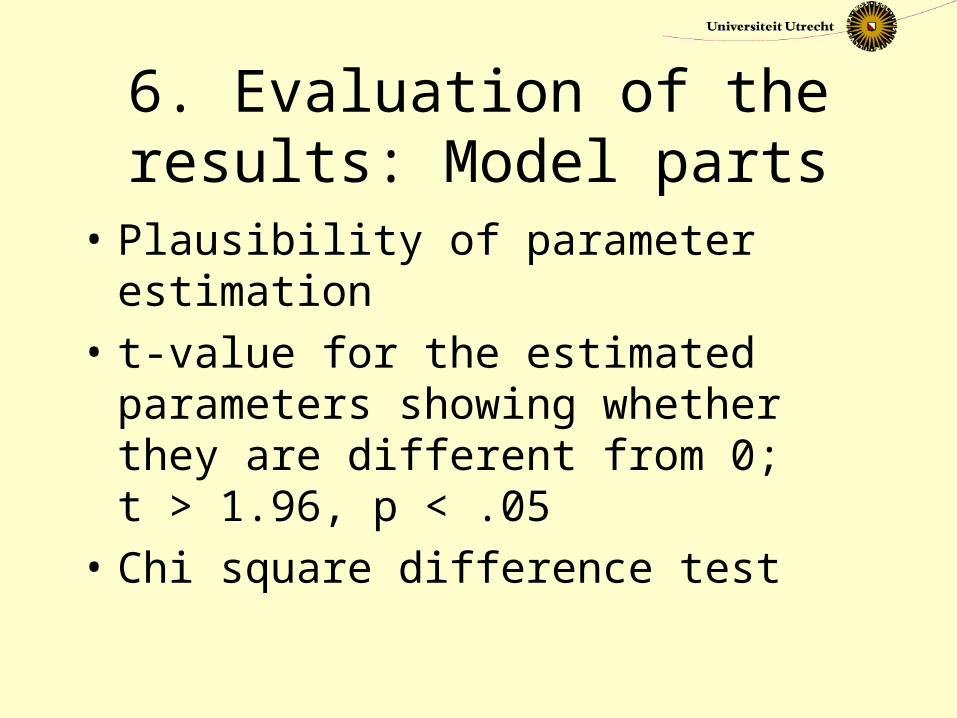
6. Evaluation of the results: Model parts
• Plausibility of parameter estimation
• t-value for the estimated parameters showing whether they are different from 0; t > 1.96, p < .05
• Chi square difference test
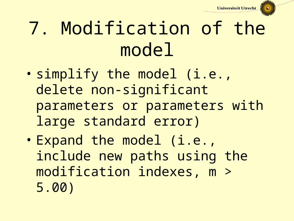
7. Modification of the model
• simplify the model (i.e., delete non-significant parameters or parameters with large standard error)
• Expand the model (i.e., include new paths using the modification indexes, m > 5.00)

Mediation
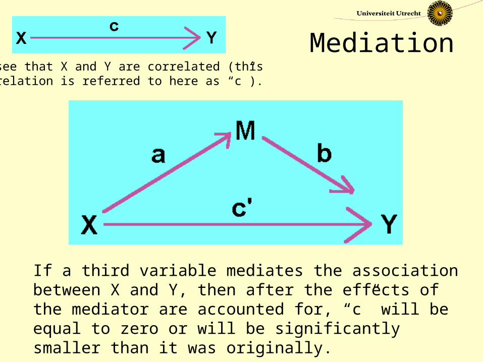
MediationWe see that X and Y are correlated (this correlation is referred to here as “c”).
If a third variable mediates the association between X and Y, then after the effects of the mediator are accounted for, “c” will be equal to zero or will be significantly smaller than it was originally.
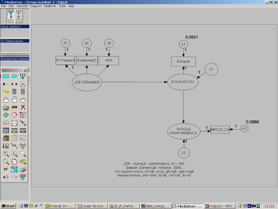
Mediation: Examples
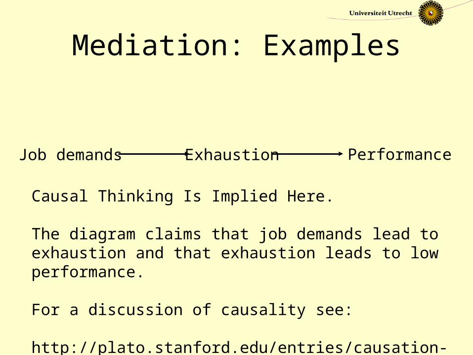
Job demands Exhaustion Performance
Causal Thinking Is Implied Here.
The diagram claims that job demands lead to exhaustion and that exhaustion leads to low performance.
For a discussion of causality see:
http://plato.stanford.edu/entries/causation-probabilistic/
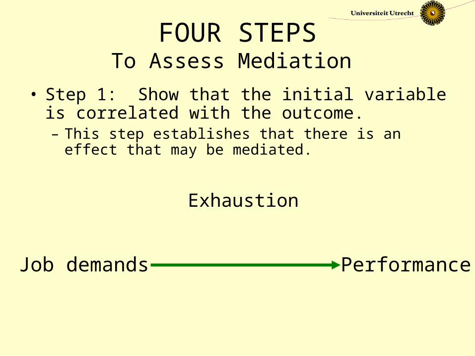
FOUR STEPSTo Assess Mediation
• Step 1: Show that the initial variable is correlated with the outcome. – This step establishes that there is an effect
that may be mediated.
Job demands
Exhaustion
Performance
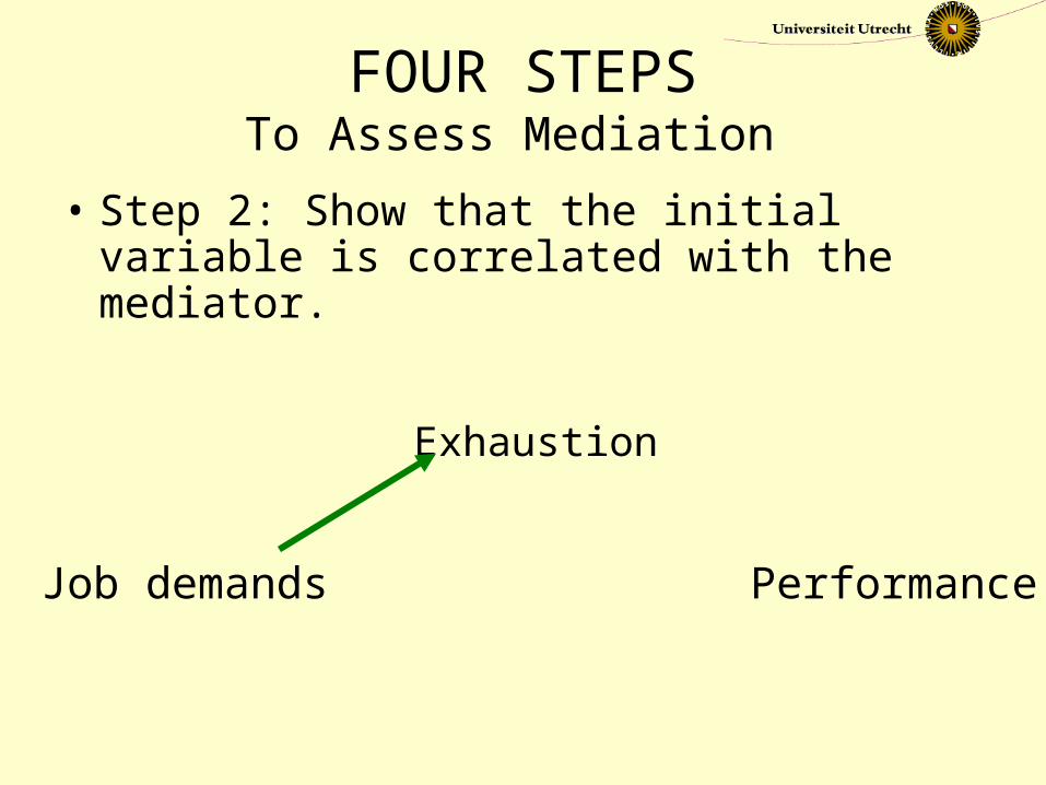
FOUR STEPSTo Assess Mediation
• Step 2: Show that the initial variable is correlated with the mediator.
Job demands
Exhaustion
Performance
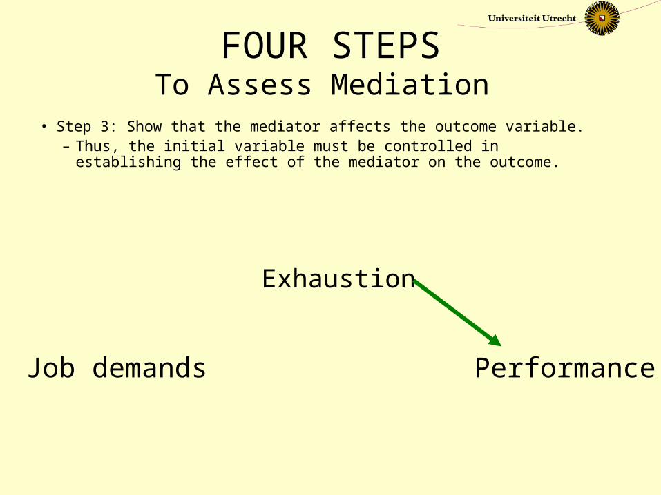
FOUR STEPSTo Assess Mediation
• Step 3: Show that the mediator affects the outcome variable. – Thus, the initial variable must be controlled in establishing the
effect of the mediator on the outcome.
Job demands
Exhaustion
Performance
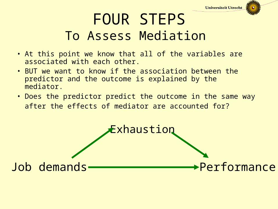
FOUR STEPSTo Assess Mediation
• At this point we know that all of the variables are associated with each other.
• BUT we want to know if the association between the predictor and the outcome is explained by the mediator.
• Does the predictor predict the outcome in the same way after the effects of mediator are accounted for?
Job demands
Exhaustion
Performance
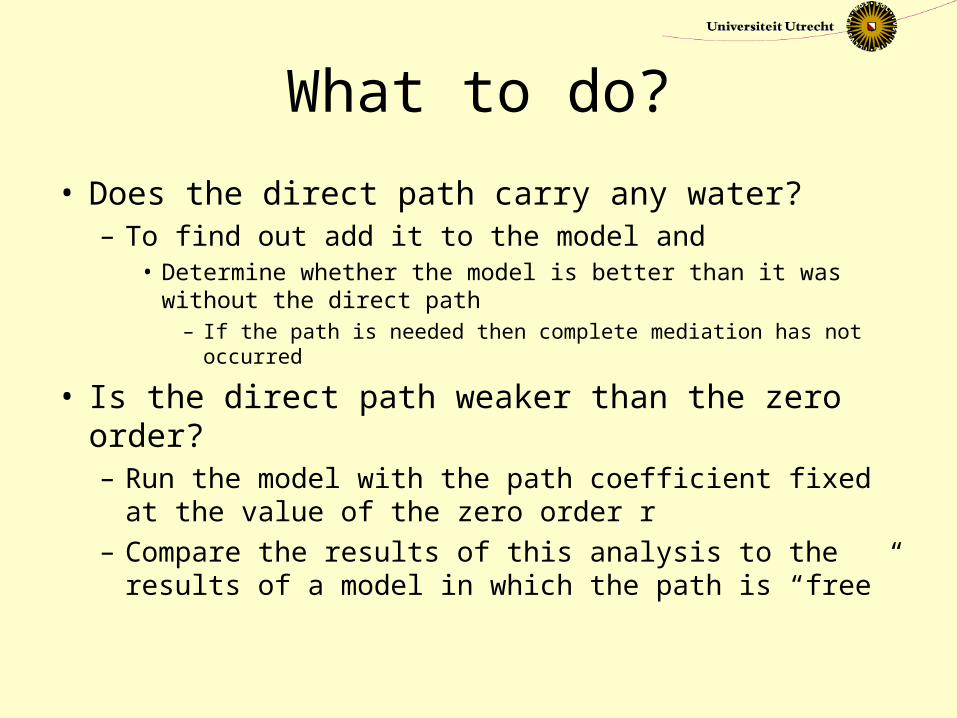
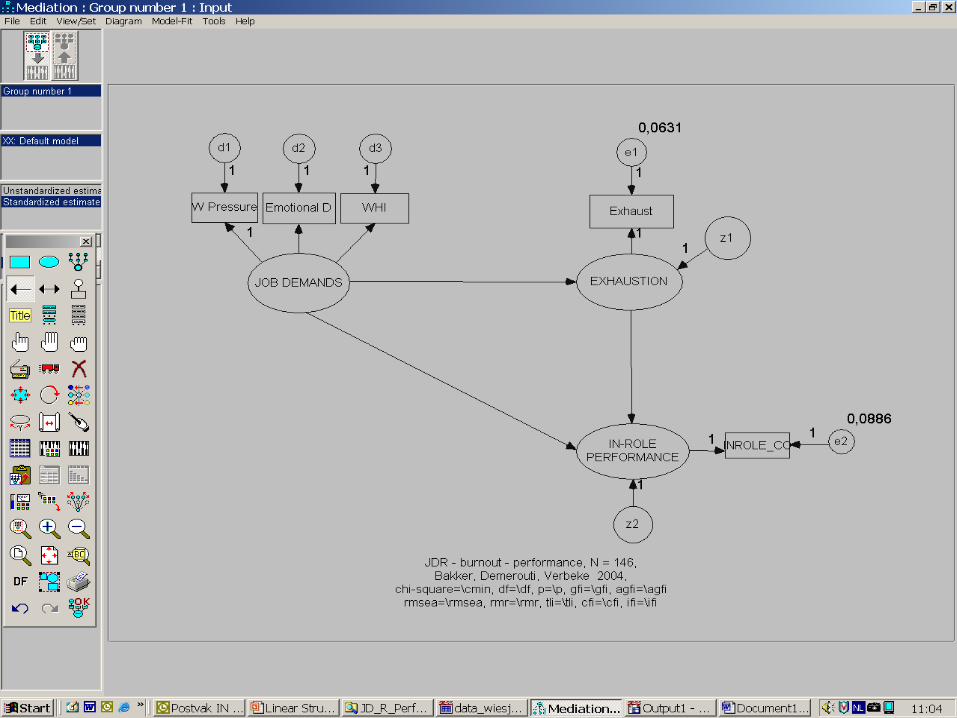
What to do?
• Does the direct path carry any water?– To find out add it to the model and
• Determine whether the model is better than it was without the direct path
– If the path is needed then complete mediation has not occurred
• Is the direct path weaker than the zero order?– Run the model with the path coefficient fixed at
the value of the zero order r– Compare the results of this analysis to the
results of a model in which the path is “free”

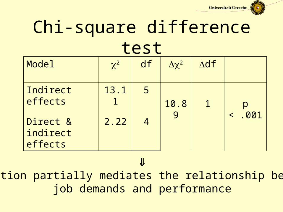
Chi-square difference testModel 2 df 2 df
Indirect effects
13.11 510.8
91 p
< .001Direct & indirect effects
2.22 4
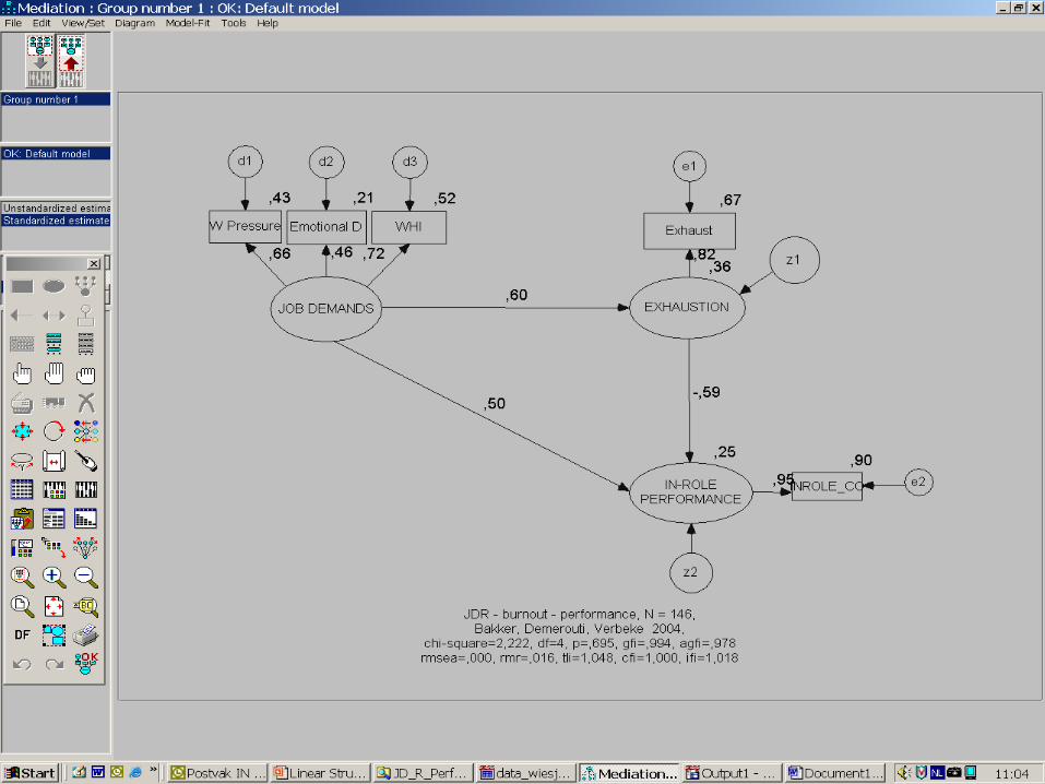
Exhaustion partially mediates the relationship between
job demands and performance

Moderation
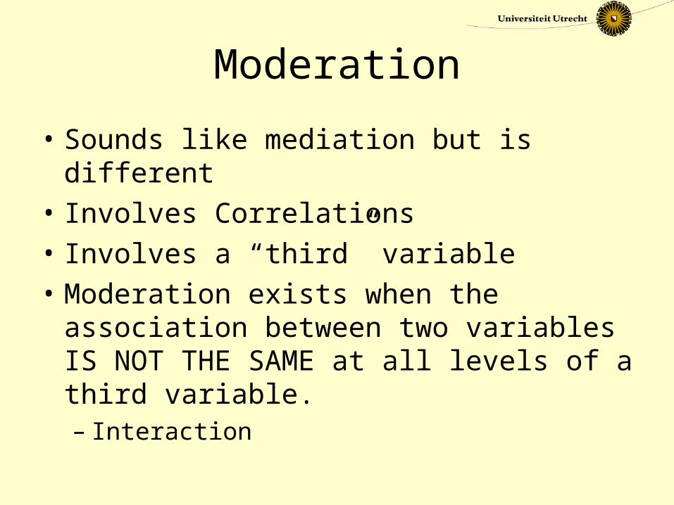
Moderation
• Sounds like mediation but is different• Involves Correlations• Involves a “third” variable• Moderation exists when the
association between two variables IS NOT THE SAME at all levels of a third variable. – Interaction
Example
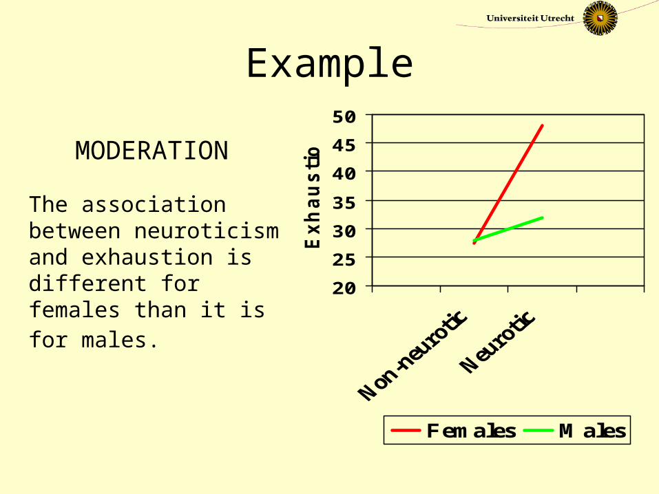
MODERATION
The association between neuroticism and exhaustion is different for females than it is for males.
20
25
30
35
40
45
50
Exhaustion
Females Males
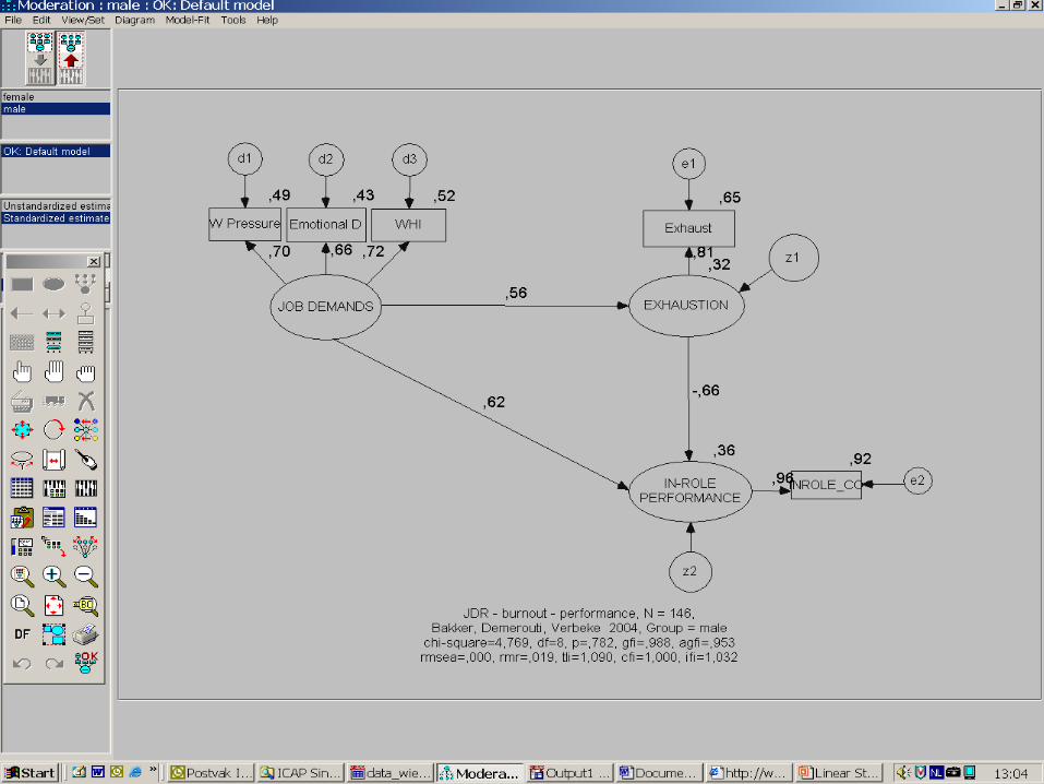
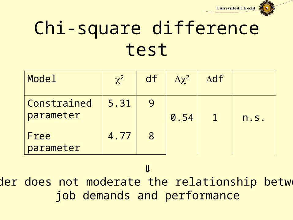
Chi-square difference test
Model 2 df 2 df
Constrained parameter
5.31 90.54 1 n.s.
Free parameter
4.77 8
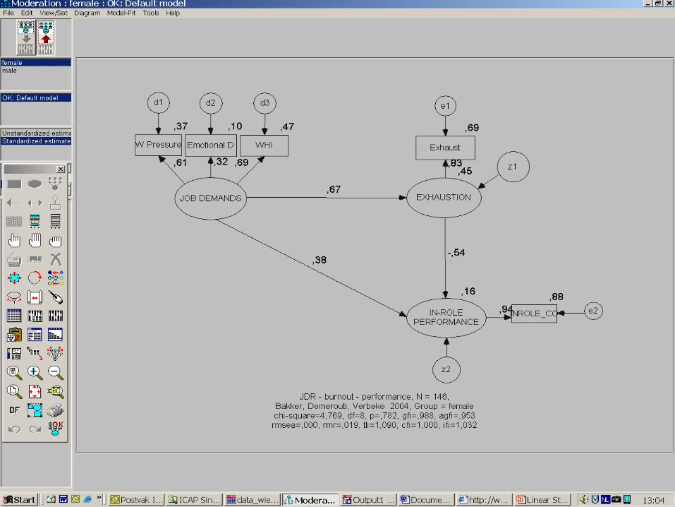
Gender does not moderate the relationship between
job demands and performance
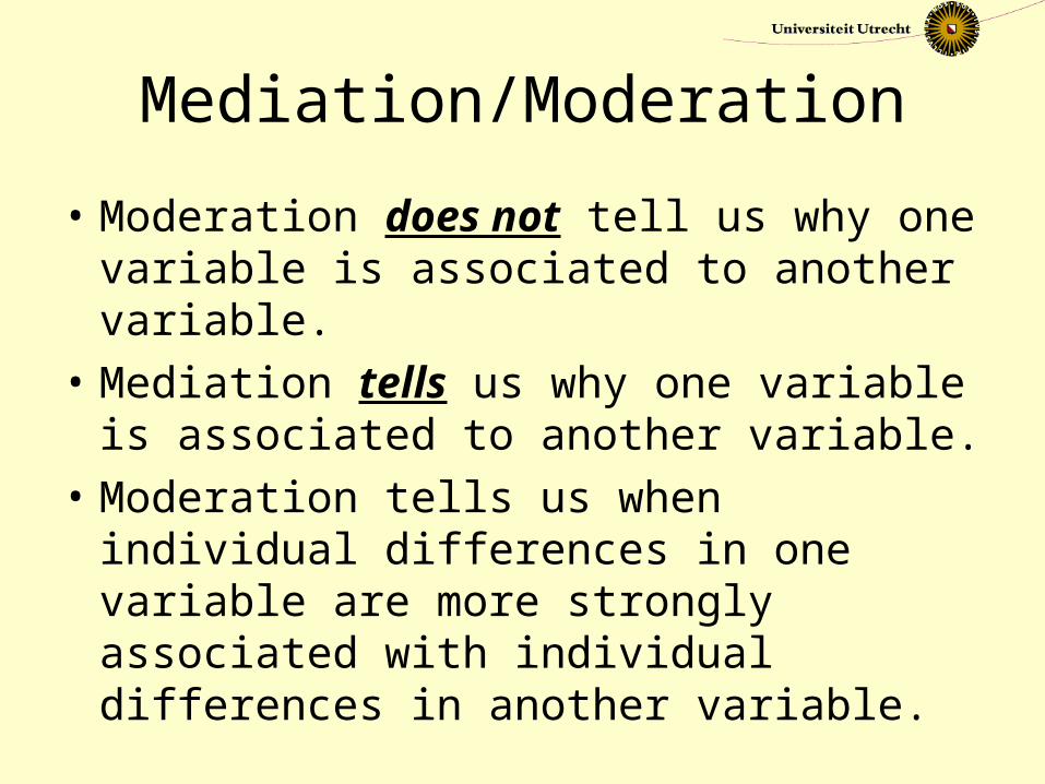
Mediation/Moderation
• Moderation does not tell us why one variable is associated to another variable.
• Mediation tells us why one variable is associated to another variable.
• Moderation tells us when individual differences in one variable are more strongly associated with individual differences in another variable.

Longitudinal Data
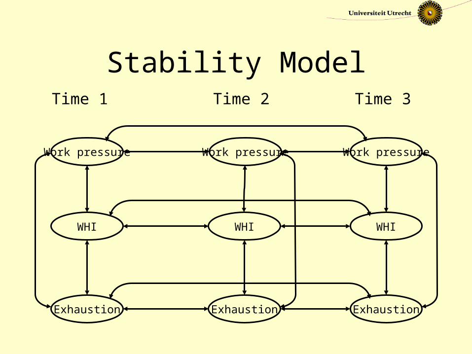
Stability Model
Work pressure Work pressure Work pressure
WHI WHI WHI
Exhaustion Exhaustion Exhaustion
Time 1 Time 2 Time 3
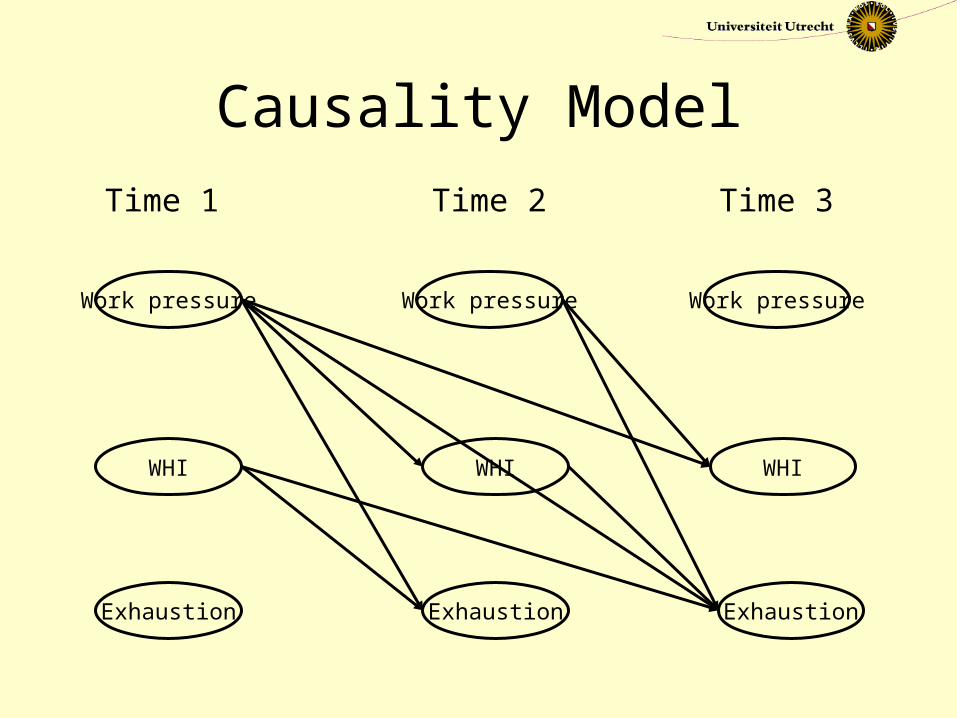
Causality Model
Work pressure Work pressure Work pressure
WHI WHI WHI
Exhaustion Exhaustion Exhaustion
Time 1 Time 2 Time 3
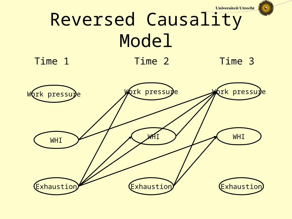
Reversed Causality Model
Time 1 Time 2 Time 3
Work pressure Work pressure Work pressure
WHI WHI WHI
Exhaustion Exhaustion Exhaustion
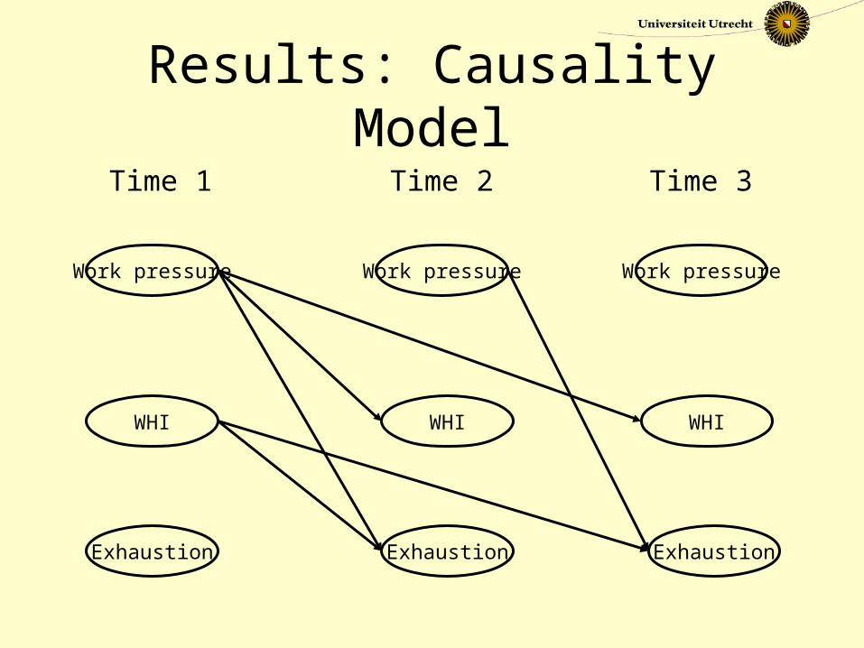
Results: Causality Model
Work pressure Work pressure Work pressure
WHI WHI WHI
Exhaustion Exhaustion Exhaustion
Time 1 Time 2 Time 3
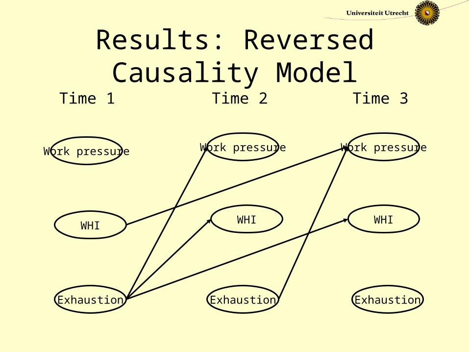
Results: Reversed Causality Model
Time 1 Time 2 Time 3
Work pressure Work pressure Work pressure
WHI WHI WHI
Exhaustion Exhaustion Exhaustion
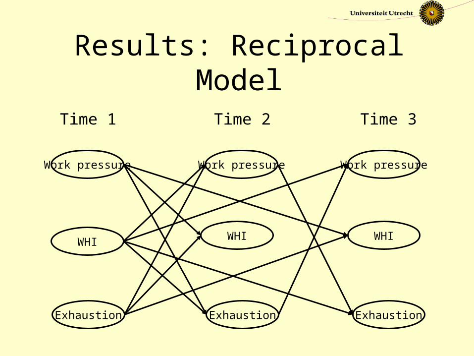
Results: Reciprocal Model
Work pressure Work pressure Work pressure
WHI WHI WHI
Exhaustion Exhaustion Exhaustion
Time 1 Time 2 Time 3
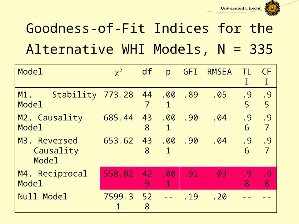
Goodness-of-Fit Indices for the
Alternative WHI Models, N = 335 Model 2 df p GFI RMSE
ATLI CFI
M1. Stability Model
773.28 447
.001
.89 .05 .95 .95
M2. Causality Model
685.44 438
.001
.90 .04 .96 .97
M3. Reversed Causality Model
653.62 438
.001
.90 .04 .96 .97
M4. Reciprocal Model
558.82 429
.001
.91 .03 .98 .98
Null Model 7599.31
528
-- .19 .20 -- --
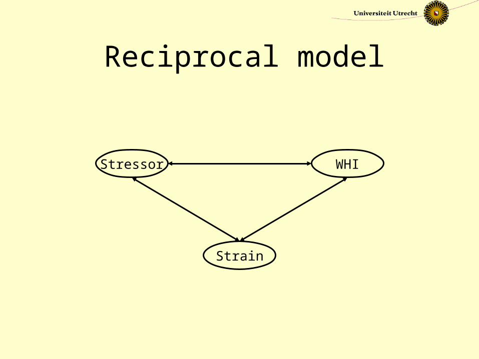
Stressor WHI
Strain
Reciprocal model

Thank you for your attention
Email: [email protected]
Student version of AMOS to download inhttp://www.amosdevelopment.com/


![Understanding the Relationship between Colleague ...1].pdf · Resources (JDR) model first suggested by Demerouti, Bakker, Nachreiner & Schaufeli (2001). The JDR model proposed workplace](https://img.pdfslide.us/doc/110x75/61281f8b20980d273a0de979/understanding-the-relationship-between-colleague-1pdf-resources-jdr-model.jpg)