Embed Size (px)
Citation preview

This article was downloaded by:[CDL Journals Account]On: 19 May 2008Access Details: [subscription number 789921171]Publisher: Psychology PressInforma Ltd Registered in England and Wales Registered Number: 1072954Registered office: Mortimer House, 37-41 Mortimer Street, London W1T 3JH, UK
Structural Equation Modeling: AMultidisciplinary JournalPublication details, including instructions for authors and subscription information:http://www.informaworld.com/smpp/title~content=t775653699
Variance Estimation Using Replication Methods inStructural Equation Modeling With Complex SampleDataLaura M. Stapleton aa University of Maryland Baltimore County,
Online Publication Date: 01 April 2008
To cite this Article: Stapleton, Laura M. (2008) 'Variance Estimation UsingReplication Methods in Structural Equation Modeling With Complex Sample Data',Structural Equation Modeling: A Multidisciplinary Journal, 15:2, 183 — 210
To link to this article: DOI: 10.1080/10705510801922316URL: http://dx.doi.org/10.1080/10705510801922316
PLEASE SCROLL DOWN FOR ARTICLE
Full terms and conditions of use: http://www.informaworld.com/terms-and-conditions-of-access.pdf
This article maybe used for research, teaching and private study purposes. Any substantial or systematic reproduction,re-distribution, re-selling, loan or sub-licensing, systematic supply or distribution in any form to anyone is expresslyforbidden.
The publisher does not give any warranty express or implied or make any representation that the contents will becomplete or accurate or up to date. The accuracy of any instructions, formulae and drug doses should beindependently verified with primary sources. The publisher shall not be liable for any loss, actions, claims, proceedings,demand or costs or damages whatsoever or howsoever caused arising directly or indirectly in connection with orarising out of the use of this material.

Dow
nloa
ded
By:
[CD
L Jo
urna
ls A
ccou
nt] A
t: 22
:18
19 M
ay 2
008
Structural Equation Modeling, 15:183–210, 2008
Copyright © Taylor & Francis Group, LLC
ISSN: 1070-5511 print/1532-8007 online
DOI: 10.1080/10705510801922316
Variance Estimation Using ReplicationMethods in Structural Equation
Modeling With Complex Sample Data
Laura M. StapletonUniversity of Maryland Baltimore County
This article discusses replication sampling variance estimation techniques that are
often applied in analyses using data from complex sampling designs: jackknife
repeated replication, balanced repeated replication, and bootstrapping. These tech-
niques are used with traditional analyses such as regression, but are currently not
used with structural equation modeling (SEM) analyses. This article provides an
extension of these methods to SEM analyses, including a proposed adjustment to
the likelihood ratio test, and presents the results from a simulation study suggesting
replication estimates are robust. Finally, a demonstration of the application of these
methods using data from the Early Childhood Longitudinal Study is included.
Secondary analysts can undertake these more robust methods of sampling vari-
ance estimation if they have access to certain SEM software packages and data
management packages such as SAS, as shown in the article.
Most national datasets are collected using sampling designs other than simple
random sampling (SRS). Most statistical analyses operate on the assumption of
independence of observations (which can be virtually assured through the use of
SRS). If this assumption does not hold, inappropriately calculated standard errors
can result, compromising hypothesis tests. Special procedures for estimating
means, ratio, and regression parameter estimates with data from complex sample
designs have been developed; however, many software programs for structural
equation modeling (SEM) do not accommodate sampling design information
Correspondence should be addressed to Laura M. Stapleton, University of Maryland Balti-
more County, Department of Psychology, 1000 Hilltop Circle, Baltimore, MD 21250. E-mail:
183

Dow
nloa
ded
By:
[CD
L Jo
urna
ls A
ccou
nt] A
t: 22
:18
19 M
ay 2
008
184 STAPLETON
or may have limited capacity to do so. This research extends a prior study by
Stapleton (2006) that examined the practical approaches that researchers can
use when analyzing covariance structure models with complex sample data. It
builds on that study by examining the robustness of sampling variance estimates
and a proposed adjusted chi-square statistic from replication methods including
jackknife repeated replication (JRR), balanced repeated replication (BRR), and
bootstrapping. These replication methods for estimating sampling variances with
complex sample data are currently not available in software for SEM and must be
specially programmed; they are available in other statistical packages for more
traditional analyses such as multiple regression and comparison of frequency
distributions.
In describing effects and procedures for this study, the Early Childhood
Longitudinal Study (ECLS; U.S. Department of Education, 2001) data collection
plan is used as a model: a stratified multistage sample. The ECLS sampling
design included three stages of sampling: the selection of primary sampling units
(PSUs) of single counties or groups of counties, then the selection of schools
within those counties, and finally selection of students within the schools. At
the first two stages of selection, stratification and probability proportional to
size sampling was used and at the final stage, stratification unequal sampling
probabilities was used; Asian/Pacific Islander students were sampled at a rate
three times higher than the sampling rate for all other students. An excellent
review of the characteristics of complex sample designs including clustering,
stratification, unequal probabilities of selection, and nonresponse and poststrati-
fication adjustment is provided by Longford (1995). This article focuses on the
problems posed when stratified multistage sampling is used.
An assumption in the use of many analysis techniques, including SEM, is
that observations are independent and identically distributed. Data obtained
through multistage sampling, however, typically demonstrate some degree of
dependence (Kish, 1965; Skinner, Holt, & Smith, 1989). Because traditional
standard error formulas assume that the correlation of the errors is zero, a
researcher using clustered data may underestimate the sampling variance, re-
sulting in inappropriate Type I error rates (Lee, Forthofer, & Lorimor, 1989).
Muthén and Satorra (1995) demonstrated the standard error bias and large chi-
square values that can result when SRS-based SEM is applied to data that were
obtained through a two-stage SRS design (they refer to this type of analysis
as “conventional”). A conventional SEM analysis of clustered data, therefore,
may lead to the mispronouncement of statistically significant relations where
only random covariation exists, as well as result in inappropriate rejection of
correct models for the finite population. Additionally, if stratification is part of
the sampling design and the response variables are homogeneous within strata,
standard error estimates from a conventional analysis will be overestimated and
represent a loss of efficiency (Asparouhov, 2004; Kish & Frankel, 1974).

Dow
nloa
ded
By:
[CD
L Jo
urna
ls A
ccou
nt] A
t: 22
:18
19 M
ay 2
008
VARIANCE ESTIMATION USING REPLICATION METHODS 185
General analytic strategies, not specific to SEM, have been developed for
appropriately estimating sampling variances of parameter estimates for the fi-
nite population when using data obtained using complex sampling designs.
The options range from simple adjustments of standard error estimates from
a conventional analysis to more complex estimators of sampling variances. An
additional option, instead of seeking to obtain a more accurate standard error
for the finite population parameter estimate, is to include the sampling design in
the analytic model itself. This model-based or model-assisted analysis approach
would include such strategies as multilevel analyses and inclusion of stratifi-
cation design variables as fixed effects. These analyses, termed disaggregated
by Muthén and Satorra (1995) are discussed in Hox (2002) and a nice applied
example is provided in Kaplan and Elliott (1997). The research question in such
analyses involves testing a theoretical model with components at each level of the
analysis. The theoretical model may exist only at the individual level, however,
and clustering effects are considered a nuisance. In this case, aggregated SEM
is appropriate (Muthén & Satorra, 1995) and is the focus of this article.
CURRENT ANALYTIC OPTIONS TO ACCOUNT FOR
THE SAMPLING DESIGN IN AGGREGATE
SEM ANALYSES
A simple method to adjust for a complex sampling design, as described in Staple-
ton (2006), might be to inflate the standard errors obtained from a conventional
weighted analysis by the square root of the design effect of the mean of the
dependent variable(s) in the analysis. A related approach, advocated in some
database user’s guides (U.S. Department of Education, 1996; Walker & Young,
2003), is to use a design effect sampling weight in the analysis. Although the
procedures of adjusting a standard error estimate by the square root of the design
effect or using an adjusted sampling weight result in accurate adjustments of the
standard error for a simple statistic such as the mean, these procedures can be
expected to result in conservative estimates of the sampling errors in complex
statistical procedures (Kish & Frankel, 1974) as was found for SEM applications
(Stapleton, 2006).
Estimating sampling variances using a linearization method is perhaps a more
appropriate approach (Kish & Frankel, 1974). With complex sample data, the
sampling variance estimate of a statistic can be approximated by the weighted
combination of the variation as assessed by the first-order derivatives across
PSUs within each stratum (Kalton, 1983; Skinner et al., 1989). Muthén and
Satorra (1995) first applied this type of approach to an SEM analysis and
Asparouhov (2005) described the quasi-pseudo maximum likelihood (QPML)
approach currently implemented in software such as Mplus (Asparouhov, 2004)

Dow
nloa
ded
By:
[CD
L Jo
urna
ls A
ccou
nt] A
t: 22
:18
19 M
ay 2
008
186 STAPLETON
and LISREL (Scientific Software International, 2004) for use with data that are
both dependent (i.e., from cluster samples) and sampled at unequal probabilities.
Assumptions in the use of this method include selection of PSUs within strata
with replacement (Muthén & Muthén, 2004) and simulations have demonstrated
that this approach provides robust estimates when assumptions are met (As-
parouhov, 2004, 2005). Whereas the QPML estimation provides robust standard
error estimates as part of the asymptotic covariance matrix, a robust likelihood
ratio chi-square statistic is approximated by correcting the conventional log-
likelihood-based chi-square statistic by using a correction factor. Specifically,
Asparouhov and Muthén (2005) derive the correction factor for the likelihood
ratio test as a function of the difference in the number of parameters and
in the variance components within the asymptotic covariance matrix across a
restricted and unrestricted model. This correction factor is similar to adjustments
to likelihood ratios as proposed by Satorra and Bentler (1988) and is a parallel
to the adjustment proposed for tests of independence by Rao and Scott (1981)
and further explicated by Rao and Thomas (1989). This adjustment is reported
to be used in the Mplus software (Asparouhov & Muthén, 2005). LISREL
documentation is not clear with regard to its calculation of the correct factor
as it offers a different formulation of the adjustment factor without derivations
(Scientific Software International, 2004). Tests of the correction factors across
these two software programs with empirical data yield very minimal differences
in the adjusted chi-square statistic; differences are found only at the second and
third decimal places. In either software program, to use the QPML estimation
functions, the user must provide unique PSU and stratum indicators with the
sample data. Monte Carlo simulation appraisals of this method demonstrated
its superiority over the conventional method on standard error and chi-square
statistic estimation for a confirmatory factor analysis under conditions of two-
stage sampling with equal (Muthén & Satorra, 1995) and unequal (Asparouhov,
2005) probabilities of selection.
In another simulation study, Stapleton (2006) compared the robustness of
estimates of standard errors and chi-square statistics from the simple adjustment
methods one could use when undertaking a covariance structure analysis with
complex sample data. The comparison included a conventional analysis, an
analysis that incorporated design effect adjustments of the standard errors from
a conventional analysis, an analysis that utilized design effect adjusted weights,
and an analysis using the QPML method. Specifically, she examined the robust-
ness of estimates under six different sampling design conditions with a large
sample size (more than 14,000 observations), mirroring typical conditions of
some national and international datasets. When there were dependencies within
sampled clusters, as expected, the conventional analysis underestimated standard
errors and the two analysis options that included design effect adjustments
overestimated standard errors. The QPML estimation was found to provide

Dow
nloa
ded
By:
[CD
L Jo
urna
ls A
ccou
nt] A
t: 22
:18
19 M
ay 2
008
VARIANCE ESTIMATION USING REPLICATION METHODS 187
fairly robust estimates under all sampling conditions. Under the most complex
sampling condition studied, the QPML estimation provided reasonable chi-
square rejection rates, close to the nominal a level, and slightly overestimated
standard errors of direct effects and variances by about 6% and 7%, respectively.
Although this QPML estimation can therefore be viewed as a viable alternative
for variance estimation, a researcher might not have access to the complex
sample functions currently available in the Mplus and LISREL software or the
dataset itself might not contain the PSU and stratum indicators necessary for
QPML estimation but instead contain predefined replicate weights. In that case,
the use of replication methods for sampling variance estimation may be more
appropriate.
REPLICATION METHODS FOR
VARIANCE ESTIMATION
Perhaps the most complicated, or at least computer-intensive, techniques that
have been developed for variance estimation include replication methods. Appli-
cation of these replication methods to SEM analysis of complex sample data has
not been discussed. Replication techniques involve repeated sampling from the
original sample and the empirical distribution of the parameter estimates across
these replicates is used as an estimate of the sampling variance of parameter
estimates. The most often used replication techniques when modeling complex
sample data with more traditional analyses, such as multiple regression, are
JRR, BRR, and bootstrapping. In general, for multistage designs, each of these
replication methods involves the selection of PSUs and subsequent selection of
all cases within the selected PSU. It has been claimed that, with such complex
multistage sampling designs, the variance estimation calculations are greatly
simplified by treating the sample as if the clusters are sampled with replacement
(Rao, Wu, & Yue, 1992). This approximation can lead to overestimation of the
sampling variance of a parameter estimate, but the bias has been found to be
small if the number of selected PSUs is small compared to the PSUs in the
stratum (Rao et al., 1992). A very nice description of each of these methods is
available in Rust and Rao (1996) and the methods are described in the section
that follows.
To better describe the methods, each is demonstrated with a small sample
dataset. Suppose that we need to collect data from students who are located
in two states and within these states there are 40 school districts (20 in each
state). Within each of the districts, there are 10 schools, and within each school
there are 100 students who are in our target population. Therefore, there are
.2 � 20 � 10 � 100 D/ 40,000 students in our population of interest. We would
like to survey a sample of these students but we do not have a list of the students,

Dow
nloa
ded
By:
[CD
L Jo
urna
ls A
ccou
nt] A
t: 22
:18
19 M
ay 2
008
188 STAPLETON
TABLE 1
Example Dataset
Stratum PSU School Student Y wraw wnorm
1 1 1 1 9 2,500 1
1 1 1 2 7 2,500 1
1 1 2 3 8 2,500 1
1 1 2 4 4 2,500 1
1 2 3 5 4 2,500 1
1 2 3 6 5 2,500 1
1 2 4 7 2 2,500 1
1 2 4 8 3 2,500 1
2 3 5 9 2 2,500 1
2 3 5 10 6 2,500 1
2 3 6 11 5 2,500 1
2 3 6 12 4 2,500 1
2 4 7 13 1 2,500 1
2 4 7 14 0 2,500 1
2 4 8 15 1 2,500 1
2 4 8 16 4 2,500 1
Note. PSU D primary sampling unit.
and thus we decide to use a stratified three-stage sampling technique. We want
to obtain survey responses from students from the two different strata (so we
have students representing both of the states) and within each of those strata, we
randomly sample two districts as PSUs. At the second stage of sampling, within
each of our four selected school districts, we randomly sample two schools,
and within each of these eight schools, we randomly sample two students. We
now have a total of 16 students in our sample and hypothesized data for these
students are shown in Table 1. The values of 1 and 2 in the stratum column refer
to State 1 and State 2, respectively. The value in the Y column represents some
measurement taken on each of the two randomly chosen students in each school.
The last two columns, wraw and wnorm, contain the raw and normalized sampling
weights that should be attributed to each student. The raw weights represent the
number of people each subject represents and will sum to the population size.
They are a function of the selection probabilities at each stage of selection. For
our specific example, the weights are equal to the inverse of the product of the
probability of the PSU being selected, PSU, the conditional probability of the
school being selected within the PSU, schjPSU, and the conditional probability of
the student being selected given selection of the school, studjsch. In this example
wraw D1
PSU � schjPSU � studjsch
D1
2
20�
2
10�
2
100
D 2,500

Dow
nloa
ded
By:
[CD
L Jo
urna
ls A
ccou
nt] A
t: 22
:18
19 M
ay 2
008
VARIANCE ESTIMATION USING REPLICATION METHODS 189
Each student in our sample represents 2,500 other students. The sum of this
raw weight over our 16 students will equal the total population size (40,000).
To obtain a normalized weight, the raw weight is divided by the average weight
across all observations in the sample, and thus the normalized weight will be
1 for all elements in our example dataset. The sampling design characteristics,
and thus the observation weight, for this example are very simple (and atypical).
If differential selection probabilities were used, if our schools sizes differed, if
the number of schools per PSU differed, or if the number of PSUs in each
stratum differed in the population, the dataset would contain observations with
weights that differed across strata and schools. This dataset will be used in
the next section to demonstrate the different replication approaches that can be
employed to obtain estimates of sampling variances and standard errors for the
estimate of the mean of the response variable, Y.
Jackknife Repeated Replication
JRR with data collected using a multistage sampling design involves the use of
replicate datasets that are typically created by dropping observations from one
PSU at a time to form a replicate until PSUs have been dropped from each
stratum (Skinner et al., 1989). The sampling weights for the observations from
the dropped PSU are set to zero and the sampling weights for the observations in
the remaining PSUs in the stratum are scaled upward to account for the dropped
observations, using a scaling factor of .Kl =.Kl � 1/ where K represents the
number of PSUs in stratum l (Rust & Rao, 1996).1 Within our small dataset,
we have four PSUs in two strata. We can drop each of these PSUs (and their
respective student observations) one at a time to create four replicate samples.
Note that because we have stratification, we need to maintain the weight of the
stratum relative to the other strata when we drop a PSU from the stratum.
Therefore, for each stratum, we can create a replicate by dropping a PSU
(by reassigning all of the case weights in that PSU to be 0) and reweighting
observations in the remaining PSU to account for that entire stratum. This set of
1A different rescaling procedure has also been suggested, using the actual sum of the weights
in the stratum, thus the scaling factor would be
1 �
JklX
j D1
njklX
iD1
wijkl
KlX
kD1
JklX
j D1
njklX
iD1
wijkl
where the summation in the numerator is for the kth PSU that was dropped from the stratum and
the summation in the denominator is across all PSUs in the selected stratum (Lee et al., 1989).

Dow
nloa
ded
By:
[CD
L Jo
urna
ls A
ccou
nt] A
t: 22
:18
19 M
ay 2
008
190 STAPLETON
new weights when we drop the first PSU in the first stratum is shown as w01 in
Table 2. A complement replicate for the first stratum is created by dropping the
second PSU in the stratum (by assigning all case weights to 0) and reweighting
the observations in the first PSU to account for the entire stratum; this second
set of new weights is shown as w001 in Table 2. This process is repeated for each
stratum until two replicate samples are created for each stratum for a total of
four replicate samples in the example.
Four analyses can now be run; each of the analyses would use one set of
the newly calculated replicate sampling weights. The standard errors of the
parameter estimates obtained from the conventional analysis using the original
full sample weight are thus determined by
seO™JACKD
v
u
u
t
LX
lD1
�
Kl � 1
Kl
� KlX
kD1
.O™.kl/ � O™/2 (1)
where L represents the number of strata, Kl is the number of sample PSUs in the
lth stratum, O™.kl/ is the estimate for the replicate that dropped PSU k in stratum
l, and O™ is the original full sample parameter estimate. Because most large
sample surveys involve paired selection in the sampling design (two PSUs are
selected from each stratum) one can undertake a simplified jackknife replication
technique, using only one pseudo-replicate for each stratum (and not utilizing
TABLE 2
Example Dataset With Jackknife Replicate Weights
Stratum PSU School Student Y w01 w00
1 w02 w00
2
1 1 1 1 9 0 2 1 1
1 1 1 2 7 0 2 1 1
1 1 2 3 8 0 2 1 1
1 1 2 4 4 0 2 1 1
1 2 3 5 4 2 0 1 1
1 2 3 6 5 2 0 1 1
1 2 4 7 2 2 0 1 1
1 2 4 8 3 2 0 1 1
2 3 5 9 2 1 1 0 2
2 3 5 10 6 1 1 0 2
2 3 6 11 5 1 1 0 2
2 3 6 12 4 1 1 0 2
2 4 7 13 1 1 1 2 0
2 4 7 14 0 1 1 2 0
2 4 8 15 1 1 1 2 0
2 4 8 16 4 1 1 2 0
Note. PSU D primary sampling unit.
Dow
nloa
ded
By:
[CD
L Jo
urna
ls A
ccou
nt] A
t: 22
:18
19 M
ay 2
008
VARIANCE ESTIMATION USING REPLICATION METHODS 191
the complement replicate). Given this approach, the standard error is estimated
as
seO™JACK2D
v
u
u
t
LX
lD1
.O™.l1/ � O™/2 (2)
and the subscript l1 indicates that the first PSU in the lth stratum is dropped
and assumes that the PSUs are randomly sorted within strata. For our example
dataset, this approach would entail only using the first and third sets of repli-
cate weights for two analyses, respectively, and Equation 2 would be used to
determine the standard error of the parameter estimate.
The type of jackknife replication one can use depends on the sampling
scheme; the replication just described assumes a stratified multistage sample.
If the sample was obtained with a single stage (no selection of PSUs) then
jackknifing could be accomplished with one observation dropped (its weight set
to zero) at a time, and the weights for the remaining observations in that stratum
would be adjusted by a function of nl
nl �1where, in this case, nl represents the
number of single observations in the stratum. If a multistage sample was taken
with no stratification, the jackknife replicates could be formed by dropping
observations for one PSU at a time and reweighting observations within all
remaining PSUs to account for the dropped PSU, with the rescaling factor being
the ratio of K=.K � 1/.
Many large-scale datasets include sets of jackknife replicate weights so that
specialized survey statistical software that include JRR estimation functions,
such as STATA and WesVar, can be used. Because the standard error formula-
tion depends on the type of JRR replicate calculation that is used to develop
the weights, the applied researcher must understand and identify the type of
jackknife replicate weighting to the software program, and therefore a detailed
reading of the user’s manual for the dataset is essential.
Balanced Repeated Replication
BRR, like JRR, involves dropping all observations within given PSUs in a
stratum, but does so by creating half-samples. One PSU from each stratum
is selected and its observations are retained, forming a pseudo-replicate, with
the set of remaining PSUs (and their respective observations) from each stratum
forming the complement replicate (Rust & Rao, 1996). BRR can thus only be
accomplished when the sampling design has been undertaken with the selection
of two PSUs from each stratum. If the sample design did not include the selection
of two PSUs from each stratum, similar strata or PSUs can be grouped to obtain
such a design (but such realignment must be done with caution).

Dow
nloa
ded
By:
[CD
L Jo
urna
ls A
ccou
nt] A
t: 22
:18
19 M
ay 2
008
192 STAPLETON
This process of allotting each pair of PSUs into pseudo- and complement
replicates is repeated many times to create a large set of half-replicates. There is
a complication in creating replicates using half of the PSUs because dependent
replicates can result, providing parameter estimates that are correlated across
replicates. For example, it is possible that if PSUs are chosen randomly from
each stratum for pseudo-replicates, two replicates could have 90% or more of
their PSUs overlapping. A solution is to balance the formation of replicates
by using an orthogonal design matrix. A selection of these matrices, sometimes
referred to as Hadamard matrices, are available from Wolter (1985). Using these
matrices, a minimal set of R balanced half-samples are created where R is
between L C 1 and L C 4. To ensure balance, the analyst must choose a design
matrix that is a multiple of four and exclude the columns of C1s from the
Hadamard matrix (Rao et al., 1992). For each of the retained PSUs as defined
by the design matrix, the weight is doubled (inflated by the familiar Kl
Kl �1). For
any given replicate, w.r/
ijkl D 2wijkl if PSU k in stratum l is retained in the
pseudo-replicate and the weight is equal to zero otherwise (Rust & Rao, 1996).
With only two strata in our dataset, we need to use four sets of replicate weights.
The weights associated with four BRR replicates (or half-samples) are provided
in Table 3. This design matrix was taken from an example provided in Lohr
(1999) and also shown in Wolter (1985).
TABLE 3
Example Dataset With Balanced Repeated Replicate Weights
Stratum PSU School Student Y w01 w0
2 w03 w0
4
1 1 1 1 9 0 2 0 2
1 1 1 2 7 0 2 0 2
1 1 2 3 8 0 2 0 2
1 1 2 4 4 0 2 0 2
1 2 3 5 4 2 0 2 0
1 2 3 6 5 2 0 2 0
1 2 4 7 2 2 0 2 0
1 2 4 8 3 2 0 2 0
2 3 5 9 2 0 0 2 2
2 3 5 10 6 0 0 2 2
2 3 6 11 5 0 0 2 2
2 3 6 12 4 0 0 2 2
2 4 7 13 1 2 2 0 0
2 4 7 14 0 2 2 0 0
2 4 8 15 1 2 2 0 0
2 4 8 16 4 2 2 0 0
Note. PSU D primary sampling unit.

Dow
nloa
ded
By:
[CD
L Jo
urna
ls A
ccou
nt] A
t: 22
:18
19 M
ay 2
008
VARIANCE ESTIMATION USING REPLICATION METHODS 193
Once these sets of replicate weights are created, a conventional analysis is
run for each set of weights, and the standard errors of the parameter estimates
are a measure of the variability across pseudo-replicates
seO™BRRD
v
u
u
u
u
t
RX
rD1
.O™r � O™/2
R: (3)
With larger datasets, BRR estimates of variance are seen by some as less
computationally taxing than JRR because they use only half-samples (Rao et al.,
1992; Rust & Rao, 1996).
Bootstrapping
Bootstrapping can be a difficult task with complex sample data, but it has been
cited as being possibly the most flexible and efficient method of analyzing survey
data because it can be used to solve a number of problems posed by the sample
design (Lahiri, 2003). Developing an appropriate bootstrapping technique, given
a particular sampling design, however, can be complicated and some have argued
that the bootstrap sampling procedure must follow the procedure used in drawing
the original sample (Kaufman, 2000). Others have claimed that, for many large
datasets from complex sampling designs, bootstrapping can occur at the first
stage of selection only (Lahiri, 2003; Rust & Rao, 1996). Within strata, it is
typical to sample .K � 1/ PSUs (from the original sample) with replacement,
where K represents the number of PSUs in the stratum in the original sample.
Defining optimal values for the number of PSUs selected for the bootstrap
sample from a stratum has been the subject of some research (Rao & Wu, 1988)
and it has been determined that there are practical advantages and little loss in
efficiency in choosing the number of PSUs to be .K � 1/ instead of K (Efron,
1982; Rust & Rao, 1996).
For each bootstrap replicate, just as with JRR and BRR, each observation’s
sampling weight is adjusted to reflect its status in the replicate sample. The
bootstrap replicate weight in a stratified three-stage sample, for example, is cal-
culated as w.r/
ijkl D wijklKl
.Kl �1/f
.r/
kl , where wijkl represents the original sampling
weight for the ith person in the jth segment in the kth PSU in the lth stratum,
and f.r/
jk represents the number of times the PSU was randomly selected with
replacement for the given r bootstrapped replicate. This method of adjusting
the sampling weights based on random sampling with replacement of the PSUs
was suggested by Rao et al. (1992) and it was found, for the general case,

Dow
nloa
ded
By:
[CD
L Jo
urna
ls A
ccou
nt] A
t: 22
:18
19 M
ay 2
008
194 STAPLETON
that the method overestimates the true variance to some extent but, like JRR
and BRR, it has the desirable feature that it does not require knowledge of the
sampling design beyond the first stage (Lahiri, 2003). Note that in two-PSUs
per stratum designs, this formula simplifies to the familiar w.r/
ijklD 2wijkl for
observations from PSUs selected for the replicate and w.r/
ijklD 0 for those not.
Also, in this case when K D 2, the process reduces to the random half-sample
replication as with BRR. One should note that with BRR one can achieve the
full precision possible for a linear estimate using slightly more than L replicates
due to the orthogonal selection of pseudo-replicates. The bootstrap, however,
because of its random selection of PSUs, provides less precision for the same
number of half-samples. Therefore, for a design with two PSUs per stratum,
there is probably little benefit of using the bootstrap over the BRR (Rao &
Wu, 1988; Rust & Rao, 1996). Table 4 contains bootstrap replicate weights for
the example dataset (note that the use of only eight sets of bootstrap replicate
weights is not typical).
Unlike JRR and BRR, the number of bootstrap replicates used does not
depend on the number of strata or PSUs in the sample. The bootstrap resampling
process is repeated hundreds (or possibly thousands) of times, and the empirical
standard deviation of the estimate across these replicates is considered the
TABLE 4
Example Dataset With Bootstrapped Replicate Weights
Stratum PSU School Student Y w01 w0
2 w03 w0
4 w05 w0
6 w07 w0
8
1 1 1 1 9 2 0 0 2 2 0 0 2
1 1 1 2 7 2 0 0 2 2 0 0 2
1 1 2 3 8 2 0 0 2 2 0 0 2
1 1 2 4 4 2 0 0 2 2 0 0 2
1 2 3 5 4 0 2 2 0 0 2 2 0
1 2 3 6 5 0 2 2 0 0 2 2 0
1 2 4 7 2 0 2 2 0 0 2 2 0
1 2 4 8 3 0 2 2 0 0 2 2 0
2 3 5 9 2 0 0 2 0 0 0 2 0
2 3 5 10 6 0 0 2 0 0 0 2 0
2 3 6 11 5 0 0 2 0 0 0 2 0
2 3 6 12 4 0 0 2 0 0 0 2 0
2 4 7 13 1 2 2 0 2 2 2 0 2
2 4 7 14 0 2 2 0 2 2 2 0 2
2 4 8 15 1 2 2 0 2 2 2 0 2
2 4 8 16 4 2 2 0 2 2 2 0 2
Note. PSU D primary sampling unit.
Dow
nloa
ded
By:
[CD
L Jo
urna
ls A
ccou
nt] A
t: 22
:18
19 M
ay 2
008
VARIANCE ESTIMATION USING REPLICATION METHODS 195
sampling error of the original parameter estimate
seO™BOOTD
v
u
u
u
u
t
RX
rD1
.O™r � O™/2
R � 1(4)
where O™r is the parameter estimate of interest in replicate r, and O™ is the original
estimate of the parameter from the full sample. The precision of the variance
estimator, of course, increases with increasing R, but the computational time that
is required to undertake the bootstrap replication process increases as well (Rust
& Rao, 1996, p. 292). Kovar, Rao, and Wu (1988) undertook a simulation study
using a typical example sampling design (based on the data collection design
of the National Assessment of Educational Progress) and found little advantage
to using R D 200 over R D 100 when examining ratio and regression variance
estimators. Although it can be more computationally intensive, an advantage to
using bootstrap replication is its ability to provide empirical confidence intervals.
That is, if 1,000 bootstrap samples are generated, an empirical 95% confidence
interval can be created by sorting the resulting 1,000 estimates and by taking
the 25th and 975th estimates as the lower and upper bounds of the confidence
interval.
Summary of Replication Methods
Three methods of resampling observations from a dataset to produce multiple
replicates have been introduced here. The treatment has been very brief, and
readers are encouraged to consult other resources before undertaking a replica-
tion analysis. Researchers have compared the robustness of variance estimates
from JRR, BRR, and Taylor series linearization for ratio and regression estima-
tors and none of the methods have performed consistently better than the others
(Skinner et al., 1989); thus the decision to use a particular strategy should depend
on availability of estimation functions in software and the type of statistic (Kish
& Frankel, 1974). For statistics such as medians and percentiles, replication
methods have been found to be more robust than the linearization method. Rao
and Wu (1988) indicated that JRR and linearization methods are asymptotically
equivalent and thus, under large sample size conditions, these estimates should
be highly similar. For the secondary analyst, the choice of replication method
may not be a salient one. Typically, with national and international datasets,
specific replicate weights have already been created and are provided on the
dataset. Given this situation, JRR or BRR has already been chosen and the
analyst must find a program that can accommodate this replication estimation

Dow
nloa
ded
By:
[CD
L Jo
urna
ls A
ccou
nt] A
t: 22
:18
19 M
ay 2
008
196 STAPLETON
process. If the user has access to PSU and stratum indicators, linearization (with
programs that accommodate it) or bootstrapping (with additional programming)
also are possible options for estimation.
A Summary of Options for SEM Analysts
Given the various techniques, an analyst might be unsure of the method that
is best suited to variance estimation for his or her SEM analysis. WesVar, SU-
DAAN, Stata, and SAS software accommodate replication and/or linearization
estimation for tables of means and proportions and for regression techniques.
These software programs, however, do not support robust variance estimation for
SEM analyses with complex sample data. Up to this point, secondary researchers
wishing to undertake SEM seem to have used two general approaches for
analyses with complex sample data, either (seemingly) ignoring the sampling
design or using design effect adjustments. In reviewing recent research articles
that use SEM techniques with National Center for Education Statistics (NCES)
probability samples, there are some articles that do not make reference at
all to issues in sampling variance estimation in SEM and therefore appear
to undertake a conventional analysis (see Coker & Borders, 2001; Singh &
Billingsley, 1998; Wang & Ma, 2001; Wang & Staver, 2001). Also, there are
some that have used a design-effect-adjusted sampling weight (see Marsh &
Yeung, 1996) or adjustment of standard error estimates from a conventional
analysis using the design effect (see Fan, 2001). Only recently has the QPML
method been made available in both the LISREL and Mplus software and thus, as
of this writing, no published articles were found using this method with applied
SEM analyses. Given previous methodological research, the linearization method
appears to provide robust estimates of the finite population parameters given
conditions found with typical NCES data (Muthén & Satorra, 1995; Stapleton,
2006). Sometimes, however, the information required to undertake the QPML
estimation is not available to the secondary analyst. Specifically, PSU indicators
or stratum indicators may not be available, but replicate weights (e.g., JRR and
BRR) might be on the dataset. Thus, the question remains as to how SEM
analysts can utilize the JRR or BRR weights on national datasets and whether
the resulting estimates are robust in the SEM context.
Adjusted Chi-Square Statistics
One problem with the application of replication methods in SEM is that the chi-
square statistic for each of the replications does not account for the sampling
design. The creation of an adjusted chi-square test statistic is proposed, similar
to the Rao–Scott correction (Rao & Scott, 1981) used with chi-square tests of
goodness of fit and independence. The extension of the Rao–Scott correction

Dow
nloa
ded
By:
[CD
L Jo
urna
ls A
ccou
nt] A
t: 22
:18
19 M
ay 2
008
VARIANCE ESTIMATION USING REPLICATION METHODS 197
to chi-square test statistics in SEM analyses is reasonable, given that likelihood
ratio tests are asymptotically equivalent to the Pearson chi-square statistic (Rao
& Scott, 1981) and that the adjusted chi-square under QPML, as derived and
proposed by Asparouhov and Muthén (2005), is functionally a correction based
on the diagonal of the asymptotic covariance matrix. For SEM replication
analyses, a division of the chi-square statistic obtained from the conventional,
original full sample analysis by the average design effect of the estimates is
proposed. Specifically, this adjustment can be undertaken as
¦2adj D ¦2
conv
q
qX
iD1
se2O™Ri
se2O™i
(5)
where q is the number of parameters, seO™R iis the estimated standard error from
the replication process for the ith parameter, seO™iis the estimated standard error
from the conventional analysis for the ith parameter, and ¦2conv is the test statistic
from the conventional analysis. An assumption in the use of an average design
effect across parameters is that the effect is equivalent across parameters, and the
design effect based on the covariance of parameters is equivalent as well. It is
suggested that such an assumption is stringent and, when violated, will provide
a conservative test (Rao & Scott, 1981). In the case of SEM, this conservative
approach would lead a researcher to fail to reject the model when the model
might actually be incorrect.
METHOD
This study extends the Stapleton (2006) study, which compared the performance
of the QPML method versus conventional and design-effect-adjusted standard
error estimation methods in SEM by including an assessment of estimates from
JRR, BRR, and bootstrapping techniques. The most complex sampling design
and population condition that was studied in Stapleton (2006) was used so that
results can be compared between the two studies. Although she examined six
sampling designs, only the most complex design, one that is similar to national
large-scale studies, was used here because the estimation methods were able to
provide fairly robust estimates under the simpler sampling designs, and some of
the replication techniques (i.e., BRR) are only applicable with the most complex
sampling design.
For this study, a population of data was created and the complex sampling
design was then repeatedly applied to it. The population data were generated
using a hierarchical structure (fictitious geographic regions, counties, schools,
and students) and consisted of 60 regions, with 12 counties in each of the

Dow
nloa
ded
By:
[CD
L Jo
urna
ls A
ccou
nt] A
t: 22
:18
19 M
ay 2
008
198 STAPLETON
regions. Within each county, school data were generated with two hypothetical
types of schools: private and public. In each county, data for seven private
schools and 23 public schools were generated. Finally, within each of the 21,600
schools, student data records were generated with varying numbers of students
per school. Private schools were designed, on average, to have 47 students
(SD D 11) and public schools had an average size of 130 (SD D 30). Within
each school, student data were generated to reflect a two-stratum structure: 70%
of the students were generated to be from a hypothetical majority group and
30% from a hypothetical minority group. The empirical population contained
more than 2,300,000 observations.
Data were generated to reflect the population model in Figure 1, and the
population intraclass correlation for all variables was generated to be at a
fairly high level, .5. Region, county, and school each accounted for a third
of the grouping variance. In the population, differences in the fixed ”11 effect
existed across strata. Data for private school students and majority students
were generated to represent higher levels of the fixed ”11 effect; the path was
generated at a standardized value of .5 with a .1 increment for each condition
(private school or majority student). So, for example, data for private school
majority students were generated with a standardized path value of .7 on average,
whereas data for public school majority students reflected a standardized path
value of .6 on average. Although the generating parameters were set values,
given random school sizes, the actual population parameters in the 2.3-million-
member population differed slightly from the intended values. The generating
and actual empirical unstandardized population parameters are shown in Table 5.
The generating values for ”11 and §11 are estimates. The values depended on
school and student type, and because student size differed randomly across the
school, the values are not known. The generating ”11 value was estimated to
be a weighted average of the ”11 across the strata, given expected population
FIGURE 1 Population model of interest.

Dow
nloa
ded
By:
[CD
L Jo
urna
ls A
ccou
nt] A
t: 22
:18
19 M
ay 2
008
VARIANCE ESTIMATION USING REPLICATION METHODS 199
TABLE 5
Population Parameter Values
œ21 œ31 •11 •22 •33 ”11 §11
Standardized generating values 0.700 0.700 0.510 0.510 0.510 0.580 0.664
Unstandardized generating values 1.000 1.000 51.000 51.000 51.000 0.406 32.516
Unstandardized empirical values 1.054 1.034 49.219 50.656 51.095 0.391 32.416
sizes within schools, and the §11 value was estimated as a function of the ”11
estimate.
The sampling design entailed a stratified three-stage approach. First, two
counties were selected in each of the 60 regions using probability proportionate
to size sampling; SAS PROC SURVEYSELECT was used for all sampling.
Within each county, the schools were chosen using stratified sampling with
unequal selection rates across the two strata and probability proportionate to size
sampling; 5 of the 23 public schools were chosen and 1 of the 7 private schools
was chosen for the sample. Within schools, 20 students were randomly sampled
from each of the two strata of students, with 10 students selected from each,
representing disproportionate sampling. The process of sampling was repeated
500 times and for each of these 500 samples, a conventional SEM analysis was
undertaken. In addition to the conventional analysis, four methods of standard
error estimation were examined: QPML, JRR, BRR, and bootstrapping. The
specifics of the estimation implementation are explained in the next section.
All analyses utilized Mplus version 3.11 software (Muthén & Muthén, 2004)
and interest was in the accuracy of standard error estimates, the design-effect-
adjusted chi-square, and in the complexity of running the analyses.
QPML Linearization
In Mplus, TYPE IS COMPLEX was specified in the ANALYSIS: section syntax
and three items required for the analysis were specified in the VARIABLE: section
of the syntax. First, the stratum identifier and the PSU identifier were provided
using the syntax statements STRAT IS region and CLUSTER IS county. Also, the
sampling weight was specified in the definition of the variable components using
the statement WEIGHT IS orig_weight. This syntax was run 500 times, once
for each sample drawn from the population, and estimated parameters, standard
errors, and chi-square statistics were saved for analysis.
Jackknife Repeated Replication
Because there were 60 strata in the sampling design with two PSUs selected in
each, two options were available for the creation of jackknife replicate weights:

Dow
nloa
ded
By:
[CD
L Jo
urna
ls A
ccou
nt] A
t: 22
:18
19 M
ay 2
008
200 STAPLETON
Either 60 sets of pseudo-replicate weights or 120 sets of pseudo- and complement
replicate weights could be created. If 60 sets of replicates weights are created,
each of the sets would be defined by randomly selecting a PSU from one of
the strata for exclusion for each replicate. For this replicate weighting scheme,
Equation 2 would be used in the estimation of the parameter standard errors.
Alternatively, 120 sets of replicate weights could be created with each of the
120 PSUs dropped one at a time, and Equation 1 would be used for standard
error estimation. For this simulation, this latter approach was used, and 120 sets
of jackknife weights were created for each of the 500 samples. Within each
of these sets, the weights for the individuals associated with one of the PSUs
for a specified stratum were set to zero, and the weights of the individuals in
the remaining PSU in the stratum were inflated by the ratio of Kl
Kl �1(Rust &
Rao, 1996), or 2 in this case. For each of the 500 samples, once the replicate
weights were defined, the model was run in Mplus 120 times, using each of
the 120 sets of jackknife weights, and the parameter estimates were saved from
each. For this analysis, the strata and cluster identifiers are not used, and each
time the model is run, data are analyzed as if from an SRS (but with their
associated JRR replicate weights). The standard error estimates for each of the
500 samples were thus calculated as shown in Equation 1, using the original
parameter estimates from the conventional analysis as O™. Adjusted chi-square
statistics were then calculated as given in Equation 5.
Balanced Repeated Replication
Because there were 60 strata and balanced repeated replicates need to be on an
order of L C 1 to L C 4, a Hadamard matrix of order 64 was taken from Wolter
(1985) to identify the set of orthogonal weights for a set of 64 replicates. For
each of the 500 samples, the sampling weights for the observations for each
PSU were set to zero or twice the original sampling weight, depending on the
replicate as defined in the design matrix. The model was then run in Mplus 64
times, using the 64 sets of balanced repeated replicate weights, and the parameter
estimates were saved from each. Again, for this analysis, the strata and cluster
identifiers are not used, and the 64 models were run as if from an SRS (but
with their associated BRR weights). The standard error estimates for each of
the 500 iterations were calculated as in Equation 3 using the 64 sets of .O™iR/
estimates and the original parameter estimates from the conventional analysis asO™. Adjusted chi-square statistics were then calculated as given in Equation 5.
Bootstrapping
For each of the 500 iterations, bootstrap replicates were selected such that,
within each of the 60 regions, one PSU was selected at random and the in-

Dow
nloa
ded
By:
[CD
L Jo
urna
ls A
ccou
nt] A
t: 22
:18
19 M
ay 2
008
VARIANCE ESTIMATION USING REPLICATION METHODS 201
dividual observations for that PSU were retained and their sampling weights
were multiplied by 2. The weights for the individuals from the nonselected PSU
were set to zero. This process of randomly sampling PSUs from all strata was
repeated 200 times for each of the 500 samples. For each sample, the model
was then run in Mplus 200 times, using the 200 sets of bootstrapped replicate
weights, and the parameter estimates were saved from each. As with JRR and
BRR, the strata and cluster identifiers are not used in the model analysis and
the 200 models were run as if the data were from an SRS (but with their
associated bootstrap weights). The standard error estimates were thus calculated
as in Equation 4 using the original parameter estimates from the conventional
analysis as O™. Adjusted chi-square statistics were then calculated as given in
Equation 5.
For each of the four estimation methods, bias of standard errors and adjusted
chi-square values were examined. Parameter estimate bias was not of concern
in this study because the replication methods assessed here are for sampling
variance estimation and parameter estimates are taken from the conventional
SEM analysis. Relative bias for the standard errors of the parameter estimates
was calculated as B.s OeO™q/ D
s OeO™q�s Oe™q
s Oe™q, where s OeO™q
is the mean of the estimated
standard errors of the qth parameter across the 500 iterations, and s OeO™qis an
estimate of the population standard error of O™q calculated as the empirical
standard deviation of O™q across the 500 iterations (Hoogland & Boomsma, 1998).
The adjusted chi-square values were used to determine the number of times the
adjusted chi-square statistic resulted in the rejection of the hypothesized model
using an alpha level of .05. Additionally, average adjusted chi-square values
were calculated.
RESULTS
All analyses converged and provided admissible solutions. As expected, param-
eter estimate bias was negligible and is not presented here. Bias of estimates of
standard errors is displayed in Table 6. As can be seen in the table, except for
the conventional analysis, the standard error bias is very similar for all methods.
The conventional analysis resulted in negatively biased estimates of standard
errors by nearly 70%. The replication methods resulted in slightly positively
biased estimates ranging from about 4% for the ”11 estimate to 10% for one of
the residual variances. As might have been expected, the standard errors were
conservatively estimated because sampling after the first stage of selection was
ignored and the sampling fraction at the first stage was not extremely small (2
out of 12 PSUs were selected). The failure to adjust for the finite population
(sampling without replacement) results in a loss of efficiency.

Dow
nloa
ded
By:
[CD
L Jo
urna
ls A
ccou
nt] A
t: 22
:18
19 M
ay 2
008
202 STAPLETON
TABLE 6
Relative Bias of Standard Error Estimates and Chi-Square Rejection Rates by Method
Conv. PML Jack BRR Boot200
Standard error bias
œ21 �0.677 0.079 0.081 0.091 0.094
œ31 �0.682 0.063 0.064 0.076 0.077
”11 �0.686 0.037 0.037 0.043 0.046
•11 �0.692 0.065 0.064 0.073 0.070
•22 �0.672 0.095 0.096 0.101 0.107
•33 �0.654 0.077 0.077 0.087 0.086
§11 �0.688 0.053 0.055 0.057 0.056
Chi-square rejection rate 74.6% 3.4% 3.2% 2.8% 3.2%
Average chi-square value 19.11 1.83 1.74 1.71 1.71
Note. PML D pseudo maximum likelihood; Jack D jackknife repeated replication; BRR D
balanced repeated replication; Boot200 D bootstrapping.
Adjusted chi-square test statistics resulted in rejection rates close to the
nominal .05 rate for the replication methods, as opposed to the nearly 75%
rejection rate for the conventional analysis. The slight underestimation of the
chi-square statistic may be a result of the slight overestimation of the standard
errors and the possible violation of equivalent design effects across parameters
and the covariance of the parameters.
As suggested from previous research on more traditional statistical estimates
(Rust & Rao, 1996), the QPML linearized standard error estimates were similar
to the JRR estimates, whereas the BRR estimates and the bootstrap estimates
were more similar to each other. In the conditions studied in this simulation, the
BRR and bootstrap estimates tended to be slightly more biased than the QPML
and JRR estimates.
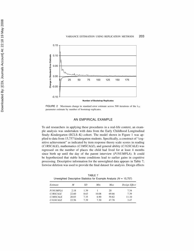
A second interest in this study was to examine the number of bootstrap
replications that were necessary for proper standard error estimation. An ex-
amination of the stability of the estimates over increasing R size from 1 to
200 was undertaken, and one example of the results is shown in Figure 2. The
maximum change in the estimated standard error at each replication across the
500 simulated datasets is shown for a representative parameter (œ31). In general,
across the 500 iterations, the estimate appeared to stabilize fairly quickly; very
little movement in the estimate occurred after 50 bootstrap samples, and certainly
estimates were stable within 100 replications. This result supports the finding in
Kovar et al. (1988), that 100 replications (as opposed to 200) might be sufficient
in this context. The findings were consistent across all three types of parameters
studied in this model.
Dow
nloa
ded
By:
[CD
L Jo
urna
ls A
ccou
nt] A
t: 22
:18
19 M
ay 2
008
VARIANCE ESTIMATION USING REPLICATION METHODS 203
FIGURE 2 Maximum change in standard error estimate across 500 iterations of the œ31
parameter estimate by number of bootstrap replicates.
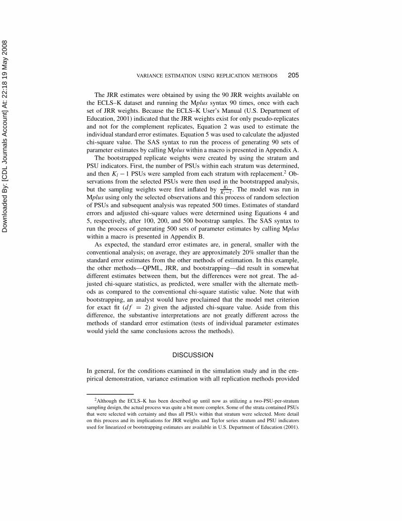
AN EMPIRICAL EXAMPLE
To aid researchers in applying these procedures in a real-life context, an exam-
ple analysis was undertaken with data from the Early Childhood Longitudinal
Study–Kindergarten (ECLS–K) cohort. The model shown in Figure 1 was ap-
plied to data from 15,757 kindergarten students. Specifically, a construct of “cog-
nitive achievement” as indicated by item response theory scale scores in reading
(C1RSCALE), mathematics (C1MSCALE), and general ability (C1GSCALE) was
regressed on the number of places the child had lived for at least 4 months
since birth up until the day of the parent interview (P1NUMPLA). It could
be hypothesized that stable home conditions lead to earlier gains in cognitive
processing. Descriptive information for the unweighted data appears in Table 7;
listwise deletion was used to provide the final dataset for analysis. Design effects
TABLE 7
Unweighted Descriptive Statistics for Example Analysis (N D 15,757)
Estimate M SD Min Max Design Effect
P1NUMPLA 2.18 1.39 1 20 7.34
C1RSCALE 22.60 8.63 10.08 69.66 7.39
C1MSCALE 20.03 7.35 6.90 59.82 11.10
C1GSCALE 22.56 7.39 7.30 47.78 3.47

Dow
nloa
ded
By:
[CD
L Jo
urna
ls A
ccou
nt] A
t: 22
:18
19 M
ay 2
008
204 STAPLETON
of the mean for each variable were calculated as the ratio of the square of the
standard error estimated via SAS PROC SURVEYMEANS over the square of
the standard error estimated via SAS PROC MEANS; the stratum and PSU
identifiers were provided in the syntax for the SURVEYMEANS procedure and
Taylor series linearization was used.
The analysis was undertaken using conventional SEM to obtain parameter
estimates and conventional estimates of standard errors (as shown in Table 8)
and then five other methods of obtaining standard error estimates and adjusted
chi-square statistics were used: QPML estimation, JRR estimation, and three
variations of bootstrapping using 100, 200, and 500 replications. The QPML
estimation was undertaken by indicating that TYPEDCOMPLEX in the Mplus
syntax as well as providing the sampling stratum variable (C1CPTSTR) and a
PSU indicator variable. Note that Mplus requires that PSU identifiers be unique
across all strata; most NCES databases have sequential numbering of PSUs
within strata, but will reuse PSU identifiers across strata (thus the first stratum
might have PSUs with indicator values of 1 and 2 and the second stratum might
also have PSUs with indicator values of 1 and 2). For this analysis, a new PSU
indicator was created by concatenating the identifier (C1CPTSTR) with the PSU
indicator (C1CPTPSU). Both the conventional and QPML estimation analyses
used the sampling weight C1CPTW0.
TABLE 8
Unstandardized Estimates From the Example Early Childhood Longitudinal Study Analysis
Estimate Conv. PML Jack Boot100 Boot200 Boot500
Model chi-square
(adjusted chi-square)
8.643 6.524 6.002 4.676 4.937 4.876
Parameter estimates
œ21 1.006 — — — — —
œ31 0.736 — — — — —
”11 �0.386 — — — — —
§11 44.824 — — — — —
•11 25.873 — — — — —
•22 6.664 — — — — —
•33 29.501 — — — — —
Standard error estimates
œ21 0.012 0.013 0.012 0.012 0.013 0.013
œ31 0.011 0.013 0.012 0.019 0.017 0.017
”11 0.040 0.051 0.050 0.054 0.051 0.053
§11 1.122 1.618 1.426 1.875 1.887 1.922
•11 0.732 0.876 0.933 0.949 0.938 0.921
•22 0.445 0.474 0.500 0.435 0.426 0.420
•33 0.422 0.519 0.548 0.599 0.521 0.549
Note. PML D pseudo maximum likelihood; Jack D jackknife repeated replication; Boot D
bootstrapping.
Dow
nloa
ded
By:
[CD
L Jo
urna
ls A
ccou
nt] A
t: 22
:18
19 M
ay 2
008
VARIANCE ESTIMATION USING REPLICATION METHODS 205
The JRR estimates were obtained by using the 90 JRR weights available on
the ECLS–K dataset and running the Mplus syntax 90 times, once with each
set of JRR weights. Because the ECLS–K User’s Manual (U.S. Department of
Education, 2001) indicated that the JRR weights exist for only pseudo-replicates
and not for the complement replicates, Equation 2 was used to estimate the
individual standard error estimates. Equation 5 was used to calculate the adjusted
chi-square value. The SAS syntax to run the process of generating 90 sets of
parameter estimates by calling Mplus within a macro is presented in Appendix A.
The bootstrapped replicate weights were created by using the stratum and
PSU indicators. First, the number of PSUs within each stratum was determined,
and then Kl � 1 PSUs were sampled from each stratum with replacement.2 Ob-
servations from the selected PSUs were then used in the bootstrapped analysis,
but the sampling weights were first inflated by Kl
Kl �1. The model was run in
Mplus using only the selected observations and this process of random selection
of PSUs and subsequent analysis was repeated 500 times. Estimates of standard
errors and adjusted chi-square values were determined using Equations 4 and
5, respectively, after 100, 200, and 500 bootstrap samples. The SAS syntax to
run the process of generating 500 sets of parameter estimates by calling Mplus
within a macro is presented in Appendix B.
As expected, the standard error estimates are, in general, smaller with the
conventional analysis; on average, they are approximately 20% smaller than the
standard error estimates from the other methods of estimation. In this example,
the other methods—QPML, JRR, and bootstrapping—did result in somewhat
different estimates between them, but the differences were not great. The ad-
justed chi-square statistics, as predicted, were smaller with the alternate meth-
ods as compared to the conventional chi-square statistic value. Note that with
bootstrapping, an analyst would have proclaimed that the model met criterion
for exact fit (df D 2) given the adjusted chi-square value. Aside from this
difference, the substantive interpretations are not greatly different across the
methods of standard error estimation (tests of individual parameter estimates
would yield the same conclusions across the methods).
DISCUSSION
In general, for the conditions examined in the simulation study and in the em-
pirical demonstration, variance estimation with all replication methods provided
2Although the ECLS–K has been described up until now as utilizing a two-PSU-per-stratum
sampling design, the actual process was quite a bit more complex. Some of the strata contained PSUs
that were selected with certainty and thus all PSUs within that stratum were selected. More detail
on this process and its implications for JRR weights and Taylor series stratum and PSU indicators
used for linearized or bootstrapping estimates are available in U.S. Department of Education (2001).

Dow
nloa
ded
By:
[CD
L Jo
urna
ls A
ccou
nt] A
t: 22
:18
19 M
ay 2
008
206 STAPLETON
similar estimates of standard errors and adjusted chi-square values, and these
values were quite similar to the estimates obtained through QPML estimation
available in current versions of LISREL and Mplus software. The use of any
of these options should be strongly preferred over the option of running a
conventional analysis when the data result from a complex sampling design.
Under conditions specified in this study, although the standard error estimates
were negatively biased by nearly 70% for the conventional analysis, all standard
errors from the replication designs were biased by less than 10.7%, although
that bias was consistently positive. This slight positive bias is the result of
assuming that the PSUs were sampled with replacement (and not utilizing a finite
population correction). In terms of the chi-square rejection rates, a conventional
analysis would suggest that the hypothesized model is not consistent with the
sample data, whereas using the adjusted chi-square value would result in a
decision that the hypothesized model is plausible. In this study, equivalent
design effects were generated for all measured variables, thus the assumption of
equivalent design effects for the Rao–Scott-type correction to the chi-square was
met. This condition might not be reasonable in empirical data; future research
might examine the impact on the chi-square adjustment of including variables
with very different design effects in one model.
With regards to chi-square, a contrary result across two analyses is of theoretic
value; a discrepancy between the chi-square statistic from a weighted conven-
tional analysis and the adjusted chi-square statistic alerts the analyst to a possible
confound of theoretic cluster effects. If the interpretations from the chi-square
statistics are discrepant, the analyst can claim that the model is plausible for the
finite population, but will need to reflect on the assumption that the clustering
is truly a nuisance. If clustering plays a role in the causal mechanism among
observed variables, then interpretations made against the finite population model
might not be appropriate for generalization and a model-based analysis, such as
multilevel SEM, might be more appropriate for theory building.
It is hoped that this article has highlighted some of the issues that must
be considered when undertaking an SEM analysis with complex sample data.
Current versions of some SEM software are not able to accommodate the
complex sampling structure behind some large-scale data; however, with the
programming tools provided in the appendices, analysts could examine for
themselves the alternate results and interpretations they might obtain if they
use a replication method for estimation. Although only one type of sampling
design and set of population characteristics were considered here, findings should
extend to other sampling designs and population structures. Because the success
of the estimation has been found to differ across statistic types (Kish & Frankel,
1974; Rao & Wu, 1988), future research could consider whether there might be
an interaction between the complexity of the model analyzed and the robustness
of the standard error estimates with any of these variance estimation techniques.

Dow
nloa
ded
By:
[CD
L Jo
urna
ls A
ccou
nt] A
t: 22
:18
19 M
ay 2
008
VARIANCE ESTIMATION USING REPLICATION METHODS 207
ACKNOWLEDGMENTS
This research was supported in part by a grant from the American Educational
Research Association, which receives funds for its AERA Grants Program from
the U.S. Department of Education’s National Center for Education Statistics of
the Institute for Education Sciences, and the National Science Foundation under
NSF Grant No. RED-9980573. Opinions reflect those of the author and do not
necessarily reflect those of the granting agencies.
REFERENCES
Asparouhov, T. (2004). Stratification in multivariate modeling (Web Notes: No. 9). Retrieved August
8, 2004, from http://www.statmodel.com/mplus/examples/webnotes/MplusNote921.pdf
Asparouhov, T. (2005). Sampling weights in latent variable modeling. Structural Equation Modeling,
23, 411–434.
Asparouhov, T., & Muthén, B. (2005). Multivariate statistical modeling with survey data. Proceedings
of the Federal Committee on Statistical Methodology Research Conference. Retrieved September
26, 2006, from http://www.fcsm.gov/05papers/Asparouhov_Muthen_IIA.pdf
Coker, J. K., & Borders, L. D. (2001). An analysis of environmental and social factors affecting
adolescent problem drinking. Journal of Counseling and Development, 79, 200–208.
Efron, B. (1982). The jackknife, the bootstrap, and other resampling plans. Philadelphia: SIAM.
Fan, X. (2001). The effect of parent involvement on high school students’ academic achievement:
A growth modeling analysis. Journal of Experimental Education, 70, 27–61.
Hoogland, J. J., & Boomsma, A. (1998). Robustness studies in covariance structure modeling: An
overview and a meta-analysis. Sociological Methods and Research, 26, 329–367.
Hox, J. J. (2002). Multilevel analysis: Techniques and applications. Mahwah, NJ: Lawrence Erlbaum
Associates, Inc.
Kalton, G. (1983). Models in the practice of survey sampling. International Statistical Review, 51,
175–188.
Kaplan, D., & Elliott, P. R. (1997). A didactic example of multilevel structural equation modeling
applicable to the study of organizations. Structural Equation Modeling, 4, 1–24.
Kaufman, S. (2000). Using the bootstrap to estimate the variance in a very complex sample design.
American Statistical Association, Proceedings of the Survey Research Methods Section, 180–185.
Retrieved March 21, 2005, from www.amstat.org/sections/srms/proceedings/y2002/files/JSM2002-
00288.pdf
Kish, L. (1965). Survey sampling. New York: Wiley.
Kish, L., & Frankel, M. R. (1974). Inference from complex samples. Journal of the Royal Statistical
Society, 36 (Series B), 1–37.
Kovar, J. G., Rao, J. N. K., & Wu, C. F. J. (1988). Bootstrap and other methods to measure errors
in survey estimates. Canadian Journal of Statistics, 16, 25–46.
Lahiri, P. (2003). On the impact of the bootstrap in survey sampling and small-area estimation.
Statistical Science, 18, 199–210.
Lee, E. S., Forthofer, R. N., & Lorimor, R. J. (1989). Analyzing complex survey data. Newbury
Park, CA: Sage.
Lohr, S. L. (1999). Sampling: Design and analysis. Pacific Grove, CA: Duxbury Press.
Longford, N. T. (1995). Model-based methods for analysis of data from 1990 NAEP trial state
assessment. Washington, DC: National Center for Education Statistics.

Dow
nloa
ded
By:
[CD
L Jo
urna
ls A
ccou
nt] A
t: 22
:18
19 M
ay 2
008
208 STAPLETON
Marsh, H. W., & Yeung, A. S. (1996). The distinctiveness of affects in specific school subjects: An
application of confirmatory factor analysis with the National Educational Longitudinal Study of
1988. American Educational Research Journal, 33, 665–689.
Muthén, B. O., & Satorra, A. (1995). Complex sample data in structural equation modeling. In P. V.
Marsden (Ed.), Sociological methodology (pp. 267–316). Washington, DC: American Sociological
Association.
Muthén, L. K., & Muthén, B. O. (2004). Mplus user’s guide version 3. Los Angeles: Muthén &
Muthén.
Rao, J. N. K., & Scott, A. J. (1981). The analysis of categorical data from complex sample surveys:
Chi-squared tests for goodness of fit and independence in two-way tables. Journal of the American
Statistical Association, 76, 221–230.
Rao, J. N. K., & Thomas, D. R. (1989). Chi-square tests for contingency tables. In C. J. Skinner,
D. Hold, & T. M. F. Smith (Eds.), Analysis of complex surveys (pp. 89–114). New York: Wiley.
Rao, J. N. K., & Wu, C. F. J. (1988). Resampling inference with complex survey data. Journal of
the American Statistical Association, 83, 231–241.
Rao, J. N. K., Wu, C. F. J., & Yue, K. (1992). Some recent work on resampling methods for complex
surveys. Survey Methodology, 18, 209–217.
Rust, K. F., & Rao, J. N. K. (1996). Variance estimation for complex surveys using replication
techniques. Statistical Methods in Medical Research, 5, 283–310.
Satorra, A., & Bentler, P. M. (1988). Scaling corrections for chi-square statistics in covariance
structure analysis. Proceedings of the Business and Economic Statistics Section of the American
Statistical Association (pp. 308–313). Alexandria, VA: American Statistical Association.
Scientific Software International. (2004). Analysis of structural equation models for continuous
random variables in the case of complex survey data. LISREL 8.7 for Windows: Technical docu-
mentation. Retrieved April 2, 2005, from http://www.ssicentral.com/lisrel/techdocs/compsem.pdf
Singh, K., & Billingsley, B. S. (1998). Professional support and its effect on teachers’ commitment.
Journal of Educational Research, 91, 229–239.
Skinner, C. J., Holt, D., & Smith, T. M. F. (1989). Analysis of complex surveys. Chichester, UK:
Wiley.
Stapleton, L. M. (2006). An assessment of practical solutions for structural equation modeling with
complex sample data. Structural Equation Modeling, 13, 28–58.
U.S. Department of Education. (1996). National Education Longitudinal Study: 1988–1994 method-
ology report. Washington, DC: National Center for Education Statistics.
U.S. Department of Education. (2001). ECLS-K, Base year public-use data file, kindergarten class
of 1998–99: Data files and electronic code book: (Child, teacher, school files). Washington, DC:
National Center for Education Statistics.
Walker, D. A., & Young, D. Y. (2003). Example of the impact of weights and design effects on
contingency tables and chi-square analyses. Journal of Modern Applied Statistical Methods, 2,
425–432.
Wang, J., & Ma, X. (2001). Effects of educational productivity on career aspiration among United
States high school students. The Alberta Journal of Educational Research, 47, 75–86.
Wang, J., & Staver, J. R. (2001). Examining relationships between factors of science education and
student career aspiration. Journal of Educational Research, 94, 312–319.
Wolter, K. M. (1985). Introduction to variance estimation. New York: Springer-Verlag.

Dow
nloa
ded
By:
[CD
L Jo
urna
ls A
ccou
nt] A
t: 22
:18
19 M
ay 2
008
VARIANCE ESTIMATION USING REPLICATION METHODS 209
APPENDIX A: SAS SYNTAX TO RUN JACKKNIFE
REPLICATION WITH THE MPLUS SOFTWARE ON
ECLS—K DATA
%MACRO JACK;
%DO J=1 %TO 90; ***run for as many jackknife weights as you have*;
DATA TEMP;
SET fall_ecls2; *this is the SAS dataset that contains the raw data and 90
sets of replicate weights*;
*next, I write out model variables to a text file*;
FILE ‘C:\TEMPdata\MPLUSDAT.DAT’;
PUT @1 C1RSCALE @11 C1MSCALE @21 C1GSCALE @41 P1NUMPLA @51 C1CPTW&J;
*note that the jackknife weights should be named
sequentially from 1 to 90;
RUN;
DM "x ‘c:\ECLS_JACK.BAT’"; *this command runs an external batch file *;
*that calls Mplus and runs prespecified input syntax*;
DATA READIN_RESULTS;
INFILE ‘C:\RESULTS_JACK’; *in Mplus, the estimates are saved to this file*;
*next, Mplus estimates are read in and saved to a dataset*;
INPUT V2INT V3INT V4INT V3F1 V4F1 E2E2 E3E3 E4E4 F1V1 D1D1 /
SEV2INT SEV3INT SEV4INT SEV3F1 SEV4F1 SEE2E2 SEE3E3 SEE4E4 SEF1V1 SED1D1/
CHISQ CHISQDF CHISQP CFI TLI LLH0 LLH1 FREEPARA AIC BIC /
ABIC RMSEA SRMR;
JACK=&J;
PROC DATASETS; APPEND BASE=LIB.RESULTS_ECLS_JACK DATA=READIN_RESULTS ; quit;
*dataset will append by 1 record each loop thru the %DO statement*;
%END;
%MEND;
%JACK;
APPENDIX B: SAS SYNTAX TO RUN BOOTSTRAP
REPLICATION WITH THE MPLUS SOFTWARE ON
ECLS—K DATA
PROC SORT DATA=fall_ecls2; BY C1CPTSTR C1CPTPSU; *sort data by stratum, PSU*;
DATA STRAT_PSUS; SET FALL_ECLS2; BY C1CPTSTR C1CPTPSU;
IF FIRST.C1CPTPSU; KEEP C1CPTSTR C1CPTPSU; *list of stratum, PSU *;
DATA STRATNUM; SET STRAT_PSUS; BY C1CPTSTR C1CPTPSU;
RETAIN NUMPSU;
IF FIRST.C1CPTSTR THEN NUMPSU=0;
IF FIRST.C1CPTPSU THEN NUMPSU=NUMPSU+1;
IF LAST.C1CPTSTR;
_NSIZE_=NUMPSU-1;
KEEP C1CPTSTR _NSIZE_; *provides data file of Stratum IDs and K-1*;

Dow
nloa
ded
By:
[CD
L Jo
urna
ls A
ccou
nt] A
t: 22
:18
19 M
ay 2
008
210 STAPLETON
PROC SURVEYSELECT DATA=STRAT_PSUS METHOD=URS SAMPSIZE=STRATNUM SEED=8923
OUT=SELECTED_PSUS REP=500;
STRATA C1CPTSTR; RUN; *requests 500 stratified samples of PSUs be drawn
*(based on C1CPTSTR) with replacement, using the
*(K-1) sample sizes contained in File STRATNUM. *;
PROC SORT DATA=SELECTED_PSUS; BY C1CPTSTR C1CPTPSU;
DATA ADD_NMINUS1;
MERGE SELECTED_PSUS STRATNUM; BY C1CPTSTR;
WEIGHTSCALE=(_NSIZE_+1)/(_NSIZE_);
*creates a constant for each stratum to be applied
*to scale weights from selected PSUs*;
%MACRO BOOT;
%DO B=1 %TO 500; ***run for as many BOOTSTRAP SAMPLES as you have*;
DATA PSU_REP;
SET ADD_NMINUS1;
IF REPLICATE=&B; *selects appropriate PSUs given bootstrap sample number*;
DATA ALLDATA;
MERGE PSU_REP (IN=A) FALL_ECLS2; BY C1CPTSTR C1CPTPSU; IF A;
*only records that match with the selected bootstrap PSUs
*are included in this analysis*;
NEWWEIGHT=WEIGHTSCALE*C1CPTW0; *weights are adjusted by K/(K - 1)*;
*next, I write out model variables to a text file *;
FILE ‘C:\TEMPdata\MPLUSDAT.DAT‘;
PUT @1 C1RSCALE @11 C1MSCALE @21 C1GSCALE @41 P1NUMPLA @51 NEWWEIGHT ;
RUN;
DM "x ‘c:\ECLS_BOOT.BAT‘"; *this command runs an external batch file *;
*that calls Mplus and runs prespecified input syntax*;
DATA READIN_RESULTS;
INFILE ‘C:\ RESULTS_BOOT‘; **in Mplus, estimates are saved to this file*;
*next, Mplus estimates are read in and saved to a dataset*;
INPUT V2INT V3INT V4INT V3F1 V4F1 E2E2 E3E3 E4E4 F1V1 D1D1 /
SEV2INT SEV3INT SEV4INT SEV3F1 SEV4F1 SEE2E2 SEE3E3 SEE4E4 SEF1V1 SED1D1/
CHISQ CHISQDF CHISQP CFI TLI LLH0 LLH1 FREEPARA AIC BIC /
ABIC RMSEA SRMR;
BOOT=&B;
PROC DATASETS; APPEND BASE=LIB.RESULTS_ECLS_BOOT DATA=READIN_RESULTS; quit;
*dataset will append by 1 record each loop thru the %DO statement*;
%END;
%MEND;
%BOOT;