Embed Size (px)
Citation preview
SEM Handbook of Experimental Structural Dynamics - Structural Dynamics Modification and Modal Modeling
Page 1 of 46
Structural Dynamics Modification and Modal Modeling
Structural Dynamics Modification (SDM) also known as eigenvalue modification [1], has become a
practical tool for improving the engineering designs of mechanical systems. It provides a quick and
inexpensive approach for investigating the effects of design modifications, in the form of mass, stiffness
and damping changers, to a structure, thus eliminating the need for costly prototype fabrication and
testing.
Modal Models
SDM is unique in that it works directly with a modal model of the structure, either an Experimental Modal
Analysis (EMA) modal model, a Finite Element Analysis (FEA) modal model, or a Hybrid modal model
consisting of both EMA and FEA modal parameters. EMA mode shapes are obtained from experimental
data and FEA mode shapes are obtaind from a finite element computer model.
A modal model consists of a set of properly scaled mode shapes. A modal model preserves the mass
and elastic properties of the structure, and therefore is a complete representation of its dynamic
properties.
In the mathematics used in this chapter, it is assumed that the mode shapes used to model the dynamics
of the structure are scaled to Unit Modal Masses. Therefore, they are referred to as UMM mode
shapes. UMM mode shape scaling is commonly used on FEA mode shapes, and is also used on EMA
mode shapes. The mathematics used to scale EMA mode shapes to Unit Modal Masses is also
presented in this chapter.
Design Modifications
Once the dynamic properties of an unmodified structure are defined in the form of its modal model, SDM
can be used to predict the dynamic effects of mechanical design modifications to the structure. These
modifications can be as simple as point mass, linear spring, or linear damper additions to or removal
from the structure, or they can be more complex modifications that are modeled using FEA elements
such as rod and beam elements, plate elements (membranes) and solid elements.
SDM is computationally very efficient because it solves an eigenvalue problem in modal space, whereas
FEA mode shapes are obtained by solving an eigenvalue problem in physical space.
Another advantage of SDM is that the modal model of the unmodified structure only has to contain data
for the DOFs (points and directions) where the modification elements are attached to the structure.
SDM then provides a new modal model of the modified structure, as depicted in Figure 1.
Figure 1. SDM Input-Output Diagram
SEM Handbook of Experimental Structural Dynamics - Structural Dynamics Modification and Modal Modeling
Page 2 of 46
Eigenvalue Modification
A variety of numerical methods have been developed over the years which only require a modal model to
represent the dynamics of a structure. Among the more traditional methods for performing these
calculations are modal synthesis, the Lagrange multiplier method, and diakoptics. However, the
local eigenvalue modification technique, developed primarily through the work of Weissenburger,
Pomazal, Hallquist, and Snyder [1], is the technique commonly used by the SDM method.
All of the early development work was done primarily with analytical FEA models. The primary objective was to provide a faster means of investigating many physical changes to a structure without having to solve a large eigenvalue problem. FEA modes are obtained by solving the problem in physical coordinates, whereas SDM solves a much smaller eigenvalue problem in modal coordinates.
In 1979, Structural Measurement Systems (SMS) began using the local eigenvalue modification method
together with EMA modal models. EMA modes are derived from experimental data acquired during a
modal test. [2]-[5]. The computational efficiency of this method made it very attractive for implementation
on a desktop calculator or computer, which could be used in a laboratory. More importantly, it gave
reasonably accurate results and required only a relatively small number of modes in the EMA modal
model of the unmodified structure. A modal model with only a few modes is called a truncated modal
model, and its use in SDM is called modal truncation.
In most cases, regardless of whether EMA or FEA mode shapes are used, a truncated modal model
does adequately characterize the dynamics of a structure. Some of the effects of using a truncated modal
model were presented in [2] and [3].
The fundamental calculation process of SDM is the solution of an eigenvalue problem. It is
computationally efficient because it only requires the solution of a small dimensional eigenvalue problem.
Its computational speed is virtually independent of the number of physical DOFs used to model a
structural modification. Hence, very large modifications are handled as efficiently as smaller modifications.
The SDM computational process is straightforward. To model a structural modification, all physical
modifications are converted into appropriate changes to the mass, stiffness, and damping matrices of the
equations of motion, in the same manner as an FEA model is constructed. These modification matrices
are then transformed to modal coordinates using the mode shapes of the unmodified structure. The
resulting transformed modifications are then added to the modal properties of the unmodified structure,
and these new equations are solved for the new modal model of the modified structure.
By comparison, if there were 1000 DOFs in a dynamic model, solving for its FEA modes requires the
solution of an eigenvalue problem with matrices of the size (1000 by 1000). However, if the dynamics of
the unmodified structure are represented with a modal model with 10 modes in it, the new modes
resulting from a structural modification are found by solving an eigenvalue problem with matrices of the
size (10 by 10).
The size of the eigenvalue problem in modal space is also independent of the number of modifications
made to the structure. Therefore, many modifications can be modeled simultaneously, and the solution
time of the eigenvalue problem does not increase significantly.
Inputs to SDM are as follows,
1. A modal model that adequately represents the dynamics of the unmodified structure
2. Finite elements attached to a geometric model of the structure that characterize the structural
modifications
With these inputs, SDM calculates a new modal model that represents the dynamics of the modified
structure.
In addition to its computational speed, it will be shown in later examples that SDM obtains results that are
very comparable to those from an FEA eigen-solution.
SEM Handbook of Experimental Structural Dynamics - Structural Dynamics Modification and Modal Modeling
Page 3 of 46
Measurement Chain to Obtain an EMA Modal Model
Before proceeding with a mathematical explanation of the SDM technique, it is important to review the
factors that can affect the accuracy of EMA modal parameters. The accuracy of the EMA parameters will
greatly influence the accuracy of the results calculated with the SDM method. To address the potential
errors that can occur in an EMA modal model, the accuracy of some of the steps in a required
measurement chain will be discussed.
The major steps of the measurement chain consist of acquiring experimental data from a test structure,
from which a set of frequency response functions (FRFs) is calculated. This set of FRFs is then curve fit
to estimate the parameters of an EMA modal model. Following is a list of things to consider in order to
calculate a set of FRFs, and ultimately estimate the parameters of an EMA modal model.
Critical Issues in the Measurement Chain
1) The test structure 2) Boundary conditions of the test structure 3) Excitation technique 4) Force and response sensors 5) Sensor mounting 6) Sensor calibration 7) Sensor cabling 8) Signal acquisition and conditioning 9) Spectrum analysis 10) FRF calculation 11) FRF curve fitting 12) Creating an EMA modal model
All of the above items involve assumptions that can impact the accuracy of the EMA modal model and
ultimately the accuracy of the SDM results. Only a few of these critical issues will be addressed here,
namely; sensors, sensor mounting, sensor calibration, FRF calculation, and FRF curve fitting.
Calculating FRFs from Experimental Data
To create an EMA modal model, a set of calibrated inertial FRF measurements is required. These
frequency domain measurements are unique in that they involve subjecting the test structure to a known
measurable force while simultaneously measuring the structural response(s) due to the force. The
structural response is measured either as acceleration, velocity, or displacement using sensors that are
either mounted on the surface, or are non-contacting but still measure the surface motion.
An FRF is a special case of a Transfer function. A Transfer function is a frequency domain relationship
between any type of input signal and any type of output signal. An FRF defines the dynamic relationship
between the excitation force applied to a structure at a specific location in a specific direction and the
resulting response motion at another specific location in a specific direction. The force input point &
direction and the response point & direction are referred to as the Degrees of Freedom (or DOFs) of the
FRF.
An FRF is also called a cross-channel measurement function. It requires the simultaneous
acquisition of both a force and its resultant response. This means that at least a 2-channel data
acquisition system or spectrum analyzer is required to measure the signals required to calculate an FRF.
The force (input) and the response (output) signals must also be simultaneously acquired, meaning that
both channels of data are amplified, filtered, and sampled at the same time.
Sensing Force & Motion
The excitation force is typically measured with a load cell. The analog signal from the load cell is fed into
one of the channels of the data acquisition system. The response is measured either with an
accelerometer, laser vibrometer, displacement probe, or other sensor that measures surface motion.
SEM Handbook of Experimental Structural Dynamics - Structural Dynamics Modification and Modal Modeling
Page 4 of 46
Accelerometers are most often used today because of their availability, relatively low cost, and variety of
sizes and sensitivities. The important characteristics of both the load cell and accelerometer are:
1) Sensitivity 2) Usable amplitude range 3) Usable frequency range 4) Transverse sensitivity 5) Mounting method
Sensitivity Flatness
The most common type of sensor today is referred to as a IEPE/CCLD/ICP/Deltatron/Isotron style of
sensor. This type of sensor requires a 2-10 milli-amp current supply, typically supplied by the data
acquisition system, and has a built-in charge amplifier. It also has a fixed sensitivity. Typical sensitivities
are 10mv/lb or 100mv/g.
The ideal magnitude of the frequency spectrum for any sensor is a “flat magnitude" over its usable
frequency range. The documented sensitivity of most sensors is typically given at a fixed frequency (such
as 100Hz, 159.2Hz, or 250Hz), and is referred to as its 0 dB level.
The sensitivity of an accelerometer is specified in units of mv/g or mv/(m/s^2) with a typical accuracy of
+/-5% at a specific frequency. The frequency spectrum of all sensors in not perfectly flat, meaning that
its sensitivity varies somewhat over its useable frequency range. The response amplitude of an ICP
accelerometer typically rolls off at low frequencies and rises at the high end of its useable frequency
range. This specification is the flatness of the sensor, with a typical variance of +/-10% to +/-15%.
All of this equates to a possible error in the sensitivity of the force or response sensor over its usable
frequency range. This means that the amplitude of an FRF might be in error by the amount that the
sensitivity changes over its measured frequency range.
Transverse Sensitivity
Adding to its flatness error is the transverse sensitivity of the sensor. A uniaxial (single axis) transducer
should only output a signal due to force or motion in the direction of its sensitive axis. Ideally, any force or
motion that is not along its sensitive axis should not yield an output signal, but this is not the case with
most sensors.
Both force and motion have a direction associated with them. That is, a force or motion must be defined
at a point in a particular direction.
All sensors have a documented specification called transverse sensitivity or cross axis sensitivity.
Transverse sensitivity specifies how much of the sensor output is due to a force or motion that comes
from a direction other than the measurement axis of the sensor. Transverse sensitivity is typically less
than 5% of the sensitivity of the sensitive axis. For example, if an accelerometer has a sensitivity of
100mv/g, its transverse sensitivity might be about 5mv/g. Therefore, 1g of motion in a direction other than
the sensitive axis of an accelerometer might add 5mv (or 0.05g) to its output signal.
Sensor Linearity
Another area affecting the accuracy of an FRF is the linearity of each sensor output signal relative to the
actual force or motion. In other words, if the sensor output signal were plotted as a function of its input
force or input motion, all of its output signal values should lie on a straight line. Any values that do not
lie on a straight line are an indication of the non-linearity of the sensor. The non-linearity specification is
typically less than 1% over the specified useable frequency range of the sensor.
As the amplitude of the measured signal becomes larger than the specified amplitude range of the
sensor, the signal will ultimately cause an overload in the internal amplifier of the sensor. This overload
results in a clipped output signal from the sensor. A clipped output signal is the reason why it is very
important to measure amplitudes that are within the specified amplitude range of a sensor.
SEM Handbook of Experimental Structural Dynamics - Structural Dynamics Modification and Modal Modeling
Page 5 of 46
Sensor Mounting
Attaching a sensor to the surface of the test article is also of critical importance. The function of a sensor
is to “transduce” a physical quantity, for example the acceleration of the surface at a point in a direction.
Therefore, it is important to attach the sensor to a surface so that it will accurately transduce the surface
motion over the frequency range of interest.
Mounting materials and techniques also have a useable frequency range just like the sensor itself. It is
very important to choose an appropriate mounting technique so that the surface motion over the desired
frequency range is not affected by the mounting material of method. Magnets, tape, putty, glue, or
contact cement are all convenient materials for attaching sensors to surfaces. However, mechanical
attachment using a threaded stud is the most reliable method, with the widest frequency range.
Leakage Errors
Another error associated with the FRF calculation is a result of the FFT algorithm itself. The FFT
algorithm is used to calculate the Digital Fourier Transform (DFT) of the force and response signals.
These DFT's are then used to calculate an FRF.
Finite Length Sampling Window
The FFT algorithm assumes that the time domain window of acquired digital data (called the sampling
window) contains all of the acquired signal. If all of an acquired signal is not captured in its sampling
window, then its spectrum will contain leakage errors.
Leakage-Free Spectrum
The spectrum of an acquired signal will be leakage-free if one of the following conditions is satisfied.
1. If a signal is periodic (like a sine wave), then it must make one or more complete cycles within
the sampled window
2. If a signal is not periodic, then it must be completely contained within the sampled window.
If an acquired signal does not meet either of the above conditions, there will be errors in its DFT, and
hence errors in the resulting FRF. This error in the DFT of a signal is called leakage error. Leakage error
causes both amplitude and frequency errors in a DFT and also in an FRF.
Leakage-Free Signals
Leakage is eliminated by using testing signals that meet one of the two conditions stated above. During
Impact testing, if the impulsive force and the impulse response signals are both completely contained
within their sampling windows, leakage-free FRFs can be calculated using those signals.
During shaker testing, if a Burst Random or a Burst Chirp (fast swept sine) shaker signal, which is
terminated prior to the end of its sampling window so that both the force and structural response signals
are completely contained within their sampling windows, leakage-free FRFs can also be calculated using
those signals
Reduced Leakage
If one of the two leakage-free conditions cannot be met by the acquired force and response signals, then
leakage errors can be minimized in their spectra by applying an appropriate time domain window to the
sampled signal before the FFT is applied to it. A Hanning window is typically applied to pure
(continuous) random signals, which are never completely contained within their sampling windows. Using
a Hanning window will minimize leakage in the resulting FRFs.
Linear versus Non-Linear Dynamics
Both EMA and FEA modal models are defined as solutions to a set of linear differential equations.
Using a modal model therefore, assumes that the linear dynamic behavior of the test article can be
SEM Handbook of Experimental Structural Dynamics - Structural Dynamics Modification and Modal Modeling
Page 6 of 46
adequately described using these equations.. However, the dynamics of a real world structure may
not be linear.
Real-world structures can have dynamic behavior ranging from linear to slightly non-linear to severely
non-linear. If the test article is in fact undergoing non-linear behavior, significant errors will occur when
attempting to extract modal parameters from a set of FRFs, which are based on a linear dynamic model.
Random Excitation & Spectrum Averaging
To reduce the effects of non-linear behavior, random excitation combined with signal post-processing
must be applied to the acquired data. The goal is to yield a set of linear FRF estimates to represent the
dynamics of the structure subject to a certain force level.
This common method for testing a non-linear structure is to excite it with one or more shakers using
random excitation signals. If these signals continually vary over time, the random excitation will excite the
non-linear behavior of the structure in a random fashion.
The FFT will convert the non-linear components of the random responses into random noise that is
spread over the entire frequency range of the DFTs of the signals. If multiple DFTs of a randomly excited
response are averaged together, the random non-linear components will be “averaged out” of the DFT
leaving only the linear resonant response peaks.
Curve Fitting FRFs
The goal of FRF-based EMA is first to calculate a set of FRFs that accurately represent the linear
dynamics of a structure over a frequency range of interest followed by curve fitting the FRFs using a
linear parametric FRF model. The ultimate goal is to obtain an accurate EMA modal model.
If the test structure has a high modal density including closely coupled modes or even repeated roots
(two modes at the same frequency with different mode shapes), extracting an accurate EMA modal model
can be challenging.
The linear parametric FRF model is a summation of contributions due to all of the modes at each
frequency sample of the FRFs. This model is commonly curve fit to the FRF data using a least-squared-
error method. This broadband curve fit approach also assumes that all of the resonances of the structure
have been adequately excited over the frequency span of the FRFs.
A wide variety of FRF-based curve fitting methods are commercially available today. All of the popular
FRF-based curve fitting algorithms assume that the FRFs represent the linear dynamics of a structure
and they are leakage-free.
Modal Models and SDM
SDM will give accurate results when used with an accurate modal model of the unmodified structure. That
model can be an EMA modal model, FEA modal model, or a Hybrid model that uses both EMA and FEA
modal parameters. We have pointed out many of the errors that can occur in an EMA modal model and
ultimately affect the accuracy of SDM results..
The real advantage of SDM is that once you have a reasonably accurate modal model of the unmodified
structure, you can quickly explore numerous structural modifications, including alternate boundary
conditions which are difficult to model with an FEA model. In the examples later in this chapter, we will
use a Hybrid modal model and SDM to model the attachment of a RIB stiffener to an aluminum plate..
(This is called a Substructuring problem.) We will then compare FEA, SDM, and experimental results.
Structural Dynamic Models
The dynamic behavior of a mechanical structure can be modeled either with a set of differential equations
in the time domain, or with an equivalent set of algebraic equations in the frequency domain. Once the
SEM Handbook of Experimental Structural Dynamics - Structural Dynamics Modification and Modal Modeling
Page 7 of 46
equations of motion have been created, they can be used to calculate mode shapes and also to calculate
structural responses to static loads or dynamic forces.
The dynamic response of most structures usually includes resonance-assisted vibration.. Dynamic
resonance-assisted response levels can far exceed the deformation levels due to static loads.
Resonance-assisted vibration is often the cause of noisy operation, uncontrollable behavior, premature
wear out of parts such as bearings, and unexpected material failure due to cyclic fatigue.
Two or more spatial deformations assembled into a vector is called an Operating Deflection Shape (or
ODS).
Structural Resonances
A mode of vibration is a mathematical representation of a structural resonance. An ODS is a summation
of mode shapes. Another way of saying this is, "All vibration is a summation of mode shapes.
Each mode is represented by a modal frequency (also call natural frequency), a damping decay constant
(the decay rate of a mode when forces are removed from the structure), and its spatially distributed
amplitude levels (its mode shape). These three modal properties (frequency, damping, and mode shape)
provide a complete mathematical representation of each structural resonance. A mode shape is the
contribution of a resonance to the overall deformation (an ODS) on the surface of a structure at each
location and in each direction.
It is shown later that both the time and frequency domain equations of motion can be represented solely
in terms of modal parameters. This powerful conclusion means that a set of modal parameters can be
used to completely represent the linear dynamics of a structure.
When properly scaled, a set of mode shapes is called a modal model. The complete dynamic properties
of the structure are represented by its modal model. SDM uses the modal model of the unmodified
structure together with the FEA elements that represent the structural modifications as inputs, and
calculates a new modal model for the modified structure.
Truncated Modal Model
All EMA and FEA modal models contain mode shapes for a finite number of modes. An EMA modal
model contains a finite number of mode shape estimates that were obtained by curve fitting a set of FRFs
that span a limited frequency range. An FEA modal model also contains a finite number of mode
shapes that are defined for a limited range of frequencies. Therefore, both EMA and FEA modal
models represent a truncated (approximate) dynamic model of a structure.
With the exception of so-called lumped parameter systems, (like a mass on a spring), all real-world
structures have an infinite number of resonances in them. Fortunately, the dynamic response of most
structures is dominated by the excitation of a few lowest frequency modes.
When using the SDM method, all the low frequency modes should be included in the modal model. In
order to account for the higher frequency modes that have been left out of the truncated modal model, it
is also important to include several modes above the highest frequency mode of interest in the modal
model.
Substructuring
To solve a substructuring problem, where one structure is mounted on or attached to another using FEA
elements, the free-body dynamics (the six rigid-body modes) of the structure to be mounted on the
other must also be included in its modal model. This will be illustrated in the example later on in this
chapter
SEM Handbook of Experimental Structural Dynamics - Structural Dynamics Modification and Modal Modeling
Page 8 of 46
Rotational DOFs
Another potential source of error in using SDM is that certain modifications require mode shapes with
rotational as well as translational DOFs in them. Normally only translational motions are acquired
experimentally, and therefore the resulting FRFs and mode shapes only have translational DOFs in them.
If a modal model does not contain rotational DOFs, accurate modifications that involve torsional
stiffnesses and/or rotary inertia effects cannot be modeled accurately.
FEA mode shapes derived from rod, beam, and plate (membrane) elements do have rotational DOFs
in them. When rotational stiffness and inertia at the modification endpoints is important, FEA mode
shapes with rotational DOFs in them can be used in a Hybrid modal model as input to SDM. Later in this
chapter, SDM will be used to model the attachment of a RIB stiffener to a plate structure. Mode shapes
with rotational.DOFs and spring elements with rotational stiffness will be used to correctly model the joint
stiffness.
Time Domain Dynamic Model
Modes of vibration are defined by assuming that the dynamic behavior of a mechanical structure or
system can be adequately described by a set of time domain differential equations. These equations
are a statement of Newton’s second law (F = Ma). They represent a force balance between the internal
inertial (mass), dissipative (damping), and restoring (stiffness) forces, and the external forces acting on
the structure. This force balance is written as a set of linear differential equations,
+ + (1)
where,
= Mass matrix (n by n)
= Damping matrix (n by n)
= Stiffness matrix (n by n)
= Accelerations (n-vector)
= Velocities (n-vector)
= Displacements (n-vector)
= Externally applied forces (n-vector)
These differential equations describe the dynamics between n-discrete points & directions or n-
degrees-of-freedom (DOFs) of a structure. To adequately describe its dynamic behavior, a sufficient
number of equations can be created involving as many DOFs as necessary. Even though equations could
be created between an infinite number of DOFs, in a practical sense only a finite number of DOFs is ever
used, but they could still number in the 100's of thousands.
Notice that the damping force is proportional to velocity. This is a model for viscous damping.
Different damping models are addressed later in this chapter.
Finite Element Analysis (FEA)
Finite element analysis (FEA) is used to generate the coefficient matrices of the time domain differential
equations written above. The mass and stiffness matrices are generated from the physical and material
properties of the structure. Material properties include the modulus of elasticity, inertia, and Poisson’s
ratio (or “sqeezability”).
Damping properties are not easily modeled for real-world structures. Hence the damping force term is
usually left out of an FEA model. Even without damping, the mass and stiffness terms are sufficient to
model resonant vibration, hence the equations of motion can be solved for modal parameters.
SEM Handbook of Experimental Structural Dynamics - Structural Dynamics Modification and Modal Modeling
Page 9 of 46
FEA Modes
The homogeneous form of the differential equations, where the external forces on the right hand side
are zero, can be solved for mode shapes and their corresponding natural frequencies. This is called an
eigen-solution. Each natural frequency is an eigenvalue, and each mode shape is an eigenvector.
These analytical mode shapes are referred to as FEA modes. The transformation of the equations of
motion into modal coordinates is covered later in this chapter
Frequency Domain Dynamic Model
In the frequency domain, the dynamics of a mechanical structure or system are represented by a set of
linear algebraic equations, in a form called a MIMO (Multiple Input Multiple Output) model or Transfer
function model. This model is also a complete description of the dynamics between n-DOFs of a
structure. It contains transfer functions between all combinations of input and response DOF pairs,
)}s(F)]{s(H[)}s(X{ (2)
where,
s Laplace variable (complex frequency)
)]s(H[ Transfer function matrix (n by n)
)}s(X{ Laplace transform of displacements (n-vector)
)}s(F{ Laplace transform of externally applied forces (n-vector)
These equations can be created between as many DOF pairs of the structure as necessary to adequately
describe its dynamic behavior over a frequency range of interest. Like the time domain differential
equations, these equations are also finite dimensional.
Parametric Models Used for Curve Fitting
Curve fitting is a numerical process by which an analytical FRF model is matched to experimental FRF
data in a manner that minimizes the squared error between the experimental data and the analytical
model. The purpose of curve fitting is to estimate the unknown modal parameters of the analytical model.
More precisely, the modal frequency, damping, and mode shape of each resonance in the frequency
range of the FRFs is estimated by curve fitting a set of FRFs.
Rational Fraction Polynomial Model
The transfer function matrix can be expressed analytically as a ratio of two polynomials. This is called a
rational fraction polynomial form of the transfer function. To estimate parameters for m-modes, the
denominator polynomial has (2m +1) terms and each numerator polynomial has (2m terms).
2m
22m
2
12m
1
2m
0
1-2m
3-2m
2
2-2m
1
1-2m
0
a...sasasa
][b...]s[b]s[b]s[b[H(s)]
(3)
where,
m Number of modes in the curve fitting analytical model
2m
22m
2
12m
1
2m
0 a...sasasa = the characteristic polynomial
2m210 a ... ,a a ,a ,, real valued coefficients
][b...]s[b]s[b]s[b -12m
3-2m
2
2-2m
1
-12m
0 = numerator polynomial (n by n)
SEM Handbook of Experimental Structural Dynamics - Structural Dynamics Modification and Modal Modeling
Page 10 of 46
][b... ][b][b][b 1-2m210 ,,,, real valued coefficient matrices (n by n)
Each transfer function in the MIMO matrix has the same denominator polynomial, called the
characteristic polynomial. Each transfer function in in the MIMO matrix has a unique numerator
polynomial.
Partial Fraction Expansion Model
The transfer function matrix can also be expressed in partial fraction expansion form. When expressed
as shown in equations (4) & (5) below, it is clear that any transfer function value at any frequency is a
summation of terms, each one called a resonance curve for a mode of vibration.
m
1k*
k
*
k
k
k
)p(s2j
][r
)p(s2j
][r[H(s)] (4)
or,
m
1k*
k
t*
k
*
k
*
k
k
t
kkk
)ps(j2
}u}{u{A
)ps(j2
}u}{u{A)]s(H[ (5)
where,
m number of modes of vibration
]r[ k Residue matrix for the thk mode (n by n)
kp kk j Pole location for the thk mode
k Damping decay of the thk mode
k Damped natural frequency of the thk mode
}u{ k Mode shape for the thk mode (n-vector)
kA Scaling constant for the thk mode
t – denotes the transposed vector
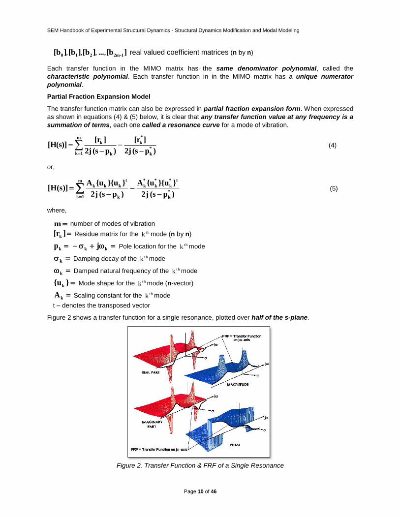
Figure 2 shows a transfer function for a single resonance, plotted over half of the s-plane.
Figure 2. Transfer Function & FRF of a Single Resonance
SEM Handbook of Experimental Structural Dynamics - Structural Dynamics Modification and Modal Modeling
Page 11 of 46
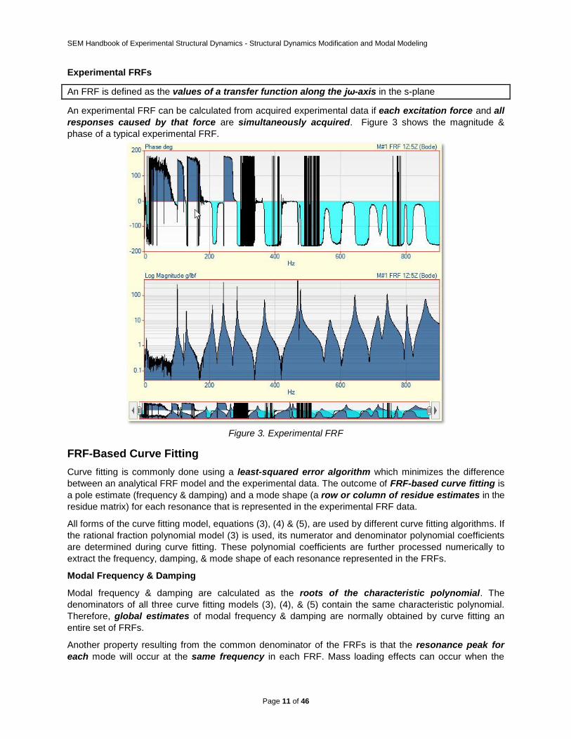
Experimental FRFs
An FRF is defined as the values of a transfer function along the jω-axis in the s-plane
An experimental FRF can be calculated from acquired experimental data if each excitation force and all
responses caused by that force are simultaneously acquired. Figure 3 shows the magnitude &
phase of a typical experimental FRF.
Figure 3. Experimental FRF
FRF-Based Curve Fitting
Curve fitting is commonly done using a least-squared error algorithm which minimizes the difference
between an analytical FRF model and the experimental data. The outcome of FRF-based curve fitting is
a pole estimate (frequency & damping) and a mode shape (a row or column of residue estimates in the
residue matrix) for each resonance that is represented in the experimental FRF data.
All forms of the curve fitting model, equations (3), (4) & (5), are used by different curve fitting algorithms. If
the rational fraction polynomial model (3) is used, its numerator and denominator polynomial coefficients
are determined during curve fitting. These polynomial coefficients are further processed numerically to
extract the frequency, damping, & mode shape of each resonance represented in the FRFs.
Modal Frequency & Damping
Modal frequency & damping are calculated as the roots of the characteristic polynomial. The
denominators of all three curve fitting models (3), (4), & (5) contain the same characteristic polynomial.
Therefore, global estimates of modal frequency & damping are normally obtained by curve fitting an
entire set of FRFs.
Another property resulting from the common denominator of the FRFs is that the resonance peak for
each mode will occur at the same frequency in each FRF. Mass loading effects can occur when the
SEM Handbook of Experimental Structural Dynamics - Structural Dynamics Modification and Modal Modeling
Page 12 of 46
response sensors add a significant amount of mass relative to the mass of the test structure. If the
sensors are moved from one point to another during a test, some resonance peaks will occur at a
different frequency in certain FRFs. When mass loading of this type occurs, a local polynomial curve
fitter, which estimates frequency, damping & residue for each mode in each FRF, will provide better
results.
Modal Residue
The modal residue, or FRF numerator, is unique for each mode and each FRF.
A modal residue is the magnitude (or strength) of a mode in an FRF. A row or column of residues in
the residue matrix defines the mode shape of the mode.
The relationship between residues and mode shapes is shown in numerators of the two curve fitting
models (4) & (5).
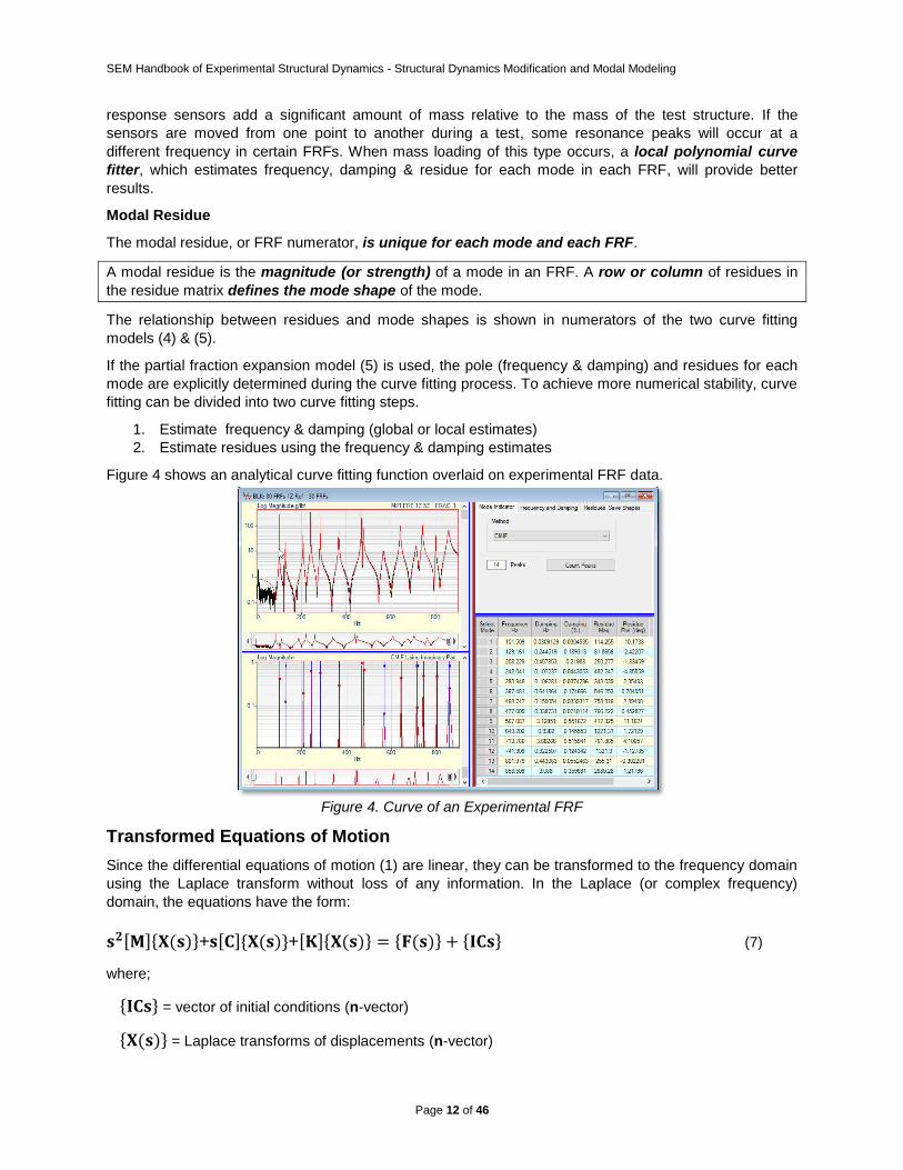
If the partial fraction expansion model (5) is used, the pole (frequency & damping) and residues for each
mode are explicitly determined during the curve fitting process. To achieve more numerical stability, curve
fitting can be divided into two curve fitting steps.
1. Estimate frequency & damping (global or local estimates)
2. Estimate residues using the frequency & damping estimates
Figure 4 shows an analytical curve fitting function overlaid on experimental FRF data.
Figure 4. Curve of an Experimental FRF
Transformed Equations of Motion
Since the differential equations of motion (1) are linear, they can be transformed to the frequency domain
using the Laplace transform without loss of any information. In the Laplace (or complex frequency)
domain, the equations have the form:
+ + (7)
where;
= vector of initial conditions (n-vector)
= Laplace transforms of displacements (n-vector)
SEM Handbook of Experimental Structural Dynamics - Structural Dynamics Modification and Modal Modeling
Page 13 of 46
= Laplace transforms of applied forces (n-vector)
All of the physical properties of the structure are preserved in the left-hand side of the equations, while
the applied forces and initial conditions {ICs} are contained on the right-hand side. The initial conditions
can be treated as a special form of the applied forces, and hence will be dropped from consideration
without loss of generality in the following development.
The equations of motion can be further simplified,
(8)
where:
= system matrix = + + (n by n) (9)
Equation (8) shows that any linear dynamic system has three basic parts: applied forces (inputs),
responses to those forces (outputs), and the physical system itself, represented by its system matrix
[B(s)].
Dynamic Model in Modal Coordinates
The modal parameters of a structure are actually the solutions to the homogeneous equations of motion.
That is, when {F(s)} = {0} the solutions to equations (8) are complex valued eigenvalues and
eigenvectors. The eigenvalues occur in complex conjugate pairs kk pp , . The eigenvalues are the
solutions (or roots) of the characteristic polynomial, which is derived from the following determinant
equation,
(10)
The eigenvalues (or poles) of the system are:
kkk jp ,
kkk jp ,
m = number of modes
kp = pole for the thk mode = kk j
*
kp = conjugate pole for the thk mode = kk j
k = damping of the thk mode
k = damped natural frequency of the thk mode,
Each eigenvalue has a corresponding eigenvector, and hence the eigenvectors also occur in complex
conjugate pairs,
kk uu , .
Each complex eigenvalue (also called a pole) contains the modal frequency and damping. Each
corresponding complex eigenvector is the mode shape.
Each eigenvector pair is a solution to the algebraic equations:
0upB kk ,
(n-vector) (11)
0upB kk ,
(n-vector) (12)
The eigenvectors (or mode shapes), can be assembled into a matrix:
SEM Handbook of Experimental Structural Dynamics - Structural Dynamics Modification and Modal Modeling
Page 14 of 46
(n by 2m) (13)
This transformation of the equations of motion means that all vibration can be represented in terms of
modal parameters.
Fundamental Law of Modal Analysis (FLMA): All vibration is a summation of mode shapes
Using the mode shape matrix [U], the time domain response of a structure {x(t)} is related to its response
in modal coordinates {z(t)} by
(n-vector) (14)
Applying the Laplace transform to equation (14) stated gives,
where
= Laplace transform of displacements in modal coordinates (2m-vector)
Applying this transformation to equations (8) gives:
F(s)Z(s)UKUCsUMs2 (n-vector) (15)
Pre-multiplying equation (15) by the transposed conjugate of the mode shape matrix tU gives:
F(s)UZ(s)UKUUCUsUMUstttt2 (2m by 2m) (16)
Three new matrices can now be defined:
UMUmt
= modal mass matrix (2m by 2m) (17)
UCUct
= modal damping matrix (2m by 2m) (18)
UKUkt
= modal stiffness matrix (2m by 2m) (19)
The equations of motion transformed into modal coordinates now become:
F(s)UZ(s)kcsmst2 (2m by 2m) (20)
Damping Assumptions
So far, no assumptions have been made regarding the damping of the structure, other than that it can be
modeled with a linear viscous force (1). If no further assumptions are made, the model is referred to as an
effective linear or non-proportional damping model.
If the structure model has no damping ([C] = 0), then it can be shown that the equations of motion in
modal coordinates (20) are uncoupled. That is, the modal mass and stiffness matrices are diagonal
matrices.
Moreover, if the damping is assumed to be proportional to the mass & stiffness, the damping can be
modeled with a proportional damping matrix, ( KMC ), where & are proportionality
constants. With proportional damping, the equations of motion (20) are again uncoupled, and the modal
mass, damping, & stiffness matrices are diagonal matrices.
SEM Handbook of Experimental Structural Dynamics - Structural Dynamics Modification and Modal Modeling
Page 15 of 46
All real-world structures have some amount of damping in them. In other words, the are one or more
damping mechanisms at work dissipating energy from the vibrating structure. However, there are usually
no physical reasons for assuming that damping is proportional to the mass and/or the stiffness.
A better assumption, and one which will yield an approximation to the uncoupled equations, is to
assume that the damping forces are significantly less than the inertial (mass) or the restoring
(stiffness) forces. In other words, the structure is lightly damped.
Lightly Damped Structure
If a structure exhibits troublesome resonance-assisted vibration problems, it is often because it is lightly
damped.
A structure is considered to be lightly damped if its modes have damping of less than 10 percent of
critical damping.
If a structure is lightly damping, then it can also be shown that its modal mass, damping, and stiffness
matrices are approximately diagonal matrices. Furthermore, its mode shapes can be shown to be
approximately normal (or real valued). In this case, its 2m-equations of motion (20) are redundant, and
can be reduced to m-equations, one corresponding to each mode.
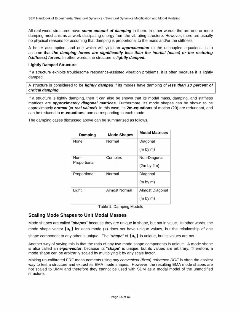
The damping cases discussed above can be summarized as follows.
Damping Mode Shapes Modal Matrices
None Normal Diagonal
(m by m)
Non-
Proportional
Complex Non-Diagonal
(2m by 2m)
Proportional Normal Diagonal
(m by m)
Light Almost Normal Almost Diagonal
(m by m)
Table 1. Damping Models
Scaling Mode Shapes to Unit Modal Masses
Mode shapes are called "shapes" because they are unique in shape, but not in value. In other words, the
mode shape vector }u{ k for each mode (k) does not have unique values, but the relationship of one
shape component to any other is unique. The "shape" of }u{ k is unique, but its values are not.
Another way of saying this is that the ratio of any two mode shape components is unique. A mode shape is also called an eigenvector, because its "shape" is unique, but its values are arbitrary. Therefore, a mode shape can be arbitrarily scaled by multiplying it by any scale factor.
Making un-calibrated FRF measurements using any convenient (fixed) reference DOF is often the easiest way to test a structure and extract its EMA mode shapes. However, the resulting EMA mode shapes are not scaled to UMM and therefore they cannot be used with SDM as a modal model of the unmodified structure.
SEM Handbook of Experimental Structural Dynamics - Structural Dynamics Modification and Modal Modeling
Page 16 of 46
Curve fitting a set of un-calibrated FRFs will yield un-scaled mode shapes, hence they are not a modal
model and cannot be used with SDM.
Modal Mass Matrix
In order to model the dynamics of an unmodified structure with SDM, a set of mode shapes must be properly scaled to preserve the mass & stiffness properties of the structure. A set of scaled mode shapes is called a modal model.
When the mass matrix is post-multiplied by the mode shape matrix and pre-multiplied by its transpose,
the result is the diagonal matrix shown in equation (26). This is a definition of modal mass.
(26)
where,
= mass matrix (n by n)
= mode shape matrix (n by m)
= modal mass matrix (m by m)
The modal mass of each mode (k) is a diagonal element of the modal mass matrix.
= modal mass k=1,…, m (27)
kp kk j pole location for the thk mode
k damped natural frequency of the thk mode
kA a scaling constant for the thk mode
Modal Stiffness Matrix
When the stiffness matrix is post-multiplied by the mode shape matrix and pre-multiplied by its transpose,
the result is a diagonal matrix, shown in equation (28). This is a definition of modal stiffness.
(28)
where,
= stiffness matrix. (n by n)
= modal stiffness matrix (m by m)
The modal stiffness of each mode (k) is a diagonal element of the modal stiffness matrix,
SEM Handbook of Experimental Structural Dynamics - Structural Dynamics Modification and Modal Modeling
Page 17 of 46
= modal stiffness: k=1,…, m (29)
where,
k damping coefficient of the thk mode
Modal Damping Matrix
When the damping matrix is post-multiplied by the mode shape matrix and pre-multiplied by its transpose,
the result is a diagonal matrix, shown in equation (30). This is a definition of modal damping.
(30)
where,
= damping matrix (n by n)
= modal damping matrix (m by m)
The modal damping of each mode (k) is a diagonal element of the modal damping matrix,
= modal damping: k=1,…, m (31)
Unit Modal Masses
Notice also, that each of the modal mass, stiffness, and damping matrix definitions (27), (29), and (31) includes a scaling constant ( . This constant is necessary because the mode shapes are not unique in value, and therefore can be arbitrarily scaled.
One of the common ways to scale mode shapes is to scale them so that the modal masses are one
(unity). Normally, if the mass matrix were available, the mode vectors would simply be scaled such
that when the triple product was formed, the resulting modal mass matrix would equal an
identity matrix.
SDM Dynamic Model
The SDM algorithm is unique in that it works directly with a modal model of the unmodified structure,
either an EMA modal model, an FEA modal model, or a Hybrid modal model made up of a combination of
both EMA & FEA modal parameters. In the sub-structuring example to follow, SDM will be used with a
Hybrid modal model.
The local eigenvalue modification process begins with a modal model of the unmodified structure. This
model consists of the damped natural frequency, modal damping (optional), and mode shape of each
mode in the modal model.
Modifications to a structure are modeled by making additions to, or subtractions from, the mass, stiffness,
or damping matrices of its differential equations of motion.
A dynamic model involving n-degrees of freedom for the unmodified structure was given in equation
(1). Similarly, the dynamic model for a modified structure is written:
SEM Handbook of Experimental Structural Dynamics - Structural Dynamics Modification and Modal Modeling
Page 18 of 46
+ + (32)
where;
= matrix of mass modifications (n by n)
= matrix of damping modifications (n by n)
= matrix of stiffness modifications (n by n)
SDM Equations Using UMM Mode Shapes
Unit Modal Mass (UMM) scaling is normally done with FEA modes because the mass matrix is available for scaling them. However, when EMA mode shapes are extracted from experimental FRFs, no mass matrix is available for scaling the mode shapes to yield Unit Modal Masses.
If the mode shapes, which are eigenvectors and hence have no unique values, are scaled so that the modal mass matrix diagonal elements are unity, then the modal mass matrix becomes an identity matrix, and the transformed equations of motion (20) become:
F(s)UZ(s)Ω2σsIst22 (m-vector) (33)
where:
I = identity modal mass matrix (m by m)
2 = diagonal modal damping matrix (m by m)
2 = diagonal modal frequency matrix (m by m)
222
From equation (33) it is clear that the entire dynamics of the unmodified structure can be represented by modal frequencies, damping, and mode shapes that have been scaled to unit modal masses.
If a set of mode shapes is scaled so that the modal mass matrix contains unit modal masses, the set of mode shapes is called a modal model. All of the mass, stiffness, and damping properties of the unmodified structure are preserved in the modal model.
Using mode shapes, the equations of motion for the modified structure (32) can also be transformed to
modal coordinates,
F(s)UZ(s)kcsmst2 (m-vector) (34)
where:
UMUImt (m by m) (35)
UCUct 2 (m by m) (36)
UKUkt 2
(m by m) (37)
SEM Handbook of Experimental Structural Dynamics - Structural Dynamics Modification and Modal Modeling
Page 19 of 46
The mode shape matrix is of dimension (n by m) since the mode shapes are assumed to be normal, or
real valued.
In the SDM method, the homogeneous form of equation (34) is solved to find the modal properties of the
modified structure.
Using the approach of Hallquist, et al [2], an additional transformation of the modification matrices M ,
C , K is made which results in a reformulation of the eigenvalue problem in modification space. For
a single modification, this problem becomes a scalar eigenvalue problem, which can be solved quickly
and efficiently. The drawback to making one modification at a time, however, is that if a large number of
modifications is required, computation time and errors can become significant.
A more practical SDM approach is to solve the homogeneous form of equation (34) directly. This is still a
relatively small (m by m) eigenvalue problem which can include as many structural modifications as
desired, but only needs to be solved once.
Equations (35) to (37) also indicate another advantage of SDM,
Only the mode shape components where the modification elements are attached to the structure
model are required.
This means that mode shape data only for those DOFs where the modification elements are attached to
the structure is necessary for SDM.
Scaling Residues to UMM Mode Shapes
Even without the mass matrix, EMA mode shapes can be scaled to Unit Modal Masses by using the relationship between residues and mode shapes. Residues are related to mode shapes by equating the numerators of equations (4) and (5),
t
kkk uuAkr }}{{)]([ k=1,…, m (38)
where,
)]k(r[ residue matrix for the mode (k) (n by n)
Residues are the numerators of the transfer function matrix when it is written in partial fraction form. For
convenience, equation (4) is re-written here,
m
1k*
k
*
k )ps(j2
)]k(r[
)ps(j2
)]k(r[)]s(H[ (39)
* -denotes the complex conjugate
Residues have engineering units associated with them and hence have unique values. FRFs have units of (motion / force), and the FRF denominators have units of Hz or (radians / second),. Therefore, residues have units of (motion / force-seconds).
SEM Handbook of Experimental Structural Dynamics - Structural Dynamics Modification and Modal Modeling
Page 20 of 46
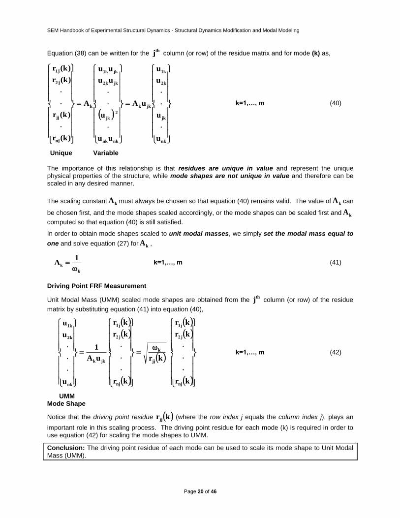
Equation (38) can be written for the th
j column (or row) of the residue matrix and for mode (k) as,
nk
jk
k2
k1
jkk
nknk
2
jk
jkk2
jkk1
k
nj
jj
j2
j1
u
u
u
u
uA
uu
u
uu
uu
A
)k(r
)k(r
)k(r
)k(r
k=1,…, m (40)
Unique Variable
The importance of this relationship is that residues are unique in value and represent the unique physical properties of the structure, while mode shapes are not unique in value and therefore can be scaled in any desired manner.
The scaling constant kA must always be chosen so that equation (40) remains valid. The value of kA can
be chosen first, and the mode shapes scaled accordingly, or the mode shapes can be scaled first and kA
computed so that equation (40) is still satisfied.
In order to obtain mode shapes scaled to unit modal masses, we simply set the modal mass equal to
one and solve equation (27) for kA ,
k
k
1A
k=1,…, m (41)
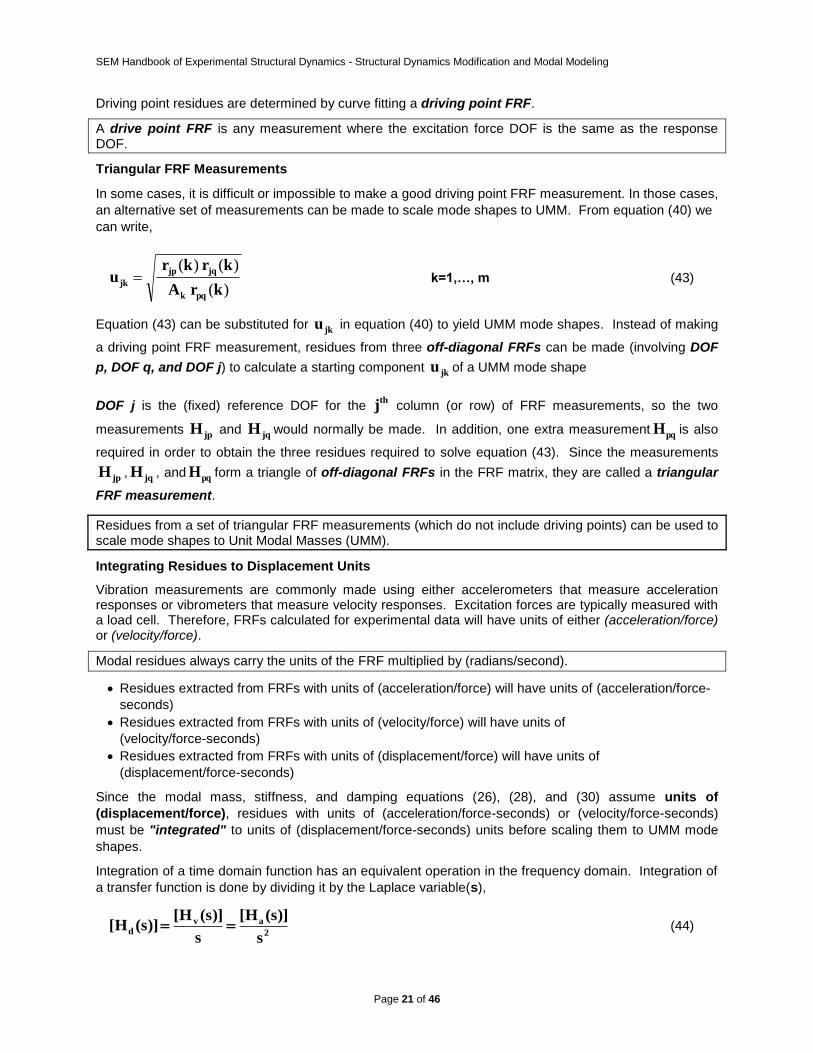
Driving Point FRF Measurement
Unit Modal Mass (UMM) scaled mode shapes are obtained from the th
j column (or row) of the residue
matrix by substituting equation (41) into equation (40),
kr
kr
kr
kr
kr
kr
kr
uA
1
u
u
u
nj
j2
j1
jj
k
nj
j2
j1
jkk
nk
k2
k1
k=1,…, m (42)
UMM Mode Shape
Notice that the driving point residue krjj (where the row index j equals the column index j), plays an
important role in this scaling process. The driving point residue for each mode (k) is required in order to use equation (42) for scaling the mode shapes to UMM.
Conclusion: The driving point residue of each mode can be used to scale its mode shape to Unit Modal Mass (UMM).
SEM Handbook of Experimental Structural Dynamics - Structural Dynamics Modification and Modal Modeling
Page 21 of 46
Driving point residues are determined by curve fitting a driving point FRF.
A drive point FRF is any measurement where the excitation force DOF is the same as the response DOF.
Triangular FRF Measurements
In some cases, it is difficult or impossible to make a good driving point FRF measurement. In those cases,
an alternative set of measurements can be made to scale mode shapes to UMM. From equation (40) we
can write,
)(
)()(
krA
krkru
pqk
jqjp
jk k=1,…, m (43)
Equation (43) can be substituted for jku in equation (40) to yield UMM mode shapes. Instead of making
a driving point FRF measurement, residues from three off-diagonal FRFs can be made (involving DOF
p, DOF q, and DOF j) to calculate a starting component jku of a UMM mode shape
DOF j is the (fixed) reference DOF for the th
j column (or row) of FRF measurements, so the two
measurements jpH and jqH would normally be made. In addition, one extra measurement pqH is also
required in order to obtain the three residues required to solve equation (43). Since the measurements
jpH , jqH , and pqH form a triangle of off-diagonal FRFs in the FRF matrix, they are called a triangular
FRF measurement.
Residues from a set of triangular FRF measurements (which do not include driving points) can be used to scale mode shapes to Unit Modal Masses (UMM).
Integrating Residues to Displacement Units
Vibration measurements are commonly made using either accelerometers that measure acceleration responses or vibrometers that measure velocity responses. Excitation forces are typically measured with a load cell. Therefore, FRFs calculated for experimental data will have units of either (acceleration/force) or (velocity/force).
Modal residues always carry the units of the FRF multiplied by (radians/second).
Residues extracted from FRFs with units of (acceleration/force) will have units of (acceleration/force-
seconds)
Residues extracted from FRFs with units of (velocity/force) will have units of
(velocity/force-seconds)
Residues extracted from FRFs with units of (displacement/force) will have units of
(displacement/force-seconds)
Since the modal mass, stiffness, and damping equations (26), (28), and (30) assume units of
(displacement/force), residues with units of (acceleration/force-seconds) or (velocity/force-seconds)
must be "integrated" to units of (displacement/force-seconds) units before scaling them to UMM mode
shapes.
Integration of a time domain function has an equivalent operation in the frequency domain. Integration of
a transfer function is done by dividing it by the Laplace variable(s),
2
avd
s
)]s(H[
s
)]s(H[)]s(H[ (44)
SEM Handbook of Experimental Structural Dynamics - Structural Dynamics Modification and Modal Modeling
Page 22 of 46
where,
)]s(H[ d = transfer matrix in (displacement/force) units.
)]s(H[ v = transfer matrix in (velocity/force) units.
)]s(H[ a = transfer matrix in (acceleration/force) units.
Since residues are the result of a partial fraction expansion of an FRF, residues can be "integrated"
directly (as if they were obtained from an integrated FRF) using the formula,
2
k
a
k
vd
)p(
)]k(r[
p
)]k(r[)]k(r[ k=1,…, m (45)
where,
)]k(r[ d = residue matrix in (displacement/force) units.
)]k(r[ v = residue matrix in (velocity/force) units.
)]k(r[ a = residue matrix in (acceleration/force) units.
kp kk j pole location for the thk mode.
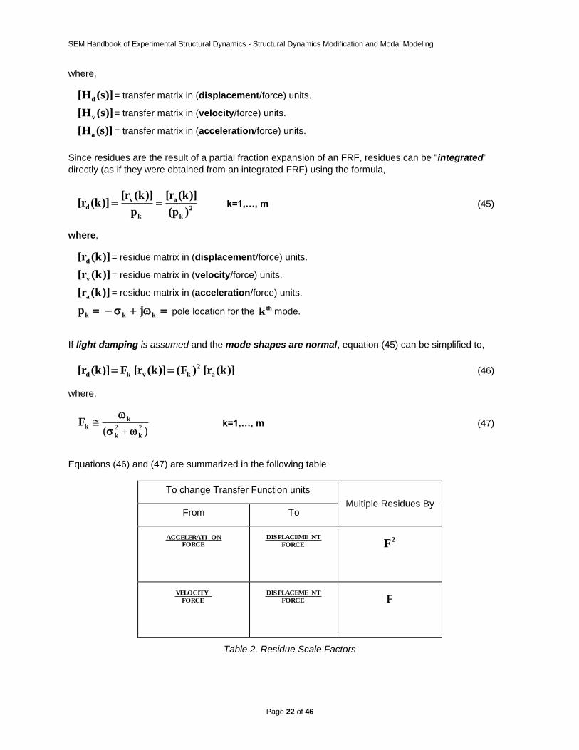
If light damping is assumed and the mode shapes are normal, equation (45) can be simplified to,
)]k(r[)F()]k(r[F)]k(r[ a
2
kvkd (46)
where,
)( 22
kk
kkF
k=1,…, m (47)
Equations (46) and (47) are summarized in the following table
To change Transfer Function units
Multiple Residues By From To
FORCEONACCELERATI
FORCE
NTDISPLACEME 2F
FORCE
VELOCITY FORCE
NTDISPLACEME F
Table 2. Residue Scale Factors
SEM Handbook of Experimental Structural Dynamics - Structural Dynamics Modification and Modal Modeling
Page 23 of 46
where, )(
F22
(seconds)
Effective Mass
From the UMM scaling discussion above, it can be concluded that,
Residues have unique values and have engineering units associated with them. Mode shapes do not have unique values and do not have engineering units.
A useful way to scale modal data is to ask the question,
“What is the effective mass of a structure at one of its resonant frequencies for a given DOF?”
In other words, if a tuned absorber or other modification were attached to the structure at a specific DOF,
“What is its mass (stiffness & damping) if it were treated like an SDOF mass-spring-damper?”
The answer to that question follows from a further use of the orthogonality equations (26), (28), and (30) and the definition of unit modal mass (UMM).mode shapes.
It has been shown that residues with units of (displacement/force-seconds) can be scaled into UMM mode shapes. One further assumption is necessary to define the effective mass at a DOF.
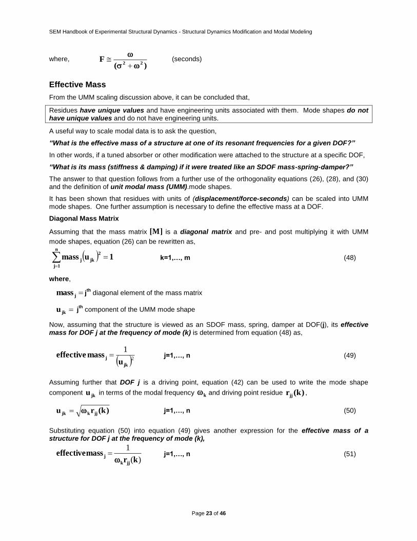
Diagonal Mass Matrix
Assuming that the mass matrix ]M[ is a diagonal matrix and pre- and post multiplying it with UMM
mode shapes, equation (26) can be rewritten as,
1umass2
jk
n
1j
j
k=1,…, m (48)
where,
jmass jth
diagonal element of the mass matrix
jku jth
component of the UMM mode shape
Now, assuming that the structure is viewed as an SDOF mass, spring, damper at DOF(j), its effective mass for DOF j at the frequency of mode (k) is determined from equation (48) as,
21
jk
ju
masseffective j=1,…, n (49)
Assuming further that DOF j is a driving point, equation (42) can be used to write the mode shape
component jku in terms of the modal frequency k and driving point residue )k(rjj
,
)k(ru jjkjk j=1,…, n (50)
Substituting equation (50) into equation (49) gives another expression for the effective mass of a structure for DOF j at the frequency of mode (k),
)(
1
krmasseffective
jjk
j
j=1,…, n (51)
SEM Handbook of Experimental Structural Dynamics - Structural Dynamics Modification and Modal Modeling
Page 24 of 46
Checking the Engineering Units
Assuming that the driving point residue )k(rjj has units of (displacement/force-seconds) as discussed
earlier, and the modal frequency k has units of (radians/second), then the effective mass would have
units of ((force-sec2) /displacement), which are units of mass.
Once the effective mass is known, the effective stiffness & damping of the structure can be calculated using equations (29) and (31).
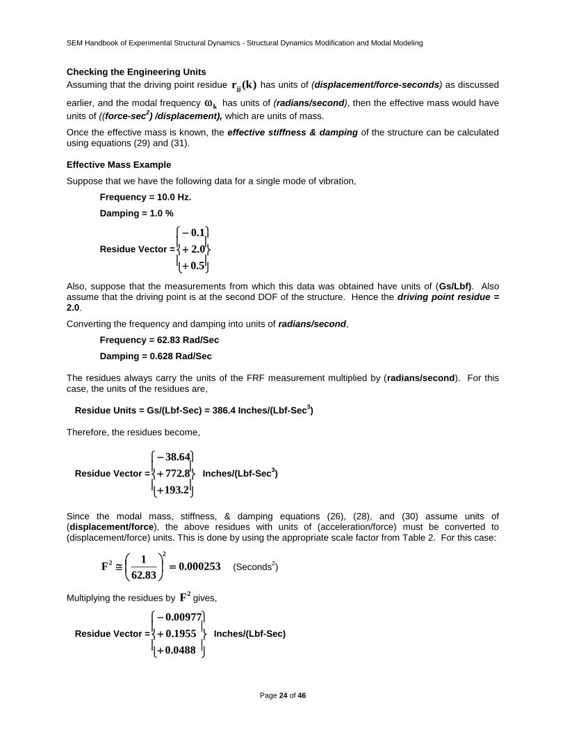
Effective Mass Example
Suppose that we have the following data for a single mode of vibration,
Frequency = 10.0 Hz.
Damping = 1.0 %
Residue Vector =
5.0
0.2
1.0
Also, suppose that the measurements from which this data was obtained have units of (Gs/Lbf). Also assume that the driving point is at the second DOF of the structure. Hence the driving point residue = 2.0.
Converting the frequency and damping into units of radians/second,
Frequency = 62.83 Rad/Sec
Damping = 0.628 Rad/Sec
The residues always carry the units of the FRF measurement multiplied by (radians/second). For this case, the units of the residues are,
Residue Units = Gs/(Lbf-Sec) = 386.4 Inches/(Lbf-Sec3)
Therefore, the residues become,
Residue Vector =
2.931
8.727
64.83
Inches/(Lbf-Sec3)
Since the modal mass, stiffness, & damping equations (26), (28), and (30) assume units of (displacement/force), the above residues with units of (acceleration/force) must be converted to (displacement/force) units. This is done by using the appropriate scale factor from Table 2. For this case:
000253.083.62
1F
2
2
(Seconds
2)
Multiplying the residues by 2
F gives,
Residue Vector =
0.0488
0.1955
0.00977
Inches/(Lbf-Sec)
SEM Handbook of Experimental Structural Dynamics - Structural Dynamics Modification and Modal Modeling
Page 25 of 46
Finally, equation (42) is used to obtain a UMM mode shape. To obtain the UMM mode shape, the residue mode shape must be multiplied by the scale factor,
927.170.1955
83.62
rSF
jj
Therefore,
UMM Mode Shape =
875.0
505.3
175.0
Inches/(Lbf-Sec)
The effective mass at the driving point is calculated using equation (49),
0814.0
505.3
1122
2
u
masseffective Lbf-sec2/in.
The effective mass at the driving point is also calculated using equation (51),
0814.0)1955.0)(83.62(
11
22
r
masseffective
Lbf-sec2/in.
Example: Using SDM to Attach a RIB Stiffener to a Flat Plate
In this example, SDM will be used to model the attachment of a RIB stiffener to a flat plate. The new
modes obtained from SDM will be compared with the EMA modes for the actual plate with the RIB
attached, and with FEA modes for the plate with the RIB attached.
Modal Assurance Criterion (MAC) values will be used to access the likeness of pairs of mode shapes for
the following three cases,
Case 1: EMA versus FEA modes of the plate without the RIB
Case 2: SDM versus FEA modes of the plate with the RIB attached
Case 3: SDM versus EMA modes of the plate with the RIB attached
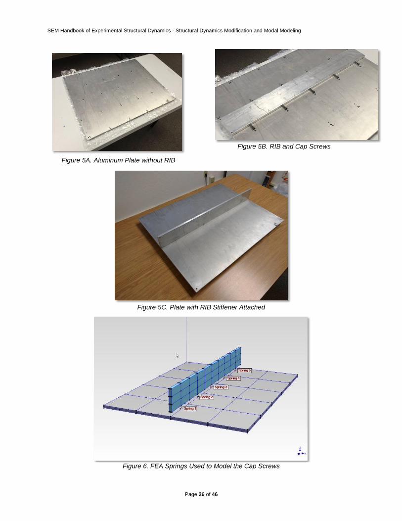
The plate and RIB are shown in Figure 5. The dimensions of the plate are 20 inches (508 mm) by 25
inches (635 mm) by 3/8 inches (9.525 mm) thick. The dimensions of the RIB are 3 inches (76.2 mm) by
25 inches (635 mm) by 3/8 inches (9.525 mm) thick.
Two roving impact modal tests were conducted on the plate, one before and one after the RIB stiffener
was attached to the plate. FRFs were calculated from the impact force and the acceleration response
only in the vertical (Z-axis) direction.
SEM Handbook of Experimental Structural Dynamics - Structural Dynamics Modification and Modal Modeling
Page 26 of 46
Figure 5A. Aluminum Plate without RIB
Figure 5B. RIB and Cap Screws
Figure 5C. Plate with RIB Stiffener Attached
Figure 6. FEA Springs Used to Model the Cap Screws
SEM Handbook of Experimental Structural Dynamics - Structural Dynamics Modification and Modal Modeling
Page 27 of 46
Modeling the Cap Screw Stiffnesses
The RIB stiffener was attached to the plate with five cap screws, shown in Figure 5B. When the RIB is
attached to the plate, translational & torsional forces are applied between the two substructures along
the length of the centerline where they are attached together. Therefore, both translational & torsional
stiffness forces must be modeled in order to represent the real-world plate with the RIB stiffener attached.
The joint stiffness was modeled using six-DOF springs located at the five cap screw locations, as shown
in Figure 6 Each six-DOF FEA spring model contains three translational DOFs and three rotational
DOFs. The six-DOF FEA springs were given stiffnesses of,
1) Translational stiffness: 1xE6 lbs/in (1.75E+05 N/mm)
2) Torsional stiffness: 1xE6 in-lbs/degree (1.75E+05 mm-N/degree)
The springs were given large stiffness values to model a tight fastening of RIB to the plate using the cap
screws.
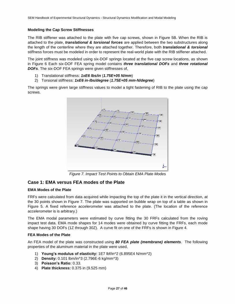
Figure 7. Impact Test Points to Obtain EMA Plate Modes
Case 1: EMA versus FEA modes of the Plate
EMA Modes of the Plate
FRFs were calculated from data acquired while impacting the top of the plate it in the vertical direction, at
the 30 points shown in Figure 7. The plate was supported on bubble wrap on top of a table as shown in
Figure 5. A fixed reference accelerometer was attached to the plate. (The location of the reference
accelerometer is is arbitrary.)
The EMA modal parameters were estimated by curve fitting the 30 FRFs calculated from the roving
impact test data. EMA mode shapes for 14 modes were obtained by curve fitting the FRFs, each mode
shape having 30 DOFs (1Z through 30Z). A curve fit on one of the FRFs is shown in Figure 4.
FEA Modes of the Plate
An FEA model of the plate was constructed using 80 FEA plate (membrane) elements. The following
properties of the aluminum material in the plate were used,
1) Young’s modulus of elasticity: 1E7 lbf/in^2 (6.895E4 N/mm^2)
2) Density: 0.101 lbm/in^3 (2.796E-6 kg/mm^3)
3) Poisson’s Ratio: 0.33.
4) Plate thickness: 0.375 in (9.525 mm)
SEM Handbook of Experimental Structural Dynamics - Structural Dynamics Modification and Modal Modeling
Page 28 of 46
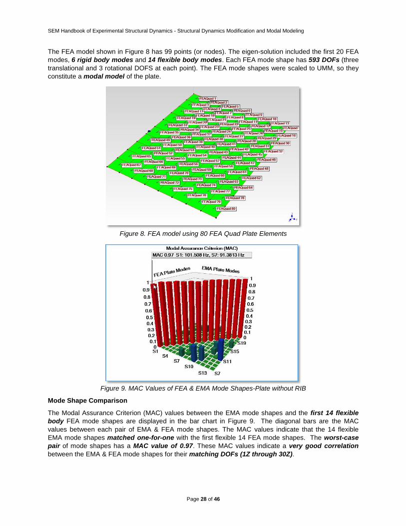
The FEA model shown in Figure 8 has 99 points (or nodes). The eigen-solution included the first 20 FEA
modes, 6 rigid body modes and 14 flexible body modes. Each FEA mode shape has 593 DOFs (three
translational and 3 rotational DOFS at each point). The FEA mode shapes were scaled to UMM, so they
constitute a modal model of the plate.
Figure 8. FEA model using 80 FEA Quad Plate Elements
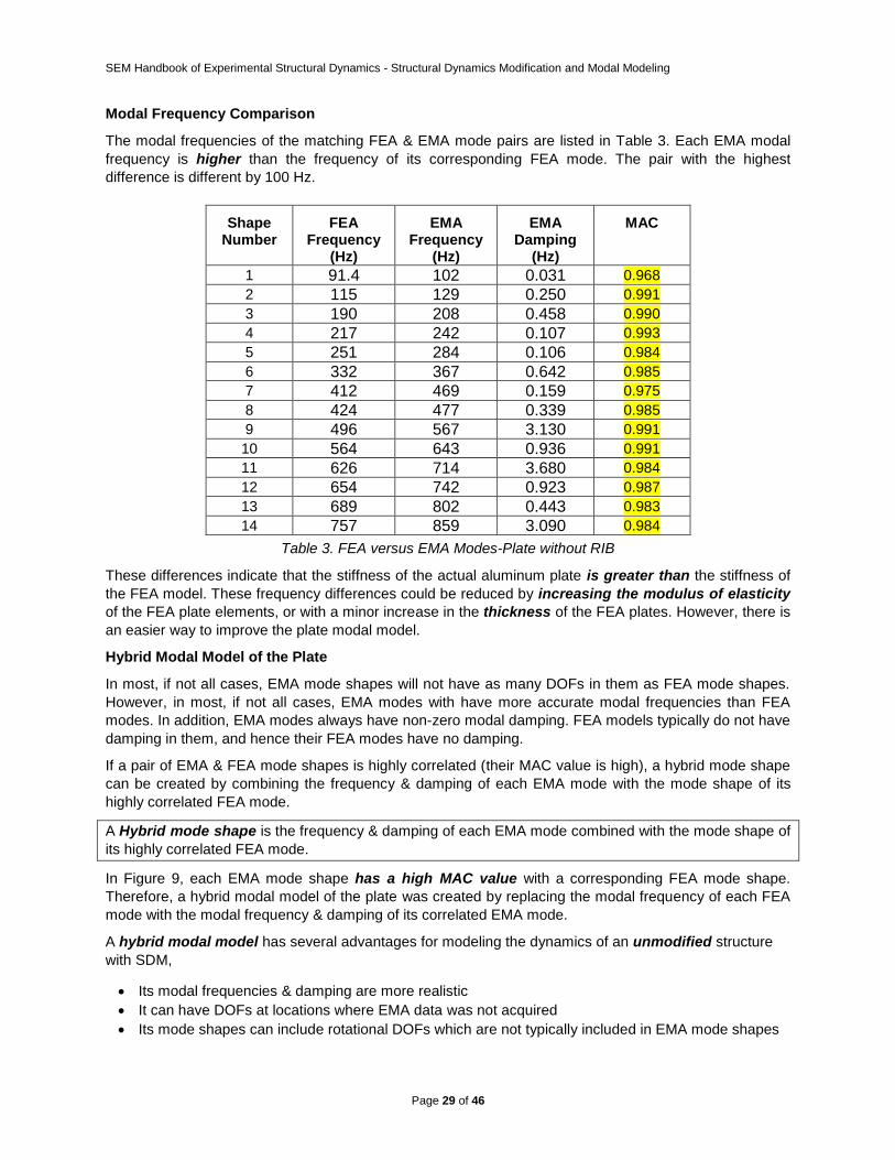
Figure 9. MAC Values of FEA & EMA Mode Shapes-Plate without RIB
Mode Shape Comparison
The Modal Assurance Criterion (MAC) values between the EMA mode shapes and the first 14 flexible
body FEA mode shapes are displayed in the bar chart in Figure 9. The diagonal bars are the MAC
values between each pair of EMA & FEA mode shapes. The MAC values indicate that the 14 flexible
EMA mode shapes matched one-for-one with the first flexible 14 FEA mode shapes. The worst-case
pair of mode shapes has a MAC value of 0.97. These MAC values indicate a very good correlation
between the EMA & FEA mode shapes for their matching DOFs (1Z through 30Z).
SEM Handbook of Experimental Structural Dynamics - Structural Dynamics Modification and Modal Modeling
Page 29 of 46
Modal Frequency Comparison
The modal frequencies of the matching FEA & EMA mode pairs are listed in Table 3. Each EMA modal
frequency is higher than the frequency of its corresponding FEA mode. The pair with the highest
difference is different by 100 Hz.
Shape Number
FEA Frequency
(Hz)
EMA Frequency
(Hz)
EMA Damping
(Hz)
MAC
1 91.4 102 0.031 0.968
2 115 129 0.250 0.991
3 190 208 0.458 0.990
4 217 242 0.107 0.993
5 251 284 0.106 0.984
6 332 367 0.642 0.985
7 412 469 0.159 0.975
8 424 477 0.339 0.985
9 496 567 3.130 0.991
10 564 643 0.936 0.991
11 626 714 3.680 0.984
12 654 742 0.923 0.987
13 689 802 0.443 0.983
14 757 859 3.090 0.984
Table 3. FEA versus EMA Modes-Plate without RIB
These differences indicate that the stiffness of the actual aluminum plate is greater than the stiffness of
the FEA model. These frequency differences could be reduced by increasing the modulus of elasticity
of the FEA plate elements, or with a minor increase in the thickness of the FEA plates. However, there is
an easier way to improve the plate modal model.
Hybrid Modal Model of the Plate
In most, if not all cases, EMA mode shapes will not have as many DOFs in them as FEA mode shapes.
However, in most, if not all cases, EMA modes with have more accurate modal frequencies than FEA
modes. In addition, EMA modes always have non-zero modal damping. FEA models typically do not have
damping in them, and hence their FEA modes have no damping.
If a pair of EMA & FEA mode shapes is highly correlated (their MAC value is high), a hybrid mode shape
can be created by combining the frequency & damping of each EMA mode with the mode shape of its
highly correlated FEA mode.
A Hybrid mode shape is the frequency & damping of each EMA mode combined with the mode shape of
its highly correlated FEA mode.
In Figure 9, each EMA mode shape has a high MAC value with a corresponding FEA mode shape.
Therefore, a hybrid modal model of the plate was created by replacing the modal frequency of each FEA
mode with the modal frequency & damping of its correlated EMA mode.
A hybrid modal model has several advantages for modeling the dynamics of an unmodified structure
with SDM,
Its modal frequencies & damping are more realistic
It can have DOFs at locations where EMA data was not acquired
Its mode shapes can include rotational DOFs which are not typically included in EMA mode shapes
SEM Handbook of Experimental Structural Dynamics - Structural Dynamics Modification and Modal Modeling
Page 30 of 46
FEA mode shapes are typically scaled to UMM
This more realistic Hybrid model now contains mode shapes with rotational DOFs. Rotational DOFs will
be required by SDM to accurately model the attachment of the RIB to the plate.
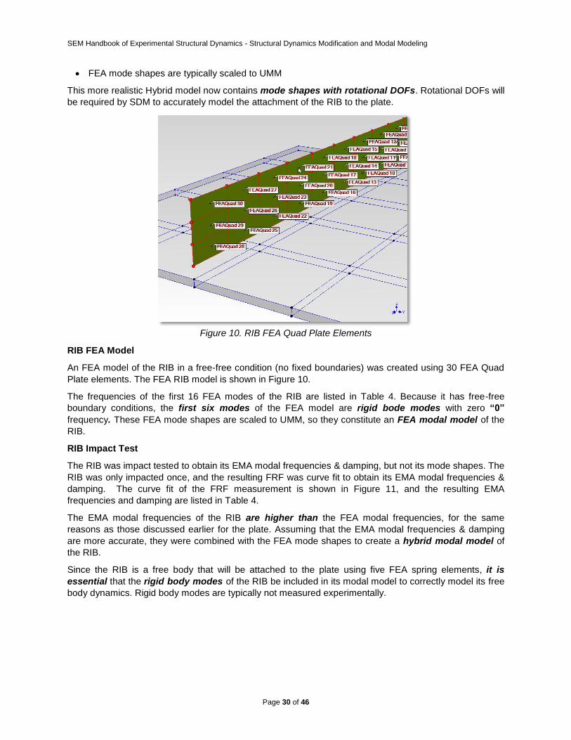
Figure 10. RIB FEA Quad Plate Elements
RIB FEA Model
An FEA model of the RIB in a free-free condition (no fixed boundaries) was created using 30 FEA Quad
Plate elements. The FEA RIB model is shown in Figure 10.
The frequencies of the first 16 FEA modes of the RIB are listed in Table 4. Because it has free-free
boundary conditions, the first six modes of the FEA model are rigid bode modes with zero “0”
frequency. These FEA mode shapes are scaled to UMM, so they constitute an FEA modal model of the
RIB.
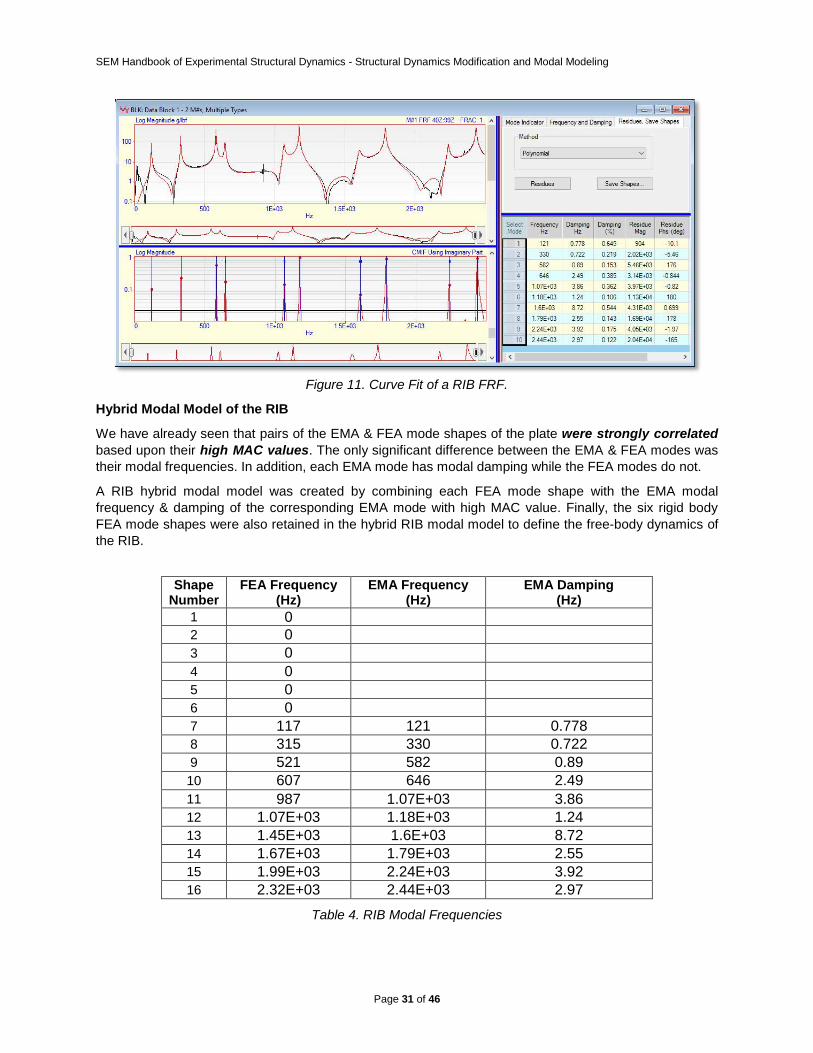
RIB Impact Test
The RIB was impact tested to obtain its EMA modal frequencies & damping, but not its mode shapes. The
RIB was only impacted once, and the resulting FRF was curve fit to obtain its EMA modal frequencies &
damping. The curve fit of the FRF measurement is shown in Figure 11, and the resulting EMA
frequencies and damping are listed in Table 4.
The EMA modal frequencies of the RIB are higher than the FEA modal frequencies, for the same
reasons as those discussed earlier for the plate. Assuming that the EMA modal frequencies & damping
are more accurate, they were combined with the FEA mode shapes to create a hybrid modal model of
the RIB.
Since the RIB is a free body that will be attached to the plate using five FEA spring elements, it is
essential that the rigid body modes of the RIB be included in its modal model to correctly model its free
body dynamics. Rigid body modes are typically not measured experimentally.
SEM Handbook of Experimental Structural Dynamics - Structural Dynamics Modification and Modal Modeling
Page 31 of 46
Figure 11. Curve Fit of a RIB FRF.
Hybrid Modal Model of the RIB
We have already seen that pairs of the EMA & FEA mode shapes of the plate were strongly correlated
based upon their high MAC values. The only significant difference between the EMA & FEA modes was
their modal frequencies. In addition, each EMA mode has modal damping while the FEA modes do not.
A RIB hybrid modal model was created by combining each FEA mode shape with the EMA modal
frequency & damping of the corresponding EMA mode with high MAC value. Finally, the six rigid body
FEA mode shapes were also retained in the hybrid RIB modal model to define the free-body dynamics of
the RIB.
Shape Number
FEA Frequency (Hz)
EMA Frequency (Hz)
EMA Damping (Hz)
1 0
2 0
3 0
4 0
5 0
6 0
7 117 121 0.778
8 315 330 0.722
9 521 582 0.89
10 607 646 2.49
11 987 1.07E+03 3.86
12 1.07E+03 1.18E+03 1.24
13 1.45E+03 1.6E+03 8.72
14 1.67E+03 1.79E+03 2.55
15 1.99E+03 2.24E+03 3.92
16 2.32E+03 2.44E+03 2.97
Table 4. RIB Modal Frequencies
SEM Handbook of Experimental Structural Dynamics - Structural Dynamics Modification and Modal Modeling
Page 32 of 46
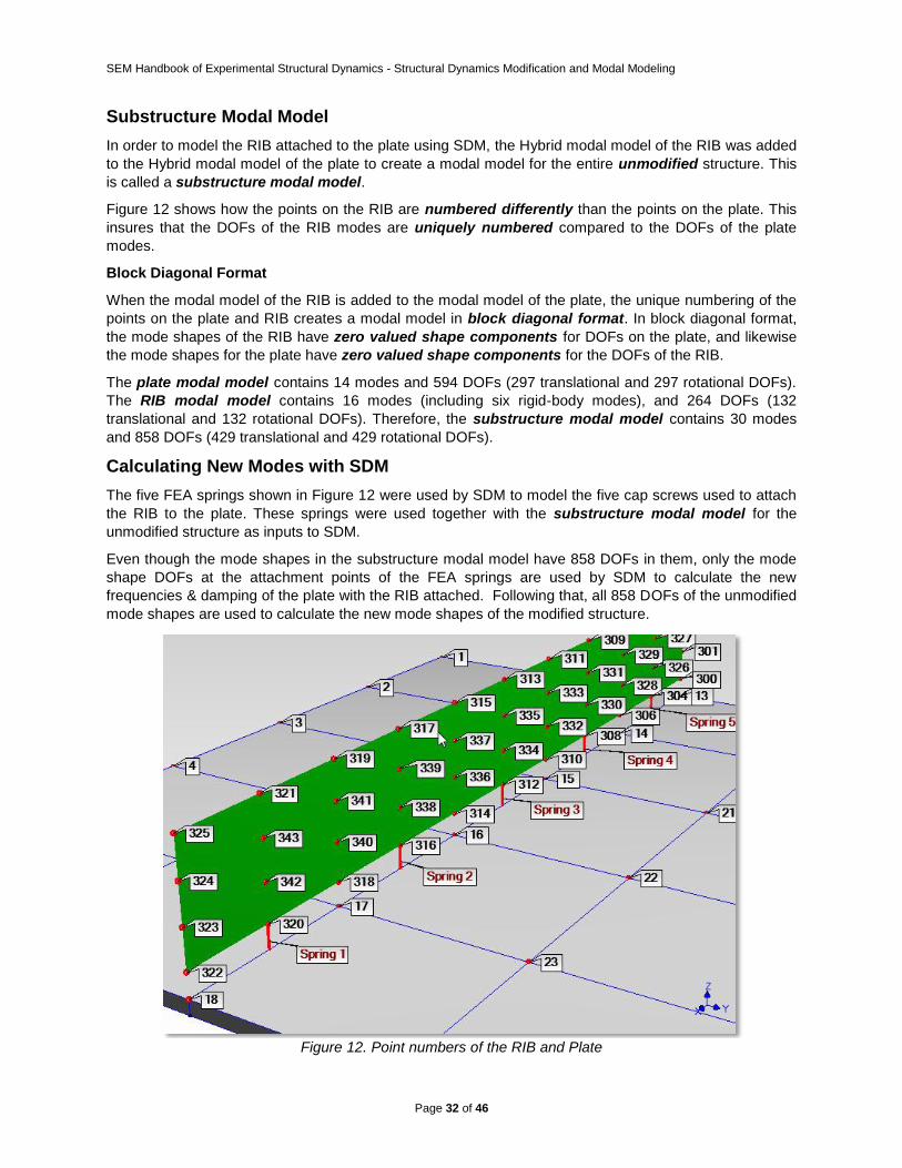
Substructure Modal Model
In order to model the RIB attached to the plate using SDM, the Hybrid modal model of the RIB was added
to the Hybrid modal model of the plate to create a modal model for the entire unmodified structure. This
is called a substructure modal model.
Figure 12 shows how the points on the RIB are numbered differently than the points on the plate. This
insures that the DOFs of the RIB modes are uniquely numbered compared to the DOFs of the plate
modes.
Block Diagonal Format
When the modal model of the RIB is added to the modal model of the plate, the unique numbering of the
points on the plate and RIB creates a modal model in block diagonal format. In block diagonal format,
the mode shapes of the RIB have zero valued shape components for DOFs on the plate, and likewise
the mode shapes for the plate have zero valued shape components for the DOFs of the RIB.
The plate modal model contains 14 modes and 594 DOFs (297 translational and 297 rotational DOFs).
The RIB modal model contains 16 modes (including six rigid-body modes), and 264 DOFs (132
translational and 132 rotational DOFs). Therefore, the substructure modal model contains 30 modes
and 858 DOFs (429 translational and 429 rotational DOFs).
Calculating New Modes with SDM
The five FEA springs shown in Figure 12 were used by SDM to model the five cap screws used to attach
the RIB to the plate. These springs were used together with the substructure modal model for the
unmodified structure as inputs to SDM.
Even though the mode shapes in the substructure modal model have 858 DOFs in them, only the mode
shape DOFs at the attachment points of the FEA springs are used by SDM to calculate the new
frequencies & damping of the plate with the RIB attached. Following that, all 858 DOFs of the unmodified
mode shapes are used to calculate the new mode shapes of the modified structure.
Figure 12. Point numbers of the RIB and Plate
SEM Handbook of Experimental Structural Dynamics - Structural Dynamics Modification and Modal Modeling
Page 33 of 46
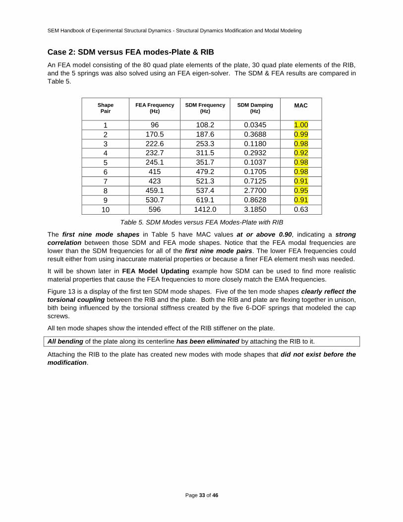
Case 2: SDM versus FEA modes-Plate & RIB
An FEA model consisting of the 80 quad plate elements of the plate, 30 quad plate elements of the RIB,
and the 5 springs was also solved using an FEA eigen-solver. The SDM & FEA results are compared in
Table 5.
Shape Pair
FEA Frequency (Hz)
SDM Frequency (Hz)
SDM Damping (Hz)
MAC
1 96 108.2 0.0345 1.00
2 170.5 187.6 0.3688 0.99
3 222.6 253.3 0.1180 0.98
4 232.7 311.5 0.2932 0.92
5 245.1 351.7 0.1037 0.98
6 415 479.2 0.1705 0.98
7 423 521.3 0.7125 0.91
8 459.1 537.4 2.7700 0.95
9 530.7 619.1 0.8628 0.91
10 596 1412.0 3.1850 0.63
Table 5. SDM Modes versus FEA Modes-Plate with RIB
The first nine mode shapes in Table 5 have MAC values at or above 0.90, indicating a strong
correlation between those SDM and FEA mode shapes. Notice that the FEA modal frequencies are
lower than the SDM frequencies for all of the first nine mode pairs. The lower FEA frequencies could
result either from using inaccurate material properties or because a finer FEA element mesh was needed.
It will be shown later in FEA Model Updating example how SDM can be used to find more realistic
material properties that cause the FEA frequencies to more closely match the EMA frequencies.
Figure 13 is a display of the first ten SDM mode shapes. Five of the ten mode shapes clearly reflect the
torsional coupling between the RIB and the plate. Both the RIB and plate are flexing together in unison,
bith being influenced by the torsional stiffness created by the five 6-DOF springs that modeled the cap
screws.
All ten mode shapes show the intended effect of the RIB stiffener on the plate.
All bending of the plate along its centerline has been eliminated by attaching the RIB to it.
Attaching the RIB to the plate has created new modes with mode shapes that did not exist before the
modification.
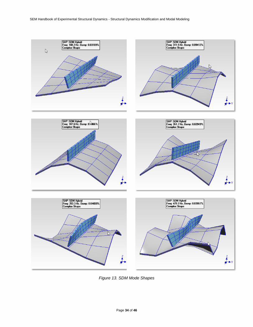
SEM Handbook of Experimental Structural Dynamics - Structural Dynamics Modification and Modal Modeling
Page 34 of 46
Figure 13. SDM Mode Shapes
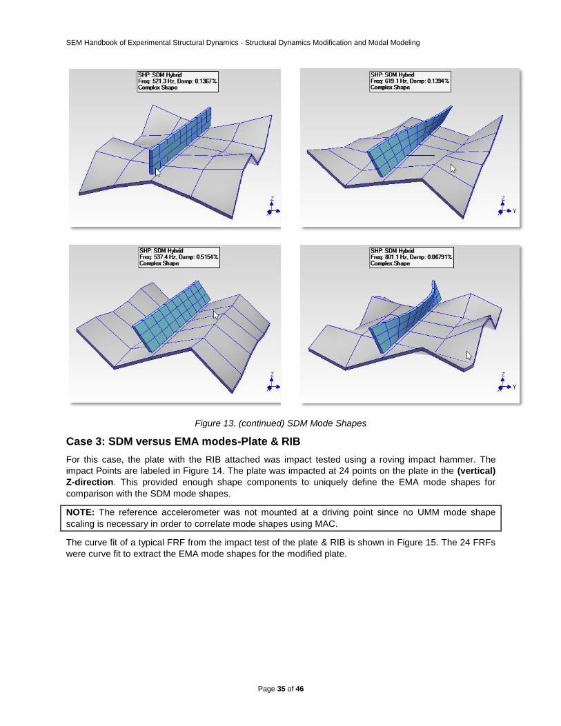
SEM Handbook of Experimental Structural Dynamics - Structural Dynamics Modification and Modal Modeling
Page 35 of 46
Figure 13. (continued) SDM Mode Shapes
Case 3: SDM versus EMA modes-Plate & RIB
For this case, the plate with the RIB attached was impact tested using a roving impact hammer. The
impact Points are labeled in Figure 14. The plate was impacted at 24 points on the plate in the (vertical)
Z-direction. This provided enough shape components to uniquely define the EMA mode shapes for
comparison with the SDM mode shapes.
NOTE: The reference accelerometer was not mounted at a driving point since no UMM mode shape
scaling is necessary in order to correlate mode shapes using MAC.
The curve fit of a typical FRF from the impact test of the plate & RIB is shown in Figure 15. The 24 FRFs
were curve fit to extract the EMA mode shapes for the modified plate.
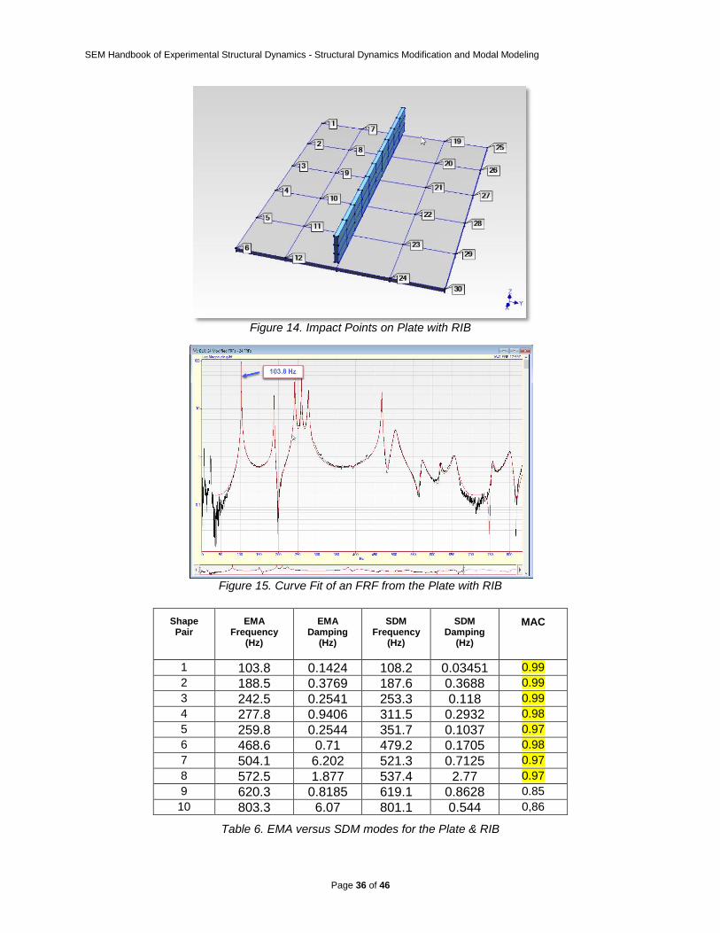
SEM Handbook of Experimental Structural Dynamics - Structural Dynamics Modification and Modal Modeling
Page 36 of 46
Figure 14. Impact Points on Plate with RIB
Figure 15. Curve Fit of an FRF from the Plate with RIB
Shape Pair
EMA Frequency
(Hz)
EMA Damping
(Hz)
SDM Frequency
(Hz)
SDM Damping
(Hz)
MAC
1 103.8 0.1424 108.2 0.03451 0.99
2 188.5 0.3769 187.6 0.3688 0.99
3 242.5 0.2541 253.3 0.118 0.99
4 277.8 0.9406 311.5 0.2932 0.98
5 259.8 0.2544 351.7 0.1037 0.97
6 468.6 0.71 479.2 0.1705 0.98
7 504.1 6.202 521.3 0.7125 0.97
8 572.5 1.877 537.4 2.77 0.97
9 620.3 0.8185 619.1 0.8628 0.85
10 803.3 6.07 801.1 0.544 0,86
Table 6. EMA versus SDM modes for the Plate & RIB
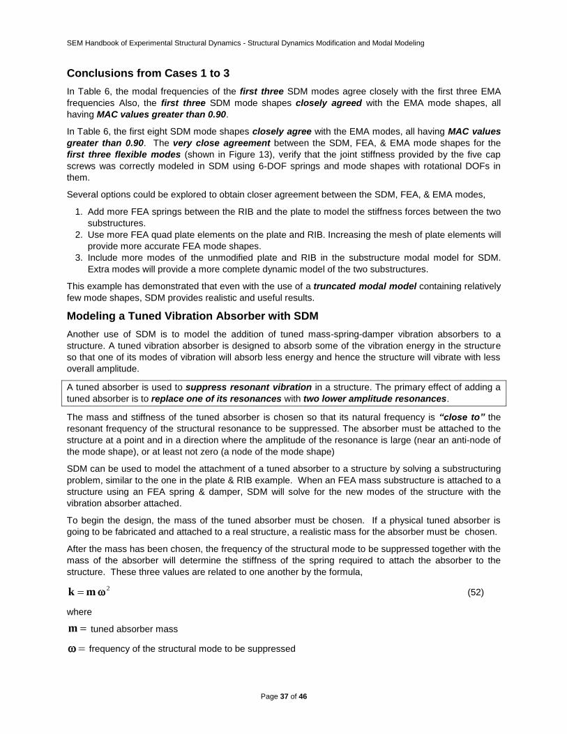
SEM Handbook of Experimental Structural Dynamics - Structural Dynamics Modification and Modal Modeling
Page 37 of 46
Conclusions from Cases 1 to 3
In Table 6, the modal frequencies of the first three SDM modes agree closely with the first three EMA
frequencies Also, the first three SDM mode shapes closely agreed with the EMA mode shapes, all
having MAC values greater than 0.90.
In Table 6, the first eight SDM mode shapes closely agree with the EMA modes, all having MAC values
greater than 0.90. The very close agreement between the SDM, FEA, & EMA mode shapes for the
first three flexible modes (shown in Figure 13), verify that the joint stiffness provided by the five cap
screws was correctly modeled in SDM using 6-DOF springs and mode shapes with rotational DOFs in
them.
Several options could be explored to obtain closer agreement between the SDM, FEA, & EMA modes,
1. Add more FEA springs between the RIB and the plate to model the stiffness forces between the two
substructures.
2. Use more FEA quad plate elements on the plate and RIB. Increasing the mesh of plate elements will
provide more accurate FEA mode shapes.
3. Include more modes of the unmodified plate and RIB in the substructure modal model for SDM.
Extra modes will provide a more complete dynamic model of the two substructures.
This example has demonstrated that even with the use of a truncated modal model containing relatively
few mode shapes, SDM provides realistic and useful results.
Modeling a Tuned Vibration Absorber with SDM
Another use of SDM is to model the addition of tuned mass-spring-damper vibration absorbers to a
structure. A tuned vibration absorber is designed to absorb some of the vibration energy in the structure
so that one of its modes of vibration will absorb less energy and hence the structure will vibrate with less
overall amplitude.
A tuned absorber is used to suppress resonant vibration in a structure. The primary effect of adding a
tuned absorber is to replace one of its resonances with two lower amplitude resonances.
The mass and stiffness of the tuned absorber is chosen so that its natural frequency is “close to” the
resonant frequency of the structural resonance to be suppressed. The absorber must be attached to the
structure at a point and in a direction where the amplitude of the resonance is large (near an anti-node of
the mode shape), or at least not zero (a node of the mode shape)
SDM can be used to model the attachment of a tuned absorber to a structure by solving a substructuring
problem, similar to the one in the plate & RIB example. When an FEA mass substructure is attached to a
structure using an FEA spring & damper, SDM will solve for the new modes of the structure with the
vibration absorber attached.
To begin the design, the mass of the tuned absorber must be chosen. If a physical tuned absorber is
going to be fabricated and attached to a real structure, a realistic mass for the absorber must be chosen.
After the mass has been chosen, the frequency of the structural mode to be suppressed together with the
mass of the absorber will determine the stiffness of the spring required to attach the absorber to the
structure. These three values are related to one another by the formula,
2mk (52)
where
m tuned absorber mass
frequency of the structural mode to be suppressed
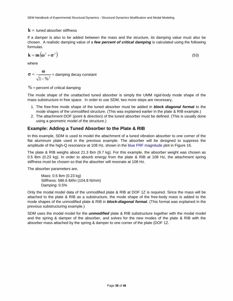
SEM Handbook of Experimental Structural Dynamics - Structural Dynamics Modification and Modal Modeling
Page 38 of 46
k tuned absorber stiffness
If a damper is also to be added between the mass and the structure, its damping value must also be
chosen. A realistic damping value of a few percent of critical damping is calculated using the following
formulas.
22 mk (53)
where
2%1
= damping decay constant
% percent of critical damping
The mode shape of the unattached tuned absorber is simply the UMM rigid-body mode shape of the
mass substructure in free space. In order to use SDM, two more steps are necessary,
1. The free-free mode shape of the tuned absorber must be added in block diagonal format to the
mode shapes of the unmodified structure. (This was explained earlier in the plate & RIB example.)
2. The attachment DOF (point & direction) of the tuned absorber must be defined. (This is usually done
using a geometric model of the structure.)
Example: Adding a Tuned Absorber to the Plate & RIB
In this example, SDM is used to model the attachment of a tuned vibration absorber to one corner of the
flat aluminum plate used in the previous example. The absorber will be designed to suppress the
amplitude of the high-Q resonance at 108 Hz, shown in the blue FRF magnitude plot in Figure 16.
The plate & RIB weighs about 21.3 lbm (9.7 kg). For this example, the absorber weight was chosen as
0.5 lbm (0.23 kg). In order to absorb energy from the plate & RIB at 108 Hz, the attachment spring
stiffness must be chosen so that the absorber will resonate at 108 Hz.
The absorber parameters are,
Mass: 0.5 lbm (0.23 kg)
Stiffness: 586.6 lbf/in (104.8 N/mm)
Damping: 0.5%
Only the modal model data of the unmodified plate & RIB at DOF 1Z is required. Since the mass will be
attached to the plate & RIB as a substructure, the mode shape of the free-body mass is added to the
mode shapes of the unmodified plate & RIB in block-diagonal format. (This format was explained in the
previous substructuring example.)
SDM uses the modal model for the unmodified plate & RIB substructure together with the modal model
and the spring & damper of the absorber, and solves for the new modes of the plate & RIB with the
absorber mass attached by the spring & damper to one corner of the plate (DOF 1Z.
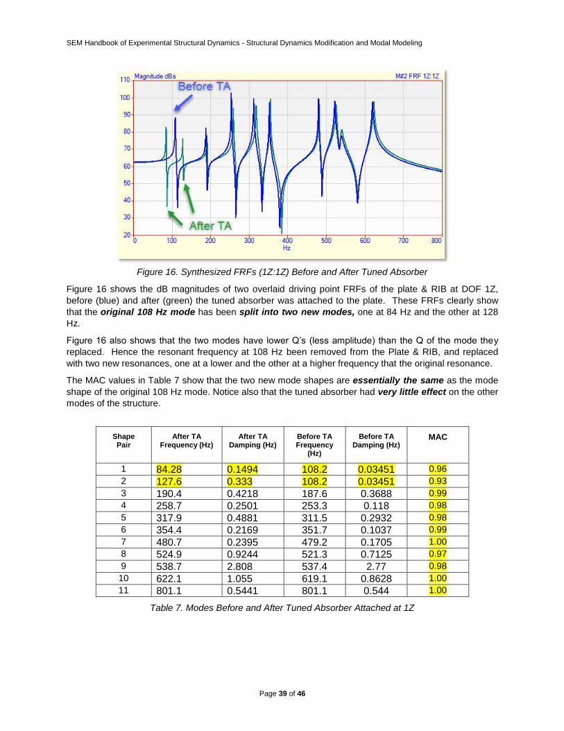
SEM Handbook of Experimental Structural Dynamics - Structural Dynamics Modification and Modal Modeling
Page 39 of 46
Figure 16. Synthesized FRFs (1Z:1Z) Before and After Tuned Absorber
Figure 16 shows the dB magnitudes of two overlaid driving point FRFs of the plate & RIB at DOF 1Z,
before (blue) and after (green) the tuned absorber was attached to the plate. These FRFs clearly show
that the original 108 Hz mode has been split into two new modes, one at 84 Hz and the other at 128
Hz.
Figure 16 also shows that the two modes have lower Q’s (less amplitude) than the Q of the mode they
replaced. Hence the resonant frequency at 108 Hz been removed from the Plate & RIB, and replaced
with two new resonances, one at a lower and the other at a higher frequency that the original resonance.
The MAC values in Table 7 show that the two new mode shapes are essentially the same as the mode
shape of the original 108 Hz mode. Notice also that the tuned absorber had very little effect on the other
modes of the structure.
Shape Pair
After TA Frequency (Hz)
After TA Damping (Hz)
Before TA Frequency
(Hz)
Before TA Damping (Hz)
MAC
1 84.28 0.1494 108.2 0.03451 0.96
2 127.6 0.333 108.2 0.03451 0.93
3 190.4 0.4218 187.6 0.3688 0.99
4 258.7 0.2501 253.3 0.118 0.98
5 317.9 0.4881 311.5 0.2932 0.98
6 354.4 0.2169 351.7 0.1037 0.99
7 480.7 0.2395 479.2 0.1705 1.00
8 524.9 0.9244 521.3 0.7125 0.97
9 538.7 2.808 537.4 2.77 0.98
10 622.1 1.055 619.1 0.8628 1.00
11 801.1 0.5441 801.1 0.544 1.00
Table 7. Modes Before and After Tuned Absorber Attached at 1Z
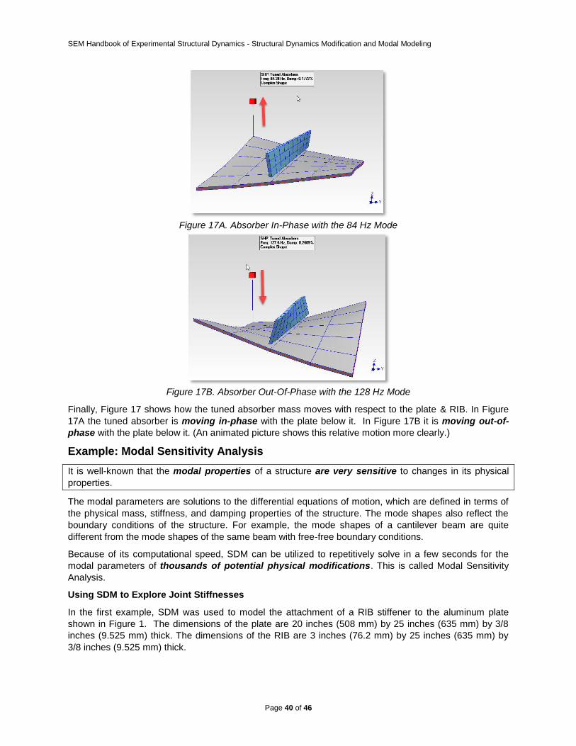
SEM Handbook of Experimental Structural Dynamics - Structural Dynamics Modification and Modal Modeling
Page 40 of 46
Figure 17A. Absorber In-Phase with the 84 Hz Mode
Figure 17B. Absorber Out-Of-Phase with the 128 Hz Mode
Finally, Figure 17 shows how the tuned absorber mass moves with respect to the plate & RIB. In Figure
17A the tuned absorber is moving in-phase with the plate below it. In Figure 17B it is moving out-of-
phase with the plate below it. (An animated picture shows this relative motion more clearly.)
Example: Modal Sensitivity Analysis
It is well-known that the modal properties of a structure are very sensitive to changes in its physical
properties.
The modal parameters are solutions to the differential equations of motion, which are defined in terms of
the physical mass, stiffness, and damping properties of the structure. The mode shapes also reflect the
boundary conditions of the structure. For example, the mode shapes of a cantilever beam are quite
different from the mode shapes of the same beam with free-free boundary conditions.
Because of its computational speed, SDM can be utilized to repetitively solve in a few seconds for the
modal parameters of thousands of potential physical modifications. This is called Modal Sensitivity
Analysis.
Using SDM to Explore Joint Stiffnesses
In the first example, SDM was used to model the attachment of a RIB stiffener to the aluminum plate
shown in Figure 1. The dimensions of the plate are 20 inches (508 mm) by 25 inches (635 mm) by 3/8
inches (9.525 mm) thick. The dimensions of the RIB are 3 inches (76.2 mm) by 25 inches (635 mm) by
3/8 inches (9.525 mm) thick.
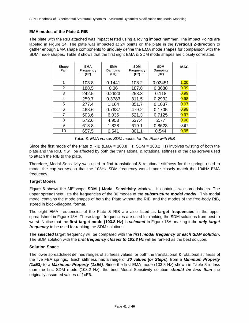
SEM Handbook of Experimental Structural Dynamics - Structural Dynamics Modification and Modal Modeling
Page 41 of 46
EMA modes of the Plate & RIB
The plate with the RIB attached was impact tested using a roving impact hammer. The impact Points are
labeled in Figure 14. The plate was impacted at 24 points on the plate in the (vertical) Z-direction to
gather enough EMA shape components to uniquely define the EMA mode shapes for comparison with the
SDM mode shapes. Table 8 shows that the first eight EMA & SDM mode shapes are closely correlated.
Shape Pair
EMA Frequency
(Hz)
EMA Damping
(Hz)
SDM Frequency
(Hz)
SDM Damping
(Hz)
MAC
1 103.8 0.1441 108.2 0.03451 1.00
2 188.5 0.36 187.6 0.3688 0.99
3 242.5 0.2623 253.3 0.118 0.99
4 259.7 0.3783 311.5 0.2932 0.98
5 277.4 1.164 351.7 0.1037 0.97
6 468.6 0.7687 479.2 0.1705 0.98
7 503.6 6.035 521.3 0.7125 0.97
8 572.6 4.953 537.4 2.77 0.98
9 618.8 1.828 619.1 0.8628 0.87
10 657.5 6.541 801.1 0.544 0,95
Table 8. EMA versus SDM modes for the Plate with RIB
Since the first mode of the Plate & RIB (EMA = 103.8 Hz, SDM = 108.2 Hz) involves twisting of both the
plate and the RIB, it will be affected by both the translational & rotational stiffness of the cap screws used
to attach the RIB to the plate.
Therefore, Modal Sensitivity was used to find translational & rotational stiffness for the springs used to
model the cap screws so that the 108Hz SDM frequency would more closely match the 104Hz EMA
frequency.
Target Modes
Figure 6 shows the ME’scope SDM | Modal Sensitivity window. It contains two spreadsheets. The
upper spreadsheet lists the frequencies of the 30 modes of the substructure modal model. This modal
model contains the mode shapes of both the Plate without the RIB, and the modes of the free-body RIB,
stored in block-diagonal format.
The eight EMA frequencies of the Plate & RIB are also listed as target frequencies in the upper
spreadsheet in Figure 18A. These target frequencies are used for ranking the SDM solutions from best to
worst. Notice that the first target mode (103.8 Hz) is selected in Figure 18A, making it the only target
frequency to be used for ranking the SDM solutions.
The selected target frequency will be compared with the first modal frequency of each SDM solution.
The SDM solution with the first frequency closest to 103.8 Hz will be ranked as the best solution.
Solution Space
The lower spreadsheet defines ranges of stiffness values for both the translational & rotational stiffness of
the five FEA springs. Each stiffness has a range of 30 values (or Steps), from a Minimum Property
(1xE3) to a Maximum Property (1xE6). Since the first EMA mode (103.8 Hz) shown in Table 8 is less
than the first SDM mode (108.2 Hz), the best Modal Sensitivity solution should be less than the
originally assumed values of 1xE6.
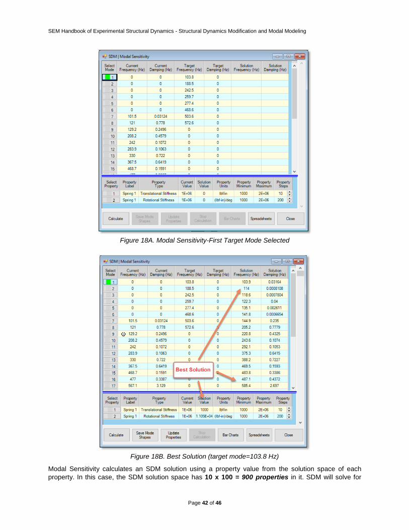
SEM Handbook of Experimental Structural Dynamics - Structural Dynamics Modification and Modal Modeling
Page 42 of 46
Figure 18A. Modal Sensitivity-First Target Mode Selected
Figure 18B. Best Solution (target mode=103.8 Hz)
Modal Sensitivity calculates an SDM solution using a property value from the solution space of each
property. In this case, the SDM solution space has 10 x 100 = 900 properties in it. SDM will solve for
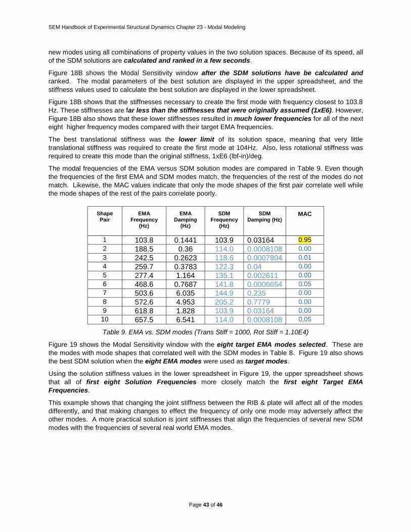
SEM Handbook of Experimental Structural Dynamics Chapter 23 - Modal Modeling
Page 43 of 46
new modes using all combinations of property values in the two solution spaces. Because of its speed, all
of the SDM solutions are calculated and ranked in a few seconds.
Figure 18B shows the Modal Sensitivity window after the SDM solutions have be calculated and
ranked. The modal parameters of the best solution are displayed in the upper spreadsheet, and the
stiffness values used to calculate the best solution are displayed in the lower spreadsheet.
Figure 18B shows that the stiffnesses necessary to create the first mode with frequency closest to 103.8
Hz. These stiffnesses are far less than the stiffnesses that were originally assumed (1xE6). However,
Figure 18B also shows that these lower stiffnesses resulted in much lower frequencies for all of the next
eight higher frequency modes compared with their target EMA frequencies.
The best translational stiffness was the lower limit of its solution space, meaning that very little
translational stiffness was required to create the first mode at 104Hz. Also, less rotational stiffness was
required to create this mode than the original stiffness, 1xE6 (lbf-in)/deg.
The modal frequencies of the EMA versus SDM solution modes are compared in Table 9. Even though
the frequencies of the first EMA and SDM modes match, the frequencies of the rest of the modes do not
match. Likewise, the MAC values indicate that only the mode shapes of the first pair correlate well while
the mode shapes of the rest of the pairs correlate poorly.
Shape Pair
EMA Frequency
(Hz)
EMA Damping
(Hz)
SDM Frequency
(Hz)
SDM Damping (Hz)
MAC
1 103.8 0.1441 103.9 0.03164 0.95
2 188.5 0.36 114.0 0.0008108 0.00
3 242.5 0.2623 118.6 0.0007804 0.01
4 259.7 0.3783 122.3 0.04 0.00
5 277.4 1.164 135.1 0.002611 0.00
6 468.6 0.7687 141.8 0.0006654 0.05
7 503.6 6.035 144.9 0.235 0.00
8 572.6 4.953 205.2 0.7779 0.00
9 618.8 1.828 103.9 0.03164 0.00
10 657.5 6.541 114.0 0.0008108 0,05
Table 9. EMA vs. SDM modes (Trans Stiff = 1000, Rot Stiff = 1.10E4)
Figure 19 shows the Modal Sensitivity window with the eight target EMA modes selected. These are
the modes with mode shapes that correlated well with the SDM modes in Table 8. Figure 19 also shows
the best SDM solution when the eight EMA modes were used as target modes.
Using the solution stiffness values in the lower spreadsheet in Figure 19, the upper spreadsheet shows
that all of first eight Solution Frequencies more closely match the first eight Target EMA
Frequencies.
This example shows that changing the joint stiffness between the RIB & plate will affect all of the modes
differently, and that making changes to effect the frequency of only one mode may adversely affect the
other modes. A more practical solution is joint stiffnesses that align the frequencies of several new SDM
modes with the frequencies of several real world EMA modes.
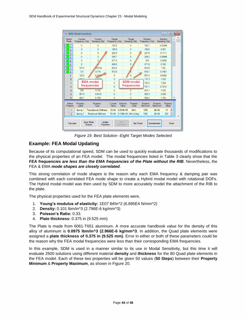
SEM Handbook of Experimental Structural Dynamics Chapter 23 - Modal Modeling
Page 44 of 46
Figure 19. Best Solution -Eight Target Modes Selected
Example: FEA Modal Updating
Because of its computational speed, SDM can be used to quickly evaluate thousands of modifications to
the physical properties of an FEA model. The modal frequencies listed in Table 3 clearly show that the
FEA frequencies are less than the EMA frequencies of the Plate without the RIB. Nevertheless, the
FEA & EMA mode shapes are closely correlated.
This strong correlation of mode shapes is the reason why each EMA frequency & damping pair was
combined with each correlated FEA mode shape to create a Hybrid modal model with rotational DOFs.
The Hybrid modal model was then used by SDM to more accurately model the attachment of the RIB to
the plate.
The physical properties used for the FEA plate elements were,
1. Young’s modulus of elasticity: 1E07 lbf/in^2 (6.895E4 N/mm^2)
2. Density: 0.101 lbm/in^3 (2.796E-6 kg/mm^3)
3. Poisson’s Ratio: 0.33.
4. Plate thickness: 0.375 in (9.525 mm)
The Plate is made from 6061-T651 aluminum. A more accurate handbook value for the density of this
alloy of aluminum is 0.0975 lbm/in^3 (2.966E-6 kg/mm^3. In addition, the Quad plate elements were
assigned a plate thickness of 0.375 in (9.525 mm). Error in either or both of these parameters could be
the reason why the FEA modal frequencies were less than their corresponding EMA frequencies.
In this example, SDM is used in a manner similar to its use in Modal Sensitivity, but this time it will
evaluate 2500 solutions using different material density and thickness for the 80 Quad plate elements in
the FEA model. Each of these two properties will be given 50 values (50 Steps) between their Property
Minimum & Property Maximum, as shown in Figure 20.
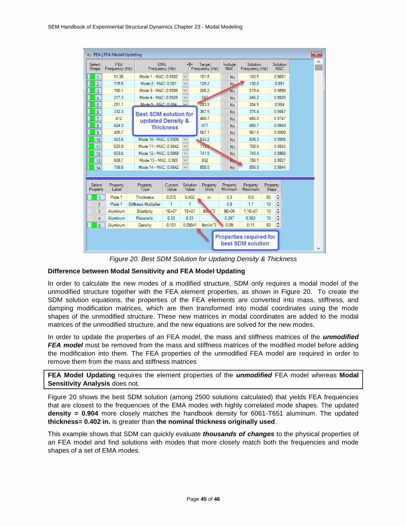
SEM Handbook of Experimental Structural Dynamics Chapter 23 - Modal Modeling
Page 45 of 46
Figure 20. Best SDM Solution for Updating Density & Thickness
Difference between Modal Sensitivity and FEA Model Updating
In order to calculate the new modes of a modified structure, SDM only requires a modal model of the
unmodified structure together with the FEA element properties, as shown in Figure 20. To create the
SDM solution equations, the properties of the FEA elements are converted into mass, stiffness, and
damping modification matrices, which are then transformed into modal coordinates using the mode
shapes of the unmodified structure. These new matrices in modal coordinates are added to the modal
matrices of the unmodified structure, and the new equations are solved for the new modes.
In order to update the properties of an FEA model, the mass and stiffness matrices of the unmodified
FEA model must be removed from the mass and stiffness matrices of the modified model before adding
the modification into them. The FEA properties of the unmodified FEA model are required in order to
remove them from the mass and stiffness matrices
FEA Model Updating requires the element properties of the unmodified FEA model whereas Modal
Sensitivity Analysis does not.
Figure 20 shows the best SDM solution (among 2500 solutions calculated) that yields FEA frequencies
that are closest to the frequencies of the EMA modes with highly correlated mode shapes. The updated
density = 0.904 more closely matches the handbook density for 6061-T651 aluminum. The updated
thickness= 0.402 in. is greater than the nominal thickness originally used.
This example shows that SDM can quickly evaluate thousands of changes to the physical properties of
an FEA model and find solutions with modes that more closely match both the frequencies and mode
shapes of a set of EMA modes.

SEM Handbook of Experimental Structural Dynamics Chapter 23 - Modal Modeling
Page 46 of 46
REFERENCES
1. Hallquist, J. “Modification and Synthesis of Large Dynamic Structural Systems” Ph.D. Dissertation, Michigan Technological University, 1974.
2. Formenti, D. & Welaratna, S. “Structural Dynamics Modification - An Extension to Modal Analysis” SAE Paper No. 811043, Oct. 1980.
3. Structural Measurement Systems, Inc. “An Introduction to the Structural Dynamics Modification System”, Technical Note No.1, February, 1980.
4. Ramsey, K. & Firmin, A. “Experimental Modal Analysis Structural Modifications and FEM Analysis - Combining Forces on a Desktop Computer” First IMAC Proceedings, Orlando, Florida, Nov. 8-10, 1982
5. Wallack, P., Skoog, P., and Richardson, M.H. “Simultaneous Structural Dynamics Modification S2DM)”
Proc. of 6th IMAC, Kissimmee, FL, 1988
6. Bathe, K.J., and Wilson, E.L. “Numerical Methods in Finite Element Analysis” Prentice Hall, Inc., 1976.
7. Yang, T.Y. “Finite Element Structural Analysis” Prentice Hall, Inc., 1986.
8. McGuire, W., and Gallagher, R.H.. “Matrix Structural Analysis” John Wiley & Sons, 1979.