Embed Size (px)
Citation preview
Structural Dynamic Analysis of
Systematic Risk
Laurent Calvet, Veronika Czellar and Christian Gourieroux∗
First version: August 2014
This version: December 27, 2015
Preliminary version
∗Calvet: Department of Finance, HEC Paris; [email protected]. Czellar: Department of Accounting,Law, Finance and Economics, EDHEC Business School; [email protected]. Gourieroux:CREST, Paris and Department of Economics, University of Toronto; [email protected]. We grate-fully acknowledge the computer support of EUROFIDAI.

Abstract
This paper introduces a structural dynamic factor model (SDFM) for stock
returns. Compared to standard linear factor models, structural modeling ac-
counts for nonlinear effects of common factors when the distance-to-default
is small. Such a SDFM has a rather complicated form, especially since the
underlying factors are unobservable and have nonlinear effects. We develop
appropriate methods to estimate such models and use them for prediction,
filtering and smoothing purposes, such as indirect inference or Approximate
Bayesian Computation (ABC) filtering and smoothing. These SDFM are ap-
plied to the analysis of systematic risk of financial institutions and to obtain
their rating of default and speculative features.
Keywords: Systematic Risk, SIFI, Merton’s Model, Value-of-the-Firm, Indi-
rect Inference, Rating, ABC Filtering and Smoothing.
1 Introduction
The analysis of systematic risk from stock returns is usually based on dynamic linear
factor models, where the factors can feature conditional heteroscedasticity. Typi-
cal examples are models derived from the Capital Asset Pricing Model (CAPM),
in which the linear factors can be interpreted in terms of market portfolio returns
(Markowitz, 1959; Sharpe, 1964; Lintner, 1965). Such models are used to separate
risk and required capital into two components: the systematic risk component mea-
sures the effects of the systematic factors, taking into account the sensitivities to

the factors (or betas); the specific risk corresponds to the residual risk once the
systematic component is taken into account.
However, the hypothesis of linear effect of the systematic factors has been ques-
tioned, in particular for factor values, which might create default of important finan-
cial institutions, the so-called systematically important financial institutions (SIFI).
Indeed, if a firm is close to default, the stock price will integrate the cost of default-
risk with a nonlinear impact of the systematic factor.1 The nonlinear effect is due
to the interpretation of a stock as a call option written on the asset component of
the balance sheet of the firm with strike its liability component. According to the
literature, this option can be either a European call (Merton, 1974), or an American
call (Black and Cox, 1976).
The nonlinear effect is expected to be more significant for financial institutions,
which have to support not only inappropriate direct credit granting, but also the often
huge investments in credit derivatives such as Mortgage Backed Securities (MBS),
Collateral Debt Obligations (CDO) and other Sovereign Credit Default Swaps (CDS).
The objective of our paper is to include the option interpretation when analyzing
systematic risk in the stock returns of financial institutions and intermediaries. Our
structural approach is in the spirit of the rating models developed by KMV (see
e.g. Crosbie and Bohn (2004)), but with more focus on the factor dynamics and the
possibility of stochastic volatility. It is also related to the structural extension of
multivariate GARCH models developed in Engle and Siriwardane (2015).
We base our analysis on stock returns of ten financial institutions. The data are
presented and discussed in Section 2. In particular, we focus on: the static linear
1We prefer to use the terminology systematic instead of systemic for the common factors. Indeed,a shock on a common factor does not necessarily imply a risk of destruction of the financial system(see e.g. Hansen (2012) for a discussion of the two notions).
2

factor, which can be exhibited and its link with the S&P 500 market return.
We consider in Section 3 a one-factor linear model for analyzing jointly the re-
turn of the financial institutions. This linear factor model differs from the standard
Sharpe-Lintner model, since it accounts for stochastic volatility effects. Two types of
stochastic volatilities are introduced, that are a stochastic volatility for the common
factor and stochastic volatilities specific to each financial institution. We assume
that both the common linear factor and the volatilities are latent. Thus we get a
nonlinear multifactor model due to the introduction of stochastic volatilities. In par-
ticular, the likelihood function of this nonlinear state-space model has a complicated
form, which involves multidimensional integrals, with a dimension increasing with
the number of observations. We develop an appropriate indirect inference approach
(Gourieroux, Monfort and Renault, 1993; Smith, 1993) to estimate the model, i.e. to
capture the factor sensitivities as well as the dynamics of the factor and volatilities.
This approach is applied to the return data. In particular, we discuss the dynamic
link between the filtered factor and the submarket portfolio derived from the static
approach.
The factor model of Section 3 does not account for default risk. Default risk is
introduced in Section 4 and creates an additional source of nonlinearity. We first
review the Value-of-the Firm model, the effect of the distance-to-default on stock
values, and approximate this nonlinear effect to get a link between the changes in
the log asset/liability rates, and the stock returns. Then, the analysis is extended to
the multiasset framework. From the modelling point of view, this leads to a model
defined in two components. The linear factor model with stochastic volatilities of
Section 3 is used to define the joint dynamics of the unobserved changes in the log
asset/liability ratios. Then a nonlinear measurement equation relates the observed
stock returns to these changes and includes the nonlinear effect of the distance-to-
3

default. This structural dynamic factor model (SDFM) is estimated and the results
are compared with the outputs of the dynamic model without option of default. Then
it is used to construct different ratings, that are a solvency rating, a rating based on
the market price of the insurance against default, and a rating for speculative feature
of the associated stock.
Section 5 concludes.
2 Data
We consider the daily logreturns between April 6, 2000, and July 31, 2015, of ten
financial institutions: MetLife Inc. (MET), ING Group (ING), Goldman Sachs
Group Inc. (GS), Lincoln National Corp. (LNC), HSBC Holdings plc. (HSBC),
JPMorgan Chase & Co. (JPM), Bank of America Corp. (BAC), Credit Suisse Group
AG (CS), Wells Fargo & Co. (WFC), Barclays plc. (BCS). The daily logreturns are
log(Pit/Pi,t−1), where Pit is the closing price of financial stock i at date t adjusted for
dividends and splits, downloaded from Yahoo Finance.2 All returns are computed
in U.S. dollars. The logreturn series are plotted in Figure 1. The sample size of the
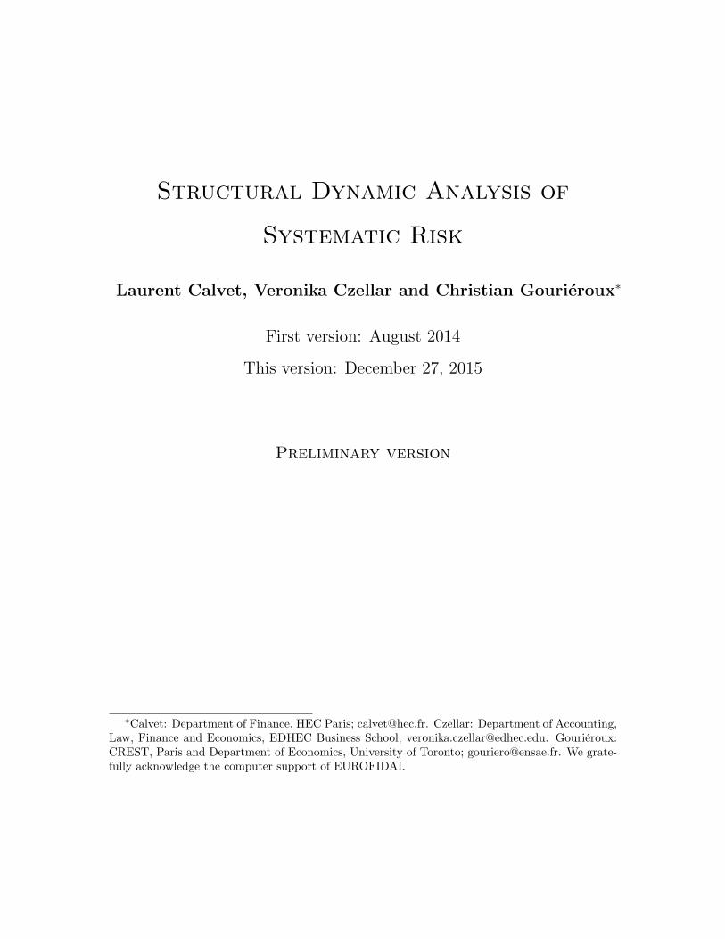
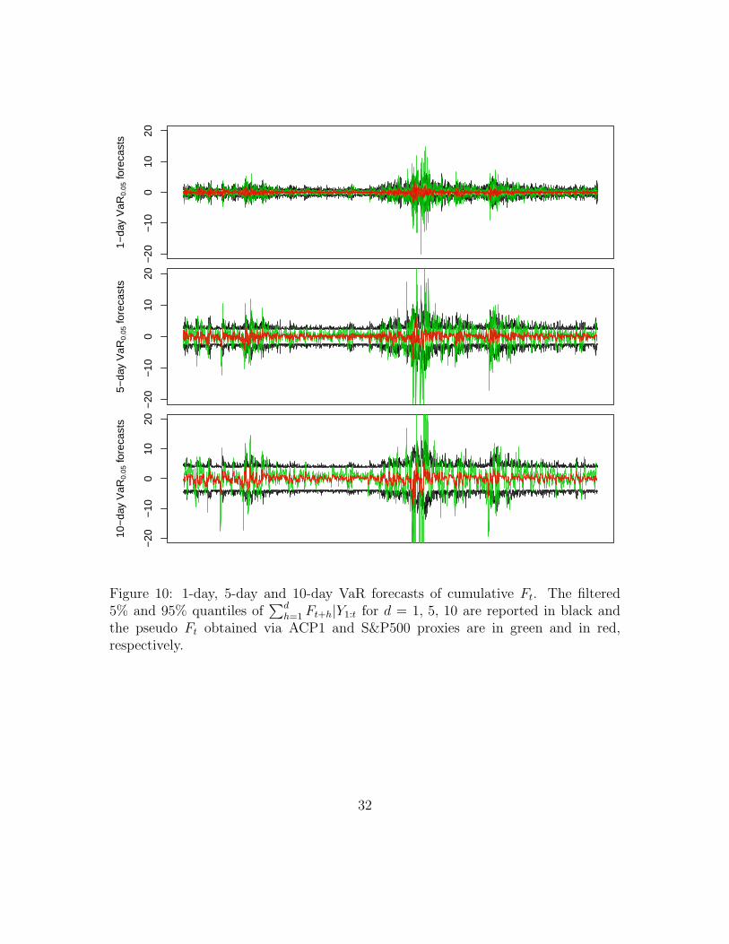
logreturn series is T = 3, 853 (trading days). Table 1 reports sample statistics of the
return series.
We immediately observe in Figure 1 stochastic and persistent volatilities. Large
volatilities arise to all series at the period of the recent financial crisis, i.e. 2008-2010,
and also for several series in 2012.
The mean returns are between -1% and 10% per year on this period, with large
kurtosis revealing fat tails. These tail features are partly due to the crises, with
negative daily returns up to 50% (for LNC and BCS), which corresponds to a decrease
2finance.yahoo.com
4

−0.
60.
00.
4
HS
BC
−0.
60.
00.
4
ING
−0.
60.
00.
4
CS
−0.
60.
00.
4
BC
S
2000 2005 2010 2015
−0.
60.
00.
4
BA
C
−0.
60.
00.
4
ME
T
−0.
60.
00.
4
GS
−0.
60.
00.
4
LNC
−0.
60.
00.
4
JPM
2000 2005 2010 2015
−0.
60.
00.
4
WF
C
Figure 1: Logreturn series.
of 40% of the price. However, we also observe large log-returns, up to a price increase
of 60% for BCS. The skewnesses are negative, except for GS, JPM and WFC. This
negative sign can be due to a crash going faster than the recovery.
The dynamics of the series are summarized by the autocorrelations of the returns
5

and squared returns, respectively. The first-order autocorrelations of the returns are
very small (the largest one in absolute value is 6.7 ·10−20 per month), as expected for
an efficient market. At the opposite, the autocorrelations of the squared returns are
larger (between 0.20 and 0.34, except for BCS), indicating the volatility persistence.
The realized daily volatility-covolatility matrix can be used for a static linear
factor analysis. We provide the set of its eigenvalues in decreasing order. The largest
eigenvalue is far above the next ones indicating the importance of the first linear
factor. Then, the next eigenvalues decrease slowly from 0.0007 to 0.0001. The first
eigenvector is (0.30, 0.36, 0.25, 0.39, 0.18, 0.30, 0.36, 0.29, 0.29, 0.37). Its components
are of a similar size and the associated portfolio is close to a submarket portfo-
lio, where the submarket only includes these ten financial institutions. Finally, we
provide the alphas and betas, when regressing the individual log-returns on the log-
arithm of the submarket portfolio. The alphas are not significant showing that this
standard consequence of the CAPM could be applied to the submarket considered
as a whole.
Finally, let us compare the submarket portfolio and the market portfolio, i.e.
the S&P500 index. Their returns are plotted in Figure 2. The slope is equal to
1.5, whereas the mean and standard errors of the submarket and market portfolios
are 0.00014, 0.02247 and 0.00009, 0.01264, respectively. Thus, the submarket is not
representative of the entire market. It features larger risk compensated by larger
expected returns.
3 Dynamic Model Without Option of Default
We first consider a linear factor model with stochastic volatilities for the stock re-
turns. The model does not take into account the possibility of default of the firms.
6
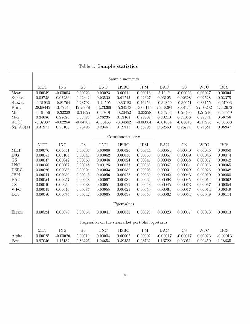
Table 1: Sample statistics
Sample moments
MET ING GS LNC HSBC JPM BAC CS WFC BCS
Mean 0.00039 -0.00003 0.00023 0.00023 0.00011 0.00016 5·10−6 -0.00003 0.00037 0.00004St.dev. 0.02758 0.03233 0.02442 0.03532 0.01743 0.02627 0.03125 0.02698 0.02528 0.03375Skewn. -0.31930 -0.81764 0.28792 -1.24505 -0.83182 0.26453 -0.34869 -0.36651 0.88155 -0.67903Kurt. 20.98442 13.47540 12.25651 43.23296 15.34543 13.03115 25.40294 8.88474 27.09202 42.12672Min. -0.31156 -0.32229 -0.21022 -0.50891 -0.20852 -0.23228 -0.34206 -0.23460 -0.27210 -0.55549Max. 0.24686 0.22626 0.23482 0.36235 0.13463 0.22392 0.30210 0.21056 0.28341 0.50756AC(1) -0.07837 -0.02256 -0.04989 -0.03458 -0.04682 -0.08004 -0.01004 -0.05813 -0.11286 -0.05603Sq. AC(1) 0.31971 0.20103 0.23496 0.29467 0.19912 0.33998 0.32550 0.25721 0.21381 0.08837
Covariance matrix
MET ING GS LNC HSBC JPM BAC CS WFC BCS
MET 0.00076 0.00051 0.00037 0.00068 0.00026 0.00044 0.00054 0.00040 0.00045 0.00050ING 0.00051 0.00104 0.00041 0.00062 0.00036 0.00050 0.00057 0.00059 0.00046 0.00074GS 0.00037 0.00042 0.00060 0.00048 0.00024 0.00045 0.00048 0.00038 0.00037 0.00042LNC 0.00068 0.00062 0.00048 0.00125 0.00033 0.00056 0.00067 0.00051 0.00055 0.00065HSBC 0.00026 0.00036 0.00024 0.00033 0.00030 0.00028 0.00031 0.00029 0.00025 0.00038JPM 0.00044 0.00050 0.00045 0.00056 0.00028 0.00069 0.00062 0.00043 0.00050 0.00050BAC 0.00054 0.00057 0.00048 0.00067 0.00031 0.00062 0.00098 0.00045 0.00064 0.00062CS 0.00040 0.00059 0.00038 0.00051 0.00029 0.00043 0.00045 0.00073 0.00037 0.00054WFC 0.00045 0.00046 0.00037 0.00055 0.00025 0.00050 0.00064 0.00037 0.00064 0.00049BCS 0.00050 0.00074 0.00042 0.00065 0.00038 0.00050 0.00062 0.00054 0.00049 0.00114
Eigenvalues
Eigenv. 0.00524 0.00070 0.00054 0.00041 0.00032 0.00026 0.00023 0.00017 0.00013 0.00013
Regression on the submarket portfolio logreturns
MET ING GS LNC HSBC JPM BAC CS WFC BCS
Alpha 0.00025 -0.00020 0.00011 0.00004 0.00002 0.00002 -0.00017 -0.00017 0.00023 -0.00013Beta 0.97036 1.15132 0.83225 1.24654 0.59355 0.98732 1.16722 0.93051 0.93459 1.18635
7

−0.2 −0.1 0.0 0.1 0.2
−0.
2−
0.1
0.0
0.1
0.2
S&P 500
Sub
mar
ket p
orfo
lio
Figure 2: Submarket portfolio versus S&P500. The submarket portfolio log-returnis plotted versus the S&P500 log-return. A simple linear regression provides anintercept of 10−5 and a slope of 1.5011.
Let us denote by Yit, i = 1, . . . , n, t = 1, . . . , T the returns at date t for firm (stock)
8

i. The return dynamics is defined by:Yit = αi + βiFt + σitϵit , i = 1, . . . , n ,
Ft = γFt−1 + ηtut ,
(3.1)
where Ft is a common unobservable linear factor, the ϵits and uts are indepen-
dent standard normal variables, the σits and ηts are specific and factor stochastic
volatilities, respectively. The stochastic volatilities are assumed mutually indepen-
dent, and independent of the standardized specific and factor innovations ϵ, u, with
autoregressive gamma (ARG) dynamics: η2t ∼ ARG[δ, ρ, (1 − ρ)(1 − γ2)/δ] and
σ2it ∼ ARG(δ, ρ, c), where νt ∼ARG(a, b, c) is equivalent with νt ∼Gamma(a+zt, c)
and zt ∼Poisson(bνt−1/c). The parameters a, b, c of the ARG(a, b, c) can be inter-
preted as a degree of freedom, a measure of serial dependence and a scale parameter,
respectively. The ARG processes are exact time discretized Cox, Ingersoll, Ross
(CIR) processes, usually employed for the modelling of stochastic volatility in con-
tinuous time [see Cox, Ingersoll and Ross (1985) for the CIR process and Gourieroux
and Jasiak (2006) and Appendix 5.1 for the properties of ARG processes].
Since a dynamic factor is defined up to a linear affine transformation, without loss
of generality the linear factor dynamics can be constrained to satisfy E(Ft) = 0 and
V (Ft) = 1, ∀t. These identification restrictions have been taken into account in the
dynamic model above. The condition E(Ft) = 0 is due to the absence of intercept in
the autoregression satisfied by the factor; the condition V (Ft) = 1 is a consequence
of the link between the three parameters of the ARG process satisfied by ηt.
The model above involves different parameters: the αis are the expected stock
returns, whereas the βis provide the sensitivities of the stock returns with respect to
the common linear factor, and γ is a measure of the factor persistence. The remaining
9

parameters characterize the volatility dynamics. The model differs from the standard
linear factor model [see e.g. Darolles and Gourieroux (2015), Chapter 3] by the
introduction of the stochastic volatilities. In this respect this is a multifactor model
with n+2 factors (state variables): Ft, ηt, σit. The factor dynamics is linear for
Ft, but nonlinear for the unobservable volatilities. We get a nonlinear state space
model (see Appendix 5.1 for the state space representation of the ARG process),
to which the standard Kalman filter does not apply. In particular, the likelihood
function corresponding to the observation of Yt = (Y1t, . . . , Ynt)′, t = 1, . . . , T , has
an integral form, since the unobservable factor paths have to be integrated out. This
likelihood involves an integral of a huge dimension equal to (n+2)T , which increases
with the number T of observation dates. To avoid the numerical optimization of
the complicated likelihood function, we consider below a simple two-step estimation
approach.
3.1 The Estimation Approach
We first consider an estimation approach of both the parameter and factor values,
which would be close to consistency if both n and T were large [see Gagliardini and
Gourieroux (2014) for the so-called granularity theory]. However, in our framework,
the number of stocks is fixed and the approach is not consistent. In a second step,
this method is adjusted for asymptotic bias by indirect inference, since model (3.1)
is easy to simulate.
3.1.1 Auxiliary Method of Moments Estimation
Our first estimation of the parameter and factor values is based on moment restric-
tions.
10

(i) Estimation of α
The vector α = (α1, . . . , αn)′ can be estimated by the first moment of observa-
tions. We have:
E(Yt) = α ,
which leads to the method of moments estimator:
α = Y ,
where Y = 1T
∑Tt=1 Yt.
(ii) Estimation of Ft
Denote the demeaned row vector by Zt = Yt−α. Denote also Z·t = n−1∑n
i=1 Zit
and its standardized version by:
Ft = Z·t/
√√√√T−1
T∑t=1
Z2·t .
(iii) Estimation of β and γ
We then estimate β by:
βi =1
T
T∑t=1
ZitFt ,
and parameter γ by:
γ =1
T − 1
T∑t=2
FtFt−1 .
11

(iv) Estimation of the parameters characterizing the dynamics of ηt
We estimate ηtut by ηtut = Ft − γFt−1. Since
E[(ηtut)4] = 3(
1
δ+ 1)(1− γ2)2 ,
and
E[(ηtut)2(ηt−1ut−1)
2] = (ρ
δ+ 1)(1− γ2)2 ,
ρ and δ can be estimated by their associated sample counterparts:
δ =
(T − 1)−1
T∑t=2
ηtut4/[3(1− γ2)2]− 1
−1
,
ρ = δ
((T − 2)−1
T∑t=3
ηtut2 ηt−1ut−1
2/[(1− γ2)2]− 1
).
(v) Estimation of the parameters characterizing the dynamics of σit
A natural estimator of σitϵit is:
σitϵit = Zit − βiFt .
Since
E[n∑
i=1
σ2itϵ
2it] = nA ,
E[n∑
i=1
σ4itϵ
4it] = 3nA2(1 + δ−1) ,
E[n∑
i=1
(σitϵit)2(σi,t−1ϵi,t−1)
2] = nA2(1 + ρ/δ) ,
12

with A = cδ/(1− ρ), the ARG parameters can be estimated by:
ˆδ =
T−1
∑Tt=1
∑ni=1 σitϵit
4
3nA2− 1
−1
,
ˆρ = ˆδ
[(T − 1)−1
∑Tt=2
∑ni=1 σitϵit
2 σi,t−1ϵi,t−12
nA2− 1
],
ˆc = (1− ˆρ)A/ˆδ ,
with A = n−1∑n
i=1
∑Tt=1 σitϵit
2.
The approach above is computationally simple and easy to interpret, since all estima-
tors have closed-form expressions. However, as mentioned above, this method is not
consistent, due to the approximate filtered value Ft, which differs from Ft for fixed
n. This explains why the results of this estimation approach have to be adjusted to
eliminate the asymptotic bias. Since the nonlinear state-space model (3.1) is easy to
simulate, this adjustment can be done by indirect inference.
3.1.2 Indirect inference estimation
Let us now describe the indirect inference adjustment and denote the vector of struc-
tural parameters by:
θ = (αini=1, βini=1, γ, δ, ρ, δ, ρ, c)′ .
Denote also the empirical dataset by Y1:T = Yiti=1,...,n, t=1,...,T and the associated set
of auxiliary statistics, non consistent moment estimators of the first step approach
given in 3.1.1, by:
µ = (α, β, γ, 1/δ, ρ/δ, 1/ˆδ, ˆρ/ˆδ, A)′ .
13

The indirect inference adjustment is based on a comparison of the auxiliary statistics
computed from the data and those computed using simulated data generated from the
structural model (3.1). More precisely, let us consider independent simulated pseudo-
data samples: Y(s)1:T (θ) = Y (s)
t (θ)Tt=1, s = 1, . . . , S, satisfying the data-generating
process (3.1), where S is the number of replications. The auxiliary estimator based
on simulated data is defined by:
µS(θ) = S−1
S∑s=1
µ[Y(s)1:T (θ)] .
The indirect inference (II) estimator of θ is defined as:
θII = argminθ[µ− µS(θ)]
′Ω[µ− µS(θ)] ,
where Ω is a symmetric, positive-definite weighting matrix. Since we use a just-
identified auxiliary estimator, the II estimator does not depend on Ω and Ω can
be conveniently replaced by the identity matrix. This two-step estimator θII is
consistent of θ.
Hereafter, in all our empirical and Monte Carlo II estimations, we use S = 10
pseudo-data samples.
3.2 Monte Carlo results
Let us illustrate the properties of the first step method of moment (MM) estimation
and of the II estimation by Monte Carlo study. We consider n = 10 stocks and a
sample size T = 3, 853 like in our empirical dataset. The true parameters are set to
the empirical estimates obtained in the following subsection and reported in Table 2,
second column.
14

We generate independently 100 datasets and for each of them we compute the
MM estimate and the II estimate. We provide in Figure 3 the boxplots corresponding
to the finite sample (T = 3, 853) properties of both estimates. The true values of
the parameters are set to the empirical estimates (see later in the second column of
Table 2) and are reported with continuous lines. We only display α1 and β1 among
the αs and βs.
Let us first consider the MM estimates. We see that the boxes do not necessarily
include the true values of the parameters, as a consequence of the nonconsistency.
This arises for parameters characterizing the volatility dynamics, especially the δ and
δ parameters. When the estimates are adjusted by indirect inference, we observe that
the boxes now all include the true parameter values.
3.3 Empirical Results
Let us now apply the estimation approach to the real dataset. Table 2 reports
auxiliary MM and II estimate. We observe that the estimated values are rather
stable with respect to the number S of replications. The estimated betas can be
directly compared with the estimated betas derived in the static analysis of Section 2.
Note that in Section 2, the submarket portfolio has not been standardized. Since
the standard error of the return of the submarket portfolio is equal to 0.022, after
standardization these betas are provided in the last column of Table 2 . We see
that the betas estimated from the static model, the auxiliary moment method and
the indirect inference estimates are rather close to each other. Thus, the interest of
the approach is essentially in the parameters characterizing the dynamics of factor
and volatilities. These parameters are required for the prediction of future rates and
in particular for the computation of the term structure of the Value-at-Risk and
15

Aux II−0.
0010
0.00
000.
0010
α 1
Aux II
0.02
00.
022
0.02
40.
026
β 1
Aux II
−0.
10−
0.05
0.00
0.05
γ
Aux II
0.05
0.10
0.15
0.20
0.25
δAux II
0.4
0.6
0.8
1.0
ρ
Aux II
0.04
0.06
0.08
0.10
δ~
Aux II
0.2
0.4
0.6
0.8
1.0
ρ~
Aux II0.
000
0.00
10.
002
0.00
30.
004
c~
Figure 3: Method of Moments and Indirect Inference Estimates. This figure illus-trates 100 MM and corresponding II estimates for n = 10 and sample size T = 3, 853as in the empirical dataset. The true parameters are set to the empirical estimatesand are reported with continuous lines.
and their sensitivities with respect to shocks on either the systematic, or specific
standardized innovations.
The estimated γ is small and negative. It has to be compared with the autore-
gressive coefficient corresponding to the return of the submarket portfolio derived
by the static approach. This coefficient is -0.053, thus has the same order as the II
16

estimates of γ.3
We observe a strong persistence, that is large ρ coefficients, for both systematic
and specific volatilities. The estimated δ and δ coefficients provide information on
the behaviour of the (marginal and conditional) distribution of volatilities in the tail
and in the neighborhood of volatility zero.
Using the II parameter estimates, we simulate series of the same size as the
original dataset. The related sample statistics are reported in Table 3.
The comparison of Tables 1 and 3 shows a reasonable goodness of fit for the
different characteristics of historical distribution, including the measures of state
dependence between returns, and of their dynamic features by means of first-order
autocorrelations of returns and squared returns.
3.4 Imputation of the hidden states (factors)
Using the II parameter estimates, let us now turn to the imputation of the hidden
states x1:T = (x1, . . . , xT ), where xt = (Ft, σitni=1, ηt), on the in-sample period April
6, 2000 and July 31, 2015.
3.4.1 Filtering
To estimate the distribution of xt|Y1:t at a given date t, we use an Approximate
Bayesian Computation (ABC) filter4 (Calvet and Czellar, 2011, 2015; Jasra et al.,
2012) with optimal kernel and bandwidth choices given in Calvet and Czellar (2015).5
3The autoregressive coefficient for the return of the S&P 500 is -0.084.4Calvet and Czellar (2011) called it State-Observation Sampling (SOS) filter.5A bootstrap particle filter (Gordon, Salmond and Smith, 1993) is theoretically applicable.
However, since the observation density f(Yt|xt) in our model is a n-variate Gaussian with largen, the bootstrap filter encounters numerical weight degeneracy problems whenever an outlier inthe return process is observed. In addition, in the structural dynamic factor model of Section 4.7,f(Yt|xt) will not be available anymore and a standard particle filtering will be inapplicable.
17

Table 2: Empirical estimates
AuxNo optionof default
With optionof default
Staticmodel
αMET 0.000395 0.000362 0.000606αING -0.000032 0.000059 0.000198αGS 0.000232 0.000200 0.000596αLNC 0.000227 0.000118 0.000358αHSBC 0.000111 0.000163 -0.000122αJPM 0.000164 0.000074 -0.000212αBAC 0.000005 -0.000047 0.000440αCS -0.000028 0.000047 0.000159αWFC 0.000366 0.000372 0.000694αBCS 0.000043 -0.000053 -0.000950βMET 0.021806∗ 0.021840∗ 0.026920 0.021348βING 0.025872∗ 0.026084∗ 0.034525 0.025329βGS 0.018702∗ 0.018239∗ 0.020364 0.018309βLNC 0.028012∗ 0.028496∗ 0.035498 0.027424βHSBC 0.013338∗ 0.012607∗ 0.016979 0.013058βJPM 0.022187∗ 0.022368∗ 0.036311 0.021721βBAC 0.026229∗ 0.026669∗ 0.034107 0.025679βCS 0.020910∗ 0.020599∗ 0.026767 0.020471βWFC 0.021002∗ 0.020969∗ 0.023378 0.020561βBCS 0.026659∗ 0.026857∗ 0.050174 0.026100γ -0.053297 -0.044679 -0.054902δ 0.162371∗ 0.129703∗ 0.161184ρ 0.787698∗ 0.742651∗ 0.869338
δ 0.077740∗ 0.064702∗ 0.077236ρ 0.815843∗ 0.842556∗ 0.856746c 0.000687 0.000792 0.000786ω 1.861301
Empirical Estimates for daily logreturns between April 6, 2000, and July 31,2015, a sample size of 3,853. Each reported II estimate is the global minimum ofthe II objective function among 1,000 local minimizations with starting valueschosen at random. In the Aux and No option of default columns, numbers withan asterix indicate significant parameters at the 5% level, where significanceis measured by means of robust standard errors IQR/1.349 where IQR is theinterquartile range over 100 Monte Carlo estimates.
18

Table 3: Sample statistics of simulated series
Sample moments
MET ING GS LNC HSBC JPM BAC CS WFC BCS
Mean 0.00070 0.00037 0.00105 0.00029 0.00039 0.00044 -8·10−6 -2·10−5 0.00056 0.00030St.dev. 0.02653 0.02931 0.02688 0.03260 0.01967 0.02718 0.03115 0.02680 0.02648 0.03060Skewn. -0.37902 -0.65573 -0.04512 -0.12469 -0.22193 -0.37643 -0.76003 -0.75318 -0.79803 -0.81506Kurt. 14.18529 14.94072 21.18191 17.27276 15.01790 15.93163 15.70523 12.95755 18.91468 18.59897Min. -0.22352 -0.27242 -0.24653 -0.29785 -0.16614 -0.25429 -0.27710 -0.21414 -0.30902 -0.34973Max. 0.16933 0.20106 0.32663 0.30655 0.16804 0.22008 0.20753 0.18743 0.25635 0.22679AC(1) -0.09970 -0.07468 -0.03627 -0.06953 -0.07767 -0.06166 -0.06460 -0.06251 -0.01950 -0.05747Sq. AC(1) 0.23862 0.25440 0.20127 0.25253 0.32141 0.26033 0.27648 0.32238 0.22400 0.27619
Covariance matrix
MET ING GS LNC HSBC JPM BAC CS WFC BCS
MET 0.00070 0.00053 0.00037 0.00059 0.00026 0.00046 0.00055 0.00042 0.00042 0.00054ING 0.00053 0.00089 0.00044 0.00070 0.00032 0.00056 0.00067 0.00050 0.00051 0.00065GS 0.00037 0.00044 0.00072 0.00049 0.00022 0.00038 0.00045 0.00035 0.00035 0.00046LNC 0.00059 0.00070 0.00049 0.00106 0.00034 0.00062 0.00074 0.00055 0.00056 0.00072HSBC 0.00026 0.00032 0.00022 0.00034 0.00039 0.00027 0.00032 0.00024 0.00025 0.00032JPM 0.00046 0.00056 0.00038 0.00062 0.00027 0.00074 0.00057 0.00043 0.00044 0.00056BAC 0.00055 0.00067 0.00045 0.00074 0.00032 0.00057 0.00097 0.00051 0.00052 0.00067CS 0.00042 0.00050 0.00035 0.00055 0.00024 0.00043 0.00051 0.00072 0.00039 0.00051WFC 0.00042 0.00051 0.00035 0.00056 0.00025 0.00044 0.00052 0.00039 0.00070 0.00052BCS 0.00054 0.00065 0.00046 0.00072 0.00032 0.00056 0.00067 0.00051 0.00052 0.00094
Eigenvalues
Eigenv. 0.00523 0.00041 0.00033 0.00030 0.00028 0.00028 0.00027 0.00026 0.00024 0.00022
Regression on mean logreturns
MET ING GS LNC HSBC JPM BAC CS WFC BCS
Alpha 0.00031 -0.00009 0.00071 -0.00022 0.00015 0.00004 -0.00049 -0.00040 0.00018 -0.00017Beta 0.96396 1.14046 0.84320 1.26499 0.58183 0.99771 1.18975 0.92071 0.92748 1.16992
Sample statistics of the simulated series using empirical estimates.
19

The idea of ABC filtering is to replace in Step 2 of the filtering algorithm the un-
available conditional distribution f(Yt|xt) by the distance of simulated observations
Y (i)t Ni=1 to the empirical observation Yt. The distance is measured by a strictly pos-
itive kernel K : Rdim y → R integrating to unity, where dim y denotes the dimension
of y. For any bandwidth ht > 0, define Kht(y) = K(
yht
)/hdim y
t . The ABC filtering
algorithm is as follows.
Step 1 (Initialization): At date t = 0, simulate x(i)0 , i = 1, . . . , N , from
the initial density f(x0).
For t = 1, . . . , T , iterate Steps 2-4.
Step 2 (Sampling): Simulate a state-observation pair (x(i)t , Y
(i)t ) from
f(xt, Yt|x(i)t−1, Y1:t−1), i = 1, . . . , N .
Step 3 (Importance weights): Observe Yt and compute the weights
ω(i)t =
1
hdim yt
K
(Y
(i)t − Yt
ht
), i = 1, . . . , N.
Step 4 (Multinomial resampling): Draw x(1)t , . . . , x
(N)t from x
(1)t , . . . , x
(N)t
with probabilitiesω(1)t∑i ω
(i)t
, . . . ,ω(N)t∑i ω
(i)t
.
ABCFiltering Algorithm
We use the quasi-Cauchy kernel K and plug-in bandwidth ht (Calvet and Czellar,
2015):
K(u) = (1 + c u⊤u)−(dimu+3)/2 and h∗t (N) =
[c2B(K) dimu
N Pt
]1/(dimu+4)
, (3.2)
where dimu is the dimension of u, c = π1+1/dimu/2Γ[(dimu+3)/2]2/dimu, B(K) =
20

2 Γ(dim u/2+3) Γ[(dim u+3)/2]/[√πΓ(dimu+3)], Γ(·) is the gamma function, and
Pt =2 tr(Σ−2
t ) + [tr(Σ−1t )]2
2dimu+2 πdimu/2 [det(Σt)]1/2, (3.3)
where Σt is the sample covariance matrix calculated with the simulated Y (i)t i=1,...,N
in Step 2 of the ABC filter.
The empirical distribution of Step 2 particles x(i)t Ni=1 finitely estimates the dis-
tribution f(xt|Y1:t−1) and the empirical distribution of Y (i)t Ni=1 estimates the dis-
tribution f(Yt|Y1:t−1), which can be used for forecasting purposes. Moreover, the
empirical distribution of Step 4 particles x(i)t Ni=1 finitely estimates the distribution
f(xt|Y1:t).
3.4.2 Smoothing
To impute the distribution of x1:T using observations Y1:T , we use a particle smooth-
ing method. If the transition density f(xt|xt−1) were available in closed form, we
could use a standard particle smoothing algorithm (Godsill et al., 2004) as given
below.
21

Step 1 (Particle filtering): Use a particle filter to obtain an approximate
particle representation of f(xt|Y1:t) at each date t = 1, . . . , T . Denote
these particles by x(i)t i=1,...,N
t=1,...,T .
For m = 1, . . . ,M , replicate Steps 2-4.
Step 2 (Positioning of the backward simulation): Choose x(m)T = x
(i)T
with probability 1/N .
Step 3 (Backward simulation): For t = T−1, . . . , 1 and each i = 1, . . . , N
(i) compute the importance weights
ω(i,m)t|t+1 = f(x
(m)t+1|x
(i)t ), i = 1, . . . , N ;
(ii) choose x(m)t = x
(i)t with probability ω
(i,m)t|t+1.
Step 4 (Path drawing): x(m)1:T = (x
(m)1 , . . . , x
(m)T ) is an approximate real-
ization from f(x1:T |Y1:T ).
Godsill et al. (2004)’s Smoothing Algorithm
In our model defined in Section 3, this transition density is not available and
a standard smoothing method is inapplicable. We therefore construct a variant of
Godsill et al. (2004)’s smoothing algorithm which is applicable in models in which
the transition kernel is intractable, but can be easily simulated from.
Godsill et al. (2004)’s algorithm is based on Bayes’ rule and on the assumption
that f(xt+1|xt) is available in closed-form:
f(xt|xt+1, Y1:T ) =f(xt|Y1:T )f(xt+1|xt) .
f(xt+1|Y1:t). (3.4)
Formula (3.4) suggests that at each date t, we need a filter x(i)t i=1,...,N estimating
22

f(xt|Y1:T ). This is provided in Step 1 of the smoothing algorithm. The numerator in
formula (3.4) then suggests that given a date t+1 state xt+1 and observations Y1:T , we
can impute the hidden states xt in a backward manner by reweighting the particles
by f(xt+1|x(i)t ). This backward reweighting procedure is summarized in Steps 2-4 in
Godsill’s algorithm.
However, in our model, f(xt+1|xt) is not available in closed form, but we can con-
veniently simulate from it. We therefore consider the joint distribution of (xt+1, xt)
where xt+1 is a pseudo-particle generated from f(xt+1|xt):
f(xt+1, xt|xt+1, Y1:t) =δ(xt+1 − xt+1)f(xt+1, xt|Y1:t)
f(xt+1|Y1:t), (3.5)
where δ denotes de Dirac distribution on Rdimx.
This suggests a variant of Godsill et al. (2004)’s algorithm in which the weights
ω(i)t|t+1 should be replaced by δ(x
(i)t+1 − xt+1) and pseudo-particles x
(i)t+1 are generated
from f(xt+1|x(i)t ). However, the Dirac function gives degenerate weights. Therefore,
we replace it by the positive kernel defined in (3.2)6. The new smoothing algorithm,
called Approximate Bayesian Computation (ABC) smoothing, is as follows.
6The quasi-Cauchy kernel with plug-in bandwidth satisfies an optimality property given in Calvetand Czellar (2015). The optimality property is likely not to be satisfied in the smoothing context.
23

Step 1 (Particle filtering): Use a particle filter to obtain an approximate
particle representation of f(xt|Y1:t) at each date t = 1, . . . , T . Denote
these particles by x(i)t i=1,...,N
t=1,...,T .
For m = 1, . . . ,M , replicate Steps 2-4.
Step 2 (Positioning of the backward simulation): Choose x(m)T = x
(i)T
with probability 1/N .
Step 3 (Backward simulation): For t = T−1, . . . , 1 and each i = 1, . . . , N
(i) generate a pseudo-particle x(i,m)t+1 from f(xt+1|x(i)
t );
(ii) compute the importance weights:
ω(i,m)t|t+1 =
Kht
(x(m)t+1 − x
(i,m)t+1
)∑Ni′=1Kht
(x(m)t+1 − x
(i′,m)t+1
) , i ∈ 1, . . . , N ;
(iii) choose x(m)t = x
(i)t with probability ω
(i,m)t|t+1.
Step 4 (Path drawing): x(m)1:T = (x
(m)1 , . . . , x
(m)T ) is an approximate real-
ization from f(x1:T |Y1:T ).
ABCSmoothing Algorithm
In Step 1 of the ABC smoothing algorithm, we apply an ABC filter to generate
particles x(i)t i=1,...,N
t=1,...,T . In Step 3, we use the kernel and bandwidth defined in (3.2),
where we naturally replace Σt by the sample covariance matrix calculated with the
simulated x(i)t i=1,...,N in Step 3 of the ABC smoothing algorithm.
We useN = 10, 000 particles in both ABC filtering and smoothing algorithms and
generate M = 100 paths (F(m)t , σitni=1, ηt, t = 1, . . . , T ), m = 1, . . . ,M in the ABC
smoothing algorithm. In Figures 4-7 we report the smoothed 90% confidence bands
for Ft, whose bounds are the 5th and 95th percentiles of the sample distribution of
24

Table 4: Goodness-of-fit measure of thelinear factor
Static model Dynamic modelMET 0.62513 0.25282ING 0.64071 0.25170GS 0.58649 0.22973LNC 0.62914 0.25735HSBC 0.58584 0.22771JPM 0.71357 0.26583BAC 0.70451 0.26740CS 0.60075 0.24063WFC 0.69037 0.25688BCS 0.62410 0.24433
the F(m)t , m = 1, . . . ,M .
In Figure 8 we report the smoothed 90% confidence bands for the various σ2it.
Finally, in Figure 9 we report the smoothed 90% confidence bands for ηt.
Table 4 reports the goodness-of-fit measure of the linear factor Ft:
R2i =
∑Tt=1(βi Ft)
2∑Tt=1(βi Ft)2 + (σit ϵt)2
,
where βi Ft in the numerator is replaced by βi times the median of the smoothed
F (m)t Mm=1 and σit ϵt is replaced by the median of Yit − αi − βi F
m)t Mm=1. We report
these measures in the second column of Table 4. As a matter of comparison, we
measure the same proportions when using a static factor model and calculate the
R2s associated with regressions of the returns on the submarket portfolio. We report
these R2 measures in the first column of Table 4.
25

May Jul Sep Nov Jan
−2
02
2000
Jan Mar May Jul Sep Nov
−3
−1
1
2001
Nov Jan Mar May Jul
−2
02
2001
/02
Sep Nov Jan Mar May
−2
02
2002
/03
May Jul Sep Nov Jan
−1.
50.
01.
5
2003
/04
Figure 4: Smoothed Ft for the period between April 6, 2000 and February 10, 2004.Smoothed 0.05th and 0.95th quantiles of the cumulated factor Ft are reported withblack lines and median Ft is reported in red.
3.4.3 In-sample forecasts
Let us now investigate the accuracy of the VaR forecasts on the in-sample pe-
riod April 6, 2000 and July 31, 2015. Using the ABC particle filter with N =
26

Mar May Jul Sep Nov
−1.
50.
0
2004
Jan Mar May Jul Sep
−0.
50.
5
2004
/05
Sep Nov Jan Mar May
−1.
00.
01.
0
2005
/06
Jul Sep Nov Jan Mar
−1.
50.
01.
5
2006
Mar May Jul Sep Nov
−2
02
2006
/07
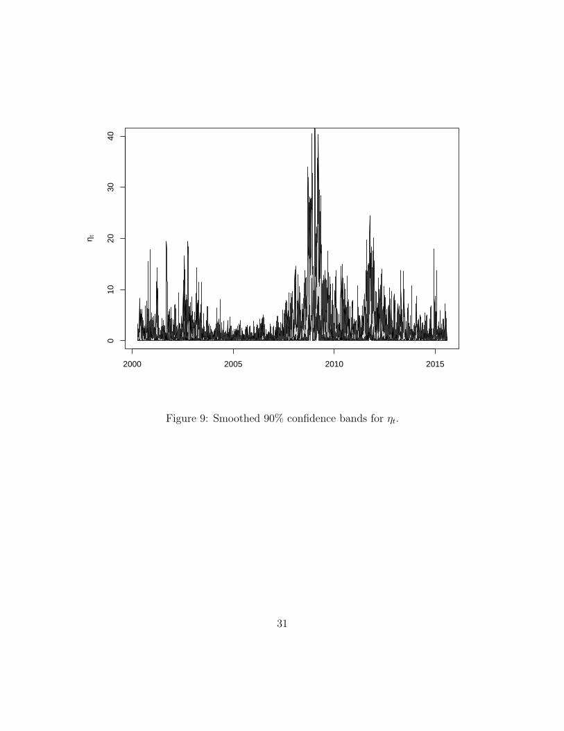
Figure 5: Smoothed Ft for the period between February 11, 2004 and December 10,2007. Smoothed 0.05th and 0.95th quantiles of Ft are reported with black lines andmedian Ft is reported in red.
10, 000 we first forecast the 0.05th and 0.95th quantiles of∑d
h=1 Ft+h|Y1:t for d =
1, 5, 10, 20, 40, 60 (1-day, 5-day, 10-day, 20-day, 40-day and 60-day horizons) that
are the VaR for the systematic risk component. Figures 10-11 report the VaR fore-
casts of cumulative Ft along with the pseudo values of Ft obtained via ACP1 and
27

Jan Mar May Jul Sep
−4
04
2007
/08
Nov Jan Mar May Jul
−10
0
2008
/09
Jul Sep Nov Jan Mar
−3
02
2009
May Jul Sep Nov Jan
−3
02
4
2009
/10
Jan Mar May Jul Sep
−6
−2
2
2010
/11
Figure 6: Smoothed Ft for the period between December 11, 2007 and October 7,2011. Smoothed 0.05th and 0.95th quantiles of Ft are reported with black lines andmedian Ft is reported in red.
S&P500 proxies, defined as
• ACP1 proxy: FACP1t =
∑ni=1 aiYit√
T−1∑T
t=1(∑n
i=1 aiYit)2, where (a1, . . . , an) is the eigen-
vector associated with the largest eigenvalue of the covariance matrix of Yit;
28

Nov Jan Mar May Jul
−4
04
2011
/12
Sep Nov Jan Mar May
−3
−1
1
2012
/13
May Jul Sep Nov Jan
−2
01
2
2013
/14
Mar May Jul Sep Nov
−1.
50.
0
2014
Nov Jan Mar May Jul
−1.
50.
01.
5
2014
/15
Figure 7: Smoothed Ft for the period between October 10, 2011 and July 30, 2015.Smoothed 0.05th and 0.95th quantiles of Ft are reported with black lines and medianFt is reported in red.
• S&P 500 proxy: F S&P500t =
YS&P500,t√T−1
∑Tt=1 Y
2S&P500,t
, where YS&P500,t is the return on
the S&P 500 at date t.
29

0.00
00.
020
ME
T
0.00
00.
020
ING
0.00
00.
020
GS
0.00
00.
020
LNC
2000 2005 2010 2015
0.00
00.
020
HS
BC
0.00
00.
020
JPM
0.00
00.
020
BA
C
0.00
00.
020
CS
0.00
00.
020
WF
C
2000 2005 2010 2015
0.00
00.
020
BC
S
Figure 8: Smoothed 90% confidence bands for σ2it.
30
2000 2005 2010 2015
010
2030
40
η t
Figure 9: Smoothed 90% confidence bands for ηt.
31
−20
−10
010
20
1−da
y V
aR0.
05 fo
reca
sts
−20
−10
010
20
5−da
y V
aR0.
05 fo
reca
sts
−20
−10
010
20
10−
day
VaR
0.05
fore
cast
s
Figure 10: 1-day, 5-day and 10-day VaR forecasts of cumulative Ft. The filtered5% and 95% quantiles of
∑dh=1 Ft+h|Y1:t for d = 1, 5, 10 are reported in black and
the pseudo Ft obtained via ACP1 and S&P500 proxies are in green and in red,respectively.
32

−30
−10
1030
20−
day
VaR
0.05
fore
cast
s
−30
−10
010
2030
40−
day
VaR
0.05
fore
cast
s
2000 2005 2010 2015
−30
−10
1030
60−
day
VaR
0.05
fore
cast
s
Figure 11: 20-day, 40-day and 60-day VaR forecasts of cumulative Ft. The filtered5% and 95% quantiles of
∑dh=1 Ft+h|Y1:t for d = 1, 5, 10 are reported in black and
the pseudo Ft obtained via ACP1 and S&P500 proxies are in green and in red,respectively.
33

4 Model With Default Risk
4.1 The Basic Model
4.1.1 Value of the Firm Model
The structural model or Value-of-the-Firm model has been initially introduced by
Black and Scholes (1973) and Merton (1974). This is a two-period model based on a
description of the balance sheet of the firm at the second period. Since the structural
model is now extended to a dynamic framework, we denote by (t, t + 1) the period
of interest. The balance sheet of the firm at date t + 1 is summarized by the asset
and liability values At+1, Lt+1, respectively. The value of the firm at date t + 1
for the shareholders is (At+1 − Lt+1)+ = max(At+1 − Lt+1, 0), taking into account
their limited liability. Thus the stock can be considered as a European call option
written on the underlying asset value with strike the level of liability. This explains
the pricing formula for the stock under the absence of arbitrage opportunity as:
Pt =Q
E[exp(−rt)(At+1 − Lt+1)
+ | It], (4.1)
where Pt is the capitalization (equity value) at date t, rt the riskfree rate for period
(t, t + 1), known at date t, It the information available at date t, and Q is the
pricing measure. In a discrete time framework, the market is incomplete, and there
is an infinite number of pricing measures compatible with the condition of absence
of arbitrage opportunity. Thus we have some flexibility on the choice of Q. Formula
(4.1) can be applied to the total number of shares, or be standardized per share, as
long as the number of shares is independent of time.
This basic model is structural, since it is based on an economic definition of
34

default from the balance sheet information. It involves three types of variables, that
can be either latent, or observable. These variables are:
1. the components A, L of the balance sheet. The asset component is assumed
unobservable and so is often the liability component7;
2. the state variables in the information set, known by the investors, but often
unobserved by the econometrician;
3. the equity value Pt, which is observable whenever the stock of the firm is quoted
on a liquid competitive market.
In the initial Value-of-the-Firm model, the liability is assumed predetermined. We
denote Lt|t+1 the value of Lt+1 assumed known at date t. Thus, formula (4.1) can be
equivalently written as:
Pt = exp(−rt)Lt|t+1
Q
E[(At+1/Lt|t+1 − 1)+ | It
]. (4.2)
Let us now choose the form of the pricing measure Q. We follow the basic Black-
Scholes-Merton formula. The information set includes only the values ofAt, rt, Lt|t+1,
and, between t and t + 1, under the pricing measure, the asset value satisfies the
geometric Brownian motion, with fixed known volatility ω2t , corresponding to the
standard Black-Scholes model. We deduce the following closed-form expression for
Pt as:
Pt = gBS(At, Lt|t+1, rt, ω2t ) , (4.3)
7When A and L are latent, we do not have to be more precise on the way they are defined.Typically, the asset component is marked-to-market, whereas the debt is generally book valued.Similarly, the debts can have different maturities. The L component has to be interpreted as thepart of the debt to be reimbursed at date t + 1. Similarly, A may be the part of assets liquid atdate t+ 1.
35

where:
gBS(At, Lt|t+1, rt, ω2t ) = AtΦ(d1,t)− LtΦ(d2,t) exp(−rt) , (4.4)
with
• d1,t =1ωt
log(
At
Lt|t+1
)+ rt +
ω2t
2
;
• d2,t = d1,t − ω2t .
In the modelling above, it is important to distinguish two time frequencies. The
discrete dates t = 1, 2, . . . are the times at which the debt is due. They define the
maturity date of the call option. The underlying continuous time model concerns
the evolution of prices and values within the period and is just introduced to get the
link with the Black-Scholes formula.
4.1.2 The Effects of Levels
The above Merton’s formula (4.3)-(4.4) will be used in a simplified way following
common practices. We set the short term rate rt = 0, assume that the intraperiod
volatility ωt = ω is constant to focus later on on the intraperiod volatilities and fix
a constant level of liability Lt|t+1 = L. Thus we get:
logPt = logL+ log
At
LΦ
[1
ωlog
(At
L
)+
ω
2
]− Φ
[1
ωlog
(At
L
)− ω
2
]≡ logL+ h
[log
(At
L− 1
);ω
],
say, and the associated stock return becomes:
Yt = log(Pt/Pt−1) = h
[log
(At
L− 1
);ω
]− h
[log
(At−1
L− 1
);ω
]. (4.5)
36

(i) Let us consider the extreme case where the asset/liability ratio is large and the
intraperiod volatility is small. In such a case, the firm is far from default and
it is easily checked that we have:
logPt ∼ logL+ log(At/L− 1) ,
and
Yt ∼ log(At/L− 1)− log(At−1/L− 1) ≡ ∆ log(At/L− 1) . (4.6)
Therefore, the relative change in firm value is equal to the relative change in
At/L−1. In particular, if these latter changes are stationary, the stock returns
are also stationary.
(ii) However, in the general case, formula (4.5) shows that the stock return depends
not only on the changes ∆ log(At/L − 1), but also on the leverage At−1/L −
1, and this leverage effect will increase with the proximity to default. As a
consequence, if the changes ∆ log(At/L − 1) are stationary, the stock returns
will become nonstationary. This nonstationary feature has to be taken into
account in the analysis.
In our application, this leverage effect can be significant, while staying limited,
since we consider financial institutions, which have not experimented default
during all the period, and thus are still at some distance to default.
37

4.2 The Structural Dynamic Factor Model (SDFM)
The effect of the distance-to-default8 will be taken into account by modifying the
linear factor model (3.1) as follows:
The State Equation
An analogue of model (3.1) will be written on the changes ait = ∆ log(Ait/L − 1)
instead of being written on the stock returns:ait = αi + βiFt + σitϵit , i = 1, . . . , n ,
Ft = γFt−1 + ηtut ,
(4.7)
with the same dynamic assumptions as in (3.1). Compared to (3.1), this dynamic
model includes new state variables that are the ait. As usual, it will be interesting
to try to reconstitute these variables, that are the implied financial leverages, from
the stock return data only.
The Measurement Equations
They are given by:
Yit = h [log (Ait/L− 1) ;ωi]− h [log (Ai,t−1/L− 1) ;ωi] , i = 1, . . . , n . (4.8)
The model includes additional parameters, that are the intraperiod volatilities ωi
appearing in the measurement equations. It is known from the theoretical model
that such a parameter ωi can be difficult to identify if the firm is very far from
default [see equation (4.6), where the effect of ωi disappears]. For this reason, we
8We use distance-to-default in its general meaning and not with the specific definition by KMV[see Crosbie and Bohn (2004)].
38

assume ωi = ω, independent of the firm, in the illustration below.
Note also that the measurement equations involve the levels log(Ait/L−1), which
will have to be reconstructed from the changes ait. This demands the introduction
of initial conditions on log(Ait/L− 1). Since the institutions under analysis are not
on default during the considered period, we can select initial values sufficiently high
to avoid default at the initial date. The results are weakly dependent on this initial
choice, which corresponds to the extreme situation of stationarity.
Finally, as noted above, the discrete time dynamic model (4.7) for the asset liabil-
ity ratios, written under the historical distribution is compatible with the Merton’s
pricing equations derived under the risk-neutral distribution. Indeed, a discrete time
framework implies an incomplete market framework, that is an infinity of discrete
time risk-neutral distribution compatible with a given historical distribution. In our
framework the risk-neutral log-normal distribution for ait given ai,t−1 is compati-
ble with the historical distribution for ait given ai,t−1 by choosing the appropriate
stochastic discount factor. Since the riskfree interest rate is set to zero, the stochastic
discount factor is just the ratio of the risk-neutral and historical transition densities.
Finally, in our specification, the investors have the information on the balance sheets
ait and on the intraperiod volatility (not only on the returns), but they do not have
the information on the underlying factors Ft, σit, ηt. In contrast, the econometrician
has only the information on the stock returns.
4.3 Comparison with the Literature
A dynamic structural model has recently been introduced in Engle and Siriwardane
(2015). Their full recursive model is deduced from expansions of the risk-neutral
dynamics and structural pricing formulas underlying a stochastic volatility model
39

written on the process of asset value. This expansion provides a simplified dynamics
for the equity returns, but its validity can be questioned, when distance-to-default
is small and nonlinear effects potentially important. For instance, the expansion
neglects the effect of time-to-maturity, the effect of the drift and of the volatility
shocks to focus on the link between equity and asset volatilities. Moreover, the
expansion is performed in continuous time, and the impact of this expansion for
discrete time data, that is the time aggregation effect, is not really taken into account.
Another difference compared to our model is the ARCH specification introduced for
the estimated econometric model, which is not in line with the underlying structural
model, where the volatilities were stochastic with their own shocks. Finally, the set
of observable variables is not the same, since the authors assumed observable by the
econometrician both the equity and asset values, whereas we preferred to assume
observable the equity values only. This is more in line with the Moody’s-KMV
practice. Moreover, our approach solves the question of the different frequencies in
which these data are available and avoid the use of proxies for the monthly asset
values9.
4.4 Estimation Results
As mentioned above, for identification reasons, we assume that ωi = ω are constant
for all i = 1, . . . , n10. We follow an approach similar to the approach in Section 3.1.
We first consider a set of moment restrictions to calibrate the parameters and the
underlying factors. This step can lead to inconsistent estimators. This lack of con-
sistency is adjusted for by indirect inference in the second step. In the first step, in
9In Engle and Siriwardane (2015) the monthly book value of the debt is obtained by an automaticexponential average with smoothing parameter of 0.01
10We have checked that the objective function of the estimation problem was poorly informativeon the individual heterogeneity of the intraperiod volatilities.
40

addition to our (2n + 6) auxiliary statistics in µ of Section 3.1.2, we need an addi-
tional statistic to identify ω. For this purpose, we use the mean standard deviation
of individual returns:
ω =1
n
n∑i=1
√√√√ 1
T − 1
T∑t=1
(exp(Yit)− exp(Yi)
)2. (4.9)
Clearly, this auxiliary moment ω will not be a consistent estimator of ω. Indeed, ω
has the interpretation of an interperiod volatility averaged on the banks and differ
from the intraperiod volatility. However, this lack of consistency will be solved by
indirect inference. Thus, we use the augmented auxiliary vector µOD = (µ′, ω)′ and
estimate the structural parameter θOD = (θ′, ω)′ by indirect inference as described
in Section 3.1.2.
The estimation results are reported in Table 2, column 4. From this table we can
compare the estimates for the models with and without option of default. The esti-
mates of the beta coefficients are significantly different for Barclays and JP Morgan.
We also observe more persistence in the stochastic volatility ηt and a value of the
intraperiod volatility indicates the need to adjust for the option of default.
To complete the comparison between the naive and structural models, we report
in Figures 12-15 the smoothed Ft values obtained via the SDFM model and in Fig-
ure 16 the smoothed median Ft via SDFM plotted against the smoothed median Ft
via the naive dynamic model.
Then, the estimated model can be used:
(i) to get the smoothed values of the state variables ait, i = 1, . . . , n, t = 1, . . . , T ;
(ii) then deduce the smoothed values of the asset/liability ratios Ait/L, i = 1, . . . , n,
t = 1, . . . , T , that are the implied financial leverages;
41

May Jul Sep Nov Jan
−2
02
2000
Jan Mar May Jul Sep Nov
−3
−1
1
2001
Nov Jan Mar May Jul
−2
02
2001
/02
Sep Nov Jan Mar May
−2
02
2002
/03
May Jul Sep Nov Jan
−1.
50.
01.
5
2003
/04
Figure 12: Smoothed Ft for the period between April 6, 2000 and February 10, 2004.Smoothed 0.05th and 0.95th quantiles of Ft are reported with black lines and medianFt is reported in red.
(iii) then we can deduce measures of distance-to-default for the different banks and
analyze how they evolved over time. Such measures are:
42

Mar May Jul Sep Nov
−1.
50.
01.
0
2004
Jan Mar May Jul Sep
−0.
60.
00.
6
2004
/05
Sep Nov Jan Mar May
−1.
00.
01.
0
2005
/06
Jul Sep Nov Jan Mar
−1.
50.
01.
5
2006
Mar May Jul Sep Nov
−2
02
2006
/07
Figure 13: Smoothed Ft for the period between February 11, 2004 and December 10,2007. Smoothed 0.05th and 0.95th quantiles of Ft are reported with black lines andmedian Ft is reported in red.
the excess asset liability ratio:
ALit = Ait/L− 1 , (4.10)
43

Jan Mar May Jul Sep
−4
02
4
2007
/08
Nov Jan Mar May Jul
−10
05
2008
/09
Jul Sep Nov Jan Mar
−3
−1
13
2009
May Jul Sep Nov Jan
−3
02
4
2009
/10
Jan Mar May Jul Sep
−4
02
2010
/11
Figure 14: Smoothed Ft for the period between December 11, 2007 and October 7,2011. Smoothed 0.05th and 0.95th quantiles of Ft are reported with black lines andmedian Ft is reported in red.
and the risk premia of the insurance against default:
DDit = hi[log(Ait/L− 1); ω]− log(Ait/L− 1) , (4.11)
44

Nov Jan Mar May Jul
−4
02
4
2011
/12
Sep Nov Jan Mar May
−3
−1
1
2012
/13
May Jul Sep Nov Jan
−2
01
2
2013
/14
Mar May Jul Sep Nov
−1.
50.
01.
0
2014
Nov Jan Mar May Jul
−1.
50.
01.
5
2014
/15
Figure 15: Smoothed Ft for the period between October 10, 2011 and July 30, 2015.Smoothed 0.05th and 0.95th quantiles of Ft are reported with black lines and medianFt is reported in red.
where ω denotes the indirect inference estimator of the intraperiod volatility.
Compared to the asset/liability ratios, this measure takes into account the
uncertainty on the ratio as evaluated by the market. The change in the risk
45

−5 0 5 10
−10
−5
05
Dynamic model Ft
SD
FM
Ft
Figure 16: Ft of the SDFM against Ft of the simple dynamic model. This figure plotsthe smoothed median of Ft obtained via the SDFM against the smoothed median ofFt obtained via the simple dynamic model.
premia is defined by:
∆DDit = hi[log(Ait/L− 1); ω]− hi[log(Ai,t−1/L− 1); ω]−∆ log(Ait/L− 1) .
(4.12)
46

The risk premia DDit capture the magnitude of the nonlinear impact of the leverage
on stock returns. In particular, when DDit is close to zero, the equity return Yit
is close to ait, and then coincides with the value of a stationary process. In other
words, we can consider that the stock SDFM is a switching regime model, passing
from an almost stationary regime to a nonstationary regime in an endogenous way.
The different measures above can be further summarized by computing their
average and volatility either over time for a given bank, or across banks for a given
date.
For each institution i and date t, the ait in step (i) is replaced by the median
ait of the smoothed a(m)it Mm=1 using M = 100 paths and N = 10, 000 particles in
the ABC smoothing algorithm (see Section 3.4). To recover the Ait/L − 1 from
the ait, we use the initial condition log(Ai0/L − 1) = 1, ∀i. The Ait/L − 1 values
are reported in Figure 17. For comparison, we also report in Figure 18 the naive
AL measures obtained by using the simple dynamic model of Section 3. Red lines
indicate the naive ALit = exp(∑t
k=1 Yik) obtained with the nonstructural model,
while black ones indicate the structural ALit measures. The evolution of the implied
asset/liability ratios are very different according to the financial institution. We
observe for several institutions a regular increase of the ratios after the financial crisis,
likely due to the more severe demand of required capital (see e.g. GS, LNC, WFC),
but several institutions (HSBC, BCS, ING, JPM) still have rather small implied
excess asset/liability ratios. The patterns for MET is expected for all insurance
companies, with on average more protection before the crisis. So the need of liquidity
during the financial crisis is partly fulfilled by their reserves, which are reconstructed
later on at a rather high level.
The comparison of the financial leverages for the two types of models show sig-
nificant differences between the naive and structural measures. This is due to the
47

option of default, which is automatically included in the misspecified naive series.
We see that this misleading effect can be either positive, or negative, according to
the institution.
To understand the differences between the two models, more information is pro-
vided by the series of distance-to-default DD. The average risk premia of the insur-
ance over the ten firms are reported in the top panel of Figure 19. Note the similarity
between the average DDt series and the VIX volatility index (bottom panel), which
is a measure of implied volatility on the S&P500 option, usually referred as the fear
index. However, we do not have a complete similarity, especially since the level of the
average risk premia is significantly higher after the financial crisis. However, these
almost similar patterns do not account for the heterogeneity among the financial
institutions.
The risk premia of the insurance for each financial institution are reported in
Figure 20. These results show that the jump in the average DD in Figure 19 (top
panel) was mainly due to two institutions: JP Morgan and Barclays. The jump in
DD for JP Morgan is likely due to its 2008 acquisitions of Bear Sterns (for 1.5 billion
dollars) and Washington Mutual (for 1.9 billion dollars), both on bankruptcy. Simi-
larly, the jump in Barclays is likely due to its 2008 acquisition of Lehman Brothers
(for 1.7 billion dollars) after its bankruptcy. The other bumps on risk premia, smaller
though, correspond to the European sovereign debt crisis. As expected, this effect is
significant for Barclay’s, which has supported a loss of about 2 billions of dollars by
speculating on the Greek and Spanish debts by means of derivatives.
Finally, Figure 21 reports the changes in insurance risk premia. We cannot rea-
sonably interpret these results obtained by analyzing stock returns, without having
in mind derivatives written on the default of these firms and, in particular, the Credit
Default Swaps (CDS). We know that these products are often used for arbitrage and,
48

015
30
AL
for
ME
T
015
30
AL
for
ING
015
30
AL
for
GS
015
30
AL
for
LNC
2000 2005 2010 2015
015
30
AL
for
HS
BC
015
30
AL
for
JPM
015
30
AL
for
BA
C
015
30
AL
for
CS
015
30
AL
for
WF
C
2000 2005 2010 2015
015
30
AL
for
BC
S
Figure 17: Implied asset/liability ratios.
hence, for speculation. In a neighborhood of the default, we expect to have more
volatility on these insurance products and this increase in volatility should appear in
the evolution of (∆DDit)2. This behaviour indeed appears in the series of Figure 21.
When the implied asset/liability ratio decreases, the variability in ∆DDit increases.
This negative correlation between A/L and (∆DDit)2 translates the financial lever-
age effect discussed by Black (1976) and Hasanhodzic and Lo (2011). More precisely,
as suggested by Black, the stylized negative correlation between return and volatility
49

510
15
Nai
ve A
L, M
ET
13
5
Nai
ve A
L, IN
G
515
25
Nai
ve A
L, G
S
510
20
Nai
ve A
L, L
NC
2000 2005 2010 2015
13
5
Nai
ve A
L, H
SB
C
02
4
Nai
ve A
L, J
PM
24
68
Nai
ve A
L, B
AC
13
57
Nai
ve A
L, C
S
515
Nai
ve A
L, W
FC
2000 2005 2010 2015
02
46
8
Nai
ve A
L, B
CS
Figure 18: Naive asset/liability ratios. Red lines indicate the naive ALit =exp(
∑tk=1 Yik), while black ones the structural ALit measures.
is likely an indirect effect by means of the balance sheet. This is this effect of A/L,
which is noted in our framework.
The three measures above, that are AL, DD and (∆DD)2, can be used to rank
50

0.1
0.2
0.3
0.4
0.5
0.6
0.7
Ave
rage
DD
t
2000 2005 2010 2015
1020
3040
5060
7080
VIX
Figure 19: Average risk premia of the insurance and VIX.
the financial institutions. They define rankings with different interpretations: by
the implied financial leverage for AL, by the distance-to-default as evaluated by the
market for DD, and as a measure of the magnitude of speculation for (∆DD)2. It
is important to get multiple rankings with different interpretations. For instance,
this will allow to distinguish an institution with small excess asset/liability ratio
51

0.0
1.0
2.0
DD
for
ME
T
0.0
1.0
2.0
DD
for
ING
0.0
1.0
2.0
DD
for
GS
0.0
1.0
2.0
DD
for
LNC
2000 2005 2010 2015
0.0
1.0
2.0
DD
for
HS
BC
0.0
1.0
2.0
DD
for
JPM
0.0
1.0
2.0
DD
for
BA
C
0.0
1.0
2.0
DD
for
CS
0.0
1.0
2.0
DD
for
WF
C
2000 2005 2010 2015
0.0
1.0
2.0
DD
for
BC
S
Figure 20: Risk premia of the insurance.
and small insurance premium, which is not necessarily risky for default from an
institution where both are large and which can be riskier. These rankings are a
solvency ranking, a ranking for the default insurance, and a ranking for speculative
asset, respectively.
The comparison of the financial institutions can be cross-sectional at a given date,
or be performed with respect to both institution and time. We successively consider
the two approaches.
52

0.00
0.08
∆2 DD
for
ME
T
0.00
0.08
∆2 DD
for
ING
0.00
0.08
∆2 DD
for
GS
0.00
0.08
∆2 DD
for
LNC
2000 2005 2010 2015
0.00
0.08
∆2 DD
for
HS
BC
0.00
0.08
∆2 DD
for
JPM
0.00
0.08
∆2 DD
for
BA
C
0.00
0.08
∆2 DD
for
CS
0.00
0.08
∆2 DD
for
WF
C
2000 2005 2010 2015
0.00
0.08
∆2 DD
for
BC
S
Figure 21: Squared change in default risk premia.
Tables 5-7 report the rankings associated with the three risk measures, respec-
tively, before the crisis (August 2006 - July 2007), during the crisis (August 2008 -
July 2009) and after the crisis (August 2010 - July 2011). The higher the rank, the
more secure and less speculative is the financial institution. As expected, the insur-
ance companies MET and LNC introduced in our set of institutions are uniformly
in the top, even if we observe a downgrade of two levels before and after the crisis
for MET. Barclays and JP Morgan are the least secure and also the most specula-
53

tive. Whereas improving its solvency and cost of default insurance ranks, ING is still
speculative. We also report the correlation between the three rankings in Table 8.
These results show that the AL and DD measures provide almost identical rankings
while ∆DD2 provides slightly different rankings.
Let us now provide ratings of these ten financial institutions that will allow for
a comparison with respect to both institution and time. Let us collect all the values
ALiti=1,...,nt=1,...,T , DDiti=1,...,n
t=1,...,T and ∆DD2iti=1,...,n
t=1,...,T and calculate selected quantiles of
the associated sample distribution. These quantiles can be used to define a risk seg-
mentation, with different ratings associated with the segments. The rating categories
are defined in Table 9 with 10 different ratings. We have noted them as usual by
aaa, aa, . . . , but they have interpretations which may be different from the ratings of
S&P and Moody’s for instance, not only since they are based on different measures.
In particular, we denote c− the last rating to avoid the notation d meaning default.
Then, we compare the values in Tables 5-7 to the subintervals. We report the
appropriate ratings in Tables 10-12. When we compare to the whole period of ob-
servations, we see that even in the period August 2006-August 2007, that is between
the drop in the price of the US real estate and the announcement of frozen funds by
Bnp Paribas and AXA, only two institutions were bbb, and the speculative ratings
systematically smaller than the two other ratings, which might be an advanced in-
dication of a future bubble crash. The bad ratings during the crisis period are not
surprising. Finally, Table 12 shows the slow recovery after the crisis, with still very
high risks on HSBC, JPM and BCS.
54

Table 5: Rankings before the crisis (Aug 2006-July 2007)
Solvency Cost of Default Ins. Speculative Assets
MET 10(15.979)
10(0.010)
10(1.75 10−8)
ING 4(5.490)
4(0.053)
3(6.73 10−7)
GS 7(9.481)
7(0.024)
6(2.05 10−7)
LNC 9(13.428)
9(0.013)
8(4.26 10−8)
HSBC 3(3.326)
3(0.106)
4(6.10 10−7)
JPM 1(2.099)
1(0.188)
1(5.99 10−6)
BAC 6(7.661)
6(0.032)
7(1.80 10−7)
CS 5(6.440)
5(0.043)
5(3.31 10−7)
WFC 8(11.075)
8(0.018)
9(3.84 10−8)
BCS 2(3.051)
2(0.119)
2(4.71 10−6)
55

Table 6: Rankings during the crisis (Aug 2008-July 2009)
Solvency Cost of Default Ins. Speculative Assets
MET 9(7.097)
8(0.050)
8(6.36 10−5)
ING 4(2.365)
4(0.203)
4(8.85 10−4)
GS 10(7.367)
10(0.038)
10(1.89 10−5)
LNC 7(5.471)
7(0.070)
5(3.26 10−4)
HSBC 3(1.951)
3(0.216)
7(1.65 10−4)
JPM 1(0.459)
1(0.972)
2(5.07 10−3)
BAC 5(2.619)
5(0.198)
3(9.19 10−4)
CS 6(2.996)
6(0.150)
6(3.09 10−4)
WFC 8(7.025)
9(0.042)
9(3.07 10−5)
BCS 2(0.606)
2(0.843)
1(9.35 10−3)
56
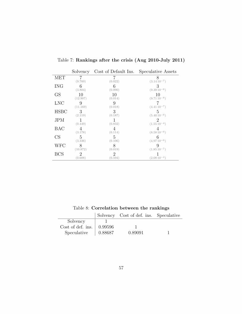
Table 7: Rankings after the crisis (Aug 2010-July 2011)
Solvency Cost of Default Ins. Speculative Assets
MET 7(9.760)
7(0.022)
8(3.14 10−7)
ING 6(3.804)
6(0.090)
3(9.39 10−6)
GS 10(12.907)
10(0.014)
10(9.71 10−8)
LNC 9(11.169)
9(0.018)
7(4.41 10−7)
HSBC 3(2.119)
3(0.187)
5(5.40 10−6)
JPM 1(0.449)
1(0.832)
2(1.55 10−4)
BAC 4(3.178)
4(0.114)
4(8.58 10−6)
CS 5(3.336)
5(0.106)
6(4.97 10−6)
WFC 8(10.872)
8(0.019)
9(1.85 10−7)
BCS 2(0.688)
2(0.594)
1(2.08 10−4)
Table 8: Correlation between the rankings
Solvency Cost of def. ins. SpeculativeSolvency 1
Cost of def. ins. 0.99596 1Speculative 0.88687 0.89091 1
57

Table 9: Rating categories
AL DD ∆DD2
aaa · ≥ qAL99% · ≤ qDD
1% · ≤ q∆DD2
1%
aa qAL99% > · ≥ qAL
97% qDD3% > · ≥ qDD
1% q∆DD2
3% > · ≥ q∆DD2
1%
a qAL97% > · ≥ qAL
95% qDD5% > · ≥ qDD
3% q∆DD2
5% > · ≥ q∆DD2
3%
bbb qAL95% > · ≥ qAL
90% qDD10% > · ≥ qDD
5% q∆DD2
10% > · ≥ q∆DD2
5%
bb qAL90% > · ≥ qAL
80% qDD20% > · ≥ qDD
10% q∆DD2
20% > · ≥ q∆DD2
10%
b qAL80% > · ≥ qAL
70% qDD30% > · ≥ qDD
20% q∆DD2
30% > · ≥ q∆DD2
20%
ccc qAL70% > · ≥ qAL
60% qDD40% > · ≥ qDD
30% q∆DD2
40% > · ≥ q∆DD2
30%
cc qAL60% > · ≥ qAL
50% qDD50% > · ≥ qDD
40% q∆DD2
50% > · ≥ q∆DD2
40%
c qAL50% > · ≥ qAL
40% qDD60% > · ≥ qDD
50% q∆DD2
60% > · ≥ q∆DD2
50%
c− · ≤ qAL40% qDD
60% ≤ · q∆DD2
60% ≤ ·
Table 10: Ratings before the crisis (Aug 2006-July 2007)
Solvency Cost of Default Ins. Speculative Assets
MET bbb bbb bING ccc ccc cGS bb bb ccLNC bbb bbb cccHSBC c c cJPM c− c− c−
BAC b b ccCS b b ccWFC bb bb bBCS c c c−
58

Table 11: Ratings during the crisis (Aug 2008-July 2009)
Solvency Cost of Default Ins. Speculative Assets
MET b ccc c−
ING c− c− c−
GS b b c−
LNC ccc ccc c−
HSBC c− c− c−
JPM c− c− c−
BAC c− c− c−
CS c c− c−
WFC b b c−
BCS c− c− c−
Table 12: Ratings after the crisis (Aug 2010-July 2011)
Solvency Cost of Default Ins. Speculative Assets
MET bb bb ccING cc cc c−
GS bbb bbb cccLNC bb bb ccHSBC c− c− c−
JPM c− c− c−
BAC c c c−
CS c c c−
WFC bb bb ccBCS c− c− c−
59

5 Conclusion
We have introduced a structural dynamic factor model (SDFM), which accounts for
linear common factor, stochastic volatilities, and also to their nonlinear impacts on
equity returns, when the distance-to-default is small. This leads to a state space
model, in which the state dynamics is stationary and the measurement equation
possibly creates nonstationarity. Due to the structural Value-of-the-Firm model,
defining the measurement equation, some latent variables such as the asset/liability
ratio have an economic interpretation in terms of balance sheets. The SDFM allows to
deduce from the observation of equity returns only approximations of these financial
ratios, the so-called implied asset/liability ratios. The model also allows for defining
different risk measures and associated rankings: a solvency ranking, a cost of default
insurance ranking and a speculative assets ranking.
Clearly, such an approach is only based on market data, as are for instance the
SRISK ranking produced by the volatility lab (see Brownlees and Engle (2012)). It
would be nice to use jointly the information on returns with the information on the
balance sheets. As mentioned in the main text, this is difficult challenge. First, the
observation frequencies are not the same; second, it is difficult to deduce from the
balance sheet the financial ratio involved in Merton’s model, that are the part of
debt to be recovered immediately and the part of asset sufficiently liquid. Finally,
several lines of the balance sheet of a bank contain financial assets, such as stock,
bonds, or derivatives, which are often marked-to-market values. Thus, they are also
partly market data.
60

References
Ball, C. and A. Roma (1994). Stochastic Volatility Option Pricing. Journal of
Financial and Quantitative Analysis, 29, 589–607.
Black, F. (1976). Studies of Stock Price Volatility Changes. Proceedings of the 1976
Meeting of the Busineess and Economic Statistics Section, American Statistical
Association, 27, 399–418.
Black, F. and J.C. Cox (1976). Valuing Corporate Securities: Some Effects of
Bond Indenture Provisions. Journal of Finance, 31, 351–367.
Black, F. and M. Scholes (1973). The Pricing of Options and Corporate Lia-
bilities. Journal of Political Economy, 81, 637–654.
Brownlees, C. and R. Engle (2012). Volatility, Correlation and Tails for Sys-
temic Risk Measurement. SSRN 1611229.
Calvet, L. and V. Czellar (2011). State-Observation Sampling and the Econo-
metrics of Learning Models. Technical report, arXiv:1105.4519.
Calvet, L. and V. Czellar (2015). Accurate Methods for Approximate Bayesian
Computation Filtering. Journal of Financial Econometrics , 13, 798–838. .
Cox, J., Ingersoll, J. and S. Ross (1985). The Theory of the Term Structure
of Interest Rates. Econometrica, 53, 385–407.
Crosbie, P. and J. Bohn (2004). Modeling Default Risk.Moody’s KMV Company.
Darolles, S. and C. Gourieroux (2015). Contagion Phenomena with Applica-
tions in Finance, Elsevier.
61

Darolles, S., Gourieroux, C. and J. Jasiak (2006). Structural Laplace Trans-
form and Compound Autoregressive Models. Journal of Time Series Analysis 27,
477–503.
Duffie, D., Filipovic, D. and W. Schachermayer (2003). Affine Processes
and Applications in Finance. Annals of Applied Probability 13, 984–1053.
Duffie, D., Pan, J. and K. Singleton (2000). Transform Analysis and Asset
Pricing for Affine Jump DIffusions. Econometrica 68, 1343–1376.
Engle, R., and E. Siriwardane (2015). Structural GARCH: The Volatility-
Leverage Connection. Harvard Business School Working Paper 16-009.
Gagliardini, P. and C., Gourieroux (2014). Granularity Theory with Applica-
tions to Finance and Insurance, Cambridge University Press.
Gallant, A. R., and G. Tauchen (1996). Which Moments to Match? Econo-
metric Theory 12, 657–681.
Godsill, S.J., Doucet, A. and M. West (2004). Monte Carlo Smoothing for
Nonlinear Time Series. Journal of the American Statistical Association 99, 156–
168.
Gordon, N., Salmond, D. and A. F. Smith (1993). Novel Approach to
Nonlinear/Non-Gaussian Bayesian State Estimation. IEE Proceedings F 140, 107–
113.
Gourieroux, C. and J. Jasiak (2006). Autoregressive Gamma Processes. Journal
of Forecasting 25, 129–152.
62
Gourieroux, C., Monfort, A. and E. Renault (1993). Indirect Inference.
Journal of Applied Econometrics 8, S85–S118.
Hansen, L.P. (2012). Challenges in Identifying and Measuring Systemic Risk.
NBER 18505.
Hasanhodzic,J., and A., Lo (2011). Black’s Leverage Effect is Not Due to Lever-
age. MIT Discussion Paper.
Heston, S.L. (1993). A Closed-Form Solution for Options with Stochastic Volatility
with Applications to Bond and Currency Options. Review of Financial Studies 6,
327–343.
Jasra, A., Singh, S., Martin, J. and E. McCoy (2012). Filtering via Approx-
imate Bayesian Computation. Statistics and Computing 22, 1223-1237.
Lintner, J. (1965). The Valuation of Risky Assets and the Selection of Risky Invest-
ments in Stock Portfolio and Capital Budgets. Review of Economics and Statistics
47, 13–37.
Markowitz, H. (1959). Portfolio Selection: Efficient Diversification of Invest-
ments. Wiley, New York.
Merton, R. (1974). On the Pricing of Corporate Debt: The Risk Structure of
Interest Rates. The Journal of Finance 29, 449–470.
Renault, E. and S. Khrapov (2013). Affine Option Pricing Model in Discrete
Time. Brown University.
Schaefer, S. and I. Strebulaev (2008). Structural Models of Credit Risk are
63

Useful: Evidence from Hedge Ratios on Corporate Bonds. Journal of Financial
Economics 90, 1–19.
Sharpe, W. (1964). Capital Asset Prices: A Theory of Market Equilibrium Under
Conditions of Risk. Journal of Finance 19, 425–42.
Smith, A.A. (1993). Estimating Nonlinear Time Series Models Using Simulated
Vector Autoregressions. Journal of Applied Econometrics 8, S63–S84.
64