Embed Size (px)
Citation preview
DOI: 10.1007/s10260-004-0093-3Statistical Methods & Applications (2004) 13: 241–258
c© Springer-Verlag 2004
Structural changes during a centuryof the world’s most popular sport
Ignacio Palacios-Huerta�
Department of Economics, Brown University, Box B; 64 Waterman Street; Providence, RI 02912, USA(e-mail: [email protected].)
Abstract. The analysis in this paper employs a methodology for dating structuralbreaks in tests with non-standard asymptotic distributions. The application exam-ines whether changes in the rules of a game and major social and political eventsduring the past century had significant effects upon various outcomes of this game.The statistical methodology first applied here proves successful as most breaks canbe traced to specific events and rule changes. Dating these breaks allows us to obtainuseful insights into production and competition processes in this industry. As such,using empirical tests we illustrate the utility of a valuable statistical technique notapplied previously.
Key words: Structural changes, changepoint estimators, time series analysis, foot-ball, sports industry
1. Introduction
In this paper, we apply a recently developed statistical methodology for datingstructural breaks in time series. The application is concerned with what is consideredto be a preeminent social phenomenon and an economically important industry.
Football (soccer) is the world’s most popular sport. The game has unrivalledworldwide appeal. Hundreds of millions of children and teenagers throughout theglobe practice it. Many more adults follow it. Countless football teams, especially inEurope and LatinAmerica but also inAfrica andAsia, are adored in their home cities.
� I am grateful to Gary S. Becker, Tony Lancaster, Robin Lumsdaine, Kevin M. Murphy, GabrielPerez-Quiros, Ana I. Saracho, Amy Serrano, an associate editor and a referee for useful suggestions.I am also indebted to Barry Blake, Vicki Bogan, Salwa Hammami and Karen Wong for able researchassistance, Tony Brown at the Association of Football Statisticians for the data the Hoover Institutionfor its hospitality, and the Spanish Ministerio de Ciencia y Tecnologia for financial support (grant BEC2003-08182). The Gauss programs used in this paper were kindly provided by Bruce E. Hansen. Anyerrors are mine alone.
242 I. Palacios-Huerta
Even in NorthAmerica, where other sports rule, many more teenagers kick footballsthan hit baseballs and there are twice as many football teams on college campusesas American football teams.1 Around the globe, the game attracts its fans at an earlyage and their passion does not typically diminish with age. Not surprisingly, starplayers are often more famous than religious and political leaders. Media proprietorsconsider fan interest almost insatiable and supply it by TV, satellite, radio andnewsprint. Sports newspapers, whose pages are mostly occupied by football news,are typically the best-selling newspapers in most European and Latin Americancountries. World Cup football matches are the biggest TV shows in the world,drawing a global television audience surpassed by no other event. World Cup 2002,for instance, drew a cumulative audience of 42.5 billion people, or the world’spopulation seven times over. Football, not surprisingly, has become an importantmedium to secure brand visibility and many corporations consider it key to gaininga global market share for their products. The game is indeed often considered oneof the most important social phenomena of the 20th century.2
The global following of this sport, as a sociological and economic phenomenon,deserves a careful study of what the game produces that makes it so attractive. So-cial sciences in general, and economics in particular, have not ignored the study ofvarious aspects of football as a game, an industry, and a product subject to one ofthe greatest demands on the planet. The demand for football has been studied, forinstance, by Kuypers (1995), Baimbridge et al. (1996), Peel and Thomas (1988,1992), and Jenett (1984).3 The economic and revenue sharing structure, as well asthe incentive and agency problems of sport leagues have been examined, for in-stance, by Atkison, Stanley and Tschirgart (1988), Fort and Quirk (1995), El-Hodiriand Quirk (1971), and Sloane (1971).4 More recently, different policy, financial andlegal aspects of the football industry and European football leagues have attractedsubstantial research attention (see Hoehn and Szymanski 1999, Szymanski andSmith 1997, Quirk and Fort 1992, Bourg and Gouget 1988).5
Despite these efforts, however, there is an important aspect of this industrythat has not been studied in the economics and statistical literature, one which hasimportant implications for all of the aforementioned aspects. In particular, little isknown about the temporal properties of the outcomes of the game. This paper isan attempt to provide the first statistical analysis of the behavior over time of theoutcomes of the game and of the structural changes that these outcomes may haveexperienced during the 20th century.
1 Data reported by the National Collegiate Athletic Association at http://www.ncaa.org.2 The term football, instead of soccer, will be used throughout the paper since this is the way the
game is referred to in most parts of the world. Modern football was essentially invented and “coded” atthe end of the 19th century in the United Kingdom. References to predecessors of the game have beenfound in ancient China and Japan, as well as in ancient Greece and Rome, in the British Isles during theMiddle Ages, in William Shakespeare’s King Lear (Act I, Scene IV), and in Italy and France throughthe 16th, 17th and 18th centuries (see http://www.fifa.com, Walvin 1994, Vallet 1998). The first officialleague competition took place in 1888 in England. From there, professional and amateur competitionsspread quickly and widely all over the world early in the past century.
3 See also Dixon and Coles (1997), Ridder et al. (1994), Maher (1982), and Reep et al. (1971).4 See also Bulow et al. (1985) and Dobson and Goddard (1998).5 See also the analyses by Deloitte and Touche (1998a, 1998b).
Structural changes during a century of the world’s most popular sport 243
We consider that the substantive question is important and that the empiricaltests can illustrate the application of a valuable statistical technique. The results maybe relevant to statistics, economics, and other social sciences for various reasons.
First, the analysis offers what to the best of our knowledge is the first applicationof a recently developed methodology to compute the p-values of a wide class oftests of structural change in econometric models.An important shortcoming in manyof these tests is that the distributions are non-standard, and thus p-values cannotbe computed from previously published information. This critical inconvenienceis overcome in Hansen (1997) which presents a method to compute convenientparametric approximation functions to the p-value functions for various asymptoticdistributions.
Second, the past decade has seen considerable empirical and theoretical researchon the detection of breaks in economic time series. Most of the series studied areconcerned with macroeconomic variables. This paper shows how this statisticalmethodology may be useful to economists and social scientists attempting to datestructural breaks in other types of time series as well, in particular in time seriesof outcomes. This application is also relevant since the last few years have seenincreasing interest in the practical applications of game theoretical analysis in eco-nomics and other social sciences. Empirical applications of game theory modelsfundamentally rely on data of the outcomes of the games under study.
Lastly, the application may be relevant in that social scientists are interestedin the production function of industries, especially those that hold large economicand social importance. Often, however, many final “products” are not quantifiablein the sense that the quantity and quality of goods such as cars, clothes, and otherscan be measured. Final outcomes of games, in particular, reflect many aspects ofthe production function of sport industries. Also, outcomes have major effects onrevenues (e.g., ticket sales, TV rights, merchandise), that is, on both the demand andsupply sides. The structure of outcomes, in turn, has an effect upon the economicstructure and the revenue sharing, incentive, and agency problems of competition.Also, it can be a determinant of different policy, legal, and structural aspects of theindustry. Thus, the results of the application of this statistical technique may bevaluable in the context of various underlying questions of interest.
This econometric study is concerned with the behavior over time of the mainoutcomes of the game of football. It studies the final scores of more than 120,000games over more than 100 years across both professional and amateur leagues.The analysis focuses on the English league competitions, where an unusually richdata set is available from the Association of Football Statisticians for the period1888–1996.
We will begin by describing the behavior over time of outcomes such as theaverage and the variability of goals scored, the margins of victory, the frequencyof scores, and the percentages of home team wins, losses and ties. The behavior ofthese and other outcomes over time may result in part from “learning” to play thegame and also from changes in inputs, production functions, and other aspects ofthe industry. Although an explicit analysis of strategic behavior and technologicalprogress is beyond the scope of analysis of the paper, the evidence to be presented
244 I. Palacios-Huerta
will be suggestive of both changes in strategic behavior and technological progressover time.6
We then will estimate, in each of the about two hundred time series of outcomesthat we study, the dates at which a structural change is statistically likely to haveoccurred. These structural changes may have been caused, for instance, by rulechanges, socioeconomic or political events (e.g., world wars), or other factors.Obviously, different changes may have had an effect in some time series but notin others (e.g., they may have affected the variability of goals scored but not theiraverage, or outcomes in professional leagues but not in amateur leagues). Ratherthan testing for structural changes at specific candidate dates, we let the structureof each time series reveal the likelihood, at each date, that a structural changehappened. In this sense we follow the typical post hoc ergo propter hoc approachfollowed in the literature. We find that once a specific date has been identified asone where, in a statistical sense, a structural change occurred, it is often possible toidentify the particular event or rule change that likely caused the structural break.The fact that most of the dates of structural breaks can be associated with specificevents shows that the methodology is highly accurate, reliable, and hence valuableas a statistical technique.
The rest of the paper is organized as follows. Section 2 describes the data andthe basic features of the time series of some of the main outcomes of the game.Section 3 describes the methodology of the tests of structural change. Section 4applies these tests to the time series we study and discusses the results. Section 5concludes with a summary and some final remarks.
2. Data description
The data come from the Association of Football Statisticians, which has collecteddata on British league competitions since their creation. They consist of the finalscores of all the games in the professional English leagues (Division I, or PremierLeague, and Division II) during the periods 1888–1996 and 1893–1996 respectively,and in the amateur English leagues (Divisions III and IV) during the period 1947–1996. There were 39,550 games in Division I, 39,796 in Division II, 20,424 inDivision III and 20,017 in Division IV, during these periods.7 With these data, time
6 For instance, players may learn to adopt more efficient offensive and defensive strategies over time,their skills may improve, and inputs may also increase as players and coaches become more “profes-sional.” The study of professional and amateur divisions, therefore, may be valuable to determiningwhether differences in certain outcomes of the game are related to differences in the skills of players,since professional players have greater skills than amateurs. Divisions that have different promotion andrelegation rules (e.g., because in top (bottom) divisions no team can be relegated (promoted) from a bet-ter (worse) division), may induce differences in the distribution of skills within divisions that could helpto explain differences in outcomes across divisions such as the number of goals scored, the proportionof wins, margins of victory, and others.
7 League competitions typically start in the Fall of one year and conclude in the Spring of the followingyear. Teams play each other twice during the season, once in each home field. Because of World Wars Iand II, leagues did not compete in England during the seasons 1915/16–1918/19 and 1939/40–1945/46.Professionalization of most players in Divisions I and II did not occur until the 1960s and 1970s (see
Structural changes during a century of the world’s most popular sport 245
Table 1. Percentages of Scores for 1888–1996
1888–1915 1920–1939 1947–1982 1983–1996 Entire periodMean Std. Dev. Mean Std. Dev. Mean Std. Dev. Mean Std. Dev. Mean Std. Dev.
Percentage of winsPremier League 0.797 0.040 0.762 0.029 0.746 0.036 0.727 0.027 0.761 0.042Division II 0.813 0.040 0.766 0.031 0.740 0.036 0.730 0.024 0.763 0.046Division III 0.731 0.029 0.737 0.013 0.733 0.024Division IV 0.741 0.032 0.737 0.017 0.740 0.028
Percentage of home winsPremier League 0.566 0.042 0.547 0.029 0.503 0.027 0.474 0.042 0.526 0.047Division II 0.596 0.033 0.550 0.028 0.515 0.028 0.486 0.020 0.539 0.047Division III 0.516 0.030 0.485 0.023 0.505 0.031Division IV 0.522 0.030 0.480 0.029 0.507 0.036
Percentage of away winsPremier League 0.231 0.029 0.215 0.017 0.244 0.028 0.253 0.023 0.236 0.028Division II 0.217 0.025 0.215 0.018 0.255 0.021 0.244 0.017 0.244 0.022Division III 0.215 0.024 0.252 0.018 0.228 0.028Division IV 0.219 0.020 0.257 0.035 0.232 0.032
Percentage of tiesPremier League 0.203 0.403 0.238 0.029 0.254 0.036 0.273 0.027 0.239 0.042Division II 0.187 0.040 0.234 0.031 0.260 0.036 0.270 0.024 0.237 0.046Division III 0.269 0.029 0.263 0.013 0.267 0.024Division IV 0.259 0.032 0.263 0.017 0.260 0.028
Notes: League competitions were stopped during 1915/16–1918/19 and 1939/40–1945/46 because ofWorld Wars I and II. Division II data start in 1893.
series are constructed for several different outcomes. This section offers a briefdescription of the data.
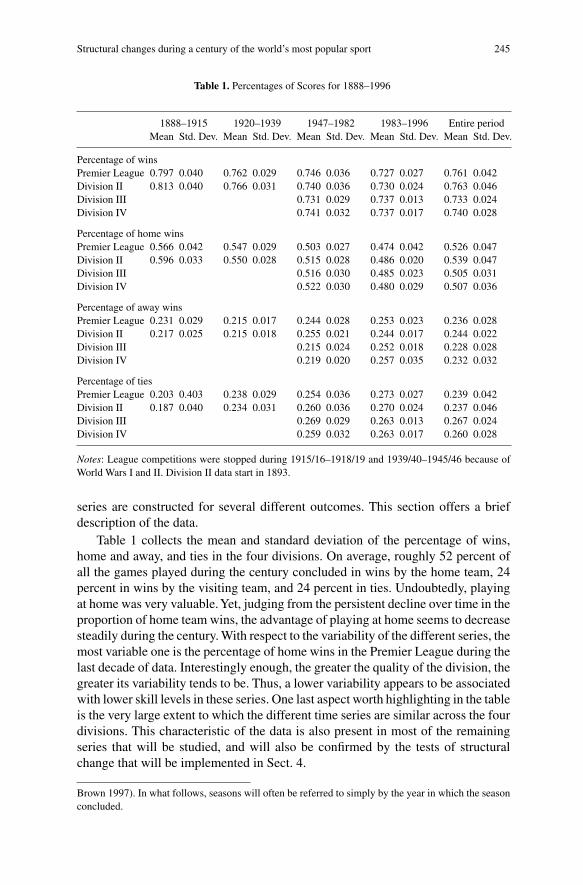
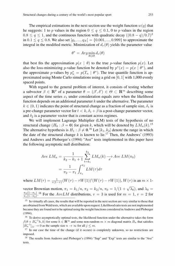
Table 1 collects the mean and standard deviation of the percentage of wins,home and away, and ties in the four divisions. On average, roughly 52 percent ofall the games played during the century concluded in wins by the home team, 24percent in wins by the visiting team, and 24 percent in ties. Undoubtedly, playingat home was very valuable.Yet, judging from the persistent decline over time in theproportion of home team wins, the advantage of playing at home seems to decreasesteadily during the century. With respect to the variability of the different series, themost variable one is the percentage of home wins in the Premier League during thelast decade of data. Interestingly enough, the greater the quality of the division, thegreater its variability tends to be. Thus, a lower variability appears to be associatedwith lower skill levels in these series. One last aspect worth highlighting in the tableis the very large extent to which the different time series are similar across the fourdivisions. This characteristic of the data is also present in most of the remainingseries that will be studied, and will also be confirmed by the tests of structuralchange that will be implemented in Sect. 4.
Brown 1997). In what follows, seasons will often be referred to simply by the year in which the seasonconcluded.
246 I. Palacios-Huerta
Percentage of Home Wins
40%
45%
50%
55%
60%
65%
70%
1890 1900 1910 1920 1930 1940 1950 1960 1970 1980 1990
Seasons
Division I
Division II
Percentage of Ties
10%
15%
20%
25%
30%
35%
1890 1900 1910 1920 1930 1940 1950 1960 1970 1980 1990
Season
Division I
Division II
Percentage of Visitor Wins
15%
19%
23%
27%
31%
1890 1900 1910 1920 1930 1940 1950 1960 1970 1980 1990
Season
Division I
Division II
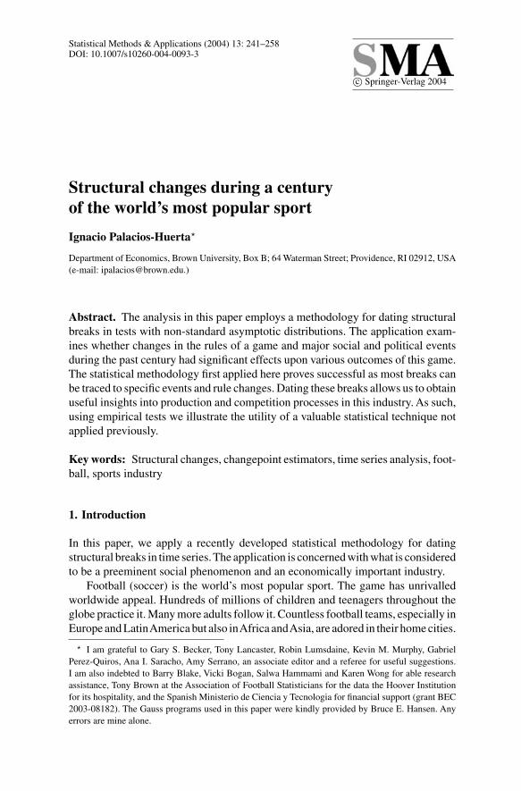
Fig. 1. Percentage of home wins, ties, and visitor wins (1889–1995)
Structural changes during a century of the world’s most popular sport 247
Avg. Number of Goals in Home Wins
2.25
2.75
3.25
3.75
4.25
4.75
5.25
1890 1900 1910 1920 1930 1940 1950 1960 1970 1980 1990
Season
Division I
Division II
Std. Dev. of Number of Goalsin Home Wins
0.085
0.115
0.145
0.175
0.205
0.235
0.265
1890 1900 1910 1920 1930 1940 1950 1960 1970 1980 1990
Season
Division I
Division II
Avg. Number of Goalsin Ties
1.2
1.7
2.2
2.7
3.2
3.7
1890 1900 1910 1920 1930 1940 1950 1960 1970 1980 1990
Season
Division I
Division II
Std. Dev. of Number of Goals in Ties
0.1
0.15
0.2
0.25
0.3
0.35
0.4
0.45
0.5
0.55
0.6
1890 1900 1910 1920 1930 1940 1950 1960 1970 1980 1990
Season
Division I
Division II
Avg. Number of Goals in Visitor Wins
2.20
2.80
3.40
4.00
4.60
5.20
1890 1900 1910 1920 1930 1940 1950 1960 1970 1980 1990Season
Division I
Division II
Std. Dev. of Number of Goalsin Visitor Wins
0.10
0.20
0.30
0.40
0.50
1890 1900 1910 1920 1930 1940 1950 1960 1970 1980 1990Season
Division I
Division II
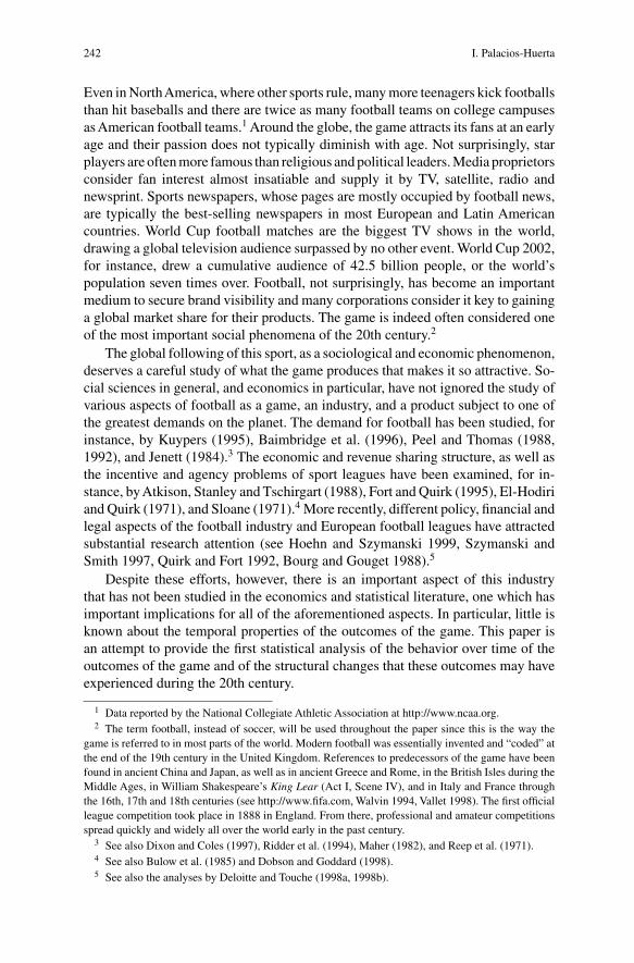
Fig. 2. Number of goals average and std. deviation 1893–1995
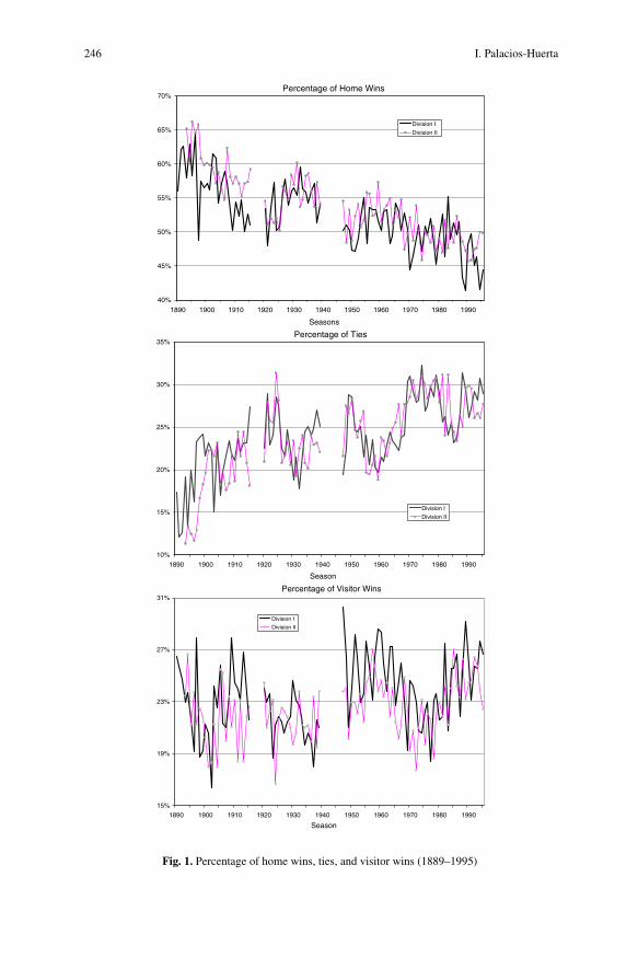
Figure 1 shows the percentage of home team wins, ties, and visitor wins forDivisions I and II. The percentage of games in which one team wins in thesedivisions decreases during the century from around 80 percent to around 72 percent.Conversely, the proportion of ties increases from around 20 percent to around 28percent. The percentage of home team wins decreases from around 57 percent toaround 47 percent, while that of away teams increases from 23 percent to 26 percent.With respect to Divisions III and IV (not shown), their trends and patterns are verysimilar to those of the top divisions. If anything, the percentage of home (visiting)team wins during the last half of the century is slightly lower (greater) in the topdivisions.
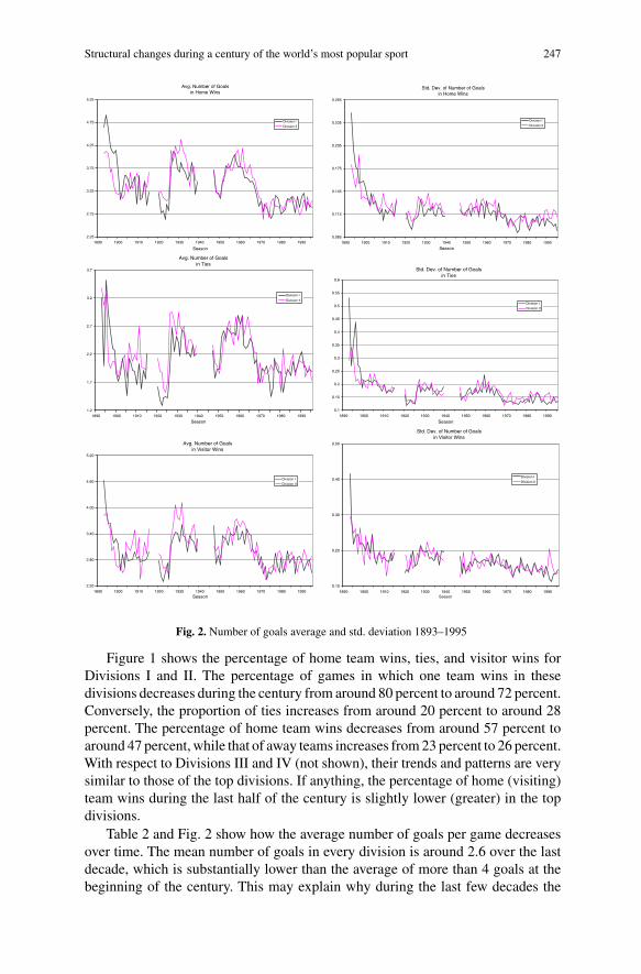
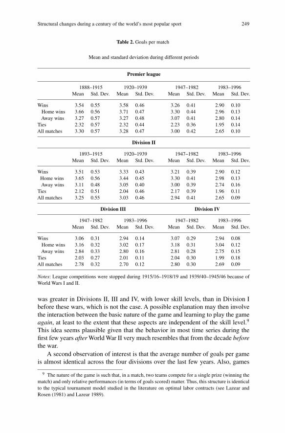
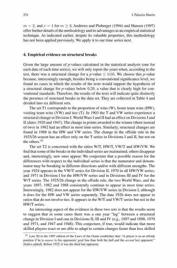
Table 2 and Fig. 2 show how the average number of goals per game decreasesover time. The mean number of goals in every division is around 2.6 over the lastdecade, which is substantially lower than the average of more than 4 goals at thebeginning of the century. This may explain why during the last few decades the
248 I. Palacios-Huerta
Average Margin of Victory
1.5
1.7
1.9
2.1
2.3
2.5
2.7
2.9
1890 1900 1910 1920 1930 1940 1950 1960 1970 1980 1990
Season
Division IDivision II
Std. Deviation of Margin of Victory
0.04
0.06
0.08
0.10
0.12
0.14
0.16
0.18
1890 1900 1910 1920 1930 1940 1950 1960 1970 1980 1990
Season
Division IDivision II
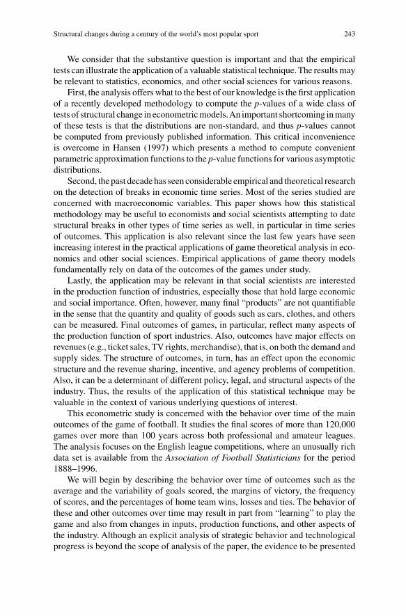
Fig. 3. Margin of victory average and standard deviation 1893–1995
governing bodies of football in England, and throughout the world as well, haveattempted to promote more scoring by modifying certain rules of the game (forexample, by awarding three points to wins instead of two and by establishing thebackpass ruling).8 Note that after World War I and World War II the number ofgoals experiences a substantial increase. This increase, in principle, does not reflectthe fact that after interrupting the game for a few years players’ skills diminished.Had this been the case, we should have observed that the average number of goals
8 See The History of the Laws of the Game and Amendments to the Laws of the Game publishedby the Federation Internationale de Football Association (FIFA). The decision to increase the pointsawarded to winners from two to three was established in 1981 by the English Football Association,and in 1996 in the rest of professional leagues in the world by FIFA. Of course, it is not clear thatawarding three points for a win, instead of two, promotes scoring. Tournament theory predicts that sucha change in the incentives to win will induce more offensive effort and more defensive effort as well,and hence scoring need not be promoted (see Garicano and Palacios-Huerta 2002). The backpass rulingestablished in 1992 worldwide penalizes players for deliberately kicking the ball to the hands of theirown goalkeepers. It is estimated that this new rule has increased the amount of time the ball is in playby about 10 percent.
Structural changes during a century of the world’s most popular sport 249
Table 2. Goals per match
Mean and standard deviation during different periods
Premier league
1888–1915 1920–1939 1947–1982 1983–1996Mean Std. Dev. Mean Std. Dev. Mean Std. Dev. Mean Std. Dev.
Wins 3.54 0.55 3.58 0.46 3.26 0.41 2.90 0.10Home wins 3.66 0.56 3.71 0.47 3.30 0.44 2.96 0.13Away wins 3.27 0.57 3.27 0.48 3.07 0.41 2.80 0.14
Ties 2.32 0.57 2.32 0.44 2.23 0.36 1.95 0.14All matches 3.30 0.57 3.28 0.47 3.00 0.42 2.65 0.10
Division II
1893–1915 1920–1939 1947–1982 1983–1996Mean Std. Dev. Mean Std. Dev. Mean Std. Dev. Mean Std. Dev.
Wins 3.51 0.53 3.33 0.43 3.21 0.39 2.90 0.12Home wins 3.65 0.56 3.44 0.45 3.30 0.41 2.98 0.13Away wins 3.11 0.48 3.05 0.40 3.00 0.39 2.74 0.16
Ties 2.12 0.51 2.04 0.46 2.17 0.39 1.96 0.11All matches 3.25 0.55 3.03 0.46 2.94 0.41 2.65 0.09
Division III Division IV
1947–1982 1983–1996 1947–1982 1983–1996Mean Std. Dev. Mean Std. Dev. Mean Std. Dev. Mean Std. Dev.
Wins 3.06 0.31 2.94 0.14 3.07 0.29 2.94 0.08Home wins 3.16 0.32 3.02 0.17 3.18 0.31 3.04 0.12Away wins 2.84 0.33 2.80 0.16 2.81 0.28 2.75 0.15
Ties 2.03 0.27 2.01 0.11 2.04 0.30 1.99 0.18All matches 2.78 0.32 2.70 0.12 2.80 0.30 2.69 0.09
Notes: League competitions were stopped during 1915/16–1918/19 and 1939/40–1945/46 because ofWorld Wars I and II.
was greater in Divisions II, III and IV, with lower skill levels, than in Division Ibefore these wars, which is not the case. A possible explanation may then involvethe interaction between the basic nature of the game and learning to play the gameagain, at least to the extent that these aspects are independent of the skill level.9
This idea seems plausible given that the behavior in most time series during thefirst few years after World War II very much resembles that from the decade beforethe war.
A second observation of interest is that the average number of goals per gameis almost identical across the four divisions over the last few years. Also, games
9 The nature of the game is such that, in a match, two teams compete for a single prize (winning thematch) and only relative performances (in terms of goals scored) matter. Thus, this structure is identicalto the typical tournament model studied in the literature on optimal labor contracts (see Lazear andRosen (1981) and Lazear 1989).
250 I. Palacios-Huerta
in which the home team wins have a greater goal average than those in whichthe visiting team wins.10 This is probably due to the more conservative, defensivestrategies typically employed by visiting teams. The time trends of these averagesby type of game (home team win, tie, visiting team win) experience a decreaseover time that is similar to that of the average number of goals for all games ingeneral. The time variability of the different time series greatly decreases over timeas well, especially over the last two decades. Overall, the differences among the fourdivisions are slim, especially over the last decade of data where the series are almostindistinguishable from each other. Around 1925/26 and after World War II, we seethe most important increase in the number of goals scored during the century. Afterthe mid-1970s, the series stabilize at about 2.6 goals per game. With respect to thecross-sectional variability of the number of goals (Fig. 2), it also decreases slowlyover time.11 The time variability over the different periods in Table 2 is around0.4–0.5 for the first three quarters of the century in the top divisions, decliningquite sharply in the last two decades to about 0.10.
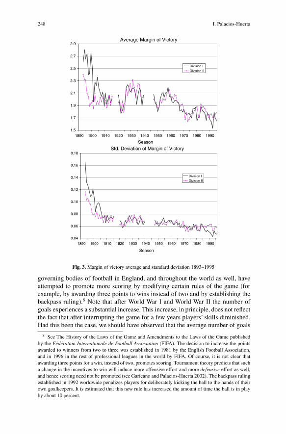
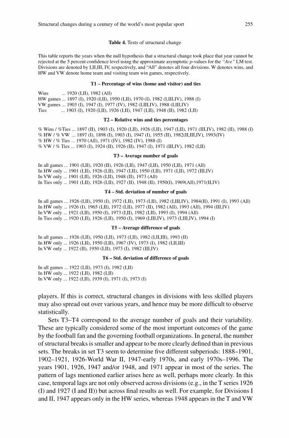
Figure 3 shows the time series of the average and the cross-section standarddeviation of the margin of victory (e.g., the margin is 1 in games whose final scoreis 1–0, 2–1, 0–1, 3–4, etc, and 0 in ties). These series, which are also very similaracross divisions, may help to explain whether some of the observed changes wereinduced by changes in strategies and/or in production functions. Not surprisingly,they follow patterns that are very similar to the previous series. Their detailedanalysis, however, is left for future research.12
Table 3 is concerned with the distribution of scores. Panel A summarizes themean and standard deviation of the relative frequency of some of the most frequentscores in the Premier League. Overall, the distribution of scores tends to narrow overtime. For instance, games in which at least one team scored more than 3 goals werearound 22 percent early the century; they are only around 11 percent in the last twodecades. The most frequent scores over the last two decades are: 1–1 (12.7%), 1–0(10.8%), 2–1 (9.3%), 0–0 (8.3%), 2–0 (8.2%), 0–1 (7.3%). Interestingly enough,almost exactly the same numbers are found for Division II, III and IV, where thequality of the players is substantially different from that in the Premier League. Thissimilarity is confirmed in Panel B, which reports the values of the Kolmogorov-
10 Home and away wins have a greater goal average than ties, which is not exceedingly surprisingsince goals are not a necessary condition for obtaining a tie.
11 Until the early 1950s, this decrease tends to be faster over time than that experienced by the numberof goals. The decreases is slower thereafter, until the early 1980s.
12 The average goal difference narrows over time, from around 2.1 early in the 20th century to around1.7 towards the end of the century. The cross-sectional variability also decreases from around 0.08 inthe early 1900s to about 0.06 in the 1990s. This may possibly be a reflection of (i) slow changes instrategies over time whereby teams become more defensive minded, and/or (ii) different progress of theoffensive and defensive production functions. Games won by the home team have a greater differenceof goals than those won by the visiting team. This suggests relatively more conservative play by visitingteams. The average number of goals per game is around 4.7 early in the century and is now around 2.6,whereas the average margin of victory was around 2.1 goals and is now about 1.7 goals. This meansthat the “average score” was 3.4–1.3 at the beginning of the century and is now about 2.15–0.45. As aresult, on average, home teams now score 1.25 fewer goals (a 36.7% decrease with respect to 3.6 goals)and visiting teams now score 0.85 fewer goals (a 65% decrease with respect to 1.3 goals) than in theearly 1900s.
Structural changes during a century of the world’s most popular sport 251
Table 3. Score frequencies and differences across divisions
Panel A: Frequency of scores in the premier league
1888–1915 1920–1939 1947–1982 1983–1996Score Mean Std. Dev. Mean Std. Dev. Mean Std. Dev Mean Std. Dev.
0–0 0.053 0.025 0.058 0.024 0.067 0.026 0.083 0.0151–0 0.087 0.029 0.081 0.027 0.091 0.028 0.108 0.0140–1 0.050 0.018 0.048 0.019 0.058 0.018 0.073 0.0091–1 0.088 0.022 0.108 0.025 0.115 0.023 0.127 0.0132–0 0.077 0.023 0.073 0.020 0.074 0.017 0.082 0.0132–1 0.086 0.017 0.080 0.015 0.087 0.013 0.093 0.0142–2 0.049 0.015 0.055 0.015 0.055 0.012 0.049 0.0090–2 0.030 0.013 0.027 0.009 0.034 0.009 0.036 0.0091–2 0.052 0.013 0.047 0.010 0.056 0.013 0.061 0.0113–0 0.053 0.012 0.049 0.013 0.046 0.010 0.046 0.0093–1 0.060 0.014 0.061 0.008 0.057 0.014 0.046 0.0143–2 0.031 0.008 0.030 0.011 0.032 0.010 0.020 0.0053–3 0.011 0.008 0.014 0.006 0.014 0.007 0.011 0.0050–3 0.015 0.007 0.014 0.005 0.015 0.006 0.016 0.0071–3 0.023 0.009 0.021 0.008 0.025 0.010 0.025 0.0062–3 0.018 0.008 0.021 0.010 0.021 0.007 0.017 0.005Others 0.218 0.094 0.212 0.064 0.155 0.059 0.108 0.019
Panel B: P -values of the Kolmogorov-Smirnov tests of equality of distributions across divisions
Division I vs II Division II vs III Division III vs IV1893–1996 1947–1996 1947–1996 1947–1996
Proportion of games with:No Goals 0.196 0.277 0.452 0.620Score 1–0 0.230 0.401 0.389 0.444Score 0–1 0.178 0.387 0.603 0.256Score 1–1 0.177 0.289 0.238 0.338Score 2–0 0.356 0.664 0.317 0.228Score 2–1 0.266 0.421 0.171 0.2553 Goals 0.503 0.323 0.501 0.4223+ Goals 0.611 0.261 0.223 0.701
Notes: League competitions were stopped during 1915/16–1918/19 and 1939/40–1945/46 because ofWorld Wars I and II. Wilconson-Mann-Whitney rank tests for the comparison of the distributions inPanel B yield similar results in that the null hypothesis cannot be rejected at conventional significancelevels.
Smirnov tests of the null hypothesis of coincidence of distributions (over time)across divisions for different scores. The results show that the null hypothesiscannot be rejected at conventional significance levels in the majority of cases.
Lastly, other time series, such as the growth rates of scores, changes in therelative proportions of the most frequent scores and others have been constructedand could be discussed. However, we believe that this description is sufficient toprovide an initial flavor for the data.
252 I. Palacios-Huerta
3. Testing for structural changes
The basic statistical methodology that will be implemented comes from Andrews(1993) and Andrews and Ploberger (1994) who found the asymptotic distributionsof a wide class of tests of structural change in econometric models. The distributionsare non-standard and depend on two parameters: the number of parameters testedand the range of the sample that is examined for the break date. One disadvantageof these tests is that because the distributions are non-standard, p values cannot becalculated from previously published information. This shortcoming is overcomein Hansen (1997), who presents a method to compute convenient parametric ap-proximation functions p(x | θ) to the asymptotic p-value functions p(x) for theAndrews and Andrews-Ploberger asymptotic distributions.13
Let Tn denote a given test of structural change and T denote the associatedasymptotic distribution. Let p(x) = P (T > x) denote the p-value function of Tand Q(q) = p−1(q) define its inverse function that satisfies q = p(Q(q)). Theparametric approximation function suggested by Hansen (1997) is constructed asfollows. Let αv(x | θ) be the vth-order polynomial in x defined as
αv(x | θ) = θ0 + θ1x + ... + θvxv.
Even though the function p(x) can be well approximated by setting p(x | θ) =αv(x | θ) for a suitable choice of the parameter θ, an improvement suggestedby MacKinnon (1994) is to set p(x | θ) = 1 − Ψ(αv(x | θ)) where Ψ(.) isa leading distribution function of interest. Hansen (1997) further improves theapproximation by allowing the distribution to depend on an unknown parameter ηand thus setting p(x | θ) = 1 − Ψ(αv(x | θ) | η). In applications, he suggestssetting Ψ(. | η) = χ2(η),14 that is, using as the approximating function
p(x | θ) = 1 − χ2 (θ0 + θ1x + ... + θvxv | η) ,
where
χ2 (z | η) =∫ z
0
yη2 −1e− y
2
Γ (η/2)2η2dy,
and θ = (θ0, θ1, ..., θv, η).To fit the approximation, he uses a weighted loss functionto make the difference |p(x | θ) − p(x)|, or equivalently the difference |p(Q(q) |θ) − q|, small. Since the uniform metric is difficult to implement numerically, heuses the Lr norm for r large (in particular, r = 8), and includes a weight functionw(q) ≥ 0, decreasing in q, in order to provide more precision in the approximationof small p values which are our main concern. The modified metric is thus
dr(θ) =[∫ 1
0|p(Q(q) | θ) − q|r w(q)dq
]1/r
.
13 See Hansen (1992) and MacKinnon (1994) for previous attempts.14 The main reason for this choice is that numerical plots of the densities of the Andrews’ (1993) and
Andrews-Ploberger’s (1994) tests resemble very closely those of the chi-square.
Structural changes during a century of the world’s most popular sport 253
The empirical estimations in the next section use the weight function w(q) thathe suggests: 1 to p values in the region 0 ≤ q ≤ 0.1, 0 to p values in the region0.8 ≤ q ≤ 1, and the continuous function with quadratic decay ((0.8 − q)/0.7)2
in 0.1 ≤ q ≤ 0.8. We also set [q1, ..., qN ] = {0.001, ..., 0.999} to approximate theintegral in the modified metric. Minimization of dr(θ) yields the parameter value
θ∗ = Arg minθ∈Θ
dr(θ)
that best fits the approximation p(x | θ) to the true p-value function p(x). Letalso the loss-minimizing p-value function be denoted by p∗(x) = p(x | θ∗), andthe approximate p-values by p∗
n = p(Tn | θ∗). The true quantile function is ap-proximated using Monte Carlo simulations using a grid on [0, 1] with 1,000 evenlyspaced points.
With regard to the general problem of interest, it consists of testing whethera subvector β ∈ Rp of a parameter θ = (β′, δ′) ∈ Θ ⊂ Rm describing someaspect of the time series xt under consideration equals zero when the likelihoodfunction depends on an additional parameter k under the alternative. The parameterk ∈ (0, 1) indicates the point of structural change as a fraction of sample size, δ1 isa pre-change parameter vector for t < k, δ1 +β is a post-change parameter vector,and δ2 is a parameter vector that is constant across regimes.
We will implement Lagrange Multiplier (LM) tests of the hypothesis of nostructural change (H0 : β = 0) for given k, which will be denoted by LMn(k).15
The alternative hypothesis is H1 : β �= 0.16 Let [k1, k2] denote the range in whichthe date of the structural change k is known to lie.17 Then, the Andrews’ (1993)and Andrews and Ploberger’s (1994) “Ave” tests implemented in this paper havethe following asymptotic null distribution:
Ave LMn =1
k2 − k1 + 1
k2∑t=k1
LMn(k) −→d
Ave LM(π0)
=1
π2 − π1
∫ π2
π1
LM(τ)dτ
where LM(τ) = 1τ(1−τ) (W (τ) − τW (1))′(W (τ) − τW (1)), W (τ) is an m × 1-
vector Brownian motion, π1 = k1/n, π2 = k2/n, π0 = 1/(1 +√
λ0), and λ0 =π2(1−π1)π1(1−π2)
.18 For the AveLM distributions, v = 3 is used for m = 1, v = 2 for
15 In virtually all cases, the results that will be reported in the next section are very similar to those thatare obtained fromWald tests, which are available upon request. Likelihood ratio tests are not implementedbecause they are found not to be optimal using the weight functions considered inAndrews and Ploberger(1994).
16 To derive asymptotically optimal tests, the likelihood function under the alternative takes the formf(θ + B−1
n h, k) for some h ∈ Rm and some non-random m × m diagonal matrix Bn that satisfies[B−1
n ]jj → 0 as the sample size n → ∞ for all j ≤ m.17 In our case the time of the change (if it occurs) is completely unknown, so no restrictions are
imposed.18 The results from Andrews and Ploberger’s (1994) “Sup” and “Exp” tests are similar to the “Ave”
tests.
254 I. Palacios-Huerta
m = 2, and v = 1 for m ≥ 3. Andrews and Ploberger (1994) and Hansen (1997)offer further details of the methodology and its advantages as an empirical statisticaltechnique. As indicated earlier, despite its valuable properties, this methodologyhas not been applied previously. We apply it to our time series next.
4. Empirical evidence on structural breaks
Given the large amount of p-values calculated in the statistical analysis (one foreach date of each time series), we will only report the years when, according to thetest, there was a structural change for a p-value ≤ 0.05. We choose this p-valuebecause, interestingly enough, besides being a conventional significance level, wefound no cases in which the results of the tests would support the hypothesis ofa structural change for p-values below 0.20, a value that is clearly high for con-ventional standards. Therefore, the results of the tests will indicate quite distinctlythe presence of structural breaks in the data set. They are collected in Table 4 anddivided into six different sets.
The set T1 corresponds to the proportion of wins (W), home team wins (HW),visiting team wins (VW) and ties (T). In 1903 the T and VW series experience astructural change in Division I. World Wars I and II had an effect on Divisions I andII (dates 1920 and 1947). The change in points awarded to the winner (three insteadof two) in 1982 had an effect in most time series. Similarly, structural changes arefound in 1988 in the HW and VW series. The change in the offside rule in the1925/26 season has an effect only on the T series in Divisions I and II, but not onthe others.19
The set T2 is concerned with the ratios W/T, HW/T, VW/T and HW/VW. Wefind that some of the breaks in the individual series are maintained, others disappearand, interestingly, new ones appear. We conjecture that a possible reason for thedifferences with respect to the individual series is that the numerator and denom-inator may be breaking in different directions and/or with different strengths. Theyear 1924 appears in the VW/T series for Division II, 1970 in all HW/VW series,and 1971 in Division I for the HW/VW series and in Divisions III and IV for theW/T series. The 1925/26 change in the offside rule, the two World Wars, and theyears 1897, 1982 and 1988 consistently continue to appear in most time series.Interestingly, 1982 does not appear for the HW/VW series in Division I, althoughit does for the HW and VW series separately. The date 1926 does not appear inratios that do not involve ties. It appears in the W/T and VW/T series but not in theHW/T series.
An interesting aspect of the evidence in these two sets is that the results seemto suggest that in some cases there was a one year “lag” between a structuralchange in Division I and one in Divisions II, III and IV (e.g., 1897 and 1898, 1970and 1971, and 1947 and 1948). This conjecture, if true, would indicate that moreskilled players react or are able to adapt to certain changes faster than less skilled
19 Law XI in the 1997 edition of the Laws of the Game establishes that: “A player is in an offsideposition if he is nearer to his opponents’ goal line than both the ball and the second last opponent.”[Italics added]. Before 1925, it was the third last opponent.
Structural changes during a century of the world’s most popular sport 255
Table 4. Tests of structural change
This table reports the years when the null hypothesis that a structural change took place that year cannot berejected at the 5 percent confidence level using the approximate asymptotic p-values for the “Ave” LM test.Divisions are denoted by I,II,III, IV, respectively, and “All” denotes all four divisions. W denotes wins, andHW and VW denote home team and visiting team win games, respectively.
T1 – Percentage of wins (home and visitor) and ties
Wins ... 1920 (I,II), 1982 (All)HW games ... 1897 (I), 1920 (I,II), 1950 (I,II), 1970 (I), 1982 (I,III,IV), 1988 (I)VW games ... 1903 (I), 1947 (I), 1977 (IV), 1982 (I,III,IV), 1988 (I,III,IV)Ties ... 1903 (I), 1920 (I,II), 1926 (I,II), 1947 (I,II), 1948 (II), 1982 (I,II)
T2 – Relative wins and ties percentages
% Wins / %Ties ... 1897 (II), 1903 (I), 1920 (I,II), 1926 (I,II), 1947 (I,II), 1971 (III,IV), 1982 (II), 1988 (I)% HW / % VW ... 1897 (I), 1898 (I), 1903 (I), 1947 (I), 1955 (II), 1982(II,III,IV), 1993(IV)% HW / % Ties ... 1970 (All), 1971 (IV), 1982 (IV), 1988 (I)% VW / % Ties ... 1903 (I), 1924 (II), 1926 (II), 1947 (I), 1971 (III,IV), 1982 (I,II)
T3 – Average number of goals
In all games ... 1901 (I,II), 1920 (II), 1926 (I,II), 1947 (I,II), 1950 (I,II), 1971 (All)In HW only ... 1901 (I,II), 1926 (I,II), 1947 (I,II), 1950 (I,II), 1971 (I,II), 1972 (III,IV)In VW only ... 1901 (I,II), 1926 (I,II), 1948 (II), 1973 (All)In Ties only ... 1901 (I,II), 1926 (I,II), 1927 (II), 1948 (II), 1950(I), 1969(All),1971(II,IV)
T4 – Std. deviation of number of goals
In all games ... 1926 (I,II), 1950 (I), 1972 (I,II), 1973 (I,II), 1982 (I,III,IV), 1984(II), 1991 (I), 1993 (All)In HW only ... 1926 (I), 1965 (I,II), 1972 (I,II), 1977 (II), 1982 (All), 1993 (All), 1994 (III,IV)In VW only ... 1921 (I,II), 1950 (I), 1973 (I,II), 1982 (I,II), 1993 (I), 1994 (All)In Ties only ... 1920 (I,II), 1926 (I,II), 1950 (I), 1969 (I,III,IV), 1973 (I,III,IV), 1994 (I)
T5 – Average difference of goals
In all games ... 1926 (I,II), 1950 (I,II), 1973 (I,II), 1982 (I,II,III), 1993 (II)In HW only ... 1926 (I,II), 1950 (I,II), 1967 (IV), 1973 (I), 1982 (I,II,III)In VW only ... 1922 (II), 1950 (I,II), 1973 (I), 1982 (III,IV)
T6 – Std. deviation of difference of goals
In all games ... 1922 (I,II), 1973 (I), 1982 (I,II)In HW only ... 1922 (I,II), 1982 (I,II)In VW only ... 1922 (I,II), 1939 (I), 1971 (I), 1973 (I)
players. If this is correct, structural changes in divisions with less skilled playersmay also spread out over various years, and hence may be more difficult to observestatistically.
Sets T3–T4 correspond to the average number of goals and their variability.These are typically considered some of the most important outcomes of the gameby the football fan and the governing football organizations. In general, the numberof structural breaks is smaller and appear to be more clearly defined than in previoussets. The breaks in set T3 seem to determine five different subperiods: 1888–1901,1902–1921, 1926-World War II, 1947-early 1970s, and early 1970s–1996. Theyears 1901, 1926, 1947 and/or 1948, and 1971 appear in most of the series. Thepattern of lags mentioned earlier arises here as well, perhaps more clearly. In thiscase, temporal lags are not only observed across divisions (e.g., in the T series 1926(I) and 1927 (I and II)) but across final results as well. For example, for Divisions Iand II, 1947 appears only in the HW series, whereas 1948 appears in the T and VW
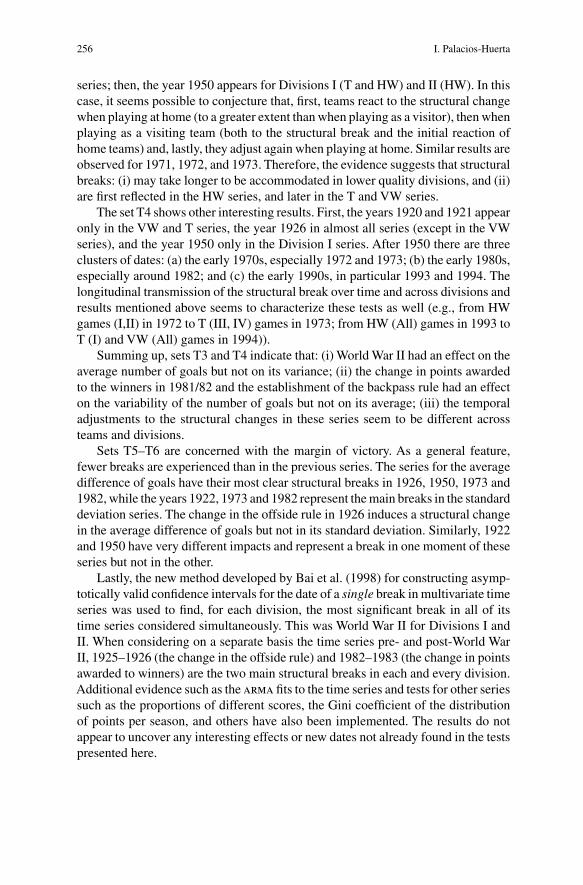
256 I. Palacios-Huerta
series; then, the year 1950 appears for Divisions I (T and HW) and II (HW). In thiscase, it seems possible to conjecture that, first, teams react to the structural changewhen playing at home (to a greater extent than when playing as a visitor), then whenplaying as a visiting team (both to the structural break and the initial reaction ofhome teams) and, lastly, they adjust again when playing at home. Similar results areobserved for 1971, 1972, and 1973. Therefore, the evidence suggests that structuralbreaks: (i) may take longer to be accommodated in lower quality divisions, and (ii)are first reflected in the HW series, and later in the T and VW series.
The set T4 shows other interesting results. First, the years 1920 and 1921 appearonly in the VW and T series, the year 1926 in almost all series (except in the VWseries), and the year 1950 only in the Division I series. After 1950 there are threeclusters of dates: (a) the early 1970s, especially 1972 and 1973; (b) the early 1980s,especially around 1982; and (c) the early 1990s, in particular 1993 and 1994. Thelongitudinal transmission of the structural break over time and across divisions andresults mentioned above seems to characterize these tests as well (e.g., from HWgames (I,II) in 1972 to T (III, IV) games in 1973; from HW (All) games in 1993 toT (I) and VW (All) games in 1994)).
Summing up, sets T3 and T4 indicate that: (i) World War II had an effect on theaverage number of goals but not on its variance; (ii) the change in points awardedto the winners in 1981/82 and the establishment of the backpass rule had an effecton the variability of the number of goals but not on its average; (iii) the temporaladjustments to the structural changes in these series seem to be different acrossteams and divisions.
Sets T5–T6 are concerned with the margin of victory. As a general feature,fewer breaks are experienced than in the previous series. The series for the averagedifference of goals have their most clear structural breaks in 1926, 1950, 1973 and1982, while the years 1922, 1973 and 1982 represent the main breaks in the standarddeviation series. The change in the offside rule in 1926 induces a structural changein the average difference of goals but not in its standard deviation. Similarly, 1922and 1950 have very different impacts and represent a break in one moment of theseseries but not in the other.
Lastly, the new method developed by Bai et al. (1998) for constructing asymp-totically valid confidence intervals for the date of a single break in multivariate timeseries was used to find, for each division, the most significant break in all of itstime series considered simultaneously. This was World War II for Divisions I andII. When considering on a separate basis the time series pre- and post-World WarII, 1925–1926 (the change in the offside rule) and 1982–1983 (the change in pointsawarded to winners) are the two main structural breaks in each and every division.Additional evidence such as the arma fits to the time series and tests for other seriessuch as the proportions of different scores, the Gini coefficient of the distributionof points per season, and others have also been implemented. The results do notappear to uncover any interesting effects or new dates not already found in the testspresented here.
Structural changes during a century of the world’s most popular sport 257
5. Concluding remarks
The analyses in this paper use an econometric methodology for dating structuralbreaks in tests with non-standard asymptotic distributions. The results indicate thatsome changes in the rules of the game of football had an effect on the mean of thedistribution of certain outcomes but not on their variance and vice versa. WWIIaffected the average number of goals but not their variance; the amendment in theoffside rule from three to two players in 1925 had an effect on the average marginof victory but not on its variability. Conversely, the change in points awarded towinners in 1981/82 and the establishment of the backpass rule in 1992 affected thevariability of the number of goals but not its average. Time series that involve thenumber of goals per match, experience fewer and more clearly defined structuralbreaks than those that involve the proportion of games won and tied. For the formerseries, however, the change in the offside rule and the establishment of the backpassrule had a significant impact, but not for the latter series. Interestingly, the evidenceshows a great degree of similarity across divisions, although it also suggests thatdivisions with high-skill players adapt to structural breaks faster than divisions withlower-skill players. The reactions that are observed seem to be driven mostly bythe behavior of teams when playing at home.
The application of this methodology proves successful as most of the structuralbreaks can be traced to specific events and changes in the rules of the game.20
Although an explicit analysis of strategic behavior and technological progress isbeyond the scope of analysis of the paper, dating these breaks is also valuable inthis dimension.
We have argued that as sports and their associated industries often representsocioeconomic phenomena of the first magnitude, it remains of great importance toevaluate the effects that different social, economic, and political events may have,the initiatives to change their foundations and basic structure, and the attempts toincrease their attractiveness. To the best of our knowledge this is the first time thatstructural breaks have been dated in the sports industry. The results of the analysismay have implications for various research issues of interest in economics, giventhat the outcomes of the game have major effects on revenues, revenue sharing,incentive and agency problems of competition, and other aspects of the economicstructure of the football industry.
References
Andrews DWK (1993) Tests for parameter instability and structural change with unknown change point.Econometrica 61: 821–856
Andrews DWK, Ploberger W (1994) Optimal tests when a nuisance parameter is present only under thealternative. Econometrica 62: 1383–1414
20 As a referee noted, apart from the reasons that are mentioned in the paper, there are other factorsrelated to the football industry (e.g., professionalization of players, pay tv contracts, possibility toemploy foreign players in different numbers, football firms being quoted in the stock market, etc) thatmay have had a non-negligible impact. Although it could be argued that some of these developments inthe industry are more gradual, they could certainly be taken into account as a possible explanation ofcertain breaks, especially the most recent ones.
258 I. Palacios-Huerta
Atkinson S, Stanley LR, Tschirhart J (1988) Revenue sharing as an incentive in an agency problem: anexample from the national football league. Rand Journal of Economics 19: 27–43
Bai J, Lumsdaine RL, Stock JH (1998) Testing for and dating common breaks in multivariate timeseries. Review of Economic Studies 65: 395–432.
Baimbridge M, Cameron S, Dawson P (1996) Satellite television and the demand for football: a wholenew ball game? Scottish Journal of Political Economy 43: 317–333
Bourg JF, Gouguet JJ (1988) Analyse economique du sport. Presses Universitaires de FranceBrown T (1997) The ultimate football league statistics book.Association of Football Statisticians, Essex,
United Kingdom, 3rd ednBulow JI, Geanokoplos JD, Klemperer PD (1985) Multimarket oligopoly, strategic substitutes and
complements. Journal of Political Economy 93: 488–511Deloitte & Touche (1998a) Annual review of football finance 1997Deloitte & Touche (1998b) Financial Review of Serie ADixon MJ, Coles SG (1997) Modelling association football scores and inefficiencies in the football
betting market. Applied Statistics 46, 265–280Dobson S, Goddard J (1998) Performance, revenue, and cross subsidization in the football league,
1927–1994. Economic History Review 51: 763–785El-Hodiri M, Quirk J (1971) An economic analysis of a professional sport league. Journal of Political
Economy 79: 1302–1319Fort R, Quirk J (1995) Cross subsidization, incentives and outcomes in professional team sport leagues.
Journal of Economic Literature 33: 1265–1299Garicano L, Palacios-Huerta I (2002) An empirical examination of multidimensional effort in tourna-
ments. Brown University, Department of Economics, Working Paper 2002-17Hansen BE (1997) Approximate asymptotic P values for structural-change tests. Journal of Business &
Economic Statistics 15: 60–67Hoehn T, Szymanski S (1999) TheAmericanization of European football. Economic Policy 28: 205–240Jennett N (1984)Attendances, uncertainty of outcome and policy in the Scottish football league. Scottish
Journal of Political Economy 31: 176–198Kuypers T (1995) The beautiful game? An econometric study of why people watch English football.
University College London Discussion Paper 96/01.Lazear E (1989) Pay equality and industrial politics. Journal of Political Economy 97: 561–580Lazear E, Rosen S (1981) Rank order tournaments as optimal labor contracts. Journal of Political
Economy 89: 841–864MacKinnon JG (1994) Approximate asymptotic distribution function for unit-root and cointegration
tests. Journal of Business & Economics Statistics 12: 167–176Maher MJ (1982) Modelling association football scores. Statistica Neerlandica 36: 109–118Peel DA, Thomas DA (1988) Outcome uncertainty and the demand for football: an analysis of match
attendances in the English football league. Scottish Journal of Political Economy 35: 242–249Peel DA, Thomas DA (1992) The demand for football: some evidence on outcome uncertainty. Empirical
Economics 17: 323–331Quirk J, Fort R (1992) Pay dirt: the business of professional team sports. Princeton University Press,
Princeton, NJReep C, Pollard R, Benjamin B (1971) Skill and chance in ball games. Journal of the Royal Statistical
Society, Series A (General) 34: 623–629Ridder G, Cramer J, Hopstaken P (1994) Down to ten: estimating the effect of a red card in soccer.
Journal of the American Statistical Association 89: 1124–1127Sloane PJ (1971) The economics of professional football: the football club as utility maximizer. Scottish
Journal of Political Economy 18: 121–146Szymanski S, Kuypers T (1999) Winners and losers: the business strategy of football. Penguin, Har-
mondsworthSzymanski S, Smith R (1997) The English football industry: profit, performance and industry structure.
International Review of Applied Economics 11: 135–153Vallet O (1998) Le football entre religion et politique. In: Boniface P (ed) Geopolitique du Football,
pp 117–131. Editions Complexe, BrusselsWalvin J (1994) The people’s game. Mainstream Press, Edinburg