Embed Size (px)
Citation preview
STRUCTURAL BREAKS, COINTEGRATION AND THE DOMESTICDEMAND FOR CHILEAN WINE
CRISTIAN TRONCOSO–VALVERDE1
Abstract. The domestic Chilean wine market is examined through the estimation of an error
correction model allowing for structural breaks in the cointegrating vector. Our findings support
both parameter instability and one structural break in the long–run relationship in 1982. The wine
demand becomes more price–elastic and cross price–elasticity between wine and beer is found to be
positive and close to one in the 1983–1998 period. This is in line with the growing substitutability
between both wine varieties and wine and beer in Chile during the last two decades. The error
correction parameter is found to be negative and highly significant supporting cointegration and
suggesting a quick adjustment to long–run equilibrium.
JEL Classification: C22, C51, Q11.
Keywords: Error correction models, structural breaks, cointegration, parameter instability.
Introduction
During the last two decades, the Chilean wine industry has experienced a strong and accelerate
process of internationalization. Investments in new production technologies, more qualified human
capital and improved marketing processes are among the main reasons that explain the observed
growth rates of 41% in wine production and 834% in wine exports during the 1990–2000 period
(Schnettler and Rivera, 2003). Notwithstanding, this industry has also suffered from the global
tendency of a declining per–capita wine consumption [Anderson et al. (2002); Schnettler and Rivera
(2003)]. In fact, Chilean per capita wine consumption has fallen from 68 liters in 1962 to 13 liters
in 1993, with some signs of recovery in last years (Costa, 2001). This decline in consumption has
been attributed to a change in consumer’s tastes, which have shown a strong tendency toward the
substitution of wine for other type of alcoholic beverages such as beer. This change in consumer’s
tastes may be viewed as a consequence of the strategy adopted by most Chilean wineries that
1Ingeniero Comercial (Universidad de Talca) y Master of Arts in Economics (Concordia University). Profesor Escuelade Ingenierıa Comercial, Facultad de Ciencias Empresariales, Universidad de Talca. 2 Norte 685, Casilla 721, Talca,Chile. E–mail: [email protected].
1
focused on producing competitive wine for international markets. Thus, varieties such as Merlot,
Chardonay, Carmenere and Syrah that were likely produced only for foreign markets, have reached
the popularity of the traditional Cabernet Sauvignon or Sauvignon Blanc in the domestic market
(Banda, 2002). In fact, some authors suggest that, as a result of the internationalization of Chilean
wineries, domestic consumers have learnt how to ‘drink’ wine in the sense that consumers now drink
less quantity but better quality of wine [c.f. CORFO (1998); Costa (2001) or Schnettler and Rivera
(2003)].
Several studies have analyzed the domestic Chilean wine market through the estimation of price
and income elasticities. The traditional domestic wine demand function has been specified as a log–
linear function of real price of wine, real income and other variables that, according to the economic
theory, might affect domestic wine demand. While Mujica and Celedon (1982); Oncken (1983) and
Mujica and Oncken (1984) have all estimated both demand and supply functions, Cremaschi (1991)
and Martinez (1995) have only considered the demand equation. This research, however, presents
conflicting evidence about own–price elasticity. For instance, Mujica and Celedon (1982) estimate
an own–price elasticity of -0.01, whereas Mujica and Oncken (1984) found an estimate of -0.74
with per capita data and -0.84 with aggregate data. Similar disagreement exists for the income
elasticity estimates. These vary from 0.031 (Martinez, 1995) to 1.50 (Mujica and Oncken, 1984).
Although, from a theoretical point of view, beer may be considered as a substitute of wine, the
aforementioned studies have been unable to find evidence supporting this conjecture [c.f. Martinez
(1995) and references therein]. This issue appears in contraposition with the claim that consumers
have shown a strong tendency to substitute wine for beer during the last two decades.
In what regards the statistical properties of the estimates of the domestic demand model, two
properties have been of particular interest. First, the magnitude of the estimates has attracted
a great deal of attention. Mujica and Celedon (1982) and Oncken (1983) use these estimates to
evaluate the effect that a potential cut in taxes would have over wine consumption and tax eva-
sion. Therefore, accurate estimates are needed for policy evaluation and problems that may induce
parameter bias should be accounted for when deciding the econometric technique to be employed.
Second, statistical inference over demand estimates has been of central interest [c.f. Mujica and
Oncken (1984); Cremaschi (1991); Martinez (1995)]. However, hypothesis testing requires knowing
the distribution of the statistic used to test these hypotheses. When variables are nonstationary,
traditional test statistics (such as the t– or the F–statistic) do not follow a normal distribution. In2
light of this, using critical values from student–t or normal distribution for hypothesis testing may
conduct the researcher to misleading conclusions.
An implicit assumption made in previous research is the stability of the demand parameters over
time. With the exception of Martinez (1995), who recognized this possibility and estimated one
set of elasticities for the 1949–1972 period and another set for the 1973–1993 period using dummy
variables, no formal attempt has been made in order to check whether demand parameters are stable
over time. Under stationarity, it is well known that hypothesis testing needs to be adjust to account
for possible structural breaks (Greene, 2000). Although structural breaks have been widely discussed
in the context of univariate autoregressive time series with unit roots [c.f. Perron (1989; 1990);
Zivot and Andrews (1992); Perron and Vogelsang (1992); Christiano (1992); Vogelsang and Perron
(1998); Lee and Strazicich (1999); Lee and Strazicich (2002)], discussion about structural breaks
and parameter instability in a multivariate nonstationary context is relatively recent. Analysis of
structural breaks in the cointegrating parameters has been addressed, among others, by Hansen
(1992), Gregory and Hansen (1996) and Kuo (1998).
The purpose of this paper is twofold. First, we analyze short– and long–run demand dynamics
through the use of error correction models that are estimated with time–series techniques that
address for nonstationarity. Second, we aim to shed some new lights about structural breaks
through the Gregory and Hansen (1996) and Bai and Perron’s (1998) methodology for the analysis of
structural break in cointegrating systems. Parameter instability is analyzed through the instability
parameter test proposed by Hansen (1992).
The plan for the rest of the paper is as follows. Next section lays out the basic setup and discusses
the econometric methodology employed in estimating the domestic wine demand model. In Section
, we carry out the empirical analysis and present our main results. Finally, section concludes the
paper with some conclusions and final remarks.
Econometric Methodology
In this section we lay out the basic model and describe the econometric methodology we use
throughout. We begin with a brief discussion about nonstationarity and cointegration. Given our
interest in modelling both short– and long–run wine demand dynamics, we distinguish two stages in
our methodology. In stage 1 we specify and estimate the long–run model and in stage 2 we estimate
the error correction model (ECM). Accordingly, section details the methodology used to obtain3
long–run estimates while section discusses the econometric aspects related to the estimation of the
error correction model.
Nonstationarity and Cointegration. A stochastic process is said to be (weakly) stationary if its
unconditional mean and variance are constant over time. Nonetheless, it is well known that many
economic variables evolve over time and are usually driven by trends that change stochastically over
time. This type of processes, called integrated of order one —I(1) in the terminology of Engle and
Granger (1987)— are by definition processes whose unconditional mean and variance vary over time.
The econometric literature is plenty of devices to determine the order of integration of individual
series. Nevertheless, DeJong et al. (1992) and Perron and Ng (1996) have shown power and size
misspecifications appear in most of unit root tests when either the root is close to but less than
unity or the moving average polynomial of the first differenced series has a large negative root.
Following the work of Elliott et al. (1996), Ng and Perron (2001) show that an appropriate selection
of the lag truncation in unit–root test together with Generalized Least Squares (GLS) detrended
data results in a class of M tests that have good size and power. In the present paper, we follow
the Ng and Perron’s (2001) suggestion and use the MGLS and the ADFGLS tests to investigate the
integration order of the model series.
The above tests assume no structural breaks in the generating process of the series. If such
breaks are present, tests such as the MGLS or the ADFGLS lose most of their power [see Vogelsang
and Perron (1998) and cites therein]. Since we have reasons to believe that there are breaks in
the series, we also test for a unit root using the tests proposed by Zivot and Andrews (1992) and
Vogelsang and Perron’s (1998) (hereafter the ZA and VP tests respectively). These tests differ from
the MGLS or the ADFGLS in that the former consider as the alternative hypothesis a stationary
series that fluctuates around a deterministic function with a broken trend. Likewise, the ZA and
the VP tests differ from the test originally proposed by Perron in the way the break date is chosen.
While Perron (1989) considered the date of break as exogenously given, Zivot and Andrews (1992)
and Vogelsang and Perron (1998) make this date endogenous. Notwithstanding, in a recent paper
Lee and Strazicich (2001) have pointed out the tendency of these tests to reject the null of a unit
root too often. According to these authors, the spurious rejection of the null is caused by the
assumption of no breaks under the null made by the ZA and the VP tests. The authors also show
that both tests tend to estimate a wrong date for the break, particulary when the magnitude of the
break increases. To overcome these problems, Lee and Strazicich (1999; 2002) suggest a Lagrange4
Multiplier (LM) test for the null of a unit root in the presence of structural breaks. Through Monte
Carlo simulations, they show that the LM test estimates more accurately the date of break and also
avoids the spurious rejection of the ZA and the VP tests. For this reason, we also test for a unit
root in model series using this LM test.
As shown by Phillips (1986), serious bias in conventional tests may arise when variables are
nonstationary. Phillips show that this bias is due to the fact that distributions of traditional statis-
tics (such as the t– or the F–statistic) under nonstationary diverge completely from those derived
under stationarity. To overcome the problems posed by nonstationarity in a multivariate setting,
Engle and Granger (1987) suggest the so–called cointegration analysis. A set of I(1) variables are
said to be cointegrated if there exists a linear combination of them that is a stationary stochastic
process1. Engle and Granger (1987) also demonstrate that a vector of cointegrated variables has
always an error correction representation (ECM). This means that it is always possible to construct
a linear model in which differences and levels of the variables are used2. This class of model has
the desirable property of retaining not only short–run information (contained in differences) but
also long–run one (contained in the levels). Engle and Granger also show that cointegration implies
and is implied by the error correction representation thus clarifying when levels information could
legitimately be retained in econometric equations (Hendry, 1986). From a practical point of view,
this result is extremely appealing because it enables us to model both short and long–run effects
separately in the same model, issue that has not been addressed by the literature on Chilean wine
demand estimation.
Long–run Model. In this stage, we specify and estimate the following long–run model:
qt = β0 + β1pt + β2pst + β3yt (1)
qt = φ′xt
where qt is the log of domestic per capita wine consumption, pt is the log of real price of wine,
pst is real price of beer, yt is real GDP per capita and φ = (β0, β1, β2, β3)′, xt = (pt, pst, yt)′. In
the light of our previous discussion, the inclusion of the price of beer as one of the regressors in
1Formally, the component of the vector xt are said to be cointegrated of order (d, b), denoted by xt ∼ CI(d, b), if (i)
all components in xt are I(d); (ii) there exists a vector α 6= 0 so that zt = α′xt ∼ I(d − b), b > 0. The vector α is
called cointegrating vector (Engle and Granger, 1987).2For further details about error correction models see Davidson et al. (1978)
5
(1) may seem surprising. However, we conjecture that the lack of significance found in previous
studies is mainly due to nonstationary in the variables. Consequently, we include price of beer in
domestic wine demand specification and tackle the possible problems posed by nonstationarity in
the estimation stage.
Parameters in (1) will be estimated using the Fully Modified (FM) single–equation method of
Phillips and Hansen (1990). As shown by Banerjee et al. (1986) the parameters estimated by
least squares from a static regression yields super–consistent3 estimates of the cointegrating vector,
although they may be substantially biased in finite samples. Phillips (1995) show that OLS estimates
of any cointegrating relation are second order bias in the sense that their limiting distribution are
shifted away from the true parameters, though they are first order unbiased (consistent). This author
also argues that this second order bias is due to the fact that OLS regressions are not designed to take
into consideration long-run endogeneities in the regressors and it is the presence of such endogeneities
which produces this bias. On the contrary, the FM technique is designed to estimate cointegrating
relations directly by modifying traditional OLS with non parametric corrections that take into
account serial correlation, caused by unit roots, and system endogeneity, caused by cointegration.
Furthermore, Phillips (1995) has shown that the FM estimation technique yields t–statistics for
parameter estimates which have a normal limiting distribution even in the presence of cointegrated
explanatory variables. Thus, standard inferential techniques can be used to test hypothesis on the
parameter estimated through the FM technique.
To investigate long–run parameter stability, we apply the econometric methodology proposed
by Hansen (1992) and Gregory and Hansen (1996). Hansen considers a set of tests (the SupF–,
MeanF– and Lc–test) which are for the null of a stable cointegrating relationship against several
alternatives of interest in the context of cointegrating regression models. He also argues that the
lack of cointegration is a special case of the alternative of an unstable intercept so his proposed
tests may be viewed as tests for the null of cointegration against the alternative of no cointegration.
On the other hand, the residual–based tests of Gregory and Hansen (1996) are extensions to the
traditional ADF−, Zα− and Zt− type of tests designed to test the null of no cointegration against
the alternative of cointegration in the presence of a possible a regime shift at an unknown time.
This econometric technique also allows us to obtain an estimate of the break point that can be
used to re–estimated model (1). Nevertheless, Gregory and Hansen’s test is designed for a one–
time structural break in the cointegrating relationship. Although Kuo (1998) suggests that multiple
3See for super–consistency of OLS estimates see Stock (1987).6
breaks can be accommodated into the alternative hypothesis of these tests, the resulting tests would
not be free of nuisance parameter making difficult their application in practice. Instead, we adopt
a different approach to address the issue of multiple structural breaks in our domestic wine demand
model. We apply the Bai and Perron (1998) methodology (henceforth the BP methodology) as
suggested by Morales and Peruga (2002) to investigate the existence of multiple structural breaks
in the postulated cointegrating relationship in (1). The BP methodology consists of estimating
and testing linear models with multiple structural breaks at an unknown date. The purpose is to
estimate unknown regression coefficients together with the break points when T observations are
available, i.e., using the entire sample. One advantage of this technique is that the algorithm used
to obtain the estimate break points uses at most least squares operations of order O(T 2), while a
standard grid search procedure (such as the one used by Gregory and Hansen (1996)) would require
least squares operations of order O(Tm), where m is the maximum number of breaks allowed in
the sample (Bai and Perron, 2001). This makes the BP algorithm more efficient than standard grid
search procedures. Although the BP methodology was developed for stationary regressors, Morales
and Peruga (2002) claims that the break point estimated by this methodology is consistent even if
regressors are nonstationary. To assess the validity of their claim, Morales and Peruga (2002) run
a set of Monte Carlo experiments with nonstationary regressors and obtain the correct break point
location in all cases. Therefore, we view the BP methodology as complementary to the Gregory
and Hansen (1996) tests.
If we find evidence of parameter instability, the following ‘two regime model’ will be estimated:
qt = β0 + β1pt + β2pst + β3yt + β4DUt + β5ptDUt + β6pstDUt + β7ytDUt + ν (2)
where DUt = 1(t > t), 1(.) is the indicator function, t is the estimated time of the break and ν is
a I(0) process. In case that evidence of multiple structural breaks is found, we re–estimate model
(1) adding a dummy variable for each break that is found. The fact that we accommodate multiple
breaks with dummy variables obeys to the small sample size we are working with. To model each
of these breaks as a regime shift would leave us with too few degrees of freedom for parameter
estimation. The residuals obtained from model (1), (2) or this more general model will be used in
the second stage and will correspond to deviations from long–run equilibrium.
Error Correction Model. Residual generated from the static model regression in (1), model
(2) or model (1) with dummies represents deviations from long–run equilibrium and can be used7
to estimate the short–run dynamics of domestic wine demand using the following error–correction
model,
∆qt = γ0 +k∑
i=1
γi∆qt−i +k∑
i=0
ζi∆pt−i +k∑
i=0
θi∆pst−i +k∑
i=0
ψi∆yt−i + ϕecmt−1 + υt (3)
where ecmt−1 is the residual from estimating (1) or (2) using FMOLS and υt v iid(0, σ). The model
in (3) is estimated via Least Squares (LS). The lag length, k, is chosen by two methods. First, we
look for the value of k that minimizes the Bayesian information criterium (BIC) and the Akaike
information criterion (AIK) from LS estimation. Second, we test sequentially the significance of the
individual parameters using standard t–tests until a parsimonious model is obtained. In both cases,
the maximum lag length considered for model selection is 4. Of special interest is the estimate of
the error correction parameter, ϕ, in model (3). This parameter is important because it measures
the speed of adjustment of the model to disequilibrating shocks. This coefficient is expected to be
negative and large values will indicate faster adjustment to long–run equilibrium given economic
shocks. Following the results of Banerjee et al. (1990) and Kremers et al. (1992), the error correction
parameter can also be viewed as a cointegration test. According to these authors, this test is more
powerful than the cointegration tests based on the residuals of a static cointegrating regression and
also performs better in finite samples. Since the cointegrating vector is estimated before the ECM,
traditional critical values can be used to test the significance of the ϕ parameter.
Empirical results
In this section we report and discuss the results obtained from applying the econometric method-
ology discussed in the previous section. We begin by analyzing the time–series properties of each
series in terms of their integration order. After this is done, the long-run model in (1) is estimated
and parameter instability test are conducted. Conditional on the results of these tests, we esti-
mate model (2), model (1) with dummies, or simply proceed with residuals from (1) in the ECM
estimation stage. Finally, model (3) is estimated and short–run elasticities are obtained.
The data set covers the 1949–1998 period and has been obtained from the National Statistical
Bureau (INE4), Minister of Agriculture5 and the Central Bank of Chile. All prices are in real terms.
A more detailed description of the variables used in this study can be found in Appendix 1.
4Instituto Nacional de Estadısticas, Chile.5Servicio Agrıcola y Ganadero, SAG. Ministerio de Agricultura, Chile.
8
Testing for a unit root. To analyze the integration order of each model series, we apply the unit
root tests outlined in section . These results are reported in Table 2 and Table 3. All tests were
conducted using GAUSS 3.6.176.
For tests without structural breaks, critical values can be obtained from Ng and Perron (2001).
Using the 5% critical values, we can not reject the null of a unit root for any individual series. In
the case of unit root tests with structural breaks, critical values can be obtained from Zivot and
Andrews (1992), Vogelsang and Perron (1998) and Lee and Strazicich (1999) for the Min LM test.
Model A corresponds to the ‘crash model’; Model B to the ‘changing growth model’ and Model C
to the ‘crash/changing model’ of Vogelsang and Perron (1998). Based on the results in Table 3, we
do not reject the null of a unit root for almost all individual series using conventional critical values.
For the case of the price of beer series the evidence is not conclusive. This is particulary evident
when we look at the results from the Min LM test. These results appear to favor the alternative
of trending stationarity under both nulls (the crash and crash/changing trend model). However,
Lee and Strazicich (1999) report critical values based on simulations for a sample size of 100 and
assuming that the break occurs in the middle of the sample. Moreover, the calculated t–ratio for
model A is close to their 1% critical value (-4.30). Nonetheless, the estimated break point obtained
by the LM test should be more accurate that the estimate break of Zivot and Andrews or Vogelsang
and Perron. As such, we may see Lee and Strazicich’s tests as a test for determining the correct
break point in each model series. Based on the evidence presented above, we conclude that the
model series can be regarded as nonstationary variables integrated of order one.
Long–run empirical model. Having characterized the model series in terms of their integration
order, we estimate the long–run model in (1) using the FM single–equation techniques of Phillips
and Hansen (1990). Table 4 reports the results.
Based on the information presented in Table 5, the null of cointegration in model (1) is not
rejected using 1% critical values. This is so because the Hansen’s Lc test can be seen as a test for
the null of cointegration against the alternative of no cointegration. Alternatively, the SupF tests
is helpful in discovering whether there was a swift shift in regime in (1). The p–value for this test
indicates that this is indeed the case. Yet a caveat regarding the SupF tests is in order here. The fact
that this test rejects the null of a stable cointegrating relationship does not necessarily mean that
we have to conclude, based on this piece of evidence alone, that there are two cointegrating regimes
6Algorithms used for conducting unit root tests are available upon author’s request.
9
which shifted at a particular point in time. The evidence only suggests that wine consumption,
price of wine, price of beer and per–capita GDP are cointegrated, but the logarithm approximation
used in (1) appears unstable or may be a misspecificated model representation. Notwithstanding,
results from regressing model (1) without taking variables in logarithm only improves the p–value
for the Lc test (it becomes 0.13059040) but still suggests that this relationship is not stable over
time7.
To further investigate possible regime shifts in (1), we use the information provided by the
Gregory and Hansen’s residual–based test (Table 6). The fact that it is possible to reject the null
of a stable cointegrating relationship at 5% only for the level shift with trend (C/T) model may be
due to the little information that can be obtained from a sample of 50 observations. In fact, critical
values are only asymptotic approximations obtained via Monte Carlo simulations and hypothesis
rejection may well be due to finite sample bias, as pointed out by Gregory and Hansen (1996).
Furthermore, computed statistics for Model C are not far from the corresponding critical values.
Bai and Perron’s methodology, nonetheless, suggests the existence of one break in the postulated
long–run relationship, based on the sequential procedure, the Bayesian (BIC) and the Liu et al.
(1997) (LWZ) information criteria. The estimated break point occurs at t = 19828. Notice how
close this estimate is from the one obtained by Gregory and Hansen’s when the alternative is a
cointegrating regime shift model (C/S model of Gregory and Hansen). Indeed, Mujica and Oncken
(1984) argues that the Chilean wine industry experienced a major crisis during the 80s which began
in 1981 and may be attributed to several reasons. Among these reasons, the authors mention the
Chilean recession at the beginning of the 80s, the liberalization of several restrictions prevalent in the
Chilean wine market until 1979 and some changes in the tax structure of this sector. Before 1979,
wine production was restricted to sixty liters per–capita as maximum per firm (Martinez, 1995)
and wine could be produced only with certain types of grapevines. By the end of 1979, practically
all these regulations were eliminated and some changes in supervision and control of tax collection
were introduced. In light of this, it appears as very reasonable to expect parameter instability
and a structural change in domestic wine demand in the beginning of the 80s. Hence, based on
this information, the results from instability tests of Hansen (1992) and the residual–based test of
7The results from running model (1) with variables in levels are not reported here but are available upon the author’s
request.8Estimation of break dates and parameters were conducted using the companion GAUSS algorithm of Bai and Perron(2001).
10
Gregory and Hansen (1996), we suggest the existence of parameter instability and a shift in regime
at t = 1982 in the postulate long–run model in (1).
As discussed in section , the presence of structural breaks and parameter instability in (1) requires
the estimation of model (2). We estimate this model by the FM estimation technique. However,
we further investigate the effect of this regime shift in the postulated cointegrating relationship by
applying the Bai and Perron (1998) algorithm in which date of break and model parameters are
estimated altogether. We are aware that a partition of the sample at t = 1982 may lead to a lost of
efficiency in the FM estimators given the small number of elements in each subsample. However,
we employ the FM technique because it is designed for nonstationary regressors whereas the BP
estimation technique is not. Table 7 exhibits these results.
From Table 7, two set of elasticities can be computed. For the 1949–1982 period, long–run
elasticities are simply the parameter estimates βi, i = 0, 3. The 1983–1998 elasticities are obtained
by adding to the corresponding βi, i = 0, 3, the value of βj , i = 4, 7. In other words, long–run price
elasticity for the 1983–1998 period is equal to β1 + β5 = −0.6341. The remaining elasticities are
compute likewise and are reported in Table 8.
As a first issue, notice the difference arising between 1949–1982 and the 1983–1998 own–price
elasticity. According to the figures in Table 7 and 8, the domestic wine demand becomes more elastic
after 1982. This result is not surprising if we consider the growth in wine varieties produced in Chile
during the last two decades. By the end of the 70s, the Chilean wine industry adopted as part of
its internationalization process a strategy known as ‘the best value’ or ‘value for money’ strategy in
order to compete with other wine producers in the demanding international wine markets (Fuentes
and Vargas, 2002). To this aim, Chilean wine producers focussed on the production of premium wine
in detriment of the lower quality wine supplied to the domestic market at that time. This increase
in wine varieties in turn implied an expansion of domestic wine market leading to a more segmented
market with consumers willing to pay higher prices for better quality (Banda, 2002; Schnettler
and Rivera, 2003). Thus, to account for this higher substitutability between wine varieties, the
aggregated domestic wine demand became more elastic.
Another issue that is worth discussing is the role played by beer when structural breaks are allowed
in demand estimation. When a stable relationship is estimated (Table 4), price of beer turns out to
be significant but with negative sign. In light of this result, we would be tempted to conclude that
wine and beer are complementary goods instead of substitutes, as suggested by previous research11
in domestic wine demand. Notwithstanding, this conclusion changes when structural breaks are
allowed. The 1949–1982 estimate parameters indicate that during this period beer is not statistically
different from zero and from a econometric point of view its exclusion from domestic wine demand
specification would be justified. However, the 1983–1998 results show a totally different picture.
First, cross price–elasticity turns out to be positive and second, the magnitude of this elasticity
is close to one and significant at a 10% level of confidence9. Consequently, the idea that beer
has become an important substitute for wine consumption in Chile during last years finds some
supporting evidence on these results.
A final issue worth to be discussed is the magnitude and significance of the income elasticity
estimate. Contrary to previous findings, income elasticity turned out to be negative both when a
stable relationship is estimated (Table 4) and when structural breaks are allowed (Table 7). In the
first case, we find an income elasticity of -1.3, whereas in the second case this estimate fluctuates
between -0.14 and -0.30 for the 1949–1982 period and between -1.72 and -2.20 for the 1983–1998
period. Similarly to the case of the own price–elasticity, these results may be reflecting the fact
that Chilean wine consumers have become more demanding in what regards wine quality but have
become ‘soft drinkers’ in what regards wine quantity. Indeed, Schnettler and Rivera (2003) claim
that Chilean wine consumers ingest less quantity but better quality of wine. If we add to this fact
the overall increase in per capita GDP during this period, it is totally expectable to find a negative
income elasticity when both wine consumption and GDP are considered in aggregate terms.
Error correction model results. As outlined in section we investigate the short–run dynamics of
domestic wine demand by estimating the error correction model in (3). The lag length was selected
using two methods: the significance of the lagged terms and the minimization of the Akaike and
the Bayesian information criteria. Results diverge in lag length selection but turn out to be similar
in terms of estimate parameters. The estimates for the ECM in (3) using a lag length of 0 and a
lag length of 1 are reported in Table 9.
Several conclusions emerge from Table 9. First, as expected the own–price elasticity is negative
and significant at 5% level of confidence. Second, cross–price elasticity turns out to be negative but
very close to zero. Thus, based purely on the short–run results we are lead to conclude that beer
acts as a complement instead of substitute, although its effect in short–run demand dynamics is not
significant. Third, income parameter turns out to be positive but not statistically significant for
9The t–ratio for this elasticity is 1.7876.
12
all model regressions. This result may be due to small sample problems, model misspecification or
problems with the proxy chosen for representing consumer’s income. Nonetheless, we could think
of domestic wine demand as a normal good in the short–run even if the estimate parameter turned
out not to be statistically significant. Finally, the error correction parameter is found to be negative
and highly significant regardless the lag length employed in the estimation of (3). As mentioned
in section , the error correction term can be regarded as a cointegration test. Using critical values
from a normal distribution, the reported t–statistic is, in all cases, highly significant. The same
conclusion is obtained if we use the non standard critical values of Ericson and MacKinnon (2002).
In this last case, the p–values for the t–statistics are 0.0134 when a lag of 0 is used and 0.0139 when
model lag is 1. Therefore, the significance of the computed error correction term indicates that
model variables are indeed cointegrated. Regarding the value of the error correction parameter, we
can claim the existence of a fast adjustment to long–run equilibrium. This is because greater values
of this parameter implies faster adjustments to long–run equilibrium. This appears indeed to be
the case for domestic wine demand.
Conclusions and Final Remarks
This paper examines the domestic Chilean wine market through the estimation of short– and
long–run elasticities using time–series techniques that address the problems posed by nonstationary
regressors. We also investigate long–run parameter instability and estimate a domestic wine demand
model allowing for structural breaks in the cointegrating vector. Results from instability tests
support both unstable cointegrating parameters and the existence of one break in 1982. From
the estimated long–run two regime shift model, domestic wine demand is more price elastic after
1982. This result is not surprising if we consider the higher substitutability between wine varieties
observed in Chile during the last two decades. When structural breaks are accounted for, cross
price–elasticity between wine and beer turns out to be positive with a value close to one for the
1983–1998 period. This result is in line with the observed growing importance of beer as a substitute
for wine consumption in Chile during last years. Results from the ECM suggest that domestic wine
demand is price inelastic and that beer acts as a complement instead of substitute, although its
effect in short–run demand dynamics is not significant. In what regards income elasticity estimates,
our findings suggest that wine is a normal good in the short–run, although income estimate is not
statistically significant at a 10% level of confidence. Finally, the error correction parameter turns
out to be negative and highly significant regardless the lag length employed in the estimation of the13
ECM. This result supports the existence of a cointegrating relationship in domestic wine demand
and points toward a fast adjustment to long–run equilibrium given economic shocks in the domestic
wine market.
Acknowledgements
I would like to thank the members of the Department of Economics at Concordia University, Mon-
treal, Canada, where part of this research was done while I was a graduate student. I would also like
to thank Ereney Hadjigeorgalis, Pablo Moran and Rodrigo Saens for their their valuable comments
and suggestions. Of course, all the errors cointained in this paper are my own responsibility.
14
References
Anderson, K., Norman, D. and Wittwer, G. (2002), Globalization of the World’s Wine Markets, Discussion paper
3169, Centre for Economic Policy Research, London, UK.
Bai, J. and Perron, P. (1998), ‘Estimating and Testing Linear Models with Multiple Structural Changes’, Econometrica
66, 47–78.
Bai, J. and Perron, P. (2001), Computation and Analysis of Multiple Structural Change Models, Working paper,
Department of Economics, Boston University, USA.
Banda, R. (2002), ‘Vinos. Profetas en su Tierra’, Revista Publimark 161, 54–58.
Banerjee, A., Dolado, J., Hendry, D. and Smith, G. (1986), ‘Exploring Equilibrium Relationships in Econometrics
through Statict Models: some Monte Carlo evidence’, Oxford Bulletin of Economics and Statistics 48, 523–277.
Banerjee, A., Galbraith, J. W. and Dolado, J. (1990), ‘Dynamic Specification and Linear Transformation of the
Autoregressive–Distributed Lag Model’, Oxford Bulletin of Economics and Statistics 52, 95–104.
Christiano, L. (1992), ‘Searching for a break in GNP’, Journal of Business & Economic Statistics 10, 237–250.
CORFO (1998), Evolucion y proyecciones de la produccion vitivinıcola. Technical Report. Corporacion de Fomento a
la Produccion, CORFO, Chile. Available at http://www.corfo.cl/publicaciones/docs/anexo1.rtf.
Costa, V. (2001), La Vitivinicultura Mundial y la situacion Chilena en 2001. Technical Report. Servicio Agrıcola y
Ganadero, S.A.G. Ministry of Agriculture, Chile. Available at http://www.sag.gob.cl.
Cremaschi, C. (1991), Analisis Comercial y Econometrico del Mercado Vitivinıcola Chileno: un Enfoque Internacional,
Unpublished manuscript, Facultad de Agronomıa, Pontificia Universidad Catolica de Chile, Chile.
Davidson, J., Hendry, D., Srba, F. and Yeo, S. (1978), ‘Econometric Modelling of the Aggregate Time–Series Rela-
tionship between Consumers’ expenditure and Income in the United Kingdom’, Economic Journal 88, 661–92.
DeJong, D., Nankervis, J., Savin, E. and Whiteman, C. (1992), ‘The Power Problem of Unit Root Tests in Time
Series with Autorregressive Errors’, Journal of Econometrics 53, 323–43.
Elliott, G., Rothenberg, T. and Stock, J. (1996), ‘Efficient Tests for an Autoregressive Unit Root’, Econometrica
64, 813–36.
Engle, R. and Granger, C. (1987), ‘Co–integration and Eror–Correction Representations, Estimation and Testing’,
Econometrica 55, 251–76.
Ericson, N. and MacKinnon, J. (2002), ‘Distribution for Error–Correction Tests for Cointegration’, Econometrics
Journal 5, 285–318.
Fuentes, P. and Vargas, G. (2002), ‘Vino Chileno: Crisis y Crecimiento’, Revista Agronomia y Forestal UC 14, 15–19.
Greene, H. (2000), Econometric Analyis, 4th edn, Prentice Hall.
Gregory, A. and Hansen, B. (1996), ‘Residual-based tests for cointegration in models with regime shifts’, Journal of
Econometrics 70, 99–126.
Hansen, B. (1992), ‘Tests for parameter instability in regressions with I(1) processes’, Journal of Business & Economic
Statistics 10, 321–335.
Hendry, D. F. (1986), ‘Econometric Modelling with Cointegrated Variables: An Overview’, Oxford Bulletin of Eco-
nomics and Statistics 48, 201–12.
15
Kremers, J., Ericsson, N. R. and Dolado, J. J. (1992), ‘The Power of Cointegration Tests’, Oxford Bulletin of Eco-
nomics and Statistics 54, 325–48.
Kuo, B. (1998), ‘Test for partial parameters stability in regressions with I(1) processes’, Journal of Econometrics
86, 337–368.
Lee, J. and Strazicich (2001), ‘Break point estimation and spurious rejections with endogenous unit root tests’, Oxford
Bulletin of Economics and Statistics 63, 535–558.
Lee, J. and Strazicich, M. (1999), Minimum LM Unit Root Test with One Structural Breaks, Discussion paper 9932,
Department of Economics, University of Central Florida, USA.
Lee, J. and Strazicich, M. (2002), Minimum LM Unit Root Test with Two Structural Breaks, Discussion paper check
02–20, Department of Economics, University of Central Florida, USA.
Liu, J., Wu, S. and Zidek, J. (1997), ‘On Segmented Multivariate Regression’, Statistica Sinica 7, 497–525.
MacKinnon, J. (1996), ‘Numerical Distribution Functions for Unit Root and Cointegration tests’, Journal of Applied
Econometrics 11, 601–18.
Martinez, J. (1995), Analisis de la evolucion de las elasticidades de la demanda de vino, Unpublished manuscript,
Departamento de Economıa Agraria, Pontificia Universidad Catolica de Chile, Chile.
Morales, A. and Peruga, R. (2002), ‘Purchasing Power Parity: Error Correction Models and Structural Breaks’, Open
Economies Review 13, 5–26.
Mujica, R. and Celedon, C. (1982), Efecto tributario de la eliminacion del iva adicional a los alcoholes, Documento
de trabajo nro.87, Instituto de Economıa, Pontificia Universidad Catolica de Chile, Chile.
Mujica, R. and Oncken, H. (1984), ‘Analisis Econometrico de la Industria Vitivinıcola en Chile’, Latin American
Journal of Economics (Cuadernos de Economıa) 21, 315–27.
Ng, S. and Perron, P. (2001), ‘Lag Length Selection and the Construction of Unit Root Tests with Good Size and
Power’, Econometrica 69, 1519–54.
Oncken, G. (1983), Un modelo econometrico de la industria vitivincola: Una aplicacion en el impuesto adicional al
vino (1948-1981), Unpublished manuscript, Departamento de Economıa Agraria, Pontificia Universidad Catolica
de Chile, Chile.
Pavez, D. (2002), Efectos de la posible alza del IVA adicional a los alcoholes sobre la industria vitivinıcola, Unpublished
manuscript, Facultad de Ciencias Economicas y Administrativas, Universidad de Chile, Chile.
Perron, P. (1989), ‘The Great Crash, the Oil Price Shock, and the Unit Root Hypothesis’, Econometrica 57, 1361–401.
Perron, P. (1990), ‘Testing for a Unit Root in a Times Series with a Changing Mean’, Journal of Business & Economic
Statistics 8, 153–162.
Perron, P. and Ng, S. (1996), ‘Useful Modifications to Unit root tests with dependent Errors and their Local Asymp-
totic Properties’, Review of Economic Studies 63, 435–465.
Perron, P. and Vogelsang, T. (1992), ‘Nonstationarity and level shifts with application to purchasing power parity’,
Journal of Business & Economic Statistics 10, 301–320.
Phillips, P. (1986), ‘Understanding Spurious Regressions in Econometrics’, Journal of Econometrics 33, 311–40.
Phillips, P. (1995), ‘Fully Modified Least Squares and Vector Autoregression’, Econometrica 63, 1023–1078.
16
Phillips, P. and Hansen, B. (1990), ‘Statistical Inference in Instrumental Variables Regressions with I(1) Processes’,
Review of Economic Studies 57, 99–125.
Schnettler, B. and Rivera, A. (2003), ‘Caracterısticas del proceso de desicion de compra de vino en la IX Region de
la Araucanıa, Chile’, Ciencias e Investigacion Agraria 30, 1–14.
Stock, J. (1987), ‘Asymptotic Properties of Least Squares Estimators of Cointegrating Vectors’, Econometrica
55(5), 1035–56.
Vogelsang, T. and Perron, P. (1998), ‘Aditional tests for a unit roots allowing for a break in the trend function at an
unknown time’, International Economic Review 39, 1073–1100.
Zivot, E. and Andrews, D. (1992), ‘Further evidence on the great crash, the oil price shock, and the unit root
hypothesis’, Journal of Business & Economic Statistics 10, 251–270.
17
Appendix 1: Data Sources 1949–1998
qt: Logarithm of per capita wine consumption. Total wine consumption is defined as the dif-
ference between total wine production minus total wine exports. Data on wine production and
wine exports were obtained from the Servicio Agrıcola y Ganadero, S.A.G., Department of Alco-
holic Beverages, Ministry of Agriculture, Chile. Data on population were obtained from Instituto
Nacional de Estadısticas, INE. (Chilean Bureau of Statistics).
pt, pst: Logarithm of real price of wine and real price of beer per liter, respectively. pt corresponds
to the ‘current price of wine’ item, while pst is the price of beer item in the consumer price survey
applied by the Instituto Nacional de Estadısticas, INE. (Chilean Bureau of Statistics). Both price
series are deflated using the consumer price index published by the INE.
yt: Logarithm of real per capita GDP. GDP series was obtained from different numbers of the
Economic Bulletin published by the Central Bank of Chile. Data on total population was obtained
from the Instituto Nacional de Estadısticas, INE. (Chilean Bureau of Statistics). This series has
been deflacted using the implicit GDP deflactor published by the Central Bank of Chile.
Appendix 2: Tables
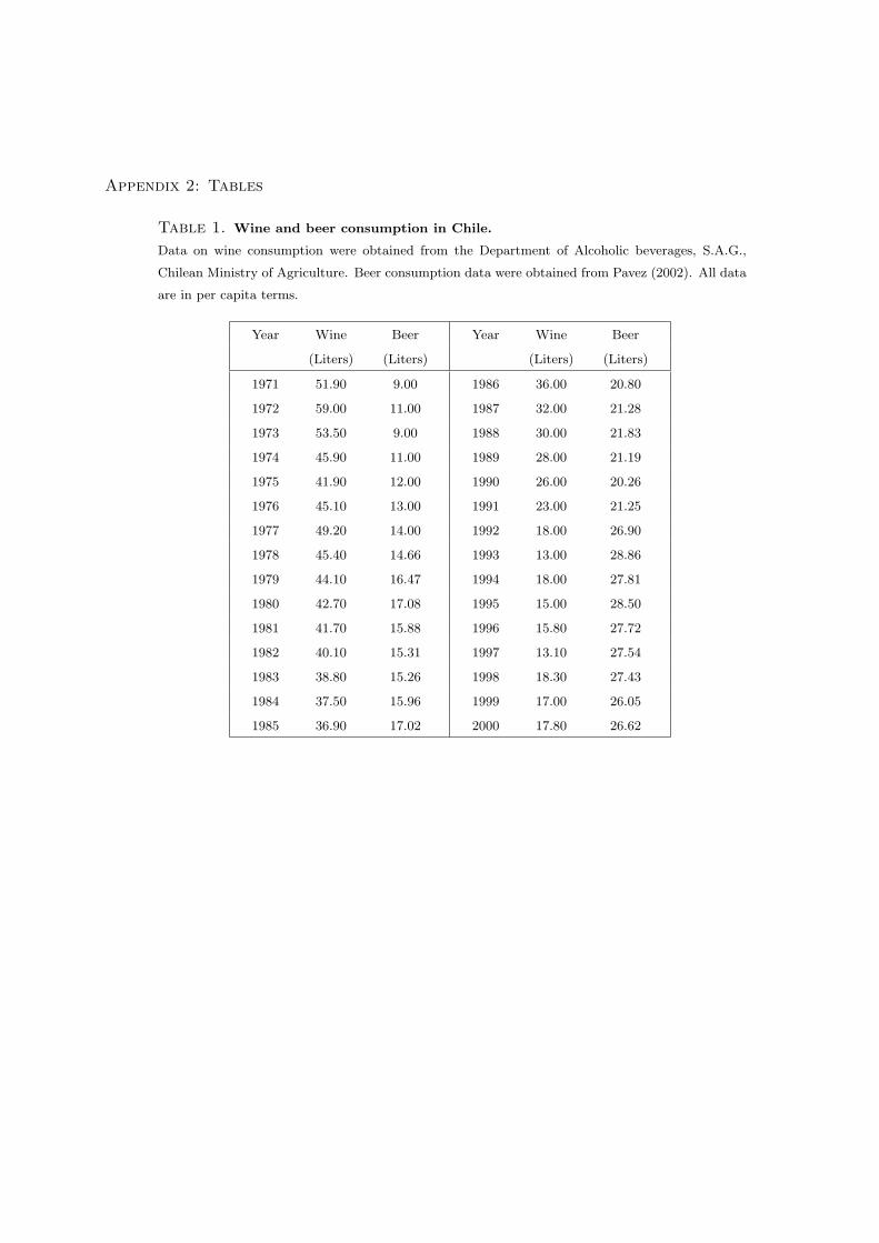
Table 1. Wine and beer consumption in Chile.
Data on wine consumption were obtained from the Department of Alcoholic beverages, S.A.G.,
Chilean Ministry of Agriculture. Beer consumption data were obtained from Pavez (2002). All data
are in per capita terms.
Year Wine Beer Year Wine Beer
(Liters) (Liters) (Liters) (Liters)
1971 51.90 9.00 1986 36.00 20.80
1972 59.00 11.00 1987 32.00 21.28
1973 53.50 9.00 1988 30.00 21.83
1974 45.90 11.00 1989 28.00 21.19
1975 41.90 12.00 1990 26.00 20.26
1976 45.10 13.00 1991 23.00 21.25
1977 49.20 14.00 1992 18.00 26.90
1978 45.40 14.66 1993 13.00 28.86
1979 44.10 16.47 1994 18.00 27.81
1980 42.70 17.08 1995 15.00 28.50
1981 41.70 15.88 1996 15.80 27.72
1982 40.10 15.31 1997 13.10 27.54
1983 38.80 15.26 1998 18.30 27.43
1984 37.50 15.96 1999 17.00 26.05
1985 36.90 17.02 2000 17.80 26.62
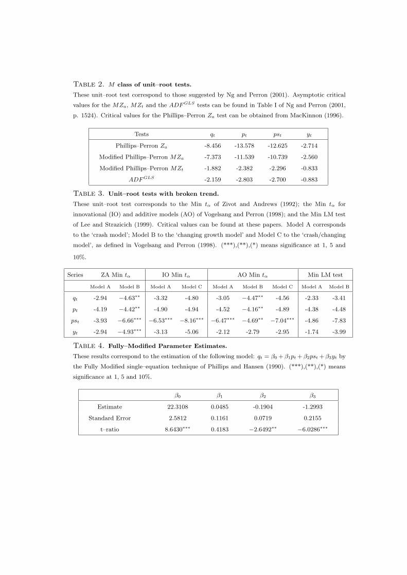
Table 2. M class of unit–root tests.
These unit–root test correspond to those suggested by Ng and Perron (2001). Asymptotic critical
values for the MZa, MZt and the ADF GLS tests can be found in Table I of Ng and Perron (2001,
p. 1524). Critical values for the Phillips–Perron Za test can be obtained from MacKinnon (1996).
Tests qt pt pst yt
Phillips–Perron Za -8.456 -13.578 -12.625 -2.714
Modified Phillips–Perron MZa -7.373 -11.539 -10.739 -2.560
Modified Phillips–Perron MZt -1.882 -2.382 -2.296 -0.833
ADF GLS -2.159 -2.803 -2.700 -0.883
Table 3. Unit–root tests with broken trend.
These unit–root test corresponds to the Min tα of Zivot and Andrews (1992); the Min tα for
innovational (IO) and additive models (AO) of Vogelsang and Perron (1998); and the Min LM test
of Lee and Strazicich (1999). Critical values can be found at these papers. Model A corresponds
to the ‘crash model’; Model B to the ‘changing growth model’ and Model C to the ‘crash/changing
model’, as defined in Vogelsang and Perron (1998). (***),(**),(*) means significance at 1, 5 and
10%.
Series ZA Min tα IO Min tα AO Min tα Min LM test
Model A Model B Model A Model C Model A Model B Model C Model A Model B
qt -2.94 −4.63∗∗ -3.32 -4.80 -3.05 −4.47∗∗ -4.56 -2.33 -3.41
pt -4.19 −4.42∗∗ -4.90 -4.94 -4.52 −4.16∗∗ -4.89 -4.38 -4.48
pst -3.93 −6.66∗∗∗ −6.53∗∗∗ −8.16∗∗∗ −6.47∗∗∗ −4.69∗∗ −7.04∗∗∗ -4.86 -7.83
yt -2.94 −4.93∗∗∗ -3.13 -5.06 -2.12 -2.79 -2.95 -1.74 -3.99
Table 4. Fully–Modified Parameter Estimates.
These results correspond to the estimation of the following model: qt = β0 + β1pt + β2pst + β3yt by
the Fully Modified single–equation technique of Phillips and Hansen (1990). (***),(**),(*) means
significance at 1, 5 and 10%.
β0 β1 β2 β3
Estimate 22.3108 0.0485 -0.1904 -1.2993
Standard Error 2.5812 0.1161 0.0719 0.2155
t–ratio 8.6430∗∗∗ 0.4183 −2.6492∗∗ −6.0286∗∗∗
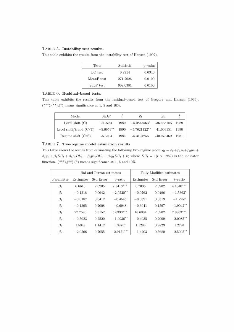
Table 5. Instability test results.
This table exhibits the results from the instability test of Hansen (1992).
Tests Statistic p–value
LC test 0.9214 0.0340
MeanF test 271.2026 0.0100
SupF test 908.0381 0.0100
Table 6. Residual–based tests.
This table exhibits the results from the residual–based test of Gregory and Hansen (1996).
(***),(**),(*) means significance at 1, 5 and 10%.
Model ADF t Zt Zα t
Level shift (C) -4.9784 1989 −5.0843563∗ -36.468185 1989
Level shift/trend (C/T) −5.6959∗∗ 1990 −5.7621122∗∗ -41.003151 1990
Regime shift (C/S) -5.5404 1984 -5.3194256 -40.975469 1981
Table 7. Two-regime model estimation results
This table shows the results from estimating the following two–regime model qt = β0+β1pt+β2pst+
β3yt + β4DUt + β5ptDUt + β6pstDUt + β7ytDUt + ν; where DUt = 1(t > 1982) is the indicator
function. (***),(**),(*) means significance at 1, 5 and 10%.
Bai and Perron estimates Fully Modified estimates
Parameter Estimates Std Error t–ratio Estimates Std Error t–ratio
β0 6.6616 2.6205 2.5418∗∗∗ 8.7035 2.0902 4.1640∗∗∗
β1 −0.1318 0.0642 −2.0520∗∗ −0.0762 0.0496 −1.5363∗
β2 −0.0187 0.0412 −0.4545 −0.0391 0.0319 −1.2257
β3 −0.1395 0.2008 −0.6948 −0.3041 0.1597 −1.9042∗∗
β4 27.7596 5.5152 5.0333∗∗∗ 16.6804 2.0902 7.9803∗∗∗
β5 −0.5023 0.2520 −1.9936∗∗ −0.4035 0.2009 −2.0085∗∗
β6 1.5948 1.1412 1.3975∗ 1.1288 0.8823 1.2794
β7 −2.0566 0.7055 −2.9151∗∗∗ −1.4203 0.5680 −2.5005∗∗
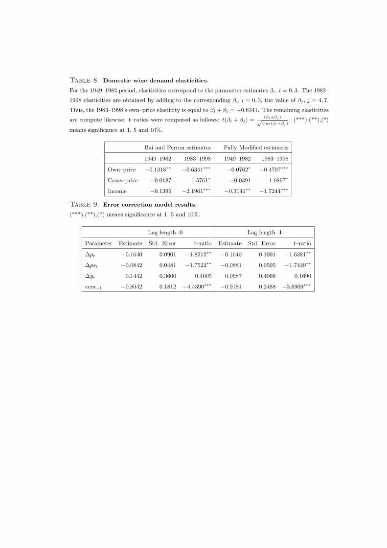
Table 8. Domestic wine demand elasticities.
For the 1949–1982 period, elasticities correspond to the parameter estimates βi, i = 0, 3. The 1983–
1998 elasticities are obtained by adding to the corresponding βi, i = 0, 3, the value of βj , j = 4, 7.
Thus, the 1983–1998’s own–price elasticity is equal to β1 +β5 = −0.6341. The remaining elasticities
are compute likewise. t–ratios were computed as follows: t(βi + βj) =(βi+βj)√
V ar(βi+βj). (***),(**),(*)
means significance at 1, 5 and 10%.
Bai and Perron estimates Fully Modified estimates
1949–1982 1983–1998 1949–1982 1983–1998
Own–price −0.1318∗∗ −0.6341∗∗∗ −0.0762∗ −0.4797∗∗∗
Cross–price −0.0187 1.5761∗ −0.0391 1.0897∗
Income −0.1395 −2.1961∗∗∗ −0.3041∗∗ −1.7244∗∗∗
Table 9. Error correction model results.
(***),(**),(*) means significance at 1, 5 and 10%.
Lag length :0 Lag length :1
Parameter Estimate Std. Error t–ratio Estimate Std. Error t–ratio
∆pt −0.1640 0.0901 −1.8212∗∗ −0.1640 0.1001 −1.6381∗∗
∆pst −0.0842 0.0481 −1.7522∗∗ −0.0881 0.0505 −1.7449∗∗
∆yt 0.1442 0.3600 0.4005 0.0687 0.4066 0.1690
ecm−1 −0.8042 0.1812 −4.4390∗∗∗ −0.9181 0.2488 −3.6909∗∗∗


![Pairs Trading, Convergence Trading, Cointegration - Freedocs.finance.free.fr/DOCS/Yats/cointegration-en[1].pdf · Pairs Trading, Convergence Trading, Cointegration ... ”Trying to](https://img.pdfslide.us/doc/110x75/5aad9ad77f8b9a9c2e8e8580/pairs-trading-convergence-trading-cointegration-1pdfpairs-trading-convergence.jpg)