Embed Size (px)
Citation preview
Structural Analysis of a Typical Trough
Bridge Using FEM
Master of Science Thesis in the Master’s Program Structural Engineering and
Building Performance Design
KLAS LUNDIN
ANDREAS MAGNANDER
Department of Civil and Environmental Engineering
Division of Structural Engineering
Concrete Structures
CHALMERS UNIVERSITY OF TECHNOLOGY
Göteborg, Sweden 2012
Master’s Thesis 2012:106

MASTER’S THESIS 2012:106
Structural Analysis of a Typical Trough Bridge Using FEM
Master of Science Thesis in the Master’s Program Structural Engineering and Building
Performance Design
KLAS LUNDIN
ANDREAS MAGNANDER
Department of Civil and Environmental Engineering
Division of Structural Engineering
Concrete Structures
CHALMERS UNIVERSITY OF TECHNOLOGY
Göteborg, Sweden 2012
Structural Analysis of a Typical Trough Bridge Using FEM
Master of Science Thesis in the Master’s Program Structural Engineering and
Building Performance Design
KLAS LUNDIN
ANDREAS MAGNANDER
© KLAS LUNDIN & ANDREAS MAGNANDER, 2012
Examensarbete / Institutionen för bygg- och miljöteknik,
Chalmers tekniska högskola 2012:106
Department of Civil and Environmental Engineering
Division of Structural Engineering
Concrete Structures
Chalmers University of Technology
SE-412 96 Göteborg
Sweden
Telephone: + 46 (0)31-772 1000
Cover:
Different FE-models of a trough bridge seen in ADINA User Interface. From upper
left: beam model, beam grillage model, combined model, shell model.
Chalmers Reproservice
Göteborg, Sweden 2012
I
Structural Analysis of a Typical Trough Bridge Using FEM
Master of Science Thesis in the Master’s Program Structural Engineering and Building
Performance Design
KLAS LUNDIN
ANDREAS MAGNANDER
Department of Civil and Environmental Engineering
Division of Structural Engineering
Concrete Structures
Chalmers University of Technology
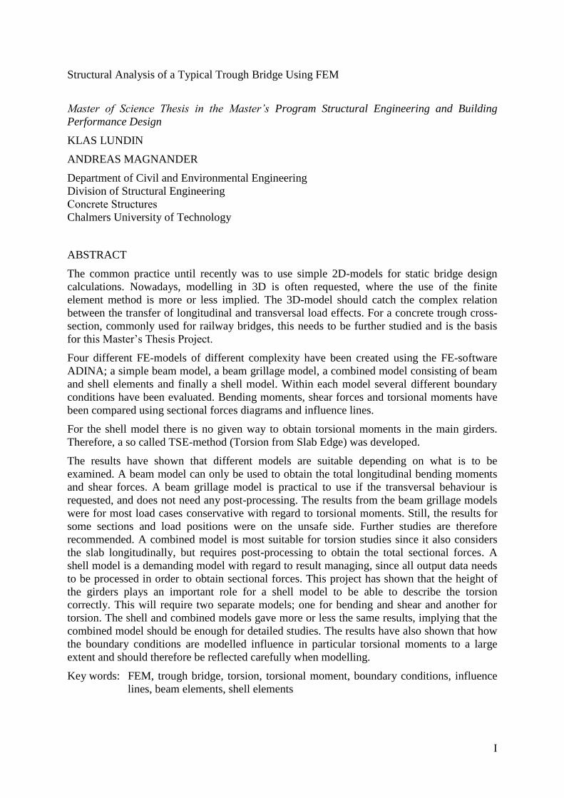
ABSTRACT
The common practice until recently was to use simple 2D-models for static bridge design
calculations. Nowadays, modelling in 3D is often requested, where the use of the finite
element method is more or less implied. The 3D-model should catch the complex relation
between the transfer of longitudinal and transversal load effects. For a concrete trough cross-
section, commonly used for railway bridges, this needs to be further studied and is the basis
for this Master’s Thesis Project.
Four different FE-models of different complexity have been created using the FE-software
ADINA; a simple beam model, a beam grillage model, a combined model consisting of beam
and shell elements and finally a shell model. Within each model several different boundary
conditions have been evaluated. Bending moments, shear forces and torsional moments have
been compared using sectional forces diagrams and influence lines.
For the shell model there is no given way to obtain torsional moments in the main girders.
Therefore, a so called TSE-method (Torsion from Slab Edge) was developed.
The results have shown that different models are suitable depending on what is to be
examined. A beam model can only be used to obtain the total longitudinal bending moments
and shear forces. A beam grillage model is practical to use if the transversal behaviour is
requested, and does not need any post-processing. The results from the beam grillage models
were for most load cases conservative with regard to torsional moments. Still, the results for
some sections and load positions were on the unsafe side. Further studies are therefore
recommended. A combined model is most suitable for torsion studies since it also considers
the slab longitudinally, but requires post-processing to obtain the total sectional forces. A
shell model is a demanding model with regard to result managing, since all output data needs
to be processed in order to obtain sectional forces. This project has shown that the height of
the girders plays an important role for a shell model to be able to describe the torsion
correctly. This will require two separate models; one for bending and shear and another for
torsion. The shell and combined models gave more or less the same results, implying that the
combined model should be enough for detailed studies. The results have also shown that how
the boundary conditions are modelled influence in particular torsional moments to a large
extent and should therefore be reflected carefully when modelling.
Key words: FEM, trough bridge, torsion, torsional moment, boundary conditions, influence
lines, beam elements, shell elements
II
Strukturanalys av en typisk trågbro med Finita Elementmetoden
Examensarbete inom mastersprogrammet Structural Engineering and Building Performance
Design
KLAS LUNDIN
ANDREAS MAGNANDER
Institutionen för bygg- och miljöteknik
Avdelningen för konstruktionsteknik
Betongbyggnad
Chalmers tekniska högskola
SAMMANFATTNING
Fram tills nyligen användes enkla 2D-modeller för att utföra statiska beräkningar vid
dimensionering av broar. Numera är modellering i 3D ofta efterfrågat, där finita
elementmetoden mer eller mindre är underförstådd som beräkningsmetod. En 3D-model ska
återge den komplexa relationen mellan transversell och longitudinell lastspridning på ett så
korrekt sätt som möjligt. För trågbroar, vanligen använda för järnvägsbroar, behövs detta
studeras närmare och ligger till grund för det här examensarbetet.
Fyra olika FE-modeller av olika komplexitet har skapats i FE-programet ADINA – en enkel
balkmodell, en balkrostmodell, en kombinerad modell bestående av både balk- och
skalelement samt en skalmodell. För varje modell har flera olika randvillkor använts och
utvärderats. Böjmoment, tvärkraft och vridmoment har jämförts mellan de olika randvillkorna
och modellerna med hjälp av snittkraftsdiagram och influenslinjer.
För skalmodellen finns det inget givet sätt att få ut vridmomenten i huvudbalkarna. Därför har
en metod, kallad TSE-metoden, utvecklats.
Resultatet har visat att olika modeller är lämpliga att använda beroende på vad som ska
undersökas. En balkmodell kan endast användas för att få ut totala böjmoment och
skjuvkrafter i longitudinell riktning. En balkrostmodell är praktisk att använda om
transversellt beteendet behöver undersökas, och behöver ingen extra bearbetning av resultatet.
Resultaten från balkrostmodellerna var för de flesta lastfall konservativa med avseende på
vridmoment. Däremot var resultat för vissa sektioner och lastplaceringar på osäker sida. Fler
undersökningar är därför att rekommendera. En kombinerad modell passar bäst för
vridmomentstudier eftersom den också beaktar plattans bidrag longitudinellt, men extra
bearbetning av resultat är nödvändig för att få ut de totala snittkrafterna. En skalmodell kräver
mycket efterarbete eftersom utdata måste bearbetas för att få ut några snittkrafter
överhuvudtaget. Detta projekt har visat att höjden på balkarna är viktig för att få en korrekt
beskrivning av vridningen i en skalmodell. Detta innebär att två modeller krävs – en för
böjning och skjuvning samt en för vridning. Eftersom skalmodellerna och de kombinerade
modellerna gav mer eller mindre samma resultat bör den kombinerade modellen vara fullt
tillräcklig för detaljerade studier. Resultaten visade även att hur randvillkoren modelleras
påverkar speciellt vridmomentet i stor utsträckning och bör därför tänkas igenom noggrant i
samband med modellering.
Nyckelord: FEM, trågbro, vridning, vridmoment, randvillkor, influenslinjer, balkelement,
skalelement
CHALMERS Civil and Environmental Engineering, Master’s Thesis 2012:106 III
Contents
ABSTRACT I
SAMMANFATTNING II
CONTENTS III
PREFACE IX
NOTATIONS X
1 INTRODUCTION 1
1.1 Background 1
1.2 Aim 1
1.3 Limitations 2
1.4 Method 2
1.5 Outline of the report 3
2 PROBLEM DESCRIPTION 4
2.1 General description of a trough bridge structure 4
2.2 Transition from 2D- to 3D-models 5
2.3 Distribution of load effects 6
2.4 Torsion in main girders 7
3 STRUCTURAL FINITE ELEMENT MODELLING AND
IMPLEMENTED THEORIES 10
3.1 Beam theory 10
3.1.1 Euler-Bernoulli beam theory 12 3.1.2 Timoshenko beam theory 13
3.2 Plate theory 13 3.2.1 Kirchhoff-Love plate theory 14
3.2.2 Reissner-Mindlin plate theory 15
3.3 Torsion theory 15 3.3.1 Saint-Venant torsion 17
3.3.2 Vlasov torsion 18
3.4 Structural finite element modelling 18 3.4.1 General description of the finite element method (FEM) 19 3.4.2 Approximations and shape functions 19 3.4.3 Isoparametric formulation 21
3.4.4 Finite element meshing 22 3.4.5 Integration points 23 3.4.6 Locking effects of finite elements 25
3.4.7 Formulation of finite elements in structural mechanics 25 3.4.7.1 Displacement-based formulation 25 3.4.7.2 Mixed finite element formulations 25
CHALMERS, Civil and Environmental Engineering, Master’s Thesis 2012:106 IV
3.4.8 Structural finite elements 26 3.4.8.1 Beam finite elements 28 3.4.8.2 Plate finite elements 29 3.4.8.3 Shell finite elements 29
3.5 Structural element modelling in ADINA 30 3.5.1 ADINA – a finite element software 30 3.5.2 Structural finite elements in ADINA 30
3.5.2.1 Beam elements 30 3.5.2.2 Shell elements 33
3.5.2.3 Rigid link 36
3.6 Influence lines 36
4 DESCRIPTION OF THE FE-ANALYSES 39
4.1 System models 39 4.1.1 Geometry, material and loading 39 4.1.2 System models 40
4.2 Deflection and rotational stiffness study 44 4.2.1 A girder modelled with shell elements 44
4.2.2 Trough models with inclined rigid links 47 4.2.3 Trough models with u-shaped cross-section 52 4.2.4 Comparison of combined and shell trough models 54
4.3 FE-models 56
4.3.1 Boundary conditions 56 4.3.2 Moving load – load stepping 58 4.3.3 Stiff elements 59
4.3.4 Longitudinal 2D beam element model 59 4.3.4.1 Input data 59
4.3.4.2 Description of model 60 4.3.4.3 Output data 61
4.3.5 3D beam grillage model 61
4.3.5.1 Input data 61 4.3.5.2 Description of models 62 4.3.5.3 Refined beam grillage model 63
4.3.5.4 Output data 64 4.3.6 Combined beam and shell elements model 64
4.3.6.1 Input data 64 4.3.6.2 Description of models 65
4.3.6.3 Refined combined model 66 4.3.6.4 Output data 66
4.3.7 Shell model 66 4.3.7.1 Input data 66 4.3.7.2 Description of models 67
4.3.7.3 Refined shell models 68 4.3.7.4 Output data 68
4.4 Managing of results – post-processing 68
4.4.1 Sign conventions 68 4.4.2 Outdata from beam elements 69
CHALMERS Civil and Environmental Engineering, Master’s Thesis 2012:106 V
4.4.3 Sectional forces for the combined and shell models 70 4.4.3.1 Shear forces for the combined and shell models 70 4.4.3.2 Bending moments for the combined and shell models 71 4.4.3.3 Torsional moments for the shell model - the TSE-
method 75 4.4.3.4 Methodology of the TSE-method 78
4.4.4 Influence lines 83 4.4.4.1 Fixed influence line 83 4.4.4.2 Corrected influence line 84
4.4.4.3 Procedures used to create influence lines 87
5 RESULTS FROM THE FE-ANALYSES 94
5.1 Analytical solution of longitudinal bending moment and shear
force distribution for the entire section 94
5.2 Comparison of FE-models 96 5.2.1 Bending moment 96 5.2.2 Shear force 103
5.2.3 Torsional moment 111
5.3 Comparison of boundary conditions 119 5.3.1 Beam grillage model 119 5.3.2 Combined model 128
5.3.3 Shell model 129
6 DISCUSSION ABOUT THE FE-ANALYSES 132
6.1 Evaluation of FE-models 132 6.1.1 Managing of results and practical aspects 132
6.1.2 Modelling issues 133 6.1.3 Torsional moment results from the models 134
6.2 Evaluation of boundary conditions 135
7 CONCLUSIONS AND SUGGESTIONS FOR FURTHER
INVESTIGATIONS 136
7.1 Conclusions 136
7.2 Suggestions for further investigations 137
8 REFERENCES 138
APPENDIX A DERIVATIONS A-1
A.1 Beam theory A-1
A.1.1 Euler-Bernoulli beam theory A-1 A.1.2 Timoshenko beam theory A-2
A.2 Plate theory A-3
A.2.1 Kirchoff-Love plate theory A-3 A.2.2 Reissner-Mindlin plate theory A-4
CHALMERS, Civil and Environmental Engineering, Master’s Thesis 2012:106 VI
A.3 Saint-Venant torsion theory A-4
APPENDIX B CALCULATIONS B-1
B.1 Cross-sectional constants B-1
B.2 Analytical bending moment and shear force diagrams B-3
B.3 Analytical solutions for the girder study B-5 B.3.1 Deflection due to bending B-6 B.3.2 Angle of twist due to an applied torque B-6
APPENDIX C FE-RESULTS – COMPARISONS OF FE-MODELS C-1
C.1 BC2 models C-1 C.1.1 Sectional force diagrams C-1
C.1.1.1 Girder C-1
C.1.1.2 Slab C-3 C.1.1.3 Entire section C-4
C.1.2 Influence lines C-5 C.1.2.1 Girder C-5
C.1.2.2 Slab C-7 C.1.2.3 Entire section C-8
C.2 BC5 models C-9 C.2.1 Sectional force diagrams C-9
C.2.1.1 Girder C-9 C.2.1.2 Slab C-11
C.2.1.3 Entire section C-12 C.2.2 Influence lines C-13
C.2.2.1 Girder C-13
C.2.2.2 Slab C-15 C.2.2.3 Entire section C-16
C.3 U-models C-17
C.3.1 Sectional force diagrams C-17 C.3.1.1 Girder C-17
C.3.1.2 Slab C-19 C.3.1.3 Entire section C-20
C.3.2 Influence lines C-21 C.3.2.1 Girder C-21 C.3.2.2 Slab C-23
C.3.2.3 Entire section C-24
C.4 Refined models C-25
C.4.1 Refined beam grillage model (BC2) C-25 C.4.1.1 Sectional force diagrams C-25 C.4.1.2 Influence lines C-26
C.4.2 Refined combined model (BC2) C-27 C.4.2.1 Sectional force diagrams C-27
C.4.2.2 Influence lines C-31
C.4.3 Refined shell models (UA and UB) C-35 C.4.3.1 Sectional force diagrams C-35 C.4.3.2 Influence lines C-35
CHALMERS Civil and Environmental Engineering, Master’s Thesis 2012:106 VII
APPENDIX D FE-RESULTS – COMPARISONS OF BOUNDARY
CONDITIONS D-1
D.1 Beam grillage models D-1 D.1.1 Sectional force diagrams D-1
D.1.2 Influence lines D-2
D.2 Combined models D-4 D.2.1 Sectional force diagrams D-4
D.2.1.1 Girder D-4 D.2.1.2 Slab D-6
D.2.1.3 Entire section D-7 D.2.2 Influence lines D-8
D.2.2.1 Girder D-8 D.2.2.2 Slab D-10 D.2.2.3 Entire section D-11
D.3 Shell models D-12 D.3.1 Sectional force diagrams D-12
D.3.1.1 Girder D-12 D.3.1.2 Slab D-14 D.3.1.3 Entire section D-15
D.3.2 Influence lines D-16
D.3.2.1 Girder D-16 D.3.2.2 Slab D-18
D.3.2.3 Entire section D-19
APPENDIX E MATLAB-PROGRAMS FOR POST-PROCESSING E-1
E.1 Combined models E-1 E.1.1 MATLAB-code to create sectional force diagrams E-1
E.1.2 MATLAB-code to create influence lines E-4
E.2 Shell models E-6 E.2.1 MATLAB-code to create sectional force diagrams
(bending moment and shear force) E-6 E.2.2 MATLAB-code to create influence lines (bending
moment and shear force) E-10
E.2.3 MATLAB-code to create sectional force diagrams and
influence lines with the TSE-method (torsional moment) E-13
APPENDIX F ADINA-IN COMMAND FILES F-1
F.1 Time function F-1
F.2 Beam model F-2
F.3 Beam grillage models F-3 F.3.1 BC2 model F-3 F.3.2 BC5 model F-4 F.3.3 U-model F-5
F.3.4 Refined model (BC2) F-6
F.4 Combined models F-7 F.4.1 BC2 model F-7
CHALMERS, Civil and Environmental Engineering, Master’s Thesis 2012:106 VIII
F.4.2 BC5 model F-8 F.4.3 U-model F-9 F.4.4 Refined model (BC2) F-10
F.5 Shell models F-11
F.5.1 UA-model F-11 F.5.2 UB-model F-12 F.5.3 Refined model (UA) F-13 F.5.4 Refined model (UB) F-14
APPENDIX G ADINA-PLOT COMMAND FILES G-1
G.1 Beam model G-1
G.2 Beam grillage models G-1
G.2.1 BC2, BC5 and the U-models G-1 G.2.2 Refined model G-1
G.3 Combined models G-2 G.3.1 BC2 and BC5 models G-2
G.3.2 U-model G-3 G.3.3 Refined model G-4
G.4 Shell models G-5 G.4.1 UA- and UB-model G-5 G.4.2 Refined models (only torsional moment) G-6

CHALMERS Civil and Environmental Engineering, Master’s Thesis 2012:106 IX
Preface
In this Master’s Thesis project the finite element method has been used in order to examine
how a trough bridge best can be modelled. The project has been carried out as a cooperation
between REINERTSEN Sverige AB and Chalmers University of Technology. The project
was completed between January 2012 and June 2012 at REINERTSEN’s office in
Gothenburg.
From REINERTSEN we would like to thank our main supervisor M. Sc. Ginko Georgiev for
great support along the project, always giving constructive feedback and sharing valuable
thoughts. Ph. D. Morgan Johansson, supporting supervisor, has also been of great help during
the project giving input and feedback. From Chalmers we thank our examiner Professor Björn
Engström for the engagement and valuable feedback.
Klas Lundin & Andreas Magnander
Göteborg, June 2012
CHALMERS, Civil and Environmental Engineering, Master’s Thesis 2012:106 X
Notations
Roman upper case letters
Area
Width
Young’s modulus
Nodal force in i direction
Shear modulus
Height
Integration weight in point i
Moment of inertia around i
Torsion constant
Length
Bending moment
Nodal moment around i-axis
Axial force
Shape function matrix
Shape function in node i
Concentrated load
Reaction nodal force in i direction
Reaction nodal moment around i-axis
Reaction torsional moment
Statical moment
Torsional moment or torque
Shear force
Global x-coordinate vector
Global y-coordinate vector
Roman lower case letters
Eccentricity
Bending moment per meter in i direction
Distributed load per meter
Thickness
Displacement
Approximated displacement
CHALMERS Civil and Environmental Engineering, Master’s Thesis 2012:106 XI
Displacement in node i
Displacement in x direction
Displacement in y direction
Displacement in z direction
Approximated displacement in node i
Shear force per meter in i direction
Displacement in z direction
Greek lower case letters
Angle
Constant parameter
Shear strain in ij direction
Deflection due to bending
Normal strain in ii direction
Rate of twist
Rotation around i-axis
Poisson’s ratio
Integration point at i
Normal stress in ii direction
Shear stress in ij direction
Shear stress due to Saint-Venant torsion
Angle of twist

CHALMERS, Civil and Environmental Engineering, Master’s Thesis 2012:106 1
1 Introduction
1.1 Background
Finite element analyses have in the last years increased considerably in the field of bridge
design. The method is powerful to perform accurate calculations of how a structure will
behave during its service life. However, an advanced finite element model is complex to work
with and the results can be hard to interpret and manage. Hence, a less complicated model,
which still represents a realistic structural response, may therefore be preferred in practice.
Previously, the most common way to model bridges has been in 2D with classical beam
theory. Using this approach the structure was analysed separately in longitudinal (primary
load transfer along the bridge spans) and transversal directions (secondary load transfer).
Nowadays, modelling in 3D is often requested, where the use of the finite element method is
more or less implied. The 3D-models should be able to represent the complex interaction
between the transfer of longitudinal and transversal load effects. For a concrete trough cross-
section, commonly used for railway bridges, the interaction needs to be further studied. The
3D-model can be established in different ways, but each model has its limitations and
advantages.
For a structure with trough cross-section the load effects from the traffic loads are distributed
in both longitudinal and transversal directions by the rail and the sleepers, through the ballast
and into the bridge slab. The load effects are then often chosen to be distributed in the
transverse direction to the two outer parts of the cross-sections, the main girders, and then
finally to the supports. Due to compatibility, the transverse bending introduces torsion in the
main girders. The load effect distribution in the slab and the rotational stiffness of the main
girders are therefore of interest. The implementation of this in the finite element method
together with the specific loading, i.e. moving loads, is the basis for this master thesis project.
1.2 Aim
The overall aim of this project was to investigate how a bridge with a concrete trough cross-
section can be represented in a 3D finite element model. Three main questions were identified
for the investigation.
What type of FE-model is best suited for a concrete bridge with a trough cross-
section? What are the limitations/disadvantages and advantages for each model?
Possible models that were studied:
o 2D beam model with longitudinal beam elements.
o 3D beam grillage, where the main girders are described by beam elements in
longitudinal direction and the bridge slab by evenly spaced beam elements in
transversal direction.
o 3D combined model with beam and shell elements, where the main girders are
described by beam elements and the bridge slab by shell elements.
o 3D shell model with shell elements for both the main girders and the bridge
slab.
How should the boundary conditions be chosen for the structure? There are several
different ways to apply boundary conditions. In this project different possibilities were
examined and evaluated.
CHALMERS, Civil and Environmental Engineering, Master’s Thesis 2012:106 2
How will torsional moments in the main girders be described by the different models
and what impact will the boundary conditions have on torsion?
1.3 Limitations
The project has been carried out using linear elastic analysis. Nonlinear analysis could have
been of interest to study the response of concrete trough bridges, but has not been covered in
this project. Influence of cracking and redistribution in the concrete was not considered, and
full compatibility between cross-section parts was assumed. The orthotropic behaviour due to
reinforcement in a bridge slab was not considered, but was modelled with isotropic material
property.
A two span trough bridge was studied with typical spans and cross-sectional dimensions.
Other dimensions, number of supports and spans were not investigated. In this bridge, only
the mid support and mid span section were studied. The results were limited to consider three
different boundary conditions.
Loading were assumed to be described by a concentrated load applied in the middle of the
cross-section. The end walls were simplified by using assumed boundary conditions.
ADINA is the only FE-software considered in this project when using FEM of the trough
bridge. Moreover, the used version of ADINA had a limitation of 900 nodes; only for some of
the FE-analyses a version with no node limitation was used.
1.4 Method
A literature study has been carried out in order to increase the knowledge of finite element
modelling. Especially the finite element method, theory behind torsion, beams, plates and
shells have been studied and their implementations in the used FE-software. The purposes of
these studies were mainly that the chosen models were created correctly and to interpret and
analyse the results. To handle moving loads a typical method is to use and create influence
lines; this has as well been studied.
The FE-models that were analysed are a longitudinal beam model, 3D beam grillage model,
combined model and shell model. All models were created with the same three different
boundary conditions in the finite element software ADINA.
The results are presented in sectional force diagrams and influence lines diagrams. Due to
limited managing of result capability in the FE-software, the results from the different FE-
models were extracted and imported in Excel where the diagrams have been created. The
combined and shell models needed extra post-processing to calculate the sectional forces, and
therefore certain MATLAB-programs were created. The results from the programs were then
again imported in Excel to create the diagrams.
In order to calculate the torsional moments in the main girders modelled with shell elements a
TSE-method was developed, which was implemented in a MATLAB-program where the
torsional moments were calculated. These results were then as well imported in Excel to
create the torsional moment diagrams and influence lines.
Essential for the TSE-method to work properly is that the rotational stiffness, of the main
girders modelled with shell elements, is described properly. In order to investigate how the
choice of mesh density affected the results from shell elements, a stiffness and convergence
study has been carried out.

CHALMERS, Civil and Environmental Engineering, Master’s Thesis 2012:106 3
All results from the different FE-models has been compared and analysed by using sectional
force diagrams and influence lines in order to evaluate the behaviours and to study
differences.
1.5 Outline of the report
Chapter 2: In detail problem description.
Chapter 3: Presentation of theories used in the project. The aim of this chapter was to
increase the understanding of finite element modelling, with emphasis of theories
implemented in ADINA. Theory regarding influence lines is also presented.
Chapter 4: Description of the FE-analyses. This chapter includes description of the studied
through bridge, the different models and boundary conditions that were studied. In
the last section explanations of how the results were obtained is included.
Chapter 5: Presentation of the results. The results are discussed and presented by
comparisons, using sectional force diagrams and influence lines.
Chapter 6: A further and summarised discussion of the results. The discussion is divided into
differences between the FE-models and the boundary conditions.
Chapter 7: Conclusions drawn from this project and suggestions for further investigations.
CHALMERS, Civil and Environmental Engineering, Master’s Thesis 2012:106 4
2 Problem description
When analysing and designing a concrete trough bridge, there are some important aspects that
have to be considered. Three major issues are the 2D to 3D transition, the distribution of load
effects and the torsion in the main girders. These are described more in detail in this chapter.
2.1 General description of a trough bridge structure
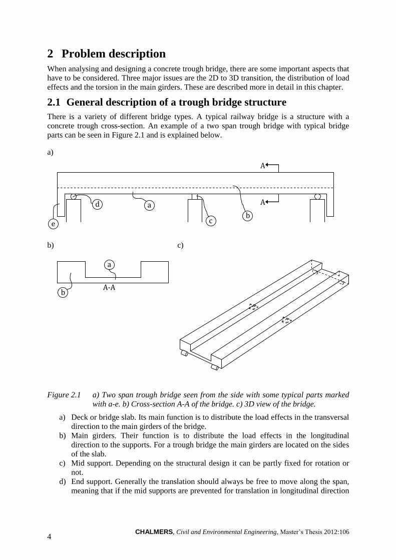
There is a variety of different bridge types. A typical railway bridge is a structure with a
concrete trough cross-section. An example of a two span trough bridge with typical bridge
parts can be seen in Figure 2.1 and is explained below.
a)
a d
e c b
A
A
b)
b A-A
a
c)
Figure 2.1 a) Two span trough bridge seen from the side with some typical parts marked
with a-e. b) Cross-section A-A of the bridge. c) 3D view of the bridge.
a) Deck or bridge slab. Its main function is to distribute the load effects in the transversal
direction to the main girders of the bridge.
b) Main girders. Their function is to distribute the load effects in the longitudinal
direction to the supports. For a trough bridge the main girders are located on the sides
of the slab.
c) Mid support. Depending on the structural design it can be partly fixed for rotation or
not.
d) End support. Generally the translation should always be free to move along the span,
meaning that if the mid supports are prevented for translation in longitudinal direction
CHALMERS, Civil and Environmental Engineering, Master’s Thesis 2012:106 5
a roll support is recommended at the adjacent end supports. Internal restraint should
always be considered and avoided, if possible, when using concrete.
e) End wall of the bridge. It contributes to the stability of the bridge in the horizontal
direction, and resists loads from accelerating or breaking vehicles. An effect from the
end walls is that they prevent the main girders from rotating around their longitudinal
axes.
In order to make the analyses practical, the structure must be simplified to an idealised static
model. This model can then be described by an FE-model. These model simplifications often
results in many assumptions that have to be correct and realistic. The bridge parts presented
above can be modelled in many different ways and with different boundary conditions. It is
important to be aware of the consequences the choice of model type and boundary conditions
will have for the final result of the FE-analysis.
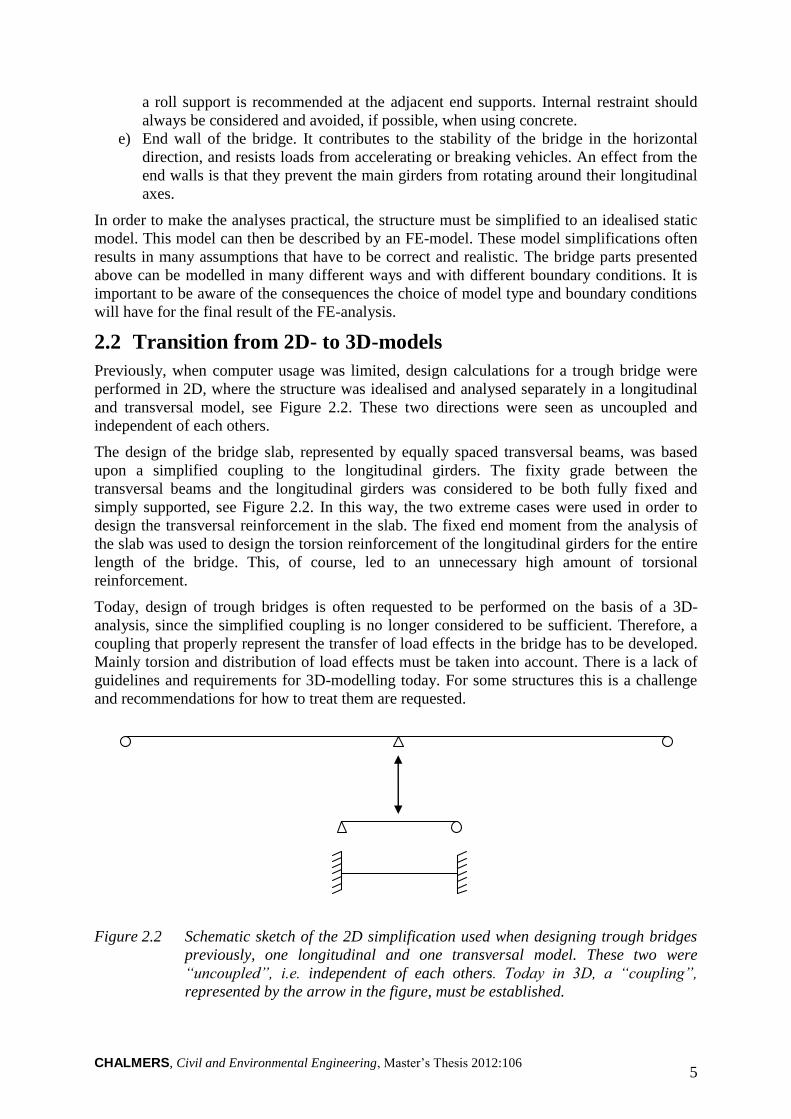
2.2 Transition from 2D- to 3D-models
Previously, when computer usage was limited, design calculations for a trough bridge were
performed in 2D, where the structure was idealised and analysed separately in a longitudinal
and transversal model, see Figure 2.2. These two directions were seen as uncoupled and
independent of each others.
The design of the bridge slab, represented by equally spaced transversal beams, was based
upon a simplified coupling to the longitudinal girders. The fixity grade between the
transversal beams and the longitudinal girders was considered to be both fully fixed and
simply supported, see Figure 2.2. In this way, the two extreme cases were used in order to
design the transversal reinforcement in the slab. The fixed end moment from the analysis of
the slab was used to design the torsion reinforcement of the longitudinal girders for the entire
length of the bridge. This, of course, led to an unnecessary high amount of torsional
reinforcement.
Today, design of trough bridges is often requested to be performed on the basis of a 3D-
analysis, since the simplified coupling is no longer considered to be sufficient. Therefore, a
coupling that properly represent the transfer of load effects in the bridge has to be developed.
Mainly torsion and distribution of load effects must be taken into account. There is a lack of
guidelines and requirements for 3D-modelling today. For some structures this is a challenge
and recommendations for how to treat them are requested.
Figure 2.2 Schematic sketch of the 2D simplification used when designing trough bridges
previously, one longitudinal and one transversal model. These two were
“uncoupled”, i.e. independent of each others. Today in 3D, a “coupling”,
represented by the arrow in the figure, must be established.
CHALMERS, Civil and Environmental Engineering, Master’s Thesis 2012:106 6
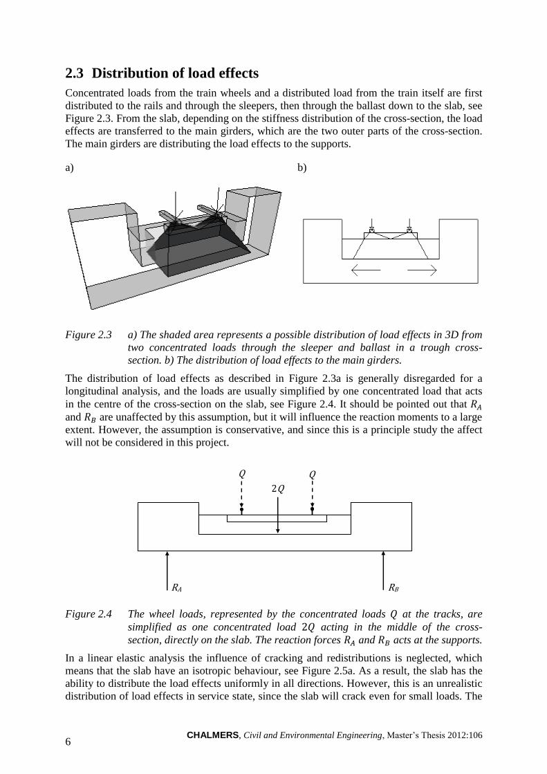
2.3 Distribution of load effects
Concentrated loads from the train wheels and a distributed load from the train itself are first
distributed to the rails and through the sleepers, then through the ballast down to the slab, see
Figure 2.3. From the slab, depending on the stiffness distribution of the cross-section, the load
effects are transferred to the main girders, which are the two outer parts of the cross-section.
The main girders are distributing the load effects to the supports.
a) b)
Figure 2.3 a) The shaded area represents a possible distribution of load effects in 3D from
two concentrated loads through the sleeper and ballast in a trough cross-
section. b) The distribution of load effects to the main girders.
The distribution of load effects as described in Figure 2.3a is generally disregarded for a
longitudinal analysis, and the loads are usually simplified by one concentrated load that acts
in the centre of the cross-section on the slab, see Figure 2.4. It should be pointed out that
and are unaffected by this assumption, but it will influence the reaction moments to a large
extent. However, the assumption is conservative, and since this is a principle study the affect
will not be considered in this project.
Q Q
2Q
RA RB
Figure 2.4 The wheel loads, represented by the concentrated loads at the tracks, are
simplified as one concentrated load acting in the middle of the cross-
section, directly on the slab. The reaction forces and acts at the supports.
In a linear elastic analysis the influence of cracking and redistributions is neglected, which
means that the slab have an isotropic behaviour, see Figure 2.5a. As a result, the slab has the
ability to distribute the load effects uniformly in all directions. However, this is an unrealistic
distribution of load effects in service state, since the slab will crack even for small loads. The
CHALMERS, Civil and Environmental Engineering, Master’s Thesis 2012:106 7
stiffness is influenced by the transversal reinforcement, i.e. redistribution of load effects
according to Figure 2.5b. This implies that a cracked slab will have an orthotropic behaviour.
a)
Q
b)
Q
Figure 2.5 Two slabs loaded with a concentrated load Q. a) A Slab with isotropic
behaviour, i.e. the load effects are distributed in all directions. b) An extreme
case of orthotropic behaviour, where no stiffness is assumed in the longitudinal
direction. This is the case for a beam grillage model.
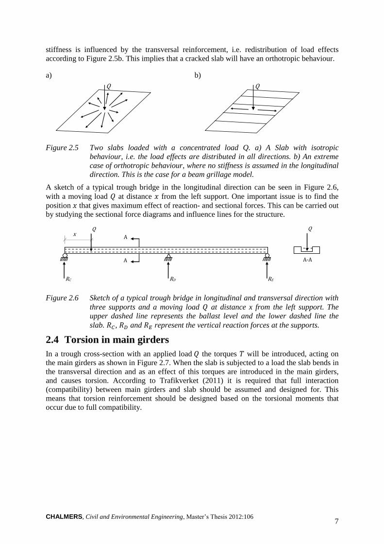
A sketch of a typical trough bridge in the longitudinal direction can be seen in Figure 2.6,
with a moving load at distance from the left support. One important issue is to find the
position that gives maximum effect of reaction- and sectional forces. This can be carried out
by studying the sectional force diagrams and influence lines for the structure.
A
Q
RC RE
A
x
RD
Q
A-A
Figure 2.6 Sketch of a typical trough bridge in longitudinal and transversal direction with
three supports and a moving load at distance x from the left support. The
upper dashed line represents the ballast level and the lower dashed line the
slab. , and represent the vertical reaction forces at the supports.
2.4 Torsion in main girders
In a trough cross-section with an applied load the torques will be introduced, acting on
the main girders as shown in Figure 2.7. When the slab is subjected to a load the slab bends in
the transversal direction and as an effect of this torques are introduced in the main girders,
and causes torsion. According to Trafikverket (2011) it is required that full interaction
(compatibility) between main girders and slab should be assumed and designed for. This
means that torsion reinforcement should be designed based on the torsional moments that
occur due to full compatibility.
CHALMERS, Civil and Environmental Engineering, Master’s Thesis 2012:106 8
T
T
Q
Figure 2.7 The torques T in the main girders, mainly due to compatibility and to some
extends also equilibrium, caused by the applied load Q.
The rotational stiffness of the cross-section varies along the bridge length depending on the
boundary conditions, see Figure 2.8. The boundary conditions can influence the torsional
moment in the main girders to a large extent and the stiffness variation longitudinally must be
taken into account.
T
Figure 2.8 Beam subjected to a torque . The rotational stiffness varies along the beam
and reaches its lowest value in the mid span.
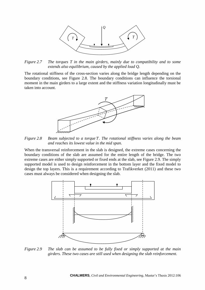
When the transversal reinforcement in the slab is designed, the extreme cases concerning the
boundary conditions of the slab are assumed for the entire length of the bridge. The two
extreme cases are either simply supported or fixed ends at the slab, see Figure 2.9. The simply
supported model is used to design reinforcement in the bottom layer and the fixed model to
design the top layers. This is a requirement according to Trafikverket (2011) and these two
cases must always be considered when designing the slab.
Figure 2.9 The slab can be assumed to be fully fixed or simply supported at the main
girders. These two cases are still used when designing the slab reinforcement.
CHALMERS, Civil and Environmental Engineering, Master’s Thesis 2012:106 9
This approach was used previously also to design the torsion reinforcement in the main
girders. The maximum reaction moment from the fixed case was used as an assumed torque
along the entire length of the bridge. This was done in order to cover all cases and to be on the
safe side. However, this approach led to an unnecessary high amount of reinforcement.
The transition from 2D to 3D implies that a coupling for torsion must be established, and the
simplification by using extreme cases can no longer be used. In other words, the torsional
moment distribution must be designed for as accurately as possible.
An important question is how to describe the transfer of load effects from the slab to the main
girders in the model. This will influence the applied torque on the girders and thus the torsion.
What is the effect on the slab, and what effect will there be on the main girders? This must be
investigated in order be able to design the torsion reinforcement.
Today there is no standard approach available for this problem and a lot of different methods
and models are used. The question is however, which solution is most correct and which one
is most appropriate to use in practice? One parameter that was studied is how well the
torsional- and bending moments are described by the different models, and how practical they
are to use.
CHALMERS, Civil and Environmental Engineering, Master’s Thesis 2012:106 10
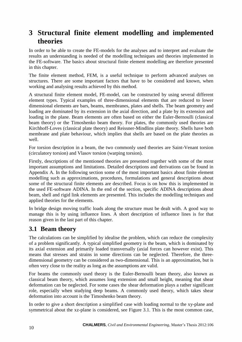
3 Structural finite element modelling and implemented
theories
In order to be able to create the FE-models for the analyses and to interpret and evaluate the
results an understanding is needed of the modelling techniques and theories implemented in
the FE-software. The basics about structural finite element modelling are therefore presented
in this chapter.
The finite element method, FEM, is a useful technique to perform advanced analyses on
structures. There are some important factors that have to be considered and known, when
working and analysing results achieved by this method.
A structural finite element model, FE-model, can be constructed by using several different
element types. Typical examples of three-dimensional elements that are reduced to lower
dimensional elements are bars, beams, membranes, plates and shells. The beam geometry and
loading are dominated by its extension in the axial direction, and a plate by its extension and
loading in the plane. Beam elements are often based on either the Euler-Bernoulli (classical
beam theory) or the Timoshenko beam theory. For plates, the commonly used theories are
Kirchhoff-Loves (classical plate theory) and Reissner-Mindlins plate theory. Shells have both
membrane and plate behaviour, which implies that shells are based on the plate theories as
well.
For torsion description in a beam, the two commonly used theories are Saint-Venant torsion
(circulatory torsion) and Vlasov torsion (warping torsion).
Firstly, descriptions of the mentioned theories are presented together with some of the most
important assumptions and limitations. Detailed descriptions and derivations can be found in
Appendix A. In the following section some of the most important basics about finite element
modelling such as approximations, procedures, formulations and general descriptions about
some of the structural finite elements are described. Focus is on how this is implemented in
the used FE-software ADINA. In the end of the section, specific ADINA descriptions about
beam, shell and rigid link elements are presented. This includes the modelling techniques and
applied theories for the elements.
In bridge design moving traffic loads along the structure must be dealt with. A good way to
manage this is by using influence lines. A short description of influence lines is for that
reason given in the last part of this chapter.
3.1 Beam theory
The calculations can be simplified by idealise the problem, which can reduce the complexity
of a problem significantly. A typical simplified geometry is the beam, which is dominated by
its axial extension and primarily loaded transversally (axial forces can however exist). This
means that stresses and strains in some directions can be neglected. Therefore, the three-
dimensional geometry can be considered as two-dimensional. This is an approximation, but is
often very close to the reality as long as the assumptions are valid.
For beams the commonly used theory is the Euler-Bernoulli beam theory, also known as
classical beam theory, which assumes long extension and small height, meaning that shear
deformation can be neglected. For some cases the shear deformation plays a rather significant
role, especially when studying deep beams. A commonly used theory, which takes shear
deformation into account is the Timoshenko beam theory.
In order to give a short description a simplified case with loading normal to the xy-plane and
symmetrical about the xz-plane is considered, see Figure 3.1. This is the most common case,
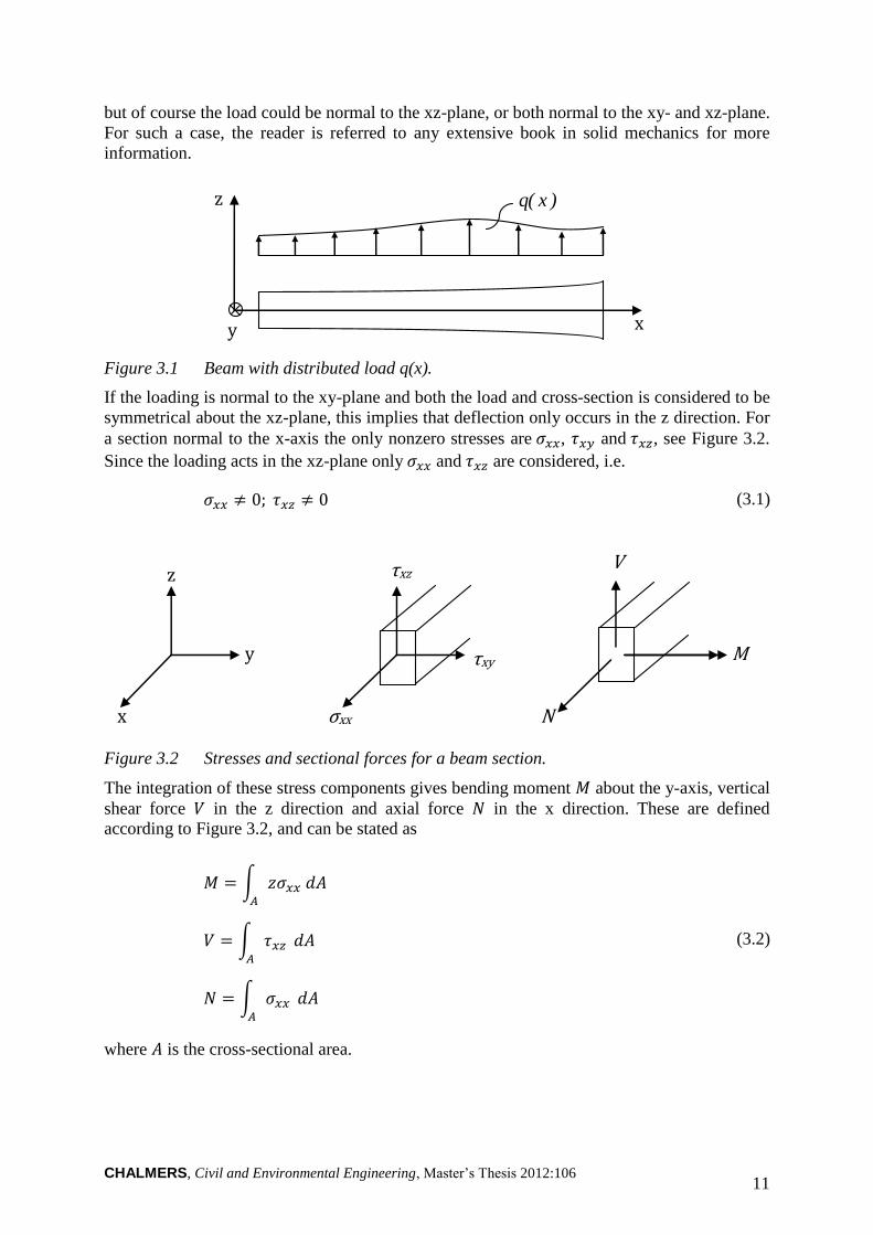
CHALMERS, Civil and Environmental Engineering, Master’s Thesis 2012:106 11
but of course the load could be normal to the xz-plane, or both normal to the xy- and xz-plane.
For such a case, the reader is referred to any extensive book in solid mechanics for more
information.
)x(q
x
z
y
Figure 3.1 Beam with distributed load q(x).
If the loading is normal to the xy-plane and both the load and cross-section is considered to be
symmetrical about the xz-plane, this implies that deflection only occurs in the z direction. For
a section normal to the x-axis the only nonzero stresses are , and , see Figure 3.2.
Since the loading acts in the xz-plane only and are considered, i.e.
(3.1)
z
x
y
τxz
τxy
σxx
V
M
N
Figure 3.2 Stresses and sectional forces for a beam section.
The integration of these stress components gives bending moment about the y-axis, vertical
shear force in the z direction and axial force in the x direction. These are defined
according to Figure 3.2, and can be stated as
∫
∫
∫
(3.2)
where is the cross-sectional area.
CHALMERS, Civil and Environmental Engineering, Master’s Thesis 2012:106 12
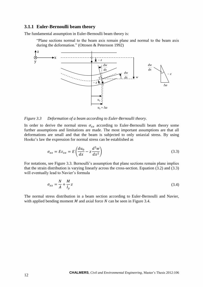
3.1.1 Euler-Bernoulli beam theory
The fundamental assumption in Euler-Bernoulli beam theory is:
“Plane sections normal to the beam axis remain plane and normal to the beam axis
during the deformation.” (Ottosen & Petersson 1992)
x
z
y
dx
dw
dx
dw dx
dw
uu Δ0
0u
z
z
w z
uΔ
Figure 3.3 Deformation of a beam according to Euler-Bernoulli theory.
In order to derive the normal stress according to Euler-Bernoulli beam theory some
further assumptions and limitations are made. The most important assumptions are that all
deformations are small and that the beam is subjected to only uniaxial stress. By using
Hooke’s law the expression for normal stress can be established as
(
) (3.3)
For notations, see Figure 3.3. Bernoulli’s assumption that plane sections remain plane implies
that the strain distribution is varying linearly across the cross-section. Equation (3.2) and (3.3)
will eventually lead to Navier’s formula
(3.4)
The normal stress distribution in a beam section according to Euler-Bernoulli and Navier,
with applied bending moment and axial force can be seen in Figure 3.4.
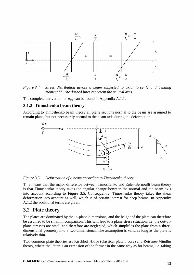
CHALMERS, Civil and Environmental Engineering, Master’s Thesis 2012:106 13
+ =
x
z
y
1zI
M
y
2zI
M
y
A
N
A
N
A
Nz
I
M
y
1
1z
2z
A
Nz
I
M
y
2
Figure 3.4 Stress distribution across a beam subjected to axial force and bending
moment . The dashed lines represent the neutral axes.
The complete derivation for can be found in Appendix A.1.1.
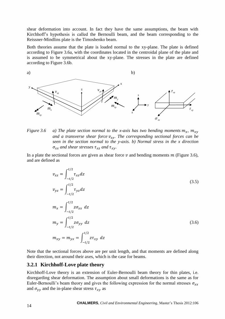
3.1.2 Timoshenko beam theory
According to Timoshenko beam theory all plane sections normal to the beam are assumed to
remain plane, but not necessarily normal to the beam axis during the deformation.
x
z
y
dx
dw z
z
z
0u
uu Δ0
w
uΔ
Figure 3.5 Deformation of a beam according to Timoshenko theory.
This means that the major difference between Timoshenko and Euler-Bernoulli beam theory
is that Timoshenko theory takes the angular change between the normal and the beam axis
into account according to Figure 3.5. Consequently, Timoshenko theory takes the shear
deformation into account as well, which is of certain interest for deep beams. In Appendix
A.1.2 the additional terms are given.
3.2 Plate theory
The plates are dominated by the in-plane dimensions, and the height of the plate can therefore
be assumed to be small in comparison. This will lead to a plane stress situation, i.e. the out-of-
plane stresses are small and therefore are neglected, which simplifies the plate from a three-
dimensional geometry into a two-dimensional. The assumption is valid as long as the plate is
relatively thin.
Two common plate theories are Kirchhoff-Love (classical plate theory) and Reissner-Mindlin
theory, where the latter is an extension of the former in the same way as for beams, i.e. taking
CHALMERS, Civil and Environmental Engineering, Master’s Thesis 2012:106 14
shear deformation into account. In fact they have the same assumptions, the beam with
Kirchhoff’s hypothesis is called the Bernoulli beam, and the beam corresponding to the
Reissner-Mindlins plate is the Timoshenko beam.
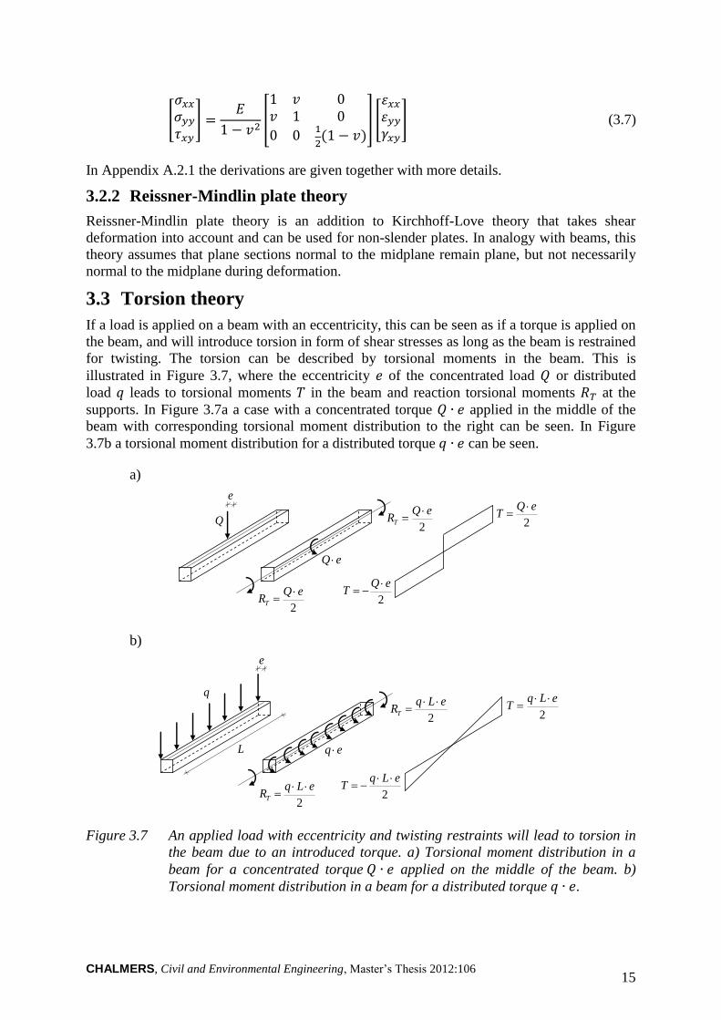
Both theories assume that the plate is loaded normal to the xy-plane. The plate is defined
according to Figure 3.6a, with the coordinates located in the centroidal plane of the plate and
is assumed to be symmetrical about the xy-plane. The stresses in the plate are defined
according to Figure 3.6b.
a)
y x
z
xym
xym xm
ym xzv yzv
b)
z
x
y
xz
xy
xx
Figure 3.6 a) The plate section normal to the x-axis has two bending moments ,
and a transverse shear force . The corresponding sectional forces can be
seen in the section normal to the y-axis. b) Normal stress in the x direction
and shear stresses and .
In a plate the sectional forces are given as shear force and bending moments (Figure 3.6),
and are defined as
∫
∫
(3.5)
∫
∫
∫
(3.6)
Note that the sectional forces above are per unit length, and that moments are defined along
their direction, not around their axes, which is the case for beams.
3.2.1 Kirchhoff-Love plate theory
Kirchhoff-Love theory is an extension of Euler-Bernoulli beam theory for thin plates, i.e.
disregarding shear deformation. The assumption about small deformations is the same as for
Euler-Bernoulli’s beam theory and gives the following expression for the normal stresses
and and the in-plane shear stress as
CHALMERS, Civil and Environmental Engineering, Master’s Thesis 2012:106 15
[
]
[
] [
] (3.7)
In Appendix A.2.1 the derivations are given together with more details.
3.2.2 Reissner-Mindlin plate theory
Reissner-Mindlin plate theory is an addition to Kirchhoff-Love theory that takes shear
deformation into account and can be used for non-slender plates. In analogy with beams, this
theory assumes that plane sections normal to the midplane remain plane, but not necessarily
normal to the midplane during deformation.
3.3 Torsion theory
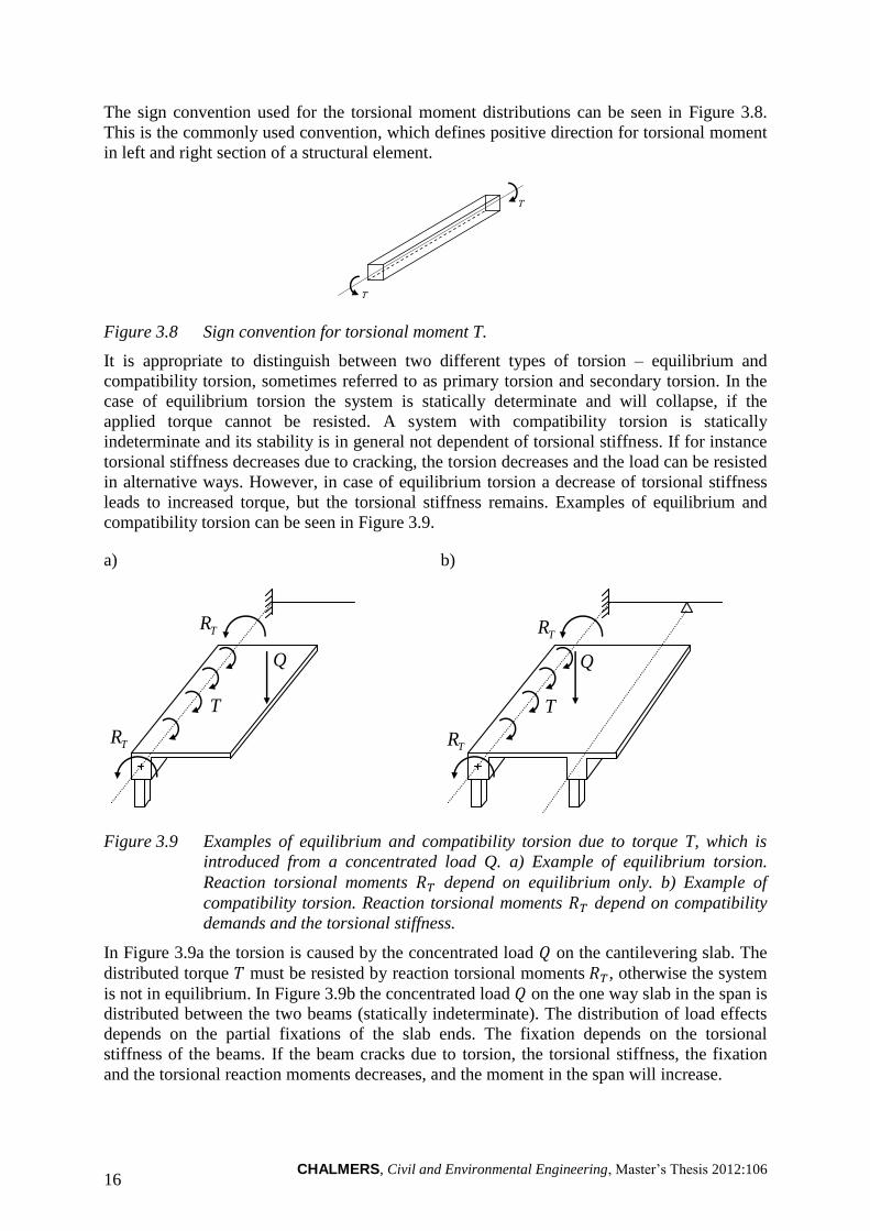
If a load is applied on a beam with an eccentricity, this can be seen as if a torque is applied on
the beam, and will introduce torsion in form of shear stresses as long as the beam is restrained
for twisting. The torsion can be described by torsional moments in the beam. This is
illustrated in Figure 3.7, where the eccentricity of the concentrated load or distributed
load leads to torsional moments in the beam and reaction torsional moments at the
supports. In Figure 3.7a a case with a concentrated torque applied in the middle of the
beam with corresponding torsional moment distribution to the right can be seen. In Figure
3.7b a torsional moment distribution for a distributed torque can be seen.
a)
Q
e
eQ
2
eQRT
2
eQRT
2
eQT
2
eQT
b)
q
e
2
eLqT
2
eLqRT
2
eLqRT
eq
2
eLqT
L
Figure 3.7 An applied load with eccentricity and twisting restraints will lead to torsion in
the beam due to an introduced torque. a) Torsional moment distribution in a
beam for a concentrated torque applied on the middle of the beam. b)
Torsional moment distribution in a beam for a distributed torque .
CHALMERS, Civil and Environmental Engineering, Master’s Thesis 2012:106 16
The sign convention used for the torsional moment distributions can be seen in Figure 3.8.
This is the commonly used convention, which defines positive direction for torsional moment
in left and right section of a structural element.
T
T
Figure 3.8 Sign convention for torsional moment T.
It is appropriate to distinguish between two different types of torsion – equilibrium and
compatibility torsion, sometimes referred to as primary torsion and secondary torsion. In the
case of equilibrium torsion the system is statically determinate and will collapse, if the
applied torque cannot be resisted. A system with compatibility torsion is statically
indeterminate and its stability is in general not dependent of torsional stiffness. If for instance
torsional stiffness decreases due to cracking, the torsion decreases and the load can be resisted
in alternative ways. However, in case of equilibrium torsion a decrease of torsional stiffness
leads to increased torque, but the torsional stiffness remains. Examples of equilibrium and
compatibility torsion can be seen in Figure 3.9.
a)
TR
TR
Q
T
b)
TR
TR
Q
T
Figure 3.9 Examples of equilibrium and compatibility torsion due to torque T, which is
introduced from a concentrated load Q. a) Example of equilibrium torsion.
Reaction torsional moments depend on equilibrium only. b) Example of
compatibility torsion. Reaction torsional moments depend on compatibility
demands and the torsional stiffness.
In Figure 3.9a the torsion is caused by the concentrated load on the cantilevering slab. The
distributed torque must be resisted by reaction torsional moments , otherwise the system
is not in equilibrium. In Figure 3.9b the concentrated load on the one way slab in the span is
distributed between the two beams (statically indeterminate). The distribution of load effects
depends on the partial fixations of the slab ends. The fixation depends on the torsional
stiffness of the beams. If the beam cracks due to torsion, the torsional stiffness, the fixation
and the torsional reaction moments decreases, and the moment in the span will increase.
CHALMERS, Civil and Environmental Engineering, Master’s Thesis 2012:106 17
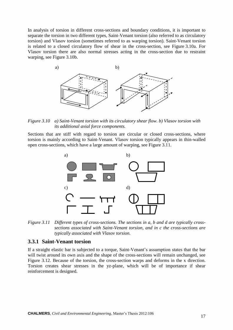
In analysis of torsion in different cross-sections and boundary conditions, it is important to
separate the torsion in two different types, Saint-Venant torsion (also referred to as circulatory
torsion) and Vlasov torsion (sometimes referred to as warping torsion). Saint-Venant torsion
is related to a closed circulatory flow of shear in the cross-section, see Figure 3.10a. For
Vlasov torsion there are also normal stresses acting in the cross-section due to restraint
warping, see Figure 3.10b.
a)
b)
Figure 3.10 a) Saint-Venant torsion with its circulatory shear flow. b) Vlasov torsion with
its additional axial force components.
Sections that are stiff with regard to torsion are circular or closed cross-sections, where
torsion is mainly according to Saint-Venant. Vlasov torsion typically appears in thin-walled
open cross-sections, which have a large amount of warping, see Figure 3.11.
a)
c)
b)
d)
Figure 3.11 Different types of cross-sections. The sections in a, b and d are typically cross-
sections associated with Saint-Venant torsion, and in c the cross-sections are
typically associated with Vlasov torsion.
3.3.1 Saint-Venant torsion
If a straight elastic bar is subjected to a torque, Saint-Venant’s assumption states that the bar
will twist around its own axis and the shape of the cross-sections will remain unchanged, see
Figure 3.12. Because of the torsion, the cross-section warps and deforms in the x direction.
Torsion creates shear stresses in the yz-plane, which will be of importance if shear
reinforcement is designed.
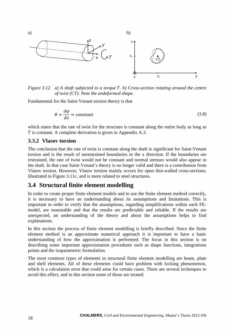
CHALMERS, Civil and Environmental Engineering, Master’s Thesis 2012:106 18
a)
x
y z
T
b)
CT 0z
z
0y x y
Figure 3.12 a) A shaft subjected to a torque . b) Cross-section rotating around the centre
of twist (CT). Note the undeformed shape.
Fundamental for the Saint-Venant torsion theory is that
(3.8)
which states that the rate of twist for the structure is constant along the entire body as long as
is constant. A complete derivation is given in Appendix A.3.
3.3.2 Vlasov torsion
The conclusion that the rate of twist is constant along the shaft is significant for Saint-Venant
torsion and is the result of unrestrained boundaries in the x direction. If the boundaries are
restrained, the rate of twist would not be constant and normal stresses would also appear in
the shaft. In that case Saint-Venant’s theory is no longer valid and there is a contribution from
Vlasov torsion. However, Vlasov torsion mainly occurs for open thin-walled cross-sections,
illustrated in Figure 3.11c, and is more related to steel structures.
3.4 Structural finite element modelling
In order to create proper finite element models and to use the finite element method correctly,
it is necessary to have an understanding about its assumptions and limitations. This is
important in order to verify that the assumptions, regarding simplifications within each FE-
model, are reasonable and that the results are predictable and reliable. If the results are
unexpected, an understanding of the theory and about the assumptions helps to find
explanations.
In this section the process of finite element modelling is briefly described. Since the finite
element method is an approximate numerical approach it is important to have a basic
understanding of how the approximation is performed. The focus in this section is on
describing some important approximation procedures such as shape functions, integrations
points and the isoparametric formulation.
The most common types of elements in structural finite element modelling are beam, plate
and shell elements. All of these elements could have problem with locking phenomenon,
which is a calculation error that could arise for certain cases. There are several techniques to
avoid this effect, and in this section some of those are treated.
CHALMERS, Civil and Environmental Engineering, Master’s Thesis 2012:106 19
3.4.1 General description of the finite element method (FEM)
The finite element method, FEM, is a useful technique to perform approximated numerical
calculations. The results can be numerically very accurate and detailed, even if the analysed
structure often is idealised to a significant extent.
The FEM approach starts by idealising a real problem into a mathematical model that is easy
to manage. The idealised model is then discretised from one continuous element into many
discrete elements, finite elements. In order to perform the numerical calculations the elements
have to be linked together and boundary conditions need to be defined. Depending on what
FE-software that is used, and what results that are obtained from the analyses, different
degrees of post-processing are required.
3.4.2 Approximations and shape functions
The exact displacement for an element in three dimensions can be described by the
approximation
(3.9)
where are constant parameters for the element. For a one-dimensional case the
approximated displacement can be described as
(3.10)
with nodal points and of order . The most common element descriptions for one-
dimensional shapes are linear and quadratic approximations, see Figure 3.13.
a)
x
u
j i
xu~ 21
ix jx
iu
ju
b)
x
u
j i k
ix jx kx
iu
ju ku
2
321 xxu~
Figure 3.13 One-dimensional element with exact nodal displacements , and and the
approximated displacement . a) Linear description. b) Quadratic description.
The displacements are often described for each nodal point and for the simplest case, when
having linear description and nodal points according to Figure 3.13a, the displacement is
divided as
(3.11)
CHALMERS, Civil and Environmental Engineering, Master’s Thesis 2012:106 20
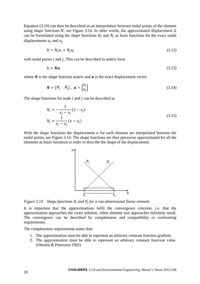
Equation (3.10) can then be described as an interpolation between nodal points of the element
using shape functions , see Figure 3.14. In other words, the approximated displacement
can be formulated using the shape functions and as basis functions for the exact nodal
displacements and
(3.12)
with nodal points and . This can be described in matrix form
(3.13)
where is the shape function matrix and is the exact displacement vector
[ ] , *
+ (3.14)
The shape functions for node and can be described as
(3.15)
With the shape functions the displacement for each element are interpolated between the
nodal points, see Figure 3.14. The shape functions are then piecewise approximated for all the
elements as basis functions in order to describe the shape of the displacement.
x
u
ix jx
iN jN
Figure 3.14 Shape functions Ni and Nj for a one-dimensional linear element.
It is important that the approximations fulfil the convergence criterion, i.e. that the
approximation approaches the exact solution, when element size approaches infinitely small.
The convergence can be described by completeness and compatibility or conforming
requirements.
The completeness requirements states that:
1. The approximation must be able to represent an arbitrary constant function gradient.
2. The approximation must be able to represent an arbitrary constant function value.
(Ottosen & Petersson 1992)
CHALMERS, Civil and Environmental Engineering, Master’s Thesis 2012:106 21
The compatibility requirement states that:
3. The approximation of the function for the element boundaries must be continuous.
(Ottosen & Petersson 1992)
Both requirements are sufficient for convergence. The completeness requirement must always
be fulfilled to satisfy the convergence criterion, whereas compatibility not always has to, e.g.
for discontinuity regions. Elements not fulfilling the compatibility requirement are called non-
conforming elements but these must still satisfy the convergence requirement.
A typical example of a discontinuity region is where two different finite element types
intersect in a mesh, for instance in a connection of a beam and shell element. In order to
obtain compatibility at the intersecting nodes, rigid links are often used. These elements have
the properties to be infinitely stiff and their purpose is to connect nodes.
3.4.3 Isoparametric formulation
In order to be able to model not only triangles and rectangles isoparametric formulation can
be used, which makes it possible to model elements with curved sides.
Isoparametric formulation means that the element is described by its own local coordinate
system (natural coordinate system) as a subspace of the global coordinate system. The local
coordinates are then transformed to the global system with the shape functions.
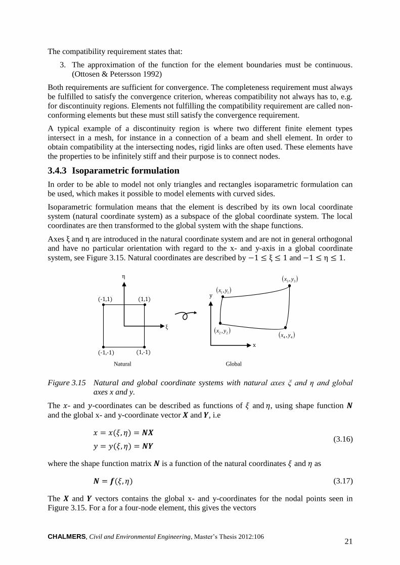
Axes and are introduced in the natural coordinate system and are not in general orthogonal
and have no particular orientation with regard to the x- and y-axis in a global coordinate
system, see Figure 3.15. Natural coordinates are described by and .
(-1,1) (1,1)
(-1,-1) (1,-1) x
y
Natural Global
11 y,x
22 y,x
33 y,x
44 y,x
Figure 3.15 Natural and global coordinate systems with natural axes ξ and η and global
axes x and y.
The - and -coordinates can be described as functions of and , using shape function
and the global x- and y-coordinate vector and , i.e
(3.16)
where the shape function matrix is a function of the natural coordinates and as
(3.17)
The and vectors contains the global x- and y-coordinates for the nodal points seen in
Figure 3.15. For a for a four-node element, this gives the vectors
CHALMERS, Civil and Environmental Engineering, Master’s Thesis 2012:106 22
[
] , [
] (3.18)
3.4.4 Finite element meshing
The FE-model should be divided into one or several areas with different mesh densities. This
should be done in order to create appropriate element shapes, which are able to describe the
behaviour within each element. There are no specific rules for how the meshing should be
established since it depends on many factors.
The accuracy of an FE-model should be thoroughly chosen. A more accurate model, with
higher mesh density, requires more resources in form of computer power and time. The more
accurate a model gets, the more extensive gets the amount of results obtained from the
analysis, which then requires more work with regard to post-processing.
There is often a need for compromising between accuracy and effectiveness. The analysis
should produce a reliable result, but at the same be time efficient. This compromise could
differ very much depending on the situation, for example how detailed the analysis should be,
the amount of time, etc. Thus, it is difficult to give a general recommendation for how an FE-
model should be created. However, there are certain aspects that can be considered, and the
most important ones are described below.
Since the accuracy of the numerical model increases with mesh density, it can be efficient to
use a mesh with varying density in different regions of the model. For critical regions, where
there is rapid change of behaviour or for areas of interest, it could be wise to use a denser
mesh. Regions with small changes or of less interest could preferably have coarser mesh.
Accuracy is also decreasing with lower order of shape functions, implying that increasing the
order sometimes is an effective way to get more accurate results without increasing the mesh
density.
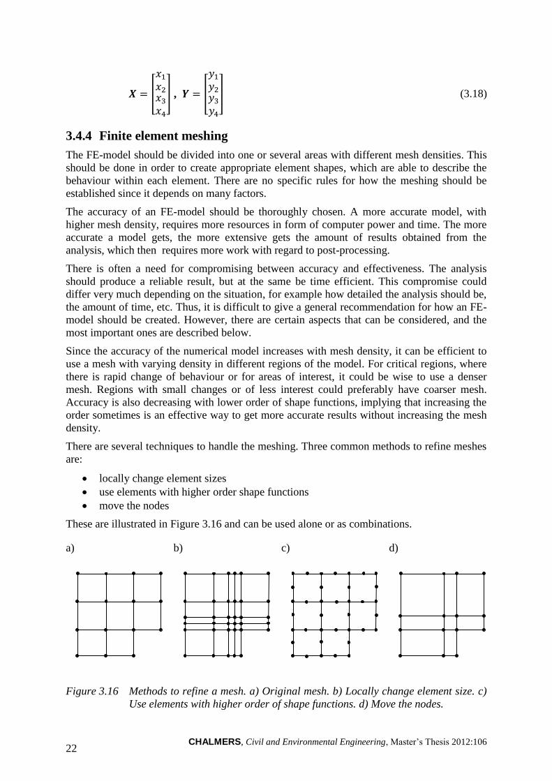
There are several techniques to handle the meshing. Three common methods to refine meshes
are:
locally change element sizes
use elements with higher order shape functions
move the nodes
These are illustrated in Figure 3.16 and can be used alone or as combinations.
a) b) c) d)
Figure 3.16 Methods to refine a mesh. a) Original mesh. b) Locally change element size. c)
Use elements with higher order of shape functions. d) Move the nodes.
CHALMERS, Civil and Environmental Engineering, Master’s Thesis 2012:106 23
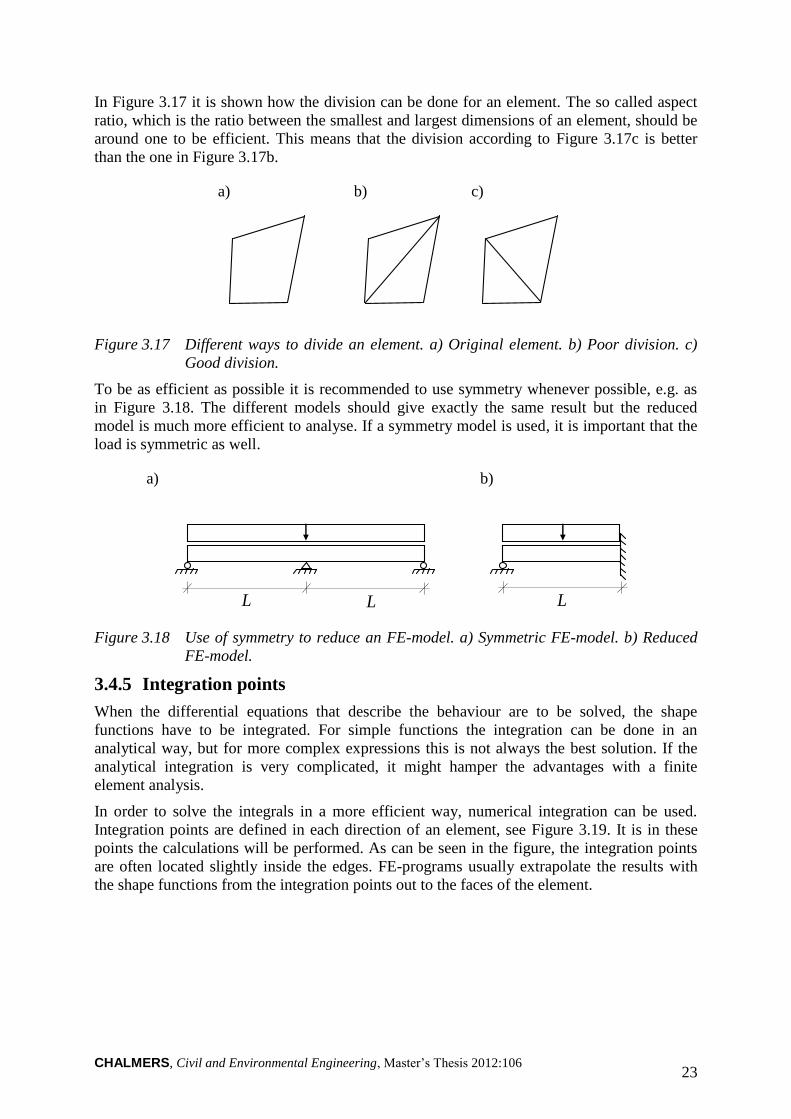
In Figure 3.17 it is shown how the division can be done for an element. The so called aspect
ratio, which is the ratio between the smallest and largest dimensions of an element, should be
around one to be efficient. This means that the division according to Figure 3.17c is better
than the one in Figure 3.17b.
a)
b)
c)
Figure 3.17 Different ways to divide an element. a) Original element. b) Poor division. c)
Good division.
To be as efficient as possible it is recommended to use symmetry whenever possible, e.g. as
in Figure 3.18. The different models should give exactly the same result but the reduced
model is much more efficient to analyse. If a symmetry model is used, it is important that the
load is symmetric as well.
a) b)
L L
L
Figure 3.18 Use of symmetry to reduce an FE-model. a) Symmetric FE-model. b) Reduced
FE-model.
3.4.5 Integration points
When the differential equations that describe the behaviour are to be solved, the shape
functions have to be integrated. For simple functions the integration can be done in an
analytical way, but for more complex expressions this is not always the best solution. If the
analytical integration is very complicated, it might hamper the advantages with a finite
element analysis.
In order to solve the integrals in a more efficient way, numerical integration can be used.
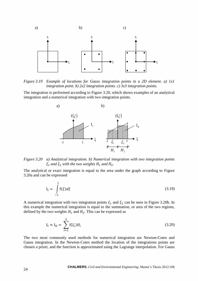
Integration points are defined in each direction of an element, see Figure 3.19. It is in these
points the calculations will be performed. As can be seen in the figure, the integration points
are often located slightly inside the edges. FE-programs usually extrapolate the results with
the shape functions from the integration points out to the faces of the element.
CHALMERS, Civil and Environmental Engineering, Master’s Thesis 2012:106 24
a)
b)
c)
Figure 3.19 Example of locations for Gauss integration points in a 2D element. a) 1x1
integration point. b) 2x2 integration points. c) 3x3 integration points.
The integration is performed according to Figure 3.20, which shows examples of an analytical
integration and a numerical integration with two integration points.
a) b)
1 -1
ξf
ξ
II
1 -1
ξf
1H 2H
1 2
III
ξ
Figure 3.20 a) Analytical integration. b) Numerical integration with two integration points
and with the two weights and .
The analytical or exact integration is equal to the area under the graph according to Figure
3.20a and can be expressed
∫
(3.19)
A numerical integration with two integration points and can be seen in Figure 3.20b. In
this example the numerical integration is equal to the summation, or area of the two regions,
defined by the two weights and . This can be expressed as
∑
(3.20)
The two most commonly used methods for numerical integration are Newton-Cotes and
Gauss integration. In the Newton-Cotes method the location of the integrations points are
chosen a priori, and the function is approximated using the Lagrange interpolation. For Gauss
CHALMERS, Civil and Environmental Engineering, Master’s Thesis 2012:106 25
integration the integration points are defined by using Gauss integration scheme. The
positions for each integration point can be calculated, but can also be found in tables.
3.4.6 Locking effects of finite elements
Element locking effects can occur because the element is getting too stiff. The phenomenon
appears because the interpolation function used for an element is not able to represent zero, or
a very small, shear or membrane strain, and is therefore called shear or membrane locking. If
the element cannot represent a small shear strain, but the physical situation corresponds to
that, the element becomes very stiff as its thickness over length ratio decreases.
Straight beam elements may have problem with shear locking, and curved 3D beam elements
may have both shear and membrane locking. The same occurs for shell elements; for flat shell
elements shear locking may occur and for curved shell elements both shear and membrane
locking can occur.
To avoid locking effects a mixed interpolation formulation can be used. This is explained in
details in the section that follows.
3.4.7 Formulation of finite elements in structural mechanics
There are mainly two formulations of structural finite elements, displacement-based
formulation and mixed finite element formulation. These are discussed briefly here; for more
information about the formulations the reader is referred to Bathe (1996).
3.4.7.1 Displacement-based formulation
In the displacement-based formulation the only solution variables are displacements, which
must satisfy the displacement boundary conditions and element conditions between the
boundaries. Once displacements are calculated other variables such as strains and stresses can
be directly obtained, since they are described as functions of displacements.
In practice, the displacement-based finite element formulation is the most commonly used
because of its simplicity and general effectiveness. However, when doing analyses of plates
and shells, the pure displacement-based formulation is not sufficiently effective. Therefore
other techniques have been developed, and are for certain cases much more effective and
appropriate to use. An effective technique for plates and shells is the mixed interpolation
formulation.
3.4.7.2 Mixed finite element formulations
The mixed finite element formulation is not only based on displacements, but also strains
and/or stresses as primary variables. In the finite element solutions the unknown variables are
therefore besides displacements, also strains and/or stresses.
There exist many extended forumulations and usage of different finite element interpolations.
In this thesis, focus is on describing theory and principles that are used in ADINA, which is
the FE-software used in this project. In ADINA a mixed interpolation formulation is used, and
is therefore only treated further.
The mixed interpolation formulations of structural finite elements are performed in the same
manner as for continuum finite elements. These elements displacements are interpolated by
nodal point displacements, while the structural finite element displacements are interpolated
by midsurface displacements and rotations. This procedure is corresponding to a continuum
isoparametric element formulation with displacement constraints. In structural elements it is
assumed that stresses normal to the midsurface is zero. The structural elements are for these

CHALMERS, Civil and Environmental Engineering, Master’s Thesis 2012:106 26
reasons called degenerate isoparametric elements, but are often just called isoparametric
elements.
3.4.8 Structural finite elements
Many structural finite elements use elements of reduced dimensions such as bars, beams,
plates and shells. The reduction from a 3D solid to a 1D line can sometimes be used for bars
and beams. The cross-sectional shape and dimensions are then used as parameters. For more
general beams it could also be possible to define the beams with values for moments of
inertia, , , and cross-sectional area , as parameters.
The reduction from 3D to 2D is sometimes possible to be described on a plane, e.g. plates and
shells. The third direction is then described as a thickness parameter. There are three types of
plane idealisations:
Plane stress, meaning that the out of plane stress is assumed to be equal to zero.
Plane strain, meaning that the strain in a certain direction is assumed to be equal to
zero.
Axisymmetric condition, meaning that geometry, loads or boundary conditions can be
described axisymmetrically. 3D solids can in this way be generated by revolving a 2D
cross-section, see Figure 3.21.
x
z
z
y
x
Figure 3.21 Revolved geometry from 2D to 3D.
In structural mechanics and finite element software’s flat thin sheets are called plates,
membranes and shells. The midplane is defined to be in the middle, between the two faces,
and is referred to as the midsurface.
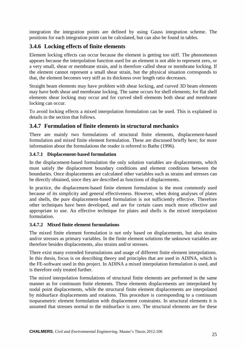
Plate elements are elements loaded only perpendicularly to its plane (out-of-plane), which
produces plate bending , and shear force according to Figure 3.22. Plates may be
used for idealised floors and roofs.
CHALMERS, Civil and Environmental Engineering, Master’s Thesis 2012:106 27
Fz
My Mx
Fz
My Mx
Fz My
Mx Mx
My Fz
z
y
x
Figure 3.22 Plate element with out-of-plane loading and corresponding nodal force and
nodal moments , .
Membrane elements are plates that are loaded in its plane (in-plane), and correspond to the
plane stress idealisation. Membrane elements have only forces in the plane, which are called
membrane forces and can be seen in Figure 3.23. Membranes may be used in plane stress,
plain strain, axisymmetric or 3D-analyses.
z
y
x
Fx Fy
Fx
Fy
Fy
Fx Fx
Fy
Figure 3.23 Membrane element with in-plane loading shown to the right and corresponding
membrane forces to the left.
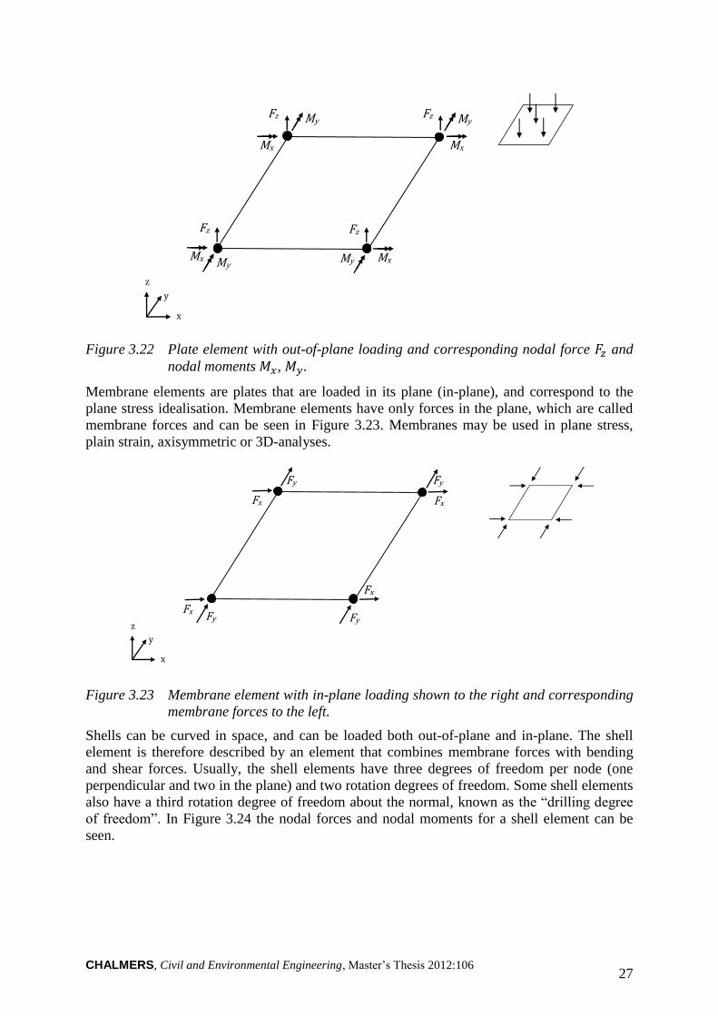
Shells can be curved in space, and can be loaded both out-of-plane and in-plane. The shell
element is therefore described by an element that combines membrane forces with bending
and shear forces. Usually, the shell elements have three degrees of freedom per node (one
perpendicular and two in the plane) and two rotation degrees of freedom. Some shell elements
also have a third rotation degree of freedom about the normal, known as the “drilling degree
of freedom”. In Figure 3.24 the nodal forces and nodal moments for a shell element can be
seen.
CHALMERS, Civil and Environmental Engineering, Master’s Thesis 2012:106 28
Fx
Fz
Fy
My
Mx
Mz
Fx Fz
Fy
My
Mx
Mz
Fx
Fz Fy
My
Mx
Mz
Mx Fx
Fy
My
Fz
Mz
z
y
x
Figure 3.24 Shell element with both out-of-plane and in-plane loading and corresponding
nodal forces , , and nodal moments , , .
Flat shell elements may be used in plane stress or 3D-analyses, while curved shells are only
used in 3D-analyses. The geometry is defined by the midsurface of the shell with a certain
thickness.
The main difference between a plate and a shell element is that plate elements are always
plane, and can describe bending and twisting but no membrane action. The shell elements
may be plane or curved, and can describe bending, twisting and membrane actions. This
means that a shell element can be used for loading both out-of-plane and in-plane, while the
plate element only can describe the behaviour for out-of-plane loading.
3.4.8.1 Beam finite elements
The most common beam element is the 2-node Hermitian beam element, which is based on
the displacement-based element and uses analytical integration of all integrals. One
disadvantage with this element is that for thin beams, shear locking may occur.
An effective beam element is obtained using mixed interpolation of displacements and
transverse shear strains, by modifying the displacement-based element to be able to represent
a nonlocking element. The trick is to interpolate the transverse shear strains and use numerical
integration. These elements are reliable in the sense that they give good convergence
behaviour and have no locking (Bathe 1996). It is also possible to use much coarser meshes
compared to the Hermitian beam element.
In addition there is a computational feature. The elements uses one less Gauss integration
point than the number of nodes in the elements. This computational approach is called
“reduced integration” of the displacement element, but is in fact full integration of the mixed
interpolation element.
The above is valid for straight beams. For curved beams a 3D beam element can be used. For
such elements also membrane locking can occur, which can be avoided by interpolating the
transverse shear, bending and membrane strains (Bathe 1996). These strain interpolations are
coupled to the nodal point displacements and rotations, by using the shape function matrix as
in Equation (3.17).
CHALMERS, Civil and Environmental Engineering, Master’s Thesis 2012:106 29
The isoparametric beam element is an alternative to the classical Hermitian beam element. In
linear analysis of straight thin beams the Hermitian elements are usually more effective, since
for a cubic displacement description the isoparametric beam elements requires twice as many
degrees of freedom. However, the isoparametric beam elements include shear deformations,
are nonlocking and can represent curved geometries accurately.
3.4.8.2 Plate finite elements
The first plate element that was developed, to model thin plates in bending, was based on
Kirchhoff-Love plate theory. A problem with this type of element is that they must fulfil
convergence and be effective in applications. Instead, it is generally more effective to
formulate elements using Reissner-Mindlin plate theory.
Displacement-based plate elements should only be used for higher order elements, but even
higher-order elements give bad capability and have problems with shear locking (Bathe
1996). Still, the shear locking effect is more pronounced when using lower-order elements.
The displacement-based formulation can be extended by using mixed interpolation of the
transverse displacement, section rotations and transverse shear strains. Consequently, the
MITC (Mixed Interpolation of Tensorial Components) element is introduced, where is the
number of element nodes. These elements describe the transverse displacements and bending
strains relatively well, but the transverse shear strain description may not be satisfactory for
very thin plates (Bathe 1996). Nonetheless, these elements do not contain any shear locking
behaviour.
3.4.8.3 Shell finite elements
The shell element can in a simplified way be described as a plate element that can be curved
and carries membrane and bending forces. There are mainly three different approaches, when
formulating a shell finite element (Chapelle & Bathe 2000).
The most simple shell element is a combined membrane and plate element. Flat shell
elements are then obtained, but can be used to model curved shells by using many flat shell
elements. A disadvantage with this approach is that it requires a relatively large amount of
elements, to represent curved shell structures to a sufficient accuracy. Thus, this is an
ineffective approach, which results in a low accuracy for curved shells.
The second approach is based on using a specific shell theory and discretising the
formulation. This approach results in difficulties for more complex shell structures, and is
only applicable to certain shell geometries.
The third approach is to use the isoparametric shell element, which is obtained by reducing
the degrees of freedom of a three-dimensional continuum to reach shell behaviour. According
to Chapelle and Bathe (2000) this is a more general finite element formulation that can be
used for any thin or moderately thick shell in linear or non-linear analysis, and is therefore the
most attractive. It is this approach that is further studied, since this is used in ADINA.
The displacement-based formulation with lower-order elements has shear locking, and when
curved also membrane locking. This can be solved by starting with the displacement-based
formulation and extend it to a mixed formulation by interpolating the in-layer and transverse
shear strains components independently, and finally couple these interpolations to the
displacement interpolations.
An example of such a four-node element is the MITC4 shell element. The element performs
relatively well in out-of-plane bending (plate bending) action, but also in in-plane
(membrane) action (Bathe 1996). To increase the capability even further, higher-order
elements can be used, e.g. 9-node and 16-node elements. These are referred to as MITC9 and
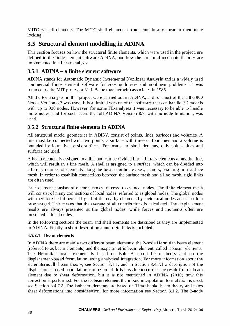
CHALMERS, Civil and Environmental Engineering, Master’s Thesis 2012:106 30
MITC16 shell elements. The MITC shell elements do not contain any shear or membrane
locking.
3.5 Structural element modelling in ADINA
This section focuses on how the structural finite elements, which were used in the project, are
defined in the finite element software ADINA, and how the structural mechanic theories are
implemented in a linear analysis.
3.5.1 ADINA – a finite element software
ADINA stands for Automatic Dynamic Incremental Nonlinear Analysis and is a widely used
commercial finite element software for solving linear- and nonlinear problems. It was
founded by the MIT professor K. J. Bathe together with associates in 1986.
All the FE-analyses in this project were carried out in ADINA, and for most of these the 900
Nodes Version 8.7 was used. It is a limited version of the software that can handle FE-models
with up to 900 nodes. However, for some FE-analyses it was necessary to be able to handle
more nodes, and for such cases the full ADINA Version 8.7, with no node limitation, was
used.
3.5.2 Structural finite elements in ADINA
All structural model geometries in ADINA consist of points, lines, surfaces and volumes. A
line must be connected with two points, a surface with three or four lines and a volume is
bounded by four, five or six surfaces. For beam and shell elements, only points, lines and
surfaces are used.
A beam element is assigned to a line and can be divided into arbitrary elements along the line,
which will result in a line mesh. A shell is assigned to a surface, which can be divided into
arbitrary number of elements along the local coordinate axes, r and s, resulting in a surface
mesh. In order to establish connections between the surface mesh and a line mesh, rigid links
are often used.
Each element consists of element nodes, referred to as local nodes. The finite element mesh
will consist of many connections of local nodes, referred to as global nodes. The global nodes
will therefore be influenced by all of the nearby elements by their local nodes and can often
be averaged. This means that the average of all contributions is calculated. The displacement
results are always presented at the global nodes, while forces and moments often are
presented at local nodes.
In the following sections the beam and shell elements are described as they are implemented
in ADINA. Finally, a short description about rigid links is included.
3.5.2.1 Beam elements
In ADINA there are mainly two different beam elements; the 2-node Hermitian beam element
(referred to as beam elements) and the isoparametric beam element, called isobeam elements.
The Hermitian beam element is based on Euler-Bernoulli beam theory and on the
displacement-based formulation, using analytical integration. For more information about the
Euler-Bernoulli beam theory, see Section 3.1.1, and in Section 3.4.7.1 a description of the
displacement-based formulation can be found. It is possible to correct the result from a beam
element due to shear deformation, but it is not mentioned in ADINA (2010) how this
correction is performed. For the isobeam element the mixed interpolation formulation is used,
see Section 3.4.7.2. The isobeam elements are based on Timoshenko beam theory and takes
shear deformations into consideration, for more information see Section 3.1.2. The 2-node
CHALMERS, Civil and Environmental Engineering, Master’s Thesis 2012:106 31
Hermitian beam element can be used for any constant cross-section, and is able to give results
as nodal forces or sectional forces. The isobeam element can only be used for rectangular
constant cross-sections, and is able to give results in form of stresses or nodal forces, but not
in sectional forces.
In linear analysis of straight beams the 2-node Hermitian elements are the most effective and
appropriate to use (ADINA 2010). One disadvantage is however that shear locking may occur
for thin elements. The isobeam element is mainly constructed to be used for curved beams,
beams with large displacements and as stiffeners to shell elements. One advantage with
isobeam elements is that neither shear- nor membrane locking can occur.
There are different variants of the 2-node Hermitian beam element, e.g. linear beam elements,
large displacement beam elements and warping beam elements. The most common is the
linear beam element, which assumes small displacements, rotations and strains, and is using
elastic-isotropic material behaviour. The linear beam element has 6 degrees of freedom at
each node, translation in r-, s- and t direction ( and ) and rotation around r-, s- and t-
axis ( and ), see Figure 3.25. The beam element is defined on the centroidal axis using
the local coordinate system (r,s,t), based on an auxiliary point K according to the figure.
1
2
K
x y
z
r s
t tu
ru su
r
s
t
Figure 3.25 Linear beam element with the auxiliary point K, which defines the local
coordinate system (r,s,t) and its 6 degrees of freedom ( ) at
each end node.
The beam element is modelled using a line, and is given a constant rectangular, U-, I- or L-
shaped cross-section. Another way to model a more general cross-section is to use constant
cross-sectional parameters such as cross-sectional area and moments of inertia.
For linear beam elements analytical integration is used, meaning that no integration points are
used. The result output can be chosen in the terms of nodal forces or sectional forces.
Sectional forces can be chosen to be calculated at a number of points (2-7) evenly distributed
between the end nodes and located on the centroidal axis of the element. Sectional forces can
be extrapolated and averaged to the global nodes, if requested. Sectional forces are axial
force, bending moments around s- and t-axis, shear forces in s and t directions and torsional
moment around r-axis. The nodal forces are calculated at the local end nodes, and cannot be
extrapolated and averaged to the global nodes. Nodal forces include the forces in r, s, and t
directions and moments around r-, s- and t-axis. A summary can be seen in Table 3.1.
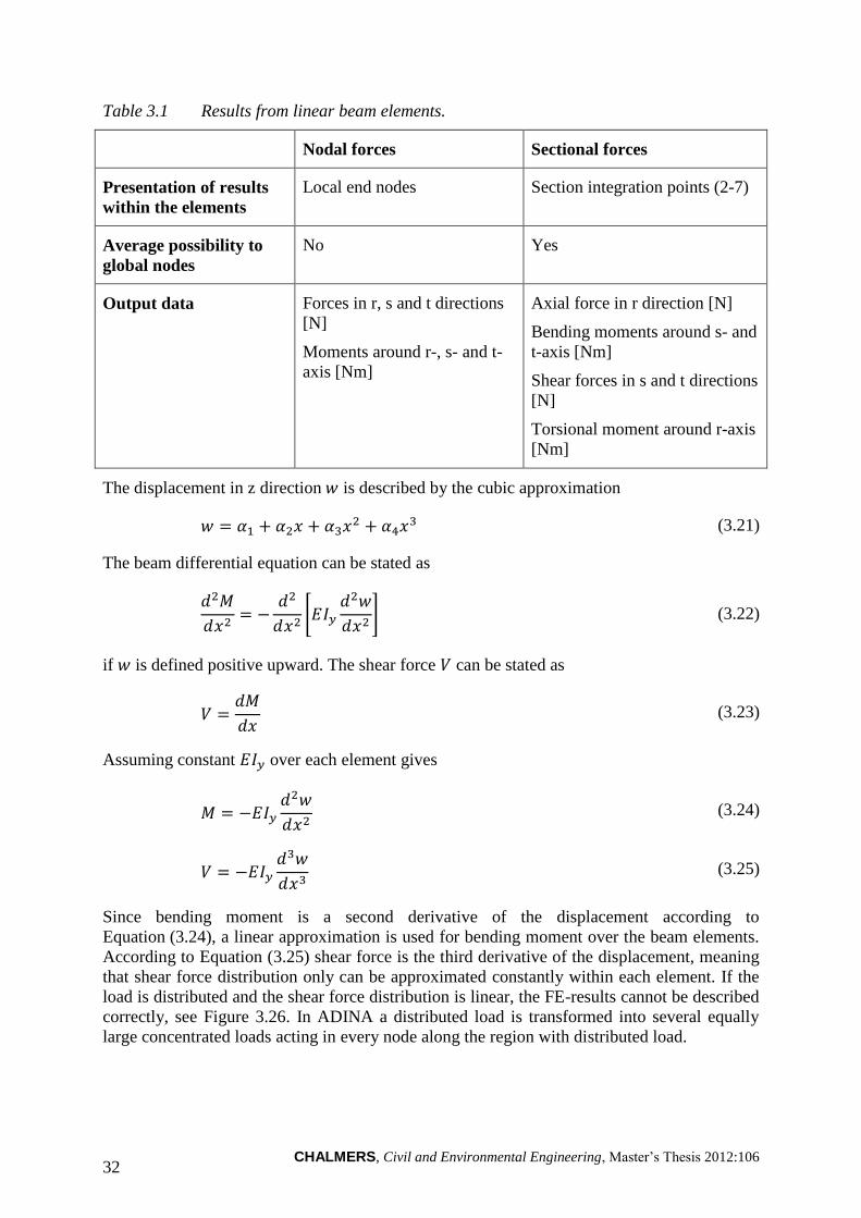
CHALMERS, Civil and Environmental Engineering, Master’s Thesis 2012:106 32
Table 3.1 Results from linear beam elements.
Nodal forces Sectional forces
Presentation of results
within the elements
Local end nodes Section integration points (2-7)
Average possibility to
global nodes
No Yes
Output data Forces in r, s and t directions
[N]
Moments around r-, s- and t-
axis [Nm]
Axial force in r direction [N]
Bending moments around s- and
t-axis [Nm]
Shear forces in s and t directions
[N]
Torsional moment around r-axis
[Nm]
The displacement in z direction is described by the cubic approximation
(3.21)
The beam differential equation can be stated as
*
+ (3.22)
if is defined positive upward. The shear force can be stated as
(3.23)
Assuming constant over each element gives
(3.24)
(3.25)
Since bending moment is a second derivative of the displacement according to
Equation (3.24), a linear approximation is used for bending moment over the beam elements.
According to Equation (3.25) shear force is the third derivative of the displacement, meaning
that shear force distribution only can be approximated constantly within each element. If the
load is distributed and the shear force distribution is linear, the FE-results cannot be described
correctly, see Figure 3.26. In ADINA a distributed load is transformed into several equally
large concentrated loads acting in every node along the region with distributed load.
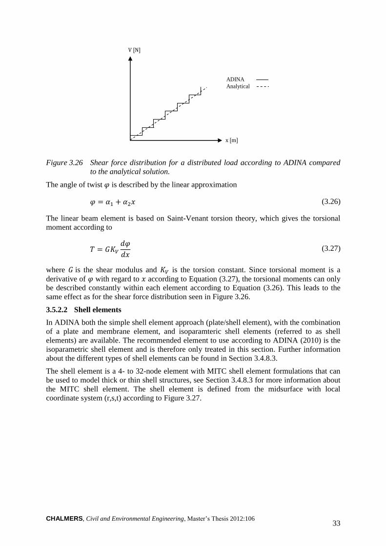
CHALMERS, Civil and Environmental Engineering, Master’s Thesis 2012:106 33
ADINA
Analytical
x [m]
V [N]
Figure 3.26 Shear force distribution for a distributed load according to ADINA compared
to the analytical solution.
The angle of twist is described by the linear approximation
(3.26)
The linear beam element is based on Saint-Venant torsion theory, which gives the torsional
moment according to
(3.27)
where is the shear modulus and is the torsion constant. Since torsional moment is a
derivative of with regard to according to Equation (3.27), the torsional moments can only
be described constantly within each element according to Equation (3.26). This leads to the
same effect as for the shear force distribution seen in Figure 3.26.
3.5.2.2 Shell elements
In ADINA both the simple shell element approach (plate/shell element), with the combination
of a plate and membrane element, and isoparamteric shell elements (referred to as shell
elements) are available. The recommended element to use according to ADINA (2010) is the
isoparametric shell element and is therefore only treated in this section. Further information
about the different types of shell elements can be found in Section 3.4.8.3.
The shell element is a 4- to 32-node element with MITC shell element formulations that can
be used to model thick or thin shell structures, see Section 3.4.8.3 for more information about
the MITC shell element. The shell element is defined from the midsurface with local
coordinate system (r,s,t) according to Figure 3.27.
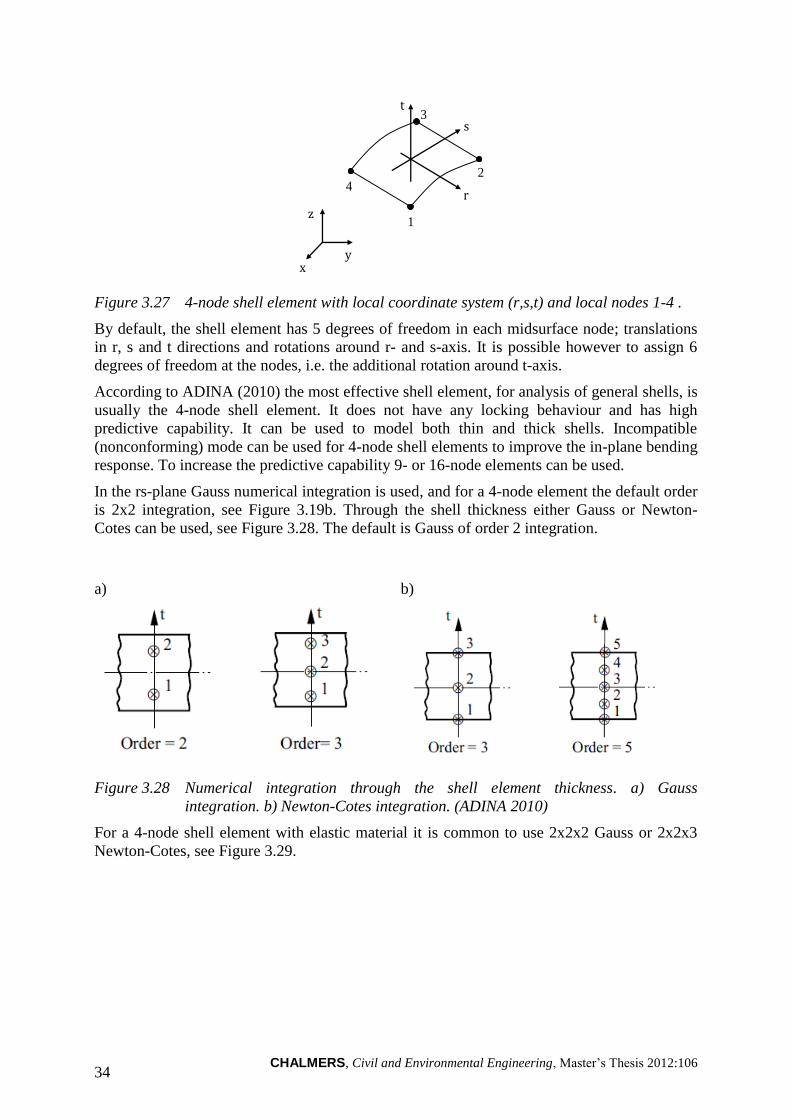
CHALMERS, Civil and Environmental Engineering, Master’s Thesis 2012:106 34
1
2
3
4 r
s
t
x y
z
Figure 3.27 4-node shell element with local coordinate system (r,s,t) and local nodes 1-4 .
By default, the shell element has 5 degrees of freedom in each midsurface node; translations
in r, s and t directions and rotations around r- and s-axis. It is possible however to assign 6
degrees of freedom at the nodes, i.e. the additional rotation around t-axis.
According to ADINA (2010) the most effective shell element, for analysis of general shells, is
usually the 4-node shell element. It does not have any locking behaviour and has high
predictive capability. It can be used to model both thin and thick shells. Incompatible
(nonconforming) mode can be used for 4-node shell elements to improve the in-plane bending
response. To increase the predictive capability 9- or 16-node elements can be used.
In the rs-plane Gauss numerical integration is used, and for a 4-node element the default order
is 2x2 integration, see Figure 3.19b. Through the shell thickness either Gauss or Newton-
Cotes can be used, see Figure 3.28. The default is Gauss of order 2 integration.
a)
b)
Figure 3.28 Numerical integration through the shell element thickness. a) Gauss
integration. b) Newton-Cotes integration. (ADINA 2010)
For a 4-node shell element with elastic material it is common to use 2x2x2 Gauss or 2x2x3
Newton-Cotes, see Figure 3.29.
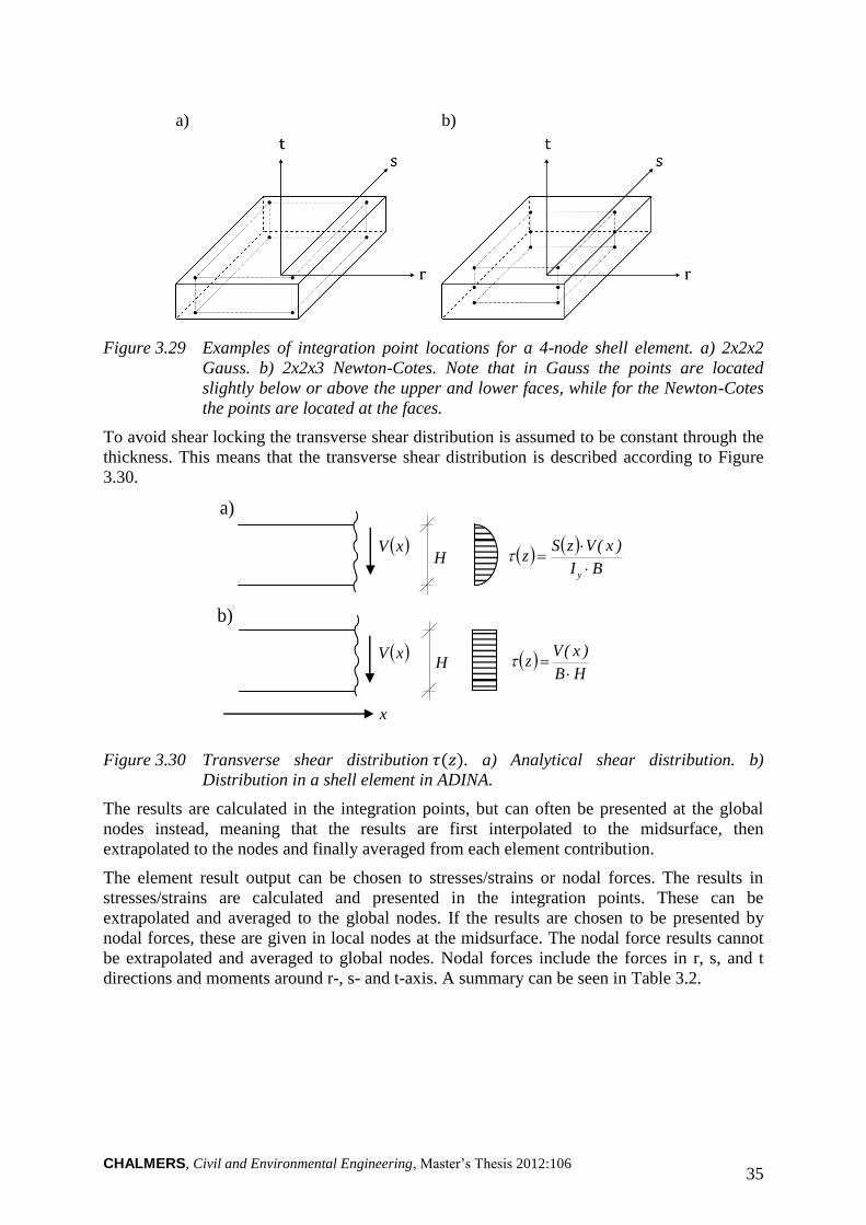
CHALMERS, Civil and Environmental Engineering, Master’s Thesis 2012:106 35
a)
b)
Figure 3.29 Examples of integration point locations for a 4-node shell element. a) 2x2x2
Gauss. b) 2x2x3 Newton-Cotes. Note that in Gauss the points are located
slightly below or above the upper and lower faces, while for the Newton-Cotes
the points are located at the faces.
To avoid shear locking the transverse shear distribution is assumed to be constant through the
thickness. This means that the transverse shear distribution is described according to Figure
3.30.
BI
)x(VzSz
y
a)
b)
HB
)x(Vz
xV
xV
x
H
H
Figure 3.30 Transverse shear distribution . a) Analytical shear distribution. b)
Distribution in a shell element in ADINA.
The results are calculated in the integration points, but can often be presented at the global
nodes instead, meaning that the results are first interpolated to the midsurface, then
extrapolated to the nodes and finally averaged from each element contribution.
The element result output can be chosen to stresses/strains or nodal forces. The results in
stresses/strains are calculated and presented in the integration points. These can be
extrapolated and averaged to the global nodes. If the results are chosen to be presented by
nodal forces, these are given in local nodes at the midsurface. The nodal force results cannot
be extrapolated and averaged to global nodes. Nodal forces include the forces in r, s, and t
directions and moments around r-, s- and t-axis. A summary can be seen in Table 3.2.
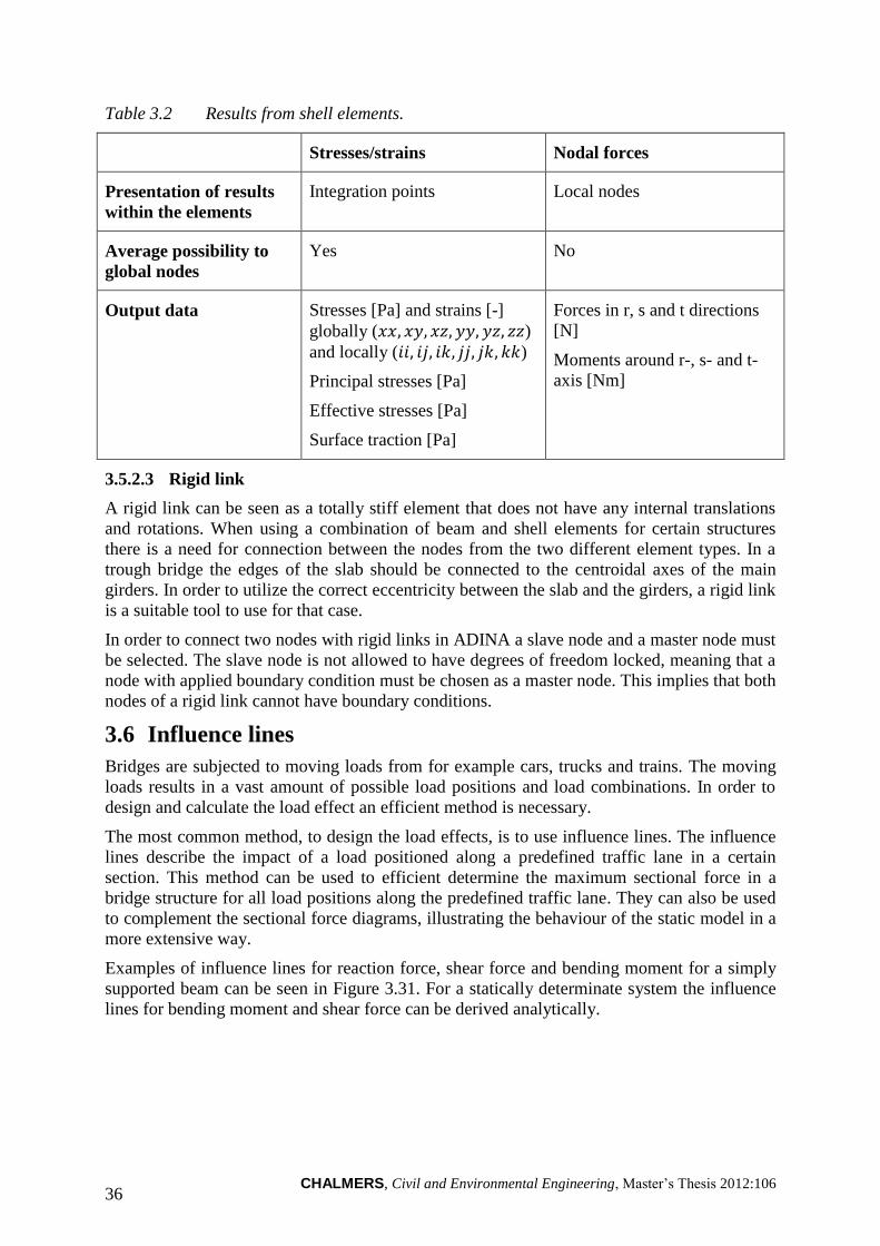
CHALMERS, Civil and Environmental Engineering, Master’s Thesis 2012:106 36
Table 3.2 Results from shell elements.
Stresses/strains Nodal forces
Presentation of results
within the elements
Integration points Local nodes
Average possibility to
global nodes
Yes No
Output data Stresses [Pa] and strains [-]
globally ( )
and locally ( )
Principal stresses [Pa]
Effective stresses [Pa]
Surface traction [Pa]
Forces in r, s and t directions
[N]
Moments around r-, s- and t-
axis [Nm]
3.5.2.3 Rigid link
A rigid link can be seen as a totally stiff element that does not have any internal translations
and rotations. When using a combination of beam and shell elements for certain structures
there is a need for connection between the nodes from the two different element types. In a
trough bridge the edges of the slab should be connected to the centroidal axes of the main
girders. In order to utilize the correct eccentricity between the slab and the girders, a rigid link
is a suitable tool to use for that case.
In order to connect two nodes with rigid links in ADINA a slave node and a master node must
be selected. The slave node is not allowed to have degrees of freedom locked, meaning that a
node with applied boundary condition must be chosen as a master node. This implies that both
nodes of a rigid link cannot have boundary conditions.
3.6 Influence lines
Bridges are subjected to moving loads from for example cars, trucks and trains. The moving
loads results in a vast amount of possible load positions and load combinations. In order to
design and calculate the load effect an efficient method is necessary.
The most common method, to design the load effects, is to use influence lines. The influence
lines describe the impact of a load positioned along a predefined traffic lane in a certain
section. This method can be used to efficient determine the maximum sectional force in a
bridge structure for all load positions along the predefined traffic lane. They can also be used
to complement the sectional force diagrams, illustrating the behaviour of the static model in a
more extensive way.
Examples of influence lines for reaction force, shear force and bending moment for a simply
supported beam can be seen in Figure 3.31. For a statically determinate system the influence
lines for bending moment and shear force can be derived analytically.
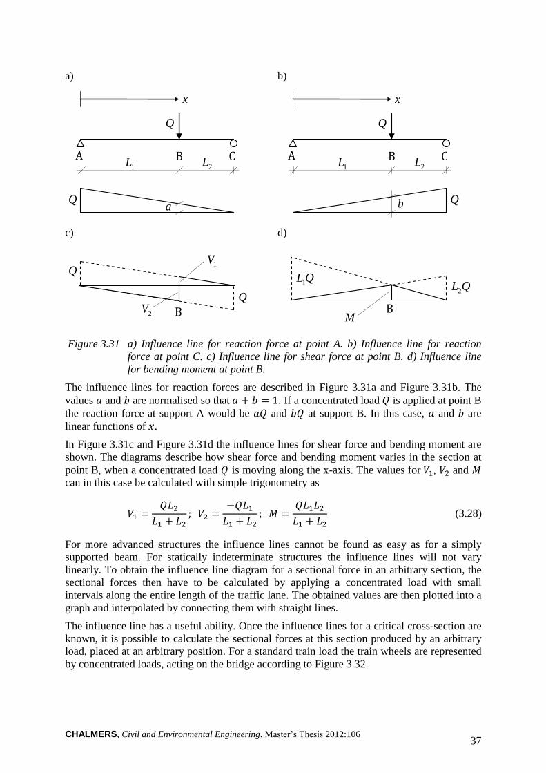
CHALMERS, Civil and Environmental Engineering, Master’s Thesis 2012:106 37
a)
Q
A B
x
1L 2L C
Q a
c)
B
Q
Q
1V
2V
b)
Q
A B
x
1L 2L C
Q b
d)
B M
QL2 QL1
Figure 3.31 a) Influence line for reaction force at point A. b) Influence line for reaction
force at point C. c) Influence line for shear force at point B. d) Influence line
for bending moment at point B.
The influence lines for reaction forces are described in Figure 3.31a and Figure 3.31b. The
values and are normalised so that . If a concentrated load is applied at point B
the reaction force at support A would be and at support B. In this case, and are
linear functions of .
In Figure 3.31c and Figure 3.31d the influence lines for shear force and bending moment are
shown. The diagrams describe how shear force and bending moment varies in the section at
point B, when a concentrated load is moving along the x-axis. The values for , and
can in this case be calculated with simple trigonometry as
(3.28)
For more advanced structures the influence lines cannot be found as easy as for a simply
supported beam. For statically indeterminate structures the influence lines will not vary
linearly. To obtain the influence line diagram for a sectional force in an arbitrary section, the
sectional forces then have to be calculated by applying a concentrated load with small
intervals along the entire length of the traffic lane. The obtained values are then plotted into a
graph and interpolated by connecting them with straight lines.
The influence line has a useful ability. Once the influence lines for a critical cross-section are
known, it is possible to calculate the sectional forces at this section produced by an arbitrary
load, placed at an arbitrary position. For a standard train load the train wheels are represented
by concentrated loads, acting on the bridge according to Figure 3.32.
CHALMERS, Civil and Environmental Engineering, Master’s Thesis 2012:106 38
B
C A 2V
1V
2Q 1Q 3Q 4Q
a b c d
Figure 3.32 Influence line for a simply supported beam at section B. The concentrated loads
- represent the wheel pairs on a train.
By using an influence line the action caused by the different concentrated loads can be
summed up, and thus gives the total sectional force as
(3.29)
In order to obtain the impact of a distributed load in a section, the same influence lines as for
concentrated loads are used. The distributed load is integrated over the length and the area
represents the force acting in the section.
CHALMERS, Civil and Environmental Engineering, Master’s Thesis 2012:106 39
4 Description of the FE-analyses
In this chapter all the FE-analyses are described. Initially, the studied trough bridge with the
dimensions and boundary conditions are described, followed by presentation of the different
system models that were used in this project. In the next section a deflection and rotational
stiffness study is presented. The aims of the study were to investigate the shell element
behaviours and to come up with appropriate mesh densities for the FE-models. After the
presentation of the stiffness study, all the FE-models are described. Since many of the FE-
models needed a lot of post-processing, all the result management that were used is described
in the last section.
4.1 System models
In order to construct the FE-models, system models were firstly defined. These are presented
in this section together with geometry, material properties and loading.
4.1.1 Geometry, material and loading
The dimensions of the trough bridge were defined according to Figure 4.1. The geometrical
dimensions were chosen to be as general as possible for a through bridge, and were based on
previous projects carried out at REINERTSEN. A bridge with three supports was studied
according to the figure.
Figure 4.1 Dimensions of the trough bridge.
All models were created with the load, lengths and material properties presented in Table 4.1.
z x
y
3.5 1.5 1.5
0.5
0.8
[m]
1.3
16 16
CHALMERS, Civil and Environmental Engineering, Master’s Thesis 2012:106 40
Table 4.1 Load, lengths and material properties.
Concentrated load, 1 kN
Total length, 32 m
Span length, 16 m
Young’s modulus, 30 GPa
Poisson’s ratio, 0.2
4.1.2 System models
The studied system models were a 2D beam model and beam grillage, combined and shell
models. All models were based on the static system of a continuous beam, see Figure 4.1. The
beam grillage and combined models were created either with inclined rigid links or with u-
shaped cross-section. The shell model was modelled either with correct total height of the
cross-section, giving a more correct bending stiffness, or with higher longitudinal girders,
giving a more correctly described torsion stiffness.
In Figure 4.2 a system model for the 2D beam model can be seen. It consists of a longitudinal
girder only, which is defined on a line in the centre of gravity of the cross-section according
to the figure.
[m]
Longitudinal girder
16 16
Figure 4.2 System model for the 2D beam model.
In Figure 4.3 a system model for the beam grillage models with inclined rigid links can be
seen, and shows the two different ways the cross-section were modelled. The left cross-
section in the figure illustrates the model where the boundary conditions were defined on the
centroidal axes of the longitudinal girders. The right cross-section in the figure shows how
additional stiff elements were included in the model, in order to be able to define the
boundary conditions at the bottom of the longitudinal girders. More information about the
stiff elements can be found in Section 4.3.3. The two main girders, modelled as longitudinal
beams, were connected to the slab, modelled as evenly spaced transversal beams, using rigid
links.
CHALMERS, Civil and Environmental Engineering, Master’s Thesis 2012:106 41
Longitudinal girder
Longitudinal girder
[m]
Rigid link Transversal beam Longitudinal girder Stiff element
16 16
Support Rigid link
Sla
b
3.5
0
.75
0
.75
1.0
Figure 4.3 System model for the beam grillage models with inclined rigid links between
transversal beams and longitudinal girders. The two ways the cross-section was
modelled can be seen at the top of the figure. The right cross-sectional figure
shows how additional stiff elements were included, to be able to define the
boundary conditions on the bottom of the longitudinal girders.
In Figure 4.4 a system model with u-shaped cross-section can be seen.
Longitudinal girder
Longitudinal girder
[m]
Transversal beam
Longitudinal girder
Rigid link
16 16
Support
1.0
Sla
b
5.0
Figure 4.4 System model for the beam grillage model with u-shaped cross-section.
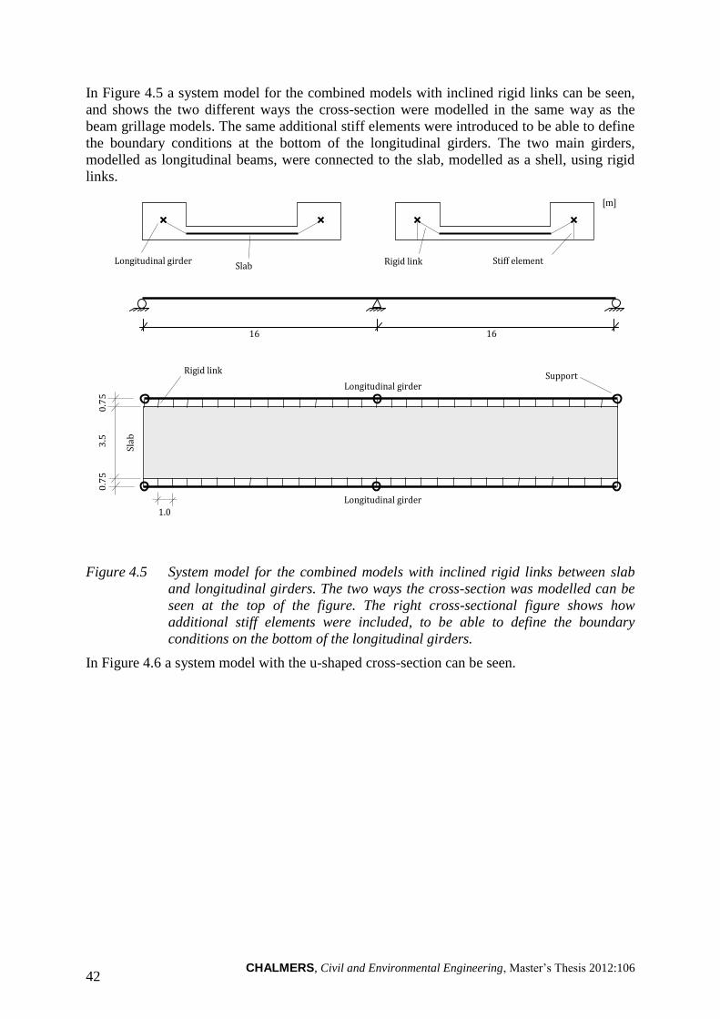
CHALMERS, Civil and Environmental Engineering, Master’s Thesis 2012:106 42
In Figure 4.5 a system model for the combined models with inclined rigid links can be seen,
and shows the two different ways the cross-section were modelled in the same way as the
beam grillage models. The same additional stiff elements were introduced to be able to define
the boundary conditions at the bottom of the longitudinal girders. The two main girders,
modelled as longitudinal beams, were connected to the slab, modelled as a shell, using rigid
links.
Longitudinal girder
Longitudinal girder
[m]
Rigid link Slab Longitudinal girder
16 16
Support
Sla
b
3.5
0
.75
0
.75
1.0
Stiff element
Rigid link
Figure 4.5 System model for the combined models with inclined rigid links between slab
and longitudinal girders. The two ways the cross-section was modelled can be
seen at the top of the figure. The right cross-sectional figure shows how
additional stiff elements were included, to be able to define the boundary
conditions on the bottom of the longitudinal girders.
In Figure 4.6 a system model with the u-shaped cross-section can be seen.
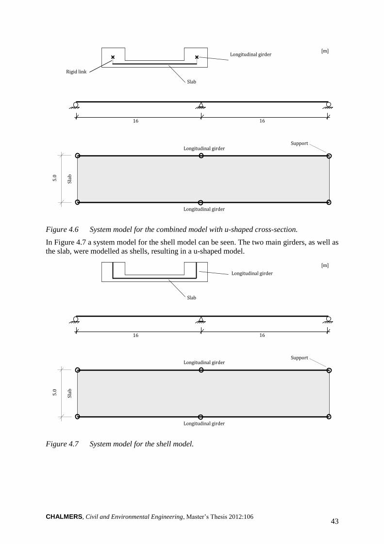
CHALMERS, Civil and Environmental Engineering, Master’s Thesis 2012:106 43
Longitudinal girder
Longitudinal girder
[m]
Slab
Longitudinal girder
Rigid link
16 16
Support
Sla
b
5.0
Figure 4.6 System model for the combined model with u-shaped cross-section.
In Figure 4.7 a system model for the shell model can be seen. The two main girders, as well as
the slab, were modelled as shells, resulting in a u-shaped model.
Longitudinal girder
Longitudinal girder
[m]
Slab
Longitudinal girder
16 16
Support
Sla
b
5.0
Figure 4.7 System model for the shell model.
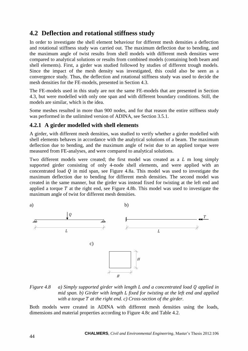
CHALMERS, Civil and Environmental Engineering, Master’s Thesis 2012:106 44
4.2 Deflection and rotational stiffness study
In order to investigate the shell element behaviour for different mesh densities a deflection
and rotational stiffness study was carried out. The maximum deflection due to bending, and
the maximum angle of twist results from shell models with different mesh densities were
compared to analytical solutions or results from combined models (containing both beam and
shell elements). First, a girder was studied followed by studies of different trough models.
Since the impact of the mesh density was investigated, this could also be seen as a
convergence study. Thus, the deflection and rotational stiffness study was used to decide the
mesh densities for the FE-models, presented in Section 4.3.
The FE-models used in this study are not the same FE-models that are presented in Section
4.3, but were modelled with only one span and with different boundary conditions. Still, the
models are similar, which is the idea.
Some meshes resulted in more than 900 nodes, and for that reason the entire stiffness study
was performed in the unlimited version of ADINA, see Section 3.5.1.
4.2.1 A girder modelled with shell elements
A girder, with different mesh densities, was studied to verify whether a girder modelled with
shell elements behaves in accordance with the analytical solutions of a beam. The maximum
deflection due to bending, and the maximum angle of twist due to an applied torque were
measured from FE-analyses, and were compared to analytical solutions.
Two different models were created; the first model was created as a m long simply
supported girder consisting of only 4-node shell elements, and were applied with an
concentrated load in mid span, see Figure 4.8a. This model was used to investigate the
maximum deflection due to bending for different mesh densities. The second model was
created in the same manner, but the girder was instead fixed for twisting at the left end and
applied a torque at the right end, see Figure 4.8b. This model was used to investigate the
maximum angle of twist for different mesh densities.
a)
L
Q
b)
L
T
c)
B
H
Figure 4.8 a) Simply supported girder with length L and a concentrated load applied in
mid span. b) Girder with length fixed for twisting at the left end and applied
with a torque at the right end. c) Cross-section of the girder.
Both models were created in ADINA with different mesh densities using the loads,
dimensions and material properties according to Figure 4.8c and Table 4.2.
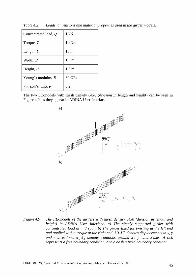
CHALMERS, Civil and Environmental Engineering, Master’s Thesis 2012:106 45
Table 4.2 Loads, dimensions and material properties used in the girder models.
Concentrated load, 1 kN
Torque, 1 kNm
Length, 16 m
Width, 1.5 m
Height, 1.3 m
Young’s modulus, 30 GPa
Poisson’s ratio, 0.2
The two FE-models with mesh density 64x8 (division in length and height) can be seen in
Figure 4.9, as they appear in ADINA User Interface.
a)
b)
Figure 4.9 The FE-models of the girders with mesh density 64x8 (division in length and
height) in ADINA User Interface. a) The simply supported girder with
concentrated load at mid span. b) The girder fixed for twisting at the left end
and applied with a torque at the right end. U1-U3 denotes displacements in x, y
and z directions, - denotes rotations around x-, y- and z-axis. A tick
represents a free boundary condition, and a dash a fixed boundary condition.
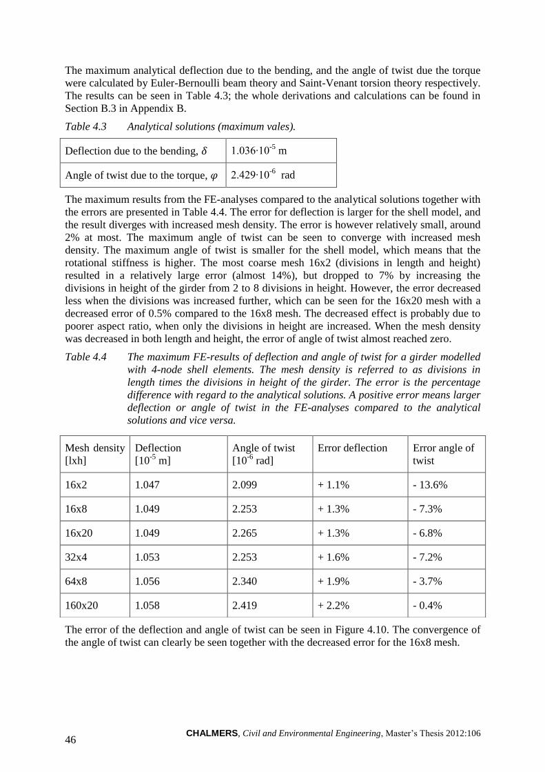
CHALMERS, Civil and Environmental Engineering, Master’s Thesis 2012:106 46
The maximum analytical deflection due to the bending, and the angle of twist due the torque
were calculated by Euler-Bernoulli beam theory and Saint-Venant torsion theory respectively.
The results can be seen in Table 4.3; the whole derivations and calculations can be found in
Section B.3 in Appendix B.
Table 4.3 Analytical solutions (maximum vales).
Deflection due to the bending, 1.036∙10-5
m
Angle of twist due to the torque, 2.429∙10-6
rad
The maximum results from the FE-analyses compared to the analytical solutions together with
the errors are presented in Table 4.4. The error for deflection is larger for the shell model, and
the result diverges with increased mesh density. The error is however relatively small, around
2% at most. The maximum angle of twist can be seen to converge with increased mesh
density. The maximum angle of twist is smaller for the shell model, which means that the
rotational stiffness is higher. The most coarse mesh 16x2 (divisions in length and height)
resulted in a relatively large error (almost 14%), but dropped to 7% by increasing the
divisions in height of the girder from 2 to 8 divisions in height. However, the error decreased
less when the divisions was increased further, which can be seen for the 16x20 mesh with a
decreased error of 0.5% compared to the 16x8 mesh. The decreased effect is probably due to
poorer aspect ratio, when only the divisions in height are increased. When the mesh density
was decreased in both length and height, the error of angle of twist almost reached zero.
Table 4.4 The maximum FE-results of deflection and angle of twist for a girder modelled
with 4-node shell elements. The mesh density is referred to as divisions in
length times the divisions in height of the girder. The error is the percentage
difference with regard to the analytical solutions. A positive error means larger
deflection or angle of twist in the FE-analyses compared to the analytical
solutions and vice versa.
The error of the deflection and angle of twist can be seen in Figure 4.10. The convergence of
the angle of twist can clearly be seen together with the decreased error for the 16x8 mesh.
Mesh density
[lxh]
Deflection
[10-5
m]
Angle of twist
[10-6
rad]
Error deflection Error angle of
twist
16x2 1.047 2.099 + 1.1% - 13.6%
16x8 1.049 2.253 + 1.3% - 7.3%
16x20 1.049 2.265 + 1.3% - 6.8%
32x4 1.053 2.253 + 1.6% - 7.2%
64x8 1.056 2.340 + 1.9% - 3.7%
160x20 1.058 2.419 + 2.2% - 0.4%
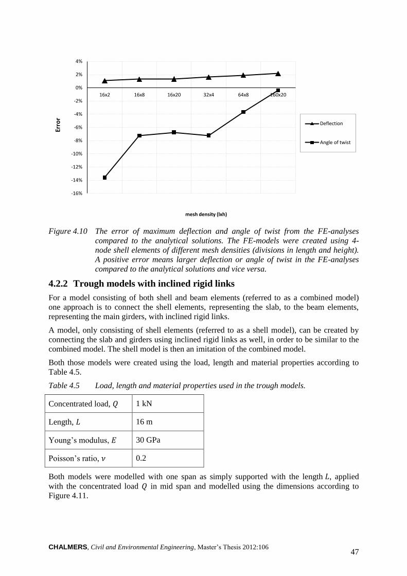
CHALMERS, Civil and Environmental Engineering, Master’s Thesis 2012:106 47
Figure 4.10 The error of maximum deflection and angle of twist from the FE-analyses
compared to the analytical solutions. The FE-models were created using 4-
node shell elements of different mesh densities (divisions in length and height).
A positive error means larger deflection or angle of twist in the FE-analyses
compared to the analytical solutions and vice versa.
4.2.2 Trough models with inclined rigid links
For a model consisting of both shell and beam elements (referred to as a combined model)
one approach is to connect the shell elements, representing the slab, to the beam elements,
representing the main girders, with inclined rigid links.
A model, only consisting of shell elements (referred to as a shell model), can be created by
connecting the slab and girders using inclined rigid links as well, in order to be similar to the
combined model. The shell model is then an imitation of the combined model.
Both those models were created using the load, length and material properties according to
Table 4.5.
Table 4.5 Load, length and material properties used in the trough models.
Concentrated load, 1 kN
Length, 16 m
Young’s modulus, 30 GPa
Poisson’s ratio, 0.2
Both models were modelled with one span as simply supported with the length , applied
with the concentrated load in mid span and modelled using the dimensions according to
Figure 4.11.
-16%
-14%
-12%
-10%
-8%
-6%
-4%
-2%
0%
2%
4%
16x2 16x8 16x20 32x4 64x8 160x20
Erro
r
mesh density (lxh)
Deflection
Angle of twist
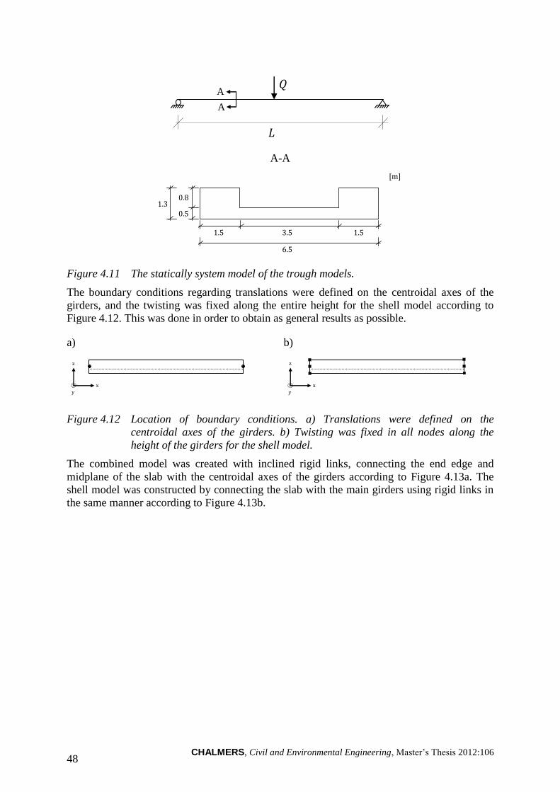
CHALMERS, Civil and Environmental Engineering, Master’s Thesis 2012:106 48
L
Q A
A
A-A
Figure 4.11 The statically system model of the trough models.
The boundary conditions regarding translations were defined on the centroidal axes of the
girders, and the twisting was fixed along the entire height for the shell model according to
Figure 4.12. This was done in order to obtain as general results as possible.
a)
b)
Figure 4.12 Location of boundary conditions. a) Translations were defined on the
centroidal axes of the girders. b) Twisting was fixed in all nodes along the
height of the girders for the shell model.
The combined model was created with inclined rigid links, connecting the end edge and
midplane of the slab with the centroidal axes of the girders according to Figure 4.13a. The
shell model was constructed by connecting the slab with the main girders using rigid links in
the same manner according to Figure 4.13b.
3.5 1.5 1.5
0.5
0.8
[m]
1.3
6.5
z
x y
z
x y
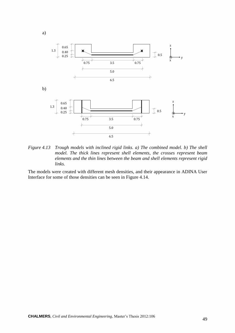
CHALMERS, Civil and Environmental Engineering, Master’s Thesis 2012:106 49
a)
b)
Figure 4.13 Trough models with inclined rigid links. a) The combined model. b) The shell
model. The thick lines represent shell elements, the crosses represent beam
elements and the thin lines between the beam and shell elements represent rigid
links.
The models were created with different mesh densities, and their appearance in ADINA User
Interface for some of those densities can be seen in Figure 4.14.
0.75
0.65
0.40 0.25
x y
z
3.5 0.75
1.3
5.0
6.5
0.5
0.75
0.65
0.40 0.25
x y
z
3.5 0.75
1.3
5.0
6.5
0.5
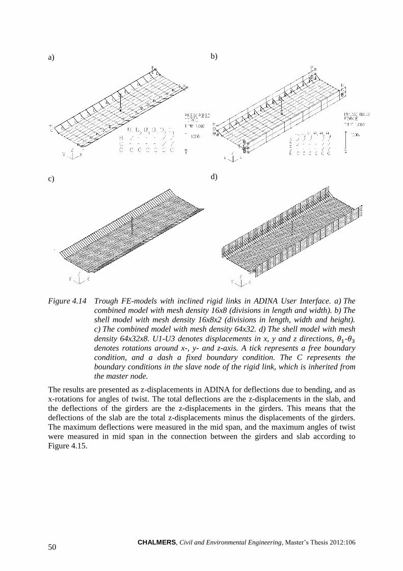
CHALMERS, Civil and Environmental Engineering, Master’s Thesis 2012:106 50
a)
b)
c)
d)
Figure 4.14 Trough FE-models with inclined rigid links in ADINA User Interface. a) The
combined model with mesh density 16x8 (divisions in length and width). b) The
shell model with mesh density 16x8x2 (divisions in length, width and height).
c) The combined model with mesh density 64x32. d) The shell model with mesh
density 64x32x8. U1-U3 denotes displacements in x, y and z directions, -
denotes rotations around x-, y- and z-axis. A tick represents a free boundary
condition, and a dash a fixed boundary condition. The C represents the
boundary conditions in the slave node of the rigid link, which is inherited from
the master node.
The results are presented as z-displacements in ADINA for deflections due to bending, and as
x-rotations for angles of twist. The total deflections are the z-displacements in the slab, and
the deflections of the girders are the z-displacements in the girders. This means that the
deflections of the slab are the total z-displacements minus the displacements of the girders.
The maximum deflections were measured in the mid span, and the maximum angles of twist
were measured in mid span in the connection between the girders and slab according to
Figure 4.15.
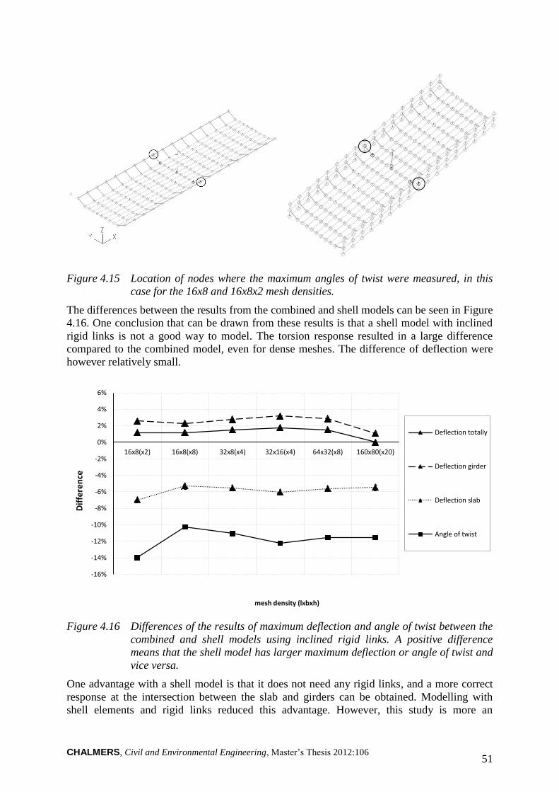
CHALMERS, Civil and Environmental Engineering, Master’s Thesis 2012:106 51
Figure 4.15 Location of nodes where the maximum angles of twist were measured, in this
case for the 16x8 and 16x8x2 mesh densities.
The differences between the results from the combined and shell models can be seen in Figure
4.16. One conclusion that can be drawn from these results is that a shell model with inclined
rigid links is not a good way to model. The torsion response resulted in a large difference
compared to the combined model, even for dense meshes. The difference of deflection were
however relatively small.
Figure 4.16 Differences of the results of maximum deflection and angle of twist between the
combined and shell models using inclined rigid links. A positive difference
means that the shell model has larger maximum deflection or angle of twist and
vice versa.
One advantage with a shell model is that it does not need any rigid links, and a more correct
response at the intersection between the slab and girders can be obtained. Modelling with
shell elements and rigid links reduced this advantage. However, this study is more an
-16%
-14%
-12%
-10%
-8%
-6%
-4%
-2%
0%
2%
4%
6%
16x8(x2) 16x8(x8) 32x8(x4) 32x16(x4) 64x32(x8) 160x80(x20)
Dif
fere
nce
mesh density (lxbxh)
Deflection totally
Deflection girder
Deflection slab
Angle of twist
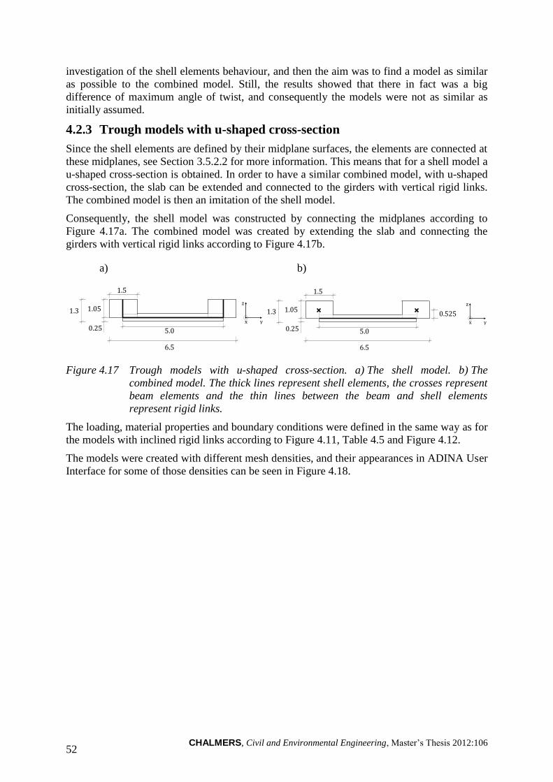
CHALMERS, Civil and Environmental Engineering, Master’s Thesis 2012:106 52
investigation of the shell elements behaviour, and then the aim was to find a model as similar
as possible to the combined model. Still, the results showed that there in fact was a big
difference of maximum angle of twist, and consequently the models were not as similar as
initially assumed.
4.2.3 Trough models with u-shaped cross-section
Since the shell elements are defined by their midplane surfaces, the elements are connected at
these midplanes, see Section 3.5.2.2 for more information. This means that for a shell model a
u-shaped cross-section is obtained. In order to have a similar combined model, with u-shaped
cross-section, the slab can be extended and connected to the girders with vertical rigid links.
The combined model is then an imitation of the shell model.
Consequently, the shell model was constructed by connecting the midplanes according to
Figure 4.17a. The combined model was created by extending the slab and connecting the
girders with vertical rigid links according to Figure 4.17b.
a) b)
Figure 4.17 Trough models with u-shaped cross-section. a) The shell model. b) The
combined model. The thick lines represent shell elements, the crosses represent
beam elements and the thin lines between the beam and shell elements
represent rigid links.
The loading, material properties and boundary conditions were defined in the same way as for
the models with inclined rigid links according to Figure 4.11, Table 4.5 and Figure 4.12.
The models were created with different mesh densities, and their appearances in ADINA User
Interface for some of those densities can be seen in Figure 4.18.
5.0
1.05
1.5
0.25
1.3 z
x y
6.5
5.0
1.05
1.5
0.25
1.3 z
x y
6.5
0.525
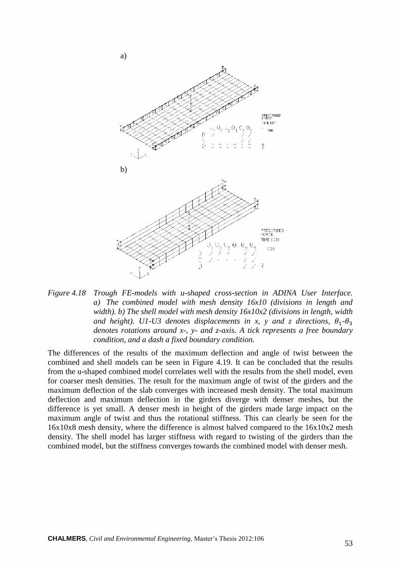
CHALMERS, Civil and Environmental Engineering, Master’s Thesis 2012:106 53
a)
b)
Figure 4.18 Trough FE-models with u-shaped cross-section in ADINA User Interface.
a) The combined model with mesh density 16x10 (divisions in length and
width). b) The shell model with mesh density 16x10x2 (divisions in length, width
and height). U1-U3 denotes displacements in x, y and z directions, -
denotes rotations around x-, y- and z-axis. A tick represents a free boundary
condition, and a dash a fixed boundary condition.
The differences of the results of the maximum deflection and angle of twist between the
combined and shell models can be seen in Figure 4.19. It can be concluded that the results
from the u-shaped combined model correlates well with the results from the shell model, even
for coarser mesh densities. The result for the maximum angle of twist of the girders and the
maximum deflection of the slab converges with increased mesh density. The total maximum
deflection and maximum deflection in the girders diverge with denser meshes, but the
difference is yet small. A denser mesh in height of the girders made large impact on the
maximum angle of twist and thus the rotational stiffness. This can clearly be seen for the
16x10x8 mesh density, where the difference is almost halved compared to the 16x10x2 mesh
density. The shell model has larger stiffness with regard to twisting of the girders than the
combined model, but the stiffness converges towards the combined model with denser mesh.
CHALMERS, Civil and Environmental Engineering, Master’s Thesis 2012:106 54
Figure 4.19 Differences of the results of maximum deflection and angle of twist between the
combined and shell models with u-shaped cross-section. A positive difference
means that the shell model has larger maximum deflection or angle of twist and
vice versa.
4.2.4 Comparison of combined and shell trough models
In order to study the impact the modelling of the height of the girders had for maximum
deflection and angle of twist, two different shell models were created and analysed. These two
models were compared to the combined model with inclined rigid links. The reason why this
combined model was used as a reference, and not the u-shaped model, was because the model
with inclined rigid links was considered to more correctly describe the connection between
the slab and girders. The development of the combined u-model was more due to mimic the
shell model.
The first shell model has a correct height of the total cross-section, but then also too low
height of the girders according to Figure 4.20a; this model is referred to as the shell model 1.
The other model has correct height of the girders, but instead a too high total cross-section,
see Figure 4.20b; this model is referred to as the shell model 2.
It should be observed that these two models are not the same as the UA- and UB-models
described in Section 4.3.7.2. The shell models 1 and 2 were only studied for one span, and the
boundary conditions were defined on the centroidal axes of the girders in order to be as
general as possible, see Figure 4.12.
The combined model with inclined rigid links can be seen in Figure 4.20c and a description
can be found in Section 4.2.2. The loading, material properties and boundary conditions were
defined in the same way as described previously according to Figure 4.11, Table 4.5 and
Figure 4.12.
-8%
-6%
-4%
-2%
0%
2%
4%
16x10(x2) 16x10(x8) 32x20(x4) 64x40(x8) 160x100(x20)
Dif
fere
nce
mesh density (lxbxh)
Deflection total
Deflection girder
Deflection slab
Angle of twist
CHALMERS, Civil and Environmental Engineering, Master’s Thesis 2012:106 55
a)
5.0
1.05
1.5
0.25
1.3
b)
5.0
1.3
1.5
0.25
1.55
c)
Figure 4.20 a) Shell model 1. b) Shell model 2. c) Combined model with inclined rigid links.
The thick lines represent shell elements, the crosses represent beam elements
and the thin lines between the beam and shell elements represent rigid links.
The results can be seen in Figure 4.21, which shows the differences of the maximum
deflection and angle of twist between the shell and combined models. The maximum angle of
twist can be seen to be more correctly described by the shell model 2, with around 4%
difference for the densest mesh. For the shell model 1 the difference of deflection is smallest,
while the difference is relatively large for the shell model 2. Both deflection and rotational
stiffness is larger for the shell model 1 and less for the shell model 2, which is reasonable
since the shell model 1 has too high total cross-section and the shell model 2 has too low
height totally.
0.75
0.65
0.40 0.25
x y
z
3.5 0.75
1.3
5.0
6.5
0.5
CHALMERS, Civil and Environmental Engineering, Master’s Thesis 2012:106 56
Figure 4.21 Differences of the results of maximum deflection and angle of twist between the
combined model and the shell models 1 and 2. A positive difference means that
the shell model has larger maximum deflection or angle of twist than the
combined model and vice versa.
4.3 FE-models
In this section all the FE-models are presented, together with descriptions of the boundary
conditions, the load stepping and the stiff elements.
4.3.1 Boundary conditions
In order to examine the impact the modelling of boundary conditions had for the analyses,
several sets of boundary conditions (Figure 4.23 and Figure 4.24) were studied at the support
sections, section I and II in Figure 4.22.
I II III
III II I
I
I
z
y x
Figure 4.22 Sections I-III of the trough bridge.
The various boundary conditions that were investigated for section I can be seen in Figure
4.23. These are referred to as BC1-BC5 (for Boundary Condition) and U1-U2 (for U-shaped
cross-section).
-40%
-30%
-20%
-10%
0%
10%
20%
16x10(x2) 16x10(x8) 32x20(x4) 64x40(x8) 160x100(x20)
Dif
fere
nce
mesh density (lxbxh)
Deflection girdershell model 1
Angle of twistshell model 1
Deflection girdershell model 2
Angle of twistshell model 2
CHALMERS, Civil and Environmental Engineering, Master’s Thesis 2012:106 57
Beam element
Structural element
Fixed twisting
Prevented translation
Rigid link/Stiff element
BC1 at section I
BC2 at section I
BC3 at section I
BC4 at section I
BC5 at section I
U1 at section I
U2 at section I
U1 (shell model) at section I
U2 (shell model) at section I
Figure 4.23 The different cross-section models and positions of boundary conditions at
section I (end support section). An explanation of the used symbols can be seen
in the upper left corner. The solid lines represent the embedded FE-models, and
the dashed lines represent the cross-section.
BC1 and BC2 are the two simplest cases, where the boundary conditions are defined directly
on the centroidal axes of the girders and on the midsurface of the shell elements. In BC3, BC4
and BC5 an eccentricity were introduced by using stiff elements so that the boundary
conditions could be defined at the bottom edges of the cross-section. More information about
the stiff elements can be found in Section 4.3.3.
Since the shell models were created as u-shaped cross-sections, the U-models were developed
in order to have similar behaviours for the beam grillage and combined models. In U1 the
twisting is fixed along the entire height, and in U2 only the bottom of the girders are fixed for
twisting.
The Figure 4.24 illustrates the cross-sections for section II and III for BC2, BC5 and U1. The
mid support was assumed to only prevent translation in transversal direction. This can be seen
in the figure, and were modelled more or less in the same way for all models. The only
difference was where in the cross-section the fixation was defined.
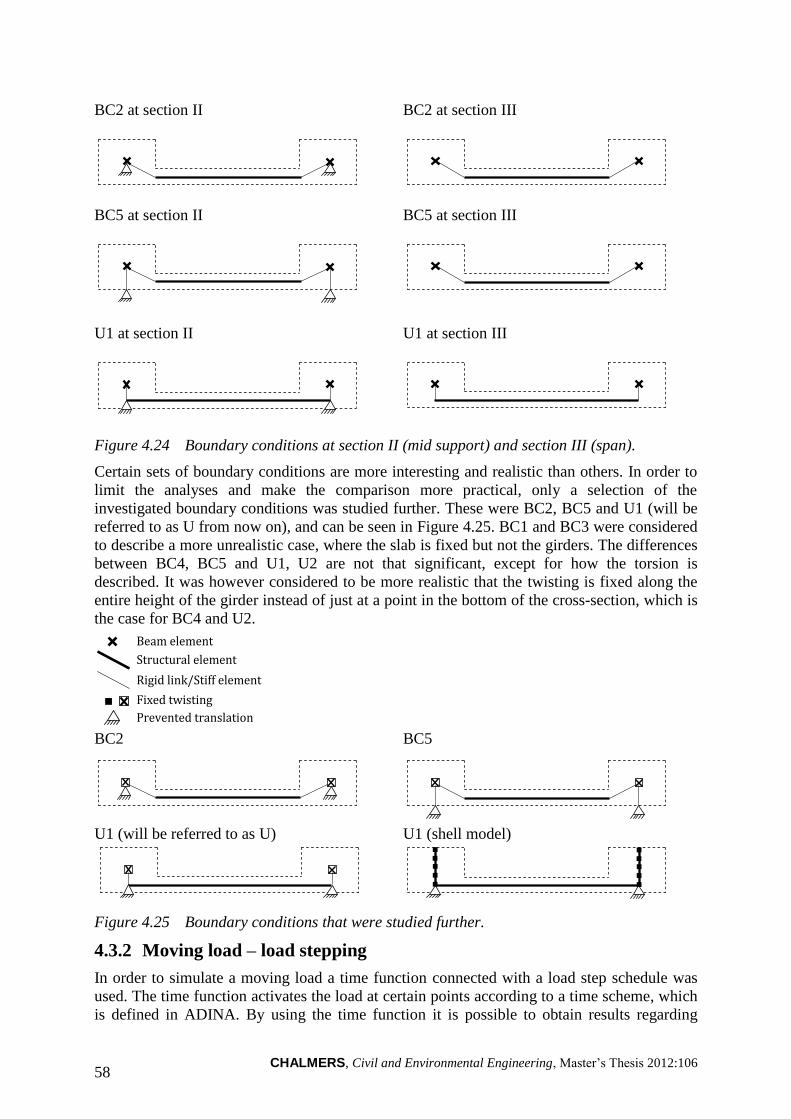
CHALMERS, Civil and Environmental Engineering, Master’s Thesis 2012:106 58
BC2 at section II
BC2 at section III
BC5 at section II
BC5 at section III
U1 at section II
U1 at section III
Figure 4.24 Boundary conditions at section II (mid support) and section III (span).
Certain sets of boundary conditions are more interesting and realistic than others. In order to
limit the analyses and make the comparison more practical, only a selection of the
investigated boundary conditions was studied further. These were BC2, BC5 and U1 (will be
referred to as U from now on), and can be seen in Figure 4.25. BC1 and BC3 were considered
to describe a more unrealistic case, where the slab is fixed but not the girders. The differences
between BC4, BC5 and U1, U2 are not that significant, except for how the torsion is
described. It was however considered to be more realistic that the twisting is fixed along the
entire height of the girder instead of just at a point in the bottom of the cross-section, which is
the case for BC4 and U2.
Beam element
Structural element
Fixed twisting
Prevented translation
Rigid link/Stiff element
BC2
BC5
U1 (will be referred to as U)
U1 (shell model)
Figure 4.25 Boundary conditions that were studied further.
4.3.2 Moving load – load stepping
In order to simulate a moving load a time function connected with a load step schedule was
used. The time function activates the load at certain points according to a time scheme, which
is defined in ADINA. By using the time function it is possible to obtain results regarding
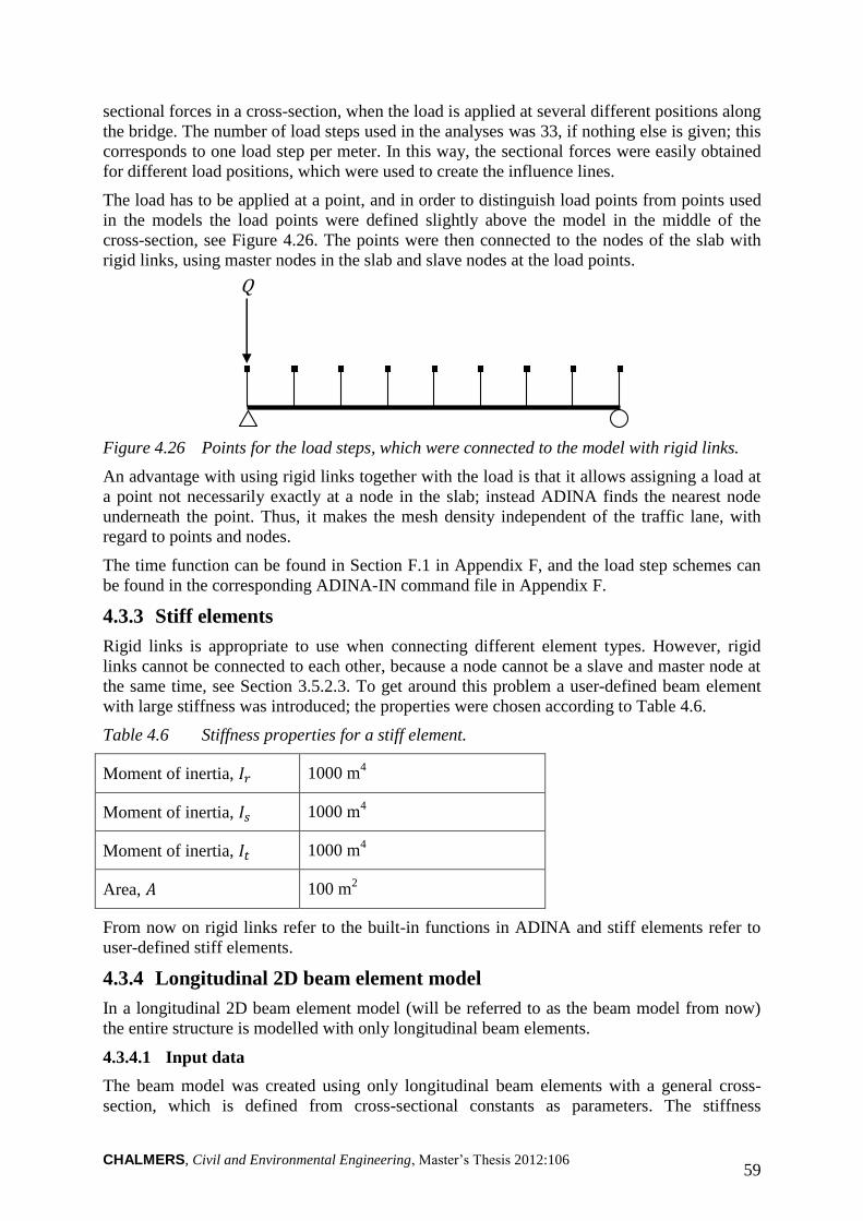
CHALMERS, Civil and Environmental Engineering, Master’s Thesis 2012:106 59
sectional forces in a cross-section, when the load is applied at several different positions along
the bridge. The number of load steps used in the analyses was 33, if nothing else is given; this
corresponds to one load step per meter. In this way, the sectional forces were easily obtained
for different load positions, which were used to create the influence lines.
The load has to be applied at a point, and in order to distinguish load points from points used
in the models the load points were defined slightly above the model in the middle of the
cross-section, see Figure 4.26. The points were then connected to the nodes of the slab with
rigid links, using master nodes in the slab and slave nodes at the load points.
Q
Figure 4.26 Points for the load steps, which were connected to the model with rigid links.
An advantage with using rigid links together with the load is that it allows assigning a load at
a point not necessarily exactly at a node in the slab; instead ADINA finds the nearest node
underneath the point. Thus, it makes the mesh density independent of the traffic lane, with
regard to points and nodes.
The time function can be found in Section F.1 in Appendix F, and the load step schemes can
be found in the corresponding ADINA-IN command file in Appendix F.
4.3.3 Stiff elements
Rigid links is appropriate to use when connecting different element types. However, rigid
links cannot be connected to each other, because a node cannot be a slave and master node at
the same time, see Section 3.5.2.3. To get around this problem a user-defined beam element
with large stiffness was introduced; the properties were chosen according to Table 4.6.
Table 4.6 Stiffness properties for a stiff element.
Moment of inertia, 1000 m4
Moment of inertia, 1000 m4
Moment of inertia, 1000 m4
Area, 100 m2
From now on rigid links refer to the built-in functions in ADINA and stiff elements refer to
user-defined stiff elements.
4.3.4 Longitudinal 2D beam element model
In a longitudinal 2D beam element model (will be referred to as the beam model from now)
the entire structure is modelled with only longitudinal beam elements.
4.3.4.1 Input data
The beam model was created using only longitudinal beam elements with a general cross-
section, which is defined from cross-sectional constants as parameters. The stiffness
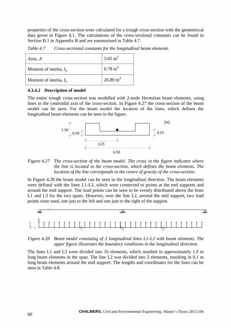
CHALMERS, Civil and Environmental Engineering, Master’s Thesis 2012:106 60
properties of the cross-section were calculated for a trough cross-section with the geometrical
data given in Figure 4.1. The calculations of the cross-sectional constants can be found in
Section B.1 in Appendix B and are summarised in Table 4.7.
Table 4.7 Cross-sectional constants for the longitudinal beam elements.
Area, 5.65 m2
Moment of inertia, 0.78 m4
Moment of inertia, 26.89 m4
4.3.4.2 Description of model
The entire trough cross-section was modelled with 2-node Hermitian beam elements, using
lines in the centroidal axis of the cross-section. In Figure 4.27 the cross-section of the beam
model can be seen. For the beam model the location of the lines, which defines the
longitudinal beam elements can be seen in the figure.
[m]
1.30
6.50
0.53 0.50
3.25
Figure 4.27 The cross-section of the beam model. The cross in the figure indicates where
the line is located in the cross-section, which defines the beam elements. The
location of the line corresponds to the centre of gravity of the cross-section.
In Figure 4.28 the beam model can be seen in the longitudinal direction. The beam elements
were defined with the lines L1-L3, which were connected to points at the end supports and
around the mid support. The load points can be seen to be evenly distributed above the lines
L1 and L3 for the two spans. However, over the line L2, around the mid support, two load
points were used, one just to the left and one just to the right of the support.
Figure 4.28 Beam model consisting of 3 longitudinal lines L1-L3 with beam elements. The
upper figure illustrates the boundary conditions in the longitudinal direction.
The lines L1 and L3 were divided into 16 elements, which resulted in approximately 1.0 m
long beam elements in the span. The line L2 was divided into 2 elements, resulting in 0.1 m
long beam elements around the mid support. The lengths and coordinates for the lines can be
seen in Table 4.8.
x
y z
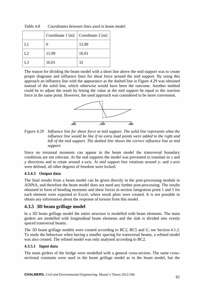
CHALMERS, Civil and Environmental Engineering, Master’s Thesis 2012:106 61
Table 4.8 Coordinates between lines used in beam model.
Coordinate 1 [m] Coordinate 2 [m]
L1 0 15.99
L2 15.99 16.01
L3 16.01 32
The reason for dividing the beam model with a short line above the mid support was to create
proper diagrams and influence lines for shear force around the mid support. By using this
approach an influence line with the appearance as the dashed line in Figure 4.29 was obtained
instead of the solid line, which otherwise would have been the outcome. Another method
could be to adjust the result by letting the value at the mid support be equal to the reaction
force in the same point. However, the used approach was considered to be more convenient.
Figure 4.29 Influence line for shear force at mid support. The solid line represents what the
influence line would be like if no extra load points were added to the right and
left of the mid support. The dashed line shows the correct influence line at mid
support.
Since no torsional moments can appear in the beam model the transversal boundary
conditions are not relevant. At the end supports the model was prevented to translate in z and
y directions and to rotate around x-axis. At mid support free rotations around y- and z-axis
were defined, all other degrees of freedom were locked.
4.3.4.3 Output data
The final results from a beam model can be given directly in the post-processing module in
ADINA, and therefore the beam model does not need any further post-processing. The results
obtained in form of bending moments and shear forces in section integration point 1 and 5 for
each element were exported to Excel, where result plots were created. It is not possible to
obtain any information about the response of torsion from this model.
4.3.5 3D beam grillage model
In a 3D beam grillage model the entire structure is modelled with beam elements. The main
girders are modelled with longitudinal beam elements and the slab is divided into evenly
spaced transversal beams.
The 3D beam grillage models were created according to BC2, BC5 and U, see Section 4.1.2.
To study the behaviour when having a smaller spacing for transversal beams, a refined model
was also created. The refined model was only analysed according to BC2.
4.3.5.1 Input data
The main girders of the bridge were modelled with a general cross-section. The same cross-
sectional constants were used in the beam grillage model as in the beam model, but the
CHALMERS, Civil and Environmental Engineering, Master’s Thesis 2012:106 62
constants were divided by two since the model includes two main girders. In other words, the
moments of inertia were calculated for half a U-section instead of an L-section. The cross-
sectional constants are given in Table 4.9.
Table 4.9 Cross-sectional constants for the longitudinal beam elements.
Area, 2.83 m2
Moment of inertia, 0.39 m4
Moment of inertia, 13.45 m4
Torsion constant, 0.45 m4
It is important to distinguish what parts of the cross-section that contributes to the different
cross-sectional constants. Area and moment of inertia was calculated based on the total area
of the cross-section according to Figure 4.30a. Since torsion is only resisted by the main
girders the calculation of torsion constant was based on the area of the main girders according
to Figure 4.30b. The calculations can be found in Section B.1 in Appendix B.
a)
b)
Figure 4.30 The shadowed areas in the figure describe what parts of the cross-section that
are used to calculate different sectional properties. The dashed line in the
centre divides the cross-section in two equally parts. These parts represent the
area for each girder. a) Area and moment of inertia , . b) Torsion
constant .
The transversal beams were modelled with a rectangular cross-section, using the dimensions
according to Table 4.10.
Table 4.10 Cross-section geometry for the transversal beam elements.
Width, 1.0 m
Height, 0.5 m
4.3.5.2 Description of models
Both the longitudinal girders and the slab were modelled with 2-node Hermitian beam
elements, using lines in centroidal axes of the slab and girders.
The beam grillage was created according to BC2, BC5 and U as in Figure 4.23. Figure 4.31
represents how the FE-models are embedded in the cross-section. For the BC2 and BC5
models the slab was assumed to be bounded by the two longitudinal girders. The slab was
connected to the main girders by inclined rigid links, giving a 3.5 m width of the slab. In the
U-model the slab was assumed to be extended to the centre of the main girders, giving a 5.0 m
wide slab. For all models the longitudinal girders were modelled by lines on the centroidal
axes of the girders, i.e. at half of the height according to Figure 4.31.
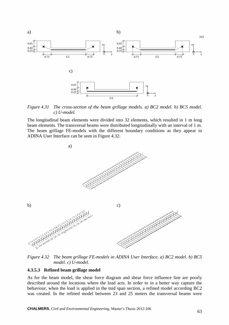
CHALMERS, Civil and Environmental Engineering, Master’s Thesis 2012:106 63
a)
b)
3.5 0.75 0.75
0.25
0.65
0.40
z
x y
[m]
c)
Figure 4.31 The cross-section of the beam grillage models. a) BC2 model. b) BC5 model.
c) U-model.
The longitudinal beam elements were divided into 32 elements, which resulted in 1 m long
beam elements. The transversal beams were distributed longitudinally with an interval of 1 m.
The beam grillage FE-models with the different boundary conditions as they appear in
ADINA User Interface can be seen in Figure 4.32.
a)
b)
c)
Figure 4.32 The beam grillage FE-models in ADINA User Interface. a) BC2 model. b) BC5
model. c) U-model.
4.3.5.3 Refined beam grillage model
As for the beam model, the shear force diagram and shear force influence line are poorly
described around the locations where the load acts. In order to in a better way capture the
behaviour, when the load is applied in the mid span section, a refined model according BC2
was created. In the refined model between 23 and 25 meters the transversal beams were
3.5 0.75 0.75
0.25
0.65
0.40
z
x y
5.0
0.25
0.65
0.40
z
x y
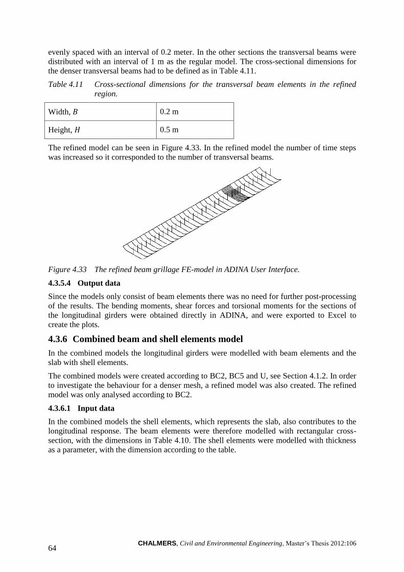
CHALMERS, Civil and Environmental Engineering, Master’s Thesis 2012:106 64
evenly spaced with an interval of 0.2 meter. In the other sections the transversal beams were
distributed with an interval of 1 m as the regular model. The cross-sectional dimensions for
the denser transversal beams had to be defined as in Table 4.11.
Table 4.11 Cross-sectional dimensions for the transversal beam elements in the refined
region.
Width, 0.2 m
Height, 0.5 m
The refined model can be seen in Figure 4.33. In the refined model the number of time steps
was increased so it corresponded to the number of transversal beams.
Figure 4.33 The refined beam grillage FE-model in ADINA User Interface.
4.3.5.4 Output data
Since the models only consist of beam elements there was no need for further post-processing
of the results. The bending moments, shear forces and torsional moments for the sections of
the longitudinal girders were obtained directly in ADINA, and were exported to Excel to
create the plots.
4.3.6 Combined beam and shell elements model
In the combined models the longitudinal girders were modelled with beam elements and the
slab with shell elements.
The combined models were created according to BC2, BC5 and U, see Section 4.1.2. In order
to investigate the behaviour for a denser mesh, a refined model was also created. The refined
model was only analysed according to BC2.
4.3.6.1 Input data
In the combined models the shell elements, which represents the slab, also contributes to the
longitudinal response. The beam elements were therefore modelled with rectangular cross-
section, with the dimensions in Table 4.10. The shell elements were modelled with thickness
as a parameter, with the dimension according to the table.
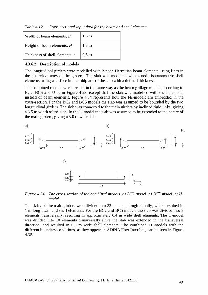
CHALMERS, Civil and Environmental Engineering, Master’s Thesis 2012:106 65
Table 4.12 Cross-sectional input data for the beam and shell elements.
Width of beam elements, 1.5 m
Height of beam elements, 1.3 m
Thickness of shell elements, 0.5 m
4.3.6.2 Description of models
The longitudinal girders were modelled with 2-node Hermitian beam elements, using lines in
the centroidal axes of the girders. The slab was modelled with 4-node isoparametric shell
elements, using a surface in the midplane of the slab with a defined thickness.
The combined models were created in the same way as the beam grillage models according to
BC2, BC5 and U as in Figure 4.23, except that the slab was modelled with shell elements
instead of beam elements. Figure 4.34 represents how the FE-models are embedded in the
cross-section. For the BC2 and BC5 models the slab was assumed to be bounded by the two
longitudinal girders. The slab was connected to the main girders by inclined rigid links, giving
a 3.5 m width of the slab. In the U-model the slab was assumed to be extended to the centre of
the main girders, giving a 5.0 m wide slab.
a)
b)
3.5 0.75 0.75
0.25
0.65
0.40
z
x y
[m]
c)
Figure 4.34 The cross-section of the combined models. a) BC2 model. b) BC5 model. c) U-
model.
The slab and the main girders were divided into 32 elements longitudinally, which resulted in
1 m long beam and shell elements. For the BC2 and BC5 models the slab was divided into 8
elements transversally, resulting in approximately 0.4 m wide shell elements. The U-model
was divided into 10 elements transversally since the slab was extended in the transversal
direction, and resulted in 0.5 m wide shell elements. The combined FE-models with the
different boundary conditions, as they appear in ADINA User Interface, can be seen in Figure
4.35.
3.5 0.75 0.75
0.25
0.65
0.40
z
x y
5.0
0.25
0.65
0.40
z
x y
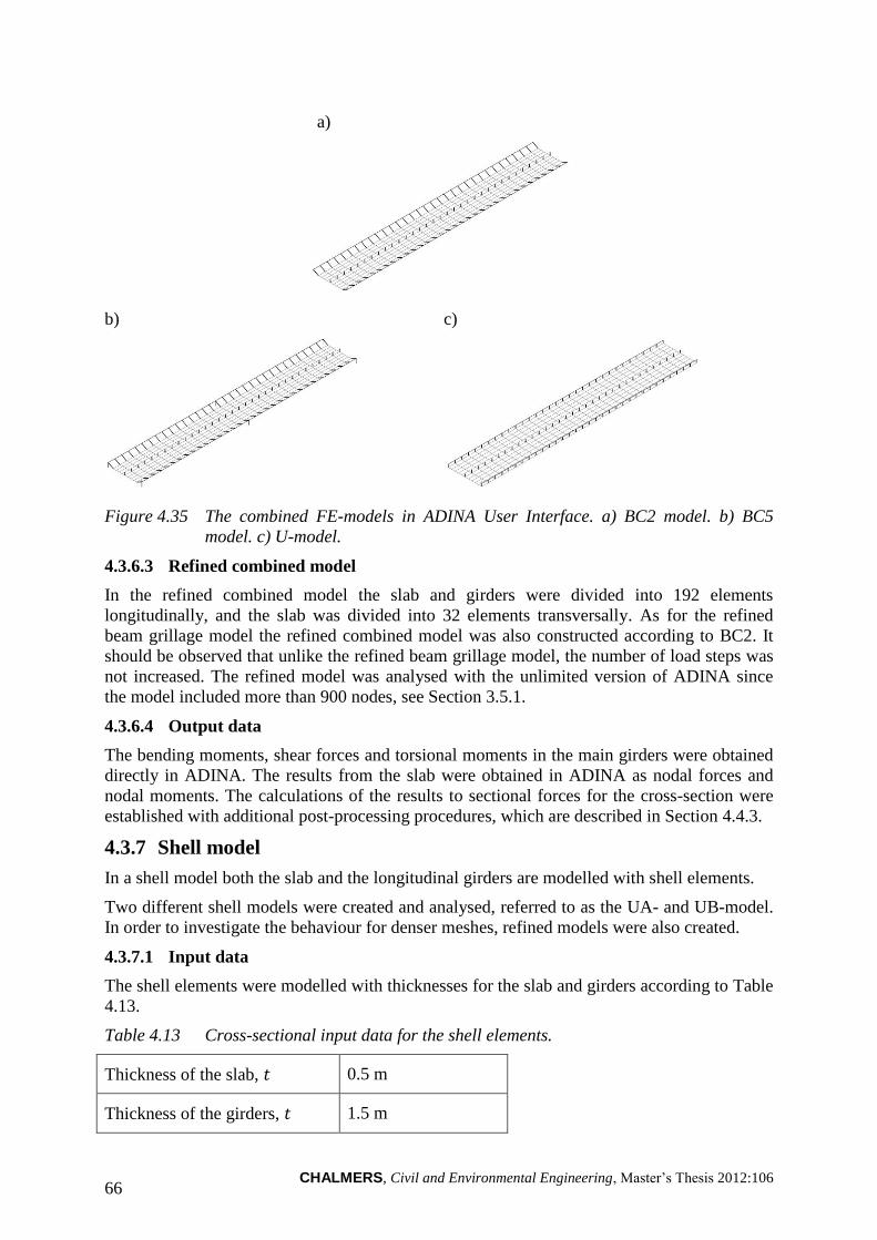
CHALMERS, Civil and Environmental Engineering, Master’s Thesis 2012:106 66
a)
b)
c)
Figure 4.35 The combined FE-models in ADINA User Interface. a) BC2 model. b) BC5
model. c) U-model.
4.3.6.3 Refined combined model
In the refined combined model the slab and girders were divided into 192 elements
longitudinally, and the slab was divided into 32 elements transversally. As for the refined
beam grillage model the refined combined model was also constructed according to BC2. It
should be observed that unlike the refined beam grillage model, the number of load steps was
not increased. The refined model was analysed with the unlimited version of ADINA since
the model included more than 900 nodes, see Section 3.5.1.
4.3.6.4 Output data
The bending moments, shear forces and torsional moments in the main girders were obtained
directly in ADINA. The results from the slab were obtained in ADINA as nodal forces and
nodal moments. The calculations of the results to sectional forces for the cross-section were
established with additional post-processing procedures, which are described in Section 4.4.3.
4.3.7 Shell model
In a shell model both the slab and the longitudinal girders are modelled with shell elements.
Two different shell models were created and analysed, referred to as the UA- and UB-model.
In order to investigate the behaviour for denser meshes, refined models were also created.
4.3.7.1 Input data
The shell elements were modelled with thicknesses for the slab and girders according to Table
4.13.
Table 4.13 Cross-sectional input data for the shell elements.
Thickness of the slab, 0.5 m
Thickness of the girders, 1.5 m
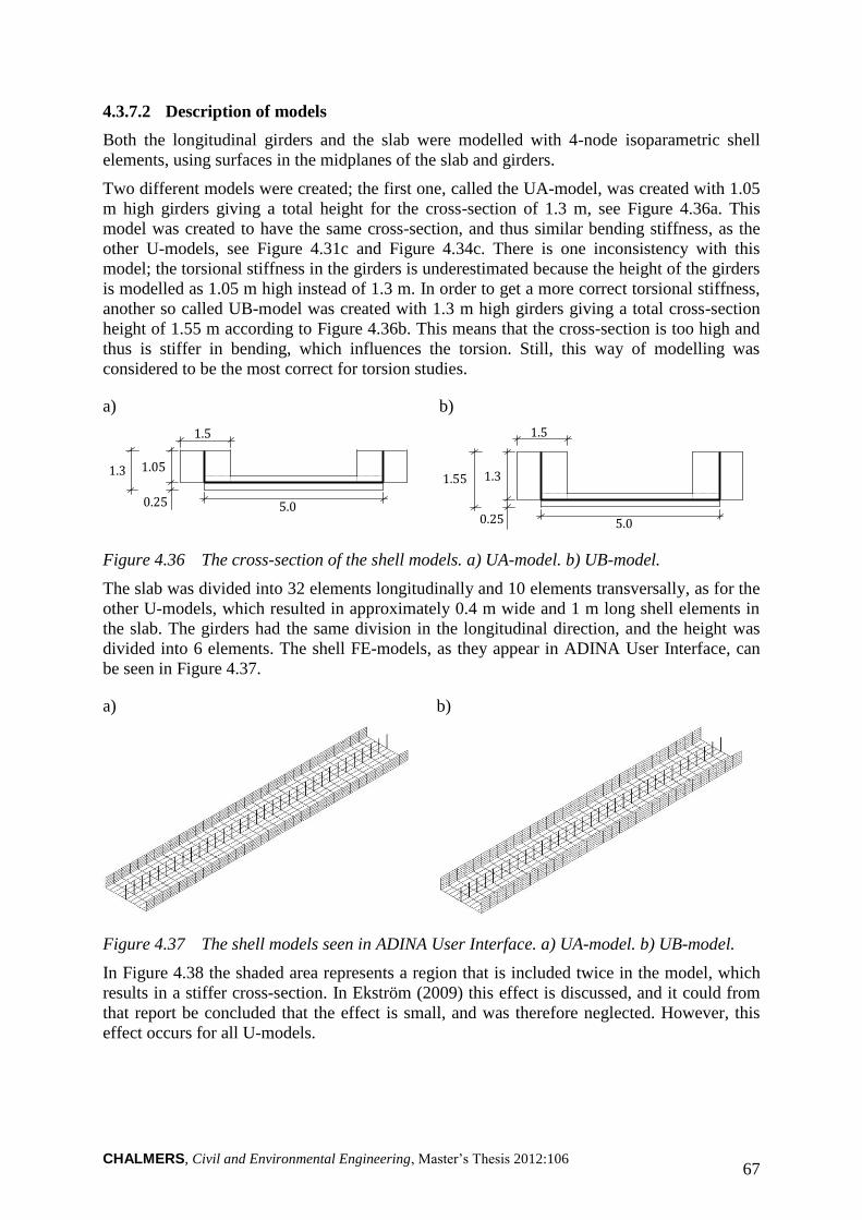
CHALMERS, Civil and Environmental Engineering, Master’s Thesis 2012:106 67
4.3.7.2 Description of models
Both the longitudinal girders and the slab were modelled with 4-node isoparametric shell
elements, using surfaces in the midplanes of the slab and girders.
Two different models were created; the first one, called the UA-model, was created with 1.05
m high girders giving a total height for the cross-section of 1.3 m, see Figure 4.36a. This
model was created to have the same cross-section, and thus similar bending stiffness, as the
other U-models, see Figure 4.31c and Figure 4.34c. There is one inconsistency with this
model; the torsional stiffness in the girders is underestimated because the height of the girders
is modelled as 1.05 m high instead of 1.3 m. In order to get a more correct torsional stiffness,
another so called UB-model was created with 1.3 m high girders giving a total cross-section
height of 1.55 m according to Figure 4.36b. This means that the cross-section is too high and
thus is stiffer in bending, which influences the torsion. Still, this way of modelling was
considered to be the most correct for torsion studies.
a)
5.0
1.05
1.5
0.25
1.3
b)
5.0
1.3
1.5
0.25
1.55
Figure 4.36 The cross-section of the shell models. a) UA-model. b) UB-model.
The slab was divided into 32 elements longitudinally and 10 elements transversally, as for the
other U-models, which resulted in approximately 0.4 m wide and 1 m long shell elements in
the slab. The girders had the same division in the longitudinal direction, and the height was
divided into 6 elements. The shell FE-models, as they appear in ADINA User Interface, can
be seen in Figure 4.37.
a)
b)
Figure 4.37 The shell models seen in ADINA User Interface. a) UA-model. b) UB-model.
In Figure 4.38 the shaded area represents a region that is included twice in the model, which
results in a stiffer cross-section. In Ekström (2009) this effect is discussed, and it could from
that report be concluded that the effect is small, and was therefore neglected. However, this
effect occurs for all U-models.
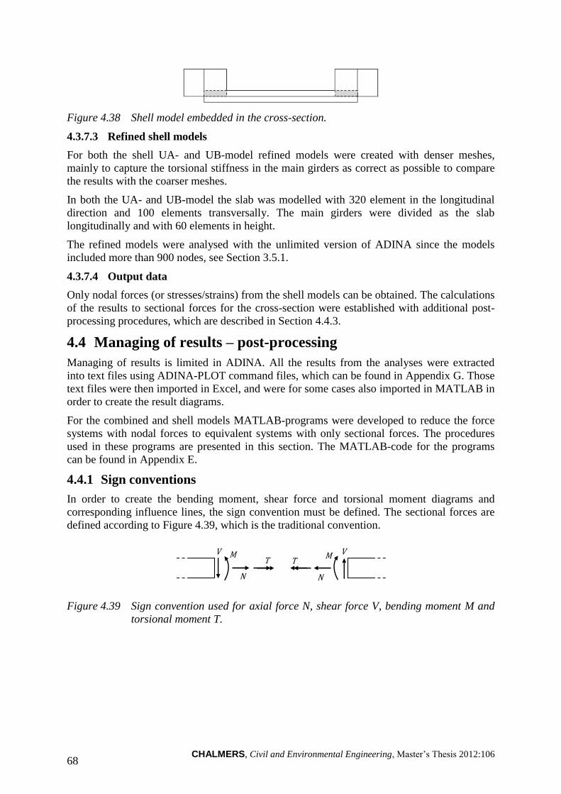
CHALMERS, Civil and Environmental Engineering, Master’s Thesis 2012:106 68
Figure 4.38 Shell model embedded in the cross-section.
4.3.7.3 Refined shell models
For both the shell UA- and UB-model refined models were created with denser meshes,
mainly to capture the torsional stiffness in the main girders as correct as possible to compare
the results with the coarser meshes.
In both the UA- and UB-model the slab was modelled with 320 element in the longitudinal
direction and 100 elements transversally. The main girders were divided as the slab
longitudinally and with 60 elements in height.
The refined models were analysed with the unlimited version of ADINA since the models
included more than 900 nodes, see Section 3.5.1.
4.3.7.4 Output data
Only nodal forces (or stresses/strains) from the shell models can be obtained. The calculations
of the results to sectional forces for the cross-section were established with additional post-
processing procedures, which are described in Section 4.4.3.
4.4 Managing of results – post-processing
Managing of results is limited in ADINA. All the results from the analyses were extracted
into text files using ADINA-PLOT command files, which can be found in Appendix G. Those
text files were then imported in Excel, and were for some cases also imported in MATLAB in
order to create the result diagrams.
For the combined and shell models MATLAB-programs were developed to reduce the force
systems with nodal forces to equivalent systems with only sectional forces. The procedures
used in these programs are presented in this section. The MATLAB-code for the programs
can be found in Appendix E.
4.4.1 Sign conventions
In order to create the bending moment, shear force and torsional moment diagrams and
corresponding influence lines, the sign convention must be defined. The sectional forces are
defined according to Figure 4.39, which is the traditional convention.
N
V T
M T
N
V M
Figure 4.39 Sign convention used for axial force N, shear force V, bending moment M and
torsional moment T.
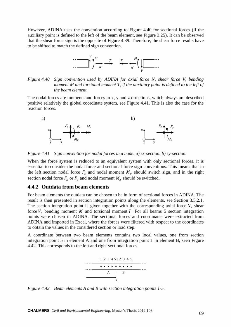
CHALMERS, Civil and Environmental Engineering, Master’s Thesis 2012:106 69
However, ADINA uses the convention according to Figure 4.40 for sectional forces (if the
auxiliary point is defined to the left of the beam element, see Figure 3.25). It can be observed
that the shear force sign is the opposite of Figure 4.39. Therefore, the shear force results have
to be shifted to match the defined sign convention.
N
V T
M T
N V
M
Figure 4.40 Sign convention used by ADINA for axial force N, shear force V, bending
moment M and torsional moment T, if the auxiliary point is defined to the left of
the beam element.
The nodal forces are moments and forces in x, y and z directions, which always are described
positive relatively the global coordinate system, see Figure 4.41. This is also the case for the
reaction forces.
a)
Fz Fx
My
Mx z
y x
b)
z
x y
Fz Fy
Mx
Figure 4.41 Sign convention for nodal forces in a node. a) zx-section. b) zy-section.
When the force system is reduced to an equivalent system with only sectional forces, it is
essential to consider the nodal force and sectional force sign conventions. This means that in
the left section nodal force and nodal moment should switch sign, and in the right
section nodal force or and nodal moment should be switched.
4.4.2 Outdata from beam elements
For beam elements the outdata can be chosen to be in form of sectional forces in ADINA. The
result is then presented in section integration points along the elements, see Section 3.5.2.1.
The section integration point is given together with the corresponding axial force , shear
force , bending moment and torsional moment . For all beams 5 section integration
points were chosen in ADINA. The sectional forces and coordinates were extracted from
ADINA and imported in Excel, where the forces were filtered with respect to the coordinates
to obtain the values in the considered section or load step.
A coordinate between two beam elements contains two local values, one from section
integration point 5 in element A and one from integration point 1 in element B, seen Figure
4.42. This corresponds to the left and right sectional forces.
Figure 4.42 Beam elements A and B with section integration points 1-5.
x
1 2 3 4 51 2 3 4 5
A B
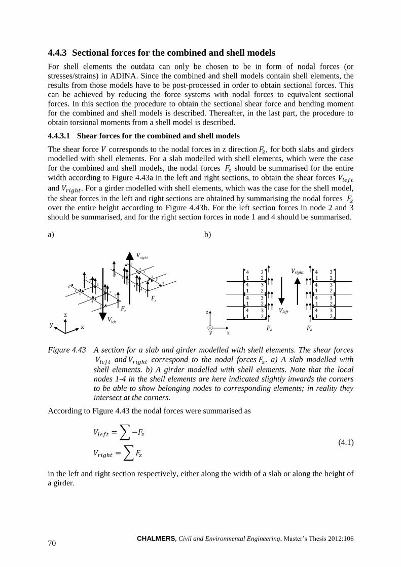
CHALMERS, Civil and Environmental Engineering, Master’s Thesis 2012:106 70
4.4.3 Sectional forces for the combined and shell models
For shell elements the outdata can only be chosen to be in form of nodal forces (or
stresses/strains) in ADINA. Since the combined and shell models contain shell elements, the
results from those models have to be post-processed in order to obtain sectional forces. This
can be achieved by reducing the force systems with nodal forces to equivalent sectional
forces. In this section the procedure to obtain the sectional shear force and bending moment
for the combined and shell models is described. Thereafter, in the last part, the procedure to
obtain torsional moments from a shell model is described.
4.4.3.1 Shear forces for the combined and shell models
The shear force corresponds to the nodal forces in z direction , for both slabs and girders
modelled with shell elements. For a slab modelled with shell elements, which were the case
for the combined and shell models, the nodal forces should be summarised for the entire
width according to Figure 4.43a in the left and right sections, to obtain the shear forces
and . For a girder modelled with shell elements, which was the case for the shell model,
the shear forces in the left and right sections are obtained by summarising the nodal forces
over the entire height according to Figure 4.43b. For the left section forces in node 2 and 3
should be summarised, and for the right section forces in node 1 and 4 should be summarised.
a) b)
x
z
y
zF 1
2 3
4 1
1 2
3
4
4
2 3
zF
leftV
1
2 3
4 1
1 2
3
4
4
2
3
rightV
z
y x Fz Fz
Vleft
Vright
2 3
1 4
2 3
1 4
2 3
1 4
2 3
1 4
2 3
1 4
2 3
1 4
2 3
1 4
2 3
1 4
Figure 4.43 A section for a slab and girder modelled with shell elements. The shear forces
and correspond to the nodal forces . a) A slab modelled with
shell elements. b) A girder modelled with shell elements. Note that the local
nodes 1-4 in the shell elements are here indicated slightly inwards the corners
to be able to show belonging nodes to corresponding elements; in reality they
intersect at the corners.
According to Figure 4.43 the nodal forces were summarised as
∑
∑
(4.1)
in the left and right section respectively, either along the width of a slab or along the height of
a girder.
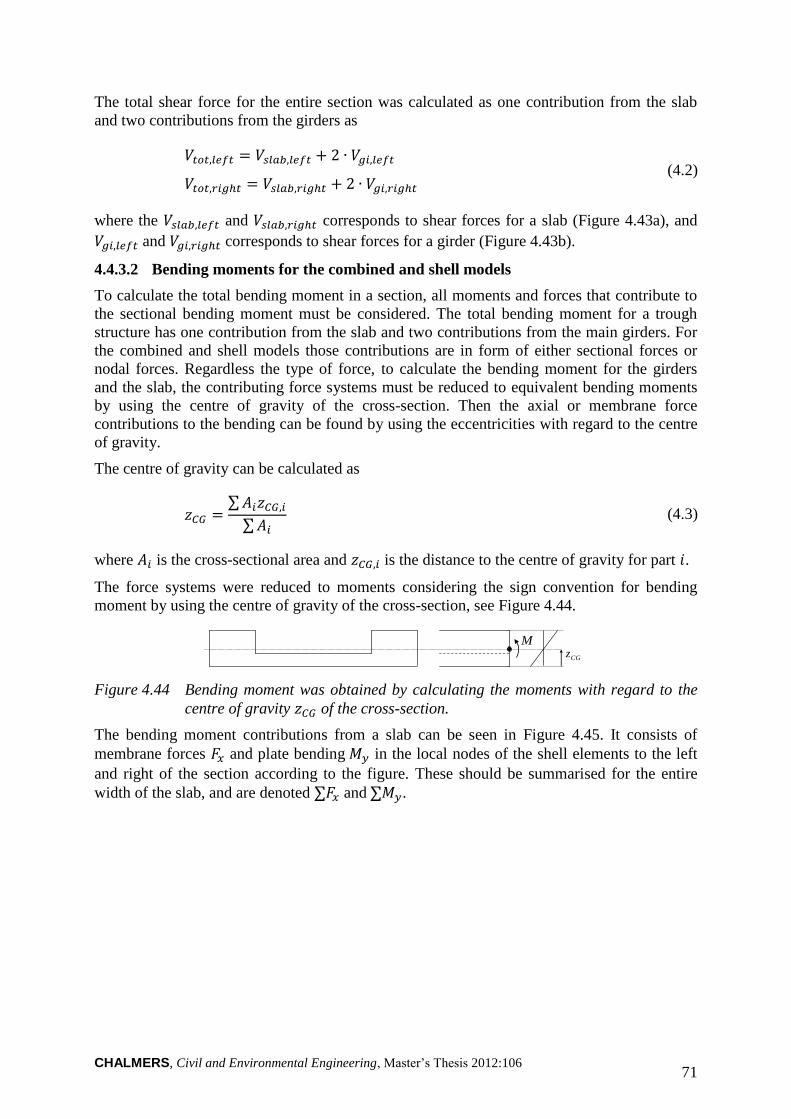
CHALMERS, Civil and Environmental Engineering, Master’s Thesis 2012:106 71
The total shear force for the entire section was calculated as one contribution from the slab
and two contributions from the girders as
(4.2)
where the and corresponds to shear forces for a slab (Figure 4.43a), and
and corresponds to shear forces for a girder (Figure 4.43b).
4.4.3.2 Bending moments for the combined and shell models
To calculate the total bending moment in a section, all moments and forces that contribute to
the sectional bending moment must be considered. The total bending moment for a trough
structure has one contribution from the slab and two contributions from the main girders. For
the combined and shell models those contributions are in form of either sectional forces or
nodal forces. Regardless the type of force, to calculate the bending moment for the girders
and the slab, the contributing force systems must be reduced to equivalent bending moments
by using the centre of gravity of the cross-section. Then the axial or membrane force
contributions to the bending can be found by using the eccentricities with regard to the centre
of gravity.
The centre of gravity can be calculated as
∑
∑ (4.3)
where is the cross-sectional area and is the distance to the centre of gravity for part .
The force systems were reduced to moments considering the sign convention for bending
moment by using the centre of gravity of the cross-section, see Figure 4.44.
CGz M
Figure 4.44 Bending moment was obtained by calculating the moments with regard to the
centre of gravity of the cross-section.
The bending moment contributions from a slab can be seen in Figure 4.45. It consists of
membrane forces and plate bending in the local nodes of the shell elements to the left
and right of the section according to the figure. These should be summarised for the entire
width of the slab, and are denoted ∑ and ∑ .
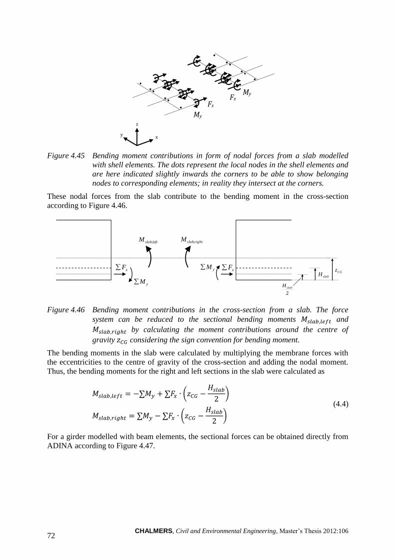
CHALMERS, Civil and Environmental Engineering, Master’s Thesis 2012:106 72
My
My
Fx Fx
x
z
y
Figure 4.45 Bending moment contributions in form of nodal forces from a slab modelled
with shell elements. The dots represent the local nodes in the shell elements and
are here indicated slightly inwards the corners to be able to show belonging
nodes to corresponding elements; in reality they intersect at the corners.
These nodal forces from the slab contribute to the bending moment in the cross-section
according to Figure 4.46.
left,slabM right,slabM
yM
xF yM xF
2
slabH
slabH CGz
Figure 4.46 Bending moment contributions in the cross-section from a slab. The force
system can be reduced to the sectional bending moments and
by calculating the moment contributions around the centre of
gravity considering the sign convention for bending moment.
The bending moments in the slab were calculated by multiplying the membrane forces with
the eccentricities to the centre of gravity of the cross-section and adding the nodal moment.
Thus, the bending moments for the right and left sections in the slab were calculated as
∑ ∑ (
)
∑ ∑ (
)
(4.4)
For a girder modelled with beam elements, the sectional forces can be obtained directly from
ADINA according to Figure 4.47.
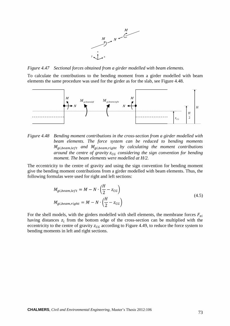
CHALMERS, Civil and Environmental Engineering, Master’s Thesis 2012:106 73
x
z
y
N M
M
Figure 4.47 Sectional forces obtained from a girder modelled with beam elements.
To calculate the contributions to the bending moment from a girder modelled with beam
elements the same procedure was used for the girder as for the slab, see Figure 4.48.
M
N N
M left,beam,giM
right,beam,giM
CGz
H
2
H
Figure 4.48 Bending moment contributions in the cross-section from a girder modelled with
beam elements. The force system can be reduced to bending moments
and by calculating the moment contributions
around the centre of gravity considering the sign convention for bending
moment. The beam elements were modelled at H/2.
The eccentricity to the centre of gravity and using the sign convention for bending moment
give the bending moment contributions from a girder modelled with beam elements. Thus, the
following formulas were used for right and left sections:
(
)
(
)
(4.5)
For the shell models, with the girders modelled with shell elements, the membrane forces
having distances from the bottom edge of the cross-section can be multiplied with the
eccentricity to the centre of gravity according to Figure 4.49, to reduce the force system to
bending moments in left and right sections.
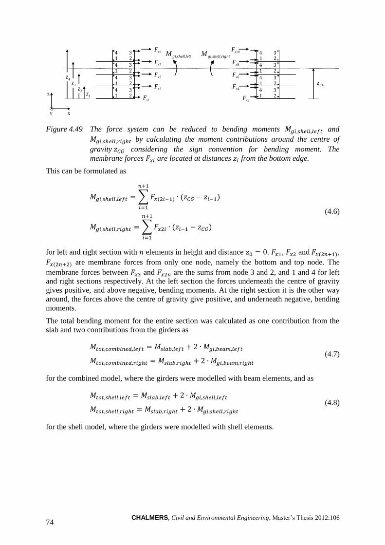
CHALMERS, Civil and Environmental Engineering, Master’s Thesis 2012:106 74
2 3
1 4
2 3
1 4
2 3
1 4
2 3
1 4
2 3
1 4
2 3
1 4
2 3
1 4
2 3
1 4
left,shell,giM right,shell,giM
CGz
1xF 2xF
5xF
7xF
9xF
6xF
8xF
10xF
3xF 4xF
1z 2z
3z 4z
z
y x
Figure 4.49 The force system can be reduced to bending moments and
by calculating the moment contributions around the centre of
gravity considering the sign convention for bending moment. The
membrane forces are located at distances from the bottom edge.
This can be formulated as
∑
∑
(4.6)
for left and right section with elements in height and distance . , and ,
are membrane forces from only one node, namely the bottom and top node. The
membrane forces between and are the sums from node 3 and 2, and 1 and 4 for left
and right sections respectively. At the left section the forces underneath the centre of gravity
gives positive, and above negative, bending moments. At the right section it is the other way
around, the forces above the centre of gravity give positive, and underneath negative, bending
moments.
The total bending moment for the entire section was calculated as one contribution from the
slab and two contributions from the girders as
(4.7)
for the combined model, where the girders were modelled with beam elements, and as
(4.8)
for the shell model, where the girders were modelled with shell elements.
CHALMERS, Civil and Environmental Engineering, Master’s Thesis 2012:106 75
4.4.3.3 Torsional moments for the shell model - the TSE-method
In order to calculate torsional moments in the main girders, the TSE-method (Torsion from
Slab Edge method) was developed. Its main idea is to start calculating a reaction torsional
moment and then add the torques, which are introduced by the slab in each section. This can
be established by calculating the decrease or increase of torsional moment in each section by
reducing the force system, from the slab edge, to torques around the centre of twist of the
girders. If starting at a node with a reaction force, where a twisting moment is known, the
reaction torsional moment in that section can be calculated, also by reducing the forces
around the centre of twist. The torsional moment in the girder can then be calculated using the
reaction torsional moments and the contributions from the slab. The contributions are added
along the girder from where the reaction torsional moment is firstly calculated. The method is
based on calculating the torsional moment distribution backwards.
In order to obtain correct twisting reaction moments at the supports, the TSE-method relies on
the correctness from the FE-software calculations of the rotational stiffness for the elements
of the girder. This was the main reason why the deflection and rotational stiffness study was
carried out, see Section 4.2. However, as long as the rotational stiffness is correct, and of
course also the reaction torsional moments, the TSE-method can be used to obtain accurate
torsional moment distributions in the main girders of a shell model.
The torsional moment response in a trough structure can easily be illustrated with a beam
grillage model, see Figure 4.50. The applied load gives axial force, shear force and bending
moment at each end of the transversal beam (the edge of the slab), which give torsional
moments in the girders. The torsional moment distribution in Figure 4.50a can be seen to
decrease further away from the section where the concentrated load is applied. The decreases
are due to the resistances in the transversal beams in form of transverse bending moments,
shear forces and axial forces. Thus, the torsional moments in the main girders are both
introduced, by the slab edge, in the section where the load is applied, and resisted further
away from the load position. How the torsional moments are introduced and resisted depends
on the response of the structure, and how this response is captured depends on the modelling.
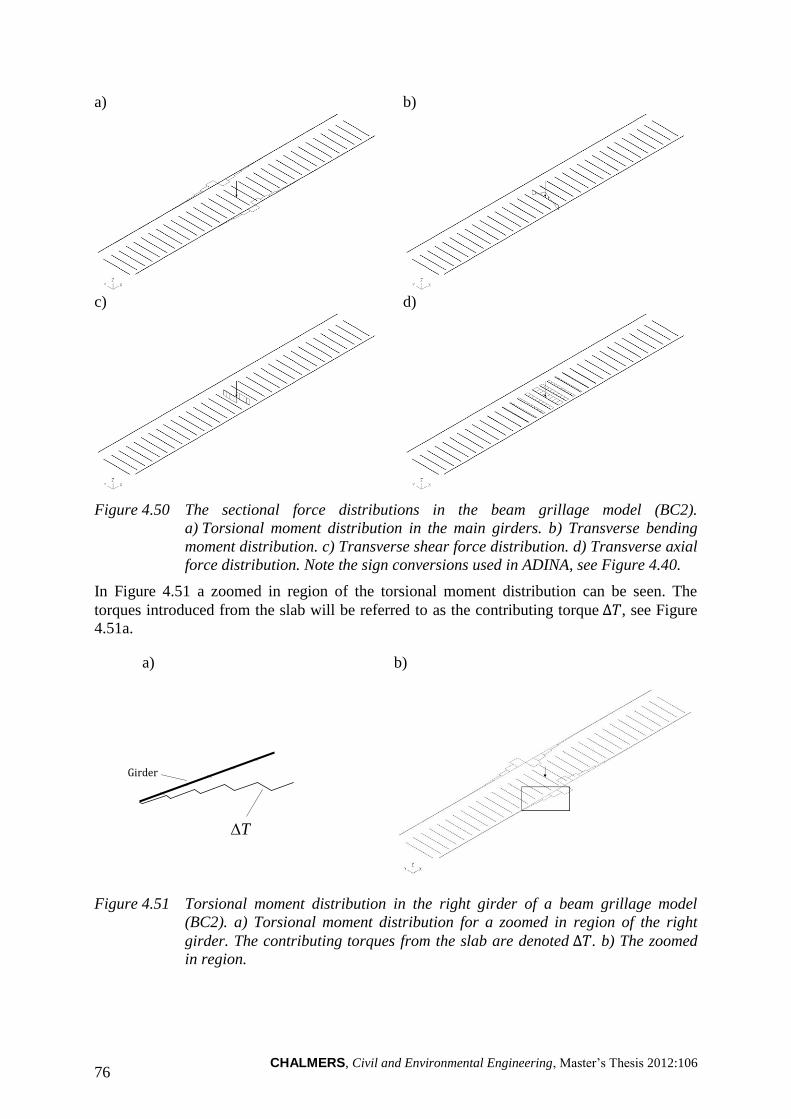
CHALMERS, Civil and Environmental Engineering, Master’s Thesis 2012:106 76
a)
b)
c)
d)
Figure 4.50 The sectional force distributions in the beam grillage model (BC2).
a) Torsional moment distribution in the main girders. b) Transverse bending
moment distribution. c) Transverse shear force distribution. d) Transverse axial
force distribution. Note the sign conversions used in ADINA, see Figure 4.40.
In Figure 4.51 a zoomed in region of the torsional moment distribution can be seen. The
torques introduced from the slab will be referred to as the contributing torque , see Figure
4.51a.
a) b)
Girder
T
Figure 4.51 Torsional moment distribution in the right girder of a beam grillage model
(BC2). a) Torsional moment distribution for a zoomed in region of the right
girder. The contributing torques from the slab are denoted . b) The zoomed
in region.
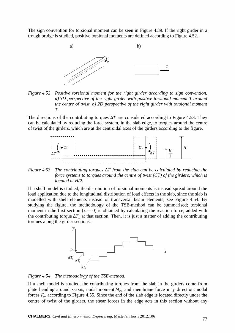
CHALMERS, Civil and Environmental Engineering, Master’s Thesis 2012:106 77
The sign convention for torsional moment can be seen in Figure 4.39. If the right girder in a
trough bridge is studied, positive torsional moments are defined according to Figure 4.52.
a) b)
T
T
Figure 4.52 Positive torsional moment for the right girder according to sign convention.
a) 3D perspective of the right girder with positive torsional moment T around
the centre of twist. b) 2D perspective of the right girder with torsional moment
T.
The directions of the contributing torques are considered according to Figure 4.53. They
can be calculated by reducing the force system, in the slab edge, to torques around the centre
of twist of the girders, which are at the centroidal axes of the girders according to the figure.
ΔT ΔT
CT CT
2
H H
Figure 4.53 The contributing torques from the slab can be calculated by reducing the
force systems to torques around the centre of twist (CT) of the girders, which is
located at H/2.
If a shell model is studied, the distribution of torsional moments is instead spread around the
load application due to the longitudinal distribution of load effects in the slab, since the slab is
modelled with shell elements instead of transversal beam elements, see Figure 4.54. By
studying the figure, the methodology of the TSE-method can be summarised; torsional
moment in the first section ( ) is obtained by calculating the reaction force, added with
the contributing torque at that section. Then, it is just a matter of adding the contributing
torques along the girder sections.
T
x TR
1T
2T
3T
Figure 4.54 The methodology of the TSE-method.
If a shell model is studied, the contributing torques from the slab in the girders come from
plate bending around x-axis, nodal moment , and membrane force in y direction, nodal
forces according to Figure 4.55. Since the end of the slab edge is located directly under the
centre of twist of the girders, the shear forces in the edge acts in this section without any
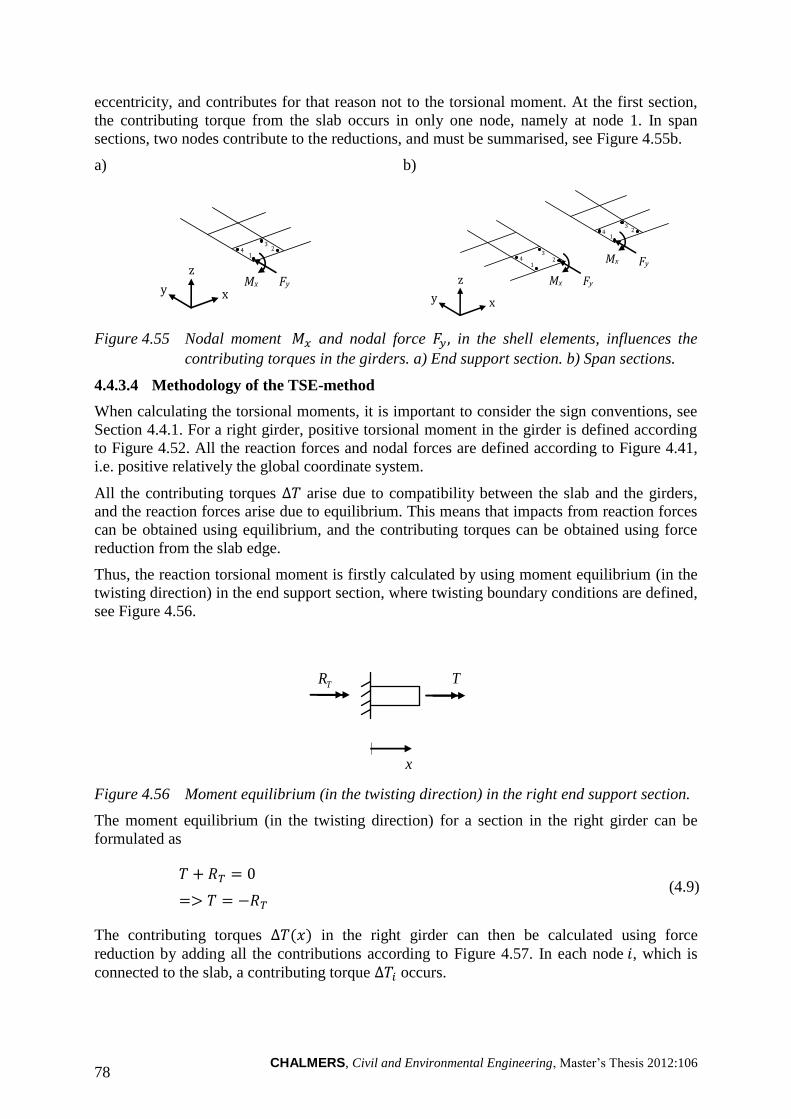
CHALMERS, Civil and Environmental Engineering, Master’s Thesis 2012:106 78
eccentricity, and contributes for that reason not to the torsional moment. At the first section,
the contributing torque from the slab occurs in only one node, namely at node 1. In span
sections, two nodes contribute to the reductions, and must be summarised, see Figure 4.55b.
a) b)
Figure 4.55 Nodal moment and nodal force in the shell elements, influences the
contributing torques in the girders. a) End support section. b) Span sections.
4.4.3.4 Methodology of the TSE-method
When calculating the torsional moments, it is important to consider the sign conventions, see
Section 4.4.1. For a right girder, positive torsional moment in the girder is defined according
to Figure 4.52. All the reaction forces and nodal forces are defined according to Figure 4.41,
i.e. positive relatively the global coordinate system.
All the contributing torques arise due to compatibility between the slab and the girders,
and the reaction forces arise due to equilibrium. This means that impacts from reaction forces
can be obtained using equilibrium, and the contributing torques can be obtained using force
reduction from the slab edge.
Thus, the reaction torsional moment is firstly calculated by using moment equilibrium (in the
twisting direction) in the end support section, where twisting boundary conditions are defined,
see Figure 4.56.
T TR
x
Figure 4.56 Moment equilibrium (in the twisting direction) in the right end support section.
The moment equilibrium (in the twisting direction) for a section in the right girder can be
formulated as
(4.9)
The contributing torques in the right girder can then be calculated using force
reduction by adding all the contributions according to Figure 4.57. In each node , which is
connected to the slab, a contributing torque occurs.
x
z
y Fy
1 2
3 4
Mx
x
z
y
1 2
3 4
Fy
Fy
1 2
3 4
Mx
Mx
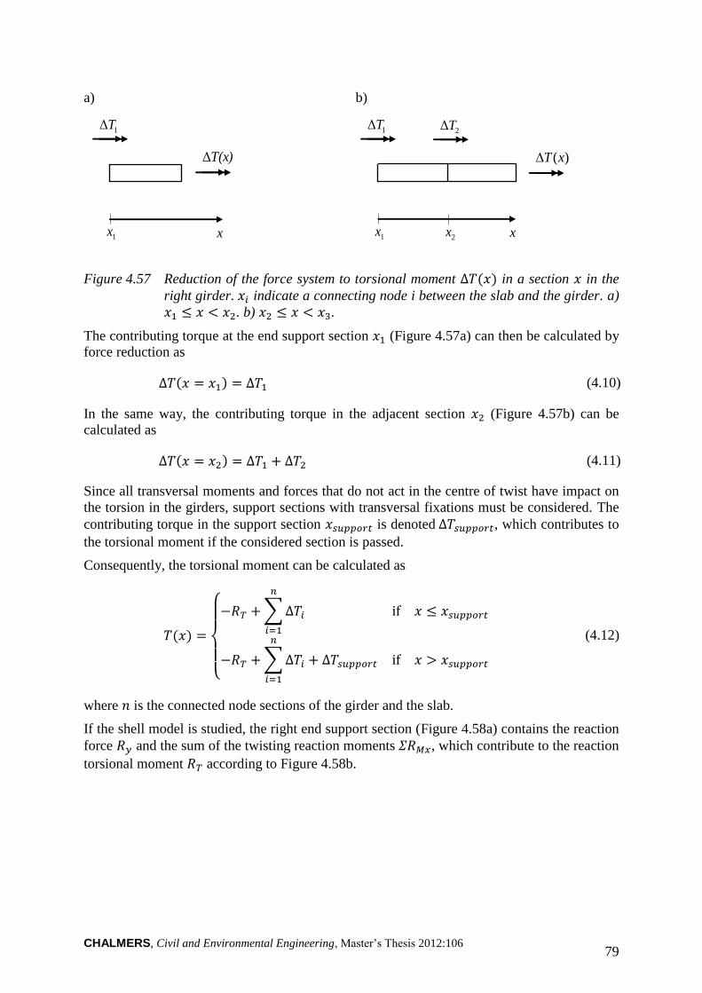
CHALMERS, Civil and Environmental Engineering, Master’s Thesis 2012:106 79
a)
T(x)Δ
1ΔT
x 1x
b)
)(xT
1ΔT
1x
2ΔT
x 2x
Figure 4.57 Reduction of the force system to torsional moment in a section in the
right girder. indicate a connecting node i between the slab and the girder. a)
. b) .
The contributing torque at the end support section (Figure 4.57a) can then be calculated by
force reduction as
(4.10)
In the same way, the contributing torque in the adjacent section (Figure 4.57b) can be
calculated as
(4.11)
Since all transversal moments and forces that do not act in the centre of twist have impact on
the torsion in the girders, support sections with transversal fixations must be considered. The
contributing torque in the support section is denoted Δ , which contributes to
the torsional moment if the considered section is passed.
Consequently, the torsional moment can be calculated as
{
∑
∑
Δ
(4.12)
where is the connected node sections of the girder and the slab.
If the shell model is studied, the right end support section (Figure 4.58a) contains the reaction
force and the sum of the twisting reaction moments , which contribute to the reaction
torsional moment according to Figure 4.58b.
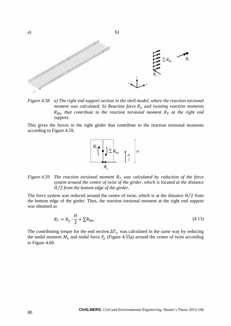
CHALMERS, Civil and Environmental Engineering, Master’s Thesis 2012:106 80
a) b)
x
z
y
MxR
yR
TR
Figure 4.58 a) The right end support section in the shell model, where the reaction torsional
moment was calculated. b) Reaction force and twisting reaction moments
that contribute to the reaction torsional moment at the right end
support.
This gives the forces in the right girder that contribute to the reaction torsional moments
according to Figure 4.59.
TR
yR
MxR
2
H H
Figure 4.59 The reaction torsional moment was calculated by reduction of the force
system around the centre of twist of the girder, which is located at the distance
⁄ from the bottom edge of the girder.
The force system was reduced around the centre of twist, which is at the distance ⁄ from
the bottom edge of the girder. Thus, the reaction torsional moment at the right end support
was obtained as
∑ (4.13)
The contributing torque for the end section , was calculated in the same way by reducing
the nodal moment and nodal force (Figure 4.55a) around the centre of twist according
to Figure 4.60.
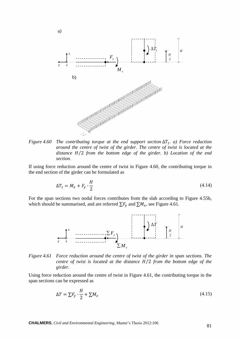
CHALMERS, Civil and Environmental Engineering, Master’s Thesis 2012:106 81
a)
yF
xM
H
2
H 1T
y x
z
b)
Figure 4.60 The contributing torque at the end support section . a) Force reduction
around the centre of twist of the girder. The centre of twist is located at the
distance ⁄ from the bottom edge of the girder. b) Location of the end
section.
If using force reduction around the centre of twist in Figure 4.60, the contributing torque in
the end section of the girder can be formulated as
(4.14)
For the span sections two nodal forces contributes from the slab according to Figure 4.55b,
which should be summarised, and are referred ∑ and ∑ , see Figure 4.61.
H
2
H TΔ
y x
z
yF
xM
Figure 4.61 Force reduction around the centre of twist of the girder in span sections. The
centre of twist is located at the distance ⁄ from the bottom edge of the
girder.
Using force reduction around the centre of twist in Figure 4.61, the contributing torque in the
span sections can be expressed as
∑
∑ (4.15)
CHALMERS, Civil and Environmental Engineering, Master’s Thesis 2012:106 82
For the mid support section (Figure 4.62b), there is a contribution from the reaction force ,
which will cause a response in the girder in the opposite direction (equilibrium), see Figure
4.62a.
a)
yF
xM
H
2
H supportTΔ
y x
z
yR
b)
Figure 4.62 The contributing torque in mid support section. a) Force reduction around the
centre of twist of the girder in mid support section. The centre of twist is located
at the distance ⁄ from the bottom edge of the girder. Note that in this figure
the reaction force is the response force acting in the girder, and is therefore
shifted due to equilibrium. b) Location of the mid support section.
The contributing torque in mid support section was calculated as
∑
∑ (4.16)
The following example should clarify the equations; study the model in Figure 4.63, which is
divided into four elements longitudinally. The twisting is fixed at the end supports and
translation is prevented in y direction at end and mid supports. According to the TSE-method,
the torsional moment in the right girder can be calculated as
{
∑
∑
Δ
(4.17)
where denotes a connecting node between the slab and the girder.
CHALMERS, Civil and Environmental Engineering, Master’s Thesis 2012:106 83
The torsional moment diagram for the right girder can then be created according to Figure
4.63.
y x
z
x
TR
T
1T 2T
3T
supportT
TR 4T
1
Q
2
3
4
5
Figure 4.63 Example of how a torsional moment diagram can be created for the right
girder, using the TSE-method on a simple shell model. The dots indicate where
the supports are located; the twisting is fixed at the end supports and
translation is prevented in y direction at end and mid supports. The numbers 1-
5 denotes the connecting nodes between the slab and the right girder.
A MATLAB-program was developed in order to carry out the TSE-method. Indata was given
in form of coordinates and nodal forces for each time step. Torsional moment distribution
diagrams and influence lines for any section could then be obtained in the MATLAB-
program. The MATLAB-code can be found in Section E.2.3 in Appendix E.
4.4.4 Influence lines
When creating influence lines using time stepping, there are some effects that must be
considered. Mainly two effects were noticed were managed by creating so called fixed and/or
corrected influence lines.
4.4.4.1 Fixed influence line
An influence line describes the response in a certain section, while the load is travelling along
a specified line. Except the first and last sections, all other sections contain a left and right
side, referred to as the left and right section. This means that for each load step, there will be
two sectional force results. Since some of these sectional forces are different in left and right
sections, this leads to a jagged appearance of certain curves. However, when the load is
applied to the left of the section, only the left section is interesting and vice versa. This means
that the jagged curve is not representing the correct influence line for the section, instead the
curve must be fixed.
In ADINA, each element has its local nodes and some of those coincide at the sections. In
Figure 4.64 beam elements A and B with five local nodes are shown. The shear force varies
along the structure for a distributed load according to Figure 4.64b.
CHALMERS, Civil and Environmental Engineering, Master’s Thesis 2012:106 84
a)
b)
Figure 4.64 a) Beam elements A and B with coinciding section integration points 5 and 1 at
section x. b) Varying shear force along element A and B. but are
obtained in the same section.
If the mid support is studied for instance, the left section should be considered when the load
is applied in the left span and the right section when the load is applied in the right span. In
Figure 4.65 the load is applied in the left span, meaning that is the interesting shear
force. If this method, by only considering left or right section, is applied for an influence line,
this will be referred to as a fixed influence line.
Q
Vleft
Vright
Figure 4.65 A section at mid support with applied load Q and shear forces and .
When creating the influence line only is considered in this example for a
load applied in the left span.
4.4.4.2 Corrected influence line
In beam elements shear forces and torsional moments are described constantly within each
element according to Equation (3.25) and (3.27). This affects the appearance of the influence
lines obtained from the analyses. In Figure 4.66 an example can be seen of the shear force
distribution over a simply supported beam, when a load travels over the element A and B.
However, the example is applicable for torsional moment as well. As the load is moving from
left to right, the shear force distribution is changed. The studied sections between elements A
and B has local nodes 2 and 1. Since the shear force is constant within each element, the value
in node 2 represents the shear force acting in element A, and node 1 the shear force in element
B. In Figure 4.66a node 2 is to the right of the load position and thus both nodes will be
negative according to the shear force distribution, which results in negative shear force for
both element A and B. In Figure 4.66b element A is positive and B negative, and in Figure
4.66c both elements are positive.
x
1 2 3 4 51 2 3 4 5
A B
x
A B
VB1 VA5
CHALMERS, Civil and Environmental Engineering, Master’s Thesis 2012:106 85
a)
b)
c)
Figure 4.66 The problem phenomenon with influence lines for shear force (and torsional
moment). Node 2 describe shear force for element A, and node 1 for element B.
a) Element A and B are negative. b) Element A is positive and B negative c)
Element A and B are positive
The example above in Figure 4.66 leads to the influence line in Figure 4.67a. However, this is
not correct; the desired appearance should rather be as in Figure 4.67b.
a)
b)
Figure 4.67 a) Influence line of shear force according to the example above. b) The
corrected influence line.
The effect of this phenomenon can be corrected by switching the shear force value for left and
right sections at the studied section, as it is done in Figure 4.67b. If this correction is
performed in an influence line, it will be referred to as a corrected influence line.
Another way to deal with the problem may be to increase the number of load steps and to
decrease the element length in the region closest around the considered section. In Figure 4.68
influence lines for shear force of a beam grillage model, created with two meshes and number
of load steps, can be seen; one with coarser mesh, and one with refined mesh and load steps
over mid span. It can be observed that the uncorrected result is more correct for the refined
mesh, but when both curves are corrected there is no difference between the curves.
A B
2 1
A B
2 1
A B
2 1
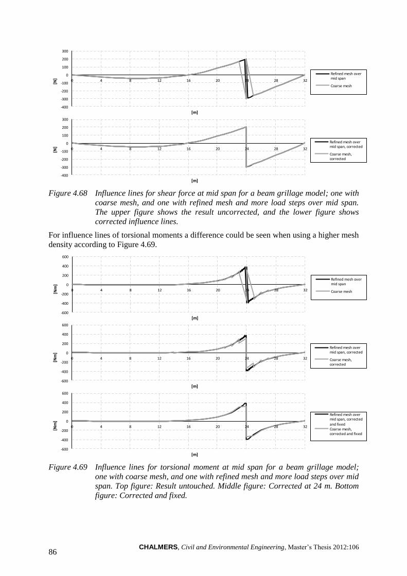
CHALMERS, Civil and Environmental Engineering, Master’s Thesis 2012:106 86
Figure 4.68 Influence lines for shear force at mid span for a beam grillage model; one with
coarse mesh, and one with refined mesh and more load steps over mid span.
The upper figure shows the result uncorrected, and the lower figure shows
corrected influence lines.
For influence lines of torsional moments a difference could be seen when using a higher mesh
density according to Figure 4.69.
Figure 4.69 Influence lines for torsional moment at mid span for a beam grillage model;
one with coarse mesh, and one with refined mesh and more load steps over mid
span. Top figure: Result untouched. Middle figure: Corrected at 24 m. Bottom
figure: Corrected and fixed.
-400
-300
-200
-100
0
100
200
300
0 4 8 12 16 20 24 28 32
[N]
[m]
Refined mesh over mid span
Coarse mesh
-400
-300
-200
-100
0
100
200
300
0 4 8 12 16 20 24 28 32
[N]
[m]
Refined mesh over mid span, corrected
Coarse mesh, corrected
-600
-400
-200
0
200
400
600
0 4 8 12 16 20 24 28 32
[Nm
]
[m]
Refined mesh over mid span
Coarse mesh
-600
-400
-200
0
200
400
600
0 4 8 12 16 20 24 28 32
[Nm
]
[m]
Refined mesh over mid span, corrected
Coarse mesh, corrected
-600
-400
-200
0
200
400
600
0 4 8 12 16 20 24 28 32
[Nm
]
[m]
Refined mesh over mid span, corrected and fixedCoarse mesh, corrected and fixed
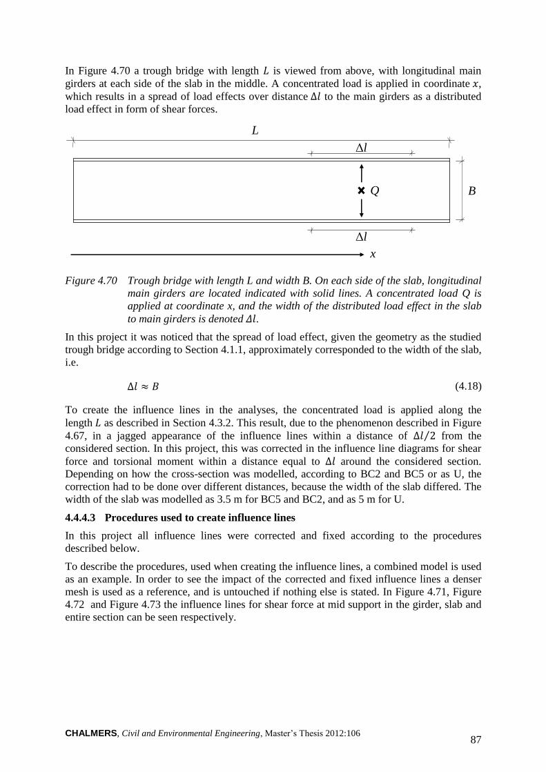
CHALMERS, Civil and Environmental Engineering, Master’s Thesis 2012:106 87
In Figure 4.70 a trough bridge with length is viewed from above, with longitudinal main
girders at each side of the slab in the middle. A concentrated load is applied in coordinate ,
which results in a spread of load effects over distance to the main girders as a distributed
load effect in form of shear forces.
Δl
x
L
B Q
Δl
Figure 4.70 Trough bridge with length L and width B. On each side of the slab, longitudinal
main girders are located indicated with solid lines. A concentrated load Q is
applied at coordinate x, and the width of the distributed load effect in the slab
to main girders is denoted .
In this project it was noticed that the spread of load effect, given the geometry as the studied
trough bridge according to Section 4.1.1, approximately corresponded to the width of the slab,
i.e.
(4.18)
To create the influence lines in the analyses, the concentrated load is applied along the
length as described in Section 4.3.2. This result, due to the phenomenon described in Figure
4.67, in a jagged appearance of the influence lines within a distance of ⁄ from the
considered section. In this project, this was corrected in the influence line diagrams for shear
force and torsional moment within a distance equal to around the considered section.
Depending on how the cross-section was modelled, according to BC2 and BC5 or as U, the
correction had to be done over different distances, because the width of the slab differed. The
width of the slab was modelled as 3.5 m for BC5 and BC2, and as 5 m for U.
4.4.4.3 Procedures used to create influence lines
In this project all influence lines were corrected and fixed according to the procedures
described below.
To describe the procedures, used when creating the influence lines, a combined model is used
as an example. In order to see the impact of the corrected and fixed influence lines a denser
mesh is used as a reference, and is untouched if nothing else is stated. In Figure 4.71, Figure
4.72 and Figure 4.73 the influence lines for shear force at mid support in the girder, slab and
entire section can be seen respectively.
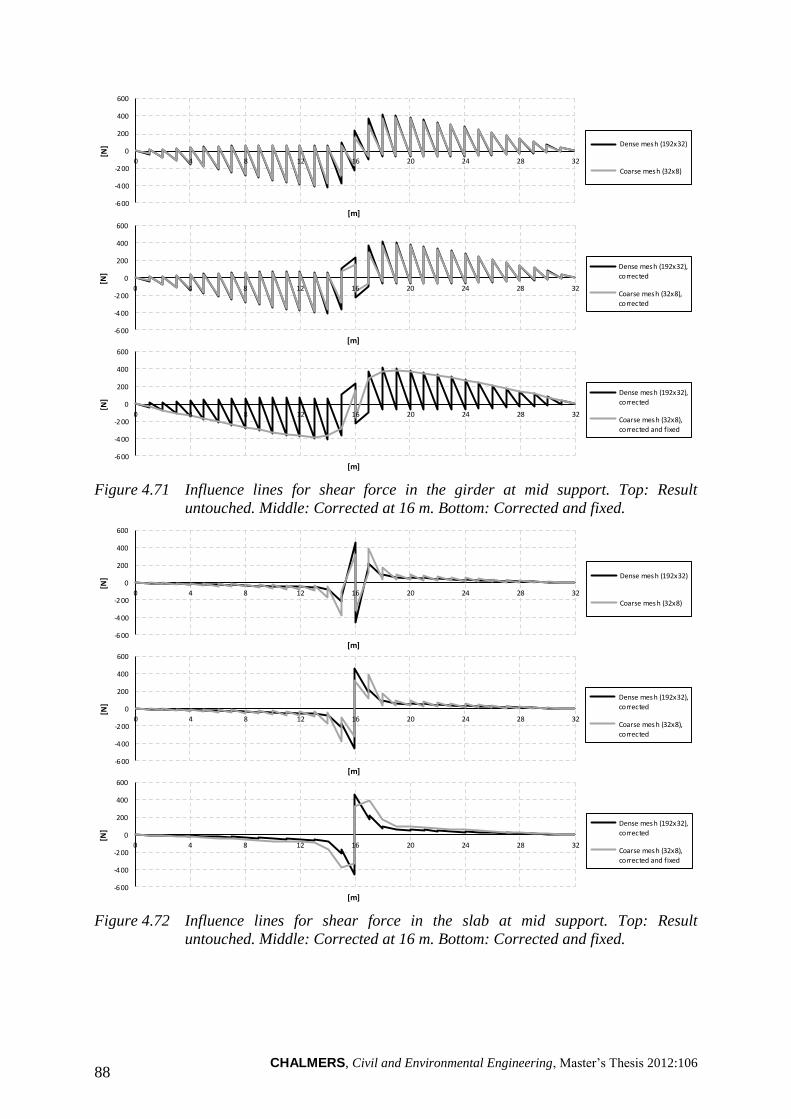
CHALMERS, Civil and Environmental Engineering, Master’s Thesis 2012:106 88
Figure 4.71 Influence lines for shear force in the girder at mid support. Top: Result
untouched. Middle: Corrected at 16 m. Bottom: Corrected and fixed.
Figure 4.72 Influence lines for shear force in the slab at mid support. Top: Result
untouched. Middle: Corrected at 16 m. Bottom: Corrected and fixed.
-600
-400
-2 00
0
200
400
600
0 4 8 12 16 20 24 28 32
[N]
[m]
Dense mesh (192x32)
Coarse mesh (32x8)
-600
-4 00
-200
0
200
400
600
0 4 8 12 16 20 24 28 32
[N]
[m]
Dense mesh (192x32),
corrected
Coarse mesh (32x8),
corrected
-600
-4 00
-200
0
200
400
600
0 4 8 12 16 20 24 28 32
[N]
[m]
Dense mesh (192x32),
corrected
Coarse mesh (32x8),
corrected and fixed
-600
-4 00
-200
0
200
400
600
0 4 8 12 16 20 24 28 32
[N]
[m]
Dense mesh (192x32)
Coarse mesh (32x8)
-600
-4 00
-200
0
200
400
600
0 4 8 12 16 20 24 28 32
[N]
[m]
Dense mesh (192x32),
corrected
Coarse mesh (32x8),
corrected
-600
-4 00
-200
0
200
400
600
0 4 8 12 16 20 24 28 32
[N]
[m]
Dense mesh (192x32),
corrected
Coarse mesh (32x8),
corrected and fixed
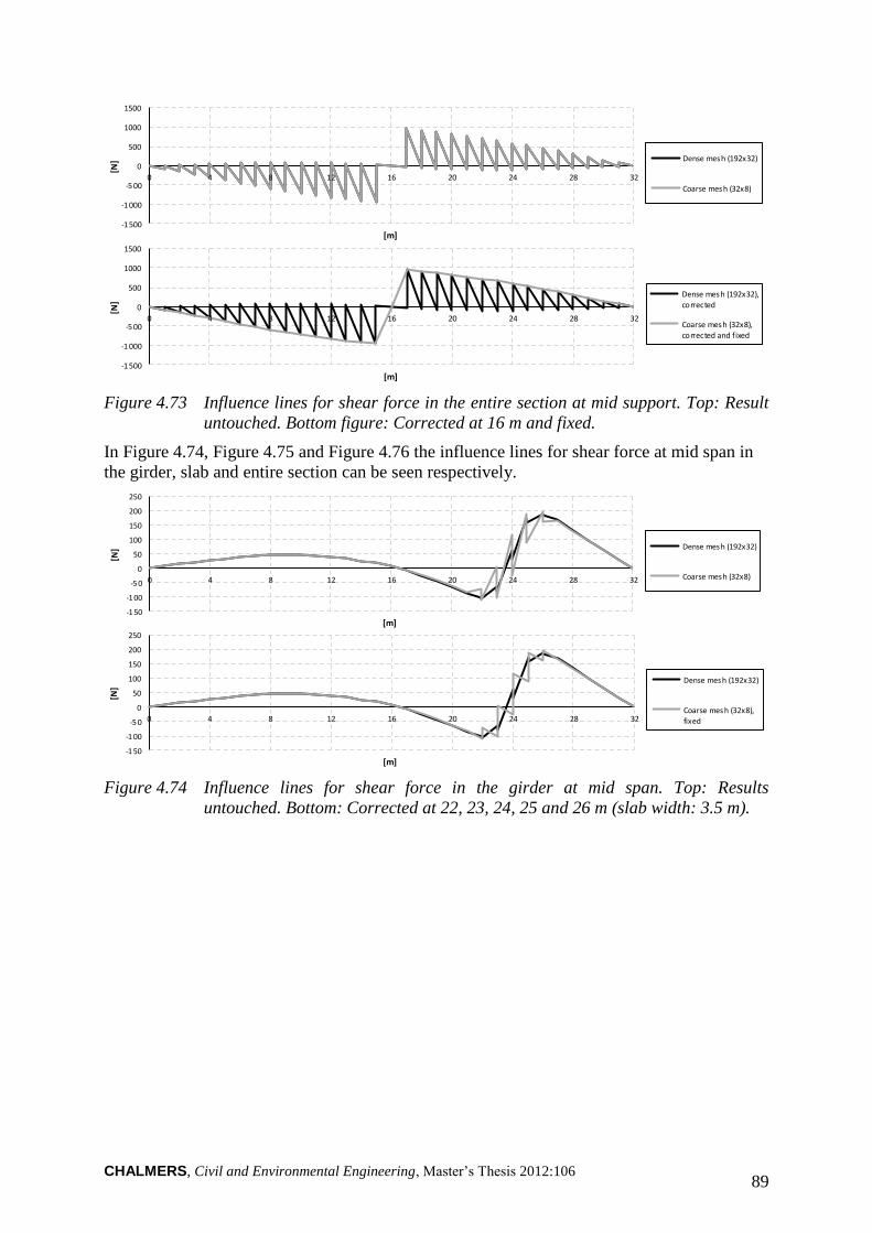
CHALMERS, Civil and Environmental Engineering, Master’s Thesis 2012:106 89
Figure 4.73 Influence lines for shear force in the entire section at mid support. Top: Result
untouched. Bottom figure: Corrected at 16 m and fixed.
In Figure 4.74, Figure 4.75 and Figure 4.76 the influence lines for shear force at mid span in
the girder, slab and entire section can be seen respectively.
Figure 4.74 Influence lines for shear force in the girder at mid span. Top: Results
untouched. Bottom: Corrected at 22, 23, 24, 25 and 26 m (slab width: 3.5 m).
-1500
-1 000
-5 00
0
500
1000
1500
0 4 8 12 16 20 24 28 32
[N]
[m]
Dense mesh (192x32)
Coarse mesh (32x8)
-1 500
-1 000
-500
0
500
1000
1500
0 4 8 12 16 20 24 28 32
[N]
[m]
Dense mesh (192x32),
corrected
Coarse mesh (32x8),
corrected and fixed
-150
-100
-50
0
50
100
150
200
250
0 4 8 12 16 20 24 28 32
[N]
[m]
Dense mesh (192x32)
Coarse mesh (32x8)
-150
-100
-50
0
50
100
150
200
250
0 4 8 12 16 20 24 28 32
[N]
[m]
Dense mesh (192x32)
Coarse mesh (32x8),
fixed
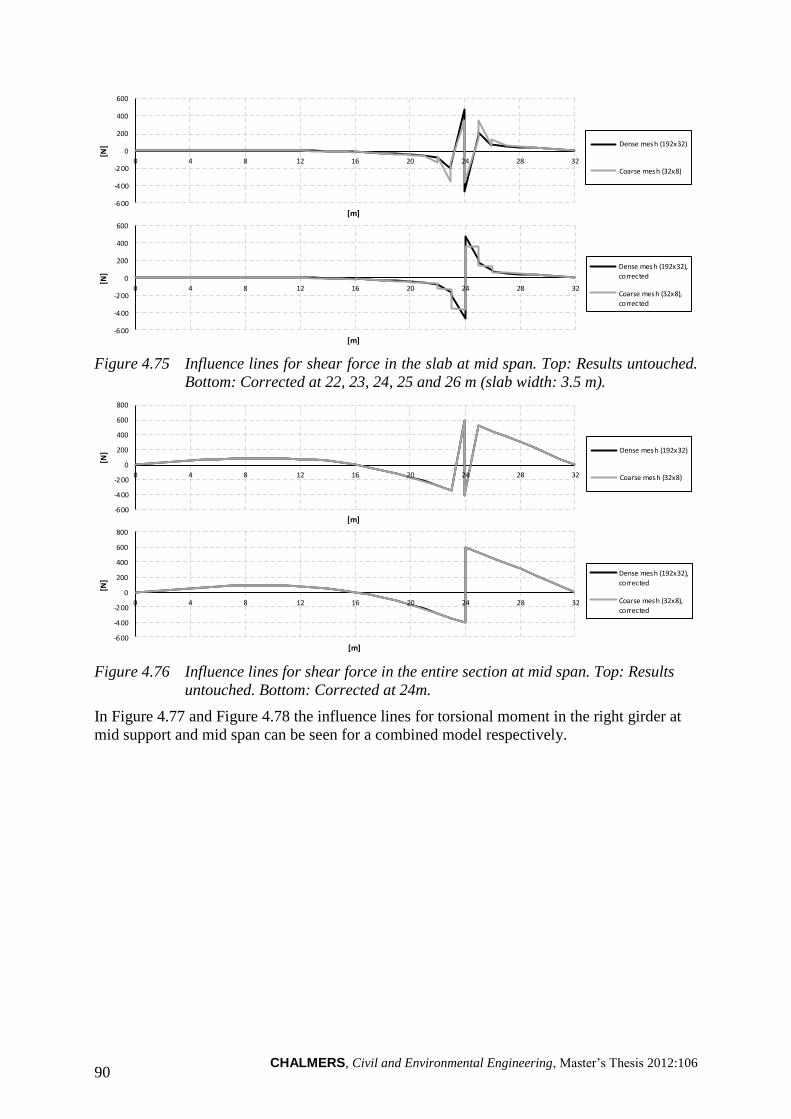
CHALMERS, Civil and Environmental Engineering, Master’s Thesis 2012:106 90
Figure 4.75 Influence lines for shear force in the slab at mid span. Top: Results untouched.
Bottom: Corrected at 22, 23, 24, 25 and 26 m (slab width: 3.5 m).
Figure 4.76 Influence lines for shear force in the entire section at mid span. Top: Results
untouched. Bottom: Corrected at 24m.
In Figure 4.77 and Figure 4.78 the influence lines for torsional moment in the right girder at
mid support and mid span can be seen for a combined model respectively.
-600
-400
-2 00
0
200
400
600
0 4 8 12 16 20 24 28 32
[N]
[m]
Dense mesh (192x32)
Coarse mesh (32x8)
-600
-4 00
-200
0
200
400
600
0 4 8 12 16 20 24 28 32
[N]
[m]
Dense mesh (192x32),
corrected
Coarse mesh (32x8),
corrected
-600
-4 00
-2 00
0
200
400
600
800
0 4 8 12 16 20 24 28 32
[N]
[m]
Dense mesh (192x32)
Coarse mesh (32x8)
-600
-400
-200
0
200
400
600
800
0 4 8 12 16 20 24 28 32
[N]
[m]
Dense mesh (192x32),
corrected
Coarse mesh (32x8),
corrected
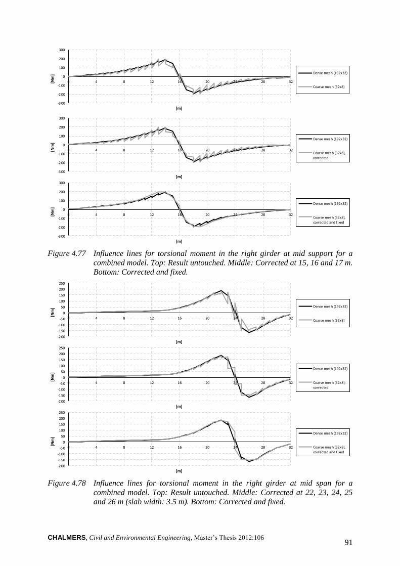
CHALMERS, Civil and Environmental Engineering, Master’s Thesis 2012:106 91
Figure 4.77 Influence lines for torsional moment in the right girder at mid support for a
combined model. Top: Result untouched. Middle: Corrected at 15, 16 and 17 m.
Bottom: Corrected and fixed.
Figure 4.78 Influence lines for torsional moment in the right girder at mid span for a
combined model. Top: Result untouched. Middle: Corrected at 22, 23, 24, 25
and 26 m (slab width: 3.5 m). Bottom: Corrected and fixed.
-3 00
-2 00
-1 00
0
100
200
300
0 4 8 12 16 20 24 28 32[Nm
]
[m]
Dense mesh (192x32)
Coarse mesh (32x8)
-3 00
-2 00
-1 00
0
100
200
300
0 4 8 12 16 20 24 28 32[Nm
]
[m]
Dense mesh (192x32)
Coarse mesh (32x8),
corrected
-3 00
-2 00
-1 00
0
100
200
300
0 4 8 12 16 20 24 28 32[Nm
]
[m]
Dense mesh (192x32)
Coarse mesh (32x8),
corrected and fixed
-2 00
-1 50
-1 00
-50
0
50
100
150
200
250
0 4 8 12 16 20 24 28 32
[Nm
]
[m]
Dense mesh (192x32)
Coarse mesh (32x8)
-2 00
-1 50
-1 00
-50
0
50
100
150
200
250
0 4 8 12 16 20 24 28 32
[Nm
]
[m]
Dense mesh (192x32)
Coarse mesh (32x8),
corrected
-2 00
-1 50
-1 00
-50
0
50
100
150
200
250
0 4 8 12 16 20 24 28 32
[Nm
]
[m]
Dense mesh (192x32)
Coarse mesh (32x8),
corrected and fixed
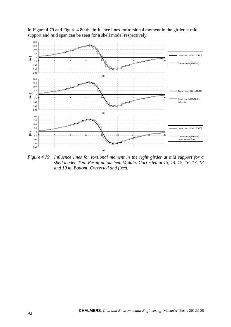
CHALMERS, Civil and Environmental Engineering, Master’s Thesis 2012:106 92
In Figure 4.79 and Figure 4.80 the influence lines for torsional moment in the girder at mid
support and mid span can be seen for a shell model respectively.
Figure 4.79 Influence lines for torsional moment in the right girder at mid support for a
shell model. Top: Result untouched. Middle: Corrected at 13, 14, 15, 16, 17, 18
and 19 m. Bottom: Corrected and fixed.
-2 00
-1 50
-1 00
-50
0
50
100
150
200
0 4 8 12 16 20 24 28 32[Nm
]
[m]
Dense mesh (320x100x60)
Coarse mesh (32x10x6)
-200
-150
-100
-50
0
50
100
150
200
0 4 8 12 16 20 24 28 32[Nm
]
[m]
Dense mesh (320x100x60)
Coarse mesh (32x10x6),
corrected
-200
-150
-100
-50
0
50
100
150
200
0 4 8 12 16 20 24 28 32[Nm
]
[m]
Dense mesh (320x100x60)
Coarse mesh (32x10x6),
corrected and fixed
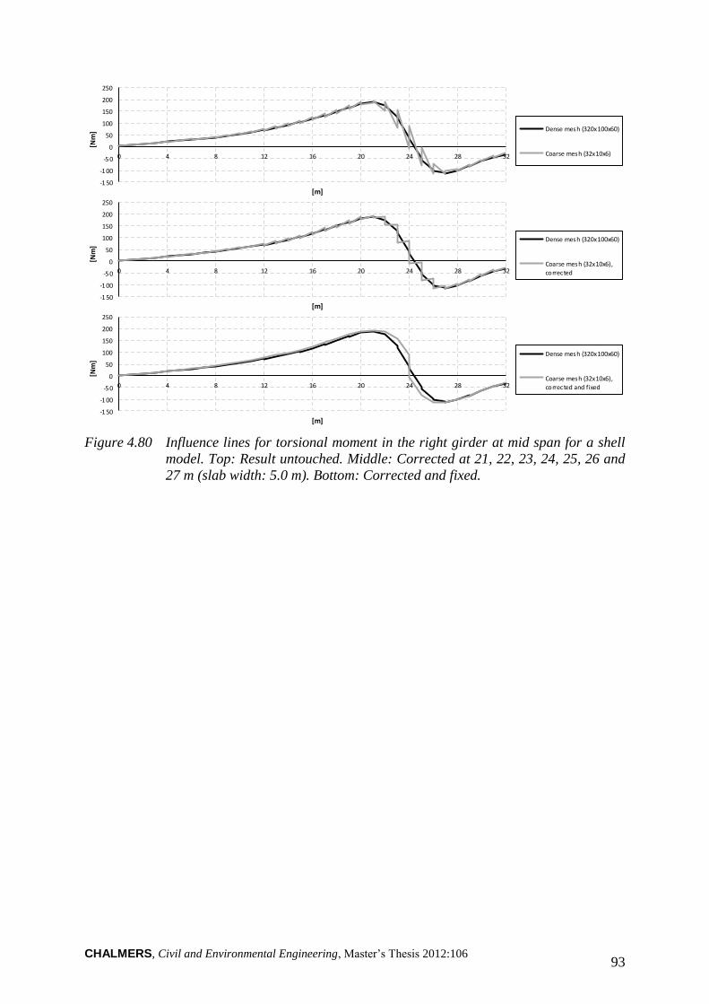
CHALMERS, Civil and Environmental Engineering, Master’s Thesis 2012:106 93
Figure 4.80 Influence lines for torsional moment in the right girder at mid span for a shell
model. Top: Result untouched. Middle: Corrected at 21, 22, 23, 24, 25, 26 and
27 m (slab width: 5.0 m). Bottom: Corrected and fixed.
-150
-100
-50
0
50
100
150
200
250
0 4 8 12 16 20 24 28 32
[Nm
]
[m]
Dense mesh (320x100x60)
Coarse mesh (32x10x6)
-150
-100
-50
0
50
100
150
200
250
0 4 8 12 16 20 24 28 32
[Nm
]
[m]
Dense mesh (320x100x60)
Coarse mesh (32x10x6),
corrected
-150
-100
-50
0
50
100
150
200
250
0 4 8 12 16 20 24 28 32
[Nm
]
[m]
Dense mesh (320x100x60)
Coarse mesh (32x10x6),
corrected and fixed
CHALMERS, Civil and Environmental Engineering, Master’s Thesis 2012:106 94
5 Results from the FE-analyses
The results from the FE-analyses are presented as sectional force diagrams and influence lines
for longitudinal bending moment and shear force, and torsional moment in the right girder
(the left girder has the same distribution but with opposite directions). These graphs are
compared for the different FE-models and boundary conditions, which are described in
Section 4.2.
The results from ADINA were only extracted from half of the cross-section due to symmetry.
This made the result managing more practical, and the final results were then multiplied by
two.
The results are divided into sectional forces in one of the girders, in the slab and in the entire
section. For the beam and beam grillage models the results were obtained directly from the
ADINA. For the combined and shell models MATLAB-programs were developed to calculate
the sectional forces in the girder, slab and entire section. Information how the MATLAB-
programs works can be found in Section 4.4, and the MATLAB-codes can be found in
Appendix E.
Since the results for the different boundary conditions resulted in very similar graphs, BC5 is
selected for presentation of bending moment and shear force, if nothing else is stated. But all
the results can be found in Appendix C and Appendix D.
For comparisons of bending moment and shear force the shell UA-model is presented, and for
comparisons of torsional moments the shell UB-model is presented. For more information
about these models, see Section 4.3.7.
The longitudinal bending moment and shear force distribution in the entire section should
correspond to the analytical solution. For the models consisting of only beam elements the
distributions should be exactly the same, because the beam elements and the analytical
solution are based on the same differential equation for a beam and uses the same
compatibility assumption. This is not the case for the combined model, which leads to
deviations compared to the analytical solution. However, since all models transfer the load
effects primary in the longitudinal direction, the entire structure behaves similar to an
idealised beam. Consequently, the longitudinal bending moment and shear force for the entire
section should be very similar between the FE-models.
The torsional moment is statically indeterminate and cannot be solved analytically, as the
bending moment and shear force. For different FE-models and choices of boundary
conditions different torsional moment results are obtained.
5.1 Analytical solution of longitudinal bending moment and shear
force distribution for the entire section
The longitudinal bending moment and the shear force distributions for a beam, which
correspond to the entire section, can be calculated analytically. Figure 5.1 shows a statically
system model of the studied trough bridge; the longitudinal distributions of bending moment
and shear force in the beam are only dependent on the applied concentrated load and the
spans . For the case when the load is applied at the mid support, there will be no bending and
shear as the load is taken by the support. For the load applied in the mid span section
according to Figure 5.1, the system is one time statically indeterminate; three unknown
reaction forces, but only two equilibrium equations.
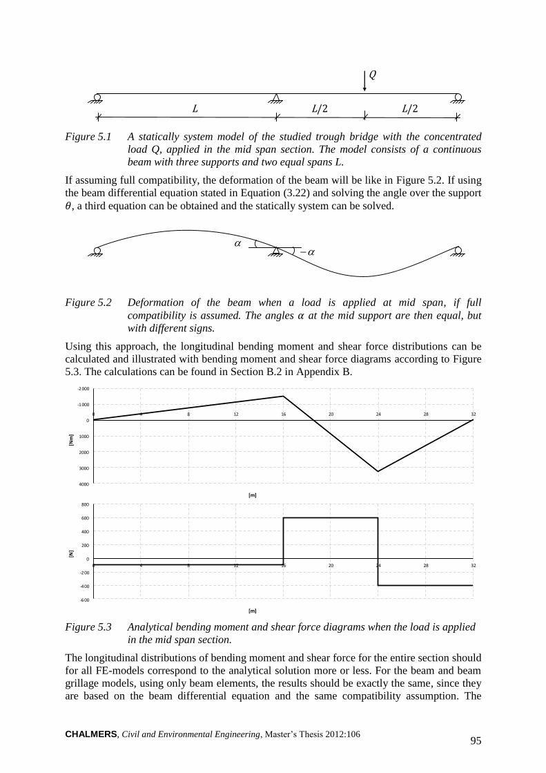
CHALMERS, Civil and Environmental Engineering, Master’s Thesis 2012:106 95
L L/2 L/2
Q
Figure 5.1 A statically system model of the studied trough bridge with the concentrated
load Q, applied in the mid span section. The model consists of a continuous
beam with three supports and two equal spans L.
If assuming full compatibility, the deformation of the beam will be like in Figure 5.2. If using
the beam differential equation stated in Equation (3.22) and solving the angle over the support
, a third equation can be obtained and the statically system can be solved.
Figure 5.2 Deformation of the beam when a load is applied at mid span, if full
compatibility is assumed. The angles at the mid support are then equal, but
with different signs.
Using this approach, the longitudinal bending moment and shear force distributions can be
calculated and illustrated with bending moment and shear force diagrams according to Figure
5.3. The calculations can be found in Section B.2 in Appendix B.
Figure 5.3 Analytical bending moment and shear force diagrams when the load is applied
in the mid span section.
The longitudinal distributions of bending moment and shear force for the entire section should
for all FE-models correspond to the analytical solution more or less. For the beam and beam
grillage models, using only beam elements, the results should be exactly the same, since they
are based on the beam differential equation and the same compatibility assumption. The
-2 000
-1 000
0
1000
2000
3000
4000
0 4 8 12 16 20 24 28 32
[Nm
]
[m]
-600
-4 00
-2 00
0
200
400
600
800
0 4 8 12 16 20 24 28 32
[N]
[m]
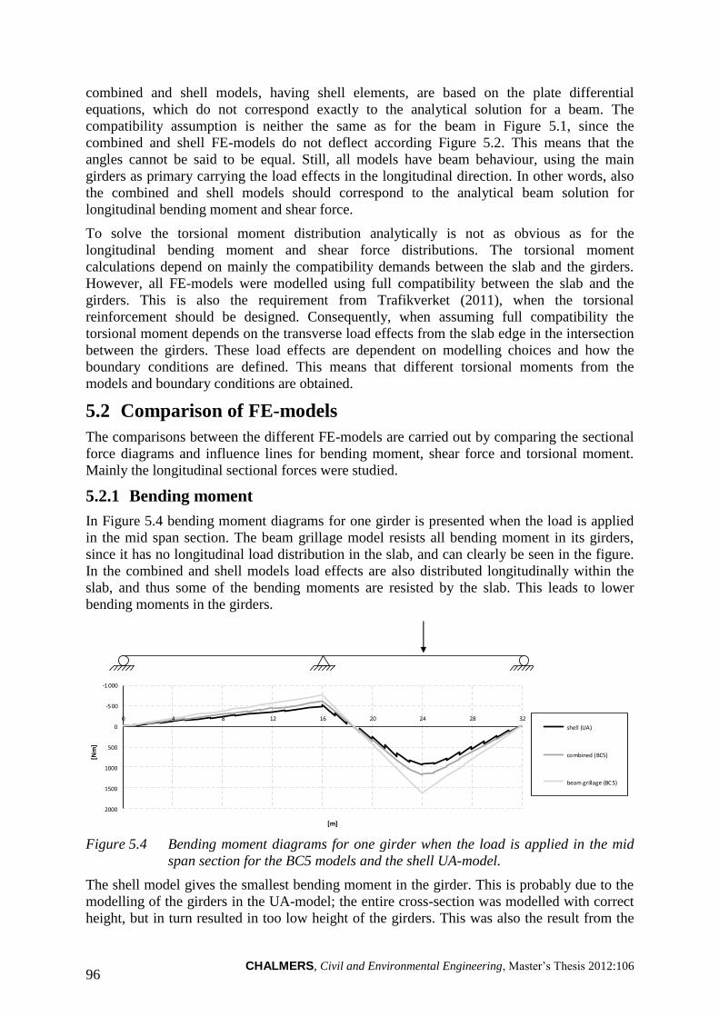
CHALMERS, Civil and Environmental Engineering, Master’s Thesis 2012:106 96
combined and shell models, having shell elements, are based on the plate differential
equations, which do not correspond exactly to the analytical solution for a beam. The
compatibility assumption is neither the same as for the beam in Figure 5.1, since the
combined and shell FE-models do not deflect according Figure 5.2. This means that the
angles cannot be said to be equal. Still, all models have beam behaviour, using the main
girders as primary carrying the load effects in the longitudinal direction. In other words, also
the combined and shell models should correspond to the analytical beam solution for
longitudinal bending moment and shear force.
To solve the torsional moment distribution analytically is not as obvious as for the
longitudinal bending moment and shear force distributions. The torsional moment
calculations depend on mainly the compatibility demands between the slab and the girders.
However, all FE-models were modelled using full compatibility between the slab and the
girders. This is also the requirement from Trafikverket (2011), when the torsional
reinforcement should be designed. Consequently, when assuming full compatibility the
torsional moment depends on the transverse load effects from the slab edge in the intersection
between the girders. These load effects are dependent on modelling choices and how the
boundary conditions are defined. This means that different torsional moments from the
models and boundary conditions are obtained.
5.2 Comparison of FE-models
The comparisons between the different FE-models are carried out by comparing the sectional
force diagrams and influence lines for bending moment, shear force and torsional moment.
Mainly the longitudinal sectional forces were studied.
5.2.1 Bending moment
In Figure 5.4 bending moment diagrams for one girder is presented when the load is applied
in the mid span section. The beam grillage model resists all bending moment in its girders,
since it has no longitudinal load distribution in the slab, and can clearly be seen in the figure.
In the combined and shell models load effects are also distributed longitudinally within the
slab, and thus some of the bending moments are resisted by the slab. This leads to lower
bending moments in the girders.
Figure 5.4 Bending moment diagrams for one girder when the load is applied in the mid
span section for the BC5 models and the shell UA-model.
The shell model gives the smallest bending moment in the girder. This is probably due to the
modelling of the girders in the UA-model; the entire cross-section was modelled with correct
height, but in turn resulted in too low height of the girders. This was also the result from the
-1 000
-5 00
0
500
1000
1500
2000
0 4 8 12 16 20 24 28 32
[Nm
]
[m]
shell (UA)
combined (BC5)
beam grillage (BC5)
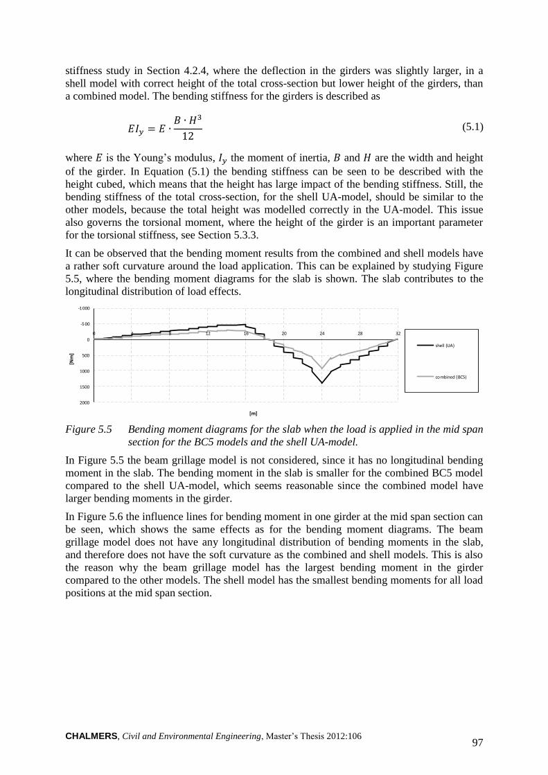
CHALMERS, Civil and Environmental Engineering, Master’s Thesis 2012:106 97
stiffness study in Section 4.2.4, where the deflection in the girders was slightly larger, in a
shell model with correct height of the total cross-section but lower height of the girders, than
a combined model. The bending stiffness for the girders is described as
(5.1)
where is the Young’s modulus, the moment of inertia, and are the width and height
of the girder. In Equation (5.1) the bending stiffness can be seen to be described with the
height cubed, which means that the height has large impact of the bending stiffness. Still, the
bending stiffness of the total cross-section, for the shell UA-model, should be similar to the
other models, because the total height was modelled correctly in the UA-model. This issue
also governs the torsional moment, where the height of the girder is an important parameter
for the torsional stiffness, see Section 5.3.3.
It can be observed that the bending moment results from the combined and shell models have
a rather soft curvature around the load application. This can be explained by studying Figure
5.5, where the bending moment diagrams for the slab is shown. The slab contributes to the
longitudinal distribution of load effects.
Figure 5.5 Bending moment diagrams for the slab when the load is applied in the mid span
section for the BC5 models and the shell UA-model.
In Figure 5.5 the beam grillage model is not considered, since it has no longitudinal bending
moment in the slab. The bending moment in the slab is smaller for the combined BC5 model
compared to the shell UA-model, which seems reasonable since the combined model have
larger bending moments in the girder.
In Figure 5.6 the influence lines for bending moment in one girder at the mid span section can
be seen, which shows the same effects as for the bending moment diagrams. The beam
grillage model does not have any longitudinal distribution of bending moments in the slab,
and therefore does not have the soft curvature as the combined and shell models. This is also
the reason why the beam grillage model has the largest bending moment in the girder
compared to the other models. The shell model has the smallest bending moments for all load
positions at the mid span section.
-1 000
-5 00
0
500
1000
1500
2000
0 4 8 12 16 20 24 28 32
[Nm
]
[m]
shell (UA)
combined (BC5)
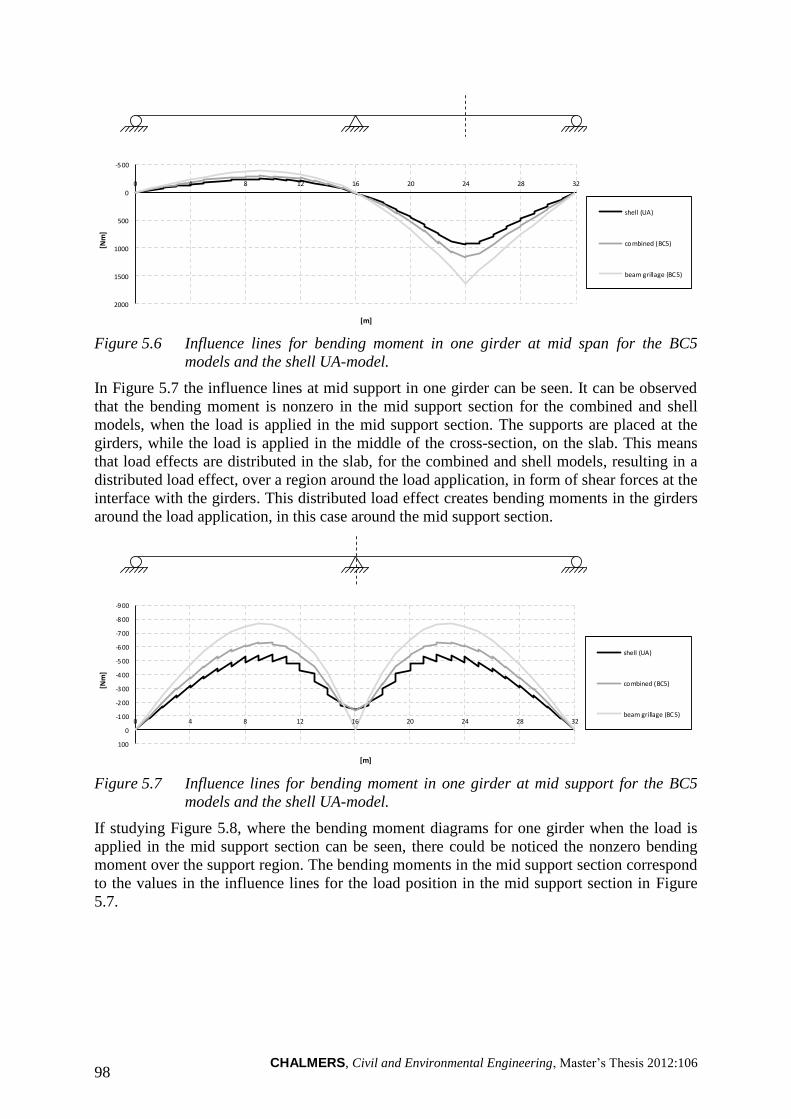
CHALMERS, Civil and Environmental Engineering, Master’s Thesis 2012:106 98
Figure 5.6 Influence lines for bending moment in one girder at mid span for the BC5
models and the shell UA-model.
In Figure 5.7 the influence lines at mid support in one girder can be seen. It can be observed
that the bending moment is nonzero in the mid support section for the combined and shell
models, when the load is applied in the mid support section. The supports are placed at the
girders, while the load is applied in the middle of the cross-section, on the slab. This means
that load effects are distributed in the slab, for the combined and shell models, resulting in a
distributed load effect, over a region around the load application, in form of shear forces at the
interface with the girders. This distributed load effect creates bending moments in the girders
around the load application, in this case around the mid support section.
Figure 5.7 Influence lines for bending moment in one girder at mid support for the BC5
models and the shell UA-model.
If studying Figure 5.8, where the bending moment diagrams for one girder when the load is
applied in the mid support section can be seen, there could be noticed the nonzero bending
moment over the support region. The bending moments in the mid support section correspond
to the values in the influence lines for the load position in the mid support section in Figure
5.7.
-5 00
0
500
1000
1500
2000
0 4 8 12 16 20 24 28 32
[Nm
]
[m]
shell (UA)
combined (BC5)
beam grillage (BC5)
-9 00
-8 00
-700
-600
-5 00
-4 00
-3 00
-2 00
-1 00
0
100
0 4 8 12 16 20 24 28 32
[Nm
]
[m]
shell (UA)
combined (BC5)
beam grillage (BC5)
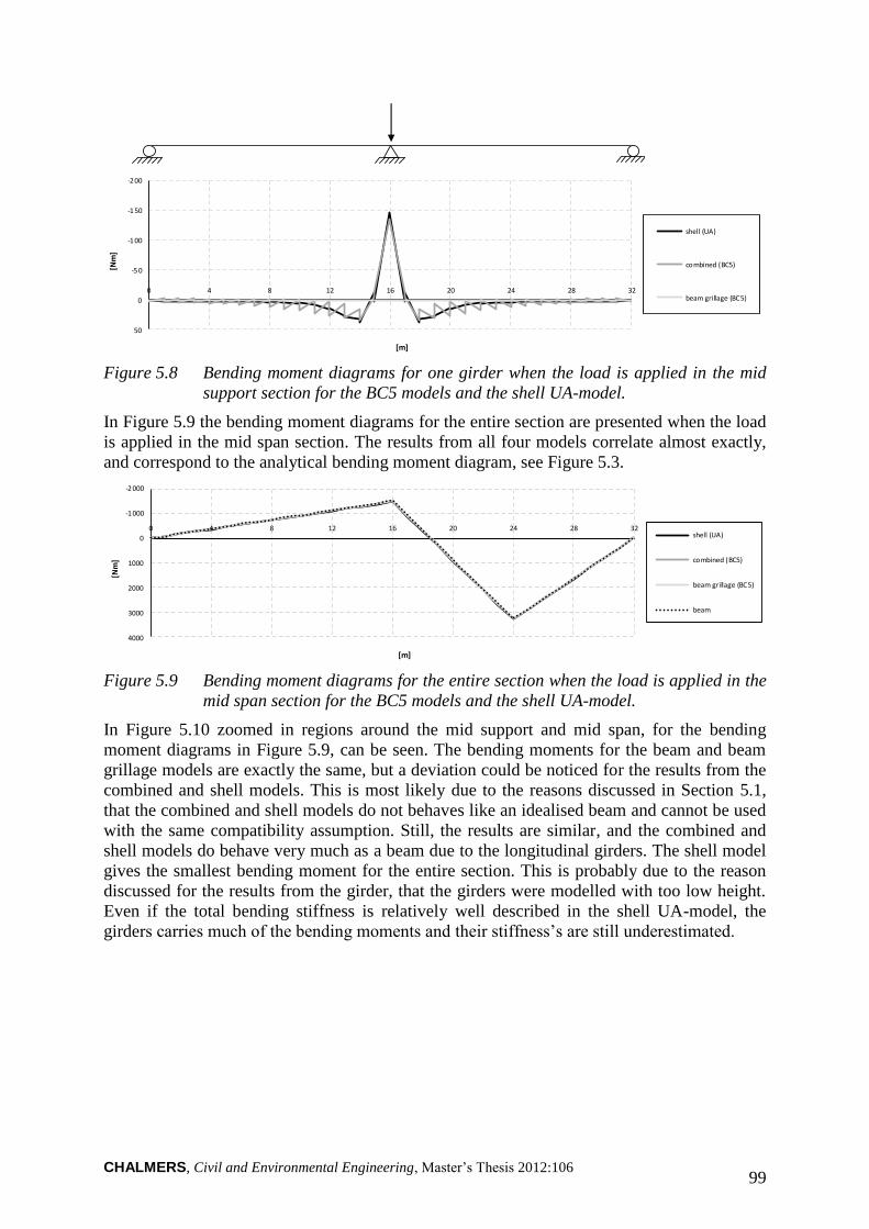
CHALMERS, Civil and Environmental Engineering, Master’s Thesis 2012:106 99
Figure 5.8 Bending moment diagrams for one girder when the load is applied in the mid
support section for the BC5 models and the shell UA-model.
In Figure 5.9 the bending moment diagrams for the entire section are presented when the load
is applied in the mid span section. The results from all four models correlate almost exactly,
and correspond to the analytical bending moment diagram, see Figure 5.3.
Figure 5.9 Bending moment diagrams for the entire section when the load is applied in the
mid span section for the BC5 models and the shell UA-model.
In Figure 5.10 zoomed in regions around the mid support and mid span, for the bending
moment diagrams in Figure 5.9, can be seen. The bending moments for the beam and beam
grillage models are exactly the same, but a deviation could be noticed for the results from the
combined and shell models. This is most likely due to the reasons discussed in Section 5.1,
that the combined and shell models do not behaves like an idealised beam and cannot be used
with the same compatibility assumption. Still, the results are similar, and the combined and
shell models do behave very much as a beam due to the longitudinal girders. The shell model
gives the smallest bending moment for the entire section. This is probably due to the reason
discussed for the results from the girder, that the girders were modelled with too low height.
Even if the total bending stiffness is relatively well described in the shell UA-model, the
girders carries much of the bending moments and their stiffness’s are still underestimated.
-2 00
-150
-1 00
-5 0
0
50
0 4 8 12 16 20 24 28 32
[Nm
]
[m]
shell (UA)
combined (BC5)
beam grillage (BC5)
-2 000
-1 000
0
1000
2000
3000
4000
0 4 8 12 16 20 24 28 32
[Nm
]
[m]
shell (UA)
combined (BC5)
beam grillage (BC5)
beam
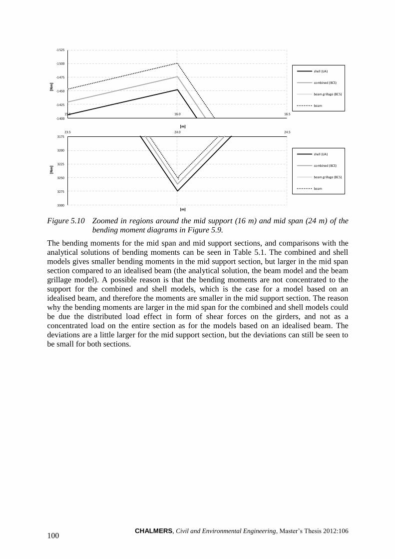
CHALMERS, Civil and Environmental Engineering, Master’s Thesis 2012:106 100
Figure 5.10 Zoomed in regions around the mid support (16 m) and mid span (24 m) of the
bending moment diagrams in Figure 5.9.
The bending moments for the mid span and mid support sections, and comparisons with the
analytical solutions of bending moments can be seen in Table 5.1. The combined and shell
models gives smaller bending moments in the mid support section, but larger in the mid span
section compared to an idealised beam (the analytical solution, the beam model and the beam
grillage model). A possible reason is that the bending moments are not concentrated to the
support for the combined and shell models, which is the case for a model based on an
idealised beam, and therefore the moments are smaller in the mid support section. The reason
why the bending moments are larger in the mid span for the combined and shell models could
be due the distributed load effect in form of shear forces on the girders, and not as a
concentrated load on the entire section as for the models based on an idealised beam. The
deviations are a little larger for the mid support section, but the deviations can still be seen to
be small for both sections.
-1 525
-1500
-1 475
-1 450
-1 425
-1400
15.5 16.0 16.5
[Nm
]
[m]
shell (UA)
combined (BC5)
beam grillage (BC5)
beam
3175
3200
3225
3250
3275
3300
23.5 24.0 24.5
[Nm
]
[m]
shell (UA)
combined (BC5)
beam grillage (BC5)
beam
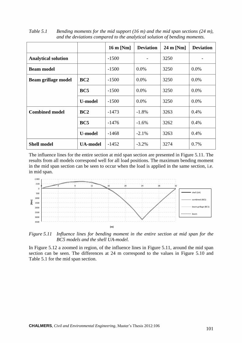
CHALMERS, Civil and Environmental Engineering, Master’s Thesis 2012:106 101
Table 5.1 Bending moments for the mid support (16 m) and the mid span sections (24 m),
and the deviations compared to the analytical solution of bending moments.
16 m [Nm] Deviation 24 m [Nm] Deviation
Analytical solution -1500 - 3250 -
Beam model -1500 0.0% 3250 0.0%
Beam grillage model BC2 -1500 0.0% 3250 0.0%
BC5 -1500 0.0% 3250 0.0%
U-model -1500 0.0% 3250 0.0%
Combined model BC2 -1473 -1.8% 3263 0.4%
BC5 -1476 -1.6% 3262 0.4%
U-model -1468 -2.1% 3263 0.4%
Shell model UA-model -1452 -3.2% 3274 0.7%
The influence lines for the entire section at mid span section are presented in Figure 5.11. The
results from all models correspond well for all load positions. The maximum bending moment
in the mid span section can be seen to occur when the load is applied in the same section, i.e.
in mid span.
Figure 5.11 Influence lines for bending moment in the entire section at mid span for the
BC5 models and the shell UA-model.
In Figure 5.12 a zoomed in region, of the influence lines in Figure 5.11, around the mid span
section can be seen. The differences at 24 m correspond to the values in Figure 5.10 and
Table 5.1 for the mid span section.
-1 000
-5 00
0
500
1000
1500
2000
2500
3000
3500
0 4 8 12 16 20 24 28 32
[Nm
]
[m]
shell (UA)
combined (BC5)
beam grillage (BC5)
beam
CHALMERS, Civil and Environmental Engineering, Master’s Thesis 2012:106 102
Figure 5.12 Zoomed in mid span region (24 m) of the influence lines in Figure 5.11.
At the mid support section in Figure 5.13 the models also show good correspondence for all
load positions. The results from the combined and shell models are slightly smaller than the
beam and beam grillage models for all load positions except around the mid support, it can be
noted that the result is nonzero in the mid support section for the combined and shell models.
Figure 5.13 Influence lines for bending moment in the entire section at mid support for the
BC5 models and the shell UA-model.
In Figure 5.14 a zoomed in mid support region, of the influence lines in Figure 5.13, can be
seen. The results from the combined and shell models are nonzero, while the beam and beam
grillage models give zero bending moments.
Figure 5.14 Zoomed in mid support region (16 m) of the influence lines in Figure 5.13.
The reason why the results are nonzero for the shell and combined models can be explained
by Figure 5.15. It shows the bending moment diagrams for the entire section, when the load is
applied in the mid support section. The beam grillage model is zero, while the combined and
shell models are nonzero. This is due to the spread of load effects in the slab around the mid
support section, giving small bending moments, together with the contributions from the
girders due to the distributed load effect in form of shear force. The values can be seen to
correspond to the values in Figure 5.14 at 24 m.
3175
3200
3225
3250
3275
3300
23.5 24.0 24.5[N
m]
[m]
shell (UA)
combined (BC5)
beam grillage (BC5)
beam
-1 800
-1 600
-1 400
-1 200
-1 000
-8 00
-600
-400
-2 00
0
200
0 4 8 12 16 20 24 28 32
[Nm
]
[m]
shell (UA)
combined (BC5)
beam grillage (BC5)
beam
0
25
50
75
15.5 16.0 16.5
[Nm
]
[m]
shell (UA)
combined (BC5)
beam grillage (BC5)
beam
CHALMERS, Civil and Environmental Engineering, Master’s Thesis 2012:106 103
Figure 5.15 Bending moment diagrams for the entire section when the load is applied in the
mid support section for the BC5 models and the shell UA-model.
In Figure 5.16 a zoomed in mid span region, of the influence lines in Figure 5.13, can be seen.
The differences at 24 m correspond to the values in Figure 5.10 and Table 5.1 for the mid
support section.
Figure 5.16 Zoomed in mid span region (24 m) of the influence lines in Figure 5.13.
If Figure 5.13 is studied it can be noticed that the maximum bending moment in the mid
support section occurs for the load applied slightly to the left of the mid span, around 23 m. In
Figure 5.17 a zoomed in region around 23 m can be seen of the influence lines in Figure 5.13.
Figure 5.17 Zoomed in region slightly to the left of the mid span section, around 23 m, of
the influence lines in Figure 5.13.
5.2.2 Shear force
The shear force diagrams in one girder for the load applied at the mid span section can be
seen in Figure 5.18. The same effect as for the bending moment can also be seen for the shear
force, i.e. for the combined and shell models there is a contribution from the slab, while in the
beam grillage model all longitudinal shear force occurs in the two main girders.
-1 0
0
10
20
30
40
50
60
0 4 8 12 16 20 24 28 32[N
m]
[m]
shell (UA)
combined (BC5)
beam grillage (BC5)
-1 525
-1500
-1 475
-1 450
-1 425
-1400
23.5 24.0 24.5
[Nm
]
[m]
shell (UA)
combined (BC5)
beam grillage (BC5)
beam
-1 575
-1550
-1 525
-1 500
-1 475
-1450
22.5 23.0 23.5
[Nm
]
[m]
shell (UA)
combined (BC5)
beam grillage (BC5)
beam
CHALMERS, Civil and Environmental Engineering, Master’s Thesis 2012:106 104
Figure 5.18 Shear force diagrams for one girder when the load is applied in the mid span
section for the BC5 and U-models.
It can be seen that the differences between the combined and the shell models are small,
especially when comparing the results from the U-models. When studying the distribution a
little bit away from the load application, all results from the models have a good correlation.
In Figure 5.19 shear force diagrams in the slab are shown when the load is applied in the mid
span section. By comparing the shear force distributions in one girder and in the slab, it can
be concluded that most of the shear force is resisted by the girders. In the slab the shear force
is mostly concentrated around the load application, while in the girder the shear force is
distributed over the entire length.
-3 00
-200
-1 00
0
100
200
300
400
0 4 8 12 16 20 24 28 32
[N]
[m]
shell (UA)
combined (BC5)
beam grillage (BC5)
-3 00
-200
-1 00
0
100
200
300
400
0 4 8 12 16 20 24 28 32
[N]
[m]
shell (UA)
combined (U)
beam grillage (U)
CHALMERS, Civil and Environmental Engineering, Master’s Thesis 2012:106 105
Figure 5.19 Shear force diagrams for the slab when the load is applied in the mid span
section for the BC5 and U-models.
In Figure 5.20 influence lines for shear force in one girder at mid span can be seen. For load
positions between 22 m and 26 m, the combined BC5 and U-model and the shell UA-model
results are similar. However, for other load positions there could be noticed a deviation in the
results between the combined BC5 model and the other models. The results from the U-
models are much better correlated.
Figure 5.20 Influence lines for shear force in one girder at mid span for the BC5 and U-
models.
-4 00
-3 00
-2 00
-1 00
0
100
200
300
400
500
0 4 8 12 16 20 24 28 32
[N]
[m]
shell (UA)
combined (BC5)
-5 00
-4 00
-3 00
-2 00
-1 00
0
100
200
300
400
500
0 4 8 12 16 20 24 28 32
[N]
[m]
shell (UA)
combined (U)
-3 00
-2 00
-1 00
0
100
200
300
400
0 4 8 12 16 20 24 28 32
[N]
[m]
shell (UA)
combined (BC5)
beam grillage (BC5)
-3 00
-2 00
-100
0
100
200
300
400
0 4 8 12 16 20 24 28 32
[N]
[m]
shell (UA)
combined (U)
beam grillage (U)
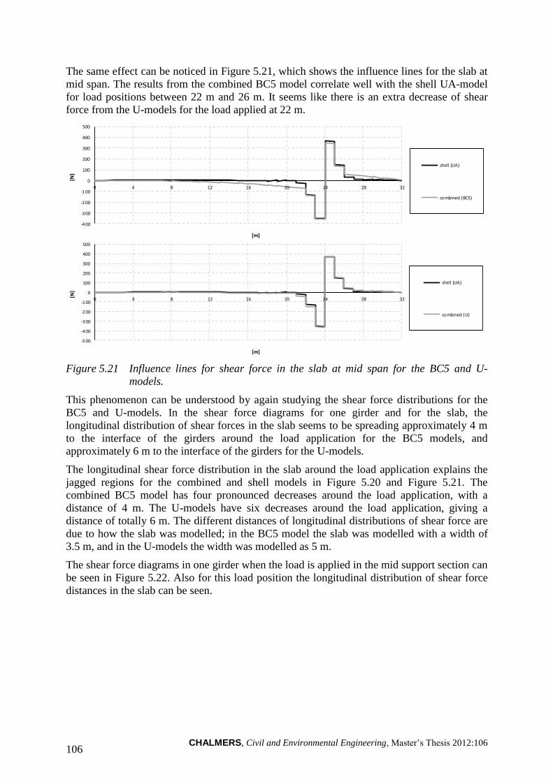
CHALMERS, Civil and Environmental Engineering, Master’s Thesis 2012:106 106
The same effect can be noticed in Figure 5.21, which shows the influence lines for the slab at
mid span. The results from the combined BC5 model correlate well with the shell UA-model
for load positions between 22 m and 26 m. It seems like there is an extra decrease of shear
force from the U-models for the load applied at 22 m.
Figure 5.21 Influence lines for shear force in the slab at mid span for the BC5 and U-
models.
This phenomenon can be understood by again studying the shear force distributions for the
BC5 and U-models. In the shear force diagrams for one girder and for the slab, the
longitudinal distribution of shear forces in the slab seems to be spreading approximately 4 m
to the interface of the girders around the load application for the BC5 models, and
approximately 6 m to the interface of the girders for the U-models.
The longitudinal shear force distribution in the slab around the load application explains the
jagged regions for the combined and shell models in Figure 5.20 and Figure 5.21. The
combined BC5 model has four pronounced decreases around the load application, with a
distance of 4 m. The U-models have six decreases around the load application, giving a
distance of totally 6 m. The different distances of longitudinal distributions of shear force are
due to how the slab was modelled; in the BC5 model the slab was modelled with a width of
3.5 m, and in the U-models the width was modelled as 5 m.
The shear force diagrams in one girder when the load is applied in the mid support section can
be seen in Figure 5.22. Also for this load position the longitudinal distribution of shear force
distances in the slab can be seen.
-400
-300
-2 00
-1 00
0
100
200
300
400
500
0 4 8 12 16 20 24 28 32
[N]
[m]
shell (UA)
combined (BC5)
-5 00
-4 00
-3 00
-2 00
-1 00
0
100
200
300
400
500
0 4 8 12 16 20 24 28 32
[N]
[m]
shell (UA)
combined (U)
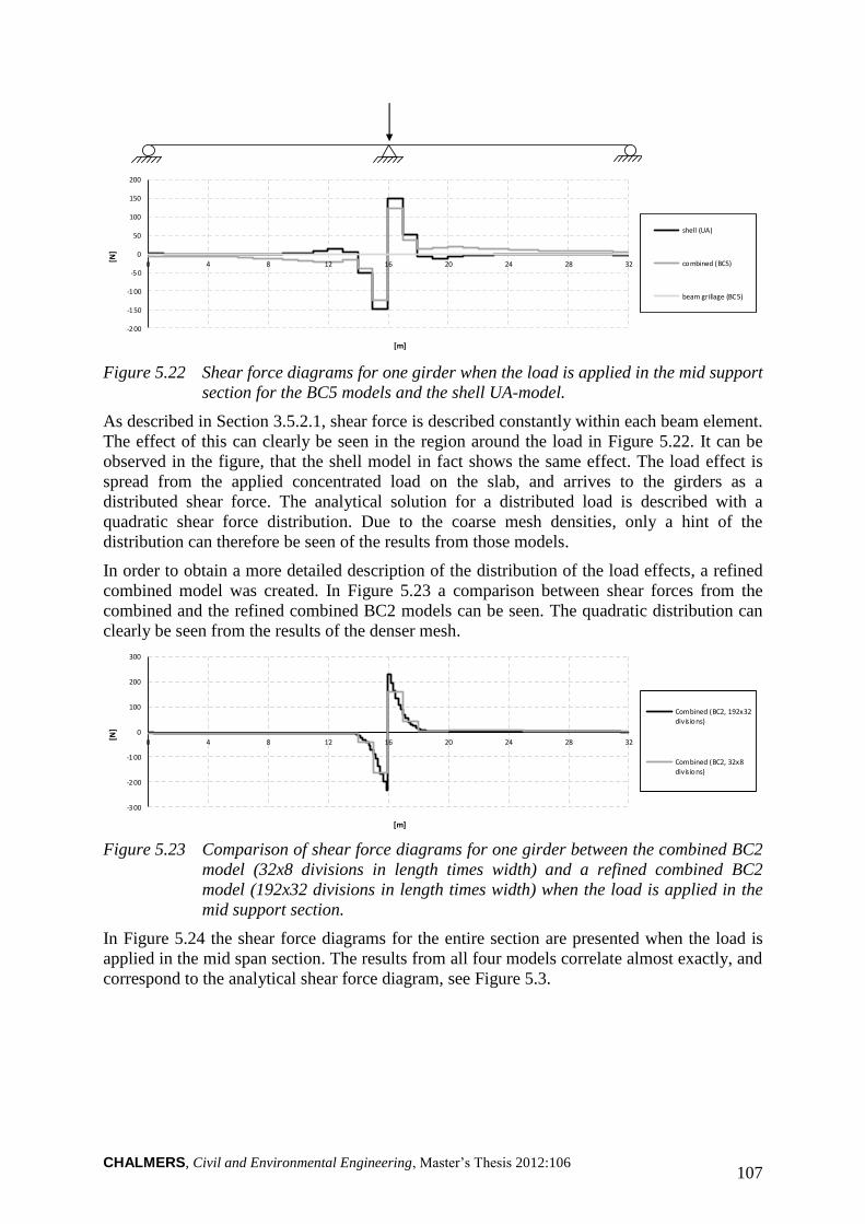
CHALMERS, Civil and Environmental Engineering, Master’s Thesis 2012:106 107
Figure 5.22 Shear force diagrams for one girder when the load is applied in the mid support
section for the BC5 models and the shell UA-model.
As described in Section 3.5.2.1, shear force is described constantly within each beam element.
The effect of this can clearly be seen in the region around the load in Figure 5.22. It can be
observed in the figure, that the shell model in fact shows the same effect. The load effect is
spread from the applied concentrated load on the slab, and arrives to the girders as a
distributed shear force. The analytical solution for a distributed load is described with a
quadratic shear force distribution. Due to the coarse mesh densities, only a hint of the
distribution can therefore be seen of the results from those models.
In order to obtain a more detailed description of the distribution of the load effects, a refined
combined model was created. In Figure 5.23 a comparison between shear forces from the
combined and the refined combined BC2 models can be seen. The quadratic distribution can
clearly be seen from the results of the denser mesh.
Figure 5.23 Comparison of shear force diagrams for one girder between the combined BC2
model (32x8 divisions in length times width) and a refined combined BC2
model (192x32 divisions in length times width) when the load is applied in the
mid support section.
In Figure 5.24 the shear force diagrams for the entire section are presented when the load is
applied in the mid span section. The results from all four models correlate almost exactly, and
correspond to the analytical shear force diagram, see Figure 5.3.
-2 00
-1 50
-100
-5 0
0
50
100
150
200
0 4 8 12 16 20 24 28 32
[N]
[m]
shell (UA)
combined (BC5)
beam grillage (BC5)
-3 00
-2 00
-100
0
100
200
300
0 4 8 12 16 20 24 28 32
[N]
[m]
Combined (BC2, 192x32divis ions)
Combined (BC2, 32x8
divis ions)
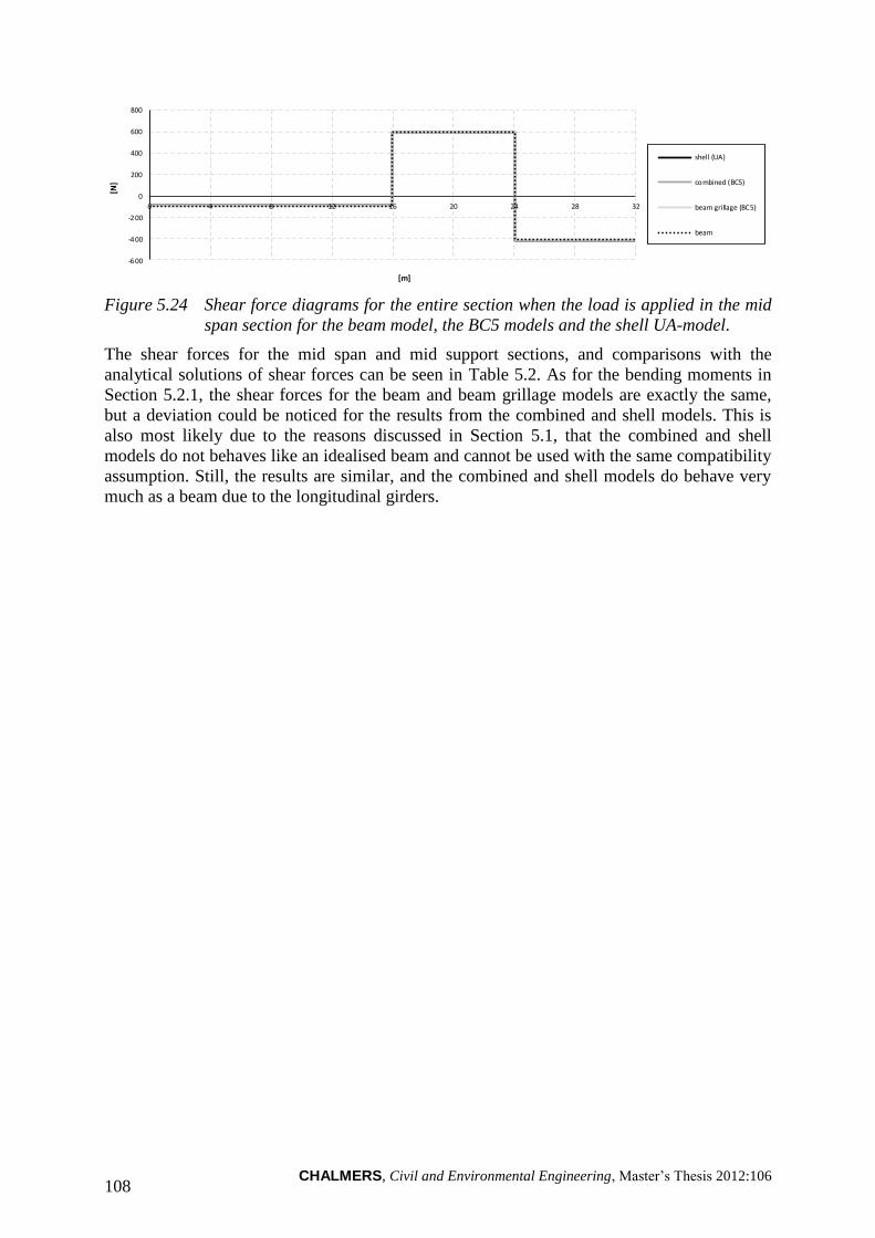
CHALMERS, Civil and Environmental Engineering, Master’s Thesis 2012:106 108
Figure 5.24 Shear force diagrams for the entire section when the load is applied in the mid
span section for the beam model, the BC5 models and the shell UA-model.
The shear forces for the mid span and mid support sections, and comparisons with the
analytical solutions of shear forces can be seen in Table 5.2. As for the bending moments in
Section 5.2.1, the shear forces for the beam and beam grillage models are exactly the same,
but a deviation could be noticed for the results from the combined and shell models. This is
also most likely due to the reasons discussed in Section 5.1, that the combined and shell
models do not behaves like an idealised beam and cannot be used with the same compatibility
assumption. Still, the results are similar, and the combined and shell models do behave very
much as a beam due to the longitudinal girders.
-600
-4 00
-2 00
0
200
400
600
800
0 4 8 12 16 20 24 28 32
[N]
[m]
shell (UA)
combined (BC5)
beam grillage (BC5)
beam
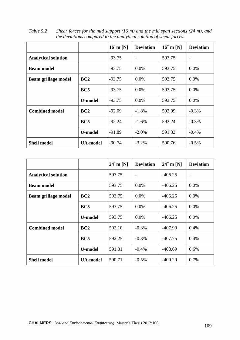
CHALMERS, Civil and Environmental Engineering, Master’s Thesis 2012:106 109
Table 5.2 Shear forces for the mid support (16 m) and the mid span sections (24 m), and
the deviations compared to the analytical solution of shear forces.
16- m [N] Deviation 16
+ m [N] Deviation
Analytical solution -93.75 - 593.75 -
Beam model -93.75 0.0% 593.75 0.0%
Beam grillage model BC2 -93.75 0.0% 593.75 0.0%
BC5 -93.75 0.0% 593.75 0.0%
U-model -93.75 0.0% 593.75 0.0%
Combined model BC2 -92.09 -1.8% 592.09 -0.3%
BC5 -92.24 -1.6% 592.24 -0.3%
U-model -91.89 -2.0% 591.33 -0.4%
Shell model UA-model -90.74 -3.2% 590.76 -0.5%
24- m [N] Deviation 24
+ m [N] Deviation
Analytical solution 593.75 - -406.25 -
Beam model 593.75 0.0% -406.25 0.0%
Beam grillage model BC2 593.75 0.0% -406.25 0.0%
BC5 593.75 0.0% -406.25 0.0%
U-model 593.75 0.0% -406.25 0.0%
Combined model BC2 592.10 -0.3% -407.90 0.4%
BC5 592.25 -0.3% -407.75 0.4%
U-model 591.31 -0.4% -408.69 0.6%
Shell model UA-model 590.71 -0.5% -409.29 0.7%
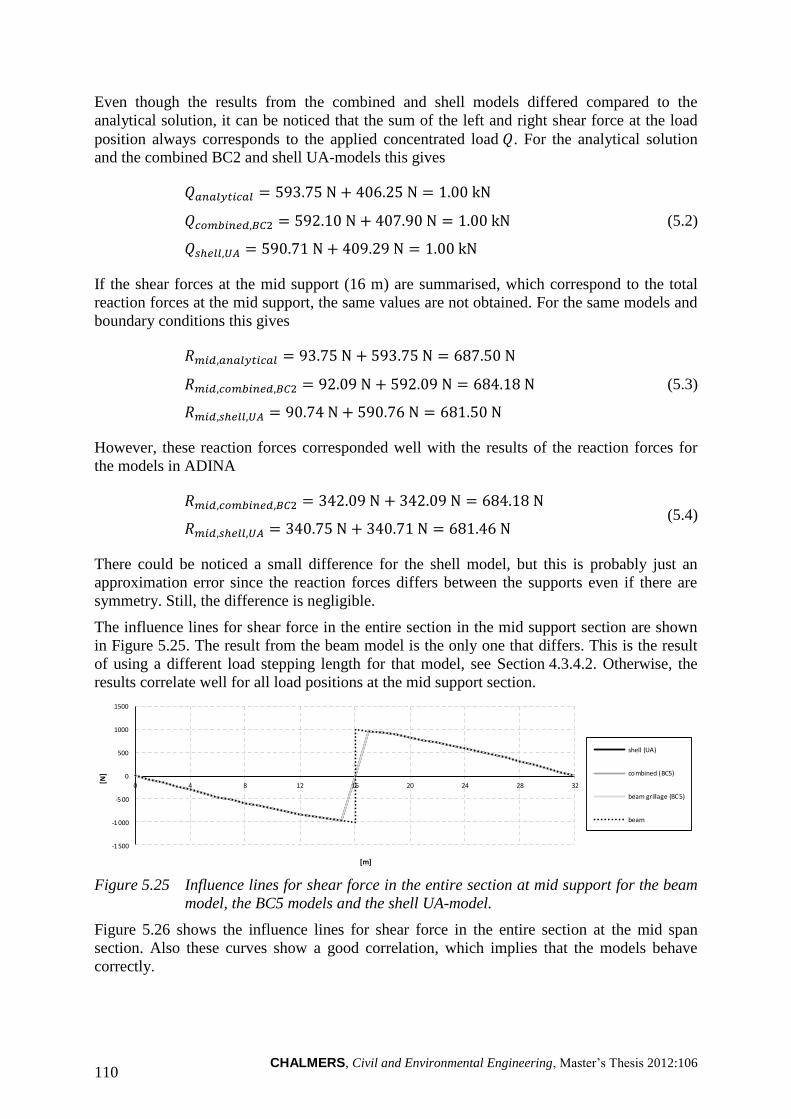
CHALMERS, Civil and Environmental Engineering, Master’s Thesis 2012:106 110
Even though the results from the combined and shell models differed compared to the
analytical solution, it can be noticed that the sum of the left and right shear force at the load
position always corresponds to the applied concentrated load . For the analytical solution
and the combined BC2 and shell UA-models this gives
(5.2)
If the shear forces at the mid support (16 m) are summarised, which correspond to the total
reaction forces at the mid support, the same values are not obtained. For the same models and
boundary conditions this gives
(5.3)
However, these reaction forces corresponded well with the results of the reaction forces for
the models in ADINA
(5.4)
There could be noticed a small difference for the shell model, but this is probably just an
approximation error since the reaction forces differs between the supports even if there are
symmetry. Still, the difference is negligible.
The influence lines for shear force in the entire section in the mid support section are shown
in Figure 5.25. The result from the beam model is the only one that differs. This is the result
of using a different load stepping length for that model, see Section 4.3.4.2. Otherwise, the
results correlate well for all load positions at the mid support section.
Figure 5.25 Influence lines for shear force in the entire section at mid support for the beam
model, the BC5 models and the shell UA-model.
Figure 5.26 shows the influence lines for shear force in the entire section at the mid span
section. Also these curves show a good correlation, which implies that the models behave
correctly.
-1500
-1 000
-5 00
0
500
1000
1500
0 4 8 12 16 20 24 28 32
[N]
[m]
shell (UA)
combined (BC5)
beam grillage (BC5)
beam
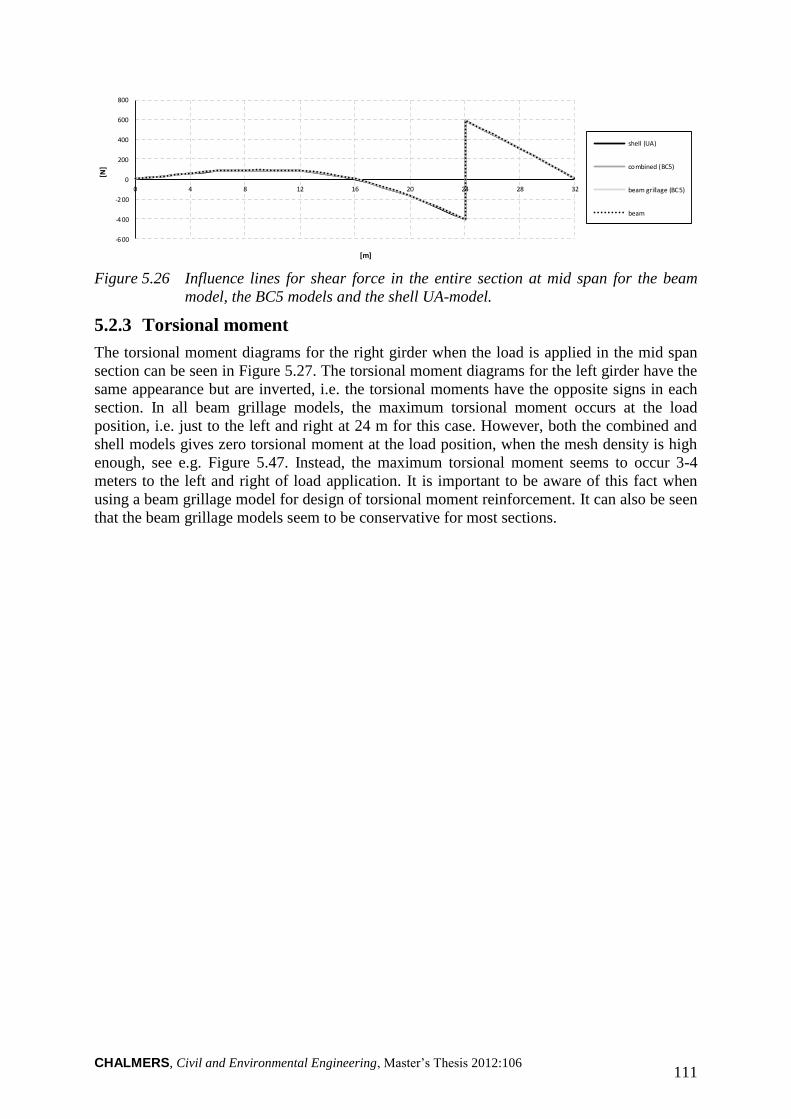
CHALMERS, Civil and Environmental Engineering, Master’s Thesis 2012:106 111
Figure 5.26 Influence lines for shear force in the entire section at mid span for the beam
model, the BC5 models and the shell UA-model.
5.2.3 Torsional moment
The torsional moment diagrams for the right girder when the load is applied in the mid span
section can be seen in Figure 5.27. The torsional moment diagrams for the left girder have the
same appearance but are inverted, i.e. the torsional moments have the opposite signs in each
section. In all beam grillage models, the maximum torsional moment occurs at the load
position, i.e. just to the left and right at 24 m for this case. However, both the combined and
shell models gives zero torsional moment at the load position, when the mesh density is high
enough, see e.g. Figure 5.47. Instead, the maximum torsional moment seems to occur 3-4
meters to the left and right of load application. It is important to be aware of this fact when
using a beam grillage model for design of torsional moment reinforcement. It can also be seen
that the beam grillage models seem to be conservative for most sections.
-600
-4 00
-2 00
0
200
400
600
800
0 4 8 12 16 20 24 28 32
[N]
[m]
shell (UA)
combined (BC5)
beam grillage (BC5)
beam
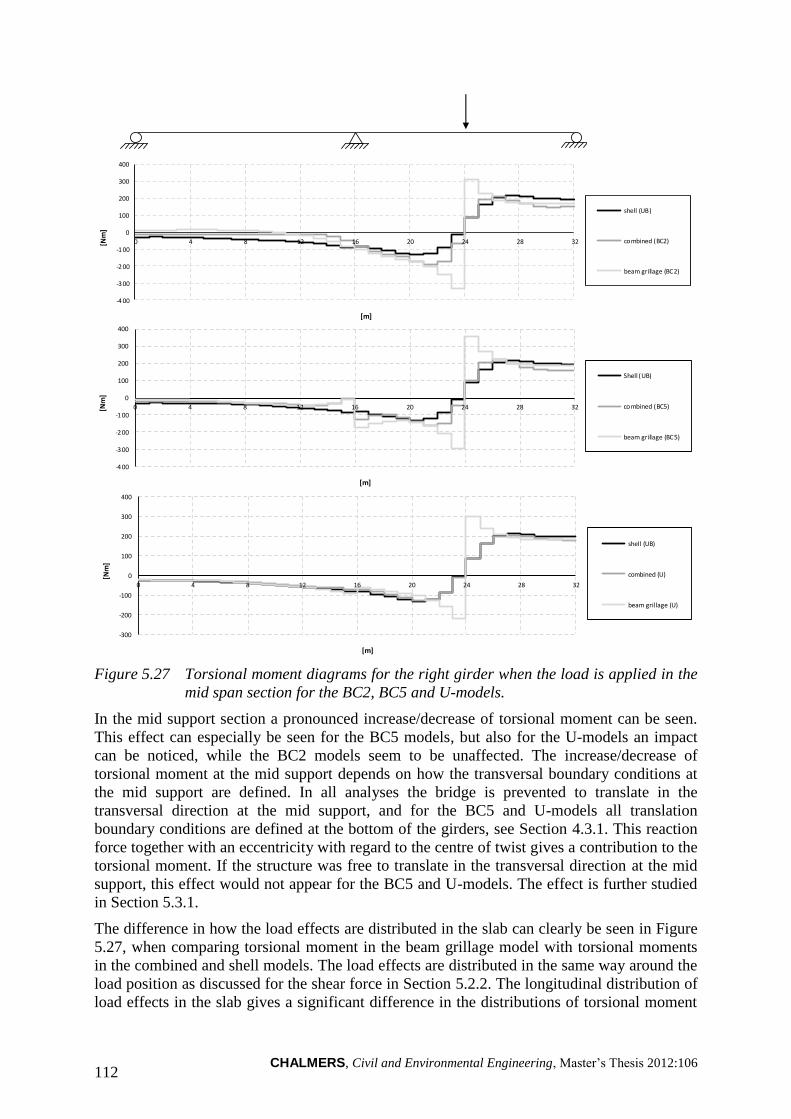
CHALMERS, Civil and Environmental Engineering, Master’s Thesis 2012:106 112
Figure 5.27 Torsional moment diagrams for the right girder when the load is applied in the
mid span section for the BC2, BC5 and U-models.
In the mid support section a pronounced increase/decrease of torsional moment can be seen.
This effect can especially be seen for the BC5 models, but also for the U-models an impact
can be noticed, while the BC2 models seem to be unaffected. The increase/decrease of
torsional moment at the mid support depends on how the transversal boundary conditions at
the mid support are defined. In all analyses the bridge is prevented to translate in the
transversal direction at the mid support, and for the BC5 and U-models all translation
boundary conditions are defined at the bottom of the girders, see Section 4.3.1. This reaction
force together with an eccentricity with regard to the centre of twist gives a contribution to the
torsional moment. If the structure was free to translate in the transversal direction at the mid
support, this effect would not appear for the BC5 and U-models. The effect is further studied
in Section 5.3.1.
The difference in how the load effects are distributed in the slab can clearly be seen in Figure
5.27, when comparing torsional moment in the beam grillage model with torsional moments
in the combined and shell models. The load effects are distributed in the same way around the
load position as discussed for the shear force in Section 5.2.2. The longitudinal distribution of
load effects in the slab gives a significant difference in the distributions of torsional moment
-4 00
-3 00
-2 00
-1 00
0
100
200
300
400
0 4 8 12 16 20 24 28 32[Nm
]
[m]
shell (UB)
combined (BC2)
beam grillage (BC2)
-4 00
-300
-2 00
-1 00
0
100
200
300
400
0 4 8 12 16 20 24 28 32[Nm
]
[m]
Shell (UB)
combined (BC5)
beam grillage (BC5)
-300
-200
-100
0
100
200
300
400
0 4 8 12 16 20 24 28 32
[Nm
]
[m]
shell (UB)
combined (U)
beam grillage (U)
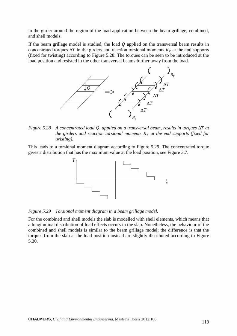
CHALMERS, Civil and Environmental Engineering, Master’s Thesis 2012:106 113
in the girder around the region of the load application between the beam grillage, combined,
and shell models.
If the beam grillage model is studied, the load applied on the transversal beam results in
concentrated torques in the girders and reaction torsional moments at the end supports
(fixed for twisting) according to Figure 5.28. The torques can be seen to be introduced at the
load position and resisted in the other transversal beams further away from the load.
Q
TΔ
TR
TR
TΔ
TΔ
TΔ TΔ
Figure 5.28 A concentrated load Q, applied on a transversal beam, results in torques at
the girders and reaction torsional moments at the end supports (fixed for
twisting).
This leads to a torsional moment diagram according to Figure 5.29. The concentrated torque
gives a distribution that has the maximum value at the load position, see Figure 3.7.
T
x
Figure 5.29 Torsional moment diagram in a beam grillage model.
For the combined and shell models the slab is modelled with shell elements, which means that
a longitudinal distribution of load effects occurs in the slab. Nonetheless, the behaviour of the
combined and shell models is similar to the beam grillage model; the difference is that the
torques from the slab at the load position instead are slightly distributed according to Figure
5.30.
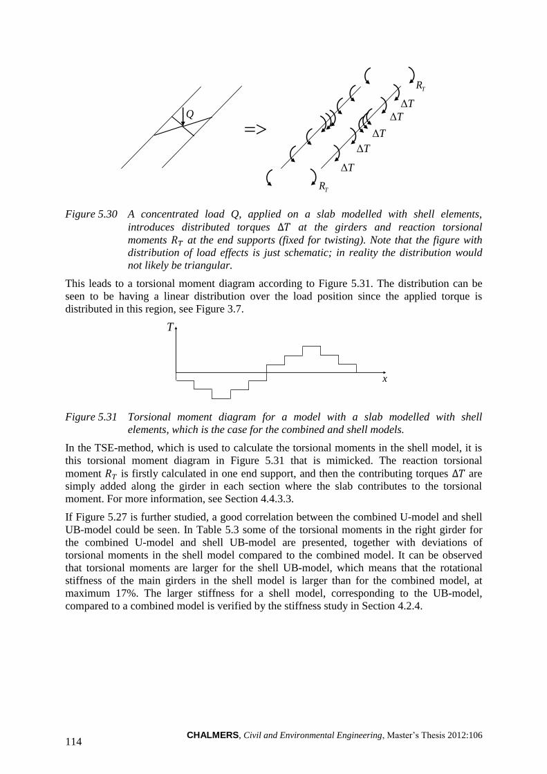
CHALMERS, Civil and Environmental Engineering, Master’s Thesis 2012:106 114
TΔ
TR
TR
TΔ
TΔ TΔ
TΔ
Q
Figure 5.30 A concentrated load Q, applied on a slab modelled with shell elements,
introduces distributed torques at the girders and reaction torsional
moments at the end supports (fixed for twisting). Note that the figure with
distribution of load effects is just schematic; in reality the distribution would
not likely be triangular.
This leads to a torsional moment diagram according to Figure 5.31. The distribution can be
seen to be having a linear distribution over the load position since the applied torque is
distributed in this region, see Figure 3.7.
T
x
Figure 5.31 Torsional moment diagram for a model with a slab modelled with shell
elements, which is the case for the combined and shell models.
In the TSE-method, which is used to calculate the torsional moments in the shell model, it is
this torsional moment diagram in Figure 5.31 that is mimicked. The reaction torsional
moment is firstly calculated in one end support, and then the contributing torques are
simply added along the girder in each section where the slab contributes to the torsional
moment. For more information, see Section 4.4.3.3.
If Figure 5.27 is further studied, a good correlation between the combined U-model and shell
UB-model could be seen. In Table 5.3 some of the torsional moments in the right girder for
the combined U-model and shell UB-model are presented, together with deviations of
torsional moments in the shell model compared to the combined model. It can be observed
that torsional moments are larger for the shell UB-model, which means that the rotational
stiffness of the main girders in the shell model is larger than for the combined model, at
maximum 17%. The larger stiffness for a shell model, corresponding to the UB-model,
compared to a combined model is verified by the stiffness study in Section 4.2.4.
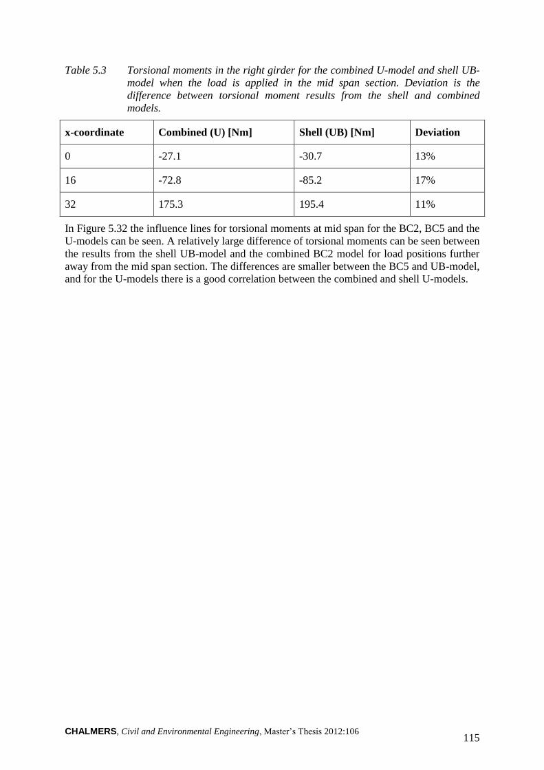
CHALMERS, Civil and Environmental Engineering, Master’s Thesis 2012:106 115
Table 5.3 Torsional moments in the right girder for the combined U-model and shell UB-
model when the load is applied in the mid span section. Deviation is the
difference between torsional moment results from the shell and combined
models.
x-coordinate Combined (U) [Nm] Shell (UB) [Nm] Deviation
0 -27.1 -30.7 13%
16 -72.8 -85.2 17%
32 175.3 195.4 11%
In Figure 5.32 the influence lines for torsional moments at mid span for the BC2, BC5 and the
U-models can be seen. A relatively large difference of torsional moments can be seen between
the results from the shell UB-model and the combined BC2 model for load positions further
away from the mid span section. The differences are smaller between the BC5 and UB-model,
and for the U-models there is a good correlation between the combined and shell U-models.
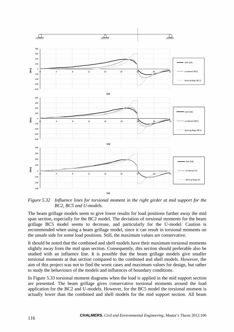
CHALMERS, Civil and Environmental Engineering, Master’s Thesis 2012:106 116
Figure 5.32 Influence lines for torsional moment in the right girder at mid support for the
BC2, BC5 and U-models.
The beam grillage models seem to give lower results for load positions further away the mid
span section, especially for the BC2 model. The deviation of torsional moments for the beam
grillage BC5 model seems to decrease, and particularly for the U-model. Caution is
recommended when using a beam grillage model, since it can result in torsional moments on
the unsafe side for some load positions. Still, the maximum values are conservative.
It should be noted that the combined and shell models have their maximum torsional moments
slightly away from the mid span section. Consequently, this section should preferable also be
studied with an influence line. It is possible that the beam grillage models give smaller
torsional moments at that section compared to the combined and shell models. However, the
aim of this project was not to find the worst cases and maximum values for design, but rather
to study the behaviours of the models and influences of boundary conditions.
In Figure 5.33 torsional moment diagrams when the load is applied in the mid support section
are presented. The beam grillage gives conservative torsional moments around the load
application for the BC2 and U-models. However, for the BC5 model the torsional moment is
actually lower than the combined and shell models for the mid support section. All beam
-4 00
-3 00
-200
-1 00
0
100
200
300
400
0 4 8 12 16 20 24 28 32[Nm
]
[m]
shell (UB)
combined (BC2)
beam grillage (BC2)
-4 00
-3 00
-2 00
-1 00
0
100
200
300
400
0 4 8 12 16 20 24 28 32[Nm
]
[m]
shell (UB)
combined (BC5)
beam grillage (BC5)
-3 00
-2 00
-100
0
100
200
300
400
0 4 8 12 16 20 24 28 32
[Nm
]
[m]
shell (UB)
combined (U)
beam grillage (U)
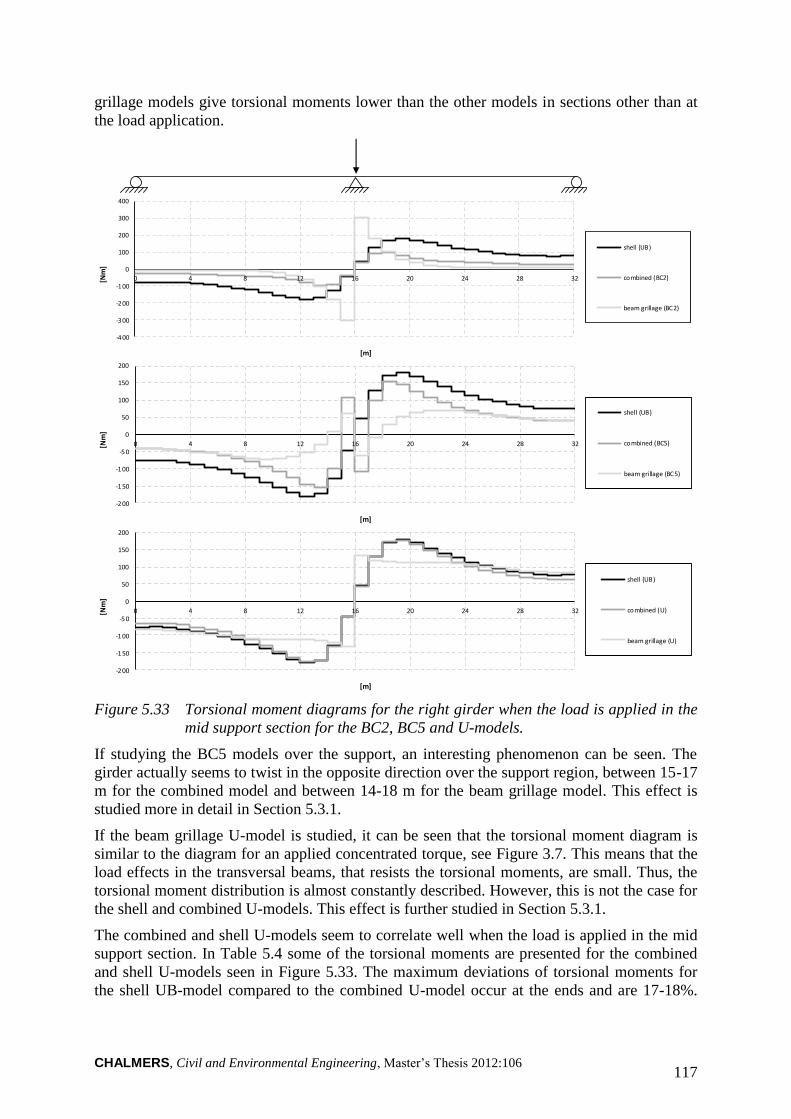
CHALMERS, Civil and Environmental Engineering, Master’s Thesis 2012:106 117
grillage models give torsional moments lower than the other models in sections other than at
the load application.
Figure 5.33 Torsional moment diagrams for the right girder when the load is applied in the
mid support section for the BC2, BC5 and U-models.
If studying the BC5 models over the support, an interesting phenomenon can be seen. The
girder actually seems to twist in the opposite direction over the support region, between 15-17
m for the combined model and between 14-18 m for the beam grillage model. This effect is
studied more in detail in Section 5.3.1.
If the beam grillage U-model is studied, it can be seen that the torsional moment diagram is
similar to the diagram for an applied concentrated torque, see Figure 3.7. This means that the
load effects in the transversal beams, that resists the torsional moments, are small. Thus, the
torsional moment distribution is almost constantly described. However, this is not the case for
the shell and combined U-models. This effect is further studied in Section 5.3.1.
The combined and shell U-models seem to correlate well when the load is applied in the mid
support section. In Table 5.4 some of the torsional moments are presented for the combined
and shell U-models seen in Figure 5.33. The maximum deviations of torsional moments for
the shell UB-model compared to the combined U-model occur at the ends and are 17-18%.
-4 00
-300
-2 00
-1 00
0
100
200
300
400
0 4 8 12 16 20 24 28 32[Nm
]
[m]
shell (UB)
combined (BC2)
beam grillage (BC2)
-2 00
-150
-1 00
-5 0
0
50
100
150
200
0 4 8 12 16 20 24 28 32[Nm
]
[m]
shell (UB)
combined (BC5)
beam grillage (BC5)
-200
-1 50
-1 00
-50
0
50
100
150
200
0 4 8 12 16 20 24 28 32[Nm
]
[m]
shell (UB)
combined (U)
beam grillage (U)
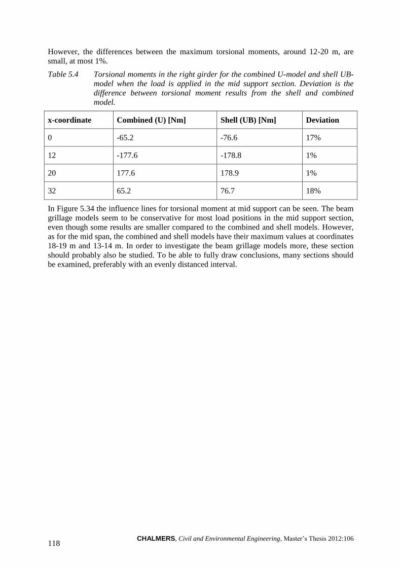
CHALMERS, Civil and Environmental Engineering, Master’s Thesis 2012:106 118
However, the differences between the maximum torsional moments, around 12-20 m, are
small, at most 1%.
Table 5.4 Torsional moments in the right girder for the combined U-model and shell UB-
model when the load is applied in the mid support section. Deviation is the
difference between torsional moment results from the shell and combined
model.
x-coordinate Combined (U) [Nm] Shell (UB) [Nm] Deviation
0 -65.2 -76.6 17%
12 -177.6 -178.8 1%
20 177.6 178.9 1%
32 65.2 76.7 18%
In Figure 5.34 the influence lines for torsional moment at mid support can be seen. The beam
grillage models seem to be conservative for most load positions in the mid support section,
even though some results are smaller compared to the combined and shell models. However,
as for the mid span, the combined and shell models have their maximum values at coordinates
18-19 m and 13-14 m. In order to investigate the beam grillage models more, these section
should probably also be studied. To be able to fully draw conclusions, many sections should
be examined, preferably with an evenly distanced interval.
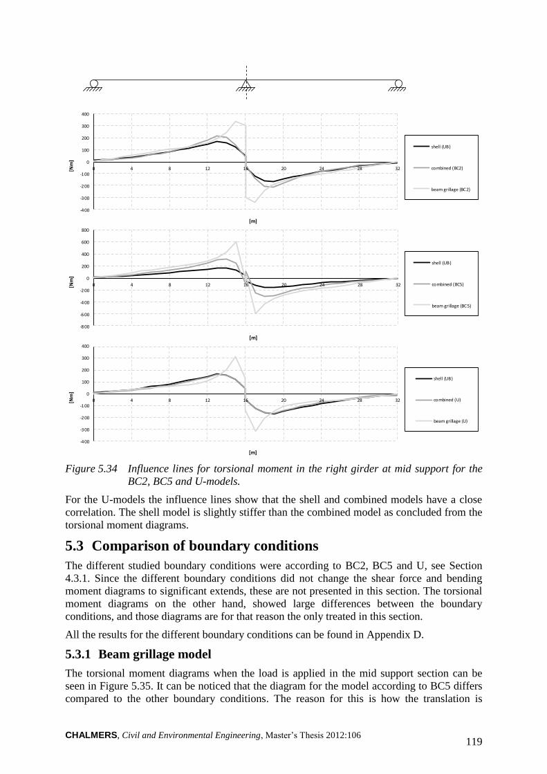
CHALMERS, Civil and Environmental Engineering, Master’s Thesis 2012:106 119
Figure 5.34 Influence lines for torsional moment in the right girder at mid support for the
BC2, BC5 and U-models.
For the U-models the influence lines show that the shell and combined models have a close
correlation. The shell model is slightly stiffer than the combined model as concluded from the
torsional moment diagrams.
5.3 Comparison of boundary conditions
The different studied boundary conditions were according to BC2, BC5 and U, see Section
4.3.1. Since the different boundary conditions did not change the shear force and bending
moment diagrams to significant extends, these are not presented in this section. The torsional
moment diagrams on the other hand, showed large differences between the boundary
conditions, and those diagrams are for that reason the only treated in this section.
All the results for the different boundary conditions can be found in Appendix D.
5.3.1 Beam grillage model
The torsional moment diagrams when the load is applied in the mid support section can be
seen in Figure 5.35. It can be noticed that the diagram for the model according to BC5 differs
compared to the other boundary conditions. The reason for this is how the translation is
-4 00
-3 00
-2 00
-1 00
0
100
200
300
400
0 4 8 12 16 20 24 28 32[Nm
]
[m]
shell (UB)
combined (BC2)
beam grillage (BC2)
-8 00
-6 00
-4 00
-2 00
0
200
400
600
800
0 4 8 12 16 20 24 28 32[Nm
]
[m]
shell (UB)
combined (BC5)
beam grillage (BC5)
-4 00
-3 00
-200
-1 00
0
100
200
300
400
0 4 8 12 16 20 24 28 32[Nm
]
[m]
shell (UB)
combined (U)
beam grillage (U)
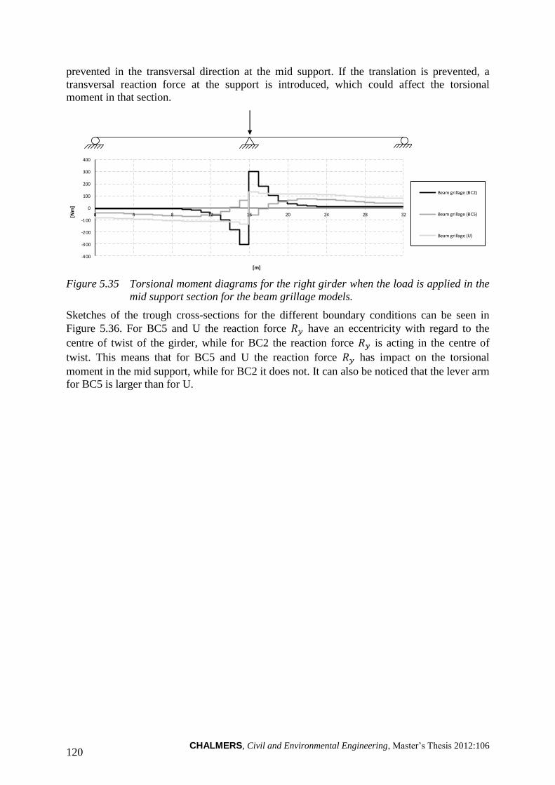
CHALMERS, Civil and Environmental Engineering, Master’s Thesis 2012:106 120
prevented in the transversal direction at the mid support. If the translation is prevented, a
transversal reaction force at the support is introduced, which could affect the torsional
moment in that section.
Figure 5.35 Torsional moment diagrams for the right girder when the load is applied in the
mid support section for the beam grillage models.
Sketches of the trough cross-sections for the different boundary conditions can be seen in
Figure 5.36. For BC5 and U the reaction force have an eccentricity with regard to the
centre of twist of the girder, while for BC2 the reaction force is acting in the centre of
twist. This means that for BC5 and U the reaction force has impact on the torsional
moment in the mid support, while for BC2 it does not. It can also be noticed that the lever arm
for BC5 is larger than for U.
-400
-3 00
-2 00
-100
0
100
200
300
400
0 4 8 12 16 20 24 28 32[Nm
]
[m]
Beam grillage (BC2)
Beam grillage (BC5)
Beam grillage (U)
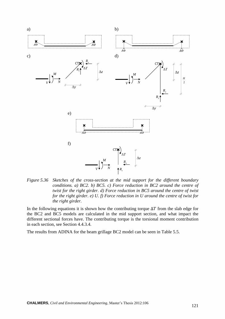
CHALMERS, Civil and Environmental Engineering, Master’s Thesis 2012:106 121
a)
b)
c) d)
V
M
N
yΔ
CT yR
TΔ zR
zΔ
V
M
N
yΔ
zΔ
CT
yR
TΔ
zR
2
H
e)
f)
V
M
N
zΔ
yR
TΔ
zR
CT
Figure 5.36 Sketches of the cross-section at the mid support for the different boundary
conditions. a) BC2. b) BC5. c) Force reduction in BC2 around the centre of
twist for the right girder. d) Force reduction in BC5 around the centre of twist
for the right girder. e) U. f) Force reduction in U around the centre of twist for
the right girder.
In the following equations it is shown how the contributing torque from the slab edge for
the BC2 and BC5 models are calculated in the mid support section, and what impact the
different sectional forces have. The contributing torque is the torsional moment contribution
in each section, see Section 4.4.3.4.
The results from ADINA for the beam grillage BC2 model can be seen in Table 5.5.
CHALMERS, Civil and Environmental Engineering, Master’s Thesis 2012:106 122
Table 5.5 Results from ADINA, together with the eccentricities for the beam grillage BC2
model.
Axial force, -451 N
Shear force, 500 N
Bending moment, 414 Nm
Eccentricity in y direction, 0.75 m
Eccentricity in z direction, 0.4 m
Using force reduction around the centre of twist of the girder for the BC2 model, the
contributing torque can be calculated. If the values in Table 5.5 are used, this leads to the
contributing torque
Nm (5.5)
As can be seen in Equation (5.5), but also in Figure 5.36c, the reaction forces are not affecting
the contributing torque, since they acts in the centre of twist of the girder.
The results from ADINA for the beam grillage BC5 model can be seen in Table 5.6.
Table 5.6 Results from ADINA, together with the eccentricities and the height of the
girder for the beam grillage BC5 model.
Axial force, 235 N
Shear force, 500 N
Bending moment, 418 Nm
Reaction force, 1551 N
Eccentricity in y direction, 0.75 m
Eccentricity in z direction, 0.4 m
Height of girder, 1.3 m
Using force reduction around the centre of twist of the girder for the BC5 model, the
contributing torque can be calculated. If the values in Table 5.6 are used, this leads to the
contributing torque
Nm
(5.6)
CHALMERS, Civil and Environmental Engineering, Master’s Thesis 2012:106 123
As can be seen in Figure 5.36d the transverse reaction force act on the girder with an
eccentricity of ⁄ to the centre of twist. In Equation (5.6) the effect on the contributing
torque can be seen to be large.
The results from ADINA for the beam grillage U-model can be seen in Table 5.7.
Table 5.7 Results from ADINA, together with the eccentricities for the beam grillage U-
model.
Axial force, 0 N
Bending moment, 592 Nm
Reaction force, 810 N
Eccentricity in z direction, 0.4 m
Using force reduction around the centre of twist of the girder for the U-model, the
contributing torque can be calculated. If the values in Table 5.7 are used, this leads to the
contributing torque
Nm (5.7)
As can be seen in Figure 5.36f the transverse reaction force act on the girder with an
eccentricity of to the centre of twist. In Table 5.7 the transverse reaction force in the U-
model can be seen to be smaller than in the BC5 model (Table 5.6). Also the eccentricity is
smaller in the U-model compared to the BC5 model. In Equation (5.7) the effect on the
contributing torque can be seen, and even if the transversal reaction force is affecting the
torque, the result is still negative as the BC2 model.
Another remark about the U-model is that the shear force is acting in the centre of twist. Thus,
the contributing torques are much smaller. This also explains why the diagram does not
decrease very much, but are rather constant, similar to a diagram for an applied concentrated
torque, see Figure 3.7.
In Table 5.8 a summary, of the calculated contributing torques, is presented. It can be
observed that the BC5 model result in a positive contributing torque at the mid support
section, while the BC2 and the U-models results in negative torques.
Table 5.8 The calculated contributing torques.
BC2, -609 Nm
BC5, 121 Nm
U-model, -268 Nm
In Figure 5.37 the directions of the torsional moments in the mid support section can be seen.
This means that the right girder in the beam grillage BC5 model has a contributing torque in
the clockwise direction, which implies a clockwise twist of the right girder at the mid support.
This is the opposite compared to the BC2 and U-models, which are only twisting counter
clockwise and corresponds to the behaviour described in Figure 5.28. This is in fact the
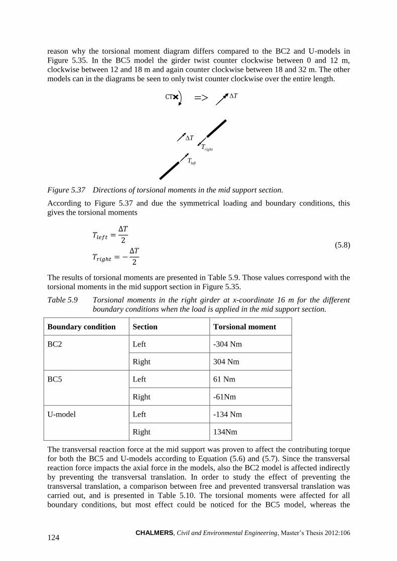
CHALMERS, Civil and Environmental Engineering, Master’s Thesis 2012:106 124
reason why the torsional moment diagram differs compared to the BC2 and U-models in
Figure 5.35. In the BC5 model the girder twist counter clockwise between 0 and 12 m,
clockwise between 12 and 18 m and again counter clockwise between 18 and 32 m. The other
models can in the diagrams be seen to only twist counter clockwise over the entire length.
T CT
leftT
rightT
T
Figure 5.37 Directions of torsional moments in the mid support section.
According to Figure 5.37 and due the symmetrical loading and boundary conditions, this
gives the torsional moments
(5.8)
The results of torsional moments are presented in Table 5.9. Those values correspond with the
torsional moments in the mid support section in Figure 5.35.
Table 5.9 Torsional moments in the right girder at x-coordinate 16 m for the different
boundary conditions when the load is applied in the mid support section.
Boundary condition Section Torsional moment
BC2 Left -304 Nm
Right 304 Nm
BC5 Left 61 Nm
Right -61Nm
U-model Left -134 Nm
Right 134Nm
The transversal reaction force at the mid support was proven to affect the contributing torque
for both the BC5 and U-models according to Equation (5.6) and (5.7). Since the transversal
reaction force impacts the axial force in the models, also the BC2 model is affected indirectly
by preventing the transversal translation. In order to study the effect of preventing the
transversal translation, a comparison between free and prevented transversal translation was
carried out, and is presented in Table 5.10. The torsional moments were affected for all
boundary conditions, but most effect could be noticed for the BC5 model, whereas the
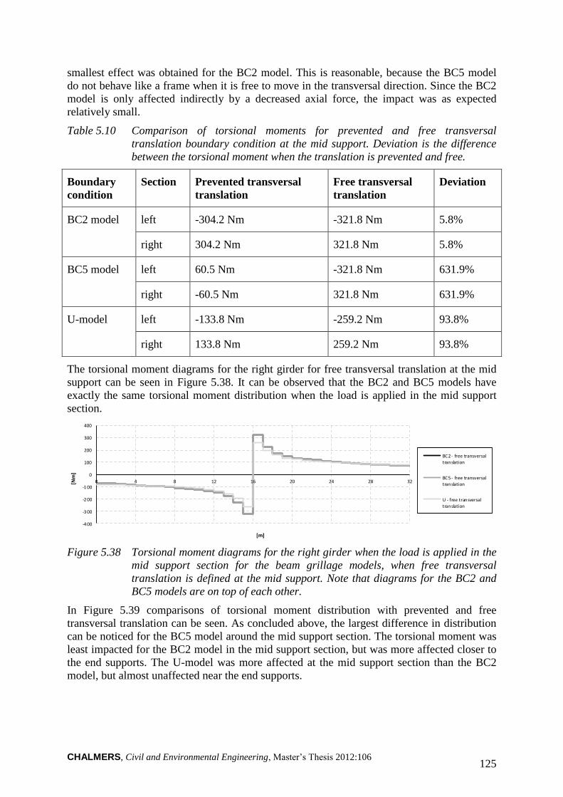
CHALMERS, Civil and Environmental Engineering, Master’s Thesis 2012:106 125
smallest effect was obtained for the BC2 model. This is reasonable, because the BC5 model
do not behave like a frame when it is free to move in the transversal direction. Since the BC2
model is only affected indirectly by a decreased axial force, the impact was as expected
relatively small.
Table 5.10 Comparison of torsional moments for prevented and free transversal
translation boundary condition at the mid support. Deviation is the difference
between the torsional moment when the translation is prevented and free.
Boundary
condition
Section Prevented transversal
translation
Free transversal
translation
Deviation
BC2 model left -304.2 Nm -321.8 Nm 5.8%
right 304.2 Nm 321.8 Nm 5.8%
BC5 model left 60.5 Nm -321.8 Nm 631.9%
right -60.5 Nm 321.8 Nm 631.9%
U-model left -133.8 Nm -259.2 Nm 93.8%
right 133.8 Nm 259.2 Nm 93.8%
The torsional moment diagrams for the right girder for free transversal translation at the mid
support can be seen in Figure 5.38. It can be observed that the BC2 and BC5 models have
exactly the same torsional moment distribution when the load is applied in the mid support
section.
Figure 5.38 Torsional moment diagrams for the right girder when the load is applied in the
mid support section for the beam grillage models, when free transversal
translation is defined at the mid support. Note that diagrams for the BC2 and
BC5 models are on top of each other.
In Figure 5.39 comparisons of torsional moment distribution with prevented and free
transversal translation can be seen. As concluded above, the largest difference in distribution
can be noticed for the BC5 model around the mid support section. The torsional moment was
least impacted for the BC2 model in the mid support section, but was more affected closer to
the end supports. The U-model was more affected at the mid support section than the BC2
model, but almost unaffected near the end supports.
-400
-3 00
-2 00
-100
0
100
200
300
400
0 4 8 12 16 20 24 28 32[Nm
]
[m]
BC2 - free transversal
translation
BC5 - free transversaltranslation
U - free transversal
translation
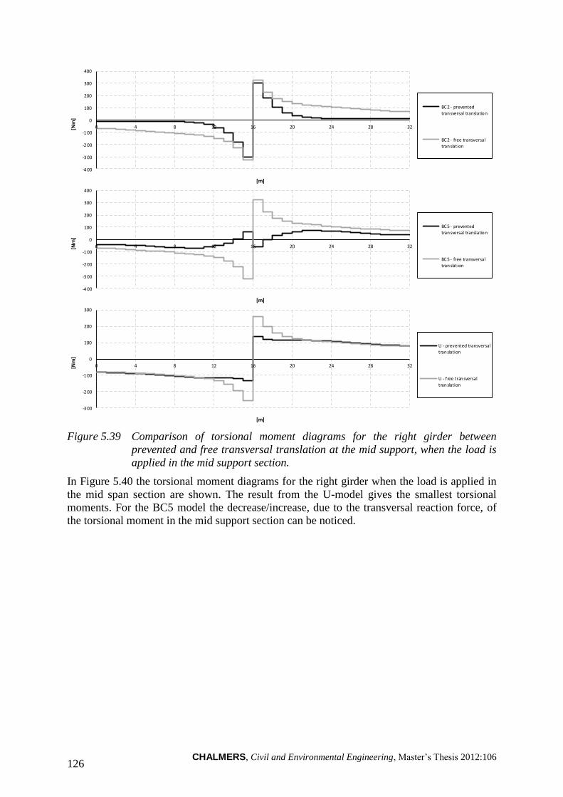
CHALMERS, Civil and Environmental Engineering, Master’s Thesis 2012:106 126
Figure 5.39 Comparison of torsional moment diagrams for the right girder between
prevented and free transversal translation at the mid support, when the load is
applied in the mid support section.
In Figure 5.40 the torsional moment diagrams for the right girder when the load is applied in
the mid span section are shown. The result from the U-model gives the smallest torsional
moments. For the BC5 model the decrease/increase, due to the transversal reaction force, of
the torsional moment in the mid support section can be noticed.
-400
-3 00
-2 00
-100
0
100
200
300
400
0 4 8 12 16 20 24 28 32[Nm
]
[m]
BC2 - prevented
transversal translation
BC2 - free transversaltranslation
-400
-3 00
-2 00
-100
0
100
200
300
400
0 4 8 12 16 20 24 28 32[Nm
]
[m]
BC5 - prevented
transversal translation
BC5 - free transversaltranslation
-300
-2 00
-1 00
0
100
200
300
0 4 8 12 16 20 24 28 32[Nm
]
[m]
U - prevented transversal
translation
U - free transversaltranslation
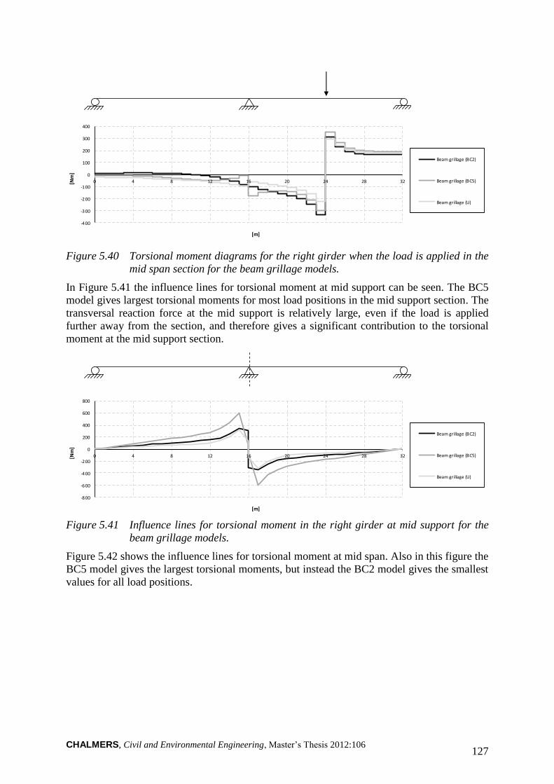
CHALMERS, Civil and Environmental Engineering, Master’s Thesis 2012:106 127
Figure 5.40 Torsional moment diagrams for the right girder when the load is applied in the
mid span section for the beam grillage models.
In Figure 5.41 the influence lines for torsional moment at mid support can be seen. The BC5
model gives largest torsional moments for most load positions in the mid support section. The
transversal reaction force at the mid support is relatively large, even if the load is applied
further away from the section, and therefore gives a significant contribution to the torsional
moment at the mid support section.
Figure 5.41 Influence lines for torsional moment in the right girder at mid support for the
beam grillage models.
Figure 5.42 shows the influence lines for torsional moment at mid span. Also in this figure the
BC5 model gives the largest torsional moments, but instead the BC2 model gives the smallest
values for all load positions.
-4 00
-3 00
-2 00
-1 00
0
100
200
300
400
0 4 8 12 16 20 24 28 32[Nm
]
[m]
Beam grillage (BC2)
Beam grillage (BC5)
Beam grillage (U)
-800
-6 00
-4 00
-200
0
200
400
600
800
0 4 8 12 16 20 24 28 32[Nm
]
[m]
Beam grillage (BC2)
Beam grillage (BC5)
Beam grillage (U)
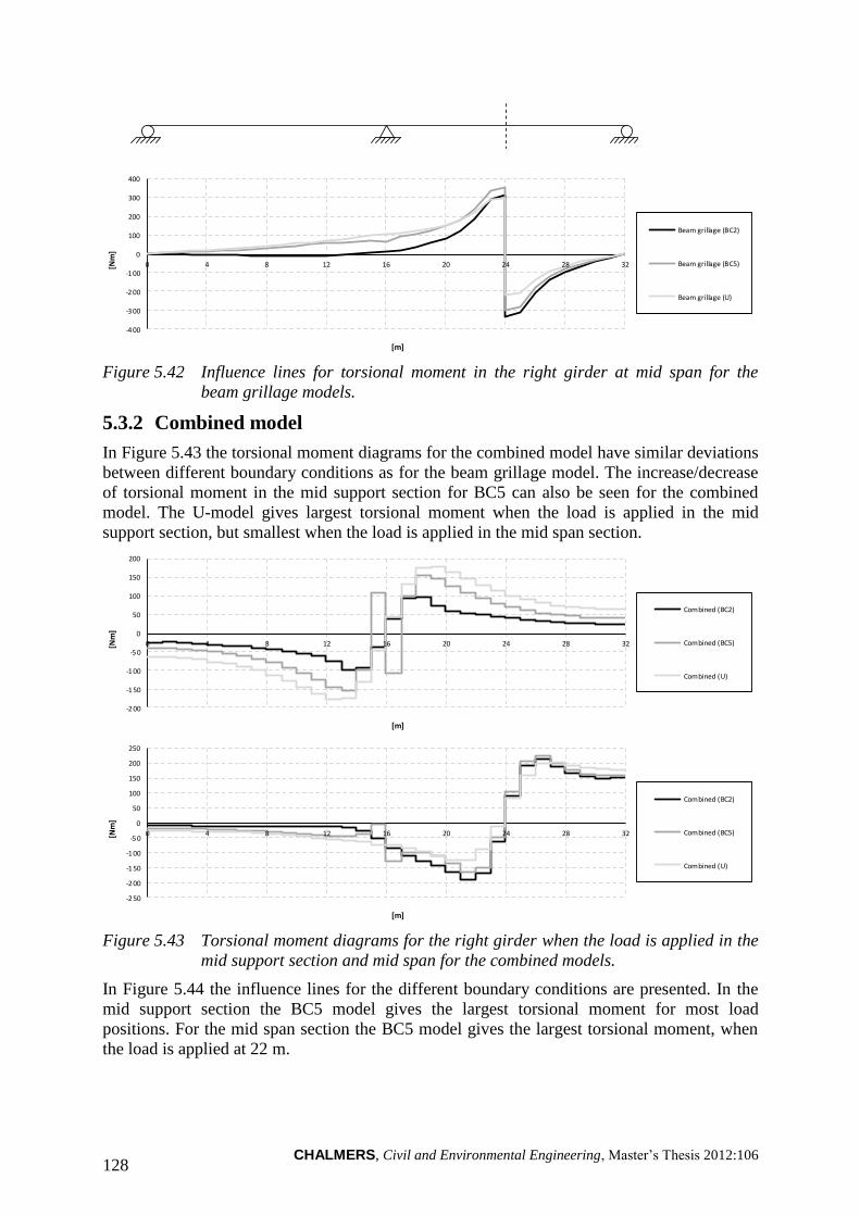
CHALMERS, Civil and Environmental Engineering, Master’s Thesis 2012:106 128
Figure 5.42 Influence lines for torsional moment in the right girder at mid span for the
beam grillage models.
5.3.2 Combined model
In Figure 5.43 the torsional moment diagrams for the combined model have similar deviations
between different boundary conditions as for the beam grillage model. The increase/decrease
of torsional moment in the mid support section for BC5 can also be seen for the combined
model. The U-model gives largest torsional moment when the load is applied in the mid
support section, but smallest when the load is applied in the mid span section.
Figure 5.43 Torsional moment diagrams for the right girder when the load is applied in the
mid support section and mid span for the combined models.
In Figure 5.44 the influence lines for the different boundary conditions are presented. In the
mid support section the BC5 model gives the largest torsional moment for most load
positions. For the mid span section the BC5 model gives the largest torsional moment, when
the load is applied at 22 m.
-400
-3 00
-2 00
-100
0
100
200
300
400
0 4 8 12 16 20 24 28 32[Nm
]
[m]
Beam grillage (BC2)
Beam grillage (BC5)
Beam grillage (U)
-200
-1 50
-1 00
-50
0
50
100
150
200
0 4 8 12 16 20 24 28 32[Nm
]
[m]
Combined (BC2)
Combined (BC5)
Combined (U)
-250
-200
-1 50
-1 00
-5 0
0
50
100
150
200
250
0 4 8 12 16 20 24 28 32[Nm
]
[m]
Combined (BC2)
Combined (BC5)
Combined (U)
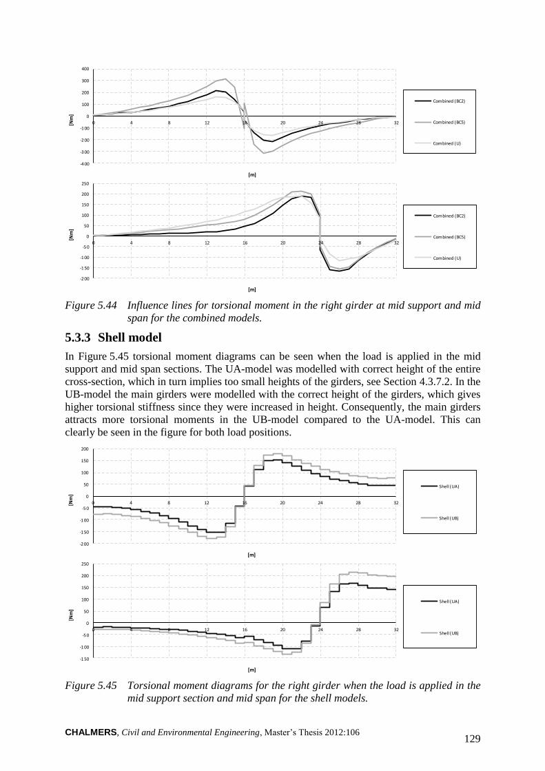
CHALMERS, Civil and Environmental Engineering, Master’s Thesis 2012:106 129
Figure 5.44 Influence lines for torsional moment in the right girder at mid support and mid
span for the combined models.
5.3.3 Shell model
In Figure 5.45 torsional moment diagrams can be seen when the load is applied in the mid
support and mid span sections. The UA-model was modelled with correct height of the entire
cross-section, which in turn implies too small heights of the girders, see Section 4.3.7.2. In the
UB-model the main girders were modelled with the correct height of the girders, which gives
higher torsional stiffness since they were increased in height. Consequently, the main girders
attracts more torsional moments in the UB-model compared to the UA-model. This can
clearly be seen in the figure for both load positions.
Figure 5.45 Torsional moment diagrams for the right girder when the load is applied in the
mid support section and mid span for the shell models.
-400
-3 00
-2 00
-100
0
100
200
300
400
0 4 8 12 16 20 24 28 32[Nm
]
[m]
Combined (BC2)
Combined (BC5)
Combined (U)
-200
-150
-1 00
-5 0
0
50
100
150
200
250
0 4 8 12 16 20 24 28 32
[Nm
]
[m]
Combined (BC2)
Combined (BC5)
Combined (U)
-200
-1 50
-1 00
-5 0
0
50
100
150
200
0 4 8 12 16 20 24 28 32[Nm
]
[m]
Shell (UA)
Shell (UB)
-1 50
-1 00
-50
0
50
100
150
200
250
0 4 8 12 16 20 24 28 32
[Nm
]
[m]
Shell (UA)
Shell (UB)
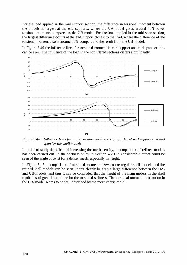
CHALMERS, Civil and Environmental Engineering, Master’s Thesis 2012:106 130
For the load applied in the mid support section, the difference in torsional moment between
the models is largest at the end supports, where the UA-model gives around 40% lower
torsional moments compared to the UB-model. For the load applied in the mid span section,
the largest difference occurs at the end support closest to the load, where the difference of the
torsional moment also is around 40% compared to the result from the UB-model.
In Figure 5.46 the influence lines for torsional moment in mid support and mid span sections
can be seen. The influence of the load in the considered sections differs significantly.
Figure 5.46 Influence lines for torsional moment in the right girder at mid support and mid
span for the shell models.
In order to study the effect of increasing the mesh density, a comparison of refined models
has been carried out. In the stiffness study in Section 4.2.1, a considerable effect could be
seen of the angle of twist for a denser mesh, especially in height.
In Figure 5.47 a comparison of torsional moments between the regular shell models and the
refined shell models can be seen. It can clearly be seen a large difference between the UA-
and UB-models, and thus it can be concluded that the height of the main girders in the shell
models is of great importance for the torsional stiffness. The torsional moment distribution in
the UB- model seems to be well described by the more coarse mesh.
-2 00
-150
-1 00
-5 0
0
50
100
150
200
0 4 8 12 16 20 24 28 32[Nm
]
[m]
Shell (UA)
Shell (UB)
-1 50
-100
-5 0
0
50
100
150
200
250
0 4 8 12 16 20 24 28 32
[Nm
]
[m]
Shell (UA)
Shell (UB)
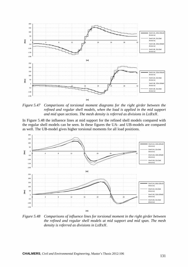
CHALMERS, Civil and Environmental Engineering, Master’s Thesis 2012:106 131
Figure 5.47 Comparisons of torsional moment diagrams for the right girder between the
refined and regular shell models, when the load is applied in the mid support
and mid span sections. The mesh density is referred as divisions in .
In Figure 5.48 the influence lines at mid support for the refined shell models compared with
the regular shell models can be seen. In these figures the UA- and UB-models are compared
as well. The UB-model gives higher torsional moments for all load positions.
Figure 5.48 Comparisons of influence lines for torsional moment in the right girder between
the refined and regular shell models at mid support and mid span. The mesh
density is referred as divisions in .
-200
-1 50
-1 00
-50
0
50
100
150
200
0 4 8 12 16 20 24 28 32[Nm
]
[m]
Shell (UA, 320x100x60
divis ions)
Shell (UA, 32x10x6
divis ions)
Shell (UB, 320x100x60divis ions)
Shell (UB, 32x10x6divis ions)
-150
-1 00
-5 0
0
50
100
150
200
250
0 4 8 12 16 20 24 28 32
[Nm
]
[m]
Shell (UA, 320x100x60
divis ions)
Shell (UA, 32x10x6
divis ions)
Shell (UB, 320x100x60divis ions)
Shell (UB, 32x10x6divis ions)
-200
-1 50
-1 00
-50
0
50
100
150
200
0 4 8 12 16 20 24 28 32[Nm
]
[m]
Shell (UA, 320x100x60
divis ions)
Shell (UA, 32x10x6
divis ions)
Shell (UB, 320x100x60divis ions)
Shell (UB, 32x10x6divis ions)
-150
-1 00
-5 0
0
50
100
150
200
250
0 4 8 12 16 20 24 28 32
[Nm
]
[m]
Shell (UA, 640x100x20
divis ions)
Shell (UA, 32x10x6
divis ions)
Shell (UB, 320x100x60divis ions)
Shell (UB, 32x10x6divis ions)
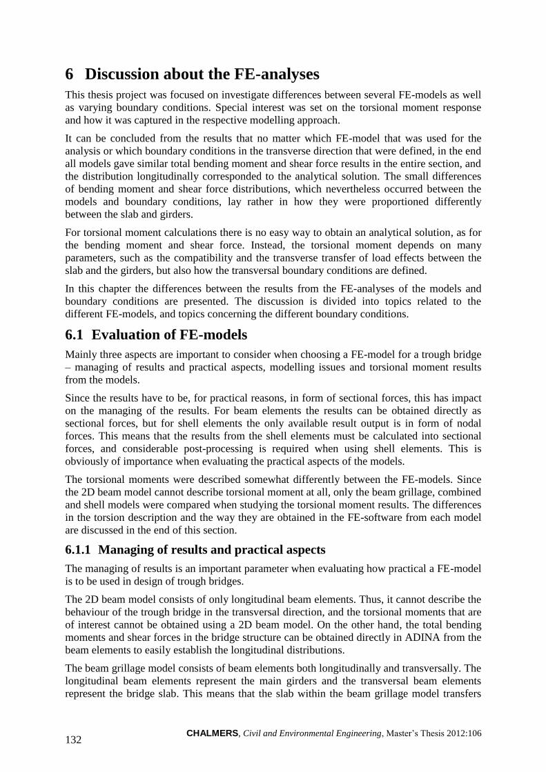
CHALMERS, Civil and Environmental Engineering, Master’s Thesis 2012:106 132
6 Discussion about the FE-analyses
This thesis project was focused on investigate differences between several FE-models as well
as varying boundary conditions. Special interest was set on the torsional moment response
and how it was captured in the respective modelling approach.
It can be concluded from the results that no matter which FE-model that was used for the
analysis or which boundary conditions in the transverse direction that were defined, in the end
all models gave similar total bending moment and shear force results in the entire section, and
the distribution longitudinally corresponded to the analytical solution. The small differences
of bending moment and shear force distributions, which nevertheless occurred between the
models and boundary conditions, lay rather in how they were proportioned differently
between the slab and girders.
For torsional moment calculations there is no easy way to obtain an analytical solution, as for
the bending moment and shear force. Instead, the torsional moment depends on many
parameters, such as the compatibility and the transverse transfer of load effects between the
slab and the girders, but also how the transversal boundary conditions are defined.
In this chapter the differences between the results from the FE-analyses of the models and
boundary conditions are presented. The discussion is divided into topics related to the
different FE-models, and topics concerning the different boundary conditions.
6.1 Evaluation of FE-models
Mainly three aspects are important to consider when choosing a FE-model for a trough bridge
– managing of results and practical aspects, modelling issues and torsional moment results
from the models.
Since the results have to be, for practical reasons, in form of sectional forces, this has impact
on the managing of the results. For beam elements the results can be obtained directly as
sectional forces, but for shell elements the only available result output is in form of nodal
forces. This means that the results from the shell elements must be calculated into sectional
forces, and considerable post-processing is required when using shell elements. This is
obviously of importance when evaluating the practical aspects of the models.
The torsional moments were described somewhat differently between the FE-models. Since
the 2D beam model cannot describe torsional moment at all, only the beam grillage, combined
and shell models were compared when studying the torsional moment results. The differences
in the torsion description and the way they are obtained in the FE-software from each model
are discussed in the end of this section.
6.1.1 Managing of results and practical aspects
The managing of results is an important parameter when evaluating how practical a FE-model
is to be used in design of trough bridges.
The 2D beam model consists of only longitudinal beam elements. Thus, it cannot describe the
behaviour of the trough bridge in the transversal direction, and the torsional moments that are
of interest cannot be obtained using a 2D beam model. On the other hand, the total bending
moments and shear forces in the bridge structure can be obtained directly in ADINA from the
beam elements to easily establish the longitudinal distributions.
The beam grillage model consists of beam elements both longitudinally and transversally. The
longitudinal beam elements represent the main girders and the transversal beam elements
represent the bridge slab. This means that the slab within the beam grillage model transfers
CHALMERS, Civil and Environmental Engineering, Master’s Thesis 2012:106 133
load effects transversally, but do not consider any longitudinal distribution within the slab. In
addition to the 2D beam model it gives torsional moments results in the main girders due to
the transversal distribution in the slab. Since the model only consists of beam elements, the
sectional force results regarding bending moments, shear force and torsional moments are
obtained directly in ADINA, and do not need any further post-processing.
In the combined model the main girders are modelled with beam elements, and the slab with
shell elements. Since the girders are modelled with beam elements the results from the girders
can be obtained in form of sectional forces directly in ADINA such as the torsional moments.
As the slab consists of shell elements, the load effects are distributed longitudinally both in
the slab and the main girders. This means that the bending moment and shear force
distributions are given for the slab and the girders separately. In order to obtain the total
moment and shear force distributions for the entire section, the results from the analysis
require post-processing to summarise the contribution in the slab with the contribution in the
main girders. The procedure for this is explained in Section 4.4.3.
The shell model is created using only shell elements, both for the slab and the main girders.
The results in ADINA for shell elements are given in form of nodal forces. In order to obtain
sectional forces, the nodal forces have to be calculated as described in Section 4.4.3.
The FE-model should preferably be able to give the sectional forces directly in ADINA in
order to be considered practical and convenient to use. This is the case for the 2D beam and
the beam grillage models, and they are consequently the most practical to be used in design.
An additional advantage with the beam grillage model is the simplified way the distribution of
load effects are described, which makes results from the model easy to analyse and handle.
The combined model is practical to use if only the girders should be studied, e.g. to study the
distribution of torsional moment along the main girders. Moreover, the torsional moments are
better described by a more realistic distribution of load effects in the slab, than the beam
grillage model, due to the contribution in the longitudinal direction. If the bending moment
and shear force distributions should be studied in a combined model, the contribution in the
slab has to be considered, which will result in extra work due to result management. The shell
model was, as expected, the less user-friendly model for all analyses. None of the bending
moment, shear force and torsional moment can be obtained without extensive result
management effort.
6.1.2 Modelling issues
A modelling issue appeared when the shell model was created. A shell element is defined
from a surface midplane. The connections between the shell elements are therefore performed
in their midplanes. This means that the cross-section in a shell model is created by connecting
the midplanes of the slab and the main girders. As a consequence, the height of the girders
must be modelled with lower heights in order to correspond to the total cross-section.
To deal with the height of the girders in the shell model, two different models were created,
referred to as the UA- and UB-model. The UA-model had the correct total height, but too low
girders, and the UB-model had the correct height of the girders, but in return also a too high
height of the entire cross-section. When studying distributions of bending moment and shear
force, a correct description of the total height of the studied cross-section is important in order
to catch the normal stress distribution longitudinally. This was the reason why the UA-model
was created. Conversely, when studying the distribution of torsional moments, it is important
to have a correct description of the torsional stiffness in the girders, which is a matter of
geometry and material. The height of the girders is an essential parameter of the geometry,
and to get this as correct as possible compared to the studied trough section, the girders
CHALMERS, Civil and Environmental Engineering, Master’s Thesis 2012:106 134
heights were increased; this lead to the development of the UB-model. For more information,
see Section 4.3.7.
In order to create a more realistic FE-model, 3D solid elements could be used. Since a solid
element is created as a 3D volume, the modelling issues related to the shell model could be
eliminated. The management of results would probably be extensive, but as the results can be
given in form of nodal forces, the same procedure as for the shell model should be possible.
The MATLAB-programs created for the shell model are rather generic and could preferably
be used on a model with solid elements.
6.1.3 Torsional moment results from the models
One key difference was observed when the torsional moment results from the FE-models
were compared. Since no longitudinal distribution occurs in the slab for the beam grillage
model, the applied torques at the main girders are concentrated in the sections at the load
positions. For the combined and shell models, a longitudinal distribution of load effects in the
slab leads to applied distributed torques on the girders. Consequently, the torsional moments
are concentrated at the load positions for the beam grillage and distributed over a region for
the combined and shell models.
Due to the differences in how the torque was applied on the main girders, as a concentrated or
distributed load effect, the maximum torsional moments occurred at different sections along
the main girder. For the combined and shell models the maximum torsional moment occurred
slightly to the left and right of the load position, while for the beam grillage model the
maximum torsional moment occurred at the load position. The maximum values from the
beam grillage models were for most cases much higher than for the other models. However,
for load applied in the mid span section, the maximum torsional moment from the combined
and shell model corresponded relatively well with the values from the beam grillage model at
the same sections. Also the influence lines showed relatively well correspondence at mid
span. But when the load was applied in the mid support section, there could be noticed
relatively large differences, near the mid support section, where the maximum torsional
moment occurred and the corresponding values.
The torsional moments for the beam grillage model were for most cases conservative at the
load positions. However, for some sections and load positions the results were lower than the
combined and shell models. This was most obvious when the load was applied in the mid
support section. The only studied sections were the mid support and the mid span section, but
the maximum values for the combined and shell model occurred slightly to the left or right of
these sections. In order to draw any final conclusions about the uncertainty of the torsional
moment results of the beam grillage model, more sections and load positions should be
studied. Thus, further investigations of torsional moments in the beam grillage model are
recommended.
It should be pointed out that the beam grillage model still correspond to the load effect
distributions in the ultimate state more correctly, while the combined and shell models with
isotropic slab better describes the behaviour in service state. However, even for small loads in
the service state, cracking occurs and causes redistribution in the slab. The reinforcement is
often designed to mainly transfer load effects transversally to the main girders, and the
distributions are more similar to the beam grillage model behaviour. This implies that the
distribution probably should be described somewhere between an isotropic slab, as in the
combined and shell models, and a beam grillage model. The most realistic solution would
however be obtained from a nonlinear analysis, allowing the load effects to redistribute due to
cracking. This is, however, not a practical alternative for bridge design. A simpler solution
CHALMERS, Civil and Environmental Engineering, Master’s Thesis 2012:106 135
could be to model the slab with an orthotropic behaviour to give it lower stiffness in the
longitudinal direction.
The torsional moment results from the combined and shell models were very similar when the
same type of models were compared, i.e. the U-models. Even if the TSE-method was
developed in order to calculate torsional moments for a shell model, a lot of extra work is still
required. The shell model can therefore be used more as a verification of the combined model.
Thus, the combined model is the recommended model to use instead of a shell model when
torsional moment is studied. An additional advantage with the combined model is that it is
possible to model the cross-section not just as a U-model with u-shaped cross-section, which
is the case for the shell model, but also in other ways, e.g. as the BC2 and BC5 models.
6.2 Evaluation of boundary conditions
In this thesis project a general trough bridge model was created, using information from
previous trough bridge projects at REINERTSEN. Several boundary condition alternatives
were created related to this model. Three of those boundary conditions, referred to as BC2,
BC5 and U, were examined and analysed. Information about the different boundary
conditions can be found in Section 4.3.1.
The results from the boundary condition models gave as stated before the same total bending
moments and shear forces for the entire section. Even the differences in results from the slab
and girders separately were relative small for bending moment and shear force. However, the
torsional moment results had a significant variation depending on the choice of boundary
conditions.
How the transversal restraints are modelled should be considered carefully. The different
choices of modelling the boundary conditions affected in most cases the torsional moments in
the girders to significant extents. The studied trough bridge was assumed to be fixed in
transversal direction at the mid support. This had impact on the torsional moments for all the
studied boundary conditions.
The twisting of the girders occurred counter clockwise for the BC2 and U-models, which
seems reasonable as a consequence from a concentrated load in the middle of the cross-
section. However, when preventing the translation in transversal direction in the BC5 models
the girders seemed to be forced to twist in the opposite direction over the mid support region.
This means that the girders were twisting clockwise around the mid support section and
counter clockwise at the end supports. This is the effect of the transversal reaction force pair
that appears only when both support points are restrained for this direction. If the translation
in the transversal direction for one of the points was free, the girders only twisted counter
clockwise.
It should be mentioned that for certain boundary conditions the beam grillage and combined
models experienced uncertainties regarding the results from the analysis. When the mesh
density was increased for the BC1, BC3 and BC4 models, the result from the analysis did not
coincide with the results from the analytical solution regarding the distributions of bending
moment and shear force. However, the results from the BC1, BC3 and BC4 models are not
presented in this thesis.
CHALMERS, Civil and Environmental Engineering, Master’s Thesis 2012:106 136
7 Conclusions and suggestions for further investigations
In this chapter conclusions from the thesis project are presented together with suggestions for
further investigations.
7.1 Conclusions
For structural analysis the 2D beam model is sufficient to determine distributions of
bending moment and shear force along the bridge. If a more detailed investigation
with the transversal behaviour is needed, the beam grillage model is proper to use. The
distribution of moment, shear force and torsional moment along the structure are
obtained directly in ADINA with no further result management needed. This is the
only FE-model in this study where that is possible.
The FE-analyses have shown that a combined model could preferably be used to
analyse the effects of torsional moment. The beam grillage model gives for most cases
sufficient result, but does not consider the longitudinal distribution of the applied
torque, which leads to concentrated and very high torsional moments at the load
position. The torsional moments are nonetheless conservative for most of the sections
even though the analyses has proven that for some sections the beam grillage model
gives torsional moments below the results from the combined and shell models. The
maximum torsional moment values occurs at different sections; for beam grillage at
the load position, while for combined and shell model slightly to left or right of the
load application due to the longitudinal distribution of load effects in the slab.
If a shell model is used for analyses of trough bridges, one should be concerned about
what cross-sectional geometry that should be used. In this thesis it was shown that in
order to get a correct torsional moment description in the girders of a shell model, the
girders must be modelled with the total height. This gives a model with a higher total
height of the cross-section, meaning that only torsion can be correctly described in
such a model. This forces the user to create two shell models in order to be able to
describe bending, shear and torsion; one model for bending and shear, and a separate
model for torsion.
The shell model with higher cross-section gives almost the same results with regard to
torsional moment as the results from the combined model. From the analyses
performed in this thesis, this implies that there is no need for a shell model if torsional
moment in a trough bridge should be studied. The shell model requires extensive
result management in order to obtain the correct distribution of torsional moments.
The shell model also has certain modelling limitations with regard to how the cross-
section can be modelled. Instead, the combined model is recommended for torsional
moment studies.
The boundary conditions should be modelled carefully, since they have a large
influence on the results with regard to torsional moment. The way the boundary
conditions are defined can end up in significantly different results.
CHALMERS, Civil and Environmental Engineering, Master’s Thesis 2012:106 137
7.2 Suggestions for further investigations
Here are issues and uncertainties that have occurred during the progress of the project, and are
suggested to be studied further:
The actual system model was chosen with specific measurements and boundary
conditions. How general is this model for a bridge with trough cross-section? Model
related investigations could be to study the effect of:
o Increasing/decreasing the height and width of the main girders.
o Increasing/decreasing the width and thickness of the slab.
o Increasing/decreasing the span, and the number of spans.
Investigation of the load distribution from wheel to slab. The load application was
represented by a resultant concentrated load that acted in the middle of the cross-
section. This load will be transferred through the track into the sleepers and then down
in the fillers and finally act on the slab as a distributed load effect. If a distributed load
instead is applied on the slab, what difference would it make compared to the
simplified concentrated load?
A number of different and possible sets of boundary condition have been investigated.
However, there are certainly more combinations and other possible conditions. A
more detailed study of the impact of these should preferably be performed.
The end walls are in this study represented by fixed twisting at the end supports. A
model where the end walls are modelled with shell elements could be of interest to
study.
Problems were found to occur when increasing mesh density for certain boundary
conditions for models that consist of beam elements, even when shear deformations
was included. Further investigations of this problem could be of interest.
The shell model led to uncertainties regarding what cross-sectional geometry that
should be used. By using an FE-model that consists of solid elements, the
uncertainties would be eliminated. The TSE-method, the method developed on order
to obtain the torsional moments in the shell models, only requires forces in the edge of
the slab where the girder and slab intersect. Torsional moment from a model made of
solid elements would be possible to obtain with further development of the TSE-
program.
Investigate the distribution of torsional moments in a non-linear analysis, where there
is no full compatibility between the slab and the main girders due to cracking.
In this project only two sections were studied, the mid support and mid span sections.
Especially the influence lines should be created for more sections in order to get a
better understanding of the models behaviour. By doing this, more conclusions can be
drawn for the beam grillage model regarding torsional moments.
Mainly the longitudinal load effect has been investigated. To get a more detailed
understanding of the distributions of load effects, also the transversal distributions
should preferably be further investigated.
CHALMERS, Civil and Environmental Engineering, Master’s Thesis 2012:106 138
8 References
ADINA (2010): Theory and Modelling Guide - Volume I: ADINA. Report ARD 10-7,
Watertown: ADINA R& D, Inc.
Bathe K.-J. (1996): Finite Element Procedures, New Jersey: Prentice-Hall, Inc.
Chapelle D. & Bathe K.-J. (2000): The mathematical shell model underlying general shell
elements, John Wiley & Sons, Ltd
Ekström J. (2009): Structural Modelling with Different Finite Element Types, Göteborg:
Chalmers University of Technology
Ottosen N. & Petersson H. (1992): Introduction to the finite element method, Edinburgh:
Pearson Education Limited
Thelandersson S. (2002): Analysis of thin-walled elastic beam, Göteborg: Chalmers
University of Technology
Trafikverket (2011): TRVK Bro 11. Stockholm: Trafikverket. (2011:085)
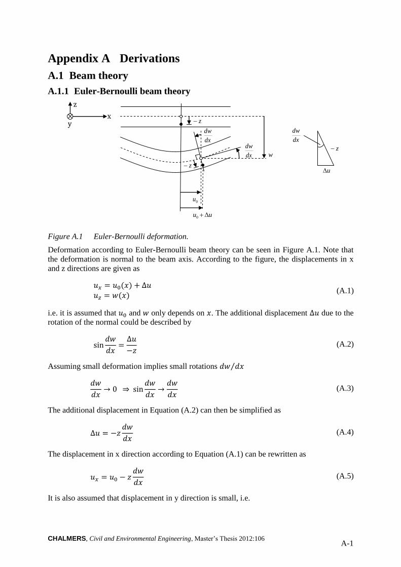
CHALMERS, Civil and Environmental Engineering, Master’s Thesis 2012:106 A-1
Appendix A Derivations
A.1 Beam theory
A.1.1 Euler-Bernoulli beam theory
x
z
y
dx
dw
dx
dw dx
dw
uu Δ0
0u
z
z
w z
uΔ
Figure A.1 Euler-Bernoulli deformation.
Deformation according to Euler-Bernoulli beam theory can be seen in Figure A.1. Note that
the deformation is normal to the beam axis. According to the figure, the displacements in x
and z directions are given as
(A.1)
i.e. it is assumed that and only depends on . The additional displacement due to the
rotation of the normal could be described by
(A.2)
Assuming small deformation implies small rotations ⁄
⇒
(A.3)
The additional displacement in Equation (A.2) can then be simplified as
(A.4)
The displacement in x direction according to Equation (A.1) can be rewritten as
(A.5)
It is also assumed that displacement in y direction is small, i.e.
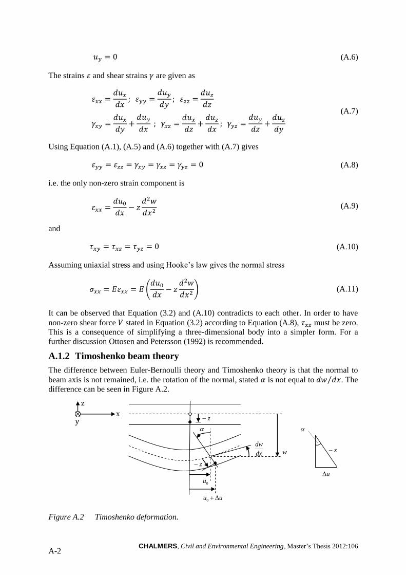
CHALMERS, Civil and Environmental Engineering, Master’s Thesis 2012:106 A-2
(A.6)
The strains and shear strains are given as
(A.7)
Using Equation (A.1), (A.5) and (A.6) together with (A.7) gives
(A.8)
i.e. the only non-zero strain component is
(A.9)
and
(A.10)
Assuming uniaxial stress and using Hooke’s law gives the normal stress
(
) (A.11)
It can be observed that Equation (3.2) and (A.10) contradicts to each other. In order to have
non-zero shear force stated in Equation (3.2) according to Equation (A.8), must be zero.
This is a consequence of simplifying a three-dimensional body into a simpler form. For a
further discussion Ottosen and Petersson (1992) is recommended.
A.1.2 Timoshenko beam theory
The difference between Euler-Bernoulli theory and Timoshenko theory is that the normal to
beam axis is not remained, i.e. the rotation of the normal, stated is not equal to ⁄ . The
difference can be seen in Figure A.2.
x
z
y
dx
dw z
z
z
0u
uu Δ0
w
uΔ
Figure A.2 Timoshenko deformation.
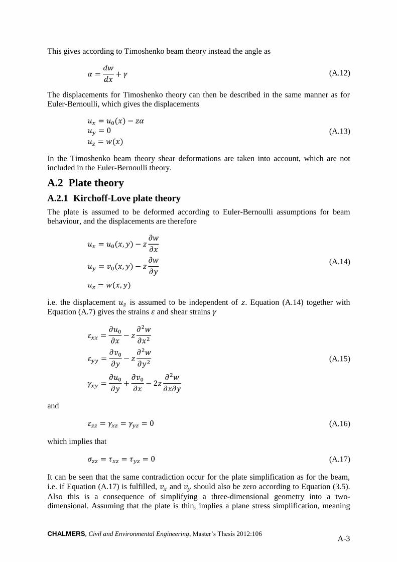
CHALMERS, Civil and Environmental Engineering, Master’s Thesis 2012:106 A-3
This gives according to Timoshenko beam theory instead the angle as
(A.12)
The displacements for Timoshenko theory can then be described in the same manner as for
Euler-Bernoulli, which gives the displacements
(A.13)
In the Timoshenko beam theory shear deformations are taken into account, which are not
included in the Euler-Bernoulli theory.
A.2 Plate theory
A.2.1 Kirchoff-Love plate theory
The plate is assumed to be deformed according to Euler-Bernoulli assumptions for beam
behaviour, and the displacements are therefore
(A.14)
i.e. the displacement is assumed to be independent of . Equation (A.14) together with
Equation (A.7) gives the strains and shear strains
(A.15)
and
(A.16)
which implies that
(A.17)
It can be seen that the same contradiction occur for the plate simplification as for the beam,
i.e. if Equation (A.17) is fulfilled, and should also be zero according to Equation (3.5).
Also this is a consequence of simplifying a three-dimensional geometry into a two-
dimensional. Assuming that the plate is thin, implies a plane stress simplification, meaning
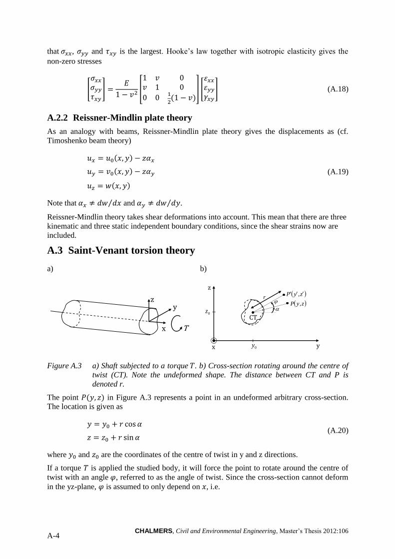
CHALMERS, Civil and Environmental Engineering, Master’s Thesis 2012:106 A-4
that , and is the largest. Hooke’s law together with isotropic elasticity gives the
non-zero stresses
[
]
[
] [
] (A.18)
A.2.2 Reissner-Mindlin plate theory
As an analogy with beams, Reissner-Mindlin plate theory gives the displacements as (cf.
Timoshenko beam theory)
(A.19)
Note that ⁄ and ⁄ .
Reissner-Mindlin theory takes shear deformations into account. This mean that there are three
kinematic and three static independent boundary conditions, since the shear strains now are
included.
A.3 Saint-Venant torsion theory
a) b)
x
y z
T
z,yP
z,yP r
0z
0y
CT
z
x y
Figure A.3 a) Shaft subjected to a torque . b) Cross-section rotating around the centre of
twist (CT). Note the undeformed shape. The distance between CT and P is
denoted r.
The point in Figure A.3 represents a point in an undeformed arbitrary cross-section.
The location is given as
(A.20)
where and are the coordinates of the centre of twist in y and z directions.
If a torque is applied the studied body, it will force the point to rotate around the centre of
twist with an angle , referred to as the angle of twist. Since the cross-section cannot deform
in the yz-plane, is assumed to only depend on , i.e.
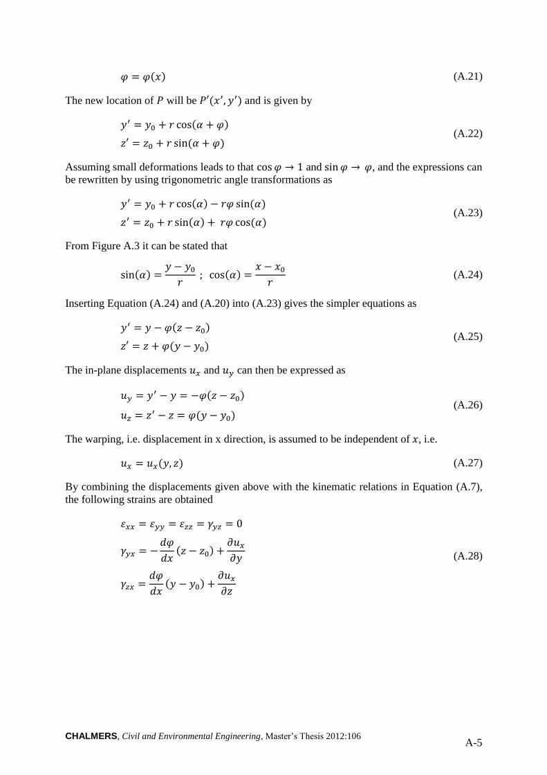
CHALMERS, Civil and Environmental Engineering, Master’s Thesis 2012:106 A-5
(A.21)
The new location of will be and is given by
(A.22)
Assuming small deformations leads to that and , and the expressions can
be rewritten by using trigonometric angle transformations as
(A.23)
From Figure A.3 it can be stated that
(A.24)
Inserting Equation (A.24) and (A.20) into (A.23) gives the simpler equations as
(A.25)
The in-plane displacements and can then be expressed as
(A.26)
The warping, i.e. displacement in x direction, is assumed to be independent of , i.e.
(A.27)
By combining the displacements given above with the kinematic relations in Equation (A.7),
the following strains are obtained
(A.28)
CHALMERS, Civil and Environmental Engineering, Master’s Thesis 2012:106 A-6
In the same way, the normal and shear stresses can be obtained in the shaft by consider the
constitutive model for linear elastic materials as
(
)
(
)
(A.29)
If no body forces are assumed to act on the shaft, e.g. gravity forces or other inertia forces,
these differential equations can be stated as
(A.30)
The shear modulus is assumed to be independent of , i.e.
(A.31)
When Equation (A.30) is combined with Equation (A.29) and using Equation (A.31), it gives
(A.32)
Since is dependent of (warping is dependent of angle of twist) and independent of
according to Equation (A.27), the rate of twist must according to Equation (A.32) be
(A.33)
Equation (A.33) is a fundamental assumption in Saint-Venant theory. This statement is valid
as long as the boundary conditions are unrestrained in twisting, and of course as long as the
applied torque is constant.
If a torque is applied on a structural element with thickness , it can be shown that the shear
stress due to Saint-Venant torsion can be stated as
(A.34)

CHALMERS, Civil and Environmental Engineering, Master’s Thesis 2012:106 A-7
The torsion constant due to Saint-Venant torsion for a rectangular cross-section with width
and height can be calculated as
*
(
)+
(A.35)
Torsional moment due to Saint-Venant torsion can be simplified as
(A.36)

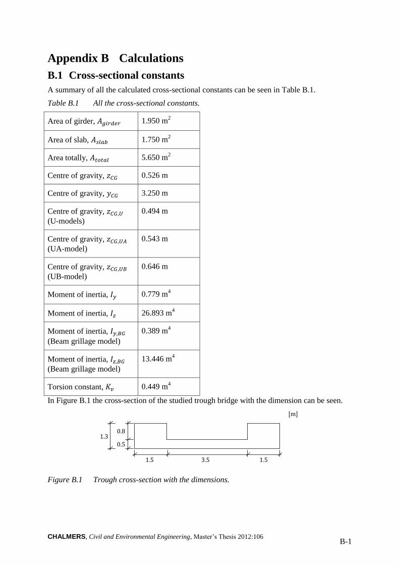
CHALMERS, Civil and Environmental Engineering, Master’s Thesis 2012:106 B-1
Appendix B Calculations
B.1 Cross-sectional constants
A summary of all the calculated cross-sectional constants can be seen in Table B.1.
Table B.1 All the cross-sectional constants.
Area of girder, 1.950 m2
Area of slab, 1.750 m2
Area totally, 5.650 m2
Centre of gravity, 0.526 m
Centre of gravity, 3.250 m
Centre of gravity,
(U-models)
0.494 m
Centre of gravity,
(UA-model)
0.543 m
Centre of gravity,
(UB-model)
0.646 m
Moment of inertia, 0.779 m4
Moment of inertia, 26.893 m4
Moment of inertia,
(Beam grillage model)
0.389 m4
Moment of inertia,
(Beam grillage model)
13.446 m4
Torsion constant, 0.449 m4
In Figure B.1 the cross-section of the studied trough bridge with the dimension can be seen.
Figure B.1 Trough cross-section with the dimensions.
3.5 1.5 1.5
0.5
0.8
[m]
1.3
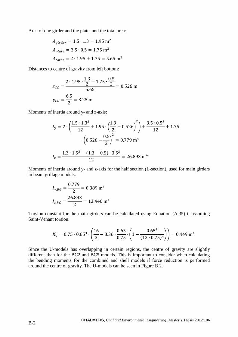
CHALMERS, Civil and Environmental Engineering, Master’s Thesis 2012:106 B-2
Area of one girder and the plate, and the total area:
Distances to centre of gravity from left bottom:
Moments of inertia around y- and z-axis:
(
(
)
)
(
)
Moments of inertia around y- and z-axis for the half section (L-section), used for main girders
in beam grillage models:
Torsion constant for the main girders can be calculated using Equation (A.35) if assuming
Saint-Venant torsion:
(
(
))
Since the U-models has overlapping in certain regions, the centre of gravity are slightly
different than for the BC2 and BC5 models. This is important to consider when calculating
the bending moments for the combined and shell models if force reduction is performed
around the centre of gravity. The U-models can be seen in Figure B.2.
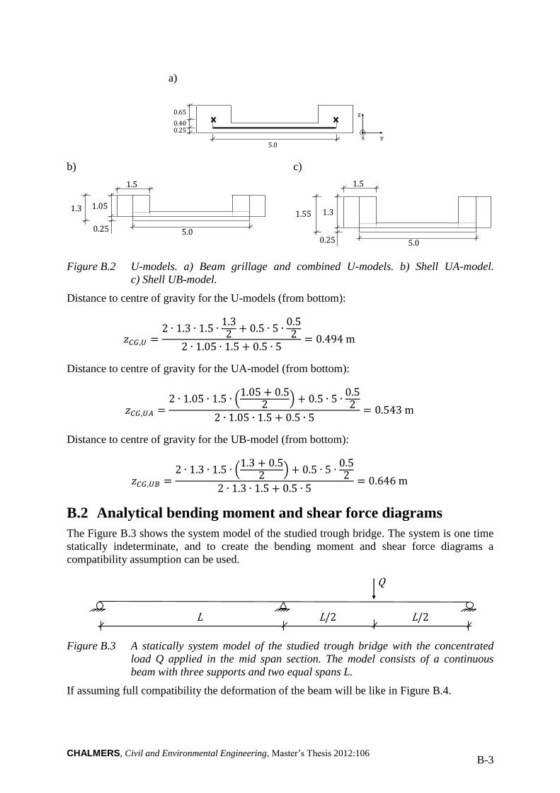
CHALMERS, Civil and Environmental Engineering, Master’s Thesis 2012:106 B-3
a)
b)
c)
Figure B.2 U-models. a) Beam grillage and combined U-models. b) Shell UA-model.
c) Shell UB-model.
Distance to centre of gravity for the U-models (from bottom):
Distance to centre of gravity for the UA-model (from bottom):
(
)
Distance to centre of gravity for the UB-model (from bottom):
(
)
B.2 Analytical bending moment and shear force diagrams
The Figure B.3 shows the system model of the studied trough bridge. The system is one time
statically indeterminate, and to create the bending moment and shear force diagrams a
compatibility assumption can be used.
Figure B.3 A statically system model of the studied trough bridge with the concentrated
load Q applied in the mid span section. The model consists of a continuous
beam with three supports and two equal spans L.
If assuming full compatibility the deformation of the beam will be like in Figure B.4.
5.0
0.25
0.65
0.40
z
x y
5.0
1.05
1.5
0.25
1.3
5.0
1.3
1.5
0.25
1.55
L L/2 L/2
Q
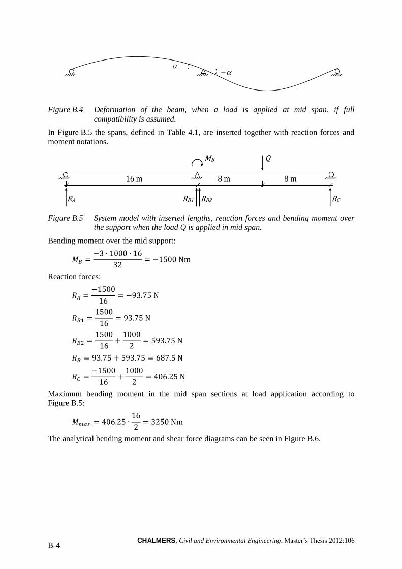
CHALMERS, Civil and Environmental Engineering, Master’s Thesis 2012:106 B-4
Figure B.4 Deformation of the beam, when a load is applied at mid span, if full
compatibility is assumed.
In Figure B.5 the spans, defined in Table 4.1, are inserted together with reaction forces and
moment notations.
Figure B.5 System model with inserted lengths, reaction forces and bending moment over
the support when the load Q is applied in mid span.
Bending moment over the mid support:
Reaction forces:
Maximum bending moment in the mid span sections at load application according to
Figure B.5:
The analytical bending moment and shear force diagrams can be seen in Figure B.6.
16 m 8 m
RA RB1 RB2 RC
MB
8 m
Q
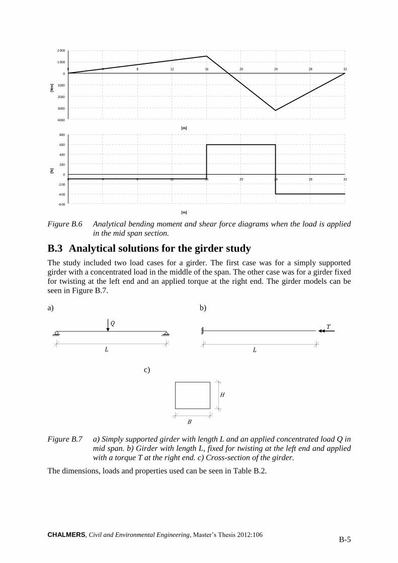
CHALMERS, Civil and Environmental Engineering, Master’s Thesis 2012:106 B-5
Figure B.6 Analytical bending moment and shear force diagrams when the load is applied
in the mid span section.
B.3 Analytical solutions for the girder study
The study included two load cases for a girder. The first case was for a simply supported
girder with a concentrated load in the middle of the span. The other case was for a girder fixed
for twisting at the left end and an applied torque at the right end. The girder models can be
seen in Figure B.7.
a)
L
Q
b)
L
T
c)
B
H
Figure B.7 a) Simply supported girder with length L and an applied concentrated load Q in
mid span. b) Girder with length L, fixed for twisting at the left end and applied
with a torque T at the right end. c) Cross-section of the girder.
The dimensions, loads and properties used can be seen in Table B.2.
-2 000
-1 000
0
1000
2000
3000
4000
0 4 8 12 16 20 24 28 32
[Nm
]
[m]
-600
-4 00
-2 00
0
200
400
600
800
0 4 8 12 16 20 24 28 32
[N]
[m]
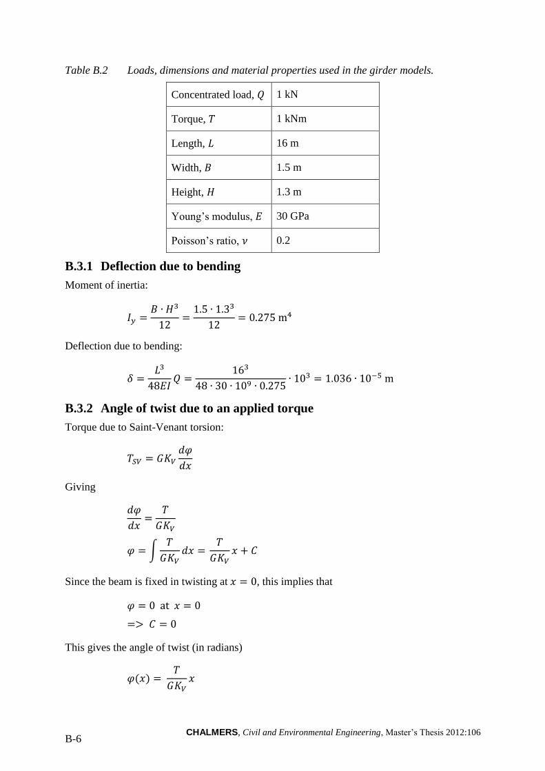
CHALMERS, Civil and Environmental Engineering, Master’s Thesis 2012:106 B-6
Table B.2 Loads, dimensions and material properties used in the girder models.
Concentrated load, 1 kN
Torque, 1 kNm
Length, 16 m
Width, 1.5 m
Height, 1.3 m
Young’s modulus, 30 GPa
Poisson’s ratio, 0.2
B.3.1 Deflection due to bending
Moment of inertia:
Deflection due to bending:
B.3.2 Angle of twist due to an applied torque
Torque due to Saint-Venant torsion:
Giving
∫
Since the beam is fixed in twisting at , this implies that
This gives the angle of twist (in radians)
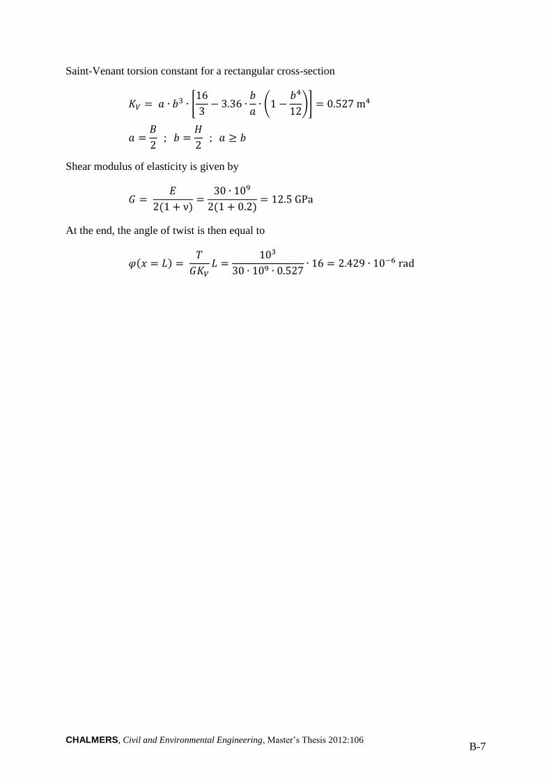
CHALMERS, Civil and Environmental Engineering, Master’s Thesis 2012:106 B-7
Saint-Venant torsion constant for a rectangular cross-section
*
(
)+
Shear modulus of elasticity is given by
At the end, the angle of twist is then equal to

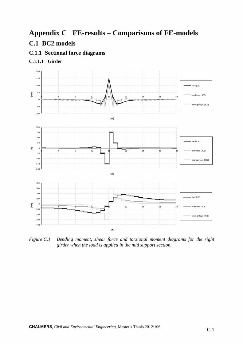
CHALMERS, Civil and Environmental Engineering, Master’s Thesis 2012:106 C-1
Appendix C FE-results – Comparisons of FE-models
C.1 BC2 models
C.1.1 Sectional force diagrams
C.1.1.1 Girder
Figure C.1 Bending moment, shear force and torsional moment diagrams for the right
girder when the load is applied in the mid support section.
-2 00
-1 50
-1 00
-5 0
0
50
100
0 4 8 12 16 20 24 28 32[Nm
]
[m]
shell (UA)
combined (BC2)
beam grillage (BC2)
-2 00
-1 50
-100
-5 0
0
50
100
150
200
0 4 8 12 16 20 24 28 32
[N]
[m]
shell (UA)
combined (BC2)
beam grillage (BC2)
-4 00
-300
-2 00
-1 00
0
100
200
300
400
0 4 8 12 16 20 24 28 32[Nm
]
[m]
shell (UB)
combined (BC2)
beam grillage (BC2)
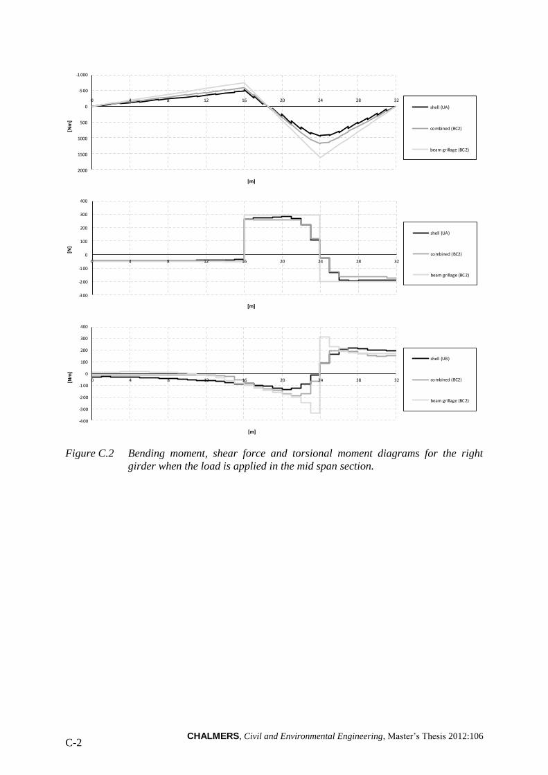
CHALMERS, Civil and Environmental Engineering, Master’s Thesis 2012:106 C-2
Figure C.2 Bending moment, shear force and torsional moment diagrams for the right
girder when the load is applied in the mid span section.
-1 000
-5 00
0
500
1000
1500
2000
0 4 8 12 16 20 24 28 32
[Nm
]
[m]
shell (UA)
combined (BC2)
beam grillage (BC2)
-3 00
-200
-1 00
0
100
200
300
400
0 4 8 12 16 20 24 28 32
[N]
[m]
shell (UA)
combined (BC2)
beam grillage (BC2)
-4 00
-3 00
-2 00
-1 00
0
100
200
300
400
0 4 8 12 16 20 24 28 32[Nm
]
[m]
shell (UB)
combined (BC2)
beam grillage (BC2)
CHALMERS, Civil and Environmental Engineering, Master’s Thesis 2012:106 C-3
C.1.1.2 Slab
Figure C.3 Bending moment and shear force diagrams for the slab when the load is
applied in the mid support section.
Figure C.4 Bending moment and shear force diagrams for the slab when the load is
applied in the mid span section.
-1 00
-5 0
0
50
100
150
200
250
300
350
400
0 4 8 12 16 20 24 28 32
[Nm
]
[m]
shell (UA)
combined (BC2)
-4 00
-300
-2 00
-1 00
0
100
200
300
400
0 4 8 12 16 20 24 28 32
[N]
[m]
shell (UA)
combined (BC2)
-1 000
-5 00
0
500
1000
1500
2000
0 4 8 12 16 20 24 28 32
[Nm
]
[m]
shell (UA)
combined (BC2)
-4 00
-3 00
-2 00
-100
0
100
200
300
400
500
0 4 8 12 16 20 24 28 32
[N]
[m]
shell (UA)
combined (BC2)
CHALMERS, Civil and Environmental Engineering, Master’s Thesis 2012:106 C-4
C.1.1.3 Entire section
Figure C.5 Bending moment and shear force diagrams for the entire section when the load
is applied in the mid support section.
Figure C.6 Bending moment and shear force diagrams for the slab when the load is
applied in the mid span section.
-1 0
0
10
20
30
40
50
60
0 4 8 12 16 20 24 28 32
[Nm
]
[m]
shell (UA)
combined (BC2)
beam grillage (BC2)
-4
-3
-2
-1
0
1
2
3
4
0 4 8 12 16 20 24 28 32
[N]
[m]
shell (UA)
combined (BC2)
beam grillage (BC2)
-2 000
-1 000
0
1000
2000
3000
4000
0 4 8 12 16 20 24 28 32
[Nm
]
[m]
shell (UA)
combined (BC2)
beam grillage (BC2)
beam
-6 00
-4 00
-2 00
0
200
400
600
800
0 4 8 12 16 20 24 28 32
[N]
[m]
shell (UA)
combined (BC2)
beam grillage (BC2)
beam
CHALMERS, Civil and Environmental Engineering, Master’s Thesis 2012:106 C-5
C.1.2 Influence lines
C.1.2.1 Girder
Figure C.7 Influence lines for bending moment, shear force and torsional moment in the
right girder at mid support.
-9 00
-8 00
-7 00
-6 00
-5 00
-4 00
-3 00
-2 00
-100
0
0 4 8 12 16 20 24 28 32
[Nm
]
[m]
shell (UA)
combined (BC2)
beam grillage (BC2)
-6 00
-4 00
-2 00
0
200
400
600
0 4 8 12 16 20 24 28 32
[N]
[m]
shell (UA)
combined (BC2)
beam grillage (BC2)
-4 00
-3 00
-200
-1 00
0
100
200
300
400
0 4 8 12 16 20 24 28 32[Nm
]
[m]
shell (UB)
combined (BC2)
beam grillage (BC2)
CHALMERS, Civil and Environmental Engineering, Master’s Thesis 2012:106 C-6
Figure C.8 Influence lines for bending moment, shear force and torsional moment in the
right girder at mid span.
-5 00
0
500
1000
1500
2000
0 4 8 12 16 20 24 28 32
[Nm
]
[m]
shell (UA)
combined (BC2)
beam grillage (BC2)
-3 00
-2 00
-100
0
100
200
300
400
0 4 8 12 16 20 24 28 32
[N]
[m]
shell (UA)
combined (BC2)
beam grillage (BC2)
-4 00
-3 00
-200
-1 00
0
100
200
300
400
0 4 8 12 16 20 24 28 32[Nm
]
[m]
shell (UB)
combined (BC2)
beam grillage (BC2)
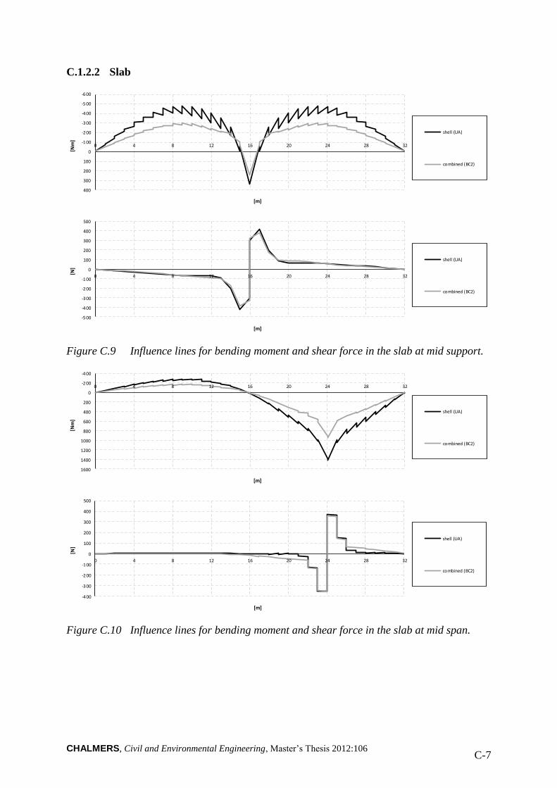
CHALMERS, Civil and Environmental Engineering, Master’s Thesis 2012:106 C-7
C.1.2.2 Slab
Figure C.9 Influence lines for bending moment and shear force in the slab at mid support.
Figure C.10 Influence lines for bending moment and shear force in the slab at mid span.
-6 00
-5 00
-4 00
-3 00
-200
-100
0
100
200
300
400
0 4 8 12 16 20 24 28 32
[Nm
]
[m]
shell (UA)
combined (BC2)
-5 00
-4 00
-3 00
-2 00
-1 00
0
100
200
300
400
500
0 4 8 12 16 20 24 28 32
[N]
[m]
shell (UA)
combined (BC2)
-4 00
-2 00
0
200
400
600
800
1000
1200
1400
1600
0 4 8 12 16 20 24 28 32
[Nm
]
[m]
shell (UA)
combined (BC2)
-4 00
-3 00
-2 00
-100
0
100
200
300
400
500
0 4 8 12 16 20 24 28 32
[N]
[m]
shell (UA)
combined (BC2)
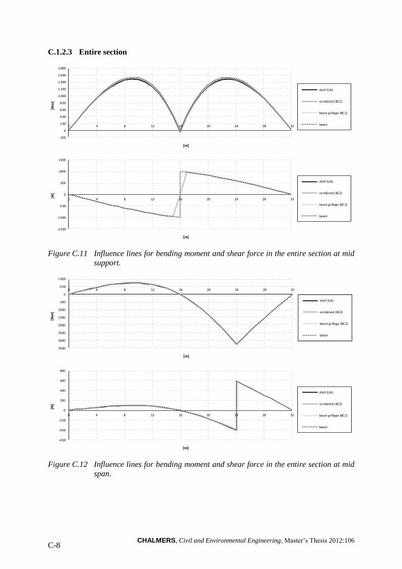
CHALMERS, Civil and Environmental Engineering, Master’s Thesis 2012:106 C-8
C.1.2.3 Entire section
Figure C.11 Influence lines for bending moment and shear force in the entire section at mid
support.
Figure C.12 Influence lines for bending moment and shear force in the entire section at mid
span.
-1 800
-1 600
-1400
-1200
-1 000
-8 00
-6 00
-4 00
-2 00
0
200
0 4 8 12 16 20 24 28 32
[Nm
]
[m]
shell (UA)
combined (BC2)
beam grillage (BC2)
beam
-1500
-1 000
-5 00
0
500
1000
1500
0 4 8 12 16 20 24 28 32
[N]
[m]
shell (UA)
combined (BC2)
beam grillage (BC2)
beam
-1 000
-5 00
0
500
1000
1500
2000
2500
3000
3500
0 4 8 12 16 20 24 28 32
[Nm
]
[m]
shell (UA)
combined (BC2)
beam grillage (BC2)
beam
-600
-4 00
-2 00
0
200
400
600
800
0 4 8 12 16 20 24 28 32
[N]
[m]
shell (UA)
combined (BC2)
beam grillage (BC2)
beam
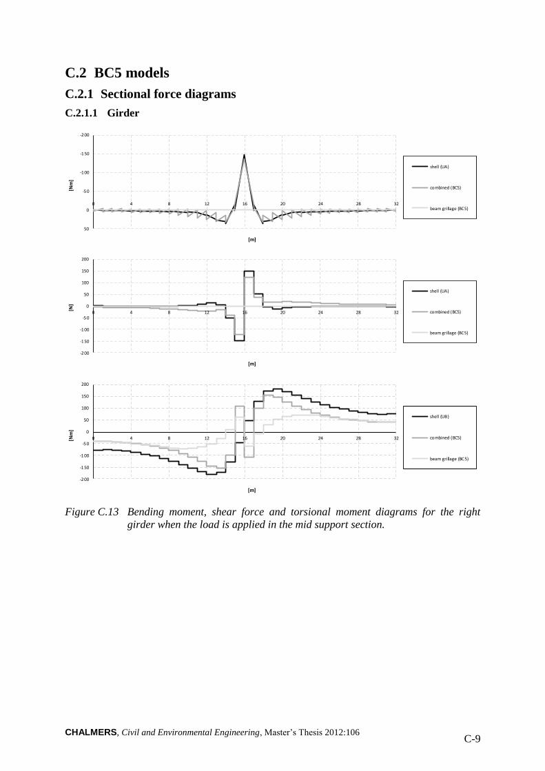
CHALMERS, Civil and Environmental Engineering, Master’s Thesis 2012:106 C-9
C.2 BC5 models
C.2.1 Sectional force diagrams
C.2.1.1 Girder
Figure C.13 Bending moment, shear force and torsional moment diagrams for the right
girder when the load is applied in the mid support section.
-2 00
-150
-1 00
-5 0
0
50
0 4 8 12 16 20 24 28 32
[Nm
]
[m]
shell (UA)
combined (BC5)
beam grillage (BC5)
-2 00
-1 50
-100
-5 0
0
50
100
150
200
0 4 8 12 16 20 24 28 32
[N]
[m]
shell (UA)
combined (BC5)
beam grillage (BC5)
-2 00
-150
-1 00
-5 0
0
50
100
150
200
0 4 8 12 16 20 24 28 32[Nm
]
[m]
shell (UB)
combined (BC5)
beam grillage (BC5)
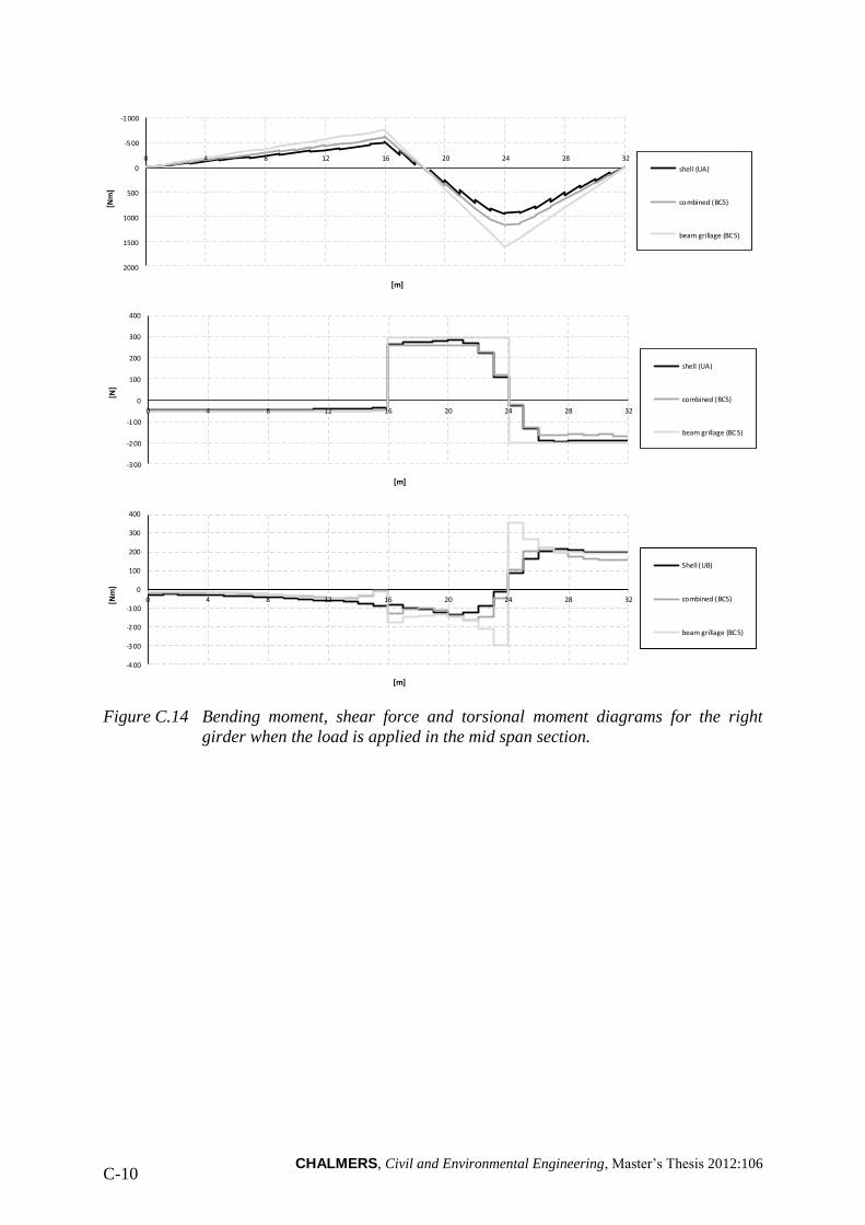
CHALMERS, Civil and Environmental Engineering, Master’s Thesis 2012:106 C-10
Figure C.14 Bending moment, shear force and torsional moment diagrams for the right
girder when the load is applied in the mid span section.
-1 000
-5 00
0
500
1000
1500
2000
0 4 8 12 16 20 24 28 32
[Nm
]
[m]
shell (UA)
combined (BC5)
beam grillage (BC5)
-3 00
-200
-1 00
0
100
200
300
400
0 4 8 12 16 20 24 28 32
[N]
[m]
shell (UA)
combined (BC5)
beam grillage (BC5)
-4 00
-300
-2 00
-1 00
0
100
200
300
400
0 4 8 12 16 20 24 28 32[Nm
]
[m]
Shell (UB)
combined (BC5)
beam grillage (BC5)

CHALMERS, Civil and Environmental Engineering, Master’s Thesis 2012:106 C-11
C.2.1.2 Slab
Figure C.15 Bending moment and shear force diagrams for the slab when the load is
applied in the mid support section.
Figure C.16 Bending moment and shear force diagrams for the slab when the load is
applied in the mid span section.
-1 00
-5 0
0
50
100
150
200
250
300
350
400
0 4 8 12 16 20 24 28 32
[Nm
]
[m]
shell (UA)
combined (BC5)
-4 00
-300
-2 00
-1 00
0
100
200
300
400
0 4 8 12 16 20 24 28 32
[N]
[m]
shell (UA)
combined (BC5)
-1 000
-5 00
0
500
1000
1500
2000
0 4 8 12 16 20 24 28 32
[Nm
]
[m]
shell (UA)
combined (BC5)
-4 00
-3 00
-2 00
-1 00
0
100
200
300
400
500
0 4 8 12 16 20 24 28 32
[N]
[m]
shell (UA)
combined (BC5)
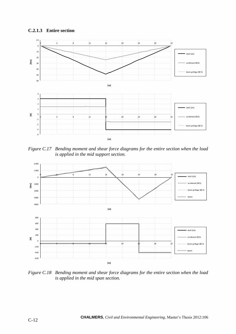
CHALMERS, Civil and Environmental Engineering, Master’s Thesis 2012:106 C-12
C.2.1.3 Entire section
Figure C.17 Bending moment and shear force diagrams for the entire section when the load
is applied in the mid support section.
Figure C.18 Bending moment and shear force diagrams for the entire section when the load
is applied in the mid span section.
-1 0
0
10
20
30
40
50
60
0 4 8 12 16 20 24 28 32
[Nm
]
[m]
shell (UA)
combined (BC5)
beam grillage (BC5)
-4
-3
-2
-1
0
1
2
3
4
0 4 8 12 16 20 24 28 32
[N]
[m]
shell (UA)
combined (BC5)
beam grillage (BC5)
-2 000
-1 000
0
1000
2000
3000
4000
0 4 8 12 16 20 24 28 32
[Nm
]
[m]
shell (UA)
combined (BC5)
beam grillage (BC5)
beam
-600
-4 00
-2 00
0
200
400
600
800
0 4 8 12 16 20 24 28 32
[N]
[m]
shell (UA)
combined (BC5)
beam grillage (BC5)
beam
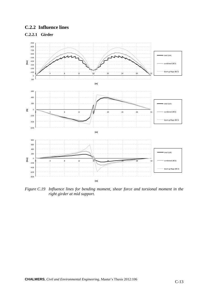
CHALMERS, Civil and Environmental Engineering, Master’s Thesis 2012:106 C-13
C.2.2 Influence lines
C.2.2.1 Girder
Figure C.19 Influence lines for bending moment, shear force and torsional moment in the
right girder at mid support.
-9 00
-8 00
-700
-600
-5 00
-4 00
-3 00
-2 00
-1 00
0
100
0 4 8 12 16 20 24 28 32
[Nm
]
[m]
shell (UA)
combined (BC5)
beam grillage (BC5)
-6 00
-4 00
-2 00
0
200
400
600
0 4 8 12 16 20 24 28 32
[N]
[m]
shell (UA)
combined (BC5)
beam grillage (BC5)
-8 00
-6 00
-4 00
-2 00
0
200
400
600
800
0 4 8 12 16 20 24 28 32[Nm
]
[m]
shell (UB)
combined (BC5)
beam grillage (BC5)

CHALMERS, Civil and Environmental Engineering, Master’s Thesis 2012:106 C-14
Figure C.20 Influence lines for bending moment, shear force and torsional moment in the
right girder at mid span.
-5 00
0
500
1000
1500
2000
0 4 8 12 16 20 24 28 32
[Nm
]
[m]
shell (UA)
combined (BC5)
beam grillage (BC5)
-3 00
-2 00
-1 00
0
100
200
300
400
0 4 8 12 16 20 24 28 32
[N]
[m]
shell (UA)
combined (BC5)
beam grillage (BC5)
-4 00
-3 00
-2 00
-1 00
0
100
200
300
400
0 4 8 12 16 20 24 28 32[Nm
]
[m]
shell (UB)
combined (BC5)
beam grillage (BC5)
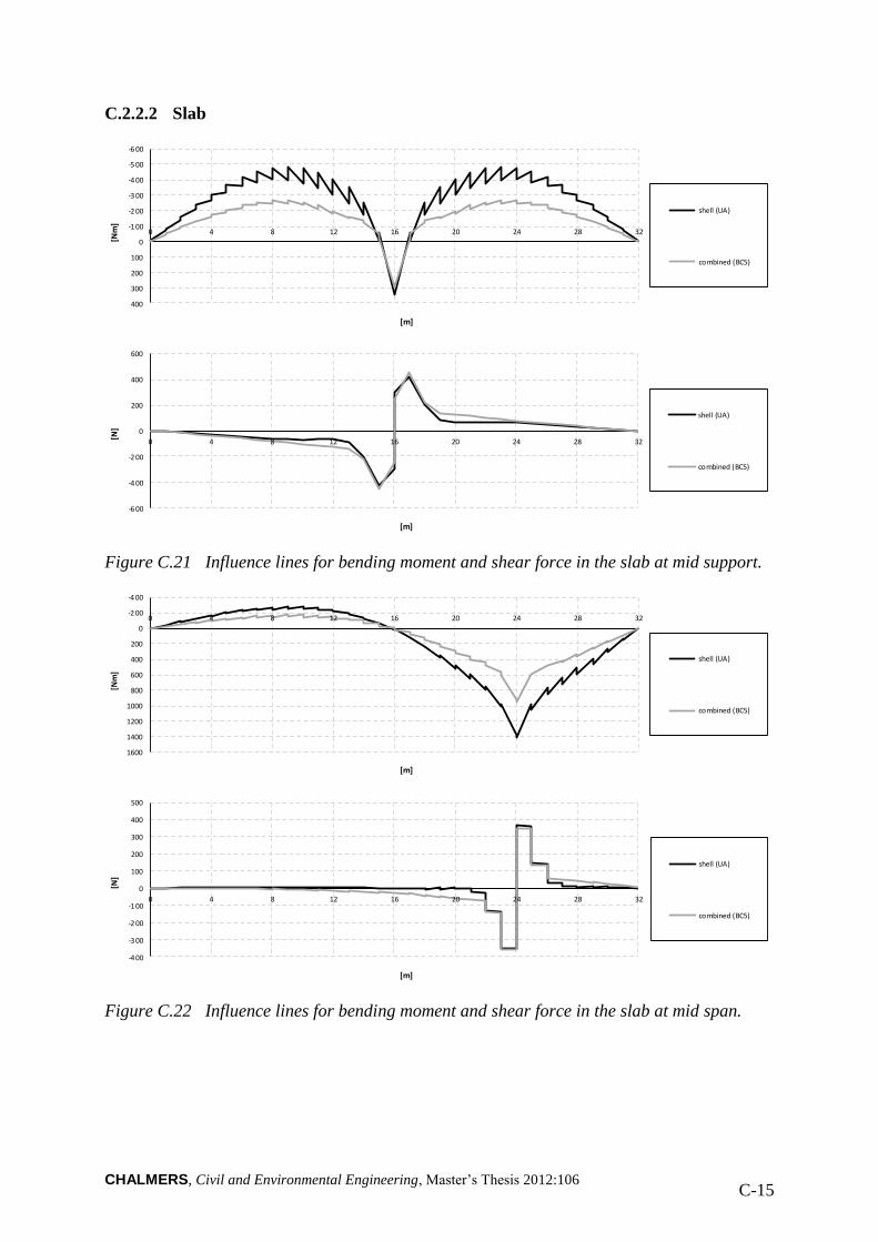
CHALMERS, Civil and Environmental Engineering, Master’s Thesis 2012:106 C-15
C.2.2.2 Slab
Figure C.21 Influence lines for bending moment and shear force in the slab at mid support.
Figure C.22 Influence lines for bending moment and shear force in the slab at mid span.
-6 00
-5 00
-4 00
-3 00
-2 00
-1 00
0
100
200
300
400
0 4 8 12 16 20 24 28 32
[Nm
]
[m]
shell (UA)
combined (BC5)
-6 00
-4 00
-2 00
0
200
400
600
0 4 8 12 16 20 24 28 32
[N]
[m]
shell (UA)
combined (BC5)
-4 00
-2 00
0
200
400
600
800
1000
1200
1400
1600
0 4 8 12 16 20 24 28 32
[Nm
]
[m]
shell (UA)
combined (BC5)
-400
-300
-2 00
-1 00
0
100
200
300
400
500
0 4 8 12 16 20 24 28 32
[N]
[m]
shell (UA)
combined (BC5)
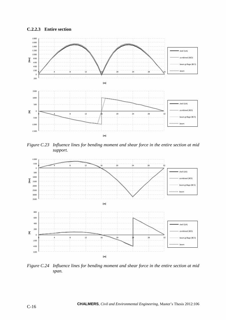
CHALMERS, Civil and Environmental Engineering, Master’s Thesis 2012:106 C-16
C.2.2.3 Entire section
Figure C.23 Influence lines for bending moment and shear force in the entire section at mid
support.
Figure C.24 Influence lines for bending moment and shear force in the entire section at mid
span.
-1 800
-1 600
-1 400
-1 200
-1 000
-8 00
-600
-400
-2 00
0
200
0 4 8 12 16 20 24 28 32
[Nm
]
[m]
shell (UA)
combined (BC5)
beam grillage (BC5)
beam
-1500
-1 000
-5 00
0
500
1000
1500
0 4 8 12 16 20 24 28 32
[N]
[m]
shell (UA)
combined (BC5)
beam grillage (BC5)
beam
-1 000
-5 00
0
500
1000
1500
2000
2500
3000
3500
0 4 8 12 16 20 24 28 32
[Nm
]
[m]
shell (UA)
combined (BC5)
beam grillage (BC5)
beam
-600
-4 00
-2 00
0
200
400
600
800
0 4 8 12 16 20 24 28 32
[N]
[m]
shell (UA)
combined (BC5)
beam grillage (BC5)
beam
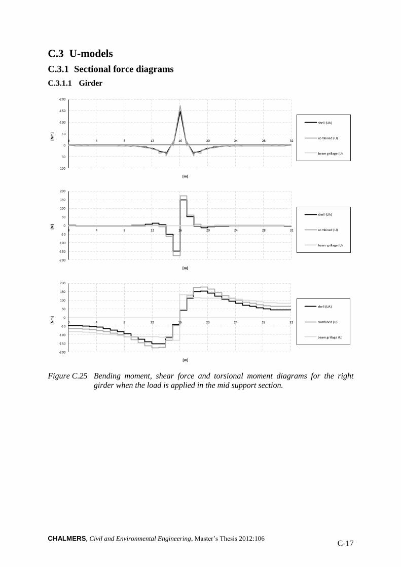
CHALMERS, Civil and Environmental Engineering, Master’s Thesis 2012:106 C-17
C.3 U-models
C.3.1 Sectional force diagrams
C.3.1.1 Girder
Figure C.25 Bending moment, shear force and torsional moment diagrams for the right
girder when the load is applied in the mid support section.
-200
-150
-1 00
-5 0
0
50
100
0 4 8 12 16 20 24 28 32[Nm
]
[m]
shell (UA)
combined (U)
beam grillage (U)
-2 00
-1 50
-100
-5 0
0
50
100
150
200
0 4 8 12 16 20 24 28 32
[N]
[m]
shell (UA)
combined (U)
beam grillage (U)
-2 00
-150
-1 00
-5 0
0
50
100
150
200
0 4 8 12 16 20 24 28 32[Nm
]
[m]
shell (UA)
combined (U)
beam grillage (U)
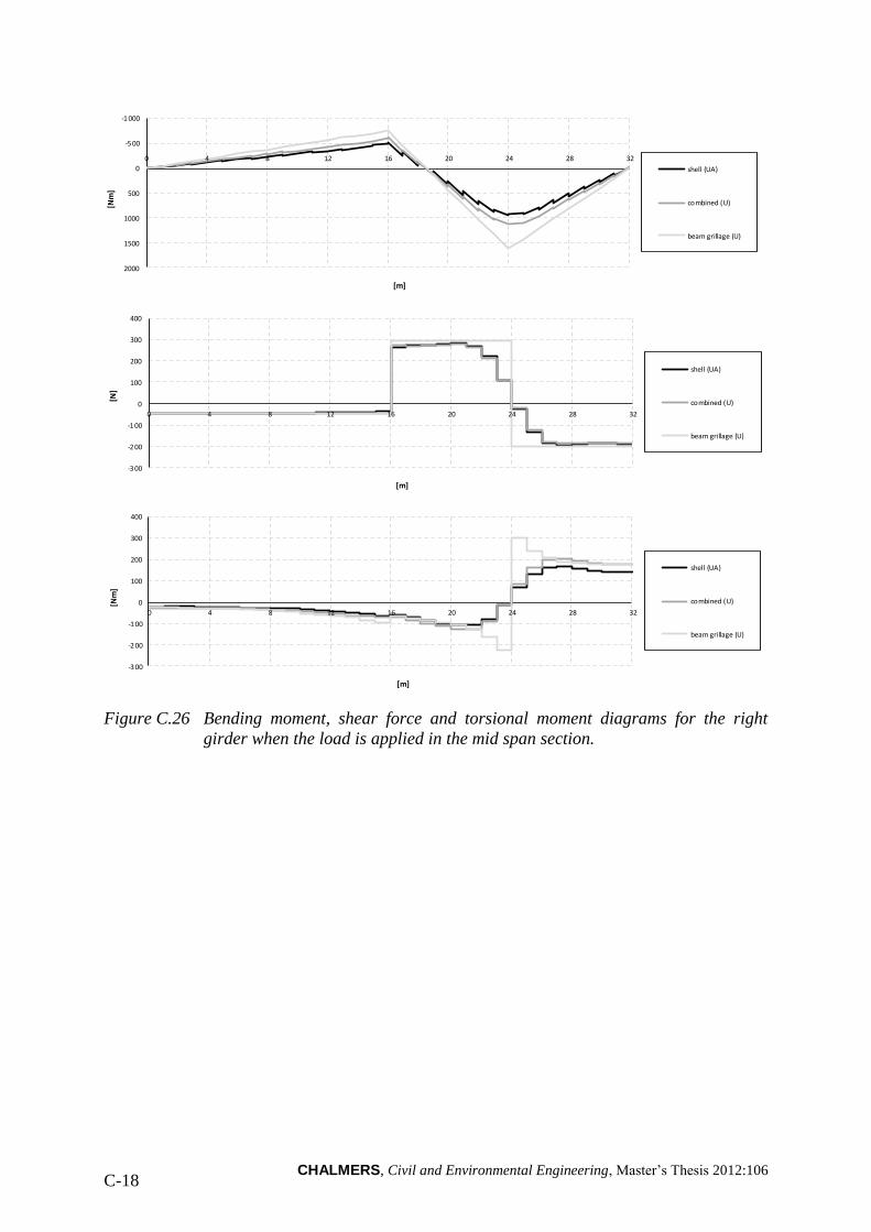
CHALMERS, Civil and Environmental Engineering, Master’s Thesis 2012:106 C-18
Figure C.26 Bending moment, shear force and torsional moment diagrams for the right
girder when the load is applied in the mid span section.
-1 000
-5 00
0
500
1000
1500
2000
0 4 8 12 16 20 24 28 32
[Nm
]
[m]
shell (UA)
combined (U)
beam grillage (U)
-3 00
-200
-1 00
0
100
200
300
400
0 4 8 12 16 20 24 28 32
[N]
[m]
shell (UA)
combined (U)
beam grillage (U)
-3 00
-2 00
-1 00
0
100
200
300
400
0 4 8 12 16 20 24 28 32
[Nm
]
[m]
shell (UA)
combined (U)
beam grillage (U)

CHALMERS, Civil and Environmental Engineering, Master’s Thesis 2012:106 C-19
C.3.1.2 Slab
Figure C.27 Bending moment and shear force diagrams for the slab when the load is
applied in the mid support section.
Figure C.28 Bending moment and shear force diagrams for the slab when the load is
applied in the mid span section.
-1 00
-5 0
0
50
100
150
200
250
300
350
400
450
0 4 8 12 16 20 24 28 32
[Nm
]
[m]
shell (UA)
combined (U)
-4 00
-300
-2 00
-1 00
0
100
200
300
400
0 4 8 12 16 20 24 28 32
[N]
[m]
shell (UA)
combined (U)
-1 000
-5 00
0
500
1000
1500
2000
0 4 8 12 16 20 24 28 32
[Nm
]
[m]
shell (UA)
combined (U)
-5 00
-4 00
-3 00
-2 00
-1 00
0
100
200
300
400
500
0 4 8 12 16 20 24 28 32
[N]
[m]
shell (UA)
combined (U)
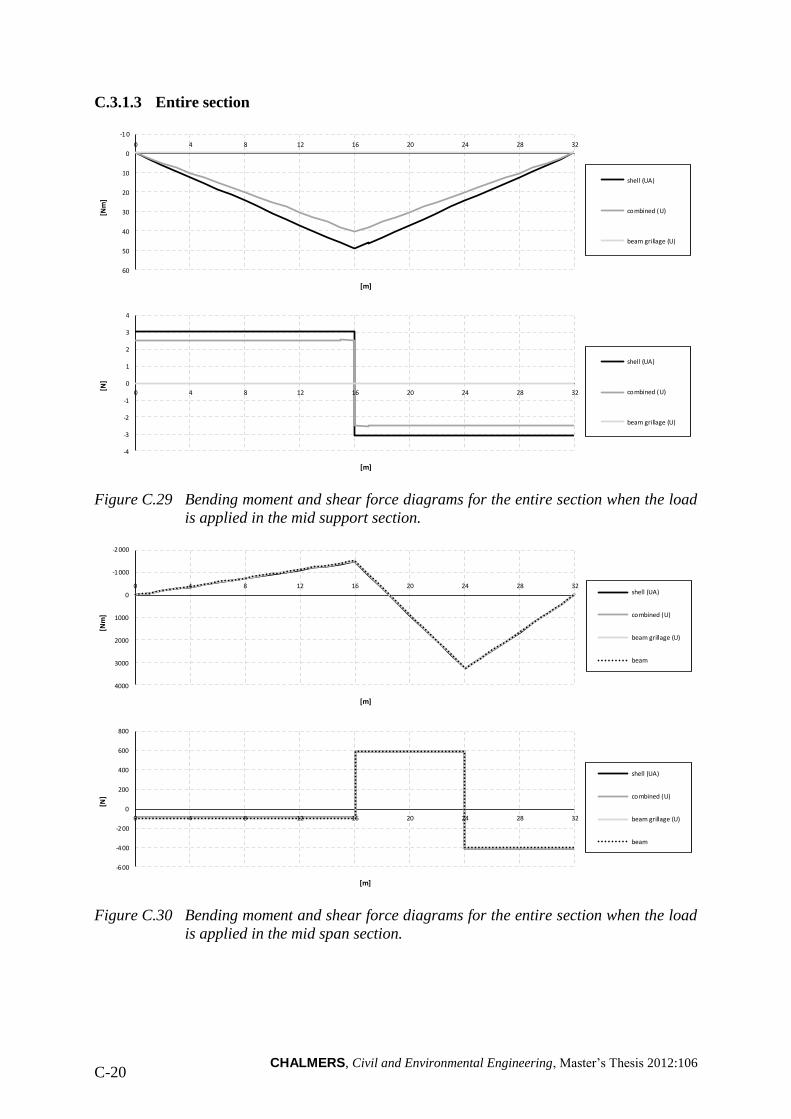
CHALMERS, Civil and Environmental Engineering, Master’s Thesis 2012:106 C-20
C.3.1.3 Entire section
Figure C.29 Bending moment and shear force diagrams for the entire section when the load
is applied in the mid support section.
Figure C.30 Bending moment and shear force diagrams for the entire section when the load
is applied in the mid span section.
-1 0
0
10
20
30
40
50
60
0 4 8 12 16 20 24 28 32
[Nm
]
[m]
shell (UA)
combined (U)
beam grillage (U)
-4
-3
-2
-1
0
1
2
3
4
0 4 8 12 16 20 24 28 32
[N]
[m]
shell (UA)
combined (U)
beam grillage (U)
-2 000
-1 000
0
1000
2000
3000
4000
0 4 8 12 16 20 24 28 32
[Nm
]
[m]
shell (UA)
combined (U)
beam grillage (U)
beam
-6 00
-4 00
-2 00
0
200
400
600
800
0 4 8 12 16 20 24 28 32
[N]
[m]
shell (UA)
combined (U)
beam grillage (U)
beam
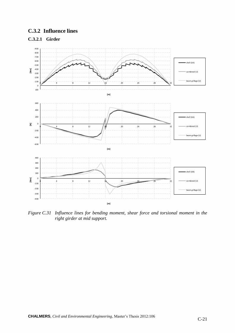
CHALMERS, Civil and Environmental Engineering, Master’s Thesis 2012:106 C-21
C.3.2 Influence lines
C.3.2.1 Girder
Figure C.31 Influence lines for bending moment, shear force and torsional moment in the
right girder at mid support.
-900
-8 00
-7 00
-6 00
-5 00
-4 00
-3 00
-200
-100
0
100
0 4 8 12 16 20 24 28 32
[Nm
]
[m]
shell (UA)
combined (U)
beam grillage (U)
-6 00
-4 00
-2 00
0
200
400
600
0 4 8 12 16 20 24 28 32
[N]
[m]
shell (UA)
combined (U)
beam grillage (U)
-4 00
-3 00
-200
-1 00
0
100
200
300
400
0 4 8 12 16 20 24 28 32[Nm
]
[m]
shell (UB)
combined (U)
beam grillage (U)
CHALMERS, Civil and Environmental Engineering, Master’s Thesis 2012:106 C-22
Figure C.32 Influence lines for bending moment, shear force and torsional moment in the
right girder at mid span.
-5 00
0
500
1000
1500
2000
0 4 8 12 16 20 24 28 32
[Nm
]
[m]
shell (UA)
combined (U)
beam grillage (U)
-3 00
-2 00
-100
0
100
200
300
400
0 4 8 12 16 20 24 28 32
[N]
[m]
shell (UA)
combined (U)
beam grillage (U)
-3 00
-2 00
-100
0
100
200
300
400
0 4 8 12 16 20 24 28 32
[Nm
]
[m]
shell (UB)
combined (U)
beam grillage (U)
CHALMERS, Civil and Environmental Engineering, Master’s Thesis 2012:106 C-23
C.3.2.2 Slab
Figure C.33 Influence lines for bending moment and shear force in the slab at mid support.
Figure C.34 Influence lines for bending moment and shear force in the slab at mid span.
-6 00
-5 00
-4 00
-300
-2 00
-1 00
0
100
200
300
400
500
0 4 8 12 16 20 24 28 32
[Nm
]
[m]
shell (UA)
combined (U)
-5 00
-4 00
-3 00
-2 00
-1 00
0
100
200
300
400
500
0 4 8 12 16 20 24 28 32
[N]
[m]
shell (UA)
combined (U)
-4 00
-2 00
0
200
400
600
800
1000
1200
1400
1600
0 4 8 12 16 20 24 28 32
[Nm
]
[m]
shell (UA)
combined (U)
-5 00
-4 00
-3 00
-2 00
-1 00
0
100
200
300
400
500
0 4 8 12 16 20 24 28 32
[N]
[m]
shell (UA)
combined (U)
CHALMERS, Civil and Environmental Engineering, Master’s Thesis 2012:106 C-24
C.3.2.3 Entire section
Figure C.35 Influence lines for bending moment and shear force in the entire section at mid
support.
Figure C.36 Influence lines for bending moment and shear force in the entire section at mid
span.
-1 800
-1 600
-1 400
-1 200
-1 000
-8 00
-6 00
-4 00
-2 00
0
200
0 4 8 12 16 20 24 28 32
[Nm
]
[m]
shell (UA)
combined (U)
beam grillage (U)
beam
-1 500
-1 000
-5 00
0
500
1000
1500
0 4 8 12 16 20 24 28 32
[N]
[m]
shell (UA)
combined (U)
beam grillage (U)
beam
-1 000
-5 00
0
500
1000
1500
2000
2500
3000
3500
0 4 8 12 16 20 24 28 32
[Nm
]
[m]
shell (UA)
combined (U)
beam grillage (U)
beam
-600
-4 00
-2 00
0
200
400
600
800
0 4 8 12 16 20 24 28 32
[N]
[m]
shell (UA)
combined (U)
beam grillage (U)
beam
CHALMERS, Civil and Environmental Engineering, Master’s Thesis 2012:106 C-25
C.4 Refined models
C.4.1 Refined beam grillage model (BC2)
C.4.1.1 Sectional force diagrams
Figure C.37 Bending moment, shear force and torsional moment diagrams for the right
girder when the load is applied in the mid span section.
-1 000
-5 00
0
500
1000
1500
2000
0 4 8 12 16 20 24 28 32
[Nm
]
[m]
Beam grillage, refined
(BC2)
Beam grillage, regular(BC2)
-300
-2 00
-1 00
0
100
200
300
400
0 4 8 12 16 20 24 28 32
[N]
[m]
Beam grillage, refined
(BC2)
Beam grillage, regular(BC2)
-5 00
-4 00
-3 00
-200
-100
0
100
200
300
400
500
0 4 8 12 16 20 24 28 32[Nm
]
[m]
Beam grillage, refined(BC2)
Beam grillage, regular
(BC2)
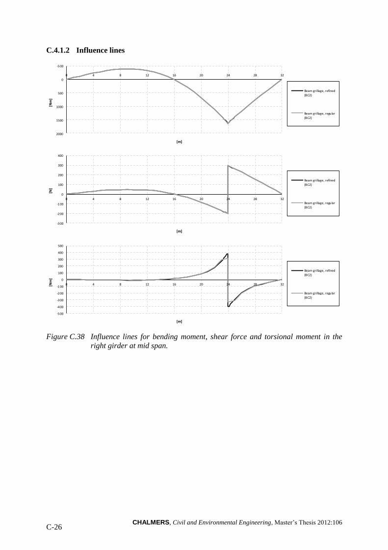
CHALMERS, Civil and Environmental Engineering, Master’s Thesis 2012:106 C-26
C.4.1.2 Influence lines
Figure C.38 Influence lines for bending moment, shear force and torsional moment in the
right girder at mid span.
-5 00
0
500
1000
1500
2000
0 4 8 12 16 20 24 28 32
[Nm
]
[m]
Beam grillage, refined
(BC2)
Beam grillage, regular(BC2)
-300
-2 00
-1 00
0
100
200
300
400
0 4 8 12 16 20 24 28 32
[N]
[m]
Beam grillage, refined
(BC2)
Beam grillage, regular(BC2)
-500
-400
-3 00
-2 00
-1 00
0
100
200
300
400
500
0 4 8 12 16 20 24 28 32[Nm
]
[m]
Beam grillage, refined
(BC2)
Beam grillage, regular(BC2)
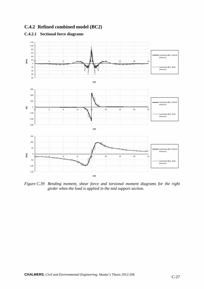
CHALMERS, Civil and Environmental Engineering, Master’s Thesis 2012:106 C-27
C.4.2 Refined combined model (BC2)
C.4.2.1 Sectional force diagrams
Figure C.39 Bending moment, shear force and torsional moment diagrams for the right
girder when the load is applied in the mid support section.
-1 20
-1 00
-80
-60
-4 0
-2 0
0
20
40
60
80
0 4 8 12 16 20 24 28 32
[Nm
]
[m]
Combined (BC2, 192x32
divis ions)
Combined (BC2, 32x8divis ions)
-3 00
-2 00
-100
0
100
200
300
0 4 8 12 16 20 24 28 32
[N]
[m]
Combined (BC2, 192x32divis ions)
Combined (BC2, 32x8
divis ions)
-1 50
-1 00
-50
0
50
100
150
0 4 8 12 16 20 24 28 32[Nm
]
[m]
Combined (BC2, 192x32divis ions)
Combined (BC2, 32x8
divis ions)
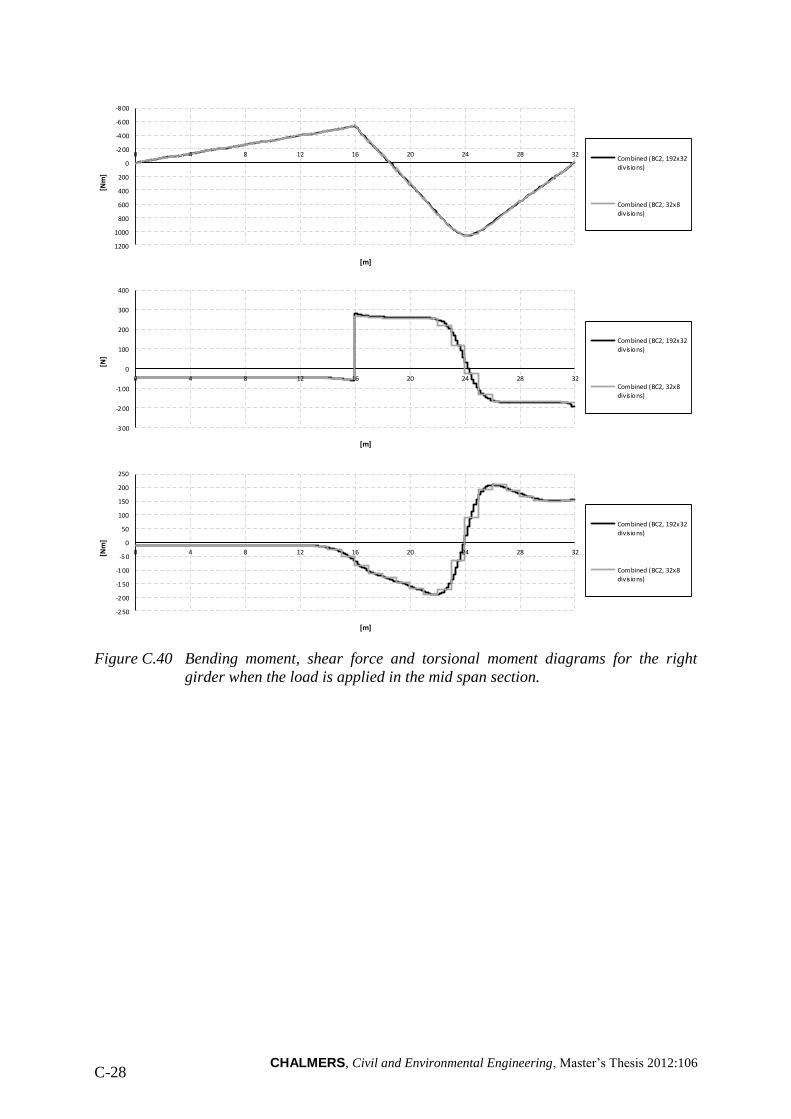
CHALMERS, Civil and Environmental Engineering, Master’s Thesis 2012:106 C-28
Figure C.40 Bending moment, shear force and torsional moment diagrams for the right
girder when the load is applied in the mid span section.
-8 00
-6 00
-400
-200
0
200
400
600
800
1000
1200
0 4 8 12 16 20 24 28 32
[Nm
]
[m]
Combined (BC2, 192x32
divis ions)
Combined (BC2, 32x8divis ions)
-300
-2 00
-1 00
0
100
200
300
400
0 4 8 12 16 20 24 28 32
[N]
[m]
Combined (BC2, 192x32
divis ions)
Combined (BC2, 32x8divis ions)
-250
-200
-1 50
-1 00
-5 0
0
50
100
150
200
250
0 4 8 12 16 20 24 28 32[Nm
]
[m]
Combined (BC2, 192x32
divis ions)
Combined (BC2, 32x8divis ions)
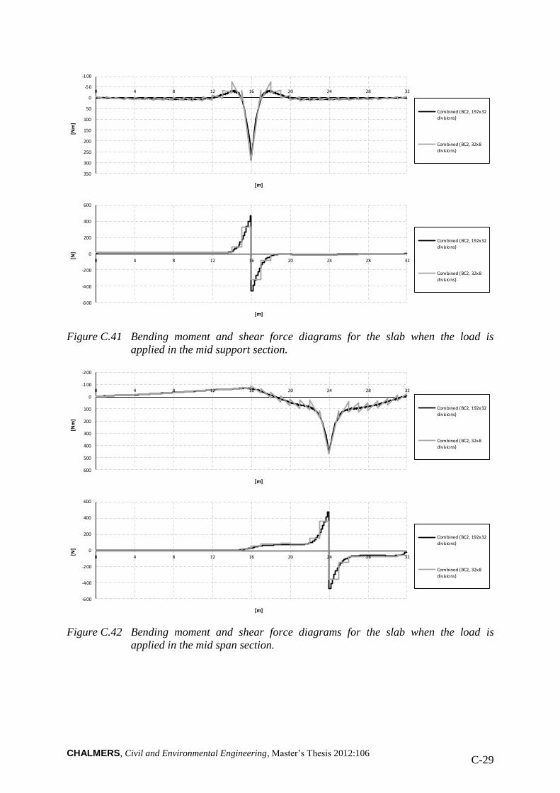
CHALMERS, Civil and Environmental Engineering, Master’s Thesis 2012:106 C-29
Figure C.41 Bending moment and shear force diagrams for the slab when the load is
applied in the mid support section.
Figure C.42 Bending moment and shear force diagrams for the slab when the load is
applied in the mid span section.
-1 00
-5 0
0
50
100
150
200
250
300
350
0 4 8 12 16 20 24 28 32
[Nm
]
[m]
Combined (BC2, 192x32divis ions)
Combined (BC2, 32x8
divis ions)
-600
-4 00
-2 00
0
200
400
600
0 4 8 12 16 20 24 28 32
[N]
[m]
Combined (BC2, 192x32
divis ions)
Combined (BC2, 32x8divis ions)
-2 00
-1 00
0
100
200
300
400
500
600
0 4 8 12 16 20 24 28 32
[Nm
]
[m]
Combined (BC2, 192x32
divis ions)
Combined (BC2, 32x8divis ions)
-6 00
-4 00
-200
0
200
400
600
0 4 8 12 16 20 24 28 32
[N]
[m]
Combined (BC2, 192x32divis ions)
Combined (BC2, 32x8
divis ions)
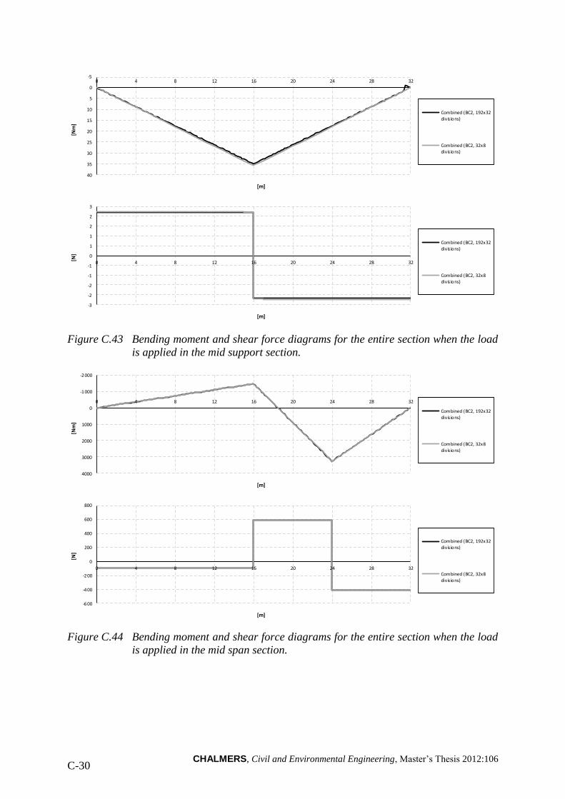
CHALMERS, Civil and Environmental Engineering, Master’s Thesis 2012:106 C-30
Figure C.43 Bending moment and shear force diagrams for the entire section when the load
is applied in the mid support section.
Figure C.44 Bending moment and shear force diagrams for the entire section when the load
is applied in the mid span section.
-5
0
5
10
15
20
25
30
35
40
0 4 8 12 16 20 24 28 32
[Nm
]
[m]
Combined (BC2, 192x32divis ions)
Combined (BC2, 32x8
divis ions)
-3
-2
-2
-1
-1
0
1
1
2
2
3
0 4 8 12 16 20 24 28 32
[N]
[m]
Combined (BC2, 192x32
divis ions)
Combined (BC2, 32x8divis ions)
-2 000
-1 000
0
1000
2000
3000
4000
0 4 8 12 16 20 24 28 32
[Nm
]
[m]
Combined (BC2, 192x32
divis ions)
Combined (BC2, 32x8divis ions)
-6 00
-4 00
-200
0
200
400
600
800
0 4 8 12 16 20 24 28 32
[N]
[m]
Combined (BC2, 192x32divis ions)
Combined (BC2, 32x8
divis ions)
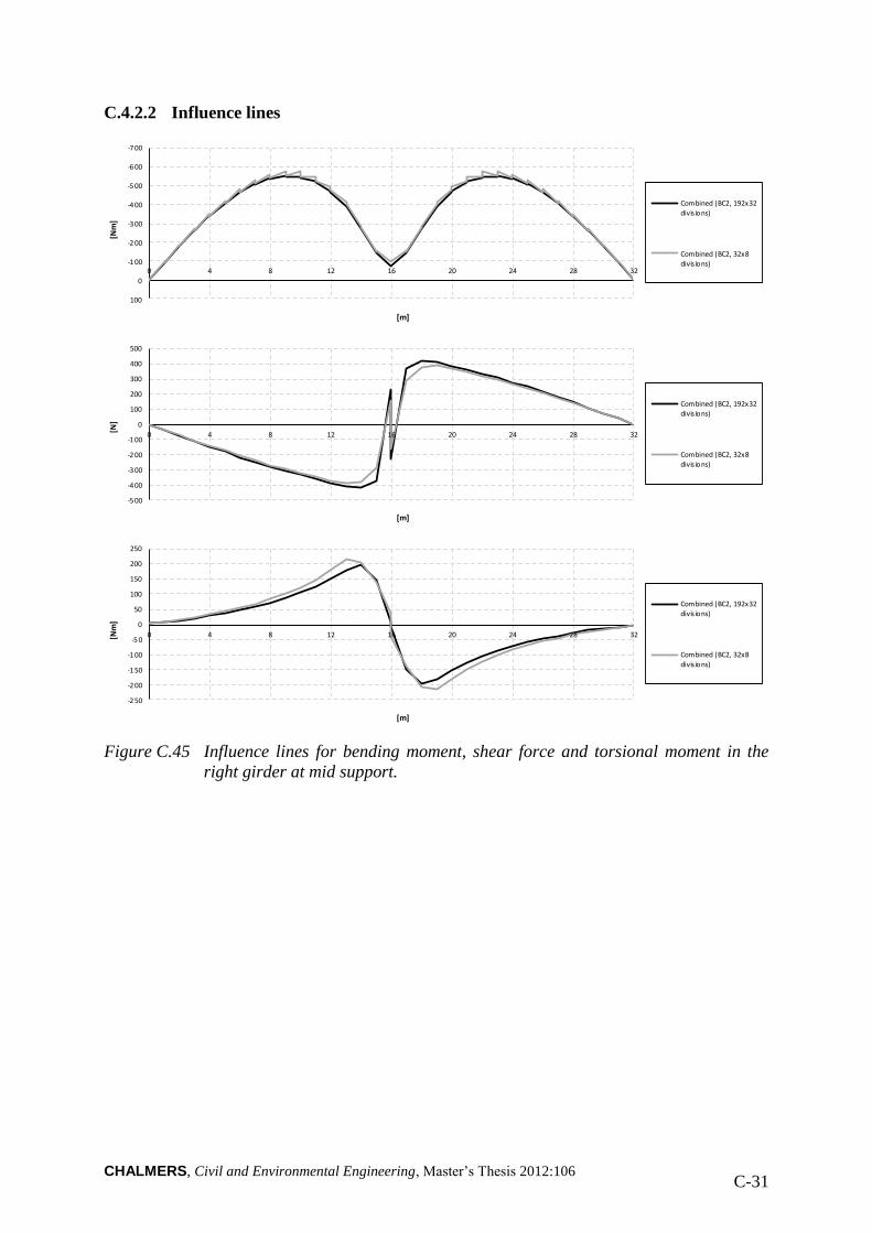
CHALMERS, Civil and Environmental Engineering, Master’s Thesis 2012:106 C-31
C.4.2.2 Influence lines
Figure C.45 Influence lines for bending moment, shear force and torsional moment in the
right girder at mid support.
-7 00
-6 00
-500
-4 00
-3 00
-200
-1 00
0
100
0 4 8 12 16 20 24 28 32
[Nm
]
[m]
Combined (BC2, 192x32
divis ions)
Combined (BC2, 32x8divis ions)
-5 00
-4 00
-3 00
-2 00
-1 00
0
100
200
300
400
500
0 4 8 12 16 20 24 28 32
[N]
[m]
Combined (BC2, 192x32divis ions)
Combined (BC2, 32x8
divis ions)
-2 50
-2 00
-1 50
-1 00
-5 0
0
50
100
150
200
250
0 4 8 12 16 20 24 28 32[Nm
]
[m]
Combined (BC2, 192x32divis ions)
Combined (BC2, 32x8
divis ions)

CHALMERS, Civil and Environmental Engineering, Master’s Thesis 2012:106 C-32
Figure C.46 Influence lines for bending moment, shear force and torsional moment in the
right girder at mid span.
-4 00
-2 00
0
200
400
600
800
1000
1200
0 4 8 12 16 20 24 28 32
[Nm
]
[m]
Combined (BC2, 192x32
divis ions)
Combined (BC2, 32x8divis ions)
-1 50
-1 00
-5 0
0
50
100
150
200
250
0 4 8 12 16 20 24 28 32
[N]
[m]
Combined (BC2, 192x32
divis ions)
Combined (BC2, 32x8divis ions)
-2 00
-1 50
-1 00
-5 0
0
50
100
150
200
250
0 4 8 12 16 20 24 28 32
[Nm
]
[m]
Combined (BC2, 192x32
divis ions)
Combined (BC2, 32x8divis ions)
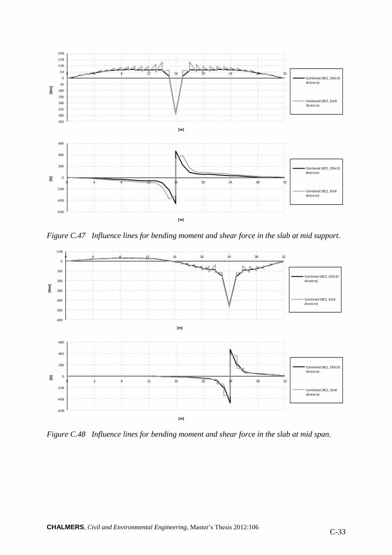
CHALMERS, Civil and Environmental Engineering, Master’s Thesis 2012:106 C-33
Figure C.47 Influence lines for bending moment and shear force in the slab at mid support.
Figure C.48 Influence lines for bending moment and shear force in the slab at mid span.
-2 00
-1 50
-1 00
-5 0
0
50
100
150
200
250
300
350
0 4 8 12 16 20 24 28 32
[Nm
]
[m]
Combined (BC2, 192x32divis ions)
Combined (BC2, 32x8
divis ions)
-6 00
-4 00
-2 00
0
200
400
600
0 4 8 12 16 20 24 28 32
[N]
[m]
Combined (BC2, 192x32divis ions)
Combined (BC2, 32x8
divis ions)
-1 00
0
100
200
300
400
500
600
0 4 8 12 16 20 24 28 32
[Nm
]
[m]
Combined (BC2, 192x32
divis ions)
Combined (BC2, 32x8divis ions)
-6 00
-4 00
-2 00
0
200
400
600
0 4 8 12 16 20 24 28 32
[N]
[m]
Combined (BC2, 192x32
divis ions)
Combined (BC2, 32x8divis ions)
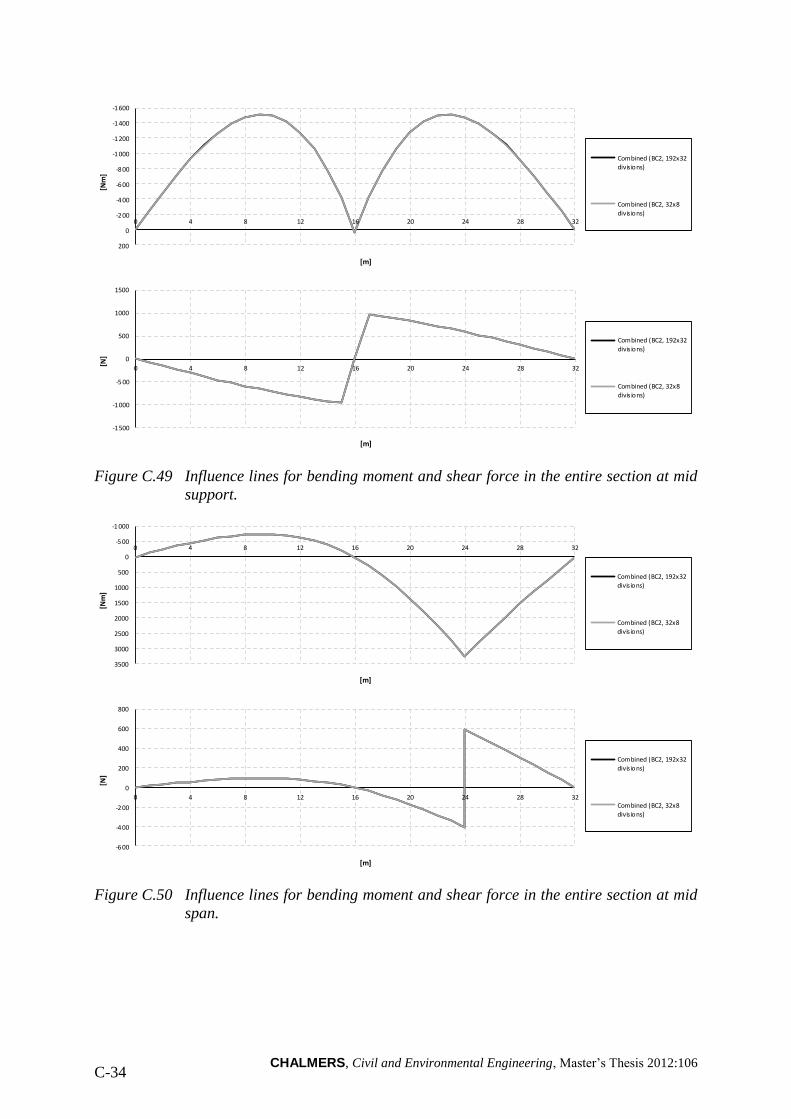
CHALMERS, Civil and Environmental Engineering, Master’s Thesis 2012:106 C-34
Figure C.49 Influence lines for bending moment and shear force in the entire section at mid
support.
Figure C.50 Influence lines for bending moment and shear force in the entire section at mid
span.
-1 600
-1 400
-1 200
-1 000
-8 00
-600
-400
-200
0
200
0 4 8 12 16 20 24 28 32
[Nm
]
[m]
Combined (BC2, 192x32divis ions)
Combined (BC2, 32x8
divis ions)
-1 500
-1 000
-5 00
0
500
1000
1500
0 4 8 12 16 20 24 28 32
[N]
[m]
Combined (BC2, 192x32
divis ions)
Combined (BC2, 32x8divis ions)
-1 000
-5 00
0
500
1000
1500
2000
2500
3000
3500
0 4 8 12 16 20 24 28 32
[Nm
]
[m]
Combined (BC2, 192x32
divis ions)
Combined (BC2, 32x8
divis ions)
-600
-4 00
-2 00
0
200
400
600
800
0 4 8 12 16 20 24 28 32
[N]
[m]
Combined (BC2, 192x32
divis ions)
Combined (BC2, 32x8divis ions)
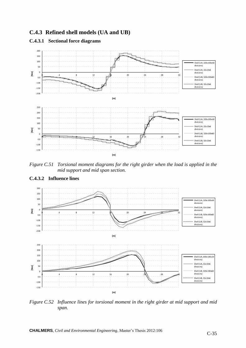
CHALMERS, Civil and Environmental Engineering, Master’s Thesis 2012:106 C-35
C.4.3 Refined shell models (UA and UB)
C.4.3.1 Sectional force diagrams
Figure C.51 Torsional moment diagrams for the right girder when the load is applied in the
mid support and mid span section.
C.4.3.2 Influence lines
Figure C.52 Influence lines for torsional moment in the right girder at mid support and mid
span.
-200
-1 50
-1 00
-50
0
50
100
150
200
0 4 8 12 16 20 24 28 32[Nm
]
[m]
Shell (UA, 320x100x60
divis ions)
Shell (UA, 32x10x6
divis ions)
Shell (UB, 320x100x60divis ions)
Shell (UB, 32x10x6divis ions)
-150
-1 00
-5 0
0
50
100
150
200
250
0 4 8 12 16 20 24 28 32
[Nm
]
[m]
Shell (UA, 320x100x60
divis ions)
Shell (UA, 32x10x6
divis ions)
Shell (UB, 320x100x60divis ions)
Shell (UB, 32x10x6divis ions)
-200
-1 50
-1 00
-50
0
50
100
150
200
0 4 8 12 16 20 24 28 32[Nm
]
[m]
Shell (UA, 320x100x60
divis ions)
Shell (UA, 32x10x6
divis ions)
Shell (UB, 320x100x60divis ions)
Shell (UB, 32x10x6divis ions)
-150
-1 00
-5 0
0
50
100
150
200
250
0 4 8 12 16 20 24 28 32
[Nm
]
[m]
Shell (UA, 640x100x20
divis ions)
Shell (UA, 32x10x6
divis ions)
Shell (UB, 320x100x60divis ions)
Shell (UB, 32x10x6divis ions)

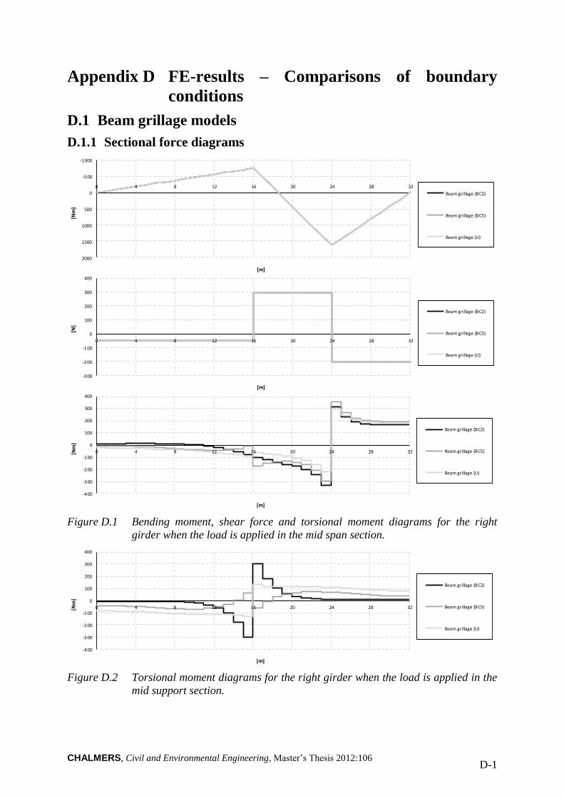
CHALMERS, Civil and Environmental Engineering, Master’s Thesis 2012:106 D-1
Appendix D FE-results – Comparisons of boundary
conditions
D.1 Beam grillage models
D.1.1 Sectional force diagrams
Figure D.1 Bending moment, shear force and torsional moment diagrams for the right
girder when the load is applied in the mid span section.
Figure D.2 Torsional moment diagrams for the right girder when the load is applied in the
mid support section.
-1 000
-5 00
0
500
1000
1500
2000
0 4 8 12 16 20 24 28 32
[Nm
]
[m]
Beam grillage (BC2)
Beam grillage (BC5)
Beam grillage (U)
-300
-2 00
-1 00
0
100
200
300
400
0 4 8 12 16 20 24 28 32
[N]
[m]
Beam grillage (BC2)
Beam grillage (BC5)
Beam grillage (U)
-400
-3 00
-2 00
-100
0
100
200
300
400
0 4 8 12 16 20 24 28 32[Nm
]
[m]
Beam grillage (BC2)
Beam grillage (BC5)
Beam grillage (U)
-4 00
-300
-2 00
-1 00
0
100
200
300
400
0 4 8 12 16 20 24 28 32[Nm
]
[m]
Beam grillage (BC2)
Beam grillage (BC5)
Beam grillage (U)
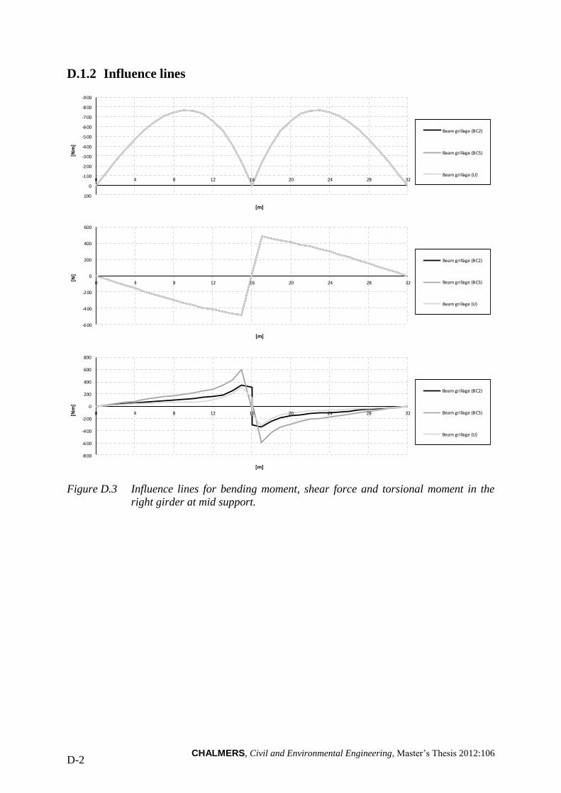
CHALMERS, Civil and Environmental Engineering, Master’s Thesis 2012:106 D-2
D.1.2 Influence lines
Figure D.3 Influence lines for bending moment, shear force and torsional moment in the
right girder at mid support.
-9 00
-8 00
-700
-600
-5 00
-4 00
-3 00
-2 00
-1 00
0
100
0 4 8 12 16 20 24 28 32
[Nm
]
[m]
Beam grillage (BC2)
Beam grillage (BC5)
Beam grillage (U)
-600
-4 00
-2 00
0
200
400
600
0 4 8 12 16 20 24 28 32
[N]
[m]
Beam grillage (BC2)
Beam grillage (BC5)
Beam grillage (U)
-800
-6 00
-4 00
-200
0
200
400
600
800
0 4 8 12 16 20 24 28 32[Nm
]
[m]
Beam grillage (BC2)
Beam grillage (BC5)
Beam grillage (U)
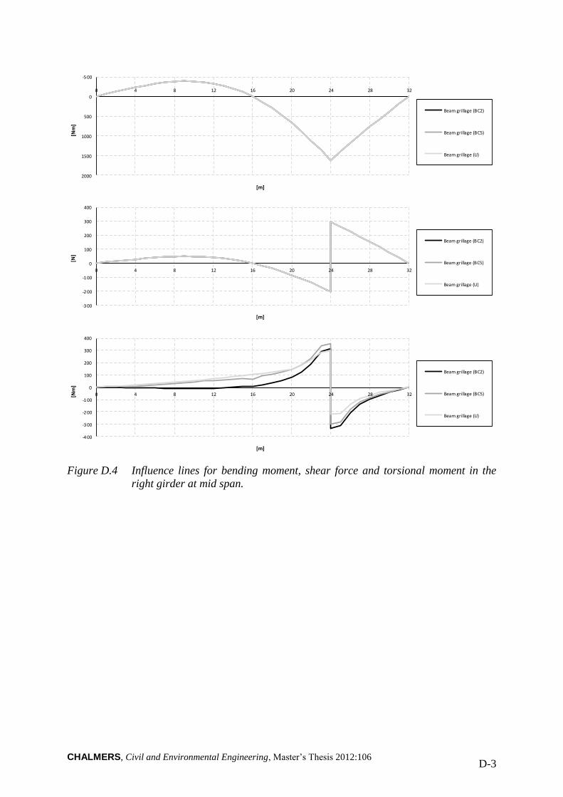
CHALMERS, Civil and Environmental Engineering, Master’s Thesis 2012:106 D-3
Figure D.4 Influence lines for bending moment, shear force and torsional moment in the
right girder at mid span.
-5 00
0
500
1000
1500
2000
0 4 8 12 16 20 24 28 32
[Nm
]
[m]
Beam grillage (BC2)
Beam grillage (BC5)
Beam grillage (U)
-300
-2 00
-1 00
0
100
200
300
400
0 4 8 12 16 20 24 28 32
[N]
[m]
Beam grillage (BC2)
Beam grillage (BC5)
Beam grillage (U)
-400
-3 00
-2 00
-100
0
100
200
300
400
0 4 8 12 16 20 24 28 32[Nm
]
[m]
Beam grillage (BC2)
Beam grillage (BC5)
Beam grillage (U)
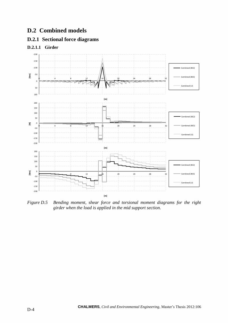
CHALMERS, Civil and Environmental Engineering, Master’s Thesis 2012:106 D-4
D.2 Combined models
D.2.1 Sectional force diagrams
D.2.1.1 Girder
Figure D.5 Bending moment, shear force and torsional moment diagrams for the right
girder when the load is applied in the mid support section.
-2 00
-1 50
-1 00
-5 0
0
50
100
0 4 8 12 16 20 24 28 32[Nm
]
[m]
Combined (BC2)
Combined (BC5)
Combined (U)
-2 00
-1 50
-1 00
-50
0
50
100
150
200
0 4 8 12 16 20 24 28 32
[N]
[m]
Combined (BC2)
Combined (BC5)
Combined (U)
-200
-1 50
-1 00
-50
0
50
100
150
200
0 4 8 12 16 20 24 28 32[Nm
]
[m]
Combined (BC2)
Combined (BC5)
Combined (U)
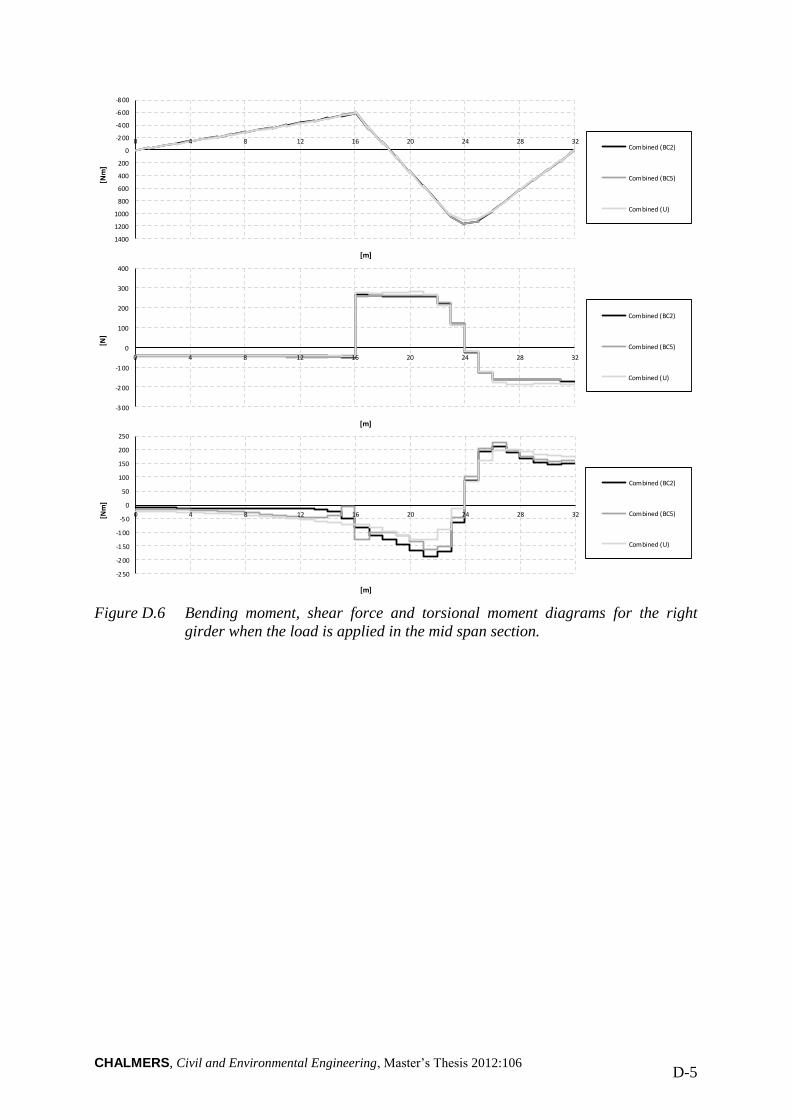
CHALMERS, Civil and Environmental Engineering, Master’s Thesis 2012:106 D-5
Figure D.6 Bending moment, shear force and torsional moment diagrams for the right
girder when the load is applied in the mid span section.
-8 00
-6 00
-4 00
-2 00
0
200
400
600
800
1000
1200
1400
0 4 8 12 16 20 24 28 32
[Nm
]
[m]
Combined (BC2)
Combined (BC5)
Combined (U)
-300
-2 00
-1 00
0
100
200
300
400
0 4 8 12 16 20 24 28 32
[N]
[m]
Combined (BC2)
Combined (BC5)
Combined (U)
-250
-200
-1 50
-1 00
-5 0
0
50
100
150
200
250
0 4 8 12 16 20 24 28 32[Nm
]
[m]
Combined (BC2)
Combined (BC5)
Combined (U)
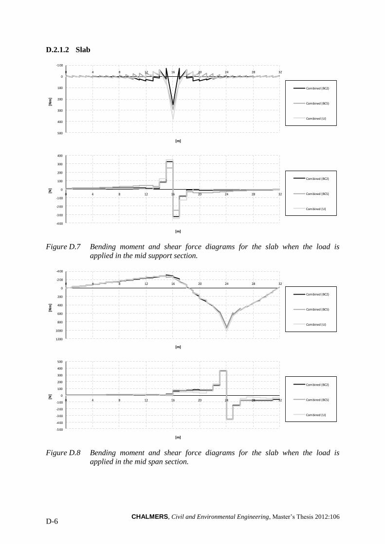
CHALMERS, Civil and Environmental Engineering, Master’s Thesis 2012:106 D-6
D.2.1.2 Slab
Figure D.7 Bending moment and shear force diagrams for the slab when the load is
applied in the mid support section.
Figure D.8 Bending moment and shear force diagrams for the slab when the load is
applied in the mid span section.
-1 00
0
100
200
300
400
500
0 4 8 12 16 20 24 28 32
[Nm
]
[m]
Combined (BC2)
Combined (BC5)
Combined (U)
-400
-3 00
-2 00
-100
0
100
200
300
400
0 4 8 12 16 20 24 28 32
[N]
[m]
Combined (BC2)
Combined (BC5)
Combined (U)
-4 00
-2 00
0
200
400
600
800
1000
1200
0 4 8 12 16 20 24 28 32
[Nm
]
[m]
Combined (BC2)
Combined (BC5)
Combined (U)
-500
-4 00
-3 00
-2 00
-1 00
0
100
200
300
400
500
0 4 8 12 16 20 24 28 32
[N]
[m]
Combined (BC2)
Combined (BC5)
Combined (U)
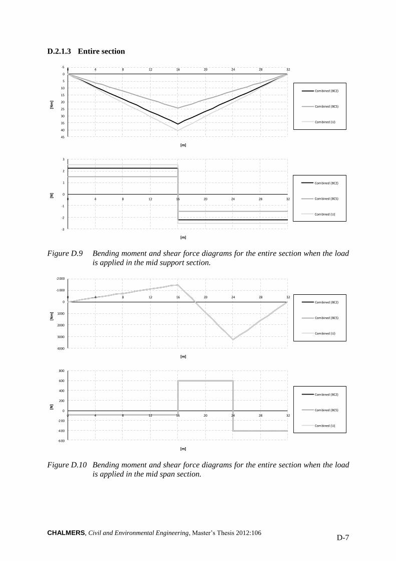
CHALMERS, Civil and Environmental Engineering, Master’s Thesis 2012:106 D-7
D.2.1.3 Entire section
Figure D.9 Bending moment and shear force diagrams for the entire section when the load
is applied in the mid support section.
Figure D.10 Bending moment and shear force diagrams for the entire section when the load
is applied in the mid span section.
-5
0
5
10
15
20
25
30
35
40
45
0 4 8 12 16 20 24 28 32
[Nm
]
[m]
Combined (BC2)
Combined (BC5)
Combined (U)
-3
-2
-1
0
1
2
3
0 4 8 12 16 20 24 28 32
[N]
[m]
Combined (BC2)
Combined (BC5)
Combined (U)
-2 000
-1 000
0
1000
2000
3000
4000
0 4 8 12 16 20 24 28 32
[Nm
]
[m]
Combined (BC2)
Combined (BC5)
Combined (U)
-600
-4 00
-2 00
0
200
400
600
800
0 4 8 12 16 20 24 28 32
[N]
[m]
Combined (BC2)
Combined (BC5)
Combined (U)
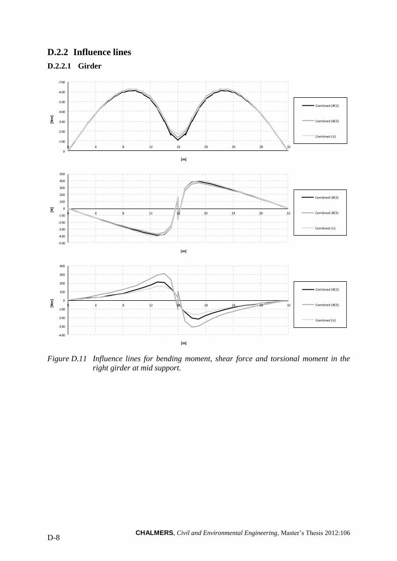
CHALMERS, Civil and Environmental Engineering, Master’s Thesis 2012:106 D-8
D.2.2 Influence lines
D.2.2.1 Girder
Figure D.11 Influence lines for bending moment, shear force and torsional moment in the
right girder at mid support.
-7 00
-6 00
-5 00
-400
-3 00
-2 00
-1 00
0
0 4 8 12 16 20 24 28 32
[Nm
]
[m]
Combined (BC2)
Combined (BC5)
Combined (U)
-5 00
-4 00
-3 00
-2 00
-1 00
0
100
200
300
400
500
0 4 8 12 16 20 24 28 32
[N]
[m]
Combined (BC2)
Combined (BC5)
Combined (U)
-400
-3 00
-2 00
-100
0
100
200
300
400
0 4 8 12 16 20 24 28 32[Nm
]
[m]
Combined (BC2)
Combined (BC5)
Combined (U)
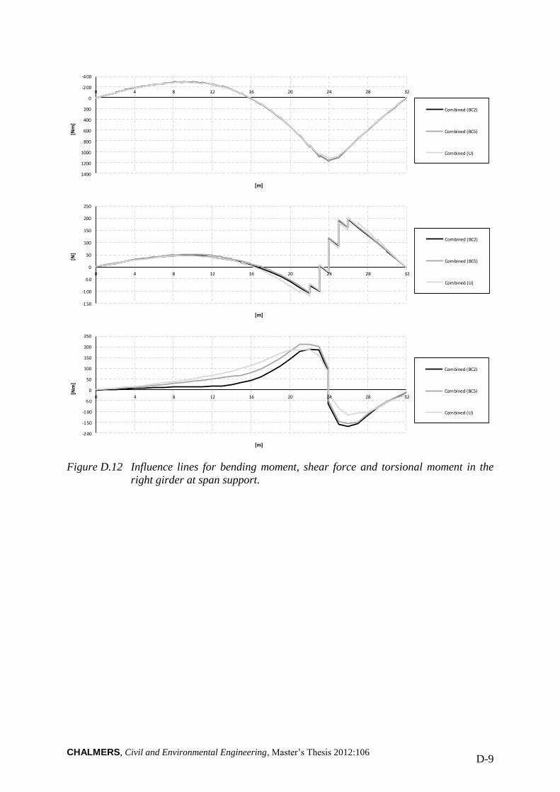
CHALMERS, Civil and Environmental Engineering, Master’s Thesis 2012:106 D-9
Figure D.12 Influence lines for bending moment, shear force and torsional moment in the
right girder at span support.
-4 00
-2 00
0
200
400
600
800
1000
1200
1400
0 4 8 12 16 20 24 28 32
[Nm
]
[m]
Combined (BC2)
Combined (BC5)
Combined (U)
-150
-1 00
-5 0
0
50
100
150
200
250
0 4 8 12 16 20 24 28 32
[N]
[m]
Combined (BC2)
Combined (BC5)
Combined (U)
-2 00
-1 50
-1 00
-5 0
0
50
100
150
200
250
0 4 8 12 16 20 24 28 32
[Nm
]
[m]
Combined (BC2)
Combined (BC5)
Combined (U)
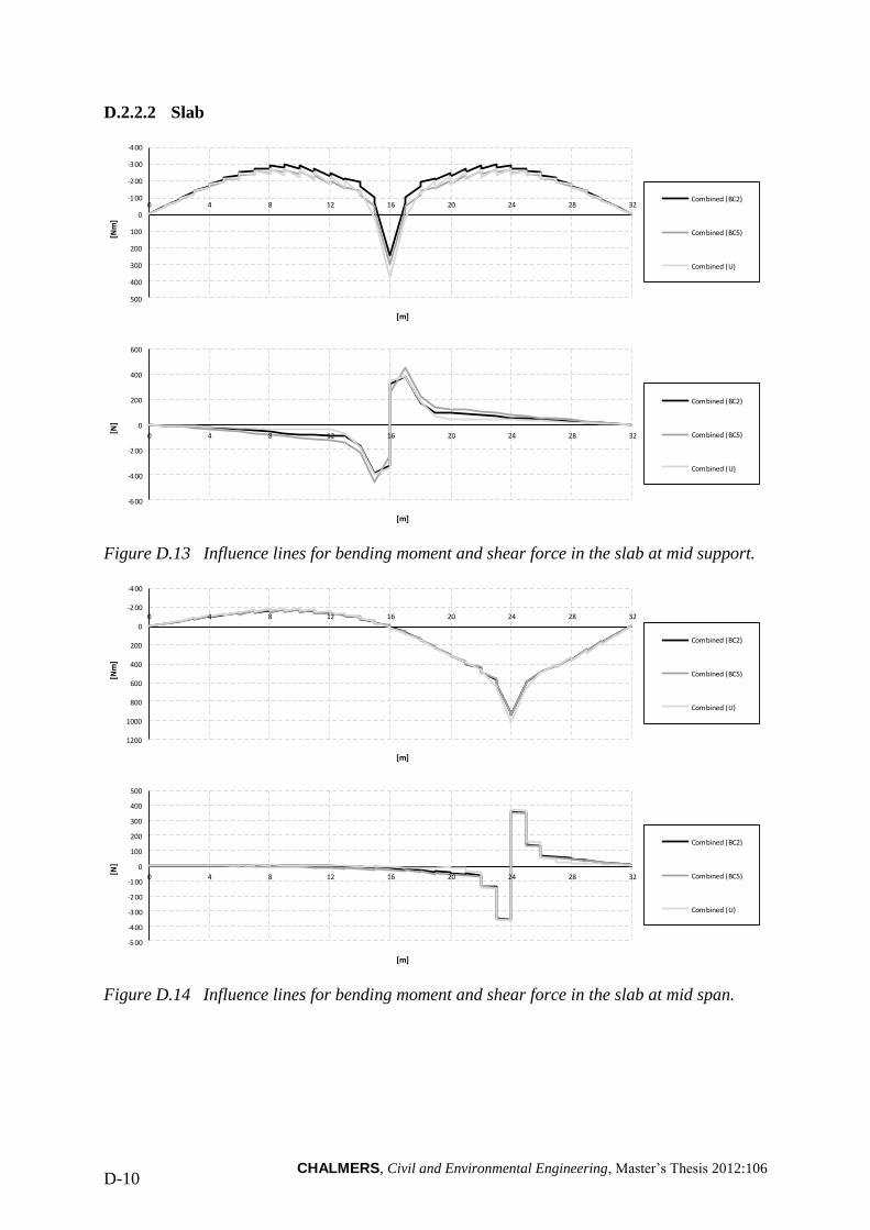
CHALMERS, Civil and Environmental Engineering, Master’s Thesis 2012:106 D-10
D.2.2.2 Slab
Figure D.13 Influence lines for bending moment and shear force in the slab at mid support.
Figure D.14 Influence lines for bending moment and shear force in the slab at mid span.
-4 00
-3 00
-2 00
-1 00
0
100
200
300
400
500
0 4 8 12 16 20 24 28 32
[Nm
]
[m]
Combined (BC2)
Combined (BC5)
Combined (U)
-600
-400
-2 00
0
200
400
600
0 4 8 12 16 20 24 28 32
[N]
[m]
Combined (BC2)
Combined (BC5)
Combined (U)
-4 00
-2 00
0
200
400
600
800
1000
1200
0 4 8 12 16 20 24 28 32
[Nm
]
[m]
Combined (BC2)
Combined (BC5)
Combined (U)
-500
-4 00
-3 00
-2 00
-1 00
0
100
200
300
400
500
0 4 8 12 16 20 24 28 32
[N]
[m]
Combined (BC2)
Combined (BC5)
Combined (U)
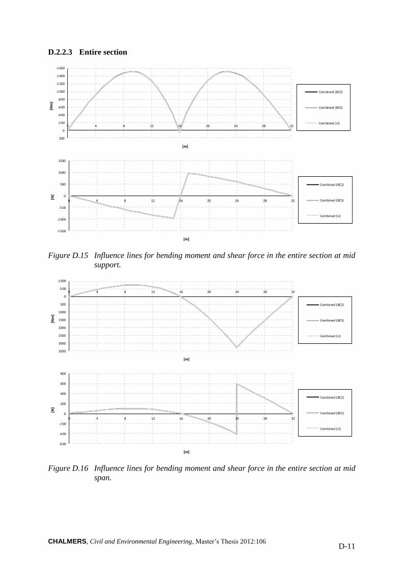
CHALMERS, Civil and Environmental Engineering, Master’s Thesis 2012:106 D-11
D.2.2.3 Entire section
Figure D.15 Influence lines for bending moment and shear force in the entire section at mid
support.
Figure D.16 Influence lines for bending moment and shear force in the entire section at mid
span.
-1 600
-1 400
-1 200
-1 000
-8 00
-600
-400
-2 00
0
200
0 4 8 12 16 20 24 28 32
[Nm
]
[m]
Combined (BC2)
Combined (BC5)
Combined (U)
-1500
-1 000
-5 00
0
500
1000
1500
0 4 8 12 16 20 24 28 32
[N]
[m]
Combined (BC2)
Combined (BC5)
Combined (U)
-1 000
-5 00
0
500
1000
1500
2000
2500
3000
3500
0 4 8 12 16 20 24 28 32
[Nm
]
[m]
Combined (BC2)
Combined (BC5)
Combined (U)
-600
-4 00
-2 00
0
200
400
600
800
0 4 8 12 16 20 24 28 32
[N]
[m]
Combined (BC2)
Combined (BC5)
Combined (U)
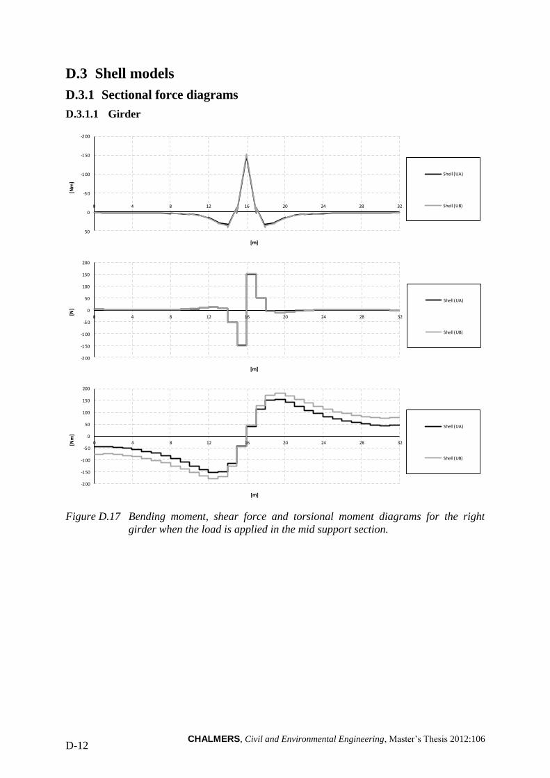
CHALMERS, Civil and Environmental Engineering, Master’s Thesis 2012:106 D-12
D.3 Shell models
D.3.1 Sectional force diagrams
D.3.1.1 Girder
Figure D.17 Bending moment, shear force and torsional moment diagrams for the right
girder when the load is applied in the mid support section.
-2 00
-150
-1 00
-5 0
0
50
0 4 8 12 16 20 24 28 32
[Nm
]
[m]
Shell (UA)
Shell (UB)
-200
-1 50
-1 00
-50
0
50
100
150
200
0 4 8 12 16 20 24 28 32
[N]
[m]
Shell (UA)
Shell (UB)
-200
-1 50
-1 00
-5 0
0
50
100
150
200
0 4 8 12 16 20 24 28 32[Nm
]
[m]
Shell (UA)
Shell (UB)
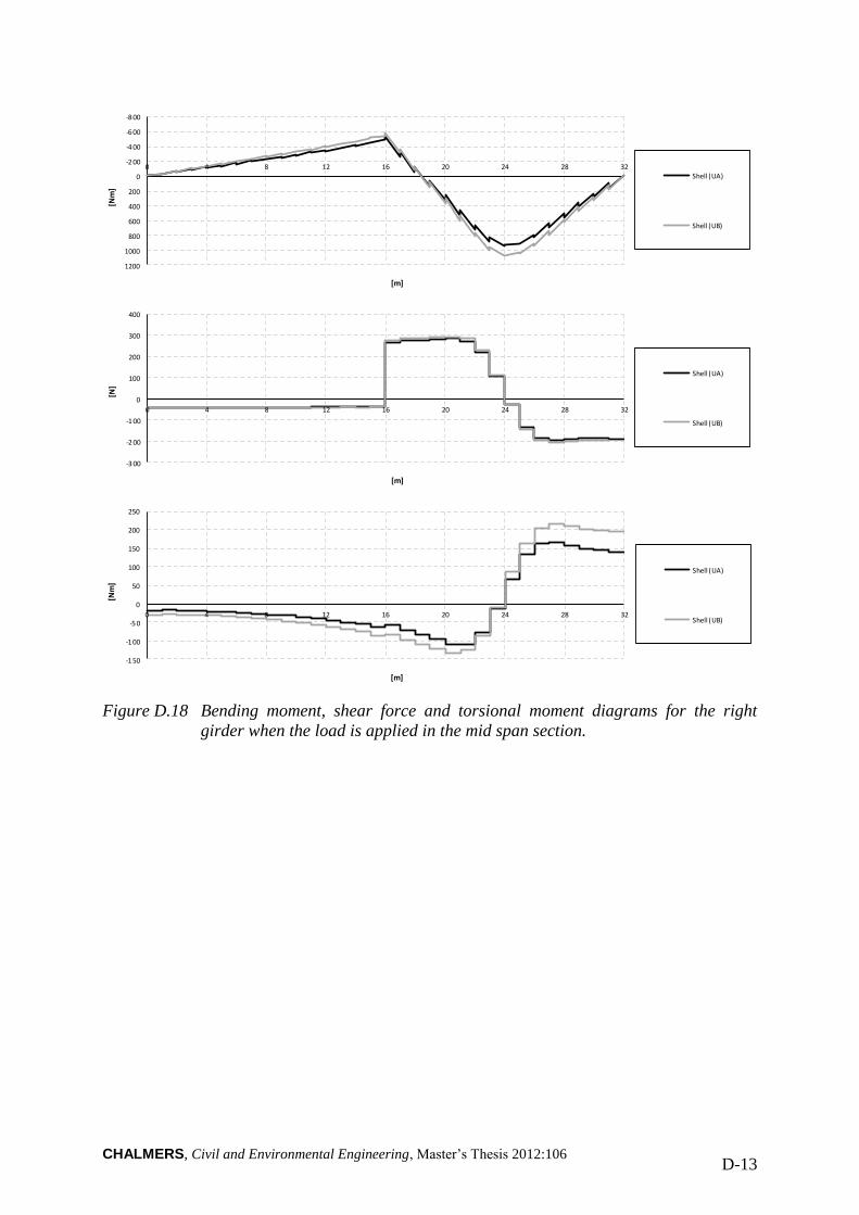
CHALMERS, Civil and Environmental Engineering, Master’s Thesis 2012:106 D-13
Figure D.18 Bending moment, shear force and torsional moment diagrams for the right
girder when the load is applied in the mid span section.
-8 00
-6 00
-4 00
-2 00
0
200
400
600
800
1000
1200
0 4 8 12 16 20 24 28 32
[Nm
]
[m]
Shell (UA)
Shell (UB)
-3 00
-2 00
-1 00
0
100
200
300
400
0 4 8 12 16 20 24 28 32
[N]
[m]
Shell (UA)
Shell (UB)
-1 50
-1 00
-5 0
0
50
100
150
200
250
0 4 8 12 16 20 24 28 32
[Nm
]
[m]
Shell (UA)
Shell (UB)
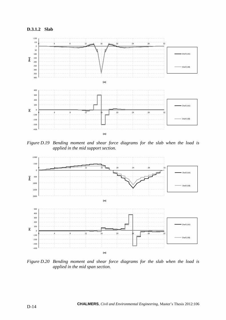
CHALMERS, Civil and Environmental Engineering, Master’s Thesis 2012:106 D-14
D.3.1.2 Slab
Figure D.19 Bending moment and shear force diagrams for the slab when the load is
applied in the mid support section.
Figure D.20 Bending moment and shear force diagrams for the slab when the load is
applied in the mid span section.
-1 00
-5 0
0
50
100
150
200
250
300
350
400
0 4 8 12 16 20 24 28 32
[Nm
]
[m]
Shell (UA)
Shell (UB)
-4 00
-300
-2 00
-1 00
0
100
200
300
400
0 4 8 12 16 20 24 28 32
[N]
[m]
Shell (UA)
Shell (UB)
-1 000
-5 00
0
500
1000
1500
2000
0 4 8 12 16 20 24 28 32
[Nm
]
[m]
Shell (UA)
Shell (UB)
-4 00
-3 00
-2 00
-1 00
0
100
200
300
400
500
0 4 8 12 16 20 24 28 32
[N]
[m]
Shell (UA)
Shell (UB)
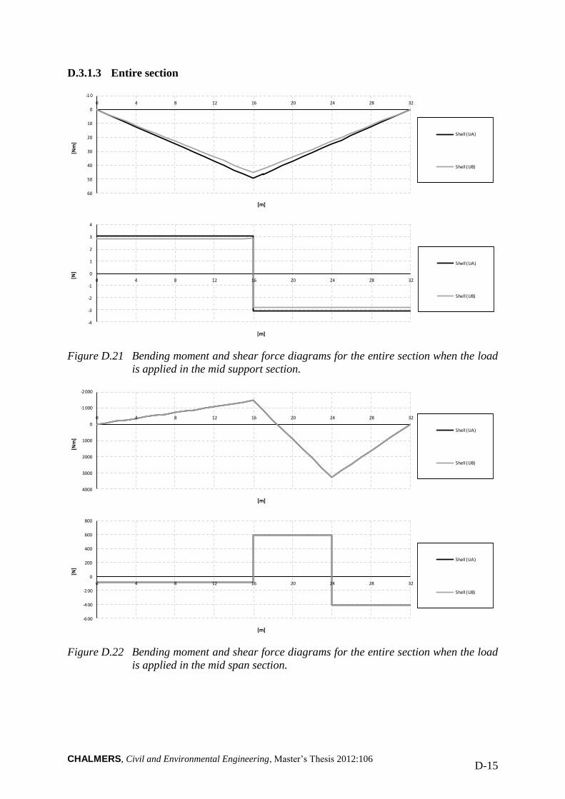
CHALMERS, Civil and Environmental Engineering, Master’s Thesis 2012:106 D-15
D.3.1.3 Entire section
Figure D.21 Bending moment and shear force diagrams for the entire section when the load
is applied in the mid support section.
Figure D.22 Bending moment and shear force diagrams for the entire section when the load
is applied in the mid span section.
-1 0
0
10
20
30
40
50
60
0 4 8 12 16 20 24 28 32
[Nm
]
[m]
Shell (UA)
Shell (UB)
-4
-3
-2
-1
0
1
2
3
4
0 4 8 12 16 20 24 28 32
[N]
[m]
Shell (UA)
Shell (UB)
-2 000
-1 000
0
1000
2000
3000
4000
0 4 8 12 16 20 24 28 32
[Nm
]
[m]
Shell (UA)
Shell (UB)
-6 00
-4 00
-2 00
0
200
400
600
800
0 4 8 12 16 20 24 28 32
[N]
[m]
Shell (UA)
Shell (UB)
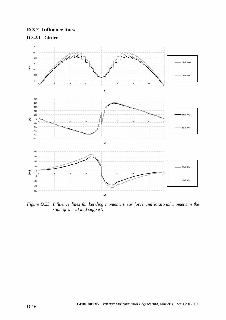
CHALMERS, Civil and Environmental Engineering, Master’s Thesis 2012:106 D-16
D.3.2 Influence lines
D.3.2.1 Girder
Figure D.23 Influence lines for bending moment, shear force and torsional moment in the
right girder at mid support.
-7 00
-6 00
-5 00
-400
-3 00
-2 00
-1 00
0
0 4 8 12 16 20 24 28 32
[Nm
]
[m]
Shell (UA)
Shell (UB)
-500
-4 00
-3 00
-2 00
-1 00
0
100
200
300
400
500
0 4 8 12 16 20 24 28 32
[N]
[m]
Shell (UA)
Shell (UB)
-2 00
-150
-1 00
-5 0
0
50
100
150
200
0 4 8 12 16 20 24 28 32[Nm
]
[m]
Shell (UA)
Shell (UB)
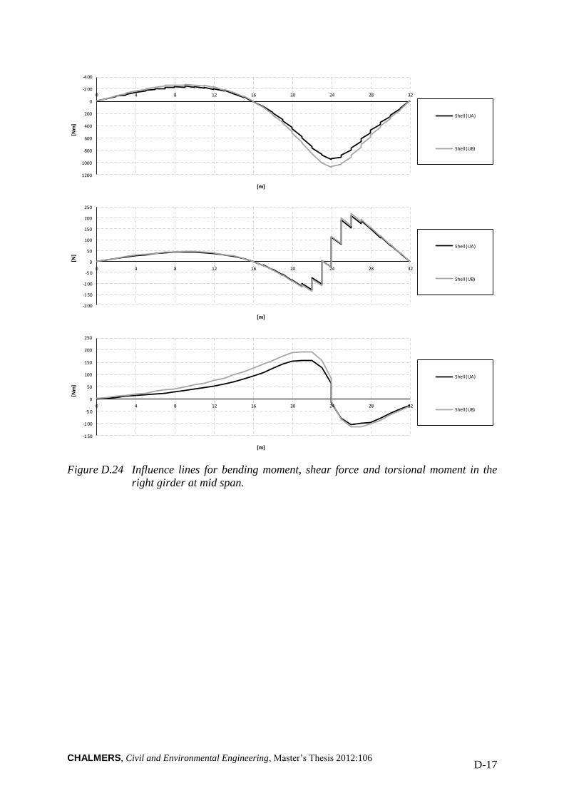
CHALMERS, Civil and Environmental Engineering, Master’s Thesis 2012:106 D-17
Figure D.24 Influence lines for bending moment, shear force and torsional moment in the
right girder at mid span.
-4 00
-2 00
0
200
400
600
800
1000
1200
0 4 8 12 16 20 24 28 32
[Nm
]
[m]
Shell (UA)
Shell (UB)
-200
-150
-100
-5 0
0
50
100
150
200
250
0 4 8 12 16 20 24 28 32
[N]
[m]
Shell (UA)
Shell (UB)
-1 50
-100
-5 0
0
50
100
150
200
250
0 4 8 12 16 20 24 28 32
[Nm
]
[m]
Shell (UA)
Shell (UB)
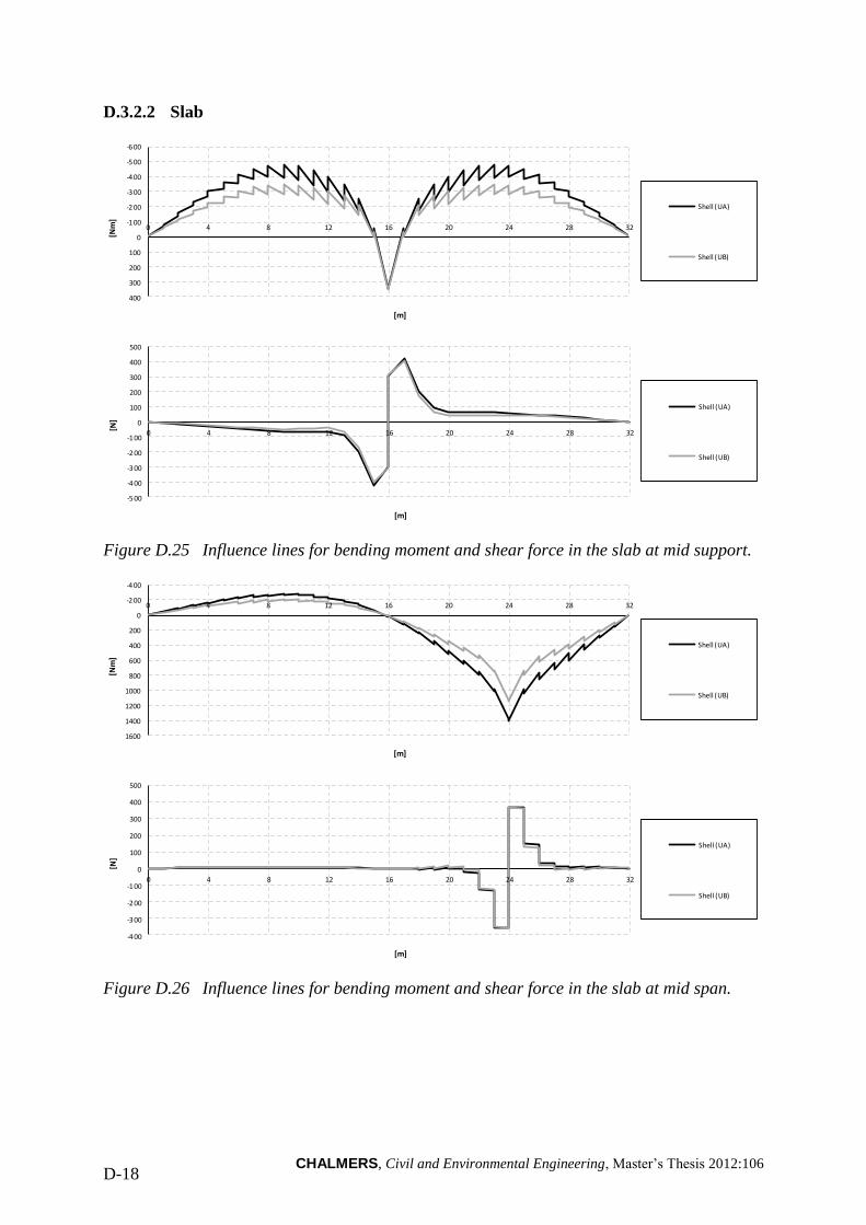
CHALMERS, Civil and Environmental Engineering, Master’s Thesis 2012:106 D-18
D.3.2.2 Slab
Figure D.25 Influence lines for bending moment and shear force in the slab at mid support.
Figure D.26 Influence lines for bending moment and shear force in the slab at mid span.
-6 00
-5 00
-400
-300
-2 00
-1 00
0
100
200
300
400
0 4 8 12 16 20 24 28 32
[Nm
]
[m]
Shell (UA)
Shell (UB)
-500
-4 00
-3 00
-2 00
-1 00
0
100
200
300
400
500
0 4 8 12 16 20 24 28 32
[N]
[m]
Shell (UA)
Shell (UB)
-4 00
-2 00
0
200
400
600
800
1000
1200
1400
1600
0 4 8 12 16 20 24 28 32
[Nm
]
[m]
Shell (UA)
Shell (UB)
-400
-300
-200
-1 00
0
100
200
300
400
500
0 4 8 12 16 20 24 28 32
[N]
[m]
Shell (UA)
Shell (UB)
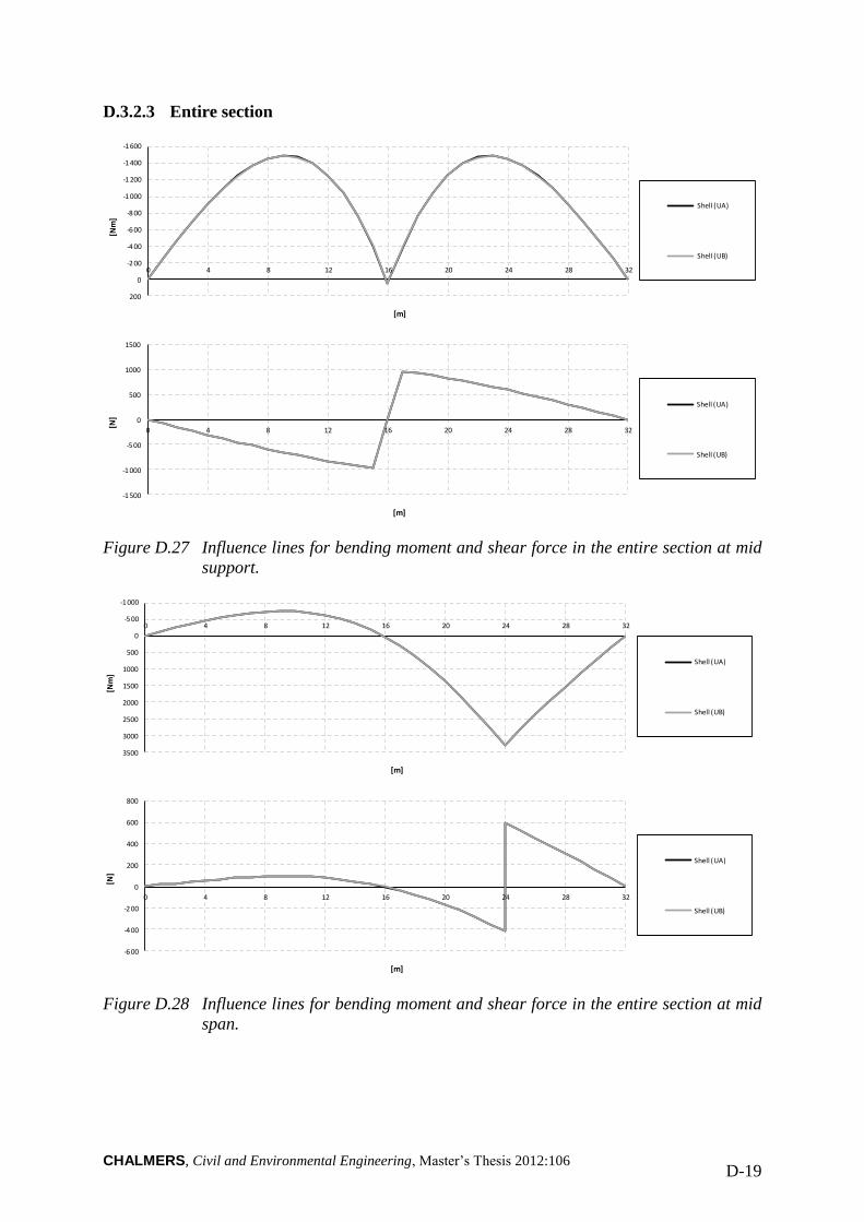
CHALMERS, Civil and Environmental Engineering, Master’s Thesis 2012:106 D-19
D.3.2.3 Entire section
Figure D.27 Influence lines for bending moment and shear force in the entire section at mid
support.
Figure D.28 Influence lines for bending moment and shear force in the entire section at mid
span.
-1 600
-1 400
-1 200
-1 000
-8 00
-6 00
-4 00
-2 00
0
200
0 4 8 12 16 20 24 28 32
[Nm
]
[m]
Shell (UA)
Shell (UB)
-1500
-1 000
-5 00
0
500
1000
1500
0 4 8 12 16 20 24 28 32
[N]
[m]
Shell (UA)
Shell (UB)
-1 000
-5 00
0
500
1000
1500
2000
2500
3000
3500
0 4 8 12 16 20 24 28 32
[Nm
]
[m]
Shell (UA)
Shell (UB)
-600
-4 00
-2 00
0
200
400
600
800
0 4 8 12 16 20 24 28 32
[N]
[m]
Shell (UA)
Shell (UB)

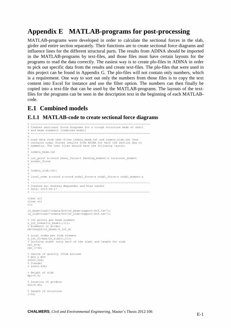
CHALMERS, Civil and Environmental Engineering, Master’s Thesis 2012:106 E-1
Appendix E MATLAB-programs for post-processing
MATLAB-programs were developed in order to calculate the sectional forces in the slab,
girder and entire section separately. Their functions are to create sectional force diagrams and
influence lines for the different structural parts. The results from ADINA should be imported
in the MATLAB-programs by text-files, and those files must have certain layouts for the
programs to read the data correctly. The easiest way is to create plo-files in ADINA in order
to pick out specific data from the results and create text-files. The plo-files that were used in
this project can be found in Appendix G. The plo-files will not contain only numbers, which
is a requirement. One way to sort out only the numbers from those files is to copy the text
content into Excel for instance and use the filter option. The numbers can then finally be
copied into a text-file that can be used by the MATLAB-programs. The layouts of the text-
files for the programs can be seen in the description text in the beginning of each MATLAB-
code.
E.1 Combined models
E.1.1 MATLAB-code to create sectional force diagrams % -------------------------------------------------------------------------
% Creates sectional force diagrams for a trough structure made of shell
% and beam elements (combined model)
% -------------------------------------------------------------------------
%
% Load data from text-files indata_beam.txt and indata_slab.txt that
% contains nodal forces results from ADINA for half the section due to
% symmetry. The text files should have the following layout:
%
% indata_beam.txt
%
% int_point x-coord shear_force-t bending_moment-s torsional_moment
% normal_force
%
%
% indata_slab.txt:
%
% local_node x-coord y-coord nodal_force-x nodal_force-z nodal_moment-y
%
% -------------------------------------------------------------------------
% Created by: Andreas Magnander and Klas Lundin
% Date: 2012-04-17
% -------------------------------------------------------------------------
clear all
close all
clc
in_beam=load('indata/bc5/sf_beam-support-bc5.txt');
in_slab=load('indata/bc5/sf_slab-support-bc5.txt');
% Int points per beam element
n_int_b=max(in_beam(:,1));
% Elements in girder
nb=length(in_beam)/n_int_b;
% Local nodes per slab element
n_int_sl=max(in_slab(:,1));
% Division width (only half of the slab) and length for slab
npl_w=4;
npl_l=32;
% Centre of gravity (from bottom)
% BC2 & BC5
zCG=0.526;
% U-model
% zCG=0.494;
% Height of slab
Hpl=0.5;
% Location of girders
zGi=0.65;
% Length of structure
l=32;
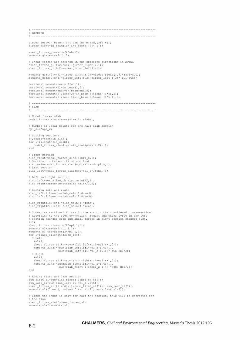
CHALMERS, Civil and Environmental Engineering, Master’s Thesis 2012:106 E-2
% -------------------------------------------------------------------------
% GIRDERS
% -------------------------------------------------------------------------
girder_left=in_beam(n_int_b:n_int_b:end,[3:4 6]);
girder_right=in_beam(1:n_int_b:end,[3:4 6]);
shear_forces_gi=zeros(2*nb,1);
moments_gi=zeros(2*nb,1);
% Shear forces are defined in the opposite directions in ADINA
shear_forces_gi(1:2:end)=-girder_right(:,1);
shear_forces_gi(2:2:end)=-girder_left(:,1);
moments_gi(1:2:end)=girder_right(:,2)-girder_right(:,3)*(zGi-zCG);
moments_gi(2:2:end)=girder_left(:,2)-girder_left(:,3)*(zGi-zCG);
torsional moment=zeros(2*nb,1);
torsional moment(1)=in_beam(1,5);
torsional moment(end)=in_beam(end,5);
torsional moment(2:2:end-2)=in_beam(5:5:end-(1*5),5);
torsional moment(3:2:end-1)=in_beam(6:5:end-(1*5-1),5);
% -------------------------------------------------------------------------
% SLAB
% -------------------------------------------------------------------------
% Nodal forces slab
nodal_forces_slab=zeros(size(in_slab));
% Number of local points for one half slab section
npl_s=2*npl_w;
% Sorting sections
[~,poss]=sort(in_slab);
for i=1:length(in_slab);
nodal_forces_slab(i,:)=in_slab(poss(i,2),:);
end
% First section
slab_first=nodal_forces_slab(1:npl_s,:);
% Sections in-between first and last
slab_main=nodal_forces_slab(npl_s+1:end-npl_s,:);
% Last section
slab_last=nodal_forces_slab(end-npl_s+1:end,:);
% Left and right section
slab_left=zeros(length(slab_main)/2,6);
slab_right=zeros(length(slab_main)/2,6);
% Section left and right
slab_left(1:2:end)=slab_main(1:4:end);
slab_left(2:2:end)=slab_main(2:4:end);
slab_right(1:2:end)=slab_main(3:4:end);
slab_right(2:2:end)=slab_main(4:4:end);
% Summarise sectional forces in the slab in the considered cross-section.
% According to the sign convention, moment and shear force in the left
% section changes sign and axial forces in right section changes sign.
k=1;
shear_forces_sl=zeros(2*npl_l,1);
moments_sl=zeros(2*npl_l,1);
moments_sl_tot=zeros(2*npl_l,1);
for i=1:npl_s:length(slab_left)
% Left
k=k+1;
shear_forces_sl(k)=-sum(slab_left(i:i+npl_s-1,5));
moments_sl(k)=-sum(slab_left(i:i+npl_s-1,6))...
+sum(slab_left(i:i+npl_s-1,4))*(zCG-Hpl/2);
% Right
k=k+1;
shear_forces_sl(k)=sum(slab_right(i:i+npl_s-1,5));
moments_sl(k)=sum(slab_right(i:i+npl_s-1,6))...
-sum(slab_right(i:i+npl_s-1,4))*(zCG-Hpl/2);
end
% Adding first and last section
sum_first_sl=sum(slab_first((1:npl_s),5:6));
sum_last_sl=sum(slab_last((1:npl_s),5:6));
shear_forces_sl([1 end],:)=[sum_first_sl(1); -sum_last_sl(1)];
moments_sl([1 end],:)=[sum_first_sl(2); -sum_last_sl(2)];
% Since the input is only for half the section, this will be corrected for
% the slab
shear_forces_sl=2*shear_forces_sl;
moments_sl=2*moments_sl;
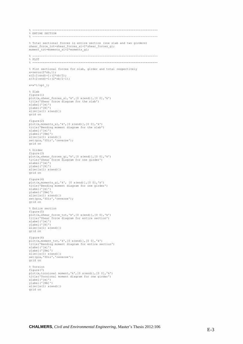
CHALMERS, Civil and Environmental Engineering, Master’s Thesis 2012:106 E-3
% -------------------------------------------------------------------------
% ENTIRE SECTION
% -------------------------------------------------------------------------
% Total sectional forces in entire section (one slab and two girders)
shear_force_tot=shear_forces_sl+2*shear_forces_gi;
moment_tot=moments_sl+2*moments_gi;
% -------------------------------------------------------------------------
% PLOT
% -------------------------------------------------------------------------
% Plot sectional forces for slab, girder and total respectively
x=zeros(2*nb,1);
x(2:2:end)=1:(2*nb/2);
x(3:2:end)=1:(2*nb/2-1);
x=x*l/npl_l;
% Slab
figure(1)
plot(x,shear_forces_sl,'k',[0 x(end)],[0 0],'k')
title('Shear force diagram for the slab')
xlabel('[m]')
ylabel('[N]')
xlim([x(1) x(end)])
grid on
figure(2)
plot(x,moments_sl,'k',[0 x(end)],[0 0],'k')
title('Bending moment diagram for the slab')
xlabel('[m]')
ylabel('[Nm]')
xlim([x(1) x(end)])
set(gca,'YDir','reverse');
grid on
% Girder
figure(3)
plot(x,shear_forces_gi,'k',[0 x(end)],[0 0],'k')
title('Shear force diagram for one girder')
xlabel('[m]')
ylabel('[N]')
xlim([x(1) x(end)])
grid on
figure(4)
plot(x,moments_gi,'k', [0 x(end)],[0 0],'k')
title('Bending moment diagram for one girder')
xlabel('[m]')
ylabel('[Nm]')
xlim([x(1) x(end)])
set(gca,'YDir','reverse');
grid on
% Entire section
figure(5)
plot(x,shear_force_tot,'k',[0 x(end)],[0 0],'k')
title('Shear force diagram for entire section')
xlabel('[m]')
ylabel('[N]')
xlim([x(1) x(end)])
grid on
figure(6)
plot(x,moment_tot,'k',[0 x(end)],[0 0],'k')
title('Bending moment diagram for entire section')
xlabel('[m]')
ylabel('[Nm]')
xlim([x(1) x(end)])
set(gca,'YDir','reverse');
grid on
% Torsion
figure(7)
plot(x,torsional moment,'k',[0 x(end)],[0 0],'k')
title('Torsional moment diagram for one girder')
xlabel('[m]')
ylabel('[Nm]')
xlim([x(1) x(end)])
grid on
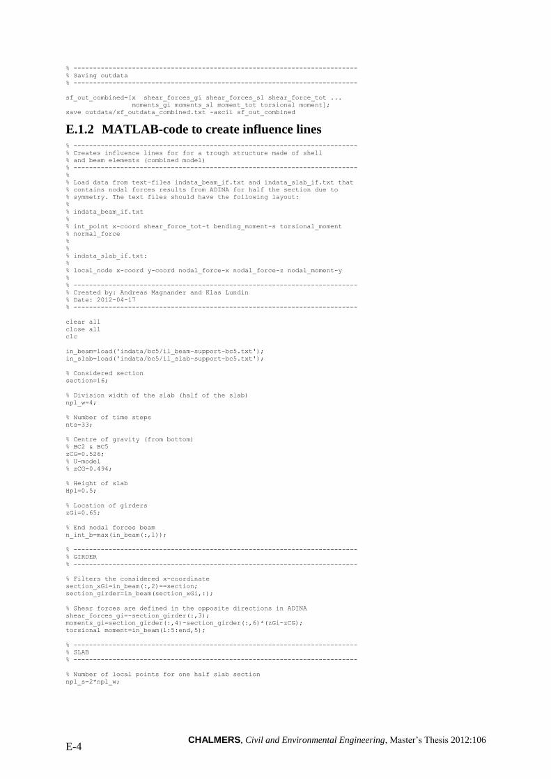
CHALMERS, Civil and Environmental Engineering, Master’s Thesis 2012:106 E-4
% -------------------------------------------------------------------------
% Saving outdata
% -------------------------------------------------------------------------
sf_out_combined=[x shear_forces_gi shear_forces_sl shear_force_tot ...
moments_gi moments_sl moment_tot torsional moment];
save outdata/sf_outdata_combined.txt -ascii sf_out_combined
E.1.2 MATLAB-code to create influence lines % -------------------------------------------------------------------------
% Creates influence lines for for a trough structure made of shell
% and beam elements (combined model)
% -------------------------------------------------------------------------
%
% Load data from text-files indata_beam_if.txt and indata_slab_if.txt that
% contains nodal forces results from ADINA for half the section due to
% symmetry. The text files should have the following layout:
%
% indata_beam_if.txt
%
% int_point x-coord shear_force_tot-t bending_moment-s torsional_moment
% normal_force
%
%
% indata_slab_if.txt:
%
% local_node x-coord y-coord nodal_force-x nodal_force-z nodal_moment-y
%
% -------------------------------------------------------------------------
% Created by: Andreas Magnander and Klas Lundin
% Date: 2012-04-17
% -------------------------------------------------------------------------
clear all
close all
clc
in_beam=load('indata/bc5/il_beam-support-bc5.txt');
in_slab=load('indata/bc5/il_slab-support-bc5.txt');
% Considered section
section=16;
% Division width of the slab (half of the slab)
npl_w=4;
% Number of time steps
nts=33;
% Centre of gravity (from bottom)
% BC2 & BC5
zCG=0.526;
% U-model
% zCG=0.494;
% Height of slab
Hpl=0.5;
% Location of girders
zGi=0.65;
% End nodal forces beam
n_int_b=max(in_beam(:,1));
% -------------------------------------------------------------------------
% GIRDER
% -------------------------------------------------------------------------
% Filters the considered x-coordinate
section_xGi=in_beam(:,2)==section;
section_girder=in_beam(section_xGi,:);
% Shear forces are defined in the opposite directions in ADINA
shear_forces_gi=-section_girder(:,3);
moments_gi=section_girder(:,4)-section_girder(:,6)*(zGi-zCG);
torsional moment=in_beam(1:5:end,5);
% -------------------------------------------------------------------------
% SLAB
% -------------------------------------------------------------------------
% Number of local points for one half slab section
npl_s=2*npl_w;
CHALMERS, Civil and Environmental Engineering, Master’s Thesis 2012:106 E-5
% Filters the considered x-coordinate
section_xSl=in_slab(:,2)==section;
section_slab=in_slab(section_xSl,:);
% Left and right section
plate_left=zeros(length(section_slab)/2,6);
plate_right=zeros(length(section_slab)/2,6);
plate_left(1:2:end)=section_slab(1:4:end);
plate_left(2:2:end)=section_slab(2:4:end);
plate_right(1:2:end)=section_slab(3:4:end);
plate_right(2:2:end)=section_slab(4:4:end);
% Summarise sectional forces in the slab in the considered cross-section.
% According to the sign convention, moment_tot and shear force in the left
% section change sign.
k=0;
shear_forces_sl=zeros(nts*2,1);
moments_sl=zeros(nts*2,1);
moments_sl_tot=zeros(nts*2,1);
for i=1:npl_s:length(plate_left)
% Left
k=k+1;
shear_forces_sl(k)=-sum(plate_left(i:i+npl_s-1,5));
moments_sl(k)=-sum(plate_left(i:i+npl_s-1,6))...
+sum(plate_left(i:i+npl_s-1,4))*(zCG-Hpl/2);
% Right
k=k+1;
shear_forces_sl(k)=sum(plate_right(i:i+npl_s-1,5));
moments_sl(k)=sum(plate_right(i:i+npl_s-1,6))...
-sum(plate_right(i:i+npl_s-1,4))*(zCG-Hpl/2);
end
% Since the input is only for half the section, this will be corrected for
% the slab
shear_forces_sl=2*shear_forces_sl;
moments_sl=2*moments_sl;
% -------------------------------------------------------------------------
% ENTIRE SECTION
% -------------------------------------------------------------------------
% Total sectional forces in entire section (one slab and two girders)
shear_force_tot=shear_forces_sl+2*shear_forces_gi;
moment_tot=moments_sl+2*moments_gi;
% -------------------------------------------------------------------------
% PLOT
% -------------------------------------------------------------------------
% Plot influence lines for slab, girder and total respectively
x=zeros(nts*2,1);
x(3:2:end)=1:nts-1;
x(4:2:end)=1:nts-1;
% Slab
figure(1)
plot(x,shear_forces_sl,'k',[0 x(end)],[0 0],'k')
title('Influence line of shear force in the slab')
xlabel('[m]')
ylabel('[N]')
xlim([x(1) x(end)])
grid on
figure(2)
plot(x,moments_sl,'k',[0 x(end)],[0 0],'k')
title('Influence line of bending moment in the slab')
xlabel('[m]')
ylabel('[Nm]')
xlim([x(1) x(end)])
set(gca,'YDir','reverse');
grid on
% Girder
figure(3)
plot(x,shear_forces_gi,'k',[0 x(end)],[0 0],'k')
title('Influence line of shear force in one girder')
xlabel('[m]')
ylabel('[N]')
xlim([x(1) x(end)])
grid on
CHALMERS, Civil and Environmental Engineering, Master’s Thesis 2012:106 E-6
figure(4)
plot(x,moments_gi,'k', [0 x(end)],[0 0],'k')
title('Influence line of bending moment in one girder')
xlabel('[m]')
ylabel('[Nm]')
xlim([x(1) x(end)])
set(gca,'YDir','reverse');
grid on
% Entire section
figure(5)
plot(x,shear_force_tot,'k',[0 x(end)],[0 0],'k')
title('Influence line of shear force in entire section')
xlabel('[m]')
ylabel('[N]')
xlim([x(1) x(end)])
grid on
figure(6)
plot(x,moment_tot,'k',[0 x(end)],[0 0],'k')
title('Influence line of bending moment in entire section')
xlabel('[m]')
ylabel('[Nm]')
xlim([x(1) x(end)])
set(gca,'YDir','reverse');
grid on
% Torsional moment
figure(7)
plot(x,torsional moment,'k',[0 x(end)],[0 0],'k')
title('Influence line of torsional moment in one girder')
xlabel('[m]')
ylabel('[Nm]')
xlim([x(1) x(end)])
grid on
% -------------------------------------------------------------------------
% Saving outdata
% -------------------------------------------------------------------------
il_out_combined=[x shear_forces_gi shear_forces_sl shear_force_tot ...
moments_gi moments_sl moment_tot torsional moment];
save outdata/il_outdata_combined.txt -ascii il_out_combined
E.2 Shell models
E.2.1 MATLAB-code to create sectional force diagrams (bending moment
and shear force) % -------------------------------------------------------------------------
% Creates sectional force diagrams for a trough structure made with shell
% elements (only bending moment and shear force)
% -------------------------------------------------------------------------
%
% Load data from text-files nodal_forces.txt and nodal_moments.txt that
% contains nodal forces result from ADINA for half the section due to
% symmetry. The text-files are listed as described below.
%
% All nodal moments and forces are summerized and stored in vectors for
% moments, shear forces and torsional moment moments.
%
%
% sf-nodal_forces.txt:
%
% int_point x-coord y-coord z-coord node_force-x node_force-y node_force-z
%
%
% sf-nodal_moments.txt:
%
% int_point x-coord y-coord z-coord node_moment-x node_moment-y
% node_moment-z
%
% The results are saved in the file "if-outdata_shell.txt" and are listed
% as follows:
%
% x-coord shear_girder shear_slab shear_total moment_girder moment_slab
% moment_total
% -------------------------------------------------------------------------
% Created by: Andreas Magnander and Klas Lundin
% Date: 2012-04-17
% -------------------------------------------------------------------------
CHALMERS, Civil and Environmental Engineering, Master’s Thesis 2012:106 E-7
clear all
close all
clc
nodal_forces=load('indata/ua/sf-nodal_forces-span-ua.txt');
nodal_moments=load('indata/ua/sf-nodal_moments-span-ua.txt');
% Length of bridge
L=32;
% Nodes per element
nno=max(nodal_forces(:,1));
% Division width (only half the width) and length for slab
npl_w=5;
npl_l=32;
% Division height and length for girders
ngi_h=6;
ngi_l=32;
% Height of slab
Hpl=0.5;
% Centre of gravity (from bottom)
% ua
zCG=0.543;
% ub
% zCG=0.646;
% Elements in slab
npl=npl_w*npl_l;
% Elements for main girders
ngi=ngi_h*ngi_l;
% Slab
nodal_forces_sl=nodal_forces(1:npl*nno,:);
nodal_moments_sl=nodal_moments(1:npl*nno,:);
% Main girders
nodal_forces_gi=nodal_forces(npl*nno+1:end,:);
nodal_moments_gi=nodal_moments(npl*nno+1:end,:);
% -------------------------------------------------------------------------
% SLAB
% -------------------------------------------------------------------------
% in_slab=[int_point x y z nodal_force-z nodal_moment-y nodal_force-x];
in_slab=[nodal_forces_sl(:,1:4) nodal_forces_sl(:,7) ...
nodal_moments_sl(:,6) nodal_forces_sl(:,5)];
% Nodal forces slab
nodal_forces_slab=zeros(size(in_slab));
% Sorting sections
[~,poss]=sort(in_slab);
for i=1:length(in_slab);
nodal_forces_slab(i,:)=in_slab(poss(i,2),:);
end
% Number of local points for one half slab section
npl_s=2*npl_w;
% First section
slab_first=nodal_forces_slab(1:npl_s,:);
% Sections in-between first and last
slab_main=nodal_forces_slab((npl_s+1):(end-npl_s),:);
% Last section
slab_last=nodal_forces_slab((end-npl_s+1):end,:);
% Left and right section
slab_left=zeros(length(slab_main(:,1))/2,7);
slab_right=zeros(length(slab_main(:,1))/2,7);
% Section left and right
slab_left(1:2:end)=slab_main(1:4:end);
slab_left(2:2:end)=slab_main(2:4:end);
slab_right(1:2:end)=slab_main(3:4:end);
slab_right(2:2:end)=slab_main(4:4:end);
CHALMERS, Civil and Environmental Engineering, Master’s Thesis 2012:106 E-8
% Summarise sectional forces in the slab in the considered cross-section.
% According to the sign convention, moment and shear force in the left
% section change sign.
k=1;
shear_forces_sl=zeros(2*npl_l,1);
moments_sl=zeros(2*npl_l,1);
for i=1:npl_s:length(slab_left)
% Left
k=k+1;
shear_forces_sl(k)=-sum(slab_left(i:i+npl_s-1,5));
moments_sl(k)=-sum(slab_left(i:i+npl_s-1,6))...
+sum(slab_left(i:i+npl_s-1,7))*(zCG-Hpl/2);
% Right
k=k+1;
shear_forces_sl(k)=sum(slab_right(i:i+npl_s-1,5));
moments_sl(k)=sum(slab_right(i:i+npl_s-1,6))...
-sum(slab_right(i:i+npl_s-1,7))*(zCG-Hpl/2);
end
% Adding first and last section
sum_first_sl=sum(slab_first((1:npl_s),5:6));
sum_last_sl=sum(slab_last((1:npl_s),5:6));
shear_forces_sl([1 end],:)=[sum_first_sl(1); -sum_last_sl(1)];
moments_sl([1 end],:)=[sum_first_sl(2); -sum_last_sl(2)];
% Since the input is only for half the section, this will be corrected for
% the slab
shear_forces_sl=2*shear_forces_sl;
moments_sl=2*moments_sl;
% -------------------------------------------------------------------------
% GIRDER
% -------------------------------------------------------------------------
% in_girder=[int_point x y z nodal_force-x nodal_force-z];
in_girder=[nodal_forces_gi(:,1:4) nodal_forces_gi(:,5)...
nodal_forces_gi(:,7)];
% Nodal forces girders
nodal_forces_girder=zeros(size(in_girder));
% Sorting sections
[~,poss]=sort(in_girder);
for i=1:length(in_girder);
nodal_forces_girder(i,:)=in_girder(poss(i,2),:);
end
% Number of local points for one half section
npl_g=2*ngi_h;
% First section
girder_first=nodal_forces_girder(1:npl_g,:);
% Sections in-between first and last
girder_main=nodal_forces_girder((npl_g+1):(end-npl_g),:);
% Last section
girder_last=nodal_forces_girder((end-npl_g+1):end,:);
% Left and right section
girder_left=zeros(length(girder_main(:,1))/2,6);
girder_right=zeros(length(girder_main(:,1))/2,6);
% Section left and right
girder_left(1:2:end)=girder_main(1:4:end);
girder_left(2:2:end)=girder_main(2:4:end);
girder_right(1:2:end)=girder_main(3:4:end);
girder_right(2:2:end)=girder_main(4:4:end);
% Summarise sectional forces in the girder in the considered cross-section.
% According to the sign convention forces in the left section change sign.
% The moment in the girders is calculated as the nodal in x direction times
% a leverarm from the center of the slab.
k=1;
shear_forces_gi=zeros(2*ngi_l,1);
moments_gi=zeros(2*ngi_l,1);
for i=1:npl_g:length(girder_left)
% Left
k=k+1;
shear_forces_gi(k)=-sum(girder_left(i:i+npl_g-1,6));
moments_gi(k)=sum(girder_left(i:i+npl_g-1,5)...
.*(zCG-(girder_left(i:i+npl_g-1,4)+Hpl/2)));
% Right
k=k+1;
shear_forces_gi(k)=sum(girder_right(i:i+npl_g-1,6));
moments_gi(k)=-sum(girder_right(i:i+npl_g-1,5)...
.*(zCG-(girder_right(i:i+npl_g-1,4)+Hpl/2)));
end
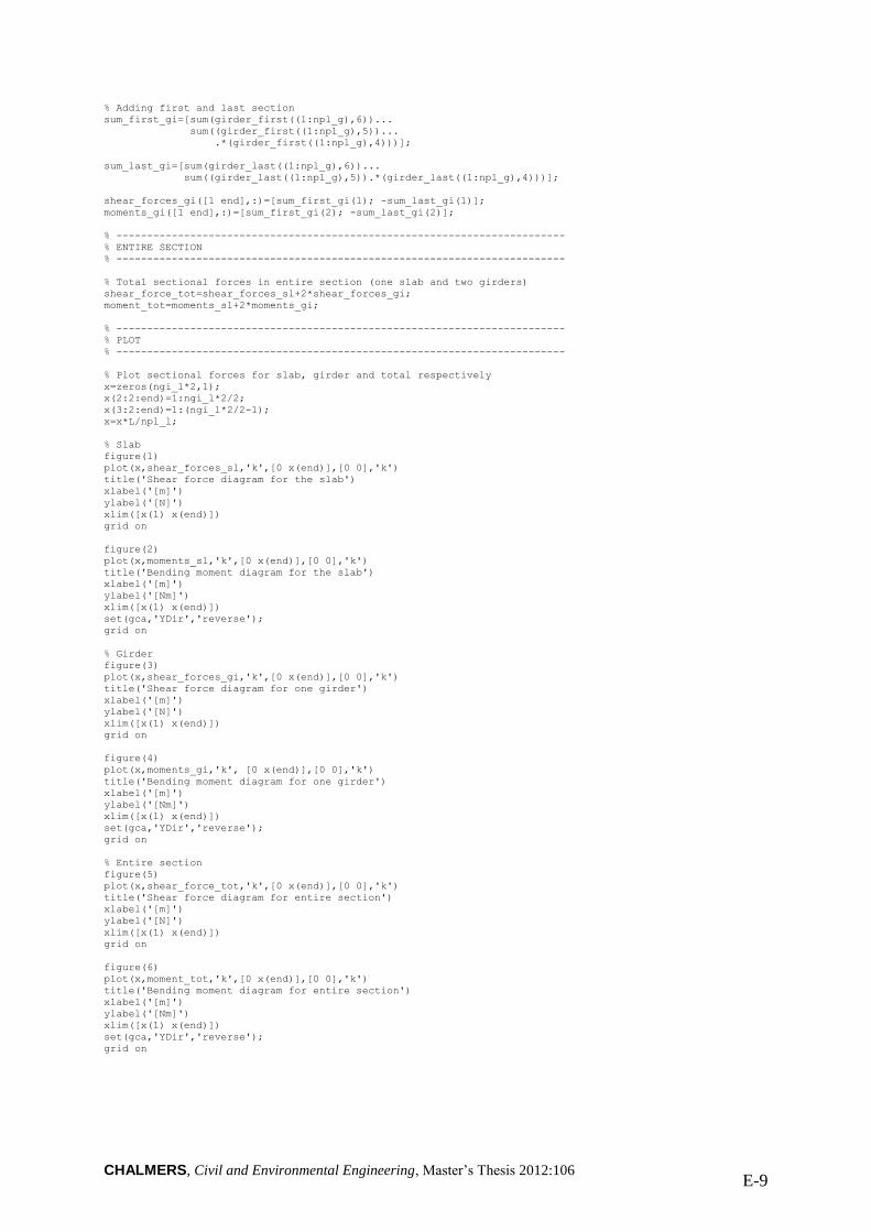
CHALMERS, Civil and Environmental Engineering, Master’s Thesis 2012:106 E-9
% Adding first and last section
sum_first_gi=[sum(girder_first((1:npl_g),6))...
sum((girder_first((1:npl_g),5))...
.*(girder_first((1:npl_g),4)))];
sum_last_gi=[sum(girder_last((1:npl_g),6))...
sum((girder_last((1:npl_g),5)).*(girder_last((1:npl_g),4)))];
shear_forces_gi([1 end],:)=[sum_first_gi(1); -sum_last_gi(1)];
moments_gi([1 end],:)=[sum_first_gi(2); -sum_last_gi(2)];
% -------------------------------------------------------------------------
% ENTIRE SECTION
% -------------------------------------------------------------------------
% Total sectional forces in entire section (one slab and two girders)
shear_force_tot=shear_forces_sl+2*shear_forces_gi;
moment_tot=moments_sl+2*moments_gi;
% -------------------------------------------------------------------------
% PLOT
% -------------------------------------------------------------------------
% Plot sectional forces for slab, girder and total respectively
x=zeros(ngi_l*2,1);
x(2:2:end)=1:ngi_l*2/2;
x(3:2:end)=1:(ngi_l*2/2-1);
x=x*L/npl_l;
% Slab
figure(1)
plot(x,shear_forces_sl,'k',[0 x(end)],[0 0],'k')
title('Shear force diagram for the slab')
xlabel('[m]')
ylabel('[N]')
xlim([x(1) x(end)])
grid on
figure(2)
plot(x,moments_sl,'k',[0 x(end)],[0 0],'k')
title('Bending moment diagram for the slab')
xlabel('[m]')
ylabel('[Nm]')
xlim([x(1) x(end)])
set(gca,'YDir','reverse');
grid on
% Girder
figure(3)
plot(x,shear_forces_gi,'k',[0 x(end)],[0 0],'k')
title('Shear force diagram for one girder')
xlabel('[m]')
ylabel('[N]')
xlim([x(1) x(end)])
grid on
figure(4)
plot(x,moments_gi,'k', [0 x(end)],[0 0],'k')
title('Bending moment diagram for one girder')
xlabel('[m]')
ylabel('[Nm]')
xlim([x(1) x(end)])
set(gca,'YDir','reverse');
grid on
% Entire section
figure(5)
plot(x,shear_force_tot,'k',[0 x(end)],[0 0],'k')
title('Shear force diagram for entire section')
xlabel('[m]')
ylabel('[N]')
xlim([x(1) x(end)])
grid on
figure(6)
plot(x,moment_tot,'k',[0 x(end)],[0 0],'k')
title('Bending moment diagram for entire section')
xlabel('[m]')
ylabel('[Nm]')
xlim([x(1) x(end)])
set(gca,'YDir','reverse');
grid on
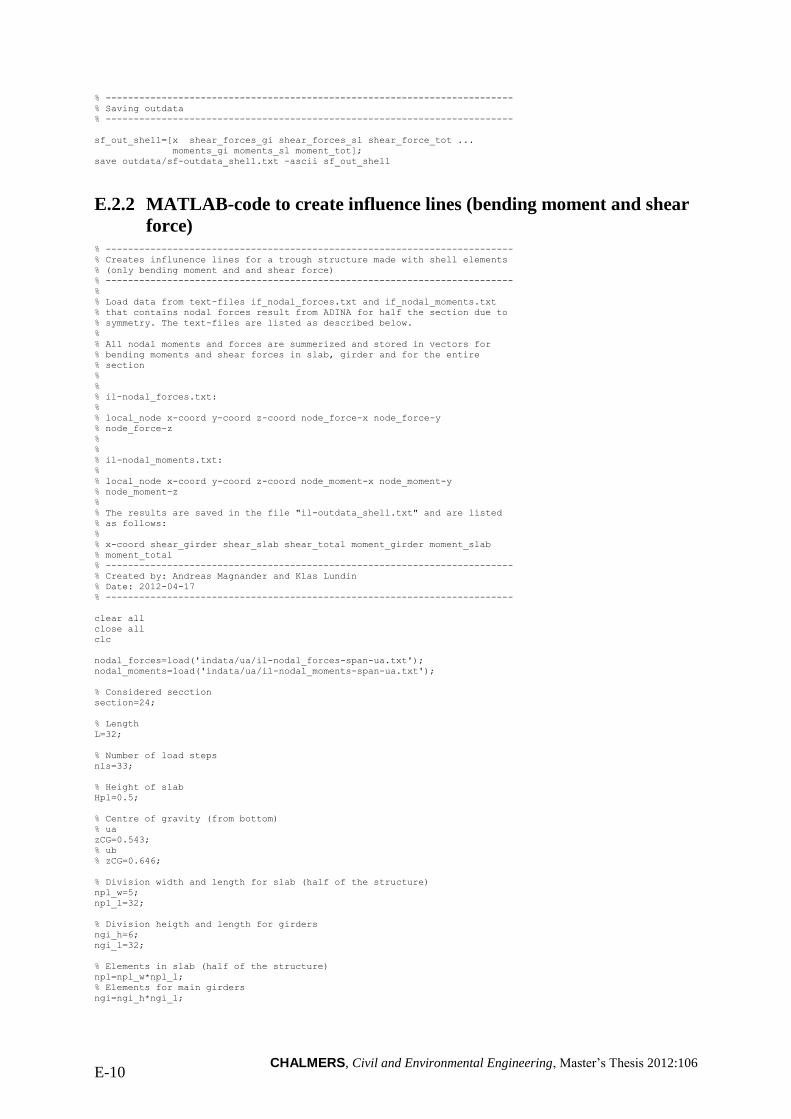
CHALMERS, Civil and Environmental Engineering, Master’s Thesis 2012:106 E-10
% -------------------------------------------------------------------------
% Saving outdata
% -------------------------------------------------------------------------
sf_out_shell=[x shear_forces_gi shear_forces_sl shear_force_tot ...
moments_gi moments_sl moment_tot];
save outdata/sf-outdata_shell.txt -ascii sf_out_shell
E.2.2 MATLAB-code to create influence lines (bending moment and shear
force) % -------------------------------------------------------------------------
% Creates influnence lines for a trough structure made with shell elements
% (only bending moment and and shear force)
% -------------------------------------------------------------------------
%
% Load data from text-files if_nodal_forces.txt and if_nodal_moments.txt
% that contains nodal forces result from ADINA for half the section due to
% symmetry. The text-files are listed as described below.
%
% All nodal moments and forces are summerized and stored in vectors for
% bending moments and shear forces in slab, girder and for the entire
% section
%
%
% il-nodal_forces.txt:
%
% local_node x-coord y-coord z-coord node_force-x node_force-y
% node_force-z
%
%
% il-nodal_moments.txt:
%
% local_node x-coord y-coord z-coord node_moment-x node_moment-y
% node_moment-z
%
% The results are saved in the file "il-outdata_shell.txt" and are listed
% as follows:
%
% x-coord shear_girder shear_slab shear_total moment_girder moment_slab
% moment_total
% -------------------------------------------------------------------------
% Created by: Andreas Magnander and Klas Lundin
% Date: 2012-04-17
% -------------------------------------------------------------------------
clear all
close all
clc
nodal_forces=load('indata/ua/il-nodal_forces-span-ua.txt');
nodal_moments=load('indata/ua/il-nodal_moments-span-ua.txt');
% Considered secction
section=24;
% Length
L=32;
% Number of load steps
nls=33;
% Height of slab
Hpl=0.5;
% Centre of gravity (from bottom)
% ua
zCG=0.543;
% ub
% zCG=0.646;
% Division width and length for slab (half of the structure)
npl_w=5;
npl_l=32;
% Division heigth and length for girders
ngi_h=6;
ngi_l=32;
% Elements in slab (half of the structure)
npl=npl_w*npl_l;
% Elements for main girders
ngi=ngi_h*ngi_l;
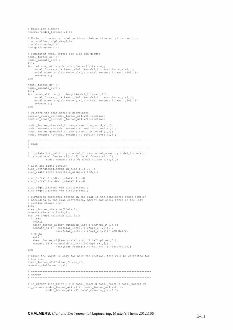
CHALMERS, Civil and Environmental Engineering, Master’s Thesis 2012:106 E-11
% Nodes per element
nno=max(nodal_forces(:,1));
% Number of nodes in total section, slab section and girder section
nno_tot=2*nno*(npl_w+ngi_h);
nno_sl=2*nno*npl_w;
nno_gi=2*nno*ngi_h;
% Separates nodal forces for slab and girder
nodal_forces_sl=[];
nodal_moments_sl=[];
k=1;
for i=1:nno_tot:length(nodal_forces(:,1))-nno_gi
nodal_forces_sl(k:k+nno_sl-1,:)=nodal_forces(i:i+nno_sl-1,:);
nodal_moments_sl(k:k+nno_sl-1,:)=nodal_moments(i:i+nno_sl-1,:);
k=k+nno_sl;
end
nodal_forces_gi=[];
nodal_moments_gi=[];
k=1;
for i=nno_sl+1:nno_tot:length(nodal_forces(:,1))
nodal_forces_gi(k:k+nno_gi-1,:)=nodal_forces(i:i+nno_gi-1,:);
nodal_moments_gi(k:k+nno_gi-1,:)=nodal_moments(i:i+nno_gi-1,:);
k=k+nno_gi;
end
% Filters the considered x-coordinate
section_coord_sl=nodal_forces_sl(:,2)==section;
section_coord_gi=nodal_forces_gi(:,2)==section;
nodal_forces_sl=nodal_forces_sl(section_coord_sl,:);
nodal_moments_sl=nodal_moments_sl(section_coord_sl,:);
nodal_forces_gi=nodal_forces_gi(section_coord_gi,:);
nodal_moments_gi=nodal_moments_gi(section_coord_gi,:);
% -------------------------------------------------------------------------
% SLAB
% -------------------------------------------------------------------------
% in_slab=[int_point x y z nodal_force-z nodal_moment-y nodal_force-x];
in_slab=[nodal_forces_sl(:,1:4) nodal_forces_sl(:,7) ...
nodal_moments_sl(:,6) nodal_forces_sl(:,5)];
% Left and right section
slab_left=zeros(length(in_slab(:,1))/2,7);
slab_right=zeros(length(in_slab(:,1))/2,7);
slab_left(1:2:end)=in_slab(1:4:end);
slab_left(2:2:end)=in_slab(2:4:end);
slab_right(1:2:end)=in_slab(3:4:end);
slab_right(2:2:end)=in_slab(4:4:end);
% Summarise sectional forces in the slab in the considered cross-section.
% According to the sign convention, moment and shear force in the left
% section change sign.
k=0;
shear_forces_sl=zeros(2*nls,1);
moments_sl=zeros(2*nls,1);
for i=1:2*npl_w:length(slab_left)
% Left
k=k+1;
shear_forces_sl(k)=-sum(slab_left(i:i+2*npl_w-1,5));
moments_sl(k)=-sum(slab_left(i:i+2*npl_w-1,6))...
+sum(slab_left(i:i+2*npl_w-1,7))*(zCG-Hpl/2);
% Right
k=k+1;
shear_forces_sl(k)=sum(slab_right(i:i+2*npl_w-1,5));
moments_sl(k)=sum(slab_right(i:i+2*npl_w-1,6))...
-sum(slab_right(i:i+2*npl_w-1,7))*(zCG-Hpl/2);
end
% Since the input is only for half the section, this will be corrected for
% the slab
shear_forces_sl=2*shear_forces_sl;
moments_sl=2*moments_sl;
% -------------------------------------------------------------------------
% GIRDER
% -------------------------------------------------------------------------
% in_girder=[int_point x y z nodal_force-x nodal_force-z nodal_moment-y];
in_girder=[nodal_forces_gi(:,1:4) nodal_forces_gi(:,5) ...
nodal_forces_gi(:,7) nodal_moments_gi(:,6)];
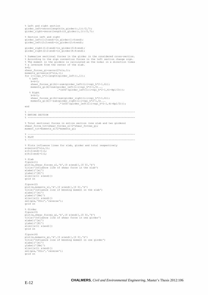
CHALMERS, Civil and Environmental Engineering, Master’s Thesis 2012:106 E-12
% Left and right section
girder_left=zeros(length(in_girder(:,1))/2,7);
girder_right=zeros(length(in_girder(:,1))/2,7);
% Section left and right
girder_left(1:2:end)=in_girder(1:4:end);
girder_left(2:2:end)=in_girder(2:4:end);
girder_right(1:2:end)=in_girder(3:4:end);
girder_right(2:2:end)=in_girder(4:4:end);
% Summarise sectional forces in the girder in the considered cross-section.
% According to the sign convention forces in the left section change sign.
% The moment in the girders is calculated as the nodal in x direction times
% a leverarm from the center of the slab.
k=0;
shear_forces_gi=zeros(2*nls,1);
moments_gi=zeros(2*nls,1);
for i=1:ngi_h*2:length(girder_left(:,1));
% Left
k=k+1;
shear_forces_gi(k)=-sum(girder_left(i:i+ngi_h*2-1,6));
moments_gi(k)=sum(girder_left(i:i+ngi_h*2-1,5)...
.*(zCG-(girder_left(i:i+ngi_h*2-1,4)+Hpl/2)));
% Right
k=k+1;
shear_forces_gi(k)=sum(girder_right(i:i+ngi_h*2-1,6));
moments_gi(k)=-sum(girder_right(i:i+ngi_h*2-1,5)...
.*(zCG-(girder_left(i:i+ngi_h*2-1,4)+Hpl/2)));
end
% -------------------------------------------------------------------------
% ENTIRE SECTION
% -------------------------------------------------------------------------
% Total sectional forces in entire section (one slab and two girders)
shear_force_tot=shear_forces_sl+2*shear_forces_gi;
moment_tot=moments_sl+2*moments_gi;
% -------------------------------------------------------------------------
% PLOT
% -------------------------------------------------------------------------
% Plots influence lines for slab, girder and total respectively
x=zeros(2*nls,1);
x(3:2:end)=1:L;
x(4:2:end)=1:L;
% Slab
figure(1)
plot(x,shear_forces_sl,'k',[0 x(end)],[0 0],'k')
title('Influence line of shear force in the slab')
xlabel('[m]')
ylabel('[N]')
xlim([x(1) x(end)])
grid on
figure(2)
plot(x,moments_sl,'k',[0 x(end)],[0 0],'k')
title('Influence line of bending moment in the slab')
xlabel('[m]')
ylabel('[Nm]')
xlim([x(1) x(end)])
set(gca,'YDir','reverse');
grid on
% Girder
figure(3)
plot(x,shear_forces_gi,'k',[0 x(end)],[0 0],'k')
title('Influence line of shear force in one girder')
xlabel('[m]')
ylabel('[N]')
xlim([x(1) x(end)])
grid on
figure(4)
plot(x,moments_gi,'k',[0 x(end)],[0 0],'k')
title('Influence line of bending moment in one girder')
xlabel('[m]')
ylabel('[Nm]')
xlim([x(1) x(end)])
set(gca,'YDir','reverse');
grid on
CHALMERS, Civil and Environmental Engineering, Master’s Thesis 2012:106 E-13
% Entire section
figure(5)
plot(x,shear_force_tot,'k',[0 x(end)],[0 0],'k')
title('Influence line of shear force for entire section')
xlabel('[m]')
ylabel('[N]')
xlim([x(1) x(end)])
grid on
figure(6)
plot(x,moment_tot,'k',[0 x(end)],[0 0],'k')
title('Influence line of bending moment for entire section')
xlabel('[m]')
ylabel('[Nm]')
xlim([x(1) x(end)])
set(gca,'YDir','reverse');
grid on
% -------------------------------------------------------------------------
% Saving outdata
% -------------------------------------------------------------------------
il_out_shell=[x shear_forces_gi shear_forces_sl shear_force_tot ...
moments_gi moments_sl moment_tot];
save outdata/il-outdata_shell.txt -ascii il_out_shell
E.2.3 MATLAB-code to create sectional force diagrams and influence lines
with the TSE-method (torsional moment) % -------------------------------------------------------------------------
% TSEM (Torsion from Slab Edge Method)
%
% The method caluclates torsional moments in a girder connected with a
% plate.
%
%
% The MATLAB program create torsional moment diagrams for a trough
% structure modelled with 4-node shell elements applied with a moving load
% using time steps. With these torsional moment diagrams, the influence lines for
% torsional moment are also created.
%
%
% Load data from text-files reaction-moment.txt, reaction-y, nodals.txt
% containing reaction and nodal force results from ADINA. The text-
% files should have the layout as described below.
%
% -------------------------------------------------------------------------
% reaction-moment.txt:
%
% reaction-moment-x end support 1 (x=0) for timestep 1
% reaction-moment-x end support 2 (x=32) for timestep 1
% reaction-moment-x end support 1 (x=0) for timestep 1
% reaction-moment-x end support 2 (x=32) for timestep 1
% .
% .
% .
% reaction-moment-x end support 1 (x=0) for timestep 1
% reaction-moment-x end support 2 (x=32) for timestep 1
% .
% .
% .
% reaction-moment-x end support 1 (x=0) for timestep 2
% reaction-moment-x end support 2 (x=32) for timestep 2
% reaction-moment-x end support 1 (x=0) for timestep 2
% reaction-moment-x end support 2 (x=32) for timestep 2
% .
% .
% .
% reaction-moment-x end support 1 (x=0) for timestep 2
% reaction-moment-x end support 2 (x=32) for timestep 2
% .
% .
% .
% reaction-moment-x end support 1 (x=0) for timestep n
% reaction-moment-x end support 2 (x=32) for timestep n
% reaction-moment-x end support 1 (x=0) for timestep n
% reaction-moment-x end support 2 (x=32) for timestep n
% .
% .
% .
% reaction-moment-x end support 1 (x=0) for timestep n
% reaction-moment-x end support 2 (x=32) for timestep n
%
CHALMERS, Civil and Environmental Engineering, Master’s Thesis 2012:106 E-14
% -------------------------------------------------------------------------
% reaction-y.txt:
%
% reaction-y end support 1 (x=0) for timestep 1
% reaction-y mid support for timestep 1
% reaction-y end support 2 (x=32) for timestep 1
% reaction-y end support 1 (x=0) for timestep 2
% reaction-y mid support for timestep 2
% reaction-y end support 2 (x=32) for timestep 2
% .
% .
% .
% reaction-y end support 1 (x=0) for timestep n
% reaction-y mid support for timestep n
% reaction-y end support 2 (x=32) for timestep n
%
% -------------------------------------------------------------------------
% nodals.txt:
%
% local_node x-coord y-coord node_force-y node_moment-x timestep 1
% local_node x-coord y-coord node_force-y node_moment-x timestep 2
% .
% .
% .
% local_node x-coord y-coord node_force-y node_moment-x timestep n
%
%
% -------------------------------------------------------------------------
% Created by: Andreas Magnander and Klas Lundin
% Date: 2012-05-10
% -------------------------------------------------------------------------
clear all
close all
clc
reaction_moment=load('indata/ua/tsem-reaction_moment_x-ua.txt');
reaction_y=load('indata/ua/tsem-reaction_y-ua.txt');
nodals=load('indata/ua/tsem-nodals-ua.txt');
% At which x-coordinate should torsional moment influence line (and section force
% diagram) be for?
coord=24;
% Division length for plate
npl=32;
% height main girders
h=1.05;
% Length of shell
l=32;
% y-translation fixed somewhere in plate?
% 1=yes, 0=no
reaction_plate=1;
% At which x-coordinate in that case?
reaction_plate_coord=16;
% Number of load steps
nls=33;
% Number of nodes fixed in height for torsional moment (just one side)
nnt=7;
% Since the nodes are at x=0, x=32, x=0, x=32, ... and so on, the nodes at
% x=0 are at position 1,3,5,... and x=32 are at positions 2,4,5,...
% Sorting the reaction forces to get all nodes at x=0 first and x=32
% thereafter for each time step
reaction_moment_sorted=zeros(size(reaction_moment));
for i=1:2*nnt:length(reaction_moment)
reaction_moment_sorted(i:(i+nnt-1))=reaction_moment(i:2:(i+2*nnt-1));
reaction_moment_sorted((i+nnt):(i+2*nnt-1))=...
reaction_moment((i+1):2:(i+2*nnt-1));
end
% Summarise reaction torsional moment at x=0 and x=32
x_moment_reactions=zeros(length(reaction_moment)/nnt,1);
k=1;
for i=1:nnt:length(reaction_moment)
x_moment_reactions(k)=sum(reaction_moment_sorted(i:i+nnt-1));
k=k+1;
end
reaction_moment=x_moment_reactions;
CHALMERS, Civil and Environmental Engineering, Master’s Thesis 2012:106 E-15
% Positions for each time step
j_reaction_moment=1:2:size(reaction_moment,1);
j_reaction_y=1:3:size(reaction_y,1);
j_nodals=1:(npl*4):(npl*4*nls);
% All torsional moment diagrams (rows) for each time step (columns)
torsional moment_diagrams=zeros(npl*2,nls);
for j=1:nls
% Element numbers
elnum=zeros(npl*2,1);
elnum(1:2:end)=1:npl;
elnum(2:2:end)=1:npl;
% Pick nodals for each load step
% Remove local node 3 and 4 and insert element numbers
nodals_el_full=nodals(j_nodals(j):(j_nodals(j)+npl*4-1),:);
nodals_el_full(3:4:end,:)=[];
nodals_el_full(3:3:end,:)=[];
nodals_el=[elnum nodals_el_full];
% Torsions from plate, from moment in first column and axial force in
% second column
torsional moment_pl=zeros(npl+1,2);
% Torsion from moment in plate
torsional moment_pl(1,1)=nodals_el(1,6);
% Torsion from axial force in plate (considered later when creating
% diagram in torsional moment(1))
torsional moment_pl(1,2)=0;
k=2;
for i=2:2:size(nodals_el,1)-1
% Torsion from moment in plate
torsional moment_pl(k,1)=nodals_el(i,6)+nodals_el(i+1,6);
% Torsion from axial force in plate
torsional moment_pl(k,2)=(nodals_el(i,5)+nodals_el(i+1,5))*h/2;
if reaction_plate && reaction_plate_coord == nodals_el(i,3)
% Torsion from axial force in plate
torsional moment_pl(k,2)=((nodals_el(i,5)+nodals_el(i+1,5)) ...
-reaction_y(j_reaction_y(j)+1))*h/2;
end
k=k+1;
end
torsional moment_pl_sum=sum(torsional moment_pl,2);
% ---------------------------------------------------------------------
% Calculate torsional moment in all sections for all load steps
% ---------------------------------------------------------------------
torsional moment=zeros(npl*2,1);
% First section
torsional moment(1)=-reaction_moment(j_reaction_moment(j)) ...
+(nodals_el(1,5)-reaction_y(j_reaction_y(j)))*h/2 ...
+torsional moment_pl_sum(1);
% Sections between first and last
k=2;
for i=2:npl
torsional moment(k)=torsional moment(k-1);
k=k+1;
torsional moment(k)=torsional moment(k-1)+torsional moment_pl_sum(i);
k=k+1;
end
% Last section
torsional moment(end)=torsional moment(end-1);
% Store all torsional moment diagrams on each column
torsional moment_diagrams(:,j)=torsional moment;
end
% -------------------------------------------------------------------------
% Create influence line of torsional moment
% -------------------------------------------------------------------------
x1=zeros(nls*2,1);
x1(1:2:end-1)=0:nls-1;
x1(2:2:end)=0:nls-1;
section=npl*2*coord/l;
CHALMERS, Civil and Environmental Engineering, Master’s Thesis 2012:106 E-16
influence_at_coord=torsional moment_diagrams(section:section+1,:)';
il_torsional moment=zeros(nls*2,1);
il_torsional moment(1:2:end-1)=influence_at_coord(:,1);
il_torsional moment(2:2:end)=influence_at_coord(:,2);
disp(['Influence line for torsional moment at ' num2str(coord) ' m'])
disp([x1 il_torsional moment])
figure(1)
plot(x1,il_torsional moment, 'k',[x1(1) x1(end)],[0 0],'k')
title(['Influence line for torsional moment at ' num2str(coord) ' m'])
xlabel('m')
ylabel('Torsion')
xlim([x1(1) x1(end)])
grid on
% -------------------------------------------------------------------------
% Create torsional moment diagram
% -------------------------------------------------------------------------
x2=zeros(npl*2,1);
x2(2:2:end)=1:npl;
x2(3:2:end)=1:(npl-1);
x2=l*x2/npl;
sf_torsional moment=torsional moment_diagrams(:,coord+1);
disp(['Torsional moment when load at ' num2str(coord) ' m'])
disp([x2 sf_torsional moment])
figure(2)
plot(x2,sf_torsional moment, 'k',[x2(1) x2(end)],[0 0],'k')
title(['Torsional moment diagram for load at ' num2str(coord) ' m'])
xlabel('m')
ylabel('Torsion')
xlim([x2(1) x2(end)])
grid on
% -------------------------------------------------------------------------
% Saving outdata
% -------------------------------------------------------------------------
il_out_torsional moment=[x1 il_torsional moment];
sf_out_torsional moment=[x2 sf_torsional moment];
save outdata/il-outdata_shell-torsional moment.txt -ascii il_out_torsional moment
save outdata/sf-outdata_shell-torsional moment.txt -ascii sf_out_torsional moment

CHALMERS, Civil and Environmental Engineering, Master’s Thesis 2012:106 F-1
Appendix F ADINA-IN command files
In ADINA an easy and convenient way to create models is to use ADINA-IN command files
(*.in) that includes all the commands that should be performed. In the command file it is
possible to call other files as functions. This is used for the load steps (the time function) since
they are same for most models.
F.1 Time function TIMESTEP NAME=DEFAULT
@CLEAR
33 1
@
TIMEFUNCTION NAME=1
@CLEAR
0 0
1 1
2 0
33 0
@
TIMEFUNCTION NAME=2
@CLEAR
0 0
1 0
2 1
3 0
33 0
@
TIMEFUNCTION NAME=3
@CLEAR
0 0
2 0
3 1
4 0
33 0
@
TIMEFUNCTION NAME=4
@CLEAR
0 0
3 0
4 1
5 0
33 0
@
TIMEFUNCTION NAME=5
@CLEAR
0 0
4 0
5 1
6 0
33 0
@
TIMEFUNCTION NAME=6
@CLEAR
0 0
5 0
6 1
7 0
33 0
@
TIMEFUNCTION NAME=7
@CLEAR
0 0
6 0
7 1
8 0
33 0
@
TIMEFUNCTION NAME=8
@CLEAR
0 0
7 0
8 1
9 0
33 0
@
TIMEFUNCTION NAME=9
@CLEAR
0 0
8 0
9 1
10 0
33 0
@
TIMEFUNCTION NAME=10
@CLEAR
0 0
9 0
10 1
11 0
33 0
@
TIMEFUNCTION NAME=11
@CLEAR
0 0
10 0
11 1
12 0
33 0
@
TIMEFUNCTION NAME=12
@CLEAR
0 0
11 0
12 1
13 0
33 0
@
TIMEFUNCTION NAME=13
@CLEAR
0 0
12 0
13 1
14 0
33 0
@
TIMEFUNCTION NAME=14
@CLEAR
0 0
13 0
14 1
15 0
33 0
@
TIMEFUNCTION NAME=15
@CLEAR
0 0
14 0
15 1
16 0
33 0
@
TIMEFUNCTION NAME=16
@CLEAR
0 0
15 0
16 1
17 0
33 0
@
TIMEFUNCTION NAME=17
@CLEAR
0 0
16 0
17 1
18 0
33 0
@
TIMEFUNCTION NAME=18
@CLEAR
0 0
17 0
18 1
19 0
33 0
@
TIMEFUNCTION NAME=19
@CLEAR
0 0
18 0
19 1
20 0
33 0
@
TIMEFUNCTION NAME=20
@CLEAR
0 0
19 0
20 1
21 0
33 0
@
TIMEFUNCTION NAME=21
@CLEAR
0 0
20 0
21 1
22 0
33 0
@
TIMEFUNCTION NAME=22
@CLEAR
0 0
21 0
22 1
23 0
33 0
@
TIMEFUNCTION NAME=23
@CLEAR
0 0
22 0
23 1
24 0
33 0
@
TIMEFUNCTION NAME=24
@CLEAR
0 0
23 0
24 1
25 0
33 0
@
TIMEFUNCTION NAME=25
@CLEAR
0 0
24 0
25 1
26 0
33 0
@
TIMEFUNCTION NAME=26
@CLEAR
0 0
25 0
26 1
27 0
33 0
@
TIMEFUNCTION NAME=27
@CLEAR
0 0
26 0
27 1
28 0
33 0
@
TIMEFUNCTION NAME=28
@CLEAR
0 0
27 0
28 1
29 0
33 0
@
TIMEFUNCTION NAME=29
@CLEAR
0 0
28 0
29 1
30 0
33 0
@
TIMEFUNCTION NAME=30
@CLEAR
0 0
29 0
30 1
31 0
33 0
@
TIMEFUNCTION NAME=31
@CLEAR
0 0
30 0
31 1
32 0
33 0
@
TIMEFUNCTION NAME=32
@CLEAR
0 0
31 0
32 1
33 0
@
TIMEFUNCTION NAME=33
@CLEAR
0 0
32 0
33 1
@
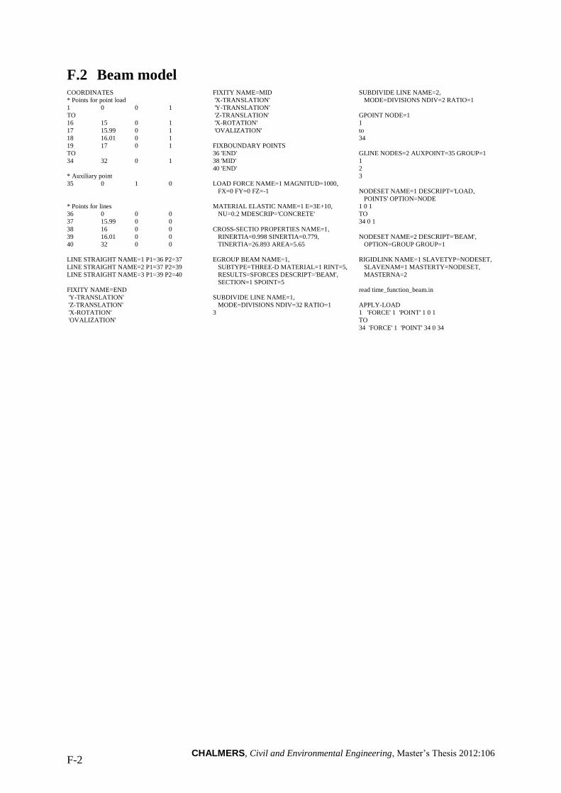
CHALMERS, Civil and Environmental Engineering, Master’s Thesis 2012:106 F-2
F.2 Beam model COORDINATES
* Points for point load
1 0 0 1
TO
16 15 0 1
17 15.99 0 1
18 16.01 0 1
19 17 0 1
TO
34 32 0 1
* Auxiliary point
35 0 1 0
* Points for lines
36 0 0 0
37 15.99 0 0
38 16 0 0
39 16.01 0 0
40 32 0 0
LINE STRAIGHT NAME=1 P1=36 P2=37
LINE STRAIGHT NAME=2 P1=37 P2=39
LINE STRAIGHT NAME=3 P1=39 P2=40
FIXITY NAME=END
'Y-TRANSLATION'
'Z-TRANSLATION'
'X-ROTATION'
'OVALIZATION'
FIXITY NAME=MID
'X-TRANSLATION'
'Y-TRANSLATION'
'Z-TRANSLATION'
'X-ROTATION'
'OVALIZATION'
FIXBOUNDARY POINTS
36 'END'
38 'MID'
40 'END'
LOAD FORCE NAME=1 MAGNITUD=1000,
FX=0 FY=0 FZ=-1
MATERIAL ELASTIC NAME=1 E=3E+10,
NU=0.2 MDESCRIP='CONCRETE'
CROSS-SECTIO PROPERTIES NAME=1,
RINERTIA=0.998 SINERTIA=0.779,
TINERTIA=26.893 AREA=5.65
EGROUP BEAM NAME=1,
SUBTYPE=THREE-D MATERIAL=1 RINT=5,
RESULTS=SFORCES DESCRIPT='BEAM',
SECTION=1 SPOINT=5
SUBDIVIDE LINE NAME=1,
MODE=DIVISIONS NDIV=32 RATIO=1
3
SUBDIVIDE LINE NAME=2,
MODE=DIVISIONS NDIV=2 RATIO=1
GPOINT NODE=1
1
to
34
GLINE NODES=2 AUXPOINT=35 GROUP=1
1
2
3
NODESET NAME=1 DESCRIPT='LOAD,
POINTS' OPTION=NODE
1 0 1
TO
34 0 1
NODESET NAME=2 DESCRIPT='BEAM',
OPTION=GROUP GROUP=1
RIGIDLINK NAME=1 SLAVETYP=NODESET,
SLAVENAM=1 MASTERTY=NODESET,
MASTERNA=2
read time_function_beam.in
APPLY-LOAD
1 'FORCE' 1 'POINT' 1 0 1
TO
34 'FORCE' 1 'POINT' 34 0 34
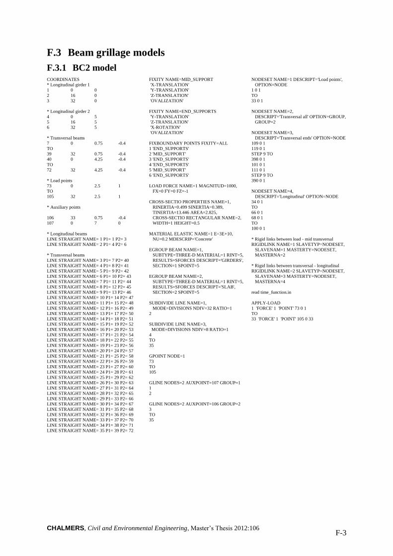
CHALMERS, Civil and Environmental Engineering, Master’s Thesis 2012:106 F-3
F.3 Beam grillage models
F.3.1 BC2 model COORDINATES
* Longitudinal girder 1
1 0 0
2 16 0
3 32 0
* Longitudinal girder 2
4 0 5
5 16 5
6 32 5
* Transversal beams
7 0 0.75 -0.4
TO
39 32 0.75 -0.4
40 0 4.25 -0.4
TO
72 32 4.25 -0.4
* Load points
73 0 2.5 1
TO
105 32 2.5 1
* Auxiliary points
106 33 0.75 -0.4
107 0 7 0
* Longitudinal beams
LINE STRAIGHT NAME= 1 P1= 1 P2= 3
LINE STRAIGHT NAME= 2 P1= 4 P2= 6
* Transversal beams
LINE STRAIGHT NAME= 3 P1= 7 P2= 40
LINE STRAIGHT NAME= 4 P1= 8 P2= 41
LINE STRAIGHT NAME= 5 P1= 9 P2= 42
LINE STRAIGHT NAME= 6 P1= 10 P2= 43
LINE STRAIGHT NAME= 7 P1= 11 P2= 44
LINE STRAIGHT NAME= 8 P1= 12 P2= 45
LINE STRAIGHT NAME= 9 P1= 13 P2= 46
LINE STRAIGHT NAME= 10 P1= 14 P2= 47
LINE STRAIGHT NAME= 11 P1= 15 P2= 48
LINE STRAIGHT NAME= 12 P1= 16 P2= 49
LINE STRAIGHT NAME= 13 P1= 17 P2= 50
LINE STRAIGHT NAME= 14 P1= 18 P2= 51
LINE STRAIGHT NAME= 15 P1= 19 P2= 52
LINE STRAIGHT NAME= 16 P1= 20 P2= 53
LINE STRAIGHT NAME= 17 P1= 21 P2= 54
LINE STRAIGHT NAME= 18 P1= 22 P2= 55
LINE STRAIGHT NAME= 19 P1= 23 P2= 56
LINE STRAIGHT NAME= 20 P1= 24 P2= 57
LINE STRAIGHT NAME= 21 P1= 25 P2= 58
LINE STRAIGHT NAME= 22 P1= 26 P2= 59
LINE STRAIGHT NAME= 23 P1= 27 P2= 60
LINE STRAIGHT NAME= 24 P1= 28 P2= 61
LINE STRAIGHT NAME= 25 P1= 29 P2= 62
LINE STRAIGHT NAME= 26 P1= 30 P2= 63
LINE STRAIGHT NAME= 27 P1= 31 P2= 64
LINE STRAIGHT NAME= 28 P1= 32 P2= 65
LINE STRAIGHT NAME= 29 P1= 33 P2= 66
LINE STRAIGHT NAME= 30 P1= 34 P2= 67
LINE STRAIGHT NAME= 31 P1= 35 P2= 68
LINE STRAIGHT NAME= 32 P1= 36 P2= 69
LINE STRAIGHT NAME= 33 P1= 37 P2= 70
LINE STRAIGHT NAME= 34 P1= 38 P2= 71
LINE STRAIGHT NAME= 35 P1= 39 P2= 72
FIXITY NAME=MID_SUPPORT
'X-TRANSLATION'
'Y-TRANSLATION'
'Z-TRANSLATION'
'OVALIZATION'
FIXITY NAME=END_SUPPORTS
'Y-TRANSLATION'
'Z-TRANSLATION'
'X-ROTATION'
'OVALIZATION'
FIXBOUNDARY POINTS FIXITY=ALL
1 'END_SUPPORTS'
2 'MID_SUPPORT'
3 'END_SUPPORTS'
4 'END_SUPPORTS'
5 'MID_SUPPORT'
6 'END_SUPPORTS'
LOAD FORCE NAME=1 MAGNITUD=1000,
FX=0 FY=0 FZ=-1
CROSS-SECTIO PROPERTIES NAME=1,
RINERTIA=0.499 SINERTIA=0.389,
TINERTIA=13.446 AREA=2.825,
CROSS-SECTIO RECTANGULAR NAME=2,
WIDTH=1 HEIGHT=0.5
MATERIAL ELASTIC NAME=1 E=3E+10,
NU=0.2 MDESCRIP='Concrete'
EGROUP BEAM NAME=1,
SUBTYPE=THREE-D MATERIAL=1 RINT=5,
RESULTS=SFORCES DESCRIPT='GIRDERS',
SECTION=1 SPOINT=5
EGROUP BEAM NAME=2,
SUBTYPE=THREE-D MATERIAL=1 RINT=5,
RESULTS=SFORCES DESCRIPT='SLAB',
SECTION=2 SPOINT=5
SUBDIVIDE LINE NAME=1,
MODE=DIVISIONS NDIV=32 RATIO=1
2
SUBDIVIDE LINE NAME=3,
MODE=DIVISIONS NDIV=8 RATIO=1
4
TO
35
GPOINT NODE=1
73
TO
105
GLINE NODES=2 AUXPOINT=107 GROUP=1
1
2
GLINE NODES=2 AUXPOINT=106 GROUP=2
3
TO
35
NODESET NAME=1 DESCRIPT='Load points',
OPTION=NODE
1 0 1
TO
33 0 1
NODESET NAME=2,
DESCRIPT='Transversal all' OPTION=GROUP,
GROUP=2
NODESET NAME=3,
DESCRIPT='Transversal ends' OPTION=NODE
109 0 1
119 0 1
STEP 9 TO
398 0 1
101 0 1
111 0 1
STEP 9 TO
390 0 1
NODESET NAME=4,
DESCRIPT='Longitudinal' OPTION=NODE
34 0 1
TO
66 0 1
68 0 1
TO
100 0 1
* Rigid links between load - mid transversal
RIGIDLINK NAME=1 SLAVETYP=NODESET,
SLAVENAM=1 MASTERTY=NODESET,
MASTERNA=2
* Rigid links between transversal - longitudinal
RIGIDLINK NAME=2 SLAVETYP=NODESET,
SLAVENAM=3 MASTERTY=NODESET,
MASTERNA=4
read time_function.in
APPLY-LOAD
1 'FORCE' 1 'POINT' 73 0 1
TO
33 'FORCE' 1 'POINT' 105 0 33
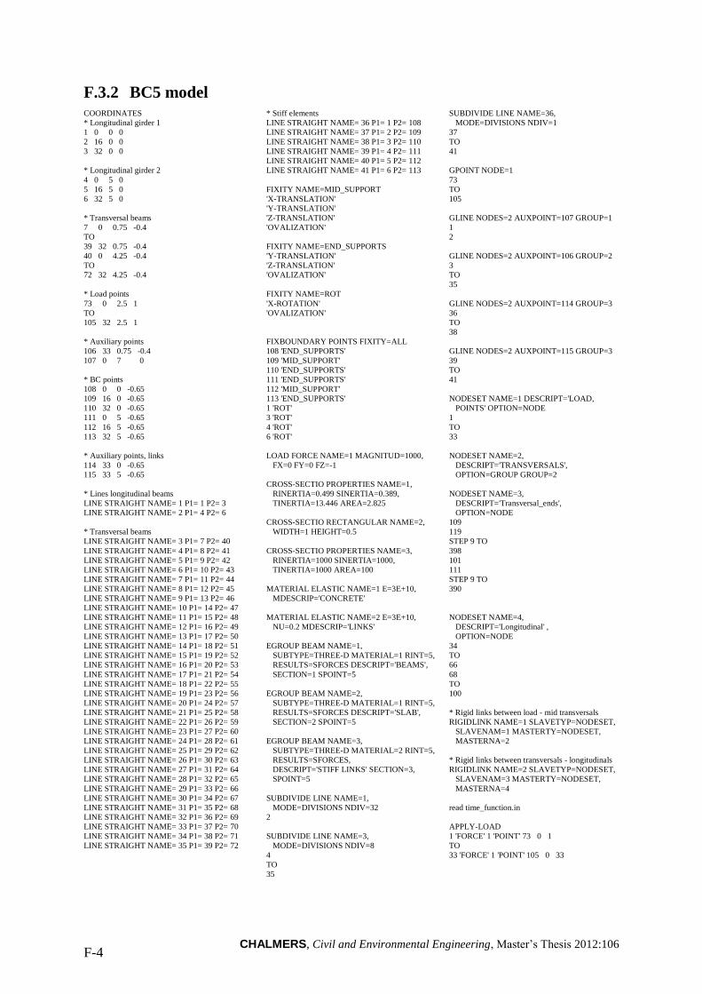
CHALMERS, Civil and Environmental Engineering, Master’s Thesis 2012:106 F-4
F.3.2 BC5 model COORDINATES
* Longitudinal girder 1
1 0 0 0
2 16 0 0
3 32 0 0
* Longitudinal girder 2
4 0 5 0
5 16 5 0
6 32 5 0
* Transversal beams
7 0 0.75 -0.4
TO
39 32 0.75 -0.4
40 0 4.25 -0.4
TO
72 32 4.25 -0.4
* Load points
73 0 2.5 1
TO
105 32 2.5 1
* Auxiliary points
106 33 0.75 -0.4
107 0 7 0
* BC points
108 0 0 -0.65
109 16 0 -0.65
110 32 0 -0.65
111 0 5 -0.65
112 16 5 -0.65
113 32 5 -0.65
* Auxiliary points, links
114 33 0 -0.65
115 33 5 -0.65
* Lines longitudinal beams
LINE STRAIGHT NAME= 1 P1= 1 P2= 3
LINE STRAIGHT NAME= 2 P1= 4 P2= 6
* Transversal beams
LINE STRAIGHT NAME= 3 P1= 7 P2= 40
LINE STRAIGHT NAME= 4 P1= 8 P2= 41
LINE STRAIGHT NAME= 5 P1= 9 P2= 42
LINE STRAIGHT NAME= 6 P1= 10 P2= 43
LINE STRAIGHT NAME= 7 P1= 11 P2= 44
LINE STRAIGHT NAME= 8 P1= 12 P2= 45
LINE STRAIGHT NAME= 9 P1= 13 P2= 46
LINE STRAIGHT NAME= 10 P1= 14 P2= 47
LINE STRAIGHT NAME= 11 P1= 15 P2= 48
LINE STRAIGHT NAME= 12 P1= 16 P2= 49
LINE STRAIGHT NAME= 13 P1= 17 P2= 50
LINE STRAIGHT NAME= 14 P1= 18 P2= 51
LINE STRAIGHT NAME= 15 P1= 19 P2= 52
LINE STRAIGHT NAME= 16 P1= 20 P2= 53
LINE STRAIGHT NAME= 17 P1= 21 P2= 54
LINE STRAIGHT NAME= 18 P1= 22 P2= 55
LINE STRAIGHT NAME= 19 P1= 23 P2= 56
LINE STRAIGHT NAME= 20 P1= 24 P2= 57
LINE STRAIGHT NAME= 21 P1= 25 P2= 58
LINE STRAIGHT NAME= 22 P1= 26 P2= 59
LINE STRAIGHT NAME= 23 P1= 27 P2= 60
LINE STRAIGHT NAME= 24 P1= 28 P2= 61
LINE STRAIGHT NAME= 25 P1= 29 P2= 62
LINE STRAIGHT NAME= 26 P1= 30 P2= 63
LINE STRAIGHT NAME= 27 P1= 31 P2= 64
LINE STRAIGHT NAME= 28 P1= 32 P2= 65
LINE STRAIGHT NAME= 29 P1= 33 P2= 66
LINE STRAIGHT NAME= 30 P1= 34 P2= 67
LINE STRAIGHT NAME= 31 P1= 35 P2= 68
LINE STRAIGHT NAME= 32 P1= 36 P2= 69
LINE STRAIGHT NAME= 33 P1= 37 P2= 70
LINE STRAIGHT NAME= 34 P1= 38 P2= 71
LINE STRAIGHT NAME= 35 P1= 39 P2= 72
* Stiff elements
LINE STRAIGHT NAME= 36 P1= 1 P2= 108
LINE STRAIGHT NAME= 37 P1= 2 P2= 109
LINE STRAIGHT NAME= 38 P1= 3 P2= 110
LINE STRAIGHT NAME= 39 P1= 4 P2= 111
LINE STRAIGHT NAME= 40 P1= 5 P2= 112
LINE STRAIGHT NAME= 41 P1= 6 P2= 113
FIXITY NAME=MID_SUPPORT
'X-TRANSLATION'
'Y-TRANSLATION'
'Z-TRANSLATION'
'OVALIZATION'
FIXITY NAME=END_SUPPORTS
'Y-TRANSLATION'
'Z-TRANSLATION'
'OVALIZATION'
FIXITY NAME=ROT
'X-ROTATION'
'OVALIZATION'
FIXBOUNDARY POINTS FIXITY=ALL
108 'END_SUPPORTS'
109 'MID_SUPPORT'
110 'END_SUPPORTS'
111 'END_SUPPORTS'
112 'MID_SUPPORT'
113 'END_SUPPORTS'
1 'ROT'
3 'ROT'
4 'ROT'
6 'ROT'
LOAD FORCE NAME=1 MAGNITUD=1000,
FX=0 FY=0 FZ=-1
CROSS-SECTIO PROPERTIES NAME=1,
RINERTIA=0.499 SINERTIA=0.389,
TINERTIA=13.446 AREA=2.825
CROSS-SECTIO RECTANGULAR NAME=2,
WIDTH=1 HEIGHT=0.5
CROSS-SECTIO PROPERTIES NAME=3,
RINERTIA=1000 SINERTIA=1000,
TINERTIA=1000 AREA=100
MATERIAL ELASTIC NAME=1 E=3E+10,
MDESCRIP='CONCRETE'
MATERIAL ELASTIC NAME=2 E=3E+10,
NU=0.2 MDESCRIP='LINKS'
EGROUP BEAM NAME=1,
SUBTYPE=THREE-D MATERIAL=1 RINT=5,
RESULTS=SFORCES DESCRIPT='BEAMS',
SECTION=1 SPOINT=5
EGROUP BEAM NAME=2,
SUBTYPE=THREE-D MATERIAL=1 RINT=5,
RESULTS=SFORCES DESCRIPT='SLAB',
SECTION=2 SPOINT=5
EGROUP BEAM NAME=3,
SUBTYPE=THREE-D MATERIAL=2 RINT=5,
RESULTS=SFORCES,
DESCRIPT='STIFF LINKS' SECTION=3,
SPOINT=5
SUBDIVIDE LINE NAME=1,
MODE=DIVISIONS NDIV=32
2
SUBDIVIDE LINE NAME=3,
MODE=DIVISIONS NDIV=8
4
TO
35
SUBDIVIDE LINE NAME=36,
MODE=DIVISIONS NDIV=1
37
TO
41
GPOINT NODE=1
73
TO
105
GLINE NODES=2 AUXPOINT=107 GROUP=1
1
2
GLINE NODES=2 AUXPOINT=106 GROUP=2
3
TO
35
GLINE NODES=2 AUXPOINT=114 GROUP=3
36
TO
38
GLINE NODES=2 AUXPOINT=115 GROUP=3
39
TO
41
NODESET NAME=1 DESCRIPT='LOAD,
POINTS' OPTION=NODE
1
TO
33
NODESET NAME=2,
DESCRIPT='TRANSVERSALS',
OPTION=GROUP GROUP=2
NODESET NAME=3,
DESCRIPT='Transversal_ends',
OPTION=NODE
109
119
STEP 9 TO
398
101
111
STEP 9 TO
390
NODESET NAME=4,
DESCRIPT='Longitudinal' ,
OPTION=NODE
34
TO
66
68
TO
100
* Rigid links between load - mid transversals
RIGIDLINK NAME=1 SLAVETYP=NODESET,
SLAVENAM=1 MASTERTY=NODESET,
MASTERNA=2
* Rigid links between transversals - longitudinals
RIGIDLINK NAME=2 SLAVETYP=NODESET,
SLAVENAM=3 MASTERTY=NODESET,
MASTERNA=4
read time_function.in
APPLY-LOAD
1 'FORCE' 1 'POINT' 73 0 1
TO
33 'FORCE' 1 'POINT' 105 0 33
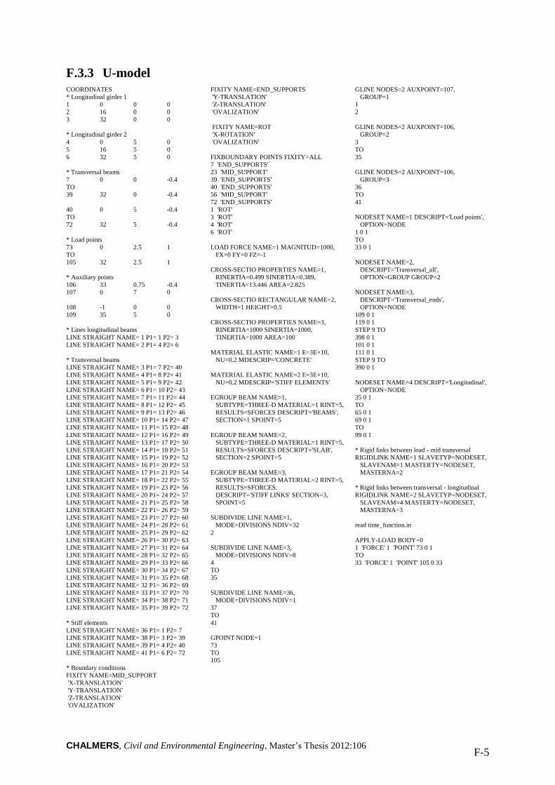
CHALMERS, Civil and Environmental Engineering, Master’s Thesis 2012:106 F-5
F.3.3 U-model COORDINATES
* Longitudinal girder 1
1 0 0 0
2 16 0 0
3 32 0 0
* Longitudinal girder 2
4 0 5 0
5 16 5 0
6 32 5 0
* Transversal beams
7 0 0 -0.4
TO
39 32 0 -0.4
40 0 5 -0.4
TO
72 32 5 -0.4
* Load points
73 0 2.5 1
TO
105 32 2.5 1
* Auxiliary points
106 33 0.75 -0.4
107 0 7 0
108 -1 0 0
109 35 5 0
* Lines longitudinal beams
LINE STRAIGHT NAME= 1 P1= 1 P2= 3
LINE STRAIGHT NAME= 2 P1= 4 P2= 6
* Transversal beams
LINE STRAIGHT NAME= 3 P1= 7 P2= 40
LINE STRAIGHT NAME= 4 P1= 8 P2= 41
LINE STRAIGHT NAME= 5 P1= 9 P2= 42
LINE STRAIGHT NAME= 6 P1= 10 P2= 43
LINE STRAIGHT NAME= 7 P1= 11 P2= 44
LINE STRAIGHT NAME= 8 P1= 12 P2= 45
LINE STRAIGHT NAME= 9 P1= 13 P2= 46
LINE STRAIGHT NAME= 10 P1= 14 P2= 47
LINE STRAIGHT NAME= 11 P1= 15 P2= 48
LINE STRAIGHT NAME= 12 P1= 16 P2= 49
LINE STRAIGHT NAME= 13 P1= 17 P2= 50
LINE STRAIGHT NAME= 14 P1= 18 P2= 51
LINE STRAIGHT NAME= 15 P1= 19 P2= 52
LINE STRAIGHT NAME= 16 P1= 20 P2= 53
LINE STRAIGHT NAME= 17 P1= 21 P2= 54
LINE STRAIGHT NAME= 18 P1= 22 P2= 55
LINE STRAIGHT NAME= 19 P1= 23 P2= 56
LINE STRAIGHT NAME= 20 P1= 24 P2= 57
LINE STRAIGHT NAME= 21 P1= 25 P2= 58
LINE STRAIGHT NAME= 22 P1= 26 P2= 59
LINE STRAIGHT NAME= 23 P1= 27 P2= 60
LINE STRAIGHT NAME= 24 P1= 28 P2= 61
LINE STRAIGHT NAME= 25 P1= 29 P2= 62
LINE STRAIGHT NAME= 26 P1= 30 P2= 63
LINE STRAIGHT NAME= 27 P1= 31 P2= 64
LINE STRAIGHT NAME= 28 P1= 32 P2= 65
LINE STRAIGHT NAME= 29 P1= 33 P2= 66
LINE STRAIGHT NAME= 30 P1= 34 P2= 67
LINE STRAIGHT NAME= 31 P1= 35 P2= 68
LINE STRAIGHT NAME= 32 P1= 36 P2= 69
LINE STRAIGHT NAME= 33 P1= 37 P2= 70
LINE STRAIGHT NAME= 34 P1= 38 P2= 71
LINE STRAIGHT NAME= 35 P1= 39 P2= 72
* Stiff elements
LINE STRAIGHT NAME= 36 P1= 1 P2= 7
LINE STRAIGHT NAME= 38 P1= 3 P2= 39
LINE STRAIGHT NAME= 39 P1= 4 P2= 40
LINE STRAIGHT NAME= 41 P1= 6 P2= 72
* Boundary conditions
FIXITY NAME=MID_SUPPORT
'X-TRANSLATION'
'Y-TRANSLATION'
'Z-TRANSLATION'
'OVALIZATION'
FIXITY NAME=END_SUPPORTS
'Y-TRANSLATION'
'Z-TRANSLATION'
'OVALIZATION'
FIXITY NAME=ROT
'X-ROTATION'
'OVALIZATION'
FIXBOUNDARY POINTS FIXITY=ALL
7 'END_SUPPORTS'
23 'MID_SUPPORT'
39 'END_SUPPORTS'
40 'END_SUPPORTS'
56 'MID_SUPPORT'
72 'END_SUPPORTS'
1 'ROT'
3 'ROT'
4 'ROT'
6 'ROT'
LOAD FORCE NAME=1 MAGNITUD=1000,
FX=0 FY=0 FZ=-1
CROSS-SECTIO PROPERTIES NAME=1,
RINERTIA=0.499 SINERTIA=0.389,
TINERTIA=13.446 AREA=2.825
CROSS-SECTIO RECTANGULAR NAME=2,
WIDTH=1 HEIGHT=0.5
CROSS-SECTIO PROPERTIES NAME=3,
RINERTIA=1000 SINERTIA=1000,
TINERTIA=1000 AREA=100
MATERIAL ELASTIC NAME=1 E=3E+10,
NU=0.2 MDESCRIP='CONCRETE'
MATERIAL ELASTIC NAME=2 E=3E+10,
NU=0.2 MDESCRIP='STIFF ELEMENTS'
EGROUP BEAM NAME=1,
SUBTYPE=THREE-D MATERIAL=1 RINT=5,
RESULTS=SFORCES DESCRIPT='BEAMS',
SECTION=1 SPOINT=5
EGROUP BEAM NAME=2,
SUBTYPE=THREE-D MATERIAL=1 RINT=5,
RESULTS=SFORCES DESCRIPT='SLAB',
SECTION=2 SPOINT=5
EGROUP BEAM NAME=3,
SUBTYPE=THREE-D MATERIAL=2 RINT=5,
RESULTS=SFORCES,
DESCRIPT='STIFF LINKS' SECTION=3,
SPOINT=5
SUBDIVIDE LINE NAME=1,
MODE=DIVISIONS NDIV=32
2
SUBDIVIDE LINE NAME=3,
MODE=DIVISIONS NDIV=8
4
TO
35
SUBDIVIDE LINE NAME=36,
MODE=DIVISIONS NDIV=1
37
TO
41
GPOINT NODE=1
73
TO
105
GLINE NODES=2 AUXPOINT=107,
GROUP=1
1
2
GLINE NODES=2 AUXPOINT=106,
GROUP=2
3
TO
35
GLINE NODES=2 AUXPOINT=106,
GROUP=3
36
TO
41
NODESET NAME=1 DESCRIPT='Load points',
OPTION=NODE
1 0 1
TO
33 0 1
NODESET NAME=2,
DESCRIPT='Transversal_all',
OPTION=GROUP GROUP=2
NODESET NAME=3,
DESCRIPT='Transversal_ends',
OPTION=NODE
109 0 1
119 0 1
STEP 9 TO
398 0 1
101 0 1
111 0 1
STEP 9 TO
390 0 1
NODESET NAME=4 DESCRIPT='Longitudinal',
OPTION=NODE
35 0 1
TO
65 0 1
69 0 1
TO
99 0 1
* Rigid links between load - mid transversal
RIGIDLINK NAME=1 SLAVETYP=NODESET,
SLAVENAM=1 MASTERTY=NODESET,
MASTERNA=2
* Rigid links between transversal - longitudinal
RIGIDLINK NAME=2 SLAVETYP=NODESET,
SLAVENAM=4 MASTERTY=NODESET,
MASTERNA=3
read time_function.in
APPLY-LOAD BODY=0
1 'FORCE' 1 'POINT' 73 0 1
TO
33 'FORCE' 1 'POINT' 105 0 33
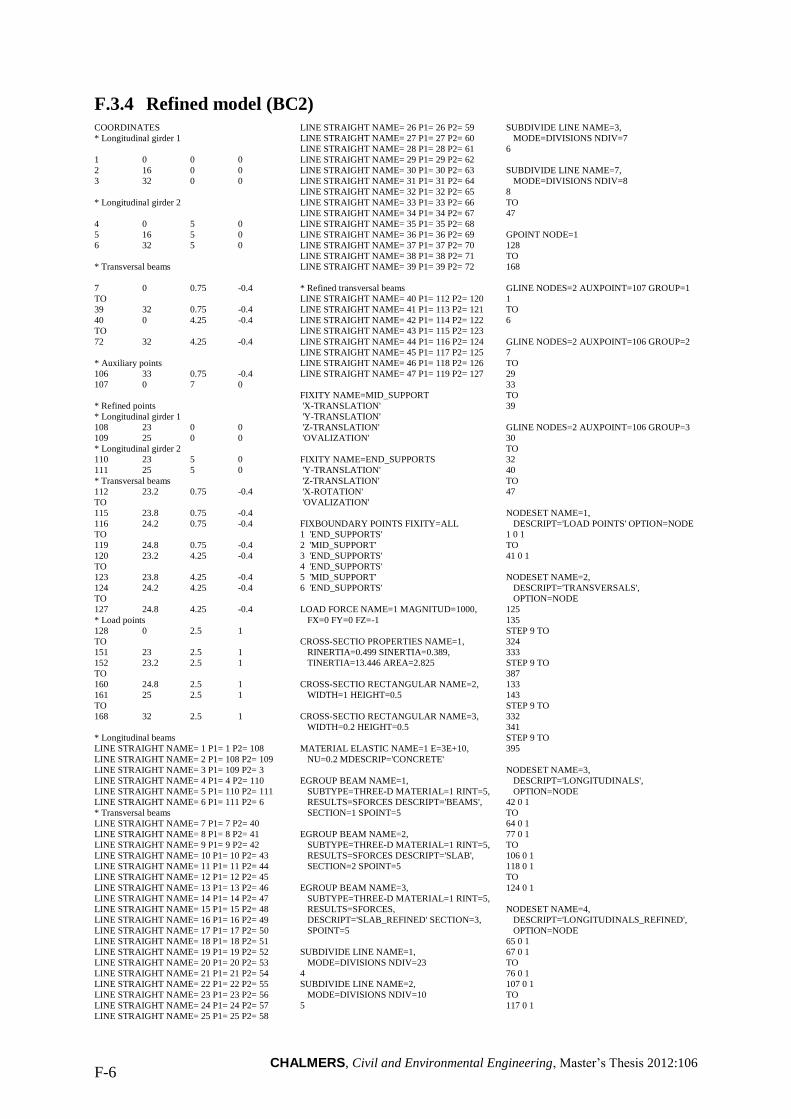
CHALMERS, Civil and Environmental Engineering, Master’s Thesis 2012:106 F-6
F.3.4 Refined model (BC2) COORDINATES
* Longitudinal girder 1
1 0 0 0
2 16 0 0
3 32 0 0
* Longitudinal girder 2
4 0 5 0
5 16 5 0
6 32 5 0
* Transversal beams
7 0 0.75 -0.4
TO
39 32 0.75 -0.4
40 0 4.25 -0.4
TO
72 32 4.25 -0.4
* Auxiliary points
106 33 0.75 -0.4
107 0 7 0
* Refined points
* Longitudinal girder 1
108 23 0 0
109 25 0 0
* Longitudinal girder 2
110 23 5 0
111 25 5 0
* Transversal beams
112 23.2 0.75 -0.4
TO
115 23.8 0.75 -0.4
116 24.2 0.75 -0.4
TO
119 24.8 0.75 -0.4
120 23.2 4.25 -0.4
TO
123 23.8 4.25 -0.4
124 24.2 4.25 -0.4
TO
127 24.8 4.25 -0.4
* Load points
128 0 2.5 1
TO
151 23 2.5 1
152 23.2 2.5 1
TO
160 24.8 2.5 1
161 25 2.5 1
TO
168 32 2.5 1
* Longitudinal beams
LINE STRAIGHT NAME= 1 P1= 1 P2= 108
LINE STRAIGHT NAME= 2 P1= 108 P2= 109
LINE STRAIGHT NAME= 3 P1= 109 P2= 3
LINE STRAIGHT NAME= 4 P1= 4 P2= 110
LINE STRAIGHT NAME= 5 P1= 110 P2= 111
LINE STRAIGHT NAME= 6 P1= 111 P2= 6
* Transversal beams
LINE STRAIGHT NAME= 7 P1= 7 P2= 40
LINE STRAIGHT NAME= 8 P1= 8 P2= 41
LINE STRAIGHT NAME= 9 P1= 9 P2= 42
LINE STRAIGHT NAME= 10 P1= 10 P2= 43
LINE STRAIGHT NAME= 11 P1= 11 P2= 44
LINE STRAIGHT NAME= 12 P1= 12 P2= 45
LINE STRAIGHT NAME= 13 P1= 13 P2= 46
LINE STRAIGHT NAME= 14 P1= 14 P2= 47
LINE STRAIGHT NAME= 15 P1= 15 P2= 48
LINE STRAIGHT NAME= 16 P1= 16 P2= 49
LINE STRAIGHT NAME= 17 P1= 17 P2= 50
LINE STRAIGHT NAME= 18 P1= 18 P2= 51
LINE STRAIGHT NAME= 19 P1= 19 P2= 52
LINE STRAIGHT NAME= 20 P1= 20 P2= 53
LINE STRAIGHT NAME= 21 P1= 21 P2= 54
LINE STRAIGHT NAME= 22 P1= 22 P2= 55
LINE STRAIGHT NAME= 23 P1= 23 P2= 56
LINE STRAIGHT NAME= 24 P1= 24 P2= 57
LINE STRAIGHT NAME= 25 P1= 25 P2= 58
LINE STRAIGHT NAME= 26 P1= 26 P2= 59
LINE STRAIGHT NAME= 27 P1= 27 P2= 60
LINE STRAIGHT NAME= 28 P1= 28 P2= 61
LINE STRAIGHT NAME= 29 P1= 29 P2= 62
LINE STRAIGHT NAME= 30 P1= 30 P2= 63
LINE STRAIGHT NAME= 31 P1= 31 P2= 64
LINE STRAIGHT NAME= 32 P1= 32 P2= 65
LINE STRAIGHT NAME= 33 P1= 33 P2= 66
LINE STRAIGHT NAME= 34 P1= 34 P2= 67
LINE STRAIGHT NAME= 35 P1= 35 P2= 68
LINE STRAIGHT NAME= 36 P1= 36 P2= 69
LINE STRAIGHT NAME= 37 P1= 37 P2= 70
LINE STRAIGHT NAME= 38 P1= 38 P2= 71
LINE STRAIGHT NAME= 39 P1= 39 P2= 72
* Refined transversal beams
LINE STRAIGHT NAME= 40 P1= 112 P2= 120
LINE STRAIGHT NAME= 41 P1= 113 P2= 121
LINE STRAIGHT NAME= 42 P1= 114 P2= 122
LINE STRAIGHT NAME= 43 P1= 115 P2= 123
LINE STRAIGHT NAME= 44 P1= 116 P2= 124
LINE STRAIGHT NAME= 45 P1= 117 P2= 125
LINE STRAIGHT NAME= 46 P1= 118 P2= 126
LINE STRAIGHT NAME= 47 P1= 119 P2= 127
FIXITY NAME=MID_SUPPORT
'X-TRANSLATION'
'Y-TRANSLATION'
'Z-TRANSLATION'
'OVALIZATION'
FIXITY NAME=END_SUPPORTS
'Y-TRANSLATION'
'Z-TRANSLATION'
'X-ROTATION'
'OVALIZATION'
FIXBOUNDARY POINTS FIXITY=ALL
1 'END_SUPPORTS'
2 'MID_SUPPORT'
3 'END_SUPPORTS'
4 'END_SUPPORTS'
5 'MID_SUPPORT'
6 'END_SUPPORTS'
LOAD FORCE NAME=1 MAGNITUD=1000,
FX=0 FY=0 FZ=-1
CROSS-SECTIO PROPERTIES NAME=1,
RINERTIA=0.499 SINERTIA=0.389,
TINERTIA=13.446 AREA=2.825
CROSS-SECTIO RECTANGULAR NAME=2,
WIDTH=1 HEIGHT=0.5
CROSS-SECTIO RECTANGULAR NAME=3,
WIDTH=0.2 HEIGHT=0.5
MATERIAL ELASTIC NAME=1 E=3E+10,
NU=0.2 MDESCRIP='CONCRETE'
EGROUP BEAM NAME=1,
SUBTYPE=THREE-D MATERIAL=1 RINT=5,
RESULTS=SFORCES DESCRIPT='BEAMS',
SECTION=1 SPOINT=5
EGROUP BEAM NAME=2,
SUBTYPE=THREE-D MATERIAL=1 RINT=5,
RESULTS=SFORCES DESCRIPT='SLAB',
SECTION=2 SPOINT=5
EGROUP BEAM NAME=3,
SUBTYPE=THREE-D MATERIAL=1 RINT=5,
RESULTS=SFORCES,
DESCRIPT='SLAB_REFINED' SECTION=3,
SPOINT=5
SUBDIVIDE LINE NAME=1,
MODE=DIVISIONS NDIV=23
4
SUBDIVIDE LINE NAME=2,
MODE=DIVISIONS NDIV=10
5
SUBDIVIDE LINE NAME=3,
MODE=DIVISIONS NDIV=7
6
SUBDIVIDE LINE NAME=7,
MODE=DIVISIONS NDIV=8
8
TO
47
GPOINT NODE=1
128
TO
168
GLINE NODES=2 AUXPOINT=107 GROUP=1
1
TO
6
GLINE NODES=2 AUXPOINT=106 GROUP=2
7
TO
29
33
TO
39
GLINE NODES=2 AUXPOINT=106 GROUP=3
30
TO
32
40
TO
47
NODESET NAME=1,
DESCRIPT='LOAD POINTS' OPTION=NODE
1 0 1
TO
41 0 1
NODESET NAME=2,
DESCRIPT='TRANSVERSALS',
OPTION=NODE
125
135
STEP 9 TO
324
333
STEP 9 TO
387
133
143
STEP 9 TO
332
341
STEP 9 TO
395
NODESET NAME=3,
DESCRIPT='LONGITUDINALS',
OPTION=NODE
42 0 1
TO
64 0 1
77 0 1
TO
106 0 1
118 0 1
TO
124 0 1
NODESET NAME=4,
DESCRIPT='LONGITUDINALS_REFINED',
OPTION=NODE
65 0 1
67 0 1
TO
76 0 1
107 0 1
TO
117 0 1
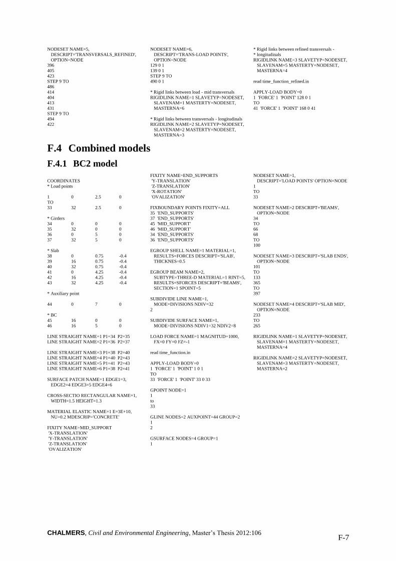
CHALMERS, Civil and Environmental Engineering, Master’s Thesis 2012:106 F-7
NODESET NAME=5,
DESCRIPT='TRANSVERSALS_REFINED',
OPTION=NODE
396
405
423
STEP 9 TO
486
414
404
413
431
STEP 9 TO
494
422
NODESET NAME=6,
DESCRIPT='TRANS-LOAD POINTS',
OPTION=NODE
129 0 1
139 0 1
STEP 9 TO
490 0 1
* Rigid links between load - mid transversals
RIGIDLINK NAME=1 SLAVETYP=NODESET,
SLAVENAM=1 MASTERTY=NODESET,
MASTERNA=6
* Rigid links between transversals - longitudinals
RIGIDLINK NAME=2 SLAVETYP=NODESET,
SLAVENAM=2 MASTERTY=NODESET,
MASTERNA=3
* Rigid links between refined transversals -
* longitudinals
RIGIDLINK NAME=3 SLAVETYP=NODESET,
SLAVENAM=5 MASTERTY=NODESET,
MASTERNA=4
read time_function_refined.in
APPLY-LOAD BODY=0
1 'FORCE' 1 'POINT' 128 0 1
TO
41 'FORCE' 1 'POINT' 168 0 41
F.4 Combined models
F.4.1 BC2 model
COORDINATES
* Load points
1 0 2.5 0
TO
33 32 2.5 0
* Girders
34 0 0 0
35 32 0 0
36 0 5 0
37 32 5 0
* Slab
38 0 0.75 -0.4
39 16 0.75 -0.4
40 32 0.75 -0.4
41 0 4.25 -0.4
42 16 4.25 -0.4
43 32 4.25 -0.4
* Auxiliary point
44 0 7 0
* BC
45 16 0 0
46 16 5 0
LINE STRAIGHT NAME=1 P1=34 P2=35
LINE STRAIGHT NAME=2 P1=36 P2=37
LINE STRAIGHT NAME=3 P1=38 P2=40
LINE STRAIGHT NAME=4 P1=40 P2=43
LINE STRAIGHT NAME=5 P1=41 P2=43
LINE STRAIGHT NAME=6 P1=38 P2=41
SURFACE PATCH NAME=1 EDGE1=3,
EDGE2=4 EDGE3=5 EDGE4=6
CROSS-SECTIO RECTANGULAR NAME=1,
WIDTH=1.5 HEIGHT=1.3
MATERIAL ELASTIC NAME=1 E=3E+10,
NU=0.2 MDESCRIP='CONCRETE'
FIXITY NAME=MID_SUPPORT
'X-TRANSLATION'
'Y-TRANSLATION'
'Z-TRANSLATION'
'OVALIZATION'
FIXITY NAME=END_SUPPORTS
'Y-TRANSLATION'
'Z-TRANSLATION'
'X-ROTATION'
'OVALIZATION'
FIXBOUNDARY POINTS FIXITY=ALL
35 'END_SUPPORTS'
37 'END_SUPPORTS'
45 'MID_SUPPORT'
46 'MID_SUPPORT'
34 'END_SUPPORTS'
36 'END_SUPPORTS'
EGROUP SHELL NAME=1 MATERIAL=1,
RESULTS=FORCES DESCRIPT='SLAB',
THICKNES=0.5
EGROUP BEAM NAME=2,
SUBTYPE=THREE-D MATERIAL=1 RINT=5,
RESULTS=SFORCES DESCRIPT='BEAMS',
SECTION=1 SPOINT=5
SUBDIVIDE LINE NAME=1,
MODE=DIVISIONS NDIV=32
2
SUBDIVIDE SURFACE NAME=1,
MODE=DIVISIONS NDIV1=32 NDIV2=8
LOAD FORCE NAME=1 MAGNITUD=1000,
FX=0 FY=0 FZ=-1
read time_function.in
APPLY-LOAD BODY=0
1 'FORCE' 1 'POINT' 1 0 1
TO
33 'FORCE' 1 'POINT' 33 0 33
GPOINT NODE=1
1
to
33
GLINE NODES=2 AUXPOINT=44 GROUP=2
1
2
GSURFACE NODES=4 GROUP=1
1
NODESET NAME=1,
DESCRIPT='LOAD POINTS' OPTION=NODE
1
TO
33
NODESET NAME=2 DESCRIPT='BEAMS',
OPTION=NODE
34
TO
66
68
TO
100
NODESET NAME=3 DESCRIPT='SLAB ENDS',
OPTION=NODE
101
TO
133
365
TO
397
NODESET NAME=4 DESCRIPT='SLAB MID',
OPTION=NODE
233
TO
265
RIGIDLINK NAME=1 SLAVETYP=NODESET,
SLAVENAM=1 MASTERTY=NODESET,
MASTERNA=4
RIGIDLINK NAME=2 SLAVETYP=NODESET,
SLAVENAM=3 MASTERTY=NODESET,
MASTERNA=2
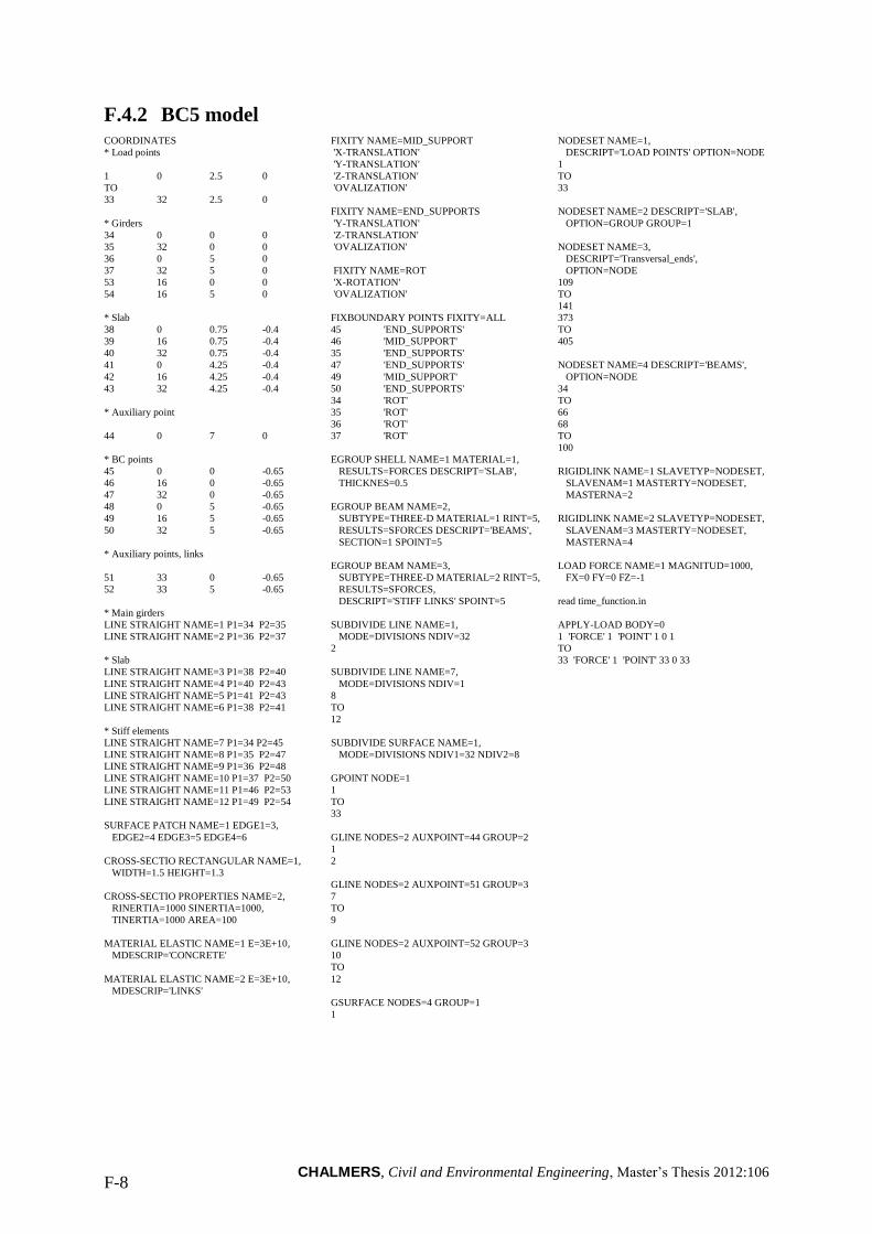
CHALMERS, Civil and Environmental Engineering, Master’s Thesis 2012:106 F-8
F.4.2 BC5 model COORDINATES
* Load points
1 0 2.5 0
TO
33 32 2.5 0
* Girders
34 0 0 0
35 32 0 0
36 0 5 0
37 32 5 0
53 16 0 0
54 16 5 0
* Slab
38 0 0.75 -0.4
39 16 0.75 -0.4
40 32 0.75 -0.4
41 0 4.25 -0.4
42 16 4.25 -0.4
43 32 4.25 -0.4
* Auxiliary point
44 0 7 0
* BC points
45 0 0 -0.65
46 16 0 -0.65
47 32 0 -0.65
48 0 5 -0.65
49 16 5 -0.65
50 32 5 -0.65
* Auxiliary points, links
51 33 0 -0.65
52 33 5 -0.65
* Main girders
LINE STRAIGHT NAME=1 P1=34 P2=35
LINE STRAIGHT NAME=2 P1=36 P2=37
* Slab
LINE STRAIGHT NAME=3 P1=38 P2=40
LINE STRAIGHT NAME=4 P1=40 P2=43
LINE STRAIGHT NAME=5 P1=41 P2=43
LINE STRAIGHT NAME=6 P1=38 P2=41
* Stiff elements
LINE STRAIGHT NAME=7 P1=34 P2=45
LINE STRAIGHT NAME=8 P1=35 P2=47
LINE STRAIGHT NAME=9 P1=36 P2=48
LINE STRAIGHT NAME=10 P1=37 P2=50
LINE STRAIGHT NAME=11 P1=46 P2=53
LINE STRAIGHT NAME=12 P1=49 P2=54
SURFACE PATCH NAME=1 EDGE1=3,
EDGE2=4 EDGE3=5 EDGE4=6
CROSS-SECTIO RECTANGULAR NAME=1,
WIDTH=1.5 HEIGHT=1.3
CROSS-SECTIO PROPERTIES NAME=2,
RINERTIA=1000 SINERTIA=1000,
TINERTIA=1000 AREA=100
MATERIAL ELASTIC NAME=1 E=3E+10,
MDESCRIP='CONCRETE'
MATERIAL ELASTIC NAME=2 E=3E+10,
MDESCRIP='LINKS'
FIXITY NAME=MID_SUPPORT
'X-TRANSLATION'
'Y-TRANSLATION'
'Z-TRANSLATION'
'OVALIZATION'
FIXITY NAME=END_SUPPORTS
'Y-TRANSLATION'
'Z-TRANSLATION'
'OVALIZATION'
FIXITY NAME=ROT
'X-ROTATION'
'OVALIZATION'
FIXBOUNDARY POINTS FIXITY=ALL
45 'END_SUPPORTS'
46 'MID_SUPPORT'
35 'END_SUPPORTS'
47 'END_SUPPORTS'
49 'MID_SUPPORT'
50 'END_SUPPORTS'
34 'ROT'
35 'ROT'
36 'ROT'
37 'ROT'
EGROUP SHELL NAME=1 MATERIAL=1,
RESULTS=FORCES DESCRIPT='SLAB',
THICKNES=0.5
EGROUP BEAM NAME=2,
SUBTYPE=THREE-D MATERIAL=1 RINT=5,
RESULTS=SFORCES DESCRIPT='BEAMS',
SECTION=1 SPOINT=5
EGROUP BEAM NAME=3,
SUBTYPE=THREE-D MATERIAL=2 RINT=5,
RESULTS=SFORCES,
DESCRIPT='STIFF LINKS' SPOINT=5
SUBDIVIDE LINE NAME=1,
MODE=DIVISIONS NDIV=32
2
SUBDIVIDE LINE NAME=7,
MODE=DIVISIONS NDIV=1
8
TO
12
SUBDIVIDE SURFACE NAME=1,
MODE=DIVISIONS NDIV1=32 NDIV2=8
GPOINT NODE=1
1
TO
33
GLINE NODES=2 AUXPOINT=44 GROUP=2
1
2
GLINE NODES=2 AUXPOINT=51 GROUP=3
7
TO
9
GLINE NODES=2 AUXPOINT=52 GROUP=3
10
TO
12
GSURFACE NODES=4 GROUP=1
1
NODESET NAME=1,
DESCRIPT='LOAD POINTS' OPTION=NODE
1
TO
33
NODESET NAME=2 DESCRIPT='SLAB',
OPTION=GROUP GROUP=1
NODESET NAME=3,
DESCRIPT='Transversal_ends',
OPTION=NODE
109
TO
141
373
TO
405
NODESET NAME=4 DESCRIPT='BEAMS',
OPTION=NODE
34
TO
66
68
TO
100
RIGIDLINK NAME=1 SLAVETYP=NODESET,
SLAVENAM=1 MASTERTY=NODESET,
MASTERNA=2
RIGIDLINK NAME=2 SLAVETYP=NODESET,
SLAVENAM=3 MASTERTY=NODESET,
MASTERNA=4
LOAD FORCE NAME=1 MAGNITUD=1000,
FX=0 FY=0 FZ=-1
read time_function.in
APPLY-LOAD BODY=0
1 'FORCE' 1 'POINT' 1 0 1
TO
33 'FORCE' 1 'POINT' 33 0 33
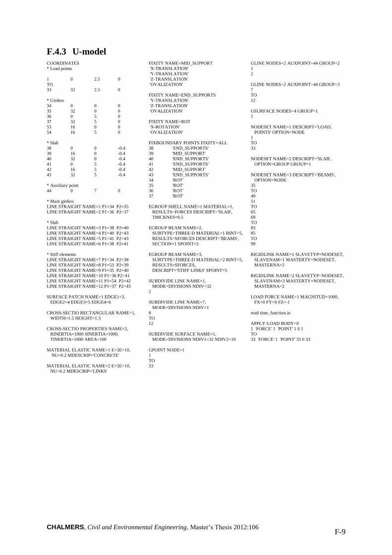
CHALMERS, Civil and Environmental Engineering, Master’s Thesis 2012:106 F-9
F.4.3 U-model COORDINATES
* Load points
1 0 2.5 0
TO
33 32 2.5 0
* Girders
34 0 0 0
35 32 0 0
36 0 5 0
37 32 5 0
53 16 0 0
54 16 5 0
* Slab
38 0 0 -0.4
39 16 0 -0.4
40 32 0 -0.4
41 0 5 -0.4
42 16 5 -0.4
43 32 5 -0.4
* Auxiliary point
44 0 7 0
* Main girders
LINE STRAIGHT NAME=1 P1=34 P2=35
LINE STRAIGHT NAME=2 P1=36 P2=37
* Slab
LINE STRAIGHT NAME=3 P1=38 P2=40
LINE STRAIGHT NAME=4 P1=40 P2=43
LINE STRAIGHT NAME=5 P1=41 P2=43
LINE STRAIGHT NAME=6 P1=38 P2=41
* Stiff elements
LINE STRAIGHT NAME=7 P1=34 P2=38
LINE STRAIGHT NAME=8 P1=53 P2=39
LINE STRAIGHT NAME=9 P1=35 P2=40
LINE STRAIGHT NAME=10 P1=36 P2=41
LINE STRAIGHT NAME=11 P1=54 P2=42
LINE STRAIGHT NAME=12 P1=37 P2=43
SURFACE PATCH NAME=1 EDGE1=3,
EDGE2=4 EDGE3=5 EDGE4=6
CROSS-SECTIO RECTANGULAR NAME=1,
WIDTH=1.5 HEIGHT=1.3
CROSS-SECTIO PROPERTIES NAME=2,
RINERTIA=1000 SINERTIA=1000,
TINERTIA=1000 AREA=100
MATERIAL ELASTIC NAME=1 E=3E+10,
NU=0.2 MDESCRIP='CONCRETE'
MATERIAL ELASTIC NAME=2 E=3E+10,
NU=0.2 MDESCRIP='LINKS'
FIXITY NAME=MID_SUPPORT
'X-TRANSLATION'
'Y-TRANSLATION'
'Z-TRANSLATION'
'OVALIZATION'
FIXITY NAME=END_SUPPORTS
'Y-TRANSLATION'
'Z-TRANSLATION'
'OVALIZATION'
FIXITY NAME=ROT
'X-ROTATION'
'OVALIZATION'
FIXBOUNDARY POINTS FIXITY=ALL
38 'END_SUPPORTS'
39 'MID_SUPPORT'
40 'END_SUPPORTS'
41 'END_SUPPORTS'
42 'MID_SUPPORT'
43 'END_SUPPORTS'
34 'ROT'
35 'ROT'
36 'ROT'
37 'ROT'
EGROUP SHELL NAME=1 MATERIAL=1,
RESULTS=FORCES DESCRIPT='SLAB',
THICKNES=0.5
EGROUP BEAM NAME=2,
SUBTYPE=THREE-D MATERIAL=1 RINT=5,
RESULTS=SFORCES DESCRIPT='BEAMS',
SECTION=1 SPOINT=5
EGROUP BEAM NAME=3,
SUBTYPE=THREE-D MATERIAL=2 RINT=5,
RESULTS=SFORCES,
DESCRIPT='STIFF LINKS' SPOINT=5
SUBDIVIDE LINE NAME=1,
MODE=DIVISIONS NDIV=32
2
SUBDIVIDE LINE NAME=7,
MODE=DIVISIONS NDIV=1
8
TO
12
SUBDIVIDE SURFACE NAME=1,
MODE=DIVISIONS NDIV1=32 NDIV2=10
GPOINT NODE=1
1
TO
33
GLINE NODES=2 AUXPOINT=44 GROUP=2
1
2
GLINE NODES=2 AUXPOINT=44 GROUP=3
7
TO
12
GSURFACE NODES=4 GROUP=1
1
NODESET NAME=1 DESCRIPT='LOAD,
POINTS' OPTION=NODE
1
TO
33
NODESET NAME=2 DESCRIPT='SLAB',
OPTION=GROUP GROUP=1
NODESET NAME=3 DESCRIPT='BEAMS',
OPTION=NODE
35
TO
49
51
TO
65
69
TO
83
85
TO
99
RIGIDLINK NAME=1 SLAVETYP=NODESET,
SLAVENAM=1 MASTERTY=NODESET,
MASTERNA=2
RIGIDLINK NAME=2 SLAVETYP=NODESET,
SLAVENAM=3 MASTERTY=NODESET,
MASTERNA=2
LOAD FORCE NAME=1 MAGNITUD=1000,
FX=0 FY=0 FZ=-1
read time_function.in
APPLY-LOAD BODY=0
1 'FORCE' 1 'POINT' 1 0 1
TO
33 'FORCE' 1 'POINT' 33 0 33
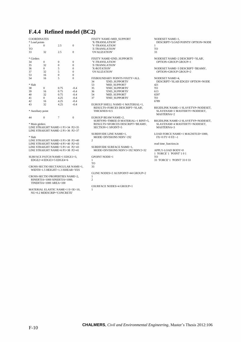
CHALMERS, Civil and Environmental Engineering, Master’s Thesis 2012:106 F-10
F.4.4 Refined model (BC2) COORDINATES
* Load points
1 0 2.5 0
TO
33 32 2.5 0
* Girders
34 0 0 0
35 32 0 0
36 0 5 0
37 32 5 0
53 16 0 0
54 16 5 0
* Slab
38 0 0.75 -0.4
39 16 0.75 -0.4
40 32 0.75 -0.4
41 0 4.25 -0.4
42 16 4.25 -0.4
43 32 4.25 -0.4
* Auxiliary point
44 0 7 0
* Main girders
LINE STRAIGHT NAME=1 P1=34 P2=35
LINE STRAIGHT NAME=2 P1=36 P2=37
* Slab
LINE STRAIGHT NAME=3 P1=38 P2=40
LINE STRAIGHT NAME=4 P1=40 P2=43
LINE STRAIGHT NAME=5 P1=41 P2=43
LINE STRAIGHT NAME=6 P1=38 P2=41
SURFACE PATCH NAME=1 EDGE1=3,
EDGE2=4 EDGE3=5 EDGE4=6
CROSS-SECTIO RECTANGULAR NAME=1,
WIDTH=1.5 HEIGHT=1.3 ISHEAR=YES
CROSS-SECTIO PROPERTIES NAME=2,
RINERTIA=1000 SINERTIA=1000,
TINERTIA=1000 AREA=100
MATERIAL ELASTIC NAME=1 E=3E+10,
NU=0.2 MDESCRIP='CONCRETE'
FIXITY NAME=MID_SUPPORT
'X-TRANSLATION'
'Y-TRANSLATION'
'Z-TRANSLATION'
'OVALIZATION'
FIXITY NAME=END_SUPPORTS
'Y-TRANSLATION'
'Z-TRANSLATION'
'X-ROTATION'
'OVALIZATION'
FIXBOUNDARY POINTS FIXITY=ALL
34 'END_SUPPORTS'
53 'MID_SUPPORT'
35 'END_SUPPORTS'
36 'END_SUPPORTS'
54 'MID_SUPPORT'
37 'END_SUPPORTS'
EGROUP SHELL NAME=1 MATERIAL=1,
RESULTS=FORCES DESCRIPT='SLAB',
THICKNES=0.5
EGROUP BEAM NAME=2,
SUBTYPE=THREE-D MATERIAL=1 RINT=5,
RESULTS=SFORCES DESCRIPT='BEAMS',
SECTION=1 SPOINT=5
SUBDIVIDE LINE NAME=1,
MODE=DIVISIONS NDIV=192
2
SUBDIVIDE SURFACE NAME=1,
MODE=DIVISIONS NDIV1=192 NDIV2=32
GPOINT NODE=1
1
TO
33
GLINE NODES=2 AUXPOINT=44 GROUP=2
1
2
GSURFACE NODES=4 GROUP=1
1
NODESET NAME=1,
DESCRIPT='LOAD POINTS' OPTION=NODE
1
TO
33
NODESET NAME=2 DESCRIPT='SLAB',
OPTION=GROUP GROUP=1
NODESET NAME=3 DESCRIPT='BEAMS',
OPTION=GROUP GROUP=2
NODESET NAME=4,
DESCRIPT='SLAB EDGES' OPTION=NODE
421
TO
613
6597
TO
6789
RIGIDLINK NAME=1 SLAVETYP=NODESET,
SLAVENAM=1 MASTERTY=NODESET,
MASTERNA=2
RIGIDLINK NAME=2 SLAVETYP=NODESET,
SLAVENAM=4 MASTERTY=NODESET,
MASTERNA=3
LOAD FORCE NAME=1 MAGNITUD=1000,
FX=0 FY=0 FZ=-1
read time_function.in
APPLY-LOAD BODY=0
1 'FORCE' 1 'POINT' 1 0 1
TO
33 'FORCE' 1 'POINT' 33 0 33
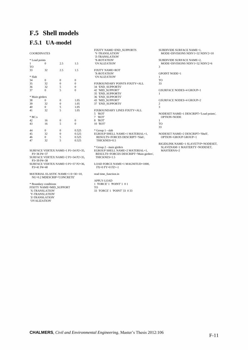
CHALMERS, Civil and Environmental Engineering, Master’s Thesis 2012:106 F-11
F.5 Shell models
F.5.1 UA-model
COORDINATES
* Load points
1 0 2.5 1.5
TO
33 32 2.5 1.5
* Slab
34 0 0 0
35 32 0 0
36 32 5 0
37 0 5 0
* Main girders
38 0 0 1.05
39 32 0 1.05
40 0 5 1.05
41 32 5 1.05
* BC:s
42 16 0 0
43 16 5 0
44 0 0 0.525
45 32 0 0.525
46 0 5 0.525
47 32 5 0.525
SURFACE VERTEX NAME=1 P1=34 P2=35,
P3=36 P4=37
SURFACE VERTEX NAME=2 P1=34 P2=35,
P3=39 P4=38
SURFACE VERTEX NAME=3 P1=37 P2=36,
P3=41 P4=40
MATERIAL ELASTIC NAME=1 E=3E+10,
NU=0.2 MDESCRIP='CONCRETE'
* Boundary conditions
FIXITY NAME=MID_SUPPORT
'X-TRANSLATION'
'Y-TRANSLATION'
'Z-TRANSLATION'
'OVALIZATION'
FIXITY NAME=END_SUPPORTS
'Y-TRANSLATION'
'Z-TRANSLATION'
'X-ROTATION'
'OVALIZATION'
FIXITY NAME=ROT
'X-ROTATION'
'OVALIZATION'
FIXBOUNDARY POINTS FIXITY=ALL
34 'END_SUPPORTS'
42 'MID_SUPPORT'
35 'END_SUPPORTS'
36 'END_SUPPORTS'
43 'MID_SUPPORT'
37 'END_SUPPORTS'
FIXBOUNDARY LINES FIXITY=ALL
5 'ROT'
7 'ROT'
8 'ROT'
10 'ROT'
* Group 1 - slab
EGROUP SHELL NAME=1 MATERIAL=1,
RESULTS=FORCES DESCRIPT='Slab',
THICKNES=0.5
* Group 2 - main girders
EGROUP SHELL NAME=2 MATERIAL=1,
RESULTS=FORCES DESCRIPT='Main girders',
THICKNES=1.5
LOAD FORCE NAME=1 MAGNITUD=1000,
FX=0 FY=0 FZ=-1
read time_function.in
APPLY-LOAD
1 'FORCE' 1 'POINT' 1 0 1
TO
33 'FORCE' 1 'POINT' 33 0 33
SUBDIVIDE SURFACE NAME=1,
MODE=DIVISIONS NDIV1=32 NDIV2=10
SUBDIVIDE SURFACE NAME=2,
MODE=DIVISIONS NDIV1=32 NDIV2=6
3
GPOINT NODE=1
1
TO
33
GSURFACE NODES=4 GROUP=1
1
GSURFACE NODES=4 GROUP=2
2
3
NODESET NAME=1 DESCRIPT='Load points',
OPTION=NODE
1
TO
33
NODESET NAME=2 DESCRIPT='Shell',
OPTION=GROUP GROUP=1
RIGIDLINK NAME=1 SLAVETYP=NODESET,
SLAVENAM=1 MASTERTY=NODESET,
MASTERNA=2
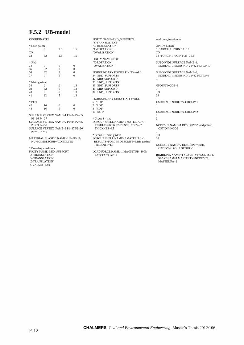
CHALMERS, Civil and Environmental Engineering, Master’s Thesis 2012:106 F-12
F.5.2 UB-model COORDINATES
* Load points
1 0 2.5 1.5
TO
33 32 2.5 1.5
* Slab
34 0 0 0
35 32 0 0
36 32 5 0
37 0 5 0
* Main girders
38 0 0 1.3
39 32 0 1.3
40 0 5 1.3
41 32 5 1.3
* BC:s
42 16 0 0
43 16 5 0
SURFACE VERTEX NAME=1 P1=34 P2=35,
P3=36 P4=37
SURFACE VERTEX NAME=2 P1=34 P2=35,
P3=39 P4=38
SURFACE VERTEX NAME=3 P1=37 P2=36,
P3=41 P4=40
MATERIAL ELASTIC NAME=1 E=3E+10,
NU=0.2 MDESCRIP='CONCRETE'
* Boundary conditions
FIXITY NAME=MID_SUPPORT
'X-TRANSLATION'
'Y-TRANSLATION'
'Z-TRANSLATION'
'OVALIZATION'
FIXITY NAME=END_SUPPORTS
'Y-TRANSLATION'
'Z-TRANSLATION'
'X-ROTATION'
'OVALIZATION'
FIXITY NAME=ROT
'X-ROTATION'
'OVALIZATION'
FIXBOUNDARY POINTS FIXITY=ALL
34 'END_SUPPORTS'
42 'MID_SUPPORT'
35 'END_SUPPORTS'
36 'END_SUPPORTS'
43 'MID_SUPPORT'
37 'END_SUPPORTS'
FIXBOUNDARY LINES FIXITY=ALL
5 'ROT'
7 'ROT'
8 'ROT'
10 'ROT'
* Group 1 - slab
EGROUP SHELL NAME=1 MATERIAL=1,
RESULTS=FORCES DESCRIPT='Slab',
THICKNES=0.5
* Group 2 - main girders
EGROUP SHELL NAME=2 MATERIAL=1,
RESULTS=FORCES DESCRIPT='Main girders',
THICKNES=1.5
LOAD FORCE NAME=1 MAGNITUD=1000,
FX=0 FY=0 FZ=-1
read time_function.in
APPLY-LOAD
1 'FORCE' 1 'POINT' 1 0 1
TO
33 'FORCE' 1 'POINT' 33 0 33
SUBDIVIDE SURFACE NAME=1,
MODE=DIVISIONS NDIV1=32 NDIV2=10
SUBDIVIDE SURFACE NAME=2,
MODE=DIVISIONS NDIV1=32 NDIV2=6
3
GPOINT NODE=1
1
TO
33
GSURFACE NODES=4 GROUP=1
1
GSURFACE NODES=4 GROUP=2
2
3
NODESET NAME=1 DESCRIPT='Load points',
OPTION=NODE
1
TO
33
NODESET NAME=2 DESCRIPT='Shell',
OPTION=GROUP GROUP=1
RIGIDLINK NAME=1 SLAVETYP=NODESET,
SLAVENAM=1 MASTERTY=NODESET,
MASTERNA=2
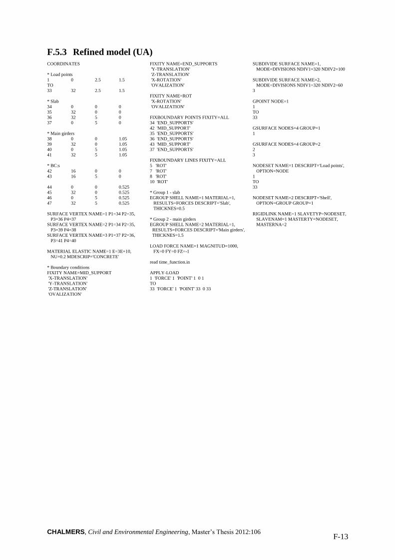
CHALMERS, Civil and Environmental Engineering, Master’s Thesis 2012:106 F-13
F.5.3 Refined model (UA) COORDINATES
* Load points
1 0 2.5 1.5
TO
33 32 2.5 1.5
* Slab
34 0 0 0
35 32 0 0
36 32 5 0
37 0 5 0
* Main girders
38 0 0 1.05
39 32 0 1.05
40 0 5 1.05
41 32 5 1.05
* BC:s
42 16 0 0
43 16 5 0
44 0 0 0.525
45 32 0 0.525
46 0 5 0.525
47 32 5 0.525
SURFACE VERTEX NAME=1 P1=34 P2=35,
P3=36 P4=37
SURFACE VERTEX NAME=2 P1=34 P2=35,
P3=39 P4=38
SURFACE VERTEX NAME=3 P1=37 P2=36,
P3=41 P4=40
MATERIAL ELASTIC NAME=1 E=3E+10,
NU=0.2 MDESCRIP='CONCRETE'
* Boundary conditions
FIXITY NAME=MID_SUPPORT
'X-TRANSLATION'
'Y-TRANSLATION'
'Z-TRANSLATION'
'OVALIZATION'
FIXITY NAME=END_SUPPORTS
'Y-TRANSLATION'
'Z-TRANSLATION'
'X-ROTATION'
'OVALIZATION'
FIXITY NAME=ROT
'X-ROTATION'
'OVALIZATION'
FIXBOUNDARY POINTS FIXITY=ALL
34 'END_SUPPORTS'
42 'MID_SUPPORT'
35 'END_SUPPORTS'
36 'END_SUPPORTS'
43 'MID_SUPPORT'
37 'END_SUPPORTS'
FIXBOUNDARY LINES FIXITY=ALL
5 'ROT'
7 'ROT'
8 'ROT'
10 'ROT'
* Group 1 - slab
EGROUP SHELL NAME=1 MATERIAL=1,
RESULTS=FORCES DESCRIPT='Slab',
THICKNES=0.5
* Group 2 - main girders
EGROUP SHELL NAME=2 MATERIAL=1,
RESULTS=FORCES DESCRIPT='Main girders',
THICKNES=1.5
LOAD FORCE NAME=1 MAGNITUD=1000,
FX=0 FY=0 FZ=-1
read time_function.in
APPLY-LOAD
1 'FORCE' 1 'POINT' 1 0 1
TO
33 'FORCE' 1 'POINT' 33 0 33
SUBDIVIDE SURFACE NAME=1,
MODE=DIVISIONS NDIV1=320 NDIV2=100
SUBDIVIDE SURFACE NAME=2,
MODE=DIVISIONS NDIV1=320 NDIV2=60
3
GPOINT NODE=1
1
TO
33
GSURFACE NODES=4 GROUP=1
1
GSURFACE NODES=4 GROUP=2
2
3
NODESET NAME=1 DESCRIPT='Load points',
OPTION=NODE
1
TO
33
NODESET NAME=2 DESCRIPT='Shell',
OPTION=GROUP GROUP=1
RIGIDLINK NAME=1 SLAVETYP=NODESET,
SLAVENAM=1 MASTERTY=NODESET,
MASTERNA=2
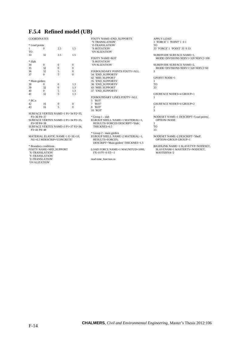
CHALMERS, Civil and Environmental Engineering, Master’s Thesis 2012:106 F-14
F.5.4 Refined model (UB) COORDINATES
* Load points
1 0 2.5 1.5
TO
33 32 2.5 1.5
* Slab
34 0 0 0
35 32 0 0
36 32 5 0
37 0 5 0
* Main girders
38 0 0 1.3
39 32 0 1.3
40 0 5 1.3
41 32 5 1.3
* BC:s
42 16 0 0
43 16 5 0
SURFACE VERTEX NAME=1 P1=34 P2=35,
P3=36 P4=37
SURFACE VERTEX NAME=2 P1=34 P2=35,
P3=39 P4=38
SURFACE VERTEX NAME=3 P1=37 P2=36,
P3=41 P4=40
MATERIAL ELASTIC NAME=1 E=3E+10,
NU=0.2 MDESCRIP='CONCRETE'
* Boundary conditions
FIXITY NAME=MID_SUPPORT
'X-TRANSLATION'
'Y-TRANSLATION'
'Z-TRANSLATION'
'OVALIZATION'
FIXITY NAME=END_SUPPORTS
'Y-TRANSLATION'
'Z-TRANSLATION'
'X-ROTATION'
'OVALIZATION'
FIXITY NAME=ROT
'X-ROTATION'
'OVALIZATION'
FIXBOUNDARY POINTS FIXITY=ALL
34 'END_SUPPORTS'
42 'MID_SUPPORT'
35 'END_SUPPORTS'
36 'END_SUPPORTS'
43 'MID_SUPPORT'
37 'END_SUPPORTS'
FIXBOUNDARY LINES FIXITY=ALL
5 'ROT'
7 'ROT'
8 'ROT'
10 'ROT'
* Group 1 - slab
EGROUP SHELL NAME=1 MATERIAL=1,
RESULTS=FORCES DESCRIPT='Slab',
THICKNES=0.5
* Group 2 - main girders
EGROUP SHELL NAME=2 MATERIAL=1,
RESULTS=FORCES,
DESCRIPT='Main girders' THICKNES=1.5
LOAD FORCE NAME=1 MAGNITUD=1000,
FX=0 FY=0 FZ=-1
read time_function.in
APPLY-LOAD
1 'FORCE' 1 'POINT' 1 0 1
TO
33 'FORCE' 1 'POINT' 33 0 33
SUBDIVIDE SURFACE NAME=1,
MODE=DIVISIONS NDIV1=320 NDIV2=100
SUBDIVIDE SURFACE NAME=2,
MODE=DIVISIONS NDIV1=320 NDIV2=60
3
GPOINT NODE=1
1
TO
33
GSURFACE NODES=4 GROUP=1
1
GSURFACE NODES=4 GROUP=2
2
3
NODESET NAME=1 DESCRIPT='Load points',
OPTION=NODE
1
TO
33
NODESET NAME=2 DESCRIPT='Shell',
OPTION=GROUP GROUP=1
RIGIDLINK NAME=1 SLAVETYP=NODESET,
SLAVENAM=1 MASTERTY=NODESET,
MASTERNA=2
CHALMERS, Civil and Environmental Engineering, Master’s Thesis 2012:106 G-1
Appendix G ADINA-PLOT command files
In ADINA an easy and convenient way to pick out certain results is to use plot command files
(*.plo) that includes all the commands that should be performed in order to extract specific
data from the results. The command file can also be used to export the results into text-files.
G.1 Beam model *---------------------------------------------------------------------------------------
* SECTIONAL FORCE DIAGRAMS
*---------------------------------------------------------------------------------------
ZONE NAME=1
'elements 1 to 34 of element group 1'
RESPONSE LOAD-STEP TIME=26
filelist inter
FILELIST F F='sf_beam-span-ADINA.txt'
ZONELIST ZONENAME=1 RESPOPTI=RESPONSE VARIABLE=X-
COORDINATE SHEAR_FORCE-T BENDING_MOMENT-S
*---------------------------------------------------------------------------------------
* INFLUENCE LINES
*---------------------------------------------------------------------------------------
ZONE NAME=2
'elements 26 to 27 of element group 1'
RESPRANGE LOAD-STEP TSTART=1 TEND=LATEST,
filelist inter
FILELIST F F='il_beam-ADINA.txt'
ZONELIST ZONENAME=2 RESPOPTI=RESPRANGE VARIABLE=X-
COORDINATE SHEAR_FORCE-T BENDING_MOMENT-S
G.2 Beam grillage models
G.2.1 BC2, BC5 and the U-models *---------------------------------------------------------------------------------------
* SECTIONAL FORCE DIAGRAMS
*---------------------------------------------------------------------------------------
ZONE NAME=1
'elements 1 to 32 of element group 1'
RESPONSE LOAD-STEP TIME=25
filelist inter
FILELIST F F='sf_beam-span-ADINA.txt'
ZONELIST ZONENAME=1 RESPOPTI=RESPONSE VARIABLE=X-
COORDINATE SHEAR_FORCE-T BENDING_MOMENT-S
TORSIONAL_MOMENT
RESPONSE LOAD-STEP TIME=17
filelist inter
FILELIST F F='sf_beam-support-ADINA.txt'
ZONELIST ZONENAME=1 RESPOPTI=RESPONSE VARIABLE=X-
COORDINATE SHEAR_FORCE-T BENDING_MOMENT-S
TORSIONAL_MOMENT
*---------------------------------------------------------------------------------------
* INFLUENCE LINES
*---------------------------------------------------------------------------------------
ZONE NAME=2
'elements 16 to 17 of element group 1'
'elements 24 to 25 of element group 1'
RESPRANGE LOAD-STEP TSTART=1 TEND=LATEST,
filelist inter
FILELIST F F='il_beam-ADINA.txt'
ZONELIST ZONENAME=2 RESPOPTI=RESPRANGE VARIABLE=X-
COORDINATE SHEAR_FORCE-T BENDING_MOMENT-S
TORSIONAL_MOMENT
G.2.2 Refined model *---------------------------------------------------------------------------------------
* SECTIONAL FORCE DIAGRAMS
*---------------------------------------------------------------------------------------
ZONE NAME=1
'elements 1 to 40 of element group 1'
RESPONSE LOAD-STEP TIME=29
filelist inter
FILELIST F F='sf_beam-span-ADINA.txt'
ZONELIST ZONENAME=1 RESPOPTI=RESPONSE VARIABLE=X-
COORDINATE SHEAR_FORCE-T BENDING_MOMENT-S
TORSIONAL_MOMENT
RESPONSE LOAD-STEP TIME=17
filelist inter
FILELIST F F='sf_beam-support-ADINA.txt'
ZONELIST ZONENAME=1 RESPOPTI=RESPONSE VARIABLE=X-
COORDINATE SHEAR_FORCE-T BENDING_MOMENT-S
TORSIONAL_MOMENT
*---------------------------------------------------------------------------------------
* INFLUENCE LINES
*---------------------------------------------------------------------------------------
ZONE NAME=2
'elements 16 to 17 of element group 1'
'elements 28 to 29 of element group 1'
RESPRANGE LOAD-STEP TSTART=1 TEND=LATEST,
filelist inter
FILELIST F F='il_beam-ADINA.txt'
ZONELIST ZONENAME=2 RESPOPTI=RESPRANGE VARIABLE=X-
COORDINATE SHEAR_FORCE-T BENDING_MOMENT-S
TORSIONAL_MOMENT
CHALMERS, Civil and Environmental Engineering, Master’s Thesis 2012:106 G-2
G.3 Combined models
G.3.1 BC2 and BC5 models *---------------------------------------------------------------------------------------
* SECTIONAL FORCE DIAGRAMS
*---------------------------------------------------------------------------------------
ZONE NAME=1
'elements 1 to 32 of element group 2'
RESPONSE LOAD-STEP TIME=25
filelist inter
FILELIST F F='sf_beam-span-ADINA.txt'
ZONELIST ZONENAME=1 RESPOPTI=RESPONSE VARIABLE=X-
COORDINATE SHEAR_FORCE-T BENDING_MOMENT-S
TORSIONAL_MOMENT AXIAL_FORCE
ZONE NAME=2
'elements 1 to 128 of element group 1'
RESPONSE LOAD-STEP TIME=25
filelist inter
FILELIST F F='sf_plate-span-ADINA.txt'
ZONELIST ZONENAME=2 RESPOPTI=RESPONSE VARIABLE=X-
COORDINATE Y-COORDINATE NODAL_FORCE-X NODAL_FORCE-Z
NODAL_MOMENT-Y
RESPONSE LOAD-STEP TIME=17
filelist inter
FILELIST F F='sf_beam-support-ADINA.txt'
ZONELIST ZONENAME=1 RESPOPTI=RESPONSE VARIABLE=X-
COORDINATE SHEAR_FORCE-T BENDING_MOMENT-S
TORSIONAL_MOMENT AXIAL_FORCE
RESPONSE LOAD-STEP TIME=17
filelist inter
FILELIST F F='sf_plate-support-ADINA.txt'
ZONELIST ZONENAME=2 RESPOPTI=RESPONSE VARIABLE=X-
COORDINATE Y-COORDINATE NODAL_FORCE-X NODAL_FORCE-Z
NODAL_MOMENT-Y
*---------------------------------------------------------------------------------------
* INFLUENCE LINES
*---------------------------------------------------------------------------------------
ZONE NAME=3
'elements 16 to 17 of element group 2'
RESPRANGE LOAD-STEP TSTART=1 TEND=LATEST,
filelist inter
FILELIST F F='il_beam-support-ADINA.txt'
ZONELIST ZONENAME=3 RESPOPTI=RESPRANGE VARIABLE=X-
COORDINATE SHEAR_FORCE-T BENDING_MOMENT-S
TORSIONAL_MOMENT AXIAL_FORCE
ZONE NAME=4
'elements 16 to 17 of element group 1'
'elements 48 to 49 of element group 1'
'elements 80 to 81 of element group 1'
'elements 112 to 113 of element group 1'
RESPRANGE LOAD-STEP TSTART=1 TEND=LATEST,
filelist inter
FILELIST F F='il_plate-support-ADINA.txt'
ZONELIST ZONENAME=4 RESPOPTI=RESPRANGE VARIABLE=X-
COORDINATE Y-COORDINATE NODAL_FORCE-X NODAL_FORCE-Z
NODAL_MOMENT-Y
ZONE NAME=5
'elements 24 to 25 of element group 2'
RESPRANGE LOAD-STEP TSTART=1 TEND=LATEST
filelist inter
FILELIST F F='il_beam-span-ADINA.txt'
ZONELIST ZONENAME=5 RESPOPTI=RESPRANGE VARIABLE=X-
COORDINATE SHEAR_FORCE-T BENDING_MOMENT-S
TORSIONAL_MOMENT AXIAL_FORCE
*
ZONE NAME=6
'elements 24 to 25 of element group 1'
'elements 56 to 57 of element group 1'
'elements 88 to 89 of element group 1'
'elements 120 to 121 of element group 1'
RESPRANGE LOAD-STEP TSTART=1 TEND=LATEST
filelist inter
FILELIST F F='il_plate-span-ADINA.txt'
ZONELIST ZONENAME=6 RESPOPTI=RESPRANGE VARIABLE=X-
COORDINATE Y-COORDINATE NODAL_FORCE-X NODAL_FORCE-Z
NODAL_MOMENT-Y
CHALMERS, Civil and Environmental Engineering, Master’s Thesis 2012:106 G-3
G.3.2 U-model *---------------------------------------------------------------------------------------
* SECTIONAL FORCE DIAGRAMS
*---------------------------------------------------------------------------------------
ZONE NAME=1
'elements 1 to 32 of element group 2'
RESPONSE LOAD-STEP TIME=25
filelist inter
FILELIST F F='sf_beam-span-ADINA.txt'
ZONELIST ZONENAME=1 RESPOPTI=RESPONSE VARIABLE=X-
COORDINATE SHEAR_FORCE-T BENDING_MOMENT-S
TORSIONAL_MOMENT AXIAL_FORCE
ZONE NAME=2
'elements 1 to 160 of element group 1'
RESPONSE LOAD-STEP TIME=25
filelist inter
FILELIST F F='sf_plate-span-ADINA.txt'
ZONELIST ZONENAME=2 RESPOPTI=RESPONSE VARIABLE=X-
COORDINATE Y-COORDINATE NODAL_FORCE-X NODAL_FORCE-Z
NODAL_MOMENT-Y
RESPONSE LOAD-STEP TIME=17
filelist inter
FILELIST F F='sf_beam-support-ADINA.txt'
ZONELIST ZONENAME=1 RESPOPTI=RESPONSE VARIABLE=X-
COORDINATE SHEAR_FORCE-T BENDING_MOMENT-S
TORSIONAL_MOMENT AXIAL_FORCE
RESPONSE LOAD-STEP TIME=17
filelist inter
FILELIST F F='sf_plate-support-ADINA.txt'
ZONELIST ZONENAME=2 RESPOPTI=RESPONSE VARIABLE=X-
COORDINATE Y-COORDINATE NODAL_FORCE-X NODAL_FORCE-Z
NODAL_MOMENT-Y
*---------------------------------------------------------------------------------------
* INFLUENCE LINES
*---------------------------------------------------------------------------------------
ZONE NAME=3
'elements 16 to 17 of element group 2'
RESPRANGE LOAD-STEP TSTART=1 TEND=LATEST,
filelist inter
FILELIST F F='il_beam-support-ADINA.txt'
ZONELIST ZONENAME=3 RESPOPTI=RESPRANGE VARIABLE=X-
COORDINATE SHEAR_FORCE-T BENDING_MOMENT-S
TORSIONAL_MOMENT AXIAL_FORCE
ZONE NAME=4
'elements 16 to 17 of element group 1'
'elements 48 to 49 of element group 1'
'elements 80 to 81 of element group 1'
'elements 112 to 113 of element group 1'
'elements 144 to 145 of element group 1'
RESPRANGE LOAD-STEP TSTART=1 TEND=LATEST,
filelist inter
FILELIST F F='il_plate-support-ADINA.txt'
ZONELIST ZONENAME=4 RESPOPTI=RESPRANGE VARIABLE=X-
COORDINATE Y-COORDINATE NODAL_FORCE-X NODAL_FORCE-Z
NODAL_MOMENT-Y
ZONE NAME=5
'elements 24 to 25 of element group 2'
RESPRANGE LOAD-STEP TSTART=1 TEND=LATEST
filelist inter
FILELIST F F='il_beam-span-ADINA.txt'
ZONELIST ZONENAME=5 RESPOPTI=RESPRANGE VARIABLE=X-
COORDINATE SHEAR_FORCE-T BENDING_MOMENT-S
TORSIONAL_MOMENT AXIAL_FORCE
*
ZONE NAME=6
'elements 24 to 25 of element group 1'
'elements 56 to 57 of element group 1'
'elements 88 to 89 of element group 1'
'elements 120 to 121 of element group 1'
'elements 152 to 153 of element group 1'
RESPRANGE LOAD-STEP TSTART=1 TEND=LATEST
filelist inter
FILELIST F F='il_plate-span-ADINA.txt'
ZONELIST ZONENAME=6 RESPOPTI=RESPRANGE VARIABLE=X-
COORDINATE Y-COORDINATE NODAL_FORCE-X NODAL_FORCE-Z
NODAL_MOMENT-Y
CHALMERS, Civil and Environmental Engineering, Master’s Thesis 2012:106 G-4
G.3.3 Refined model *---------------------------------------------------------------------------------------
* SECTIONAL FORCE DIAGRAMS
*---------------------------------------------------------------------------------------
ZONE NAME=1
'elements 1 to 192 of element group 2'
RESPONSE LOAD-STEP TIME=25
filelist inter
FILELIST F F='sf_beam-span-ADINA.txt'
ZONELIST ZONENAME=1 RESPOPTI=RESPONSE VARIABLE=X-
COORDINATE SHEAR_FORCE-T BENDING_MOMENT-S
TORSIONAL_MOMENT AXIAL_FORCE
ZONE NAME=2
'elements 1 to 3072 of element group 1'
RESPONSE LOAD-STEP TIME=25
filelist inter
FILELIST F F='sf_plate-span-ADINA.txt'
ZONELIST ZONENAME=2 RESPOPTI=RESPONSE VARIABLE=X-
COORDINATE Y-COORDINATE NODAL_FORCE-X NODAL_FORCE-Z
NODAL_MOMENT-Y
RESPONSE LOAD-STEP TIME=17
filelist inter
FILELIST F F='sf_beam-support-ADINA.txt'
ZONELIST ZONENAME=1 RESPOPTI=RESPONSE VARIABLE=X-
COORDINATE SHEAR_FORCE-T BENDING_MOMENT-S
TORSIONAL_MOMENT AXIAL_FORCE
RESPONSE LOAD-STEP TIME=17
filelist inter
FILELIST F F='sf_plate-support-ADINA.txt'
ZONELIST ZONENAME=2 RESPOPTI=RESPONSE VARIABLE=X-
COORDINATE Y-COORDINATE NODAL_FORCE-X NODAL_FORCE-Z
NODAL_MOMENT-Y
*---------------------------------------------------------------------------------------
* INFLUENCE LINES
*---------------------------------------------------------------------------------------
ZONE NAME=3
'elements 96 to 97 of element group 2'
RESPRANGE LOAD-STEP TSTART=1 TEND=LATEST,
filelist inter
FILELIST F F='il_beam-support-ADINA.txt'
ZONELIST ZONENAME=3 RESPOPTI=RESPRANGE VARIABLE=X-
COORDINATE SHEAR_FORCE-T BENDING_MOMENT-S
TORSIONAL_MOMENT AXIAL_FORCE
ZONE NAME=4
'elements 96 to 97 of element group 1'
'elements 288 to 289 of element group 1'
'elements 480 to 481 of element group 1'
'elements 672 to 673 of element group 1'
'elements 864 to 865 of element group 1'
'elements 1056 to 1057 of element group 1'
'elements 1248 to 1249 of element group 1'
'elements 1440 to 1441 of element group 1'
'elements 1632 to 1633 of element group 1'
'elements 1824 to 1825 of element group 1'
'elements 2016 to 2017 of element group 1'
'elements 2208 to 2209 of element group 1'
'elements 2400 to 2401 of element group 1'
'elements 2592 to 2593 of element group 1'
'elements 2784 to 2785 of element group 1'
'elements 2976 to 2977 of element group 1'
RESPRANGE LOAD-STEP TSTART=1 TEND=LATEST,
filelist inter
FILELIST F F='il_plate-support-ADINA.txt'
ZONELIST ZONENAME=4 RESPOPTI=RESPRANGE VARIABLE=X-
COORDINATE Y-COORDINATE NODAL_FORCE-X NODAL_FORCE-Z
NODAL_MOMENT-Y
ZONE NAME=5
'elements 144 to 145 of element group 2'
RESPRANGE LOAD-STEP TSTART=1 TEND=LATEST
filelist inter
FILELIST F F='il_beam-span-ADINA.txt'
ZONELIST ZONENAME=5 RESPOPTI=RESPRANGE VARIABLE=X-
COORDINATE SHEAR_FORCE-T BENDING_MOMENT-S
TORSIONAL_MOMENT AXIAL_FORCE
ZONE NAME=6
'elements 144 to 145 of element group 1'
'elements 336 to 337 of element group 1'
'elements 528 to 529 of element group 1'
'elements 720 to 721 of element group 1'
'elements 912 to 913 of element group 1'
'elements 1104 to 1105 of element group 1'
'elements 1296 to 1297 of element group 1'
'elements 1488 to 1489 of element group 1'
'elements 1680 to 1681 of element group 1'
'elements 1872 to 1873 of element group 1'
'elements 2064 to 2065 of element group 1'
'elements 2256 to 2257 of element group 1'
'elements 2448 to 2449 of element group 1'
'elements 2640 to 2641 of element group 1'
'elements 2832 to 2833 of element group 1'
'elements 3024 to 3025 of element group 1'
RESPRANGE LOAD-STEP TSTART=1 TEND=LATEST
filelist inter
FILELIST F F='il_plate-span-ADINA.txt'
ZONELIST ZONENAME=6 RESPOPTI=RESPRANGE VARIABLE=X-
COORDINATE Y-COORDINATE NODAL_FORCE-X NODAL_FORCE-Z
NODAL_MOMENT-Y
CHALMERS, Civil and Environmental Engineering, Master’s Thesis 2012:106 G-5
G.4 Shell models
G.4.1 UA- and UB-model *---------------------------------------------------------------------------------------
* SECTIONAL FORCE DIAGRAMS (BENDING AND SHEAR)
*---------------------------------------------------------------------------------------
ZONE NAME=1
'elements 1 to 192 of element group 2'
'elements 1 to 160 of element group 1'
RESPONSE LOAD-STEP TIME=17
filelist inter
FILELIST F F='sf-nodal_forces-support-ADINA.txt'
ZONELIST ZONENAME=1 RESPOPTI=RESPONSE VARIABLE=X-
COORDINATE Y-COORDINATE Z-COORDINATE NODAL_FORCE-X
NODAL_FORCE-Y NODAL_FORCE-Z
filelist inter
FILELIST F F='sf-nodal_moments-support-ADINA.txt'
ZONELIST ZONENAME=1 RESPOPTI=RESPONSE VARIABLE=X-
COORDINATE Y-COORDINATE Z-COORDINATE NODAL_MOMENT-
X NODAL_MOMENT-Y NODAL_MOMENT-Z
RESPONSE LOAD-STEP TIME=25
filelist inter
FILELIST F F='sf-nodal_forces-span-ADINA.txt'
ZONELIST ZONENAME=1 RESPOPTI=RESPONSE VARIABLE=X-
COORDINATE Y-COORDINATE Z-COORDINATE NODAL_FORCE-X
NODAL_FORCE-Y NODAL_FORCE-Z
filelist inter
FILELIST F F='sf-nodal_moments-span-ADINA.txt'
ZONELIST ZONENAME=1 RESPOPTI=RESPONSE VARIABLE=X-
COORDINATE Y-COORDINATE Z-COORDINATE NODAL_MOMENT-
X NODAL_MOMENT-Y NODAL_MOMENT-Z
*---------------------------------------------------------------------------------------
* INFLUENCE LINES (BENDING AND SHEAR)
*---------------------------------------------------------------------------------------
ZONE NAME=2
'elements 16 to 17 of element group 2'
'elements 48 to 49 of element group 2'
'elements 80 to 81 of element group 2'
'elements 112 to 113 of element group 2'
'elements 144 to 145 of element group 2'
'elements 176 to 177 of element group 2'
'elements 16 to 17 of element group 1'
'elements 48 to 49 of element group 1'
'elements 80 to 81 of element group 1'
'elements 112 to 113 of element group 1'
'elements 144 to 145 of element group 1'
RESPRANGE LOAD-STEP TSTART=1 TEND=LATEST
filelist inter
FILELIST F F='il-nodal_forces-support-ADINA.txt'
ZONELIST ZONENAME=2 RESPOPTI=RESPRANGE VARIABLE=X-
COORDINATE Y-COORDINATE Z-COORDINATE NODAL_FORCE-X
NODAL_FORCE-Y NODAL_FORCE-Z
filelist inter
FILELIST F F='il-nodal_moments-support-ADINA.txt'
ZONELIST ZONENAME=2 RESPOPTI=RESPRANGE VARIABLE=X-
COORDINATE Y-COORDINATE Z-COORDINATE NODAL_MOMENT-
X NODAL_MOMENT-Y NODAL_MOMENT-Z
ZONE NAME=3
'elements 24 to 25 of element group 2'
'elements 56 to 57 of element group 2'
'elements 88 to 89 of element group 2'
'elements 120 to 121 of element group 2'
'elements 152 to 153 of element group 2'
'elements 184 to 185 of element group 2'
'elements 24 to 25 of element group 1'
'elements 56 to 57 of element group 1'
'elements 88 to 89 of element group 1'
'elements 120 to 121 of element group 1'
'elements 152 to 153 of element group 1'
RESPRANGE LOAD-STEP TSTART=1 TEND=LATEST
filelist inter
FILELIST F F='il-nodal_forces-span-ADINA.txt'
ZONELIST ZONENAME=3 RESPOPTI=RESPRANGE VARIABLE=X-
COORDINATE Y-COORDINATE Z-COORDINATE NODAL_FORCE-X
NODAL_FORCE-Y NODAL_FORCE-Z
filelist inter
FILELIST F F='il-nodal_moments-span-ADINA.txt'
ZONELIST ZONENAME=3 RESPOPTI=RESPRANGE VARIABLE=X-
COORDINATE Y-COORDINATE Z-COORDINATE NODAL_MOMENT-
X NODAL_MOMENT-Y NODAL_MOMENT-Z
*---------------------------------------------------------------------------------------*
TSE-method (TORSION)
*---------------------------------------------------------------------------------------
ZONE NAME=4
'node 34'
'node 397'
'node 430'
'node 463'
'node 496'
'node 529'
'node 562'
'node 66'
'node 429'
'node 462'
'node 495'
'node 528'
'node 561'
'node 594'
RESPRANGE LOAD-STEP TSTART=1 TEND=LATEST
filelist inter
FILELIST F F='tsem -reaction_moment_x-ADINA.txt'
ZONELIST ZONENAME=4 RESPOPTI=RESPRANGE VARIABLE=X-
MOMENT_REACTION
ZONE NAME=5
'node 34'
'node 50'
'node 66'
RESPRANGE LOAD-STEP TSTART=1 TEND=LATEST
filelist inter
FILELIST F F='tsem-reaction_y-ADINA.txt'
ZONELIST ZONENAME=5 RESPOPTI=RESPRANGE VARIABLE=Y-
REACTION
ZONE NAME=6
'elements 1 to 32 of element group 1'
RESPRANGE LOAD-STEP TSTART=1 TEND=LATEST
filelist inter
FILELIST F F='tsem-nodals-ADINA.txt'
ZONELIST ZONENAME=6 RESPOPTI=RESPRANGE VARIABLE=X-
COORDINATE Y-COORDINATE NODAL_FORCE-Y
NODAL_MOMENT-X
CHALMERS, Civil and Environmental Engineering, Master’s Thesis 2012:106 G-6
G.4.2 Refined models (only torsional moment) *-----------------------------------------------------
* TSE-method (TORSION)
*-----------------------------------------------------
ZONE NAME=1
'node 34'
'node 32455'
'node 32776'
'node 33097'
'node 33418'
'node 33739'
'node 34060'
'node 34381'
'node 34702'
'node 35023'
'node 35344'
'node 35665'
'node 35986'
'node 36307'
'node 36628'
'node 36949'
'node 37270'
'node 37591'
'node 37912'
'node 38233'
'node 38554'
'node 38875'
'node 39196'
'node 39517'
'node 39838'
'node 40159'
'node 40480'
'node 40801'
'node 41122'
'node 41443'
'node 41764'
'node 42085'
'node 42406'
'node 42727'
'node 43048'
'node 43369'
'node 43690'
'node 44011'
'node 44332'
'node 44653'
'node 44974'
'node 45295'
'node 45616'
'node 45937'
'node 46258'
'node 46579'
'node 46900'
'node 47221'
'node 47542'
'node 47863'
'node 48184'
'node 48505'
'node 48826'
'node 49147'
'node 49468'
'node 49789'
'node 50110'
'node 50431'
'node 50752'
'node 51073'
'node 51394'
'node 354'
'node 32775'
'node 33096'
'node 33417'
'node 33738'
'node 34059'
'node 34380'
'node 34701'
'node 35022'
'node 35343'
'node 35664'
'node 35985'
'node 36306'
'node 36627'
'node 36948'
'node 37269'
'node 37590'
'node 37911'
'node 38232'
'node 38553'
'node 38874'
'node 39195'
'node 39516'
'node 39837'
'node 40158'
'node 40479'
'node 40800'
'node 41121'
'node 41442'
'node 41763'
'node 42084'
'node 42405'
'node 42726'
'node 43047'
'node 43368'
'node 43689'
'node 44010'
'node 44331'
'node 44652'
'node 44973'
'node 45294'
'node 45615'
'node 45936'
'node 46257'
'node 46578'
'node 46899'
'node 47220'
'node 47541'
'node 47862'
'node 48183'
'node 48504'
'node 48825'
'node 49146'
'node 49467'
'node 49788'
'node 50109'
'node 50430'
'node 50751'
'node 51072'
'node 51393'
'node 51714'
RESPRANGE LOAD-STEP TSTART=1
TEND=LATEST
filelist inter
FILELIST F F='data\tsem-reaction_moment_x-
320x100x60-ADINA.txt'
ZONELIST ZONENAME=1
RESPOPTI=RESPRANGE VARIABLE=X-
MOMENT_REACTION
ZONE NAME=2
'node 34'
'node 194'
'node 354'
RESPRANGE LOAD-STEP TSTART=1
TEND=LATEST
filelist inter
FILELIST F F='data\tsem-reaction_y-
320x100x60-ADINA.txt'
ZONELIST ZONENAME=2
RESPOPTI=RESPRANGE VARIABLE=Y-
REACTION
ZONE NAME=3
'elements 1 to 320 of element group 1'
RESPRANGE LOAD-STEP TSTART=1
TEND=LATEST
filelist inter
FILELIST F F='data\tsem-nodals-320x100x60-
ADINA.txt'
ZONELIST ZONENAME=3
RESPOPTI=RESPRANGE VARIABLE=X-
COORDINATE Y-COORDINATE
NODAL_FORCE-Y NODAL_MOMENT-X