STRUCTURAL ANALYSIS COMPUTER PROGRAMS FOR RIGID MULTICOMPONENT

PAVEMENT STRUCTURES WITH DISCONTINUITIES-WESLIQID AND WESLAYER

Report I

PROGRAM DEVELOPMENT NUMERICAL PRESENTATIONSby

Yu T. Chou

Geotechnical LaboratoryU. S. Army Engineer Waterways Experiment Station

P. O. Box 631, Vicksburg, Miss. 39180

May 1981

Report I o f a Series

TA7.W34t GL-81-6 1981 Vol. 1

Prepared for Office, Chief of Engineers, U. S. Army Washington, D. C. 2 0 3 14

Under Project No. 4A 7627I9A T 40, Work Units 00I and 003

f r i tTLIBRRRY

OCT 2 2 1981Bureau of Reclamation

Denver* Colorado

Destroy this report when no longer needed. Do not return it to the originator.

The find ings in th is report are not to be construed as an o ff ic ia l Department of the Army position u n le ss so designated ,

by other authorized docum ents.

The contents of this report are not to be used for advertising, publication, or promotional purposes. Citation of trade names does not constitute an official endorsement or approval of the use of

such commercial products.

'A S“« “ UOfum.___

Unclassified t - 'S E C U R IT Y C L A S S IF IC A T IO N O F TH IS P A G E (When D ata Entered)

REPORT DOCUMENTATION PAGE1. R E P O R T NUM BER 2. G O VT ACCESSION NO.

Technical Report GL-81-64. T IT L E (and Subtitle)

STRUCTURAL ANALYSIS COMPUTER PROGRAMS FOR RIGID MULTICOMPONENT PAVEMENT STRUCTURES WITH DISCON­TINU ITIES^-WESLIQID AND WESLAYER; Report 1, Program Develonment and Numerical Presentations -________7. A U T H O R *»

Yu T. Chou

9. P E R FO R M IN G O R G A N IZ A T IO N NA M E AND ADDRESSU. S. "Army Engineer Waterways Experiment StationGeotechnical LaboratoryP. 0. Box 631, Vicksburg, Miss. 3918011. C O N T R O L L IN G O F F IC E NAM E AND ADDRESS

Office, Chief of Engineers, U. S. Army Washington, D. C. 2031^+14. M O N ITO R IN G A G EN CY NAM E & ADDRESS^// different from Controlling O ffice )

READ INSTRUCTIONS BEFORE COMPLETING FORM3. R E C IP IE N T 'S C A TA LO G NU M BER

T Y P E O F R E P O R T & P E R IO D C O V E R E D

Report 1 of a series6. P E R FO R M IN G ORG. R E P O R T NUM BER

8. C O N T R A C T OR G R A N T N U M B E R *»

10. PROGRAM E L E M E N T , P R O J E C T , TASK AR EA & WORK U N IT NUM BERS

RDT&E Project No. UA762719ATI+O, Work Units 001 and 001

1 2 R E P O R T D A T E

"'May 1981.13. NU M BER O F PAGES

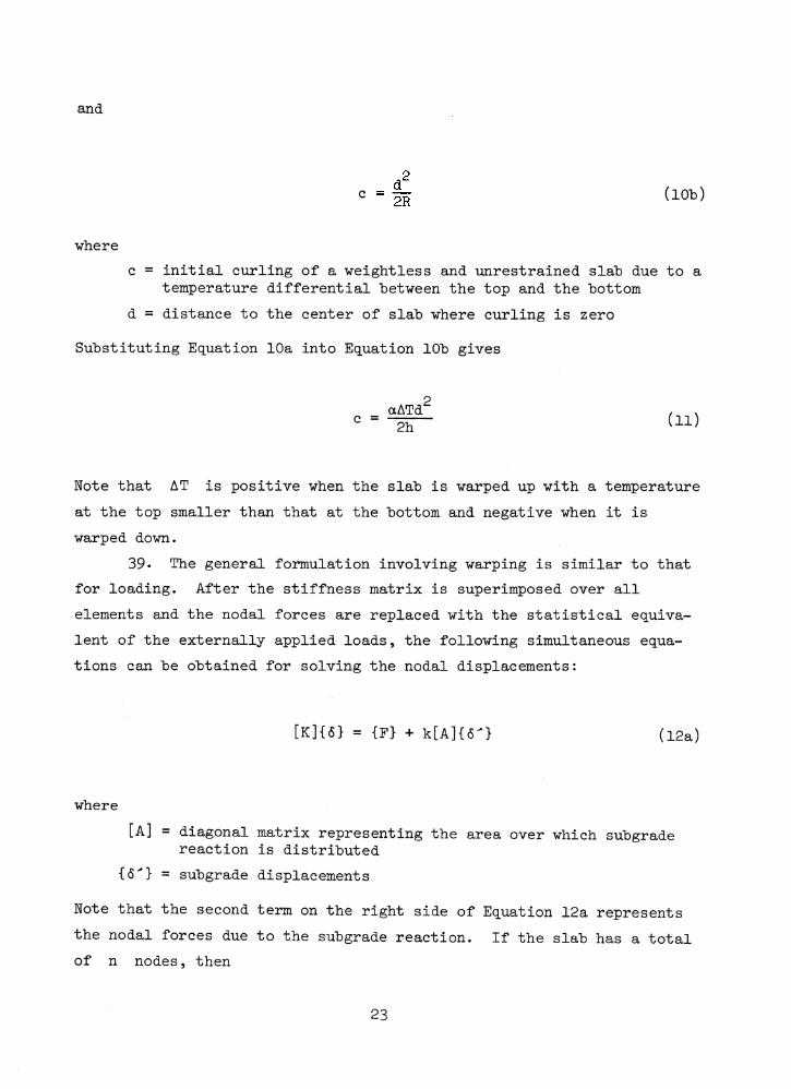
15. S E C U R IT Y CLASS, (o f thia report)

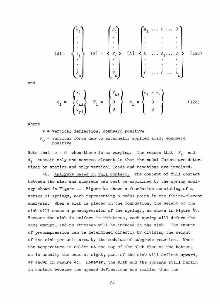
Unclassified15a. DECLASSI F IC A T IO N /D O W N G R A D IN G

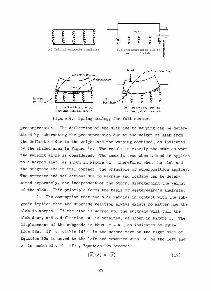
S C H E D U L E

16. D IS T R IB U T IO N S T A T E M E N T (o f th ia Report)

Approved for public release; distribution unlimited.

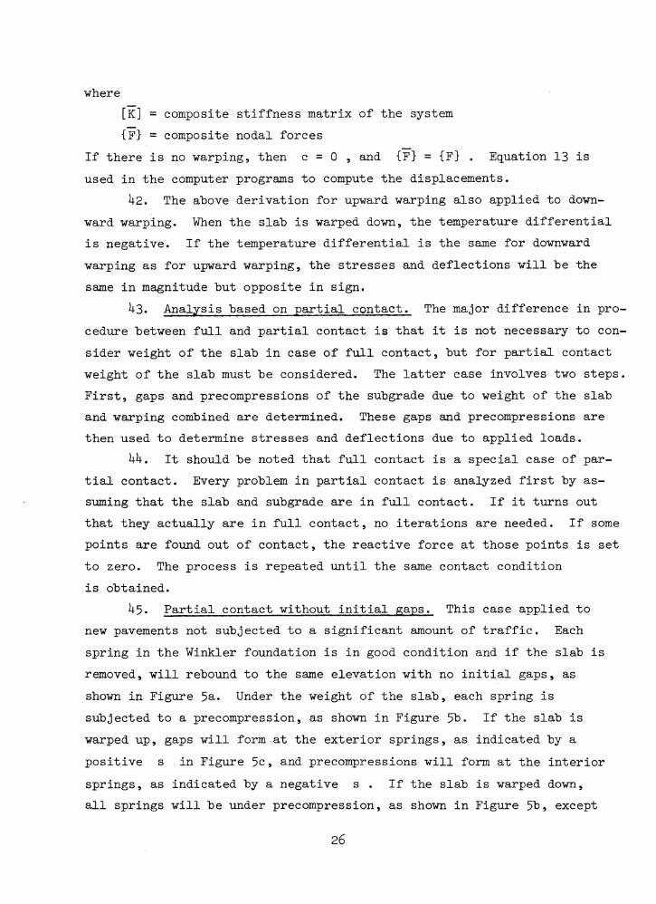
17. D IS T R IB U T IO N S T A T E M E N T (o f the abatract entered in B lock 20, i t d ifferent from Report)

18. S U P P L E M E N T A R Y NO TES

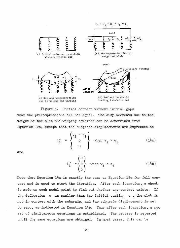
Available from National Technical Information Service, Springfield, Va. 22161.

19. K E Y WORDS (Continue on reverse side i f necessary and identify by block number)

20. ABSTR A C T (Continue on reverse aide ft necessary and. identity by block number)

This study was conducted to develop finite element computer programs to calculate stresses and deflections in rigid pavements with cracks and joints subjected to loads and temperature warping, as well as in the supporting sub­grade soil. The joints are connected by dowel bars or other load transfer devices. The slabs can have full or partial loss of subgrade support over designated regions of the slabs. Multiple-wheel loads can be handled and the

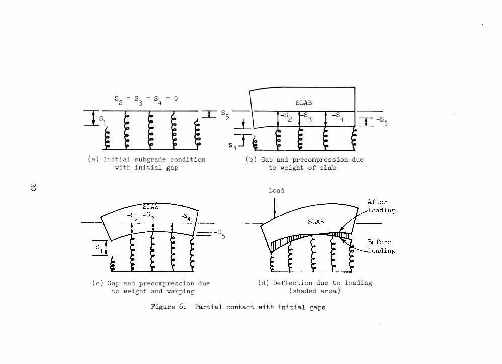
(Continued)DD * FORM JAN 73 1473 E D IT IO N O F t N O V 6 5 IS O B S O L E T E Unclassified

SECURITY CLASSIFICATION OF THIS PAGE (When Data Entered)

92056351

_________ Unclassified -S E C U R IT Y C L A S S IF IC A T IO N O F TH IS P A G E flW ifi D ata Entered)

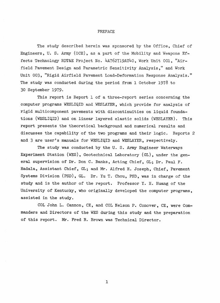
20. ABSTRACT (Continued).number of wheels is not limited. Two programs were developed, one called WESLIQID and the other WESLAYER. The former is for pavements on liquid foundations and the latter is for linear layered elastic solids. Variable slab thicknesses and moduli of subgrade reaction are incorporated in the WESLIQID program, and any number of slabs arrayed in an arbitrary pattern can be handled. Because of larger computer storage requirement and compu­tational complexity, the WESLAYER program is limited to two slabs.

The theoretical background of the model is presented first, and the capability and logic of the programs are fully described. A discussion of the load transfer mechanism along the joints and cracks is then given. Results computed by the WESLIQID program were compared with those of avail­able solutions, such as the Westergaard solution and Pickett and Rayfs in­fluence charts, and the comparisons were very favorable. The comparisons with the discrete-element computer program were excellent, except that the edge stresses computed by the discrete element program were much smaller. The WESLIQID and WESLAYER programs were used to analyze test pavements at eight U. S. Air Force bases and at the Ohio River Division Laboratories.The comparisons were centered on the percent stress transfer across the joint, and the comparisons were good. Based on the conclusions of the com­puted results, the design implication of WESLIQID in the rigid pavements is discussed.

UnclassifiedS E C U R IT Y C LA S S IF IC A T IO N O F TH IS PAGEfWFien Data Entered)

PREFACE

The study described herein was sponsored by the Office, Chief of Engineers, U. S. Army (OCE), as a part of the Mobility and Weapons Ef­fects Technology RDT&E Project No. ^A762T19AT^0, Work Unit 001, "Air­field Pavement Design and Parametric Sensitivity Analysis," and Work Unit 003, "Rigid Airfield Pavement Load-Deformation Response Analysis." The study was conducted during the period from 1 October 1978 to 30 September 1979*

This report is Report 1 of a three-report series concerning the computer programs WESLIQID and WESLAYER, which provide for analysis of rigid multicomponent pavements with discontinuities on liquid founda­tions (WESLIQID) and on linear layered elastic solids (WESLAYER). This report presents the theoretical background and numerical results and discusses the capability of the two programs and their logic. Reports 2 and 3 are user’s manuals for WESLIQID and WESLAYER, respectively.

The study was conducted by the U. S. Army Engineer Waterways Experiment Station (WES), Geotechnical Laboratory (GL), under the gen­eral supervision of Dr. Don C. Banks, Acting Chief, GL; Dr. Paul F. Hadala, Assistant Chief, GL; and Mr. Alfred H. Joseph, Chief, Pavement Systems Division (PSD), GL. Dr. Yu T. Chou, PSD, was in charge of the study and is the author of the report. Professor Y. H. Huang of the University of Kentucky, who originally developed the computer programs, assisted in the study.

COL John L. Cannon, CE, and COL Nelson P. Conover, CE, were Com­manders and Directors of the WES during this study and the preparation of this report. Mr. Fred R. Brown was Technical Director.

1

CONTENTS

PagePREFACE .......................................................... 1CONVERSION FACTORS, U. S. CUSTOMARY TO METRIC (Si)UNITS OF MEASUREMENT................................... k

PART I: INTRODUCTION . .......................................... 5Background .................................................. 5P u r p o s e ........... 6S c o p e ...................................................... 7

PART II: FINITE ELEMENT PLATE-BENDING M O D E L .................... 9Introduction ................................................ 9Brief Description of the Model.............................. 10Description and Capability of the Programs.................. 18Stress Transfer Along the Joints and Cracks ................ 32

PART III: PRESENTATION OF NUMERICAL RESULTS FOR THEWESLIQID PROGRAM................................. .. . Ul

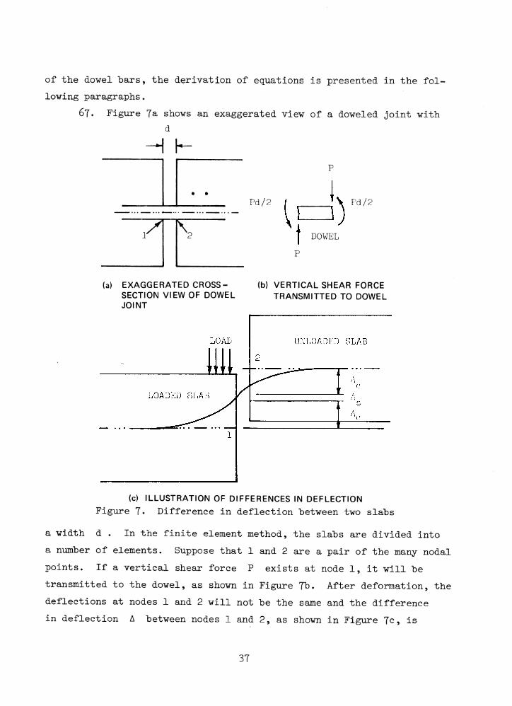
Comparison with Available Solutions ...................... klComparison with Experimental Results ..................... ^8

PART IV: PRESENTATION OF NUMERICAL RESULTS FOR THEWESLAYER P R O G R A M .................... ............. . . 62

Introduction ................................................ 62Stress and Deflection Basins ................................ 62Comparison with Strain Measurements from the Corpsof Engineers.............................................. 66

Effect of Subgrade Elastic Modulus E on StressTransfer Across a Joint .................................. 67

PART V: DESIGN IMPLICATIONS...................... 70Efficiency of Load Transfer by Dowel Bars . ................. 70Effect of Joint Conditions on Stresses and Deflections

for Center and Joint Loading Conditions .................. 76Effect of Loading Position on Stresses and Deflections

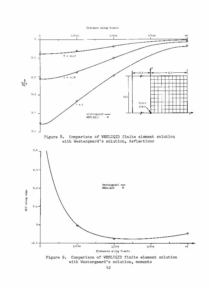
in Jointed Pavements...................................... 78Effect of Temperature and Gaps Under the Slabs.......... 88Continuously Reinforced Concrete Pavement (CRCP) ............ 101

PART VI: CONCLUSIONS AND RECOMMENDATIONS . ...................... 115Conclusions..................................... 115Recommendations.............................................. 117

REFERENCES . ....................................................... 118TABLES 1-22

2

PageAPPENDIX A: EQUATIONS FOR STRESSES AND DEFLECTIONS UNDER

A POINT LOAD AND UNDER A CIRCULAR L O A D ..............A1APPENDIX B: NOTATION ............................................ B1

3

CONVERSION FACTORS, U. S. CUSTOMARY TO METRIC (Si) UNITS OF MEASUREMENT

U. S. customary units of measurement used in this report can be con­verted to metric (Si) units as follows:

Multiply By To ObtainFahrenheit degrees 0 .5 5 5 Celsius degrees or Kelvins*feet 0.30U8 metresinches 2.5!+ centimetrespounds (force) k. 1+U8222 newtonspounds

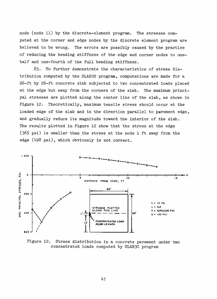
inch(force) per cubic 0.2711+ megapascals per metre

pounds (force) per inch 1 7 5 .1 2 6 8 newtons per metrepounds

inch(force) per square 6.891+757 kilopascals

* To obtain Celsius (C) temperature readings from Fahrenheit (F) readings, use the following formula: C = 0.555(F - 32). To obtainKelvin (K) readings, use: K = 0.555(F - 32) - 273.15*

STRUCTURAL ANALYSIS COMPUTER PROGRAMS FOR RIGIDMULTICOMPONENT PAVEMENT STRUCTURES WITH DIS­

CONTINUITIES— WESLIQID AND WESLAYER

PROGRAM DEVELOPMENT AND NUMERICAL PRESENTATIONS

PART I: INTRODUCTION

Background

1. The determination of stresses and deflections in concrete pave­ments due to -wheel loads has "been a subject of major concern for nearly half a century. In the early 1920's, Westergaard (1 9 2 5) assumed the sub­grade to be a Winkler foundation* and assumed that the slab was infinite in extent in all directions away from the load, and used the theory of elasticity to develop a mathematical method for determining the stresses in concrete pavements resulting from corner, edge, and interior loads.In extending the method to airport pavements, he later developed new formulas (Westergaard 1 9 3 9 5 1 9 ^ 8 ) that give the stresses and deflections at an edge point far from any corner and at an interior point far from any edge. These formulas were then employed by Pickett and Ray ( 1 9 5 1 )

to develop influence charts, which have been used by the Portland Cement Association ( 1 9 5 5 * 1 9 6 6 ) for the design of highway and airport pavements.

2. In spite of their wide acceptance and usage, the Westergaard solutions have been subject to many criticisms, including the following:

sl. The solutions are based on an infinitely large slab, with a load at the corner, on the edge, or in the interior.They may not be applicable to today's airfield pavements for aircraft equipped with large multiple-wheel gear loads.

b. The assumption of a Winkler foundation is not realistic because a Winkler foundation consists of a series of springs in which the pressure at any point between the

* A Winkler foundation is also called a liquid foundation. The inten­sity of the reaction of the subgrade is assumed to be proportional to the deflection of the slab and to be vertical only; frictional forces are neglected.

5

slab and the subgrade is directly proportional to the deflection only at that point and not elsewhere.

c_. The slab and the subgrade may not always be in full con­tact as assumed in the Westergaard solution. Gaps are frequently observed in the subgrade near the joint because of pumping action or plastic deformation. Temperature warping can also cause the slab to curl up and lose con­tact with the subgrade.

dh Westergaard solutions are based bn an infinitely largeslab with no discontinuities and thus could not be applied to analyze stress conditions at a joint or at a crack.

3. In the 1960's, a discrete element method based on the finite difference technique was developed at the University of Texas (Hudson and Matlock 1966) to analyze concrete slabs. The method considers the slab to be an assemblage of elastic joints, rigid bars, and torsional bars. This method of modeling was helpful in visualizing the problem and forming the solution. It does give reasonable values for pavement deflections, but there are problems in achieving accurate stress values along the edges. Serious problems exist in the analysis of joints, cracks, and gaps under the slab because of the nature of the method.

U. The Corps of Engineers (CE) realizes that much of the main­tenance of rigid pavements is associated with cracks and joints. The current CE rigid pavement design procedures (Department of the Army and the Air Force 1970) have certain limitations that were imposed by the state of the art at the particular stage of development. During the development of the procedure, it was necessary to make simplifying assump­tions and in many instances to ignore the effects of cracks and joints. Since the advent of high-speed computers and the development of the finite element method, a more comprehensive investigation of the state of stress at pavement joints, cracks, and other locations in multicomponent pavement structures is now tractable within the assumptions of the theory of elasticity. Consequently, a better and more reasonable design method may be developed for rigid pavements.

Purpose

5. The purpose of the study was to develop two-dimensional workable

6

finite element computer programs that have the capability of analyzing stress conditions in a rigid pavement containing cracks and joints and in the supporting subgrade soil. The programs should be able to analyze slabs made up of two layers of materials with different engineering properties, and should be able to accommodate full or partial loss of subgrade support over designated regions of the slabs. The subgrade soil can be either the Winkler foundation or a layered elastic solid.The program should be easy and economical to operate.

Scope

6. The finite element computer programs originally developed by Professor Y. H. Huang (Huang and Wang 1973, 197^; Huang 197^a, 197^b) of the University of Kentucky were modified and extended to suit the purpose of this study. The programs were developed based on the two- dimensional plate-bending theory. Two computer programs were developed: one named WESLIQID and the other WESLAYER. WESLIQID is developed for subgrade soil represented as a Winkler foundation. The program can treat any number of slabs connected by steel bars or other load trans­fer devices at the joints. WESLIQID can be applied to two-layer slabs, either bonded or unbonded. WESLAYER is for subgrade soil representedas either a linear elastic solid or a linear elastic layered system. Because of additional computer storage space and other computational complexity, WESLAYER is limited to two slabs connected by load transfer devices.

7. Report 1 of this series presents the basic theoretical development of the programs. Explanations are given in the concept of stress transfer along the joint and the capability of the programs. Numerical results are presented comparing the values computed by the computer programs with field measurements and with those computed by the Westergaard and other available programs. The design implication of the computed results are discussed.

8. Reports 2 and 3 are user?s manuals for WESLIQID and WESLAYER, respectively. Descriptions of the two programs are presented in detail,

7

and the programming approaches and logics are also explained. The flow­charts and input guidance are presented with several example problems that illustrate the use of the input guides.

8

PART II: FINITE ELEMENT PLATE-BENDING MODEL

Introduction

9. To analyze the stress conditions of a rigid pavement involv­ing cracks and joints, the most ideal representation of such a system would he the application of a three-dimensional finite element method. The inherent flexibility of such an approach permits the analysis of a rigid pavement with steel bars and stabilized layers and provides an efficient tool for analyzing stress conditions at the joint. Unfor­tunately, such a procedure would require a tremendously large amount of computer core space to solve an extremely large number of simultaneous equations. Such a procedure is highly uneconomical and impractical until much larger, less costly computers become available. Also, the use of a three-dimensional finite element method still could not solve some basic problems existing in a rigid pavement, such as the loss of support between the pavement and the subgrade due to temperature warping or other causes. The difficulty lies in satisfying the continuity con­ditions in the three-dimensional finite element method. However, this problem does not exist in the two-dimensional plate-bending model used in this study.

10. Recently, several researchers used the finite element plate­bending model for analysis of concrete pavement with considerable success. They are: Eberhardt (1973a, 1973b), Huang and Wang (Huang andWang 1973, 197^; Huang 197^a, 197^b), Pichumani (l97l)> and Tabatabaie and Barenberg (1978). The obvious advantage of the plate-bending model is that it is two-dimensional; it can thus save greatly on the computer core space and computing time and can make the model workable and more acceptable to the general users.

11. After a thorough review of the available models, it was decided that the models developed by Huang and Wang (1973, 197 -) were more complete than the others. Mainly, these programs consider the partial subgrade contact of the pavement and elastic subgrade

9

foundation, which are essential considerations in a rational pavement

design.

Brief Description of the Model

12. The finite element method employed in this study is based on

the classical theory of a thin plate by assuming that the plane before

bending remains a plane after bending. Because the slab is modeled as

a thin plate, there is no variation in vertical deflection along the

thickness of the plate; i.e., the deflection at the top of the plate

is the same as that at the bottom. When the slab is divided into

rectangular finite elements, the division is made only in the longitu­

dinal and transverse directions; the vertical direction is not needed.

The model is thus two-dimensional. Another advantage of the plate­

bending model is that the application of finite element method does not

involve the subgrade soil and thus saves computer time. Only the sub­

grade reactive forces acting at the nodes are important. The subgrade

reactive forces are evaluated by numerical procedures.

13. The procedure of the model can be found in many textbooks and

papers, such as Zienkiewicz and Cheung (1967) and Cheung and Zienkiewicz

(1965)j and.will not be presented herein. Only the general approach is

described.

Slabs on the Winkler foundation

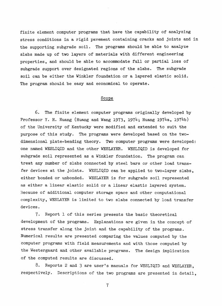
Ik. Figure 1 shows a rectangular finite element with nodes* i ,

j , k , and l . At each node, there are three fictitious forces and

three corresponding displacements. The three forces are a vertical

force F ; a moment about the x-axis M ; and a moment about the w x

y-axis My . The three displacements are the deflection in the

z-direction w ; a rotation about the x-axis 0 ; and a rotation aboutxthe y-axis 0 . These forces and displacements, for plates on a

Winkler foundation, are related by

* Symbols used in this report are listed and defined in the Notation (Appendix B).

10

■where[K] = stiffness matrix of the slab, the coefficients of which

depend on the dimensions a and b of the element and the Young’s modulus and Poisson’s ratio of the slab

6 = displacements in the slab61 = displacements in the subgradek = modulus of subgrade reaction

At any given node i

FORCES AND CORRESPONDING DISPLACEMENTS Figure 1* Rectangular plate element

11

15. The stiffness matrix for a rectangular element was tabulated

in Table 7*1 of the book by Zienkiewicz and Cheung (1967) and is used in the analysis. The type of elements used is isoparametric. For illus­

trative purposes, assuming i J k , and l are 1, 2, 3 > and b ,

respectively, Equation 1 can be expanded into 12 simultaneous equations:

wlMxlMyi‘w2Mx2M

( F '

y2

M

M

M

M

w3 =

x3

y3

F»i.

xb& J

K11

K21

K31

Kla

K.12

K,22

K.32

K.

K.13

K,23

K33

K,k2 k3

K.lb

K.2 b

K3b

K■ u u

W1 W1

exl 0

CD

H 0

W2 W2

9 x 2 0

CD

ro

L i0

V3>+ kab<

W3

0x30

ey30

WU wl*

exU 0

JVUJ0L J

(3)

in which K. . = 3 x 3 submatrix; i J

1 to b. For instance,

j = nodal numbers varying from

where

11

!X

H H

OJHM

k13

K . . = k21 k22 k23

_k31 k32 k33

vertical force (index l) deflection (index l) wj

Fwi at iat node ,

(h)

k^g = vertical force (index l) Fwiabout x-axis (index 2) 0xj at node j

i due to vertical

at node i due to rotation

k = moment about x-axis (index 2)rotation about y-axis (index 3) 0vi at node

Mxi at node3yj

i due toj

k^2 = moment about y-axis (index 3) Myi at node i due torotation about x-axis (index 2) 0xj at node j

12

with similar meanings for k ^ , k ^ , k ^ , k ^ , and k ^ . It is also to he noted in Equation 3 that vertical deflection w^ at the subgrade surface is implicitly assumed to he equal to vertical deflec­tion w. of the slah.1

16. By superimposing stiffness matrices over all elements and replacing the assumed fictitious nodal forces with the statistical equivalent of the externally applied loads, a set of simultaneous equa­tions can he obtained for solving the unknown nodal displacements.

17. For illustrative purposes, Figure 2 shows a pavement with

Figure 2. Computation of stresses under a point load acting at the corner of a slah

8l nodes. Since each node has three unknowns, there are 2^3 (8l x 3 = 2^3) simultaneous equations to he solved for the 2U3 unknown displace­ments. The nodal numbering system shown in Figure 2 (9 nodes in the vertical direction) indicates the half bandwidth is (9 + 2) X 3 = 33 ,

13

so the number of coefficients in the stiffness matrix [K] needing to be stored in the core is only 33 x 2^3 = 8,019 , instead of a full matrix 2k3 x 2^3 = 59*0^9 elements. The reason that the coefficients outside the half bandwidth need not be stored is that they are all zeros.

18. Once the nodal displacements are computed, the nodal moments are then computed using the stress matrix tabulated in Table 7*2 of Zienkiewicz and Cheung (1967). The nodal stresses are then computed from the nodal moments. Because the stresses at a given node computed by means of one element might be different from that computed by means of neighboring elements, the stresses in all adjoining elements were computed and their average values obtained.Slabs on an elastic foundation

19. Similar to Equation 1 for the Winkler foundation, the rela­tionship for the forces and displacements can be written as:

{F} = externally applied nodal forces[K] = stiffness matrix of the slab, the coefficients of which

depend on the finite element configuration and the flexural rigidity of the slab

[H] = stiffness matrix of the subgrade, the coefficients of which depend on the nodal spacings and the Young’s modulus and Poisson’s ratio of the subgrade

{6} = nodal displacements, each consisting of a vertical deflec­tion and two rotations

(5)

in which

{F}

and

20. The characteristics of Equation 5 are such that the stiffness

matrix of the slab [K] is handed, hut the stiffness of the suhgrade matrix [H] is not handed. When the two matrices are added, the composite matrix [P] , i.e., [P] = [K] + [H] , is not handed. Aniterative scheme was developed hy Huang (l97^h) to make [P] a handed matrix to save computer storage space.

21. To illustrate the iterative scheme, consider a simple example for a slah divided into only two finite elements with a total of six nodes. Because each node has three unknown displacements, there are 18 simultaneous equations:

K11 K12 K13 K1U 0 0 S’61

K22 K23 K2U 0 0 62K33 K3U K35 K36 J63

Symmetric KUU V KU6\

K55 K 56 «5K66_ 66V J

H11 H12 H13 HlU H15 Hl6 V VH22 H23 E 2k H25 H26 S2 F2

H33 H3U H35 H36 <53 F3Symmetric \ Fl,

H55 H56 s F5

H66 L Wwhere

K. . = 3 hy 3 suhmatrix 13

H. . = 3 hy 3 suhmatrixi = nodal numbers from 1 to 6 j = nodal numbers from 1 to 6

(6)

and

15

(7)<5 .i-^ yi

F .I wi.0

where0 . = rotation about x-axis xi0 . = rotation about y-axis yi JF = equivalent vertical force determined by statics

As no angular continuity is assumed between the slab and the subgrade

ij 0 00 0 00 0 0

(8)

where h ^ is vertical force at node i due to vertical displacement at node j .

22. The developed scheme is to transfer part of the [H] matrix to the right side of Equation 6, or

~P11 P12 p!3 Piu ° °r *\6i

P P„, 0 0 622 23 2k 2

P33 ? 3k P35 P36 I 63Symmetric P ^ P^6

P55 P 56 «5P66 S

V " o 0 0 0 H15 VF2 0 0 0 0 0 H26 S2

■< P3 >- 0 0 0 0 0 0 <S3pl. 0 0 0 0 0 0

F5 H15 0 0 0 0 0s 5

W _H16 H26 0 0 0 0 L6d16

(9)

First, assume the displacement {6} on the right side of Equation 9 as zero and compute a set of nodal displacements {6} by solving Equation 9* Enter the displacements thus computed into the right side of Equation 95 and find a new set of displacements. The process is repeated until the displacements converge to a specified tolerance.

23. In separating the [H] matrix, any half bandwidth may be used. The coefficients within the half bandwidth are placed on the left of Equation 95 whereas those outside the half bandwidth are transferred to the right. It was found that when the number of equa­tions is large while the half bandwidth is small, the displacements may not converge, and a larger bandwidth should be used.

2k. In solving Equation 9* each slab can be considered separately. First consider the left slab only, and the first set of nodal displace­ments is determined from Equation 8. Next, consider the right slab.The existence of the left slab has two effects on the right slab:(a) the vertical deflections along the joint in the right slab must be set equal to those in the left slab; and (b) the vertical nodal forces in the right slab must include those due to the deflections of the left slab. Because the deflections of the left slab have been previously determined, the nodal displacements of the right slab can be computed. Then return to the left slab again. The existence of the right slab also has two effects on the left slab: (a) the displacements of theright slab will induce a set of nodal forces along the joint, which must be transferred to the left slab; and (b) the deflections of the right slab will induce vertical reactive forces in the left slab. By taking these effects into consideration, a new set of displacements for the left slab is determined. The process is repeated until the nodal displacements converge.Basic differences between the liquid (Winkler) foundation and the elastic foundation

25. The basic difference between the liquid foundation and the elastic foundation is that in a liquid foundation, the deflection at a given node depends only on the forces at the node and does not depend on forces or deflections at any other nodes. In an elastic foundation,

IT

however, the deflection at a given node depends not only on the forces at the node, hut also on the forces or deflections at other nodes.

26. In both the WESLIQID and WESLAYER computer programs, separate nodal numbers are used at nodes at either side of the joint. The dis­tance between the two nodes is zero; i.e., these two nodes are physi­cally one node. The use of separate nodal numbers is necessary because the stresses and deflections in the two slabs across the joint may not be the same. The presence of separate nodal points across a joint is not a problem in a liquid foundation because in this case the deflection at a nodal point along the joint does not depend on deflections else­where. In an elastic foundation, however, the problem is more involved. For instance, a deflection at a node away from the joint will produce a certain subgrade reactive force at nodes along the joint.

Description and Capability of the Programs

Program logic27. The programming approaches for programs WESLIQID and WESLAYER

are presented separately in Reports 2 and 3 of this series, respectively. For convenience of discussion, the basic logic of the programs is pre­sented. Two cycles of iterations are involved in the programs. One is for checking the subgrade contact condition, and the other is for check­ing pavement shear forces for a deflection convergence. At the outset of the computation, the program first assumes a full contact between the slab and the subgrade, except at the nodes where gaps are preassigned.The gaps may be a result of pumping or plastic deformation of the sub­grade. Deflections are computed sequentially for each slab by succes­sive approximations until the deflection convergence criterion is met.

28. The relationships between the slabs along the joints are such that after the deflections are computed for slab i , the deflec­tions are superimposed to the adjacent (i + l)^*1 slab through the joint, and when the iteration returns to computing the deflections of slab I , shear forces exist at slab i along the joint between slabs i and (i + l) induced by the deflections of slab (i + l) .

18

29. When the deflections have all converged, the deflection at each node is checked as to whether the contact condition has changed.If the condition has not changed, the computed deflections are the final values; if it has changed, a new subgrade contact condition is assigned and the iteration for deflection computation starts again until the sub­grade contact condition ceases to change. To assure proper convergence, an underrelaxation factor is used in the programs to change the relaxa­tion factor automatically.Subgrade types

30. As was explained earlier, the application of the two- dimensional finite element process does not involve the subgrade soil.Only the subgrade reactive forces between the subgrade and the slab at each node are important. The subgrade reactive forces can be due either to deflection of the subgrade at the node or to deflections of an adja­cent slab transferred through the joint. The subgrade reactive forces at nodal points are combined with the externally applied forces when the displacements are being solved in the simultaneous equations shown in Equation 1. The subgrade reactive forces can be evaluated readily in the case of Winkler foundation but are more laborious in the case of the elastic foundation. These forces are explained in the following paragraphs.

31. Winkler foundation. The reactive force between the subgrade and the slab at each node equals the product of the modulus of the sub­grade reaction k and the deflection w at the node. For reactive forces at nodes along the joint that are induced by the deflections of adjacent slabs, the forces are computed through the stiffness matrix of the elements adjacent to the joint.

32. Elastic foundation. BoussinesqTs solution and Burmister’s layered elastic solution are used to compute subgrade surface deflec­tions for the cases of a homogeneous elastic foundation and a layered elastic foundation, respectively. Once the flexibility matrix is formed, a matrix inversion subroutine is used to invert the flexibility matrix to the stiffness matrix. The subgrade stiffness matrix is not banded, and at each node there is only a vertical component.

19

Stresses, strains, and deflections in the supporting subgrade soil

33. Once the subgrade reactive forces between the subgrade and the slab at each node are determined, stresses and strains in the sup­porting subgrade soil can be computed. The stresses and strains are in­duced by the nodal reactive forces, but the forces are acting in the direction opposite to those when the stress conditions in the slab were computed. When the subgrade soil is represented by the Winkler founda­tion (WESLIQID program), the Boussinesq's equations can be used to com­pute the stresses and strains induced by the concentrated nodal forces.In order to use the equations, an equivalent elastic modulus E corre­sponding to the modulus of subgrade reaction k (used in the program to compute stress condition in the slab) should be selected. When the sub­grade soil is represented by a layered elastic foundation, Burmister’s layered elastic solution is used for computation. Since the stresses and strains in the subgrade soil -under the concrete slabs are very small, the principle of superposition is valid and is used to compute the stresses and strains in the soil induced by all the nodal forces. It should be pointed out that at the subgrade surface, the deflection at the subgrade at a node is the same as that of the concrete slab at the same node; the vertical stress at the node is equal to the reactive force acting at the node divided by the affected area.

3 -. In the WESLIQID computer program, the BoussinesqTs equations for a point load (Harr 1966) are used to compute the stresses and deflec­tion in the supporting elastic subgrade soil. In using the equations, however, the stresses and deflections become infinitely large or inde­terminate at the surface directly under the point load and at locations very close to the point load. However, closed-form solutions for uni­formly applied circular loads are available only for the vertical stressa and vertical deflections w directly under the center of the cir- zcular load. These equations are presented in Appendix A. For computed locations in the subgrade soil not directly under a node, the computa­tions are made based on the point loads acting at the nodes. Since the computed values at locations close to a point load may be erroneous, the

20

computations are not made at shallow depths (less than 1 in.* in theprogram), except for the vertical stress a and vertical deflectionzw at computed locations directly under a node. This problem does not exist in the layered elastic subgrade soil (WESLAYER program) in which uniformly applied circular loads are used.

35* When the subgrade soil is represented as an elastic solid (WESLAYER program), the nodal reactive forces are larger at the slab edges than at the slab center where the load is applied. The distribu­tion of contact pressures under a rigid footing can be found in the textbook by Terzaghi and Peck (1962),Subgrade contact options

36. The concept of full and partial subgrade contact was origi­nally developed by Huang (197*0- Most materials presented in this sec­tion are taken from this source.

37* Discussion on the Westergaard solution. Complete subgrade contact condition was assumed in the Westergaard solution. The slab always has full contact with the subgrade soil, and gaps are not allowed between the slab and subgrade, no matter how much the slab has warped upward due to temperature change or to the applied load. In other words, the slab is supported by a group of springs, and the springs are always connected to the slab. In reality, the pavement can lose subgrade sup­port at some parts due to temperature warping, pumping, and plastic de­formation of the subgrade. Results from the Arlington test (Teller and Sutherland 1935* 1936, 19^2) indicated that the pavement and the sub­grade were not in full contact even when the slab was flat and there was no temperature differential between the top and the bottom. It was also found that the stresses in concrete pavements due to corner loading de­pended strongly on the condition of warping. When the corner was warped down and the slab and subgrade were in full contact, the observed corner stresses checked favorably with Westergaard1s solutions. However, the observed stresses were ^0 to 50 percent greater when the corner was warped up. Consequently, Westergaard1s equation for corner loading was* A table of factors for converting U. S. customary to metric (Si) units of measurement is presented on page U.

21

modified by Bradbury (1938), Kelley (1939)» Spangler (19^2), and Pickett (1951) to account for the loss of subgrade contact due to temperature warping, pumping, and plastic deformation of the subgrade. These modifications were based on empirical results, and no theoretical methods to the author’s knowledge have been developed so far. With the advent of high-speed computers and the finite element method, it is now possible to analyze concrete pavements subjected to warping and loading without assuming that the slab and the subgrade are in full contact.

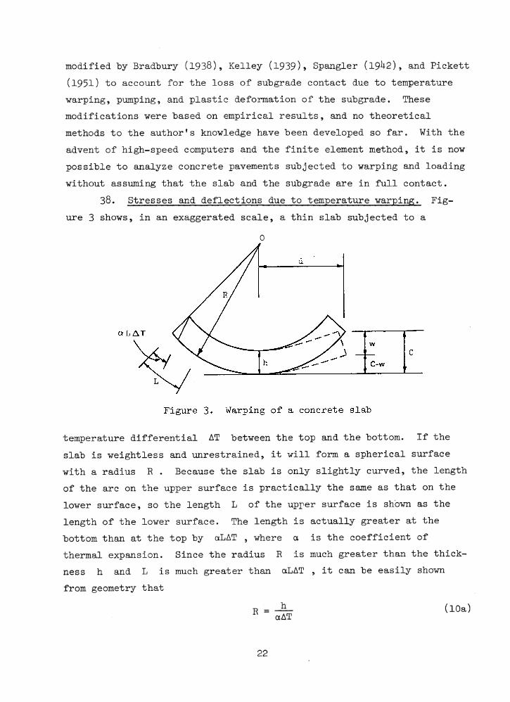
38. Stresses and deflections due to temperature warping. Fig­ure 3 shows, in an exaggerated scale, a thin slab subjected to a

0

temperature differential AT between the top and the bottom. If the slab is weightless and unrestrained, it will form a spherical surface with a radius R . Because the slab is only slightly curved, the length of the arc on the upper surface is practically the same as that on the lower surface, so the length L of the upper surface is shown as the length of the lower surface. The length is actually greater at the bottom than at the top by aLAT , where a is the coefficient of thermal expansion. Since the radius R is much greater than the thick­ness h and L is much greater than aLAT , it can be easily shown from geometry that

R = ha AT (10a)

22

c (10b)

wherec = initial curling of a weightless and unrestrained slab due to a

temperature differential "between the top and the "bottomd = distance to the center of slab where curling is zero

Substituting Equation 10a into Equation 10b gives

aATd22h (11)

Note that AT is positive when the slab is warped up with a temperature at the top smaller than that at the bottom and negative when it is warped down.

39- The general formulation involving warping is similar to that for loading. After the stiffness matrix is superimposed over all elements and the nodal forces are replaced with the statistical equiva­lent of the externally applied loads, the following simultaneous equa­tions can be obtained for solving the nodal displacements:

[K]{6} = {F} + k[A]{6'} (12a)

where[A] = diagonal matrix representing the area over which subgrade

reaction is distributed{&'} = subgrade displacements

Note that the second term on the right side of Equation 12a represents the nodal forces due to the subgrade reaction. If the slab has a total of n nodes, then

and

f p ^ (k. ... o ... o"li 1•

•

1

{6} = ^ 5.l

6

► (F> = < F.l

F

> [A] =<! 0 ... A.... 0 >1• • •

• • •

• • •

0 ... 0 ... An J n)

6 .1

F.1

F .vi00

6 .i

c. -l V.100

(12c)

wherev = vertical deflection, downward positiveF = vertical force due to externally applied load, downward

positiveNote that c = 0 when there is no warping. The reason that F^ and 6 contain only one nonzero element is that the nodal forces are deter­mined by statics and only vertical loads and reactions are involved.

ho. Analysis based on full contact. The concept of full contact between the slab and subgrade can best be explained by the spring anal­ogy shown in Figure h. Figure ha shows, a foundation consisting of a series of springs, each representing a nodal point in the finite-element analysis. When a slab is placed on the foundation, the weight of the slab will cause a precompression of the springs, as shown in Figure Ub. Because the slab is uniform in thickness, each spring will deform the same amount, and no stresses will be induced in the slab. The amount of precompression can be determined directly by dividing the weight of the slab per unit area by the modulus of subgrade reaction. When the temperature is colder at the top of the slab than at the bottom, as is usually the case at night, part of the slab will deflect upward, as shown in Figure Uc. However, the slab and the springs still remain in contact because the upward deflections are smaller than the

2h

(a) Initial subgrade condition (b) Precompression due to ç weight of slab §

Figure k. Spring analogy for full contact

precompression. The deflection of the slab due to warping can he deter­mined by subtracting the precompression due to the weight of slab from the deflection due to the weight and the warping combined, as indicated by the shaded area in Figure he. The result is exactly the same as when the warping alone is considered. The same is true when a load is applied to a warped slab, as shown in Figure hd. Therefore, when the slab and the subgrade are in full contact, the principle of superposition applies. The stresses and deflections due to warping and loading can be deter­mined separately, one independent of the other, disregarding the weight of the slab. This principle forms the basis of Westergaard1s analysis.

hi. The assumption that the slab remains in contact with the sub­grade implies that the subgrade reaction always exists no matter how the slab is warped. If the slab is warped up, the subgrade will pull the slab down, and a deflection w is obtained, as shown in Figure 3. The displacement of the subgrade is thus c - w , as indicated by Equa­tion 12c. If w within {6f} in the second term on the right side of Equation 12a is moved to the left and combined with w on the left and c is combined with {F} , Equation 12a becomes

[K]{6} = {?} (13)

25

where[K] = composite stiffness matrix of the system {F} = composite nodal forces

If there is no warping, then c = 0 , and {F} = {F} . Equation 13 is used in the computer programs to compute the displacements.

U2. The above derivation for upward warping also applied to down­ward warping. When the slab is warped down, the temperature differential is negative. If the temperature differential is the same for downward warping as for upward warping, the stresses and deflections will be the same in magnitude but opposite in sign.

3* Analysis based on partial contact. The major difference in pro cedure between full and partial contact is that it is not necessary to con sider weight of the slab in case of full contact, but for partial contact weight of the slab must be considered. The latter case involves two steps First, gaps and precompressions of the subgrade due to weight of the slab and warping combined are determined. These gaps and precompressions are then used to determine stresses and deflections due to applied loads.

UU. It should be noted that full contact is a special case of par­tial contact. Every problem in partial contact is analyzed first by as­suming that the slab and subgrade are in full contact. If it turns out that they actually are in full contact, no iterations are needed. If some points are found out of contact, the reactive force at those points is set to zero. The process is repeated until the same contact condition is obtained.

^5* Partial contact without initial gaps. This case applied to new pavements not subjected to a significant amount of traffic. Each spring in the Winkler foundation is in good condition and if the slab is removed, will rebound to the same elevation with no initial gaps, as shown in Figure 5a* Under the weight of the slab, each spring is subjected to a precompression, as shown in Figure 5b. If the slab is warped up, gaps will form at the exterior springs, as indicated by a positive s in Figure 5c, and precompressions will form at the interior springs, as indicated by a negative s . If the slab is warped down, all springs will be under precompression, as shown in Figure 5b, except

26

(a) Initial subgrade condition (b) Precompression due towithout initial gap weight of slab

(c) Gap and precompression (d) Deflection due todue to weight and warping loading (shaded area)

Figure 5- Partial contact without initial gaps that the precompressions are not equal. The displacements due to the weight of the slab and warping combined can be determined from Equation 12a, except that the subgrade displacements are expressed as

and

6T1 when w. > c. i i (lUa)

sri

o00

when w. < c.i i

(lVb)

Note that Equation lUa is exactly the same as Equation 12c for full con- tact and is used to start the iteration. After each iteration, a check is made on each nodal point to find out whether any contact exists. If the deflection w is smaller than the initial curling c , the slab is not in contact with the subgrade, and the subgrade displacement is set to zero, as indicated in Equation lUb. Thus after each iteration, a new set of simultaneous equations is established. The process is repeated until the same equations are obtained. In most cases, this can be

27

achieved by five or six iterations. After the deflections due to the weight and warping are determined, the gaps and precompressions can be computed and used later for computing the stresses and deflections due to the load alone.

b6. To determine the stresses and deflections due to the load alone requires that the gaps and precompressions shown in Figures 5b and 5c, depending on whether warping exists, first be determined. When these gaps and precompressions are used as s , the deflections due to the load alone (Figure 5d) can be determined from Equation 12, except that the subgrade displacements are expressed as

6:i00

0when w . < s .l l

s:i when w . > s . and s. > 0l i l

6;i when w . > s . and s. 0l i i

(15a)

(15b)

(15c)

When w is checked with s , downward deflection is considered positive, upward deflection is considered negative, gap is considered positive, and precompression is considered negative. First, assume that the slab and the subgrade are in full contact and the deflections of the slab due to the applied load are determined. Then check the deflections with s and form a new set of equations based on Equation 15. The process is repeated until the same equations are obtained.

lj-7. When the slab and the subgrade are in partial contact, the principle of superposition no longer applies. To determine the stresses and deflections due to an applied load requires that the deformed shape of the slab immediately before the application of the load be computed first. Since the deformed shape depends strongly on the condition of

28

warping, the stresses and deflections due to loading ate affected, apprer- ciably by warping. This fact was borne out in both the Maryland (.High­way Research Board 1952) and the AASHO (Highway Research Board 1962) road tests.

U8. In the method presented here, the stresses and deflections due to weight and warping are computed separately from those due to loading. This is desirable because the modulus of subgrade reaction under the sustained action of weight and warping is much smaller than that under the transient load of traffic. If the same modulus of sub­grade reaction is used, the stresses and deflections due to the combined effect of weight, warping, and loading can be computed in the same way as those due to weight and warping, except that additional nodal forces are needed to account for the applied loads.

^9* Partial contact with initial gaps. This case applies to pave­ments subjected to a high intensity of traffic, such as the traffic loops in the AASHO road test (Highway Research Board 1962). Because of pumping or plastic deformation of the subgrade, some springs in the Winkler foundation become defective and, if the slab is removed, will not return to the original elevation. Thus, initial gaps are formed, as indicated by the two exterior springs shown in Figure 6a. These gaps s must be assumed before an analysis can be made.

50. The displacements due to the weight of the slab, as shown in Figure 6b, can be determined from Equation 12a, except that the subgrade displacements must be expressed as

First, assume that the slab and the subgrade are in full contact. The

when w . > s.1 1

(16a)

when w. < s.1 1

(16b)

29

U)O

(a) Initial subgrade condition with initial gap

(b) Gap and precompression due to weight of slab

Load

(c) Gap and precompression due to weight and warping

(d) Deflection due to loading (shaded area)

Figure 6. Partial contact with initial gaps

vertical deflections of the slab are determined from Equation 12a.Then check the deflection at each node against the gap s . If the de­flection is smaller than the gap, as shown by the left spring in Figure 6b, Equation l6b is used. If the deflection is greater than the gap, as shown by the other springs in Figure 6b, Equation l6a is used. The process is repeated until the same equations are obtained. After the deflections are obtained, the gaps and precompressions can be computed and used later for computing the stresses and deflections due to load­ing, if no warping exists.

51. If the springs are of the same length, as shown in Figure U, the"weight of the slab will result in a uniform precompression, and no stresses will be set up in the slab. However, if the springs are of unequal lengths, the deflections will no longer be uniform, and stress­ing of the slab will occur.

52. Figure 6c shows the combined effect of weight and warpingwhen the slab is warped down. The reason that downward warping is con­sidered here, instead of the upward warping, is that the case of upward warping is similar to that shown in Figure 5c except that the gaps are measured from the top of the defective springs. The method is applic­able to both upward and downward warping, but downward warping is used for an illustration. The procedure for determining the deflections is similar to that involving the weight of slab alone except that the ini­tial curling of the slab, as indicated by Equation'll, is added to the gap shown in Figure 6a to form the total gap and precompression s foruse in Equation l6. Since the gap is either positive or zero and theinitial curling may be positive or negative, depending on whether the slab is warped up or down, s may be positive or negative. After the deflections of the slab are obtained, the gaps and precompressions, as shown in Figure 6c, can be determined. These gaps and precompressions are used for computing the stresses and deflections due to the load alone, as shown in Figure 6d.Symmetry

5 3 . The application of the finite element method for analyzingrigid pavements involves solving a large set of simultaneous equations.

31

However, due to symmetry the number of simultaneous equations could be greatly reduced by considering only one half or one quarter of the slabs. Consequently, the computer time and storage necessary can be greatly reduced and the results yielded are the same as for the use of the whole slab.

Stress Transfer Along the Joints and Cracks

5 . Joints are placed in rigid pavements to control cracking and provide enough space and freedom for movement. Load is transferred across a joint or crack principally by shear forces and in some cases by moment transfer. Shear force is provided either by dowel bars, key joint, or aggregate interlock. Moment transfer, on the other hand, is provided by the strength of the concrete slab and/or in-plane thrust (which is ignored in this analysis) but is produced by heating of the slab. When a joint or a crack has a visible opening, however, the transfer of moment across the joint or crack becomes negligible. It is therefore justified to assume there is no moment transfer across a joint or a crack, except in cases such as a tied joint where some moment trans­fer may be expected if the joint remains tightly closed.

55. In a continuously reinforced concrete pavement (CHCP), a large number of closely spaced cracks may form soon after placing the concrete. The tightly closed cracks can transfer a large percentage of moment during the early life of the pavement, but as traffic load is applied, the openings of the cracks will increase and the ability of moment transfer across the cracks will decrease.

56. If moment transfer across a joint is neglected, the amount of stress transfer at a joint is governed by the difference in deflec­tion between the two slabs along the joint. In other words, the shear transfer is 100 percent if deflections at both slabs are equal. This difference in deflection depends on the shear deformation of the dowel bar and the dowel-concrete interaction. The analyses presented later indicate that the effect of dowel-concrete interaction is more dominant than the shear deformation of the dowel bar. Neglecting the deformation

32

of concrete surrounding the dowel bar in the program can make the bar more effective than in reality. Field measurements conducted by the Corps of Engineers in many military airfields (Ohio River Division Lab­oratories 1959) indicated that the dowel bars were not very effective; the average stress transfer across a joint was only about 25 percent. Detailed discussion in this respect is presented in Part III.Shear and moment trans- fer across joints and cracks

57* The program provides three options for specifying shear trans­fer, but only one for moment transfer. The three options for shear transfer are: (a) efficiency of shear transfer, (b) spring constant,and (c) diameter and spacing of dowels. The only option for moment transfer is to assume an efficiency of moment transfer across the joint. The advantages and disadvantages of each option are discussed in the next section.

58. Efficiency of shear transfer. The efficiency of shear trans­fer is defined as the ratio of vertical deflections along the joint be­tween the unloaded, or less heavily loaded, slab and the adjacent more heavily loaded slab. This is the easiest method to specify shear trans­fer. By assigning an efficiency between 0.0 (no shear transfer) and 1.0 (complete shear transfer), reasonable results can be obtained with a minimum number of iterations. The efficiency can be easily checked on the printout by comparing each pair of deflections along the joint. However, the use of a given efficiency for all nodes along a joint is not realistic because the deflection ratios in an actual pavement should vary along the joint, with the smallest ratio at a point where the de­flection is the largest. To determine the efficiency in the field by measuring the deflection of both slabs along their common joint, the ratio at the point of largest deflection should be used, thus giving a more conservative estimate of the efficiency. The method has the further disadvantage that the slabs must be numbered according to the magnitude of load. This aspect is discussed in Report 2 of this series. In the computer programs, the slabs are numbered according to the magnitude of load.

33

59- Spring constant. The use of imaginary shear transfer springs along the joint between two slabs to determine the difference in deflec­tion is more realistic than the use of the efficiency of load transfer because the use of imaginary springs takes into consideration the shear force at the joint. The spring constant is defined as the force in pounds per linear inch to cause a difference in deflection of 1 in.; so the unit of the spring constant is in pounts per inch per inch. This option can be used either for key joints or joints with aggregate inter­lock (such as tightly closed cracks) or joints using both dowel bars and aggregate interlock for shear transfer. The spring constant can be determined in deflections at a number of points along the joint. The ratio between the average load (applied along the joint) per unit width and the average difference in deflection is the spring constant of the joint. A disadvantage of the method is that, without any test data, it is very difficult to assume a proper spring constant. The use of an improper spring constant may result in an unreasonably large difference in deflection and thus require a large number of iterations to obtain a convergent solution. It should be emphasized that the spring constant should not be determined based on test data of a single wheel load. The ideal test procedure is to place a long piece of steel beam adjacent to the joint and to apply the load to the beam through a series of wheel loads, preferably four to six wheels.

60. Once the value of the spring constant is determined for a certain joint in a rigid pavement, the difference in deflections at each nodal point across the joint can be determined based on the shear forces at each node computed at the particular stage during the itera­tion cycles.

61. Diameter and spacing of dowels. This method is most straight­forward and does not require a field test to determine either the effi­ciency of shear transfer or the spring constant. This option takes into consideration the diameter and spacing of dowels or steel bars. While this option should yield results far superior to the other two options, the method has some disadvantages, which are described below.

a. This method is applicable only when steel bars are the

3 ^

sole means of shear transfer. In a tied joint that remains closed, the shear transfer is principally pro­vided by the granular interlock, not by the thin tie bars. Therefore, the use of this method to specify the shear transfer of a tied joint would result in an effi­ciency less than the actual value.

b. This method requires an estimate of the modulus of dowel support, which may vary considerably depending on the type of dowel, strength of concrete, and method of con­struction. The condition of the dowel bars in the joint, i.e., the degree of looseness of dowels in the concrete, can affect the modulus value of dowel support. In Part IV, computed results of stress transfer across the joint for many military airfield pavements are presented. The re­sults indicate that the joint performance varies greatly with the modulus of dowel support used in the computation. Field tests conducted in a number of military airfields (Ohio River Division Laboratories 1959) indicated that in many airfields the dowel bars in the concrete were loose (i.e., excessive amounts of space around the dowels in the concrete).

62. Efficiency of moment transfer. Analysis of moment transfer across a joint or a crack is more involved than analysis of the transfer of shear force. The amount of moment transfer depends on the width of the crack, thickness of the slab, amount of reinforcing steel, and many other factors, and is difficult to analyze. It is believed that for a crack with a visible opening, the transfer of moment is negligible.

63. While the method of efficiency of shear transfer works well in specifying shear transfer across a joint, the efficiency of moment transfer, if defined as the rotation ratio between the unloaded and loaded slabs, is not applicable because an efficiency of zero indicates a zero rotation of the unloaded slab and a zero rotation is not realis­tic. The shear forces in a joint not only cause the slabs to deflect, but also cause the slabs to rotate. In the case of a crack with a vis­ible opening, the rotation at the unloaded slab is not zero; the joint acts as a hinge with large rotational movements at the joint. Unlikea zero deflection, a zero rotation actually requires the addition of a very large moment in the unloaded slab, which contradicts the defini­tion of zero moment transfer. Because the moments are very sensitive to the rotations, and could cause problems in solution convergence, it

35

is thus impractical to use a rotational constant similar to the spring constant to determine the difference in rotation. The following method for moment transfer was developed and found to be satisfactory.

6k. Moment transfer across the joint (or crack) is specified by the efficiency of moment transfer. One hundred percent moment transfer is defined by equal rotations at nodal points at both sides of the joint with the moments computed accordingly. Zero percent moment transfer is defined to be that the moments of nodal points along the joint are all zero while the rotations are not required to be zero. The efficiency is not defined as the rotation ratio between the unloaded and loaded slabs, but as a fraction of the full moment, which is determined by assuming that the rotations on both sides of the joint are the same. Unless the efficiency of moment transfer for all cracks is either 0.0 or 1.0, it is necessary to analyze the problem twice. First, an efficiency of 1.0 is assumed for all cracks having an efficiency other than zero, and the moments at each node along the crack are computed. These full moments are then multiplied by the efficiency of moment transfer at the corres­ponding joint to determine the moments that actually exist. These moments are then assigned for each slab edge, as externally applied moments, and a second analysis of the slabs is made.

6 5. It can be seen that the efficiency of moment transfer is de­fined differently than the efficiency of shear transfer. The efficiency of shear transfer is based on vertical deflections instead of vertical forces, whereas the efficiency of moment transfer is based on moments, instead of rotations. It is possible to define shear transfer on the basis of vertical forces, in the same way as for moment transfer, and analyze the problem twice. However, this is not warranted because many of the practical problems involve shear transfer only and can be solved in one analysis when shear transfer is defined by vertical deflections. Also, in the efficiency of shear transfer, the vertical deflections on both sides of the slab are different, but in the efficiency of moment transfer, the moments on both sides of the slabs are the same. Computations for dowel bars

66. For stress transfer using the method of diameter and spacing

36

of the dowel bars, the derivation of equations is presented in the fol­lowing paragraphs.

67. Figure 7a shows an exaggerated view of a doweled joint withd

H I—

• •

171 2

P

Pd/2

DOWEL

Pd/2

P

(a) EXAGGERATED CROSS- (b) VERTICAL SHEAR FORCESECTION VIEW OF DOWEL TRANSMITTED TO DOWELJOINT

(c) ILLUSTRATION OF DIFFERENCES IN DEFLECTIONFigure 7• Difference in deflection between two slabs

a width d . In the finite element method, the slabs are divided into a number of elements. Suppose that 1 and 2 are a pair of the many nodal points. If a vertical shear force P exists at node 1, it will be transmitted to the dowel, as shown in Figure 7b. After deformation, the deflections at nodes 1 and 2 will not be the same and the difference in deflection A between nodes 1 and 2, as shown in Figure 7c, is

37

A = A + 2A s c (17)where

A = shear deformation of the dowel sA = shear deformation of the concrete due to the bending of the

dowel as a beam on an elastic (concrete) foundation68. The shear deformation of the dowel can be determined approx­

imately bya - P dA S GA (18)

in which G and A are the shear modulus and the area of the dowel, respectively. By considering the dowel as a beam on an elastic founda­tion, A^ can be determined by (Timoshenko and Lessels 1925, Yoder and Witczak 1975)

= ■ X (2 + 3d)Ue3 (19a)

B = b UEI (19b)

whereE = modulus of elasticity of the dowel I = moment of inertia of the dowel K = modulus of dowel support, pci b = diameter of the dowel

By using realistic values for the parameters in Equations 18, 19a, and19b, it can be shown that A is one or more orders of magnitude smallersthan A^ and can usually be neglected; thus, the difference in deflec­tion depends principally on the dowel-concrete interaction. Because the amount of stress transfer across the joint is governed by the difference in deflection, the negligence of the dowel-concrete interaction will re­sult in a stress transfer that is too large.

69. It should be pointed out that the dowel bars are not modeled as bar elements in the programs. The joints or cracks in a rigid pave­ment generally have a width of l/l6 to 1/32 in., which is much smaller

38

than the bar diameter. A dowel bar in a joint should therefore serve merely as a key to transmit shear forces. If it is desirable to model dowels as bar elements, meaningful results can be obtained only if the theory of the deep beam is employed in the analysis, which, of course, is very complex. Tabatabaie and Barenberg (1978) modeled dowel bars as bar elements in their work; a detailed discussion in this aspect was made by Huang and Chou (1978).Modulus of dowel support

70. The stresses in dowel bars result from shear, bending, and bearing forces. These stresses can be analyzed to determine factors that affect the load transfer characteristics. The stress analysis of dowels is based upon work by Timoshenko (Timoshenko and Lessels 1925); Timonshenko modeled a dowel bar encased in concrete as a beam on a Wink­ler foundation. The ratio between the bearing pressure and the deflec­tion of the dowel bar was termed as modulus of dowel support K .Table 1 shows a wide range of moduli of dowel support produced by many investigators. The information was gathered by Finney (1956). Finney reported that while testing procedures varied among investigators, K values also varied between specimens for a given test procedure. A study of these investigations seems to indicate that K is not a con­stant quantity, but varies with the concrete properties, dowel bar di­ameter and length, slab thickness, and the degree of dowel looseness in the concrete.* Yoder and Witczak (1975) suggested that values of K range between 300,000 and 1 ,500,000 pci and that the use of 1 ,500,000 pci appears to be warranted. It was found in this study that while large changes in the modulus do not affect the stress calculations in theslab greatly, they do affect the deflection of the dowel which in turn can cause the change in the stress transfer across a joint.

71. To account in the computer program for the possible loose­ness of dowels, two different moduli of dowel support K can be speci­fied. (This is done only in the WESLIQID program.) When A < A" ,s — cK - ; when > A^ , K = ; where A' = an input parameter

* Slight looseness on one side of the dowel is often intentionally- built into the system in construction practice of rigid pavements.

39

specifying the deformation of concrete below which modulus isused and above which modulus is used. If a very large A' isassigned in the input, only will be used in the computation.

72. If Ac , as computed from Equation 19a and based on K = is not greater than A' , it will be used in Equation 17 to determine the difference in deflection. Otherwise, the following equations are used:

in which P ' = shear force on dowel to affect A ' , and g can be determined from Equation 19i> with K = .

c (2 0 )2 + gd

A = A ' +c c - P ' (2 + gd)Ug EI

(21)

In Equation 21, is used to determine 3

PART III: PRESENTATION OF NUMERICAL RESULTSFOR THE WESLIQID PROGRAM

Comparison with Available Solutions

73. To check the accuracy of the finite element method and the correctness of the computer program, it is desirable to compare the finite element solutions with other theoretical solutions available, especially with those involving discontinuities such as the stress at the free edge of a slab. Westergaard's original work and Pickett and Ray's influence charts can be used for such purposes. Because these available solutions are based on an infinite slab, a very large slab was used in the finite element analysis.Westergaard1s solutions

7^. The finite element solutions were obtained by using a large slab, 20£ long by 10£ wide, where £ is the radius of relative stiff­ness.

whereE = Young's modulus of the pavement t = thickness of the pavement v = Poisson's ratio of the pavement k = modulus of subgrade reaction

Because the problem is symmetrical with respect to the y-axis, only one half of the slab was considered. The slab was divided into rectangular finite elements as shown in Figure 8. Both the x and y coordinates are 0 , tt£/8 , tt£ A , tt£/2 , 3tt£ A , hi , 5£ , 6£ , 7£ , 8£ , 9£ , and 10£ . (Note the elements are not equally spaced for x and y smaller than U£ .) The Poisson's ratio of the concrete is 0.25. The finite elements are so divided because the Westergaard's solution for the problem at these coordinates is available in Westergaard (1925).

75* Figures 8 and 9 show the comparison between Westergaard's exact solutions and the WESLIQID finite element solution for deflection

hi

M/P

along

edge

Distance along X-axis

0 1 / U tt J2, l / 2 7 i i , 3 A i r i . t t £

Figure 9. Comparison of WESLIQID finite element solution with Westergaard's solution, moments

1+2

and moment, respectively. The former is for an infinite slab with a point load P acting at one edge far from any corner. The Westergaard solutions are indicated by the solid curves, and the finite element solutions are indicated by the small circles. The bonding moments M about the y-axis are computed along the edge of the slab, and the de­flections w are along the edge and at distances -nl/b and tt&/2 from the edge. The Westergaard solutions for moment and deflection are obtained from those shown in Figures 11 and 8, respectively, of Wester­gaard (1925)« It can be seen that the finite element solutions check very closely with Westergaard*s results.

76. Westergaard computed critical stresses in concrete pavements under three types of loading conditions. Type 1 is a wheel load acting close to a rectangular corner of a large panel of the slab. The criti­cal stress is a tension at the top of the slab. Type 2 is a wheel load acting at a considerable distance from the edges and is generally called a center load. The critical tension occurs at the bottom of the slab under the center of the load. Type 3 is a wheel load acting at the edge of the slab but at a considerable distance from any corner; it is generally called an edge load. The critical stress is a tension at the bottom under the center of the loaded circle.

77- The WESLIQID finite element program was used to compute stresses in concrete pavements for these three types of load. Point loads were used because they are easier to work with in the finite ele­ment method. The pavement was assumed to be 10 in. thick in all calcula­tions, and the modulus of subgrade reaction had three different values. The computed maximum stresses are tabulated in Table 2 together with those computed values obtained by the Westergaard method (1925).

78. In the cases of interior and edge load, the stresses com­puted by the finite element method are slightly higher than those of the Westergaard solution. This could be attributed to the fact that the Westergaard solution uses a semi-inifinite slab, while the finite element method employs a finite-size slab. It is believed that if the slab size is increased in the finite element method, the computed stresses will be reduced slightly. In the case of corner load, the

stresses computed by the finite element method are considerably less than the 300 psi computed by the Westergaard solution. The explanation of this discrepancy is that the corner stress computed by the Wester­gaard solution is the maximum stress under the point load, but the corner stresses computed by the finite element method as given in Table 2 are not the maximum values but the stresses computed at node 11 in Figure 2. More discussion in this respect is given in the next paragraph.

79* Figure 2 shows the finite element layout of a concrete slab subjected to a point load acting at the corner of the slab. The stresses computed at the nodes surrounding the load are presented in Table 3.It is seen that node 11 has the highest stress among those nodes where stresses were computed, but the stress at node 11 is not necessarily the maximum in the slab under the load. The maximum stress in the slab lies possibly between nodes 1 and 11 (or between 11 and 12, 21, or 20), depending on the modulus of subgrade reaction, and it can be determined only by further dividing the finite element grid. Since the stresses under the corner load computed by the finite element method in Table 2 are not the maximum stresses, they are therefore smaller than the maxi­mum stresses computed by the Westergaard solution. The discrepancy is greater for a greater modulus of subgrade reaction. In Figure 2, node 11 is 28.3 in. away from the corner; it is believed that when the mod­ulus of the subgrade reaction increases, the location of the maximum stress in the slab would be closer to the corner where the load is applied.

80. Influence charts by Pickett and Ray (1951) were not used di­rectly to check the finite element results. Instead, the results of the WESLIQID program were checked with those computed by the H-51 computer program. H-51 was developed by the General Dynamics Corporation to com­pute edge stress in a concrete pavement based on the Westergaard solu­tion. The program has been used by the Corps of Engineers for several years to determine edge stresses under multiple-wheel loads. It was found that the edge stresses computed by H-51 compare very closely with those from Pickett and Ray’s influence charts (1951).

8l. Figure 10 shows the layouts of the finite element and H-51

Finite Element Program

k

50,000 LB LO A D

-2 4 0

210

190

170

150

ö•H130

120 5

• no 9I

90

- 70

- 50

- 30

- 020 40 6 5 90 115 140 165 I 90 210 240

X-axis, in.

H-51 Program

Concrete slabt = 15 in.E = 6,000,000 psi v ^ 0.2 k = 100 pci

13.3

Uniform load: 50,000 lbContact area: 265 sq in.

1oo

Figure 10. Computation of edge stresses using WESLIQID finite element and H-51 program

programs to compute the edge stresses under a 50,000-lb wheel load. In the finite element method, a 20-ft by 20-ft slab was used, and because of symmetry only one half of the slab and a 25,000-lb load were used in the computation. The maximum radial tensile stress computed by the H-51 program was 607*3 psi, and that computed by the finite element pro­gram was 62^.3 psi, a difference of 2.7 percent.Discrete element solution

82. The finite element solutions were also compared with the discrete element solution developed at the University of Texas. The program is called SLAB30 (Hudson and Matlock 1965). The discrete ele­ment approach is mathematically equivalent to the finite difference method. The pavement slab is represented as a combination of elastic blocks, rigid bars, and torsion bars. Figure 11 shows the layout of

the finite element solution. The slab has four edges with four concen­trated loads acting at nodes 18, 19, 20, and 21. The same slab with the same loading condition was used for the SLAB30 program, except that the slab was divided with equal increments of 1 ft in both x- and y- directions. Table k presents the comparisons of the computed stresses and deflections at the nodal points designated in Figure 11. It can be

II 22 33

9

7

4 4 55 6641t2° 31 42 53 644¡is 29 40 51 62

17 26 39 50 61

16 27

15 26Nodalapplj

Pavement 1 Modulus E Poisson's ft Subgrade n

. points -ed, 7 2 ,thickness t = 6,000,01

atio v » 0. nodulus k

where los 000 lb eac= 15 in.

00 psi 2= 100 pci

id is 5h

14

111

25

13 2 4 35

12 23 3 4

_L

tttI4'

\a!1

I 3’ 3‘ 3'- 4 ' — --- 4 '

Figure 11. Computations of stresses and deflections using the WESLIQID finite element program, single slab

seen that excellent agreement was obtained on deflections but that the stresses agree only at the interior nodes. For nodes along the edge, the absolute values of the stresses computed by the discrete-element program are generally much smaller than those computed by the finite- element program. Theoretically, the stresses at the corner of a slab should be zero, but fairly large stresses are computed at the corner

U6

MAX

P

RIN

CIP

AL

ST

RE

SS

ES

, P

SI

node (node 11) by the discrete-element program. The stresses com­puted at the corner and edge nodes by the discrete element program are believed to be wrong. The errors are possibly caused by the practice of reducing the bending stiffness of the edge and corner nodes to one- half and one-fourth of the full bending stiffness.

83. To further demonstrate the characteristics of stress dis­tribution computed by the SLAB30 program, computations are made for a 26-ft by 26-ft concrete slab subjected to two concentrated loads placed at the edge but away from the corners of the slab. The maximum princi­pal stresses are plotted along the center line of the slab, as shown in Figure 12. Theoretically, maximum tensile stress should occur at the loaded edge of the slab and in the direction parallel to pavement edge, and gradually reduce its magnitude toward the interior of the slab.The results plotted in Figure 12 show that the stress at the edge (365 psi) is smaller than the stress at the node 1 ft away from the edge (U98 psi), which obviously is not correct.

Figure 12. Stress distribution in a concrete pavement under two concentrated loads computed by SLAB30 program

Comparison with Experimental Results

AASHO road tests8U. Efforts were made to compare the finite element solution

with the strain measurements from the (Highway Research Board 1962)AASHO road tests. Because a similar comparison had been made by Tabatabaie and Barenberg (1978), also using the two-dimensional finite element plate-bending model, the same test section, material properties, and loads were thus used in the computation. The following information is excerpted from Tabatabaie and Barenberg:

Tests were conducted on the main traffic loops where the strain due to moving traffic 12 to 22 in. from the edge was measured at the slab edge. The lengths of slabs were 15-ft nonreinforced sections and 1*0-ft reinforced slabs. Slab thickness ranged from 5 to 12.5 in. The measured dynamic modulus of elasticity and Poisson’s ratio of concrete were found to be 6.25 x 106 psi and 0.28, respectively.The modulus of subgrade reaction (k-values) on the subbase obtained by the plate-bearing tests varied from approximately 85 to 200 pci over all of the loops throughout the two-year t^st period. An average of 150 pci was used for modulus of subgrade reaction in the finite element analysis.

85. Figure 13 shows the comparison of the WESLIQID finite ele­ment solutions with AASHO experimental results and the calculations by Tabatabaie and Barenberg (1978). Except for the results computed by the WESLIQID program, the plotted results shown in Figure 13 are taken di­rectly from Tabatabaie and Barenberg. It is seen that excellent agree­ment is obtained in the theoretical solutions computed by the program prepared by Tabatabaie and Barenberg and the WESLIQID program prepared by the WES. This agreement is not surprising because both programs were developed based on the plate-bending theory. The computed results should be very close when the problem is dealing with a single slab that has full contact with the subgrade. The computed results may differ when joint and partial contact are considered.

U8

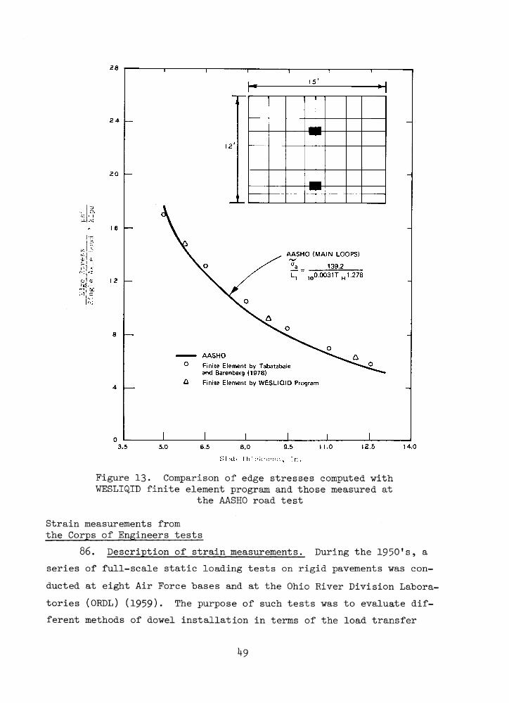
Figure 13. Comparison of edge stresses computed with WESLIQID finite element program and those measured at

the AASHO road test

Strain measurements from the Corps of Engineers tests

86. Description of strain measurements. During the 1950!s, a series of full-scale static loading tests on rigid pavements was con­ducted at eight Air Force bases and at the Ohio River Division Labora­tories (ORDL) (1959)• The purpose of such tests was to evaluate dif­ferent methods of dowel installation in terms of the load transfer

achieved at the joint and to check whether any of the methods failed to provide a joint meeting the minimum requirements of 25 percent load transfer as assumed in the design and evaluation of rigid pavements.

87. Doweled joints investigated for the study were constructed by five different methods, which included (a) cast in place, (b) remove and replace, (c) split dowels (screw-type only), (d) dummy half-dowel, and (e) oversize dummy half-dowel (cement grout only). Aircraft used in the loading tests included B-^7* B-52, and KC-97 aircraft. The test cart used on the ORDL experimental pavement had a four-wheel twin- tandem configuration similar to that used as the main gear for the B-36 aircraft. Joint performance was evaluated on the basis of strain mea­surements at the pavement surface in the direction parallel to the joint. Test procedures included the no load, load, and rebound measurements.

88. The description of test sites, instrumentation, test proce­dures, and test results of the study are documented in Ohio River Divi­sion Laboratories (1959). Table 5 is a summary of pavement, joint, and subgrade characteristics pertinent to the evaluation. Table 6 presents a summary of the average strain measurements obtained from the loading tests at each of the field test sites. Comparative average strains are shown for the load wheels on the bonded and unbonded sides of thé dowel, as well as. for the load positioned either directly over a dowel or mid­way between adjacent dowels. At ORDL Test Track nA,n no mine detector was available for locating the dowels. Therefore, the data for this test area were the average strains for all measurements without regard to the relative positioning of the strain gages and the dowels. Table 7 presents a summary of the average amount of load transfer measured at each of the nine test areas. The load transfer is defined as the ratio of the strain on the unloaded side of joint to that of the total strain (the sum of the strains on both unloaded and loaded sides) expressed as a percentage. Further discussion on the adequacy of the definition of "load transfer" is given in paragraph 93.

89. It was pointed out in Ohio River Division Laboratories (1959) that based on WestergaardVs theoretical analysis of rigid pave­ments, the sum of the strains on the loaded and unloaded sides of a

50

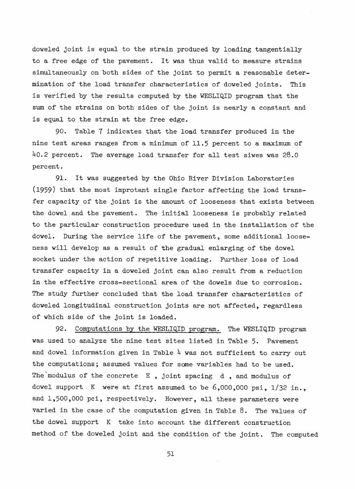
doweled joint is equal to the strain produced hy loading tangentially to a free edge of the pavement. It was thus valid to measure strains simultaneously on both sides of the joint to permit a reasonable deter­mination of the load transfer characteristics of doweled joints. This is verified by the results computed by the WESLIQID program that the sum of the strains on both sides of the joint is nearly a constant and is equal to the strain at the free edge.

90. Table 7 indicates that the load transfer produced in the nine test areas ranges from a minimum of 11.5 percent to a maximum of ^0.2 percent. The average load transfer for all test siwes was 28.0 percent.

91. It was suggested by the Ohio River Division Laboratories (1 9 5 9) that the most improtant single factor affecting the load trans­fer capacity of the joint is the amount of looseness that exists between the dowel and the pavement. The initial looseness is probably related to the particular construction procedure used in the installation of the dowel. During the service life of the pavement, some additional loose­ness will develop as a result of the gradual enlarging of the dowel socket under the action of repetitive loading. Further loss of load transfer capacity in a doweled joint can also result from a reductionin the effective cross-sectional area of the dowels due to corrosion.The study further concluded that the load transfer characteristics of doweled longitudinal construction joints are not affected, regardless of which side of the joint is loaded.

92. Computations by the WESLIQID program. The WESLIQID program was used to analyze the nine test sites listed in Table 5. Pavement and dowel information given in Table b was not sufficient to carry out the computations; assumed values for some variables had to be used.The"modulus of the concrete E , joint spacing d , and modulus of dowel support K were at first assumed to be 6,000,000 psi, 1/32 in., and 1,500,000 pci, respectively. However, all these parameters were varied in the case of the computation given in Table 8. The values of the dowel support K take into account the different construction method of the doweled joint and the condition of the joint. The computed

51

strains and load transfer were generally close to those measured values. It was found also that the computed values were influenced greatly with changes of E and K , but insignificantly with the change of joint spacing d . Increasing the E value decreases the strains on both sides of the joint and vice versa. Since the changes are nearly the same on both sides of the joint, the load transfer is not influenced significantly by the changes of E values. On the other hand, increas­ing the modulus of dowel support K makes the concrete surrounding the dowel bars stiffer, reduces the strains at the loaded side, and in­creases the strains at the unloaded side of the joint. The combined effect significantly increases the load transfer of the joint.

93. Table 8 shows the measured and computed strains and load transfers for the nine test sites. The computed stresses a in the

ydirection parallel to the joint are also shown in the table. It should be noted that in the theoretical computations, the load is placed di­rectly next to the joint and the strains are computed at the joint. In the actual field measurements, however, the strain gages were placed a small distance away from the joint, and the load is then placed a small distance from the gage. Therefore, the actual strains measured should be slightly less than those computed. Also in Table 8, the term "load transfer" is changed to "stress transfer." Current design criteria for rigid pavements for military airfields are based on either the premise that all types of joints transfer a minimum of 25 percent of the load applied along the joint to the adjacent slab. The stresses along the joints with adequate dowel construction are calculated as 75 percent of the free edge stresses with the load applied at the edge of the pavement. It is believed that the term "stress transfer" describes the situation better than the term "load transfer."

9 b . The comparisons between the computed and measured values in Table 8 are discussed separately for each test site as follows:

a,. Lockbourne AFB, Ohio. Entry 1-a shows the measuredstrains and stress transfer. The values shown in entry 1-b are computed with E , K , and d equal to 6,000,000 psi, 1,500,000 pci, and 1/32 in., respectively. The stress transfer is 6 percent higher than the measured value, and the computed strains are much higher than

52

those measured. Entry 1-c shows the values computed with E = 8,000,000 psi. It is seen that the strain values are reduced considerably and are very close to those measured values. Also, the stress transfer value is reduced by about 2 percent. Entry 1-d shows the com­puted values by keeping the value of E to 6,000,000 psi but reducing the modulus of dowel support K to 300,000 pci. It is seen that while the stress transfer is further reduced (2 percent less than measured value), the strain values increased considerably, particularly on the loaded side. In other words, when the modulus of dowel support Is reduced, the strains in the concrete increase; and since the strain in the loaded side increases much more than that in the unloaded side, the percentage of stress transfer is thus decreased. To check the effect of the crack opening d on the computed values,* a value of 1/2 in. was used with E and K equal to 6,000,000 psi and 1,500,000 pci, respectively. The computed values are tabulated in entry 1-e. It is seen that the computed values are insignificantly different from those in entry 1-b, indicating that the crack opening has very little influence on the joint performance.

b. Lincoln AFB, Nebraska. Entry 2-a shows the measuredstrains and stress transfer. Entry 2-b shows the values computed with the E , K , and d values equal to 6,000,000 psi, 1,500,000 pci, and 1/32 in., respectively. It is seen that the difference in total strain is very small between the measured and computed values, but there is a 9-percent difference in the stress transfer, result­ing from too large a computed strain in the loaded side and too small a computed strain in the unloaded side.By increasing the modulus of dowel support K from 1,500,000 to 9*000,000 pci (i.e., the concrete surrounding the dowel becomes stiffer or the looseness in the doweled joint is reduced), the strain in the loaded side decreases noticeably and the strain in the unloaded side increases slightly. The combined effect results in a computed stress transfer very close to the measured value, although the computed total strain becomes slightly less than the measured. The good comparison between the computed (entry 2-c) and measured values suggests that the dowel bars had a very good and tight fit in the joint in the rigid pavements tested at Lincoln AFB.

c_. Hunter AFB, Georgia. Entry 3-a shows the measured strains and stress transfer. With E , K , and d values of 6,000,000 psi, 1,500,000 pci, and 1/32 in.,

In this report, the crack opening is treated the same way as the joint spacing in the computer programs.

53

respectively* the computed values shown in entry 3-b are very close to measured values. Similar to the ex­planation given for entry 2-c, it is believed that by increasing slightly the modulus of dowel support K , the computed values can be closer to those measured.

jd. McCoy AFB» Florida. The values shown in entry H-b are computed with E , K * and d equal to 6,000,000 psi, 1,500,000 pci, and 1/32 in., respectively. It is seen that the computed stress transfer is very close to the measured value, but the computed strains are slightly higher than those measured. The differences can be readily corrected by increasing slightly the modulus of concrete E . However, this small difference may be merely due to the test method explained earlier that while the strains are computed exactly at the joint with the load placed directly next to the joint, the strain gages were actually placed at a small distance away from the joint and the load is then placed behind the gages.

£. ORDL Test Track "A".(1) Three different airfield pavements were tested at

the 0HDL test track. Pavement and joint information can be found in Table 5* The measured strains shown in entry 5-a are the average strains for all mea­surements. The strains computed for the three test pavements are shown separately in entries 5-b to 5-d. The average computed strains and stress trans­fer are listed in entry 5-e. While the computed strain values vary among the three different pave­ments, the computed stress transfers are nearly the same. This is reasonable because the test pavements were designed and constructed in accordance with the criteria, so the computed stress transfers across the joints for the three pavements are nearly iden­tical. Also, under a given loading condition, the strain decreases as the thickness of the concrete pavement increases. This explains why the .computed strain varies among the three pavements.

(2) The average strains and stress transfer shown in entry 5-e indicate that the computed total 'strain and stress transfer are considerably larger than the measured values. The strain at the loaded side of the joint is slightly less than the measured, but the strain at the unloaded side is much greater than the measured, resulting in a much greater computed stress transfer. With such strong dowel bars in the joints, i.e., 2, 3, and h in. in diameter, it is hard to believe that the average transfer is only 28.1 percent. The only explanation for the discrep­ancies is that the pavements at the ORDL test tracks

5^

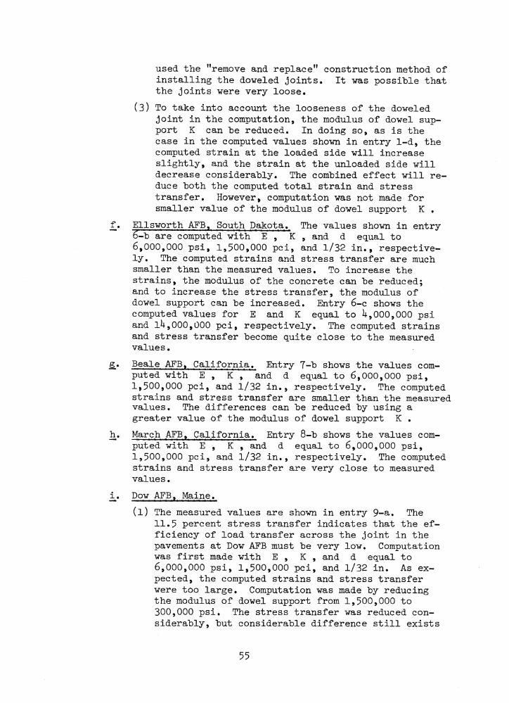
used the "remove and replace" construction method of installing the doweled joints. It was possible that the joints were very loose.

(3) To take into account the looseness of the doweled joint in the computation, the modulus of dowel sup­port K can be reduced. In doing so, as is the case in the computed values shown in entry 1-d, the computed strain at the loaded side will increase slightly, and the strain at the unloaded side will decrease considerably. The combined effect will re­duce both the computed total strain and stress transfer. However, computation was not made for smaller value of the modulus of dowel support K .

f# Ellsworth AFB, South Dakota. The values shown in entry ¿-b are computed with E~^ K , and d equal to 6,000,000 psi, 1,500,000 pci, and 1/32 in., respective­ly. The computed strains and stress transfer are much smaller than the measured values. To increase the strains, the modulus of the concrete can be reduced; and to increase the stress transfer, the modulus of dowel support can be increased. Entry 6-c shows the computed values for E and K equal to U,000,000 psi and 1^,000,000 pci, respectively. The computed strains and stress transfer become quite close to the measured values.

jg.* Beale AFB, California. Entry 7-b shows the values com­puted with E , K , and d equal to 6,000,000 psi,1.500.000 pci, and l/32 in., respectively. The computed strains and stress transfer are smaller than the measured values. The differences can be reduced by using a greater value of the modulus of dowel support K .

h. March AFB» California. Entry 8-b shows the values com­puted with E , K , and d equal to 6,000,000 psi,1.500.000 pci, and 1/32 in., respectively. The computedstrains and stress transfer are very close to measured values.

i* Dew AFB, Maine.(l) The measured values are shown in entry 9-a. The

11.5 percent stress transfer indicates that the ef­ficiency of load transfer across the joint in the pavements at Dow AFB must be very low. Computation was first made with E , K , and d equal to6,000,000 psi, 1,500,000 pci, and 1/32 in. As ex­pected, the computed strains and stress transfer were too large. Computation was made by reducing the modulus of dowel support from 1,500,000 to300,000 psi. The stress transfer was reduced con­siderably, but considerable difference still exists

55

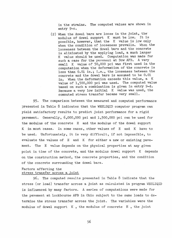
in the strains. The computed values are shown in entry 9-c.

(2) When the dowel bars are loose in the joint, the' modulus of dowel support K must be low. It is possible, however, that the K value is low only when the condition of looseness prevails. When the looseness between the dowel bars and the concrete is eliminated by the applying load, a much larger K value should be used. Computation was made for such a case for the pavement at Dow APB. A very small K value of 50,000 pci was first used in the computation when the deformation of the concrete is less than 0.01 in.; i.e., the looseness between the concrete and the dowel bars is assumed to be 0.01 in. When the deformation exceeds this value, a K value of 1,500,000 pci was used. The computed value based on such a combination is given in entry 9-d. Because a very low initial K value was used, the computed stress transfer became very small.

95* The comparison between the measured and computed performance presented in Table 8 indicates that the WESLIQID computer program can yield satisfactory results to predict joint performance for a rigid pavement. Generally, 6,000,000 psi and 1,500,000 pci can be used for the modulus of the concrete E and the modulus of the dowel support K in most cases. In some cases, other values of E and K have to be used. Unfortunately, it is very difficult, if not impossible, to evaluate the values of E and K for either a new or existing pave­ment. The E value depends on the physical properties at any given point in time of the concrete, and the modulus dowel support K depends on the construction method, the concrete properties, and the condition of the concrete surrounding the dowel bars.Factors affecting the stress transfer across a joint

96. The computed results presented in Table 8 indicate that the stress (or load) transfer across a joint as calculated in program WESLIQID is influenced by many factors. A series of computations were made for the pavement at Lockbourne AFB in Ohio subject to the same loads to de­termine the stress transfer across the joint. The variables were the modulus of dowel support K , the modulus of concrete E , the joint

56

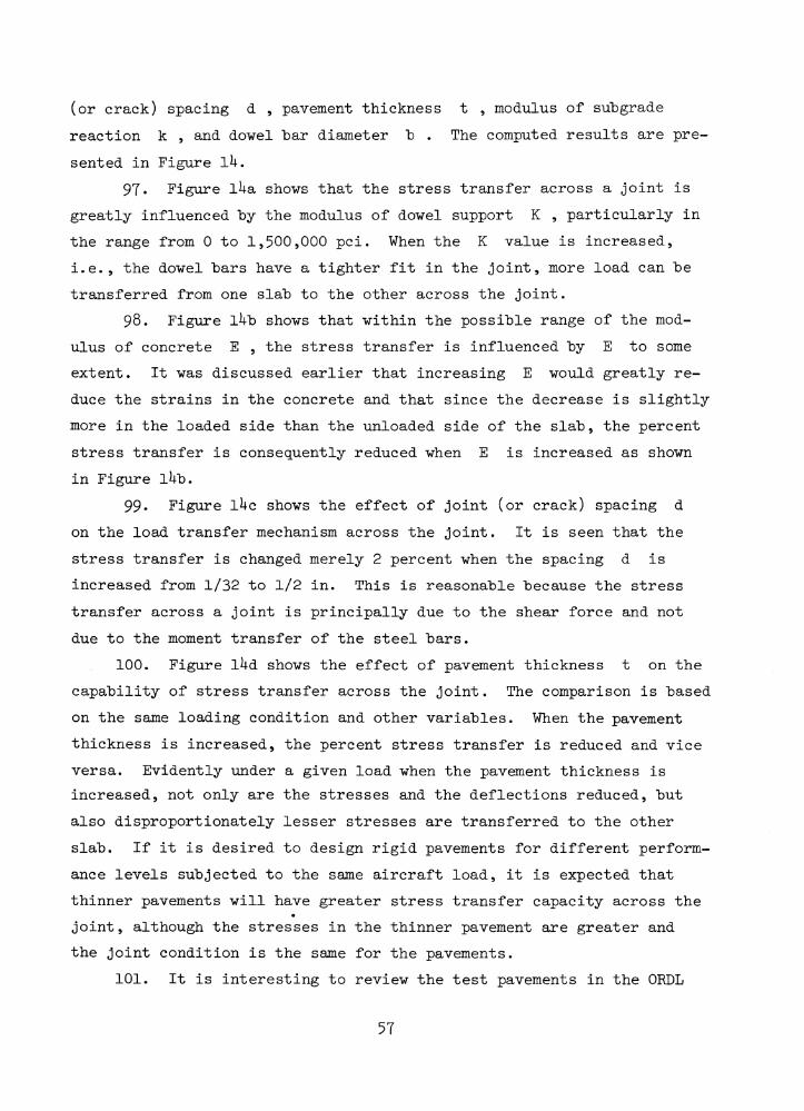
(or crack) spacing d , pavement thickness t , modulus of subgrade reaction k , and dowel bar diameter b . The computed results are pre­sented in Figure ik.

97• Figure iba. shows that the stress transfer across a joint is greatly influenced by the modulus of dowel support K , particularly in the range from 0 to 1,500,000 pci. When the K value is increased, i.e., the dowel bars have a tighter fit in the joint, more load can be transferred from one slab to the other across the joint.

98. Figure ibb shows that within the possible range of the mod­ulus of concrete E , the stress transfer is influenced by E to some extent. It was discussed earlier that increasing E would greatly re­duce the strains in the concrete and that since the decrease is slightly more in the loaded side than the unloaded side of the slab, the percent stress transfer is consequently reduced when E is increased as shown in Figure lUb.

99* Figure ihc shows the effect of joint (or crack) spacing d on the load transfer mechanism across the joint. It is seen that the stress transfer is changed merely 2 percent when the spacing d is increased from 1/32 to 1/2 in. This is reasonable because the stress transfer across a joint is principally due to the shear force and not due to the moment transfer of the steel bars.

100. Figure ibd shows the effect of pavement thickness t on the capability of stress transfer across the joint. The comparison is based on the same loading condition and other variables. When the pavement thickness is increased, the percent stress transfer is reduced and vice versa. Evidently under a given load when the pavement thickness is increased, not only are the stresses and the deflections reduced, but also disproportionately lesser stresses are transferred to the other slab. If it is desired to design rigid pavements for different perform­ance levels subjected to the same aircraft load, it is expected that thinner pavements will have greater stress transfer capacity across the joint, although the stresses in the thinner pavement are greater and the joint condition is the same for the pavements.

101. It is interesting to review the test pavements in the 0RDL

57

STRESS TRANSFER ACROSS J O I N T , PERCENTNOTE: Joint condition: 1-in. dowel bars 15 in. apart, pavement thickness 12 in.# modulus of subgrade reaction k = 75 pci.

Stress transfer is defined to be the ratio of the stress (or strain) on the unloaded side of joint to that of the sum of the stresses (or strains) on both loaded and unloaded sides.

Figure Ik. Variations of stress (or load) transfer across a joint (Sheet 1 of 2)

CO

NC

RE

TE

P

AV

EM

EN

T

TH

ICK

NE

SS

n

NOTE: Modulus of dowel support k = 1,500,000 pci, modulus of concrete E = 6,000,000 psi, joint spacing d = 1/32 in. Stress transfer is defined to be the ratio of the stress (or strain) on the unloaded side of joint to that of the sum of the stresses (or strains) on both loaded and unloaded sides.

(Figure l^. (Sheet 2 of 2)

test track in connection with the stress transfer capability. The three test pavements listed in Table 5 have thicknesses of 2k, 28, and 32 in., and their corresponding dowel diameters and spacings are 2, 3, and U in. and 17, 17, and 27 in., respectively. The numbers were determined based on the Corps of Engineers design criteria for rigid pavement. In other words, the stress transfers for the three test pavements were ex­pected to be the same. The measured stress transfers for the three pavements were all close, and the computed stress transfers shown in Table 8 were nearly identical, even though the measured and computed values for each pavement do not agree with each other.

102. Figure ike shows the effect of the modulus of subgrade re­action k on the stress transfer capability of the joint. As the k value is increased, the stress transfer is decreased. Similar to the discussion about the relationship between the pavement thickness t and the stress transfer shown in Figure lUd, when the strength of the subgrade is increased, the stresses and deflections are reduced, but disproportionately lesser stresses are transferred to the other slab. Therefore, if the subgrade soil of a rigid pavement is stabilized and other conditions are kept identical, the stress transfer across the joint can be expected to reduce slightly, although the stresses in the pavement with stabilized subgrade are smaller.

103. Figure ll+f shows the effect of dowel bar diameter b on the stress transfer capability. The computations were made for different diameters of dowel bars at a constant 6-in. dowel spacing. As was ex­pected, the amount of stress transfer is dominated by the number and size of dowel bars used in the joint. It should be pointed out that according to the definition of percent stress transfer used in this report, a 50 percent stress transfer is a total load transfer, i.e., the stresses on both sides of the joint are identical. For a l+-in. dowel bar spaced 6 in. apart, the stress transfer is still less thana total transfer, thus indicating that the dowel bar is not a very efficient load transfer device. This aspect will be discussed later in the report.

60

10U. The computed results presented in this paper indicate that the stress (or load) transfer across a joint in a rigid pavement is affected by many factors. These factors, such as bar diameter and spacing, subgrade modulus, and pavement thickness, can be readily measured and thus appropriately accounted for. However, the factors, such as modulus of concrete E and modulus of dowel support K , are hard to measure and estimate, but their effects on the stress transfer are very large. It is also known that the value of K in a rigid pavement can decrease with time because of the repetitive action of aircraft loads.

6l

PART IV: PRESENTATION OF NUMERICAL RESULTSFOR THE WESLAYER PROGRAM

Introduction

105- In using the WESLAYER computer program to analyze field mea­surements of test sections, the primary difficulty lies in the selection of proper modulus values E and Poisson’s ratio v to represent the material properties of the layered elastic subgrade because most test sections measured k (modulus of subgrade reaction) values for sub­grade soils. Efforts were made to establish correlations between k and E values for a given value of v for the case of a single layer under the pavement. This was done by computing the stresses and deflec­tions for a given pavement with a range of subgrade k values (using the WESLIQID program) and for the same pavement with a range of subgrade E values (using the WESLAYER program and assuming the subgrade is homogeneous and v = O.U). The corresponding E and k values were determined by matching the maximum (or near maximum as will be explained later) stress or deflection at a critical nodal point in two pavements that have the same loading and geometrical conditions but have different subgrade conditions. The reason for selecting maximum values is that the shapes of the stress and deflection basins under the liquid founda­tion (represented by the WESLIQID program) and the elastic foundation (represented by the WESLAYER program) are different. In the computation the elastic modulus of the concrete E was assumed to be 6,000,000 psi.

Stress and Deflection Basins

106. The computed results indicate that the correlations between the k and E values are not unique. The correlations are presented in Figure 15 for three joint conditions for stress-based computations.*

* The equation relating k and E values developed by Vesic and Saxena (1970) was compared with the relations shown in Figure 15 and was found unsatisfactory in some cases.

62

Figure 15. Correlations between subgrade E and k for the Lockbourne AFB test pavement; the subgrade is assumed to be one layer and homogeneous and the Poisson’s ratio

v assumed to be 0.J+

The pavement and loading conditions are the same as those used in the Lockbourne AFB test pavement (see Table 5). Figure 15 shows that the differences among the three different joint conditions are large, espe­cially for the dowel bar case. Computations were also made for other pavements. It was found that the correlations were different for dif­ferent pavements and different loading positions.

107. As explained earlier, the correlations of E and v , shown

63

in Figure 15, were established by matching the maximum stress or deflec­tions at a certain nodal point in the pavement. The reason for select­ing the maximum (or near maximum) values is that the shapes of the stress and deflection basins under the liquid foundation (represented by the WESLIQID program) and the elastic foundation (represented by the WESLAYER program) are different due to the nature of the assumption.In a liquid subgrade, the deflection at a node depends solely on the modulus of subgrade reaction k at the node and not elsewhere. In an elastic subgrade, however, the deflection at a node depends not only on the elastic modulus E of the subgrade, but also on the deflections at other nodes. Consequently, the deflection basin should be steeper in the liquid subgrade than in the elastic subgrade.

108. The stress and deflection basins for the Lockbourne AFB test pavement for two different joint conditions are presented in Figure 16 . The stresses (a ) and deflections are normalized with respect to the values at node 31 (see Part V) at the joint. These basins show the cross sections along the X-axis for nodes 1, 6, 11, l6, 21, 26, and 31. The computations were based on the assumption that the subgrade elastic modulus E was equal to U0,000 psi. The corresponding values of modu­lus of subgrade reaction k used in the computations are determined from Figure 15 for different cases.

109. Figures l6a and l6b show the normalized deflection basins for the conditions of 100 and 50 percent shear transfers across the joint, respectively. It can be seen that the basins are much flatter when the subgrade is elastic than when it is liquid and when the joint has better load transfer capability.

110. Figures l6c and l6d show the shapes of the stress basins for the two joint conditions. The curvatures of the stress basins for the elastic and liquid subgrades are nearly the same. It is interesting to note the hump near the wheel load at node 21 in the stress basin for the liquid subgrade shown in Figure l6c. It is believed that the hump (sharp change of stress magnitude) is attributable to the assumption of liquid foundation; i.e., the large deflection under the applied wheel

6U

NODAL POINT ALONG THE X -A X IS

80"________ ^ _________8CT_________ r | a 60" 40" t ^ 2 0 ^ ,20; i

21 31

NODAL POINT ALONG THE X -A X IS

Figure l6. Normalized stress and deflection basins for Lockbourne AFB test pavement; transverse joint passes through node 31; the subgrade is assumed to be one layer and the

elastic modulus E equals k ,000,000 psi65

NO

RM

AL

IZE

D S

TR

ESS

(o

j IN

PE

RC

EN

T

NO

RM

AL

IZE

D D

EF

LE

CT

ION

IN

PE

RC

EN

T

load is primarily supported by the spring under the load and causes larger stresses in the slab near the load. In the elastic subgrade condition, however, the wheel load is supported by the entire elastic soil and the distribution of slab stress around the load is more uni­form and thus the hump is not observed in the elastic subgrade condi­tion. Nevertheless, the basins shown in Figure l6 indicate that the use of elastic subgrade soil (WESLAYER program) can better represent the response of the slab to the load than does the liquid subgrade soil (WESLIQID program).

111. The question may arise as to why humps shown in Figures l6c and l6d are not observed in deflection basins in Figures l6a and l6b for the liquid subgrade case. The answer may be that although the sub­grade springs near the wheel load are affected much more than those else­where, the portion of the slab near the load cannot deflect much more than elsewhere because of the rigidity of the concrete slab.

112. It should be pointed out here that although maximum stress occurs at node 26, the equivalent subgrade modulus was determined by matching the stresses at node 31.

Comparisons with Strain Measurements from the Corps of Engineers

113- The test pavements shown in Table 5 were analyzed by the WESLIQID program and the results are presented earlier in Part III of this report. The same pavements were also analyzed by the WESLAYER program and the results are presented in the following paragraphs. In the computations, the E values for each pavement were determined from the k versus E relations for the dowel bar case. The finite element layout is shown in Part V.

Ilk. The percentages of stress transfer across the joint are computed based on stress at nodes 31 and 36. Table 9 shows thecomputed results for five test pavements. All of the pavements were tested under the B-l+7 aircraft loads. For completeness, the percentages of stress transfer computed for liquid subgrade using the WESLIQID

66

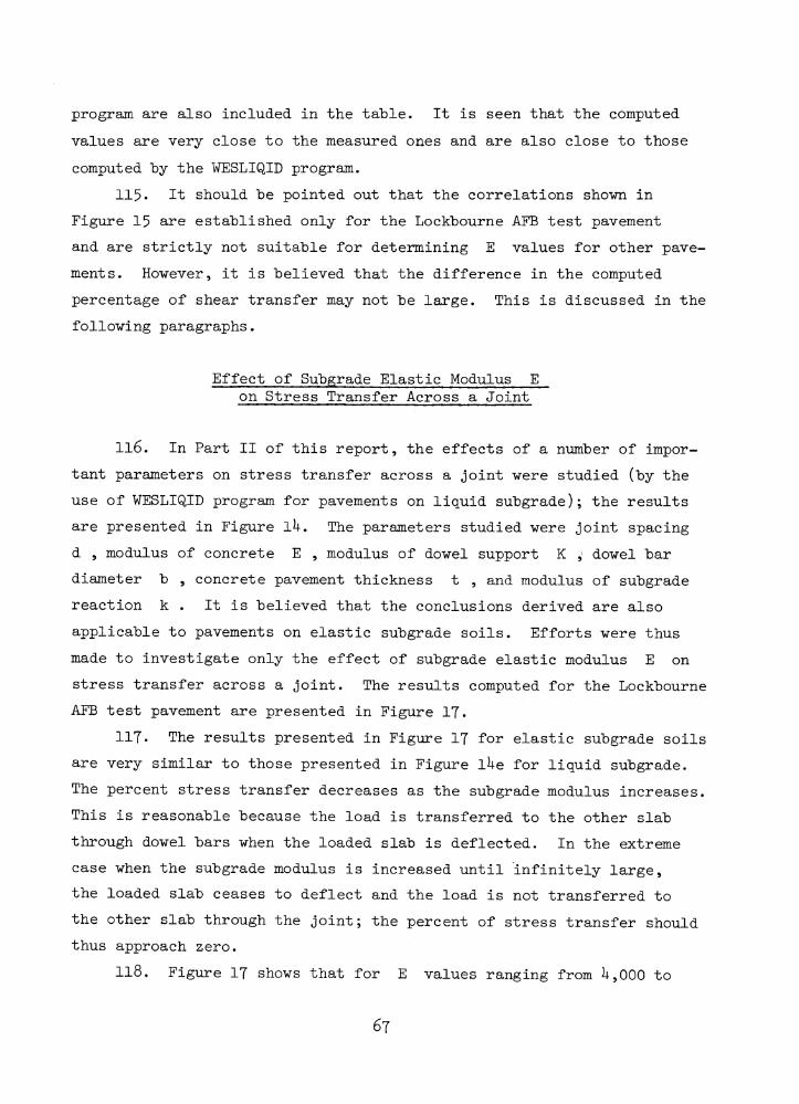
program are also included in the table. It is seen that the computed values are very close to the measured ones and are also close to those computed by the WESLIQID program.

115- It should be pointed out that the correlations shown in Figure 15 are established only for the Lockbourne AFB test pavement and are strictly not suitable for determining E values for other pave­ments. However, it is believed that the difference in the computed percentage of shear transfer may not be large. This is discussed in the following paragraphs.

Effect of Subgrade Elastic Modulus E on Stress Transfer Across a Joint

116. In Part II of this report, the effects of a number of impor­tant parameters on stress transfer across a joint were studied (by the use of WESLIQID program for pavements on liquid subgrade); the results are presented in Figure lU. The parameters studied were joint spacing d , modulus of concrete E , modulus of dowel support K ,' dowel bar diameter b , concrete pavement thickness t , and modulus of subgrade reaction k . It is believed that the conclusions derived are also applicable to pavements on elastic subgrade soils. Efforts were thus made to investigate only the effect of subgrade elastic modulus E on stress transfer across a joint. The results computed for the Lockbourne AFB test pavement are presented in Figure 17.

117. The results presented in Figure 17 for elastic subgrade soils are very similar to those presented in Figure lUe for liquid subgrade. The percent stress transfer decreases as the subgrade modulus increases. This is reasonable because the load is transferred to the other slab through dowel bars when the loaded slab is deflected. In the extreme case when the subgrade modulus is increased until infinitely large,the loaded slab ceases to deflect and the load is not transferred to the other slab through the joint; the percent of stress transfer should thus approach zero.

118. Figure 17 shows that for E values ranging from l+,000 to

6 7

Figure IT* Relationship between stress transfer across a joint and subgrade elastic modulus, Lockbourne AFB

test pavement

200,000 psi, the percent of stress transfer varies from 12.9 to 29. +. However, the subgrade elastic modulus of the five test pavements ana­lyzed (Table 5) ranges only from 7,^00 to 15,000 psi, and the corre­sponding variation of stress transfer is only 3 percent, shown in Figure 17» which is not significant at all.

68

119* It should be pointed out that if the option of percent shear transfer across the joint is used rather than the option of dowel bars as in Figure IT9 the percent of stress transfer across the joint is in­dependent of subgrade elastic modulus E (or modulus of subgrade reac­tion k ).

69

PART V: DESIGN IMPLICATIONS

120. The results and discussions presented in this part of the report are limited to the use of WESLIQID program, i.e., pavements on a liquid subgrade. For illustrative and comparative purposes, some example problems were computed using either heavy loads, or thin con­crete slab, or weak subgrade soil, or extreme temperature differential; computed stresses were thus too large and had exceeded the elastic limit of the concrete. Also, in some cases the load intensities were chosen arbitrarily and had resulted in very large stresses. It should be noted, however, the finite element method employed in this study is limited to the linear elastic theory; i.e., the stresses and displace­ments are linearly proportional to the load. If the computed stresses are beyond the elastic limit of the concrete, the computed stresses can be reduced to whatever values desired when the load is proportionally reduced.

Efficiency of Load Transfer by Dowel Bars

121. The shear forces across a joint in a rigid pavement are transferred by dowel bars and concrete interlock. It is difficult to evaluate the amount of shear force transferred by the concrete inter­lock, but the amount of shear force transferred by the dowel bars can be evaluated using the WESLIQID program. Using the pavement and loading condition at Lockbourne AFB (Table 5)9 stresses in the pavement are com­puted for different sizes and spacings of dowel bars, assuming either 100 percent or zero percent moment transfer across the joint. The com­puted stresses at selected nodes are presented in Table 10 for the con­dition of 100 percent moment transfer. The finite element layout show­ing the nodal numbers is presented in Figure 18. Special attention should be given to nodes 31 and 36 where maximum stresses and deflections occur. Node 31 is in the loaded slab and node 36 is the corresponding node in the unloaded slab across the joint.

122. When the efficiency of shear and moment transfer across a

70

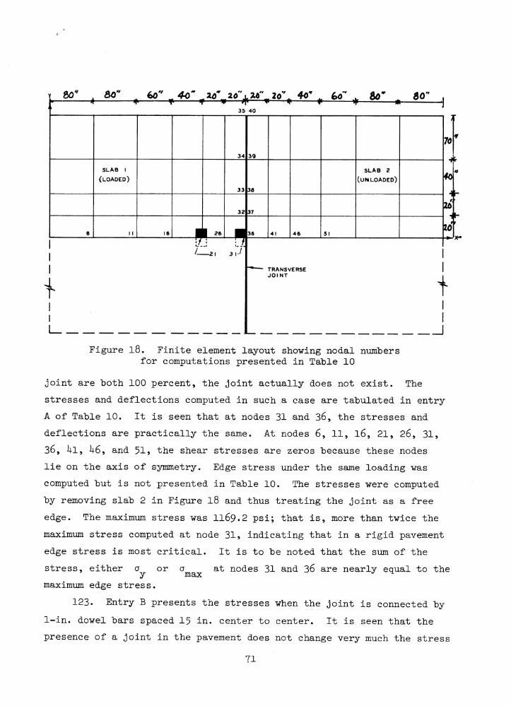
60" . &Q" . 6o" „ 4o~ 2ô~ 20' lU" 2o \ 4V . fc<T . &T ao'- 4 - ^ ------------» ~ » - * - ,j

35 40

34 3 9

SLAB 1

(LO A DED)

33 36

SLAB 2

( u n l o a d e d )

32 37

6 1 1 16__ I1» ■ L_ 41 4 6 51

70T■ü-40

120•it-

bd"

I

/ -------21 3 1-^

TRANSVERSEJ O IN T

- X -

+

,_ lFigure 18. Finite element layout shoving nodal numbers

for computations presented in Table 10joint are both 100 percent, the joint actually does not exist. Thestresses and deflections computed in such a case are tabulated in entryA of Table 10. It is seen that at nodes 31 and 36, the stresses anddeflections are practically the same. At nodes 6, 11, l6, 21, 26, 31,36, bl9 k69 and 51» the shear stresses are zeros because these nodeslie on the axis of symmetry. Edge stress under the same loading wascomputed but is not presented in Table 10. The stresses vere computedby removing slab 2 in Figure 18 and thus treating the joint as a freeedge. The maximum stress vas 1169.2 psi; that is, more than twice themaximum stress computed at node 31, indicating that in a rigid pavementedge stress is most critical. It is to be noted that the sum of thestress, either a or a at nodes 31 and 36 are nearly equal to the y maxmaximum edge stress.

123. Entry B presents the stresses when the joint is connected by 1-in. dowel bars spaced 15 in. center to center. It is seen that the presence of a joint in the pavement does not change very much the stress

71

in the direction perpendicular to the joint, hut changes consider­ably the stress a near the load in the direction parallel to the

yjoint. The reason that the stresses at both sides of the jointare equal and are close to those values computed before the joint was created is due to the assumption of 100 percent moment transfer across the joint. It is noted that the stress a^ increases considerably near the load in the loaded slab but decreases considerably in the unloaded side. At nodes 31 and 36 across the joint, the stress (or load) transfer computed from a has a value of 265.6/(265.6 + 75*+. 3) =

y26 percent , and the shear transfer computed from the deflections is 0.05^/0.065 = 83 percent . It should be noted that the shear forces transferred by the concrete interlock are neglected in the computation; otherwise, the stress (or load) and shear transfers may be greater.

12*+. Comparing the values between entries A and B, deflections are increased in the loaded slab, but are decreased in the unloaded slab when a (doweled) joint is present. Increasing pavement deflection means greater subgrade stresses.

125. It is rather interesting to note that when a joint is con­nected by dowel bars, the sum of the stresses at both sides of the joint is approximately equal to the free edge stress. At nodes 31 and 36 in entry B, the sum of a is (75*+. 3 + 265.6) = 1019-9 psi, and the sum

yof the maximum principal stress a is (75*+.3 + 379-2) = 1133.8 psi,maxwhich is very close to the 1169.2-psi free edge stress computed atnode 31. Note at the free edge (node 3l), the shear stress t andthe stress perpendicular to the edge are all zero; the maximumprincipal stress a equals the stress amax y

126. Entry C presents the computed values for the case of 2-in.dowel bars spaced 6 in. center to center. As the reinforcement across the joint is increased, while the stresses still remain nearlythe same due to the assumption of 100 percent moment transfer, the de­flections and stresses a are reduced in the loaded slab but are in-

ycreased in the unloaded one. The stress (a ) and shear (deflection) transfers at nodes 31 and 36 across the joint are increased from 26 to 39 percent and from 83 to 97 percent, respectively. At other nodes the

72

stresses a and deflections are reduced in the loaded slab and are maxincreased in the unloaded slab when the number and size of the dowel bars are increased. Note that in this case the stress a at node 31

y(6l8.3 psi) is considerably larger than the corresponding value shown in entry A (505-6 psi) where 100 percent shear and moment transfers are assumed, indicating that the 2-in. dowel bars spaced 6 in. apart at the joint still cannot transfer the full stresses from the loaded slab to the unloaded one; i.e., the stresses on both sides of the joint are still not equal. The computed values shown in entry C also demonstrate that deflection across a joint may not be a very descriptive parameter for the joint performance. At nodes 31 and 36, the shear transfer com­puted based on deflections is 97 percent, but the stress transfer com­puted based on stress a is only 39 percent, although the method of

ycalculating the percent transfer is different for these two parameters (the numerical computations for these values can be found in paragraph123).

127. Similar to the results presented in entry B, entry C also shows that the sum of the stresses at both sides of a doweled joint is nearly equal to the free edge stress.

128. Entry D shows the computed values for the case of extremely heavy reinforcement across the joint. The dowel bars are 8 in. in diameter and are spaced 9 in. center to center; i.e., the spacing be­tween the dowels is only 1 in. The stresses and deflections are nearly identical to those shown in entry A in which 100 percent of shear and moment are transferred. This is reasonable because with the extremely heavy reinforcement across the joint and with the assumption of a 100 percent moment transfer, the joint becomes so rigid that the slabs act as if the joint does not exist.

129. Table 10 presents the computed results under the assumption that the joint has 100 percent moment transfer. Similar computations were also made for the assumption that the joint is not capable of transferring moments at all (Table ll). The purposes of the computa­tions were twofold. The first was to check the efficiency of dowel bars in transferring the stresses across a joint in which the efficiency of

73

moment transfer is not assumed. The second was to compare the stress and deflection distributions in the pavement as a function of the effi­ciency of moment transfer across the joint.

130. When the computed values in entry A of Table 11 are compared with those in entry A of Table 10, it is seen that the stresses and de­flections change drastically along the joint when the efficiency of mo­ment transfer is reduced to zero. (Note that 100 percent shear transfer is not changed.) The stresses (perpendicular to the joint) at no­dal points along the joint are all diminished, and the deflections are increased greatly. Stress a and o , however, are changed insig- nificantly. Greater deflections mean greater stresses in the subgrade. The significance of this will be discussed later. At nodes away from the edge, however, the deflections are less and the stresses are slightly less in the loaded slab and are generally slightly more in the unloaded slab, when the efficiency of moment transfer is reduced to zero. Because the shear transfer is assumed to be 100 percent efficient, the stress transfer at nodes 31 and 36 across the joint has a full transfer, i.e.,50 percent.

131. Entry B shows the computed values for 1-in. bars spaced 15 in. apart, as compared with the 100 percent shear transfer in entry A. Because of the weaker shear transfer across the joint, the deflections at nodes along the joint increase in the loaded slab and decrease in the unloaded slab. This is also true for stress a a t nodes under the load that result in a stress (or load) transfer of 289.7/(289.7 +812.7) = 26 percent and a shear transfer of 0.058/0.071 = 82 percent . These values are identical to those computed and presented in entry B of Table 10 (or see paragraph 123) in which 100 percent moment transfer is assumed. In other words, the efficiency of moment transfer across a joint does not affect the values of the stress (or load) and shear transfers, although the values of deflections and stresses a^ alongthe joint are generally greater in the case when zero percent moment transfer is assumed.

132. At nodes away from the joint, the stresses and deflections

are also increased slightly in the loaded slab and decreased slightly in the unloaded one when the efficiency of shear transfer across the joint is reduced.

133. Entry C shows the computed values for the case when 2-in. dowel bars spaced 6 in. apart are installed at the joint. Similar to the conclusions derived from the computed values shown in entry C of Table 10 (100 percent moment transfer across the joint), the deflections and stresses a along the joint are decreased in the loaded slab and increased in the unloaded slab when the number and size of dowel bars are increased. The computed stress (or load) and shear transfers across the joint at nodes 31 and 36 are kkl. 2/(kkl.2 + 658.3) = +0 percent and O.O63/O.O65 = 97 percent , respectively. Again, these values are identical with those computed in entry C of Table 10 in which the same number of dowel bars is used but the efficiency of moment transfer is assumed to be 100 percent.

13^. At nodes away from the joint, the deflections and stresses decrease in the loaded slab, but increase in the unloaded slab, as the number of dowels across the joint increases.

135* Several conclusions can be drawn from the computations pre­sented in Tables 10 and 11. They are discussed as follows:

While the conventional dowel bars cannot transfer moment at all, they are not a very effective device for trans­ferring stresses (or loads) across a joint either. For instance, for 1-in. dowel bars spaced 15 in. apart, the stress transfer is only 26 percent; i.e., the stress a in the loaded slab is about three times as much as tie stress in the unloaded slab across the joint. The stress transfer is increased to 39 percent for 2-in. dowel bars spaced 6 in. apart; i.e., the stress a in the loaded slab is one and one-half times as much Xs the stress in the unloaded slab. The computed values are the same for either 100 or zero percent efficiency of moment transfer across the joint. As was previously stated, 100 percent moment transfer is defined by equal rotations at nodal points at both sides of the joint with the moments computed accordingly. Zero percent moment transfer is defined to be that the moments at nodal points along the joint are all zero while the ro­tations are not required to be zero.

b. For a given number and size of dowel bars at the joint

75

and when the efficiency of moment transfer is reduced to zero, i.e., the opening of the joint “becomes visi­ble, the computed results show that (l) the deflections along the joint increase and the stresses cx perpen­dicular to the joint diminish, (2) the stress Oy paral­lel to the joint and the deflection near the load increase slightly in both the loaded and the unloaded slab, but the values of the load and shear transfers are generally not changed, and (3) at nodal points away from the joint, the deflections are reduced and the stresses are reduced slightly in the loaded slab but are generally increased slightly in the unloaded slab. Greater pavement deflec­tion implies greater subgrade stress and vice versa.

c_. While the vertical deflections are easy to measure in a rigid pavement, one should be cautious in using deflec­tions to estimate the efficiency of stress transfer across a joint because deflections do not change as much as the stress Oy along the joint. For instance, entry C of Tables 10 and 11 shows that for 2-in. dowel bars spaced 6 in. apart, the stress Oy at the node at the loaded slab is one and one-half times greater than that at the corresponding node at the unloaded slab, but the difference in the deflections between the two nodes is only 3 percent, which can be difficult to measure.

Effect of Joint Conditions on Stresses and Deflections for Center and Joint Loading Conditions

136. It is known that the condition of stress transfer at the joint can affect the stress distributions in the pavement and therefore influence the thickness design. The computed results by WESLIQID found that this is true only if the load is placed next to the joint. When the load is placed at the pavement’s center, the joint condition has a minimal effect on the stress distribution in the pavement. Figure 19 shows the finite element layouts of a two-slab system for two loading positions. One loading position is the internal load where the load is placed at the center of the slab, and the other position is the joint load where the load is placed next to and at the center of the joint. Because of symmetry, only half of the slabs are used for the computations as shown in Figure 19- Note that a shorter length of unloaded slab is used, which is permissible. In the computation, the slab thickness,

76

y

(SLj

[Load*fVB 1 ed SIab ) (Uni

SLAB 2 oaded S!Lab)

38 1*537 1+1+ «»■— D o w id e d J o in t

1 8 15 22 29 ■ 50 57 61+ 71 781+0" I 3 0 ” 3 0 " I 3 0 " 2 0 " 2 0 " 2 0 " 3 0 " 3 0 " 3 0 " 3 0 " 3 0 " 3 0 " 30 "

a. Center loady

~ 1r ~ ltoweled1 '

f J o in t

On

e-h

alf

sla

b w

idth

^

I

SLA(Loade

B 1d Slab) (

SLA!Unloade*

B 2d Slab)

6o

59

58

1 8 15 22 29 36 1+3 3 ■50" 1+0" 30" 30" 30" ! 30" 20" 20" 20" |_20" | 30M L 30" .L ^0"

b. Load next to joint

x

Figure 19. Finite element layouts shoving nodal numbers for computations presented in Table 12 for a center load

and in Table 13 for a load next to a joint

elastic modulus, and Poisson’s ratio of the concrete, and the modulus of subgrade reaction are 8 in., 6,000,000 psi, 0.2 and 100 pci, respec­tively. The uniformly applied load has a pressure of 125 psi.

137- Tables 12 and 13 show the computed stresses and deflections at selected nodal points for the center and the joint loading conditions, respectively. Assuming the efficiency of moment transfer to be zero, the computations were made for three different efficiencies of shear

77

transfer. The definition of 100 percent shear transfer is that the de­flections at both sides of the joint are equal, and for zero percent of shear and moment transfers, the load transfer across the joint is zero.

138. Table 12 shows that when the load is far away from the joint, the condition of the joint has no effect at all on the stresses and de­flections in the slab, except at nodes near the joint where the stresses and deflections increase as the efficiency of the joint decreases. Since the stresses and deflections are so small near the joint when the load is far away from the joint, the change of stresses and deflections has no effect on the overall pavement design. Unlike the results presented in Table 12, results presented in Table 13 show that when the load is placed next to the joint, the stresses and deflections at nodes near the joint are affected significantly by the joint efficiency. For instance, at node 57 where maximum stresses and deflections occur, the stress a is

y23^0.9 psi when load transfer at the joint is zero, i.e., the edge load case. The stress a is reduced to II60.8 psi when the efficiency of shear transfer is increased to 100 percent, a 50 percent reduction from the edge load condition. Since in an actual airfield pavement with 1- to l-l/2-in. dowel bars spaced 12 in. apart at the joint, the measured shear transfer could be about 90 percent, the reduction of stress in the pavement should thus be very significant, possibly a reduction of U5 per­cent from the edge load. The results presented in Table 13 indicate that the efficiency of stress transfer at the joint affects the pavement de­sign when the load is placed near the joint.

Effect of Loading Position on Stresses and Deflections in Jointed Pavements

139* The results presented in Table 13 indicate that when the load is placed close to the joint, stress can be reduced with an effi­cient stress transfer device at the joint. A question arises concerning whether the pavement thickness can be reduced because of the existence of efficient dowel bars in the transverse joint. The WESLIQID program was used to analyze such conditions, and the results are presented in

78

Tables lb and 15 Tor edge and center loading, respectively.Edge loads

ibO. Figure 20 shows the four edge loading positions in the pave­ment. For clarity, the finite element layout is shown only in Figure 20c. The stresses are computed at the nodes where the nodal numbers are shown. The loading used in the computation consists of a twin- tandem truck load, with two concentrated loads representing one-wheel load. The use of concentrated loads rather than uniformly applied loads is for the convenience of preparing input data in the finite element programs. The computation was first made under the assumption that the transfer joint does not exist, as shown in Figure 20a. The computations were then followed by the cases that a transverse joint is present when (a) the twin-tandem load is next to the joint (Figure 20b), (b) the twin-tandem load is b ft away from the joint (Figure 20c), (c) the front axle load is next to the joint (Figure 20d), and (d) the rear axle load is k ft away from the joint (Figure 20e). The joint condition was as­sumed to have a 100 percent efficiency of shear transfer but a zero per­cent efficiency for the moment transfer. The purpose of the computa­tions C and D was to determine which axle load produces higher stresses in the pavement. The computed stresses and deflections are tabulated in Table lb for the five cases. Different stress components and deflec­tions are discussed separately. The letters a, b, c, d, and e in the table refer to the loading positions and the pavement condition shown in Figure 20.

a,. The stresses perpendicular to the joint, . Tablelb shows that the maximum a occurs when the trans­verse joint does not exist (column a). When a trans­verse joint is present and when the twin-tandem load is placed next to the joint (column b), the stresses a are reduced drastically (about 50 percent), and the maxi­mum stress occurs along the edge of the rear axle load away from the joint. The maximum a under the front axle load (386.6 psi) is only 55 percent of that under the rear axle load (709 psi). Column c shows the dis­tribution of a when the twin-tandem load is placed b ft away from ihe joint. Under node i+9* the maximum

occurs, having a magnitude of 1307- - psi, which is very close to the maximum stress (1359-2 psi in column a)

79

y

c. TWIN-TANDEM CENTER EDGE LOAD, JOINTED PAVEMENT

COO

70 77 ^9 56

• <68 75

Concentrated load = 10,000 lb each Modulus of concrete E = 6,000,000 psi Pavement thickness t = 8 in.Modulus of subgrade reaction k = 100 pci

^ J o in t

• •hi 5h

^ W o i n t

d. FRONT SET OF THE TWIN-TANDEM, NEXT TO THE JOINT REAR SET OF THE TWIN-TANDEM, 4 FT AWAY FROM THE JOINT

Figure 20. Finite element layout showing loading positions and nodal numbers for computations presented in Table l4, a two-slab pavement system with edge loads

in which the transverse joint is not present and the load is a full twin-tandem load. This small discrepancy is believed to be caused by the small dimensions of the slab length. In other words, if the slab length were increased and the load were placed farther away from the joint, the maximum stress in column c would be increased and reach the same value as though the joint did not exist (column a). Column d shows the distribution of a under the front axle load alone. It is interesting to note that the maximum a does not occur under any load, but occurs at node b-9, which is 5 ft away from the joint. Column e shows the distribution of a under the rear axle load alone. It is also interesting to note that the maximum a has a magnitude of 1259‘ 6 psi, which is nearly equal to the maximum a (1307-^ psi in column c) under the twin-tandem wheel load when the load is lj- ft away from the joint, but is much greater than the maximum a (709 psi in column b) when the twin- tandem load is placed next to the joint. This subject will be further discussed later.

b. The stresses parallel to the joint, cr . Table lb-shows that when the loads are placed along the edge of the pavement, the stresses a are much smaller than the stresses o in all the ¥ive cases, i.e., a, b, c, d, and e in Tabie ih. Similar to the distribution of o , maximum a occurs when the twin-tandem load is piaced k ft awa r from the joint (column c). Unlike the stresses a , however, the stresses a induced by the rear axle load (column e) are smaller than those induced by the front axle load (column d) and are much smaller than those induced by the twin-tandem load (column b).

c. The maximum principal stress, a . Since the stresses— ____________________________ maxo are much greater than the stresses a , the magni­tudes of the computed maximum principal stresses are very close to those of o . The discussions presented with respect to a are applicable to the maximum principal stresses amax

d. . Vertical deflections. Table lb shows that the maximumdeflection occurs at the edge of the joint (node 77) when the twin-tandem load is placed next to the joint (column b), although the stresses are the smallest at this loading position. The maximum deflection at the joint is 0.3^2 in., as compared with the 0.212 and 0.17 - in. when there is no transverse joint (column a) and when the load is placed away from the joints (column c), respectively.

lUl. Some results presented in Table lb are plotted in Figure 21.

81

1+9 56

Nodal NumbersTO

ITT

I1500

to

1000

COCOCDVt-PCO

500

P*oc

• H

0

-500

-1000

63

NOTE: Nodal numbers are shown in Figure 20.Curves A -E refer to loading position and pavement structure in the same figure.

Figure 21. Distributions of stresses and deflections along the pavementT s edge under edge loads in a two-

slab pavement system, WESLIQID program

The plotted results are limited to nodal points b9, 56, 63, TO, and 77 (see Figure 20c) along the pavement edge where maximum stresses and deflections occur. Critical stresses occur in the pavement near nodal point 56 in loading positions a, c, and e. Maximum deflection occurs at the pavement corner (node 77) 'in the loading position b.Center loads

lk2. Results presented in Table lb are for loads traveling along the edge of the pavement. Computations were also made for loads moving along the center line of the pavement. Figure 22 shows the finite ele­ment layout and the two loading positions for the computation. Because of the symmetry of the loading, only one half of the pavement was used in computations. The stresses are computed at the nodes where the nodal numbers are shown. The efficiency of the joint is assumed to be 100 percent shear transfer and zero percent moment transfer as used for edge load cases. The loading used in the computation also consists of a twin-tandem truck load with two concentrated loads representing a

8 2

30"

13 18 23 28 33 38 k3 he 53 58 1 8 "

12 IT 22 27 32 37 b2 1+7 52 57 12" [

11 l6 21 2 6 31 3 6 hi 51 56 12" i

, 36" , 2b" 12' 12" 1 8 " f .l 8 " . 12"9 12" 12 ’ 12 ’’ 12" 12" , 2k” 2h” ¡ 36"

c. NODAL NUMBERS AND FINITE ELEMENT LAYOUT

Figure 22• Finite element layout showing loading positions and nodal numbers for computations presented in Table 15* a two-slab pavement

system with center loads, WESLIQID program

83

one-wheel load. The computed results are presented in Table 15 in columns a, b, and c. The values in columns a and b refer to loading positions a and b, respectively, in Figure 22. The values in column c are similar to those in column b except that the transverse joint is removed. The significance of the values tabulated in columns d and e will be explained later.

lU3. Table 15 shows that when the twin-tandem load is travelingalong the center of the pavement, the stresses a perpendicular to thexjoint when the load is k ft away from the joint (701.0 psi in column b)are 107 percent greater than that when the load is next to the joint(338.U psi in column a). Similar to the edge loading condition in TablelU, the maximum a occurs at a distance k ft away from the joint (node x37) when the twin-tandem load is placed next to the joint (Figure 22a). The stresses in columns c and d will be discussed later.

ikk. The maximum stresses , in the direction parallel to thejoint, are nearly the same when the load is next to the joint (653.2 psi in column a) and when the load is away from the joint (692.9 psi in column b). Table 15 shows that the maximum principal stress, which is a combination of , and the shear stress t , is slightly greaterwhen the load is away from the joint (71^*9 psi in column b) than when the load is next to the joint {6 5k.0 psi in column a). In other words, unlike the case when the load travels along the pavement edge, the mag- nitude of stresses (mainly the maximum principal stress, amax ) in the

pavement changes only slightly when the load is traveling along the cen­ter of the pavement. However, this same conclusion does not hold true for deflections. Table 15 shows that when the load is placed next to the joint, the maximum deflection (0.1l6 in. in column a) is nearly twice as much as the deflection when the twin-tandem load is k ft away from the joint (0.068 in. in column b).

IU5. The results tabulated in columns a and b of Table 15 are plotted in Figure 23 at the longitudinal line along the nodal points 12, 179 22, 275 32, 375 k2 9 bj9 52, and 57* it is seen that the maximum stresses are nearly the same under the two different loading positions,

8k

Q.OCi—aEDEx032

12 17 22 27 32 37 h2 kl 52 57Nodal Numbers

Nodal Numbers

NOTE: Curve A: Loads placed next to the jointCurve B: Loads are 4 ft away from the joint Loading position and nodal points are shown in Figure 22.

Figure 23. Distributions of stresses and deflections near the center line of the pavement under center loads in a

two-slab pavement system, WESLIQID program

but the deflections are much greater when the loads are placed next to the joint. As stated before, greater deflection along the joint would cause greater subgrade stress and consequently more damage in the pave­ment along the joint.

lk6. The computed values shown in column c are similar to those shown in column b except the transverse joint is removed. It is seen

85

that the stresses are generally reduced, but very slightly, indicating that if the load is far enough away from the joint, the stresses near the load are the same as if the pavement joint does not exist.

1^7• Column d in Table 15 shows the computed stresses and deflec­tions with butted joints (i.e., thickened edge at the joint). The thick­ened section starts from the midpoint of the slab and increases gradu­ally to 10 in. at the joint— an increase of 25 percent in thickness.The twin-tandem load is placed only next to the joint. Comparing the values in columns a and c, it is seen that the stresses are reduced about 20 percent because of the increased pavement thickness, but the pavement deflections are reduced insignificantly.

lU8. Column e in Table 15 shows the computed values when the modulus of subgrade reaction k along the same joint as in a, b, and d is increased from 100 to U00 pci. The subgrade soil involved has a width of 18 in. at each side of the joint. The twin-tandem load is placed next to the joint. Compared to values in column a, it is seen that the maximum principal stresses have changed insignificantly, but the deflections are reduced drastically. It is also noted that because the strengthening of subgrade soil is limited to the nodal points along the joint, the maximum deflections occur at nodal points 36 and h l 9 which are about h ft away from the joint.

1^9. It should be pointed out that when the load is traveling along the center of the pavement, although the maximum principal stress­es a are nearly the same as when the load is next to or away fromthe transverse joint, the stresses a perpendicular to the joint arexnearly twice as large as when the load is away from the transverse joint than those when the load is next to the joint.

150. The discussions presented concerning the computed results in Tables ih and 15 can be summarized in the following paragraphs.

151. The most critical condition in a rigid pavement occurs when there are no transverse joints or cracks in the pavement and also when the load is moving along its edge. In a jointed pavement, the critical stress occurs when the load is halfway between the joints at an edge and the stress has a magnitude close to that of a pavement with no transverse

86

joint. When the load is placed next to the joint, a good load trans­fer device along the joint can reduce pavement stresses, but the maxi­mum stress at the joint with a zero percent load transfer efficiency is nearly equal to the critical stress when the load is halfway between the joints (and when the distance between the joints is long enough).In other words, the pavement thickness cannot be reduced because of the existence of efficient dowel bars in the transverse joint. When the load is moving along the center of the pavement, the stresses are smal­ler and are nearly independent of whether the load is at the center or next to the joint of the point. The maximum stresses of , anda are 701.0, 697*6, and 71^*9 psi (column b of Table 15), respec- maxtively, when the load is moving along the center of the pavement, as compared with the corresponding maximum stresses of 1271.8, 233.7, and 1271.8 psi (column c of Table 1*0 when the load is traveling along the edge in a jointed pavement. Maximum deflections occur when the load is next to the transverse joint for both interior (0.1l6 in.; column a of Table 15) and edge (0.3*+2 in.; column b of Table 1*0 loads. The corre­sponding maximum deflections are merly 0.068 in. (column b of Table 15) and 0.17*+ in. (column c of Table 1*0 when the loads are h ft away from the joint. Greater pavement deflections mean greater subgrade stresses and subsequently more subgrade-related damage near the joint. Based on the limited amount of analysis, it seems that to reduce pavement deflec­tions along the joint, it is more beneficial to stabilize the subgrade soil along the joint than to use butted joints.

152. In the design of a rigid pavement with joints, it can be con­cluded that the critical stress should be computed by placing the loads at pavement edge halfway between the joints. (The stresses may be re­duced by decreasing the pavement length.) The presence of an efficient transverse joint next to the loads can reduce the stresses greatly but increase the deflections along the joint drastically and consequently increase the subgrade stresses causing pavement damage along the joint.

153* Computations were made here assuming the joint has a 100 percent efficiency of shear transfer, i.e., very strong dowel bars at the joint. In reality, most pavements transfer less than 100 percent

87

shear across the joint. Therefore, deflections along the loaded slab’s joint should he greater than those in Tables ih and 15.

Effect of Temperature and Gaps Under the Slabs

15^. Temperature differentials cause concrete pavements to warp upward (edge up) in the night and downward (edge down) in the day. Be­cause of the concrete’s weight, temperature stresses are produced in the warped pavement, such as tensile stresses at the bottom of the slab in a downward warped pavement. Depending upon the loading position, stresses in the pavement can be magnified when temperature is considered.

155. Gaps exist under pavements for a number of reasons, such as pumping, plastic deformation of the subgrade, and poor construction practices. The presence of gaps under the pavement is equivalent tothe removal of subgrade support for the pavement and consequently greater stresses in the pavement. Pavement stresses can be magnified when gaps are combined with temperature warping. The following sections present example problems computed using WESLIQID to show the effects of tempera­ture warping and gaps under the slab.A single slab

156. Figure 2h shows the computed stresses cr and deflections in a single concrete slab subjected to temperature warping. A large gap exists in the subgrade at the slab’s center under the applied load. The gap has a magnitude of 1 in. as shown in the figure. The Young’s modulus and Poisson’s ratio of the concrete are 6,000,000 psi and 0.2, respectively. The weight of the concrete slab is considered in the computation.

157. Curve A shows the distribution of the computed results sub­jected to the applied load alone without consideration of temperature.The slab is in full contact with the subgrade. Maximum stress occurs at the slab’s center, with tension at the bottom. Away from the load near the slab edge, however, small tensile stresses occur at the top of the slab. Curve B shows similar results, except the gap under the slab is considered in the computation. Distributions of curves A and B

88

downwardCurve D - Gap and temperature

considered, slab curled upward

NOTE: Temperature differential 3.75°F per inch of pavement.Positive stress indicates tension at the bottom of the pavement and negative stress indicates tension at the top of the pave­ment; weight of slab is considered.

Figure 2k. Stresses and deflections in a single concrete slab subjected to temperature conditions and gaps under the slab, WESLIQID program

89

are similar, except the magnitude of stresses and deflections are greater in curve B because of the existence of the gap at slab center.

158. Curve C shows the distribution of stresses and deflections when the gap and temperature are considered. The temperature differen­tial is -1+5°F between the top and the bottom of the slab, i.e., 3.75°F per inch of the concrete slab, and the slab warps downward. It should be noted that a U5°F temperature differential is an extreme case; the use of such a large value is for the purpose of illustration. Figure 2k shows that in spite of the applied load at slab center, the center por­tion of the slab cnrls up due to the large temperature differential and loses contact with the supporting subgrade. Along the slab edge, the slab sinks into the ground. This is called precompression in this re­port. In the figure it is seen that two thirds of the slab (at the center) has lost the subgrade contact and therefore produces very large tensile stress under the load and slab weight.

159. Curve D shows the distributions of stresses and deflections for the case of positive temperature differential (+U5°F). Because of the large temperature differential and also the existence of gap at pavement center, one third of the slab along the edge curls above the ground; the deflection at slab center is also the largest in all the cases. However, the tensile stresses at slab center in this case are the smallest, because under a positive temperature differential, the slab warps upward and because of the slab weight, compression develops at the bottom of the concrete slab, while under the load the bottom of the slab is always under tension. The effect of the applied load and positive temperature cancels the stresses in the concrete slab. Fig­ure 2h also shows that fairly large tensile stress developed at the por­tion of the slab away from the center load. Because of the slab curling up at the pavement edge and because of the weight of the slab pulling the slab edge downward, tensile stresses are thus developed at the top of the concrete slab.

A single slab: comparisonwith the Westergaard solution

160. A complete subgrade contact condition was assumed in the

90

Westergaard solution (1925). The slab always has a full contact with the subgrade soil, and gaps are not allowed between the slab and sub­grade, no matter how much the slab has warped upward due to temperature change or the applied load. In other words, the slab is supported by a group of springs, and the springs are always connected to the slab.In reality, the pavement can lose subgrade support at some points due to temperature warping, pumping, and plastic deformation of the subgrade. Computations were made to demonstrate the difference between the solu­tions obtained from the Westergaard solution and the WESLIQID program.In the latter case, the slab can lose subgrade support from temperature warping.

l6l. The same slab and the same loading used in the computation shown in Figure 2k were used in this computation, except that the gap under the pavement was removed because the Westergaard solution is not capable of considering gap under the pavement. Figure 25 shows the plotted results of the computations.

| _ 150 in. I

h -

■n

f | | p = 200 psij>. V <3 v , -¿t?:4;•; . 1 &

1l 1 1 . 1 1 4 I

0.10

0.05

INITIAL BOTTOM SURFACE OF THE SLAB

/

E

Q.

Q

0.20C CURVE B: WESTERGAARD SOLUTION

(FULL CONTACT & WEIGHT­LESS), SLAB CURLED UP

CURVE C: COMPUTED BY WESLIQID(PARTIAL CONTACT AND WEIGHT OF SLAB CONSID­ERED), SLAB CURLED UP

£

ck = 100 pci

Figure 25. Comparison of computed results illustrating the significance of subgrade support condition

91

162. Curve A shows the deflections and stresses computed by the Westergaard solution whem temperature is not considered. Slight tensile stress (tension at the top of the slabs) is computed near the slab edges. Note in the Westergaard solution that the slab is assumed to be weightless. Cruves B and C show, respectively, the plotted results computed by the Westergaard solution and the WESLIQID program. In both cases, the positive temperature effect causing the slab to warp upward was considered. Because a complete subgrade contact was assumed in the Westergaard solution, the negative edge deflections computed by the Westergaard solution (curve B) are much smaller than those by the WESLIQID program (curve C) in which the slab is free to curl up due to the temperature change. On the other hand, because of the restraint imposed near the slab edges, the positive deflections (downward direc­tion) near the slab center computed by the Westergaard solution are also smaller than those computed by the WESLIQID program where there is no restraint in the subgrade support.

163. Although the deflections computed by the WESLIQID program are much greater than those of the Westergaard solution because of the subgrade restraint in the latter case, the negative stresses computed by the Westergaard solution are greater than those computed by the WESLIQID program, also because of the restraint in the subgrade support. The negative stresses shown in curve C are induced by the weight of the slab because the slab’s edges are curled up. When the slab is pulled down along the edges by the subgrade reaction forces as in the case of the Westergaard solution, greater negative stresses are developed in the slab, as shown in curve B. At the slab’s center, stresses computed by the Westergaard solution are smaller than those computed by the WESLIQID program. The results presented in Figure 25 demonstrate the signifi­cance of subgrade support in a rigid pavement and the inadequacies of the Westergaard solution in some cases. Similar computation for negative temperature effect causing the slab to warp downward was made, but the difference between the results computed by the WESLIQID program and the Westergaard solution was not significant.

92

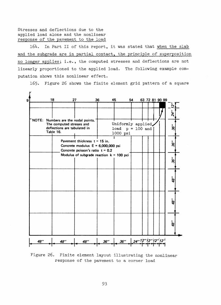
Stresses and deflections due to the applied load alone and the nonlinear response of the pavement to the load

1 6 k . In Part II of this report, it was stated that when the slab and the subgrade are in partial contact, the principle of superposition no longer applies; i.e., the computed stresses and deflections are not linearly proportioned to the applied load. The following example com­putation shows this nonlinear effect.

1 6 5 . Figure 26 shows the finite element grid pattern of a square

‘ NOTE: Nur The defl Tab

nbers are the 1 computed str

ections are tat le 16.--------------- 1

nodal points, esses and Hilated in

I_______________

18 27 36 45 54 63 72 81 90 99

Uniformly applied, load p = 100 and 1000 psiI

Pavement thickness t = 15 in.Concrete modulus E = 6,000,000 psi Concrete poisson's ratio t = 0.2 Modulus of subgrade reaction k = 100 pci

O i ,

35

&

50

SS

%

$

48" I_ 48" _ | 48" 1, 36" | 36" I 24" ) 2 " ? ? " .r t * ~ ~ ------- ---- i i r I iFigure 26. Finite element layout illustrating the nonlinear

response of the pavement to a corner load

93

slab subjected to a corner load. The temperature differential between the top and the bottom of the slab is 3°F, which causes the slab to warp upward. Two computations were made separately. The first one was to compute the stresses and deflections due to the temperature and the slab weight, and the second was to compute those when the effect of the temperature and the load are combined. The differences between the com­puted results are the stresses and deflections induced by the applied load alone. It should be noted that in the field of pavement engineer­ing research, it is very difficult to measure thermal stresses. Pave­ment engineers tend to measure stresses due to the load only. When a stress gage is embedded in a test pavement, the stress induced by the applied load is derived from the difference in the readings taken be­fore and after the application of the load. The reading taken before the application of the load takes into account the effect of temperature, slab weight, and many other factors. The reading taken after the appli­cation of the load has the effect of load, slab weight, temperature, and other factors. The difference in the two readings is thus the ef­fect due to the applied load alone.

166. Table 16 presents the distributions of stress and deflection computed under the various conditions. Entry 1 shows the initial curl­ing due to temperature. The computation is made under the assumption that the slab is weightless. Entry 2 shows the stresses and deflections induced by temperature, slab weight, and applied load. Two loads were used separately in computations. One had a unit pressure p = 100 psi and the other p = 1000 psi . It is seen that the stresses and deflec­tions under the large load (p = 1000 psi) are much greater but not 10 times greater than those computed under the smaller load (p = 100 psi); i.e., the principle of superposition (as assumed by the Westergaard solution) does not hold. Under the smaller load, the nodes along the slab edge are still curled up due to the temperature warping, but many nodes near the load are sunk into the subgrade under the load.

167. Entry 3 presents the computed stresses and deflections in­duced by temperature and the slab weight. The effect of applied load was excluded. Because the effects of temperature and slab weight are

9^

uniform on the slab, the deflections at the corner nodes 9 and 99 are supposed to be equal because of symmetry. The slight difference in the deflections in nodes 9 and 99 is caused by the nonsymmetrical lay­out of the finite element grid and is considered insignificant.

168. Entry k presents the stresses and deflections induced by the applied load alone. This is obtained by subtracting the values in entry 3 from entry 2. Similar to entry 2, the stresses and deflections in­duced by the p = 1000 psi load are not 10 times greater than those induced by the p = 100 psi load.

1 6 9* It should be reiterated that in the field of rigid pavements the design engineers are interested in the stresses induced by the com­bined effect of the applied load, temperature, and slab weight. But pavement engineers are interested in the stresses induced by the applied load alone because it is the only stress that engineers can measure with confidence. These stresses can be computed separately by use of the pro­grams developed in this report.A doweled two-slab pavement system subjected to center and corner loads at the joint

170. In Part III of this report, computations were made to com­pare the theoretical computations with field measurements obtained in a number of airfields in the United States. The variables compared were the strains and the stress transfer across the joint. The computations were made assuming that (a) the pavements have an initial full contact with the subgrade, and (b) there are no temperature variations. The agreement between the measurements and the computed values were general­ly good. Computations were made later for the test pavement at Lockbourne AFB (Table 5)» assuming that temperature variations and gaps existed along the joints. Besides the placement of loads next to the joint at the interior of the concrete slab as was done during the tests, loads were also placed at a corner of the slab. The purpose of the computa­tions was to examine the combined effect of temperature, in terms of day and night conditions, and gaps under the joint on the stress and deflec­tion distribution when the load is placed at different locations along the joint.

95

171. The finite element grid patterns for both center and corner loads are shown in Figure 27. The grid patterns are different because of the difference in loading positions. The deflections computed for seven different conditions at nodal points along the transverse joint are plotted. Negative deflection indicates upward movements. Curve 1 presents the deflections due to the loads only. Maximum deflections occur under the load, and the maximum deflection under the corner load is nearly three times as great as that in the center load case.

172. Curve 2 shows the deflection distribution due to temperature warping alone. The positive temperature differential caused the slabs to warp upward, leaving the pavement along the joint out of contact with the subgrade. The temperature differential between the top and the bottom of the pavement is 3.75°F per inch of the pavement, a very extreme condition. Nodes 31 and k5 in the plots for the case of center and corner loads, respectively, are located at the same location next to the joint along the center line of the pavement.

173. Curve 3 shows the deflection curves similar to curve 2 ex­cept that the loads are added on. In the case of center loads, the center of the pavement along the joint sinks into the subgrade, while the pavement edge is still above the ground. Under the corner load, the center of the pavement is above the ground because of the positive temperature differential. However, the edge of the pavement sinks into the ground due to the applied load.

17^. Curve k shows the deflection curves similar to curve 3 ex­cept that a 1-in. gap under the pavement along the joint is considered. The gap has a width of 12 in.; it can be caused by either pumping or plastic deformation due to the load. It is interesting to note that in the case of the center load, the deflection curves 3 and k are very nearly the same, because the pavement curls up along the joint; thus the gap beneath the joint has no effect on the pavement deformation along the joint. Under the corner load, the shapes of curves 3 and h are simi­lar except the corner deflection is greater due to the existence of the gap. Note that the shape of curve k would be different if the magnitude of the gap under the pavement were less than the maximum deflection due to the load.

96

VO

LEGEND

Temp. Warping** Gap*

No NoUpward NoUpward NoUpward YesDownward NoDownward NoDownward Yes

mcrete considered ** Temperature differential 3.75°F per

inch of pavementt 1-in. gap in the subgrade along the

joint, initial full subgrade contact elsewhere

Curve* Load

1 Yes2 No3 Yes4 Yes5 No6 Yes7 Yes

* Weight of

300"

SLAB 1

Loads, 47,250 lb each

SLAB 2

“ ■ ^ 13233 "

Nodal Nos. .

34 "

36 37 38 39I

Doweled joint7Center loads

m 300"

Pavement tl E = 6,000,C 1-in. dowel

Itickness t 100 psi, v bars 15 ir

I= 12 in. = 0.15 i. apart

SL>\B 1

¡_ctads, 47,:Idal Nos.

>7

INo l 1

v . f n! N ^ 4 0 «45 46 47 48

/ SL

___________I

52 53 i 54

AB 2 I I /I Doweled jo in t 'I_______l_____I______

55 11

Corner! loads

Figure 27. Shapes of deflected surface along the joint in a two-slab concrete pavement under central and corner loads (33 7 aircraft), Lockbourne AFB (Table 5) WESLIQID program

175- Curve 5 is similar to curve 2 except that the negative tem­perature differential caused the slabs to warp downward, leaving the pavement along the joint to sink into the subgrade. Note that the pave­ment along the edge sinks into the subgrade more than that at the center.

176. Curve 6 is a deflection curve similar to curve 5 except that the load is added on. Under the center and corner loads, the pavement along the joint sinks further into the subgrade, with maximum deflection at a location under the load.

177. Curve 7 is similar to curve 6 except that a 1-in. gap along the joint is considered. Under both the center and the corner loads, the pavement along the joint sinks into the subgrade more as compared with those in curve 6 because of the existence of the gap along the joint. Also, it should be noted that the shape of curve 7 would be different if the magnitude of the gap were less than the deflections computed.

178. The stress distributions computed for the seven curves for varied conditions shown in Figure 27 are presented in Tables 17 and l8 for center and corner loads, respectively. The tabulated stresses are at nodal points along the joint and near the loads. The locations of the numbered nodes are given in Figure 27. In the center load case (Table 1 7) the percent stress (or load) transfer was computed only at nodes .31 and 36 under the load. Under the corner load, however, the percent stress (or load) transfer is difficult to determine according to the adopted definition of percent stress transfer, because the stress at most nodal points changes signs across the joint.

179. In curves 1-7 shown in Figure 27, positive stress indicates that the tensile stress is developed at the bottom of the pavement, and negative stress indicates that the tensile stress is developed at the top of the pavement. Positive temperature differential causes the pave­ment to curl upward (curves 2-U), and because of the weight of the pave­ment, negative stress is developed in the pavement. Negative temperature differential causes the pavement to curl downward (curves 5-7) and develops positive stress in the pavement.

180. It is interesting to note that when temperature and gaps are

98

not considered, stresses under the center load are generally greater than those under the corner load, while the deflections are reverse in the two loading cases.

l8l. In the case of center load in Table 17> the stresses due to load alone are positive (curve 1 with tension at the bottom of the pave­ment). Since the thermal stresses are negative when the pavement is warped upward (curve 2 compression at the bottom of the pavement) and are positive when the pavement is warped downward (curve 5 with tension at the bottom of the pavement), the stresses in curves 3 and b in which the pavement is warped upward are less than those in curve 1 because the stresses due to temperature and stresses due to load have different signs. However, in curves 6 and 7 in which the pavement is warped down­ward, the stresses are much greater than those in curve 1,* because the stresses due to temperature and stresses due to load have same sign. It can be concluded that under the center load, the positive temperature differential (nighttime condition) causing the pavement to warp upward can reduce the stresses, but the negative temperature differential (day­time condition) causing the pavement to warp downward increases the stresses. It is also noted in Table 17 that the percent stress transfer in conditions (or curves) 3 and b are less than the 25 percent under the load shown in curve 1, but the percent stress transfer in curves 6 and 7 are more than the 25 percent. This is true because when the pavement is warping upward, the stresses on the unloaded side of the joint reduce more than those reduced on the loaded side. The reverse is true when the pavement is warped downward.

182. Table 17 also shows that stress changes very slightlywhen the gap under the pavement is present. This can be readily ex­plained for the case when the pavement is warped upward (curve b ). The major portion of deflection curve k shown in Figure 27 is still above the subgrade, so the existence of the gap under the pavement does not change the stress distribution significantly. In the case of the pave­ment warping downward sinking into the subgrade (curve 7), however, the

* The maximum edge stress in the pavement when the same loads are placed at the pavement edge halfway between the joints is 1151.5 psi.

99

lack of change of stresses from curve 6 in which the gap is not present is difficult to explain. When the pavement is warped downward and the applied load is forcing the pavement into the subgrade (curve 6), the full subgrade reactive forces are resisting the pavement’s deflection. When the subgrade reactive forces are removed as in curve 7 in which the gap exists along the joint, the pavement is allowed to deflect more freely and consequently pavement stresses should be increased. However, this is apparently not the case because the computed stresses listed for curve 7 are nearly the same as those computed in curve 6. The only explanation in this case is that deflection curves 6 and 7 shown in Figure 27 (under the center loads) are nearly parallel to each other. Since stresses in a pavement are induced by a change in the curvature of the pavement, the stresses thus remain the same. It is also noted in Figure 27 that deflection curves 3 and k are parallel to each other, explaining why the stresses do not change from curve 3 to curve k .

183. It should be emphasized that deflection curves 6 and 7 may not be parallel to each other if either the modulus of subgrade reaction k is increased or the pavement thickness is decreased. Under such conditions, the shape of deflection curve 6 may change more than that of curve 7*

18U. Table 18 shows the stress distribution under the corner loads. The stresses are tabulated at nodal points around the load and are generally smaller than those computed under the center loads shown in Table 17- Unlike the center load case, the effect of temperature warping on the stress distribution in the corner load case is not sig­nificant. Under temperature warping, the stresses increase in some nodal points but decrease in some others. The changes were, however, not significant.

I85. It should be pointed out that the presence of the load transfer dowel bars can reduce the stresses in the pavement near the joint, and the reduction is generally more in the corner load cases than in the center load. To clarify this point, computations were made for the test pavements in Lockbourne AFB, under the assumption that there was no load transfer across the joint, and the results are

100

presented in Table 19* For simplicity, the comparison was made only for the case when the temperature effects and the gaps under the pave­ment are not considered.

186. Table 19 shows that pavement stresses (Qmax) are drastically increased when the dowel bars at the joint are removed, and the effect is more pronounced in the corner load case. Shear stresses t play a more important role when the loads are applied at the corner of the pavement than when the loads are applied at the pavement center where the shear stress is zero because of symmetry.

187. Results presented in Figure 27 and Tables 17* 18, and 19 for a two-slab pavement system with dowel bars subjected to corner and center loads at the joint are summarized, and conclusions are made in the following paragraphs.

188. Whether temperature and gaps under the joint are considered or not, aircraft load placed at the corner produces much larger deflec­tions than when the load is placed at pavement center (curve 1 of Figure 27). When the pavement is warped downward (daytime condition), the differences in deflections between the corner and center loads be­come even greater.

189• When temperature and gaps are not considered, stresses under the center load (curve 1 of Table 17) are generally greater than those under the corner load (curve 1 of Table 18). Under the center load, when the pavement is warped upward (nighttime conditions), stresses in the concrete pavement can be reduced; the opposite is true when the pavement is warped downward (daytime condition). The effect of tem­perature is not so significant and clear when the load is placed at the corner.

190. The presence of dowel bars in the joint can reduce the stresses in the pavement near the joint. The reduction is more signi­ficant in the corner load case.

Continuously Reinforced Concrete Pavement (CRCP)

191. Results presented in Table ik indicate that in a jointed pavement, maximum stresses occur when the edge load is placed halfway

101

between the joints, and the stresses can reach the maximum stresses that occur in a pavement without transverse joints if the pavement is long enough in the longitudinal direction. The question arises as to whether the pavement stress would be reduced with a reduction in pave­ment length. It is known that in CRCP closely spaced transverse cracks developed shortly after the construction, but the cracks are held very tightly by the steel reinforcements. It is reasonable to assume that the cracks can transfer 100 percent shear force and a small amount of moment when the pavement is in sound structural condition. Computations were thus made in a CRCP to compare the computed values with values for a regularly jointed pavement. The CRCP used in the computation is a five-slab pavement divided by four cracks. For the WESLIQID program, the cracks were treated the same as the joints. The loading condition and pavement dimensions for the CRCP are the same as those used in the previous examples of the regular jointed pavement, except the pavement length is reduced to b ft. The joint (or crack) condition is also identical, i.e., 100 percent shear transfer and zero percent moment transfer. The finite element layout is shown in Figure 28, and the com­puted results are presented in Table 20. The discussions on the com­parisons between Table 20 (CRCP with closely spaced cracks) and Table lb (regularly jointed pavement with edge loads) and Table 15 (regularly jointed pavement with center loads) are presented as follows. It should be pointed out that the maximum stresses may change signs when condi­tions change; the comparisons should be based on the absolute values.

, stresses per- pendicular to the joint

192. Edge loads placed next to the joint (loading position c).When the crack spacing is reduced (or the number of cracks is increased)as in a CRCP, the maximum stress is reduced from 709-0 psi (column b ofTable lb) to kb^.k psi (column c of Table 20). It is noted that incolumn d of Table lb when the front-axle loads are placed next to thejoint at the pavement’s edge, the maximum a occurs at a point farxaway from the joint. It is thus reasonable to find that when the pave­ment length is reduced, such as in a CRCP, the stress q^ is reduced.

102

yi.

y

ouo

1 1 3 4 5161^7 18 19 20<\TVc\rv«« < \ ■cm!K i.

3

!$9C'O

6 7>— i---- r —i8 910121 22 23 2425

r . k i I—( 11

► i12 141526

V '27 28 2930

§

I 2 4 " | 2 4 " | 2 4 " | 2 4 " 12" 12" 12" 12" 12" 12" 12" 12" 12" 2 4 "r -H * H * » r ^r r r r r i ^ r i ' T i 1^

r _ _ T _ _ i _ _ T — i 1

i i i i i

I I I I I• •7 8

• •22 23

a. EDGE LOADS BETWEEN CRACKS

1 2 16 17

b. CENTER LOADS BETWEEN CRACKS

c. EDGE LOADS NEXT TO CRACKS d. CENTER LOADS NEXT TO CRACKS

Figure 28. Finite element layout showing loading positions and nodal numbersfor a CROP with U-ft crack spacing

193. Edge loads placed between the joints (loading position a). When the crack spacing is reduced, the maximum stress is reduced from 1307.^ psi (column c of Table lb) to 735*6 psi (column a of Table 20). This is reasonable because the results presented in columns b and c of Table lb show that the stresses are greatly decreased when theedge loads are moved toward the joint.

19U. Center loads placed next to the joint (loading position d). The maximum stress is reduced from 338.^ psi (column a of Table 15) to 168.7 psi (column d of Table 20).

195. Center loads placed between the joints (loading position b). The maximum stress is reduced from 701 psi (column b of Table 15) to b2b.b psi (column b of Table 20).Qy , stresses parallel to the joint

196. Edge loads placed next to the joint (loading position c).When the crack spacing is reduced, the maximum stress has changed very little— from -216.7 psi (column b of Table 1*0 to -218.9 psi (column c of Table 20).

197. Edge loads placed between the joints (loading position a).The maximum stress also has not changed much from -233.7 psi (column c of Table lU) to -22^.7 psi (column a of Table 20).

198. Center loads placed next to the joint (loading position d). The maximum stress has changed very little— from 653.b psi (column a of Table 15) to 6U6.5 psi (column d of Table 20).

199. Center loads placed between the joints (loading position b). The maximum stress is also slightly reduced from 697.6 psi (column b of Table lb) to 6l8.3 psi (column b of Table 20).a , maximum principal stress max *_________1_______________

200. Edge loads placed next to the joint (loading position c).When the pavement length is reduced, the maximum principal stress is reduced from 709-0 psi (column b of Table lb) to -536.0 psi (column c of Table 20).

201. Edge loads placed between the joints (loading position a).

The maximum principal stress is drastically reduced from 1307.b psi (column c of Table lb) to 735*6 psi (column a of Table 20).

202. Center loads placed next to the joint (loading position d). The maximum principal stress has changed very little— from 65^.2 psi (column a of Table 15) to 651.1 psi (column d of Table 20).

203. Center loads placed between the joints (loading position b). The maximum stress is reduced from 71^.9 psi (column b of Table 15) to 619.^ psi (column b of Table 20).w , vertical deflections

20b. Edge loads placed next to the joint (loading position c).When the pavement length is reduced, the maximum deflection is reduced from 0.3^2 in. (column b of Table lb) to O.I85 in. (column c of Table 20). The maximum deflections in both cases occur at the corner node of the joint.

205. Edge loads placed between the joints (loading position a).The maximum deflection is increased from 0.17^ in. (column c of Table lb) to 0.183 in. (column a of Table 20). It is to be noted that while the deflection is increased, the 0.l83-in. maximum deflection is much less than the 0.3^2 in. (column b of Table 1^) produced by the loads placed next to the joint.

206. Center load placed next to the joint (loading position d).The maximum deflection is reduced from 0.116 in. (column a of Table 15) to 0.087 in. (column d of Table 20). The maximum deflections in both cases occur at nodes along the joint.

207• Center load placed between the joints (loading position b). The maximum deflection is increased from 0.069 in. (column b of Table 15) to O.O85 in. (column b of Table 20). Similar to the maximum deflec­tion produced by the edge loads placed between the joints, while the deflection is increased when the pavement length is reduced, the 0.085- in. maximum deflection is much less than the 0.3^2 in. (column b of Table 1 ) produced by the edge loads placed next to the joint.

208. The values of the maximum stress and deflections computed for different loading positions for both the regularly jointed pavement and

105

the CRCP are tabulated in Table 21. It is seen that the stress(in the direction perpendicular to the transverse joint) is drasticallyreduced in all the four loading positions, but the stress a _ (in thedirection parallel to the joint) changes very little. The maximumprincipal stress a is reduced greatly in the edge load conditionmaxbut is changed insignificantly in the center load conditions. The vertical deflection w is reduced nearly 50 percent when the edge loads are placed next to the joint but is changed insignificantly, as far as the pavement design is concerned, in the other conditions.

209. Since in practice the thickness of the CRCP is less than that of regular rigid pavement, computations were also made for the same CRCP, but the thickness of the rigid pavement was reduced from 8 to 6 in., and the maximum values computed are presented in Table 21. It is seen that when the thickness of the CRCP is reduced by 2 in., while the stresses and deflections are increased greatly, the values do not exceed those in an 8-in. regularly jointed pavement.

210. It should be pointed out that the computations presented in Tables 20 and 21 for the CRCP are based on the condition that the cracks (or joints) have zero efficiency of moment transfer. In fact, a certain amount of moment should be transferred across the cracks when the pave­ment is in good condition. Therefore, the stresses and deflections can actually be smaller than those computed values shown in Tables 20 and 21.

211. From the discussions presented above, it can be concluded that as far as the stresses and deflections are concerned, it is advan­tageous to reduce the joint spacing, such as with a CRCP, provided that the joints (or cracks) are kept in good condition.

212. The computations for the CRCP are limited to U-ft crack spacing, and the cracks are assumed to be 100 percent efficient in the transfer of shear forces. In reality, when the traffic repetition in a CRCP is increased, the number of cracks would be increased, and the efficiency of load transfer across the cracks would also be reduced.When punchout distresses become imminent, the opening of the cracks become so large that the transfer of load across the crack becomes negligible. To investigate this case, computations were made for the

106

same CROP under the same twin-tandem truck load for the following two cases: (a) the crack opening is reduced from k to 2 ft, hut the effi­ciencies of shear and moment transfer are still assumed to he 100 and zero percent, respectively, and (h) the crack spacing is 2 ft, hut the efficiencies of shear and moment transfer are hoth assumed to he zero percent, i.e., the cracks become so large that there is no load transfer across the cracks. The CROP used in the computation is a seven-slah pavement divided hy six cracks. The computations were limited to two loading positions: (a) the edge load placed next to the joint and (h) the center load placed next to the joint. Computations for loads placed between the joints were not done because the crack spacing is too small for a twin-tandem load. The computed maximum stresses and deflections for the two loading positions are presented in Table 22.For comparison, the computed maximum stresses and deflections for the other two pavements, i.e., jointed concrete pavement with 15-ft slab lengths and the CRCP with U-ft crack spacing, were included.

213. It should be pointed out that when the crack spacing is re­duced from H to 2 ft, the two sets of dual-wheel loads of the twin- tandem truck load are placed in two different slabs. When the crack opening becomes large enough that there is no load transfer across the crack, this 2-ft-long slab is subjected to one set of dual-wheel load and receives no effect from the other set of dual wheels. Mechanically, the 2-ft-long slab has lost the advantage of the slab action and reacts to the load as a 2-ft-wide beam. Consequently, the stresses in the pavement would increase drastically.

2lb. Table 22 shows that under both the edge and center loads, when the crack spacing is reduced from 1+ to 2 ft (cases b and c), the maximum stress in the direction perpendicular to the transversejoint is reduced, but the maximum stress o is increased. The maxi-

ymum principal stress in this case is increased partly due to the in­crease of shear stress (as shown in the computer output). As expected, the maximum deflection increases drastically as the crack spacing is reduced. It should also be noted that in case a the maximum deflection in a regular jointed pavement is 0.3^2 in., which is greater than those

107

in the CRCP. The reason for this is that in a regular jointed pavement, the twin-tandem load is placed in one slab, while in the CRCP, the two sets of the dual wheels are placed on separate slabs.

215- Computed values shown in columns c and d of Table 22 showthat in both the center and edge load cases, the maximum principal stressa (and o ) and deflections are more than nearly double when the max yefficiency of shear transfer across the crack is reduced from 100 (column c) to zero percent (column d). The significance of the increase in stress is further discussed in the following paragraph.

216. It is a well-known fact that maximum stresses occur at the edge of a rigid pavement at a direction parallel to the edge of the slab (a in Figure 20a) under an edge load. When the slab length is reduced, i.e., more cracks have developed and lost the load transfer capability, the computed results indicate that the location of the maxi­mum stress is no longer at the pavement edge but has moved toward the pavement interior, and in particular the magnitude of the stress has in­creased drastically. In this case, the critical stress is no longera but a (or a ). The increase in the number of cracks alsox max yhas a profound effect on pavement stresses in the center load case.

217* Figure 29 shows the distributions of stress a across they12-ft pavement cross section under the center and edge loadings. While Figure 29 shows that the stress is smallest in the regular jointedpavement (case a), it should be noted that the most critical stress in a concrete pavement occurs at the pavement’s edge in the direction perpendicular to the transverse joint (a ) when the edge load is placed between the joints (1307*^ psi shown in Table 22 and column c of Table lU). Also, for a CRCP with U-ft crack spacing, maximum stress occurs also at the pavement’s edge in the direction perpendicular to the joint (a ) when the edge load is placed between the cracks (735-6 psi in Table 22 and column a of Table 20). The primary purpose of presenting the results in Figure 29 is to illustrate the important fact that in a CRCP layer, stresses have shifted from the pavement’s edge toward the pavement’s center (at a location about 5 ft away from the edge in this case).

108

I 2

C E N T E R

E D 6 EL O A D S 4 1

* 4 * • -ò ’w V '£><4 :%JOINT OR CR A CK CO ND IT IO N

2 0 0 0 - -

I 5 0 0 -

I 0 0 0 -

5 0 0

CU RV E SH EA R TR A N SFER M O M ENT TF

A 100% 0%B 100% 0%C 100% 0%D 0% 0%

NOTE: PO SIT IVE ST RESS IN D ICA T ES TENSION AT THE BOTTOM AN D CO M PRESSIO N AT THE TOP OF THE PAVEM ENT. N EG A ­T IV E STRESS IN D ICA T ES TENSION AT TOP AN D CO M PRESSIO N AT BOTTOM.

Figure 29. Distributions of stress Oy in a concrete pavement with different crack spacings under two different loading positions, WESLIQID

program

109

218. Figure 29 shows that for a 2-ft crack spacing in the pave­ment when the efficiency of shear transfer across the cracks is reduced to zero, the maximum stress increases from 88U.8 psi (curve C) to 1878.7

psi (curve D) under the center load and from -537«9 psi (curve 0) to -1702.6 psi (curve D) under the edge load. It is to be noted that incurve D, the maximum a under the center load is nearly the same as ___________ Z____________ ;_________________________that under the edge load, which is contrary to the well-established fact that the edge load is more critical than the center load in a regular jointed concrete pavement (see Tables ik and 15).

219. Computations were also made for pavement condition D of Table 22 and it was assumed that the pavement had lost subgrade contact due to pumping. In the edge load case, the nodes along the pavement edge were assumed to be out of contact. The maximum stress a was

ycomputed to be -3^98.7 psi, which is twice as much as that if the pave­ment had full subgrade contact. The situation can be worse if the tem­perature differential is considered. In the center load case, the nodes along the cracks were assumed to be out of contact. The stresses com­puted were not significantly different from those computed when full contact was assumed.

220. It is interesting to note in Figure 29 that under the edge load, negative stresses are developed near the center of the 12-ft-wide concrete pavement and that under the center load, positive stresses are developed directly under the load. The question arises as to whether the actual stresses in a concrete pavement are smaller than those indi­cated in Figure 29 because the stresses induced by the left and right truck loads may cancel each other. Computations were made to verify this concept, and the results are presented in Figure 30. Two series of computations were made, one where the truck travels at the pavement center and the other where the truck travels at the pavement edge. The total width of the truck from the edge of one tire to the edge of the other is assumed to be 8 ft and the width of each twin-tandem load is2 ft, as used in previous computations. The CROP is assumed to have 2-ft crack spacing.

110

, PAR

ALLE

L TO

THE

TRA

NSVE

RSE

CRAC

K, p

si

tr *‘ •! ' ' ' 1 ’ 4' H* + I B ~ B

I2 H .

6 ’ 1 m i A - A

f 1 • iA ” A

' 2 ‘ B -Bf

____________________ i _____________ t : __________________ ■ i

Ii

NOTE: 1. LOADING A-A DENOTES A SINGLE TWIN-TANDEM AND LOADING B-B DENOTES A PAIR OF TWIN-TANDEM LOADS ACTING ON THE PAVEMENT.

2. POSITIVE STRESS INDICATES TENSION AT THE BOTTOM AND COMPRESSION AT THE TOP OF THE PAVEMENT AND VICE VERSA.

3. THE CONFIGURATION OF THE TWIN-TANDEM LOAD IS SHOWN IN FIGURE 29.

Figure 30. Distribution of stress Oy in a CHOP with 2-ft crack spacing under various loading positions, WESLIQID program

111

Center load221. Figure 30a shows the distribution of stress a along they

transverse crack when the center of the truck is in line with the center of the pavement. Curve A-A shows the distribution under the left twin- tandem load alone. A maximum positive stress of 1027*5 psi was computed under the inner wheel and some negative stresses computed at the other half of the 12-ft lane. Curve B-B shows the distribution under the full truck load, i.e., both left and right twin-tandem loads. The distribu­tion is symmetrical with respect to the pavement’s center, and the max­imum stress is reduced from the 1027*5 psi (curve A-A) to 895*5 psi.The reduction of stresses is, of course, caused by the cancellation of negative stresses shown in curve A-A.Edge load

222. Figure 30b shows the distributions when the edge of the left twin-tandem load is at the edge of the pavement. Curve A-A shows the distribution under the left twin-tandem load placed at the pavement’s edge that causes the entire pavement along the crack to have negative stresses with a maximum stress of 1702.6 psi. Curve B-B shows the dis­tribution under the full truck load. Because the right side twin-tandem load produces positive stresses in most parts of the pavement along the crack, the combined effect due to both left and right loads reduces the pavement stresses as shown in curve B-B. It is interesting to note that in curve B-B under either the center or the edge load, the maximum stress occurs at a section from 3 to 5 ft away from the pavement’sedge and that the center load causes the pavement to have positive stress and the edge load causes the pavement to have negative stress. This is believed to be the primary cause of the punchout failure frequently observed in highway CRCP.

223* This study found that the maximum stress in a highway CRCP does not occur at the pavement’s edge, but occurs at the interior part of the slab. This was also concluded by Darter, LaCoursiere, and Smiley (1979) in their computation of a 12-ft-wide highway CRCP sub­jected to an 18-kip axle load. They found that when the crack spacing has reduced to 1 or 2 ft and the crack opening has become so large that

112

no load is transferred across the cracks, the most critical tensile stress developed in the pavement at a location about h-6 ft away from the pavement’s edge. They concluded that this critical stress can be the main cause for the punchout failures frequently observed in CRCP’s in the State of Indiana.

22k. Results presented in Figures 29 and 30 and in Tables 13,15, 20, 21, and 22 are summarized and conclusions are made in the fol­lowing paragraphs.

225. In a regular concrete pavement with joints spaced at 15 ft or more, the most critical condition occurs when the single twin-tandem highway truck load is placed at the pavement’s edge away from the joints (1307.^-psi edge stress shown in column c of Table lk). Compared witha regular jointed concrete pavement, the stresses and deflection in a CRCP are reduced if the pavement is in good condition. However, when the number of cracks is increased and consequently the crack spacing is reduced, such as the 2-ft case presented in the computations of this report, not only the stresses start to increase, but also the location of the maximum stress (under the edge load) shifts from the pavement’s edge to the interior part of the pavement. As the load transfer capa­bility across the crack is reduced to zero due to the increased load application, the stresses in the pavement increase drastically. It is important to realize that under a single twin-tandem load, the maximum stress is no longer at the pavement’s edge due to the edge load as generally known, but at locations directly under the center loads.This drastic increase in stresses at locations away from the pavement’s edge induced by either the edge load or the center load may be the effect responsible for the punchout failures frequently observed in a highway CRCP when the number of cracks becomes larger and when the crack openings become visible. The stresses in the edge load case can be doubled if the pavement has lost the subgrade support along the pavement’s edge due to pumping or other reasons.

226. Pavement stresses under a full truck load, i.e., both left and right twin-tandem loads, are less than those under a single

113

twin-tandem load placed at either the pavementfs edge or the pave­ment’s center due to the cancelling effect, since the edge load causes the pavement to have negative stresses and the center load to have positive stresses. The maximum stress occurs at a section about 3 to 5 ft away from the pavementsTs edge.

llU

PART VI: CONCLUSIONS AND RECOMMENDATIONS

Conclusions

227. The computer programs WESLIQID and WESLAYER have the capa­bilities of calculating the stresses and deflections in a rigid pavement with cracks and joints. WESLIQID is designed for pavements on a liquid foundation, and WESLAYER is for pavements on layered linear elastic solids.

228. Comparisons were good between the computed results of WESLIQID and those of available solutions, such as the Westergaard solution, Pickett and Ray’s influence charts, and the discrete element method. The comparisons between the percent stress (or load) transfer across the joint computed by the WESLIQID and WESLAYER programs and those measured in a series of full-scale test sites were also good.

229. The following conclusions were derived based on the results of the analysis of many pavements with the WESLIQID program:

si. The dowel is not a very efficient load transfer device across the joint in a rigid pavement. The current Corps of Engineers practice of assuming only a 25-percent stress (or load) transfer in the design and evaluation of rigid pavements is warranted.

b. The stress transfer across a joint, as modeled in this code, is influenced by many factors, most drastically by the modulus of dowel support (or subgrade elastic modu­lus) and the number and size of steel bars in the joint and to a lesser degree by the modulus of concrete, joint spacing, pavement thickness, and modulus of subgrade reaction.

£. While vertical deflections are easy to measure in a rigid pavement, one should be cautious in the use of deflec­tions across a joint to estimate the efficiency of stress transfer because unless the pavement is failed, the de­flections across a joint do not differ as much as the

' stress cry along the joint. Stress a is in the di­rection parallel to the joint. ^

d_. The efficiency of stress transfer across a joint has an insignificant effect on the stresses and deflections in the slab when the load is placed at the center of the

115

slab, but has a significant effect when the load is placed next to the joint.

<e. When the slab is in partial contact with the subgrade due to temperature warping or other causes, the princi­ple of superposition, as assumed by the Westergaard solu­tion, is no longer valid; i.e., the pavement stresses and displacements are not linearly proportional to the load, even though the slab is still within the elastic range.

f_. The most critical condition in a rigid pavement occurs when there is no transverse joint or crack in the pave­ment and also when the load is moving along its edge. Under the edge load, the presence of joints and cracks can reduce pavement stresses near the joint and the cracks but increase the deflections in the same area.In a jointed pavement, the critical stress occurs when the load is halfway between the joints and the stress can have a magnitude close to that of a pavement with no transverse joint. Therefore, the presence of a joint does not reduce the maximum stress in a pavement. When the load is moving along the center of the pavement, the stresses are smaller and are nearly independent of whether the load is at the center or next to the pavement joint. Under both center and edge loads, maximum deflec­tion occurs when the load is next to the transverse joint. Greater pavement deflections induce greater sub­grade stresses and consequently more severe plastic de­formation in the subgrade soil, which may lead to the creation of voids in the subgrade soil along the joint and cause earlier pavement failure. To reduce pavement deflections along the joint, stabilizing the subgrade soil was found more beneficial than using the butted joints.Compared with a regular jointed concrete pavement, the stresses in a CROP are reduced if the pavement is kept in good condition. However, when the number of cracks is increased and consequently the crack spacing is re­duced, not only the stresses start to increase, but also the location of the maximum stress under the edge load shifts from the pavement edge to the interior part of the pavement. As the load transfer capability across the crack is reduced to zero due to the increased load applications, the stresses increase drastically in the center load case reaching that under the edge load.This drastic increase in stresses at locations away from the pavement edge induced by either the edge load or the center load can be attributed to the punchout failures frequently observed in a highway CROP when the number of cracks is increased and when the crack openings become

116

visible. The stresses in the edge load case can be doubled if the pavement has lost the subgrade support along the pavement edge due to pumping, temperature warping, or other reasons.

h. In a CRCP, stresses under a full truck load, i.e., both left and right twin-tandem loads, are less than those under a single twin-tandem load placed either at the pavement edge or pavement center. The edge load causes the pavement to have negative stresses, and the center load causes the pavement to have positive stresses. The combined effect of edge and center loads reduces the pavement stresses. The maximum stress occurs at a section about 3 to 5 ft away from the pavement edge.

Recommendations

230. The computer program WESLIQID, developed for rigid pavements on liquid foundations, is versatile since it has many options to deal with problems of different natures. The program is economical to oper­ate and requires only reasonable computer core space. It is recommended, therefore, that the WESLIQID program be used for routine pavement design, analysis, and research purposes. Because the computer program WESLAYER, developed for rigid pavements on layered elastic solids, is limited only to two-slab systems and requires more computer core space and computer time to operate, it is recommended, therefore, that the program be used for research and analysis purposes.

117

REFERENCES

Bradbury, R. D. 1938. "Reinforced Concrete Pavements," Wire Reinforce­ment Institute, Washington, D. C.Cheung, Y. K. and Zienkiewicz, 0. C. 1965* "Plates and Tanks on Elas­tic Foundations: An Application of Finite Element Method," Internation­al Journal of Solids and Structures, Vol 1, pp k51-k6l.Darter, M. I., LaCoursiere, S. A., and Smiley, S. A. 1979- "Distress Types and Mechanisms in CRCP," 98th Annual Meeting of the Transportation Research Board.Department of the Army and the Air Force. 1970. Rigid Pavements for Airfields Other Than Army, TM 5-82U-3/AFM 88-6, Chapter 3, Washington,D. C.

Eberhardt, A. C. 1973. "Aircraft-Pavement Interaction Studies Phase I: A Finite Element Model of a Jointed Concrete Pavement on a Non-Linear Viscous Subgrade," Report S-19, U. S. Army Engineer Construction Engi­neering Research Laboratory, Champaign, 111.Eberhardt, A. C. and Willmer, J. L. 1973. "Computer Program for the Finite-Element Analysis of Concrete Airfield Pavements," Technical Re­port S-26, U. S. Army Engineer Construction Engineering Research Lab­oratory, Champaign, 111.Finney, E. A. 1956. "Structural Design Considerations for Pavement Joints," Journal of the American Concrete Institute, Vol 53, No. 1.Highway Research Board. 1952. "Road Test One-MD, Final Report: Effectof Controlled Axle Loadings on Concrete Pavement," Special Report U.__________. 1962. "The AASHO Road Test: Report 5-Pavement Research,"Special Report 6lE.Huang, Y. H. 197 -a. "Analysis of Summetrically Loaded Slab on Elastic Solid," Technical Notes, Journal, Transportation Engineering, American Society of Civil Engineers, Vol 100, No. TE2.__________. 197 +b. "Finite Element Analysis of Slabs on ElasticSolids," Journal, Transportation Engineering, American Society of Civil Engineers, Vol 100, No. TE2.__________. 197^c. "Finite Element Analysis of Concrete Pavements withPartial Subgrade Contact," Transportation Research Record ^8 5, Transpor­tation Research Board.

Huang, Y. H. and Chou, Y. T. 1978. Discussion of the paper, "Finite

118

Element Analysis of Jointed or Cracked Concrete Pavements,” by Amir M. Tabatabaie and Ernest J. Barenberg, Transportation Research Record 671.Huang, Y. H. and Wang, S. T. 1973. "Finite Element Analysis of Concrete Slabs and Its Implications for Rigid Pavement Design," Highway Research Record 466.

Hudson, W. R. and Matlock, H. 1965- "Discontinuous Orthotropic Plates and Pavement Slabs," Research Report No. 56-6, Center for Highway Re­search, The University of Texas, Austin, Tex.__________ . 1966. "Analysis of Discontinuous Orthotropic PavementSlabs Subjected to Combined Loads," Highway Research Record 131, pp 1-48.

Kelley, E. F. 1939* "Application of the Results of Research to the Structural Design of Concrete Pavement," Public Roads, Vol 20, pp 83-104.

Ohio River Division Laboratories. 1959. "Field Tests of Doweled Joint Performance," Final Report, U. S. Army Engineer Division, Ohio River, Cincinnati, Ohio.

Pichumani, R. 1971. "Theoretical Analysis of Airfield Pavement Struc­tures," Air Force Weapons Laboratory, Technical Report No. AFWL-TR-71- 26, Kirtland Air Force Base, N. Mex.

Pickett, G. 1951- "Concrete Pavement Design: Appendix III— A Studyof Stresses in the Corner Region of Concrete Pavement Slabs Under Large Corner Loads," Portland Cement Association, pp 77-87.Pickett, G. and Ray, G. K. 1951* "Influence Charts for Concrete Pave­ments," Transactions, American Society of Civil Engineers, Vol ll6,PP 49-73.Portland Cement Association. 1955* "Design of Concrete Airport Pave­ments.”

__________ • 1966. "Thickness Design for Concrete Pavements," ConcreteInformation.

Spangler, M. G. 1942. "Stresses in the Corner Region of Concrete Pave­ments," Bulletin 1575 Engineering Experiment Station, Iowa State College, Ames, Iowa.

Tabatabaie, A. M. and Barenberg, E. J. 1978. "Finite Element Analysis of Joints in Concrete Pavement," Transportation Research Record No. 671, pp 11-17.Teller, L. W. and Sutherland, E. C. "The Structural Design of Concrete Pavements," Public Roads, Vol l6, 1935, PP 145-158, 169-197, 201-221;Vol 17, 1936, pp 143-171, 175-192; Vol 23, 1942, pp 167-211.

119

Terzaghi, K. and Peck, R. B. 1 9 6 2. Soil Mechanics in Engineering Practice, John Wiley and Sons, New York, pp 213.Timoshenko, S. and Goodier, J. N. 1951. Theory of Elasticity, 2d ed., McGraw-Hill, New York, p 33.Timoshenko, S. and Lessels, J. M. 1925. "Applied Elasticity," Westing- house Technical Night School Press, Pittsburgh, Pa.Vesic, A. S. and Saxena, K. 1970. "Analysis of Structural Behavior of AASHO Road Test Rigid Pavements," NCHRP Report No, 97.. Highway Research Board.Westergaard, H. M. 1925* "Computation of Stresses in Concrete Roads," Highway Research Board Proceedings, Vol 5, Part 1, pp 90-112.__________ . 1939* "Stress in Concrete Runways of Airports," HighwayResearch Board Proceedings, Vol 19, pp 197-202.__________ . 19^8. "New Formulas for Stresses in Concrete Pavements,"Transactions, American Society of Civil Engineers, Vol 113, pp h25-bkk.

Yoder, E. J. and Witczak, M. W. 1975« Principles of Pavement Design,2d ed., John Wiley and Sons, New York, p 99-Zienkiewicz, 0. C. and Cheung, Y. K. 1967* "Bending of Plates," The Finite Element Method in Structural and Continuum Mechanics, McGraw- Hill, New York.

120

Table 1Range of Modulus of Dowel Reactions from

Various Sources (Finney 1956)

Range of Modulus of Dowel Reactiong

______10 pci______ Source ______Remarks

0.3 to 1.5 Grinter Estimation

Max. 2.5 Friberg Tests on embedded dowels, 1938

0.71 to 1.17 MS HD* Load-deflection test, 19^7

0.78 to 5.89 MS HD* Tests on embedded dowels, 19^7

0.89 to 8.3 Marcus Dowels with uniform bearing pressure

2.1+5 Loe Load-deflect ion tests, 1952

0.9 to 8.6 MS HD* Tests on embedded dowels, 195*+

* Michigan State Highway Department,

T able 2

Comparison o f S t r e s s e s Computed from th e W estergaard S o lu tio n

and th e F in i t e Element Method fo r Three D if fe r e n t Loading

C on dition s a t D if fe r e n t Subgrade S o i l C on dition s

P = 1 0 ,0 0 0 l b , E = 3 , 00 0,0 00 p s i , y = 0.1 5

Maximum S t r e s s in S lab w ith a = 0 , p s i

Loaded Radius

T h ickn essModulus o f

SubgradeW estergaard1

S o lu tio n *s F in i t e Element

WESLIQIDMethod

o f S la b , h in .

R e a c tio n , k p c i

Corner I n t e r io r Load Load

EdgeLoad

CornerLoad

I n t e r io rLoad

EdgeLoad

50 300 l 8 l 287 2 7 2 .6 20 0 .9 30 1 .1

10 10 0 300 17 2 270 2 6 2 .0 1 9 1 . 1 2 9 5 .0

200 300 16 2 253 21+7.7 1 8 1 . 3 2 7 1 . 1+

* Computed v a lu e s a re a v a i la b le W estergaard ( 1 9 2 5 )•

in T ab les I I , I I I , and IV o f

D is t r ib u t io n o f

Table 3

S t r e s s e s Around the C oncentrated Corner Load in a

Concrete Pavement, P = 1 0 , 0 0 0 l b , h = 10 i n . , E =: 3 , 0 0 0,0 00 p s i ,

y = 0 . 1 5 » k = 100 p c i

Node aX

ay.

T xy amax 0 .mm Tmax

1 0 .0 0 .0 0.0 0 .0 0 .0 0 .0

2 0 .0 -15 1+ .8 0.0 -15 1+ .8 0 .0 77. k

3 0 .0 - 1 7 ^ .3 0.0 - 17 1+ .3 0 .0 8 7 . 1

10 -15 1+ .8 0 .0 0.0 -15 1+ .8 0 .0 7 7 .3

1 1 - 9 7 . 1 - 9 7 . 1 16k. 9 2 6 2 .0 * 6 7 .8 161+.9

1 2 69.8 - 13 1+ .3 1 2 3 .2 -229.1+ 2 5 .3 127.1+

19 -17 1+ .3 0 .0 0.0 - 1 7 U.3 0 .0 8 7 . 1

20 -13 1+ .3 -6 9 .8 1 2 3 .2 -229.I+ 2 5 .3 127.1+

2 1 -9 6 .9 -9 6 .9 9 7 .8 -19 I+ .7 9 1 .5 9 7 .8

* Maximum s t r e s s .

Table U

Comparison of Stresses and Deflections Between the

Finite Element and the Discrete Element Methods

Maximum Principal Stresses, psi Vertical Deflections, in.Finite Discrete % Finite Discrete %

Nodes Element Element Difference Element Element Difference

7* 68U.5+ 691.0 — 0.398 0.1+11 3 . 1 6

8* 1 0 6 5 . 1 7 5 3 . 0 — 0.1+37 0.1+51 3 . 1 0

9* 1101.8 675.0 — 0.1+73 0 .1+87 2 .8 7

10* 771+.3 1+56.0 — 0.505 0.520 2 .8 8

11** 0.0 -55.1 — 0 .5 3 5 0.550 2 . 7 3

18 11+68.7 1550.0 5 . 2 5 0 .3 58 0.370 3 .21+

19 1 5 8 3 . 2 1630.0 2 . 8 7 0.39^ 0.1+06 2 .9 6

20 11+27.8 11+60.0 2.21 0.1+27 0.1+1+0 2 . 9 5

21 1091.2 1090.0 0.0 0.1+58 0.1+71 2 . 7 6

22* 550.1+ 356.0 — 0.1+86 0.500 2.8 0

29 - 1 2 7 6 . 8 -1270.0 0 . 5 3 0.278 0.286 2.8 0

30 -1120.8 - 1100.0 1 . 8 2 0.307 0 . 3 1 6 2 . 8 5

31 -972.1 -951+.0 1 . 8 6 0.335 0.31+1+ 2 .6 2

32 -856 .2 -860.0 0.1+1+ 0.361 0 . 3 7 1 2 .7 0

33* -1+28.1+ -1+33.0 — 0.387 0.397 2 . 5 2

1+0 -1 I+9U . 9 -1510.0 1.00 0.172 0.177 2 . 8 2

1+1 -11+95.0 -1500.0 0 . 3 3 0.192 0.197 2 .51+1+2 -11+81+.6 -1500.0 1.02 0.211 0.217 2 . 7 6

1+3 -11+71.6 -11+90.0 1.23 0.230 0.236 2 .51+

1+1+* -121+7.3 -753.0 — 0.21+9 0.255 2 . 3 5

51 -1289.1 -1310.0 1 . 6 0 0.093 0.096 3 . 1 3

52 -1327.2 -131+0.0 0.96 0 .106 0.109 2 . 7 5

53 -1359.6 -1370.0 0.76 0.119 0.122 2.1+6

5l+ -1387.1+ -ll+OO.O 0.90 0.131 0.131+ 2.21+

55* -1 2 5 8 . 3 -711.0 — 0.11+3 0.11+6 2.05

62 -951.8 -965.0 1.37 0.01+2 0.01+3 2.33

63 -989.5 -1000.0 1.05 0.01+9 0.051 3.92

61+ -1021.2 -1030.0 0.85 0.057 0.059 3.39

65 -101+6.6 -1060.0 1 . 2 6 O.O65 0.066 1 . 5 2

66* -981+.1 -51+0.0 — 0.072 0.071+ 2.70

* Nodes along the edge.** Node at the corner.t Positive stress indicates tension at the bottom of the slab.

Table 5Description of Doweled Joint Test Sites (Ohio River Division Laboratories 1959)

LocationPavementFeature

PavementThickness

in.

Modulusof

Rupturepsi

Modulusof

SubgradeReactionpci

Method of Dowel

Installation

DowelSpacing

in.

DowelLength

in.

DowelDiameter

in. AircraftLockbourne AFB, Ohio

Parkingapron

12* 680 75 Cast in place 15 20 1.00 B-l+7

Lincoln AFB, Nebraska

Taxiway 21 675 65 Cast in place 10 20 1.50 B-l+7

Hunter AFB, Georgia

Taxiway 18 715 175 Remove and replace

18 20 1.50 B-l+7

McCoy AFB, Florida

Taxiway 18 670 225 Remove and replace

18 20 1.50 B-l+7

ORDL Test Track "A"

Experimental 2b, 28, 32

81+0 75 Remove and replace

1 7, 1 7,2l+

2k, 30, 36

2, 3, k Load Rig

Ellsworth AFB, South Dakota

Taxiway 23 675 215 Dummyhalf-dowel

18 2k 2.00 B-52

Beale AFB, California

Taxiway 25 61+2 150 Oversize dummy half-dowel

17 2k 2.00 B-52

March AFB, California

Taxi way l6 81+0 100 Split dowel 17 20 1.50 B-l+7

Dow AFB, Maine Taxiway 19 700 350 Split dowel 18 20 1.50 KC-97

* Reinforced. (.No special consideration is given to the reinforcing steel in the concrete pavement in the finite element analysis because it is assumed that the steel is not effective until the slab has reached beyond its elastic range.)

Table 6Summary of Strain Measurements for Doweled Joints (Ohio River Division Laboratories 1959)

Load Over a Dowel Load Between DowelsLoaded Loaded Unloaded Loaded UnloadedSide Side of Side of Total Side of Side of Total

Location of Dowel Joint Joint Strain* Joint Joint Strain*Lockbourne AFB, Bonded 122 35 157 129 3 5 161+

Ohio Unbonded 123 30 153 133 35 16 8

Lincoln AFB, Bonded 60 30 90 55 3 2 87Nebraska Unbounded 60 37 97 1*5 30 75

Hunter AFB, Bonded 68 31 99 82 29 i nGeorgia Unbounded 68 2 k 92 63 20 83

McCoy AFB, Bonded 50 1 8 68 58 1 9 7 7Florida Unbounded 68 21 89 64 1 6 80

ORDL Test Bonded 8l 35 ll6 8 1 3 5 1 1 6Track "A" Unbounded 81+ 30 ll 1+ 81+ 30 1 1 1+

Ellsworth AFB, Bonded 65 1+2 107 66 1+0 10 6South Dakota Unbounded 65 k o 105 6i 50 i n

Beale AFB, Bonded 65 32 97 82 3 2 1 1 1+California Unbounded 55 2 k 79 67 39 10 6

March AFB, Bonded 99 38 137 99 56 1 5 5California Unbounded 86 1+0 1 2 6 13l+ 67 2 0 1

Dow AFB, Bonded 51* 1+ 58 56 10 66Maine Unbounded 56 2 58 1*9 10 59

Note: Strain measurements are indiated in microinches.Total strain is the sum of the strain measured at the loaded and unloaded sides of the joint

Table 7Summary of Average Load Transfer for Doweled Joints

(Ohio River Division Laboratories 1959)

Average Measured Strain-6x 10 in./in.

LocationMethod of Dowel

InstallationLoaded Side of Joint

Unloaded Side of Joint

TotalStrain

LoadTransfer

%Lockbourne AFB,

OhioCast in place 127 3k l6l 21.1

Lincoln AFB, Nebraska

Cast in place 55 32 87 36.8

Hunter AFB, Georgia

Remove and replace

70 26 96 27.1

McCoy AFB, Florida

Remove and replace

60 18 78 23.1

ORDL Test Track "A"

Remove and replace

82 32 111* 28.1

Ellsworth AFB, South Dakota

Dummyhalf-dowel

6k 1*3 107 k0 .2

Beale AFB, California

Oversize dummy half-dowel

67 32 99 32.3

March AFB, California

Split dowel ioU 50 151* 32.5

Dow AFB, Maine Split dowel 51* 7 6l 11.5

Table 8

Comparisons of Joint Performance by Measured and Computed Values for the Nine Test Sites

E* K* -6 Stress1,000,000 100,000 d* Stress a , psi

yStrain e , 10

yin./in. Transfer

Location Entry psi pci in. Loaded Unloaded Loaded Unloaded Total % Remarks

Lockbourne AFB, 1-a _ _ _ _ 127 3l+ l6l 21.1 MeasuredOhio 1-b 6 15 1/32 9 6 0 .1 3 5 0 .5 1 6O.O 58.1+ 2 1 8 .1+ 2 7 .0 Computed44

1-c 8 15 1/32 950.3 311*. 8 1 1 8 . 8 39.6 158.1+ 21+.9 Computed1-d 6 3 1/32 lOlU.O 21*1.2 169.1 1+0.2 209.3 19.0 Computed1-e 6 15 1/2 909.0 302.0 151.5 50.1+ 201.9 25.0 Computed

Lincoln AFB, 2-a _ _ _ _ _ 55 32 87 36.8 MeasuredNebraska 2-b 6 15 1/32 38 5.6 ll*8.2 61+.3 21+.7 89.0 2 7 .8 Computed

2-c 6 90 1/32 3 1 9 . 8 1 6 3 . 2 53.3 2 7 . 2 80.5 31+.0 Computed

Hunter AFB, 3-a — — — — — 70 26 96 27.1 MeasuredGeorgia 3-b 6 15 1/32 1*1*3.2 130.3 73.9 21.7 95.6 23 Computed

McCoy AFB, l+-a — — — — — 60 18 78 23.1 MeasuredFlorida l+-b 6 15 1/32 1*32.2 120.9 7 2 .0 20. 2 92.2 22.0 Computed

0RDL Test 5-a _ _ _ _ _ 82.0 32.0 lll+.O 28.1 MeasuredTrack "A" 5-b** 6 15 1/32 602.0 39k. 9 100.3 6 5 .8 1 6 6 . 1 39.6 Computed

5-ct 1*53.5 310.7 75.6 51.8 127.1+ 1+0.6 Computed5-dtt 35>*. 2 238.0 59.0 39.7 98.7 1+0.2 Computed5-e 78.3 52.1+ 130.7 1+0 . 1 Avg computed values

Ellsworth 6-a _ _ _ _ _ 61+.0 1+3.0 107.0 1+0.2 MeasuredAFB., South 6-b 6 15 1/32 35**. 6 120.8 59.1 20.1 79.2 25.1+ ComputedDakota 6-c 1+ ikO 1/32 2 8 2.1* 156.1+ 70.6 39.1 109.7 36.0 Computed

Beale AFB, T-a _ _ — — _ 67 32 99 32.3 MeasuredCalifornia T-b 6 15 1/32 3 2 3.1* 111.1+ 53.9 1 8 . 6 72.5 26.0 Computed

March AFB, 8-a _ _ _ _ _ 10l+ 50 151+ 32.5 MeasuredCalifornia 8-b 6 15 1/32 621*. 6 2l*l*.7 101+.1 1+0.8 11+0.9 28 Computed

Dow AFB, 9-a _ _ _ _ — 51+ 7 6l 11-5 MeasuredMaine 9-b 6 15 1/32 1*20.6 111.? 70.1 1 8 . 6 88.7 20.9 Computed

9-c 6 3 1/32 1*16.1* 67.8 69.1+ 11.3 80.7 ll+.O Computed9-d 6 Varied4= 1/32 1*39.8 35.6 73.3 5.9 79.2 7.5 Computed

* E , K , and d are modulus of the concrete, modulus of dowel support, and joint spacing , respectively.** Pavement information. Thickness t = 2h in., bar diam D = 2 in.., 17 in. c to c.t Pavement information. t = 28 in., D = 3 in., IT in. «c to c.

ft Pavement information. t = 32 in., D = 4 in., 2k in. 1c to c.* A K value of 50,000 psi is assumed when the deformation of the concrete is less than 0.01 in. When the deformation

is greater than 0.01 in., a K value of 1,500,000 psi is used.44 Computed by the WESLIQID finite element program.

Table 9Comparison of Strains and Stress Transfer Between Theoretical

Solutions and Experimental Measurements

LocationPavementThickness

in.Modiolus

of Subgrade pci

Equivalent Subgrade Elastic Modulus E**

psiDowelDiameter

in.DowelSpacing

in.StressTransfer

%SubgradeType Method

Lockbourne AFB, Ohio

12* 75 7,800 1.0 15 21.127.026.5

LiquidElastic

MeasuredWESLIQIDWESLAYER

Lincoln AFB, Nebraska

21 65 7,400 1.5 10 36.827.831.4

LiquidElastic

MeasuredWESLIQIDWESLAYER

Hunter AFB, Georgia

18 175 12,500 1.5 18 27-123.026.9

LiquidElastic

MeasuredWESLIQIDWESLAYER

McCoy AFB, Florida

18 225 15,000 1.5 18 23.122.026.0

LiquidElastic

MeasuredWESLIQIDWESLAYER

March AFB, California

16 100 8,800 1.5 17 32.528.028.8

LiquidElastic

MeasuredWESLIQIDWESLAYER

* Reinforced.** Determined from the correlations shown in Figure 15.

Table 10Comparisons of Stresses and Deflections for Different Sizes and Spacings of Dowel Bars

Under Interior Loads Computed by the WESLIQID Program, 100 Percent Moment Transfer Across the Joint

Entry A Entry B Entry C Entry D100# Shear Transfer 1-in. Bar, 15 in. c to c 2-in. Bar, 6 in. c to c 8-in. Bar, 9 in. c to c

Slab** Deflection ax ay Txy a t max Deflection aX ay Txy a t max Deflection aX

ay Txy a t max Deflection aX ay Txy a t maxNode* No. in. psi psi psi psi in. psi psi psi psi in. psi psi psi psi in. psi psi psi psi31 1 0.059 383.3 505.6 0.0 509.0 O.0 6 5 3 9 8 .3 751+.3 0.0 751* .6 0 .0 6 0 391.0 6 1 8 .3 0.0 619.1+ 0.059 383.8 509.5 0.0 512.836 2 0.059 386.9 513.9 0.0 516.0 0.051+ 373.0 265.6 0.0 379.2 0.058 379.0 1+0 1 .0 0.0 1+11+.1+ 0.059 386.5 510.1 0.0 512.333 1 0.01+9 172.8 69.1+ 6l.l 201.2 0.052 171.1 -1+.2 21+.9 176.3 0.050 172.3 1+1+. 6 56.2 193.6 0.050 172.9 69.1+ 6 1 . 2 201.1+38 2 0.01+9 170.1 63.7 63.1 199.5 0.01+8 173.1 131+.2 2 6 .8 191.2 0.050 170.8 88.7 58.2 200.9 0.01+9 170.1 63.7 63.2 199.535 1 0.015 1 6 . 9 0.0 0.0 35.1 0.015 16.5 0.0 0.0 37.3 0.015 16.9 0.0 0.0 35.2 0.015 1 6 . 9 0.0 0.0 35.11+0 2 0.015 16.5 0.0 0.0 31.7 0.015 16.7 0.0 0.0 31+.2 0.015 16.5 0.0 0.0 31.9 0.015 16.5 0.0 0.0 31.76 1 0.015 -27.5 0.0 -27.5 0.015 -27.7 1+.8 0.0 -27.7 0.015 -27.5 M 0.0 -27.5 0.015 -27.5 1+.7 0.0 -27.5il 1 0 .0 2 6 -86.0 1+0 .3 0.0 -86.0 0.027 -89.6 1+1.1+ 0.0 -89.6 0 .0 2 6 -86.1+ 1+0 .5 0.0 -86.1+ 0 .0 2 6 -86.0 1+0 .3 0.0 -86.0l6 1 0.0U8 -1 9 . 5 2 0 5 .3 0.0 205.3 0.01+9 -30.9 211+.7 0.0 211+.7 0.01+8 -21.1 2 0 6 .9 0.0 2 0 6 .9 0.01+8* -1 9 . 5 2 0 .5 0.0 205.1+21 1 0 .0 6 2 1+38.9 5 6 8 .2 0.0 568.2 0.065 1+1 8 .0 607.7 0.0 607.7 0 .0 6 2 1+31+.9 577.1 0.0 577.1 0 .06l 1+38.9 5 6 8 .5 0.0 568.526 1 0.063 323.5 5 3 1 .3 0.0 531.3 0.067 286.7 6 2 2 .2 0.0 6 2 2*. 3 0.061+ 309.1+ 558.0 0.0 558.0 0.063 323.2 5 3 1.1+ 0.0 531.31+1 2 0.052 53.6 2 8 1 . 1 0.0 281.1 0.01+7 91.1 190.1+ 0.0 190.1+ 0.051 6 7 .8 2 5 ^ .3 0.0 251+.3 0.052 5I+.0 2 8 0 .5 0.0 280.51+6 2 0.01+3 -31.3 1 6 3 . 6 0.0 1 6 3 . 6 o.oi+o -10.2 121+.1+ 0.0 121+.1+ 0.01+3 -2 7 .2 15 1+ .7 0.0 151+.7 0.01+2 -31.2 1 6 3 .1+ 0.0 163.551 2 0.029 -82.1+ 5 7 .3 0.0 -82.1+ 0.028 -71.1 1+8.1 0.0 -71.1 0.029 -80.7 55.8 0.0 -8O . 7 0.029 -82.3 5 7 .3 0.0 -82.1+

* The locations of nodal numbers are shown in Figure 18.** Slab 1 is the loaded slab and slab 2 is the unloaded slab, t The computed free edge stress is 1169.2 psi (amax = ay )*

Table 11Comparisons of Stresses and Deflections for Different Sizes and Spaclngs of Dowel Bars

Under Interior Loads Computed by the WESLIQID Program, Zero Moment Transfer Across the Joint

________Entry A_________________ ________________Entry B_________________ _________ ______ Entry C________100# Shear Transfer 1-in. Bar, 15 in. c to c 2-in. Bar, 6 in. c to c

Zero % Moment Transfer__________ ________Zero I Moment Transfer__________ ________Zero % Moment Transfer

Node*Slat.**Ho.

Deflectionin.

0 Xpsi

0y

psiT xypsi

a + maxTpsi

Deflectionin.

aXpsi

0ypsi

T xypsi

0 maxpsi

Deflectionin.

0Xpsi

0ypsi

T xypsi

Ömaxpsi

31 1 0.0 64 0.0 5I+5. 6 0.0 5U5 . 6 O.O7 1 0.0 8 1 2 . 7 0.0 8 1 2 . 7 O.O65 0.0 65 8 .3 0.0 658.336 2 0.064 0.0 5 5U. 1 0.0 5 5 h .l O.O58 0.0 289. 7 0.0 2 89. 7 O.O63 0.0 441.2 0.0 441.233 1 O .052 0.0 5 7 7 . 3 -25.4 578.1+ O.O56 0.0 -1 2 . 9 -62.5 -69. 2 0.053 0.0 3 2 .8 -30.4 5 1 . 0

38 2 O.O52 0.0 520.8 149.4 560.6 0.050 0.0 1 2 5 . 2 II3 . 7 192.1+ O.O52 0.0 77.1 144.5 1 8 8 . 1

35 1 0.009 0.0 0.0 0.0 0.0 0.009 0.0 0.0 0.0 0.0 0.009 0.0 0.0 0.0 0.040 2 0.009 0.0 0.0 0.0 0.0 0.010 0.0 0.0 0.0 0.0 0.009 0.0 0.0 0.0 0.0

6 1 0.0 -2 2 . 1 5 . 0 0.0 -2 2 . 1 0.0 -22.3 5.1 0.0 -22.3 0.0 -2 2 . 1 5 . 0 0.0 -2 2 . 1

1 1* 1 0.009 -93.6 3 6 . 1 0.0 -93.6 0.010 -97.6 37.2 0.0 -97.6 0.009 -94.0 3 6. 2 0.0 -94.016 1 0.031 -83 .4 1 8 9 . 7 0.0 1 8 9 . 7 0.032 -96.2. 199.0 0.0 I99.O 0.031 -85.1 1 9 1 . 2 0.0 I9I .2

21 1 0 .0 5 1 295.2 5J+.7 0.0 51+6 .6 O.O54 2 7 2 . 3 586.4 0.0 586.1+ O.O5I 29I.I 5 5 5 . 5 0.0 555.526 1 O.O58 II6. 9 51.4 0.0 5 1 3 . 7 O.O63 78.0 605.3 0.0 605. 3 0.059 IO2 . 7 540.5 0.0 540.54i 2 0.047 -1 5 2 . 3 2 6 3 . 8 0.0 2 6 3 . 8 0.043 -115.6 174.1 0.0 r j i + . i 0.046 -138.2 2 3 7.O 0.0 -1 3 8 . 2

46 2 O.O32 -174.6 11+2 . 2 0.0 -1 7 I+.6 0.030 -154.8 103.6 0.0 I5l+. 8 0.032 -1 7 0 . 6 133.3 0.0 -1 7 0 . 6

51 2 0.013 -IU6 . 2 1+1 . 8 0.0 -II+6. 2 0.012 -136.3 32.8 0.0 -136.3 0.012 -144.6 40.2 0.0 -144.6

* The locations of nodal numbers are shown in Figure 18.** Slab 1 is the loaded slab and slab 2 is the unloaded slab.t The computed free edge stress is 1169.2 psi (a = a ).^ max y

Table 12Distributions of Stresses and Deflections for a Center Load in a Jointed Pavement with

Varying Shear Transfer Efficiencies, Zero Moment Transfer, Using WESLIQID Program

Node*

Shear Transfer Efficiency%

Shear Transfer Efficiency %

Shear Transfer Efficiency % Shear Transfer Efficiency

%100 50ox , psi

0 10 0 50<Jy , psi

0 100 500 , psi max

0100 50

Deflection,0

2 in.

1 0.0 0.0 0.0 - 1 . 8 - 1 . 8 - 1 . 8 - 1 . 8 - 1 . 8 - 1 . 8 0 .0 0 2 1 0 .0 0 2 2 0 .0 0 2 1

8 - 9 6 .2 - 9 6 . I -96.1+ 2 0 .0 2 0 .0 2 0 .0 - 9 6 .2 - 9 6 . 1 -96.1+ 0 .0 1 1 3 0 .0 1 1 3 0 .0 1 1 3

1 5 - l 6 0 . 0 - 1 5 9 . 9 -16 0 .I+ 71+.3 71+.3 71+.2 - 1 6 0 .O - 1 5 9 . 9 -160 .1+ 0 .0 2 2 2 0 .0 2 2 2 0 .0 2 2 2

22 -1 1 + 1 .3 - l l + l . l -11+ 1.8 221+.8 221+.8 221+.6 221+.8 221+.8 221+.6 0 .0 3 9 3 0 .0 3 9 3 0.0391+

29 1 8 2 .7 1 8 2 .7 1 8 2 .6 601+.2 601+.2 601+.2 601+.2 601+.2 601+.2 0 .0 6 l6 O .O 615 O .O 6 17

3 6 ** 1 0 9 3 .3 + 1 0 9 2 .9 t 1091+.0 1 0 9 7 .8 1 0 9 7 .7 1 0 9 8 .0 1 0 9 7 .8 1 0 9 7 .7 1 0 9 8 .0 0 .0 7 3 8 0 .0 7 3 8 0.071+0

3 7 * * 81+6.2 81+5.8 81+6.9 61+5.2 61+5.1 61+5.3 8 8 6 .1 8 8 5 .8 8 8 6 .8 0 .0 6 7 7 O .O 676 0 .0 6 7 8

38 1+56.2 1+55.8 1+56.9 5 2 .3 5 2 .3 5 2 .5 1+78.9 1+78.6 1+79.7 0 .0 5 3 9 0 .0 5 3 8 0.051+1

1+3** 1 0 9 2 .9 1 0 9 1 .9 I0 9 l+ .8 t 1 0 9 8 .6 t 1 0 9 8 .5 t 1 0 9 9 .2 t 1 0 9 8 .9 t 1 0 9 8 .5 t 1 0 9 9 .2 t 0 . 0 7 3 9 t 0 .0 7 3 8 t 0.07l+0t

1 ^ * * 81+1+.5 81+3.5 81+6.5 61+6.1+ 61+6.2 61+6.9 8 8 3 .1 8 8 2 .3 881+.8 0 .0 6 7 7 O.O 676 0 .0 6 7 9

1+5 1+55.7 U5I+.7 1+57.7 5 2 .1 5 1 .2 5 2 .5 1+77.0 1+76.0 1+78.9 0 .0 5 3 9 0 .0 5 3 8 0.051+1

50 1 7 7 .0 1 7 5 . 2 1 8 0 .7 6 0 6 .2 6 0 5 .8 6 0 7 .1 6 0 6 .2 6 0 5 .8 6 0 7 .1 0 .0 6 l7 O .O 6 17 0 .0 6 l9

57 - 1 5 6 . 3 - 1 5 9 . 8 -1I+ 9 .2 271+.1 2 7 3 .1 2 7 7 .6 27I+ .I 2 7 3 . 1 2 7 7 .6 0 .0 3 9 8 0 .0 3 9 8 0 .0 3 9 8

7 1 - 9 9 .5 -10 I+ .6 -89.1+ 7 1 . 2 7 0 .5 7 7 - 5 - 9 9 .5 -10 I+ .6 7 7 .5 0 .0 1 1 9 0 .0 1 2 6 0 .0 10 9

78 0 .0 0 .0 0 .0 1 . 7 2 .8 5 .0 1 . 7 2 .8 5 .0 O.OOl+l 0 .0 0 5 3 0 .0 0 18

* The locations of nodal numbers are shown in Figure 19• ** Nodes under the load, t Maximum stress.

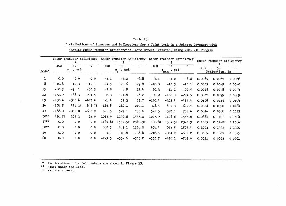
Table 13Distributions of Stresses and Deflections for a Joint Load in a Jointed Pavement with

Varying Shear Transfer Efficiencies, Zero Moment Transfer, Using WESLIQID Program

Node*

Shear Transfer Efficiency%

Shear Transfer Efficiency %

Shear Transfer Efficiency %

Shear Transfer Efficiency%100 50

a , psiX

0 100 500 y , psi

0 1001

50J , psi max

01 0 0 5 0

Deflection.0

in.1 0.0 0.0 0.0 -l*.l - 5 . 0 -6.8 -i*.i -5 . 0 -6.8 0 . 0 0 6 5 0 . 0 0 6 5 0 . 0 0 6 6

8 -10.8 -10.3 -10.1 -U.5 - 5 . 6 -7.8 -1 0 . 8 -1 0 . 3 -1 0 . 1 0 . 0 0 5 5 0 .0 0 1 * 9 0 .0 0 1 * 0

15 -60.3 -71.1 -90.5 - 5 . 8 -8 . 5 -13.1* -6 0 . 3 -7 1 . 1 -9 0 . 5 0 . 0 0 5 8 0 .0 0 1 * 8 0 .0 0 3 1*22 -132.9 -166.3 - 2 2 k . 5 2.3 -1.8 -8.2 1 3 2 . 9 -1 6 6 . 3 -221*. 5 0 . 0 0 8 7 0 . 0 0 7 9 0 . 0 0 6 9

29 -230.1* -302.k -*+27.** 1*1 . 1* 39-3 39.7 -230.1* -302.1* -1*27.1* 0 . 0 1 6 8 0 . 0 1 7 5 0 .0 1 9 1*3 6 -308.5 -**31.3+ -61*5.7t 1 6 6 . 8 182.1 219.1 -308. 5 -1*31.3 -61*5.7 0 . 0 3 3 8 0 . 0 3 9 0 0.01*81*h 3 -1 8 8 . 0 -350.0 -636.9 521.5 597.1 755.6 5 2 1 . 5 597.1 755.6 0 . 0 6 2 6 0 . 0 7 6 8 0.102250** 1*96.7+ 353.3 9**.0 1023.9 1198.6 1553.0 1023.9 1198.6 1553.0 0 .0 8 6 1* 0 . 1 1 0 1 0.1521*57** 0.0 0.0 0.0 1 1 6 0 .8 + 1551*. 5+ 23l*0.9t II6 O.8 + 155l*. 5+ 231*0.9+ 0 .1 0 8 5 + 0.11*1*2+ 0.2081*+58** 0.0 0.0 0.0 660.3 883.1 1328.0 698.1* 961*. 5 1503.1* 0 . 1 0 0 3 0.1333 0.192059 0.0 0.0 0.0 -5.1 -12.8 -28.1* -2 1 6 . 5 -3 5 I*. 9 -631.2 0 . 0 8 1 5 0.1083 0.151*56 0 0.0 0.0 0.0 -21*9.3 -33l*. 6 -5 0 5 . 2 -335-7 -1*78.1 -763.9 0 . 0 5 2 2 0.0693 0.0961

* The locations of nodal numbers are shown in Figure 19.* * Nodes under the load, t Maximum stress.

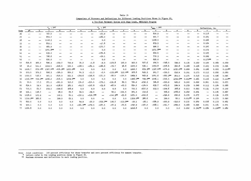
Table lUComparison of Stresses and Deflections for Different Loading Positions Shown in Figure 20

a Two-Slab Pavement System with Edge Loads, WESLIQID Program

Node

a , psiX a , psi y0 , psi max Deflection, in.

a* * b c d e a b c d e a b c d e a b c d e

26 _ _ 767. u _ — — — -25.9 — — — — 820.9 — — — — 0.118 — —

27 — — 872.7 — — — — -186.0 — — — — 921.7 — — — — O.lUl — —

28 — — 11U8.5 — — — — 0.0 — — — — 11U8.5 — -- — — 0.166 — —

33 — — 872.1 — — — — -17.8 — — — — 879.5 — ~ - - 0.12U - —3U — — 985.9 — — — — -175.7 — — — — 990.5 — — — — 0 .1U7 — —35 — — 1271.8** — — — — 0.0 — — — — 1271.8** — — — — 0.172 — —Uo — — 635.0 — — — — -17U.6 — — — — 6U0.U — — — — 0.125 — —Ul — — 766.6 — — — — - 50.1 — — — — 772.3 — — — — 0 .1 U9 — —U2 — — 695.0 — — — — 0.0 — — — — 695.0 — — — — 0.17U** — —h i 83U.8 366.2 896.3 - 379.7 793.9 3U.2 -1.8 - 3.3 -123.8 105.0 922.9 U77.6 9U6.U -U98.5 799.0 0.13U 0.152 0.120 0.06U 0.079U8 9h .2 UUl.U 1019.u -U26.6 93U.U -1U8.U -181.1 -166.6 - 79.7 96.8 1025.0 53U.1 1053.8 -528.U 9U0.8 0.166 0.196 0 .1U3 0.079 0.09Uh9 1206.7 679.u** 1307 . U** _I*7U.9** 1235.0** 0.0 0.0 0.0 0.0 0.0 1206.7 679 . 3** 1307.u** -U7U.9 1235 .0** 0.200 0.2U1 0.166 0.093 0.110**5h 953.5 379.2 806.3 -36U.O 80U.2 UU.3 - 11.5 -2.U - 133 .9** 112.U** 978.8 U22.3 9U1 .7 - 529.5 816. U O.lUl 0.173 0.112 0.080 0.080

55 1050.5 U36.U 921.1 -UlU.O 931.1 -IU9.6 - 195.6 -171.0 -82. U -10U.U 1069.5 U62.9 IOU1.6 - 562.3** 9U3 .0 0.17U 0.218 0.133 0.096 0.09U56 1356. h** 709.0** 1206.2 -U5U.5 1259. 6** 0.0 0.0 0.0 0.0 0.0 1356.U** 709 . 0** 1206.1 -U5U.5 1259.6** 0.212** 0.26U 0.156 0.110 0.110**6i 7 0 . k 17.5 271.1 -261.9 312.2 13U.2 -2lU.U -173.1 -131.8 82.3 70U.2 -232.3 56U.8 -505.9 U20.0 0 .1U5 0.202 0.9U1 0.011 0.07562 83U.lt 59 . u 311.0 -238.6 385.1 -U3.7 -107.8 - 73.6 - 6 7 . u - 25.5 83U.2 -12U.U 635.7 -U73.5 50U.U 0.179 0.2U8 0.113 0.12U 0.088

63 755.5 65.7 233.5 - 309.6 3U8 .9 0.0 0.0 0.0 0.0 0.0 755.5 - 657.2 233.5 - 309.6 3U8 .9 0.215 0.293 0.131 0.1U2 0.10268 93U.1 138.7 — 98.0 85.7 U6.U - 39.5 — 72.1 -101.5 971.3 1U2.6 — 358.0 -278.0 0.1U2 0.231 — 0.13U 0.067

69 1058.6 125.9 — 102.1 80.1 -152.I -216.7** — - l U o . 3 * * - 55.8 1071.0 -216.8 — -296.6 282.6 0.176 0.277 — 0.13U 0.07870 1359.2** 386.6 — 399.0 62.1 0.0 0.0 — 0.0 0.0 1359 .2** 386.6 — 399.0 62.1 0.211** 0.32U — 0.175 0.090

75 862.5 0.0 0.0 0.0 0.0 U9 .9 - 22.2 -233 .7** 105.7 -113 .8** -22.1 -28.1 -58U.9 -205.9 -312.0 0.135 0 .2U9 0.058 0.153 0.06l76 930.1 0.0 0.0 0.0 0.0 -16U.5** - 179.5 -187.5 - 77.3 -70.6 -232.9 -187.2 -568.1 - 231.7 -289.O 0.168 0.295 0.071 0.17U 0.071

77 1266.8 0.0 0.0 0.0 0.0 0.0 0.0 0.0 0.0 0.0 1216.8 0.0 0.0 0.0 0.0 0.202 0.3U2** 0.08U 0.196** 0.082

Note: Joint condition: 100 percent efficiency for shear transfer and zero percent efficiency for moment transfer.* Letters refer to the loading position shown in Figure 20.** Maximum stresses and deflections in each loading position.

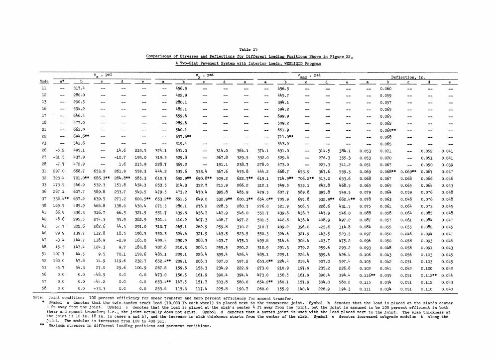
Table 15

Comparisons of Stresses and Deflections for Different Loading Positions Shown in Figure 22

A Two-Slab Pavement System with Interior Loads; WESLIQID Program

Node

a , psiX °y ’ psl c ,max psi Deflection, in.a* * b c d e a b c d e a b c d e a b c d e

11 — 317.1* — — — — 1+56.5 — — — — 1+56.5 — — — — 0.060 — — —

12 — 280.0 — — — — 1+22.9 — — — — 1+1+5.7 — — — — 0.059 — — —

13 — 290.5 — — — — 280.1 — — — — 39U.1 — — — — 0.057 — — —

16 — 59*+. 2 — — — — 1+8 2.1 — — — — 59U.2 — — — — 0.065 — — —

IT - 61+6.1+ — — — — 659.6 — — — — 699.9 — — — — 0.065 — — —

18 — 1+77.0 — — — — 289.6 — — — — 509.2 — — — — 0.062 — — —

21 — 661.9 — __ — — 51+0.1 — — — — 661.9 — — — — 0.069** — — —

22 — 69I+.6** — — — — 697.6** — — — — 711.0** — — — — 0.068 — — —

23 — 51+1.6 — — — — 319.1+ — — — — 51+3.0 — — — — 0.065 — — —

26 -5.2 1+95.1 — 11+.6 219.5 371+.1 631.0 — 311+.0 38U .1 371+.1 631.0 — 311+.5 381+.1 0.053 0.071 -- 0.052 o.oi+ i27 -31.5 1+37.9 — -10.7 193.0 319.5 529.8 — 267.8 329.5 332.0 529.8 — 276.3 355.3 0.053 0.070 — 0.051 O.Ol+l28 -7.7 1+72.9 — 1 .6 215.9 228.7 369.2 — 191.1 238.7 278.0 1+73.0 — 225.3 31+1.2 0.051 0.067 — 0.050 0.03931 297.0 668.7 653.9 261.9 559.3 1+1+1+.2 535.6 533.1+ 367.6 1+55.8 1+1+1+.2 668.7 653.9 367.6 559-3 0.069 0.068** 0.069** 0.067 0.01+732 323. b 70 1.0** 686.3** 281+.8** 585.3 610.7 692.9** 690.8** 509.2 622.7** 619.1 711+.9** 706.2** 513.0 653.6 0.068 0.067 0.068 0.066 0.01+633 173.5 51+6.9 532.3 15 1.8 1+3U.3 253.5 311+.3 312.7 211.9 266.2 312.1 51+9.5 535.1 21+3.8 1+68.5 0.065 0.065 0.065 0.061+ 0.01+336 287.1 607.7 589.8 233.7 51+9.5 1+79.5 1+73.2 1+70.1+ 395.8 1+85.9 1+79-5 607.7 589.8 395.8 51+9.5 0.079 0.061+ 0.059 0.076 0.01+8

37 338.1+** 657.2 639.5 271.2 600.5** 653.2** 651.5 61+9.0 532.9** 600.3** 65U.O** 705.9 695.8 532.9** 662.1+** 0.078 0.063 0.01+8 0.076 0.01+838 169.5 1+85.9 1+68.8 138.0 1+30.1+ 271.5 280.1 278.2 228.5 280.7 276.0 521.9 506.5 228.6 1+31.5 0.075 0.06l 0.061+ 0.073 0.01+5kl 86.9 338.3 316.7 66.3 321.5 551.7 1+39.8 1+36.7 1+1+7.9 5I+6.O 551.7 1+39.8 1+36.7 1+1+7.9 5I+6.O 0.088 0.058 0.061+ 0.085 0.01+8b2 1+8.6 295.5 27U.3 35.9 282.9 501.1+ 1+10.2 1+07.3 1+08.7 1+97-2 501.5 1+1+2.8 1+36.1+ 1+08.9 1+97.2 0.087 0.057 0.06l 0.081+ 0.01+7b3 57.7 302.6 282.6 1+1+. 5 291.0 310.7 265.1 262.9 259.8 310.2 310.7 1+09.2 396.0 1+25.6 311+.8 0.081+ 0.055 0.055 0.082 0.01+5b6 29.9 139.7 112 .8 18 .5 198.3 550.3 321+.6 321.9 1+1+3.5 523.5 550.3 321+.6 321.9 1+1+3.5 523.5 0.097 0.050 0.01+6 0.091+ 0.01+71+7 -3.1+ 1 I+I+.7 118.9 -2.9 165.0 1+99.1+ 290.9 288.3 1+03.7 1+75.1 1+99.8 311+.6 308.1+ 1+03.7 1+75.2 0.096 0.050 0.058 0.093 0.01+61+8 15.5 11+7.1+ 121+.3 9.7 183.8 307.8 210.3 208.1 259.5 290.2 310.9 291.3 279.2 259.6 293.2 0.093 0.01+8 0.058 0.091 0.01+3

51 107.7 1+1+.5 9.5 70.1 159.6 1+85.1 229.1 228.1+ 399.1+ 1+26.1+ I+85.I 229.1 228.1+ 399.1+ 1+26.1+ 0.106 0.01+3 0.056 0.103 0.01+552 180.0 1+7.8 11+.9 119 .6 232.7 652.1+** 209.1 208.3 507.0 597.2 653.0** 22U.1+ 219.1+ 507.0 597.1+ 0.105 0.01+2 0.051 0.103 0.01+553 1+5.7 51+.3 27.0 29.6 100.9 267.8 159.6 158.3 231+.9 222.9 273.0 210.9 197.9 235.2 226.8 0.102 0.01+1 0.01+2 0.100 0.01+256 0.0 0.0 -1+8.9 0.0 0.0 1+73.0 156.5 16 1 .9 390.1+ 391+.1+ 1+73.0 156.5 161.9 390.1+ 391+.1+ 0.116** 0.035 0.051 0.112** O.0U+57 0.0 0.0 -1+1+ .2 0.0 0.0 653.1+** 11+7.5 151.7 503.8 580.0 65U.2** 160 .1 157.9 501+.0 580.2 0.115 0.031+ 0.051 0.112 0.01+358 0.0 0.0 -33.3 0 . 0 0 . 0 253.8 115 .6 117.1+ 225.8 190.7 260.0 155.9 11+0.1+ 226.9 191+.3 0 .111 0.031+ 0.051 0.110 o.oi+o

Note: Joint condition: 100 percent efficiency for shear transfer and zero percent efficiency for moment transfer.* Symbol a denotes that the twin-tandem truck load (10,000 lb each wheel) is placed next to the transverse joint. Symbol b denotes that the load is placed at the slab's center h ft away from the joint. Symbol c denotes that the load is placed at the slab's center b ft away from the joint, but the joint is assumed to be 100 percent efficient in both

shear and moment transfer; i.e., the joint actually does not exist. Symbol d denotes that a butted joint is used with the load placed next to the joint. The slab thickness at the joint is 10 in. (8 in. in cases a and b), and the increase in slab thickness starts from the center of the slab. Symbol e denotes increased subgrade modulus k along the joint. The modulus is increased from 100 to 1+00 pci.

** Maximum stresses in different loading positions and pavement conditions.

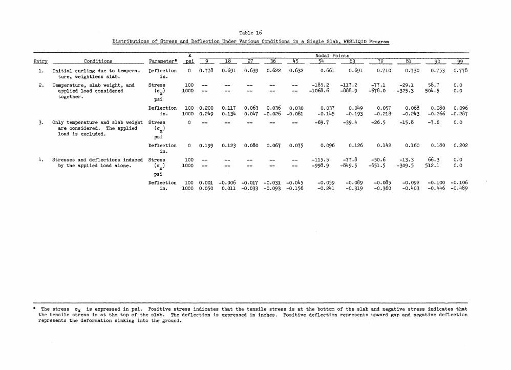
Table l6

Distributions of Stress and Deflection Under Various Conditions in a Single Slab, WESLIQID Program

k _________________________________________ Nodal PointsEntry Conditions Parameter* psi 9 18 27 36 k5 51* 63 72 81 90 99

1. Initial curling due to tempera- Deflection 0 0 .778 0.691 0.639 0.622 0.632 O .661 O.69I 0.710 0.730 0.753 0.778ture, weightless slab. in.

2. Temperature, slab weight, and Stress 100 — — — — — -1 8 5 . 2 -II7 . 2 -77.1 -2 9.I 58.7 0.0applied load considered (°x ) 1000 — — — — — -IO68.6 -888.9 -678.O -325.3 50l*. 5 0.0together. psi

Deflection 100 0.200 0.117 O.O63 0.036 0.030 0.037 0.01*9 0.057 O .068 0.080 0.096in. 1000 0.21*9 0.13k 0.0l*7 -O .026 -O.O8I -O.1 U5 -0.193 -O .2 18 -0.21*3 -O .266 -O .287

3. Only temperature and slab weight Stress 0 — — — — — -69.7 -39. k -26.5 -15.8 -7.6 0.0are considered. The applied (°x >load is excluded. psi

Deflectionin.

0 0.199 0.123 O.O8O O .067 0.075 0.096 0 .12 6 0.11+2 O .160 0.180 0.202

1*. Stresses and deflections induced Stress 100 _ _ _ _ _ -II5 . 5 -77.8 -50.6 -13.3 66.3 0.0by the applied load alone.

<‘x> 1000 — — — — — -998.9 -81*9.5 -6 5 1 . 5 -309.5 512.1 0.0

psi

Deflection 100 0.001 -O.OO6 -0.017 -0.031 -O.OU5 -0.059 -O.O89 -O.O85 -O.O92 -0.100 -O.IO6in. 1000 0.050 0.011 -0.033 -0.093 -O.I56 -0.21*1 -0.319 -O.36O -0.1*03 -0.1*1*6 -O.U89

* The stress ax is expressed in psi. Positive stress indicates that the tensile stress is at the bottom of the slab and negative stress indicates that the tensile stress is at the top of the slab. The deflection is expressed in inches. Positive deflection represents upward gap and negative deflection represents the deformation sinking into the ground.

Table 17Stresses a

XAlong the Joint in a Two-Slab Pavement Subject to Center Loads, WESLIQID Program

Stresses a tt at Nodal Points, psi______________ JL.............. .% StressCurve* Load Temperature Warping** Gapt 314= 36 Transfer 4=4= 32 37 33 38 3b 39 35 bO

1 Yes No No 885.0 29I». 8 25 3 31 . 9 21*3 .5 1 8 . 7 155.0 -ill*. 6 -50.8 0.0 0.02 No Upward No -1 8U .9 -18I1.9 50 -1 7 7 .6 -1 7 7 . 6 -1 5 7 . 3 -157.3 -97.2 -97.2 0.0 0.03 Yes Upward No 628.7 39.7 5 .9 9 1 . 3 U A -175 A -32.8 -179.8 -117.8 0.0 0.0b Yes Upward Yes 6 k k .6 52.6 7 . 5 10U .2 lU .7 -169.3 -33.0 -18 5 .0 -120.0 0.0 0.05 No Downward No 393.1 393.1 50 385.3 385.3 315.9 315.9 170.3 170.3 0.0 0.06 Yes Downward No 1388.8§ 795-8 3 6.1» 822 .2 731.1 1+70.3 605.1 171». 5 233.6 0.0 0.07 Yes Downward Yes 1381». 8§ 789.9 36.3 8 1 7 . 1 J2 k . 8 1*63.6 598.3 1 6 6A 226.3 0.0 0.0

* Condition number coincides with the curve number shown in Figure 27. In all of the computations, the pavement weight is considered.

** Temperature differential is 3.75°F per inch of pavement, t 1-in. gap in the subgrade along the joint, full contact elsewhere.

tt Stress o-y acts in the direction parallel to the joint. Positive stress indicates tension at the bottom of the pavement and negative stress indicates tension at the top of the pavement.

4s The locations of nodal points are shown in Figure 27.+4= Percent stress transfer is defined to be the stress at the unloaded side divided by the sum of the stress at loaded and

unloaded sides.§ Maximum stresses.

Table 18Stresses a Along the Joint in a Two-Slab Pavement Subject to Corner Loads, WESLIQID Program. ■ —. ——, , t f ---_—__________________________ __________________________________ ______ _

Stress a ft at Nodal Points Stress a ft at Nodal Pointsy y

Condition__________________ ______________ Along the Joint_____________ ________Along the Edge________Condition* Load* Temperature Warping** Gapt i*r* 5^ 1*8 55 Ji£ 56 Jt£ 5 6 1+2 35 28

1 Yes No No -5 3 3 .1 -9 7 .5 -139.U -2 2 9 .2 0.0 0.0 0.0 0.0 311.1 620.1** -2 0 0 .52 No Upward No -7 1 .2 -7 1 .2 -3 0 .5 -3 0 .5 0.0 0.0 0.0 0.0 -2 1 .7 -1*6.6 -111*. 7*3 Yes Upward No -618 .3*+ -1 7 8 .2 -1 2 7 .7 21*9.5 0.0 0.0 0.0 0.0 321.7 570.6 -1+26.2k Yes Upward Yes -6 5 0 .9 * * -1 8 7 .8 -11*9.1* 261*. 6 0.0 0.0 0.0 0.0 337.6 590.1* -1*12.95 No Downward No 13U.8** 13^.8 1*8.0 1*8.0 0.0 0.0 0.0 0.0 — — —6 Yes Downward No -U3U.8 -1.1* -1 6 5 .7 1 9 9 .2 0.0 0.0 0.0 0.0 281+.6 661.1*** 57 .07 Yes Downward Yes -5 0 8 .6 -5U .0 -151*. 2 2l*1.2 0.0 0.0 0.0 0.0 313.9 61*2.1+** -1 6 .5

* Condition number coincides with the curve number shown in Figure 27. In all of the computations, the pavement weight is considered.

** Temperature differential is 3.75°F per inch of pavement.t 1-in. gap in the subgrade along the joint, full contact elsewhere,

ft Stress Oy acts in the direction parallel to the joint and stress ax acts in the direction perpendicular to the joint. Positive stress indicates tension at the bottom of the pavement and negative stress indicates tension at the top of the pavement.

* The locations of nodal points are shown in Figure 27.^ Maximum stresses.

Table 19

LoadingCondition

Centerload

Cornerload

Stress Distributions in a Pavement With and Without the Load Transfer Device Acrossthe Joint, Temperature Effect Not Considered

1-in. Dowel 15 in. Apart for ShearTransfer, Zero Moment Transfer______ Zero % Shear and Moment Transfer

Nodal*Number

a tX-- Psi

a typsi

Tpsi

amaxpsi

aX

psiOJpsi

Tpsi

0maxpsi

16 -108.2 228.7 0.0 228.7 -21+8.6** 271+.1 0.0 271+.121 2 7 1.9** 631.0 0.0 631.0 121.1 71+6.9 0.0 71+6.926 7 7 .6 660.5 0.0 660.5 -31.0 81+1 .9 0.0 81+1 .931 0.0 885.0** 0.0 885.0** 0.0 1169.2** 0.0 1169.2**32 0.0 331.9 -101.6** 360.5 0.0 565.1+ 0.0 565.1+33 0.0 18.7 -7 7 .1 87.0 0.0 16I+.7 0.0 161+.73U 0.0 -111+.6 -3 2 .3 -123.0 0.0 -168.3 0.0 -168.335 0.0 0.0 0.0 0.0 0.0 0.0 0.0 0.0

27 -111+.5 -117.3 325.2** -1+51+.8 -1+5 5 .0 -175.9 1+83.5 -818.728 -2 0 0 .5 0.0 0.0 -2 0 0 .5 -5 5 3 .0 0.0 0.0 -5 5 3 .033 9 6 .6 -^29.5 203.5 -1+9 9 .0 -150.6 -51+1.1 1+56.5 -81+2 .3**3h 3 8 5 .8 -78.3 260.3 5 0 1 .6 7 2 .0 -115.0 1+90.1+** -5 2 0 .735 620.1** 0.0 0.0 620.1** 2 7 8 .3 0.0 0.0 278.31+0 8 3 .8 -1+6 9 .6 121+.3 -I+96.3 -76.1 -571.9** 1+26.1 -817.0Ul 2 2 2 .2 -1 2 0 .0 11+9.0 278.0 -1 0 .6 -92.0 1+08.3 -I+61.71+2 3 1 1 .1 0.0 0.0 3 1 1 .1 1 0 2 .1 0.0 0.0 1 0 2 .11+7 0.0 -5 3 3.1** 1 0 3 .0 5 5 2 .3 -6 3 2.2** 0.0 0.0 -6 3 2 .21+8 0.0 -1 3 9.1+ 129.2 -216.5 0.0 87.3 0.0 8 7 .3

* The locations of nodal points are shown in Figure 2 7.** Maximum stressses. The maximum free edge stress is 1 1 5 1 .5 psi (a = a ).max "Vt The coordinates of x- and y-axis are shown in Figure 2 7. J

Table 20Comparisons of Stresses and Strains in a Five-Slab Continuously Reinforced Concrete Pavement for Various

Loading Positions Shown in Figure 23; Thickness of the Pavement t = 8 in.

cX , psi a >y

psi amax » psi Deflection w, in.Node a* b c d a b c d a b c d a b c d

1 0.0 0.0 0.0 0.0 0.0 388.8 0.0 1+32.3 0.0 388.8 0.0 1+32.3 0.183** 0.01+6 0.159 0.0702 680.2 238.1+ 370.8 1+5.7 0.0 383.1+ 0.0 1+21.7 680.2 383.1+ 370.8 1+21.7 0.165 0.057 0.166 0.0733 735.6** 235. k -179.5 -107.8 0.0 1+28.1 0.0 1+91+.2 735.6** 1+28.1 -179.5 1+91+.2 0.11+3 0.067 0.172 0.077k 115.8 1+2U.U** -223.3 -136.9 0.0 516.7 0.0 510.5 115.8 516.7 -223.3 510.5 0.118 0.076 0.178 0.0825 0.0 0.0 0.0 0.0 0.0 531.1+ 0.0 1+58.8 0.0 531.1+ 0.0 1+58.8 0.092 0.085** 0.185** 0.0876 0.0 0.0 0.0 0.0 -1+2.0 350. k. -132.0 1+78.3 58.9 361.1 -211.8 578.5 0.158 0.01+5 0.137 0.068T 389.8 27U.1 76.5 113.9 -205.5 571.1 -205.8 590.8 1+21.9 579.5 -228.5 590.9 0.1U1 0.055 0.11+3 0.0728 1+1+1+.7 275.5 -111.1+ -132.9 -213.6 605.0** -113.6 1+1+9.7 51+6.1+ 606.1** -II+9.6 1+1+9.7 0.121 0.065 0.11+8 0.0759 179.8 2.01 -171+.1 -I5O.2 -120.9 1+72.8 -97.5 1+56.9 1+12.2 1+73.0 -198.3 1+58.2 0.098 0.07^ 0.15!+ 0.080

10 0.0 0.0 0.0 0.0 -127.1 1+80.1 -152.6 61+6.5** -1+21.7 1+80.9 -171+.2 650.6 0.071+ 0.081+ 0.l6l 0.08611 0.0 0.0 0.0 0.0 -155.0 221.8 -11+.6 225.9 -237.8 273.8 —81+. 0 227.1 0.131+ 0.01+1 0.115 0.061+12 328.0 13k.k 97.6 -5.1+ -I6.O 212.5 -23.1+ 227.5 1+01+.7 271+.2 -50.3 229.0 0.118 0.051 0.120 0.06813 376. b I3I+.U -158.7 -89.2 -31.1 232.3 -179.3 268.1 518.1+ 237.8 -219.2 268.3 0.099 0.06l 0.125 0.071Ik 95. k 278.5 -I8O.7 -98.5 -186.9 279.3 -171.2 273.3 -1+18.9 299.1+ -21+8.6 280.7 0.079 0.070 0.131 0.07615 0.0 0.0 0.0 0.0 -22I+.7** 290.9 26.2 239.7 -1+83.3 291+.3 111.2 276.5 0.057 0.079 0.137 0.081l6 0.0 0.0 0.0 0.0 0.0 535.8 0.0 1+63.8 0.0 535.8 0.0 1+63.8 0.123 0.085** 0.185** 0.087**IT 67U.2 21+0.0 U1+5.1+** 108.3 0.0 1+38.0 0.0 391+.3 671+.3 1+38.0 1+1+6.9 391+.3 0.11+3 0.071 0.153 0.06518 698.9 269.8 -1+6.9 7.1+ 0.0 399.5 0.0 380.3 699.0 399.5 -1+6.9 380.3 0.159 0.056 0.118 O.Oi+319 70.5 92.6 -100.8 -37.3 0.0 397.3 0.0 291.1+ 70.5 397.3 -100.8 291.1+ 0.171 O.Ol+l 0.081+ 0.02120 0.0 0.0 0.0 0.0 0.0 303.5 0.0 211.8 0.0 303.5 0.0 211.6 0.183 0.026 0.050 - 0.00121 0.0 0.0 0.0 0.0 -67.1 1+7U.8 -132.6 61+1.6** -1+01.5 1+75.0 -387.7 651.1** 0.101+ 0.081+ 0.l6l 0.08622 386.6 276.2 150.7 168.7** -208.I 618.3** -201.1 571.0 512.7 619.1+** -I+29.3 585.5 0.121 0.070 0.130 0.061+23 H 0 U .8 307.5 22.1+ - 21.1 -206.0 582.6 -111+.1+ 357.3 1+1+5.9 592.7 -1+62.6 373.9 0.135 0.055 0.099 0.0i+22k 122. k 50.1+ -51+.7 -30.0 -96.3 373.2 -III+.9 261.1 151.0 388.6 -1+77.2 277.3 0.11+7 O.Ol+O 0.068 0.02025 0.0 0.0 0.0 0.0 -61.5 273.3 -11+3.6 196.6 -II5.3 289.9 -1+1+7.3 211+.5 0.158 0.021+ 0.037 0.00026 0.0 0.0 0.0 0.0 -167.6 291.2 13.8 21+0.0 -1+13.9 291.1+ 386.9 301.6 0.085 0.079 0.137 0.08l27 323.5 137.8 161+.3 50.1+ -10.1 21+0.3 -12.8 217.1 1+79.5 21+7.2 1+80.9 297.3 0.100 0.065 0.109 0.06028 336.2 161.1+ -31.9 0.89 -21.5 221+.2 -172.9 222.8 1+08.2 296.3 -526.2 295.8 0.113 0.051 0.08l 0.03929 36.0 61+. 7 -37.3 -20.1+ -163.2 23U.0 -201+.0 190.0 -215.3 301+.2 -536.0** 21+1+.8 0.121+ 0.036 0.052 0.01830 0.0 0.0 0.0 0.0 -139.9 199.8 -218.9** 157.3 -202.1+ 251+.3 -516.8 210.1 0.131+ 0.021 0.023 -0.002

* Letters refer to loading positions shown in Figure 28.** Maximum stresses or deflections.

Comparison of Maximum Stresses and Deflections for Three Pavements under Various Loading Positions

o *X

, psi C7 * , psiy 0 * , psi max w* , in.

Loading Position8-in.

Regular**8-in. CRCP

6-in. CRCP

8-in. Regular

8-in. CRCP

6-in. CRCP

8-in. Regular

8-in.CRCP

6-in.CRCP

8-in.Regular

8-in.CRCP

6-in.CRCP

Edge loads placed next to the joint, edge load

7 0 9 . 0 itu 5 .it 7 U 1 .8 - 2 1 6 . 7 - 2 1 8 .9 - 3 9 3 .2 7 0 9 .0 - 5 3 6 .0 - 7 8 9 .3 0.3U 2+ 0 .1 8 5 0 .2 3 0

Edge loads placed between the joint, edge load

1 3 0 7 . Ut 7 3 5 .6 1 2 U 0 .0 - 2 3 3 .7 -2 2 U .7 - 3 8 5 .6 1 3 0 7 .u t 7 3 5 .6 12 U 0 .0 0 . 1 7 u 0 .1 8 3 0 . 2 2 U

Center load placed next to the joint, center load

338.4 1 6 8 .7 - 2 7 5 .9 6 53.U 6 U 6 .5 9 9 5 .9 + 6 5U .0 6 5 1 . 1 1 0 0 3 .6 0 .1 1 6 0 .0 8 7 0 . 1 0 0

Center load placed between the joint, center load

7 0 1 .0 lt2 lt.lt lt8 0 .lt 6 9 7 .6 6 1 8 .3 9 5 1 .6 7 1 U .9 6 1 9 . u 9 5 3 .5 0 .0 6 9 0 .0 8 5 0 . 0 9 3

* The stresses and deflections are the maximum values for the given loading position. The coordinates of x- and y-axis are shown in Figure 28.

** The three pavements are (l) an 8-in.-thick regular jointed pavement with a pavement length of 15 ft, (2) an 8-in.-thick continuous reinforced concrete pavement (CRCP) with ¿-ft crack spacing, and (3) a 6-in.-thick CRCP with ¿-ft crack spacing. The joint conditions are assumed to have 100 percent of efficiency in shear transfer and zero percent moment transfer. Note in the 8-in.-thick regular jointed pavement, the twin-tandem load is placed in one slab while in the CRCP, the two sets of dual wheels of the twin-tandem load are placed at separate slabs,

t Maximum value in a most critical loading position.

Table 22Comparison of Maximum Stresses and Deflections for Four Pavements Under Two Loading Positions

ax* , psi a * , psiy

a * , psi max * w* , in.a b c d a b c d a b c d a b c d

Pavement type Regular CROP CRCP CRCP Regular CRCP CRCP CRCP Regular CRCP CRCP CRCP Regular CRCP CRCP CRCPPavement thickness, in.

8 8 8 8 8 8 8 8 8 8 8 8 8 8 8 8

Pavement length or crack spac­ing, ft

15 1+ 2 2 15 1+ 2 2 15 1+ 2 2 15 1+ 2 2

Efficiency in shear transfer across the joint, percent

100 100 100 0 100 100 100 0 100 100 100 0 100 100 100 0

Efficiency in moment transfer across the joint, percent

0 0 0 0 0 0 0 0 0 0 0 0 0 0 0 0

Edge load** 13 0 7 .‘tt 735.6 5U7.9 186.7 -233.7 -22U.7 -537.9 -1702.6+ 1307.1+ 735.6 916.2 -1702.6+ 0.3*t2 0.185 0.288 0.630+Center load** 7 0 1 .Of 1+21+.1+ 182.7 133.7 6 9 7 . 6 61+6.5 881+.8 18 78 .1++ 7l'+.9 651.1 887.1 I878.I++ 0 .116 0.087 0.176 0.312+

* The stresses and deflections are the maximum values for the given loading position. The coordinates of x- and y-axis are shown in Figure 28.** In cases a and b the values are at maximum when the load is placed next to the joint (or crack) or placed between the joint. In cases c and d

the values are computed when the load is placed next to the cracks.t Maximum value in a given loading postion. In case a the twin-tandem load is placed in one slab and in cases b, c, and d the two sets of dual wheels are placed at separate slabs.

APPENDIX A: EQUATIONS FOR STRESSES AND DEFLECTIONSUNDER A POINT LOAD AND UNDER A CIRCULAR LOAD

1. The stresses and vertical deflection in a linear elastic medium under a point load can he computed from the following equations (Harr 1966).

a = P2ir[3zr2 _ 1 - 2y ~|

r5 R(R + z) I

_ 3P= 2» r5

r _ 3P ¿r_ rZ 2,1

°e = (1 - 2"> [R<e1+ ' R3] (Al)

_ P(1 + y) [z2 2(1 - y)l2’E s Jwhere

a , ar normal stresses in the r , 0 , and zdirections

Pr , z , R

TrzwyE

a point load see Figure Alshear stress in the rz direction 'vertical deflection Poisson’s ratio elastic modulus

2. Under a circular load, the vertical stress a and deflec-ztion w under the center of the circular load can he computed by the following two equations (Harr 1966)

az <1 1 [(a/z)2 + 1]3/2r = 0 (A2)

Al

r = 0 (A3)N

p)VT"T?J ’

whereq = unit pressure a = radius of the loaded area n = z/a

w(o,z) = ■) oi1 + n - n) 1 +■ 2(1 -

A2

APPENDIX Bj NOTATION

a,bA

[A]

bc

dE

Fw{F}{F}

Gh

ij[H]

H. .ij

IkK

[K][K]KiJ

l

LM

MxM

yppp f

DimensionsArea of the dowel barDiagonal matrix representing the area over which subgrade reaction is distributedDowel bar diameterInitial curling of a weightless and unrestrained slab due to a temperature differential between the top and the bottomJoint spacing or one half of the slab lengthModulus of concrete or modulus of dowelVertical forceNodal forcesComposite nodal forcesShear modulus of steelThickness of the concrete slabVertical force at node i due to vertical displacement at node jStiffness matrix of the subgradeVertical force at node i due to displacement at node j NodeMoment of inertia of the slab sectionModulus of subgrade reactionModulus of dowel supportStiffness matrix of the concrete slabComposite stiffness matrix of the systemVertical force at node i due to vertical displacement at node jRadius of relative stiffness Length of the concrete slab Moment sMoment about the x-axis Moment about the y-axis Unit pressureVertical shear force or a point loadShear force on dowel to affect A 1c

B1

[P] A composite matrix and is equal to [K] + [H]R Radius of the spherical surfaces Precomposition or gapt Pavement thicknessw Deflection in the z-directiona Coefficient of thermal expansiong A parameter

{6} Nodal displacements, each consisting of a vertical deflec­tion and two rotations

{61} Subgrade displacementA Difference in deflection across the joint

Ac Deformation of concrete due to shear force on the dowelInput parameter specifying the deformation of concrete below

c which modulus is used and above which modulus K2 isused

As Shear deformation of the dowel bar AT Temperature differential0x Rotation about the x-axis0y Rotation about the y-axisv Poisson’s ratio of the concrete

amax Maximum principal stressax Stress in the x-directionOy Stress in the y-directiont Shear stress

xXy Shear stress in the x-y direction

B2

In accordance with letter from DAEN-RDC, DAEN-ASI dated 22 July 1977, Subject: Facsimile Catalog Cards forLaboratory Technical Publications, a facsimile catalog card in Library of Congress MARC format is reproduced below.

Chou, Yu T.Structural analysis computer programs for rigid

multicomponent pavement structures with dis­continuities— WESLIQID and WESLAYER : Report 1 : Program development and numerical presentations / by Yu T. Chou (Geotechnical Laboratory, U.S. Army Engineer Waterways Experiment Station), — Vicksburg, Miss. : The Station ; Springfield, Va. : available from NTIS, [1981].

1^5 p. in various pagings : ill. ; 27 cm. — (Technical report / U.S. Army Engineer Waterways Experiment Station ; GL-81-6, Report l)

Cover title."May 1981.""Prepared for Office, Chief of Engineers, U.S. Army

under RDT&E Project Wo. l*A762719ATl*0, Work Units 001 and 003."

Bibliography: p. 118-120.

Chou, Yu T.Structural analysis computer programs for rigid : ... 1981.

(Card 2)

1. Computer programs. 2. Finite element method.3. Pavements. 4. WESLAYER (Computer program).5. WESLIQID (Computer program). I. United States.Army Corps of Engineers. Office of the Chief of Engineers. II. U.S. Army Engineer Waterways Experiment Station. Geotechnical Laboratory. III. Title IV. Series: Technical report (U.S. Army Engineer Waterways Experiment Station) ; GL-81-6, Report 1.TA7.W3^ no.GL-81-6, Report 1