The Pennsylvania State University

The Graduate School

Eberly College of Science

STRONG ENCOUNTERS WITH BLACK HOLES IN

GLOBULAR CLUSTERS

A Dissertation in

Astronomy & Astrophysics

by

Drew Reid Clausen

c© 2013 Drew Reid Clausen

Submitted in Partial Fulfillmentof the Requirements

for the Degree of

Doctor of Philosophy

August 2013

The dissertation of Drew Reid Clausen was reviewed and approved* by the following:

Michael EracleousProfessor of Astronomy & AstrophysicsDissertation Co-AdviserChair of Committee

Steinn SigurdssonProfessor of Astronomy & AstrophysicsDissertation Co-AdviserHead of the Astronomy & Astrophysics Graduate Program

Richard WadeAssociate Professor of Astronomy & Astrophysics

Yuexing LiAssistant Professor of Astronomy & Astrophysics

Lee Samuel FinnProfessor of Physics

*Signatures are on file in the Graduate School.

AbstractAs many as 1000 black holes could be produced when a globular cluster’s most massivestars end their lives. Following its formation, a globular cluster’s black hole populationis transformed by the dynamical processes that occur within dense stellar systems.After decades of theoretical and observational study, the outcomes of this evolutionremain uncertain. Outstanding questions include the fraction of clusters that retainblack holes, the size of the retained population, and the mass distribution of theseblack holes. In this thesis, we model encounters between black holes and other clustermembers to identify observable indicators of the presence and masses of black holesin globular clusters.

In one line of research, we model the formation of black hole–neutron star bina-ries via dynamical interactions in globular clusters. We find that in dense, massiveclusters, many of the black hole–neutron star binaries formed by these encountersundergo gravitational radiation driven mergers. Black holes retained by the clusterafter merging with a neutron star can acquire subsequent neutron star companionsand undergo several mergers. However, the post-merger recoil is only suppressed be-low the globular cluster escape velocity for black holes with masses exceeding 30 M�.Thus, the merger rate is sensitive to the black hole mass distribution. Models with35 M� black holes predict Advanced LIGO detection rates in the range 0.04−0.7 yr−1.Systems that do not merge may be observable as black hole–millisecond pulsar bi-naries. We discuss the distribution of orbital parameters in such binaries and thecluster properties that promote their formation. We find that the upper limit for thenumber of dynamically formed black hole–millisecond pulsar binaries in the MilkyWay globular cluster system is ∼ 10.

In a complementary study, we model the emission lines produced in the pho-toionized debris of tidally disrupted white dwarfs and horizontal branch stars. Theseemission lines can be used to investigate the intermediate mass black holes that maybe present in some globular clusters. We find that bright, broad, asymmetric C IV

λ1549 and [O III] λ5007 emission lines can be used to identify white dwarf tidal disrup-tion events. When a horizontal branch star is disrupted, the brightest optical emissionlines are [N II] λ6583 and [O III] λ5007. We compare our models with two candidatewhite dwarf tidal disruption events that have been observed in globular clusters. Wefind several drawbacks to interpreting either of these sources as a white dwarf tidaldisruption event. However, models of a red clump horizontal branch star undergoingmild disruption by a 50− 100 M� black hole yield an emission line spectrum that isin good agreement with one of these sources.

iii

Contents

List of Figures vi

List of Tables xiv

1 Introduction 11.1 General Overview . . . . . . . . . . . . . . . . . . . . . . . . . . . . . 11.2 Structure and Dynamical Evolution . . . . . . . . . . . . . . . . . . . 41.3 Binaries in Globular Clusters . . . . . . . . . . . . . . . . . . . . . . 71.4 Neutron Stars in Globular Clusters . . . . . . . . . . . . . . . . . . . 81.5 Stellar and Intermediate Mass Black Holes in Globular Clusters . . . 101.6 Thesis Overview . . . . . . . . . . . . . . . . . . . . . . . . . . . . . . 15

2 Black Hole–Neutron Star Mergers in Globular Clusters 162.1 Introduction . . . . . . . . . . . . . . . . . . . . . . . . . . . . . . . . 162.2 Method . . . . . . . . . . . . . . . . . . . . . . . . . . . . . . . . . . 18

2.2.1 Dynamics . . . . . . . . . . . . . . . . . . . . . . . . . . . . . 192.2.2 Gravitational radiation effects on the evolution BH+NS binaries 212.2.3 Formation of a new binary from a single BH by stellar interactions 21

2.3 Results . . . . . . . . . . . . . . . . . . . . . . . . . . . . . . . . . . . 242.3.1 Single merger scenario . . . . . . . . . . . . . . . . . . . . . . 24

2.3.1.1 Without single BHs . . . . . . . . . . . . . . . . . . 242.3.1.2 With single BHs . . . . . . . . . . . . . . . . . . . . 29

2.3.2 Multiple merger scenario . . . . . . . . . . . . . . . . . . . . . 322.4 Discussion . . . . . . . . . . . . . . . . . . . . . . . . . . . . . . . . . 38

2.4.1 Uncertainties . . . . . . . . . . . . . . . . . . . . . . . . . . . 382.4.2 LIGO detection rate . . . . . . . . . . . . . . . . . . . . . . . 402.4.3 Comparison with previous studies . . . . . . . . . . . . . . . . 41

3 Dynamically Formed Black Hole+Millisecond Pulsar Binaries in Glob-ular Clusters 433.1 Introduction . . . . . . . . . . . . . . . . . . . . . . . . . . . . . . . . 433.2 Method . . . . . . . . . . . . . . . . . . . . . . . . . . . . . . . . . . 45

iv

3.3 BH+MSP Binary Orbital Parameters . . . . . . . . . . . . . . . . . . 463.3.1 Eccentricity distribution . . . . . . . . . . . . . . . . . . . . . 473.3.2 Orbital separation distribution . . . . . . . . . . . . . . . . . . 49

3.4 BH+MSP Binary Population Size . . . . . . . . . . . . . . . . . . . . 563.5 Discussion . . . . . . . . . . . . . . . . . . . . . . . . . . . . . . . . . 61

4 Emission Lines From the Photoionized Debris of Tidally Disrupted,Evolved Stars 634.1 Introduction . . . . . . . . . . . . . . . . . . . . . . . . . . . . . . . . 634.2 The Dynamical Model for the Debris . . . . . . . . . . . . . . . . . . 66

4.2.1 The accretion disk . . . . . . . . . . . . . . . . . . . . . . . . 674.2.2 The unbound debris . . . . . . . . . . . . . . . . . . . . . . . 68

4.3 Modeling The Emission Lines . . . . . . . . . . . . . . . . . . . . . . 694.3.1 Photoionization models . . . . . . . . . . . . . . . . . . . . . . 714.3.2 Line profiles . . . . . . . . . . . . . . . . . . . . . . . . . . . . 75

4.4 The Emission Line Signature of WD Tidal Disruptions . . . . . . . . 774.5 Extending the Model to Horizontal Branch Stars . . . . . . . . . . . . 83

4.5.1 Horizontal branch star structure and composition . . . . . . . 864.6 The Emission Line Signature of HB Star Tidal Disruptions . . . . . . 874.7 Discussion of the Models . . . . . . . . . . . . . . . . . . . . . . . . . 894.8 Comparison to Observations . . . . . . . . . . . . . . . . . . . . . . . 91

4.8.1 HB star tidal disruption candidate . . . . . . . . . . . . . . . 944.8.1.1 Analysis of the HB star tidal disruption scenario . . 98

4.9 Conclusion . . . . . . . . . . . . . . . . . . . . . . . . . . . . . . . . . 102

5 Summary and Outlook 1035.1 Suggestions for Future Study . . . . . . . . . . . . . . . . . . . . . . . 106

Bibliography 109

v

List of Figures

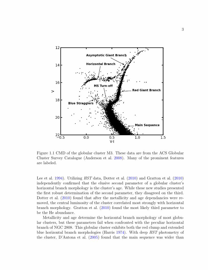
1.1 CMD of the globular cluster M3. These data are from the ACS Glob-ular Cluster Survey Catalogue (Anderson et al. 2008). Many of theprominent features are labeled. . . . . . . . . . . . . . . . . . . . . . 3

2.1 Initial locations of the BH+NS binaries in the (1 − e2)–a plane. Thepoints shown here are from simulations in cluster model D with MBH =7 M�. tGW0 is constant along the solid lines. From left to right, thelines correspond to tGW0 = 105, 106, 107, 108, 109, 1010 yrs. . . . . . . . 28

2.2 The actual amount of time it took a BH+NS binary to merge tGW vs.the amount of time expected for the BH+NS binary to merge, giventhe binary’s initial configuration, tGW0 for the BH+NS binaries thatmerge in a simulation of cluster model D with MBH = 7 M�. Notethat many systems formed with tGW0 � a Hubble time. Subsequentinteractions between these binaries and single stars greatly reducedtGW. We excluded systems where the initial binary was randomlychosen to contain a BH and NS in our merger rate estimates to avoidinitial condition bias and because these would happen at high redshiftand be unobservable. . . . . . . . . . . . . . . . . . . . . . . . . . . 29

2.3 Distribution of the merger times for BH+NS binaries in clusters D(left panel), C (center panel), and B (right panel) with MBH = 7 M�.These merger times include the time taken to form the BH+NS systemthrough binary–single star interactions. The solid histogram is basedon runs that extended only until the initial BH binary either merged orwas disrupted; it shows the distribution of tmrg when a merger occurred.The dotted histograms show the merger time distribution for runs thatallowed BHs that lost their binary companions to exchange into a newbinary. In these runs we have used the FIR binary population withfb = 0.5. With this change, a larger number runs produced a merg-ing BH+NS binary, and the distribution shifts towards longer mergertimes. The larger merger times are due to the significant amount oftime it takes for the single BH to exchange back into a binary. In allof the runs shown here, the BH is ejected from the cluster after themerger. . . . . . . . . . . . . . . . . . . . . . . . . . . . . . . . . . . 31

vi

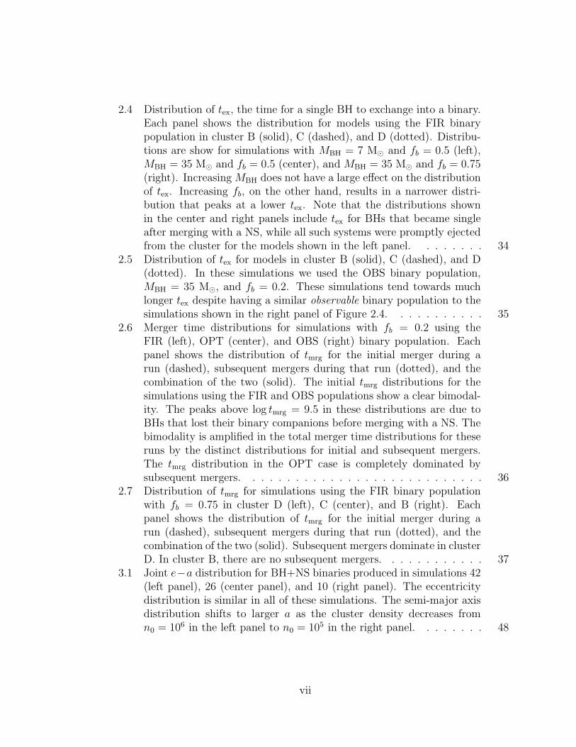
2.4 Distribution of tex, the time for a single BH to exchange into a binary.Each panel shows the distribution for models using the FIR binarypopulation in cluster B (solid), C (dashed), and D (dotted). Distribu-tions are show for simulations with MBH = 7 M� and fb = 0.5 (left),MBH = 35 M� and fb = 0.5 (center), and MBH = 35 M� and fb = 0.75(right). Increasing MBH does not have a large effect on the distributionof tex. Increasing fb, on the other hand, results in a narrower distri-bution that peaks at a lower tex. Note that the distributions shownin the center and right panels include tex for BHs that became singleafter merging with a NS, while all such systems were promptly ejectedfrom the cluster for the models shown in the left panel. . . . . . . . 34

2.5 Distribution of tex for models in cluster B (solid), C (dashed), and D(dotted). In these simulations we used the OBS binary population,MBH = 35 M�, and fb = 0.2. These simulations tend towards muchlonger tex despite having a similar observable binary population to thesimulations shown in the right panel of Figure 2.4. . . . . . . . . . . 35

2.6 Merger time distributions for simulations with fb = 0.2 using theFIR (left), OPT (center), and OBS (right) binary population. Eachpanel shows the distribution of tmrg for the initial merger during arun (dashed), subsequent mergers during that run (dotted), and thecombination of the two (solid). The initial tmrg distributions for thesimulations using the FIR and OBS populations show a clear bimodal-ity. The peaks above log tmrg = 9.5 in these distributions are due toBHs that lost their binary companions before merging with a NS. Thebimodality is amplified in the total merger time distributions for theseruns by the distinct distributions for initial and subsequent mergers.The tmrg distribution in the OPT case is completely dominated bysubsequent mergers. . . . . . . . . . . . . . . . . . . . . . . . . . . . 36

2.7 Distribution of tmrg for simulations using the FIR binary populationwith fb = 0.75 in cluster D (left), C (center), and B (right). Eachpanel shows the distribution of tmrg for the initial merger during arun (dashed), subsequent mergers during that run (dotted), and thecombination of the two (solid). Subsequent mergers dominate in clusterD. In cluster B, there are no subsequent mergers. . . . . . . . . . . . 37

3.1 Joint e−a distribution for BH+NS binaries produced in simulations 42(left panel), 26 (center panel), and 10 (right panel). The eccentricitydistribution is similar in all of these simulations. The semi-major axisdistribution shifts to larger a as the cluster density decreases fromn0 = 106 in the left panel to n0 = 105 in the right panel. . . . . . . . 48

vii

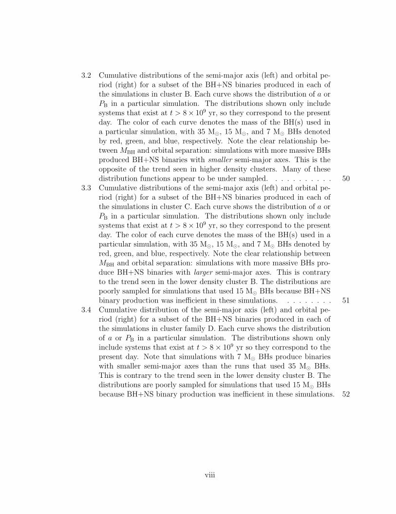
3.2 Cumulative distributions of the semi-major axis (left) and orbital pe-riod (right) for a subset of the BH+NS binaries produced in each ofthe simulations in cluster B. Each curve shows the distribution of a orPB in a particular simulation. The distributions shown only includesystems that exist at t > 8× 109 yr, so they correspond to the presentday. The color of each curve denotes the mass of the BH(s) used ina particular simulation, with 35 M�, 15 M�, and 7 M� BHs denotedby red, green, and blue, respectively. Note the clear relationship be-tween MBH and orbital separation: simulations with more massive BHsproduced BH+NS binaries with smaller semi-major axes. This is theopposite of the trend seen in higher density clusters. Many of thesedistribution functions appear to be under sampled. . . . . . . . . . . 50

3.3 Cumulative distributions of the semi-major axis (left) and orbital pe-riod (right) for a subset of the BH+NS binaries produced in each ofthe simulations in cluster C. Each curve shows the distribution of a orPB in a particular simulation. The distributions shown only includesystems that exist at t > 8× 109 yr, so they correspond to the presentday. The color of each curve denotes the mass of the BH(s) used in aparticular simulation, with 35 M�, 15 M�, and 7 M� BHs denoted byred, green, and blue, respectively. Note the clear relationship betweenMBH and orbital separation: simulations with more massive BHs pro-duce BH+NS binaries with larger semi-major axes. This is contraryto the trend seen in the lower density cluster B. The distributions arepoorly sampled for simulations that used 15 M� BHs because BH+NSbinary production was inefficient in these simulations. . . . . . . . . 51

3.4 Cumulative distribution of the semi-major axis (left) and orbital pe-riod (right) for a subset of the BH+NS binaries produced in each ofthe simulations in cluster family D. Each curve shows the distributionof a or PB in a particular simulation. The distributions shown onlyinclude systems that exist at t > 8× 109 yr so they correspond to thepresent day. Note that simulations with 7 M� BHs produce binarieswith smaller semi-major axes than the runs that used 35 M� BHs.This is contrary to the trend seen in the lower density cluster B. Thedistributions are poorly sampled for simulations that used 15 M� BHsbecause BH+NS binary production was inefficient in these simulations. 52

viii

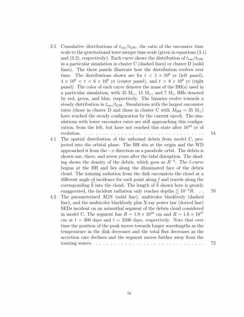
3.5 Cumulative distributions of tenc/tGW, the ratio of the encounter timescale to the gravitational wave merger time scale (given in equations (3.1)and (3.2), respectively). Each curve shows the distribution of tenc/tGW

in a particular simulation in cluster C (dashed lines) or cluster D (solidlines). The three panels illustrate how the distribution evolves overtime. The distributions shown are for t < 1 × 109 yr (left panel),4 × 109 < t < 6 × 109 yr (center panel), and t > 8 × 109 yr (rightpanel). The color of each curve denotes the mass of the BH(s) used ina particular simulation, with 35 M�, 15 M�, and 7 M� BHs denotedby red, green, and blue, respectively. The binaries evolve towards asteady distribution in tenc/tGW. Simulations with the largest encounterrates (those in cluster D and those in cluster C with MBH = 35 M�)have reached the steady configuration by the current epoch. The sim-ulations with lower encounter rates are still approaching this configu-ration, from the left, but have not reached this state after 1010 yr ofevolution. . . . . . . . . . . . . . . . . . . . . . . . . . . . . . . . . . 54

4.1 The spatial distribution of the unbound debris from model C, pro-jected into the orbital plane. The BH sits at the origin and the WDapproached it from the −x direction on a parabolic orbit. The debris isshown one, three, and seven years after the tidal disruption. The shad-ing shows the density of the debris, which goes as R−3. The `-curvebegins at the BH and lies along the illuminated face of the debriscloud. The ionizing radiation from the disk encounters the cloud at adifferent angle of incidence for each point along ` and travels along thecorresponding ~h into the cloud. The length of ~h shown here is greatlyexaggerated, the incident radiation only reaches depths . 10−3R. . . 70

4.2 The parameterized AGN (solid line), multicolor blackbody (dashedline), and the multicolor blackbody plus X-ray power law (dotted line)SEDs incident on an azimuthal segment of the debris cloud consideredin model C. The segment has R = 1.9 × 1016 cm and R = 1.6 × 1017

cm at t = 300 days and t = 2500 days, respectively. Note that overtime the position of the peak moves towards longer wavelengths as thetemperature in the disk decreases and the total flux decreases as theaccretion rate declines and the segment moves further away from theionizing source. . . . . . . . . . . . . . . . . . . . . . . . . . . . . . . 72

ix

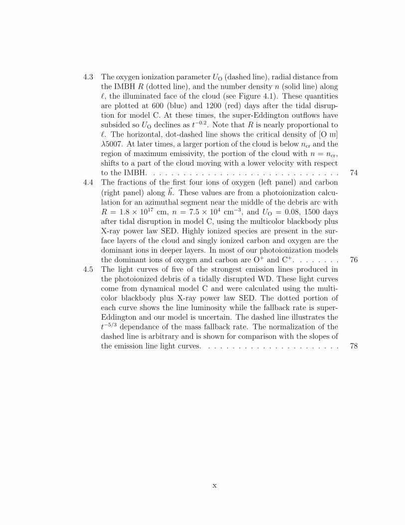
4.3 The oxygen ionization parameter UO (dashed line), radial distance fromthe IMBH R (dotted line), and the number density n (solid line) along`, the illuminated face of the cloud (see Figure 4.1). These quantitiesare plotted at 600 (blue) and 1200 (red) days after the tidal disrup-tion for model C. At these times, the super-Eddington outflows havesubsided so UO declines as t−0.2. Note that R is nearly proportional to`. The horizontal, dot-dashed line shows the critical density of [O III]λ5007. At later times, a larger portion of the cloud is below ncr and theregion of maximum emissivity, the portion of the cloud with n = ncr,shifts to a part of the cloud moving with a lower velocity with respectto the IMBH. . . . . . . . . . . . . . . . . . . . . . . . . . . . . . . . 74

4.4 The fractions of the first four ions of oxygen (left panel) and carbon

(right panel) along ~h. These values are from a photoionization calcu-lation for an azimuthal segment near the middle of the debris arc withR = 1.8 × 1017 cm, n = 7.5 × 104 cm−3, and UO = 0.08, 1500 daysafter tidal disruption in model C, using the multicolor blackbody plusX-ray power law SED. Highly ionized species are present in the sur-face layers of the cloud and singly ionized carbon and oxygen are thedominant ions in deeper layers. In most of our photoionization modelsthe dominant ions of oxygen and carbon are O+ and C+. . . . . . . . 76

4.5 The light curves of five of the strongest emission lines produced inthe photoionized debris of a tidally disrupted WD. These light curvescome from dynamical model C and were calculated using the multi-color blackbody plus X-ray power law SED. The dotted portion ofeach curve shows the line luminosity while the fallback rate is super-Eddington and our model is uncertain. The dashed line illustrates thet−5/3 dependance of the mass fallback rate. The normalization of thedashed line is arbitrary and is shown for comparison with the slopes ofthe emission line light curves. . . . . . . . . . . . . . . . . . . . . . . 78

x

4.6 The [O III] λ5007 (left panel) and C IIIλ1549 (right panel) light curvesfor each model given in Table 4.1. The photoionization calculationsthat produced these light curves used the multicolor blackbody plusX-ray power law SED; calculations that exclude the X-ray componentproduce nearly identical results. The dotted portion of each curveshows the line luminosity while the fallback rate is super-Eddingtonand our model is uncertain. The curves in the left panel differ fromthose in the right because [O III] λ5007 is a forbidden emission line andthe density in the debris cloud must drop to the critical density for thistransition for this emission line to form. Curves B and D in the leftpanel are different from the others because they correspond to modelswith β = 3. Similarly, the curves in the right panel corresponding tomodels with β = 3 differ from all the others by their steep decline atearly times. The dashed line illustrates the t−5/3 dependance of themass fallback rate. The normalization of the dashed line is arbitraryand is shown for comparison with the slopes of the emission line lightcurves. . . . . . . . . . . . . . . . . . . . . . . . . . . . . . . . . . . 81

4.7 The time evolution of the [O III] λ5007 emission-line profile as seen byan observer at i0 = 45◦ and θ0 = −5◦. Time increases from bottom totop and the time for each profile is written on the plot. The dottedlines show the Fλ = 0 level for each profile. The horizontal axis showsz = (λ−5007A)/5007A. Each profile has been normalized so that it hasa maximum height of 1 and the profiles are offset by one unit for clarity.Note that in addition to becoming broader with time, the peak of theline profile shifts to lower velocity. Once most of the cloud is below ncr,the emissivity per unit volume decreases throughout the cloud and thepeak shifts back towards higher velocities that correspond to regionsin the tail with larger volume and a larger fraction of O++. . . . . . 84

4.8 The time evolution of the [O III] λ5007 emission-line profile as seen byan observer at i0 = 45◦ and θ0 = 30◦. Time increases from bottom totop and the time for each profile is written on the plot. The dottedlines show the Fλ = 0 level for each profile. The horizontal axis showsz = (λ−5007A)/5007A. Each profile has been normalized so that it hasa maximum height of 1 and the profiles are offset by one unit for clarity.Note that in addition to becoming broader with time, the peak of theline profile shifts to lower velocity. Once most of the cloud is below ncr,the emissivity per unit volume decreases throughout the cloud and thepeak shifts back towards higher velocities that correspond to regionsin the tail with larger volume and a larger fraction of O++. . . . . . 85

xi

4.9 Mass fractions (top) of carbon (solid), nitrogen (dotted), and oxy-gen (dashed) vs. time and radius (bottom) vs. time from the MESA

star model of a 1 M� star with Z = Z�/2. . . . . . . . . . . . . . . 874.10 Light curves produced in the photoionized debris of a tidally disrupted

HB star. In this model we used a red clump star with M? = 0.67 M�and R? = 6.2 R� and an IMBH with MBH = 1000M�. The dottedportions of the curves denote the super-Eddington fallback phase. Notethe qualitative similarities to the WD case shown in Figure 4.5. . . . 88

4.11 The [O III] λλ4959, 5007 line profile for model C, 1750 days after tidaldisruption, as seen by an observer at i0 = 89◦ and θ0 = −12◦. Theprofile has been smoothed to a spectral resolution of 400 for comparisonwith observations of Zepf et al. (2008). The profile is normalized tohave a height of 1 and does not include contributions from the continuum. 93

4.12 Emission-line luminosity ratios over time from several tidal disruptionmodels with varying MBH. The long-dashed line in the top panel showsthe constraint on the [N III]/[O III] ratio measured by Irwin et al. (2010).Models that fall near this line are consistent with observations. In thelower two panels, the shaded region indicates line ratios ruled out bythe observations of Irwin et al. (2010), only models that reach intothe unshaded region are consistent with observations. For each modelshown here, we considered a red clump star on an orbit with Rp = RT. 95

4.13 Emission-line luminosity ratios over time from several tidal disruptionmodels with varying MBH, tidal disruption parameter β, and stellartype. The long-dashed line in the top panel shows the constraint onthe [N III]/[O III] ratio measured by Irwin et al. (2010). Models that fallnear this line are consistent with observations. In the lower two panels,the shaded region indicates line ratios ruled out by the observations ofIrwin et al. (2010), only models that reach into the unshaded regionare consistent with observations. . . . . . . . . . . . . . . . . . . . . . 96

4.14 FWHM of the [N II] λ6583 emission line 125 years after tidal disruption,synthesized from a model using the red clump star, β = 1, and MBH =100 M�. The angles θ0 and i0 describe the orientation of the observer(see Figure 4.1). The black curve marks the observed FWHM. Any pairof θ0 and i0 along the black line produces a FWHM that is consistentwith observations. . . . . . . . . . . . . . . . . . . . . . . . . . . . . . 98

xii

4.15 Evolution of [N III]/[O III] for HB stars of different composition. Weshow two sets of models – young HB stars 30 Myr after He ignitionwhen the nitrogen and oxygen abundance are equal (MBH = 50M�dashed; MBH = 100M� dotted) and the same models but with theHB star older so that 80 Myr of He burning has made oxygen twiceas abundant as nitrogen (MBH = 50M� dot-dashed; MBH = 100M�solid). For a 100 M� BH, the observed [N III]/[O III] ratio cannot bereproduced once helium burning has created an oxygen abundance thatis twice the nitrogen abundance. . . . . . . . . . . . . . . . . . . . . 100

4.16 UV Light curves from a model using the fiducial red clump HB star,β = 1, and MBH = 100 M�. Emission line light curves are shownfor N IIIλ1240, C IIIλ1548, O IIIλ1035, N IIIλ1486, C III] λ1909, andLyman-α. The dashed curve shows LX scaled down by a factor of2000. These UV lines can be used to test the HB star tidal disruptionhypothesis and to better constrain the mass of the IMBH. The dottedportion of each curve shows the line luminosity while the fallback rateis super-Eddington and our model is uncertain. . . . . . . . . . . . . 102

5.1 Core radius vs the photometric binary fraction for a sample of MilkyWay globular clusters. Clusters with higher binary fractions tend tohave larger core radii. The data are from Milone et al. (2012b). . . . 107

xiii

List of Tables

2.1 Background Globular Cluster Model Parameters . . . . . . . . . . . . 192.2 Globular Cluster Models and Merger Rates . . . . . . . . . . . . . . . 252.3 Probability Scaling Tests . . . . . . . . . . . . . . . . . . . . . . . . . 393.1 Background Globular Cluster Model Parameter Ranges . . . . . . . . 473.2 Globular Cluster Models and BH+MSP Binary Properties . . . . . . 574.1 Model Parameters . . . . . . . . . . . . . . . . . . . . . . . . . . . . 674.2 Predicted Line Luminosities . . . . . . . . . . . . . . . . . . . . . . . 79

xiv

Chapter 1

Introduction

Many significant processes in the dynamical evolution of a self gravitating system,including mass segregation, relaxation, and core collapse, occur in globular clusterswithin a Hubble time. As such, globular clusters offer an ideal testbed for our un-derstanding of many-body gravitational dynamics. The dynamical evolution of thecluster as a whole is closely linked to the evolution of individual stars within thecluster. Much as the addition of a binary companion opens up evolutionary channelsthat are inaccessible to single stars, dynamical interactions between stars and bina-ries within the cluster enable evolutionary paths that cannot occur in the field. Thisinterplay encodes the dynamical processes at play within the cluster on the stellarand binary populations. In the introduction we will outline important developmentsin the field of globular cluster dynamics and the role that these developments playedin understanding observations of both the structure and the exotic stellar populationsof globular clusters.

1.1 General Overview

Globular clusters are collections of 104−107 stars found in the bulge and halo regionsof the Galaxy. The clusters are nearly spherical with 75% having a projected ellipticityof less than 0.1. The stellar density in the clusters is much higher than in the solarneighborhood. A typical central value is n = 104 pc−3, but the density can be ashigh as 106 pc−3. Compared to the Sun, globular clusters are metal poor. Themetallicity distribution amongst the Milky Way globular clusters is bimodal withpeaks at [Fe/H] = −1.6 and −0.6 (Harris 1996, 2010 version1). Within a singlecluster, however, [Fe/H] does not vary much from star to star. The red giant branch(RGB) and lower main sequence are clearly visible in the color magnitude diagrams(CMDs) of globular clusters, but the blue end of the main sequence is absent. Starswith mass ∼ 0.8 M� can be seen “turning off” the main sequence and those moremassive than this have already evolved up the RGB and beyond. Figure 1.1 shows

1http://physwww.mcmaster.ca/∼harris/mwgc.dat

1

2

a CMD for the globular cluster M3. These features of the CMD, along with themetallicity measurements, are the basis of the long held notion that globular clusterscontain a single, coeval, chemically homogenous stellar population. The age of aglobular cluster can, therefore, be determined by fitting its CMD with isochronesgenerated from stellar evolution models. As stellar evolution models became moresophisticated, and the input physics required for such models was better understood,the estimated age of the Milky Way globular cluster system evolved from more than20 Gyr to the currently accepted value2 of 13 Gyr (Meylan & Heggie 1997; Carrettaet al. 2000).

Recent technological advances have allowed for comprehensive, homogenous, highprecision photometric studies of globular clusters that have solved long standing prob-lems and challenged enduring ideas. Principal among these studies are observations ofglobular clusters carried out with the Hubble Space Telescope (HST). HST has beenespecially useful in studying globular clusters outside of the Milky Way. Previousground based studies had shown that early type galaxies possess much richer glob-ular cluster populations than the Milky Way (Harris 1991; Brodie & Strader 2006),but HST made measurements of individual globular clusters within these populationspossible. Surveys of the globular clusters associated with M31 and galaxies in theFornax and Virgo clusters have shown that the distributions of structural parame-ters, luminosity, and metallicity in these clusters are similar to these distributions inthe Milky Way globular cluster system (Jordan et al. 2005; Peng et al. 2006; Jordanet al. 2007; Madrid et al. 2009; Masters et al. 2010; Strader et al. 2011). These re-sults suggest that lessons learned from dynamical models of the well studied MilkyWay globular cluster system can be applied to globular clusters associated with othergalaxies.

One component of a globular cluster’s stellar population that has been studiedextensively are the horizontal branch stars. A globular cluster’s horizontal branchmorphology is strongly influenced by its metallicity, with the horizontal branchesin relatively metal rich globular clusters lying redward of the instability strip andthose of most low metallicity clusters lying to the blue side. However, it has beenknown for some time that metallicity alone cannot account for the range of horizontalbranch morphologies observed, and that horizontal branch morphology is determinedby metallicity and at least a second parameter (e.g., Sandage & Wallerstein 1960;van den Bergh 1967). By the mid 1990s, a number of studies had established clusterage as a likely solution to the second parameter problem (e.g. Searle & Zinn 1978;

2Meissner & Weiss (2006) argued that isochrone fitting methods still need improvement becausethey cannot fit all age indicators (e.g., the difference in the brightness of the main sequence turn offand the bump on the red giant branch) simultaneously. One possibility for more robust age deter-mination is to combine CMD isochrone fitting with constraints from precisely determined masses,radii, and luminosities of stars in detached, eclipsing binaries within the cluster (e.g. Thompsonet al. 2001).

3

Figure 1.1 CMD of the globular cluster M3. These data are from the ACS GlobularCluster Survey Catalogue (Anderson et al. 2008). Many of the prominent featuresare labeled.

Lee et al. 1994). Utilizing HST data, Dotter et al. (2010) and Gratton et al. (2010)independently confirmed that the elusive second parameter of a globular cluster’shorizontal branch morphology is the cluster’s age. While these new studies presentedthe first robust determination of the second parameter, they disagreed on the third.Dotter et al. (2010) found that after the metallicity and age dependancies were re-moved, the central luminosity of the cluster correlated most strongly with horizontalbranch morphology. Gratton et al. (2010) found the most likely third parameter tobe the He abundance.

Metallicity and age determine the horizontal branch morphology of most globu-lar clusters, but these parameters fail when confronted with the peculiar horizontalbranch of NGC 2808. This globular cluster exhibits both the red clump and extendedblue horizontal branch morphologies (Harris 1974). With deep HST photometry ofthe cluster, D’Antona et al. (2005) found that the main sequence was wider than

4

expected for a single population, and argued that the cluster had undergone self-enrichment. In this process, at least a second generation of stars was born out ofthe He enriched material shed by the first generation of stars as they evolved up theasymptotic giant branch (AGB). The presence of multiple generations of stars withdifferent initial He abundances can account for the dual nature of the cluster’s hori-zontal branch, but this finding is contrary to the traditional assumption that globularclusters contain a single stellar population. Evidence of abundance anomalies in glob-ular cluster stars had been mounting since the 1970s (Gratton et al. 2004), but theCMD of NGC 2808 was the first unambiguous sign that multiple stellar populationswere present within some globular clusters3 (Piotto et al. 2007). Subsequently, severalother clusters were shown to have multiple stellar populations, including NGC 1851(Milone et al. 2008), NGC 6656 (Marino et al. 2009), 47 Tuc (Anderson et al. 2009),NGC 6752 (Milone et al. 2010), NGC 2419 (di Criscienzo et al. 2011), and NGC6397 (Milone et al. 2012a). With mounting evidence that globular clusters containmultiple stellar generations, Downing & Sills (2007) examined whether such systemswere plausible dynamically. They found that a two generation globular cluster wasnot only plausible, but similar to a single generation model both dynamically andstructurally.

1.2 Structure and Dynamical Evolution

Below we will sketch some of the basic processes and equations that govern the dynam-ical evolution of a globular cluster following Spitzer (1987) and Binney & Tremaine(1987). Three characteristic radii are used to describe globular clusters. The core ra-dius rc is the distance at which the surface brightness drops to half its central value.The half-mass radius rh is the radius of a circle containing half of the cluster’s mass.At the tidal radius rt, the gravitational field of the galaxy becomes more importantthan that of the cluster. The stellar density goes to zero at the tidal radius.

Much of the early work on globular clusters assumed that the clusters were static(Meylan & Heggie 1997). A globular cluster will undergo significant dynamical evo-lution during its lifetime, but static models are a valid representation of a cluster fortimes of order the half mass relaxation time, trh. The value of trh varies significantlyfrom cluster to cluster in the Milky Way system, but is ∼ 1 Gyr for many clusters.If, in addition to the cluster being static, one further assumes that the positions andvelocities of stars in the cluster are well described by a smooth phase space distri-bution, f(r,v), where r and v are position and velocity vectors, and that the starsmove under the influence of a smooth gravitational potential φ, then such a system

3Lee et al. (1999) had previously shown that ω Centauri had multiple RGBs, but ω Centauri islikely the remnant core of a stripped dwarf galaxy and not a typical globular cluster (e.g., Bekki &Freeman 2003; Lee et al. 2009). It has also been suggested that NGC 2808 may be the remnant coreof a dwarf galaxy (e.g., Forbes et al. 2004).

5

can be described by the collisionless Boltzmann equation:

∂f

∂t−∇φ · ∂f

∂v+ v · ∇f = 0. (1.1)

The potential must satisfy Poisson’s equation:

∇2φ(r) = 4πGρ (1.2)

where G is the gravitational constant and ρ is the mass density.Michie (1963) and King (1966) developed solutions to equation (1.1) that re-

produce many features observed in globular clusters. These models use a loweredMaxwellian distribution function that limits the cluster to the tidal radius and anangular momentum distribution that permits velocity anisotropy in the cluster halo.Assuming that all stars in the cluster have the same mass, the distribution is givenby:

f(ε, L) =ρ0

(2πv2m)3/2

exp

(−L2

2r2av

2m

)(eε/v

2m − 1

). (1.3)

Here, ε is the relative energy per unit mass, vm is the velocity dispersion of the stars,ρ is the central mass density, L is the angular momentum per unit mass, and ra is theradius at which the velocity distribution goes from isotropic to radial. The relativeenergy and angular momentum are related to r and v through:

ε = Ψ(r)− 1

2v2 (1.4)

L = rv sin θ, (1.5)

where θ is the angle between r and v and Ψ is the relative potential, Ψ(r) = φ(rt)−φ(r). This distribution can be extended to include multiple mass groups with separatevalues for vm and ρ0 for each group. We will make extensive use of such models inlater chapters.

In a globular cluster, the gravitational potential is not completely smooth andencounters between pairs of stars will drive the cluster’s evolution. A number oftechniques are used to study how the cluster evolves as a result of these encounters.Perhaps the most intuitive approach is the N-body method, in which the gravitationalinteractions between all stars are are calculated directly (e.g., Aarseth 1999; PortegiesZwart et al. 2001). N-body simulations require few restrictive assumptions but areextremely expensive computationally. Fokker-Planck methods, on the other hand,require some simplifying assumptions but greatly reduce the computational burden.In such a model, the zero on the right hand side of equation (1.1) is replaced by aterm that describes how the distribution function changes with time as a result ofsuch encounters, (∂f/∂t)enc = Γ(f). Under the local approximation, in which it is

6

assumed that encounters only produce small velocity perturbations and do not affectthe position of a star, one can derive an analytic approximation for the change in fbrought about by encounters:

Γ(f) = −3∑i

∂

∂vi[fD(∆vi)] +

1

2

3∑i,j=1

∂2

∂vi∂vj[fD(∆vi∆vj)]. (1.6)

Here, D(∆vi) and D(∆vi∆vj) are diffusion coefficients, which describe how starsdiffuse through phase space as a result of encounters. The first term in equation (1.6)describes the drift in velocity space known as dynamical friction. The second termaccounts for diffusion in velocity space due to random kicks from stellar encounters.Substituting the Γ(f) given in equation (1.6) for the zero on the right hand side ofequation (1.1) produces the so called Fokker-Planck equation. In models of globularcluster evolution, the Fokker-Planck equation can be numerically integrated directly(e.g., Cohn 1979; Chernoff & Weinberg 1990) or, more commonly, integrated withMonte Carlo methods (e.g. Spitzer & Hart 1971; Giersz 1998; Joshi et al. 2000; Freitag& Benz 2001). Explorations of globular cluster evolution using either the N-body orthe Fokker-Planck method indicate that a number of interesting phenomena occur ina cluster’s lifetime.

First, since globular clusters contain stars of different masses, over time interac-tions between the stars drive the system towards energy equipartition. The more mas-sive stars tend to slow down and sink into the cluster core and lower mass stars gainkinetic energy and move to wider orbits. As a result, the cluster becomes mass seg-regated. Mass stratification has been observed in Milky Way globular clusters (Kinget al. 1995). N-body (Khalisi et al. 2007) and Fokker Planck (Watters et al. 2000)calculations of multi-mass clusters confirm that the velocity dispersion of a group ofstars with mass m will settle to an equilibrium value that is inversely proportional tom. Spitzer (1969) showed that it is not always possible for a two component clusterto reach equilibrium. If the total mass of the more massive component exceeds acritical value, these stars will quickly sink to the center of the cluster and producea subcluster that undergoes a runaway collapse. This equipartition instability alsooccurs in N-body and Fokker-Planck models, though each find a slightly differentcriterion for instability (Watters et al. 2000; Khalisi et al. 2007).

Next, stellar dynamical systems are subject to the gravothermal catastrophe(Lynden-Bell & Wood 1968). This instability arises because self gravitating systemshave a negative heat capacity. As the systems lose energy they become dynamicallyhotter, which increases the flow of energy and drives the system away from equilib-rium. N-body and Fokker-Plank models have explored a primary consequence of thegravothermal catastrophe: core collapse. Models show that the central density of thecluster approaches infinity after ∼ 15 trh, although the value depends on the initialconditions and physics included (eg. Cohn 1979; Chernoff & Weinberg 1990; Joshi

7

et al. 2000; Watters et al. 2000; Khalisi et al. 2007). For example, core collapse isaccelerated in multi-mass models that are also subject to the equipartition instability.It was soon realized that at such high densities, binaries could form through three-body interactions and act as a heat source to halt and reverse core collapse (Inagaki& Lynden-Bell 1983; Cohn & Hut 1984; Goodman 1984). If clusters were formedwith a population of primordial binaries, then core collapse could be postponed (Hills1975a).

1.3 Binaries in Globular Clusters

By the mid 1980s considerable evidence for the presence of binaries in globular clustershad accumulated, both observationally and on theoretical grounds (Hut et al. 1992b;Meylan & Heggie 1997). From a dynamical perspective, binaries are an importantsource of energy in the cluster. A study of the outcomes of three-body interactionsbetween a binary and a single star by Heggie (1975) found that hard binaries becomemore tightly bound and transfer kinetic energy to the third body during an encounter.A binary is considered hard if its binding energy exceeds the kinetic energy of thesurrounding stars. The degree of a binary’s hardness to an encounter is typicallyparameterized as the ratio of the single star’s relative velocity to a critical velocityvc. A field star of mass m3 interacting with a binary consisting of stars with massesm1 and m2 with semi-major axis a, must have a relative velocity

v2c =

Gm1m2(m1 +m2 +m3)

m3(m1 +m2)a(1.7)

at infinity to disrupt the binary. Heggie (1975) found that a hard binary’s bindingenergy increased by an average of 40% after an encounter. The process of increasingthe binary’s binding energy through encounters is often referred to as “hardening.”The liberated energy causes the binary and single star to recoil with increased kineticenergy, thereby heating the cluster. Alternatively, soft binaries tend to be disruptedas the result of a three body interaction.

Binary-single star interactions can be split into two categories, prompt and reso-nant. Prompt encounters occur in less than one binary orbital period. In a resonantencounter, a temporary three-body system that can survive for several orbital periodsis formed. Furthermore, the outcome of these encounters can be described as a flyby,exchange, or disruption. In a flyby the membership of the binary does not changeduring the encounter. In an exchange, the single star ejects one member of the binaryand becomes bound to the other. In a disruption all three stars are unbound at theend of the encounter. There is also the possibility of two of the stars involved in theencounter merging. Millions of binary-single interactions were simulated to determinethe cross section for each of the above outcomes and the resulting energy exchange

8

(e.g., Hut & Bahcall 1983; Sigurdsson & Phinney 1993). These cross sections can beused in Monte Carlo codes to study the effect of a population of primordial binarieson the evolution of a cluster.

Both N-body and Monte Carlo calculations for the evolution of a globular clus-ter with a primordial binary fraction of 5 − 20% show a prolonged state of “binaryburning.” During this phase, binding energy is extracted from the primordial binariesthrough dynamical encounters between these binaries and single stars or other bina-ries. The energy generated in these interactions can halt and reverse core collapse,allowing the cluster to remain in a quasi-equilibrium state for many trh (McMillanet al. 1990; Gao et al. 1991; Hut et al. 1992a; Fregeau et al. 2003). However, duringthe binary burning phase, the binary population is depleted. The binaries are ejected,driven to merger, or disrupted in encounters with other binaries. In a detailed studythat included the effects of binary stellar evolution, cluster dynamics, and explicit in-tegration of three and four body encounters involving binaries, Ivanova et al. (2005a)found that the binary population in a dense cluster’s core was depleted so rapidlythat an initial binary fraction of 100% was required to yield the value of ∼ 5% ob-served in some clusters. These authors also pointed out the importance of includingboth stellar evolution and dynamics in globular cluster simulations. For example, abinary can merge as the result of dynamically unstable mass transfer and commonenvelope evolution, but a purely dynamical model would not account for this process.At the same time, through exchange and hardening, dynamical interactions drive bi-naries towards common envelope evolution. Hence, while it is clear that primordialbinaries play an influential role in the dynamical evolution of a globular cluster, dy-namical interactions also have a profound effect on the population of binaries withinthe cluster.

1.4 Neutron Stars in Globular Clusters

When X-ray sources were observed in globular clusters, it was proposed that thesesources could be accreting neutron stars (NS) or black holes (BH; Clark et al. 1975).Katz (1975) noted that the number of the X-ray sources found in globular clusterswas intriguingly large considering that the clusters make up less than 0.1% of theGalaxy’s mass. The increased X-ray-luminosity-to-mass ratio is evidence that theformation of such sources in globular clusters takes place through dynamical channelsthat are unavailable to systems in the field. Hills (1976) proposed that the enhancedproduction of X-ray sources in globular clusters was the result of BHs or NSs ex-changing into primordial binaries. The first hint that the accretors in these systemswere NSs and not BHs came when Grindlay et al. (1984) observed the positions of theX-ray sources within the clusters. Assuming a mass segregated cluster, the measuredcluster radii of the X-ray sources suggested that they had masses of ∼ 1.5 M�. Todaythere are 15 known bright low mass X-ray binaries (LMXBs) in Milky Way globular

9

clusters (Benacquista 2006). Surprisingly, six of these systems have orbital periodsof less than one hour and are classified as ultra-compact X-ray binaries (e.g Deutschet al. 2000). All 15 undergo X-ray bursts, which confirms that these LMXBs haveNS accretors (in’t Zand et al. 2003) because X-ray bursts are thermonuclear flasheson the NS’s surface, and such flashes cannot occur on a BH.

Gravitational radiation will drive NS+NS binaries formed through exchange in-teractions in globular clusters to coalescence. Such mergers are thought to be theorigin of short gamma ray bursts (GRBs). Models by Grindlay et al. (2006) andIvanova et al. (2008) predict that 10− 30% of short GRBs are due to NS+NS bina-ries formed by dynamical interactions in globular clusters. Another consequence ofthe high stellar density in the cores of globular clusters are physical stellar collisions.Ivanova et al. (2005b) showed that the rate of collisions between NS and RGB starsin globular clusters was large enough to produce the observed excess of ultra-compactX-ray binary systems. During the collision, the RGB star’s envelope is stripped leav-ing an eccentric NS+white dwarf (WD) binary. The binary then decays by emissionof gravitational radiation, eventually becoming an ultra-compact X-ray binary.

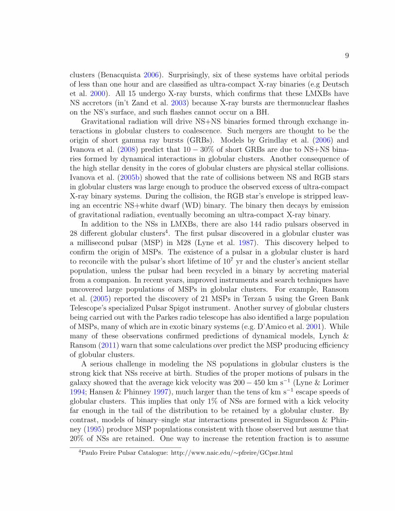
In addition to the NSs in LMXBs, there are also 144 radio pulsars observed in28 different globular clusters4. The first pulsar discovered in a globular cluster wasa millisecond pulsar (MSP) in M28 (Lyne et al. 1987). This discovery helped toconfirm the origin of MSPs. The existence of a pulsar in a globular cluster is hardto reconcile with the pulsar’s short lifetime of 107 yr and the cluster’s ancient stellarpopulation, unless the pulsar had been recycled in a binary by accreting materialfrom a companion. In recent years, improved instruments and search techniques haveuncovered large populations of MSPs in globular clusters. For example, Ransomet al. (2005) reported the discovery of 21 MSPs in Terzan 5 using the Green BankTelescope’s specialized Pulsar Spigot instrument. Another survey of globular clustersbeing carried out with the Parkes radio telescope has also identified a large populationof MSPs, many of which are in exotic binary systems (e.g. D’Amico et al. 2001). Whilemany of these observations confirmed predictions of dynamical models, Lynch &Ransom (2011) warn that some calculations over predict the MSP producing efficiencyof globular clusters.

A serious challenge in modeling the NS populations in globular clusters is thestrong kick that NSs receive at birth. Studies of the proper motions of pulsars in thegalaxy showed that the average kick velocity was 200− 450 km s−1 (Lyne & Lorimer1994; Hansen & Phinney 1997), much larger than the tens of km s−1 escape speeds ofglobular clusters. This implies that only 1% of NSs are formed with a kick velocityfar enough in the tail of the distribution to be retained by a globular cluster. Bycontrast, models of binary–single star interactions presented in Sigurdsson & Phin-ney (1995) produce MSP populations consistent with those observed but assume that20% of NSs are retained. One way to increase the retention fraction is to assume

4Paulo Freire Pulsar Catalogue: http://www.naic.edu/∼pfreire/GCpsr.html

10

that some of the NSs were formed in binary systems. Pfahl et al. (2002) showed thatunder these conditions the retention fraction could be as large as 8%. Tuning cou-pled dynamical and binary evolution models to the observed globular cluster LMXBpopulation, Ivanova et al. (2008) derived a NS retention fraction of 5 − 7%, corre-sponding to 220 NS for every 2 × 105 M�. Most of the NS retained in these modelswere formed through electron capture supernovae, which resulted in kick velocitiesten times smaller than core collapse supernovae. A portion of the electron capturesupernovae occurred during the evolution of single stars, but many were the resultof massive WDs undergoing accretion induced collapse (AIC). AIC had previouslybeen proposed as a source of the globular cluster NSs (e.g., Bailyn & Grindlay 1990),and these new results indicate the channel’s importance. Even though the mecha-nism that keeps NSs in globular clusters remains uncertain, both observations anddynamical models indicate that globular clusters retain 100s of NSs.

1.5 Stellar and Intermediate Mass Black Holes in GlobularClusters

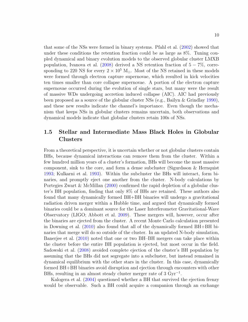
From a theoretical perspective, it is uncertain whether or not globular clusters containBHs, because dynamical interactions can remove them from the cluster. Within afew hundred million years of a cluster’s formation, BHs will become the most massivecomponent, sink to the core, and form a dense subcluster (Sigurdsson & Hernquist1993; Kulkarni et al. 1993). Within the subcluster the BHs will interact, form bi-naries, and promptly eject one another from the cluster. N-body calculations byPortegies Zwart & McMillan (2000) confirmed the rapid depletion of a globular clus-ter’s BH population, finding that only 8% of BHs are retained. These authors alsofound that many dynamically formed BH+BH binaries will undergo a gravitationalradiation driven merger within a Hubble time, and argued that dynamically formedbinaries could be a dominant source for the Laser Interferometer Gravitational-WaveObservatory (LIGO; Abbott et al. 2009). These mergers will, however, occur afterthe binaries are ejected from the cluster. A recent Monte Carlo calculation presentedin Downing et al. (2010) also found that all of the dynamically formed BH+BH bi-naries that merge will do so outside of the cluster. In an updated N-body simulation,Banerjee et al. (2010) noted that one or two BH–BH mergers can take place withinthe cluster before the entire BH population is ejected, but most occur in the field.Sadowski et al. (2008) avoided complete ejection of the cluster’s BH population byassuming that the BHs did not segregate into a subcluster, but instead remained indynamical equilibrium with the other stars in the cluster. In this case, dynamicallyformed BH+BH binaries avoid disruption and ejection through encounters with otherBHs, resulting in an almost steady cluster merger rate of 3 Gyr−1.

Kalogera et al. (2004) questioned whether a BH that survived the ejection frenzywould be observable. Such a BH could acquire a companion through an exchange

11

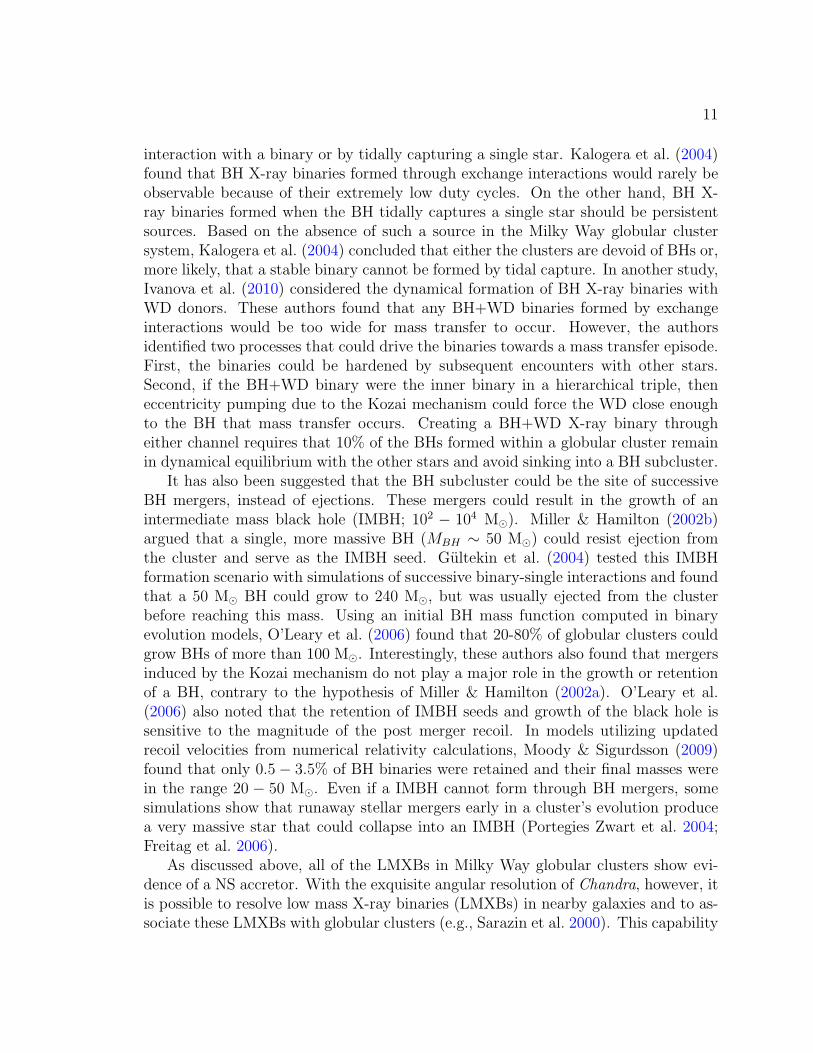
interaction with a binary or by tidally capturing a single star. Kalogera et al. (2004)found that BH X-ray binaries formed through exchange interactions would rarely beobservable because of their extremely low duty cycles. On the other hand, BH X-ray binaries formed when the BH tidally captures a single star should be persistentsources. Based on the absence of such a source in the Milky Way globular clustersystem, Kalogera et al. (2004) concluded that either the clusters are devoid of BHs or,more likely, that a stable binary cannot be formed by tidal capture. In another study,Ivanova et al. (2010) considered the dynamical formation of BH X-ray binaries withWD donors. These authors found that any BH+WD binaries formed by exchangeinteractions would be too wide for mass transfer to occur. However, the authorsidentified two processes that could drive the binaries towards a mass transfer episode.First, the binaries could be hardened by subsequent encounters with other stars.Second, if the BH+WD binary were the inner binary in a hierarchical triple, theneccentricity pumping due to the Kozai mechanism could force the WD close enoughto the BH that mass transfer occurs. Creating a BH+WD X-ray binary througheither channel requires that 10% of the BHs formed within a globular cluster remainin dynamical equilibrium with the other stars and avoid sinking into a BH subcluster.

It has also been suggested that the BH subcluster could be the site of successiveBH mergers, instead of ejections. These mergers could result in the growth of anintermediate mass black hole (IMBH; 102 − 104 M�). Miller & Hamilton (2002b)argued that a single, more massive BH (MBH ∼ 50 M�) could resist ejection fromthe cluster and serve as the IMBH seed. Gultekin et al. (2004) tested this IMBHformation scenario with simulations of successive binary-single interactions and foundthat a 50 M� BH could grow to 240 M�, but was usually ejected from the clusterbefore reaching this mass. Using an initial BH mass function computed in binaryevolution models, O’Leary et al. (2006) found that 20-80% of globular clusters couldgrow BHs of more than 100 M�. Interestingly, these authors also found that mergersinduced by the Kozai mechanism do not play a major role in the growth or retentionof a BH, contrary to the hypothesis of Miller & Hamilton (2002a). O’Leary et al.(2006) also noted that the retention of IMBH seeds and growth of the black hole issensitive to the magnitude of the post merger recoil. In models utilizing updatedrecoil velocities from numerical relativity calculations, Moody & Sigurdsson (2009)found that only 0.5− 3.5% of BH binaries were retained and their final masses werein the range 20 − 50 M�. Even if a IMBH cannot form through BH mergers, somesimulations show that runaway stellar mergers early in a cluster’s evolution producea very massive star that could collapse into an IMBH (Portegies Zwart et al. 2004;Freitag et al. 2006).

As discussed above, all of the LMXBs in Milky Way globular clusters show evi-dence of a NS accretor. With the exquisite angular resolution of Chandra, however, itis possible to resolve low mass X-ray binaries (LMXBs) in nearby galaxies and to as-sociate these LMXBs with globular clusters (e.g., Sarazin et al. 2000). This capability

12

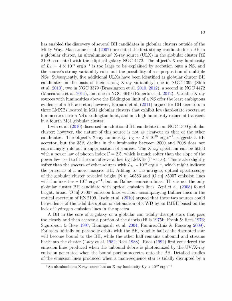
has enabled the discovery of several BH candidates in globular clusters outside of theMilky Way. Maccarone et al. (2007) presented the first strong candidate for a BH ina globular cluster, an ultraluminous5 X-ray source (ULX) in the globular cluster RZ2109 associated with the elliptical galaxy NGC 4472. The object’s X-ray luminosityof LX = 4 × 1039 erg s−1 is too large to be explained by accretion onto a NS, andthe source’s strong variability rules out the possibility of a superposition of multipleNSs. Subsequently, five additional ULXs have been identified as globular cluster BHcandidates on the basis of their strong X-ray variability; one in NGC 1399 (Shihet al. 2010), two in NGC 3379 (Brassington et al. 2010, 2012), a second in NGC 4472(Maccarone et al. 2011), and one in NGC 4649 (Roberts et al. 2012). Variable X-raysources with luminosities above the Eddington limit of a NS offer the least ambiguousevidence of a BH accretor; however, Barnard et al. (2011) argued for BH accretors inthree LMXBs located in M31 globular clusters that exhibit low/hard-state spectra atluminosities near a NS’s Eddington limit, and in a high luminosity recurrent transientin a fourth M31 globular cluster.

Irwin et al. (2010) discussed an additional BH candidate in an NGC 1399 globularcluster; however, the nature of this source is not as clear-cut as that of the othercandidates. The object’s X-ray luminosity, LX ∼ 2 × 1039 erg s−1, suggests a BHaccretor, but the 35% decline in the luminosity between 2000 and 2008 does notconvincingly rule out a superposition of sources. The X-ray spectrum can be fittedwith a power law of photon index Γ = 2.5, which is much softer than the slope of thepower law used to fit the sum of several low LX LMXBs (Γ ∼ 1.6). This is also slightlysofter than the spectra of other sources with LX ∼ 1039 erg s−1, which might indicatethe presence of a more massive BH. Adding to the intrigue, optical spectroscopyof the globular cluster revealed bright [N II] λ6583 and [O III] λ5007 emission lineswith luminosities ∼1036 erg s−1, but no Balmer emission lines. This is not the onlyglobular cluster BH candidate with optical emission lines, Zepf et al. (2008) foundbright, broad [O III] λ5007 emission lines without accompanying Balmer lines in theoptical spectrum of RZ 2109. Irwin et al. (2010) argued that these two sources couldbe evidence of the tidal disruption or detonation of a WD by an IMBH based on thelack of hydrogen emission lines in the spectra.

A BH in the core of a galaxy or a globular can tidally disrupt stars that passtoo closely and then accrete a portion of the debris (Hills 1975b; Frank & Rees 1976;Sigurdsson & Rees 1997; Baumgardt et al. 2004; Ramirez-Ruiz & Rosswog 2009).For stars initially on parabolic orbits with the BH, roughly half of the disrupted starwill become bound to the BH, while the other half remains unbound and streamsback into the cluster (Lacy et al. 1982; Rees 1988). Roos (1992) first considered theemission lines produced when the unbound debris is photoionized by the UV/X-rayemission generated when the bound portion accretes onto the BH. Detailed studiesof the emission lines produced when a main-sequence star is tidally disrupted by a

5An ultraluminous X-ray source has an X-ray luminosity LX > 1039 erg s−1

13

massive BH have been made using numerical (Bogdanovic et al. 2004) and analytic(Strubbe & Quataert 2009, 2011) models for the dynamical evolution of the debris.These studies found that the emission lines have substantial diagnostic power, as theycan validate tidal disruption candidates and constrain properties of the black hole.Further study is required to determine if the sources in RZ 2109 and NGC 1399 arethe result of a WD being tidally disputed by a BH.

Although the recently identified ULXs in extragalactic globular clusters indicatethat some globular clusters contain a BH, whether the accretors are stellar mass BHs,similar in mass to those found in the field, or IMBHs remains unclear. Shortly afterX-ray sources were observed in globular clusters, it was also proposed that thesesources were not X-ray binaries, but instead central ∼ 103 M� BHs accreting the gasshed by stars during their evolution (Bahcall & Ostriker 1975; Silk & Arons 1975).Subsequently, Bahcall & Wolf (1976, 1977) calculated how the presence of an IMBHwould impact a globular cluster’s structure and found that the IMBH would producea ρ ∝ r−7/2 density cusp in the center of the cluster. Newell et al. (1976) measured thesurface brightness profile of M15 and argued that the observed central cusp requiredthe presence of a 800±300 M� BH. The claim was quickly disputed by Illingworth &King (1977), who were able to reproduce the central excess with a central collectionof binaries or NSs instead of a massive BH. The presence of an IMBH in M15 isstill debated because high precision measurements of the central surface brightnessand velocity dispersion profiles made with HST are also well explained by modelswith and without an IMBH (Gerssen et al. 2002; Murphy et al. 2011). A similardebate exists over whether or not a 104 M� IMBH is needed to explain the surfacebrightness and kinematics observed in the core of G1, a globular cluster associatedwith M31(Baumgardt et al. 2003; Gebhardt et al. 2005). Fitting observations withmodels is complicated because converting the observed surface brightness to a mass-density profile requires assumptions about the mass-to-light ratio in the cluster. UsingN-body models, Baumgardt et al. (2005) found that the surface brightness profilewould exhibit a much shallower cusp than previously expected. In the models, the corewas dominated by the cluster’s most massive members, non-luminous remnants thatwould not impact the surface brightness. The models also showed that the velocitydispersion of the cluster stars should rise in the region where r < (MBH/MGC)rh,prompting the authors to argue that the definite detection of an IMBH would requireobservations of such a velocity dispersion profile. The surface brightness and velocitydispersion profiles of NGC 6388 are consistent with these predictions if the clusterharbors a 1.7± 0.9× 103 M� IMBH (Lanzoni et al. 2007; Lutzgendorf et al. 2011).

While the core of a globular cluster may be the most obvious place to look forthe effects of an IMBH, the dynamical imprint of a central IMBH can also be seenin the cluster’s outer regions. NGC 6752 is host to five MSPs, all of which exhibitpeculiar properties that could be evidence of a central IMBH (D’Amico et al. 2002).Two of the MSPs were found on the cluster’s outskirts at radii of 1.4rh and 3.3rh, and

14

the outermost MSP was determined to have a companion. Colpi et al. (2002, 2003)considered several scenarios to account for the location of the most distant MSP, andconcluded that the binary could have been ejected from the core by interacting witha single IMBH or an IMBH–stellar mass BH binary. The three other MSPs reside inthe core of the cluster and have P that cannot be explained by accelerations due toluminous matter in the cluster core, suggesting, again, the presence of a substantial,non-luminous mass. In addition to ejecting MSPs from the core, a binary IMBHcould also interact with normal stars and create a population of a few hundred high-velocity stars (Mapelli et al. 2005). The spatial distribution of these high velocity starswould peak around 3rc. Furthermore, Mapelli et al. (2005) found that the angularmomentum of many of these high velocity stars would be aligned with that of thebinary IMBH, inducing an anisotropy in the stars’ angular momentum distribution.

Recent searches for IMBHs in globular clusters have been conducted in the radioband. These searches were motivated the fundamental plane of BH activity, whichrelates the radio luminosities, X-ray luminosities, and masses of BHs accreting atvery low rates (Merloni et al. 2003; Falcke et al. 2004). According to this relation,the radio to X-ray luminosity ratio increases for more massive BHs and BHs withlower accretion rates. Furthermore, this relationship is observed in both stellar massand supermassive BHs, suggesting that it is a universal property of accretion ontoBHs. Based on the scaling relations implied by the fundamental plane of BH activity,Strader et al. (2012b) argued that radio observations may be more sensitive to IMBHsaccreting at extremely low rates than X-ray observations. These authors carried outdeep radio observations of three Milky Way globular clusters, M15, M19, and M22.No central sources were detected in these observations, which prompted Strader et al.(2012b) to conclude that IMBHs in globular clusters, with MBH & 1000 M�, areeither rare or accreting at extremely low rates.

Although these radio searches did not find the IMBHs that they were lookingfor, they did identify three stellar mass BH candidates in the Milky Way globularcluster system. Strader et al. (2012a) reported the discovery of two flat-spectrumradio sources near the center of M22. After ruling out several possible alternatives,the authors concluded that these sources were accreting BHs with masses of MBH ∼15 M�. Strader et al. (2012a) further argued that the fact that this cluster harborstwo observable BHs suggests that the cluster has a total BH population of 5–100BHs. Chomiuk et al. (2013) discussed the discovery of a third BH candidate, whichis in the cluster M62. The discovery of several BH candidates in the Milky Way haslead to a renewed interest in globular cluster BHs. Prompted by the discovery ofthese BHs, new N-body and Monte Carlo simulations found that it may be possiblefor globular clusters to retain a significant fraction of their BH populations, afterall (Sippel & Hurley 2013; Morscher et al. 2013). These recent developments havemotivated our study, which aims to identify additional means of probing the BHs inglobular clusters.

15

1.6 Thesis Overview

Complementary theoretical and observational efforts have shown that dynamical in-teractions in globular clusters yield binary populations distinct from those in the field.Given their relatively small mass, globular clusters produce an excessive fraction ofthe observed X-ray binaries and short GRBs, and are thought to produce a dispro-portionally large fraction of merging BH+BH binaries. Observational evidence forthe presence of BHs in globular clusters is mounting, but several questions about thenature of the globular cluster BH populations remain unanswered. What fractionof globular clusters retain BHs? How large are the retained BH populations? Fur-thermore, what is the mass distribution of BHs in globular clusters? In this thesis,we explore the production of BH+NS binaries through binary-single star interactionsand the tidal disruption of evolved stars by IMBHs; both of which offer observationalprobes of globular cluster BH populations. We will investigate how these probes canaid in answering these open questions.

In Chapter 2, we study the formation of BH+NS binaries that will coalesce thoughemission of gravitational radiation within a Hubble time. Exchange interactions allowa single BH to merge with multiple NSs resulting in a merger rate that is significantwhen compared to the rate expected from binary evolution alone (e.g, Sipior & Sig-urdsson 2002; Belczynski et al. 2007; O’Shaughnessy et al. 2010). Chapter 3 willdiscus the formation of long lived BH+MSP binaries. We examine the distributionsof these systems’ orbital parameters and the globular cluster properties that pro-mote their formation. In Chapter 4, we present models of the emission-line spectraproduced when WDs and horizontal branch stars are tidally disrupted by IMBHs.We will consider whether the models are consistent with the optical emission linesobserved in globular clusters hosting ULXs, and determine if the models can placeconstraints on the nature of the BHs in these clusters. Finally, in Chapter 5 wesummarize the results and assess prospects for future study.

Chapter 2

Black Hole–Neutron Star Mergers in Globular Clus-

ters

The work presented in this chapter appeared in Clausen, D., Sigurdsson, S., & Cher-noff, D. F. 2013, MNRAS, 428, 3618

2.1 Introduction

As was described in chapter 1, surveys of the Milky Way globular cluster systemhave discovered 15 low mass X-ray binaries (Deutsch et al. 2000; Sidoli et al. 2001)and 144 pulsars, many of which are recycled, millisecond pulsars (MSPs) and/ormembers of exotic binaries (Lynch & Ransom 2011; Freire et al. 2007; Hessels et al.2006; Ransom et al. 2005; D’Amico et al. 2001). These observations reveal that1) some fraction of the neutron stars (NSs) formed in globular clusters are retaineddespite their natal kicks, and 2) multibody interactions in the cores of globular clustersgreatly enhance the formation rate of binary systems that contain a NS, resulting inan over abundance of low mass X-ray binaries and MSPs relative to the field (Katz1975; Clark et al. 1975; Verbunt & Hut 1987). It has long been recognized thatbinary–single star interactions between NSs and primordial binaries can result in theNS exchanging into the binary by ejecting one member and becoming bound to theother (Hills 1976; Hut & Bahcall 1983; Sigurdsson & Phinney 1995; Ivanova et al.2008). Such binary–single star interactions could also result in the formation of blackhole (BH)+NS binaries (Sigurdsson 2003; Devecchi et al. 2007), which are expectedto produce gravitational waves detectable by the ground-based interferometer LIGOif they coalesce (Abbott et al. 2009). Observations of a BH–NS merger would providea test of General Relativity in the dynamical strong-field regime and could probe theNS equation of state (Kyutoku et al. 2009; Duez et al. 2010). Additionally, BH–NSmergers are also a likely progenitor of some short gamma-ray bursts (Nakar 2007).

Whether or not dynamical interactions in globular clusters can efficiently produceBH+NS binaries is unclear. Models suggest that the stellar mass BHs that formwithin a globular cluster will rapidly sink to the core of the cluster and interact with,

16

17

and eject one another, severely depleting the cluster’s BH population within 1 Gyr(Kulkarni et al. 1993; Sigurdsson & Hernquist 1993; O’Leary et al. 2006; Moody &Sigurdsson 2009; Banerjee et al. 2010; Aarseth 2012). Even though most of a globularcluster’s BHs are ejected early in its evolution, there are models (Miller & Hamilton2002a) and mounting observational evidence that show some globular clusters retainat least one BH. Several extragalactic globular clusters harbor highly variable X-raysources with luminosities ≥ 1039 erg s−1, well in excess of the Eddington luminosity ofan accreting NS, that are strong candidates for BHs in globular clusters (Maccaroneet al. 2011). Even if a globular cluster only retains a single BH, it may be possible forthis BH to merge with multiple NSs if the BH exchanges into another NS-containingbinary after each merger.

What is the maximum rate for such successive mergers? If we assume that the BHand NS merge instantaneously, then the maximum merger rate is equal to the rate atwhich the BH can exchange into a NS-containing binary, Rex = nNSσexvrel, where nNS

is the density of NS-binaries, σex is the cross section for an exchange, and vrel is therelative velocity of the BH and the binary. Ivanova et al. (2008) found that globularclusters tend to retain ∼ 220 NS per 2×105M�. Due to mass segregation, NSs will beconcentrated near the center of a globular cluster, and the central NS fraction, fNS,can be as high as 0.1. Assuming that all of the NSs at the center of the cluster are ina binary and that the collision cross section is dominated by gravitational focusing,we can approximate the maximum BH–NS merger rate as

Rex ∼ 2× 10−10 yr−1

(fNS

0.1

)(n

105 pc−3

)( a

1 au

)×(MBH

1 M�

)( vm10 km s−1

)−1

.

(2.1)

Here, n is the total central stellar density, a is the typical semi-major axis of a NSbinary, MBH is the BH mass, and vm is the mean central velocity dispersion.

In this chapter we present detailed models that investigate the rate at which theBHs and NSs retained by a globular cluster will form binaries that merge via theemission of gravitational radiation and the corresponding detection rate for LIGO.We will begin by discussing the methods used in our simulations in section 2.2. Insection 2.3.1, we will describe the results of simulations that only allowed BHs tomerge with a single NS, and in section 2.3.2 we will describe how the results changewhen the BH is allowed to under go successive mergers as sketched above. We willconclude in section 2.4 by computing the LIGO detection rate and comparing ourwork with previous calculations.

18

2.2 Method

We modeled the formation of BH+NS binaries through binary–single star interactionsusing the method presented in Sigurdsson & Phinney (1995) and Mapelli et al. (2005).For each simulation, an ensemble of binaries was evolved in a static backgroundcluster. The background clusters were multi-mass King models, with the stars ofeach mass group α following the isotropic distribution function

fα(ε) =

n0α

(2πv2mα)3/2

(eε/v2mα − 1) ε > 0

0 ε ≤ 0, (2.2)

where vmα is the mass group’s core velocity dispersion, n0α is a normalizing constant,and ε = Ψ(r)− v2

∗/2 is the relative energy per unit mass. Here, v∗ is the velocity andΨ(r) is the relative potential given by Φ(rt) − Φ(r), where Φ(r) is the gravitationalpotential with respect to infinity at a distance r from the cluster center and rt isthe cluster’s tidal radius. To explore how the BH–NS merger rate is impacted bythe structural properties of the globular cluster, we varied the central stellar numberdensity, nc, the density weighted mean central velocity dispersion, vm, and the Kingparameter W0 ≡ Ψ(0)/v2

m to generate clusters of different mass and concentration.The values of nc, vm, and W0 were chosen to create a set of background clusterswith core radii rc and concentrations cGC = log(rt/rc) similar to observed clusters.Furthermore, these clusters probe a range of core interaction rates Γ ∝ n1.5

c r2c , a

quantity that is known to correlate with another product of dynamical interactions,the number of X-ray binaries present in a cluster (Pooley et al. 2003). We list thevalues used in our models in Table 2.1.

For each cluster, we used the initial stellar mass function

ξ(m) ∝

{m−1.3 m < 0.55 M�

m−2.35 m > 0.55 M�(2.3)

(Kroupa 2001), and binned the evolved population into 10 mass groups. The mainsequence (MS) turnoff mass, mto, was set to 0.85 M� and stars with initial massabove the turnoff mass were assumed to be completely evolved. The evolved stars fellinto one of three groups, those with initial mass mi < 8 M� evolved into white dwarfs(WDs) with masses given by mWD = 0.38 + 0.12 mi (Catalan et al. 2008). Stars withinitial mass in the range 8 M� ≤ mi < 25 M� were assumed to form 1.4 M� NSs andthose with initial mass > 25 M� formed BHs.

We performed calculations using two different values for the BH mass. Recentstatistical analyses of low mass X-ray binaries in the Galaxy have found that themasses of BHs are narrowly distributed around 7 M� (Ozel et al. 2010; Farr et al.2011). Motivated by this, we have run models in which all BHs have a mass of 7 M�.

19

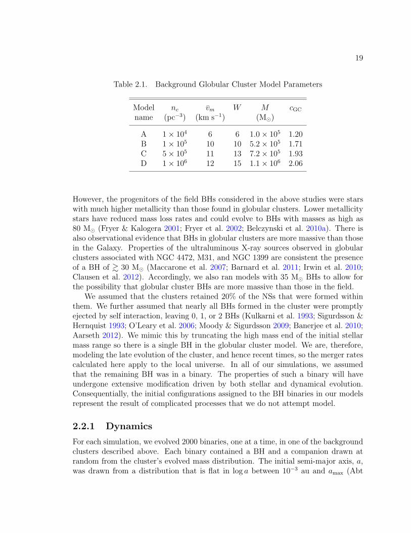
Table 2.1. Background Globular Cluster Model Parameters

Model nc vm W M cGC

name (pc−3) (km s−1) (M�)

A 1× 104 6 6 1.0× 105 1.20B 1× 105 10 10 5.2× 105 1.71C 5× 105 11 13 7.2× 105 1.93D 1× 106 12 15 1.1× 106 2.06

However, the progenitors of the field BHs considered in the above studies were starswith much higher metallicity than those found in globular clusters. Lower metallicitystars have reduced mass loss rates and could evolve to BHs with masses as high as80 M� (Fryer & Kalogera 2001; Fryer et al. 2002; Belczynski et al. 2010a). There isalso observational evidence that BHs in globular clusters are more massive than thosein the Galaxy. Properties of the ultraluminous X-ray sources observed in globularclusters associated with NGC 4472, M31, and NGC 1399 are consistent the presenceof a BH of & 30 M� (Maccarone et al. 2007; Barnard et al. 2011; Irwin et al. 2010;Clausen et al. 2012). Accordingly, we also ran models with 35 M� BHs to allow forthe possibility that globular cluster BHs are more massive than those in the field.

We assumed that the clusters retained 20% of the NSs that were formed withinthem. We further assumed that nearly all BHs formed in the cluster were promptlyejected by self interaction, leaving 0, 1, or 2 BHs (Kulkarni et al. 1993; Sigurdsson &Hernquist 1993; O’Leary et al. 2006; Moody & Sigurdsson 2009; Banerjee et al. 2010;Aarseth 2012). We mimic this by truncating the high mass end of the initial stellarmass range so there is a single BH in the globular cluster model. We are, therefore,modeling the late evolution of the cluster, and hence recent times, so the merger ratescalculated here apply to the local universe. In all of our simulations, we assumedthat the remaining BH was in a binary. The properties of such a binary will haveundergone extensive modification driven by both stellar and dynamical evolution.Consequentially, the initial configurations assigned to the BH binaries in our modelsrepresent the result of complicated processes that we do not attempt model.

2.2.1 Dynamics

For each simulation, we evolved 2000 binaries, one at a time, in one of the backgroundclusters described above. Each binary contained a BH and a companion drawn atrandom from the cluster’s evolved mass distribution. The initial semi-major axis, a,was drawn from a distribution that is flat in log a between 10−3 au and amax (Abt

20

1983). We used a different value of amax for each background cluster, namely 100 au,33 au, 15 au, and 10 au for clusters A, B, C, and D, respectively. These values of amax

were chosen to cover the range of possibilities that might result from the complicatedevolutionary histories of the BH binaries mentioned above. The initial eccentricitywas drawn from f(e) ∝ 2e (Duquennoy & Mayor 1991).

Each binary was initially placed in the cluster core, with its position selected fromthe radial density distribution of the third most massive mass group. The results areinsensitive to this somewhat arbitrary choice because the initial position and velocityof the binary are rapidly forgotten. The binaries were evolved in the cluster potentialwith dynamical friction and random kicks to account for scattering by individualstars. At each point along the binary’s trajectory, we computed the probability thatit would experience a strong encounter with a single star using

Penc = ∆t∑α

∫nα(r)σ(v,v∗)|v − v∗|fα(v∗)d

3v∗, (2.4)

where the subscripts α correspond to the mass groups, ∆t is the time step, n isthe number density, f(v∗) is the velocity distribution of single stars given in equa-tion (2.2), v and v∗ are the velocity of the binary and a single star, respectively,and σ is the encounter cross section. Throughout this chapter we are interested inencounters that alter the energy, angular momentum or components of the binary.Previous studies have shown that the bulk of these changes involve a background starapproaching the binary center of mass closer than a few times the binary’s physi-cal size and conversely that numerous, more distant encounters have relatively smalleffect. We choose the critical pericenter distance for simulated encounters to bep = a[4 + 0.6(1 + e)] where a is the binary semi-major axis and e is its eccentricity(Hut & Bahcall 1983). The corresponding cross section for such encounters is

σ(v,v∗) = πp2 +2πG(mbin +mα)p

|v − v∗|2, (2.5)

where mbin is the mass of the binary. An encounter took place if Penc was greaterthan a random number drawn from a uniform distribution between 0 and 1. Giventhat an encounter occurred, we randomly chose which particular mass group wasinvolved based on the fractional encounter probabilities of all the groups. Then, thethree-body interaction between the stars was integrated explicitly as described inSigurdsson & Phinney (1993). There were many possible outcomes to the three-bodyencounter, including mergers, exchanges, and disruption of the binary, but if a binarystill existed at the end of the interaction, then we continued to evolve the binary inthe cluster.

We performed two types of simulations. In the first class of simulations we wereonly concerned with the fate of the initial BH binary, while in the second class we

21

sought to determine the ultimate fate of the BH. In the former set, a run continueduntil either the initial binary was disrupted, merged, or ejected, or the run hadcovered 1010 yrs. In the latter set of models, we continued a run when the mergeror disruption of a binary resulted in an isolated BH (see section 2.2.3). These runsended only after the BH was ejected from the cluster or the maximum run time of1010 yrs was reached. In both simulation types, a small fraction of the runs (. 5%)were aborted because integration of a three-body interaction exceeded the maximumnumber of allowed steps, 8× 107.

2.2.2 Gravitational radiation effects on the evolution BH+NSbinaries

Between interactions the eccentricity and semi-major axis of each BH+NS systemwere decreased to account to account for the emission of gravitational radiation usingthe relations given in Peters (1964). For the simulations in which we used a BHmass MBH = 7 M�, we stopped the calculation when a BH+NS binary coalesced.Numerical relativity simulations have found that the remnant formed by a BH–NSmerger at this mass ratio will receive a kick from anisotropic emission of gravitationalradiation that exceeds the globular cluster’s escape velocity (Shibata et al. 2009;Etienne et al. 2009; Foucart et al. 2011). In the models where we used MBH = 35 M�,the post-merger recoil velocity was suppressed because of the much smaller mass ratio(q = MNS/MBH). For the case of non-spinning point masses, the merger of a 1.4 M�NS and a 35 M� BH would result in a recoil velocity of 14.6 km s−1, well below theescape velocity for the clusters models that we considered (Gonzalez et al. 2007).However, we allowed for spinning BHs and NSs, and computed the recoil velocityusing the parameterization given in Campanelli et al. (2007, however, see Hirata 2011for discussion of a resonant recoil, not included in this parameterization, that candominate when the BH spin is nearly maximal and q � 1). At the beginning ofeach run, the BH spin parameter was randomly selected from a uniform distributionbetween 0 and 1. When a BH+NS binary merged, the NS spin was randomly selectedfrom a uniform distribution between 0 and 0.7 (a spin parameter of 0.7 correspondsto a NS spinning at the break up frequency Miller et al. 2011) and the two spins wererandomly oriented with respect to one another and to the orbital plane. The resultwas a range of kick velocities (∼ 10 − 100 km s−1), some of which were low enoughthat the single BH was retained by the cluster after the merger.

2.2.3 Formation of a new binary from a single BH by stellarinteractions

In some of our models, when the BH lost its binary companion, either through aninteraction with a background star or as the result of a gravitational radiation driven

22

merger with a NS, we continued to evolve the now single BH in the cluster. Asthe BH moved through the cluster, we sought to determine the single BH’s nextbinary companion by generating binaries with a semi-major axis a, an eccentricitye, a primary of mass m1, and a secondary of mass m2. The semi-major axis andeccentricity were drawn from the same distributions as those of the initial BH binaries.The only difference is that we have chosen amax = 1 au for these systems to ensurethat the binaries were hard. Our choices for m1 and m2 are described below.

We determined whether or not the single BH would interact with the binary bytemporarily replacing the secondary with the BH. We then calculated the probabilitythat this temporary binary would interact with a background star of mass m2 (thesecondary), P(1,BH)+2, using equation (2.4). Next, P(1,BH)+2 was scaled to P(1,2)+BH bycomparing the rates of two related exchange encounters, [(1,BH) + 2→ (2,BH) + 1]and [(1, 2) + BH → (1,BH) + 2]. The rate for an arbitrary interaction between abinary (a,b) and single star c can be expressed in the form

R(X) =Gmamb(ma +mb +mc)

mc(ma +mb)

ainnσ(X)

v, (2.6)

where X refers to the type of interaction (e.g., one of the desired exchange reactions),v is the relative velocity of the binary and the single star, ain is the semi-major axisof the binary, n is the density of single stars, σ(X) is a numerically determined,dimensionless cross section, G is the gravitational constant, and mi is the mass ofstar i. Using equation (2.6), we computed the relative rates of the above exchangeinteractions, assuming that ain, n, and v were the same in each case.

The required dimensionless cross sections were computed by Sigurdsson & Phinney(1993), who found σ[(1,BH)+2→ (2,BH)+1] ∼ 2× σ[(1, 2)+BH→ (1,BH)+2]. Inaddition, we made the simplifying approximation that m1 = m2 �MBH, because theBH was much more massive than either the primary or the secondary. This reducedthe ratio of the mass factors to m2/2MBH. Combining these, we approximated theprobability that the single BH would interact with a binary containing the primaryand the secondary as

P(1,2)+BH ∼fb

1− fbm2

MBH

P(1,BH)+2, (2.7)

where fb is the binary fraction and relates the densities of single and binary stars.Note that the right hand side of this expression diverges as fb → 1. Thus, for largevalues of fb, use of equation (2.7) will overestimate the rate at which a single BHcan exchange back into a binary. Furthermore, we have used the relative rates oftwo exchange encounters to scale the total encounter probability. The exchange crosssection is a significant fraction of the total interaction cross section, but we willexplore the consequences of this choice in section 2.4.1. We chose to compute theencounter probability using the scaling relation given in equation (2.7) because the

23

distribution of binaries in globular clusters is poorly understood and this techniqueoffers an efficient and adequate estimation of the rates within the limitations of ourcode. When an encounter was deemed to have occurred, we restored the originalbinary and explicitly integrated the three-body interaction between the binary andthe BH, accepting any outcome. We repeated this process until the BH exchangedinto a binary, the BH was ejected from the cluster, or the maximum integration timewas reached. If the BH exchanged into a binary, we continued the simulation asdescribed in section 2.2.1.

We explored several different binary populations and values of fb. In one setof models, we drew the primary’s mass from the cluster’s evolved mass distributionand required that m1 ≥ mto, but we did not chose the secondary’s mass, initially.Instead, we used a binary consisting of the primary and the BH to compute thescaled probability that a BH would interact with a binary containing the primaryand a member of any mass group. If an encounter occurred, then the secondarywas chosen to belong to the mass group that interacted with the temporary binary.We then integrated the three-body interaction as described above. This method ofselecting the secondary resulted in a binary population that is composed largely ofsystems that contain a NS. For the simulations in cluster D, more than 50% of thebinaries that interacted with a single BH contained a NS. We have labeled the runsthat use this binary population OPT, for optimized, because this method produces abinary population that is tuned to interact with the single BH. Furthermore, becausemany of the binaries in this population already contain a NS, the single BH can gaina NS companion immediately.

The second binary population that we considered was closely linked to obser-vational constraints. A number of studies have used the fact that unresolved MSbinaries appear brighter and redder than single MS stars to investigate binaries inglobular clusters. The binary fraction can be measured by comparing the number ofobjects in the offset binary sequence to the number of stars that lie along the MS,with observed values typically found to be in the range fb = 0.05− 0.3 (e.g., Romani& Weinberg 1991; Sollima et al. 2007; Davis et al. 2008; Milone et al. 2012a). Wegenerated a population that resembles these observed populations by independentlydrawing two stars from the cluster’s evolved stellar mass distribution and requiringthat one of the stars have a mass m ≥ mto. The result was a collection of systemsthat consisted primarily (& 85%) of MS-MS binaries. We have labeled simulationsthat use this binary population OBS, and considered values for the binary fractionwithin the observed range: 0.05, 0.1, and 0.2.

We also considered a population that was motived by detailed models of binaryevolution in globular clusters. Analytic, Monte Carlo, and N-body models have indi-cated that over time the hard binary fraction will increase in the cluster core (Sollima2008; Fregeau et al. 2009; Hurley et al. 2007). For such models to be consistent withthe observations described above, the initial binary fraction in globular clusters would

24

have to have been quite low. Alternatively, as Fregeau et al. (2009) suggested, if manyof the binaries in a globular cluster consisted of a MS star and a WD or two WDs,they would be “hidden” from observers. Following on this result, we have run simu-lations that use a binary population similar to that described in table 1 of Fregeauet al. (2009). This population consisted of 44% MS+WD binaries, 32% WD+WDbinaries, 23% MS+MS binaries, and 1% binaries containing a NS. Runs that used thisbinary population were labeled FIR. Furthermore, because only 23% of this binarypopulation would be measured by the observations described above, we have usedlarger values of fb with this population: 0.2, 0.5, and 0.75.

2.3 Results

In all of our simulations, binary–single star interactions produced BH+NS binaries.However, the number of BH+NS binaries formed and the properties of these systemswere very sensitive to the structure of the globular cluster and the assumed binarypopulation. Our simulations are summarized in Table 2.2. The initial conditionsfor each simulation, including the cluster model, the binary population (where ap-plicable), the binary fraction (where applicable), and MBH, are given. Also listedare fBHNS, the fraction of runs that produced a BH+NS binary, NBHNS, the totalnumber of BH+NS binaries formed in all 2000 runs, Nmrg, the number of BH–NSmergers during the simulation, tex, the average amount of time taken for a single BHto exchange back into a binary, Nmax, the maximum number of mergers in a singlerun, and RGC , the BH-NS merger rate for that model. We describe the results indetail below, beginning with models that assumed that the BH was ejected from theglobular cluster after merging with a NS, followed by descriptions of models withmore massive BHs, which allowed for a single BH to merge with multiple NS.

2.3.1 Single merger scenario

2.3.1.1 Without single BHs

In this section we describe simulations that ended if the binary containing the BHwas disrupted or merged. These models did not require any assumptions about theglobular cluster’s binary population as a whole because they were terminated as soonas the BH lost its companion. We have computed one such simulation in each of ourbackground clusters, and in all of these simulations we assumed MBH = 7 M�.

In the lowest density cluster considered here, cluster A, only eight BH+NS binarieswere formed in our 2000 runs, none of which merged during the 1010 yr simulations.In all of the other clusters, however, some fraction of the BH+NS binaries mergedduring the simulation. Figure 2.1 shows the initial semi-major axis and eccentricityof the BH+NS systems formed in simulations using cluster model D. Also plotted

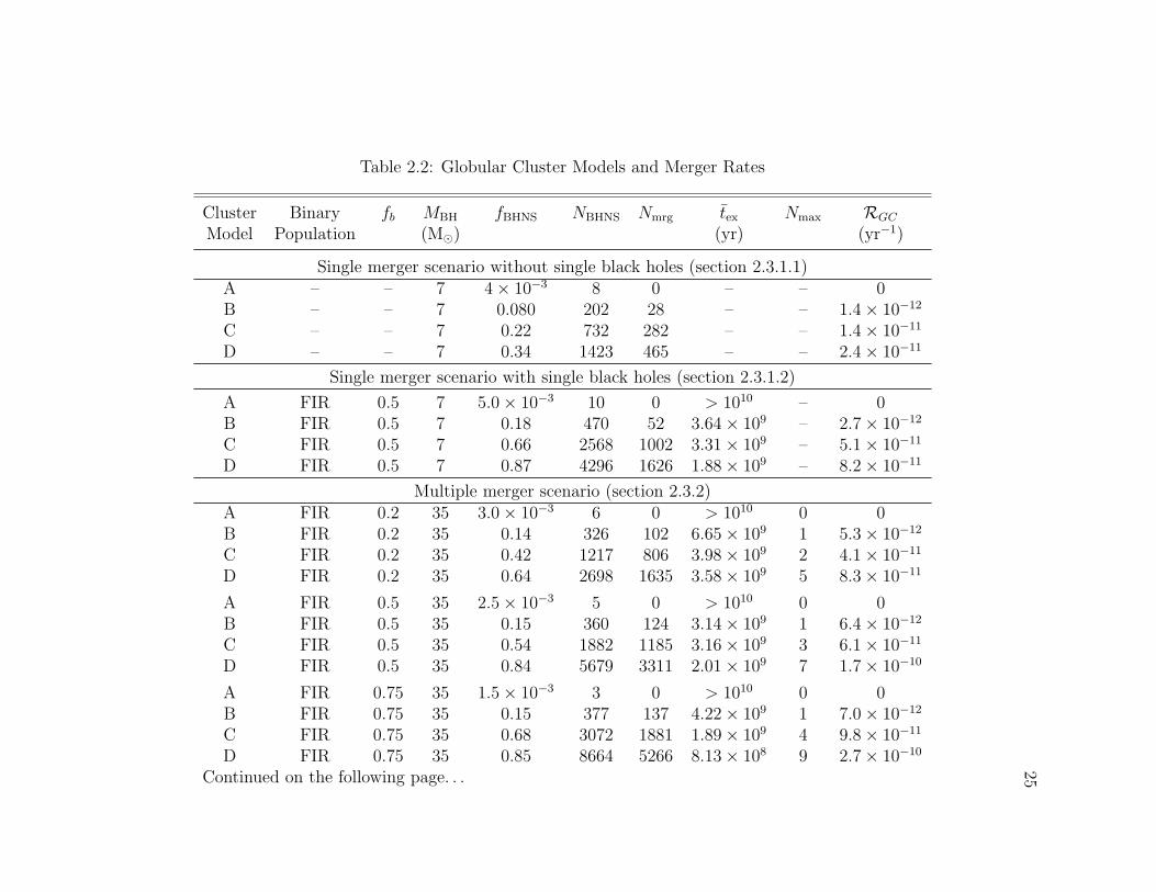
25

Table 2.2: Globular Cluster Models and Merger Rates

Cluster Binary fb MBH fBHNS NBHNS Nmrg tex Nmax RGC

Model Population (M�) (yr) (yr−1)

Single merger scenario without single black holes (section 2.3.1.1)A – – 7 4× 10−3 8 0 – – 0B – – 7 0.080 202 28 – – 1.4× 10−12

C – – 7 0.22 732 282 – – 1.4× 10−11

D – – 7 0.34 1423 465 – – 2.4× 10−11

Single merger scenario with single black holes (section 2.3.1.2)

A FIR 0.5 7 5.0× 10−3 10 0 > 1010 – 0B FIR 0.5 7 0.18 470 52 3.64× 109 – 2.7× 10−12

C FIR 0.5 7 0.66 2568 1002 3.31× 109 – 5.1× 10−11

D FIR 0.5 7 0.87 4296 1626 1.88× 109 – 8.2× 10−11

Multiple merger scenario (section 2.3.2)A FIR 0.2 35 3.0× 10−3 6 0 > 1010 0 0B FIR 0.2 35 0.14 326 102 6.65× 109 1 5.3× 10−12

C FIR 0.2 35 0.42 1217 806 3.98× 109 2 4.1× 10−11

D FIR 0.2 35 0.64 2698 1635 3.58× 109 5 8.3× 10−11

A FIR 0.5 35 2.5× 10−3 5 0 > 1010 0 0B FIR 0.5 35 0.15 360 124 3.14× 109 1 6.4× 10−12

C FIR 0.5 35 0.54 1882 1185 3.16× 109 3 6.1× 10−11

D FIR 0.5 35 0.84 5679 3311 2.01× 109 7 1.7× 10−10

A FIR 0.75 35 1.5× 10−3 3 0 > 1010 0 0B FIR 0.75 35 0.15 377 137 4.22× 109 1 7.0× 10−12

C FIR 0.75 35 0.68 3072 1881 1.89× 109 4 9.8× 10−11

D FIR 0.75 35 0.85 8664 5266 8.13× 108 9 2.7× 10−10

Continued on the following page. . .

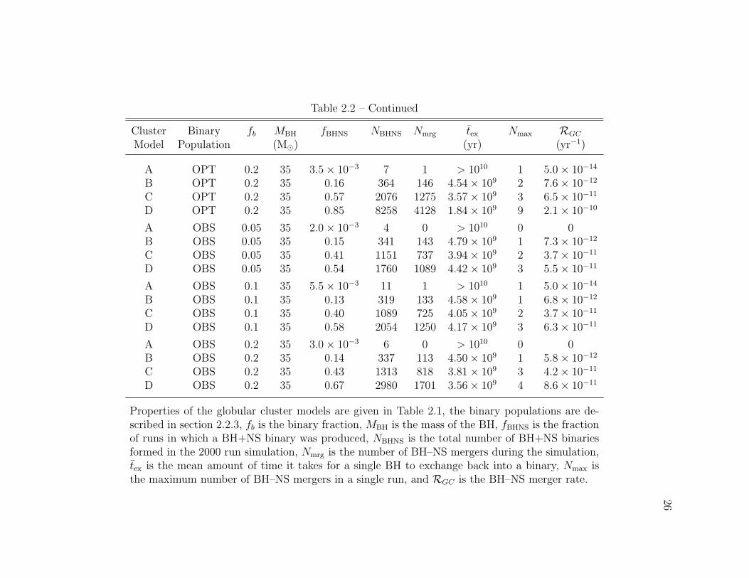
26

Table 2.2 – Continued

Cluster Binary fb MBH fBHNS NBHNS Nmrg tex Nmax RGC

Model Population (M�) (yr) (yr−1)

A OPT 0.2 35 3.5× 10−3 7 1 > 1010 1 5.0× 10−14

B OPT 0.2 35 0.16 364 146 4.54× 109 2 7.6× 10−12

C OPT 0.2 35 0.57 2076 1275 3.57× 109 3 6.5× 10−11

D OPT 0.2 35 0.85 8258 4128 1.84× 109 9 2.1× 10−10

A OBS 0.05 35 2.0× 10−3 4 0 > 1010 0 0B OBS 0.05 35 0.15 341 143 4.79× 109 1 7.3× 10−12

C OBS 0.05 35 0.41 1151 737 3.94× 109 2 3.7× 10−11

D OBS 0.05 35 0.54 1760 1089 4.42× 109 3 5.5× 10−11

A OBS 0.1 35 5.5× 10−3 11 1 > 1010 1 5.0× 10−14

B OBS 0.1 35 0.13 319 133 4.58× 109 1 6.8× 10−12

C OBS 0.1 35 0.40 1089 725 4.05× 109 2 3.7× 10−11

D OBS 0.1 35 0.58 2054 1250 4.17× 109 3 6.3× 10−11

A OBS 0.2 35 3.0× 10−3 6 0 > 1010 0 0B OBS 0.2 35 0.14 337 113 4.50× 109 1 5.8× 10−12

C OBS 0.2 35 0.43 1313 818 3.81× 109 3 4.2× 10−11

D OBS 0.2 35 0.67 2980 1701 3.56× 109 4 8.6× 10−11

Properties of the globular cluster models are given in Table 2.1, the binary populations are de-scribed in section 2.2.3, fb is the binary fraction, MBH is the mass of the BH, fBHNS is the fractionof runs in which a BH+NS binary was produced, NBHNS is the total number of BH+NS binariesformed in the 2000 run simulation, Nmrg is the number of BH–NS mergers during the simulation,tex is the mean amount of time it takes for a single BH to exchange back into a binary, Nmax isthe maximum number of BH–NS mergers in a single run, and RGC is the BH–NS merger rate.

27

are lines of constant gravitational radiation merger time. A majority of the systemslie above the right most line, which corresponds to a merger time 1010 yr. If thesesystems were to evolve in isolation, it would take more than a Hubble time for themto merge. However, in the massive globular clusters considered here subsequent in-teractions with single stars extracted energy from the binary’s orbit and drove someof these systems to high eccentricity and/or small separations, greatly acceleratingthe merger process. This mechanism is illustrated in Figure 2.2. BH+NS bina-ries with expected merger times, given their initial eccentricity and semi-major axis,tGW0 > 107 yr underwent several interactions with single stars after their formation,which altered the orbital parameters of the binary and reduced the actual amount oftime between the formation of the BH+NS binary and the merger of the binary, tGW,by several orders of magnitude. In these simulations, binary–single star encountersnot only produced BH+NS binaries, but in some cases enhanced the rate at whichthese systems merged.

In other situations, subsequent interactions reduced the merger rate. In modelsthat used cluster B, many BH+NS binaries were destroyed when a WD exchangedinto the binary. In this relatively low concentration cluster, the density of WDs wasmuch greater than the density of NSs, so multiple encounters with WDs overcame thelow probability of a WD exchanging into the BH+NS binary. This property of lowconcentration clusters has implications for the formation of mass transfer binaries,and hence X-ray luminosity of such clusters, which we will investigate in a futurestudy. At the end of most runs in cluster B, the BH remains in the cluster. TheBH is ejected in 3% of the runs. Of those ejected, 42% are ejected after a BH–NSmerger and 58% are ejected after a super-elastic collision between the binary and abackground star. In the majority of runs (63%), the BH remains in the cluster witha non-NS binary companion. The BH loses its companion but remains in the clusterin the remaining 34%.

This over-density of WDs did not occur in the high concentration clusters, C andD. In these simulations, if a BH+NS binary was destroyed by an exchange, it wasusually another NS exchanging into the system. The simulations suggest that in theclusters with n ≥ 5 × 105 pc−3, there is a high likelihood that a BH retained by thecluster after the initial phase of self interaction will become part of a BH+NS binarythat merges within a Hubble time. This, coupled with the high post-merger kickspredicted by numerical relativity, suggests that if globular cluster BHs have the samemass distribution as those in the field, BHs will only be retained in massive clusterswith n ≤ 105 pc−3.

The distribution of BH–NS merger times, tmrg, for the different globular clustersmodels are shown as solid histograms in Figure 2.3. We note that tmrg > tGW becausetmrg includes the time taken to produce the BH+NS binary. Encounters occurredfrequently in simulations of the more massive, higher density clusters, so the BH+NSbinaries were formed earlier and, as described above, encounters after their formation

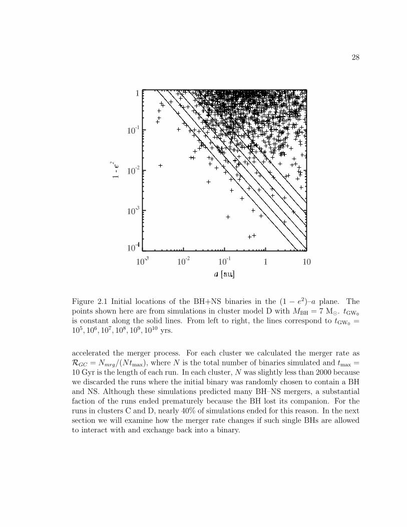
28

Figure 2.1 Initial locations of the BH+NS binaries in the (1 − e2)–a plane. Thepoints shown here are from simulations in cluster model D with MBH = 7 M�. tGW0

is constant along the solid lines. From left to right, the lines correspond to tGW0 =105, 106, 107, 108, 109, 1010 yrs.

accelerated the merger process. For each cluster we calculated the merger rate asRGC = Nmrg/(Ntmax), where N is the total number of binaries simulated and tmax =10 Gyr is the length of each run. In each cluster, N was slightly less than 2000 becausewe discarded the runs where the initial binary was randomly chosen to contain a BHand NS. Although these simulations predicted many BH–NS mergers, a substantialfaction of the runs ended prematurely because the BH lost its companion. For theruns in clusters C and D, nearly 40% of simulations ended for this reason. In the nextsection we will examine how the merger rate changes if such single BHs are allowedto interact with and exchange back into a binary.

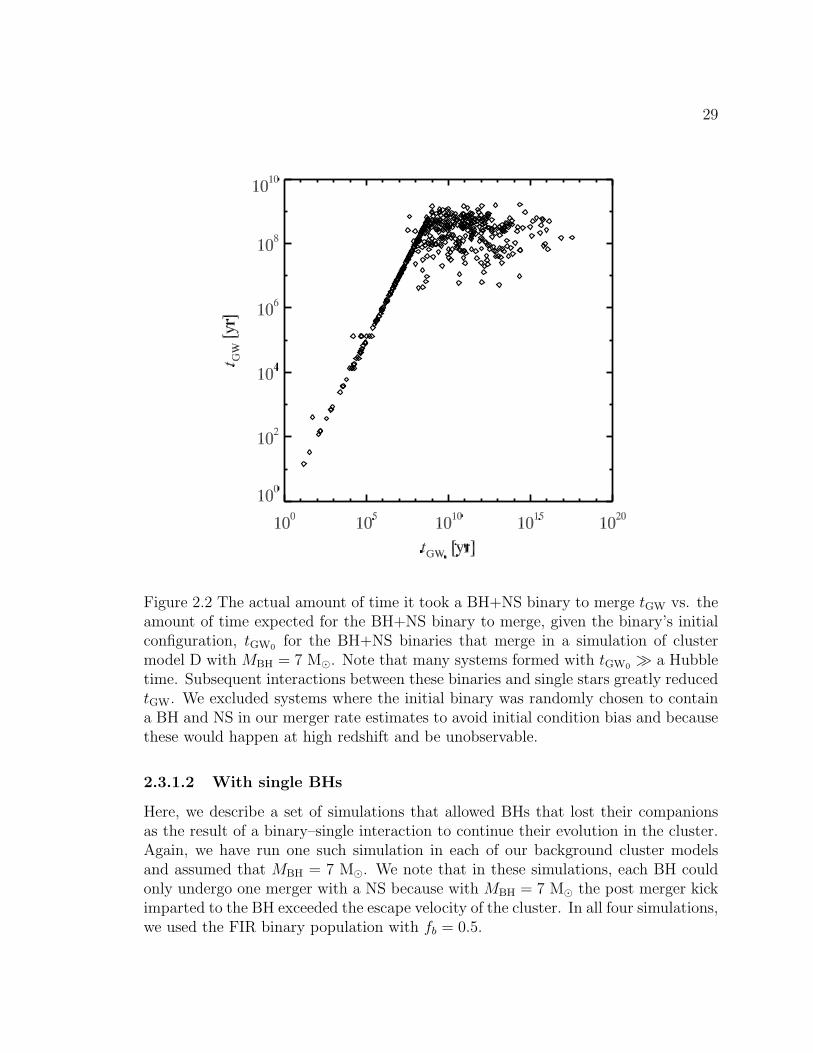
29

Figure 2.2 The actual amount of time it took a BH+NS binary to merge tGW vs. theamount of time expected for the BH+NS binary to merge, given the binary’s initialconfiguration, tGW0 for the BH+NS binaries that merge in a simulation of clustermodel D with MBH = 7 M�. Note that many systems formed with tGW0 � a Hubbletime. Subsequent interactions between these binaries and single stars greatly reducedtGW. We excluded systems where the initial binary was randomly chosen to containa BH and NS in our merger rate estimates to avoid initial condition bias and becausethese would happen at high redshift and be unobservable.

2.3.1.2 With single BHs

Here, we describe a set of simulations that allowed BHs that lost their companionsas the result of a binary–single interaction to continue their evolution in the cluster.Again, we have run one such simulation in each of our background cluster modelsand assumed that MBH = 7 M�. We note that in these simulations, each BH couldonly undergo one merger with a NS because with MBH = 7 M� the post merger kickimparted to the BH exceeded the escape velocity of the cluster. In all four simulations,we used the FIR binary population with fb = 0.5.

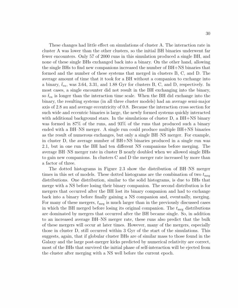
30

These changes had little effect on simulations of cluster A. The interaction rate incluster A was lower than the other clusters, so the initial BH binaries underwent farfewer encounters. Only 57 of 2000 runs in this simulation produced a single BH, andnone of these single BHs exchanged back into a binary. On the other hand, allowingthe single BHs to find new companions increased the number of BH+NS binaries thatformed and the number of these systems that merged in clusters B, C, and D. Theaverage amount of time that it took for a BH without a companion to exchange intoa binary, tex, was 3.64, 3.31, and 1.88 Gyr for clusters B, C, and D, respectively. Inmost cases, a single encounter did not result in the BH exchanging into the binary,so tex is longer than the interaction time scale. When the BH did exchange into thebinary, the resulting systems (in all three cluster models) had an average semi-majoraxis of 2.8 au and average eccentricity of 0.8. Because the interaction cross section forsuch wide and eccentric binaries is large, the newly formed systems quickly interactedwith additional background stars. In the simulations of cluster D, a BH+NS binarywas formed in 87% of the runs, and 93% of the runs that produced such a binaryended with a BH–NS merger. A single run could produce multiple BH+NS binariesas the result of numerous exchanges, but only a single BH–NS merger. For example,in cluster D, the average number of BH+NS binaries produced in a single run was2.1, but in one run the BH had ten different NS companions before merging. Theaverage BH–NS merger rate in cluster B nearly doubled when we allowed single BHsto gain new companions. In clusters C and D the merger rate increased by more thana factor of three.

The dotted histograms in Figure 2.3 show the distribution of BH–NS mergertimes in this set of models. These dotted histograms are the combination of two tmrg

distributions. One distribution, similar to the solid histograms, is due to BHs thatmerge with a NS before losing their binary companion. The second distribution is formergers that occurred after the BH lost its binary companion and had to exchangeback into a binary before finally gaining a NS companion and, eventually, merging.For many of these mergers, tmrg is much larger than in the previously discussed casesin which the BH merged before losing its original companion. The tmrg distributionsare dominated by mergers that occurred after the BH became single. So, in additionto an increased average BH–NS merger rate, these runs also predict that the bulkof these mergers will occur at later times. However, many of the mergers, especiallythose in cluster D, still occurred within 3 Gyr of the start of the simulations. Thissuggests, again, that if globular cluster BHs are of similar mass to those found in theGalaxy and the large post-merger kicks predicted by numerical relativity are correct,most of the BHs that survived the initial phase of self-interaction will be ejected fromthe cluster after merging with a NS well before the current epoch.

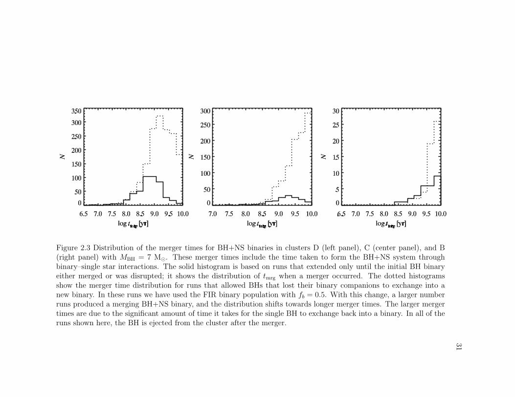
31

Figure 2.3 Distribution of the merger times for BH+NS binaries in clusters D (left panel), C (center panel), and B(right panel) with MBH = 7 M�. These merger times include the time taken to form the BH+NS system throughbinary–single star interactions. The solid histogram is based on runs that extended only until the initial BH binaryeither merged or was disrupted; it shows the distribution of tmrg when a merger occurred. The dotted histogramsshow the merger time distribution for runs that allowed BHs that lost their binary companions to exchange into anew binary. In these runs we have used the FIR binary population with fb = 0.5. With this change, a larger numberruns produced a merging BH+NS binary, and the distribution shifts towards longer merger times. The larger mergertimes are due to the significant amount of time it takes for the single BH to exchange back into a binary. In all of theruns shown here, the BH is ejected from the cluster after the merger.

32

2.3.2 Multiple merger scenario

So far, we have considered scenarios in which the BH receives a post-merger kickthat exceeds the escape velocity of the globular cluster. Under this constraint, eachBH can undergo at most one merger. If globular cluster BHs are more massive thanthose found in field, then it is possible for the BH to remain bound to the clusterafter the merger, regain a NS companion, and merge again. In this section we willdiscuss models that assumed MBH = 35 M�. For small values of the mass ratio q,the magnitude of the recoil velocity is approximately proportional to q2. With a BHmass of 35 M�, q is reduced to 0.04 and the recoil velocity becomes comparable to theglobular cluster escape velocity. Thus, we explored the case in which the suppressedkick velocity helped but did not ensure that the post-merger BH would be retainedby the cluster. The fraction of post-merger BHs retained in simulations using eachbackground cluster depended on that cluster’s escape velocity vesc ≈

√2Wvm. Among

all the models that varied the binary population and binary fraction, in simulationsusing clusters A, B, C, and D, 50%, 23%, 20%, and 10% of the BHs that underwenta merger were ejected, respectively1. However, in these simulations many of the BHsremained bound to the cluster after merging with a NS. A fraction of these singleBHs then gained new NS companions and underwent multiple mergers.

The number of times a BH could merge with a NS depended on how quickly thesingle BH could exchange into a binary after each merger. While the post merger kickwas not always large enough to remove the BH from the cluster, the BH was expelledfrom the core after most mergers. Before it was able to exchange into a binary, itneeded to sink back into the core where the interaction rates were highest. Thisprocess occurred rapidly in all of the simulations. The mass segregation time scale isproportional to m/MBH, where m is the average stellar mass in the cluster. The BHsin these models were 35 M�, which gave m/MBH between 0.014–0.027. Typically,a kicked BH would return to the core on a time scale O(107) yrs. As can be seenfrom Table 2.2, this time scale is short compared to the total time it takes the singleBH to exchange into a binary. There was, therefore, little difference between thetex distributions for BHs that became single because of a BH–NS merger and thosethat lost their companions after a binary–single interaction. We make no distinctionbetween these distributions in the discussion below.

Figure 2.4 shows how the distribution of tex is affected by the mass of the BH,the structural parameters of the globular cluster, and the binary fraction. All of thesimulations shown here used the FIR binary population. Changing the mass of the BHhad little impact on both the distribution of tex and its average value. As expected,tex decreases with increasing cluster concentration. Increasing the binary fractionproduced slightly narrower tex distributions with peaks shifted to shorter times. The

1Note that only two BH–NS mergers occurred in cluster A, so the ejection fraction derived fromthe models is smaller than expected.

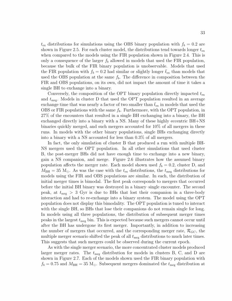
33

tex distributions for simulations using the OBS binary population with fb = 0.2 areshown in Figure 2.5. For each cluster model, the distributions tend towards longer tex

when compared to the models using the FIR population shown in Figure 2.4. This isonly a consequence of the larger fb allowed in models that used the FIR population,because the bulk of the FIR binary population is unobservable. Models that usedthe FIR population with fb = 0.2 had similar or slightly longer tex than models thatused the OBS population at the same fb. The difference in composition between theFIR and OBS populations, on its own, did not impact the amount of time it takes asingle BH to exchange into a binary.

Conversely, the composition of the OPT binary population directly impacted tex

and tmrg. Models in cluster D that used the OPT population resulted in an averageexchange time that was nearly a factor of two smaller than tex in models that used theOBS or FIR populations with the same fb. Furthermore, with the OPT population, in27% of the encounters that resulted in a single BH exchanging into a binary, the BHexchanged directly into a binary with a NS. Many of these highly eccentric BH+NSbinaries quickly merged, and such mergers accounted for 10% of all mergers in theseruns. In models with the other binary populations, single BHs exchanging directlyinto a binary with a NS accounted for less than 0.3% of all mergers.

In fact, the only simulation of cluster B that produced a run with multiple BH-NS mergers used the OPT population. In all other simulations that used clusterB, the post-merger BHs did not have enough time to exchange into a new binary,gain a NS companion, and merge. Figure 2.6 illustrates how the assumed binarypopulation affects the merger rate. Each model shown used fb = 0.2, cluster D, andMBH = 35 M�. As was the case with the tex distributions, the tmrg distributions formodels using the FIR and OBS populations are similar. In each, the distribution ofinitial merger times is bimodal. The first peak corresponds to mergers that occurredbefore the initial BH binary was destroyed in a binary–single encounter. The secondpeak, at tmrg > 3 Gyr is due to BHs that lost their companion in a three-bodyinteraction and had to re-exchange into a binary system. The model using the OPTpopulation does not display this bimodality. The OPT population is tuned to interactwith the single BH, so BHs that lose their companions do not remain single for long.In models using all three populations, the distribution of subsequent merger timespeaks in the largest tmrg bin. This is expected because such mergers cannot occur untilafter the BH has undergone its first merger. Importantly, in addition to increasingthe number of mergers that occurred, and the corresponding merger rate, RGC , themultiple merger scenario shifted the peak of all tmrg distributions to much later times.This suggests that such mergers could be observed during the current epoch.

As with the single merger scenario, the more concentrated cluster models producedlarger merger rates. The tmrg distribution for models in clusters B, C, and D areshown in Figure 2.7. Each of the models shown used the FIR binary population withfb = 0.75 and MBH = 35 M�. Subsequent mergers dominated the tmrg distribution at

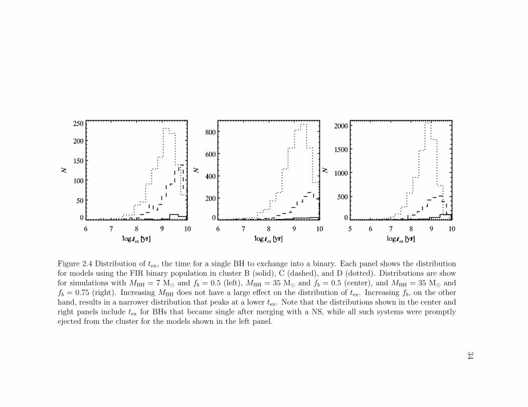
34

Figure 2.4 Distribution of tex, the time for a single BH to exchange into a binary. Each panel shows the distributionfor models using the FIR binary population in cluster B (solid), C (dashed), and D (dotted). Distributions are showfor simulations with MBH = 7 M� and fb = 0.5 (left), MBH = 35 M� and fb = 0.5 (center), and MBH = 35 M� andfb = 0.75 (right). Increasing MBH does not have a large effect on the distribution of tex. Increasing fb, on the otherhand, results in a narrower distribution that peaks at a lower tex. Note that the distributions shown in the center andright panels include tex for BHs that became single after merging with a NS, while all such systems were promptlyejected from the cluster for the models shown in the left panel.

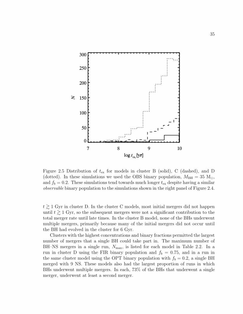
35

Figure 2.5 Distribution of tex for models in cluster B (solid), C (dashed), and D(dotted). In these simulations we used the OBS binary population, MBH = 35 M�,and fb = 0.2. These simulations tend towards much longer tex despite having a similarobservable binary population to the simulations shown in the right panel of Figure 2.4.

t & 1 Gyr in cluster D. In the cluster C models, most initial mergers did not happenuntil t & 1 Gyr, so the subsequent mergers were not a significant contribution to thetotal merger rate until late times. In the cluster B model, none of the BHs underwentmultiple mergers, primarily because many of the initial mergers did not occur untilthe BH had evolved in the cluster for 6 Gyr.

Clusters with the highest concentrations and binary fractions permitted the largestnumber of mergers that a single BH could take part in. The maximum number ofBH–NS mergers in a single run, Nmax, is listed for each model in Table 2.2. In arun in cluster D using the FIR binary population and fb = 0.75, and in a run inthe same cluster model using the OPT binary population with fb = 0.2, a single BHmerged with 9 NS. These models also had the largest proportion of runs in whichBHs underwent multiple mergers. In each, 73% of the BHs that underwent a singlemerger, underwent at least a second merger.

36

Figure 2.6 Merger time distributions for simulations with fb = 0.2 using the FIR (left), OPT (center), and OBS(right) binary population. Each panel shows the distribution of tmrg for the initial merger during a run (dashed),subsequent mergers during that run (dotted), and the combination of the two (solid). The initial tmrg distributionsfor the simulations using the FIR and OBS populations show a clear bimodality. The peaks above log tmrg = 9.5 inthese distributions are due to BHs that lost their binary companions before merging with a NS. The bimodality isamplified in the total merger time distributions for these runs by the distinct distributions for initial and subsequentmergers. The tmrg distribution in the OPT case is completely dominated by subsequent mergers.

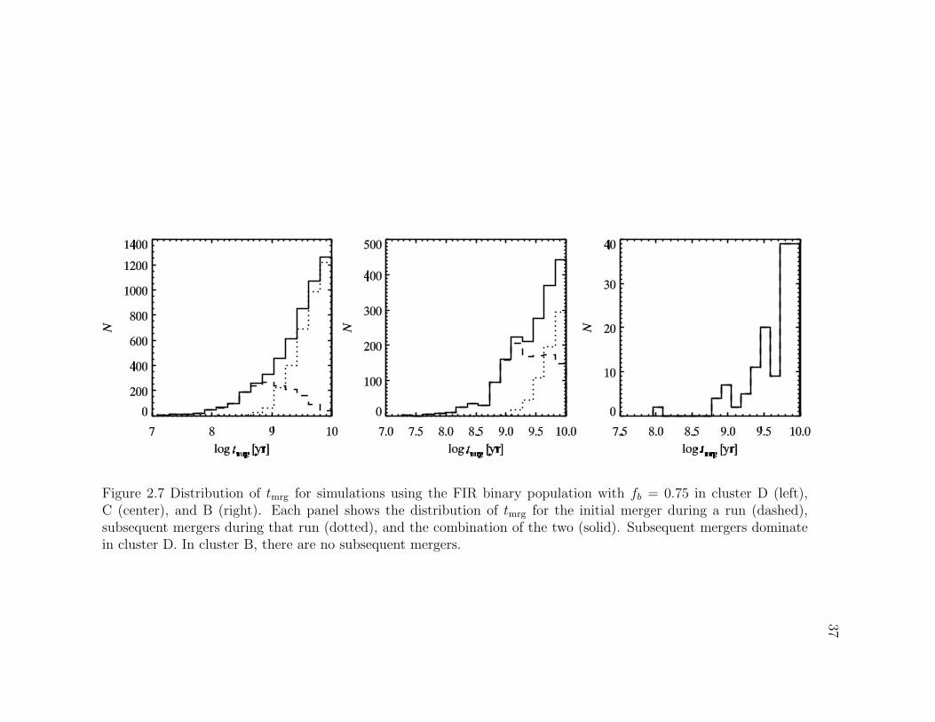
37

Figure 2.7 Distribution of tmrg for simulations using the FIR binary population with fb = 0.75 in cluster D (left),C (center), and B (right). Each panel shows the distribution of tmrg for the initial merger during a run (dashed),subsequent mergers during that run (dotted), and the combination of the two (solid). Subsequent mergers dominatein cluster D. In cluster B, there are no subsequent mergers.

38

2.4 Discussion

We have shown that binary–single star interactions in globular clusters can produceBH+NS binaries that will merge within a Hubble time. The rate at which the mergersoccur is sensitive to the globular cluster structural parameters, the mass of the BH,and properties of the globular cluster’s binary population. If the BHs in globularclusters follow a similar mass distribution to those found in the disk of the Galaxy,then it is unlikely that any high concentration clusters could retain a BH until thecurrent epoch. In such clusters, most BHs that managed to survive the early period ofself-interaction, described in previous studies, would gain a NS companion, undergoa gravitational radiation driven merger, and be ejected from the cluster within ∼ 3Gyr. If, on the other had, globular cluster BHs are more massive than typical fieldBHs, many clusters could retain a BH and that BH could continue to merge with NSsuntil late times.

2.4.1 Uncertainties

The BH–NS merger rates calculated here depend on the uncertain distributions ofseveral quantities. The distributions of some parameters are better constrained thanothers (e.g., a Abt 1983 and e Duquennoy & Mayor 1991 distributions, NS retentionfraction Pfahl et al. 2002, and the structure of extragalactic globular clusters Straderet al. 2011). However, both the globular cluster BH mass function and the natureof globular cluster binary populations strongly influence the predicted rates and arenot well constrained by observations. We have sampled several plausible scenarios foreach, and the results suggest that the observed merger rate could be used to probeboth the BH mass distribution and binary populations present in globular clusters.

Some of the simplifying assumptions that we made in the models also impacted thepredicted merger rates. In our calculation of the probability that a single BH wouldexchange into a new binary, we related the densities of single and binary stars usingan approximation that diverges for large binary fractions, fb/(1 − fb). In the mostextreme case considered here, fb = 0.75, this term increases the encounter probabilityby a factor of 3. Any overestimate due to this term is of the same magnitude as errorsintroduced by other approximations made in our calculation. In addition to thisapproximation, in the calculations described above we used a relationship betweenthe rates of specific exchange encounters to scale the total encounter rate. At the veryleast, this resulted in longer tex because we only integrated the three-body encounterif the probability for a specific exchange [(1, 2)+BH→ (1,BH)+2] was large enough,but we allowed for any outcome of the three-body interaction.

We have run two additional simulations to explore how these assumptions affectedour calculations. In these tests, we evolved 500 binaries in cluster D using the FIRbinary population with fb = 0.5. In one simulation, marked Retry, we scaled the

39

Table 2.3. Probability Scaling Tests

Class tex Nmax RGC

(yr) (yr−1)

Original 2.01× 109 7 1.7× 10−10

Retry 9.96× 108 8 2.3× 10−10

Total 1.18× 109 8 2.5× 10−10

encounter probability using equation (2.7), as before. However, in these runs if theprobability of exchange was larger than the random number, we re-ran the three-body integrator until the desired exchange, [(1, 2) + BH→ (1,BH) + 2], occurred. Ifthe integration resulted in a different outcome (e.g., flyby or an exchange creating abinary (BH,2)), we changed the orbital phase of the initial binary and the orientationof the encounter, and then simulated the interaction again. In another simulation,marked Total, we scaled P(1,BH)+2 by the ratio of the total encounter cross sections,not just the single, desired exchange cross section. In the mass ratios consideredhere (∼ 1 : 1 : 35), the value of σ(X) for the BH to exchange into a binary withthe primary is roughly equal to σ(X) for the BH to exchange into a binary withthe secondary, and roughly half the value σ(X) for a flyby (Sigurdsson & Phinney1993). This results in a factor of 2-3 increase in the encounter probability over theprobabilities used in the previous runs. For the Total runs, as in the runs presentedin section 2.3.2, if an encounter occurred we accepted any outcome of the three-bodyintegration.

The results of these tests are listed in Table 2.3. Both methods for correcting theprobability scaling increased the exchange and merger rates. Furthermore, making thecorrection either of two ways gave consistent results, illustrating that the probabilityscaling argument used in our models is valid. The maximum number of mergers ineach of the test runs increased from 7 to 8. The fact that this quantity did not changeby a factor of two, as tex did, suggests that the time it takes a single BH to exchangeback into a binary may not be the rate limiting step in the BH-NS merger process.Finally, these runs suggest that the factor of a few uncertainties in the exchangeprobability resulting from the approximations we made can lead to uncertainties of asimilar magnitude in the BH–NS merger rates. As such, the rates given in Table 2.2should be treated as having a factor of ∼ 2 uncertainty.

In addition to uncertainties in the components of the models, physical processesand properties of globular clusters that we have omitted from the models could alterthe BH–NS merger rates. We have not explicitly included an increase in the binarydensity at the cluster center. Since, next to the BH, NS-containing binaries are the

40

heaviest objects in the cluster they would likely be concentrated near the center. Thesituation could be similar to the models presented here that made use of the OPTbinary population, which contained a large fraction of NS binaries. These modelsresulted in higher merger rates than models that used OBS or FIR binary populationswith the same binary fraction. On the other hand, a high binary concentration couldresult in significant heating, expanding the radial profile expected for a populationof thermalized binaries. A high concentration of binaries would also result in binary-binary interactions, which were not included in our models. Some binary–binaryencounters could enhance the merger rate. For example, the interaction of a BH+MSbinary with a NS+MS binary could produce a BH+NS binary. However, there isa high likelihood that a binary-binary encounter will result in the disruption of abinary. Because the rate of binary-binary encounters increases with fb, this limits thebinary fraction. So, binary-binary interactions could cause a reduction in the BH–NSmerger rate, compared to the rates predicted here, by limiting fb and making it moredifficult for a single BH to find a new binary companion. Detailed models that includebinary-binary interactions are necessary to determine which process dominates.

2.4.2 LIGO detection rate

We estimated the LIGO detection rate following Belczynski et al. (2007) and Banerjeeet al. (2010). We computed the detection rate with

RLIGO =4π

3ρGC

(D0

(mch

mch,NSNS

)5/6)3

RGC , (2.8)

where ρGC is the space density of globular clusters, mch is the chirp mass of the binary(mch = (m1m2)3/5/(m1 + m2)1/5), and mch,NSNS is the chirp mass of a binary withtwo 1.4 M� NSs. D0 is the maximum distance from which the gravitational wavesfrom a merging NS+NS binary can be detected, and has a value of 18 and 300 Mpcfor LIGO and Advanced LIGO (aLIGO), respectively. Using the galaxy luminosityfunction parameters estimated in Croton et al. (2005) and the specific frequency ofglobular clusters per 8.5× 107 L� of galaxy luminosity presented in Brodie & Strader(2006), we calculated ρGC = 8 Mpc−3. Our calculations above showed that RGC isstrongly dependent on the cluster mass. To compute a merger rate that is averagedover all globular clusters, RGC , we used the globular cluster mass function presentedin McLaughlin & Pudritz (1996).

Although we have shown that the bulk of such mergers occur quickly, and thereforeat high redshift, we compute the aLIGO detection rate for models with 7 M� BHsfor illustrative purposes. For these BH+NS binaries, mch = 2.6 M�. For the modelsthat do not allow single BHs, we found RGC = 3.4 × 10−12 yr−1 GC−1. To make aconservative estimate for the aLIGO detection rate, we assumed that 10% of clusters

41

retain one BH and arrived at the rate of 2 × 10−3 yr−1. Using instead the ratesfrom runs that did allow single BHs to exchange back into binaries, we found anaLIGO detection rate of 10−2 yr−1. Even if mergers between 7 M� BHs and NS wereoccurring in globular clusters at the current epoch, the event rates are so low thatthey would not be detected by aLIGO. For example, the rates calculated for clustermodels B and C may be applicable to massive intermediate age clusters. With agesof 1-5 Gyr, these clusters are young enough that any retained BHs would only now bemerging with a NS. However, the space density of massive intermediate age clustersclusters is even lower than that of globular clusters, so the conclusion remains thesame. If globular cluster BHs follow the same mass distribution as field BHs, BH–NSmergers resulting from binary-single star interactions in clusters cannot be detectedby aLIGO.

The detection rate could be much higher than this conservative estimate if globularcluster BHs are more massive than typical field BHs. Higher mass BHs enhance thedetection rate in two ways. First, more massive binaries can be detected out tolarger distances. Second, since the post-merger kick is suppressed for high mass ratioinspirals, the BH remains in the cluster and can undergo multiple mergers with NSs.Models with the FIR binary population and fb = 0.75 produced the largest averagedmerger rate, RGC = 4.2× 10−11 yr−1 GC−1. Assuming that 10% of globular clustersretain a 35 M� BH, this corresponds to a aLIGO detection rate of 0.14 yr−1. If50% of globular cluster retain a BH the rate would approach 0.7 yr−1. The FIRbinary population with fb = 0.75 represents an optimistic, yet physically motivatedpopulation. On the low merger rate side, models with the OBS population andfb = 0.05 would yield an aLIGO detection rate of 0.04 yr−1 if 10% of clusters retaineda 35 M� BH. Although the aLIGO detection rates are not promising, the predictedmerger rates are large enough that BH–NS mergers in globular clusters will be seenin the next generation of gravitational wave detectors (e.g., the Einstein TelescopePunturo et al. 2010).

2.4.3 Comparison with previous studies

Previous studies have estimated the BH–NS merger rate in the field and in globularclusters. The field rates are typically calculated using binary population synthesismodels that are subject to uncertainties in common envelope evolution, wind massloss from high mass stars, and natal kicks, resulting in a wide range of predictedaLIGO detection rates, 0.68− 42.8 yr−1(Sipior & Sigurdsson 2002; Pfahl et al. 2005;Belczynski et al. 2007; O’Shaughnessy et al. 2010; Belczynski et al. 2010b). However,a case study of the likely BH+NS binary progenitor Cyg X-1 presented in Belczynskiet al. (2011) avoids many of the poorly constrained components of binary populationsynthesis and predicts much lower field BH–NS merger detection rates in the range(0.4− 2.8)× 10−2 yr−1.

42

Our results are consistent with previous studies of the globular cluster mergerrate that conclude the cluster merger rate for both NS+NS and BH+NS binaries ismuch lower than the field rate for corresponding pessimistic, realistic, or optimisticpredictions (Phinney 1991; Grindlay et al. 2006; Sadowski et al. 2008). However, if theuncertainties in the field merger rate push it towards the pessimistic estimates, whichis suggested by the models presented in Belczynski et al. (2011) that circumvent manyof these uncertainties, and multiple mergers increase the globular cluster rate, thenthe BH–NS mergers detected by aLIGO might be dominated by, or consist entirelyof, systems that form through multibody interactions in globular clusters.

Chapter 3

Dynamically Formed Black Hole+Millisecond Pul-

sar Binaries in Globular Clusters

3.1 Introduction

Radio pulsars in binary systems provide constraints on the processes that drive bi-nary stellar evolution and unparalleled tests of general relativity in the strong-fieldregime. In most cases, the pulsars in these binaries are “recycled.” That is, the neu-tron star (NS) has been spun-up by accreting mass and angular momentum fromits companion (Alpar et al. 1982). Compared to “normal” pulsars, recycled pulsarsexhibit greater stability and have much shorter spin periods (PS . 100 ms), bothof which facilitate high precession measurements of the pulse arrival times (Lorimer2008). The outcomes of binary evolution can be probed by using the recycled pulsarin such a system as a stable clock to precisely determine the binary’s Keplerian or-bital parameters and the properties of its component stars. If the recycled pulsar’scompanion is another neutron star, it is possible to measure post-Keplerian orbitalparameters in a model-independent fashion and then compare these measurementswith the predictions of various theories of gravity (Stairs 2004). The post-Keplerianparameters measured in the double pulsar binary PSR J0737-3039 offer the best testof gravity in the strong field limit, to date, and are in excellent agreement with thepredictions of general relativity (Kramer et al. 2006). An even better test of generalrelativity may be possible by applying these techniques to a binary comprising a blackhole (BH) and a recycled pulsar, however such a system has yet to be discovered.

It is possible to produce a BH+recycled pulsar binary through standard evolution-ary processes in an isolated, high-mass binary. The scenario requires that the primary(the initially more massive member of the binary, which evolves faster than its com-panion) produces a NS at the end of its lifetime and that the secondary produces aBH. This can occur if the primary transfers enough material to its companion to drivethe companion’s mass above the threshold for BH production. The NS created bythe primary could then be recycled by accreting material from the companion beforeit evolves to become a BH. Under the assumption that these recycled pulsars would

43

44

have lifetimes longer that 1010 yr, Narayan et al. (1991) placed an empirical upperlimit on the formation rate of such BH+recycled pulsar binaries of 10−6 yr−1 withinthe Galaxy. Population synthesis models by Lipunov et al. (1994) found a comparableformation rate, while similar studies by Sipior & Sigurdsson (2002), Voss & Tauris(2003), Sipior et al. (2004), and Pfahl et al. (2005) favored lower BH+recycled pulsarbinary formation rates of ∼ 10−7 yr−1. Additionally, Pfahl et al. (2005) argued thatthe NSs in these systems would only be mildly recycled. Due to the rapid evolutionof its massive companion, the NS, accreting at the Eddington limit, would only havetime to accrete 10−3−10−4 M� of material before the secondary collapsed into a BH.These mildly recycled pulsars would only have lifetimes of 108 yr. With these revisedformation rates and lifetimes the number of BH+recycled pulsar binaries expected toexist in the Milky Way is only ∼ 10.

As we have discussed in chapters 1 and 2, in a globular cluster, a BH+recycledpulsar binary need not form through the evolution of a primordial binary. The highstellar density in globular clusters leads to dynamical encounters between clustermembers, which open a wide array of evolutionary pathways that are inaccessible toisolated binaries. For example, a single NS in a globular cluster can gain a companionby exchanging into a primordial binary during a three-body interaction. Subsequentevolution of these newly created binaries can result in the NS being spun-up into arecycled, millisecond pulsar (MSP; Hills 1976; Sigurdsson & Phinney 1995; Ivanovaet al. 2008). These encounters are evidenced by the enhanced formation rates oflow mass X-ray binaries and their progeny, MSPs, observed in globular clusters (e.gKatz 1975; Verbunt & Hut 1987; Pooley et al. 2003; Camilo & Rasio 2005). In fact,three-body interactions in globular clusters produce MSPs so efficiently that nearlytwo-thirds of all known MSPs are found in globular clusters (e.g., Manchester et al.1991; Ransom et al. 2005). Any BHs present in the cluster could acquire a MSPcompanion through similar interactions (Sigurdsson 2003). However, uncertaintiesin the size and nature of the BH population present in globular clusters complicateinvestigations of this formation channel.

Kulkarni et al. (1993) and Sigurdsson & Hernquist (1993) argued that the stellarmass BHs formed in a globular cluster would rapidly sink to the center of the clusterand eject one another in a phase of intense self-interaction. The frenzy of ejectionsresults in a substantial depilation of the cluster’s stellar mass BH population duringthe first Gyr of evolution. The fact that a firm BH candidate had not been identifiedin a globular cluster during decades of observational study was inline with this the-oretical picture. Given the meager BH populations implied by these investigations,the dynamical formation of BH+MSP binaries in globular clusters has received littleattention. After all, this channel closes if there is not a population of BHs present inglobular clusters. Nevertheless, the production of BH+MSP binaries through multi-body interactions has been considered in dense stellar environments, analogous toglobular clusters, that are likely to harbor BHs. Faucher-Giguere & Loeb (2011)

45

showed that a few dynamically formed BH+MSP binaries should be present in theGalactic Center, where a cluster of ∼ 104 stellar mass BH is expected to exist. Thisresult indicates that BH+MSP binaries could be produced in globular clusters if theclusters retained some of their stellar mass BHs.

Recent observational efforts have shown that there are BHs present in some glob-ular clusters, prompting a renewed interest in the nature of globular cluster BHpopulations. A number of promising BH candidates have been discovered in X-rayobservations of extragalactic globular clusters (Maccarone et al. 2007, 2011; Irwinet al. 2010; Shih et al. 2010; Brassington et al. 2010, 2012; Roberts et al. 2012;Barnard et al. 2012). Furthermore, three BH candidates have been identified in deepradio observations of Milky Way globular clusters; two candidates reside in M22 andone candidate is in M62 (Strader et al. 2012a; Chomiuk et al. 2013). There is alsoa growing body of theoretical work suggesting that it may be possible for globularclusters to retain a substantial fraction of their stellar mass BH populations, undercertain circumstances (Mackey et al. 2008; Sippel & Hurley 2013; Morscher et al.2013). Motivated by these new results, we set out to explore how efficiently three-body exchanges produce BH+MSP binaries in globular clusters.

It has also been suggested that globular clusters may harbor IMBHs. Previousstudies have considered the consequences of interactions between MSPs and theseIMBHs. The encounters could result in a MSP being significantly displaced from theglobular cluster core (Colpi et al. 2003), produce a IMBH+MSP binary (Devecchiet al. 2007), or populate the Milky Way halo with several high velocity MSPs (Sesanaet al. 2012). We will not include IMBHs in the models presented here, and insteadfocus on stellar mass BHs.

This chapter is organized as follows. We describe the features of our models andthe motivate the range of initial conditions that our simulations explore in section 3.2.In section 3.3 we discuss the orbital parameters of the BH+MSP binaries produced inour models. We discuss the size of the BH+MSP binary population and the possibilityof detecting such a binary in section 3.4. Finally, in section 3.5, we summarize anddiscuss our findings.

3.2 Method

Several characteristics of a globular cluster can influence the nature of the BH+MSPbinaries produced within it. The observed diversity in globular cluster structurecombined with uncertainties in the clusters’ binary and BH populations yield a vastrange of plausible starting points for our models. Exploring this parameter spaceefficiently necessitates the use of fast, approximate methods. The goals of the param-eter exploration presented here are to motivate and inform the observations requiredto constrain the parameter space, and identify interesting regions in this space forfollowup with detailed N-body or Monte Carlo calculations.

46

We simulated the dynamical formation of BH+MSP binaries by evolving a varietyof BH binaries in fixed background globular cluster models using the method describedin section 2.2. In fact, many of the simulations discussed in this chapter were alsodiscussed in chapter 2 in the context of BH–NS mergers. In all of the simulationspresented in chapter 2, we assumed that globular clusters only retained one stellarmass BH. In this chapter we will present additional simulations that considered largerBH populations. We have also improved the treatment of single BHs (BHs that do nothave a binary companion) in the new models discussed in this chapter. Specifically,these additional simulations used the “Retry” method, described in section 2.4.1, tomodel the process of a single BH exchanging into a background binary. In all otherrespects, these new models follow the procedure outlined in section 2.2.

As we have discussed in the preceding chapters, the BH populations in globularclusters are poorly constrained. Therefore, we considered a range of BH masses,MBH, and population sizes. By analogy to the BHs found in the Galaxy, we usedMBH = 7 M� (Ozel et al. 2010; Farr et al. 2011). A second value of MBH = 15 M�was motivated by Strader et al. (2012a), who used mass segregation arguments toestimate the masses of the BH candidates in M22 to be ∼ 15 M�. We also usedMBH = 35 M� in some of our runs, because observations of the BH candidates inextragalactic globular cluster indicate that these BHs may have masses & 30 M�(Maccarone et al. 2007; Barnard et al. 2012; Irwin et al. 2010; Clausen et al. 2012).The use of such massive BHs was also motivated by theoretical studies that haveshown that more massive BHs are produced in low metallicity environments, andthat massive BHs are more likely to be retained by globular clusters (Belczynski et al.2010a; Miller & Hamilton 2002b). Again, we controlled the number of BHs presentin each simulation by truncating the high-mass end of the initial mass function. Ina subset of our runs, we assumed that nearly every BH formed in the cluster wasejected, as described in chapter 1, leaving a lone BH. In other runs, we allowed theclusters to retain several BHs, with the number of BHs in the range NBH = 7− 191.Including these large BH populations in our static background globular clusters, whichwere assumed to be in mass-segregated equilibrium, had a substantial impact on themass and structure of these clusters. To facilitate comparisons between models withdifferent values of NBH, we adjusted the free parameters in these models, slightly, tomaintain similar values of nc, vm, cGC, and MGC when NBH was varied. The rangesof these parameters are given in Table 3.1.

3.3 BH+MSP Binary Orbital Parameters

The results of our simulations are summarized in Table 3.2. The first column listsan identification number for each simulation. The next six columns describe theinitial conditions used for the simulations, noting the background cluster, binarypopulation, binary fraction (fb), NS retention fraction (fret), the BH mass (MBH),

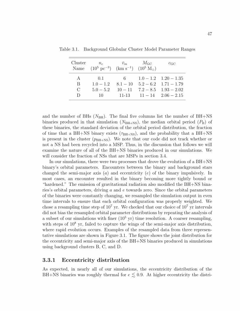
47

Table 3.1. Background Globular Cluster Model Parameter Ranges

Cluster nc vm MGC cGC

Name (105 pc−3) (km s−1) (105 M�)

A 0.1 6 1.0− 1.2 1.20− 1.35B 1.0− 1.2 8.1− 10 5.2− 6.2 1.71− 1.79C 5.0− 5.2 10− 11 7.2− 8.5 1.93− 2.02D 10 11-13 11− 14 2.06− 2.15

and the number of BHs (NBH). The final five columns list the number of BH+NSbinaries produced in that simulation (NBH+NS), the median orbital period (PB) ofthese binaries, the standard deviation of the orbital period distribution, the fractionof time that a BH+NS binary exists (τBH+NS), and the probability that a BH+NSis present in the cluster (pBH+NS). We note that our code did not track whether ornot a NS had been recycled into a MSP. Thus, in the discussion that follows we willexamine the nature of all of the BH+NS binaries produced in our simulations. Wewill consider the fraction of NSs that are MSPs in section 3.4.

In our simulations, there were two processes that drove the evolution of a BH+NSbinary’s orbital parameters. Encounters between the binary and background starschanged the semi-major axis (a) and eccentricity (e) of the binary impulsively. Inmost cases, an encounter resulted in the binary becoming more tightly bound or“hardened.” The emission of gravitational radiation also modified the BH+NS bina-ries’s orbital parameters, driving a and e towards zero. Since the orbital parametersof the binaries were constantly changing, we resampled the simulation output in eventime intervals to ensure that each orbital configuration was properly weighted. Wechose a resampling time step of 107 yr. We checked that our choice of 107 yr intervalsdid not bias the resampled orbital parameter distributions by repeating the analysis ofa subset of our simulations with finer (105 yr) time resolution. A coarser resampling,with steps of 108 yr, failed to capture the wings of the semi-major axis distribution,where rapid evolution occurs. Examples of the resampled data from three represen-tative simulations are shown in Figure 3.1. The figure shows the joint distribution forthe eccentricity and semi-major axis of the BH+NS binaries produced in simulationsusing background clusters B, C, and D.

3.3.1 Eccentricity distribution

As expected, in nearly all of our simulations, the eccentricity distribution of theBH+NS binaries was roughly thermal for e . 0.9. At higher eccentricity the distri-

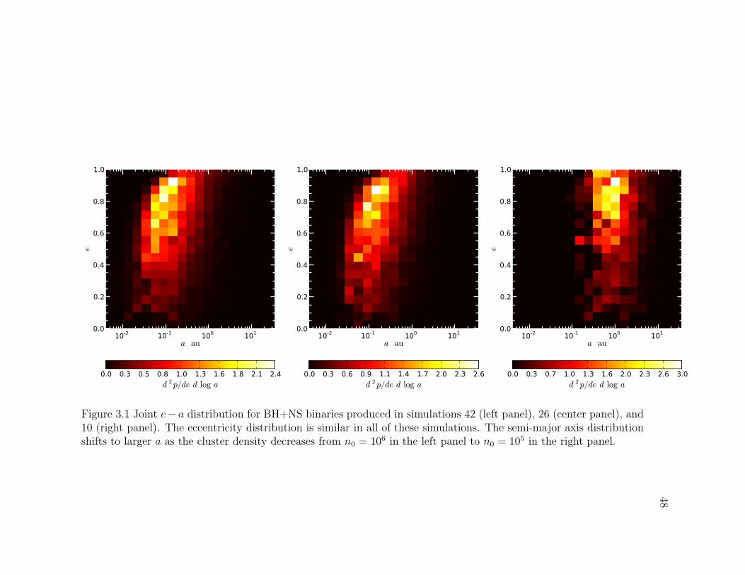
48

10-2 10-1 100 101

a au

0.0

0.2

0.4

0.6

0.8

1.0

e

10-2 10-1 100 101

a au

0.0

0.2

0.4

0.6

0.8

1.0

e

10-2 10-1 100 101

a au

0.0

0.2

0.4

0.6

0.8

1.0

e

0.0 0.3 0.5 0.8 1.0 1.3 1.6 1.8 2.1 2.4

d 2 p/de d log a

0.0 0.3 0.6 0.9 1.1 1.4 1.7 2.0 2.3 2.6

d 2 p/de d log a

0.0 0.3 0.7 1.0 1.3 1.6 2.0 2.3 2.6 3.0

d 2 p/de d log a

Figure 3.1 Joint e− a distribution for BH+NS binaries produced in simulations 42 (left panel), 26 (center panel), and10 (right panel). The eccentricity distribution is similar in all of these simulations. The semi-major axis distributionshifts to larger a as the cluster density decreases from n0 = 106 in the left panel to n0 = 105 in the right panel.

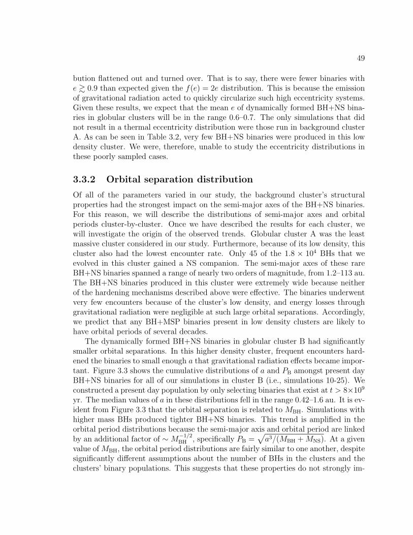
49

bution flattened out and turned over. That is to say, there were fewer binaries withe & 0.9 than expected given the f(e) = 2e distribution. This is because the emissionof gravitational radiation acted to quickly circularize such high eccentricity systems.Given these results, we expect that the mean e of dynamically formed BH+NS bina-ries in globular clusters will be in the range 0.6–0.7. The only simulations that didnot result in a thermal eccentricity distribution were those run in background clusterA. As can be seen in Table 3.2, very few BH+NS binaries were produced in this lowdensity cluster. We were, therefore, unable to study the eccentricity distributions inthese poorly sampled cases.

3.3.2 Orbital separation distribution

Of all of the parameters varied in our study, the background cluster’s structuralproperties had the strongest impact on the semi-major axes of the BH+NS binaries.For this reason, we will describe the distributions of semi-major axes and orbitalperiods cluster-by-cluster. Once we have described the results for each cluster, wewill investigate the origin of the observed trends. Globular cluster A was the leastmassive cluster considered in our study. Furthermore, because of its low density, thiscluster also had the lowest encounter rate. Only 45 of the 1.8 × 104 BHs that weevolved in this cluster gained a NS companion. The semi-major axes of these rareBH+NS binaries spanned a range of nearly two orders of magnitude, from 1.2–113 au.The BH+NS binaries produced in this cluster were extremely wide because neitherof the hardening mechanisms described above were effective. The binaries underwentvery few encounters because of the cluster’s low density, and energy losses throughgravitational radiation were negligible at such large orbital separations. Accordingly,we predict that any BH+MSP binaries present in low density clusters are likely tohave orbital periods of several decades.

The dynamically formed BH+NS binaries in globular cluster B had significantlysmaller orbital separations. In this higher density cluster, frequent encounters hard-ened the binaries to small enough a that gravitational radiation effects became impor-tant. Figure 3.3 shows the cumulative distributions of a and PB amongst present dayBH+NS binaries for all of our simulations in cluster B (i.e., simulations 10-25). Weconstructed a present day population by only selecting binaries that exist at t > 8×109

yr. The median values of a in these distributions fell in the range 0.42–1.6 au. It is ev-ident from Figure 3.3 that the orbital separation is related to MBH. Simulations withhigher mass BHs produced tighter BH+NS binaries. This trend is amplified in theorbital period distributions because the semi-major axis and orbital period are linkedby an additional factor of ∼M

−1/2BH , specifically PB =

√a3/(MBH +MNS). At a given

value of MBH, the orbital period distributions are fairly similar to one another, despitesignificantly different assumptions about the number of BHs in the clusters and theclusters’ binary populations. This suggests that these properties do not strongly im-

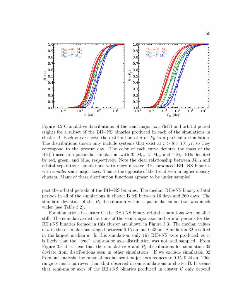
50

10-2 10-1 100 101

a [au]

0.0

0.1

0.2

0.3

0.4

0.5

0.6

0.7

0.8

0.9

1.0f(<a)

MBH =35 M¯MBH =15 M¯MBH =7 M¯

10-1 100 101 102 103 104

PB [day]

0.0

0.1

0.2

0.3

0.4

0.5

0.6

0.7

0.8

0.9

1.0

f(<P

B)

MBH =35 M¯MBH =15 M¯MBH =7 M¯

Figure 3.2 Cumulative distributions of the semi-major axis (left) and orbital period(right) for a subset of the BH+NS binaries produced in each of the simulations incluster B. Each curve shows the distribution of a or PB in a particular simulation.The distributions shown only include systems that exist at t > 8 × 109 yr, so theycorrespond to the present day. The color of each curve denotes the mass of theBH(s) used in a particular simulation, with 35 M�, 15 M�, and 7 M� BHs denotedby red, green, and blue, respectively. Note the clear relationship between MBH andorbital separation: simulations with more massive BHs produced BH+NS binarieswith smaller semi-major axes. This is the opposite of the trend seen in higher densityclusters. Many of these distribution functions appear to be under sampled.

pact the orbital periods of the BH+NS binaries. The median BH+NS binary orbitalperiods in all of the simulations in cluster B fell between 16 days and 260 days. Thestandard deviation of the PB distribution within a particular simulation was muchwider (see Table 3.2).

For simulations in cluster C, the BH+NS binary orbital separations were smallerstill. The cumulative distributions of the semi-major axis and orbital periods for theBH+NS binaries formed in this cluster are shown in Figure 3.3. The median valuesof a in these simulations ranged between 0.15 au and 0.43 au. Simulation 32 resultedin the largest median a. In this simulation, only 167 BH+NS were produced, so itis likely that the “true” semi-major axis distribution was not well sampled. FromFigure 3.3 it is clear that the cumulative a and PB distributions for simulation 32deviate from distributions seen in other simulations. If we exclude simulation 32from our analysis, the range of median semi-major axes reduces to 0.15–0.24 au. Thisrange is much narrower than that observed in our simulations in cluster B. It seemsthat semi-major axes of the BH+NS binaries produced in cluster C only depend

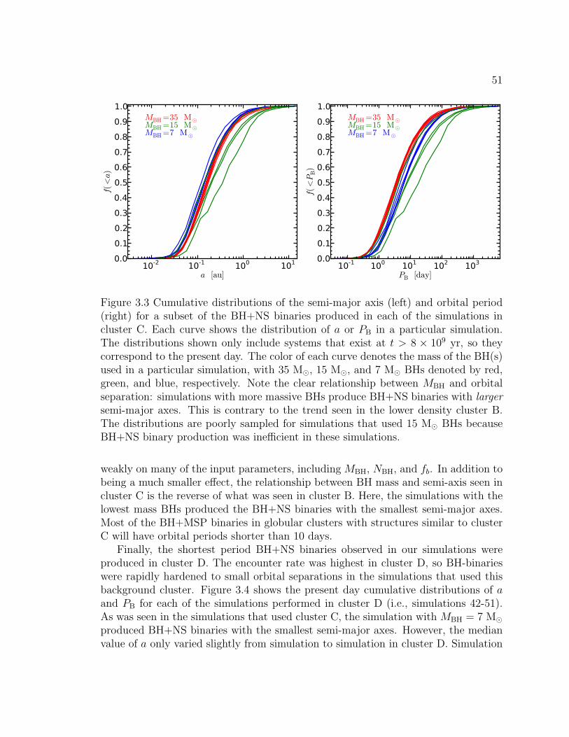
51

10-2 10-1 100 101

a [au]

0.0

0.1

0.2

0.3

0.4

0.5

0.6

0.7

0.8

0.9

1.0f(<a)

MBH =35 M¯MBH =15 M¯MBH =7 M¯

10-1 100 101 102 103

PB [day]

0.0

0.1

0.2

0.3

0.4

0.5

0.6

0.7

0.8

0.9

1.0

f(<P

B)

MBH =35 M¯MBH =15 M¯MBH =7 M¯

Figure 3.3 Cumulative distributions of the semi-major axis (left) and orbital period(right) for a subset of the BH+NS binaries produced in each of the simulations incluster C. Each curve shows the distribution of a or PB in a particular simulation.The distributions shown only include systems that exist at t > 8 × 109 yr, so theycorrespond to the present day. The color of each curve denotes the mass of the BH(s)used in a particular simulation, with 35 M�, 15 M�, and 7 M� BHs denoted by red,green, and blue, respectively. Note the clear relationship between MBH and orbitalseparation: simulations with more massive BHs produce BH+NS binaries with largersemi-major axes. This is contrary to the trend seen in the lower density cluster B.The distributions are poorly sampled for simulations that used 15 M� BHs becauseBH+NS binary production was inefficient in these simulations.

weakly on many of the input parameters, including MBH, NBH, and fb. In addition tobeing a much smaller effect, the relationship between BH mass and semi-axis seen incluster C is the reverse of what was seen in cluster B. Here, the simulations with thelowest mass BHs produced the BH+NS binaries with the smallest semi-major axes.Most of the BH+MSP binaries in globular clusters with structures similar to clusterC will have orbital periods shorter than 10 days.

Finally, the shortest period BH+NS binaries observed in our simulations wereproduced in cluster D. The encounter rate was highest in cluster D, so BH-binarieswere rapidly hardened to small orbital separations in the simulations that used thisbackground cluster. Figure 3.4 shows the present day cumulative distributions of aand PB for each of the simulations performed in cluster D (i.e., simulations 42-51).As was seen in the simulations that used cluster C, the simulation with MBH = 7 M�produced BH+NS binaries with the smallest semi-major axes. However, the medianvalue of a only varied slightly from simulation to simulation in cluster D. Simulation

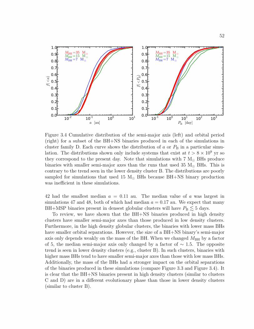
52

10-2 10-1 100 101

a [au]

0.0

0.1

0.2

0.3

0.4

0.5

0.6

0.7

0.8

0.9

1.0f(<a)

MBH =35 M¯MBH =15 M¯MBH =7 M¯

10-1 100 101 102 103

PB [day]

0.0

0.1

0.2

0.3

0.4

0.5

0.6

0.7

0.8

0.9

1.0

f(<P

B)

MBH =35 M¯MBH =15 M¯MBH =7 M¯

Figure 3.4 Cumulative distribution of the semi-major axis (left) and orbital period(right) for a subset of the BH+NS binaries produced in each of the simulations incluster family D. Each curve shows the distribution of a or PB in a particular simu-lation. The distributions shown only include systems that exist at t > 8× 109 yr sothey correspond to the present day. Note that simulations with 7 M� BHs producebinaries with smaller semi-major axes than the runs that used 35 M� BHs. This iscontrary to the trend seen in the lower density cluster B. The distributions are poorlysampled for simulations that used 15 M� BHs because BH+NS binary productionwas inefficient in these simulations.

42 had the smallest median a = 0.11 au. The median value of a was largest insimulations 47 and 48, both of which had median a = 0.17 au. We expect that manyBH+MSP binaries present in densest globular clusters will have PB . 5 days.

To review, we have shown that the BH+NS binaries produced in high densityclusters have smaller semi-major axes than those produced in low density clusters.Furthermore, in the high density globular clusters, the binaries with lower mass BHshave smaller orbital separations. However, the size of a BH+NS binary’s semi-majoraxis only depends weakly on the mass of the BH. When we changed MBH by a factorof 5, the median semi-major axis only changed by a factor of ∼ 1.5. The oppositetrend is seen in lower density clusters (e.g., cluster B). In such clusters, binaries withhigher mass BHs tend to have smaller semi-major axes than those with low mass BHs.Additionally, the mass of the BHs had a stronger impact on the orbital separationsof the binaries produced in these simulations (compare Figure 3.3 and Figure 3.4). Itis clear that the BH+NS binaries present in high density clusters (similar to clustersC and D) are in a different evolutionary phase than those in lower density clusters(similar to cluster B).

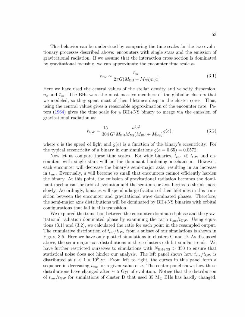
53

This behavior can be understood by comparing the time scales for the two evolu-tionary processes described above: encounters with single stars and the emission ofgravitational radiation. If we assume that the interaction cross section is dominatedby gravitational focusing, we can approximate the encounter time scale as

tenc ∼vm

2πG(MBH +MNS)nca. (3.1)

Here we have used the central values of the stellar density and velocity dispersion,nc and vm. The BHs were the most massive members of the globular clusters thatwe modeled, so they spent most of their lifetimes deep in the cluster cores. Thus,using the central values gives a reasonable approximation of the encounter rate. Pe-ters (1964) gives the time scale for a BH+NS binary to merge via the emission ofgravitational radiation as:

tGW =15

304

a4c5

G3MBHMNS(MBH +MNS)g(e), (3.2)

where c is the speed of light and g(e) is a function of the binary’s eccentricity. Forthe typical eccentricity of a binary in our simulations g(e = 0.65) = 0.0572.

Now let us compare these time scales. For wide binaries, tenc � tGW and en-counters with single stars will be the dominant hardening mechanism. However,each encounter will decrease the binary’s semi-major axis, resulting in an increasein tenc. Eventually, a will become so small that encounters cannot efficiently hardenthe binary. At this point, the emission of gravitational radiation becomes the domi-nant mechanism for orbital evolution and the semi-major axis begins to shrink moreslowly. Accordingly, binaries will spend a large fraction of their lifetimes in this tran-sition between the encounter and gravitational wave dominated phases. Therefore,the semi-major axis distributions will be dominated by BH+NS binaries with orbitalconfigurations that fall in this transition.

We explored the transition between the encounter dominated phase and the grav-itational radiation dominated phase by examining the ratio tenc/tGW. Using equa-tions (3.1) and (3.2), we calculated the ratio for each point in the resampled output.The cumulative distribution of tenc/tGW from a subset of our simulations is shown inFigure 3.5. Here we have only plotted simulations in clusters C and D. As discussedabove, the semi-major axis distributions in these clusters exhibit similar trends. Wehave further restricted ourselves to simulations with NBH+NS > 350 to ensure thatstatistical noise does not hinder our analysis. The left panel shows how tenc/tGW isdistributed at t < 1 × 109 yr. From left to right, the curves in this panel form asequence in decreasing tenc for a given value of a. The center panel shows how thesedistributions have changed after ∼ 5 Gyr of evolution. Notice that the distributionof tenc/tGW for simulations of cluster D that used 35 M� BHs has hardly changed.

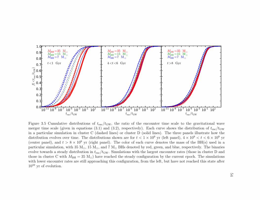
54

10-11 10-9 10-7 10-5 10-3 10-1 101

tenc/tGW

0.0

0.1

0.2

0.3

0.4

0.5

0.6

0.7

0.8

0.9

1.0

f(<t e

nc/t G

W)

MBH =35 M¯MBH =15 M¯MBH =7 M¯

t <1 Gyr

10-11 10-9 10-7 10-5 10-3 10-1 101

tenc/tGW

MBH =35 M¯MBH =15 M¯MBH =7 M¯

4<t<6 Gyr

10-11 10-9 10-7 10-5 10-3 10-1 101

tenc/tGW

MBH =35 M¯MBH =15 M¯MBH =7 M¯

t >8 Gyr

Figure 3.5 Cumulative distributions of tenc/tGW, the ratio of the encounter time scale to the gravitational wavemerger time scale (given in equations (3.1) and (3.2), respectively). Each curve shows the distribution of tenc/tGW

in a particular simulation in cluster C (dashed lines) or cluster D (solid lines). The three panels illustrate how thedistribution evolves over time. The distributions shown are for t < 1 × 109 yr (left panel), 4 × 109 < t < 6 × 109 yr(center panel), and t > 8 × 109 yr (right panel). The color of each curve denotes the mass of the BH(s) used in aparticular simulation, with 35 M�, 15 M�, and 7 M� BHs denoted by red, green, and blue, respectively. The binariesevolve towards a steady distribution in tenc/tGW. Simulations with the largest encounter rates (those in cluster D andthose in cluster C with MBH = 35 M�) have reached the steady configuration by the current epoch. The simulationswith lower encounter rates are still approaching this configuration, from the left, but have not reached this state after1010 yr of evolution.

55

The distributions in all of the other simulations, with lower encounter rates, evolvedtowards these stationary curves. The right panel shows how tenc/tGW is distributed atthe present day, after an additional ∼ 3 Gyr of evolution. All of the tenc/tGW distribu-tions from simulations in cluster D (solid lines) lie on top of one another. Simulationsin cluster C (dashed lines) that used MBH = 35 M� also closely follow this trend,while the simulations with lower mass BHs exhibit smaller values of tenc/tGW.

We interpret this evolution as follows. Given sufficient time, the distributionof tenc/tGW in all clusters will approach the steady configuration seen in the rightpanel of Figure 3.5. At this stage, the orbital evolution of most of the BH+NSbinaries has slowed as they make the transition from the encounter dominated phaseto the gravitational radiation dominated phase. The median value of tenc/tGW inthis steady configuration is ∼ 2 × 10−3. Even though tenc is still a few orders ofmagnitude smaller than tGW at this point, this ratio corresponds to the beginning oftransition between the encounter and gravitational wave dominated phases. Giventhe steep dependance of tGW on a, such binary is only about one encounter awayfrom an orbit in which tenc ∼ tGW. We note that despite the similarities illustrated inFigure 3.5, the tenc/tGW distributions from each simulation are formally distinct fromone another, in most cases. We performed the two-sample Kolmogorov-Smirnov testbetween each pair of distributions and found that only those from simulations 44,45, and 46 were consistent with coming from the same parent distribution. However,our interpretation does not require that the distributions be identical, it only requiresthat each distribution is dominated by systems that are in the transition phase.Since the binaries evolve towards a constant configuration in tenc/tGW, we can useequations (3.1) and (3.2) and derive a scaling relation for the median semi-major axisof the BH+NS binaries during this phase:

a ∝(MBHMNSvm

nc

)1/5

. (3.3)

In deriving this expression we have also assumed that g(e) does not vary from clusterto cluster, which is justified because the eccentricity distributions in every simulationwere similar (see section 3.3.1). Many facets of this scaling relation are seen in thesemi-major axis distributions from simulations computed in clusters C and D. Mostimportantly this scaling relation accounts for the rather weak dependance of the thesesemi-major axis distributions on many of the input parameters. The relation alsoaccounts for the fact that the runs with lower mass BHs produced BH+NS binarieswith smaller semi-major axes.

Most of our simulations did not evolve to the steady tenc/tGW distribution de-scribed above. In clusters with low encounter rates (1/tenc), many of the BH+NSbinaries will not be hardened fast enough to reach the transition from the encounterdominated regime to the gravitational radiation dominated regime within a Hubble

56

time. Therefore, the orbital parameters of most BH+NS binaries in these clusters aredetermined by binary–single encounters alone. Accordingly, we expect that the semi-major axes of the binaries in these clusters will follow a different scaling relationshipthan those in the high density cluster. Since each encounter will reduce a, binarieswith shorter encounter times will have smaller semi-major axes. This is what weobserved in simulations in cluster B; the binaries with higher mass BHs had smallertenc, and were hardened to smaller a than the binaries with low mass BHs.

3.4 BH+MSP Binary Population Size

The 51 simulations presented in this chapter investigated how several parametersimpact the dynamical formation of BH+NS binaries in globular clusters. Below wewill describe how each of these traits affects the likelihood that a BH+NS binaryexists within a cluster. We will use two metrics to characterize the likelihood thata cluster harbors a BH+NS binary. The first metric is the fraction of time that theBHs in our simulations had a NS companion, τBH+NS = tBH+NS/(Nrunstmax). HeretBH+NS is the sum of the time that a BH had a NS companion during all of the runsin a particular simulation, tmax = 1010 yr is the duration of each run, and Nruns is thenumber of runs in a simulation. As was the case in chapter 2, Nruns is slightly less than2000 because we rejected a small number of runs in which the initial BH-binary wasrandomly selected to contain a NS. The second metric that we use is the probabilitythat a cluster contains a BH+NS binary pBH+NS = NBHτBH+NS. In simulations withmultiple BHs, τBH+NS corresponds to the probability that any one of these BHs hasa NS companion, and must therefore be scaled by NBH to find the probability thata BH+NS binary exists in the cluster. The values of these metrics for each of oursimulations are listed in Table 3.2.

As was the case with the orbital parameter distributions, the structure of thebackground globular cluster had a large impact on the values of τBH+NS. In clusterA (nc = 104 pc−3), the BH+NS binaries had a mean lifetime of 7× 109 yr. However,because of the low encounter rate, these binaries were produced so rarely that τBH+NS.2× 10−3 in every simulation in this cluster. Simulations in cluster D (nc = 106 pc−3)had the opposite problem. The BH+NS binaries in this cluster were rapidly drivento coalescence because of the high encounter rate. The intermediate encounter ratesin clusters B (nc = 105 pc−3) and C (nc = 5 × 105 pc−3) struck a balance betweenthe production and destruction of BH+NS binaries. All other parameters held equal,simulations in clusters B or C had the largest values of τBH+NS. The BHs in theseclusters typically spent a few percent of their lifetimes with a NS companion.

The amount of time that the BHs in our simulations had NS companions decreasedwith increasing MBH. Both of the evolutionary processes that drive the BH+NSbinaries to merge speed up when the mass of the BH is increased. A more massiveBH leads to a larger gravitational focusing cross-section, which increases the encounter

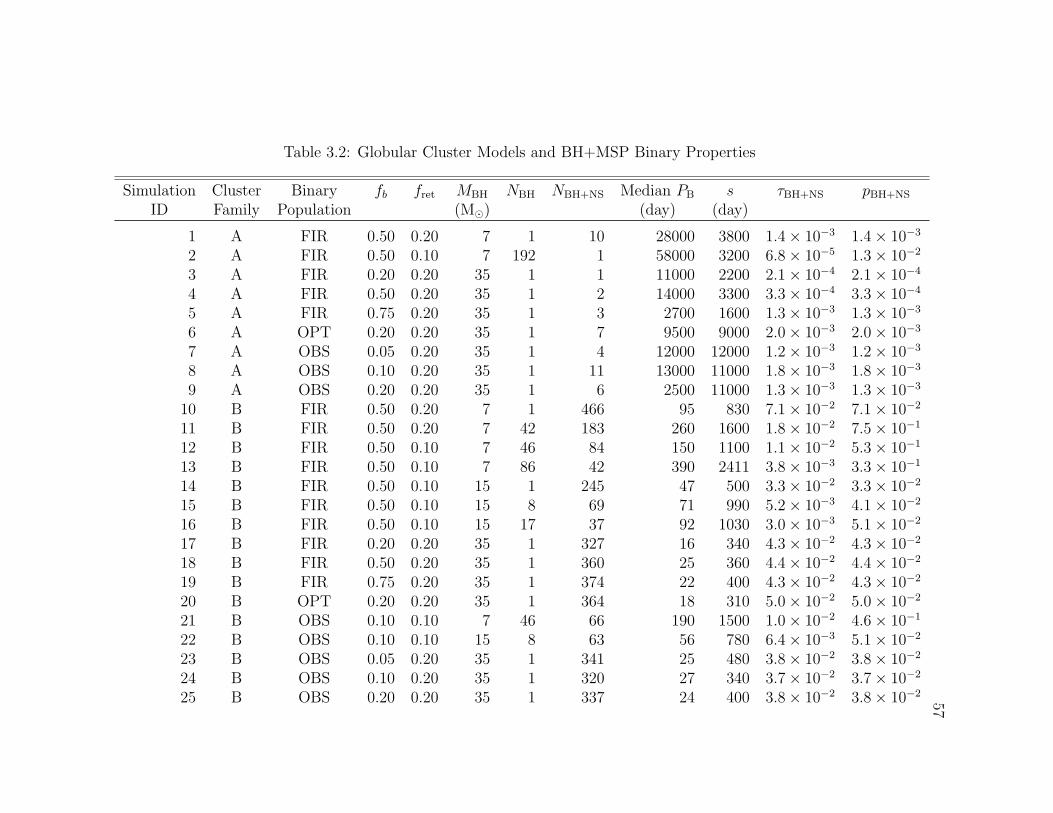
57

Table 3.2: Globular Cluster Models and BH+MSP Binary Properties

Simulation Cluster Binary fb fret MBH NBH NBH+NS Median PB s τBH+NS pBH+NS

ID Family Population (M�) (day) (day)

1 A FIR 0.50 0.20 7 1 10 28000 3800 1.4× 10−3 1.4× 10−3

2 A FIR 0.50 0.10 7 192 1 58000 3200 6.8× 10−5 1.3× 10−2

3 A FIR 0.20 0.20 35 1 1 11000 2200 2.1× 10−4 2.1× 10−4

4 A FIR 0.50 0.20 35 1 2 14000 3300 3.3× 10−4 3.3× 10−4

5 A FIR 0.75 0.20 35 1 3 2700 1600 1.3× 10−3 1.3× 10−3

6 A OPT 0.20 0.20 35 1 7 9500 9000 2.0× 10−3 2.0× 10−3

7 A OBS 0.05 0.20 35 1 4 12000 12000 1.2× 10−3 1.2× 10−3

8 A OBS 0.10 0.20 35 1 11 13000 11000 1.8× 10−3 1.8× 10−3

9 A OBS 0.20 0.20 35 1 6 2500 11000 1.3× 10−3 1.3× 10−3

10 B FIR 0.50 0.20 7 1 466 95 830 7.1× 10−2 7.1× 10−2

11 B FIR 0.50 0.20 7 42 183 260 1600 1.8× 10−2 7.5× 10−1

12 B FIR 0.50 0.10 7 46 84 150 1100 1.1× 10−2 5.3× 10−1

13 B FIR 0.50 0.10 7 86 42 390 2411 3.8× 10−3 3.3× 10−1

14 B FIR 0.50 0.10 15 1 245 47 500 3.3× 10−2 3.3× 10−2

15 B FIR 0.50 0.10 15 8 69 71 990 5.2× 10−3 4.1× 10−2

16 B FIR 0.50 0.10 15 17 37 92 1030 3.0× 10−3 5.1× 10−2

17 B FIR 0.20 0.20 35 1 327 16 340 4.3× 10−2 4.3× 10−2

18 B FIR 0.50 0.20 35 1 360 25 360 4.4× 10−2 4.4× 10−2

19 B FIR 0.75 0.20 35 1 374 22 400 4.3× 10−2 4.3× 10−2

20 B OPT 0.20 0.20 35 1 364 18 310 5.0× 10−2 5.0× 10−2

21 B OBS 0.10 0.10 7 46 66 190 1500 1.0× 10−2 4.6× 10−1

22 B OBS 0.10 0.10 15 8 63 56 780 6.4× 10−3 5.1× 10−2

23 B OBS 0.05 0.20 35 1 341 25 480 3.8× 10−2 3.8× 10−2

24 B OBS 0.10 0.20 35 1 320 27 340 3.7× 10−2 3.7× 10−2

25 B OBS 0.20 0.20 35 1 337 24 400 3.8× 10−2 3.8× 10−2

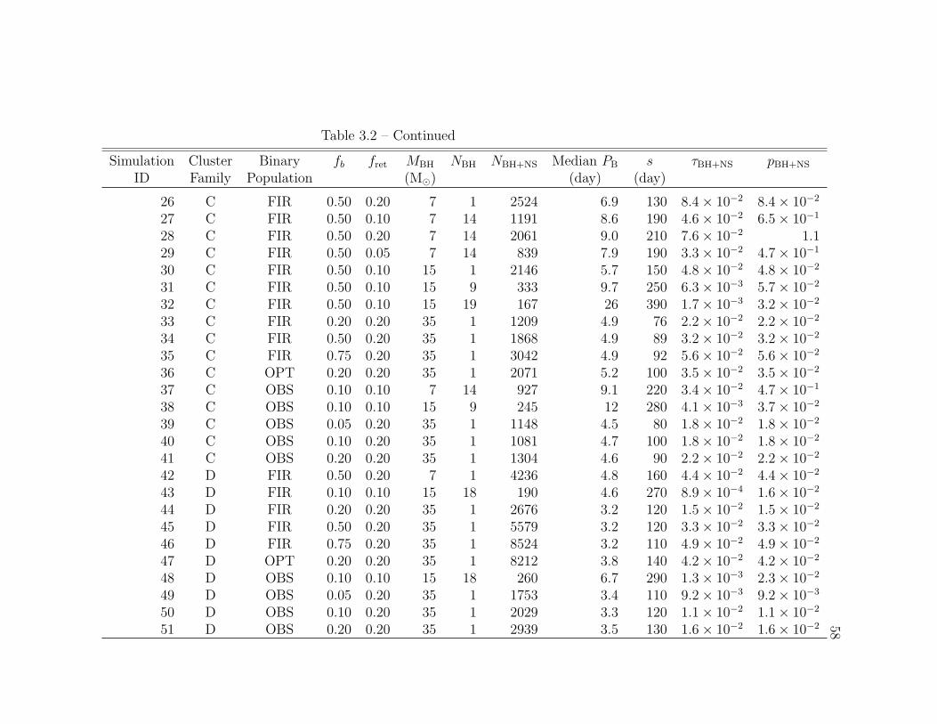
58

Table 3.2 – Continued

Simulation Cluster Binary fb fret MBH NBH NBH+NS Median PB s τBH+NS pBH+NS

ID Family Population (M�) (day) (day)

26 C FIR 0.50 0.20 7 1 2524 6.9 130 8.4× 10−2 8.4× 10−2

27 C FIR 0.50 0.10 7 14 1191 8.6 190 4.6× 10−2 6.5× 10−1

28 C FIR 0.50 0.20 7 14 2061 9.0 210 7.6× 10−2 1.129 C FIR 0.50 0.05 7 14 839 7.9 190 3.3× 10−2 4.7× 10−1

30 C FIR 0.50 0.10 15 1 2146 5.7 150 4.8× 10−2 4.8× 10−2

31 C FIR 0.50 0.10 15 9 333 9.7 250 6.3× 10−3 5.7× 10−2

32 C FIR 0.50 0.10 15 19 167 26 390 1.7× 10−3 3.2× 10−2

33 C FIR 0.20 0.20 35 1 1209 4.9 76 2.2× 10−2 2.2× 10−2

34 C FIR 0.50 0.20 35 1 1868 4.9 89 3.2× 10−2 3.2× 10−2

35 C FIR 0.75 0.20 35 1 3042 4.9 92 5.6× 10−2 5.6× 10−2

36 C OPT 0.20 0.20 35 1 2071 5.2 100 3.5× 10−2 3.5× 10−2

37 C OBS 0.10 0.10 7 14 927 9.1 220 3.4× 10−2 4.7× 10−1

38 C OBS 0.10 0.10 15 9 245 12 280 4.1× 10−3 3.7× 10−2

39 C OBS 0.05 0.20 35 1 1148 4.5 80 1.8× 10−2 1.8× 10−2

40 C OBS 0.10 0.20 35 1 1081 4.7 100 1.8× 10−2 1.8× 10−2

41 C OBS 0.20 0.20 35 1 1304 4.6 90 2.2× 10−2 2.2× 10−2

42 D FIR 0.50 0.20 7 1 4236 4.8 160 4.4× 10−2 4.4× 10−2

43 D FIR 0.10 0.10 15 18 190 4.6 270 8.9× 10−4 1.6× 10−2

44 D FIR 0.20 0.20 35 1 2676 3.2 120 1.5× 10−2 1.5× 10−2

45 D FIR 0.50 0.20 35 1 5579 3.2 120 3.3× 10−2 3.3× 10−2

46 D FIR 0.75 0.20 35 1 8524 3.2 110 4.9× 10−2 4.9× 10−2

47 D OPT 0.20 0.20 35 1 8212 3.8 140 4.2× 10−2 4.2× 10−2

48 D OBS 0.10 0.10 15 18 260 6.7 290 1.3× 10−3 2.3× 10−2

49 D OBS 0.05 0.20 35 1 1753 3.4 110 9.2× 10−3 9.2× 10−3

50 D OBS 0.10 0.20 35 1 2029 3.3 120 1.1× 10−2 1.1× 10−2

51 D OBS 0.20 0.20 35 1 2939 3.5 130 1.6× 10−2 1.6× 10−2

59

rate. Furthermore, orbital energy is lost more rapidly through gravitational radiationwhen MBH increases.

The assumed background binary population did not influence τBH+NS in clustersA and B. In these clusters mergers and disruptive encounters rarely occurred. Ac-cordingly, there were few single BHs in these clusters that needed to interact withthe background binary population to acquire a new companion. In clusters C and D,on the other hand, the nature of the background binary population had a substantialinfluence on τBH+NS. In both clusters it appears that there is a threshold aroundfb ∼ 0.2. Simulations with fb < 0.2 all exhibit similar values of τBH+NS. At larger fb,τBH+NS increases as ∼ f 2

b . The composition of the binary population does not seem toimpact the results much. As we explained in section 2.3.2, the main advantage of theFIR population over the OBS population is that it allows for larger binary fractionswithin observational constraints. At the same value of fb, simulations using the FIRpopulation and the OBS population produce BH+NS binaries with equal efficiency.Use of the OPT population did, however, lead to larger τBH+NS. in clusters B, C, andD.

The runs presented in this chapter also explored how changing the size of theNS and BH populations impacted the formation of BH+NS binaries. The value ofτBH+NS responded linearly to changes in the NS retention fraction (fret). In every runwith NBH > 1, the increased size of the BH population lead to a reduction in the valueof τBH+NS. When there was more than one BH in the simulation, it was common forthe BH-binaries that we were evolving to interact with the other BHs in the cluster.Nearly half of all three-body encounters between a BH+star binary and a second BHwill result in the formation of a BH+BH binary (Sigurdsson & Phinney 1993). Oncea BH+BH binary formed, it was nearly impossible for a NS to exchange into thesystem. These BHs were essentially locked up for the rest of the run, leading to thereduction in τBH+NS. In addition to preventing the formation of BH+NS binaries,the presence of several BHs can also result in the destruction of BH+NS binaries.In our runs with multiple BHs, 10-50% of BH+NS binaries were destroyed whenanother BH exchanged into the binary. For relatively small BH populations the valueof pBH+NS increased compared to simulations with a single BH. In these simulationsthe small decline in τBH+NS was outpaced by increase in NBH. However, pBH+NS issubject to the law of diminishing returns. Comparing simulations 14, 15, and 16, wesee that pBH+NS increases as we add more BHs to the cluster. Extrapolating the trendseen in τBH+NS to larger values of NBH, we find that increasing NBH to 100 will onlyboost the probability that this cluster harbors a BH+NS binary from 0.051 to 0.06.Of course, one should use caution in drawing conclusions from such an extrapolation,but it seems unlikely that the presence of a substantial BH population would increasethe size of a cluster’s BH+NS binary population. In fact, such a large number of BHscould reduce the size of the BH+NS binary population. This behavior is seen in someof our simulations. In simulations 12 & 13 and 31 & 32 an increase in NBH resulted

60

in a reduction of pBH+NS. When there were many BHs in a cluster, the production ofBH+BH binaries was favored over the production of BH+NS binaries.

Combining all of the effects described above, we conclude that the probabilityof finding a BH+MSP binary is highest in massive globular clusters with nc ∼few × 105 pc−3, fb & 0.2, and BH populations that comprise a few dozen ∼ 10 M�BHs. We can estimate the number of BH+MSP binaries in the Milky Way globularcluster system as:

NBH+MSP = NGC fGC fMSP fBH pBH+NS, (3.4)

where, following Narayan et al. (1991), we have implicitly assumed that the lifetime ofa MSP is > 1010 yr. Here NGC = 150 is the number of globular clusters in the MilkyWay. The fraction of globular clusters with structural properties similar to thoseused in our simulations is denoted fGC. Approximately 15 − 20% of the Milky Wayglobular clusters have nc ∼ 105 pc−3, MGC = several× 105 M�, and 1.7 < cGC < 2.0(Harris 1996; Gnedin & Ostriker 1997). We gauged the fraction of NSs that havebeen recycled into MSPs, fMSP, using observational constraints on the total numberof MSPs in 47 Tuc and Terzan 5. Abdo et al. (2010) used the integrated gamma-rayflux emitted by these clusters to estimate the number of MSPs, finding that 47 Tucharbors 33+15

−15 MSPs and Terzan 5 contains 180+100−100. Using radio measurements, the

total numbers of MSPs in 47 Tuc and Terzan 5 have been estimated to be 163+108−70

and 294+224−130, respectively (Chennamangalam et al. 2013). Assuming that each of these

clusters retains a total of 500-1000 NSs, we estimate that fMSP is between 5% and30% (Pfahl et al. 2002; Ivanova et al. 2008). The fraction of globular clusters thatretain at least one BH, fBH , is poorly constrained by observations. However, we canplace an upper limit on the number of BH+MSP binaries by assuming that everymassive globular cluster retains a BH population. If we further assume the maximumreasonable value for every factor in equation (3.4), we find that the upper limit for thenumber of BH+MSP binaries in the Milky Way globular cluster system is 10. Herewe have used the value of pBH+NS = 1.1 computed in simulation 28. The number ofdetectable BH+MSP binaries is a factor of 2–3 smaller due to beaming effects. Theupper limit on the number of dynamically formed BH+MSP binaries presented hereis similar to the number of BH+MSP binaries expected to form through the evolutionof isolated binaries (Sipior et al. 2004; Pfahl et al. 2005).

We also estimated the total number of BH+MSP binaries by generating severalMonte Carlo realizations of the Milky Way globular cluster population and countingthe number of BH+MSP binaries in each realization. In these models we used NGC =150. The mass of each cluster was drawn from the globular cluster mass functionpresented in McLaughlin & Pudritz (1996). We then assigned each cluster a pBH+NS byrandomly selecting one of our simulations that was done in a globular cluster ofsimilar mass. Next, we chose fMSP for each cluster from a normal distribution with amean of 0.13 and a standard deviation of 0.07. Based on 104 realizations, we foundNBH+MSP = fBH 0.6 ± 0.2. In computing this number we assumed that the size of

61

each globular cluster’s BH population was random. It is possible that the sizes ofthe BH populations are correlated, i.e., the globular clusters that retain BHs eitherall retain several or all retain ∼ 1. If we recompute our Monte Carlo realizationsand require that NBH > 1, then we find NBH+MSP = fBH 1.3 ± 0.3. If we onlyconsider simulations that used NBH = 1, the size of the BH+MSP binary populationis reduced to NBH+MSP = fBH 0.2 ± 0.1. We have not accounted for the fact thatmany components of these estimates, (e.g., NBH, fBH, and fMSP) are likely to befunctions of the globular clusters’ structural parameters. However, it is unlikely thatincluding these dependancies will significantly alter our conclusion that NBH+MSP . 1.Unfortunately, it appears that dynamically formed BH+MSP binaries in globularclusters may be even rarer than those produced through standard binary evolutionin the disk of the Galaxy.

3.5 Discussion

We have presented a study of the dynamically formed BH+MSP binaries in globularclusters. We found that in the highest density clusters (nc & 5 × 105 pc−3), thesemi-major axis distribution of the BH+MSP binaries is nearly independent of allof the parameters that we varied in our study. This property of the BH+NS binarypopulations is beneficial for observes who hope to identify such systems. Regardlessof the nature of many uncertain characteristics, including the globular cluster BHand binary populations, the vast majority of BH+MSP binaries produced in denseglobular clusters will have 2 < PB < 10 days. In lower density clusters, MBH doesinfluence the expected orbital periods of the BH+MSP binaries. In clusters withnc ∼ 105 pc−3 BH+MSP binaries with massive stellar mass BHs (MBH = 35 M�)will typically have orbital periods around 20 days. For BH+MSP binaries with 7 M�BHs, the expected orbital periods are much longer, with typical periods in the 150 to250 day range.

Unfortunately, we have also found that dynamically formed BH+MSP binaries arequite rare. We estimated that the maximum number of detectible BH+MSP binariesin the Milky Way globular cluster system is 5. This result is not a consequence of theassumption that most stellar mass black holes are ejected from the cluster early inits evolution. The presence of a large BH population will also reduce the probabilitythat a cluster harbors a BH+MSP binary. BH+MSP binary formation can be stifledby as few as 19 BHs. If there are several BHs in the cluster the BHs will preferentiallyinteract with each other and not the NSs. Furthermore, any BH+NS binaries that areformed may be destroyed when another BH exchanges into the binary. This behaviorhas also been seen in models that considered the evolution of the BH population as awhole. Sadowski et al. (2008) and Downing et al. (2010) found that very few BH+NSbinaries were produced in their simulations, which included several hundred to overone thousand BHs. We expect dynamically formed BH+MSP binaries to be rare

62

regardless of the size of the retained BH population.Some of the limitations of our method will impact the results of our simulations.

Because our simulations do not include binary–binary encounters, they do not captureseveral processes that affect the formation of BH+MSP binaries. As discussed above,binary–binary interactions open up additional BH+NS binary formation channels.Furthermore, in clusters with multiple BHs, collisions between pairs of BH+BH bina-ries could eject or disrupt many BH+BH binaries (e.g. O’Leary et al. 2006; Banerjeeet al. 2010; Downing et al. 2010). Reducing the number of BHs in the cluster andfreeing BHs from otherwise impenetrable BH+BH binaries would increase the like-lihood that BH+MSP binary is produced. However, binary–binary interactions willalso disrupt and eject BH+MSP binaries. As we concluded in section 2.4.1, modelsthat include binary–binary interactions are needed to see which processes dominate.Finally, as a consequence of our assumption that the background cluster was static,we forced the BHs to remain in equilibrium with the rest of the cluster. If we hadallowed for the dynamical evolution of the BHs, they might have decoupled fromthe rest of the cluster. This would have further reduced the number of encountersbetween BHs and NSs.

Although the number of BH+MSP binaries in the Milky Way globular clustersystem is expected to be small, searching for these binaries is still feasible. We knowthat these binaries are in globular clusters, and our models make specific predictionsabout the types of globular clusters that are likely to harbor BH+MSP binaries.Given the potential scientific payoff, deep radio observations of the cores of the ∼ 20Milky Way globular clusters with appropriate structural properties may be justified.Likely BH+MSP binary hosts include 47 Tuc, Terzan 5, NGC 1851, NGC 6266, andNGC 6441. Finally, even though there might not be any BH+MSP binaries in theMilky Way globular cluster system, such binaries could be detected in extra-galacticglobular clusters with the Square Kilometer Array (SKA). SKA should be able todetect most pulsars within 10 Mpc (Cordes 2007), and our models predict therecould be ∼ 100 dynamically formed BH+MSPs binaries within this volume.

Chapter 4

Emission Lines From the Photoionized Debris of

Tidally Disrupted, Evolved Stars

The work presented in this chapter appeared in Clausen, D., & Eracleous, M. 2011,ApJ, 726, 34 and Clausen, D., Sigurdsson, S., Eracleous, M., & Irwin, J. A. 2012,MNRAS, 424, 1268

4.1 Introduction

A star is tidally disrupted when its orbit brings it too close to a black hole (BH).If the two bodies are separated by less than the tidal disruption radius, RT ∼R?(MBH/M?)

1/3, where R? is the radius of the star and MBH and M? are the massesof the BH and star, respectively, the star is ripped apart because the tidal forceacross its diameter exceeds its self gravity. Frank & Rees (1976) calculated the rateat which a BH in the core of a globular cluster or galaxy would disrupt and ingestmain sequence (MS) stars and suggested that the associated ultraviolet (UV)/X-rayflare would mark the presence of an otherwise undetectable BH. This is possible be-cause after the star is disrupted, about half of the debris becomes bound to the BH.As this bound gas falls back towards the BH, shocks and accretion onto the BHproduce a luminous flare that peaks in the UV/X-ray (Lacy et al. 1982; Rees 1988;Ulmer 1999). A number of analytic (e.g., Phinney 1989; Kochanek 1994; Khokhlov& Melia 1996; Strubbe & Quataert 2009) and numerical (e.g., Evans & Kochanek1989; Laguna et al. 1993; Khokhlov et al. 1993; Bogdanovic et al. 2004; Guillochon& Ramirez-Ruiz 2013) studies have explored the behavior of the debris after a MSstar is tidally disrupted and the feasibility of using the luminosity and evolution ofthe flare to search for and determine properties of the BH. Others have proposedflares and possible detonation of the star due to tidal compression as an additionalobservable consequence of tidal disruptions (Carter & Luminet 1982, 1983; Bicknell& Gingold 1983; Luminet & Marck 1985; Kobayashi et al. 2004). Recent work alongthese lines suggests that the compression will produce shocks capable of raising thestar’s surface temperature to that of its core, resulting in a prompt flare (Guillochon

63

64

et al. 2009; Brassart & Luminet 2008, 2010).Detailed models have also been employed to predict the rate at which MS stars

are tidally disrupted by supermassive BHs. However, uncertainties in the supermas-sive BH mass spectrum, the stellar distribution function in galactic bulges, and therelation between the two complicate calculations of this rate. For example, improvedmeasurements of the mean ratio of BH mass to bulge mass made between the studiesconducted by Magorrian & Tremaine (1999) and Wang & Merritt (2004) resulted ina factor of ten increase in the predicted event rate, raising it to ∼ 10−5 yr−1 Mpc−3.This rate is constrained by systematic surveys for tidal disruption flares. Historically,around ten candidate tidal disruptions were first identified by serendipitous obser-vations of UV/X-ray flares in surveys (e.g., Grupe et al. 1995; Brandt et al. 1995;Komossa & Bade 1999; Komossa & Greiner 1999; Gezari et al. 2006; Cappelluti et al.2009; Maksym et al. 2010). Follow up observations of the variability of these sourcesruled out other explanations and confirmed that the luminosity of the sources de-clined with the same t−5/3 time dependance that models predict for the decline inthe mass fallback rate (Halpern et al. 2004; Esquej et al. 2008). Subsequent studieshave discovered additional tidal disruption candidates and, by accounting for the ef-ficiency and sky coverage of the surveys, determined that supermassive BHs tidallydisrupt MS stars at a rate consistent with 10−5 − 10−4 yr−1 galaxy−1 (Donley et al.2002; Gezari et al. 2008, 2009; Esquej et al. 2008; Luo et al. 2008). The high energyaccretion flares are the brightest and most immediate sign of a MS star being tidallydisrupted by a BH, but they are not the only sign.

In addition to the UV/X-ray emission, Roos (1992) proposed that the unboundportion of the debris can be photoionized and produce optical emission lines. Thenature of the optical emission lines was explored in detail in the numerical models ofBogdanovic et al. (2004) and the analytic models developed by Strubbe & Quataert(2009, hereafter SQ09). In each of these studies, the source of the ionizing photons isthe accretion flare. The prospect of optical emission from tidal disruptions is excitingfor the following reasons. First, SQ09 showed that tidal disruptions are bright enoughin the optical band that they are potential sources for large transient surveys (e.g. TheLarge Synoptic Survey Telescope, The Palomar Transient Factory, and Pan-STARS),which suggests that the number of detected candidate events will increase in thenear future. Second, the emission-line signature of such an event helps us identify itsnature and distinguish it from other, more common transients that can occur nearthe nuclei of galaxies, such as supernovae.

While flares from tidally disrupted MS stars might be a more frequent probe ofdormant BHs in dense stellar systems, Sigurdsson & Rees (1997) pointed out thatthese BHs can capture compact objects as well because this region is also populatedwith the products of stellar evolution. In particular, white dwarfs (WDs) are alsosubject to the processes that drive MS stars into orbits around the central BH withpericenter distancesRp < RT, and can therefore be tidally disrupted as well. However,

65

since the mass of a WD is comparable to that of a low mass MS star and its radius issmaller by a factor of ∼ 100, RT is much closer to the BH for a WD than for a MS star.Consequently, if MBH & 5×105 M�, RT for a WD is inside of the BH’s Schwarzschildradius, RS = 2GMBH/c

2. When RT ≤ RS, the WD plunges into the BH horizonbefore being tidally disrupted, making such events undetectable by electromagneticobservations. This makes WD tidal disruptions an excellent indicator of the presenceof an IMBH in the center of a galaxy or globular cluster, because if the central BHwere more massive than ∼ 105 M� we would not observe anything.

Like the MS case, using WD tidal disruption events to probe IMBHs requires priortheoretical studies to determine how the observed flares are related to the properties ofthe WD-IMBH system. While this scenario has not received as much attention as theMS case, the early stages of the tidal disruption of a WD in an unbound orbit aroundan IMBH were studied numerically by Frolov et al. (1994), who found that materialflowed away from the WD in supersonic jets as it was disrupted. Rosswog et al.(2009) followed the evolution of the debris further and found that gas returns to theBH at a rate that is sufficient to power an accretion flare at the Eddington luminosity,LEdd = 1.3 × 1041(MBH/103M�) erg s−1, for up to one year. Additionally, since it issupported by degeneracy pressure, when Rp . 0.5RT the tidal compression of the WDcan lead to explosive nuclear burning (Luminet & Pichon 1989; Rosswog et al. 2009).The latter authors found that, in the most favorable cases, the energy generated bythermonuclear burning during the compression phase exceeds the binding energy ofthe WD and is similar to that of a Type Ia supernova. However, if the WD does notpenetrate too deeply within RT, the case is similar to that of the tidally disruptedMS stars described above, in which a portion of the debris is accreted by the BH andthe rest of the material remains unbound and flows away from the BH. Sesana et al.(2008) calculated the light curves of optical and near-UV emission lines producedwhen the unbound debris is photoionized by the accretion flare and proposed theselines might be an electromagnetic counterpart to the gravitational radiation emittedas a WD initially on a bound orbit spirals into the IMBH. Here, we revise and updatethese results by considering the case of a WD initially on an unbound orbit and usinga more sophisticated model for the behavior of the debris.

Interestingly, there are two extragalactic globular clusters that exhibit both hall-marks of a tidal disruption event, a bright X-ray source and bright optical emissionlines. One of these sources, in the globular cluster RZ 2109, associated with NGC4472, undergoes large luminosity variations that suggest that the accretor is a BH(Maccarone et al. 2007). Optical spectroscopy of the globular cluster hosting thissource revealed an extremely broad [O III] λ5007 emission line with a luminosityL = 1.4 × 1037 erg s−1, but did not detect any hydrogen emission lines (Zepf et al.2008). The other source, in a globular cluster associated with NGC 1399, has a softerspectrum than typical ultraluminous X-ray sources, which suggests that it is alsolikely to be an accreting BH (Irwin et al. 2010). An optical spectrum of the host

66

globular cluster showed [O III] λ5007 and [N II] λ6583 emission lines, each with L ∼few ×1036 erg s−1. Intriguingly, there are no hydrogen lines in this spectrum either.Irwin et al. (2010) suggested that the high X-ray luminosities and peculiar emissionline spectra seen in these globular clusters could be evidence of WD tidal disruptionevents. The absence of hydrogen emission lines in each source may indicate that thematerial producing the lines has the same composition as an evolved star. However,models are necessary to determine if these lines could be produced in the debris of atidally disrupted star.

In this chapter we will model the emission lines produced when a WD or horizontalbranch (HB) star is tidally disrupted by an IMBH, and then compare the results withthe emission lines observed in two candidate WD tidal disruption events. We willbegin by looking at the tidal disruption of a WD in detail. The dynamical modelfor the debris, which is an adaptation of the model derived by SQ09, is described insection 4.2. In section 4.3 we will discuss how the emission line luminosities and line-profiles are computed. The observational signatures of WD tidal disruption eventswill be presented in section 4.4. In section 4.5 and section 4.6 we will extend ourmodels to study the emission lines produced in the photoionized debris of tidallydisrupted HB stars. We will discuss some strengths and weaknesses of the models insection 4.7. Finally, we will confront the results of the models with the observationsin section 4.8.

4.2 The Dynamical Model for the Debris

We adopted the analytic prescriptions of SQ09 to model the evolution of the debrisafter a WD is tidally disrupted by an IMBH. Their model describes a MS star ap-proaching a supermassive BH on a parabolic orbit with pericenter distance Rp ≤ RT .However, since all of the relevant quantities depend only on the BH mass, the peri-center distance, and the mass and radius of the star, the model can also be appliedto the case of a WD being tidally disrupted by an IMBH. Furthermore, even thoughthe WD equation of state is stiffer than that of a MS star, the deviations in the tidaldisruption process and the behavior of the debris that arise from this difference aresmall, so the approximate formulae developed in SQ09 give a reasonable descriptionof the WD case. The model assumes that half of the material becomes bound tothe BH and forms an accretion disk after the WD is disrupted, and that the otherhalf of the debris is ejected on hyperbolic orbits. The details of these components inthe SQ09 model and the adaptations we have made are described below. For a fullderivation of the model, we refer the reader to SQ09.

The evolution of the debris was modeled for a range of initial conditions. Toexplore how the optical emission lines are affected by the mass of the IMBH, wecomputed models with MBH = 102, 103, and 104 M�. Even though a WD of themass used in the models would be tidally disrupted outside of the event horizon of

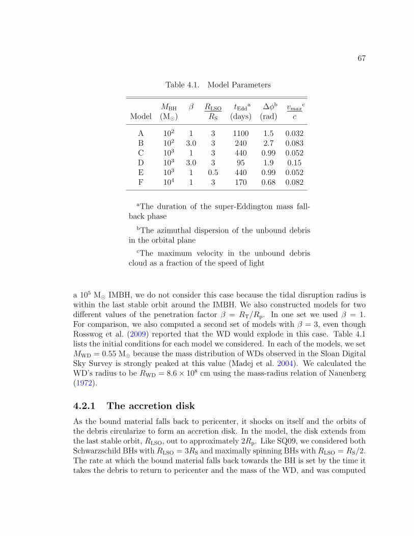
67

Table 4.1. Model Parameters

MBH β RLSO tEdda ∆φb vmax

c

Model (M�) RS (days) (rad) c

A 102 1 3 1100 1.5 0.032B 102 3.0 3 240 2.7 0.083C 103 1 3 440 0.99 0.052D 103 3.0 3 95 1.9 0.15E 103 1 0.5 440 0.99 0.052F 104 1 3 170 0.68 0.082

aThe duration of the super-Eddington mass fall-back phase

bThe azimuthal dispersion of the unbound debrisin the orbital plane

cThe maximum velocity in the unbound debriscloud as a fraction of the speed of light

a 105 M� IMBH, we do not consider this case because the tidal disruption radius iswithin the last stable orbit around the IMBH. We also constructed models for twodifferent values of the penetration factor β = RT/Rp. In one set we used β = 1.For comparison, we also computed a second set of models with β = 3, even thoughRosswog et al. (2009) reported that the WD would explode in this case. Table 4.1lists the initial conditions for each model we considered. In each of the models, we setMWD = 0.55 M� because the mass distribution of WDs observed in the Sloan DigitalSky Survey is strongly peaked at this value (Madej et al. 2004). We calculated theWD’s radius to be RWD = 8.6× 108 cm using the mass-radius relation of Nauenberg(1972).

4.2.1 The accretion disk

As the bound material falls back to pericenter, it shocks on itself and the orbits ofthe debris circularize to form an accretion disk. In the model, the disk extends fromthe last stable orbit, RLSO, out to approximately 2Rp. Like SQ09, we considered bothSchwarzschild BHs with RLSO = 3RS and maximally spinning BHs with RLSO = RS/2.The rate at which the bound material falls back towards the BH is set by the time ittakes the debris to return to pericenter and the mass of the WD, and was computed

68

using equations given in SQ09:

Mfb ∼1

3

MWD

tfb

(t

tfb

)−5/3

(4.1)

where the fallback time is given by

tfb ≈2π

63/2

(Rp

RWD

)3/2( R3p

GMBH

)1/2

. (4.2)

The mass fallback rate decreases as t−5/3, and at early times it can exceed the Edding-ton mass accretion rate, MEdd = 10LEdd/c

2. We capped the rate at which materialis accreted by the BH, M , at MEdd and, following SQ09, we assumed that the excessmass is blown off in a radiation driven wind. Because the nature of these outflows isuncertain, we did not consider emission from the outflows or how the outflows mightaffect the emission lines produced in the unbound material. SQ09 suggested thatthe material in the outflows can also be photoionized and produce additional lineluminosity, making the predictions of this model lower limits. In a followup paper,Strubbe & Quataert (2011) considered the photoionization of the out-flowing gas thatis outside the photosphere of the outflow and calculated the resulting absorption-linespectrum. Furthermore, the outflows could alter the radiation field that photoionizesthe unbound material and, thus, change the ionization state of the unbound debris.Since these effects were not accounted for in our model, the emission line luminosi-ties predicted during the super-Eddington phase are uncertain. The outflows subsideafter a time tEdd, given in equation (3) of SQ09 as

tEdd ∼ 0.1

(MBH

106 M�

)2/5 (Rp

3RS

)6/5 (MWD

M�

)3/5 (RWD

R�

)−3/5

yr. (4.3)

In Table 4.1 we list the value of tEdd for each of our models.

4.2.2 The unbound debris

As the star approaches the BH, it is tidally stretched along the direction of its motionand then spun up, resulting in a spread in the specific energy of the debris (Rees1988). SQ09 calculated how this range of specific energies leads to an expanding,curved wedge of unbound debris spanning a range of azimuthal angles and radialdistances from the BH (see Figure 4.1). The accretion flare illuminates the insideface of this wedge, and the gas along this edge reprocesses the radiation and producesthe optical emission lines we are interested in. SQ09 modeled the extent of this face interms of Rmax,∆φ, and ∆i, the maximum radial distance from the BH, the azimuthaldispersion of the debris in the orbital plane, and the angular dispersion of the debris

69

perpendicular to the orbital plane, respectively. We adopt their equations for theangular dispersion of the unbound material:

∆φ ∼(

12RWD

Rp

)1/2

(4.4)

and

∆i ∼ 2RWD

Rp

. (4.5)

However, we make a minor modification to calculate the distance between the BHand material along the debris arc. Since we considered several points along the arc,not just the most distant material, we calculated the distance to the BH at any pointalong the arc with

R(φ) ∼ vp t cot

(φ

2

), (4.6)

where vp is the pericenter velocity of the WD, t is the time since pericenter passage,and φ is the angle in the orbital plane between pericenter and the point in the debriscloud being considered and is in the range (π−∆φ) < φ < π. The WD is initially ona parabolic orbit, so vp = (2GMBH/Rp)1/2. SQ09 calculated Rmax in a similar mannerand our equation (4.6) is consistent with the derivation of Evans & Kochanek (1989)for the values of φ considered here. In Table 4.1, we list ∆φ and vmax/c, the maximumvelocity in the unbound debris cloud as a fraction of the speed of light, for each setof initial conditions. In addition to R and φ, we define the `-curve, which begins atthe IMBH and lies along the illuminated face of the debris cloud.

Furthermore, because we computed photoionization models at several points alongthe inside face of the cloud of unbound debris, we also had to deviate from SQ09’smodel when we calculated the density of the unbound debris, n. Kochanek (1994)found that the density in the stream of unbound material was not uniform and de-creased with distance from the BH as n ∝ R−3 because the material is undergoingfree expansion. We used this density profile in our model and normalized it using thefact that the mass of the wedge of unbound material was half the mass of the WD.

4.3 Modeling The Emission Lines

Predicting the emission lines we will observe when a WD is tidally disrupted by anIMBH requires a model for the emission from both the bound and unbound portions ofthe debris. To calculate the luminosity and spectrum of the accretion flare generatedby the disk of bound gas, SQ09 assumed a “slim disk” model (Abramowicz et al.1988) and derived an expression for the effective temperatures as a function of radius

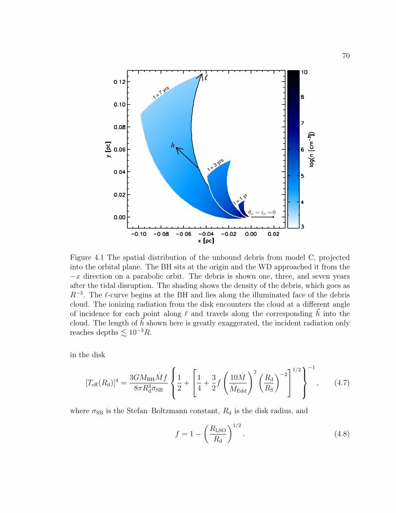
70

l

h

t = 7 yrs

t = 3 yrs

t = 1 yr

θo = io = 0

Figure 4.1 The spatial distribution of the unbound debris from model C, projectedinto the orbital plane. The BH sits at the origin and the WD approached it from the−x direction on a parabolic orbit. The debris is shown one, three, and seven yearsafter the tidal disruption. The shading shows the density of the debris, which goes asR−3. The `-curve begins at the BH and lies along the illuminated face of the debriscloud. The ionizing radiation from the disk encounters the cloud at a different angleof incidence for each point along ` and travels along the corresponding ~h into thecloud. The length of ~h shown here is greatly exaggerated, the incident radiation onlyreaches depths . 10−3R.

in the disk

[Teff(Rd)]4 =3GMBHMf

8πR3dσSB

1

2+

1

4+

3

2f

(10M

MEdd

)2(Rd

RS

)−21/2

−1

, (4.7)

where σSB is the Stefan–Boltzmann constant, Rd is the disk radius, and

f = 1−(RLSO

Rd

)1/2

. (4.8)

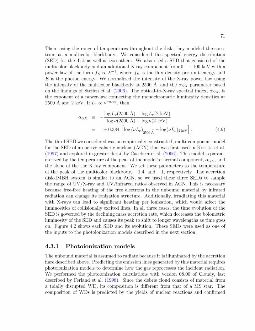
71

Then, using the range of temperatures throughout the disk, they modeled the spec-trum as a multicolor blackbody. We considered this spectral energy distribution(SED) for the disk as well as two others. We also used a SED that consisted of themulticolor blackbody and an additional X-ray component from 0.1− 100 keV with apower law of the form fE ∝ E−1, where fE is the flux density per unit energy andE is the photon energy. We normalized the intensity of the X-ray power law usingthe intensity of the multicolor blackbody at 2500 A and the αOX parameter basedon the findings of Steffen et al. (2006). The optical-to-X-ray spectral index, αOX , isthe exponent of a power-law connecting the monochromatic luminosity densities at2500 A and 2 keV. If Lν ∝ ν−αOX , then

αOX ≡ − logLν(2500 A)− logLν(2 keV)

log ν(2500 A)− log ν(2 keV)

= 1 + 0.384[log (νLν)

2500 A− log(νLν)2 keV

]. (4.9)

The third SED we considered was an empirically constructed, multi-component modelfor the SED of an active galactic nucleus (AGN) that was first used in Korista et al.(1997) and explored in greater detail by Casebeer et al. (2006). This model is param-eterized by the temperature of the peak of the model’s thermal component, αOX , andthe slope of the the X-ray component. We set these parameters to the temperatureof the peak of the multicolor blackbody, −1.4, and −1, respectively. The accretiondisk-IMBH system is similar to an AGN, so we used these three SEDs to samplethe range of UV/X-ray and UV/infrared ratios observed in AGN. This is necessarybecause free-free heating of the free electrons in the unbound material by infraredradiation can change its ionization structure. Additionally, irradiating this materialwith X-rays can lead to significant heating per ionization, which would affect theluminosities of collisionally excited lines. In all three cases, the time evolution of theSED is governed by the declining mass accretion rate, which decreases the bolometricluminosity of the SED and causes its peak to shift to longer wavelengths as time goeson. Figure 4.2 shows each SED and its evolution. These SEDs were used as one ofthe inputs to the photoionization models described in the next section.

4.3.1 Photoionization models

The unbound material is assumed to radiate because it is illuminated by the accretionflare described above. Predicting the emission lines generated by this material requiresphotoionization models to determine how the gas reprocesses the incident radiation.We performed the photoionization calculations with version 08.00 of Cloudy, lastdescribed by Ferland et al. (1998). Since the debris cloud consists of material froma tidally disrupted WD, its composition is different from that of a MS star. Thecomposition of WDs is predicted by the yields of nuclear reactions and confirmed

72

Figure 4.2 The parameterized AGN (solid line), multicolor blackbody (dashed line), and the multicolor blackbodyplus X-ray power law (dotted line) SEDs incident on an azimuthal segment of the debris cloud considered in model C.The segment has R = 1.9×1016 cm and R = 1.6×1017 cm at t = 300 days and t = 2500 days, respectively. Note thatover time the position of the peak moves towards longer wavelengths as the temperature in the disk decreases and thetotal flux decreases as the accretion rate declines and the segment moves further away from the ionizing source.

73

with asteroseismology (Metcalfe 2003). Following Madej et al. (2004), we assumedmass fractions of 67% O, 32% C, and 1% He and all other elements with their relativeabundances scaled from the solar values. Hydrogen is assumed to make up 0.001% ofthe WD’s mass. For each set of initial conditions (i.e., models A-F in Table 4.1), wecalculated the state of the accretion flare SED and the wedge of unbound debris at aseries of times after the tidal disruption. For each time step, we split the wedge into sixazimuthal segments. With six segments, we were able smoothly interpolate quantitiesalong the ` direction. Next, we calculated the density of the gas and the intensityof the ionizing radiation at the center of each segment. Several considerations wentinto the calculation of the latter. First, each segment is at a different distance fromthe accretion disk and has a correspondingly different geometric attenuation factor.Next, since the segments lie along an arc, the ionizing radiation’s angle of incidenceis also different for each segment. Finally, in addition to changes in the intensity ofthe incident radiation, the shape of the SED incident on each segment also varies.The light travel time, tlt, to the unbound debris furthest from the BH is comparableto the timescale on which the accretion flare evolves, so the SED of the radiationincident on these portions of the wedge was emitted at t− tlt, when the peak was ata higher energy. Each of these considerations has a significant effect on our models.Geometric attenuation and light travel time dominate for more distant regions, butthe material nearest the disk is illuminated at nearly glancing incidence, significantlyreducing the intensity of the incident radiation despite the proximity to the disk.With these parameters, we are able to calculate how the unbound debris responds tothe ionizing radiation emitted by the accretion disk.

The ionization state of the gas is conventionally described by the ionization pa-rameter UH = QH/(4πnHR

2c), where QH is the emission rate of photons with energygreater than 1 Ry, nH is the hydrogen number density, and R is the distance tothe ionizing source. However, since hydrogen is depleted in the material consideredhere, it is advantageous to use a more abundant reference element when calculatingthe ionization parameter. We chose to use oxygen because its first ionization poten-tial is very near that of hydrogen so the ratio of the two ionization parameters isUO/UH = XH/XO, where XO and XH are the oxygen and hydrogen abundances bynumber, respectively. Thus, UO is the ratio of the density of photons capable of singlyionizing oxygen to the total density of oxygen atoms. Figure 4.3 shows how UO, the to-tal number density of all elements, and the radial distance to the IMBH change alongthe illuminated face of the debris cloud, `, for model C at 600 and 1200 days after tidaldisruption. Since the density drops faster with distance from the accretion disk thanthe flux of ionizing photons does, UO increases along the `-curve. While the fallbackrate is super-Eddington, the value of UO increases linearly with time at all pointsalong the `-curve because the luminosity of the ionizing source remains constant atLEdd, while the density of the expanding debris cloud decreases. We find numericallythat UO declines approximately as t−0.2 after the super-Eddington accretion phase

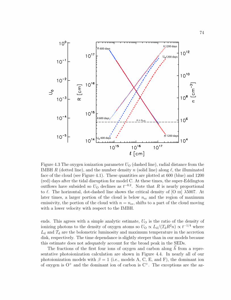
74

600 days

600 days

R 600 days

1200 days

1200 days

R 1200 days

n = ncrit

Figure 4.3 The oxygen ionization parameter UO (dashed line), radial distance from theIMBH R (dotted line), and the number density n (solid line) along `, the illuminatedface of the cloud (see Figure 4.1). These quantities are plotted at 600 (blue) and 1200(red) days after the tidal disruption for model C. At these times, the super-Eddingtonoutflows have subsided so UO declines as t−0.2. Note that R is nearly proportionalto `. The horizontal, dot-dashed line shows the critical density of [O III] λ5007. Atlater times, a larger portion of the cloud is below ncr and the region of maximumemissivity, the portion of the cloud with n = ncr, shifts to a part of the cloud movingwith a lower velocity with respect to the IMBH.

ends. This agrees with a simple analytic estimate, UO is the ratio of the density ofionizing photons to the density of oxygen atoms so UO ∝ Ld/(TdR

2n) ∝ t−1/4 whereLd and Td are the bolometric luminosity and maximum temperature in the accretiondisk, respectively. The time dependance is slightly steeper than in our models becausethis estimate does not adequately account for the broad peak in the SEDs.

The fractions of the first four ions of oxygen and carbon along ~h from a repre-sentative photoionization calculation are shown in Figure 4.4. In nearly all of ourphotoionization models with β = 1 (i.e., models A, C, E, and F), the dominant ionof oxygen is O+ and the dominant ion of carbon is C+. The exceptions are the az-

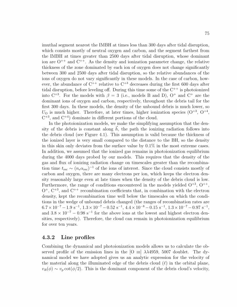
75

imuthal segment nearest the IMBH at times less than 300 days after tidal disruption,which consists mostly of neutral oxygen and carbon, and the segment farthest fromthe IMBH at times greater than 2500 days after tidal disruption, whose dominantion are O++ and C++. As the density and ionization parameter change, the relativethickness of the zone dominated by each ion of oxygen does not change significantlybetween 300 and 2500 days after tidal disruption, so the relative abundances of theions of oxygen do not vary significantly in these models. In the case of carbon, how-ever, the abundance of C++ relative to C+3 decreases during the first 600 days aftertidal disruption, before leveling off. During this time some of the C++ is photoionizedinto C+3. For the models with β = 3 (i.e., models B and D), O+ and C+ are thedominant ions of oxygen and carbon, respectively, throughout the debris tail for thefirst 300 days. In these models, the density of the unbound debris is much lower, soUO is much higher. Therefore, at later times, higher ionization species (O+3, O+4,C+3, and C+4) dominate in different portions of the cloud.

In the photoionization models, we make the simplifying assumption that the den-sity of the debris is constant along ~h, the path the ionizing radiation follows intothe debris cloud (see Figure 4.1). This assumption is valid because the thickness ofthe ionized layer is very small compared to the distance to the BH, so the densityin this skin only deviates from the surface value by 0.1% in the most extreme cases.In addition, we assumed that the ionized gas remains in photoionization equilibriumduring the 4000 days probed by our models. This requires that the density of thegas and flux of ionizing radiation change on timescales greater than the recombina-tion time trec ∼ (neαrec)

−1 of the ions of interest. Since the cloud consists mostly ofcarbon and oxygen, there are many electrons per ion, which keeps the electron den-sity reasonably large even at late times when the density of the debris cloud is low.Furthermore, the range of conditions encountered in the models yielded O+3, O++,O+, C+3, and C++ recombination coefficients that, in combination with the electrondensity, kept the recombination time well below the timescales on which the condi-tions in the wedge of unbound debris changed (the ranges of recombination rates are6.7×10−7−1.9 s−1, 1.3×10−7−0.52 s−1, 4.4×10−8−0.15 s−1, 1.3×10−7−0.97 s−1,and 3.8 × 10−7 − 0.98 s−1 for the above ions at the lowest and highest electron den-sities, respectively). Therefore, the cloud can remain in photoionization equilibriumfor over ten years.

4.3.2 Line profiles

Combining the dynamical and photoionization models allows us to calculate the ob-served profile of the emission lines in the [O III] λλ4959, 5007 doublet. The dy-namical model we have adopted gives us an analytic expression for the velocity ofthe material along the illuminated edge of the debris cloud (`) in the orbital plane,vR(φ) ∼ vp cot(φ/2). This is the dominant component of the debris cloud’s velocity,

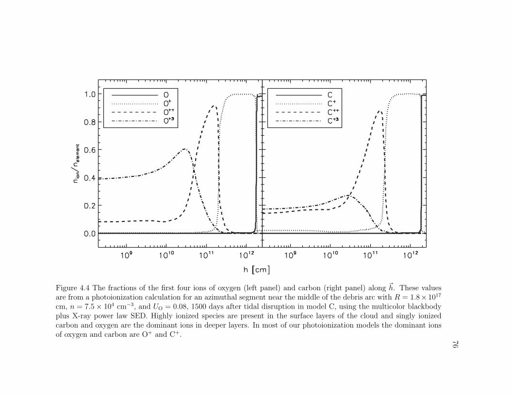
76

Figure 4.4 The fractions of the first four ions of oxygen (left panel) and carbon (right panel) along ~h. These valuesare from a photoionization calculation for an azimuthal segment near the middle of the debris arc with R = 1.8× 1017

cm, n = 7.5× 104 cm−3, and UO = 0.08, 1500 days after tidal disruption in model C, using the multicolor blackbodyplus X-ray power law SED. Highly ionized species are present in the surface layers of the cloud and singly ionizedcarbon and oxygen are the dominant ions in deeper layers. In most of our photoionization models the dominant ionsof oxygen and carbon are O+ and C+.

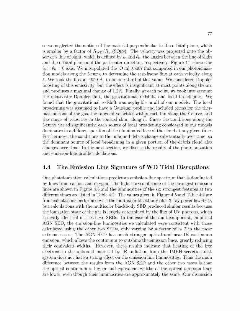
77

so we neglected the motion of the material perpendicular to the orbital plane, whichis smaller by a factor of RWD/Rp (SQ09). The velocity was projected onto the ob-server’s line of sight, which is defined by i0 and θ0, the angles between the line of sightand the orbital plane and the pericenter direction, respectively. Figure 4.1 shows thei0 = θ0 = 0 axis. We interpolated the [O III] λ5007 flux computed in our photoioniza-tion models along the `-curve to determine the rest-frame flux at each velocity along`. We took the flux at 4959 A to be one third of this value. We considered Dopplerboosting of this emissivity, but the effect is insignificant at most points along the arcand produces a maximal change of 1.2%. Finally, at each point, we took into accountthe relativistic Doppler shift, the gravitational redshift, and local broadening. Wefound that the gravitational redshift was negligible in all of our models. The localbroadening was assumed to have a Gaussian profile and included terms for the ther-mal motions of the gas, the range of velocities within each bin along the `-curve, andthe range of velocities in the ionized skin, along ~h. Since the conditions along the`-curve varied significantly, each source of local broadening considered in our modelsdominates in a different portion of the illuminated face of the cloud at any given time.Furthermore, the conditions in the unbound debris change substantially over time, sothe dominant source of local broadening in a given portion of the debris cloud alsochanges over time. In the next section, we discuss the results of the photoionizationand emission-line profile calculations.

4.4 The Emission Line Signature of WD Tidal Disruptions

Our photoionization calculations predict an emission-line spectrum that is dominatedby lines from carbon and oxygen. The light curves of some of the strongest emissionlines are shown in Figure 4.5 and the luminosities of the six strongest features at twodifferent times are listed in Table 4.2. The values given in Figure 4.5 and Table 4.2 arefrom calculations performed with the multicolor blackbody plus X-ray power law SED,but calculations with the multicolor blackbody SED produced similar results becausethe ionization state of the gas is largely determined by the flux of UV photons, whichis nearly identical in these two SEDs. In the case of the multicomponent, empiricalAGN SED, the emission-line luminosities we calculated were consistent with thosecalculated using the other two SEDs, only varying by a factor of ∼ 2 in the mostextreme cases. The AGN SED has much stronger optical and near-IR continuumemission, which allows the continuum to outshine the emission lines, greatly reducingtheir equivalent widths. However, these results indicate that heating of the freeelectrons in the unbound material by IR radiation from the IMBH-accretion disksystem does not have a strong effect on the emission line luminosities. Thus the maindifference between the results from the AGN SED and the other two cases is thatthe optical continuum is higher and equivalent widths of the optical emission linesare lower, even though their luminosities are approximately the same. Our discussion

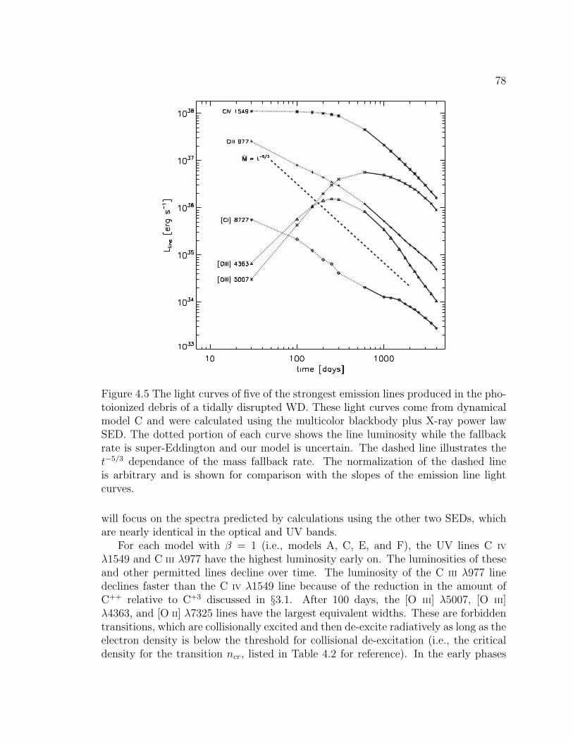
78

Figure 4.5 The light curves of five of the strongest emission lines produced in the pho-toionized debris of a tidally disrupted WD. These light curves come from dynamicalmodel C and were calculated using the multicolor blackbody plus X-ray power lawSED. The dotted portion of each curve shows the line luminosity while the fallbackrate is super-Eddington and our model is uncertain. The dashed line illustrates thet−5/3 dependance of the mass fallback rate. The normalization of the dashed lineis arbitrary and is shown for comparison with the slopes of the emission line lightcurves.

will focus on the spectra predicted by calculations using the other two SEDs, whichare nearly identical in the optical and UV bands.

For each model with β = 1 (i.e., models A, C, E, and F), the UV lines C IV

λ1549 and C III λ977 have the highest luminosity early on. The luminosities of theseand other permitted lines decline over time. The luminosity of the C III λ977 linedeclines faster than the C IV λ1549 line because of the reduction in the amount ofC++ relative to C+3 discussed in §3.1. After 100 days, the [O III] λ5007, [O III]λ4363, and [O II] λ7325 lines have the largest equivalent widths. These are forbiddentransitions, which are collisionally excited and then de-excite radiatively as long as theelectron density is below the threshold for collisional de-excitation (i.e., the criticaldensity for the transition ncr, listed in Table 4.2 for reference). In the early phases

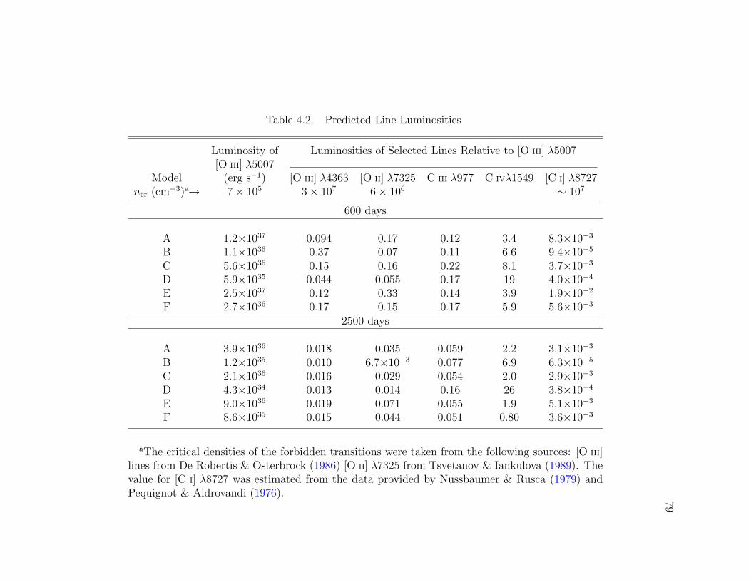
79

Table 4.2. Predicted Line Luminosities

Luminosity of Luminosities of Selected Lines Relative to [O III] λ5007[O III] λ5007

Model (erg s−1) [O III] λ4363 [O II] λ7325 C III λ977 C IVλ1549 [C I] λ8727ncr (cm−3)a→ 7× 105 3× 107 6× 106 ∼ 107

600 days

A 1.2×1037 0.094 0.17 0.12 3.4 8.3×10−3

B 1.1×1036 0.37 0.07 0.11 6.6 9.4×10−5

C 5.6×1036 0.15 0.16 0.22 8.1 3.7×10−3

D 5.9×1035 0.044 0.055 0.17 19 4.0×10−4

E 2.5×1037 0.12 0.33 0.14 3.9 1.9×10−2

F 2.7×1036 0.17 0.15 0.17 5.9 5.6×10−3

2500 days

A 3.9×1036 0.018 0.035 0.059 2.2 3.1×10−3

B 1.2×1035 0.010 6.7×10−3 0.077 6.9 6.3×10−5

C 2.1×1036 0.016 0.029 0.054 2.0 2.9×10−3

D 4.3×1034 0.013 0.014 0.16 26 3.8×10−4

E 9.0×1036 0.019 0.071 0.055 1.9 5.1×10−3

F 8.6×1035 0.015 0.044 0.051 0.80 3.6×10−3

aThe critical densities of the forbidden transitions were taken from the following sources: [O III]lines from De Robertis & Osterbrock (1986) [O II] λ7325 from Tsvetanov & Iankulova (1989). Thevalue for [C I] λ8727 was estimated from the data provided by Nussbaumer & Rusca (1979) andPequignot & Aldrovandi (1976).

80

of the evolution of the debris (the super-Eddington phase), the luminosity of theseforbidden lines rises with time and the lines reach their maximum luminosities at600, 250, and 300 days, respectively, when the outer tip of the ionized debris tail isat the corresponding critical density. After the peak, the line luminosities begin todecline, like the permitted lines. To understand this trend, we note that, at densitiesbelow the critical density of a transition the line emissivity per unit volume increaseslinearly with density and peaks at the critical density. As the density increases abovethe critical density, the line emissivity per unit volume drops by a factor of several(with the depletion of the upper level population by collisions) and then levels off (asthe upper level is re-populated by collisions and radiative decays from higher levels).We verified this behavior by solving the population equations for the [O III] λ5007transition and then combining the resulting level populations with the luminosity perunit density of ions in the lower level of the transition. To carry out this exercise,we assumed a 5-level ion and followed the methodology in chapter 3 of Osterbrock &Ferland (2006). Thus, the initial rise in the luminosity of the forbidden lines is theresult of the expansion of the debris while the density is above the critical density ofthe transition. This expansion occurs during the super-Eddington phase, when theionizing luminosity is constant. During this expansion, the peak luminosity in thelight curves corresponds to the time when the density at the outer tip of the debristail reaches the critical density. After that time the density of an increasing portion ofthe debris drops below the critical density (causing a reduction in the emissivity perunit volume) and the total luminosity declines. We can quantify the rate of the initialrise in a forbidden emission line’s luminosity if it occurs while the ionizing luminosityis constant and the density in the debris cloud is above the critical density. As thedebris expands, the column density of the ionized skin remains constant because thedecline in the flux of ionizing photons resulting from the increasing distance from theIMBH is balanced by the increase in the cloud’s surface area. This column sustainsa constant emission line flux at the surface of the cloud, so the rise in the forbiddenemission line luminosity is driven by the cloud’s expanding emitting area. This areagrows as t2, and this evolution can be seen in Figures 4.5 and 4.6.

We show the [O III] λ5007 and C IV λ1549 light curves for each of the modelsin Figure 4.6. These curves come from calculations performed with the multicolorblackbody plus X-ray power law SED and we note that calculations that exclude theX-ray component of the incident radiation predict luminosities within a few percentof those shown. We calculated the luminosities by multiplying the emergent fluxcomputed by Cloudy in each azimuthal segment by that segment’s emitting area andthen summing the luminosities across the entire illuminated face. The light curvesindicate how the evolution of the [O III] λ5007 line depends on the properties ofthe WD-IMBH system and how its evolution can be used to identify such a tidaldisruption event. First, the luminosity of the line at any given time increases as themass of the IMBH decreases. This is because both the initial, maximal mass accretion

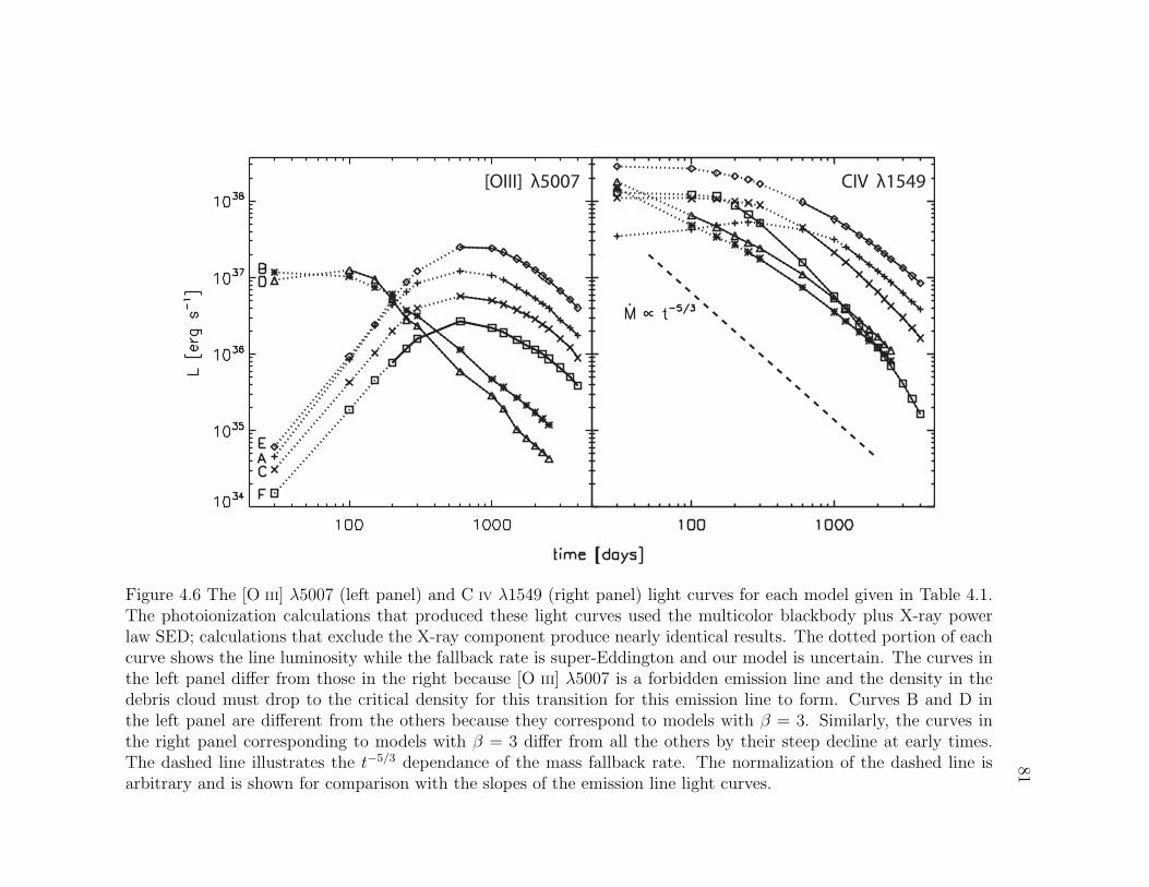
81

[OIII] λ5007 CIV λ1549

Figure 4.6 The [O III] λ5007 (left panel) and C IV λ1549 (right panel) light curves for each model given in Table 4.1.The photoionization calculations that produced these light curves used the multicolor blackbody plus X-ray powerlaw SED; calculations that exclude the X-ray component produce nearly identical results. The dotted portion of eachcurve shows the line luminosity while the fallback rate is super-Eddington and our model is uncertain. The curves inthe left panel differ from those in the right because [O III] λ5007 is a forbidden emission line and the density in thedebris cloud must drop to the critical density for this transition for this emission line to form. Curves B and D inthe left panel are different from the others because they correspond to models with β = 3. Similarly, the curves inthe right panel corresponding to models with β = 3 differ from all the others by their steep decline at early times.The dashed line illustrates the t−5/3 dependance of the mass fallback rate. The normalization of the dashed line isarbitrary and is shown for comparison with the slopes of the emission line light curves.

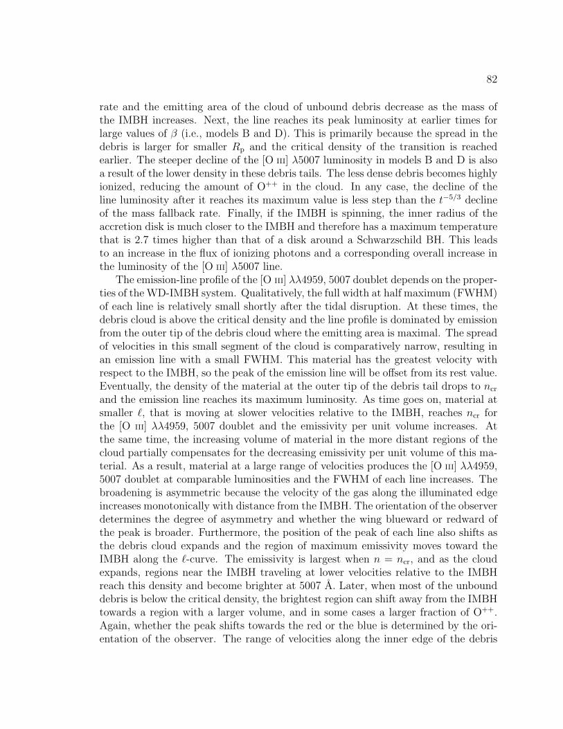
82

rate and the emitting area of the cloud of unbound debris decrease as the mass ofthe IMBH increases. Next, the line reaches its peak luminosity at earlier times forlarge values of β (i.e., models B and D). This is primarily because the spread in thedebris is larger for smaller Rp and the critical density of the transition is reachedearlier. The steeper decline of the [O III] λ5007 luminosity in models B and D is alsoa result of the lower density in these debris tails. The less dense debris becomes highlyionized, reducing the amount of O++ in the cloud. In any case, the decline of theline luminosity after it reaches its maximum value is less step than the t−5/3 declineof the mass fallback rate. Finally, if the IMBH is spinning, the inner radius of theaccretion disk is much closer to the IMBH and therefore has a maximum temperaturethat is 2.7 times higher than that of a disk around a Schwarzschild BH. This leadsto an increase in the flux of ionizing photons and a corresponding overall increase inthe luminosity of the [O III] λ5007 line.

The emission-line profile of the [O III] λλ4959, 5007 doublet depends on the proper-ties of the WD-IMBH system. Qualitatively, the full width at half maximum (FWHM)of each line is relatively small shortly after the tidal disruption. At these times, thedebris cloud is above the critical density and the line profile is dominated by emissionfrom the outer tip of the debris cloud where the emitting area is maximal. The spreadof velocities in this small segment of the cloud is comparatively narrow, resulting inan emission line with a small FWHM. This material has the greatest velocity withrespect to the IMBH, so the peak of the emission line will be offset from its rest value.Eventually, the density of the material at the outer tip of the debris tail drops to ncr

and the emission line reaches its maximum luminosity. As time goes on, material atsmaller `, that is moving at slower velocities relative to the IMBH, reaches ncr forthe [O III] λλ4959, 5007 doublet and the emissivity per unit volume increases. Atthe same time, the increasing volume of material in the more distant regions of thecloud partially compensates for the decreasing emissivity per unit volume of this ma-terial. As a result, material at a large range of velocities produces the [O III] λλ4959,5007 doublet at comparable luminosities and the FWHM of each line increases. Thebroadening is asymmetric because the velocity of the gas along the illuminated edgeincreases monotonically with distance from the IMBH. The orientation of the observerdetermines the degree of asymmetry and whether the wing blueward or redward ofthe peak is broader. Furthermore, the position of the peak of each line also shifts asthe debris cloud expands and the region of maximum emissivity moves toward theIMBH along the `-curve. The emissivity is largest when n = ncr, and as the cloudexpands, regions near the IMBH traveling at lower velocities relative to the IMBHreach this density and become brighter at 5007 A. Later, when most of the unbounddebris is below the critical density, the brightest region can shift away from the IMBHtowards a region with a larger volume, and in some cases a larger fraction of O++.Again, whether the peak shifts towards the red or the blue is determined by the ori-entation of the observer. The range of velocities along the inner edge of the debris

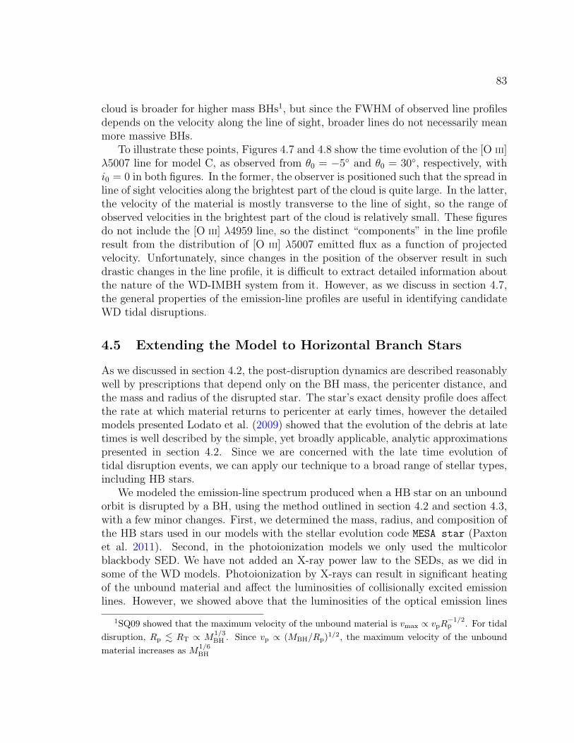
83

cloud is broader for higher mass BHs1, but since the FWHM of observed line profilesdepends on the velocity along the line of sight, broader lines do not necessarily meanmore massive BHs.

To illustrate these points, Figures 4.7 and 4.8 show the time evolution of the [O III]λ5007 line for model C, as observed from θ0 = −5◦ and θ0 = 30◦, respectively, withi0 = 0 in both figures. In the former, the observer is positioned such that the spread inline of sight velocities along the brightest part of the cloud is quite large. In the latter,the velocity of the material is mostly transverse to the line of sight, so the range ofobserved velocities in the brightest part of the cloud is relatively small. These figuresdo not include the [O III] λ4959 line, so the distinct “components” in the line profileresult from the distribution of [O III] λ5007 emitted flux as a function of projectedvelocity. Unfortunately, since changes in the position of the observer result in suchdrastic changes in the line profile, it is difficult to extract detailed information aboutthe nature of the WD-IMBH system from it. However, as we discuss in section 4.7,the general properties of the emission-line profiles are useful in identifying candidateWD tidal disruptions.

4.5 Extending the Model to Horizontal Branch Stars

As we discussed in section 4.2, the post-disruption dynamics are described reasonablywell by prescriptions that depend only on the BH mass, the pericenter distance, andthe mass and radius of the disrupted star. The star’s exact density profile does affectthe rate at which material returns to pericenter at early times, however the detailedmodels presented Lodato et al. (2009) showed that the evolution of the debris at latetimes is well described by the simple, yet broadly applicable, analytic approximationspresented in section 4.2. Since we are concerned with the late time evolution oftidal disruption events, we can apply our technique to a broad range of stellar types,including HB stars.

We modeled the emission-line spectrum produced when a HB star on an unboundorbit is disrupted by a BH, using the method outlined in section 4.2 and section 4.3,with a few minor changes. First, we determined the mass, radius, and composition ofthe HB stars used in our models with the stellar evolution code MESA star (Paxtonet al. 2011). Second, in the photoionization models we only used the multicolorblackbody SED. We have not added an X-ray power law to the SEDs, as we did insome of the WD models. Photoionization by X-rays can result in significant heatingof the unbound material and affect the luminosities of collisionally excited emissionlines. However, we showed above that the luminosities of the optical emission lines

1SQ09 showed that the maximum velocity of the unbound material is vmax ∝ vpR−1/2p . For tidal

disruption, Rp . RT ∝ M1/3BH . Since vp ∝ (MBH/Rp)1/2, the maximum velocity of the unbound

material increases as M1/6BH

84

Figure 4.7 The time evolution of the [O III] λ5007 emission-line profile as seen by anobserver at i0 = 45◦ and θ0 = −5◦. Time increases from bottom to top and the timefor each profile is written on the plot. The dotted lines show the Fλ = 0 level foreach profile. The horizontal axis shows z = (λ − 5007A)/5007A. Each profile hasbeen normalized so that it has a maximum height of 1 and the profiles are offset byone unit for clarity. Note that in addition to becoming broader with time, the peakof the line profile shifts to lower velocity. Once most of the cloud is below ncr, theemissivity per unit volume decreases throughout the cloud and the peak shifts backtowards higher velocities that correspond to regions in the tail with larger volumeand a larger fraction of O++.

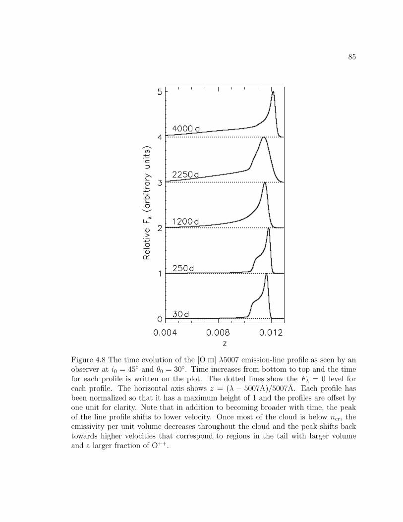
85

Figure 4.8 The time evolution of the [O III] λ5007 emission-line profile as seen by anobserver at i0 = 45◦ and θ0 = 30◦. Time increases from bottom to top and the timefor each profile is written on the plot. The dotted lines show the Fλ = 0 level foreach profile. The horizontal axis shows z = (λ − 5007A)/5007A. Each profile hasbeen normalized so that it has a maximum height of 1 and the profiles are offset byone unit for clarity. Note that in addition to becoming broader with time, the peakof the line profile shifts to lower velocity. Once most of the cloud is below ncr, theemissivity per unit volume decreases throughout the cloud and the peak shifts backtowards higher velocities that correspond to regions in the tail with larger volumeand a larger fraction of O++.

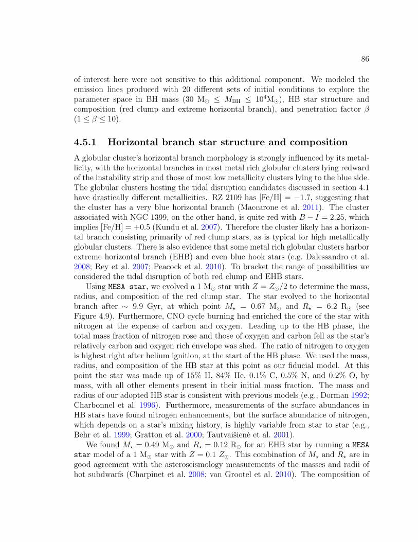
86

of interest here were not sensitive to this additional component. We modeled theemission lines produced with 20 different sets of initial conditions to explore theparameter space in BH mass (30 M� ≤ MBH ≤ 104M�), HB star structure andcomposition (red clump and extreme horizontal branch), and penetration factor β(1 ≤ β ≤ 10).

4.5.1 Horizontal branch star structure and composition

A globular cluster’s horizontal branch morphology is strongly influenced by its metal-licity, with the horizontal branches in most metal rich globular clusters lying redwardof the instability strip and those of most low metallicity clusters lying to the blue side.The globular clusters hosting the tidal disruption candidates discussed in section 4.1have drastically different metallicities. RZ 2109 has [Fe/H] = −1.7, suggesting thatthe cluster has a very blue horizontal branch (Maccarone et al. 2011). The clusterassociated with NGC 1399, on the other hand, is quite red with B − I = 2.25, whichimplies [Fe/H] = +0.5 (Kundu et al. 2007). Therefore the cluster likely has a horizon-tal branch consisting primarily of red clump stars, as is typical for high metallicallyglobular clusters. There is also evidence that some metal rich globular clusters harborextreme horizontal branch (EHB) and even blue hook stars (e.g. Dalessandro et al.2008; Rey et al. 2007; Peacock et al. 2010). To bracket the range of possibilities weconsidered the tidal disruption of both red clump and EHB stars.

Using MESA star, we evolved a 1 M� star with Z = Z�/2 to determine the mass,radius, and composition of the red clump star. The star evolved to the horizontalbranch after ∼ 9.9 Gyr, at which point M? = 0.67 M� and R? = 6.2 R� (seeFigure 4.9). Furthermore, CNO cycle burning had enriched the core of the star withnitrogen at the expense of carbon and oxygen. Leading up to the HB phase, thetotal mass fraction of nitrogen rose and those of oxygen and carbon fell as the star’srelatively carbon and oxygen rich envelope was shed. The ratio of nitrogen to oxygenis highest right after helium ignition, at the start of the HB phase. We used the mass,radius, and composition of the HB star at this point as our fiducial model. At thispoint the star was made up of 15% H, 84% He, 0.1% C, 0.5% N, and 0.2% O, bymass, with all other elements present in their initial mass fraction. The mass andradius of our adopted HB star is consistent with previous models (e.g., Dorman 1992;Charbonnel et al. 1996). Furthermore, measurements of the surface abundances inHB stars have found nitrogen enhancements, but the surface abundance of nitrogen,which depends on a star’s mixing history, is highly variable from star to star (e.g.,Behr et al. 1999; Gratton et al. 2000; Tautvaisiene et al. 2001).

We found M? = 0.49 M� and R? = 0.12 R� for an EHB star by running a MESA

star model of a 1 M� star with Z = 0.1 Z�. This combination of M? and R? are ingood agreement with the asteroseismology measurements of the masses and radii ofhot subdwarfs (Charpinet et al. 2008; van Grootel et al. 2010). The composition of

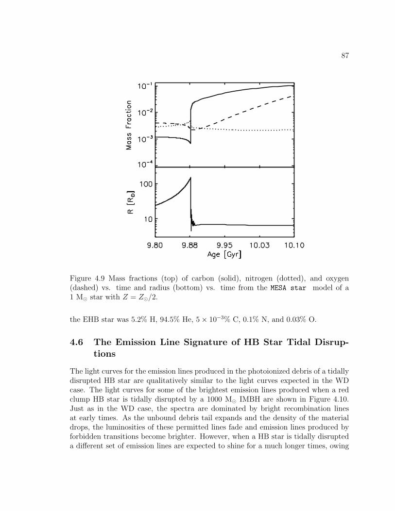
87

Figure 4.9 Mass fractions (top) of carbon (solid), nitrogen (dotted), and oxygen(dashed) vs. time and radius (bottom) vs. time from the MESA star model of a1 M� star with Z = Z�/2.

the EHB star was 5.2% H, 94.5% He, 5× 10−3% C, 0.1% N, and 0.03% O.

4.6 The Emission Line Signature of HB Star Tidal Disrup-tions

The light curves for the emission lines produced in the photoionized debris of a tidallydisrupted HB star are qualitatively similar to the light curves expected in the WDcase. The light curves for some of the brightest emission lines produced when a redclump HB star is tidally disrupted by a 1000 M� IMBH are shown in Figure 4.10.Just as in the WD case, the spectra are dominated by bright recombination linesat early times. As the unbound debris tail expands and the density of the materialdrops, the luminosities of these permitted lines fade and emission lines produced byforbidden transitions become brighter. However, when a HB star is tidally disrupteda different set of emission lines are expected to shine for a much longer times, owing

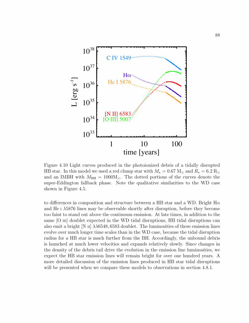
88

1 10 100time [years]

1033

1034

1035

1036

1037

1038

L [e

rg s-1

]

C IV 1549

[O III] 5007

H

[N II] 6583

He I 5876

Figure 4.10 Light curves produced in the photoionized debris of a tidally disruptedHB star. In this model we used a red clump star with M? = 0.67 M� and R? = 6.2 R�and an IMBH with MBH = 1000M�. The dotted portions of the curves denote thesuper-Eddington fallback phase. Note the qualitative similarities to the WD caseshown in Figure 4.5.

to differences in composition and structure between a HB star and a WD. Bright Hαand He I λ5876 lines may be observable shortly after disruption, before they becometoo faint to stand out above the continuum emission. At late times, in addition to thesame [O III] doublet expected in the WD tidal disruptions, HB tidal disruptions canalso emit a bright [N II] λλ6548, 6583 doublet. The luminosities of these emission linesevolve over much longer time scales than in the WD case, because the tidal disruptionradius for a HB star is much further from the BH. Accordingly, the unbound debrisis launched at much lower velocities and expands relatively slowly. Since changes inthe density of the debris tail drive the evolution in the emission line luminosities, weexpect the HB star emission lines will remain bright for over one hundred years. Amore detailed discussion of the emission lines produced in HB star tidal disruptionswill be presented when we compare these models to observations in section 4.8.1.

89

4.7 Discussion of the Models

We have presented calculations of the line emission produced when the unbounddebris of a WD that has been tidally disrupted by an IMBH is illuminated by theassociated accretion flare. We found that the two strongest emission lines, by far, areC IV λ1549 at early times and [O III] λ5007 at late times. Furthermore, the emissionlines formed in the illuminated face of the debris cloud will have broad, asymmetricprofiles with velocity widths of several hundred to a few thousand km s−1. Our resultssuggest that UV and optical spectra whose strongest features are broad C IV λ1549and [O III] λ5007 emission lines can serve to identify WD tidal disruption events,when they are detected in addition to an X-ray flare in the center of a globularcluster or dwarf elliptical galaxy. Figure 4.6 shows how the characteristic timescalesand luminosities of these emission lines scale with Rp and the mass of the IMBH. Theluminosities of the C IV λ1549 and [O III] λ5007 lines decline more slowly if β = 1 thanthey do if β = 3. For a constant β, the shapes of the emission-line light curves do notchange much when the mass of the IMBH is changed, however, systems with lowermass IMBHs produce brighter C IV λ1549 and [O III] λ5007 emission. The emissionline luminosities are sensitive to the density of the photoionized debris, and sincethis density is only weakly dependent on MBH, the line luminosities evolve on similartimescales despite a factor of 100 increase in MBH. In these models n = n0/R

3, wherethe normalization factor

n0 =M

5/6WDM

1/6BH

8µ(3β)1/2

tan

(π −∆φ

2

)sin ∆i [log

(sin

∆φ

2

)+ 6]

(4.10)

ensures that the mass of the unbound debris tail is 0.5 MWD. Here we have usedthe mean molecular mass µ. Numerical fits to the quantity in the curly bracketsshow that it increases with the mass of the IMBH as M0.54

BH when β is held constant.Altogether, we find that the density of the unbound debris is only weakly dependenton the mass of the IMBH, n ∝ M0.21

BH , so it is difficult to constrain MBH with the[O III] λ5007 light curve.

We have also presented models of HB star tidal disruptions. We found that theemission lines produced in the photoionized debris of a disrupted HB star will remainbright for hundreds of years. During these late stages of the disruption, we expectthe optical spectra emitted by the HB star debris to be similar to that emitted in thelate stages of a WD tidal disruption. In both cases the spectra exhibit bright [O III]doublets and are devoid of hydrogen Balmer lines. However, the presence of a bright[N II] doublet, unique to HB disruptions, can be used to discriminate between the twoscenarios.

Our work drew heavily on the SQ09 model for the tidal disruption of a MS star

90

by an supermassive BH, so we summarize the uncertainties in the model describedthere. First, since the accretion disk becomes geometrically thin after M drops belowthe Eddington rate, it becomes susceptible to viscous instabilities that impede thesteady flow of material through the disk and this could result in a deviation fromthe smooth t−5/3 dependance of the ionizing radiation. Material will accumulate inthe disk rather than accreting onto the BH when disk’s viscous timescale becomescomparable to the time since tidal disruption. This occurs at t ∼ 8 − 12 yr for thedisks in our WD tidal disruption models and at t ∼ 200 yr in the HB star disruptionmodels. Furthermore, the model is no longer valid when the mass accretion ratedrops below ∼ 0.01 MEdd and the disk becomes radiatively inefficient. The finaltime steps in WD models B-F are nearing this limit, and this change will lead to areduction in the number of UV photons not accounted for in this model. Since thephotoionization cross-sections for O and C decline significantly from UV to X-rayenergies, the ionization state of the unbound debris depends sensitively on the fluxof UV photons whose energies are near the ionization potentials of C and O. Next,a significant amount of initially bound material can be driven away from the IMBHin the super-Eddington outflows. The impact that the outflows have on emissionfrom the unbound material is uncertain. SQ09 pointed out that the outflows couldalso be photoionized by the accretion flare and generate additional line luminosity.Additionally, since we did not account for how the outflows affect the radiation thatilluminates the unbound debris, the emission line luminosities predicted for t < tEdd

are uncertain. The impact of the super-Eddington fallback phase is especially strongin our HB star tidal disruption models, where this phase lasts between 90 and 155years.

The modifications we made to the SQ09 model allowed us to test how some of theirsimplifications affect the predictions of the model. In their photoionization calcula-tions, they simplify the geometry of the wedge of unbound debris by approximatingit as a cloud separated from the ionizing source by Rmax (i.e. the maximum of equa-tion (4.6) or R(π−∆φ)). Furthermore, they assume that the density of the unboundmaterial is uniform and evaluate it by placing half the mass of the star in a region ofvolume R2

max ∆R∆i∆φ. In our calculations, on the other hand, we have accountedfor the changing ionization state of the material along the illuminated edge of thecloud by allowing the density and intensity of the ionizing radiation to vary alongthis edge, as discussed in section 4.3.1. Both methods produce similar emission-linelight curves, with the SQ09 model predicting slightly higher luminosities for mostlines. This was true for both the WD-IMBH case and the MS-supermassive BH case.Our models also show that the choice of SED for the accretion flare does not havea strong affect on the emission line luminosities. We conclude, therefore, that theirsimpler method is sufficient to predict the luminosities and light curves of opticalemission lines from tidally disrupted stars.

One interesting facet of our WD tidal disruption models that deserves further

91

exploration involves the composition of the unbound material. The models of Luminet& Pichon (1989) and Rosswog et al. (2009) found that compression of the WD as itpasses through pericenter resulted in nuclear burning. The amount of energy releasedby these reactions and how significantly they alter the composition of the debrisdepends on the initial composition of the WD, MBH, and Rp. To explore how a changein the abundances brought about by nuclear burning would influence the emissionlines emitted by the unbound debris, we also computed photoionization models usingabundances given in Rosswog et al. (2009) for a 1.2 M� WD (RWD = 2.7 × 108 cm)that is tidally disrupted by a 500 M� IMBH with β = 3.2. For the first year, thebrightest lines are the UV lines C IV λ1549, Si III λ1888, and O VI λ1035. Laterhowever, the emission-line spectrum is dominated by forbidden iron lines rather thancarbon and oxygen lines. The most luminous lines include [Fe X] λ6373, [Fe VII] λ6807,[Si VIII] λ1446, [Fe VII] λ3759, [Fe V] λ3892, and [Fe VII ]λ5271. While, this scenariorepresents an extreme case in which the energy released by nuclear burning is greaterthan the binding energy of the WD, the presence of these iron and silicon lines ina spectrum that is otherwise similar to that described above could be evidence ofnuclear burning during the tidal disruption.

4.8 Comparison to Observations

The next question to consider is how often we should expect to see emission lines fromtidally disrupted WDs or HB stars. Ramirez-Ruiz & Rosswog (2009) estimate thatthe rate of LEdd flares from MS stars being tidally disrupted by 103− 104M� IMBHsin globular clusters is ∼ 4000 yr−1 Gpc−3. Following these authors, we assume allglobular clusters have an IMBH in their center and adopt a globular cluster spacedensity of nGC ∼ 6 Mpc−3 (Brodie & Strader 2006). We take the WD tidal disruptionrate of 10−8 yr−1 (globular cluster)−1 from Sigurdsson & Rees (1997) and arrive at aWD tidal disruption rate of ∼ 60 yr−1 Gpc−3, 67 times lower than the MS rate. Thisrate is a very optimistic estimate because it is unlikely that every globular cluster hasan IMBH in its center and the actual rate could be much lower. The likelihood ofobserving such an event is further reduced by its relatively short lifetime of ∼ 10 yr.

As was mentioned in section 4.1, despite the meager rate and limited observingwindow, Irwin et al. (2010) proposed the tidal disruption of a WD by an IMBHas an explanation for two recent observations of X-ray and optical emission in thecenters of globular clusters. We will review the observations in greater detail now.The first candidate is in the center of globular cluster RZ 2109 associated with NGC4472. Maccarone et al. (2007) measured the source’s X-ray luminosity to be LX =4× 1039 erg s−1. In follow up optical observations, Zepf et al. (2008) found that the[O III] λ5007 line luminosity was 1.4 × 1037 erg s−1 and that the line’s FWHM was1500 km s−1. Irwin et al. (2010) reported on the second candidate, the ultraluminousX-ray source CXOJ033831.8-352604, which lies in a globular cluster associated with

92

NGC 1399. The source has a 0.3− 10 keV luminosity of ∼ 2× 1039 erg s−1 as well as[O III] λ5007 and [N II] λ6583 emission lines with luminosities of few × 1036 erg s−1

and FWHMs of 140 km s−1. Balmer lines were not detected in the spectrum, butthe following lower limits were placed on the emission line luminosity ratios: [N II]λ6583/Hα > 7 and [O III] λ5007/Hβ > 5.

The X-ray luminosity of the source in RZ 2109 is consistent with the WD tidaldisruption models that assumed a multicolor blackbody plus X-ray power law SED forthe accretion flare. The optical emission lines observed by Zepf et al. (2008) are alsoconsistent with these models in terms of both luminosity and FWHM. The observedluminosity of the [O III] λ5007 line falls within the range of luminosities predicted forsystems with IMBH masses between 100 - 1000 M�. Figure 4.11 shows a synthesized[O III] λλ4959, 5007 emission-line profile that has been smoothed to the same spectralresolution as the observations of Zepf et al. (2008). The line profile was synthesizedfor model C with the observer at i0 = 89◦ and θ0 = −12◦. We have chosen these valuesto match the shape of the observed emission-line profile. The first similarity betweenthe model and the observations is that the lines are so broad that they are blended.The FWHM of the model line profile is 1700 km s−1. Also, both the observed andmodeled profiles are asymmetric, with the blue wing much broader than the red. Thissuggests that we are oriented with the flow such that vmax is nearly parallel to ourline of sight.

Even though there seems to be good agreement between our models and the ob-servations, there are several drawbacks to interpreting the source in RZ 2109 as a WDtidal disruption. The first involves the duration of the X-ray flare and the observed[O III] λ5007 luminosity. An X-ray luminosity of 8.5× 1039 erg s−1 was measured forthis source with ROSAT in 1992 (Colbert & Ptak 2002). The change in luminositybetween the ROSAT observation and the observation reported in Maccarone et al.(2007) is consistent with the model for the X-ray flare, if the ROSAT observationdetected the flare ∼ 1 year after the WD was tidally disrupted. However, this meansthat the [O III] λ5007 luminosity was still 1.4× 1037 erg s−1 more than 15 years afterthe tidal disruption, and long after the peak in [O III] λ5007 emission predicted bythis model (see Figure 4.6). The model can only explain this [O III] λ5007 luminosityif the IMBH in this globular cluster is 100 M� and maximally spinning. Even thoughit is possible to tune the model to explain the observed X-ray and [O III] λ5007 lu-minosities, because the high emission line luminosity persists for many years longerthan it would in all but the most favorable scenario, it is unlikely that this source isa WD that has been tidally disrupted by a IMBH, according to the model. Next, thelarge amplitude X-ray variability of the source reported in Maccarone et al. (2010)is inconsistent with the steady luminosity decline expected from a tidal disruptionevent. Finally, improved measurements have revealed that the photoionized debrisof a tidally disrupted WD is an unlikely origin of [O III] λλ4959, 5007 doublet seenRZ 2109. Using a higher spectral resolution and signal-to-noise ratio observation of

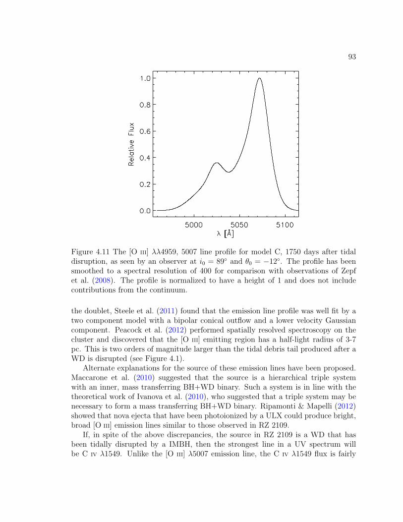
93

Figure 4.11 The [O III] λλ4959, 5007 line profile for model C, 1750 days after tidaldisruption, as seen by an observer at i0 = 89◦ and θ0 = −12◦. The profile has beensmoothed to a spectral resolution of 400 for comparison with observations of Zepfet al. (2008). The profile is normalized to have a height of 1 and does not includecontributions from the continuum.

the doublet, Steele et al. (2011) found that the emission line profile was well fit by atwo component model with a bipolar conical outflow and a lower velocity Gaussiancomponent. Peacock et al. (2012) performed spatially resolved spectroscopy on thecluster and discovered that the [O III] emitting region has a half-light radius of 3-7pc. This is two orders of magnitude larger than the tidal debris tail produced after aWD is disrupted (see Figure 4.1).

Alternate explanations for the source of these emission lines have been proposed.Maccarone et al. (2010) suggested that the source is a hierarchical triple systemwith an inner, mass transferring BH+WD binary. Such a system is in line with thetheoretical work of Ivanova et al. (2010), who suggested that a triple system may benecessary to form a mass transferring BH+WD binary. Ripamonti & Mapelli (2012)showed that nova ejecta that have been photoionized by a ULX could produce bright,broad [O III] emission lines similar to those observed in RZ 2109.

If, in spite of the above discrepancies, the source in RZ 2109 is a WD that hasbeen tidally disrupted by a IMBH, then the strongest line in a UV spectrum willbe C IV λ1549. Unlike the [O III] λ5007 emission line, the C IV λ1549 flux is fairly

94

constant across the illuminated face of the cloud so most of this line’s luminosity isgenerated in the outer portions of the debris tail where the emitting area is largest.This results in a emission-line profile consisting of a redshifted core with a FWHMof several hundred km s−1 and a broad blue shoulder. Furthermore, if the X-raysdecline dramatically in the future, the [O III] luminosity should also dim over thecourse of one year according to this model. The delay in the decline is due to thelight travel time from the IMBH to the distant portions of the unbound debris thatgenerate most of the [O III] luminosity.

4.8.1 HB star tidal disruption candidate

Although Irwin et al. (2010) proposed that CXOJ033831.8-352604 and the spatiallycoincident [O III] and [N II] emission lines were the result of a WD tidal disruption,the observational properties of this source are better explained by our HB star tidaldisruption models. In fact, each combination of MBH, HB star type, and β that weconsidered in our suite of HB star tidal disruption models predicted [N II] λ6583 and[O III] λ5007 emission lines with luminosities ∼ 1036 erg s−1 at some point during thepost tidal disruption evolution. Beyond merely identifying this source as a HB startidal disruption candidate, we can use our models to probe the BH present in thisglobular cluster. Only models with a red clump HB star, a BH with MBH . 200 M�,and β ∼ 1 were able to reproduce the [N II] λ6583/Hα, [O III] λ5007/Hβ, and [N II]λ6583/[O III] λ5007 emission line luminosity ratios reported in Irwin et al. (2010).

We illustrate this fact in Figure 4.12, which shows the time evolution of the lineratios in a subset of our models. In the models plotted here, we have used ourfiducial red clump HB star and assumed that β = 1, but varied MBH. In each ofthese models, the Balmer lines outshone the [O III] and [N II] lines initially. Then,as the debris cloud expanded and n decreased, the luminosity of the Balmer linesdeclined because the volume emissivity of these permitted transitions is proportionalto the product of the electron and ionized hydrogen number densities. At the sametime, the [O III] λ5007 and [N II] λ6583 lines became brighter. These forbidden linesare produced when ions are collisionally excited into a metastable state and thende-excite radiatively. As the density in the unbound debris decreased, the collisionrate declined, allowing a larger fraction of the excited ions to decay radiatively, asopposed to collisionally, and the forbidden emission-lines grew brighter. As a result,all of the models shown in Figure 4.12 can satisfy the [O III]/Hβ constraint, providedwe are observing the debris more than 40 years after tidal disruption. The modelswith MBH = 103 and 104 M� were unable to reproduce the observed [N II]/Hα ratio.These more massive BHs permitted higher accretion rates that led to an increasedflux of ionizing photons. By the time the density in the debris was low enough toproduce a significant [N II] luminosity, [N II] emission was suppressed because thecloud had become so highly ionized that much of the N+ was further ionized to N++.

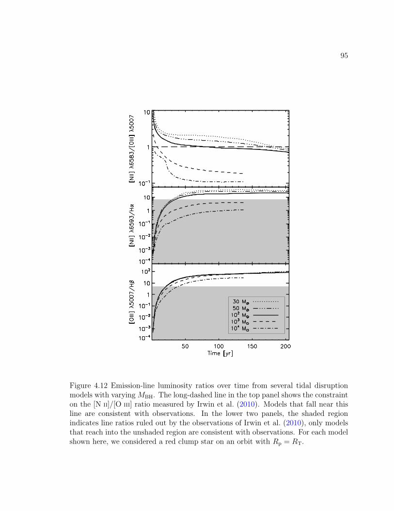
95

Figure 4.12 Emission-line luminosity ratios over time from several tidal disruptionmodels with varying MBH. The long-dashed line in the top panel shows the constrainton the [N II]/[O III] ratio measured by Irwin et al. (2010). Models that fall near thisline are consistent with observations. In the lower two panels, the shaded regionindicates line ratios ruled out by the observations of Irwin et al. (2010), only modelsthat reach into the unshaded region are consistent with observations. For each modelshown here, we considered a red clump star on an orbit with Rp = RT.

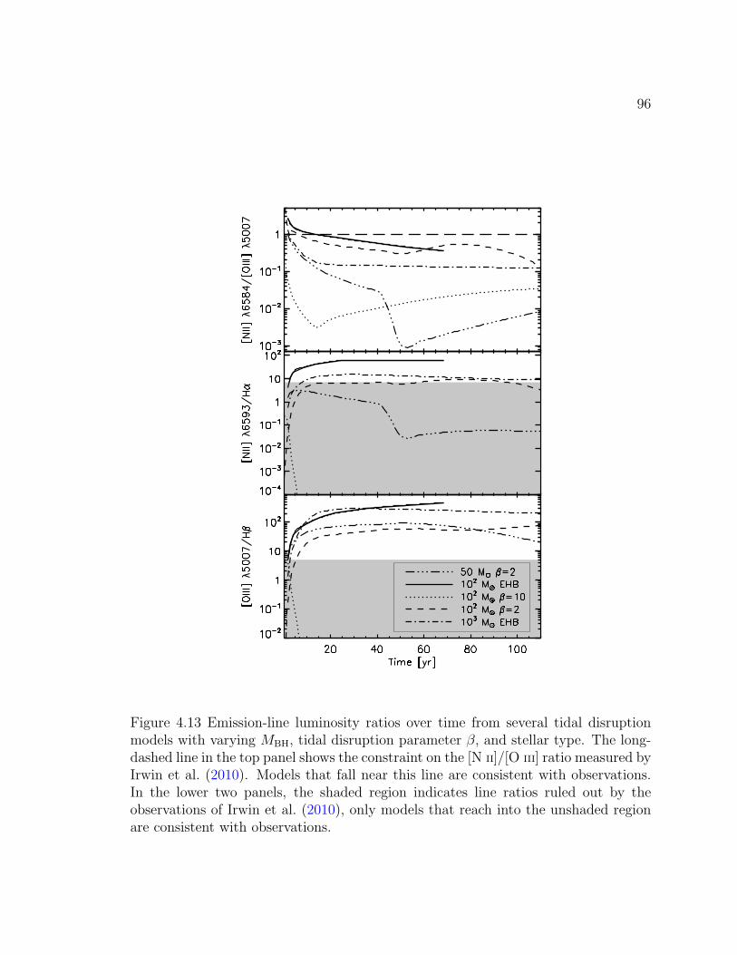
96

Figure 4.13 Emission-line luminosity ratios over time from several tidal disruptionmodels with varying MBH, tidal disruption parameter β, and stellar type. The long-dashed line in the top panel shows the constraint on the [N II]/[O III] ratio measured byIrwin et al. (2010). Models that fall near this line are consistent with observations.In the lower two panels, the shaded region indicates line ratios ruled out by theobservations of Irwin et al. (2010), only models that reach into the unshaded regionare consistent with observations.

97

This over-ionization of the unbound debris drove the evolution of the [N II]/[O III]ratio. In all of the models, the ratio steadily declined as an increasing portion ofthe oxygen and nitrogen in the cloud became doubly ionized. With MBH = 103 or104 M�, the unbound debris became too highly ionized for the [N II]/[O III] ratioto be ∼ 1 within ten years of tidal disruption (see Figure 4.12). We found that inmodels with MBH < 200M�, the decline is slow enough that the luminosities of thetwo forbidden emission lines can differ by less than a factor of two for up to 200 years.

Figure 4.13, shows a number of alternative models for strong disruption and/orblue HB stars. These models fail to reproduce the observed [N II]/[O III] ratio for anextended period of time, in contrast to our models of weakly disrupted red HB stars.Like the models involving high mass BHs discussed above, the unbound debris cloudbecomes too highly ionized to produce significant [N II] emission. Using a simpleestimate of the ionization parameter UH (defined in section 4.3.1), we can illustratewhy some debris clouds become over ionized and others do not. Recasting the ion-ization parameter in terms of our model parameters, we find UH ∝ R

−1/2? β3M3/4t.

Debris from stars with a larger kinetic energy at pericenter passage, due to a morecompact star with smaller RT, an orbit with β > 1, or a more massive BH, spanneda wider range in velocity and quickly expanded to a low density, resulting in a largeUH. As mentioned above, more massive BHs lead to a higher flux of ionizing photons,also contributing to increased UH. During the super-Eddington phase, M ∝ MBH

was constant and the ionization parameter increased with time. The N+ fractionreached a maximum1 when UH ∼ 0.06, and at larger values of UH, the luminosityof the [N II] line declined. Keeping the ionization state in the unbound debris lowenough to produce significant [N II] emission after the super-Eddington phase hadended required the relatively large radius of the red clump star and a BH of relativelylow mass, MBH < 200 M�. After the super-Eddington phase, U declined as t−1/4 andN++ recombined into N+. This drove the [N II]/[O III] ratio back towards unity insome cases (see models with β > 1 in Figure 4.13). However, at this point the densityin the cloud is so low that the luminosities of the lines are well below the observedvalues.

Finally, by combining the dynamical model with the photoionization model, wesynthesized the emission line profiles of the [N II] and [O III] lines. Figure 4.14 showsthe range of observed FWHM of the [N II] line produced in a the model of a redclump star on an orbit with β = 1 being tidally disrupted by a 100 M� BH, 125 yearsafter tidal disruption. The angles θ0 and i0 describe the orientation of the observer,and are the angle between the line of site and the direction of pericenter and theorbital plane, respectively (see Figure 4.1). The black line shows the observed FWHM= 140 km s−1. For a range of observer orientations, the FWHM of the synthesized

1The value of UH at which this maximum occurs is abundance dependent. The value given isfor the red clump star composition. The maximum occurs at a much smaller value of UH if solarabundances are used.

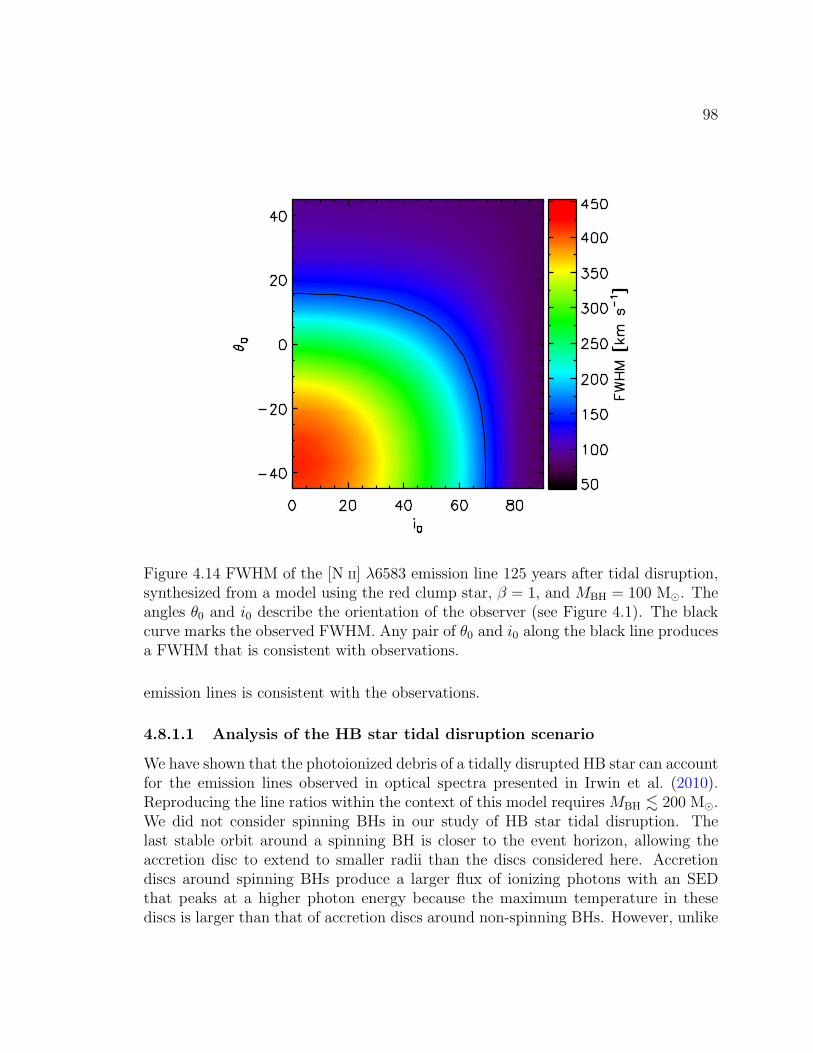
98

Figure 4.14 FWHM of the [N II] λ6583 emission line 125 years after tidal disruption,synthesized from a model using the red clump star, β = 1, and MBH = 100 M�. Theangles θ0 and i0 describe the orientation of the observer (see Figure 4.1). The blackcurve marks the observed FWHM. Any pair of θ0 and i0 along the black line producesa FWHM that is consistent with observations.

emission lines is consistent with the observations.

4.8.1.1 Analysis of the HB star tidal disruption scenario

We have shown that the photoionized debris of a tidally disrupted HB star can accountfor the emission lines observed in optical spectra presented in Irwin et al. (2010).Reproducing the line ratios within the context of this model requires MBH . 200 M�.We did not consider spinning BHs in our study of HB star tidal disruption. Thelast stable orbit around a spinning BH is closer to the event horizon, allowing theaccretion disc to extend to smaller radii than the discs considered here. Accretiondiscs around spinning BHs produce a larger flux of ionizing photons with an SEDthat peaks at a higher photon energy because the maximum temperature in thesediscs is larger than that of accretion discs around non-spinning BHs. However, unlike

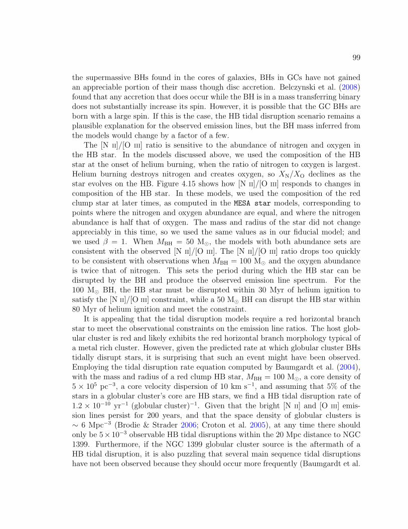
99

the supermassive BHs found in the cores of galaxies, BHs in GCs have not gainedan appreciable portion of their mass though disc accretion. Belczynski et al. (2008)found that any accretion that does occur while the BH is in a mass transferring binarydoes not substantially increase its spin. However, it is possible that the GC BHs areborn with a large spin. If this is the case, the HB tidal disruption scenario remains aplausible explanation for the observed emission lines, but the BH mass inferred fromthe models would change by a factor of a few.

The [N II]/[O III] ratio is sensitive to the abundance of nitrogen and oxygen inthe HB star. In the models discussed above, we used the composition of the HBstar at the onset of helium burning, when the ratio of nitrogen to oxygen is largest.Helium burning destroys nitrogen and creates oxygen, so XN/XO declines as thestar evolves on the HB. Figure 4.15 shows how [N II]/[O III] responds to changes incomposition of the HB star. In these models, we used the composition of the redclump star at later times, as computed in the MESA star models, corresponding topoints where the nitrogen and oxygen abundance are equal, and where the nitrogenabundance is half that of oxygen. The mass and radius of the star did not changeappreciably in this time, so we used the same values as in our fiducial model; andwe used β = 1. When MBH = 50 M�, the models with both abundance sets areconsistent with the observed [N II]/[O III]. The [N II]/[O III] ratio drops too quicklyto be consistent with observations when MBH = 100 M� and the oxygen abundanceis twice that of nitrogen. This sets the period during which the HB star can bedisrupted by the BH and produce the observed emission line spectrum. For the100 M� BH, the HB star must be disrupted within 30 Myr of helium ignition tosatisfy the [N II]/[O III] constraint, while a 50 M� BH can disrupt the HB star within80 Myr of helium ignition and meet the constraint.

It is appealing that the tidal disruption models require a red horizontal branchstar to meet the observational constraints on the emission line ratios. The host glob-ular cluster is red and likely exhibits the red horizontal branch morphology typical ofa metal rich cluster. However, given the predicted rate at which globular cluster BHstidally disrupt stars, it is surprising that such an event might have been observed.Employing the tidal disruption rate equation computed by Baumgardt et al. (2004),with the mass and radius of a red clump HB star, MBH = 100 M�, a core density of5 × 105 pc−3, a core velocity dispersion of 10 km s−1, and assuming that 5% of thestars in a globular cluster’s core are HB stars, we find a HB tidal disruption rate of1.2 × 10−10 yr−1 (globular cluster)−1. Given that the bright [N II] and [O III] emis-sion lines persist for 200 years, and that the space density of globular clusters is∼ 6 Mpc−3 (Brodie & Strader 2006; Croton et al. 2005), at any time there shouldonly be 5×10−3 observable HB tidal disruptions within the 20 Mpc distance to NGC1399. Furthermore, if the NGC 1399 globular cluster source is the aftermath of aHB tidal disruption, it is also puzzling that several main sequence tidal disruptionshave not been observed because they should occur more frequently (Baumgardt et al.

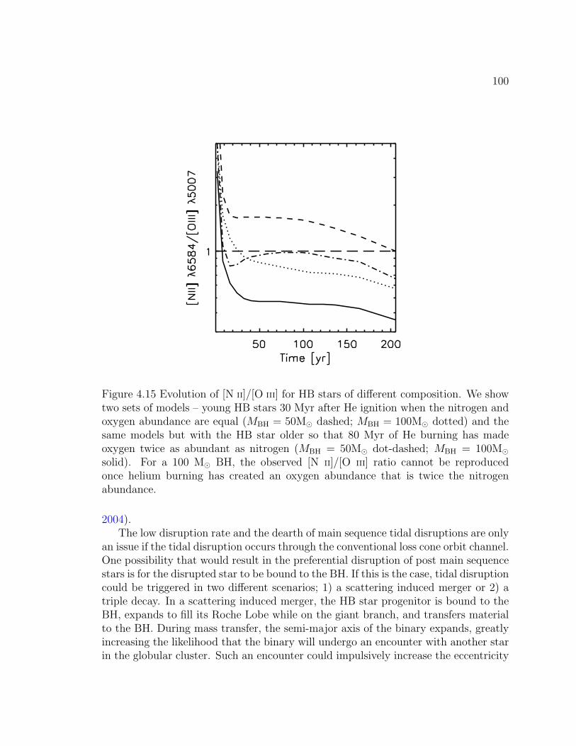
100

Figure 4.15 Evolution of [N II]/[O III] for HB stars of different composition. We showtwo sets of models – young HB stars 30 Myr after He ignition when the nitrogen andoxygen abundance are equal (MBH = 50M� dashed; MBH = 100M� dotted) and thesame models but with the HB star older so that 80 Myr of He burning has madeoxygen twice as abundant as nitrogen (MBH = 50M� dot-dashed; MBH = 100M�solid). For a 100 M� BH, the observed [N II]/[O III] ratio cannot be reproducedonce helium burning has created an oxygen abundance that is twice the nitrogenabundance.

2004).The low disruption rate and the dearth of main sequence tidal disruptions are only

an issue if the tidal disruption occurs through the conventional loss cone orbit channel.One possibility that would result in the preferential disruption of post main sequencestars is for the disrupted star to be bound to the BH. If this is the case, tidal disruptioncould be triggered in two different scenarios; 1) a scattering induced merger or 2) atriple decay. In a scattering induced merger, the HB star progenitor is bound to theBH, expands to fill its Roche Lobe while on the giant branch, and transfers materialto the BH. During mass transfer, the semi-major axis of the binary expands, greatlyincreasing the likelihood that the binary will undergo an encounter with another starin the globular cluster. Such an encounter could impulsively increase the eccentricity

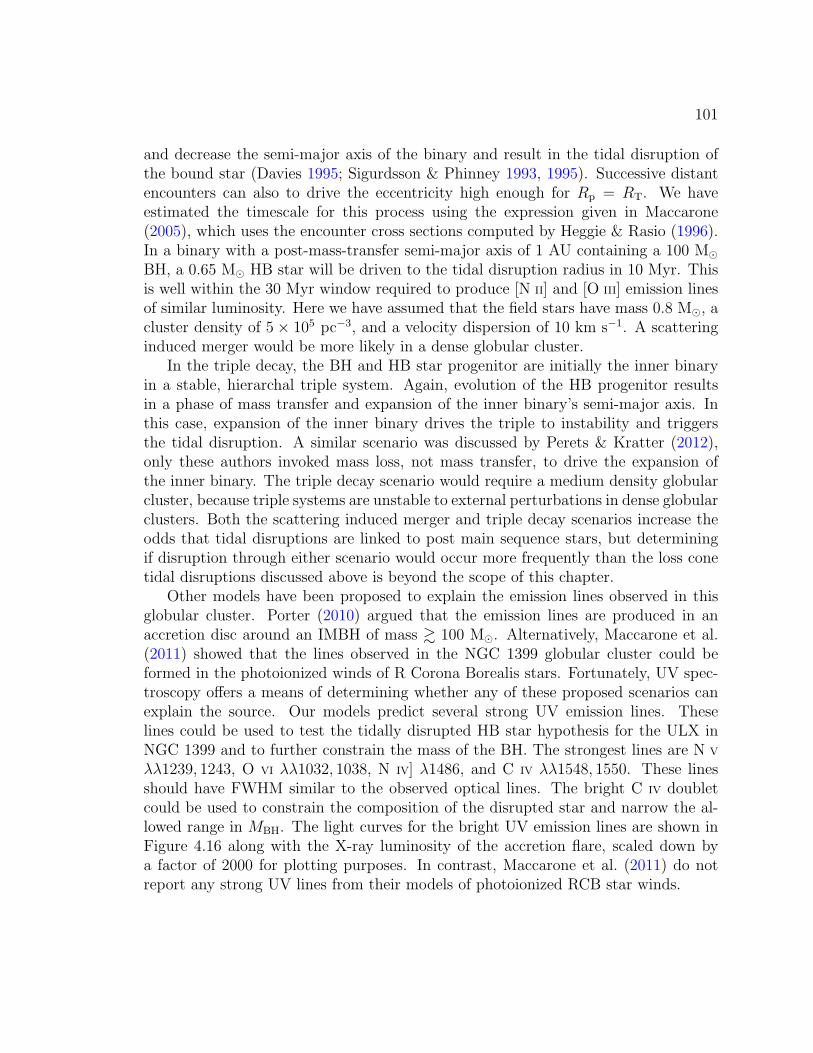
101

and decrease the semi-major axis of the binary and result in the tidal disruption ofthe bound star (Davies 1995; Sigurdsson & Phinney 1993, 1995). Successive distantencounters can also to drive the eccentricity high enough for Rp = RT. We haveestimated the timescale for this process using the expression given in Maccarone(2005), which uses the encounter cross sections computed by Heggie & Rasio (1996).In a binary with a post-mass-transfer semi-major axis of 1 AU containing a 100 M�BH, a 0.65 M� HB star will be driven to the tidal disruption radius in 10 Myr. Thisis well within the 30 Myr window required to produce [N II] and [O III] emission linesof similar luminosity. Here we have assumed that the field stars have mass 0.8 M�, acluster density of 5× 105 pc−3, and a velocity dispersion of 10 km s−1. A scatteringinduced merger would be more likely in a dense globular cluster.

In the triple decay, the BH and HB star progenitor are initially the inner binaryin a stable, hierarchal triple system. Again, evolution of the HB progenitor resultsin a phase of mass transfer and expansion of the inner binary’s semi-major axis. Inthis case, expansion of the inner binary drives the triple to instability and triggersthe tidal disruption. A similar scenario was discussed by Perets & Kratter (2012),only these authors invoked mass loss, not mass transfer, to drive the expansion ofthe inner binary. The triple decay scenario would require a medium density globularcluster, because triple systems are unstable to external perturbations in dense globularclusters. Both the scattering induced merger and triple decay scenarios increase theodds that tidal disruptions are linked to post main sequence stars, but determiningif disruption through either scenario would occur more frequently than the loss conetidal disruptions discussed above is beyond the scope of this chapter.

Other models have been proposed to explain the emission lines observed in thisglobular cluster. Porter (2010) argued that the emission lines are produced in anaccretion disc around an IMBH of mass & 100 M�. Alternatively, Maccarone et al.(2011) showed that the lines observed in the NGC 1399 globular cluster could beformed in the photoionized winds of R Corona Borealis stars. Fortunately, UV spec-troscopy offers a means of determining whether any of these proposed scenarios canexplain the source. Our models predict several strong UV emission lines. Theselines could be used to test the tidally disrupted HB star hypothesis for the ULX inNGC 1399 and to further constrain the mass of the BH. The strongest lines are N V

λλ1239, 1243, O VI λλ1032, 1038, N IV] λ1486, and C IV λλ1548, 1550. These linesshould have FWHM similar to the observed optical lines. The bright C IV doubletcould be used to constrain the composition of the disrupted star and narrow the al-lowed range in MBH. The light curves for the bright UV emission lines are shown inFigure 4.16 along with the X-ray luminosity of the accretion flare, scaled down bya factor of 2000 for plotting purposes. In contrast, Maccarone et al. (2011) do notreport any strong UV lines from their models of photoionized RCB star winds.

102

50 100 150 200Time [yr]

36.0

36.2

36.4

36.6

36.8

37.0

37.2lo

g L

line [

erg

s-1] N V 1240

C IV 1548O VI 1035N IV] 1486

C III] 1909

Ly

LX/2000

Figure 4.16 UV Light curves from a model using the fiducial red clump HB star,β = 1, and MBH = 100 M�. Emission line light curves are shown for N V λ1240,C IV λ1548, O VI λ1035, N IV λ1486, C III] λ1909, and Lyman-α. The dashed curveshows LX scaled down by a factor of 2000. These UV lines can be used to test theHB star tidal disruption hypothesis and to better constrain the mass of the IMBH.The dotted portion of each curve shows the line luminosity while the fallback rate issuper-Eddington and our model is uncertain.

4.9 Conclusion

We have presented models for the emission lines generated in the photoionized debrisof tidally disrupted WDs and HB stars. We have compared our models with obser-vations of two WD tidal disruption candidates, and we disfavor the interpretationof either sources as a WD tidal disruption event. However given the capabilities ofcurrent and planed optical and X-ray transient surveys, the number of candidate WDtidal disruption events should increase in the near future. These candidates can bevetted with follow up optical and UV spectroscopy that searches for strong, broad[O III] λ5007 and C IV λ1549 lines that evolve as shown if Figure 4.6. Finally, withinthe assumptions made in our models, the emission line spectrum produced when a redclump star is disrupted by a BH with MBH . 200 is consistent with the optical emis-sion lines observed by Irwin et al. (2010) in the ULX hosting globular cluster in NGC1399. The models also make testable predictions about the source’s UV-emissionline spectrum. Observations of the UV-emission lines could significantly improve ourunderstanding of this source and are likely possible with the Hubble Space Telescope.

Chapter 5

Summary and Outlook

As a consequence of the high stellar density in globular clusters, any BHs presentin these clusters are likely to undergo strong encounters with stars and other stellarremnants within the cluster. The goal of this thesis was to investigate how theobservable outcomes of such interactions can be used to probe the nature of the BHsharbored by globular clusters. Since little is known about the mass distribution andsize of a globular clusters’s BH population, we considered a wide range of possibilities.Our models studied encounters involving both stellar and intermediate mass BHs,and considered populations ranging from a single BH up to nearly 200 BHs. Ineach case, we determined how the properties of these populations are imprinted onsources of electromagnetic and/or gravitational radiation in the cluster. We willbriefly summarize our findings and suggest some directions for future study below.

We explored the dynamical formation of BH+NS binaries through exchange in-teractions between binary and single stars. In chapter 2, we discussed the prospectof detecting the gravitational waves emitted by these binaries as they merge. Themerger rate depends critically upon whether or not the BH is retained by the clusterafter the merger. If the BH is retained, it can acquire and merge with additional NScompanions, thereby greatly enhancing the merger rate. General relativistic simu-lations indicate that the magnitude of the kick imparted to a ∼ 7 M� BH after itmerges with a NS will exceed a globular cluster’s escape velocity (e.g. Shibata et al.2009). For mergers involving more massive BHs, the recoil speed is suppressed andthe BH can remain in the cluster after each merger. In addition to increasing themerger rate per cluster, the coalescence of a NS with a more massive BH can bedetected out to much larger distances. Thus, the rate of detectable mergers is ex-tremely sensitive to the mass of the BH. However, the BH mass function is not theonly poorly understood characteristic of a globular cluster that strongly impacts theBH+NS merger rate. Our models show that the rate is also sensitive to the nature ofa cluster’s binary population. A post-merger BH is more likely to gain a subsequentNS companion if there is a large reservoir of background binaries for this newly singleBH to exchange into. Given the uncertainty in these inputs to our models, we predict

103

104

a broad range of aLIGO detection rates, 0 – 0.7 yr−1.Only a fraction of the BH+NS binaries formed through exchange interactions in

globular clusters will merge within a Hubble time. However, if the NS had been spunup into a MSP before exchanging into a binary with a BH, then these BH+MSPbinaries could be observed in the electromagnetic band. We explored this possibilityextensively in chapter 3. The orbital period distributions of these dynamically formedBH+MSP binaries are most sensitive to the structural properties of the globularcluster in which they are produced, and not the uncertain nature of the underlyingBH or binary populations. In dense, massive clusters, where the encounter rate islarge, the BH+MSP binaries are rapidly hardened to small orbital separations. Themedian orbital period of the BH+MSP binaries in such clusters is around 5 days. Onthe other hand, in lower density clusters, where binaries are not hardened as quickly,the typical orbital period of a BH+MSP binary is over 100 days. The more gradualhardening process in these clusters also results in longer lifetimes for the BH+MSPbinaries, which increases the probability that such a system can be observed. However,the probability that a BH+MSP binary exists in a globular cluster also depends onthe BH mass function, the number of BHs present in the cluster, and properties ofthe cluster’s binary population. BH+MSP binaries are produced most efficiently inclusters with a few dozen low-mass BHs and high binary fractions. Our optimisticestimates predict that there could be as many as 10 BH+MSP binaries in the MilkyWay globular cluster system. Clusters with structures similar to 47 Tuc, NGC 1851,M62, and Terzan 5 are most likely to harbor a BH+MSP binary.

We have investigated two ways in which the BH+NS binaries produced in globularclusters might reveal themselves, as gravitational wave sources when they coalesce andas radio sources while they are BH+MSP binaries. Interestingly, these two observ-able manifestations are sensitive to different ends of the BH mass function. BH–NSmergers will only be detected if the stellar mass BHs in globular clusters are substan-tially more massive than the stellar mass BHs observed in the field. Conversely, theformation and survival of a BH+MSP binary is most likely if the stellar mass BHsin globular clusters are of similar mass to those in the field. Unfortunately, the dy-namical production of BH+NS binaries may be too inefficient for either manifestationto be detected using the current generation of instruments. However, the EinsteinGravitational Wave Telescope is expected to detect BH+NS mergers out to z & 6(Sathyaprakash et al. 2012). Furthermore, the Square Kilometer Array will be ableto detect most pulsars within 10 Mpc (Cordes 2007). With the much larger volumesprobed by these next generation detectors, the discovery of a dynamically formedBH+NS binary is expected in all but the most pessimistic cases investigated in ourmodels.

In a complementary study, we investigated a mechanism that probes the IMBHsthat might be lurking in the centers of globular clusters. In chapter 4, we presentedmodels of the emission lines produced in the photoionized debris of WDs and HB stars

105

that have been tidally disrupted by an IMBH. We found that bright, broad C IV λ1549and [O III] λλ4959, 5007 emission lines can be used to identify WD tidal disruptionevents, provided that there are no hydrogen lines observed along side these featuresin the spectrum, and that the emission lines are seen in concert with an UV/X-ray flare near the center of a globular cluster or a galaxy. The peak luminosity ofthe [O III] λ5007 emission line depends weakly on the mass of the IMBH, but thismass dependance is degenerate with changes in the peak luminosity produced byvarying the IMBH’s spin. Additional uncertainties arise if we consider the possibilitythat the assumptions made in our models do not adequately describe what occursin nature. For example, little is understood about the structure of the accretionflow and the efficiency at which the bound debris’s potential energy is converted intoionizing radiation following a tidal disruption event. Therefore, we concluded that itis difficult to determine the IMBH’s mass to better than an order of magnitude givenobservations of the [O III] λ5007 line alone.

Our HB star tidal disruption models showed that the emission lines produced inthese events can remain bright for more than a century. Our models suggest that thephotoionized debris of a tidally disrupted HB star may emit detectable Hα and Hβlines shortly after disruption. At late times, however, the spectra should be devoid ofhydrogen lines. In addition to the [O III] doublet expected in WD tidal disruptions,the photoionized debris of a tidally disrupted HB star will also emit a bright [N II]λλ6548, 6583 doublet. The [N II] doublet is produced because the core of a HB staris enriched with nitrogen as a result of CNO-cycle burning.

We compared our modeled emission line luminosities and profiles to two WD tidaldisruption candidates in extragalactic globular clusters. Both candidates exhibit abright X-ray source and an [O III] λ5007 emission line luminosity that is comparableto that predicted by our models. However, there are drawbacks to interpreting eithersource as a WD tidal disruption. This is not surprising because the predicted rateof WD tidal disruption events is low enough that it is unlikely that one should havebeen observed (Ramirez-Ruiz & Rosswog 2009).

Interestingly, the optical spectrum of the WD tidal disruption candidate in a glob-ular cluster associated with NGC 1399 exhibits both of the bright emission featurespredicted by our HB star tidal disruption models. Beyond identifying this source asa HB star tidal disruption candidate, we can use the observed [N II]/[O III] emissionline luminosity ratio, and the limits on the [N II]/Hα and [O III]/Hβ ratios, to con-strain the mass of the BH in this cluster. Reproducing the observed [N II]/[O III] ∼ 1requires that MBH < 200 M�. This places the BH on the low mass end of the IMBHmass spectrum. Again, though, given the predicted rate for HB star tidal disruptionevents, it is surprising that such an event has been observed. It is also puzzling thatwe have yet to observe evidence of a main sequence star’s tidal disruption in a glob-ular cluster because this should occur 20 times more often than the disruption of anevolved star.

106

Given its enigmatic nature, the candidate HB star tidal disruption event warrantsfurther investigation. There are alternative explanations for the emission lines ob-served in this cluster. The emission lines could be produced if the radiation emittedby the accreting BH photoionizes material ejected by an unrelated source within thecluster (Maccarone & Warner 2011; Ripamonti & Mapelli 2012). It is also possible togenerate these emission lines in the IMBH’s accretion disk itself (Porter 2010). Oneway to distinguish between these varied explanations is to obtain a UV spectrum ofthe source, as each model predicts a very distinctive spectral features in the UV. Ifthe observed UV spectrum supports the HB star tidal disruption hypothesis, thenthe mass of the BH can be better constrained based upon the luminosities of the UVemission lines.

5.1 Suggestions for Future Study

Now that several promising BH candidates have been discovered in globular clusters,it is obvious that at least a few clusters are able to retain some of the BHs thatform within them. A clear question to ask is whether there are common traits amongthese clusters that promote BH retention. Unfortunately, it is difficult to measure thestructural parameters of many of these clusters because most of the BH candidatesare in distant, extragalactic clusters. By comparing the luminosities and colors ofthe extragalactic globular clusters that contain BH candidates to those of clustersthat do not, Maccarone et al. (2011) argued that BHs are more likely to be found inmassive, metal-rich clusters. It is not clear, however, whether this is because massive,metal-rich clusters are more likely to retain BHs (e.g. Moody & Sigurdsson 2009) orbecause X-ray binary formation is more efficient in high metallicity clusters (Ivanovaet al. 2012).

The structure of the Milky Way globular cluster that contains two BH candidates,M22, can be studied in detail. In fact, at 1.24 pc the core radius of M22 is peculiarlylarge (Strader et al. 2012a). As was discussed in chapter 1, the binaries in a clustercan serve as a source of energy and halt a cluster’s collapse. Miller & Davies (2012)argued that the hard binary fraction alone may determine whether or not a densestellar system will collapse. Figure 5.1 shows a plot of the core radius, rc, vs. thephotometric binary fraction, fb, for globular clusters in the Milky Way (data fromMilone et al. 2012b). It does appear that clusters with higher binary fractions do havelarger core radii. It is conceivable that in addition to supporting the entire clusteragainst collapse, the presence of a substantial population of hard binaries may alsoprevent the formation of the dense BH subcluster. There is evidence of a bimodalityin the distribution of core radii in massive star clusters associated with the LargeMagellanic Cloud. Elson et al. (1989) noted that the rc evolution of these clustersappears to bifurcate; the cores of some clusters expand with time while the coresof others contract. Perhaps the clusters with a large enough binary population to

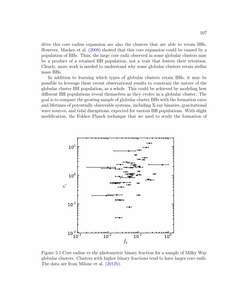
107

drive this core radius expansion are also the clusters that are able to retain BHs.However, Mackey et al. (2008) showed that this core expansion could be caused by apopulation of BHs. Thus, the large core radii observed in some globular clusters maybe a product of a retained BH population, not a trait that fosters their retention.Clearly, more work is needed to understand why some globular clusters retain stellarmass BHs.

In addition to learning which types of globular clusters retain BHs, it may bepossible to leverage these recent observational results to constrain the nature of theglobular cluster BH population, as a whole. This could be achieved by modeling howdifferent BH populations reveal themselves as they evolve in a globular cluster. Thegoal is to compare the growing sample of globular cluster BHs with the formation ratesand lifetimes of potentially observable systems, including X-ray binaries, gravitationalwave sources, and tidal disruptions, expected for various BH populations. With slightmodification, the Fokker–Planck technique that we used to study the formation of

10-3 10-2 10-1 100

fb

10-2

10-1

100

101

r c

Figure 5.1 Core radius vs the photometric binary fraction for a sample of Milky Wayglobular clusters. Clusters with higher binary fractions tend to have larger core radii.The data are from Milone et al. (2012b).

108

BH+NS binaries would be an excellent tool to address this problem. Adapting thecode to make the background cluster dynamic and adding distribution functions thatdescribe the globular cluster’s binary population would greatly improve the models.Adding binaries is essential to understanding the production of observable BH systemsbecause interactions between two binaries can result in the formation of a hierarchicaltriple. Evolution of these triple systems may result in the formation of an X-ray binaryor a tidal disruption, either of which could explain the bright X-ray sources seen insome globular clusters.

To better understand the nature of BHs in globular clusters, the evolution ofBH+WD X-ray binaries should also be investigated. Previous work suggests thatthese systems might be the dominant means by which globular cluster BHs revealthemselves (e.g. Ivanova et al. 2010; Maccarone et al. 2010). Using the stellar evo-lution code MESA star it is possible to determine, in detail, how the WDs in thesesystems respond to mass loss, which in turn governs the rate and stability of masstransfer. By computing a grid of detailed binary evolution models with MESA star itis possible to characterize the stability, rate, and timescale of mass transfer in suchsystems. These results can then be used to establish the X-ray luminosity and theoutburst properties of the BH+WD binaries. Furthermore, as the BH accretes mate-rial shed by the WD, emission lines can be produced in a wind and/or in the accretiondisk itself. The BH’s mass might be encoded in these emission lines, as it is in thetidal disruption case described in chapter 4. Modeling the electromagnetic signaturesof these binaries is vital to comparing the outcomes of dynamical models with theobserved BH candidates, thereby constraining the nature of the globular cluster blackhole population, and shedding light on an enduring astrophysical problem.

Bibliography

Aarseth, S. J. 1999, PASP, 111, 1333

—. 2012, MNRAS, 422, 841

Abbott, B. P., Abbott, R., Adhikari, R., et al. 2009, Rep. Prog. Phys., 72, 076901

Abdo, A. A., Ackermann, M., Ajello, M., et al. 2010, A&A, 524, A75

Abramowicz, M. A., Czerny, B., Lasota, J. P., & Szuszkiewicz, E. 1988, ApJ, 332,646

Abt, H. A. 1983, ARA&A, 21, 343

Alpar, M. A., Cheng, A. F., Ruderman, M. A., & Shaham, J. 1982, Nat, 300, 728

Anderson, J., Piotto, G., King, I. R., Bedin, L. R., & Guhathakurta, P. 2009, ApJL.,697, L58

Anderson, J., Sarajedini, A., Bedin, L. R., et al. 2008, AJ, 135, 2055

Bahcall, J. N., & Ostriker, J. P. 1975, Nat, 256, 23

Bahcall, J. N., & Wolf, R. A. 1976, ApJ, 209, 214

—. 1977, ApJ, 216, 883

Bailyn, C. D., & Grindlay, J. E. 1990, ApJ, 353, 159

Banerjee, S., Baumgardt, H., & Kroupa, P. 2010, MNRAS, 402, 371

Barnard, R., Garcia, M., Li, Z., Primini, F., & Murray, S. S. 2011, ApJ, 734, 79

Barnard, R., Garcia, M., & Murray, S. S. 2012, ApJ, 757, 40

Baumgardt, H., Makino, J., & Ebisuzaki, T. 2004, ApJ, 613, 1143

Baumgardt, H., Makino, J., & Hut, P. 2005, ApJ, 620, 238

Baumgardt, H., Makino, J., Hut, P., McMillan, S., & Portegies Zwart, S. 2003, ApJL.,589, L25

Behr, B. B., Cohen, J. G., McCarthy, J. K., & Djorgovski, S. G. 1999, ApJL., 517,L135

Bekki, K., & Freeman, K. C. 2003, MNRAS, 346, L11

Belczynski, K., Bulik, T., & Bailyn, C. 2011, ApJL., 742, L2

Belczynski, K., Bulik, T., Fryer, C. L., et al. 2010a, ApJ, 714, 1217

Belczynski, K., Dominik, M., Bulik, T., et al. 2010b, ApJL., 715, L138

Belczynski, K., Taam, R. E., Kalogera, V., Rasio, F. A., & Bulik, T. 2007, ApJ, 662,504

109

110

Belczynski, K., Taam, R. E., Rantsiou, E., & van der Sluys, M. 2008, ApJ, 682, 474

Benacquista, M. J. 2006, Living Reviews in Relativity, 9, 2

Bicknell, G. V., & Gingold, R. A. 1983, ApJ, 273, 749

Binney, J., & Tremaine, S. 1987, Galactic Dynamics, 1st edn. (Princeton, NJ: Prince-ton University Press)

Bogdanovic, T., Eracleous, M., Mahadevan, S., Sigurdsson, S., & Laguna, P. 2004,ApJ, 610, 707

Brandt, W. N., Pounds, K. A., & Fink, H. 1995, MNRAS, 273, L47

Brassart, M., & Luminet, J. 2008, A&A, 481, 259

—. 2010, A&A, 511, 80

Brassington, N. J., Fabbiano, G., Blake, S., et al. 2010, ApJ, 725, 1805

Brassington, N. J., Fabbiano, G., Zezas, A., et al. 2012, ApJ, 755, 162

Brodie, J. P., & Strader, J. 2006, ARA&A, 44, 193

Camilo, F., & Rasio, F. A. 2005, in Astronomical Society of the Pacific ConferenceSeries, Vol. 328, Binary Radio Pulsars, ed. F. A. Rasio & I. H. Stairs, 147

Campanelli, M., Lousto, C., Zlochower, Y., & Merritt, D. 2007, ApJL., 659, L5

Cappelluti, N., Ajello, M., Rebusco, P., et al. 2009, A&A, 495, L9

Carretta, E., Gratton, R. G., Clementini, G., & Fusi Pecci, F. 2000, ApJ, 533, 215

Carter, B., & Luminet, J. 1983, A&A, 121, 97

Carter, B., & Luminet, J. P. 1982, Nat, 296, 211

Casebeer, D. A., Leighly, K. M., & Baron, E. 2006, ApJ, 637, 157

Catalan, S., Isern, J., Garcıa-Berro, E., & Ribas, I. 2008, MNRAS, 387, 1693

Charbonnel, C., Meynet, G., Maeder, A., & Schaerer, D. 1996, A&AS, 115, 339

Charpinet, S., van Grootel, V., Reese, D., et al. 2008, A&A, 489, 377

Chennamangalam, J., Lorimer, D. R., Mandel, I., & Bagchi, M. 2013, MNRAS, 431,874

Chernoff, D. F., & Weinberg, M. D. 1990, ApJ, 351, 121

Chomiuk, L., Strader, J., Maccarone, T. J., Miller-Jones, J. C. A., & Seth, A. C.2013, in Abstracts of 13th HEAD Meeting, Vol. 1, 206.13

Clark, G. W., Markert, T. H., & Li, F. K. 1975, ApJL., 199, L93

Clausen, D., & Eracleous, M. 2011, ApJ, 726, 34

Clausen, D., Sigurdsson, S., & Chernoff, D. F. 2013, MNRAS, 428, 3618

Clausen, D., Sigurdsson, S., Eracleous, M., & Irwin, J. A. 2012, MNRAS, 424, 1268

Cohn, H. 1979, ApJ, 234, 1036

Cohn, H., & Hut, P. 1984, ApJL., 277, L45

Colbert, E. J. M., & Ptak, A. F. 2002, ApJS, 143, 25

Colpi, M., Mapelli, M., & Possenti, A. 2003, ApJ, 599, 1260

Colpi, M., Possenti, A., & Gualandris, A. 2002, ApJL., 570, L85

Cordes, J. M. 2007, SKA Memo, 97

111

Croton, D. J., Farrar, G. R., Norberg, P., et al. 2005, MNRAS, 356, 1155

Dalessandro, E., Lanzoni, B., Ferraro, F. R., et al. 2008, ApJ, 677, 1069

D’Amico, N., Lyne, A. G., Manchester, R. N., Possenti, A., & Camilo, F. 2001, ApJL.,548, L171

D’Amico, N., Possenti, A., Fici, L., et al. 2002, ApJL., 570, L89

D’Antona, F., Bellazzini, M., Caloi, V., et al. 2005, ApJ, 631, 868

Davies, M. B. 1995, MNRAS, 276, 887

Davis, D. S., Richer, H. B., Anderson, J., et al. 2008, AJ, 135, 2155

De Robertis, M. M., & Osterbrock, D. E. 1986, ApJ, 301, 727

Deutsch, E. W., Margon, B., & Anderson, S. F. 2000, ApJL., 530, L21

Devecchi, B., Colpi, M., Mapelli, M., & Possenti, A. 2007, MNRAS, 380, 691

di Criscienzo, M., D’Antona, F., Milone, A. P., et al. 2011, MNRAS, 414, 3381

Donley, J. L., Brandt, W. N., Eracleous, M., & Boller, T. 2002, AJ, 124, 1308

Dorman, B. 1992, ApJS, 81, 221

Dotter, A., Sarajedini, A., Anderson, J., et al. 2010, ApJ, 708, 698

Downing, J. M. B., Benacquista, M. J., Giersz, M., & Spurzem, R. 2010, MNRAS,407, 1946

Downing, J. M. B., & Sills, A. 2007, ApJ, 662, 341

Duez, M. D., Foucart, F., Kidder, L. E., Ott, C. D., & Teukolsky, S. A. 2010, Classicaland Quantum Gravity, 27, 114106

Duquennoy, A., & Mayor, M. 1991, A&A, 248, 485

Elson, R. A. W., Freeman, K. C., & Lauer, T. R. 1989, ApJL., 347, L69

Esquej, P., Saxton, R. D., Komossa, S., et al. 2008, A&A, 489, 543

Etienne, Z. B., Liu, Y. T., Shapiro, S. L., & Baumgarte, T. W. 2009, Phys. Rev. D,79, 044024

Evans, C. R., & Kochanek, C. S. 1989, ApJL., 346, L13

Falcke, H., Kording, E., & Markoff, S. 2004, A&A, 414, 895

Farr, W. M., Sravan, N., Cantrell, A., et al. 2011, ApJ, 741, 103

Faucher-Giguere, C. A., & Loeb, A. 2011, MNRAS, 415, 3951

Ferland, G. J., Korista, K. T., Verner, D. A., et al. 1998, PASP, 110, 761

Forbes, D. A., Strader, J., & Brodie, J. P. 2004, AJ, 127, 3394

Foucart, F., Duez, M. D., Kidder, L. E., & Teukolsky, S. A. 2011, Phys. Rev. D, 83,024005

Frank, J., & Rees, M. J. 1976, MNRAS, 176, 633

Fregeau, J. M., Gurkan, M. A., Joshi, K. J., & Rasio, F. A. 2003, ApJ, 593, 772

Fregeau, J. M., Ivanova, N., & Rasio, F. A. 2009, ApJ, 707, 1533

Freire, P. C. C., Ransom, S. M., & Gupta, Y. 2007, ApJ, 662, 1177

Freitag, M., & Benz, W. 2001, A&A, 375, 711

Freitag, M., Gurkan, M. A., & Rasio, F. A. 2006, MNRAS, 368, 141

112

Frolov, V. P., Khokhlov, A. M., Novikov, I. D., & Pethick, C. J. 1994, ApJ, 432, 680

Fryer, C. L., Heger, A., Langer, N., & Wellstein, S. 2002, ApJ, 578, 335

Fryer, C. L., & Kalogera, V. 2001, ApJ, 554, 548

Gao, B., Goodman, J., Cohn, H., & Murphy, B. 1991, ApJ, 370, 567

Gebhardt, K., Rich, R. M., & Ho, L. C. 2005, ApJ, 634, 1093

Gerssen, J., van der Marel, R. P., Gebhardt, K., et al. 2002, AJ, 124, 3270

Gezari, S., Martin, D. C., Milliard, B., et al. 2006, ApJL., 653, L25

Gezari, S., Basa, S., Martin, D. C., et al. 2008, ApJ, 676, 944

Gezari, S., Heckman, T., Cenko, S. B., et al. 2009, ApJ, 698, 1367

Giersz, M. 1998, MNRAS, 298, 1239

Gnedin, O. Y., & Ostriker, J. P. 1997, ApJ, 474, 223

Gonzalez, J. A., Sperhake, U., Brugmann, B., Hannam, M., & Husa, S. 2007, Phys.Rev. Lett., 98, 091101

Goodman, J. 1984, ApJ, 280, 298

Gratton, R., Sneden, C., & Carretta, E. 2004, ARA&A, 42, 385

Gratton, R. G., Carretta, E., Bragaglia, A., Lucatello, S., & D’Orazi, V. 2010, A&A,517, A81

Gratton, R. G., Sneden, C., Carretta, E., & Bragaglia, A. 2000, A&A, 354, 169

Grindlay, J., Portegies Zwart, S., & McMillan, S. 2006, Nature Physics, 2, 116

Grindlay, J. E., Hertz, P., Steiner, J. E., Murray, S. S., & Lightman, A. P. 1984,ApJL., 282, L13

Grupe, D., Beuerman, K., Mannheim, K., et al. 1995, A&A, 300, L21

Guillochon, J., & Ramirez-Ruiz, E. 2013, ApJ, 767, 25

Guillochon, J., Ramirez-Ruiz, E., Rosswog, S., & Kasen, D. 2009, ApJ, 705, 844

Gultekin, K., Miller, M. C., & Hamilton, D. P. 2004, ApJ, 616, 221

Halpern, J. P., Gezari, S., & Komossa, S. 2004, ApJ, 604, 572

Hansen, B. M. S., & Phinney, E. S. 1997, MNRAS, 291, 569

Harris, W. E. 1974, ApJL., 192, L161

—. 1991, ARA&A, 29, 543

—. 1996, AJ, 112, 1487

Heggie, D. C. 1975, MNRAS, 173, 729

Heggie, D. C., & Rasio, F. A. 1996, MNRAS, 282, 1064

Hessels, J. W. T., Ransom, S. M., Stairs, I. H., et al. 2006, Science, 311, 1901

Hills, J. G. 1975a, AJ, 80, 809

—. 1975b, Nat, 254, 295

—. 1976, MNRAS, 175, 1P

Hirata, C. M. 2011, Phys. Rev. D, 83, 104024

Hurley, J. R., Aarseth, S. J., & Shara, M. M. 2007, ApJ, 665, 707

Hut, P., & Bahcall, J. N. 1983, ApJ, 268, 319

113

Hut, P., McMillan, S., & Romani, R. W. 1992a, ApJ, 389, 527

Hut, P., McMillan, S., Goodman, J., et al. 1992b, PASP, 104, 981

Illingworth, G., & King, I. R. 1977, ApJL., 218, L109

Inagaki, S., & Lynden-Bell, D. 1983, MNRAS, 205, 913

in’t Zand, J. J. M., Hulleman, F., Markwardt, C. B., et al. 2003, A&A, 406, 233

Irwin, J. A., Brink, T. G., Bregman, J. N., & Roberts, T. P. 2010, ApJL., 712, L1

Ivanova, N., Belczynski, K., Fregeau, J. M., & Rasio, F. A. 2005a, MNRAS, 358, 572

Ivanova, N., Chaichenets, S., Fregeau, J., et al. 2010, ApJ, 717, 948

Ivanova, N., Heinke, C. O., Rasio, F. A., Belczynski, K., & Fregeau, J. M. 2008,MNRAS, 386, 553

Ivanova, N., Rasio, F. A., Lombardi, Jr., J. C., Dooley, K. L., & Proulx, Z. F. 2005b,ApJL., 621, L109

Ivanova, N., Fragos, T., Kim, D. W., et al. 2012, ApJL., 760, L24

Jordan, A., Cote, P., Blakeslee, J. P., et al. 2005, ApJ, 634, 1002

Jordan, A., McLaughlin, D. E., Cote, P., et al. 2007, ApJS, 171, 101

Joshi, K. J., Rasio, F. A., & Portegies Zwart, S. 2000, ApJ, 540, 969

Kalogera, V., King, A. R., & Rasio, F. A. 2004, ApJL., 601, L171

Katz, J. I. 1975, Nat, 253, 698

Khalisi, E., Amaro-Seoane, P., & Spurzem, R. 2007, MNRAS, 374, 703

Khokhlov, A., & Melia, F. 1996, ApJL., 457, L61

Khokhlov, A., Novikov, I. D., & Pethick, C. J. 1993, ApJ, 418, 181

King, I. R. 1966, AJ, 71, 64

King, I. R., Sosin, C., & Cool, A. M. 1995, ApJL., 452, L33

Kobayashi, S., Laguna, P., Phinney, E. S., & Meszaros, P. 2004, ApJ, 615, 855

Kochanek, C. S. 1994, ApJ, 422, 508

Komossa, S., & Bade, N. 1999, A&A, 343, 775

Komossa, S., & Greiner, J. 1999, A&A, 349, L45

Korista, K., Ferland, G., & Baldwin, J. 1997, ApJ, 487, 555

Kramer, M., Stairs, I. H., Manchester, R. N., et al. 2006, Science, 314, 97

Kroupa, P. 2001, MNRAS, 322, 231

Kulkarni, S. R., Hut, P., & McMillan, S. 1993, Nat, 364, 421

Kundu, A., Maccarone, T. J., & Zepf, S. E. 2007, ApJ, 662, 525

Kyutoku, K., Shibata, M., & Taniguchi, K. 2009, Phys. Rev. D, 79, 124018

Lacy, J. H., Townes, C. H., & Hollenbach, D. J. 1982, ApJ, 262, 120

Laguna, P., Miller, W. A., Zurek, W. H., & Davies, M. B. 1993, ApJL., 410, L83

Lanzoni, B., Dalessandro, E., Ferraro, F. R., et al. 2007, ApJL., 668, L139

Lee, J. W., Kang, Y. W., Lee, J., & Lee, Y. W. 2009, Nat, 462, 480

Lee, Y. W., Demarque, P., & Zinn, R. 1994, ApJ, 423, 248

Lee, Y. W., Joo, J. M., Sohn, Y. J., et al. 1999, Nat, 402, 55

114

Lipunov, V. M., Postnov, K. A., Prokhorov, M. E., & Osminkin, E. Y. 1994, ApJL.,423, L121

Lodato, G., King, A. R., & Pringle, J. E. 2009, MNRAS, 392, 332

Lorimer, D. R. 2008, Living Reviews in Relativity, 11, 8

Luminet, J., & Marck, J. 1985, MNRAS, 212, 57

Luminet, J., & Pichon, B. 1989, A&A, 209, 103

Luo, B., Brandt, W. N., Steffen, A. T., & Bauer, F. E. 2008, ApJ, 674, 122

Lutzgendorf, N., Kissler-Patig, M., Noyola, E., et al. 2011, A&A, 533, A36

Lynch, R. S., & Ransom, S. M. 2011, ApJL., 730, L11

Lynden-Bell, D., & Wood, R. 1968, MNRAS, 138, 495

Lyne, A. G., Brinklow, A., Middleditch, J., Kulkarni, S. R., & Backer, D. C. 1987,Nat, 328, 399

Lyne, A. G., & Lorimer, D. R. 1994, Nat, 369, 127

Maccarone, T. J. 2005, MNRAS, 364, 971

Maccarone, T. J., Kundu, A., Zepf, S. E., & Rhode, K. L. 2007, Nat, 445, 183

—. 2010, MNRAS, 409, L84

—. 2011, MNRAS, 410, 1655

Maccarone, T. J., & Warner, B. 2011, MNRAS, 410, L32

Mackey, A. D., Wilkinson, M. I., Davies, M. B., & Gilmore, G. F. 2008, MNRAS,386, 65

Madej, J., Nalezyty, M., & Althaus, L. G. 2004, A&A, 419, L5

Madrid, J. P., Harris, W. E., Blakeslee, J. P., & Gomez, M. 2009, ApJ, 705, 237

Magorrian, J., & Tremaine, S. 1999, MNRAS, 309, 447

Maksym, W. P., Ulmer, M. P., & Eracleous, M. 2010, ApJ, 722, 1035

Manchester, R. N., Lyne, A. G., Robinson, C., Bailes, M., & D’Amico, N. 1991, Nat,352, 219

Mapelli, M., Colpi, M., Possenti, A., & Sigurdsson, S. 2005, MNRAS, 364, 1315

Marino, A. F., Milone, A. P., Piotto, G., et al. 2009, A&A, 505, 1099

Masters, K. L., Jordan, A., Cote, P., et al. 2010, ApJ, 715, 1419

McLaughlin, D. E., & Pudritz, R. E. 1996, ApJ, 457, 578

McMillan, S., Hut, P., & Makino, J. 1990, ApJ, 362, 522

Meissner, F., & Weiss, A. 2006, A&A, 456, 1085

Merloni, A., Heinz, S., & di Matteo, T. 2003, MNRAS, 345, 1057

Metcalfe, T. S. 2003, ApJL., 587, L43

Meylan, G., & Heggie, D. C. 1997, A&A Rev., 8, 1

Michie, R. W. 1963, MNRAS, 125, 127

Miller, J. M., Miller, M. C., & Reynolds, C. S. 2011, ApJL., 731, L5

Miller, M. C., & Davies, M. B. 2012, ApJ, 755, 81

Miller, M. C., & Hamilton, D. P. 2002a, ApJ, 576, 894

115

—. 2002b, MNRAS, 330, 232

Milone, A. P., Marino, A. F., Piotto, G., et al. 2012a, ApJ, 745, 27

Milone, A. P., Bedin, L. R., Piotto, G., et al. 2008, ApJ, 673, 241

Milone, A. P., Piotto, G., King, I. R., et al. 2010, ApJ, 709, 1183

Milone, A. P., Piotto, G., Bedin, L. R., et al. 2012b, A&A, 540, A16

Moody, K., & Sigurdsson, S. 2009, ApJ, 690, 1370

Morscher, M., Umbreit, S., Farr, W. M., & Rasio, F. A. 2013, ApJL., 763, L15

Murphy, B. W., Cohn, H. N., & Lugger, P. M. 2011, ApJ, 732, 67

Nakar, E. 2007, Physics Reports, 442, 166

Narayan, R., Piran, T., & Shemi, A. 1991, ApJL., 379, L17

Nauenberg, M. 1972, ApJ, 175, 417

Newell, B., Da Costa, G. S., & Norris, J. 1976, ApJL., 208, L55

Nussbaumer, H., & Rusca, C. 1979, A&A, 72, 129

O’Leary, R. M., Rasio, F. A., Fregeau, J. M., Ivanova, N., & O’Shaughnessy, R. 2006,ApJ, 637, 937

O’Shaughnessy, R., Kalogera, V., & Belczynski, K. 2010, ApJ, 716, 615

Osterbrock, D. E., & Ferland, G. J. 2006, Astrophysics of gaseous nebulae and activegalactic nuclei, 2nd edn. (Sausalito, CA: University Scienc Books)

Ozel, F., Psaltis, D., Narayan, R., & McClintock, J. E. 2010, ApJ, 725, 1918

Paxton, B., Bildsten, L., Dotter, A., et al. 2011, ApJS, 192, 3

Peacock, M. B., Maccarone, T. J., Knigge, C., et al. 2010, MNRAS, 402, 803

Peacock, M. B., Zepf, S. E., Kundu, A., et al. 2012, ApJ, 759, 126

Peng, E. W., Jordan, A., Cote, P., et al. 2006, ApJ, 639, 95

Pequignot, D., & Aldrovandi, S. M. V. 1976, A&A, 50, 141

Perets, H. B., & Kratter, K. M. 2012, ApJ, 760, 99

Peters, P. C. 1964, Physical Review, 136, 1224

Pfahl, E., Podsiadlowski, P., & Rappaport, S. 2005, ApJ, 628, 343

Pfahl, E., Rappaport, S., & Podsiadlowski, P. 2002, ApJ, 573, 283

Phinney, E. S. 1989, in IAU Symposium, Vol. 136, The Center of the Galaxy, ed.M. Morris, 543

Phinney, E. S. 1991, ApJL., 380, L17

Piotto, G., Bedin, L. R., Anderson, J., et al. 2007, ApJL., 661, L53

Pooley, D., Lewin, W. H. G., Anderson, S. F., et al. 2003, ApJL., 591, L131

Portegies Zwart, S. F., Baumgardt, H., Hut, P., Makino, J., & McMillan, S. L. W.2004, Nat, 428, 724

Portegies Zwart, S. F., & McMillan, S. L. W. 2000, ApJL., 528, L17

Portegies Zwart, S. F., McMillan, S. L. W., Hut, P., & Makino, J. 2001, MNRAS,321, 199

Porter, R. L. 2010, MNRAS, 407, L59

116

Punturo, M., Abernathy, M., Acernese, F., et al. 2010, Classical and Quantum Grav-ity, 27, 194002

Ramirez-Ruiz, E., & Rosswog, S. 2009, ApJL., 697, L77

Ransom, S. M., Hessels, J. W. T., Stairs, I. H., et al. 2005, Science, 307, 892

Rees, M. J. 1988, Nat, 333, 523

Rey, S. C., Rich, R. M., Sohn, S. T., et al. 2007, ApJS, 173, 643

Ripamonti, E., & Mapelli, M. 2012, MNRAS, in press (arXiv:1203.4233)

Roberts, T. P., Fabbiano, G., Luo, B., et al. 2012, ApJ, in press, arXiv:1210.5163

Romani, R. W., & Weinberg, M. D. 1991, ApJ, 372, 487

Roos, N. 1992, ApJ, 385, 108

Rosswog, S., Ramirez-Ruiz, E., & Hix, W. R. 2009, ApJ, 695, 404

Sadowski, A., Belczynski, K., Bulik, T., et al. 2008, ApJ, 676, 1162

Sandage, A., & Wallerstein, G. 1960, ApJ, 131, 598

Sarazin, C. L., Irwin, J. A., & Bregman, J. N. 2000, ApJL., 544, L101

Sathyaprakash, B., Abernathy, M., Acernese, F., et al. 2012, Classical and QuantumGravity, 29, 124013

Searle, L., & Zinn, R. 1978, ApJ, 225, 357

Sesana, A., Sartore, N., Devecchi, B., & Possenti, A. 2012, MNRAS, 427, 502

Sesana, A., Vecchio, A., Eracleous, M., & Sigurdsson, S. 2008, MNRAS, 391, 718

Shibata, M., Kyutoku, K., Yamamoto, T., & Taniguchi, K. 2009, Phys. Rev. D, 79,044030

Shih, I. C., Kundu, A., Maccarone, T. J., Zepf, S. E., & Joseph, T. D. 2010, ApJ,721, 323

Sidoli, L., Parmar, A. N., Oosterbroek, T., et al. 2001, A&A, 368, 451

Sigurdsson, S. 2003, in Astronomical Society of the Pacific Conference Series, Vol.302, Radio Pulsars, ed. M. Bailes, D. J. Nice, & S. E. Thorsett, 391

Sigurdsson, S., & Hernquist, L. 1993, Nat, 364, 423

Sigurdsson, S., & Phinney, E. S. 1993, ApJ, 415, 631

—. 1995, ApJ, 99, 609

Sigurdsson, S., & Rees, M. J. 1997, MNRAS, 284, 318

Silk, J., & Arons, J. 1975, ApJL., 200, L131

Sipior, M. S., Portegies Zwart, S., & Nelemans, G. 2004, MNRAS, 354, L49

Sipior, M. S., & Sigurdsson, S. 2002, ApJ, 572, 962

Sippel, A. C., & Hurley, J. R. 2013, MNRAS, 430, L30

Sollima, A. 2008, MNRAS, 388, 307

Sollima, A., Beccari, G., Ferraro, F. R., Fusi Pecci, F., & Sarajedini, A. 2007, MN-RAS, 380, 781

Spitzer, L. 1987, Dynamical Evolution of Globular Clusters (Princeton, NJ: PrincetonUniversity Press)

117

Spitzer, Jr., L. 1969, ApJL., 158, L139

Spitzer, Jr., L., & Hart, M. H. 1971, ApJ, 164, 399

Stairs, I. H. 2004, Science, 304, 547

Steele, M. M., Zepf, S. E., Kundu, A., et al. 2011, ApJ, 739, 95

Steffen, A. T., Strateva, I., Brandt, W. N., et al. 2006, AJ, 131, 2826

Strader, J., Caldwell, N., & Seth, A. C. 2011, AJ, 142, 8

Strader, J., Chomiuk, L., Maccarone, T., Miller-Jones, J., & Seth, A. 2012a, Nat,490, 71

Strader, J., Chomiuk, L., Maccarone, T. J., et al. 2012b, ApJL., 750, L27

Strubbe, L. E., & Quataert, E. 2009, MNRAS, 400, 2070

—. 2011, MNRAS, 415, 168

Tautvaisiene, G., Edvardsson, B., Tuominen, I., & Ilyin, I. 2001, A&A, 380, 578

Thompson, I. B., Kaluzny, J., Pych, W., et al. 2001, AJ, 121, 3089

Tsvetanov, Z. I., & Iankulova, I. M. 1989, MNRAS, 237, 707

Ulmer, A. 1999, ApJ, 514, 180

van den Bergh, S. 1967, AJ, 72, 70

van Grootel, V., Charpinet, S., Fontaine, G., Green, E. M., & Brassard, P. 2010,A&A, 524, A63

Verbunt, F., & Hut, P. 1987, in IAU Symposium, Vol. 125, The Origin and Evolutionof Neutron Stars, ed. D. J. Helfand & J. H. Huang, 187

Voss, R., & Tauris, T. M. 2003, MNRAS, 342, 1169

Wang, J., & Merritt, D. 2004, ApJ, 600, 149

Watters, W. A., Joshi, K. J., & Rasio, F. A. 2000, ApJ, 539, 331

Zepf, S. E., Stern, D., Maccarone, T. J., et al. 2008, ApJL., 683, L139

VitaDrew Reid Clausen

education The Pennsylvania State University, University Park, PAPh.D. in Astronomy & Astrophysics, expected August 2013

University of Colorado, Boulder, COB.A. in Astronomy, magna cum laude, 2004B.F.A. Film Production, with distinction, 2004

honors & awards Penn State Academic Computing Fellowship 2011-2013Pennsylvania Space Grant Consortium Fellowship 2011-2013Downsborough Graduate Fellowship in Astrophysics 2011Zaccheus Daniel Fellowship 2010, 2012Penn State Graduate Research Exhibition, 3rd Place 2010Stephen B. Brumbach Fellowship in Astrophysics 2009Teaching Assistant of the Year 2008Homer F. Braddock Fellowship 2007Dean’s List 2000-2004

ResearchExperience

Graduate Research Assistant May 2008 – presentDepartment of Astronomy & AstrophysicsThe Pennsylvania State University

Undergraduate Research Assistant Sep 2003 – Dec 2004Department of Astrophysical and Planetary SciencesUniversity of Colorado

TeachingExperience

Instructor Summer 2010ASTRO 001: Astronomical UniverseThe Pennsylvania State University

Teaching Assistant Fall 2007 – Spring 2009ASTRO 11: Elementary Astronomy LabThe Pennsylvania State University

Learning Team Coach Spring 2001 – Spring 2004ASTR 1120: General Astronomy – Stars and GalaxiesUniversity of Colorado