Embed Size (px)
Citation preview
Eur. Phys. J. B 16, 85–105 (2000) THE EUROPEANPHYSICAL JOURNAL Bc©
EDP SciencesSocieta Italiana di FisicaSpringer-Verlag 2000
Strong-coupling perturbation theory of the Hubbard model
S. Pairault1, D. Senechal1,a, and A.-M.S. Tremblay1,2
1 Centre de Recherche sur les Proprietes Electroniques de Materiaux Avances et Departement de Physique,Universite de Sherbrooke, Sherbrooke, Quebec, Canada J1K 2R1
2 Institut canadien de recherches avancees, Universite de Sherbrooke, Sherbrooke, Quebec, Canada J1K 2R1
Received 25 October 1999
Abstract. The strong-coupling perturbation theory of the Hubbard model is presented and carried out toorder (t/U)5 for the one-particle Green function in arbitrary dimension. The spectral weight A(k, ω) isexpressed as a Jacobi continued fraction and compared with new Monte-Carlo data of the one-dimensional,half-filled Hubbard model. Different regimes (insulator, conductor and short-range antiferromagnet) areidentified in the temperature-hopping integral (T, t) plane. This work completes a first paper on the subject(Phys. Rev. Lett. 80, 5389 (1998)) by providing details on diagrammatic rules and higher-order results.In addition, the non half-filled case, infinite resummations of diagrams and the double occupancy arediscussed. Various tests of the method are also presented.
PACS. 71.10.Fd Lattice fermion models (Hubbard model, etc.) – 71.10.Hf Non-Fermi-liquid ground states,electron phase diagrams and phase transitions in model systems – 71.10.Ca Electron gas, Fermi gas
1 Introduction
The study of strongly-correlated electrons has become inthe last decade one of the most active fields of condensedmatter physics. The electronic properties of an increas-ing body of materials cannot be described adequately byLandau’s theory of weakly-interacting quasiparticles(Fermi liquid theory) [1,2]. Best known are the high-Tc
superconductors and organic conductors. In both cases,a strong anisotropy and a narrow conduction band con-tribute to make the effects of interactions between elec-trons (mainly Coulomb repulsion) dramatic.
From a theoretical point of view, quasi-one dimen-sional (e.g. organic conductors) and quasi-two dimensional(e.g. high-Tc superconductors) systems are quite differ-ent. In one dimension, it is possible to solve satisfactorilya great number of models: lattice Hamiltonians such asthe Hubbard model [3] can be solved exactly by BetheAnsatz [4], whereas nonperturbative results can be ob-tained for the Tomonaga-Luttinger [5,6] and the g-ologymodels from bosonization [7] and renormalization-grouptechniques [8,9]. Conformal field theory has been appliedas well, in particular to the Hubbard model [10,11], whoseBethe Ansatz solution has limited practical utility. Aunified phenomenology of the so-called Luttinger liquidsemerges from these works, whose most striking feature isprobably spin-charge separation [12].
On the other hand, the above methods and results can-not be generalized to the case of two dimensions, relevant
a e-mail: [email protected]
to the CuO2 planes present in all high-Tc superconduc-tors. With a half-filled conduction band, all the parentcompounds of the cuprates are antiferromagnetic insula-tors, and the main challenge is to understand, first to-wards which kind of metal they evolve upon doping, andsecondly whether superconductivity can occur, without aphonon-mediated coupling, in the vicinity of this antifer-romagnetic phase. Moreover, the linear temperature de-pendence of the resistivity [13] is a strong experimentalindication that the normal phase of high-Tc superconduc-tors is not a Fermi liquid.
In this context, the Hubbard model [3]
H = −t∑〈i,j〉σ
c†iσcjσ + U∑i
c†i↑c†i↓ci↓ci↑ (1)
has spurred renewed interest for its ability to accountfor antiferromagnetic correlations and the Mott metal-insulator transition. It is also the simplest model ofinteracting electrons. In equation (1), t represents the hop-ping amplitude between two neighboring sites in a tight-binding approximation, and U the strength of the veryeffectively screened (and thus taken to be local) Coulombrepulsion. At half-filling and for t U , the Hubbardmodel is equivalent to a Heisenberg model with antifer-romagnetic exchange J = 4t2/U , and its ground statehas long-range Neel order in any dimension d ≥ 2. AMott transition can occur towards a metallic state eitherupon doping, or by increasing the ratio t/U . Thus, theHubbard model is the prototype of strongly-correlatedelectrons systems and has been intensely studied, although
86 The European Physical Journal B
a more realistic model of the CuO2 planes of the cupratesshould involve several bands [14].
Solving the Hubbard model is a difficult problem by it-self, even in dimension d = 1, where the complexity of theBethe Ansatz solution prevents one from actually com-puting most physical quantities. For example, its spectralweight is known only in the limit U → ∞ and at zerotemperature [15]. In any dimension d ≥ 2, only approxi-mate [3,16–19] or numerical [20–25] methods are available.Only in the limit d→∞ do important simplifications oc-cur [26], allowing to compute most physically interestingquantities in an essentially exact way [27,28]. In particu-lar, the Mott transition has been studied in great detail,and is still under discussion [29,30]. Strong coupling per-turbation theory, which considers the interaction term ofthe Hamiltonian as dominant, and the kinetic term as aperturbation, has been somewhat neglected so far. Therewas some pioneering work of Harris and Lange [31] us-ing the moment technique, but that method cannot eas-ily be pushed to higher order in t. Others have obtainedperturbative series for the thermodynamical potential upto order t4 [32–34], but these approaches do not yielddynamical correlation functions. An original method ef-fectively achieving infinite summations of terms, the so-called Grassmannian Hubbard-Stratonovich transforma-tion, was introduced independently by Bourbonnais [35]and Sarker [36], but contained great difficulties which wereovercome only recently [37] by the authors. The purpose ofthe present paper is to develop the ideas of reference [37]in greater detail, and to present new results that have beenobtained in the meantime.
Although we are naturally interested in the two-particle correlation functions (magnetic susceptibility,conductivity, compressibility) and the phase transitionsof the Hubbard model, it has proven simpler to first elu-cidate one-particle properties. Furthermore, spin-chargeseparation in d = 1 is mostly visible in the spectralweight [38,39], and it is possible to gain significant in-sight into the metal-insulator transition [14] and an-tiferromagnetic correlations from the spectral weightalone. Thus, we will focus on the one-particle prop-erties of the Hubbard model throughout most of thispaper. From an experimental point of view, angle-resolved photoemission spectroscopy (ARPES) is theprobe of choice to measure the spectral weight. Ex-periments have recently been conducted on quasi one-dimensional SrCuO2 [40] and NaV2O5 [41], and on quasitwo-dimensional SrCuCl2O2 [42] antiferromagnetic com-pounds, and further analyzed with the help of exact diag-onalizations [43] and with an application of the methodsof the present paper to the t− t′ − U model [44].
In Section 2, we present the strong-coupling expan-sion for dynamical correlation functions, and provide ex-plicit examples of diagram calculation in Appendix A.The method is applied to the half-filled Hubbard model inSection 3, and the resulting spectral weight and double-occupation are compared to Monte-Carlo data in Sec-tion 4. Partially self-consistent solutions, involving aninfinite sum of diagrams, are investigated in Section 5,
and the question of doping addressed in Section 6.Appendix B provides the atomic one- and two-particle cor-relation functions, necessary to apply the method, and Ap-pendix C presents a practical test of the method on a toymodel. Higher-order terms of the expansion are given inAppendix D.
2 The strong-coupling expansion
In this section we derive the strong-coupling expansion ofcorrelation functions for a wide class of Hamiltonians. Wefirst specify the form that the Hamiltonian should havein order for the method to work. Then we introduce theGrassmannian Hubbard-Stratonovich transformation, andthe diagrammatic perturbation theory itself.
2.1 The Hamiltonian
Consider a Hamiltonian H = H0 + H1, where the un-perturbed part H0 is diagonal in a certain variable i (forinstance a site variable), and let us denote collectively byσ all the other variables of the problem (for instance aspin variable). From now on we will call i the “site vari-able” and σ the “spin variable” for definiteness, thoughthey may represent any set of quantum numbers. ThisHamiltonian describes the behavior of fermions, and wesuppose that it is normal-ordered in terms of the annihi-lation and creation operators c(†)iσ . H0 may be written asa sum over i of on-site Hamiltonians involving only theoperators c(†)iσ at site i:
H0 =∑i
hi(c†iσ , ciσ). (2)
Whenever doing actual calculations, we will use theHubbard model. For the latter, H0 corresponds to theatomic limit, that is
hi(c†iσ, ciσ) = Uc†i↑c
†i↓ci↓ci↑. (3)
We will use the notation u = U/2 throughout this paperfor convenience. We suppose that the perturbation H1 isa one-body operator:
H1 =∑σ
∑ij
Vijc†iσcjσ , (4)
with V a Hermitian matrix. Here, we suppose in additionthat the perturbation is diagonal in the spin variable, butthis needs not be the case. For the Hubbard model, H1
represents the kinetic term, and V is the matrix of hoppingamplitudes.
Introducing the imaginary-time dependent Grassmannfields γiσ(τ), γ?iσ(τ), the partition function at some tem-perature T = 1/β may be written using the Feynman
S. Pairault et al.: Strong-coupling perturbation theory of the Hubbard model 87
path-integral formalism:
Z =∫
[dγ?dγ] exp−∫ β
0
dτ
∑iσ
γ?iσ(τ)(∂
∂τ− µ
)γiσ(τ)
+∑i
hi(γ?iσ(τ), γiσ(τ)) +∑ijσ
Vijγ?iσ(τ)γjσ(τ)
· (5)
In order to lighten the notation, we will use the first fewLatin letters (a, b, ...) to denote sets such as (i, σ, τ), anduse bra-ket notation. For instance:∫ β
0
dτ∑ijσ
Vijγ?iσ(τ)γjσ(τ) =
∑ab
Vabγ?aγb = 〈γ|V |γ〉 ·
(6)
2.2 The Grassmannian Hubbard-Stratonovichtransformation
At this point, one could use standard perturbation the-ory and expand the S-matrix in terms of unperturbedcorrelation functions. Due to the absence of Wick theo-rem in the case of a nonquadratic unperturbed Hamilto-nian, this approach does not lend itself to a satisfactorydiagrammatic theory. One cannot define one-particle irre-ducibility for the diagrams, and one has to be very care-ful in order to avoid double counting of certain contribu-tions. For example, Pan and Wang [33], and Bartkowiakand Chao [34] had to deal with over five hundred differ-ent diagrams in order to obtain the thermodynamic po-tential of the Hubbard model up to fourth order. Theseproblems were solved by Metzner [45], who organized theperturbation series as a cumulant expansion, and formu-lated diagrammatic rules with unrestricted sums over mo-menta. In this subsection we show that Metzner’s resultscan be obtained in a straightforward fashion and even fur-ther simplified by means of a simple transformation on thepartition function. This transformation was first proposedby Bourbonnais [35] and applied (at zeroth order) to theHubbard model by Sarker [36]. Boies et al. also used it tostudy the stability of several Luttinger liquids coupled byan interchain hopping [46].
The Grassmannian Hubbard-Stratonovich transforma-tion amounts to expressing the perturbation part of theexponential as the result of a Gaussian integral over aux-iliary Grassmann fields ψiσ(τ), ψ?iσ(τ) as follows:∫
[dψ?dψ] e〈ψ|V−1|ψ〉+〈ψ|γ〉+〈γ|ψ〉 = det(V −1) e−〈γ|V |γ〉.
(7)
In terms of the auxiliary field, the partition functionbecomes, up to a normalization factor:
Z = Z0
∫[dψ?dψ] e〈ψ|V
−1|ψ〉⟨
e〈ψ|γ〉+〈γ|ψ〉⟩
0, (8)
where 〈...〉0 means averaging with respect to the unper-turbed Hamiltonian. Denoting by 〈...〉0,c the cumulant
averages, and owing to the block-diagonality of H0, theaverage in equation (8) can be rewritten as:
exp∞∑R=1
1(R!)2
∑iσl,σ′l
∫ β
0
R∏l=1
dτldτ ′lψ?iσ1
(τ1)
× ψ?iσR(τR)ψiσ′R (τ ′R)...ψiσ′1(τ ′1)
×⟨γiσ1(τ1)...γiσR(τR)γ?iσ′R (τ ′R)...γ?iσ′1(τ ′1)
⟩0,c. (9)
We will denote by GR(c)a1...aRb1...bR
= (−)R⟨γa1 ...γaRγ
?bR...γ?b1
⟩0,(c)
the various Green functions of the unperturbedHamiltonian. The partition function now takes thefamiliar form
Z ∝∫
[dψ?dψ] exp
−S0[ψ?, ψ]−
∞∑R=1
SRint[ψ?, ψ]
,
(10)
where the action has a free (Gaussian) part
S0[ψ?, ψ] = −⟨ψ|V −1|ψ
⟩, (11)
and an infinite number of interaction terms [47]
SRint[ψ?, ψ] =
−1(R!)2
∑al,bl
′ψa1 ...ψaRψ
?bR ...ψ
?b1G
Rcb1...bRa1...aR
.
(12)
The primed summation in equation (12) reminds us thatall the fields in a given term of the sum share the samevalue of the site index. The free propagator for the auxil-iary fermions is just V , and we may now use Wick’s the-orem to derive diagrammatic rules in order to treat theinteraction terms perturbatively. Appendix A gives a thor-ough description of the diagrammatic rules as well as twoexplicit examples of application to the one-particle Greenfunction and the thermodynamical potential.
One may wonder why we did not include the first in-teraction term into the free part of the action S0[ψ?, ψ],since it is quadratic in the field ψ. The reason is that wewant to count precisely the order of a given diagram inthe perturbation V . By separating the free and interact-ing parts of the action as in equations (11, 12), the orderof a given diagram is simply the number of ψ propaga-tors, whereas the alternate method mixes all powers of Vfrom zero to infinity. This question will be discussed morethoroughly in Section 5 below.
2.3 Electron Green functions
We now show how to deduce the correlation functionsof the original electrons (γ) from those of the auxil-iary fermions (ψ) to which the perturbation theory ap-plies. When coupling the electron field γ to an external
88 The European Physical Journal B
Grassmannian source J?a , Ja, the partition function takesthe form (very similar to Eq. (8)):
Z(J?, J) =∫
[dψ?dψ] e〈ψ|V−1|ψ〉
⟨e〈ψ+J|γ〉+〈γ|ψ+J〉
⟩0.
(13)
A 2R-point correlation function reads
GRa1...aRb1...bR
= (−)R⟨γa1 ...γaRγ
?bR ...γ
?b1
⟩=
1Z
∫[dψ?dψ]
[δ⟨
e〈ψ+J|γ〉+〈γ|ψ+J〉⟩0
δJ?a1...δJ?aRδJbR ...δJb1
]J=0J?=0
× e〈ψ|V−1|ψ〉. (14)
Noticing that[δ⟨
e〈ψ+J|γ〉+〈γ|ψ+J〉⟩0
δJ?a1...δJ?aRδJbR ...δJb1
]J=0J?=0
=δ⟨
e〈ψ|γ〉+〈γ|ψ〉⟩
0
δψ?a1...δψ?aRδψbR ...δψb1
,
(15)
we perform 2R integrations by parts, and obtain:
GRa1...aRb1...bR
=(−)R
Z
∫[dψ?dψ]
(δ e〈ψ|V
−1|ψ〉δψb1 ...δψbRδψ
?aR ...δψ
?a1
)×⟨
e〈ψ|γ〉+〈γ|ψ〉⟩
0, (16)
which expresses GR in terms of correlation functions of theψ field. For instance, a straightforward calculation givesthe relation between the Green functions Gab = −〈γaγ?b 〉and Vab = −〈ψaψ?b 〉, which we write in matrix form
G = −V −1 + V −1VV −1. (17)
If Γ denotes the self-energy of the auxiliary field,then
G =(Γ−1 − V
)−1. (18)
Likewise, a connected 2-point correlation function ofthe original fermions is the corresponding amputated,connected 2-point correlation function of the auxiliaryfermions.
GIIca1a2,b1b2 = (V −1)a1a′1
(V −1)a2a′2VIIca′1a′2,b′1b′2
× (V −1)b′1b1(V −1)b′2b2 , (19)
where a summation over repeated indices is implicit onthe right-hand side.
To conclude this section, let us summarize our line ofthought up to now. We wish to compute physical quanti-ties within a strongly correlated fermion model (say, theHubbard model). Given that the energy of the interactionis greater than the bandwidth, we want to build a strong-coupling expansion. Ordinary perturbation theory turnsout to be quite cumbersome, but the simple transforma-tion (7) restores Wick’s theorem and a (nearly standard)diagrammatic approach for the auxiliary fermions. Finally,the simple relations (17–19) make the connection back toelectron Green functions.
3 Application to the half-filled Hubbardmodel
We apply the method presented in the previous sectionto the Hubbard model at half filling in any dimension.When doing so, we first have to deal with an unexpectedcausality problem, whose solution can be viewed as part ofthe method itself. Then we compute the spectral functionand the density of states, and discuss their relevance to theMott metal-insulator transition and to antiferromagneticcorrelations.
3.1 Lehmann representability and the one-particleGreen function up to order three
The simplest dynamical quantity amenable to our methodis the one-particle spectral function:
A(k, ω) = limη→0+
−2 Im G(k, ω + iη). (20)
It is the simplest energy and wavevector resolved correla-tion function. As such, it contains a lot of physical infor-mation, far more detailed than the density of states, whichis only its momentum-integrated version. It is also the besttool to investigate the Fermi liquid character of the sys-tem, i.e., whether or not it is dominated by a narrow peakat the Fermi level. Finally, it is very badly known from atheoretical (and numerical) point of view, whereas exper-iments of angle-resolved photoemission have recently be-come more reliable and precise. To obtain the Green func-tion, we have to compute the self-energy Γ of the auxiliaryfermions. From now on we will use the nearest-neighborHubbard model
H = −t∑〈i,j〉σ
c†iσcjσ + 2u∑i
c†i↑c†i↓ci↓ci↑(
u ≡ U
2
), (21)
which means that V (k) = −2tc(k), where c(k) =∑dm=1 cos km. Throughout this section, we work at half-
filling by setting the chemical potential to µ = u = U/2.The simplest diagram contributing to Γ , of order zero int, is just the atomic Green function
Γ (0)(k, iω) = G(iω) =iω
(iω)2 − u2, (22)
where iω stand for a complex frequency (we keep the sym-bol ω for a real frequency). This leads to the followingapproximate Green function:
G(1)(iω) =1
(iω)2 − u2
iω + 2tc(k)· (23)
One recognizes in equation (23) the result of the Hubbard-I approximation [3], whose properties are well-known. Theoriginal atomic levels at ±u are spread out by the hopping
S. Pairault et al.: Strong-coupling perturbation theory of the Hubbard model 89
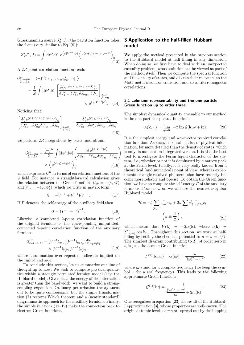
Fig. 1. Diagrams contributing to the self-energy Γ of the aux-iliary fermions up to order t3.
term into two symmetric bands called Hubbard bands.The lower band has band edges at ±2td −
√(2td)2 + u2
and never reaches the Fermi level, however large t maybe. Thus, this approximation fails to describe the Mottmetal-insulator transition. But in the method used here,the Hubbard-I approximation simply stems from the ze-roth order value of Γ , and we know a systematic way ofimproving it.
The diagrams contributing to Γ up to order t3 arepresented in Figure 1. Actually, there are more diagramsat this order, but they vanish due to the precise form ofV (k). To compute these diagrams, we need the explicit ex-pression of GIIc
σ1σ2,σ3σ4(iω1, iω2; iω3, iω4). The calculation
of this atomic correlation function is a bit cumbersome,though simple in principle. The main result as well asseveral useful remarks are presented in Appendix B. Forthe time being, let us focus on the result:
Γ (3)(k, iω) =iω
(iω)2 − u2+
6t2du2iω
((iω)2 − u2)3
+ 6t3c(k)
βu2 tanh
(βu2
)((iω)2 − u2)2 +
u2(2(iω)2 − u2
)((iω)2 − u2)4
· (24)
By injecting the above approximate value of Γ intoequation (18) for the Green function, one obtains a ra-tional function of iω, presenting a finite number of polesin the complex plane. Such a result is already somewhatdisappointing since it cannot account for a continuousspectral weight. But more seriously, the Green functionpresents pairs of complex conjugate poles away from thereal axis, and as a consequence does not verify Kramers-Kronig relations. Furthermore, for a wavevector verifyingV (k) = 0, the Green function is equal to Γ itself, andhas high-order poles at ±u, leading to negative spectralweight. So by simply replacing Γ by its approximate valueto third order in t in equation (18), one ends up witha noncausal Green function, whose spectral function isneither positive, nor normalized.
Any Green function acceptable on physical groundsshould be causal and have a positive spectral weight, i.e.,be a sum (finite or infinite) of simple real poles with pos-itive residues. We call such a function Lehmann repre-sentable since these properties are proven rigorously usingthe Lehmann representation of the exact Green function.The way out of the problems mentioned in the previousparagraph is to recall that the power series expansion ofthe Lehmann representation of the exact Green functionshould give, order by order, the same expansion of G asthat obtained by diagrams, and this for all values of fre-quency. This simple observation will allow us to build back
a Lehmann representable function from the power series,as shown below.
The systematic way of building a Lehnmannrepresentable function whose power series equalsthat of G is provided by a theorem reportedin reference [48]: a rational function is Lehmannrepresentable if and only if it can be written as a Jacobicontinued fraction
GJ (iω) =a0
iω + b1−a1
iω + b2−...
an−1
iω + bn, (25)
with
bl real and al > 0. (26)
In any finite system, the exact Green function can be castinto the form (25) with a finite value of n (the numberof floors of the continued fraction). If we consider the co-efficients al and bl as functions of t and expand GJ(iω)in powers of t, we should obtain the same power series asthat of G but at the price of destroying the continued frac-tion structure, and creating, in general, an approximationthat suffers from causality and normalization problems.On the other hand, if the power series in t for the coeffi-cients themselves are left where they belong in GJ (iω), wecan still expect their truncated Taylor series to verify con-ditions equation (26), and consequently the perturbativeGJ(iω) obtained this way to be Lehmann representable.
The objective, then, is to obtain in a unique way thepower series for al and bl from that of G and use the cor-responding GJ (iω) as our perturbatively calculated Greenfunction. For practical calculations, it is useful to knowthat their exists a double recurrence relation giving the aland bl starting from the moments of the function. Sincewe know the exact Taylor expansion of G up to order t3,we know all its spectral moments to the same order. Sowe simply need to work out the recurrence relations andcompute the coefficients of the continued fraction up tothe order available. Once an al is found to be zero to thebest of our knowledge – that is, if it contributes to the fullGJ , given the preceding coefficients, at an order higherthan the working precision (t3 in this section) – we maytruncate the continued fraction. In all the cases that wetreated, such an al always occurred rather quickly (thedeepest continued fraction we had to deal with had eightfloors). This means that the density of poles is alwaysweak, and the poles remain essentially well separated:they cannot account for the precise shape of a continuousspectral weight, but can sample it adequately (the mo-ments of the distribution are well represented). More im-portant, the Green function GJ (iω) thus obtained is uniqueat any given order in perturbation theory and is causal aslong as conditions (26) are satisfied by the perturbativeexpression for al and bl.
In order to test both the diagrammatic theory and thecontinued fraction representation, we treated the exactlysolvable case of the atomic limit itself, away from half-filling. Indeed, setting the chemical potential to µ = u+t0,one can either compute the exact Green function, then ex-pand the solution in powers of t0, or notice that the shift
90 The European Physical Journal B
of chemical potential has the form of a zero-range hoppingand obtain the t0 expansion from diagrams. This proce-dure is presented in Appendix C, and leads to the follow-ing main conclusions: the diagrams actually give the cor-rect answer, which however presents the same causalityproblems as already mentioned, and the continued frac-tion representation properly builds back the poles and theresidues of the exact solution. We also tested our approachon the (again exactly solvable) two-site problem, wherethe same conclusions apply.
The above considerations also shed new light on theusual weak-coupling perturbation theory. In that case too,one gets multiple poles when truncating the series for G,and the way out of this difficulty is to use Dyson’s equa-tion – valid because Wick’s theorem applies directly tothe original fermions – and to compute the self-energy.If the self-energy is Lehmann representable, that is, if itpossesses an underlying continued fraction structure, thenthe Green function will inherit this structure from it andwill be Lehmann representable too. We did not find anydefinite answer as to why the self-energy itself, as obtainedfrom a few diagrams, turns out to be acceptable in general,but there are some plausible explanations. One is that theunperturbed case already presents a continuum of levels,instead of only two. So if a double pole appears in theexpression of a diagram, it is likely that its isolated con-tribution will be negligible in the thermodynamic limit.Also, the vertices of weak-coupling theories are often localin time or, if retarded, depend only on two times, whereashere the vertices have a full dependence on all frequenciesentering them, which is quite peculiar. Finally, nothingproves that a finite-order weak-coupling self-energy is al-ways Lehmann representable, and counter-examples maywell exist.
Applying the above procedure to the result (24) yieldsthe following continued fraction:
GJ (k, iω) =1
iω + 2tc(k)−u2
iω − 3βt3 tanh (βu/2)c(k)/u−6t2d
iω − 2tc(k)/d−u2
iω + tc(k)/d, (27)
which has exactly the same Taylor expansion as the exactGreen function up to order t3, verifies the conditions (26),and is normalized to unity. The next two subsections showthat the spectral weight deduced from equation (24) de-scribes the Mott metal-insulator transition, and the ap-pearance of strong antiferromagnetic correlations at lowtemperature in the Hubbard model.
3.2 The Mott transition
Strictly speaking, there is no agreed upon definition of theMott transition in terms of one-particle properties only.But one can use as a heuristic criterion (even at nonzerotemperature) the appearance of spectral weight at theFermi level. With the normalization (20) of the spectral
Vauto
G Ic
G IIc
G IIIc...+ +
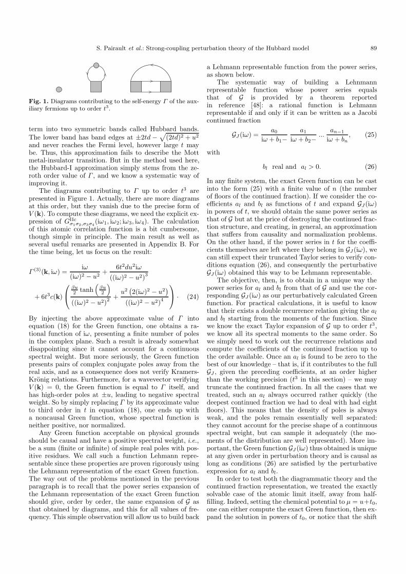
Fig. 2. Diagrams yielding the exact Γ (iω) when d → ∞.Vauto(k, iω) = V (k)/(1−Γ (iω)V (k)) is itself dressed with thesediagrams.
weight, the density of states has the following expression:
N(ω) =∫ π
−π
ddk(2π)d
A(k, ω). (28)
We observe that in the density of states, as t increasesfrom zero, the two symmetric Hubbard bands – reducedto two delta functions at ±u in the atomic limit – widen,and eventually mix for t beyond some critical value. Athigh temperature (T > u), the gap is closed by excitationsof momentum k = (0, ..., 0) and k = (π, ..., π), making itpossible to compute the exact value of the critical hopping:
tc = u
√1 +√
1 + 12d2
2d√
3· (29)
This gives Uc ' 3.2t for d = 1, to be compared withUc ' 3.5t found in the Hubbard-III approximation. Notethat tc scales properly with the dimension, and leads toUc = 1.86t? (with t? = 2t
√d) in the limit of infinite di-
mension. This critical value of interaction strength is toolarge [27,49] for two reasons. First, when d→∞ our crite-rion corresponds to subbands that meet with an exponen-tially small density of states, therefore not yet truly closingthe gap. Secondly, when d → ∞, the order of a diagramhas to be counted in a different way. Any nonlocal contri-bution becomes negligible, as is visible for example on thecontributions of the third-order term of equation (24) tothe continued fraction equation (27). Actually, the exactsolution in d → ∞ is given by the diagrams depicted inFigure 2, as was mentioned in reference [45]. Therefore,the approximation (24) becomes quite crude in infinite di-mension. Note that our criterion for the Mott transitiondiffers from that used in d→∞, since we simply demandthe closure of the gap at the Fermi level, without requir-ing the appearance of a new coherent peak in A(k, ω)at ω = 0. Such a peak does not appear in the presentapproach.
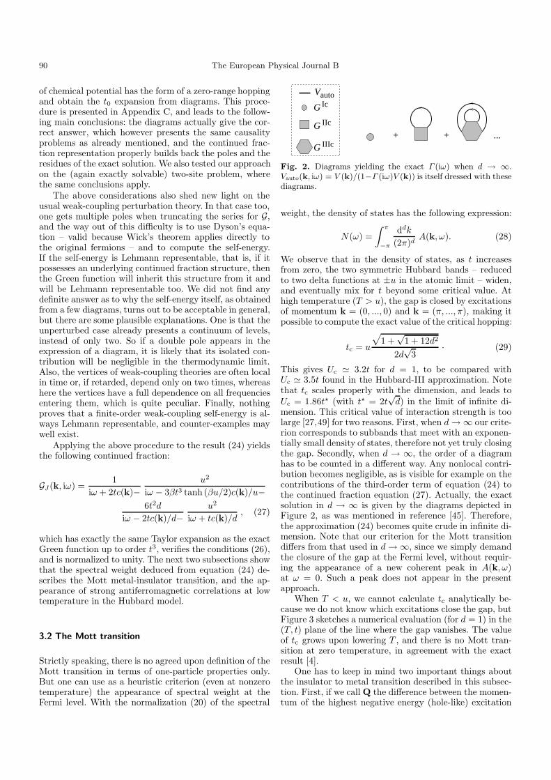
When T < u, we cannot calculate tc analytically be-cause we do not know which excitations close the gap, butFigure 3 sketches a numerical evaluation (for d = 1) in the(T, t) plane of the line where the gap vanishes. The valueof tc grows upon lowering T , and there is no Mott tran-sition at zero temperature, in agreement with the exactresult [4].
One has to keep in mind two important things aboutthe insulator to metal transition described in this subsec-tion. First, if we call Q the difference between the momen-tum of the highest negative energy (hole-like) excitation
S. Pairault et al.: Strong-coupling perturbation theory of the Hubbard model 91
0.5 1 1.5 2 2.5 3
0.2
0.4
0.6
0.8
1
1.2
1.4
T
t
insulator
Short-rangeAF
conductor
AB
H
(× u)
(× u
)
D
EF
G
C
Fig. 3. Crossover diagram of the one-dimensional half-filledHubbard model as obtained from the third-order Green func-tion. The estimated domain of validity of the approximation isthe region under the dot-dashed line.
and that of the lowest positive energy (particle-like) exci-tation, then Q takes the value (π, ..., π) at high temper-ature, and goes to zero when T → 0, but the gap alwaysremains indirect. Secondly, even when the gap has beenclosed, the spectral weight at the Fermi energy still hasseveral well separated peaks. A(k, ω) is never dominatedat small ω by a single narrow quasiparticle peak allowingto define a Fermi wavevector and a Fermi velocity. Thus,when extrapolating it beyond the transition, our solutiondoes not describe a Fermi liquid. This is not surprisingsince we do not expect a perturbative method startingfrom the completely localized insulating state to be ableto describe both phases satisfactorily.
3.3 Antiferromagnetic correlations
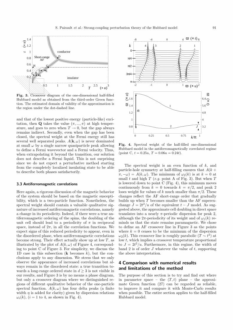
Here again, a rigorous discussion of the magnetic behaviorof the system should be based on the magnetic suscepti-bility, which is a two-particle function. Nonetheless, thespectral weight should contain a valuable qualitative sig-nature of increased antiferromagnetic correlations, namelya change in its periodicity. Indeed, if there were a true an-tiferromagnetic ordering of the spins, the doubling of theunit cell should lead to a periodicity of π in reciprocalspace, instead of 2π, in all the correlation functions. Weexpect signs of this reduced periodicity to appear, even inthe disordered phase, when antiferromagnetic correlationsbecome strong. Their effect actually show up at low T , asillustrated by the plot of A(k, ω) of Figure 4, correspond-ing to point C of Figure 3. For simplicity, we discuss the1D case in this subsection (k becomes k), but the con-clusions apply to any dimension. We stress that we onlyobserve the appearance of increased correlations but al-ways remain in the disordered state: a true transition to-wards a long-range ordered state in d ≥ 3 is not visible inour results, and Figure 3 is by no means a phase diagram,but only a crossover diagram where we distinguished re-gions of different qualitative behavior of the one-particlespectral function. A(k, ω) has four delta peaks (a finitewidth η is added for clarity) given by dispersion relationsωi(k), (i = 1 to 4, as shown in Fig. 4).
0 0.25 0.5 0.75 1
0.8
1
1.2
1.4
1.6
3.2
4
4.8
5.6
6.4
k/π
ω
(× u
) ω (× t)
-2 -1 0 1 2
-8 -4 0 4 8
ω (× u)
ω (× t)
k
π
π/2
π/4
3π/4
0
1
1234
2 J
4t
Fig. 4. Spectral weight of the half-filled one-dimensionalHubbard model in the antiferromagnetically correlated regime(point C, t = 0.25u, T = 0.06u = 0.24t).
The spectral weight is an even function of k, andparticle-hole symmetry at half-filling ensures that A(k +π,−ω) = A(k, ω). The minimum of ω2(k) is at k = 0 atsmall t and high T (e.g. point A of Fig. 3). But when Tis lowered down to point C (Fig. 4), this minimum movescontinuously from k = 0 towards k = π/2, and peak 2loses weight for values of k much smaller than π/2. Thesechanges reflect the AF short-range order that graduallybuilds up when T becomes smaller than the AF superex-change J = 2t2/u of the equivalent t − J model. As sug-gested above, the approximate cell doubling in direct spacetranslates into a nearly π-periodic dispersion for peak 2,although the 2π-periodicity of its weight and of ω1(k) re-minds us that the state remains paramagnetic. We choseto define an AF crossover line in Figure 3 as the pointswhere k = 0 ceases to be the minimum of the dispersionω2(k). This crossover line is roughly parabolic (T ∼ t2) atlow t, which implies a crossover temperature proportionalto J = 2t2/u. Furthermore, in this regime, the width ofband 2 is of order J whatever the value of t, supportingthe above interpretation.
4 Comparison with numerical resultsand limitations of the method
The purpose of this section is to try and find out wherein parameter space – the (T, t) plane – the approxi-mate Green function (27) can be regarded as reliable,to improve it and compare it with Monte-Carlo resultswhen possible. The entire section applies to the half-filledHubbard model.
92 The European Physical Journal B
4.1 Reliability of the third-order solution
It is not an easy task to define a domain of validity for thepresent approximation scheme for several reasons. First,the expansion parameter being the hopping amplitude t,any hopping process is considered on an equal footing re-gardless of whether it involves a change in the double oc-cupancy or not. As a consequence, we expect the ratio t/Tto play as important a role as t/u. Secondly the end re-sult involves t in a complicated way, and not only througha power series. Nevertheless, since the atomic Greenfunction is just
1
iω − u2
iω
(30)
and gives spectral weight only at iω = ±u, we expect anapproximation of the form (25) to be valid when the bl’sof equation (25) are small with respect to u. When appliedto equation (27), this criterion leads to the conditions:
2dt < u and(t
u
)3
<13d
(T
u
)· (31)
The first requirement is quite intuitive: it expresses thatthe bandwidth is smaller that the on-site interaction,which was the basic assumption anyway. The second onegives the low-temperature limitation of the method. Indimension d = 1, the region where the two conditionsequation (31) are fulfilled lies under the dashed line ofFigure 3. When extrapolating the results outside this re-gion, one cannot predict how fast the approximation maydeteriorate. In particular, it is worth mentioning that thet → ∞ (free-particle) limit is recovered properly. Onthe other hand, at small t the T → 0 limit again givesa free-particle behavior (except for a singular behaviorfor wavevectors such that V (k) = 0), which is obviouslywrong. This allows us to define, besides the region of (al-most) certain validity under the dashed line in Figure 3,a hatched region of acknowledged failure. For the one-dimensional case, the theoretical [39] and exact [15] re-sults describing spin-charge separation fall in this regionof parameter space, which prevents us from making anymeaningful comparison. However, a definite prediction ofour work is that upon raising the temperature, there ap-pears noticeable spectral weight near k = π (for ω < 0).This new feature of the spectral weight, visible as peak3 of Figure 4 and absent from the zero-temperature solu-tions, might correspond to the “question-mark” features inFigure 1 of reference [40]. Thus, temperature seems tohave a drastic effect on the distribution of spectral weight.
4.2 Beyond third order
We have also computed the Green function to fourth andfifth order. Let us stress straight away that one is nevercertain to improve a perturbative result by adding higher-order terms. Actually, in most of the cases where pertur-bation theory is used, the series is asymptotic rather than
convergent, and there is an optimal order – typically of theorder of the inverse of the expansion parameter – beyondwhich the approximation deteriorates quickly with eachnew term [50]. Computing the fourth and fifth order pre-sented a substantial technical difficulty, since it involvedthe atomic function GIIIc having a different expressionfor each of the 5! = 120 possible time orderings (one ofthe times can be set to zero). We overcame this difficultyby designing a symbolic manipulation program dedicatedto this problem, taking advantage of the very systematicform of the expressions in the atomic limit. Let us mentionthat up to fifth order – and that seems to be general – theeven orders lead to a modification of the partial numera-tors (al) only, and the odd orders lead to a modificationof the partial denominators (bl) only, within the contin-ued fraction (25). Appendix D presents the diagrams andthe result for Γ (k, iω) up to fourth order. Γ (k, iω) andthe corresponding continued fraction have been computedup to fifth order included, but the analytic expression istoo lengthy to be presented: It is available on the inter-net (Ref. [51]). Plots of the solution will be presented infollowing sections.
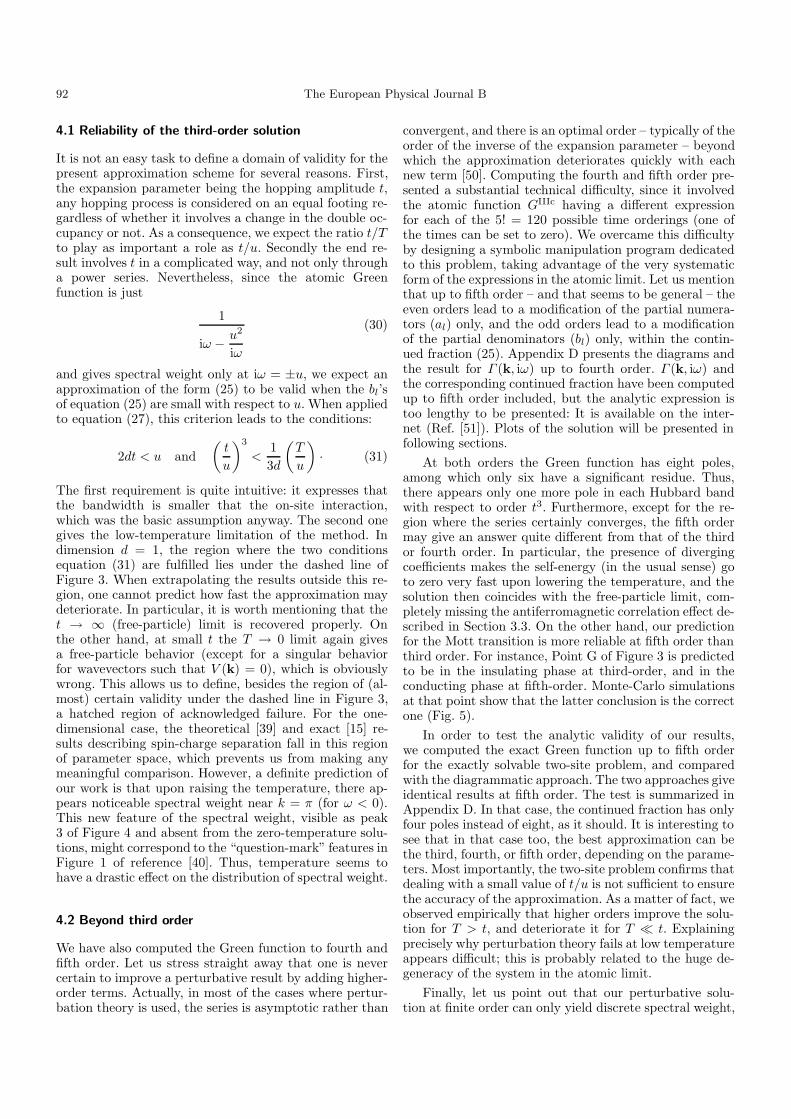
At both orders the Green function has eight poles,among which only six have a significant residue. Thus,there appears only one more pole in each Hubbard bandwith respect to order t3. Furthermore, except for the re-gion where the series certainly converges, the fifth ordermay give an answer quite different from that of the thirdor fourth order. In particular, the presence of divergingcoefficients makes the self-energy (in the usual sense) goto zero very fast upon lowering the temperature, and thesolution then coincides with the free-particle limit, com-pletely missing the antiferromagnetic correlation effect de-scribed in Section 3.3. On the other hand, our predictionfor the Mott transition is more reliable at fifth order thanthird order. For instance, Point G of Figure 3 is predictedto be in the insulating phase at third-order, and in theconducting phase at fifth-order. Monte-Carlo simulationsat that point show that the latter conclusion is the correctone (Fig. 5).
In order to test the analytic validity of our results,we computed the exact Green function up to fifth orderfor the exactly solvable two-site problem, and comparedwith the diagrammatic approach. The two approaches giveidentical results at fifth order. The test is summarized inAppendix D. In that case, the continued fraction has onlyfour poles instead of eight, as it should. It is interesting tosee that in that case too, the best approximation can bethe third, fourth, or fifth order, depending on the parame-ters. Most importantly, the two-site problem confirms thatdealing with a small value of t/u is not sufficient to ensurethe accuracy of the approximation. As a matter of fact, weobserved empirically that higher orders improve the solu-tion for T > t, and deteriorate it for T t. Explainingprecisely why perturbation theory fails at low temperatureappears difficult; this is probably related to the huge de-generacy of the system in the atomic limit.
Finally, let us point out that our perturbative solu-tion at finite order can only yield discrete spectral weight,
S. Pairault et al.: Strong-coupling perturbation theory of the Hubbard model 93
-2 -1 0 1 2
k=0
k=π/2
k=π
n=3
-2 -1 0 1 2
n=4
-2 -1 0 1 2(× u)ω
k=0
k=π/2
k=π
n=5
-2 -1 0 1 2(× u)ω
k=0
k=π/2
k=π
-2 -1 0 1 2
k=0
k=π/2
k=π
n=3
n=5
-2 -1 0 1 2
k=0
k=π/2
k=π
n=4
Point A Point B
(× u)ω
-2 -1 0 1 2
k=0
k=π/2
k=π
n=3
-2 -1 0 1 2
k=0
k=π/2
k=π
n=4
-2 -1 0 1 2
k=0
k=π/2
k=π
n=5
-2 -1 0 1 2
k=0
k=π/2
k=π
n=3
-2 -1 0 1 2
k=0
k=π/2
k=π
n=4
-2 -1 0 1 2(× u)ω
k=0
k=π/2
k=π
n=5
Point E Point F
-2 -1 0 1 2(× u)ω
k=0
k=π/2
k=π
-2 -1 0 1 2
k=0
k=π/2
k=π-2 -1 0 1 2
k=0
k=π/2
k=π
n=3
n=5
n=4
-2 -1 0 1 2
k=0
k=π/2
k=π
n=3
-2 -1 0 1 2
k=0
k=π/2
k=π
n=4
-2 -1 0 1 2
k=0
k=π/2
k=π
(× u)ω
n=5
Point G Point D
-2
-1
0
1
2
k=0 k=π/2 k=π
-2
-1
0
1
2
k=0 k=π/2 k=π
-4
-2
0
2
4
k=0 k=π/2 k=π
-2
-1
0
1
2
k=0 k=π/2 k=π -4
-2
0
2
4
k=0 k=π/2 k=π
-4
-2
0
2
4
k=0 k=π/2 k=π
Fig. 5. Spectral weight associated with points A,B,E,F,G and D of the crossover diagrams (Figs. 3 and 7). For each point,we give the spectral weight obtained from order t3 (top left), t4 (top right), and t5 (bottom left). A finite width η = 0.02 wasadded for clarity. The Monte-Carlo results [52] (smooth curves) were used to establish the density plot (bottom right). Notethat: Point A lies within the insulating paramagnetic region, as can be deduced from the presence of a gap and the monotonousdispersion of the bottom of the upper band (see text for details). For these values of the parameters, order t4 seems the bestapproximation. Point B is in the antiferromagnetically correlated region: The minimum in the dispersion of the bottom of theband has shifted to k > 0. Orders t3 and t4 are best suited there. Point E is in the insulating paramagnetic region and is bestdescribed by the fourth-order result. Point F is just at the edge of the antiferromagnetically correlated region. The third-orderapproximation is the best one. Point G is in the metallic region. Only order t5 gives the closure of the gap for this point. Point Dis well within the metallic region.
94 The European Physical Journal B
whereas the exact solution in the thermodynamic limitcertainly has a continuous distribution of poles on the realaxis. Such a continuous distribution is in general necessaryto account for spin-charge separation, or a finite lifetimeof one-particle excitations. Therefore, an approximationdescribing the spectral weight as a sum of four delta func-tions is necessarily a crude one. The reason why it is dif-ficult to obtain a continuous spectral weight is the hugedegeneracy of the unperturbed Hamiltonian. The startingpoint being a collection of independent atoms with thesame two energy levels, it is not likely that a finite-orderperturbation scheme can produce a macroscopic numberof distinct approximate eigenvalues. We will discuss inSection 5 a partially self-consistent approach leading toan extended spectral weight. But in the latter case, weno longer have the freedom to add higher-order terms inorder to solve the causality problem.
4.3 Comparison with Monte-Carlo data
We now present Monte-Carlo data supporting and illus-trating the conclusions claimed so far, regarding the phys-ical behavior of the model, as well as the accuracy ofour approximation at various orders in t. The simula-tions [52] were done for a twenty-site one-dimensional lat-tice for reasons of computing power and time. The spectralweight was deduced from imaginary time Green functionsby the maximum entropy method [53]. The first interest-ing region is the crossover between the ordinary param-agnetic insulator and the strongly AF correlated insula-tor. Figure 5 shows the spectral weight for the points A(t = 0.25u, T = 0.25) and B (t = 0.25u, T = 0.125) oneach side of the crossover (Points A to G are indicated inFigs. 3 and 7). Third-, fourth-, and fifth-order results aredisplayed. Of course, A and B being very close to eachother, they have largely similar spectral weights, but theirqualitative difference defined in Section 3.3 is supportedby the density plot. The fact that orders t3 and t4 areequally well suited for these two points, located respec-tively on the lines T = t and T = t/2, is consistent withour argument that order t5 deteriorates compared to or-der t3 precisely in that region. Let us mention that in onedimension, the Monte-Carlo data show that the antiferro-magnetically correlated region is tiny, and that a spectralfunction reminiscent of spin-charge separation (with animportant transfer of weight from low to high energy fork < π/2, ω > 0 and k > π/2, ω < 0) appears when lower-ing T a little further (actually when entering the shadedarea of Fig. 3). However no such thing is expected in twodimensions, for which the antiferromagnetically correlatedregion extends without spin-charge separation down toT = 0 where true long-range order takes place.
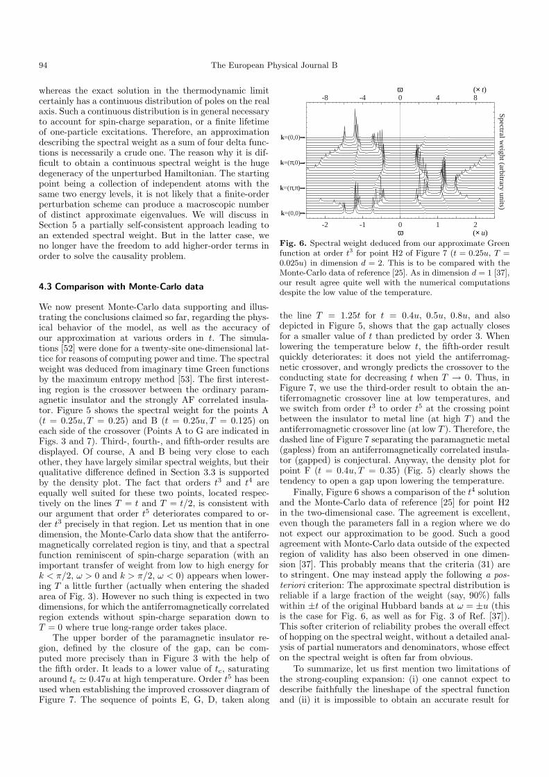
The upper border of the paramagnetic insulator re-gion, defined by the closure of the gap, can be com-puted more precisely than in Figure 3 with the help ofthe fifth order. It leads to a lower value of tc, saturatingaround tc ' 0.47u at high temperature. Order t5 has beenused when establishing the improved crossover diagram ofFigure 7. The sequence of points E, G, D, taken along
-2 -1 0 1 2
k=(π,0)
k=(0,0)
k=(π,π)
k=(0,0)
(× u)ω
-8 -4 0 4 8(× t)ω
Spectral weight (arbitrary units)
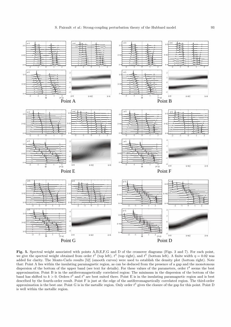
Fig. 6. Spectral weight deduced from our approximate Greenfunction at order t3 for point H2 of Figure 7 (t = 0.25u, T =0.025u) in dimension d = 2. This is to be compared with theMonte-Carlo data of reference [25]. As in dimension d = 1 [37],our result agree quite well with the numerical computationsdespite the low value of the temperature.
the line T = 1.25t for t = 0.4u, 0.5u, 0.8u, and alsodepicted in Figure 5, shows that the gap actually closesfor a smaller value of t than predicted by order 3. Whenlowering the temperature below t, the fifth-order resultquickly deteriorates: it does not yield the antiferromag-netic crossover, and wrongly predicts the crossover to theconducting state for decreasing t when T → 0. Thus, inFigure 7, we use the third-order result to obtain the an-tiferromagnetic crossover line at low temperatures, andwe switch from order t3 to order t5 at the crossing pointbetween the insulator to metal line (at high T ) and theantiferromagnetic crossover line (at low T ). Therefore, thedashed line of Figure 7 separating the paramagnetic metal(gapless) from an antiferromagnetically correlated insula-tor (gapped) is conjectural. Anyway, the density plot forpoint F (t = 0.4u, T = 0.35) (Fig. 5) clearly shows thetendency to open a gap upon lowering the temperature.
Finally, Figure 6 shows a comparison of the t4 solutionand the Monte-Carlo data of reference [25] for point H2in the two-dimensional case. The agreement is excellent,even though the parameters fall in a region where we donot expect our approximation to be good. Such a goodagreement with Monte-Carlo data outside of the expectedregion of validity has also been observed in one dimen-sion [37]. This probably means that the criteria (31) areto stringent. One may instead apply the following a pos-teriori criterion: The approximate spectral distribution isreliable if a large fraction of the weight (say, 90%) fallswithin ±t of the original Hubbard bands at ω = ±u (thisis the case for Fig. 6, as well as for Fig. 3 of Ref. [37]).This softer criterion of reliability probes the overall effectof hopping on the spectral weight, without a detailed anal-ysis of partial numerators and denominators, whose effecton the spectral weight is often far from obvious.
To summarize, let us first mention two limitations ofthe strong-coupling expansion: (i) one cannot expect todescribe faithfully the lineshape of the spectral functionand (ii) it is impossible to obtain an accurate result for
S. Pairault et al.: Strong-coupling perturbation theory of the Hubbard model 95
1.0
1.0
1.50.5
0.5
Temperature T
Hop
ping
inte
gral
t
Insulator
Short-range AF
Conductor
(× u)
(× u
)
?
?
Spin-chargeseparation?
1.0
1.0
1.50.5
0.5
Temperature T
Hop
ping
inte
gral
t
Insulator
Conductor
(× u)
(× u
)
H2
H G
D
EF
ABC
Short-range AF
Fig. 7. Improved crossover diagram of the half-filled Hubbardmodel in dimension d = 1 (top) and d = 2 (bottom). The dot-dashed line reminds the estimated validity region in one di-mension. The antiferromagnetic crossover was calculated withthe t3 order result, and the Mott transition line with the helpof order t5. The limit between the metallic and the insulatingantiferromagnetic regions is no longer clearly defined.
any temperature much lower than t. We add that going be-yond fifth order within the systematic approach describedin this paper would be difficult and unpractical, sincethe (intractable) result would be relevant only deep inthe insulating region. On the positive side, Monte-Carlocalculations agree well with our results as far as the overalldistribution of the weight is concerned. In particular, thefifth order calculation has led to a reliable prediction forthe Mott conductor-insulator crossover shown in Figure 7.
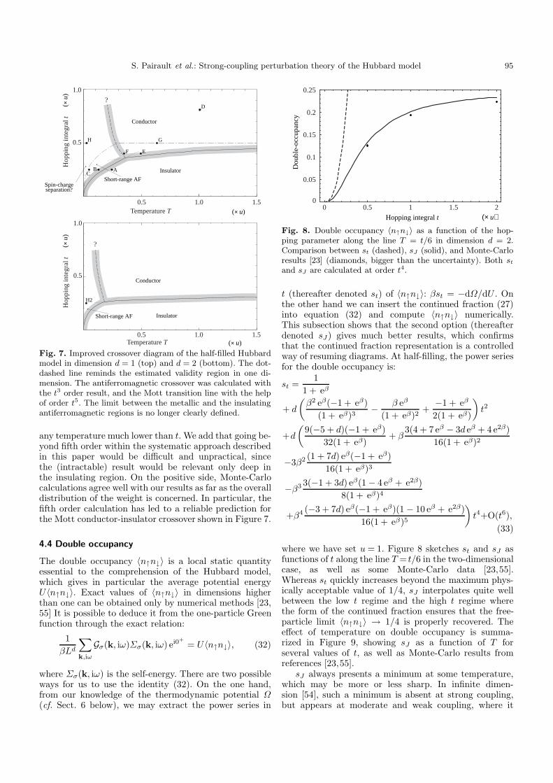
4.4 Double occupancy
The double occupancy 〈n↑n↓〉 is a local static quantityessential to the comprehension of the Hubbard model,which gives in particular the average potential energyU〈n↑n↓〉. Exact values of 〈n↑n↓〉 in dimensions higherthan one can be obtained only by numerical methods [23,55] It is possible to deduce it from the one-particle Greenfunction through the exact relation:
1βLd
∑k,iω
Gσ(k, iω)Σσ(k, iω) ei0+= U〈n↑n↓〉, (32)
where Σσ(k, iω) is the self-energy. There are two possibleways for us to use the identity (32). On the one hand,from our knowledge of the thermodynamic potential Ω(cf. Sect. 6 below), we may extract the power series in
0 0.5 1 1.5 2
0.05
0.1
0.15
0.2
0.25
0
Dou
ble-
occu
panc
y
Hopping integral t (× u)
Fig. 8. Double occupancy 〈n↑n↓〉 as a function of the hop-ping parameter along the line T = t/6 in dimension d = 2.Comparison between st (dashed), sJ (solid), and Monte-Carloresults [23] (diamonds, bigger than the uncertainty). Both stand sJ are calculated at order t4.
t (thereafter denoted st) of 〈n↑n↓〉: βst = −dΩ/dU . Onthe other hand we can insert the continued fraction (27)into equation (32) and compute 〈n↑n↓〉 numerically.This subsection shows that the second option (thereafterdenoted sJ) gives much better results, which confirmsthat the continued fraction representation is a controlledway of resuming diagrams. At half-filling, the power seriesfor the double occupancy is:
st =1
1 + eβ
+ d
(β2 eβ(−1 + eβ)
(1 + eβ)3− β eβ
(1 + eβ)2+−1 + eβ
2(1 + eβ)
)t2
+d(
9(−5 + d)(−1 + eβ)32(1 + eβ)
+ β3(4 + 7 eβ − 3d eβ + 4 e2β)
16(1 + eβ)2
−3β2 (1 + 7d) eβ(−1 + eβ)16(1 + eβ)3
−β3 3(−1 + 3d) eβ(1− 4 eβ + e2β)8(1 + eβ)4
+β4 (−3 + 7d) eβ(−1 + eβ)(1− 10 eβ + e2β)16(1 + eβ)5
)t4+O(t6),
(33)
where we have set u= 1. Figure 8 sketches st and sJ asfunctions of t along the line T = t/6 in the two-dimensionalcase, as well as some Monte-Carlo data [23,55].Whereas st quickly increases beyond the maximum phys-ically acceptable value of 1/4, sJ interpolates quite wellbetween the low t regime and the high t regime wherethe form of the continued fraction ensures that the free-particle limit 〈n↑n↓〉 → 1/4 is properly recovered. Theeffect of temperature on double occupancy is summa-rized in Figure 9, showing sJ as a function of T forseveral values of t, as well as Monte-Carlo results fromreferences [23,55].
sJ always presents a minimum at some temperature,which may be more or less sharp. In infinite dimen-sion [54], such a minimum is absent at strong coupling,but appears at moderate and weak coupling, where it
96 The European Physical Journal B
0 0.2 0.4 0.6 0.8 1
0.05
0.1
0.15
0.2
0.25
0
Temperature T
Dou
ble-
occu
panc
y
(× u)
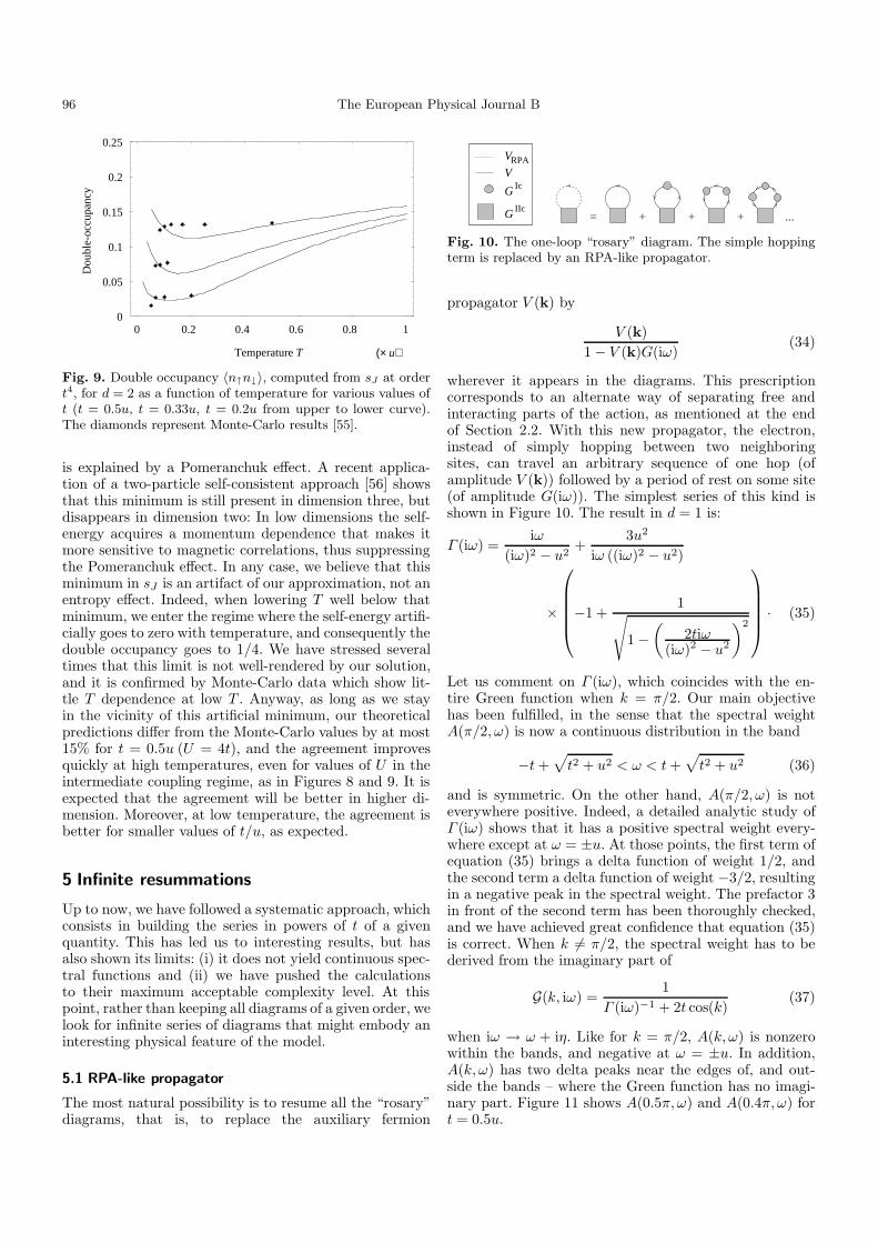
Fig. 9. Double occupancy 〈n↑n↓〉, computed from sJ at ordert4, for d = 2 as a function of temperature for various values oft (t = 0.5u, t = 0.33u, t = 0.2u from upper to lower curve).The diamonds represent Monte-Carlo results [55].
is explained by a Pomeranchuk effect. A recent applica-tion of a two-particle self-consistent approach [56] showsthat this minimum is still present in dimension three, butdisappears in dimension two: In low dimensions the self-energy acquires a momentum dependence that makes itmore sensitive to magnetic correlations, thus suppressingthe Pomeranchuk effect. In any case, we believe that thisminimum in sJ is an artifact of our approximation, not anentropy effect. Indeed, when lowering T well below thatminimum, we enter the regime where the self-energy artifi-cially goes to zero with temperature, and consequently thedouble occupancy goes to 1/4. We have stressed severaltimes that this limit is not well-rendered by our solution,and it is confirmed by Monte-Carlo data which show lit-tle T dependence at low T . Anyway, as long as we stayin the vicinity of this artificial minimum, our theoreticalpredictions differ from the Monte-Carlo values by at most15% for t = 0.5u (U = 4t), and the agreement improvesquickly at high temperatures, even for values of U in theintermediate coupling regime, as in Figures 8 and 9. It isexpected that the agreement will be better in higher di-mension. Moreover, at low temperature, the agreement isbetter for smaller values of t/u, as expected.
5 Infinite resummations
Up to now, we have followed a systematic approach, whichconsists in building the series in powers of t of a givenquantity. This has led us to interesting results, but hasalso shown its limits: (i) it does not yield continuous spec-tral functions and (ii) we have pushed the calculationsto their maximum acceptable complexity level. At thispoint, rather than keeping all diagrams of a given order, welook for infinite series of diagrams that might embody aninteresting physical feature of the model.
5.1 RPA-like propagator
The most natural possibility is to resume all the “rosary”diagrams, that is, to replace the auxiliary fermion
= + + + ...
V
G Ic
G IIc
VRPA
Fig. 10. The one-loop “rosary” diagram. The simple hoppingterm is replaced by an RPA-like propagator.
propagator V (k) by
V (k)1− V (k)G(iω)
(34)
wherever it appears in the diagrams. This prescriptioncorresponds to an alternate way of separating free andinteracting parts of the action, as mentioned at the endof Section 2.2. With this new propagator, the electron,instead of simply hopping between two neighboringsites, can travel an arbitrary sequence of one hop (ofamplitude V (k)) followed by a period of rest on some site(of amplitude G(iω)). The simplest series of this kind isshown in Figure 10. The result in d = 1 is:
Γ (iω) =iω
(iω)2 − u2+
3u2
iω ((iω)2 − u2)
×
−1 +1√
1−(
2tiω(iω)2 − u2
)2
· (35)
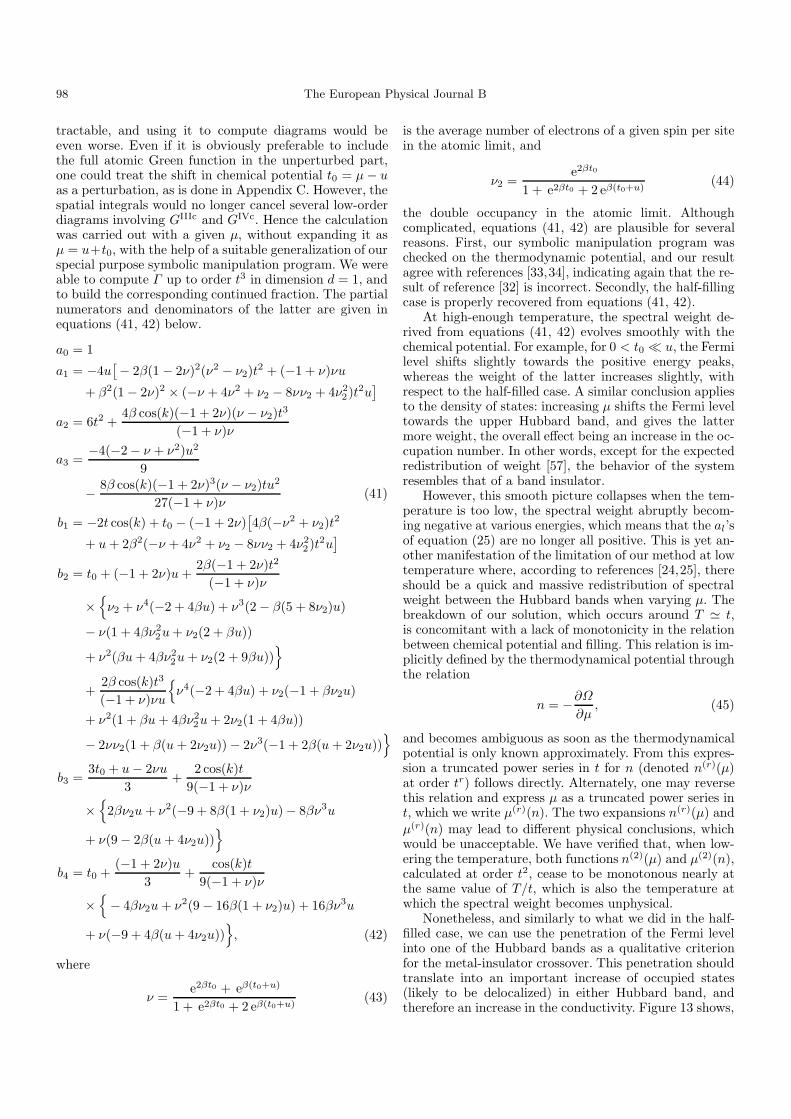
Let us comment on Γ (iω), which coincides with the en-tire Green function when k = π/2. Our main objectivehas been fulfilled, in the sense that the spectral weightA(π/2, ω) is now a continuous distribution in the band
−t+√t2 + u2 < ω < t+
√t2 + u2 (36)
and is symmetric. On the other hand, A(π/2, ω) is noteverywhere positive. Indeed, a detailed analytic study ofΓ (iω) shows that it has a positive spectral weight every-where except at ω = ±u. At those points, the first term ofequation (35) brings a delta function of weight 1/2, andthe second term a delta function of weight −3/2, resultingin a negative peak in the spectral weight. The prefactor 3in front of the second term has been thoroughly checked,and we have achieved great confidence that equation (35)is correct. When k 6= π/2, the spectral weight has to bederived from the imaginary part of
G(k, iω) =1
Γ (iω)−1 + 2t cos(k)(37)
when iω → ω + iη. Like for k = π/2, A(k, ω) is nonzerowithin the bands, and negative at ω = ±u. In addition,A(k, ω) has two delta peaks near the edges of, and out-side the bands – where the Green function has no imagi-nary part. Figure 11 shows A(0.5π, ω) and A(0.4π, ω) fort = 0.5u.
S. Pairault et al.: Strong-coupling perturbation theory of the Hubbard model 97
-2 -1 0 1 2(× u)ω
Spec
tral
wei
ght (
arbi
trar
y un
its) t = 0.5 u
k = 0.4 πk = 0.5 π
Fig. 11. Spectral weight obtained with the auxiliary self-energy of Figure 10, with hopping term t = 0.5u, and mo-mentum k = 0.5π (full curve) and k = 0.4π (dashed curve).The spectral weight is not everywhere positive within this ap-proximation.
Thus, the one-loop diagram of leads to a normalized,but nonpositive spectral weight. We have also lost theinteresting physical effects of order three: the result istemperature-independent and always has a gap at theFermi level. We did not find any acceptable way to curethis negative-weight problem. One could suggest to reducethe normalization of the one-loop diagram of Figure 10,but introducing such an arbitrary factor is by no meansjustified.
5.2 One-loop self-consistent approximation
Another natural attempt involving an infinite subset of di-agrams is to compute the one-loop self-consistent solution:We keep the first two diagrams of Figure 2, and discardall vertices beyond GIIc. The self-consistent solution Γ (iω)obeys the following equation:
Γσ(iω) = Gσ(iω)− 1βLd
∑σ1,k1,iω1
GIIcσ,σ1;σ,σ1
(iω, iω1; iω, iω1)
× V (k1)1− V (k1)Γ (iω1)
· (38)
The sum in equation (38) can be computed exactly, giventhe following property of GIIc at half filling and zero mag-netic field:
∑σ1
GIIcσ,σ1;σ,σ1
(iω, iω1; iω, iω1) =−3βu2δ(iω − iω1)
((iω)2 − u2)2
+ E(iω, iω1), (39)
where E is an even function of iω1. Since we expect Γσ(iω)to be antisymmetric in iω, the self-consistent propagatorin equation (38) is antisymmetric when iω1 → −iω1 and
0 0.5 1 1.5 2(× u)ω
k = 0
k = π/2
k = π
Spectral weight (arbitrary units)
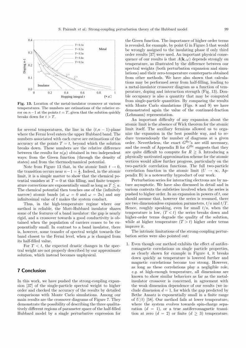
Fig. 12. Spectral weight of the one-loop self-consistent solu-tion, for t = tc = 0.39u. The wavevector goes from k = 0(top) to k = π (bottom). The spectral function is clearly notnormalized within this approximation.
k1 → (π, ..., π)−k1. Therefore, E does not contribute and
Γσ(iω) = Gσ(iω) +3u2
((iω)2 − u2)2
1Ld
×∑k1
V (k1)1− V (k1)Γ (iω)
· (40)
Equation (40) can easily be solved numerically. Amongthe various solutions for the spectral weight, we retainthe positive one having a compact support at very smallt, and follow its evolution when increasing t. The resultis shown in Figure 12 for t = 0.25u, and is obviously notnormalized. The quick suppression of spectral weight closeto ω = ±u when k differs slightly from π/2 is a surprisingfeature too. However, we have recovered the closure of thegap for t ' 0.39u, a value close to the prediction of ordert5 at high temperature.
The two examples just described show that it is noteasy to include self-consistency in strong-coupling per-turbation theory. Lack of positivity or normalization ap-pears in the simplest attempts, and there is no clue onhow to solve this problem. However, it seems the onlyway of obtaining a continuous spectral function, and fur-ther developments should probably include a dose of self-consistency.
6 Doping
Studying the Hubbard model at arbitrary filling is impor-tant for several reasons. First of all, the charge gap of thehalf-filled system disappears upon doping, and in dimen-sion d = 1, bosonization shows that this implies dramaticchanges in the spectral weight. Furthermore, in dimensiond = 2, a slight doping is directly relevant to the high-Tc su-perconductors. Finally, the metal-insulator transition canbe induced by doping rather than by interactions. We ad-dress the latter aspect in this section.
On technical grounds, working with arbitrary chemi-cal potential is extremely difficult, since the complete ex-pression of GIIc given in Appendix B is already hardly
98 The European Physical Journal B
tractable, and using it to compute diagrams would beeven worse. Even if it is obviously preferable to includethe full atomic Green function in the unperturbed part,one could treat the shift in chemical potential t0 = µ− uas a perturbation, as is done in Appendix C. However, thespatial integrals would no longer cancel several low-orderdiagrams involving GIIIc and GIVc. Hence the calculationwas carried out with a given µ, without expanding it asµ = u+t0, with the help of a suitable generalization of ourspecial purpose symbolic manipulation program. We wereable to compute Γ up to order t3 in dimension d = 1, andto build the corresponding continued fraction. The partialnumerators and denominators of the latter are given inequations (41, 42) below.
a0 = 1
a1 = −4u[− 2β(1− 2ν)2(ν2 − ν2)t2 + (−1 + ν)νu
+ β2(1− 2ν)2 × (−ν + 4ν2 + ν2 − 8νν2 + 4ν22)t2u
]a2 = 6t2 +
4β cos(k)(−1 + 2ν)(ν − ν2)t3
(−1 + ν)ν
a3 =−4(−2− ν + ν2)u2
9
− 8β cos(k)(−1 + 2ν)3(ν − ν2)tu2
27(−1 + ν)ν(41)
b1 = −2t cos(k) + t0 − (−1 + 2ν)[4β(−ν2 + ν2)t2
+ u+ 2β2(−ν + 4ν2 + ν2 − 8νν2 + 4ν22)t2u
]b2 = t0 + (−1 + 2ν)u+
2β(−1 + 2ν)t2
(−1 + ν)ν
×ν2 + ν4(−2 + 4βu) + ν3(2− β(5 + 8ν2)u)
− ν(1 + 4βν22u+ ν2(2 + βu))
+ ν2(βu+ 4βν22u+ ν2(2 + 9βu))
+
2β cos(k)t3
(−1 + ν)νu
ν4(−2 + 4βu) + ν2(−1 + βν2u)
+ ν2(1 + βu+ 4βν22u+ 2ν2(1 + 4βu))
− 2νν2(1 + β(u+ 2ν2u))− 2ν3(−1 + 2β(u+ 2ν2u))
b3 =3t0 + u− 2νu
3+
2 cos(k)t9(−1 + ν)ν
×
2βν2u+ ν2(−9 + 8β(1 + ν2)u)− 8βν3u
+ ν(9− 2β(u+ 4ν2u))
b4 = t0 +(−1 + 2ν)u
3+
cos(k)t9(−1 + ν)ν
×− 4βν2u+ ν2(9− 16β(1 + ν2)u) + 16βν3u
+ ν(−9 + 4β(u+ 4ν2u)), (42)
where
ν =e2βt0 + eβ(t0+u)
1 + e2βt0 + 2 eβ(t0+u)(43)
is the average number of electrons of a given spin per sitein the atomic limit, and
ν2 =e2βt0
1 + e2βt0 + 2 eβ(t0+u)(44)
the double occupancy in the atomic limit. Althoughcomplicated, equations (41, 42) are plausible for severalreasons. First, our symbolic manipulation program waschecked on the thermodynamic potential, and our resultagree with references [33,34], indicating again that the re-sult of reference [32] is incorrect. Secondly, the half-fillingcase is properly recovered from equations (41, 42).
At high-enough temperature, the spectral weight de-rived from equations (41, 42) evolves smoothly with thechemical potential. For example, for 0 < t0 u, the Fermilevel shifts slightly towards the positive energy peaks,whereas the weight of the latter increases slightly, withrespect to the half-filled case. A similar conclusion appliesto the density of states: increasing µ shifts the Fermi leveltowards the upper Hubbard band, and gives the lattermore weight, the overall effect being an increase in the oc-cupation number. In other words, except for the expectedredistribution of weight [57], the behavior of the systemresembles that of a band insulator.
However, this smooth picture collapses when the tem-perature is too low, the spectral weight abruptly becom-ing negative at various energies, which means that the al’sof equation (25) are no longer all positive. This is yet an-other manifestation of the limitation of our method at lowtemperature where, according to references [24,25], thereshould be a quick and massive redistribution of spectralweight between the Hubbard bands when varying µ. Thebreakdown of our solution, which occurs around T ' t,is concomitant with a lack of monotonicity in the relationbetween chemical potential and filling. This relation is im-plicitly defined by the thermodynamical potential throughthe relation
n = −∂Ω∂µ
, (45)
and becomes ambiguous as soon as the thermodynamicalpotential is only known approximately. From this expres-sion a truncated power series in t for n (denoted n(r)(µ)at order tr) follows directly. Alternately, one may reversethis relation and express µ as a truncated power series int, which we write µ(r)(n). The two expansions n(r)(µ) andµ(r)(n) may lead to different physical conclusions, whichwould be unacceptable. We have verified that, when low-ering the temperature, both functions n(2)(µ) and µ(2)(n),calculated at order t2, cease to be monotonous nearly atthe same value of T/t, which is also the temperature atwhich the spectral weight becomes unphysical.
Nonetheless, and similarly to what we did in the half-filled case, we can use the penetration of the Fermi levelinto one of the Hubbard bands as a qualitative criterionfor the metal-insulator crossover. This penetration shouldtranslate into an important increase of occupied states(likely to be delocalized) in either Hubbard band, andtherefore an increase in the conductivity. Figure 13 shows,
S. Pairault et al.: Strong-coupling perturbation theory of the Hubbard model 99
0.2 0.4 0.6 0.8 1
0.1
0.2
0.3
0.4
0.00
T= 0.1u
T= 0.2u
T= 0.3u
T= 0.4u
T= 0.5u
Hopping integral t (× u)
Dop
ing
n-1
3%12%
19% 22%21%
Insulator
Metal
Fig. 13. Location of the metal-insulator crossover at varioustemperatures. The numbers are estimations of the relative er-ror on n−1 at the points t = T , given that the solution quicklybreaks down for t > T .
for several temperatures, the line in the (t,n − 1)-planewhere the Fermi level enters the upper Hubbard band. Thenumbers associated with each curve are estimations of theaccuracy at the points T = t, beyond which the solutionbreaks down. These numbers are the relative differencebetween the results for n(µ) obtained in two independentways: from the Green function (through the density ofstates) and from the thermodynamical potential.
Note from Figure 13 that, in the atomic limit t → 0,the transition occurs near n−1 = 1
3 . Indeed, in the atomiclimit, it is a simple matter to show that the chemical po-tential vanishes at T = 0 at this filling, and finite temper-ature corrections are exponentially small as long as T . u.The chemical potential then touches one of the (infinitelynarrow) atomic bands (at ω = 0 and ω = 2u) and anyinfinitesimal value of t makes the system conduct.
Thus, in the high-temperature regime where ourmethod is reliable, the Mott-Hubbard insulator sharessome of the features of a band insulator: the gap is nearlyrigid, and a crossover towards a good conductivity is ob-tained when the population of carriers ceases to be ex-ponentially small. In contrast to a band insulator, thereis, however, some transfer of spectral weight towards theband closest to the Fermi level, when µ is changed fromits half-filled value.
For T < t, the expected drastic changes in the spec-tral weight are not properly described by our approximatesolution, which instead becomes unphysical.
7 Conclusion
In this work, we have pushed the strong-coupling expan-sion [37] of the single-particle spectral weight to higherorder and checked the accuracy of the results by detailedcomparisons with Monte Carlo simulations. Among ourmain results are the crossover diagrams of Figure 7. Theydemonstrate the possibility of describing the three qualita-tively different regions of parameter space of the half-filledHubbard model by a single perturbative expression for
the Green function. The importance of higher order termsis revealed, for example, by point G in Figure 5 that wouldbe wrongly assigned to the insulating phase if only thirdorder results [37] were used. An important physical conse-quence of our results is that A(k, ω) depends strongly ontemperature, as illustrated by the difference between ourspectral weights (both perturbation expansion and simu-lations) and their zero-temperature counterparts obtainedfrom other methods. We have also shown that calcula-tions may be performed away from half-filling, leading toa metal-insulator crossover diagram as a function of tem-perature, doping and interaction strength (Fig. 13). Dou-ble occupancy is also a quantity that may be computedfrom single-particle quantities. By comparing the resultswith Monte Carlo simulations (Figs. 8 and 9) we havedemonstrated again the value of the continued-fraction(Lehmann) representation.
An important difficulty of any expansion about theatomic limit is the absence of Wick theorem for the atomiclimit itself. The auxiliary fermions allowed us to orga-nize the expansion in the best possible way, and to re-duce tremendously the number of diagrams at a givenorder. Nevertheless, the exact GRc’s are still necessary,and the result of Appendix B for GIIc suggests that theyare quite difficult to compute for R ≥ 3. Introducing aphysically motivated approximation scheme for the atomicvertices would allow further progress, particularly on thetwo-particle correlation functions. The full two-particlecorrelation function in the atomic limit (U → ∞, Ap-pendix B) is a noteworthy byproduct of our work.
Perturbation series for interacting electrons are by na-ture asymptotic. We have also discussed in detail and invarious contexts the subtleties involved when the series ispushed to higher order. In an expansion in powers of t, oneshould assume that, however the series is resumed, thereare two dimensionless expansion parameters, t/u and t/T .Hence, roughly speaking, even for small t/u, when thetemperature is low, (T < t) the series breaks down andhigher-order terms degrade the quality of the solution,while at higher temperature (T > t) higher order termsimprove it.
The intrinsic limitations of the strong-coupling pertur-bation series were also pointed out:
1. Even though our method exhibits the effect of antifer-romagnetic correlations on single particle properties,as clearly shown for example in Figure 4, it breaksdown quickly as temperature is lowered further andmagnetic correlations become too strong. However,as long as these correlations play a negligible role,e.g. at high-enough temperature, all dimensions areknown to show similar behaviors as far as the metal-insulator crossover is concerned, in agreement withthe weak dimension dependence of our results (we in-clude dimension d = 1, for which the gap predicted byBethe Ansatz is exponentially small in a finite rangeof U/t) [58]. Our method fails at lower temperature,where the system evolves towards spin-charge sepa-ration (d = 1), or a true antiferromagnetic transi-tion at zero (d = 2) or finite (d ≥ 3) temperature.
100 The European Physical Journal B
Nevertheless, the possibility to take into accountthe effect of antiferromagnetic fluctuations on single-particle properties above the antiferromagnetic transi-tion, is an improvement over d =∞ methods [28].
2. The systematic strong-coupling expansion can onlyprovide a finite number of poles in the continued frac-tion and the corresponding approximate Green func-tion cannot have continuous spectral weight. This doesnot prevent meaningful comparisons with Monte-Carlodata, since the overall spectral weight distribution canbe assessed. This “discreteness problem” might besolved with the help of a suitable termination func-tion within the continued fraction [59], but this is im-possible without any prior knowledge about the Greenfunction. Furthermore, we have shown that the sim-plest ways of obtaining a continuous spectral weightfrom infinite subsets of diagrams lead to nonpositiveor unnormalized functions. One way of increasing thenumber of significant poles is to treat a cluster of sitesas a single “site” from the point of view of the strong-coupling expansion, and to carry the calculations nu-merically [60].
The major challenge faced by the strong-couplingperturbation theory is the low-temperature barrier. Wepointed out that the exponentially large degeneracy ofthe atomic ground state is likely to be the source ofthe problem. One possible solution to this difficulty isto select a ground state more likely to connect with thelow-temperature phases and to organize the perturbationseries around that ground state, which would imply acertain amount of self-consistency. Work along these linesis in progress.
While this paper focused on properties derived fromthe one-particle Green function, two-particle Green func-tions are also accessible within the method presented here,but their systematic computation is more involved at or-der t4 (it requires the atomic four-particle function GIV).For this reason, we defer discussion of two-particle corre-lations to a future publication.
We thank C. Bourbonnais and N. Dupuis for many useful dis-cussions. We are grateful to H. Touchette, S. Moukouri, L.Chen, and especially D. Poulin and S. Allen for sharing theirnumerical results. Monte Carlo simulations were performed inpart on an IBM SP2 at the Centre d’applications du calcul par-allele de l’Universite de Sherbrooke. This work was partiallysupported by NSERC (Canada), by FCAR (Quebec) and by ascholarship from MESR (France) to S.P.
Appendix A: Diagrammatic rules
This appendix is devoted to deriving and illustrating thediagrammatic theory valid for the auxiliary field intro-duced in Section 2.2. For definiteness, we suppose thatthe site index describes a d-dimensional hypercubic lattice,and we only consider Hamiltonians where the hi’s do notexplicitly depend on i, so that the interaction terms aretranslation invariant, in addition to being local in space.
The first step consists in expanding the exponential ofthe interaction terms of equation (10):
Z =∫
[dψ?dψ] e−S0[ψ?,ψ]∞∑P=0
(−)P
P !
( ∞∑R=1
SRint[ψ?, ψ]
)P.
(A.1)
For a given P , and taking into account the factor (−)P /P !,we have a sum of terms of the following form:
(−)P
C1!...CH !SR1
int [ψ?, ψ]...SRPint [ψ?, ψ], (A.2)
where R1, ..., RP are P integers, and C1, ..., CH the multi-plicities of the different values that occur in the sequenceR1, ..., RP . Suppose we are interested in the following cor-relation function:
VRa0
1...a0R
b01...b0R
= (−)R0
⟨ψa0
1...ψa0
R0ψ?b0R0
...ψ?b01
⟩. (A.3)
The contribution of a given power P to (A.3) is the sum,for all possible sequences R1, ..., RP , of
ZGauss
Z
∑apr ,bprp=1...Pr=1...Rp
′GR1cb1ra1
r...GRP c
bPr aPr 〈ψa0
1...ψa0
R0ψa1
1...ψa1
R1
× ...ψaP1 ...ψaPRP ψ?bPRP
...ψ?bP1ψ?b1R1
...ψ?b11...ψ?b0R0
...ψ?b01〉Gauss,
(A.4)
times a overall factor
(−)R0
C1!...CH !(R1!)2...(RP !)2, (A.5)
which takes into account the minus signs coming with SRint.Again, let us stress that the indices in the sum do not runover all their possible values, but rather are restricted tohave a common site index if they refer to the same vertex(this restriction is encoded in the primed sum). Since theaction is Gaussian, Wick’s theorem is valid, and one cancompute the average in expression (A.4) as a sum over allpossible permutations ϑ of R0 +R1 + ...+RP elements:
(A.4) =ZGauss
Z
∑ϑ
(−)ϑ∑
apr ,bprp=1...Pr=1...Rp
′GR1cϑ(b1r)a1
r...
GRP cϑ(bPr )aPr
⟨ψa0
1ψ?ϑ(b01)
⟩Gauss
...
⟨ψaPRP
ψ?ϑ(bPRP)
⟩Gauss
,
(A.6)
where (−)ϑ stands for the signature of the permutation,and
⟨ψaji
ψ?ϑ(bji )
⟩Gauss
= −Vajiϑ(bji ). A term in the sumover
S. Pairault et al.: Strong-coupling perturbation theory of the Hubbard model 101
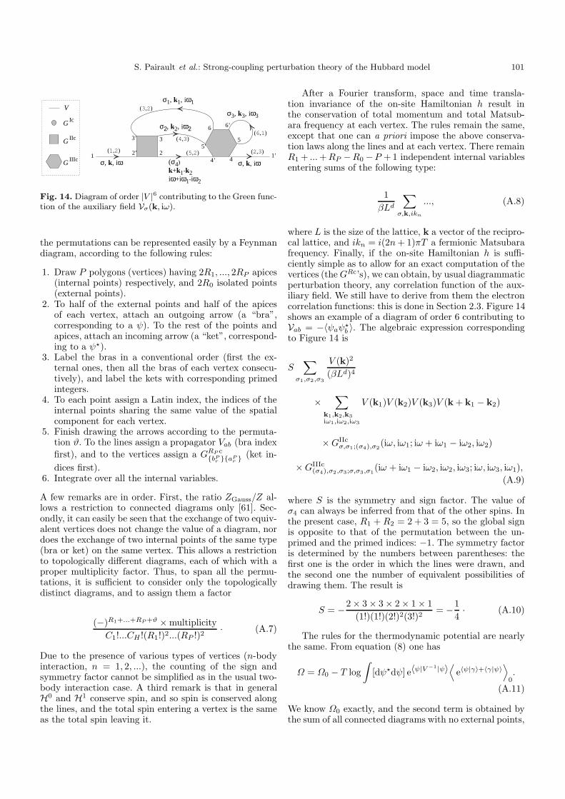
1 1’4
5
6’6
4’
5’33’
2’ 2
(σ4)
k+k1-k2iω+iω1-iω2
(1,2) (2,3)
(3,2)
(5,2)
(4,3)(6,1)
V
G Ic
G IIc
G IIIc
σ1, k1, iω1
σ2, k2, iω2
σ, k, iω
σ3, k3, iω3
σ, k, iω
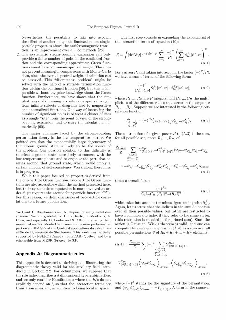
Fig. 14. Diagram of order |V |6 contributing to the Green func-tion of the auxiliary field Vσ(k, iω).
the permutations can be represented easily by a Feynmandiagram, according to the following rules:
1. Draw P polygons (vertices) having 2R1, ..., 2RP apices(internal points) respectively, and 2R0 isolated points(external points).
2. To half of the external points and half of the apicesof each vertex, attach an outgoing arrow (a “bra”,corresponding to a ψ). To the rest of the points andapices, attach an incoming arrow (a “ket”, correspond-ing to a ψ?).
3. Label the bras in a conventional order (first the ex-ternal ones, then all the bras of each vertex consecu-tively), and label the kets with corresponding primedintegers.
4. To each point assign a Latin index, the indices of theinternal points sharing the same value of the spatialcomponent for each vertex.
5. Finish drawing the arrows according to the permuta-tion ϑ. To the lines assign a propagator Vab (bra indexfirst), and to the vertices assign a GRP c
bPr aPr (ket in-
dices first).6. Integrate over all the internal variables.
A few remarks are in order. First, the ratio ZGauss/Z al-lows a restriction to connected diagrams only [61]. Sec-ondly, it can easily be seen that the exchange of two equiv-alent vertices does not change the value of a diagram, nordoes the exchange of two internal points of the same type(bra or ket) on the same vertex. This allows a restrictionto topologically different diagrams, each of which with aproper multiplicity factor. Thus, to span all the permu-tations, it is sufficient to consider only the topologicallydistinct diagrams, and to assign them a factor
(−)R1+...+RP+ϑ ×multiplicityC1!...CH !(R1!)2...(RP !)2
· (A.7)
Due to the presence of various types of vertices (n-bodyinteraction, n = 1, 2, ...), the counting of the sign andsymmetry factor cannot be simplified as in the usual two-body interaction case. A third remark is that in generalH0 and H1 conserve spin, and so spin is conserved alongthe lines, and the total spin entering a vertex is the sameas the total spin leaving it.
After a Fourier transform, space and time transla-tion invariance of the on-site Hamiltonian h result inthe conservation of total momentum and total Matsub-ara frequency at each vertex. The rules remain the same,except that one can a priori impose the above conserva-tion laws along the lines and at each vertex. There remainR1 + ...+RP −R0−P + 1 independent internal variablesentering sums of the following type:
1βLd
∑σ,k,ikn
..., (A.8)
where L is the size of the lattice, k a vector of the recipro-cal lattice, and ikn = i(2n+ 1)πT a fermionic Matsubarafrequency. Finally, if the on-site Hamiltonian h is suffi-ciently simple as to allow for an exact computation of thevertices (theGRc’s), we can obtain, by usual diagrammaticperturbation theory, any correlation function of the aux-iliary field. We still have to derive from them the electroncorrelation functions: this is done in Section 2.3. Figure 14shows an example of a diagram of order 6 contributing toVab = −〈ψaψ?b 〉. The algebraic expression correspondingto Figure 14 is
S∑
σ1,σ2,σ3
V (k)2
(βLd)4
×∑
k1,k2,k3iω1,iω2,iω3
V (k1)V (k2)V (k3)V (k + k1 − k2)
×GIIcσ,σ1;(σ4),σ2
(iω, iω1; iω + iω1 − iω2, iω2)
×GIIIc(σ4),σ2,σ3;σ,σ3,σ1
(iω + iω1 − iω2, iω2, iω3; iω, iω3, iω1),(A.9)
where S is the symmetry and sign factor. The value ofσ4 can always be inferred from that of the other spins. Inthe present case, R1 + R2 = 2 + 3 = 5, so the global signis opposite to that of the permutation between the un-primed and the primed indices: −1. The symmetry factoris determined by the numbers between parentheses: thefirst one is the order in which the lines were drawn, andthe second one the number of equivalent possibilities ofdrawing them. The result is
S = −2× 3× 3× 2× 1× 1(1!)(1!)(2!)2(3!)2
= −14· (A.10)
The rules for the thermodynamic potential are nearlythe same. From equation (8) one has
Ω = Ω0 − T log∫
[dψ?dψ] e〈ψ|V−1|ψ〉
⟨e〈ψ|γ〉+〈γ|ψ〉
⟩0.
(A.11)
We know Ω0 exactly, and the second term is obtained bythe sum of all connected diagrams with no external points,
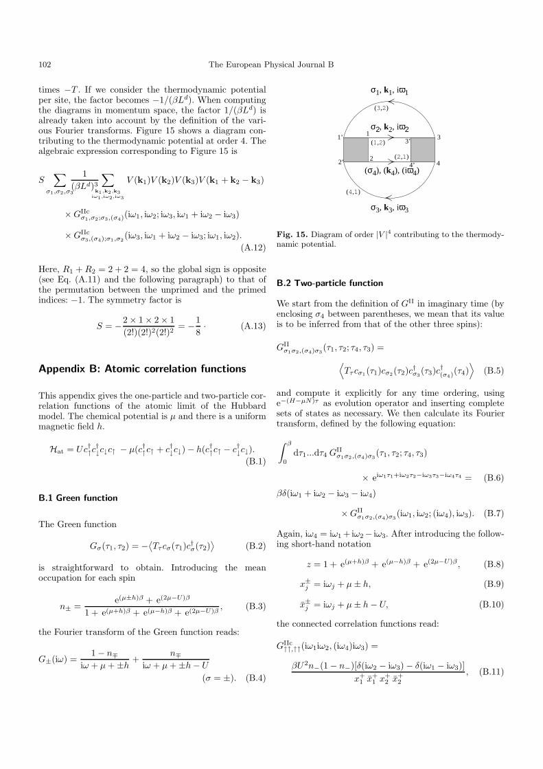
102 The European Physical Journal B
times −T . If we consider the thermodynamic potentialper site, the factor becomes −1/(βLd). When computingthe diagrams in momentum space, the factor 1/(βLd) isalready taken into account by the definition of the vari-ous Fourier transforms. Figure 15 shows a diagram con-tributing to the thermodynamic potential at order 4. Thealgebraic expression corresponding to Figure 15 is
S∑
σ1,σ2,σ3
1(βLd)3
∑k1,k2,k3
iω1,iω2,iω3
V (k1)V (k2)V (k3)V (k1 + k2 − k3)
×GIIcσ1,σ2;σ3,(σ4)(iω1, iω2; iω3, iω1 + iω2 − iω3)
×GIIcσ3,(σ4);σ1,σ2
(iω3, iω1 + iω2 − iω3; iω1, iω2).(A.12)
Here, R1 + R2 = 2 + 2 = 4, so the global sign is opposite(see Eq. (A.11) and the following paragraph) to that ofthe permutation between the unprimed and the primedindices: −1. The symmetry factor is
S = −2× 1× 2× 1(2!)(2!)2(2!)2
= −18· (A.13)
Appendix B: Atomic correlation functions
This appendix gives the one-particle and two-particle cor-relation functions of the atomic limit of the Hubbardmodel. The chemical potential is µ and there is a uniformmagnetic field h.
Hat = Uc†↑c†↓c↓c↑ − µ(c†↑c↑ + c†↓c↓)− h(c†↑c↑ − c
†↓c↓).
(B.1)
B.1 Green function
The Green function
Gσ(τ1, τ2) = −⟨Tτcσ(τ1)c†σ(τ2)
⟩(B.2)
is straightforward to obtain. Introducing the meanoccupation for each spin
n± =e(µ±h)β + e(2µ−U)β
1 + e(µ+h)β + e(µ−h)β + e(2µ−U)β, (B.3)
the Fourier transform of the Green function reads:
G±(iω) =1− n∓
iω + µ+±h +n∓
iω + µ+±h− U(σ = ±). (B.4)
2’
1’
2
13’
4’
3
4
(3,2)
(2,1)
(4,1)
(1,2)
σ2, k2, iω2
(σ4), (k4), (iω4)
σ1, k1, iω1
σ3, k3, iω3
Fig. 15. Diagram of order |V |4 contributing to the thermody-namic potential.
B.2 Two-particle function
We start from the definition of GII in imaginary time (byenclosing σ4 between parentheses, we mean that its valueis to be inferred from that of the other three spins):
GIIσ1σ2,(σ4)σ3
(τ1, τ2; τ4, τ3) =⟨Tτcσ1(τ1)cσ2(τ2)c†σ3
(τ3)c†(σ4)(τ4)⟩
(B.5)
and compute it explicitly for any time ordering, usinge−(H−µN)τ as evolution operator and inserting completesets of states as necessary. We then calculate its Fouriertransform, defined by the following equation:∫ β
0
dτ1...dτ4 GIIσ1σ2,(σ4)σ3
(τ1, τ2; τ4, τ3)
× eiω1τ1+iω2τ2−iω3τ3−iω4τ4 = (B.6)
βδ(iω1 + iω2 − iω3 − iω4)
×GIIσ1σ2,(σ4)σ3
(iω1, iω2; (iω4), iω3). (B.7)
Again, iω4 = iω1 + iω2− iω3. After introducing the follow-ing short-hand notation
z = 1 + e(µ+h)β + e(µ−h)β + e(2µ−U)β , (B.8)
x±j = iωj + µ± h, (B.9)
x±j = iωj + µ± h− U, (B.10)
the connected correlation functions read:
GIIc↑↑,↑↑(iω1iω2, (iω4)iω3) =
βU2n−(1− n−)[δ(iω2 − iω3)− δ(iω1 − iω3)]x+
1 x+1 x
+2 x
+2
, (B.11)
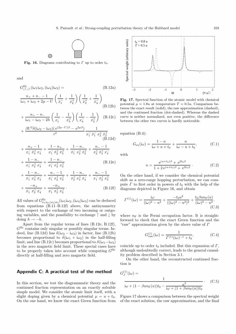
S. Pairault et al.: Strong-coupling perturbation theory of the Hubbard model 103
Fig. 16. Diagrams contributing to Γ up to order t0.
and
GIIc↓↑,↓↑(iω1iω2, (iω4)iω3) = (B.12a)
n+ + n− − 1iω1 + iω2 + 2µ− U
(1x−1
+1x+
2
)(1x+
3
+1x−4
)(B.12b)
+n+ − n−
iω1 − iω3 − 2h
(1x−1− 1x+
3
)(1x−4− 1x+
2
)(B.12c)
+βU2δ(iω2 − iω3)( e(2µ−U)β − e2µβ)
z2
1x−1 x
−1 x
+2 x
+2
(B.12d)
+n+ − 1x−1 x
+3 x−4
+1− n+
x−1 x+2 x
+3
+1− n−x−1 x
+2 x
+3
+n− − 1x+
2 x+3 x−4
+1− n−x−1 x
+2 x−4
+1− n−x−1 x
+2 x
+3
(B.12e)
+1− n−x−1 x
+3 x−4
+n− − 1x−1 x
+2 x
+3
+1− n−x+
2 x+3 x−4
+n− − 1x−1 x
+2 x
+3
+−n+
x−1 x+2 x−4
+−n+
x−1 x+2 x
+3
· (B.12f)
All values of GIIcσ1σ2,(σ4)σ3
(iω1iω2, (iω4)iω3) can be deducedfrom equations (B.11–B.12f) above, the antisymmetrywith respect to the exchange of two incoming or outgo-ing variables, and the possibility to exchange ↑ and ↓ bydoing h→ −h.
Apart from the regular terms of lines (B.12e, B.12f),GIIc contains only singular or possibly singular terms. In-deed, line (B.12d) has δ(iω2 − iω3) in factor, line (B.12b)becomes proportional to δ(iω1 + iω2) in the half-fillinglimit, and line (B.12c) becomes proportional to δ(iω1−iω3)in the zero magnetic field limit. These special cases haveto be properly taken into account while computing GIIc
directly at half-filling and zero magnetic field.
Appendix C: A practical test of the method
In this section, we test the diagrammatic theory and thecontinued fraction representation on an exactly solvablesimple model. We consider the atomic limit itself, with aslight doping given by a chemical potential µ = u + t0.On the one hand, we know the exact Green function from
-3 -2 -1 0 1 2
Spec
tral
wei
ght (
arbi
trar
y un
its)
ω (× u)
t0 = 0.8 uT = 0.5 u
Fig. 17. Spectral function of the atomic model with chemicalpotential µ = 1.8u at temperature T = 0.5u. Comparison be-tween the exact result (solid), the raw approximation (dashed),and the continued fraction (dot-dashed). Whereas the dashedcurve is neither normalized, nor even positive, the differencebetween the other two curves is hardly noticeable.
equation (B.4):
Gex(iω) =1− n
iω + u+ t0+
n
iω − u+ t0, (C.1)
with
n =e(u+t0)β + e2t0β
1 + 2 e(u+t0)β + e2t0β· (C.2)
On the other hand, if we consider the chemical potentialshift as a zero-range hopping perturbation, we can com-pute Γ to first order in powers of t0 with the help of thediagrams depicted in Figure 16, and obtain
Γ (1)(iω) =iω
(iω)2 − u2+
−t0u2
((iω)2 − u2)2+t0βunF(u)(iω)2 − u2
,
(C.3)
where nF is the Fermi occupation factor. It is straight-forward to check that the exact Green function and the“raw” approximation given by the above value of Γ
G(1)raw(iω) =
1Γ (1)(iω)−1 + t0
, (C.4)
coincide up to order t0 included. But this expansion of Γ ,although undoubtedly correct, leads to the general causal-ity problem described in Section 3.1.
On the other hand, the reconstructed continued frac-tion is
G(1)J (iω) =
1
iω + (1− βunF(u))t0 − u2
iω + (1 + βunF(u))t0
· (C.5)
Figure 17 shows a comparison between the spectral weightof the exact solution, the raw approximation, and the final
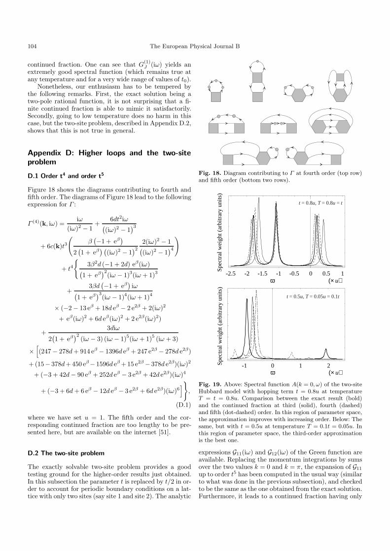
104 The European Physical Journal B
continued fraction. One can see that G(1)J (iω) yields an
extremely good spectral function (which remains true atany temperature and for a very wide range of values of t0).
Nonetheless, our enthusiasm has to be tempered bythe following remarks. First, the exact solution being atwo-pole rational function, it is not surprising that a fi-nite continued fraction is able to mimic it satisfactorily.Secondly, going to low temperature does no harm in thiscase, but the two-site problem, described in Appendix D.2,shows that this is not true in general.
Appendix D: Higher loops and the two-siteproblem
D.1 Order t4 and order t5
Figure 18 shows the diagrams contributing to fourth andfifth order. The diagrams of Figure 18 lead to the followingexpression for Γ :
Γ (4)(k, iω) =iω
(iω)2 − 1+
6dt2iω((iω)2 − 1
)3+ 6c(k)t3
(β(−1 + eβ
)2(1 + eβ
) ((iω)2 − 1
)2 2(iω)2 − 1((iω)2 − 1
)4)
+ t4
3β2d (−1 + 2d) eβ(iω)(
1 + eβ)2
(iω − 1)3(iω + 1)3
+3βd
(−1 + eβ
)iω(
1 + eβ)3
(iω − 1)4(iω + 1)4
× (−2− 13 eβ + 18d eβ − 2 e2β + 2(iω)2
+ eβ(iω)2 + 6d eβ(iω)2 + 2 e2β(iω)2)
+3diω
2(1 + eβ
)2(iω − 3) (iω − 1)5(iω + 1)5 (iω + 3)
×[(247− 278d+ 914 eβ − 1396d eβ + 247 e2β − 278d e2β)
+ (15− 378d+ 450 eβ− 1596d eβ + 15 e2β− 378d e2β)(iω)2
+ (−3 + 42d− 90 eβ + 252d eβ − 3 e2β + 42d e2β)(iω)4
+ (−3 + 6d+ 6 eβ − 12d eβ − 3 e2β + 6d e2β)(iω)6],
(D.1)
where we have set u = 1. The fifth order and the cor-responding continued fraction are too lengthy to be pre-sented here, but are available on the internet [51].
D.2 The two-site problem
The exactly solvable two-site problem provides a goodtesting ground for the higher-order results just obtained.In this subsection the parameter t is replaced by t/2 in or-der to account for periodic boundary conditions on a lat-tice with only two sites (say site 1 and site 2). The analytic
Fig. 18. Diagram contributing to Γ at fourth order (top row)and fifth order (bottom two rows).
-1 0 1 2Spec
tral
wei
ght (
arbi
trar
y un
its)
ω (× u)
t = 0.5u, T = 0.05u = 0.1t
-2.5 -2 -1.5 -1 -0.5 0 0.5 1
Spec
tral
wei
ght (
arbi
trar
y un
its)
ω (× u)
t = 0.8u, T = 0.8u = t
Fig. 19. Above: Spectral function A(k = 0, ω) of the two-siteHubbard model with hopping term t = 0.8u at temperatureT = t = 0.8u. Comparison between the exact result (bold)and the continued fraction at third (solid), fourth (dashed)and fifth (dot-dashed) order. In this region of parameter space,the approximation improves with increasing order. Below: Thesame, but with t = 0.5u at temperature T = 0.1t = 0.05u. Inthis region of parameter space, the third-order approximationis the best one.
expressions G11(iω) and G12(iω) of the Green function areavailable. Replacing the momentum integrations by sumsover the two values k = 0 and k = π, the expansion of G11
up to order t5 has been computed in the usual way (similarto what was done in the previous subsection), and checkedto be the same as the one obtained from the exact solution.Furthermore, it leads to a continued fraction having only
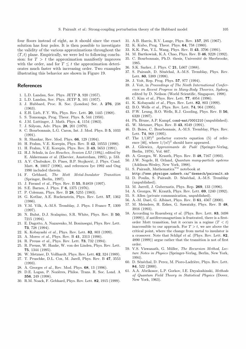
S. Pairault et al.: Strong-coupling perturbation theory of the Hubbard model 105
four floors instead of eight, as it should since the exactsolution has four poles. It is then possible to investigatethe validity of the various approximations throughout the(T, t) plane. Empirically, we were led to following conclu-sion: for T > t the approximation manifestly improveswith the order, and for T ≤ t the approximation deteri-orates much faster with increasing order. Two examplesillustrating this behavior are shown in Figure 19.
References
1. L.D. Landau, Sov. Phys. JETP 3, 920 (1957).2. L.D. Landau, Sov. Phys. JETP 5, 101 (1957).3. J. Hubbard, Proc. R. Soc. (London) Ser. A 276, 238
(1963).4. E.H. Lieb, F.Y. Wu, Phys. Rev. Lett. 20, 1445 (1968).5. S. Tomonaga, Prog. Theor. Phys. 5, 544 (1950).6. J.M. Luttinger, J. Math. Phys. 4, 1154 (1963).7. J. Solyom, Adv. Phys. 28, 201 (1979).8. C. Bourbonnais, L.G. Caron, Int. J. Mod. Phys. B 5, 1033
(1991).9. R. Shankar, Rev. Mod. Phys. 66, 129 (1994).
10. H. Frahm, V.E. Korepin, Phys. Rev. B 42, 10553 (1990).11. H. Frahm, V.E. Korepin, Phys. Rev. B 43, 5653 (1991).12. H.J. Schulz, in Les Houches, Session LXI (1994), edited by
E. Akkermans et al. (Elsevier, Amsterdam, 1995), p. 533.13. A.V. Chubukov, D. Pines, B.P. Stojkovic, J. Phys. Cond.
Matt. 8, 10017 (1996), and references Iye 1992 and Ong1990 included therein.
14. F. Gebhard, The Mott Metal-Insulator Transition(Springer, Berlin, 1997).
15. J. Favand et al., Phys. Rev. B 55, R4859 (1997).16. S.E. Barnes, J. Phys. F 6, 1375 (1976).17. P. Coleman, Phys. Rev. B 28, 5255 (1983).18. G. Kotliar, A.E. Ruckenstein, Phys. Rev. Lett. 57, 1362
(1986).19. Y.M. Vilk, A.-M.S. Tremblay, J. Phys. I France 7, 1309
(1997).20. N. Bulut, D.J. Scalapino, S.R. White, Phys. Rev. B 50,
7215 (1994).21. E. Dagotto, A. Nazarenko, M. Boninsegni, Phys. Rev. Lett.
73, 728 (1994).22. K. Kobayashi et al., Phys. Rev. Lett. 82, 803 (1999).23. A. Moreo et al., Phys. Rev. B 41, 2313 (1990).24. R. Preuss et al., Phys. Rev. Lett. 73, 732 (1994).25. R. Preuss, W. Hanke, W. von der Linden, Phys. Rev. Lett.
75, 1344 (1995).26. W. Metzner, D. Vollhardt, Phys. Rev. Lett. 62, 324 (1989).27. T. Pruschke, D.L. Cox, M. Jarell, Phys. Rev. B 47, 3553
(1993).28. A. Georges et al., Rev. Mod. Phys. 68, 13 (1996).29. D.E. Logan, P. Nozieres, Philos. Trans. R. Soc. Lond. A
356, 249 (1998).30. R.M. Noack, F. Gebhard, Phys. Rev. Lett. 82, 1915 (1999).
31. A.B. Harris, R.V. Lange, Phys. Rev. 157, 295 (1967).32. K. Kubo, Prog. Theor. Phys. 64, 758 (1980).33. K.K. Pan, Y.L. Wang, Phys. Rev. B 43, 3706 (1991).34. M. Bartkowiak, K.A. Chao, Phys. Rev. B 46, 9228 (1992).35. C. Bourbonnais, Ph.D. thesis, Universite de Sherbrooke,
1985.36. S.K. Sarker, J. Phys. C 21, L667 (1988).37. S. Pairault, D. Senechal, A.-M.S. Tremblay, Phys. Rev.
Lett. 80, 5389 (1998).38. J. Voit, Rep. Prog. Phys. 57, 977 (1994).39. J. Voit, in Proceedings of The Ninth International Confer-
ence on Recent Progress in Many-Body Theories, Sydney,edited by D. Neilson (World Scientific, Singapore, 1998).
40. C. Kim et al., Phys. Rev. Lett. 77, 4054 (1996).41. K. Kobayashi et al., Phys. Rev. Lett. 82, 803 (1999).42. B.O. Wells et al., Phys. Rev. Lett. 74, 964 (1995).43. P.W. Leung, B.O. Wells, R.J. Gooding, Phys. Rev. B 56,
6320 (1997).44. Ph. Brune, A.P. Kampf, cond-mat/0001210 (unpublished).45. W. Metzner, Phys. Rev. B 43, 8549 (1991).46. D. Boies, C. Bourbonnais, A.-M.S. Tremblay, Phys. Rev.
Lett. 74, 968 (1995).47. The 1/(R!)2 prefactor corrects equation (5) of refer-
ence [46], where 1/(n!)2 should have appeared.48. J. Gilewicz, Approximants de Pade (Springer-Verlag,
Berlin, 1978), Vol. 667.49. A. Georges, W. Krauth, Phys. Rev. B 48, 7167 (1993).50. J.W. Negele, H. Orland, Quantum many-particle systems
(Addison-Wesley, New York, 1988).51. S. Pairault, MathematicaTM notebook at
http://www.physique.usherb.ca/~dsenech/pairault.nb
52. D. Poulin, S. Pairault. D. Senechal, A.-M.S. Tremblay(unpublished).
53. M. Jarrell, J. Gubernatis, Phys. Rep. 269, 133 (1996).54. A. Georges, W. Krauth, Phys. Rev. Lett. 69, 1240 (1992).55. S. Allen (private communication, unpublished).56. A.-M. Dare, G. Albinet, Phys. Rev. B 61, 4567 (2000).57. M. Meinders, H. Eskes, G. Sawatzky, Phys. Rev. B 48,
3916 (1993).58. According to Rozenberg et al. (Phys. Rev. Lett. 83, 3498
(1999)), if antiferromagnetism is frustrated, there is a first-order Mott transition, but it occurs in a regime (T < t)inaccessible to our approach. For T > t, we are above thecritical point, where the change from metal to insulator isa crossover. Note that Schlipf et al. (Phys. Rev. Lett. 82,4890 (1999)) argue rather that the transition is not of firstorder.
59. V.S. Viswanath, G. Muller, The Recursion Method, Lec-ture Notes in Physics (Springer-Verlag, Berlin, New York,1994).
60. D. Senechal, D. Perez, M. Pioro-Ladriere, Phys. Rev. Lett.84, 522 (2000).
61. A.A. Abrikosov, L.P. Gorkov, I.E. Dzyaloshinski, Methodsof Quantum Field Theory in Statistical Physics (Dover,New York, 1963).


![Strong-Coupling Perturbation Theory of the Hubbard · PDF filearXiv:cond-mat/9905242v1 [cond-mat.str-el] 17 May 1999 Strong-Coupling Perturbation Theory of the Hubbard Model St´ephane](https://img.pdfslide.us/doc/110x75/5a7a65387f8b9a05538d69b5/strong-coupling-perturbation-theory-of-the-hubbard-cond-mat9905242v1-cond-matstr-el.jpg)


![Ferromagnetism of the Hubbard Model at Strong Coupling in ...15] has found a Hubbard model that displays ferromagnetism in all dimensions. Tasaki also reviews rigorous results on ferromagnetism](https://img.pdfslide.us/doc/110x75/5e6df2e4fd3d5431115989ad/ferromagnetism-of-the-hubbard-model-at-strong-coupling-in-15-has-found-a-hubbard.jpg)