Strong correlations in gravity and

biophysics

Dmitry Krotov

A Dissertation

Presented to the Faculty

of Princeton University

in Candidacy for the Degree

of Doctor of Philosophy

Recommended for Acceptance

by the Department of

Physics

Advisers: Professors William Bialek and Alexander Polyakov

September 2014

c© Copyright by Dmitry Krotov, 2014.

All rights reserved.

Abstract

The unifying theme of this dissertation is the use of correlations. In the first part

(chapter 2), we investigate correlations in quantum field theories in de Sitter space. In

the second part (chapters 3,4,5), we use correlations to investigate a theoretical pro-

posal that real (observed in nature) transcriptional networks of biological organisms

are operating at a critical point in their phase diagram.

In chapter 2 we study the infrared dependence of correlators in various external

backgrounds. Using the Schwinger-Keldysh formalism we calculate loop corrections

to the correlators in the case of the Poincare patch and the complete de Sitter space.

In the case of the Poincare patch, the loop correction modifies the behavior of the

correlator at large distances. In the case of the complete de Sitter space, the loop

correction has a strong dependence on the infrared cutoff in the past. It grows linearly

with time, suggesting that at some point the correlations become strong and break

the symmetry of the classical background.

In chapter 3 we derive the signatures of critical behavior in a model organism,

the embryo of Drosophila melanogaster. They are: strong correlations in the fluctua-

tions of different genes, a slowing of dynamics, long range correlations in space, and

departures from a Gaussian distribution of these fluctuations. We argue that these

signatures are observed experimentally.

In chapter 4 we construct an effective theory for the zero mode in this system.

This theory is different from the standard Landau-Ginsburg description. It contains

gauge fields (the result of the broken translational symmetry inside the cell), which

produce observable contributions to the two-point function of the order parameter.

We show that the behavior of the two-point function for the network of N genes is

described by the action of a relativistic particle moving on the surface of the N − 1

dimensional sphere. We derive a theoretical bound on the decay of the correlations

and compare it with experimental data.

How difficult is it to tune a network to criticality? In chapter 5 we construct

the space of all possible networks within a simple thermodynamic model of biological

enhancers. We demonstrate that there is a reasonable number of models within this

framework that accurately capture the mean expression profiles of the gap genes that

are observed experimentally.

iii

Acknowledgements

During my time at Princeton I have been very lucky to have the opportunity to

interact with and learn from two communities within the Physics Department: the

High Energy Physics Theory group and the Theoretical Biophysics group. I am highly

indebted to the members of both of them for making the Physics Department such a

great place to develop as a scientist.

In the fall of 2008, my first semester at Princeton, I was fortunate to take a class on

Quantum Field Theory taught by my eventual adviser Professor Alexander Polyakov.

This was the first time that I was exposed to a completely new level of thinking

about this subject, one that went far deeper compared to the textbooks that I used

to read before and far broader than just calculating the scattering cross-sections.

Highly inspirational discussions after every class led me to my first research project

at Princeton, which was related to the infrared properties of quantum field theories

in external backgrounds. I worked on this project for three years and absorbed an

enormous (on my scale) wealth of methods and tools that are used in various areas of

theoretical physics. I would like to thank Alexander Markovich for his generosity in

sharing some of his thoughts with me, his dedicated mentoring and his help at every

step of the way both with my first project and those that have followed. The ratio

of what I knew about theoretical physics before I started working with him to what

I (hopefully) know now is almost negligible.

A second pivotal moment in my scientific life was a class on Biophysics taught by

a highly inspiring scientist, and also my eventual adviser, Professor William Bialek.

Although the idea of working in the field of Biological Sciences had crossed my mind

on a few occasions before then, I had never taken it too seriously because of the

(incorrect) impression that biology lacks a theoretical approach and the feeling that

what is called “theory” in biology is just a tool that helps to quantify a little bit

something that was already obvious in advance. I am very thankful to Bill for helping

iv

me understand the crucial role that theory plays in biological research, one that is

similar to those it plays in other subfields of physics. I am very grateful to Bill for

the many lessons on how to work with biological data, something that I had never

done before. His deep vision and a subtle taste to problems in theoretical biophysics

have significantly influenced my research interests and will continue to do so in the

future.

My very special thanks go to Curtis Callan and Eric Wieschaus for many ex-

tremely thought-provoking discussions, careful guidance, and their constant support

throughout my time at Princeton.

Finally, I would like to thank my friends and colleagues in the Physics Department

and Lewis–Sigler Institute for Integrative Genomics: Ji Hyun Bak, Gordon Berman,

Farzan Beroz, Anne-Florence Bitbol, Chase Broedersz, Michele Castellana, Kostya

Doubrovinski, Julien Dubuis, John Hopfield, Mark Ioffe, Igor Klebanov, Jeongseog

Lee, Ben Machta, Leenoy Meshulam, Vitya Mikhaylov, Anand and Arvind Murugans,

Armita Nourmohammad, Miriam Osterfield, Stephanie Palmer, Yeje Park, Guilherme

Pimentel, Kanaka Rajan, Zack Sethna, David Schwab, DJ Strouse, Grisha Tarnopol-

skiy, Thibaud Taillefumier, Misha Tikhonov, Ned Wingreen, and Sasha Zhiboedov.

I consider myself very lucky to have had the opportunity to learn from so many

talented and thoughtful scientists during the last six years.

v

Publications and preprints associated with this dissertation

1. D. Krotov and A. M. Polyakov, “Infrared Sensitivity of Unstable Vacua”,

Nucl.Phys. B849, 410-432 (2011), arXiv:1012.2107(hep-th).

2. D.Krotov, J.O.Dubuis, T.Gregor, and W.Bialek, “Morphogenesis at criticality”,

Proceedings of the National Academy of Sciences, 111-10, 3683–3688 (2014),

arXiv:1309.2614(q-bio).

Materials from this dissertation have been publicly presented at the following confer-

ences and seminars:

1. American Physical Society March Meeting, Denver, CO (2014)

2. Seminar at Rockefeller University, New York (2014)

3. Seminar at KITP, Santa Barbara (2014)

4. Seminar at SEAS, Harvard University (2013)

5. Seminar at the Simons Center for Systems Biology, IAS, Princeton (2013)

6. Biophysics Seminar, Rutgers University (2013)

7. Q-bio Conference, Santa Fe, NM (2013)

8. NA School of Information Theory, Purdue University, (2013) (poster)

9. American Physical Society March Meeting, Baltimore, MD (2013)

10. Cells, Circuits, and Computation, Harvard University (2013)

11. International Physics of Living Systems: iPoLS, Montpellier, France (2012)

vi

Contents

Abstract . . . . . . . . . . . . . . . . . . . . . . . . . . . . . . . . . . . . . iii

Acknowledgements . . . . . . . . . . . . . . . . . . . . . . . . . . . . . . . iv

List of Tables . . . . . . . . . . . . . . . . . . . . . . . . . . . . . . . . . . ix

List of Figures . . . . . . . . . . . . . . . . . . . . . . . . . . . . . . . . . . x

1 Introduction 1

1.1 Part one. Infrared effects in external fields. . . . . . . . . . . . . . . . 2

1.2 Part two. Criticality in transcriptional networks. . . . . . . . . . . . . 4

1.3 Historical Comments . . . . . . . . . . . . . . . . . . . . . . . . . . . 7

2 Infrared effects in external backgrounds 11

2.1 Infrared dependence of the induced current (free fields) . . . . . . . . 12

2.2 Expanding Universe (free fields) . . . . . . . . . . . . . . . . . . . . . 17

2.3 Contracting Universe (free fields) . . . . . . . . . . . . . . . . . . . . 20

2.4 Secular interactions and the leading logarithms, Poincare patch . . . 22

2.5 Secular interactions and leading logarithms, complete dS space . . . . 27

3 Morphogenesis at criticality? Theoretical signatures and hints from

the data 31

3.1 Introduction . . . . . . . . . . . . . . . . . . . . . . . . . . . . . . . . 32

3.2 Criticality in a network of two genes . . . . . . . . . . . . . . . . . . 34

3.3 Signatures of criticality in the data . . . . . . . . . . . . . . . . . . . 37

vii

3.4 Conclusions . . . . . . . . . . . . . . . . . . . . . . . . . . . . . . . . 44

4 Effective theory for the zero mode 46

4.1 Theory . . . . . . . . . . . . . . . . . . . . . . . . . . . . . . . . . . . 47

4.2 Comparison with experiments . . . . . . . . . . . . . . . . . . . . . . 55

5 Explicit examples of transcriptional networks 59

5.1 Taking a simple model seriously . . . . . . . . . . . . . . . . . . . . . 60

5.2 Zooming in on the Hb-Kr crossing . . . . . . . . . . . . . . . . . . . . 64

5.3 Comparing the architecture of enhancers with experiments . . . . . . 69

5.4 Phase diagram in the space of expression levels . . . . . . . . . . . . 70

5.5 Conclusions . . . . . . . . . . . . . . . . . . . . . . . . . . . . . . . . 74

6 Conclusion 75

Bibliography 77

viii

List of Tables

5.1 Viable MWC models . . . . . . . . . . . . . . . . . . . . . . . . . . . 69

ix

List of Figures

1.1 A cartoon of the gap gene network . . . . . . . . . . . . . . . . . . . 5

2.1 One-loop diagram responsible for infrared logarithms in Poincare patch 23

2.2 Conformal diagram of the dS space . . . . . . . . . . . . . . . . . . . 26

2.3 Relevant diagram, leading to IR divergence, in complete dS space. . . 28

3.1 Normalized gap gene expression levels in the early Drosophila embryo 33

3.2 Local correlations and non-gaussianity . . . . . . . . . . . . . . . . . 38

3.3 Dynamics at the Hb–Kr crossing point . . . . . . . . . . . . . . . . . 40

3.4 Non-local correlations in gene expression . . . . . . . . . . . . . . . . 42

4.1 Auto-correlation function of the order parameter . . . . . . . . . . . . 56

5.1 Schematic of an enhancer with two binding sites . . . . . . . . . . . . 61

5.2 Linearity of Hb and Kr profiles near the crossing point . . . . . . . . 65

5.3 The space of all MWC models . . . . . . . . . . . . . . . . . . . . . . 67

5.4 Clusters of binding sites from the ChIP/chip study . . . . . . . . . . 71

5.5 The trajectory of Kruppel vs Hunchback in the space of expression levels 72

5.6 The trajectory of Kruppel vs Hunchback in the space of expression

levels superimposed on the critical surface with non-zero dissociation

constant . . . . . . . . . . . . . . . . . . . . . . . . . . . . . . . . . . 73

x

Chapter 1

Introduction

The central theme that runs through this dissertation is the use of correlations. More

specifically we1 discuss two projects. One pertains to the study of quantum fields

in de Sitter space, the other one pertains to the study of transcriptional networks

in biological organisms. In the first problem the correlators are calculated by av-

eraging over quantum fluctuations, in the second problem they are calculated by

averaging over an ensemble of biological cells. In each particular cell of the ensemble

the state of the transcriptional network is slightly different, resulting in fluctuations

of the concentrations of proteins around their mean values. Just as studying the

scattering cross-sections of elementary particles provides information on the under-

lying lagrangian describing particle interactions, studying the correlations of protein

concentrations can help us to elucidate properties of transcriptional networks of real

biological cells - a question of crucial importance for our understanding of biological

systems.

In both projects we discover correlators that become large in certain situations,

and in both projects these correlations persist over long distances. The physical

consequences, however, are different. In the case of de Sitter space these long-range1Most of the ideas discussed in this dissertation were developed in collaboration. Therefore I use

”we” referring to my coauthors and myself.

1

correlations signal the symmetry breaking of the classical geometry. In the case of

biological cells, these strong correlations suggest a theoretical hypothesis that the

transcriptional networks we study are operating in the vicinity of critical surfaces in

their phase digram.

Below we present two separate introduction sections that more specifically address

the questions that we discuss in the two projects. They are presented in chronological

order.

1.1 Part one. Infrared effects in external fields.

De Sitter space plays a fundamental role in physics. It is a maximally symmetric

space, it is important for applications to cosmology, it is important in the context of

dS/CFT correspondence, etc. In spite of its crucial role, the quantum field theory

on this space conceals many puzzles and confusions. Geometrically, this space can

be defined as an analytic continuation from the sphere. Therefore, it is tempting

to define the following rules for calculating the quantum correlation functions: first

calculate a correlator that we are interested in on the sphere (this is often a simple

calculation) and then analytically continue the final answer to the de Sitter space. In

certain cases such a recipe works, in others it does not. Therefore, it seems important

to me to outline the range of problems where such an analytic continuation is possible

and where it is not, and, more importantly, find the correct results for the quantum

correlators in those cases when the analytic continuation fails.

Historically the topic of quantum field theories in external backrounds may sound

like a relatively old and well developed area of research, that used to be popular in

the eighties (see the classical textbook [6] for a review of the field at that time). It

is important to emphasize, however, that most of the work on the subject has been

done in free theories, leaving aside the effects due to non-linear interactions (which

2

is the main topic of the present study). The other problem is that even in linear

theories, the calculations are quite complicated so that different papers often arrive

at opposite conclusions, in part because of subtleties of the analytic continuation from

the sphere (see the next section for the specific examples). The situation gets even

more complicated if we recall that the de Sitter space has several different coordinate

systems that sometimes cover various parts of the whole space. Quantum field theories

on these subspaces of the complete de Sitter hyperboloid may look very different

from each other and very different from the theory that is obtained by the analytical

continuation from the sphere. The first part of the present dissertation is an attempt

to address some of the many questions that exist in this field. More specifically, we

focus on the theory on the complete de Sitter space and on the Poincare patch of

the de Sitter space, which is believed to be relevant for cosmology. Our main results

are the existence of infrared corrections to the free Green functions that arise from

loop diagrams. We often use a toy-model example of an electric field to illustrate the

unusual (from the perspective of conventional, equilibrium, quantum field theory)

features of the formalism.

There is a separate, phenomenological, motivation for this work that stems from an

attempt to solve the problem of the cosmological constant. The idea is the following

[40, 41, 28, 42]: imagine that we start from an empty de Sitter space with some

massive field (a scalar field for simplicity) minimally coupled to gravity. In the course

of time evolution (expansion of the Universe) the expectation value of the energy-

momentum tensor of the scalar field changes with time. It is possible that at some

point, in the course of expansion, it becomes large because of the infrared corrections

that we study. If this happens, we can no longer treat the metric as a background and

must take into account the back reaction of the scalar field on the time evolution of the

metric after that moment. There are many steps on the way of turning this proposal

into a physical mechanism. Perhaps the first step is to identify the situations when

3

the infrared corrections appear, and, among those cases, the situations when these

corrections lead to a strong backreaction that signals the instability of the classical

geometry.

Although this phenomenological motivation exists, it is not the main subject of

the present dissertation. Our primary goal is theoretical – to investigate the infrared

properties of quantum field theories on the de Sitter space.

Most of the results discussed here are published in [28]. These ideas are a devel-

opment of an earlier proposal [40, 41].

1.2 Part two. Criticality in transcriptional networks.

All cells in the body of a multicellular organism contain almost identical DNA, yet

cells of different tissues (for example skin cells vs. neurons) are very different. These

differences arise because only a fraction of all the proteins encoded in the DNA are

expressed in a given cell. What proteins are expressed and what proteins are not is

determined by a combination of transcription factors, the proteins that bind to DNA

and induce transcription of certain genes. Some of the proteins encoded by the genes

that are transcribed are also transcription factors that can influence expression levels

of themselves or of other genes. Thus we have a network of proteins whose concentra-

tions are determined by some dynamical equations, and the rate of production of each

individual protein depends on the concentrations of all the transcription factors that

are part of the network. For different choices of the parameters of these equations,

the behavior of the network can be very different. It can have a single steady state,

it can have multiple steady states, it can have no steady states at all (leading to per-

sistent oscillations), etc. All these different regimes represent different phases on the

phase diagram of the network. Much has been said about genetic networks operating

deeply inside any of these phases [50, 13, 48]. In the present dissertation we explore

4

Maternal input

Zygotic Gap gene expression

Transcriptional network

Bcd

Anterior-posterior position (x/L)Anterior-posterior position (x/L)

Expr

essi

on le

vel o

f Bcd

Expr

essi

on le

vels

of G

ap g

enes

c(x) = be−x/λ

0 0.2 0.4 0.6 0.8 10

0.2

0.4

0.6

0.8

1

0 0.2 0.4 0.6 0.8 10

0.2

0.4

0.6

0.8

1

anterior−posterior position (x/L)

expr

essi

on le

vel

HbKrKniGt

Figure 1.1: Left panel shows the anterior-posterior distribution of the Bicoid protein(this is just a cartoon and not the real data), which is one of the transcription factorsinvolved in the patterning of the embryo. The coordinate-dependent profile providesan input to the network of gap genes. These genes are dynamically expressed andinteract with each other forming the transcriptional network (this is just a cartoonof the network and not the real network, see [20] for a summary of the known detailsabout the real network). As an output of this network we observe a pattern of gapgene expression profiles. The anterior-posterior dependence of the mean expressionprofiles is shown on the right panel (data from [11]). The network produces theseprofiles at the late stage of nuclear cycle 14. The error bars represent variability (±standard deviation) of individual profiles around the mean profile.

the possibility that real genetic networks are operating in the vicinity of boundaries

between the phases - the critical surfaces. From physical intuition we know that the

behavior of the network at criticality is qualitatively different from any of the above

mentioned scenarios. Therefore, it deserves investigation.

We address these questions using a model system - the early embryonic develop-

ment of Drosophila melanogaster. This system is interesting for several reasons. First

of all it is a well studied organism biologically - most genes forming the transcrip-

tional network are identified. Second, the transcriptional network that controls the

early development of this organism contains a relatively small number of genes, of

the order of ten genes2 [20]. This makes this organism a particularly appealing model

system for studying the properties of transcriptional networks.2If we focus on the anterior-posterior patterning.

5

At the stage that we study the embryo is one giant cell (about half a millimeter

long). Unlike most biological cells that have one nucleus per cell, this particular

cell has many nuclei. Each nucleus contains its own transcriptional network and

produces the messenger RNAs that can be translated into proteins. There are no

cellular membranes that separate the nuclei at this stage therefore the proteins can

diffuse throughout the embryonic cell. Fig. 1.1 schematically illustrates the structure

of the network. We consider the spatial distribution of the proteins inside the cell

along the anterior-posterior axis, which is the coordinate along the major axis of

the embryo (x = 0 corresponds to the position of the head of the future organism,

x = 1 corresponds to the posterior extreme). There are several morphogens that are

deposited inside the cell (the embryo of the fruit fly) in a position-dependent way

prior to the stage that we study. These are called the maternal morphogens. The

anterior-posterior dependence of one of them - the Bicoid protein - is shown on the

left panel. These morphogens serve as an input into the network of downstream genes

- the gap genes. Since the inputs are coordinate-dependent, the network of the gap

genes operates in different regimes at different positions inside the cell. Thus the

crucial role of the maternal inputs is to break the translational invariance inside the

cell. As an output from the gap gene network we observe a sophisticated pattern

of expression. The mean expression pattern (averaged over the ensemble of many

cells) as a function of the anterior-posterior axis is shown on the right panel. The

error bars on this graph show the variability of the expression profiles across the

ensemble of cells. These fluctuations - deviations of the profile in an individual cell

from the mean profile - are the main subject of the present dissertation. As we know

from many examples in physics, the structure of correlations of these fluctuations can

carry information about the underlying equations (that encode the architecture of the

transcriptional network) describing the production of this pattern. More importantly,

6

it can carry information about which particular phase the network is operating in, on

the phase diagram of all the networks that one can imagine theoretically.

Before proceeding, we would like to emphasize that although part of our message

is that the existing experimental data can be interpreted from the perspective of the

criticality hypothesis, this statement is not the main goal of this part of the disser-

tation. Rather, the main goal is theoretical exploration. What would morphogenesis

look like at criticality? How can we describe theoretically the relevant degrees of

freedom in such systems? These are examples of the main questions that we will try

to address.

Another important issue is that criticality may not be, and does not have to be,

exact for the purposes of our discussion. What is important is a sufficiently large

separation of scales in the effective mass of the zero mode and of the remaining exci-

tations. If such separation exists, the concept of criticality might provide a theoretical

tool for systematic identification of relevant degrees of freedom in the system (and

perhaps more generally in biological systems). Importantly, these relevant degrees of

freedom will be collective excitations (involving simultaneous variation of all the pro-

teins in the network) and not the physical degrees of freedom (involving the change

of one particular protein).

1.3 Historical Comments

In this section we will try to put the questions that we discuss in the present disserta-

tion in historical context. We will outline some of the previous ideas and results that

has led to or influenced in a significant way the questions discussed in the dissertation.

We also discuss some of the subsequent developments.

7

De Sitter space

An important landmark in de Sitter physics is the paper [8] by Chernikov and Tagirov

and the paper [7] by Bunch and Davies that defined a propagator (known as the

Bunch-Davies propagator) as an analytic continuation from the sphere (where the

propagator is uniquely defined). For a while this propagator was (incorrectly) inter-

preted as the Feynman propagator on the de Sitter space. This propagator, however,

is real at coincident points, therefore, if interpreted as the Feynman one, one must

conclude that there is no particle production in the de Sitter space. This (incor-

rect) conclusion was adopted for example in the classical textbook [6] as well as in

numerous other papers. It contradicts, however, results obtained by the method of

Bogolyubov transformations. In the Bogolyubov framework, the reflection coefficients

are non-zero, suggesting that particles are being produced. The puzzle was solved

(to the best of my knowledge for the first time) in [40], where it was shown that

the Bunch-Davis propagator is the in-in propagator and not the Feynman one. The

subsequent investigation in [28] (see appendix B) pointed out that the latter state-

ment is true only when we are talking about the Poincare patch and not the complete

de Sitter space. Both in-in and in-out propagators for the complete de Sitter space

are different from the Bunch-Davies one. Among many other things, the paper [40]

suggested the composition principle, which is the criterion for selecting the Feynman

propagator among other Green functions.

The existence of infrared divergences resulting from loop corrections was addressed

in [28]. It was shown (in the one loop approximation) that the infrared corrections

to the Green functions appear both in the Poincare patch as well as in the complete

de Sitter space. In the Poincare patch this correction modifies the behavior of the

Green function at large distances. Direct resummation of leading logarithms has

been done in [22]. Although the technical results of [22] coincide with the results

of [28], the interpretation of this correction as an imaginary renormalization of mass

8

seems problematic. If this were true, then one of the terms in the renormalized

version of Eq (2.22) would decay faster compared to the corresponding term in the

bare Green function, while the other term would decay slower. This is not what

is happening - both terms are decaying faster [28]. Another result of [28] is the

existence of infrared corrections in the complete de Sitter space. These corrections

have a strong dependence on the infrared cutoff in the past. Explicit resummation of

these contributions remains an open problem to the best of my knowledge. As was

pointed out in [34], these results are beyond the reach of the Euclidean formalism,

and therefore require calculations in the de Sitter space. It was also pointed out in

[34] that these corrections disappear in the limit where the argument of the Green

function is taken to infinite future. It is not clear to what extent such a problem is

physical, however, since to reach this future infinity we will have to pass through the

region where this correction was already large at earlier times. Thus, it seems to me

that subsequent work is required to clarify these issues.

Criticality

The idea that biological systems might operate near a critical point or critical sur-

face is not new. There have been a lot of discussions in the past about self-organized

criticality [2], criticality tuned by learning mechanisms [33], criticality in boolean net-

works [23] (see also a recent revitalization of these ideas in [1] ), etc. Although the idea

might look quite plausible on a qualitative level, it languished for lack of connection

to experiments. It has re-emerged [36] through the analysis of new data on systems

with large numbers of elements, such as networks of neurons [45], flocks of birds [4],

or the network of interactions among amino acids that determine the structure of

proteins in a given family [37]. In these various problems, however, the appearance of

criticality looks very different from the point of view of both theoretical description

and experimental signatures. In the context of self-organized criticality, the discussion

9

is centered around the power law in the distribution of sizes of avalanches [2]. In the

context of networks of neurons [45] and the diversity of antibodies [37], the signatures

of criticality are seen through the lens of the maximum entropy models and Zipf law.

In the context of flocks of birds [4] and transcriptional networks [27] the key element

is the behavior of the correlation functions. These individual observations may look

quite unrelated at the moment, therefore it would be interesting to see if they are

different parts of a single general phenomenon.

10

Chapter 2

Infrared effects in external

backgrounds

In this chapter we discuss the process of non-equilibrium particle production in ex-

ternal electric and gravitational fields. These backgrounds violate either conservation

or positivity of energy, thus allowing creation of particles from vacuum. Because

of its non-equilibrium nature these processes can not be described in the conven-

tional language of Feynman diagrams and require a special treatment based on the

Schwinger-Keldysh formalism [44, 24]. We discuss the vacuum expectation values

of the scalar field in the expanding Poincare patch and in the complete de Sitter

space, and show that the infrared corrections appear in both cases. In the case of the

Poincare patch these corrections modify the behavior of the Green function at large

distances. In the case of the complete de Sitter space these corrections contribute

to the interference term of the Green function, and therefore are much stronger. We

start with a toy model example of a strong electric field, to illustrate the main fea-

tures of the formalism that is used in the subsequent sections for the gravitational

backgrounds.

The text of this chapter has previously been published in [28].

11

2.1 Infrared dependence of the induced current (free

fields)

Pair production by electric fields has been discussed in hundreds of papers. We return

to this problem for two reasons. First, we need to present it in a form which can be

easily generalized to the gravitational case. Second, we will find an unusual anomalous

vacuum polarization which may have unexpected applications.

Let us consider a massive scalar field in an electric field, described by a time-

dependent vector potential A1(t). We assume that the electric field is switched on

and off adiabatically. This means that it has the form E = E( tT

) so that for

|t| << T , it remains constant while for |t| >> T , E → 0. A good concrete example

of such behavior (already considered in [38]) is to take

A1(t) = ET tanh( tT

)(2.1)

E(t) = Ecosh( t

T)2, but the explicit shape of the potential is not important. The

Klein-Gordon equation has the form

(∂2t +

(k − A(t)

)2+ k2

⊥ + m2)ϕ = 0 (2.2)

We are interested in the ’in’ solution which is defined as the ’Jost function’, i.e. it

has the asymptotic behavior

ϕin(t, k) →t→−∞1√2ω−k

e−iω−k t (2.3)

where ω±k =√(

k − A(±∞))2

+ k2⊥ + m2. The solution is normalized by the

condition that Wronskian W (ϕ, ϕ∗) = −i.

12

As we go to late times t→∞, we have

ϕin(t, k)→t→∞1√2ω+

k

[α(k)e−iω

+k t + β(k)eiω

+k t]

(2.4)

where α and β are Bogolyubov coefficients also related to the transmission and re-

flection amplitudes.

If we start with ϕin and blindly apply the WKB approximation, we get

ϕin(t, k) ∼ 1√2ωk(t)

e−i

t∫0

ωk(t′)dt′

(2.5)

for late times, with ωk(t) =√(

k − A(t))2

+ k2⊥ + m2. Of course, this way we lose

the over barrier reflection and thus the above formula cannot be valid everywhere.

Indeed the WKB requires that the de Broglie wave length λ = 1ωk

satisfies

γ =dλ

dt=

(k − A

)A(t)

[(k − A)2 + k2

⊥ + m2] 3

2

1 (2.6)

We see that the approximation is good for the early times when |k−A(t)| m. In

this case

γ ∼ E

|k − A|2 ∼m2

|k − A|2E

m2 1 (2.7)

if we assume E ∼ m2.

However, around the point where the mode ’reaches the horizon’, defined by k =

A(tk), we get γ ∼ 1 and the WKB breaks down. As we go to t tk, |k −A| starts

growing again and the WKB is valid again. In this region the solution must contain

two exponentials:

ϕin(t, k) ∼ 1√2ωk(t)

[α(k)e

−it∫0

ωk(t′)dt′

+ β(k)eit∫0

ωk(t′)dt′]t tk (2.8)

13

As usual, α and β can be found by matching (2.3) and (2.8).

In the domain |t| T the electric field is constant and A(t) ∼ Et. The equation

(2.2) now depends on the variable t − kE, hence ϕin ∼ fin(t − k

E). The function fin,

as well known, is the parabolic cylinder function

ϕin ∼ D− 12− iλ

[−√

2Eeiπ4 (t − k

E)]

t→ −∞, λ =m2 + k2

⊥2E

(2.9)

but we will not need its explicit form. What is important is that due to the symmetry

k → k + κ, t → t − κE

the resulting α and β do not depend on k in a certain range,

which we determine in a moment, but do depend on k⊥ and m.

To find this range we notice that the ’horizon crossing’ (k = A(t)) occurs at

tk = kE. We can use the constant field approximation only if tk T . Hence we

conclude that α and β do not depend on k only if A(−∞) < k < A(∞). Outside this

interval, the reflection coefficient β quickly decreases to zero.

The field ϕ can be expanded in terms of creation and annihilation operators as

ϕ =∑

k

(akf

in∗k eikx + b†kf

ink e−ikx

)(2.10)

and the Green function is equal to

G(x1, t1|x2, t2) = in〈0|Tϕ(x1, t1)ϕ(x2, t2)∗|0〉in =

∫f ink (t<)f in∗k (t>)eik(x1−x2)dk

(2.11)

We can calculate the induced current which can be used to estimate the back reaction.

The general formula for the current is

〈J(t)〉 =

∫ (k − A(t)

)|ϕin(k, t)|2 dk

14

As we will see, the current is dominated by the two semi-classical domains described

above. Before the ’horizon crossing’ we have

〈J(t)〉(1) =

∫

A(t)<k

dk dk⊥(k − A(t))

2ωk(t)=

∞∫

0

dp p dk⊥

2√p2 + k2

⊥ +m2(2.12)

where p = k − A(t) is ’physical momentum’. After horizon crossing, we have to use

(2.4). Keeping only non-oscillating terms, which are dominant, we obtain

〈J〉(2) =

∫

k<A(t)

dk dk⊥k − A(t)

2√

(k − A)2 + k2⊥ +m2

(|α(k)|2 + |β(k)|2

)

Using the general relation |α(k)|2 − |β(k)|2 = 1 we get:

〈J〉(2) =

0∫

−∞

dp dk⊥ p

2√p2 + k2

⊥ +m2+ 2

0∫

−∞

dp dk⊥ |β(k, k⊥)|2 p2√p2 + k2

⊥ +m2

The first term in this formula combines with (2.12) and gives zero due to p → −p

symmetry. The second term is really interesting. The key feature of it is that the

reflection coefficient β depends on the ’comoving’ momentum k and not the physical

one p. As we saw, this coefficient is constant for A(−∞) k A(∞) and quickly

vanishes outside this interval. In terms of p, this means the time-dependent cut-off

A(−∞) p + A(t) A(∞). We also have a cut-off on k⊥, k⊥ E1/2. Hence, the

total current is given by

〈J〉 =

0∫

A(−∞)−A(t)

dpp

|p|

∫dk⊥ |β(k⊥, k)|2 = −

(A(t)− A(−∞)

)|β|2E d−1

2 · const (2.13)

In the last expression |β|2 = e−πm2

E . This result is physically transparent. It

means that, as time goes by, more and more k modes cross the horizon k = A(t)

and begin to contribute to the induced current. This fact is important. It shows

15

that the induced current is proportional to the vector potential and not the field

strength. Together with gauge invariance this implies a highly non-local behavior.

Indeed, A(t) − A(−∞) =t∫−∞

dt′E(t′). Thus, the gauge invariant expressions can’t

be expressed locally in terms of the field strengths.

This result implies a strong back reaction, since the current is growing with time.

Another interpretation of this result is symmetry breaking. Indeed, in the constant

field we have time translation invariance. This invariance is broken in the expression

for the current due to the influence of the past when the field was turning on. We

will return to this phenomenon later, while discussing the gravitational case.

We can also use the in/out Green function

Gin/out =1

αϕink (t<)ϕout∗k (t>)

The sign of vacuum instability here is ImG(t|t) 6= 0. Let us notice that the matrix

element 〈out|J1|in〉 = 0 because the in/out Green function is Lorentz invariant

(modulo a phase factor).

It is also instructive to change the gauge. If we take A0 = Ez we get the

Klein-Gordon equation

(∂2z + (ω − Ez)2 − m2)ϕ = 0

As in the time-dependent gauge, we have a Schrodinger equation for an inverted oscil-

lator, but this time the effect of pair creation comes from the underbarrier penetration

rather than from the overbarrier reflection. The two are related by the analytic contin-

uation. In this gauge the energy ω = Ez +√p2 +m2 is conserved but non-positive

which allows particle production.

16

2.2 Expanding Universe (free fields)

When we look at the de Sitter space, we find that there are striking similarities with

the electric case. Let us consider what happens when the curvature of dS space is

adiabatically switched on. In this setting we have two quite different problems -

expanding and contracting universes. The arrow of time is set up by defining the

infinite past as a Minkowski space in which our field is in the ground state and

solutions to the wave equation are chosen to be the Jost functions. Let us begin with

the expanding Universe. Analogously to the electric case we will assume that the

FRW metric

ds2 = a(t)2d~x 2 − dt2

is such that aa

= H( tT

), time T is supposed to be large, and H(0) = 1, while

H(±∞) = 0. A representative example of such a metric is

a(t) = eT tanh tT

H(t) = 1cosh( t

T)2. It is convenient to rescale the standard scalar field ϕ by defining

ϕ = a−d2φ. The Klein-Gordon equation takes the form

φin +(m2 − r(t) +

k2

a(t)2

)φin = 0

with r(t) = d(d−2)4

( aa)2 + d

2aa. As before, the ’in’ solution is defined by

φin =1√2ω−k

e−iω−k t (2.14)

as t→ −∞ with ω−k =(m2 + k2

a(−∞)2

). Its quasiclassical expression is given by the

formula (2.5) where ωk(t) =√m2 − r(t) + k2

a(t)2. This WKB expression is applicable

17

if

γ = λ =d

dt

( 1

ωk

)∼ 1(m2 − r + k2

a2

) 32

k2

a2

a

a 1

If we assume that H = aa∼ m and H is small, we see that WKB breaks down when

the given mode crosses the horizon, k ∼ ma(t). Before that we had k ma(t)

and λ 1. Long after that, we reach the semi-classical regime again, but with

two exponentials as in (2.4). Let us consider the time evolution of the quantity

〈in|ϕ(t)2|in〉. We have:

〈in|ϕ(t)2|in〉 =

∫ddk |ϕin(t, k)|2

Splitting the integral as before into the regions |k| ma(t) and |k| ma(t) we get

〈in|ϕ(t)2|in〉 = a(t)−d∫

|k|ma(t)

ddk

2ωk(t)+ a(t)−d

∫

|k|ma(t)

ddk

2ωk(t)

[|α(k)|2 + |β(k)|2

]=

= a−d(∫

ddk

2ωk(t)+ 2

∫

|k|ma(t)

ddk

2ωk(t)|β(k)|2

)

(2.15)

The reflection amplitude β(k) is k-independent in a certain interval, just as it was in

the electric case. The reason is that the de Sitter wave equation is invariant under

k → λk and t→ t+log λ. However this amplitude quickly vanishes when k is such that

the horizon crossing happens outside the de Sitter stage. Namely, if tk is determined

from the equation k = ma(tk), the constant reflection occurs for |tk| T . If we

introduce the cut-offs defined by kmina(−∞)

= kmineT = m and kmax

a(+∞)= kmaxe

−T = m, we

have reflection only if kmin k kmax. We see that the contribution of the second

term in (2.15), which represents the created particles, is small in the expanding case.

18

Due to the infrared convergence of the integral we obtain

〈ϕ(t)2〉(2) ∼ |β|2md−1 (2.16)

This formula has a clear physical interpretation. By the moment t we excite the

modes with |k| < ma(t) and the average excitation number is n ∼ |β|2. The created

particles are non-relativistic due to the upper boundary on k. Let us stress that

there is no dilution of the created particles in the sense that their physical (not

comoving) density remains constant in time, however their main contribution is just

a renormalization of the cosmological constant which is unobservable.

The key difference from the electric case is the absence of dynamical symmetry

breaking, which we define as a long-term memory. By this we mean the following.

As we already noted, the current in the electric case depends on the time passed

from the first appearance of the field. This effect is a dynamical counterpart of the

usual spontaneous symmetry breaking. In the latter case, the magnetic field at the

boundary induces magnetic moment in the bulk, as in the Ising model for example.

In our case the role of the boundary is played by the infinite past. The expression

(2.16) does not depend on time. Hence, there is no dynamical breaking of de Sitter

symmetry in this case. Life becomes more interesting if we switch on interactions or

consider a contracting universe.

We could calculate things in the regime of the constant curvature and get the

right results. In this case

ϕin ∼ τd2H

(1)iµ (kτ)

with τ = e−t and

〈in|ϕ(t)2|in〉 ∼ τ d∫ddk |H(1)

iµ (kτ)|2 =

∫ddp |H(1)

iµ (p)|2 = const

19

The UV divergence in this integral is the same as in the flat space and the time

independence in this formula is just the result of the de Sitter symmetry. The back

reaction is thus small and uninteresting. Really non-trivial things begin to happen

when we either include interactions or consider a contracting universe. We start with

the latter.

2.3 Contracting Universe (free fields)

Let us repeat the above calculations in the case of the contracting Universe. At the

first glance it may seem that, since the de Sitter space is time-symmetric, expansion

and contraction can’t lead to different results. However, as was stated above there

is an arrow of time in our problem. We defined the past by the condition that our

field is in the Minkowski vacuum state. Generally speaking, in the future we should

expect a complicated excited state. In this setting contraction is very different from

expansion. We can once again take

a(t) = e−T tanh tT

The modes with k > ma(−∞) = meT will always stay in the WKB regime, since a(t)

will be decreasing. On the other hand, the modes with ma(∞) k ma(−∞) will

cross the horizon at some time, k ≈ ma(tk). If we once again define the ’in’ modes,

ϕin(k, t) by the condition (2.14), we find that for k ma(t) the horizon crossing

(WKB breaking) has not occurred yet (remember that a(t) is decreasing) and hence

we have a single exponential (2.14).

For ma(t) k ma(−∞) the horizon crossing is already in the past and we

have two exponentials with coefficients α and β, which satisfy |α(k)|2 − |β(k)|2 = 1.

For k ma(−∞), the horizon crossing has never occurred and β → 0. As in the

20

previous section we get

〈in|ϕ(t)2|in〉 = a(t)−d∫

|k|ma(t), |k|ma(−∞)

ddk

2ωk(t)+ a(t)−d

∫

ma(t)|k|ma(−∞)

ddk

2ωk(t)

[|α(k)|2 + |β(k)|2

]=

= a−d(∫

ddk

2ωk(t)+ 2

∫

ma(t)|k|ma(−∞)

ddk

2ωk(t)|β(k)|2

)

(2.17)

Collecting different terms we get

〈ϕ(t)2〉 = a−d∫

|k|Λa(t)

ddk

2ωk+ 2|β|2a−d

∫

ma(t)<|k|<ma(−∞)

ddk

2ωk(t)≈

≈ const · Λd−1 + |β|2(a(−∞)

a(t)

)d−1

md−1

(2.18)

The first term in this formula is just the same UV divergent term as in the Minkowski

space. The heart of the matter is the second term which displays the symmetry

breaking through the long-term memory (dependence on a(−∞)). However, the

memory can’t be too long, since we have a standard UV cut-off at the Planck mass.

Because of this, the above formulae are valid if p = k/a(t) < Mpl and therefore

a(−∞)/a(t) < Mpl/m.

Let us sum up the above discussion. In the expanding universe the contribution

from the created particles comes from the region ma(−∞) k ma(t). No long

term memory is present, and the time-dependent back reaction is small, of the order

of(a(−∞)a(t)

)d−1

. Created particles are non-relativistic due to the red shift.

In the case of the contracting universe, particles come from ma(t) < |k| <

min(ma(−∞), Mpla(t)

). They are ultra-relativistic and their contribution is of the

order(a(−∞)a(t)

)d−1

→ ∞. All these conclusions are correct only for non-interacting

particles.

21

It is also possible to calculate the energy-momentum tensor. We have

T00 =

∫ddk(

(∂0ϕ)2 +1

a(t)2(∂iϕ)2 + m2ϕ2

)

In the contracting case the order of magnitude of this quantity is defined by the

integral:

T00 ∼ a−d∫

ddk

2ωk

k2

a2|β|2 ∼ a−d−1

∫

ma<k<ma(−∞)

ddk |k| |β|2 ∼ md+1(a(−∞)

a(t)

)d+1

|β|2

This corresponds to ultra-relativistic particles with the equation of state p = 1dε. In

the expanding case the contribution to T00 comes from a small number of created non-

relativistic particles. In both cases there is no reason to believe that created particles

are in thermal equilibrium. Let us also stress that the above formula represents a

non-local contribution to T00 similar to (2.13). In contrast with this formula, the local

contributions should depend on the quantities taken at the time t only.

2.4 Secular interactions and the leading logarithms,

Poincare patch

In this section we discuss a very peculiar property of the de Sitter space. Namely,

it turns out that the interactions of massive particles generate infrared corrections.

We start with the second order of perturbation theory in the case of λϕ3 interactions

(which we choose to simplify notations; the phenomenon we are after is general and

has nothing to do with the naive lack of the ground state of the above interaction). We

first calculate the correction to the Green’s function G(~q, τ) = 〈in|ϕ(~q, τ)ϕ(−~q, τ)|in〉

where ~q is a comoving momentum in the Poincare patch and τ is a conformal time.

Our goal is to show that if the physical momentum p = qτ µ, there are corrections

22

of the order (λ2 log µp)n where µ is the particle mass; notice also that these logarithms

are powers of the physical time t = − log τ .

We are interested in the loop corrections to the one-point function 〈ϕ(t)2〉. The

magnitude of this quantity determines the strength of the backreaction. To find it

we have to use the Schwinger- Keldysh perturbation theory. These methods are well

known and we will add a few explanations to specify notations. Let us suppress first

the momentum dependence and expand ϕ = f ∗a + fa+ , where f(t) are the "in"

modes and a is the annihilation operator. The relevant one-loop diagram is shown at

Fig.3. Its contribution to G(~q, τ) = 〈in| ϕ(~q, τ) ϕ(−~q, τ) |in〉 is given by

G(~q, τ) = −λ2 f ∗q (t)2

t∫

−∞

dt1dt2 fq(t1)fq(t2)

∫ddk

(2π)dfk(t<)f ∗k (t>)fk+q(t<)f ∗k+q(t>)

−c.c. + 2 · λ2 |fq(t)|2t∫

−∞

dt1dt2 fq(t1)f ∗q (t2)

∫ddk

(2π)dfk(t1)f ∗k (t2)fk+q(t1)f ∗k+q(t2)

(2.19)

In the first line we have the contribution of the (+/+) and (−/−) diagrams (the signs

refer to the points t1,2 of the physical time, or τ1,2 of conformal time at the diagram

in Fig.3), while in the second line we have (+/−) and (−/+) diagrams.

Figure 2.1: One-loop diagram responsible for infrared logarithms in Poincare patch.

23

We choose the "in" wave function to be the Hankel function

fk(t) = τd2h(kτ) = const τ d/2H

(1)iµ (kτ)

where the normalization is fixed by the condition h(x)→ (2x)−12 eix as x→∞. With

this normalization, the asymptotic behavior at x→ 0 is given by

h(x)→ A(µ)xiµ + A(−µ)x−iµ (2.20)

where A-s are some specific functions which we discuss later.

As we will show in a moment, there are infrared logarithmic corrections to

G(~q, τ) = τ dg(qτ) when qτ µ. In this regime we can use asymptotic expressions

(2.20) to get, λ = λ2 log(µqτ

)

g(x) = A(µ)A∗(−µ) Γ(λ, µ) x2iµ +A(−µ)A∗(µ) Γ∗(λ, µ) x−2iµ +(|A(µ)|2+|A(−µ)|2

)C(λ, µ)

when the interaction is off (λ = 0), the coefficients Γ(0) = C(0) = 1. Our goal is to

find these quantities at non-zero λ. We start with the interference term C.

In order to obtain the contribution to g(qτ) we have to integrate the diagrams

of Fig.3 over the momentum k and the time variables t1 and t2 . The logarithmic

contribution comes from the domain τ1,2 ∼ µ/k and µ/τ k q. In this domain

we get the contribution from the first term in (2.19) in the form

g(qτ)I = −2λ2 h∗(qτ)2

∫ddk

∫ ∞

τ

dτ1

∫ ∞

τ1

dτ2(τ1τ2)d/2−1h(qτ1)h(qτ2)h∗(kτ1)2h(kτ2)2−c.c.

Taking the limit q → 0 and interchanging 1 and 2 in the complex conjugate term

gives

g(qτ)I =

∫ µτ

q

ddk

kdCI(µ) = CI log(

µ

qτ)

24

Here the coefficient is given by

CI = −4λ2|A(µ)A(−µ)|2(|g(µ)|2 + |g(−µ)|2)

g(µ) =

∫ ∞

0

dx xd/2−1+iµ h2(x)

The second term is treated analogously. It has the form

g(qτ)II = 2λ2h∗(qτ)h(qτ)

∫ddk

∫ ∞

τ

dτ1dτ2(τ1τ2)d/2−1h∗(qτ1)h(qτ2)h∗(kτ1)2h(kτ2)2

(2.21)

Integration gives another logarithm. Summing these contributions finally gives us the

interference term

〈ϕ2q〉 = g(qτ)I+g(qτ)II = 2·

(B(µ)−B(−µ)

)·(B(µ)|g(µ)|2−B(−µ)|g(−µ)|2

)·λ2 log

( µqτ

)

where

B(µ) = |A(µ)|2 =1

4µeπµ

1

sinh(πµ)

The first multiple here is a Wronskian of the eigenmodes. The second one turns out to

be equal to zero. To see this, note that the functions h(x) satisfy h(x)∗ = eiπ2 h(eiπx)

which implies the following relation for g(µ):

|g(µ)|2 = e−2πµ|g(−µ)|2

The physical meaning of this equality is the detailed balance relation with the

Gibbons-Hawking temperature for de Sitter space. Combining this with the similar

property for A(µ), we conclude that the one-loop contribution to the coefficient

in front of the logarithmic divergence in the interference term is equal to zero

C(1)(λ, µ) = 0.

25

The next step is to calculate Γ. The imaginary part of this quantity determines

a renormalization of mass µ, which we are not interested in at the moment. Using

similar tricks1 to those used above we find the following expression for the real part

Re(

Γ(1))

= λ2(B(µ)−B(−µ)

)(|g(µ)|2 − |g(−µ)|2

)log( µqτ

)

This quantity is non-zero and negative.

The above calculation refers to the IR properties of the two-point function. In the

case of the Poincare patch there is no IR contribution to the one-point quantities, as

can be seen from the conformal diagram in Fig.4. The Poincare patch is shown here

by the gray area. Interactions contributing to the one-point function must be located

inside the past light cone due to causality. Therefore we have to consider only the

intersection of the light-cone with the gray area defining the Poincare patch. Thus

Figure 2.2: Conformal diagram. Poincare patch is shown by the gray area. Solidblack line represents the past light cone of the observer. The intersection of this conewith Poincare patch touches past infinity only at one point.

infrared effects in the Poincare patch can not have dramatic consequences because

the past infinity is represented only by one point. In the complete de Sitter space the

situation is quite different and is discussed in the next section.1It is convenient to rescale k from the integrals over τ1,2 and note that

Y =

∞∫

0

dx

∞∫

x

dy (xy)d2−1((xy

)iµ+(xy

)−iµ)h(y)2h∗(x)2 =

1

2

(|g(µ)|2 + |g(−µ)|2

)+ iA

where A is some real number, contributing to renormalization of µ only.

26

Although infrared corrections do not appear in the 1-point function 〈ϕ(t)2〉, they

contribute to the two point function 〈ϕ(1)ϕ(2)〉. To illustrate this consider the limit

when τ1 = τ2 = τ and x2 = (~x1−~x2)2 τ 2. This corresponds to z → −∞. The bare

Green’s function in this limit is given by

G0(z, µ) =1√−2z

[N(µ)(−z)iµ + N(−µ)(−z)−iµ

](2.22)

The exact Green’s function is equal to2

G(z) =[1 +

λ2

2

(B(µ)−B(−µ)

)(|g(µ)|2 − |g(−µ)|2

)log(−z)

]G0(z, µ+ δµ) =

=[1 − λ2

4µ

(1− e−2πµ

)|g(−µ)|2 log(−z)

]G0(z, µ+ δµ)

We see that besides the infrared renormalization of mass, which we ignore in the

present thesis, the bare Green’s function is multiplied by the function of log(−z).

Thus, even in the Poincare patch, infrared corrections appear when the two points

are separated by a large geodesic distance. It would be interesting to understand the

consequences of this result for the inflationary models in the Poincare patch.

2.5 Secular interactions and leading logarithms,

complete dS space

In order to describe the global dS space, we use the standard metric ds2 = dt2 −

cosh2 t(dΩd)2. The eigenmodes for the Bunch-Davies vacuum are inherited from the

2To derive this formula we can make a Fourier transform∫ µ

τ

dq · τ[A(µ)A∗(−µ) Γ (qτ)2iµ + A(−µ)A∗(µ) Γ∗ (qτ)−2iµ +

(|A(µ)|2 + |A(−µ)|2

)C]eiqx

and retain only terms of the order λ2 log(−z) while neglecting the terms of the order λ2.

27

sphere. To simplify notations we write them for d = 1:

fq(t) ∝ P−q− 12

+iµ(i sinh t)

where q is an integer. These modes are selected by the condition that they are regular

when continued to the southern hemisphere (t = −iϑ; ϑ > 0).

The logarithmic divergences appear when |q|1 and |t|→∞. In this regions the

Legendre functions can be replaced by the Bessel functions. We have:

fq(t) −−−→q→∞

τ d/2h(qτ), τ = e−t, t→∞;

τ d/2h∗(qτ), τ = e+t, t→ −∞.

As it should be, this is exactly the doubled Poincare patch.

Let us use these modes to calculate perturbative corrections to 〈ϕ2(n)〉, assum-

ing that the interaction begins adiabatically in the far past, with τ = ε→ 0, while

the "observer" sits in the future at fixed τ . The most important contribution comes

from the +− term in the Fig.5. We have

τ2

τ

τ

τ

1

+

+

Figure 2.3: Relevant diagram, leading to IR divergence, in complete dS space.

28

〈ϕ2(n)〉 = λ2τ d∫

ddq

(2π)d|h(qτ)|2

∞∫

ε

dτ1dτ2

τ1τ2

(h∗(qτ1)h(qτ2)

)·(τ1τ2)

d2 ·σq(τ1, τ2) (2.23)

where

σq(τ1, τ2) =

∫ddk

(2π)dh∗(kτ1)h(kτ2)·h∗(|k − q|τ1)h(|k − q|τ2).

We consider here only the dominant contribution, when t1, t2 are both in the far past.

If k q, we get the following property: σq(τ1, τ2) ≈ σ0(τ1, τ2). The integral (2.23)

becomes:

〈ϕ2(n)〉 = λ2τ d∫

ddq

(2π)d|h(qτ)|2

∫ddk

kd

∞∫

kε

dx dy(xy) d

2−1h∗( qkx)h( qky)h∗(x)2 h(y)2 =

= const · λ2 · τ d∫ddq|h(qτ)|2 log

( µqε

).

The UV divergence at large q must be cut off by the condition qτ.Mpl. Thus we get

the result

〈ϕ2(n)〉 = const · λ2Md−1Pl log

( µ

MPl

τ

ε

). (2.24)

This formula is valid if:

ε µ

MPl

τ

which means that the time T during which the interaction was on, satisfies

T =1

Hlog(

τ

ε) 1

Hlog(MPl

m

)

(where we reinstated the Hubble constant).

In the Schwinger - Keldysh language we accounted for the (+/−) self-energy

part. There are, of course other insertions, (+/+) and (−/−), also generating secular

logarithms. However, they are proportional to∫ddq h2(qτ) and its conjugate. This

integral is UV convergent due to the oscillations of h(qτ). Hence there are no UV/IR

29

mixing in these terms, and their secular contribution, while non-zero, does not contain

Mpl, unlike (2.24).

In higher orders there are higher powers of the logarithms. Their summation

requires a renormalization group equation and remains an interesting open problem.

30

Chapter 3

Morphogenesis at criticality?

Theoretical signatures and hints from

the data

Spatial patterns in the early fruit fly embryo emerge from a network of interactions

among transcription factors, the gap genes, driven by maternal inputs. Such networks

can exhibit many qualitatively different behaviors, separated by critical surfaces. At

criticality, we should observe strong correlations in the fluctuations of different genes

around their mean expression levels, a slowing of the dynamics along some but not all

directions in the space of possible expression levels, correlations of expression fluctua-

tions over long distances in the embryo, and departures from a Gaussian distribution

of these fluctuations. Analysis of recent experiments on the gap genes shows that all

these signatures are observed, and that the different signatures are related in ways

predicted by theory. While there might be other explanations for these individual

phenomena, the confluence of evidence suggests that this genetic network is tuned to

criticality.

The text of this chapter has previously been published in [27].

31

3.1 Introduction

Genetic regulatory networks are described by many parameters: the rate constants for

binding and unbinding of transcription factors to their target sites along the genome,

the interactions between these binding events and the rate of transcription, the life-

times of mRNA and protein molecules, and more. Even with just two genes, each

encoding a transcription factor that represses the other, changing parameters allows

for several qualitatively different behaviors [16]. With delays (e.g., in translation

from mRNA to protein), mutual repression can lead to persistent oscillations. Alter-

natively, if mutual repression is sufficiently strong, the two genes can form a bistable

switch, admitting both on/off and off/on states, with the choice between these states

modulated by inputs to the network [13]. Finally, if interactions are weak, the two

interacting genes have just one stable state, and the expression levels in this state

are controlled primarily by the inputs. The bistable switch and the graded response

to inputs are limiting cases; presumably the real system lies somewhere in between.

But if we imagine smooth changes in the strength of the repressive interactions, the

transition from graded response to switch–like behavior is not smooth: the behavior

is qualitatively different depending on whether the relevant interactions are stronger

or weaker than a critical value. Here we explore the possibility that the gap gene

network in the Drosophila embryo might be tuned to such a critical point.

Early events in the fruit fly embryo provide an experimentally accessible example

of many questions about genetic networks [39, 29, 15]. Along the anterior–posterior

axis, for example, information about the position of nuclei flows from primary mater-

nal morophogens to the gap genes, shown in Fig 3.1 [20, 11, 12], to the pair rule and

segment polarity genes. Although the structure of the gap gene network is not com-

pletely known, there is considerable evidence that the transcription factors encoded

by these genes are mutually repressive [20, 19, 47, 18]. If we focus on a small region

near the midpoint of the embryo (near x/L = 0.47), then just two gap genes, hunch-

32

back (Hb) and kruppel (Kr), are expressed at significant levels, and this is repeated

at a succession of crossing points or expression boundaries: Hb–Kr, Kr–Kni (knirps;

x/L = 0.57), Kni–Gt (giant; x/L = 0.66), and Gt–Hb (x/L = 0.75), as we move

from anterior to posterior. In each crossing region, it is plausible that the dynamics

of the network are dominated by the interactions among just the pair of genes whose

expression levels are crossing.

Expr

essi

on l

evel

Anterior-posterior position (x/L)

0 0.2 0.4 0.6 0.8 1

0

0.2

0.4

0.6

0.8

1

anterior−posterior position (x/L)

expr

essio

n le

vel

HbKrKniGt

0 0.2 0.4 0.6 0.8 10

0.2

0.4

0.6

0.8

1

anterior−posterior position (x/L)

expr

essi

on le

vel

0.44 0.46 0.480

0.20.4

0.60.81

0.55 0.57 0.590

0.20.4

0.60.81

0.64 0.66 0.680

0.20.4

0.60.81

0.73 0.75 0.770

0.2

0.4

0.6

KrHb

KniGt

Figure 3.1: Normalized gap gene expression levels in the early Drosophila embryo,from Ref [11]. Measurements by simultaneous immunoflourescent staining of all fourproteins, along the dorsal edge of the mid–saggital plane of the embryo, 38–49 mininto nuclear cycle 14; error bars are standard deviations across N = 24 embryos.Upper left shows an expanded view of the shaded regions, near the crossings betweenHb and Kr levels, where just these two genes have significant expression, and similarlyfor the Kr–Kni, Kni–Gt, and Gt–Hb crossings in upper panels from left to right.

We argue that criticality in a system of two mutually repressive genes generates

several clear, experimentally observable signatures. First, there should be nearly

perfect anti–correlations between the fluctuations in the two expression levels. As a

33

result, there are two linear combinations of the expression levels, or “modes,” that

have very different variances. Second, fluctuations in the large variance mode should

have a significantly non–Gaussian distributions, while the small variance mode is

nearly Gaussian. Third, there should be a dramatic slowing down of the dynamics

along one direction in the space of possible expression levels. Finally, there should be

correlations among fluctuations at distant points in the embryo. These signatures are

related: the small variance mode will be the direction of fast dynamics, and under

some conditions the large variance mode will be the direction of slow dynamics; the

fast fluctuations should be nearly Gaussian, while the slow modes are non–Gaussian;

and only the slow mode should exhibit long–ranged spatial correlations. We will

see that all of these effects are found in the gap gene network. Importantly, these

signatures do not depend on the molecular details.

3.2 Criticality in a network of two genes

To see that signatures of criticality are quite general, we consider a broad class of

models for a genetic regulatory circuit. The rate at which gene products are synthe-

sized depends on the concentration of all the relevant transcription factors, and we

also expect that the gene products are degraded. To simplify, we ignore delays, so

that the rate at which the protein encoded by a gene is synthesized depends instan-

taneously on the other protein (transcription factor) concentrations, and we assume

that degradation obeys first order kinetics. We also focus on a single cell, leaving

aside (for the moment) the role of diffusion. Then, by choosing our units correctly

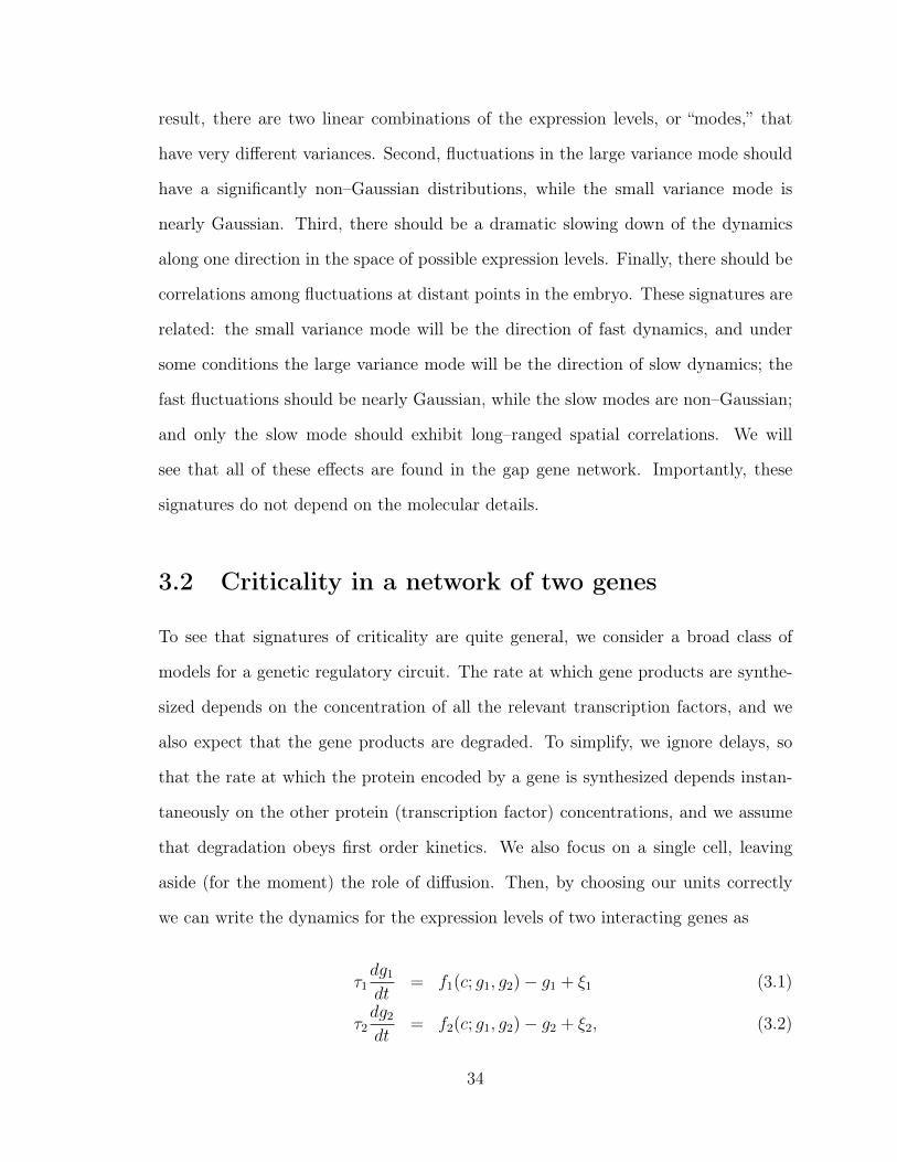
we can write the dynamics for the expression levels of two interacting genes as

τ1dg1

dt= f1(c; g1, g2)− g1 + ξ1 (3.1)

τ2dg2

dt= f2(c; g1, g2)− g2 + ξ2, (3.2)

34

where g1 and g2 are the normalized expression levels of the two genes, τ1 and τ2 are

the lifetimes of the proteins, and c represents the external (maternal) inputs. The

functions f1 and f2 are the “regulation functions” that express how the transcriptional

activity of each gene depends on the expression level of all the other genes; with our

choice of units, the regulation function runs between zero (gene off) and one (full

induction). All of the molecular details of transcriptional regulation are hidden in

the precise form of these regulation functions [5], which we will not need to specify.

Finally, the random functions ξ1 and ξ2 model the effects of noise in the system.

If the interactions are weak, then for any value of the external inputs c there is

a single steady state response, defined by expression levels g1(c) and g2(c). We can

check whether this hypothesis is consistent by asking what happens to small changes

in the expression levels around this steady state. We write g1 = g1 +δg1, and similarly

for g1, and then expand Eqs (3.1, 3.2) assuming that δg1 and δg2 are small. The result

is

d

dt

δg1

δg2

=

−Γ1 γ12

γ21 −Γ2

δg1

δg2

+

η1

η2

. (3.3)

Here Γ1 and Γ2 are effective decay rates for the two proteins, which must be positive

if the steady state we have identified is stable. The parameter γ12 reflects the incre-

mental effect of gene 2 on gene 1—γ12 < 0 means that the protein encoded by gene

2 is a repressor of gene 1—and similarly for γ21. The noise terms η1 and η2 play the

same role as ξ1 and ξ2, but have different normalization.

If the steady state that we have identified is stable, then the matrix

M ≡

−Γ1 γ12

γ21 −Γ2

(3.4)

must have two eigenvalues with negative real parts. This is guaranteed if the interac-

tions are weak (γ12, γ21 → 0), but as the interactions become stronger it is possible for

35

one of the eigenvalues to vanish. This is the critical point. Notice that we can define

the critical point without giving a microscopic description of all the interactions that

determine the form of the regulation functions.

The linearized Eqs (3.3) predict that the relaxation of average expression levels

to their steady states can be written as combinations of two exponential decays,

〈g1(t)〉

〈g2(t)〉

=

g1(c)

g2(c)

+

A1s A1f

A2s A2f

eΛst

eΛf t

(3.5)

where Λs and Λf are the “slow” and “fast” eigenvalues of M . Thus, while we measure

the two expression levels, there are linear combinations of these expression levels—

different directions in the (g1, g2) plane—that provide more natural coordinates for

the dynamics, such that motion along each direction is a single exponential function

of time. As we approach criticality, the dynamics along the slow direction becomes

very slow, so that Λs → 0.

The linearized Eqs (3.3) also predict the fluctuations around the steady state. As

we approach criticality, things simplify, and we find the covariance matrix

〈(δg1)2〉 〈δg1δg2〉

〈δg1δg2〉 〈(δg2)2〉

→ σ2

1 Γ1/γ12

Γ1/γ12 (Γ1/γ12)2

, (3.6)

where σ2 is the variance in the expression level of the first gene. As with the dynamics,

there are two “natural” directions in the (g1, g2) plane corresponding to eigenvectors

of this covariance matrix (principal components). In this linear approximation, the

critical point is the point where we “lose” one of the dimensions, and the fluctuations in

the two expression levels become perfectly correlated or anti–correlated. In addition,

the direction with small fluctuations is the direction of fast relaxation.

36

3.3 Signatures of criticality in the data

Testing the predictions of criticality requires measuring the time dependence of gap

gene expression levels, with an accuracy better than the intrinsic noise levels of the

system. Absent live movies of the expression levels, the progress of cellularization

provides a clock that can be used to mark the time during nuclear cycle fourteen at

which an embryo was fixed [30], accurate to within one minute [11]. Fixed embryos,

with immunofluorescent staining of the relevant proteins, thus provide a sequence of

snapshots that can be placed accurately along the time axis of development. Im-

munofluorescent staining itself provides a measurement of relative protein concentra-

tions that is accurate to within ∼ 3% of the maximum expression levels in the embryo

[11].

In Fig 3.2a we show the correlations between fluctuations in pairs of gap genes

at each position. Gap gene expression levels plateau at ∼ 40 min into nuclear cycle

fourteen [11], and the mean expression levels are shown as a function of anterior–

posterior position in Fig 3.1. At each position we can look across the many embryos

in our sample, and analyze the fluctuations around the mean, as in Ref [12]. We

see that, precisely in the “crossing region” where Hb and Kr are the only genes with

significant expression (marked A in Fig 3.2a), the correlation coefficient approaches

C = −1, perfect (anti–)correlation, as expected at criticality. This pattern repeats

at the crossing between Kr and Kni (B), at the crossing between Kni and Gt (C),

and, perhaps less perfectly1, at the crossing between Gt and Hb (D). These strong

anti–correlations are shown explicitly in Fig 3.2b, where we plot the two relevant gene

expression levels against one another at each crossing point. In all cases, the direction

of small fluctuations is along the positive diagonal, while the large fluctuations are

along the negative diagonal.1Since we observe substantial anti–correlations both in the Gt–Hb pair and in the Hb–Kni pair,

it is likely that the system is more nearly three dimensional in the neighborhood of this crossing, sothat no single pair can achieve perfect correlation.

37

slow

0 0.2 0.4 0.6 0.8 10

0.2

0.4

0.6

0.8

1

−0.5

0 0.5

0

0.5

1

−0.5

0 0.5

−0.5

0 0.5

−0.5

0 0.5

0 0.2 0.4 0.6 0.8 1 −0.5

0 0.5

Anterior-posterior position

Cor

rela

tion

coe

ffici

ent

(x/L)

g1(x/L)

g 2(x

/L

)

fast

Hb-Kr

FE

E

B

A

CD

F

G

G

Kr-Kni

Kni-Gt

Gt-Hb

Hb-Kni

H

a b

c

Fluctuation amplitude (s.d= )

Prob

abili

ty d

ensi

ty

−3 −2 −1 0 1 2 30

0.1

0.2

0.3

0.4

0.5

slow0 0.2 0.4 0.6 0.8 10

0.2

0.4

0.6

0.8

1

−0.5

0 0.5

0

0.5

1

−0.5

0 0.5

−0.5

0 0.5

−0.5

0 0.5

0 0.2 0.4 0.6 0.8 1 −0.5

0 0.5

Anterior-posterior position

Cor

rela

tion

coe

ffici

ent

Mea

n ex

pres

sion

(x/L)

g1(x/L)

g 2(x

/L

)

fast

Hb-Kr

FE

E

B

A

CD

F

G

G

Kr-Kni

Kni-Gt

Gt-Hb

Hb-Kni

H

a b

c

Fluctuation amplitude (s.d.= )

Prob

abili

ty d

ensi

ty

−3 −2 −1 0 1 2 30

0.1

0.2

0.3

0.4

0.5

−3 −2 −1 0 1 2 30

0.1

0.2

0.3

0.4

0.5

g

Figure 3.2: Fluctuations in gap gene expression levels. (a) Pairwise correlation coeffi-cients between fluctuations in the different gap genes vs. anterior–posterior position,from the same data as in Fig 3.1. Mean expression levels at top to guide the eye,colors as in Fig 3.1; error bars are from bootstrap analysis. Correlations which arenot significant at p = 0.01 are shown as zero. Major crossing points of the meanexpression profiles are labelled A, B, C, and D; other points marked as described inthe text. (b) Scatter plot of expression levels for pairs of genes in individual embryos:Kr vs Hb at point A (grey circles), Kni vs Kr at point B (blue diamonds), Gt vs Kniat point C (green squares), and Hb vs Gt at point D (red triangles). (c) Probabilitydistribution of expression fluctuations. In each of the crossing regions from Fig 1,we form the combinations δgf (fast modes, cyan) and δgs (slow modes, magenta),and normalize the fluctuations across embryos to have unit variance at each position.Data from all four regions are pooled to estimate the distributions; error bars arefrom random divisions of the set of 24 embryos. Gaussian distribution (black) shownfor comparison.

38

It is important that the strong anti–correlations tell us something about the un-

derlying network, rather than being a necessary (perhaps even artifactual) corollary

of the mean expression profiles. A notable feature of Fig 3.2a thus is what happens

away from the major crossing points. There is a Hb–Kni crossing at x/L = 0.1 (E),

but this does not have any signature in the correlations, perhaps because spatial vari-

ations in expression levels at this point are dominated by maternal inputs rather than

being intrinsic to the gap gene network [43, 25]. This is evidence that we can have

crossings without correlations, and we can also have correlations without crossings,

as with Hb and Kr at point H; interestingly, H marks the point where an additional

posterior Kr stripe appears during gastrulation [17, 14]. We also note that strong

correlations can appear when expression levels are very small, as with Hb and Kni

at points F and G; there also are extended regions of positive Kr–Kni and Kni–Gt

correlations in parts of the embryo where the expression levels of Kr and Kni both

are very low. Taken together, these data indicate that the pattern of correlations is

not simply a reflection of the mean spatial profiles, but an independent measure of

network behavior.

If we transfrom Eq (3.3) to a description in terms of the fast and slow modes gf

and gs, then precisely at criticality there is no “restoring force” for fluctuations in gs

and formally the variance σ2 in Eq (3.6) should diverge. This is cut off by higher

order terms in the expansion of the regulation functions around the steady state, and

this leads to a non–Gaussian distribution of fluctuations in gs. Although the data are

limited, we do find, as shown in Fig 3.2c, that fluctuations in the small variance (fast)

direction are almost perfectly Gaussian, while the large variance (slow) direction show

significant departures form Gaussianity, in the expected direction.

The time dependence of Hb and Kr expression levels during nuclear cycle fourteen

is shown, at the crossing point x/L = 0.47, in Fig 3.3. Criticality predicts that if

we take a linear combination of these expression levels corresponding to the direction

39

0.20.40.60.8

1

0 10 20 30 40 50−0.4−0.2

00.20.4

0.20.40.60.8

1

Hb

0 10 20 30 40 5000.20.40.60.8

time, min

Kr

Hb

Time (min)

slow

fast

Time (min)

gf = 1√2(Hb+Kr)

gs = 1√2(Kr−Hb)

Kr

a b

Figure 3.3: Dynamics at the Hb–Kr crossing point. (a) Normalized expression levelsof the individual genes, plotted vs. time during nuclear cycle fourteen; data from Ref[11]. (b) Linear combinations of expression levels corresponding to the small variance(fast) and large variance (slow) directions in Fig 3.2b. Curves are best fit singleexponentials for each mode and are also shown projected back into the individualexpression levels in (a). Eigenvalues, as in Eq (3.5), are Λf = −0.04±0.01 min−1 andΛs = −0.002± 0.007 min−1.

of small fluctuations in Fig 3.2b (cyan), then we will see relatively fast dynamics,

and this is what we observe. In contrast, if we project onto the direction of large

fluctuations (magenta), we see only very slow variations over nearly one hour. Indeed,

the expression level along this slow direction seems almost to diffuse freely, with

growing variance rather than systematic evolution. Thus, strong (anti–)correlations

are accompanied by a dramatic slowing of the dynamics along one direction in the

space of possible expression levels, and a similar pattern is found at each of the

crossings, Kr–Kni, Kni–Gt, and Gt–Hb (data not shown). Again, this is consistent

with what we expect for two–gene systems at criticality.

If we move along the anterior-posterior axis in the vicinity of the crossing point,

the sum of expression levels of two genes, which is proportional to the fast mode,

remains approximately constant, while the difference, which is proportional to the

slow mode, changes. Therefore the dynamics of the slow mode, shown in Fig 3.3, will

40

generate motion of the pattern along the anterior–posterior axis. This slow shift is

well known [11, 21].

The slow dynamics associated with criticality also implies that correlations should

extend over long distance in space. As is clear from Fig 3.3, the eigenvalues Λs and Λf

define time scales τs = −1/Λs and τf = −1/Λf . If we add diffusion to the dynamics

in Eqs (3.3), then these time scales define length scales, through the usual relation

`s,f =√Dτs,f ; although there is some dependence on details of the underlying model,

these lengths define the distances over which we expect fluctuations to be correlated.

In particular, as we approach criticality, Λs vanishes and the associated correlation

length `s can become infinitely long, limited only by the size L of the embryo itself.

Searching for these long–ranged correlations is complicated by the fact that the system

is inhomogeneous, but we have a built in control, since we should see the long ranged

correlations only in the slow, large variance mode δgs, and not in δgf . This control also

helps us discriminate against systematic errors that might have generated spurious

correlations.

In Fig 3.4a we show the normalized correlation function

Css(x, y) =〈δgs(x)δgs(y)〉

(〈[δgs(x)]2〉〈[δgs(y)]2〉)1/2, (3.7)

with x held fixed at the Hb–Kr crossing and y allowed to vary. We see that this corre-

lation function is essentially constant throughout the crossing region. In contrast, the

same correlation computed for the fast mode decays rapidly, with a length constant

ξ/L ∼ 0.02, just a few nuclear spacings along the anterior–posterior axis.

The dominant slow mode corresponds to different combinations of expression levels

in different regions of the embryo. Generally, we can write the slow mode as a weighted

41

0 0.1 0.2 0.3 0.4 0.5 0.6 0.7 0.8 0.9 10

0.40.8

0.44 0.45 0.46 0.47 0.48 0.49 0.5

−0.4

−0.2

0

0 0.1 0.2 0.3 0.4 0.5 0.6 0.7 0.8 0.9 1−1

−0.8

−0.6

−0.4

−0.2

0

Profiles

ln(correlation)

ln(correlation)

y/L

y/L

Cff (0.48, y/L)

Css(0.48, y/L)

1√2(δHb−δGt)

1√2(δKni−δKr)1√

2(δKr−δHb)

1√2(δGt−δKni)

a

ξ/L ≈ 0.02

b

1√2(δKr−δHb)

1√2(δKni−δKr)

1√2(δKni−δKr)

1√2(δHb−δGt)

0 0.1 0.2 0.3 0.4 0.5 0.6 0.7 0.8 0.9 10

0.4

0.8

0.44 0.45 0.46 0.47 0.48 0.49 0.5 0.51 0.52

−0.4

−0.2

0

−0.8

−0.6

−0.4

−0.2

0

0 0.1 0.2 0.3 0.4 0.5 0.6 0.7 0.8 0.9 10

0.4

0.8

0.44 0.45 0.46 0.47 0.48 0.49 0.5 0.51 0.52

−0.4

−0.2

0

−0.8

−0.6

−0.4

−0.2

0

AA ABAC AD

0 0.1 0.2 0.3 0.4 0.5 0.6 0.7 0.8 0.9 10

0.40.8

0.44 0.45 0.46 0.47 0.48 0.49 0.5 0.51 0.52

−0.4

−0.2

0

0 0.1 0.2 0.3 0.4 0.5 0.6 0.7 0.8 0.9 1−1

−0.8

−0.6

−0.4

−0.2

0Cff (0.465, y/L) Css(0.465, y/L)

Css(0.47, y/L)Cff (0.47, y/L)

ln(C

)ln

(C)

0 0.1 0.2 0.3 0.4 0.5 0.6 0.7 0.8 0.9 10

0.40.8

0.44 0.45 0.46 0.47 0.48 0.49 0.5

−0.4

−0.2

0

0 0.1 0.2 0.3 0.4 0.5 0.6 0.7 0.8 0.9 1−1

−0.8

−0.6

−0.4

−0.2

0

Figure 3.4: Spatial correlations of fluctuations in gene expression. (a) Auto–correlations of slow (magenta) and fast (cyan) modes near the Hb–Kr crossing, asdefined in Eq (3.7). Line shows a fit, Cff (x, y) ∝ e−|x−y|/ξ, with ξ/L = 0.015± 0.002.(b) Correlations between the slow mode at the Hb–Kr crossing and slow modes atother crossings, as defined in Eq (3.10), indicated by the colors. All correlation func-tions are evaluated at x/L = 0.47 with y varying as shown. Middle peak is the same(auto–)correlation function Css as in (a). Dashed line is e−|x−y|/ξ, with ξ = L.

42

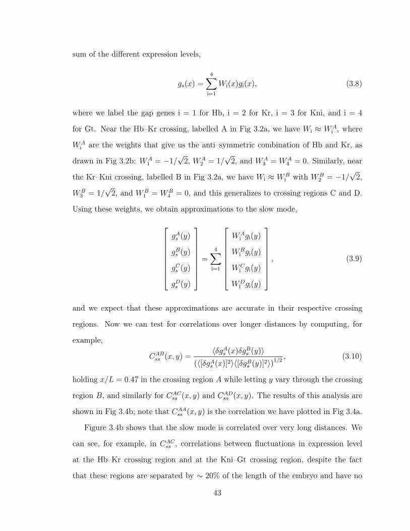
sum of the different expression levels,

gs(x) =4∑

i=1

Wi(x)gi(x), (3.8)

where we label the gap genes i = 1 for Hb, i = 2 for Kr, i = 3 for Kni, and i = 4

for Gt. Near the Hb–Kr crossing, labelled A in Fig 3.2a, we have Wi ≈ WAi , where

WAi are the weights that give us the anti–symmetric combination of Hb and Kr, as

drawn in Fig 3.2b: WA1 = −1/

√2, WA

2 = 1/√

2, and WA3 = WA

4 = 0. Similarly, near

the Kr–Kni crossing, labelled B in Fig 3.2a, we have Wi ≈ WBi with WB

2 = −1/√

2,

WB3 = 1/

√2, and WB

1 = WB4 = 0, and this generalizes to crossing regions C and D.

Using these weights, we obtain approximations to the slow mode,

gAs (y)

gBs (y)

gCs (y)

gDs (y)

=4∑

i=1

WAi gi(y)

WBi gi(y)

WCi gi(y)

WDi gi(y)

, (3.9)

and we expect that these approximations are accurate in their respective crossing

regions. Now we can test for correlations over longer distances by computing, for

example,

CABss (x, y) =

〈δgAs (x)δgBs (y)〉(〈[δgAs (x)]2〉〈[δgBs (y)]2〉)1/2

, (3.10)

holding x/L = 0.47 in the crossing region A while letting y vary through the crossing

region B, and similarly for CACss (x, y) and CAD

ss (x, y). The results of this analysis are

shown in Fig 3.4b; note that CAAss (x, y) is the correlation we have plotted in Fig 3.4a.

Figure 3.4b shows that the slow mode is correlated over very long distances. We

can see, for example, in CACss , correlations between fluctuations in expression level

at the Hb–Kr crossing region and at the Kni–Gt crossing region, despite the fact

that these regions are separated by ∼ 20% of the length of the embryo and have no

43

significantly expressed genes in common. These peaks in the correlation functions

appear also at points anterior to the crossing regions, presumably at places where

our approximations in Eq (3.9) come close to some underlying slow mode in the

network. The pattern of correlations has an envelope corresponding to an exponential

decay with correlation length ξ = L (dashed line in Fig 3.4b), and similar results

are obtained for the correlation functions CBCss , CBD

ss , CCDss , etc.. This means that

fluctuations in expression level are correlated along essentially the entire length of

the embryo, as expected at criticality.

3.4 Conclusions

To summarize, the patterns of gap gene expression in the early Drosophila embryo ex-

hibit several signatures of criticality: near perfect anti–correlations of fluctuations in

the expression levels of different genes at the same point, non–Gaussian distributions

of the fluctuations in the large variance modes, slowing down of the dynamics of these

modes, and spatial correlations of the slow modes that extend over a large fraction

of the embryo. While each of these observations could have other explanations, the

confluence of results strikes us as highly suggestive. Note that we have focused on

aspects of the data that are connected to the hypothesis of criticality in a very general

way, independent of other assumptions, rather than trying to build a model for the

entire network.

The possibility that biological systems might be poised near critical points, often

discussed in the past [2], has been re–invigorated by new data and analyses on systems

ranging from ensembles of amino acid sequences to networks of neurons to flocks

of birds [36]. In the specific context of transcriptional regulation, the approach to

criticality serves to generate long time scales, which may serve to reduce noise and

optimize information transmission [46]. For the embryo in particular, these long time

44

scales and the corresponding long length scales may give us a different view of the

problem of scaling expression patterns to variations in the size of the egg [50, 3].

Even leaving aside the possibility of criticality, the aspects of the data that we

have described here are not at all what we would see if the gap gene network is

described by generic parameter values. There must be something about the system

that is finely tuned in order to generate such large differences in the time scales for

variation along different dimensions in the space of expression levels, or to insure that

correlations are so nearly perfect and extend over such long distances.

45

Chapter 4

Effective theory for the zero mode

As is familiar from many examples in physics, for systems near the critical point, it

might be useful to integrate out the heavy excitations from the microscopic equations

of motion, and obtain an effective theory for the strongly fluctuating mode - the

zero mode or order parameter. This effective equations are usually given by the

Landau-Ginsburg theory. One important insight from the previous discussion is that

criticality in the developing embryo does not exactly copy the standard examples from

physics textbooks. As we explained in the previous chapter, the order parameter in

the former case is a linear combination of physical degrees of freedom (the expression

levels of the gap genes), but which genes enter this linear combination - depends on

the position along the embryo. In other words the microscopic composition of the

order parameter changes as we move along the anterior-posterior axis. Is it possible

to write a general effective field theory for the zero mode in this situation? Can this

theory teach us anything interesting about the development of fruit flies? These are

the questions that we discuss in this chapter.

It turns out that for proper treatment of this problem we will have to introduce

gauge fields into our equations. These gauge fields produce observable contributions

to Green functions of the zero mode. The central result of this chapter is that the

46

normalized two point correlation function of the order parameter, for the network on

N genes, is given by the action of a relativistic particle moving on the product space

of the N − 1 dimensional sphere and the anterior-posterior axis of the fruit fly. We

start with the theory, and compare it with experiments at the end of the chapter.

4.1 Theory

Let’s again start with equations similar to (3.1,3.2), but now include diffusion. For

the network of N genes we have

gα = Fα(gβ; c

)+ D ∂2

x

(gα)

(4.1)

Here the functions Fα(gβ; c

)are responsible for all the production and degradation

processes of transcription factors, and we also assume that the proteins can diffuse

with some diffusion coefficient D that is assumed to be equal for all the transcription

factors. In the steady state we have expression profiles gα(x) which satisfy

Fα(gβ; c

)+ D ∂2

x

(gα)

= 0 (4.2)

and for the dynamics of the fluctuations, gα(t, x) = gα(x) + δgα(t, x), we obtain

δgα = Mαβδgβ + D ∂2x

(δgα), Mαβ(x) =

∂Fα∂gβ

∣∣∣∣g(x),c(x)

(4.3)

The dynamical matrix Mαβ(x) depends on the position along the embryo. Let’s

consider first a toy model example of a symmetric matrix. Then we can decompose

it as

Mαβ(x) =N∑

i=1

ψiα(x)λi(x)ψiβ(x) (4.4)

47

where λi and ψiα are eigenvalues and eigenvectors of Mαβ. Since Mαβ is symmetric,

we have

ψiαψjα = δij (4.5)

First of all we would like to project Eq (4.3) onto the eigenmodes of the matrix Mαβ.

In order to do this we need to multiply Eq (4.3) by ψkα and introduce a new set of

variables - the eigenfluctuations

gk = ψkαδgα (4.6)

We obtain

gk = λkgk + Dψkα∂2x

(δgα)

(4.7)

The problem with this equation is that the eigenvectors ψiα(x) depend on the position,

therefore we can not commute the x-derivative and ψkα in the last term. Thus, in

order to rewrite Eq (4.3) in the covariant form with respect to latin indices we have

to introduce a gauge connection.

The set of eigenvectors ψiα form a complete basis in the space of fluctuations.

Therefore we can decompose the spatial derivative of an eigenvector in this basis

∂xψkα = Akiψiα (4.8)

for some coefficients Aki. If we differentiate the orthogonality constraint (4.5) with

respect to x, we can find that the matrices Aij(x) must be antisymmetric at every

point in space

Aij + Aji = 0 (4.9)

Now we can introduce the covariant derivative

ψkα∂x(δgα)

= ∂xgk − Akigi =

(Dg)k (4.10)

48

Applying this trick twice we can rewrite Eq (4.7) in the fully covariant form

gk = λkgk + D(D2g

)k(4.11)

or more explicitly

gk = λkgk + D[∂2xg

k − Aki∂xgi − ∂x(Akigi) + AkiAilgl]

(4.12)

The coefficients Aij play the familiar role of a gauge field. In the case of the symmetric

matrix Mαβ the gauge group is O(N) for the network of N genes. The gauge field is

an element of the adjoint representation, and therefore should be an antisymmetric

matrix, as was shown above.

Thus far we haven’t made any assumptions, all that we did is to transform Eq

(4.3) from the basis of genes (greek indices) to the basis of collective modes (latin

indices). But these two systems of equations are completely equivalent. Now we

would like to make a reduction to the effective theory for the zero mode. In order

to do this let’s assume that all the eigenvalues λi (i = 2...N) are negative and large,

and the eigenvalue λ1(x) = −ε(x), where ε(x) is a small position-dependent function.

We do not assume any specific sign of ε(x). In the critical regime ε(x) approaches

zero everywhere along the anterior-posterior axis. In this limit all the fluctuations

gi (i = 2...N) become small and g1 becomes large. In order to find the effective

theory for the zero mode we simply need to drop all the modes gi (i = 2...N) whose

fluctuations are small and retain only terms that couple to g1 in Eq (4.12). The result

is

g1 = −m2(x)g1 + D∂2xg

1 (4.13)

where

m2(x) = ε(x) + D

N∑

i=2

(A1i)2 (4.14)

49

Thus the effective equation for the zero mode is very similar to the original equation

(4.7) but with a renormalized mass of the zero mode. This renormalization is impor-

tant. It tells us that the effective mass of the zero mode comes from two sources: the

bare mass ε(x) - the local (in space) property of the transcriptional network - and the

gauge field A(x), which is non-zero only if the operating point of the transcriptional

network is changing as we move along the anterior-posterior axis. The biological ori-

gin of this second term can be traced to the presence of the maternal morphogens

inside the cell that break translational symmetry and induce coordinate dependence

of the dynamical matrix. Another important point is that this correction to the mass

is always positive. This means that the non-local effects that we discuss here can only

increase the effective mass. If the bare mass were already positive, this would push

the system further away from criticality. If the bare mass were negative, this would

stabilize the system and push it towards criticality.

Finally, we would like to emphasize the analogies and contrasts of this effect with

the Higgs mechanism. In the latter case a scalar field receives a non-zero vacuum ex-

pectation value because of the external potential. This non-zero vacuum expectation

value produces the mass for the gauge field. In our problem the situation is exactly

the opposite. The maternal morphogens break translational symmetry inside the cell

and this induces a non-zero value of the gauge field. This background gauge field

produces the contribution to the mass of the scalar field - the zero mode.

To analyze these effects in a more quantitative way it is nice to go back to Eq

(4.13) and introduce a dynamic noise that mimics the stochastic effects of transcrip-

tional activity in various parts of the cell. We assume that the noise is white and

translationally invariant for simplicity

〈ξα(x, t)〉 = 0 〈ξα(x1, t1)ξβ(x2, t2)〉 = N δ(x1 − x2)δ(t1 − t2)δαβ

50

From now on we assume that D = 1, for convenience. We also use the following

notations for the order parameter, the corresponding eigenvectors and the noise:

ψα(x) = ψ1α(x), g(x, t) = g1(x, t) = ψα(x)δgα(x, t), ξ(x, t) = ψα(x)ξα(x, t)

Our goal is to find the two-point function of the zero mode, which satisfies

∂tg = −m2(x)g + ∂2xg + ξ(x, t), (4.15)

averaged over the noise. We introduce two Green functions: one for the time-

dependent problem

[∂t − ∂2

x +m2(x)]∆(x, t|y, t) = δ(t− t)δ(x− y), (4.16)

and one for the static problem

[− ∂2

x +m2(x)]G(x, y) = δ(x− y). (4.17)

One can transform Eq (4.16) into Fourier space over time. The corresponding Green

function is then given by

∆(x, y, ω) =∞∑

n=0

ϕn(x)ϕ∗n(y)

−iω + σn, (4.18)

where ϕn(x) and σn are eigenfunctions and eigenvalues of the static differential oper-

ator[− ∂2

x +m2(x)]ϕn(x) = σnϕn(x). (4.19)

51

Using this representation we can calculate the two-point function of the zero mode

〈g(x, t)g(y, t)〉 = N∫dzdt ∆(x, t|z, t)∆(y, t|z, t) = N

∫dz

dω

2π∆(x, z, ω)∆(y, z,−ω) =

= N∞∑

n=0

∫dω

2π

ϕn(x)ϕ∗n(y)

ω2 + σ2n

=N2

∞∑

n=0

ϕn(x)ϕ∗n(y)

σn=N2G(x, y).

(4.20)

Thus, the two-point function in the theory with the dynamic noise is equal to the

Green function of the static differential operator (4.17), multiplied by N /2. The first

three equalities in (4.20) can be also interpreted as consequence of the fluctuation-

dissipation theorem.

In order to solve (4.17) we will assume that the embryo is large so that the correct

Green function is selected by the condition that G(x, y)→ 0 as the distance between

x and y becomes large. In other words we neglect by the possible influence of the

boundary conditions at the ends of the embryo on the pattern of correlations that

we are trying to find. Since we do not know the explicit dependence of the effective

mass on the position, we can not solve (4.17) exactly. However it is instructive to use

quasiclassical approximation to find the main features of the solution. Quasiclassics

is valid in this problem as long as m(x) is a sufficiently slow varying function of the

position. In this limit we obtain

G(x1, x2) =1

2√m(x1)m(x2)

e−x>∫x<

m(z)dz

(4.21)

Our ultimate goal is to find a quantity analogous to (3.7). Using (4.20) and (4.21)

we obtain, assuming that y > x,

C(x, y) =〈 g(x, t) g(y, t) 〉√〈g(x, t)2〉 〈g(y, t)2〉

= e−S(x,y) (4.22)

52

where

S(x, y) =

y∫

x

m(z)dz =

y∫

x

dz

√√√√N∑

k=2

(A1k(z)

)2

− λ(z) (4.23)

From now on we will assume that the lightest eigenvalue λ(z) = λ1(z) = −ε(z) of the

dynamical matrix Mαβ is slightly positive or is equal to zero. Using definition (4.8)

we can express the gauge field through the eigenvectors as

A1k = ψkα∂xψα (4.24)

By exploiting the completeness property of the eigenvectors

N∑

k=1

ψkαψkβ = δαβ

and using that A11 = 0, we can rewrite the action as (in the last formula we restored

the diffusion coefficient that was assumed to be equal to one in the previous formulas)

S(x, y) =

y∫

x

dz

√√√√N∑

k=1

ψkαψkβ ∂zψα∂zψβ − λ(z) =

y∫

x

dz

√(∂zψα

)2 − λ

D(4.25)

This last form has a very transparent geometrical meaning - this is the action of a

relativistic particle on the (N − 1)-dimensional sphere with “time” representing the

motion along the anterior-posterior axis of the fruit fly embryo.

In principle, this action should be calculated along the real trajectory on SN−1 ×

[0, L] (product of the unit sphere by the anterior-posterior axis) that is dictated by

the non-linear equations (4.2). To get a lower bound on this action it is however

possible to calculate it on the geodesic trajectory - the shortest path connecting the

53

initial and the final state. In order to do this we introduce the “effective time”

∆χ =

y∫

x

√λ(z)

Ddz (4.26)

and the angle between the initial and the final position of the particle on the sphere

ψα(x)ψα(y) = cos(∆φ) (4.27)

The action calculated on the geodesic is then equal to

Sgeodesic =

√(∆φ)2 −

(∆χ)2 (4.28)

This quantity gives the lower bound on the value of the action evaluated on the

realistic trajectory of the gap genes, given the dependence λ(x) and the initial and

final positions on the sphere.

Sgap > Sgeodesic (4.29)

Thus e−Sgeodesic provides the upper bound on the behavior of the correlation coefficient

(4.22), given the anterior-posterior position dependence of the zero eigenvalue λ(z).

The general case of an arbitrary (non-symmetric) matrix Mαβ can be treated in

a similar way. We notice that it can be decomposed as

Mαβ(x) =N∑

i=1

ζ iα(x)λi(x)ψiβ(x) (4.30)

so that now we have left and right orthogonal matrices ζ iα(x) and ψiβ(x). Multiplying

Eq (4.3) by ψkα we obtain

gk = Πkigi + D(D2g

)k(4.31)

54

where the matrix of eigenvalues is now weighted with the overlap of the left and the

right eigenvectors

Πki = ψkαζiαλ

i (4.32)

After the reduction to the effective theory for the zero mode, we obtain exactly the

same equations (4.13,4.14) as in the symmetric case, with λ1 replaced by λ1ψ1αζ

1α.

4.2 Comparison with experiments

In the previous section we derived the relationship between the correlation functions

of the order parameter and the motion of the particle on the unit sphere of expression

levels, Eq (4.22, 4.28). In this section we will argue that the qualitative features

predicted by these equations can be seen in the real data. We can construct the

full covariance matrix of the network of four gap genes at every position along the

anterior-posterior axis

Cαβ(x) = 〈δgα(x)δgβ(x)〉 (4.33)

At every position we can identify the linear combination of the four gap genes that

has the largest variance. We will define the order parameter, see Eq (4.6), as this

linear combination. Thus

g(x) = ψα(x)δgα(x) (4.34)

where ψα(x) now is the eigenvector of the covariance matrix. Now we can calculate

experimentally the correlation coefficient (4.22). The result is shown in the lower

panel of Fig. 4.1. From the previous analysis and from the diagonalization of the

covariance matrix we know the eigenvectors ψα at the four underlined intersection

55

0.20.40.60.8 1

0 0.2 0.4 0.6 0.8 10

0.2

0.4

0.6

0.8

1

anterior-posterior position

C(x

,y)

g α

0.2

0.4

0.6

0.8

1

HbKrKniGt

0 0.2 0.4 0.6 0.8 10

0.2

0.4

0.6

0.8

1

ψ(1)α ψ(2)

α ψ(3)αψ(4)α

Figure 4.1: Top panel: mean expression profiles gα(x) of the four gap genes. Lowerpanel: auto-correlation coefficient C(x, y) of the order parameter, defined as the modewith the largest variance. We keep x = 0.47 (the crossing point of Hb and Kr) andplot C(x, y) as a function of y. This is a replotting of the spatial correlation graphfrom [27].

regions. They are approximately equal to

ψ(1)α =

1√2

−1

1

0

0

ψ(2)α =

1√2

0

−1

1

0

ψ(3)α =

1√2

0

0

−1

1

ψ(4)α =

1√2

1

0

0

−1

(4.35)

throughout the underlined regions. In between, in the regions marked by the arrows,

the eigenvectors presumably smoothly interpolate between the two values. These are

the regions where we expect the gauge field to be non-zero. Within the underlined

regions the gauge field is equal to zero.

56

Consider the following drastic approximation. Imagine that the lowest eigenvalue

λ(z) of the dynamical matrix is equal to zero everywhere along the anterior-posterior

axis. As we will show in a moment this assumption is incorrect, but it is still useful

to illustrate the logic. If that is true, the ∆χ term in Eq (4.28) is equal to zero and

the decay of the correlations is entirely determined by the variation of the eigenvector

ψα. Within the underlined regions in Fig. 4.1 this eigenvector does not change,

therefore Sgeodesic = 0 and the correlations should not decrease. In between the

underlined regions, the eigenvector rotates, therefore the correlations should decrease.

Qualitatively, this is precisely what the magenta curve in Fig. 4.1 looks like. It

is relatively flat within the underlined regions, and there is a step-like decrease in

the correlation once we transition from one plateau to the next. In principle, our

approximation allows us to calculate the heights of the steps between the neighboring

plateaus. The eigenvectors (4.35) are defined modulo reflections. We will assume

that, as we move from the first plateau (corresponding to the eigenvector ψ(1)) to

the second plateau (corresponding to the eigenvector ψ(2)), the eigenvector changes

in such a way that the angle between the initial and the final states is minimal. In

this specific example this means that if we start from ψ(1), the final eigenvector will

be equal to −ψ(2) instead of ψ(2). The angle between the initial and the final vectors

is then equal to

∆φ =π

3

This means that the upper bound on the correlation coefficient within the region

corresponding to the second plateau is equal to

Cbound = e−π/3 ≈ 0.35

If our approximation were correct the real value of the correlation should be smaller

than Cbound, because realistic trajectories do not have to coincide with geodesics.

57

Experimental value of the correlation in this region, however, is equal to C ≈ 0.9,

violating this bound.

Of course, the approximation that λ(z) = 0 is very naive and is motivated mostly

by our inability to extract this quantity from the data. For the system to be critical

what we really need is that the effective mass of the zero mode m(z) is equal to zero,

not that the “bare” mass λ(z) equals zero. If our picture is correct, this observation

suggests that in the absence of the non-local effects related to the rotation of the

eigenvector ψα the transcriptional network is locally unstable. This corresponds to

positive values of λ(x) in the gaps between the neighboring plateaus. This positive

contribution is compensated by the kinetic term for the vector ψ in such a way that

the total, effective, mass is close to zero. It would be interesting to see if future

experiments can help to independently determine the dynamical matrix Mαβ(x) and

its lowest eigenvalue to test this prediction.

An alternative explanation for the violation of this bound is that the real network

can be larger than the four genes that we discuss. If that is true, the angle between

the initial and the final eigenvectors can be different from π/3. This can modify

the heights of the steps. Again, it would be interesting to check experimentally if

an additional gene, whose fluctuations are large and significantly contribute to the

zero mode, exists and how it can modify the predictions of the theory regarding the

correlations.

58

Chapter 5

Explicit examples of transcriptional

networks

How difficult is it to tune a network to criticality? All the analyses that we discussed

above do not rely on any specific model of transcriptional regulation. This is an

advantage of this approach, since we don’t know the microscopic details of what

is happening at the promoters when multiple transcription factors bind to them.

Having achieved this “model independent” understanding of the system, it is nice to

go back and construct explicitly the regulatory networks within some broad class of

models. A particularly attractive idea is to use the Monod-Wyman-Changeux (MWC)

scheme [35], originally developed to describe the allosteric regulation of enzymes, to

model the regulation machinery. Within this simple picture, we can calculate the

regulation functions exactly and construct explicitly the phase diagram of all possible

transcriptional networks that one can theoretically imagine. Can we now try to locate

real embryos on this phase diagram? From the previous arguments we know that

they must be located in the vicinity of the critical surfaces. But how densely is this

region covered with hypothetical (theoretically designed) networks? Such a “model

dependent” approach can help us to explore the space of all possible models and to

59

answer the question of how difficult it is to tune a network to criticality. In addition,

such explicit models can be tested by comparing their predictions for the architecture

of enhancers (number of binding sites) with ChIP/chip and other experimental data.

The text of this chapter was written jointly by D.Krotov and W.Bialek as part of

an unpublished draft [26].

5.1 Taking a simple model seriously

In the previous chapters we worked with arbitrary activations functions fα(c; gβ)

that enter equations (3.1,3.2). Now we need to specify the form of these functions.

The Monod–Wyman–Changeux (MWC) model [35, 3], originally developed to de-

scribe allosteric regulation of enzymes, provides a simple physical picture within which

we can calculate the regulation functions exactly (Fig 5.1). We imagine that the

transcriptional apparatus for each gene has two states, active and inactive, and that

switching between these states is fast enough that the effective rate of transcription is

proportional to the probability of being in the active state. Each transcription factor

that binds shifts the equilibrium between active and inactive states: activators lower

the free energy of the active state relative to the inactive state, while repressors do the

opposite. The key simplification of the MWC model is to assume that all the binding

events are intrinsically independent; they interact, and binding becomes cooperative,

only through the shifting equilibrium between the active and inactive states.

Imagine that in the enhancer region of gene α there are Nαβ binding sites for

the transcription factor encoded by gene β, and these binding sites are described by

dissociation constants Qonαβ when the system is in the active state, and Qoff

αβ when the

system is in the inactive state; we could imagine a more complex model in which each

of the binding sites had a different affinity, but we’ll see that this isn’t essential to the

discussion. In a similar way, we imagine that the enhancer for gene α has nα binding

60

Figure 5.1: A schematic of an enhancer with two binding sites. The enhancer canexist in two states: ON or OFF . Transcription factors can bind to the two bindingsites independently with dissociation constants Kon and Koff . Assuming that thetranscription factor (at external concentration c) is an activator, the equilibriumfavors the OFF state when the binding sites are empty. However, binding is strongerto the ON state, Kon c Koff . Therefore, as more sites are occupied, theequlibrium shifts toward the ON state. The length of the arrows is proportional tothe probability of transition between the states.

sites for the primary input morphogen, and these binding sites have dissociation

constants Konα and Koff

α depending on whether the system is in the active or inactive

state. If a transcription factor binds to the active and inactive states with different

binding constants, then the binding event will shift the equilibrium between the two

states.

Once we know the dissociation constant for each binding event, we can enu-

merate all the possible states of the system (occupied/unoccupied binding sites, ac-

tive/inactive transcription) and give each state its appropriate Boltzmann weight on

the assumption that binding reactions come to equilibrium. Finally, we can sum over

all the different combinations of bound and unbound sites to obtain the effective free

energy difference between active and inactive states, which determines the probability

61

fα that the system is in the active state. The result is:

fα(gβ; c) =1

1 + exp [θ′α − Fα(gβ; c)](5.1)

Fα = nα ln

(1 + c/Kon

α

1 + c/Koffα

)+∑

β

Nαβ ln

(1 + gβ/Q

onαβ

1 + gβ/Qoffαβ

)(5.2)

where Fα is the part of the free energy (normalized by kBT ) that depends on the con-

centrations of the various regulators, and θ′α reflects the intrinsic free energy difference

between active and inactive states.

If the transcription factor encoded by gene β activates the expression of gene α,

then we must have Qonαβ < Qoff

αβ, which means that the transcription factor binds more

strongly (with smaller dissociation constant) to the active state. If this difference in

binding strengths is very large, then it is plausible that over some range of expression

levels for the transcription factor we will have Qonαβ gβ Qoff

αβ. In this limit, we

can approximate

Nαβ ln

(1 + gβ/Q

onαβ

1 + gβ/Qoffαβ

)≈ Nαβ ln gβ − Nαβ lnQon

αβ (5.3)

In contrast, if the transcription factor encoded by gene β is a repressor, we have

Qonαβ > Qoff

αβ, and the limit analogous to Eq (5.3) becomes

Nαβ ln

(1 + gβ/Q

onαβ

1 + gβ/Qoffαβ

)≈ −Nαβ ln gβ + Nαβ lnQoff

αβ (5.4)

One can make a similar argument about the input morphogen, which we assume is

an activator, so that

nα ln

(1 + c/Kon

α

1 + c/Koffα

)≈ nα ln c− nα lnKon (5.5)

62

Putting all of these terms together, we have

Fα ≈ constant + nα ln c+∑

β

Nαβ ln gβ (5.6)

where Nαβ = Nαβ if β is an activator, and Nαβ = −Nαβ if β is a repressor. Thus for

the network of M genes we have:

fα(gβ; c) =1

1 + Aαc−nαg−Nα11 g−Nα22 ...g−NαMM

(5.7)

where the constants Aα are determined by the intrinsic free energy difference between

the active and inactive states and the dissociation constants of all the transcription

factors affecting gene α. The absolute value of integers |Nαβ| counts the number of

binding sites, and the sign of Nαβ distinguishes activators (Nαβ > 0) from repressors

(Nαβ < 0).

The main focus of this chapter is the study of the mean expression profiles within

the crossing regions of the neighboring gap genes. As we will see in a moment, the

spatial profiles in these regions are well approximated by linear functions. Since

the Laplacian operator gives zero when it acts on a linear function, we will ignore

the effects of diffusion throughout this section. Therefore we discuss the following

equations

ταdgαdt

= fα(gβ; c)− gα (5.8)

Using the explicit expressions for the activation functions (5.7) we can calculate the

dynamical matrix

Mαβ(x) =∂fα∂gβ

∣∣∣∣g(x),c(x)

− δαβ (5.9)

63

Using that in the steady state the expression profiles satisfy fα(gβ; c) = gα, we

obtain

Mαβ = Nαβgαgβ

(1− gα)− δαβ (5.10)

What is important about Eq (5.10) is that, in the limits we are considering, the dy-

namical matrix depends only on the expression levels themselves and on the numbers

of binding sites for the transcriptions factors. The numbers of binding sites Nαβ pro-

vide a measure for the strength of the interactions, and when these interactions are

weak (Nαβ → 0) any steady state is stable. Importantly, the condition for criticality—

the point where one of the eigenvalues of Mαβ vanishes—then defines a relationship

among the expression levels of the different genes: given the parameters Nαβ, the

critical surface becomes a surface in the space of expression levels.

5.2 Zooming in on the Hb-Kr crossing

As we move from the anterior to the posterior of the Drosophila embryo, there is a

region near the point where the mean expression levels of Hb and Kr cross, where just

these two genes have significant expression levels (see 3.1). In this region, it makes

sense to consider a model of just two interacting genes, driven by maternal input from

Bicoid. In this case Eq (5.8) become more explicitly,

τ1dg1

dt= f1(g1, g2, c)− g1 (5.11)

τ2dg2

dt= f2(g1, g2, c)− g2 (5.12)

where g1 refers to the expression level of Hb and g2 refers to the expression level of Kr;

the external input is provided by Bcd, which is at concentration c. These equations

describe the dynamics of expression in one nucleus, and each nucleus along the length

of the embryo has a different value of c, following the Bcd gradient.

64

0.44 0.46 0.480

0.2

0.4

0.6

0.8

1

Figure 5.2: Zoomed in expression levels of Hb (blue) and Kr (red) with Kni (green)and Gt (yellow) as a function of the anterior–posterior axis of the embryo. Black lines- linear fits to the data - are good descriptions of the profiles over roughly 10− 90%of the full dynamic range

If the spatial profiles of gap gene expression reach a steady state, then Eqs (5.11,

5.12) predict that

g1(x) = f1(g1(x), g2(x), c(x)) (5.13)

g2(x) = f2(g1(x), g2(x), c(x)) (5.14)

where now we make the spatial dependence of all expression levels explicit, along with

that of the input morphogen, Bicoid. It is striking that, near the Hb–Kr crossing

point, the spatial profiles of gene expression are very well approximated as linear;

straight lines are good descriptions of the profiles over roughly 10 − 90% of the full

dynamic range (Fig 5.2). Thus it is interesting to ask what our model predicts about

the slopes of the expression levels near the crossing. Since Eq (5.13,5.14) should

be satisfied for every x along the anterior–posterior axis, we can differentiate them,

remembering that all the expression levels gα and the concentration c of the primary

65

morphogen depend on x. Thus, we obtain

M11 M12

M21 M22

s1

s2

=

∂f1∂c

∂f2∂c

[−dc(x)

dx

](5.15)

where s1 = dg1/dx is the spatial slope of Hb expression, and similarly s2 = dg2/dx is

the spatial slope of Kr expression. Importantly, the matrix Mαβ that appears here is

the same dynamical matrix that appeared above.

The MWC model also gives us an explicit expression for the terms ∂fα/∂c, in the

same limits as above,∂fα∂c

=nαcgα(1− gα) (5.16)

where there are nα binding sites for the input morphogen on the enhancer for gene

α. Experimentally, the spatial profile of Bicoid concentration is approximately expo-

nential, c(x) = c0e−x/`, so that dc(x)/dx = −c(x)/`. Finally, since we are expanding

around the crossing point, we have g1 = g2 = g0. Putting all of these pieces together,

we have −1 +N11(1− g0) N12(1− g0)

N21(1− g0) −1 +N22(1− g0)

s1

s2

= A

n1

n2

(5.17)

where A = −g0(1− g0)/`.

Equation (5.17) predicts relationships among four measurable quantities: the ex-

pression level (g0) and two slopes (s1, s2) at the Hb–Kr crossing, and the length

constant (`) of the Bicoid profile. If, for example, we take the slopes as given, then

every choice of the integers Nαβ and nα that defines the numbers of binding sites

generates a prediction of the expression level and length constant, which we can plot

as a point in the (g0, `) plane. But not all of the models are allowed, and hence not

all points in the (g0, `) plane are consistent with the observed slopes. It is implausible

that there are too many binding sites for one transcription factor on a single enhancer,

66

0.16 0.17 0.18 0.19 0.2 0.21 0.22 0.23

0.584

0.588

0.592

0.596

0.6

B

C

D

Bicoid length constant /L

expre

ssio

nle

vel

g 0at

Hb-K

rcr

oss

ing

A

eigenvalues of matrix Mαβ

−2 −1.8 −1.6 −1.4 −1.2 −1 −0.8 −0.6 −0.4 −0.2 00

20

40

−2 −1.8 −1.6 −1.4 −1.2 −1 −0.8 −0.6 −0.4 −0.2 00204060

−2 −1.8 −1.6 −1.4 −1.2 −1 −0.8 −0.6 −0.4 −0.2 00

20

40

−2 −1.8 −1.6 −1.4 −1.2 −1 −0.8 −0.6 −0.4 −0.2 0050100150

C

B

D

A

0 0.1 0.2 0.3 0.4 0.5 0.6 0.7 0.8 0.9 10

0.1

0.2

0.3

0.4

0.5

0.6

0.7

0.8

0.9

1

aaaaaaaaaaaaaaaaaaaaaaaaaaaaaaaaaaaaaaaaaaaaa

λs < −0.2−0.2 < λs < −0.1−0.1 < λs

pro

bability

den

sity

Figure 5.3: Exploring all possible MWC models for the HB–Kr crossing point. Wework in the strong binding limit, and vary the numbers of binding sites Nαβ and nαfrom 0 to 6 (117649 models in total). Given the slopes of the expression levels inthe neighborhood of the Hb–Kr crossing Eqs (5.18, 5.19), each model predicts theexpression level g0 at the crossing and the length constant, ` of the Bicoid gradient,from Eq (5.17). Each point on the left plot corresponds to a stable (in the region0.45 < x/L < 0.48) model (total 3014 models). The model is considered stable ifthe real parts of both eigenvalues of matrix Mαβ are negative; in practice we retainedthe models with the smallest (in absolute value) eigenvalue λs < +0.03 to keeptrack of those models that are critical within the error bars. Each point is colorcoded according to the value of the smallest eigenvalue. The region of relevance toexperiment (0.16 < `/L < 0.23 [32] and 0.582 < g0 < 0.602 from Fig 3.1) is shownby the black rectangle. There are 4 models that fall into it, which are shown in Table5.1. We expand the region of relevance to experiment on the right panel, showingthe 4 models that fit the data. Each model is now represented by a cloud of points,generated by drawing values of slopes s1,2 from a random subset of embryos from thedata set. Lower right panel shows the eigenvalues of the matrix Mαβ for each of thesemodels; the errors in our measurement of g0 generate a distribution of results. Notethat in each case the distribution of the smallest eigenvalue is concentrated very closeto zero.

67

and we must also insist that the steady state predicted by the model is stable at the

point where both expression levels are equal to the predicted g0.

Because the spatial profiles of Hb and Kr are so nearly linear near their crossing

point (see Fig. 5.2), the expression level at the crossing point (g0 = 0.59±0.005 mean

± standard error of the mean) and the slopes

s1 ≡dgHb

dx= −

(1

L

)(15.75± 0.45) (5.18)

s2 ≡dgKr

dx= +

(1

L

)(14.11± 0.36) (5.19)

are really all we can extract from the profiles in this region. We note that all these

quantities are determined with an accuracy of better than 3% if we focus on a single

time point during development (here, t = 42.7 ± 3.1 min from the start of nuclear

cycle 14). For a more detailed discussion of accuracy in these measurements see Ref

[11].

Taking the slopes of the profiles as given by Eqs (5.18) and (5.19), we can walk

through all possible choices of the numbers Nαβ, nα, checking for stability in the

region 0.45 < x/L < 0.48, and then plot in the (g0, `) plane all the points that

correspond to stable models; we restrict the number of binding sites to be less than

six though precise limit for most of them is not important (see discussion below).

We also restrict the mutual regulation to being repressive [19, 47, 18] or neutral

(N12 ≤ 0, N21 ≤ 0), autoregulation to being positive [49, 47] or absent (N11 ≥ 0,

N22 ≥ 0) and Bcd to being an activator [9, 10, 18] (nα ≥ 0). The results of this

calculation are shown in Fig 5.3. We see that in some regions of the (g0, `) plane, the

points corresponding to stable models are very dense. In contrast, in the region of

the plane that corresponds to what we actually find in the Drosophila embryo, stable

models are quite sparse. Indeed, expanding the relevant region, we see that there are

just a handful of possible models.

68

model N11 N12 N21 N22 n1 n2

A 0 -2 -3 0 3 4B 1 -1 -3 0 3 4C 1 -1 -3 0 3 5D 1 -1 -2 1 3 4

Table 5.1: Models for the Hb–Kr crossing point, from Fig 5.3. Parameters are asdescribed in the text: Nαβ counts the number of binding sites on the enhancer ofgene α for the transcription factor encoded by gene β, with the positive sign foractivators and negative sign for repressors, and nα counts the number of binding sitesfor Bicoid on the enhancer for gene α. Gene 1 is hunchback and gene 2 is kruppel.

The conclusion from Fig 5.3 is that there are just a few models that are consistent

with the observed combination of expression level, slopes, and input gradient that is

observed near the Hb–Kr crossing point. These models are listed in Table 5.1. They

are very special, since in each case if we look at the matrix Mαβ we find that it has

very nearly zero determinant, so that we are close to the critical surface. Note that

in the absence of network interactions (all Nαβ = 0), both eigenvalues of Mαβ are

equal to −1, while criticality is the point where one of these eigenvalues crosses zero.

Thus we can measure the approach to criticality by the size of the eigenvalue that

is nearest to zero. Since the matrix Mαβ depends on the expression level g0 at the

crossing point, the small errors in our measurement of this quantity propagate to give

a distribution of eigenvalues in each model, and this is shown in Fig 5.3. We see that

each of the models that are consistent with the data have eigenvalues that are within

a few percent of zero, and thus are nearly critical.

5.3 Comparing the architecture of enhancers with

experiments

The architecture of the gap gene enhancers has been extensivly studied in prior pub-

lications, which allows us to compare the models selected in our procedure with the

69

results of previous experiments. The Hb enhancer responsible for the patterning of

the anterior part of the embryo is believed to have 3 strong binding sites of Bcd

[9, 10]; the binding sites of Kr and Hb has been also reported [47]. The central

domain enhancer of Kr is believed to have 5 Bcd binding sites and 1-6 Hb binding

sites [18]. These numbers should be considered as upper limits, since some of the

binding sites might be used for patterning of regions away from the crossing point.

All these results are consistent with Table 5.1 which contains the numbers of binding

sites in the strong binding approximation. Existence of clusters of binding sites have

also been reported by high-throughput experiments [31]. The results are summarized

in Fig. 5.4. The general conclusion is that the known enhancers of the gap genes

have clusters of binding sites for all the four gap gene transcription factors as well as

Bicoid. This results do not allow us to determine the number of binding sites within

the clusters or the number of "functional" binding sites that are actually required for

generation of the pattern.

Finally, in our selection procedure we restricted the number of binding sites to

be fewer than 6 to make the computation feasible. It turns out that this upper limit

can be relaxed for all the integers except n1 without generation of additional models

in the experimentally relevant window. Allowing more than 6 Bcd binding sites on

the Hb promoter we can find other models, some of which are non-critical, in the

experimentally relevant range of parameters.

5.4 Phase diagram in the space of expression levels

We can think of moving along the anterior–posterior axis of the embryo as tracing a

trajectory through the space of expression levels. Focusing on Hb and Kr, the relevant

space is a plane, and the trajectory is (roughly) a counterclockwise orbit (Fig 5.5):

we start at the anterior end of the embryo where both expression levels are near zero,

70

ScalechrX:

bcd AB 2 FDR1% (fit)hb AB 1 FDR1% (fit)Kr AB 2 FDR1% (fit)kni AB 2 FDR1% (fit)gt AB 2 FDR1% (fit)

5 kb dm32,321,000 2,322,000 2,323,000 2,324,000 2,325,000 2,326,000 2,327,000 2,328,000 2,329,000 2,330,000 2,331,000 2,332,000 2,333,000

gtID=gt_-1_construct

ID=gt_-3_constructID=gt_CE8001

ID=gt_-6_constructID=gt_gt1

ID=gt_-10_constructID=gt_gt23

Hb

Kr

Kni

Gt

Scalechr3R:

bcd AB 2 FDR1% (fit)hb AB 1 FDR1% (fit)Kr AB 2 FDR1% (fit)kni AB 2 FDR1% (fit)gt AB 2 FDR1% (fit)

5 kb dm34,513,000 4,514,000 4,515,000 4,516,000 4,517,000 4,518,000 4,519,000 4,520,000 4,521,000 4,522,000 4,523,000 4,524,000 4,525,000 4,526,000 4,527,000 4,528,000

hbhb

CG8112

ID=hb_0.7ID=hb_anterior_activator

ID=hb_P1_promoter ID=hb_HZ340ID=hb_upstream_enhancer

ID=hb_HZ1.4ID=hb_HZ526

ID=bcd_hb:REDFLY:TF001045ID=bcd_hb:REDFLY:TF001046ID=bcd_hb:REDFLY:TF001047

ID=hb_hb:REDFLY:TF001048ID=bcd_hb:REDFLY:TF001049ID=bcd_hb:REDFLY:TF001050ID=bcd_hb:REDFLY:TF001051ID=bcd_hb:REDFLY:TF001052ID=bcd_hb:REDFLY:TF001053

ID=Kr_hb:REDFLY:TF001054ID=hb_hb:REDFLY:TF001055ID=Kr_hb:REDFLY:TF001056

ID=bcd_hb:REDFLY:TF001057ID=bcd_hb:REDFLY:TF001058

ID=hb_hb:REDFLY:TF001059

ID=hb_hb:REDFLY:TF001060ID=hb_hb:REDFLY:TF001061

ID=hb_hb:REDFLY:TF001062ID=hb_hb:REDFLY:TF001063ID=hb_hb:REDFLY:TF001064

ID=tll_hb:REDFLY:TF001065ID=tll_hb:REDFLY:TF001066

ID=tll_hb:REDFLY:TF001067ID=tll_hb:REDFLY:TF001068ID=tll_hb:REDFLY:TF001069ID=tll_hb:REDFLY:TF001070ID=tll_hb:REDFLY:TF001071

ID=tll_hb:REDFLY:TF001072ID=tll_hb:REDFLY:TF001073

Scalechr2R:

bcd AB 2 FDR1% (fit)hb AB 1 FDR1% (fit)Kr AB 2 FDR1% (fit)kni AB 2 FDR1% (fit)gt AB 2 FDR1% (fit)

kni AB 2 FDR25%

5 kb dm321,109,000 21,110,000 21,111,000 21,112,000 21,113,000 21,114,000 21,115,000 21,116,000 21,117,000 21,118,000

KrID=Kr_CD1

ID=Kr_StH0.6HZID=Kr_StBg1.2HZ

ID=Kr_HBg0.6HZID=Kr_NcS1.7HZ

ID=Kr_H/J

ID=Kr_SN1.7KrZID=Kr_H/I

ID=Kr_Kr/F

ID=tll_Kr:REDFLY:TF000536ID=hb_Kr:REDFLY:TF000537

ID=hb_Kr:REDFLY:TF000538ID=bcd_Kr:REDFLY:TF000539

ID=tll_Kr:REDFLY:TF000540ID=hb_Kr:REDFLY:TF000541

ID=tll_Kr:REDFLY:TF000542ID=bcd_Kr:REDFLY:TF000543

ID=tll_Kr:REDFLY:TF000544ID=bcd_Kr:REDFLY:TF000545

ID=tll_Kr:REDFLY:TF000546ID=hb_Kr:REDFLY:TF000547ID=hb_Kr:REDFLY:TF000548

ID=tll_Kr:REDFLY:TF000549ID=hb_Kr:REDFLY:TF000550ID=kni_Kr:REDFLY:TF000551

ID=bcd_Kr:REDFLY:TF000552ID=tll_Kr:REDFLY:TF000553ID=gt_Kr:REDFLY:TF000554

ID=gt_Kr:REDFLY:TF000555ID=Trl_Kr:REDFLY:TF000556ID=Trl_Kr:REDFLY:TF000557ID=Trl_Kr:REDFLY:TF000558ID=Trl_Kr:REDFLY:TF000559

ID=Unspecified_Kr:REDFLY:TF000560ID=Unspecified_Kr:REDFLY:TF000561

ID=Trl_Kr:REDFLY:TF000562ID=Trl_Kr:REDFLY:TF000563ID=Trl_Kr:REDFLY:TF000564

Scalechr3L:

bcd AB 2 FDR1% (fit)hb AB 1 FDR1% (fit)Kr AB 2 FDR1% (fit)kni AB 2 FDR1% (fit)gt AB 2 FDR1% (fit)

2 kb dm320,686,000 20,687,000 20,688,000 20,689,000 20,690,000 20,691,000 20,692,000 20,693,000 20,694,000

kniID=kni_+1_construct ID=kni_KD

ID=kni_64ID=kni_223

ID=kni_-5_construct

ID=Kr_kni:REDFLY:TF000772ID=hb_kni:REDFLY:TF000773ID=tll_kni:REDFLY:TF000774ID=tll_kni:REDFLY:TF000775

ID=hb_kni:REDFLY:TF000776ID=Kr_kni:REDFLY:TF000777

ID=tll_kni:REDFLY:TF000778ID=hb_kni:REDFLY:TF000779ID=Kr_kni:REDFLY:TF000780ID=tll_kni:REDFLY:TF000781ID=Kr_kni:REDFLY:TF000782ID=Kr_kni:REDFLY:TF000783

ID=tll_kni:REDFLY:TF000784ID=tll_kni:REDFLY:TF000785ID=tll_kni:REDFLY:TF000786ID=hb_kni:REDFLY:TF000787ID=gt_kni:REDFLY:TF000788ID=hb_kni:REDFLY:TF000789ID=gt_kni:REDFLY:TF000790

ID=hb_kni:REDFLY:TF000791ID=hb_kni:REDFLY:TF000792

ID=hb_kni:REDFLY:TF000793ID=hb_kni:REDFLY:TF000794ID=bcd_kni:REDFLY:TF000795

ID=His2B_kni:REDFLY:TF000796ID=His2B_kni:REDFLY:TF000797ID=His2B_kni:REDFLY:TF000798ID=His2B_kni:REDFLY:TF000799

ID=cad_kni:REDFLY:TF000800ID=bcd_kni:REDFLY:TF000801

ID=His2B_kni:REDFLY:TF000802ID=hb_kni:REDFLY:TF000804

ID=cad_kni:REDFLY:TF000803ID=cad_kni:REDFLY:TF000805ID=cad_kni:REDFLY:TF000806ID=cad_kni:REDFLY:TF000807ID=cad_kni:REDFLY:TF000808

ID=hb_kni:REDFLY:TF000809ID=cad_kni:REDFLY:TF000810

Figure 5.4: Clusters of binding sites from the ChIP/chip study [31]. Blue colorrepresents the gene of interest, magenta denotes known CRMs associated with thegene, green represents the clusters of transcription factor binding sites.

then Hb rises to near its maximal value with Kr remaining near zero, then Kr rises as

Hb falls, leading into the other corner of the plane, and Kr falls while Hb is near zero;

after this loop, there is a second excursion to intermediate Hb levels as Kr remains

near zero. But the condition for criticality—vanishing of one of the eigenvalues of

the matrix Mαβ—also defines a trajectory through the space of expression levels, the

“critical surface,” and we can compute this surface for each of the models in Table

5.1; the results are shown in Fig 5.5, overlaid on the data. What we see is that the

trajectory of expression levels in the embryo stays very close to the critical surface

throughout the region where our two dimensional description makes sense.

It is worth emphasizing that the data follows the shape of the critical surface quite

well and that our theoretical model does not have any continuous fitting parameters

(it is parametrized by the set of integers Nαβ only). If we now relax the assumption71

0 0.1 0.2 0.3 0.4 0.5 0.6 0.7 0.8 0.9 10

0.1

0.2

0.3

0.4

0.5

0.6

0.7

0.8

0.9

1

expression level of Hb

expr

essi

on le

vel o

f Kr

datamodel Amodel B & Cmodel D

Figure 5.5: The trajectory of Kruppel vs Hunchback expression levels along theanterior–posterior axis of the embryo. This is a replotting of the data in Fig 3.1,emphasizing the “orbit” in expression space. For comparison we plot the critical sur-faces det(M) = 0 for the four models in Table 5.1. We see that the real expressionlevels trace along the critical surface throughout much of the “crossing region” wherejust these two genes are expressed. Error bars are standard error of the mean.

of strong binding in our model, the dynamical matrix Mαβ becomes

Mαβ =Nαβ gα(1− gα)

gβ +Qαβ

− δαβ (5.20)

where the matrix Qαβ is the matrix of dissociation constants of transcription factor

β on the enhancer of gene α. If we just add one continuous parameter Qαβ = Q

(assuming that all four dissociation constants are equal), the agreement between the

models A, B, C, D and the data can be made even more impressive. We illustrate

this in Fig. 5.6 for model D.

72

expression level of Hb

expr

essi

on le

vel o

f Kr

Nαβ =

1 −1−2 1

Qαβ = 0.01

det(M) > 0

det(M) < 0

Figure 5.6: The trajectory of Kruppel vs Hunchback expression levels along theanterior–posterior axis of the embryo (blue) superimposed on the region of stabil-ity (pink), defined by det(M) > 0, and the region of instability (white), defined bydet(M) < 0. The two regions are separated by the critical surface. This plot is pro-duced for model D with equal values of all four dissociation constants Qαβ = 0.01.Compared to the strong binding limit, the regions of stability at small concentrationsof transcription factors appear at finite Q. The agreement between the model andthe data can be further improved by choosing different dissociation constants for alltranscription factors.

73

5.5 Conclusions

When we think about the possibility of tuning a genetic network to criticality our

naive expectation would be that it is a very difficult thing to do, since the critical sur-

face is always a surface of co-dimension one in the space of parameters of our models.

The main result of this chapter is that this intuition is actually wrong, and that given

the experimental mean field profiles of expression and our prior knowledge about the

architecture of enhancers, there are plenty of critical models in the experimentally

relevant window of parameters. All this is valid of course through the lens of a simple

physical MWC model for the binding events of transcription factors. It is also worth

emphasizing the striking similarity of the critical surfaces for models of Table 5.1 with

the experimental profiles, Fig. 5.5, 5.6.

74

Chapter 6

Conclusion

In this chapter we will briefly discuss some future directions of research suggested by

the results discussed in the main chapters.

In relation to the de Sitter project perhaps the biggest challenge is to write a

general renormalization group equation that can be applied to any initial state both

in the Poincare patch and the complete de Sitter space. The question was partly

addressed in the Poincare patch for a specific initial condition - the Bunch-Davies

vacuum [22]. In principle one can imagine alternative setups. For example, we can

start not from an empty space, but from a space with some small initial occupation

numbers. Even in the Poincare patch the loop diagrams have interference terms in

this situation that are absent in the case of the Bunch-Davies vacuum. It would be

interesting to see if these interference contributions can produce any physical effects.

Another interesting direction is to explore alternative (not Bunch-Davies) vacua.

For example in the case of the complete de Sitter space the in-in vacuum is different

from the Bunch-Davies one. It would be interesting to see if this in-in initial state

can produce any new effects in loop calculations.

In relation to the criticality project one immediate question is how patterns of

correlations differ in mutant flies. By doing genetic manipulations one can modify

75

the architecture of the gap gene network. A variety of modifications are possible. One

can knock out one of the maternal morphogens, or one of the gap genes, or even make

a fruit fly that expresses a gap protein that is disfunctional (i.e. with a mutagenized

binding domain). All these modifications of the wild-type genetic network should

influence the pattern of correlations that we have observed in the wild-type. By

analyzing these alterations of correlations we can further improve our understanding

of the interactions between various transcription factors within the network.

Another hope is that one of these mutants will not show any signatures of criti-

cality at all. In this case, we might be able to say how the developmental process is

altered in this mutant compared to the normal wild type fruit fly. This might help

to identify precisely the role of criticality in development.

A separate question is about the the origin of fine-tuning in this system. The

pattern of correlations that was observed in [27] suggests that the regulatory network

responsible for producing this pattern is non-generic, meaning that the parameters

of this network are tuned to certain values. What kind of biological function might

this fine tuning be designed for? One promising possibility is that it may be used

for the scaling of the gene expression pattern with the size of the embryo. As we

saw in the previous chapters, the fluctuations of expression levels of different genes

turn out to be strongly correlated over a large distance in space. Such long-range

correlations provide a conceptual possibility for how the information about boundary

conditions imposed at the ends of the embryo can propagate sufficiently deep inside

the egg (far away from the boundary) to allow the pattern of morphogenic gradients

to adjust to variations in the overall size of the embryo. It would be nice to investigate

this possibility and more generally establish a relationship between the patterns of

correlations and the problem of biological scaling.

76

Bibliography

[1] Maximino Aldana, Susan Coppersmith, and Leo P Kadanoff. Boolean dynamicswith random couplings. In Perspectives and Problems in Nolinear Science, pages23–89. Springer, 2003.

[2] Per Bak. How nature works. Oxford university press Oxford, 1997.

[3] William Bialek. Biophysics: searching for principles. Princeton University Press,2012.

[4] William Bialek, Andrea Cavagna, Irene Giardina, Thierry Mora, Oliver Pohl,Edmondo Silvestri, Massimiliano Viale, and Aleksandra M Walczak. Social in-teractions dominate speed control in poising natural flocks near criticality. Pro-ceedings of the National Academy of Sciences, 111(20):7212–7217, 2014.

[5] Lacramioara Bintu, Nicolas E Buchler, Hernan G Garcia, Ulrich Gerland, Ter-ence Hwa, Jane Kondev, and Rob Phillips. Transcriptional regulation by thenumbers: models. Current opinion in genetics & development, 15(2):116–124,2005.

[6] Nicholas David Birrell and Paul Charles William Davies. Quantum fields incurved space. Number 7. Cambridge university press, 1984.

[7] Timothy S Bunch and Paul CW Davies. Quantum field theory in de sitter space:renormalization by point-splitting. Proceedings of the Royal Society of London.A. Mathematical and Physical Sciences, 360(1700):117–134, 1978.

[8] NA Chernikov and EA Tagirov. Quantum theory of scalar field in de sitter space-time. In Annales de l’institut Henri Poincare (A) Physique theorique, volume 9,pages 109–141. Gauthier-villars, 1968.

[9] Wolfgang Driever and Christiane Nusslein-Volhard. The bicoid protein is a posi-tive regulator of hunchback transcription in the early drosophila embryo. Nature,337(6203):138–143, 1989.

[10] Wolfgang Driever, Gudrun Thoma, and Christiane Nusslein-Volhard. Determi-nation of spatial domains of zygotic gene expression in the drosophila embryo bythe affinity of binding sites for the bicoid morphogen. Nature, 340(6232):363–367,1989.

77

[11] Julien O Dubuis, Reba Samanta, and Thomas Gregor. Accurate measurementsof dynamics and reproducibility in small genetic networks. Molecular systemsbiology, 9(1), 2013.

[12] Julien O Dubuis, Gasper Tkacik, Eric FWieschaus, Thomas Gregor, andWilliamBialek. Positional information, in bits. Proceedings of the National Academy ofSciences, 110(41):16301–16308, 2013.

[13] Timothy S Gardner, Charles R Cantor, and James J Collins. Construction of agenetic toggle switch in escherichia coli. Nature, 403(6767):339–342, 2000.

[14] Ulrike Gaul and Detlef Weigel. Regulation of kruppel expression in the anlage ofthe malpighian tubules in the drosophila embryo. Mechanisms of development,33(1):57–67, 1990.

[15] John Gerhart, Marc Kirschner, and Eileen Starr Moderbacher. Cells, embryos,and evolution: Toward a cellular and developmental understanding of phenotypicvariation and evolutionary adaptability. Blackwell Science Malden, MA, 1997.

[16] Jeff Hasty, David McMillen, Farren Isaacs, and James J Collins. Computationalstudies of gene regulatory networks: in numero molecular biology. Nature Re-views Genetics, 2(4):268–279, 2001.

[17] Michael Hoch, C Schroder, Eveline Seifert, and H Jackle. cis-acting controlelements for kruppel expression in the drosophila embryo. The EMBO journal,9(8):2587, 1990.

[18] Michael Hoch, Eveline Seifert, and H Jackle. Gene expression mediated by cis-acting sequences of the kruppel gene in response to the drosophila morphogensbicoid and hunchback. The EMBO journal, 10(8):2267, 1991.

[19] Herbert Jackle, Diethard Tautz, Reinhard Schuh, Eveline Seifert, and RuthLehmann. Cross-regulatory interactions among the gap genes of drosophila. 1986.

[20] Johannes Jaeger. The gap gene network. Cellular and Molecular Life Sciences,68(2):243–274, 2011.

[21] Johannes Jaeger, Svetlana Surkova, Maxim Blagov, Hilde Janssens, David Kos-man, Konstantin N Kozlov, et al. Dynamic control of positional information inthe early drosophila embryo. Nature, 430(6997):368–371, 2004.

[22] Dileep P. Jatkar, Louis Leblond, and Arvind Rajaraman. On the Decay of Mas-sive Fields in de Sitter. Phys.Rev., D85:024047, 2012.

[23] Stuart A. Kauffman. The origins of order: Self-organization and selection inevolution. Oxford university press, 1993.

[24] LV Keldysh. Diagram technique for nonequilibrium processes. Sov. Phys. JETP,20(4):1018–1026, 1965.

78

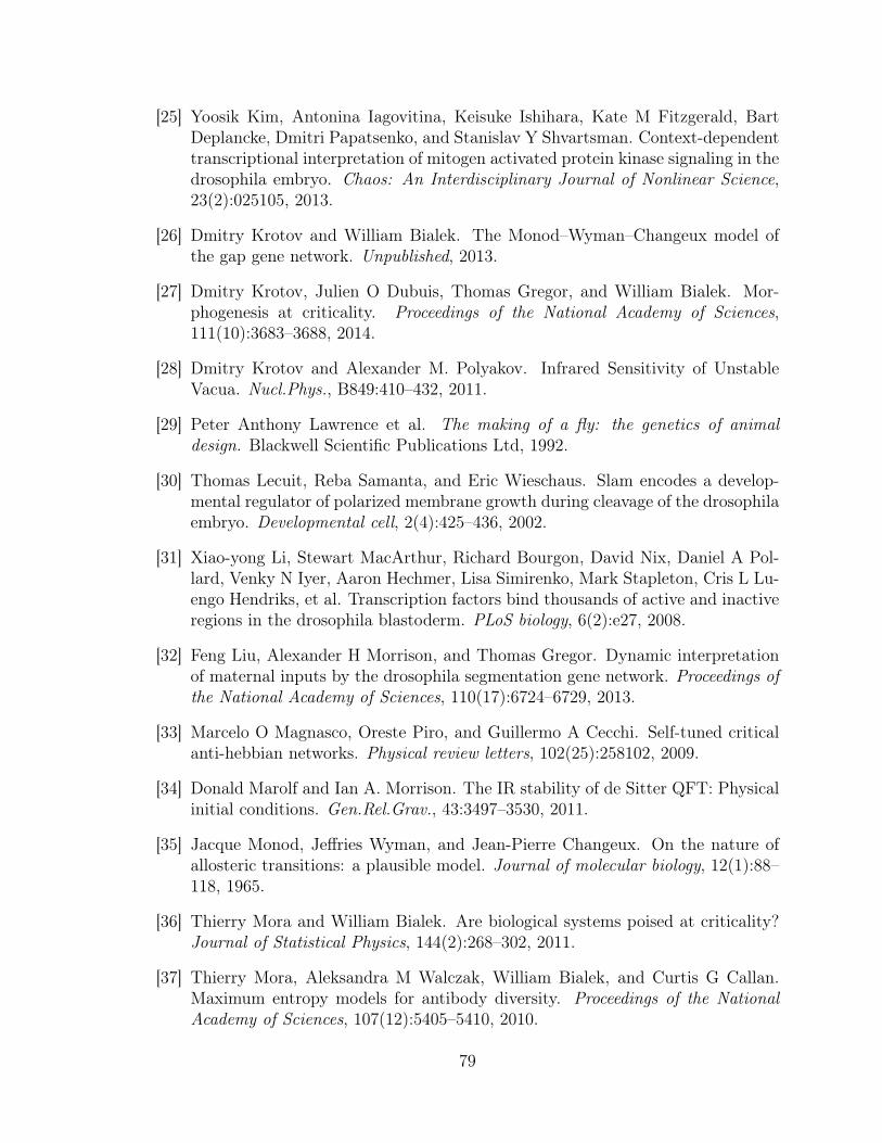
[25] Yoosik Kim, Antonina Iagovitina, Keisuke Ishihara, Kate M Fitzgerald, BartDeplancke, Dmitri Papatsenko, and Stanislav Y Shvartsman. Context-dependenttranscriptional interpretation of mitogen activated protein kinase signaling in thedrosophila embryo. Chaos: An Interdisciplinary Journal of Nonlinear Science,23(2):025105, 2013.

[26] Dmitry Krotov and William Bialek. The Monod–Wyman–Changeux model ofthe gap gene network. Unpublished, 2013.

[27] Dmitry Krotov, Julien O Dubuis, Thomas Gregor, and William Bialek. Mor-phogenesis at criticality. Proceedings of the National Academy of Sciences,111(10):3683–3688, 2014.

[28] Dmitry Krotov and Alexander M. Polyakov. Infrared Sensitivity of UnstableVacua. Nucl.Phys., B849:410–432, 2011.

[29] Peter Anthony Lawrence et al. The making of a fly: the genetics of animaldesign. Blackwell Scientific Publications Ltd, 1992.

[30] Thomas Lecuit, Reba Samanta, and Eric Wieschaus. Slam encodes a develop-mental regulator of polarized membrane growth during cleavage of the drosophilaembryo. Developmental cell, 2(4):425–436, 2002.

[31] Xiao-yong Li, Stewart MacArthur, Richard Bourgon, David Nix, Daniel A Pol-lard, Venky N Iyer, Aaron Hechmer, Lisa Simirenko, Mark Stapleton, Cris L Lu-engo Hendriks, et al. Transcription factors bind thousands of active and inactiveregions in the drosophila blastoderm. PLoS biology, 6(2):e27, 2008.

[32] Feng Liu, Alexander H Morrison, and Thomas Gregor. Dynamic interpretationof maternal inputs by the drosophila segmentation gene network. Proceedings ofthe National Academy of Sciences, 110(17):6724–6729, 2013.

[33] Marcelo O Magnasco, Oreste Piro, and Guillermo A Cecchi. Self-tuned criticalanti-hebbian networks. Physical review letters, 102(25):258102, 2009.

[34] Donald Marolf and Ian A. Morrison. The IR stability of de Sitter QFT: Physicalinitial conditions. Gen.Rel.Grav., 43:3497–3530, 2011.

[35] Jacque Monod, Jeffries Wyman, and Jean-Pierre Changeux. On the nature ofallosteric transitions: a plausible model. Journal of molecular biology, 12(1):88–118, 1965.

[36] Thierry Mora and William Bialek. Are biological systems poised at criticality?Journal of Statistical Physics, 144(2):268–302, 2011.

[37] Thierry Mora, Aleksandra M Walczak, William Bialek, and Curtis G Callan.Maximum entropy models for antibody diversity. Proceedings of the NationalAcademy of Sciences, 107(12):5405–5410, 2010.

79

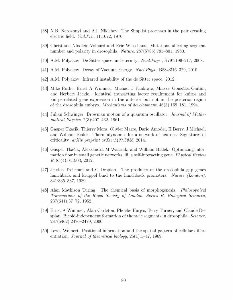
[38] N.B. Narozhnyi and A.I. Nikishov. The Simplist processes in the pair creatingelectric field. Yad.Fiz., 11:1072, 1970.

[39] Christiane Nusslein-Volhard and Eric Wieschaus. Mutations affecting segmentnumber and polarity in drosophila. Nature, 287(5785):795–801, 1980.

[40] A.M. Polyakov. De Sitter space and eternity. Nucl.Phys., B797:199–217, 2008.

[41] A.M. Polyakov. Decay of Vacuum Energy. Nucl.Phys., B834:316–329, 2010.

[42] A.M. Polyakov. Infrared instability of the de Sitter space. 2012.

[43] Mike Rothe, Ernst A Wimmer, Michael J Pankratz, Marcos Gonzalez-Gaitan,and Herbert Jackle. Identical transacting factor requirement for knirps andknirps-related gene expression in the anterior but not in the posterior regionof the drosophila embryo. Mechanisms of development, 46(3):169–181, 1994.

[44] Julian Schwinger. Brownian motion of a quantum oscillator. Journal of Mathe-matical Physics, 2(3):407–432, 1961.

[45] Gasper Tkacik, Thierry Mora, Olivier Marre, Dario Amodei, II Berry, J Michael,and William Bialek. Thermodynamics for a network of neurons: Signatures ofcriticality. arXiv preprint arXiv:1407.5946, 2014.

[46] Gasper Tkacik, Aleksandra M Walczak, and William Bialek. Optimizing infor-mation flow in small genetic networks. iii. a self-interacting gene. Physical ReviewE, 85(4):041903, 2012.

[47] Jessica Treisman and C Desplan. The products of the drosophila gap geneshunchback and kruppel bind to the hunchback promoters. Nature (London),341:335–337, 1989.

[48] Alan Mathison Turing. The chemical basis of morphogenesis. PhilosophicalTransactions of the Royal Society of London. Series B, Biological Sciences,237(641):37–72, 1952.

[49] Ernst A Wimmer, Alan Carleton, Phoebe Harjes, Terry Turner, and Claude De-splan. Bicoid-independent formation of thoracic segments in drosophila. Science,287(5462):2476–2479, 2000.

[50] Lewis Wolpert. Positional information and the spatial pattern of cellular differ-entiation. Journal of theoretical biology, 25(1):1–47, 1969.

80