Embed Size (px)
Citation preview

MAGISTERARBEIT
Titel der Magisterarbeit
Strong Conservation Form
and Grid Generation
in Nonsteady Curvilinear Coordinates
Numerical Methodsfor Implicit Radiation Hydrodynamics in 2D and 3D
angestrebter akademischer Grad:
Magister der Naturwissenschaften (Mag.rer.nat.)
Verfasser: Harald Holler, Bakk.rer.nat.
Matrikelnummer: 0104177
Studienrichtung: Astronomie A 066 861
Betreut von: Ao.Univ.-Prof.Dr. Ernst Dorfi
Wien, 25. Marz 2010


Danksagung
Allen Menschen, Tieren und Behorden, die mich im Laufe des Studiumsunterstutzt haben, mochte ich herzlich danken und vielen davon ein Bussigeben.
Ich verneige mich vor meinem Betreuer Prof. Ernst Dorfi fur die geduldigenund wegweisenden Diskussionen, seine fordernde Hartnackigkeit und dievielen motivierenden Anekdoten aus der Welt der Wissenschaft.
Diese Arbeit ist Kollegen Nonius Skala gewidmet.

Erklarung
Ich erklare ehrenwortlich, dass ich die vorliegende Arbeit selbstandig und ohne fremdeHilfe verfasst, andere als die angegebenen Quellen nicht benutzt und die den benutztenQuellen wortlich oder inhaltlich entnommenen Stellen als solche kenntlich gemacht habe.
Wien, am 25. Marz 2010

Contents
1 Fundamental Mathematics of RHD 9
1.1 The Hyperbolic Part . . . . . . . . . . . . . . . . . . . . . . . . . . . . . . 91.1.1 Hyperbolic Conservation Laws . . . . . . . . . . . . . . . . . . . . 91.1.2 Weak Solutions . . . . . . . . . . . . . . . . . . . . . . . . . . . . . 111.1.3 Rankine-Hugoniot and Entropy Conditions . . . . . . . . . . . . . 12
1.2 The Elliptic Part . . . . . . . . . . . . . . . . . . . . . . . . . . . . . . . . 141.2.1 The Poisson Equation . . . . . . . . . . . . . . . . . . . . . . . . . 151.2.2 Harmonic Functions and the Maximum Principle . . . . . . . . . . 16
2 Fundamental Physics of RHD 17
2.1 Hydrodynamics . . . . . . . . . . . . . . . . . . . . . . . . . . . . . . . . . 172.1.1 Continuity Equation . . . . . . . . . . . . . . . . . . . . . . . . . . 182.1.2 Equation of Motion . . . . . . . . . . . . . . . . . . . . . . . . . . 182.1.3 Energy Equation . . . . . . . . . . . . . . . . . . . . . . . . . . . . 19
2.2 Radiation . . . . . . . . . . . . . . . . . . . . . . . . . . . . . . . . . . . . 202.2.1 The Radiation Field and its Momenta . . . . . . . . . . . . . . . . 202.2.2 Interaction with Matter . . . . . . . . . . . . . . . . . . . . . . . . 212.2.3 Radiation Closure Relation . . . . . . . . . . . . . . . . . . . . . . 232.2.4 Fluid Frame . . . . . . . . . . . . . . . . . . . . . . . . . . . . . . . 25
2.3 Gravitation . . . . . . . . . . . . . . . . . . . . . . . . . . . . . . . . . . . 272.3.1 Self-Gravitation in 2D and 3D . . . . . . . . . . . . . . . . . . . . 272.3.2 Non-Static Gravitation Equation . . . . . . . . . . . . . . . . . . . 28
2.4 Full Set of RHD Equations with Self-Gravitation . . . . . . . . . . . . . . 30
3 Conservative Numerics 31
3.1 Numerical Methods for Conservation Laws . . . . . . . . . . . . . . . . . . 313.1.1 Introduction to Discretization Methods . . . . . . . . . . . . . . . 313.1.2 Error and Stability in the Linear Case . . . . . . . . . . . . . . . . 323.1.3 Conservative Methods and Lax Wendroff Theorem . . . . . . . . . 343.1.4 Artificial Viscosity . . . . . . . . . . . . . . . . . . . . . . . . . . . 373.1.5 Flux Limiters . . . . . . . . . . . . . . . . . . . . . . . . . . . . . . 38
3.2 Conservative Methods in General Curvilinear Coordinates . . . . . . . . . 393.2.1 Tensor Calculus and Elementary Differential Geometry . . . . . . 40
5

Contents
3.2.2 Strong Conservation Form . . . . . . . . . . . . . . . . . . . . . . . 433.2.3 Adaptive Grids . . . . . . . . . . . . . . . . . . . . . . . . . . . . . 473.2.4 Artificial Viscosity . . . . . . . . . . . . . . . . . . . . . . . . . . . 48
3.3 Strong Conservation Form of RHD in Spherical and Polar Coordinates . . 493.3.1 Continuity Equation . . . . . . . . . . . . . . . . . . . . . . . . . . 503.3.2 Equation of Motion . . . . . . . . . . . . . . . . . . . . . . . . . . 513.3.3 Equation of Internal Energy . . . . . . . . . . . . . . . . . . . . . . 573.3.4 Equation of Radiation Energy . . . . . . . . . . . . . . . . . . . . . 583.3.5 Radiative Flux Equation . . . . . . . . . . . . . . . . . . . . . . . . 59
4 Orthogonal and Nonorthogonal Adaptive Grids 63
4.1 Basic Principles of Grid Generation . . . . . . . . . . . . . . . . . . . . . . 634.2 The Grid We Are Looking For . . . . . . . . . . . . . . . . . . . . . . . . 644.3 Remarks on Grid Generation Methods . . . . . . . . . . . . . . . . . . . . 65
4.3.1 Differential Methods . . . . . . . . . . . . . . . . . . . . . . . . . . 664.3.2 Laplace Systems . . . . . . . . . . . . . . . . . . . . . . . . . . . . 664.3.3 Conformal Mapping . . . . . . . . . . . . . . . . . . . . . . . . . . 674.3.4 Algebraic Methods . . . . . . . . . . . . . . . . . . . . . . . . . . . 684.3.5 Equidistribution . . . . . . . . . . . . . . . . . . . . . . . . . . . . 68
4.4 Equidistribution and Interpolation Attempt . . . . . . . . . . . . . . . . . 694.4.1 Toy Model . . . . . . . . . . . . . . . . . . . . . . . . . . . . . . . 694.4.2 Analysis . . . . . . . . . . . . . . . . . . . . . . . . . . . . . . . . . 71
4.5 On the Peculiarity of Orthogonal Coordinates . . . . . . . . . . . . . . . . 724.6 Quasi-Polar Coordinates Attempt . . . . . . . . . . . . . . . . . . . . . . . 73
4.6.1 Toy Model . . . . . . . . . . . . . . . . . . . . . . . . . . . . . . . 734.6.2 Analysis . . . . . . . . . . . . . . . . . . . . . . . . . . . . . . . . . 74
4.7 Strong Conservation Form in Nonorthogonal Coordinates . . . . . . . . . 75
5 Conclusions and Prospective 77
6 Appendix 79
6.1 Arguments and Details . . . . . . . . . . . . . . . . . . . . . . . . . . . . . 796.1.1 Symmetry of the Stress Tensor . . . . . . . . . . . . . . . . . . . . 796.1.2 Rankine-Hugoniot Conditions . . . . . . . . . . . . . . . . . . . . . 796.1.3 Diffusion Approximation . . . . . . . . . . . . . . . . . . . . . . . . 816.1.4 Strong Conservation Form on Adaptive Grids . . . . . . . . . . . . 81
6.2 Mathematica Files . . . . . . . . . . . . . . . . . . . . . . . . . . . . . . . 84
6

Prologue
Motivation
In astrophysics a multitude of systems and configurations are described with conceptsfrom hydrodynamics coupled with gravitation, radiation and magnetism. Mathemati-cally radiation hydrodynamics (RHD) and magnetohydrodynamics (MHD) are systemsof coupled nonlinear partial differential equations. Multiple fields in astrophysics havebeen adopting and developing sophisticated numerical methods for solving these PDEsin various applications.
Explicit numerical schemes in computational fluid dynamics have been popular formany years and received substantial boosts due to advances in technology and paral-lelizing techniques. Riemann solvers and related methods are extensively adapted in 2Dand 3D computations however they have one main disadvantage. An inherent limitationfor time steps in explicit schemes impedes applications where various time scales are ofinterest. Hence a majority of these calculations emphasize on small temporal and spatialscales but fail to treat phenomenons properly on very diverse scales.
Techniques for implicit numerics are computationally more expensive since they arehardly parallelizable but do not limit the increments of the scheme intrinsically. ImplicitRHD in 1D has proven favorable for describing astrophysical processes on large spatialand temporal scales like nonlinear pulsation or long term development of supernovae.The idea of this thesis was to study suitable generalizations of these concepts to 2Dand 3D. Additional degrees of freedom in multi-dimensional implicit RHD would dis-close the treatment of large scale convection and how it interacts with rotation, mixing,the coupling of rotation and pulsation, transport of angular momentum and mass loss,interactions of discs and stars during star formation processes etc. The target of thisthesis was to find the strong conservation form of the equations of radiation hydrody-namics in non-steady curvilinear coordinates and to study multi-dimensional adaptivegrid generation.
7

Synopsis
The Euler equations of hydrodynamics, the Maxwell equations as well as radiative trans-port equations are hyperbolic PDEs that connect certain densities and fluxes via con-servation laws. Generally they emerge from natural symmetries that constitute majorprinciples in mathematical physics. The numerical implementation of these equationsessentially needs to comprise these qualities. Applied mathematics have developed anarticulate framework of numerical methods for conservation laws that ensure the con-servation of mass, momentum, energy etc. if applied properly. The main challenge isto compute the fluxes correctly which indeed will be the issue of the first three chap-ters in this paper. Self gravitation is described via the Poisson equation that poses anextra challenge due to its elliptic nature. While 1D computations avoid solving thispure boundary value problem by considering an integrated form we will have to designa different approach to self gravitation in 2D and 3D.
A generalization of implicit conservative numerics to multiple dimensions requires ad-vanced concepts of tensor analysis and differential geometry and hence a more thoroughdedication to mathematical fundamentals than maybe expected at first glance. Hencewe begin to discuss fundamental mathematics and physics of RHD with special focus ondifferential geometric consistency and study numerical methods for nonlinear conserva-tion laws to gain a solid definition of the term conservative. The efforts in tensor analysiswill be needed when applying Vinokurs theorem to gain the strong conservation formfor conservation laws in general curvilinear coordinates. Moreover, it will be required toslightly reformulate the artificial viscosity for such nonlinear coordinates.
Astronomical objects are characterized by fast flows and high propagation speeds onthe one hand but astronomical length and time scales on the other hand. Implicit nu-merical schemes are not affected by the Courant Friedrichs Levy condition which limitsexplicit schemes to rather impracticably small time steps. Implicit methods however pro-duce algebraic problems that require matrix inversion which is computationally expen-sive. In order to achieve viable resolution, adaptive grid techniques have been developed.It is desired to treat processes on small length scales like shocks and ionization fronts aswell as physics at the extent of the objects dimension itself like large scale convectionflows and pulsations. The combination of implicit schemes and adaptive grids allows toresolve astrophysics appropriately at various scales.
In the last chapter of this paper we study problem oriented adaptive grid generationin 2D and 3D. We establish three main postulations for an ideal grid and analyze severalfeasible approaches.
8

1 Fundamental Mathematics of RHD
The equations of radiation hydrodynamics (RHD) are a system of nonlinear secondorder partial differential equations with hyperbolic and elliptic parts. Generally theyare posed as an initial value problem with boundary conditions. The simultaneoussolution of hyperbolic terms, as coming from the dynamics and the strictly ellipticalPoisson equation constitute one major problem for finding suitable solution methods.In the following chapter we will retrieve the fundamental mathematics of hyperbolicconservation laws as they appear in hydrodynamics and radiation transfer as well assome basic concepts for elliptic partial differential equations like the Poisson equation inorder to motivate certain numerical concepts that will arise in chapter 3. As we will see,accurate analysis provides expedient approaches to our numerical problem.
1.1 The Hyperbolic Part
Dynamical physical processes are mathematically described via hyperbolic partial dif-ferential equations1. The wave equation, the Burgers’ equation, the equations of hy-drodynamics and the Dirac equation are prominent examples of hyperbolic evolutionequations. They always characterize systems with finite propagation speeds, a qualityoften referred to as causality. Information from a point in space and time is causallyassociated solely with a finite region, a domain of dependence. In chapter 3 we will resortto this important issue when we discuss stability and convergence of numerical methods.
In the following section we want to define some fundamental mathematical terms andpresent important concepts that will accompany the entire paper.
1.1.1 Hyperbolic Conservation Laws
The Euler equations of hydrodynamics as well as the angular moment equations ofradiative transfer can be derived from conservation laws originating from one of themost fundamental theorems of mathematical physics, the Noether Theorem (see e.g.Bhutani (1981) [4], Kambe (2007) [21]). In hydrodynamics, the conservation of mass,momentum and energy leads to the continuity equation, the equation of motion andthe energy equation. Analog correspondences are derived for radiation. Mathematically
1The Schrodinger equation of quantum mechanics is excepted.
9

1 Fundamental Mathematics of RHD
the equations of radiation hydrodynamics form a system of hyperbolic conservation lawsthat describe the interaction of a density function d
d : Rn × [0,∞)→ Rm
and its flux ff : U → Rm, U ⊆ Rm, U open.
The temporal and spatial change of the integrated density in a connected space Ω ∈ Rn
then equals the flux over the boundary ∂Ω, where S is the outward oriented surfaceelement.
∂t
∫Ω
d dV +∫∂Ω
f · dS = 0 ∀ t > 0 (1.1)
Hyperbolicity is granted if the Jacobian matrix associated with the fluxes ∇df has realeigenvalues and there exists a complete set of eigenvectors. Provided it is physically jus-tified, demanding this quality on a set of equations even can help to formulate constraintsto the solutions (see subsection 2.2.3).
For the in section 2.1 further motivated physical problem of hydrodynamics this systemgains the following form as an example2.
d(x, t) =
ρ(x, t)(ρu)(x, t)(
ρε)(x, t)
, f(d) =
ρuuρu + Pρεu + P · u
(1.2)
∂t
∫Ω
ρ dV +∫∂Ω
ρu · dS = 0
∂t
∫Ω
uρ dV +∫∂Ω
(uρu + P
)· dS = 0
∂t
∫Ω
ρε dV +∫∂Ω
(ρεu + P · u
)· dS = 0 (1.3)
Let f be a continuously differentiable function, then we can rewrite equation (1.1) viathe divergence theorem as follows.∫
t
∫Ω
(∂td + div f(d)
)dV dt = 0 ∀ t > 0,Ω ⊂ Rn (1.4)
2Notation: Summations respectively projections of tensorial quantities are always denoted by · or :whereas tensor products ⊗ are omitted, i.e. uu = u⊗ u.
10

1.1 The Hyperbolic Part
Locally the system of partial differential equations
∂td + div f(d) = 0 (1.5)
gives pointwise solutions for our vector field d that describes the conserved densities orstate variables of mass, momentum and energy. With initial condition (or the initialstate of the density function) d0
d(x, 0) = d0(x) ∀x ∈ Rn (1.6)
Equation (1.5) with initial condition (1.6) is called Cauchy problem. The main theoremfor this class of partial differential equations associated with analytic initial conditionsis the theorem of Cauchy-Kovalevskaja which states local existence and uniqueness alsofor nonlinear Cauchy problems. However, with analyticity demanded this theorem hashardly any practical relevance. Questions of local and global well-posedness for generalnonlinear Cauchy problems require sophisticated concepts of functional analysis (see e.g.Adams [1], Evans [14]). We want to mention some basic concepts of these variationalformulations of partial differential equations in an extent that they arise in the contextof radiation hydrodynamics and accordingly numerics.
1.1.2 Weak Solutions
Since even the simplest examples of one-dimensional scalar conservation laws like theBurgers’ equation have classical solutions only in some special cases, one has to broadenthe considered function space of possible solutions (the adequate function spaces areSobolev spaces, see Evans [14]). For so called weak solutions, we appeal to generalizedfunctions where also discontinuities can be dealt with. The generalized concept of differ-entiation of distributions shifts operations to test functions γ(x, t). These test functionsγ : G ∈ Rn × R+ → R have compact support, meaning that there exists a compactsubset (here i.e. closed and bounded) K such that γ(x, t) = 0 ∀x ∈ G \K(γ).∫
t≥0
∫Rn
(∂td + div f(u)
)γ dV dt = 0 ∀ γ ∈ G (1.7)
11

1 Fundamental Mathematics of RHD
To simplify matters, we let these test functions be continuously differentiable. Thenwith partial integration and our postulations for γ
∫t≥0
∂td γ dt = γ d∣∣∣∞0−∞∫0
d ∂tγ dt
= γ(x, 0) d0(x)−∞∫0
d ∂tγ dt∫Rn
div f(d) γ dV = γ f∣∣∣...
∣∣∣∞−∞︸ ︷︷ ︸
=0
−∫
Rnf grad γ dV (1.8)
we derive the weak formulation of our conservation law (1.4).∫t≥0
∫Rn
(d ∂tγ + f(d) grad γ
)dV dt = −
∫Rn
γ(x, 0) d0(x) dV (1.9)
The function d ∈ L∞ is called weak solution of the Cauchy problem (1.4), if it satisfies(1.9) and d ∈ U with d0 ∈ L∞. This weak solution is not necessarily unique andnormally further constraints have to be imposed.
1.1.3 Rankine-Hugoniot and Entropy Conditions
For the most physical problems it will be sufficient to look for weak solutions in thefunction space of piecewise continuously differentiable functions. The physical variablesd are weak solutions, if they are a classical solutions wherever they are C1 and at discon-tinuities (shocks) they need to satisfy additional conditions. As we will see in chapter 2,these conditions posses direct physical relevance when applied to a physical system likeradiation hydrodynamics. The full derivation of the one-dimensional Riemann-problemfor (1.4) considered can be found in the Appendix 6.1.2.
We conclude,
∞∫0
∞∫−∞
(d ∂tγ + f(d) ∂xγ) dxdt = −∞∫−∞
γ(x, 0) d0(x) dx+
+∞∫0
γ(x, x/us)(f(dl)− f(dr)
us−(dl − dr
))dx (1.10)
is weak solution of the Riemann-problem, if
f(dl)− f(dr)us
−(dl − dr
)= 0 (1.11)
12

1.1 The Hyperbolic Part
respectively
us = f(dl)− f(dr)dl − dr
. (1.12)
We call us shock velocity and (1.12) Rankine-Hugoniot condition.
As already mentioned, weak solutions of the Cauchy problem are not necessarily uniqueand thus may be physically pointless. However, there is a way to pick physically valuablesolutions out of multiple. One method is to implement an artificial viscosity term
∂td∗ + div f(d∗) = εν∆d∗, ε > 0 (1.13)
and evaluate the equation for ε → 0 as limit case of the original one. The idea ismotivated from physical diffusion, which broadens sincere discontinuities to differentiablesteep gradients. The physical solution of the weakly formulated problem has to be thezero diffusion limit of the diffusive problem. However, in analytical practice this limitis rather bulky to calculate, hence simpler conditions have to be found. The commontechnique to do this is motivated from continuum physics as well, where an additionalconservation law holds for the entropy of the fluid flow as long as the solutions remainsmooth. Moreover, it is known, that along admissible shocks this physical variable neverdecreases, so the conservation law for the entropy can be reformulated as inequality.
We regard a scalar entropy function σ(d) and an entropy flux φ(d) which satisfy
∂tσ(d) + divφ(d) = 0. (1.14)
Assuming differentiable functions, we rewrite that conservation law via the chain ruleand compare it to (1.5) multiplied with ∇dσ to obtain
∇dσ ∂td +∇dφ∇xd = 0∇dσ ∂td +∇dσ∇df ∇xd = 0
∇dσ div f = divφ (1.15)
where in the more dimensional case the appearing matrices of gradients have to fulfillsome further constraints (see e.g. Godlewski and Raviart (1992) [16]). For scalar equa-tions, it is always possible to find an entropy function of that kind. Furthermore wepostulate convexity for the entropy function.3
∇2dσ > 0, ∀d (1.16)
3In physical entropy one would require an eventual inequality with ≥ in place of ≤ but mathematicalliterature commonly chooses σ′′ > 0.
13

1 Fundamental Mathematics of RHD
To get our actual entropy condition, we rewrite (1.14) in the viscous form
∂tσ(d∗) + divφ(d∗) = εν∇dσ(d∗)∆d∗ (1.17)
and integrate over an arbitrary time interval [t0, t1].
t1∫t0
∫Ω
(∂tσ(d∗) + divφ(d∗)
)dV dt = εν
t1∫t0
∫Ω
∇dσ(d∗)∆d∗ dV dt =
= εν
t1∫t0
∫∂Ω
(∇xd∗∇dσ(d∗)
)· dSdt− εν
t1∫t0
∫Ω
∇x,id∗ ∇2σ(d∗)︸ ︷︷ ︸>0
∇x,id∗ dV dt
(1.18)
When we now consider our non diffusive limit for ε→ 0, the first term on the right handside vanishes without further restriction whereas the second term has to remain nonpositive. With partial integration and divergence theorem we get our entropy condition(1.19).
t1∫t0
∫Ω
(∂tσ(d) + divφ(d)
)dV dt ≤ 0
∫Ω
σ(d(x, t1)) dV ≤∫Ω
σ(d(x, t0)) dV −t1∫t0
∫∂Ω
φ(d) dSdt
(1.19)
For bounded, continuous pointwise solutions d∗ with d∗ → d for ε → 0, the vanishingviscosity solution d is weak solution of the initial value problem (1.4) and fulfills entropycondition (1.19). Generally spoken, applying the entropy condition systems with shocksolutions unveils those propagation velocities that ensure that no characteristics rise fromdiscontinuities which would be non-physical. For details and proofs we refer to LeVeque[26].
In chapter 3 we will discuss these analytic concepts in numerical context and work outits concrete applications for (radiation) hydrodynamics.
1.2 The Elliptic Part
As already elaborated radiation hydrodynamics are partial differential equations of thehyperbolic type. However, the dynamics are only one part of the challenge emerging inastrophysical applications. Self gravitation in classical astronomical objects is described
14

1.2 The Elliptic Part
via the Poisson equation, an elliptical partial differential equation which emerges aspure boundary value problem for the gravitational potential. Unlike hyperbolic PDEselliptical problems mostly describe equilibrium physics and their solutions are typicallyquite smooth as we will see.
1.2.1 The Poisson Equation
The Poisson equation describes the spatial distribution of a scalar field Φ
Φ : U ⊆ Rn → R (1.20)
induced by a source ρρ : U ⊆ Rn → R (1.21)
and has the following form; the choice of the minus sign originates from the customarydefinition for ellipticity of differential operators.
−∆Φ = ρ. (1.22)
When it comes to our physical application of self-gravitation, we will pull the sign intothe definition of the gravitational potential and consider ∆Φgrav = 4πGρm.
The Poisson equation is posed with Dirichlet or Neumann boundary conditions whichmeans either boundary values or their derivatives are given. Often it is useful to imposemixed boundary conditions, where the boundary of the region ∂Ω is separated in a partwith Dirichlet conditions ∂ΩDir and a part with Neumann boundary conditions ∂ΩNeu
and ∂Ω = ∂ΩDir ∪ ∂ΩNeu.
Φ = ψDir in ∂ΩDir
n · ∇Φ = ψNeu in ∂ΩNeu (1.23)
The Poisson equation can be understood as the inhomogeneous generalization of theLaplace equation ∆Φ = 0. Physically, latter equation describes a solenoidal, irrotationalvector field u = ∇Φ with div u = rot u = 0. This circumstance implies that Φ mustbe invariant under rotation and can be used to derive the fundamental solution. WithGreen’s function and convolution of the inhomogeneous term ρ we derive the analyticalsolution of the Laplace equation4. In the light of these presumptions, we can investigatefundamental attributes of solutions of the Laplace equation in order to learn somethingabout the solutions of the Poisson equation.
4Φ(x) = Φ(r), ∂ir = xi
r. . . → Green’s functions of the fundamental solution of the Laplace equation
in 3D is ∆(3) (− 14πr
)= δ(3)(x) and Φ =
∫G(x,x′)ρ(x′) dV is solution of ∆Φ = ρ.
15

1 Fundamental Mathematics of RHD
1.2.2 Harmonic Functions and the Maximum Principle
One important aspect of the Laplace operator as it emerges in Poisson and Laplaceequation is the fact that it acts regularizing; the according theorem follows. Hence itwill be adequate to deal with differentiable functions when we look for solutions of (1.22).Any function satisfying ∆Φ = 0 in U and C2 is called harmonic function.
Given Φ is harmonic, we can derive a mean-value formula which states that on aspherical subset5 B(x, r) ⊂ U , a solution Φ(x) equals both the average of Φ over thesphere ∂B and the average of Φ on the entire ball B.
Φ(x) =Γ(n2 + 1)nπn/2rn−1
∫∂B(x,r)
Φ dS =Γ(n2 + 1)πn/2rn
∫B(x,r)
Φ dV (1.24)
In 3 dimensions this simply yields Φ(x) = 14πr2
∫Φ dS = 3
4πr3∫
Φ dV with correspond-ing integration ranges. In the light of these conclusions, we deduce some interestingproperties of harmonic functions.
The (strong) maximum principle states for a Φ ∈ C2(U) ∩ C(U) harmonic within U ,
i.) maxU Φ = max∂U Φ.
ii.) Furthermore, if U is connected and ∃x0 ∈ U such that u(x0) = maxU Φ, it followsthat Φ is constant within all U .
Assertion i.) implies that the maximum will be found at the boundary of the domain andii.) states that if a maximum is on the inside of the boundary the function Φ consequentlyis constant within U . Another important conclusion of this theorem concerns the Poissonequation. It can be shown that for the boundary value problem
−∆Φ = ρ inU
Φ = g in ∂U (1.25)
there exists at most one solution Φ ∈ C2(U) ∩ C(U). With this uniqueness theorem wegain at least some comfort for the gravitational part of our numerical problem. As afurther side note we mention the regularity theorem. It reveals that if Φ ∈ C2 is harmonicthen it automatically is infinitely differentiable, i.e. Φ ∈ C∞.
Without dwelling on the Laplace equation any further, we recapitulate that math-ematical analysis of the elliptical part of our system of equations brings forward lesssophisticated problems than the hyperbolic part. Obviously, uniqueness and regularityare soothing qualities when it comes to solving partial differential equations. All the-orems and proofs of this section can be found in Lawrence C. Evans (1998), p.17 ff.[14].
5Closed n-dimensional ball B(x, r) with center x, radius r > 0.
16

2 Fundamental Physics of RHD
Astronomical objects are basically self-gravitating aggregations of (gaseous) materialwith magnetic fields and radiation. Radiation hydrodynamics as we will discuss them,factor out magnetic effects and solely consider radiative contributions through photons.
The fundamental equations of hydrodynamics describe the motion of fluids in in termsof continuous quantities. The dynamics and kinetics of fluid particles are described bymacroscopic functions like the mass density ρ, its velocity u, internal energy and gaseouspressure as primary variables mostly. In this model, infinitesimal volume elements of thefluid are still big enough that intermolecular forces can be neglected, meaning that theycontain a sufficient number of molecules. The thermodynamic variables intrinsicallyare assumed to be well defined (equilibrium thermodynamics) and characterized by anequation of state.
The radiative transfer equation describes energy transfer in form of electromagneticradiation, affected by absorption, emission and scattering. The fundamental quantityto describe the radiative field is the spectral intensity Iγ , which can be understood asmacroscopic quantity to describe the photonic energy flow. The mass density ρ is alsosource for the gravitational potential Φ. In the following sections we will physicallymotivate the set of equations of radiation hydrodynamics with gravitation bit by bit.
One major intention in the upcoming paragraphs will be rigorous and consistent (interms of differential geometry) definitions of the physical variables which will be crucialfor the numerical methods in general cuvilinear coordinates investigated in section 3.2.
2.1 Hydrodynamics
As anticipated, the equations of hydrodynamics can be derived from conservation lawsof mass, momentum and energy. Since the fundamentals of hydrodynamics are morethan well documented (e.g. in Landau, Lifschitz [23]) we confine our portrayal to a briefsynopsis and concentrate on a few interesting details.
17
2 Fundamental Physics of RHD
2.1.1 Continuity Equation
The conservation of mass is physically justified as long as no mass is generated or anni-hilated
dm
dt= d
dt
∫V (t)
ρ dV = 0 (2.1)
and leads to the continuity equation.∫V (t)
(∂tρ+ div
(ρu))dV = 0
∫V (t)
∂tρ+∫
∂V (t)
(ρu)· dS = 0 (2.2)
Clearly the domain Ω of the conservation law, introduced in section 1.1 is an n-dimensionalVolume that is a bounded subset of the Rn, n = 1, 2, 3. The mass density ρ is a non neg-ative scalar field ρ(x, t) : Rn+1 → R+ and the velocity u a vector field u(x, t) : Rn+1 →Rn+1. Solutions of these primary variables ρ,u, that is densities of the conservationlaws, will emerge as piecewise continuous functions.
As a side note the flow is called stationary if ∂tρ = 0 and incompressible if divu = 0.However, in astrophysical applications these special cases will fail to describe the physicsappropriately.
2.1.2 Equation of Motion
In order to yield the equation of motion from the conservation of momentum it is re-quired to specify which forces act upon the fluid. Now we are concerned with a non-scalarconservation law and as we will see in chapter 3, in this case we will have to avail our-selves of general tensorial notation. Thus, at this point we introduce one main tensorialquantity (and secondary physical variable), the non-relativistic viscous stress tensor.
T = ρuu + P− σT ij = ρuiuj + P ij − σij (2.3)
T(x, t) : Rn+1 × Rn+1 → Rn+1 × Rn+1. This symmetric1 tensor (T ij = T ji) describescontributions from momentum ρui in j-direction, generally anisotropic pressure P ij andfriction σij forces. Diagonal elements express pressure and off-diagonal elements shear
1T is symmetric, if conservation of angular momentum ρx×u is invoked, see derivation in the Appendix6.1.1.
18

2.1 Hydrodynamics
stresses. The equation of motion in then yields2
∫V (t)
(∂t(ρu)+ div T
)dV = 0
∫V (t)
∂t(ρu)dV +
∫∂V (t)
(ρuu + P− σ
)· dS = 0. (2.4)
Special cases for the energy-stress tensor in fluid dynamics are e.g. the dust model whereno particle interaction is assumed P = σ = 0. Anyway, in numerous physical applicationsthe pressure forces can be expected to be isotropic. If so, the pressure tensor simplifiesto a diagonal tensor which consists of the scalar gaseous pressure p and a measure of
uniformity, the the metric tensor g, which yields P = pg. The divergence of that tensorcan be further simplified to the well known gradient of the gaseous pressure. We willextensively occupy ourselves with the viscous pressure tensor σ in succession, especiallyin section 3.2.4. At this point it shall only be mentioned that we neglect physical viscositysince the gas of a star is easily approximated as ideal fluid. As indicated in section 1.1.3,we will impose artificial dynamic viscosity when we concern ourselves with mathematicalmethods for solving nonlinear conservation laws.
Implicitly we already have defined a thermodynamic equation of state which describesthe state of the fluid in terms of pressure p, volume V and temperature T by imposingan ideal fluid. Since stars are largely composed of hot, low-pressure hydrogen gas, it isquite reasonable to apply this model.
2.1.3 Energy Equation
The energy balance of a fluid includes kinetic and pressure parts as well as inner energy.Latter is once more a thermodynamic quantity which is associated with the equationof state. We define a new non-negative scalar field, the specific inner energy ε(x, t) :Rn+1 → R+ which in case of an ideal fluid equals its thermic energy. The conservationof the total energy of a bounded fluid element in this strictly hydrodynamic case yields3
∫V (t)
(∂t(12ρu2 + ρε
)+ div
(T · u + ρεu
))dV = 0
∫V (t)
∂t(12ρu2 + ρε
)dV +
∫∂V (t)
((12ρu2 + ρε
)u +
(P− σ
)· u)· dS = 0.
(2.5)2In general relativity the conservation of momentum can be found in its most elegant form ∇ ·T = 0.
In this case all variables are defined in a four-dimensional spacetime, where the 0-component of thecovariant nabla operator contains the temporal derivative.
3Using ∇( 12 u2) = u∇ · u.
19

2 Fundamental Physics of RHD
This total energy equation can be dissected into a mechanical and an internal part, whereformer describes the change of kinetic energy of a fluid as the rate of work done on anelement by pressure and stress forces. The gas energy part can be formulated as entropyconservation (∂t(ρs) + div (ρsu) = 0) and hence implies, that the flow is adiabatic.
2.2 Radiation
The fundamentals of radiative transfer and its moments can be found in several appro-priate text books (see e.g. Mihalas and Mihalas [32]), therefore we will concentrate onsome noteworthy highlights in this section as well. In the previous paragraph we treatedthe physics of fluids which we now want to extend to radiating fluids in a nutshell.
Radiation contributes to the total energy, momentum, stress and pressure in the fluid.In succession we will work out means of coupling among these physical quantities in thematerial. When we concerned ourselves with the fundamental mathematics of conser-vation laws, we denoted that also the fundamental dynamics of radiation will appearas hyperbolic conservation laws. In fact, the crucial equation to describe radiation isthe radiation transfer equation (RTE), which basically expresses conservation of energy.However, we shall begin to define the fundamental dynamical properties of the radiationfield.
2.2.1 The Radiation Field and its Momenta
The macroscopic quantities of the radiation field are based on statistical physics of amicroscopic description of ultra-relativistic massless particles, i.e. photons. To establishthe nexus to the continuum view which we will pursuit, we define the scalar non-negativephoton distribution function fγ(x, t; n, ν) : R3+1×R3×R→ R+ which can be interpretedas photon density in the corresponding phase space4. The central physical quantity forthe upcoming description of the radiation field is the spectral intensity Iγ(x, t; n, ν)defined by
Iγ = h4ν3
c2fγ . (2.6)
That implicitly describes a radiative energy transport in the following sense
dEγ = Iγ dS · n dωdνdt. (2.7)
The spectral intensity Iγ at position (x, t), traveling in direction n with frequency ν isdefined to account for the energy Eγ transported by radiation of frequencies dν across a
4The momentum of a photon, traveling in direction n is given by pγ = hνc
n. ν is the frequency, c thespeed of light and h the Planck constant. fγ is invariant under Lorentz transformations. The subsetγ is chosen to discern mere radiation (here photonic) variables.
20

2.2 Radiation
surface element dS in time dt into a solid angle dω around n. Further useful propertiesare the angular moments of the radiation field, that is the mean intensity Jγ (zerothmoment), the radiation flux Fγ (first moment) and the evidently symmetric radiationpressure tensor Pγ (second moment). The velocity of our particles will simply be givenby the speed of light and their direction of motion u = cn, which also illustrates the linkto the procedure we carried out for deriving the equations of hydrodynamics.
Jγ(x, t; ν) = 14π
∫Iγ dω
Fγ(x, t; ν) =∫Iγn dω
Pγ(x, t; ν) = 1c
∫Iγnn dω (2.8)
Analogously to our fundamental equations of hydrodynamics, we can derive dynamicequations for the radiation field by considering the conservation of density Jγ and mo-
mentum Fγ . ∫V (t)
(∂tJγ + div
(cFγ
))dV = 0
∫V (t)
(∂tFγ + div
(c2Pγ
))dV = 0 (2.9)
From the viewpoint we pursued in section 1.1 discussing hyperbolic conservation laws wedefine a density function d(x, t; ν) = (Jγ ,Fγ) and a flux f(d) = c(Fγ , cPγ). Equations(2.9) can hence be interpreted as homogeneous outlook to the moments of the radiationtransfer equation with collision terms (2.12) in the forthcoming section.
2.2.2 Interaction with Matter
For the treatment of radiation hydrodynamics it will be necessary to describe the inter-action of the radiation field with the fluid. Again the macroscopic approach chosen hereto describe this interaction can be understood canonically with concepts from statisticalphysics and quantum mechanics. Moreover, it will be required to process the variablesof the radiation field into the fluid frame of the material correctly via Lorentz transfor-mation and account for the frequency change with respect to the lab frame that comeswith Doppler shift.
When radiation passes through material, energy generally will be removed dependedon a material property, the opacity or extinction coefficient χγ . On the other hand, thematerial releases radiation in terms of an emission coefficient ηγ which will be isotropicin its rest frame. Both properties are defined as non-negative scalar functions of posi-
21

2 Fundamental Physics of RHD
tion, time, radiation direction and frequency (χγ , ηγ)(x, t; n, ν) : R3+1 × R3 × R → R+.Both processes, extinction and emission, can be further divided in thermal and scatter-ing events. Thermal extinction and emission converts radiation energy to thermal andvice versa, whereas scattering in principle changes direction and frequency of travelingphotons. The amount of energy removed along a material element of length dl is
dEγ =(χthermγ + χscat
γ
)Iγ dSdldωdνdt (2.10)
and the amount of radiation energy released by emission is
dEγ =(ηthermγ + ηscat
γ
)dSdldωdνdt. (2.11)
The conservation of spectral intensity (2.9) considering emission and extinction yields∫V (t)
(1c∂tIγ + div
(Iγn
)− ηγ + χγIγ
)dV = 0 (2.12)
and is called radiation transfer equation in the laboratory frame. In practice of RHD,upper equation and its momenta have yet to be transformed into the fluid frame asmentioned and simplified in several ways.
Firstly the monochromatic quantities Iγ , χγ , . . . will solely be considered with theircollective effects by integrating them over all frequencies5.
Jγ(x, t) = c
4πEγ = 1
4π
∫Iγ dωdν
Fγ(x, t) = 4πHγ(x, t) =∫Iγn dωdν
Pγ(x, t) = 4πc
Kγ(x, t) = 1c
∫IγnnT dωdν (2.13)
Another commonly used simplification to determine the proportion of extinction andemissivity by a source function Sγ is to impose local thermal equilibrium (LTE) wherethe radiation field is characterized by one single variable, the temperature T (black bodyradiation). In this case, the specific intensity depends only on the gas temperature andis given by Planck’s law
Iγ,LTE(x, t; ν) = 2hν3
c21
e
hν
kT − 1
(2.14)
and the collective, frequency integrated form yields the source function Sγ(x, t) : R3+1 →
5Many authors use a notation, where the frequency ν is written as subset, instead of in the list ofarguments Iν(x, t; n) and the frequency integrated variables lack of that subset I, χ, . . . .
22

2.2 Radiation
R+
Sγ = 4πηγχγ,P
=∞∫0
Iγ,LTE dν = 8π5k4
15c3h3T4. (2.15)
With χγ,P we introduce a Planck mean opacity χγ,P respectively the Planck mean opacityper mass κγ,P
κγ,Pρ = χγ,P =
∞∫0χγIγ,LTE dν
∞∫0Iγ,LTE dν
(2.16)
and with χγ,R a Rosseland mean which will emerge in the radiation energy equation.
1κγ,Rρ
= χγ,R =
∞∫0
1χγ
∂Iγ,LTE
∂Tdν
∞∫0
∂Iγ,LTE
∂Tdν
(2.17)
At this point we have defined all necessary variables and motivated a list of simplificationsfor our system of radiation hydrodynamics equations. However, two important steps areto be provided yet. First, one has to deal with the problem that in particular equations(2.9) but respectively all n moment equations contain in each case n + 1 momenta ofthe radiation field which is known as closure problem. The last step to the full set ofequations of RHD will be the Lorentz transformation into the fluid frame.
2.2.3 Radiation Closure Relation
In section 1.1 it was mentioned, that imposing hyperbolicity on the conservation law canhelp to narrow possible solutions in some way. A conservation law is called hyperbolic ifthe Jacobian matrix associated with the fluxes ∇df has real eigenvalues and there existsa complete set of corresponding eigenvectors. As we have seen, interaction with matteradds source terms to our radiation conservation laws, we abbreviate them from now onwith S0
γ and S1γ .
∂tJγ + div(cFγ
)=
∫ (ηγ − χγIγ
)dω︸ ︷︷ ︸
S0γ
∂tFγ + div(c2Pγ
)=
∫ (ηγ − χγIγ
)n dω︸ ︷︷ ︸
S1γ
(2.18)
However, these terms do not influence if the system is hyperbolic or not since they appearwithout derivatives. We define the two Eddington factors (actually they are non-negative
23

2 Fundamental Physics of RHD
tensors)
F = Fγ
Jγ, P = Pγ
Jγ(2.19)
which can be interpreted as normalized flux and pressure and therefore are a measure of
the geometry of the radiative field. It is reasonable to assume that P is only a fuction ofF and henceforth we write dP/dF = P ′. Likewise we define the norms of the Eddingtonfactors f = |F| and p = |P · F/f |. Now we express the density function and the flux ofthe conservation law by means of the Eddington factors which represents our choice ofdependend and independend variables for the Jacobian.
dγ =(Jγ , cFJγ
), fγ =
(cFJγ , c2PJγ
)(2.20)
The Jacobian of the radiative conservation law yields6
∇dγ fγ = ∂f i
∂dj=(
0 1c2(P − FP ′
)cP ′
). (2.21)
For upper Jacobian we obtain the following characteristic equation
λ = 12
(cp′ ±
√c2 (4p+ p′ (−4f + p′))
)
and system (2.20) is hyperbolic if the discriminant is not negative i.e. (p′ − 2f)2 +4(p− f2) ≥ 0 respectively as long as the constraint f2 ≤ p holds. Moreover, f and p as
normalized moments obey (p, f) ≤ 1 and we derive the important conclusion
f2 ≤ p ≤ 1. (2.22)
Equation (2.22) can be interpreted as flux limiter, which ensures causal values for theflux function, namely that it can not get greater than the energy density Jγ times thespeed of light c. Physically it is clear that f and p take the value 1 for transparencywhich is often called the free-streaming limit. In this case, radiation propagates freelyand the total amount of intensity is transported by the flux function. The characteristicspeeds in this regime evidently yield λ = ±c.
On the other end of the opacity scale, the optically thick regime, photons have verysmall mean free paths lγ and underlie random-walk processes through the material. Inthis case, the radiation field is totally isotropic, the net flux vanishes Fγ = 0 and theradiation stress tensor Pγ = 1
31Jγ gets diagonal (for arguments see Appendix 6.1.3).Consequently the eigenvalues of the Jacobian yield λ = ±c
√1/3 which are the charac-
teristic propagation speeds in this case.
6Using∂cFJγ∂Jγ
∣∣∣(FJγ)
= 0 and ∂ 1F = − 1
F2 ∂F .
24

2.2 Radiation
When we will discuss numerical high resolution methods for such nonlinear conserva-tion laws in section 3.1.4 we will encounter the concept of flux limiting again. To learnmore about possible closure relations associated with the hyperbolicity approach, seePons, Ibanez, Miralles (2000) [35].
2.2.4 Fluid Frame
In order to account for the local radiation properties of a fluid, we need to consider theinteraction of matter and radiation in a common frame, ideally the comoving frame ofthe fluid flow. The transformation however not only has to describe advection effects(i.e. change in photon number density), but also impacts on momentum, energy anddirections due to the Doppler shift of the photons. For the purpose of simplicity we willignore pure scattering terms and assume local thermal equilibrium (LTE) again.
An adequate procedure, especially with possibly relativistic fluid flows allowed is toapply Lorentz transformations. Introductions to Minkowski geometry and Lorentz trans-formation can be found in several appropriate text books like Ray d’Inverno [10]. At thispoint we just note that the relation between a four-vector x = (ct, r) in the lab frameand the moving frame x→ x0 is given via(
ct0r0
)=(
γ −γcu
−γcu 1 + (γ − 1)uu
u2
)︸ ︷︷ ︸
L
(ct
r
)(2.23)
respectively xα0 = Lαβxβ with (α, β) = 0, 1, 2, 3. The subset 0 denotes variables in
the comoving frame, the gamma factor is defined by γ−1 =√
1− |u|2/c2 where u isthe fluid relative velocity. When we apply these rules to the photon four-momentumpαγ = hν
c (1, nα), we obtain the required relations for the photon propagation in the fluidframe.
ν0 = γν
(1− n · u
c
)n0 = ν
ν0
(n− γu
c
(1−
γ n·uc
γ + 1))
(2.24)
These formulae for redshift (respectively blueshift) and aberration often are yet simplifiedfor practical astrophysical applications, arguing that terms O(uc )
2 can be neglected sincefluid velocities are at least one magnitude smaller than the speed of light. This reductionalso implies that the outstanding transformation is mere spatial as with γ = ∂t
∂t0= 1
follows t = t0.
When we intend to transform the radiative quantities like the spectral intensity and itsderived variables we need to occupy ourselves with relativistic kinetics respectively with
25

2 Fundamental Physics of RHD
a relativistic form of the Boltzmann transport equation. To wit, the spectral intensityitself is not Lorentz invariant but the photon distribution function fγ defined earlier.These considerations date back to Thomas (1930) [42] respectively Lindquist (1966)[29], who drafted a general relativistic formulation.
The connection between the spectral intensity, emissivity and absorption in the labframe and in the comoving frame accordingly yield
Iγ =(ν
ν0
)3Iγ0, ηγ =
(ν
ν0
)2ηγ0, χγ = ν
ν0χγ0. (2.25)
The frequency integrated moments of the radiation field occur as elements of the radia-tion energy-stress tensor which is defined by
Tαβγ = c2∫dpεγpαpβfγ (2.26)
and can easily be rewritten to a more familiar form7.
Tγ = 1c
∫ ∫ ( 1 nn nn
)Iγ dνdΩ =
(Eγ Fγ/c
Fγ/c Pγ
)(2.27)
The conservation law associated with radiation transfer gains its most elegant form inthis notation, namely ∇ · Tγ = Sγ with source terms Sγ = (S0
γ ,S1γ) as defined before.
The Lorentz transformation of Tγ yields Tγ0 = LTγL as the operator is unitary andthus L = LT .s When we confine ourselves to small velocities again and discard termshigher O(uc )
2, we would receive the applicable approximation formulae.
What is left to do, is to mark the moments of the transport equation in this classicallimit. For forcible deduction we refer to Buchler (1979) [6] and (1983) [7] who elaborateda fluid frame description in arbitrary geometry inclusive of terms O(uc ). The frequencyintegrated radiation energy equation and the radiation flux equation in the comovingframe accordingly yield
∂tJγ0 + div(uJγ0
)+ cdiv Hγ0 + Kγ0 : grad u− cχγ,P0
(Jγ0 − Sγ0
)= 0
∂tHγ0 + div(uHT
γ0)+ cdiv Kγ0 + Hγ0 · grad u + cχγ,R0Hγ0 = 0.
(2.28)
Notation: from now on, the neat radiation variables (J,H, . . . ) shall be read as photonic,frequency integrated functions in the comoving frame (Jγ0, Hγ0, . . . ).
7Using pαγ = hνc
(1, nα) and εγ = hν.
26

2.3 Gravitation
2.3 Gravitation
In section 1.2 we highlighted some mathematical basics for the Laplace and the Poissonequation in context of elliptical partial differential equations. The Poisson equation forthe gravitational potential, a scalar function Φgrav(x, t) : Rn+1 → R yields
∆Φgrav = 4πGρm (2.29)
where ρm(x, t) : Rn+1 → R+ is the time dependend mass density again in n = 1, 2, 3spatial dimensions.
However, most applications of radiation hydrodynamics with gravitation avoid solvingthe Poisson equation for the gravitational potential per se, especially in spherical sym-metric applications8. The main challenge associated with self gravitation in 2D and 3Dis that it requires the numerical solution of the Poisson equation in each time step whichis computationally expensive. Moreover, it is not trivial to find appropriate boundaryconditions for this elliptical problem in astrophysical context since most objects are notbounded naturally but artificially respectively numerically.
2.3.1 Self-Gravitation in 2D and 3D
There have been efforts in finding and applying solution methods for self-gravitatingflows in multiple dimensions since decades. Differential algorithms solve the Poissonequation in the form (2.29) whereas integral methods rather consider the theory ofGreens functions as briefly mentioned in section 1.2 where the formal solution in 3Dyields
Φgrav = −G∫
ρ(x)x− x′
dx.
With latter family of algorithms the grids boundary causes no problems and the inte-gration could principally be conducted with standard methods. However, the number ofgrid cells to be summed (∼ N2) and therewith the computational cost get huge in mul-tiple dimensions. Several authors thus suggest to expand the integrand e.g. in sphericalharmonics in order to reduce operations to an order ∼ N . Muller and Steinmetz (1995)[34] developed an efficient Poisson solver based on such a separation ansatz. Cosmo-logical hydrodynamic simulations have affiliated these ideas and implemented them in anumber of cosmological codes.
Spingel (2009) [39] suggests an interesting method to realize self gravitation in a con-servative way by reformulating the total energy equation. He adds a gravitational source
8With radial symmetry, the gravitational acceleration G(r) is simply determined by the integrated
mass m(r) =∫ r
0 4πρm(r′)dr′ via the well known relation G(r) = −∂rΦgrav = −Gm(r)r2 , an integrated
form of the Poisson equation.
27

2 Fundamental Physics of RHD
term on the right hand side of equation (2.5) whereby it gains the form of a conservationlaw that ensures the total energy to remain constant. The total energy of the systemconsequently yields the sum over all integrated cell energies. In stars however this mod-ification is rather inapplicable since the contribution by potential energy exceeds allother energy terms by far and this term would numerically dominate the energy equa-tion which is unfit in practice. Hence we stick with the formulation where changes inpotential energy directly contribute to the momentum equation (see the full set of equa-tions 2.4). Alternatively we suggest a non-static equation for the gravitational force inmultiple dimensions.
2.3.2 Non-Static Gravitation Equation
The gravitational potential Φgrav is not needed explicitly at any point of the computationsince coupling is accomplished via the gravitational force respectively the gradient of thepotential i.e. grad Φgrav.
We define the gravitational force vector G(x, t) : Rn+1 → Rn+1 in the familiar way
G = −grad Φgrav (2.30)
hence the Poisson equation can be written div G = −4πGρ. We differentiate with respectto t and use the continuity equation (2.2) to obtain
∂t div G = −4πG∂tρ= 4πGdiv
(ρu).
Since Φgrav is C∞ it is reasonable to assume that the derivatives with respect to t ex-ists and is continuous as well, the operations can be interchanged. We consider theconservative, integral form of these equations again and use the divergence theorem.∫
V (t)
div ∂t G dV =∫V (t)
4πGdiv(ρu)dV
∫∂V (t)
∂t G · dS = 4πG∫
∂V (t)
(ρu)· dS (2.31)
We obtain an equation for the gravitational force in form of a pure initial value problem.
∂t G = 4πGρu (2.32)
This way we avoid solving the Poisson equation in multiple dimensions by solely con-sidering its gradient, the gravitational force. Equation (2.32) describes gravitation non-statically by understanding temporal changes of gravitational forces as mass transport.
28

2.3 Gravitation
If, respectively in what extent, this formulation is numerically preferable will have to bestudied in future computations.
Self-gravitation expressed via (2.32) would not have to be solved at any time of theevolution but only initially contrary to Poisson equation implementations. Hence it issupposedly especially suited for explicit and parallelized methods.
29

2 Fundamental Physics of RHD
2.4 Full Set of RHD Equations with Self-Gravitation
The system of equations of radiation hydrodynamics with gravitation is now presentedin its for our purposes somewhat simplified formulation. The following system has beenbasis for a number of implicit RHD computations like Dorfi (1999) [13] and Stokl (2006)[40]. In latter PhD thesis physical assumptions and simplifications are illustrated andtheir consequences executed more detailed than in this paper.
Continuity Equation
∂tρ+ div (uρ) = 0 (2.33)
Equation of motion
∂t(ρu)+ div
(ρuu + P− σ
)− ρG− 4π
cχRH = 0 (2.34)
Equation of Internal Energy
∂t(ρε)+ div
(ρεu +
(P− σ
)· u)− 4πχP (J − S) = 0 (2.35)
Equation of Radiation Energy
∂tJ + div(uJ)+ cdiv H + K : grad u− cχP
(J − S
)= 0 (2.36)
Radiation Flux Equation
∂tH + div(uH
)+ cdiv K + H · grad u + cχRH = 0 (2.37)
Poisson Equation
∆φ = 4πGρ (2.38)
respectively
Non-Static Gravitation Equation
∂t G = 4πGρu (2.39)
Basically we collected equations (2.2), (2.4), (2.5) plus (2.28) and added gravitation.The viscosity σ will be replaced by an artificial viscous pressure −Q which we establishin section 3.1.4. In section 3.3 we present this system of equations in strong conservationform for non-steady curvilinear coordinates.
30

3 Conservative Numerics
In this chapter we want to develop some numerical methods for conservation laws afterhaving motivated and anticipated relevant mathematical concepts in the previous sec-tions. Concepts for error functions, convergence and stability for linear and nonlinearequations will be studied in form of an overview. A particular focus will lie on conserva-tive methods for nonlinear problems in general curvilinear coordinates which will requiresome tensor analysis and differential geometry.
In sections 3.2 and 3.3 we will present the mathematical framework for strong conser-vative numerics in non-steady curvilinear coordinates and exemplarily sketch the systemof RHD in spherical and polar coordinates. An articulate introduction and motivationto computational methods in astrophysical context can be found in LeVeque, Mihalas,Dorfi, Muller [25].
3.1 Numerical Methods for Conservation Laws
Standard numerical methods for partial differential equations are established under theassumption of (classical) differentiability. Routine finite difference schemes of first orderusually smear or smoothen the solution in the vicinity of discontinuities, since they comewith intrinsic numerical viscosity. Standard second order methods show something tothe effect of the Gibbs phenomenon, where we see oscillations around shocks. In thepast decades so called high resolution methods have been developed in order to achieveproper accuracy and resolution for nonlinear, discontinuous problems as they appearalso in radiation hydrodynamics. In the following sections we will introduce some basictechnical terms in discrete numerical methods for conservation laws and present someimportant concepts for nonlinear problems.
3.1.1 Introduction to Discretization Methods
The basic idea of discretization methods for PDEs is to represent functions by a finiteamount of data and to approximate differential operators by difference operators. Tosimplify matters, we confine ourselves to 1 + 1 dimensional problems and constant in-crements in the upcoming introductory sections. Our toy model for analysis shall bethe time-dependent Cauchy problem (1.5), namely ∂td +div f(d) = 0 but in linear form
31

3 Conservative Numerics
and one space dimension1 ∂td + A∂xd = 0 with constant A. Concerning structure andnomenclature we basically follow LeVeque [26] in the following sections.
For the spatial part we introduce a mesh width h = ∆x and a time step k = ∆t forthe temporal discretization. Any point in this computational domain can be attainedby multiple steps in t and x, that is (xj , tn) = (jh, nk), where j ∈ Z and n ∈ N withstarting point or initial condition d(xj , t0). What we want to obtain is the approximatesolution of the exact d(x, t) at discrete grid points d(xj , tn) and we characterize theseapproximation as Dn
j .
The difference scheme is somewhat arbitrary and its design depends on the concreteproblem to be approximated. The essential requirement is that in the limit of (j, n)→ 0the difference operator reproduces the differential operator. The method is called explicitwhen the function at the new time step is calculated directly via function values at priortime steps. We introduce a special notation for such operators with H(Dn; j) = Dn+1
j
which reproduces the vector of approximations at the new time step Dn+1j . Some well
known explicit schemes for our toy model are for example the so called Upwind, Lax-Friedrichs, Leapfrog and Lax-Wendroff method.
H(Dn; j) = Dnj −
k
hA(Dn
j −Dnj−1)
= 12(Dn
j−1 + Dnj+1)−
k
2hA(Dn
j+1 −Dnj−1)
= Dn−1j − k
hA(Dn
j+1 −Dnj−1)
= Dnj −
k
2hA(Dn
j+1 −Dnj−1) + k2
2h2A2(Dn
j+1 − 2Dnj + Dn
j−1)
(3.1)
3.1.2 Error and Stability in the Linear Case
There is a number of criteria that reveal the quality of a numerical method, however themost obvious is to define an error function which states the difference between the exactand the numerical approximate solution. In this sense the pointwise error is defined by
Enj = Dn
j − dnj . (3.2)
1We maintain the tensor notation in boldface d for densities and fluxes for distinction purposes als in1+1 dimensions.
32

3.1 Numerical Methods for Conservation Laws
In conjunction with conservation laws the numerical solution is often seen as an approx-imation to a cell average of d(xj , tn), defined by
dnj = 2xj+1 − xj−1
xj+1/2∫xj−1/2
d(x′, tn) dx′, (3.3)
where the half step is simply xj+1/2 = xj + h/2 and the pointwise error in terms of cellaverages yields
Enj = Dn
j − dnj . (3.4)
Let be Dk(x, t) = Dnj for (x, t) ∈ [xj−1/2, xj+1/2)× [tn, tn+1), then the error function in
terms of piecewise constant functions is defined by
Ek(x, t) = Uk(x, t)− u(x, t). (3.5)
We have already mentioned that the difference operator has to approximate the differ-ential operator properly. Regarding the temporal iteration we want that smaller timesteps cause smaller errors. We call the numerical method convergent (in a norm2), if forarbitrary initial condition d0, ∀ t > 0
limk→0‖Ek(·, t)‖ = 0. (3.6)
Assuming smooth solution we always can expand the exact solution into a Taylor seriesand compare the leading terms to the numerical scheme. By that means we get a measureof how well the difference equation reproduces the difference equation locally. The localtruncation error is therefore defined by
Lk(x, t) = 1k
(d(x, t+ k)−H
(d(., t);x
))(3.7)
and we call the numerical method consistent, if
limk→0‖Lk(., t)‖ = 0. (3.8)
The method is of order p, if for all sufficiently smooth initial data with compact support,there is some constant CL, such that
‖Lk(., t)‖ ≤ CLkp, (3.9)
2For conservation laws the a practicable norm is the 1-norm ‖ . . . ‖ =∫∞−∞ | . . . | dx, since more rigorous
demands come into conflict with approximation of discontinuities; ‖Dk(., tn)‖1 = h∑
j|Dn
j |.
33

3 Conservative Numerics
for all k < k0 and t < T . The restriction to a local T falls for stable methods, where theorder remains the same for any t or k.
There is a profound stability theory for linear methods; its details can be found inseveral relevant text books (e.g. Richtmeyer, Morton [36]). Nevertheless, at this pointwe shall mention the Lax-Richtmeyer stability which states that a method is stable if foreach time T there is a constant CS and a value k0 > 0 such that
‖Hnk‖ ≤ CS (3.10)
for all nk ≤ T , where k < k0. The important Lax equivalence theorem claims that forconsistent linear methods stability is necessary and sufficient for convergence.
In this context we also should mention the Courant, Friedrichs, Lewy (CFL) condi-tion, which seizes the fact that hyperbolic equations stand out due to a bounded domainof dependence. The solution at a point d(x, t) is determined by initial data within somefinite distance to this point. This range of influence is related to the fact, that hyperbolicequations always have finite propagation speed, as briefly mentioned in the introductionto section 1.1. When Courant, Friedrichs and Lewy studied convergence of numericalschemes for hyperbolic conservation laws, they observed that one necessary condition forconvergence is that the domain of dependence of the finite difference scheme includes thedomain of dependence of the PDE. In other words, data from one time point must notpropagate faster than the characteristic speed of the original equation. Mathematicallyworded, the domain of dependence D(x, t) is a set of points (x, t) with the propertythat a disturbance of d(x, t) influences the solution at (x, t). The numerical domain ofinfluence Dk(x, t) is analogously defined. For the satbility of an (explicit) method it isnecessary that for h, k → 0 the numerical domain of dependence Ωk(x, t) contains asymp-totically the domain of dependence the corresponding initial value problem. Practically,an inevitable (but not sufficient) stability condition for such methods is represented by alimited ratio of time step to mesh size. For a scalar advection equation with propagationspeed a, the CFL condition yields 0 ≥ ak
h ≥ 1 as an example.
3.1.3 Conservative Methods and Lax Wendroff Theorem
In the linear case, the Lax equivalence theorem states that a consistent and stable dis-cretization scheme automatically converges to the weak solution of the conservation law.For nonlinear equations, consistent methods do not necessarily converge to the weaksolution of the conservation law3. We have already mentioned that nonlinear conserva-tion laws can have several weak solutions but we are only interested in those, that also
3E.g. the CIR method, a nonlinear generalization of the Upwind scheme, is not applicable for discon-tinuous solutions, since it is not conservative.
34

3.1 Numerical Methods for Conservation Laws
satisfy the entropy condition. So it is not surprising that it is required to make sure, thenumerical scheme satisfies some discrete analogon of the entropy condition (1.14).
The proper postulation to the numerical scheme that prevents convergence to non-solutions is that the difference method has conservation form, i.e.
Dn+1j = Dn
j −k
h
(F(Dnj−p, . . . ,Dn
j+q)− F
(Dnj−p−1, . . . ,Dn
j+q−1))
(3.11)
for a numerical flux function F of p + q + 1 arguments. This numerical flux canbe interpreted as averaged flux through xj+1/2 and [tn, tn+1] in the sense that F ∼=1k
∫ tn+1tn f
(d(xj+1/2, t)
)dt. In section 3.2 we will turn our intensive attention to this
numerical quantity when we concern ourselves with conservative methods in generalcoordinates.
We also reformulate the concept of consistency for conservative schemes. The con-servative method is consistent with the original conservation law, if the numerical fluxfunction F reproduces the true flux f in the case of constant flow d so that
F(d, . . . , d) = f(d). (3.12)
Moreover, we require as the arguments of F approach a common value d, that the valueof F meets f(d) smoothly4. So for each d there may exist some constant K > 0 so that∥∥∥F(Dj−p, . . . ,Dj+q
)− f(d)
∥∥∥ ≤ K max−p≤l≤q
∥∥∥Dj+l − d∥∥∥ . (3.13)
Before we can establish a nonlinear convergence theorem we first have to define a totalvariation of an arbitrary L∞ function v.
TV(v) = lim supε→0
1ε
∞∫−∞
‖v(x)− v(x− ε)‖ dx (3.14)
which reduces to a more familiar look for differentiable v respectively appropriate dis-tribution derivatives, namely TV(v) =
∫∞−∞ ‖v′‖ dx. We call a sequence of solutions Di
convergent to a solution d, if for every bounded set [a, b]× [0, T ]
T∫0
b∫a
‖Di(x, t)− d(x, t)‖ dxdt → 0 for i→∞ (3.15)
4The requirement is Lipschitz continuousity which is exigently given for any smooth and consequentlydifferentiable flux function f .
35

3 Conservative Numerics
and there exists an upper bound R for the total variation such that
TV(Di(·, t)
)< R (3.16)
for 0 ≤ t ≤ T and i ∈ N.
This leads us to the essential Lax-Wendroff theorem which averts the following. LetDi(x, t) be a sequence of solutions of a conservative and consistent difference methodfor the one dimensional conservation law, where the mesh parameters (k, h) → 0 fori→∞. Suppose the numerical approximation at the i-th grid Di(x, t) converges to afunction d(x, t) in the sense made precise before; then d(x, t) is a weak solution of theconservation law.
Still, the consistent conservative scheme can converge to a weak solution that does notsatisfy the entropy condition (1.14). We add a comparable condition for the numericalmethod in form of the Lax-Wendroff corollary. Let σ entropy function and φ entropyflux and let be Φ the consistent (in the above defined sense) corresponding numericalflux function. Given the Lax-Wendroff theorem is satisfied and
σ(Dn+1j
)≤ σ
(Dnj
)− k
h
(Φ(Dn, j
)− Φ
(Dn, j − 1
))(3.17)
holds, then d(x, t) satisfies entropy condition (1.19).
As in the linear case, the picture is not drawn completely until we clarify stability of thenumerical method. All we know now is, that if a sequence of approximation converges,the limit is a weak solution. However, we require intrinsic stability of the method inorder to ensure convergence of the difference scheme. Without going into details, totalvariation stability is the suitable concept for nonlinear methods, for which the Laxequivalence theorem is not applicable. It can be shown that TV-stability, consistencyand conservativeness guarantee nonoscillatory convergence of the advection scheme.
As a further remark to the topic of methods for nonlinear conservation laws, we wantto present an important class of methods that ensure TV-stability. The idea goes backto Harten (1983) [18], who was studying high resolution methods for hyperbolic conser-vation laws and proposed so called total variation diminishing (TVD) (originally non-increasing) methods. We call a numerical scheme H(Dn; j) total variation diminishingif
TV(Dn+1) ≤ TV(Dn) (3.18)
for all grid functions Dn at all time steps n. Of course, the true solution of the conser-vation law must be compatible with this postulation and indeed it can be shown, thatany weak solution d(x, t) satisfies TV(d(·, tn+1)) ≤ TV(d(·, tn)) for any n > 0.
In the upcoming two subsections we want to present some sophisticated high resolutionnumerical methods incorporating these techniques for nonlinear conservation laws. The
36

3.1 Numerical Methods for Conservation Laws
emphasis will lie on concepts and techniques relevant for our RHD problem as they havebeen implemented in applications like Dorfi (1999) [13] respectively Dorfi et al. (2004)[12]
3.1.4 Artificial Viscosity
The TVD approach is not the only one to find entropy-satisfying weak solutions withnumerical schemes. One of the simplest techniques are monotone methods5, however thehave one main disadvantage. Monotone methods are at most first order accurate. Inthe past decades major efforts were made in developing numerical methods for nonlinearhyperbolic conservation laws that are at least second order.
One patent attempt to finding such a high resolution method is to adapt a well knownhigh order method like Lax-Wendroff for nonlinear problems. As we have contemplatedin section 1.1.3 we can add an artificial viscosity term to the conservation law in a waythat the entropy condition is satisfied. Numerically we are keen to design this viscosityin a manner that it affects discontinuities but vanishes sufficiently elsewhere so thatthe order of accuracy can be maintained those regimes where the solution is smooth.Interestingly this idea was inspired by physical dissipation mechanisms and dates backmore than half a century to VonNeumann and Richtmeyer (1950) [47] who investigatednew methods to treat shocks in hydrodynamic simulations. Bearing in mind that wehave to provide conservation form, the numerical flux function gets modified by a anartificial viscosity q(D; j) for instance in the following way.
Fvisc(D; j) = F(D; j)− hq(D; j)(Dj+1 −Dj
)(3.19)
Since the original design of this additional viscous pressure in the form q = c2ρ(∆u)2,c2 ∈ R, for one dimensional advection ∂td + a∂xd = q∂xxd it underwent a number ofmodifications and generalizations. It turned out to be numerically prerferable to add alinear term, see Landshoff (1955) [24] in order to control oscillations, generalizations tomulti-dimensional flows mostly retained the original analogy to physical dissipation andreformulated the velocity term accordingly, e.g. Wilkins (1980) [49].
In any case artificial viscosity broadens shocks to steep gradients at some characteristiclength scale but on the other hand shall not cause unintentional smearing. The concretecomposition and implementation of this artificial viscosity coefficient q depends on theapplication. Tscharnuter and Winkler (1979) [44] pointed out that the viscous pressurein 3D radiation hydrodynamics has to unravel normal stress, quantified by the divergenceof the velocity field and shear stress, which is expressed by the symmetrized gradient ofthe velocity field according to the general theory of viscosity. It is designed to switch on
5The more general concept is called l1-contracting methods, see e.g. Harten et al. (1976) [19].
37

3 Conservative Numerics
only in case of compression (div u < 0) yielding
Q = −q22l2viscρmax(−div u, 0)([∇u
]s− 1
3e div u
), (3.20)
and is set zero otherwise. In section 3.2.4 we will elaborate, why we have to modify thisdefinition for general geometries by replacing the unit tensor e by a metric tensor g. Insection 3.3 we will specify co- and contravariant components of the artificial viscositytensor in spherical coordinates.
3.1.5 Flux Limiters
When we discussed the radiation closure relation in section 2.2.3, the approach was ana-lytical respectively physical. Hyperbolicity of a conservation law implies real eigenvaluesof the corresponding Jacobian ∇df which leads to characteristic propagation speedswhich in case of radiation are connected with the speed of light. Pons, Ibanez, Mi-ralles (2000) [35] studied flux limiting in context of Gudonov-methods based on theseconstraints on propagation speeds, Levermore (1984) [27] studied flux limiters and Ed-dington factors in anisotropic cases.
Flux limiters (or slope limiters) basically restrain solution gradients near shocks andthereby avoid oscillation in high resolutions methods (such as second order TVD). Withflux limiting, the advection scheme gets split up in high order fluxes in smooth regionsand lower order schemes (like Upwind) in the vicinity of discontinuities. With a limiterfunction Φ(D; j) the flux yields F = Flow + Φ
(Fhigh − Flow
)respectively in a more
pracitical formulation
F(D; j) = Fhigh(D; j)− (1− Φ(D; j))(Fhigh(D; j)− Flow(D; j)
). (3.21)
There is a number of different ways in implementing such a flux limiter albeit they aretypically functions of the steepness of the gradient. One ambiguity lies in this measure of
smoothness in discrete terms, in this context commonly denominated θj . One passableway is the ratio of consecutive gradients
θj = Dj −Dj−1Dj+1 −Dj
(3.22)
and is obviously near 1 for smooth data. Several flux limiter methods, i.e. differentfunctions Φ(θj) have been suggested and tested extensively (e.g. Van Leer (1979) [45]).In implicit RHD computations like Dorfi et al. (2004) [12] and previous papers implement
38

3.2 Conservative Methods in General Curvilinear Coordinates
0.0 0.5 1.0 1.5 2.0 2.5 3.0
0.5
1.0
1.5
2.0
Figure 3.1: Van Leer Limiter
the Van Leer limiter which is constructed in the following way.
Φ(θj) =
2θ
1 + θif θ ≥ 0
0 otherwise(3.23)
The Van Leer limiter describes a smooth function, a somewhat distinct characteristic incomparison to other feasible methods. In figure 3.1 the gray region denotes TVD; fordetails we refer to LeVeque [26] once again.
3.2 Conservative Methods in General Curvilinear Coordinates
In the previous section we presented necessary premises for conservative difference schemes,particularly the conservation form for a numerical method (3.11). The numerical fluxfunction F we defined can be interpreted as flux averaged over a cell (3.3) and a timeinterval F ∼= 1
k
∫ tn+1tn f
(d(xj+1/2, t)
)dt. Descriptively written, the conservation form en-
sures that whatever fraction of the density gets transported from one to another cell,arrives there. In other words, if supposedly all density of one cell gets advected to another, we need to find the same physical amount in there afterwards. However, if thecell volumes differ and the flux is a cell integrated quantity it is required to assess thecell volume itself properly. Hence in order to conserve a certain density function d(x, t)in general coordinates where non non-steady, nonlinear volume elements occur, we needto investigate the numerical flux more thoroughly in terms of differential and integralcalculus.
Mathematically the fluxes that occur in hyperbolic conservation laws are generated viaspatial differential operators which are obtained by applying the divergence theorem toa differential volume, bounded by a surface (1.4). In the upcoming subsections we want
39

3 Conservative Numerics
to elaborate how differential geometric considerations lead to a reformulation of thesedifferential operators, Gradient and Divergence in a geometrically conservative form.
3.2.1 Tensor Calculus and Elementary Differential Geometry
To begin with, we want to recapitulate some relations from tensor analysis and elemen-tary differential geometry and define linear and nonlinear coordinate systems, coordi-nate transformations, base vectors and co- and contravariant vector components. In thefollowing section we will use Einstein summation convention, indices in braces do notdesignate components but coordinate sytems. Consequent argumentations and proofscan be found in Lichnerowicz [28], Schutz [37] and Liseikin [31].
LetM be an affine space with corresponding vector space V and Σ(α) a linear coordi-nate system. The coordinate system maps points x ∈ M (linear, bijective) to a d-tupleof numbers xi. Σ(α) : M → Rd, x 7→ (x(α)
i). Coordinate lines of a linear coordinatesystem are straight lines on the affine space. Two linear coordinate systems Σ(α) andΣ(β) are connected via a coordinate transformation
x(α)i = Λ(αβ)
ijx(β)
j + λ(αβ)i. (3.24)
Such affine transformations imply translation (λ(αβ)i) as well as rotation and shearing
(Λ(αβ)ij) of coordinate lines. The natural base vectors of any coordinate system are
tangential vectors to the coordinate lines and thus constant in the linear case.
e(α)i = ∂x∂x(α)i
(3.25)
The index i in this case denotes the i-th base vector. The dual base is implicitly definedvia the inner product e(α)
i ·e(α)j = δij ; the dual base e(α)i ∈ V∗ is a linear map V∗ → R,
which maps the base vectors e(α)j ∈ V to zero or one. The natural and the dual basevectors transform unequally to a new coordinate system Σ(β).
e(β)i = Λ(αβ)ji
e(α)j =∂x(α)
j
∂x(β)ie(α)j
e(β)i = Λ(αβ)
ij
e(α)j =
∂x(α)i
∂x(β)je(α)
j (3.26)
The matrix Λ(αβ) is referred to as Jacobian of the coordinate transformation.
A transformation to a curvilinear coordinate system is no longer necessarily linearnor bijective. With nonlinear coordinate systems, the base vectors are not constant but
40

3.2 Conservative Methods in General Curvilinear Coordinates
functions of position.
e(α)i(x) = ∂x∂x(α)i
(3.27)
Of course, the entries of the Jacobian Λ(αβ) are now functions too
Λ(αβ)ij(x) =
∂x(α)i
∂x(β)j(3.28)
and e(α)i(x) · e(α)j(x) = δij is valid pointwise. All vectorial and tensorial quantities T ......
in this domain are defined via their components with respect to the local base in thefollowing sense.
T(α)i...jρ...σ
(x) = T (e(α)i(x), . . . , e(α)
j(x), e(α)ρ(x), . . . e(α)ρ(x)) (3.29)
We define the covariant components of the metric tensor g as local measure of distancesin the coordinate system
ei(x) · ej(x) = gij(x). (3.30)
The metric tensor is obviously symmetrical due to commutativity of the scalar productand implicates a symmetrical bilinear form x · y = gijx
iyj on the Euclidean vectorspace V. From now on lower indices designate covariant and upper indices contravariantcomponents. Together with the contravariant metric tensor ei(x) · ej(x) = gij(x) wegain the following transformation rules between co- and contravariant components of atensor.
vi = gijvj , vi = gijvj (3.31)
Raising and lowering indices in linear coordinates just means to transpose respectivelyto interchange rows and columns of higher rank tensors. With curvilinear coordinatesystems the dual space is also metrically different.
Next we want to liaise the recently defined geometrical items with differential calculus.Vectorial and tensorial quantities feature a native construction in differential geometricterms. Vector components that are generated via a Gradient of a scalar are covariant bydefinition, e.g. ∂iφ = pi whereas coordinates xi are contravariant. Higher rank tensorsare constructed by differentiation or tensorial products, e.g. t = pq6, and its nativedepiction in components is tij = piq
j . The explicit form of such a tensor t in coordinatesxl is
t(x) = tij(x)ei(x)ej(x). (3.32)
For this reason, the tensorial physical quantities in the equations of radiation hydrody-namics will have to be considered firstly in their native form as well. When performing
6We generally omit explicit tensor products pq = p⊗ q respectively eiej = ei ⊗ ej .
41

3 Conservative Numerics
operations at and between them it will be necessary to consider a consistent denotation(e.g. contravariant components) and raising and lowering indices according to (3.31) willbe required.
Evidently when differentiating a tensor we have to consider not only its componentsas functions but also the generally non constant base vectors in the coordinate systemΣ(α). Without forceful motivation we define a covariant derivative of a vector field ∇(α)vand the Christoffel symbols Γ(α) in the following way. Let ∇ be a map that transformsa tensor of rank (m,n) to a tensor of rank (m,n+ 1), satisfying ∇φ = ∂φ for any scalarφ. Let it furthermore satisfy all congenital demands on a derivative like the Leibnitzrule, additivity, commutativity and torsion-freeness and it shall be associated with thepartial derivative via
∇ivj = ∂ivj + Γj ikvk (3.33)
where the Christoffel symbols compensate for the locality of the base vectors.
Γj ik(x)ej(x) = ∂iek(x) (3.34)
We postulate that this covariant derivative provides the proper affine connection am im-plicitly defines the correct transformations between general coordinate systems and canbe expanded to tensors of higher rank and arbitrary composition of co- and contravariantcomponents.
∇ivi = ∂ivi + Γiikvk = div v
∇ivj = ∂ivj − Γkijvk∇itjk = ∂itj
k + Γklitj l − Γljitlk
. . . = . . . (3.35)
For linear coordinate systems the Christoffel symbols vanish trivially and the covariantderivative is identical to the partial derivative. Moreover, the covariant derivative can becalled metrical in terms of compatibility with the metric tensor g. The Ricci Lemma forthe fundamental tensor states that the covariant derivative of the covariant componentsof g vanish, which can be checked quickly.
∇igjk = ∂igjk − Γlijglk − Γlikgjl = 0 (3.36)
When we contract upper equation with gjk we obtain gjk∂igjk−Γj ij−Γkik = 0 and gainan interesting formula
Γjjk = 12gjk∂igjk (3.37)
which reminds of the derivative of the determinant of the metric tensor det g = g which
42

3.2 Conservative Methods in General Curvilinear Coordinates
is∂ig = ggjk∂igjk. (3.38)
This yields to the following important relation between the Christoffel symbols and themetric.
Γkki = 12∂ig
g= ∂i
√|g|√|g|
(3.39)
We recognize the left hand side as a geometrical term in the divergence of a vector field(3.35) which leads to a meaningful reformulation of this derivative.
div v = 1√|g|∂i
[√|g|vi
](3.40)
Immediately we see the connection to the divergence theorem from integral calculuswhen we remember that the Jacobian determinant defines the volume element dV(α) =|Λ(α)|dxi and we know that |Λ(α)| =
√|g(α)|.∫
div v dV =∫ 1√
|g|∂i
[√|g|vi
]√|g| dx1 . . . dxn
=∫∂i
[√|g|vi
]dx1 . . . dxn (3.41)
Latter expression equals the flux of the vector field v over the boarders of the volume, afactor which shall be crucial for our geometrically conservative formulation of the equa-tions of RHD. Unfortunately the clue (3.41) is confined to scalar equations which isexpressed in Vinokur’s theorem published by Vinokur (1974) [46] and proven elegantlyby Bridges (2008) [5]. It states, how strong conservation form (i.e. geometrically con-servative in our diction) can be maintained regardless of what coordinate system usedalso for vectorial conservation laws.
3.2.2 Strong Conservation Form
The numerical flux function we introduced in (3.11) as integral quantity has to be un-derstood not solely as a function at nodes but as a function of cells and their geometries,that is to say
F = F(D,√|g|, ei). (3.42)
Before we postulate how we obtain geometrically conservative fluxes or in other word,how we need to rephrase the covariant derivative (3.35) generally, we gain insight toanother eclectic concept in differential geometry. The theory of differential forms is anapproach to differential calculus in more dimensions that is independent of coordinates.Again we have to refer to relevant literature like Bishop and Goldberg [17] for stringent
43

3 Conservative Numerics
motivation and definitions. For us, differential forms shall just be objects that emerge
under integrals, like wdx, fdS, φdV, . . . and in that manner we have seen them consis-tently. We are going to like them because our (numerical) fluxes are objects that emergeunder integrals as well. Moreover, we accept that there is a peculiar generalized con-cept of differentiating such differential forms which basically simplifies to the covariantderivatives when we settle for particular coordinates.
We introduce a new notation, the wedge product of two vectors p and q as the followingantisymmetric tensor7
p ∧ q = pq − qp. (3.43)
Tensor analytically this wedge product is motivated from the observation that any an-tisymmetric tensor t can be decomposed to linear combinations t = tij(eiej − ejei),(i < j) respectively in terms of the wedge product t = tijei ∧ ej .
We define a p-form (i.e. a differential form of degree p) by
ω = wi1...ip dxi1 ∧ dxi2 ∧ . . . ∧ dxip (3.44)
which is obviously totally antisymmetric in its indices. The exterior derivative dω of ap-form ω = wi1...ip dx
i1 ∧ . . . ∧ dxip is
dω = ∂jwi1...ip dxj ∧ dxi1 ∧ . . . ∧ dxip (3.45)
which yields a (p+1)-form. As an example, the exterior derivative of a 1-form ω = wi dxi
yields dω = ∂iwj dxidxj . The general Stokes theorem shows the connection of the exterior
derivative on differential forms to integration theory, namely∫Ω
dω =∫∂Ω
ω. (3.46)
The generalized concept of the covariant derivative maps a p-form to a (p− 1)-form andis defined by
δω = (−1)p+1 ∗ d ∗ ω (3.47)
where ∗ is the Hodge star operator which could be understood as generalization of theLevi-Civita tensor ε with metrical weight.
∗(dxi1 ∧ . . . ∧ dxip
)= dxip+1 ∧ dxip+2 ∧ . . . ∧ dxin (3.48)
The Hodge operator is the source for the volume form ωVol = ∗1 =√|g| dx1 ∧ . . . ∧ dxn
which we already encountered in the divergence theorem (3.41).
The benefit of dealing with differential forms shows when we associate them with well7Of course we imply tensor products pq = p⊗ q again.
44

3.2 Conservative Methods in General Curvilinear Coordinates
known concepts of tensor calculus. The exterior derivative of an 1-form ω in R3 yieldsthe Curl, to wit d(w dx) = curlw dS which in component notation is often expressed byd(w dx) = ∂iw
jεijkdSk. Moreover, as pointer to the nativeness of dealing with differential
forms we mention that we mathematically defined the Curl of a vector field via a closedline integral (in a plane orthogonal to a normal vector n) in the limit of vanishing path,i.e. (curlω) · n = limA→0
1A
∮ω · dr8. The main difference to tensorial concepts is, that
with operations on differential forms we map something that emerges under an integral
to something that emerges under an integral. Without further excursions we claim thatwe now have the munition to design geometrically conservative differential operators forgeneral coordinates.
The first elaborate insight to geometrically conservative differential operators can befound in Thompson, Warsi, Mastin [43], although they completely exclude differentialforms and play extensively with tensor analysis what makes the book a little delicateto comprehend. However, differential form theory perfectly endorses their conclusionsand also Bridges’ proof (2008) [5] of Vinokur’s theorem resorts to differential forms asvirtually inherent description for conservation laws. We conclude the connection betweencovariant derivatives in terms of (3.35) and differential forms. The covariant derivativeon a 1-form ω = wi dx
i yields explicitly
δω = ∗d ∗ ω= ∗d
( 1(3− 1)!
ωigijεjkl
√|g| dxkdxl
)= ∗
(12εjkl ∂m
[wig
ij√|g|]dxmdxkdxl
)= 1
2εjkl ∂m
[wig
ij√|g|] 1
0!gmrgksgltεrst︸ ︷︷ ︸|g|−1εmkl
√|g|
= 1√|g|∂m
[√|g|wm
](3.49)
which we recognize as result (3.40), namely divw. For the strong conservation formof the equations of radiation hydrodynamics we will basically need the following threeoperations.
Gradient of a scalar φ
gradφ = ∇iφ ei = 1√|g|∂i
[√|g|eiφ
](3.50)
8Let be ω = a dx + b dy + c dz, then dω = (∂ya dy + ∂za dz) ∧ dx + · · · = (∂yc − ∂zb) dy ∧ dz + (∂za −∂xc) dz ∧ dx+ (∂xb− ∂ya) dx ∧ dy = rotω where dy ∧ dz = e1, dz ∧ dx = e2 etc.
45

3 Conservative Numerics
Divergence of a vector field v
div v = ∇ivi = 1√|g|∂i
[√|g|ei · v
](3.51)
Divergence of a second rank tensor t
div t = ∇itijej = 1√|g|∂i
[√|g|ei · t
](3.52)
Of course these differential operators can be translated to the well known covariantderivatives (3.35) with tensor analysis as well.
1√|g|∂µ
[√|g|φ eµ
]= Γννµeµφ+ ∂µeµφ+ eµ∂µφ
= Γννµeµφ+ ∂µ(gµρeρ)φ+ eµ∂µφ= Γννµeµφ− Γµµσeσφ+ eµ∂µφ= eµ∂µφ (3.53)
The canonic shape of tensorial conservation laws∫ (∂td+div f(d)
)dV dt = 0 in strong
conservation form for non-steady coordinates9 yields
∂t[√|g|d
]+ ∂i
[√|g| f(d) · ei
]= 0 (3.54)
where of course d and f still have to be decomposed according to their native tensorialcomponents.
We substantiate upper proposition by an example of a vector conservation law, theequation of motion (2.4) in n dimensions. The differential expression
∂t[√|g|ρu
]+ ∂i
[√|g| (ρuu + P + σ) · ei
]= 0, i = 1, . . . , n (3.55)
implicates the integral form of conservation of momentum which would be considerednumerically for non-steady coordinates. The important difference to a component-wisestructure is that in this case undifferentiated terms would arise in n equations (seeVinokur (1974) [46]).
Neither the covariant derivative form for the divergence ∇(.) = ∂(.) + Γ(.), nor the k-th component of the expression ∂i[
√|g| f ik] which would even be analytically true only
for antisymmetric tensors f anyway, satisfies the conservation law adequately. Sincethe base vectors ei are functions of position for general coordinates, a separation asimplied would introduce undifferentiated terms. However, the k Cartesian components
9In the following section we will argue, why the volume element√|g| also appears in the time derivative.
46

3.2 Conservative Methods in General Curvilinear Coordinates
of equation (3.55) are geometrically conservative which means they satisfy the strongconservation form that we demand10.
∂t[√|g|ρulel
]+ ∂i
[√|g|(ρuiul + pil + σil
)el]k
= 0
By now we have established a mathematical framework to deal with nonlinear conser-vation laws in curvilinear coordinates. For practical astrophysical applications thoughwe will have to dissect this framework a little further to time dependent coordinate sys-tems in order to work with adaptive grids as we motivated them for implicit numericalmethods.
3.2.3 Adaptive Grids
In fluid dynamics we basically distinguish two main reference systems that suit unequallyfor various applications. The Eulerian frame is the fixed reference system of an externalobserver in which the fluid moves with velocity u whereas the Lagrangian specificationdescribes the physics in the rest frame of the fluid. The transformation of an advectionterm for a density d between these two systems that obviously move with relative velocityu is given via the material derivative Dt = ∂td + u · ∇d. Hence, when we work withcomoving frames, the coordinate system respectively the computational grid is timedependent. There is a number of purposes where strict Eulerian or Lagrangian grids aresuboptimal and we need to generalize the concept of the comoving frame to ubiquitousgrid movements. We will come back to this topic in chapter 4 when we deal withgeneration of moving grids in multiple dimensions.
For now we want to evolve the strong conservation form for time dependent generalcoordinate systems. The time derivative of a density d in the coordinate system Σ(β)relative to a (e.g. static) coordinate system Σ(α) is given by ∂td(β) = ∂td(α)+∇(α)d ∂tx(β)and from the view point of system Σ(α), the time derivative yields
∂td(α) = ∂td(β) − x∇(α)d. (3.56)
With x we introduced the grid velocity and the second term on the right side we callgrid advection, see e.g. Warsi (1981) [48] and Thompson, Warsi, Mastin [43]. Now letus consider an inhomogeneous advective term of a conservation law K = dt + div (ud)referring to a fixed coordinate system.
K = dt − x · ∇d + div (ud) (3.57)
When we apply transformation rules (3.50), (3.51), (3.52) to the spatial derivatives, we
10Here we simply used tjlejel · ei = tjlejδli = tjiej .
47

3 Conservative Numerics
gain the following form.
K = dt − x · 1√|g|∂i[√|g|eid
]+ 1√
|g|∂i[√|g|u · eid
]. (3.58)
Admittedly this is not yet geometrically conservative, since it is not of an integral struc-ture. Following the idea of the Reynolds transport theorem we consider the temporalderivative of the volume respectively the determinant of the time dependent metric ten-sor
√|g(x, t)| in order to study the conservation of a density function in variable volumes
and obtain the strong conservation form for time dependent coordinate systems11.√|g|K = ∂t
[√|g|d
]+ ∂i
[√|g|ei · (u− x)d
](3.59)
If we define the contravariant velocity components relative to the moving grid by U i =ei · (u− x) the upper equations yields√
|g|K = ∂t[√|g|d
]+ ∂i
[√|g|U id
]. (3.60)
3.2.4 Artificial Viscosity
We introduced artificial viscosity in form of a three dimensional viscous pressure tensorin section 3.1.4 according to Tscharnuter and Winkler (1979) [44] by equation (3.20) butalso mentioned that we will have to adapt it slightly for curvilinear coordinates.
This has to do with one previous comment to the native form of tensorial quantities asthey are generated in differential geometry. The crucial term in (3.20) is the symmetrizedvelocity gradient that accounts for shear stresses. The symmetrization rule is definedfor lower indices and yields in component formulation [∇u]sij = 1
2(∇iuj +∇jui) whichcomes into conflict with the demand of vanishing trace TrQ = 0 when the divergenceterm contains the unit tensor e.
Proposition. The correct form of the viscous pressure tensor in general coordinates is
Q = −q22l2viscρmax(−div u, 0)([∇u
]s− 1
3g div u
). (3.61)
Since this is an important result, we want to deduce this explicitly step by step. Theviscous pressure tensor must be symmetrical by definition, i.e. Qij = Qji and as alreadystated TrQ = Qii = 0 so we first consider its native covariant components
Qij = −µ2 max(−div u, 0)(1
2(∇iuj +∇jui)−
13gij div u
)(3.62)
11A derivation of the strong conservative form for adaptive grids can be found in Appendix 6.1.4
48

3.3 Strong Conservation Form of RHD in Spherical and Polar Coordinates
where we renamed q22l2viscρ = µ2. In order to proof that the trace vanishes, we need to
raise an index with the metric and use the essential identity gliglj = gij = δij .
Qij = Qljgli = −µ2 max(−div u, 0)
(12gli(∇luj +∇jul)−
13δij div u
)The Ricci Lemma (3.36) for the fundamental tensor naturally also holds for the con-travariant components and we can permute g into the derivatives ∇lgliuj and ∇jgliulwhich yields twice the Divergence ∇iui = div u when we conduct the contraction j → i.In three dimensions the summation δii = 3 and we obtain our desired result
Qii = . . .
(12(2 div u)− 1
33 div u
)= 0. (3.63)
Tscharnuter and Winklers form of Q is not compatible with our differential geometricdefinitions, since the symmetrization is only defined for lower indices whereas the unitelement e of a metric space is only defined for mixed indices, meaning there is no suchthing as δij . However, they and other authors like Mihalas and Mihalas [32] did not noticethat little inconsistency since they considered mixed indices from the start respectively1D flows at last. Corrections have been suggested by Benson (1993) [3] albeit they do notepxlicitly concern curvilinear coordinates and were derived based on a TVD approach.The usefulness of our correction might not show until even more general coordinatesystems respectively grids are considered. In chapter 4 we will discuss nonorthogonalgrids and concern ourselves with the question at what step in the calculation geometricoperations like raising or lowering indices should be made ideally.
In the upcoming section we will recapitulate our general results for spherical coordi-nates without explicitly performing the discretization and marking down numerical fluxesaccording to (3.11) respectively Dorfi et al. (2004) [12]. It will become comprehensiblewhy we suggest generating these discretized equations with Mathematica as well.
3.3 Strong Conservation Form of RHD in Spherical and Polar
Coordinates
When we think of problem oriented coordinate systems in astrophysical applicationsspherical and polar coordinates are a first natural choice. In the following section wepresent the geometrically conservative form of the equations of radiation hydrodynamicsin these cases exemplarily. We consider the transformation (x, y, z) → (r ∈ R+, ϑ ∈[0, π], ϕ ∈ [0, 2π]) with x = r sinϑ cosϕ, y = r sinϑ sinϕ and z = r cosϑ as sphericalcoordinates. The map (x, z) → (r ∈ R+, ϑ ∈ [0, 2π]) shall be our polar coordinatesx = r sinϑ and z = r cosϑ. This convention was chosen in favor of somewhat simplifiedgeneration of the equations components for which we used the computer algebra system
49

3 Conservative Numerics
Mathematica. Some of the equation generating files as well as some computational testson consistency like Qii = 0 and Qij = Qji can be found in the Appendix 6.2.
For the sake of completeness we mention some important geometrical attributes of ourchoice.
Spherical Coordinates The covariant components of the metric tensor for these spher-ical coordinates are gij = diag(1, r2, r2 sinϑ) and due to their orthogonality thecontravariant components simply yield gij = diag(1, 1/r2, 1/(r2 sinϑ)) and thevolume element
√|g| = r2 sinϑ. For the contravariant base vectors we obtain
er = (cosϕ sinϑ, sinϕ sinϑ, cosϑ)
eϑ =(cosϕ cosϑ
r,cosϑ sinϕ
r,−sinϑ
r
)eϕ =
(−cscϑ sinϕ
r,cosϕ cscϑ
r, 0)
(3.64)
and the non vanishing Christoffel symbols
Γrϑϑ = −r, Γrϕϕ = −r sin2 ϑ
Γϑrϑ = Γϑϑr = 1r, Γϑϕϕ = − cosϑ sinϑ
Γϕrϕ = Γϕϕr = 1r, Γϕϕϑ = cotϑ. (3.65)
Polar Coordinates Also polar coordinates are orthogonal and the metric componentsyield gij = diag(1, r2) respectively gij = diag(1, 1/r2). For the volume element weobtain
√|g| = r. The contravariant base vectors yield
er = (sinϑ, cosϑ)
eϑ =(cosϑ
r,−sinϑ
r
)(3.66)
and the non vanishing Christoffel symbols are
Γϑrϑ = 1r, Γϑϑr = 1
r, Γrϑϑ = −r. (3.67)
3.3.1 Continuity Equation
The strong conservation form of the conservation of mass (2.2) in form of the continuityequation
∂tρ+ div (ρu) = 0 (3.68)
50

3.3 Strong Conservation Form of RHD in Spherical and Polar Coordinates
for time dependend coordinates yields
∂t[√|g|ρ
]+ ∂i
[√|g|ei · (u− x)ρ
]= 0. (3.69)
Since the conservation of mass is scalar the divergence term may also be written incomponents ∂t[
√|g|ρ] + ∂i[
√|g|(ui − xi)ρ] = 0. The explicit form of (3.69) in spherical
coordinates yields
∂t[r2 sinϑρ
]+ ∂r
[r2 sinϑ (ur − xr) ρ
]+
+∂ϑ[r2 sinϑ
(uϑ − xϑ
)ρ]+ ∂ϕ
[r2 sinϑ (uϕ − xϕ) ρ
]= 0 (3.70)
which we can rewrite via the transformation cosϑ = µ with differential dϑ = −√
1− µ2dµ
and divide the equation by√
1− µ2 in the case of solely radial adaptivity. Note thateven for solely radially adaptive grids the grid velocity x contains angular dependencies,e.g. xr = r sinϑ cosϕ which obviously means x 6= r.
∂t[r2ρ]+ ∂r
[r2 (ur − xr) ρ
]−
−r2∂µ[√
1− µ2(uϑ − xϑ
)ρ]+ r2∂ϕ
[(uϕ − xϕ) ρ
]= 0 (3.71)
With the radial grid velocity expanded we obtain the following form of the conservationof mass.
∂t[r2ρ]+ ∂r
[r2(ur − r
√1− µ2 cosϕ
)ρ]−
−r2∂µ[√
1− µ2(uϑ − r
√1− µ2 sinϕ
)ρ]+ r2∂ϕ
[(uϕ − rµ) ρ
]= 0 (3.72)
In the case of 2D polar coordinates the continuity equation yields
∂t[rρ]+ ∂r
[r (ur − xr) ρ
]− r
√1− µ2∂µ
[ (uϑ − xϑ
)ρ]
= 0 (3.73)
respectively in case of radially time dependent coordinates
∂t[rρ]+ ∂r
[r
(ur − r
√1− µ2
)ρ]− r
√1− µ2∂µ
[ (uϑ − rµ
)ρ]
= 0. (3.74)
3.3.2 Equation of Motion
The equation of motion that we consider in radiation hydrodynamics contains the con-servation of moment of plain fluid dynamics (2.4) as well as the radiative flux as coupling
51

3 Conservative Numerics
term (2.18), gravitational force as indicated in section 2.3.2 and artificial viscosity (3.61).
∂t(ρu) + div(ρuu + P + Q
)+ ρG− 4π
cκRρH = 0 (3.75)
We investigate the elements of the energy stress tensor a little closer before we desig-nate the consistent strong conservation form. We define an effective tensor of gaseousmomentum R that accounts for the motion of the coordinates
R = rijeiej = ρ(u− x)u (3.76)
with components rij = ρ(ui − xi)uj . The isotropic gas pressure tensor P as anticipatedis defined by the scalar pressure and the metric tensor
P = pg (3.77)
with obvious decomposition P ij = pgij . The viscous pressure tensor Q needs somespecial attention. We emanate from the following definition
Q = −
q1lviscρcS︸ ︷︷ ︸µ1
+ q22l2viscρ︸ ︷︷ ︸µ2
max(−div u, 0)
([∇u]s− g1
3∇ · u
), (3.78)
and remember that in order to get its contravariant components we need to raise themwith our metric.
Qij = (µ1 + µ2 max(−div u, 0))(
(∇iuj +∇jui)− gij13div u
)Qij = Qljg
li = . . .
(gli(∇luj +∇jul)− δij
13div u
)Qij = Qlmg
ligmj = . . .
(gligmj(∇lum +∇jum)− gij 1
3div u
)(3.79)
We also promised to particularly calculate the trace of Q in spherical coordinates inorder to confirm consistency. To do so, we need the mixed components which are listedon the following page.
52

3.3 Strong Conservation Form of RHD in Spherical and Polar Coordinates
Qrr = Qrrgrr +Qϑrg
ϑr +Qϕrgϕr = Qrr
= −13div u + ∂rur
Qrϑ = Qrϑgrr +Qϑϑg
ϑr +Qϕϑgϕr = Qϑr
= −1ruϑ + 1
2∂ruϑ + 1
2∂ϑur
Qrϕ = Qrϕgrr +Qϑϕg
ϑr +Qϕϕgϕr = Qrϕ
= −1ruϕ + 1
2∂ruϕ + 1
2∂ϕur
Qϑr = Qrrgrϑ +Qϑrg
ϑϑ +Qϕrgϕϑ = 1
r2Qϑr
= 1r2
(−1ruϑ + 1
2∂ruϑ + 1
2∂ϑur
)Qϑϑ = Qrϑg
rϑ +Qϑϑgϑϑ +Qϕϑg
ϕϑ = 1r2Qϑϑ
= −13div u + 1
rur + 1
r2∂ϑuϑ
Qϑϕ = Qrϕgrϑ +Qϑϕg
ϑϑ +Qϕϕgϕϑ = 1
r2Qϑϕ
= 1r2
(− cotϑuϕ + 1
2∂ϕuϑ + 1
2∂ϑuϕ
)Qϕr = Qrrg
rϕ +Qϑrgϑϕ +Qϕrg
ϕϕ = 1r2 sin2 ϑ
Qϕr
= 1r2 sin2 ϑ
(−1ruϕ + 1
2∂ϕur + 1
2∂ruϑ
)Qϕϑ = Qrϑg
rϕ +Qϑϑgϑϕ +Qϕϑg
ϕϕ = 1r2 sin2 ϑ
Qϕϑ
= 1r2 sin2 ϑ
(− cotϑuϕ + 1
2∂ϕuϑ + 1
2∂ϑuϕ
)Qϕϕ = Qrϕg
rϕ +Qϑϕgϑϕ +Qϕϕg
ϕϕ = 1r2 sin2 ϑ
Qϕϕ
= −13div u + 1
rur + 1
r2cotϑuϑ + 1
r2 sin2 ϑ∂ϕuϕ
53

3 Conservative Numerics
TrQ = Qii = −13div u + ∂rur −
13div u + 1
rur + 1
r2∂ϑuϑ −
13div u + 1
rur +
+ 1r2
cotϑuϑ + 1r2 sin2 ϑ
∂ϕuϕ
= −div u + 2r
+ 1r2
cotϑuϑ + ∂rur + 1r2∂ϑuϑ + 1
r2 sin2 ϑ∂ϕuϕ
= −div u + 2r
+ cotϑuϑ + ∂rur + ∂ϑu
ϑ + ∂ϕuϕ︸ ︷︷ ︸
div u
= 0
So in fact the viscous pressure tensors trace vanishes in spherical coordinates explictly12.
The native decompositions of our tensors R and P are contravariant hence we willconsider also Q’s contravariant components for the sake of coherency. In the followingarray we list Qij for spherical coordiantes.
Qrr = −13divu + ∂rur
Qrϑ = 1r2
(−1ruϑ + 1
2∂ruϑ + 1
2∂ϑur
)Qrϕ = 1
r2 sin2 ϑ
(−1ruϕ + 1
2∂ϕur + 1
2∂ruϕ
)Qϑr = 1
r2
(−1ruϑ + 1
2∂ruϑ + 1
2∂ϑur
)Qϑϑ = 1
r2
(−1
3divu + 1
rur + 1
r2∂ϑuϑ
)Qϑϕ = 1
r4 sin2 ϑ
(− cotϑuϕ + 1
2∂ϕuϑ + 1
2∂ϑuϕ
)Qϕr = 1
r2 sin2 ϑ
(−1ruϕ + 1
2∂ϕur + 1
2∂ruϑ
)Qϕϑ = 1
r4 sin2 ϑ
(− cotϑuϕ + 1
2∂ϕuϑ + 1
2∂ϑuϕ
)Qϕϕ = 1
r2 sin2 ϑ
(−1
3divu + 1
rur + 1
r2cotϑuϑ + 1
r2 sin2 ϑ∂ϕuϕ
)
We will investigate the following strong conservation form of the equation of motion
∂t[√|g|ρu
]+ ∂i
[√|g|(R + P + Q
)· ei]+
+ ρ∂i[√|g|Φei
]− 4π
cκR
√|g|ρH = 0. (3.80)
The k-th component of the strong conservation equation of motion is given by the k-thcartesic component of our unit vector, e.g. er = cosϕ sinϑex+sinϕ sinϑey+cosϑez and12The geometrical terms 2/r and cotϑ are Christoffel symbols of the spherical coordinates (3.65) from∇iui = ∂iu
i + Γiikuk.
54

3.3 Strong Conservation Form of RHD in Spherical and Polar Coordinates
its derivatives. The projection of each physical tensor on the contravariant coordinatelines can be simplified by its contravariant components with respect to its covariant basiswithout losing strong conservation form, i.e. f · ei = f inen. We prefer this form withcontravariant components since it meets the native design of the stress tensor (2.3).
∂t[√|g|ρunen
]+ ∂i
[√|g|(rin + pin +Qin
)en]+
ρ∂n[√|g|Φen
]− 4π
cκR
√|g|ρHnen
k= 0 (3.81)
The three components of upper equation in spherical coordinates are listed in the fol-lowing arrays.
∂t
[ρr2√
1− µ2 cosϕur + ρr3µρ cosϕuϑ − ρr3√
1− µ2 sinϕuϕ]+
+∂r[r2√
1− µ2 cosϕ(ρur(ur − xr) + p+Qrr
)+ r3µ cosϕ
(ρuϑ(ur − xr) +Qrϑ
)−
−r3√
1− µ2 sinϕ(ρuϕ(ur − xr) +Qrϕ
)]− ∂µ
[r2(1− µ2) cosϕ
(ρur(uϑ − xϑ) +Qϑr
)+
+r3µ√
1− µ2 cosϕ(ρuϑ(uϑ − xϑ) +
1r2 p+Qϑϑ
)− r3(1− µ2) sinϕ
(ρuϕ(uϑ − xϑ) +Qϑϕ
)]+
+∂ϕ[r2√
1− µ2 cosϕ(ρur(uϕ − xϕ) +Qϕr
)+ r3µ cosϕ
(ρuϑ(uϕ − xϕ +Qϕϑ)
)−
−r3√
1− µ2 sinϕ(ρuϕ(uϕ − xϕ) +
1r2(1− µ2)
p+Qϕϕ)]
+
+ρ(∂r
[r2√
1− µ2 cosϕΦ]− ∂µ
[µr√
1− µ2 cosϕΦ]
+1√
1− µ2∂ϕ
[− r sinϕΦ
])−
−4πcr2(√
1− µ2 cosϕHr + µr cosϕHϑ −√
1− µ2r sinϕHϕ)
= 0.
(3.82)
∂t
[r2√
1− µ2ρ sinϕur + r3µρ sinϕuϑ + r3√
1− µ2ρ cosϕuϕ]+
+∂r[r2√
1− µ2 sinϕ(ρur(ur − xr) + p+Qrr
)+ r3µ sinϕ
(ρuϑ(ur − xr) +Qrϑ
)+
+r3√
1− µ2 cosϕ(ρuϕ(ur − xr) +Qrϕ
)]− ∂µ
[r2(1− µ2) sinϕ
(ρur(uϑ − xϑ) +Qϑr
)+
+r3µ√
1− µ2 sinϕ(ρuϑ(uϑ − xϑ) +
p
r2 +Qϑϑ)
+ r3(1− µ2) cosϕ(ρuϕ(uϑ − xϑ) +Qϑϕ
)]+
∂ϕ
[r2√
1− µ2 sinϕ(ρur(uϕ − xϕ) +Qϕr
)+ r3µ sinϕ
(ρuϑ(uϕ − xϕ) +Qϕϑ
)+
+r3√
1− µ2 cosϕ(ρuϕ(uϕ − xϕ) +
p
r2(1− µ2)+Qϕϕ
)]+
+ρ(∂r
[r2√
1− µ2 sinϕΦ]− ∂µ
[µr√
1− µ2 sinϕΦ]
+1√
1− µ2∂ϕ
[r cosϕΦ
])−
−4πcr2(√
1− µ2 sinϕHr + µr sinϕHϑ +√
1− µ2r cosϕHϕ)
= 0.
(3.83)
55

3 Conservative Numerics
∂t
[r2µρur − r3
√1− µ2ρuϑ
]+
+∂r[r2µ
(ρur(ur − xr) + p+Qrr
)− r3
√1− µ2
(ρuϑ(ur − xr) +Qrϑ
)]−
−∂µ[r2µ√
1− µ2(ρur(uϑ − xϑ) +Qϑr
)− r3(1− µ2)
(ρuϑ(uϑ − xϑ) +
p
r2 +Qϑϑ)]
+
+∂ϕ[µr2(ρur(uϕ − xϕ) +Qϕr
)− r3
√1− µ2
(ρuϑ(uϕ − xϕ) +Qϕϑ
)]+
+∂r[r2µΦ
]+ ∂µ
[r(1− µ2)Φ
]−
4πcr2(µHr − r
√1− µ2Hϑ
)= 0.
(3.84)
When we paste the contravariant components of the artificial viscosity explicitly, the1-component yields as an example
∂t
[ρr2(1− µ2) cosϕur + ρr3µ
√1− µ2ρ cosϕuϑ − ρr3(1− µ2) sinϕuϕ
]+
+∂r[r2(1− µ2) cosϕ
(ρur(ur − xr) + p−
13div u + ∂rur
)+
r3µ√
1− µ2 cosϕ(ρuϑ(ur − xr) +
1r2
(−
1ruϑ +
12∂ruϑ +
12∂ϑur
))−
−r3(1− µ2) sinϕ(ρuϕ(ur − xr) +
1r2(1− µ2)
(−
1ruϕ +
12∂ϕur +
12∂ruϕ
))]−
−√
1− µ2∂µ
[r2(1− µ2) cosϕ
(ρur(uϑ − xϑ) +
1r2
(−
1ruϑ +
12∂ruϑ +
12∂ϑur
))+
+r3µ√
1− µ2 cosϕ(ρuϑ(uϑ − xϑ) +
1r2 p+
1r2
(−
13div u +
1rur +
1r2 ∂ϑuϑ
))−
−r3(1− µ2) sinϕ(ρuϕ(uϑ − xϑ) +
1r4(1− µ2)
(−
µ√1− µ2
uϕ +12∂ϕuϑ +
12∂ϑuϕ
))]+
+∂ϕ[r2(1− µ2) cosϕ
(ρur(uϕ − xϕ) +
1r2(1− µ2)
(−
1ruϕ +
12∂ϕur +
12∂ruϑ
))+
+r3µ√
1− µ2 cosϕ(ρuϑ(uϕ − xϕ) +
1r4(1− µ2)
(−
µ√1− µ2
uϕ +12∂ϕuϑ +
12∂ϑuϕ
))−
−r3(1− µ2) sinϕ(ρuϕ(uϕ − xϕ) +
1r2(1− µ2)
p+
+1
r2(1− µ2)
(−
13div u +
1rur +
1r2
µ√1− µ2
uϑ +1
r2(1− µ2)∂ϕuϕ
))]+
+ρ(∂r
[r2(1− µ2) cosϕΦ
]−√
1− µ2∂µ
[µr√
1− µ2 cosϕΦ]
+ ∂ϕ
[− r sinϕΦ
])−
−4πcr2√
1− µ2(√
1− µ2 cosϕHr + µr cosϕHϑ −√
1− µ2r sinϕHϕ)
= 0.
(3.85)
The two components of the equation of motion in polar coordinates yield
56

3.3 Strong Conservation Form of RHD in Spherical and Polar Coordinates
∂t
[r√
1− µ2ρur + r2µρuϑ]+
+∂r[r√
1− µ2(ρur(ur − xr) + p+Qrr
)+ r2µ
(ρuϑ(ur − xr) +Qrϑ
)]−
−√
1− µ2∂µ
[r√
1− µ2(ρur(uϑ − xϑ) +Qϑr
)+ r2µ
(ρuϑ(uϑ − xϑ) +
p
r2 +Qϑϑ)]
+
+ρ(√
1− µ2∂r
[rΦ]−√
1− µ2∂µ
[µΦ])−
4πcr
(√1− µ2Hr + rµHϑ
)= 0.
(3.86)
∂t
[rµρur − r2
√1− µ2ρuϑ
]+
+∂r[rµ
(ρur(ur − xr) + p+Qrr
)− r2
√1− µ2
(ρuϑ(ur − xr) +Qrϑ
)]−
−√
1− µ2∂µ
[rµ
(ρur(uϑ − xϑ) +Qϑr
)− r2
√1− µ2
(ρuϑ(uϑ − xϑ) +
p
r2 +Qϑϑ)]
+
+ρ(µ∂r
[rΦ]
+√
1− µ2∂µ
[√1− µ2Φ
])−
4πcr
(µHr − r
√1− µ2Hϑ
)= 0.
(3.87)
3.3.3 Equation of Internal Energy
The energy equation we are going to impose contains the thermodynamics of the fluid(2.5) as well as the energy exchange with the radiation field (2.18) and viscous energydissipation, expressed by the contraction of the viscosity with the velocity gradient Q :∇u.
∂t(ρε) + div (uρε) + P : ∇u− 4πκPρ(J − S) + Q : ∇u = 0 (3.88)
Since we assume isotropic gas pressure P = pg we can reformulate its contribution viathe Ricci Lemma (3.36) and obtain a very simple scalar expression.
P : ∇u = gijp∇iuj= p∇iui = p div u (3.89)
The viscous energy dissipation is a little more work to do, since both matrices containa priori no zeros. However, for this contraction we do not need to appeal to strong
57

3 Conservative Numerics
conservation differentiation since this term does not have its seeds in a conservation law.
Q : ∇u = Qij∇iuj= Qij
(∂iuj − Γkijuk
)= Qrr∂rur +Qrϑ
(∂ruϑ −
1ruϑ)
+Qrϕ(∂ruϕ −
1ruϕ)
+ . . .
= Ediss (3.90)
Of course also this quantity from now on denominated Ediss is calculated with the aid ofMathematica.
The strong conservative form of the energy equation yields
∂t[√|g|ρε
]+ ∂i
[√|g|ρε ei · (u− x)
]+√|g|p div u−
− 4π√|g|κPρ(J − S) +
√|g|Ediss = 0. (3.91)
We project the velocities on the covariant base, multiply with√|g| and divide by
√1− µ2
to obtain the energy equation in spherical
∂t[r2ρε
]+ ∂r
[r2ρε(ur − xr)
]− r2∂µ
[√1− µ2ρε(uϑ − xϑ)
]+
+ r2∂ϕ[ρε(uϕ − xϕ)
]+ r2p div u− 4πr2κPρ(J − S) + r2Ediss = 0
(3.92)
and polar coordinates.
∂t[rρε]+ ∂r
[rρε(ur − xr)
]− r
√1− µ2∂µ
[ρε(uϑ − xϑ)
]+
+ rpdiv u− 4πrκPρ(J − S) + rEdiss = 0 (3.93)
3.3.4 Equation of Radiation Energy
The simplified frequency integrated radiation energy equation in the comoving framewas defined in equation (2.28).
∂tJ + div (uJ) + cdiv H + K : ∇u + cχP (J − S) = 0 (3.94)
58

3.3 Strong Conservation Form of RHD in Spherical and Polar Coordinates
For the scalar energy input of radiative pressure into the material we analogously definea new coupling variable
K : ∇u = Kij∇iuj
= Krr∂rur +Krϑ(∂ruϑ −
1ruϑ)
+Krϕ(∂ruϕ −
1ruϕ)
+ . . .
= Pcoup (3.95)
In strong conservation form it yields
∂t[√|g|J
]+ ∂i
[√|g| ei · (J(u− x) + cH)
]+
+√|g|Pcoup +
√|g|cχP (J − S) = 0. (3.96)
In spherical coordinates with fixed ϑ we obtain
∂t[r2J
]+ ∂r
[r2 (J(ur − xr) + cHr)
]−
r2∂µ[√
1− µ2(J(uϑ − xϑ) + cHϑ
) ]+
+ r2∂ϕ[(J(uϕ − xϕ) + cHϕ)
]+ r2Pcoup + r2cχP (J − S) = 0.
(3.97)
and the radiation energy equation in polar coordinates yields
∂t[rJ]+ ∂r
[r (J(ur − xr) + cHr)
]−√
1− µ2r∂µ[ (J(uϑ − xϑ) + cHϑ
) ]+ rPcoup + rcχP (J − S) = 0.
(3.98)
3.3.5 Radiative Flux Equation
The radiative flux equation, another vectorial conservation law remains to be sketched instrong conservation form for general non-steady coordinates. We emanate from equation(2.28).
∂tH + div (uH) + cdiv K + H · ∇u + cχRH = 0 (3.99)
and for a start define an effective radiative flux tensor L analogously to the effectivetensor of gaseous momentum.
(u− x)H = L = lijeiejlij = (ui − xi)Hj (3.100)
59

3 Conservative Numerics
The contribution of radiative momentum to the material H · ∇u will be abbreviated viaanother new coupling variable with components
Fjcoup = H i∇iuj .
The geometrically conservative form in non-steady coordinates of upper equation willbe considered in the following shape.
∂t[√|g|H
]+ ∂i
[√|g| ei · (L + cK)
]+
+√|g|Fcoup +
√|g|κRρH = 0. (3.101)
The three components of the radiative flux equation in spherical coordinates yields
60

3.3 Strong Conservation Form of RHD in Spherical and Polar Coordinates
∂t
[r2√
1− µ2 cosϕHr + r3µ cosϕHϑ − r3√
1− µ2 sinϕHϕ]+
+ ∂r
[r2√
1− µ2 cosϕ(Hr(ur − xr) + cKrr
)+ r3µ cosϕ
(Hϑ(xr − xr) + cKrϑ
)−
− r3√
1− µ2 sinϕ(Hϕ(xr − xr)
)]− ∂µ
[r2(1− µ2) cosϕ
(Hr(uϑ − xϑ) + cKθr
)+
+ r3µ√
1− µ2 cosϕ(Hϑ(uϑ − xϑ) + cKϑϑ
)− r3(1− µ2) sinϕ
(Hϕ(xϑ − xϑ) + cKϑϕ
)]+
∂ϕ
[r2√
1− µ2 cosϕ(Hr(uϕ − xϕ) + cKϕr
)+ r3µ cosϕ
(Hϑ(uϕ − xϕ) + cKϕϑ
)−
− r3√
1− µ2 sinϕ(Hϕ(uϕ − xϕ) + cKϕϕ
)]+
+ r2(√
1− µ2 cosϕFrcoup + rµ cosϕFϑcoup − r√
1− µ2 sinϕFϕcoup
)+
+ constr2(√
1− µ2 cosϕHr + rµ cosϕHϑ − r√
1− µ2 sinϕHϕ)
= 0.
(3.102)
∂t
[r2√
1− µ2 sinϕHr + r3µ sinϕHϑ + r3√
1− µ2 cosϕHϕ]+
+ ∂r
[r2√
1− µ2 sinϕ(Hr(ur − xr) + cKrr
)+ r3µ sinϕ
(Hϑ(ur − xr) + cKrϑ
)+
+ r3√
1− µ2 cosϕ(Hϕ(xr − xr) + cKrϕ
)]− ∂µ
[r2(1− µ2) sinϕ
(Hr(uϑ − xϑ) + cKϑr
)+
+ r3µ√
1− µ2 sinϕ(Hϑ(uϑ − xϑ) + cKϑϑ
)+ r3(1− µ2) cosϕ
(Hϕ(uϑ − xϑ) + cKϑϕ
)]+
∂ϕ
[r2√
1− µ2 sinϕ(Hr(uϕ − xϕ) + cKϕr
)+ r3µ sinϕ
(Hϑ(uϕ − xϕ) + cKϕϑ
)+
r3√
1− µ2 cosϕ(Hϕ(uϕ − xϕ) + cKϕϕ
)]+
+ r2(√
1− µ2 sinϕFrcoup + µr sinϕFϑcoup + r√
1− µ2 cosϕFϕcoup
)+
+constr2(√
1− µ2 sinϕHr +√
1− µ2 cosϕHϕ + rµ sinϕHϑ)
= 0.
(3.103)
∂t
[r2µHr − r3
√1− µ2Hϑ
]+
+ ∂r
[r2µ
(Hr(ur − xr) + cKrr
)− r3
√1− µ2
(Hϑ(xr − xr) + cKrϑ
)]−
− ∂µ[r2µ√
1− µ2(Hr(uϑ − xϑ) + cKϑr
)− r3(1− µ2)
(Hϑ(uϑ − xϑ) + cKϑϑ
)]+
∂ϕ
[r2µ
(Hr(uϕ − xϕ) + cKϕr
)− r3
√1− µ2
(Hϑ(uϕ − xϕ) + cKϕϑ
)]+
+ r2(µFrcoup − r
√1− µ2Fϑcoup
)+ constr2
(µHr − r
√1− µ2Hϑ
)= 0. (3.104)
61

3 Conservative Numerics
The two components in polar coordinates can be found in the following arrays.
∂t
[r√
1− µ2Hr + r2µHϑ]+
+ ∂r
[r√
1− µ2(Hr(ur − xr) + cKrr
)+ r2µ
(Hϑ(ur − xr) + cKrϑ
)]−
−√
1− µ2∂µ
[r√
1− µ2(Hr(uϑ − xϑ) + cKϑr
)+ r2µ
(Hϑ(uϑ − xϑ) + cKϑϑ
)]+
+ r
(√1− µ2HradUr + rµFϑcoup
)+ constr
(√1− µ2Hr + rµHϑ
)= 0. (3.105)
∂t
[r2µHr − r2
√1− µ2Hϑ
]+
+ ∂r
[rµ
(Hr(ur − xr) + cKrr
)− r2
√1− µ2
(Hϑ(ur − r) + cKrϑ
)]−
−√
1− µ2∂µ
[rµ
(Hr(uϑ − xϑ) + cKϑr
)− r2
√1− µ2
(Hϑ(uϑ − xϑ) + cKϑϑ
)]+
+ r
(µFrcoup − r
√1− µ2Hϑ
)+ constr
(µHr − r
√1− µ2Hϑ
)= 0. (3.106)
62

4 Orthogonal and Nonorthogonal Adaptive
Grids
In the forthcoming sections we want to motivate and discuss the necessity for multi-dimensionally adaptive grids for astrophysical applications with radiation hydrodynamicsin 2D and 3D and thereby justify our excessive mathematics hitherto. At first we willgive a brief introduction to fundamental concepts in grid generation and then phrasethree crucial postulations for suitable adaptive grids in implicit RHD numerics. We willdiscover that not all three postulation can be fulfilled and therefore occupy ourselveswith possible compromises and prospective continuation of our ideas and approaches.
4.1 Basic Principles of Grid Generation
Finite difference and finite element methods for numerical solutions of partial differentialequations require a grid which represents the physical domain in discrete terms, oftenreferred to as the logical space. Generally the grid is a set of points, lines, (hyper)surfacesand (hyper)volumes that arise from an appropriate transformation between these twodomains. In many applications the points, also called nodes and volumes or cells areto be chosen in a way that the underlying problem gets simplified; for instance a trans-formation to a rectangular, an orthogonal or a merely smooth domain. Such structuredmeshes can be obtained via coordinate transformations, algebraic methods like poly-nomial interpolation or differential methods respectively hybrid variants (a textbookgiving a profound overview is e.g. Knupp and Steinberg [22]). In chapter 3 we antic-ipated generating a structured mesh by discretization of coordinates we obtained froma well known coordinate transformation even though we never explicitly conducted thistransition from (r, ϑ, ϕ) to (ri, ϑj , ϕk) and differential to difference operators.
Unstructured grids cover the computational domain with cells of arbitrary shape anddo rather appear with complex geometrical domains. Practical problems of unstructuredmeshes arise from numbering and ordering the cells and edges which puts high compu-tational demands even if boundaries do not move. Clearly also the numerical solutionof a partial differential equation on such an unstructured is more expensive than on astructured mesh. However, one advantage of unstructured grids is a quite handy localmesh refinement by dividing grid cells appropriately (Liseikin [30]).
63

4 Orthogonal and Nonorthogonal Adaptive Grids
Grid generation itself must be understood as an essential step of finding suitablemethods for solving PDEs numerically1. In the following sections we want to point outsome possible approaches to grid generation in 2 and 3 dimensions. However, for thesake of clearness 2D grids will be favored.
Time dependent problems with steep gradients as they appear in hydrodynamics statespecial challenges for numerical techniques, likewise for numerical grid generation. Ba-sically one can distinguish between three main approaches to handle non static finitedifferences or finite elements; the Eulerian, the Lagrangian and methods that allowgenerally adaptive grids. As pointed out in section 3.2.3, Eulerian grids remain staticthroughout the computation and all physical quantities and fluxes are calculated withrespect to steady nodes and cells whereas Lagrangian grids move with the very velocity ofone particular physically interesting component, in most cases the gas. Analysis reveales(Furzeland et al. (1990) [15]) that generally adaptive grids are definitely privileged.Connecting the grid with physical quantities respectively some measure of their compu-tational error and adjusting its profile iteratively provides the best results whenever thenumber of nodes is fixed (i.e. no mesh refinement).
Fundamental ideas of dynamically adaptive grids in RHD were developed by Winkler(1977) [50], Winkler, Norman and Mihalas (1984) [51] and [33] respectively a sophis-ticated method for grid control in 1D was found by Dorfi and Drury (1987) [11]. Inthe following paragraphs we shall investigate some potential amplifications to multi-dimensionally adaptive grids.
4.2 The Grid We Are Looking For
First and foremost we are looking for a grid that geometrically operates radiation hydro-dynamics in problem-oriented domains. Since we know that all stars rotate and thereforeare rather geoids than spheres, polar and spherical coordinates do not match optimally.In latter geometries, shock waves would not propagate alongside coordinate lines respec-tively within coordinate surfaces but skew to them. Immense fluxes in multiple directionswould be the consequence which is numerically troublesome. Hence, an adaptive gridthat satisfies our demands ideally would have to allow adaptiveness in more than onedimension but remain orthogonal all along.
Postulation. The grid should be adaptive in more than one dimension but remain or-thogonal throughout the computation.
In the case of strong conservation finite volume methods in complex geometries theorthogonality of the coordinate lines would ensure that the metric tensor (as we have
1There are popular numerical methods working without meshes like the family of spectral methods orsmoothed-particle hydrodnamics but as the chapter title suggests we concern ourselves with grid-based techniques exclusively.
64

4.3 Remarks on Grid Generation Methods
seen a function of space and time) remains diagonal. With more general metrics, not onlythe volume element |g| becomes rather elaborate as it is calculated by the determinantof the metric. All projections and summations of our physical tensors require far morearithmetic operations. For instance, each of the nine contravariant component of theviscous pressure Q requires nine arithmetic operations. In discrete terms this implicatesto execute these 27 × 2 operations at each node and time step at worst.
Qij = Qlmgligmj = . . .
(gligmj(∇lum +∇jum)− gij 1
3div u
)With orthogonal grids, all off diagonal components of the metric are zero gij = 0∀ i 6= j
and in this case 54 operations reduce to effective six. After all this objection is notthat relevant practically, since in implicit radiation hydrodynamics most CPU time isconsumed by the matrix inversion (Dorfi (1999) [13]).
Even if orthogonality can not be maintained (which indeed will be one of our con-clusions), the adaptive grids by any means needs some kind of mollifying property thatavoids excessively twisted, acute-angled or one another overtaking cells.
Postulation. Grid cells should basically maintain their local geometries.
Moreover, the one dimensional special case of simple radial geometry shall be inherentin more dimensional grid generation so that one can easily compare calculations, e.g.with previous works in implicit RHD numerics like Dorfi (1999) [13] respectively Dorfiet al. (2004) [12].
Postulation. The more dimensional grid should contain the one dimensional specialcase of radial geometry.
In the upcoming section we will discuss several approaches to grid generation in the faceof problem oriented geometries and suggest feasible approaches to multi-dimensionallyadaptive grids in 2D and 3D radiation hydrodynamics.
4.3 Remarks on Grid Generation Methods
In this section we present some possible approaches to grid generation for implicit adap-tive mesh techniques and discuss their compatibility with our three postulations. Acommon premise is an a priori fixed number of grid points that is redistributed duringthe temporal evolution. Again our perspective emphasizes on methods for neither fullyEulerian nor fully Lagrangian grid but a hybrid where gas velocity and grid velocity areassociated but not equal as introduced in section 3.2.3.
Before we glance at adaptive grid techniques we present some fundamental static gridgeneration methods that could be adapted for time dependent problems.
65

4 Orthogonal and Nonorthogonal Adaptive Grids
4.3.1 Differential Methods
Grid generation using differential equation techniques are very popular for structuredmeshes, especially with complex geometries. The idea is to set up a system of partialdifferential equations whose solution defines a coordinate transformation. Well knownproperties of special differential equations can be used to control coordinates to someextent and on the other hand help to find suitable solution methods. These and a lot ofother methods are well described in several text books, e.g. Castillo [8] or Liseikin [30].
Grid generation methods based on solving partial differential equations are natu-rally classified elliptic, hyperbolic and parabolic. Hyperbolic equations are preferredfor meshes around bodies but prove inappropriate for internal and closed domains whichmeans they naturally disqualify for astrophysical applications. Moreover, inherent sin-gularities propagate and grid oscillation and overlapping of volumes is encountered fre-quently. Parabolic techniques combine some positive aspects of hyperbolic propertieslike being able to formulate an initial value problem on the one hand and elliptical prop-erties like diffusion effects smoothing out singularities on the other hand. Numerousreferences to hyperbolic and parabolic as well as combined techniques can also be foundin [30], p191 ff. Mathematical fundamentals as well as research activities in the field ofdifferential grid generation are presented in Knupp and Steinberg [22].
Exemplary we want to sketch some basic properties of elliptic systems using Laplace orPoisson equations. Elliptic equations have one important characteristic as they ensuresmooth solutions in the total interior of the domain even if the boundaries are non-smooth. For smooth boundaries continuous derivatives of the resulting coordinates arealso granted on the boundaries. Elliptic equations that obey the extremum principle likethe Laplace Equation are also known to have very small tendency for folding of grid cells(see e.g. Spekreijse (1995) [38], Zhang et al. (2006) [53]). However, we should mentionthat elliptic systems are numerically costly and Laplace-type equations allow practicallyno control of the geometric properties of the grid. In anticipation of more sophisticatedmethods the Laplace system is presented briefly.
4.3.2 Laplace Systems
Many of the commonly used techniques to generate grids via differential equations arederivations of a method proposed by Winslow (1966) [52] where the nonlinear two di-mensional Poisson equation is solved. In these approaches the constructed meshes canbe understood as equipotential surfaces.
We shall study an archetype of such an elliptical grid generation method and considera computational domain Ξd, a physical domain Xd and a coordinate system Σ(α).
Σ(α) : Ξd → Xd, x(ξ) 7→ (x(α)i(ξ)), i = 1, . . . , d (4.1)
66

4.3 Remarks on Grid Generation Methods
The most obvious elliptic system is the Laplace system that can be formulated in thephysical
∆xi = ∂2
∂ξj2xi = 0 (4.2)
or computational domain (interchange x and ξ) which is equivalent with glm∂l∂mxi = 0,a coupled quasilinear system of partial differential equations in Ξ. In most cases thetransformation x(ξ) will be considered since this formulation in the physical space allowsdirect control of grid spacing and orthogonality.
One main requirement for the transformation is that the Jacobian of the transfor-mation x(ξ) : Ξn → Xn is nonzero, i.e. the two domains are diffeomorphic which isconfirmed by the theorem of Rado for harmonic functions. This leads us to the firstdiscrepancies with our postulations made before. There is no diffeomorphism betweenCartesian and polar respectively spherical coordinates that includes r = 0. Moreover,even if we cut out the origin, polar and spherical coordinates do not even satisfy theLaplace nor a Poisson equation.
Nevertheless we briefly discuss one application and consider the transformation x(ξ, η)in a a two dimensional simply connected bounded domain X2 and let Ξ2 be a unit squareas commonly imposed. In section 3.2.1 when we introduced basic differential geometricrelations, we also mentioned that the metric tensor g is symmetric which leads to thefollowing boundary value problem2.
(gξξ∂2
ξ + 2gξη∂ξ∂η + gηη∂2η
)xi = 0 (4.3)
Computations as well as differential geometric deliberations reveal that grid lines ob-tained by (4.3) are attracted to concave boundaries and repelled in the vicinity of con-vex boundaries. In stellar astrophysics this would implicate that the mesh gets tightertowards the center of the star automatically. The bottom line is that such ellipticalsystems as pure boundary value problems disqualify for grid adaptiveness with respectto inner domain dynamics.
4.3.3 Conformal Mapping
When thinking about our first postulation of more dimensional adaptivity and orthog-onality one might consider conformal maps since they are angle-preserving. Conformaltransformations would remain orthogonal throughout the evolution of the grid which isrepresented by a diagonal metric gij = diag(gii). Unfortunately coordinate caustics andoverlapping problems are not the only challenges one would have to face. Both domains,
2For our orthogonal reference, the polar coordinates we obtain a contradiction (∂2r +
1r∂2ϑ)(r cosϑ, r sinϑ) 6= 0.
67

4 Orthogonal and Nonorthogonal Adaptive Grids
Ξn and Xn have to be conformally equivalent which is expressed by the fact that themetric tensor is a multiple of the unit matrix.
gij = g(ξ)δij (4.4)
Again we come into conflict with our postulations given that our reference systems, polarand spherical coordinates are not conformally equivalent to Cartesian ones3.
4.3.4 Algebraic Methods
Algebraic grid generation methods rely on coordinate transformations constructed byinterpolation techniques. According to concrete requirements to the solutions, differentinterpolation functions respectively polynomials are evaluated and transformations aregoverned by the coefficients of these polynomials.
These schemes prove computationally efficient but lack some convenient intrinsic prop-erties we presented in context of differential methods. Algebraic grid generation requiressignificant control techniques to obtain practicable meshes otherwise skewness of cellsand grid point spacing can get messy. There are several ideas to regulate the grid suchas adding differential calculus elements in order to inhibit that coordinate surfaces cometoo close or even overlap respectively degenerate. Other approaches directly influencethe interpolation coefficients.
In the following section we present an idea of a hybrid method that combines conceptsof algebraic methods with equidistribution techniques.
4.3.5 Equidistribution
The idea of equidistribution methods is to place the grid nodes in a way that the numericalerror is distributed uniformly throughout the computational domain. In practice thatmeans to adjust the mesh size locally according to the local numerical derivatives - thesteeper the gradients the higher the spatial resolution required in order to get uniformresolution. In one dimension a given physical quantity gets equidistributed along an arc(see e.g. Thompson, Warsi, Mastin [43], Dorfi and Drury (1987) [11]) and the grid isdetermined uniquely by imposing a proper grid equation.
The approach presented in [11] is to construct a grid equation distributing the nodes niproportionally to a desired resolution R which is defined in terms of the arc-length alongthe graph of an approximated function f , R =
√1 + (df/dx)2 which originates from the
definition of the line element ds2 = gijdxidxj . The choice of function f depends on what
regime in the calculation shall be the focus of resolution, e.g. pressure or temperature.
3In polar coordinates the metric yields gij = diag(1, r) 6= g(r, ϑ)δij .
68

4.4 Equidistribution and Interpolation Attempt
A smoothing respectively variation limiting control of the grid is obtained by imposingconstraints on grid spacing and the resolution function.
Generalizations to more dimensions follow different strategies. Several attempts havebeen made to generalize one-dimensional equidistribution directly to two and more di-mensions by applying a series of 1D equidistributions along coordinate arcs. The conceptof arc equidistribution however can only be satisfied locally but not globally in the do-main as pointed out by Anderson (1987) [2] as well as Hunag and Sloan (1995) [20].Moreover, successive arc equidistributions along fixed coordinates fails to adapt the ge-ometries of the cells which was one of our postulations. Hence such a straight approachis rather comparable to adaptive mesh refinement methods.
As motivated in previous chapters, it is reasonable to perceive physical quantities andtheir numerical pendants in strong conservation form in a volume integrated frameworkrespectively even in terms of differential forms. So it would seem natural to investigatemethods that equidistribute a quantity with respect to surfaces and volumes, studiede.g. in Delzanno et al. (2008) [9] or Sulman, Williams and Russell (2009) [41].
One of our first attempts to obtain a multi-dimensionally adaptive grid that remainsorthogonal during temporal evolution was to combine one dimensional equidistributiontechniques and algebraic methods.
4.4 Equidistribution and Interpolation Attempt
The intention is to generate a 2D grid that allows certain deformations from a polarcoordinate system but remain orthogonal globally4. One family of curves shall representthe angular coordinate and a family of normal curves would define the radial one. Op-timally we would start with a polar grid and according to an equidistribution principle,e.g. the angular curves would deform and intrinsically define the family of orthogonalradial coordinates.
4.4.1 Toy Model
Let us consider a transformation ξ(x, y, t), η(x, y, t) where the coordinates (ξ, η) are rep-resented as angular and a radial family of curves. In favor of simplification we assumeazimuthal symmetry and confine our analysis on a quadrant of the real plane. The mostobvious deformation we would want to be considered is oblateness by rotation whichmeans in 2D the deformation from a circle to an elliptical shape. As naive toy model we
4For the time being we shall blind out that this undertaking is futile altogether and refer to posteriorfindings.
69

4 Orthogonal and Nonorthogonal Adaptive Grids
Figure 4.1: Angular coordinate lines of toy model
Figure 4.2: Coverage and Caustic
let η : R× R× R+ → R be a polynomial with a family of time dependent coefficients5.
η(x, τ, t) =∑
i<imax
ai(τ, t)xi (4.5)
The coefficients ai are partially determined by boundary conditions as we demand normaltangents of η at y = 0 and x = 0 in order to guarantee smooth transitions to the otherquadrants of the real plane. The ξ curve at a point x0 is expectedly determined by
ξ(x, τ, t) = η(x0, τ, t)−1
η′(x0, τ, t)(x− x0). (4.6)
For principal analysis we set imax = 3 and studied this system in Mathematica. Thischoice determines the angular curves with noted boundary conditions uniquely, eachfurther term would bring ambiguousness into the grid that could be used to includephysics respectively grid control mechanisms.
5Evidently with this ansatz our reference frame, the polar coordinates are not included which we alsoblind out for the present.
70

4.4 Equidistribution and Interpolation Attempt
Figure 4.3: Normal vectors
4.4.2 Analysis
We define differently equidistributed points at the x- and the y-axis. Since the boundarycondition for the η curves at y = 0 would imply infinite slope, we rotated the wholesetting by α = π/4. What we get is a set of curves that increases in ellipticity with theradius which describes the physical situation of a rotating configuration, drafted in figure4.1. As already mentioned both the angular coordinate lines and their normal curvesare determined a priori. With determination of one orthogonal curve at a point x0, itnecessarily would have to be normal at all intersections if there existed such a familyof curves. The most obvious observation we make in figure 4.2 is that the radial curvesdo not intersect with the natural point of origin nor reproduce the (45 degree rotated)x-axis and cause coordinate caustics. Of course with growing order of the polynomialsfurther boundary conditions can be imposed.
However, this leads to the second quite evident observation that the orthogonal curvesto the outermost polynomial are not normal at all other intersections with inner polyno-mials. If we wanted to impose orthogonality at n intersections, the order of polynomialin this ansatz would at least have to match the number of radial nodes imax ≥ n whichis rather pointless when we consider e.g. 500 radii.
This graphical analysis already discloses the limitation of grid generation in two di-mensions considering our postulations. Any deviation from polar coordinates reproduceseither nonorthogonal grids or fails to reproduce the domains boundaries; hence postu-lation one will have to be renounced in its original form. The only kind of orthogonaladaptiveness in a polar grid is dislocation of nodes alongside the original coordinate lineswhich corresponds to adaptive mesh refinement methods. In the following section wewant to substantiate our conclusions analytically.
71

4 Orthogonal and Nonorthogonal Adaptive Grids
4.5 On the Peculiarity of Orthogonal Coordinates
In section 3.2.1 we studied differential geometry of coordinate transformations such asthe definition of base vectors (3.27) and the metric tensor (3.30). We noticed that orthog-onal coordinates imply diagonal metrics, a factor that can be used to study this familyof coordinate transformations. Since one feature of coordinate lines is that all othercoordinates are constant alongside the coordinate, transformations have to factorize andthe following product ansatz is justified6.
x(ξ, η) = a(ξ)α(η), y(ξ, η) = b(ξ)β(η) (4.7)
With aforesaid definitions we obtain the base vectors eξ = (αa′, βb′), eη = (aα′bβ′) andfollowing covariant metric components.
gξξ = α2a′2 + β2b′2
gηη = a2α′2 + b2β′2
gξη = gηξ = aαa′α′ + bβb′β′ (4.8)
In order to obtain a PDE we can study and solve analytically, the off diagonal entriesgξη are set zero and functions of ξ are separated from functions of η which yields
aa′
bb′= −ββ
′
αα′= λ (4.9)
where λ ∈ R. With the substitution A = a2 and B = b2 we obtain A′/B′ = λ repectivelya2 = λb2 + c with c ∈ R is an arbitrary constant. Our boundary conditions come fromthe postulation that the coordinate system shall in principle contain the special caseof polar coordinates hence we set the point of origin for the radial coordinate to zeroa(0) = 0, b(0) = 0 and obtain
a =√λb (4.10)
which means that the a and b differ just by an arbitrary factor. When we replaceα2 = A, β2 = B we obtain B = −λA + k and determine the constant k with theboundary conditions that the angular coordinate reproduces the x-axis at η = 0 and they-axis at η = 1 to k = λ yielding
β =√λ√
1− α2. (4.11)
6We confine the analysis on 2D but reasoning and results are equivalent in 3D of course.
72

4.6 Quasi-Polar Coordinates Attempt
A general orthogonal coordinate transformation which contains the reference frame ofpolar coordinates hence necessarily has to satisfy
x(ξ, η) =√λb(ξ)α(η), y(ξ, η) =
√λb(ξ)
√1− α(η)2. (4.12)
The scaling factor√λ can evidently be set to
√λ = 1 without loss of generality which
leads to our resulta = b, α2 + β2 = 1. (4.13)
The postulation for orthogonality inevitably leads to radial symmetry and the grid cannever gain an elliptic or even more deformed shape.
4.6 Quasi-Polar Coordinates Attempt
Evidently it is necessary to adapt our postulations for a multi-dimensionally adaptivegrid in the light of our previous results. Since orthogonality can not be sustained werenounce that strong demand and concentrate on producing adaptive grids that includeour reference frame. The following ansatz includes algebraic elements as well as somedifferential boundary conditions that control the grid properly.
4.6.1 Toy Model
Again we consider a transformation ξ(x, y, t), η(x, y, t) with radial and angular coordi-nates (ξ, η) and azimuthal symmetry. The product ansatz we suggest is
a(ξ, t) =imax∑i=1
ai(t)ξi, b(ξ, t) =imax∑i=1
bi(t)ξi
α(η, t) =(1 +
jmax∑j=1
αj(t)ηj)
sin η, β(η, t) =(1 +
jmax∑j=1
βj(t)ηj)
cos η
(4.14)
where (ai, bi, αj , βj) are time dependent coefficients that govern the adaptivity of the grid.One main feature of this approach is that it allows to turn off all deviations from radialsymmetry by setting (a1, b1) = 1 and (ai, bi) = 0∀i ≥ 2 plus (αj , βj) = 0 which yieldsploar coordinates. Basically the unknown coefficients are determined via appropriateboundary conditions and whatever coupling with physics would be implemented (e.g.equidistribution along coordinate arcs or with respect to cell volumes).
In order to discuss basic characterictics of this proposal, we set imax = 2 and jmax = 3and dissect the system in Mathematica.
73

4 Orthogonal and Nonorthogonal Adaptive Grids
0.0 0.2 0.4 0.6 0.8 1.00.0
0.2
0.4
0.6
0.8
1.0
(a)
0.0 0.2 0.4 0.6 0.8 1.00.0
0.2
0.4
0.6
0.8
1.0
(b)
0.0 0.2 0.4 0.6 0.8 1.00.0
0.2
0.4
0.6
0.8
1.0
(c)
0.0 0.2 0.4 0.6 0.8 1.00.0
0.2
0.4
0.6
0.8
1.0
(d)
Figure 4.4: Toy Model Grids
4.6.2 Analysis
For feasible analysis of course we need to constrain the degrees of freedom of our toymodel but leave some undetermined parameters to be manipulated. With boundaryconditions that on the one hand assure smooth transitions to other quadrants (normalderivatives at x- and y-axis) and on the other hand are consistent with the referenceframe we effectively solve a system of algebraic equations in eight unknowns and gainthree free parameters. The Mathematica Notebook we used for solving and plotting thesefunctions can be found in Appendix 6.2.
One example of a coordinate transformation that in principle satisfies all postulationsfrom 4.2 besides orthogonality yields
x = ξ cos η
y =(b1ξ + b2ξ
2)(1 +(β3π
3 − 16b2ξ + b2β3π3ξ)
4π(1 + b2ξ)η +
+(−β3π
3 + 4b2ξ − b2β3π3ξ)
π2(1 + b2ξ)η2 + β3η
3)
sin η (4.15)
where b1, b2 and β3 ∈ R are free parameters. Certainly they are not totally free but needto be confined to certain bounds that ensure unique covering of the domain. Further
74

4.7 Strong Conservation Form in Nonorthogonal Coordinates
Table 4.1: Maximaa of geometrical parameters for toy model
b1 b2 β3 max |g12(ξ, η)/ξ| max√grel
(ξ, η)(a) 1 0 0 0 1(b) 0.8 0 0 0.18 at (0.85, 0.73) 0.64 at (0.9, 0.71)(c) 0.8 0 0.5 0.13 at (0.89, 0.79) 1.19 at (0.86, 0.33)(d) 0.8 0.2 0.5 0.25 at (1, 0.43) 1.62 at (1, 0.29)
constraints emerge from differential geometric requirements to the grid like a maximalskewness of cells.
In figure 4.4 we visualize grids with varying parameters that are listed in table 4.1 alongwith some characteristics of the grid. The off-diagonal metric elements g12 = g21 6= 0quantify the skewness of the grid and
√grel
designates the local cell volume in rela-tion to polar coordinates. Both characteristics were numerically maximized in Math-
ematica in the ranges ξ ∈ (0, 1] and η ∈ [0, π/2] since the functional expressions getrather bulky. For the simplest quasi-polar model (b) however the coordinate trans-formation is x = ξ cos η, y = 0.8 ξ sin η and the grid characteristics yield explicitlyg12,(b) = −0.36 ξ cos η sin η and
√grel,(b)
= 0.64. Due to our boundary conditions theminima are mostly to be found at the origin respectively at the axes, for details seesection 6.2.
4.7 Strong Conservation Form in Nonorthogonal Coordinates
In section 3.3 the equations of RHD were explicitly formulated in polar and sphericalcoordinates and we noticed that even with orthogonal coordinates the expressions getrather cumbersome. From the view point of tensor calculus, the number of operationslike raising and lowering of indices with non-diagonal metrics increases with the squareof the spatial dimension considered. Strong conservation form radiation hydrodynamicsin general curvilinear coordinates hence can be expected to arouse extensive equations.
In fact, if we take the full ansatz (4.14) into our Mathematica files that generate theequations of radiation hydrodynamics in strong conservation form the computing time forjust generating the equations gets sizable and the outputs become huge. The questionarises at what point of such calculations the geometric relations and terms are to bedetermined respectively computed ideally. A profound answer will have to be given infuture investigations. However, without a doubt the actual solution of the RHD systemwhich is a matrix inversion problem in implicit numerics as described e.g. in Dorfi etal. (2004) [12] will remain the most time consuming part even or especially in multipledimensions.
75

4 Orthogonal and Nonorthogonal Adaptive Grids
76

5 Conclusions and Prospective
We present versatile conceptual and methodical fundamentals for strong conservationnumerics in general non-steady curvilinear coordinates in 2D and 3D. The first chapters1, 2 and 3 emphasize on mathematical rigorousness and consistency which led to theimportant finding (3.61) where we reformulated the artificial viscosity for curvilinearcoordinates. The relevance of this finding does not come clear until general curvilinearcoordinates are used that is why previous calculations were not necessarily affected bythis inconsistency.
As lateral result we suggest a dynamic equation for the self-gravitation in multipledimensions by considering the specific gravitational force and the continuity equation(2.32). We avoid pursuing the Laplace equation in 2D and 3D where its unique nature aselliptical PDE in our otherwise hyperbolic problem evokes difficulties in posing adequateboundary conditions. Our non-static gravitation equation will have to be studied infuture calculations whereat its imaginable applications range from stellar physics togalactic and cosmological computations where self-gravitation plays a role.
We derive the equations of RHD in strong conservation form an exemplarily sketchthem in polar and spherical coordinates in chapter 3.3. They might be understood asintermediate step to more applicable implementations in general curvilinear coordinatesand play a role as reference frame a after all.
In chapter 4 we study adaptive grid generation for curvilinear coordinates and findthat orthogonality of coordinate lines can not be maintained for multi-dimensionallyadaptive grids that contain the reference frames of polar and spherical coordinates.In this sense the polar and polar spherical take an exceptional position as orthogonalgrids in 2D and 3D. However, we propose an interesting ansatz that satisfies our mainpostulations for an astrophysically applicable grid and study possible adoptions. Forpractical implementation one has to develop means of controling the skewness of the gridrespectively the off-diagonal elements of the metric tensor adequately. A stringent designof such a technique would have exceeded the extent of this thesis and will have to bedeferred to future investigations. Moreover one will have to contemplate feasible methodsof generating and handling the enormous equations that emerge with non-orthogonalcoordinates considered. Clearly, one will have to pursue automatized techniques likethose presented with Mathematica. Concrete implementations shall also indicate at whatpoint in the computations the geometric terms are to be calculated ideally.
77

5 Conclusions and Prospective
78

6 Appendix
6.1 Arguments and Details
6.1.1 Symmetry of the Stress Tensor
In section 2.1 we argue that the symmetry of the stress tensor is due to the conservationof angular momentum. If so, the rate of change of the angular momentum of a fluidρx × v must equal the total applied torque. With dS oriented with normal n, let t bethe surface force across this element and the i-th component be defined by ti = T ijnj .∫
V (t)
(x× ∂t
(ρu))dV +
∫∂V (t)
(x× t
)· dS = 0
∫V (t)
∂t(ρεijkx
juk)dV +
∫∂V (t)
εijkxjT lknl dS = 0
∫V (t)
(∂t(ρεijkx
juk)+∇lεijkxjT lk
)dV = 0
Since the volume of our conservation law is arbitrary, we can focus on the integrand.
∂t(ρεijkx
juk)+ εijkx
jT lk,l︸ ︷︷ ︸=εijkxj(∂tρuk+T lk,l)=0
+εijkxj ,lT lk = 0
εijkδjlTlk = 0
εijkTjk = 0 (6.1)
The left hand side of equation (6.1) is zero, if T jk = T kj ∀ j, k.
6.1.2 Rankine-Hugoniot Conditions
We consider a one-dimensional Riemann-problem for 1.4 with discontinuous initial con-dition
d0(x) =dl, x < 0dr, x > 0
(6.2)
79

6 Appendix
and look for a solution d(x, t) for the left and the right hand side of the shock
d(x, t) =dl, x < ust
dr, x > ust(6.3)
with positive velocity us. To do so, we split the integrals in (1.9) cleverly at the discon-tinuity and get for the first term
∞∫0
∞∫−∞
d ∂tγ dxdt =0∫
−∞
∞∫0
d ∂tγ dxdt+∞∫0
x/us∫0
d ∂tγ dxdt+
+∞∫0
∞∫us/x
d ∂tγ dxdt
= −dl0∫
−∞
γ(x, 0) dx− dr∞∫0
γ(x, 0) dx+
+∞∫0
γ(x, x/us)(dr − dl
)dx
= −∞∫−∞
γ(x, 0)d0(x) dx−∞∫0
γ(x, x/us)(dl − dr
)dx. (6.4)
For the flux term on the right hand side we proceed analogously and rewrite the integralover dx with t = x/us.
∞∫0
∞∫−∞
f(d) ∂xγ dxdt =∞∫0
ust∫−∞
γ ∂xf(d) dx+∞∫
ust
∂xf(d) dx
dt=
∞∫0
γ(ust, t)(f(dl)− f(dr)
)dt
= 1us
∞∫0
γ(x, x/us)(f(dl)− f(dr)
)dx (6.5)
∞∫0
∞∫−∞
(d ∂tγ + f(d) ∂xγ) dxdt = −∞∫−∞
γ(x, 0) d0(x) dx+
+∞∫0
γ(x, x/us)(f(dl)− f(dr)
us−(dl − dr
))dx (6.6)
80

6.1 Arguments and Details
(6.6) is weak solution of the Riemann-problem, if
f(dl)− f(dr)us
−(dl − dr
)= 0 (6.7)
orus = f(dl)− f(dr)
dl − dr. (6.8)
We call us shock velocity and (6.8) Rankine-Hugoniot condition.
6.1.3 Diffusion Approximation
If the radiation field does not depend on the direction i.e. it is isotropic Iγ,diff = Jγ,diff 6=Jγ,diff(n), the integration over the solid angle can be executed straightforward. Let beer the normal vector n in local spherical coordinates.
Fγ,diff =2π∫0
π∫0
Iγer sinϑ dϑdϕ = Iγ
2π∫0
π∫0
sinϑ
cosϕ sinϑsinϕ sinϑ
cosϑ
dϑdϕ = 0
Pγ,diff = 1c
2π∫0
π∫0
Iγerer sinϑ dϑdϕ = Iγc
2π∫0
π∫0
sinϑ dϑdϕ ·
·
cosϕ2 sinϑ2 cosϕ sinϕ sinϑ2 cosϕ cosϑ sinϑcosϕ sinϕ sinϑ2 sinϕ2 sinϑ2 cosϑ sinϕ sinϑcosϕ cosϑ sinϑ cosϑ sinϕ sinϑ cosϑ2
=
= Iγc
4π3 0 00 4π
3 00 0 4π
3
= 13
1Jγ (6.9)
6.1.4 Strong Conservation Form on Adaptive Grids
In section 3.2.3 we outlined the strong conservation form for time dependent coordinates.Following Thompson, Warsi, Mastin [43] we present the full deduction of this conclusion.
The time derivative of a physical quantity d in the non-steady coordinate system Σ(β)relative to a coordinate system Σ(α) is given by ∂td(β) = ∂td(α) +∇(α)d∂tx(β) which isbasically the Reynolds transport theorem. In system (α) the time derivative of d yields∂td(α) = ∂td(β) − x∇(α)d. With x we introduced the grid velocity, the second termon the right hand side we also call grid advection. An advection term in a hyperbolicconservation law as we consider them usually gains the form
K = dt + div (ud) (6.10)
81

6 Appendix
respectively in the transformed system
K = dt − x · ∇d + div (ud). (6.11)
Applying the strong conservation form of our spatial differential operators we developedin section 3.2.2, this convection term yields
K = dt − x · 1√|g|∂i[√|g|eid
]+ 1√
|g|∂i[√|g|u · eid
]. (6.12)
Since we deal with non-steady coordinates both the base vectors and the metric arefunctions of time. We resort to an identity from tensor analysis for the metric tensor toconsider the temporal derivative of
√|g|
∂t
√|g| = ∂t
[e1 · (e2 × e3)
]= ∂te1 · (e2 × e3) + ∂te2 · (e3 × e1) + . . .
=√|g|∂t ei · ei (6.13)
using ei = |g|−1/2(ej × ek). Moreover, we remember the definition of the covariant basevector
e(α)i = ∂x∂xi(α)
(6.14)
which leads to an interesting conclusion for non-steady coordinates respectively adaptivegrids.
∂t
√|g| =
√|g|∂ix · ei (6.15)
The variation of the volume element in time hence is connected with the derivatives ofthe grid velocity in all directions. Again we mention that even for solely radially adaptivegrids the term x contains angular contributions, to wit x 6= r.
We consider following expression in order to asses the temporal change of a geometri-
cally weighted in comparison to a plain density function d
1√|g|∂t[√|g|d
]= 1√
|g|
[∂t
√|g|d +
√|g|∂td
]= 1√
|g|
[√|g|∂ix · eid +
√|g|∂td
]and obtain
∂td = 1√|g|∂t[√|g|d
]− ∂ix · eid. (6.16)
We compare that result with our convection term (6.12) to gain the strong conservation
82

6.1 Arguments and Details
form of the advection term in non-steady coordinates.
K = 1√|g|∂t[√|g|d
]− ∂ix · eid− x · 1√
|g|∂i[√|g|eid
]+ 1√
|g|∂i[√|g|u · eid
]= 1√
|g|∂t[√|g|d
]− 1√
|g|∂i[√|g|x · eid
]+ 1√
|g|∂i[√|g|u · eid
]√|g|K = ∂t
[√|g|d
]+ ∂i
[√|g|ei · (u− x)d
](6.17)
If we define the contravariant velocity components relative to the moving grid by
U i ≡ ei · (u− x)
the upper equations yields√|g|K = ∂t
[√|g|d
]+ ∂i
[√|g|U id
]. (6.18)
83

6 Appendix
6.2 Mathematica Files
On the following pages some examples of Mathematica Notebooks are presented that wereused for tensor analytical computations in several coordinates and generation of strongconservation form equations. The analysis of the grid generation toy models presentedin sections 4.4 and 4.6 conclude the Appendix.
Technical remark: in order to ensure that integral respectively conserved quantitiesare not divided automatically by the computer algebra system, we make use of Patterns.In this sense the partial derivatives act on braced expressions like ∂i [. . . ] that would beprocessed for the discretization.
Spherical Coordinates (spherical_coordinates.nb) Differential geometric definitionsand relations for base vectors, metric components and Christoffel symbols, exem-plarily executed with spherical coordinates. If the initial definition of the coordi-nate transformation gets modified to a nonorthogonal coordinate system, minorchanges have to be made.
Artificial Viscosity in Spherical Coordinates (artificial_viscosity.nb) Using resultsfrom spherical_coordinates.nb we compute co- and contravariant componentsof the viscous pressure tensor in spherical coordinates. Symmetry of Q and van-ishing trace are evaluated explicitly.
Equation of Motion in Spherical Coordiantes (EOM_3D_sph.nb) Using the previous def-initions for geometric quantities and the viscous pressure we generate the equationof motion in spherical coordinates in strong conservation form for non-steady grids.
Polynomial Coordinates Ansatz (poly_coordinates.nb) Graphical analysis of a poly-nomial ansatz for orthogonal family of curves.
Polar Non-Orthogonal Grid Ansatz (quasi_polar_grid.nb) Generation of a non-orthogonalgrid that in principle satisfies all postulations from 4.2 besides orthogonality. Withthe coordinate transformation determined one could go run through upper files andgenerate strong conservation form equations on non-steady non-orthogonal grids.
84

Spherical Coordinates
Differential Geometric Definitions and Relations
Coordinate Transformation
In[1]:= x := r Sin@thetaD Cos@phiDy := r Sin@thetaD Sin@phiDz := r Cos@thetaD
In[4]:= lij = 88D@x, rD, D@x, thetaD, D@x, phiD<, 8D@y, rD, D@y, thetaD, D@y, phiD<,8D@z, rD, D@z, thetaD, D@z, phiD<<; H* Jacobian of transformation *L
In[5]:= lijtransposed := Transpose@lijD
Covariant Components of Metric Tensor
In[6]:= gij = lijtransposed.lij FullSimplify H* from gij=ei.ej *L
Out[6]= 981, 0, 0<, 90, r2, 0=, 90, 0, r2 Sin@thetaD2==
In[7]:= g = Det@gijD
Out[7]= r4 Sin@thetaD2
In[8]:= rootg = Assuming@8r > 0, Sin@thetaD > 0<, Refine@Sqrt@gDDD
Out[8]= r2 Sin@thetaD
Covariant Base Vectors
In[9]:= er = lijtransposed@@1DDH* ð-st row of Jacobian defines the ð-st convariant base vector *L
Out[9]= 8Cos@phiD Sin@thetaD, Sin@phiD Sin@thetaD, Cos@thetaD<
In[10]:= etheta = lijtransposed@@2DD
Out[10]= 8r Cos@phiD Cos@thetaD, r Cos@thetaD Sin@phiD, -r Sin@thetaD<
In[11]:= ephi = lijtransposed@@3DD
Out[11]= 8-r Sin@phiD Sin@thetaD, r Cos@phiD Sin@thetaD, 0<
Contravariant Base Vectors
In[12]:= Er = 1 rootg * Cross@etheta, ephiD FullSimplifyH* this identity is only satisfied for orthogonal coordinates;
for nonorthogonal coordinats one needs to raise indices gijej *L
Out[12]= 8Cos@phiD Sin@thetaD, Sin@phiD Sin@thetaD, Cos@thetaD<
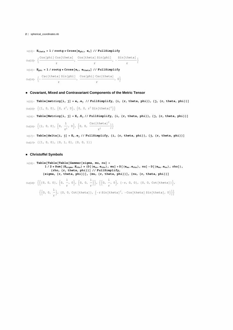
In[13]:= Etheta = 1 rootg * Cross@ephi, erD FullSimplify
Out[13]= :Cos@phiD Cos@thetaD
r,Cos@thetaD Sin@phiD
r, -
Sin@thetaD
r>
In[14]:= Ephi = 1 rootg * Cross@er, ethetaD FullSimplify
Out[14]= :-
Csc@thetaD Sin@phiD
r,Cos@phiD Csc@thetaD
r, 0>
Covariant, Mixed and Contravariant Components of the Metric Tensor
In[15]:= Table@metricg@i, jD = ei.ej FullSimplify, 8i, 8r, theta, phi<<, 8j, 8r, theta, phi<<D
Out[15]= 981, 0, 0<, 90, r2, 0=, 90, 0, r2 Sin@thetaD2==
In[16]:= Table@Metricg@i, jD = Ei.Ej FullSimplify, 8i, 8r, theta, phi<<, 8j, 8r, theta, phi<<D
Out[16]= :81, 0, 0<, :0,1
r2, 0>, :0, 0,
Csc@thetaD2
r2>>
In[17]:= Table@delta@i, jD = Ei.ej FullSimplify, 8i, 8r, theta, phi<<, 8j, 8r, theta, phi<<D
Out[17]= 881, 0, 0<, 80, 1, 0<, 80, 0, 1<<
Christoffel Symbols
In[18]:= Table@Table@Table@Gammer@sigma, mu, nuD =
1 2 * [email protected] * [email protected], muD + [email protected], nuD - [email protected], rhoDL,8rho, 8r, theta, phi<<D FullSimplify,
8sigma, 8r, theta, phi<<D, 8mu, 8r, theta, phi<<D, 8nu, 8r, theta, phi<<D
Out[18]= ::80, 0, 0<, :0,1
r, 0>, :0, 0,
1
r>>, ::0,
1
r, 0>, 8-r, 0, 0<, 80, 0, Cot@thetaD<>,
::0, 0,1
r>, 80, 0, Cot@thetaD<, 9-r Sin@thetaD2, -Cos@thetaD Sin@thetaD, 0=>>
2 spherical_coordinates.nb

Artificial Viscosity
Viscous Pressure Tensor
Definitions of Viscous Pressure
In order to proof consistency of our modified artificial viscosity we use different definitions and relations.
In[19]:= Table@qschlange@i, jD =
1 2 * Hd@iD@u@jDD + d@jD@u@iDD - Sum@Gammer@k, i, jD * u@kD, 8k, 8r, theta, phi<<D -
Sum@Gammer@k, j, iD * u@kD, 8k, 8r, theta, phi<<DL - 1 3 * metricg@i, jD * div@uD,8i, 8r, theta, phi<<, 8j, 8r, theta, phi<<D; H* covariant componentes *L
In[20]:= Table@qschlangeoben@m, nD = Sum@HMetricg@m, kD * Metricg@n, lDL *
H1 2 * Hd@kD@u@lDD + d@lD@u@kDD - Sum@Gammer@o, k, lD * u@oD, 8o, 8r, theta, phi<<D -
Sum@Gammer@o, l, kD * u@oD, 8o, 8r, theta, phi<<DL -
1 3 * metricg@m, nD * div@uDL, 8k, 8r, theta, phi<<, 8l, 8r, theta, phi<<D,8m, 8r, theta, phi<<, 8n, 8r, theta, phi<<D; H* contravariant components *L
In[21]:= Table@qoben@m, nD = Sum@HMetricg@m, iD * Metricg@n, jDL qschlange@i, jD,
8i, 8r, theta, phi<<, 8j, 8r, theta, phi<<D,8m, 8r, theta, phi<<, 8n, 8r, theta, phi<<D; H* contravariant components *L
In[22]:= Table@qmix@i, jD = Sum@Metricg@l, iD * qschlange@l, jD, 8l, 8r, theta, phi<<D,8i, 8r, theta, phi<<, 8j, 8r, theta, phi<<D; H* mixed components *L
In[23]:= Table@qmix2@i, nD = Sum@metricg@j, nD * qschlangeoben@i, jD, 8j, 8r, theta, phi<<D,8i, 8r, theta, phi<<, 8n, 8r, theta, phi<<D; H* mixed components *L

Components Explicitly
In[24]:= Table@qmix@m, nD, 8m, 8r, theta, phi<<, 8n, 8r, theta, phi<<D FullSimplify Expand
Out[24]= ::-
div@uD
3+ d@rD@u@rDD, -
u@thetaD
r+
1
2d@rD@u@thetaDD +
1
2d@thetaD@u@rDD,
-
u@phiD
r+
1
2d@phiD@u@rDD +
1
2d@rD@u@phiDD>,
:-
u@thetaD
r3+
d@rD@u@thetaDD
2 r2+
d@thetaD@u@rDD
2 r2, -
div@uD
3+
u@rD
r+
d@thetaD@u@thetaDD
r2,
-
Cot@thetaD u@phiD
r2+
d@phiD@u@thetaDD
2 r2+
d@thetaD@u@phiDD
2 r2>,
:-
Csc@thetaD2 u@phiD
r3+
Csc@thetaD2 d@phiD@u@rDD
2 r2+
Csc@thetaD2 d@rD@u@phiDD
2 r2,
-
Cot@thetaD Csc@thetaD2 u@phiD
r2+
Csc@thetaD2 d@phiD@u@thetaDD
2 r2+
Csc@thetaD2 d@thetaD@u@phiDD
2 r2,
-
div@uD
3+
u@rD
r+
Cot@thetaD u@thetaD
r2+
Csc@thetaD2 d@phiD@u@phiDD
r2>>
In[25]:= Do@Print@Q@m, nD, " = ", qschlange@m, nD FullSimplify ExpandD,8m, 8r, theta, phi<<, 8n, 8r, theta, phi<<D
Q@r, rD = -
div@uD
3+ d@rD@u@rDD
Q@r, thetaD = -
u@thetaD
r+
1
2d@rD@u@thetaDD +
1
2d@thetaD@u@rDD
Q@r, phiD = -
u@phiD
r+
1
2d@phiD@u@rDD +
1
2d@rD@u@phiDD
Q@theta, rD = -
u@thetaD
r+
1
2d@rD@u@thetaDD +
1
2d@thetaD@u@rDD
Q@theta, thetaD = -
1
3r2 div@uD + r u@rD + d@thetaD@u@thetaDD
Q@theta, phiD = -Cot@thetaD u@phiD +
1
2d@phiD@u@thetaDD +
1
2d@thetaD@u@phiDD
Q@phi, rD = -
u@phiD
r+
1
2d@phiD@u@rDD +
1
2d@rD@u@phiDD
Q@phi, thetaD = -Cot@thetaD u@phiD +
1
2d@phiD@u@thetaDD +
1
2d@thetaD@u@phiDD
Q@phi, phiD =
-
1
3r2 div@uD Sin@thetaD2
+ r Sin@thetaD2 u@rD + Cos@thetaD Sin@thetaD u@thetaD + d@phiD@u@phiDD
In[26]:= Do@Print@Qcontra@m, nD, " = ", qschlangeoben@m, nD FullSimplify ExpandD,8m, 8r, theta, phi<<, 8n, 8r, theta, phi<<D
2 artificial_viscosity.nb

Qcontra@r, rD = -
div@uD
3+ d@rD@u@rDD
Qcontra@r, thetaD = -
u@thetaD
r3+
d@rD@u@thetaDD
2 r2+
d@thetaD@u@rDD
2 r2
Qcontra@r, phiD = -
Csc@thetaD2 u@phiD
r3+
Csc@thetaD2 d@phiD@u@rDD
2 r2+
Csc@thetaD2 d@rD@u@phiDD
2 r2
Qcontra@theta, rD = -
u@thetaD
r3+
d@rD@u@thetaDD
2 r2+
d@thetaD@u@rDD
2 r2
Qcontra@theta, thetaD = -
div@uD
3 r2+
u@rD
r3+
d@thetaD@u@thetaDD
r4
Qcontra@theta, phiD =
-
Cot@thetaD Csc@thetaD2 u@phiD
r4+
Csc@thetaD2 d@phiD@u@thetaDD
2 r4+
Csc@thetaD2 d@thetaD@u@phiDD
2 r4
Qcontra@phi, rD = -
Csc@thetaD2 u@phiD
r3+
Csc@thetaD2 d@phiD@u@rDD
2 r2+
Csc@thetaD2 d@rD@u@phiDD
2 r2
Qcontra@phi, thetaD =
-
Cot@thetaD Csc@thetaD2 u@phiD
r4+
Csc@thetaD2 d@phiD@u@thetaDD
2 r4+
Csc@thetaD2 d@thetaD@u@phiDD
2 r4
Qcontra@phi, phiD = -
Csc@thetaD2 div@uD
3 r2+
Csc@thetaD2 u@rD
r3+
Cot@thetaD Csc@thetaD2 u@thetaD
r4+
Csc@thetaD4 d@phiD@u@phiDD
r4
Symmetry
In fact Q is symmetric in its co- and contravariant components.
In[27]:= Table@qschlangeoben@m, nD === qschlangeoben@n, mD, 8m, 8r, theta, phi<<, 8n, 8r, theta, phi<<D
Out[27]= 88True, True, True<, 8True, True, True<, 8True, True, True<<
In[28]:= Table@qschlange@m, nD === qschlange@n, mD, 8m, 8r, theta, phi<<, 8n, 8r, theta, phi<<D
Out[28]= 88True, True, True<, 8True, True, True<, 8True, True, True<<
In[29]:= Table@qmix@m, nD === qmix@n, mD, 8m, 8r, theta, phi<<, 8n, 8r, theta, phi<<D
Out[29]= 88True, False, False<, 8False, True, False<, 8False, False, True<<
Trace of Q
The trace vanishes as expected.
artificial_viscosity.nb 3

In[30]:= Sum@qmix@m, mD, 8m, 8r, theta, phi<<D
Out[30]= -
div@uD
3+
1
r2Csc@thetaD2
-
1
3r2 div@uD Sin@thetaD2
+
1
2I2 r Sin@thetaD2 u@rD + 2 Cos@thetaD Sin@thetaD u@thetaD + 2 d@phiD@u@phiDDM +
d@rD@u@rDD +
-1
3r2 div@uD +
1
2H2 r u@rD + 2 d@thetaD@u@thetaDDL
r2
In[31]:= Sum@qmix@m, mD, 8m, 8r, theta, phi<<D .
9div@uD ->
2 u@rD
r+
Cot@thetaD u@thetaD
r2+
Csc@thetaD2 d@phiD@u@phiDD
r2+
d@rD@u@rDD +
d@thetaD@u@thetaDD
r2= FullSimplify Expand
Out[31]= 0
In[32]:= Sum@qmix2@m, mD, 8m, 8r, theta, phi<<D .
9div@uD ->
2 u@rD
r+
Cot@thetaD u@thetaD
r2+
Csc@thetaD2 d@phiD@u@phiDD
r2+
d@rD@u@rDD +
d@thetaD@u@thetaDD
r2= FullSimplify Expand
Out[32]= 0
4 artificial_viscosity.nb

Equation of Motion in Spherical Coordinates
Generation of Strong Conservation Form Equation
Definition of Contravariant Components of Tensors
Table@rschlange@i, jD = rho * Hu@iD - xdot@iDL * u@jD FullSimplify,8i, 8r, theta, phi<<, 8j, 8r, theta, phi<<D
Table@p@i, jD = p * Metricg@i, jD FullSimplify, 8i, 8r, theta, phi<<, 8j, 8r, theta, phi<<DTable@q@i, jD = Sum@HMetricg@i, mD * Metricg@j, nDL
H1 2 * Hd@nD@u@mDD + d@nD@u@mDD - Sum@Gammer@k, m, mD * u@kD, 8k, 8r, theta, phi<<D -
Sum@Gammer@k, m, nD * u@kD, 8k, 8r, theta, phi<<DL - 1 3 * metricg@n, mD * div@uDL,8n, 8r, theta, phi<<, 8m, 8r, theta, phi<<D FullSimplify,
8i, 8r, theta, phi<<, 8j, 8r, theta, phi<<DH* note that there emerge covariant velocity components in Q due to its definition *L
Out[33]= 88rho u@rD Hu@rD - xdot@rDL, rho u@thetaD Hu@rD - xdot@rDL, rho u@phiD Hu@rD - xdot@rDL<,8rho u@rD Hu@thetaD - xdot@thetaDL, rho u@thetaD Hu@thetaD - xdot@thetaDL,rho u@phiD Hu@thetaD - xdot@thetaDL<, 8rho u@rD Hu@phiD - xdot@phiDL,rho u@thetaD Hu@phiD - xdot@phiDL, rho u@phiD Hu@phiD - xdot@phiDL<<
Out[34]= :8p, 0, 0<, :0,p
r2, 0>, :0, 0,
p Csc@thetaD2
r2>>
Out[35]= ::-
div@uD
3+ d@rD@u@rDD,
-
u@thetaD - 2 r d@thetaD@u@rDD
2 r3, -
Csc@thetaD2 Hu@phiD - 2 r d@phiD@u@rDDL
2 r3>,
:r2 u@rD - u@thetaD + 2 r d@rD@u@thetaDD
2 r3,
-r2 div@uD + 3 Hr u@rD + d@thetaD@u@thetaDDL
3 r4,
Csc@thetaD2 H-Cot@thetaD u@phiD + r u@rD + 2 d@phiD@u@thetaDDL
2 r4>,
:r2 u@rD + r Cot@thetaD u@thetaD - Csc@thetaD2 Hu@phiD - 2 r d@rD@u@phiDDL
2 r3,
-Cot@thetaD Csc@thetaD2 u@phiD + r u@rD + Cot@thetaD u@thetaD + 2 Csc@thetaD2 d@thetaD@u@phiDD
2 r4,
Csc@thetaD2 I-r2 div@uD + 3 Ir u@rD + Cot@thetaD u@thetaD + Csc@thetaD2 d@phiD@u@phiDDMM
3 r4>>
Equation of Motion in Spherical Coordinates and Strong Conservation Form
In[36]:= Table@d@tD@Sum@Sqrt@gD * rho * u@nD * en@@kDD, 8n, 8r, theta, phi<<DD + Sum@Sum@d@iD@Sqrt@gD * H rschlange@i, jD + p@i, jD + Qkomp@i, jDL * ej@@kDDD, 8i, 8r, theta, phi<<D,8j, 8r, theta, phi<<D + rho * Sum@d@lD@Sqrt@gD * Phi * El@@kDDD, 8l, 8r, theta, phi<<D -
4 Pi c * Sqrt@gD * HSum@H@oD * eo@@kDD, 8o, 8r, theta, phi<<DL .8Sin@thetaD ® Sqrt@1 - mu^2D, d@thetaD ® -Sqrt@1 - mu^2D d@muD,Csc@thetaD ® 1 Sqrt@1 - mu^2D, Cos@thetaD ® mu<, 8k, 81, 2, 3<<D
Out[36]=

Out[36]= :-
4 Π I1 - mu2M r4 1 - mu2 Cos@phiD H@rD + mu r Cos@phiD H@thetaD - 1 - mu2 r H@phiD Sin@phiD
c+
- 1 - mu2 d@muD B- 1 - mu2 r I1 - mu2M r4 Sin@phiD
HQkomp@theta, phiD + rho u@phiD Hu@thetaD - xdot@thetaDLLF + - 1 - mu2 d@muD B
1 - mu2 I1 - mu2M r4 Cos@phiD HQkomp@theta, rD + rho u@rD Hu@thetaD - xdot@thetaDLLF +
- 1 - mu2 d@muD Bmu r I1 - mu2M r4 Cos@phiD
p
r2+ Qkomp@theta, thetaD + rho u@thetaD Hu@thetaD - xdot@thetaDL F + d@phiDB- 1 - mu2 r
I1 - mu2M r4 Sin@phiDp
I1 - mu2M r2+ Qkomp@phi, phiD + rho u@phiD Hu@phiD - xdot@phiDL F +
d@phiDB 1 - mu2 I1 - mu2M r4 Cos@phiD HQkomp@phi, rD + rho u@rD Hu@phiD - xdot@phiDLLF +
d@phiDBmu r I1 - mu2M r4 Cos@phiD HQkomp@phi, thetaD + rho u@thetaD Hu@phiD - xdot@phiDLLF +
rho - 1 - mu2 d@muD Bmu Phi I1 - mu2M r4 Cos@phiD
rF +
d@phiDB-
Phi I1 - mu2M r4 Sin@phiD
1 - mu2 r
F + d@rDB 1 - mu2 Phi I1 - mu2M r4 Cos@phiDF +
d@rDB- 1 - mu2 r I1 - mu2M r4 Sin@phiD HQkomp@r, phiD + rho u@phiD Hu@rD - xdot@rDLLF +
d@rDB 1 - mu2 I1 - mu2M r4 Cos@phiD Hp + Qkomp@r, rD + rho u@rD Hu@rD - xdot@rDLLF +
d@rDBmu r I1 - mu2M r4 Cos@phiD HQkomp@r, thetaD + rho u@thetaD Hu@rD - xdot@rDLLF +
d@tDB- 1 - mu2 r I1 - mu2M r4 rho Sin@phiD u@phiD +
1 - mu2 I1 - mu2M r4 rho Cos@phiD u@rD + mu r I1 - mu2M r4 rho Cos@phiD u@thetaDF,
-
4 Π I1 - mu2M r4 1 - mu2 r Cos@phiD H@phiD + 1 - mu2 H@rD Sin@phiD + mu r H@thetaD Sin@phiD
c+
- 1 - mu2 d@muD B 1 - mu2 r I1 - mu2M r4 Cos@phiD
F +
+
2 EOM_3D_sph.nb

Out[36]=
HQkomp@theta, phiD + rho u@phiD Hu@thetaD - xdot@thetaDLLF + - 1 - mu2 d@muD B
1 - mu2 I1 - mu2M r4 Sin@phiD HQkomp@theta, rD + rho u@rD Hu@thetaD - xdot@thetaDLLF +
- 1 - mu2 d@muD Bmu r I1 - mu2M r4 Sin@phiD
p
r2+ Qkomp@theta, thetaD + rho u@thetaD Hu@thetaD - xdot@thetaDL F + d@phiDB 1 - mu2 r
I1 - mu2M r4 Cos@phiDp
I1 - mu2M r2+ Qkomp@phi, phiD + rho u@phiD Hu@phiD - xdot@phiDL F +
d@phiDB 1 - mu2 I1 - mu2M r4 Sin@phiD HQkomp@phi, rD + rho u@rD Hu@phiD - xdot@phiDLLF +
d@phiDBmu r I1 - mu2M r4 Sin@phiD HQkomp@phi, thetaD + rho u@thetaD Hu@phiD - xdot@phiDLLF +
rho - 1 - mu2 d@muD Bmu Phi I1 - mu2M r4 Sin@phiD
rF +
d@phiDBPhi I1 - mu2M r4 Cos@phiD
1 - mu2 r
F + d@rDB 1 - mu2 Phi I1 - mu2M r4 Sin@phiDF +
d@rDB 1 - mu2 r I1 - mu2M r4 Cos@phiD HQkomp@r, phiD + rho u@phiD Hu@rD - xdot@rDLLF +
d@rDB 1 - mu2 I1 - mu2M r4 Sin@phiD Hp + Qkomp@r, rD + rho u@rD Hu@rD - xdot@rDLLF +
d@rDBmu r I1 - mu2M r4 Sin@phiD HQkomp@r, thetaD + rho u@thetaD Hu@rD - xdot@rDLLF +
d@tDB 1 - mu2 r I1 - mu2M r4 rho Cos@phiD u@phiD +
1 - mu2 I1 - mu2M r4 rho Sin@phiD u@rD + mu r I1 - mu2M r4 rho Sin@phiD u@thetaDF,
-
4 Π I1 - mu2M r4 mu H@rD - 1 - mu2 r H@thetaD
c+ - 1 - mu2 d@muD @0D +
- 1 - mu2 d@muD Bmu I1 - mu2M r4 HQkomp@theta, rD + rho u@rD Hu@thetaD - xdot@thetaDLLF +
- 1 - mu2 d@muD B
- 1 - mu2 r I1 - mu2M r4p
r2+ Qkomp@theta, thetaD + rho u@thetaD Hu@thetaD - xdot@thetaDL F +
d@phiD@0D + d@phiDBmu I1 - mu2M r4 HQkomp@phi, rD + rho u@rD Hu@phiD - xdot@phiDLLF + d@phiDB
F + +
+
EOM_3D_sph.nb 3

Out[36]=
- 1 - mu2 r I1 - mu2M r4 HQkomp@phi, thetaD + rho u@thetaD Hu@phiD - xdot@phiDLLF + d@rD@0D +
rho - 1 - mu2 d@muD B-
1 - mu2 Phi I1 - mu2M r4
rF + d@phiD@0D + d@rDBmu Phi I1 - mu2M r4 F +
d@rDBmu I1 - mu2M r4 Hp + Qkomp@r, rD + rho u@rD Hu@rD - xdot@rDLLF +
d@rDB- 1 - mu2 r I1 - mu2M r4 HQkomp@r, thetaD + rho u@thetaD Hu@rD - xdot@rDLLF +
d@tDBmu I1 - mu2M r4 rho u@rD - 1 - mu2 r I1 - mu2M r4 rho u@thetaDF>
EOM with Q explicitly
In[37]:= Table@d@tD@Sum@Sqrt@gD * rho * u@nD * en@@kDD, 8n, 8r, theta, phi<<DD +
Sum@Sum@d@iD@Sqrt@gD * H rschlange@i, jD + p@i, jD + q@i, jDL * ej@@kDDD, 8i, 8r, theta, phi<<D,8j, 8r, theta, phi<<D - +rho * Sum@d@lD@Sqrt@gD * Phi * El@@kDDD, 8l, 8r, theta, phi<<D4 Pi c * Sqrt@gD * HSum@H@oD * eo@@kDD, 8o, 8r, theta, phi<<DL .
8Sin@thetaD ® Sqrt@1 - mu^2D, d@thetaD ® -Sqrt@1 - mu^2D d@muD,Csc@thetaD ® 1 Sqrt@1 - mu^2D, Cos@thetaD ® mu<, 8k, 81, 2, 3<<D
Out[37]= : - 1 - mu2 d@muD Bmu r I1 - mu2M r4 Cos@phiDp
r2+ rho u@thetaD Hu@thetaD - xdot@thetaDL +
-r2 div@uD + 3 r u@rD + - 1 - mu2 d@muD @u@thetaDD
3 r4F +
- 1 - mu2 d@muD B- 1 - mu2 r I1 - mu2M r4 Sin@phiD
rho u@phiD Hu@thetaD - xdot@thetaDL +
-Cot@thetaD u@phiD + r u@rD + 2 d@phiD@u@thetaDD
2 I1 - mu2M r4F +
- 1 - mu2 d@muD B 1 - mu2 I1 - mu2M r4 Cos@phiD
rho u@rD Hu@thetaD - xdot@thetaDL +
r2 u@rD - u@thetaD + 2 r d@rD@u@thetaDD
2 r3F +
4 EOM_3D_sph.nb

Out[37]=
d@phiDBmu r I1 - mu2M r4 Cos@phiD rho u@thetaD Hu@phiD - xdot@phiDL +
-Cot@thetaD u@phiD
1-mu2+ r u@rD + Cot@thetaD u@thetaD +
2 - 1-mu2 d@muD @u@phiDD
1-mu2
2 r4F +
d@phiDB- 1 - mu2 r I1 - mu2M r4 Sin@phiDp
I1 - mu2M r2+ rho u@phiD Hu@phiD - xdot@phiDL +
-r2 div@uD + 3 Jr u@rD + Cot@thetaD u@thetaD +d@phiD@u@phiDD
1-mu2N
3 I1 - mu2M r4F +
d@phiDB 1 - mu2 I1 - mu2M r4 Cos@phiD rho u@rD Hu@phiD - xdot@phiDL +
r2 u@rD + r Cot@thetaD u@thetaD -u@phiD-2 r d@rD@u@phiDD
1-mu2
2 r3F -
1
c4 Π I1 - mu2M r4
rho 1 - mu2 Cos@phiD H@rD + mu r Cos@phiD H@thetaD - 1 - mu2 r H@phiD Sin@phiD
- 1 - mu2 d@muD Bmu Phi I1 - mu2M r4 Cos@phiD
rF + d@phiDB-
Phi I1 - mu2M r4 Sin@phiD
1 - mu2 r
F +
d@rDB 1 - mu2 Phi I1 - mu2M r4 Cos@phiDF + d@rDBmu r I1 - mu2M r4 Cos@phiD
rho u@thetaD Hu@rD - xdot@rDL -
u@thetaD - 2 r - 1 - mu2 d@muD @u@rDD
2 r3F + d@rDB
- 1 - mu2 r I1 - mu2M r4 Sin@phiD rho u@phiD Hu@rD - xdot@rDL -
u@phiD - 2 r d@phiD@u@rDD
2 I1 - mu2M r3F +
+
EOM_3D_sph.nb 5

Out[37]=
d@rDB 1 - mu2 I1 - mu2M r4 Cos@phiD p -
div@uD
3+ rho u@rD Hu@rD - xdot@rDL + d@rD@u@rDD F +
d@tDB- 1 - mu2 r I1 - mu2M r4 rho Sin@phiD u@phiD +
1 - mu2 I1 - mu2M r4 rho Cos@phiD u@rD + mu r I1 - mu2M r4 rho Cos@phiD u@thetaDF,
- 1 - mu2 d@muD Bmu r I1 - mu2M r4 Sin@phiDp
r2+ rho u@thetaD Hu@thetaD - xdot@thetaDL +
-r2 div@uD + 3 r u@rD + - 1 - mu2 d@muD @u@thetaDD
3 r4F +
- 1 - mu2 d@muD B 1 - mu2 r I1 - mu2M r4 Cos@phiD
rho u@phiD Hu@thetaD - xdot@thetaDL +
-Cot@thetaD u@phiD + r u@rD + 2 d@phiD@u@thetaDD
2 I1 - mu2M r4F +
- 1 - mu2 d@muD B 1 - mu2 I1 - mu2M r4 Sin@phiD
rho u@rD Hu@thetaD - xdot@thetaDL +
r2 u@rD - u@thetaD + 2 r d@rD@u@thetaDD
2 r3F +
d@phiDBmu r I1 - mu2M r4 Sin@phiD rho u@thetaD Hu@phiD - xdot@phiDL +
-Cot@thetaD u@phiD
1-mu2+ r u@rD + Cot@thetaD u@thetaD +
2 - 1-mu2 d@muD @u@phiDD
1-mu2
2 r4F +
d@phiDB 1 - mu2 r I1 - mu2M r4 Cos@phiDp
I1 - mu2M r2+ rho u@phiD Hu@phiD - xdot@phiDL +
-r2 div@uD + 3 Jr u@rD + Cot@thetaD u@thetaD +d@phiD@u@phiDD
1-mu2N
3 I1 - mu2M r4F +
-
6 EOM_3D_sph.nb

Out[37]=
d@phiDB 1 - mu2 I1 - mu2M r4 Sin@phiD rho u@rD Hu@phiD - xdot@phiDL +
r2 u@rD + r Cot@thetaD u@thetaD -u@phiD-2 r d@rD@u@phiDD
1-mu2
2 r3F -
1
c4 Π I1 - mu2M r4
rho 1 - mu2 r Cos@phiD H@phiD + 1 - mu2 H@rD Sin@phiD + mu r H@thetaD Sin@phiD
- 1 - mu2 d@muD Bmu Phi I1 - mu2M r4 Sin@phiD
rF + d@phiDB
Phi I1 - mu2M r4 Cos@phiD
1 - mu2 r
F +
d@rDB 1 - mu2 Phi I1 - mu2M r4 Sin@phiDF + d@rDBmu r I1 - mu2M r4 Sin@phiD
rho u@thetaD Hu@rD - xdot@rDL -
u@thetaD - 2 r - 1 - mu2 d@muD @u@rDD
2 r3F + d@rDB
1 - mu2 r I1 - mu2M r4 Cos@phiD rho u@phiD Hu@rD - xdot@rDL -
u@phiD - 2 r d@phiD@u@rDD
2 I1 - mu2M r3F +
d@rDB 1 - mu2 I1 - mu2M r4 Sin@phiD p -
div@uD
3+ rho u@rD Hu@rD - xdot@rDL + d@rD@u@rDD F +
d@tDB 1 - mu2 r I1 - mu2M r4 rho Cos@phiD u@phiD + 1 - mu2 I1 - mu2M r4 rho Sin@phiD u@rD +
mu r I1 - mu2M r4 rho Sin@phiD u@thetaDF, - 1 - mu2 d@muD @0D +
- 1 - mu2 d@muD B- 1 - mu2 r I1 - mu2M r4p
r2+ rho u@thetaD Hu@thetaD - xdot@thetaDL +
-r2 div@uD + 3 r u@rD + - 1 - mu2 d@muD @u@thetaDD
3 r4F + - 1 - mu2 d@muD B
mu I1 - mu2M r4 rho u@rD Hu@thetaD - xdot@thetaDL +
r2 u@rD - u@thetaD + 2 r d@rD@u@thetaDD
2 r3F +
+
EOM_3D_sph.nb 7

Out[37]=
d@phiD@0D + d@phiDB- 1 - mu2 r I1 - mu2M r4 rho u@thetaD Hu@phiD - xdot@phiDL +
-Cot@thetaD u@phiD
1-mu2+ r u@rD + Cot@thetaD u@thetaD +
2 - 1-mu2 d@muD @u@phiDD
1-mu2
2 r4F +
d@phiDBmu I1 - mu2M r4 rho u@rD Hu@phiD - xdot@phiDL +
r2 u@rD + r Cot@thetaD u@thetaD -u@phiD-2 r d@rD@u@phiDD
1-mu2
2 r3F +
d@rD@0D -
1
c4 Π I1 - mu2M r4 rho mu H@rD - 1 - mu2 r H@thetaD
- 1 - mu2 d@muD B-
1 - mu2 Phi I1 - mu2M r4
rF + d@phiD@0D + d@rDBmu Phi I1 - mu2M r4 F +
d@rDB- 1 - mu2 r I1 - mu2M r4
rho u@thetaD Hu@rD - xdot@rDL -
u@thetaD - 2 r - 1 - mu2 d@muD @u@rDD
2 r3F +
d@rDBmu I1 - mu2M r4 p -
div@uD
3+ rho u@rD Hu@rD - xdot@rDL + d@rD@u@rDD F +
d@tDBmu I1 - mu2M r4 rho u@rD - 1 - mu2 r I1 - mu2M r4 rho u@thetaDF>
8 EOM_3D_sph.nb

Polynomial Coordinates Ansatz
Grid Generation via Orthogonal Curves
Ansatz for Polynomial Curves
In[1]:= Η@x_, r_, t_D = a0@r, tD + a1@r, tD * x + a2@r, tD * x^2 + a3@r, tD * x^3H*+a4@r,tD*x^4+a5@r,tD*x^5*L;
First derivative to determine slope
In[2]:= g@x_, r_, t_D = D@Η@x, r, tD, xD;
Second derivative
In[3]:= h@x_, r_, t_D = D@Η@x, r, tD, x, xD;
Rotation Matrix to Rotate Coordinate System
Since infinite slope cannot be requiremeent for linear equation system, the whole coorindate system gets rotated by 45 degree. Sothe slopes are + 1 and - 1.
In[4]:= A@Α_D = 88Cos@ΑD, -Sin@ΑD<, 8Sin@ΑD, Cos@ΑD<<;
In[5]:= coeff = Table@P1 = A@Pi 4D.80.1 + n * 0.13, 0<;P2 = A@Pi 4D.80, 0.1 + n * 0.1<;Solve@8Η@P1@@1DD, r, tD P1@@2DD, Η@P2@@1DD, r, tD P2@@2DD,
g@P1@@1DD, r, tD -1, g@P2@@1DD, r, tD 1H*,f@0,r,tD0.1+n*0.12,g@0,r,tD0*L<,8a0@r, tD, a1@r, tD, a2@r, tD, a3@r, tDH*,a4@r,tD,a5@r,tD*L<D, 8n, 0, 10<D
H* generation of polynomials intersecting with two equidistanced points at x-
and y-axis *L
Out[5]= 888a0@r, tD ® 0.106066, a1@r, tD ® 0., a2@r, tD ® -7.07107, a3@r, tD ® 0.<<,88a0@r, tD ® 0.226564, a1@r, tD ® 0.173909, a2@r, tD ® -3.24084, a3@r, tD ® -1.5093<<,88a0@r, tD ® 0.346169, a1@r, tD ® 0.226146, a2@r, tD ® -2.08962, a3@r, tD ® -0.834794<<,88a0@r, tD ® 0.465575, a1@r, tD ® 0.251258, a2@r, tD ® -1.54026, a3@r, tD ® -0.510661<<,88a0@r, tD ® 0.584904, a1@r, tD ® 0.266012, a2@r, tD ® -1.21921, a3@r, tD ® -0.341655<<,88a0@r, tD ® 0.704197, a1@r, tD ® 0.27572, a2@r, tD ® -1.00877, a3@r, tD ® -0.243865<<,88a0@r, tD ® 0.823468, a1@r, tD ® 0.282592, a2@r, tD ® -0.860221, a3@r, tD ® -0.182541<<,88a0@r, tD ® 0.942727, a1@r, tD ® 0.287713, a2@r, tD ® -0.749781, a3@r, tD ® -0.141659<<,88a0@r, tD ® 1.06198, a1@r, tD ® 0.291675, a2@r, tD ® -0.664457, a3@r, tD ® -0.113079<<,88a0@r, tD ® 1.18122, a1@r, tD ® 0.294833, a2@r, tD ® -0.59656, a3@r, tD ® -0.0923307<<,88a0@r, tD ® 1.30046, a1@r, tD ® 0.297408, a2@r, tD ® -0.541248, a3@r, tD ® -0.0768<<<

In[6]:= Rotate@Show@Plot@8Evaluate@Η@x, r, tD . 8coeff<DH*,Evaluate@f@x,r,tD.8ergmore2<D*L, Abs@xD, 0<,
8x, -1.2, 1.2<, PlotRange ® 8-0.1, 1.5<, AspectRatio ® Automatic, Background ® White,Axes ® None, PlotStyle ® 88Black, Thick<, 8Gray, Thick<, 8Gray, Thick<<DH*,
Graphics@8Thick,Red,Arrow@880,0<,81,0<<D,Thick,Blue,Arrow@880,0<,80,1<<D,Thick,Black,Dashed,Arrow@880,0<,1*81,0<+1*80,1<<D<D*LD, -45 DegreeD
Out[6]=
Orthogonal Curves
In[7]:= po1@x_D = Η@x, r, tD . 8coeff@@1DD<; H* define polynomial functions *Lpo2@x_D = Η@x, r, tD . 8coeff@@2DD<;po3@x_D = Η@x, r, tD . 8coeff@@3DD<;po4@x_D = Η@x, r, tD . 8coeff@@4DD<;po5@x_D = Η@x, r, tD . 8coeff@@5DD<;po6@x_D = Η@x, r, tD . 8coeff@@6DD<;po7@x_D = Η@x, r, tD . 8coeff@@7DD<;po8@x_D = Η@x, r, tD . 8coeff@@8DD<;
In[15]:= ort4@x0_, x_D = -1 HD@po4@xD, xDL * Hx - x0L + po7@x0D;H* orthogonal curves to polynomial ð *Lort7@x0_, x_D = -1 HD@po7@xD, xDL * Hx - x0L + po7@x0D;ort8@x0_, x_D = -1 HD@po8@xD, xDL * Hx - x0L + po8@x0D;
In[18]:= Table@intersectort8po7@mD =
FindInstance@8Evaluate@[email protected] + 0.1 * m, xDD == po7@xD, x > 0.18, x < 0.8<, x, RealsD@@1DD@@1DD H* determine intersections *L
,8m,0,4<D
Out[18]= 8x ® 0.2382, x ® 0.320295, x ® 0.403032, x ® 0.487458, x ® 0.574101<
2 poly_coordinates.nb

In[19]:= Table@intersectort7po8old@nD =
FindInstance@8Evaluate@[email protected] + 0.1 * n, xDD == po8@xD, x > 0.18, x < 0.8<, x, RealsD@@1DD@@1DD
,8n,0,4<D
Out[19]= 8x ® 0.279988, x ® 0.409555, x ® 0.530964, x ® 0.645, x ® 0.754393<
In[20]:= Show@Plot@8H*neu8@xD,neu7@xD,*Lpo7@xD, po6@xD, po5@xD, po4@xD,po3@xD, po2@xD, po1@xD, Abs@xD, 0<, 8x, 0, 0.8<, PlotRange ® 8-0.05, 1.<,
AspectRatio ® Automatic, Background ® White, PlotStyle ® 88Gray, Thick<<, Axes ® FalseD,Table@Plot@Evaluate@[email protected] + 0.09 * m, xDD, 8x, 0.17, 0.8<,
AspectRatio ® Automatic, Background ® White, PlotRange ® 80., 1.<,PlotStyle ® 8Black, Dashed, Thick<, Axes ® FalseD, 8m, 0, 8<D
H*Table@Plot@Evaluate@[email protected]@nD,xDD,8x,0.2,0.8<,AspectRatio®Automatic,Background®White,PlotRange®80.4,1.2<,PlotStyle®8Blue<,Axes®FalseD,8n,0,3<D,*L
D
Out[20]=
Normal Vectors
In[21]:= slope7@x_D = -1 HD@po7@xD, xDL
Out[21]= ::-1
0.282592 - 1.72044 x - 0.547624 x2>>
poly_coordinates.nb 3

In[22]:= vecend@n_D = 80.25 + 0.1 * n, [email protected] + 0.1 * nD@@1DD@@1DD< +
80.25 + 0.1 * n + 1, [email protected] + 0.1 * nD@@1DD@@1DD + [email protected] + 0.1 * nD@@1DD@@1DD<
Out[22]= :1.5 + 0.2 n, 1.64694 -1
0.282592 - 1.72044 H0.25 + 0.1 nL - 0.547624 H0.25 + 0.1 nL2+
0.565184 H0.25 + 0.1 nL - 1.72044 H0.25 + 0.1 nL2- 0.365083 H0.25 + 0.1 nL3>
In[23]:= slope8@x_D = -1 HD@po8@xD, xDL
Out[23]= ::-1
0.287713 - 1.49956 x - 0.424976 x2>>
In[24]:= Table@intersectort7po8@nD = x . FindInstance@
8Evaluate@[email protected] + 0.1 * n, xDD == po8@xD, x > 0.18, x < 0.8<, x, RealsD@@1DD@@1DD,8n,0,4<D
Out[24]= 80.279988, 0.409555, 0.530964, 0.645, 0.754393<
In[25]:= Table@vecend8@mD =
8intersectort7po8@mD, po8@intersectort7po8@mDD@@1DD@@1DD< + 8intersectort7po8@mD + 1,po8@intersectort7po8@mDD@@1DD@@1DD + slope8@intersectort7po8@mDD@@1DD@@1DD<, 8m, 0, 3<D
Out[25]= 881.55998, 7.9665<, 81.81911, 4.36444<, 82.06193, 3.31738<, 82.29, 2.72453<<
4 poly_coordinates.nb

In[26]:= Show@Plot@8po8@xD, po7@xD, po6@xD, po5@xD, Abs@xD<, 8x, 0.1, 0.9<, PlotRange ® 80.5, 1.3<,AspectRatio ® Automatic, Background ® White, PlotStyle ® 88Gray, Thick<<, Axes ® FalseD,
Table@Plot@Evaluate@[email protected] + 0.1 * m, xDD, 8x, 0.2, 0.9<,AspectRatio ® Automatic, Background ® White, PlotRange ® 80.5, 1.2<,PlotStyle ® 8Gray, Dashed, Thick<, Axes ® FalseD, 8m, 0, 3<D,
Table@Plot@Evaluate@ort8@x . intersectort7po8old@nD, xDD, 8x, 0.2, 0.8<,AspectRatio ® Automatic, Background ® White, PlotRange ® 80.5, 1.2<,PlotStyle ® 8Gray, Dashed, Thick<, Axes ® FalseD, 8n, 0, 3<D,
Table@Graphics@8Thick, Black, [email protected] + 0.1 * n, [email protected] + 0.1 * nD@@1DD@@1DD<,80.25 + 0.1 * n + 0.7 Norm@vecend@nDD^2 * 1, [email protected] + 0.1 * nD@@1DD@@1DD +
0.7 Norm@vecend@nDD^2 * [email protected] + 0.1 * nD@@1DD@@1DD<<D<D, 8n, 0, 3<D,Table@Graphics@8Thick, Black, Arrow@88intersectort7po8@nD,
po8@intersectort7po8@nDD@@1DD@@1DD<,8intersectort7po8@nD + 0.7 Norm@vecend8@nDD^2 * 1, po8@intersectort7po8@nDD@@1DD@@1DD +
0.7 Norm@vecend8@nDD^2 * slope8@intersectort7po8@nDD@@1DD@@1DD<<D<D, 8n, 0, 3<D
D
Out[26]=
poly_coordinates.nb 5

Polar Non-Orthogonal Grid Ansatz
Generation of Quasi-Polar Grid in 2D
Ansatz for Quasi-Polar Coordinates
Coordinate Transformation with Product Ansatz
We define a coordinate transformation with product ansatz, which is reasonable for any kind of coordinate system.
In[1]:= x = X@Ξ, ΗD;y = Y@Ξ, ΗD;
In[3]:= X@Ξ_, Η_D = a@ΞD * Α@ΗD;Y@Ξ_, Η_D = b@ΞD * Β@ΗD;
In[5]:= Α@Η_D = H1 + alpha1 * Η + alpha2 * Η^2 + alpha3 * Η^3L * Cos@ΗD;Β@Η_D = H1 + beta1 * Η + beta2 * Η^2 + beta3 * Η^3L * Sin@ΗD;a@Ξ_D = Ha1 * Ξ + a2 * Ξ^2L ;b@Ξ_D = Hb1 * Ξ + b2 * Ξ^2L ;
We calculate the Jacobian of this transformation to get the base vectors in the new coordinate system.
In[9]:= lij = 88D@x, ΞD, D@x, ΗD<, 8D@y, ΞD, D@y, ΗD<<;
In[10]:= lijtransposed := Transpose@lijD
Covariant Components of Metric Tensor
For trivial signatures, the metric tensor is simply given by the Jacobian times its transpositon. The off diagonal elements containthe information about the non-orthogonality (angles), the diagonal elements are measures of lenght in the coordinate directions.
In[11]:= gij = lijtransposed.lij;
In[12]:= g11@Ξ_, Η_D = gij@@1, 1DD;g12@Ξ_, Η_D = gij@@1, 2DD;g21@Ξ_, Η_D = gij@@2, 1DD;g22@Ξ_, Η_D = gij@@2, 2DD;
Covariant Base Vectors
The base vectors yield
In[16]:= eΞ@Ξ_, Η_D = lijtransposed@@1DD
Out[16]= 9I1 + alpha1 Η + alpha2 Η2
+ alpha3 Η3M Ha1 + 2 a2 ΞL Cos@ΗD,
I1 + beta1 Η + beta2 Η2
+ beta3 Η3M Hb1 + 2 b2 ΞL Sin@ΗD=
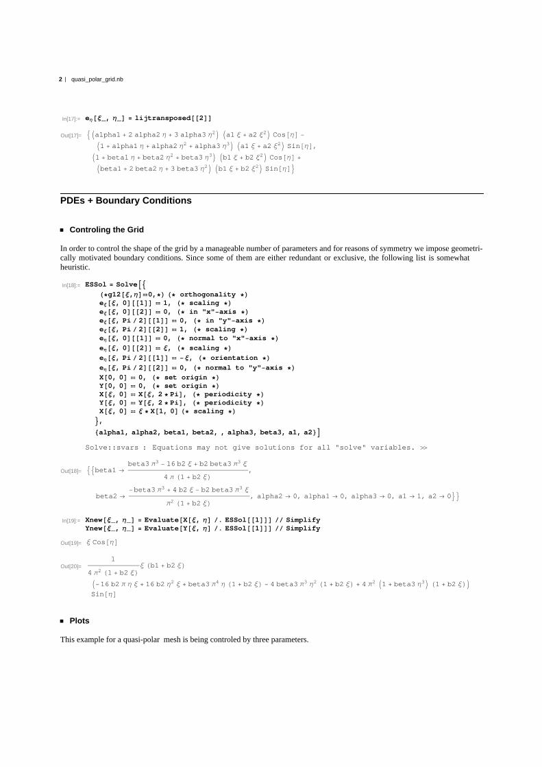
In[17]:= eΗ@Ξ_, Η_D = lijtransposed@@2DD
Out[17]= 9Ialpha1 + 2 alpha2 Η + 3 alpha3 Η2M Ia1 Ξ + a2 Ξ
2M Cos@ΗD -
I1 + alpha1 Η + alpha2 Η2
+ alpha3 Η3M Ia1 Ξ + a2 Ξ
2M Sin@ΗD,
I1 + beta1 Η + beta2 Η2
+ beta3 Η3M Ib1 Ξ + b2 Ξ
2M Cos@ΗD +
Ibeta1 + 2 beta2 Η + 3 beta3 Η2M Ib1 Ξ + b2 Ξ
2M Sin@ΗD=
PDEs + Boundary Conditions
Controling the Grid
In order to control the shape of the grid by a manageable number of parameters and for reasons of symmetry we impose geometri-cally motivated boundary conditions. Since some of them are either redundant or exclusive, the following list is somewhatheuristic.
In[18]:= ESSol = SolveA9
H*g12@Ξ,ΗD0,*L H* orthogonality *LeΞ@Ξ, 0D@@1DD 1, H* scaling *LeΞ@Ξ, 0D@@2DD 0, H* in "x"-axis *LeΞ@Ξ, Pi 2D@@1DD 0, H* in "y"-axis *LeΞ@Ξ, Pi 2D@@2DD 1, H* scaling *LeΗ@Ξ, 0D@@1DD 0, H* normal to "x"-axis *L
eΗ@Ξ, 0D@@2DD Ξ, H* scaling *L
eΗ@Ξ, Pi 2D@@1DD -Ξ, H* orientation *L
eΗ@Ξ, Pi 2D@@2DD 0, H* normal to "y"-axis *L
X@0, 0D 0, H* set origin *LY@0, 0D 0, H* set origin *LX@Ξ, 0D X@Ξ, 2 * PiD, H* periodicity *LY@Ξ, 0D Y@Ξ, 2 * PiD, H* periodicity *LX@Ξ, 0D Ξ * X@1, 0D H* scaling *L
=,
8alpha1, alpha2, beta1, beta2, , alpha3, beta3, a1, a2<E
Solve::svars : Equations may not give solutions for all "solve" variables.
Out[18]= 99beta1 ®beta3 Π3 - 16 b2 Ξ + b2 beta3 Π3 Ξ
4 Π H1 + b2 ΞL,
beta2 ®-beta3 Π3 + 4 b2 Ξ - b2 beta3 Π3 Ξ
Π2 H1 + b2 ΞL, alpha2 ® 0, alpha1 ® 0, alpha3 ® 0, a1 ® 1, a2 ® 0==
In[19]:= Xnew@Ξ_, Η_D = Evaluate@X@Ξ, ΗD . ESSol@@1DDD SimplifyYnew@Ξ_, Η_D = Evaluate@Y@Ξ, ΗD . ESSol@@1DDD Simplify
Out[19]= Ξ Cos@ΗD
Out[20]=1
4 Π2 H1 + b2 ΞLΞ Hb1 + b2 ΞL
I-16 b2 Π Η Ξ + 16 b2 Η2
Ξ + beta3 Π4
Η H1 + b2 ΞL - 4 beta3 Π3
Η2 H1 + b2 ΞL + 4 Π
2 I1 + beta3 Η3M H1 + b2 ΞLM
Sin@ΗD
Plots
This example for a quasi-polar mesh is being controled by three parameters.
2 quasi_polar_grid.nb

In[21]:= ManipulateA
ParametricPlotA9Ξ Cos@ΗD,1
4 Π2 H1 + b2 ΞLΞ Hb1 + b2 ΞL I-16 b2 Π Η Ξ + 16 b2 Η
2Ξ + beta3 Π
4Η H1 + b2 ΞL -
4 beta3 Π3
Η2 H1 + b2 ΞL + 4 Π
2 I1 + beta3 Η3M H1 + b2 ΞLM Sin@ΗD=,
8Ξ, 0, 1<, 8Η, 0, Pi 2<, AspectRatio ® 1, PlotRange ® 80, 1<, Axes ® None,BoundaryStyle ® [email protected], .2, .2D, Thick<,MeshStyle ® [email protected], .2, .2D, Thick<<, MeshFunctions ® Automatic,
MeshShading -> 88White, White<, 8White, White<<, Background ® WhiteH*,LabelStyle®*LE,
88b1, 1<, -1, 1<, 88b2, 0<, -1, 1<, 8 8beta3, 0<, -1, 1<E
Out[21]=
b1
b2
beta3
0.0 0.2 0.4 0.6 0.8 1.00.0
0.2
0.4
0.6
0.8
1.0
Geometrical Characteristics of Toy Models
Determination of maximal relative volumes respectively off-diagonal metric elements.
In[22]:= lijnew = 88D@Xnew@Ξ, ΗD, ΞD, D@Xnew@Ξ, ΗD, ΗD<, 8D@Ynew@Ξ, ΗD, ΞD, D@Ynew@Ξ, ΗD, ΗD<<;
In[23]:= gijnew = [email protected];
In[24]:= grida = 8b1 ® 1, b2 ® 0, beta3 ® 0<;gridb = 8b1 ® 0.8, b2 ® 0, beta3 ® 0<;gridc = 8b1 ® 0.8, b2 ® 0, beta3 ® 0.5<;gridd = 8b1 ® 0.8, b2 ® 0.2, beta3 ® 0.5<;
quasi_polar_grid.nb 3

In[28]:= deta@Ξ_, Η_D = Evaluate@Det@gijnewD . gridaD;detb@Ξ_, Η_D = Evaluate@Det@gijnewD . gridbD;detc@Ξ_, Η_D = Evaluate@Det@gijnewD . gridcD;detd@Ξ_, Η_D = Evaluate@Det@gijnewD . griddD;
In[32]:= offa@Ξ_, Η_D = Evaluate@gijnew@@1, 2DD . gridaD;offb@Ξ_, Η_D = Evaluate@gijnew@@1, 2DD . gridbD;offc@Ξ_, Η_D = Evaluate@gijnew@@1, 2DD . gridcD;offd@Ξ_, Η_D = Evaluate@gijnew@@1, 2DD . griddD;
Maxima
In[36]:= FindMaximum@8deta@Ξ, ΗD Ξ^2, Ξ ³ 0 && Η ³ 0 && Ξ £ 1 && Η £ Pi 4<, 8Ξ, Η<D
Out[36]= 81., 8Ξ ® 0.899989, Η ® 0.706847<<
In[37]:= FindMaximum@8Abs@offa@Ξ, ΗD ΞD, Ξ ³ 0 && Η ³ 0 && Ξ £ 1 && Η £ Pi 4<, 8Ξ, Η<D
Out[37]= 80., 8Ξ ® 0., Η ® 0.<<
In[38]:= FindMaximum@8detb@Ξ, ΗD Ξ^2, Ξ ³ 0 && Η ³ 0 && Ξ £ .8 && Η £ Pi 4<, 8Ξ, Η<D
Out[38]= 80.64, 8Ξ ® 0.719994, Η ® 0.706852<<
In[39]:= FindMaximum@8Abs@offb@Ξ, ΗD ΞD, Ξ ³ 0 && Η ³ 0 && Ξ £ 1 && Η £ Pi 4<, 8Ξ, Η<D
Out[39]= 80.179999, 8Ξ ® 0.851429, Η ® 0.783879<<
In[40]:= FindMaximum@8detc@Ξ, ΗD Ξ^2, Ξ ³ 0 && Η ³ 0 && Ξ £ 1 && Η £ Pi 4<, 8Ξ, Η<D
Out[40]= 81.19161, 8Ξ ® 0.860374, Η ® 0.327134<<
In[41]:= FindMaximum@8Abs@offc@Ξ, ΗD ΞD, Ξ ³ 0 && Η ³ 0 && Ξ £ 1 && Η £ Pi 4<, 8Ξ, Η<D
Out[41]= 80.128795, 8Ξ ® 0.899702, Η ® 0.785398<<
In[42]:= FindMaximum@8detd@Ξ, ΗD Ξ^2, Ξ ³ 0 && Η ³ 0 && Ξ £ 1 && Η £ Pi 4<, 8Ξ, Η<D
Out[42]= 81.62084, 8Ξ ® 1., Η ® 0.293574<<
In[43]:= FindMaximum@8Abs@offd@Ξ, ΗD ΞD, Ξ ³ 0 && Η ³ 0 && Ξ £ 1 && Η £ Pi 4<, 8Ξ, Η<D
Out[43]= 80.248654, 8Ξ ® 0.999999, Η ® 0.424638<<
Minima
In[44]:= FindMinimum@8deta@Ξ, ΗD Ξ^2, Ξ ³ 0 && Η ³ 0 && Ξ £ 1 && Η £ Pi 4<, 8Ξ, Η<D
Out[44]= 81., 8Ξ ® 0.899989, Η ® 0.706847<<
In[45]:= FindMinimum@8Abs@offa@Ξ, ΗD ΞD, Ξ ³ 0 && Η ³ 0 && Ξ £ 1 && Η £ Pi 4<, 8Ξ, Η<D
Out[45]= 80., 8Ξ ® 0., Η ® 0.<<
In[46]:= FindMinimum@8detb@Ξ, ΗD Ξ^2, Ξ ³ 0 && Η ³ 0 && Ξ £ .8 && Η £ Pi 4<, 8Ξ, Η<D
Out[46]= 80.64, 8Ξ ® 0.719994, Η ® 0.706852<<
4 quasi_polar_grid.nb

In[47]:= FindMinimum@8Abs@offb@Ξ, ΗD ΞD, Ξ ³ 0 && Η ³ 0 && Ξ £ 1 && Η £ Pi 4<, 8Ξ, Η<D
Out[47]= 98.29014 ´ 10-8, 9Ξ ® 0.772027, Η ® 2.30282 ´ 10-7==
In[48]:= FindMinimum@8detc@Ξ, ΗD Ξ^2, Ξ ³ 0 && Η ³ 0 && Ξ £ 1 && Η £ Pi 4<, 8Ξ, Η<D
Out[48]= 80.757631, 8Ξ ® 0.897993, Η ® 0.785396<<
In[49]:= FindMinimum@8Abs@offc@Ξ, ΗD ΞD, Ξ ³ 0 && Η ³ 0 && Ξ £ 1 && Η £ Pi 4<, 8Ξ, Η<D
Out[49]= 92.46448 ´ 10-8, 9Ξ ® 0.734207, Η ® 6.84577 ´ 10-8==
In[50]:= FindMinimum@8detd@Ξ, ΗD Ξ^2, Ξ ³ 0 && Η ³ 0 && Ξ £ 1 && Η £ Pi 4<, 8Ξ, Η<D
Out[50]= 90.75763, 9Ξ ® 5.89009 ´ 10-7, Η ® 0.785398==
In[53]:= FindMinimum@8Abs@offd@Ξ, ΗD ΞD, Ξ ³ 0 && Η ³ 0 && Ξ £ 1 && Η £ Pi 4<, 8Ξ, Η<D
FindMinimum::eit :The algorithm does not converge to the tolerance of 4.806217383937354`*^-6
in 500 iterations. The best estimated solution, withfeasibility residual, KKT residual, or complementary residualof 80.000658608, 0.100761, 0.000246563<, is returned.
Out[53]= 93.42416 ´ 10-6, 8Ξ ® 0.709494, Η ® 0.716048<=
quasi_polar_grid.nb 5

Bibliography
[1] R. Adams. Sobolev Spaces, Pure and Applied Mathematics. Academic Press, Boston,MA, 1975.
[2] D. A. Anderson. Equidistribution schemes, poisson generators, and adaptive grids.Applied Mathematics and Computation, 24(3):211 – 227, 1987.
[3] D. J. Benson and S. Schoenfeld. A total variation diminishing shock viscosity.Computational Mechanics, 11:107 – 121, 1993.
[4] O. P. Bhutani and P. Dewanwala. Invariance and conservation laws for physicalsystems. Journal of Mathematical and Physical Sciences, 15:225–237, June 1981.
[5] T. J. Bridges. Conservation laws in curvilinear coordinates: A short proof of vi-nokur’s theorem using differential forms. Applied Mathematics and Computation,202(2):882 – 885, 2008.
[6] J. R. Buchler. Radiation hydrodynamics in the fluid frame. Journal of QuantitativeSpectroscopy and Radiative Transfer, 22(3):293 – 300, 1979.
[7] J. R. Buchler. Radiation transfer in the fluid frame. Journal of Quantitative Spec-troscopy and Radiative Transfer, 30(5):395 – 407, 1983.
[8] J. Castillo, editor. Mathematical Aspects of Numerical Grid Generation. Societyfor Industrial and Applied Mathematics, 1991.
[9] G. Delzanno, L. Chacon, J. Finn, Y. Chung, and G. Lapenta. An optimal ro-bust equidistribution method for two-dimensional grid adaptation based on monge-kantorovich optimization. Journal of Computational Physics, 227(23):9841 – 9864,2008.
[10] R. d’Inverno. Einfuhrung in die Relativitatstheorie. WILEY-VCH, 2009.
[11] E. Dorfi and L. Drury. Simple adaptive grids for 1 - d initial value problems. Journalof Computational Physics, 69(1):175 – 195, 1987.
[12] E. Dorfi, H. Pikall, A. Stokl, and A. Gautschy. Towards a more consistent discretiza-tion scheme for adaptive implicit rhd computations. Computer Physics Communi-cations, 174(10):771 – 782, 2006.
[13] E. A. Dorfi. Implicit radiation hydrodynamics for 1d-problems. Journal of Compu-tational and Applied Mathematics, 109(1-2):153 – 171, 1999.
109

Bibliography
[14] L. C. Evans. Partial Differential Equations. American Mathematical Society, Chel-sae, 1998.
[15] R. Furzeland, J. Verwer, and P. Zegeling. A numerical study of three moving-gridmethods for one-dimensional partial differential equations which are based on themethod of lines. Journal of Computational Physics, 89(2):349 – 388, 1990.
[16] E. Godlewski and P. Raviart. Numerical approximation of hyperbolic systems ofconservation laws. Applied Mathematica Sciences, 18(18), 1992.
[17] S. I. Goldberg and R. L. Bishop. Tensor Analysis on Manifolds. Dover Publications,December 1980.
[18] A. Harten. High resolution schemes for hyperbolic conservation laws,. Journal ofComputational Physics, 135(2):260 – 278, 1997. Reprinted from Volume 49, Number3, March 1983, pages 357 to 393.
[19] A. Harten, J. Hyman, P. Lax, and B. Keyfitz. On finite-difference approximationsand entropy conditions for shocks. Communications on Pure and Applied Mathe-matics, XXIX:297 – 322, 1976.
[20] W. Huang and D. M. Sloan. A simple adaptive grid method in two dimensions.SIAM Journal on Scientific Computing, 15(4):776–797, 1994.
[21] T. Kambe. Gauge principle and variational formulation for ideal fluids with referenceto translation symmetry. Fluid Dynamics Research, 39(1-3):98 – 120, 2007. Inmemoriam: Professor Isao Imai, 1914-2004.
[22] P. Knupp and S. Steinberg. Fundamentals of Grid Generation. CRC Press, 1993.
[23] L. Landau and E. Lifschitz. Lehrbuch der theoretischen Physik, 10 Bde., Bd.6,Hydrodynamik. Akademie Verlag, Berlin, 1974.
[24] R. Landshoff. A numerical method for treating fluid flow in the presence of shocks.Los Alamos National Laboratory Report, LA-1930, 1955.
[25] R. LeVeque, D. Mihalas, E. Dorfi, and E. Muller. Computational Methods forAstrophysical Fluid Flow. Springer, 1997. Saas-Fee Advanced Courses.
[26] R. J. LeVeque. Numerical methods for conservation laws. Lectures in Mathematics,ETH-Zurich, 1990.
[27] C. D. Levermore. Relating eddington factors to flux limiters. Journal of QuantitativeSpectroscopy and Radiative Transfer, 31(2):149 – 160, 1984.
[28] A. Lichnerowicz. Einfuhrung in die Tensoranalysis. Bibliographisches Institut AG,Mannheim, 1966.
[29] R. W. Lindquist. Relativistic transport theory. Annals of Physics, 37(3):487 – 518,1966.
110

Bibliography
[30] V. D. Liseikin. Grid Generation Methods. Springer-Verlag, Berlin Heidelberg, 1999.
[31] V. D. Liseikin. A Computational Differential Geometry Approach to Grid Genera-tion. Springer-Verlag, Berlin Heidelberg, 2004.
[32] D. Mihalas and B. W. Mihalas. Foundations of Radiation Hydrodynamics. OxfordUniversity Press, 1984.
[33] D. Mihalas, K.-H. A. Winkler, and M. L. Norman. Adaptive-mesh radiationhydrodynamics–ii. the radiation and fluid equations in relativistic flows. Journal ofQuantitative Spectroscopy and Radiative Transfer, 31(6):479 – 489, 1984.
[34] E. Muller and M. Steinmetz. Simulating self-gravitating hydrodynamic flows. Com-puter Physics Communications, 89(1-3):45 – 58, 1995. Numerical Methods in As-trophysical Hydrodynamics.
[35] J. A. Pons, J. M. Ibanez, and J. A. Miralles. Hyperbolic character of the angularmoment equations of radiative transfer and numerical methods. Monthly Notices ofthe Royal Astronomical Society, 317(3):550–562, 2000.
[36] R. D. Richtmyer and K. W. Morton. Difference Methods for Initial-Value Problems.Krieger Pub Co, 1994.
[37] B. Schutz. Geometrical Methods of Mathematical Physics. Press Syndicate of theUniversity of Cambridge, 1980.
[38] S. P. Spekreijse. Elliptic grid generation based on laplace equations and algebraictransformations. Journal of Computational Physics, 118(1):38 – 61, 1995.
[39] V. Springel. E pur si muove: Galilean-invariant cosmological hydrodynamical sim-ulations on a moving mesh. Monthly Notices of the Royal Astronomical Society,401(2):791 – 851, 2009.
[40] A. Stokl. Implicit Radiation Hydrodynamics on Adaptive Grids. PhD thesis, Uni-versity of Vienna, Vienna, 2006.
[41] M. Sulman, J. F. Williams, and R. D. Russell. Monge-Kantorovich Approach forGrid Generation. In T. E. Simos, G. Psihoyios, & C. Tsitouras, editor, AmericanInstitute of Physics Conference Series, volume 1168, pages 25–28, Sept. 2009.
[42] L. H. Thomas. The Radiation Field in a Fluid in Motion. Quarterly Journal ofMathematics, os-1(1):239–251, 1930.
[43] J. F. Thompson, Z. U. Warsi, and C. W. Mastin. Numerical grid generation: foun-dations and applications. Elsevier North-Holland, Inc., New York, NY, USA, 1985.
[44] W. M. Tscharnuter and K. H. Winkler. A method for computing selfgravitating gasflows with radiation. Computer Physics Communications, 18(2):171 – 199, 1979.
111

Bibliography
[45] B. van Leer. Towards the ultimate conservative difference scheme. v. a second-ordersequel to godunov’s method. Journal of Computational Physics, 32(1):101 – 136,1979.
[46] M. Vinokur. Conservation equations of gasdynamics in curvilinear coordinate sys-tems. Journal of Computational Physics, 14(2):105 – 125, 1974.
[47] J. VonNeumann and R. D. Richtmyer. A method for the numerical calculation ofhydrodynamic shocks. Journal of Applied Physics, 21(3):232–237, 1950.
[48] Z. U. A. Warsi. Conservation form of the navier-stokes equations in general non-steady coordinates. AIAA Journal, 19:240–242, 1981.
[49] M. L. Wilkins. Use of artificial viscosity in multidimensional fluid dynamic calcula-tions,. Journal of Computational Physics, 36(3):281 – 303, 1980.
[50] K.-H. A. Winkler. Uber ein numerische Verfahren zur Berechnung instationarerspharischer Stossfronten mit Strahlung. PhD thesis, Max-Planck Institut fur Physikund Astrophysik, Munchen, 1977.
[51] K.-H. A. Winkler, M. L. Norman, and D. Mihalas. Adaptive-mesh radiationhydrodynamics–i. the radiation transport equation in a completely adaptive coordi-nate system. Journal of Quantitative Spectroscopy and Radiative Transfer, 31(6):473– 478, 1984.
[52] A. M. Winslow. Numerical solution of the quasilinear poisson equation in a nonuni-form triangle mesh. Journal of Computational Physics, 1(2):149 – 172, 1966.
[53] Y. Zhang, Y. Jia, and S. S. Wang. 2d nearly orthogonal mesh generation withcontrols on distortion function. Journal of Computational Physics, 218(2):549 –571, 2006.
112

Abstract
We study conservative numerical methods for implicit radiation hydrodynamics (RHD)in general non-steady coordinates in 2D and 3D.
We discuss fundamental mathematics and physics of RHD with special focus on dif-ferential geometric consistency and study numerical methods for nonlinear conservationlaws. We apply Vinokurs theorem to obtain the strong conservation form for conser-vation laws in general curvilinear coordinates. Differential geometric derivations in thiscontext lead to a reformulation of artificial viscosity in such general coordinates.
A non-static gravitation equation in order to avoid solving the Poisson equation forthe gravitational potential is suggested.
It is shown that there is no coordinate system in 2D and 3D that contains the po-lar respectively spherical coordinates and allows multi-dimensionally adaptiveness. Wesuggest an ansatz to generate non-orthogonal non-steady coordinates that contain theseorthogonal reference frames.
Zusammenfassung
Wir untersuchen konservative, implizite numerische Methoden im Rahmen der Strahlung-shydrodynamik (SHD) in allgemeinen Koordinaten.
Grundlegende mathematische und physikalische Konzepte werden mit speziellem Fokusauf geometrische Konsistenz diskutiert und numerische Methoden fur nichtlineare Er-haltungssatze untersucht. Mit Hilfe des Vinokurschen Theorems lasst sich die konser-vative Form der Erhaltungssatze auf allgemeinen Koordinaten formulieren. Differential-geometrische Uberlegungen in diesem Zusammenhang fuhren zu einer Umformulierungder kunstlichen Viskositat fur solch allgemeine Koordinatensysteme.
Wir schlagen eine nicht-statische Gleichung fur die Eigengravitation vor, um die Lo-sung der Poisson-Gleichung fur das Gravitationspotential zu umgehen.
Es wird gezeigt, dass kein Koordinatensystem in 2D und 3D existiert, das die Polar-bzw. Kugelkoordinaten beinhaltet und mehrdimensionale Adaptivitat des Gitters er-laubt. Wir schlagen einen Ansatz fur nicht-orthogonale zeitabhangige Koordinaten vor,der diese Referenzgitter enthalt.

Curriculum Vitae
Name: Harald HOLLER Bakk.rer.natDatum und Ort der Geburt: 04. Marz 1983 in Villach, OsterreichEltern: Anna HOLLER und Engelbert Viktor HOLLER
Adresse: Alszeile 119, 1170 WienE-Mail: [email protected]
Homepage: http://homepage.univie.ac.at/harald.hoeller/
Stationen
2009, 2010 Lektor an der Fakultat fur Physik - Lehrveranstaltungen aus The-oretischer Physik und Mathematischer Methoden.
08/2007-01/2010 Projektmitarbeiter bei eLearnPhysik - E-Learning an der Fakultatfur Physik. Schwerpunkte waren die redaktionelle und technischeBetreuung des Wiki der Fakultat fur Physik, Content und Usabil-ity Fragen, sowie E-Learning im Bereich Theoretische Physik undder Einsatz von Computeralgebra in der Lehre.
2007, 2008 eTutor an der Fakultat fur Physik - Lehrveranstaltungen aus Ex-perimentalphysik sowie Theoretischer Physik und MathematischerMethoden.
2007, 2008, 2009 Seminare und Workshops im Rahmen der KinderUni Wien,des Wissenschaftsclub fur Jugendliche sowie der StauneLauneForschungswochen.
Sommer 2005, 2006 Ferialpraktikant bei Infineon Technologies Austria AG am Stan-dort Villach im Bereich Forschung und Entwicklung.

Schule und Studium
seit 2005 Magisterstudium Astronomie.seit 2003 Diplomstudium Physik (Zweitstudium) an der Universitat Wien.
2002, 2005 Zuerkennung von Leistungsstipendium.2005 Abschluss des Bakkalaureatsstudiums Astronomie mit ausgezeich-
netem Erfolg.2005 Unterstellung in neuen Studienplan; Bakkalaureatsstudium As-
tronomie.2001-2005 Diplomstudium Astronomie an der Universitat Wien.
2001 Matura am BORG Klagenfurt mit ausgezeichnetem Erfolg.
Publikation
• Wiki Based Teaching and Learning Scenarios at the University of Vi-enna, Harald Holler und Peter Reisinger, Vortrag auf der World Conference onEducational Multimedia, Hypermedia & Telecommunications (ED-MEDIA 30.06.-04.07.08, Technische Universitat Wien), in den Proceedings erschienen.
Eingeladene Vortrage
• Hearing zum Finale des Medida Prix 2009 , Franz Embacher, Harald Holler,Christian Primetshofer, Peter Reisinger, Brigitte Wolny - Vorstellung des ProjektseLearnPhysik, 15.09.2009, Berlin.
• Phaidra, Wiki und die Content-Strategie der Fakultat fur Physik, HaraldHoller, Peter Reisinger im Rahmen des Phaidra Day an der Fakultat fur Physikam 01.10.2009 .
• eLearnPhysik, Franz Embacher, Harald Holler, Christian Primetshofer, PeterReisinger - Vorstellung des Projekts im Rahmen der Friday Lectures am Projek-tzentrum Lehrentwicklung am 07.12.2007.