STRIX OCCIDENTALIS LUCIDA) IN GILA NATIONAL … · Table 1. Potential predictor variables and data sources used in modeling habitat suitability of Mexican spotted owl in GNF

i

HABITAT SUITABILITY MODELING OF MEXICAN SPOTTED OWL

(STRIX OCCIDENTALIS LUCIDA) IN GILA NATIONAL FOREST, NEW MEXICO

by

Andrew Isner

A Thesis Presented to the FACULTY OF THE USC GRADUATE SCHOOL

UNIVERSITY OF SOUTHERN CALIFORNIA In Partial Fulfillment of the

Requirements for the Degree MASTER OF SCIENCE

(GEOGRAPHIC INFORMATION SCIENCE AND TECHNOLOGY)

December 2014

Copyright 2014 Andrew Isner

ii

DEDICATION I would like to dedicate this document to my family for their constant support and

patience throughout this process.

iii

ACKNOWLEDGEMENTS First of all, I would personally like to thank my thesis advisor Dr. John P. Wilson and

the USC Spatial Sciences Institute staff for their patience, knowledge, and complete

support in helping me successfully complete this thesis. I would also like to

apologize to my other thesis committee members Drs Travis R. Longcore and

Jennifer N. Swift for not keeping in contact and reaching out for more assistance. I

greatly appreciate the advice you have given me and hope that you can appreciate the

work I have completed.

iv

TABLE OF CONTENTS Dedication ------------------------------------------------------------------------------------------------ ii Acknowledgements ------------------------------------------------------------------------------------ iii List of tables --------------------------------------------------------------------------------------------- vi List of figures ------------------------------------------------------------------------------------------ viii List of abbreviations------------------------------------------------------------------------------------ x Abstract ------------------------------------------------------------------------------------------------- xiii

Chapter 1: Introduction -------------------------------------------------------------------------------- 1 1.1 Habitat Suitability Modeling--------------------------------------------------------------- 3 1.2 Description of the Study Area ------------------------------------------------------------- 4 1.3 Thesis Organization ------------------------------------------------------------------------- 7

Chapter 2: Related work ------------------------------------------------------------------------------- 9 2.1 Deductive vs. Inductive Modeling ------------------------------------------------------- 10 2.2 Habitat Modeling Techniques ------------------------------------------------------------ 14

2.2.2 Generalized Linear Model (GLM) ------------------------------------------------- 17 2.2.3 Model Performance Measures ------------------------------------------------------ 18 2.2.4 Habitat Suitability Influencing Variables ----------------------------------------- 18

Chapter 3: Data and Methods ----------------------------------------------------------------------- 24 3.1 Biological Input Data Management ----------------------------------------------------- 24

3.1.1 Species’ Presence Data Extraction ------------------------------------------------- 24 3.1.2 Species’ Absence Data Creation ---------------------------------------------------- 26

3.2 Environmental Variables ------------------------------------------------------------------ 29 3.3 Multicollinearity Analysis ----------------------------------------------------------------- 47 3.4 Habitat Suitability Modeling Technique ------------------------------------------------ 48

3.4.1 Maximum Entropy (Maxent) -------------------------------------------------------- 49 3.4.2 Generalized Linear Models (GLMs) ----------------------------------------------- 54

3.5 Model Validation --------------------------------------------------------------------------- 56 3.5.1 Threshold Dependent ----------------------------------------------------------------- 58 3.5.2 Threshold Independent --------------------------------------------------------------- 59

3.6 Mapping Habitat Suitability -------------------------------------------------------------- 60 3.7 Habitat Suitability Agreement ------------------------------------------------------------ 61

Chapter 4: Results ------------------------------------------------------------------------------------- 64 4.1 Multicollinearity Analysis ----------------------------------------------------------------- 64 4.2 Maxent Habitat Suitability Modeling --------------------------------------------------- 66

4.2.1 Model Selection ----------------------------------------------------------------------- 67

v

4.2.2 Relative Importance of Environmental Variables ------------------------------- 69 4.2.3 Response of Environmental Variables to Mexican Spotted Owl Presence - 70 4.2.4 Model Validation ---------------------------------------------------------------------- 73 4.2.5 Habitat Suitability Maps ------------------------------------------------------------- 75

4.3 GLM Habitat Suitability Modeling ------------------------------------------------------ 77 4.3.1 Model Selection ----------------------------------------------------------------------- 77 4.3.2 Relative Importance of Environmental Variables ------------------------------- 78 4.3.3 Model Validation ---------------------------------------------------------------------- 80 4.3.4 Habitat Suitability Maps ------------------------------------------------------------- 82

4.4 Habitat Suitability Model Agreement --------------------------------------------------- 85

Chapter 5: Discussion and Conclusion ------------------------------------------------------------ 87 5.1 Model Selection ----------------------------------------------------------------------------- 87 5.2 Relative Importance of Environmental Variables------------------------------------- 87 5.3 Model Validation --------------------------------------------------------------------------- 88 5.4 Habitat Suitability -------------------------------------------------------------------------- 89 5.5 Modeling Limitations and Assumptions ------------------------------------------------ 91 5.6 Future Research ----------------------------------------------------------------------------- 92 5.7 Final Thoughts ------------------------------------------------------------------------------ 93

References----------------------------------------------------------------------------------------------- 95

vi

LIST OF TABLES Table 1. Potential predictor variables and data sources used in modeling habitat

suitability of Mexican spotted owl in GNF------------------------------------- 30 Table 2. Raster settings used for NED mosiac -------------------------------------------- 32 Table 3. GNF percent canopy cover reclassification ------------------------------------ 36 Table 4. GNF tree size reclassification ----------------------------------------------------- 36 Table 5. Landsat 7 ETM+ scene reference data ------------------------------------------ 37 Table 6. TOA radiances, rescaled gains and biases -------------------------------------- 39 Table 7. Landsat 7 ETM+ scene values for day of the year, d, and θSE -------------- 40 Table 8. Landsat 7 ETM+ band specific solar irradiance ------------------------------- 41 Table 9. Linear regression parameters for identifying slope of soil line ------------- 43 Table 10. Tasseled cap coefficients for Landsat 7 ETM+ at-satellite reflectance --- 44 Table 11. Landsat 7 ETM+ thermal band atmospheric correction parameters ------- 45 Table 12. Confusion matrix for presence/pseudo-absence ------------------------------- 59 Table 13. Maxent and GLM combined grid confusion matrix for suitable and

unsuitable habitat-------------------------------------------------------------------- 63 Table 14. Highly correlated environmental variables (Pearson’s correlation

coefficient, r > 0.75) ---------------------------------------------------------------- 65 Table 15. Correlated variable removal runs using VIF ----------------------------------- 65 Table 16. Multicollinearity analysis results for continuous environmental

variables ------------------------------------------------------------------------------ 66 Table 17. Pearson correlation of binary vegetation variables (Phi correlation

coefficient, r > 0.75) ---------------------------------------------------------------- 66 Table 18. Relative contributions of the environmental variables to Maxent

model-1 ------------------------------------------------------------------------------- 67 Table 19. Results of backward stepwise Maxent models with AICc ------------------- 68

vii

Table 20. Error matrix of Maxent Model 9 validation using independent test data presences/pseudo-absences (n=202) --------------------------------------------- 73

Table 21. Accuracy measures of Maxent Model 9 validation using independent

test data presences/pseudo-absences (n=202) ---------------------------------- 73 Table 22. Habitat suitability class area and percent of total area ----------------------- 77 Table 23. The logistic regression best subset model results with AICc values ------- 78 Table 24. Coefficients and Wald statistics of the environmental variables in the

best logistic regression model ---------------------------------------------------- 78 Table 25. Error matrix of best GLM model validation using independent test data

presences/pseudo-absences (n=202) --------------------------------------------- 81 Table 26. Accuracy measures of the GLM model validation using independent

test data presences/pseudo-absences (n=202) ---------------------------------- 81 Table 27. Habitat suitability class area and percent of total area ----------------------- 84 Table 28. Error matrix of Maxent and logistic regression combined suitability

model ---------------------------------------------------------------------------------- 85

viii

LIST OF FIGURES Figure 1. GNF within New Mexico ----------------------------------------------------------- 5 Figure 2. General data flow of inductive and deductive GIS species

distribution/habitat models -------------------------------------------------------- 10 Figure 3. Training and testing presences for Mexican spotted owl in GNF ---------- 27 Figure 4. Training and test absences for Mexican spotted owl in GNF --------------- 28 Figure 5. Method for calculating profile and planimetric curvatures in a 3 x 3

matrix --------------------------------------------------------------------------------- 34 Figure 6. Maxent habitat suitability modeling process ----------------------------------- 50 Figure 7. GLM logistic regression habitat suitability modeling process -------------- 55 Figure 8. Model validation and comparison process ------------------------------------- 57 Figure 9. Overlay of two input raster datasets. Syntax: outgrid = combine (Ingrid

1, Ingrid 2) --------------------------------------------------------------------------- 62 Figure 10. Maxent Model-1 jackknife test of variable importance in the

regularized training gain ----------------------------------------------------------- 68 Figure 11. Maxent Model-9 jackknife test of variable importance in the

regularized training gain ----------------------------------------------------------- 70 Figure 12. Response curves for the three environmental variable in Maxent

Model-9: (a) lst low, (b) elevation, and (c) sprox with 10% training theshold ------------------------------------------------------------------------------- 71

Figure 13. ROC of Maxent Model-9 validation using independent test data

presences/pseudo-absences (n=202) --------------------------------------------- 74 Figure 14. Presence probability map of Mexican spotted owl in GNF predicted by

Maxent Model 9 --------------------------------------------------------------------- 75 Figure 15. Habitat suitability class map of Mexican spotted owl in GNF predicted

by Maxent Model 9 ----------------------------------------------------------------- 76 Figure 16. ROC of best GLM model validation using independent test data

presences/pseudo-absences (n=202) --------------------------------------------- 82

ix

Figure 17. Presence probability map of Mexican spotted owl in GNF predicted by best logistic regression model ---------------------------------------------------- 83

Figure 18. Habitat suitability class map of Mexican spotted owl in GNF predicted

by the best logistic regression model -------------------------------------------- 84 Figure 19. Maxent and logistic regression suitable habitat agreement map ----------- 85 Figure 20. Maxent habitat suitability model (a) and logistic regression habitat

suitability model (b) ---------------------------------------------------------------- 90

x

LIST OF ABBREVIATIONS AIC Akaike Information Criteria AICc Akaike Information Criteria Corrected ASCII American Standard Code for Information Interchange AOU American Ornithologists Union AUC Area Under the Curve BIOCLIM Bioclimatic Prediction and Modeling System CSV Comma Separated Values CT Classification Tree CTI Compound Topographic Index DN Digital Numbers ENFA Ecological Niche Factor Analysis ENMTools Ecological Niche Modeling Tools ESA Endangered Species Act ETM+ Enhanced Thematic Mapper Plus FAC Flow Accumulation FDR Flow Direction Raster FN False Negative FP False Positive GAM Generalized Additive Model GARP Genetic Algorithms for Rule Set Prediction GIS Geographic Information System GLM Generalized Linear Model

xi

GPS Global Positioning System HSI Habitat Suitability Index ITRF International Terrestrial Reference Frame MAHAL Mahalanobis MAXENT Maximum Entropy Modeling MCP Minimum Convex Polygon MSAVI Modified Soil Adjusted Vegetation Index NAD North American Datum NDVI Normalized Difference Vegetation Index NED National Elevation Dataset NHD National Hydrography Dataset NHDP National Hydrography Dataset Plus NRIS Natural Resource Information System PAC Protected Activity Center PCA Principle Component Analysis ROC Receiver Operator Curve SAVI Soil Adjusted Vegetation Index SQL Structured Query Language SWD Sample With Data TN True Negative TOA Top of Atmosphere TP True Positive USDI United States Department of the Interior

xii

USFS United States Forest Service USFWS United States Fish and Wildlife Service USGS United States Geological Survey UTM Universal Transverse Mercator VIF Variance Inflation Factor WDVI Weighted Difference Vegetation Index WGS World Geodetic System WHR Wildlife Habitat Relationships WRS World Reference System

xiii

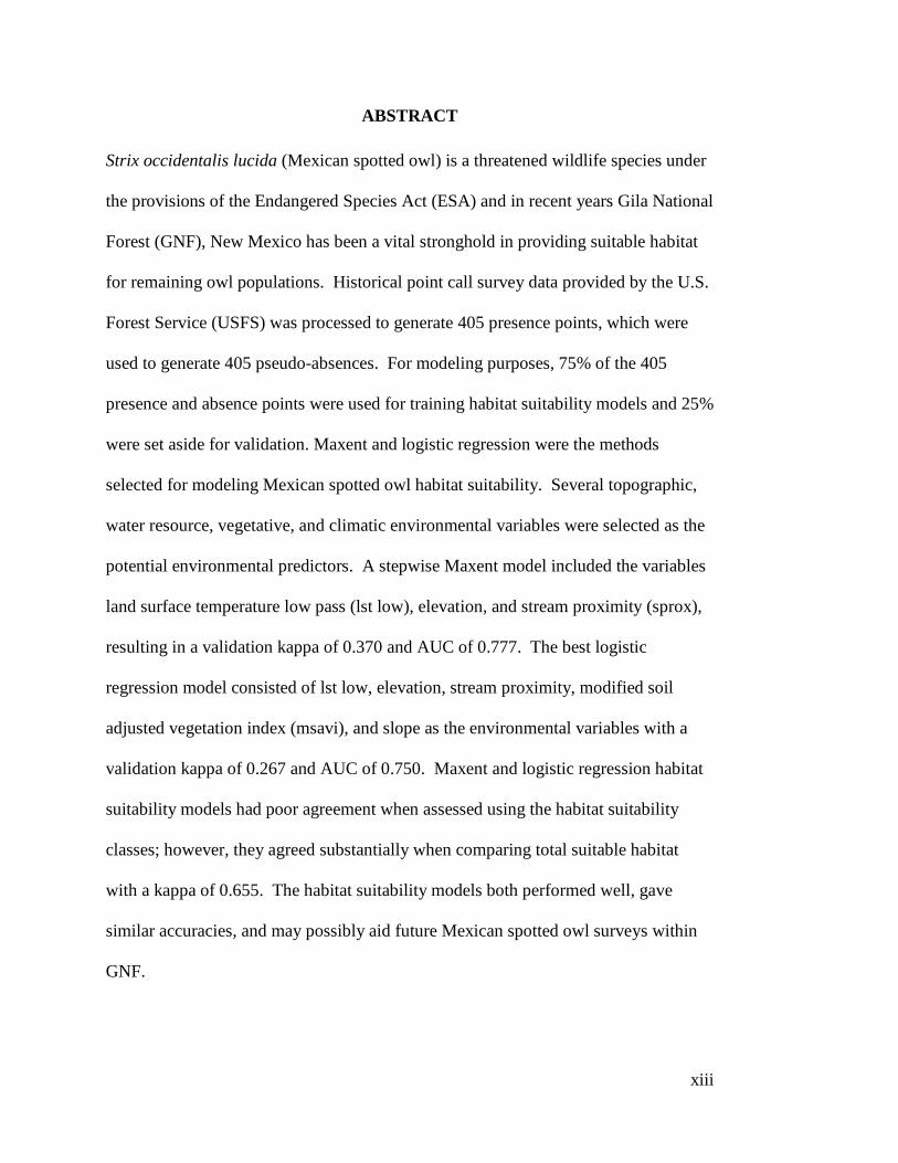
ABSTRACT Strix occidentalis lucida (Mexican spotted owl) is a threatened wildlife species under

the provisions of the Endangered Species Act (ESA) and in recent years Gila National

Forest (GNF), New Mexico has been a vital stronghold in providing suitable habitat

for remaining owl populations. Historical point call survey data provided by the U.S.

Forest Service (USFS) was processed to generate 405 presence points, which were

used to generate 405 pseudo-absences. For modeling purposes, 75% of the 405

presence and absence points were used for training habitat suitability models and 25%

were set aside for validation. Maxent and logistic regression were the methods

selected for modeling Mexican spotted owl habitat suitability. Several topographic,

water resource, vegetative, and climatic environmental variables were selected as the

potential environmental predictors. A stepwise Maxent model included the variables

land surface temperature low pass (lst low), elevation, and stream proximity (sprox),

resulting in a validation kappa of 0.370 and AUC of 0.777. The best logistic

regression model consisted of lst low, elevation, stream proximity, modified soil

adjusted vegetation index (msavi), and slope as the environmental variables with a

validation kappa of 0.267 and AUC of 0.750. Maxent and logistic regression habitat

suitability models had poor agreement when assessed using the habitat suitability

classes; however, they agreed substantially when comparing total suitable habitat

with a kappa of 0.655. The habitat suitability models both performed well, gave

similar accuracies, and may possibly aid future Mexican spotted owl surveys within

GNF.

1

CHAPTER 1: INTRODUCTION The Mexican spotted owl (Strix occidentalis lucida) is one of three sub-species of

spotted owl recognized by the American Ornithologists Union (AOU). The other two

species are the Northern (Strix occidentalis caurina) and California spotted owl (Strix

occidentalis occidentalis), which are geographically isolated from the Mexican

spotted owl. In 1993, the U.S. Fish and Wildlife Service (USFWS) designated the

Mexican spotted as “Threatened” under the provisions of the Endangered Species

Act. Two primary reasons for its listing were alterations to its habitat due to

inadequate timber management practices and the continuation of these practices, and

catastrophic wildfires (USDI 1995).

At the time of its listing the USFWS developed a formal Mexican spotted owl

Recovery Plan which was completed in 1995. This Recovery Plan was the USFWS’s

attempt at restoring and conserving the population of Mexican spotted owls.

Management actions for the Mexican spotted owl recovery plan were specifically

designed to enhance the critical habitat of Mexican spotted owls. Critical habitat

refers to specific geographic locations vital for the conservation of threatened or

endangered species requiring special management actions. Critical habitat

designation only pertains to areas receiving federal funding, permits or authorization.

The Mexican spotted owl recovery plan proposed three levels of management: (1)

Protected areas; (2) Restricted areas; and (3) Other forests and woodland types.

Protected regions are considered the most important to the status of Mexican spotted

owls. Protected Activity Centers (PACs) include an area at least 243 hectares (600

acres) around known or historical nest or roost sites (generally slopes > 40% in

mixed-conifer and pine-oak forests that have not been harvested within the past 20

2

years) and adjacent foraging areas which may be in open Ponderosa pine (pinus

ponderosa) or even Piñon-Juniper stands.

The conservation and management of wildlife species is highly reliant on the

geographic location of potential habitat (Margules and Pressey 2000) that, in turn,

relies on research which clarifies the habitat preferences of the species. The Mexican

spotted owl recovery plan resulted in the designation of 4,629,883 acres of Mexican

spotted owl critical habitat. Of this total acreage, 1,125,955 acres are located within

Gila National Forest (GNF), comprising 24% of the total critical habitat in the U.S.

GNF contains three regions designated as critical habitat and 286 as Mexican spotted

owl protected activity centers (PACs). Despite these statistics, GNF has not been

entirely surveyed. The unsurveyed and remote locations may exhibit environmental

conditions suitable for Mexican spotted owl populations and as such may deserve

special management consideration.

The purpose of the study is to identify areas within GNF which may be

considered “suitable habitat” for use by the Mexican spotted owl. This work meets a

principal objective of the Mexican spotted owl Recovery Plan to identify and

delineate potential and occupied habitat (USDI 1995). Suitable habitat was predicted

using the presence-only and presence-absence statistical modeling methods of

maximum entropy and logistic regression. This study examines the accuracy of each

modeling method in predicting suitable habitat. In addition, this study seeks to

determine which potential environmental variables are most important to Mexican

spotted owl habitat. The level of agreement between the presence-only and presence-

3

absence habitat suitability models is calculated to determine if any differences exist

and if so to what degree.

1.1 Habitat Suitability Modeling

In terms of ecology, a habitat suitability model can be used to identify spatial aspects

or abiotic characteristics of habitat that affect the presence, abundance, or diversity of

organisms (Dzeroski 2009). These models use sets of environmental characteristics

to identify those spatial units most associated with the species of interest. They can

incorporate three different types of input data: abiotic, biotic, and resources variables

related to human activity and their impacts on the environment. Abiotic

environmental variables include terrain, geological composition (soil type, substrate),

physical and chemical properties of the soil, air and water, temperature, and

precipitation. Biological (i.e. biotic) input variables of the environment are coarser,

being more directly related to the species of interest. For example, modeling of

Mexican spotted owl habitat should include information such as snag density and

downed logs. Some environmental variables like land cover, exhibit abiotic and

biotic characteristics. The third group of environmental variables relates to human

impacts, such as fire, proximity to roadways, and adjacent development.

Habitat suitability models are developed through a variety of approaches.

Some of the earliest attempts to predict wildlife presence and relative abundance

included the Wildlife-Habitat Relationship System (WHR) and Habitat Suitability

Index (HSI). These habitat models have been used frequently; however, they are

literature based, usually do not pertain to well-defined populations, and lack any

4

statistical foundation (Dettmers and Bart 1999). The use of statistical models for

predicting the likely occurrence or distribution of species is fitting in wildlife

conservation and management (Pearce and Ferrier 2000b). Habitat suitability models

can be generated through several statistical analysis methods: linear regression,

logistic regression, discriminant analysis, principal component analysis, canocial

component analysis, and classification and regression tree analysis. Given that most

species exist in specific habitat conditions, the spatial distribution of many species

can be predicted by linking their occurrence patterns with selected environmental

parameters (Guisan and Zimmerman 2000). The most accurate habitat models are

derived from wildlife distribution data. However, collection of such data is often

expensive and labor intensive. Habitat suitability models using geographic

information systems (GIS) are cost effective in identifying and predicting suitable

habitat. GNF has been subjected to GIS modeling of Mexican spotted owl habitat,

but the model biological inputs were older and less cumbersome. Particular attention

is needed within this region, since it serves as a vital stronghold for Mexican spotted

owl populations (Ganey 2004).

1.2 Description of the Study Area GNF is located in west-central New Mexico (Figure 1). The forest encompasses

approximately 3.3 million acres of public land, making it the sixth largest national forest

in the continental U.S. Its landscape is dominated by rocky mountain ranges dissected by

river valleys. Elevations range from 1,370 to 3,350 m. GNF also contains the largest

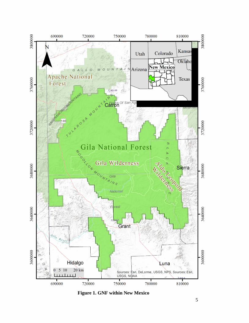
5

Figure 1. GNF within New Mexico

6

wilderness area within the Southwest, and vegetation ranges from semi-desert shrubland

and grasslands in lower elevations and to subalpine forest in higher elevations. Mid-

elevation regions are dominated by mixed woodlands of pinyon (Pinus edulis), juniper

(Juniperus spp.), and oak (Quercus spp.) and forests of ponderosa pine (Pinus

ponderosa) intermixed with plains-mesa grasslands. Montane coniferous forests of white

fir (Abies concolor), blue spruce (Picea pungens), Douglas-fir (Pseudotsuga menziesii),

and southwestern white pine (Pinus strobiformis) occupy large expanses of the upper

elevations with the highest slopes and ridges dominated by subalpine coniferous forests

of subalpine fir (Abies lasiocarpa) and Engelmann spruce (Picea engelmannii).

Interspersion of broadleaf forests of quaking aspen (Populus tremuloides) and gambel

oak (Quercus gambelii) occur throughout the montane and subalpine regions (Dahms and

Geils 1997).

GNF climate consists of dry mild winters and dry summers interspersed with a

monsoon season of about two months starting in mid-July. Average daily temperatures in

low elevation (< 2,500 m) areas range seasonally from 1.7°C to 21°C and higher

elevation areas (> 2,500 m) exhibit average daily temperatures from -5°C to 14°C.

Average annual precipitation can range from < 200 mm in the low elevation shrublands

to > 1,000 mm in the upper elevation subalpine forests.

This region contains large road-less areas, reducing the pressure of habitat loss

that can occur with regular land use. GNF contains a series of rocky mountain ranges

separated by river valleys and streams. The landscape within GNF has been highly

dissected by intense rainstorms which expedite erosion and geomorphological processes,

thus generating diverse topographic and biophysical settings.

7

1.3 Thesis Organization The remainder of the thesis is organized as follows. Chapter 2 introduces habitat

suitability modeling using GIS and briefly discusses its increased usage in ecological

applications. Deductive and inductive modeling approaches will be described using

details about their processes and applications. A summary of the available habitat

suitability modeling techniques is provided as well as details about the most

commonly used techniques: maximum entropy and generalized linear models

(GLMs). Habitat suitability model performance measures and influencing variables

are also briefly discussed.

Chapter 3 describes the methodology used in this study, beginning with the

methods for generating presence and presence-absence data. The selection and

preparation of environmental variables will be described in detail here. The habitat

suitability modeling process for presence-only and presence-absence models also will

be explained in detail, including multicollinearity analysis among environmental

variables, model selection, validation, mapping, and comparison.

The results of this study are shown in Chapter 4, beginning with the

mulitcollinearity analysis of the selected environmental variables. The presence-only

and presence-absence modeling results are summarized next and the chapter

concludes with an assessment of the level of agreement between the presence-only

and presence-absence habitat suitability models.

8

Chapter 5 compares the results of the presence-only and presence-absence

modeling methods as they relate to previous research. The limitations and

assumptions of habitat suitability models are discussed along with recommendations

for future research. The significant findings resulting from this study are highlighted

in the final thoughts.

9

CHAPTER 2: RELATED WORK Ecological research has continually identified the habitat requirements of many

species of wildlife using species distribution, abundance, and suitability models

(Store and Jokimäki 2003). These habitat requirements vary among species and

entail the natural resources and environmental conditions present within a species

location. GIS applications are currently playing a pivotal role in ecological modeling,

by offering the capacity to generate habitat models derived from existing and

accessible data (vegetation surveys, remote sensing data, topographic maps, and

digital elevation models).

With the advent of GIS, predictive modeling of species niche requirements

and the spatial distribution of species has increased interest within wildlife

management related issues (Hirzel et al. 2006). Predictive models such as habitat

suitability models have been used for wildlife species distribution management

(Palma, Peja, and Rodrigues 1999), risk of biological invasion or endangered species

management (Guisan and Thuiller 2005), ecosystem restoration (Mladenoff et al.

1997), species reintroduction (Lenton, Fa, and Del Val 2000), population viability

analysis (Akçakaya, McCarthy, and Pearce 1995), and wildlife-human interfaces (Le

Lay, Clergeau, and Hubert-May 2001). Habitat suitability models have a variety of

uses with the utmost priority of predicting the presences or absences of species in an

area of interest based on the suitability of the species-environment relationships. In

addition, these models facilitate the rapid implementation of management decisions

with limited information (Palma, Beja, and Rodrigues 1999).

10

2.1 Deductive vs. Inductive Modeling According to Stoms, David, and Cogan (1992), GIS technology is capable of

modeling species distributions and habitats through two main approaches-inductive

and deductive. Exclusively both approaches have proven to be effective in modeling

species distributions; however, deductive is implemented the most. Deductive

approaches are determined a priori and attempt to predict the species spatial

arrangement by selecting the ecological requirements considered the most important.

The process of deductive habitat modeling involves the selection of the most

favorable environmental conditions required for the species survival by specialists

with experience and knowledge of the species (Figure 2).

Figure 2. General data flow of inductive and deductive GIS species

distribution/habitat models Source: adapted from Corsi, De Leeuw, and Skidmore (2000)

11

After identifying these environmental requirements a model can be generated

by logical or arithmetic map overlay processes (Jensen 1992; Congalton, Stenback,

and Barrett 1993). Results of these operations will produce a model indicating the

combined effects of all the environmental variables. Deductive approaches utilize

GIS layers in the analysis to create habitat models, since the species-environment

relationships are known.

Where species ecological requirements are unknown, inductive approaches

can be used. Inductive approaches use locations of species to identify their ecological

requirements. The end result of inductive habitat modeling is the same as deductive;

however, the analysis methods used in inductive models are more objectively driven.

Inductive approaches use GIS layers to both derive species-environment relationships

and to generate the habitat model (Figure 2). Both deductive and inductive

approaches can be implemented in an analytical or descriptive manner to derive

species-environment relationships. Deductive analytical approaches establish

variability by considering the advice of different specialists in order to define species-

environment relationships.

These approaches promote the inclusion of an acceptable range of

environmental variables based on species observation data. Analytical approaches

whether deductive or inductive can potentially identify which environmental

variables are the most important for species survival (Corsi, De Leeuw, and Skidmore

2000).

Deductive-analytical approaches are often implemented through methods such

as multi-criteria decision making or nominal group techniques, requiring inputs from

12

more than one specialist. Inductive-analytical approaches derive species-environment

relationships by using some type of statistical analysis such as classification trees,

generalized linear models (GLM), generalized additive models (GAM) (Guisan and

Zimmermann 2000), Bayes theorem approach (Grubb et al. 2003), discriminant

analysis, neural networks, logistic regression (Manel, Williams, and Ormerod 1999),

principal component analysis (PCA) (Singh et al. 2009), cluster analysis (Lazenby et

al. 2008), and mahalanobis distance (Hellgren et al. 2006).

Deductive-descriptive modeling uses prior specialist knowledge in a

deterministic manner, identifying associations of a species presence or absence with

environmental variables. Inductive-descriptive approaches typically involve overlay

of known species locations with the associated environmental variables. In

comparison, descriptive models whether deductive or inductive tend to incorporate

fewer environmental variables than analytical models and fail to identify variability

and relationships among the variables. Descriptive models lack information

indicating the importance of one variable over another (Corsi, De Leeuw, and

Skidmore 2000).

Deductive and inductive habitat modeling results can be classified as either

categorical-discrete or probabilistic-continuous. Categorical-discrete models are

typically polygon maps which classify each polygon in agreement with presence-

absence conditions or by nominal category. Discrete models are usually generated

using deductive modeling and link the presence of species to polygons of land unit

types (e.g., land-use, vegetation categories, and stewardship). Discrete model results

are static in illustrating species distribution, failing to account for species mobility.

13

Probabilistic-continuous models are continuous surfaces of an index illustrating

species presence in terms of relative importance of any given location with respect to

all the others. Examples of continuous model indices include suitability indices,

probability of presence, and ecological distances from optimum conditions.

Continuous models can identify and describe the randomness associated with locating

an individual of a species (Akçakaya 1993).

These predictive models typically are implemented to identify species-

relationships for predicting the occurrence of species in un-sampled locations (Hirzel

et al. 2006). Such models are very effective in modeling the habitat of threatened

species which are difficult to identify and locate (Store and Jokimäki 2003).

According to Guisan and Zimmermann (2000), predictive modeling involves

conceptual model formulation, calibration, and evaluation.

The conceptual model is composed of an ecological model and a data model.

Formulation of the conceptual model is achieved through descriptive data from

literature, field data, and laboratory experiments. Assumptions and theories to be

tested can also be incorporated into the ecological component of the conceptual

model. For instance, it may be assumed that Mexican spotted owl nest locations are

primarily determined by number of snags per acre rather than by forest species

composition. The methodology for the collection, measurement, and estimation of

data is vital to conceptual model formulation, since the majority of problems arise in

the data modeling process. Such problems include the selection of the appropriate

scale of observations and the ensuing positional accuracy when ecological field data

are used with GIS (Austin 2002).

14

Statistical model formulation or verification involves: (1) the selection of an

appropriate algorithm for predicting a particular type of response variable and estimating

the model coefficients; and (2) an optimal statistical approach with regard to the

modeling context (Guisan and Zimmermann 2000). Model selection requires extensive

knowledge about species-environment relationships and should only be performed after

acquiring such an understanding (Austin 2002). Statistical models can be effective in

providing a description of the realized niche of a species but conversely, poor in

representing a species fundamental niche (Guisan and Zimmermann 2000). Although

statistical models provide us with some underlying reasons why species prevail in certain

environmental conditions they fail to represent the realized niche that occurs in nature

(Silvertown 2004). The majority of statistical models is designed for specific purposes

and prior to usage should be tested to verify their adequacy for the intended research

goals. These models are accountable for the choice and format of the data and depend on

concrete assumptions about the data (Hirzel and Guisan 2002).

2.2. Habitat Modeling Techniques

Habitat suitability models can be generated using a variety of methods by either

utilizing presence-only or presence-absence species data. Generally these models

entail the counting of individuals of the target species within each plot. Plots are

considered the sampling units and variables are identified as either the number of

animals present or one or more habitat descriptors. According to this approach, zero

means “none present” and one represents “present”. When the quantity of a specific

species is recorded in this 0-1 binary format the data is referred to as presence-

15

absence data, which is not typical of most wildlife surveys. The majority of wildlife

surveys consist of presence-only data, where data is collected only from locations

where animals were actually observed. Presence-only data is frequently used for

surveying wildlife species which are highly mobile, and have the potential to use

other plots when the observer is not present. In such instances, an observer records

information of other plots used by the target species to alleviate the impossibility of

potential use (Dettmers and Bart 1999). Presence-only data models have performed

less accurately than presence-absence models and require more complex statistical

methods. Presence-absence data is generally incorporated into models using multiple

regression methods with generalized techniques and classification trees (GLM, GAM,

and CT; Guisan and Zimmermann 2000). Modeling techniques requiring presence-

only species data include ecological niche variable analysis (ENFA); e.g. Braunisch

et al. (2008), and Hirzel and Guisan (2002), environmental envelopes (BIOCLIM;

e.g. Beaumont, Hughes, and Poulsen 2005), maximum entropy modeling (MAXENT;

e.g. Phillips, Hughes, and Poulsen 2006), mahalanobis statistic (MAHAL; e.g.

Dettmers and Bart 1999), and Genetic Algorithms for Rule-Set Prediction (GARP;

e.g. Levin, Peterson, and Benedict 2004). One example from each class is examined

in more detail in the two subsections that follow.

2.2.1 Maximum Entropy Modeling

Maximum entropy is a well formulated statistical approach for making predictions or

assumptions about incomplete data. The idea of maximum entropy is to estimate a target

probability distribution by finding the probability distribution of maximum entropy (i.e.

16

that is most spread out, or closest to uniform), subject to a set of constraints that represent

our incomplete information about the target distribution. The information available about

the target distribution often presents itself as a set of real-valued variables, called

“features”, and the constraints are that the expected value of each feature should match its

empirical average (average value for a set of sample points taken from the target

distribution) (Phillips, Hughes, and Poulsen 2006).

Several advantages associated with maximum entropy modeling include:

(1) requires presence-only data; (2) can utilize continuous and categorical data,

and can include interactions between different variables; (3) implements

deterministic algorithms that ensure selection of the most optimal probability

distribution; (4) can use regularization to avoid over-fitting; (5) model outputs are

continuous, permitting improved classification of modeled habitat suitability; and

(6) can be applied to presence-absence data using conditional models (as in

Berger et al. 1996). Drawbacks of maximum entropy modeling are: (1) it

provides a general statistical method that lacks the error prediction techniques of

established methods such as GLM and GAM; (2) regularization is a relatively

new concept and requires further study; (3) it uses an exponential model for

probabilities, which is not confined to a range of values facilitating the prediction

of values for environmental conditions outside the range present in the study area

therefore attention is needed when extrapolating prediction data to another study

area or to future or past climatic conditions; and (4) special-purpose software is

required, as maximum entropy is not available in standard statistical packages

(Phillips, Hughes, and Poulsen 2006).

17

2.2.2 Generalized Linear Model (GLM) Logistic regression is a statistical modeling tool employed for estimating event

probabilities when the response variable is present or absent (Zarri et al. 2008). The

response variable in a habitat suitability model is represented by the target species

and the exploratory variables are the influencing variables. These designations can be

both interval or categorical (such as percent canopy cover and vegetation type).

Specific examples of logistic regression include GLMs and GAMs. GLMs are

logistic regression models which relate a linear combination of environmental

variables (exploratory variables) to the predicted variable (response variable) by use

of a logistic link function which limits the predicted variable to a probability of 0 to 1

(Guisan and Zimmermann 2000). GAMs are an extension of GLM but have the

ability to deal with highly non-linear and non-monotonic relationships between the

predicted variable and the environmental variables (Hirzel et al. 2006). Logistic

regression has been extensively used to predict the occurrence and habitat use by an

assortment of different wildlife species including gopher tortoise (Gopherusp

olyphemus) (Baskaran et al. 2006), Greater prairie chicken (Tympanuchus cupido)

(Keating 2004), Rocky Mountain elk (Cervus elaphus nelsoni) (Bian and West 1997),

roe deer (Capreolus capreolus) (Pompilio and Meriggi 2001), Bonelli’s eagle

(Hieraaetus fasciatus) (Lopez-Lopez et al. 2006), and Mexican spotted owl (Hathcock

and Haarman 2008).

18

2.2.3 Model Performance Measures Model validation is an important part in model building and is used to test the

performance of modeling approaches (Vaughn and Ormerod 2005). Model

performance can be accessed through a variety of methods; the most commonly used

are the receiver operator characteristic (ROC) curve and Cohen’s Kappa Statistic, i.e.

kappa statistic. ROC curves are built by using all conceivable thresholds to arrange

scores into confusion matrices, acquiring sensitivity and specificity for each matrix

and then plotting all sensitivity values (true positive fraction) on the y axis against

their equivalent (1 - specificity) values (false positive fraction) on the x axis (Fielding

and Bell 1997). The ROC can be summarized by the area under the curve (AUC) as a

measure of overall accuracy that is threshold independent and values range from 0.5

to 1.0. Values close to 0.5 indicate a fit no better than random expectance, while a

value of 1.0 indicates a perfect fit (Baldwin 2009).

The kappa statistic is a threshold dependent performance measure which

compares the agreement against that which might be expected by random chance, i.e.

chance-corrected proportional agreement. Kappa statistic values range from -1 complete

disagreement) through 0 (no agreement above that expected by random chance) to +1

(complete agreement).

2.2.4 Habitat Suitability Influencing Variables Though GIS technology has increased the efficiency of modeling wildlife habitat, it is

important to keep in mind that underlying variables constantly influence the

predictability of these models in terms of wildlife habitat use and suitability.

19

Research indicates the use of presence-absence data produces the most accurate

habitat suitability model; however, the quality of this data ultimately determines the

level of accuracy. Two common problems associated with presence-absence data are

those of commission and omission. Commission errors are a result of predicting

species where they do not occur, whereas omission errors fail to predict where a

species does occur (Guisan and Thuiller 2005). The quality of presence-absence data

relies on the sampling size of the observation data, i.e. the number of occurrences,

which can drastically impact modeling accuracy (Stockwell and Peterson 2005). The

sample size is directly related to the modeling technique to be implemented. For

example, Stockwell and Peterson (2005) found that surrogate logistic regression

models produced the least accurate results at lower sampling sizes, while accuracy

was greatest when sample size was maximized. In addition, Stockwell and Peterson

(2005) concluded that GARP requires half the sampling size of logistic regression to

achieve the same level of accuracy.

To improve modeling accuracy the sampling design should consider the method

of presence-absence data collection. The majority of habitat models which implement

observational data lack appropriate sampling designs (Guisan and Zimmermann 2000).

An effective sampling design should designate an appropriate spatial scale (Fitzgerald

and Lees 1994), set of ecologically meaningful variables (Guisan and Zimmermann

2000), and a sampling strategy that identifies all the influencing variables and satisfies

modeling objectives (Wessels et al. 1998). To maximize habitat modeling accuracy, the

sampling design needs to embrace the resource, direct, and indirect ecological gradients

related to the target species (Guisan and Zimmermann 2000).

20

Accuracy in modeling of wildlife habitat suitability is significantly impacted by

the quality and quantity of species presence data; however, accurate absence data is

equally important. Confirmation of species absences is difficult and is a result of the

survey failing to detect a species that is currently residing within that location; even if the

species is roosting or residing elsewhere within its home range (MacKenzie 2005).

The assumption that species are absent due to unsuitable habitat may be invalid

for the following-reasons habitat population dynamics, fragmentation, rate of dispersal or

history-which may force species to use least optimal habitats (Brotons et al. 2004; Araujo

and Williams 2000). If absences are correlated to low suitable habitat the information

derived from them should enhance model accuracy (Hirzel et al. 2006). As with

presence-absence data that exhibit omission and commission errors, absences can be

either true of false. True absences are those occurring in locations that are deemed

unsuitable and false absences refer to instances in which the survey fails to detect the

species in habitat it is currently using. MacKenzie (2005) suggests that conducting

multiple surveys in a location within a short time frame can minimize the frequency of

false absences.

Survey detection of a species is influenced by many variables including the

sampling methods, environmental conditions, population density, and species-specific

characteristics. Species-specific characteristics are vitally important, especially when

species of wildlife change their activity patterns according to the time of day and the

seasons. For instance, species such as Mexican spotted owl are nocturnal, thus the

majority of surveys are conducted at night. Population density also has an influence. The

more individuals present, the greater the probability of detection. Accurate collection of

21

absence data can be achieved through sampling methods that guarantee high probability

of detection and sufficient sampling effort. Some effective sampling methods of species

occupancy include standard design, double sampling, and removal sampling. Removal

sampling designs are identified as the most efficient methods for determining species

occupancy especially when detection probability is constant (MacKenzie and Royle

2005).

MacKenzie (2005) indicates that detection probability should be a high priority in

collecting presence-absence data and is vital to making informed management decisions.

MacKenzie and Royle (2005) suggest that low probability of false absences should

incorporate more sampling units rather than increasing surveys per sampling unit. When

the probability of detecting a false absence is high, supplementary surveys need to be

performed. Prior to developing a sampling strategy, the why, what, and how of the

intended study need to be fully addressed: why collect the data, what type of data to

collect, and how should the data in field be collected and analyzed (Yoccoz, Nichols and

Boulinier 2001).

Uncertainty about presence-absence data can significantly impact modeling

accuracy; however, other variables can influence habitat suitability modeling success as

well. The spatial scale or resolution of models can affect the relationships that are

identified between the habitat variables and species presence-absences (see Graf et al.

2005). Model accuracy is affected by the spatial scale of habitat variables, for example,

Graf et al. (2005) identified that some habitat variables explained species occurrences

better at small scales, while others performed better at large scales. The type of habitat

analysis being conducted is ultimately going to determine the appropriate scale to use.

22

For instance, if the research objective is to model suitable habitat patches of a target

species, the model should be developed at a relatively small scale. If the research aim is

to model the population distribution and connectivity, implementation of large scale

models is more appropriate (Graf et al. 2005). Research has indicated that multi-scaled

approaches are effective tools in modeling wildlife habitat at small and large scales (e.g.

Graf et al. 2005, Store and Jokimäki 2003). In addition, spatial scale influences the

impact spatial autocorrelation has on a model. Characteristically species distributions are

positively autocorrelated, thus indicating that nearby locations are exhibiting more

similar characteristics than would be expected by random chance (Lichstein et al. 2002).

Spatial autocorrelation results may be exacerbated when the sampling locations are

positioned too close together, voiding the independence of species observations, hence

potentially overestimating the effects of habitat variables, which themselves are

autocorrelated (Guisan and Zimmermann 2000; Gumpertz, Graham, and Ristaino 1997).

Using sampling distances larger than the minimum distances at which autocorrelation

occurs can help avoid autocorrelation. In situations where sampling distance is too low

to avoid autocorrelation, an autocorrelative model can be used (Guisan and Zimmermann

2000; Roxburg and Chesson 1998).

Accuracy in habitat suitability modeling is also influenced by the choice of habitat

variables, the method by which they are selected, and level of model complexity.

Research by Duff and Morrell (2005) shows that specific habitat variables such as

elevation are better in predicting silver haired bats (Lasionycteris noctivagans) and big

brown bats (Eptesicus fuscus), while distance from lakes and ponds is better for

predicting presence of Yuma myotis (Myotis yumanensis). Since habitat variables make

23

or break the modeling process, proper methodology needs to be used in selecting these

variables. Ideally the selected habitat variables need to produce the best suitability model

for the target species in terms of predictive accuracy, within the limits of biological

knowledge and data (Pearce and Ferrier 2000b).

According to Hosmer and Lemeshow (1989) the selection of habitat variables

needs to incorporate: (1) a plan of action to select the habitat variables; and (2)

methods for assessing the sufficiency of the model both in terms of individual

variable and collective variable modeling accuracy. When generating habitat

suitability models, in which the target species is not well understood or the

importance of individual habitat variables and associations are not known, stepwise

selection should be used (Hosmer and Lemeshow 1989).

24

CHAPTER 3: DATA AND METHODS In this chapter, the methodology used to construct spatial models of Mexican spotted

owl habitat suitability using different techniques is discussed in detail. This

methodology is organized and discussed using the following subsections: (1)

biological input data management; (2) multicolinearity analysis; (3) modeling and

analysis; (4) model validation; and (5) agreement between predictive models.

3.1 Biological Input Data Management The first procedure details the processes used to generate the biological input data

needed for model formulation. The biological input data are divided into two parts:

(1) species’ observation data extraction; and (2) environmental variable selection and

creation.

3.1.1 Species’ Presence Data Extraction Mexican spotted owl presence data were derived from the Natural Resource

Information System (NRIS) geodatabase provided by the U.S. Forest Service Region

3, GNF. Two point feature classes identified as NRIS Wildlife Observations and

NRIS Wildlife Sites were used from the geodatabase which consisted of: (1) Global

Positioning System (GPS) point locations of wildlife survey observations and

historical records; and (2) wildlife site visits. These point feature classes contained

survey observations and site visit observations for all wildlife species surveyed within

the GNF administrative bounds, which included a section of Apache National Forest.

25

To include only point presences within the study area, Esri ArcMap 10.0 was used to

clip both feature classes to the boundary of the study area.

After clipping to the study area, both presence feature classes still contained point

locations of species that were not of interest. To select only presences of Mexican

spotted owl, ArcMap ‘Select by Attributes’ was used to perform the following Structured

Query Language (SQL) query:

SELECT * FROM NRIS Wildlife Observations NRIS Wildlife Sites

WHERE: “COMMON NAM” = Mexican Spotted Owl.

(1)

Each selection output was exported into a new point shapefile containing observations

(Mexican spotted owl Observations) and site visits (Mexican spotted owl Site Visits) of

Mexican spotted owl. The NRIS Wildlife Observation and NRIS Site Visit selection

layers were exported into shapefiles because ‘Select by Attributes’ will not work on

layers created from selections unless the layer is exported and saved as a shapefile or

feature class. Although the Mexican spotted owl observation dataset contained extensive

historical records, ‘Select by Attributes’ was used to select only observations collected

from 1990 through 2009. To prepare the Mexican spotted owl SiteVisit dataset, the

sampling point locations were deleted, leaving the nest and roost locations for model

development. The preceding clipping and select by attribute operations of the presence

data resulted in 1,535 visual/aural observations, 108 nests, and 102 roosts.

The Mexican spotted owl presence data displayed a clustered distribution pattern

with significant spatial autocorrelation, which is typical of ecological data. Spatial

autocorrelation indicates a lack of independence between pairs of observations at given

distances in space or time (Legendre 1993). To ensure independence and reduce spatial

26

autocorrelation, 182 ha buffers were applied to all presence locations using the

ArcToolbox ‘Buffer’ tool, to enforce a minimum distance of 761.13 m between

presences. Collection date and type of presence was used in eliminating locations failing

to meet these minimum distances. The priority of presence types followed sequentially,

nests, roosts, and observations. The most recent presences meeting minimum distance

requirements were retained for training and testing the models. Results of the minimum

distance analysis yielded a total of 320 owl observations, 54 nest, and 31 roost sites.

Processed Mexican spotted owl Observation and Mexican spotted owl Site Visit

presences were merged into a single Mexican spotted owl presence shapefile and

assigned XY coordinates using the spatial reference system selected for this research:

Universal Transverse Mercator (UTM), North American Datum 1983 (NAD83), Zone 12

North (12N), meters. The Mexican spotted owl presence dataset was used to directly

train and test the habitat suitability models. The ArcMap Geostatistical Analyst ‘Subset

Features’ tool was used to split the 405 Mexican spotted owl presences into 304 (75% of

405) for training and 101 (25% of 405) for testing (Figure 3).

3.1.2 Species’ Absence Data Creation Appropriate selection of presence data is essential for presence-only and presence-

absence habitat suitability modeling; however, the appropriate selection of pseudo-

absences or background locations is equally important. Instead of generating random

pseudo-absences throughout the study area, random sampling was confined to the convex

hull of all the presences and excluded from the 182 ha buffers of all the presences. This

selection was designed to compensate for the spatial bias associated with the presences.

27

Figure 3. Training and testing presences for Mexican spotted owl in GNF

28

Figure 4. Training and test absences for Mexican spotted owl in GNF

29

The Esri ArcToolbox was used to generate a minimum convex polygon (MCP) of

all 1,745 presences prior to presence data preparation. The MCP of all presences was

then clipped to the boundary of GNF. Using the MCP as the input feature and 182 ha

presence buffers as the erase features, the ArcToolbox ‘Erase’ function was executed to

generate the pseudo-absence sampling area. The pseudo-absence sampling area was then

used for generating random pseudo absence points for training and testing the Maxent

and GLM models.

Using the pseudo-absence sampling area polygon as the constraining feature

class, 10,000 as the number of points, and 30 m as the linear threshold between points,

the ArcToolbox ‘Create Random Point’ function was used to create the Maxent training

pseudo absences or the target background. Maxent and GLM validation was performed

using the same independent pseudo-absences. Unlike Maxent, GLM required pseudo-

absences for training as well as validation. A total of 405 pseudo-absences were

generated using the same procedures for generating the Maxent target background. The

405 pseudo-absences were split into 304 (75% of 405) for training the GLM and 101

(25% of 405) for testing Maxent and GLM using the same procedure as was used for the

presence data (Figure 4). The pseudo-absence data sets were assigned XY coordinates

using the same coordinate system as the presence data. Preparation of the pseudo-

absence datasets was complete aside from extracting the environmental variable values.

3.2 Environmental Variables Sixteen environmental variables were selected as potential predictor variables of

Mexican spotted owl distribution according to the scientific literature and expert’s

30

hypotheses. These variables were categorized into four groups: topographic, water

resources, vegetation, and climatic variables. Table 1 lists the units and data sources

for the potential environmental variables.

Table 1. Potential predictor variables and data sources used in modeling habitat suitability of Mexican spotted owl in GNF

Environmental variable Units Data source

Topographic

Compound topographic index (cti) --

USGS 1-arc second NED

Eastness (e) --

Elevation (elev) m

Northness (n) --

Planimetric Curvature (curve)

Radiansm

Slope º Water Resources Stream Proximity (sprox) m USGS NHD (1:24,000)

Vegetation

Percent Canopy Cover (cc) % canopy cover

USFS Region 3 mid-scale vegetation geodatabase

Tree Size (ts) DBH size classes

Normalized difference vegetation index (ndvi) --

USGS Landsat 7 ETM+ Bands 3 and 4 Modified soil adjusted

vegetation index (msavi) --

Tasseled Cap Brightness (bright) --

USGS Landsat 7 ETM+ Bands 1-5 and 7

Tasseled Cap Greenness (green) --

Tasseled Cap Wetness (wet) --

Climatic

Land surface temperature low pass (lst low) º C USGS Landsat 7 ETM+

Band 6 low and high pass Land surface temperature high pass (lst high) º C

31

Unlike the wildlife distribution data which required special use permits from the

USFS, the data sources used for all the environmental variables are freely available

through public access websites. Topographic variables were taken from National

Elevation Dataset (NED) snapshots obtained from the National Hydrography Dataset

Plus (NHDP) website accessible at http://www.horizon-systems.com/nhdplus. The

NHDP contains water resources variables in low resolution (1:100,000); however, high

resolution (1:24,000) hydrology data was preferred for model formulation. The high

resolution hydrology data and categorical vegetation data (% canopy cover, tree size)

used for this study is available through the USFS GNF GIS data portal. Data sources for

generating Landsat derived vegetation indices and climatic variables are freely available

from the U.S. Geological Survey (USGS) LandsatLook Viewer.

3.2.1 Topographic Variables Topographic variables were derived from snapshots of the 1 arc-second NED. The 1

arc-second NED was selected because it matched the 30 m by 30 m cell size that was

used for all of the other environmental variables. The NED was authored in

December, 2011 from the USGS, yet was obtained from the Horizon Systems

Corporation NHDP Version 2 hydrologic data. The NHDP data is distributed by

major drainage areas of the U.S. GNF is located within the Colorado and Rio Grande

drainage areas. These drainage areas are divided into vector processing units,

containing several raster processing units. This study required 1 arc-second NED

snapshot grids of raster processing units 15a and 13a. The vertical measurement

unit of the NED was centimeters and prior to mosiacing, the grid measurements were

http://www.horizon-systems.com/nhdplus/

32

converted to meters. The NEDs were mosiacked into one raster grid using Esri’s

‘Mosiac to New Raster’ function with specific settings (Table 2).

Table 2. Raster settings used for NED mosiac

Settings Values Spatial reference UTM NAD83 Zone 12N Pixel type 32-bit float Cell size 30 Number of bands 1 Mosiac operator Mean Mosiac colormap mode First

Before calculation of topographic derivatives, the NED mosaic was clipped to the

study area using the ArcToolbox ‘Extract by Mask’ tool to reduce computation time. The

imperfections of the NED were then removed, by using Esri’s ‘Fill sinks’ function.

Using the NED, three topographic derivatives (eastness, northness, and slope) were

calculated using Esri’s ArcGIS Desktop 10.0 Spatial Analyst Extension. Slope was

calculated in degrees and provided a measurement of terrain steepness; the greater the

value the steeper the terrain. Aspect is a circular measure of degrees from north and can

cause misleading results. For instance, a cell with an aspect of 359° would be assigned a

much different value than a cell with an aspect of 1° even though in reality their

orientations are similar. Hence, aspect was divided into two linear components of

eastness and northness by calculating the sine (eastness) and cosine (northness) of the

original aspect values using Esri’s ‘Raster Calculator’. Both eastness and northness

ranged from -1 to 1, with negative values indicating west and south facing aspects and

positive values indicating east and north facing aspects, respectively.

33

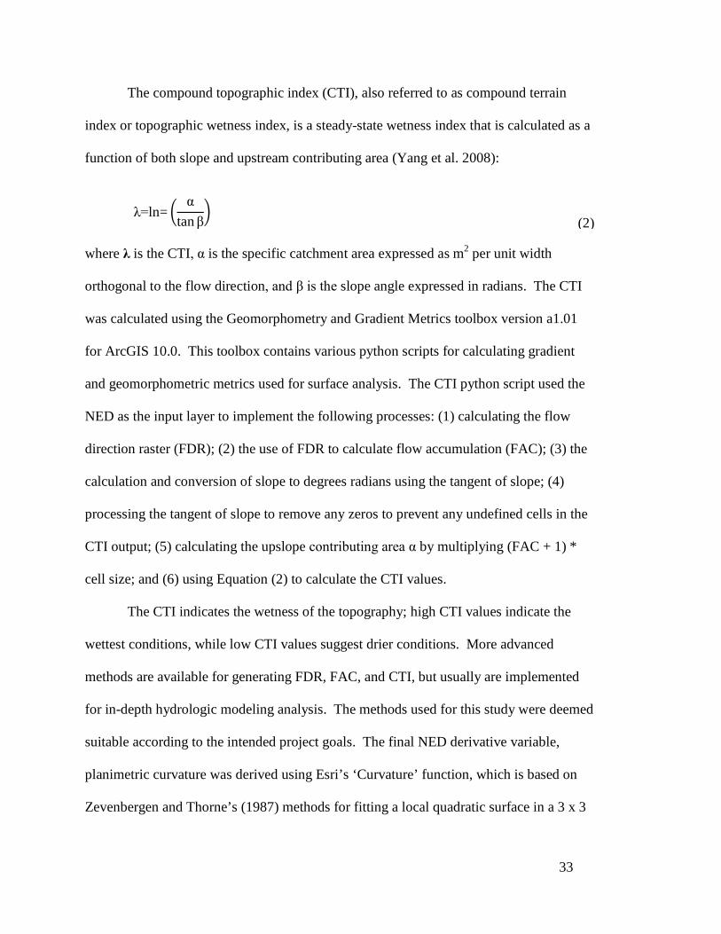
The compound topographic index (CTI), also referred to as compound terrain

index or topographic wetness index, is a steady-state wetness index that is calculated as a

function of both slope and upstream contributing area (Yang et al. 2008):

λ=ln= �α

tan β�

(2) where λ is the CTI, α is the specific catchment area expressed as m2 per unit width

orthogonal to the flow direction, and β is the slope angle expressed in radians. The CTI

was calculated using the Geomorphometry and Gradient Metrics toolbox version a1.01

for ArcGIS 10.0. This toolbox contains various python scripts for calculating gradient

and geomorphometric metrics used for surface analysis. The CTI python script used the

NED as the input layer to implement the following processes: (1) calculating the flow

direction raster (FDR); (2) the use of FDR to calculate flow accumulation (FAC); (3) the

calculation and conversion of slope to degrees radians using the tangent of slope; (4)

processing the tangent of slope to remove any zeros to prevent any undefined cells in the

CTI output; (5) calculating the upslope contributing area α by multiplying (FAC + 1) *

cell size; and (6) using Equation (2) to calculate the CTI values.

The CTI indicates the wetness of the topography; high CTI values indicate the

wettest conditions, while low CTI values suggest drier conditions. More advanced

methods are available for generating FDR, FAC, and CTI, but usually are implemented

for in-depth hydrologic modeling analysis. The methods used for this study were deemed

suitable according to the intended project goals. The final NED derivative variable,

planimetric curvature was derived using Esri’s ‘Curvature’ function, which is based on

Zevenbergen and Thorne’s (1987) methods for fitting a local quadratic surface in a 3 x 3

34

matrix, around a given point z5 (Figure 5). Planimetric curvature can be derived using

Equation (3):

plan= -2�dh2+ eg2- fgh�

(g2+ h2)

(3) where z is the elevation of the cell center, d = [(z4 + z6)/2-z5]/L2, e = [(z2 + z8)/2-z5]/L2, f

= [(-z1 + z3 + z7 – z9)/2-z5]/4L2, g = (-z4 – z6)/2L, h = (z2 – z8)/2L, and L = Cell size. The

planimetric curvature reveals the curvature of the surface perpendicular to the slope

direction.

All resulting topographic variable grids were then resampled using Esri’s

‘Resample’ tool and bilinear interpolation. The resampled topographic variables were

later used for logistic regression analysis and converted to the American Standard Code

for Information Interchange (ASCII) format using Esri’s ‘Raster to ASCII’ function for

use in Maxent.

Figure 5. Method for calculating profile and planimetric curvatures in a 3 x 3 matrix Source: adapted from Zevenbergen and Thorne (1987)

35

3.2.2 Water Resources

The water resources variable (stream proximity) was created from the high resolution

NHD that the USFS Service Region 3 provided. This hydrology dataset contained many

hydrologic features and the ephemeral, intermittent, and perennial stream features were

chosen for use in this study. The ArcMap ‘Select by Attributes’ and ‘Create Layer From

Selection’ functions were used to generate a hydrology dataset containing only these

stream features. The Spatial Analyst ‘Euclidean Distance’ function was used to produce

a stream proximity grid with a 30 m cell size. This grid measured the proximity to the

nearest water source, such that low values are closer to the water source and high values

are further away. The geographic bounds, geographic projection, resampling method,

and data format (Esri Grid and ASCII) of the stream proximity variable were uniformly

defined to match those of all other variables.

3.2.3 Vegetation Variables The vegetation variables percent canopy cover and tree size were derived from the

USFS Region 3 mid-scale vegetation geodatabase. These data sources provided the

most current vegetation data for GNF. The mid-scale vegetation data were vector-

based; however, the modeling software required gridded datasets. The ArcToolbox

‘Feature to Raster’ tool was run to convert both mid-scale vegetation datasets to Esri

grid format using the description attribute field for assigning values to the output

raster and a 30 m cell size. The resulting percent canopy cover and tree size grids

were classified into eight description classes. Both mid-scale vegetation grids were

reclassified into four descriptive classes (Tables 3 and 4).

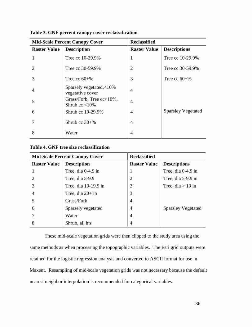
36

Table 3. GNF percent canopy cover reclassification

Table 4. GNF tree size reclassification

Mid-Scale Percent Canopy Cover Reclassified Raster Value Description Raster Value Descriptions 1 Tree, dia 0-4.9 in 1 Tree, dia 0-4.9 in 2 Tree, dia 5-9.9 2 Tree, dia 5-9.9 in 3 Tree, dia 10-19.9 in 3 Tree, dia > 10 in 4 Tree, dia 20+ in 3

Sparsley Vegetated 5 Grass/Forb 4 6 Sparsely vegetated 4 7 Water 4 8 Shrub, all hts 4

These mid-scale vegetation grids were then clipped to the study area using the

same methods as when processing the topographic variables. The Esri grid outputs were

retained for the logistic regression analysis and converted to ASCII format for use in

Maxent. Resampling of mid-scale vegetation grids was not necessary because the default

nearest neighbor interpolation is recommended for categorical variables.

Mid-Scale Percent Canopy Cover Reclassified Raster Value Description Raster Value Descriptions

1 Tree cc 10-29.9% 1 Tree cc 10-29.9%

2 Tree cc 30-59.9% 2 Tree cc 30-59.9%

3 Tree cc 60+% 3 Tree cc 60+%

4 Sparsely vegetated,<10% vegetative cover 4

Sparsley Vegetated

5 Grass/Forb, Tree cc<10%, Shrub cc <10%

4

6 Shrub cc 10-29.9% 4

7 Shrub cc 30+% 4

8 Water 4

37

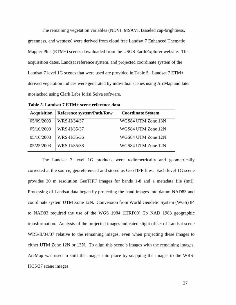
The remaining vegetation variables (NDVI, MSAVI, tasseled cap-brightness,

greenness, and wetness) were derived from cloud free Landsat 7 Enhanced Thematic

Mapper Plus (ETM+) scenes downloaded from the USGS EarthExplorer website. The

acquisition dates, Landsat reference system, and projected coordinate system of the

Landsat 7 level 1G scenes that were used are provided in Table 5. Landsat 7 ETM+

derived vegetation indices were generated by individual scenes using ArcMap and later

mosiacked using Clark Labs Idrisi Selva software.

Table 5. Landsat 7 ETM+ scene reference data

Acquisition

Reference system/Path/Row Coordinate System

05/09/2003 WRS-II/34/37 WGS84 UTM Zone 13N




The Landsat 7 level 1G products were radiometrically and geometrically

corrected at the source, georeferenced and stored as GeoTIFF files. Each level 1G scene

provides 30 m resolution GeoTIFF images for bands 1-8 and a metadata file (mtl).

Processing of Landsat data began by projecting the band images into datum NAD83 and

coordinate system UTM Zone 12N. Conversion from World Geodetic System (WGS) 84

to NAD83 required the use of the WGS_1984_(ITRF00)_To_NAD_1983 geographic

transformation. Analysis of the projected images indicated slight offset of Landsat scene

WRS-II/34/37 relative to the remaining images, even when projecting these images to

either UTM Zone 12N or 13N. To align this scene’s images with the remaining images,

ArcMap was used to shift the images into place by snapping the images to the WRS-

II/35/37 scene images.

38

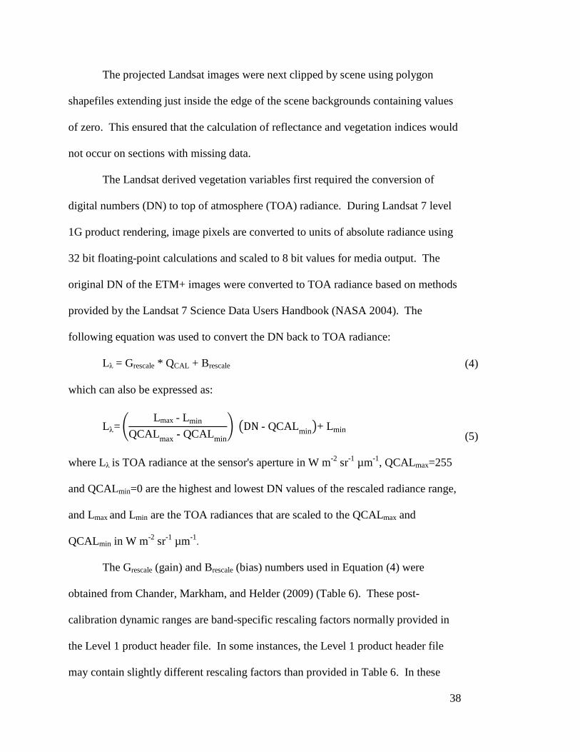
The projected Landsat images were next clipped by scene using polygon

shapefiles extending just inside the edge of the scene backgrounds containing values

of zero. This ensured that the calculation of reflectance and vegetation indices would

not occur on sections with missing data.

The Landsat derived vegetation variables first required the conversion of

digital numbers (DN) to top of atmosphere (TOA) radiance. During Landsat 7 level

1G product rendering, image pixels are converted to units of absolute radiance using

32 bit floating-point calculations and scaled to 8 bit values for media output. The

original DN of the ETM+ images were converted to TOA radiance based on methods

provided by the Landsat 7 Science Data Users Handbook (NASA 2004). The

following equation was used to convert the DN back to TOA radiance:

Lλ = Grescale * QCAL + Brescale

(4) which can also be expressed as:

Lλ=�Lmax - Lmin

QCALmax - QCALmin� �DN - QCALmin�+ Lmin

(5) where Lλ is TOA radiance at the sensor's aperture in W m-2 sr-1 µm-1, QCALmax=255

and QCALmin=0 are the highest and lowest DN values of the rescaled radiance range,

and Lmax and Lmin are the TOA radiances that are scaled to the QCALmax and

QCALmin in W m-2 sr-1 µm-1.

The Grescale (gain) and Brescale (bias) numbers used in Equation (4) were

obtained from Chander, Markham, and Helder (2009) (Table 6). These post-

calibration dynamic ranges are band-specific rescaling factors normally provided in

the Level 1 product header file. In some instances, the Level 1 product header file

may contain slightly different rescaling factors than provided in Table 6. In these

39

cases, the user should use the product header file information to convert image pixel

DNs to TOA radiance. TOA radiance was calculated for bands 1-7.

Table 6. TOA radiances, rescaled gains and biases

Band Lmin Lmax Grescale (Gain = High,Low)

Brescale (Bias)

1 -6.2 191.6 0.778740 High -6.98 2 -6.4 196.5 0.798819 High -7.20 3 -5.0 152.9 0.621664 High -5.62 4 -5.1 241.1 0.969291 Low -6.07 5 -1.0 31.06 0.126220 High -1.13 6 L 0.0 17.04 0.067087 Low -0.07 6 H 3.2 12.65 0.037205 High 3.16 7 -0.35 10.80 0.043898 High -0.39

While spectral radiance is the measure quantified by Landsat sensors, a

conversion to TOA reflectance was needed to reduce scene to scene variability.

Reflectance removes differences caused by the position of the sun and the differing

amounts of energy output by the sun in each band. The TOA reflectance was

calculated with the following equation:

Pλ= π *Lλ *d2

ESUNλ- sin(θSE) (6)

where Pλ is the TOA reflectance, Lλ is TOA radiance (W m-2 sr-1 µm-1), d is the earth

to sun distance in astronomical units at the acquisition date, ESUNλ is the band

specific solar irradiance (W m-2 sr-1 µm-1), and θSE is the solar zenith angle in degrees.

In addition to Lλ, three other pieces of information were required for calculating

reflectance. The first two were d, the earth-sun distance, and θSE, the solar elevation

angle. Both values are scene dependent, specifically the day of the year and the time

of the day when the scene was captured. The day of the year and solar elevation

40

angle were stored in the Landsat scene Level I header files ending with _MTL.txt.

These header files were searched to identify the day of the year labeled

“Date_Hour_Contact_Period” and solar elevation angle labeled “Sun Elevation”. The

date was in the following format “YYDDDHH” where the three “D” digits identify

the day of the year and solar elevation angle was in degrees. After acquiring the day

of the year, Table 7 from Chander, Markham, and Helder (2009) was used to find the

earth-sun distance for that day. The third piece of information ESUNλ, the band

specific solar irradiance, was also obtained from Chander, Markham, and Helder

(2009) (Table 8).

Once all of the necessary pieces of information for each individual scene were

obtained, the ArcMap raster calculator was used to compute reflectance for bands 1-5

and 7 using:

Pλ= π *Lλ *d2

ESUNλ- sin �θSE* π180.0�

(7)

Table 7. Landsat 7 ETM+ scene values for day of the year, d, and θSE

Landsat Scenes

Date Hour Contact Period (YYDDDHH)

d

(astronomical)

θSE

(degrees)

WRS-II/34/37 0312917 1.00952 63.6195766

WRS-II/35/37 0313617 1.01108 64.7472745

WRS-II/35/36 0313617 1.01108 64.2585779

WRS-II/35/38 0314517 1.01286 66.0676183

Source: from Chander, Markham, and Helder (2009)

41

Table 8. Landsat 7 ETM+ band specific solar irradiance

Band ESUNλ W m-2 sr-1 µm-1

1 1997

2 1812

3 1533

4 1039

5 230.8

7 84.9 Source: from Chander, Markham, and Helder (2009)

In some cases, calculation of reflectance from radiance can result in small

negative reflectances, which are not realistic and as a consequence, these were set to

zero. Negative reflectances were identified and set to zero in the same ArcMap raster

calculator.

Normalized Difference Vegetation Index (NDVI) is a reflectance-derived

vegetation index that is frequently used for quantifying productivity and the above-

ground biomass of ecosystems (Niamir et al. 2011). The NDVI states the ratio

between red and near-infared reflectance captured by satellite sensors and is

calculated by using the following equation:

NDVI=RNIR – RRED

RNIR + RRED=

Band 4 – Band 3Band 4 + Band 3

(8)

where RNIR and RRED indicate reflectance in the near-infared and red wavebands. The

NDVI values range from -1.0 to + 1.0. The negative values of NDVI (< 0) typically

correspond to water and urban features. NDVI values ranging from 0 to 0.1 represent

barren areas of rock, sand or snow. Moderate NDVI values (0.1 to 0.2) represent

grasslands and shrubs, while high values (0.2 to 1) indicate dense green leaf

42

vegetation (Lu et al. 2004). The ArcMap raster calculator was used to calculate

NDVI.

The Modified Soil Adjusted Vegetation Index (MSAVI) is a modified version

of the soil adjusted vegetation index (SAVI) that reduces the sensitivity of the NDVI

soil background by incorporating a self-adjusting soil factor. MSAVI was selected

because it has constant sensitivity over all ranges of vegetative cover making it quite

useful for general-purpose vegetation classification (Rondeaux, Steven, and

Baret.1996). To decrease the sensitivity to soil noise, MSAVI incorporates an

empirical L function into the NDVI equation:

MSAVI= �RNIR-RRED

RNIR+RRED+L� *(1+L)

(9)

where L = 1-2α * NDVI * Weight Difference Vegetation Index (WDVI), WDVI =

RNIR - αRRED (i.e. the weighted difference vegetation index), and α is the slope of the

soil line.

Calculating L, the soil adjustment factor, involved finding α, the slope of the

soil line. To find α, the NDVI grid was reclassified into a bare soil grid where NDVI

values ranging from 0 to 0.1 were assigned a value of 1, indicating bare soils, and all

NDVI values outside this range were assigned a value of 0, indicating not bare soil.

The bare soil grid was converted to an Esri point shapefile using the grid code as the

assigning value. To extract RRED and RNIR values from locations identified as bare

soils, ArcMap was used to generate a shapefile containing points classified as 1, bare

soils. The bare soils point data were used to extract RRED and RNIR values using the

extract multi-values to points tool within ArcMap. The bare soil attribute table was

then exported into a database file for linear regression analysis using the Microsoft

43

Excel add-in XL-Stats. Experimental studies have indicated that for a given type of

soil variability, the soil reflectance at the RRED wavelength is functionally related to

the reflectance in the RNIR wavelength (Rondeaux. Steven, and Baret 1996). This

relationship was approximated using the following simple linear equation:

p (RNIR)= α p (RRED) + b

(10)

where α, the slope and b, the intercept are coefficients dependent on both wavelengths

(RNIR, RRED) and the type of variability. The linear regression parameters that were

used to determine the slope of the line in XL-Stats are provided in Table 9.

Table 9. Linear regression parameters for identifying slope of soil line

Parameters Values

Explanatory Variable / X RRED

Dependent Variable / Y RNIR

Confidence Interval % 95

Tolerance 0.0001

The slope (α = 1.06) value derived from linear regression was entered into the

WDVI equation to obtain the final parameter for calculating L. After calculating L,

the ArcMap raster calculator was used to calculate MSAVI using Equation (9).

L usually ranges from 0 to 1; but small negative L values may occur with high

vegetation percentage cover (Qi et al. 1994). Vegetated areas show positive MSAVI

values up to 1, while non-vegetated areas will show negatives value down to -1.

The tasseled cap transformation is a channeled and scaled Principle

Component Analysis, which compresses the six Landsat ETM+ bands (1-5, and 7)

into three bands associated with soil brightness, vegetation greenness, and

soil/vegetation wetness. Essentially, tasseled cap transformations of Landsat ETM+

44

are either DN or reflectance factor based. Tasseled cap transformations for this study

were based on at-satellite reflectance, to eliminate the need for atmospheric

correction. The decision to use tasseled cap transformations was justified because

linear-based vegetation indices can provide better measures of forest stand parameters

than ratio-based indices (Lu et al. 2004). The tasseled cap transformations

measuring brightness, greenness, and wetness were calculated using the following

linear equation:

tas.capi=(coeff1*RBand1)+(coeff2*RBand2)+(coeff3*RBand3) +(coeff4*RBand4)+(coeff5*RBand5)+(coeff7*RBand7)

(11)

where tas.capi is the tasseled cap index for brightness, greenness, or wetness

depending on the coefficients used, RBand is the TOA reflectance, and the coefficients

for Landsat 7 ETM+ are as summarized in Table 10.

Table 10. Tasseled cap coefficients for Landsat 7 ETM+ at-satellite reflectance

Index Band 1 Band 2 Band 3 Band 4 Band 5 Band 7 Brightness 0.3561 0.3972 0.3904 0.6966 0.2286 0.1596

Greenness -0.3344 -0.3544 -0.4556 0.6966 -0.0242 -0.2630

Wetness 0.2626 0.2141 0.0926 0.0656 -0.7629 -0.5388 Source: from Huang et al. (2002)

Tasseled cap brightness, greenness, and wetness provided unitless measures

with values ranging from -1 to 1. Brightness measured overall reflectance, and was

used to differentiate the levels of soil exposure where -1 to 1 indicates the least

exposed to most exposed soil surface. Greenness is the difference between near-

infrared and visible reflectance and served as an index of vegetative cover density and

vigor, similar to NDVI, however it used six ETM+ bands instead of two. The value

range (-1, 1) of greenness indicates lowest density to highest density of vegetation.

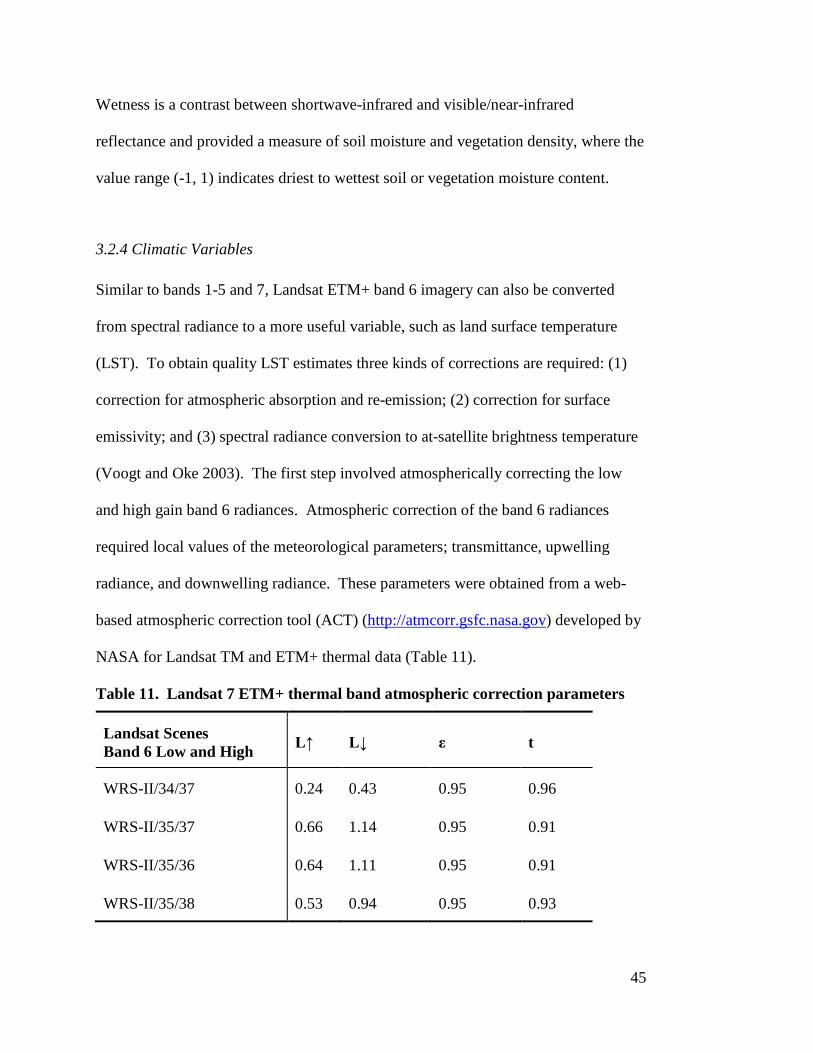
45

Wetness is a contrast between shortwave-infrared and visible/near-infrared

reflectance and provided a measure of soil moisture and vegetation density, where the

value range (-1, 1) indicates driest to wettest soil or vegetation moisture content.

3.2.4 Climatic Variables Similar to bands 1-5 and 7, Landsat ETM+ band 6 imagery can also be converted

from spectral radiance to a more useful variable, such as land surface temperature

(LST). To obtain quality LST estimates three kinds of corrections are required: (1)

correction for atmospheric absorption and re-emission; (2) correction for surface

emissivity; and (3) spectral radiance conversion to at-satellite brightness temperature

(Voogt and Oke 2003). The first step involved atmospherically correcting the low

and high gain band 6 radiances. Atmospheric correction of the band 6 radiances

required local values of the meteorological parameters; transmittance, upwelling

radiance, and downwelling radiance. These parameters were obtained from a web-

based atmospheric correction tool (ACT) (http://atmcorr.gsfc.nasa.gov) developed by

NASA for Landsat TM and ETM+ thermal data (Table 11).

Table 11. Landsat 7 ETM+ thermal band atmospheric correction parameters

Landsat Scenes Band 6 Low and High L↑ L↓ ε t

WRS-II/34/37 0.24 0.43 0.95 0.96

WRS-II/35/37 0.66 1.14 0.95 0.91

WRS-II/35/36 0.64 1.11 0.95 0.91

WRS-II/35/38 0.53 0.94 0.95 0.93

http://atmcorr.gsfc.nasa.gov/

46

Data are currently available from 2000 to the present. Using the values

obtained from the ACT, scene-specific atmospheric corrections were applied using

the equation:

CVR2= �CVR1- L↑

εt� - �

1- εε�L↓ (12)

where CVR2 is the atmospherically corrected cell value radiance, CVR1 is the cell

value of radiance from band 6 low or high gain, L↑ is the upwelling radiance, L↓ is

the downwelling radiance, ε is emissivity, and t is the transmittance. Once the band

6 radiance grids were atmospherically corrected, the inverse of the Planck function

was applied to derive temperature values. The inverse of the Planck function

converts the atmospherically corrected spectral radiance to LST using pre-launch

calibration constants. The conversion equation using atmospheric correction is:

LSTK = K2

ln �K1Lλ

+ 1�

(13) where LSTK is the land surface temperature in degrees Kelvin, Lλ is spectral radiance

in W m-2 sr-1 µm-1; and K2 and K1 are pre-launch calibration constants. For Landsat 7

ETM+, K2 = 1282.71 K, and K1 = 666.09 W m-2 sr-1 µm-1. A further subtraction of

273.15 K from both low and high gain derived LST was made to provide LST

measurements in degrees Celsius.

Further processing of Landsat derived vegetation indices was needed because

the Esri ArcToolbox ‘Mosiac to New Raster’ function did not level the grey scales

across all scenes. To generate mosaics of each vegetation index, the Esri grids were

converted to ASCII format and imported into Clark Labs Idrisi Selva software as

Idrisi raster files (.rst). The Idrisi raster files of each scene were input into the image

47

processing tools mosaic operation, where all default settings were used except the

overlap method which was changed to the average method. Mosiacked vegetation

indices were exported from Selva in Esri ASCII format and imported into ArcMap as

floating point grids. These grids were then clipped to the study area, resampled using

bilinear interpolation, and converted to ASCII format to provide raster grids for GLM

and Maxent.

3.3 Multicollinearity Analysis Before habitat modeling, a multicollinearity test was conducted to denote the

presence of a linear relationship or near linear relationship among environmental

variables. Multicollinearity analysis is essential in habitat suitability modeling, for

checking if the environmental variables in the model are correlated, which negatively

affects model performance (Peason et al 2007). Multicollinearity among continuous

variables was assessed using the most preferred method, the calculation of the

variance inflation factor (VIF) as shown in Equation (14) below:

VIFi= 1

1- Ri2

(14)

where Ri

2 is the coefficient of determination obtained after regressing the ith variable on

the remaining variables. Based on the above equation, if R2 is 0, then VIF will be 1, if R2

is 1, then VIF will approach infinity. VIFs higher than 10 indicate the presence of strong

multicollinearity. Correlation among the categorical variables (percent canopy cover and

tree size) was tested using the Phi coefficient from Pearson correlation among binary

variables.

48

Calculating VIFs and Phi coefficients of the environmental variables required the

use of Esri’s ‘Band Collection Statistics’ function, to generate ASCII text files containing

basic statistics and correlation matrices of environmental variable grids. Correlation

matrices of continuous and categorical variables were opened in Microsoft Excel as space

delimited text files. In Excel, the ‘MINVERSE’ function was used on correlation

coefficients of continuous variables to solve for Equation (14), while Phi coefficients of

categorical variables were analyzed for correlation. VIFs of continuous environmental

variables can be identified in the respective diagonal cells of the ‘MINVERSE’ output.

Variables with correlation coefficients > 0.75 were considered redundant and as

candidates for removal.

The correlated continuous variables with the highest VIFs were removed and

operations were repeated until the remaining variables had VIFs less than 10. Categorical

variables were binary for testing the correlation among percent canopy cover and tree

size classes; hence, the presence of correlated classes meant removal of an entire dataset.

3.4 Habitat Suitability Modeling Technique Many different modeling techniques and algorithms exist for predicting the

probability of species occurrences by using environmental variables as limiting

factors for species’ survival. Two modeling algorithms: Maximum Entropy (Maxent)

and Generalized Linear Models (GLMs) were used to predict the habitat suitability

for Mexican spotted owl in GNF. Maxent used presence-only data to train the model,

while GLM trained the model with presence/pseudo absence data, and both were

validated using an independent presence/pseudo absence dataset.

49

Maxent and GLMs both have their advantages and disadvantages. The

advantage of Maxent is that it requires only presence data of a species, while GLMs

require presence and absence data. Maxent is also able to fit complex relationships

between the species and the environmental variables, including interactions between

variables, unlike GLMs. On the other hand, GLMs and Maxent are useful for

analyzing predictor variable importance, and interpreting the response of the species

to each predictor. An equation derived from the Maxent algorithm is a “black box”;

such that it is not easy to understand how the algorithm is operating, whereas a GLM

can be expressed in a predictive equation. Maxent is deficient in that it extrapolates

the algorithm blindly from sample to population without user-customizable statistical

analysis. Conversely, users can statistically analyze data when GLMs are built.

Maxent is designed to make predictive maps of the area of interest, while GLMs are

not. Both model algorithms can utilize continuous and categorical environmental

variables.

3.4.1 Maximum Entropy (Maxent) Habitat suitability was modeled with Maxent version 3.3.3 k and the procedure shown

in Figure 6 was used for this thesis research project. Maximum entropy is a general

purpose machine learning technique, which predicts the probability distribution of a

target species based on presence-only data points and certain environmental variables

Phillips, Anderson, and Schapire 2006; Elith et al. 2011). It incorporates the

maximum entropy principle to estimate a target probability distribution by finding the

probability distribution closest to uniform, or spread out, subject to the constraints of

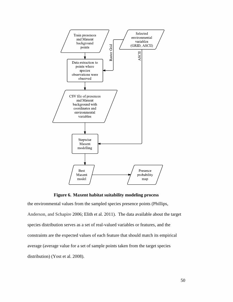
50

the environmental values from the sampled species presence points (Phillips,

Anderson, and Schapire 2006; Elith et al. 2011). The data available about the target

species distribution serves as a set of real-valued variables or features, and the

constraints are the expected values of each feature that should match its empirical

average (average value for a set of sample points taken from the target species

distribution) (Yost et al. 2008).

Figure 6. Maxent habitat suitability modeling process

51

To run models with Maxent, the Mexican spotted owl presence samples and

environmental variable layers were prepared in the “samples with data” (SWD) format to

expedite model processing and to avoid masking operations. For input of the Mexican

spotted owl training presence sample, a CSV file was created to contain only columns of

species common name, X and Y coordinates, and the extracted values of the

environmental variables to those point locations.

As input for the environmental layers, the target background of 10,000 point

locations was used to extract the values of the environmental variable layers to those

points using ArcMap 10.1. A new CSV file containing the columns of the

background label, X and Y coordinates and environmental values of each

environmental variable layer was prepared.

To reduce computational demand and model complexity, only the variables

remaining from multicollinearity analysis were extracted and used in modeling. Maxent

can utilize both categorical and continuous data; therefore, within the model settings

interface the environmental variable layers were identified as such (Phillips, Anderson,

and Schapire 2006). Since a targeted background was used both the Mexican spotted owl

and background samples had to be in SWD format. Because the SWD format does not

produce pictures or output grids, the model was trained on the SWD data, and then

projected onto full grids using ASCII layers of the environmental variables to generate a

probability map for each 30 by 30 m cell throughout the study area.

Maxent model runs used regularization (i.e. response curve smoothing) and the

sample bias mitigation techniques, recommended by Phillips, Anderson, and Schapire

(2006), using a target background. By using a target background the models will not

52

focus on sample selection bias, but will focus on any differentiation between the

distribution of presences and that of the background. In other words, if the species

occupies specific habitats within the study area, the model will highlight these habitats,

rather than just areas that are intensely sampled (Phillips et al. 2009). Since traditional

implementation of maximum entropy is prone to over-fitting, Maxent uses a smoothing

procedure called regularization, which constrains the estimated distribution so that the

average value of a given predictor is close to the empirical average rather than equal to it.

For detailed explanation of the mathematical formulas, see Phillips, Anderson, and

Schapire (2006).

All default parameters of Maxent were used except for increasing the maximum

number of iterations from 500 to 5,000 to allow the models to converge. Default settings

included: regularization multiplier = 1, convergence threshold = 0.00001, maximum

number of background points = 10,000, replicates = 1, replicated run type = cross

validate, and feature type = “Auto features”. By default, regularization and selection of

features are carried out automatically, following default rules dependent on the number of

samples and sample size. These default parameters were used; in part due to Phillips and

Dudík (2008), who concluded that Maxent defaults are applicable to a wide range of

presence-only datasets, prominently datasets with 11-13 environmental variables and >

100 presences. To achieve statistically consistent results, Maxent was run with the “add

samples to background” option enabled as the presence data was from field survey

studies that are sampled with spatial bias. In contrast, if the presence data were simulated

from a true model without spatial bias, the “add samples to background” option must be

disabled to achieve dependable results (Warren and Seifert 2011).

53

The Maxent model runs used the 10th percentile training presence as a suitability

threshold, as suggested by Phillips and Dudik (2008). The 10th percentile threshold has

been more commonly used because it provides a highly conservative estimate of a

species’ tolerance to each predictor, considering the environmental complexity of the

area; hence, this threshold provides more ecologically significant results (Brito et al.

2008; Lobo, Jiménez-Valverde, and Hortal 2010; Moreuta-Holme, Flojgaard, and

Svenning 2010). This threshold has been widely used because the true absence data have

been unavailable (Brito et al. 2008).

The main outputs of Maxent included jackknife tests of variable importance, an

ROC curve, response curves, and probability maps in ASCII formats of both in raw and

logistic values. The jackknife test of variable importance explains the importance of each

environmental variable to the distribution of Mexican spotted owl. The ROC curve

provides a measure of the model’s accuracy, the response curves show how each

environmental variable affects the model prediction, and the probability maps show the

spatial distribution of the predicted presence probability.

Maxent model runs were performed using a backward stepwise method based on

the jackknife tests results, specifically the environmental variables’ percent contributions.

The environmental variable contributing the least to the model was removed and the

model was rerun with the remaining variables. Model runs were performed using both

logistic and raw outputs; logistic outputs were used for generating the habitat suitability

models and raw outputs were used for model selection. Warren and Seifert (2011)

concluded that successful use of model selection requires suitability scores to be in raw

format.

54

The results in raw format were used for selecting the best model using the

corrected Akaike Information Criteria (AICc). AICc model selection was performed

using a Perl script graphical user interface that is part of the Ecological Niche Modeling

Tools (ENMTools) version 1.3 developed by Warren, Glor, and Turelli (2010). The

ENMTools require a script file containing a CSV file of all presences along with ASCII

raw value probability maps and .lambdas files for the models being compared. As

indicated by Warren and Siefert (2011), the training and test presences were combined

into a CSV file to calculate the likelihood. The model resulting in the lowest AICc value

was chosen as the more parsimonious and best fit model. The lower the AICc value the

better the fit. Area under the curve (AUC) was not used for model selection because it

ignores the predicted probability values and the goodness-of-fit of the model (Lobo,

Jiménez-Valverde, and Real 2008).

3.4.2 Generalized Linear Models (GLMs)

GLMs are the most widely used technique to model species distributions based on

presence-absence data (Guisan, Edwards, and Hastie 2002) and when applied with binary

dependent variables they are called logistic regression models. In addition, GLMs built

with random pseudo absences are not expected to perform as well as those with real

absences, yet can yield useful results. Once the Mexican spotted owl habitat was

predicted using the Maxent approach, a Generalized Linear Model (GLM) was created

using the same data in addition to random pseudo-absences. The processes used in GLM

modeling are briefly outlined in Figure 7.

55

As the dependent variable used in the GLM was binary (Mexican spotted owl

presence and absence), the GLM incorporated logistic regression wherein the

relationship between the species occurrence and its dependency on several variables

can be quantitatively expressed using the logit link function:

p =1

1+exp-z

(15) where p is the probability of an event occurring. For this analysis, the value p is the

estimated probability of Mexican spotted owl occurrence and ranges from 0 to 1 on a

sigmoid curve. The linear model, z, is computed as:

z = b0 + b1x1+b2x2+…+ bn xn (16)

Figure 7. GLM logistic regression habitat suitability modeling process

56

where b0 is the intercept of the model, the bi (i-0, 1, 2, …, n) are the slope coefficients of

the model, and the xi (i = 0, 1, 2, …, n) are the independent variables.

Using Microsoft Excel XL-Stats add-in package, a logistic regression analysis

incorporating a best subset model selection method was used to relate the presence or

absence of Mexican spotted owl to the environmental variables. The best subset method

was preferred over stepwise methods because it assesses all possible models and presents

users with the best candidates. Best subset selection included a minimum of one

independent variable to as many variables remaining from the multicollinearity analysis.

For consistency, similar to Maxent, the best GLM was selected using AICc values.

Defaults of XL-stats logistic regression were used except for the stop conditions

which included changing the iterations from 100 to 5,000 and the convergence from

0.000001 to 0.00001, to match the settings of Maxent. Defaults included setting the

tolerance = 0.001, confidence interval = 95%, number of iterations = 100, and the

convergence = 0.000001. To handle categorical environmental variables, the XL-stats

constraints option was used so that the parameter of the first category of each categorical

variable was set to 0. All outputs of XL-stats were executed. The key outputs included a

summary of variables, goodness of fit statistics, Type III analysis, model coefficients, the

equation of the model, predictions and residuals, ROC, and a confusion matrix.

3.5 Model Validation The best models of Maxent and GLM were compared on the basis of their

performance and were validated with the same independent test dataset consisting of

101 presences and 101 pseudo-absences. Validation was assessed using threshold

57

dependent and independent methods. The process of model validation and

comparison is summarized in Figure 8.

Within ArcMap the independent test dataset was used to extract the pixel

values of the habitat suitability maps produced by the different algorithms. This test

dataset was then used to generate a spreadsheet containing columns with the

presence-pseudo absence data (presence = 1, pseudo-absence = 0) as the ground truth,

and predicted values by Maxent and GLM. All threshold dependent and independent

performance measures were calculated using the test data spreadsheet. In addition to

Figure 8. Model validation and comparison process

58

evaluating individual model performance, a combination of Maxent and GLM habitat

suitability classes was generated to evaluate their levels of agreement.

3.5.1 Threshold Dependent Model validation was performed using the most implemented threshold dependent

measures: confusion matrices, along with calculating Cohen’s kappa statistics values

from these matrices (McKinney et al. 2012; Hirzel et al. 2006; Stohlgren et al. 2010). A

confusion matrix compares predicted observations with the actual observations, yielding

percentages of correct observations, while kappa statistic takes this further by correcting

for expected accuracy due to chance (Allouche, Tsoar, and Kadmon 2006). Using the

10th percentile training presence threshold resulting from Maxent as the cutoff point for

presence and absence, the confusion matrix (Table 12) accompanied by the following

equations (Equation 17) were used to calculate sensitivity, specificity, overall accuracy,

and the kappa statistic. The most accurate models exhibit high sensitivity and specificity,

and therefore indicate high overall accuracy. The accepted performance rating of kappa

is as follows: 0 to 0.2 = slight, 0.21 to 0.4 = fair, 0.41 to 0.6 = moderate, 0.61 to 0.8 =

substantial and 0.81 to 1 = near perfect agreement (Landis and Koch 1977; Manel,

Williams and Ormerod 2001). As kappa is sensitive to prevalence (the proportion of

presence points) in the testing dataset, the decision to use an equal number of presences

and pseudo-absences in the independent test dataset was valid, thus reduced any bias.

59

Table 12. Confusion matrix for presence/pseudo-absence

Recorded Totals

presence (+) absence (-)

Predicted presence (+) true positive (TP) false positive (FP) TP +FP

absence (-) false negative (FN) true negative (TN) FN + TN

Totals TP + FN FP + TN Total

3.5.2 Threshold Independent In the threshold-independent method, a ROC curve and its AUC were used to evaluate

the predictive performance of the models. ROC is widely used for evaluating model

performance and has proved to be highly correlated with other statistical tests such as the

kappa statistics (Manel, Williams, and Ormerod 2001). The AUC of the ROC measures

the ability of models to discriminate between observed presence and absence (Elith and

Graham 2009). The automated ROC output for Maxent was not used for validation,

because the same background points would have been used to train and test the model.

XL-stats gives users the option to output ROC curves; however, it only generates ROC

curves for the training data. The ROC curves and AUC of both modeling approaches

were calculated in the MedCalc statistical software using the test data spreadsheet.

Sensitivity = TP

TP + FN

(17)

Specificity = TN

FP + TN

Overall Accuracy = TP + TN

Total

Kappa = �TP+TN

n � - (TP+FP)(TP+FN)+(FN+TN)(TN+FP)n2

1 - (TP+FP)(TP+FN)+(FN+TN)(TN+FP)n2

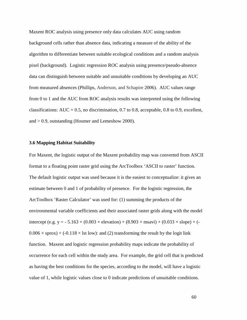
60

Maxent ROC analysis using presence only data calculates AUC using random

background cells rather than absence data, indicating a measure of the ability of the

algorithm to differentiate between suitable ecological conditions and a random analysis

pixel (background). Logistic regression ROC analysis using presence/pseudo-absence

data can distinguish between suitable and unsuitable conditions by developing an AUC

from measured absences (Phillips, Anderson, and Schapire 2006). AUC values range

from 0 to 1 and the AUC from ROC analysis results was interpreted using the following

classifications: AUC = 0.5, no discrimination, 0.7 to 0.8, acceptable, 0.8 to 0.9, excellent,

and > 0.9, outstanding (Hosmer and Lemeshow 2000).

3.6 Mapping Habitat Suitability For Maxent, the logistic output of the Maxent probability map was converted from ASCII

format to a floating point raster grid using the ArcToolbox ‘ASCII to raster’ function.

The default logistic output was used because it is the easiest to conceptualize: it gives an

estimate between 0 and 1 of probability of presence. For the logistic regression, the

ArcToolbox ‘Raster Calculator’ was used for: (1) summing the products of the

environmental variable coefficients and their associated raster grids along with the model

intercept (e.g. y = - 5.163 + (0.003 × elevation) + (8.903 × msavi) + (0.033 × slope) + (-

0.006 × sprox) + (-0.118 × lst low): and (2) transforming the result by the logit link

function. Maxent and logistic regression probability maps indicate the probability of

occurrence for each cell within the study area. For example, the grid cell that is predicted

as having the best conditions for the species, according to the model, will have a logistic

value of 1, while logistic values close to 0 indicate predictions of unsuitable conditions.

61

To effectively distinguish unsuitable habitat from suitable habitat, reclassification

of the probability maps was performed using a crisp threshold. The threshold should

identify the point at which suitable habitat becomes unsuitable, and provides a prediction

of presence and absence. Several methods have been developed to select this threshold,

and the majority of them rely on balancing false-positive and false-negative predictions

typically in presence-absence data models (Lui et al. 2005).

The threshold selection of habitat suitability models was based upon the Maxent

10th percentile training presence threshold (0.222) (Pearson et al. 2007). Habitat

suitability models were reclassified into four classes; unsuitable, low, medium, and high.

Unsuitable identified any areas exhibiting habitat suitability scores lower than the 10th

percentile training presence threshold (0.222). The remaining suitability classes

reflecting low, medium, and high were (0.222-0.30), (0.30-0.70), and (0.70-1.0), as

suggested by Hathcock and Haarmann (2008). Initially, the minimum presence threshold

was going to be 30%, which is indicative of suitable reproductive and nesting habitat.

However, many owls not having a mate, justified the choice of the lower threshold value

(i.e. 0.222). Implementing such a high threshold would have reduced the total amount of

Mexican spotted owl habitat, by reclassifying all areas <30% as unsuitable, despite

known inhabitance of single owls in poorer conditions.

3.7 Habitat Suitability Agreement In addition to assessing the predictive potential of each modeling approach, this study

investigated how well the models agreed by determining the spatial overlap between

the areas where the Maxent and GLM models predicted suitable habitat. Maxent and

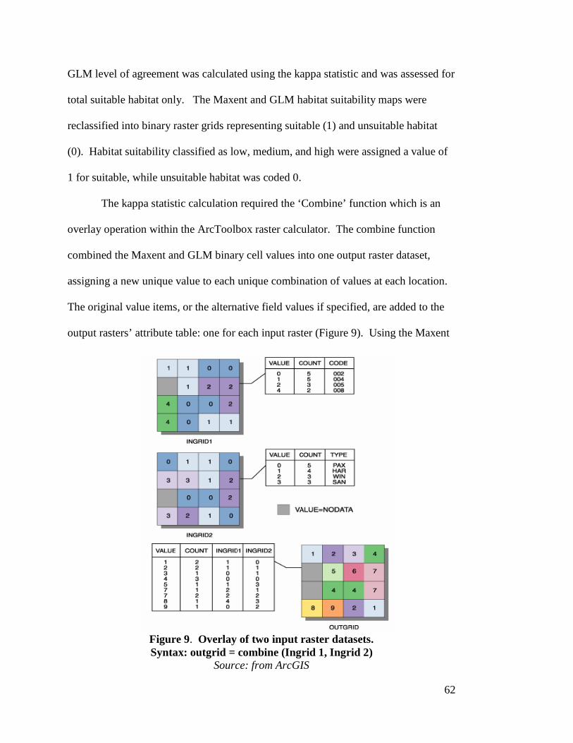
62

GLM level of agreement was calculated using the kappa statistic and was assessed for

total suitable habitat only. The Maxent and GLM habitat suitability maps were

reclassified into binary raster grids representing suitable (1) and unsuitable habitat

(0). Habitat suitability classified as low, medium, and high were assigned a value of

1 for suitable, while unsuitable habitat was coded 0.

The kappa statistic calculation required the ‘Combine’ function which is an

overlay operation within the ArcToolbox raster calculator. The combine function

combined the Maxent and GLM binary cell values into one output raster dataset,

assigning a new unique value to each unique combination of values at each location.

The original value items, or the alternative field values if specified, are added to the

output rasters’ attribute table: one for each input raster (Figure 9). Using the Maxent

Figure 9. Overlay of two input raster datasets. Syntax: outgrid = combine (Ingrid 1, Ingrid 2)

Source: from ArcGIS

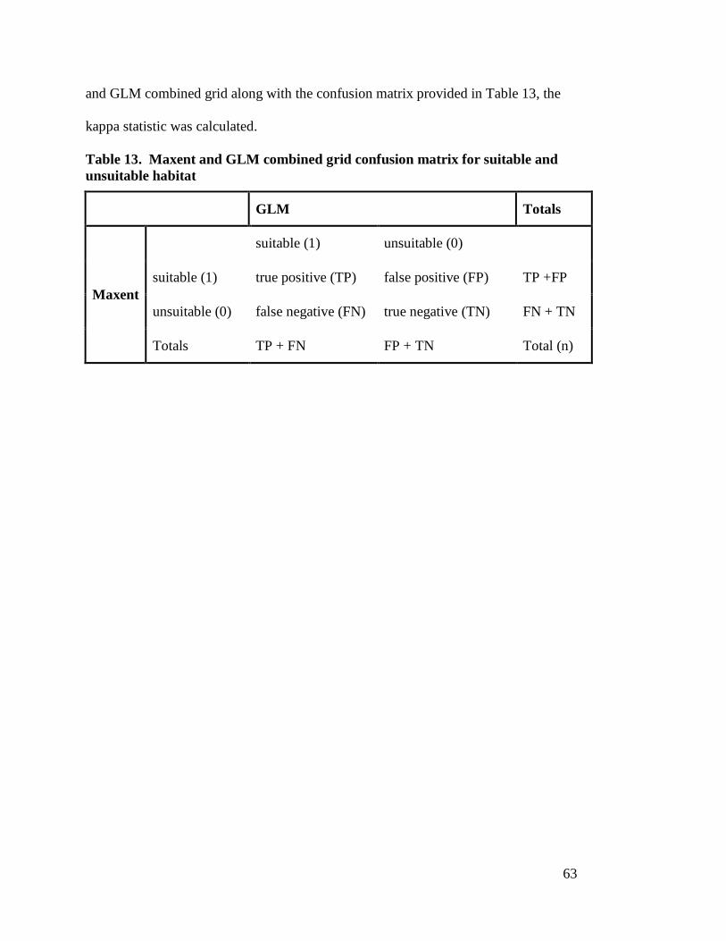
63

and GLM combined grid along with the confusion matrix provided in Table 13, the

kappa statistic was calculated.

Table 13. Maxent and GLM combined grid confusion matrix for suitable and unsuitable habitat

GLM Totals

Maxent

suitable (1) unsuitable (0)

suitable (1) true positive (TP) false positive (FP) TP +FP

unsuitable (0) false negative (FN) true negative (TN) FN + TN

Totals TP + FN FP + TN Total (n)

64

CHAPTER 4: RESULTS

This chapter presents the results from both the Maxent and GLM habitat suitability

modeling approaches. The multicollinearity analysis results are presented first,

followed by the Maxent and GLM model selection, relative importance and response

of environmental variables, model validation, and habitat suitability map results. The

final section of this chapter presents the results of the level of agreement between the

Maxent and GLM habitat suitability models.

4.1 Multicollinearity Analysis Based on the potential biological relevance to the presence of Mexican spotted owl and

ease of interpretation, only one environmental variable from a set of highly cross-

correlated variables was included in the models. Any multicollinearity was reduced by

eliminating the correlated (r > 0.75) variable with the highest VIF. Pearson correlation

coefficient results indicated the highest degree of collinearity among the Landsat derived

vegetation indices and climatic variables, specifically the high and low pass land surface

temperature variables (Table 14).

The variable for land surface temperature high pass (lst high) had the highest VIF.

This variable was the main contributor to the multicollinearity problem and as a

consequence was eliminated first. After removing the variable lst high, mulitcollinearity

was reduced; however, the environmental variables (green, msavi, ndvi, bright, and wet)

still had VIF’s > 10 indicating high correlation between environmental variables. As a

result, the variable elimination process was repeated three more times where the

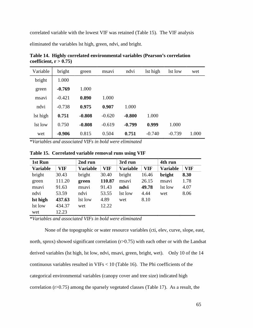
65

correlated variable with the lowest VIF was retained (Table 15). The VIF analysis

eliminated the variables lst high, green, ndvi, and bright.

Table 14. Highly correlated environmental variables (Pearson’s correlation coefficient, r > 0.75)

Variable bright green msavi ndvi lst high lst low wet

bright 1.000 green -0.769 1.000 msavi -0.421 0.890 1.000 ndvi -0.738 0.975 0.907 1.000

lst high 0.751 -0.808 -0.620 -0.800 1.000 lst low 0.750 -0.808 -0.619 -0.799 0.999 1.000

wet -0.906 0.815 0.504 0.751 -0.740 -0.739 1.000 *Variables and associated VIFs in bold were eliminated Table 15. Correlated variable removal runs using VIF

1st Run 2nd run 3rd run 4th run Variable VIF Variable VIF Variable VIF Variable VIF bright 30.43 bright 30.40 bright 16.46 bright 8.30 green 111.20 green 110.87 msavi 26.15 msavi 1.78 msavi 91.63 msavi 91.43 ndvi 49.78 lst low 4.07 ndvi 53.59 ndvi 53.55 lst low 4.44 wet 8.06 lst high 437.63 lst low 4.89 wet 8.10 lst low 434.37 wet 12.22 wet 12.23

*Variables and associated VIFs in bold were eliminated None of the topographic or water resource variables (cti, elev, curve, slope, east,

north, sprox) showed significant correlation (r>0.75) with each other or with the Landsat

derived variables (lst high, lst low, ndvi, msavi, green, bright, wet). Only 10 of the 14

continuous variables resulted in VIFs < 10 (Table 16). The Phi coefficients of the

categorical environmental variables (canopy cover and tree size) indicated high

correlation (r>0.75) among the sparsely vegetated classes (Table 17). As a result, the

66

variable representing tree size class was eliminated based on literature implicating

canopy cover as a stronger correlate of spotted owl habitat.

Table 16. Multicollinearity analysis results for continuous environmental variables

Variable VIF cti 1.522895 elev 1.605714 curve 1.165871 slope 1.638945 east 1.000015 north 1.000016 wet 2.300558 sprox 1.058977 msavi 1.658277 lst low 3.954105

Table 17. Pearson correlation of binary vegetation variables (Phi correlation coefficient, r > 0.75)

Variable cc-1 cc-2 cc-3 cc-4 ts-1 ts-2 ts-3 ts-4 cc-1 1.000 cc-2 -0.669 1.000 cc-3 -0.220 -0.326 1.000 cc-4 -0.217 -0.321 -0.106 1.000 ts-1 0.056 0.019 -0.023 -0.097 1.000 ts-2 0.188 -0.029 -0.083 -0.164 -0.152 1.000 ts-3 -0.057 0.207 0.146 -0.411 -0.382 -0.645 1.000 ts-4 -0.217 -0.321 -0.106 1.000 -0.097 -0.164 -0.411 1.000

4.2 Maxent Habitat Suitability Modeling This section presents the outputs of the Maxent habitat suitability modeling using

presence only Mexican spotted owl data. The Maxent model selection, relative

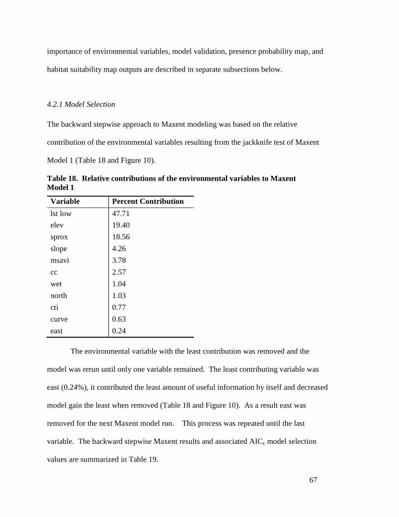
67

importance of environmental variables, model validation, presence probability map, and

habitat suitability map outputs are described in separate subsections below.

4.2.1 Model Selection The backward stepwise approach to Maxent modeling was based on the relative

contribution of the environmental variables resulting from the jackknife test of Maxent

Model 1 (Table 18 and Figure 10).

Table 18. Relative contributions of the environmental variables to Maxent Model 1

Variable Percent Contribution lst low 47.71 elev 19.40 sprox 18.56 slope 4.26 msavi 3.78 cc 2.57 wet 1.04 north 1.03 cti 0.77 curve 0.63 east 0.24

The environmental variable with the least contribution was removed and the

model was rerun until only one variable remained. The least contributing variable was

east (0.24%), it contributed the least amount of useful information by itself and decreased

model gain the least when removed (Table 18 and Figure 10). As a result east was

removed for the next Maxent model run. This process was repeated until the last

variable. The backward stepwise Maxent results and associated AICc model selection

values are summarized in Table 19.

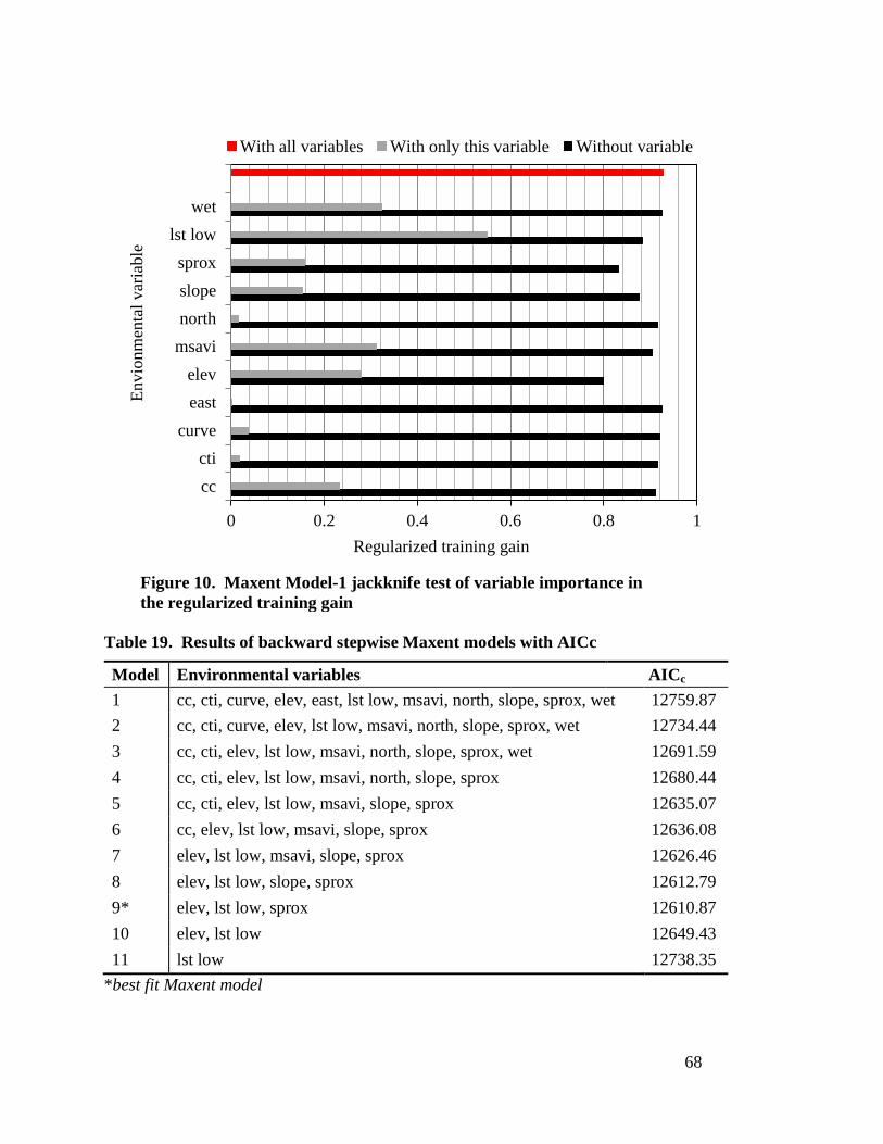
68

Table 19. Results of backward stepwise Maxent models with AICc

Model Environmental variables AICc 1 cc, cti, curve, elev, east, lst low, msavi, north, slope, sprox, wet 12759.87 2 cc, cti, curve, elev, lst low, msavi, north, slope, sprox, wet 12734.44 3 cc, cti, elev, lst low, msavi, north, slope, sprox, wet 12691.59 4 cc, cti, elev, lst low, msavi, north, slope, sprox 12680.44 5 cc, cti, elev, lst low, msavi, slope, sprox 12635.07 6 cc, elev, lst low, msavi, slope, sprox 12636.08 7 elev, lst low, msavi, slope, sprox 12626.46 8 elev, lst low, slope, sprox 12612.79 9* elev, lst low, sprox 12610.87 10 elev, lst low 12649.43 11 lst low 12738.35

*best fit Maxent model

0 0.2 0.4 0.6 0.8 1

cccti

curveeastelev

msavinorthslopesprox

lst lowwet

Regularized training gain

Envi

onm

enta

l var

iabl

e With all variables With only this variable Without variable

Figure 10. Maxent Model-1 jackknife test of variable importance in the regularized training gain

69

Table 19 shows the goodness of fit of each Maxent model using AICc values.

Model 1 had the highest AICc (12759.87), indicating it provided the least fit of all the

models. The AICc values continually decreased from Models 2-9, indicating an

improvement in the goodness of fit when removing additional variables that were limited

in their contributions (Tables 18 and 19).

Models 8 and 9 had similar AICc values; however, Model 9 was considered the

best fit because the AICc was slightly lower and included fewer variables. Model 9

included the variables elev, lst low, and sprox, which contributed the most useful

information according to the jackknife test of variable importance of Model 1. The

removal of the variables sprox and elev in Models 10 and 11 indicated decreases in

model fit further signifying the importance of these variables to the fit of the model.

4.2.2 Relative Importance of Environmental Variables lst low was the most important predictor of Mexican spotted owl presence with a total

contribution of 57.6% followed by elevation (21.3%) and sprox (21.1%). Figure 11

shows the results of the jackknife test of variable importance for Maxent Model 9. The

environmental variable lst low had the highest training gain when used in isolation, which

therefore appears to provide the most useful information by itself. In isolation, this

variable is followed by elev and sprox in terms of training gain values. The

environmental variable that decreases the gain the most when omitted from the model is

lst low, which therefore appears to provide the most useful information that is not present

in any other variables. In omitting variables from the model lst low is followed by sprox

and elev in terms of training gain decreases.

70

4.2.3 Response of Environmental Variables to Mexican Spotted Owl Presence The marginal response curves for Maxent Model 9 show how each environmental

variable affected the Maxent prediction (Figures 12 a-c). These curves show how the

logistic prediction changes as each environmental variable is varied, keeping all other

environmental variables at their average sample values. The response curve for lst low

(Figure 12a) shows the highest probability of Mexican spotted owl presence between 4

and 20°C. After lst low exceeds 20°C the probability of presence drastically decreases.

By using a 10% training presence threshold (0.222), Mexican spotted owls potentially

occur in areas experiencing temperatures as cold as 4°C and as warm as 34°C. The

response curve for elevation (Figure 12b) resembles a bell-shape, starting its ascent at

0.7005

0.6658

0.5086

0.2792

0.1582

0.5486

0.823

0 0.2 0.4 0.6 0.8 1

elev

sprox

lst low

Regularized training gain

Env

iron

men

tal v

aria

ble

With all variables With only this variable Without variable

Figure 11. Maxent Model-9 jackknife test of variable importance in the regularized training gain

71

approximately 1,550 m, climaxing around 2,525 m, and culminating its bell-shape around

3,200 m. By applying a threshold of 0.222, Mexican spotted owl presence is expected in

the elevation range of 2,087 to 2,860 m, which is a significantly smaller elevation range

than if a threshold was not applied. The response curve for sprox (Figure 12c) shows a

nearly linear relationship between probability of Mexican spotted owl presence and

proximity to streams. Mexican spotted owl probability of presence increases as the

distance from streams or water sources decreases. By using a threshold of 0.222,

Mexican spotted owl presence probability is the lowest beyond 770 m and further from

streams.

0.222

0

0.1

0.2

0.3

0.4

0.5

0.6

0.7

0.8

0.9

1

0 10 20 30 40 50 60

Log

istic

out

put (

prob

abili

ty o

f pre

senc

e)

lst low (C°)

10% training presence threshold

a

Figure 12. Response curves for the three environmental variable in Maxent Model-9: (a) lst low, (b) elevation, and (c) sprox with 10% training theshold

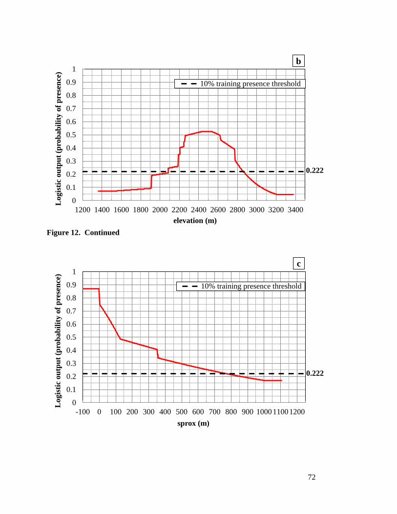
72

Figure 12. Continued

0.222

0

0.1

0.2

0.3

0.4

0.5

0.6

0.7

0.8

0.9

1

1200 1400 1600 1800 2000 2200 2400 2600 2800 3000 3200 3400

Log

istic

out

put (

prob

abili

ty o

f pre

senc

e)

elevation (m)


b

0.222

0

0.1

0.2

0.3

0.4

0.5

0.6

0.7

0.8

0.9

1

-100 0 100 200 300 400 500 600 700 800 900 100011001200

Log

istic

out

put (

prob

abili

ty o

f pre

senc

e)

sprox (m)


c

73

4.2.4 Model Validation The accuracy of Maxent Model 9 using the 10% training presence threshold can be

described by the threshold dependent measures of sensitivity, specificity, overall

accuracy, and kappa statistics calculated from the error matrix summarized in Table 20.

Table 20. Error matrix of Maxent Model 9 validation using independent test data presences/pseudo-absences (n=202)

Recorded Totals presence (+) absence (-)

Predicted presence (+) 84 47 131 absence (-) 17 54 71

Totals 101 101 202 Overall accuracy of the Maxent model was 0.683. This means the model

correctly predicted 68.3% of the presence and pseudo-absence points to either be

included in predicted Mexican spotted owl habitat or excluded from predicted Mexican

spotted owl habitat. It is key to indicate that the model performed better in correctly

predicting Mexican spotted owl habitat where presences occurred (sensitivity = 83.2%)

than it did in predicting non-Mexican spotted owl habitat where pseudo-absences

occurred (specificity = 53.5%) (Table 21).

Table 21. Accuracy measures of Maxent Model 9 validation using independent test data presences/pseudo-absences (n=202)

Measures Values

Sensitivity 0.832

Specificity 0.535

Overall accuracy 0.683

Kappa statistic 0.370

This implies the model poorly distinguished between Mexican spotted owl habitat

and non-Mexican spotted owl habitat by accentuating the prediction of Mexican spotted

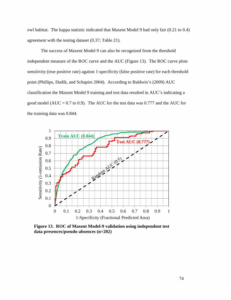
74

owl habitat. The kappa statistic indicated that Maxent Model 9 had only fair (0.21 to 0.4)

agreement with the testing dataset (0.37; Table 21).

The success of Maxent Model 9 can also be recognized from the threshold

independent measure of the ROC curve and the AUC (Figure 13). The ROC curve plots

sensitivity (true positive rate) against 1-specificity (false positive rate) for each threshold

point (Phillips, Dudík, and Schapire 2004). According to Baldwin’s (2009) AUC

classification the Maxent Model 9 training and test data resulted in AUC’s indicating a

good model (AUC = 0.7 to 0.9). The AUC for the test data was 0.777 and the AUC for

the training data was 0.844.

0

0.1

0.2

0.3

0.4

0.5

0.6

0.7

0.8

0.9

1

0 0.1 0.2 0.3 0.4 0.5 0.6 0.7 0.8 0.9 1

Sens

itivi

ty (1

-om

issi

on R

ate)

1-Specificity (Fractional Predicted Area)

Train AUC (0.844) Test AUC (0.777)

Figure 13. ROC of Maxent Model-9 validation using independent test data presences/pseudo-absences (n=202)

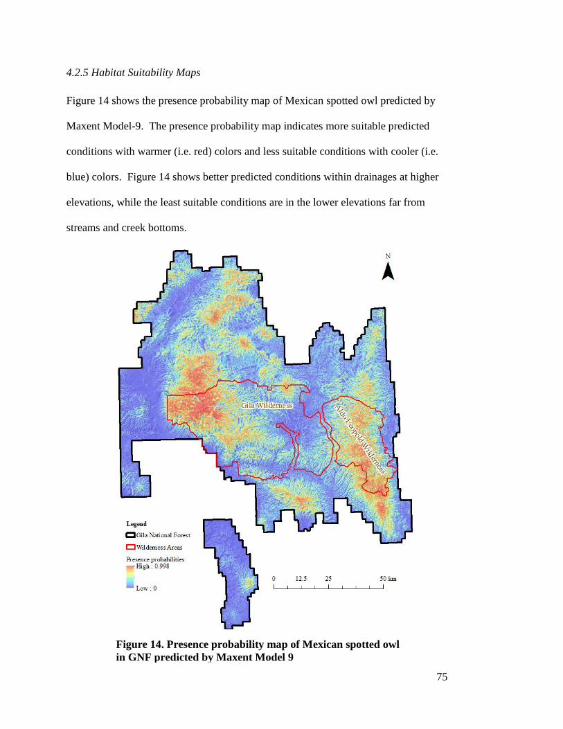
75

4.2.5 Habitat Suitability Maps Figure 14 shows the presence probability map of Mexican spotted owl predicted by

Maxent Model-9. The presence probability map indicates more suitable predicted

conditions with warmer (i.e. red) colors and less suitable conditions with cooler (i.e.

blue) colors. Figure 14 shows better predicted conditions within drainages at higher

elevations, while the least suitable conditions are in the lower elevations far from

streams and creek bottoms.

Figure 14. Presence probability map of Mexican spotted owl in GNF predicted by Maxent Model 9

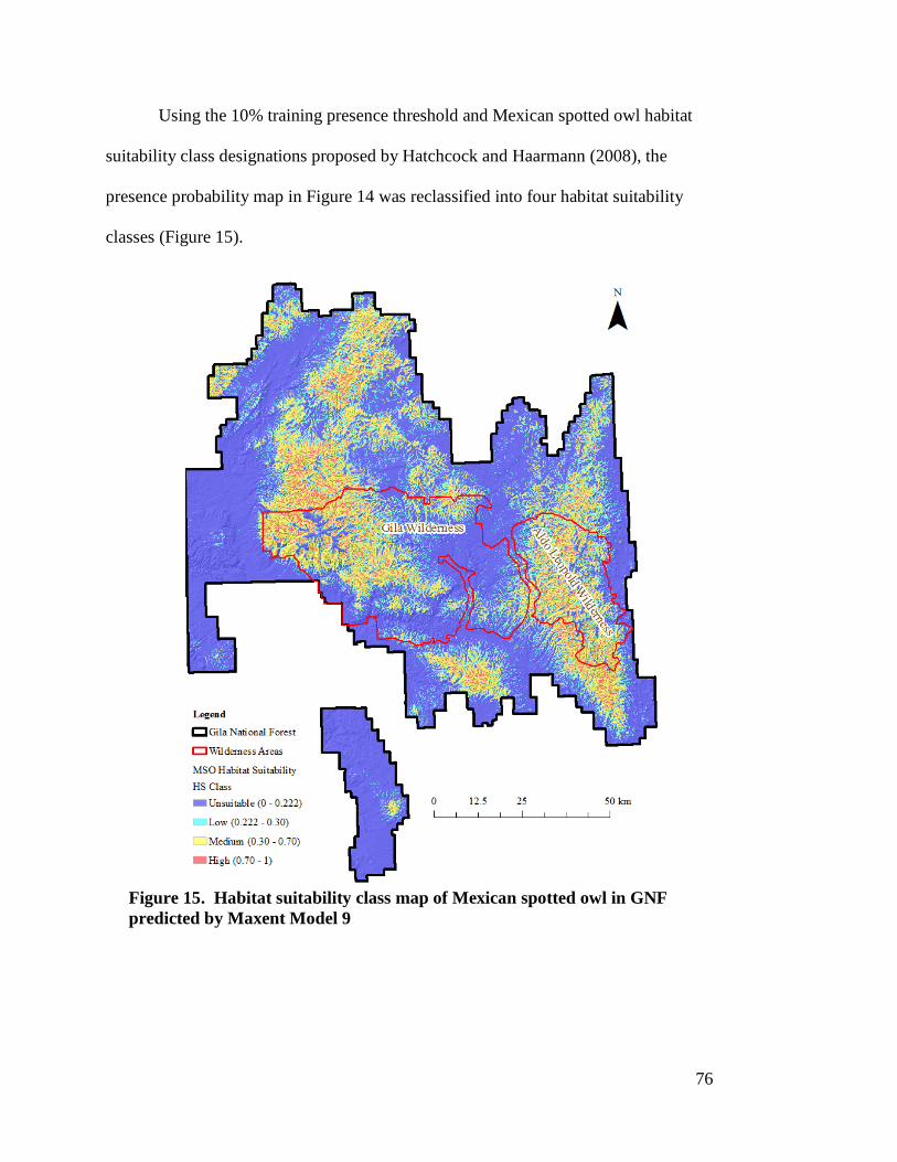
76

Using the 10% training presence threshold and Mexican spotted owl habitat

suitability class designations proposed by Hatchcock and Haarmann (2008), the

presence probability map in Figure 14 was reclassified into four habitat suitability

classes (Figure 15).

Figure 15. Habitat suitability class map of Mexican spotted owl in GNF predicted by Maxent Model 9

77

A visual inspection of Figure 15 shows the highest quality habitat within the Gila

and Aldo Leopold Wilderness Areas. Using the habitat suitability class designations,

approximately 33% of the total area is classified as suitable spotted owl habitat, while the

remaining 67% is unsuitable. Of the 33% classified as suitable habitat, 8% is low

suitability, 22% is medium suitability, and only 3% is high suitability (Table 22).

Table 22. Habitat suitability class area and percent of total area

Habitat Suitability Class km2 Percent of Total Area

Unsuitable (0 - 0.222) 7458.5826 67%

Low (0.222 - 0.30) 947.9061 8%

Medium (0.30 - 0.70) 2425.2165 22%

High (0.70 - 1.0) 357.7437 3%

4.3 GLM Habitat Suitability Modeling The following subsections present the results of the GLM habitat suitability modeling

using presence and pseudo-absence Mexican spotted owl data. The GLM model

selection, relative importance of environmental variables, model evaluation, presence

probability map, and habitat suitability map results are described in separate subsections

as was done with the Maxent model results.

4.3.1 Model Selection The best candidate model resulting from best subset logistic regression are summarized in

Table 23. The seventh model from the logistic regression analysis, (Model 7) was

selected as the best fit GLM because it provided the lowest AICc. The lowest AICc

means the lowest adjusted residual deviance with the number of predictors. The AICc

decreases until Model 7, and then increases for Models 8 through 11.

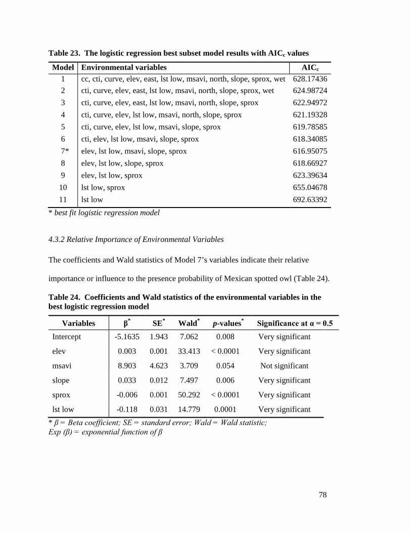
78

Table 23. The logistic regression best subset model results with AICc values

Model Environmental variables AICc 1 cc, cti, curve, elev, east, lst low, msavi, north, slope, sprox, wet 628.17436 2 cti, curve, elev, east, lst low, msavi, north, slope, sprox, wet 624.98724 3 cti, curve, elev, east, lst low, msavi, north, slope, sprox 622.94972 4 cti, curve, elev, lst low, msavi, north, slope, sprox 621.19328 5 cti, curve, elev, lst low, msavi, slope, sprox 619.78585 6 cti, elev, lst low, msavi, slope, sprox 618.34085

7* elev, lst low, msavi, slope, sprox 616.95075 8 elev, lst low, slope, sprox 618.66927 9 elev, lst low, sprox 623.39634 10 lst low, sprox 655.04678 11 lst low 692.63392

* best fit logistic regression model

4.3.2 Relative Importance of Environmental Variables The coefficients and Wald statistics of Model 7’s variables indicate their relative

importance or influence to the presence probability of Mexican spotted owl (Table 24).

Table 24. Coefficients and Wald statistics of the environmental variables in the best logistic regression model

Variables β* SE* Wald* p-values* Significance at α = 0.5 Intercept -5.1635 1.943 7.062 0.008 Very significant

elev 0.003 0.001 33.413 < 0.0001 Very significant

msavi 8.903 4.623 3.709 0.054 Not significant

slope 0.033 0.012 7.497 0.006 Very significant

sprox -0.006 0.001 50.292 < 0.0001 Very significant

lst low -0.118 0.031 14.779 0.0001 Very significant * β = Beta coefficient; SE = standard error; Wald = Wald statistic; Exp (β) = exponential function of β

79

Using the model coefficients, a logistic regression equation using the logit link

function in XL-stats:

p =1

1+𝑒−(−5.1635+(0.003×𝑋1)+(8.903×𝑋2)+(0.033×𝑋3)−(0.006×𝑋4)−(0.118×𝑋5) (18)

where p is the presence probability of Mexican spotted owl. The intercept of -5.1635 is

the logit of presence probability when all the environmental variables are equal to zero.

This is equal to the presence probability of 0.00572 and can be considered as the zero

probability. The relative importance of each environmental variable is described by the

coefficients and Wald statistics within Table 24.

Elevation (elev) showed a positive influence (β = 0.003) on Mexican spotted owl

presence. As the elevation increases, the presence probability of Mexican spotted owl

increases; in fact, the logit of presence probability will increase 0.003 with every one

meter increase in elevation. Elevation is very significant at α = 0.05, indicating a

significant effect of elevation on the logit of presence probability. The Wald statistic of

elevation (33.413) indicated it was the second most influential variable (Table 24).

The modified soil adjusted vegetation index (msavi) indicated a positive

relationship (β = 8.903) to Mexican spotted owl presence probability. The higher the

msavi, the higher the presence probability of Mexican spotted owl will be. Based on the

p-values msavi (p = 0.053) is borderline significant and not significant at α = 0.05. The

Wald statistics of msavi (3.709) was the lowest, indicating it was the least influential

variable (Table 24).

The slope was the last variable that had a positive relationship (β = 0.033) with

Mexican spotted owl presence probability. The logit of Mexican spotted owl presence

probability will increase 0.033 with every one degree increase in slope. At α = 0.05,

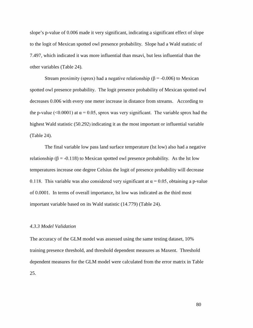
80

slope’s p-value of 0.006 made it very significant, indicating a significant effect of slope

to the logit of Mexican spotted owl presence probability. Slope had a Wald statistic of

7.497, which indicated it was more influential than msavi, but less influential than the

other variables (Table 24).

Stream proximity (sprox) had a negative relationship (β = -0.006) to Mexican

spotted owl presence probability. The logit presence probability of Mexican spotted owl

decreases 0.006 with every one meter increase in distance from streams. According to

the p-value (<0.0001) at α = 0.05, sprox was very significant. The variable sprox had the

highest Wald statistic (50.292) indicating it as the most important or influential variable

(Table 24).

The final variable low pass land surface temperature (lst low) also had a negative

relationship (β = -0.118) to Mexican spotted owl presence probability. As the lst low

temperatures increase one degree Celsius the logit of presence probability will decrease

0.118. This variable was also considered very significant at α = 0.05, obtaining a p-value

of 0.0001. In terms of overall importance, lst low was indicated as the third most

important variable based on its Wald statistic (14.779) (Table 24).

4.3.3 Model Validation The accuracy of the GLM model was assessed using the same testing dataset, 10%

training presence threshold, and threshold dependent measures as Maxent. Threshold

dependent measures for the GLM model were calculated from the error matrix in Table

25.

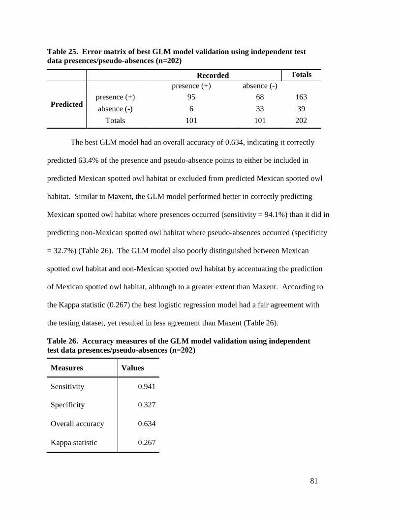
81

Table 25. Error matrix of best GLM model validation using independent test data presences/pseudo-absences (n=202)

Recorded Totals presence (+) absence (-)

Predicted presence (+) 95 68 163 absence (-) 6 33 39

Totals 101 101 202 The best GLM model had an overall accuracy of 0.634, indicating it correctly

predicted 63.4% of the presence and pseudo-absence points to either be included in

predicted Mexican spotted owl habitat or excluded from predicted Mexican spotted owl

habitat. Similar to Maxent, the GLM model performed better in correctly predicting

Mexican spotted owl habitat where presences occurred (sensitivity = 94.1%) than it did in

predicting non-Mexican spotted owl habitat where pseudo-absences occurred (specificity

= 32.7%) (Table 26). The GLM model also poorly distinguished between Mexican

spotted owl habitat and non-Mexican spotted owl habitat by accentuating the prediction

of Mexican spotted owl habitat, although to a greater extent than Maxent. According to

the Kappa statistic (0.267) the best logistic regression model had a fair agreement with

the testing dataset, yet resulted in less agreement than Maxent (Table 26).

Table 26. Accuracy measures of the GLM model validation using independent test data presences/pseudo-absences (n=202)

Measures Values

Sensitivity 0.941

Specificity 0.327

Overall accuracy 0.634

Kappa statistic 0.267

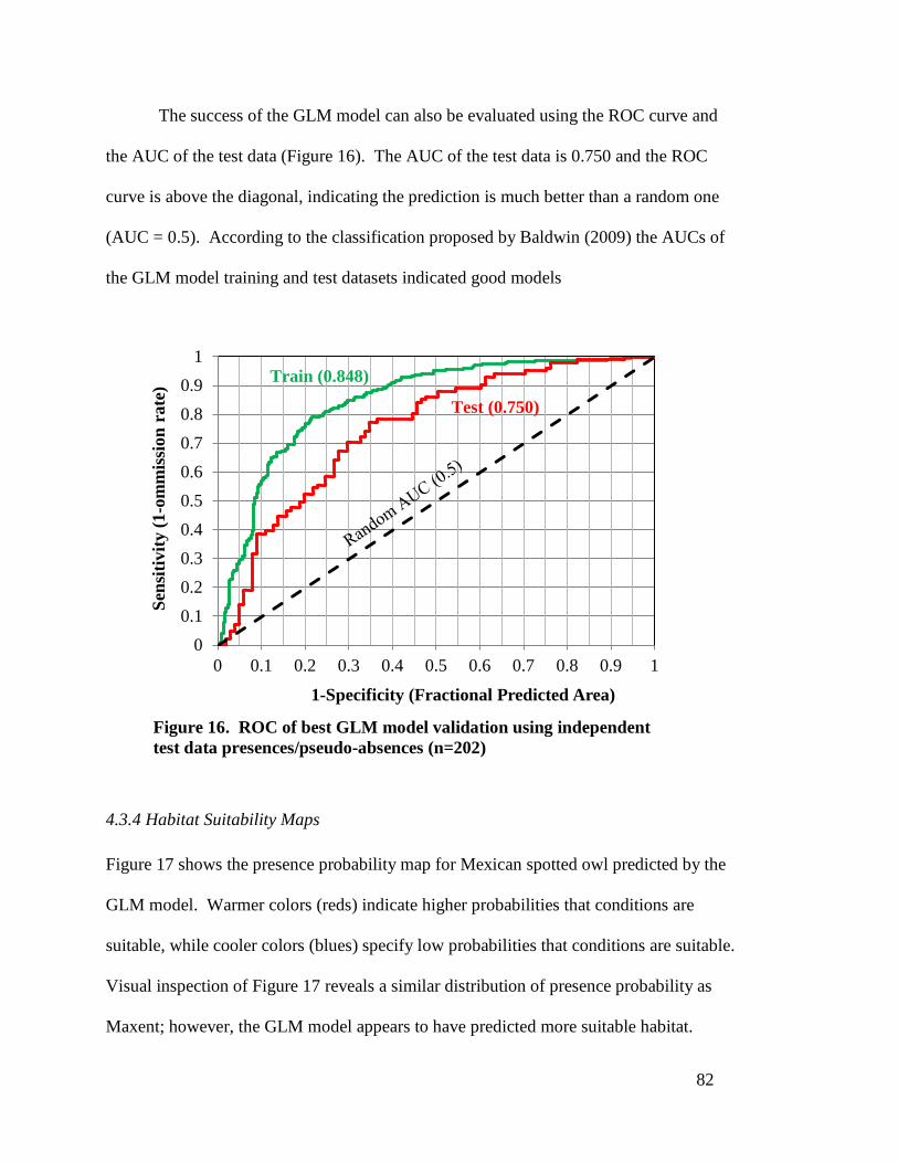
82

The success of the GLM model can also be evaluated using the ROC curve and

the AUC of the test data (Figure 16). The AUC of the test data is 0.750 and the ROC

curve is above the diagonal, indicating the prediction is much better than a random one

(AUC = 0.5). According to the classification proposed by Baldwin (2009) the AUCs of

the GLM model training and test datasets indicated good models

4.3.4 Habitat Suitability Maps Figure 17 shows the presence probability map for Mexican spotted owl predicted by the

GLM model. Warmer colors (reds) indicate higher probabilities that conditions are

suitable, while cooler colors (blues) specify low probabilities that conditions are suitable.

Visual inspection of Figure 17 reveals a similar distribution of presence probability as

Maxent; however, the GLM model appears to have predicted more suitable habitat.

00.10.20.30.40.50.60.70.80.9

1

0 0.1 0.2 0.3 0.4 0.5 0.6 0.7 0.8 0.9 1

Sens

itivi

ty (1

-om

mis

sion

rat

e)

1-Specificity (Fractional Predicted Area)

Train (0.848)

Test (0.750)

Figure 16. ROC of best GLM model validation using independent test data presences/pseudo-absences (n=202)

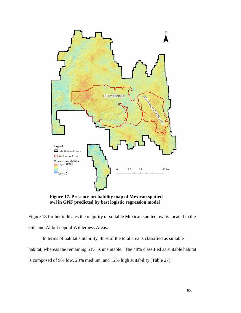
83

Figure 18 further indicates the majority of suitable Mexican spotted owl is located in the

Gila and Aldo Leopold Wilderness Areas.

In terms of habitat suitability, 48% of the total area is classified as suitable

habitat, whereas the remaining 51% is unsuitable. The 48% classified as suitable habitat

is composed of 9% low, 28% medium, and 12% high suitability (Table 27).

Figure 17. Presence probability map of Mexican spotted owl in GNF predicted by best logistic regression model

84

Table 27. Habitat suitability class area and percent of total area

Habitat Suitability Class km2 Percent of Total Area

Unsuitable (0 - 0.222) 5,767.9335 51%

Low (0.222 - 0.30) 989.6931 9%

Medium (0.30 - 0.70) 3,091.2282 28%

High (0.70 - 1.0) 1,340.9604 12%

Figure 18. Habitat suitability class map of Mexican spotted owl in GNF predicted by the best logistic regression model

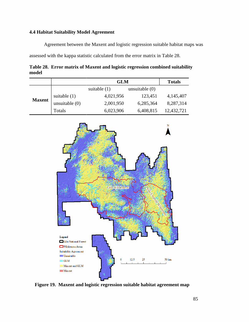
85

4.4 Habitat Suitability Model Agreement

Agreement between the Maxent and logistic regression suitable habitat maps was

assessed with the kappa statistic calculated from the error matrix in Table 28.

Table 28. Error matrix of Maxent and logistic regression combined suitability model

GLM Totals

Maxent

suitable (1) unsuitable (0) suitable (1) 4,021,956 123,451 4,145,407 unsuitable (0) 2,001,950 6,285,364 8,287,314 Totals 6,023,906 6,408,815 12,432,721

Figure 19. Maxent and logistic regression suitable habitat agreement map

86

The values within Table 28 were produced from the attribute table of the Maxent

and logistic regression combined suitable habitat map. The calculated kappa statistic of

0.655 indicates that the suitable habitat maps of Maxent and GLM are in substantial

agreement. Figure 19 shows the spatial pattern of the agreement and disagreement

between the Maxent and GLM suitable habitat maps.

87

CHAPTER 5: DISCUSSION AND CONCLUSIONS This study revealed that despite the differences between presence-only and presence-

absence based modeling methods, each method is capable of producing accurate and

useful habitat suitability models. The next sections address these differences and

their implications for previous and future research.

5.1 Model Selection Although model selection for both Maxent and logistic regression used AICc values,

different models were selected. According to the model AICc values the best Maxent

model only included three environmental variables, while the logistic regression

model included five variables. This presumably is a result of the underlying

assumptions and complexity of the different modeling methods. For instance,

Maxent calculated AICc using all the presences, while logistic regression only

included the training presence-absence data. Additionally Maxent considered linear,

non-linear, and interaction effects, whereas GLM only considered linear responses.

AICc selection is known to reduce model complexity; hence, the reason why so few

environmental variables are included in either model. By using AICc instead of AUC

for model selection both Maxent and logistic regression models were less subject to

over or under-parameterization (Warren and Seifert 2011).

5.2 Relative Importance of Environmental Variables Maxent and logistic regression models considered the environmental variables lst

low, elevation, and sprox important environmental variables in terms of Mexican

88

spotted owl habitat. Surprisingly, neither Maxent nor the logistic regression best fit

models included the environmental variable percent canopy cover, notwithstanding

the conventional logic by which it is considered a critical element for suitable spotted

owl habitat. The environmental variables in both models including the slope and

msavi of the logistic regression model are all influencing factors of vegetation

composition (canopy cover), which suggests these variables are more influential than

percent canopy cover itself. Environmental variable importance varied between

Maxent and logistic regression as well. For instance, Maxent considered lst low the

most important variable according to percent contribution, while the logistic

regression identified sprox as the most influential variable using the Wald statistic.

These habitat suitability models differ in their distributions because Maxent explains

environmental variable relationships in a non-linear approach, whereas the GLM uses

a linear approach. Based on the Maxent response curves and GLM coefficients of the

environmental variables suitable Mexican spotted owl habitat is located in the mid-to-

high elevations, and close to streams or water sources. These findings support several

research efforts assessing Mexican spotted owl habitat (Ganey et al. 2005; Ganey

2004; Zwank et al. 1994).

5.3 Model Validation Model validation using the threshold dependent measure of the kappa statistic showed

that both Maxent and GLM models were in fair agreement with the test dataset, but

that Maxent performed slightly better. This supports the findings of other presence-

only and presence-absence habitat suitability model research in which Maxent

89

outperforms logistic regression according to the kappa statistic (Kumar et al. 2009).

Sensitivity is the only threshold dependent measure for which Maxent did not

outperform logistic regression. The specificity of logistic regression was surprisingly

lower than Maxent’s considering it was generated using presence-absence data.

Specificity is the fraction of correctly predicted absences, one would assume that if

generated with absence data model specificity would improve. The Maxent model

performed better than logistic regression because of its intricate underlying algorithm

and its ability to model the complex shapes of the owls’ responses to the

environmental variables (Kumar et al. 2009). Using the test dataset and the resulting

threshold independent measure of AUC, Maxent again outperformed the logistic

regression model. This signifies that valid and resourceful habitat suitability models

can be constructed using fewer environmental variables.

5.4 Habitat Suitability In analyzing the model validation performance measures of both models, minor

differences exist between their threshold dependent and independent performance

measures, giving an indication of how well they potentially agree with one another.

Regardless of the similar model validation performance measures, the Maxent and

logistic regression habitat suitability models exhibited differing distributions of

Mexican spotted owl habitat suitability classes. The logistic regression habitat

suitability model predicted the highest percentage (48%) of suitable habitat, though it

included two more environmental variables (slope, msavi) than the Maxent model.

Potentially these two additional variables are the cause of the habitat suitability

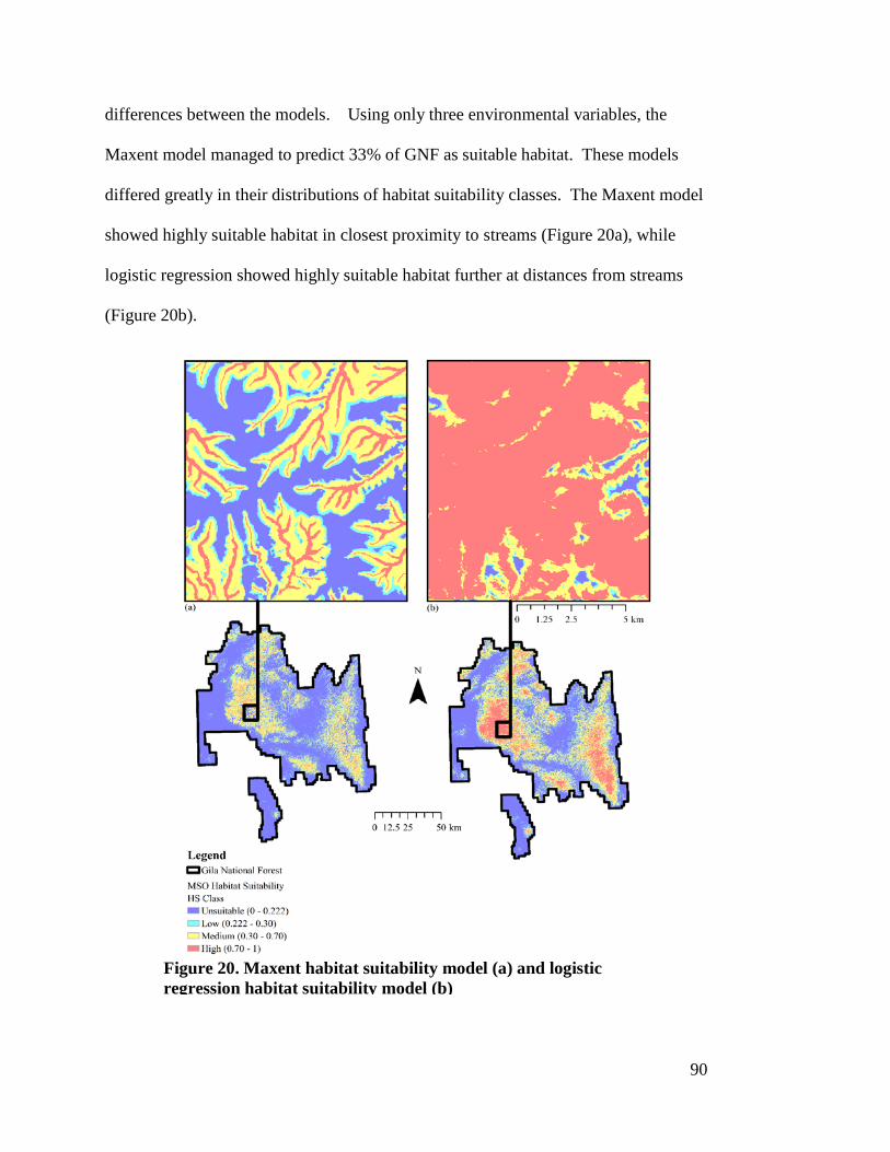
90

differences between the models. Using only three environmental variables, the

Maxent model managed to predict 33% of GNF as suitable habitat. These models

differed greatly in their distributions of habitat suitability classes. The Maxent model

showed highly suitable habitat in closest proximity to streams (Figure 20a), while

logistic regression showed highly suitable habitat further at distances from streams

(Figure 20b).

Figure 20. Maxent habitat suitability model (a) and logistic regression habitat suitability model (b)

91

When comparing the Maxent and logistic regression models using the four habitat

suitability classes, the models display poor agreement. However, when comparing

available suitable habitat, the models are in substantial agreement resulting in a kappa

statistic of 0.655. These results are significant because it signifies that presence-only

methods can produce useful habitat suitability models if absence data are not

available (Babar et al. 2012; Millar and Blouin-Demers 2012; Lui et al. 2011).

5.5 Modeling Limitations and Assumptions This study produced useful habitat suitability models for Mexican spotted owl within

GNF, although not without some limitations. These models incorporated

environmental variables considered important for Mexican spotted owl habitat, but

excluded some other important variables such as snag density and canopy structure

(Ganey et al. 2005). Microhabitat characteristics such as these play critical roles in

Mexican spotted owl, yet are difficult to collect and represent spatially.

Comparison of the Maxent and logistic regression models which contained

different environmental variables could prove to be invalid; however, this study

sought to compare the Maxent and logistic regression methods, and not just to

compare habitat suitability models using the same environmental variables. If the

Maxent and logistic regression best models contained the same environmental

variables a more valid comparison might be made (Stohlgren et al. 2010). In

analyzing the habitat suitability models it appears that Maxent underestimated the

area of suitable habitat, while logistic regression overestimated the area of suitable

habitat.

92

The habitat suitability models also contain some bias as a result of the data

collection methods. For instance, many point observations included in the presence

data were aural observations, which means their locations had to be estimated. In

addition to using estimated point locations, the surveys occurred along designated

trails restricting presence locations to the easily accessible areas. By implementing a

target background some of this bias was expected to be reduced but not eliminated

(VanDerWal 2009).

Bias is also evident in the generation of the absence data used for model

validation and GLM training. The absences used were randomly selected outside

known presence locations; however, without field verification, it is impossible to

know whether these sites contain owls or potential suitable habitat. To improve

absence data, one should determine true absence points in the field, by marking

coordinates for locations where Mexican spotted owls have not been detected or in

areas considered not suitable habitat. This raises a concern of true habitat

unsuitability or merely that owls have not been detected at that location due to

random chance. Even if certain habitat is suitable for Mexican spotted owl, they

potentially may not occupy or use that entire suitable habitat (Gu and Swihart 2004).

5.6 Future Research The results of this study raise additional questions that have been addressed by

previous research. For instance, this study could assess the impact of using target

backgrounds in habitat suitability modeling, potentially providing useful insights to

research conducted by VanDerWal et al. (2009). To improve predictive performance

93

of habitat suitability models for Mexican spotted owl in GNF, future ground surveys

could be designed to account for absence as well as presence during each season of

the year. Such research could potentially determine whether true absences are

significantly better than pseudo-absences in generating presence-absence habitat

suitability models (Wise and Guisan 2009). The biological input data for this study

could be implemented for accessing the other pseudo-absence selection methods and

their impact on model generation and selection (Lütolf, Kienast, and Guisan 2006;

MacKenzie 2005). Future research might involve evaluating the impacts of changing

the threshold probabilities indicative of species presence. This study only

implemented the 10% training presence threshold, and it would be beneficial to

understand what impacts other threshold criteria such as minimum presence threshold

(MPT) or fixed thresholds have on habitat suitability models (Jiménez-Valverde,

Lobo, and Hortal 2008).

5.7 Final Thoughts This study compared presence-only and presence-absence modeling methods using

model selection, variable importance, model validation, and habitat suitability. In

conclusion, the AICc model selection results indicated Maxent and logistic regression

differ in their methods of selecting the most appropriate combination of

environmental variables for modeling Mexican spotted owl habitat.

Both models included the environmental variables lst low, sprox, and

elevation; however, the importance of each variable varied between Maxent and

logistic regression. Maxent considered the variable lst low the most important,

94

whereas logistic regression considered sprox the most influential. These models vary

in their methods for selecting variables and how they determine relative importance

or influence.

Maxent and logistic regression were nearly identical according to the

threshold dependent and independent performance measures, still Maxent performed

slightly better. When comparing the models using habitat suitability classes, the

Maxent and logistic regression models significantly differ, but when comparing total

suitable habitat the models showed substantial agreement. Results of this study like

previous research indicate how powerful and useful presence-only or presence-

absence models can be in predicting the habitat of sensitive species such as the

Mexican spotted owl (Meynard and Quinn 2007).

95

REFERENCES Akçakaya, H. R. 1993. RAMAS/GIS: Linking Landscape DataWith Population Viability Analysis. Applied Biomathematics, New York. Akçakaya, H. R., M. A. McCarthy, and J. L. Pearce. 1995. Linking landscape data with population viability analysis: management options for the helmeted honeyeater Lichenostomus melanops cassidix. Biological Conservation 73 (2): 169–176. Allouche, O., A. Tsoar, and R. Kadmon. 2006. Assessing the accuracy of species distribution models: prevalence, kappa and the true skill statistic (TSS). Journal of Applied Ecology 43 (6): 1223−1232 Araujo, M. B., and P. H. Williams. 2000. Selecting areas for species persistence using occurrence data. Biological Conservation 96 (3): 331-345. Austin, M. P. 2002. Spatial prediction of species distribution: an interface between ecological theory and statistical modelling. Ecological Modelling 157 (2-3): 101-118. Baldwin, R. 2009. Use of maximum entropy in wildlife research. Entropy 11 (4): 854-866. Babar, S., G. Amarnath, C.S. Reddy, A. Jentsch, and S. Sudhakar. 2012. Species distribution models: ecological explanation and prediction of an endemic and endangered plant species (Pterocarpus santalinus L.f.). Current Science 102 (8): 1157–1165. Baskaran, L. M., V. H. Dale, R. A. Efroymson, and W. Birkhead. 2006. Habitat Modeling Within a Regional Context: An Example Using Gopher Tortoise. American Midland Naturalist 155 (2): 335-351.

Beaumont, L. J., L. Hughes, and M. Poulsen. 2005. Predicting species distributions: use of climatic parameters in BIOCLIM and its impact on predictions of species’ current and future distributions. Ecological Modelling 186 (2): 251-270. Bian, L., and E. West. 1997. GIS modeling of elk calving habitat in a prairie environment with statistics. Photogrammetric Engineering & Remote Sensing 63 (2): 161-167. Braunisch, V., K. Bollmann, R. F. Graf, and A. H. Hirzel. 2008. Living on the edge—Modelling habitat suitability for species at the edge of their fundamental niche. Ecological Modelling 214 (2-4): 153-167. Brito, J. C., S. Santos, J. M. Pleguezuelos, and N. Sillero. 2008. Inferring evolutionary scenarios with geostatistics and geographical information systems for the viperid snakes Vipera latastei and V. Monticola. Biological Journal of the Linnean Society 95 (4): 790–806.

96

Brotons, L., W. Thuiller, M. B. Araújo, and A. H. Hirzel. 2004. Presence-absence versus presence-only modelling methods for predicting bird habitat suitability. Ecography 27 (4): 437-448. Chander, G., B. L. Markham, and D. L. Helder. 2009. Summary of current radiometric calibration coefficients for Landsat MSS, TM, ETM+, and EO-1 ALI sensors. Remote Sensing of the Environment 113 (5): 893-903.

Congalton, R. G., J. M. Stenback, and R. H. Barrett. 1993. Mapping deer habitat suitability using remote sensing and geographic information systems. Geocarto International 3 (8): 23-33.

Coris, F., J. D. Leeuw, and A. Skidmore. 2000. Modeling species distributions with GIS. In Biotoni L Fuller T K (eds) Research Techniques in Animal Ecology. NY, Columbia University Press: 389-434. Dettmers, R., and J. Bart. 1999. A GIS modelling method applied to predicting forest songbird habitat. Ecological Applications 9 (1): 152-163. Dzeroski, S. 2009. Machine learning applications in habitat suitability modeling. In Haupt S E (eds) Artificial Intelligence Methods in the Environmental Science. Berlin: Springer: 391-411. Duff, A. A., and T. E. Morrell. 2007. Predictive occurrence models for bat species in California. Journal of Wildlife Management 71 (3): 693-700. Elith, J., and H. Graham. 2009. Do they? how do they? why do they differ? on finding reasons for differing performances of species distribution models. Ecography 32 (1): 66-77. Elith, J., S. J. Phillips, T. Hastie, M. Dudík, Y. E. Chee, and C. J. Yates. 2011. A statistical explanation for Maxent for ecologists. Diversity and Distributions 17 (1): 43-57. Fielding, A. H., and J. F. Bell. 1997. A review of methods for the assessment of prediction errors in conservation presence/absence models. Environmental Conservation 24 (1): 38-49. Fitzgerald, R. W., and B. G. Lees. 1994. Spatial context and scale relationships in raster data for thematic mapping in natural systems. In Advances in GIS research, vol.1, eds Waugh, T.C., and R. G. Healey, 462–475. Southhampton: Taylor and Francis. Ganey, J. L. 2004. Thermal regimes of Mexican spotted owl nest stands. The Southwestern Naturalist 49 (4): 478-486.

97

Ganey, J. L., W. M. Block, J. P. Ward, and B. E. Strohmeyer. 2005. Home range, habitat use, survival, and fecundity of Mexican spotted owls in the Sacramento Mountains, New Mexico. The Southwestern Naturalist 50 (3): 323-333. Graf, R. F., K. Bollmann, W. Suter, and H. Bugmann. 2005. The importance of spatial scale in habitat models: capercaillie in the Swiss Alps. Landscape Ecology 20 (6): 703–717. Grubb, G. G., W. W. Bowerman, A. J. Bath, J. P. Giesy, D.V.C. Weseloh. 2003. Evaluating Great Lakes Bald Eagle nesting Habitat with Bayesian Inference. Research Paper RMRS-RP-45. United States Department of Agriculture, Forest Service, Rocky Mountain Research Station, Fort Collins, CO, 10 pp. Gu, G., and R. K. Swihart. 2004. Absent of undected? Effects of non-detection of species occurrence on wildlife-habitat models. Biological Conservation 116 (1): 195-203. Guisan, A., T. C. Edwards, and T. Hastie. 2002. Generalized linear and generalized additive models in studies of species distribution: setting the scene. Ecological Modelling 157 (2-3): 89-100. Guisan, A., and W. Thuiller. 2005. Predicting species distribution: offering more than simple habitat models. Ecology Letters 8 (9): 993–1009. Guisan, A., and N. E. Zimmermann. 2000. Predictive habitat distribution models in ecology. Ecological Modelling 135 (2-3): 147-186. Gumpertz, M. L., J. M. Graham, and J. D. Ristaino. 1997. Autologistic model of spatial pattern of Phytophthora epidemic in bell pepper: effects of soil variables on disease presence. Journal of Agricultural, Biological, and Environmental Statistics 2 (2): 131–156. Hathcock, C. D., and T. K. Haarmann. 2008. Development of a predictive model for habitat of the habitat of the Mexican spotted owl in northern New Mexico. The Southwestern Naturalist 53 (1): 34–38. Hellgren, E. C., S. L. Bales, M. S. Gregory, D. M. Leslie, and J. Clark. 2006. Testing a Mahalanobis Distance Model of Black Bear Habitat Use in the Ouachita Mountains of Oklahoma. Journal of Wildlife Management 71 (3): 924-928. Hirzel, A. H., and A. Guisan. 2002. Which is the optimal sampling strategy for habitat suitability modeling. Ecological Modelling 157 (2-3): 331-341. Hirzel, A. H., G. Le Laya, V. Helfera, C. Randina, and A. Guisan. 2006. Evaluating the ability of habitat suitability models to predict species presences. Ecological Modelling 199 (2): 142-152.

98

Hosmer, D.W. Jr., and S. Lemeshow. 1989. Applied Logistic Regression. New York: Wiley.

Huang, C., B. Wylie, L. Yang, C. Homer, and G. Zylstra. 2002. Derivation of a tasselled cap transformation based on Landsat 7 at-satellite reflectance. International Journal of Remote Sensing 23 (8): 1741-1748. Jensen, W. F. 1992. Mule deer habitat use in the North Dakota badlands. The Prairie Naturalist 24: 97-108. Jiménez-Valverde, A., J. M. Lobo, and J. Hortal. 2008. Not as good as they seem: the importance of concepts in species distribution modelling. Diversity and Distributions 14 (6): 885-890. Keating, K. 2004. Use and interpretation of logistic regression in habitat-selection studies. Journal of Wildlife Management 68 (4): 774–789. Kumar, S., S. A. Spaulding, T. J. Stohlgren, K. A. Hermann, T. S. Schmidt, and L. L. Bahls. 2009. Potential habitat distribution for the freshwater diatom Didymosphenia geminate in the continental US. Frontiers in Ecology and the Environment 7 (8): 415-420. Landis, J.R. and G.G. Koch. 1977. The measurements of observer agreement for categorical data. Biometrics 33 (1): 159–174. Lazenby B T, Pye T, Richardson A, and Bryant S A 2008 Towards a habitat model for the New Holland Mouse Pseudomys novaehollandiae in Tasmania – population vegetation associations and an investigation into individual habitat use. Australian Mammalogy 29 (2): 137-148. Legendre, P. 1993. Spatial autocorrelation: trouble or new paradigm. Ecology 74 (6): 1659–1673. Le Lay, G., P. Clergeau, L. Hubert-Moy. 2001. Computerized map of risk to manage wildlife species in urban areas. Environmental Management 27 (3): 451–461. Lenton, S. M., J. E. Fa, and J. P. Del Val. 2000. A simple non-parametric GIS model for predicting species distribution: endemic birds in Bioko Island, West Africa. Biodiversity and Convervation 9 (7): 869–885. Levin, R. S., A. T. Peterson, and M. Q. Benedict. 2004. Geographic and ecological distributions of the anopheles gambiae complex predicted using a genetic algorithm. American Journal of Tropical Medicine and Hygiene 70 (2): 105-109.

99

Lichstein, J. W., T. R. Simons, S. A. Shriner, and K. E. Franzreb. 2002. Spatial autocorrelation and autoregressive models in ecology. Ecological Monographs 72 (3): 445-463. Lobo, J. M., A. Jiménez-Valverde, and J. Hortal. 2010. The uncertain nature of absences and their importance in species distribution modeling. Ecography 33 (1): 103-114. Lobo, J. M., A. Jiménez-Valverde, and R. Real. 2008. AUC: a misleading measure of the performance of predictive distribution models. Global Ecology and Biogeography 17 (2): 145-304. Lopez-Lopez, P., C. Garcıa-Ripolles, J. Miguel Aguilar, F. Garcıa-Lopez, and J. Verdejo. 2006. Modelling breeding habitat preferences of Bonelli’s eagle (Hieraaetus fasciatus) in relation to topography, disturbance, climate and land use at different spatial scales. Journal of Ornithology 147 (1): 97-106. Lu, D., P. Mausel, E. Brondízio, and E. Moran. 2004. Relationships between forest stand parameters and Landsat TM spectral responses in the Brazilian Amazon Basin. Forest Ecology and Management, 198 (1-3): 149–167. Lui, C., P. M. Berry, T. P. Dawson, and R. G. Pearson. 2005. Selecting thresholds of occurrence in the prediction of species distributions. Ecography 28 (3): 385-393. Lui, X., Z. Guo, Z. Ke, S. Wang, and Y. Li. 2011. Increasing potential risk of a global aquatic invader in europe in contrast to other continents under future climate change. PLoS ONE 6 (3): e18429. Lütolf, M., F. Kienast, and A. Guisan. 2006. The ghost of past species occurrence: improving species distribution models for presence-only data. Journal of Applied Ecology 43 (4):802-815. MacKenzie, D. I. 2005. What are the issues with presence-absence data for wildlife managers? Journal of Wildlife Management 69 (3): 849-860. MacKenzie, D. I., and J. A. Royle. 2005. Designing efficient occupancy studies: general advice and tips on allocation of survey effort. Journal of Applied Ecology 42 (6): 1105-1114. Manel, S., J. M. Dias, and S. J. Ormerod. 1999. Comparing discriminant analysis, neural networks and logistic regression for predicting species distributions: a case study with a Himalayan river bird. Ecological Modelling 120 (2-3): 337-347. Manel, S., H. C. Williams, S. J. Ormerod. 2001. Evaluating presence–absence models in ecology: the need to account for prevalence. Journal of Applied Ecology 38 (5): 921–931. Margules, C. R., and R. L. Pressey. 2000. Systematic conservation planning. Nature 405: 243-253.

100

McKinney, J. A., E. R. Hoffmayer, W. Wu, R. Fulford, and J. M. Hendon. 2012. Feeding habitat of the whale shark Rhincodon typus in the northern Gulf of Mexico determined using species distribution modelling. Marine Ecological Progress Series 458: 199-211. Meynard, C. N., and J. F. Quinn. 2007. Predicting species distributions: a critical comparison of the most common statistical models using artificial species. Journal of Biogeography 34 (8): 1455–1469. Millar, C. S., and G. Blouin-Demers. 2012. Habitat suitability modelling for species at risk is sensitive to algorithm and scale: A case study of Blanding’s turtle, Emydoidea blandingii, in Ontario, Canada. Journal for Nature Conservation 20 (1): 18-29. Mladenoff, D. J., R. C. Haight, T. A. Sickley, and A. P. Wydeven. 1997. Causes and implications of species restoration in altered ecosystems. A spatial landscape projection of wolf population recovery. Bioscience 47 (1): 21–31. Morueta-Holme, N., C. Flojgaard, and J. C. Svenning. 2010. Climate change risks and conservation implications for a threatened small-range mammal species. PLoS ONE 5 (4): e10360. NASA, 2004, Landsat Project Science Office: Landsat 7 Science Data Users Handbook, Greenbelt, Maryland. NASA Goddard Space Flight Center. Niamir, A., A. K. Skidmore, A. G. Toxopeus, A. R. Muñoz, and R. Real. 2011. Finessing atlas data for species distribution models. Diversity and Distributions 17 (6): 1173-1185. Palma, L., P. Beja, and M. Rodgrigues. 1999. The use of sighting data to analyse Iberian lynx habitat and distribution. Journal of Applied Ecology 36: 812–824. Pearce, J., and S. Ferrier. 2000a. An evaluation of alternative algorithms for fitting species distribution models using logistic regression. Ecological Modelling 128 (2-3): 127-147. Pearce, J., and S. Ferrier. 2000b. Evaluating the predictive performance of habitat models developed using logistic regression. Ecological Modelling 133 (3): 225-245. Pearson, R. G., C. J. Raxworthy, M. Nakamura, and A. T. Peterson. 2007. Predicting species distributions from small numbers of occurrence records: a test case using cryptic geckos in Madagascar. Journal of Biogeography 34 (1): 102–117. Phillips, S. J., and M. Dudik. 2008. Modeling of species distributions with Maxent: new extensions and a comprehensive evaluation. Ecography 31 (2): 161-175. Phillips, S. J., M. Dudík, J. Elith, C. H. Graham, A. Lehmann, J. Leathwick, and S. Ferrier. 2009. Sample selection bias and presence-only distribution models: implications for background and pseudo-absence data. Ecological Applications 19 (1): 181-197.

101

Phillips, S.J., M. Dudík, and R. E. Schapire. 2004. A maximum entropy approach to species distribution modeling. In: Proceedings of the 21st International Conference on Machine Learning. ACMPress, New York, pp. 655–662. Phillips, S. J., R. P. Hughes, and M. Poulsen. 2006. Maximum entropy modeling of species geographic distributions. Ecological Modelling 190 (3-4): 231-259. Pompilio, L., and A. Meriggi. 2001. Modelling wild ungulate distribution in alpine habitat: a case study. Italian Journal of Zoology 68 (4): 281-289. Qi, J., A. Chehbouni, A. R. Huete, Y. H. Kerr, and S. Sorooshian. 1994. A modified soil adjusted vegetation index. Remote Sensing of the Environment 48 (2): 119-126. Rondeaux, G., M. Steven, and F. Baret. 1996. Optimization of soil-adjusted vegetation indices. Remote Sensing of the Environment 55 (2): 95-107. Roxburg, S. H., and P. Chesson. 1998. A new method for detecting species associations with spatially autocorrelated data. Ecology 79 (6): 2180–2192. Silvertown, J., 2004. The ghost of competition past in the phylogeny of island endemic plants. Journal of Ecology 92 (1): 168-173. Singh, R., P. K. Joshi, M. Kumar, P. P. Dash, and B. D. Joshi. 2009. Development of tiger habitat suitability model using geospatial tools—a case study in Achankmar Wildlife Sanctuary (AMWLS), Chhattisgarh India. Environmental Monitoring and Assessment 155 (1-4): 555-567. Stockwell, D., and A. T. Peterson. 2005. Effects of sample size on accuracy of species distribution models. Ecological Modeling 148 (1): 1-13. Stohlgren, T. J., P. Ma, S. Kumar, M. Rocca, J. T. Morisette, C. S. Jarnevich, and N. Benson. 2010. Ensemble habitat mapping of invasive plant species. Risk Analysis 30 (2): 224-235. Stoms, D. M., F. W. Davis, and C. B. Cogan. 1992. Sensitivity of wildlife habitat models to uncertainties in GIS data. Journal of Photogrammatic Engineering and Remote Sensing 58 (6): 843-850. Store, R., and J. Jokimäki. 2003. A GIS-based multi-scale approach to habitat suitability modeling. Ecological Modelling 169 (1): 1–15. USDI 1995 Recovery plan for the Mexican Spotted Owl (Strix occidentalis lucida), vols. 1–2. Fish and Wildlife Service, Albuquerque, New Mexico.

102

VanDerWal, J., L. P. Shoo, C. Graham, and S. E. Williams. 2009. Selecting pseudo-absence data for presence-only distribution modeling: how far should you stray from what you know? Ecological Modelling 220 (4): 589-594. Vaughn, I., & Ormerod S. 2005 The continuing challenges of testing species distribution model. Journal of Applied Ecology 42 (4): 720-730. Voogt, J. A., and T. R. Oke. 2003. Thermal remote sensing of urbanlimate. Remote Sensing of the Environment 86 (3): 370-384. Warren, D. L., R. E. Glor, and M. Turelli. 2010. ENMTools: a toolbox for comparative studies of environmental niche models. Ecography 33 (3): 607-611. Warren, D. L., and S. N. Seifert. 2011 Ecological niche modeling in Maxent: the importance of model complexity and the performance of model selection criteria. Ecological Applications 21 (2): 335-342. Wessels, K. J., A. S. Van Jaarsveld, J. D. Grimbeek, and M. J. Van der Linde. 1998. An evaluation of the gradsect biological survey method. Biodiversity and Conservation 7 (8): 1093–1121. Wise, M. S., and A. Guisan. Do pseudo-absence selection strategies influence species distribution models and their predictions? An information-theoretic approach based on simulated data. BMC Ecology 9 (1): 8. Yang, X., G. A. Chapman, J. M. Gray, and M. A. Young. 2008. Delineating soil landscape facets from digital elevation models using compound topographic index in a geographic information system. Soil Research 45 (8): 569-576. Yoccoz, N. G., J. D. Nichols, and T. Boulinier. 2001. Monitoring of biological diversity in space and time. Trends in Ecology and Evolution 16 (8): 446–453. Yost, A. C., S. L. Peterson, M. Gregg, and R. Miller. 2008. Predicting modeling and mapping sage grouse (Centrocercus urophasianus) nesting habitat using maximum entropy and a long-term dataset from southern Oregon. Ecological Informatics 3 (6): 375-386. Zarri, A. A., A. R. Rahmani, A. Singh, and S.P.S Kushwaha. 2008. Habitat suitability assessment for the endangered Nilgiri Laughingthrush: A multiple logistic regression approach. Current Science 94 (11): 1487-1494. Zevenbergen, L. W., and C.R. Thorne. 1987. Quantitative analysis of land surface topography. Earth Surface Processes and Landforms 12 (1): 47-56. Zwank, P. J., K. W. Kroel, D. M. Levin, G. M. Southward, and R. C. Rommé. 1994. Journal of Field Ornithology 65 (3): 324-334.

Documents

STRIX OCCIDENTALIS LUCIDA) IN GILA NATIONAL … · Table 1. Potential predictor variables and data sources used in modeling habitat suitability of Mexican spotted owl in GNF