Strict Confluent Drawing

David Eppstein1, Danny Holten2, Maarten Loffler3,Martin Nollenburg4, Bettina Speckmann5, and Kevin Verbeek6

1 Computer Science Department, University of California, Irvine, USA, eppstein@uci.edu2 Synerscope BV, Eindhoven, the Netherlands, danny.holten@synerscope.com

3 Department of Computing and Information Sciences, Utrecht University, the Netherlands,m.loffler@uu.nl

4 Institute of Theoretical Informatics, Karlsruhe Institute of Technology, Germany,noellenburg@kit.edu

5 Department of Mathematics and Computer Science, Technical University Eindhoven, theNetherlands, speckman@win.tue.nl

6 Department of Computer Science, University of California, Santa Barbara, USA,kverbeek@cs.ucsb.edu

Abstract. We define strict confluent drawing, a form of confluent drawing inwhich the existence of an edge is indicated by the presence of a smooth paththrough a system of arcs and junctions (without crossings), and in which such apath, if it exists, must be unique. We prove that it is NP-complete to determinewhether a given graph has a strict confluent drawing but polynomial to determinewhether it has an outerplanar strict confluent drawing with a fixed vertex ordering(a drawing within a disk, with the vertices placed in a given order on the boundary).

1 Introduction

Confluent drawing is a style of graph drawing in which edges are not drawn explicitly;instead vertex adjacency is indicated by the existence of a smooth path through a systemof arcs and junctions that resemble train tracks. These types of drawings allow even verydense graphs, such as complete graphs and complete bipartite graphs, to be drawn in aplanar way [4]. Since its introduction, there has been much subsequent work on confluentdrawing [7,6,9,10,13,17], but the complexity of confluent drawing has remained unclear:how difficult is it to determine whether a given graph has a confluent drawing? Confluentdrawings have a certain visual similarity to a graph drawing technique called edgebundling [3,5,11,12,14], in which “similar” edges are routed together in “bundles”, butwe note that these drawings should be interpreted differently. In particular, sets of edgesbundled together form visual junctions, however, interpreting them as confluent junctionscan create false adjacencies.

Formally, a confluent drawing may be defined as a collection of vertices, junctionsand arcs in the plane, such that all arcs are smooth and start and end at either a junctionor a vertex, such that arcs intersect only at their endpoints, and such that all arcs thatmeet at a junction share the same tangent line there. A confluent drawing D representsa graph G defined as follows: the vertices of G are the vertices of D, and there is anedge between two vertices u and v if and only if there exists a smooth path in D from

u to v that does not pass any other vertex. (In some variants of confluent drawing anadditional restriction is made that the smooth path may not intersect itself [13]; however,this constraint is not relevant for our work.)

(a) (b)

Fig. 1. (a) A drawing with aduplicate path. (b) A draw-ing with a self-loop.

Contribution. In this paper we introduce a subclass of con-fluent drawings, which we call strict confluent drawings.Strict confluent drawings are confluent drawings with theadditional restrictions that between any pair of vertices therecan be at most one smooth path, and there cannot be anypaths from a vertex to itself. Figure 1 illustrates the forbid-den configurations. To avoid irrelevant components in thedrawing, we also require all arcs of the drawing to be partof at least one smooth path representing an edge. We believethat these restrictions may make strict drawings easier to read, by reducing the ambiguitycaused by the existence of multiple paths between vertices. In addition, as we show, theassumption of strictness allows us to completely characterize their complexity, the firstsuch characterization for any form of confluence on arbitrary undirected graphs.

We prove the following:

– It is NP-complete to determine whether a given graph has a strict confluent drawing.– For a given graph, with a given cyclic ordering of its vertices, there is a polynomial

time algorithm to find an outerplanar strict confluent drawing, if it exists: this is adrawing in a disk, with the vertices in the given order on the boundary of the disk

– When a graph has an outerplanar strict confluent drawing, an algorithm based oncircle packing can construct a layout of the drawing in which every arc is drawnusing at most two circular arcs.

See Fig. 2(a) for an example of an outerplanar strict confluent drawing. Previous workon tree-confluent [13] and delta-confluent drawings [6] characterized special cases ofouterplanar strict confluent drawings as being the chordal bipartite graphs and distance-hereditary graphs respectively, so these graphs as well as the outerplanar graphs are allouterplanar strict confluent. The six-vertex wheel graph in Fig. 2(b) provides an exampleof a graph that does not have an outerplanar strict confluent drawing. (The central vertex

(a)

u

a

b

cd

e

ua

b

cd

e

(b)

Fig. 2. (a) Outerplanar strict confluent drawing of the GD2011 contest graph. (b) A graph with noouterplanar strict confluent drawing.

u needs to be placed between two of the outer vertices, say, a and b. The smooth pathfrom u to the opposite vertex d separates a and b, so there must be a junction shared bythe u–d and a–b paths, creating a wrong adjacency with d.)

2 Preliminaries

Let G = (V,E) be a graph. We call an edge e in a drawing D direct if it consists onlyof a single arc (that does not pass through junctions). We call the angle between twoconsecutive arcs at a junction or vertex sharp if the two arcs do not form a smooth path;each junction has exactly two angles that are not sharp, and every angle at a vertex issharp (so the number of sharp angles equals the degree of the vertex).

Lemma 1. Let G be a graph, and let E′ ⊆ E be the edges of E that are incident to atleast one vertex of degree 2. If G has a strict confluent drawing D, then it also has astrict confluent drawing D′ in which all edges in E′ are direct.

Proof. Let v be a degree-2 vertex in G with two incident edges e and f . We considerthe representation of e and f in D and modify D so that e and f are single arcs. Thereare two cases. If e and f leave v on two disjoint paths, then these paths have only mergejunctions from v’s perspective. We can simply separate these junctions from e and f asshown in Fig. 3(a). If, on the other hand, e and f share the same path leaving v, thentheir paths split at some point. We need to reroute the merge junctions prior to the splitand separate the merge junctions after the split as shown in Fig. 3(b). This is alwayspossible since v has no other incident edges. Because D was strict and these changes donot affect strictness, D′ is still a strict confluent drawing and edges e and f are direct. �

v v

(a)

v v

(b)

Fig. 3. The two cases of creating single arcs for edges incident to a degree-2 vertex.

Lemma 2. Let G be a graph. If G has no K2,2 as a subgraph, whose vertices havedegrees ≥ 3 in G, then G has a strict confluent drawing if and only if G is planar.

Proof. Since every planar drawing is also a strict confluent drawing, that implication isobvious. So let D be a strict confluent drawing for a graph G without a K2,2 subgraph,whose vertices have degrees ≥ 3 in G. Since larger junctions, where more than threearcs meet, can easily be transformed into an equivalent sequence of binary junctions, wecan assume that every junction in D is binary, i.e., two arcs merge into one (or, from a

different perspective, one arc splits into two). By Lemma 1 we can further transformD so that all edges incident to degree-2 vertices are direct. Now for any vertex u in Dnone of its outgoing paths to some neighbor v can visit a merge junction before visitinga split junction as this would imply either a non-strict drawing or a K2,2 subgraph withvertex degrees ≥ 3. So the sequence of junctions on any u-v path consists of a numberof split junctions followed by a number of merge junctions. But any such path can beunbundled from its junctions to the left and right and turned into a direct edge withoutcreating arc intersections as illustrated in Fig. 4. This shows that D can be transformedinto a standard planar drawing of G. �

v

u

v

u

Fig. 4. Any strict confluent drawing of a graph without a K2,2 subgraph can be transformed into astandard planar drawing.

Lemma 3 characterizes the combinatorial complexity of strict confluent drawings.Its proof is found in the full paper [8] and uses Euler’s formula and double counting.

Lemma 3. The combinatorial complexity of any strict confluent drawing D of a graph G,i.e., the number of arcs, junctions, and faces in D, is linear in the number of verticesof G.

Lemma 3 is in contrast to previous methods for confluently drawing interval graphs [4]and for drawing confluent Hasse diagrams [9], both of which may produce (non-strict)drawings with quadratically many features.

3 Computational Complexity

We will show by a reduction from planar 3-SAT [15] that it is NP-complete to decidewhether a graph G has a strict confluent drawing in which all edges incident to degree-2vertices are direct. By Lemma 1, this is enough to show that it is also NP-complete todecide if G has any strict confluent drawing.

Consider the subdivided grid graph (a grid with one extra vertex on each edge). Inthis graph, all edges are adjacent to a degree 2 vertex. Since a grid graph more than onesquare wide has only one fixed planar embedding (up to choice of the outer face), thesubdivided grid graph has only one confluent embedding in which all edges are direct.We will base our construction on a number of such grids.

Let S be a planar 3-SAT formula. Globally speaking, we will create a grid graph foreach variable of S, of size depending on the number of clauses that the variable appearsin. The external edges of this grid graph are alternatingly colored green and red. Weconnect the variable graphs by identifying certain vertices: for each of the three variablesthat appear in a clause, we select one subdivided edge (that is, three vertices connected

¬x3 ∨ x4 ∨ x5

x2 ∨ x3 ∨ x4

¬x1 ∨ ¬x4 ∨ ¬x5

x1 ∨ x3 ∨ ¬x5

¬x1 ∨ ¬x2 ∨ x4

x1 ∨ x2 ∨ ¬x3

x1 x2 x3 x4 x5

(a)

x1 x2 x3 x4 x5

(b)

Fig. 5. (a) A planar 3-SAT formula. (b) The corresponding global frame of the construction:one grid graph per variable, with some vertices identified at each clause. Green boundary edgescorrespond to positive literals, red edges to negated literals. For easier readability the grids in thisfigure are larger than strictly necessary.

Fig. 6. K4 and its two strict confluent drawings, without moving the vertices and keeping all arcsinside the convex hull of the vertices.

by two edges) on the outer face, and identify the endpoints of these edges into a triangleof subdivided edges (that is, a 6-cycle). We choose a green edge for a positive occurrenceof the variable and a red edge for a negated occurrence. This will become clear below.We call the resulting graph F the frame of the construction; all edges of F are adjacentto a degree-2 vertex and F has only one planar embedding (up to choice of the outerface). Figure 5 shows an example.

(a) (b) (c)

Fig. 7. (a) A variable gadget consists of a grid of K4’s. Green (light) edges of the frame highlightnormal literals, red (dark) edges negated ones. (b) One of the two possible strict confluent drawings,corresponding to the value true. (c) The other strict confluent drawing, corresponding to false.

(a) (b) (c) (d)

Fig. 9. (a) The input graph of the clause. (b, c, d) Three different strict confluent drawings.

Fig. 8. Three variables attached to aclause gadget. The top left variableoccurs in the clause as a positive lit-eral, the others as negative literals. Theclause can be satisfied because the topright variable is set to false.

The main idea of the construction is based onthe fact that K4, when drawn with all four verticeson the outer face, has exactly two strict confluentdrawings: we need to create a junction that mergesthe diagonal edges with one pair of opposite edges,and we can choose the pair. Figure 6 illustratesthis. We will add a copy of K4 to every cell of theframe graph F . Recall that every cell, except forthe triangular clause faces, is a subdivided square(that is, an 8-cycle). We add K4 on the four gridvertices (not the subdivision vertices). The edgesthat connect external grid vertices are called lit-eral edges. Figure 7(a) shows this for a small grid.Since neighboring grid cells share a (subdivided)edge, the K4’s are not edge-independent. This im-plies that in a strict confluent drawing, we cannot“use” such a common edge in both cells. Therefore,we need to orient the K4-junctions alternatingly,as illustrated in Figures 7(b) and 7(c). If the grid is sufficiently large (every cell is part ofa larger at least size-(2× 2) grid) these choices are completely propagated through theentire grid, so there are two structurally different possible embeddings, which we use torepresent the values true and false of the corresponding variable. For every green edgeof the frame in the true state and every red edge in the false state there is one remainingliteral edge in the outer face, which can still be drawn either inside or outside their gridcells. In the opposite states these literal edges are needed inside the grid cells to createthe K4 junctions. The availability of at least one literal edge (corresponding to a trueliteral) is important for satisfying the clause gadgets, which we describe next.

Inside each triangular clause face, we add the graph depicted in Figure 9(a). Thisgraph has several strict confluent drawings; however, in every drawing at least one of thethree outer edges needs to be drawn inside the subdivided triangle.

Lemma 4. There is no strict confluent drawing of the clause graph in which all threelong edges are drawn outside. Moreover, there is a strict confluent drawing of the clausegraph with two of these edges outside, for every pair.

Proof. Recall that by Lemma 1 the subdivided triangle must be embedded as a 6-cycleof direct arcs. To prove the first part of the lemma, assume that the triangle edges are alldrawn outside this cycle. The remainder of the graph has no 4-cycles without subdivisionvertices (that is, no K2,2 with higher-degree vertices), so by Lemma 2 it can only havea strict confluent drawing if it is planar. However, it is a subdivided K5, which is notplanar. To prove the second part of the lemma, we refer to Figures 9(b), 9(c) and 9(d). �

This describes the reduction from a planar 3-SAT instance to a graph consisting ofvariable and clause gadgets. Next we show that this graph has a strict confluent drawingif and only if the planar 3-SAT formula is satisfiable. For a given satisfying assignmentwe choose the corresponding embeddings of all variable gadgets. The assignment has atleast one true literal per clause, and correspondingly in each clause gadget one of thethree literal edges can be drawn inside the clause triangle, allowing a strict confluentdrawing by Lemma 4. Conversely, in any strict confluent drawing, each clause must bedrawn with at least one literal edge inside the clause triangle by Lemma 4, so translatingthe state of each variable gadget into its truth value yields a satisfying assignment.

To show that testing strict confluence is in NP, recall that by Lemma 3 the combina-torial complexity of the drawing is linear in the number of vertices. Thus the existenceof a drawing can be verified by guessing its combinatorial structure and verifying that itis planar and a drawing of the correct graph.

Theorem 1. Deciding whether a graph has a strict confluent drawing is NP-complete.

4 Outerplanar Strict Confluent Drawings

For a graph G with a fixed cyclic ordering of its vertices, we can test in polynomial timewhether an outerplanar strict confluent drawing with this vertex ordering exists, and, ifso, construct one. This algorithm uses the closely related notion of a canonical diagramof G, which is unique and exists if and only if an outerplanar strict confluent drawingexists. From the canonical diagram a confluent drawing can be constructed. We furthershow that the drawing can be constructed such that every arc consists of at most twocircular arcs.

4.1 Canonical Diagrams

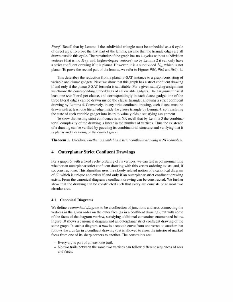
We define a canonical diagram to be a collection of junctions and arcs connecting thevertices in the given order on the outer face (as in a confluent drawing), but with someof the faces of the diagram marked, satisfying additional constraints enumerated below.Figure 10 shows a canonical diagram and an outerplanar strict confluent drawing of thesame graph. In such a diagram, a trail is a smooth curve from one vertex to another thatfollows the arcs (as in a confluent drawing) but is allowed to cross the interior of markedfaces from one of its sharp corners to another. The constraints are:

– Every arc is part of at least one trail.– No two trails between the same two vertices can follow different sequences of arcs

and faces.

* *

Fig. 10. Three views of the same graph as a node-link diagram (left), canonical diagram (center),and outerplanar strict confluent drawing (right).

– Each marked face must have at least four angles, all of which are sharp.– Each arc must have either sharp angles or vertices at both of its ends.– For each junction j with exactly two arcs in each direction, let f and f ′ be the two

faces with sharp angles at j. Then it is not allowed for f and f ′ to both be eithermarked or to be a triangle (a face with three angles, all sharp).

Let j be a junction of a canonical diagram D. Then define the funnel of j to be the4-tuple of vertices a, b, c, d where a is the vertex reached by a path that leaves j in onedirection and continues as far clockwise as possible, b is the most counterclockwisevertex reachable in the same direction from j, c is the most clockwise vertex reachablein the other direction, and d is the most counterclockwise vertex reachable in the otherdirection. Note that none of the paths from j to a, b, c, and d can intersect each otherwithout contradicting the uniqueness of trails. We call the circular intervals of vertices[a, b] and [c, d] (in the counterclockwise direction) the funnel intervals of the respectivefunnel. We say a circular interval [a, b] is separated if either a and b are not adjacent inG, or there exists a junction in the canonical diagram with funnel intervals [a, e] and[f, b], where e, f ∈ [a, b].

A canonical diagram represents a graph G in which the edges in G correspond totrails in the diagram. As we show in the full paper [8], a graph G has a canonical diagramif and only if it has an outerplanar strict confluent drawing, and if a canonical diagramexists then it is unique.

4.2 Algorithm

By using the properties of canonical diagrams (see the full paper [8]), we may obtain analgorithm that constructs a canonical diagram and strict confluent drawing of a givencyclically-ordered graph G, or reports that no drawing exists, in time and space O(n2).This bound is optimal in the worst case, as it matches the input size of a graph that mayhave quadratically many edges.

Steps 1–3 of the algorithm, detailed below, build some simple data structures thatspeed up the subsequent computations. Step 4 discovers all of the funnels in the input,from which it constructs a list of all of the junctions of the canonical diagram. Step 5connects these junctions into a planar drawing, a subset of the canonical diagram. Step 6

builds a graph for each face of this drawing that will be used to complete it into theentire canonical diagram, and step 7 uses these graphs to find the remaining arcs of thediagram and to determine which faces of the diagram are marked. Step 8 checks thatthe diagram constructed by the previous steps correctly represents the input graph, andstep 9 splits the marked faces, converting the diagram into a strict confluent drawing.

1. Number the vertices clockwise around the boundary cycle from 0 to n− 1.2. Build a table, containing for each pair i, j, the number of ordered pairs (i′, j′) with

i′ ≤ i, j′ ≤ j, and vertices i′ and j′ adjacent in G. By performing a constant numberof lookups in this table we may determine in constant time how many edges existbetween any two disjoint intervals of the boundary cycle.

3. Build a table that lists, for each ordered pair u, v of vertices, the neighbor w of uthat is closest in clockwise order to v. That is, w is adjacent to u, and the intervalfrom v clockwise to w contains no other neighbors of u. The table entries for ucan be found in linear time by a single counterclockwise scan. Repeat the sameconstruction in the opposite orientation.

4. For each separated interval [a, b], let c be the next neighbor of a that is counter-clockwise of b, and let d be the next neighbor of b that is clockwise of a. If (i) cis a neighbor of b, (ii) d is a neighbor of a, (iii) a is the next neighbor of c that iscounterclockwise of d, and (iv) b is the next neighbor of d that is clockwise of c,then (if a confluent diagram exists) a, b, c, d must form the funnel of a junction, andall funnels have this form. We check all circular intervals in increasing order of theircardinalities. For each discovered funnel, we mark the intervals that are separated bythe corresponding junction. This way we can check in O(1) time whether a circularinterval is separated. If the number of funnels exceeds the linear bound of Lemma 3on the number of junctions in a confluent drawing, abort the algorithm.

5. Create a junction for each of the funnels found in step 4. For each vertex v, makea set Jv of the junctions whose funnel includes that vertex; if they are to be drawnas part of a canonical diagram, the junctions of Jv need to be connected to v by aconfluent tree. For any two junctions in Jv, it is possible to determine in constanttime whether one is an ancestor of another in this tree, or if not whether one isclockwise of the other, by examining the cyclic ordering of vertices in their funnels.Construct the trees of junctions and their planar embedding in this way. The resultof this stage of the algorithm should be a planar embedding of part of the canonicaldiagram consisting of all vertices and junctions, and the subset of the arcs that arepart of a path from a junction to one of its funnel vertices. Check that the embeddingis planar by computing its Euler characteristic, and abort the algorithm if it is not.

6. For each face f of the drawing created in step 5, and each pair j, j′ of junctionsbelonging to f , use the data structure from step 2 to test whether there is an edgewhose trail passes through both j and j′. This results in a graph Hf in which thevertices represent the vertices or junctions on the boundary of f and the edgesrepresent pairs of vertices or junctions that must be connected, either by an arc or byshared membership in a marked face. The remaining arcs to be drawn in f will beexactly the edges of Hf that are not crossed by other edges of Hf ; the marked facesin f will be exactly the faces that contain pairs of crossing edges of Hf .

7. Within each face f of the drawing so far, build a table using the same construction asin step 2 that can be used to determine the existence of a crossing edge for an edge in

Hf in constant time. Use this data structure to identify the crossed edges, and drawan arc in f for each uncrossed edge. For each face g of the resulting subdivision off , if g has four or more vertices or junctions, find two pairs that would cross andtest whether both pairs correspond to edges in Hf ; if so, mark g.

8. Construct a directed graph that has a vertex for each vertex of G, two vertices foreach junction of the diagram (one in each direction), two directed edges for each arc,and a directed edge for each ordered pair of sharp angles that are non-consecutive ina marked face. By performing a depth-first search in this graph, determine whetherthere exist multiple smooth paths in the resulting drawing from any vertex of G toany other point in the drawing, and abort the algorithm if any such pair of paths isfound. Determine the set of vertices of G reachable from v and verify that it is thesame set of vertices that are reachable in the original graph. Additionally, verifythat the diagram satisfies the requirements in the definition of a canonical diagram.Abort the algorithm if any inconsistency is found in this step.

9. Convert the canonical diagram into a confluent drawing and return it.

Theorem 2. For a given n-vertex graph G, and a given circular ordering of its vertices,it is possible to determine whether G has an outerplanar strict confluent drawing withthe given vertex ordering, and if so to construct one, in time O(n2).

4.3 Drawings with low curve complexity

Suppose that we are given a topological description of an outerplanar strict confluentdrawing D of a connected graph G, describing the tangency pattern and ordering ofthe arcs at each junction. It still remains to draw D (or possibly an equivalent butcombinatorially different outerplanar strict confluent drawing) in the plane using concretecurves for its arcs. If we ignore the tangency requirements at its junctions, the arcs andjunctions of D form a planar graph, but applying standard planar graph drawing methodswill generate arcs that may not be smooth and that are not tangent to each other at thejunctions. So how are we to draw D? Here we use a circle packing method to draw Dwith a small number of circular arcs for each arc of D. Thus, these drawings have lowcurve complexity in the sense of Bekos et al. [1], but with this complexity measuredalong arcs of the confluent diagram rather than edges of another type of graph drawing.

Given such a drawing D, let D′ be a modified version of D in which every junctionis incident to exactly three arcs, formed from D by suppressing two-arc junctionsand splitting junctions with more than three arcs. Assume also (again by adding morejunctions if necessary) that each vertex in D′ has only a single arc incident to it.

Given the topological diagram D′, we form a planar graph H that has a vertex foreach vertex or junction of D′, and an edge for each arc of D′. Additionally, we create anedge in H for each two vertices that are consecutive in the cyclic ordering of the verticesaround the disk containing the drawing.

Lemma 5. H is planar, 3-regular, and 3-vertex-connected.

Proof. Planarity and 3-regularity follow immediately from the construction of H . Everytwo vertices of G are connected by three vertex-disjoint paths in H: at least one (not

necessarily a smooth path) through D, using the assumption that G is connected, and twomore around the boundary of the disk. Therefore, if H were not 3-vertex-connected, onlyone of its 3-connected components could contain vertices of G. The other componentswould either contain components of D that are not part of any smooth path betweenvertices of G (forbidden in a strict confluent drawing) or would contain more than onesmooth path between the same sets of vertices (also forbidden). �

Theorem 3. Let D be an outerplanar strict confluent drawing of a graph G, giventopologically but not geometrically. Then we can construct an outerplanar strict confluentdrawing of G in which each arc of the drawing is represented by a smooth curve that iseither a circular arc or the union of two circular arcs.

Proof. By the Koebe–Thurston–Andreev circle packing theorem, there exists a systemC of circles representing the faces of H , such that two circles are adjacent exactlywhen the corresponding faces share an edge. We may assume (by performing a Mobiustransformation if necessary) that the outer circle of this circle packing corresponds to theouter face of H . C may be found efficiently (although not in strongly polynomial time)by a numerical iteration that quickly converges to the system of radii of the circles, fromwhich their centers can also be computed easily [2,16].

Fig. 11. Constructing an outerplanar strictconfluent drawing from a circle packing. Thevertices of the drawing correspond to triangu-lar gaps adjacent to the outer circle, and thejunctions to the remaining triangular gaps.

Each vertex of G corresponds in C to oneof the triangular gaps between the outer circleand two other circles, and may be placed atthe point of tangency of the two non-outer cir-cles (one of the vertices of this triangle); seeFig. 11. The junctions in D′ lie at the meetingpoint of three faces of H , and correspond inC to the remaining triangular gaps betweenthree circles. A confluent drawing of G maybe formed by removing the outer circle, re-moving all circular arcs bounding the trian-gular gaps incident to the outer circle, and ineach remaining triangular gap removing thearc that is on the other side of the sharp angle.The resulting drawing contracts some edgesof D′ to form junctions with four incidentarcs, but this does not affect the correctnessof the drawing. In the resulting drawing, arcsof the diagram that have merge points or ver-tices at both of their endpoints are drawn as two circular arcs (possibly both from thesame circle); other arcs of the diagram are drawn as a single circular arc. ut

5 Conclusions

We have shown that, in confluent drawing, restricting attention to the strict drawingsallows us to completely characterize their complexity, and we have also shown thatouterplanar strict confluent drawings with a fixed vertex ordering may be constructed in

polynomial time. The most pressing problem left open by this research is to recognizethe graphs that have outerplanar strict confluent drawings, without imposing a fixedvertex order. Can we recognize these graphs in polynomial time?

Acknowledgements. This work originated at Dagstuhl seminar 13151, Drawing Graphsand Maps with Curves. D.E. was supported in part by the National Science Foundationunder grants 0830403 and 1217322, and by the Office of Naval Research under MURIgrant N00014-08-1-1015. M.L. was supported by the Netherlands Organisation forScientific Research (NWO) under grant 639.021.123. M.N. received financial support bythe ‘Concept for the Future’ of KIT under grant YIG 10-209.

References1. M. A. Bekos, M. Kaufmann, S. G. Kobourov, and A. Symvonis. Smooth orthogonal layouts.

In W. Didimo and M. Patrignani (eds.), Graph Drawing 2012, vol. 7704 of LNCS, pp 150–161.Springer, 2013.

2. C. R. Collins and K. Stephenson. A circle packing algorithm. Comput. Geom. Theory Appl.,25(3):233–256, 2003.

3. W. Cui, H. Zhou, H. Qu, P. C. Wong, and X. Li. Geometry-based edge clustering for graphvisualization. IEEE TVCG, 14(6):1277–84, 2008.

4. M. Dickerson, D. Eppstein, M. T. Goodrich, and J. Y. Meng. Confluent drawings: Visualizingnon-planar diagrams in a planar way. J. Graph Algorithms Appl., 9(1):31–52, 2005.

5. T. Dwyer, K. Marriott, and M. Wybrow. Integrating edge routing into force-directed layout.In M. Kaufmann and D. Wagner (eds.), Graph Drawing 2006, vol. 4372 of LNCS, pp. 8–19.Springer, 2007.

6. D. Eppstein, M. T. Goodrich, and J. Y. Meng. Delta-confluent drawings. In P. Healy and N. S.Nikolov (eds.), Graph Drawing 2005, vol. 3843 of LNCS, pp. 165–176. Springer, 2006.

7. D. Eppstein, M. T. Goodrich, and J. Y. Meng. Confluent layered drawings. Algorithmica,47(4):439–452, 2007.

8. D. Eppstein, D. Holten, M. Loffler, M. Nollenburg, B. Speckmann, and K. Verbeek. Strictconfluent drawing. CoRR, abs/1308.6824, 2013.

9. D. Eppstein and J. A. Simons. Confluent Hasse diagrams. In M. J. van Kreveld andB. Speckmann (eds.), Graph Drawing 2011, vol. 7034 of LNCS, pp. 2–13. Springer, 2012.

10. M. Hirsch, H. Meijer, and D. Rappaport. Biclique edge cover graphs and confluent drawings.In M. Kaufmann and D. Wagner (eds.), Graph Drawing 2006, vol. 4372 of LNCS, pp. 405–416.Springer, 2007.

11. D. Holten. Hierarchical edge bundles: visualization of adjacency relations in hierarchical data.IEEE TVCG, 12(5):741–8, 2006.

12. D. Holten and J. J. van Wijk. Force-Directed Edge Bundling for Graph Visualization. Com-puter Graphics Forum, 28(3):983–990, 2009.

13. P. Hui, M. J. Pelsmajer, M. Schaefer, and D. Stefankovic. Train tracks and confluent drawings.Algorithmica, 47(4):465–479, 2007.

14. C. Hurter, O. Ersoy, and A. Telea. Graph Bundling by Kernel Density Estimation. ComputerGraphics Forum, 31(3pt1):865–874, 2012.

15. D. Lichtenstein. Planar formulae and their uses. SIAM J. Comput., 11(2):329–343, 1982.16. B. Mohar. A polynomial time circle packing algorithm. Discrete Math., 117(1–3):257–263,

1993.17. G. Quercini and M. Ancona. Confluent drawing algorithms using rectangular dualization. In

U. Brandes and S. Cornelsen (eds.), Graph Drawing 2010, vol. 6502 of LNCS, pp. 341–352.Springer, 2011.