Embed Size (px)
Citation preview
STRESS-WAVE ANALYSIS TECHNIQUE STUDY ON THICK-WALLED
TYPE A302B STEEL PRESSURE VESSELS
by
CE Hartbower FJ Climent C Morals PP Crimmins
July 1969
Prepared under Contract NAS 9-7759 Modification 1 for the
NASA Manned Spacecraft Center
Houston Texas
Advanced Materials Technology Section Research amp Technology Department
Aerojet-General CorporationSacramento CaliforniaS a r m e t 1969
0 RECEIVED
Rpodluced by the~fT1AGLTe CLEARINGHOUSE IF r SInformation for Federal Scientifi amp Technic~aSprngfIed Va 2Z151 )
tog IIUOAJ~id~fLe
httpsntrsnasagovsearchjspR=19690026814 2020-03-26T043734+0000Z
STRESS-WAVE ANALYSIS TECHNIQUE STUDY ON THICK-WALLED
TYPE A302B STEEL PRESSURE VESSELS
by
CE Hartbower FJ Climent C Morais PP Crimmins
July 1969
Prepared under Contract NAS 9-7759 Modification 1 for the
NASA Manned Spacecraft Center
Houston Texas
Advanced Materials Technology Section Research amp Technology Department Aerojet-General Corporation
Sacramento California
FOREWORD
This report was prepared byAerojet-General Corporation Sacramento
California under NASA Contract NAS 9-7759 Modification No 1 during the
period of July 1968 to July 1969 The work was administered under the
Technical Direction of Mr W E Clautice NASA-Kennedy Space Flight Center
Florida
The study program at the Aerojet-General Corporation was performed
under the technical direction of C E Hartbower Aerojet personnel who also
participated in the program include W G Reuter A T Green C Morais
F J Climent and P P Crimmins of the Materials Integrity Section All of
these personnel participated in the preparation of this report
ii
ABSTRACT
The results of investigations to determine relationships between
stress-wave-emission characteristics and subcritical crack growth in Type A302
Grade B alloy steel are presented Stress-wave-emission characteristics which
can be used as precursors for instability (failure) for unhydrogenated and
hydrogenated material tested in air and 3 NaCl-water environments are discussed
The fracture behavior of unhydrogenated and hydrogenated A302B steel in these
environments is also described The results of background noise measurements
at the Pad A and VAB Bottle Fields at the Kennedy Space Flight Center are
presented and the feasibility of monitoring subcritical crack growth in
Type A302B steel determined by correlating these results with the laboratory
stress wave emission-fracture test data Stress-wave-emission attenuation
data are also presented and employed to determine sensor patterns for the
pressure vessels at Pad A and the VAB Bottle Field
iii
TABLE OF CONTENTS
Page
Abstract iii
I Introduction 1
II Summary 2
III Laboratory Specimen Design and Test Procedures 4
A Material and Specimen Configuration 4
B Crack-Opening Displacement Stress Intensity and 8 Specimen Loading Procedure
C Hydrogenation Procedure 15
D Stress-Wave Instrumentation - Laboratory Evaluations 16
IV Laboratory Test Results and Discussion 20
A Bend Tests in Air Without Deliberate Addition 20 of Hydrogen
B Bend Tests in Water Without Deliberate Addition 21 of Hydrogen
C Bend Tests in Air With Deliberate Addition of 27 Hydrogen
D Bend Tests in 3 NaCi-Water With Deliberate 48 Addition of Hydrogen
E WOL Tests 48
F Discussion 53
1 Material-Environment Consideration 53
2 Stress-Wave-Emission Characterization 54
V Background Measurements and Associated Laboratory Tests 56
A Background Measurements at Kennedy Space Flight Center 56
B Laboratory Signal Attenuation Evaluations 58
C Sensor Spacing 70
VI Conclusions 75
VII Recommendations for Further Work 76
References 77
iv
LIST OF TABLES
Table Page
I Material Characterization Data 5
II Details of SWE Data Obtained for Specimen 4 A302B 28
Steel During Hold at 17 kips in 3 NaCi-Water
Environment
III Wave Velocity Based on Visual Analysis of Oscilloscope 62 Traces - Pipe Tests
IV Computed Arrival Times - Pipe Tests 62
V Signal Amplitude vs Distance - Pipe Tests 63
VI Statistically Corrected Values of Signal Amplitude - 66 Pipe Tests
VII Signal Amplitude vs Distance Plate Tests 69
VIII Comparison of Statistically Corrected and Test- 70 Determined Values of Signal Amplitude - Plate Tests
LIST OF FIGURES
Figure Page
1 Notch-Bend Specimen Geometry and Crack-Opening 6 Displacement Gage
2 Configuration of WOL Specimen 7
3 Three-Point Bend Test Fixture Design 9
4 Calibration Curve for Three-Point Bend Specimen 11
5 Numerical Constant C for WOL Specimen 13
6 Crack-Opening-Displacement vs Load - WOL Specimen 14
7 Schematic Representation of SWAT Data Acquisition 17 and Data Analysis Instrumentation
8 Schematic of Instrumentation Used at Kennedy Space 19 Center
9 Cumulative Stress Wave Count vs Time Specimen 4 23 A302B Steel 15 Kip Hold 3 NaCi-Water Environment
10 Cumulative Stress Wave Count vs Time Specimen 4 24 A302B Steel 15 Kip Hold 3 NaCl-Water Environment
11 Cumulative Stress Wave Count vs Time Specimen 4 25 A302B Steel 15 Kip Hold After Replenishing the 3 NaCi-Water Environment
v
LIST OF FIGURES (cont)
Figure Page
12 Cumulative Stress Wave Count vs Time Specimen 4
A302B Steel 3 NaCi-Water Environment
26
13 Cumulative Stress Wave Count vs Time Specimen 4 A302B Steel 3 NaCl-Water Environment
34
14 Cumulative Stress Wave Count vs Time Specimen 4 A302B Steel After 1 min at 17-kip Hold in 3 NaCi-Water Environment
35
15 Cumulative Stress Wave Count vs Time Specimen 4 A302B Steel After 1-12 min at 17-kip Hold in 3 NaCi-Water Environment
36
16 Cumulative Stress Wave Count vs Time Specimen 5 A302B Steel Hydrogenated and Tested in Air
37
17 Cumulative Stress Wave Count and COD vs Time Specimen 5 A302B Steel Hydrogenated and Held at 14 kips in Air
39
18 Stress Wave Count Rate vs Time - Specimen 5 A302B Steel Hydrogenated and Tested in Air
40
19 Cumulative Stress Wave Count vs Time Specimen 5 A302B Steel Hydrogenated and Tested in Air
41
20 Cumulative Stress Wave Count vs Time Specimen 6 A302B Steel Hydrogenated and Tested in Air
42
21 Cumulative Stress Wave Count vs Time Specimen 7 A302B Steel Hydrogenated and Tested in Air
44
22 Cumulative Stress Wave Count vs Time Specimen 8 A302B Steel Hydrogenated and Tested in Air
47
23 Cumulative Stress Wave Count vs Time Specimen 9 A302B Steel Hydrogenated and Tested in 3 NaCi-Water
Environment
49
24 Cumulative Stress Wave Count vs Time at Hold WOL Specimen 1 A302B Steel Hydrogenated and Tested in 3 NaCl-Water Environment
51
25 Cumulative Stress Wave Count vs Time at Hold WOL Specimen 2 A302B Steel Hydrogenated and Tested in Air
52
26 Oscillograph Traces for Pipe Tests 60
27 Signal Amplitude vs Distance - Pipe Tests 65
28 Oscillograph Traces for Plate Tests 67
vi
LIST OF FIGURES (cont)
Figure Page
29 Signal Amplitude vs Distance - Plate Tests 71
30 Schematic of Sensor Spacings for Bottles at Pad A 73
31 Schematic of Sensor Spacings for Bottles at VAB 74 Bottle Field
vii
I INTRODUCTION
The reliability and continuous satisfactory performance of steel
pressure vessels in the propellant systems of the J F Kennedy Space Center
Launch Complex are essential to ensure personnel safety and mission reliability
To ensure continued fail-safe operation of these components a nondestructive
test technique is required which can be employed to continuously or periodically
monitor the vessels and which is sensitive enough to determine if a marginal
flaw possibly present in these vessels propagates during service The Stress
Wave Analysis Technique (SWAT) offers promise as a nondestructive test technique
for this purpose
Previous experience has shown that it is possible to monitor
subcritical crack growth by utilizing transducers to detect stress-wave
emissions which accompany the energy release occurring when a flaw propagates
This principle coupled with seismic triangulation techniques has led to the
development of the Aerojet Stress Wave Analysis Technique (SWAT) which has
been employed in the monitoring of pressure vessels during hydrotest including
the Polaris (Ref l) LEM (Ref 2) and 260-in-dia chambers (Ref 3) The
technique has also been successfully employed as a unique laboratory test
method to monitor crack growth in structural metals (Ref 4 5 and 6) and to
study the mechanism by which it occurs
Through these studies relationships between the onset of catastrophic
failure in various structural materials and stress-wave-emission characteristics
including rate of emission and amplitude have also been established for a
number of materials However these previous programs have shown that it is
necessary to characterize the stress-wave emissions associated with fracture
for the material conditions and environments (media loading rate temperature
etc) particular to each application This is necessary because of the
pronounced effect such variables exert on metal fracture the mechanism by
References appear at dnd of text
I Introduction (cont)
which it occurs and the instrumentation requirements necessary to detect such
flaw growth under actual service conditions Consequently this program was
undertaken with the following objectives
A Develop relationships between subcritical crack growth and stressshy
wave-emission characteristics in Type A302 Grade B alloy steel
B Characterize background noise existing in typical bottle fields at
the Kennedy Space Center
C Determine the feasibility of monitoring subcritical crack growth
in pressure vessels in bottle fields at Kennedy Space Center by correlating
the results of the background noise characterization and signal attenuation
tests with those obtained through laboratory tests relating stress-wave
characteristics and subcritical crack growth
Ii SUMMARY
Tests were performed using unhydrogenated and hydrogenated Type A302B
steel specimens exposed to air and a 3 NaCl-water environment Both rising
load to failure (air environment only) and sustained load tests were performed
using the Stress Wave Analysis Technique (SWAT) and a crack-opening-displacement
(COD) gage to monitor subcritical crack growth The results of these tests
showed that detectable stress-wave emissions although of small (lt001 g)
amplitude were observed to be associated with crack growth in this material
Under all test conditions the stress-wave emissions were observed during
rising load and when failure (instability) was imminent Both the amplitude
and rate of occurrence of stress-wave emission increased as failure was
approached and could be employed as precursors of the onset of instability
2
II Summary (cont)
During hold varying stress-wave-emission characteristics depending
on the test conditions were observed When tested in an air environment in
the unhydrogenated condition neither SWE nor crack growth was observed When
hydrogenated material was tested in an air environment a creep phenomenon
evidenced by increasing SWE count and apparent crack size was observed With
time at hold and at applied stress intensities less than critical the creep
phenomenon eventually stopped as did the occurrence of stress-wave emissions
Unhydrogenated material tested in 3 NaCl-water produced continuous stress-wave
emission punctuated by abrupt increases in SWE count indicating continuous
crack extension with larger crack jumps corresponding to abrupt increases in
SWE count However failure was not observed during hold when testing
unhydrogenated material in salt water or hydrogenated material in air
indicating the crack-growth rate was very low Continuous incremental crack
extension characterized by continuous SWE interspersed by abrupt increases
in SWE count indicating occasional crack jumps was also observed in testing
hydrogenated material in a 3-NaCl-water environment However the crack
growth rate for the latter test condition was much faster in comparison to
other test environments indicating a synergistic effect due to the combinashy
tion of sea water and hydrogen in interstitial solid solution
Background noise measurements conducted at the Pad A and VAB bottle
fields at the Kennedy Space Flight Center indicated that the quiescent backshy
ground noise level was much lower than the amplitude of burst-type SWE assoshy
ciated with crack growth in A302B steel Thus it is possible to detect SWE
associated with fracture under these conditions Difficulty is expected in
detecting such flaw growth during tank blowdown and repressurization periods
However the blowdown and repressurization periods are of short duration and
the materials behavior observed during this program indicate considerable
prefailure crack growth would be expected prior to failure Consequently
even under these conditions significant flaw growth andor creep could still
3
II Summary (cont)
be detected by SWAT prior to failure which would permit triangulation to the
source and tank depressurization prior to failure Signal attenuation evaluashy
tions performed both at the Kennedy Space Flight Center and Aerojet were used
to establish sensor spacing and locations for typical vessels at both Pad A
and the VAB Bottle Field
III LABORATORY SPECIMEN DESIGN AND TEST PROCEDURES
A MATERIAL AND SPECIMEN CONFIGURATION
The Type A302B nickel modified steel plate (35-in thick) tested
in this program was supplied by the Kennedy Space Center The material
characterization data shown in Table I was also supplied by NASA The bend
specimen design shown in Figure 1 was employed for the initial stress-waveshy
emissioncrack-growth tests performed at Aerojet the test specimens were
obtained from the surface and center locations in plate material supplied by
NASA Subsequently Wedge Opening Loading (WOL) tests were also employed
The WOL specimen was described by Novak and Rolfe (Ref 7) and is essentially
a modified compact tension specimen which can be used for Klscc environmental
testing The specimen is self-stressed with a bolt and therefore the loading
is constant displacement so that the initial KI value decreases to KIscc as
the crack propagates Because the specimen is self-stressed it can be
completely divorced of all extraneous noise by encasing the loaded test specimen
in a sound-proof chamber Due to the limited amount of material available
(ends of the SEN-bend specimens) the X-type WOL configuration (1 x 1 x 144 in)
was used as originally designed by Manjoine and shown in Figure 2
Prior to testing the bend specimens were precracked using an
electrodynamic vibration system During cracking the bend specimen was
gripped using a vise attachment near the specimen notch while the other end
was weighted thereby producing the maximum bending moment at the specimen notch
4
TABLE I
MATERIALS CHARACTERIZATION DATA SUPPLIED BY NASA KENNEDY SPACE CENTER
Size of Plate 3-716 x 14 x 18 in
Specification A302B Nickel Modified
Heat Treatment 1650degF3-L2 hr
Water Quench
1125degF5 hr draw
Air Cool
1100F3-12 hr Temper
Air Cool
Mechanical Properties Ftu 1162 ksi 11575 ksi
F 975 ksi ty 973 ksi
Elong 220 200
RA 610
574
CVN (ft-lb)
+50degF -40degF
34 21
29 21 28 18
Chemistry C-023 Mn-l16 P-0012 S-0019 Si-027 Mo-052 Ni-063 B-00023
5
120
206
L60--O
14 Pin Hole for Mounting
Accelerometers
Becorder
3k
T1 Ci
1251
010
~20k
L- 05 020
0-O005r 0o j
_o6o 9
010 -oo-_o250
0_75 _0200
TI
T2
r-
Figure 1 Notch-Bend Specimen Geometry and Crack-Opening
Displacement Gage
6
P
z w VIRTUAL PLANE OF
EXTENSION
H
NOTCH -shy
o
W H B
5oo
=1125
= 0500 =1000
-
050 p =002 611735-2B
Figure 2 Configuration of WOL Specimen
7
III A Material and Specimen Configuration (cont)
The specimen was then vibrated at resonant frequency (approximately 225 cps)
until a crack approximately 010 in deep appeared below the vertex of the
elox-machined notch The time required to produce the desired crack depth
was approximately 10 min or 135000 cycles The WOL specimens were precracked
(010-in depth) following hydrogenation (as described in the following parashy
graphs) in tension-tension fatigue
B CRACK-OPENING DISPLACEMENT STRESS INTENSITY AND SPECIMEN LOADING PROCEDURE
The bend specimens were tested using the three-point bend fixture
shown in Figure 3 and a hydraulic tensile machine During loading a crossshy
head speed of approximately 01 inmin was employed load control during hold
periods was maintained manually by the tensile machine operator The exact
specimen loading profiles varied between specimens and is discussed under the
resufts obtained for each specimen
During testing of the bend specimens crack-opening displacement
was measured between knife edges machined at the end of the specimen notch
(Figure 1) The measuring device consisted of a full bridge of electricshy
resistance strain gages mounted on a double-cantilever beam The amount of
flexure in the cantilever arms was controlled by the thickness of the spacer
between the arms at the base of the cantilever The design of the gage is
such that it is linear within 0001 in over the range of 0200 to 0250 in
During the initial tests of this program the output of the crackshy
opening-displacement gage was routinely recorded on a Sanborn strip chart
While this procedure is adequate for fracture toughness testing (straight
rising load to failure) because of drift and normal fluctuations in output
within the specification of the equipment manufacturer this procedure is not
sufficiently sensitive to detect the very small increments of crack extension
8
Load
K 20
k
36
15 3505
150
IU 06
1See Rolle below
240 220
200
L 20_
10020 203
Figure 3 Three-Point Bend Test Fixture Design
9
III B Crack-Opening Displacement Stress Intensity and Specimen Loading Procedure (cont)
which can occur during slow-crack-growth studies This is particularly true
in testing A302B steel where extension probably occurs through a micro-void
coalescence mechanism and in very small increments
In view of this problem a test system has been developed by
Aerojet which is capable of detecting very small increments of crack extension
This system uses the crack-opening-displacement gage recommended by ASTM and
described above however instead of a Sanborn recorder the signal from the
gage goes to a bridge balancing unit to a DC amplifier and then to a DC
millivolt recorder This system was operated at a gain of 1200 with less than
1 peak-to-peak instability The system also has a zero suppression capability
which allows the gain of 1200 to be fully utilized even though the crack
opening may increase as much as 005 in The main advantage of this system
is the extremely high sensitivity capability which was required in order to
detect incremental crack growth in the A302B nickel modified steel tested
during this program
The crack-opening displacements from the millivolt recorder were
used to determine crack length from the notch-bend calibration curve shown in
Figure 4 Stress intensity was calculated using the secant offset method
recommended by the ASTM Committee for Three-Point Bend Testing The following
relationships were employed for this purpose
PQL
K BD32 f(aD) (Eq 1)
where L is one-half the span length D is the specimen depth B is the specimen
thickness a is the crack depth and P is the load at which a secant with a
slope 5 less than the tangent slope interacts the load-displacement curve
10
200
175
150
O Each Data Point Represents an Average of Triplicate Tests
125
100
75 -
50 -
-250
010
03
Figure 4
04 05 06 07 08 aW
Calibration Curve for Three-Point Bend Specimen
11
III B Crack-Opening Displacement Stress Intensity and Specimen Loading Procedure (cont)
The parameter for crack length to depth is a numerically determined polynomial
given by
a 12 a 32+ a 52 a 72+ a 92 f(aD) = 5 8( ) -9 2(= +436(i) -753() 774(-) (Eq 2)
DDD D
The stress intensity K is a valid KIc measurement if 25(K ays) 2 is less
than both the specimen thickness and the crack depth
Calculation of the applied stress-intensity factor for the WOL
specimen was accomplished using the following expression
K PC (Eq 3)
where P is the applied load a is the crack depth B is the specimen width
and C is obtained graphically from Figure 5
Prior to precracking the WOL specimens were hydrogenated cadmium
plated and baked (same procedure as for the bend specimens) The specimens
were then precracked (01 in deep) in tension-tension fatigue Each specimen
was then calibrated by use of a crack-opening-displacement gage this was
accomplished by tensile loading the specimens and recording COD versus load
with an X-Y plotter The calibration curves for Specimen WOL-l are shown in
Figure 6 The specimens were then self-stressed by applying torque to the
bolt (bearing against a hardened steel pin) until the COD gage indicated the
desired load The load for a given stress intensity was calculated as follows
given a = 066 in (measured in specimen surfaces)
W = 1125 in
aW = 0586
12
20 I I
U I
1-z
18
16
1 4
12
-18-W
= 0444
0
U 10 -
-U-C- 8
l z
6
4
2 F 1 2 3 4 5
I __ 6 7
oW
Figure 5 Numerical Constant C for WOL Specimen
13
4500
4000
3500
3000
2500
4 2000 0
1500
1000
500
0-- 0002 in
CRACK OPENING DISPLACEMENT (IN)
Figure 6 Crack-Opening-Displacement vs Load - WOL Specimen
III B Crack-Opening Displacement Stress Intensity and Specimen Loading Procedure (cont)
C = 108 (graphically)
KI = PCB a
KSB p =
C
2 50 ksi-in1KI =for a
P = 3650 lb
Each WOL specimen was tested with an applied load correpponding to 12
K = 50 ksi-ins
C HYDROGENATION PROCEDURE
Selected bend and WOL specimens were tested after prior hydrogenashy
tion to determine the effect of this variable on the stress-wave-emissionslowshy
crack-growth relationships The hydrogenation procedure employed for this
purpose was developed by Battelle Memorial Institute and has been successfully
employed during other programs at Aerojet The hydrogen was introduced by
cathodic charging as follows
Solution 4 by weight H2SO4 5 dropsliter of poison
Poison 2 gm of phosphorus dissolved in 40 ml of carbon disulphide
Charging Time 5 min
Current Density 10 main2
The evolution of hydrogen at room temperature was prevented by
cadmium plating the test specimens within 5 min after hydrogenation The
cadmium-plating procedure was as follows
15
III C Hydrogenation Procedure (cont)
Cadmium Plating 4 ozgal CdO
Solution 16 ozgal NaCN with 1 by volume at pH 13
Current Density 70 main 2
Plating Time 30 min
Subsequent to hydrogenation and plating the specimens were baked
at 3000 F for 3 hr Baking was performed immediately prior to testing to
ensure a uniform hydrogen content throughout the test specimen
D STRESS-WAVE INSTRUMENTATION - LABORATORY EVALUATIONS
The stress-wave-detection system used for the laboratory evaluashy
tions prior to the background noise measurements at the Kennedy Space Center
is shown schematically in Figure 7 and consists of accelerometers amplifiers
filters tape recorders and an electronic counter and digital printer During
testing the accelerometers were attached to the specimens using a linear forceshy
coiled spring technique
Two basic systems were employed for stress-wave-emission data
acquisition During laboratory tests prior to the background measurements
at Kennedy Space Center the electronic counter system was employed This
system provides Very high sensitivity (signal amplifications of 10000 to
100000X) and also provides a real-time automatic count (both rate of emission
and cumulative count) of the stress-wave emissions occurring throughout each
test period The high-pass filter in the system eliminates a major portion of
the extraneous low-frequency background noises which tend to mask very small
amplitude stress waves
16
OSCILLOSCOPE
e TEKTRONIX MODEL 535
ELECTRONIC ELECTRONICSENSOR AMPLIFIER FILTER AMPLIFIER
COUNTER PRINTER S101HEWLETT PACK- HEWLETT PACK-
XIPA 00ARD MODEL 5231 ARD MODEL 5050
TAPE _ RECORDERTAPE ____________
RECORDER AMPLIFIER OSCILLOGRAPH
AMPEX MOD) T SP 300
KDATA ACQUISITION
OSCILLOSCOPE
TEKTRONIX _
eMODEL 535
DATA ANALYSIS
Figure 7 Schematic Representation of SWAT Data Acquisition and Data Analysis Instrumentation
III D Stress-Wave Instrumentation - Laboratory Evaluations (cont)
During testing of the WOL specimens maximum SWAT system amplifishy
cation was employed This was made possible because the specimens immersed
(COD gage up out of the water) in the water environment were enclosed in a
sound-proof box For these tests the electronic counter trigger level was
set just above the inherent noise (electrical) of the system Initially a
WOL test was run to determine whether the system was in fact completely free
of extraneous noise With the COD gage connected and all recording systems
in the circuit and with the specimen under no load and in air environment
after 5-12 hr in the sound-proof chamber there were only 16 signals
counted Presumably these were electrical disturbances The test was run
during regular working hours the WOL tests reported in the following parashy
graphs were tun during off-hours (nights and weekends) when there should have
been an absolute minimum of electrical disturbances
A second data acquisition system was also used for a limited
number of bend tests following the background noise measurements at Cape Kennedy
A schematic of this system is shown in Figure 8 The purpose of these tests
was to obtain stress-wave amplitude measurements using the instrumentation
employed at Cape Kennedy to ensure that the stress-wave emissions accompanying
crack extension could be detected under the background conditions observed at
Kennedy Space Center The tape recordings were made by direct recording during
test and were subsequently analyzed through playback and analysis as shown in
Figure 7
18
TEKTRONIX
OSCILLOSCOPE
ENDEVCO Dynamics Model 2213 Filter Accelerometer Model
Amplifier Amplifier 6364MQ 20-50 Kc Band Pass
KcENDEVCO30
Model 2213 CHigh-PassH Accelerometer Filter
kFI
TAPE Amplifier Amplifier RECORDER
AMPEX SP-300
Figure 8 Schematic of Instrumentation Used at Kennedy Space Center
IV LABORATORY TEST RESULTS AND DISCUSSION
As indicated in the following paragraphs two environments (air and
3 NaCl-water) and two material conditions (unhydrogenated and hydrogenated)
were utilized in the laboratory tests performed at Aerojet These conditions
are considered those most likely to be encountered during the service life of
the pressure vessels Also both straight rising load to failure and sustained
loading profiles were employed The sustained load profiles were employed
since failure of the pressure vessel may occur at constant load due to
environmentally induced slow crack growth from a prior flaw Since the
effectiveness of a failure warning system will obviously depend on the ability
to detect subcritical crack extension whether it occurs during sustained load
or on rising to failure it is important to determine if crack extension andor
failure will occur under both conditions Both effects can be studied through
the laboratory tests performed during this program
A BEND TESTS IN AIR WITHOUT DELIBERATE ADDITION OF HYDROGEN
Initially bend tests were performed in an air environment Both
the crack-opening-displacement gage and stress-wave-analysis technique were
employed to monitor the occurrence of pop-in and subcritical crack growth
The fracture data for these tests are shown below
Specimen Specimen Failure Notch Plus Apparent K
Thickness (B) Depth (D) Fatigue Crack (a) Load 1 2 No in in in aD P Kips ksi-in
1 10 20 090 045 200 130
2 097 20 091 0455 158 136
3 10 20 1036 0518 1656 133
Intermediate hold at 123 ksi-in12
20
IV A Bend Tests in Air Without Deliberate Addition of Hydrogen (cont)
The straight rising load to failure tests (No 1 and 2) indicated 12
a K value of 130 to 136 ksi-in as did the specimen (No 3) which failed
during rising load after previous holding at a stress intensity of approximately 12123 ksi-in As indicated previously in this report the ASTM recommends
for valid KIc measurements a specimen thickness exceeding that corresponding
to 25 (Kys)2 By this criterion a specimen thickness of approximately
44 in would be required for the A302B steel tested in this program
Consequently the KQ values noted above while not valid KIc measurements
indicate a high level of toughness in this material
No significant slow-crack growth or stress-wave emissions were
observed during hold in the air environment Conversely slow-crack growth
(increase in apparent crack size) and accompanying stress-wave emissions were
observed during rising load to failure The stress waves were generally very
small in amplitude (clt0Olg) but increased in amplitude with increasing crack
extension immediately prior to failure Increased rate of stress-wave
emission was also observed immediately prior to failure
B BEND TESTS IN WATER WITHOUT DELIBERATE ADDITION OF HYDROGEN
Bend specimen 4 was loaded initially to 15000 lb
(88 ksi-in 2) and held at constant load for 18 hr in 3 sodium-chloride
simulated sea water The specimen showed indications of crack growth early in
the hold period However analysis of the crack-opening-displacement gage data
indicated only very small amounts of crack extension Although the gage
employed for this purpose corresponded to the design recommended by the ASTM
its use was found unsatisfactory for tests of the type performed during this
program The COD gage was then modified and the modified version used during
the testing of the hydrogenated material described in subsequent sections of
this report
21
IV B Bend Tests in Water Without Deliberate Addition of Hydrogen (cont)
When the specimens (without hydrogenation) tested in the salt-water
environment were fractured the fracture surfaces were examined for evidence
of slow-crack growth during hold Although a small band of slow-crack growth
from the original fatigue precrack was observed it was not possible to detershy
mine how much of the crack extension occurred during rising load Onthe basis
of the COD data it would appear the majority of the extension occurred during
rising load to 15 kips from 15 to 17 kips and from 17 kips to failure although
the SWE data indicated that slow crack growth however small was occurring
during the hold periods
Figure 9 is a plot of cumulative stress-wave count over a period
of approximately 1-12 hr during hold at 15000 lb Note the indications of
a variable rate of subcritical crack growth Figure 10 shows the SWAT data
in detail (electronic counter reading every second) starting 23 min after
reaching the 15-kip load level Note that the cumfilative stress-waampe count
increased more or less continuously with brief intervals of increased slope
(when plotted to the scale of Figure 10 the increased slope was approximately 450) Figure 11 shows the SWE data obtained after adding fresh 3 NaCl-water
solution to the notch During the period of sustained load represented in
Figure 11 there were a few abrupt increases in count indicating discontinuous
crack growth together with additional intervals of increased slope (again
close to 45)
Figure 12 corresponds to the endof a short 16-kip hold (same
specimen) followed by a rise to 17 kips (approximately 125 ksi-in1 2 ) and
then a period of sustained load in 3 NaCl-water solution at 17 kips Note
the increased slope associated with the increase in load followed by abrupt
increases in count characteristic of discontinuous crack growth Approximately
600 sec after starting the hold at 17 kips an air hose produced high-frequency
noise too high to be removed by the filter This was recorded as an abrupt
increase in couni followed by a period of increased slope (again approximately 45) It cannot be definitely stated whether the increased slope indicating
22
1400
1200
1000
Li 800 3
LU
D 600
400
SEE FIGURE 10 200 FOR DETAILS
0 0 I I I I I
0 10 20 30 40 50 60 70 80 90 100
-MINUTES HOLD AT 15 KIPS
Figure 9 Cumulative Stress Wave Count vs Time Specimen No 4
A302B Steel 15 Kip Hold 3 NaCi-Water Environment
23
600
I0
20-
TIME (SECONDS)
224
6050
10 10 1O 1in20 20a 2100 2150
TIME (SECONDS) 220 3 am250 20 20 3w245 24W
43O
600
40
20
140
011 115 la 1in0 1 TIME (SECONDS)
a 14W 1m 53 0 inlW
Figure 11 Cumulative Stress Wave Count vs Time Specimen No 4 A302B Steel 15 Kip Hold After Replenishing the 3 NaCl-Water Environment
25
23
00
60
20
20
- 4o
o_ 4 o l~ ~ aiE~
220
IV B Bend Tests in Water Without Deliberate Addition of Hydrogen (cont)
continuous stress-wave emission was an artifact produced by the high-frequency
noise or the increased slope was the result of crack growth stimulated by the
high-frequency sound (crack growth after periods of dormancy can be initiated
by tapping a test specimen under load) Figure 13 is a plot of the cumulative
count for the 17-kip hold (corrected to zero at the start of hold and corrected
for noise which occurred at 836 sec) Note the tendency for increasing slope
with increasing time at load Figure 14 presents the SWAT data in detail
after 1 min at 17 kips load Figure 15 presents the data obtained after
1-12 min at 17 kips load Both Figures 14 and 15 are plotted to the same
scale as Figures 10 11 and 12 Table II presents the data plotted in
Figures 13 14 and 15 without correction for noise which occurred at 836 sec
this tabulation shows the detailed information that can be obtained by SWAT
On the basis of the SWE dpta this specimen showed evidence of
very slow continuous crack growth of the type one might expect of electroshy
chemical dissolution at the crack tip interspersed with short periods of more
rapid continuous crack growth There was little or no evidence of disconshy
tinuous crack growth with clearly defined periods of dormancy and there were
few instances of abrupt increase in count to signify crack jumps
C BEND TESTS IN AIR WITH DELIBERATE ADDITION OF HYDROGEN
After hydrogenation and baking 3 hr at 3000 F to produce a
homogeneous interstitial solid solution specimens were tested in 70degF air
Specimen 5 (Figure 16) developed discontinuous crack growth while under
sustained load starting at 9000 lb (75 ksi-in 2) but the occurrences were
sporadic and infrequent At 13000 lb (110 ksi-in 2) there was only one
stress wave large enough to be recorded as a cumulative count (cumulative
count increased from 3086 to 3110 corresponding to 464 SWEsec count rate)
Otherwise there was no increase in the SWE cumulative count during hold at
13000 lb
27
TABLE II
DETAILS OF SWE DATA OBTAINED FOR SPECIMEN NO 4 A302B STEEL DURING HOLD AT 17 KIPS IN 3 NaCI-WATER ENVIRONMENT
Time at Count Interval Time at Count Interval Load Rate Cumulative At Load Rate Cumulative A t (sec) (SWEsec) Count (sec) (set) (SWEsec) Count (sec)
27 57 8 - 1330 11 632 9 47 134 12 20 1331 20 634 1 101 4 14 54 1341 58 635 10 152 3 16 51 1392 232 652 51 299 10 27 147 1400 262 653 8
5 MINUTES 1405 134 654 5 329 1 29 30 1415 9 656 10 357 47 37 28 1443 85 657 28 444 72 49 87 1446 48 659 3 460 64 56 16 1478 131 675 32 494 221 60 34 1479 2 676 1 511 145 62 17 1495 29 685 16
10 MINUTES 25 MINUTES 616 115 72 105 1503 170 689 8 744 128 85 128 1505 72 691 2 788 2 92 44 1526 171 697 21 836 2 411(Noise) 48 1527 1 698 1 838 7 411 2 1537 187 702 10 843 10 431 5 1546 220 705 9 845 68 431 2 1584 89 715 38 846 7 431 1 1597 119 726 13 855 161 447 9 1650 146 738 53 880 160 468 25 1666 1 749 16
15 MINUTES 1671 162 756 5 904 11 492 24 1674 86 758 3 915 209 500 11 1695 120 780 21 943 5 523 28 1708 75 782 13 956 22 537 13 1717 1 787 9 980 4 541 24 1721 84 792 4 992 13 542 12 1732 114 794 11
1012 69 544 20 30 MINUTES 1088 21 558 76 1808 228 803 76 1108 151 569 20 1821 179 805 13 1136 il 576 28 1825 22 808 4 1154 5 582 18 1833 196 809 8 1172 38 583 18 1839 120 811 6 1178 19 585 6 1852 45 814 13 1182 9 -592 4 1866 146 816 14 1196 26 594 14 1888 168 819 22
20 MINUTES 1895 14 823 7 1228 80 598 32 1909 157 826 14 1229 13 599 1 1933 29 832 24 1238 2 605 9 1950 10 836 17 1256 1 610 18 1956 46 837 6 1312 91 613 56 1977 71 838 21 1318 1 619 6 1988 101 839 11 1321 1 621 3 2000 10 841 12
TABLE II (cont)
Time at Count Interval Time at Count Interval Load Rate Cumulative At Load Rate Cumulative Lt (sec) (SWBsec) Count (sec) (sec) (SWEsec) Count (sec)
2002 59 843 2 2515 40 1013 34 2017 119 845 15 2518 207 1017 3 2020 148 847 3 2521 1 1023 3 2033 165 848 13 2525 602 1029 4 2039 103 850 6 2527 22 1034 2 2048 9 857 9 2548 52 1052 21 2061 129 860 13 2561 47 1058 13 2063 156 862 2 2573 17 1062 12 2069 167 864 6 2585 69 1072 12 2075 98 874 6 2588 42 1073 3 2076 3 879 1 2599 240 1075 11 2093 21 881 17 2605 4 1077 6
35 MINUTES 2615 23 1078 10 2107 1 883 14 2616 57 1079 1 2108 103 884 1 2613 11 1080 15 2118 121 885 10 2638 42 1081 7 2119 191 887 1 2648 2 1087 10 2135 154 891 16 2650 87 1088 2 2140 11 892 5 2653 100 1089 3 2146 3 894 6 2656 56 1090 3 2150 178 897 4 2661 63 1091 5 2159 51 902 9 2685 28 1094 24 2162 7 905 3 2693 35 1097 8 2180 57 909 18 45 MINUTES 2182 58 910 2 2701 113 1104 8 2193 17 913 11 2703 50 1105 2 2195 113 916 2 2713 53 1109 10 2207 115 919 12 2719 20 1110 6 2221 34 923 14 2721 33 1112 2 2223 87 926 2 2738 72 1115 17 2238 35 936 15 2740 15 1116 2 2258 2 943 20 2752 100 1117 12 2268 204 947 10 2756 85 1119 4 2289 10 949 21 2768 56 1121 12 2307 1 952 18 2780 13 1130 12 2319 121 955 12 2782 28 1135 2 2346 20 959 27 2795 60 1142 13 2366 69 963 20 2809 65 1144 14 2386 20 975 20 2841 55 1156 32 2387 5 976 1 2848 3 1157 7 2392 158 978 5 2851 2 1159 3 2396 8 981 4 2862 45 1163 11
40 MINUTES 2869 35 1166 7 2403 21 983 7 2879 18 1169 10 2409 241 986 6 2885 62 1171 6 2449 95 996 40 2905 55 1175 20 2457 24 998 8 2908 54 1178 3 2473 104 1002 16 2918 7 1182 10 2481 3 1003 8 2924 8 1186 6
29
TABLE II (cont)
Time at Count Interval Time at Count Interval Load Rate Cumulative t Load Rate Cumulative t (sec) (SWIsec) Count (sec) (sec) (SWEsec) Count (sec)
2938 12 1193 14 3341 207 1410 2948 95 1201 10 3366 103 1421 25 2966 10 1215 18 3377 8 1424 11 2968 43 1216 2 3378 12 1425 1 2972 22 1217 4 3390 2 1429 12 2979 8 1221 7 3396 3 1430 6 2987 8 1223 8 3397 14 1432 1 2998 38 1226 11 3401 8 1434 4
50 MINUTES 3402 98 1438 1 3002 36 1228 4 3408 12 1443 6 3010 55 1230 8 3410 16 1448 2 3011 3 1234 1 3413 6 1452 3 3016 1 1236 5 3431 2 1454 8 3017 3 1237 1 3433 17 1458 2 3023 3 1239 6 3435 30 1460 - 2 3029 3 1240 6 3438 22 1462 3 3033 1 1243 4 3450 8 1475 12 3036 110 1245 3 3455 62 1484 5 3037 4 1248 1 3461 154 1490 6 3053 83 1259 16 3462 7 1493 1 3054 7 1260 1 3466 11 1501 4 3061 2 1265 7 3472 2 1507 6 3062 83 1266 1 3476 46 1509 4 3076 62 1275 14 3489 18 1515 13 3080 5 1278 4 3490 8 1517 1 3098 32 1294 18 3508 15 1534 18 3100 15 1296 2 3513 25 1541 5 3102 16 1297 2 3520 220 1549 7 3108 7 1299 6 3538 29 1566 18 3114 7 1301 6 3542 9 1572 4 3127 6 1304 13 3543 107 1575 1 3129 1 1305 2 3558 240 1588 15 3133 1 1306 4 3568 30 1601 10 3140 5 1309 7 3570 21 1603 2 3154 30 1312 14 3573 66 1607 3 3170 6 1320 16 3579 9 1613 6 3175 77 1322 5 3591 37 1619 12 3177 110 1323 2 60 MINUTES 3178 5 1324 1 3607 128 1622 16 3183 4 1326 5 3608 70 1626 1 3187 137 1331 4 3609 2 1629 1 3191 14 1332 4 3624 50 1638 15 3200 3 1336 9 3630 14 1642 6 3206 2 1340 6 3639 86 1645 9 3214 20 1343 8 3660 56 1662 21 3219 22 1345 5 3678 13 1669 18
55 MINUTES
30
TABLE II (cont)
Time at Count Interval Time at Count Interval Load Rate Cumulative At Load Rate Cumulative At (sec) (SWEsec) Count (sec) (see) (SWEsec) Count (sec)
3688 33 1680 10 4535 105 2574 28 3692 35 1682 4 4547 3 2589 12
3709 209 1688 17 4583 4 2616 36 3712 7 1689 3 4623 460 2670 40 3720 78 1691 8 4624 37 2703 1
3730 93 1694 10 4626 18 2715 2 3731 5 1695 1 4627 840 2729 1 3743 13 1703 12 4630 141 2737 3 3744 120 1709 1 4662 2 2758 32
3750 24 1715 6 4671 1 2763 9 3755 142 1724 5 4698 1 2774 27 3767 45 1738 12 4710 8 2782 12 3796 69 1770 29 4719 6 2784 9 3823 21 1808 27 4731 128 2785 12 3844 10 1838 21 4761 17 2810 30 3854 82 1851 10 4783 22 2822 22 3856 13 1855 2 4786 23 282A 3 3895 75 1915 39 80 MINUTES
65 MINUTES 4822 96 2831 36 3901 18 1920 6 4852 1 2842 30 3905 54 1927 4 4934 59 2890 82
3946 58 1963 41 4953 200 2907 19 3970 2 1985 24 4954 26 2910 1 3971 181 1988 1 4957 16 2916 3 3974 61 1990 3 4964 56 2923 7 3975 28 1992 1 4988 29 2941 24 3987 51 2004 12 5000 88 2951 12 4012 2 2022 25 5031 10 2977 31 4013 31 2026 1 5032 9 2978 1 4022 7 2036 9 5045 56 2982 13 4054 4 2062 32 5054 4 2984 9 4056 16 2066 2 5093 220 2992 39 4084 37 2093 28 85 MINUTES 4091 36 2099 7 5122 115 2996 29 4100 3 2111 9 5166 17 3019 44 4129 16 2142 29 5190 172 3042 24 4156 6 2165 27 5193 55 3045 3
70 MINUTES 5194 2 3048 1 4241 19 2253 85 5224 313 3081 30 4292 4 2299 51 5248 23 3106 24 4331 42 2339 39 5266 32 3123 18 4338 19 2348 7 5281 24 3138 15 4340 66 2350 2 5291 10 3150 10 4345 10 2359 5 5303 25 3164 12 4385 4 2419 40 5306 1 3169 3 4397 121 2432 12 5324 56 3187 18
75 MINUTES 5330 58 3193 6 4500 40 2534 103 5345 31 3211 15 4507 6 2542 7 5351 155 3217 6
31
TABLE II (cont)
Time at Count Interval Time at Count Interval Load Rate Cumulative At Load Rate Cumulative At (sec) (SWBsec) Count (sec) (sec) (SWEsec) Count (sec)
5357 211 3223 6 5887 185 3536 1 5363 29 3233 6 5905 65 3559 18 5364 20 3237 1 5923 31 3575 18
90 MINUTES 5924 22 3576 1 5403 118 3276 39 5933 109 3578 9 5418 79 3295 15 5934 5 3579 1 5419 44 3298 1 5961 43 3582 27 5420 35 3300 1 100 MINUTES 5448 27 3324 28 6000 23 3585 39 5460 118 3327 12 6001 13 3586 1 5466 97 3329 6 6002 166 3588 1 5472 184 3331 6 6008 9 3590 6 5484 28 3333 12 6032 29 3592 24 5499 45 3338 15 6041 111 3596 9 5505 2 3341 6 6062 116 3601 21 5506 173 3344 1 6083 1 3603 21 5512 72 3346 6 6084 236 3606 1 5515 8 3348 3 6090 140 3607 6 5536 199 3352 21 6091 104 3608 1 5548 5 3356 12 6106 21 3609 15 5553 199 3359 5 6115 31 3611 9 5554 34 3360 1 6121 29 3614 6shy5587 190 3364 33 6124 1 3622 3 5593 2 3365 6 6139 51 3630 15 5605 6 3367 12 6160 25 3634 21 5611 12 3369 6 6175 5 3636 15 5638 3 3373 27 6184 196 3639 9 5644 57 3374 6 6217 275 3645 33 5645 78 3376 1 6223 84 3648 6 5669 21 3379 24 6238 23 3649 - 15 5693 22 3384 24 6244 99 3650 6 5699 48 3385 6 6250 81 3652 6
95 MINUTES 6259 39 3654 9 5702 74 3387 3 6265 15 3656 6 5703 85 3389 1 6271 21 3658 6 5725 21 3391 22 6283 85 3660 12 5737 1 3394 12 105 IWNUTES 5752 72 3396 15 6304 143 3662 21 5761 106 3398 9 6331 50 3672 27 5788 1 3414 27 6340 179 3674 9 5794 176 3422 6 6341 37 3675 1 5809 2 3441 15 6365 34 3677 24 5810 15 3445 1 6366 ill 3680 1 5813 42 3448 3 6393 150 3682 27 5814 189 3451 1 6405 43 3684 12 5823 180 3461 9 6429 4 3687 24 5832 171 3472 9 6435 127 3690 6 5838 46 3481 6 6459 31 3691 24 5859 63 3505 21 6483 7 3694 24 5865 15 3511 6 6495 30 3696 12 5886 2 3533 21 6501 128 3700 6
32
TABLE II (cont)
Time at Count Interval Time at Count Interval Load Rate Cumulative At Load Rate Cumulative At (sec) (SWEsec) Count (sec) (sec) (SWEsec) Count (sec)
6522 87 3703 21 7278 21 4158 6 6531 16 3704 9 7302 2 4174 24 6555 102 3706 24 7303 3 4174 1 6567 7 3709 12 7318 125 4186 15 6570 10 3710 3 7348 88 4205 30 6576 87 3711 6 7402 86 4238 54 6577 89 3713 1 7435 90 4258 33 6578 131 3714 1 7447 14 4262 12 6599 4 3717 21 7474 14 4277 27
6600 110 MINUTES
8 3718 1 7486 7504
9 125 MINUTES
89
4286
4304
12
18 6603 37 3720 3 7510 39 4308 6 6639 15 3724 36 7531 52 4331 21 6669 48 3728 30 7540 208 4344 9 6675 23 3729 6 7549 38 4353 9 6684 57 3731 9 7576 72 4376 27 6705 23 3757 21 7594 24 4392 18 6744 53 3807 39 7603 55 4403 9 6762 240 3830 18 7615 160 4415 12 6783 5 3854 21 7621 134 4420 6 6801 26 3874 18 7627 160 4423 6 6822 181 3901 21 7639 180 4430 12 6852 24 3934 30 7648 5 4432 9 6879 44 3962 27 7658 100 4437 10 6882 2 3965 3 7679 319 4445 21
115 MINUTES 7694 72 4449 15 6906 63 3991 24 7709 23 4451 15 6927 176 4001 21 7721 34 4453 12 6930 15 4006 3 130 MINUTES 6931 54 4011 1 7800 Test Terminated 6952 305 4026 21 6953 40 4033 1 6980 3 4037 27 6989 99 4039 9 7040 387 4080 51 7041 53 4095 1 7056 23 4100 15 7086 354 4108 30 7095 21 4110 9 7125 70 4117 30 7131 2 4120 6 7167 97 4129 36 7176 11 4130 9 7197 18 4133 21
120 MINUTES 7218 28 4136 21 7227 39 4138 9 7248 72 4146 21 7272 50 4153 24
33
40
38W
3400
32W
30
28M
260
= 2400
S 22DD
i20
1600
1400
1200
10
600
400
200
06 1a 20 30 40 50 60 70 80 90 tW 110120130
MINUTE-S-H-OLD 17KIPS
Figure 13 Cumulative Stress Wave Count vs Time SpecimE A302B Steels 3 NaC1-Water Environment
34
3503
0
~0
40
20
3203
00
20
C0
20
310
03
(0
40
= = 20 0 I- 365~
05
20 00
20
0shy20
2003
20 ~~0 C
20
20 40
- 20
2835
0
(0
20
20shy
20020
20 -
3403 3450 3720 3750 fl 3550 3003 3050 40) 4050 4003 4050 4~fl 4200 4020 4350 4440 4450
TIME (SECONDS)
Figure 14 Cumulative Stress Wave Count vs Time Specimen No 4 A302B Steel After 1 Minute at 17 Kip Hold in 3 NaCi-Water Environment
35
48
0
I-
S 40
us 50 50 70 5 90 0 60 60 10 6 6 t 20CO DS
- iue1CmlaieSrs av on sTme pcmnN A0BSel
Afe2-0iue t1 i todi NC-ae niomn
Page60
4520 -
so- lao
F
122021 amp~
20 4
400
20
20 22
3540 =
20
3024
20
50
45
20
20520
20
20
45
20
no
I
40
4~
20
40
20
20
4
20
2020
20
gt
20
20 4
20
20
3545
20
Iino200j
5505
2220
1120
20
001
20
20 shy
00
1
45
OX
I
I I
I I
0 50
020 000
205 200
20 200
Z
40 505
550 400
TIM
E (S
EC
ON
DS
)
Figure 16
Cumulative Stress Wave Count vs
Time Specimen No
5 A302B Steel
Hydrogenated and Tested in Air
37
IV C Bend Tests in Air With Deliberate Addition of Hydrogen (cont)
On raising the load from 13000 to 14000 lb (122 ksi-in )
there was evidence of a creep phenomenon as shown in Figure 17 The crackshy
opening-displacement gage confirmed the occurrence of crack growth continuing
after reaching the 14000-lb hold Stress-wave emission showed the mechanism
to be discontinuous cracking rather than a deformation process When the
count rate was plotted as in Figure 18 the activity carrying into the
14000-lb hold again was discontinuous After approximately 300 sec at 14 kips
the SWE associated with the creep phenomenon had subsided During the 14-kip
hold there were two crack jumps one after 920 sec (cumulative count increased
from 5618 to 5720 and the count rate associated with the jump was 181 as
counted over a 10-sec interval or 18 SWEsec) and one after 2130 sec (cumulashy
tive count increased from 5721 to 5755 and the count rate was 139 in 10 see)
After 5000 sec at 14 kips the load on Specimen 5 was raised As
seen in Figure 19 the stress-wave activity was an unmistakable presage of
instability which occurred after 20 sec into hold The load reached a maximum
of 145 kips (145 ksi-in 2) Technically the onset of instability occurred
shortly after starting to increase the load ie at approximately
132 ksi-inI2 which agrees with the KQ value obtained through rising load
tests of unhydrogenated material in an air environment
Because of the very long test period and multiple loadings involved
in the testing of the Specimen 6 only data obtained during rising load to
19500 and 19800 ib during sustained test periods at these loads and during
specimen failure are shown in Figure 20 These data indicate essentially the
same SWE-crack growth relationships discussed previously for Specimen 5 except
that on reaching hold the crack tended to grow slowly for a longer period of
time in comparison to the behavior noted for Specimen 5 Also the incremental
nature of crack extension was more readily observed by the stress-wave-emission
data for Specimen 6
38
20
560
80
60
40
20
5500
80
60
40
20
5400
o 5100
808
60
40
20
5000 u-J
4500
4480 80 4- START 14-KI P HOLD
CODC 75lt
4000
3980 70
3960
6553120 l
- END13-KIP HOLD
3100 160 0 40 80 120 160 200 240 280 320
TIME AT LOAD (SECONDS)
Figure 17 Cumulative Stress Wave Count and COD vs Time Specimen No 5 A302B Steel fydrogenated and Held at 14 Kips in Air
39
200
LU
LU
1- 100
50 END 13-KIP
25 HOLD-I
0 1- TIME
100 INSECONDS AT
200 14KIPS
300
(COUNT EVERY 10 SEC)
Figure 18 Stress Wave Count Rate vs Time - Specimen No 5 A302B Steel Hydrogenated and Tested in Air
40
INSTABILITY
9580
9560
9540
9380
928D0
9260
842D
8440
73O I-shyz 7220
o 7260
U 7240
7220
7180I-shy
7160
- 7140
7120
7100
7080
7060
5900
5880
5860
5840
5820
5800
578D
5460
0 40 80 120 160 SEC
4M 4960 50D RISING LOAD-SECONDS AT 14 KIPS
Figure 19 Cumulative Stress Wave Count vs Time Specimen No 5 A302B Steel Hydrogenated and Tested in Air
41
20000
18000
FAILURE
18290 sec a- 1 17-in K - 199 s - Y
z
-
16000
14000
l0
1200
I-9 Iin
1014in K 152 ki- in -i
o-1 09 n K- 176ksmn
- 1 07 in I 170 iis-
o -1 042in K 12ks-in
c023i NK15ks-n
-shy
-
10000
REACH 19800 lbs
START TO 19800 bs
10000 11000 12000 13000 14000 15000 16000 17000 18000 19000
TIMESECONDS
12000
11000 s
p9000
T LOAD ADJUSTMEA
7n000
READOUT6000 OTE STRESS WAVE DATA A UST T
500 Vgt 0 ENT CORRESPONDIG TO SLOPELOAADJUSTM15 CHANGES PLOTTED
a 4000
3000
LOAD ADJUSTMENT2000 SECONDSECMENIME
1000 START HOLD AT 19500 1b
900 1l6070 D0 8 0 00 0 000600
0 1000 50002000 3000 4000
TIME SECONDS
Figure 20 Cumulative Stress Wave Count vs Time Specimen No 6 A302B Steel Hydrogenated and Tested in Air
Page 42
IV C Bend Tests in Air With Deliberate Addition of Hydrogen (cont)
As indicated in Figure 20 the increase in crack length during
the initial period of hold at 19500 lb resulted in an increase in the applied
stress intensity and was accompanied by significant stress-wave-emission
activity To maintain the desired load it was also necessary to make frequent
load adjustments at the start of hold During the first 3600 sec the effecshy
tive crack length increased from approximately 0963 to 1000 in and was
accompanied by about 7000 SWE As indicated in Figure 20 the majority of the
SWE activity and increase in crack length occurred during the first 3000 sec
of the hold at 19500 lb After this period both the stress-wave-emission
activity and rate of increase in crack length gradually decreased For example
during the entire period from 5000 to 17600 sec when the load was increased
to 19800 lb the apparent crack length and SWE count increased by only approxishy
mately 0020 in and 2500 respectively
After approximately 17000 sec at 19500 lb the load was increased
to 19800 lb and specimen failure occurred after approximately 600 sec at
19800 lb The load was maintained for this period however it was apparent
from both the SWE and COD gage data that the crack was extending and specimen
failure would occur without a further increase in load although it was necesshy
sary to continually adjust the tensile machine to maintain the desired load
The failure stress intensity approximated 199 ksi-in 2however technically
the onset of instability occurred after starting to increase the load at
approximately 153 ksi-in1 2
Specimen 7 was also hydrogenated baked at 300F for 3 hr and
tested in air Figure 21 is a detailed plot of the SWAT data (electronic
counter print-out every second) indicating crack growth of a discontinuous
nature starting at 2400-lb load Note the periods of dormancy (no increase
in SWE count) interspersed with abrupt increases in count indicating disconshy
tinuous crack growth Note also that there was little or no evidence of
continuous stress-wave emission until the load (stress intensity level) was
high approaching failure
43
CUMULAIY STRESS-VAVE COUNTCU LTISTE W E ON
I OT A~II I OI I L I I I I I I I I I I I I I I i I I I I I
- N LB
I I I I I I I I I I I I I i I I
--L - 0OTO11
-0101
(lNIML~ 33383338
8
133113-
3IiC)0 83) 3103 31-3(31-
~0
33 331
3l3C0C~
38318shy
111(10 CAVMSS3 nfl CAliVi flWfl3
________________________________________________________________________
111fl0~ 3KvM~s~a1Ff~TfvTifwT
FPAIAE
hY
A Ii
8
INa
CZ
8 C0 U CI
33 S
1 H
H
03 -I
~ 3lt
0 Cd 33
~C3 ~ H
8 0003
A
Ofli3i~~ C)
Page 45
IV C Bend Tests in Air With Deliberate Addition of Hydrogen (cont)
Figure 22 presents the SWE data from a hydrogenated bend specimen
(No 8) tested in air The load was increased continuously to 9800 lb
(70 ksi-in 2) where there was a short hold (approximately 400 sec) Note
the discontinuous crack growth followed by a short period of continuous
emission (less than 450 slope) The load was then raised to 14800 lb
(109 ksi-in 2) and held for approximately 400 sec Again there were jumps
in the SWE cumulative count but this time interspersed with continuous
emission The SWAT system employed for this test corresponded to that employed
for the background measurements at Kennedy Space Flight Center and shown in
Figure 8 only one channel was employed viz
Endevco 2213 Amplifier Amplifier Band-Pass Filter 10OX 10OX 20 to 50 Kcps
The continuous stress-wave emission observed during hold at the higher stressshy
intensity level in this specimen was not observed in the other hydrogenated
specimens tested in air The primary purpose of this test (Specimen 8) was to
record SWE data for subsequent playback and analysis to determine the amplitude
of burst-type stress-wave emissions associated with fracture in Type A302B
steel These analyses were performed using the instrumentation shown in
Figures 7 and 8 with the following results which are discussed in more detail
in conjunction with the results of the background measurements performed at
Kennedy Space Flight Center (Section V)
Maximum SWE Amplitude - 39 x 10-3g
Minimum SWE Amplitude - 12 x 10-3 g
Average SWE Amplitude - 22 x 10-3g
Laboratory Background - 11 x 10-3g
46
00 o z~ 20 ~
40
~40
S20 1 2 0 0 0 0
TIIAEAT 4 S-KIPHOLD (10KS(51IN A)
407
IV Laboratory Test Results and Discussion (cont)
D BEND TESTS IN 3 NaCI-WATER WITH DELIBERATE ADDITION OF HYDROGEN
Specimen 9 was hydrogenated baked and tested in 80F water
The electronic counter indicated continuous stress-wave emission interspersed
with abrupt increases in count indicating occasional crack jumps Figure 23
shows the details of stress-wave emission that occurred during both rising
load and holding load The crack length determined from the COD chart at
selected loads is also shown Note from the SWE data that there were no
periods of dormancy and the slope of the plot of cumulative count versus time
indicated moderately rapid continuouas crack growth such as might occur with
electrochemical dissolution at the crack tip The COD gage data shown in
Figure 23 also indicate crack extension however the actual amount appears
to be quite small (lt01 in) which would be consistent with the relatively
small number of stress-wave emissions detected even at the high system
sensitivity employed The dramatic difference between the behavior in
Figures 21 and 23 for hydrogenated material tested in air (Figure 21) and
water (Figure 23) indicates that hydrogen and 3 sodium chloride solution
acting together have a greater total effect than the sum of their individual
effects ie working together they appear to have produced a synergism
E WOL TESTS
Because of the possible significance of the synergistic-effect
noted above on the life of the hydrogen pressure vessels at Kennedy Space
Flight Center additional testing was performed using hydrogenated WOL specishy
mens cut from the fractured bend specimens The first WOL specimen was
initially loaded to-3650 lb (50 ksi-in 2) and then placed in 3 NaCl solution
(notch immersed) There was 30 min of essentially continuous stress-wave
emission (recorder started approximately 5 min after loading the specimen)
Subsequently therewas one sizable jump in the SWE cumulative count after
48
V30
760
740-M
$
720 -s
680shy
60
610
40 w
w
520 w
i
20500
HOLDD]N
340
20 760
7200
ING
IV
O
shy
420
60
40
20 0 2
04
0Q
0
60DO
LO0
01 200
250 300
350 400
450 500
550 6M
650
700 750
TIME
(SECONDS)
Figure 23
Cumulative Stress Wave Count vs Time Specimen No 9 A302B Steel
Hydrogenated and Tested in 3 NaCi-Water Environment
49
IV E WOL Tests (cont)
approximately 3 hr 40 min Then 3 hr 20 min later several jumps occurred
followed by 8 hr 20 min of stress-iave activity After this the crack was
dormant (total test time 17 hr 25 min) These data are shown in Figure 24
The load was then increased slightly (torque was increased from 200 to
255 in-lb) an additional 1-12 hr in 3 NaCl solution produced no significant
increase in the cumulative stress-wave count The reason for this apparently
anomalous behavior was not determined although it may result from a blunting
effect at the crack tip produced during the initial hold period
The fatigue crack was then extended (approximately 005 in) in
tension-tension fatigue and the specimen reloaded to approximately 51 ksi-in2
Stress-wave emission started almost immediately (dashed curve in Figure 24)
After approximately 3 hr of discontinuous activity the periods of dormancy
tended to increase interspersed with relatively small jumps (as counted over
10-sec intervals) The results of the initial loading and the reloading are
shown in Figure 24 note that there was appreciably lower cumulative count in
the reloaded specimen as compared with the initial loading for a comparable
period of test
A second hydrogenated WOL specimen was then tested in air at
50 ksi-in 2 there were stress waves initially (creep) but then very little
activity over the remaining 35-hr test period After the first hour the
count increased from approximately 150 to only 280 in the final 34 hr of test
Figure 25 shows the long peribds of dormancy punctuated by occasional 1-count
increases This is in marked contrast to the results obtained from the
hydrogenated WOL specimens tested in 3 NaCl solution and the bend-test
findings of a synergistic effect were confirmed
50
------------
aa
L- -- -- - ------ - --- I
3
IN DO
INTES) 3 S IOTI E( LI N LU
Ino
a
N O
TIME (MINUTES) IN 3 NCI SOLUTION
Figure 24 Cumulative Stress Wave Count vs Time at Hold WOL Specimen No 1
A302B Steel Hydrogenated and Tested in 3 NaCi-Water Environment
51
000 In 0 M6020 126 24 022 in0 1180 10 11 100 IWO l 100M M-C 0 90w6 a0 w6
t t t t 5W MOD4
10
TIME (MINUTES)
Figure 25 Cumulative Stress Wave Count vs Time at Hold WL Specimen No 2 A302B Steel Hydrogenated and Testd in Air
52
IV Laboratory Test Results and Discussion (cont)
F DISCUSSION
1 Material-Environment Consideration
The Type A302B steel supplied for evaluation exhibited a
very high level of fracture toughness Although quantitative plane-strain
fracture toughness measurements were not possible because of the large specimen
size required the KQ value associated with failure approximated 135 ksi-in1 2
This material was also found resistant to environmentally induced failure in
that the rate of crack growth of a prior flaw at applied stress-intensity
factors as high as 90 of the KQ value appeared to be very low This effect
was observed for unhydrogenated-material tested in air and a 3 NaCl-water
environment and hydrogenated material tested in an air environment However
the hydrogenated specimens tested in 3 NaCl-water environment had a much
faster rate of subcritical crack gr~wth in comparison to the other test condishy
tions indicating a synergistic effect due to the combination of sea water and
hydrogen in interstitial solid solution This synergistic effect indicates
that the Type A302B steel hydrogen storage tanks in the Kennedy Space Flight
Center environment may have limited life as the result of subcritical crack
growth if subjected to the same combination of stress and environmental
factors-
The WOL test results tended to confirm the possible synergism
due to the combined effects of 3 NaCl-water and hydrogen in interstitial solid
solution Marked SWE activity was observed when the hydrogenated specimens
were immersed in the salt water whereas in an air environment after the
initial period at hold when a creep phenomenon was observed there was essenshy
tially no stress-wave emission The fact that failure was not produced on
holding (in contradiction to the bend tests) can be explained by the fact that
the WOL test as-performed in this program is a self-arresting test because
53
IV F Discussion (cont)
the occurrence of crack growth results in a reduction in the applied load
Conversely in the bend tests the load was constantly applied as the crack
extended and eventually resulted in specimen failure
2 Stress-Wave-Emission Characterization
Detectable stress-wave emissions although of small amplitude
(ltOOlg) were observed to be associated with crack growth in Type A302B steel
Under all test conditions the stress-wave emissions were observed both during
rising load and when failure (instability) was imminent During hold various
SWE characteristics depending on the test conditions were observed When
tested in the hydrogenated condition in-an air environment a creep phenomenon
evidenced by increasing count of SWE and an accompanying increase in apparent
crack size was observed With time at hold and at applied stress-intensity
levels less than critical the creep phenomenon eventually stopped as did the
occurrence of stress-wave emissions Unhydrogenated material tested in the
3 NaCl-water environment produced continuous stress-wave emission punctuated
by abrupt increases in SWE count This behavior indicates both continuous
very small increments of crack extension with larger crack jumps corresponding
to the abrupt increases in SWE count Continuous incremental crack extension
characterized by continuous SWE interspersed with abrupt increases in SWE count
indicating occasional crack jumps was also observed in testing hydrogenated
material in a 3 NaCl-water environment
In all instances when failure (instability) occurred both
the amplitude and rate of stress-wave emission increased and could be employed
as a precursor of the onset of instability however even when failure was
approached-the SWE amplitude was small (ltOlg) In the other instances where
failure was not produced evidence of crack extension (although very small in
some instances) was observed on the specimen fracture face Once evidence of
54
IV F Discussion (cont)
crack growth was observed (by SWE or COD) it is obvious that failure would
eventually occur (assuming a constantly applied load) although depending on
the initial flaw size and subcritical growth rate the time to failure may be
very long In actual practice the SWE data could be employed (1) to locate
the propagating flaw (2) to monitor its occurrence and (3) as a basis for
terminating service so that repairs could be made before failure The stressshy
wave emissions associated with crack growth during rising load or increasing
stress intensity and the creep phenomenon during the initial part of hold
can be employed for this purpose
5S
V BACKGROUND MEASUREMENTS AND ASSOCIATED LABORATORY TESTS
A BACKGROUND MEASUREMENTS AT KENNEDY SPACE FLIGHT CENTER
Background noise measurements were made at two locations the VAB
Bottle Field and Pad A at the Kennedy Space Flight Center The data were tape
recorded and in addition to general background noise included tank blowdown
and repressurization periods The instrumentation for this purpose is shown
schematically in Figure 8 analysis of the data was performed by playback onto
an oscillograph and comparison with the SWE-crack growth data obtained during
the laboratory testing of bend specimens
The analysis of the signal amplitude data for tests at Cape Kennedy
is indicated below
1 Pad A Bottle Field
Signal Amplitude
a Quiescent Background
Filter at 20 Kcps - 50 Kcps -BandPass- 99 x 10 gsBand Pass
Filter at 200 cps - 32 Kcps
Band Pass
b Tank Blowdown - System Saturation (gt llg peak to peak)
C Tank Repressurization - System Saturation (gt llg peak to peak)
2 VAB Bottle Field
a Quiescent Background - 22 x 10- 4 gs
56
V A Background Measurements at Kennedy Space Flight Center (cont)
Signal Amplitude
b Tank Blowdown - System Saturation (gt llg peak to peak)
C Tank Repressurization - System Saturation (gt llg peak to peak)
Analysis of the tape-recorded data of bend tests at Aerojet indicates
the following signal amplitude for burstf-type stress-wave emissions associated
with crack growth and fracture in Type A302B steel
Maximum Amplitude - 39 x 10-3g
Minimum Amplitude - 12 x 10-3g
Average Amplitude - 22 x 10-3g
Laboratory Background - 11 x 10-3g
Thus the amplitude of SWE associated with crack growth in A302B steel is
approximately an order of magnitude larger than the background noise noted
previously Consequently the above results show that it is possible to detect
stress-wave emissions associated with fracture in A302B steel under the quiescent
background conditions existing at the Kennedy Space Center Difficulty is
expected in detecting such flaw growth during tank blowdown and repressurization
periods unless filtering can be employed to screen out the noise associated
with these periods However the blowdown and repressurization periods are of
very short duration and the materials behavior observed in this program indishy
cated that considerable prefailure crack extension would be expected from any
flaw of a size expected to be present in these pressure vessels Also
immediately on reaching load a creep phenomenon evidenced by an extension
in apparent crack length and accompanied by detectable stress-wave emission
was observed Consequently even if noise associated with blowdown and
57
V A Background Measurements at Kennedy Space Flight Center (cont)
repressurization cannot be effectively filtered out significant flaw growth
andor creep could still be detected and tank depressurization accomplished
prior to catastrophic failure assuming a capability for such depressurization
exists at these locations
B LABORATORY SIGNAL ATTENUATION EVALUATIONS
Subsequent to the background measurements at the Kennedy Space
Flight Center and the bend tests at Aerojet two series of tests were made at
Aerojet using a section of pipe and plate both of SAE 4130 steel alloy The
purpose of these tests was to determine the coefficient of signal attenuation
which in conjunction with the previous test data could be used to establish
the sensor spacing which would insure detection of SWE associated with crack
growth in the pressure-vessels at the Kennedy Space Flight Center
In these tests a constant pulse was imparted to the specimen by
a Tektronix 115 Pulse Generator using a Clevite PZT-5 Crystal (2125 in dia
and 0250 in thick) The piezoelectric crystal was mounted on a small alumishy
num block which in turn was adhered to the surface of the specimen The
signal was received by a 2217-E-Endevcq accelerometer placed at various disshy
tances from the pulser The pulse used was 10 n-sec rise and fall time with
a duration of 20 microsec at an amplitude of 12v
1 Pipe Tests
A SAE 4130 steel pipe (8-58 in OD 7-18 in ID and 22 ft
10-78 in long) was used as specimen for this test series The pulser was
mounted normal to the external surface of the pipe as close as possible to the
edge The accelerometer (2217-E-Endevco) was successively placed on the pipe
58
V B Laboratory Signal Attenuation Evalutions (cont)
surface at positions I to 8 that were at 4 6 8 10 12 14 16 and 20 ft
from the pulser The signal received by the accelerometer was displayed on a
Tektronix 422 osilloscope Typical signals are shown in Figure 26
The velocities of the compressional and shear waves in steel
are
29 lO06 x38103 Vc= -x lg ) (l-26) = O2 x06(- 0 x386 = 227000 insec(+j 012)283 (1+030) (1-060)
29x106 x 386 = 91 36= 123000 insec
s 2 ( + p) p 2 (i + 030) x 0283
where E = Youngs Modulus p = Poissons Ratio and p = density The times of
arrival of these waves at the computed velocities are indicated on the oscilloshy
scope photos shown in Figure 26 The point of shear wave arrival (T ) coincides
in most of the photos to a distinct change of pattern in the trace The
arrival of the compressional wave is difficult to determine accurately because
the amplitude of this wave attenuates very fast with distance
A visual comparison of the curves shows that Figure 26a
representing the signal received 4 ft from the impulse indicates a perfectly
detectable arrival of the compressional wave conversely Figure 26h (at 20 ft
from the impulse) shows the visually detectable arrival of a wave almost at the
computed arrival of the shear wave This is due to the fact that the amplitude
of the first cycles of the compressional wave have become essentially impercepshy
tible at a distance of 20 ft from the pulse An attempt to determine signal
arrival time by visual inspection only of the traces in Figure 26 would result
in the wave velocities indicated in Table III The computed arrival times of
the compressional and shear waves are shown in Table IV If an integration of
the positive portions of the cycles comprised in 200 p sec after arrival of the
59
VERTICAL SCALE 1 DIV= 01 V VERTICAL SCALE 1 DIV = 01 V HORIZONTAL SCALE 1 DIV= 50p SEC HORIZONTAL SCALE 1 DIV = 100 pSEC
a 4FT FROM PULSER b6 FEET FROM PULSER
Tc Ts Tc Ts
VERTICAL SCALE I DIV 01 V VERTICAL SCALE I DIV = 01 V HORIZONTAL SCALE I DIV = 100 I SEC HORIZONTAL SCALE 1 DIV = 200 p SEC
c 8 FEET FROM PULSER d 10 FEET FROM PULSER
Tc = Arrival of Compressional Wave
T = Arrival of Shear Wove
Figure 26 Oscillograph Traces for Pipe Tests (Sheet 1 of 2)
6o NOT REPRODUCTBLE
VERTICAL SCALE 1 DIV = 01 V VERTICAL SCALE 1 DIV 01 V HORIZONTAL SCALE 1 DIV = 200y SEC HORIZONTAL SCALE I DIV 200 p SEC
e 12 FEET FROM PULSER f 14 FEET FROM PULSER
T TS T T
VERTICAL SCALE 1 DIV = 01 V VERTICAL SCALE 1 DIV = 01 V HORIZONTAL SCALE 1 DIV = 200 v SEC HORIZONTAL SCALE I DIV =5001p SEC
g 16 FEET FROM PULSER h 20 FEET FROM PULSER
Figure 26 Oscillograph Traces for Pipe Tests (Sheet 2 of 2)
61
V B Laboratory Signal Attenuation Evaluations (cont)
shear wave is performed the average amplitudes determined in this manner
become quite meaningful These average amplitudes are shown in Table V
TABLE III
WAVE VELOCITY BASED ON VISUAL ANALYSIS OF OSCILLOSCOPE TRACES - PIPE TESTS
Distance from Pulse Arrival Velocities Photo ft in Time psc (ftsec)
1 4 48 210 228000
2 6 72 400 180000
3 8 96 600 160000
4 10 120 800 150000
5 12 144 1000 144000
6 14 168 1200 140000
7 16 192 1400 137000
8 20 240 1750 137000
TABLE IV
COMPUTED ARRIVAL TIMES - PIPE TESTS
Compressional Wave Shear Wave Distance from Pulse Arrival Time Arrival Time
Photo in psec Osc Div sec Ose Div
1 48 212 423 390 780
2 72 317 317 583 583
3 96 422 422 778 778
4 120 530 265 972 486
5 144 635 317 1163 581
6 168 740 370 1360 680
7 192 840 420 1545 771
8 240 1050 21 1930 387
62
V B Laboratory Signal Attenuation Evalutions (cont)
TABLE V
SIGNAL AMPLITUDE VS DISTANCE - PIPE TESTS
Average Signal Amplitude Distance from 200 Psec after Arrival
Test Pulser in of Comp Wave mv
1 48 230
2 72 145
3 96 85
4 120 60
5 144 45
6 168 28
7 192 22
8 240 18
The general equation for the amplitude attenuation curve is
C x e-Xy =
where y = amplitude at distance x in volts
x = distance in inches from pulse source
C = amplitude of pulse in volts
a = attenuation factor
or iny= 1 C + (- ax) = I C - ax (Eq 4)n n
To determine the values of C and a the following statistical analysis was
performed
63
V B Laboratory Signal Attenuation Evaluations (cont)
Distance Yo y y2 X X2 Test in m v n n
1 48 230 543 +142 2010 -87 7580 - 124 261
2 72 145 499 +098 0960 -63 3960 - 62 360
3 96 85 445 +044 0194 -39 1520 - 17 427
4 120 60 409 +008 0006 -15 225 - 1 490
5 144 45 380 -021 0044 + 9 81 - 2 548
6 168 28 334 -067 0450 +33 1090 - 21 560
7 192 22 309 -092 0847 +57 3250 - 52 592
8 240 18 289 -112 1250 +105 11000 - 118 690
EY2 EX2pound x = 1080 ElnY =3208 5761 28706 SXY-397 XxIny3928
- 1080 - 3208 x =- = 135 ny = 401
EXY -397 00138 1 C =l1y + oshy
pound 2 x2 28706 n i x
= 401+(0138)(135)=401+186= 587
C - 355 mv
It is now possible to compute the statistically corrected values of the signal
amplitude y at the distances from the pulse where they were measured The
general formula will be
ny = 587 -(00138) X
and the results are tabulated in Table VI The computed value of pulse amplishy
tude at source is found to be C = 355 my The values shown on Table VI are
plotted in Figure 27 which graphically shows the signal attenuation as a
function of distance from the pulse source
64
350
300
250 STATISTICALLY COMPUTED k VALUES FOR REGRESSION CURVE
--0gt 200
EXPERIMENTALLY DETERMINED
-- MATERIAL SAE 4130 STEEL U= SPECIMEN PIPE-S758 in D aZ
00
15 7 18 in D22 ft 10 78 in LONG
-J
100
50 I
0 I I I
5 I I I
DISTANCE
I
10 FROM SOURCE
I
FEET
I
15 20
Figure 27 Signal Amplitude vs Distance - Pipe Tests
V B Laboratory Signal Attenuation Evaluations (cont)
TABLE VI
STATISTICALLY CORRECTED VALUES OF SIGNAL AMPLITUDE - PIPE TESTS
Experimentally Distance from 1 Corrected Signal Determined Signal
Test Pulse in ny Amplitude (y) mv Amplitude (y) my
1 48 521 182 230
2 72 488 130 145
3 96 455 95 85
4 120 421 67 60
5 144 388 48 45
6 168 355 35 28
7 192 322 25 22
8 240 255 127 18
- 2 Plate Tests
An SAE 4130 steel plate (73-12 in long 48-12 in wide
and 34 in thick) was used for this test series The two diagonals were
marked on the plate The pulser was placed at the center of the plate and
the receiver accelerometer was placed on one of the diagonals at locations
spaced in increments of 6 in from the center The received signals were
observed on the oscilloscope and photos were taken of these signals Figure
28 shows oscillographs of the signals received at 6 12 18 24 30 36 and
42 in from the pulser The times of arrival of the shear wave are also shown
in Figure 28 The velocity used was v = 123000 insec An integration
was performed of the positive positions of the cycles comprised in a 20 Psec
interval after the arrival of the shear wave The average amplitudes detershy
mined from these integrations are shown in Table VII Only Tests 1 to 4 are
used because reflection (from the plate edges) in Tests 5 to 8 obscured the
66
b 12 INCHES FROM PULSERa 6 INCHES FROM PULSER
TBTs
c 18 INCHES FROM PULSER d 24 INCHES FROM PULSER
IT s = Arrival of Shear Wave
Vertical Scale 1 DIV = 01 Volt Horizontal Scale 1 DIV = 20 ASec
Figure 28 Oscillograph Traces for Plate Tests (Sheet 1 of 2)
Page 67
f 36 INCHES FROM PULSER e 30 INCHES FROM PULSER
g 42 INCHES FROM PULSER
= Arrival of Shear WaveTs
Vertical Scale 1 DIV = 01 Volt = 20 4SecHorizontal Scale 1 DIV
Figure 28 Oscillograph Traces for Plate Tests (Sheet 2 of 2)
08 gOTPRODUCIB1A
V B Laboratory Signal Attenuation Evaluations (cont)
data These reflections were received in Tests 5 to 8 because of the relashy
tively small plate that was available for this test series
TABLE VII
SIGNAL AMPLITUDE VS DISTANCE - PLATE TESTS
Distance from Average Amplitude Test Pulse in(x) in 20 p see mv
1 6 150
2 12 110
3 18 70
4 24 45
The following statistical analysis was performed to determine the values of
C and a in Equation 4
Test
Distance from
Pulse in(x)
y
m v
1
ny Y
2
Y 2
X XY
X1 y
n
1 6 150 500 +056 0314 -9 81 -502 3000
2
3
12
18
110
70
470
425
+026
-019
0067
0036
-3
+3
9
9
-078
-057
5640
7650
4 24 45 381 -063 0397 +9 81 -567 9149
60 1776 0814 180 -1204 25439
-x=
60 w= 15
4ny
iY 1
1nC
-
=
16=44 1776 =44
E YX 1204= __=
E y2 180
ny +(0067)(15) =
+0067
444 + 0067(15)
69
=
C
444 + 100
= 230 my
= 544
V B Laboratory Signal Attenuation Evaluations (cont)
Subsequently the values of signal amplitude (y) were statistically corrected
as before and the experimentally determined values of y are compared to the
results obtained in Table VIII
TABLE VIII
COMPARISON Or STATISTICALLY CORRECTED AND TEST-DETERMINED VALUES OF SIGNAL AMPLITUDE - PLATE TESTS
Experimentally Distance from Corrected Signal Determined Signal
Test Pulse in nY Amplitude (y) mv Amplitude (y) my
1 6 504 155 150
2 12 464 103 110
3 18 417 65 70
4 24 383 46 45
The computed value of the pulse amplitude at the source at
C equals 230 mv The regression curve and the experimentally determined points
are plotted in Figure 29 It should be observed that the attenuation coefshy
ficient for the pipe test was a = 00138 and for the plate test was 0067
This is due to the much larger rate of front area that the pulse meets in the
plate
C SENSOR SPACING
The quiescent background noise measurements performed at the test
sites using a 20 to 50 KHz band-pass filter are
Pad A Bottle Field - 0000099g
VAB Bottle Field 0000220g
70
250
200 - EXPERIMENTALLY DETERMINED
0o
gt
M a-100 34
STATISTICALLY COMPUTEDVALUES FOR REGRESSION CURVE
MATERIAL SAE 4130 STEEL
SPECIMEN PLATE - 73 12 in LONG 48 12 in WIDE
in THICK
J
50
0
0 5 SII
10 15
DISTANCE FROM SOURCE FEET
I
20 I
25
Figure 29 Signal Amplitude vs Distance - Plate Tests
V C Sensor Spacing (cont)
The recorded stress-wave-emission data obtained from the A302B steel bend tests
made at the Aerojet-General Corporation laboratory show that the minimum
acceleration at the source is 0O012g the average 00022g and the maximum
00039g Based on the above data and the attenuation factor X = 0067 detershy
mined from the plate tests the sensor spacings required to detect crack growth
in the vessels at the Kennedy Space Center were computed and the results are
tabulated below
Quiescent Sensor Spacing
Amplitude at Background in the Source(C) g Amplitude(y) g Cy ln(CIy) ln(CIy)
Pad A
Min Signal 00012 000015 800 208 310
Avg Signal 00022 000015 1470 269 402
Max Signal 00039 000015 2600 326 487
VAB Bottle Field
Min Signal 00012 000033 363 129 193
Avg Signal 00022 000033 668 190 283
Max Signal 00039 000033 1080 238 356
This threshold is 15 x 0000099 - 000015g (at Pad A)
This threshold is 15 x 000022 = 000033g (at VAB Bottle Field)
Figures 30 and 31 present schematically the location and spacings of sensors
on the pressure vessels
72
- 502 IN 8 IN
HEAD -- _
DEVELOPED + + CYLINDRICAL FOR MINIMUM SIGNAL-22 SENSORS AS SHOWN
SURFACE FOR AVERAGE SIGNAL-16 SENSORS
+ +I
FOR MAXIMUM SIGNAL- 14 SENSORS
282438 IN+ +
+ +
9 SPACINGS AT 313 IN
-I- +
+ +shy
+ -plusmn
HEAD _ __
8 IN
Figure 30 Schematic of Sensor Spacings for Bottles at Pad A
73
14601 IN
HEAD (6SENSORS) 23 14 INI I I - I I I
t plusmn + plusmn + +
+ + 4 + + + DEVELOPED CYL SURFACE
+ + 4A 1 13 LINES OF
+ + + SENSORS SPACED4 + + AT 2086 IN
+ + + + + +
+ + 4 + + +
251 1516 IN + + + +-I- +
+ + + 4- +
-1- 298438 IN+ -I- -+- -i- +
+I
23 14 INHEAD (6 SENSORS) 1
FOR MINIMUM SIGNAL-103 SENSORS AS SHOWN
FOR AVERAGE SIGNAL- 82 SENSORS FOR MAXIMUM SIGNAL- 58 SENSORS
Figure 31 Schematic of Sensor Spacings for Bottles at VAB Bottle Field
74
VI CONCLUSIONS
A The Type A302B steel supplied for evaluation exhibited a high level
of fracture toughness Although quantitative plane-strain fracture toughness
measurements were not possible because of the large specimen size required
the K value associated with failure approximated 135 ksi-inI 2
Q
B The Type A302B steel was found resistant to environmentally induced
slow crack growth when tested in the hydrogenated condition in an air environshy
ment and in the unhydrogenated condition in a 3 NaCl-water environment Howshy
ever hydrogenated material tested in 3 NaCl-water had a much faster rate of
subcritical crack growth indicating a synergistic effect due to the combinashy
tion of sea water and hydrogen in interstitial solid solution
C The synergistic effect indicates the Type A302B steel hydrogen
storage tanks in the Kennedy Space Flight Center may have limited life as a
result of subcritical crack growth if subjected to the same combination of
stress and environmental factors
D Detectable stress-wave emissions although of small amplitude
(ltOOlg) were observed to be associated with crack growth in Type A302B steel
In all test conditions the stress-wave emissions were observed during rising
load and when failure (instability) was imminent Both the amplitude and rate
of stress-wave emission increased as failure was approached and could be
employed as a precursor of the onset of instability
E Stress-wave emissions associated with crack growth in Type A302B
steel can be detected under quiescent background conditions at the Pad A and
VAB Bottle fields at the Kennedy Space Flight Center However it would be
difficult to detect such stress-wave emissions during tank blowdown and
repressurization periods unless filtering can be employed to screen out the
noise associated with these periods
75
VI Conclusions (cont)
F Even in the presence of background noise from tank blowdown and
repressurization these periods are considered short in the overall life of
the pressure vessels Consequently flaw growth or creep which was observed
during rising load or the initial part of hold could be detected by SWAT
permitting triangulation to the source and tank depressurization prior to
failure
G Stress-wave-emission attenuation test data were obtained and employed
in conjunction with the site background measurements addbnd test stress-waveshy
emission characterization data to determine sensor mounting patterns for the
hydrogen pressure vessels at Pad A and the VAB Bottle Field
VII RECOMMENDATIONS FOR FURTHER WORK
If the synergistic effect of hydrogen and 3 NaCi solution occurs in
Kennedy Space Flight Center tankage the life of the tankage will be limited
Obviously slow-crack growth from any cause whether continuous or disconshy
tinuous and regardless of how slow the rate of cracking will eventually
produce failure This investigation showed that subcritical crack growth is
in all likelihood occurring with each pressurization A question remains
however as to the rate of crack growth without knowledge of the rate there
is no way to anticipate the life of the tankage However with SWAT one can
monitor the occurrence of crack growth and most importantly make judgment
as to whether a given crack is approaching critical size Consequently it
is recommended that additional tests be performed to (1) verify the existence
of subcritical cracking in actual on-site tankage and (2) incorporate an
automatic system for continuously monitoring on-site tankage at Kennedy Space
Flight Center
76
REFERENCES
1 Steel R K Green A T Lockman C S Acoustic Verification of Structural Integrity of Polaris Chambers Society of Plastic Engineers 20th Meeting Atlantic City N Y January 1964
2 Pressure Testing of AFRM-017 Service Propulsion System Fuel Tank Utilizing Aerojet-General Corporations Stress-Wave Analysis Technique
Report NAS 9-6766-003 Aerojet-General Corp for NASA MSC Houston Texas Contract NAS 9-6766 May 1967
3 Srawley J E and Esgar J B Investigation of Hydrotest Failure of Thiokol Chemical Corp 260-Inch-Diameter SL-1 Motor Case NASA-TMX shy1194 January 1964
4 Hartbower C E Gerberich W W and Crimmins P P Mechanisms of Slow Crack Growth in High-Strength Steels AFML-TR-67-26 Vol 1 February 1967
5 -Hartbower C E Gerberich W W and Crimmins P P Characterization of Fatigue-Crack Growth by Stress Wave Emission Final Report on Conshytract NAS 1-4902 for NASA-Langley Research Center Hampton Virginia June 1966
6 IHartbower C E Gerberich W W Reuter W G and Crimmins P P Stress Wave Characteristics in Constructional Alloys Final Report on Office of Naval Research Contract N00014-66-C-0340 July 1967
7 Novak S R and Rolfe S T Modified WOL Specimen for KIscc Environmental Testing U S Steel Corp paper submitted to ASTM for publication
77
LIST OF FIGURES (cont)
Figure Page
29 Signal Amplitude vs Distance - Plate Tests 71
30 Schematic of Sensor Spacings for Bottles at Pad A 73
31 Schematic of Sensor Spacings for Bottles at VAB 74 Bottle Field
vii
I INTRODUCTION
The reliability and continuous satisfactory performance of steel
pressure vessels in the propellant systems of the J F Kennedy Space Center
Launch Complex are essential to ensure personnel safety and mission reliability
To ensure continued fail-safe operation of these components a nondestructive
test technique is required which can be employed to continuously or periodically
monitor the vessels and which is sensitive enough to determine if a marginal
flaw possibly present in these vessels propagates during service The Stress
Wave Analysis Technique (SWAT) offers promise as a nondestructive test technique
for this purpose
Previous experience has shown that it is possible to monitor
subcritical crack growth by utilizing transducers to detect stress-wave
emissions which accompany the energy release occurring when a flaw propagates
This principle coupled with seismic triangulation techniques has led to the
development of the Aerojet Stress Wave Analysis Technique (SWAT) which has
been employed in the monitoring of pressure vessels during hydrotest including
the Polaris (Ref l) LEM (Ref 2) and 260-in-dia chambers (Ref 3) The
technique has also been successfully employed as a unique laboratory test
method to monitor crack growth in structural metals (Ref 4 5 and 6) and to
study the mechanism by which it occurs
Through these studies relationships between the onset of catastrophic
failure in various structural materials and stress-wave-emission characteristics
including rate of emission and amplitude have also been established for a
number of materials However these previous programs have shown that it is
necessary to characterize the stress-wave emissions associated with fracture
for the material conditions and environments (media loading rate temperature
etc) particular to each application This is necessary because of the
pronounced effect such variables exert on metal fracture the mechanism by
References appear at dnd of text
I Introduction (cont)
which it occurs and the instrumentation requirements necessary to detect such
flaw growth under actual service conditions Consequently this program was
undertaken with the following objectives
A Develop relationships between subcritical crack growth and stressshy
wave-emission characteristics in Type A302 Grade B alloy steel
B Characterize background noise existing in typical bottle fields at
the Kennedy Space Center
C Determine the feasibility of monitoring subcritical crack growth
in pressure vessels in bottle fields at Kennedy Space Center by correlating
the results of the background noise characterization and signal attenuation
tests with those obtained through laboratory tests relating stress-wave
characteristics and subcritical crack growth
Ii SUMMARY
Tests were performed using unhydrogenated and hydrogenated Type A302B
steel specimens exposed to air and a 3 NaCl-water environment Both rising
load to failure (air environment only) and sustained load tests were performed
using the Stress Wave Analysis Technique (SWAT) and a crack-opening-displacement
(COD) gage to monitor subcritical crack growth The results of these tests
showed that detectable stress-wave emissions although of small (lt001 g)
amplitude were observed to be associated with crack growth in this material
Under all test conditions the stress-wave emissions were observed during
rising load and when failure (instability) was imminent Both the amplitude
and rate of occurrence of stress-wave emission increased as failure was
approached and could be employed as precursors of the onset of instability
2
II Summary (cont)
During hold varying stress-wave-emission characteristics depending
on the test conditions were observed When tested in an air environment in
the unhydrogenated condition neither SWE nor crack growth was observed When
hydrogenated material was tested in an air environment a creep phenomenon
evidenced by increasing SWE count and apparent crack size was observed With
time at hold and at applied stress intensities less than critical the creep
phenomenon eventually stopped as did the occurrence of stress-wave emissions
Unhydrogenated material tested in 3 NaCl-water produced continuous stress-wave
emission punctuated by abrupt increases in SWE count indicating continuous
crack extension with larger crack jumps corresponding to abrupt increases in
SWE count However failure was not observed during hold when testing
unhydrogenated material in salt water or hydrogenated material in air
indicating the crack-growth rate was very low Continuous incremental crack
extension characterized by continuous SWE interspersed by abrupt increases
in SWE count indicating occasional crack jumps was also observed in testing
hydrogenated material in a 3-NaCl-water environment However the crack
growth rate for the latter test condition was much faster in comparison to
other test environments indicating a synergistic effect due to the combinashy
tion of sea water and hydrogen in interstitial solid solution
Background noise measurements conducted at the Pad A and VAB bottle
fields at the Kennedy Space Flight Center indicated that the quiescent backshy
ground noise level was much lower than the amplitude of burst-type SWE assoshy
ciated with crack growth in A302B steel Thus it is possible to detect SWE
associated with fracture under these conditions Difficulty is expected in
detecting such flaw growth during tank blowdown and repressurization periods
However the blowdown and repressurization periods are of short duration and
the materials behavior observed during this program indicate considerable
prefailure crack growth would be expected prior to failure Consequently
even under these conditions significant flaw growth andor creep could still
3
II Summary (cont)
be detected by SWAT prior to failure which would permit triangulation to the
source and tank depressurization prior to failure Signal attenuation evaluashy
tions performed both at the Kennedy Space Flight Center and Aerojet were used
to establish sensor spacing and locations for typical vessels at both Pad A
and the VAB Bottle Field
III LABORATORY SPECIMEN DESIGN AND TEST PROCEDURES
A MATERIAL AND SPECIMEN CONFIGURATION
The Type A302B nickel modified steel plate (35-in thick) tested
in this program was supplied by the Kennedy Space Center The material
characterization data shown in Table I was also supplied by NASA The bend
specimen design shown in Figure 1 was employed for the initial stress-waveshy
emissioncrack-growth tests performed at Aerojet the test specimens were
obtained from the surface and center locations in plate material supplied by
NASA Subsequently Wedge Opening Loading (WOL) tests were also employed
The WOL specimen was described by Novak and Rolfe (Ref 7) and is essentially
a modified compact tension specimen which can be used for Klscc environmental
testing The specimen is self-stressed with a bolt and therefore the loading
is constant displacement so that the initial KI value decreases to KIscc as
the crack propagates Because the specimen is self-stressed it can be
completely divorced of all extraneous noise by encasing the loaded test specimen
in a sound-proof chamber Due to the limited amount of material available
(ends of the SEN-bend specimens) the X-type WOL configuration (1 x 1 x 144 in)
was used as originally designed by Manjoine and shown in Figure 2
Prior to testing the bend specimens were precracked using an
electrodynamic vibration system During cracking the bend specimen was
gripped using a vise attachment near the specimen notch while the other end
was weighted thereby producing the maximum bending moment at the specimen notch
4
TABLE I
MATERIALS CHARACTERIZATION DATA SUPPLIED BY NASA KENNEDY SPACE CENTER
Size of Plate 3-716 x 14 x 18 in
Specification A302B Nickel Modified
Heat Treatment 1650degF3-L2 hr
Water Quench
1125degF5 hr draw
Air Cool
1100F3-12 hr Temper
Air Cool
Mechanical Properties Ftu 1162 ksi 11575 ksi
F 975 ksi ty 973 ksi
Elong 220 200
RA 610
574
CVN (ft-lb)
+50degF -40degF
34 21
29 21 28 18
Chemistry C-023 Mn-l16 P-0012 S-0019 Si-027 Mo-052 Ni-063 B-00023
5
120
206
L60--O
14 Pin Hole for Mounting
Accelerometers
Becorder
3k
T1 Ci
1251
010
~20k
L- 05 020
0-O005r 0o j
_o6o 9
010 -oo-_o250
0_75 _0200
TI
T2
r-
Figure 1 Notch-Bend Specimen Geometry and Crack-Opening
Displacement Gage
6
P
z w VIRTUAL PLANE OF
EXTENSION
H
NOTCH -shy
o
W H B
5oo
=1125
= 0500 =1000
-
050 p =002 611735-2B
Figure 2 Configuration of WOL Specimen
7
III A Material and Specimen Configuration (cont)
The specimen was then vibrated at resonant frequency (approximately 225 cps)
until a crack approximately 010 in deep appeared below the vertex of the
elox-machined notch The time required to produce the desired crack depth
was approximately 10 min or 135000 cycles The WOL specimens were precracked
(010-in depth) following hydrogenation (as described in the following parashy
graphs) in tension-tension fatigue
B CRACK-OPENING DISPLACEMENT STRESS INTENSITY AND SPECIMEN LOADING PROCEDURE
The bend specimens were tested using the three-point bend fixture
shown in Figure 3 and a hydraulic tensile machine During loading a crossshy
head speed of approximately 01 inmin was employed load control during hold
periods was maintained manually by the tensile machine operator The exact
specimen loading profiles varied between specimens and is discussed under the
resufts obtained for each specimen
During testing of the bend specimens crack-opening displacement
was measured between knife edges machined at the end of the specimen notch
(Figure 1) The measuring device consisted of a full bridge of electricshy
resistance strain gages mounted on a double-cantilever beam The amount of
flexure in the cantilever arms was controlled by the thickness of the spacer
between the arms at the base of the cantilever The design of the gage is
such that it is linear within 0001 in over the range of 0200 to 0250 in
During the initial tests of this program the output of the crackshy
opening-displacement gage was routinely recorded on a Sanborn strip chart
While this procedure is adequate for fracture toughness testing (straight
rising load to failure) because of drift and normal fluctuations in output
within the specification of the equipment manufacturer this procedure is not
sufficiently sensitive to detect the very small increments of crack extension
8
Load
K 20
k
36
15 3505
150
IU 06
1See Rolle below
240 220
200
L 20_
10020 203
Figure 3 Three-Point Bend Test Fixture Design
9
III B Crack-Opening Displacement Stress Intensity and Specimen Loading Procedure (cont)
which can occur during slow-crack-growth studies This is particularly true
in testing A302B steel where extension probably occurs through a micro-void
coalescence mechanism and in very small increments
In view of this problem a test system has been developed by
Aerojet which is capable of detecting very small increments of crack extension
This system uses the crack-opening-displacement gage recommended by ASTM and
described above however instead of a Sanborn recorder the signal from the
gage goes to a bridge balancing unit to a DC amplifier and then to a DC
millivolt recorder This system was operated at a gain of 1200 with less than
1 peak-to-peak instability The system also has a zero suppression capability
which allows the gain of 1200 to be fully utilized even though the crack
opening may increase as much as 005 in The main advantage of this system
is the extremely high sensitivity capability which was required in order to
detect incremental crack growth in the A302B nickel modified steel tested
during this program
The crack-opening displacements from the millivolt recorder were
used to determine crack length from the notch-bend calibration curve shown in
Figure 4 Stress intensity was calculated using the secant offset method
recommended by the ASTM Committee for Three-Point Bend Testing The following
relationships were employed for this purpose
PQL
K BD32 f(aD) (Eq 1)
where L is one-half the span length D is the specimen depth B is the specimen
thickness a is the crack depth and P is the load at which a secant with a
slope 5 less than the tangent slope interacts the load-displacement curve
10
200
175
150
O Each Data Point Represents an Average of Triplicate Tests
125
100
75 -
50 -
-250
010
03
Figure 4
04 05 06 07 08 aW
Calibration Curve for Three-Point Bend Specimen
11
III B Crack-Opening Displacement Stress Intensity and Specimen Loading Procedure (cont)
The parameter for crack length to depth is a numerically determined polynomial
given by
a 12 a 32+ a 52 a 72+ a 92 f(aD) = 5 8( ) -9 2(= +436(i) -753() 774(-) (Eq 2)
DDD D
The stress intensity K is a valid KIc measurement if 25(K ays) 2 is less
than both the specimen thickness and the crack depth
Calculation of the applied stress-intensity factor for the WOL
specimen was accomplished using the following expression
K PC (Eq 3)
where P is the applied load a is the crack depth B is the specimen width
and C is obtained graphically from Figure 5
Prior to precracking the WOL specimens were hydrogenated cadmium
plated and baked (same procedure as for the bend specimens) The specimens
were then precracked (01 in deep) in tension-tension fatigue Each specimen
was then calibrated by use of a crack-opening-displacement gage this was
accomplished by tensile loading the specimens and recording COD versus load
with an X-Y plotter The calibration curves for Specimen WOL-l are shown in
Figure 6 The specimens were then self-stressed by applying torque to the
bolt (bearing against a hardened steel pin) until the COD gage indicated the
desired load The load for a given stress intensity was calculated as follows
given a = 066 in (measured in specimen surfaces)
W = 1125 in
aW = 0586
12
20 I I
U I
1-z
18
16
1 4
12
-18-W
= 0444
0
U 10 -
-U-C- 8
l z
6
4
2 F 1 2 3 4 5
I __ 6 7
oW
Figure 5 Numerical Constant C for WOL Specimen
13
4500
4000
3500
3000
2500
4 2000 0
1500
1000
500
0-- 0002 in
CRACK OPENING DISPLACEMENT (IN)
Figure 6 Crack-Opening-Displacement vs Load - WOL Specimen
III B Crack-Opening Displacement Stress Intensity and Specimen Loading Procedure (cont)
C = 108 (graphically)
KI = PCB a
KSB p =
C
2 50 ksi-in1KI =for a
P = 3650 lb
Each WOL specimen was tested with an applied load correpponding to 12
K = 50 ksi-ins
C HYDROGENATION PROCEDURE
Selected bend and WOL specimens were tested after prior hydrogenashy
tion to determine the effect of this variable on the stress-wave-emissionslowshy
crack-growth relationships The hydrogenation procedure employed for this
purpose was developed by Battelle Memorial Institute and has been successfully
employed during other programs at Aerojet The hydrogen was introduced by
cathodic charging as follows
Solution 4 by weight H2SO4 5 dropsliter of poison
Poison 2 gm of phosphorus dissolved in 40 ml of carbon disulphide
Charging Time 5 min
Current Density 10 main2
The evolution of hydrogen at room temperature was prevented by
cadmium plating the test specimens within 5 min after hydrogenation The
cadmium-plating procedure was as follows
15
III C Hydrogenation Procedure (cont)
Cadmium Plating 4 ozgal CdO
Solution 16 ozgal NaCN with 1 by volume at pH 13
Current Density 70 main 2
Plating Time 30 min
Subsequent to hydrogenation and plating the specimens were baked
at 3000 F for 3 hr Baking was performed immediately prior to testing to
ensure a uniform hydrogen content throughout the test specimen
D STRESS-WAVE INSTRUMENTATION - LABORATORY EVALUATIONS
The stress-wave-detection system used for the laboratory evaluashy
tions prior to the background noise measurements at the Kennedy Space Center
is shown schematically in Figure 7 and consists of accelerometers amplifiers
filters tape recorders and an electronic counter and digital printer During
testing the accelerometers were attached to the specimens using a linear forceshy
coiled spring technique
Two basic systems were employed for stress-wave-emission data
acquisition During laboratory tests prior to the background measurements
at Kennedy Space Center the electronic counter system was employed This
system provides Very high sensitivity (signal amplifications of 10000 to
100000X) and also provides a real-time automatic count (both rate of emission
and cumulative count) of the stress-wave emissions occurring throughout each
test period The high-pass filter in the system eliminates a major portion of
the extraneous low-frequency background noises which tend to mask very small
amplitude stress waves
16
OSCILLOSCOPE
e TEKTRONIX MODEL 535
ELECTRONIC ELECTRONICSENSOR AMPLIFIER FILTER AMPLIFIER
COUNTER PRINTER S101HEWLETT PACK- HEWLETT PACK-
XIPA 00ARD MODEL 5231 ARD MODEL 5050
TAPE _ RECORDERTAPE ____________
RECORDER AMPLIFIER OSCILLOGRAPH
AMPEX MOD) T SP 300
KDATA ACQUISITION
OSCILLOSCOPE
TEKTRONIX _
eMODEL 535
DATA ANALYSIS
Figure 7 Schematic Representation of SWAT Data Acquisition and Data Analysis Instrumentation
III D Stress-Wave Instrumentation - Laboratory Evaluations (cont)
During testing of the WOL specimens maximum SWAT system amplifishy
cation was employed This was made possible because the specimens immersed
(COD gage up out of the water) in the water environment were enclosed in a
sound-proof box For these tests the electronic counter trigger level was
set just above the inherent noise (electrical) of the system Initially a
WOL test was run to determine whether the system was in fact completely free
of extraneous noise With the COD gage connected and all recording systems
in the circuit and with the specimen under no load and in air environment
after 5-12 hr in the sound-proof chamber there were only 16 signals
counted Presumably these were electrical disturbances The test was run
during regular working hours the WOL tests reported in the following parashy
graphs were tun during off-hours (nights and weekends) when there should have
been an absolute minimum of electrical disturbances
A second data acquisition system was also used for a limited
number of bend tests following the background noise measurements at Cape Kennedy
A schematic of this system is shown in Figure 8 The purpose of these tests
was to obtain stress-wave amplitude measurements using the instrumentation
employed at Cape Kennedy to ensure that the stress-wave emissions accompanying
crack extension could be detected under the background conditions observed at
Kennedy Space Center The tape recordings were made by direct recording during
test and were subsequently analyzed through playback and analysis as shown in
Figure 7
18
TEKTRONIX
OSCILLOSCOPE
ENDEVCO Dynamics Model 2213 Filter Accelerometer Model
Amplifier Amplifier 6364MQ 20-50 Kc Band Pass
KcENDEVCO30
Model 2213 CHigh-PassH Accelerometer Filter
kFI
TAPE Amplifier Amplifier RECORDER
AMPEX SP-300
Figure 8 Schematic of Instrumentation Used at Kennedy Space Center
IV LABORATORY TEST RESULTS AND DISCUSSION
As indicated in the following paragraphs two environments (air and
3 NaCl-water) and two material conditions (unhydrogenated and hydrogenated)
were utilized in the laboratory tests performed at Aerojet These conditions
are considered those most likely to be encountered during the service life of
the pressure vessels Also both straight rising load to failure and sustained
loading profiles were employed The sustained load profiles were employed
since failure of the pressure vessel may occur at constant load due to
environmentally induced slow crack growth from a prior flaw Since the
effectiveness of a failure warning system will obviously depend on the ability
to detect subcritical crack extension whether it occurs during sustained load
or on rising to failure it is important to determine if crack extension andor
failure will occur under both conditions Both effects can be studied through
the laboratory tests performed during this program
A BEND TESTS IN AIR WITHOUT DELIBERATE ADDITION OF HYDROGEN
Initially bend tests were performed in an air environment Both
the crack-opening-displacement gage and stress-wave-analysis technique were
employed to monitor the occurrence of pop-in and subcritical crack growth
The fracture data for these tests are shown below
Specimen Specimen Failure Notch Plus Apparent K
Thickness (B) Depth (D) Fatigue Crack (a) Load 1 2 No in in in aD P Kips ksi-in
1 10 20 090 045 200 130
2 097 20 091 0455 158 136
3 10 20 1036 0518 1656 133
Intermediate hold at 123 ksi-in12
20
IV A Bend Tests in Air Without Deliberate Addition of Hydrogen (cont)
The straight rising load to failure tests (No 1 and 2) indicated 12
a K value of 130 to 136 ksi-in as did the specimen (No 3) which failed
during rising load after previous holding at a stress intensity of approximately 12123 ksi-in As indicated previously in this report the ASTM recommends
for valid KIc measurements a specimen thickness exceeding that corresponding
to 25 (Kys)2 By this criterion a specimen thickness of approximately
44 in would be required for the A302B steel tested in this program
Consequently the KQ values noted above while not valid KIc measurements
indicate a high level of toughness in this material
No significant slow-crack growth or stress-wave emissions were
observed during hold in the air environment Conversely slow-crack growth
(increase in apparent crack size) and accompanying stress-wave emissions were
observed during rising load to failure The stress waves were generally very
small in amplitude (clt0Olg) but increased in amplitude with increasing crack
extension immediately prior to failure Increased rate of stress-wave
emission was also observed immediately prior to failure
B BEND TESTS IN WATER WITHOUT DELIBERATE ADDITION OF HYDROGEN
Bend specimen 4 was loaded initially to 15000 lb
(88 ksi-in 2) and held at constant load for 18 hr in 3 sodium-chloride
simulated sea water The specimen showed indications of crack growth early in
the hold period However analysis of the crack-opening-displacement gage data
indicated only very small amounts of crack extension Although the gage
employed for this purpose corresponded to the design recommended by the ASTM
its use was found unsatisfactory for tests of the type performed during this
program The COD gage was then modified and the modified version used during
the testing of the hydrogenated material described in subsequent sections of
this report
21
IV B Bend Tests in Water Without Deliberate Addition of Hydrogen (cont)
When the specimens (without hydrogenation) tested in the salt-water
environment were fractured the fracture surfaces were examined for evidence
of slow-crack growth during hold Although a small band of slow-crack growth
from the original fatigue precrack was observed it was not possible to detershy
mine how much of the crack extension occurred during rising load Onthe basis
of the COD data it would appear the majority of the extension occurred during
rising load to 15 kips from 15 to 17 kips and from 17 kips to failure although
the SWE data indicated that slow crack growth however small was occurring
during the hold periods
Figure 9 is a plot of cumulative stress-wave count over a period
of approximately 1-12 hr during hold at 15000 lb Note the indications of
a variable rate of subcritical crack growth Figure 10 shows the SWAT data
in detail (electronic counter reading every second) starting 23 min after
reaching the 15-kip load level Note that the cumfilative stress-waampe count
increased more or less continuously with brief intervals of increased slope
(when plotted to the scale of Figure 10 the increased slope was approximately 450) Figure 11 shows the SWE data obtained after adding fresh 3 NaCl-water
solution to the notch During the period of sustained load represented in
Figure 11 there were a few abrupt increases in count indicating discontinuous
crack growth together with additional intervals of increased slope (again
close to 45)
Figure 12 corresponds to the endof a short 16-kip hold (same
specimen) followed by a rise to 17 kips (approximately 125 ksi-in1 2 ) and
then a period of sustained load in 3 NaCl-water solution at 17 kips Note
the increased slope associated with the increase in load followed by abrupt
increases in count characteristic of discontinuous crack growth Approximately
600 sec after starting the hold at 17 kips an air hose produced high-frequency
noise too high to be removed by the filter This was recorded as an abrupt
increase in couni followed by a period of increased slope (again approximately 45) It cannot be definitely stated whether the increased slope indicating
22
1400
1200
1000
Li 800 3
LU
D 600
400
SEE FIGURE 10 200 FOR DETAILS
0 0 I I I I I
0 10 20 30 40 50 60 70 80 90 100
-MINUTES HOLD AT 15 KIPS
Figure 9 Cumulative Stress Wave Count vs Time Specimen No 4
A302B Steel 15 Kip Hold 3 NaCi-Water Environment
23
600
I0
20-
TIME (SECONDS)
224
6050
10 10 1O 1in20 20a 2100 2150
TIME (SECONDS) 220 3 am250 20 20 3w245 24W
43O
600
40
20
140
011 115 la 1in0 1 TIME (SECONDS)
a 14W 1m 53 0 inlW
Figure 11 Cumulative Stress Wave Count vs Time Specimen No 4 A302B Steel 15 Kip Hold After Replenishing the 3 NaCl-Water Environment
25
23
00
60
20
20
- 4o
o_ 4 o l~ ~ aiE~
220
IV B Bend Tests in Water Without Deliberate Addition of Hydrogen (cont)
continuous stress-wave emission was an artifact produced by the high-frequency
noise or the increased slope was the result of crack growth stimulated by the
high-frequency sound (crack growth after periods of dormancy can be initiated
by tapping a test specimen under load) Figure 13 is a plot of the cumulative
count for the 17-kip hold (corrected to zero at the start of hold and corrected
for noise which occurred at 836 sec) Note the tendency for increasing slope
with increasing time at load Figure 14 presents the SWAT data in detail
after 1 min at 17 kips load Figure 15 presents the data obtained after
1-12 min at 17 kips load Both Figures 14 and 15 are plotted to the same
scale as Figures 10 11 and 12 Table II presents the data plotted in
Figures 13 14 and 15 without correction for noise which occurred at 836 sec
this tabulation shows the detailed information that can be obtained by SWAT
On the basis of the SWE dpta this specimen showed evidence of
very slow continuous crack growth of the type one might expect of electroshy
chemical dissolution at the crack tip interspersed with short periods of more
rapid continuous crack growth There was little or no evidence of disconshy
tinuous crack growth with clearly defined periods of dormancy and there were
few instances of abrupt increase in count to signify crack jumps
C BEND TESTS IN AIR WITH DELIBERATE ADDITION OF HYDROGEN
After hydrogenation and baking 3 hr at 3000 F to produce a
homogeneous interstitial solid solution specimens were tested in 70degF air
Specimen 5 (Figure 16) developed discontinuous crack growth while under
sustained load starting at 9000 lb (75 ksi-in 2) but the occurrences were
sporadic and infrequent At 13000 lb (110 ksi-in 2) there was only one
stress wave large enough to be recorded as a cumulative count (cumulative
count increased from 3086 to 3110 corresponding to 464 SWEsec count rate)
Otherwise there was no increase in the SWE cumulative count during hold at
13000 lb
27
TABLE II
DETAILS OF SWE DATA OBTAINED FOR SPECIMEN NO 4 A302B STEEL DURING HOLD AT 17 KIPS IN 3 NaCI-WATER ENVIRONMENT
Time at Count Interval Time at Count Interval Load Rate Cumulative At Load Rate Cumulative A t (sec) (SWEsec) Count (sec) (set) (SWEsec) Count (sec)
27 57 8 - 1330 11 632 9 47 134 12 20 1331 20 634 1 101 4 14 54 1341 58 635 10 152 3 16 51 1392 232 652 51 299 10 27 147 1400 262 653 8
5 MINUTES 1405 134 654 5 329 1 29 30 1415 9 656 10 357 47 37 28 1443 85 657 28 444 72 49 87 1446 48 659 3 460 64 56 16 1478 131 675 32 494 221 60 34 1479 2 676 1 511 145 62 17 1495 29 685 16
10 MINUTES 25 MINUTES 616 115 72 105 1503 170 689 8 744 128 85 128 1505 72 691 2 788 2 92 44 1526 171 697 21 836 2 411(Noise) 48 1527 1 698 1 838 7 411 2 1537 187 702 10 843 10 431 5 1546 220 705 9 845 68 431 2 1584 89 715 38 846 7 431 1 1597 119 726 13 855 161 447 9 1650 146 738 53 880 160 468 25 1666 1 749 16
15 MINUTES 1671 162 756 5 904 11 492 24 1674 86 758 3 915 209 500 11 1695 120 780 21 943 5 523 28 1708 75 782 13 956 22 537 13 1717 1 787 9 980 4 541 24 1721 84 792 4 992 13 542 12 1732 114 794 11
1012 69 544 20 30 MINUTES 1088 21 558 76 1808 228 803 76 1108 151 569 20 1821 179 805 13 1136 il 576 28 1825 22 808 4 1154 5 582 18 1833 196 809 8 1172 38 583 18 1839 120 811 6 1178 19 585 6 1852 45 814 13 1182 9 -592 4 1866 146 816 14 1196 26 594 14 1888 168 819 22
20 MINUTES 1895 14 823 7 1228 80 598 32 1909 157 826 14 1229 13 599 1 1933 29 832 24 1238 2 605 9 1950 10 836 17 1256 1 610 18 1956 46 837 6 1312 91 613 56 1977 71 838 21 1318 1 619 6 1988 101 839 11 1321 1 621 3 2000 10 841 12
TABLE II (cont)
Time at Count Interval Time at Count Interval Load Rate Cumulative At Load Rate Cumulative Lt (sec) (SWBsec) Count (sec) (sec) (SWEsec) Count (sec)
2002 59 843 2 2515 40 1013 34 2017 119 845 15 2518 207 1017 3 2020 148 847 3 2521 1 1023 3 2033 165 848 13 2525 602 1029 4 2039 103 850 6 2527 22 1034 2 2048 9 857 9 2548 52 1052 21 2061 129 860 13 2561 47 1058 13 2063 156 862 2 2573 17 1062 12 2069 167 864 6 2585 69 1072 12 2075 98 874 6 2588 42 1073 3 2076 3 879 1 2599 240 1075 11 2093 21 881 17 2605 4 1077 6
35 MINUTES 2615 23 1078 10 2107 1 883 14 2616 57 1079 1 2108 103 884 1 2613 11 1080 15 2118 121 885 10 2638 42 1081 7 2119 191 887 1 2648 2 1087 10 2135 154 891 16 2650 87 1088 2 2140 11 892 5 2653 100 1089 3 2146 3 894 6 2656 56 1090 3 2150 178 897 4 2661 63 1091 5 2159 51 902 9 2685 28 1094 24 2162 7 905 3 2693 35 1097 8 2180 57 909 18 45 MINUTES 2182 58 910 2 2701 113 1104 8 2193 17 913 11 2703 50 1105 2 2195 113 916 2 2713 53 1109 10 2207 115 919 12 2719 20 1110 6 2221 34 923 14 2721 33 1112 2 2223 87 926 2 2738 72 1115 17 2238 35 936 15 2740 15 1116 2 2258 2 943 20 2752 100 1117 12 2268 204 947 10 2756 85 1119 4 2289 10 949 21 2768 56 1121 12 2307 1 952 18 2780 13 1130 12 2319 121 955 12 2782 28 1135 2 2346 20 959 27 2795 60 1142 13 2366 69 963 20 2809 65 1144 14 2386 20 975 20 2841 55 1156 32 2387 5 976 1 2848 3 1157 7 2392 158 978 5 2851 2 1159 3 2396 8 981 4 2862 45 1163 11
40 MINUTES 2869 35 1166 7 2403 21 983 7 2879 18 1169 10 2409 241 986 6 2885 62 1171 6 2449 95 996 40 2905 55 1175 20 2457 24 998 8 2908 54 1178 3 2473 104 1002 16 2918 7 1182 10 2481 3 1003 8 2924 8 1186 6
29
TABLE II (cont)
Time at Count Interval Time at Count Interval Load Rate Cumulative t Load Rate Cumulative t (sec) (SWIsec) Count (sec) (sec) (SWEsec) Count (sec)
2938 12 1193 14 3341 207 1410 2948 95 1201 10 3366 103 1421 25 2966 10 1215 18 3377 8 1424 11 2968 43 1216 2 3378 12 1425 1 2972 22 1217 4 3390 2 1429 12 2979 8 1221 7 3396 3 1430 6 2987 8 1223 8 3397 14 1432 1 2998 38 1226 11 3401 8 1434 4
50 MINUTES 3402 98 1438 1 3002 36 1228 4 3408 12 1443 6 3010 55 1230 8 3410 16 1448 2 3011 3 1234 1 3413 6 1452 3 3016 1 1236 5 3431 2 1454 8 3017 3 1237 1 3433 17 1458 2 3023 3 1239 6 3435 30 1460 - 2 3029 3 1240 6 3438 22 1462 3 3033 1 1243 4 3450 8 1475 12 3036 110 1245 3 3455 62 1484 5 3037 4 1248 1 3461 154 1490 6 3053 83 1259 16 3462 7 1493 1 3054 7 1260 1 3466 11 1501 4 3061 2 1265 7 3472 2 1507 6 3062 83 1266 1 3476 46 1509 4 3076 62 1275 14 3489 18 1515 13 3080 5 1278 4 3490 8 1517 1 3098 32 1294 18 3508 15 1534 18 3100 15 1296 2 3513 25 1541 5 3102 16 1297 2 3520 220 1549 7 3108 7 1299 6 3538 29 1566 18 3114 7 1301 6 3542 9 1572 4 3127 6 1304 13 3543 107 1575 1 3129 1 1305 2 3558 240 1588 15 3133 1 1306 4 3568 30 1601 10 3140 5 1309 7 3570 21 1603 2 3154 30 1312 14 3573 66 1607 3 3170 6 1320 16 3579 9 1613 6 3175 77 1322 5 3591 37 1619 12 3177 110 1323 2 60 MINUTES 3178 5 1324 1 3607 128 1622 16 3183 4 1326 5 3608 70 1626 1 3187 137 1331 4 3609 2 1629 1 3191 14 1332 4 3624 50 1638 15 3200 3 1336 9 3630 14 1642 6 3206 2 1340 6 3639 86 1645 9 3214 20 1343 8 3660 56 1662 21 3219 22 1345 5 3678 13 1669 18
55 MINUTES
30
TABLE II (cont)
Time at Count Interval Time at Count Interval Load Rate Cumulative At Load Rate Cumulative At (sec) (SWEsec) Count (sec) (see) (SWEsec) Count (sec)
3688 33 1680 10 4535 105 2574 28 3692 35 1682 4 4547 3 2589 12
3709 209 1688 17 4583 4 2616 36 3712 7 1689 3 4623 460 2670 40 3720 78 1691 8 4624 37 2703 1
3730 93 1694 10 4626 18 2715 2 3731 5 1695 1 4627 840 2729 1 3743 13 1703 12 4630 141 2737 3 3744 120 1709 1 4662 2 2758 32
3750 24 1715 6 4671 1 2763 9 3755 142 1724 5 4698 1 2774 27 3767 45 1738 12 4710 8 2782 12 3796 69 1770 29 4719 6 2784 9 3823 21 1808 27 4731 128 2785 12 3844 10 1838 21 4761 17 2810 30 3854 82 1851 10 4783 22 2822 22 3856 13 1855 2 4786 23 282A 3 3895 75 1915 39 80 MINUTES
65 MINUTES 4822 96 2831 36 3901 18 1920 6 4852 1 2842 30 3905 54 1927 4 4934 59 2890 82
3946 58 1963 41 4953 200 2907 19 3970 2 1985 24 4954 26 2910 1 3971 181 1988 1 4957 16 2916 3 3974 61 1990 3 4964 56 2923 7 3975 28 1992 1 4988 29 2941 24 3987 51 2004 12 5000 88 2951 12 4012 2 2022 25 5031 10 2977 31 4013 31 2026 1 5032 9 2978 1 4022 7 2036 9 5045 56 2982 13 4054 4 2062 32 5054 4 2984 9 4056 16 2066 2 5093 220 2992 39 4084 37 2093 28 85 MINUTES 4091 36 2099 7 5122 115 2996 29 4100 3 2111 9 5166 17 3019 44 4129 16 2142 29 5190 172 3042 24 4156 6 2165 27 5193 55 3045 3
70 MINUTES 5194 2 3048 1 4241 19 2253 85 5224 313 3081 30 4292 4 2299 51 5248 23 3106 24 4331 42 2339 39 5266 32 3123 18 4338 19 2348 7 5281 24 3138 15 4340 66 2350 2 5291 10 3150 10 4345 10 2359 5 5303 25 3164 12 4385 4 2419 40 5306 1 3169 3 4397 121 2432 12 5324 56 3187 18
75 MINUTES 5330 58 3193 6 4500 40 2534 103 5345 31 3211 15 4507 6 2542 7 5351 155 3217 6
31
TABLE II (cont)
Time at Count Interval Time at Count Interval Load Rate Cumulative At Load Rate Cumulative At (sec) (SWBsec) Count (sec) (sec) (SWEsec) Count (sec)
5357 211 3223 6 5887 185 3536 1 5363 29 3233 6 5905 65 3559 18 5364 20 3237 1 5923 31 3575 18
90 MINUTES 5924 22 3576 1 5403 118 3276 39 5933 109 3578 9 5418 79 3295 15 5934 5 3579 1 5419 44 3298 1 5961 43 3582 27 5420 35 3300 1 100 MINUTES 5448 27 3324 28 6000 23 3585 39 5460 118 3327 12 6001 13 3586 1 5466 97 3329 6 6002 166 3588 1 5472 184 3331 6 6008 9 3590 6 5484 28 3333 12 6032 29 3592 24 5499 45 3338 15 6041 111 3596 9 5505 2 3341 6 6062 116 3601 21 5506 173 3344 1 6083 1 3603 21 5512 72 3346 6 6084 236 3606 1 5515 8 3348 3 6090 140 3607 6 5536 199 3352 21 6091 104 3608 1 5548 5 3356 12 6106 21 3609 15 5553 199 3359 5 6115 31 3611 9 5554 34 3360 1 6121 29 3614 6shy5587 190 3364 33 6124 1 3622 3 5593 2 3365 6 6139 51 3630 15 5605 6 3367 12 6160 25 3634 21 5611 12 3369 6 6175 5 3636 15 5638 3 3373 27 6184 196 3639 9 5644 57 3374 6 6217 275 3645 33 5645 78 3376 1 6223 84 3648 6 5669 21 3379 24 6238 23 3649 - 15 5693 22 3384 24 6244 99 3650 6 5699 48 3385 6 6250 81 3652 6
95 MINUTES 6259 39 3654 9 5702 74 3387 3 6265 15 3656 6 5703 85 3389 1 6271 21 3658 6 5725 21 3391 22 6283 85 3660 12 5737 1 3394 12 105 IWNUTES 5752 72 3396 15 6304 143 3662 21 5761 106 3398 9 6331 50 3672 27 5788 1 3414 27 6340 179 3674 9 5794 176 3422 6 6341 37 3675 1 5809 2 3441 15 6365 34 3677 24 5810 15 3445 1 6366 ill 3680 1 5813 42 3448 3 6393 150 3682 27 5814 189 3451 1 6405 43 3684 12 5823 180 3461 9 6429 4 3687 24 5832 171 3472 9 6435 127 3690 6 5838 46 3481 6 6459 31 3691 24 5859 63 3505 21 6483 7 3694 24 5865 15 3511 6 6495 30 3696 12 5886 2 3533 21 6501 128 3700 6
32
TABLE II (cont)
Time at Count Interval Time at Count Interval Load Rate Cumulative At Load Rate Cumulative At (sec) (SWEsec) Count (sec) (sec) (SWEsec) Count (sec)
6522 87 3703 21 7278 21 4158 6 6531 16 3704 9 7302 2 4174 24 6555 102 3706 24 7303 3 4174 1 6567 7 3709 12 7318 125 4186 15 6570 10 3710 3 7348 88 4205 30 6576 87 3711 6 7402 86 4238 54 6577 89 3713 1 7435 90 4258 33 6578 131 3714 1 7447 14 4262 12 6599 4 3717 21 7474 14 4277 27
6600 110 MINUTES
8 3718 1 7486 7504
9 125 MINUTES
89
4286
4304
12
18 6603 37 3720 3 7510 39 4308 6 6639 15 3724 36 7531 52 4331 21 6669 48 3728 30 7540 208 4344 9 6675 23 3729 6 7549 38 4353 9 6684 57 3731 9 7576 72 4376 27 6705 23 3757 21 7594 24 4392 18 6744 53 3807 39 7603 55 4403 9 6762 240 3830 18 7615 160 4415 12 6783 5 3854 21 7621 134 4420 6 6801 26 3874 18 7627 160 4423 6 6822 181 3901 21 7639 180 4430 12 6852 24 3934 30 7648 5 4432 9 6879 44 3962 27 7658 100 4437 10 6882 2 3965 3 7679 319 4445 21
115 MINUTES 7694 72 4449 15 6906 63 3991 24 7709 23 4451 15 6927 176 4001 21 7721 34 4453 12 6930 15 4006 3 130 MINUTES 6931 54 4011 1 7800 Test Terminated 6952 305 4026 21 6953 40 4033 1 6980 3 4037 27 6989 99 4039 9 7040 387 4080 51 7041 53 4095 1 7056 23 4100 15 7086 354 4108 30 7095 21 4110 9 7125 70 4117 30 7131 2 4120 6 7167 97 4129 36 7176 11 4130 9 7197 18 4133 21
120 MINUTES 7218 28 4136 21 7227 39 4138 9 7248 72 4146 21 7272 50 4153 24
33
40
38W
3400
32W
30
28M
260
= 2400
S 22DD
i20
1600
1400
1200
10
600
400
200
06 1a 20 30 40 50 60 70 80 90 tW 110120130
MINUTE-S-H-OLD 17KIPS
Figure 13 Cumulative Stress Wave Count vs Time SpecimE A302B Steels 3 NaC1-Water Environment
34
3503
0
~0
40
20
3203
00
20
C0
20
310
03
(0
40
= = 20 0 I- 365~
05
20 00
20
0shy20
2003
20 ~~0 C
20
20 40
- 20
2835
0
(0
20
20shy
20020
20 -
3403 3450 3720 3750 fl 3550 3003 3050 40) 4050 4003 4050 4~fl 4200 4020 4350 4440 4450
TIME (SECONDS)
Figure 14 Cumulative Stress Wave Count vs Time Specimen No 4 A302B Steel After 1 Minute at 17 Kip Hold in 3 NaCi-Water Environment
35
48
0
I-
S 40
us 50 50 70 5 90 0 60 60 10 6 6 t 20CO DS
- iue1CmlaieSrs av on sTme pcmnN A0BSel
Afe2-0iue t1 i todi NC-ae niomn
Page60
4520 -
so- lao
F
122021 amp~
20 4
400
20
20 22
3540 =
20
3024
20
50
45
20
20520
20
20
45
20
no
I
40
4~
20
40
20
20
4
20
2020
20
gt
20
20 4
20
20
3545
20
Iino200j
5505
2220
1120
20
001
20
20 shy
00
1
45
OX
I
I I
I I
0 50
020 000
205 200
20 200
Z
40 505
550 400
TIM
E (S
EC
ON
DS
)
Figure 16
Cumulative Stress Wave Count vs
Time Specimen No
5 A302B Steel
Hydrogenated and Tested in Air
37
IV C Bend Tests in Air With Deliberate Addition of Hydrogen (cont)
On raising the load from 13000 to 14000 lb (122 ksi-in )
there was evidence of a creep phenomenon as shown in Figure 17 The crackshy
opening-displacement gage confirmed the occurrence of crack growth continuing
after reaching the 14000-lb hold Stress-wave emission showed the mechanism
to be discontinuous cracking rather than a deformation process When the
count rate was plotted as in Figure 18 the activity carrying into the
14000-lb hold again was discontinuous After approximately 300 sec at 14 kips
the SWE associated with the creep phenomenon had subsided During the 14-kip
hold there were two crack jumps one after 920 sec (cumulative count increased
from 5618 to 5720 and the count rate associated with the jump was 181 as
counted over a 10-sec interval or 18 SWEsec) and one after 2130 sec (cumulashy
tive count increased from 5721 to 5755 and the count rate was 139 in 10 see)
After 5000 sec at 14 kips the load on Specimen 5 was raised As
seen in Figure 19 the stress-wave activity was an unmistakable presage of
instability which occurred after 20 sec into hold The load reached a maximum
of 145 kips (145 ksi-in 2) Technically the onset of instability occurred
shortly after starting to increase the load ie at approximately
132 ksi-inI2 which agrees with the KQ value obtained through rising load
tests of unhydrogenated material in an air environment
Because of the very long test period and multiple loadings involved
in the testing of the Specimen 6 only data obtained during rising load to
19500 and 19800 ib during sustained test periods at these loads and during
specimen failure are shown in Figure 20 These data indicate essentially the
same SWE-crack growth relationships discussed previously for Specimen 5 except
that on reaching hold the crack tended to grow slowly for a longer period of
time in comparison to the behavior noted for Specimen 5 Also the incremental
nature of crack extension was more readily observed by the stress-wave-emission
data for Specimen 6
38
20
560
80
60
40
20
5500
80
60
40
20
5400
o 5100
808
60
40
20
5000 u-J
4500
4480 80 4- START 14-KI P HOLD
CODC 75lt
4000
3980 70
3960
6553120 l
- END13-KIP HOLD
3100 160 0 40 80 120 160 200 240 280 320
TIME AT LOAD (SECONDS)
Figure 17 Cumulative Stress Wave Count and COD vs Time Specimen No 5 A302B Steel fydrogenated and Held at 14 Kips in Air
39
200
LU
LU
1- 100
50 END 13-KIP
25 HOLD-I
0 1- TIME
100 INSECONDS AT
200 14KIPS
300
(COUNT EVERY 10 SEC)
Figure 18 Stress Wave Count Rate vs Time - Specimen No 5 A302B Steel Hydrogenated and Tested in Air
40
INSTABILITY
9580
9560
9540
9380
928D0
9260
842D
8440
73O I-shyz 7220
o 7260
U 7240
7220
7180I-shy
7160
- 7140
7120
7100
7080
7060
5900
5880
5860
5840
5820
5800
578D
5460
0 40 80 120 160 SEC
4M 4960 50D RISING LOAD-SECONDS AT 14 KIPS
Figure 19 Cumulative Stress Wave Count vs Time Specimen No 5 A302B Steel Hydrogenated and Tested in Air
41
20000
18000
FAILURE
18290 sec a- 1 17-in K - 199 s - Y
z
-
16000
14000
l0
1200
I-9 Iin
1014in K 152 ki- in -i
o-1 09 n K- 176ksmn
- 1 07 in I 170 iis-
o -1 042in K 12ks-in
c023i NK15ks-n
-shy
-
10000
REACH 19800 lbs
START TO 19800 bs
10000 11000 12000 13000 14000 15000 16000 17000 18000 19000
TIMESECONDS
12000
11000 s
p9000
T LOAD ADJUSTMEA
7n000
READOUT6000 OTE STRESS WAVE DATA A UST T
500 Vgt 0 ENT CORRESPONDIG TO SLOPELOAADJUSTM15 CHANGES PLOTTED
a 4000
3000
LOAD ADJUSTMENT2000 SECONDSECMENIME
1000 START HOLD AT 19500 1b
900 1l6070 D0 8 0 00 0 000600
0 1000 50002000 3000 4000
TIME SECONDS
Figure 20 Cumulative Stress Wave Count vs Time Specimen No 6 A302B Steel Hydrogenated and Tested in Air
Page 42
IV C Bend Tests in Air With Deliberate Addition of Hydrogen (cont)
As indicated in Figure 20 the increase in crack length during
the initial period of hold at 19500 lb resulted in an increase in the applied
stress intensity and was accompanied by significant stress-wave-emission
activity To maintain the desired load it was also necessary to make frequent
load adjustments at the start of hold During the first 3600 sec the effecshy
tive crack length increased from approximately 0963 to 1000 in and was
accompanied by about 7000 SWE As indicated in Figure 20 the majority of the
SWE activity and increase in crack length occurred during the first 3000 sec
of the hold at 19500 lb After this period both the stress-wave-emission
activity and rate of increase in crack length gradually decreased For example
during the entire period from 5000 to 17600 sec when the load was increased
to 19800 lb the apparent crack length and SWE count increased by only approxishy
mately 0020 in and 2500 respectively
After approximately 17000 sec at 19500 lb the load was increased
to 19800 lb and specimen failure occurred after approximately 600 sec at
19800 lb The load was maintained for this period however it was apparent
from both the SWE and COD gage data that the crack was extending and specimen
failure would occur without a further increase in load although it was necesshy
sary to continually adjust the tensile machine to maintain the desired load
The failure stress intensity approximated 199 ksi-in 2however technically
the onset of instability occurred after starting to increase the load at
approximately 153 ksi-in1 2
Specimen 7 was also hydrogenated baked at 300F for 3 hr and
tested in air Figure 21 is a detailed plot of the SWAT data (electronic
counter print-out every second) indicating crack growth of a discontinuous
nature starting at 2400-lb load Note the periods of dormancy (no increase
in SWE count) interspersed with abrupt increases in count indicating disconshy
tinuous crack growth Note also that there was little or no evidence of
continuous stress-wave emission until the load (stress intensity level) was
high approaching failure
43
CUMULAIY STRESS-VAVE COUNTCU LTISTE W E ON
I OT A~II I OI I L I I I I I I I I I I I I I I i I I I I I
- N LB
I I I I I I I I I I I I I i I I
--L - 0OTO11
-0101
(lNIML~ 33383338
8
133113-
3IiC)0 83) 3103 31-3(31-
~0
33 331
3l3C0C~
38318shy
111(10 CAVMSS3 nfl CAliVi flWfl3
________________________________________________________________________
111fl0~ 3KvM~s~a1Ff~TfvTifwT
FPAIAE
hY
A Ii
8
INa
CZ
8 C0 U CI
33 S
1 H
H
03 -I
~ 3lt
0 Cd 33
~C3 ~ H
8 0003
A
Ofli3i~~ C)
Page 45
IV C Bend Tests in Air With Deliberate Addition of Hydrogen (cont)
Figure 22 presents the SWE data from a hydrogenated bend specimen
(No 8) tested in air The load was increased continuously to 9800 lb
(70 ksi-in 2) where there was a short hold (approximately 400 sec) Note
the discontinuous crack growth followed by a short period of continuous
emission (less than 450 slope) The load was then raised to 14800 lb
(109 ksi-in 2) and held for approximately 400 sec Again there were jumps
in the SWE cumulative count but this time interspersed with continuous
emission The SWAT system employed for this test corresponded to that employed
for the background measurements at Kennedy Space Flight Center and shown in
Figure 8 only one channel was employed viz
Endevco 2213 Amplifier Amplifier Band-Pass Filter 10OX 10OX 20 to 50 Kcps
The continuous stress-wave emission observed during hold at the higher stressshy
intensity level in this specimen was not observed in the other hydrogenated
specimens tested in air The primary purpose of this test (Specimen 8) was to
record SWE data for subsequent playback and analysis to determine the amplitude
of burst-type stress-wave emissions associated with fracture in Type A302B
steel These analyses were performed using the instrumentation shown in
Figures 7 and 8 with the following results which are discussed in more detail
in conjunction with the results of the background measurements performed at
Kennedy Space Flight Center (Section V)
Maximum SWE Amplitude - 39 x 10-3g
Minimum SWE Amplitude - 12 x 10-3 g
Average SWE Amplitude - 22 x 10-3g
Laboratory Background - 11 x 10-3g
46
00 o z~ 20 ~
40
~40
S20 1 2 0 0 0 0
TIIAEAT 4 S-KIPHOLD (10KS(51IN A)
407
IV Laboratory Test Results and Discussion (cont)
D BEND TESTS IN 3 NaCI-WATER WITH DELIBERATE ADDITION OF HYDROGEN
Specimen 9 was hydrogenated baked and tested in 80F water
The electronic counter indicated continuous stress-wave emission interspersed
with abrupt increases in count indicating occasional crack jumps Figure 23
shows the details of stress-wave emission that occurred during both rising
load and holding load The crack length determined from the COD chart at
selected loads is also shown Note from the SWE data that there were no
periods of dormancy and the slope of the plot of cumulative count versus time
indicated moderately rapid continuouas crack growth such as might occur with
electrochemical dissolution at the crack tip The COD gage data shown in
Figure 23 also indicate crack extension however the actual amount appears
to be quite small (lt01 in) which would be consistent with the relatively
small number of stress-wave emissions detected even at the high system
sensitivity employed The dramatic difference between the behavior in
Figures 21 and 23 for hydrogenated material tested in air (Figure 21) and
water (Figure 23) indicates that hydrogen and 3 sodium chloride solution
acting together have a greater total effect than the sum of their individual
effects ie working together they appear to have produced a synergism
E WOL TESTS
Because of the possible significance of the synergistic-effect
noted above on the life of the hydrogen pressure vessels at Kennedy Space
Flight Center additional testing was performed using hydrogenated WOL specishy
mens cut from the fractured bend specimens The first WOL specimen was
initially loaded to-3650 lb (50 ksi-in 2) and then placed in 3 NaCl solution
(notch immersed) There was 30 min of essentially continuous stress-wave
emission (recorder started approximately 5 min after loading the specimen)
Subsequently therewas one sizable jump in the SWE cumulative count after
48
V30
760
740-M
$
720 -s
680shy
60
610
40 w
w
520 w
i
20500
HOLDD]N
340
20 760
7200
ING
IV
O
shy
420
60
40
20 0 2
04
0Q
0
60DO
LO0
01 200
250 300
350 400
450 500
550 6M
650
700 750
TIME
(SECONDS)
Figure 23
Cumulative Stress Wave Count vs Time Specimen No 9 A302B Steel
Hydrogenated and Tested in 3 NaCi-Water Environment
49
IV E WOL Tests (cont)
approximately 3 hr 40 min Then 3 hr 20 min later several jumps occurred
followed by 8 hr 20 min of stress-iave activity After this the crack was
dormant (total test time 17 hr 25 min) These data are shown in Figure 24
The load was then increased slightly (torque was increased from 200 to
255 in-lb) an additional 1-12 hr in 3 NaCl solution produced no significant
increase in the cumulative stress-wave count The reason for this apparently
anomalous behavior was not determined although it may result from a blunting
effect at the crack tip produced during the initial hold period
The fatigue crack was then extended (approximately 005 in) in
tension-tension fatigue and the specimen reloaded to approximately 51 ksi-in2
Stress-wave emission started almost immediately (dashed curve in Figure 24)
After approximately 3 hr of discontinuous activity the periods of dormancy
tended to increase interspersed with relatively small jumps (as counted over
10-sec intervals) The results of the initial loading and the reloading are
shown in Figure 24 note that there was appreciably lower cumulative count in
the reloaded specimen as compared with the initial loading for a comparable
period of test
A second hydrogenated WOL specimen was then tested in air at
50 ksi-in 2 there were stress waves initially (creep) but then very little
activity over the remaining 35-hr test period After the first hour the
count increased from approximately 150 to only 280 in the final 34 hr of test
Figure 25 shows the long peribds of dormancy punctuated by occasional 1-count
increases This is in marked contrast to the results obtained from the
hydrogenated WOL specimens tested in 3 NaCl solution and the bend-test
findings of a synergistic effect were confirmed
50
------------
aa
L- -- -- - ------ - --- I
3
IN DO
INTES) 3 S IOTI E( LI N LU
Ino
a
N O
TIME (MINUTES) IN 3 NCI SOLUTION
Figure 24 Cumulative Stress Wave Count vs Time at Hold WOL Specimen No 1
A302B Steel Hydrogenated and Tested in 3 NaCi-Water Environment
51
000 In 0 M6020 126 24 022 in0 1180 10 11 100 IWO l 100M M-C 0 90w6 a0 w6
t t t t 5W MOD4
10
TIME (MINUTES)
Figure 25 Cumulative Stress Wave Count vs Time at Hold WL Specimen No 2 A302B Steel Hydrogenated and Testd in Air
52
IV Laboratory Test Results and Discussion (cont)
F DISCUSSION
1 Material-Environment Consideration
The Type A302B steel supplied for evaluation exhibited a
very high level of fracture toughness Although quantitative plane-strain
fracture toughness measurements were not possible because of the large specimen
size required the KQ value associated with failure approximated 135 ksi-in1 2
This material was also found resistant to environmentally induced failure in
that the rate of crack growth of a prior flaw at applied stress-intensity
factors as high as 90 of the KQ value appeared to be very low This effect
was observed for unhydrogenated-material tested in air and a 3 NaCl-water
environment and hydrogenated material tested in an air environment However
the hydrogenated specimens tested in 3 NaCl-water environment had a much
faster rate of subcritical crack gr~wth in comparison to the other test condishy
tions indicating a synergistic effect due to the combination of sea water and
hydrogen in interstitial solid solution This synergistic effect indicates
that the Type A302B steel hydrogen storage tanks in the Kennedy Space Flight
Center environment may have limited life as the result of subcritical crack
growth if subjected to the same combination of stress and environmental
factors-
The WOL test results tended to confirm the possible synergism
due to the combined effects of 3 NaCl-water and hydrogen in interstitial solid
solution Marked SWE activity was observed when the hydrogenated specimens
were immersed in the salt water whereas in an air environment after the
initial period at hold when a creep phenomenon was observed there was essenshy
tially no stress-wave emission The fact that failure was not produced on
holding (in contradiction to the bend tests) can be explained by the fact that
the WOL test as-performed in this program is a self-arresting test because
53
IV F Discussion (cont)
the occurrence of crack growth results in a reduction in the applied load
Conversely in the bend tests the load was constantly applied as the crack
extended and eventually resulted in specimen failure
2 Stress-Wave-Emission Characterization
Detectable stress-wave emissions although of small amplitude
(ltOOlg) were observed to be associated with crack growth in Type A302B steel
Under all test conditions the stress-wave emissions were observed both during
rising load and when failure (instability) was imminent During hold various
SWE characteristics depending on the test conditions were observed When
tested in the hydrogenated condition in-an air environment a creep phenomenon
evidenced by increasing count of SWE and an accompanying increase in apparent
crack size was observed With time at hold and at applied stress-intensity
levels less than critical the creep phenomenon eventually stopped as did the
occurrence of stress-wave emissions Unhydrogenated material tested in the
3 NaCl-water environment produced continuous stress-wave emission punctuated
by abrupt increases in SWE count This behavior indicates both continuous
very small increments of crack extension with larger crack jumps corresponding
to the abrupt increases in SWE count Continuous incremental crack extension
characterized by continuous SWE interspersed with abrupt increases in SWE count
indicating occasional crack jumps was also observed in testing hydrogenated
material in a 3 NaCl-water environment
In all instances when failure (instability) occurred both
the amplitude and rate of stress-wave emission increased and could be employed
as a precursor of the onset of instability however even when failure was
approached-the SWE amplitude was small (ltOlg) In the other instances where
failure was not produced evidence of crack extension (although very small in
some instances) was observed on the specimen fracture face Once evidence of
54
IV F Discussion (cont)
crack growth was observed (by SWE or COD) it is obvious that failure would
eventually occur (assuming a constantly applied load) although depending on
the initial flaw size and subcritical growth rate the time to failure may be
very long In actual practice the SWE data could be employed (1) to locate
the propagating flaw (2) to monitor its occurrence and (3) as a basis for
terminating service so that repairs could be made before failure The stressshy
wave emissions associated with crack growth during rising load or increasing
stress intensity and the creep phenomenon during the initial part of hold
can be employed for this purpose
5S
V BACKGROUND MEASUREMENTS AND ASSOCIATED LABORATORY TESTS
A BACKGROUND MEASUREMENTS AT KENNEDY SPACE FLIGHT CENTER
Background noise measurements were made at two locations the VAB
Bottle Field and Pad A at the Kennedy Space Flight Center The data were tape
recorded and in addition to general background noise included tank blowdown
and repressurization periods The instrumentation for this purpose is shown
schematically in Figure 8 analysis of the data was performed by playback onto
an oscillograph and comparison with the SWE-crack growth data obtained during
the laboratory testing of bend specimens
The analysis of the signal amplitude data for tests at Cape Kennedy
is indicated below
1 Pad A Bottle Field
Signal Amplitude
a Quiescent Background
Filter at 20 Kcps - 50 Kcps -BandPass- 99 x 10 gsBand Pass
Filter at 200 cps - 32 Kcps
Band Pass
b Tank Blowdown - System Saturation (gt llg peak to peak)
C Tank Repressurization - System Saturation (gt llg peak to peak)
2 VAB Bottle Field
a Quiescent Background - 22 x 10- 4 gs
56
V A Background Measurements at Kennedy Space Flight Center (cont)
Signal Amplitude
b Tank Blowdown - System Saturation (gt llg peak to peak)
C Tank Repressurization - System Saturation (gt llg peak to peak)
Analysis of the tape-recorded data of bend tests at Aerojet indicates
the following signal amplitude for burstf-type stress-wave emissions associated
with crack growth and fracture in Type A302B steel
Maximum Amplitude - 39 x 10-3g
Minimum Amplitude - 12 x 10-3g
Average Amplitude - 22 x 10-3g
Laboratory Background - 11 x 10-3g
Thus the amplitude of SWE associated with crack growth in A302B steel is
approximately an order of magnitude larger than the background noise noted
previously Consequently the above results show that it is possible to detect
stress-wave emissions associated with fracture in A302B steel under the quiescent
background conditions existing at the Kennedy Space Center Difficulty is
expected in detecting such flaw growth during tank blowdown and repressurization
periods unless filtering can be employed to screen out the noise associated
with these periods However the blowdown and repressurization periods are of
very short duration and the materials behavior observed in this program indishy
cated that considerable prefailure crack extension would be expected from any
flaw of a size expected to be present in these pressure vessels Also
immediately on reaching load a creep phenomenon evidenced by an extension
in apparent crack length and accompanied by detectable stress-wave emission
was observed Consequently even if noise associated with blowdown and
57
V A Background Measurements at Kennedy Space Flight Center (cont)
repressurization cannot be effectively filtered out significant flaw growth
andor creep could still be detected and tank depressurization accomplished
prior to catastrophic failure assuming a capability for such depressurization
exists at these locations
B LABORATORY SIGNAL ATTENUATION EVALUATIONS
Subsequent to the background measurements at the Kennedy Space
Flight Center and the bend tests at Aerojet two series of tests were made at
Aerojet using a section of pipe and plate both of SAE 4130 steel alloy The
purpose of these tests was to determine the coefficient of signal attenuation
which in conjunction with the previous test data could be used to establish
the sensor spacing which would insure detection of SWE associated with crack
growth in the pressure-vessels at the Kennedy Space Flight Center
In these tests a constant pulse was imparted to the specimen by
a Tektronix 115 Pulse Generator using a Clevite PZT-5 Crystal (2125 in dia
and 0250 in thick) The piezoelectric crystal was mounted on a small alumishy
num block which in turn was adhered to the surface of the specimen The
signal was received by a 2217-E-Endevcq accelerometer placed at various disshy
tances from the pulser The pulse used was 10 n-sec rise and fall time with
a duration of 20 microsec at an amplitude of 12v
1 Pipe Tests
A SAE 4130 steel pipe (8-58 in OD 7-18 in ID and 22 ft
10-78 in long) was used as specimen for this test series The pulser was
mounted normal to the external surface of the pipe as close as possible to the
edge The accelerometer (2217-E-Endevco) was successively placed on the pipe
58
V B Laboratory Signal Attenuation Evalutions (cont)
surface at positions I to 8 that were at 4 6 8 10 12 14 16 and 20 ft
from the pulser The signal received by the accelerometer was displayed on a
Tektronix 422 osilloscope Typical signals are shown in Figure 26
The velocities of the compressional and shear waves in steel
are
29 lO06 x38103 Vc= -x lg ) (l-26) = O2 x06(- 0 x386 = 227000 insec(+j 012)283 (1+030) (1-060)
29x106 x 386 = 91 36= 123000 insec
s 2 ( + p) p 2 (i + 030) x 0283
where E = Youngs Modulus p = Poissons Ratio and p = density The times of
arrival of these waves at the computed velocities are indicated on the oscilloshy
scope photos shown in Figure 26 The point of shear wave arrival (T ) coincides
in most of the photos to a distinct change of pattern in the trace The
arrival of the compressional wave is difficult to determine accurately because
the amplitude of this wave attenuates very fast with distance
A visual comparison of the curves shows that Figure 26a
representing the signal received 4 ft from the impulse indicates a perfectly
detectable arrival of the compressional wave conversely Figure 26h (at 20 ft
from the impulse) shows the visually detectable arrival of a wave almost at the
computed arrival of the shear wave This is due to the fact that the amplitude
of the first cycles of the compressional wave have become essentially impercepshy
tible at a distance of 20 ft from the pulse An attempt to determine signal
arrival time by visual inspection only of the traces in Figure 26 would result
in the wave velocities indicated in Table III The computed arrival times of
the compressional and shear waves are shown in Table IV If an integration of
the positive portions of the cycles comprised in 200 p sec after arrival of the
59
VERTICAL SCALE 1 DIV= 01 V VERTICAL SCALE 1 DIV = 01 V HORIZONTAL SCALE 1 DIV= 50p SEC HORIZONTAL SCALE 1 DIV = 100 pSEC
a 4FT FROM PULSER b6 FEET FROM PULSER
Tc Ts Tc Ts
VERTICAL SCALE I DIV 01 V VERTICAL SCALE I DIV = 01 V HORIZONTAL SCALE I DIV = 100 I SEC HORIZONTAL SCALE 1 DIV = 200 p SEC
c 8 FEET FROM PULSER d 10 FEET FROM PULSER
Tc = Arrival of Compressional Wave
T = Arrival of Shear Wove
Figure 26 Oscillograph Traces for Pipe Tests (Sheet 1 of 2)
6o NOT REPRODUCTBLE
VERTICAL SCALE 1 DIV = 01 V VERTICAL SCALE 1 DIV 01 V HORIZONTAL SCALE 1 DIV = 200y SEC HORIZONTAL SCALE I DIV 200 p SEC
e 12 FEET FROM PULSER f 14 FEET FROM PULSER
T TS T T
VERTICAL SCALE 1 DIV = 01 V VERTICAL SCALE 1 DIV = 01 V HORIZONTAL SCALE 1 DIV = 200 v SEC HORIZONTAL SCALE I DIV =5001p SEC
g 16 FEET FROM PULSER h 20 FEET FROM PULSER
Figure 26 Oscillograph Traces for Pipe Tests (Sheet 2 of 2)
61
V B Laboratory Signal Attenuation Evaluations (cont)
shear wave is performed the average amplitudes determined in this manner
become quite meaningful These average amplitudes are shown in Table V
TABLE III
WAVE VELOCITY BASED ON VISUAL ANALYSIS OF OSCILLOSCOPE TRACES - PIPE TESTS
Distance from Pulse Arrival Velocities Photo ft in Time psc (ftsec)
1 4 48 210 228000
2 6 72 400 180000
3 8 96 600 160000
4 10 120 800 150000
5 12 144 1000 144000
6 14 168 1200 140000
7 16 192 1400 137000
8 20 240 1750 137000
TABLE IV
COMPUTED ARRIVAL TIMES - PIPE TESTS
Compressional Wave Shear Wave Distance from Pulse Arrival Time Arrival Time
Photo in psec Osc Div sec Ose Div
1 48 212 423 390 780
2 72 317 317 583 583
3 96 422 422 778 778
4 120 530 265 972 486
5 144 635 317 1163 581
6 168 740 370 1360 680
7 192 840 420 1545 771
8 240 1050 21 1930 387
62
V B Laboratory Signal Attenuation Evalutions (cont)
TABLE V
SIGNAL AMPLITUDE VS DISTANCE - PIPE TESTS
Average Signal Amplitude Distance from 200 Psec after Arrival
Test Pulser in of Comp Wave mv
1 48 230
2 72 145
3 96 85
4 120 60
5 144 45
6 168 28
7 192 22
8 240 18
The general equation for the amplitude attenuation curve is
C x e-Xy =
where y = amplitude at distance x in volts
x = distance in inches from pulse source
C = amplitude of pulse in volts
a = attenuation factor
or iny= 1 C + (- ax) = I C - ax (Eq 4)n n
To determine the values of C and a the following statistical analysis was
performed
63
V B Laboratory Signal Attenuation Evaluations (cont)
Distance Yo y y2 X X2 Test in m v n n
1 48 230 543 +142 2010 -87 7580 - 124 261
2 72 145 499 +098 0960 -63 3960 - 62 360
3 96 85 445 +044 0194 -39 1520 - 17 427
4 120 60 409 +008 0006 -15 225 - 1 490
5 144 45 380 -021 0044 + 9 81 - 2 548
6 168 28 334 -067 0450 +33 1090 - 21 560
7 192 22 309 -092 0847 +57 3250 - 52 592
8 240 18 289 -112 1250 +105 11000 - 118 690
EY2 EX2pound x = 1080 ElnY =3208 5761 28706 SXY-397 XxIny3928
- 1080 - 3208 x =- = 135 ny = 401
EXY -397 00138 1 C =l1y + oshy
pound 2 x2 28706 n i x
= 401+(0138)(135)=401+186= 587
C - 355 mv
It is now possible to compute the statistically corrected values of the signal
amplitude y at the distances from the pulse where they were measured The
general formula will be
ny = 587 -(00138) X
and the results are tabulated in Table VI The computed value of pulse amplishy
tude at source is found to be C = 355 my The values shown on Table VI are
plotted in Figure 27 which graphically shows the signal attenuation as a
function of distance from the pulse source
64
350
300
250 STATISTICALLY COMPUTED k VALUES FOR REGRESSION CURVE
--0gt 200
EXPERIMENTALLY DETERMINED
-- MATERIAL SAE 4130 STEEL U= SPECIMEN PIPE-S758 in D aZ
00
15 7 18 in D22 ft 10 78 in LONG
-J
100
50 I
0 I I I
5 I I I
DISTANCE
I
10 FROM SOURCE
I
FEET
I
15 20
Figure 27 Signal Amplitude vs Distance - Pipe Tests
V B Laboratory Signal Attenuation Evaluations (cont)
TABLE VI
STATISTICALLY CORRECTED VALUES OF SIGNAL AMPLITUDE - PIPE TESTS
Experimentally Distance from 1 Corrected Signal Determined Signal
Test Pulse in ny Amplitude (y) mv Amplitude (y) my
1 48 521 182 230
2 72 488 130 145
3 96 455 95 85
4 120 421 67 60
5 144 388 48 45
6 168 355 35 28
7 192 322 25 22
8 240 255 127 18
- 2 Plate Tests
An SAE 4130 steel plate (73-12 in long 48-12 in wide
and 34 in thick) was used for this test series The two diagonals were
marked on the plate The pulser was placed at the center of the plate and
the receiver accelerometer was placed on one of the diagonals at locations
spaced in increments of 6 in from the center The received signals were
observed on the oscilloscope and photos were taken of these signals Figure
28 shows oscillographs of the signals received at 6 12 18 24 30 36 and
42 in from the pulser The times of arrival of the shear wave are also shown
in Figure 28 The velocity used was v = 123000 insec An integration
was performed of the positive positions of the cycles comprised in a 20 Psec
interval after the arrival of the shear wave The average amplitudes detershy
mined from these integrations are shown in Table VII Only Tests 1 to 4 are
used because reflection (from the plate edges) in Tests 5 to 8 obscured the
66
b 12 INCHES FROM PULSERa 6 INCHES FROM PULSER
TBTs
c 18 INCHES FROM PULSER d 24 INCHES FROM PULSER
IT s = Arrival of Shear Wave
Vertical Scale 1 DIV = 01 Volt Horizontal Scale 1 DIV = 20 ASec
Figure 28 Oscillograph Traces for Plate Tests (Sheet 1 of 2)
Page 67
f 36 INCHES FROM PULSER e 30 INCHES FROM PULSER
g 42 INCHES FROM PULSER
= Arrival of Shear WaveTs
Vertical Scale 1 DIV = 01 Volt = 20 4SecHorizontal Scale 1 DIV
Figure 28 Oscillograph Traces for Plate Tests (Sheet 2 of 2)
08 gOTPRODUCIB1A
V B Laboratory Signal Attenuation Evaluations (cont)
data These reflections were received in Tests 5 to 8 because of the relashy
tively small plate that was available for this test series
TABLE VII
SIGNAL AMPLITUDE VS DISTANCE - PLATE TESTS
Distance from Average Amplitude Test Pulse in(x) in 20 p see mv
1 6 150
2 12 110
3 18 70
4 24 45
The following statistical analysis was performed to determine the values of
C and a in Equation 4
Test
Distance from
Pulse in(x)
y
m v
1
ny Y
2
Y 2
X XY
X1 y
n
1 6 150 500 +056 0314 -9 81 -502 3000
2
3
12
18
110
70
470
425
+026
-019
0067
0036
-3
+3
9
9
-078
-057
5640
7650
4 24 45 381 -063 0397 +9 81 -567 9149
60 1776 0814 180 -1204 25439
-x=
60 w= 15
4ny
iY 1
1nC
-
=
16=44 1776 =44
E YX 1204= __=
E y2 180
ny +(0067)(15) =
+0067
444 + 0067(15)
69
=
C
444 + 100
= 230 my
= 544
V B Laboratory Signal Attenuation Evaluations (cont)
Subsequently the values of signal amplitude (y) were statistically corrected
as before and the experimentally determined values of y are compared to the
results obtained in Table VIII
TABLE VIII
COMPARISON Or STATISTICALLY CORRECTED AND TEST-DETERMINED VALUES OF SIGNAL AMPLITUDE - PLATE TESTS
Experimentally Distance from Corrected Signal Determined Signal
Test Pulse in nY Amplitude (y) mv Amplitude (y) my
1 6 504 155 150
2 12 464 103 110
3 18 417 65 70
4 24 383 46 45
The computed value of the pulse amplitude at the source at
C equals 230 mv The regression curve and the experimentally determined points
are plotted in Figure 29 It should be observed that the attenuation coefshy
ficient for the pipe test was a = 00138 and for the plate test was 0067
This is due to the much larger rate of front area that the pulse meets in the
plate
C SENSOR SPACING
The quiescent background noise measurements performed at the test
sites using a 20 to 50 KHz band-pass filter are
Pad A Bottle Field - 0000099g
VAB Bottle Field 0000220g
70
250
200 - EXPERIMENTALLY DETERMINED
0o
gt
M a-100 34
STATISTICALLY COMPUTEDVALUES FOR REGRESSION CURVE
MATERIAL SAE 4130 STEEL
SPECIMEN PLATE - 73 12 in LONG 48 12 in WIDE
in THICK
J
50
0
0 5 SII
10 15
DISTANCE FROM SOURCE FEET
I
20 I
25
Figure 29 Signal Amplitude vs Distance - Plate Tests
V C Sensor Spacing (cont)
The recorded stress-wave-emission data obtained from the A302B steel bend tests
made at the Aerojet-General Corporation laboratory show that the minimum
acceleration at the source is 0O012g the average 00022g and the maximum
00039g Based on the above data and the attenuation factor X = 0067 detershy
mined from the plate tests the sensor spacings required to detect crack growth
in the vessels at the Kennedy Space Center were computed and the results are
tabulated below
Quiescent Sensor Spacing
Amplitude at Background in the Source(C) g Amplitude(y) g Cy ln(CIy) ln(CIy)
Pad A
Min Signal 00012 000015 800 208 310
Avg Signal 00022 000015 1470 269 402
Max Signal 00039 000015 2600 326 487
VAB Bottle Field
Min Signal 00012 000033 363 129 193
Avg Signal 00022 000033 668 190 283
Max Signal 00039 000033 1080 238 356
This threshold is 15 x 0000099 - 000015g (at Pad A)
This threshold is 15 x 000022 = 000033g (at VAB Bottle Field)
Figures 30 and 31 present schematically the location and spacings of sensors
on the pressure vessels
72
- 502 IN 8 IN
HEAD -- _
DEVELOPED + + CYLINDRICAL FOR MINIMUM SIGNAL-22 SENSORS AS SHOWN
SURFACE FOR AVERAGE SIGNAL-16 SENSORS
+ +I
FOR MAXIMUM SIGNAL- 14 SENSORS
282438 IN+ +
+ +
9 SPACINGS AT 313 IN
-I- +
+ +shy
+ -plusmn
HEAD _ __
8 IN
Figure 30 Schematic of Sensor Spacings for Bottles at Pad A
73
14601 IN
HEAD (6SENSORS) 23 14 INI I I - I I I
t plusmn + plusmn + +
+ + 4 + + + DEVELOPED CYL SURFACE
+ + 4A 1 13 LINES OF
+ + + SENSORS SPACED4 + + AT 2086 IN
+ + + + + +
+ + 4 + + +
251 1516 IN + + + +-I- +
+ + + 4- +
-1- 298438 IN+ -I- -+- -i- +
+I
23 14 INHEAD (6 SENSORS) 1
FOR MINIMUM SIGNAL-103 SENSORS AS SHOWN
FOR AVERAGE SIGNAL- 82 SENSORS FOR MAXIMUM SIGNAL- 58 SENSORS
Figure 31 Schematic of Sensor Spacings for Bottles at VAB Bottle Field
74
VI CONCLUSIONS
A The Type A302B steel supplied for evaluation exhibited a high level
of fracture toughness Although quantitative plane-strain fracture toughness
measurements were not possible because of the large specimen size required
the K value associated with failure approximated 135 ksi-inI 2
Q
B The Type A302B steel was found resistant to environmentally induced
slow crack growth when tested in the hydrogenated condition in an air environshy
ment and in the unhydrogenated condition in a 3 NaCl-water environment Howshy
ever hydrogenated material tested in 3 NaCl-water had a much faster rate of
subcritical crack growth indicating a synergistic effect due to the combinashy
tion of sea water and hydrogen in interstitial solid solution
C The synergistic effect indicates the Type A302B steel hydrogen
storage tanks in the Kennedy Space Flight Center may have limited life as a
result of subcritical crack growth if subjected to the same combination of
stress and environmental factors
D Detectable stress-wave emissions although of small amplitude
(ltOOlg) were observed to be associated with crack growth in Type A302B steel
In all test conditions the stress-wave emissions were observed during rising
load and when failure (instability) was imminent Both the amplitude and rate
of stress-wave emission increased as failure was approached and could be
employed as a precursor of the onset of instability
E Stress-wave emissions associated with crack growth in Type A302B
steel can be detected under quiescent background conditions at the Pad A and
VAB Bottle fields at the Kennedy Space Flight Center However it would be
difficult to detect such stress-wave emissions during tank blowdown and
repressurization periods unless filtering can be employed to screen out the
noise associated with these periods
75
VI Conclusions (cont)
F Even in the presence of background noise from tank blowdown and
repressurization these periods are considered short in the overall life of
the pressure vessels Consequently flaw growth or creep which was observed
during rising load or the initial part of hold could be detected by SWAT
permitting triangulation to the source and tank depressurization prior to
failure
G Stress-wave-emission attenuation test data were obtained and employed
in conjunction with the site background measurements addbnd test stress-waveshy
emission characterization data to determine sensor mounting patterns for the
hydrogen pressure vessels at Pad A and the VAB Bottle Field
VII RECOMMENDATIONS FOR FURTHER WORK
If the synergistic effect of hydrogen and 3 NaCi solution occurs in
Kennedy Space Flight Center tankage the life of the tankage will be limited
Obviously slow-crack growth from any cause whether continuous or disconshy
tinuous and regardless of how slow the rate of cracking will eventually
produce failure This investigation showed that subcritical crack growth is
in all likelihood occurring with each pressurization A question remains
however as to the rate of crack growth without knowledge of the rate there
is no way to anticipate the life of the tankage However with SWAT one can
monitor the occurrence of crack growth and most importantly make judgment
as to whether a given crack is approaching critical size Consequently it
is recommended that additional tests be performed to (1) verify the existence
of subcritical cracking in actual on-site tankage and (2) incorporate an
automatic system for continuously monitoring on-site tankage at Kennedy Space
Flight Center
76
REFERENCES
1 Steel R K Green A T Lockman C S Acoustic Verification of Structural Integrity of Polaris Chambers Society of Plastic Engineers 20th Meeting Atlantic City N Y January 1964
2 Pressure Testing of AFRM-017 Service Propulsion System Fuel Tank Utilizing Aerojet-General Corporations Stress-Wave Analysis Technique
Report NAS 9-6766-003 Aerojet-General Corp for NASA MSC Houston Texas Contract NAS 9-6766 May 1967
3 Srawley J E and Esgar J B Investigation of Hydrotest Failure of Thiokol Chemical Corp 260-Inch-Diameter SL-1 Motor Case NASA-TMX shy1194 January 1964
4 Hartbower C E Gerberich W W and Crimmins P P Mechanisms of Slow Crack Growth in High-Strength Steels AFML-TR-67-26 Vol 1 February 1967
5 -Hartbower C E Gerberich W W and Crimmins P P Characterization of Fatigue-Crack Growth by Stress Wave Emission Final Report on Conshytract NAS 1-4902 for NASA-Langley Research Center Hampton Virginia June 1966
6 IHartbower C E Gerberich W W Reuter W G and Crimmins P P Stress Wave Characteristics in Constructional Alloys Final Report on Office of Naval Research Contract N00014-66-C-0340 July 1967
7 Novak S R and Rolfe S T Modified WOL Specimen for KIscc Environmental Testing U S Steel Corp paper submitted to ASTM for publication
77
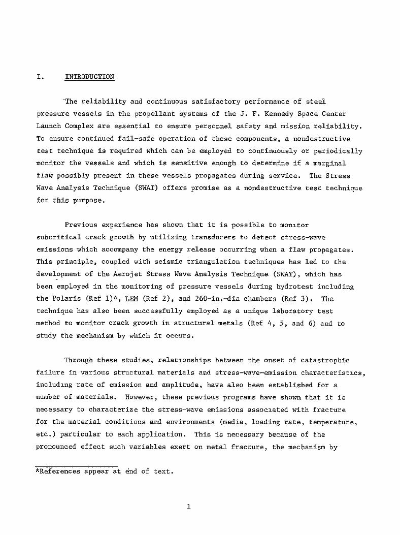
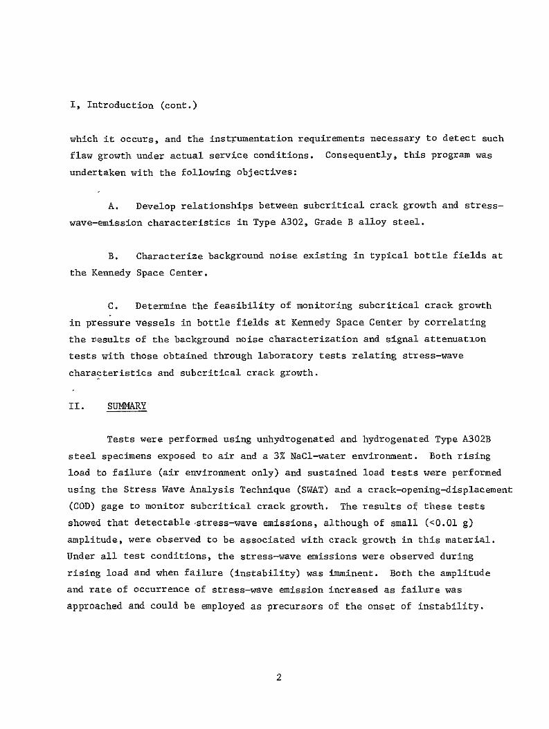
II Summary (cont)
be detected by SWAT prior to failure which would permit triangulation to the
source and tank depressurization prior to failure Signal attenuation evaluashy
tions performed both at the Kennedy Space Flight Center and Aerojet were used
to establish sensor spacing and locations for typical vessels at both Pad A
and the VAB Bottle Field
III LABORATORY SPECIMEN DESIGN AND TEST PROCEDURES
A MATERIAL AND SPECIMEN CONFIGURATION
The Type A302B nickel modified steel plate (35-in thick) tested
in this program was supplied by the Kennedy Space Center The material
characterization data shown in Table I was also supplied by NASA The bend
specimen design shown in Figure 1 was employed for the initial stress-waveshy
emissioncrack-growth tests performed at Aerojet the test specimens were
obtained from the surface and center locations in plate material supplied by
NASA Subsequently Wedge Opening Loading (WOL) tests were also employed
The WOL specimen was described by Novak and Rolfe (Ref 7) and is essentially
a modified compact tension specimen which can be used for Klscc environmental
testing The specimen is self-stressed with a bolt and therefore the loading
is constant displacement so that the initial KI value decreases to KIscc as
the crack propagates Because the specimen is self-stressed it can be
completely divorced of all extraneous noise by encasing the loaded test specimen
in a sound-proof chamber Due to the limited amount of material available
(ends of the SEN-bend specimens) the X-type WOL configuration (1 x 1 x 144 in)
was used as originally designed by Manjoine and shown in Figure 2
Prior to testing the bend specimens were precracked using an
electrodynamic vibration system During cracking the bend specimen was
gripped using a vise attachment near the specimen notch while the other end
was weighted thereby producing the maximum bending moment at the specimen notch
4
TABLE I
MATERIALS CHARACTERIZATION DATA SUPPLIED BY NASA KENNEDY SPACE CENTER
Size of Plate 3-716 x 14 x 18 in
Specification A302B Nickel Modified
Heat Treatment 1650degF3-L2 hr
Water Quench
1125degF5 hr draw
Air Cool
1100F3-12 hr Temper
Air Cool
Mechanical Properties Ftu 1162 ksi 11575 ksi
F 975 ksi ty 973 ksi
Elong 220 200
RA 610
574
CVN (ft-lb)
+50degF -40degF
34 21
29 21 28 18
Chemistry C-023 Mn-l16 P-0012 S-0019 Si-027 Mo-052 Ni-063 B-00023
5
120
206
L60--O
14 Pin Hole for Mounting
Accelerometers
Becorder
3k
T1 Ci
1251
010
~20k
L- 05 020
0-O005r 0o j
_o6o 9
010 -oo-_o250
0_75 _0200
TI
T2
r-
Figure 1 Notch-Bend Specimen Geometry and Crack-Opening
Displacement Gage
6
P
z w VIRTUAL PLANE OF
EXTENSION
H
NOTCH -shy
o
W H B
5oo
=1125
= 0500 =1000
-
050 p =002 611735-2B
Figure 2 Configuration of WOL Specimen
7
III A Material and Specimen Configuration (cont)
The specimen was then vibrated at resonant frequency (approximately 225 cps)
until a crack approximately 010 in deep appeared below the vertex of the
elox-machined notch The time required to produce the desired crack depth
was approximately 10 min or 135000 cycles The WOL specimens were precracked
(010-in depth) following hydrogenation (as described in the following parashy
graphs) in tension-tension fatigue
B CRACK-OPENING DISPLACEMENT STRESS INTENSITY AND SPECIMEN LOADING PROCEDURE
The bend specimens were tested using the three-point bend fixture
shown in Figure 3 and a hydraulic tensile machine During loading a crossshy
head speed of approximately 01 inmin was employed load control during hold
periods was maintained manually by the tensile machine operator The exact
specimen loading profiles varied between specimens and is discussed under the
resufts obtained for each specimen
During testing of the bend specimens crack-opening displacement
was measured between knife edges machined at the end of the specimen notch
(Figure 1) The measuring device consisted of a full bridge of electricshy
resistance strain gages mounted on a double-cantilever beam The amount of
flexure in the cantilever arms was controlled by the thickness of the spacer
between the arms at the base of the cantilever The design of the gage is
such that it is linear within 0001 in over the range of 0200 to 0250 in
During the initial tests of this program the output of the crackshy
opening-displacement gage was routinely recorded on a Sanborn strip chart
While this procedure is adequate for fracture toughness testing (straight
rising load to failure) because of drift and normal fluctuations in output
within the specification of the equipment manufacturer this procedure is not
sufficiently sensitive to detect the very small increments of crack extension
8
Load
K 20
k
36
15 3505
150
IU 06
1See Rolle below
240 220
200
L 20_
10020 203
Figure 3 Three-Point Bend Test Fixture Design
9
III B Crack-Opening Displacement Stress Intensity and Specimen Loading Procedure (cont)
which can occur during slow-crack-growth studies This is particularly true
in testing A302B steel where extension probably occurs through a micro-void
coalescence mechanism and in very small increments
In view of this problem a test system has been developed by
Aerojet which is capable of detecting very small increments of crack extension
This system uses the crack-opening-displacement gage recommended by ASTM and
described above however instead of a Sanborn recorder the signal from the
gage goes to a bridge balancing unit to a DC amplifier and then to a DC
millivolt recorder This system was operated at a gain of 1200 with less than
1 peak-to-peak instability The system also has a zero suppression capability
which allows the gain of 1200 to be fully utilized even though the crack
opening may increase as much as 005 in The main advantage of this system
is the extremely high sensitivity capability which was required in order to
detect incremental crack growth in the A302B nickel modified steel tested
during this program
The crack-opening displacements from the millivolt recorder were
used to determine crack length from the notch-bend calibration curve shown in
Figure 4 Stress intensity was calculated using the secant offset method
recommended by the ASTM Committee for Three-Point Bend Testing The following
relationships were employed for this purpose
PQL
K BD32 f(aD) (Eq 1)
where L is one-half the span length D is the specimen depth B is the specimen
thickness a is the crack depth and P is the load at which a secant with a
slope 5 less than the tangent slope interacts the load-displacement curve
10
200
175
150
O Each Data Point Represents an Average of Triplicate Tests
125
100
75 -
50 -
-250
010
03
Figure 4
04 05 06 07 08 aW
Calibration Curve for Three-Point Bend Specimen
11
III B Crack-Opening Displacement Stress Intensity and Specimen Loading Procedure (cont)
The parameter for crack length to depth is a numerically determined polynomial
given by
a 12 a 32+ a 52 a 72+ a 92 f(aD) = 5 8( ) -9 2(= +436(i) -753() 774(-) (Eq 2)
DDD D
The stress intensity K is a valid KIc measurement if 25(K ays) 2 is less
than both the specimen thickness and the crack depth
Calculation of the applied stress-intensity factor for the WOL
specimen was accomplished using the following expression
K PC (Eq 3)
where P is the applied load a is the crack depth B is the specimen width
and C is obtained graphically from Figure 5
Prior to precracking the WOL specimens were hydrogenated cadmium
plated and baked (same procedure as for the bend specimens) The specimens
were then precracked (01 in deep) in tension-tension fatigue Each specimen
was then calibrated by use of a crack-opening-displacement gage this was
accomplished by tensile loading the specimens and recording COD versus load
with an X-Y plotter The calibration curves for Specimen WOL-l are shown in
Figure 6 The specimens were then self-stressed by applying torque to the
bolt (bearing against a hardened steel pin) until the COD gage indicated the
desired load The load for a given stress intensity was calculated as follows
given a = 066 in (measured in specimen surfaces)
W = 1125 in
aW = 0586
12
20 I I
U I
1-z
18
16
1 4
12
-18-W
= 0444
0
U 10 -
-U-C- 8
l z
6
4
2 F 1 2 3 4 5
I __ 6 7
oW
Figure 5 Numerical Constant C for WOL Specimen
13
4500
4000
3500
3000
2500
4 2000 0
1500
1000
500
0-- 0002 in
CRACK OPENING DISPLACEMENT (IN)
Figure 6 Crack-Opening-Displacement vs Load - WOL Specimen
III B Crack-Opening Displacement Stress Intensity and Specimen Loading Procedure (cont)
C = 108 (graphically)
KI = PCB a
KSB p =
C
2 50 ksi-in1KI =for a
P = 3650 lb
Each WOL specimen was tested with an applied load correpponding to 12
K = 50 ksi-ins
C HYDROGENATION PROCEDURE
Selected bend and WOL specimens were tested after prior hydrogenashy
tion to determine the effect of this variable on the stress-wave-emissionslowshy
crack-growth relationships The hydrogenation procedure employed for this
purpose was developed by Battelle Memorial Institute and has been successfully
employed during other programs at Aerojet The hydrogen was introduced by
cathodic charging as follows
Solution 4 by weight H2SO4 5 dropsliter of poison
Poison 2 gm of phosphorus dissolved in 40 ml of carbon disulphide
Charging Time 5 min
Current Density 10 main2
The evolution of hydrogen at room temperature was prevented by
cadmium plating the test specimens within 5 min after hydrogenation The
cadmium-plating procedure was as follows
15
III C Hydrogenation Procedure (cont)
Cadmium Plating 4 ozgal CdO
Solution 16 ozgal NaCN with 1 by volume at pH 13
Current Density 70 main 2
Plating Time 30 min
Subsequent to hydrogenation and plating the specimens were baked
at 3000 F for 3 hr Baking was performed immediately prior to testing to
ensure a uniform hydrogen content throughout the test specimen
D STRESS-WAVE INSTRUMENTATION - LABORATORY EVALUATIONS
The stress-wave-detection system used for the laboratory evaluashy
tions prior to the background noise measurements at the Kennedy Space Center
is shown schematically in Figure 7 and consists of accelerometers amplifiers
filters tape recorders and an electronic counter and digital printer During
testing the accelerometers were attached to the specimens using a linear forceshy
coiled spring technique
Two basic systems were employed for stress-wave-emission data
acquisition During laboratory tests prior to the background measurements
at Kennedy Space Center the electronic counter system was employed This
system provides Very high sensitivity (signal amplifications of 10000 to
100000X) and also provides a real-time automatic count (both rate of emission
and cumulative count) of the stress-wave emissions occurring throughout each
test period The high-pass filter in the system eliminates a major portion of
the extraneous low-frequency background noises which tend to mask very small
amplitude stress waves
16
OSCILLOSCOPE
e TEKTRONIX MODEL 535
ELECTRONIC ELECTRONICSENSOR AMPLIFIER FILTER AMPLIFIER
COUNTER PRINTER S101HEWLETT PACK- HEWLETT PACK-
XIPA 00ARD MODEL 5231 ARD MODEL 5050
TAPE _ RECORDERTAPE ____________
RECORDER AMPLIFIER OSCILLOGRAPH
AMPEX MOD) T SP 300
KDATA ACQUISITION
OSCILLOSCOPE
TEKTRONIX _
eMODEL 535
DATA ANALYSIS
Figure 7 Schematic Representation of SWAT Data Acquisition and Data Analysis Instrumentation
III D Stress-Wave Instrumentation - Laboratory Evaluations (cont)
During testing of the WOL specimens maximum SWAT system amplifishy
cation was employed This was made possible because the specimens immersed
(COD gage up out of the water) in the water environment were enclosed in a
sound-proof box For these tests the electronic counter trigger level was
set just above the inherent noise (electrical) of the system Initially a
WOL test was run to determine whether the system was in fact completely free
of extraneous noise With the COD gage connected and all recording systems
in the circuit and with the specimen under no load and in air environment
after 5-12 hr in the sound-proof chamber there were only 16 signals
counted Presumably these were electrical disturbances The test was run
during regular working hours the WOL tests reported in the following parashy
graphs were tun during off-hours (nights and weekends) when there should have
been an absolute minimum of electrical disturbances
A second data acquisition system was also used for a limited
number of bend tests following the background noise measurements at Cape Kennedy
A schematic of this system is shown in Figure 8 The purpose of these tests
was to obtain stress-wave amplitude measurements using the instrumentation
employed at Cape Kennedy to ensure that the stress-wave emissions accompanying
crack extension could be detected under the background conditions observed at
Kennedy Space Center The tape recordings were made by direct recording during
test and were subsequently analyzed through playback and analysis as shown in
Figure 7
18
TEKTRONIX
OSCILLOSCOPE
ENDEVCO Dynamics Model 2213 Filter Accelerometer Model
Amplifier Amplifier 6364MQ 20-50 Kc Band Pass
KcENDEVCO30
Model 2213 CHigh-PassH Accelerometer Filter
kFI
TAPE Amplifier Amplifier RECORDER
AMPEX SP-300
Figure 8 Schematic of Instrumentation Used at Kennedy Space Center
IV LABORATORY TEST RESULTS AND DISCUSSION
As indicated in the following paragraphs two environments (air and
3 NaCl-water) and two material conditions (unhydrogenated and hydrogenated)
were utilized in the laboratory tests performed at Aerojet These conditions
are considered those most likely to be encountered during the service life of
the pressure vessels Also both straight rising load to failure and sustained
loading profiles were employed The sustained load profiles were employed
since failure of the pressure vessel may occur at constant load due to
environmentally induced slow crack growth from a prior flaw Since the
effectiveness of a failure warning system will obviously depend on the ability
to detect subcritical crack extension whether it occurs during sustained load
or on rising to failure it is important to determine if crack extension andor
failure will occur under both conditions Both effects can be studied through
the laboratory tests performed during this program
A BEND TESTS IN AIR WITHOUT DELIBERATE ADDITION OF HYDROGEN
Initially bend tests were performed in an air environment Both
the crack-opening-displacement gage and stress-wave-analysis technique were
employed to monitor the occurrence of pop-in and subcritical crack growth
The fracture data for these tests are shown below
Specimen Specimen Failure Notch Plus Apparent K
Thickness (B) Depth (D) Fatigue Crack (a) Load 1 2 No in in in aD P Kips ksi-in
1 10 20 090 045 200 130
2 097 20 091 0455 158 136
3 10 20 1036 0518 1656 133
Intermediate hold at 123 ksi-in12
20
IV A Bend Tests in Air Without Deliberate Addition of Hydrogen (cont)
The straight rising load to failure tests (No 1 and 2) indicated 12
a K value of 130 to 136 ksi-in as did the specimen (No 3) which failed
during rising load after previous holding at a stress intensity of approximately 12123 ksi-in As indicated previously in this report the ASTM recommends
for valid KIc measurements a specimen thickness exceeding that corresponding
to 25 (Kys)2 By this criterion a specimen thickness of approximately
44 in would be required for the A302B steel tested in this program
Consequently the KQ values noted above while not valid KIc measurements
indicate a high level of toughness in this material
No significant slow-crack growth or stress-wave emissions were
observed during hold in the air environment Conversely slow-crack growth
(increase in apparent crack size) and accompanying stress-wave emissions were
observed during rising load to failure The stress waves were generally very
small in amplitude (clt0Olg) but increased in amplitude with increasing crack
extension immediately prior to failure Increased rate of stress-wave
emission was also observed immediately prior to failure
B BEND TESTS IN WATER WITHOUT DELIBERATE ADDITION OF HYDROGEN
Bend specimen 4 was loaded initially to 15000 lb
(88 ksi-in 2) and held at constant load for 18 hr in 3 sodium-chloride
simulated sea water The specimen showed indications of crack growth early in
the hold period However analysis of the crack-opening-displacement gage data
indicated only very small amounts of crack extension Although the gage
employed for this purpose corresponded to the design recommended by the ASTM
its use was found unsatisfactory for tests of the type performed during this
program The COD gage was then modified and the modified version used during
the testing of the hydrogenated material described in subsequent sections of
this report
21
IV B Bend Tests in Water Without Deliberate Addition of Hydrogen (cont)
When the specimens (without hydrogenation) tested in the salt-water
environment were fractured the fracture surfaces were examined for evidence
of slow-crack growth during hold Although a small band of slow-crack growth
from the original fatigue precrack was observed it was not possible to detershy
mine how much of the crack extension occurred during rising load Onthe basis
of the COD data it would appear the majority of the extension occurred during
rising load to 15 kips from 15 to 17 kips and from 17 kips to failure although
the SWE data indicated that slow crack growth however small was occurring
during the hold periods
Figure 9 is a plot of cumulative stress-wave count over a period
of approximately 1-12 hr during hold at 15000 lb Note the indications of
a variable rate of subcritical crack growth Figure 10 shows the SWAT data
in detail (electronic counter reading every second) starting 23 min after
reaching the 15-kip load level Note that the cumfilative stress-waampe count
increased more or less continuously with brief intervals of increased slope
(when plotted to the scale of Figure 10 the increased slope was approximately 450) Figure 11 shows the SWE data obtained after adding fresh 3 NaCl-water
solution to the notch During the period of sustained load represented in
Figure 11 there were a few abrupt increases in count indicating discontinuous
crack growth together with additional intervals of increased slope (again
close to 45)
Figure 12 corresponds to the endof a short 16-kip hold (same
specimen) followed by a rise to 17 kips (approximately 125 ksi-in1 2 ) and
then a period of sustained load in 3 NaCl-water solution at 17 kips Note
the increased slope associated with the increase in load followed by abrupt
increases in count characteristic of discontinuous crack growth Approximately
600 sec after starting the hold at 17 kips an air hose produced high-frequency
noise too high to be removed by the filter This was recorded as an abrupt
increase in couni followed by a period of increased slope (again approximately 45) It cannot be definitely stated whether the increased slope indicating
22
1400
1200
1000
Li 800 3
LU
D 600
400
SEE FIGURE 10 200 FOR DETAILS
0 0 I I I I I
0 10 20 30 40 50 60 70 80 90 100
-MINUTES HOLD AT 15 KIPS
Figure 9 Cumulative Stress Wave Count vs Time Specimen No 4
A302B Steel 15 Kip Hold 3 NaCi-Water Environment
23
600
I0
20-
TIME (SECONDS)
224
6050
10 10 1O 1in20 20a 2100 2150
TIME (SECONDS) 220 3 am250 20 20 3w245 24W
43O
600
40
20
140
011 115 la 1in0 1 TIME (SECONDS)
a 14W 1m 53 0 inlW
Figure 11 Cumulative Stress Wave Count vs Time Specimen No 4 A302B Steel 15 Kip Hold After Replenishing the 3 NaCl-Water Environment
25
23
00
60
20
20
- 4o
o_ 4 o l~ ~ aiE~
220
IV B Bend Tests in Water Without Deliberate Addition of Hydrogen (cont)
continuous stress-wave emission was an artifact produced by the high-frequency
noise or the increased slope was the result of crack growth stimulated by the
high-frequency sound (crack growth after periods of dormancy can be initiated
by tapping a test specimen under load) Figure 13 is a plot of the cumulative
count for the 17-kip hold (corrected to zero at the start of hold and corrected
for noise which occurred at 836 sec) Note the tendency for increasing slope
with increasing time at load Figure 14 presents the SWAT data in detail
after 1 min at 17 kips load Figure 15 presents the data obtained after
1-12 min at 17 kips load Both Figures 14 and 15 are plotted to the same
scale as Figures 10 11 and 12 Table II presents the data plotted in
Figures 13 14 and 15 without correction for noise which occurred at 836 sec
this tabulation shows the detailed information that can be obtained by SWAT
On the basis of the SWE dpta this specimen showed evidence of
very slow continuous crack growth of the type one might expect of electroshy
chemical dissolution at the crack tip interspersed with short periods of more
rapid continuous crack growth There was little or no evidence of disconshy
tinuous crack growth with clearly defined periods of dormancy and there were
few instances of abrupt increase in count to signify crack jumps
C BEND TESTS IN AIR WITH DELIBERATE ADDITION OF HYDROGEN
After hydrogenation and baking 3 hr at 3000 F to produce a
homogeneous interstitial solid solution specimens were tested in 70degF air
Specimen 5 (Figure 16) developed discontinuous crack growth while under
sustained load starting at 9000 lb (75 ksi-in 2) but the occurrences were
sporadic and infrequent At 13000 lb (110 ksi-in 2) there was only one
stress wave large enough to be recorded as a cumulative count (cumulative
count increased from 3086 to 3110 corresponding to 464 SWEsec count rate)
Otherwise there was no increase in the SWE cumulative count during hold at
13000 lb
27
TABLE II
DETAILS OF SWE DATA OBTAINED FOR SPECIMEN NO 4 A302B STEEL DURING HOLD AT 17 KIPS IN 3 NaCI-WATER ENVIRONMENT
Time at Count Interval Time at Count Interval Load Rate Cumulative At Load Rate Cumulative A t (sec) (SWEsec) Count (sec) (set) (SWEsec) Count (sec)
27 57 8 - 1330 11 632 9 47 134 12 20 1331 20 634 1 101 4 14 54 1341 58 635 10 152 3 16 51 1392 232 652 51 299 10 27 147 1400 262 653 8
5 MINUTES 1405 134 654 5 329 1 29 30 1415 9 656 10 357 47 37 28 1443 85 657 28 444 72 49 87 1446 48 659 3 460 64 56 16 1478 131 675 32 494 221 60 34 1479 2 676 1 511 145 62 17 1495 29 685 16
10 MINUTES 25 MINUTES 616 115 72 105 1503 170 689 8 744 128 85 128 1505 72 691 2 788 2 92 44 1526 171 697 21 836 2 411(Noise) 48 1527 1 698 1 838 7 411 2 1537 187 702 10 843 10 431 5 1546 220 705 9 845 68 431 2 1584 89 715 38 846 7 431 1 1597 119 726 13 855 161 447 9 1650 146 738 53 880 160 468 25 1666 1 749 16
15 MINUTES 1671 162 756 5 904 11 492 24 1674 86 758 3 915 209 500 11 1695 120 780 21 943 5 523 28 1708 75 782 13 956 22 537 13 1717 1 787 9 980 4 541 24 1721 84 792 4 992 13 542 12 1732 114 794 11
1012 69 544 20 30 MINUTES 1088 21 558 76 1808 228 803 76 1108 151 569 20 1821 179 805 13 1136 il 576 28 1825 22 808 4 1154 5 582 18 1833 196 809 8 1172 38 583 18 1839 120 811 6 1178 19 585 6 1852 45 814 13 1182 9 -592 4 1866 146 816 14 1196 26 594 14 1888 168 819 22
20 MINUTES 1895 14 823 7 1228 80 598 32 1909 157 826 14 1229 13 599 1 1933 29 832 24 1238 2 605 9 1950 10 836 17 1256 1 610 18 1956 46 837 6 1312 91 613 56 1977 71 838 21 1318 1 619 6 1988 101 839 11 1321 1 621 3 2000 10 841 12
TABLE II (cont)
Time at Count Interval Time at Count Interval Load Rate Cumulative At Load Rate Cumulative Lt (sec) (SWBsec) Count (sec) (sec) (SWEsec) Count (sec)
2002 59 843 2 2515 40 1013 34 2017 119 845 15 2518 207 1017 3 2020 148 847 3 2521 1 1023 3 2033 165 848 13 2525 602 1029 4 2039 103 850 6 2527 22 1034 2 2048 9 857 9 2548 52 1052 21 2061 129 860 13 2561 47 1058 13 2063 156 862 2 2573 17 1062 12 2069 167 864 6 2585 69 1072 12 2075 98 874 6 2588 42 1073 3 2076 3 879 1 2599 240 1075 11 2093 21 881 17 2605 4 1077 6
35 MINUTES 2615 23 1078 10 2107 1 883 14 2616 57 1079 1 2108 103 884 1 2613 11 1080 15 2118 121 885 10 2638 42 1081 7 2119 191 887 1 2648 2 1087 10 2135 154 891 16 2650 87 1088 2 2140 11 892 5 2653 100 1089 3 2146 3 894 6 2656 56 1090 3 2150 178 897 4 2661 63 1091 5 2159 51 902 9 2685 28 1094 24 2162 7 905 3 2693 35 1097 8 2180 57 909 18 45 MINUTES 2182 58 910 2 2701 113 1104 8 2193 17 913 11 2703 50 1105 2 2195 113 916 2 2713 53 1109 10 2207 115 919 12 2719 20 1110 6 2221 34 923 14 2721 33 1112 2 2223 87 926 2 2738 72 1115 17 2238 35 936 15 2740 15 1116 2 2258 2 943 20 2752 100 1117 12 2268 204 947 10 2756 85 1119 4 2289 10 949 21 2768 56 1121 12 2307 1 952 18 2780 13 1130 12 2319 121 955 12 2782 28 1135 2 2346 20 959 27 2795 60 1142 13 2366 69 963 20 2809 65 1144 14 2386 20 975 20 2841 55 1156 32 2387 5 976 1 2848 3 1157 7 2392 158 978 5 2851 2 1159 3 2396 8 981 4 2862 45 1163 11
40 MINUTES 2869 35 1166 7 2403 21 983 7 2879 18 1169 10 2409 241 986 6 2885 62 1171 6 2449 95 996 40 2905 55 1175 20 2457 24 998 8 2908 54 1178 3 2473 104 1002 16 2918 7 1182 10 2481 3 1003 8 2924 8 1186 6
29
TABLE II (cont)
Time at Count Interval Time at Count Interval Load Rate Cumulative t Load Rate Cumulative t (sec) (SWIsec) Count (sec) (sec) (SWEsec) Count (sec)
2938 12 1193 14 3341 207 1410 2948 95 1201 10 3366 103 1421 25 2966 10 1215 18 3377 8 1424 11 2968 43 1216 2 3378 12 1425 1 2972 22 1217 4 3390 2 1429 12 2979 8 1221 7 3396 3 1430 6 2987 8 1223 8 3397 14 1432 1 2998 38 1226 11 3401 8 1434 4
50 MINUTES 3402 98 1438 1 3002 36 1228 4 3408 12 1443 6 3010 55 1230 8 3410 16 1448 2 3011 3 1234 1 3413 6 1452 3 3016 1 1236 5 3431 2 1454 8 3017 3 1237 1 3433 17 1458 2 3023 3 1239 6 3435 30 1460 - 2 3029 3 1240 6 3438 22 1462 3 3033 1 1243 4 3450 8 1475 12 3036 110 1245 3 3455 62 1484 5 3037 4 1248 1 3461 154 1490 6 3053 83 1259 16 3462 7 1493 1 3054 7 1260 1 3466 11 1501 4 3061 2 1265 7 3472 2 1507 6 3062 83 1266 1 3476 46 1509 4 3076 62 1275 14 3489 18 1515 13 3080 5 1278 4 3490 8 1517 1 3098 32 1294 18 3508 15 1534 18 3100 15 1296 2 3513 25 1541 5 3102 16 1297 2 3520 220 1549 7 3108 7 1299 6 3538 29 1566 18 3114 7 1301 6 3542 9 1572 4 3127 6 1304 13 3543 107 1575 1 3129 1 1305 2 3558 240 1588 15 3133 1 1306 4 3568 30 1601 10 3140 5 1309 7 3570 21 1603 2 3154 30 1312 14 3573 66 1607 3 3170 6 1320 16 3579 9 1613 6 3175 77 1322 5 3591 37 1619 12 3177 110 1323 2 60 MINUTES 3178 5 1324 1 3607 128 1622 16 3183 4 1326 5 3608 70 1626 1 3187 137 1331 4 3609 2 1629 1 3191 14 1332 4 3624 50 1638 15 3200 3 1336 9 3630 14 1642 6 3206 2 1340 6 3639 86 1645 9 3214 20 1343 8 3660 56 1662 21 3219 22 1345 5 3678 13 1669 18
55 MINUTES
30
TABLE II (cont)
Time at Count Interval Time at Count Interval Load Rate Cumulative At Load Rate Cumulative At (sec) (SWEsec) Count (sec) (see) (SWEsec) Count (sec)
3688 33 1680 10 4535 105 2574 28 3692 35 1682 4 4547 3 2589 12
3709 209 1688 17 4583 4 2616 36 3712 7 1689 3 4623 460 2670 40 3720 78 1691 8 4624 37 2703 1
3730 93 1694 10 4626 18 2715 2 3731 5 1695 1 4627 840 2729 1 3743 13 1703 12 4630 141 2737 3 3744 120 1709 1 4662 2 2758 32
3750 24 1715 6 4671 1 2763 9 3755 142 1724 5 4698 1 2774 27 3767 45 1738 12 4710 8 2782 12 3796 69 1770 29 4719 6 2784 9 3823 21 1808 27 4731 128 2785 12 3844 10 1838 21 4761 17 2810 30 3854 82 1851 10 4783 22 2822 22 3856 13 1855 2 4786 23 282A 3 3895 75 1915 39 80 MINUTES
65 MINUTES 4822 96 2831 36 3901 18 1920 6 4852 1 2842 30 3905 54 1927 4 4934 59 2890 82
3946 58 1963 41 4953 200 2907 19 3970 2 1985 24 4954 26 2910 1 3971 181 1988 1 4957 16 2916 3 3974 61 1990 3 4964 56 2923 7 3975 28 1992 1 4988 29 2941 24 3987 51 2004 12 5000 88 2951 12 4012 2 2022 25 5031 10 2977 31 4013 31 2026 1 5032 9 2978 1 4022 7 2036 9 5045 56 2982 13 4054 4 2062 32 5054 4 2984 9 4056 16 2066 2 5093 220 2992 39 4084 37 2093 28 85 MINUTES 4091 36 2099 7 5122 115 2996 29 4100 3 2111 9 5166 17 3019 44 4129 16 2142 29 5190 172 3042 24 4156 6 2165 27 5193 55 3045 3
70 MINUTES 5194 2 3048 1 4241 19 2253 85 5224 313 3081 30 4292 4 2299 51 5248 23 3106 24 4331 42 2339 39 5266 32 3123 18 4338 19 2348 7 5281 24 3138 15 4340 66 2350 2 5291 10 3150 10 4345 10 2359 5 5303 25 3164 12 4385 4 2419 40 5306 1 3169 3 4397 121 2432 12 5324 56 3187 18
75 MINUTES 5330 58 3193 6 4500 40 2534 103 5345 31 3211 15 4507 6 2542 7 5351 155 3217 6
31
TABLE II (cont)
Time at Count Interval Time at Count Interval Load Rate Cumulative At Load Rate Cumulative At (sec) (SWBsec) Count (sec) (sec) (SWEsec) Count (sec)
5357 211 3223 6 5887 185 3536 1 5363 29 3233 6 5905 65 3559 18 5364 20 3237 1 5923 31 3575 18
90 MINUTES 5924 22 3576 1 5403 118 3276 39 5933 109 3578 9 5418 79 3295 15 5934 5 3579 1 5419 44 3298 1 5961 43 3582 27 5420 35 3300 1 100 MINUTES 5448 27 3324 28 6000 23 3585 39 5460 118 3327 12 6001 13 3586 1 5466 97 3329 6 6002 166 3588 1 5472 184 3331 6 6008 9 3590 6 5484 28 3333 12 6032 29 3592 24 5499 45 3338 15 6041 111 3596 9 5505 2 3341 6 6062 116 3601 21 5506 173 3344 1 6083 1 3603 21 5512 72 3346 6 6084 236 3606 1 5515 8 3348 3 6090 140 3607 6 5536 199 3352 21 6091 104 3608 1 5548 5 3356 12 6106 21 3609 15 5553 199 3359 5 6115 31 3611 9 5554 34 3360 1 6121 29 3614 6shy5587 190 3364 33 6124 1 3622 3 5593 2 3365 6 6139 51 3630 15 5605 6 3367 12 6160 25 3634 21 5611 12 3369 6 6175 5 3636 15 5638 3 3373 27 6184 196 3639 9 5644 57 3374 6 6217 275 3645 33 5645 78 3376 1 6223 84 3648 6 5669 21 3379 24 6238 23 3649 - 15 5693 22 3384 24 6244 99 3650 6 5699 48 3385 6 6250 81 3652 6
95 MINUTES 6259 39 3654 9 5702 74 3387 3 6265 15 3656 6 5703 85 3389 1 6271 21 3658 6 5725 21 3391 22 6283 85 3660 12 5737 1 3394 12 105 IWNUTES 5752 72 3396 15 6304 143 3662 21 5761 106 3398 9 6331 50 3672 27 5788 1 3414 27 6340 179 3674 9 5794 176 3422 6 6341 37 3675 1 5809 2 3441 15 6365 34 3677 24 5810 15 3445 1 6366 ill 3680 1 5813 42 3448 3 6393 150 3682 27 5814 189 3451 1 6405 43 3684 12 5823 180 3461 9 6429 4 3687 24 5832 171 3472 9 6435 127 3690 6 5838 46 3481 6 6459 31 3691 24 5859 63 3505 21 6483 7 3694 24 5865 15 3511 6 6495 30 3696 12 5886 2 3533 21 6501 128 3700 6
32
TABLE II (cont)
Time at Count Interval Time at Count Interval Load Rate Cumulative At Load Rate Cumulative At (sec) (SWEsec) Count (sec) (sec) (SWEsec) Count (sec)
6522 87 3703 21 7278 21 4158 6 6531 16 3704 9 7302 2 4174 24 6555 102 3706 24 7303 3 4174 1 6567 7 3709 12 7318 125 4186 15 6570 10 3710 3 7348 88 4205 30 6576 87 3711 6 7402 86 4238 54 6577 89 3713 1 7435 90 4258 33 6578 131 3714 1 7447 14 4262 12 6599 4 3717 21 7474 14 4277 27
6600 110 MINUTES
8 3718 1 7486 7504
9 125 MINUTES
89
4286
4304
12
18 6603 37 3720 3 7510 39 4308 6 6639 15 3724 36 7531 52 4331 21 6669 48 3728 30 7540 208 4344 9 6675 23 3729 6 7549 38 4353 9 6684 57 3731 9 7576 72 4376 27 6705 23 3757 21 7594 24 4392 18 6744 53 3807 39 7603 55 4403 9 6762 240 3830 18 7615 160 4415 12 6783 5 3854 21 7621 134 4420 6 6801 26 3874 18 7627 160 4423 6 6822 181 3901 21 7639 180 4430 12 6852 24 3934 30 7648 5 4432 9 6879 44 3962 27 7658 100 4437 10 6882 2 3965 3 7679 319 4445 21
115 MINUTES 7694 72 4449 15 6906 63 3991 24 7709 23 4451 15 6927 176 4001 21 7721 34 4453 12 6930 15 4006 3 130 MINUTES 6931 54 4011 1 7800 Test Terminated 6952 305 4026 21 6953 40 4033 1 6980 3 4037 27 6989 99 4039 9 7040 387 4080 51 7041 53 4095 1 7056 23 4100 15 7086 354 4108 30 7095 21 4110 9 7125 70 4117 30 7131 2 4120 6 7167 97 4129 36 7176 11 4130 9 7197 18 4133 21
120 MINUTES 7218 28 4136 21 7227 39 4138 9 7248 72 4146 21 7272 50 4153 24
33
40
38W
3400
32W
30
28M
260
= 2400
S 22DD
i20
1600
1400
1200
10
600
400
200
06 1a 20 30 40 50 60 70 80 90 tW 110120130
MINUTE-S-H-OLD 17KIPS
Figure 13 Cumulative Stress Wave Count vs Time SpecimE A302B Steels 3 NaC1-Water Environment
34
3503
0
~0
40
20
3203
00
20
C0
20
310
03
(0
40
= = 20 0 I- 365~
05
20 00
20
0shy20
2003
20 ~~0 C
20
20 40
- 20
2835
0
(0
20
20shy
20020
20 -
3403 3450 3720 3750 fl 3550 3003 3050 40) 4050 4003 4050 4~fl 4200 4020 4350 4440 4450
TIME (SECONDS)
Figure 14 Cumulative Stress Wave Count vs Time Specimen No 4 A302B Steel After 1 Minute at 17 Kip Hold in 3 NaCi-Water Environment
35
48
0
I-
S 40
us 50 50 70 5 90 0 60 60 10 6 6 t 20CO DS
- iue1CmlaieSrs av on sTme pcmnN A0BSel
Afe2-0iue t1 i todi NC-ae niomn
Page60
4520 -
so- lao
F
122021 amp~
20 4
400
20
20 22
3540 =
20
3024
20
50
45
20
20520
20
20
45
20
no
I
40
4~
20
40
20
20
4
20
2020
20
gt
20
20 4
20
20
3545
20
Iino200j
5505
2220
1120
20
001
20
20 shy
00
1
45
OX
I
I I
I I
0 50
020 000
205 200
20 200
Z
40 505
550 400
TIM
E (S
EC
ON
DS
)
Figure 16
Cumulative Stress Wave Count vs
Time Specimen No
5 A302B Steel
Hydrogenated and Tested in Air
37
IV C Bend Tests in Air With Deliberate Addition of Hydrogen (cont)
On raising the load from 13000 to 14000 lb (122 ksi-in )
there was evidence of a creep phenomenon as shown in Figure 17 The crackshy
opening-displacement gage confirmed the occurrence of crack growth continuing
after reaching the 14000-lb hold Stress-wave emission showed the mechanism
to be discontinuous cracking rather than a deformation process When the
count rate was plotted as in Figure 18 the activity carrying into the
14000-lb hold again was discontinuous After approximately 300 sec at 14 kips
the SWE associated with the creep phenomenon had subsided During the 14-kip
hold there were two crack jumps one after 920 sec (cumulative count increased
from 5618 to 5720 and the count rate associated with the jump was 181 as
counted over a 10-sec interval or 18 SWEsec) and one after 2130 sec (cumulashy
tive count increased from 5721 to 5755 and the count rate was 139 in 10 see)
After 5000 sec at 14 kips the load on Specimen 5 was raised As
seen in Figure 19 the stress-wave activity was an unmistakable presage of
instability which occurred after 20 sec into hold The load reached a maximum
of 145 kips (145 ksi-in 2) Technically the onset of instability occurred
shortly after starting to increase the load ie at approximately
132 ksi-inI2 which agrees with the KQ value obtained through rising load
tests of unhydrogenated material in an air environment
Because of the very long test period and multiple loadings involved
in the testing of the Specimen 6 only data obtained during rising load to
19500 and 19800 ib during sustained test periods at these loads and during
specimen failure are shown in Figure 20 These data indicate essentially the
same SWE-crack growth relationships discussed previously for Specimen 5 except
that on reaching hold the crack tended to grow slowly for a longer period of
time in comparison to the behavior noted for Specimen 5 Also the incremental
nature of crack extension was more readily observed by the stress-wave-emission
data for Specimen 6
38
20
560
80
60
40
20
5500
80
60
40
20
5400
o 5100
808
60
40
20
5000 u-J
4500
4480 80 4- START 14-KI P HOLD
CODC 75lt
4000
3980 70
3960
6553120 l
- END13-KIP HOLD
3100 160 0 40 80 120 160 200 240 280 320
TIME AT LOAD (SECONDS)
Figure 17 Cumulative Stress Wave Count and COD vs Time Specimen No 5 A302B Steel fydrogenated and Held at 14 Kips in Air
39
200
LU
LU
1- 100
50 END 13-KIP
25 HOLD-I
0 1- TIME
100 INSECONDS AT
200 14KIPS
300
(COUNT EVERY 10 SEC)
Figure 18 Stress Wave Count Rate vs Time - Specimen No 5 A302B Steel Hydrogenated and Tested in Air
40
INSTABILITY
9580
9560
9540
9380
928D0
9260
842D
8440
73O I-shyz 7220
o 7260
U 7240
7220
7180I-shy
7160
- 7140
7120
7100
7080
7060
5900
5880
5860
5840
5820
5800
578D
5460
0 40 80 120 160 SEC
4M 4960 50D RISING LOAD-SECONDS AT 14 KIPS
Figure 19 Cumulative Stress Wave Count vs Time Specimen No 5 A302B Steel Hydrogenated and Tested in Air
41
20000
18000
FAILURE
18290 sec a- 1 17-in K - 199 s - Y
z
-
16000
14000
l0
1200
I-9 Iin
1014in K 152 ki- in -i
o-1 09 n K- 176ksmn
- 1 07 in I 170 iis-
o -1 042in K 12ks-in
c023i NK15ks-n
-shy
-
10000
REACH 19800 lbs
START TO 19800 bs
10000 11000 12000 13000 14000 15000 16000 17000 18000 19000
TIMESECONDS
12000
11000 s
p9000
T LOAD ADJUSTMEA
7n000
READOUT6000 OTE STRESS WAVE DATA A UST T
500 Vgt 0 ENT CORRESPONDIG TO SLOPELOAADJUSTM15 CHANGES PLOTTED
a 4000
3000
LOAD ADJUSTMENT2000 SECONDSECMENIME
1000 START HOLD AT 19500 1b
900 1l6070 D0 8 0 00 0 000600
0 1000 50002000 3000 4000
TIME SECONDS
Figure 20 Cumulative Stress Wave Count vs Time Specimen No 6 A302B Steel Hydrogenated and Tested in Air
Page 42
IV C Bend Tests in Air With Deliberate Addition of Hydrogen (cont)
As indicated in Figure 20 the increase in crack length during
the initial period of hold at 19500 lb resulted in an increase in the applied
stress intensity and was accompanied by significant stress-wave-emission
activity To maintain the desired load it was also necessary to make frequent
load adjustments at the start of hold During the first 3600 sec the effecshy
tive crack length increased from approximately 0963 to 1000 in and was
accompanied by about 7000 SWE As indicated in Figure 20 the majority of the
SWE activity and increase in crack length occurred during the first 3000 sec
of the hold at 19500 lb After this period both the stress-wave-emission
activity and rate of increase in crack length gradually decreased For example
during the entire period from 5000 to 17600 sec when the load was increased
to 19800 lb the apparent crack length and SWE count increased by only approxishy
mately 0020 in and 2500 respectively
After approximately 17000 sec at 19500 lb the load was increased
to 19800 lb and specimen failure occurred after approximately 600 sec at
19800 lb The load was maintained for this period however it was apparent
from both the SWE and COD gage data that the crack was extending and specimen
failure would occur without a further increase in load although it was necesshy
sary to continually adjust the tensile machine to maintain the desired load
The failure stress intensity approximated 199 ksi-in 2however technically
the onset of instability occurred after starting to increase the load at
approximately 153 ksi-in1 2
Specimen 7 was also hydrogenated baked at 300F for 3 hr and
tested in air Figure 21 is a detailed plot of the SWAT data (electronic
counter print-out every second) indicating crack growth of a discontinuous
nature starting at 2400-lb load Note the periods of dormancy (no increase
in SWE count) interspersed with abrupt increases in count indicating disconshy
tinuous crack growth Note also that there was little or no evidence of
continuous stress-wave emission until the load (stress intensity level) was
high approaching failure
43
CUMULAIY STRESS-VAVE COUNTCU LTISTE W E ON
I OT A~II I OI I L I I I I I I I I I I I I I I i I I I I I
- N LB
I I I I I I I I I I I I I i I I
--L - 0OTO11
-0101
(lNIML~ 33383338
8
133113-
3IiC)0 83) 3103 31-3(31-
~0
33 331
3l3C0C~
38318shy
111(10 CAVMSS3 nfl CAliVi flWfl3
________________________________________________________________________
111fl0~ 3KvM~s~a1Ff~TfvTifwT
FPAIAE
hY
A Ii
8
INa
CZ
8 C0 U CI
33 S
1 H
H
03 -I
~ 3lt
0 Cd 33
~C3 ~ H
8 0003
A
Ofli3i~~ C)
Page 45
IV C Bend Tests in Air With Deliberate Addition of Hydrogen (cont)
Figure 22 presents the SWE data from a hydrogenated bend specimen
(No 8) tested in air The load was increased continuously to 9800 lb
(70 ksi-in 2) where there was a short hold (approximately 400 sec) Note
the discontinuous crack growth followed by a short period of continuous
emission (less than 450 slope) The load was then raised to 14800 lb
(109 ksi-in 2) and held for approximately 400 sec Again there were jumps
in the SWE cumulative count but this time interspersed with continuous
emission The SWAT system employed for this test corresponded to that employed
for the background measurements at Kennedy Space Flight Center and shown in
Figure 8 only one channel was employed viz
Endevco 2213 Amplifier Amplifier Band-Pass Filter 10OX 10OX 20 to 50 Kcps
The continuous stress-wave emission observed during hold at the higher stressshy
intensity level in this specimen was not observed in the other hydrogenated
specimens tested in air The primary purpose of this test (Specimen 8) was to
record SWE data for subsequent playback and analysis to determine the amplitude
of burst-type stress-wave emissions associated with fracture in Type A302B
steel These analyses were performed using the instrumentation shown in
Figures 7 and 8 with the following results which are discussed in more detail
in conjunction with the results of the background measurements performed at
Kennedy Space Flight Center (Section V)
Maximum SWE Amplitude - 39 x 10-3g
Minimum SWE Amplitude - 12 x 10-3 g
Average SWE Amplitude - 22 x 10-3g
Laboratory Background - 11 x 10-3g
46
00 o z~ 20 ~
40
~40
S20 1 2 0 0 0 0
TIIAEAT 4 S-KIPHOLD (10KS(51IN A)
407
IV Laboratory Test Results and Discussion (cont)
D BEND TESTS IN 3 NaCI-WATER WITH DELIBERATE ADDITION OF HYDROGEN
Specimen 9 was hydrogenated baked and tested in 80F water
The electronic counter indicated continuous stress-wave emission interspersed
with abrupt increases in count indicating occasional crack jumps Figure 23
shows the details of stress-wave emission that occurred during both rising
load and holding load The crack length determined from the COD chart at
selected loads is also shown Note from the SWE data that there were no
periods of dormancy and the slope of the plot of cumulative count versus time
indicated moderately rapid continuouas crack growth such as might occur with
electrochemical dissolution at the crack tip The COD gage data shown in
Figure 23 also indicate crack extension however the actual amount appears
to be quite small (lt01 in) which would be consistent with the relatively
small number of stress-wave emissions detected even at the high system
sensitivity employed The dramatic difference between the behavior in
Figures 21 and 23 for hydrogenated material tested in air (Figure 21) and
water (Figure 23) indicates that hydrogen and 3 sodium chloride solution
acting together have a greater total effect than the sum of their individual
effects ie working together they appear to have produced a synergism
E WOL TESTS
Because of the possible significance of the synergistic-effect
noted above on the life of the hydrogen pressure vessels at Kennedy Space
Flight Center additional testing was performed using hydrogenated WOL specishy
mens cut from the fractured bend specimens The first WOL specimen was
initially loaded to-3650 lb (50 ksi-in 2) and then placed in 3 NaCl solution
(notch immersed) There was 30 min of essentially continuous stress-wave
emission (recorder started approximately 5 min after loading the specimen)
Subsequently therewas one sizable jump in the SWE cumulative count after
48
V30
760
740-M
$
720 -s
680shy
60
610
40 w
w
520 w
i
20500
HOLDD]N
340
20 760
7200
ING
IV
O
shy
420
60
40
20 0 2
04
0Q
0
60DO
LO0
01 200
250 300
350 400
450 500
550 6M
650
700 750
TIME
(SECONDS)
Figure 23
Cumulative Stress Wave Count vs Time Specimen No 9 A302B Steel
Hydrogenated and Tested in 3 NaCi-Water Environment
49
IV E WOL Tests (cont)
approximately 3 hr 40 min Then 3 hr 20 min later several jumps occurred
followed by 8 hr 20 min of stress-iave activity After this the crack was
dormant (total test time 17 hr 25 min) These data are shown in Figure 24
The load was then increased slightly (torque was increased from 200 to
255 in-lb) an additional 1-12 hr in 3 NaCl solution produced no significant
increase in the cumulative stress-wave count The reason for this apparently
anomalous behavior was not determined although it may result from a blunting
effect at the crack tip produced during the initial hold period
The fatigue crack was then extended (approximately 005 in) in
tension-tension fatigue and the specimen reloaded to approximately 51 ksi-in2
Stress-wave emission started almost immediately (dashed curve in Figure 24)
After approximately 3 hr of discontinuous activity the periods of dormancy
tended to increase interspersed with relatively small jumps (as counted over
10-sec intervals) The results of the initial loading and the reloading are
shown in Figure 24 note that there was appreciably lower cumulative count in
the reloaded specimen as compared with the initial loading for a comparable
period of test
A second hydrogenated WOL specimen was then tested in air at
50 ksi-in 2 there were stress waves initially (creep) but then very little
activity over the remaining 35-hr test period After the first hour the
count increased from approximately 150 to only 280 in the final 34 hr of test
Figure 25 shows the long peribds of dormancy punctuated by occasional 1-count
increases This is in marked contrast to the results obtained from the
hydrogenated WOL specimens tested in 3 NaCl solution and the bend-test
findings of a synergistic effect were confirmed
50
------------
aa
L- -- -- - ------ - --- I
3
IN DO
INTES) 3 S IOTI E( LI N LU
Ino
a
N O
TIME (MINUTES) IN 3 NCI SOLUTION
Figure 24 Cumulative Stress Wave Count vs Time at Hold WOL Specimen No 1
A302B Steel Hydrogenated and Tested in 3 NaCi-Water Environment
51
000 In 0 M6020 126 24 022 in0 1180 10 11 100 IWO l 100M M-C 0 90w6 a0 w6
t t t t 5W MOD4
10
TIME (MINUTES)
Figure 25 Cumulative Stress Wave Count vs Time at Hold WL Specimen No 2 A302B Steel Hydrogenated and Testd in Air
52
IV Laboratory Test Results and Discussion (cont)
F DISCUSSION
1 Material-Environment Consideration
The Type A302B steel supplied for evaluation exhibited a
very high level of fracture toughness Although quantitative plane-strain
fracture toughness measurements were not possible because of the large specimen
size required the KQ value associated with failure approximated 135 ksi-in1 2
This material was also found resistant to environmentally induced failure in
that the rate of crack growth of a prior flaw at applied stress-intensity
factors as high as 90 of the KQ value appeared to be very low This effect
was observed for unhydrogenated-material tested in air and a 3 NaCl-water
environment and hydrogenated material tested in an air environment However
the hydrogenated specimens tested in 3 NaCl-water environment had a much
faster rate of subcritical crack gr~wth in comparison to the other test condishy
tions indicating a synergistic effect due to the combination of sea water and
hydrogen in interstitial solid solution This synergistic effect indicates
that the Type A302B steel hydrogen storage tanks in the Kennedy Space Flight
Center environment may have limited life as the result of subcritical crack
growth if subjected to the same combination of stress and environmental
factors-
The WOL test results tended to confirm the possible synergism
due to the combined effects of 3 NaCl-water and hydrogen in interstitial solid
solution Marked SWE activity was observed when the hydrogenated specimens
were immersed in the salt water whereas in an air environment after the
initial period at hold when a creep phenomenon was observed there was essenshy
tially no stress-wave emission The fact that failure was not produced on
holding (in contradiction to the bend tests) can be explained by the fact that
the WOL test as-performed in this program is a self-arresting test because
53
IV F Discussion (cont)
the occurrence of crack growth results in a reduction in the applied load
Conversely in the bend tests the load was constantly applied as the crack
extended and eventually resulted in specimen failure
2 Stress-Wave-Emission Characterization
Detectable stress-wave emissions although of small amplitude
(ltOOlg) were observed to be associated with crack growth in Type A302B steel
Under all test conditions the stress-wave emissions were observed both during
rising load and when failure (instability) was imminent During hold various
SWE characteristics depending on the test conditions were observed When
tested in the hydrogenated condition in-an air environment a creep phenomenon
evidenced by increasing count of SWE and an accompanying increase in apparent
crack size was observed With time at hold and at applied stress-intensity
levels less than critical the creep phenomenon eventually stopped as did the
occurrence of stress-wave emissions Unhydrogenated material tested in the
3 NaCl-water environment produced continuous stress-wave emission punctuated
by abrupt increases in SWE count This behavior indicates both continuous
very small increments of crack extension with larger crack jumps corresponding
to the abrupt increases in SWE count Continuous incremental crack extension
characterized by continuous SWE interspersed with abrupt increases in SWE count
indicating occasional crack jumps was also observed in testing hydrogenated
material in a 3 NaCl-water environment
In all instances when failure (instability) occurred both
the amplitude and rate of stress-wave emission increased and could be employed
as a precursor of the onset of instability however even when failure was
approached-the SWE amplitude was small (ltOlg) In the other instances where
failure was not produced evidence of crack extension (although very small in
some instances) was observed on the specimen fracture face Once evidence of
54
IV F Discussion (cont)
crack growth was observed (by SWE or COD) it is obvious that failure would
eventually occur (assuming a constantly applied load) although depending on
the initial flaw size and subcritical growth rate the time to failure may be
very long In actual practice the SWE data could be employed (1) to locate
the propagating flaw (2) to monitor its occurrence and (3) as a basis for
terminating service so that repairs could be made before failure The stressshy
wave emissions associated with crack growth during rising load or increasing
stress intensity and the creep phenomenon during the initial part of hold
can be employed for this purpose
5S
V BACKGROUND MEASUREMENTS AND ASSOCIATED LABORATORY TESTS
A BACKGROUND MEASUREMENTS AT KENNEDY SPACE FLIGHT CENTER
Background noise measurements were made at two locations the VAB
Bottle Field and Pad A at the Kennedy Space Flight Center The data were tape
recorded and in addition to general background noise included tank blowdown
and repressurization periods The instrumentation for this purpose is shown
schematically in Figure 8 analysis of the data was performed by playback onto
an oscillograph and comparison with the SWE-crack growth data obtained during
the laboratory testing of bend specimens
The analysis of the signal amplitude data for tests at Cape Kennedy
is indicated below
1 Pad A Bottle Field
Signal Amplitude
a Quiescent Background
Filter at 20 Kcps - 50 Kcps -BandPass- 99 x 10 gsBand Pass
Filter at 200 cps - 32 Kcps
Band Pass
b Tank Blowdown - System Saturation (gt llg peak to peak)
C Tank Repressurization - System Saturation (gt llg peak to peak)
2 VAB Bottle Field
a Quiescent Background - 22 x 10- 4 gs
56
V A Background Measurements at Kennedy Space Flight Center (cont)
Signal Amplitude
b Tank Blowdown - System Saturation (gt llg peak to peak)
C Tank Repressurization - System Saturation (gt llg peak to peak)
Analysis of the tape-recorded data of bend tests at Aerojet indicates
the following signal amplitude for burstf-type stress-wave emissions associated
with crack growth and fracture in Type A302B steel
Maximum Amplitude - 39 x 10-3g
Minimum Amplitude - 12 x 10-3g
Average Amplitude - 22 x 10-3g
Laboratory Background - 11 x 10-3g
Thus the amplitude of SWE associated with crack growth in A302B steel is
approximately an order of magnitude larger than the background noise noted
previously Consequently the above results show that it is possible to detect
stress-wave emissions associated with fracture in A302B steel under the quiescent
background conditions existing at the Kennedy Space Center Difficulty is
expected in detecting such flaw growth during tank blowdown and repressurization
periods unless filtering can be employed to screen out the noise associated
with these periods However the blowdown and repressurization periods are of
very short duration and the materials behavior observed in this program indishy
cated that considerable prefailure crack extension would be expected from any
flaw of a size expected to be present in these pressure vessels Also
immediately on reaching load a creep phenomenon evidenced by an extension
in apparent crack length and accompanied by detectable stress-wave emission
was observed Consequently even if noise associated with blowdown and
57
V A Background Measurements at Kennedy Space Flight Center (cont)
repressurization cannot be effectively filtered out significant flaw growth
andor creep could still be detected and tank depressurization accomplished
prior to catastrophic failure assuming a capability for such depressurization
exists at these locations
B LABORATORY SIGNAL ATTENUATION EVALUATIONS
Subsequent to the background measurements at the Kennedy Space
Flight Center and the bend tests at Aerojet two series of tests were made at
Aerojet using a section of pipe and plate both of SAE 4130 steel alloy The
purpose of these tests was to determine the coefficient of signal attenuation
which in conjunction with the previous test data could be used to establish
the sensor spacing which would insure detection of SWE associated with crack
growth in the pressure-vessels at the Kennedy Space Flight Center
In these tests a constant pulse was imparted to the specimen by
a Tektronix 115 Pulse Generator using a Clevite PZT-5 Crystal (2125 in dia
and 0250 in thick) The piezoelectric crystal was mounted on a small alumishy
num block which in turn was adhered to the surface of the specimen The
signal was received by a 2217-E-Endevcq accelerometer placed at various disshy
tances from the pulser The pulse used was 10 n-sec rise and fall time with
a duration of 20 microsec at an amplitude of 12v
1 Pipe Tests
A SAE 4130 steel pipe (8-58 in OD 7-18 in ID and 22 ft
10-78 in long) was used as specimen for this test series The pulser was
mounted normal to the external surface of the pipe as close as possible to the
edge The accelerometer (2217-E-Endevco) was successively placed on the pipe
58
V B Laboratory Signal Attenuation Evalutions (cont)
surface at positions I to 8 that were at 4 6 8 10 12 14 16 and 20 ft
from the pulser The signal received by the accelerometer was displayed on a
Tektronix 422 osilloscope Typical signals are shown in Figure 26
The velocities of the compressional and shear waves in steel
are
29 lO06 x38103 Vc= -x lg ) (l-26) = O2 x06(- 0 x386 = 227000 insec(+j 012)283 (1+030) (1-060)
29x106 x 386 = 91 36= 123000 insec
s 2 ( + p) p 2 (i + 030) x 0283
where E = Youngs Modulus p = Poissons Ratio and p = density The times of
arrival of these waves at the computed velocities are indicated on the oscilloshy
scope photos shown in Figure 26 The point of shear wave arrival (T ) coincides
in most of the photos to a distinct change of pattern in the trace The
arrival of the compressional wave is difficult to determine accurately because
the amplitude of this wave attenuates very fast with distance
A visual comparison of the curves shows that Figure 26a
representing the signal received 4 ft from the impulse indicates a perfectly
detectable arrival of the compressional wave conversely Figure 26h (at 20 ft
from the impulse) shows the visually detectable arrival of a wave almost at the
computed arrival of the shear wave This is due to the fact that the amplitude
of the first cycles of the compressional wave have become essentially impercepshy
tible at a distance of 20 ft from the pulse An attempt to determine signal
arrival time by visual inspection only of the traces in Figure 26 would result
in the wave velocities indicated in Table III The computed arrival times of
the compressional and shear waves are shown in Table IV If an integration of
the positive portions of the cycles comprised in 200 p sec after arrival of the
59
VERTICAL SCALE 1 DIV= 01 V VERTICAL SCALE 1 DIV = 01 V HORIZONTAL SCALE 1 DIV= 50p SEC HORIZONTAL SCALE 1 DIV = 100 pSEC
a 4FT FROM PULSER b6 FEET FROM PULSER
Tc Ts Tc Ts
VERTICAL SCALE I DIV 01 V VERTICAL SCALE I DIV = 01 V HORIZONTAL SCALE I DIV = 100 I SEC HORIZONTAL SCALE 1 DIV = 200 p SEC
c 8 FEET FROM PULSER d 10 FEET FROM PULSER
Tc = Arrival of Compressional Wave
T = Arrival of Shear Wove
Figure 26 Oscillograph Traces for Pipe Tests (Sheet 1 of 2)
6o NOT REPRODUCTBLE
VERTICAL SCALE 1 DIV = 01 V VERTICAL SCALE 1 DIV 01 V HORIZONTAL SCALE 1 DIV = 200y SEC HORIZONTAL SCALE I DIV 200 p SEC
e 12 FEET FROM PULSER f 14 FEET FROM PULSER
T TS T T
VERTICAL SCALE 1 DIV = 01 V VERTICAL SCALE 1 DIV = 01 V HORIZONTAL SCALE 1 DIV = 200 v SEC HORIZONTAL SCALE I DIV =5001p SEC
g 16 FEET FROM PULSER h 20 FEET FROM PULSER
Figure 26 Oscillograph Traces for Pipe Tests (Sheet 2 of 2)
61
V B Laboratory Signal Attenuation Evaluations (cont)
shear wave is performed the average amplitudes determined in this manner
become quite meaningful These average amplitudes are shown in Table V
TABLE III
WAVE VELOCITY BASED ON VISUAL ANALYSIS OF OSCILLOSCOPE TRACES - PIPE TESTS
Distance from Pulse Arrival Velocities Photo ft in Time psc (ftsec)
1 4 48 210 228000
2 6 72 400 180000
3 8 96 600 160000
4 10 120 800 150000
5 12 144 1000 144000
6 14 168 1200 140000
7 16 192 1400 137000
8 20 240 1750 137000
TABLE IV
COMPUTED ARRIVAL TIMES - PIPE TESTS
Compressional Wave Shear Wave Distance from Pulse Arrival Time Arrival Time
Photo in psec Osc Div sec Ose Div
1 48 212 423 390 780
2 72 317 317 583 583
3 96 422 422 778 778
4 120 530 265 972 486
5 144 635 317 1163 581
6 168 740 370 1360 680
7 192 840 420 1545 771
8 240 1050 21 1930 387
62
V B Laboratory Signal Attenuation Evalutions (cont)
TABLE V
SIGNAL AMPLITUDE VS DISTANCE - PIPE TESTS
Average Signal Amplitude Distance from 200 Psec after Arrival
Test Pulser in of Comp Wave mv
1 48 230
2 72 145
3 96 85
4 120 60
5 144 45
6 168 28
7 192 22
8 240 18
The general equation for the amplitude attenuation curve is
C x e-Xy =
where y = amplitude at distance x in volts
x = distance in inches from pulse source
C = amplitude of pulse in volts
a = attenuation factor
or iny= 1 C + (- ax) = I C - ax (Eq 4)n n
To determine the values of C and a the following statistical analysis was
performed
63
V B Laboratory Signal Attenuation Evaluations (cont)
Distance Yo y y2 X X2 Test in m v n n
1 48 230 543 +142 2010 -87 7580 - 124 261
2 72 145 499 +098 0960 -63 3960 - 62 360
3 96 85 445 +044 0194 -39 1520 - 17 427
4 120 60 409 +008 0006 -15 225 - 1 490
5 144 45 380 -021 0044 + 9 81 - 2 548
6 168 28 334 -067 0450 +33 1090 - 21 560
7 192 22 309 -092 0847 +57 3250 - 52 592
8 240 18 289 -112 1250 +105 11000 - 118 690
EY2 EX2pound x = 1080 ElnY =3208 5761 28706 SXY-397 XxIny3928
- 1080 - 3208 x =- = 135 ny = 401
EXY -397 00138 1 C =l1y + oshy
pound 2 x2 28706 n i x
= 401+(0138)(135)=401+186= 587
C - 355 mv
It is now possible to compute the statistically corrected values of the signal
amplitude y at the distances from the pulse where they were measured The
general formula will be
ny = 587 -(00138) X
and the results are tabulated in Table VI The computed value of pulse amplishy
tude at source is found to be C = 355 my The values shown on Table VI are
plotted in Figure 27 which graphically shows the signal attenuation as a
function of distance from the pulse source
64
350
300
250 STATISTICALLY COMPUTED k VALUES FOR REGRESSION CURVE
--0gt 200
EXPERIMENTALLY DETERMINED
-- MATERIAL SAE 4130 STEEL U= SPECIMEN PIPE-S758 in D aZ
00
15 7 18 in D22 ft 10 78 in LONG
-J
100
50 I
0 I I I
5 I I I
DISTANCE
I
10 FROM SOURCE
I
FEET
I
15 20
Figure 27 Signal Amplitude vs Distance - Pipe Tests
V B Laboratory Signal Attenuation Evaluations (cont)
TABLE VI
STATISTICALLY CORRECTED VALUES OF SIGNAL AMPLITUDE - PIPE TESTS
Experimentally Distance from 1 Corrected Signal Determined Signal
Test Pulse in ny Amplitude (y) mv Amplitude (y) my
1 48 521 182 230
2 72 488 130 145
3 96 455 95 85
4 120 421 67 60
5 144 388 48 45
6 168 355 35 28
7 192 322 25 22
8 240 255 127 18
- 2 Plate Tests
An SAE 4130 steel plate (73-12 in long 48-12 in wide
and 34 in thick) was used for this test series The two diagonals were
marked on the plate The pulser was placed at the center of the plate and
the receiver accelerometer was placed on one of the diagonals at locations
spaced in increments of 6 in from the center The received signals were
observed on the oscilloscope and photos were taken of these signals Figure
28 shows oscillographs of the signals received at 6 12 18 24 30 36 and
42 in from the pulser The times of arrival of the shear wave are also shown
in Figure 28 The velocity used was v = 123000 insec An integration
was performed of the positive positions of the cycles comprised in a 20 Psec
interval after the arrival of the shear wave The average amplitudes detershy
mined from these integrations are shown in Table VII Only Tests 1 to 4 are
used because reflection (from the plate edges) in Tests 5 to 8 obscured the
66
b 12 INCHES FROM PULSERa 6 INCHES FROM PULSER
TBTs
c 18 INCHES FROM PULSER d 24 INCHES FROM PULSER
IT s = Arrival of Shear Wave
Vertical Scale 1 DIV = 01 Volt Horizontal Scale 1 DIV = 20 ASec
Figure 28 Oscillograph Traces for Plate Tests (Sheet 1 of 2)
Page 67
f 36 INCHES FROM PULSER e 30 INCHES FROM PULSER
g 42 INCHES FROM PULSER
= Arrival of Shear WaveTs
Vertical Scale 1 DIV = 01 Volt = 20 4SecHorizontal Scale 1 DIV
Figure 28 Oscillograph Traces for Plate Tests (Sheet 2 of 2)
08 gOTPRODUCIB1A
V B Laboratory Signal Attenuation Evaluations (cont)
data These reflections were received in Tests 5 to 8 because of the relashy
tively small plate that was available for this test series
TABLE VII
SIGNAL AMPLITUDE VS DISTANCE - PLATE TESTS
Distance from Average Amplitude Test Pulse in(x) in 20 p see mv
1 6 150
2 12 110
3 18 70
4 24 45
The following statistical analysis was performed to determine the values of
C and a in Equation 4
Test
Distance from
Pulse in(x)
y
m v
1
ny Y
2
Y 2
X XY
X1 y
n
1 6 150 500 +056 0314 -9 81 -502 3000
2
3
12
18
110
70
470
425
+026
-019
0067
0036
-3
+3
9
9
-078
-057
5640
7650
4 24 45 381 -063 0397 +9 81 -567 9149
60 1776 0814 180 -1204 25439
-x=
60 w= 15
4ny
iY 1
1nC
-
=
16=44 1776 =44
E YX 1204= __=
E y2 180
ny +(0067)(15) =
+0067
444 + 0067(15)
69
=
C
444 + 100
= 230 my
= 544
V B Laboratory Signal Attenuation Evaluations (cont)
Subsequently the values of signal amplitude (y) were statistically corrected
as before and the experimentally determined values of y are compared to the
results obtained in Table VIII
TABLE VIII
COMPARISON Or STATISTICALLY CORRECTED AND TEST-DETERMINED VALUES OF SIGNAL AMPLITUDE - PLATE TESTS
Experimentally Distance from Corrected Signal Determined Signal
Test Pulse in nY Amplitude (y) mv Amplitude (y) my
1 6 504 155 150
2 12 464 103 110
3 18 417 65 70
4 24 383 46 45
The computed value of the pulse amplitude at the source at
C equals 230 mv The regression curve and the experimentally determined points
are plotted in Figure 29 It should be observed that the attenuation coefshy
ficient for the pipe test was a = 00138 and for the plate test was 0067
This is due to the much larger rate of front area that the pulse meets in the
plate
C SENSOR SPACING
The quiescent background noise measurements performed at the test
sites using a 20 to 50 KHz band-pass filter are
Pad A Bottle Field - 0000099g
VAB Bottle Field 0000220g
70
250
200 - EXPERIMENTALLY DETERMINED
0o
gt
M a-100 34
STATISTICALLY COMPUTEDVALUES FOR REGRESSION CURVE
MATERIAL SAE 4130 STEEL
SPECIMEN PLATE - 73 12 in LONG 48 12 in WIDE
in THICK
J
50
0
0 5 SII
10 15
DISTANCE FROM SOURCE FEET
I
20 I
25
Figure 29 Signal Amplitude vs Distance - Plate Tests
V C Sensor Spacing (cont)
The recorded stress-wave-emission data obtained from the A302B steel bend tests
made at the Aerojet-General Corporation laboratory show that the minimum
acceleration at the source is 0O012g the average 00022g and the maximum
00039g Based on the above data and the attenuation factor X = 0067 detershy
mined from the plate tests the sensor spacings required to detect crack growth
in the vessels at the Kennedy Space Center were computed and the results are
tabulated below
Quiescent Sensor Spacing
Amplitude at Background in the Source(C) g Amplitude(y) g Cy ln(CIy) ln(CIy)
Pad A
Min Signal 00012 000015 800 208 310
Avg Signal 00022 000015 1470 269 402
Max Signal 00039 000015 2600 326 487
VAB Bottle Field
Min Signal 00012 000033 363 129 193
Avg Signal 00022 000033 668 190 283
Max Signal 00039 000033 1080 238 356
This threshold is 15 x 0000099 - 000015g (at Pad A)
This threshold is 15 x 000022 = 000033g (at VAB Bottle Field)
Figures 30 and 31 present schematically the location and spacings of sensors
on the pressure vessels
72
- 502 IN 8 IN
HEAD -- _
DEVELOPED + + CYLINDRICAL FOR MINIMUM SIGNAL-22 SENSORS AS SHOWN
SURFACE FOR AVERAGE SIGNAL-16 SENSORS
+ +I
FOR MAXIMUM SIGNAL- 14 SENSORS
282438 IN+ +
+ +
9 SPACINGS AT 313 IN
-I- +
+ +shy
+ -plusmn
HEAD _ __
8 IN
Figure 30 Schematic of Sensor Spacings for Bottles at Pad A
73
14601 IN
HEAD (6SENSORS) 23 14 INI I I - I I I
t plusmn + plusmn + +
+ + 4 + + + DEVELOPED CYL SURFACE
+ + 4A 1 13 LINES OF
+ + + SENSORS SPACED4 + + AT 2086 IN
+ + + + + +
+ + 4 + + +
251 1516 IN + + + +-I- +
+ + + 4- +
-1- 298438 IN+ -I- -+- -i- +
+I
23 14 INHEAD (6 SENSORS) 1
FOR MINIMUM SIGNAL-103 SENSORS AS SHOWN
FOR AVERAGE SIGNAL- 82 SENSORS FOR MAXIMUM SIGNAL- 58 SENSORS
Figure 31 Schematic of Sensor Spacings for Bottles at VAB Bottle Field
74
VI CONCLUSIONS
A The Type A302B steel supplied for evaluation exhibited a high level
of fracture toughness Although quantitative plane-strain fracture toughness
measurements were not possible because of the large specimen size required
the K value associated with failure approximated 135 ksi-inI 2
Q
B The Type A302B steel was found resistant to environmentally induced
slow crack growth when tested in the hydrogenated condition in an air environshy
ment and in the unhydrogenated condition in a 3 NaCl-water environment Howshy
ever hydrogenated material tested in 3 NaCl-water had a much faster rate of
subcritical crack growth indicating a synergistic effect due to the combinashy
tion of sea water and hydrogen in interstitial solid solution
C The synergistic effect indicates the Type A302B steel hydrogen
storage tanks in the Kennedy Space Flight Center may have limited life as a
result of subcritical crack growth if subjected to the same combination of
stress and environmental factors
D Detectable stress-wave emissions although of small amplitude
(ltOOlg) were observed to be associated with crack growth in Type A302B steel
In all test conditions the stress-wave emissions were observed during rising
load and when failure (instability) was imminent Both the amplitude and rate
of stress-wave emission increased as failure was approached and could be
employed as a precursor of the onset of instability
E Stress-wave emissions associated with crack growth in Type A302B
steel can be detected under quiescent background conditions at the Pad A and
VAB Bottle fields at the Kennedy Space Flight Center However it would be
difficult to detect such stress-wave emissions during tank blowdown and
repressurization periods unless filtering can be employed to screen out the
noise associated with these periods
75
VI Conclusions (cont)
F Even in the presence of background noise from tank blowdown and
repressurization these periods are considered short in the overall life of
the pressure vessels Consequently flaw growth or creep which was observed
during rising load or the initial part of hold could be detected by SWAT
permitting triangulation to the source and tank depressurization prior to
failure
G Stress-wave-emission attenuation test data were obtained and employed
in conjunction with the site background measurements addbnd test stress-waveshy
emission characterization data to determine sensor mounting patterns for the
hydrogen pressure vessels at Pad A and the VAB Bottle Field
VII RECOMMENDATIONS FOR FURTHER WORK
If the synergistic effect of hydrogen and 3 NaCi solution occurs in
Kennedy Space Flight Center tankage the life of the tankage will be limited
Obviously slow-crack growth from any cause whether continuous or disconshy
tinuous and regardless of how slow the rate of cracking will eventually
produce failure This investigation showed that subcritical crack growth is
in all likelihood occurring with each pressurization A question remains
however as to the rate of crack growth without knowledge of the rate there
is no way to anticipate the life of the tankage However with SWAT one can
monitor the occurrence of crack growth and most importantly make judgment
as to whether a given crack is approaching critical size Consequently it
is recommended that additional tests be performed to (1) verify the existence
of subcritical cracking in actual on-site tankage and (2) incorporate an
automatic system for continuously monitoring on-site tankage at Kennedy Space
Flight Center
76
REFERENCES
1 Steel R K Green A T Lockman C S Acoustic Verification of Structural Integrity of Polaris Chambers Society of Plastic Engineers 20th Meeting Atlantic City N Y January 1964
2 Pressure Testing of AFRM-017 Service Propulsion System Fuel Tank Utilizing Aerojet-General Corporations Stress-Wave Analysis Technique
Report NAS 9-6766-003 Aerojet-General Corp for NASA MSC Houston Texas Contract NAS 9-6766 May 1967
3 Srawley J E and Esgar J B Investigation of Hydrotest Failure of Thiokol Chemical Corp 260-Inch-Diameter SL-1 Motor Case NASA-TMX shy1194 January 1964
4 Hartbower C E Gerberich W W and Crimmins P P Mechanisms of Slow Crack Growth in High-Strength Steels AFML-TR-67-26 Vol 1 February 1967
5 -Hartbower C E Gerberich W W and Crimmins P P Characterization of Fatigue-Crack Growth by Stress Wave Emission Final Report on Conshytract NAS 1-4902 for NASA-Langley Research Center Hampton Virginia June 1966
6 IHartbower C E Gerberich W W Reuter W G and Crimmins P P Stress Wave Characteristics in Constructional Alloys Final Report on Office of Naval Research Contract N00014-66-C-0340 July 1967
7 Novak S R and Rolfe S T Modified WOL Specimen for KIscc Environmental Testing U S Steel Corp paper submitted to ASTM for publication
77
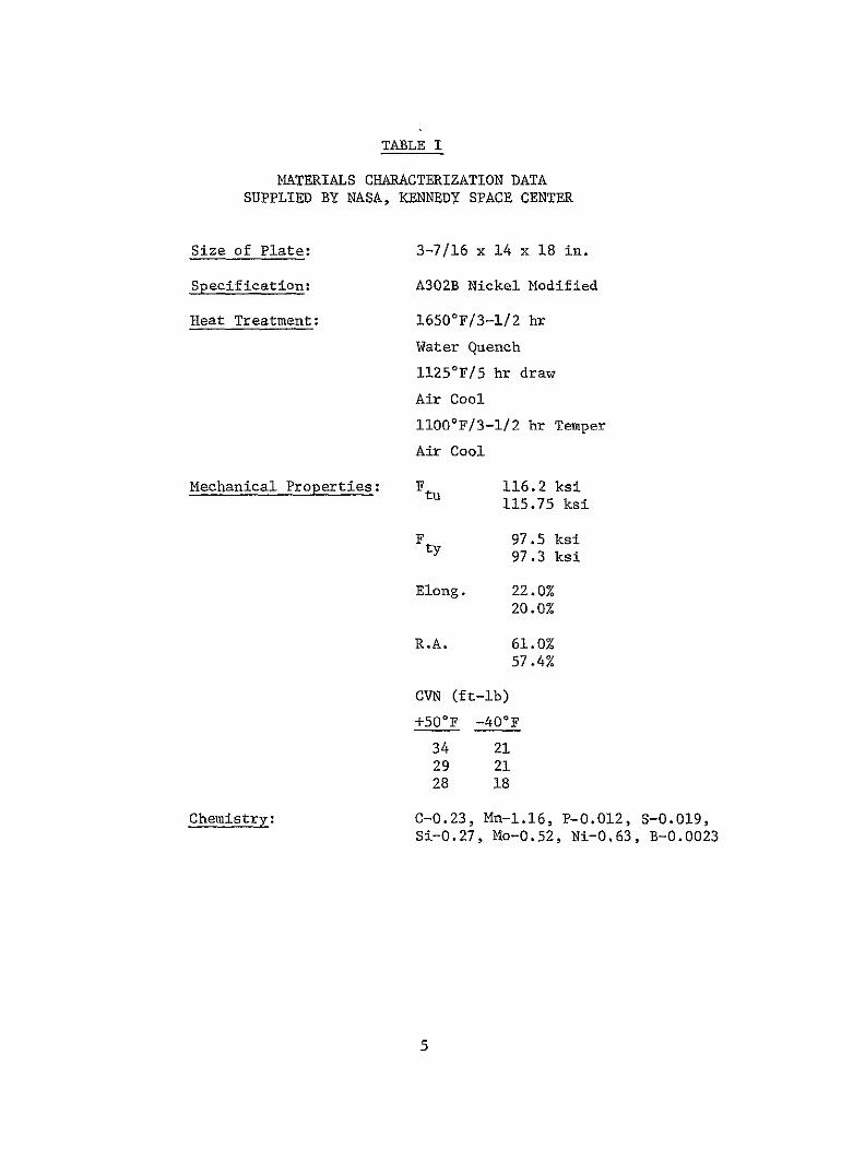
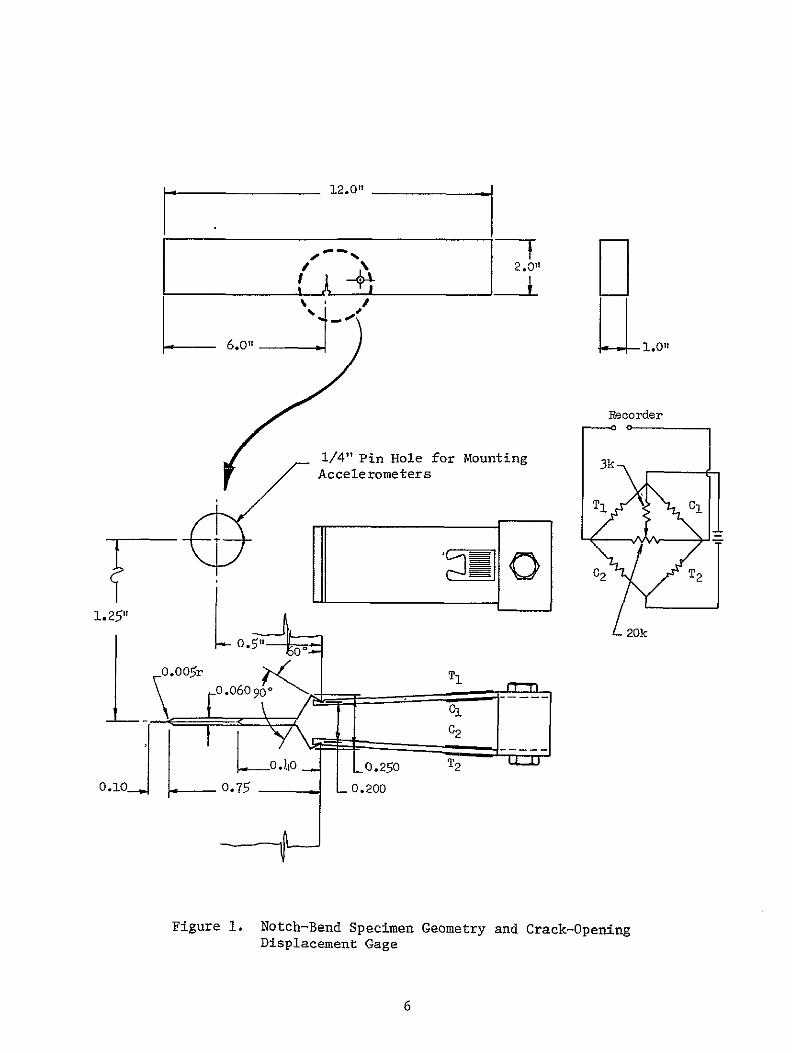
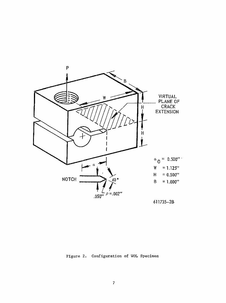
III B Crack-Opening Displacement Stress Intensity and Specimen Loading Procedure (cont)
which can occur during slow-crack-growth studies This is particularly true
in testing A302B steel where extension probably occurs through a micro-void
coalescence mechanism and in very small increments
In view of this problem a test system has been developed by
Aerojet which is capable of detecting very small increments of crack extension
This system uses the crack-opening-displacement gage recommended by ASTM and
described above however instead of a Sanborn recorder the signal from the
gage goes to a bridge balancing unit to a DC amplifier and then to a DC
millivolt recorder This system was operated at a gain of 1200 with less than
1 peak-to-peak instability The system also has a zero suppression capability
which allows the gain of 1200 to be fully utilized even though the crack
opening may increase as much as 005 in The main advantage of this system
is the extremely high sensitivity capability which was required in order to
detect incremental crack growth in the A302B nickel modified steel tested
during this program
The crack-opening displacements from the millivolt recorder were
used to determine crack length from the notch-bend calibration curve shown in
Figure 4 Stress intensity was calculated using the secant offset method
recommended by the ASTM Committee for Three-Point Bend Testing The following
relationships were employed for this purpose
PQL
K BD32 f(aD) (Eq 1)
where L is one-half the span length D is the specimen depth B is the specimen
thickness a is the crack depth and P is the load at which a secant with a
slope 5 less than the tangent slope interacts the load-displacement curve
10
200
175
150
O Each Data Point Represents an Average of Triplicate Tests
125
100
75 -
50 -
-250
010
03
Figure 4
04 05 06 07 08 aW
Calibration Curve for Three-Point Bend Specimen
11
III B Crack-Opening Displacement Stress Intensity and Specimen Loading Procedure (cont)
The parameter for crack length to depth is a numerically determined polynomial
given by
a 12 a 32+ a 52 a 72+ a 92 f(aD) = 5 8( ) -9 2(= +436(i) -753() 774(-) (Eq 2)
DDD D
The stress intensity K is a valid KIc measurement if 25(K ays) 2 is less
than both the specimen thickness and the crack depth
Calculation of the applied stress-intensity factor for the WOL
specimen was accomplished using the following expression
K PC (Eq 3)
where P is the applied load a is the crack depth B is the specimen width
and C is obtained graphically from Figure 5
Prior to precracking the WOL specimens were hydrogenated cadmium
plated and baked (same procedure as for the bend specimens) The specimens
were then precracked (01 in deep) in tension-tension fatigue Each specimen
was then calibrated by use of a crack-opening-displacement gage this was
accomplished by tensile loading the specimens and recording COD versus load
with an X-Y plotter The calibration curves for Specimen WOL-l are shown in
Figure 6 The specimens were then self-stressed by applying torque to the
bolt (bearing against a hardened steel pin) until the COD gage indicated the
desired load The load for a given stress intensity was calculated as follows
given a = 066 in (measured in specimen surfaces)
W = 1125 in
aW = 0586
12
20 I I
U I
1-z
18
16
1 4
12
-18-W
= 0444
0
U 10 -
-U-C- 8
l z
6
4
2 F 1 2 3 4 5
I __ 6 7
oW
Figure 5 Numerical Constant C for WOL Specimen
13
4500
4000
3500
3000
2500
4 2000 0
1500
1000
500
0-- 0002 in
CRACK OPENING DISPLACEMENT (IN)
Figure 6 Crack-Opening-Displacement vs Load - WOL Specimen
III B Crack-Opening Displacement Stress Intensity and Specimen Loading Procedure (cont)
C = 108 (graphically)
KI = PCB a
KSB p =
C
2 50 ksi-in1KI =for a
P = 3650 lb
Each WOL specimen was tested with an applied load correpponding to 12
K = 50 ksi-ins
C HYDROGENATION PROCEDURE
Selected bend and WOL specimens were tested after prior hydrogenashy
tion to determine the effect of this variable on the stress-wave-emissionslowshy
crack-growth relationships The hydrogenation procedure employed for this
purpose was developed by Battelle Memorial Institute and has been successfully
employed during other programs at Aerojet The hydrogen was introduced by
cathodic charging as follows
Solution 4 by weight H2SO4 5 dropsliter of poison
Poison 2 gm of phosphorus dissolved in 40 ml of carbon disulphide
Charging Time 5 min
Current Density 10 main2
The evolution of hydrogen at room temperature was prevented by
cadmium plating the test specimens within 5 min after hydrogenation The
cadmium-plating procedure was as follows
15
III C Hydrogenation Procedure (cont)
Cadmium Plating 4 ozgal CdO
Solution 16 ozgal NaCN with 1 by volume at pH 13
Current Density 70 main 2
Plating Time 30 min
Subsequent to hydrogenation and plating the specimens were baked
at 3000 F for 3 hr Baking was performed immediately prior to testing to
ensure a uniform hydrogen content throughout the test specimen
D STRESS-WAVE INSTRUMENTATION - LABORATORY EVALUATIONS
The stress-wave-detection system used for the laboratory evaluashy
tions prior to the background noise measurements at the Kennedy Space Center
is shown schematically in Figure 7 and consists of accelerometers amplifiers
filters tape recorders and an electronic counter and digital printer During
testing the accelerometers were attached to the specimens using a linear forceshy
coiled spring technique
Two basic systems were employed for stress-wave-emission data
acquisition During laboratory tests prior to the background measurements
at Kennedy Space Center the electronic counter system was employed This
system provides Very high sensitivity (signal amplifications of 10000 to
100000X) and also provides a real-time automatic count (both rate of emission
and cumulative count) of the stress-wave emissions occurring throughout each
test period The high-pass filter in the system eliminates a major portion of
the extraneous low-frequency background noises which tend to mask very small
amplitude stress waves
16
OSCILLOSCOPE
e TEKTRONIX MODEL 535
ELECTRONIC ELECTRONICSENSOR AMPLIFIER FILTER AMPLIFIER
COUNTER PRINTER S101HEWLETT PACK- HEWLETT PACK-
XIPA 00ARD MODEL 5231 ARD MODEL 5050
TAPE _ RECORDERTAPE ____________
RECORDER AMPLIFIER OSCILLOGRAPH
AMPEX MOD) T SP 300
KDATA ACQUISITION
OSCILLOSCOPE
TEKTRONIX _
eMODEL 535
DATA ANALYSIS
Figure 7 Schematic Representation of SWAT Data Acquisition and Data Analysis Instrumentation
III D Stress-Wave Instrumentation - Laboratory Evaluations (cont)
During testing of the WOL specimens maximum SWAT system amplifishy
cation was employed This was made possible because the specimens immersed
(COD gage up out of the water) in the water environment were enclosed in a
sound-proof box For these tests the electronic counter trigger level was
set just above the inherent noise (electrical) of the system Initially a
WOL test was run to determine whether the system was in fact completely free
of extraneous noise With the COD gage connected and all recording systems
in the circuit and with the specimen under no load and in air environment
after 5-12 hr in the sound-proof chamber there were only 16 signals
counted Presumably these were electrical disturbances The test was run
during regular working hours the WOL tests reported in the following parashy
graphs were tun during off-hours (nights and weekends) when there should have
been an absolute minimum of electrical disturbances
A second data acquisition system was also used for a limited
number of bend tests following the background noise measurements at Cape Kennedy
A schematic of this system is shown in Figure 8 The purpose of these tests
was to obtain stress-wave amplitude measurements using the instrumentation
employed at Cape Kennedy to ensure that the stress-wave emissions accompanying
crack extension could be detected under the background conditions observed at
Kennedy Space Center The tape recordings were made by direct recording during
test and were subsequently analyzed through playback and analysis as shown in
Figure 7
18
TEKTRONIX
OSCILLOSCOPE
ENDEVCO Dynamics Model 2213 Filter Accelerometer Model
Amplifier Amplifier 6364MQ 20-50 Kc Band Pass
KcENDEVCO30
Model 2213 CHigh-PassH Accelerometer Filter
kFI
TAPE Amplifier Amplifier RECORDER
AMPEX SP-300
Figure 8 Schematic of Instrumentation Used at Kennedy Space Center
IV LABORATORY TEST RESULTS AND DISCUSSION
As indicated in the following paragraphs two environments (air and
3 NaCl-water) and two material conditions (unhydrogenated and hydrogenated)
were utilized in the laboratory tests performed at Aerojet These conditions
are considered those most likely to be encountered during the service life of
the pressure vessels Also both straight rising load to failure and sustained
loading profiles were employed The sustained load profiles were employed
since failure of the pressure vessel may occur at constant load due to
environmentally induced slow crack growth from a prior flaw Since the
effectiveness of a failure warning system will obviously depend on the ability
to detect subcritical crack extension whether it occurs during sustained load
or on rising to failure it is important to determine if crack extension andor
failure will occur under both conditions Both effects can be studied through
the laboratory tests performed during this program
A BEND TESTS IN AIR WITHOUT DELIBERATE ADDITION OF HYDROGEN
Initially bend tests were performed in an air environment Both
the crack-opening-displacement gage and stress-wave-analysis technique were
employed to monitor the occurrence of pop-in and subcritical crack growth
The fracture data for these tests are shown below
Specimen Specimen Failure Notch Plus Apparent K
Thickness (B) Depth (D) Fatigue Crack (a) Load 1 2 No in in in aD P Kips ksi-in
1 10 20 090 045 200 130
2 097 20 091 0455 158 136
3 10 20 1036 0518 1656 133
Intermediate hold at 123 ksi-in12
20
IV A Bend Tests in Air Without Deliberate Addition of Hydrogen (cont)
The straight rising load to failure tests (No 1 and 2) indicated 12
a K value of 130 to 136 ksi-in as did the specimen (No 3) which failed
during rising load after previous holding at a stress intensity of approximately 12123 ksi-in As indicated previously in this report the ASTM recommends
for valid KIc measurements a specimen thickness exceeding that corresponding
to 25 (Kys)2 By this criterion a specimen thickness of approximately
44 in would be required for the A302B steel tested in this program
Consequently the KQ values noted above while not valid KIc measurements
indicate a high level of toughness in this material
No significant slow-crack growth or stress-wave emissions were
observed during hold in the air environment Conversely slow-crack growth
(increase in apparent crack size) and accompanying stress-wave emissions were
observed during rising load to failure The stress waves were generally very
small in amplitude (clt0Olg) but increased in amplitude with increasing crack
extension immediately prior to failure Increased rate of stress-wave
emission was also observed immediately prior to failure
B BEND TESTS IN WATER WITHOUT DELIBERATE ADDITION OF HYDROGEN
Bend specimen 4 was loaded initially to 15000 lb
(88 ksi-in 2) and held at constant load for 18 hr in 3 sodium-chloride
simulated sea water The specimen showed indications of crack growth early in
the hold period However analysis of the crack-opening-displacement gage data
indicated only very small amounts of crack extension Although the gage
employed for this purpose corresponded to the design recommended by the ASTM
its use was found unsatisfactory for tests of the type performed during this
program The COD gage was then modified and the modified version used during
the testing of the hydrogenated material described in subsequent sections of
this report
21
IV B Bend Tests in Water Without Deliberate Addition of Hydrogen (cont)
When the specimens (without hydrogenation) tested in the salt-water
environment were fractured the fracture surfaces were examined for evidence
of slow-crack growth during hold Although a small band of slow-crack growth
from the original fatigue precrack was observed it was not possible to detershy
mine how much of the crack extension occurred during rising load Onthe basis
of the COD data it would appear the majority of the extension occurred during
rising load to 15 kips from 15 to 17 kips and from 17 kips to failure although
the SWE data indicated that slow crack growth however small was occurring
during the hold periods
Figure 9 is a plot of cumulative stress-wave count over a period
of approximately 1-12 hr during hold at 15000 lb Note the indications of
a variable rate of subcritical crack growth Figure 10 shows the SWAT data
in detail (electronic counter reading every second) starting 23 min after
reaching the 15-kip load level Note that the cumfilative stress-waampe count
increased more or less continuously with brief intervals of increased slope
(when plotted to the scale of Figure 10 the increased slope was approximately 450) Figure 11 shows the SWE data obtained after adding fresh 3 NaCl-water
solution to the notch During the period of sustained load represented in
Figure 11 there were a few abrupt increases in count indicating discontinuous
crack growth together with additional intervals of increased slope (again
close to 45)
Figure 12 corresponds to the endof a short 16-kip hold (same
specimen) followed by a rise to 17 kips (approximately 125 ksi-in1 2 ) and
then a period of sustained load in 3 NaCl-water solution at 17 kips Note
the increased slope associated with the increase in load followed by abrupt
increases in count characteristic of discontinuous crack growth Approximately
600 sec after starting the hold at 17 kips an air hose produced high-frequency
noise too high to be removed by the filter This was recorded as an abrupt
increase in couni followed by a period of increased slope (again approximately 45) It cannot be definitely stated whether the increased slope indicating
22
1400
1200
1000
Li 800 3
LU
D 600
400
SEE FIGURE 10 200 FOR DETAILS
0 0 I I I I I
0 10 20 30 40 50 60 70 80 90 100
-MINUTES HOLD AT 15 KIPS
Figure 9 Cumulative Stress Wave Count vs Time Specimen No 4
A302B Steel 15 Kip Hold 3 NaCi-Water Environment
23
600
I0
20-
TIME (SECONDS)
224
6050
10 10 1O 1in20 20a 2100 2150
TIME (SECONDS) 220 3 am250 20 20 3w245 24W
43O
600
40
20
140
011 115 la 1in0 1 TIME (SECONDS)
a 14W 1m 53 0 inlW
Figure 11 Cumulative Stress Wave Count vs Time Specimen No 4 A302B Steel 15 Kip Hold After Replenishing the 3 NaCl-Water Environment
25
23
00
60
20
20
- 4o
o_ 4 o l~ ~ aiE~
220
IV B Bend Tests in Water Without Deliberate Addition of Hydrogen (cont)
continuous stress-wave emission was an artifact produced by the high-frequency
noise or the increased slope was the result of crack growth stimulated by the
high-frequency sound (crack growth after periods of dormancy can be initiated
by tapping a test specimen under load) Figure 13 is a plot of the cumulative
count for the 17-kip hold (corrected to zero at the start of hold and corrected
for noise which occurred at 836 sec) Note the tendency for increasing slope
with increasing time at load Figure 14 presents the SWAT data in detail
after 1 min at 17 kips load Figure 15 presents the data obtained after
1-12 min at 17 kips load Both Figures 14 and 15 are plotted to the same
scale as Figures 10 11 and 12 Table II presents the data plotted in
Figures 13 14 and 15 without correction for noise which occurred at 836 sec
this tabulation shows the detailed information that can be obtained by SWAT
On the basis of the SWE dpta this specimen showed evidence of
very slow continuous crack growth of the type one might expect of electroshy
chemical dissolution at the crack tip interspersed with short periods of more
rapid continuous crack growth There was little or no evidence of disconshy
tinuous crack growth with clearly defined periods of dormancy and there were
few instances of abrupt increase in count to signify crack jumps
C BEND TESTS IN AIR WITH DELIBERATE ADDITION OF HYDROGEN
After hydrogenation and baking 3 hr at 3000 F to produce a
homogeneous interstitial solid solution specimens were tested in 70degF air
Specimen 5 (Figure 16) developed discontinuous crack growth while under
sustained load starting at 9000 lb (75 ksi-in 2) but the occurrences were
sporadic and infrequent At 13000 lb (110 ksi-in 2) there was only one
stress wave large enough to be recorded as a cumulative count (cumulative
count increased from 3086 to 3110 corresponding to 464 SWEsec count rate)
Otherwise there was no increase in the SWE cumulative count during hold at
13000 lb
27
TABLE II
DETAILS OF SWE DATA OBTAINED FOR SPECIMEN NO 4 A302B STEEL DURING HOLD AT 17 KIPS IN 3 NaCI-WATER ENVIRONMENT
Time at Count Interval Time at Count Interval Load Rate Cumulative At Load Rate Cumulative A t (sec) (SWEsec) Count (sec) (set) (SWEsec) Count (sec)
27 57 8 - 1330 11 632 9 47 134 12 20 1331 20 634 1 101 4 14 54 1341 58 635 10 152 3 16 51 1392 232 652 51 299 10 27 147 1400 262 653 8
5 MINUTES 1405 134 654 5 329 1 29 30 1415 9 656 10 357 47 37 28 1443 85 657 28 444 72 49 87 1446 48 659 3 460 64 56 16 1478 131 675 32 494 221 60 34 1479 2 676 1 511 145 62 17 1495 29 685 16
10 MINUTES 25 MINUTES 616 115 72 105 1503 170 689 8 744 128 85 128 1505 72 691 2 788 2 92 44 1526 171 697 21 836 2 411(Noise) 48 1527 1 698 1 838 7 411 2 1537 187 702 10 843 10 431 5 1546 220 705 9 845 68 431 2 1584 89 715 38 846 7 431 1 1597 119 726 13 855 161 447 9 1650 146 738 53 880 160 468 25 1666 1 749 16
15 MINUTES 1671 162 756 5 904 11 492 24 1674 86 758 3 915 209 500 11 1695 120 780 21 943 5 523 28 1708 75 782 13 956 22 537 13 1717 1 787 9 980 4 541 24 1721 84 792 4 992 13 542 12 1732 114 794 11
1012 69 544 20 30 MINUTES 1088 21 558 76 1808 228 803 76 1108 151 569 20 1821 179 805 13 1136 il 576 28 1825 22 808 4 1154 5 582 18 1833 196 809 8 1172 38 583 18 1839 120 811 6 1178 19 585 6 1852 45 814 13 1182 9 -592 4 1866 146 816 14 1196 26 594 14 1888 168 819 22
20 MINUTES 1895 14 823 7 1228 80 598 32 1909 157 826 14 1229 13 599 1 1933 29 832 24 1238 2 605 9 1950 10 836 17 1256 1 610 18 1956 46 837 6 1312 91 613 56 1977 71 838 21 1318 1 619 6 1988 101 839 11 1321 1 621 3 2000 10 841 12
TABLE II (cont)
Time at Count Interval Time at Count Interval Load Rate Cumulative At Load Rate Cumulative Lt (sec) (SWBsec) Count (sec) (sec) (SWEsec) Count (sec)
2002 59 843 2 2515 40 1013 34 2017 119 845 15 2518 207 1017 3 2020 148 847 3 2521 1 1023 3 2033 165 848 13 2525 602 1029 4 2039 103 850 6 2527 22 1034 2 2048 9 857 9 2548 52 1052 21 2061 129 860 13 2561 47 1058 13 2063 156 862 2 2573 17 1062 12 2069 167 864 6 2585 69 1072 12 2075 98 874 6 2588 42 1073 3 2076 3 879 1 2599 240 1075 11 2093 21 881 17 2605 4 1077 6
35 MINUTES 2615 23 1078 10 2107 1 883 14 2616 57 1079 1 2108 103 884 1 2613 11 1080 15 2118 121 885 10 2638 42 1081 7 2119 191 887 1 2648 2 1087 10 2135 154 891 16 2650 87 1088 2 2140 11 892 5 2653 100 1089 3 2146 3 894 6 2656 56 1090 3 2150 178 897 4 2661 63 1091 5 2159 51 902 9 2685 28 1094 24 2162 7 905 3 2693 35 1097 8 2180 57 909 18 45 MINUTES 2182 58 910 2 2701 113 1104 8 2193 17 913 11 2703 50 1105 2 2195 113 916 2 2713 53 1109 10 2207 115 919 12 2719 20 1110 6 2221 34 923 14 2721 33 1112 2 2223 87 926 2 2738 72 1115 17 2238 35 936 15 2740 15 1116 2 2258 2 943 20 2752 100 1117 12 2268 204 947 10 2756 85 1119 4 2289 10 949 21 2768 56 1121 12 2307 1 952 18 2780 13 1130 12 2319 121 955 12 2782 28 1135 2 2346 20 959 27 2795 60 1142 13 2366 69 963 20 2809 65 1144 14 2386 20 975 20 2841 55 1156 32 2387 5 976 1 2848 3 1157 7 2392 158 978 5 2851 2 1159 3 2396 8 981 4 2862 45 1163 11
40 MINUTES 2869 35 1166 7 2403 21 983 7 2879 18 1169 10 2409 241 986 6 2885 62 1171 6 2449 95 996 40 2905 55 1175 20 2457 24 998 8 2908 54 1178 3 2473 104 1002 16 2918 7 1182 10 2481 3 1003 8 2924 8 1186 6
29
TABLE II (cont)
Time at Count Interval Time at Count Interval Load Rate Cumulative t Load Rate Cumulative t (sec) (SWIsec) Count (sec) (sec) (SWEsec) Count (sec)
2938 12 1193 14 3341 207 1410 2948 95 1201 10 3366 103 1421 25 2966 10 1215 18 3377 8 1424 11 2968 43 1216 2 3378 12 1425 1 2972 22 1217 4 3390 2 1429 12 2979 8 1221 7 3396 3 1430 6 2987 8 1223 8 3397 14 1432 1 2998 38 1226 11 3401 8 1434 4
50 MINUTES 3402 98 1438 1 3002 36 1228 4 3408 12 1443 6 3010 55 1230 8 3410 16 1448 2 3011 3 1234 1 3413 6 1452 3 3016 1 1236 5 3431 2 1454 8 3017 3 1237 1 3433 17 1458 2 3023 3 1239 6 3435 30 1460 - 2 3029 3 1240 6 3438 22 1462 3 3033 1 1243 4 3450 8 1475 12 3036 110 1245 3 3455 62 1484 5 3037 4 1248 1 3461 154 1490 6 3053 83 1259 16 3462 7 1493 1 3054 7 1260 1 3466 11 1501 4 3061 2 1265 7 3472 2 1507 6 3062 83 1266 1 3476 46 1509 4 3076 62 1275 14 3489 18 1515 13 3080 5 1278 4 3490 8 1517 1 3098 32 1294 18 3508 15 1534 18 3100 15 1296 2 3513 25 1541 5 3102 16 1297 2 3520 220 1549 7 3108 7 1299 6 3538 29 1566 18 3114 7 1301 6 3542 9 1572 4 3127 6 1304 13 3543 107 1575 1 3129 1 1305 2 3558 240 1588 15 3133 1 1306 4 3568 30 1601 10 3140 5 1309 7 3570 21 1603 2 3154 30 1312 14 3573 66 1607 3 3170 6 1320 16 3579 9 1613 6 3175 77 1322 5 3591 37 1619 12 3177 110 1323 2 60 MINUTES 3178 5 1324 1 3607 128 1622 16 3183 4 1326 5 3608 70 1626 1 3187 137 1331 4 3609 2 1629 1 3191 14 1332 4 3624 50 1638 15 3200 3 1336 9 3630 14 1642 6 3206 2 1340 6 3639 86 1645 9 3214 20 1343 8 3660 56 1662 21 3219 22 1345 5 3678 13 1669 18
55 MINUTES
30
TABLE II (cont)
Time at Count Interval Time at Count Interval Load Rate Cumulative At Load Rate Cumulative At (sec) (SWEsec) Count (sec) (see) (SWEsec) Count (sec)
3688 33 1680 10 4535 105 2574 28 3692 35 1682 4 4547 3 2589 12
3709 209 1688 17 4583 4 2616 36 3712 7 1689 3 4623 460 2670 40 3720 78 1691 8 4624 37 2703 1
3730 93 1694 10 4626 18 2715 2 3731 5 1695 1 4627 840 2729 1 3743 13 1703 12 4630 141 2737 3 3744 120 1709 1 4662 2 2758 32
3750 24 1715 6 4671 1 2763 9 3755 142 1724 5 4698 1 2774 27 3767 45 1738 12 4710 8 2782 12 3796 69 1770 29 4719 6 2784 9 3823 21 1808 27 4731 128 2785 12 3844 10 1838 21 4761 17 2810 30 3854 82 1851 10 4783 22 2822 22 3856 13 1855 2 4786 23 282A 3 3895 75 1915 39 80 MINUTES
65 MINUTES 4822 96 2831 36 3901 18 1920 6 4852 1 2842 30 3905 54 1927 4 4934 59 2890 82
3946 58 1963 41 4953 200 2907 19 3970 2 1985 24 4954 26 2910 1 3971 181 1988 1 4957 16 2916 3 3974 61 1990 3 4964 56 2923 7 3975 28 1992 1 4988 29 2941 24 3987 51 2004 12 5000 88 2951 12 4012 2 2022 25 5031 10 2977 31 4013 31 2026 1 5032 9 2978 1 4022 7 2036 9 5045 56 2982 13 4054 4 2062 32 5054 4 2984 9 4056 16 2066 2 5093 220 2992 39 4084 37 2093 28 85 MINUTES 4091 36 2099 7 5122 115 2996 29 4100 3 2111 9 5166 17 3019 44 4129 16 2142 29 5190 172 3042 24 4156 6 2165 27 5193 55 3045 3
70 MINUTES 5194 2 3048 1 4241 19 2253 85 5224 313 3081 30 4292 4 2299 51 5248 23 3106 24 4331 42 2339 39 5266 32 3123 18 4338 19 2348 7 5281 24 3138 15 4340 66 2350 2 5291 10 3150 10 4345 10 2359 5 5303 25 3164 12 4385 4 2419 40 5306 1 3169 3 4397 121 2432 12 5324 56 3187 18
75 MINUTES 5330 58 3193 6 4500 40 2534 103 5345 31 3211 15 4507 6 2542 7 5351 155 3217 6
31
TABLE II (cont)
Time at Count Interval Time at Count Interval Load Rate Cumulative At Load Rate Cumulative At (sec) (SWBsec) Count (sec) (sec) (SWEsec) Count (sec)
5357 211 3223 6 5887 185 3536 1 5363 29 3233 6 5905 65 3559 18 5364 20 3237 1 5923 31 3575 18
90 MINUTES 5924 22 3576 1 5403 118 3276 39 5933 109 3578 9 5418 79 3295 15 5934 5 3579 1 5419 44 3298 1 5961 43 3582 27 5420 35 3300 1 100 MINUTES 5448 27 3324 28 6000 23 3585 39 5460 118 3327 12 6001 13 3586 1 5466 97 3329 6 6002 166 3588 1 5472 184 3331 6 6008 9 3590 6 5484 28 3333 12 6032 29 3592 24 5499 45 3338 15 6041 111 3596 9 5505 2 3341 6 6062 116 3601 21 5506 173 3344 1 6083 1 3603 21 5512 72 3346 6 6084 236 3606 1 5515 8 3348 3 6090 140 3607 6 5536 199 3352 21 6091 104 3608 1 5548 5 3356 12 6106 21 3609 15 5553 199 3359 5 6115 31 3611 9 5554 34 3360 1 6121 29 3614 6shy5587 190 3364 33 6124 1 3622 3 5593 2 3365 6 6139 51 3630 15 5605 6 3367 12 6160 25 3634 21 5611 12 3369 6 6175 5 3636 15 5638 3 3373 27 6184 196 3639 9 5644 57 3374 6 6217 275 3645 33 5645 78 3376 1 6223 84 3648 6 5669 21 3379 24 6238 23 3649 - 15 5693 22 3384 24 6244 99 3650 6 5699 48 3385 6 6250 81 3652 6
95 MINUTES 6259 39 3654 9 5702 74 3387 3 6265 15 3656 6 5703 85 3389 1 6271 21 3658 6 5725 21 3391 22 6283 85 3660 12 5737 1 3394 12 105 IWNUTES 5752 72 3396 15 6304 143 3662 21 5761 106 3398 9 6331 50 3672 27 5788 1 3414 27 6340 179 3674 9 5794 176 3422 6 6341 37 3675 1 5809 2 3441 15 6365 34 3677 24 5810 15 3445 1 6366 ill 3680 1 5813 42 3448 3 6393 150 3682 27 5814 189 3451 1 6405 43 3684 12 5823 180 3461 9 6429 4 3687 24 5832 171 3472 9 6435 127 3690 6 5838 46 3481 6 6459 31 3691 24 5859 63 3505 21 6483 7 3694 24 5865 15 3511 6 6495 30 3696 12 5886 2 3533 21 6501 128 3700 6
32
TABLE II (cont)
Time at Count Interval Time at Count Interval Load Rate Cumulative At Load Rate Cumulative At (sec) (SWEsec) Count (sec) (sec) (SWEsec) Count (sec)
6522 87 3703 21 7278 21 4158 6 6531 16 3704 9 7302 2 4174 24 6555 102 3706 24 7303 3 4174 1 6567 7 3709 12 7318 125 4186 15 6570 10 3710 3 7348 88 4205 30 6576 87 3711 6 7402 86 4238 54 6577 89 3713 1 7435 90 4258 33 6578 131 3714 1 7447 14 4262 12 6599 4 3717 21 7474 14 4277 27
6600 110 MINUTES
8 3718 1 7486 7504
9 125 MINUTES
89
4286
4304
12
18 6603 37 3720 3 7510 39 4308 6 6639 15 3724 36 7531 52 4331 21 6669 48 3728 30 7540 208 4344 9 6675 23 3729 6 7549 38 4353 9 6684 57 3731 9 7576 72 4376 27 6705 23 3757 21 7594 24 4392 18 6744 53 3807 39 7603 55 4403 9 6762 240 3830 18 7615 160 4415 12 6783 5 3854 21 7621 134 4420 6 6801 26 3874 18 7627 160 4423 6 6822 181 3901 21 7639 180 4430 12 6852 24 3934 30 7648 5 4432 9 6879 44 3962 27 7658 100 4437 10 6882 2 3965 3 7679 319 4445 21
115 MINUTES 7694 72 4449 15 6906 63 3991 24 7709 23 4451 15 6927 176 4001 21 7721 34 4453 12 6930 15 4006 3 130 MINUTES 6931 54 4011 1 7800 Test Terminated 6952 305 4026 21 6953 40 4033 1 6980 3 4037 27 6989 99 4039 9 7040 387 4080 51 7041 53 4095 1 7056 23 4100 15 7086 354 4108 30 7095 21 4110 9 7125 70 4117 30 7131 2 4120 6 7167 97 4129 36 7176 11 4130 9 7197 18 4133 21
120 MINUTES 7218 28 4136 21 7227 39 4138 9 7248 72 4146 21 7272 50 4153 24
33
40
38W
3400
32W
30
28M
260
= 2400
S 22DD
i20
1600
1400
1200
10
600
400
200
06 1a 20 30 40 50 60 70 80 90 tW 110120130
MINUTE-S-H-OLD 17KIPS
Figure 13 Cumulative Stress Wave Count vs Time SpecimE A302B Steels 3 NaC1-Water Environment
34
3503
0
~0
40
20
3203
00
20
C0
20
310
03
(0
40
= = 20 0 I- 365~
05
20 00
20
0shy20
2003
20 ~~0 C
20
20 40
- 20
2835
0
(0
20
20shy
20020
20 -
3403 3450 3720 3750 fl 3550 3003 3050 40) 4050 4003 4050 4~fl 4200 4020 4350 4440 4450
TIME (SECONDS)
Figure 14 Cumulative Stress Wave Count vs Time Specimen No 4 A302B Steel After 1 Minute at 17 Kip Hold in 3 NaCi-Water Environment
35
48
0
I-
S 40
us 50 50 70 5 90 0 60 60 10 6 6 t 20CO DS
- iue1CmlaieSrs av on sTme pcmnN A0BSel
Afe2-0iue t1 i todi NC-ae niomn
Page60
4520 -
so- lao
F
122021 amp~
20 4
400
20
20 22
3540 =
20
3024
20
50
45
20
20520
20
20
45
20
no
I
40
4~
20
40
20
20
4
20
2020
20
gt
20
20 4
20
20
3545
20
Iino200j
5505
2220
1120
20
001
20
20 shy
00
1
45
OX
I
I I
I I
0 50
020 000
205 200
20 200
Z
40 505
550 400
TIM
E (S
EC
ON
DS
)
Figure 16
Cumulative Stress Wave Count vs
Time Specimen No
5 A302B Steel
Hydrogenated and Tested in Air
37
IV C Bend Tests in Air With Deliberate Addition of Hydrogen (cont)
On raising the load from 13000 to 14000 lb (122 ksi-in )
there was evidence of a creep phenomenon as shown in Figure 17 The crackshy
opening-displacement gage confirmed the occurrence of crack growth continuing
after reaching the 14000-lb hold Stress-wave emission showed the mechanism
to be discontinuous cracking rather than a deformation process When the
count rate was plotted as in Figure 18 the activity carrying into the
14000-lb hold again was discontinuous After approximately 300 sec at 14 kips
the SWE associated with the creep phenomenon had subsided During the 14-kip
hold there were two crack jumps one after 920 sec (cumulative count increased
from 5618 to 5720 and the count rate associated with the jump was 181 as
counted over a 10-sec interval or 18 SWEsec) and one after 2130 sec (cumulashy
tive count increased from 5721 to 5755 and the count rate was 139 in 10 see)
After 5000 sec at 14 kips the load on Specimen 5 was raised As
seen in Figure 19 the stress-wave activity was an unmistakable presage of
instability which occurred after 20 sec into hold The load reached a maximum
of 145 kips (145 ksi-in 2) Technically the onset of instability occurred
shortly after starting to increase the load ie at approximately
132 ksi-inI2 which agrees with the KQ value obtained through rising load
tests of unhydrogenated material in an air environment
Because of the very long test period and multiple loadings involved
in the testing of the Specimen 6 only data obtained during rising load to
19500 and 19800 ib during sustained test periods at these loads and during
specimen failure are shown in Figure 20 These data indicate essentially the
same SWE-crack growth relationships discussed previously for Specimen 5 except
that on reaching hold the crack tended to grow slowly for a longer period of
time in comparison to the behavior noted for Specimen 5 Also the incremental
nature of crack extension was more readily observed by the stress-wave-emission
data for Specimen 6
38
20
560
80
60
40
20
5500
80
60
40
20
5400
o 5100
808
60
40
20
5000 u-J
4500
4480 80 4- START 14-KI P HOLD
CODC 75lt
4000
3980 70
3960
6553120 l
- END13-KIP HOLD
3100 160 0 40 80 120 160 200 240 280 320
TIME AT LOAD (SECONDS)
Figure 17 Cumulative Stress Wave Count and COD vs Time Specimen No 5 A302B Steel fydrogenated and Held at 14 Kips in Air
39
200
LU
LU
1- 100
50 END 13-KIP
25 HOLD-I
0 1- TIME
100 INSECONDS AT
200 14KIPS
300
(COUNT EVERY 10 SEC)
Figure 18 Stress Wave Count Rate vs Time - Specimen No 5 A302B Steel Hydrogenated and Tested in Air
40
INSTABILITY
9580
9560
9540
9380
928D0
9260
842D
8440
73O I-shyz 7220
o 7260
U 7240
7220
7180I-shy
7160
- 7140
7120
7100
7080
7060
5900
5880
5860
5840
5820
5800
578D
5460
0 40 80 120 160 SEC
4M 4960 50D RISING LOAD-SECONDS AT 14 KIPS
Figure 19 Cumulative Stress Wave Count vs Time Specimen No 5 A302B Steel Hydrogenated and Tested in Air
41
20000
18000
FAILURE
18290 sec a- 1 17-in K - 199 s - Y
z
-
16000
14000
l0
1200
I-9 Iin
1014in K 152 ki- in -i
o-1 09 n K- 176ksmn
- 1 07 in I 170 iis-
o -1 042in K 12ks-in
c023i NK15ks-n
-shy
-
10000
REACH 19800 lbs
START TO 19800 bs
10000 11000 12000 13000 14000 15000 16000 17000 18000 19000
TIMESECONDS
12000
11000 s
p9000
T LOAD ADJUSTMEA
7n000
READOUT6000 OTE STRESS WAVE DATA A UST T
500 Vgt 0 ENT CORRESPONDIG TO SLOPELOAADJUSTM15 CHANGES PLOTTED
a 4000
3000
LOAD ADJUSTMENT2000 SECONDSECMENIME
1000 START HOLD AT 19500 1b
900 1l6070 D0 8 0 00 0 000600
0 1000 50002000 3000 4000
TIME SECONDS
Figure 20 Cumulative Stress Wave Count vs Time Specimen No 6 A302B Steel Hydrogenated and Tested in Air
Page 42
IV C Bend Tests in Air With Deliberate Addition of Hydrogen (cont)
As indicated in Figure 20 the increase in crack length during
the initial period of hold at 19500 lb resulted in an increase in the applied
stress intensity and was accompanied by significant stress-wave-emission
activity To maintain the desired load it was also necessary to make frequent
load adjustments at the start of hold During the first 3600 sec the effecshy
tive crack length increased from approximately 0963 to 1000 in and was
accompanied by about 7000 SWE As indicated in Figure 20 the majority of the
SWE activity and increase in crack length occurred during the first 3000 sec
of the hold at 19500 lb After this period both the stress-wave-emission
activity and rate of increase in crack length gradually decreased For example
during the entire period from 5000 to 17600 sec when the load was increased
to 19800 lb the apparent crack length and SWE count increased by only approxishy
mately 0020 in and 2500 respectively
After approximately 17000 sec at 19500 lb the load was increased
to 19800 lb and specimen failure occurred after approximately 600 sec at
19800 lb The load was maintained for this period however it was apparent
from both the SWE and COD gage data that the crack was extending and specimen
failure would occur without a further increase in load although it was necesshy
sary to continually adjust the tensile machine to maintain the desired load
The failure stress intensity approximated 199 ksi-in 2however technically
the onset of instability occurred after starting to increase the load at
approximately 153 ksi-in1 2
Specimen 7 was also hydrogenated baked at 300F for 3 hr and
tested in air Figure 21 is a detailed plot of the SWAT data (electronic
counter print-out every second) indicating crack growth of a discontinuous
nature starting at 2400-lb load Note the periods of dormancy (no increase
in SWE count) interspersed with abrupt increases in count indicating disconshy
tinuous crack growth Note also that there was little or no evidence of
continuous stress-wave emission until the load (stress intensity level) was
high approaching failure
43
CUMULAIY STRESS-VAVE COUNTCU LTISTE W E ON
I OT A~II I OI I L I I I I I I I I I I I I I I i I I I I I
- N LB
I I I I I I I I I I I I I i I I
--L - 0OTO11
-0101
(lNIML~ 33383338
8
133113-
3IiC)0 83) 3103 31-3(31-
~0
33 331
3l3C0C~
38318shy
111(10 CAVMSS3 nfl CAliVi flWfl3
________________________________________________________________________
111fl0~ 3KvM~s~a1Ff~TfvTifwT
FPAIAE
hY
A Ii
8
INa
CZ
8 C0 U CI
33 S
1 H
H
03 -I
~ 3lt
0 Cd 33
~C3 ~ H
8 0003
A
Ofli3i~~ C)
Page 45
IV C Bend Tests in Air With Deliberate Addition of Hydrogen (cont)
Figure 22 presents the SWE data from a hydrogenated bend specimen
(No 8) tested in air The load was increased continuously to 9800 lb
(70 ksi-in 2) where there was a short hold (approximately 400 sec) Note
the discontinuous crack growth followed by a short period of continuous
emission (less than 450 slope) The load was then raised to 14800 lb
(109 ksi-in 2) and held for approximately 400 sec Again there were jumps
in the SWE cumulative count but this time interspersed with continuous
emission The SWAT system employed for this test corresponded to that employed
for the background measurements at Kennedy Space Flight Center and shown in
Figure 8 only one channel was employed viz
Endevco 2213 Amplifier Amplifier Band-Pass Filter 10OX 10OX 20 to 50 Kcps
The continuous stress-wave emission observed during hold at the higher stressshy
intensity level in this specimen was not observed in the other hydrogenated
specimens tested in air The primary purpose of this test (Specimen 8) was to
record SWE data for subsequent playback and analysis to determine the amplitude
of burst-type stress-wave emissions associated with fracture in Type A302B
steel These analyses were performed using the instrumentation shown in
Figures 7 and 8 with the following results which are discussed in more detail
in conjunction with the results of the background measurements performed at
Kennedy Space Flight Center (Section V)
Maximum SWE Amplitude - 39 x 10-3g
Minimum SWE Amplitude - 12 x 10-3 g
Average SWE Amplitude - 22 x 10-3g
Laboratory Background - 11 x 10-3g
46
00 o z~ 20 ~
40
~40
S20 1 2 0 0 0 0
TIIAEAT 4 S-KIPHOLD (10KS(51IN A)
407
IV Laboratory Test Results and Discussion (cont)
D BEND TESTS IN 3 NaCI-WATER WITH DELIBERATE ADDITION OF HYDROGEN
Specimen 9 was hydrogenated baked and tested in 80F water
The electronic counter indicated continuous stress-wave emission interspersed
with abrupt increases in count indicating occasional crack jumps Figure 23
shows the details of stress-wave emission that occurred during both rising
load and holding load The crack length determined from the COD chart at
selected loads is also shown Note from the SWE data that there were no
periods of dormancy and the slope of the plot of cumulative count versus time
indicated moderately rapid continuouas crack growth such as might occur with
electrochemical dissolution at the crack tip The COD gage data shown in
Figure 23 also indicate crack extension however the actual amount appears
to be quite small (lt01 in) which would be consistent with the relatively
small number of stress-wave emissions detected even at the high system
sensitivity employed The dramatic difference between the behavior in
Figures 21 and 23 for hydrogenated material tested in air (Figure 21) and
water (Figure 23) indicates that hydrogen and 3 sodium chloride solution
acting together have a greater total effect than the sum of their individual
effects ie working together they appear to have produced a synergism
E WOL TESTS
Because of the possible significance of the synergistic-effect
noted above on the life of the hydrogen pressure vessels at Kennedy Space
Flight Center additional testing was performed using hydrogenated WOL specishy
mens cut from the fractured bend specimens The first WOL specimen was
initially loaded to-3650 lb (50 ksi-in 2) and then placed in 3 NaCl solution
(notch immersed) There was 30 min of essentially continuous stress-wave
emission (recorder started approximately 5 min after loading the specimen)
Subsequently therewas one sizable jump in the SWE cumulative count after
48
V30
760
740-M
$
720 -s
680shy
60
610
40 w
w
520 w
i
20500
HOLDD]N
340
20 760
7200
ING
IV
O
shy
420
60
40
20 0 2
04
0Q
0
60DO
LO0
01 200
250 300
350 400
450 500
550 6M
650
700 750
TIME
(SECONDS)
Figure 23
Cumulative Stress Wave Count vs Time Specimen No 9 A302B Steel
Hydrogenated and Tested in 3 NaCi-Water Environment
49
IV E WOL Tests (cont)
approximately 3 hr 40 min Then 3 hr 20 min later several jumps occurred
followed by 8 hr 20 min of stress-iave activity After this the crack was
dormant (total test time 17 hr 25 min) These data are shown in Figure 24
The load was then increased slightly (torque was increased from 200 to
255 in-lb) an additional 1-12 hr in 3 NaCl solution produced no significant
increase in the cumulative stress-wave count The reason for this apparently
anomalous behavior was not determined although it may result from a blunting
effect at the crack tip produced during the initial hold period
The fatigue crack was then extended (approximately 005 in) in
tension-tension fatigue and the specimen reloaded to approximately 51 ksi-in2
Stress-wave emission started almost immediately (dashed curve in Figure 24)
After approximately 3 hr of discontinuous activity the periods of dormancy
tended to increase interspersed with relatively small jumps (as counted over
10-sec intervals) The results of the initial loading and the reloading are
shown in Figure 24 note that there was appreciably lower cumulative count in
the reloaded specimen as compared with the initial loading for a comparable
period of test
A second hydrogenated WOL specimen was then tested in air at
50 ksi-in 2 there were stress waves initially (creep) but then very little
activity over the remaining 35-hr test period After the first hour the
count increased from approximately 150 to only 280 in the final 34 hr of test
Figure 25 shows the long peribds of dormancy punctuated by occasional 1-count
increases This is in marked contrast to the results obtained from the
hydrogenated WOL specimens tested in 3 NaCl solution and the bend-test
findings of a synergistic effect were confirmed
50
------------
aa
L- -- -- - ------ - --- I
3
IN DO
INTES) 3 S IOTI E( LI N LU
Ino
a
N O
TIME (MINUTES) IN 3 NCI SOLUTION
Figure 24 Cumulative Stress Wave Count vs Time at Hold WOL Specimen No 1
A302B Steel Hydrogenated and Tested in 3 NaCi-Water Environment
51
000 In 0 M6020 126 24 022 in0 1180 10 11 100 IWO l 100M M-C 0 90w6 a0 w6
t t t t 5W MOD4
10
TIME (MINUTES)
Figure 25 Cumulative Stress Wave Count vs Time at Hold WL Specimen No 2 A302B Steel Hydrogenated and Testd in Air
52
IV Laboratory Test Results and Discussion (cont)
F DISCUSSION
1 Material-Environment Consideration
The Type A302B steel supplied for evaluation exhibited a
very high level of fracture toughness Although quantitative plane-strain
fracture toughness measurements were not possible because of the large specimen
size required the KQ value associated with failure approximated 135 ksi-in1 2
This material was also found resistant to environmentally induced failure in
that the rate of crack growth of a prior flaw at applied stress-intensity
factors as high as 90 of the KQ value appeared to be very low This effect
was observed for unhydrogenated-material tested in air and a 3 NaCl-water
environment and hydrogenated material tested in an air environment However
the hydrogenated specimens tested in 3 NaCl-water environment had a much
faster rate of subcritical crack gr~wth in comparison to the other test condishy
tions indicating a synergistic effect due to the combination of sea water and
hydrogen in interstitial solid solution This synergistic effect indicates
that the Type A302B steel hydrogen storage tanks in the Kennedy Space Flight
Center environment may have limited life as the result of subcritical crack
growth if subjected to the same combination of stress and environmental
factors-
The WOL test results tended to confirm the possible synergism
due to the combined effects of 3 NaCl-water and hydrogen in interstitial solid
solution Marked SWE activity was observed when the hydrogenated specimens
were immersed in the salt water whereas in an air environment after the
initial period at hold when a creep phenomenon was observed there was essenshy
tially no stress-wave emission The fact that failure was not produced on
holding (in contradiction to the bend tests) can be explained by the fact that
the WOL test as-performed in this program is a self-arresting test because
53
IV F Discussion (cont)
the occurrence of crack growth results in a reduction in the applied load
Conversely in the bend tests the load was constantly applied as the crack
extended and eventually resulted in specimen failure
2 Stress-Wave-Emission Characterization
Detectable stress-wave emissions although of small amplitude
(ltOOlg) were observed to be associated with crack growth in Type A302B steel
Under all test conditions the stress-wave emissions were observed both during
rising load and when failure (instability) was imminent During hold various
SWE characteristics depending on the test conditions were observed When
tested in the hydrogenated condition in-an air environment a creep phenomenon
evidenced by increasing count of SWE and an accompanying increase in apparent
crack size was observed With time at hold and at applied stress-intensity
levels less than critical the creep phenomenon eventually stopped as did the
occurrence of stress-wave emissions Unhydrogenated material tested in the
3 NaCl-water environment produced continuous stress-wave emission punctuated
by abrupt increases in SWE count This behavior indicates both continuous
very small increments of crack extension with larger crack jumps corresponding
to the abrupt increases in SWE count Continuous incremental crack extension
characterized by continuous SWE interspersed with abrupt increases in SWE count
indicating occasional crack jumps was also observed in testing hydrogenated
material in a 3 NaCl-water environment
In all instances when failure (instability) occurred both
the amplitude and rate of stress-wave emission increased and could be employed
as a precursor of the onset of instability however even when failure was
approached-the SWE amplitude was small (ltOlg) In the other instances where
failure was not produced evidence of crack extension (although very small in
some instances) was observed on the specimen fracture face Once evidence of
54
IV F Discussion (cont)
crack growth was observed (by SWE or COD) it is obvious that failure would
eventually occur (assuming a constantly applied load) although depending on
the initial flaw size and subcritical growth rate the time to failure may be
very long In actual practice the SWE data could be employed (1) to locate
the propagating flaw (2) to monitor its occurrence and (3) as a basis for
terminating service so that repairs could be made before failure The stressshy
wave emissions associated with crack growth during rising load or increasing
stress intensity and the creep phenomenon during the initial part of hold
can be employed for this purpose
5S
V BACKGROUND MEASUREMENTS AND ASSOCIATED LABORATORY TESTS
A BACKGROUND MEASUREMENTS AT KENNEDY SPACE FLIGHT CENTER
Background noise measurements were made at two locations the VAB
Bottle Field and Pad A at the Kennedy Space Flight Center The data were tape
recorded and in addition to general background noise included tank blowdown
and repressurization periods The instrumentation for this purpose is shown
schematically in Figure 8 analysis of the data was performed by playback onto
an oscillograph and comparison with the SWE-crack growth data obtained during
the laboratory testing of bend specimens
The analysis of the signal amplitude data for tests at Cape Kennedy
is indicated below
1 Pad A Bottle Field
Signal Amplitude
a Quiescent Background
Filter at 20 Kcps - 50 Kcps -BandPass- 99 x 10 gsBand Pass
Filter at 200 cps - 32 Kcps
Band Pass
b Tank Blowdown - System Saturation (gt llg peak to peak)
C Tank Repressurization - System Saturation (gt llg peak to peak)
2 VAB Bottle Field
a Quiescent Background - 22 x 10- 4 gs
56
V A Background Measurements at Kennedy Space Flight Center (cont)
Signal Amplitude
b Tank Blowdown - System Saturation (gt llg peak to peak)
C Tank Repressurization - System Saturation (gt llg peak to peak)
Analysis of the tape-recorded data of bend tests at Aerojet indicates
the following signal amplitude for burstf-type stress-wave emissions associated
with crack growth and fracture in Type A302B steel
Maximum Amplitude - 39 x 10-3g
Minimum Amplitude - 12 x 10-3g
Average Amplitude - 22 x 10-3g
Laboratory Background - 11 x 10-3g
Thus the amplitude of SWE associated with crack growth in A302B steel is
approximately an order of magnitude larger than the background noise noted
previously Consequently the above results show that it is possible to detect
stress-wave emissions associated with fracture in A302B steel under the quiescent
background conditions existing at the Kennedy Space Center Difficulty is
expected in detecting such flaw growth during tank blowdown and repressurization
periods unless filtering can be employed to screen out the noise associated
with these periods However the blowdown and repressurization periods are of
very short duration and the materials behavior observed in this program indishy
cated that considerable prefailure crack extension would be expected from any
flaw of a size expected to be present in these pressure vessels Also
immediately on reaching load a creep phenomenon evidenced by an extension
in apparent crack length and accompanied by detectable stress-wave emission
was observed Consequently even if noise associated with blowdown and
57
V A Background Measurements at Kennedy Space Flight Center (cont)
repressurization cannot be effectively filtered out significant flaw growth
andor creep could still be detected and tank depressurization accomplished
prior to catastrophic failure assuming a capability for such depressurization
exists at these locations
B LABORATORY SIGNAL ATTENUATION EVALUATIONS
Subsequent to the background measurements at the Kennedy Space
Flight Center and the bend tests at Aerojet two series of tests were made at
Aerojet using a section of pipe and plate both of SAE 4130 steel alloy The
purpose of these tests was to determine the coefficient of signal attenuation
which in conjunction with the previous test data could be used to establish
the sensor spacing which would insure detection of SWE associated with crack
growth in the pressure-vessels at the Kennedy Space Flight Center
In these tests a constant pulse was imparted to the specimen by
a Tektronix 115 Pulse Generator using a Clevite PZT-5 Crystal (2125 in dia
and 0250 in thick) The piezoelectric crystal was mounted on a small alumishy
num block which in turn was adhered to the surface of the specimen The
signal was received by a 2217-E-Endevcq accelerometer placed at various disshy
tances from the pulser The pulse used was 10 n-sec rise and fall time with
a duration of 20 microsec at an amplitude of 12v
1 Pipe Tests
A SAE 4130 steel pipe (8-58 in OD 7-18 in ID and 22 ft
10-78 in long) was used as specimen for this test series The pulser was
mounted normal to the external surface of the pipe as close as possible to the
edge The accelerometer (2217-E-Endevco) was successively placed on the pipe
58
V B Laboratory Signal Attenuation Evalutions (cont)
surface at positions I to 8 that were at 4 6 8 10 12 14 16 and 20 ft
from the pulser The signal received by the accelerometer was displayed on a
Tektronix 422 osilloscope Typical signals are shown in Figure 26
The velocities of the compressional and shear waves in steel
are
29 lO06 x38103 Vc= -x lg ) (l-26) = O2 x06(- 0 x386 = 227000 insec(+j 012)283 (1+030) (1-060)
29x106 x 386 = 91 36= 123000 insec
s 2 ( + p) p 2 (i + 030) x 0283
where E = Youngs Modulus p = Poissons Ratio and p = density The times of
arrival of these waves at the computed velocities are indicated on the oscilloshy
scope photos shown in Figure 26 The point of shear wave arrival (T ) coincides
in most of the photos to a distinct change of pattern in the trace The
arrival of the compressional wave is difficult to determine accurately because
the amplitude of this wave attenuates very fast with distance
A visual comparison of the curves shows that Figure 26a
representing the signal received 4 ft from the impulse indicates a perfectly
detectable arrival of the compressional wave conversely Figure 26h (at 20 ft
from the impulse) shows the visually detectable arrival of a wave almost at the
computed arrival of the shear wave This is due to the fact that the amplitude
of the first cycles of the compressional wave have become essentially impercepshy
tible at a distance of 20 ft from the pulse An attempt to determine signal
arrival time by visual inspection only of the traces in Figure 26 would result
in the wave velocities indicated in Table III The computed arrival times of
the compressional and shear waves are shown in Table IV If an integration of
the positive portions of the cycles comprised in 200 p sec after arrival of the
59
VERTICAL SCALE 1 DIV= 01 V VERTICAL SCALE 1 DIV = 01 V HORIZONTAL SCALE 1 DIV= 50p SEC HORIZONTAL SCALE 1 DIV = 100 pSEC
a 4FT FROM PULSER b6 FEET FROM PULSER
Tc Ts Tc Ts
VERTICAL SCALE I DIV 01 V VERTICAL SCALE I DIV = 01 V HORIZONTAL SCALE I DIV = 100 I SEC HORIZONTAL SCALE 1 DIV = 200 p SEC
c 8 FEET FROM PULSER d 10 FEET FROM PULSER
Tc = Arrival of Compressional Wave
T = Arrival of Shear Wove
Figure 26 Oscillograph Traces for Pipe Tests (Sheet 1 of 2)
6o NOT REPRODUCTBLE
VERTICAL SCALE 1 DIV = 01 V VERTICAL SCALE 1 DIV 01 V HORIZONTAL SCALE 1 DIV = 200y SEC HORIZONTAL SCALE I DIV 200 p SEC
e 12 FEET FROM PULSER f 14 FEET FROM PULSER
T TS T T
VERTICAL SCALE 1 DIV = 01 V VERTICAL SCALE 1 DIV = 01 V HORIZONTAL SCALE 1 DIV = 200 v SEC HORIZONTAL SCALE I DIV =5001p SEC
g 16 FEET FROM PULSER h 20 FEET FROM PULSER
Figure 26 Oscillograph Traces for Pipe Tests (Sheet 2 of 2)
61
V B Laboratory Signal Attenuation Evaluations (cont)
shear wave is performed the average amplitudes determined in this manner
become quite meaningful These average amplitudes are shown in Table V
TABLE III
WAVE VELOCITY BASED ON VISUAL ANALYSIS OF OSCILLOSCOPE TRACES - PIPE TESTS
Distance from Pulse Arrival Velocities Photo ft in Time psc (ftsec)
1 4 48 210 228000
2 6 72 400 180000
3 8 96 600 160000
4 10 120 800 150000
5 12 144 1000 144000
6 14 168 1200 140000
7 16 192 1400 137000
8 20 240 1750 137000
TABLE IV
COMPUTED ARRIVAL TIMES - PIPE TESTS
Compressional Wave Shear Wave Distance from Pulse Arrival Time Arrival Time
Photo in psec Osc Div sec Ose Div
1 48 212 423 390 780
2 72 317 317 583 583
3 96 422 422 778 778
4 120 530 265 972 486
5 144 635 317 1163 581
6 168 740 370 1360 680
7 192 840 420 1545 771
8 240 1050 21 1930 387
62
V B Laboratory Signal Attenuation Evalutions (cont)
TABLE V
SIGNAL AMPLITUDE VS DISTANCE - PIPE TESTS
Average Signal Amplitude Distance from 200 Psec after Arrival
Test Pulser in of Comp Wave mv
1 48 230
2 72 145
3 96 85
4 120 60
5 144 45
6 168 28
7 192 22
8 240 18
The general equation for the amplitude attenuation curve is
C x e-Xy =
where y = amplitude at distance x in volts
x = distance in inches from pulse source
C = amplitude of pulse in volts
a = attenuation factor
or iny= 1 C + (- ax) = I C - ax (Eq 4)n n
To determine the values of C and a the following statistical analysis was
performed
63
V B Laboratory Signal Attenuation Evaluations (cont)
Distance Yo y y2 X X2 Test in m v n n
1 48 230 543 +142 2010 -87 7580 - 124 261
2 72 145 499 +098 0960 -63 3960 - 62 360
3 96 85 445 +044 0194 -39 1520 - 17 427
4 120 60 409 +008 0006 -15 225 - 1 490
5 144 45 380 -021 0044 + 9 81 - 2 548
6 168 28 334 -067 0450 +33 1090 - 21 560
7 192 22 309 -092 0847 +57 3250 - 52 592
8 240 18 289 -112 1250 +105 11000 - 118 690
EY2 EX2pound x = 1080 ElnY =3208 5761 28706 SXY-397 XxIny3928
- 1080 - 3208 x =- = 135 ny = 401
EXY -397 00138 1 C =l1y + oshy
pound 2 x2 28706 n i x
= 401+(0138)(135)=401+186= 587
C - 355 mv
It is now possible to compute the statistically corrected values of the signal
amplitude y at the distances from the pulse where they were measured The
general formula will be
ny = 587 -(00138) X
and the results are tabulated in Table VI The computed value of pulse amplishy
tude at source is found to be C = 355 my The values shown on Table VI are
plotted in Figure 27 which graphically shows the signal attenuation as a
function of distance from the pulse source
64
350
300
250 STATISTICALLY COMPUTED k VALUES FOR REGRESSION CURVE
--0gt 200
EXPERIMENTALLY DETERMINED
-- MATERIAL SAE 4130 STEEL U= SPECIMEN PIPE-S758 in D aZ
00
15 7 18 in D22 ft 10 78 in LONG
-J
100
50 I
0 I I I
5 I I I
DISTANCE
I
10 FROM SOURCE
I
FEET
I
15 20
Figure 27 Signal Amplitude vs Distance - Pipe Tests
V B Laboratory Signal Attenuation Evaluations (cont)
TABLE VI
STATISTICALLY CORRECTED VALUES OF SIGNAL AMPLITUDE - PIPE TESTS
Experimentally Distance from 1 Corrected Signal Determined Signal
Test Pulse in ny Amplitude (y) mv Amplitude (y) my
1 48 521 182 230
2 72 488 130 145
3 96 455 95 85
4 120 421 67 60
5 144 388 48 45
6 168 355 35 28
7 192 322 25 22
8 240 255 127 18
- 2 Plate Tests
An SAE 4130 steel plate (73-12 in long 48-12 in wide
and 34 in thick) was used for this test series The two diagonals were
marked on the plate The pulser was placed at the center of the plate and
the receiver accelerometer was placed on one of the diagonals at locations
spaced in increments of 6 in from the center The received signals were
observed on the oscilloscope and photos were taken of these signals Figure
28 shows oscillographs of the signals received at 6 12 18 24 30 36 and
42 in from the pulser The times of arrival of the shear wave are also shown
in Figure 28 The velocity used was v = 123000 insec An integration
was performed of the positive positions of the cycles comprised in a 20 Psec
interval after the arrival of the shear wave The average amplitudes detershy
mined from these integrations are shown in Table VII Only Tests 1 to 4 are
used because reflection (from the plate edges) in Tests 5 to 8 obscured the
66
b 12 INCHES FROM PULSERa 6 INCHES FROM PULSER
TBTs
c 18 INCHES FROM PULSER d 24 INCHES FROM PULSER
IT s = Arrival of Shear Wave
Vertical Scale 1 DIV = 01 Volt Horizontal Scale 1 DIV = 20 ASec
Figure 28 Oscillograph Traces for Plate Tests (Sheet 1 of 2)
Page 67
f 36 INCHES FROM PULSER e 30 INCHES FROM PULSER
g 42 INCHES FROM PULSER
= Arrival of Shear WaveTs
Vertical Scale 1 DIV = 01 Volt = 20 4SecHorizontal Scale 1 DIV
Figure 28 Oscillograph Traces for Plate Tests (Sheet 2 of 2)
08 gOTPRODUCIB1A
V B Laboratory Signal Attenuation Evaluations (cont)
data These reflections were received in Tests 5 to 8 because of the relashy
tively small plate that was available for this test series
TABLE VII
SIGNAL AMPLITUDE VS DISTANCE - PLATE TESTS
Distance from Average Amplitude Test Pulse in(x) in 20 p see mv
1 6 150
2 12 110
3 18 70
4 24 45
The following statistical analysis was performed to determine the values of
C and a in Equation 4
Test
Distance from
Pulse in(x)
y
m v
1
ny Y
2
Y 2
X XY
X1 y
n
1 6 150 500 +056 0314 -9 81 -502 3000
2
3
12
18
110
70
470
425
+026
-019
0067
0036
-3
+3
9
9
-078
-057
5640
7650
4 24 45 381 -063 0397 +9 81 -567 9149
60 1776 0814 180 -1204 25439
-x=
60 w= 15
4ny
iY 1
1nC
-
=
16=44 1776 =44
E YX 1204= __=
E y2 180
ny +(0067)(15) =
+0067
444 + 0067(15)
69
=
C
444 + 100
= 230 my
= 544
V B Laboratory Signal Attenuation Evaluations (cont)
Subsequently the values of signal amplitude (y) were statistically corrected
as before and the experimentally determined values of y are compared to the
results obtained in Table VIII
TABLE VIII
COMPARISON Or STATISTICALLY CORRECTED AND TEST-DETERMINED VALUES OF SIGNAL AMPLITUDE - PLATE TESTS
Experimentally Distance from Corrected Signal Determined Signal
Test Pulse in nY Amplitude (y) mv Amplitude (y) my
1 6 504 155 150
2 12 464 103 110
3 18 417 65 70
4 24 383 46 45
The computed value of the pulse amplitude at the source at
C equals 230 mv The regression curve and the experimentally determined points
are plotted in Figure 29 It should be observed that the attenuation coefshy
ficient for the pipe test was a = 00138 and for the plate test was 0067
This is due to the much larger rate of front area that the pulse meets in the
plate
C SENSOR SPACING
The quiescent background noise measurements performed at the test
sites using a 20 to 50 KHz band-pass filter are
Pad A Bottle Field - 0000099g
VAB Bottle Field 0000220g
70
250
200 - EXPERIMENTALLY DETERMINED
0o
gt
M a-100 34
STATISTICALLY COMPUTEDVALUES FOR REGRESSION CURVE
MATERIAL SAE 4130 STEEL
SPECIMEN PLATE - 73 12 in LONG 48 12 in WIDE
in THICK
J
50
0
0 5 SII
10 15
DISTANCE FROM SOURCE FEET
I
20 I
25
Figure 29 Signal Amplitude vs Distance - Plate Tests
V C Sensor Spacing (cont)
The recorded stress-wave-emission data obtained from the A302B steel bend tests
made at the Aerojet-General Corporation laboratory show that the minimum
acceleration at the source is 0O012g the average 00022g and the maximum
00039g Based on the above data and the attenuation factor X = 0067 detershy
mined from the plate tests the sensor spacings required to detect crack growth
in the vessels at the Kennedy Space Center were computed and the results are
tabulated below
Quiescent Sensor Spacing
Amplitude at Background in the Source(C) g Amplitude(y) g Cy ln(CIy) ln(CIy)
Pad A
Min Signal 00012 000015 800 208 310
Avg Signal 00022 000015 1470 269 402
Max Signal 00039 000015 2600 326 487
VAB Bottle Field
Min Signal 00012 000033 363 129 193
Avg Signal 00022 000033 668 190 283
Max Signal 00039 000033 1080 238 356
This threshold is 15 x 0000099 - 000015g (at Pad A)
This threshold is 15 x 000022 = 000033g (at VAB Bottle Field)
Figures 30 and 31 present schematically the location and spacings of sensors
on the pressure vessels
72
- 502 IN 8 IN
HEAD -- _
DEVELOPED + + CYLINDRICAL FOR MINIMUM SIGNAL-22 SENSORS AS SHOWN
SURFACE FOR AVERAGE SIGNAL-16 SENSORS
+ +I
FOR MAXIMUM SIGNAL- 14 SENSORS
282438 IN+ +
+ +
9 SPACINGS AT 313 IN
-I- +
+ +shy
+ -plusmn
HEAD _ __
8 IN
Figure 30 Schematic of Sensor Spacings for Bottles at Pad A
73
14601 IN
HEAD (6SENSORS) 23 14 INI I I - I I I
t plusmn + plusmn + +
+ + 4 + + + DEVELOPED CYL SURFACE
+ + 4A 1 13 LINES OF
+ + + SENSORS SPACED4 + + AT 2086 IN
+ + + + + +
+ + 4 + + +
251 1516 IN + + + +-I- +
+ + + 4- +
-1- 298438 IN+ -I- -+- -i- +
+I
23 14 INHEAD (6 SENSORS) 1
FOR MINIMUM SIGNAL-103 SENSORS AS SHOWN
FOR AVERAGE SIGNAL- 82 SENSORS FOR MAXIMUM SIGNAL- 58 SENSORS
Figure 31 Schematic of Sensor Spacings for Bottles at VAB Bottle Field
74
VI CONCLUSIONS
A The Type A302B steel supplied for evaluation exhibited a high level
of fracture toughness Although quantitative plane-strain fracture toughness
measurements were not possible because of the large specimen size required
the K value associated with failure approximated 135 ksi-inI 2
Q
B The Type A302B steel was found resistant to environmentally induced
slow crack growth when tested in the hydrogenated condition in an air environshy
ment and in the unhydrogenated condition in a 3 NaCl-water environment Howshy
ever hydrogenated material tested in 3 NaCl-water had a much faster rate of
subcritical crack growth indicating a synergistic effect due to the combinashy
tion of sea water and hydrogen in interstitial solid solution
C The synergistic effect indicates the Type A302B steel hydrogen
storage tanks in the Kennedy Space Flight Center may have limited life as a
result of subcritical crack growth if subjected to the same combination of
stress and environmental factors
D Detectable stress-wave emissions although of small amplitude
(ltOOlg) were observed to be associated with crack growth in Type A302B steel
In all test conditions the stress-wave emissions were observed during rising
load and when failure (instability) was imminent Both the amplitude and rate
of stress-wave emission increased as failure was approached and could be
employed as a precursor of the onset of instability
E Stress-wave emissions associated with crack growth in Type A302B
steel can be detected under quiescent background conditions at the Pad A and
VAB Bottle fields at the Kennedy Space Flight Center However it would be
difficult to detect such stress-wave emissions during tank blowdown and
repressurization periods unless filtering can be employed to screen out the
noise associated with these periods
75
VI Conclusions (cont)
F Even in the presence of background noise from tank blowdown and
repressurization these periods are considered short in the overall life of
the pressure vessels Consequently flaw growth or creep which was observed
during rising load or the initial part of hold could be detected by SWAT
permitting triangulation to the source and tank depressurization prior to
failure
G Stress-wave-emission attenuation test data were obtained and employed
in conjunction with the site background measurements addbnd test stress-waveshy
emission characterization data to determine sensor mounting patterns for the
hydrogen pressure vessels at Pad A and the VAB Bottle Field
VII RECOMMENDATIONS FOR FURTHER WORK
If the synergistic effect of hydrogen and 3 NaCi solution occurs in
Kennedy Space Flight Center tankage the life of the tankage will be limited
Obviously slow-crack growth from any cause whether continuous or disconshy
tinuous and regardless of how slow the rate of cracking will eventually
produce failure This investigation showed that subcritical crack growth is
in all likelihood occurring with each pressurization A question remains
however as to the rate of crack growth without knowledge of the rate there
is no way to anticipate the life of the tankage However with SWAT one can
monitor the occurrence of crack growth and most importantly make judgment
as to whether a given crack is approaching critical size Consequently it
is recommended that additional tests be performed to (1) verify the existence
of subcritical cracking in actual on-site tankage and (2) incorporate an
automatic system for continuously monitoring on-site tankage at Kennedy Space
Flight Center
76
REFERENCES
1 Steel R K Green A T Lockman C S Acoustic Verification of Structural Integrity of Polaris Chambers Society of Plastic Engineers 20th Meeting Atlantic City N Y January 1964
2 Pressure Testing of AFRM-017 Service Propulsion System Fuel Tank Utilizing Aerojet-General Corporations Stress-Wave Analysis Technique
Report NAS 9-6766-003 Aerojet-General Corp for NASA MSC Houston Texas Contract NAS 9-6766 May 1967
3 Srawley J E and Esgar J B Investigation of Hydrotest Failure of Thiokol Chemical Corp 260-Inch-Diameter SL-1 Motor Case NASA-TMX shy1194 January 1964
4 Hartbower C E Gerberich W W and Crimmins P P Mechanisms of Slow Crack Growth in High-Strength Steels AFML-TR-67-26 Vol 1 February 1967
5 -Hartbower C E Gerberich W W and Crimmins P P Characterization of Fatigue-Crack Growth by Stress Wave Emission Final Report on Conshytract NAS 1-4902 for NASA-Langley Research Center Hampton Virginia June 1966
6 IHartbower C E Gerberich W W Reuter W G and Crimmins P P Stress Wave Characteristics in Constructional Alloys Final Report on Office of Naval Research Contract N00014-66-C-0340 July 1967
7 Novak S R and Rolfe S T Modified WOL Specimen for KIscc Environmental Testing U S Steel Corp paper submitted to ASTM for publication
77
200
175
150
O Each Data Point Represents an Average of Triplicate Tests
125
100
75 -
50 -
-250
010
03
Figure 4
04 05 06 07 08 aW
Calibration Curve for Three-Point Bend Specimen
11
III B Crack-Opening Displacement Stress Intensity and Specimen Loading Procedure (cont)
The parameter for crack length to depth is a numerically determined polynomial
given by
a 12 a 32+ a 52 a 72+ a 92 f(aD) = 5 8( ) -9 2(= +436(i) -753() 774(-) (Eq 2)
DDD D
The stress intensity K is a valid KIc measurement if 25(K ays) 2 is less
than both the specimen thickness and the crack depth
Calculation of the applied stress-intensity factor for the WOL
specimen was accomplished using the following expression
K PC (Eq 3)
where P is the applied load a is the crack depth B is the specimen width
and C is obtained graphically from Figure 5
Prior to precracking the WOL specimens were hydrogenated cadmium
plated and baked (same procedure as for the bend specimens) The specimens
were then precracked (01 in deep) in tension-tension fatigue Each specimen
was then calibrated by use of a crack-opening-displacement gage this was
accomplished by tensile loading the specimens and recording COD versus load
with an X-Y plotter The calibration curves for Specimen WOL-l are shown in
Figure 6 The specimens were then self-stressed by applying torque to the
bolt (bearing against a hardened steel pin) until the COD gage indicated the
desired load The load for a given stress intensity was calculated as follows
given a = 066 in (measured in specimen surfaces)
W = 1125 in
aW = 0586
12
20 I I
U I
1-z
18
16
1 4
12
-18-W
= 0444
0
U 10 -
-U-C- 8
l z
6
4
2 F 1 2 3 4 5
I __ 6 7
oW
Figure 5 Numerical Constant C for WOL Specimen
13
4500
4000
3500
3000
2500
4 2000 0
1500
1000
500
0-- 0002 in
CRACK OPENING DISPLACEMENT (IN)
Figure 6 Crack-Opening-Displacement vs Load - WOL Specimen
III B Crack-Opening Displacement Stress Intensity and Specimen Loading Procedure (cont)
C = 108 (graphically)
KI = PCB a
KSB p =
C
2 50 ksi-in1KI =for a
P = 3650 lb
Each WOL specimen was tested with an applied load correpponding to 12
K = 50 ksi-ins
C HYDROGENATION PROCEDURE
Selected bend and WOL specimens were tested after prior hydrogenashy
tion to determine the effect of this variable on the stress-wave-emissionslowshy
crack-growth relationships The hydrogenation procedure employed for this
purpose was developed by Battelle Memorial Institute and has been successfully
employed during other programs at Aerojet The hydrogen was introduced by
cathodic charging as follows
Solution 4 by weight H2SO4 5 dropsliter of poison
Poison 2 gm of phosphorus dissolved in 40 ml of carbon disulphide
Charging Time 5 min
Current Density 10 main2
The evolution of hydrogen at room temperature was prevented by
cadmium plating the test specimens within 5 min after hydrogenation The
cadmium-plating procedure was as follows
15
III C Hydrogenation Procedure (cont)
Cadmium Plating 4 ozgal CdO
Solution 16 ozgal NaCN with 1 by volume at pH 13
Current Density 70 main 2
Plating Time 30 min
Subsequent to hydrogenation and plating the specimens were baked
at 3000 F for 3 hr Baking was performed immediately prior to testing to
ensure a uniform hydrogen content throughout the test specimen
D STRESS-WAVE INSTRUMENTATION - LABORATORY EVALUATIONS
The stress-wave-detection system used for the laboratory evaluashy
tions prior to the background noise measurements at the Kennedy Space Center
is shown schematically in Figure 7 and consists of accelerometers amplifiers
filters tape recorders and an electronic counter and digital printer During
testing the accelerometers were attached to the specimens using a linear forceshy
coiled spring technique
Two basic systems were employed for stress-wave-emission data
acquisition During laboratory tests prior to the background measurements
at Kennedy Space Center the electronic counter system was employed This
system provides Very high sensitivity (signal amplifications of 10000 to
100000X) and also provides a real-time automatic count (both rate of emission
and cumulative count) of the stress-wave emissions occurring throughout each
test period The high-pass filter in the system eliminates a major portion of
the extraneous low-frequency background noises which tend to mask very small
amplitude stress waves
16
OSCILLOSCOPE
e TEKTRONIX MODEL 535
ELECTRONIC ELECTRONICSENSOR AMPLIFIER FILTER AMPLIFIER
COUNTER PRINTER S101HEWLETT PACK- HEWLETT PACK-
XIPA 00ARD MODEL 5231 ARD MODEL 5050
TAPE _ RECORDERTAPE ____________
RECORDER AMPLIFIER OSCILLOGRAPH
AMPEX MOD) T SP 300
KDATA ACQUISITION
OSCILLOSCOPE
TEKTRONIX _
eMODEL 535
DATA ANALYSIS
Figure 7 Schematic Representation of SWAT Data Acquisition and Data Analysis Instrumentation
III D Stress-Wave Instrumentation - Laboratory Evaluations (cont)
During testing of the WOL specimens maximum SWAT system amplifishy
cation was employed This was made possible because the specimens immersed
(COD gage up out of the water) in the water environment were enclosed in a
sound-proof box For these tests the electronic counter trigger level was
set just above the inherent noise (electrical) of the system Initially a
WOL test was run to determine whether the system was in fact completely free
of extraneous noise With the COD gage connected and all recording systems
in the circuit and with the specimen under no load and in air environment
after 5-12 hr in the sound-proof chamber there were only 16 signals
counted Presumably these were electrical disturbances The test was run
during regular working hours the WOL tests reported in the following parashy
graphs were tun during off-hours (nights and weekends) when there should have
been an absolute minimum of electrical disturbances
A second data acquisition system was also used for a limited
number of bend tests following the background noise measurements at Cape Kennedy
A schematic of this system is shown in Figure 8 The purpose of these tests
was to obtain stress-wave amplitude measurements using the instrumentation
employed at Cape Kennedy to ensure that the stress-wave emissions accompanying
crack extension could be detected under the background conditions observed at
Kennedy Space Center The tape recordings were made by direct recording during
test and were subsequently analyzed through playback and analysis as shown in
Figure 7
18
TEKTRONIX
OSCILLOSCOPE
ENDEVCO Dynamics Model 2213 Filter Accelerometer Model
Amplifier Amplifier 6364MQ 20-50 Kc Band Pass
KcENDEVCO30
Model 2213 CHigh-PassH Accelerometer Filter
kFI
TAPE Amplifier Amplifier RECORDER
AMPEX SP-300
Figure 8 Schematic of Instrumentation Used at Kennedy Space Center
IV LABORATORY TEST RESULTS AND DISCUSSION
As indicated in the following paragraphs two environments (air and
3 NaCl-water) and two material conditions (unhydrogenated and hydrogenated)
were utilized in the laboratory tests performed at Aerojet These conditions
are considered those most likely to be encountered during the service life of
the pressure vessels Also both straight rising load to failure and sustained
loading profiles were employed The sustained load profiles were employed
since failure of the pressure vessel may occur at constant load due to
environmentally induced slow crack growth from a prior flaw Since the
effectiveness of a failure warning system will obviously depend on the ability
to detect subcritical crack extension whether it occurs during sustained load
or on rising to failure it is important to determine if crack extension andor
failure will occur under both conditions Both effects can be studied through
the laboratory tests performed during this program
A BEND TESTS IN AIR WITHOUT DELIBERATE ADDITION OF HYDROGEN
Initially bend tests were performed in an air environment Both
the crack-opening-displacement gage and stress-wave-analysis technique were
employed to monitor the occurrence of pop-in and subcritical crack growth
The fracture data for these tests are shown below
Specimen Specimen Failure Notch Plus Apparent K
Thickness (B) Depth (D) Fatigue Crack (a) Load 1 2 No in in in aD P Kips ksi-in
1 10 20 090 045 200 130
2 097 20 091 0455 158 136
3 10 20 1036 0518 1656 133
Intermediate hold at 123 ksi-in12
20
IV A Bend Tests in Air Without Deliberate Addition of Hydrogen (cont)
The straight rising load to failure tests (No 1 and 2) indicated 12
a K value of 130 to 136 ksi-in as did the specimen (No 3) which failed
during rising load after previous holding at a stress intensity of approximately 12123 ksi-in As indicated previously in this report the ASTM recommends
for valid KIc measurements a specimen thickness exceeding that corresponding
to 25 (Kys)2 By this criterion a specimen thickness of approximately
44 in would be required for the A302B steel tested in this program
Consequently the KQ values noted above while not valid KIc measurements
indicate a high level of toughness in this material
No significant slow-crack growth or stress-wave emissions were
observed during hold in the air environment Conversely slow-crack growth
(increase in apparent crack size) and accompanying stress-wave emissions were
observed during rising load to failure The stress waves were generally very
small in amplitude (clt0Olg) but increased in amplitude with increasing crack
extension immediately prior to failure Increased rate of stress-wave
emission was also observed immediately prior to failure
B BEND TESTS IN WATER WITHOUT DELIBERATE ADDITION OF HYDROGEN
Bend specimen 4 was loaded initially to 15000 lb
(88 ksi-in 2) and held at constant load for 18 hr in 3 sodium-chloride
simulated sea water The specimen showed indications of crack growth early in
the hold period However analysis of the crack-opening-displacement gage data
indicated only very small amounts of crack extension Although the gage
employed for this purpose corresponded to the design recommended by the ASTM
its use was found unsatisfactory for tests of the type performed during this
program The COD gage was then modified and the modified version used during
the testing of the hydrogenated material described in subsequent sections of
this report
21
IV B Bend Tests in Water Without Deliberate Addition of Hydrogen (cont)
When the specimens (without hydrogenation) tested in the salt-water
environment were fractured the fracture surfaces were examined for evidence
of slow-crack growth during hold Although a small band of slow-crack growth
from the original fatigue precrack was observed it was not possible to detershy
mine how much of the crack extension occurred during rising load Onthe basis
of the COD data it would appear the majority of the extension occurred during
rising load to 15 kips from 15 to 17 kips and from 17 kips to failure although
the SWE data indicated that slow crack growth however small was occurring
during the hold periods
Figure 9 is a plot of cumulative stress-wave count over a period
of approximately 1-12 hr during hold at 15000 lb Note the indications of
a variable rate of subcritical crack growth Figure 10 shows the SWAT data
in detail (electronic counter reading every second) starting 23 min after
reaching the 15-kip load level Note that the cumfilative stress-waampe count
increased more or less continuously with brief intervals of increased slope
(when plotted to the scale of Figure 10 the increased slope was approximately 450) Figure 11 shows the SWE data obtained after adding fresh 3 NaCl-water
solution to the notch During the period of sustained load represented in
Figure 11 there were a few abrupt increases in count indicating discontinuous
crack growth together with additional intervals of increased slope (again
close to 45)
Figure 12 corresponds to the endof a short 16-kip hold (same
specimen) followed by a rise to 17 kips (approximately 125 ksi-in1 2 ) and
then a period of sustained load in 3 NaCl-water solution at 17 kips Note
the increased slope associated with the increase in load followed by abrupt
increases in count characteristic of discontinuous crack growth Approximately
600 sec after starting the hold at 17 kips an air hose produced high-frequency
noise too high to be removed by the filter This was recorded as an abrupt
increase in couni followed by a period of increased slope (again approximately 45) It cannot be definitely stated whether the increased slope indicating
22
1400
1200
1000
Li 800 3
LU
D 600
400
SEE FIGURE 10 200 FOR DETAILS
0 0 I I I I I
0 10 20 30 40 50 60 70 80 90 100
-MINUTES HOLD AT 15 KIPS
Figure 9 Cumulative Stress Wave Count vs Time Specimen No 4
A302B Steel 15 Kip Hold 3 NaCi-Water Environment
23
600
I0
20-
TIME (SECONDS)
224
6050
10 10 1O 1in20 20a 2100 2150
TIME (SECONDS) 220 3 am250 20 20 3w245 24W
43O
600
40
20
140
011 115 la 1in0 1 TIME (SECONDS)
a 14W 1m 53 0 inlW
Figure 11 Cumulative Stress Wave Count vs Time Specimen No 4 A302B Steel 15 Kip Hold After Replenishing the 3 NaCl-Water Environment
25
23
00
60
20
20
- 4o
o_ 4 o l~ ~ aiE~
220
IV B Bend Tests in Water Without Deliberate Addition of Hydrogen (cont)
continuous stress-wave emission was an artifact produced by the high-frequency
noise or the increased slope was the result of crack growth stimulated by the
high-frequency sound (crack growth after periods of dormancy can be initiated
by tapping a test specimen under load) Figure 13 is a plot of the cumulative
count for the 17-kip hold (corrected to zero at the start of hold and corrected
for noise which occurred at 836 sec) Note the tendency for increasing slope
with increasing time at load Figure 14 presents the SWAT data in detail
after 1 min at 17 kips load Figure 15 presents the data obtained after
1-12 min at 17 kips load Both Figures 14 and 15 are plotted to the same
scale as Figures 10 11 and 12 Table II presents the data plotted in
Figures 13 14 and 15 without correction for noise which occurred at 836 sec
this tabulation shows the detailed information that can be obtained by SWAT
On the basis of the SWE dpta this specimen showed evidence of
very slow continuous crack growth of the type one might expect of electroshy
chemical dissolution at the crack tip interspersed with short periods of more
rapid continuous crack growth There was little or no evidence of disconshy
tinuous crack growth with clearly defined periods of dormancy and there were
few instances of abrupt increase in count to signify crack jumps
C BEND TESTS IN AIR WITH DELIBERATE ADDITION OF HYDROGEN
After hydrogenation and baking 3 hr at 3000 F to produce a
homogeneous interstitial solid solution specimens were tested in 70degF air
Specimen 5 (Figure 16) developed discontinuous crack growth while under
sustained load starting at 9000 lb (75 ksi-in 2) but the occurrences were
sporadic and infrequent At 13000 lb (110 ksi-in 2) there was only one
stress wave large enough to be recorded as a cumulative count (cumulative
count increased from 3086 to 3110 corresponding to 464 SWEsec count rate)
Otherwise there was no increase in the SWE cumulative count during hold at
13000 lb
27
TABLE II
DETAILS OF SWE DATA OBTAINED FOR SPECIMEN NO 4 A302B STEEL DURING HOLD AT 17 KIPS IN 3 NaCI-WATER ENVIRONMENT
Time at Count Interval Time at Count Interval Load Rate Cumulative At Load Rate Cumulative A t (sec) (SWEsec) Count (sec) (set) (SWEsec) Count (sec)
27 57 8 - 1330 11 632 9 47 134 12 20 1331 20 634 1 101 4 14 54 1341 58 635 10 152 3 16 51 1392 232 652 51 299 10 27 147 1400 262 653 8
5 MINUTES 1405 134 654 5 329 1 29 30 1415 9 656 10 357 47 37 28 1443 85 657 28 444 72 49 87 1446 48 659 3 460 64 56 16 1478 131 675 32 494 221 60 34 1479 2 676 1 511 145 62 17 1495 29 685 16
10 MINUTES 25 MINUTES 616 115 72 105 1503 170 689 8 744 128 85 128 1505 72 691 2 788 2 92 44 1526 171 697 21 836 2 411(Noise) 48 1527 1 698 1 838 7 411 2 1537 187 702 10 843 10 431 5 1546 220 705 9 845 68 431 2 1584 89 715 38 846 7 431 1 1597 119 726 13 855 161 447 9 1650 146 738 53 880 160 468 25 1666 1 749 16
15 MINUTES 1671 162 756 5 904 11 492 24 1674 86 758 3 915 209 500 11 1695 120 780 21 943 5 523 28 1708 75 782 13 956 22 537 13 1717 1 787 9 980 4 541 24 1721 84 792 4 992 13 542 12 1732 114 794 11
1012 69 544 20 30 MINUTES 1088 21 558 76 1808 228 803 76 1108 151 569 20 1821 179 805 13 1136 il 576 28 1825 22 808 4 1154 5 582 18 1833 196 809 8 1172 38 583 18 1839 120 811 6 1178 19 585 6 1852 45 814 13 1182 9 -592 4 1866 146 816 14 1196 26 594 14 1888 168 819 22
20 MINUTES 1895 14 823 7 1228 80 598 32 1909 157 826 14 1229 13 599 1 1933 29 832 24 1238 2 605 9 1950 10 836 17 1256 1 610 18 1956 46 837 6 1312 91 613 56 1977 71 838 21 1318 1 619 6 1988 101 839 11 1321 1 621 3 2000 10 841 12
TABLE II (cont)
Time at Count Interval Time at Count Interval Load Rate Cumulative At Load Rate Cumulative Lt (sec) (SWBsec) Count (sec) (sec) (SWEsec) Count (sec)
2002 59 843 2 2515 40 1013 34 2017 119 845 15 2518 207 1017 3 2020 148 847 3 2521 1 1023 3 2033 165 848 13 2525 602 1029 4 2039 103 850 6 2527 22 1034 2 2048 9 857 9 2548 52 1052 21 2061 129 860 13 2561 47 1058 13 2063 156 862 2 2573 17 1062 12 2069 167 864 6 2585 69 1072 12 2075 98 874 6 2588 42 1073 3 2076 3 879 1 2599 240 1075 11 2093 21 881 17 2605 4 1077 6
35 MINUTES 2615 23 1078 10 2107 1 883 14 2616 57 1079 1 2108 103 884 1 2613 11 1080 15 2118 121 885 10 2638 42 1081 7 2119 191 887 1 2648 2 1087 10 2135 154 891 16 2650 87 1088 2 2140 11 892 5 2653 100 1089 3 2146 3 894 6 2656 56 1090 3 2150 178 897 4 2661 63 1091 5 2159 51 902 9 2685 28 1094 24 2162 7 905 3 2693 35 1097 8 2180 57 909 18 45 MINUTES 2182 58 910 2 2701 113 1104 8 2193 17 913 11 2703 50 1105 2 2195 113 916 2 2713 53 1109 10 2207 115 919 12 2719 20 1110 6 2221 34 923 14 2721 33 1112 2 2223 87 926 2 2738 72 1115 17 2238 35 936 15 2740 15 1116 2 2258 2 943 20 2752 100 1117 12 2268 204 947 10 2756 85 1119 4 2289 10 949 21 2768 56 1121 12 2307 1 952 18 2780 13 1130 12 2319 121 955 12 2782 28 1135 2 2346 20 959 27 2795 60 1142 13 2366 69 963 20 2809 65 1144 14 2386 20 975 20 2841 55 1156 32 2387 5 976 1 2848 3 1157 7 2392 158 978 5 2851 2 1159 3 2396 8 981 4 2862 45 1163 11
40 MINUTES 2869 35 1166 7 2403 21 983 7 2879 18 1169 10 2409 241 986 6 2885 62 1171 6 2449 95 996 40 2905 55 1175 20 2457 24 998 8 2908 54 1178 3 2473 104 1002 16 2918 7 1182 10 2481 3 1003 8 2924 8 1186 6
29
TABLE II (cont)
Time at Count Interval Time at Count Interval Load Rate Cumulative t Load Rate Cumulative t (sec) (SWIsec) Count (sec) (sec) (SWEsec) Count (sec)
2938 12 1193 14 3341 207 1410 2948 95 1201 10 3366 103 1421 25 2966 10 1215 18 3377 8 1424 11 2968 43 1216 2 3378 12 1425 1 2972 22 1217 4 3390 2 1429 12 2979 8 1221 7 3396 3 1430 6 2987 8 1223 8 3397 14 1432 1 2998 38 1226 11 3401 8 1434 4
50 MINUTES 3402 98 1438 1 3002 36 1228 4 3408 12 1443 6 3010 55 1230 8 3410 16 1448 2 3011 3 1234 1 3413 6 1452 3 3016 1 1236 5 3431 2 1454 8 3017 3 1237 1 3433 17 1458 2 3023 3 1239 6 3435 30 1460 - 2 3029 3 1240 6 3438 22 1462 3 3033 1 1243 4 3450 8 1475 12 3036 110 1245 3 3455 62 1484 5 3037 4 1248 1 3461 154 1490 6 3053 83 1259 16 3462 7 1493 1 3054 7 1260 1 3466 11 1501 4 3061 2 1265 7 3472 2 1507 6 3062 83 1266 1 3476 46 1509 4 3076 62 1275 14 3489 18 1515 13 3080 5 1278 4 3490 8 1517 1 3098 32 1294 18 3508 15 1534 18 3100 15 1296 2 3513 25 1541 5 3102 16 1297 2 3520 220 1549 7 3108 7 1299 6 3538 29 1566 18 3114 7 1301 6 3542 9 1572 4 3127 6 1304 13 3543 107 1575 1 3129 1 1305 2 3558 240 1588 15 3133 1 1306 4 3568 30 1601 10 3140 5 1309 7 3570 21 1603 2 3154 30 1312 14 3573 66 1607 3 3170 6 1320 16 3579 9 1613 6 3175 77 1322 5 3591 37 1619 12 3177 110 1323 2 60 MINUTES 3178 5 1324 1 3607 128 1622 16 3183 4 1326 5 3608 70 1626 1 3187 137 1331 4 3609 2 1629 1 3191 14 1332 4 3624 50 1638 15 3200 3 1336 9 3630 14 1642 6 3206 2 1340 6 3639 86 1645 9 3214 20 1343 8 3660 56 1662 21 3219 22 1345 5 3678 13 1669 18
55 MINUTES
30
TABLE II (cont)
Time at Count Interval Time at Count Interval Load Rate Cumulative At Load Rate Cumulative At (sec) (SWEsec) Count (sec) (see) (SWEsec) Count (sec)
3688 33 1680 10 4535 105 2574 28 3692 35 1682 4 4547 3 2589 12
3709 209 1688 17 4583 4 2616 36 3712 7 1689 3 4623 460 2670 40 3720 78 1691 8 4624 37 2703 1
3730 93 1694 10 4626 18 2715 2 3731 5 1695 1 4627 840 2729 1 3743 13 1703 12 4630 141 2737 3 3744 120 1709 1 4662 2 2758 32
3750 24 1715 6 4671 1 2763 9 3755 142 1724 5 4698 1 2774 27 3767 45 1738 12 4710 8 2782 12 3796 69 1770 29 4719 6 2784 9 3823 21 1808 27 4731 128 2785 12 3844 10 1838 21 4761 17 2810 30 3854 82 1851 10 4783 22 2822 22 3856 13 1855 2 4786 23 282A 3 3895 75 1915 39 80 MINUTES
65 MINUTES 4822 96 2831 36 3901 18 1920 6 4852 1 2842 30 3905 54 1927 4 4934 59 2890 82
3946 58 1963 41 4953 200 2907 19 3970 2 1985 24 4954 26 2910 1 3971 181 1988 1 4957 16 2916 3 3974 61 1990 3 4964 56 2923 7 3975 28 1992 1 4988 29 2941 24 3987 51 2004 12 5000 88 2951 12 4012 2 2022 25 5031 10 2977 31 4013 31 2026 1 5032 9 2978 1 4022 7 2036 9 5045 56 2982 13 4054 4 2062 32 5054 4 2984 9 4056 16 2066 2 5093 220 2992 39 4084 37 2093 28 85 MINUTES 4091 36 2099 7 5122 115 2996 29 4100 3 2111 9 5166 17 3019 44 4129 16 2142 29 5190 172 3042 24 4156 6 2165 27 5193 55 3045 3
70 MINUTES 5194 2 3048 1 4241 19 2253 85 5224 313 3081 30 4292 4 2299 51 5248 23 3106 24 4331 42 2339 39 5266 32 3123 18 4338 19 2348 7 5281 24 3138 15 4340 66 2350 2 5291 10 3150 10 4345 10 2359 5 5303 25 3164 12 4385 4 2419 40 5306 1 3169 3 4397 121 2432 12 5324 56 3187 18
75 MINUTES 5330 58 3193 6 4500 40 2534 103 5345 31 3211 15 4507 6 2542 7 5351 155 3217 6
31
TABLE II (cont)
Time at Count Interval Time at Count Interval Load Rate Cumulative At Load Rate Cumulative At (sec) (SWBsec) Count (sec) (sec) (SWEsec) Count (sec)
5357 211 3223 6 5887 185 3536 1 5363 29 3233 6 5905 65 3559 18 5364 20 3237 1 5923 31 3575 18
90 MINUTES 5924 22 3576 1 5403 118 3276 39 5933 109 3578 9 5418 79 3295 15 5934 5 3579 1 5419 44 3298 1 5961 43 3582 27 5420 35 3300 1 100 MINUTES 5448 27 3324 28 6000 23 3585 39 5460 118 3327 12 6001 13 3586 1 5466 97 3329 6 6002 166 3588 1 5472 184 3331 6 6008 9 3590 6 5484 28 3333 12 6032 29 3592 24 5499 45 3338 15 6041 111 3596 9 5505 2 3341 6 6062 116 3601 21 5506 173 3344 1 6083 1 3603 21 5512 72 3346 6 6084 236 3606 1 5515 8 3348 3 6090 140 3607 6 5536 199 3352 21 6091 104 3608 1 5548 5 3356 12 6106 21 3609 15 5553 199 3359 5 6115 31 3611 9 5554 34 3360 1 6121 29 3614 6shy5587 190 3364 33 6124 1 3622 3 5593 2 3365 6 6139 51 3630 15 5605 6 3367 12 6160 25 3634 21 5611 12 3369 6 6175 5 3636 15 5638 3 3373 27 6184 196 3639 9 5644 57 3374 6 6217 275 3645 33 5645 78 3376 1 6223 84 3648 6 5669 21 3379 24 6238 23 3649 - 15 5693 22 3384 24 6244 99 3650 6 5699 48 3385 6 6250 81 3652 6
95 MINUTES 6259 39 3654 9 5702 74 3387 3 6265 15 3656 6 5703 85 3389 1 6271 21 3658 6 5725 21 3391 22 6283 85 3660 12 5737 1 3394 12 105 IWNUTES 5752 72 3396 15 6304 143 3662 21 5761 106 3398 9 6331 50 3672 27 5788 1 3414 27 6340 179 3674 9 5794 176 3422 6 6341 37 3675 1 5809 2 3441 15 6365 34 3677 24 5810 15 3445 1 6366 ill 3680 1 5813 42 3448 3 6393 150 3682 27 5814 189 3451 1 6405 43 3684 12 5823 180 3461 9 6429 4 3687 24 5832 171 3472 9 6435 127 3690 6 5838 46 3481 6 6459 31 3691 24 5859 63 3505 21 6483 7 3694 24 5865 15 3511 6 6495 30 3696 12 5886 2 3533 21 6501 128 3700 6
32
TABLE II (cont)
Time at Count Interval Time at Count Interval Load Rate Cumulative At Load Rate Cumulative At (sec) (SWEsec) Count (sec) (sec) (SWEsec) Count (sec)
6522 87 3703 21 7278 21 4158 6 6531 16 3704 9 7302 2 4174 24 6555 102 3706 24 7303 3 4174 1 6567 7 3709 12 7318 125 4186 15 6570 10 3710 3 7348 88 4205 30 6576 87 3711 6 7402 86 4238 54 6577 89 3713 1 7435 90 4258 33 6578 131 3714 1 7447 14 4262 12 6599 4 3717 21 7474 14 4277 27
6600 110 MINUTES
8 3718 1 7486 7504
9 125 MINUTES
89
4286
4304
12
18 6603 37 3720 3 7510 39 4308 6 6639 15 3724 36 7531 52 4331 21 6669 48 3728 30 7540 208 4344 9 6675 23 3729 6 7549 38 4353 9 6684 57 3731 9 7576 72 4376 27 6705 23 3757 21 7594 24 4392 18 6744 53 3807 39 7603 55 4403 9 6762 240 3830 18 7615 160 4415 12 6783 5 3854 21 7621 134 4420 6 6801 26 3874 18 7627 160 4423 6 6822 181 3901 21 7639 180 4430 12 6852 24 3934 30 7648 5 4432 9 6879 44 3962 27 7658 100 4437 10 6882 2 3965 3 7679 319 4445 21
115 MINUTES 7694 72 4449 15 6906 63 3991 24 7709 23 4451 15 6927 176 4001 21 7721 34 4453 12 6930 15 4006 3 130 MINUTES 6931 54 4011 1 7800 Test Terminated 6952 305 4026 21 6953 40 4033 1 6980 3 4037 27 6989 99 4039 9 7040 387 4080 51 7041 53 4095 1 7056 23 4100 15 7086 354 4108 30 7095 21 4110 9 7125 70 4117 30 7131 2 4120 6 7167 97 4129 36 7176 11 4130 9 7197 18 4133 21
120 MINUTES 7218 28 4136 21 7227 39 4138 9 7248 72 4146 21 7272 50 4153 24
33
40
38W
3400
32W
30
28M
260
= 2400
S 22DD
i20
1600
1400
1200
10
600
400
200
06 1a 20 30 40 50 60 70 80 90 tW 110120130
MINUTE-S-H-OLD 17KIPS
Figure 13 Cumulative Stress Wave Count vs Time SpecimE A302B Steels 3 NaC1-Water Environment
34
3503
0
~0
40
20
3203
00
20
C0
20
310
03
(0
40
= = 20 0 I- 365~
05
20 00
20
0shy20
2003
20 ~~0 C
20
20 40
- 20
2835
0
(0
20
20shy
20020
20 -
3403 3450 3720 3750 fl 3550 3003 3050 40) 4050 4003 4050 4~fl 4200 4020 4350 4440 4450
TIME (SECONDS)
Figure 14 Cumulative Stress Wave Count vs Time Specimen No 4 A302B Steel After 1 Minute at 17 Kip Hold in 3 NaCi-Water Environment
35
48
0
I-
S 40
us 50 50 70 5 90 0 60 60 10 6 6 t 20CO DS
- iue1CmlaieSrs av on sTme pcmnN A0BSel
Afe2-0iue t1 i todi NC-ae niomn
Page60
4520 -
so- lao
F
122021 amp~
20 4
400
20
20 22
3540 =
20
3024
20
50
45
20
20520
20
20
45
20
no
I
40
4~
20
40
20
20
4
20
2020
20
gt
20
20 4
20
20
3545
20
Iino200j
5505
2220
1120
20
001
20
20 shy
00
1
45
OX
I
I I
I I
0 50
020 000
205 200
20 200
Z
40 505
550 400
TIM
E (S
EC
ON
DS
)
Figure 16
Cumulative Stress Wave Count vs
Time Specimen No
5 A302B Steel
Hydrogenated and Tested in Air
37
IV C Bend Tests in Air With Deliberate Addition of Hydrogen (cont)
On raising the load from 13000 to 14000 lb (122 ksi-in )
there was evidence of a creep phenomenon as shown in Figure 17 The crackshy
opening-displacement gage confirmed the occurrence of crack growth continuing
after reaching the 14000-lb hold Stress-wave emission showed the mechanism
to be discontinuous cracking rather than a deformation process When the
count rate was plotted as in Figure 18 the activity carrying into the
14000-lb hold again was discontinuous After approximately 300 sec at 14 kips
the SWE associated with the creep phenomenon had subsided During the 14-kip
hold there were two crack jumps one after 920 sec (cumulative count increased
from 5618 to 5720 and the count rate associated with the jump was 181 as
counted over a 10-sec interval or 18 SWEsec) and one after 2130 sec (cumulashy
tive count increased from 5721 to 5755 and the count rate was 139 in 10 see)
After 5000 sec at 14 kips the load on Specimen 5 was raised As
seen in Figure 19 the stress-wave activity was an unmistakable presage of
instability which occurred after 20 sec into hold The load reached a maximum
of 145 kips (145 ksi-in 2) Technically the onset of instability occurred
shortly after starting to increase the load ie at approximately
132 ksi-inI2 which agrees with the KQ value obtained through rising load
tests of unhydrogenated material in an air environment
Because of the very long test period and multiple loadings involved
in the testing of the Specimen 6 only data obtained during rising load to
19500 and 19800 ib during sustained test periods at these loads and during
specimen failure are shown in Figure 20 These data indicate essentially the
same SWE-crack growth relationships discussed previously for Specimen 5 except
that on reaching hold the crack tended to grow slowly for a longer period of
time in comparison to the behavior noted for Specimen 5 Also the incremental
nature of crack extension was more readily observed by the stress-wave-emission
data for Specimen 6
38
20
560
80
60
40
20
5500
80
60
40
20
5400
o 5100
808
60
40
20
5000 u-J
4500
4480 80 4- START 14-KI P HOLD
CODC 75lt
4000
3980 70
3960
6553120 l
- END13-KIP HOLD
3100 160 0 40 80 120 160 200 240 280 320
TIME AT LOAD (SECONDS)
Figure 17 Cumulative Stress Wave Count and COD vs Time Specimen No 5 A302B Steel fydrogenated and Held at 14 Kips in Air
39
200
LU
LU
1- 100
50 END 13-KIP
25 HOLD-I
0 1- TIME
100 INSECONDS AT
200 14KIPS
300
(COUNT EVERY 10 SEC)
Figure 18 Stress Wave Count Rate vs Time - Specimen No 5 A302B Steel Hydrogenated and Tested in Air
40
INSTABILITY
9580
9560
9540
9380
928D0
9260
842D
8440
73O I-shyz 7220
o 7260
U 7240
7220
7180I-shy
7160
- 7140
7120
7100
7080
7060
5900
5880
5860
5840
5820
5800
578D
5460
0 40 80 120 160 SEC
4M 4960 50D RISING LOAD-SECONDS AT 14 KIPS
Figure 19 Cumulative Stress Wave Count vs Time Specimen No 5 A302B Steel Hydrogenated and Tested in Air
41
20000
18000
FAILURE
18290 sec a- 1 17-in K - 199 s - Y
z
-
16000
14000
l0
1200
I-9 Iin
1014in K 152 ki- in -i
o-1 09 n K- 176ksmn
- 1 07 in I 170 iis-
o -1 042in K 12ks-in
c023i NK15ks-n
-shy
-
10000
REACH 19800 lbs
START TO 19800 bs
10000 11000 12000 13000 14000 15000 16000 17000 18000 19000
TIMESECONDS
12000
11000 s
p9000
T LOAD ADJUSTMEA
7n000
READOUT6000 OTE STRESS WAVE DATA A UST T
500 Vgt 0 ENT CORRESPONDIG TO SLOPELOAADJUSTM15 CHANGES PLOTTED
a 4000
3000
LOAD ADJUSTMENT2000 SECONDSECMENIME
1000 START HOLD AT 19500 1b
900 1l6070 D0 8 0 00 0 000600
0 1000 50002000 3000 4000
TIME SECONDS
Figure 20 Cumulative Stress Wave Count vs Time Specimen No 6 A302B Steel Hydrogenated and Tested in Air
Page 42
IV C Bend Tests in Air With Deliberate Addition of Hydrogen (cont)
As indicated in Figure 20 the increase in crack length during
the initial period of hold at 19500 lb resulted in an increase in the applied
stress intensity and was accompanied by significant stress-wave-emission
activity To maintain the desired load it was also necessary to make frequent
load adjustments at the start of hold During the first 3600 sec the effecshy
tive crack length increased from approximately 0963 to 1000 in and was
accompanied by about 7000 SWE As indicated in Figure 20 the majority of the
SWE activity and increase in crack length occurred during the first 3000 sec
of the hold at 19500 lb After this period both the stress-wave-emission
activity and rate of increase in crack length gradually decreased For example
during the entire period from 5000 to 17600 sec when the load was increased
to 19800 lb the apparent crack length and SWE count increased by only approxishy
mately 0020 in and 2500 respectively
After approximately 17000 sec at 19500 lb the load was increased
to 19800 lb and specimen failure occurred after approximately 600 sec at
19800 lb The load was maintained for this period however it was apparent
from both the SWE and COD gage data that the crack was extending and specimen
failure would occur without a further increase in load although it was necesshy
sary to continually adjust the tensile machine to maintain the desired load
The failure stress intensity approximated 199 ksi-in 2however technically
the onset of instability occurred after starting to increase the load at
approximately 153 ksi-in1 2
Specimen 7 was also hydrogenated baked at 300F for 3 hr and
tested in air Figure 21 is a detailed plot of the SWAT data (electronic
counter print-out every second) indicating crack growth of a discontinuous
nature starting at 2400-lb load Note the periods of dormancy (no increase
in SWE count) interspersed with abrupt increases in count indicating disconshy
tinuous crack growth Note also that there was little or no evidence of
continuous stress-wave emission until the load (stress intensity level) was
high approaching failure
43
CUMULAIY STRESS-VAVE COUNTCU LTISTE W E ON
I OT A~II I OI I L I I I I I I I I I I I I I I i I I I I I
- N LB
I I I I I I I I I I I I I i I I
--L - 0OTO11
-0101
(lNIML~ 33383338
8
133113-
3IiC)0 83) 3103 31-3(31-
~0
33 331
3l3C0C~
38318shy
111(10 CAVMSS3 nfl CAliVi flWfl3
________________________________________________________________________
111fl0~ 3KvM~s~a1Ff~TfvTifwT
FPAIAE
hY
A Ii
8
INa
CZ
8 C0 U CI
33 S
1 H
H
03 -I
~ 3lt
0 Cd 33
~C3 ~ H
8 0003
A
Ofli3i~~ C)
Page 45
IV C Bend Tests in Air With Deliberate Addition of Hydrogen (cont)
Figure 22 presents the SWE data from a hydrogenated bend specimen
(No 8) tested in air The load was increased continuously to 9800 lb
(70 ksi-in 2) where there was a short hold (approximately 400 sec) Note
the discontinuous crack growth followed by a short period of continuous
emission (less than 450 slope) The load was then raised to 14800 lb
(109 ksi-in 2) and held for approximately 400 sec Again there were jumps
in the SWE cumulative count but this time interspersed with continuous
emission The SWAT system employed for this test corresponded to that employed
for the background measurements at Kennedy Space Flight Center and shown in
Figure 8 only one channel was employed viz
Endevco 2213 Amplifier Amplifier Band-Pass Filter 10OX 10OX 20 to 50 Kcps
The continuous stress-wave emission observed during hold at the higher stressshy
intensity level in this specimen was not observed in the other hydrogenated
specimens tested in air The primary purpose of this test (Specimen 8) was to
record SWE data for subsequent playback and analysis to determine the amplitude
of burst-type stress-wave emissions associated with fracture in Type A302B
steel These analyses were performed using the instrumentation shown in
Figures 7 and 8 with the following results which are discussed in more detail
in conjunction with the results of the background measurements performed at
Kennedy Space Flight Center (Section V)
Maximum SWE Amplitude - 39 x 10-3g
Minimum SWE Amplitude - 12 x 10-3 g
Average SWE Amplitude - 22 x 10-3g
Laboratory Background - 11 x 10-3g
46
00 o z~ 20 ~
40
~40
S20 1 2 0 0 0 0
TIIAEAT 4 S-KIPHOLD (10KS(51IN A)
407
IV Laboratory Test Results and Discussion (cont)
D BEND TESTS IN 3 NaCI-WATER WITH DELIBERATE ADDITION OF HYDROGEN
Specimen 9 was hydrogenated baked and tested in 80F water
The electronic counter indicated continuous stress-wave emission interspersed
with abrupt increases in count indicating occasional crack jumps Figure 23
shows the details of stress-wave emission that occurred during both rising
load and holding load The crack length determined from the COD chart at
selected loads is also shown Note from the SWE data that there were no
periods of dormancy and the slope of the plot of cumulative count versus time
indicated moderately rapid continuouas crack growth such as might occur with
electrochemical dissolution at the crack tip The COD gage data shown in
Figure 23 also indicate crack extension however the actual amount appears
to be quite small (lt01 in) which would be consistent with the relatively
small number of stress-wave emissions detected even at the high system
sensitivity employed The dramatic difference between the behavior in
Figures 21 and 23 for hydrogenated material tested in air (Figure 21) and
water (Figure 23) indicates that hydrogen and 3 sodium chloride solution
acting together have a greater total effect than the sum of their individual
effects ie working together they appear to have produced a synergism
E WOL TESTS
Because of the possible significance of the synergistic-effect
noted above on the life of the hydrogen pressure vessels at Kennedy Space
Flight Center additional testing was performed using hydrogenated WOL specishy
mens cut from the fractured bend specimens The first WOL specimen was
initially loaded to-3650 lb (50 ksi-in 2) and then placed in 3 NaCl solution
(notch immersed) There was 30 min of essentially continuous stress-wave
emission (recorder started approximately 5 min after loading the specimen)
Subsequently therewas one sizable jump in the SWE cumulative count after
48
V30
760
740-M
$
720 -s
680shy
60
610
40 w
w
520 w
i
20500
HOLDD]N
340
20 760
7200
ING
IV
O
shy
420
60
40
20 0 2
04
0Q
0
60DO
LO0
01 200
250 300
350 400
450 500
550 6M
650
700 750
TIME
(SECONDS)
Figure 23
Cumulative Stress Wave Count vs Time Specimen No 9 A302B Steel
Hydrogenated and Tested in 3 NaCi-Water Environment
49
IV E WOL Tests (cont)
approximately 3 hr 40 min Then 3 hr 20 min later several jumps occurred
followed by 8 hr 20 min of stress-iave activity After this the crack was
dormant (total test time 17 hr 25 min) These data are shown in Figure 24
The load was then increased slightly (torque was increased from 200 to
255 in-lb) an additional 1-12 hr in 3 NaCl solution produced no significant
increase in the cumulative stress-wave count The reason for this apparently
anomalous behavior was not determined although it may result from a blunting
effect at the crack tip produced during the initial hold period
The fatigue crack was then extended (approximately 005 in) in
tension-tension fatigue and the specimen reloaded to approximately 51 ksi-in2
Stress-wave emission started almost immediately (dashed curve in Figure 24)
After approximately 3 hr of discontinuous activity the periods of dormancy
tended to increase interspersed with relatively small jumps (as counted over
10-sec intervals) The results of the initial loading and the reloading are
shown in Figure 24 note that there was appreciably lower cumulative count in
the reloaded specimen as compared with the initial loading for a comparable
period of test
A second hydrogenated WOL specimen was then tested in air at
50 ksi-in 2 there were stress waves initially (creep) but then very little
activity over the remaining 35-hr test period After the first hour the
count increased from approximately 150 to only 280 in the final 34 hr of test
Figure 25 shows the long peribds of dormancy punctuated by occasional 1-count
increases This is in marked contrast to the results obtained from the
hydrogenated WOL specimens tested in 3 NaCl solution and the bend-test
findings of a synergistic effect were confirmed
50
------------
aa
L- -- -- - ------ - --- I
3
IN DO
INTES) 3 S IOTI E( LI N LU
Ino
a
N O
TIME (MINUTES) IN 3 NCI SOLUTION
Figure 24 Cumulative Stress Wave Count vs Time at Hold WOL Specimen No 1
A302B Steel Hydrogenated and Tested in 3 NaCi-Water Environment
51
000 In 0 M6020 126 24 022 in0 1180 10 11 100 IWO l 100M M-C 0 90w6 a0 w6
t t t t 5W MOD4
10
TIME (MINUTES)
Figure 25 Cumulative Stress Wave Count vs Time at Hold WL Specimen No 2 A302B Steel Hydrogenated and Testd in Air
52
IV Laboratory Test Results and Discussion (cont)
F DISCUSSION
1 Material-Environment Consideration
The Type A302B steel supplied for evaluation exhibited a
very high level of fracture toughness Although quantitative plane-strain
fracture toughness measurements were not possible because of the large specimen
size required the KQ value associated with failure approximated 135 ksi-in1 2
This material was also found resistant to environmentally induced failure in
that the rate of crack growth of a prior flaw at applied stress-intensity
factors as high as 90 of the KQ value appeared to be very low This effect
was observed for unhydrogenated-material tested in air and a 3 NaCl-water
environment and hydrogenated material tested in an air environment However
the hydrogenated specimens tested in 3 NaCl-water environment had a much
faster rate of subcritical crack gr~wth in comparison to the other test condishy
tions indicating a synergistic effect due to the combination of sea water and
hydrogen in interstitial solid solution This synergistic effect indicates
that the Type A302B steel hydrogen storage tanks in the Kennedy Space Flight
Center environment may have limited life as the result of subcritical crack
growth if subjected to the same combination of stress and environmental
factors-
The WOL test results tended to confirm the possible synergism
due to the combined effects of 3 NaCl-water and hydrogen in interstitial solid
solution Marked SWE activity was observed when the hydrogenated specimens
were immersed in the salt water whereas in an air environment after the
initial period at hold when a creep phenomenon was observed there was essenshy
tially no stress-wave emission The fact that failure was not produced on
holding (in contradiction to the bend tests) can be explained by the fact that
the WOL test as-performed in this program is a self-arresting test because
53
IV F Discussion (cont)
the occurrence of crack growth results in a reduction in the applied load
Conversely in the bend tests the load was constantly applied as the crack
extended and eventually resulted in specimen failure
2 Stress-Wave-Emission Characterization
Detectable stress-wave emissions although of small amplitude
(ltOOlg) were observed to be associated with crack growth in Type A302B steel
Under all test conditions the stress-wave emissions were observed both during
rising load and when failure (instability) was imminent During hold various
SWE characteristics depending on the test conditions were observed When
tested in the hydrogenated condition in-an air environment a creep phenomenon
evidenced by increasing count of SWE and an accompanying increase in apparent
crack size was observed With time at hold and at applied stress-intensity
levels less than critical the creep phenomenon eventually stopped as did the
occurrence of stress-wave emissions Unhydrogenated material tested in the
3 NaCl-water environment produced continuous stress-wave emission punctuated
by abrupt increases in SWE count This behavior indicates both continuous
very small increments of crack extension with larger crack jumps corresponding
to the abrupt increases in SWE count Continuous incremental crack extension
characterized by continuous SWE interspersed with abrupt increases in SWE count
indicating occasional crack jumps was also observed in testing hydrogenated
material in a 3 NaCl-water environment
In all instances when failure (instability) occurred both
the amplitude and rate of stress-wave emission increased and could be employed
as a precursor of the onset of instability however even when failure was
approached-the SWE amplitude was small (ltOlg) In the other instances where
failure was not produced evidence of crack extension (although very small in
some instances) was observed on the specimen fracture face Once evidence of
54
IV F Discussion (cont)
crack growth was observed (by SWE or COD) it is obvious that failure would
eventually occur (assuming a constantly applied load) although depending on
the initial flaw size and subcritical growth rate the time to failure may be
very long In actual practice the SWE data could be employed (1) to locate
the propagating flaw (2) to monitor its occurrence and (3) as a basis for
terminating service so that repairs could be made before failure The stressshy
wave emissions associated with crack growth during rising load or increasing
stress intensity and the creep phenomenon during the initial part of hold
can be employed for this purpose
5S
V BACKGROUND MEASUREMENTS AND ASSOCIATED LABORATORY TESTS
A BACKGROUND MEASUREMENTS AT KENNEDY SPACE FLIGHT CENTER
Background noise measurements were made at two locations the VAB
Bottle Field and Pad A at the Kennedy Space Flight Center The data were tape
recorded and in addition to general background noise included tank blowdown
and repressurization periods The instrumentation for this purpose is shown
schematically in Figure 8 analysis of the data was performed by playback onto
an oscillograph and comparison with the SWE-crack growth data obtained during
the laboratory testing of bend specimens
The analysis of the signal amplitude data for tests at Cape Kennedy
is indicated below
1 Pad A Bottle Field
Signal Amplitude
a Quiescent Background
Filter at 20 Kcps - 50 Kcps -BandPass- 99 x 10 gsBand Pass
Filter at 200 cps - 32 Kcps
Band Pass
b Tank Blowdown - System Saturation (gt llg peak to peak)
C Tank Repressurization - System Saturation (gt llg peak to peak)
2 VAB Bottle Field
a Quiescent Background - 22 x 10- 4 gs
56
V A Background Measurements at Kennedy Space Flight Center (cont)
Signal Amplitude
b Tank Blowdown - System Saturation (gt llg peak to peak)
C Tank Repressurization - System Saturation (gt llg peak to peak)
Analysis of the tape-recorded data of bend tests at Aerojet indicates
the following signal amplitude for burstf-type stress-wave emissions associated
with crack growth and fracture in Type A302B steel
Maximum Amplitude - 39 x 10-3g
Minimum Amplitude - 12 x 10-3g
Average Amplitude - 22 x 10-3g
Laboratory Background - 11 x 10-3g
Thus the amplitude of SWE associated with crack growth in A302B steel is
approximately an order of magnitude larger than the background noise noted
previously Consequently the above results show that it is possible to detect
stress-wave emissions associated with fracture in A302B steel under the quiescent
background conditions existing at the Kennedy Space Center Difficulty is
expected in detecting such flaw growth during tank blowdown and repressurization
periods unless filtering can be employed to screen out the noise associated
with these periods However the blowdown and repressurization periods are of
very short duration and the materials behavior observed in this program indishy
cated that considerable prefailure crack extension would be expected from any
flaw of a size expected to be present in these pressure vessels Also
immediately on reaching load a creep phenomenon evidenced by an extension
in apparent crack length and accompanied by detectable stress-wave emission
was observed Consequently even if noise associated with blowdown and
57
V A Background Measurements at Kennedy Space Flight Center (cont)
repressurization cannot be effectively filtered out significant flaw growth
andor creep could still be detected and tank depressurization accomplished
prior to catastrophic failure assuming a capability for such depressurization
exists at these locations
B LABORATORY SIGNAL ATTENUATION EVALUATIONS
Subsequent to the background measurements at the Kennedy Space
Flight Center and the bend tests at Aerojet two series of tests were made at
Aerojet using a section of pipe and plate both of SAE 4130 steel alloy The
purpose of these tests was to determine the coefficient of signal attenuation
which in conjunction with the previous test data could be used to establish
the sensor spacing which would insure detection of SWE associated with crack
growth in the pressure-vessels at the Kennedy Space Flight Center
In these tests a constant pulse was imparted to the specimen by
a Tektronix 115 Pulse Generator using a Clevite PZT-5 Crystal (2125 in dia
and 0250 in thick) The piezoelectric crystal was mounted on a small alumishy
num block which in turn was adhered to the surface of the specimen The
signal was received by a 2217-E-Endevcq accelerometer placed at various disshy
tances from the pulser The pulse used was 10 n-sec rise and fall time with
a duration of 20 microsec at an amplitude of 12v
1 Pipe Tests
A SAE 4130 steel pipe (8-58 in OD 7-18 in ID and 22 ft
10-78 in long) was used as specimen for this test series The pulser was
mounted normal to the external surface of the pipe as close as possible to the
edge The accelerometer (2217-E-Endevco) was successively placed on the pipe
58
V B Laboratory Signal Attenuation Evalutions (cont)
surface at positions I to 8 that were at 4 6 8 10 12 14 16 and 20 ft
from the pulser The signal received by the accelerometer was displayed on a
Tektronix 422 osilloscope Typical signals are shown in Figure 26
The velocities of the compressional and shear waves in steel
are
29 lO06 x38103 Vc= -x lg ) (l-26) = O2 x06(- 0 x386 = 227000 insec(+j 012)283 (1+030) (1-060)
29x106 x 386 = 91 36= 123000 insec
s 2 ( + p) p 2 (i + 030) x 0283
where E = Youngs Modulus p = Poissons Ratio and p = density The times of
arrival of these waves at the computed velocities are indicated on the oscilloshy
scope photos shown in Figure 26 The point of shear wave arrival (T ) coincides
in most of the photos to a distinct change of pattern in the trace The
arrival of the compressional wave is difficult to determine accurately because
the amplitude of this wave attenuates very fast with distance
A visual comparison of the curves shows that Figure 26a
representing the signal received 4 ft from the impulse indicates a perfectly
detectable arrival of the compressional wave conversely Figure 26h (at 20 ft
from the impulse) shows the visually detectable arrival of a wave almost at the
computed arrival of the shear wave This is due to the fact that the amplitude
of the first cycles of the compressional wave have become essentially impercepshy
tible at a distance of 20 ft from the pulse An attempt to determine signal
arrival time by visual inspection only of the traces in Figure 26 would result
in the wave velocities indicated in Table III The computed arrival times of
the compressional and shear waves are shown in Table IV If an integration of
the positive portions of the cycles comprised in 200 p sec after arrival of the
59
VERTICAL SCALE 1 DIV= 01 V VERTICAL SCALE 1 DIV = 01 V HORIZONTAL SCALE 1 DIV= 50p SEC HORIZONTAL SCALE 1 DIV = 100 pSEC
a 4FT FROM PULSER b6 FEET FROM PULSER
Tc Ts Tc Ts
VERTICAL SCALE I DIV 01 V VERTICAL SCALE I DIV = 01 V HORIZONTAL SCALE I DIV = 100 I SEC HORIZONTAL SCALE 1 DIV = 200 p SEC
c 8 FEET FROM PULSER d 10 FEET FROM PULSER
Tc = Arrival of Compressional Wave
T = Arrival of Shear Wove
Figure 26 Oscillograph Traces for Pipe Tests (Sheet 1 of 2)
6o NOT REPRODUCTBLE
VERTICAL SCALE 1 DIV = 01 V VERTICAL SCALE 1 DIV 01 V HORIZONTAL SCALE 1 DIV = 200y SEC HORIZONTAL SCALE I DIV 200 p SEC
e 12 FEET FROM PULSER f 14 FEET FROM PULSER
T TS T T
VERTICAL SCALE 1 DIV = 01 V VERTICAL SCALE 1 DIV = 01 V HORIZONTAL SCALE 1 DIV = 200 v SEC HORIZONTAL SCALE I DIV =5001p SEC
g 16 FEET FROM PULSER h 20 FEET FROM PULSER
Figure 26 Oscillograph Traces for Pipe Tests (Sheet 2 of 2)
61
V B Laboratory Signal Attenuation Evaluations (cont)
shear wave is performed the average amplitudes determined in this manner
become quite meaningful These average amplitudes are shown in Table V
TABLE III
WAVE VELOCITY BASED ON VISUAL ANALYSIS OF OSCILLOSCOPE TRACES - PIPE TESTS
Distance from Pulse Arrival Velocities Photo ft in Time psc (ftsec)
1 4 48 210 228000
2 6 72 400 180000
3 8 96 600 160000
4 10 120 800 150000
5 12 144 1000 144000
6 14 168 1200 140000
7 16 192 1400 137000
8 20 240 1750 137000
TABLE IV
COMPUTED ARRIVAL TIMES - PIPE TESTS
Compressional Wave Shear Wave Distance from Pulse Arrival Time Arrival Time
Photo in psec Osc Div sec Ose Div
1 48 212 423 390 780
2 72 317 317 583 583
3 96 422 422 778 778
4 120 530 265 972 486
5 144 635 317 1163 581
6 168 740 370 1360 680
7 192 840 420 1545 771
8 240 1050 21 1930 387
62
V B Laboratory Signal Attenuation Evalutions (cont)
TABLE V
SIGNAL AMPLITUDE VS DISTANCE - PIPE TESTS
Average Signal Amplitude Distance from 200 Psec after Arrival
Test Pulser in of Comp Wave mv
1 48 230
2 72 145
3 96 85
4 120 60
5 144 45
6 168 28
7 192 22
8 240 18
The general equation for the amplitude attenuation curve is
C x e-Xy =
where y = amplitude at distance x in volts
x = distance in inches from pulse source
C = amplitude of pulse in volts
a = attenuation factor
or iny= 1 C + (- ax) = I C - ax (Eq 4)n n
To determine the values of C and a the following statistical analysis was
performed
63
V B Laboratory Signal Attenuation Evaluations (cont)
Distance Yo y y2 X X2 Test in m v n n
1 48 230 543 +142 2010 -87 7580 - 124 261
2 72 145 499 +098 0960 -63 3960 - 62 360
3 96 85 445 +044 0194 -39 1520 - 17 427
4 120 60 409 +008 0006 -15 225 - 1 490
5 144 45 380 -021 0044 + 9 81 - 2 548
6 168 28 334 -067 0450 +33 1090 - 21 560
7 192 22 309 -092 0847 +57 3250 - 52 592
8 240 18 289 -112 1250 +105 11000 - 118 690
EY2 EX2pound x = 1080 ElnY =3208 5761 28706 SXY-397 XxIny3928
- 1080 - 3208 x =- = 135 ny = 401
EXY -397 00138 1 C =l1y + oshy
pound 2 x2 28706 n i x
= 401+(0138)(135)=401+186= 587
C - 355 mv
It is now possible to compute the statistically corrected values of the signal
amplitude y at the distances from the pulse where they were measured The
general formula will be
ny = 587 -(00138) X
and the results are tabulated in Table VI The computed value of pulse amplishy
tude at source is found to be C = 355 my The values shown on Table VI are
plotted in Figure 27 which graphically shows the signal attenuation as a
function of distance from the pulse source
64
350
300
250 STATISTICALLY COMPUTED k VALUES FOR REGRESSION CURVE
--0gt 200
EXPERIMENTALLY DETERMINED
-- MATERIAL SAE 4130 STEEL U= SPECIMEN PIPE-S758 in D aZ
00
15 7 18 in D22 ft 10 78 in LONG
-J
100
50 I
0 I I I
5 I I I
DISTANCE
I
10 FROM SOURCE
I
FEET
I
15 20
Figure 27 Signal Amplitude vs Distance - Pipe Tests
V B Laboratory Signal Attenuation Evaluations (cont)
TABLE VI
STATISTICALLY CORRECTED VALUES OF SIGNAL AMPLITUDE - PIPE TESTS
Experimentally Distance from 1 Corrected Signal Determined Signal
Test Pulse in ny Amplitude (y) mv Amplitude (y) my
1 48 521 182 230
2 72 488 130 145
3 96 455 95 85
4 120 421 67 60
5 144 388 48 45
6 168 355 35 28
7 192 322 25 22
8 240 255 127 18
- 2 Plate Tests
An SAE 4130 steel plate (73-12 in long 48-12 in wide
and 34 in thick) was used for this test series The two diagonals were
marked on the plate The pulser was placed at the center of the plate and
the receiver accelerometer was placed on one of the diagonals at locations
spaced in increments of 6 in from the center The received signals were
observed on the oscilloscope and photos were taken of these signals Figure
28 shows oscillographs of the signals received at 6 12 18 24 30 36 and
42 in from the pulser The times of arrival of the shear wave are also shown
in Figure 28 The velocity used was v = 123000 insec An integration
was performed of the positive positions of the cycles comprised in a 20 Psec
interval after the arrival of the shear wave The average amplitudes detershy
mined from these integrations are shown in Table VII Only Tests 1 to 4 are
used because reflection (from the plate edges) in Tests 5 to 8 obscured the
66
b 12 INCHES FROM PULSERa 6 INCHES FROM PULSER
TBTs
c 18 INCHES FROM PULSER d 24 INCHES FROM PULSER
IT s = Arrival of Shear Wave
Vertical Scale 1 DIV = 01 Volt Horizontal Scale 1 DIV = 20 ASec
Figure 28 Oscillograph Traces for Plate Tests (Sheet 1 of 2)
Page 67
f 36 INCHES FROM PULSER e 30 INCHES FROM PULSER
g 42 INCHES FROM PULSER
= Arrival of Shear WaveTs
Vertical Scale 1 DIV = 01 Volt = 20 4SecHorizontal Scale 1 DIV
Figure 28 Oscillograph Traces for Plate Tests (Sheet 2 of 2)
08 gOTPRODUCIB1A
V B Laboratory Signal Attenuation Evaluations (cont)
data These reflections were received in Tests 5 to 8 because of the relashy
tively small plate that was available for this test series
TABLE VII
SIGNAL AMPLITUDE VS DISTANCE - PLATE TESTS
Distance from Average Amplitude Test Pulse in(x) in 20 p see mv
1 6 150
2 12 110
3 18 70
4 24 45
The following statistical analysis was performed to determine the values of
C and a in Equation 4
Test
Distance from
Pulse in(x)
y
m v
1
ny Y
2
Y 2
X XY
X1 y
n
1 6 150 500 +056 0314 -9 81 -502 3000
2
3
12
18
110
70
470
425
+026
-019
0067
0036
-3
+3
9
9
-078
-057
5640
7650
4 24 45 381 -063 0397 +9 81 -567 9149
60 1776 0814 180 -1204 25439
-x=
60 w= 15
4ny
iY 1
1nC
-
=
16=44 1776 =44
E YX 1204= __=
E y2 180
ny +(0067)(15) =
+0067
444 + 0067(15)
69
=
C
444 + 100
= 230 my
= 544
V B Laboratory Signal Attenuation Evaluations (cont)
Subsequently the values of signal amplitude (y) were statistically corrected
as before and the experimentally determined values of y are compared to the
results obtained in Table VIII
TABLE VIII
COMPARISON Or STATISTICALLY CORRECTED AND TEST-DETERMINED VALUES OF SIGNAL AMPLITUDE - PLATE TESTS
Experimentally Distance from Corrected Signal Determined Signal
Test Pulse in nY Amplitude (y) mv Amplitude (y) my
1 6 504 155 150
2 12 464 103 110
3 18 417 65 70
4 24 383 46 45
The computed value of the pulse amplitude at the source at
C equals 230 mv The regression curve and the experimentally determined points
are plotted in Figure 29 It should be observed that the attenuation coefshy
ficient for the pipe test was a = 00138 and for the plate test was 0067
This is due to the much larger rate of front area that the pulse meets in the
plate
C SENSOR SPACING
The quiescent background noise measurements performed at the test
sites using a 20 to 50 KHz band-pass filter are
Pad A Bottle Field - 0000099g
VAB Bottle Field 0000220g
70
250
200 - EXPERIMENTALLY DETERMINED
0o
gt
M a-100 34
STATISTICALLY COMPUTEDVALUES FOR REGRESSION CURVE
MATERIAL SAE 4130 STEEL
SPECIMEN PLATE - 73 12 in LONG 48 12 in WIDE
in THICK
J
50
0
0 5 SII
10 15
DISTANCE FROM SOURCE FEET
I
20 I
25
Figure 29 Signal Amplitude vs Distance - Plate Tests
V C Sensor Spacing (cont)
The recorded stress-wave-emission data obtained from the A302B steel bend tests
made at the Aerojet-General Corporation laboratory show that the minimum
acceleration at the source is 0O012g the average 00022g and the maximum
00039g Based on the above data and the attenuation factor X = 0067 detershy
mined from the plate tests the sensor spacings required to detect crack growth
in the vessels at the Kennedy Space Center were computed and the results are
tabulated below
Quiescent Sensor Spacing
Amplitude at Background in the Source(C) g Amplitude(y) g Cy ln(CIy) ln(CIy)
Pad A
Min Signal 00012 000015 800 208 310
Avg Signal 00022 000015 1470 269 402
Max Signal 00039 000015 2600 326 487
VAB Bottle Field
Min Signal 00012 000033 363 129 193
Avg Signal 00022 000033 668 190 283
Max Signal 00039 000033 1080 238 356
This threshold is 15 x 0000099 - 000015g (at Pad A)
This threshold is 15 x 000022 = 000033g (at VAB Bottle Field)
Figures 30 and 31 present schematically the location and spacings of sensors
on the pressure vessels
72
- 502 IN 8 IN
HEAD -- _
DEVELOPED + + CYLINDRICAL FOR MINIMUM SIGNAL-22 SENSORS AS SHOWN
SURFACE FOR AVERAGE SIGNAL-16 SENSORS
+ +I
FOR MAXIMUM SIGNAL- 14 SENSORS
282438 IN+ +
+ +
9 SPACINGS AT 313 IN
-I- +
+ +shy
+ -plusmn
HEAD _ __
8 IN
Figure 30 Schematic of Sensor Spacings for Bottles at Pad A
73
14601 IN
HEAD (6SENSORS) 23 14 INI I I - I I I
t plusmn + plusmn + +
+ + 4 + + + DEVELOPED CYL SURFACE
+ + 4A 1 13 LINES OF
+ + + SENSORS SPACED4 + + AT 2086 IN
+ + + + + +
+ + 4 + + +
251 1516 IN + + + +-I- +
+ + + 4- +
-1- 298438 IN+ -I- -+- -i- +
+I
23 14 INHEAD (6 SENSORS) 1
FOR MINIMUM SIGNAL-103 SENSORS AS SHOWN
FOR AVERAGE SIGNAL- 82 SENSORS FOR MAXIMUM SIGNAL- 58 SENSORS
Figure 31 Schematic of Sensor Spacings for Bottles at VAB Bottle Field
74
VI CONCLUSIONS
A The Type A302B steel supplied for evaluation exhibited a high level
of fracture toughness Although quantitative plane-strain fracture toughness
measurements were not possible because of the large specimen size required
the K value associated with failure approximated 135 ksi-inI 2
Q
B The Type A302B steel was found resistant to environmentally induced
slow crack growth when tested in the hydrogenated condition in an air environshy
ment and in the unhydrogenated condition in a 3 NaCl-water environment Howshy
ever hydrogenated material tested in 3 NaCl-water had a much faster rate of
subcritical crack growth indicating a synergistic effect due to the combinashy
tion of sea water and hydrogen in interstitial solid solution
C The synergistic effect indicates the Type A302B steel hydrogen
storage tanks in the Kennedy Space Flight Center may have limited life as a
result of subcritical crack growth if subjected to the same combination of
stress and environmental factors
D Detectable stress-wave emissions although of small amplitude
(ltOOlg) were observed to be associated with crack growth in Type A302B steel
In all test conditions the stress-wave emissions were observed during rising
load and when failure (instability) was imminent Both the amplitude and rate
of stress-wave emission increased as failure was approached and could be
employed as a precursor of the onset of instability
E Stress-wave emissions associated with crack growth in Type A302B
steel can be detected under quiescent background conditions at the Pad A and
VAB Bottle fields at the Kennedy Space Flight Center However it would be
difficult to detect such stress-wave emissions during tank blowdown and
repressurization periods unless filtering can be employed to screen out the
noise associated with these periods
75
VI Conclusions (cont)
F Even in the presence of background noise from tank blowdown and
repressurization these periods are considered short in the overall life of
the pressure vessels Consequently flaw growth or creep which was observed
during rising load or the initial part of hold could be detected by SWAT
permitting triangulation to the source and tank depressurization prior to
failure
G Stress-wave-emission attenuation test data were obtained and employed
in conjunction with the site background measurements addbnd test stress-waveshy
emission characterization data to determine sensor mounting patterns for the
hydrogen pressure vessels at Pad A and the VAB Bottle Field
VII RECOMMENDATIONS FOR FURTHER WORK
If the synergistic effect of hydrogen and 3 NaCi solution occurs in
Kennedy Space Flight Center tankage the life of the tankage will be limited
Obviously slow-crack growth from any cause whether continuous or disconshy
tinuous and regardless of how slow the rate of cracking will eventually
produce failure This investigation showed that subcritical crack growth is
in all likelihood occurring with each pressurization A question remains
however as to the rate of crack growth without knowledge of the rate there
is no way to anticipate the life of the tankage However with SWAT one can
monitor the occurrence of crack growth and most importantly make judgment
as to whether a given crack is approaching critical size Consequently it
is recommended that additional tests be performed to (1) verify the existence
of subcritical cracking in actual on-site tankage and (2) incorporate an
automatic system for continuously monitoring on-site tankage at Kennedy Space
Flight Center
76
REFERENCES
1 Steel R K Green A T Lockman C S Acoustic Verification of Structural Integrity of Polaris Chambers Society of Plastic Engineers 20th Meeting Atlantic City N Y January 1964
2 Pressure Testing of AFRM-017 Service Propulsion System Fuel Tank Utilizing Aerojet-General Corporations Stress-Wave Analysis Technique
Report NAS 9-6766-003 Aerojet-General Corp for NASA MSC Houston Texas Contract NAS 9-6766 May 1967
3 Srawley J E and Esgar J B Investigation of Hydrotest Failure of Thiokol Chemical Corp 260-Inch-Diameter SL-1 Motor Case NASA-TMX shy1194 January 1964
4 Hartbower C E Gerberich W W and Crimmins P P Mechanisms of Slow Crack Growth in High-Strength Steels AFML-TR-67-26 Vol 1 February 1967
5 -Hartbower C E Gerberich W W and Crimmins P P Characterization of Fatigue-Crack Growth by Stress Wave Emission Final Report on Conshytract NAS 1-4902 for NASA-Langley Research Center Hampton Virginia June 1966
6 IHartbower C E Gerberich W W Reuter W G and Crimmins P P Stress Wave Characteristics in Constructional Alloys Final Report on Office of Naval Research Contract N00014-66-C-0340 July 1967
7 Novak S R and Rolfe S T Modified WOL Specimen for KIscc Environmental Testing U S Steel Corp paper submitted to ASTM for publication
77
III B Crack-Opening Displacement Stress Intensity and Specimen Loading Procedure (cont)
The parameter for crack length to depth is a numerically determined polynomial
given by
a 12 a 32+ a 52 a 72+ a 92 f(aD) = 5 8( ) -9 2(= +436(i) -753() 774(-) (Eq 2)
DDD D
The stress intensity K is a valid KIc measurement if 25(K ays) 2 is less
than both the specimen thickness and the crack depth
Calculation of the applied stress-intensity factor for the WOL
specimen was accomplished using the following expression
K PC (Eq 3)
where P is the applied load a is the crack depth B is the specimen width
and C is obtained graphically from Figure 5
Prior to precracking the WOL specimens were hydrogenated cadmium
plated and baked (same procedure as for the bend specimens) The specimens
were then precracked (01 in deep) in tension-tension fatigue Each specimen
was then calibrated by use of a crack-opening-displacement gage this was
accomplished by tensile loading the specimens and recording COD versus load
with an X-Y plotter The calibration curves for Specimen WOL-l are shown in
Figure 6 The specimens were then self-stressed by applying torque to the
bolt (bearing against a hardened steel pin) until the COD gage indicated the
desired load The load for a given stress intensity was calculated as follows
given a = 066 in (measured in specimen surfaces)
W = 1125 in
aW = 0586
12
20 I I
U I
1-z
18
16
1 4
12
-18-W
= 0444
0
U 10 -
-U-C- 8
l z
6
4
2 F 1 2 3 4 5
I __ 6 7
oW
Figure 5 Numerical Constant C for WOL Specimen
13
4500
4000
3500
3000
2500
4 2000 0
1500
1000
500
0-- 0002 in
CRACK OPENING DISPLACEMENT (IN)
Figure 6 Crack-Opening-Displacement vs Load - WOL Specimen
III B Crack-Opening Displacement Stress Intensity and Specimen Loading Procedure (cont)
C = 108 (graphically)
KI = PCB a
KSB p =
C
2 50 ksi-in1KI =for a
P = 3650 lb
Each WOL specimen was tested with an applied load correpponding to 12
K = 50 ksi-ins
C HYDROGENATION PROCEDURE
Selected bend and WOL specimens were tested after prior hydrogenashy
tion to determine the effect of this variable on the stress-wave-emissionslowshy
crack-growth relationships The hydrogenation procedure employed for this
purpose was developed by Battelle Memorial Institute and has been successfully
employed during other programs at Aerojet The hydrogen was introduced by
cathodic charging as follows
Solution 4 by weight H2SO4 5 dropsliter of poison
Poison 2 gm of phosphorus dissolved in 40 ml of carbon disulphide
Charging Time 5 min
Current Density 10 main2
The evolution of hydrogen at room temperature was prevented by
cadmium plating the test specimens within 5 min after hydrogenation The
cadmium-plating procedure was as follows
15
III C Hydrogenation Procedure (cont)
Cadmium Plating 4 ozgal CdO
Solution 16 ozgal NaCN with 1 by volume at pH 13
Current Density 70 main 2
Plating Time 30 min
Subsequent to hydrogenation and plating the specimens were baked
at 3000 F for 3 hr Baking was performed immediately prior to testing to
ensure a uniform hydrogen content throughout the test specimen
D STRESS-WAVE INSTRUMENTATION - LABORATORY EVALUATIONS
The stress-wave-detection system used for the laboratory evaluashy
tions prior to the background noise measurements at the Kennedy Space Center
is shown schematically in Figure 7 and consists of accelerometers amplifiers
filters tape recorders and an electronic counter and digital printer During
testing the accelerometers were attached to the specimens using a linear forceshy
coiled spring technique
Two basic systems were employed for stress-wave-emission data
acquisition During laboratory tests prior to the background measurements
at Kennedy Space Center the electronic counter system was employed This
system provides Very high sensitivity (signal amplifications of 10000 to
100000X) and also provides a real-time automatic count (both rate of emission
and cumulative count) of the stress-wave emissions occurring throughout each
test period The high-pass filter in the system eliminates a major portion of
the extraneous low-frequency background noises which tend to mask very small
amplitude stress waves
16
OSCILLOSCOPE
e TEKTRONIX MODEL 535
ELECTRONIC ELECTRONICSENSOR AMPLIFIER FILTER AMPLIFIER
COUNTER PRINTER S101HEWLETT PACK- HEWLETT PACK-
XIPA 00ARD MODEL 5231 ARD MODEL 5050
TAPE _ RECORDERTAPE ____________
RECORDER AMPLIFIER OSCILLOGRAPH
AMPEX MOD) T SP 300
KDATA ACQUISITION
OSCILLOSCOPE
TEKTRONIX _
eMODEL 535
DATA ANALYSIS
Figure 7 Schematic Representation of SWAT Data Acquisition and Data Analysis Instrumentation
III D Stress-Wave Instrumentation - Laboratory Evaluations (cont)
During testing of the WOL specimens maximum SWAT system amplifishy
cation was employed This was made possible because the specimens immersed
(COD gage up out of the water) in the water environment were enclosed in a
sound-proof box For these tests the electronic counter trigger level was
set just above the inherent noise (electrical) of the system Initially a
WOL test was run to determine whether the system was in fact completely free
of extraneous noise With the COD gage connected and all recording systems
in the circuit and with the specimen under no load and in air environment
after 5-12 hr in the sound-proof chamber there were only 16 signals
counted Presumably these were electrical disturbances The test was run
during regular working hours the WOL tests reported in the following parashy
graphs were tun during off-hours (nights and weekends) when there should have
been an absolute minimum of electrical disturbances
A second data acquisition system was also used for a limited
number of bend tests following the background noise measurements at Cape Kennedy
A schematic of this system is shown in Figure 8 The purpose of these tests
was to obtain stress-wave amplitude measurements using the instrumentation
employed at Cape Kennedy to ensure that the stress-wave emissions accompanying
crack extension could be detected under the background conditions observed at
Kennedy Space Center The tape recordings were made by direct recording during
test and were subsequently analyzed through playback and analysis as shown in
Figure 7
18
TEKTRONIX
OSCILLOSCOPE
ENDEVCO Dynamics Model 2213 Filter Accelerometer Model
Amplifier Amplifier 6364MQ 20-50 Kc Band Pass
KcENDEVCO30
Model 2213 CHigh-PassH Accelerometer Filter
kFI
TAPE Amplifier Amplifier RECORDER
AMPEX SP-300
Figure 8 Schematic of Instrumentation Used at Kennedy Space Center
IV LABORATORY TEST RESULTS AND DISCUSSION
As indicated in the following paragraphs two environments (air and
3 NaCl-water) and two material conditions (unhydrogenated and hydrogenated)
were utilized in the laboratory tests performed at Aerojet These conditions
are considered those most likely to be encountered during the service life of
the pressure vessels Also both straight rising load to failure and sustained
loading profiles were employed The sustained load profiles were employed
since failure of the pressure vessel may occur at constant load due to
environmentally induced slow crack growth from a prior flaw Since the
effectiveness of a failure warning system will obviously depend on the ability
to detect subcritical crack extension whether it occurs during sustained load
or on rising to failure it is important to determine if crack extension andor
failure will occur under both conditions Both effects can be studied through
the laboratory tests performed during this program
A BEND TESTS IN AIR WITHOUT DELIBERATE ADDITION OF HYDROGEN
Initially bend tests were performed in an air environment Both
the crack-opening-displacement gage and stress-wave-analysis technique were
employed to monitor the occurrence of pop-in and subcritical crack growth
The fracture data for these tests are shown below
Specimen Specimen Failure Notch Plus Apparent K
Thickness (B) Depth (D) Fatigue Crack (a) Load 1 2 No in in in aD P Kips ksi-in
1 10 20 090 045 200 130
2 097 20 091 0455 158 136
3 10 20 1036 0518 1656 133
Intermediate hold at 123 ksi-in12
20
IV A Bend Tests in Air Without Deliberate Addition of Hydrogen (cont)
The straight rising load to failure tests (No 1 and 2) indicated 12
a K value of 130 to 136 ksi-in as did the specimen (No 3) which failed
during rising load after previous holding at a stress intensity of approximately 12123 ksi-in As indicated previously in this report the ASTM recommends
for valid KIc measurements a specimen thickness exceeding that corresponding
to 25 (Kys)2 By this criterion a specimen thickness of approximately
44 in would be required for the A302B steel tested in this program
Consequently the KQ values noted above while not valid KIc measurements
indicate a high level of toughness in this material
No significant slow-crack growth or stress-wave emissions were
observed during hold in the air environment Conversely slow-crack growth
(increase in apparent crack size) and accompanying stress-wave emissions were
observed during rising load to failure The stress waves were generally very
small in amplitude (clt0Olg) but increased in amplitude with increasing crack
extension immediately prior to failure Increased rate of stress-wave
emission was also observed immediately prior to failure
B BEND TESTS IN WATER WITHOUT DELIBERATE ADDITION OF HYDROGEN
Bend specimen 4 was loaded initially to 15000 lb
(88 ksi-in 2) and held at constant load for 18 hr in 3 sodium-chloride
simulated sea water The specimen showed indications of crack growth early in
the hold period However analysis of the crack-opening-displacement gage data
indicated only very small amounts of crack extension Although the gage
employed for this purpose corresponded to the design recommended by the ASTM
its use was found unsatisfactory for tests of the type performed during this
program The COD gage was then modified and the modified version used during
the testing of the hydrogenated material described in subsequent sections of
this report
21
IV B Bend Tests in Water Without Deliberate Addition of Hydrogen (cont)
When the specimens (without hydrogenation) tested in the salt-water
environment were fractured the fracture surfaces were examined for evidence
of slow-crack growth during hold Although a small band of slow-crack growth
from the original fatigue precrack was observed it was not possible to detershy
mine how much of the crack extension occurred during rising load Onthe basis
of the COD data it would appear the majority of the extension occurred during
rising load to 15 kips from 15 to 17 kips and from 17 kips to failure although
the SWE data indicated that slow crack growth however small was occurring
during the hold periods
Figure 9 is a plot of cumulative stress-wave count over a period
of approximately 1-12 hr during hold at 15000 lb Note the indications of
a variable rate of subcritical crack growth Figure 10 shows the SWAT data
in detail (electronic counter reading every second) starting 23 min after
reaching the 15-kip load level Note that the cumfilative stress-waampe count
increased more or less continuously with brief intervals of increased slope
(when plotted to the scale of Figure 10 the increased slope was approximately 450) Figure 11 shows the SWE data obtained after adding fresh 3 NaCl-water
solution to the notch During the period of sustained load represented in
Figure 11 there were a few abrupt increases in count indicating discontinuous
crack growth together with additional intervals of increased slope (again
close to 45)
Figure 12 corresponds to the endof a short 16-kip hold (same
specimen) followed by a rise to 17 kips (approximately 125 ksi-in1 2 ) and
then a period of sustained load in 3 NaCl-water solution at 17 kips Note
the increased slope associated with the increase in load followed by abrupt
increases in count characteristic of discontinuous crack growth Approximately
600 sec after starting the hold at 17 kips an air hose produced high-frequency
noise too high to be removed by the filter This was recorded as an abrupt
increase in couni followed by a period of increased slope (again approximately 45) It cannot be definitely stated whether the increased slope indicating
22
1400
1200
1000
Li 800 3
LU
D 600
400
SEE FIGURE 10 200 FOR DETAILS
0 0 I I I I I
0 10 20 30 40 50 60 70 80 90 100
-MINUTES HOLD AT 15 KIPS
Figure 9 Cumulative Stress Wave Count vs Time Specimen No 4
A302B Steel 15 Kip Hold 3 NaCi-Water Environment
23
600
I0
20-
TIME (SECONDS)
224
6050
10 10 1O 1in20 20a 2100 2150
TIME (SECONDS) 220 3 am250 20 20 3w245 24W
43O
600
40
20
140
011 115 la 1in0 1 TIME (SECONDS)
a 14W 1m 53 0 inlW
Figure 11 Cumulative Stress Wave Count vs Time Specimen No 4 A302B Steel 15 Kip Hold After Replenishing the 3 NaCl-Water Environment
25
23
00
60
20
20
- 4o
o_ 4 o l~ ~ aiE~
220
IV B Bend Tests in Water Without Deliberate Addition of Hydrogen (cont)
continuous stress-wave emission was an artifact produced by the high-frequency
noise or the increased slope was the result of crack growth stimulated by the
high-frequency sound (crack growth after periods of dormancy can be initiated
by tapping a test specimen under load) Figure 13 is a plot of the cumulative
count for the 17-kip hold (corrected to zero at the start of hold and corrected
for noise which occurred at 836 sec) Note the tendency for increasing slope
with increasing time at load Figure 14 presents the SWAT data in detail
after 1 min at 17 kips load Figure 15 presents the data obtained after
1-12 min at 17 kips load Both Figures 14 and 15 are plotted to the same
scale as Figures 10 11 and 12 Table II presents the data plotted in
Figures 13 14 and 15 without correction for noise which occurred at 836 sec
this tabulation shows the detailed information that can be obtained by SWAT
On the basis of the SWE dpta this specimen showed evidence of
very slow continuous crack growth of the type one might expect of electroshy
chemical dissolution at the crack tip interspersed with short periods of more
rapid continuous crack growth There was little or no evidence of disconshy
tinuous crack growth with clearly defined periods of dormancy and there were
few instances of abrupt increase in count to signify crack jumps
C BEND TESTS IN AIR WITH DELIBERATE ADDITION OF HYDROGEN
After hydrogenation and baking 3 hr at 3000 F to produce a
homogeneous interstitial solid solution specimens were tested in 70degF air
Specimen 5 (Figure 16) developed discontinuous crack growth while under
sustained load starting at 9000 lb (75 ksi-in 2) but the occurrences were
sporadic and infrequent At 13000 lb (110 ksi-in 2) there was only one
stress wave large enough to be recorded as a cumulative count (cumulative
count increased from 3086 to 3110 corresponding to 464 SWEsec count rate)
Otherwise there was no increase in the SWE cumulative count during hold at
13000 lb
27
TABLE II
DETAILS OF SWE DATA OBTAINED FOR SPECIMEN NO 4 A302B STEEL DURING HOLD AT 17 KIPS IN 3 NaCI-WATER ENVIRONMENT
Time at Count Interval Time at Count Interval Load Rate Cumulative At Load Rate Cumulative A t (sec) (SWEsec) Count (sec) (set) (SWEsec) Count (sec)
27 57 8 - 1330 11 632 9 47 134 12 20 1331 20 634 1 101 4 14 54 1341 58 635 10 152 3 16 51 1392 232 652 51 299 10 27 147 1400 262 653 8
5 MINUTES 1405 134 654 5 329 1 29 30 1415 9 656 10 357 47 37 28 1443 85 657 28 444 72 49 87 1446 48 659 3 460 64 56 16 1478 131 675 32 494 221 60 34 1479 2 676 1 511 145 62 17 1495 29 685 16
10 MINUTES 25 MINUTES 616 115 72 105 1503 170 689 8 744 128 85 128 1505 72 691 2 788 2 92 44 1526 171 697 21 836 2 411(Noise) 48 1527 1 698 1 838 7 411 2 1537 187 702 10 843 10 431 5 1546 220 705 9 845 68 431 2 1584 89 715 38 846 7 431 1 1597 119 726 13 855 161 447 9 1650 146 738 53 880 160 468 25 1666 1 749 16
15 MINUTES 1671 162 756 5 904 11 492 24 1674 86 758 3 915 209 500 11 1695 120 780 21 943 5 523 28 1708 75 782 13 956 22 537 13 1717 1 787 9 980 4 541 24 1721 84 792 4 992 13 542 12 1732 114 794 11
1012 69 544 20 30 MINUTES 1088 21 558 76 1808 228 803 76 1108 151 569 20 1821 179 805 13 1136 il 576 28 1825 22 808 4 1154 5 582 18 1833 196 809 8 1172 38 583 18 1839 120 811 6 1178 19 585 6 1852 45 814 13 1182 9 -592 4 1866 146 816 14 1196 26 594 14 1888 168 819 22
20 MINUTES 1895 14 823 7 1228 80 598 32 1909 157 826 14 1229 13 599 1 1933 29 832 24 1238 2 605 9 1950 10 836 17 1256 1 610 18 1956 46 837 6 1312 91 613 56 1977 71 838 21 1318 1 619 6 1988 101 839 11 1321 1 621 3 2000 10 841 12
TABLE II (cont)
Time at Count Interval Time at Count Interval Load Rate Cumulative At Load Rate Cumulative Lt (sec) (SWBsec) Count (sec) (sec) (SWEsec) Count (sec)
2002 59 843 2 2515 40 1013 34 2017 119 845 15 2518 207 1017 3 2020 148 847 3 2521 1 1023 3 2033 165 848 13 2525 602 1029 4 2039 103 850 6 2527 22 1034 2 2048 9 857 9 2548 52 1052 21 2061 129 860 13 2561 47 1058 13 2063 156 862 2 2573 17 1062 12 2069 167 864 6 2585 69 1072 12 2075 98 874 6 2588 42 1073 3 2076 3 879 1 2599 240 1075 11 2093 21 881 17 2605 4 1077 6
35 MINUTES 2615 23 1078 10 2107 1 883 14 2616 57 1079 1 2108 103 884 1 2613 11 1080 15 2118 121 885 10 2638 42 1081 7 2119 191 887 1 2648 2 1087 10 2135 154 891 16 2650 87 1088 2 2140 11 892 5 2653 100 1089 3 2146 3 894 6 2656 56 1090 3 2150 178 897 4 2661 63 1091 5 2159 51 902 9 2685 28 1094 24 2162 7 905 3 2693 35 1097 8 2180 57 909 18 45 MINUTES 2182 58 910 2 2701 113 1104 8 2193 17 913 11 2703 50 1105 2 2195 113 916 2 2713 53 1109 10 2207 115 919 12 2719 20 1110 6 2221 34 923 14 2721 33 1112 2 2223 87 926 2 2738 72 1115 17 2238 35 936 15 2740 15 1116 2 2258 2 943 20 2752 100 1117 12 2268 204 947 10 2756 85 1119 4 2289 10 949 21 2768 56 1121 12 2307 1 952 18 2780 13 1130 12 2319 121 955 12 2782 28 1135 2 2346 20 959 27 2795 60 1142 13 2366 69 963 20 2809 65 1144 14 2386 20 975 20 2841 55 1156 32 2387 5 976 1 2848 3 1157 7 2392 158 978 5 2851 2 1159 3 2396 8 981 4 2862 45 1163 11
40 MINUTES 2869 35 1166 7 2403 21 983 7 2879 18 1169 10 2409 241 986 6 2885 62 1171 6 2449 95 996 40 2905 55 1175 20 2457 24 998 8 2908 54 1178 3 2473 104 1002 16 2918 7 1182 10 2481 3 1003 8 2924 8 1186 6
29
TABLE II (cont)
Time at Count Interval Time at Count Interval Load Rate Cumulative t Load Rate Cumulative t (sec) (SWIsec) Count (sec) (sec) (SWEsec) Count (sec)
2938 12 1193 14 3341 207 1410 2948 95 1201 10 3366 103 1421 25 2966 10 1215 18 3377 8 1424 11 2968 43 1216 2 3378 12 1425 1 2972 22 1217 4 3390 2 1429 12 2979 8 1221 7 3396 3 1430 6 2987 8 1223 8 3397 14 1432 1 2998 38 1226 11 3401 8 1434 4
50 MINUTES 3402 98 1438 1 3002 36 1228 4 3408 12 1443 6 3010 55 1230 8 3410 16 1448 2 3011 3 1234 1 3413 6 1452 3 3016 1 1236 5 3431 2 1454 8 3017 3 1237 1 3433 17 1458 2 3023 3 1239 6 3435 30 1460 - 2 3029 3 1240 6 3438 22 1462 3 3033 1 1243 4 3450 8 1475 12 3036 110 1245 3 3455 62 1484 5 3037 4 1248 1 3461 154 1490 6 3053 83 1259 16 3462 7 1493 1 3054 7 1260 1 3466 11 1501 4 3061 2 1265 7 3472 2 1507 6 3062 83 1266 1 3476 46 1509 4 3076 62 1275 14 3489 18 1515 13 3080 5 1278 4 3490 8 1517 1 3098 32 1294 18 3508 15 1534 18 3100 15 1296 2 3513 25 1541 5 3102 16 1297 2 3520 220 1549 7 3108 7 1299 6 3538 29 1566 18 3114 7 1301 6 3542 9 1572 4 3127 6 1304 13 3543 107 1575 1 3129 1 1305 2 3558 240 1588 15 3133 1 1306 4 3568 30 1601 10 3140 5 1309 7 3570 21 1603 2 3154 30 1312 14 3573 66 1607 3 3170 6 1320 16 3579 9 1613 6 3175 77 1322 5 3591 37 1619 12 3177 110 1323 2 60 MINUTES 3178 5 1324 1 3607 128 1622 16 3183 4 1326 5 3608 70 1626 1 3187 137 1331 4 3609 2 1629 1 3191 14 1332 4 3624 50 1638 15 3200 3 1336 9 3630 14 1642 6 3206 2 1340 6 3639 86 1645 9 3214 20 1343 8 3660 56 1662 21 3219 22 1345 5 3678 13 1669 18
55 MINUTES
30
TABLE II (cont)
Time at Count Interval Time at Count Interval Load Rate Cumulative At Load Rate Cumulative At (sec) (SWEsec) Count (sec) (see) (SWEsec) Count (sec)
3688 33 1680 10 4535 105 2574 28 3692 35 1682 4 4547 3 2589 12
3709 209 1688 17 4583 4 2616 36 3712 7 1689 3 4623 460 2670 40 3720 78 1691 8 4624 37 2703 1
3730 93 1694 10 4626 18 2715 2 3731 5 1695 1 4627 840 2729 1 3743 13 1703 12 4630 141 2737 3 3744 120 1709 1 4662 2 2758 32
3750 24 1715 6 4671 1 2763 9 3755 142 1724 5 4698 1 2774 27 3767 45 1738 12 4710 8 2782 12 3796 69 1770 29 4719 6 2784 9 3823 21 1808 27 4731 128 2785 12 3844 10 1838 21 4761 17 2810 30 3854 82 1851 10 4783 22 2822 22 3856 13 1855 2 4786 23 282A 3 3895 75 1915 39 80 MINUTES
65 MINUTES 4822 96 2831 36 3901 18 1920 6 4852 1 2842 30 3905 54 1927 4 4934 59 2890 82
3946 58 1963 41 4953 200 2907 19 3970 2 1985 24 4954 26 2910 1 3971 181 1988 1 4957 16 2916 3 3974 61 1990 3 4964 56 2923 7 3975 28 1992 1 4988 29 2941 24 3987 51 2004 12 5000 88 2951 12 4012 2 2022 25 5031 10 2977 31 4013 31 2026 1 5032 9 2978 1 4022 7 2036 9 5045 56 2982 13 4054 4 2062 32 5054 4 2984 9 4056 16 2066 2 5093 220 2992 39 4084 37 2093 28 85 MINUTES 4091 36 2099 7 5122 115 2996 29 4100 3 2111 9 5166 17 3019 44 4129 16 2142 29 5190 172 3042 24 4156 6 2165 27 5193 55 3045 3
70 MINUTES 5194 2 3048 1 4241 19 2253 85 5224 313 3081 30 4292 4 2299 51 5248 23 3106 24 4331 42 2339 39 5266 32 3123 18 4338 19 2348 7 5281 24 3138 15 4340 66 2350 2 5291 10 3150 10 4345 10 2359 5 5303 25 3164 12 4385 4 2419 40 5306 1 3169 3 4397 121 2432 12 5324 56 3187 18
75 MINUTES 5330 58 3193 6 4500 40 2534 103 5345 31 3211 15 4507 6 2542 7 5351 155 3217 6
31
TABLE II (cont)
Time at Count Interval Time at Count Interval Load Rate Cumulative At Load Rate Cumulative At (sec) (SWBsec) Count (sec) (sec) (SWEsec) Count (sec)
5357 211 3223 6 5887 185 3536 1 5363 29 3233 6 5905 65 3559 18 5364 20 3237 1 5923 31 3575 18
90 MINUTES 5924 22 3576 1 5403 118 3276 39 5933 109 3578 9 5418 79 3295 15 5934 5 3579 1 5419 44 3298 1 5961 43 3582 27 5420 35 3300 1 100 MINUTES 5448 27 3324 28 6000 23 3585 39 5460 118 3327 12 6001 13 3586 1 5466 97 3329 6 6002 166 3588 1 5472 184 3331 6 6008 9 3590 6 5484 28 3333 12 6032 29 3592 24 5499 45 3338 15 6041 111 3596 9 5505 2 3341 6 6062 116 3601 21 5506 173 3344 1 6083 1 3603 21 5512 72 3346 6 6084 236 3606 1 5515 8 3348 3 6090 140 3607 6 5536 199 3352 21 6091 104 3608 1 5548 5 3356 12 6106 21 3609 15 5553 199 3359 5 6115 31 3611 9 5554 34 3360 1 6121 29 3614 6shy5587 190 3364 33 6124 1 3622 3 5593 2 3365 6 6139 51 3630 15 5605 6 3367 12 6160 25 3634 21 5611 12 3369 6 6175 5 3636 15 5638 3 3373 27 6184 196 3639 9 5644 57 3374 6 6217 275 3645 33 5645 78 3376 1 6223 84 3648 6 5669 21 3379 24 6238 23 3649 - 15 5693 22 3384 24 6244 99 3650 6 5699 48 3385 6 6250 81 3652 6
95 MINUTES 6259 39 3654 9 5702 74 3387 3 6265 15 3656 6 5703 85 3389 1 6271 21 3658 6 5725 21 3391 22 6283 85 3660 12 5737 1 3394 12 105 IWNUTES 5752 72 3396 15 6304 143 3662 21 5761 106 3398 9 6331 50 3672 27 5788 1 3414 27 6340 179 3674 9 5794 176 3422 6 6341 37 3675 1 5809 2 3441 15 6365 34 3677 24 5810 15 3445 1 6366 ill 3680 1 5813 42 3448 3 6393 150 3682 27 5814 189 3451 1 6405 43 3684 12 5823 180 3461 9 6429 4 3687 24 5832 171 3472 9 6435 127 3690 6 5838 46 3481 6 6459 31 3691 24 5859 63 3505 21 6483 7 3694 24 5865 15 3511 6 6495 30 3696 12 5886 2 3533 21 6501 128 3700 6
32
TABLE II (cont)
Time at Count Interval Time at Count Interval Load Rate Cumulative At Load Rate Cumulative At (sec) (SWEsec) Count (sec) (sec) (SWEsec) Count (sec)
6522 87 3703 21 7278 21 4158 6 6531 16 3704 9 7302 2 4174 24 6555 102 3706 24 7303 3 4174 1 6567 7 3709 12 7318 125 4186 15 6570 10 3710 3 7348 88 4205 30 6576 87 3711 6 7402 86 4238 54 6577 89 3713 1 7435 90 4258 33 6578 131 3714 1 7447 14 4262 12 6599 4 3717 21 7474 14 4277 27
6600 110 MINUTES
8 3718 1 7486 7504
9 125 MINUTES
89
4286
4304
12
18 6603 37 3720 3 7510 39 4308 6 6639 15 3724 36 7531 52 4331 21 6669 48 3728 30 7540 208 4344 9 6675 23 3729 6 7549 38 4353 9 6684 57 3731 9 7576 72 4376 27 6705 23 3757 21 7594 24 4392 18 6744 53 3807 39 7603 55 4403 9 6762 240 3830 18 7615 160 4415 12 6783 5 3854 21 7621 134 4420 6 6801 26 3874 18 7627 160 4423 6 6822 181 3901 21 7639 180 4430 12 6852 24 3934 30 7648 5 4432 9 6879 44 3962 27 7658 100 4437 10 6882 2 3965 3 7679 319 4445 21
115 MINUTES 7694 72 4449 15 6906 63 3991 24 7709 23 4451 15 6927 176 4001 21 7721 34 4453 12 6930 15 4006 3 130 MINUTES 6931 54 4011 1 7800 Test Terminated 6952 305 4026 21 6953 40 4033 1 6980 3 4037 27 6989 99 4039 9 7040 387 4080 51 7041 53 4095 1 7056 23 4100 15 7086 354 4108 30 7095 21 4110 9 7125 70 4117 30 7131 2 4120 6 7167 97 4129 36 7176 11 4130 9 7197 18 4133 21
120 MINUTES 7218 28 4136 21 7227 39 4138 9 7248 72 4146 21 7272 50 4153 24
33
40
38W
3400
32W
30
28M
260
= 2400
S 22DD
i20
1600
1400
1200
10
600
400
200
06 1a 20 30 40 50 60 70 80 90 tW 110120130
MINUTE-S-H-OLD 17KIPS
Figure 13 Cumulative Stress Wave Count vs Time SpecimE A302B Steels 3 NaC1-Water Environment
34
3503
0
~0
40
20
3203
00
20
C0
20
310
03
(0
40
= = 20 0 I- 365~
05
20 00
20
0shy20
2003
20 ~~0 C
20
20 40
- 20
2835
0
(0
20
20shy
20020
20 -
3403 3450 3720 3750 fl 3550 3003 3050 40) 4050 4003 4050 4~fl 4200 4020 4350 4440 4450
TIME (SECONDS)
Figure 14 Cumulative Stress Wave Count vs Time Specimen No 4 A302B Steel After 1 Minute at 17 Kip Hold in 3 NaCi-Water Environment
35
48
0
I-
S 40
us 50 50 70 5 90 0 60 60 10 6 6 t 20CO DS
- iue1CmlaieSrs av on sTme pcmnN A0BSel
Afe2-0iue t1 i todi NC-ae niomn
Page60
4520 -
so- lao
F
122021 amp~
20 4
400
20
20 22
3540 =
20
3024
20
50
45
20
20520
20
20
45
20
no
I
40
4~
20
40
20
20
4
20
2020
20
gt
20
20 4
20
20
3545
20
Iino200j
5505
2220
1120
20
001
20
20 shy
00
1
45
OX
I
I I
I I
0 50
020 000
205 200
20 200
Z
40 505
550 400
TIM
E (S
EC
ON
DS
)
Figure 16
Cumulative Stress Wave Count vs
Time Specimen No
5 A302B Steel
Hydrogenated and Tested in Air
37
IV C Bend Tests in Air With Deliberate Addition of Hydrogen (cont)
On raising the load from 13000 to 14000 lb (122 ksi-in )
there was evidence of a creep phenomenon as shown in Figure 17 The crackshy
opening-displacement gage confirmed the occurrence of crack growth continuing
after reaching the 14000-lb hold Stress-wave emission showed the mechanism
to be discontinuous cracking rather than a deformation process When the
count rate was plotted as in Figure 18 the activity carrying into the
14000-lb hold again was discontinuous After approximately 300 sec at 14 kips
the SWE associated with the creep phenomenon had subsided During the 14-kip
hold there were two crack jumps one after 920 sec (cumulative count increased
from 5618 to 5720 and the count rate associated with the jump was 181 as
counted over a 10-sec interval or 18 SWEsec) and one after 2130 sec (cumulashy
tive count increased from 5721 to 5755 and the count rate was 139 in 10 see)
After 5000 sec at 14 kips the load on Specimen 5 was raised As
seen in Figure 19 the stress-wave activity was an unmistakable presage of
instability which occurred after 20 sec into hold The load reached a maximum
of 145 kips (145 ksi-in 2) Technically the onset of instability occurred
shortly after starting to increase the load ie at approximately
132 ksi-inI2 which agrees with the KQ value obtained through rising load
tests of unhydrogenated material in an air environment
Because of the very long test period and multiple loadings involved
in the testing of the Specimen 6 only data obtained during rising load to
19500 and 19800 ib during sustained test periods at these loads and during
specimen failure are shown in Figure 20 These data indicate essentially the
same SWE-crack growth relationships discussed previously for Specimen 5 except
that on reaching hold the crack tended to grow slowly for a longer period of
time in comparison to the behavior noted for Specimen 5 Also the incremental
nature of crack extension was more readily observed by the stress-wave-emission
data for Specimen 6
38
20
560
80
60
40
20
5500
80
60
40
20
5400
o 5100
808
60
40
20
5000 u-J
4500
4480 80 4- START 14-KI P HOLD
CODC 75lt
4000
3980 70
3960
6553120 l
- END13-KIP HOLD
3100 160 0 40 80 120 160 200 240 280 320
TIME AT LOAD (SECONDS)
Figure 17 Cumulative Stress Wave Count and COD vs Time Specimen No 5 A302B Steel fydrogenated and Held at 14 Kips in Air
39
200
LU
LU
1- 100
50 END 13-KIP
25 HOLD-I
0 1- TIME
100 INSECONDS AT
200 14KIPS
300
(COUNT EVERY 10 SEC)
Figure 18 Stress Wave Count Rate vs Time - Specimen No 5 A302B Steel Hydrogenated and Tested in Air
40
INSTABILITY
9580
9560
9540
9380
928D0
9260
842D
8440
73O I-shyz 7220
o 7260
U 7240
7220
7180I-shy
7160
- 7140
7120
7100
7080
7060
5900
5880
5860
5840
5820
5800
578D
5460
0 40 80 120 160 SEC
4M 4960 50D RISING LOAD-SECONDS AT 14 KIPS
Figure 19 Cumulative Stress Wave Count vs Time Specimen No 5 A302B Steel Hydrogenated and Tested in Air
41
20000
18000
FAILURE
18290 sec a- 1 17-in K - 199 s - Y
z
-
16000
14000
l0
1200
I-9 Iin
1014in K 152 ki- in -i
o-1 09 n K- 176ksmn
- 1 07 in I 170 iis-
o -1 042in K 12ks-in
c023i NK15ks-n
-shy
-
10000
REACH 19800 lbs
START TO 19800 bs
10000 11000 12000 13000 14000 15000 16000 17000 18000 19000
TIMESECONDS
12000
11000 s
p9000
T LOAD ADJUSTMEA
7n000
READOUT6000 OTE STRESS WAVE DATA A UST T
500 Vgt 0 ENT CORRESPONDIG TO SLOPELOAADJUSTM15 CHANGES PLOTTED
a 4000
3000
LOAD ADJUSTMENT2000 SECONDSECMENIME
1000 START HOLD AT 19500 1b
900 1l6070 D0 8 0 00 0 000600
0 1000 50002000 3000 4000
TIME SECONDS
Figure 20 Cumulative Stress Wave Count vs Time Specimen No 6 A302B Steel Hydrogenated and Tested in Air
Page 42
IV C Bend Tests in Air With Deliberate Addition of Hydrogen (cont)
As indicated in Figure 20 the increase in crack length during
the initial period of hold at 19500 lb resulted in an increase in the applied
stress intensity and was accompanied by significant stress-wave-emission
activity To maintain the desired load it was also necessary to make frequent
load adjustments at the start of hold During the first 3600 sec the effecshy
tive crack length increased from approximately 0963 to 1000 in and was
accompanied by about 7000 SWE As indicated in Figure 20 the majority of the
SWE activity and increase in crack length occurred during the first 3000 sec
of the hold at 19500 lb After this period both the stress-wave-emission
activity and rate of increase in crack length gradually decreased For example
during the entire period from 5000 to 17600 sec when the load was increased
to 19800 lb the apparent crack length and SWE count increased by only approxishy
mately 0020 in and 2500 respectively
After approximately 17000 sec at 19500 lb the load was increased
to 19800 lb and specimen failure occurred after approximately 600 sec at
19800 lb The load was maintained for this period however it was apparent
from both the SWE and COD gage data that the crack was extending and specimen
failure would occur without a further increase in load although it was necesshy
sary to continually adjust the tensile machine to maintain the desired load
The failure stress intensity approximated 199 ksi-in 2however technically
the onset of instability occurred after starting to increase the load at
approximately 153 ksi-in1 2
Specimen 7 was also hydrogenated baked at 300F for 3 hr and
tested in air Figure 21 is a detailed plot of the SWAT data (electronic
counter print-out every second) indicating crack growth of a discontinuous
nature starting at 2400-lb load Note the periods of dormancy (no increase
in SWE count) interspersed with abrupt increases in count indicating disconshy
tinuous crack growth Note also that there was little or no evidence of
continuous stress-wave emission until the load (stress intensity level) was
high approaching failure
43
CUMULAIY STRESS-VAVE COUNTCU LTISTE W E ON
I OT A~II I OI I L I I I I I I I I I I I I I I i I I I I I
- N LB
I I I I I I I I I I I I I i I I
--L - 0OTO11
-0101
(lNIML~ 33383338
8
133113-
3IiC)0 83) 3103 31-3(31-
~0
33 331
3l3C0C~
38318shy
111(10 CAVMSS3 nfl CAliVi flWfl3
________________________________________________________________________
111fl0~ 3KvM~s~a1Ff~TfvTifwT
FPAIAE
hY
A Ii
8
INa
CZ
8 C0 U CI
33 S
1 H
H
03 -I
~ 3lt
0 Cd 33
~C3 ~ H
8 0003
A
Ofli3i~~ C)
Page 45
IV C Bend Tests in Air With Deliberate Addition of Hydrogen (cont)
Figure 22 presents the SWE data from a hydrogenated bend specimen
(No 8) tested in air The load was increased continuously to 9800 lb
(70 ksi-in 2) where there was a short hold (approximately 400 sec) Note
the discontinuous crack growth followed by a short period of continuous
emission (less than 450 slope) The load was then raised to 14800 lb
(109 ksi-in 2) and held for approximately 400 sec Again there were jumps
in the SWE cumulative count but this time interspersed with continuous
emission The SWAT system employed for this test corresponded to that employed
for the background measurements at Kennedy Space Flight Center and shown in
Figure 8 only one channel was employed viz
Endevco 2213 Amplifier Amplifier Band-Pass Filter 10OX 10OX 20 to 50 Kcps
The continuous stress-wave emission observed during hold at the higher stressshy
intensity level in this specimen was not observed in the other hydrogenated
specimens tested in air The primary purpose of this test (Specimen 8) was to
record SWE data for subsequent playback and analysis to determine the amplitude
of burst-type stress-wave emissions associated with fracture in Type A302B
steel These analyses were performed using the instrumentation shown in
Figures 7 and 8 with the following results which are discussed in more detail
in conjunction with the results of the background measurements performed at
Kennedy Space Flight Center (Section V)
Maximum SWE Amplitude - 39 x 10-3g
Minimum SWE Amplitude - 12 x 10-3 g
Average SWE Amplitude - 22 x 10-3g
Laboratory Background - 11 x 10-3g
46
00 o z~ 20 ~
40
~40
S20 1 2 0 0 0 0
TIIAEAT 4 S-KIPHOLD (10KS(51IN A)
407
IV Laboratory Test Results and Discussion (cont)
D BEND TESTS IN 3 NaCI-WATER WITH DELIBERATE ADDITION OF HYDROGEN
Specimen 9 was hydrogenated baked and tested in 80F water
The electronic counter indicated continuous stress-wave emission interspersed
with abrupt increases in count indicating occasional crack jumps Figure 23
shows the details of stress-wave emission that occurred during both rising
load and holding load The crack length determined from the COD chart at
selected loads is also shown Note from the SWE data that there were no
periods of dormancy and the slope of the plot of cumulative count versus time
indicated moderately rapid continuouas crack growth such as might occur with
electrochemical dissolution at the crack tip The COD gage data shown in
Figure 23 also indicate crack extension however the actual amount appears
to be quite small (lt01 in) which would be consistent with the relatively
small number of stress-wave emissions detected even at the high system
sensitivity employed The dramatic difference between the behavior in
Figures 21 and 23 for hydrogenated material tested in air (Figure 21) and
water (Figure 23) indicates that hydrogen and 3 sodium chloride solution
acting together have a greater total effect than the sum of their individual
effects ie working together they appear to have produced a synergism
E WOL TESTS
Because of the possible significance of the synergistic-effect
noted above on the life of the hydrogen pressure vessels at Kennedy Space
Flight Center additional testing was performed using hydrogenated WOL specishy
mens cut from the fractured bend specimens The first WOL specimen was
initially loaded to-3650 lb (50 ksi-in 2) and then placed in 3 NaCl solution
(notch immersed) There was 30 min of essentially continuous stress-wave
emission (recorder started approximately 5 min after loading the specimen)
Subsequently therewas one sizable jump in the SWE cumulative count after
48
V30
760
740-M
$
720 -s
680shy
60
610
40 w
w
520 w
i
20500
HOLDD]N
340
20 760
7200
ING
IV
O
shy
420
60
40
20 0 2
04
0Q
0
60DO
LO0
01 200
250 300
350 400
450 500
550 6M
650
700 750
TIME
(SECONDS)
Figure 23
Cumulative Stress Wave Count vs Time Specimen No 9 A302B Steel
Hydrogenated and Tested in 3 NaCi-Water Environment
49
IV E WOL Tests (cont)
approximately 3 hr 40 min Then 3 hr 20 min later several jumps occurred
followed by 8 hr 20 min of stress-iave activity After this the crack was
dormant (total test time 17 hr 25 min) These data are shown in Figure 24
The load was then increased slightly (torque was increased from 200 to
255 in-lb) an additional 1-12 hr in 3 NaCl solution produced no significant
increase in the cumulative stress-wave count The reason for this apparently
anomalous behavior was not determined although it may result from a blunting
effect at the crack tip produced during the initial hold period
The fatigue crack was then extended (approximately 005 in) in
tension-tension fatigue and the specimen reloaded to approximately 51 ksi-in2
Stress-wave emission started almost immediately (dashed curve in Figure 24)
After approximately 3 hr of discontinuous activity the periods of dormancy
tended to increase interspersed with relatively small jumps (as counted over
10-sec intervals) The results of the initial loading and the reloading are
shown in Figure 24 note that there was appreciably lower cumulative count in
the reloaded specimen as compared with the initial loading for a comparable
period of test
A second hydrogenated WOL specimen was then tested in air at
50 ksi-in 2 there were stress waves initially (creep) but then very little
activity over the remaining 35-hr test period After the first hour the
count increased from approximately 150 to only 280 in the final 34 hr of test
Figure 25 shows the long peribds of dormancy punctuated by occasional 1-count
increases This is in marked contrast to the results obtained from the
hydrogenated WOL specimens tested in 3 NaCl solution and the bend-test
findings of a synergistic effect were confirmed
50
------------
aa
L- -- -- - ------ - --- I
3
IN DO
INTES) 3 S IOTI E( LI N LU
Ino
a
N O
TIME (MINUTES) IN 3 NCI SOLUTION
Figure 24 Cumulative Stress Wave Count vs Time at Hold WOL Specimen No 1
A302B Steel Hydrogenated and Tested in 3 NaCi-Water Environment
51
000 In 0 M6020 126 24 022 in0 1180 10 11 100 IWO l 100M M-C 0 90w6 a0 w6
t t t t 5W MOD4
10
TIME (MINUTES)
Figure 25 Cumulative Stress Wave Count vs Time at Hold WL Specimen No 2 A302B Steel Hydrogenated and Testd in Air
52
IV Laboratory Test Results and Discussion (cont)
F DISCUSSION
1 Material-Environment Consideration
The Type A302B steel supplied for evaluation exhibited a
very high level of fracture toughness Although quantitative plane-strain
fracture toughness measurements were not possible because of the large specimen
size required the KQ value associated with failure approximated 135 ksi-in1 2
This material was also found resistant to environmentally induced failure in
that the rate of crack growth of a prior flaw at applied stress-intensity
factors as high as 90 of the KQ value appeared to be very low This effect
was observed for unhydrogenated-material tested in air and a 3 NaCl-water
environment and hydrogenated material tested in an air environment However
the hydrogenated specimens tested in 3 NaCl-water environment had a much
faster rate of subcritical crack gr~wth in comparison to the other test condishy
tions indicating a synergistic effect due to the combination of sea water and
hydrogen in interstitial solid solution This synergistic effect indicates
that the Type A302B steel hydrogen storage tanks in the Kennedy Space Flight
Center environment may have limited life as the result of subcritical crack
growth if subjected to the same combination of stress and environmental
factors-
The WOL test results tended to confirm the possible synergism
due to the combined effects of 3 NaCl-water and hydrogen in interstitial solid
solution Marked SWE activity was observed when the hydrogenated specimens
were immersed in the salt water whereas in an air environment after the
initial period at hold when a creep phenomenon was observed there was essenshy
tially no stress-wave emission The fact that failure was not produced on
holding (in contradiction to the bend tests) can be explained by the fact that
the WOL test as-performed in this program is a self-arresting test because
53
IV F Discussion (cont)
the occurrence of crack growth results in a reduction in the applied load
Conversely in the bend tests the load was constantly applied as the crack
extended and eventually resulted in specimen failure
2 Stress-Wave-Emission Characterization
Detectable stress-wave emissions although of small amplitude
(ltOOlg) were observed to be associated with crack growth in Type A302B steel
Under all test conditions the stress-wave emissions were observed both during
rising load and when failure (instability) was imminent During hold various
SWE characteristics depending on the test conditions were observed When
tested in the hydrogenated condition in-an air environment a creep phenomenon
evidenced by increasing count of SWE and an accompanying increase in apparent
crack size was observed With time at hold and at applied stress-intensity
levels less than critical the creep phenomenon eventually stopped as did the
occurrence of stress-wave emissions Unhydrogenated material tested in the
3 NaCl-water environment produced continuous stress-wave emission punctuated
by abrupt increases in SWE count This behavior indicates both continuous
very small increments of crack extension with larger crack jumps corresponding
to the abrupt increases in SWE count Continuous incremental crack extension
characterized by continuous SWE interspersed with abrupt increases in SWE count
indicating occasional crack jumps was also observed in testing hydrogenated
material in a 3 NaCl-water environment
In all instances when failure (instability) occurred both
the amplitude and rate of stress-wave emission increased and could be employed
as a precursor of the onset of instability however even when failure was
approached-the SWE amplitude was small (ltOlg) In the other instances where
failure was not produced evidence of crack extension (although very small in
some instances) was observed on the specimen fracture face Once evidence of
54
IV F Discussion (cont)
crack growth was observed (by SWE or COD) it is obvious that failure would
eventually occur (assuming a constantly applied load) although depending on
the initial flaw size and subcritical growth rate the time to failure may be
very long In actual practice the SWE data could be employed (1) to locate
the propagating flaw (2) to monitor its occurrence and (3) as a basis for
terminating service so that repairs could be made before failure The stressshy
wave emissions associated with crack growth during rising load or increasing
stress intensity and the creep phenomenon during the initial part of hold
can be employed for this purpose
5S
V BACKGROUND MEASUREMENTS AND ASSOCIATED LABORATORY TESTS
A BACKGROUND MEASUREMENTS AT KENNEDY SPACE FLIGHT CENTER
Background noise measurements were made at two locations the VAB
Bottle Field and Pad A at the Kennedy Space Flight Center The data were tape
recorded and in addition to general background noise included tank blowdown
and repressurization periods The instrumentation for this purpose is shown
schematically in Figure 8 analysis of the data was performed by playback onto
an oscillograph and comparison with the SWE-crack growth data obtained during
the laboratory testing of bend specimens
The analysis of the signal amplitude data for tests at Cape Kennedy
is indicated below
1 Pad A Bottle Field
Signal Amplitude
a Quiescent Background
Filter at 20 Kcps - 50 Kcps -BandPass- 99 x 10 gsBand Pass
Filter at 200 cps - 32 Kcps
Band Pass
b Tank Blowdown - System Saturation (gt llg peak to peak)
C Tank Repressurization - System Saturation (gt llg peak to peak)
2 VAB Bottle Field
a Quiescent Background - 22 x 10- 4 gs
56
V A Background Measurements at Kennedy Space Flight Center (cont)
Signal Amplitude
b Tank Blowdown - System Saturation (gt llg peak to peak)
C Tank Repressurization - System Saturation (gt llg peak to peak)
Analysis of the tape-recorded data of bend tests at Aerojet indicates
the following signal amplitude for burstf-type stress-wave emissions associated
with crack growth and fracture in Type A302B steel
Maximum Amplitude - 39 x 10-3g
Minimum Amplitude - 12 x 10-3g
Average Amplitude - 22 x 10-3g
Laboratory Background - 11 x 10-3g
Thus the amplitude of SWE associated with crack growth in A302B steel is
approximately an order of magnitude larger than the background noise noted
previously Consequently the above results show that it is possible to detect
stress-wave emissions associated with fracture in A302B steel under the quiescent
background conditions existing at the Kennedy Space Center Difficulty is
expected in detecting such flaw growth during tank blowdown and repressurization
periods unless filtering can be employed to screen out the noise associated
with these periods However the blowdown and repressurization periods are of
very short duration and the materials behavior observed in this program indishy
cated that considerable prefailure crack extension would be expected from any
flaw of a size expected to be present in these pressure vessels Also
immediately on reaching load a creep phenomenon evidenced by an extension
in apparent crack length and accompanied by detectable stress-wave emission
was observed Consequently even if noise associated with blowdown and
57
V A Background Measurements at Kennedy Space Flight Center (cont)
repressurization cannot be effectively filtered out significant flaw growth
andor creep could still be detected and tank depressurization accomplished
prior to catastrophic failure assuming a capability for such depressurization
exists at these locations
B LABORATORY SIGNAL ATTENUATION EVALUATIONS
Subsequent to the background measurements at the Kennedy Space
Flight Center and the bend tests at Aerojet two series of tests were made at
Aerojet using a section of pipe and plate both of SAE 4130 steel alloy The
purpose of these tests was to determine the coefficient of signal attenuation
which in conjunction with the previous test data could be used to establish
the sensor spacing which would insure detection of SWE associated with crack
growth in the pressure-vessels at the Kennedy Space Flight Center
In these tests a constant pulse was imparted to the specimen by
a Tektronix 115 Pulse Generator using a Clevite PZT-5 Crystal (2125 in dia
and 0250 in thick) The piezoelectric crystal was mounted on a small alumishy
num block which in turn was adhered to the surface of the specimen The
signal was received by a 2217-E-Endevcq accelerometer placed at various disshy
tances from the pulser The pulse used was 10 n-sec rise and fall time with
a duration of 20 microsec at an amplitude of 12v
1 Pipe Tests
A SAE 4130 steel pipe (8-58 in OD 7-18 in ID and 22 ft
10-78 in long) was used as specimen for this test series The pulser was
mounted normal to the external surface of the pipe as close as possible to the
edge The accelerometer (2217-E-Endevco) was successively placed on the pipe
58
V B Laboratory Signal Attenuation Evalutions (cont)
surface at positions I to 8 that were at 4 6 8 10 12 14 16 and 20 ft
from the pulser The signal received by the accelerometer was displayed on a
Tektronix 422 osilloscope Typical signals are shown in Figure 26
The velocities of the compressional and shear waves in steel
are
29 lO06 x38103 Vc= -x lg ) (l-26) = O2 x06(- 0 x386 = 227000 insec(+j 012)283 (1+030) (1-060)
29x106 x 386 = 91 36= 123000 insec
s 2 ( + p) p 2 (i + 030) x 0283
where E = Youngs Modulus p = Poissons Ratio and p = density The times of
arrival of these waves at the computed velocities are indicated on the oscilloshy
scope photos shown in Figure 26 The point of shear wave arrival (T ) coincides
in most of the photos to a distinct change of pattern in the trace The
arrival of the compressional wave is difficult to determine accurately because
the amplitude of this wave attenuates very fast with distance
A visual comparison of the curves shows that Figure 26a
representing the signal received 4 ft from the impulse indicates a perfectly
detectable arrival of the compressional wave conversely Figure 26h (at 20 ft
from the impulse) shows the visually detectable arrival of a wave almost at the
computed arrival of the shear wave This is due to the fact that the amplitude
of the first cycles of the compressional wave have become essentially impercepshy
tible at a distance of 20 ft from the pulse An attempt to determine signal
arrival time by visual inspection only of the traces in Figure 26 would result
in the wave velocities indicated in Table III The computed arrival times of
the compressional and shear waves are shown in Table IV If an integration of
the positive portions of the cycles comprised in 200 p sec after arrival of the
59
VERTICAL SCALE 1 DIV= 01 V VERTICAL SCALE 1 DIV = 01 V HORIZONTAL SCALE 1 DIV= 50p SEC HORIZONTAL SCALE 1 DIV = 100 pSEC
a 4FT FROM PULSER b6 FEET FROM PULSER
Tc Ts Tc Ts
VERTICAL SCALE I DIV 01 V VERTICAL SCALE I DIV = 01 V HORIZONTAL SCALE I DIV = 100 I SEC HORIZONTAL SCALE 1 DIV = 200 p SEC
c 8 FEET FROM PULSER d 10 FEET FROM PULSER
Tc = Arrival of Compressional Wave
T = Arrival of Shear Wove
Figure 26 Oscillograph Traces for Pipe Tests (Sheet 1 of 2)
6o NOT REPRODUCTBLE
VERTICAL SCALE 1 DIV = 01 V VERTICAL SCALE 1 DIV 01 V HORIZONTAL SCALE 1 DIV = 200y SEC HORIZONTAL SCALE I DIV 200 p SEC
e 12 FEET FROM PULSER f 14 FEET FROM PULSER
T TS T T
VERTICAL SCALE 1 DIV = 01 V VERTICAL SCALE 1 DIV = 01 V HORIZONTAL SCALE 1 DIV = 200 v SEC HORIZONTAL SCALE I DIV =5001p SEC
g 16 FEET FROM PULSER h 20 FEET FROM PULSER
Figure 26 Oscillograph Traces for Pipe Tests (Sheet 2 of 2)
61
V B Laboratory Signal Attenuation Evaluations (cont)
shear wave is performed the average amplitudes determined in this manner
become quite meaningful These average amplitudes are shown in Table V
TABLE III
WAVE VELOCITY BASED ON VISUAL ANALYSIS OF OSCILLOSCOPE TRACES - PIPE TESTS
Distance from Pulse Arrival Velocities Photo ft in Time psc (ftsec)
1 4 48 210 228000
2 6 72 400 180000
3 8 96 600 160000
4 10 120 800 150000
5 12 144 1000 144000
6 14 168 1200 140000
7 16 192 1400 137000
8 20 240 1750 137000
TABLE IV
COMPUTED ARRIVAL TIMES - PIPE TESTS
Compressional Wave Shear Wave Distance from Pulse Arrival Time Arrival Time
Photo in psec Osc Div sec Ose Div
1 48 212 423 390 780
2 72 317 317 583 583
3 96 422 422 778 778
4 120 530 265 972 486
5 144 635 317 1163 581
6 168 740 370 1360 680
7 192 840 420 1545 771
8 240 1050 21 1930 387
62
V B Laboratory Signal Attenuation Evalutions (cont)
TABLE V
SIGNAL AMPLITUDE VS DISTANCE - PIPE TESTS
Average Signal Amplitude Distance from 200 Psec after Arrival
Test Pulser in of Comp Wave mv
1 48 230
2 72 145
3 96 85
4 120 60
5 144 45
6 168 28
7 192 22
8 240 18
The general equation for the amplitude attenuation curve is
C x e-Xy =
where y = amplitude at distance x in volts
x = distance in inches from pulse source
C = amplitude of pulse in volts
a = attenuation factor
or iny= 1 C + (- ax) = I C - ax (Eq 4)n n
To determine the values of C and a the following statistical analysis was
performed
63
V B Laboratory Signal Attenuation Evaluations (cont)
Distance Yo y y2 X X2 Test in m v n n
1 48 230 543 +142 2010 -87 7580 - 124 261
2 72 145 499 +098 0960 -63 3960 - 62 360
3 96 85 445 +044 0194 -39 1520 - 17 427
4 120 60 409 +008 0006 -15 225 - 1 490
5 144 45 380 -021 0044 + 9 81 - 2 548
6 168 28 334 -067 0450 +33 1090 - 21 560
7 192 22 309 -092 0847 +57 3250 - 52 592
8 240 18 289 -112 1250 +105 11000 - 118 690
EY2 EX2pound x = 1080 ElnY =3208 5761 28706 SXY-397 XxIny3928
- 1080 - 3208 x =- = 135 ny = 401
EXY -397 00138 1 C =l1y + oshy
pound 2 x2 28706 n i x
= 401+(0138)(135)=401+186= 587
C - 355 mv
It is now possible to compute the statistically corrected values of the signal
amplitude y at the distances from the pulse where they were measured The
general formula will be
ny = 587 -(00138) X
and the results are tabulated in Table VI The computed value of pulse amplishy
tude at source is found to be C = 355 my The values shown on Table VI are
plotted in Figure 27 which graphically shows the signal attenuation as a
function of distance from the pulse source
64
350
300
250 STATISTICALLY COMPUTED k VALUES FOR REGRESSION CURVE
--0gt 200
EXPERIMENTALLY DETERMINED
-- MATERIAL SAE 4130 STEEL U= SPECIMEN PIPE-S758 in D aZ
00
15 7 18 in D22 ft 10 78 in LONG
-J
100
50 I
0 I I I
5 I I I
DISTANCE
I
10 FROM SOURCE
I
FEET
I
15 20
Figure 27 Signal Amplitude vs Distance - Pipe Tests
V B Laboratory Signal Attenuation Evaluations (cont)
TABLE VI
STATISTICALLY CORRECTED VALUES OF SIGNAL AMPLITUDE - PIPE TESTS
Experimentally Distance from 1 Corrected Signal Determined Signal
Test Pulse in ny Amplitude (y) mv Amplitude (y) my
1 48 521 182 230
2 72 488 130 145
3 96 455 95 85
4 120 421 67 60
5 144 388 48 45
6 168 355 35 28
7 192 322 25 22
8 240 255 127 18
- 2 Plate Tests
An SAE 4130 steel plate (73-12 in long 48-12 in wide
and 34 in thick) was used for this test series The two diagonals were
marked on the plate The pulser was placed at the center of the plate and
the receiver accelerometer was placed on one of the diagonals at locations
spaced in increments of 6 in from the center The received signals were
observed on the oscilloscope and photos were taken of these signals Figure
28 shows oscillographs of the signals received at 6 12 18 24 30 36 and
42 in from the pulser The times of arrival of the shear wave are also shown
in Figure 28 The velocity used was v = 123000 insec An integration
was performed of the positive positions of the cycles comprised in a 20 Psec
interval after the arrival of the shear wave The average amplitudes detershy
mined from these integrations are shown in Table VII Only Tests 1 to 4 are
used because reflection (from the plate edges) in Tests 5 to 8 obscured the
66
b 12 INCHES FROM PULSERa 6 INCHES FROM PULSER
TBTs
c 18 INCHES FROM PULSER d 24 INCHES FROM PULSER
IT s = Arrival of Shear Wave
Vertical Scale 1 DIV = 01 Volt Horizontal Scale 1 DIV = 20 ASec
Figure 28 Oscillograph Traces for Plate Tests (Sheet 1 of 2)
Page 67
f 36 INCHES FROM PULSER e 30 INCHES FROM PULSER
g 42 INCHES FROM PULSER
= Arrival of Shear WaveTs
Vertical Scale 1 DIV = 01 Volt = 20 4SecHorizontal Scale 1 DIV
Figure 28 Oscillograph Traces for Plate Tests (Sheet 2 of 2)
08 gOTPRODUCIB1A
V B Laboratory Signal Attenuation Evaluations (cont)
data These reflections were received in Tests 5 to 8 because of the relashy
tively small plate that was available for this test series
TABLE VII
SIGNAL AMPLITUDE VS DISTANCE - PLATE TESTS
Distance from Average Amplitude Test Pulse in(x) in 20 p see mv
1 6 150
2 12 110
3 18 70
4 24 45
The following statistical analysis was performed to determine the values of
C and a in Equation 4
Test
Distance from
Pulse in(x)
y
m v
1
ny Y
2
Y 2
X XY
X1 y
n
1 6 150 500 +056 0314 -9 81 -502 3000
2
3
12
18
110
70
470
425
+026
-019
0067
0036
-3
+3
9
9
-078
-057
5640
7650
4 24 45 381 -063 0397 +9 81 -567 9149
60 1776 0814 180 -1204 25439
-x=
60 w= 15
4ny
iY 1
1nC
-
=
16=44 1776 =44
E YX 1204= __=
E y2 180
ny +(0067)(15) =
+0067
444 + 0067(15)
69
=
C
444 + 100
= 230 my
= 544
V B Laboratory Signal Attenuation Evaluations (cont)
Subsequently the values of signal amplitude (y) were statistically corrected
as before and the experimentally determined values of y are compared to the
results obtained in Table VIII
TABLE VIII
COMPARISON Or STATISTICALLY CORRECTED AND TEST-DETERMINED VALUES OF SIGNAL AMPLITUDE - PLATE TESTS
Experimentally Distance from Corrected Signal Determined Signal
Test Pulse in nY Amplitude (y) mv Amplitude (y) my
1 6 504 155 150
2 12 464 103 110
3 18 417 65 70
4 24 383 46 45
The computed value of the pulse amplitude at the source at
C equals 230 mv The regression curve and the experimentally determined points
are plotted in Figure 29 It should be observed that the attenuation coefshy
ficient for the pipe test was a = 00138 and for the plate test was 0067
This is due to the much larger rate of front area that the pulse meets in the
plate
C SENSOR SPACING
The quiescent background noise measurements performed at the test
sites using a 20 to 50 KHz band-pass filter are
Pad A Bottle Field - 0000099g
VAB Bottle Field 0000220g
70
250
200 - EXPERIMENTALLY DETERMINED
0o
gt
M a-100 34
STATISTICALLY COMPUTEDVALUES FOR REGRESSION CURVE
MATERIAL SAE 4130 STEEL
SPECIMEN PLATE - 73 12 in LONG 48 12 in WIDE
in THICK
J
50
0
0 5 SII
10 15
DISTANCE FROM SOURCE FEET
I
20 I
25
Figure 29 Signal Amplitude vs Distance - Plate Tests
V C Sensor Spacing (cont)
The recorded stress-wave-emission data obtained from the A302B steel bend tests
made at the Aerojet-General Corporation laboratory show that the minimum
acceleration at the source is 0O012g the average 00022g and the maximum
00039g Based on the above data and the attenuation factor X = 0067 detershy
mined from the plate tests the sensor spacings required to detect crack growth
in the vessels at the Kennedy Space Center were computed and the results are
tabulated below
Quiescent Sensor Spacing
Amplitude at Background in the Source(C) g Amplitude(y) g Cy ln(CIy) ln(CIy)
Pad A
Min Signal 00012 000015 800 208 310
Avg Signal 00022 000015 1470 269 402
Max Signal 00039 000015 2600 326 487
VAB Bottle Field
Min Signal 00012 000033 363 129 193
Avg Signal 00022 000033 668 190 283
Max Signal 00039 000033 1080 238 356
This threshold is 15 x 0000099 - 000015g (at Pad A)
This threshold is 15 x 000022 = 000033g (at VAB Bottle Field)
Figures 30 and 31 present schematically the location and spacings of sensors
on the pressure vessels
72
- 502 IN 8 IN
HEAD -- _
DEVELOPED + + CYLINDRICAL FOR MINIMUM SIGNAL-22 SENSORS AS SHOWN
SURFACE FOR AVERAGE SIGNAL-16 SENSORS
+ +I
FOR MAXIMUM SIGNAL- 14 SENSORS
282438 IN+ +
+ +
9 SPACINGS AT 313 IN
-I- +
+ +shy
+ -plusmn
HEAD _ __
8 IN
Figure 30 Schematic of Sensor Spacings for Bottles at Pad A
73
14601 IN
HEAD (6SENSORS) 23 14 INI I I - I I I
t plusmn + plusmn + +
+ + 4 + + + DEVELOPED CYL SURFACE
+ + 4A 1 13 LINES OF
+ + + SENSORS SPACED4 + + AT 2086 IN
+ + + + + +
+ + 4 + + +
251 1516 IN + + + +-I- +
+ + + 4- +
-1- 298438 IN+ -I- -+- -i- +
+I
23 14 INHEAD (6 SENSORS) 1
FOR MINIMUM SIGNAL-103 SENSORS AS SHOWN
FOR AVERAGE SIGNAL- 82 SENSORS FOR MAXIMUM SIGNAL- 58 SENSORS
Figure 31 Schematic of Sensor Spacings for Bottles at VAB Bottle Field
74
VI CONCLUSIONS
A The Type A302B steel supplied for evaluation exhibited a high level
of fracture toughness Although quantitative plane-strain fracture toughness
measurements were not possible because of the large specimen size required
the K value associated with failure approximated 135 ksi-inI 2
Q
B The Type A302B steel was found resistant to environmentally induced
slow crack growth when tested in the hydrogenated condition in an air environshy
ment and in the unhydrogenated condition in a 3 NaCl-water environment Howshy
ever hydrogenated material tested in 3 NaCl-water had a much faster rate of
subcritical crack growth indicating a synergistic effect due to the combinashy
tion of sea water and hydrogen in interstitial solid solution
C The synergistic effect indicates the Type A302B steel hydrogen
storage tanks in the Kennedy Space Flight Center may have limited life as a
result of subcritical crack growth if subjected to the same combination of
stress and environmental factors
D Detectable stress-wave emissions although of small amplitude
(ltOOlg) were observed to be associated with crack growth in Type A302B steel
In all test conditions the stress-wave emissions were observed during rising
load and when failure (instability) was imminent Both the amplitude and rate
of stress-wave emission increased as failure was approached and could be
employed as a precursor of the onset of instability
E Stress-wave emissions associated with crack growth in Type A302B
steel can be detected under quiescent background conditions at the Pad A and
VAB Bottle fields at the Kennedy Space Flight Center However it would be
difficult to detect such stress-wave emissions during tank blowdown and
repressurization periods unless filtering can be employed to screen out the
noise associated with these periods
75
VI Conclusions (cont)
F Even in the presence of background noise from tank blowdown and
repressurization these periods are considered short in the overall life of
the pressure vessels Consequently flaw growth or creep which was observed
during rising load or the initial part of hold could be detected by SWAT
permitting triangulation to the source and tank depressurization prior to
failure
G Stress-wave-emission attenuation test data were obtained and employed
in conjunction with the site background measurements addbnd test stress-waveshy
emission characterization data to determine sensor mounting patterns for the
hydrogen pressure vessels at Pad A and the VAB Bottle Field
VII RECOMMENDATIONS FOR FURTHER WORK
If the synergistic effect of hydrogen and 3 NaCi solution occurs in
Kennedy Space Flight Center tankage the life of the tankage will be limited
Obviously slow-crack growth from any cause whether continuous or disconshy
tinuous and regardless of how slow the rate of cracking will eventually
produce failure This investigation showed that subcritical crack growth is
in all likelihood occurring with each pressurization A question remains
however as to the rate of crack growth without knowledge of the rate there
is no way to anticipate the life of the tankage However with SWAT one can
monitor the occurrence of crack growth and most importantly make judgment
as to whether a given crack is approaching critical size Consequently it
is recommended that additional tests be performed to (1) verify the existence
of subcritical cracking in actual on-site tankage and (2) incorporate an
automatic system for continuously monitoring on-site tankage at Kennedy Space
Flight Center
76
REFERENCES
1 Steel R K Green A T Lockman C S Acoustic Verification of Structural Integrity of Polaris Chambers Society of Plastic Engineers 20th Meeting Atlantic City N Y January 1964
2 Pressure Testing of AFRM-017 Service Propulsion System Fuel Tank Utilizing Aerojet-General Corporations Stress-Wave Analysis Technique
Report NAS 9-6766-003 Aerojet-General Corp for NASA MSC Houston Texas Contract NAS 9-6766 May 1967
3 Srawley J E and Esgar J B Investigation of Hydrotest Failure of Thiokol Chemical Corp 260-Inch-Diameter SL-1 Motor Case NASA-TMX shy1194 January 1964
4 Hartbower C E Gerberich W W and Crimmins P P Mechanisms of Slow Crack Growth in High-Strength Steels AFML-TR-67-26 Vol 1 February 1967
5 -Hartbower C E Gerberich W W and Crimmins P P Characterization of Fatigue-Crack Growth by Stress Wave Emission Final Report on Conshytract NAS 1-4902 for NASA-Langley Research Center Hampton Virginia June 1966
6 IHartbower C E Gerberich W W Reuter W G and Crimmins P P Stress Wave Characteristics in Constructional Alloys Final Report on Office of Naval Research Contract N00014-66-C-0340 July 1967
7 Novak S R and Rolfe S T Modified WOL Specimen for KIscc Environmental Testing U S Steel Corp paper submitted to ASTM for publication
77
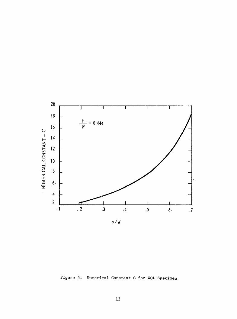
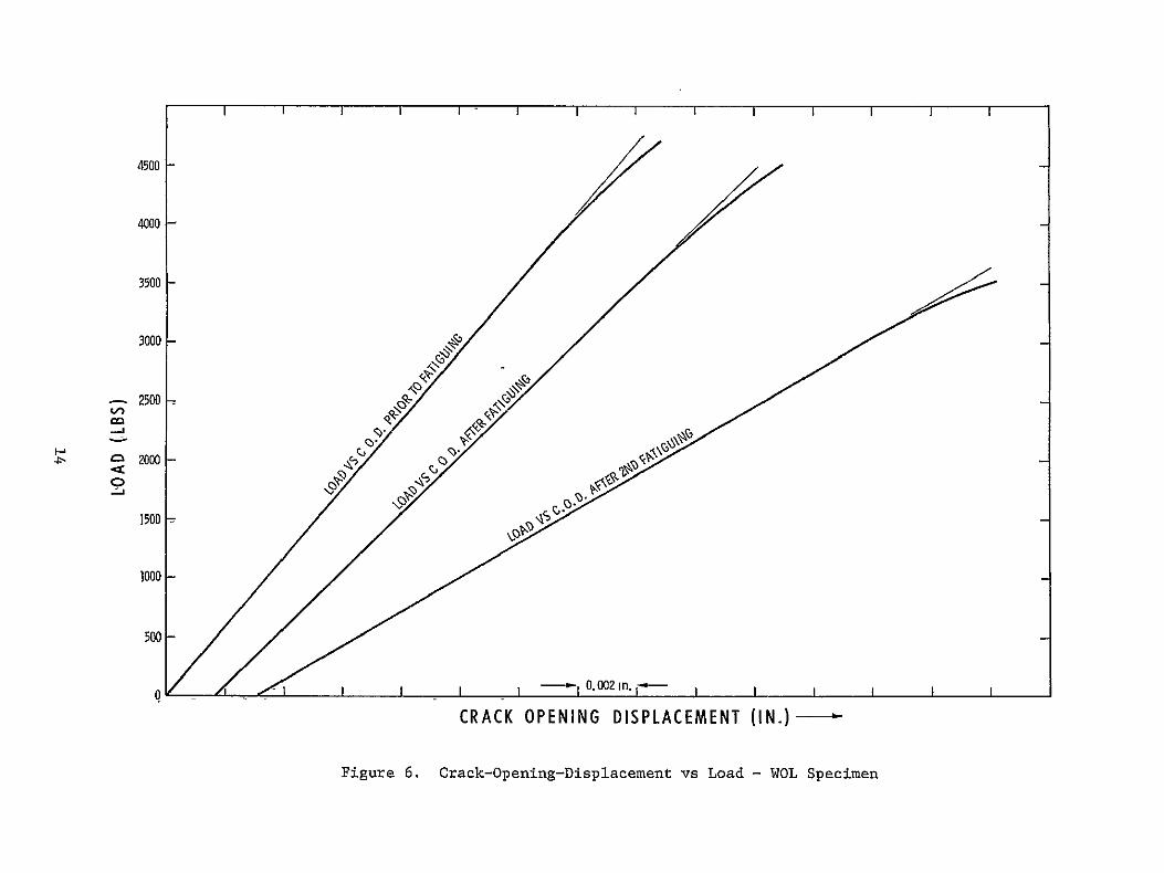
4500
4000
3500
3000
2500
4 2000 0
1500
1000
500
0-- 0002 in
CRACK OPENING DISPLACEMENT (IN)
Figure 6 Crack-Opening-Displacement vs Load - WOL Specimen
III B Crack-Opening Displacement Stress Intensity and Specimen Loading Procedure (cont)
C = 108 (graphically)
KI = PCB a
KSB p =
C
2 50 ksi-in1KI =for a
P = 3650 lb
Each WOL specimen was tested with an applied load correpponding to 12
K = 50 ksi-ins
C HYDROGENATION PROCEDURE
Selected bend and WOL specimens were tested after prior hydrogenashy
tion to determine the effect of this variable on the stress-wave-emissionslowshy
crack-growth relationships The hydrogenation procedure employed for this
purpose was developed by Battelle Memorial Institute and has been successfully
employed during other programs at Aerojet The hydrogen was introduced by
cathodic charging as follows
Solution 4 by weight H2SO4 5 dropsliter of poison
Poison 2 gm of phosphorus dissolved in 40 ml of carbon disulphide
Charging Time 5 min
Current Density 10 main2
The evolution of hydrogen at room temperature was prevented by
cadmium plating the test specimens within 5 min after hydrogenation The
cadmium-plating procedure was as follows
15
III C Hydrogenation Procedure (cont)
Cadmium Plating 4 ozgal CdO
Solution 16 ozgal NaCN with 1 by volume at pH 13
Current Density 70 main 2
Plating Time 30 min
Subsequent to hydrogenation and plating the specimens were baked
at 3000 F for 3 hr Baking was performed immediately prior to testing to
ensure a uniform hydrogen content throughout the test specimen
D STRESS-WAVE INSTRUMENTATION - LABORATORY EVALUATIONS
The stress-wave-detection system used for the laboratory evaluashy
tions prior to the background noise measurements at the Kennedy Space Center
is shown schematically in Figure 7 and consists of accelerometers amplifiers
filters tape recorders and an electronic counter and digital printer During
testing the accelerometers were attached to the specimens using a linear forceshy
coiled spring technique
Two basic systems were employed for stress-wave-emission data
acquisition During laboratory tests prior to the background measurements
at Kennedy Space Center the electronic counter system was employed This
system provides Very high sensitivity (signal amplifications of 10000 to
100000X) and also provides a real-time automatic count (both rate of emission
and cumulative count) of the stress-wave emissions occurring throughout each
test period The high-pass filter in the system eliminates a major portion of
the extraneous low-frequency background noises which tend to mask very small
amplitude stress waves
16
OSCILLOSCOPE
e TEKTRONIX MODEL 535
ELECTRONIC ELECTRONICSENSOR AMPLIFIER FILTER AMPLIFIER
COUNTER PRINTER S101HEWLETT PACK- HEWLETT PACK-
XIPA 00ARD MODEL 5231 ARD MODEL 5050
TAPE _ RECORDERTAPE ____________
RECORDER AMPLIFIER OSCILLOGRAPH
AMPEX MOD) T SP 300
KDATA ACQUISITION
OSCILLOSCOPE
TEKTRONIX _
eMODEL 535
DATA ANALYSIS
Figure 7 Schematic Representation of SWAT Data Acquisition and Data Analysis Instrumentation
III D Stress-Wave Instrumentation - Laboratory Evaluations (cont)
During testing of the WOL specimens maximum SWAT system amplifishy
cation was employed This was made possible because the specimens immersed
(COD gage up out of the water) in the water environment were enclosed in a
sound-proof box For these tests the electronic counter trigger level was
set just above the inherent noise (electrical) of the system Initially a
WOL test was run to determine whether the system was in fact completely free
of extraneous noise With the COD gage connected and all recording systems
in the circuit and with the specimen under no load and in air environment
after 5-12 hr in the sound-proof chamber there were only 16 signals
counted Presumably these were electrical disturbances The test was run
during regular working hours the WOL tests reported in the following parashy
graphs were tun during off-hours (nights and weekends) when there should have
been an absolute minimum of electrical disturbances
A second data acquisition system was also used for a limited
number of bend tests following the background noise measurements at Cape Kennedy
A schematic of this system is shown in Figure 8 The purpose of these tests
was to obtain stress-wave amplitude measurements using the instrumentation
employed at Cape Kennedy to ensure that the stress-wave emissions accompanying
crack extension could be detected under the background conditions observed at
Kennedy Space Center The tape recordings were made by direct recording during
test and were subsequently analyzed through playback and analysis as shown in
Figure 7
18
TEKTRONIX
OSCILLOSCOPE
ENDEVCO Dynamics Model 2213 Filter Accelerometer Model
Amplifier Amplifier 6364MQ 20-50 Kc Band Pass
KcENDEVCO30
Model 2213 CHigh-PassH Accelerometer Filter
kFI
TAPE Amplifier Amplifier RECORDER
AMPEX SP-300
Figure 8 Schematic of Instrumentation Used at Kennedy Space Center
IV LABORATORY TEST RESULTS AND DISCUSSION
As indicated in the following paragraphs two environments (air and
3 NaCl-water) and two material conditions (unhydrogenated and hydrogenated)
were utilized in the laboratory tests performed at Aerojet These conditions
are considered those most likely to be encountered during the service life of
the pressure vessels Also both straight rising load to failure and sustained
loading profiles were employed The sustained load profiles were employed
since failure of the pressure vessel may occur at constant load due to
environmentally induced slow crack growth from a prior flaw Since the
effectiveness of a failure warning system will obviously depend on the ability
to detect subcritical crack extension whether it occurs during sustained load
or on rising to failure it is important to determine if crack extension andor
failure will occur under both conditions Both effects can be studied through
the laboratory tests performed during this program
A BEND TESTS IN AIR WITHOUT DELIBERATE ADDITION OF HYDROGEN
Initially bend tests were performed in an air environment Both
the crack-opening-displacement gage and stress-wave-analysis technique were
employed to monitor the occurrence of pop-in and subcritical crack growth
The fracture data for these tests are shown below
Specimen Specimen Failure Notch Plus Apparent K
Thickness (B) Depth (D) Fatigue Crack (a) Load 1 2 No in in in aD P Kips ksi-in
1 10 20 090 045 200 130
2 097 20 091 0455 158 136
3 10 20 1036 0518 1656 133
Intermediate hold at 123 ksi-in12
20
IV A Bend Tests in Air Without Deliberate Addition of Hydrogen (cont)
The straight rising load to failure tests (No 1 and 2) indicated 12
a K value of 130 to 136 ksi-in as did the specimen (No 3) which failed
during rising load after previous holding at a stress intensity of approximately 12123 ksi-in As indicated previously in this report the ASTM recommends
for valid KIc measurements a specimen thickness exceeding that corresponding
to 25 (Kys)2 By this criterion a specimen thickness of approximately
44 in would be required for the A302B steel tested in this program
Consequently the KQ values noted above while not valid KIc measurements
indicate a high level of toughness in this material
No significant slow-crack growth or stress-wave emissions were
observed during hold in the air environment Conversely slow-crack growth
(increase in apparent crack size) and accompanying stress-wave emissions were
observed during rising load to failure The stress waves were generally very
small in amplitude (clt0Olg) but increased in amplitude with increasing crack
extension immediately prior to failure Increased rate of stress-wave
emission was also observed immediately prior to failure
B BEND TESTS IN WATER WITHOUT DELIBERATE ADDITION OF HYDROGEN
Bend specimen 4 was loaded initially to 15000 lb
(88 ksi-in 2) and held at constant load for 18 hr in 3 sodium-chloride
simulated sea water The specimen showed indications of crack growth early in
the hold period However analysis of the crack-opening-displacement gage data
indicated only very small amounts of crack extension Although the gage
employed for this purpose corresponded to the design recommended by the ASTM
its use was found unsatisfactory for tests of the type performed during this
program The COD gage was then modified and the modified version used during
the testing of the hydrogenated material described in subsequent sections of
this report
21
IV B Bend Tests in Water Without Deliberate Addition of Hydrogen (cont)
When the specimens (without hydrogenation) tested in the salt-water
environment were fractured the fracture surfaces were examined for evidence
of slow-crack growth during hold Although a small band of slow-crack growth
from the original fatigue precrack was observed it was not possible to detershy
mine how much of the crack extension occurred during rising load Onthe basis
of the COD data it would appear the majority of the extension occurred during
rising load to 15 kips from 15 to 17 kips and from 17 kips to failure although
the SWE data indicated that slow crack growth however small was occurring
during the hold periods
Figure 9 is a plot of cumulative stress-wave count over a period
of approximately 1-12 hr during hold at 15000 lb Note the indications of
a variable rate of subcritical crack growth Figure 10 shows the SWAT data
in detail (electronic counter reading every second) starting 23 min after
reaching the 15-kip load level Note that the cumfilative stress-waampe count
increased more or less continuously with brief intervals of increased slope
(when plotted to the scale of Figure 10 the increased slope was approximately 450) Figure 11 shows the SWE data obtained after adding fresh 3 NaCl-water
solution to the notch During the period of sustained load represented in
Figure 11 there were a few abrupt increases in count indicating discontinuous
crack growth together with additional intervals of increased slope (again
close to 45)
Figure 12 corresponds to the endof a short 16-kip hold (same
specimen) followed by a rise to 17 kips (approximately 125 ksi-in1 2 ) and
then a period of sustained load in 3 NaCl-water solution at 17 kips Note
the increased slope associated with the increase in load followed by abrupt
increases in count characteristic of discontinuous crack growth Approximately
600 sec after starting the hold at 17 kips an air hose produced high-frequency
noise too high to be removed by the filter This was recorded as an abrupt
increase in couni followed by a period of increased slope (again approximately 45) It cannot be definitely stated whether the increased slope indicating
22
1400
1200
1000
Li 800 3
LU
D 600
400
SEE FIGURE 10 200 FOR DETAILS
0 0 I I I I I
0 10 20 30 40 50 60 70 80 90 100
-MINUTES HOLD AT 15 KIPS
Figure 9 Cumulative Stress Wave Count vs Time Specimen No 4
A302B Steel 15 Kip Hold 3 NaCi-Water Environment
23
600
I0
20-
TIME (SECONDS)
224
6050
10 10 1O 1in20 20a 2100 2150
TIME (SECONDS) 220 3 am250 20 20 3w245 24W
43O
600
40
20
140
011 115 la 1in0 1 TIME (SECONDS)
a 14W 1m 53 0 inlW
Figure 11 Cumulative Stress Wave Count vs Time Specimen No 4 A302B Steel 15 Kip Hold After Replenishing the 3 NaCl-Water Environment
25
23
00
60
20
20
- 4o
o_ 4 o l~ ~ aiE~
220
IV B Bend Tests in Water Without Deliberate Addition of Hydrogen (cont)
continuous stress-wave emission was an artifact produced by the high-frequency
noise or the increased slope was the result of crack growth stimulated by the
high-frequency sound (crack growth after periods of dormancy can be initiated
by tapping a test specimen under load) Figure 13 is a plot of the cumulative
count for the 17-kip hold (corrected to zero at the start of hold and corrected
for noise which occurred at 836 sec) Note the tendency for increasing slope
with increasing time at load Figure 14 presents the SWAT data in detail
after 1 min at 17 kips load Figure 15 presents the data obtained after
1-12 min at 17 kips load Both Figures 14 and 15 are plotted to the same
scale as Figures 10 11 and 12 Table II presents the data plotted in
Figures 13 14 and 15 without correction for noise which occurred at 836 sec
this tabulation shows the detailed information that can be obtained by SWAT
On the basis of the SWE dpta this specimen showed evidence of
very slow continuous crack growth of the type one might expect of electroshy
chemical dissolution at the crack tip interspersed with short periods of more
rapid continuous crack growth There was little or no evidence of disconshy
tinuous crack growth with clearly defined periods of dormancy and there were
few instances of abrupt increase in count to signify crack jumps
C BEND TESTS IN AIR WITH DELIBERATE ADDITION OF HYDROGEN
After hydrogenation and baking 3 hr at 3000 F to produce a
homogeneous interstitial solid solution specimens were tested in 70degF air
Specimen 5 (Figure 16) developed discontinuous crack growth while under
sustained load starting at 9000 lb (75 ksi-in 2) but the occurrences were
sporadic and infrequent At 13000 lb (110 ksi-in 2) there was only one
stress wave large enough to be recorded as a cumulative count (cumulative
count increased from 3086 to 3110 corresponding to 464 SWEsec count rate)
Otherwise there was no increase in the SWE cumulative count during hold at
13000 lb
27
TABLE II
DETAILS OF SWE DATA OBTAINED FOR SPECIMEN NO 4 A302B STEEL DURING HOLD AT 17 KIPS IN 3 NaCI-WATER ENVIRONMENT
Time at Count Interval Time at Count Interval Load Rate Cumulative At Load Rate Cumulative A t (sec) (SWEsec) Count (sec) (set) (SWEsec) Count (sec)
27 57 8 - 1330 11 632 9 47 134 12 20 1331 20 634 1 101 4 14 54 1341 58 635 10 152 3 16 51 1392 232 652 51 299 10 27 147 1400 262 653 8
5 MINUTES 1405 134 654 5 329 1 29 30 1415 9 656 10 357 47 37 28 1443 85 657 28 444 72 49 87 1446 48 659 3 460 64 56 16 1478 131 675 32 494 221 60 34 1479 2 676 1 511 145 62 17 1495 29 685 16
10 MINUTES 25 MINUTES 616 115 72 105 1503 170 689 8 744 128 85 128 1505 72 691 2 788 2 92 44 1526 171 697 21 836 2 411(Noise) 48 1527 1 698 1 838 7 411 2 1537 187 702 10 843 10 431 5 1546 220 705 9 845 68 431 2 1584 89 715 38 846 7 431 1 1597 119 726 13 855 161 447 9 1650 146 738 53 880 160 468 25 1666 1 749 16
15 MINUTES 1671 162 756 5 904 11 492 24 1674 86 758 3 915 209 500 11 1695 120 780 21 943 5 523 28 1708 75 782 13 956 22 537 13 1717 1 787 9 980 4 541 24 1721 84 792 4 992 13 542 12 1732 114 794 11
1012 69 544 20 30 MINUTES 1088 21 558 76 1808 228 803 76 1108 151 569 20 1821 179 805 13 1136 il 576 28 1825 22 808 4 1154 5 582 18 1833 196 809 8 1172 38 583 18 1839 120 811 6 1178 19 585 6 1852 45 814 13 1182 9 -592 4 1866 146 816 14 1196 26 594 14 1888 168 819 22
20 MINUTES 1895 14 823 7 1228 80 598 32 1909 157 826 14 1229 13 599 1 1933 29 832 24 1238 2 605 9 1950 10 836 17 1256 1 610 18 1956 46 837 6 1312 91 613 56 1977 71 838 21 1318 1 619 6 1988 101 839 11 1321 1 621 3 2000 10 841 12
TABLE II (cont)
Time at Count Interval Time at Count Interval Load Rate Cumulative At Load Rate Cumulative Lt (sec) (SWBsec) Count (sec) (sec) (SWEsec) Count (sec)
2002 59 843 2 2515 40 1013 34 2017 119 845 15 2518 207 1017 3 2020 148 847 3 2521 1 1023 3 2033 165 848 13 2525 602 1029 4 2039 103 850 6 2527 22 1034 2 2048 9 857 9 2548 52 1052 21 2061 129 860 13 2561 47 1058 13 2063 156 862 2 2573 17 1062 12 2069 167 864 6 2585 69 1072 12 2075 98 874 6 2588 42 1073 3 2076 3 879 1 2599 240 1075 11 2093 21 881 17 2605 4 1077 6
35 MINUTES 2615 23 1078 10 2107 1 883 14 2616 57 1079 1 2108 103 884 1 2613 11 1080 15 2118 121 885 10 2638 42 1081 7 2119 191 887 1 2648 2 1087 10 2135 154 891 16 2650 87 1088 2 2140 11 892 5 2653 100 1089 3 2146 3 894 6 2656 56 1090 3 2150 178 897 4 2661 63 1091 5 2159 51 902 9 2685 28 1094 24 2162 7 905 3 2693 35 1097 8 2180 57 909 18 45 MINUTES 2182 58 910 2 2701 113 1104 8 2193 17 913 11 2703 50 1105 2 2195 113 916 2 2713 53 1109 10 2207 115 919 12 2719 20 1110 6 2221 34 923 14 2721 33 1112 2 2223 87 926 2 2738 72 1115 17 2238 35 936 15 2740 15 1116 2 2258 2 943 20 2752 100 1117 12 2268 204 947 10 2756 85 1119 4 2289 10 949 21 2768 56 1121 12 2307 1 952 18 2780 13 1130 12 2319 121 955 12 2782 28 1135 2 2346 20 959 27 2795 60 1142 13 2366 69 963 20 2809 65 1144 14 2386 20 975 20 2841 55 1156 32 2387 5 976 1 2848 3 1157 7 2392 158 978 5 2851 2 1159 3 2396 8 981 4 2862 45 1163 11
40 MINUTES 2869 35 1166 7 2403 21 983 7 2879 18 1169 10 2409 241 986 6 2885 62 1171 6 2449 95 996 40 2905 55 1175 20 2457 24 998 8 2908 54 1178 3 2473 104 1002 16 2918 7 1182 10 2481 3 1003 8 2924 8 1186 6
29
TABLE II (cont)
Time at Count Interval Time at Count Interval Load Rate Cumulative t Load Rate Cumulative t (sec) (SWIsec) Count (sec) (sec) (SWEsec) Count (sec)
2938 12 1193 14 3341 207 1410 2948 95 1201 10 3366 103 1421 25 2966 10 1215 18 3377 8 1424 11 2968 43 1216 2 3378 12 1425 1 2972 22 1217 4 3390 2 1429 12 2979 8 1221 7 3396 3 1430 6 2987 8 1223 8 3397 14 1432 1 2998 38 1226 11 3401 8 1434 4
50 MINUTES 3402 98 1438 1 3002 36 1228 4 3408 12 1443 6 3010 55 1230 8 3410 16 1448 2 3011 3 1234 1 3413 6 1452 3 3016 1 1236 5 3431 2 1454 8 3017 3 1237 1 3433 17 1458 2 3023 3 1239 6 3435 30 1460 - 2 3029 3 1240 6 3438 22 1462 3 3033 1 1243 4 3450 8 1475 12 3036 110 1245 3 3455 62 1484 5 3037 4 1248 1 3461 154 1490 6 3053 83 1259 16 3462 7 1493 1 3054 7 1260 1 3466 11 1501 4 3061 2 1265 7 3472 2 1507 6 3062 83 1266 1 3476 46 1509 4 3076 62 1275 14 3489 18 1515 13 3080 5 1278 4 3490 8 1517 1 3098 32 1294 18 3508 15 1534 18 3100 15 1296 2 3513 25 1541 5 3102 16 1297 2 3520 220 1549 7 3108 7 1299 6 3538 29 1566 18 3114 7 1301 6 3542 9 1572 4 3127 6 1304 13 3543 107 1575 1 3129 1 1305 2 3558 240 1588 15 3133 1 1306 4 3568 30 1601 10 3140 5 1309 7 3570 21 1603 2 3154 30 1312 14 3573 66 1607 3 3170 6 1320 16 3579 9 1613 6 3175 77 1322 5 3591 37 1619 12 3177 110 1323 2 60 MINUTES 3178 5 1324 1 3607 128 1622 16 3183 4 1326 5 3608 70 1626 1 3187 137 1331 4 3609 2 1629 1 3191 14 1332 4 3624 50 1638 15 3200 3 1336 9 3630 14 1642 6 3206 2 1340 6 3639 86 1645 9 3214 20 1343 8 3660 56 1662 21 3219 22 1345 5 3678 13 1669 18
55 MINUTES
30
TABLE II (cont)
Time at Count Interval Time at Count Interval Load Rate Cumulative At Load Rate Cumulative At (sec) (SWEsec) Count (sec) (see) (SWEsec) Count (sec)
3688 33 1680 10 4535 105 2574 28 3692 35 1682 4 4547 3 2589 12
3709 209 1688 17 4583 4 2616 36 3712 7 1689 3 4623 460 2670 40 3720 78 1691 8 4624 37 2703 1
3730 93 1694 10 4626 18 2715 2 3731 5 1695 1 4627 840 2729 1 3743 13 1703 12 4630 141 2737 3 3744 120 1709 1 4662 2 2758 32
3750 24 1715 6 4671 1 2763 9 3755 142 1724 5 4698 1 2774 27 3767 45 1738 12 4710 8 2782 12 3796 69 1770 29 4719 6 2784 9 3823 21 1808 27 4731 128 2785 12 3844 10 1838 21 4761 17 2810 30 3854 82 1851 10 4783 22 2822 22 3856 13 1855 2 4786 23 282A 3 3895 75 1915 39 80 MINUTES
65 MINUTES 4822 96 2831 36 3901 18 1920 6 4852 1 2842 30 3905 54 1927 4 4934 59 2890 82
3946 58 1963 41 4953 200 2907 19 3970 2 1985 24 4954 26 2910 1 3971 181 1988 1 4957 16 2916 3 3974 61 1990 3 4964 56 2923 7 3975 28 1992 1 4988 29 2941 24 3987 51 2004 12 5000 88 2951 12 4012 2 2022 25 5031 10 2977 31 4013 31 2026 1 5032 9 2978 1 4022 7 2036 9 5045 56 2982 13 4054 4 2062 32 5054 4 2984 9 4056 16 2066 2 5093 220 2992 39 4084 37 2093 28 85 MINUTES 4091 36 2099 7 5122 115 2996 29 4100 3 2111 9 5166 17 3019 44 4129 16 2142 29 5190 172 3042 24 4156 6 2165 27 5193 55 3045 3
70 MINUTES 5194 2 3048 1 4241 19 2253 85 5224 313 3081 30 4292 4 2299 51 5248 23 3106 24 4331 42 2339 39 5266 32 3123 18 4338 19 2348 7 5281 24 3138 15 4340 66 2350 2 5291 10 3150 10 4345 10 2359 5 5303 25 3164 12 4385 4 2419 40 5306 1 3169 3 4397 121 2432 12 5324 56 3187 18
75 MINUTES 5330 58 3193 6 4500 40 2534 103 5345 31 3211 15 4507 6 2542 7 5351 155 3217 6
31
TABLE II (cont)
Time at Count Interval Time at Count Interval Load Rate Cumulative At Load Rate Cumulative At (sec) (SWBsec) Count (sec) (sec) (SWEsec) Count (sec)
5357 211 3223 6 5887 185 3536 1 5363 29 3233 6 5905 65 3559 18 5364 20 3237 1 5923 31 3575 18
90 MINUTES 5924 22 3576 1 5403 118 3276 39 5933 109 3578 9 5418 79 3295 15 5934 5 3579 1 5419 44 3298 1 5961 43 3582 27 5420 35 3300 1 100 MINUTES 5448 27 3324 28 6000 23 3585 39 5460 118 3327 12 6001 13 3586 1 5466 97 3329 6 6002 166 3588 1 5472 184 3331 6 6008 9 3590 6 5484 28 3333 12 6032 29 3592 24 5499 45 3338 15 6041 111 3596 9 5505 2 3341 6 6062 116 3601 21 5506 173 3344 1 6083 1 3603 21 5512 72 3346 6 6084 236 3606 1 5515 8 3348 3 6090 140 3607 6 5536 199 3352 21 6091 104 3608 1 5548 5 3356 12 6106 21 3609 15 5553 199 3359 5 6115 31 3611 9 5554 34 3360 1 6121 29 3614 6shy5587 190 3364 33 6124 1 3622 3 5593 2 3365 6 6139 51 3630 15 5605 6 3367 12 6160 25 3634 21 5611 12 3369 6 6175 5 3636 15 5638 3 3373 27 6184 196 3639 9 5644 57 3374 6 6217 275 3645 33 5645 78 3376 1 6223 84 3648 6 5669 21 3379 24 6238 23 3649 - 15 5693 22 3384 24 6244 99 3650 6 5699 48 3385 6 6250 81 3652 6
95 MINUTES 6259 39 3654 9 5702 74 3387 3 6265 15 3656 6 5703 85 3389 1 6271 21 3658 6 5725 21 3391 22 6283 85 3660 12 5737 1 3394 12 105 IWNUTES 5752 72 3396 15 6304 143 3662 21 5761 106 3398 9 6331 50 3672 27 5788 1 3414 27 6340 179 3674 9 5794 176 3422 6 6341 37 3675 1 5809 2 3441 15 6365 34 3677 24 5810 15 3445 1 6366 ill 3680 1 5813 42 3448 3 6393 150 3682 27 5814 189 3451 1 6405 43 3684 12 5823 180 3461 9 6429 4 3687 24 5832 171 3472 9 6435 127 3690 6 5838 46 3481 6 6459 31 3691 24 5859 63 3505 21 6483 7 3694 24 5865 15 3511 6 6495 30 3696 12 5886 2 3533 21 6501 128 3700 6
32
TABLE II (cont)
Time at Count Interval Time at Count Interval Load Rate Cumulative At Load Rate Cumulative At (sec) (SWEsec) Count (sec) (sec) (SWEsec) Count (sec)
6522 87 3703 21 7278 21 4158 6 6531 16 3704 9 7302 2 4174 24 6555 102 3706 24 7303 3 4174 1 6567 7 3709 12 7318 125 4186 15 6570 10 3710 3 7348 88 4205 30 6576 87 3711 6 7402 86 4238 54 6577 89 3713 1 7435 90 4258 33 6578 131 3714 1 7447 14 4262 12 6599 4 3717 21 7474 14 4277 27
6600 110 MINUTES
8 3718 1 7486 7504
9 125 MINUTES
89
4286
4304
12
18 6603 37 3720 3 7510 39 4308 6 6639 15 3724 36 7531 52 4331 21 6669 48 3728 30 7540 208 4344 9 6675 23 3729 6 7549 38 4353 9 6684 57 3731 9 7576 72 4376 27 6705 23 3757 21 7594 24 4392 18 6744 53 3807 39 7603 55 4403 9 6762 240 3830 18 7615 160 4415 12 6783 5 3854 21 7621 134 4420 6 6801 26 3874 18 7627 160 4423 6 6822 181 3901 21 7639 180 4430 12 6852 24 3934 30 7648 5 4432 9 6879 44 3962 27 7658 100 4437 10 6882 2 3965 3 7679 319 4445 21
115 MINUTES 7694 72 4449 15 6906 63 3991 24 7709 23 4451 15 6927 176 4001 21 7721 34 4453 12 6930 15 4006 3 130 MINUTES 6931 54 4011 1 7800 Test Terminated 6952 305 4026 21 6953 40 4033 1 6980 3 4037 27 6989 99 4039 9 7040 387 4080 51 7041 53 4095 1 7056 23 4100 15 7086 354 4108 30 7095 21 4110 9 7125 70 4117 30 7131 2 4120 6 7167 97 4129 36 7176 11 4130 9 7197 18 4133 21
120 MINUTES 7218 28 4136 21 7227 39 4138 9 7248 72 4146 21 7272 50 4153 24
33
40
38W
3400
32W
30
28M
260
= 2400
S 22DD
i20
1600
1400
1200
10
600
400
200
06 1a 20 30 40 50 60 70 80 90 tW 110120130
MINUTE-S-H-OLD 17KIPS
Figure 13 Cumulative Stress Wave Count vs Time SpecimE A302B Steels 3 NaC1-Water Environment
34
3503
0
~0
40
20
3203
00
20
C0
20
310
03
(0
40
= = 20 0 I- 365~
05
20 00
20
0shy20
2003
20 ~~0 C
20
20 40
- 20
2835
0
(0
20
20shy
20020
20 -
3403 3450 3720 3750 fl 3550 3003 3050 40) 4050 4003 4050 4~fl 4200 4020 4350 4440 4450
TIME (SECONDS)
Figure 14 Cumulative Stress Wave Count vs Time Specimen No 4 A302B Steel After 1 Minute at 17 Kip Hold in 3 NaCi-Water Environment
35
48
0
I-
S 40
us 50 50 70 5 90 0 60 60 10 6 6 t 20CO DS
- iue1CmlaieSrs av on sTme pcmnN A0BSel
Afe2-0iue t1 i todi NC-ae niomn
Page60
4520 -
so- lao
F
122021 amp~
20 4
400
20
20 22
3540 =
20
3024
20
50
45
20
20520
20
20
45
20
no
I
40
4~
20
40
20
20
4
20
2020
20
gt
20
20 4
20
20
3545
20
Iino200j
5505
2220
1120
20
001
20
20 shy
00
1
45
OX
I
I I
I I
0 50
020 000
205 200
20 200
Z
40 505
550 400
TIM
E (S
EC
ON
DS
)
Figure 16
Cumulative Stress Wave Count vs
Time Specimen No
5 A302B Steel
Hydrogenated and Tested in Air
37
IV C Bend Tests in Air With Deliberate Addition of Hydrogen (cont)
On raising the load from 13000 to 14000 lb (122 ksi-in )
there was evidence of a creep phenomenon as shown in Figure 17 The crackshy
opening-displacement gage confirmed the occurrence of crack growth continuing
after reaching the 14000-lb hold Stress-wave emission showed the mechanism
to be discontinuous cracking rather than a deformation process When the
count rate was plotted as in Figure 18 the activity carrying into the
14000-lb hold again was discontinuous After approximately 300 sec at 14 kips
the SWE associated with the creep phenomenon had subsided During the 14-kip
hold there were two crack jumps one after 920 sec (cumulative count increased
from 5618 to 5720 and the count rate associated with the jump was 181 as
counted over a 10-sec interval or 18 SWEsec) and one after 2130 sec (cumulashy
tive count increased from 5721 to 5755 and the count rate was 139 in 10 see)
After 5000 sec at 14 kips the load on Specimen 5 was raised As
seen in Figure 19 the stress-wave activity was an unmistakable presage of
instability which occurred after 20 sec into hold The load reached a maximum
of 145 kips (145 ksi-in 2) Technically the onset of instability occurred
shortly after starting to increase the load ie at approximately
132 ksi-inI2 which agrees with the KQ value obtained through rising load
tests of unhydrogenated material in an air environment
Because of the very long test period and multiple loadings involved
in the testing of the Specimen 6 only data obtained during rising load to
19500 and 19800 ib during sustained test periods at these loads and during
specimen failure are shown in Figure 20 These data indicate essentially the
same SWE-crack growth relationships discussed previously for Specimen 5 except
that on reaching hold the crack tended to grow slowly for a longer period of
time in comparison to the behavior noted for Specimen 5 Also the incremental
nature of crack extension was more readily observed by the stress-wave-emission
data for Specimen 6
38
20
560
80
60
40
20
5500
80
60
40
20
5400
o 5100
808
60
40
20
5000 u-J
4500
4480 80 4- START 14-KI P HOLD
CODC 75lt
4000
3980 70
3960
6553120 l
- END13-KIP HOLD
3100 160 0 40 80 120 160 200 240 280 320
TIME AT LOAD (SECONDS)
Figure 17 Cumulative Stress Wave Count and COD vs Time Specimen No 5 A302B Steel fydrogenated and Held at 14 Kips in Air
39
200
LU
LU
1- 100
50 END 13-KIP
25 HOLD-I
0 1- TIME
100 INSECONDS AT
200 14KIPS
300
(COUNT EVERY 10 SEC)
Figure 18 Stress Wave Count Rate vs Time - Specimen No 5 A302B Steel Hydrogenated and Tested in Air
40
INSTABILITY
9580
9560
9540
9380
928D0
9260
842D
8440
73O I-shyz 7220
o 7260
U 7240
7220
7180I-shy
7160
- 7140
7120
7100
7080
7060
5900
5880
5860
5840
5820
5800
578D
5460
0 40 80 120 160 SEC
4M 4960 50D RISING LOAD-SECONDS AT 14 KIPS
Figure 19 Cumulative Stress Wave Count vs Time Specimen No 5 A302B Steel Hydrogenated and Tested in Air
41
20000
18000
FAILURE
18290 sec a- 1 17-in K - 199 s - Y
z
-
16000
14000
l0
1200
I-9 Iin
1014in K 152 ki- in -i
o-1 09 n K- 176ksmn
- 1 07 in I 170 iis-
o -1 042in K 12ks-in
c023i NK15ks-n
-shy
-
10000
REACH 19800 lbs
START TO 19800 bs
10000 11000 12000 13000 14000 15000 16000 17000 18000 19000
TIMESECONDS
12000
11000 s
p9000
T LOAD ADJUSTMEA
7n000
READOUT6000 OTE STRESS WAVE DATA A UST T
500 Vgt 0 ENT CORRESPONDIG TO SLOPELOAADJUSTM15 CHANGES PLOTTED
a 4000
3000
LOAD ADJUSTMENT2000 SECONDSECMENIME
1000 START HOLD AT 19500 1b
900 1l6070 D0 8 0 00 0 000600
0 1000 50002000 3000 4000
TIME SECONDS
Figure 20 Cumulative Stress Wave Count vs Time Specimen No 6 A302B Steel Hydrogenated and Tested in Air
Page 42
IV C Bend Tests in Air With Deliberate Addition of Hydrogen (cont)
As indicated in Figure 20 the increase in crack length during
the initial period of hold at 19500 lb resulted in an increase in the applied
stress intensity and was accompanied by significant stress-wave-emission
activity To maintain the desired load it was also necessary to make frequent
load adjustments at the start of hold During the first 3600 sec the effecshy
tive crack length increased from approximately 0963 to 1000 in and was
accompanied by about 7000 SWE As indicated in Figure 20 the majority of the
SWE activity and increase in crack length occurred during the first 3000 sec
of the hold at 19500 lb After this period both the stress-wave-emission
activity and rate of increase in crack length gradually decreased For example
during the entire period from 5000 to 17600 sec when the load was increased
to 19800 lb the apparent crack length and SWE count increased by only approxishy
mately 0020 in and 2500 respectively
After approximately 17000 sec at 19500 lb the load was increased
to 19800 lb and specimen failure occurred after approximately 600 sec at
19800 lb The load was maintained for this period however it was apparent
from both the SWE and COD gage data that the crack was extending and specimen
failure would occur without a further increase in load although it was necesshy
sary to continually adjust the tensile machine to maintain the desired load
The failure stress intensity approximated 199 ksi-in 2however technically
the onset of instability occurred after starting to increase the load at
approximately 153 ksi-in1 2
Specimen 7 was also hydrogenated baked at 300F for 3 hr and
tested in air Figure 21 is a detailed plot of the SWAT data (electronic
counter print-out every second) indicating crack growth of a discontinuous
nature starting at 2400-lb load Note the periods of dormancy (no increase
in SWE count) interspersed with abrupt increases in count indicating disconshy
tinuous crack growth Note also that there was little or no evidence of
continuous stress-wave emission until the load (stress intensity level) was
high approaching failure
43
CUMULAIY STRESS-VAVE COUNTCU LTISTE W E ON
I OT A~II I OI I L I I I I I I I I I I I I I I i I I I I I
- N LB
I I I I I I I I I I I I I i I I
--L - 0OTO11
-0101
(lNIML~ 33383338
8
133113-
3IiC)0 83) 3103 31-3(31-
~0
33 331
3l3C0C~
38318shy
111(10 CAVMSS3 nfl CAliVi flWfl3
________________________________________________________________________
111fl0~ 3KvM~s~a1Ff~TfvTifwT
FPAIAE
hY
A Ii
8
INa
CZ
8 C0 U CI
33 S
1 H
H
03 -I
~ 3lt
0 Cd 33
~C3 ~ H
8 0003
A
Ofli3i~~ C)
Page 45
IV C Bend Tests in Air With Deliberate Addition of Hydrogen (cont)
Figure 22 presents the SWE data from a hydrogenated bend specimen
(No 8) tested in air The load was increased continuously to 9800 lb
(70 ksi-in 2) where there was a short hold (approximately 400 sec) Note
the discontinuous crack growth followed by a short period of continuous
emission (less than 450 slope) The load was then raised to 14800 lb
(109 ksi-in 2) and held for approximately 400 sec Again there were jumps
in the SWE cumulative count but this time interspersed with continuous
emission The SWAT system employed for this test corresponded to that employed
for the background measurements at Kennedy Space Flight Center and shown in
Figure 8 only one channel was employed viz
Endevco 2213 Amplifier Amplifier Band-Pass Filter 10OX 10OX 20 to 50 Kcps
The continuous stress-wave emission observed during hold at the higher stressshy
intensity level in this specimen was not observed in the other hydrogenated
specimens tested in air The primary purpose of this test (Specimen 8) was to
record SWE data for subsequent playback and analysis to determine the amplitude
of burst-type stress-wave emissions associated with fracture in Type A302B
steel These analyses were performed using the instrumentation shown in
Figures 7 and 8 with the following results which are discussed in more detail
in conjunction with the results of the background measurements performed at
Kennedy Space Flight Center (Section V)
Maximum SWE Amplitude - 39 x 10-3g
Minimum SWE Amplitude - 12 x 10-3 g
Average SWE Amplitude - 22 x 10-3g
Laboratory Background - 11 x 10-3g
46
00 o z~ 20 ~
40
~40
S20 1 2 0 0 0 0
TIIAEAT 4 S-KIPHOLD (10KS(51IN A)
407
IV Laboratory Test Results and Discussion (cont)
D BEND TESTS IN 3 NaCI-WATER WITH DELIBERATE ADDITION OF HYDROGEN
Specimen 9 was hydrogenated baked and tested in 80F water
The electronic counter indicated continuous stress-wave emission interspersed
with abrupt increases in count indicating occasional crack jumps Figure 23
shows the details of stress-wave emission that occurred during both rising
load and holding load The crack length determined from the COD chart at
selected loads is also shown Note from the SWE data that there were no
periods of dormancy and the slope of the plot of cumulative count versus time
indicated moderately rapid continuouas crack growth such as might occur with
electrochemical dissolution at the crack tip The COD gage data shown in
Figure 23 also indicate crack extension however the actual amount appears
to be quite small (lt01 in) which would be consistent with the relatively
small number of stress-wave emissions detected even at the high system
sensitivity employed The dramatic difference between the behavior in
Figures 21 and 23 for hydrogenated material tested in air (Figure 21) and
water (Figure 23) indicates that hydrogen and 3 sodium chloride solution
acting together have a greater total effect than the sum of their individual
effects ie working together they appear to have produced a synergism
E WOL TESTS
Because of the possible significance of the synergistic-effect
noted above on the life of the hydrogen pressure vessels at Kennedy Space
Flight Center additional testing was performed using hydrogenated WOL specishy
mens cut from the fractured bend specimens The first WOL specimen was
initially loaded to-3650 lb (50 ksi-in 2) and then placed in 3 NaCl solution
(notch immersed) There was 30 min of essentially continuous stress-wave
emission (recorder started approximately 5 min after loading the specimen)
Subsequently therewas one sizable jump in the SWE cumulative count after
48
V30
760
740-M
$
720 -s
680shy
60
610
40 w
w
520 w
i
20500
HOLDD]N
340
20 760
7200
ING
IV
O
shy
420
60
40
20 0 2
04
0Q
0
60DO
LO0
01 200
250 300
350 400
450 500
550 6M
650
700 750
TIME
(SECONDS)
Figure 23
Cumulative Stress Wave Count vs Time Specimen No 9 A302B Steel
Hydrogenated and Tested in 3 NaCi-Water Environment
49
IV E WOL Tests (cont)
approximately 3 hr 40 min Then 3 hr 20 min later several jumps occurred
followed by 8 hr 20 min of stress-iave activity After this the crack was
dormant (total test time 17 hr 25 min) These data are shown in Figure 24
The load was then increased slightly (torque was increased from 200 to
255 in-lb) an additional 1-12 hr in 3 NaCl solution produced no significant
increase in the cumulative stress-wave count The reason for this apparently
anomalous behavior was not determined although it may result from a blunting
effect at the crack tip produced during the initial hold period
The fatigue crack was then extended (approximately 005 in) in
tension-tension fatigue and the specimen reloaded to approximately 51 ksi-in2
Stress-wave emission started almost immediately (dashed curve in Figure 24)
After approximately 3 hr of discontinuous activity the periods of dormancy
tended to increase interspersed with relatively small jumps (as counted over
10-sec intervals) The results of the initial loading and the reloading are
shown in Figure 24 note that there was appreciably lower cumulative count in
the reloaded specimen as compared with the initial loading for a comparable
period of test
A second hydrogenated WOL specimen was then tested in air at
50 ksi-in 2 there were stress waves initially (creep) but then very little
activity over the remaining 35-hr test period After the first hour the
count increased from approximately 150 to only 280 in the final 34 hr of test
Figure 25 shows the long peribds of dormancy punctuated by occasional 1-count
increases This is in marked contrast to the results obtained from the
hydrogenated WOL specimens tested in 3 NaCl solution and the bend-test
findings of a synergistic effect were confirmed
50
------------
aa
L- -- -- - ------ - --- I
3
IN DO
INTES) 3 S IOTI E( LI N LU
Ino
a
N O
TIME (MINUTES) IN 3 NCI SOLUTION
Figure 24 Cumulative Stress Wave Count vs Time at Hold WOL Specimen No 1
A302B Steel Hydrogenated and Tested in 3 NaCi-Water Environment
51
000 In 0 M6020 126 24 022 in0 1180 10 11 100 IWO l 100M M-C 0 90w6 a0 w6
t t t t 5W MOD4
10
TIME (MINUTES)
Figure 25 Cumulative Stress Wave Count vs Time at Hold WL Specimen No 2 A302B Steel Hydrogenated and Testd in Air
52
IV Laboratory Test Results and Discussion (cont)
F DISCUSSION
1 Material-Environment Consideration
The Type A302B steel supplied for evaluation exhibited a
very high level of fracture toughness Although quantitative plane-strain
fracture toughness measurements were not possible because of the large specimen
size required the KQ value associated with failure approximated 135 ksi-in1 2
This material was also found resistant to environmentally induced failure in
that the rate of crack growth of a prior flaw at applied stress-intensity
factors as high as 90 of the KQ value appeared to be very low This effect
was observed for unhydrogenated-material tested in air and a 3 NaCl-water
environment and hydrogenated material tested in an air environment However
the hydrogenated specimens tested in 3 NaCl-water environment had a much
faster rate of subcritical crack gr~wth in comparison to the other test condishy
tions indicating a synergistic effect due to the combination of sea water and
hydrogen in interstitial solid solution This synergistic effect indicates
that the Type A302B steel hydrogen storage tanks in the Kennedy Space Flight
Center environment may have limited life as the result of subcritical crack
growth if subjected to the same combination of stress and environmental
factors-
The WOL test results tended to confirm the possible synergism
due to the combined effects of 3 NaCl-water and hydrogen in interstitial solid
solution Marked SWE activity was observed when the hydrogenated specimens
were immersed in the salt water whereas in an air environment after the
initial period at hold when a creep phenomenon was observed there was essenshy
tially no stress-wave emission The fact that failure was not produced on
holding (in contradiction to the bend tests) can be explained by the fact that
the WOL test as-performed in this program is a self-arresting test because
53
IV F Discussion (cont)
the occurrence of crack growth results in a reduction in the applied load
Conversely in the bend tests the load was constantly applied as the crack
extended and eventually resulted in specimen failure
2 Stress-Wave-Emission Characterization
Detectable stress-wave emissions although of small amplitude
(ltOOlg) were observed to be associated with crack growth in Type A302B steel
Under all test conditions the stress-wave emissions were observed both during
rising load and when failure (instability) was imminent During hold various
SWE characteristics depending on the test conditions were observed When
tested in the hydrogenated condition in-an air environment a creep phenomenon
evidenced by increasing count of SWE and an accompanying increase in apparent
crack size was observed With time at hold and at applied stress-intensity
levels less than critical the creep phenomenon eventually stopped as did the
occurrence of stress-wave emissions Unhydrogenated material tested in the
3 NaCl-water environment produced continuous stress-wave emission punctuated
by abrupt increases in SWE count This behavior indicates both continuous
very small increments of crack extension with larger crack jumps corresponding
to the abrupt increases in SWE count Continuous incremental crack extension
characterized by continuous SWE interspersed with abrupt increases in SWE count
indicating occasional crack jumps was also observed in testing hydrogenated
material in a 3 NaCl-water environment
In all instances when failure (instability) occurred both
the amplitude and rate of stress-wave emission increased and could be employed
as a precursor of the onset of instability however even when failure was
approached-the SWE amplitude was small (ltOlg) In the other instances where
failure was not produced evidence of crack extension (although very small in
some instances) was observed on the specimen fracture face Once evidence of
54
IV F Discussion (cont)
crack growth was observed (by SWE or COD) it is obvious that failure would
eventually occur (assuming a constantly applied load) although depending on
the initial flaw size and subcritical growth rate the time to failure may be
very long In actual practice the SWE data could be employed (1) to locate
the propagating flaw (2) to monitor its occurrence and (3) as a basis for
terminating service so that repairs could be made before failure The stressshy
wave emissions associated with crack growth during rising load or increasing
stress intensity and the creep phenomenon during the initial part of hold
can be employed for this purpose
5S
V BACKGROUND MEASUREMENTS AND ASSOCIATED LABORATORY TESTS
A BACKGROUND MEASUREMENTS AT KENNEDY SPACE FLIGHT CENTER
Background noise measurements were made at two locations the VAB
Bottle Field and Pad A at the Kennedy Space Flight Center The data were tape
recorded and in addition to general background noise included tank blowdown
and repressurization periods The instrumentation for this purpose is shown
schematically in Figure 8 analysis of the data was performed by playback onto
an oscillograph and comparison with the SWE-crack growth data obtained during
the laboratory testing of bend specimens
The analysis of the signal amplitude data for tests at Cape Kennedy
is indicated below
1 Pad A Bottle Field
Signal Amplitude
a Quiescent Background
Filter at 20 Kcps - 50 Kcps -BandPass- 99 x 10 gsBand Pass
Filter at 200 cps - 32 Kcps
Band Pass
b Tank Blowdown - System Saturation (gt llg peak to peak)
C Tank Repressurization - System Saturation (gt llg peak to peak)
2 VAB Bottle Field
a Quiescent Background - 22 x 10- 4 gs
56
V A Background Measurements at Kennedy Space Flight Center (cont)
Signal Amplitude
b Tank Blowdown - System Saturation (gt llg peak to peak)
C Tank Repressurization - System Saturation (gt llg peak to peak)
Analysis of the tape-recorded data of bend tests at Aerojet indicates
the following signal amplitude for burstf-type stress-wave emissions associated
with crack growth and fracture in Type A302B steel
Maximum Amplitude - 39 x 10-3g
Minimum Amplitude - 12 x 10-3g
Average Amplitude - 22 x 10-3g
Laboratory Background - 11 x 10-3g
Thus the amplitude of SWE associated with crack growth in A302B steel is
approximately an order of magnitude larger than the background noise noted
previously Consequently the above results show that it is possible to detect
stress-wave emissions associated with fracture in A302B steel under the quiescent
background conditions existing at the Kennedy Space Center Difficulty is
expected in detecting such flaw growth during tank blowdown and repressurization
periods unless filtering can be employed to screen out the noise associated
with these periods However the blowdown and repressurization periods are of
very short duration and the materials behavior observed in this program indishy
cated that considerable prefailure crack extension would be expected from any
flaw of a size expected to be present in these pressure vessels Also
immediately on reaching load a creep phenomenon evidenced by an extension
in apparent crack length and accompanied by detectable stress-wave emission
was observed Consequently even if noise associated with blowdown and
57
V A Background Measurements at Kennedy Space Flight Center (cont)
repressurization cannot be effectively filtered out significant flaw growth
andor creep could still be detected and tank depressurization accomplished
prior to catastrophic failure assuming a capability for such depressurization
exists at these locations
B LABORATORY SIGNAL ATTENUATION EVALUATIONS
Subsequent to the background measurements at the Kennedy Space
Flight Center and the bend tests at Aerojet two series of tests were made at
Aerojet using a section of pipe and plate both of SAE 4130 steel alloy The
purpose of these tests was to determine the coefficient of signal attenuation
which in conjunction with the previous test data could be used to establish
the sensor spacing which would insure detection of SWE associated with crack
growth in the pressure-vessels at the Kennedy Space Flight Center
In these tests a constant pulse was imparted to the specimen by
a Tektronix 115 Pulse Generator using a Clevite PZT-5 Crystal (2125 in dia
and 0250 in thick) The piezoelectric crystal was mounted on a small alumishy
num block which in turn was adhered to the surface of the specimen The
signal was received by a 2217-E-Endevcq accelerometer placed at various disshy
tances from the pulser The pulse used was 10 n-sec rise and fall time with
a duration of 20 microsec at an amplitude of 12v
1 Pipe Tests
A SAE 4130 steel pipe (8-58 in OD 7-18 in ID and 22 ft
10-78 in long) was used as specimen for this test series The pulser was
mounted normal to the external surface of the pipe as close as possible to the
edge The accelerometer (2217-E-Endevco) was successively placed on the pipe
58
V B Laboratory Signal Attenuation Evalutions (cont)
surface at positions I to 8 that were at 4 6 8 10 12 14 16 and 20 ft
from the pulser The signal received by the accelerometer was displayed on a
Tektronix 422 osilloscope Typical signals are shown in Figure 26
The velocities of the compressional and shear waves in steel
are
29 lO06 x38103 Vc= -x lg ) (l-26) = O2 x06(- 0 x386 = 227000 insec(+j 012)283 (1+030) (1-060)
29x106 x 386 = 91 36= 123000 insec
s 2 ( + p) p 2 (i + 030) x 0283
where E = Youngs Modulus p = Poissons Ratio and p = density The times of
arrival of these waves at the computed velocities are indicated on the oscilloshy
scope photos shown in Figure 26 The point of shear wave arrival (T ) coincides
in most of the photos to a distinct change of pattern in the trace The
arrival of the compressional wave is difficult to determine accurately because
the amplitude of this wave attenuates very fast with distance
A visual comparison of the curves shows that Figure 26a
representing the signal received 4 ft from the impulse indicates a perfectly
detectable arrival of the compressional wave conversely Figure 26h (at 20 ft
from the impulse) shows the visually detectable arrival of a wave almost at the
computed arrival of the shear wave This is due to the fact that the amplitude
of the first cycles of the compressional wave have become essentially impercepshy
tible at a distance of 20 ft from the pulse An attempt to determine signal
arrival time by visual inspection only of the traces in Figure 26 would result
in the wave velocities indicated in Table III The computed arrival times of
the compressional and shear waves are shown in Table IV If an integration of
the positive portions of the cycles comprised in 200 p sec after arrival of the
59
VERTICAL SCALE 1 DIV= 01 V VERTICAL SCALE 1 DIV = 01 V HORIZONTAL SCALE 1 DIV= 50p SEC HORIZONTAL SCALE 1 DIV = 100 pSEC
a 4FT FROM PULSER b6 FEET FROM PULSER
Tc Ts Tc Ts
VERTICAL SCALE I DIV 01 V VERTICAL SCALE I DIV = 01 V HORIZONTAL SCALE I DIV = 100 I SEC HORIZONTAL SCALE 1 DIV = 200 p SEC
c 8 FEET FROM PULSER d 10 FEET FROM PULSER
Tc = Arrival of Compressional Wave
T = Arrival of Shear Wove
Figure 26 Oscillograph Traces for Pipe Tests (Sheet 1 of 2)
6o NOT REPRODUCTBLE
VERTICAL SCALE 1 DIV = 01 V VERTICAL SCALE 1 DIV 01 V HORIZONTAL SCALE 1 DIV = 200y SEC HORIZONTAL SCALE I DIV 200 p SEC
e 12 FEET FROM PULSER f 14 FEET FROM PULSER
T TS T T
VERTICAL SCALE 1 DIV = 01 V VERTICAL SCALE 1 DIV = 01 V HORIZONTAL SCALE 1 DIV = 200 v SEC HORIZONTAL SCALE I DIV =5001p SEC
g 16 FEET FROM PULSER h 20 FEET FROM PULSER
Figure 26 Oscillograph Traces for Pipe Tests (Sheet 2 of 2)
61
V B Laboratory Signal Attenuation Evaluations (cont)
shear wave is performed the average amplitudes determined in this manner
become quite meaningful These average amplitudes are shown in Table V
TABLE III
WAVE VELOCITY BASED ON VISUAL ANALYSIS OF OSCILLOSCOPE TRACES - PIPE TESTS
Distance from Pulse Arrival Velocities Photo ft in Time psc (ftsec)
1 4 48 210 228000
2 6 72 400 180000
3 8 96 600 160000
4 10 120 800 150000
5 12 144 1000 144000
6 14 168 1200 140000
7 16 192 1400 137000
8 20 240 1750 137000
TABLE IV
COMPUTED ARRIVAL TIMES - PIPE TESTS
Compressional Wave Shear Wave Distance from Pulse Arrival Time Arrival Time
Photo in psec Osc Div sec Ose Div
1 48 212 423 390 780
2 72 317 317 583 583
3 96 422 422 778 778
4 120 530 265 972 486
5 144 635 317 1163 581
6 168 740 370 1360 680
7 192 840 420 1545 771
8 240 1050 21 1930 387
62
V B Laboratory Signal Attenuation Evalutions (cont)
TABLE V
SIGNAL AMPLITUDE VS DISTANCE - PIPE TESTS
Average Signal Amplitude Distance from 200 Psec after Arrival
Test Pulser in of Comp Wave mv
1 48 230
2 72 145
3 96 85
4 120 60
5 144 45
6 168 28
7 192 22
8 240 18
The general equation for the amplitude attenuation curve is
C x e-Xy =
where y = amplitude at distance x in volts
x = distance in inches from pulse source
C = amplitude of pulse in volts
a = attenuation factor
or iny= 1 C + (- ax) = I C - ax (Eq 4)n n
To determine the values of C and a the following statistical analysis was
performed
63
V B Laboratory Signal Attenuation Evaluations (cont)
Distance Yo y y2 X X2 Test in m v n n
1 48 230 543 +142 2010 -87 7580 - 124 261
2 72 145 499 +098 0960 -63 3960 - 62 360
3 96 85 445 +044 0194 -39 1520 - 17 427
4 120 60 409 +008 0006 -15 225 - 1 490
5 144 45 380 -021 0044 + 9 81 - 2 548
6 168 28 334 -067 0450 +33 1090 - 21 560
7 192 22 309 -092 0847 +57 3250 - 52 592
8 240 18 289 -112 1250 +105 11000 - 118 690
EY2 EX2pound x = 1080 ElnY =3208 5761 28706 SXY-397 XxIny3928
- 1080 - 3208 x =- = 135 ny = 401
EXY -397 00138 1 C =l1y + oshy
pound 2 x2 28706 n i x
= 401+(0138)(135)=401+186= 587
C - 355 mv
It is now possible to compute the statistically corrected values of the signal
amplitude y at the distances from the pulse where they were measured The
general formula will be
ny = 587 -(00138) X
and the results are tabulated in Table VI The computed value of pulse amplishy
tude at source is found to be C = 355 my The values shown on Table VI are
plotted in Figure 27 which graphically shows the signal attenuation as a
function of distance from the pulse source
64
350
300
250 STATISTICALLY COMPUTED k VALUES FOR REGRESSION CURVE
--0gt 200
EXPERIMENTALLY DETERMINED
-- MATERIAL SAE 4130 STEEL U= SPECIMEN PIPE-S758 in D aZ
00
15 7 18 in D22 ft 10 78 in LONG
-J
100
50 I
0 I I I
5 I I I
DISTANCE
I
10 FROM SOURCE
I
FEET
I
15 20
Figure 27 Signal Amplitude vs Distance - Pipe Tests
V B Laboratory Signal Attenuation Evaluations (cont)
TABLE VI
STATISTICALLY CORRECTED VALUES OF SIGNAL AMPLITUDE - PIPE TESTS
Experimentally Distance from 1 Corrected Signal Determined Signal
Test Pulse in ny Amplitude (y) mv Amplitude (y) my
1 48 521 182 230
2 72 488 130 145
3 96 455 95 85
4 120 421 67 60
5 144 388 48 45
6 168 355 35 28
7 192 322 25 22
8 240 255 127 18
- 2 Plate Tests
An SAE 4130 steel plate (73-12 in long 48-12 in wide
and 34 in thick) was used for this test series The two diagonals were
marked on the plate The pulser was placed at the center of the plate and
the receiver accelerometer was placed on one of the diagonals at locations
spaced in increments of 6 in from the center The received signals were
observed on the oscilloscope and photos were taken of these signals Figure
28 shows oscillographs of the signals received at 6 12 18 24 30 36 and
42 in from the pulser The times of arrival of the shear wave are also shown
in Figure 28 The velocity used was v = 123000 insec An integration
was performed of the positive positions of the cycles comprised in a 20 Psec
interval after the arrival of the shear wave The average amplitudes detershy
mined from these integrations are shown in Table VII Only Tests 1 to 4 are
used because reflection (from the plate edges) in Tests 5 to 8 obscured the
66
b 12 INCHES FROM PULSERa 6 INCHES FROM PULSER
TBTs
c 18 INCHES FROM PULSER d 24 INCHES FROM PULSER
IT s = Arrival of Shear Wave
Vertical Scale 1 DIV = 01 Volt Horizontal Scale 1 DIV = 20 ASec
Figure 28 Oscillograph Traces for Plate Tests (Sheet 1 of 2)
Page 67
f 36 INCHES FROM PULSER e 30 INCHES FROM PULSER
g 42 INCHES FROM PULSER
= Arrival of Shear WaveTs
Vertical Scale 1 DIV = 01 Volt = 20 4SecHorizontal Scale 1 DIV
Figure 28 Oscillograph Traces for Plate Tests (Sheet 2 of 2)
08 gOTPRODUCIB1A
V B Laboratory Signal Attenuation Evaluations (cont)
data These reflections were received in Tests 5 to 8 because of the relashy
tively small plate that was available for this test series
TABLE VII
SIGNAL AMPLITUDE VS DISTANCE - PLATE TESTS
Distance from Average Amplitude Test Pulse in(x) in 20 p see mv
1 6 150
2 12 110
3 18 70
4 24 45
The following statistical analysis was performed to determine the values of
C and a in Equation 4
Test
Distance from
Pulse in(x)
y
m v
1
ny Y
2
Y 2
X XY
X1 y
n
1 6 150 500 +056 0314 -9 81 -502 3000
2
3
12
18
110
70
470
425
+026
-019
0067
0036
-3
+3
9
9
-078
-057
5640
7650
4 24 45 381 -063 0397 +9 81 -567 9149
60 1776 0814 180 -1204 25439
-x=
60 w= 15
4ny
iY 1
1nC
-
=
16=44 1776 =44
E YX 1204= __=
E y2 180
ny +(0067)(15) =
+0067
444 + 0067(15)
69
=
C
444 + 100
= 230 my
= 544
V B Laboratory Signal Attenuation Evaluations (cont)
Subsequently the values of signal amplitude (y) were statistically corrected
as before and the experimentally determined values of y are compared to the
results obtained in Table VIII
TABLE VIII
COMPARISON Or STATISTICALLY CORRECTED AND TEST-DETERMINED VALUES OF SIGNAL AMPLITUDE - PLATE TESTS
Experimentally Distance from Corrected Signal Determined Signal
Test Pulse in nY Amplitude (y) mv Amplitude (y) my
1 6 504 155 150
2 12 464 103 110
3 18 417 65 70
4 24 383 46 45
The computed value of the pulse amplitude at the source at
C equals 230 mv The regression curve and the experimentally determined points
are plotted in Figure 29 It should be observed that the attenuation coefshy
ficient for the pipe test was a = 00138 and for the plate test was 0067
This is due to the much larger rate of front area that the pulse meets in the
plate
C SENSOR SPACING
The quiescent background noise measurements performed at the test
sites using a 20 to 50 KHz band-pass filter are
Pad A Bottle Field - 0000099g
VAB Bottle Field 0000220g
70
250
200 - EXPERIMENTALLY DETERMINED
0o
gt
M a-100 34
STATISTICALLY COMPUTEDVALUES FOR REGRESSION CURVE
MATERIAL SAE 4130 STEEL
SPECIMEN PLATE - 73 12 in LONG 48 12 in WIDE
in THICK
J
50
0
0 5 SII
10 15
DISTANCE FROM SOURCE FEET
I
20 I
25
Figure 29 Signal Amplitude vs Distance - Plate Tests
V C Sensor Spacing (cont)
The recorded stress-wave-emission data obtained from the A302B steel bend tests
made at the Aerojet-General Corporation laboratory show that the minimum
acceleration at the source is 0O012g the average 00022g and the maximum
00039g Based on the above data and the attenuation factor X = 0067 detershy
mined from the plate tests the sensor spacings required to detect crack growth
in the vessels at the Kennedy Space Center were computed and the results are
tabulated below
Quiescent Sensor Spacing
Amplitude at Background in the Source(C) g Amplitude(y) g Cy ln(CIy) ln(CIy)
Pad A
Min Signal 00012 000015 800 208 310
Avg Signal 00022 000015 1470 269 402
Max Signal 00039 000015 2600 326 487
VAB Bottle Field
Min Signal 00012 000033 363 129 193
Avg Signal 00022 000033 668 190 283
Max Signal 00039 000033 1080 238 356
This threshold is 15 x 0000099 - 000015g (at Pad A)
This threshold is 15 x 000022 = 000033g (at VAB Bottle Field)
Figures 30 and 31 present schematically the location and spacings of sensors
on the pressure vessels
72
- 502 IN 8 IN
HEAD -- _
DEVELOPED + + CYLINDRICAL FOR MINIMUM SIGNAL-22 SENSORS AS SHOWN
SURFACE FOR AVERAGE SIGNAL-16 SENSORS
+ +I
FOR MAXIMUM SIGNAL- 14 SENSORS
282438 IN+ +
+ +
9 SPACINGS AT 313 IN
-I- +
+ +shy
+ -plusmn
HEAD _ __
8 IN
Figure 30 Schematic of Sensor Spacings for Bottles at Pad A
73
14601 IN
HEAD (6SENSORS) 23 14 INI I I - I I I
t plusmn + plusmn + +
+ + 4 + + + DEVELOPED CYL SURFACE
+ + 4A 1 13 LINES OF
+ + + SENSORS SPACED4 + + AT 2086 IN
+ + + + + +
+ + 4 + + +
251 1516 IN + + + +-I- +
+ + + 4- +
-1- 298438 IN+ -I- -+- -i- +
+I
23 14 INHEAD (6 SENSORS) 1
FOR MINIMUM SIGNAL-103 SENSORS AS SHOWN
FOR AVERAGE SIGNAL- 82 SENSORS FOR MAXIMUM SIGNAL- 58 SENSORS
Figure 31 Schematic of Sensor Spacings for Bottles at VAB Bottle Field
74
VI CONCLUSIONS
A The Type A302B steel supplied for evaluation exhibited a high level
of fracture toughness Although quantitative plane-strain fracture toughness
measurements were not possible because of the large specimen size required
the K value associated with failure approximated 135 ksi-inI 2
Q
B The Type A302B steel was found resistant to environmentally induced
slow crack growth when tested in the hydrogenated condition in an air environshy
ment and in the unhydrogenated condition in a 3 NaCl-water environment Howshy
ever hydrogenated material tested in 3 NaCl-water had a much faster rate of
subcritical crack growth indicating a synergistic effect due to the combinashy
tion of sea water and hydrogen in interstitial solid solution
C The synergistic effect indicates the Type A302B steel hydrogen
storage tanks in the Kennedy Space Flight Center may have limited life as a
result of subcritical crack growth if subjected to the same combination of
stress and environmental factors
D Detectable stress-wave emissions although of small amplitude
(ltOOlg) were observed to be associated with crack growth in Type A302B steel
In all test conditions the stress-wave emissions were observed during rising
load and when failure (instability) was imminent Both the amplitude and rate
of stress-wave emission increased as failure was approached and could be
employed as a precursor of the onset of instability
E Stress-wave emissions associated with crack growth in Type A302B
steel can be detected under quiescent background conditions at the Pad A and
VAB Bottle fields at the Kennedy Space Flight Center However it would be
difficult to detect such stress-wave emissions during tank blowdown and
repressurization periods unless filtering can be employed to screen out the
noise associated with these periods
75
VI Conclusions (cont)
F Even in the presence of background noise from tank blowdown and
repressurization these periods are considered short in the overall life of
the pressure vessels Consequently flaw growth or creep which was observed
during rising load or the initial part of hold could be detected by SWAT
permitting triangulation to the source and tank depressurization prior to
failure
G Stress-wave-emission attenuation test data were obtained and employed
in conjunction with the site background measurements addbnd test stress-waveshy
emission characterization data to determine sensor mounting patterns for the
hydrogen pressure vessels at Pad A and the VAB Bottle Field
VII RECOMMENDATIONS FOR FURTHER WORK
If the synergistic effect of hydrogen and 3 NaCi solution occurs in
Kennedy Space Flight Center tankage the life of the tankage will be limited
Obviously slow-crack growth from any cause whether continuous or disconshy
tinuous and regardless of how slow the rate of cracking will eventually
produce failure This investigation showed that subcritical crack growth is
in all likelihood occurring with each pressurization A question remains
however as to the rate of crack growth without knowledge of the rate there
is no way to anticipate the life of the tankage However with SWAT one can
monitor the occurrence of crack growth and most importantly make judgment
as to whether a given crack is approaching critical size Consequently it
is recommended that additional tests be performed to (1) verify the existence
of subcritical cracking in actual on-site tankage and (2) incorporate an
automatic system for continuously monitoring on-site tankage at Kennedy Space
Flight Center
76
REFERENCES
1 Steel R K Green A T Lockman C S Acoustic Verification of Structural Integrity of Polaris Chambers Society of Plastic Engineers 20th Meeting Atlantic City N Y January 1964
2 Pressure Testing of AFRM-017 Service Propulsion System Fuel Tank Utilizing Aerojet-General Corporations Stress-Wave Analysis Technique
Report NAS 9-6766-003 Aerojet-General Corp for NASA MSC Houston Texas Contract NAS 9-6766 May 1967
3 Srawley J E and Esgar J B Investigation of Hydrotest Failure of Thiokol Chemical Corp 260-Inch-Diameter SL-1 Motor Case NASA-TMX shy1194 January 1964
4 Hartbower C E Gerberich W W and Crimmins P P Mechanisms of Slow Crack Growth in High-Strength Steels AFML-TR-67-26 Vol 1 February 1967
5 -Hartbower C E Gerberich W W and Crimmins P P Characterization of Fatigue-Crack Growth by Stress Wave Emission Final Report on Conshytract NAS 1-4902 for NASA-Langley Research Center Hampton Virginia June 1966
6 IHartbower C E Gerberich W W Reuter W G and Crimmins P P Stress Wave Characteristics in Constructional Alloys Final Report on Office of Naval Research Contract N00014-66-C-0340 July 1967
7 Novak S R and Rolfe S T Modified WOL Specimen for KIscc Environmental Testing U S Steel Corp paper submitted to ASTM for publication
77
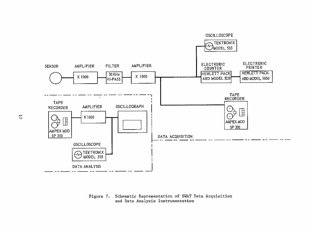
OSCILLOSCOPE
e TEKTRONIX MODEL 535
ELECTRONIC ELECTRONICSENSOR AMPLIFIER FILTER AMPLIFIER
COUNTER PRINTER S101HEWLETT PACK- HEWLETT PACK-
XIPA 00ARD MODEL 5231 ARD MODEL 5050
TAPE _ RECORDERTAPE ____________
RECORDER AMPLIFIER OSCILLOGRAPH
AMPEX MOD) T SP 300
KDATA ACQUISITION
OSCILLOSCOPE
TEKTRONIX _
eMODEL 535
DATA ANALYSIS
Figure 7 Schematic Representation of SWAT Data Acquisition and Data Analysis Instrumentation
III D Stress-Wave Instrumentation - Laboratory Evaluations (cont)
During testing of the WOL specimens maximum SWAT system amplifishy
cation was employed This was made possible because the specimens immersed
(COD gage up out of the water) in the water environment were enclosed in a
sound-proof box For these tests the electronic counter trigger level was
set just above the inherent noise (electrical) of the system Initially a
WOL test was run to determine whether the system was in fact completely free
of extraneous noise With the COD gage connected and all recording systems
in the circuit and with the specimen under no load and in air environment
after 5-12 hr in the sound-proof chamber there were only 16 signals
counted Presumably these were electrical disturbances The test was run
during regular working hours the WOL tests reported in the following parashy
graphs were tun during off-hours (nights and weekends) when there should have
been an absolute minimum of electrical disturbances
A second data acquisition system was also used for a limited
number of bend tests following the background noise measurements at Cape Kennedy
A schematic of this system is shown in Figure 8 The purpose of these tests
was to obtain stress-wave amplitude measurements using the instrumentation
employed at Cape Kennedy to ensure that the stress-wave emissions accompanying
crack extension could be detected under the background conditions observed at
Kennedy Space Center The tape recordings were made by direct recording during
test and were subsequently analyzed through playback and analysis as shown in
Figure 7
18
TEKTRONIX
OSCILLOSCOPE
ENDEVCO Dynamics Model 2213 Filter Accelerometer Model
Amplifier Amplifier 6364MQ 20-50 Kc Band Pass
KcENDEVCO30
Model 2213 CHigh-PassH Accelerometer Filter
kFI
TAPE Amplifier Amplifier RECORDER
AMPEX SP-300
Figure 8 Schematic of Instrumentation Used at Kennedy Space Center
IV LABORATORY TEST RESULTS AND DISCUSSION
As indicated in the following paragraphs two environments (air and
3 NaCl-water) and two material conditions (unhydrogenated and hydrogenated)
were utilized in the laboratory tests performed at Aerojet These conditions
are considered those most likely to be encountered during the service life of
the pressure vessels Also both straight rising load to failure and sustained
loading profiles were employed The sustained load profiles were employed
since failure of the pressure vessel may occur at constant load due to
environmentally induced slow crack growth from a prior flaw Since the
effectiveness of a failure warning system will obviously depend on the ability
to detect subcritical crack extension whether it occurs during sustained load
or on rising to failure it is important to determine if crack extension andor
failure will occur under both conditions Both effects can be studied through
the laboratory tests performed during this program
A BEND TESTS IN AIR WITHOUT DELIBERATE ADDITION OF HYDROGEN
Initially bend tests were performed in an air environment Both
the crack-opening-displacement gage and stress-wave-analysis technique were
employed to monitor the occurrence of pop-in and subcritical crack growth
The fracture data for these tests are shown below
Specimen Specimen Failure Notch Plus Apparent K
Thickness (B) Depth (D) Fatigue Crack (a) Load 1 2 No in in in aD P Kips ksi-in
1 10 20 090 045 200 130
2 097 20 091 0455 158 136
3 10 20 1036 0518 1656 133
Intermediate hold at 123 ksi-in12
20
IV A Bend Tests in Air Without Deliberate Addition of Hydrogen (cont)
The straight rising load to failure tests (No 1 and 2) indicated 12
a K value of 130 to 136 ksi-in as did the specimen (No 3) which failed
during rising load after previous holding at a stress intensity of approximately 12123 ksi-in As indicated previously in this report the ASTM recommends
for valid KIc measurements a specimen thickness exceeding that corresponding
to 25 (Kys)2 By this criterion a specimen thickness of approximately
44 in would be required for the A302B steel tested in this program
Consequently the KQ values noted above while not valid KIc measurements
indicate a high level of toughness in this material
No significant slow-crack growth or stress-wave emissions were
observed during hold in the air environment Conversely slow-crack growth
(increase in apparent crack size) and accompanying stress-wave emissions were
observed during rising load to failure The stress waves were generally very
small in amplitude (clt0Olg) but increased in amplitude with increasing crack
extension immediately prior to failure Increased rate of stress-wave
emission was also observed immediately prior to failure
B BEND TESTS IN WATER WITHOUT DELIBERATE ADDITION OF HYDROGEN
Bend specimen 4 was loaded initially to 15000 lb
(88 ksi-in 2) and held at constant load for 18 hr in 3 sodium-chloride
simulated sea water The specimen showed indications of crack growth early in
the hold period However analysis of the crack-opening-displacement gage data
indicated only very small amounts of crack extension Although the gage
employed for this purpose corresponded to the design recommended by the ASTM
its use was found unsatisfactory for tests of the type performed during this
program The COD gage was then modified and the modified version used during
the testing of the hydrogenated material described in subsequent sections of
this report
21
IV B Bend Tests in Water Without Deliberate Addition of Hydrogen (cont)
When the specimens (without hydrogenation) tested in the salt-water
environment were fractured the fracture surfaces were examined for evidence
of slow-crack growth during hold Although a small band of slow-crack growth
from the original fatigue precrack was observed it was not possible to detershy
mine how much of the crack extension occurred during rising load Onthe basis
of the COD data it would appear the majority of the extension occurred during
rising load to 15 kips from 15 to 17 kips and from 17 kips to failure although
the SWE data indicated that slow crack growth however small was occurring
during the hold periods
Figure 9 is a plot of cumulative stress-wave count over a period
of approximately 1-12 hr during hold at 15000 lb Note the indications of
a variable rate of subcritical crack growth Figure 10 shows the SWAT data
in detail (electronic counter reading every second) starting 23 min after
reaching the 15-kip load level Note that the cumfilative stress-waampe count
increased more or less continuously with brief intervals of increased slope
(when plotted to the scale of Figure 10 the increased slope was approximately 450) Figure 11 shows the SWE data obtained after adding fresh 3 NaCl-water
solution to the notch During the period of sustained load represented in
Figure 11 there were a few abrupt increases in count indicating discontinuous
crack growth together with additional intervals of increased slope (again
close to 45)
Figure 12 corresponds to the endof a short 16-kip hold (same
specimen) followed by a rise to 17 kips (approximately 125 ksi-in1 2 ) and
then a period of sustained load in 3 NaCl-water solution at 17 kips Note
the increased slope associated with the increase in load followed by abrupt
increases in count characteristic of discontinuous crack growth Approximately
600 sec after starting the hold at 17 kips an air hose produced high-frequency
noise too high to be removed by the filter This was recorded as an abrupt
increase in couni followed by a period of increased slope (again approximately 45) It cannot be definitely stated whether the increased slope indicating
22
1400
1200
1000
Li 800 3
LU
D 600
400
SEE FIGURE 10 200 FOR DETAILS
0 0 I I I I I
0 10 20 30 40 50 60 70 80 90 100
-MINUTES HOLD AT 15 KIPS
Figure 9 Cumulative Stress Wave Count vs Time Specimen No 4
A302B Steel 15 Kip Hold 3 NaCi-Water Environment
23
600
I0
20-
TIME (SECONDS)
224
6050
10 10 1O 1in20 20a 2100 2150
TIME (SECONDS) 220 3 am250 20 20 3w245 24W
43O
600
40
20
140
011 115 la 1in0 1 TIME (SECONDS)
a 14W 1m 53 0 inlW
Figure 11 Cumulative Stress Wave Count vs Time Specimen No 4 A302B Steel 15 Kip Hold After Replenishing the 3 NaCl-Water Environment
25
23
00
60
20
20
- 4o
o_ 4 o l~ ~ aiE~
220
IV B Bend Tests in Water Without Deliberate Addition of Hydrogen (cont)
continuous stress-wave emission was an artifact produced by the high-frequency
noise or the increased slope was the result of crack growth stimulated by the
high-frequency sound (crack growth after periods of dormancy can be initiated
by tapping a test specimen under load) Figure 13 is a plot of the cumulative
count for the 17-kip hold (corrected to zero at the start of hold and corrected
for noise which occurred at 836 sec) Note the tendency for increasing slope
with increasing time at load Figure 14 presents the SWAT data in detail
after 1 min at 17 kips load Figure 15 presents the data obtained after
1-12 min at 17 kips load Both Figures 14 and 15 are plotted to the same
scale as Figures 10 11 and 12 Table II presents the data plotted in
Figures 13 14 and 15 without correction for noise which occurred at 836 sec
this tabulation shows the detailed information that can be obtained by SWAT
On the basis of the SWE dpta this specimen showed evidence of
very slow continuous crack growth of the type one might expect of electroshy
chemical dissolution at the crack tip interspersed with short periods of more
rapid continuous crack growth There was little or no evidence of disconshy
tinuous crack growth with clearly defined periods of dormancy and there were
few instances of abrupt increase in count to signify crack jumps
C BEND TESTS IN AIR WITH DELIBERATE ADDITION OF HYDROGEN
After hydrogenation and baking 3 hr at 3000 F to produce a
homogeneous interstitial solid solution specimens were tested in 70degF air
Specimen 5 (Figure 16) developed discontinuous crack growth while under
sustained load starting at 9000 lb (75 ksi-in 2) but the occurrences were
sporadic and infrequent At 13000 lb (110 ksi-in 2) there was only one
stress wave large enough to be recorded as a cumulative count (cumulative
count increased from 3086 to 3110 corresponding to 464 SWEsec count rate)
Otherwise there was no increase in the SWE cumulative count during hold at
13000 lb
27
TABLE II
DETAILS OF SWE DATA OBTAINED FOR SPECIMEN NO 4 A302B STEEL DURING HOLD AT 17 KIPS IN 3 NaCI-WATER ENVIRONMENT
Time at Count Interval Time at Count Interval Load Rate Cumulative At Load Rate Cumulative A t (sec) (SWEsec) Count (sec) (set) (SWEsec) Count (sec)
27 57 8 - 1330 11 632 9 47 134 12 20 1331 20 634 1 101 4 14 54 1341 58 635 10 152 3 16 51 1392 232 652 51 299 10 27 147 1400 262 653 8
5 MINUTES 1405 134 654 5 329 1 29 30 1415 9 656 10 357 47 37 28 1443 85 657 28 444 72 49 87 1446 48 659 3 460 64 56 16 1478 131 675 32 494 221 60 34 1479 2 676 1 511 145 62 17 1495 29 685 16
10 MINUTES 25 MINUTES 616 115 72 105 1503 170 689 8 744 128 85 128 1505 72 691 2 788 2 92 44 1526 171 697 21 836 2 411(Noise) 48 1527 1 698 1 838 7 411 2 1537 187 702 10 843 10 431 5 1546 220 705 9 845 68 431 2 1584 89 715 38 846 7 431 1 1597 119 726 13 855 161 447 9 1650 146 738 53 880 160 468 25 1666 1 749 16
15 MINUTES 1671 162 756 5 904 11 492 24 1674 86 758 3 915 209 500 11 1695 120 780 21 943 5 523 28 1708 75 782 13 956 22 537 13 1717 1 787 9 980 4 541 24 1721 84 792 4 992 13 542 12 1732 114 794 11
1012 69 544 20 30 MINUTES 1088 21 558 76 1808 228 803 76 1108 151 569 20 1821 179 805 13 1136 il 576 28 1825 22 808 4 1154 5 582 18 1833 196 809 8 1172 38 583 18 1839 120 811 6 1178 19 585 6 1852 45 814 13 1182 9 -592 4 1866 146 816 14 1196 26 594 14 1888 168 819 22
20 MINUTES 1895 14 823 7 1228 80 598 32 1909 157 826 14 1229 13 599 1 1933 29 832 24 1238 2 605 9 1950 10 836 17 1256 1 610 18 1956 46 837 6 1312 91 613 56 1977 71 838 21 1318 1 619 6 1988 101 839 11 1321 1 621 3 2000 10 841 12
TABLE II (cont)
Time at Count Interval Time at Count Interval Load Rate Cumulative At Load Rate Cumulative Lt (sec) (SWBsec) Count (sec) (sec) (SWEsec) Count (sec)
2002 59 843 2 2515 40 1013 34 2017 119 845 15 2518 207 1017 3 2020 148 847 3 2521 1 1023 3 2033 165 848 13 2525 602 1029 4 2039 103 850 6 2527 22 1034 2 2048 9 857 9 2548 52 1052 21 2061 129 860 13 2561 47 1058 13 2063 156 862 2 2573 17 1062 12 2069 167 864 6 2585 69 1072 12 2075 98 874 6 2588 42 1073 3 2076 3 879 1 2599 240 1075 11 2093 21 881 17 2605 4 1077 6
35 MINUTES 2615 23 1078 10 2107 1 883 14 2616 57 1079 1 2108 103 884 1 2613 11 1080 15 2118 121 885 10 2638 42 1081 7 2119 191 887 1 2648 2 1087 10 2135 154 891 16 2650 87 1088 2 2140 11 892 5 2653 100 1089 3 2146 3 894 6 2656 56 1090 3 2150 178 897 4 2661 63 1091 5 2159 51 902 9 2685 28 1094 24 2162 7 905 3 2693 35 1097 8 2180 57 909 18 45 MINUTES 2182 58 910 2 2701 113 1104 8 2193 17 913 11 2703 50 1105 2 2195 113 916 2 2713 53 1109 10 2207 115 919 12 2719 20 1110 6 2221 34 923 14 2721 33 1112 2 2223 87 926 2 2738 72 1115 17 2238 35 936 15 2740 15 1116 2 2258 2 943 20 2752 100 1117 12 2268 204 947 10 2756 85 1119 4 2289 10 949 21 2768 56 1121 12 2307 1 952 18 2780 13 1130 12 2319 121 955 12 2782 28 1135 2 2346 20 959 27 2795 60 1142 13 2366 69 963 20 2809 65 1144 14 2386 20 975 20 2841 55 1156 32 2387 5 976 1 2848 3 1157 7 2392 158 978 5 2851 2 1159 3 2396 8 981 4 2862 45 1163 11
40 MINUTES 2869 35 1166 7 2403 21 983 7 2879 18 1169 10 2409 241 986 6 2885 62 1171 6 2449 95 996 40 2905 55 1175 20 2457 24 998 8 2908 54 1178 3 2473 104 1002 16 2918 7 1182 10 2481 3 1003 8 2924 8 1186 6
29
TABLE II (cont)
Time at Count Interval Time at Count Interval Load Rate Cumulative t Load Rate Cumulative t (sec) (SWIsec) Count (sec) (sec) (SWEsec) Count (sec)
2938 12 1193 14 3341 207 1410 2948 95 1201 10 3366 103 1421 25 2966 10 1215 18 3377 8 1424 11 2968 43 1216 2 3378 12 1425 1 2972 22 1217 4 3390 2 1429 12 2979 8 1221 7 3396 3 1430 6 2987 8 1223 8 3397 14 1432 1 2998 38 1226 11 3401 8 1434 4
50 MINUTES 3402 98 1438 1 3002 36 1228 4 3408 12 1443 6 3010 55 1230 8 3410 16 1448 2 3011 3 1234 1 3413 6 1452 3 3016 1 1236 5 3431 2 1454 8 3017 3 1237 1 3433 17 1458 2 3023 3 1239 6 3435 30 1460 - 2 3029 3 1240 6 3438 22 1462 3 3033 1 1243 4 3450 8 1475 12 3036 110 1245 3 3455 62 1484 5 3037 4 1248 1 3461 154 1490 6 3053 83 1259 16 3462 7 1493 1 3054 7 1260 1 3466 11 1501 4 3061 2 1265 7 3472 2 1507 6 3062 83 1266 1 3476 46 1509 4 3076 62 1275 14 3489 18 1515 13 3080 5 1278 4 3490 8 1517 1 3098 32 1294 18 3508 15 1534 18 3100 15 1296 2 3513 25 1541 5 3102 16 1297 2 3520 220 1549 7 3108 7 1299 6 3538 29 1566 18 3114 7 1301 6 3542 9 1572 4 3127 6 1304 13 3543 107 1575 1 3129 1 1305 2 3558 240 1588 15 3133 1 1306 4 3568 30 1601 10 3140 5 1309 7 3570 21 1603 2 3154 30 1312 14 3573 66 1607 3 3170 6 1320 16 3579 9 1613 6 3175 77 1322 5 3591 37 1619 12 3177 110 1323 2 60 MINUTES 3178 5 1324 1 3607 128 1622 16 3183 4 1326 5 3608 70 1626 1 3187 137 1331 4 3609 2 1629 1 3191 14 1332 4 3624 50 1638 15 3200 3 1336 9 3630 14 1642 6 3206 2 1340 6 3639 86 1645 9 3214 20 1343 8 3660 56 1662 21 3219 22 1345 5 3678 13 1669 18
55 MINUTES
30
TABLE II (cont)
Time at Count Interval Time at Count Interval Load Rate Cumulative At Load Rate Cumulative At (sec) (SWEsec) Count (sec) (see) (SWEsec) Count (sec)
3688 33 1680 10 4535 105 2574 28 3692 35 1682 4 4547 3 2589 12
3709 209 1688 17 4583 4 2616 36 3712 7 1689 3 4623 460 2670 40 3720 78 1691 8 4624 37 2703 1
3730 93 1694 10 4626 18 2715 2 3731 5 1695 1 4627 840 2729 1 3743 13 1703 12 4630 141 2737 3 3744 120 1709 1 4662 2 2758 32
3750 24 1715 6 4671 1 2763 9 3755 142 1724 5 4698 1 2774 27 3767 45 1738 12 4710 8 2782 12 3796 69 1770 29 4719 6 2784 9 3823 21 1808 27 4731 128 2785 12 3844 10 1838 21 4761 17 2810 30 3854 82 1851 10 4783 22 2822 22 3856 13 1855 2 4786 23 282A 3 3895 75 1915 39 80 MINUTES
65 MINUTES 4822 96 2831 36 3901 18 1920 6 4852 1 2842 30 3905 54 1927 4 4934 59 2890 82
3946 58 1963 41 4953 200 2907 19 3970 2 1985 24 4954 26 2910 1 3971 181 1988 1 4957 16 2916 3 3974 61 1990 3 4964 56 2923 7 3975 28 1992 1 4988 29 2941 24 3987 51 2004 12 5000 88 2951 12 4012 2 2022 25 5031 10 2977 31 4013 31 2026 1 5032 9 2978 1 4022 7 2036 9 5045 56 2982 13 4054 4 2062 32 5054 4 2984 9 4056 16 2066 2 5093 220 2992 39 4084 37 2093 28 85 MINUTES 4091 36 2099 7 5122 115 2996 29 4100 3 2111 9 5166 17 3019 44 4129 16 2142 29 5190 172 3042 24 4156 6 2165 27 5193 55 3045 3
70 MINUTES 5194 2 3048 1 4241 19 2253 85 5224 313 3081 30 4292 4 2299 51 5248 23 3106 24 4331 42 2339 39 5266 32 3123 18 4338 19 2348 7 5281 24 3138 15 4340 66 2350 2 5291 10 3150 10 4345 10 2359 5 5303 25 3164 12 4385 4 2419 40 5306 1 3169 3 4397 121 2432 12 5324 56 3187 18
75 MINUTES 5330 58 3193 6 4500 40 2534 103 5345 31 3211 15 4507 6 2542 7 5351 155 3217 6
31
TABLE II (cont)
Time at Count Interval Time at Count Interval Load Rate Cumulative At Load Rate Cumulative At (sec) (SWBsec) Count (sec) (sec) (SWEsec) Count (sec)
5357 211 3223 6 5887 185 3536 1 5363 29 3233 6 5905 65 3559 18 5364 20 3237 1 5923 31 3575 18
90 MINUTES 5924 22 3576 1 5403 118 3276 39 5933 109 3578 9 5418 79 3295 15 5934 5 3579 1 5419 44 3298 1 5961 43 3582 27 5420 35 3300 1 100 MINUTES 5448 27 3324 28 6000 23 3585 39 5460 118 3327 12 6001 13 3586 1 5466 97 3329 6 6002 166 3588 1 5472 184 3331 6 6008 9 3590 6 5484 28 3333 12 6032 29 3592 24 5499 45 3338 15 6041 111 3596 9 5505 2 3341 6 6062 116 3601 21 5506 173 3344 1 6083 1 3603 21 5512 72 3346 6 6084 236 3606 1 5515 8 3348 3 6090 140 3607 6 5536 199 3352 21 6091 104 3608 1 5548 5 3356 12 6106 21 3609 15 5553 199 3359 5 6115 31 3611 9 5554 34 3360 1 6121 29 3614 6shy5587 190 3364 33 6124 1 3622 3 5593 2 3365 6 6139 51 3630 15 5605 6 3367 12 6160 25 3634 21 5611 12 3369 6 6175 5 3636 15 5638 3 3373 27 6184 196 3639 9 5644 57 3374 6 6217 275 3645 33 5645 78 3376 1 6223 84 3648 6 5669 21 3379 24 6238 23 3649 - 15 5693 22 3384 24 6244 99 3650 6 5699 48 3385 6 6250 81 3652 6
95 MINUTES 6259 39 3654 9 5702 74 3387 3 6265 15 3656 6 5703 85 3389 1 6271 21 3658 6 5725 21 3391 22 6283 85 3660 12 5737 1 3394 12 105 IWNUTES 5752 72 3396 15 6304 143 3662 21 5761 106 3398 9 6331 50 3672 27 5788 1 3414 27 6340 179 3674 9 5794 176 3422 6 6341 37 3675 1 5809 2 3441 15 6365 34 3677 24 5810 15 3445 1 6366 ill 3680 1 5813 42 3448 3 6393 150 3682 27 5814 189 3451 1 6405 43 3684 12 5823 180 3461 9 6429 4 3687 24 5832 171 3472 9 6435 127 3690 6 5838 46 3481 6 6459 31 3691 24 5859 63 3505 21 6483 7 3694 24 5865 15 3511 6 6495 30 3696 12 5886 2 3533 21 6501 128 3700 6
32
TABLE II (cont)
Time at Count Interval Time at Count Interval Load Rate Cumulative At Load Rate Cumulative At (sec) (SWEsec) Count (sec) (sec) (SWEsec) Count (sec)
6522 87 3703 21 7278 21 4158 6 6531 16 3704 9 7302 2 4174 24 6555 102 3706 24 7303 3 4174 1 6567 7 3709 12 7318 125 4186 15 6570 10 3710 3 7348 88 4205 30 6576 87 3711 6 7402 86 4238 54 6577 89 3713 1 7435 90 4258 33 6578 131 3714 1 7447 14 4262 12 6599 4 3717 21 7474 14 4277 27
6600 110 MINUTES
8 3718 1 7486 7504
9 125 MINUTES
89
4286
4304
12
18 6603 37 3720 3 7510 39 4308 6 6639 15 3724 36 7531 52 4331 21 6669 48 3728 30 7540 208 4344 9 6675 23 3729 6 7549 38 4353 9 6684 57 3731 9 7576 72 4376 27 6705 23 3757 21 7594 24 4392 18 6744 53 3807 39 7603 55 4403 9 6762 240 3830 18 7615 160 4415 12 6783 5 3854 21 7621 134 4420 6 6801 26 3874 18 7627 160 4423 6 6822 181 3901 21 7639 180 4430 12 6852 24 3934 30 7648 5 4432 9 6879 44 3962 27 7658 100 4437 10 6882 2 3965 3 7679 319 4445 21
115 MINUTES 7694 72 4449 15 6906 63 3991 24 7709 23 4451 15 6927 176 4001 21 7721 34 4453 12 6930 15 4006 3 130 MINUTES 6931 54 4011 1 7800 Test Terminated 6952 305 4026 21 6953 40 4033 1 6980 3 4037 27 6989 99 4039 9 7040 387 4080 51 7041 53 4095 1 7056 23 4100 15 7086 354 4108 30 7095 21 4110 9 7125 70 4117 30 7131 2 4120 6 7167 97 4129 36 7176 11 4130 9 7197 18 4133 21
120 MINUTES 7218 28 4136 21 7227 39 4138 9 7248 72 4146 21 7272 50 4153 24
33
40
38W
3400
32W
30
28M
260
= 2400
S 22DD
i20
1600
1400
1200
10
600
400
200
06 1a 20 30 40 50 60 70 80 90 tW 110120130
MINUTE-S-H-OLD 17KIPS
Figure 13 Cumulative Stress Wave Count vs Time SpecimE A302B Steels 3 NaC1-Water Environment
34
3503
0
~0
40
20
3203
00
20
C0
20
310
03
(0
40
= = 20 0 I- 365~
05
20 00
20
0shy20
2003
20 ~~0 C
20
20 40
- 20
2835
0
(0
20
20shy
20020
20 -
3403 3450 3720 3750 fl 3550 3003 3050 40) 4050 4003 4050 4~fl 4200 4020 4350 4440 4450
TIME (SECONDS)
Figure 14 Cumulative Stress Wave Count vs Time Specimen No 4 A302B Steel After 1 Minute at 17 Kip Hold in 3 NaCi-Water Environment
35
48
0
I-
S 40
us 50 50 70 5 90 0 60 60 10 6 6 t 20CO DS
- iue1CmlaieSrs av on sTme pcmnN A0BSel
Afe2-0iue t1 i todi NC-ae niomn
Page60
4520 -
so- lao
F
122021 amp~
20 4
400
20
20 22
3540 =
20
3024
20
50
45
20
20520
20
20
45
20
no
I
40
4~
20
40
20
20
4
20
2020
20
gt
20
20 4
20
20
3545
20
Iino200j
5505
2220
1120
20
001
20
20 shy
00
1
45
OX
I
I I
I I
0 50
020 000
205 200
20 200
Z
40 505
550 400
TIM
E (S
EC
ON
DS
)
Figure 16
Cumulative Stress Wave Count vs
Time Specimen No
5 A302B Steel
Hydrogenated and Tested in Air
37
IV C Bend Tests in Air With Deliberate Addition of Hydrogen (cont)
On raising the load from 13000 to 14000 lb (122 ksi-in )
there was evidence of a creep phenomenon as shown in Figure 17 The crackshy
opening-displacement gage confirmed the occurrence of crack growth continuing
after reaching the 14000-lb hold Stress-wave emission showed the mechanism
to be discontinuous cracking rather than a deformation process When the
count rate was plotted as in Figure 18 the activity carrying into the
14000-lb hold again was discontinuous After approximately 300 sec at 14 kips
the SWE associated with the creep phenomenon had subsided During the 14-kip
hold there were two crack jumps one after 920 sec (cumulative count increased
from 5618 to 5720 and the count rate associated with the jump was 181 as
counted over a 10-sec interval or 18 SWEsec) and one after 2130 sec (cumulashy
tive count increased from 5721 to 5755 and the count rate was 139 in 10 see)
After 5000 sec at 14 kips the load on Specimen 5 was raised As
seen in Figure 19 the stress-wave activity was an unmistakable presage of
instability which occurred after 20 sec into hold The load reached a maximum
of 145 kips (145 ksi-in 2) Technically the onset of instability occurred
shortly after starting to increase the load ie at approximately
132 ksi-inI2 which agrees with the KQ value obtained through rising load
tests of unhydrogenated material in an air environment
Because of the very long test period and multiple loadings involved
in the testing of the Specimen 6 only data obtained during rising load to
19500 and 19800 ib during sustained test periods at these loads and during
specimen failure are shown in Figure 20 These data indicate essentially the
same SWE-crack growth relationships discussed previously for Specimen 5 except
that on reaching hold the crack tended to grow slowly for a longer period of
time in comparison to the behavior noted for Specimen 5 Also the incremental
nature of crack extension was more readily observed by the stress-wave-emission
data for Specimen 6
38
20
560
80
60
40
20
5500
80
60
40
20
5400
o 5100
808
60
40
20
5000 u-J
4500
4480 80 4- START 14-KI P HOLD
CODC 75lt
4000
3980 70
3960
6553120 l
- END13-KIP HOLD
3100 160 0 40 80 120 160 200 240 280 320
TIME AT LOAD (SECONDS)
Figure 17 Cumulative Stress Wave Count and COD vs Time Specimen No 5 A302B Steel fydrogenated and Held at 14 Kips in Air
39
200
LU
LU
1- 100
50 END 13-KIP
25 HOLD-I
0 1- TIME
100 INSECONDS AT
200 14KIPS
300
(COUNT EVERY 10 SEC)
Figure 18 Stress Wave Count Rate vs Time - Specimen No 5 A302B Steel Hydrogenated and Tested in Air
40
INSTABILITY
9580
9560
9540
9380
928D0
9260
842D
8440
73O I-shyz 7220
o 7260
U 7240
7220
7180I-shy
7160
- 7140
7120
7100
7080
7060
5900
5880
5860
5840
5820
5800
578D
5460
0 40 80 120 160 SEC
4M 4960 50D RISING LOAD-SECONDS AT 14 KIPS
Figure 19 Cumulative Stress Wave Count vs Time Specimen No 5 A302B Steel Hydrogenated and Tested in Air
41
20000
18000
FAILURE
18290 sec a- 1 17-in K - 199 s - Y
z
-
16000
14000
l0
1200
I-9 Iin
1014in K 152 ki- in -i
o-1 09 n K- 176ksmn
- 1 07 in I 170 iis-
o -1 042in K 12ks-in
c023i NK15ks-n
-shy
-
10000
REACH 19800 lbs
START TO 19800 bs
10000 11000 12000 13000 14000 15000 16000 17000 18000 19000
TIMESECONDS
12000
11000 s
p9000
T LOAD ADJUSTMEA
7n000
READOUT6000 OTE STRESS WAVE DATA A UST T
500 Vgt 0 ENT CORRESPONDIG TO SLOPELOAADJUSTM15 CHANGES PLOTTED
a 4000
3000
LOAD ADJUSTMENT2000 SECONDSECMENIME
1000 START HOLD AT 19500 1b
900 1l6070 D0 8 0 00 0 000600
0 1000 50002000 3000 4000
TIME SECONDS
Figure 20 Cumulative Stress Wave Count vs Time Specimen No 6 A302B Steel Hydrogenated and Tested in Air
Page 42
IV C Bend Tests in Air With Deliberate Addition of Hydrogen (cont)
As indicated in Figure 20 the increase in crack length during
the initial period of hold at 19500 lb resulted in an increase in the applied
stress intensity and was accompanied by significant stress-wave-emission
activity To maintain the desired load it was also necessary to make frequent
load adjustments at the start of hold During the first 3600 sec the effecshy
tive crack length increased from approximately 0963 to 1000 in and was
accompanied by about 7000 SWE As indicated in Figure 20 the majority of the
SWE activity and increase in crack length occurred during the first 3000 sec
of the hold at 19500 lb After this period both the stress-wave-emission
activity and rate of increase in crack length gradually decreased For example
during the entire period from 5000 to 17600 sec when the load was increased
to 19800 lb the apparent crack length and SWE count increased by only approxishy
mately 0020 in and 2500 respectively
After approximately 17000 sec at 19500 lb the load was increased
to 19800 lb and specimen failure occurred after approximately 600 sec at
19800 lb The load was maintained for this period however it was apparent
from both the SWE and COD gage data that the crack was extending and specimen
failure would occur without a further increase in load although it was necesshy
sary to continually adjust the tensile machine to maintain the desired load
The failure stress intensity approximated 199 ksi-in 2however technically
the onset of instability occurred after starting to increase the load at
approximately 153 ksi-in1 2
Specimen 7 was also hydrogenated baked at 300F for 3 hr and
tested in air Figure 21 is a detailed plot of the SWAT data (electronic
counter print-out every second) indicating crack growth of a discontinuous
nature starting at 2400-lb load Note the periods of dormancy (no increase
in SWE count) interspersed with abrupt increases in count indicating disconshy
tinuous crack growth Note also that there was little or no evidence of
continuous stress-wave emission until the load (stress intensity level) was
high approaching failure
43
CUMULAIY STRESS-VAVE COUNTCU LTISTE W E ON
I OT A~II I OI I L I I I I I I I I I I I I I I i I I I I I
- N LB
I I I I I I I I I I I I I i I I
--L - 0OTO11
-0101
(lNIML~ 33383338
8
133113-
3IiC)0 83) 3103 31-3(31-
~0
33 331
3l3C0C~
38318shy
111(10 CAVMSS3 nfl CAliVi flWfl3
________________________________________________________________________
111fl0~ 3KvM~s~a1Ff~TfvTifwT
FPAIAE
hY
A Ii
8
INa
CZ
8 C0 U CI
33 S
1 H
H
03 -I
~ 3lt
0 Cd 33
~C3 ~ H
8 0003
A
Ofli3i~~ C)
Page 45
IV C Bend Tests in Air With Deliberate Addition of Hydrogen (cont)
Figure 22 presents the SWE data from a hydrogenated bend specimen
(No 8) tested in air The load was increased continuously to 9800 lb
(70 ksi-in 2) where there was a short hold (approximately 400 sec) Note
the discontinuous crack growth followed by a short period of continuous
emission (less than 450 slope) The load was then raised to 14800 lb
(109 ksi-in 2) and held for approximately 400 sec Again there were jumps
in the SWE cumulative count but this time interspersed with continuous
emission The SWAT system employed for this test corresponded to that employed
for the background measurements at Kennedy Space Flight Center and shown in
Figure 8 only one channel was employed viz
Endevco 2213 Amplifier Amplifier Band-Pass Filter 10OX 10OX 20 to 50 Kcps
The continuous stress-wave emission observed during hold at the higher stressshy
intensity level in this specimen was not observed in the other hydrogenated
specimens tested in air The primary purpose of this test (Specimen 8) was to
record SWE data for subsequent playback and analysis to determine the amplitude
of burst-type stress-wave emissions associated with fracture in Type A302B
steel These analyses were performed using the instrumentation shown in
Figures 7 and 8 with the following results which are discussed in more detail
in conjunction with the results of the background measurements performed at
Kennedy Space Flight Center (Section V)
Maximum SWE Amplitude - 39 x 10-3g
Minimum SWE Amplitude - 12 x 10-3 g
Average SWE Amplitude - 22 x 10-3g
Laboratory Background - 11 x 10-3g
46
00 o z~ 20 ~
40
~40
S20 1 2 0 0 0 0
TIIAEAT 4 S-KIPHOLD (10KS(51IN A)
407
IV Laboratory Test Results and Discussion (cont)
D BEND TESTS IN 3 NaCI-WATER WITH DELIBERATE ADDITION OF HYDROGEN
Specimen 9 was hydrogenated baked and tested in 80F water
The electronic counter indicated continuous stress-wave emission interspersed
with abrupt increases in count indicating occasional crack jumps Figure 23
shows the details of stress-wave emission that occurred during both rising
load and holding load The crack length determined from the COD chart at
selected loads is also shown Note from the SWE data that there were no
periods of dormancy and the slope of the plot of cumulative count versus time
indicated moderately rapid continuouas crack growth such as might occur with
electrochemical dissolution at the crack tip The COD gage data shown in
Figure 23 also indicate crack extension however the actual amount appears
to be quite small (lt01 in) which would be consistent with the relatively
small number of stress-wave emissions detected even at the high system
sensitivity employed The dramatic difference between the behavior in
Figures 21 and 23 for hydrogenated material tested in air (Figure 21) and
water (Figure 23) indicates that hydrogen and 3 sodium chloride solution
acting together have a greater total effect than the sum of their individual
effects ie working together they appear to have produced a synergism
E WOL TESTS
Because of the possible significance of the synergistic-effect
noted above on the life of the hydrogen pressure vessels at Kennedy Space
Flight Center additional testing was performed using hydrogenated WOL specishy
mens cut from the fractured bend specimens The first WOL specimen was
initially loaded to-3650 lb (50 ksi-in 2) and then placed in 3 NaCl solution
(notch immersed) There was 30 min of essentially continuous stress-wave
emission (recorder started approximately 5 min after loading the specimen)
Subsequently therewas one sizable jump in the SWE cumulative count after
48
V30
760
740-M
$
720 -s
680shy
60
610
40 w
w
520 w
i
20500
HOLDD]N
340
20 760
7200
ING
IV
O
shy
420
60
40
20 0 2
04
0Q
0
60DO
LO0
01 200
250 300
350 400
450 500
550 6M
650
700 750
TIME
(SECONDS)
Figure 23
Cumulative Stress Wave Count vs Time Specimen No 9 A302B Steel
Hydrogenated and Tested in 3 NaCi-Water Environment
49
IV E WOL Tests (cont)
approximately 3 hr 40 min Then 3 hr 20 min later several jumps occurred
followed by 8 hr 20 min of stress-iave activity After this the crack was
dormant (total test time 17 hr 25 min) These data are shown in Figure 24
The load was then increased slightly (torque was increased from 200 to
255 in-lb) an additional 1-12 hr in 3 NaCl solution produced no significant
increase in the cumulative stress-wave count The reason for this apparently
anomalous behavior was not determined although it may result from a blunting
effect at the crack tip produced during the initial hold period
The fatigue crack was then extended (approximately 005 in) in
tension-tension fatigue and the specimen reloaded to approximately 51 ksi-in2
Stress-wave emission started almost immediately (dashed curve in Figure 24)
After approximately 3 hr of discontinuous activity the periods of dormancy
tended to increase interspersed with relatively small jumps (as counted over
10-sec intervals) The results of the initial loading and the reloading are
shown in Figure 24 note that there was appreciably lower cumulative count in
the reloaded specimen as compared with the initial loading for a comparable
period of test
A second hydrogenated WOL specimen was then tested in air at
50 ksi-in 2 there were stress waves initially (creep) but then very little
activity over the remaining 35-hr test period After the first hour the
count increased from approximately 150 to only 280 in the final 34 hr of test
Figure 25 shows the long peribds of dormancy punctuated by occasional 1-count
increases This is in marked contrast to the results obtained from the
hydrogenated WOL specimens tested in 3 NaCl solution and the bend-test
findings of a synergistic effect were confirmed
50
------------
aa
L- -- -- - ------ - --- I
3
IN DO
INTES) 3 S IOTI E( LI N LU
Ino
a
N O
TIME (MINUTES) IN 3 NCI SOLUTION
Figure 24 Cumulative Stress Wave Count vs Time at Hold WOL Specimen No 1
A302B Steel Hydrogenated and Tested in 3 NaCi-Water Environment
51
000 In 0 M6020 126 24 022 in0 1180 10 11 100 IWO l 100M M-C 0 90w6 a0 w6
t t t t 5W MOD4
10
TIME (MINUTES)
Figure 25 Cumulative Stress Wave Count vs Time at Hold WL Specimen No 2 A302B Steel Hydrogenated and Testd in Air
52
IV Laboratory Test Results and Discussion (cont)
F DISCUSSION
1 Material-Environment Consideration
The Type A302B steel supplied for evaluation exhibited a
very high level of fracture toughness Although quantitative plane-strain
fracture toughness measurements were not possible because of the large specimen
size required the KQ value associated with failure approximated 135 ksi-in1 2
This material was also found resistant to environmentally induced failure in
that the rate of crack growth of a prior flaw at applied stress-intensity
factors as high as 90 of the KQ value appeared to be very low This effect
was observed for unhydrogenated-material tested in air and a 3 NaCl-water
environment and hydrogenated material tested in an air environment However
the hydrogenated specimens tested in 3 NaCl-water environment had a much
faster rate of subcritical crack gr~wth in comparison to the other test condishy
tions indicating a synergistic effect due to the combination of sea water and
hydrogen in interstitial solid solution This synergistic effect indicates
that the Type A302B steel hydrogen storage tanks in the Kennedy Space Flight
Center environment may have limited life as the result of subcritical crack
growth if subjected to the same combination of stress and environmental
factors-
The WOL test results tended to confirm the possible synergism
due to the combined effects of 3 NaCl-water and hydrogen in interstitial solid
solution Marked SWE activity was observed when the hydrogenated specimens
were immersed in the salt water whereas in an air environment after the
initial period at hold when a creep phenomenon was observed there was essenshy
tially no stress-wave emission The fact that failure was not produced on
holding (in contradiction to the bend tests) can be explained by the fact that
the WOL test as-performed in this program is a self-arresting test because
53
IV F Discussion (cont)
the occurrence of crack growth results in a reduction in the applied load
Conversely in the bend tests the load was constantly applied as the crack
extended and eventually resulted in specimen failure
2 Stress-Wave-Emission Characterization
Detectable stress-wave emissions although of small amplitude
(ltOOlg) were observed to be associated with crack growth in Type A302B steel
Under all test conditions the stress-wave emissions were observed both during
rising load and when failure (instability) was imminent During hold various
SWE characteristics depending on the test conditions were observed When
tested in the hydrogenated condition in-an air environment a creep phenomenon
evidenced by increasing count of SWE and an accompanying increase in apparent
crack size was observed With time at hold and at applied stress-intensity
levels less than critical the creep phenomenon eventually stopped as did the
occurrence of stress-wave emissions Unhydrogenated material tested in the
3 NaCl-water environment produced continuous stress-wave emission punctuated
by abrupt increases in SWE count This behavior indicates both continuous
very small increments of crack extension with larger crack jumps corresponding
to the abrupt increases in SWE count Continuous incremental crack extension
characterized by continuous SWE interspersed with abrupt increases in SWE count
indicating occasional crack jumps was also observed in testing hydrogenated
material in a 3 NaCl-water environment
In all instances when failure (instability) occurred both
the amplitude and rate of stress-wave emission increased and could be employed
as a precursor of the onset of instability however even when failure was
approached-the SWE amplitude was small (ltOlg) In the other instances where
failure was not produced evidence of crack extension (although very small in
some instances) was observed on the specimen fracture face Once evidence of
54
IV F Discussion (cont)
crack growth was observed (by SWE or COD) it is obvious that failure would
eventually occur (assuming a constantly applied load) although depending on
the initial flaw size and subcritical growth rate the time to failure may be
very long In actual practice the SWE data could be employed (1) to locate
the propagating flaw (2) to monitor its occurrence and (3) as a basis for
terminating service so that repairs could be made before failure The stressshy
wave emissions associated with crack growth during rising load or increasing
stress intensity and the creep phenomenon during the initial part of hold
can be employed for this purpose
5S
V BACKGROUND MEASUREMENTS AND ASSOCIATED LABORATORY TESTS
A BACKGROUND MEASUREMENTS AT KENNEDY SPACE FLIGHT CENTER
Background noise measurements were made at two locations the VAB
Bottle Field and Pad A at the Kennedy Space Flight Center The data were tape
recorded and in addition to general background noise included tank blowdown
and repressurization periods The instrumentation for this purpose is shown
schematically in Figure 8 analysis of the data was performed by playback onto
an oscillograph and comparison with the SWE-crack growth data obtained during
the laboratory testing of bend specimens
The analysis of the signal amplitude data for tests at Cape Kennedy
is indicated below
1 Pad A Bottle Field
Signal Amplitude
a Quiescent Background
Filter at 20 Kcps - 50 Kcps -BandPass- 99 x 10 gsBand Pass
Filter at 200 cps - 32 Kcps
Band Pass
b Tank Blowdown - System Saturation (gt llg peak to peak)
C Tank Repressurization - System Saturation (gt llg peak to peak)
2 VAB Bottle Field
a Quiescent Background - 22 x 10- 4 gs
56
V A Background Measurements at Kennedy Space Flight Center (cont)
Signal Amplitude
b Tank Blowdown - System Saturation (gt llg peak to peak)
C Tank Repressurization - System Saturation (gt llg peak to peak)
Analysis of the tape-recorded data of bend tests at Aerojet indicates
the following signal amplitude for burstf-type stress-wave emissions associated
with crack growth and fracture in Type A302B steel
Maximum Amplitude - 39 x 10-3g
Minimum Amplitude - 12 x 10-3g
Average Amplitude - 22 x 10-3g
Laboratory Background - 11 x 10-3g
Thus the amplitude of SWE associated with crack growth in A302B steel is
approximately an order of magnitude larger than the background noise noted
previously Consequently the above results show that it is possible to detect
stress-wave emissions associated with fracture in A302B steel under the quiescent
background conditions existing at the Kennedy Space Center Difficulty is
expected in detecting such flaw growth during tank blowdown and repressurization
periods unless filtering can be employed to screen out the noise associated
with these periods However the blowdown and repressurization periods are of
very short duration and the materials behavior observed in this program indishy
cated that considerable prefailure crack extension would be expected from any
flaw of a size expected to be present in these pressure vessels Also
immediately on reaching load a creep phenomenon evidenced by an extension
in apparent crack length and accompanied by detectable stress-wave emission
was observed Consequently even if noise associated with blowdown and
57
V A Background Measurements at Kennedy Space Flight Center (cont)
repressurization cannot be effectively filtered out significant flaw growth
andor creep could still be detected and tank depressurization accomplished
prior to catastrophic failure assuming a capability for such depressurization
exists at these locations
B LABORATORY SIGNAL ATTENUATION EVALUATIONS
Subsequent to the background measurements at the Kennedy Space
Flight Center and the bend tests at Aerojet two series of tests were made at
Aerojet using a section of pipe and plate both of SAE 4130 steel alloy The
purpose of these tests was to determine the coefficient of signal attenuation
which in conjunction with the previous test data could be used to establish
the sensor spacing which would insure detection of SWE associated with crack
growth in the pressure-vessels at the Kennedy Space Flight Center
In these tests a constant pulse was imparted to the specimen by
a Tektronix 115 Pulse Generator using a Clevite PZT-5 Crystal (2125 in dia
and 0250 in thick) The piezoelectric crystal was mounted on a small alumishy
num block which in turn was adhered to the surface of the specimen The
signal was received by a 2217-E-Endevcq accelerometer placed at various disshy
tances from the pulser The pulse used was 10 n-sec rise and fall time with
a duration of 20 microsec at an amplitude of 12v
1 Pipe Tests
A SAE 4130 steel pipe (8-58 in OD 7-18 in ID and 22 ft
10-78 in long) was used as specimen for this test series The pulser was
mounted normal to the external surface of the pipe as close as possible to the
edge The accelerometer (2217-E-Endevco) was successively placed on the pipe
58
V B Laboratory Signal Attenuation Evalutions (cont)
surface at positions I to 8 that were at 4 6 8 10 12 14 16 and 20 ft
from the pulser The signal received by the accelerometer was displayed on a
Tektronix 422 osilloscope Typical signals are shown in Figure 26
The velocities of the compressional and shear waves in steel
are
29 lO06 x38103 Vc= -x lg ) (l-26) = O2 x06(- 0 x386 = 227000 insec(+j 012)283 (1+030) (1-060)
29x106 x 386 = 91 36= 123000 insec
s 2 ( + p) p 2 (i + 030) x 0283
where E = Youngs Modulus p = Poissons Ratio and p = density The times of
arrival of these waves at the computed velocities are indicated on the oscilloshy
scope photos shown in Figure 26 The point of shear wave arrival (T ) coincides
in most of the photos to a distinct change of pattern in the trace The
arrival of the compressional wave is difficult to determine accurately because
the amplitude of this wave attenuates very fast with distance
A visual comparison of the curves shows that Figure 26a
representing the signal received 4 ft from the impulse indicates a perfectly
detectable arrival of the compressional wave conversely Figure 26h (at 20 ft
from the impulse) shows the visually detectable arrival of a wave almost at the
computed arrival of the shear wave This is due to the fact that the amplitude
of the first cycles of the compressional wave have become essentially impercepshy
tible at a distance of 20 ft from the pulse An attempt to determine signal
arrival time by visual inspection only of the traces in Figure 26 would result
in the wave velocities indicated in Table III The computed arrival times of
the compressional and shear waves are shown in Table IV If an integration of
the positive portions of the cycles comprised in 200 p sec after arrival of the
59
VERTICAL SCALE 1 DIV= 01 V VERTICAL SCALE 1 DIV = 01 V HORIZONTAL SCALE 1 DIV= 50p SEC HORIZONTAL SCALE 1 DIV = 100 pSEC
a 4FT FROM PULSER b6 FEET FROM PULSER
Tc Ts Tc Ts
VERTICAL SCALE I DIV 01 V VERTICAL SCALE I DIV = 01 V HORIZONTAL SCALE I DIV = 100 I SEC HORIZONTAL SCALE 1 DIV = 200 p SEC
c 8 FEET FROM PULSER d 10 FEET FROM PULSER
Tc = Arrival of Compressional Wave
T = Arrival of Shear Wove
Figure 26 Oscillograph Traces for Pipe Tests (Sheet 1 of 2)
6o NOT REPRODUCTBLE
VERTICAL SCALE 1 DIV = 01 V VERTICAL SCALE 1 DIV 01 V HORIZONTAL SCALE 1 DIV = 200y SEC HORIZONTAL SCALE I DIV 200 p SEC
e 12 FEET FROM PULSER f 14 FEET FROM PULSER
T TS T T
VERTICAL SCALE 1 DIV = 01 V VERTICAL SCALE 1 DIV = 01 V HORIZONTAL SCALE 1 DIV = 200 v SEC HORIZONTAL SCALE I DIV =5001p SEC
g 16 FEET FROM PULSER h 20 FEET FROM PULSER
Figure 26 Oscillograph Traces for Pipe Tests (Sheet 2 of 2)
61
V B Laboratory Signal Attenuation Evaluations (cont)
shear wave is performed the average amplitudes determined in this manner
become quite meaningful These average amplitudes are shown in Table V
TABLE III
WAVE VELOCITY BASED ON VISUAL ANALYSIS OF OSCILLOSCOPE TRACES - PIPE TESTS
Distance from Pulse Arrival Velocities Photo ft in Time psc (ftsec)
1 4 48 210 228000
2 6 72 400 180000
3 8 96 600 160000
4 10 120 800 150000
5 12 144 1000 144000
6 14 168 1200 140000
7 16 192 1400 137000
8 20 240 1750 137000
TABLE IV
COMPUTED ARRIVAL TIMES - PIPE TESTS
Compressional Wave Shear Wave Distance from Pulse Arrival Time Arrival Time
Photo in psec Osc Div sec Ose Div
1 48 212 423 390 780
2 72 317 317 583 583
3 96 422 422 778 778
4 120 530 265 972 486
5 144 635 317 1163 581
6 168 740 370 1360 680
7 192 840 420 1545 771
8 240 1050 21 1930 387
62
V B Laboratory Signal Attenuation Evalutions (cont)
TABLE V
SIGNAL AMPLITUDE VS DISTANCE - PIPE TESTS
Average Signal Amplitude Distance from 200 Psec after Arrival
Test Pulser in of Comp Wave mv
1 48 230
2 72 145
3 96 85
4 120 60
5 144 45
6 168 28
7 192 22
8 240 18
The general equation for the amplitude attenuation curve is
C x e-Xy =
where y = amplitude at distance x in volts
x = distance in inches from pulse source
C = amplitude of pulse in volts
a = attenuation factor
or iny= 1 C + (- ax) = I C - ax (Eq 4)n n
To determine the values of C and a the following statistical analysis was
performed
63
V B Laboratory Signal Attenuation Evaluations (cont)
Distance Yo y y2 X X2 Test in m v n n
1 48 230 543 +142 2010 -87 7580 - 124 261
2 72 145 499 +098 0960 -63 3960 - 62 360
3 96 85 445 +044 0194 -39 1520 - 17 427
4 120 60 409 +008 0006 -15 225 - 1 490
5 144 45 380 -021 0044 + 9 81 - 2 548
6 168 28 334 -067 0450 +33 1090 - 21 560
7 192 22 309 -092 0847 +57 3250 - 52 592
8 240 18 289 -112 1250 +105 11000 - 118 690
EY2 EX2pound x = 1080 ElnY =3208 5761 28706 SXY-397 XxIny3928
- 1080 - 3208 x =- = 135 ny = 401
EXY -397 00138 1 C =l1y + oshy
pound 2 x2 28706 n i x
= 401+(0138)(135)=401+186= 587
C - 355 mv
It is now possible to compute the statistically corrected values of the signal
amplitude y at the distances from the pulse where they were measured The
general formula will be
ny = 587 -(00138) X
and the results are tabulated in Table VI The computed value of pulse amplishy
tude at source is found to be C = 355 my The values shown on Table VI are
plotted in Figure 27 which graphically shows the signal attenuation as a
function of distance from the pulse source
64
350
300
250 STATISTICALLY COMPUTED k VALUES FOR REGRESSION CURVE
--0gt 200
EXPERIMENTALLY DETERMINED
-- MATERIAL SAE 4130 STEEL U= SPECIMEN PIPE-S758 in D aZ
00
15 7 18 in D22 ft 10 78 in LONG
-J
100
50 I
0 I I I
5 I I I
DISTANCE
I
10 FROM SOURCE
I
FEET
I
15 20
Figure 27 Signal Amplitude vs Distance - Pipe Tests
V B Laboratory Signal Attenuation Evaluations (cont)
TABLE VI
STATISTICALLY CORRECTED VALUES OF SIGNAL AMPLITUDE - PIPE TESTS
Experimentally Distance from 1 Corrected Signal Determined Signal
Test Pulse in ny Amplitude (y) mv Amplitude (y) my
1 48 521 182 230
2 72 488 130 145
3 96 455 95 85
4 120 421 67 60
5 144 388 48 45
6 168 355 35 28
7 192 322 25 22
8 240 255 127 18
- 2 Plate Tests
An SAE 4130 steel plate (73-12 in long 48-12 in wide
and 34 in thick) was used for this test series The two diagonals were
marked on the plate The pulser was placed at the center of the plate and
the receiver accelerometer was placed on one of the diagonals at locations
spaced in increments of 6 in from the center The received signals were
observed on the oscilloscope and photos were taken of these signals Figure
28 shows oscillographs of the signals received at 6 12 18 24 30 36 and
42 in from the pulser The times of arrival of the shear wave are also shown
in Figure 28 The velocity used was v = 123000 insec An integration
was performed of the positive positions of the cycles comprised in a 20 Psec
interval after the arrival of the shear wave The average amplitudes detershy
mined from these integrations are shown in Table VII Only Tests 1 to 4 are
used because reflection (from the plate edges) in Tests 5 to 8 obscured the
66
b 12 INCHES FROM PULSERa 6 INCHES FROM PULSER
TBTs
c 18 INCHES FROM PULSER d 24 INCHES FROM PULSER
IT s = Arrival of Shear Wave
Vertical Scale 1 DIV = 01 Volt Horizontal Scale 1 DIV = 20 ASec
Figure 28 Oscillograph Traces for Plate Tests (Sheet 1 of 2)
Page 67
f 36 INCHES FROM PULSER e 30 INCHES FROM PULSER
g 42 INCHES FROM PULSER
= Arrival of Shear WaveTs
Vertical Scale 1 DIV = 01 Volt = 20 4SecHorizontal Scale 1 DIV
Figure 28 Oscillograph Traces for Plate Tests (Sheet 2 of 2)
08 gOTPRODUCIB1A
V B Laboratory Signal Attenuation Evaluations (cont)
data These reflections were received in Tests 5 to 8 because of the relashy
tively small plate that was available for this test series
TABLE VII
SIGNAL AMPLITUDE VS DISTANCE - PLATE TESTS
Distance from Average Amplitude Test Pulse in(x) in 20 p see mv
1 6 150
2 12 110
3 18 70
4 24 45
The following statistical analysis was performed to determine the values of
C and a in Equation 4
Test
Distance from
Pulse in(x)
y
m v
1
ny Y
2
Y 2
X XY
X1 y
n
1 6 150 500 +056 0314 -9 81 -502 3000
2
3
12
18
110
70
470
425
+026
-019
0067
0036
-3
+3
9
9
-078
-057
5640
7650
4 24 45 381 -063 0397 +9 81 -567 9149
60 1776 0814 180 -1204 25439
-x=
60 w= 15
4ny
iY 1
1nC
-
=
16=44 1776 =44
E YX 1204= __=
E y2 180
ny +(0067)(15) =
+0067
444 + 0067(15)
69
=
C
444 + 100
= 230 my
= 544
V B Laboratory Signal Attenuation Evaluations (cont)
Subsequently the values of signal amplitude (y) were statistically corrected
as before and the experimentally determined values of y are compared to the
results obtained in Table VIII
TABLE VIII
COMPARISON Or STATISTICALLY CORRECTED AND TEST-DETERMINED VALUES OF SIGNAL AMPLITUDE - PLATE TESTS
Experimentally Distance from Corrected Signal Determined Signal
Test Pulse in nY Amplitude (y) mv Amplitude (y) my
1 6 504 155 150
2 12 464 103 110
3 18 417 65 70
4 24 383 46 45
The computed value of the pulse amplitude at the source at
C equals 230 mv The regression curve and the experimentally determined points
are plotted in Figure 29 It should be observed that the attenuation coefshy
ficient for the pipe test was a = 00138 and for the plate test was 0067
This is due to the much larger rate of front area that the pulse meets in the
plate
C SENSOR SPACING
The quiescent background noise measurements performed at the test
sites using a 20 to 50 KHz band-pass filter are
Pad A Bottle Field - 0000099g
VAB Bottle Field 0000220g
70
250
200 - EXPERIMENTALLY DETERMINED
0o
gt
M a-100 34
STATISTICALLY COMPUTEDVALUES FOR REGRESSION CURVE
MATERIAL SAE 4130 STEEL
SPECIMEN PLATE - 73 12 in LONG 48 12 in WIDE
in THICK
J
50
0
0 5 SII
10 15
DISTANCE FROM SOURCE FEET
I
20 I
25
Figure 29 Signal Amplitude vs Distance - Plate Tests
V C Sensor Spacing (cont)
The recorded stress-wave-emission data obtained from the A302B steel bend tests
made at the Aerojet-General Corporation laboratory show that the minimum
acceleration at the source is 0O012g the average 00022g and the maximum
00039g Based on the above data and the attenuation factor X = 0067 detershy
mined from the plate tests the sensor spacings required to detect crack growth
in the vessels at the Kennedy Space Center were computed and the results are
tabulated below
Quiescent Sensor Spacing
Amplitude at Background in the Source(C) g Amplitude(y) g Cy ln(CIy) ln(CIy)
Pad A
Min Signal 00012 000015 800 208 310
Avg Signal 00022 000015 1470 269 402
Max Signal 00039 000015 2600 326 487
VAB Bottle Field
Min Signal 00012 000033 363 129 193
Avg Signal 00022 000033 668 190 283
Max Signal 00039 000033 1080 238 356
This threshold is 15 x 0000099 - 000015g (at Pad A)
This threshold is 15 x 000022 = 000033g (at VAB Bottle Field)
Figures 30 and 31 present schematically the location and spacings of sensors
on the pressure vessels
72
- 502 IN 8 IN
HEAD -- _
DEVELOPED + + CYLINDRICAL FOR MINIMUM SIGNAL-22 SENSORS AS SHOWN
SURFACE FOR AVERAGE SIGNAL-16 SENSORS
+ +I
FOR MAXIMUM SIGNAL- 14 SENSORS
282438 IN+ +
+ +
9 SPACINGS AT 313 IN
-I- +
+ +shy
+ -plusmn
HEAD _ __
8 IN
Figure 30 Schematic of Sensor Spacings for Bottles at Pad A
73
14601 IN
HEAD (6SENSORS) 23 14 INI I I - I I I
t plusmn + plusmn + +
+ + 4 + + + DEVELOPED CYL SURFACE
+ + 4A 1 13 LINES OF
+ + + SENSORS SPACED4 + + AT 2086 IN
+ + + + + +
+ + 4 + + +
251 1516 IN + + + +-I- +
+ + + 4- +
-1- 298438 IN+ -I- -+- -i- +
+I
23 14 INHEAD (6 SENSORS) 1
FOR MINIMUM SIGNAL-103 SENSORS AS SHOWN
FOR AVERAGE SIGNAL- 82 SENSORS FOR MAXIMUM SIGNAL- 58 SENSORS
Figure 31 Schematic of Sensor Spacings for Bottles at VAB Bottle Field
74
VI CONCLUSIONS
A The Type A302B steel supplied for evaluation exhibited a high level
of fracture toughness Although quantitative plane-strain fracture toughness
measurements were not possible because of the large specimen size required
the K value associated with failure approximated 135 ksi-inI 2
Q
B The Type A302B steel was found resistant to environmentally induced
slow crack growth when tested in the hydrogenated condition in an air environshy
ment and in the unhydrogenated condition in a 3 NaCl-water environment Howshy
ever hydrogenated material tested in 3 NaCl-water had a much faster rate of
subcritical crack growth indicating a synergistic effect due to the combinashy
tion of sea water and hydrogen in interstitial solid solution
C The synergistic effect indicates the Type A302B steel hydrogen
storage tanks in the Kennedy Space Flight Center may have limited life as a
result of subcritical crack growth if subjected to the same combination of
stress and environmental factors
D Detectable stress-wave emissions although of small amplitude
(ltOOlg) were observed to be associated with crack growth in Type A302B steel
In all test conditions the stress-wave emissions were observed during rising
load and when failure (instability) was imminent Both the amplitude and rate
of stress-wave emission increased as failure was approached and could be
employed as a precursor of the onset of instability
E Stress-wave emissions associated with crack growth in Type A302B
steel can be detected under quiescent background conditions at the Pad A and
VAB Bottle fields at the Kennedy Space Flight Center However it would be
difficult to detect such stress-wave emissions during tank blowdown and
repressurization periods unless filtering can be employed to screen out the
noise associated with these periods
75
VI Conclusions (cont)
F Even in the presence of background noise from tank blowdown and
repressurization these periods are considered short in the overall life of
the pressure vessels Consequently flaw growth or creep which was observed
during rising load or the initial part of hold could be detected by SWAT
permitting triangulation to the source and tank depressurization prior to
failure
G Stress-wave-emission attenuation test data were obtained and employed
in conjunction with the site background measurements addbnd test stress-waveshy
emission characterization data to determine sensor mounting patterns for the
hydrogen pressure vessels at Pad A and the VAB Bottle Field
VII RECOMMENDATIONS FOR FURTHER WORK
If the synergistic effect of hydrogen and 3 NaCi solution occurs in
Kennedy Space Flight Center tankage the life of the tankage will be limited
Obviously slow-crack growth from any cause whether continuous or disconshy
tinuous and regardless of how slow the rate of cracking will eventually
produce failure This investigation showed that subcritical crack growth is
in all likelihood occurring with each pressurization A question remains
however as to the rate of crack growth without knowledge of the rate there
is no way to anticipate the life of the tankage However with SWAT one can
monitor the occurrence of crack growth and most importantly make judgment
as to whether a given crack is approaching critical size Consequently it
is recommended that additional tests be performed to (1) verify the existence
of subcritical cracking in actual on-site tankage and (2) incorporate an
automatic system for continuously monitoring on-site tankage at Kennedy Space
Flight Center
76
REFERENCES
1 Steel R K Green A T Lockman C S Acoustic Verification of Structural Integrity of Polaris Chambers Society of Plastic Engineers 20th Meeting Atlantic City N Y January 1964
2 Pressure Testing of AFRM-017 Service Propulsion System Fuel Tank Utilizing Aerojet-General Corporations Stress-Wave Analysis Technique
Report NAS 9-6766-003 Aerojet-General Corp for NASA MSC Houston Texas Contract NAS 9-6766 May 1967
3 Srawley J E and Esgar J B Investigation of Hydrotest Failure of Thiokol Chemical Corp 260-Inch-Diameter SL-1 Motor Case NASA-TMX shy1194 January 1964
4 Hartbower C E Gerberich W W and Crimmins P P Mechanisms of Slow Crack Growth in High-Strength Steels AFML-TR-67-26 Vol 1 February 1967
5 -Hartbower C E Gerberich W W and Crimmins P P Characterization of Fatigue-Crack Growth by Stress Wave Emission Final Report on Conshytract NAS 1-4902 for NASA-Langley Research Center Hampton Virginia June 1966
6 IHartbower C E Gerberich W W Reuter W G and Crimmins P P Stress Wave Characteristics in Constructional Alloys Final Report on Office of Naval Research Contract N00014-66-C-0340 July 1967
7 Novak S R and Rolfe S T Modified WOL Specimen for KIscc Environmental Testing U S Steel Corp paper submitted to ASTM for publication
77
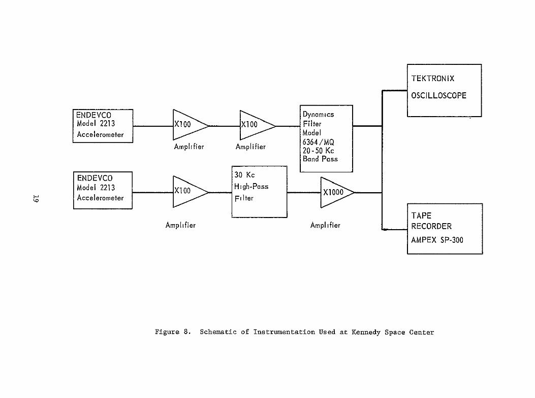
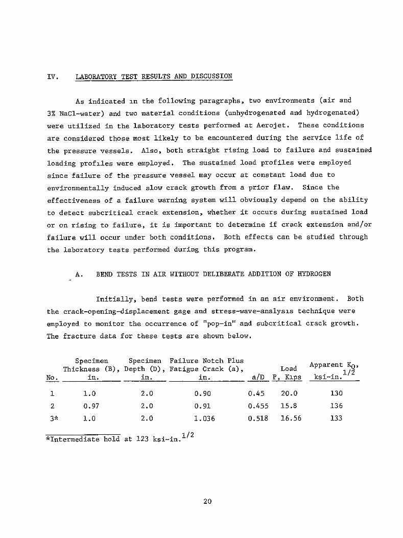
IV B Bend Tests in Water Without Deliberate Addition of Hydrogen (cont)
When the specimens (without hydrogenation) tested in the salt-water
environment were fractured the fracture surfaces were examined for evidence
of slow-crack growth during hold Although a small band of slow-crack growth
from the original fatigue precrack was observed it was not possible to detershy
mine how much of the crack extension occurred during rising load Onthe basis
of the COD data it would appear the majority of the extension occurred during
rising load to 15 kips from 15 to 17 kips and from 17 kips to failure although
the SWE data indicated that slow crack growth however small was occurring
during the hold periods
Figure 9 is a plot of cumulative stress-wave count over a period
of approximately 1-12 hr during hold at 15000 lb Note the indications of
a variable rate of subcritical crack growth Figure 10 shows the SWAT data
in detail (electronic counter reading every second) starting 23 min after
reaching the 15-kip load level Note that the cumfilative stress-waampe count
increased more or less continuously with brief intervals of increased slope
(when plotted to the scale of Figure 10 the increased slope was approximately 450) Figure 11 shows the SWE data obtained after adding fresh 3 NaCl-water
solution to the notch During the period of sustained load represented in
Figure 11 there were a few abrupt increases in count indicating discontinuous
crack growth together with additional intervals of increased slope (again
close to 45)
Figure 12 corresponds to the endof a short 16-kip hold (same
specimen) followed by a rise to 17 kips (approximately 125 ksi-in1 2 ) and
then a period of sustained load in 3 NaCl-water solution at 17 kips Note
the increased slope associated with the increase in load followed by abrupt
increases in count characteristic of discontinuous crack growth Approximately
600 sec after starting the hold at 17 kips an air hose produced high-frequency
noise too high to be removed by the filter This was recorded as an abrupt
increase in couni followed by a period of increased slope (again approximately 45) It cannot be definitely stated whether the increased slope indicating
22
1400
1200
1000
Li 800 3
LU
D 600
400
SEE FIGURE 10 200 FOR DETAILS
0 0 I I I I I
0 10 20 30 40 50 60 70 80 90 100
-MINUTES HOLD AT 15 KIPS
Figure 9 Cumulative Stress Wave Count vs Time Specimen No 4
A302B Steel 15 Kip Hold 3 NaCi-Water Environment
23
600
I0
20-
TIME (SECONDS)
224
6050
10 10 1O 1in20 20a 2100 2150
TIME (SECONDS) 220 3 am250 20 20 3w245 24W
43O
600
40
20
140
011 115 la 1in0 1 TIME (SECONDS)
a 14W 1m 53 0 inlW
Figure 11 Cumulative Stress Wave Count vs Time Specimen No 4 A302B Steel 15 Kip Hold After Replenishing the 3 NaCl-Water Environment
25
23
00
60
20
20
- 4o
o_ 4 o l~ ~ aiE~
220
IV B Bend Tests in Water Without Deliberate Addition of Hydrogen (cont)
continuous stress-wave emission was an artifact produced by the high-frequency
noise or the increased slope was the result of crack growth stimulated by the
high-frequency sound (crack growth after periods of dormancy can be initiated
by tapping a test specimen under load) Figure 13 is a plot of the cumulative
count for the 17-kip hold (corrected to zero at the start of hold and corrected
for noise which occurred at 836 sec) Note the tendency for increasing slope
with increasing time at load Figure 14 presents the SWAT data in detail
after 1 min at 17 kips load Figure 15 presents the data obtained after
1-12 min at 17 kips load Both Figures 14 and 15 are plotted to the same
scale as Figures 10 11 and 12 Table II presents the data plotted in
Figures 13 14 and 15 without correction for noise which occurred at 836 sec
this tabulation shows the detailed information that can be obtained by SWAT
On the basis of the SWE dpta this specimen showed evidence of
very slow continuous crack growth of the type one might expect of electroshy
chemical dissolution at the crack tip interspersed with short periods of more
rapid continuous crack growth There was little or no evidence of disconshy
tinuous crack growth with clearly defined periods of dormancy and there were
few instances of abrupt increase in count to signify crack jumps
C BEND TESTS IN AIR WITH DELIBERATE ADDITION OF HYDROGEN
After hydrogenation and baking 3 hr at 3000 F to produce a
homogeneous interstitial solid solution specimens were tested in 70degF air
Specimen 5 (Figure 16) developed discontinuous crack growth while under
sustained load starting at 9000 lb (75 ksi-in 2) but the occurrences were
sporadic and infrequent At 13000 lb (110 ksi-in 2) there was only one
stress wave large enough to be recorded as a cumulative count (cumulative
count increased from 3086 to 3110 corresponding to 464 SWEsec count rate)
Otherwise there was no increase in the SWE cumulative count during hold at
13000 lb
27
TABLE II
DETAILS OF SWE DATA OBTAINED FOR SPECIMEN NO 4 A302B STEEL DURING HOLD AT 17 KIPS IN 3 NaCI-WATER ENVIRONMENT
Time at Count Interval Time at Count Interval Load Rate Cumulative At Load Rate Cumulative A t (sec) (SWEsec) Count (sec) (set) (SWEsec) Count (sec)
27 57 8 - 1330 11 632 9 47 134 12 20 1331 20 634 1 101 4 14 54 1341 58 635 10 152 3 16 51 1392 232 652 51 299 10 27 147 1400 262 653 8
5 MINUTES 1405 134 654 5 329 1 29 30 1415 9 656 10 357 47 37 28 1443 85 657 28 444 72 49 87 1446 48 659 3 460 64 56 16 1478 131 675 32 494 221 60 34 1479 2 676 1 511 145 62 17 1495 29 685 16
10 MINUTES 25 MINUTES 616 115 72 105 1503 170 689 8 744 128 85 128 1505 72 691 2 788 2 92 44 1526 171 697 21 836 2 411(Noise) 48 1527 1 698 1 838 7 411 2 1537 187 702 10 843 10 431 5 1546 220 705 9 845 68 431 2 1584 89 715 38 846 7 431 1 1597 119 726 13 855 161 447 9 1650 146 738 53 880 160 468 25 1666 1 749 16
15 MINUTES 1671 162 756 5 904 11 492 24 1674 86 758 3 915 209 500 11 1695 120 780 21 943 5 523 28 1708 75 782 13 956 22 537 13 1717 1 787 9 980 4 541 24 1721 84 792 4 992 13 542 12 1732 114 794 11
1012 69 544 20 30 MINUTES 1088 21 558 76 1808 228 803 76 1108 151 569 20 1821 179 805 13 1136 il 576 28 1825 22 808 4 1154 5 582 18 1833 196 809 8 1172 38 583 18 1839 120 811 6 1178 19 585 6 1852 45 814 13 1182 9 -592 4 1866 146 816 14 1196 26 594 14 1888 168 819 22
20 MINUTES 1895 14 823 7 1228 80 598 32 1909 157 826 14 1229 13 599 1 1933 29 832 24 1238 2 605 9 1950 10 836 17 1256 1 610 18 1956 46 837 6 1312 91 613 56 1977 71 838 21 1318 1 619 6 1988 101 839 11 1321 1 621 3 2000 10 841 12
TABLE II (cont)
Time at Count Interval Time at Count Interval Load Rate Cumulative At Load Rate Cumulative Lt (sec) (SWBsec) Count (sec) (sec) (SWEsec) Count (sec)
2002 59 843 2 2515 40 1013 34 2017 119 845 15 2518 207 1017 3 2020 148 847 3 2521 1 1023 3 2033 165 848 13 2525 602 1029 4 2039 103 850 6 2527 22 1034 2 2048 9 857 9 2548 52 1052 21 2061 129 860 13 2561 47 1058 13 2063 156 862 2 2573 17 1062 12 2069 167 864 6 2585 69 1072 12 2075 98 874 6 2588 42 1073 3 2076 3 879 1 2599 240 1075 11 2093 21 881 17 2605 4 1077 6
35 MINUTES 2615 23 1078 10 2107 1 883 14 2616 57 1079 1 2108 103 884 1 2613 11 1080 15 2118 121 885 10 2638 42 1081 7 2119 191 887 1 2648 2 1087 10 2135 154 891 16 2650 87 1088 2 2140 11 892 5 2653 100 1089 3 2146 3 894 6 2656 56 1090 3 2150 178 897 4 2661 63 1091 5 2159 51 902 9 2685 28 1094 24 2162 7 905 3 2693 35 1097 8 2180 57 909 18 45 MINUTES 2182 58 910 2 2701 113 1104 8 2193 17 913 11 2703 50 1105 2 2195 113 916 2 2713 53 1109 10 2207 115 919 12 2719 20 1110 6 2221 34 923 14 2721 33 1112 2 2223 87 926 2 2738 72 1115 17 2238 35 936 15 2740 15 1116 2 2258 2 943 20 2752 100 1117 12 2268 204 947 10 2756 85 1119 4 2289 10 949 21 2768 56 1121 12 2307 1 952 18 2780 13 1130 12 2319 121 955 12 2782 28 1135 2 2346 20 959 27 2795 60 1142 13 2366 69 963 20 2809 65 1144 14 2386 20 975 20 2841 55 1156 32 2387 5 976 1 2848 3 1157 7 2392 158 978 5 2851 2 1159 3 2396 8 981 4 2862 45 1163 11
40 MINUTES 2869 35 1166 7 2403 21 983 7 2879 18 1169 10 2409 241 986 6 2885 62 1171 6 2449 95 996 40 2905 55 1175 20 2457 24 998 8 2908 54 1178 3 2473 104 1002 16 2918 7 1182 10 2481 3 1003 8 2924 8 1186 6
29
TABLE II (cont)
Time at Count Interval Time at Count Interval Load Rate Cumulative t Load Rate Cumulative t (sec) (SWIsec) Count (sec) (sec) (SWEsec) Count (sec)
2938 12 1193 14 3341 207 1410 2948 95 1201 10 3366 103 1421 25 2966 10 1215 18 3377 8 1424 11 2968 43 1216 2 3378 12 1425 1 2972 22 1217 4 3390 2 1429 12 2979 8 1221 7 3396 3 1430 6 2987 8 1223 8 3397 14 1432 1 2998 38 1226 11 3401 8 1434 4
50 MINUTES 3402 98 1438 1 3002 36 1228 4 3408 12 1443 6 3010 55 1230 8 3410 16 1448 2 3011 3 1234 1 3413 6 1452 3 3016 1 1236 5 3431 2 1454 8 3017 3 1237 1 3433 17 1458 2 3023 3 1239 6 3435 30 1460 - 2 3029 3 1240 6 3438 22 1462 3 3033 1 1243 4 3450 8 1475 12 3036 110 1245 3 3455 62 1484 5 3037 4 1248 1 3461 154 1490 6 3053 83 1259 16 3462 7 1493 1 3054 7 1260 1 3466 11 1501 4 3061 2 1265 7 3472 2 1507 6 3062 83 1266 1 3476 46 1509 4 3076 62 1275 14 3489 18 1515 13 3080 5 1278 4 3490 8 1517 1 3098 32 1294 18 3508 15 1534 18 3100 15 1296 2 3513 25 1541 5 3102 16 1297 2 3520 220 1549 7 3108 7 1299 6 3538 29 1566 18 3114 7 1301 6 3542 9 1572 4 3127 6 1304 13 3543 107 1575 1 3129 1 1305 2 3558 240 1588 15 3133 1 1306 4 3568 30 1601 10 3140 5 1309 7 3570 21 1603 2 3154 30 1312 14 3573 66 1607 3 3170 6 1320 16 3579 9 1613 6 3175 77 1322 5 3591 37 1619 12 3177 110 1323 2 60 MINUTES 3178 5 1324 1 3607 128 1622 16 3183 4 1326 5 3608 70 1626 1 3187 137 1331 4 3609 2 1629 1 3191 14 1332 4 3624 50 1638 15 3200 3 1336 9 3630 14 1642 6 3206 2 1340 6 3639 86 1645 9 3214 20 1343 8 3660 56 1662 21 3219 22 1345 5 3678 13 1669 18
55 MINUTES
30
TABLE II (cont)
Time at Count Interval Time at Count Interval Load Rate Cumulative At Load Rate Cumulative At (sec) (SWEsec) Count (sec) (see) (SWEsec) Count (sec)
3688 33 1680 10 4535 105 2574 28 3692 35 1682 4 4547 3 2589 12
3709 209 1688 17 4583 4 2616 36 3712 7 1689 3 4623 460 2670 40 3720 78 1691 8 4624 37 2703 1
3730 93 1694 10 4626 18 2715 2 3731 5 1695 1 4627 840 2729 1 3743 13 1703 12 4630 141 2737 3 3744 120 1709 1 4662 2 2758 32
3750 24 1715 6 4671 1 2763 9 3755 142 1724 5 4698 1 2774 27 3767 45 1738 12 4710 8 2782 12 3796 69 1770 29 4719 6 2784 9 3823 21 1808 27 4731 128 2785 12 3844 10 1838 21 4761 17 2810 30 3854 82 1851 10 4783 22 2822 22 3856 13 1855 2 4786 23 282A 3 3895 75 1915 39 80 MINUTES
65 MINUTES 4822 96 2831 36 3901 18 1920 6 4852 1 2842 30 3905 54 1927 4 4934 59 2890 82
3946 58 1963 41 4953 200 2907 19 3970 2 1985 24 4954 26 2910 1 3971 181 1988 1 4957 16 2916 3 3974 61 1990 3 4964 56 2923 7 3975 28 1992 1 4988 29 2941 24 3987 51 2004 12 5000 88 2951 12 4012 2 2022 25 5031 10 2977 31 4013 31 2026 1 5032 9 2978 1 4022 7 2036 9 5045 56 2982 13 4054 4 2062 32 5054 4 2984 9 4056 16 2066 2 5093 220 2992 39 4084 37 2093 28 85 MINUTES 4091 36 2099 7 5122 115 2996 29 4100 3 2111 9 5166 17 3019 44 4129 16 2142 29 5190 172 3042 24 4156 6 2165 27 5193 55 3045 3
70 MINUTES 5194 2 3048 1 4241 19 2253 85 5224 313 3081 30 4292 4 2299 51 5248 23 3106 24 4331 42 2339 39 5266 32 3123 18 4338 19 2348 7 5281 24 3138 15 4340 66 2350 2 5291 10 3150 10 4345 10 2359 5 5303 25 3164 12 4385 4 2419 40 5306 1 3169 3 4397 121 2432 12 5324 56 3187 18
75 MINUTES 5330 58 3193 6 4500 40 2534 103 5345 31 3211 15 4507 6 2542 7 5351 155 3217 6
31
TABLE II (cont)
Time at Count Interval Time at Count Interval Load Rate Cumulative At Load Rate Cumulative At (sec) (SWBsec) Count (sec) (sec) (SWEsec) Count (sec)
5357 211 3223 6 5887 185 3536 1 5363 29 3233 6 5905 65 3559 18 5364 20 3237 1 5923 31 3575 18
90 MINUTES 5924 22 3576 1 5403 118 3276 39 5933 109 3578 9 5418 79 3295 15 5934 5 3579 1 5419 44 3298 1 5961 43 3582 27 5420 35 3300 1 100 MINUTES 5448 27 3324 28 6000 23 3585 39 5460 118 3327 12 6001 13 3586 1 5466 97 3329 6 6002 166 3588 1 5472 184 3331 6 6008 9 3590 6 5484 28 3333 12 6032 29 3592 24 5499 45 3338 15 6041 111 3596 9 5505 2 3341 6 6062 116 3601 21 5506 173 3344 1 6083 1 3603 21 5512 72 3346 6 6084 236 3606 1 5515 8 3348 3 6090 140 3607 6 5536 199 3352 21 6091 104 3608 1 5548 5 3356 12 6106 21 3609 15 5553 199 3359 5 6115 31 3611 9 5554 34 3360 1 6121 29 3614 6shy5587 190 3364 33 6124 1 3622 3 5593 2 3365 6 6139 51 3630 15 5605 6 3367 12 6160 25 3634 21 5611 12 3369 6 6175 5 3636 15 5638 3 3373 27 6184 196 3639 9 5644 57 3374 6 6217 275 3645 33 5645 78 3376 1 6223 84 3648 6 5669 21 3379 24 6238 23 3649 - 15 5693 22 3384 24 6244 99 3650 6 5699 48 3385 6 6250 81 3652 6
95 MINUTES 6259 39 3654 9 5702 74 3387 3 6265 15 3656 6 5703 85 3389 1 6271 21 3658 6 5725 21 3391 22 6283 85 3660 12 5737 1 3394 12 105 IWNUTES 5752 72 3396 15 6304 143 3662 21 5761 106 3398 9 6331 50 3672 27 5788 1 3414 27 6340 179 3674 9 5794 176 3422 6 6341 37 3675 1 5809 2 3441 15 6365 34 3677 24 5810 15 3445 1 6366 ill 3680 1 5813 42 3448 3 6393 150 3682 27 5814 189 3451 1 6405 43 3684 12 5823 180 3461 9 6429 4 3687 24 5832 171 3472 9 6435 127 3690 6 5838 46 3481 6 6459 31 3691 24 5859 63 3505 21 6483 7 3694 24 5865 15 3511 6 6495 30 3696 12 5886 2 3533 21 6501 128 3700 6
32
TABLE II (cont)
Time at Count Interval Time at Count Interval Load Rate Cumulative At Load Rate Cumulative At (sec) (SWEsec) Count (sec) (sec) (SWEsec) Count (sec)
6522 87 3703 21 7278 21 4158 6 6531 16 3704 9 7302 2 4174 24 6555 102 3706 24 7303 3 4174 1 6567 7 3709 12 7318 125 4186 15 6570 10 3710 3 7348 88 4205 30 6576 87 3711 6 7402 86 4238 54 6577 89 3713 1 7435 90 4258 33 6578 131 3714 1 7447 14 4262 12 6599 4 3717 21 7474 14 4277 27
6600 110 MINUTES
8 3718 1 7486 7504
9 125 MINUTES
89
4286
4304
12
18 6603 37 3720 3 7510 39 4308 6 6639 15 3724 36 7531 52 4331 21 6669 48 3728 30 7540 208 4344 9 6675 23 3729 6 7549 38 4353 9 6684 57 3731 9 7576 72 4376 27 6705 23 3757 21 7594 24 4392 18 6744 53 3807 39 7603 55 4403 9 6762 240 3830 18 7615 160 4415 12 6783 5 3854 21 7621 134 4420 6 6801 26 3874 18 7627 160 4423 6 6822 181 3901 21 7639 180 4430 12 6852 24 3934 30 7648 5 4432 9 6879 44 3962 27 7658 100 4437 10 6882 2 3965 3 7679 319 4445 21
115 MINUTES 7694 72 4449 15 6906 63 3991 24 7709 23 4451 15 6927 176 4001 21 7721 34 4453 12 6930 15 4006 3 130 MINUTES 6931 54 4011 1 7800 Test Terminated 6952 305 4026 21 6953 40 4033 1 6980 3 4037 27 6989 99 4039 9 7040 387 4080 51 7041 53 4095 1 7056 23 4100 15 7086 354 4108 30 7095 21 4110 9 7125 70 4117 30 7131 2 4120 6 7167 97 4129 36 7176 11 4130 9 7197 18 4133 21
120 MINUTES 7218 28 4136 21 7227 39 4138 9 7248 72 4146 21 7272 50 4153 24
33
40
38W
3400
32W
30
28M
260
= 2400
S 22DD
i20
1600
1400
1200
10
600
400
200
06 1a 20 30 40 50 60 70 80 90 tW 110120130
MINUTE-S-H-OLD 17KIPS
Figure 13 Cumulative Stress Wave Count vs Time SpecimE A302B Steels 3 NaC1-Water Environment
34
3503
0
~0
40
20
3203
00
20
C0
20
310
03
(0
40
= = 20 0 I- 365~
05
20 00
20
0shy20
2003
20 ~~0 C
20
20 40
- 20
2835
0
(0
20
20shy
20020
20 -
3403 3450 3720 3750 fl 3550 3003 3050 40) 4050 4003 4050 4~fl 4200 4020 4350 4440 4450
TIME (SECONDS)
Figure 14 Cumulative Stress Wave Count vs Time Specimen No 4 A302B Steel After 1 Minute at 17 Kip Hold in 3 NaCi-Water Environment
35
48
0
I-
S 40
us 50 50 70 5 90 0 60 60 10 6 6 t 20CO DS
- iue1CmlaieSrs av on sTme pcmnN A0BSel
Afe2-0iue t1 i todi NC-ae niomn
Page60
4520 -
so- lao
F
122021 amp~
20 4
400
20
20 22
3540 =
20
3024
20
50
45
20
20520
20
20
45
20
no
I
40
4~
20
40
20
20
4
20
2020
20
gt
20
20 4
20
20
3545
20
Iino200j
5505
2220
1120
20
001
20
20 shy
00
1
45
OX
I
I I
I I
0 50
020 000
205 200
20 200
Z
40 505
550 400
TIM
E (S
EC
ON
DS
)
Figure 16
Cumulative Stress Wave Count vs
Time Specimen No
5 A302B Steel
Hydrogenated and Tested in Air
37
IV C Bend Tests in Air With Deliberate Addition of Hydrogen (cont)
On raising the load from 13000 to 14000 lb (122 ksi-in )
there was evidence of a creep phenomenon as shown in Figure 17 The crackshy
opening-displacement gage confirmed the occurrence of crack growth continuing
after reaching the 14000-lb hold Stress-wave emission showed the mechanism
to be discontinuous cracking rather than a deformation process When the
count rate was plotted as in Figure 18 the activity carrying into the
14000-lb hold again was discontinuous After approximately 300 sec at 14 kips
the SWE associated with the creep phenomenon had subsided During the 14-kip
hold there were two crack jumps one after 920 sec (cumulative count increased
from 5618 to 5720 and the count rate associated with the jump was 181 as
counted over a 10-sec interval or 18 SWEsec) and one after 2130 sec (cumulashy
tive count increased from 5721 to 5755 and the count rate was 139 in 10 see)
After 5000 sec at 14 kips the load on Specimen 5 was raised As
seen in Figure 19 the stress-wave activity was an unmistakable presage of
instability which occurred after 20 sec into hold The load reached a maximum
of 145 kips (145 ksi-in 2) Technically the onset of instability occurred
shortly after starting to increase the load ie at approximately
132 ksi-inI2 which agrees with the KQ value obtained through rising load
tests of unhydrogenated material in an air environment
Because of the very long test period and multiple loadings involved
in the testing of the Specimen 6 only data obtained during rising load to
19500 and 19800 ib during sustained test periods at these loads and during
specimen failure are shown in Figure 20 These data indicate essentially the
same SWE-crack growth relationships discussed previously for Specimen 5 except
that on reaching hold the crack tended to grow slowly for a longer period of
time in comparison to the behavior noted for Specimen 5 Also the incremental
nature of crack extension was more readily observed by the stress-wave-emission
data for Specimen 6
38
20
560
80
60
40
20
5500
80
60
40
20
5400
o 5100
808
60
40
20
5000 u-J
4500
4480 80 4- START 14-KI P HOLD
CODC 75lt
4000
3980 70
3960
6553120 l
- END13-KIP HOLD
3100 160 0 40 80 120 160 200 240 280 320
TIME AT LOAD (SECONDS)
Figure 17 Cumulative Stress Wave Count and COD vs Time Specimen No 5 A302B Steel fydrogenated and Held at 14 Kips in Air
39
200
LU
LU
1- 100
50 END 13-KIP
25 HOLD-I
0 1- TIME
100 INSECONDS AT
200 14KIPS
300
(COUNT EVERY 10 SEC)
Figure 18 Stress Wave Count Rate vs Time - Specimen No 5 A302B Steel Hydrogenated and Tested in Air
40
INSTABILITY
9580
9560
9540
9380
928D0
9260
842D
8440
73O I-shyz 7220
o 7260
U 7240
7220
7180I-shy
7160
- 7140
7120
7100
7080
7060
5900
5880
5860
5840
5820
5800
578D
5460
0 40 80 120 160 SEC
4M 4960 50D RISING LOAD-SECONDS AT 14 KIPS
Figure 19 Cumulative Stress Wave Count vs Time Specimen No 5 A302B Steel Hydrogenated and Tested in Air
41
20000
18000
FAILURE
18290 sec a- 1 17-in K - 199 s - Y
z
-
16000
14000
l0
1200
I-9 Iin
1014in K 152 ki- in -i
o-1 09 n K- 176ksmn
- 1 07 in I 170 iis-
o -1 042in K 12ks-in
c023i NK15ks-n
-shy
-
10000
REACH 19800 lbs
START TO 19800 bs
10000 11000 12000 13000 14000 15000 16000 17000 18000 19000
TIMESECONDS
12000
11000 s
p9000
T LOAD ADJUSTMEA
7n000
READOUT6000 OTE STRESS WAVE DATA A UST T
500 Vgt 0 ENT CORRESPONDIG TO SLOPELOAADJUSTM15 CHANGES PLOTTED
a 4000
3000
LOAD ADJUSTMENT2000 SECONDSECMENIME
1000 START HOLD AT 19500 1b
900 1l6070 D0 8 0 00 0 000600
0 1000 50002000 3000 4000
TIME SECONDS
Figure 20 Cumulative Stress Wave Count vs Time Specimen No 6 A302B Steel Hydrogenated and Tested in Air
Page 42
IV C Bend Tests in Air With Deliberate Addition of Hydrogen (cont)
As indicated in Figure 20 the increase in crack length during
the initial period of hold at 19500 lb resulted in an increase in the applied
stress intensity and was accompanied by significant stress-wave-emission
activity To maintain the desired load it was also necessary to make frequent
load adjustments at the start of hold During the first 3600 sec the effecshy
tive crack length increased from approximately 0963 to 1000 in and was
accompanied by about 7000 SWE As indicated in Figure 20 the majority of the
SWE activity and increase in crack length occurred during the first 3000 sec
of the hold at 19500 lb After this period both the stress-wave-emission
activity and rate of increase in crack length gradually decreased For example
during the entire period from 5000 to 17600 sec when the load was increased
to 19800 lb the apparent crack length and SWE count increased by only approxishy
mately 0020 in and 2500 respectively
After approximately 17000 sec at 19500 lb the load was increased
to 19800 lb and specimen failure occurred after approximately 600 sec at
19800 lb The load was maintained for this period however it was apparent
from both the SWE and COD gage data that the crack was extending and specimen
failure would occur without a further increase in load although it was necesshy
sary to continually adjust the tensile machine to maintain the desired load
The failure stress intensity approximated 199 ksi-in 2however technically
the onset of instability occurred after starting to increase the load at
approximately 153 ksi-in1 2
Specimen 7 was also hydrogenated baked at 300F for 3 hr and
tested in air Figure 21 is a detailed plot of the SWAT data (electronic
counter print-out every second) indicating crack growth of a discontinuous
nature starting at 2400-lb load Note the periods of dormancy (no increase
in SWE count) interspersed with abrupt increases in count indicating disconshy
tinuous crack growth Note also that there was little or no evidence of
continuous stress-wave emission until the load (stress intensity level) was
high approaching failure
43
CUMULAIY STRESS-VAVE COUNTCU LTISTE W E ON
I OT A~II I OI I L I I I I I I I I I I I I I I i I I I I I
- N LB
I I I I I I I I I I I I I i I I
--L - 0OTO11
-0101
(lNIML~ 33383338
8
133113-
3IiC)0 83) 3103 31-3(31-
~0
33 331
3l3C0C~
38318shy
111(10 CAVMSS3 nfl CAliVi flWfl3
________________________________________________________________________
111fl0~ 3KvM~s~a1Ff~TfvTifwT
FPAIAE
hY
A Ii
8
INa
CZ
8 C0 U CI
33 S
1 H
H
03 -I
~ 3lt
0 Cd 33
~C3 ~ H
8 0003
A
Ofli3i~~ C)
Page 45
IV C Bend Tests in Air With Deliberate Addition of Hydrogen (cont)
Figure 22 presents the SWE data from a hydrogenated bend specimen
(No 8) tested in air The load was increased continuously to 9800 lb
(70 ksi-in 2) where there was a short hold (approximately 400 sec) Note
the discontinuous crack growth followed by a short period of continuous
emission (less than 450 slope) The load was then raised to 14800 lb
(109 ksi-in 2) and held for approximately 400 sec Again there were jumps
in the SWE cumulative count but this time interspersed with continuous
emission The SWAT system employed for this test corresponded to that employed
for the background measurements at Kennedy Space Flight Center and shown in
Figure 8 only one channel was employed viz
Endevco 2213 Amplifier Amplifier Band-Pass Filter 10OX 10OX 20 to 50 Kcps
The continuous stress-wave emission observed during hold at the higher stressshy
intensity level in this specimen was not observed in the other hydrogenated
specimens tested in air The primary purpose of this test (Specimen 8) was to
record SWE data for subsequent playback and analysis to determine the amplitude
of burst-type stress-wave emissions associated with fracture in Type A302B
steel These analyses were performed using the instrumentation shown in
Figures 7 and 8 with the following results which are discussed in more detail
in conjunction with the results of the background measurements performed at
Kennedy Space Flight Center (Section V)
Maximum SWE Amplitude - 39 x 10-3g
Minimum SWE Amplitude - 12 x 10-3 g
Average SWE Amplitude - 22 x 10-3g
Laboratory Background - 11 x 10-3g
46
00 o z~ 20 ~
40
~40
S20 1 2 0 0 0 0
TIIAEAT 4 S-KIPHOLD (10KS(51IN A)
407
IV Laboratory Test Results and Discussion (cont)
D BEND TESTS IN 3 NaCI-WATER WITH DELIBERATE ADDITION OF HYDROGEN
Specimen 9 was hydrogenated baked and tested in 80F water
The electronic counter indicated continuous stress-wave emission interspersed
with abrupt increases in count indicating occasional crack jumps Figure 23
shows the details of stress-wave emission that occurred during both rising
load and holding load The crack length determined from the COD chart at
selected loads is also shown Note from the SWE data that there were no
periods of dormancy and the slope of the plot of cumulative count versus time
indicated moderately rapid continuouas crack growth such as might occur with
electrochemical dissolution at the crack tip The COD gage data shown in
Figure 23 also indicate crack extension however the actual amount appears
to be quite small (lt01 in) which would be consistent with the relatively
small number of stress-wave emissions detected even at the high system
sensitivity employed The dramatic difference between the behavior in
Figures 21 and 23 for hydrogenated material tested in air (Figure 21) and
water (Figure 23) indicates that hydrogen and 3 sodium chloride solution
acting together have a greater total effect than the sum of their individual
effects ie working together they appear to have produced a synergism
E WOL TESTS
Because of the possible significance of the synergistic-effect
noted above on the life of the hydrogen pressure vessels at Kennedy Space
Flight Center additional testing was performed using hydrogenated WOL specishy
mens cut from the fractured bend specimens The first WOL specimen was
initially loaded to-3650 lb (50 ksi-in 2) and then placed in 3 NaCl solution
(notch immersed) There was 30 min of essentially continuous stress-wave
emission (recorder started approximately 5 min after loading the specimen)
Subsequently therewas one sizable jump in the SWE cumulative count after
48
V30
760
740-M
$
720 -s
680shy
60
610
40 w
w
520 w
i
20500
HOLDD]N
340
20 760
7200
ING
IV
O
shy
420
60
40
20 0 2
04
0Q
0
60DO
LO0
01 200
250 300
350 400
450 500
550 6M
650
700 750
TIME
(SECONDS)
Figure 23
Cumulative Stress Wave Count vs Time Specimen No 9 A302B Steel
Hydrogenated and Tested in 3 NaCi-Water Environment
49
IV E WOL Tests (cont)
approximately 3 hr 40 min Then 3 hr 20 min later several jumps occurred
followed by 8 hr 20 min of stress-iave activity After this the crack was
dormant (total test time 17 hr 25 min) These data are shown in Figure 24
The load was then increased slightly (torque was increased from 200 to
255 in-lb) an additional 1-12 hr in 3 NaCl solution produced no significant
increase in the cumulative stress-wave count The reason for this apparently
anomalous behavior was not determined although it may result from a blunting
effect at the crack tip produced during the initial hold period
The fatigue crack was then extended (approximately 005 in) in
tension-tension fatigue and the specimen reloaded to approximately 51 ksi-in2
Stress-wave emission started almost immediately (dashed curve in Figure 24)
After approximately 3 hr of discontinuous activity the periods of dormancy
tended to increase interspersed with relatively small jumps (as counted over
10-sec intervals) The results of the initial loading and the reloading are
shown in Figure 24 note that there was appreciably lower cumulative count in
the reloaded specimen as compared with the initial loading for a comparable
period of test
A second hydrogenated WOL specimen was then tested in air at
50 ksi-in 2 there were stress waves initially (creep) but then very little
activity over the remaining 35-hr test period After the first hour the
count increased from approximately 150 to only 280 in the final 34 hr of test
Figure 25 shows the long peribds of dormancy punctuated by occasional 1-count
increases This is in marked contrast to the results obtained from the
hydrogenated WOL specimens tested in 3 NaCl solution and the bend-test
findings of a synergistic effect were confirmed
50
------------
aa
L- -- -- - ------ - --- I
3
IN DO
INTES) 3 S IOTI E( LI N LU
Ino
a
N O
TIME (MINUTES) IN 3 NCI SOLUTION
Figure 24 Cumulative Stress Wave Count vs Time at Hold WOL Specimen No 1
A302B Steel Hydrogenated and Tested in 3 NaCi-Water Environment
51
000 In 0 M6020 126 24 022 in0 1180 10 11 100 IWO l 100M M-C 0 90w6 a0 w6
t t t t 5W MOD4
10
TIME (MINUTES)
Figure 25 Cumulative Stress Wave Count vs Time at Hold WL Specimen No 2 A302B Steel Hydrogenated and Testd in Air
52
IV Laboratory Test Results and Discussion (cont)
F DISCUSSION
1 Material-Environment Consideration
The Type A302B steel supplied for evaluation exhibited a
very high level of fracture toughness Although quantitative plane-strain
fracture toughness measurements were not possible because of the large specimen
size required the KQ value associated with failure approximated 135 ksi-in1 2
This material was also found resistant to environmentally induced failure in
that the rate of crack growth of a prior flaw at applied stress-intensity
factors as high as 90 of the KQ value appeared to be very low This effect
was observed for unhydrogenated-material tested in air and a 3 NaCl-water
environment and hydrogenated material tested in an air environment However
the hydrogenated specimens tested in 3 NaCl-water environment had a much
faster rate of subcritical crack gr~wth in comparison to the other test condishy
tions indicating a synergistic effect due to the combination of sea water and
hydrogen in interstitial solid solution This synergistic effect indicates
that the Type A302B steel hydrogen storage tanks in the Kennedy Space Flight
Center environment may have limited life as the result of subcritical crack
growth if subjected to the same combination of stress and environmental
factors-
The WOL test results tended to confirm the possible synergism
due to the combined effects of 3 NaCl-water and hydrogen in interstitial solid
solution Marked SWE activity was observed when the hydrogenated specimens
were immersed in the salt water whereas in an air environment after the
initial period at hold when a creep phenomenon was observed there was essenshy
tially no stress-wave emission The fact that failure was not produced on
holding (in contradiction to the bend tests) can be explained by the fact that
the WOL test as-performed in this program is a self-arresting test because
53
IV F Discussion (cont)
the occurrence of crack growth results in a reduction in the applied load
Conversely in the bend tests the load was constantly applied as the crack
extended and eventually resulted in specimen failure
2 Stress-Wave-Emission Characterization
Detectable stress-wave emissions although of small amplitude
(ltOOlg) were observed to be associated with crack growth in Type A302B steel
Under all test conditions the stress-wave emissions were observed both during
rising load and when failure (instability) was imminent During hold various
SWE characteristics depending on the test conditions were observed When
tested in the hydrogenated condition in-an air environment a creep phenomenon
evidenced by increasing count of SWE and an accompanying increase in apparent
crack size was observed With time at hold and at applied stress-intensity
levels less than critical the creep phenomenon eventually stopped as did the
occurrence of stress-wave emissions Unhydrogenated material tested in the
3 NaCl-water environment produced continuous stress-wave emission punctuated
by abrupt increases in SWE count This behavior indicates both continuous
very small increments of crack extension with larger crack jumps corresponding
to the abrupt increases in SWE count Continuous incremental crack extension
characterized by continuous SWE interspersed with abrupt increases in SWE count
indicating occasional crack jumps was also observed in testing hydrogenated
material in a 3 NaCl-water environment
In all instances when failure (instability) occurred both
the amplitude and rate of stress-wave emission increased and could be employed
as a precursor of the onset of instability however even when failure was
approached-the SWE amplitude was small (ltOlg) In the other instances where
failure was not produced evidence of crack extension (although very small in
some instances) was observed on the specimen fracture face Once evidence of
54
IV F Discussion (cont)
crack growth was observed (by SWE or COD) it is obvious that failure would
eventually occur (assuming a constantly applied load) although depending on
the initial flaw size and subcritical growth rate the time to failure may be
very long In actual practice the SWE data could be employed (1) to locate
the propagating flaw (2) to monitor its occurrence and (3) as a basis for
terminating service so that repairs could be made before failure The stressshy
wave emissions associated with crack growth during rising load or increasing
stress intensity and the creep phenomenon during the initial part of hold
can be employed for this purpose
5S
V BACKGROUND MEASUREMENTS AND ASSOCIATED LABORATORY TESTS
A BACKGROUND MEASUREMENTS AT KENNEDY SPACE FLIGHT CENTER
Background noise measurements were made at two locations the VAB
Bottle Field and Pad A at the Kennedy Space Flight Center The data were tape
recorded and in addition to general background noise included tank blowdown
and repressurization periods The instrumentation for this purpose is shown
schematically in Figure 8 analysis of the data was performed by playback onto
an oscillograph and comparison with the SWE-crack growth data obtained during
the laboratory testing of bend specimens
The analysis of the signal amplitude data for tests at Cape Kennedy
is indicated below
1 Pad A Bottle Field
Signal Amplitude
a Quiescent Background
Filter at 20 Kcps - 50 Kcps -BandPass- 99 x 10 gsBand Pass
Filter at 200 cps - 32 Kcps
Band Pass
b Tank Blowdown - System Saturation (gt llg peak to peak)
C Tank Repressurization - System Saturation (gt llg peak to peak)
2 VAB Bottle Field
a Quiescent Background - 22 x 10- 4 gs
56
V A Background Measurements at Kennedy Space Flight Center (cont)
Signal Amplitude
b Tank Blowdown - System Saturation (gt llg peak to peak)
C Tank Repressurization - System Saturation (gt llg peak to peak)
Analysis of the tape-recorded data of bend tests at Aerojet indicates
the following signal amplitude for burstf-type stress-wave emissions associated
with crack growth and fracture in Type A302B steel
Maximum Amplitude - 39 x 10-3g
Minimum Amplitude - 12 x 10-3g
Average Amplitude - 22 x 10-3g
Laboratory Background - 11 x 10-3g
Thus the amplitude of SWE associated with crack growth in A302B steel is
approximately an order of magnitude larger than the background noise noted
previously Consequently the above results show that it is possible to detect
stress-wave emissions associated with fracture in A302B steel under the quiescent
background conditions existing at the Kennedy Space Center Difficulty is
expected in detecting such flaw growth during tank blowdown and repressurization
periods unless filtering can be employed to screen out the noise associated
with these periods However the blowdown and repressurization periods are of
very short duration and the materials behavior observed in this program indishy
cated that considerable prefailure crack extension would be expected from any
flaw of a size expected to be present in these pressure vessels Also
immediately on reaching load a creep phenomenon evidenced by an extension
in apparent crack length and accompanied by detectable stress-wave emission
was observed Consequently even if noise associated with blowdown and
57
V A Background Measurements at Kennedy Space Flight Center (cont)
repressurization cannot be effectively filtered out significant flaw growth
andor creep could still be detected and tank depressurization accomplished
prior to catastrophic failure assuming a capability for such depressurization
exists at these locations
B LABORATORY SIGNAL ATTENUATION EVALUATIONS
Subsequent to the background measurements at the Kennedy Space
Flight Center and the bend tests at Aerojet two series of tests were made at
Aerojet using a section of pipe and plate both of SAE 4130 steel alloy The
purpose of these tests was to determine the coefficient of signal attenuation
which in conjunction with the previous test data could be used to establish
the sensor spacing which would insure detection of SWE associated with crack
growth in the pressure-vessels at the Kennedy Space Flight Center
In these tests a constant pulse was imparted to the specimen by
a Tektronix 115 Pulse Generator using a Clevite PZT-5 Crystal (2125 in dia
and 0250 in thick) The piezoelectric crystal was mounted on a small alumishy
num block which in turn was adhered to the surface of the specimen The
signal was received by a 2217-E-Endevcq accelerometer placed at various disshy
tances from the pulser The pulse used was 10 n-sec rise and fall time with
a duration of 20 microsec at an amplitude of 12v
1 Pipe Tests
A SAE 4130 steel pipe (8-58 in OD 7-18 in ID and 22 ft
10-78 in long) was used as specimen for this test series The pulser was
mounted normal to the external surface of the pipe as close as possible to the
edge The accelerometer (2217-E-Endevco) was successively placed on the pipe
58
V B Laboratory Signal Attenuation Evalutions (cont)
surface at positions I to 8 that were at 4 6 8 10 12 14 16 and 20 ft
from the pulser The signal received by the accelerometer was displayed on a
Tektronix 422 osilloscope Typical signals are shown in Figure 26
The velocities of the compressional and shear waves in steel
are
29 lO06 x38103 Vc= -x lg ) (l-26) = O2 x06(- 0 x386 = 227000 insec(+j 012)283 (1+030) (1-060)
29x106 x 386 = 91 36= 123000 insec
s 2 ( + p) p 2 (i + 030) x 0283
where E = Youngs Modulus p = Poissons Ratio and p = density The times of
arrival of these waves at the computed velocities are indicated on the oscilloshy
scope photos shown in Figure 26 The point of shear wave arrival (T ) coincides
in most of the photos to a distinct change of pattern in the trace The
arrival of the compressional wave is difficult to determine accurately because
the amplitude of this wave attenuates very fast with distance
A visual comparison of the curves shows that Figure 26a
representing the signal received 4 ft from the impulse indicates a perfectly
detectable arrival of the compressional wave conversely Figure 26h (at 20 ft
from the impulse) shows the visually detectable arrival of a wave almost at the
computed arrival of the shear wave This is due to the fact that the amplitude
of the first cycles of the compressional wave have become essentially impercepshy
tible at a distance of 20 ft from the pulse An attempt to determine signal
arrival time by visual inspection only of the traces in Figure 26 would result
in the wave velocities indicated in Table III The computed arrival times of
the compressional and shear waves are shown in Table IV If an integration of
the positive portions of the cycles comprised in 200 p sec after arrival of the
59
VERTICAL SCALE 1 DIV= 01 V VERTICAL SCALE 1 DIV = 01 V HORIZONTAL SCALE 1 DIV= 50p SEC HORIZONTAL SCALE 1 DIV = 100 pSEC
a 4FT FROM PULSER b6 FEET FROM PULSER
Tc Ts Tc Ts
VERTICAL SCALE I DIV 01 V VERTICAL SCALE I DIV = 01 V HORIZONTAL SCALE I DIV = 100 I SEC HORIZONTAL SCALE 1 DIV = 200 p SEC
c 8 FEET FROM PULSER d 10 FEET FROM PULSER
Tc = Arrival of Compressional Wave
T = Arrival of Shear Wove
Figure 26 Oscillograph Traces for Pipe Tests (Sheet 1 of 2)
6o NOT REPRODUCTBLE
VERTICAL SCALE 1 DIV = 01 V VERTICAL SCALE 1 DIV 01 V HORIZONTAL SCALE 1 DIV = 200y SEC HORIZONTAL SCALE I DIV 200 p SEC
e 12 FEET FROM PULSER f 14 FEET FROM PULSER
T TS T T
VERTICAL SCALE 1 DIV = 01 V VERTICAL SCALE 1 DIV = 01 V HORIZONTAL SCALE 1 DIV = 200 v SEC HORIZONTAL SCALE I DIV =5001p SEC
g 16 FEET FROM PULSER h 20 FEET FROM PULSER
Figure 26 Oscillograph Traces for Pipe Tests (Sheet 2 of 2)
61
V B Laboratory Signal Attenuation Evaluations (cont)
shear wave is performed the average amplitudes determined in this manner
become quite meaningful These average amplitudes are shown in Table V
TABLE III
WAVE VELOCITY BASED ON VISUAL ANALYSIS OF OSCILLOSCOPE TRACES - PIPE TESTS
Distance from Pulse Arrival Velocities Photo ft in Time psc (ftsec)
1 4 48 210 228000
2 6 72 400 180000
3 8 96 600 160000
4 10 120 800 150000
5 12 144 1000 144000
6 14 168 1200 140000
7 16 192 1400 137000
8 20 240 1750 137000
TABLE IV
COMPUTED ARRIVAL TIMES - PIPE TESTS
Compressional Wave Shear Wave Distance from Pulse Arrival Time Arrival Time
Photo in psec Osc Div sec Ose Div
1 48 212 423 390 780
2 72 317 317 583 583
3 96 422 422 778 778
4 120 530 265 972 486
5 144 635 317 1163 581
6 168 740 370 1360 680
7 192 840 420 1545 771
8 240 1050 21 1930 387
62
V B Laboratory Signal Attenuation Evalutions (cont)
TABLE V
SIGNAL AMPLITUDE VS DISTANCE - PIPE TESTS
Average Signal Amplitude Distance from 200 Psec after Arrival
Test Pulser in of Comp Wave mv
1 48 230
2 72 145
3 96 85
4 120 60
5 144 45
6 168 28
7 192 22
8 240 18
The general equation for the amplitude attenuation curve is
C x e-Xy =
where y = amplitude at distance x in volts
x = distance in inches from pulse source
C = amplitude of pulse in volts
a = attenuation factor
or iny= 1 C + (- ax) = I C - ax (Eq 4)n n
To determine the values of C and a the following statistical analysis was
performed
63
V B Laboratory Signal Attenuation Evaluations (cont)
Distance Yo y y2 X X2 Test in m v n n
1 48 230 543 +142 2010 -87 7580 - 124 261
2 72 145 499 +098 0960 -63 3960 - 62 360
3 96 85 445 +044 0194 -39 1520 - 17 427
4 120 60 409 +008 0006 -15 225 - 1 490
5 144 45 380 -021 0044 + 9 81 - 2 548
6 168 28 334 -067 0450 +33 1090 - 21 560
7 192 22 309 -092 0847 +57 3250 - 52 592
8 240 18 289 -112 1250 +105 11000 - 118 690
EY2 EX2pound x = 1080 ElnY =3208 5761 28706 SXY-397 XxIny3928
- 1080 - 3208 x =- = 135 ny = 401
EXY -397 00138 1 C =l1y + oshy
pound 2 x2 28706 n i x
= 401+(0138)(135)=401+186= 587
C - 355 mv
It is now possible to compute the statistically corrected values of the signal
amplitude y at the distances from the pulse where they were measured The
general formula will be
ny = 587 -(00138) X
and the results are tabulated in Table VI The computed value of pulse amplishy
tude at source is found to be C = 355 my The values shown on Table VI are
plotted in Figure 27 which graphically shows the signal attenuation as a
function of distance from the pulse source
64
350
300
250 STATISTICALLY COMPUTED k VALUES FOR REGRESSION CURVE
--0gt 200
EXPERIMENTALLY DETERMINED
-- MATERIAL SAE 4130 STEEL U= SPECIMEN PIPE-S758 in D aZ
00
15 7 18 in D22 ft 10 78 in LONG
-J
100
50 I
0 I I I
5 I I I
DISTANCE
I
10 FROM SOURCE
I
FEET
I
15 20
Figure 27 Signal Amplitude vs Distance - Pipe Tests
V B Laboratory Signal Attenuation Evaluations (cont)
TABLE VI
STATISTICALLY CORRECTED VALUES OF SIGNAL AMPLITUDE - PIPE TESTS
Experimentally Distance from 1 Corrected Signal Determined Signal
Test Pulse in ny Amplitude (y) mv Amplitude (y) my
1 48 521 182 230
2 72 488 130 145
3 96 455 95 85
4 120 421 67 60
5 144 388 48 45
6 168 355 35 28
7 192 322 25 22
8 240 255 127 18
- 2 Plate Tests
An SAE 4130 steel plate (73-12 in long 48-12 in wide
and 34 in thick) was used for this test series The two diagonals were
marked on the plate The pulser was placed at the center of the plate and
the receiver accelerometer was placed on one of the diagonals at locations
spaced in increments of 6 in from the center The received signals were
observed on the oscilloscope and photos were taken of these signals Figure
28 shows oscillographs of the signals received at 6 12 18 24 30 36 and
42 in from the pulser The times of arrival of the shear wave are also shown
in Figure 28 The velocity used was v = 123000 insec An integration
was performed of the positive positions of the cycles comprised in a 20 Psec
interval after the arrival of the shear wave The average amplitudes detershy
mined from these integrations are shown in Table VII Only Tests 1 to 4 are
used because reflection (from the plate edges) in Tests 5 to 8 obscured the
66
b 12 INCHES FROM PULSERa 6 INCHES FROM PULSER
TBTs
c 18 INCHES FROM PULSER d 24 INCHES FROM PULSER
IT s = Arrival of Shear Wave
Vertical Scale 1 DIV = 01 Volt Horizontal Scale 1 DIV = 20 ASec
Figure 28 Oscillograph Traces for Plate Tests (Sheet 1 of 2)
Page 67
f 36 INCHES FROM PULSER e 30 INCHES FROM PULSER
g 42 INCHES FROM PULSER
= Arrival of Shear WaveTs
Vertical Scale 1 DIV = 01 Volt = 20 4SecHorizontal Scale 1 DIV
Figure 28 Oscillograph Traces for Plate Tests (Sheet 2 of 2)
08 gOTPRODUCIB1A
V B Laboratory Signal Attenuation Evaluations (cont)
data These reflections were received in Tests 5 to 8 because of the relashy
tively small plate that was available for this test series
TABLE VII
SIGNAL AMPLITUDE VS DISTANCE - PLATE TESTS
Distance from Average Amplitude Test Pulse in(x) in 20 p see mv
1 6 150
2 12 110
3 18 70
4 24 45
The following statistical analysis was performed to determine the values of
C and a in Equation 4
Test
Distance from
Pulse in(x)
y
m v
1
ny Y
2
Y 2
X XY
X1 y
n
1 6 150 500 +056 0314 -9 81 -502 3000
2
3
12
18
110
70
470
425
+026
-019
0067
0036
-3
+3
9
9
-078
-057
5640
7650
4 24 45 381 -063 0397 +9 81 -567 9149
60 1776 0814 180 -1204 25439
-x=
60 w= 15
4ny
iY 1
1nC
-
=
16=44 1776 =44
E YX 1204= __=
E y2 180
ny +(0067)(15) =
+0067
444 + 0067(15)
69
=
C
444 + 100
= 230 my
= 544
V B Laboratory Signal Attenuation Evaluations (cont)
Subsequently the values of signal amplitude (y) were statistically corrected
as before and the experimentally determined values of y are compared to the
results obtained in Table VIII
TABLE VIII
COMPARISON Or STATISTICALLY CORRECTED AND TEST-DETERMINED VALUES OF SIGNAL AMPLITUDE - PLATE TESTS
Experimentally Distance from Corrected Signal Determined Signal
Test Pulse in nY Amplitude (y) mv Amplitude (y) my
1 6 504 155 150
2 12 464 103 110
3 18 417 65 70
4 24 383 46 45
The computed value of the pulse amplitude at the source at
C equals 230 mv The regression curve and the experimentally determined points
are plotted in Figure 29 It should be observed that the attenuation coefshy
ficient for the pipe test was a = 00138 and for the plate test was 0067
This is due to the much larger rate of front area that the pulse meets in the
plate
C SENSOR SPACING
The quiescent background noise measurements performed at the test
sites using a 20 to 50 KHz band-pass filter are
Pad A Bottle Field - 0000099g
VAB Bottle Field 0000220g
70
250
200 - EXPERIMENTALLY DETERMINED
0o
gt
M a-100 34
STATISTICALLY COMPUTEDVALUES FOR REGRESSION CURVE
MATERIAL SAE 4130 STEEL
SPECIMEN PLATE - 73 12 in LONG 48 12 in WIDE
in THICK
J
50
0
0 5 SII
10 15
DISTANCE FROM SOURCE FEET
I
20 I
25
Figure 29 Signal Amplitude vs Distance - Plate Tests
V C Sensor Spacing (cont)
The recorded stress-wave-emission data obtained from the A302B steel bend tests
made at the Aerojet-General Corporation laboratory show that the minimum
acceleration at the source is 0O012g the average 00022g and the maximum
00039g Based on the above data and the attenuation factor X = 0067 detershy
mined from the plate tests the sensor spacings required to detect crack growth
in the vessels at the Kennedy Space Center were computed and the results are
tabulated below
Quiescent Sensor Spacing
Amplitude at Background in the Source(C) g Amplitude(y) g Cy ln(CIy) ln(CIy)
Pad A
Min Signal 00012 000015 800 208 310
Avg Signal 00022 000015 1470 269 402
Max Signal 00039 000015 2600 326 487
VAB Bottle Field
Min Signal 00012 000033 363 129 193
Avg Signal 00022 000033 668 190 283
Max Signal 00039 000033 1080 238 356
This threshold is 15 x 0000099 - 000015g (at Pad A)
This threshold is 15 x 000022 = 000033g (at VAB Bottle Field)
Figures 30 and 31 present schematically the location and spacings of sensors
on the pressure vessels
72
- 502 IN 8 IN
HEAD -- _
DEVELOPED + + CYLINDRICAL FOR MINIMUM SIGNAL-22 SENSORS AS SHOWN
SURFACE FOR AVERAGE SIGNAL-16 SENSORS
+ +I
FOR MAXIMUM SIGNAL- 14 SENSORS
282438 IN+ +
+ +
9 SPACINGS AT 313 IN
-I- +
+ +shy
+ -plusmn
HEAD _ __
8 IN
Figure 30 Schematic of Sensor Spacings for Bottles at Pad A
73
14601 IN
HEAD (6SENSORS) 23 14 INI I I - I I I
t plusmn + plusmn + +
+ + 4 + + + DEVELOPED CYL SURFACE
+ + 4A 1 13 LINES OF
+ + + SENSORS SPACED4 + + AT 2086 IN
+ + + + + +
+ + 4 + + +
251 1516 IN + + + +-I- +
+ + + 4- +
-1- 298438 IN+ -I- -+- -i- +
+I
23 14 INHEAD (6 SENSORS) 1
FOR MINIMUM SIGNAL-103 SENSORS AS SHOWN
FOR AVERAGE SIGNAL- 82 SENSORS FOR MAXIMUM SIGNAL- 58 SENSORS
Figure 31 Schematic of Sensor Spacings for Bottles at VAB Bottle Field
74
VI CONCLUSIONS
A The Type A302B steel supplied for evaluation exhibited a high level
of fracture toughness Although quantitative plane-strain fracture toughness
measurements were not possible because of the large specimen size required
the K value associated with failure approximated 135 ksi-inI 2
Q
B The Type A302B steel was found resistant to environmentally induced
slow crack growth when tested in the hydrogenated condition in an air environshy
ment and in the unhydrogenated condition in a 3 NaCl-water environment Howshy
ever hydrogenated material tested in 3 NaCl-water had a much faster rate of
subcritical crack growth indicating a synergistic effect due to the combinashy
tion of sea water and hydrogen in interstitial solid solution
C The synergistic effect indicates the Type A302B steel hydrogen
storage tanks in the Kennedy Space Flight Center may have limited life as a
result of subcritical crack growth if subjected to the same combination of
stress and environmental factors
D Detectable stress-wave emissions although of small amplitude
(ltOOlg) were observed to be associated with crack growth in Type A302B steel
In all test conditions the stress-wave emissions were observed during rising
load and when failure (instability) was imminent Both the amplitude and rate
of stress-wave emission increased as failure was approached and could be
employed as a precursor of the onset of instability
E Stress-wave emissions associated with crack growth in Type A302B
steel can be detected under quiescent background conditions at the Pad A and
VAB Bottle fields at the Kennedy Space Flight Center However it would be
difficult to detect such stress-wave emissions during tank blowdown and
repressurization periods unless filtering can be employed to screen out the
noise associated with these periods
75
VI Conclusions (cont)
F Even in the presence of background noise from tank blowdown and
repressurization these periods are considered short in the overall life of
the pressure vessels Consequently flaw growth or creep which was observed
during rising load or the initial part of hold could be detected by SWAT
permitting triangulation to the source and tank depressurization prior to
failure
G Stress-wave-emission attenuation test data were obtained and employed
in conjunction with the site background measurements addbnd test stress-waveshy
emission characterization data to determine sensor mounting patterns for the
hydrogen pressure vessels at Pad A and the VAB Bottle Field
VII RECOMMENDATIONS FOR FURTHER WORK
If the synergistic effect of hydrogen and 3 NaCi solution occurs in
Kennedy Space Flight Center tankage the life of the tankage will be limited
Obviously slow-crack growth from any cause whether continuous or disconshy
tinuous and regardless of how slow the rate of cracking will eventually
produce failure This investigation showed that subcritical crack growth is
in all likelihood occurring with each pressurization A question remains
however as to the rate of crack growth without knowledge of the rate there
is no way to anticipate the life of the tankage However with SWAT one can
monitor the occurrence of crack growth and most importantly make judgment
as to whether a given crack is approaching critical size Consequently it
is recommended that additional tests be performed to (1) verify the existence
of subcritical cracking in actual on-site tankage and (2) incorporate an
automatic system for continuously monitoring on-site tankage at Kennedy Space
Flight Center
76
REFERENCES
1 Steel R K Green A T Lockman C S Acoustic Verification of Structural Integrity of Polaris Chambers Society of Plastic Engineers 20th Meeting Atlantic City N Y January 1964
2 Pressure Testing of AFRM-017 Service Propulsion System Fuel Tank Utilizing Aerojet-General Corporations Stress-Wave Analysis Technique
Report NAS 9-6766-003 Aerojet-General Corp for NASA MSC Houston Texas Contract NAS 9-6766 May 1967
3 Srawley J E and Esgar J B Investigation of Hydrotest Failure of Thiokol Chemical Corp 260-Inch-Diameter SL-1 Motor Case NASA-TMX shy1194 January 1964
4 Hartbower C E Gerberich W W and Crimmins P P Mechanisms of Slow Crack Growth in High-Strength Steels AFML-TR-67-26 Vol 1 February 1967
5 -Hartbower C E Gerberich W W and Crimmins P P Characterization of Fatigue-Crack Growth by Stress Wave Emission Final Report on Conshytract NAS 1-4902 for NASA-Langley Research Center Hampton Virginia June 1966
6 IHartbower C E Gerberich W W Reuter W G and Crimmins P P Stress Wave Characteristics in Constructional Alloys Final Report on Office of Naval Research Contract N00014-66-C-0340 July 1967
7 Novak S R and Rolfe S T Modified WOL Specimen for KIscc Environmental Testing U S Steel Corp paper submitted to ASTM for publication
77
1400
1200
1000
Li 800 3
LU
D 600
400
SEE FIGURE 10 200 FOR DETAILS
0 0 I I I I I
0 10 20 30 40 50 60 70 80 90 100
-MINUTES HOLD AT 15 KIPS
Figure 9 Cumulative Stress Wave Count vs Time Specimen No 4
A302B Steel 15 Kip Hold 3 NaCi-Water Environment
23
600
I0
20-
TIME (SECONDS)
224
6050
10 10 1O 1in20 20a 2100 2150
TIME (SECONDS) 220 3 am250 20 20 3w245 24W
43O
600
40
20
140
011 115 la 1in0 1 TIME (SECONDS)
a 14W 1m 53 0 inlW
Figure 11 Cumulative Stress Wave Count vs Time Specimen No 4 A302B Steel 15 Kip Hold After Replenishing the 3 NaCl-Water Environment
25
23
00
60
20
20
- 4o
o_ 4 o l~ ~ aiE~
220
IV B Bend Tests in Water Without Deliberate Addition of Hydrogen (cont)
continuous stress-wave emission was an artifact produced by the high-frequency
noise or the increased slope was the result of crack growth stimulated by the
high-frequency sound (crack growth after periods of dormancy can be initiated
by tapping a test specimen under load) Figure 13 is a plot of the cumulative
count for the 17-kip hold (corrected to zero at the start of hold and corrected
for noise which occurred at 836 sec) Note the tendency for increasing slope
with increasing time at load Figure 14 presents the SWAT data in detail
after 1 min at 17 kips load Figure 15 presents the data obtained after
1-12 min at 17 kips load Both Figures 14 and 15 are plotted to the same
scale as Figures 10 11 and 12 Table II presents the data plotted in
Figures 13 14 and 15 without correction for noise which occurred at 836 sec
this tabulation shows the detailed information that can be obtained by SWAT
On the basis of the SWE dpta this specimen showed evidence of
very slow continuous crack growth of the type one might expect of electroshy
chemical dissolution at the crack tip interspersed with short periods of more
rapid continuous crack growth There was little or no evidence of disconshy
tinuous crack growth with clearly defined periods of dormancy and there were
few instances of abrupt increase in count to signify crack jumps
C BEND TESTS IN AIR WITH DELIBERATE ADDITION OF HYDROGEN
After hydrogenation and baking 3 hr at 3000 F to produce a
homogeneous interstitial solid solution specimens were tested in 70degF air
Specimen 5 (Figure 16) developed discontinuous crack growth while under
sustained load starting at 9000 lb (75 ksi-in 2) but the occurrences were
sporadic and infrequent At 13000 lb (110 ksi-in 2) there was only one
stress wave large enough to be recorded as a cumulative count (cumulative
count increased from 3086 to 3110 corresponding to 464 SWEsec count rate)
Otherwise there was no increase in the SWE cumulative count during hold at
13000 lb
27
TABLE II
DETAILS OF SWE DATA OBTAINED FOR SPECIMEN NO 4 A302B STEEL DURING HOLD AT 17 KIPS IN 3 NaCI-WATER ENVIRONMENT
Time at Count Interval Time at Count Interval Load Rate Cumulative At Load Rate Cumulative A t (sec) (SWEsec) Count (sec) (set) (SWEsec) Count (sec)
27 57 8 - 1330 11 632 9 47 134 12 20 1331 20 634 1 101 4 14 54 1341 58 635 10 152 3 16 51 1392 232 652 51 299 10 27 147 1400 262 653 8
5 MINUTES 1405 134 654 5 329 1 29 30 1415 9 656 10 357 47 37 28 1443 85 657 28 444 72 49 87 1446 48 659 3 460 64 56 16 1478 131 675 32 494 221 60 34 1479 2 676 1 511 145 62 17 1495 29 685 16
10 MINUTES 25 MINUTES 616 115 72 105 1503 170 689 8 744 128 85 128 1505 72 691 2 788 2 92 44 1526 171 697 21 836 2 411(Noise) 48 1527 1 698 1 838 7 411 2 1537 187 702 10 843 10 431 5 1546 220 705 9 845 68 431 2 1584 89 715 38 846 7 431 1 1597 119 726 13 855 161 447 9 1650 146 738 53 880 160 468 25 1666 1 749 16
15 MINUTES 1671 162 756 5 904 11 492 24 1674 86 758 3 915 209 500 11 1695 120 780 21 943 5 523 28 1708 75 782 13 956 22 537 13 1717 1 787 9 980 4 541 24 1721 84 792 4 992 13 542 12 1732 114 794 11
1012 69 544 20 30 MINUTES 1088 21 558 76 1808 228 803 76 1108 151 569 20 1821 179 805 13 1136 il 576 28 1825 22 808 4 1154 5 582 18 1833 196 809 8 1172 38 583 18 1839 120 811 6 1178 19 585 6 1852 45 814 13 1182 9 -592 4 1866 146 816 14 1196 26 594 14 1888 168 819 22
20 MINUTES 1895 14 823 7 1228 80 598 32 1909 157 826 14 1229 13 599 1 1933 29 832 24 1238 2 605 9 1950 10 836 17 1256 1 610 18 1956 46 837 6 1312 91 613 56 1977 71 838 21 1318 1 619 6 1988 101 839 11 1321 1 621 3 2000 10 841 12
TABLE II (cont)
Time at Count Interval Time at Count Interval Load Rate Cumulative At Load Rate Cumulative Lt (sec) (SWBsec) Count (sec) (sec) (SWEsec) Count (sec)
2002 59 843 2 2515 40 1013 34 2017 119 845 15 2518 207 1017 3 2020 148 847 3 2521 1 1023 3 2033 165 848 13 2525 602 1029 4 2039 103 850 6 2527 22 1034 2 2048 9 857 9 2548 52 1052 21 2061 129 860 13 2561 47 1058 13 2063 156 862 2 2573 17 1062 12 2069 167 864 6 2585 69 1072 12 2075 98 874 6 2588 42 1073 3 2076 3 879 1 2599 240 1075 11 2093 21 881 17 2605 4 1077 6
35 MINUTES 2615 23 1078 10 2107 1 883 14 2616 57 1079 1 2108 103 884 1 2613 11 1080 15 2118 121 885 10 2638 42 1081 7 2119 191 887 1 2648 2 1087 10 2135 154 891 16 2650 87 1088 2 2140 11 892 5 2653 100 1089 3 2146 3 894 6 2656 56 1090 3 2150 178 897 4 2661 63 1091 5 2159 51 902 9 2685 28 1094 24 2162 7 905 3 2693 35 1097 8 2180 57 909 18 45 MINUTES 2182 58 910 2 2701 113 1104 8 2193 17 913 11 2703 50 1105 2 2195 113 916 2 2713 53 1109 10 2207 115 919 12 2719 20 1110 6 2221 34 923 14 2721 33 1112 2 2223 87 926 2 2738 72 1115 17 2238 35 936 15 2740 15 1116 2 2258 2 943 20 2752 100 1117 12 2268 204 947 10 2756 85 1119 4 2289 10 949 21 2768 56 1121 12 2307 1 952 18 2780 13 1130 12 2319 121 955 12 2782 28 1135 2 2346 20 959 27 2795 60 1142 13 2366 69 963 20 2809 65 1144 14 2386 20 975 20 2841 55 1156 32 2387 5 976 1 2848 3 1157 7 2392 158 978 5 2851 2 1159 3 2396 8 981 4 2862 45 1163 11
40 MINUTES 2869 35 1166 7 2403 21 983 7 2879 18 1169 10 2409 241 986 6 2885 62 1171 6 2449 95 996 40 2905 55 1175 20 2457 24 998 8 2908 54 1178 3 2473 104 1002 16 2918 7 1182 10 2481 3 1003 8 2924 8 1186 6
29
TABLE II (cont)
Time at Count Interval Time at Count Interval Load Rate Cumulative t Load Rate Cumulative t (sec) (SWIsec) Count (sec) (sec) (SWEsec) Count (sec)
2938 12 1193 14 3341 207 1410 2948 95 1201 10 3366 103 1421 25 2966 10 1215 18 3377 8 1424 11 2968 43 1216 2 3378 12 1425 1 2972 22 1217 4 3390 2 1429 12 2979 8 1221 7 3396 3 1430 6 2987 8 1223 8 3397 14 1432 1 2998 38 1226 11 3401 8 1434 4
50 MINUTES 3402 98 1438 1 3002 36 1228 4 3408 12 1443 6 3010 55 1230 8 3410 16 1448 2 3011 3 1234 1 3413 6 1452 3 3016 1 1236 5 3431 2 1454 8 3017 3 1237 1 3433 17 1458 2 3023 3 1239 6 3435 30 1460 - 2 3029 3 1240 6 3438 22 1462 3 3033 1 1243 4 3450 8 1475 12 3036 110 1245 3 3455 62 1484 5 3037 4 1248 1 3461 154 1490 6 3053 83 1259 16 3462 7 1493 1 3054 7 1260 1 3466 11 1501 4 3061 2 1265 7 3472 2 1507 6 3062 83 1266 1 3476 46 1509 4 3076 62 1275 14 3489 18 1515 13 3080 5 1278 4 3490 8 1517 1 3098 32 1294 18 3508 15 1534 18 3100 15 1296 2 3513 25 1541 5 3102 16 1297 2 3520 220 1549 7 3108 7 1299 6 3538 29 1566 18 3114 7 1301 6 3542 9 1572 4 3127 6 1304 13 3543 107 1575 1 3129 1 1305 2 3558 240 1588 15 3133 1 1306 4 3568 30 1601 10 3140 5 1309 7 3570 21 1603 2 3154 30 1312 14 3573 66 1607 3 3170 6 1320 16 3579 9 1613 6 3175 77 1322 5 3591 37 1619 12 3177 110 1323 2 60 MINUTES 3178 5 1324 1 3607 128 1622 16 3183 4 1326 5 3608 70 1626 1 3187 137 1331 4 3609 2 1629 1 3191 14 1332 4 3624 50 1638 15 3200 3 1336 9 3630 14 1642 6 3206 2 1340 6 3639 86 1645 9 3214 20 1343 8 3660 56 1662 21 3219 22 1345 5 3678 13 1669 18
55 MINUTES
30
TABLE II (cont)
Time at Count Interval Time at Count Interval Load Rate Cumulative At Load Rate Cumulative At (sec) (SWEsec) Count (sec) (see) (SWEsec) Count (sec)
3688 33 1680 10 4535 105 2574 28 3692 35 1682 4 4547 3 2589 12
3709 209 1688 17 4583 4 2616 36 3712 7 1689 3 4623 460 2670 40 3720 78 1691 8 4624 37 2703 1
3730 93 1694 10 4626 18 2715 2 3731 5 1695 1 4627 840 2729 1 3743 13 1703 12 4630 141 2737 3 3744 120 1709 1 4662 2 2758 32
3750 24 1715 6 4671 1 2763 9 3755 142 1724 5 4698 1 2774 27 3767 45 1738 12 4710 8 2782 12 3796 69 1770 29 4719 6 2784 9 3823 21 1808 27 4731 128 2785 12 3844 10 1838 21 4761 17 2810 30 3854 82 1851 10 4783 22 2822 22 3856 13 1855 2 4786 23 282A 3 3895 75 1915 39 80 MINUTES
65 MINUTES 4822 96 2831 36 3901 18 1920 6 4852 1 2842 30 3905 54 1927 4 4934 59 2890 82
3946 58 1963 41 4953 200 2907 19 3970 2 1985 24 4954 26 2910 1 3971 181 1988 1 4957 16 2916 3 3974 61 1990 3 4964 56 2923 7 3975 28 1992 1 4988 29 2941 24 3987 51 2004 12 5000 88 2951 12 4012 2 2022 25 5031 10 2977 31 4013 31 2026 1 5032 9 2978 1 4022 7 2036 9 5045 56 2982 13 4054 4 2062 32 5054 4 2984 9 4056 16 2066 2 5093 220 2992 39 4084 37 2093 28 85 MINUTES 4091 36 2099 7 5122 115 2996 29 4100 3 2111 9 5166 17 3019 44 4129 16 2142 29 5190 172 3042 24 4156 6 2165 27 5193 55 3045 3
70 MINUTES 5194 2 3048 1 4241 19 2253 85 5224 313 3081 30 4292 4 2299 51 5248 23 3106 24 4331 42 2339 39 5266 32 3123 18 4338 19 2348 7 5281 24 3138 15 4340 66 2350 2 5291 10 3150 10 4345 10 2359 5 5303 25 3164 12 4385 4 2419 40 5306 1 3169 3 4397 121 2432 12 5324 56 3187 18
75 MINUTES 5330 58 3193 6 4500 40 2534 103 5345 31 3211 15 4507 6 2542 7 5351 155 3217 6
31
TABLE II (cont)
Time at Count Interval Time at Count Interval Load Rate Cumulative At Load Rate Cumulative At (sec) (SWBsec) Count (sec) (sec) (SWEsec) Count (sec)
5357 211 3223 6 5887 185 3536 1 5363 29 3233 6 5905 65 3559 18 5364 20 3237 1 5923 31 3575 18
90 MINUTES 5924 22 3576 1 5403 118 3276 39 5933 109 3578 9 5418 79 3295 15 5934 5 3579 1 5419 44 3298 1 5961 43 3582 27 5420 35 3300 1 100 MINUTES 5448 27 3324 28 6000 23 3585 39 5460 118 3327 12 6001 13 3586 1 5466 97 3329 6 6002 166 3588 1 5472 184 3331 6 6008 9 3590 6 5484 28 3333 12 6032 29 3592 24 5499 45 3338 15 6041 111 3596 9 5505 2 3341 6 6062 116 3601 21 5506 173 3344 1 6083 1 3603 21 5512 72 3346 6 6084 236 3606 1 5515 8 3348 3 6090 140 3607 6 5536 199 3352 21 6091 104 3608 1 5548 5 3356 12 6106 21 3609 15 5553 199 3359 5 6115 31 3611 9 5554 34 3360 1 6121 29 3614 6shy5587 190 3364 33 6124 1 3622 3 5593 2 3365 6 6139 51 3630 15 5605 6 3367 12 6160 25 3634 21 5611 12 3369 6 6175 5 3636 15 5638 3 3373 27 6184 196 3639 9 5644 57 3374 6 6217 275 3645 33 5645 78 3376 1 6223 84 3648 6 5669 21 3379 24 6238 23 3649 - 15 5693 22 3384 24 6244 99 3650 6 5699 48 3385 6 6250 81 3652 6
95 MINUTES 6259 39 3654 9 5702 74 3387 3 6265 15 3656 6 5703 85 3389 1 6271 21 3658 6 5725 21 3391 22 6283 85 3660 12 5737 1 3394 12 105 IWNUTES 5752 72 3396 15 6304 143 3662 21 5761 106 3398 9 6331 50 3672 27 5788 1 3414 27 6340 179 3674 9 5794 176 3422 6 6341 37 3675 1 5809 2 3441 15 6365 34 3677 24 5810 15 3445 1 6366 ill 3680 1 5813 42 3448 3 6393 150 3682 27 5814 189 3451 1 6405 43 3684 12 5823 180 3461 9 6429 4 3687 24 5832 171 3472 9 6435 127 3690 6 5838 46 3481 6 6459 31 3691 24 5859 63 3505 21 6483 7 3694 24 5865 15 3511 6 6495 30 3696 12 5886 2 3533 21 6501 128 3700 6
32
TABLE II (cont)
Time at Count Interval Time at Count Interval Load Rate Cumulative At Load Rate Cumulative At (sec) (SWEsec) Count (sec) (sec) (SWEsec) Count (sec)
6522 87 3703 21 7278 21 4158 6 6531 16 3704 9 7302 2 4174 24 6555 102 3706 24 7303 3 4174 1 6567 7 3709 12 7318 125 4186 15 6570 10 3710 3 7348 88 4205 30 6576 87 3711 6 7402 86 4238 54 6577 89 3713 1 7435 90 4258 33 6578 131 3714 1 7447 14 4262 12 6599 4 3717 21 7474 14 4277 27
6600 110 MINUTES
8 3718 1 7486 7504
9 125 MINUTES
89
4286
4304
12
18 6603 37 3720 3 7510 39 4308 6 6639 15 3724 36 7531 52 4331 21 6669 48 3728 30 7540 208 4344 9 6675 23 3729 6 7549 38 4353 9 6684 57 3731 9 7576 72 4376 27 6705 23 3757 21 7594 24 4392 18 6744 53 3807 39 7603 55 4403 9 6762 240 3830 18 7615 160 4415 12 6783 5 3854 21 7621 134 4420 6 6801 26 3874 18 7627 160 4423 6 6822 181 3901 21 7639 180 4430 12 6852 24 3934 30 7648 5 4432 9 6879 44 3962 27 7658 100 4437 10 6882 2 3965 3 7679 319 4445 21
115 MINUTES 7694 72 4449 15 6906 63 3991 24 7709 23 4451 15 6927 176 4001 21 7721 34 4453 12 6930 15 4006 3 130 MINUTES 6931 54 4011 1 7800 Test Terminated 6952 305 4026 21 6953 40 4033 1 6980 3 4037 27 6989 99 4039 9 7040 387 4080 51 7041 53 4095 1 7056 23 4100 15 7086 354 4108 30 7095 21 4110 9 7125 70 4117 30 7131 2 4120 6 7167 97 4129 36 7176 11 4130 9 7197 18 4133 21
120 MINUTES 7218 28 4136 21 7227 39 4138 9 7248 72 4146 21 7272 50 4153 24
33
40
38W
3400
32W
30
28M
260
= 2400
S 22DD
i20
1600
1400
1200
10
600
400
200
06 1a 20 30 40 50 60 70 80 90 tW 110120130
MINUTE-S-H-OLD 17KIPS
Figure 13 Cumulative Stress Wave Count vs Time SpecimE A302B Steels 3 NaC1-Water Environment
34
3503
0
~0
40
20
3203
00
20
C0
20
310
03
(0
40
= = 20 0 I- 365~
05
20 00
20
0shy20
2003
20 ~~0 C
20
20 40
- 20
2835
0
(0
20
20shy
20020
20 -
3403 3450 3720 3750 fl 3550 3003 3050 40) 4050 4003 4050 4~fl 4200 4020 4350 4440 4450
TIME (SECONDS)
Figure 14 Cumulative Stress Wave Count vs Time Specimen No 4 A302B Steel After 1 Minute at 17 Kip Hold in 3 NaCi-Water Environment
35
48
0
I-
S 40
us 50 50 70 5 90 0 60 60 10 6 6 t 20CO DS
- iue1CmlaieSrs av on sTme pcmnN A0BSel
Afe2-0iue t1 i todi NC-ae niomn
Page60
4520 -
so- lao
F
122021 amp~
20 4
400
20
20 22
3540 =
20
3024
20
50
45
20
20520
20
20
45
20
no
I
40
4~
20
40
20
20
4
20
2020
20
gt
20
20 4
20
20
3545
20
Iino200j
5505
2220
1120
20
001
20
20 shy
00
1
45
OX
I
I I
I I
0 50
020 000
205 200
20 200
Z
40 505
550 400
TIM
E (S
EC
ON
DS
)
Figure 16
Cumulative Stress Wave Count vs
Time Specimen No
5 A302B Steel
Hydrogenated and Tested in Air
37
IV C Bend Tests in Air With Deliberate Addition of Hydrogen (cont)
On raising the load from 13000 to 14000 lb (122 ksi-in )
there was evidence of a creep phenomenon as shown in Figure 17 The crackshy
opening-displacement gage confirmed the occurrence of crack growth continuing
after reaching the 14000-lb hold Stress-wave emission showed the mechanism
to be discontinuous cracking rather than a deformation process When the
count rate was plotted as in Figure 18 the activity carrying into the
14000-lb hold again was discontinuous After approximately 300 sec at 14 kips
the SWE associated with the creep phenomenon had subsided During the 14-kip
hold there were two crack jumps one after 920 sec (cumulative count increased
from 5618 to 5720 and the count rate associated with the jump was 181 as
counted over a 10-sec interval or 18 SWEsec) and one after 2130 sec (cumulashy
tive count increased from 5721 to 5755 and the count rate was 139 in 10 see)
After 5000 sec at 14 kips the load on Specimen 5 was raised As
seen in Figure 19 the stress-wave activity was an unmistakable presage of
instability which occurred after 20 sec into hold The load reached a maximum
of 145 kips (145 ksi-in 2) Technically the onset of instability occurred
shortly after starting to increase the load ie at approximately
132 ksi-inI2 which agrees with the KQ value obtained through rising load
tests of unhydrogenated material in an air environment
Because of the very long test period and multiple loadings involved
in the testing of the Specimen 6 only data obtained during rising load to
19500 and 19800 ib during sustained test periods at these loads and during
specimen failure are shown in Figure 20 These data indicate essentially the
same SWE-crack growth relationships discussed previously for Specimen 5 except
that on reaching hold the crack tended to grow slowly for a longer period of
time in comparison to the behavior noted for Specimen 5 Also the incremental
nature of crack extension was more readily observed by the stress-wave-emission
data for Specimen 6
38
20
560
80
60
40
20
5500
80
60
40
20
5400
o 5100
808
60
40
20
5000 u-J
4500
4480 80 4- START 14-KI P HOLD
CODC 75lt
4000
3980 70
3960
6553120 l
- END13-KIP HOLD
3100 160 0 40 80 120 160 200 240 280 320
TIME AT LOAD (SECONDS)
Figure 17 Cumulative Stress Wave Count and COD vs Time Specimen No 5 A302B Steel fydrogenated and Held at 14 Kips in Air
39
200
LU
LU
1- 100
50 END 13-KIP
25 HOLD-I
0 1- TIME
100 INSECONDS AT
200 14KIPS
300
(COUNT EVERY 10 SEC)
Figure 18 Stress Wave Count Rate vs Time - Specimen No 5 A302B Steel Hydrogenated and Tested in Air
40
INSTABILITY
9580
9560
9540
9380
928D0
9260
842D
8440
73O I-shyz 7220
o 7260
U 7240
7220
7180I-shy
7160
- 7140
7120
7100
7080
7060
5900
5880
5860
5840
5820
5800
578D
5460
0 40 80 120 160 SEC
4M 4960 50D RISING LOAD-SECONDS AT 14 KIPS
Figure 19 Cumulative Stress Wave Count vs Time Specimen No 5 A302B Steel Hydrogenated and Tested in Air
41
20000
18000
FAILURE
18290 sec a- 1 17-in K - 199 s - Y
z
-
16000
14000
l0
1200
I-9 Iin
1014in K 152 ki- in -i
o-1 09 n K- 176ksmn
- 1 07 in I 170 iis-
o -1 042in K 12ks-in
c023i NK15ks-n
-shy
-
10000
REACH 19800 lbs
START TO 19800 bs
10000 11000 12000 13000 14000 15000 16000 17000 18000 19000
TIMESECONDS
12000
11000 s
p9000
T LOAD ADJUSTMEA
7n000
READOUT6000 OTE STRESS WAVE DATA A UST T
500 Vgt 0 ENT CORRESPONDIG TO SLOPELOAADJUSTM15 CHANGES PLOTTED
a 4000
3000
LOAD ADJUSTMENT2000 SECONDSECMENIME
1000 START HOLD AT 19500 1b
900 1l6070 D0 8 0 00 0 000600
0 1000 50002000 3000 4000
TIME SECONDS
Figure 20 Cumulative Stress Wave Count vs Time Specimen No 6 A302B Steel Hydrogenated and Tested in Air
Page 42
IV C Bend Tests in Air With Deliberate Addition of Hydrogen (cont)
As indicated in Figure 20 the increase in crack length during
the initial period of hold at 19500 lb resulted in an increase in the applied
stress intensity and was accompanied by significant stress-wave-emission
activity To maintain the desired load it was also necessary to make frequent
load adjustments at the start of hold During the first 3600 sec the effecshy
tive crack length increased from approximately 0963 to 1000 in and was
accompanied by about 7000 SWE As indicated in Figure 20 the majority of the
SWE activity and increase in crack length occurred during the first 3000 sec
of the hold at 19500 lb After this period both the stress-wave-emission
activity and rate of increase in crack length gradually decreased For example
during the entire period from 5000 to 17600 sec when the load was increased
to 19800 lb the apparent crack length and SWE count increased by only approxishy
mately 0020 in and 2500 respectively
After approximately 17000 sec at 19500 lb the load was increased
to 19800 lb and specimen failure occurred after approximately 600 sec at
19800 lb The load was maintained for this period however it was apparent
from both the SWE and COD gage data that the crack was extending and specimen
failure would occur without a further increase in load although it was necesshy
sary to continually adjust the tensile machine to maintain the desired load
The failure stress intensity approximated 199 ksi-in 2however technically
the onset of instability occurred after starting to increase the load at
approximately 153 ksi-in1 2
Specimen 7 was also hydrogenated baked at 300F for 3 hr and
tested in air Figure 21 is a detailed plot of the SWAT data (electronic
counter print-out every second) indicating crack growth of a discontinuous
nature starting at 2400-lb load Note the periods of dormancy (no increase
in SWE count) interspersed with abrupt increases in count indicating disconshy
tinuous crack growth Note also that there was little or no evidence of
continuous stress-wave emission until the load (stress intensity level) was
high approaching failure
43
CUMULAIY STRESS-VAVE COUNTCU LTISTE W E ON
I OT A~II I OI I L I I I I I I I I I I I I I I i I I I I I
- N LB
I I I I I I I I I I I I I i I I
--L - 0OTO11
-0101
(lNIML~ 33383338
8
133113-
3IiC)0 83) 3103 31-3(31-
~0
33 331
3l3C0C~
38318shy
111(10 CAVMSS3 nfl CAliVi flWfl3
________________________________________________________________________
111fl0~ 3KvM~s~a1Ff~TfvTifwT
FPAIAE
hY
A Ii
8
INa
CZ
8 C0 U CI
33 S
1 H
H
03 -I
~ 3lt
0 Cd 33
~C3 ~ H
8 0003
A
Ofli3i~~ C)
Page 45
IV C Bend Tests in Air With Deliberate Addition of Hydrogen (cont)
Figure 22 presents the SWE data from a hydrogenated bend specimen
(No 8) tested in air The load was increased continuously to 9800 lb
(70 ksi-in 2) where there was a short hold (approximately 400 sec) Note
the discontinuous crack growth followed by a short period of continuous
emission (less than 450 slope) The load was then raised to 14800 lb
(109 ksi-in 2) and held for approximately 400 sec Again there were jumps
in the SWE cumulative count but this time interspersed with continuous
emission The SWAT system employed for this test corresponded to that employed
for the background measurements at Kennedy Space Flight Center and shown in
Figure 8 only one channel was employed viz
Endevco 2213 Amplifier Amplifier Band-Pass Filter 10OX 10OX 20 to 50 Kcps
The continuous stress-wave emission observed during hold at the higher stressshy
intensity level in this specimen was not observed in the other hydrogenated
specimens tested in air The primary purpose of this test (Specimen 8) was to
record SWE data for subsequent playback and analysis to determine the amplitude
of burst-type stress-wave emissions associated with fracture in Type A302B
steel These analyses were performed using the instrumentation shown in
Figures 7 and 8 with the following results which are discussed in more detail
in conjunction with the results of the background measurements performed at
Kennedy Space Flight Center (Section V)
Maximum SWE Amplitude - 39 x 10-3g
Minimum SWE Amplitude - 12 x 10-3 g
Average SWE Amplitude - 22 x 10-3g
Laboratory Background - 11 x 10-3g
46
00 o z~ 20 ~
40
~40
S20 1 2 0 0 0 0
TIIAEAT 4 S-KIPHOLD (10KS(51IN A)
407
IV Laboratory Test Results and Discussion (cont)
D BEND TESTS IN 3 NaCI-WATER WITH DELIBERATE ADDITION OF HYDROGEN
Specimen 9 was hydrogenated baked and tested in 80F water
The electronic counter indicated continuous stress-wave emission interspersed
with abrupt increases in count indicating occasional crack jumps Figure 23
shows the details of stress-wave emission that occurred during both rising
load and holding load The crack length determined from the COD chart at
selected loads is also shown Note from the SWE data that there were no
periods of dormancy and the slope of the plot of cumulative count versus time
indicated moderately rapid continuouas crack growth such as might occur with
electrochemical dissolution at the crack tip The COD gage data shown in
Figure 23 also indicate crack extension however the actual amount appears
to be quite small (lt01 in) which would be consistent with the relatively
small number of stress-wave emissions detected even at the high system
sensitivity employed The dramatic difference between the behavior in
Figures 21 and 23 for hydrogenated material tested in air (Figure 21) and
water (Figure 23) indicates that hydrogen and 3 sodium chloride solution
acting together have a greater total effect than the sum of their individual
effects ie working together they appear to have produced a synergism
E WOL TESTS
Because of the possible significance of the synergistic-effect
noted above on the life of the hydrogen pressure vessels at Kennedy Space
Flight Center additional testing was performed using hydrogenated WOL specishy
mens cut from the fractured bend specimens The first WOL specimen was
initially loaded to-3650 lb (50 ksi-in 2) and then placed in 3 NaCl solution
(notch immersed) There was 30 min of essentially continuous stress-wave
emission (recorder started approximately 5 min after loading the specimen)
Subsequently therewas one sizable jump in the SWE cumulative count after
48
V30
760
740-M
$
720 -s
680shy
60
610
40 w
w
520 w
i
20500
HOLDD]N
340
20 760
7200
ING
IV
O
shy
420
60
40
20 0 2
04
0Q
0
60DO
LO0
01 200
250 300
350 400
450 500
550 6M
650
700 750
TIME
(SECONDS)
Figure 23
Cumulative Stress Wave Count vs Time Specimen No 9 A302B Steel
Hydrogenated and Tested in 3 NaCi-Water Environment
49
IV E WOL Tests (cont)
approximately 3 hr 40 min Then 3 hr 20 min later several jumps occurred
followed by 8 hr 20 min of stress-iave activity After this the crack was
dormant (total test time 17 hr 25 min) These data are shown in Figure 24
The load was then increased slightly (torque was increased from 200 to
255 in-lb) an additional 1-12 hr in 3 NaCl solution produced no significant
increase in the cumulative stress-wave count The reason for this apparently
anomalous behavior was not determined although it may result from a blunting
effect at the crack tip produced during the initial hold period
The fatigue crack was then extended (approximately 005 in) in
tension-tension fatigue and the specimen reloaded to approximately 51 ksi-in2
Stress-wave emission started almost immediately (dashed curve in Figure 24)
After approximately 3 hr of discontinuous activity the periods of dormancy
tended to increase interspersed with relatively small jumps (as counted over
10-sec intervals) The results of the initial loading and the reloading are
shown in Figure 24 note that there was appreciably lower cumulative count in
the reloaded specimen as compared with the initial loading for a comparable
period of test
A second hydrogenated WOL specimen was then tested in air at
50 ksi-in 2 there were stress waves initially (creep) but then very little
activity over the remaining 35-hr test period After the first hour the
count increased from approximately 150 to only 280 in the final 34 hr of test
Figure 25 shows the long peribds of dormancy punctuated by occasional 1-count
increases This is in marked contrast to the results obtained from the
hydrogenated WOL specimens tested in 3 NaCl solution and the bend-test
findings of a synergistic effect were confirmed
50
------------
aa
L- -- -- - ------ - --- I
3
IN DO
INTES) 3 S IOTI E( LI N LU
Ino
a
N O
TIME (MINUTES) IN 3 NCI SOLUTION
Figure 24 Cumulative Stress Wave Count vs Time at Hold WOL Specimen No 1
A302B Steel Hydrogenated and Tested in 3 NaCi-Water Environment
51
000 In 0 M6020 126 24 022 in0 1180 10 11 100 IWO l 100M M-C 0 90w6 a0 w6
t t t t 5W MOD4
10
TIME (MINUTES)
Figure 25 Cumulative Stress Wave Count vs Time at Hold WL Specimen No 2 A302B Steel Hydrogenated and Testd in Air
52
IV Laboratory Test Results and Discussion (cont)
F DISCUSSION
1 Material-Environment Consideration
The Type A302B steel supplied for evaluation exhibited a
very high level of fracture toughness Although quantitative plane-strain
fracture toughness measurements were not possible because of the large specimen
size required the KQ value associated with failure approximated 135 ksi-in1 2
This material was also found resistant to environmentally induced failure in
that the rate of crack growth of a prior flaw at applied stress-intensity
factors as high as 90 of the KQ value appeared to be very low This effect
was observed for unhydrogenated-material tested in air and a 3 NaCl-water
environment and hydrogenated material tested in an air environment However
the hydrogenated specimens tested in 3 NaCl-water environment had a much
faster rate of subcritical crack gr~wth in comparison to the other test condishy
tions indicating a synergistic effect due to the combination of sea water and
hydrogen in interstitial solid solution This synergistic effect indicates
that the Type A302B steel hydrogen storage tanks in the Kennedy Space Flight
Center environment may have limited life as the result of subcritical crack
growth if subjected to the same combination of stress and environmental
factors-
The WOL test results tended to confirm the possible synergism
due to the combined effects of 3 NaCl-water and hydrogen in interstitial solid
solution Marked SWE activity was observed when the hydrogenated specimens
were immersed in the salt water whereas in an air environment after the
initial period at hold when a creep phenomenon was observed there was essenshy
tially no stress-wave emission The fact that failure was not produced on
holding (in contradiction to the bend tests) can be explained by the fact that
the WOL test as-performed in this program is a self-arresting test because
53
IV F Discussion (cont)
the occurrence of crack growth results in a reduction in the applied load
Conversely in the bend tests the load was constantly applied as the crack
extended and eventually resulted in specimen failure
2 Stress-Wave-Emission Characterization
Detectable stress-wave emissions although of small amplitude
(ltOOlg) were observed to be associated with crack growth in Type A302B steel
Under all test conditions the stress-wave emissions were observed both during
rising load and when failure (instability) was imminent During hold various
SWE characteristics depending on the test conditions were observed When
tested in the hydrogenated condition in-an air environment a creep phenomenon
evidenced by increasing count of SWE and an accompanying increase in apparent
crack size was observed With time at hold and at applied stress-intensity
levels less than critical the creep phenomenon eventually stopped as did the
occurrence of stress-wave emissions Unhydrogenated material tested in the
3 NaCl-water environment produced continuous stress-wave emission punctuated
by abrupt increases in SWE count This behavior indicates both continuous
very small increments of crack extension with larger crack jumps corresponding
to the abrupt increases in SWE count Continuous incremental crack extension
characterized by continuous SWE interspersed with abrupt increases in SWE count
indicating occasional crack jumps was also observed in testing hydrogenated
material in a 3 NaCl-water environment
In all instances when failure (instability) occurred both
the amplitude and rate of stress-wave emission increased and could be employed
as a precursor of the onset of instability however even when failure was
approached-the SWE amplitude was small (ltOlg) In the other instances where
failure was not produced evidence of crack extension (although very small in
some instances) was observed on the specimen fracture face Once evidence of
54
IV F Discussion (cont)
crack growth was observed (by SWE or COD) it is obvious that failure would
eventually occur (assuming a constantly applied load) although depending on
the initial flaw size and subcritical growth rate the time to failure may be
very long In actual practice the SWE data could be employed (1) to locate
the propagating flaw (2) to monitor its occurrence and (3) as a basis for
terminating service so that repairs could be made before failure The stressshy
wave emissions associated with crack growth during rising load or increasing
stress intensity and the creep phenomenon during the initial part of hold
can be employed for this purpose
5S
V BACKGROUND MEASUREMENTS AND ASSOCIATED LABORATORY TESTS
A BACKGROUND MEASUREMENTS AT KENNEDY SPACE FLIGHT CENTER
Background noise measurements were made at two locations the VAB
Bottle Field and Pad A at the Kennedy Space Flight Center The data were tape
recorded and in addition to general background noise included tank blowdown
and repressurization periods The instrumentation for this purpose is shown
schematically in Figure 8 analysis of the data was performed by playback onto
an oscillograph and comparison with the SWE-crack growth data obtained during
the laboratory testing of bend specimens
The analysis of the signal amplitude data for tests at Cape Kennedy
is indicated below
1 Pad A Bottle Field
Signal Amplitude
a Quiescent Background
Filter at 20 Kcps - 50 Kcps -BandPass- 99 x 10 gsBand Pass
Filter at 200 cps - 32 Kcps
Band Pass
b Tank Blowdown - System Saturation (gt llg peak to peak)
C Tank Repressurization - System Saturation (gt llg peak to peak)
2 VAB Bottle Field
a Quiescent Background - 22 x 10- 4 gs
56
V A Background Measurements at Kennedy Space Flight Center (cont)
Signal Amplitude
b Tank Blowdown - System Saturation (gt llg peak to peak)
C Tank Repressurization - System Saturation (gt llg peak to peak)
Analysis of the tape-recorded data of bend tests at Aerojet indicates
the following signal amplitude for burstf-type stress-wave emissions associated
with crack growth and fracture in Type A302B steel
Maximum Amplitude - 39 x 10-3g
Minimum Amplitude - 12 x 10-3g
Average Amplitude - 22 x 10-3g
Laboratory Background - 11 x 10-3g
Thus the amplitude of SWE associated with crack growth in A302B steel is
approximately an order of magnitude larger than the background noise noted
previously Consequently the above results show that it is possible to detect
stress-wave emissions associated with fracture in A302B steel under the quiescent
background conditions existing at the Kennedy Space Center Difficulty is
expected in detecting such flaw growth during tank blowdown and repressurization
periods unless filtering can be employed to screen out the noise associated
with these periods However the blowdown and repressurization periods are of
very short duration and the materials behavior observed in this program indishy
cated that considerable prefailure crack extension would be expected from any
flaw of a size expected to be present in these pressure vessels Also
immediately on reaching load a creep phenomenon evidenced by an extension
in apparent crack length and accompanied by detectable stress-wave emission
was observed Consequently even if noise associated with blowdown and
57
V A Background Measurements at Kennedy Space Flight Center (cont)
repressurization cannot be effectively filtered out significant flaw growth
andor creep could still be detected and tank depressurization accomplished
prior to catastrophic failure assuming a capability for such depressurization
exists at these locations
B LABORATORY SIGNAL ATTENUATION EVALUATIONS
Subsequent to the background measurements at the Kennedy Space
Flight Center and the bend tests at Aerojet two series of tests were made at
Aerojet using a section of pipe and plate both of SAE 4130 steel alloy The
purpose of these tests was to determine the coefficient of signal attenuation
which in conjunction with the previous test data could be used to establish
the sensor spacing which would insure detection of SWE associated with crack
growth in the pressure-vessels at the Kennedy Space Flight Center
In these tests a constant pulse was imparted to the specimen by
a Tektronix 115 Pulse Generator using a Clevite PZT-5 Crystal (2125 in dia
and 0250 in thick) The piezoelectric crystal was mounted on a small alumishy
num block which in turn was adhered to the surface of the specimen The
signal was received by a 2217-E-Endevcq accelerometer placed at various disshy
tances from the pulser The pulse used was 10 n-sec rise and fall time with
a duration of 20 microsec at an amplitude of 12v
1 Pipe Tests
A SAE 4130 steel pipe (8-58 in OD 7-18 in ID and 22 ft
10-78 in long) was used as specimen for this test series The pulser was
mounted normal to the external surface of the pipe as close as possible to the
edge The accelerometer (2217-E-Endevco) was successively placed on the pipe
58
V B Laboratory Signal Attenuation Evalutions (cont)
surface at positions I to 8 that were at 4 6 8 10 12 14 16 and 20 ft
from the pulser The signal received by the accelerometer was displayed on a
Tektronix 422 osilloscope Typical signals are shown in Figure 26
The velocities of the compressional and shear waves in steel
are
29 lO06 x38103 Vc= -x lg ) (l-26) = O2 x06(- 0 x386 = 227000 insec(+j 012)283 (1+030) (1-060)
29x106 x 386 = 91 36= 123000 insec
s 2 ( + p) p 2 (i + 030) x 0283
where E = Youngs Modulus p = Poissons Ratio and p = density The times of
arrival of these waves at the computed velocities are indicated on the oscilloshy
scope photos shown in Figure 26 The point of shear wave arrival (T ) coincides
in most of the photos to a distinct change of pattern in the trace The
arrival of the compressional wave is difficult to determine accurately because
the amplitude of this wave attenuates very fast with distance
A visual comparison of the curves shows that Figure 26a
representing the signal received 4 ft from the impulse indicates a perfectly
detectable arrival of the compressional wave conversely Figure 26h (at 20 ft
from the impulse) shows the visually detectable arrival of a wave almost at the
computed arrival of the shear wave This is due to the fact that the amplitude
of the first cycles of the compressional wave have become essentially impercepshy
tible at a distance of 20 ft from the pulse An attempt to determine signal
arrival time by visual inspection only of the traces in Figure 26 would result
in the wave velocities indicated in Table III The computed arrival times of
the compressional and shear waves are shown in Table IV If an integration of
the positive portions of the cycles comprised in 200 p sec after arrival of the
59
VERTICAL SCALE 1 DIV= 01 V VERTICAL SCALE 1 DIV = 01 V HORIZONTAL SCALE 1 DIV= 50p SEC HORIZONTAL SCALE 1 DIV = 100 pSEC
a 4FT FROM PULSER b6 FEET FROM PULSER
Tc Ts Tc Ts
VERTICAL SCALE I DIV 01 V VERTICAL SCALE I DIV = 01 V HORIZONTAL SCALE I DIV = 100 I SEC HORIZONTAL SCALE 1 DIV = 200 p SEC
c 8 FEET FROM PULSER d 10 FEET FROM PULSER
Tc = Arrival of Compressional Wave
T = Arrival of Shear Wove
Figure 26 Oscillograph Traces for Pipe Tests (Sheet 1 of 2)
6o NOT REPRODUCTBLE
VERTICAL SCALE 1 DIV = 01 V VERTICAL SCALE 1 DIV 01 V HORIZONTAL SCALE 1 DIV = 200y SEC HORIZONTAL SCALE I DIV 200 p SEC
e 12 FEET FROM PULSER f 14 FEET FROM PULSER
T TS T T
VERTICAL SCALE 1 DIV = 01 V VERTICAL SCALE 1 DIV = 01 V HORIZONTAL SCALE 1 DIV = 200 v SEC HORIZONTAL SCALE I DIV =5001p SEC
g 16 FEET FROM PULSER h 20 FEET FROM PULSER
Figure 26 Oscillograph Traces for Pipe Tests (Sheet 2 of 2)
61
V B Laboratory Signal Attenuation Evaluations (cont)
shear wave is performed the average amplitudes determined in this manner
become quite meaningful These average amplitudes are shown in Table V
TABLE III
WAVE VELOCITY BASED ON VISUAL ANALYSIS OF OSCILLOSCOPE TRACES - PIPE TESTS
Distance from Pulse Arrival Velocities Photo ft in Time psc (ftsec)
1 4 48 210 228000
2 6 72 400 180000
3 8 96 600 160000
4 10 120 800 150000
5 12 144 1000 144000
6 14 168 1200 140000
7 16 192 1400 137000
8 20 240 1750 137000
TABLE IV
COMPUTED ARRIVAL TIMES - PIPE TESTS
Compressional Wave Shear Wave Distance from Pulse Arrival Time Arrival Time
Photo in psec Osc Div sec Ose Div
1 48 212 423 390 780
2 72 317 317 583 583
3 96 422 422 778 778
4 120 530 265 972 486
5 144 635 317 1163 581
6 168 740 370 1360 680
7 192 840 420 1545 771
8 240 1050 21 1930 387
62
V B Laboratory Signal Attenuation Evalutions (cont)
TABLE V
SIGNAL AMPLITUDE VS DISTANCE - PIPE TESTS
Average Signal Amplitude Distance from 200 Psec after Arrival
Test Pulser in of Comp Wave mv
1 48 230
2 72 145
3 96 85
4 120 60
5 144 45
6 168 28
7 192 22
8 240 18
The general equation for the amplitude attenuation curve is
C x e-Xy =
where y = amplitude at distance x in volts
x = distance in inches from pulse source
C = amplitude of pulse in volts
a = attenuation factor
or iny= 1 C + (- ax) = I C - ax (Eq 4)n n
To determine the values of C and a the following statistical analysis was
performed
63
V B Laboratory Signal Attenuation Evaluations (cont)
Distance Yo y y2 X X2 Test in m v n n
1 48 230 543 +142 2010 -87 7580 - 124 261
2 72 145 499 +098 0960 -63 3960 - 62 360
3 96 85 445 +044 0194 -39 1520 - 17 427
4 120 60 409 +008 0006 -15 225 - 1 490
5 144 45 380 -021 0044 + 9 81 - 2 548
6 168 28 334 -067 0450 +33 1090 - 21 560
7 192 22 309 -092 0847 +57 3250 - 52 592
8 240 18 289 -112 1250 +105 11000 - 118 690
EY2 EX2pound x = 1080 ElnY =3208 5761 28706 SXY-397 XxIny3928
- 1080 - 3208 x =- = 135 ny = 401
EXY -397 00138 1 C =l1y + oshy
pound 2 x2 28706 n i x
= 401+(0138)(135)=401+186= 587
C - 355 mv
It is now possible to compute the statistically corrected values of the signal
amplitude y at the distances from the pulse where they were measured The
general formula will be
ny = 587 -(00138) X
and the results are tabulated in Table VI The computed value of pulse amplishy
tude at source is found to be C = 355 my The values shown on Table VI are
plotted in Figure 27 which graphically shows the signal attenuation as a
function of distance from the pulse source
64
350
300
250 STATISTICALLY COMPUTED k VALUES FOR REGRESSION CURVE
--0gt 200
EXPERIMENTALLY DETERMINED
-- MATERIAL SAE 4130 STEEL U= SPECIMEN PIPE-S758 in D aZ
00
15 7 18 in D22 ft 10 78 in LONG
-J
100
50 I
0 I I I
5 I I I
DISTANCE
I
10 FROM SOURCE
I
FEET
I
15 20
Figure 27 Signal Amplitude vs Distance - Pipe Tests
V B Laboratory Signal Attenuation Evaluations (cont)
TABLE VI
STATISTICALLY CORRECTED VALUES OF SIGNAL AMPLITUDE - PIPE TESTS
Experimentally Distance from 1 Corrected Signal Determined Signal
Test Pulse in ny Amplitude (y) mv Amplitude (y) my
1 48 521 182 230
2 72 488 130 145
3 96 455 95 85
4 120 421 67 60
5 144 388 48 45
6 168 355 35 28
7 192 322 25 22
8 240 255 127 18
- 2 Plate Tests
An SAE 4130 steel plate (73-12 in long 48-12 in wide
and 34 in thick) was used for this test series The two diagonals were
marked on the plate The pulser was placed at the center of the plate and
the receiver accelerometer was placed on one of the diagonals at locations
spaced in increments of 6 in from the center The received signals were
observed on the oscilloscope and photos were taken of these signals Figure
28 shows oscillographs of the signals received at 6 12 18 24 30 36 and
42 in from the pulser The times of arrival of the shear wave are also shown
in Figure 28 The velocity used was v = 123000 insec An integration
was performed of the positive positions of the cycles comprised in a 20 Psec
interval after the arrival of the shear wave The average amplitudes detershy
mined from these integrations are shown in Table VII Only Tests 1 to 4 are
used because reflection (from the plate edges) in Tests 5 to 8 obscured the
66
b 12 INCHES FROM PULSERa 6 INCHES FROM PULSER
TBTs
c 18 INCHES FROM PULSER d 24 INCHES FROM PULSER
IT s = Arrival of Shear Wave
Vertical Scale 1 DIV = 01 Volt Horizontal Scale 1 DIV = 20 ASec
Figure 28 Oscillograph Traces for Plate Tests (Sheet 1 of 2)
Page 67
f 36 INCHES FROM PULSER e 30 INCHES FROM PULSER
g 42 INCHES FROM PULSER
= Arrival of Shear WaveTs
Vertical Scale 1 DIV = 01 Volt = 20 4SecHorizontal Scale 1 DIV
Figure 28 Oscillograph Traces for Plate Tests (Sheet 2 of 2)
08 gOTPRODUCIB1A
V B Laboratory Signal Attenuation Evaluations (cont)
data These reflections were received in Tests 5 to 8 because of the relashy
tively small plate that was available for this test series
TABLE VII
SIGNAL AMPLITUDE VS DISTANCE - PLATE TESTS
Distance from Average Amplitude Test Pulse in(x) in 20 p see mv
1 6 150
2 12 110
3 18 70
4 24 45
The following statistical analysis was performed to determine the values of
C and a in Equation 4
Test
Distance from
Pulse in(x)
y
m v
1
ny Y
2
Y 2
X XY
X1 y
n
1 6 150 500 +056 0314 -9 81 -502 3000
2
3
12
18
110
70
470
425
+026
-019
0067
0036
-3
+3
9
9
-078
-057
5640
7650
4 24 45 381 -063 0397 +9 81 -567 9149
60 1776 0814 180 -1204 25439
-x=
60 w= 15
4ny
iY 1
1nC
-
=
16=44 1776 =44
E YX 1204= __=
E y2 180
ny +(0067)(15) =
+0067
444 + 0067(15)
69
=
C
444 + 100
= 230 my
= 544
V B Laboratory Signal Attenuation Evaluations (cont)
Subsequently the values of signal amplitude (y) were statistically corrected
as before and the experimentally determined values of y are compared to the
results obtained in Table VIII
TABLE VIII
COMPARISON Or STATISTICALLY CORRECTED AND TEST-DETERMINED VALUES OF SIGNAL AMPLITUDE - PLATE TESTS
Experimentally Distance from Corrected Signal Determined Signal
Test Pulse in nY Amplitude (y) mv Amplitude (y) my
1 6 504 155 150
2 12 464 103 110
3 18 417 65 70
4 24 383 46 45
The computed value of the pulse amplitude at the source at
C equals 230 mv The regression curve and the experimentally determined points
are plotted in Figure 29 It should be observed that the attenuation coefshy
ficient for the pipe test was a = 00138 and for the plate test was 0067
This is due to the much larger rate of front area that the pulse meets in the
plate
C SENSOR SPACING
The quiescent background noise measurements performed at the test
sites using a 20 to 50 KHz band-pass filter are
Pad A Bottle Field - 0000099g
VAB Bottle Field 0000220g
70
250
200 - EXPERIMENTALLY DETERMINED
0o
gt
M a-100 34
STATISTICALLY COMPUTEDVALUES FOR REGRESSION CURVE
MATERIAL SAE 4130 STEEL
SPECIMEN PLATE - 73 12 in LONG 48 12 in WIDE
in THICK
J
50
0
0 5 SII
10 15
DISTANCE FROM SOURCE FEET
I
20 I
25
Figure 29 Signal Amplitude vs Distance - Plate Tests
V C Sensor Spacing (cont)
The recorded stress-wave-emission data obtained from the A302B steel bend tests
made at the Aerojet-General Corporation laboratory show that the minimum
acceleration at the source is 0O012g the average 00022g and the maximum
00039g Based on the above data and the attenuation factor X = 0067 detershy
mined from the plate tests the sensor spacings required to detect crack growth
in the vessels at the Kennedy Space Center were computed and the results are
tabulated below
Quiescent Sensor Spacing
Amplitude at Background in the Source(C) g Amplitude(y) g Cy ln(CIy) ln(CIy)
Pad A
Min Signal 00012 000015 800 208 310
Avg Signal 00022 000015 1470 269 402
Max Signal 00039 000015 2600 326 487
VAB Bottle Field
Min Signal 00012 000033 363 129 193
Avg Signal 00022 000033 668 190 283
Max Signal 00039 000033 1080 238 356
This threshold is 15 x 0000099 - 000015g (at Pad A)
This threshold is 15 x 000022 = 000033g (at VAB Bottle Field)
Figures 30 and 31 present schematically the location and spacings of sensors
on the pressure vessels
72
- 502 IN 8 IN
HEAD -- _
DEVELOPED + + CYLINDRICAL FOR MINIMUM SIGNAL-22 SENSORS AS SHOWN
SURFACE FOR AVERAGE SIGNAL-16 SENSORS
+ +I
FOR MAXIMUM SIGNAL- 14 SENSORS
282438 IN+ +
+ +
9 SPACINGS AT 313 IN
-I- +
+ +shy
+ -plusmn
HEAD _ __
8 IN
Figure 30 Schematic of Sensor Spacings for Bottles at Pad A
73
14601 IN
HEAD (6SENSORS) 23 14 INI I I - I I I
t plusmn + plusmn + +
+ + 4 + + + DEVELOPED CYL SURFACE
+ + 4A 1 13 LINES OF
+ + + SENSORS SPACED4 + + AT 2086 IN
+ + + + + +
+ + 4 + + +
251 1516 IN + + + +-I- +
+ + + 4- +
-1- 298438 IN+ -I- -+- -i- +
+I
23 14 INHEAD (6 SENSORS) 1
FOR MINIMUM SIGNAL-103 SENSORS AS SHOWN
FOR AVERAGE SIGNAL- 82 SENSORS FOR MAXIMUM SIGNAL- 58 SENSORS
Figure 31 Schematic of Sensor Spacings for Bottles at VAB Bottle Field
74
VI CONCLUSIONS
A The Type A302B steel supplied for evaluation exhibited a high level
of fracture toughness Although quantitative plane-strain fracture toughness
measurements were not possible because of the large specimen size required
the K value associated with failure approximated 135 ksi-inI 2
Q
B The Type A302B steel was found resistant to environmentally induced
slow crack growth when tested in the hydrogenated condition in an air environshy
ment and in the unhydrogenated condition in a 3 NaCl-water environment Howshy
ever hydrogenated material tested in 3 NaCl-water had a much faster rate of
subcritical crack growth indicating a synergistic effect due to the combinashy
tion of sea water and hydrogen in interstitial solid solution
C The synergistic effect indicates the Type A302B steel hydrogen
storage tanks in the Kennedy Space Flight Center may have limited life as a
result of subcritical crack growth if subjected to the same combination of
stress and environmental factors
D Detectable stress-wave emissions although of small amplitude
(ltOOlg) were observed to be associated with crack growth in Type A302B steel
In all test conditions the stress-wave emissions were observed during rising
load and when failure (instability) was imminent Both the amplitude and rate
of stress-wave emission increased as failure was approached and could be
employed as a precursor of the onset of instability
E Stress-wave emissions associated with crack growth in Type A302B
steel can be detected under quiescent background conditions at the Pad A and
VAB Bottle fields at the Kennedy Space Flight Center However it would be
difficult to detect such stress-wave emissions during tank blowdown and
repressurization periods unless filtering can be employed to screen out the
noise associated with these periods
75
VI Conclusions (cont)
F Even in the presence of background noise from tank blowdown and
repressurization these periods are considered short in the overall life of
the pressure vessels Consequently flaw growth or creep which was observed
during rising load or the initial part of hold could be detected by SWAT
permitting triangulation to the source and tank depressurization prior to
failure
G Stress-wave-emission attenuation test data were obtained and employed
in conjunction with the site background measurements addbnd test stress-waveshy
emission characterization data to determine sensor mounting patterns for the
hydrogen pressure vessels at Pad A and the VAB Bottle Field
VII RECOMMENDATIONS FOR FURTHER WORK
If the synergistic effect of hydrogen and 3 NaCi solution occurs in
Kennedy Space Flight Center tankage the life of the tankage will be limited
Obviously slow-crack growth from any cause whether continuous or disconshy
tinuous and regardless of how slow the rate of cracking will eventually
produce failure This investigation showed that subcritical crack growth is
in all likelihood occurring with each pressurization A question remains
however as to the rate of crack growth without knowledge of the rate there
is no way to anticipate the life of the tankage However with SWAT one can
monitor the occurrence of crack growth and most importantly make judgment
as to whether a given crack is approaching critical size Consequently it
is recommended that additional tests be performed to (1) verify the existence
of subcritical cracking in actual on-site tankage and (2) incorporate an
automatic system for continuously monitoring on-site tankage at Kennedy Space
Flight Center
76
REFERENCES
1 Steel R K Green A T Lockman C S Acoustic Verification of Structural Integrity of Polaris Chambers Society of Plastic Engineers 20th Meeting Atlantic City N Y January 1964
2 Pressure Testing of AFRM-017 Service Propulsion System Fuel Tank Utilizing Aerojet-General Corporations Stress-Wave Analysis Technique
Report NAS 9-6766-003 Aerojet-General Corp for NASA MSC Houston Texas Contract NAS 9-6766 May 1967
3 Srawley J E and Esgar J B Investigation of Hydrotest Failure of Thiokol Chemical Corp 260-Inch-Diameter SL-1 Motor Case NASA-TMX shy1194 January 1964
4 Hartbower C E Gerberich W W and Crimmins P P Mechanisms of Slow Crack Growth in High-Strength Steels AFML-TR-67-26 Vol 1 February 1967
5 -Hartbower C E Gerberich W W and Crimmins P P Characterization of Fatigue-Crack Growth by Stress Wave Emission Final Report on Conshytract NAS 1-4902 for NASA-Langley Research Center Hampton Virginia June 1966
6 IHartbower C E Gerberich W W Reuter W G and Crimmins P P Stress Wave Characteristics in Constructional Alloys Final Report on Office of Naval Research Contract N00014-66-C-0340 July 1967
7 Novak S R and Rolfe S T Modified WOL Specimen for KIscc Environmental Testing U S Steel Corp paper submitted to ASTM for publication
77
600
I0
20-
TIME (SECONDS)
224
6050
10 10 1O 1in20 20a 2100 2150
TIME (SECONDS) 220 3 am250 20 20 3w245 24W
43O
600
40
20
140
011 115 la 1in0 1 TIME (SECONDS)
a 14W 1m 53 0 inlW
Figure 11 Cumulative Stress Wave Count vs Time Specimen No 4 A302B Steel 15 Kip Hold After Replenishing the 3 NaCl-Water Environment
25
23
00
60
20
20
- 4o
o_ 4 o l~ ~ aiE~
220
IV B Bend Tests in Water Without Deliberate Addition of Hydrogen (cont)
continuous stress-wave emission was an artifact produced by the high-frequency
noise or the increased slope was the result of crack growth stimulated by the
high-frequency sound (crack growth after periods of dormancy can be initiated
by tapping a test specimen under load) Figure 13 is a plot of the cumulative
count for the 17-kip hold (corrected to zero at the start of hold and corrected
for noise which occurred at 836 sec) Note the tendency for increasing slope
with increasing time at load Figure 14 presents the SWAT data in detail
after 1 min at 17 kips load Figure 15 presents the data obtained after
1-12 min at 17 kips load Both Figures 14 and 15 are plotted to the same
scale as Figures 10 11 and 12 Table II presents the data plotted in
Figures 13 14 and 15 without correction for noise which occurred at 836 sec
this tabulation shows the detailed information that can be obtained by SWAT
On the basis of the SWE dpta this specimen showed evidence of
very slow continuous crack growth of the type one might expect of electroshy
chemical dissolution at the crack tip interspersed with short periods of more
rapid continuous crack growth There was little or no evidence of disconshy
tinuous crack growth with clearly defined periods of dormancy and there were
few instances of abrupt increase in count to signify crack jumps
C BEND TESTS IN AIR WITH DELIBERATE ADDITION OF HYDROGEN
After hydrogenation and baking 3 hr at 3000 F to produce a
homogeneous interstitial solid solution specimens were tested in 70degF air
Specimen 5 (Figure 16) developed discontinuous crack growth while under
sustained load starting at 9000 lb (75 ksi-in 2) but the occurrences were
sporadic and infrequent At 13000 lb (110 ksi-in 2) there was only one
stress wave large enough to be recorded as a cumulative count (cumulative
count increased from 3086 to 3110 corresponding to 464 SWEsec count rate)
Otherwise there was no increase in the SWE cumulative count during hold at
13000 lb
27
TABLE II
DETAILS OF SWE DATA OBTAINED FOR SPECIMEN NO 4 A302B STEEL DURING HOLD AT 17 KIPS IN 3 NaCI-WATER ENVIRONMENT
Time at Count Interval Time at Count Interval Load Rate Cumulative At Load Rate Cumulative A t (sec) (SWEsec) Count (sec) (set) (SWEsec) Count (sec)
27 57 8 - 1330 11 632 9 47 134 12 20 1331 20 634 1 101 4 14 54 1341 58 635 10 152 3 16 51 1392 232 652 51 299 10 27 147 1400 262 653 8
5 MINUTES 1405 134 654 5 329 1 29 30 1415 9 656 10 357 47 37 28 1443 85 657 28 444 72 49 87 1446 48 659 3 460 64 56 16 1478 131 675 32 494 221 60 34 1479 2 676 1 511 145 62 17 1495 29 685 16
10 MINUTES 25 MINUTES 616 115 72 105 1503 170 689 8 744 128 85 128 1505 72 691 2 788 2 92 44 1526 171 697 21 836 2 411(Noise) 48 1527 1 698 1 838 7 411 2 1537 187 702 10 843 10 431 5 1546 220 705 9 845 68 431 2 1584 89 715 38 846 7 431 1 1597 119 726 13 855 161 447 9 1650 146 738 53 880 160 468 25 1666 1 749 16
15 MINUTES 1671 162 756 5 904 11 492 24 1674 86 758 3 915 209 500 11 1695 120 780 21 943 5 523 28 1708 75 782 13 956 22 537 13 1717 1 787 9 980 4 541 24 1721 84 792 4 992 13 542 12 1732 114 794 11
1012 69 544 20 30 MINUTES 1088 21 558 76 1808 228 803 76 1108 151 569 20 1821 179 805 13 1136 il 576 28 1825 22 808 4 1154 5 582 18 1833 196 809 8 1172 38 583 18 1839 120 811 6 1178 19 585 6 1852 45 814 13 1182 9 -592 4 1866 146 816 14 1196 26 594 14 1888 168 819 22
20 MINUTES 1895 14 823 7 1228 80 598 32 1909 157 826 14 1229 13 599 1 1933 29 832 24 1238 2 605 9 1950 10 836 17 1256 1 610 18 1956 46 837 6 1312 91 613 56 1977 71 838 21 1318 1 619 6 1988 101 839 11 1321 1 621 3 2000 10 841 12
TABLE II (cont)
Time at Count Interval Time at Count Interval Load Rate Cumulative At Load Rate Cumulative Lt (sec) (SWBsec) Count (sec) (sec) (SWEsec) Count (sec)
2002 59 843 2 2515 40 1013 34 2017 119 845 15 2518 207 1017 3 2020 148 847 3 2521 1 1023 3 2033 165 848 13 2525 602 1029 4 2039 103 850 6 2527 22 1034 2 2048 9 857 9 2548 52 1052 21 2061 129 860 13 2561 47 1058 13 2063 156 862 2 2573 17 1062 12 2069 167 864 6 2585 69 1072 12 2075 98 874 6 2588 42 1073 3 2076 3 879 1 2599 240 1075 11 2093 21 881 17 2605 4 1077 6
35 MINUTES 2615 23 1078 10 2107 1 883 14 2616 57 1079 1 2108 103 884 1 2613 11 1080 15 2118 121 885 10 2638 42 1081 7 2119 191 887 1 2648 2 1087 10 2135 154 891 16 2650 87 1088 2 2140 11 892 5 2653 100 1089 3 2146 3 894 6 2656 56 1090 3 2150 178 897 4 2661 63 1091 5 2159 51 902 9 2685 28 1094 24 2162 7 905 3 2693 35 1097 8 2180 57 909 18 45 MINUTES 2182 58 910 2 2701 113 1104 8 2193 17 913 11 2703 50 1105 2 2195 113 916 2 2713 53 1109 10 2207 115 919 12 2719 20 1110 6 2221 34 923 14 2721 33 1112 2 2223 87 926 2 2738 72 1115 17 2238 35 936 15 2740 15 1116 2 2258 2 943 20 2752 100 1117 12 2268 204 947 10 2756 85 1119 4 2289 10 949 21 2768 56 1121 12 2307 1 952 18 2780 13 1130 12 2319 121 955 12 2782 28 1135 2 2346 20 959 27 2795 60 1142 13 2366 69 963 20 2809 65 1144 14 2386 20 975 20 2841 55 1156 32 2387 5 976 1 2848 3 1157 7 2392 158 978 5 2851 2 1159 3 2396 8 981 4 2862 45 1163 11
40 MINUTES 2869 35 1166 7 2403 21 983 7 2879 18 1169 10 2409 241 986 6 2885 62 1171 6 2449 95 996 40 2905 55 1175 20 2457 24 998 8 2908 54 1178 3 2473 104 1002 16 2918 7 1182 10 2481 3 1003 8 2924 8 1186 6
29
TABLE II (cont)
Time at Count Interval Time at Count Interval Load Rate Cumulative t Load Rate Cumulative t (sec) (SWIsec) Count (sec) (sec) (SWEsec) Count (sec)
2938 12 1193 14 3341 207 1410 2948 95 1201 10 3366 103 1421 25 2966 10 1215 18 3377 8 1424 11 2968 43 1216 2 3378 12 1425 1 2972 22 1217 4 3390 2 1429 12 2979 8 1221 7 3396 3 1430 6 2987 8 1223 8 3397 14 1432 1 2998 38 1226 11 3401 8 1434 4
50 MINUTES 3402 98 1438 1 3002 36 1228 4 3408 12 1443 6 3010 55 1230 8 3410 16 1448 2 3011 3 1234 1 3413 6 1452 3 3016 1 1236 5 3431 2 1454 8 3017 3 1237 1 3433 17 1458 2 3023 3 1239 6 3435 30 1460 - 2 3029 3 1240 6 3438 22 1462 3 3033 1 1243 4 3450 8 1475 12 3036 110 1245 3 3455 62 1484 5 3037 4 1248 1 3461 154 1490 6 3053 83 1259 16 3462 7 1493 1 3054 7 1260 1 3466 11 1501 4 3061 2 1265 7 3472 2 1507 6 3062 83 1266 1 3476 46 1509 4 3076 62 1275 14 3489 18 1515 13 3080 5 1278 4 3490 8 1517 1 3098 32 1294 18 3508 15 1534 18 3100 15 1296 2 3513 25 1541 5 3102 16 1297 2 3520 220 1549 7 3108 7 1299 6 3538 29 1566 18 3114 7 1301 6 3542 9 1572 4 3127 6 1304 13 3543 107 1575 1 3129 1 1305 2 3558 240 1588 15 3133 1 1306 4 3568 30 1601 10 3140 5 1309 7 3570 21 1603 2 3154 30 1312 14 3573 66 1607 3 3170 6 1320 16 3579 9 1613 6 3175 77 1322 5 3591 37 1619 12 3177 110 1323 2 60 MINUTES 3178 5 1324 1 3607 128 1622 16 3183 4 1326 5 3608 70 1626 1 3187 137 1331 4 3609 2 1629 1 3191 14 1332 4 3624 50 1638 15 3200 3 1336 9 3630 14 1642 6 3206 2 1340 6 3639 86 1645 9 3214 20 1343 8 3660 56 1662 21 3219 22 1345 5 3678 13 1669 18
55 MINUTES
30
TABLE II (cont)
Time at Count Interval Time at Count Interval Load Rate Cumulative At Load Rate Cumulative At (sec) (SWEsec) Count (sec) (see) (SWEsec) Count (sec)
3688 33 1680 10 4535 105 2574 28 3692 35 1682 4 4547 3 2589 12
3709 209 1688 17 4583 4 2616 36 3712 7 1689 3 4623 460 2670 40 3720 78 1691 8 4624 37 2703 1
3730 93 1694 10 4626 18 2715 2 3731 5 1695 1 4627 840 2729 1 3743 13 1703 12 4630 141 2737 3 3744 120 1709 1 4662 2 2758 32
3750 24 1715 6 4671 1 2763 9 3755 142 1724 5 4698 1 2774 27 3767 45 1738 12 4710 8 2782 12 3796 69 1770 29 4719 6 2784 9 3823 21 1808 27 4731 128 2785 12 3844 10 1838 21 4761 17 2810 30 3854 82 1851 10 4783 22 2822 22 3856 13 1855 2 4786 23 282A 3 3895 75 1915 39 80 MINUTES
65 MINUTES 4822 96 2831 36 3901 18 1920 6 4852 1 2842 30 3905 54 1927 4 4934 59 2890 82
3946 58 1963 41 4953 200 2907 19 3970 2 1985 24 4954 26 2910 1 3971 181 1988 1 4957 16 2916 3 3974 61 1990 3 4964 56 2923 7 3975 28 1992 1 4988 29 2941 24 3987 51 2004 12 5000 88 2951 12 4012 2 2022 25 5031 10 2977 31 4013 31 2026 1 5032 9 2978 1 4022 7 2036 9 5045 56 2982 13 4054 4 2062 32 5054 4 2984 9 4056 16 2066 2 5093 220 2992 39 4084 37 2093 28 85 MINUTES 4091 36 2099 7 5122 115 2996 29 4100 3 2111 9 5166 17 3019 44 4129 16 2142 29 5190 172 3042 24 4156 6 2165 27 5193 55 3045 3
70 MINUTES 5194 2 3048 1 4241 19 2253 85 5224 313 3081 30 4292 4 2299 51 5248 23 3106 24 4331 42 2339 39 5266 32 3123 18 4338 19 2348 7 5281 24 3138 15 4340 66 2350 2 5291 10 3150 10 4345 10 2359 5 5303 25 3164 12 4385 4 2419 40 5306 1 3169 3 4397 121 2432 12 5324 56 3187 18
75 MINUTES 5330 58 3193 6 4500 40 2534 103 5345 31 3211 15 4507 6 2542 7 5351 155 3217 6
31
TABLE II (cont)
Time at Count Interval Time at Count Interval Load Rate Cumulative At Load Rate Cumulative At (sec) (SWBsec) Count (sec) (sec) (SWEsec) Count (sec)
5357 211 3223 6 5887 185 3536 1 5363 29 3233 6 5905 65 3559 18 5364 20 3237 1 5923 31 3575 18
90 MINUTES 5924 22 3576 1 5403 118 3276 39 5933 109 3578 9 5418 79 3295 15 5934 5 3579 1 5419 44 3298 1 5961 43 3582 27 5420 35 3300 1 100 MINUTES 5448 27 3324 28 6000 23 3585 39 5460 118 3327 12 6001 13 3586 1 5466 97 3329 6 6002 166 3588 1 5472 184 3331 6 6008 9 3590 6 5484 28 3333 12 6032 29 3592 24 5499 45 3338 15 6041 111 3596 9 5505 2 3341 6 6062 116 3601 21 5506 173 3344 1 6083 1 3603 21 5512 72 3346 6 6084 236 3606 1 5515 8 3348 3 6090 140 3607 6 5536 199 3352 21 6091 104 3608 1 5548 5 3356 12 6106 21 3609 15 5553 199 3359 5 6115 31 3611 9 5554 34 3360 1 6121 29 3614 6shy5587 190 3364 33 6124 1 3622 3 5593 2 3365 6 6139 51 3630 15 5605 6 3367 12 6160 25 3634 21 5611 12 3369 6 6175 5 3636 15 5638 3 3373 27 6184 196 3639 9 5644 57 3374 6 6217 275 3645 33 5645 78 3376 1 6223 84 3648 6 5669 21 3379 24 6238 23 3649 - 15 5693 22 3384 24 6244 99 3650 6 5699 48 3385 6 6250 81 3652 6
95 MINUTES 6259 39 3654 9 5702 74 3387 3 6265 15 3656 6 5703 85 3389 1 6271 21 3658 6 5725 21 3391 22 6283 85 3660 12 5737 1 3394 12 105 IWNUTES 5752 72 3396 15 6304 143 3662 21 5761 106 3398 9 6331 50 3672 27 5788 1 3414 27 6340 179 3674 9 5794 176 3422 6 6341 37 3675 1 5809 2 3441 15 6365 34 3677 24 5810 15 3445 1 6366 ill 3680 1 5813 42 3448 3 6393 150 3682 27 5814 189 3451 1 6405 43 3684 12 5823 180 3461 9 6429 4 3687 24 5832 171 3472 9 6435 127 3690 6 5838 46 3481 6 6459 31 3691 24 5859 63 3505 21 6483 7 3694 24 5865 15 3511 6 6495 30 3696 12 5886 2 3533 21 6501 128 3700 6
32
TABLE II (cont)
Time at Count Interval Time at Count Interval Load Rate Cumulative At Load Rate Cumulative At (sec) (SWEsec) Count (sec) (sec) (SWEsec) Count (sec)
6522 87 3703 21 7278 21 4158 6 6531 16 3704 9 7302 2 4174 24 6555 102 3706 24 7303 3 4174 1 6567 7 3709 12 7318 125 4186 15 6570 10 3710 3 7348 88 4205 30 6576 87 3711 6 7402 86 4238 54 6577 89 3713 1 7435 90 4258 33 6578 131 3714 1 7447 14 4262 12 6599 4 3717 21 7474 14 4277 27
6600 110 MINUTES
8 3718 1 7486 7504
9 125 MINUTES
89
4286
4304
12
18 6603 37 3720 3 7510 39 4308 6 6639 15 3724 36 7531 52 4331 21 6669 48 3728 30 7540 208 4344 9 6675 23 3729 6 7549 38 4353 9 6684 57 3731 9 7576 72 4376 27 6705 23 3757 21 7594 24 4392 18 6744 53 3807 39 7603 55 4403 9 6762 240 3830 18 7615 160 4415 12 6783 5 3854 21 7621 134 4420 6 6801 26 3874 18 7627 160 4423 6 6822 181 3901 21 7639 180 4430 12 6852 24 3934 30 7648 5 4432 9 6879 44 3962 27 7658 100 4437 10 6882 2 3965 3 7679 319 4445 21
115 MINUTES 7694 72 4449 15 6906 63 3991 24 7709 23 4451 15 6927 176 4001 21 7721 34 4453 12 6930 15 4006 3 130 MINUTES 6931 54 4011 1 7800 Test Terminated 6952 305 4026 21 6953 40 4033 1 6980 3 4037 27 6989 99 4039 9 7040 387 4080 51 7041 53 4095 1 7056 23 4100 15 7086 354 4108 30 7095 21 4110 9 7125 70 4117 30 7131 2 4120 6 7167 97 4129 36 7176 11 4130 9 7197 18 4133 21
120 MINUTES 7218 28 4136 21 7227 39 4138 9 7248 72 4146 21 7272 50 4153 24
33
40
38W
3400
32W
30
28M
260
= 2400
S 22DD
i20
1600
1400
1200
10
600
400
200
06 1a 20 30 40 50 60 70 80 90 tW 110120130
MINUTE-S-H-OLD 17KIPS
Figure 13 Cumulative Stress Wave Count vs Time SpecimE A302B Steels 3 NaC1-Water Environment
34
3503
0
~0
40
20
3203
00
20
C0
20
310
03
(0
40
= = 20 0 I- 365~
05
20 00
20
0shy20
2003
20 ~~0 C
20
20 40
- 20
2835
0
(0
20
20shy
20020
20 -
3403 3450 3720 3750 fl 3550 3003 3050 40) 4050 4003 4050 4~fl 4200 4020 4350 4440 4450
TIME (SECONDS)
Figure 14 Cumulative Stress Wave Count vs Time Specimen No 4 A302B Steel After 1 Minute at 17 Kip Hold in 3 NaCi-Water Environment
35
48
0
I-
S 40
us 50 50 70 5 90 0 60 60 10 6 6 t 20CO DS
- iue1CmlaieSrs av on sTme pcmnN A0BSel
Afe2-0iue t1 i todi NC-ae niomn
Page60
4520 -
so- lao
F
122021 amp~
20 4
400
20
20 22
3540 =
20
3024
20
50
45
20
20520
20
20
45
20
no
I
40
4~
20
40
20
20
4
20
2020
20
gt
20
20 4
20
20
3545
20
Iino200j
5505
2220
1120
20
001
20
20 shy
00
1
45
OX
I
I I
I I
0 50
020 000
205 200
20 200
Z
40 505
550 400
TIM
E (S
EC
ON
DS
)
Figure 16
Cumulative Stress Wave Count vs
Time Specimen No
5 A302B Steel
Hydrogenated and Tested in Air
37
IV C Bend Tests in Air With Deliberate Addition of Hydrogen (cont)
On raising the load from 13000 to 14000 lb (122 ksi-in )
there was evidence of a creep phenomenon as shown in Figure 17 The crackshy
opening-displacement gage confirmed the occurrence of crack growth continuing
after reaching the 14000-lb hold Stress-wave emission showed the mechanism
to be discontinuous cracking rather than a deformation process When the
count rate was plotted as in Figure 18 the activity carrying into the
14000-lb hold again was discontinuous After approximately 300 sec at 14 kips
the SWE associated with the creep phenomenon had subsided During the 14-kip
hold there were two crack jumps one after 920 sec (cumulative count increased
from 5618 to 5720 and the count rate associated with the jump was 181 as
counted over a 10-sec interval or 18 SWEsec) and one after 2130 sec (cumulashy
tive count increased from 5721 to 5755 and the count rate was 139 in 10 see)
After 5000 sec at 14 kips the load on Specimen 5 was raised As
seen in Figure 19 the stress-wave activity was an unmistakable presage of
instability which occurred after 20 sec into hold The load reached a maximum
of 145 kips (145 ksi-in 2) Technically the onset of instability occurred
shortly after starting to increase the load ie at approximately
132 ksi-inI2 which agrees with the KQ value obtained through rising load
tests of unhydrogenated material in an air environment
Because of the very long test period and multiple loadings involved
in the testing of the Specimen 6 only data obtained during rising load to
19500 and 19800 ib during sustained test periods at these loads and during
specimen failure are shown in Figure 20 These data indicate essentially the
same SWE-crack growth relationships discussed previously for Specimen 5 except
that on reaching hold the crack tended to grow slowly for a longer period of
time in comparison to the behavior noted for Specimen 5 Also the incremental
nature of crack extension was more readily observed by the stress-wave-emission
data for Specimen 6
38
20
560
80
60
40
20
5500
80
60
40
20
5400
o 5100
808
60
40
20
5000 u-J
4500
4480 80 4- START 14-KI P HOLD
CODC 75lt
4000
3980 70
3960
6553120 l
- END13-KIP HOLD
3100 160 0 40 80 120 160 200 240 280 320
TIME AT LOAD (SECONDS)
Figure 17 Cumulative Stress Wave Count and COD vs Time Specimen No 5 A302B Steel fydrogenated and Held at 14 Kips in Air
39
200
LU
LU
1- 100
50 END 13-KIP
25 HOLD-I
0 1- TIME
100 INSECONDS AT
200 14KIPS
300
(COUNT EVERY 10 SEC)
Figure 18 Stress Wave Count Rate vs Time - Specimen No 5 A302B Steel Hydrogenated and Tested in Air
40
INSTABILITY
9580
9560
9540
9380
928D0
9260
842D
8440
73O I-shyz 7220
o 7260
U 7240
7220
7180I-shy
7160
- 7140
7120
7100
7080
7060
5900
5880
5860
5840
5820
5800
578D
5460
0 40 80 120 160 SEC
4M 4960 50D RISING LOAD-SECONDS AT 14 KIPS
Figure 19 Cumulative Stress Wave Count vs Time Specimen No 5 A302B Steel Hydrogenated and Tested in Air
41
20000
18000
FAILURE
18290 sec a- 1 17-in K - 199 s - Y
z
-
16000
14000
l0
1200
I-9 Iin
1014in K 152 ki- in -i
o-1 09 n K- 176ksmn
- 1 07 in I 170 iis-
o -1 042in K 12ks-in
c023i NK15ks-n
-shy
-
10000
REACH 19800 lbs
START TO 19800 bs
10000 11000 12000 13000 14000 15000 16000 17000 18000 19000
TIMESECONDS
12000
11000 s
p9000
T LOAD ADJUSTMEA
7n000
READOUT6000 OTE STRESS WAVE DATA A UST T
500 Vgt 0 ENT CORRESPONDIG TO SLOPELOAADJUSTM15 CHANGES PLOTTED
a 4000
3000
LOAD ADJUSTMENT2000 SECONDSECMENIME
1000 START HOLD AT 19500 1b
900 1l6070 D0 8 0 00 0 000600
0 1000 50002000 3000 4000
TIME SECONDS
Figure 20 Cumulative Stress Wave Count vs Time Specimen No 6 A302B Steel Hydrogenated and Tested in Air
Page 42
IV C Bend Tests in Air With Deliberate Addition of Hydrogen (cont)
As indicated in Figure 20 the increase in crack length during
the initial period of hold at 19500 lb resulted in an increase in the applied
stress intensity and was accompanied by significant stress-wave-emission
activity To maintain the desired load it was also necessary to make frequent
load adjustments at the start of hold During the first 3600 sec the effecshy
tive crack length increased from approximately 0963 to 1000 in and was
accompanied by about 7000 SWE As indicated in Figure 20 the majority of the
SWE activity and increase in crack length occurred during the first 3000 sec
of the hold at 19500 lb After this period both the stress-wave-emission
activity and rate of increase in crack length gradually decreased For example
during the entire period from 5000 to 17600 sec when the load was increased
to 19800 lb the apparent crack length and SWE count increased by only approxishy
mately 0020 in and 2500 respectively
After approximately 17000 sec at 19500 lb the load was increased
to 19800 lb and specimen failure occurred after approximately 600 sec at
19800 lb The load was maintained for this period however it was apparent
from both the SWE and COD gage data that the crack was extending and specimen
failure would occur without a further increase in load although it was necesshy
sary to continually adjust the tensile machine to maintain the desired load
The failure stress intensity approximated 199 ksi-in 2however technically
the onset of instability occurred after starting to increase the load at
approximately 153 ksi-in1 2
Specimen 7 was also hydrogenated baked at 300F for 3 hr and
tested in air Figure 21 is a detailed plot of the SWAT data (electronic
counter print-out every second) indicating crack growth of a discontinuous
nature starting at 2400-lb load Note the periods of dormancy (no increase
in SWE count) interspersed with abrupt increases in count indicating disconshy
tinuous crack growth Note also that there was little or no evidence of
continuous stress-wave emission until the load (stress intensity level) was
high approaching failure
43
CUMULAIY STRESS-VAVE COUNTCU LTISTE W E ON
I OT A~II I OI I L I I I I I I I I I I I I I I i I I I I I
- N LB
I I I I I I I I I I I I I i I I
--L - 0OTO11
-0101
(lNIML~ 33383338
8
133113-
3IiC)0 83) 3103 31-3(31-
~0
33 331
3l3C0C~
38318shy
111(10 CAVMSS3 nfl CAliVi flWfl3
________________________________________________________________________
111fl0~ 3KvM~s~a1Ff~TfvTifwT
FPAIAE
hY
A Ii
8
INa
CZ
8 C0 U CI
33 S
1 H
H
03 -I
~ 3lt
0 Cd 33
~C3 ~ H
8 0003
A
Ofli3i~~ C)
Page 45
IV C Bend Tests in Air With Deliberate Addition of Hydrogen (cont)
Figure 22 presents the SWE data from a hydrogenated bend specimen
(No 8) tested in air The load was increased continuously to 9800 lb
(70 ksi-in 2) where there was a short hold (approximately 400 sec) Note
the discontinuous crack growth followed by a short period of continuous
emission (less than 450 slope) The load was then raised to 14800 lb
(109 ksi-in 2) and held for approximately 400 sec Again there were jumps
in the SWE cumulative count but this time interspersed with continuous
emission The SWAT system employed for this test corresponded to that employed
for the background measurements at Kennedy Space Flight Center and shown in
Figure 8 only one channel was employed viz
Endevco 2213 Amplifier Amplifier Band-Pass Filter 10OX 10OX 20 to 50 Kcps
The continuous stress-wave emission observed during hold at the higher stressshy
intensity level in this specimen was not observed in the other hydrogenated
specimens tested in air The primary purpose of this test (Specimen 8) was to
record SWE data for subsequent playback and analysis to determine the amplitude
of burst-type stress-wave emissions associated with fracture in Type A302B
steel These analyses were performed using the instrumentation shown in
Figures 7 and 8 with the following results which are discussed in more detail
in conjunction with the results of the background measurements performed at
Kennedy Space Flight Center (Section V)
Maximum SWE Amplitude - 39 x 10-3g
Minimum SWE Amplitude - 12 x 10-3 g
Average SWE Amplitude - 22 x 10-3g
Laboratory Background - 11 x 10-3g
46
00 o z~ 20 ~
40
~40
S20 1 2 0 0 0 0
TIIAEAT 4 S-KIPHOLD (10KS(51IN A)
407
IV Laboratory Test Results and Discussion (cont)
D BEND TESTS IN 3 NaCI-WATER WITH DELIBERATE ADDITION OF HYDROGEN
Specimen 9 was hydrogenated baked and tested in 80F water
The electronic counter indicated continuous stress-wave emission interspersed
with abrupt increases in count indicating occasional crack jumps Figure 23
shows the details of stress-wave emission that occurred during both rising
load and holding load The crack length determined from the COD chart at
selected loads is also shown Note from the SWE data that there were no
periods of dormancy and the slope of the plot of cumulative count versus time
indicated moderately rapid continuouas crack growth such as might occur with
electrochemical dissolution at the crack tip The COD gage data shown in
Figure 23 also indicate crack extension however the actual amount appears
to be quite small (lt01 in) which would be consistent with the relatively
small number of stress-wave emissions detected even at the high system
sensitivity employed The dramatic difference between the behavior in
Figures 21 and 23 for hydrogenated material tested in air (Figure 21) and
water (Figure 23) indicates that hydrogen and 3 sodium chloride solution
acting together have a greater total effect than the sum of their individual
effects ie working together they appear to have produced a synergism
E WOL TESTS
Because of the possible significance of the synergistic-effect
noted above on the life of the hydrogen pressure vessels at Kennedy Space
Flight Center additional testing was performed using hydrogenated WOL specishy
mens cut from the fractured bend specimens The first WOL specimen was
initially loaded to-3650 lb (50 ksi-in 2) and then placed in 3 NaCl solution
(notch immersed) There was 30 min of essentially continuous stress-wave
emission (recorder started approximately 5 min after loading the specimen)
Subsequently therewas one sizable jump in the SWE cumulative count after
48
V30
760
740-M
$
720 -s
680shy
60
610
40 w
w
520 w
i
20500
HOLDD]N
340
20 760
7200
ING
IV
O
shy
420
60
40
20 0 2
04
0Q
0
60DO
LO0
01 200
250 300
350 400
450 500
550 6M
650
700 750
TIME
(SECONDS)
Figure 23
Cumulative Stress Wave Count vs Time Specimen No 9 A302B Steel
Hydrogenated and Tested in 3 NaCi-Water Environment
49
IV E WOL Tests (cont)
approximately 3 hr 40 min Then 3 hr 20 min later several jumps occurred
followed by 8 hr 20 min of stress-iave activity After this the crack was
dormant (total test time 17 hr 25 min) These data are shown in Figure 24
The load was then increased slightly (torque was increased from 200 to
255 in-lb) an additional 1-12 hr in 3 NaCl solution produced no significant
increase in the cumulative stress-wave count The reason for this apparently
anomalous behavior was not determined although it may result from a blunting
effect at the crack tip produced during the initial hold period
The fatigue crack was then extended (approximately 005 in) in
tension-tension fatigue and the specimen reloaded to approximately 51 ksi-in2
Stress-wave emission started almost immediately (dashed curve in Figure 24)
After approximately 3 hr of discontinuous activity the periods of dormancy
tended to increase interspersed with relatively small jumps (as counted over
10-sec intervals) The results of the initial loading and the reloading are
shown in Figure 24 note that there was appreciably lower cumulative count in
the reloaded specimen as compared with the initial loading for a comparable
period of test
A second hydrogenated WOL specimen was then tested in air at
50 ksi-in 2 there were stress waves initially (creep) but then very little
activity over the remaining 35-hr test period After the first hour the
count increased from approximately 150 to only 280 in the final 34 hr of test
Figure 25 shows the long peribds of dormancy punctuated by occasional 1-count
increases This is in marked contrast to the results obtained from the
hydrogenated WOL specimens tested in 3 NaCl solution and the bend-test
findings of a synergistic effect were confirmed
50
------------
aa
L- -- -- - ------ - --- I
3
IN DO
INTES) 3 S IOTI E( LI N LU
Ino
a
N O
TIME (MINUTES) IN 3 NCI SOLUTION
Figure 24 Cumulative Stress Wave Count vs Time at Hold WOL Specimen No 1
A302B Steel Hydrogenated and Tested in 3 NaCi-Water Environment
51
000 In 0 M6020 126 24 022 in0 1180 10 11 100 IWO l 100M M-C 0 90w6 a0 w6
t t t t 5W MOD4
10
TIME (MINUTES)
Figure 25 Cumulative Stress Wave Count vs Time at Hold WL Specimen No 2 A302B Steel Hydrogenated and Testd in Air
52
IV Laboratory Test Results and Discussion (cont)
F DISCUSSION
1 Material-Environment Consideration
The Type A302B steel supplied for evaluation exhibited a
very high level of fracture toughness Although quantitative plane-strain
fracture toughness measurements were not possible because of the large specimen
size required the KQ value associated with failure approximated 135 ksi-in1 2
This material was also found resistant to environmentally induced failure in
that the rate of crack growth of a prior flaw at applied stress-intensity
factors as high as 90 of the KQ value appeared to be very low This effect
was observed for unhydrogenated-material tested in air and a 3 NaCl-water
environment and hydrogenated material tested in an air environment However
the hydrogenated specimens tested in 3 NaCl-water environment had a much
faster rate of subcritical crack gr~wth in comparison to the other test condishy
tions indicating a synergistic effect due to the combination of sea water and
hydrogen in interstitial solid solution This synergistic effect indicates
that the Type A302B steel hydrogen storage tanks in the Kennedy Space Flight
Center environment may have limited life as the result of subcritical crack
growth if subjected to the same combination of stress and environmental
factors-
The WOL test results tended to confirm the possible synergism
due to the combined effects of 3 NaCl-water and hydrogen in interstitial solid
solution Marked SWE activity was observed when the hydrogenated specimens
were immersed in the salt water whereas in an air environment after the
initial period at hold when a creep phenomenon was observed there was essenshy
tially no stress-wave emission The fact that failure was not produced on
holding (in contradiction to the bend tests) can be explained by the fact that
the WOL test as-performed in this program is a self-arresting test because
53
IV F Discussion (cont)
the occurrence of crack growth results in a reduction in the applied load
Conversely in the bend tests the load was constantly applied as the crack
extended and eventually resulted in specimen failure
2 Stress-Wave-Emission Characterization
Detectable stress-wave emissions although of small amplitude
(ltOOlg) were observed to be associated with crack growth in Type A302B steel
Under all test conditions the stress-wave emissions were observed both during
rising load and when failure (instability) was imminent During hold various
SWE characteristics depending on the test conditions were observed When
tested in the hydrogenated condition in-an air environment a creep phenomenon
evidenced by increasing count of SWE and an accompanying increase in apparent
crack size was observed With time at hold and at applied stress-intensity
levels less than critical the creep phenomenon eventually stopped as did the
occurrence of stress-wave emissions Unhydrogenated material tested in the
3 NaCl-water environment produced continuous stress-wave emission punctuated
by abrupt increases in SWE count This behavior indicates both continuous
very small increments of crack extension with larger crack jumps corresponding
to the abrupt increases in SWE count Continuous incremental crack extension
characterized by continuous SWE interspersed with abrupt increases in SWE count
indicating occasional crack jumps was also observed in testing hydrogenated
material in a 3 NaCl-water environment
In all instances when failure (instability) occurred both
the amplitude and rate of stress-wave emission increased and could be employed
as a precursor of the onset of instability however even when failure was
approached-the SWE amplitude was small (ltOlg) In the other instances where
failure was not produced evidence of crack extension (although very small in
some instances) was observed on the specimen fracture face Once evidence of
54
IV F Discussion (cont)
crack growth was observed (by SWE or COD) it is obvious that failure would
eventually occur (assuming a constantly applied load) although depending on
the initial flaw size and subcritical growth rate the time to failure may be
very long In actual practice the SWE data could be employed (1) to locate
the propagating flaw (2) to monitor its occurrence and (3) as a basis for
terminating service so that repairs could be made before failure The stressshy
wave emissions associated with crack growth during rising load or increasing
stress intensity and the creep phenomenon during the initial part of hold
can be employed for this purpose
5S
V BACKGROUND MEASUREMENTS AND ASSOCIATED LABORATORY TESTS
A BACKGROUND MEASUREMENTS AT KENNEDY SPACE FLIGHT CENTER
Background noise measurements were made at two locations the VAB
Bottle Field and Pad A at the Kennedy Space Flight Center The data were tape
recorded and in addition to general background noise included tank blowdown
and repressurization periods The instrumentation for this purpose is shown
schematically in Figure 8 analysis of the data was performed by playback onto
an oscillograph and comparison with the SWE-crack growth data obtained during
the laboratory testing of bend specimens
The analysis of the signal amplitude data for tests at Cape Kennedy
is indicated below
1 Pad A Bottle Field
Signal Amplitude
a Quiescent Background
Filter at 20 Kcps - 50 Kcps -BandPass- 99 x 10 gsBand Pass
Filter at 200 cps - 32 Kcps
Band Pass
b Tank Blowdown - System Saturation (gt llg peak to peak)
C Tank Repressurization - System Saturation (gt llg peak to peak)
2 VAB Bottle Field
a Quiescent Background - 22 x 10- 4 gs
56
V A Background Measurements at Kennedy Space Flight Center (cont)
Signal Amplitude
b Tank Blowdown - System Saturation (gt llg peak to peak)
C Tank Repressurization - System Saturation (gt llg peak to peak)
Analysis of the tape-recorded data of bend tests at Aerojet indicates
the following signal amplitude for burstf-type stress-wave emissions associated
with crack growth and fracture in Type A302B steel
Maximum Amplitude - 39 x 10-3g
Minimum Amplitude - 12 x 10-3g
Average Amplitude - 22 x 10-3g
Laboratory Background - 11 x 10-3g
Thus the amplitude of SWE associated with crack growth in A302B steel is
approximately an order of magnitude larger than the background noise noted
previously Consequently the above results show that it is possible to detect
stress-wave emissions associated with fracture in A302B steel under the quiescent
background conditions existing at the Kennedy Space Center Difficulty is
expected in detecting such flaw growth during tank blowdown and repressurization
periods unless filtering can be employed to screen out the noise associated
with these periods However the blowdown and repressurization periods are of
very short duration and the materials behavior observed in this program indishy
cated that considerable prefailure crack extension would be expected from any
flaw of a size expected to be present in these pressure vessels Also
immediately on reaching load a creep phenomenon evidenced by an extension
in apparent crack length and accompanied by detectable stress-wave emission
was observed Consequently even if noise associated with blowdown and
57
V A Background Measurements at Kennedy Space Flight Center (cont)
repressurization cannot be effectively filtered out significant flaw growth
andor creep could still be detected and tank depressurization accomplished
prior to catastrophic failure assuming a capability for such depressurization
exists at these locations
B LABORATORY SIGNAL ATTENUATION EVALUATIONS
Subsequent to the background measurements at the Kennedy Space
Flight Center and the bend tests at Aerojet two series of tests were made at
Aerojet using a section of pipe and plate both of SAE 4130 steel alloy The
purpose of these tests was to determine the coefficient of signal attenuation
which in conjunction with the previous test data could be used to establish
the sensor spacing which would insure detection of SWE associated with crack
growth in the pressure-vessels at the Kennedy Space Flight Center
In these tests a constant pulse was imparted to the specimen by
a Tektronix 115 Pulse Generator using a Clevite PZT-5 Crystal (2125 in dia
and 0250 in thick) The piezoelectric crystal was mounted on a small alumishy
num block which in turn was adhered to the surface of the specimen The
signal was received by a 2217-E-Endevcq accelerometer placed at various disshy
tances from the pulser The pulse used was 10 n-sec rise and fall time with
a duration of 20 microsec at an amplitude of 12v
1 Pipe Tests
A SAE 4130 steel pipe (8-58 in OD 7-18 in ID and 22 ft
10-78 in long) was used as specimen for this test series The pulser was
mounted normal to the external surface of the pipe as close as possible to the
edge The accelerometer (2217-E-Endevco) was successively placed on the pipe
58
V B Laboratory Signal Attenuation Evalutions (cont)
surface at positions I to 8 that were at 4 6 8 10 12 14 16 and 20 ft
from the pulser The signal received by the accelerometer was displayed on a
Tektronix 422 osilloscope Typical signals are shown in Figure 26
The velocities of the compressional and shear waves in steel
are
29 lO06 x38103 Vc= -x lg ) (l-26) = O2 x06(- 0 x386 = 227000 insec(+j 012)283 (1+030) (1-060)
29x106 x 386 = 91 36= 123000 insec
s 2 ( + p) p 2 (i + 030) x 0283
where E = Youngs Modulus p = Poissons Ratio and p = density The times of
arrival of these waves at the computed velocities are indicated on the oscilloshy
scope photos shown in Figure 26 The point of shear wave arrival (T ) coincides
in most of the photos to a distinct change of pattern in the trace The
arrival of the compressional wave is difficult to determine accurately because
the amplitude of this wave attenuates very fast with distance
A visual comparison of the curves shows that Figure 26a
representing the signal received 4 ft from the impulse indicates a perfectly
detectable arrival of the compressional wave conversely Figure 26h (at 20 ft
from the impulse) shows the visually detectable arrival of a wave almost at the
computed arrival of the shear wave This is due to the fact that the amplitude
of the first cycles of the compressional wave have become essentially impercepshy
tible at a distance of 20 ft from the pulse An attempt to determine signal
arrival time by visual inspection only of the traces in Figure 26 would result
in the wave velocities indicated in Table III The computed arrival times of
the compressional and shear waves are shown in Table IV If an integration of
the positive portions of the cycles comprised in 200 p sec after arrival of the
59
VERTICAL SCALE 1 DIV= 01 V VERTICAL SCALE 1 DIV = 01 V HORIZONTAL SCALE 1 DIV= 50p SEC HORIZONTAL SCALE 1 DIV = 100 pSEC
a 4FT FROM PULSER b6 FEET FROM PULSER
Tc Ts Tc Ts
VERTICAL SCALE I DIV 01 V VERTICAL SCALE I DIV = 01 V HORIZONTAL SCALE I DIV = 100 I SEC HORIZONTAL SCALE 1 DIV = 200 p SEC
c 8 FEET FROM PULSER d 10 FEET FROM PULSER
Tc = Arrival of Compressional Wave
T = Arrival of Shear Wove
Figure 26 Oscillograph Traces for Pipe Tests (Sheet 1 of 2)
6o NOT REPRODUCTBLE
VERTICAL SCALE 1 DIV = 01 V VERTICAL SCALE 1 DIV 01 V HORIZONTAL SCALE 1 DIV = 200y SEC HORIZONTAL SCALE I DIV 200 p SEC
e 12 FEET FROM PULSER f 14 FEET FROM PULSER
T TS T T
VERTICAL SCALE 1 DIV = 01 V VERTICAL SCALE 1 DIV = 01 V HORIZONTAL SCALE 1 DIV = 200 v SEC HORIZONTAL SCALE I DIV =5001p SEC
g 16 FEET FROM PULSER h 20 FEET FROM PULSER
Figure 26 Oscillograph Traces for Pipe Tests (Sheet 2 of 2)
61
V B Laboratory Signal Attenuation Evaluations (cont)
shear wave is performed the average amplitudes determined in this manner
become quite meaningful These average amplitudes are shown in Table V
TABLE III
WAVE VELOCITY BASED ON VISUAL ANALYSIS OF OSCILLOSCOPE TRACES - PIPE TESTS
Distance from Pulse Arrival Velocities Photo ft in Time psc (ftsec)
1 4 48 210 228000
2 6 72 400 180000
3 8 96 600 160000
4 10 120 800 150000
5 12 144 1000 144000
6 14 168 1200 140000
7 16 192 1400 137000
8 20 240 1750 137000
TABLE IV
COMPUTED ARRIVAL TIMES - PIPE TESTS
Compressional Wave Shear Wave Distance from Pulse Arrival Time Arrival Time
Photo in psec Osc Div sec Ose Div
1 48 212 423 390 780
2 72 317 317 583 583
3 96 422 422 778 778
4 120 530 265 972 486
5 144 635 317 1163 581
6 168 740 370 1360 680
7 192 840 420 1545 771
8 240 1050 21 1930 387
62
V B Laboratory Signal Attenuation Evalutions (cont)
TABLE V
SIGNAL AMPLITUDE VS DISTANCE - PIPE TESTS
Average Signal Amplitude Distance from 200 Psec after Arrival
Test Pulser in of Comp Wave mv
1 48 230
2 72 145
3 96 85
4 120 60
5 144 45
6 168 28
7 192 22
8 240 18
The general equation for the amplitude attenuation curve is
C x e-Xy =
where y = amplitude at distance x in volts
x = distance in inches from pulse source
C = amplitude of pulse in volts
a = attenuation factor
or iny= 1 C + (- ax) = I C - ax (Eq 4)n n
To determine the values of C and a the following statistical analysis was
performed
63
V B Laboratory Signal Attenuation Evaluations (cont)
Distance Yo y y2 X X2 Test in m v n n
1 48 230 543 +142 2010 -87 7580 - 124 261
2 72 145 499 +098 0960 -63 3960 - 62 360
3 96 85 445 +044 0194 -39 1520 - 17 427
4 120 60 409 +008 0006 -15 225 - 1 490
5 144 45 380 -021 0044 + 9 81 - 2 548
6 168 28 334 -067 0450 +33 1090 - 21 560
7 192 22 309 -092 0847 +57 3250 - 52 592
8 240 18 289 -112 1250 +105 11000 - 118 690
EY2 EX2pound x = 1080 ElnY =3208 5761 28706 SXY-397 XxIny3928
- 1080 - 3208 x =- = 135 ny = 401
EXY -397 00138 1 C =l1y + oshy
pound 2 x2 28706 n i x
= 401+(0138)(135)=401+186= 587
C - 355 mv
It is now possible to compute the statistically corrected values of the signal
amplitude y at the distances from the pulse where they were measured The
general formula will be
ny = 587 -(00138) X
and the results are tabulated in Table VI The computed value of pulse amplishy
tude at source is found to be C = 355 my The values shown on Table VI are
plotted in Figure 27 which graphically shows the signal attenuation as a
function of distance from the pulse source
64
350
300
250 STATISTICALLY COMPUTED k VALUES FOR REGRESSION CURVE
--0gt 200
EXPERIMENTALLY DETERMINED
-- MATERIAL SAE 4130 STEEL U= SPECIMEN PIPE-S758 in D aZ
00
15 7 18 in D22 ft 10 78 in LONG
-J
100
50 I
0 I I I
5 I I I
DISTANCE
I
10 FROM SOURCE
I
FEET
I
15 20
Figure 27 Signal Amplitude vs Distance - Pipe Tests
V B Laboratory Signal Attenuation Evaluations (cont)
TABLE VI
STATISTICALLY CORRECTED VALUES OF SIGNAL AMPLITUDE - PIPE TESTS
Experimentally Distance from 1 Corrected Signal Determined Signal
Test Pulse in ny Amplitude (y) mv Amplitude (y) my
1 48 521 182 230
2 72 488 130 145
3 96 455 95 85
4 120 421 67 60
5 144 388 48 45
6 168 355 35 28
7 192 322 25 22
8 240 255 127 18
- 2 Plate Tests
An SAE 4130 steel plate (73-12 in long 48-12 in wide
and 34 in thick) was used for this test series The two diagonals were
marked on the plate The pulser was placed at the center of the plate and
the receiver accelerometer was placed on one of the diagonals at locations
spaced in increments of 6 in from the center The received signals were
observed on the oscilloscope and photos were taken of these signals Figure
28 shows oscillographs of the signals received at 6 12 18 24 30 36 and
42 in from the pulser The times of arrival of the shear wave are also shown
in Figure 28 The velocity used was v = 123000 insec An integration
was performed of the positive positions of the cycles comprised in a 20 Psec
interval after the arrival of the shear wave The average amplitudes detershy
mined from these integrations are shown in Table VII Only Tests 1 to 4 are
used because reflection (from the plate edges) in Tests 5 to 8 obscured the
66
b 12 INCHES FROM PULSERa 6 INCHES FROM PULSER
TBTs
c 18 INCHES FROM PULSER d 24 INCHES FROM PULSER
IT s = Arrival of Shear Wave
Vertical Scale 1 DIV = 01 Volt Horizontal Scale 1 DIV = 20 ASec
Figure 28 Oscillograph Traces for Plate Tests (Sheet 1 of 2)
Page 67
f 36 INCHES FROM PULSER e 30 INCHES FROM PULSER
g 42 INCHES FROM PULSER
= Arrival of Shear WaveTs
Vertical Scale 1 DIV = 01 Volt = 20 4SecHorizontal Scale 1 DIV
Figure 28 Oscillograph Traces for Plate Tests (Sheet 2 of 2)
08 gOTPRODUCIB1A
V B Laboratory Signal Attenuation Evaluations (cont)
data These reflections were received in Tests 5 to 8 because of the relashy
tively small plate that was available for this test series
TABLE VII
SIGNAL AMPLITUDE VS DISTANCE - PLATE TESTS
Distance from Average Amplitude Test Pulse in(x) in 20 p see mv
1 6 150
2 12 110
3 18 70
4 24 45
The following statistical analysis was performed to determine the values of
C and a in Equation 4
Test
Distance from
Pulse in(x)
y
m v
1
ny Y
2
Y 2
X XY
X1 y
n
1 6 150 500 +056 0314 -9 81 -502 3000
2
3
12
18
110
70
470
425
+026
-019
0067
0036
-3
+3
9
9
-078
-057
5640
7650
4 24 45 381 -063 0397 +9 81 -567 9149
60 1776 0814 180 -1204 25439
-x=
60 w= 15
4ny
iY 1
1nC
-
=
16=44 1776 =44
E YX 1204= __=
E y2 180
ny +(0067)(15) =
+0067
444 + 0067(15)
69
=
C
444 + 100
= 230 my
= 544
V B Laboratory Signal Attenuation Evaluations (cont)
Subsequently the values of signal amplitude (y) were statistically corrected
as before and the experimentally determined values of y are compared to the
results obtained in Table VIII
TABLE VIII
COMPARISON Or STATISTICALLY CORRECTED AND TEST-DETERMINED VALUES OF SIGNAL AMPLITUDE - PLATE TESTS
Experimentally Distance from Corrected Signal Determined Signal
Test Pulse in nY Amplitude (y) mv Amplitude (y) my
1 6 504 155 150
2 12 464 103 110
3 18 417 65 70
4 24 383 46 45
The computed value of the pulse amplitude at the source at
C equals 230 mv The regression curve and the experimentally determined points
are plotted in Figure 29 It should be observed that the attenuation coefshy
ficient for the pipe test was a = 00138 and for the plate test was 0067
This is due to the much larger rate of front area that the pulse meets in the
plate
C SENSOR SPACING
The quiescent background noise measurements performed at the test
sites using a 20 to 50 KHz band-pass filter are
Pad A Bottle Field - 0000099g
VAB Bottle Field 0000220g
70
250
200 - EXPERIMENTALLY DETERMINED
0o
gt
M a-100 34
STATISTICALLY COMPUTEDVALUES FOR REGRESSION CURVE
MATERIAL SAE 4130 STEEL
SPECIMEN PLATE - 73 12 in LONG 48 12 in WIDE
in THICK
J
50
0
0 5 SII
10 15
DISTANCE FROM SOURCE FEET
I
20 I
25
Figure 29 Signal Amplitude vs Distance - Plate Tests
V C Sensor Spacing (cont)
The recorded stress-wave-emission data obtained from the A302B steel bend tests
made at the Aerojet-General Corporation laboratory show that the minimum
acceleration at the source is 0O012g the average 00022g and the maximum
00039g Based on the above data and the attenuation factor X = 0067 detershy
mined from the plate tests the sensor spacings required to detect crack growth
in the vessels at the Kennedy Space Center were computed and the results are
tabulated below
Quiescent Sensor Spacing
Amplitude at Background in the Source(C) g Amplitude(y) g Cy ln(CIy) ln(CIy)
Pad A
Min Signal 00012 000015 800 208 310
Avg Signal 00022 000015 1470 269 402
Max Signal 00039 000015 2600 326 487
VAB Bottle Field
Min Signal 00012 000033 363 129 193
Avg Signal 00022 000033 668 190 283
Max Signal 00039 000033 1080 238 356
This threshold is 15 x 0000099 - 000015g (at Pad A)
This threshold is 15 x 000022 = 000033g (at VAB Bottle Field)
Figures 30 and 31 present schematically the location and spacings of sensors
on the pressure vessels
72
- 502 IN 8 IN
HEAD -- _
DEVELOPED + + CYLINDRICAL FOR MINIMUM SIGNAL-22 SENSORS AS SHOWN
SURFACE FOR AVERAGE SIGNAL-16 SENSORS
+ +I
FOR MAXIMUM SIGNAL- 14 SENSORS
282438 IN+ +
+ +
9 SPACINGS AT 313 IN
-I- +
+ +shy
+ -plusmn
HEAD _ __
8 IN
Figure 30 Schematic of Sensor Spacings for Bottles at Pad A
73
14601 IN
HEAD (6SENSORS) 23 14 INI I I - I I I
t plusmn + plusmn + +
+ + 4 + + + DEVELOPED CYL SURFACE
+ + 4A 1 13 LINES OF
+ + + SENSORS SPACED4 + + AT 2086 IN
+ + + + + +
+ + 4 + + +
251 1516 IN + + + +-I- +
+ + + 4- +
-1- 298438 IN+ -I- -+- -i- +
+I
23 14 INHEAD (6 SENSORS) 1
FOR MINIMUM SIGNAL-103 SENSORS AS SHOWN
FOR AVERAGE SIGNAL- 82 SENSORS FOR MAXIMUM SIGNAL- 58 SENSORS
Figure 31 Schematic of Sensor Spacings for Bottles at VAB Bottle Field
74
VI CONCLUSIONS
A The Type A302B steel supplied for evaluation exhibited a high level
of fracture toughness Although quantitative plane-strain fracture toughness
measurements were not possible because of the large specimen size required
the K value associated with failure approximated 135 ksi-inI 2
Q
B The Type A302B steel was found resistant to environmentally induced
slow crack growth when tested in the hydrogenated condition in an air environshy
ment and in the unhydrogenated condition in a 3 NaCl-water environment Howshy
ever hydrogenated material tested in 3 NaCl-water had a much faster rate of
subcritical crack growth indicating a synergistic effect due to the combinashy
tion of sea water and hydrogen in interstitial solid solution
C The synergistic effect indicates the Type A302B steel hydrogen
storage tanks in the Kennedy Space Flight Center may have limited life as a
result of subcritical crack growth if subjected to the same combination of
stress and environmental factors
D Detectable stress-wave emissions although of small amplitude
(ltOOlg) were observed to be associated with crack growth in Type A302B steel
In all test conditions the stress-wave emissions were observed during rising
load and when failure (instability) was imminent Both the amplitude and rate
of stress-wave emission increased as failure was approached and could be
employed as a precursor of the onset of instability
E Stress-wave emissions associated with crack growth in Type A302B
steel can be detected under quiescent background conditions at the Pad A and
VAB Bottle fields at the Kennedy Space Flight Center However it would be
difficult to detect such stress-wave emissions during tank blowdown and
repressurization periods unless filtering can be employed to screen out the
noise associated with these periods
75
VI Conclusions (cont)
F Even in the presence of background noise from tank blowdown and
repressurization these periods are considered short in the overall life of
the pressure vessels Consequently flaw growth or creep which was observed
during rising load or the initial part of hold could be detected by SWAT
permitting triangulation to the source and tank depressurization prior to
failure
G Stress-wave-emission attenuation test data were obtained and employed
in conjunction with the site background measurements addbnd test stress-waveshy
emission characterization data to determine sensor mounting patterns for the
hydrogen pressure vessels at Pad A and the VAB Bottle Field
VII RECOMMENDATIONS FOR FURTHER WORK
If the synergistic effect of hydrogen and 3 NaCi solution occurs in
Kennedy Space Flight Center tankage the life of the tankage will be limited
Obviously slow-crack growth from any cause whether continuous or disconshy
tinuous and regardless of how slow the rate of cracking will eventually
produce failure This investigation showed that subcritical crack growth is
in all likelihood occurring with each pressurization A question remains
however as to the rate of crack growth without knowledge of the rate there
is no way to anticipate the life of the tankage However with SWAT one can
monitor the occurrence of crack growth and most importantly make judgment
as to whether a given crack is approaching critical size Consequently it
is recommended that additional tests be performed to (1) verify the existence
of subcritical cracking in actual on-site tankage and (2) incorporate an
automatic system for continuously monitoring on-site tankage at Kennedy Space
Flight Center
76
REFERENCES
1 Steel R K Green A T Lockman C S Acoustic Verification of Structural Integrity of Polaris Chambers Society of Plastic Engineers 20th Meeting Atlantic City N Y January 1964
2 Pressure Testing of AFRM-017 Service Propulsion System Fuel Tank Utilizing Aerojet-General Corporations Stress-Wave Analysis Technique
Report NAS 9-6766-003 Aerojet-General Corp for NASA MSC Houston Texas Contract NAS 9-6766 May 1967
3 Srawley J E and Esgar J B Investigation of Hydrotest Failure of Thiokol Chemical Corp 260-Inch-Diameter SL-1 Motor Case NASA-TMX shy1194 January 1964
4 Hartbower C E Gerberich W W and Crimmins P P Mechanisms of Slow Crack Growth in High-Strength Steels AFML-TR-67-26 Vol 1 February 1967
5 -Hartbower C E Gerberich W W and Crimmins P P Characterization of Fatigue-Crack Growth by Stress Wave Emission Final Report on Conshytract NAS 1-4902 for NASA-Langley Research Center Hampton Virginia June 1966
6 IHartbower C E Gerberich W W Reuter W G and Crimmins P P Stress Wave Characteristics in Constructional Alloys Final Report on Office of Naval Research Contract N00014-66-C-0340 July 1967
7 Novak S R and Rolfe S T Modified WOL Specimen for KIscc Environmental Testing U S Steel Corp paper submitted to ASTM for publication
77
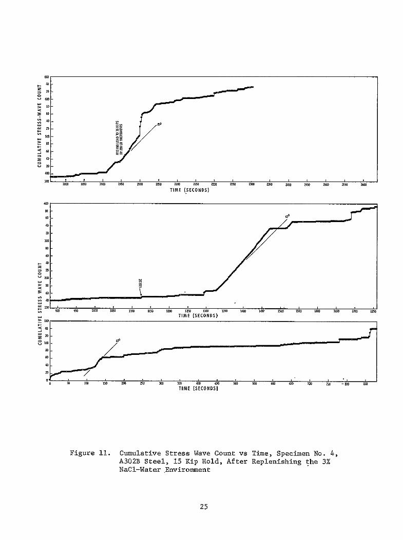
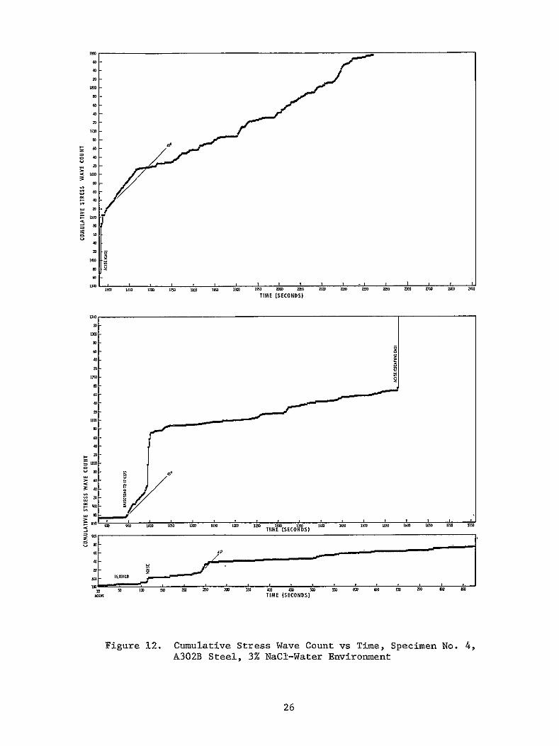
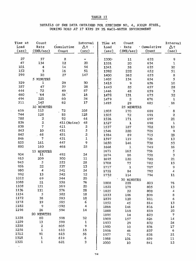
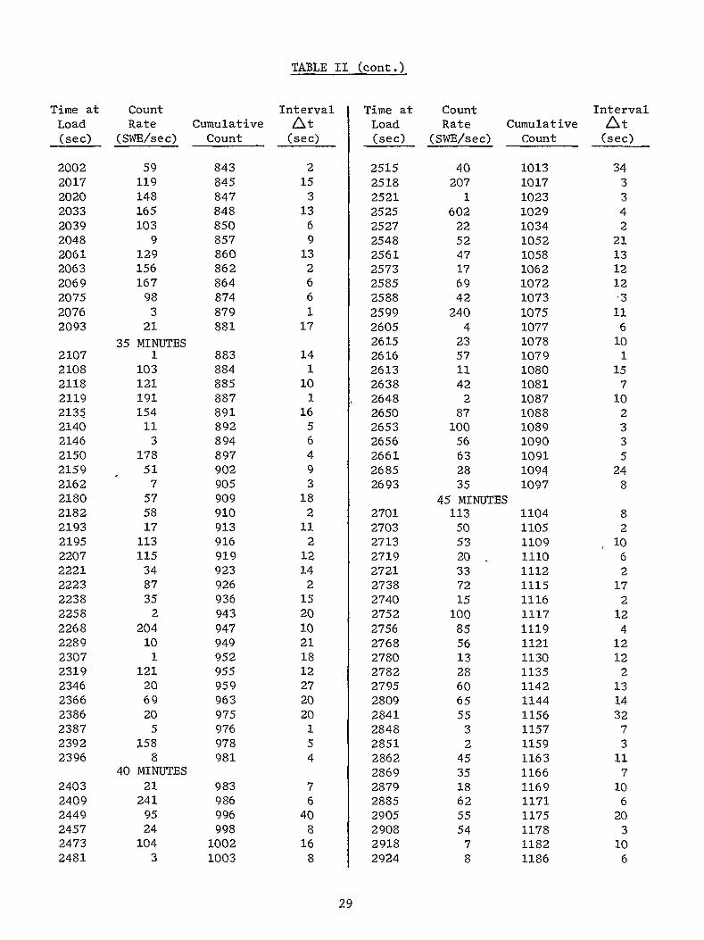
TABLE II (cont)
Time at Count Interval Time at Count Interval Load Rate Cumulative At Load Rate Cumulative Lt (sec) (SWBsec) Count (sec) (sec) (SWEsec) Count (sec)
2002 59 843 2 2515 40 1013 34 2017 119 845 15 2518 207 1017 3 2020 148 847 3 2521 1 1023 3 2033 165 848 13 2525 602 1029 4 2039 103 850 6 2527 22 1034 2 2048 9 857 9 2548 52 1052 21 2061 129 860 13 2561 47 1058 13 2063 156 862 2 2573 17 1062 12 2069 167 864 6 2585 69 1072 12 2075 98 874 6 2588 42 1073 3 2076 3 879 1 2599 240 1075 11 2093 21 881 17 2605 4 1077 6
35 MINUTES 2615 23 1078 10 2107 1 883 14 2616 57 1079 1 2108 103 884 1 2613 11 1080 15 2118 121 885 10 2638 42 1081 7 2119 191 887 1 2648 2 1087 10 2135 154 891 16 2650 87 1088 2 2140 11 892 5 2653 100 1089 3 2146 3 894 6 2656 56 1090 3 2150 178 897 4 2661 63 1091 5 2159 51 902 9 2685 28 1094 24 2162 7 905 3 2693 35 1097 8 2180 57 909 18 45 MINUTES 2182 58 910 2 2701 113 1104 8 2193 17 913 11 2703 50 1105 2 2195 113 916 2 2713 53 1109 10 2207 115 919 12 2719 20 1110 6 2221 34 923 14 2721 33 1112 2 2223 87 926 2 2738 72 1115 17 2238 35 936 15 2740 15 1116 2 2258 2 943 20 2752 100 1117 12 2268 204 947 10 2756 85 1119 4 2289 10 949 21 2768 56 1121 12 2307 1 952 18 2780 13 1130 12 2319 121 955 12 2782 28 1135 2 2346 20 959 27 2795 60 1142 13 2366 69 963 20 2809 65 1144 14 2386 20 975 20 2841 55 1156 32 2387 5 976 1 2848 3 1157 7 2392 158 978 5 2851 2 1159 3 2396 8 981 4 2862 45 1163 11
40 MINUTES 2869 35 1166 7 2403 21 983 7 2879 18 1169 10 2409 241 986 6 2885 62 1171 6 2449 95 996 40 2905 55 1175 20 2457 24 998 8 2908 54 1178 3 2473 104 1002 16 2918 7 1182 10 2481 3 1003 8 2924 8 1186 6
29
TABLE II (cont)
Time at Count Interval Time at Count Interval Load Rate Cumulative t Load Rate Cumulative t (sec) (SWIsec) Count (sec) (sec) (SWEsec) Count (sec)
2938 12 1193 14 3341 207 1410 2948 95 1201 10 3366 103 1421 25 2966 10 1215 18 3377 8 1424 11 2968 43 1216 2 3378 12 1425 1 2972 22 1217 4 3390 2 1429 12 2979 8 1221 7 3396 3 1430 6 2987 8 1223 8 3397 14 1432 1 2998 38 1226 11 3401 8 1434 4
50 MINUTES 3402 98 1438 1 3002 36 1228 4 3408 12 1443 6 3010 55 1230 8 3410 16 1448 2 3011 3 1234 1 3413 6 1452 3 3016 1 1236 5 3431 2 1454 8 3017 3 1237 1 3433 17 1458 2 3023 3 1239 6 3435 30 1460 - 2 3029 3 1240 6 3438 22 1462 3 3033 1 1243 4 3450 8 1475 12 3036 110 1245 3 3455 62 1484 5 3037 4 1248 1 3461 154 1490 6 3053 83 1259 16 3462 7 1493 1 3054 7 1260 1 3466 11 1501 4 3061 2 1265 7 3472 2 1507 6 3062 83 1266 1 3476 46 1509 4 3076 62 1275 14 3489 18 1515 13 3080 5 1278 4 3490 8 1517 1 3098 32 1294 18 3508 15 1534 18 3100 15 1296 2 3513 25 1541 5 3102 16 1297 2 3520 220 1549 7 3108 7 1299 6 3538 29 1566 18 3114 7 1301 6 3542 9 1572 4 3127 6 1304 13 3543 107 1575 1 3129 1 1305 2 3558 240 1588 15 3133 1 1306 4 3568 30 1601 10 3140 5 1309 7 3570 21 1603 2 3154 30 1312 14 3573 66 1607 3 3170 6 1320 16 3579 9 1613 6 3175 77 1322 5 3591 37 1619 12 3177 110 1323 2 60 MINUTES 3178 5 1324 1 3607 128 1622 16 3183 4 1326 5 3608 70 1626 1 3187 137 1331 4 3609 2 1629 1 3191 14 1332 4 3624 50 1638 15 3200 3 1336 9 3630 14 1642 6 3206 2 1340 6 3639 86 1645 9 3214 20 1343 8 3660 56 1662 21 3219 22 1345 5 3678 13 1669 18
55 MINUTES
30
TABLE II (cont)
Time at Count Interval Time at Count Interval Load Rate Cumulative At Load Rate Cumulative At (sec) (SWEsec) Count (sec) (see) (SWEsec) Count (sec)
3688 33 1680 10 4535 105 2574 28 3692 35 1682 4 4547 3 2589 12
3709 209 1688 17 4583 4 2616 36 3712 7 1689 3 4623 460 2670 40 3720 78 1691 8 4624 37 2703 1
3730 93 1694 10 4626 18 2715 2 3731 5 1695 1 4627 840 2729 1 3743 13 1703 12 4630 141 2737 3 3744 120 1709 1 4662 2 2758 32
3750 24 1715 6 4671 1 2763 9 3755 142 1724 5 4698 1 2774 27 3767 45 1738 12 4710 8 2782 12 3796 69 1770 29 4719 6 2784 9 3823 21 1808 27 4731 128 2785 12 3844 10 1838 21 4761 17 2810 30 3854 82 1851 10 4783 22 2822 22 3856 13 1855 2 4786 23 282A 3 3895 75 1915 39 80 MINUTES
65 MINUTES 4822 96 2831 36 3901 18 1920 6 4852 1 2842 30 3905 54 1927 4 4934 59 2890 82
3946 58 1963 41 4953 200 2907 19 3970 2 1985 24 4954 26 2910 1 3971 181 1988 1 4957 16 2916 3 3974 61 1990 3 4964 56 2923 7 3975 28 1992 1 4988 29 2941 24 3987 51 2004 12 5000 88 2951 12 4012 2 2022 25 5031 10 2977 31 4013 31 2026 1 5032 9 2978 1 4022 7 2036 9 5045 56 2982 13 4054 4 2062 32 5054 4 2984 9 4056 16 2066 2 5093 220 2992 39 4084 37 2093 28 85 MINUTES 4091 36 2099 7 5122 115 2996 29 4100 3 2111 9 5166 17 3019 44 4129 16 2142 29 5190 172 3042 24 4156 6 2165 27 5193 55 3045 3
70 MINUTES 5194 2 3048 1 4241 19 2253 85 5224 313 3081 30 4292 4 2299 51 5248 23 3106 24 4331 42 2339 39 5266 32 3123 18 4338 19 2348 7 5281 24 3138 15 4340 66 2350 2 5291 10 3150 10 4345 10 2359 5 5303 25 3164 12 4385 4 2419 40 5306 1 3169 3 4397 121 2432 12 5324 56 3187 18
75 MINUTES 5330 58 3193 6 4500 40 2534 103 5345 31 3211 15 4507 6 2542 7 5351 155 3217 6
31
TABLE II (cont)
Time at Count Interval Time at Count Interval Load Rate Cumulative At Load Rate Cumulative At (sec) (SWBsec) Count (sec) (sec) (SWEsec) Count (sec)
5357 211 3223 6 5887 185 3536 1 5363 29 3233 6 5905 65 3559 18 5364 20 3237 1 5923 31 3575 18
90 MINUTES 5924 22 3576 1 5403 118 3276 39 5933 109 3578 9 5418 79 3295 15 5934 5 3579 1 5419 44 3298 1 5961 43 3582 27 5420 35 3300 1 100 MINUTES 5448 27 3324 28 6000 23 3585 39 5460 118 3327 12 6001 13 3586 1 5466 97 3329 6 6002 166 3588 1 5472 184 3331 6 6008 9 3590 6 5484 28 3333 12 6032 29 3592 24 5499 45 3338 15 6041 111 3596 9 5505 2 3341 6 6062 116 3601 21 5506 173 3344 1 6083 1 3603 21 5512 72 3346 6 6084 236 3606 1 5515 8 3348 3 6090 140 3607 6 5536 199 3352 21 6091 104 3608 1 5548 5 3356 12 6106 21 3609 15 5553 199 3359 5 6115 31 3611 9 5554 34 3360 1 6121 29 3614 6shy5587 190 3364 33 6124 1 3622 3 5593 2 3365 6 6139 51 3630 15 5605 6 3367 12 6160 25 3634 21 5611 12 3369 6 6175 5 3636 15 5638 3 3373 27 6184 196 3639 9 5644 57 3374 6 6217 275 3645 33 5645 78 3376 1 6223 84 3648 6 5669 21 3379 24 6238 23 3649 - 15 5693 22 3384 24 6244 99 3650 6 5699 48 3385 6 6250 81 3652 6
95 MINUTES 6259 39 3654 9 5702 74 3387 3 6265 15 3656 6 5703 85 3389 1 6271 21 3658 6 5725 21 3391 22 6283 85 3660 12 5737 1 3394 12 105 IWNUTES 5752 72 3396 15 6304 143 3662 21 5761 106 3398 9 6331 50 3672 27 5788 1 3414 27 6340 179 3674 9 5794 176 3422 6 6341 37 3675 1 5809 2 3441 15 6365 34 3677 24 5810 15 3445 1 6366 ill 3680 1 5813 42 3448 3 6393 150 3682 27 5814 189 3451 1 6405 43 3684 12 5823 180 3461 9 6429 4 3687 24 5832 171 3472 9 6435 127 3690 6 5838 46 3481 6 6459 31 3691 24 5859 63 3505 21 6483 7 3694 24 5865 15 3511 6 6495 30 3696 12 5886 2 3533 21 6501 128 3700 6
32
TABLE II (cont)
Time at Count Interval Time at Count Interval Load Rate Cumulative At Load Rate Cumulative At (sec) (SWEsec) Count (sec) (sec) (SWEsec) Count (sec)
6522 87 3703 21 7278 21 4158 6 6531 16 3704 9 7302 2 4174 24 6555 102 3706 24 7303 3 4174 1 6567 7 3709 12 7318 125 4186 15 6570 10 3710 3 7348 88 4205 30 6576 87 3711 6 7402 86 4238 54 6577 89 3713 1 7435 90 4258 33 6578 131 3714 1 7447 14 4262 12 6599 4 3717 21 7474 14 4277 27
6600 110 MINUTES
8 3718 1 7486 7504
9 125 MINUTES
89
4286
4304
12
18 6603 37 3720 3 7510 39 4308 6 6639 15 3724 36 7531 52 4331 21 6669 48 3728 30 7540 208 4344 9 6675 23 3729 6 7549 38 4353 9 6684 57 3731 9 7576 72 4376 27 6705 23 3757 21 7594 24 4392 18 6744 53 3807 39 7603 55 4403 9 6762 240 3830 18 7615 160 4415 12 6783 5 3854 21 7621 134 4420 6 6801 26 3874 18 7627 160 4423 6 6822 181 3901 21 7639 180 4430 12 6852 24 3934 30 7648 5 4432 9 6879 44 3962 27 7658 100 4437 10 6882 2 3965 3 7679 319 4445 21
115 MINUTES 7694 72 4449 15 6906 63 3991 24 7709 23 4451 15 6927 176 4001 21 7721 34 4453 12 6930 15 4006 3 130 MINUTES 6931 54 4011 1 7800 Test Terminated 6952 305 4026 21 6953 40 4033 1 6980 3 4037 27 6989 99 4039 9 7040 387 4080 51 7041 53 4095 1 7056 23 4100 15 7086 354 4108 30 7095 21 4110 9 7125 70 4117 30 7131 2 4120 6 7167 97 4129 36 7176 11 4130 9 7197 18 4133 21
120 MINUTES 7218 28 4136 21 7227 39 4138 9 7248 72 4146 21 7272 50 4153 24
33
40
38W
3400
32W
30
28M
260
= 2400
S 22DD
i20
1600
1400
1200
10
600
400
200
06 1a 20 30 40 50 60 70 80 90 tW 110120130
MINUTE-S-H-OLD 17KIPS
Figure 13 Cumulative Stress Wave Count vs Time SpecimE A302B Steels 3 NaC1-Water Environment
34
3503
0
~0
40
20
3203
00
20
C0
20
310
03
(0
40
= = 20 0 I- 365~
05
20 00
20
0shy20
2003
20 ~~0 C
20
20 40
- 20
2835
0
(0
20
20shy
20020
20 -
3403 3450 3720 3750 fl 3550 3003 3050 40) 4050 4003 4050 4~fl 4200 4020 4350 4440 4450
TIME (SECONDS)
Figure 14 Cumulative Stress Wave Count vs Time Specimen No 4 A302B Steel After 1 Minute at 17 Kip Hold in 3 NaCi-Water Environment
35
48
0
I-
S 40
us 50 50 70 5 90 0 60 60 10 6 6 t 20CO DS
- iue1CmlaieSrs av on sTme pcmnN A0BSel
Afe2-0iue t1 i todi NC-ae niomn
Page60
4520 -
so- lao
F
122021 amp~
20 4
400
20
20 22
3540 =
20
3024
20
50
45
20
20520
20
20
45
20
no
I
40
4~
20
40
20
20
4
20
2020
20
gt
20
20 4
20
20
3545
20
Iino200j
5505
2220
1120
20
001
20
20 shy
00
1
45
OX
I
I I
I I
0 50
020 000
205 200
20 200
Z
40 505
550 400
TIM
E (S
EC
ON
DS
)
Figure 16
Cumulative Stress Wave Count vs
Time Specimen No
5 A302B Steel
Hydrogenated and Tested in Air
37
IV C Bend Tests in Air With Deliberate Addition of Hydrogen (cont)
On raising the load from 13000 to 14000 lb (122 ksi-in )
there was evidence of a creep phenomenon as shown in Figure 17 The crackshy
opening-displacement gage confirmed the occurrence of crack growth continuing
after reaching the 14000-lb hold Stress-wave emission showed the mechanism
to be discontinuous cracking rather than a deformation process When the
count rate was plotted as in Figure 18 the activity carrying into the
14000-lb hold again was discontinuous After approximately 300 sec at 14 kips
the SWE associated with the creep phenomenon had subsided During the 14-kip
hold there were two crack jumps one after 920 sec (cumulative count increased
from 5618 to 5720 and the count rate associated with the jump was 181 as
counted over a 10-sec interval or 18 SWEsec) and one after 2130 sec (cumulashy
tive count increased from 5721 to 5755 and the count rate was 139 in 10 see)
After 5000 sec at 14 kips the load on Specimen 5 was raised As
seen in Figure 19 the stress-wave activity was an unmistakable presage of
instability which occurred after 20 sec into hold The load reached a maximum
of 145 kips (145 ksi-in 2) Technically the onset of instability occurred
shortly after starting to increase the load ie at approximately
132 ksi-inI2 which agrees with the KQ value obtained through rising load
tests of unhydrogenated material in an air environment
Because of the very long test period and multiple loadings involved
in the testing of the Specimen 6 only data obtained during rising load to
19500 and 19800 ib during sustained test periods at these loads and during
specimen failure are shown in Figure 20 These data indicate essentially the
same SWE-crack growth relationships discussed previously for Specimen 5 except
that on reaching hold the crack tended to grow slowly for a longer period of
time in comparison to the behavior noted for Specimen 5 Also the incremental
nature of crack extension was more readily observed by the stress-wave-emission
data for Specimen 6
38
20
560
80
60
40
20
5500
80
60
40
20
5400
o 5100
808
60
40
20
5000 u-J
4500
4480 80 4- START 14-KI P HOLD
CODC 75lt
4000
3980 70
3960
6553120 l
- END13-KIP HOLD
3100 160 0 40 80 120 160 200 240 280 320
TIME AT LOAD (SECONDS)
Figure 17 Cumulative Stress Wave Count and COD vs Time Specimen No 5 A302B Steel fydrogenated and Held at 14 Kips in Air
39
200
LU
LU
1- 100
50 END 13-KIP
25 HOLD-I
0 1- TIME
100 INSECONDS AT
200 14KIPS
300
(COUNT EVERY 10 SEC)
Figure 18 Stress Wave Count Rate vs Time - Specimen No 5 A302B Steel Hydrogenated and Tested in Air
40
INSTABILITY
9580
9560
9540
9380
928D0
9260
842D
8440
73O I-shyz 7220
o 7260
U 7240
7220
7180I-shy
7160
- 7140
7120
7100
7080
7060
5900
5880
5860
5840
5820
5800
578D
5460
0 40 80 120 160 SEC
4M 4960 50D RISING LOAD-SECONDS AT 14 KIPS
Figure 19 Cumulative Stress Wave Count vs Time Specimen No 5 A302B Steel Hydrogenated and Tested in Air
41
20000
18000
FAILURE
18290 sec a- 1 17-in K - 199 s - Y
z
-
16000
14000
l0
1200
I-9 Iin
1014in K 152 ki- in -i
o-1 09 n K- 176ksmn
- 1 07 in I 170 iis-
o -1 042in K 12ks-in
c023i NK15ks-n
-shy
-
10000
REACH 19800 lbs
START TO 19800 bs
10000 11000 12000 13000 14000 15000 16000 17000 18000 19000
TIMESECONDS
12000
11000 s
p9000
T LOAD ADJUSTMEA
7n000
READOUT6000 OTE STRESS WAVE DATA A UST T
500 Vgt 0 ENT CORRESPONDIG TO SLOPELOAADJUSTM15 CHANGES PLOTTED
a 4000
3000
LOAD ADJUSTMENT2000 SECONDSECMENIME
1000 START HOLD AT 19500 1b
900 1l6070 D0 8 0 00 0 000600
0 1000 50002000 3000 4000
TIME SECONDS
Figure 20 Cumulative Stress Wave Count vs Time Specimen No 6 A302B Steel Hydrogenated and Tested in Air
Page 42
IV C Bend Tests in Air With Deliberate Addition of Hydrogen (cont)
As indicated in Figure 20 the increase in crack length during
the initial period of hold at 19500 lb resulted in an increase in the applied
stress intensity and was accompanied by significant stress-wave-emission
activity To maintain the desired load it was also necessary to make frequent
load adjustments at the start of hold During the first 3600 sec the effecshy
tive crack length increased from approximately 0963 to 1000 in and was
accompanied by about 7000 SWE As indicated in Figure 20 the majority of the
SWE activity and increase in crack length occurred during the first 3000 sec
of the hold at 19500 lb After this period both the stress-wave-emission
activity and rate of increase in crack length gradually decreased For example
during the entire period from 5000 to 17600 sec when the load was increased
to 19800 lb the apparent crack length and SWE count increased by only approxishy
mately 0020 in and 2500 respectively
After approximately 17000 sec at 19500 lb the load was increased
to 19800 lb and specimen failure occurred after approximately 600 sec at
19800 lb The load was maintained for this period however it was apparent
from both the SWE and COD gage data that the crack was extending and specimen
failure would occur without a further increase in load although it was necesshy
sary to continually adjust the tensile machine to maintain the desired load
The failure stress intensity approximated 199 ksi-in 2however technically
the onset of instability occurred after starting to increase the load at
approximately 153 ksi-in1 2
Specimen 7 was also hydrogenated baked at 300F for 3 hr and
tested in air Figure 21 is a detailed plot of the SWAT data (electronic
counter print-out every second) indicating crack growth of a discontinuous
nature starting at 2400-lb load Note the periods of dormancy (no increase
in SWE count) interspersed with abrupt increases in count indicating disconshy
tinuous crack growth Note also that there was little or no evidence of
continuous stress-wave emission until the load (stress intensity level) was
high approaching failure
43
CUMULAIY STRESS-VAVE COUNTCU LTISTE W E ON
I OT A~II I OI I L I I I I I I I I I I I I I I i I I I I I
- N LB
I I I I I I I I I I I I I i I I
--L - 0OTO11
-0101
(lNIML~ 33383338
8
133113-
3IiC)0 83) 3103 31-3(31-
~0
33 331
3l3C0C~
38318shy
111(10 CAVMSS3 nfl CAliVi flWfl3
________________________________________________________________________
111fl0~ 3KvM~s~a1Ff~TfvTifwT
FPAIAE
hY
A Ii
8
INa
CZ
8 C0 U CI
33 S
1 H
H
03 -I
~ 3lt
0 Cd 33
~C3 ~ H
8 0003
A
Ofli3i~~ C)
Page 45
IV C Bend Tests in Air With Deliberate Addition of Hydrogen (cont)
Figure 22 presents the SWE data from a hydrogenated bend specimen
(No 8) tested in air The load was increased continuously to 9800 lb
(70 ksi-in 2) where there was a short hold (approximately 400 sec) Note
the discontinuous crack growth followed by a short period of continuous
emission (less than 450 slope) The load was then raised to 14800 lb
(109 ksi-in 2) and held for approximately 400 sec Again there were jumps
in the SWE cumulative count but this time interspersed with continuous
emission The SWAT system employed for this test corresponded to that employed
for the background measurements at Kennedy Space Flight Center and shown in
Figure 8 only one channel was employed viz
Endevco 2213 Amplifier Amplifier Band-Pass Filter 10OX 10OX 20 to 50 Kcps
The continuous stress-wave emission observed during hold at the higher stressshy
intensity level in this specimen was not observed in the other hydrogenated
specimens tested in air The primary purpose of this test (Specimen 8) was to
record SWE data for subsequent playback and analysis to determine the amplitude
of burst-type stress-wave emissions associated with fracture in Type A302B
steel These analyses were performed using the instrumentation shown in
Figures 7 and 8 with the following results which are discussed in more detail
in conjunction with the results of the background measurements performed at
Kennedy Space Flight Center (Section V)
Maximum SWE Amplitude - 39 x 10-3g
Minimum SWE Amplitude - 12 x 10-3 g
Average SWE Amplitude - 22 x 10-3g
Laboratory Background - 11 x 10-3g
46
00 o z~ 20 ~
40
~40
S20 1 2 0 0 0 0
TIIAEAT 4 S-KIPHOLD (10KS(51IN A)
407
IV Laboratory Test Results and Discussion (cont)
D BEND TESTS IN 3 NaCI-WATER WITH DELIBERATE ADDITION OF HYDROGEN
Specimen 9 was hydrogenated baked and tested in 80F water
The electronic counter indicated continuous stress-wave emission interspersed
with abrupt increases in count indicating occasional crack jumps Figure 23
shows the details of stress-wave emission that occurred during both rising
load and holding load The crack length determined from the COD chart at
selected loads is also shown Note from the SWE data that there were no
periods of dormancy and the slope of the plot of cumulative count versus time
indicated moderately rapid continuouas crack growth such as might occur with
electrochemical dissolution at the crack tip The COD gage data shown in
Figure 23 also indicate crack extension however the actual amount appears
to be quite small (lt01 in) which would be consistent with the relatively
small number of stress-wave emissions detected even at the high system
sensitivity employed The dramatic difference between the behavior in
Figures 21 and 23 for hydrogenated material tested in air (Figure 21) and
water (Figure 23) indicates that hydrogen and 3 sodium chloride solution
acting together have a greater total effect than the sum of their individual
effects ie working together they appear to have produced a synergism
E WOL TESTS
Because of the possible significance of the synergistic-effect
noted above on the life of the hydrogen pressure vessels at Kennedy Space
Flight Center additional testing was performed using hydrogenated WOL specishy
mens cut from the fractured bend specimens The first WOL specimen was
initially loaded to-3650 lb (50 ksi-in 2) and then placed in 3 NaCl solution
(notch immersed) There was 30 min of essentially continuous stress-wave
emission (recorder started approximately 5 min after loading the specimen)
Subsequently therewas one sizable jump in the SWE cumulative count after
48
V30
760
740-M
$
720 -s
680shy
60
610
40 w
w
520 w
i
20500
HOLDD]N
340
20 760
7200
ING
IV
O
shy
420
60
40
20 0 2
04
0Q
0
60DO
LO0
01 200
250 300
350 400
450 500
550 6M
650
700 750
TIME
(SECONDS)
Figure 23
Cumulative Stress Wave Count vs Time Specimen No 9 A302B Steel
Hydrogenated and Tested in 3 NaCi-Water Environment
49
IV E WOL Tests (cont)
approximately 3 hr 40 min Then 3 hr 20 min later several jumps occurred
followed by 8 hr 20 min of stress-iave activity After this the crack was
dormant (total test time 17 hr 25 min) These data are shown in Figure 24
The load was then increased slightly (torque was increased from 200 to
255 in-lb) an additional 1-12 hr in 3 NaCl solution produced no significant
increase in the cumulative stress-wave count The reason for this apparently
anomalous behavior was not determined although it may result from a blunting
effect at the crack tip produced during the initial hold period
The fatigue crack was then extended (approximately 005 in) in
tension-tension fatigue and the specimen reloaded to approximately 51 ksi-in2
Stress-wave emission started almost immediately (dashed curve in Figure 24)
After approximately 3 hr of discontinuous activity the periods of dormancy
tended to increase interspersed with relatively small jumps (as counted over
10-sec intervals) The results of the initial loading and the reloading are
shown in Figure 24 note that there was appreciably lower cumulative count in
the reloaded specimen as compared with the initial loading for a comparable
period of test
A second hydrogenated WOL specimen was then tested in air at
50 ksi-in 2 there were stress waves initially (creep) but then very little
activity over the remaining 35-hr test period After the first hour the
count increased from approximately 150 to only 280 in the final 34 hr of test
Figure 25 shows the long peribds of dormancy punctuated by occasional 1-count
increases This is in marked contrast to the results obtained from the
hydrogenated WOL specimens tested in 3 NaCl solution and the bend-test
findings of a synergistic effect were confirmed
50
------------
aa
L- -- -- - ------ - --- I
3
IN DO
INTES) 3 S IOTI E( LI N LU
Ino
a
N O
TIME (MINUTES) IN 3 NCI SOLUTION
Figure 24 Cumulative Stress Wave Count vs Time at Hold WOL Specimen No 1
A302B Steel Hydrogenated and Tested in 3 NaCi-Water Environment
51
000 In 0 M6020 126 24 022 in0 1180 10 11 100 IWO l 100M M-C 0 90w6 a0 w6
t t t t 5W MOD4
10
TIME (MINUTES)
Figure 25 Cumulative Stress Wave Count vs Time at Hold WL Specimen No 2 A302B Steel Hydrogenated and Testd in Air
52
IV Laboratory Test Results and Discussion (cont)
F DISCUSSION
1 Material-Environment Consideration
The Type A302B steel supplied for evaluation exhibited a
very high level of fracture toughness Although quantitative plane-strain
fracture toughness measurements were not possible because of the large specimen
size required the KQ value associated with failure approximated 135 ksi-in1 2
This material was also found resistant to environmentally induced failure in
that the rate of crack growth of a prior flaw at applied stress-intensity
factors as high as 90 of the KQ value appeared to be very low This effect
was observed for unhydrogenated-material tested in air and a 3 NaCl-water
environment and hydrogenated material tested in an air environment However
the hydrogenated specimens tested in 3 NaCl-water environment had a much
faster rate of subcritical crack gr~wth in comparison to the other test condishy
tions indicating a synergistic effect due to the combination of sea water and
hydrogen in interstitial solid solution This synergistic effect indicates
that the Type A302B steel hydrogen storage tanks in the Kennedy Space Flight
Center environment may have limited life as the result of subcritical crack
growth if subjected to the same combination of stress and environmental
factors-
The WOL test results tended to confirm the possible synergism
due to the combined effects of 3 NaCl-water and hydrogen in interstitial solid
solution Marked SWE activity was observed when the hydrogenated specimens
were immersed in the salt water whereas in an air environment after the
initial period at hold when a creep phenomenon was observed there was essenshy
tially no stress-wave emission The fact that failure was not produced on
holding (in contradiction to the bend tests) can be explained by the fact that
the WOL test as-performed in this program is a self-arresting test because
53
IV F Discussion (cont)
the occurrence of crack growth results in a reduction in the applied load
Conversely in the bend tests the load was constantly applied as the crack
extended and eventually resulted in specimen failure
2 Stress-Wave-Emission Characterization
Detectable stress-wave emissions although of small amplitude
(ltOOlg) were observed to be associated with crack growth in Type A302B steel
Under all test conditions the stress-wave emissions were observed both during
rising load and when failure (instability) was imminent During hold various
SWE characteristics depending on the test conditions were observed When
tested in the hydrogenated condition in-an air environment a creep phenomenon
evidenced by increasing count of SWE and an accompanying increase in apparent
crack size was observed With time at hold and at applied stress-intensity
levels less than critical the creep phenomenon eventually stopped as did the
occurrence of stress-wave emissions Unhydrogenated material tested in the
3 NaCl-water environment produced continuous stress-wave emission punctuated
by abrupt increases in SWE count This behavior indicates both continuous
very small increments of crack extension with larger crack jumps corresponding
to the abrupt increases in SWE count Continuous incremental crack extension
characterized by continuous SWE interspersed with abrupt increases in SWE count
indicating occasional crack jumps was also observed in testing hydrogenated
material in a 3 NaCl-water environment
In all instances when failure (instability) occurred both
the amplitude and rate of stress-wave emission increased and could be employed
as a precursor of the onset of instability however even when failure was
approached-the SWE amplitude was small (ltOlg) In the other instances where
failure was not produced evidence of crack extension (although very small in
some instances) was observed on the specimen fracture face Once evidence of
54
IV F Discussion (cont)
crack growth was observed (by SWE or COD) it is obvious that failure would
eventually occur (assuming a constantly applied load) although depending on
the initial flaw size and subcritical growth rate the time to failure may be
very long In actual practice the SWE data could be employed (1) to locate
the propagating flaw (2) to monitor its occurrence and (3) as a basis for
terminating service so that repairs could be made before failure The stressshy
wave emissions associated with crack growth during rising load or increasing
stress intensity and the creep phenomenon during the initial part of hold
can be employed for this purpose
5S
V BACKGROUND MEASUREMENTS AND ASSOCIATED LABORATORY TESTS
A BACKGROUND MEASUREMENTS AT KENNEDY SPACE FLIGHT CENTER
Background noise measurements were made at two locations the VAB
Bottle Field and Pad A at the Kennedy Space Flight Center The data were tape
recorded and in addition to general background noise included tank blowdown
and repressurization periods The instrumentation for this purpose is shown
schematically in Figure 8 analysis of the data was performed by playback onto
an oscillograph and comparison with the SWE-crack growth data obtained during
the laboratory testing of bend specimens
The analysis of the signal amplitude data for tests at Cape Kennedy
is indicated below
1 Pad A Bottle Field
Signal Amplitude
a Quiescent Background
Filter at 20 Kcps - 50 Kcps -BandPass- 99 x 10 gsBand Pass
Filter at 200 cps - 32 Kcps
Band Pass
b Tank Blowdown - System Saturation (gt llg peak to peak)
C Tank Repressurization - System Saturation (gt llg peak to peak)
2 VAB Bottle Field
a Quiescent Background - 22 x 10- 4 gs
56
V A Background Measurements at Kennedy Space Flight Center (cont)
Signal Amplitude
b Tank Blowdown - System Saturation (gt llg peak to peak)
C Tank Repressurization - System Saturation (gt llg peak to peak)
Analysis of the tape-recorded data of bend tests at Aerojet indicates
the following signal amplitude for burstf-type stress-wave emissions associated
with crack growth and fracture in Type A302B steel
Maximum Amplitude - 39 x 10-3g
Minimum Amplitude - 12 x 10-3g
Average Amplitude - 22 x 10-3g
Laboratory Background - 11 x 10-3g
Thus the amplitude of SWE associated with crack growth in A302B steel is
approximately an order of magnitude larger than the background noise noted
previously Consequently the above results show that it is possible to detect
stress-wave emissions associated with fracture in A302B steel under the quiescent
background conditions existing at the Kennedy Space Center Difficulty is
expected in detecting such flaw growth during tank blowdown and repressurization
periods unless filtering can be employed to screen out the noise associated
with these periods However the blowdown and repressurization periods are of
very short duration and the materials behavior observed in this program indishy
cated that considerable prefailure crack extension would be expected from any
flaw of a size expected to be present in these pressure vessels Also
immediately on reaching load a creep phenomenon evidenced by an extension
in apparent crack length and accompanied by detectable stress-wave emission
was observed Consequently even if noise associated with blowdown and
57
V A Background Measurements at Kennedy Space Flight Center (cont)
repressurization cannot be effectively filtered out significant flaw growth
andor creep could still be detected and tank depressurization accomplished
prior to catastrophic failure assuming a capability for such depressurization
exists at these locations
B LABORATORY SIGNAL ATTENUATION EVALUATIONS
Subsequent to the background measurements at the Kennedy Space
Flight Center and the bend tests at Aerojet two series of tests were made at
Aerojet using a section of pipe and plate both of SAE 4130 steel alloy The
purpose of these tests was to determine the coefficient of signal attenuation
which in conjunction with the previous test data could be used to establish
the sensor spacing which would insure detection of SWE associated with crack
growth in the pressure-vessels at the Kennedy Space Flight Center
In these tests a constant pulse was imparted to the specimen by
a Tektronix 115 Pulse Generator using a Clevite PZT-5 Crystal (2125 in dia
and 0250 in thick) The piezoelectric crystal was mounted on a small alumishy
num block which in turn was adhered to the surface of the specimen The
signal was received by a 2217-E-Endevcq accelerometer placed at various disshy
tances from the pulser The pulse used was 10 n-sec rise and fall time with
a duration of 20 microsec at an amplitude of 12v
1 Pipe Tests
A SAE 4130 steel pipe (8-58 in OD 7-18 in ID and 22 ft
10-78 in long) was used as specimen for this test series The pulser was
mounted normal to the external surface of the pipe as close as possible to the
edge The accelerometer (2217-E-Endevco) was successively placed on the pipe
58
V B Laboratory Signal Attenuation Evalutions (cont)
surface at positions I to 8 that were at 4 6 8 10 12 14 16 and 20 ft
from the pulser The signal received by the accelerometer was displayed on a
Tektronix 422 osilloscope Typical signals are shown in Figure 26
The velocities of the compressional and shear waves in steel
are
29 lO06 x38103 Vc= -x lg ) (l-26) = O2 x06(- 0 x386 = 227000 insec(+j 012)283 (1+030) (1-060)
29x106 x 386 = 91 36= 123000 insec
s 2 ( + p) p 2 (i + 030) x 0283
where E = Youngs Modulus p = Poissons Ratio and p = density The times of
arrival of these waves at the computed velocities are indicated on the oscilloshy
scope photos shown in Figure 26 The point of shear wave arrival (T ) coincides
in most of the photos to a distinct change of pattern in the trace The
arrival of the compressional wave is difficult to determine accurately because
the amplitude of this wave attenuates very fast with distance
A visual comparison of the curves shows that Figure 26a
representing the signal received 4 ft from the impulse indicates a perfectly
detectable arrival of the compressional wave conversely Figure 26h (at 20 ft
from the impulse) shows the visually detectable arrival of a wave almost at the
computed arrival of the shear wave This is due to the fact that the amplitude
of the first cycles of the compressional wave have become essentially impercepshy
tible at a distance of 20 ft from the pulse An attempt to determine signal
arrival time by visual inspection only of the traces in Figure 26 would result
in the wave velocities indicated in Table III The computed arrival times of
the compressional and shear waves are shown in Table IV If an integration of
the positive portions of the cycles comprised in 200 p sec after arrival of the
59
VERTICAL SCALE 1 DIV= 01 V VERTICAL SCALE 1 DIV = 01 V HORIZONTAL SCALE 1 DIV= 50p SEC HORIZONTAL SCALE 1 DIV = 100 pSEC
a 4FT FROM PULSER b6 FEET FROM PULSER
Tc Ts Tc Ts
VERTICAL SCALE I DIV 01 V VERTICAL SCALE I DIV = 01 V HORIZONTAL SCALE I DIV = 100 I SEC HORIZONTAL SCALE 1 DIV = 200 p SEC
c 8 FEET FROM PULSER d 10 FEET FROM PULSER
Tc = Arrival of Compressional Wave
T = Arrival of Shear Wove
Figure 26 Oscillograph Traces for Pipe Tests (Sheet 1 of 2)
6o NOT REPRODUCTBLE
VERTICAL SCALE 1 DIV = 01 V VERTICAL SCALE 1 DIV 01 V HORIZONTAL SCALE 1 DIV = 200y SEC HORIZONTAL SCALE I DIV 200 p SEC
e 12 FEET FROM PULSER f 14 FEET FROM PULSER
T TS T T
VERTICAL SCALE 1 DIV = 01 V VERTICAL SCALE 1 DIV = 01 V HORIZONTAL SCALE 1 DIV = 200 v SEC HORIZONTAL SCALE I DIV =5001p SEC
g 16 FEET FROM PULSER h 20 FEET FROM PULSER
Figure 26 Oscillograph Traces for Pipe Tests (Sheet 2 of 2)
61
V B Laboratory Signal Attenuation Evaluations (cont)
shear wave is performed the average amplitudes determined in this manner
become quite meaningful These average amplitudes are shown in Table V
TABLE III
WAVE VELOCITY BASED ON VISUAL ANALYSIS OF OSCILLOSCOPE TRACES - PIPE TESTS
Distance from Pulse Arrival Velocities Photo ft in Time psc (ftsec)
1 4 48 210 228000
2 6 72 400 180000
3 8 96 600 160000
4 10 120 800 150000
5 12 144 1000 144000
6 14 168 1200 140000
7 16 192 1400 137000
8 20 240 1750 137000
TABLE IV
COMPUTED ARRIVAL TIMES - PIPE TESTS
Compressional Wave Shear Wave Distance from Pulse Arrival Time Arrival Time
Photo in psec Osc Div sec Ose Div
1 48 212 423 390 780
2 72 317 317 583 583
3 96 422 422 778 778
4 120 530 265 972 486
5 144 635 317 1163 581
6 168 740 370 1360 680
7 192 840 420 1545 771
8 240 1050 21 1930 387
62
V B Laboratory Signal Attenuation Evalutions (cont)
TABLE V
SIGNAL AMPLITUDE VS DISTANCE - PIPE TESTS
Average Signal Amplitude Distance from 200 Psec after Arrival
Test Pulser in of Comp Wave mv
1 48 230
2 72 145
3 96 85
4 120 60
5 144 45
6 168 28
7 192 22
8 240 18
The general equation for the amplitude attenuation curve is
C x e-Xy =
where y = amplitude at distance x in volts
x = distance in inches from pulse source
C = amplitude of pulse in volts
a = attenuation factor
or iny= 1 C + (- ax) = I C - ax (Eq 4)n n
To determine the values of C and a the following statistical analysis was
performed
63
V B Laboratory Signal Attenuation Evaluations (cont)
Distance Yo y y2 X X2 Test in m v n n
1 48 230 543 +142 2010 -87 7580 - 124 261
2 72 145 499 +098 0960 -63 3960 - 62 360
3 96 85 445 +044 0194 -39 1520 - 17 427
4 120 60 409 +008 0006 -15 225 - 1 490
5 144 45 380 -021 0044 + 9 81 - 2 548
6 168 28 334 -067 0450 +33 1090 - 21 560
7 192 22 309 -092 0847 +57 3250 - 52 592
8 240 18 289 -112 1250 +105 11000 - 118 690
EY2 EX2pound x = 1080 ElnY =3208 5761 28706 SXY-397 XxIny3928
- 1080 - 3208 x =- = 135 ny = 401
EXY -397 00138 1 C =l1y + oshy
pound 2 x2 28706 n i x
= 401+(0138)(135)=401+186= 587
C - 355 mv
It is now possible to compute the statistically corrected values of the signal
amplitude y at the distances from the pulse where they were measured The
general formula will be
ny = 587 -(00138) X
and the results are tabulated in Table VI The computed value of pulse amplishy
tude at source is found to be C = 355 my The values shown on Table VI are
plotted in Figure 27 which graphically shows the signal attenuation as a
function of distance from the pulse source
64
350
300
250 STATISTICALLY COMPUTED k VALUES FOR REGRESSION CURVE
--0gt 200
EXPERIMENTALLY DETERMINED
-- MATERIAL SAE 4130 STEEL U= SPECIMEN PIPE-S758 in D aZ
00
15 7 18 in D22 ft 10 78 in LONG
-J
100
50 I
0 I I I
5 I I I
DISTANCE
I
10 FROM SOURCE
I
FEET
I
15 20
Figure 27 Signal Amplitude vs Distance - Pipe Tests
V B Laboratory Signal Attenuation Evaluations (cont)
TABLE VI
STATISTICALLY CORRECTED VALUES OF SIGNAL AMPLITUDE - PIPE TESTS
Experimentally Distance from 1 Corrected Signal Determined Signal
Test Pulse in ny Amplitude (y) mv Amplitude (y) my
1 48 521 182 230
2 72 488 130 145
3 96 455 95 85
4 120 421 67 60
5 144 388 48 45
6 168 355 35 28
7 192 322 25 22
8 240 255 127 18
- 2 Plate Tests
An SAE 4130 steel plate (73-12 in long 48-12 in wide
and 34 in thick) was used for this test series The two diagonals were
marked on the plate The pulser was placed at the center of the plate and
the receiver accelerometer was placed on one of the diagonals at locations
spaced in increments of 6 in from the center The received signals were
observed on the oscilloscope and photos were taken of these signals Figure
28 shows oscillographs of the signals received at 6 12 18 24 30 36 and
42 in from the pulser The times of arrival of the shear wave are also shown
in Figure 28 The velocity used was v = 123000 insec An integration
was performed of the positive positions of the cycles comprised in a 20 Psec
interval after the arrival of the shear wave The average amplitudes detershy
mined from these integrations are shown in Table VII Only Tests 1 to 4 are
used because reflection (from the plate edges) in Tests 5 to 8 obscured the
66
b 12 INCHES FROM PULSERa 6 INCHES FROM PULSER
TBTs
c 18 INCHES FROM PULSER d 24 INCHES FROM PULSER
IT s = Arrival of Shear Wave
Vertical Scale 1 DIV = 01 Volt Horizontal Scale 1 DIV = 20 ASec
Figure 28 Oscillograph Traces for Plate Tests (Sheet 1 of 2)
Page 67
f 36 INCHES FROM PULSER e 30 INCHES FROM PULSER
g 42 INCHES FROM PULSER
= Arrival of Shear WaveTs
Vertical Scale 1 DIV = 01 Volt = 20 4SecHorizontal Scale 1 DIV
Figure 28 Oscillograph Traces for Plate Tests (Sheet 2 of 2)
08 gOTPRODUCIB1A
V B Laboratory Signal Attenuation Evaluations (cont)
data These reflections were received in Tests 5 to 8 because of the relashy
tively small plate that was available for this test series
TABLE VII
SIGNAL AMPLITUDE VS DISTANCE - PLATE TESTS
Distance from Average Amplitude Test Pulse in(x) in 20 p see mv
1 6 150
2 12 110
3 18 70
4 24 45
The following statistical analysis was performed to determine the values of
C and a in Equation 4
Test
Distance from
Pulse in(x)
y
m v
1
ny Y
2
Y 2
X XY
X1 y
n
1 6 150 500 +056 0314 -9 81 -502 3000
2
3
12
18
110
70
470
425
+026
-019
0067
0036
-3
+3
9
9
-078
-057
5640
7650
4 24 45 381 -063 0397 +9 81 -567 9149
60 1776 0814 180 -1204 25439
-x=
60 w= 15
4ny
iY 1
1nC
-
=
16=44 1776 =44
E YX 1204= __=
E y2 180
ny +(0067)(15) =
+0067
444 + 0067(15)
69
=
C
444 + 100
= 230 my
= 544
V B Laboratory Signal Attenuation Evaluations (cont)
Subsequently the values of signal amplitude (y) were statistically corrected
as before and the experimentally determined values of y are compared to the
results obtained in Table VIII
TABLE VIII
COMPARISON Or STATISTICALLY CORRECTED AND TEST-DETERMINED VALUES OF SIGNAL AMPLITUDE - PLATE TESTS
Experimentally Distance from Corrected Signal Determined Signal
Test Pulse in nY Amplitude (y) mv Amplitude (y) my
1 6 504 155 150
2 12 464 103 110
3 18 417 65 70
4 24 383 46 45
The computed value of the pulse amplitude at the source at
C equals 230 mv The regression curve and the experimentally determined points
are plotted in Figure 29 It should be observed that the attenuation coefshy
ficient for the pipe test was a = 00138 and for the plate test was 0067
This is due to the much larger rate of front area that the pulse meets in the
plate
C SENSOR SPACING
The quiescent background noise measurements performed at the test
sites using a 20 to 50 KHz band-pass filter are
Pad A Bottle Field - 0000099g
VAB Bottle Field 0000220g
70
250
200 - EXPERIMENTALLY DETERMINED
0o
gt
M a-100 34
STATISTICALLY COMPUTEDVALUES FOR REGRESSION CURVE
MATERIAL SAE 4130 STEEL
SPECIMEN PLATE - 73 12 in LONG 48 12 in WIDE
in THICK
J
50
0
0 5 SII
10 15
DISTANCE FROM SOURCE FEET
I
20 I
25
Figure 29 Signal Amplitude vs Distance - Plate Tests
V C Sensor Spacing (cont)
The recorded stress-wave-emission data obtained from the A302B steel bend tests
made at the Aerojet-General Corporation laboratory show that the minimum
acceleration at the source is 0O012g the average 00022g and the maximum
00039g Based on the above data and the attenuation factor X = 0067 detershy
mined from the plate tests the sensor spacings required to detect crack growth
in the vessels at the Kennedy Space Center were computed and the results are
tabulated below
Quiescent Sensor Spacing
Amplitude at Background in the Source(C) g Amplitude(y) g Cy ln(CIy) ln(CIy)
Pad A
Min Signal 00012 000015 800 208 310
Avg Signal 00022 000015 1470 269 402
Max Signal 00039 000015 2600 326 487
VAB Bottle Field
Min Signal 00012 000033 363 129 193
Avg Signal 00022 000033 668 190 283
Max Signal 00039 000033 1080 238 356
This threshold is 15 x 0000099 - 000015g (at Pad A)
This threshold is 15 x 000022 = 000033g (at VAB Bottle Field)
Figures 30 and 31 present schematically the location and spacings of sensors
on the pressure vessels
72
- 502 IN 8 IN
HEAD -- _
DEVELOPED + + CYLINDRICAL FOR MINIMUM SIGNAL-22 SENSORS AS SHOWN
SURFACE FOR AVERAGE SIGNAL-16 SENSORS
+ +I
FOR MAXIMUM SIGNAL- 14 SENSORS
282438 IN+ +
+ +
9 SPACINGS AT 313 IN
-I- +
+ +shy
+ -plusmn
HEAD _ __
8 IN
Figure 30 Schematic of Sensor Spacings for Bottles at Pad A
73
14601 IN
HEAD (6SENSORS) 23 14 INI I I - I I I
t plusmn + plusmn + +
+ + 4 + + + DEVELOPED CYL SURFACE
+ + 4A 1 13 LINES OF
+ + + SENSORS SPACED4 + + AT 2086 IN
+ + + + + +
+ + 4 + + +
251 1516 IN + + + +-I- +
+ + + 4- +
-1- 298438 IN+ -I- -+- -i- +
+I
23 14 INHEAD (6 SENSORS) 1
FOR MINIMUM SIGNAL-103 SENSORS AS SHOWN
FOR AVERAGE SIGNAL- 82 SENSORS FOR MAXIMUM SIGNAL- 58 SENSORS
Figure 31 Schematic of Sensor Spacings for Bottles at VAB Bottle Field
74
VI CONCLUSIONS
A The Type A302B steel supplied for evaluation exhibited a high level
of fracture toughness Although quantitative plane-strain fracture toughness
measurements were not possible because of the large specimen size required
the K value associated with failure approximated 135 ksi-inI 2
Q
B The Type A302B steel was found resistant to environmentally induced
slow crack growth when tested in the hydrogenated condition in an air environshy
ment and in the unhydrogenated condition in a 3 NaCl-water environment Howshy
ever hydrogenated material tested in 3 NaCl-water had a much faster rate of
subcritical crack growth indicating a synergistic effect due to the combinashy
tion of sea water and hydrogen in interstitial solid solution
C The synergistic effect indicates the Type A302B steel hydrogen
storage tanks in the Kennedy Space Flight Center may have limited life as a
result of subcritical crack growth if subjected to the same combination of
stress and environmental factors
D Detectable stress-wave emissions although of small amplitude
(ltOOlg) were observed to be associated with crack growth in Type A302B steel
In all test conditions the stress-wave emissions were observed during rising
load and when failure (instability) was imminent Both the amplitude and rate
of stress-wave emission increased as failure was approached and could be
employed as a precursor of the onset of instability
E Stress-wave emissions associated with crack growth in Type A302B
steel can be detected under quiescent background conditions at the Pad A and
VAB Bottle fields at the Kennedy Space Flight Center However it would be
difficult to detect such stress-wave emissions during tank blowdown and
repressurization periods unless filtering can be employed to screen out the
noise associated with these periods
75
VI Conclusions (cont)
F Even in the presence of background noise from tank blowdown and
repressurization these periods are considered short in the overall life of
the pressure vessels Consequently flaw growth or creep which was observed
during rising load or the initial part of hold could be detected by SWAT
permitting triangulation to the source and tank depressurization prior to
failure
G Stress-wave-emission attenuation test data were obtained and employed
in conjunction with the site background measurements addbnd test stress-waveshy
emission characterization data to determine sensor mounting patterns for the
hydrogen pressure vessels at Pad A and the VAB Bottle Field
VII RECOMMENDATIONS FOR FURTHER WORK
If the synergistic effect of hydrogen and 3 NaCi solution occurs in
Kennedy Space Flight Center tankage the life of the tankage will be limited
Obviously slow-crack growth from any cause whether continuous or disconshy
tinuous and regardless of how slow the rate of cracking will eventually
produce failure This investigation showed that subcritical crack growth is
in all likelihood occurring with each pressurization A question remains
however as to the rate of crack growth without knowledge of the rate there
is no way to anticipate the life of the tankage However with SWAT one can
monitor the occurrence of crack growth and most importantly make judgment
as to whether a given crack is approaching critical size Consequently it
is recommended that additional tests be performed to (1) verify the existence
of subcritical cracking in actual on-site tankage and (2) incorporate an
automatic system for continuously monitoring on-site tankage at Kennedy Space
Flight Center
76
REFERENCES
1 Steel R K Green A T Lockman C S Acoustic Verification of Structural Integrity of Polaris Chambers Society of Plastic Engineers 20th Meeting Atlantic City N Y January 1964
2 Pressure Testing of AFRM-017 Service Propulsion System Fuel Tank Utilizing Aerojet-General Corporations Stress-Wave Analysis Technique
Report NAS 9-6766-003 Aerojet-General Corp for NASA MSC Houston Texas Contract NAS 9-6766 May 1967
3 Srawley J E and Esgar J B Investigation of Hydrotest Failure of Thiokol Chemical Corp 260-Inch-Diameter SL-1 Motor Case NASA-TMX shy1194 January 1964
4 Hartbower C E Gerberich W W and Crimmins P P Mechanisms of Slow Crack Growth in High-Strength Steels AFML-TR-67-26 Vol 1 February 1967
5 -Hartbower C E Gerberich W W and Crimmins P P Characterization of Fatigue-Crack Growth by Stress Wave Emission Final Report on Conshytract NAS 1-4902 for NASA-Langley Research Center Hampton Virginia June 1966
6 IHartbower C E Gerberich W W Reuter W G and Crimmins P P Stress Wave Characteristics in Constructional Alloys Final Report on Office of Naval Research Contract N00014-66-C-0340 July 1967
7 Novak S R and Rolfe S T Modified WOL Specimen for KIscc Environmental Testing U S Steel Corp paper submitted to ASTM for publication
77
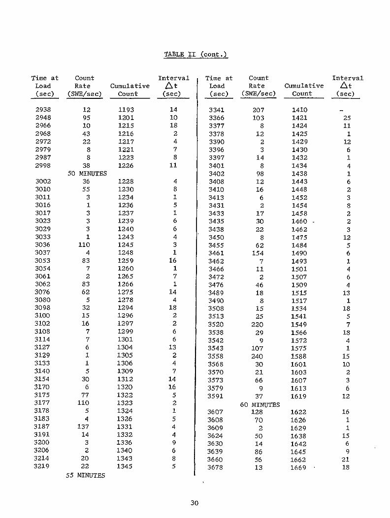
TABLE II (cont)
Time at Count Interval Time at Count Interval Load Rate Cumulative t Load Rate Cumulative t (sec) (SWIsec) Count (sec) (sec) (SWEsec) Count (sec)
2938 12 1193 14 3341 207 1410 2948 95 1201 10 3366 103 1421 25 2966 10 1215 18 3377 8 1424 11 2968 43 1216 2 3378 12 1425 1 2972 22 1217 4 3390 2 1429 12 2979 8 1221 7 3396 3 1430 6 2987 8 1223 8 3397 14 1432 1 2998 38 1226 11 3401 8 1434 4
50 MINUTES 3402 98 1438 1 3002 36 1228 4 3408 12 1443 6 3010 55 1230 8 3410 16 1448 2 3011 3 1234 1 3413 6 1452 3 3016 1 1236 5 3431 2 1454 8 3017 3 1237 1 3433 17 1458 2 3023 3 1239 6 3435 30 1460 - 2 3029 3 1240 6 3438 22 1462 3 3033 1 1243 4 3450 8 1475 12 3036 110 1245 3 3455 62 1484 5 3037 4 1248 1 3461 154 1490 6 3053 83 1259 16 3462 7 1493 1 3054 7 1260 1 3466 11 1501 4 3061 2 1265 7 3472 2 1507 6 3062 83 1266 1 3476 46 1509 4 3076 62 1275 14 3489 18 1515 13 3080 5 1278 4 3490 8 1517 1 3098 32 1294 18 3508 15 1534 18 3100 15 1296 2 3513 25 1541 5 3102 16 1297 2 3520 220 1549 7 3108 7 1299 6 3538 29 1566 18 3114 7 1301 6 3542 9 1572 4 3127 6 1304 13 3543 107 1575 1 3129 1 1305 2 3558 240 1588 15 3133 1 1306 4 3568 30 1601 10 3140 5 1309 7 3570 21 1603 2 3154 30 1312 14 3573 66 1607 3 3170 6 1320 16 3579 9 1613 6 3175 77 1322 5 3591 37 1619 12 3177 110 1323 2 60 MINUTES 3178 5 1324 1 3607 128 1622 16 3183 4 1326 5 3608 70 1626 1 3187 137 1331 4 3609 2 1629 1 3191 14 1332 4 3624 50 1638 15 3200 3 1336 9 3630 14 1642 6 3206 2 1340 6 3639 86 1645 9 3214 20 1343 8 3660 56 1662 21 3219 22 1345 5 3678 13 1669 18
55 MINUTES
30
TABLE II (cont)
Time at Count Interval Time at Count Interval Load Rate Cumulative At Load Rate Cumulative At (sec) (SWEsec) Count (sec) (see) (SWEsec) Count (sec)
3688 33 1680 10 4535 105 2574 28 3692 35 1682 4 4547 3 2589 12
3709 209 1688 17 4583 4 2616 36 3712 7 1689 3 4623 460 2670 40 3720 78 1691 8 4624 37 2703 1
3730 93 1694 10 4626 18 2715 2 3731 5 1695 1 4627 840 2729 1 3743 13 1703 12 4630 141 2737 3 3744 120 1709 1 4662 2 2758 32
3750 24 1715 6 4671 1 2763 9 3755 142 1724 5 4698 1 2774 27 3767 45 1738 12 4710 8 2782 12 3796 69 1770 29 4719 6 2784 9 3823 21 1808 27 4731 128 2785 12 3844 10 1838 21 4761 17 2810 30 3854 82 1851 10 4783 22 2822 22 3856 13 1855 2 4786 23 282A 3 3895 75 1915 39 80 MINUTES
65 MINUTES 4822 96 2831 36 3901 18 1920 6 4852 1 2842 30 3905 54 1927 4 4934 59 2890 82
3946 58 1963 41 4953 200 2907 19 3970 2 1985 24 4954 26 2910 1 3971 181 1988 1 4957 16 2916 3 3974 61 1990 3 4964 56 2923 7 3975 28 1992 1 4988 29 2941 24 3987 51 2004 12 5000 88 2951 12 4012 2 2022 25 5031 10 2977 31 4013 31 2026 1 5032 9 2978 1 4022 7 2036 9 5045 56 2982 13 4054 4 2062 32 5054 4 2984 9 4056 16 2066 2 5093 220 2992 39 4084 37 2093 28 85 MINUTES 4091 36 2099 7 5122 115 2996 29 4100 3 2111 9 5166 17 3019 44 4129 16 2142 29 5190 172 3042 24 4156 6 2165 27 5193 55 3045 3
70 MINUTES 5194 2 3048 1 4241 19 2253 85 5224 313 3081 30 4292 4 2299 51 5248 23 3106 24 4331 42 2339 39 5266 32 3123 18 4338 19 2348 7 5281 24 3138 15 4340 66 2350 2 5291 10 3150 10 4345 10 2359 5 5303 25 3164 12 4385 4 2419 40 5306 1 3169 3 4397 121 2432 12 5324 56 3187 18
75 MINUTES 5330 58 3193 6 4500 40 2534 103 5345 31 3211 15 4507 6 2542 7 5351 155 3217 6
31
TABLE II (cont)
Time at Count Interval Time at Count Interval Load Rate Cumulative At Load Rate Cumulative At (sec) (SWBsec) Count (sec) (sec) (SWEsec) Count (sec)
5357 211 3223 6 5887 185 3536 1 5363 29 3233 6 5905 65 3559 18 5364 20 3237 1 5923 31 3575 18
90 MINUTES 5924 22 3576 1 5403 118 3276 39 5933 109 3578 9 5418 79 3295 15 5934 5 3579 1 5419 44 3298 1 5961 43 3582 27 5420 35 3300 1 100 MINUTES 5448 27 3324 28 6000 23 3585 39 5460 118 3327 12 6001 13 3586 1 5466 97 3329 6 6002 166 3588 1 5472 184 3331 6 6008 9 3590 6 5484 28 3333 12 6032 29 3592 24 5499 45 3338 15 6041 111 3596 9 5505 2 3341 6 6062 116 3601 21 5506 173 3344 1 6083 1 3603 21 5512 72 3346 6 6084 236 3606 1 5515 8 3348 3 6090 140 3607 6 5536 199 3352 21 6091 104 3608 1 5548 5 3356 12 6106 21 3609 15 5553 199 3359 5 6115 31 3611 9 5554 34 3360 1 6121 29 3614 6shy5587 190 3364 33 6124 1 3622 3 5593 2 3365 6 6139 51 3630 15 5605 6 3367 12 6160 25 3634 21 5611 12 3369 6 6175 5 3636 15 5638 3 3373 27 6184 196 3639 9 5644 57 3374 6 6217 275 3645 33 5645 78 3376 1 6223 84 3648 6 5669 21 3379 24 6238 23 3649 - 15 5693 22 3384 24 6244 99 3650 6 5699 48 3385 6 6250 81 3652 6
95 MINUTES 6259 39 3654 9 5702 74 3387 3 6265 15 3656 6 5703 85 3389 1 6271 21 3658 6 5725 21 3391 22 6283 85 3660 12 5737 1 3394 12 105 IWNUTES 5752 72 3396 15 6304 143 3662 21 5761 106 3398 9 6331 50 3672 27 5788 1 3414 27 6340 179 3674 9 5794 176 3422 6 6341 37 3675 1 5809 2 3441 15 6365 34 3677 24 5810 15 3445 1 6366 ill 3680 1 5813 42 3448 3 6393 150 3682 27 5814 189 3451 1 6405 43 3684 12 5823 180 3461 9 6429 4 3687 24 5832 171 3472 9 6435 127 3690 6 5838 46 3481 6 6459 31 3691 24 5859 63 3505 21 6483 7 3694 24 5865 15 3511 6 6495 30 3696 12 5886 2 3533 21 6501 128 3700 6
32
TABLE II (cont)
Time at Count Interval Time at Count Interval Load Rate Cumulative At Load Rate Cumulative At (sec) (SWEsec) Count (sec) (sec) (SWEsec) Count (sec)
6522 87 3703 21 7278 21 4158 6 6531 16 3704 9 7302 2 4174 24 6555 102 3706 24 7303 3 4174 1 6567 7 3709 12 7318 125 4186 15 6570 10 3710 3 7348 88 4205 30 6576 87 3711 6 7402 86 4238 54 6577 89 3713 1 7435 90 4258 33 6578 131 3714 1 7447 14 4262 12 6599 4 3717 21 7474 14 4277 27
6600 110 MINUTES
8 3718 1 7486 7504
9 125 MINUTES
89
4286
4304
12
18 6603 37 3720 3 7510 39 4308 6 6639 15 3724 36 7531 52 4331 21 6669 48 3728 30 7540 208 4344 9 6675 23 3729 6 7549 38 4353 9 6684 57 3731 9 7576 72 4376 27 6705 23 3757 21 7594 24 4392 18 6744 53 3807 39 7603 55 4403 9 6762 240 3830 18 7615 160 4415 12 6783 5 3854 21 7621 134 4420 6 6801 26 3874 18 7627 160 4423 6 6822 181 3901 21 7639 180 4430 12 6852 24 3934 30 7648 5 4432 9 6879 44 3962 27 7658 100 4437 10 6882 2 3965 3 7679 319 4445 21
115 MINUTES 7694 72 4449 15 6906 63 3991 24 7709 23 4451 15 6927 176 4001 21 7721 34 4453 12 6930 15 4006 3 130 MINUTES 6931 54 4011 1 7800 Test Terminated 6952 305 4026 21 6953 40 4033 1 6980 3 4037 27 6989 99 4039 9 7040 387 4080 51 7041 53 4095 1 7056 23 4100 15 7086 354 4108 30 7095 21 4110 9 7125 70 4117 30 7131 2 4120 6 7167 97 4129 36 7176 11 4130 9 7197 18 4133 21
120 MINUTES 7218 28 4136 21 7227 39 4138 9 7248 72 4146 21 7272 50 4153 24
33
40
38W
3400
32W
30
28M
260
= 2400
S 22DD
i20
1600
1400
1200
10
600
400
200
06 1a 20 30 40 50 60 70 80 90 tW 110120130
MINUTE-S-H-OLD 17KIPS
Figure 13 Cumulative Stress Wave Count vs Time SpecimE A302B Steels 3 NaC1-Water Environment
34
3503
0
~0
40
20
3203
00
20
C0
20
310
03
(0
40
= = 20 0 I- 365~
05
20 00
20
0shy20
2003
20 ~~0 C
20
20 40
- 20
2835
0
(0
20
20shy
20020
20 -
3403 3450 3720 3750 fl 3550 3003 3050 40) 4050 4003 4050 4~fl 4200 4020 4350 4440 4450
TIME (SECONDS)
Figure 14 Cumulative Stress Wave Count vs Time Specimen No 4 A302B Steel After 1 Minute at 17 Kip Hold in 3 NaCi-Water Environment
35
48
0
I-
S 40
us 50 50 70 5 90 0 60 60 10 6 6 t 20CO DS
- iue1CmlaieSrs av on sTme pcmnN A0BSel
Afe2-0iue t1 i todi NC-ae niomn
Page60
4520 -
so- lao
F
122021 amp~
20 4
400
20
20 22
3540 =
20
3024
20
50
45
20
20520
20
20
45
20
no
I
40
4~
20
40
20
20
4
20
2020
20
gt
20
20 4
20
20
3545
20
Iino200j
5505
2220
1120
20
001
20
20 shy
00
1
45
OX
I
I I
I I
0 50
020 000
205 200
20 200
Z
40 505
550 400
TIM
E (S
EC
ON
DS
)
Figure 16
Cumulative Stress Wave Count vs
Time Specimen No
5 A302B Steel
Hydrogenated and Tested in Air
37
IV C Bend Tests in Air With Deliberate Addition of Hydrogen (cont)
On raising the load from 13000 to 14000 lb (122 ksi-in )
there was evidence of a creep phenomenon as shown in Figure 17 The crackshy
opening-displacement gage confirmed the occurrence of crack growth continuing
after reaching the 14000-lb hold Stress-wave emission showed the mechanism
to be discontinuous cracking rather than a deformation process When the
count rate was plotted as in Figure 18 the activity carrying into the
14000-lb hold again was discontinuous After approximately 300 sec at 14 kips
the SWE associated with the creep phenomenon had subsided During the 14-kip
hold there were two crack jumps one after 920 sec (cumulative count increased
from 5618 to 5720 and the count rate associated with the jump was 181 as
counted over a 10-sec interval or 18 SWEsec) and one after 2130 sec (cumulashy
tive count increased from 5721 to 5755 and the count rate was 139 in 10 see)
After 5000 sec at 14 kips the load on Specimen 5 was raised As
seen in Figure 19 the stress-wave activity was an unmistakable presage of
instability which occurred after 20 sec into hold The load reached a maximum
of 145 kips (145 ksi-in 2) Technically the onset of instability occurred
shortly after starting to increase the load ie at approximately
132 ksi-inI2 which agrees with the KQ value obtained through rising load
tests of unhydrogenated material in an air environment
Because of the very long test period and multiple loadings involved
in the testing of the Specimen 6 only data obtained during rising load to
19500 and 19800 ib during sustained test periods at these loads and during
specimen failure are shown in Figure 20 These data indicate essentially the
same SWE-crack growth relationships discussed previously for Specimen 5 except
that on reaching hold the crack tended to grow slowly for a longer period of
time in comparison to the behavior noted for Specimen 5 Also the incremental
nature of crack extension was more readily observed by the stress-wave-emission
data for Specimen 6
38
20
560
80
60
40
20
5500
80
60
40
20
5400
o 5100
808
60
40
20
5000 u-J
4500
4480 80 4- START 14-KI P HOLD
CODC 75lt
4000
3980 70
3960
6553120 l
- END13-KIP HOLD
3100 160 0 40 80 120 160 200 240 280 320
TIME AT LOAD (SECONDS)
Figure 17 Cumulative Stress Wave Count and COD vs Time Specimen No 5 A302B Steel fydrogenated and Held at 14 Kips in Air
39
200
LU
LU
1- 100
50 END 13-KIP
25 HOLD-I
0 1- TIME
100 INSECONDS AT
200 14KIPS
300
(COUNT EVERY 10 SEC)
Figure 18 Stress Wave Count Rate vs Time - Specimen No 5 A302B Steel Hydrogenated and Tested in Air
40
INSTABILITY
9580
9560
9540
9380
928D0
9260
842D
8440
73O I-shyz 7220
o 7260
U 7240
7220
7180I-shy
7160
- 7140
7120
7100
7080
7060
5900
5880
5860
5840
5820
5800
578D
5460
0 40 80 120 160 SEC
4M 4960 50D RISING LOAD-SECONDS AT 14 KIPS
Figure 19 Cumulative Stress Wave Count vs Time Specimen No 5 A302B Steel Hydrogenated and Tested in Air
41
20000
18000
FAILURE
18290 sec a- 1 17-in K - 199 s - Y
z
-
16000
14000
l0
1200
I-9 Iin
1014in K 152 ki- in -i
o-1 09 n K- 176ksmn
- 1 07 in I 170 iis-
o -1 042in K 12ks-in
c023i NK15ks-n
-shy
-
10000
REACH 19800 lbs
START TO 19800 bs
10000 11000 12000 13000 14000 15000 16000 17000 18000 19000
TIMESECONDS
12000
11000 s
p9000
T LOAD ADJUSTMEA
7n000
READOUT6000 OTE STRESS WAVE DATA A UST T
500 Vgt 0 ENT CORRESPONDIG TO SLOPELOAADJUSTM15 CHANGES PLOTTED
a 4000
3000
LOAD ADJUSTMENT2000 SECONDSECMENIME
1000 START HOLD AT 19500 1b
900 1l6070 D0 8 0 00 0 000600
0 1000 50002000 3000 4000
TIME SECONDS
Figure 20 Cumulative Stress Wave Count vs Time Specimen No 6 A302B Steel Hydrogenated and Tested in Air
Page 42
IV C Bend Tests in Air With Deliberate Addition of Hydrogen (cont)
As indicated in Figure 20 the increase in crack length during
the initial period of hold at 19500 lb resulted in an increase in the applied
stress intensity and was accompanied by significant stress-wave-emission
activity To maintain the desired load it was also necessary to make frequent
load adjustments at the start of hold During the first 3600 sec the effecshy
tive crack length increased from approximately 0963 to 1000 in and was
accompanied by about 7000 SWE As indicated in Figure 20 the majority of the
SWE activity and increase in crack length occurred during the first 3000 sec
of the hold at 19500 lb After this period both the stress-wave-emission
activity and rate of increase in crack length gradually decreased For example
during the entire period from 5000 to 17600 sec when the load was increased
to 19800 lb the apparent crack length and SWE count increased by only approxishy
mately 0020 in and 2500 respectively
After approximately 17000 sec at 19500 lb the load was increased
to 19800 lb and specimen failure occurred after approximately 600 sec at
19800 lb The load was maintained for this period however it was apparent
from both the SWE and COD gage data that the crack was extending and specimen
failure would occur without a further increase in load although it was necesshy
sary to continually adjust the tensile machine to maintain the desired load
The failure stress intensity approximated 199 ksi-in 2however technically
the onset of instability occurred after starting to increase the load at
approximately 153 ksi-in1 2
Specimen 7 was also hydrogenated baked at 300F for 3 hr and
tested in air Figure 21 is a detailed plot of the SWAT data (electronic
counter print-out every second) indicating crack growth of a discontinuous
nature starting at 2400-lb load Note the periods of dormancy (no increase
in SWE count) interspersed with abrupt increases in count indicating disconshy
tinuous crack growth Note also that there was little or no evidence of
continuous stress-wave emission until the load (stress intensity level) was
high approaching failure
43
CUMULAIY STRESS-VAVE COUNTCU LTISTE W E ON
I OT A~II I OI I L I I I I I I I I I I I I I I i I I I I I
- N LB
I I I I I I I I I I I I I i I I
--L - 0OTO11
-0101
(lNIML~ 33383338
8
133113-
3IiC)0 83) 3103 31-3(31-
~0
33 331
3l3C0C~
38318shy
111(10 CAVMSS3 nfl CAliVi flWfl3
________________________________________________________________________
111fl0~ 3KvM~s~a1Ff~TfvTifwT
FPAIAE
hY
A Ii
8
INa
CZ
8 C0 U CI
33 S
1 H
H
03 -I
~ 3lt
0 Cd 33
~C3 ~ H
8 0003
A
Ofli3i~~ C)
Page 45
IV C Bend Tests in Air With Deliberate Addition of Hydrogen (cont)
Figure 22 presents the SWE data from a hydrogenated bend specimen
(No 8) tested in air The load was increased continuously to 9800 lb
(70 ksi-in 2) where there was a short hold (approximately 400 sec) Note
the discontinuous crack growth followed by a short period of continuous
emission (less than 450 slope) The load was then raised to 14800 lb
(109 ksi-in 2) and held for approximately 400 sec Again there were jumps
in the SWE cumulative count but this time interspersed with continuous
emission The SWAT system employed for this test corresponded to that employed
for the background measurements at Kennedy Space Flight Center and shown in
Figure 8 only one channel was employed viz
Endevco 2213 Amplifier Amplifier Band-Pass Filter 10OX 10OX 20 to 50 Kcps
The continuous stress-wave emission observed during hold at the higher stressshy
intensity level in this specimen was not observed in the other hydrogenated
specimens tested in air The primary purpose of this test (Specimen 8) was to
record SWE data for subsequent playback and analysis to determine the amplitude
of burst-type stress-wave emissions associated with fracture in Type A302B
steel These analyses were performed using the instrumentation shown in
Figures 7 and 8 with the following results which are discussed in more detail
in conjunction with the results of the background measurements performed at
Kennedy Space Flight Center (Section V)
Maximum SWE Amplitude - 39 x 10-3g
Minimum SWE Amplitude - 12 x 10-3 g
Average SWE Amplitude - 22 x 10-3g
Laboratory Background - 11 x 10-3g
46
00 o z~ 20 ~
40
~40
S20 1 2 0 0 0 0
TIIAEAT 4 S-KIPHOLD (10KS(51IN A)
407
IV Laboratory Test Results and Discussion (cont)
D BEND TESTS IN 3 NaCI-WATER WITH DELIBERATE ADDITION OF HYDROGEN
Specimen 9 was hydrogenated baked and tested in 80F water
The electronic counter indicated continuous stress-wave emission interspersed
with abrupt increases in count indicating occasional crack jumps Figure 23
shows the details of stress-wave emission that occurred during both rising
load and holding load The crack length determined from the COD chart at
selected loads is also shown Note from the SWE data that there were no
periods of dormancy and the slope of the plot of cumulative count versus time
indicated moderately rapid continuouas crack growth such as might occur with
electrochemical dissolution at the crack tip The COD gage data shown in
Figure 23 also indicate crack extension however the actual amount appears
to be quite small (lt01 in) which would be consistent with the relatively
small number of stress-wave emissions detected even at the high system
sensitivity employed The dramatic difference between the behavior in
Figures 21 and 23 for hydrogenated material tested in air (Figure 21) and
water (Figure 23) indicates that hydrogen and 3 sodium chloride solution
acting together have a greater total effect than the sum of their individual
effects ie working together they appear to have produced a synergism
E WOL TESTS
Because of the possible significance of the synergistic-effect
noted above on the life of the hydrogen pressure vessels at Kennedy Space
Flight Center additional testing was performed using hydrogenated WOL specishy
mens cut from the fractured bend specimens The first WOL specimen was
initially loaded to-3650 lb (50 ksi-in 2) and then placed in 3 NaCl solution
(notch immersed) There was 30 min of essentially continuous stress-wave
emission (recorder started approximately 5 min after loading the specimen)
Subsequently therewas one sizable jump in the SWE cumulative count after
48
V30
760
740-M
$
720 -s
680shy
60
610
40 w
w
520 w
i
20500
HOLDD]N
340
20 760
7200
ING
IV
O
shy
420
60
40
20 0 2
04
0Q
0
60DO
LO0
01 200
250 300
350 400
450 500
550 6M
650
700 750
TIME
(SECONDS)
Figure 23
Cumulative Stress Wave Count vs Time Specimen No 9 A302B Steel
Hydrogenated and Tested in 3 NaCi-Water Environment
49
IV E WOL Tests (cont)
approximately 3 hr 40 min Then 3 hr 20 min later several jumps occurred
followed by 8 hr 20 min of stress-iave activity After this the crack was
dormant (total test time 17 hr 25 min) These data are shown in Figure 24
The load was then increased slightly (torque was increased from 200 to
255 in-lb) an additional 1-12 hr in 3 NaCl solution produced no significant
increase in the cumulative stress-wave count The reason for this apparently
anomalous behavior was not determined although it may result from a blunting
effect at the crack tip produced during the initial hold period
The fatigue crack was then extended (approximately 005 in) in
tension-tension fatigue and the specimen reloaded to approximately 51 ksi-in2
Stress-wave emission started almost immediately (dashed curve in Figure 24)
After approximately 3 hr of discontinuous activity the periods of dormancy
tended to increase interspersed with relatively small jumps (as counted over
10-sec intervals) The results of the initial loading and the reloading are
shown in Figure 24 note that there was appreciably lower cumulative count in
the reloaded specimen as compared with the initial loading for a comparable
period of test
A second hydrogenated WOL specimen was then tested in air at
50 ksi-in 2 there were stress waves initially (creep) but then very little
activity over the remaining 35-hr test period After the first hour the
count increased from approximately 150 to only 280 in the final 34 hr of test
Figure 25 shows the long peribds of dormancy punctuated by occasional 1-count
increases This is in marked contrast to the results obtained from the
hydrogenated WOL specimens tested in 3 NaCl solution and the bend-test
findings of a synergistic effect were confirmed
50
------------
aa
L- -- -- - ------ - --- I
3
IN DO
INTES) 3 S IOTI E( LI N LU
Ino
a
N O
TIME (MINUTES) IN 3 NCI SOLUTION
Figure 24 Cumulative Stress Wave Count vs Time at Hold WOL Specimen No 1
A302B Steel Hydrogenated and Tested in 3 NaCi-Water Environment
51
000 In 0 M6020 126 24 022 in0 1180 10 11 100 IWO l 100M M-C 0 90w6 a0 w6
t t t t 5W MOD4
10
TIME (MINUTES)
Figure 25 Cumulative Stress Wave Count vs Time at Hold WL Specimen No 2 A302B Steel Hydrogenated and Testd in Air
52
IV Laboratory Test Results and Discussion (cont)
F DISCUSSION
1 Material-Environment Consideration
The Type A302B steel supplied for evaluation exhibited a
very high level of fracture toughness Although quantitative plane-strain
fracture toughness measurements were not possible because of the large specimen
size required the KQ value associated with failure approximated 135 ksi-in1 2
This material was also found resistant to environmentally induced failure in
that the rate of crack growth of a prior flaw at applied stress-intensity
factors as high as 90 of the KQ value appeared to be very low This effect
was observed for unhydrogenated-material tested in air and a 3 NaCl-water
environment and hydrogenated material tested in an air environment However
the hydrogenated specimens tested in 3 NaCl-water environment had a much
faster rate of subcritical crack gr~wth in comparison to the other test condishy
tions indicating a synergistic effect due to the combination of sea water and
hydrogen in interstitial solid solution This synergistic effect indicates
that the Type A302B steel hydrogen storage tanks in the Kennedy Space Flight
Center environment may have limited life as the result of subcritical crack
growth if subjected to the same combination of stress and environmental
factors-
The WOL test results tended to confirm the possible synergism
due to the combined effects of 3 NaCl-water and hydrogen in interstitial solid
solution Marked SWE activity was observed when the hydrogenated specimens
were immersed in the salt water whereas in an air environment after the
initial period at hold when a creep phenomenon was observed there was essenshy
tially no stress-wave emission The fact that failure was not produced on
holding (in contradiction to the bend tests) can be explained by the fact that
the WOL test as-performed in this program is a self-arresting test because
53
IV F Discussion (cont)
the occurrence of crack growth results in a reduction in the applied load
Conversely in the bend tests the load was constantly applied as the crack
extended and eventually resulted in specimen failure
2 Stress-Wave-Emission Characterization
Detectable stress-wave emissions although of small amplitude
(ltOOlg) were observed to be associated with crack growth in Type A302B steel
Under all test conditions the stress-wave emissions were observed both during
rising load and when failure (instability) was imminent During hold various
SWE characteristics depending on the test conditions were observed When
tested in the hydrogenated condition in-an air environment a creep phenomenon
evidenced by increasing count of SWE and an accompanying increase in apparent
crack size was observed With time at hold and at applied stress-intensity
levels less than critical the creep phenomenon eventually stopped as did the
occurrence of stress-wave emissions Unhydrogenated material tested in the
3 NaCl-water environment produced continuous stress-wave emission punctuated
by abrupt increases in SWE count This behavior indicates both continuous
very small increments of crack extension with larger crack jumps corresponding
to the abrupt increases in SWE count Continuous incremental crack extension
characterized by continuous SWE interspersed with abrupt increases in SWE count
indicating occasional crack jumps was also observed in testing hydrogenated
material in a 3 NaCl-water environment
In all instances when failure (instability) occurred both
the amplitude and rate of stress-wave emission increased and could be employed
as a precursor of the onset of instability however even when failure was
approached-the SWE amplitude was small (ltOlg) In the other instances where
failure was not produced evidence of crack extension (although very small in
some instances) was observed on the specimen fracture face Once evidence of
54
IV F Discussion (cont)
crack growth was observed (by SWE or COD) it is obvious that failure would
eventually occur (assuming a constantly applied load) although depending on
the initial flaw size and subcritical growth rate the time to failure may be
very long In actual practice the SWE data could be employed (1) to locate
the propagating flaw (2) to monitor its occurrence and (3) as a basis for
terminating service so that repairs could be made before failure The stressshy
wave emissions associated with crack growth during rising load or increasing
stress intensity and the creep phenomenon during the initial part of hold
can be employed for this purpose
5S
V BACKGROUND MEASUREMENTS AND ASSOCIATED LABORATORY TESTS
A BACKGROUND MEASUREMENTS AT KENNEDY SPACE FLIGHT CENTER
Background noise measurements were made at two locations the VAB
Bottle Field and Pad A at the Kennedy Space Flight Center The data were tape
recorded and in addition to general background noise included tank blowdown
and repressurization periods The instrumentation for this purpose is shown
schematically in Figure 8 analysis of the data was performed by playback onto
an oscillograph and comparison with the SWE-crack growth data obtained during
the laboratory testing of bend specimens
The analysis of the signal amplitude data for tests at Cape Kennedy
is indicated below
1 Pad A Bottle Field
Signal Amplitude
a Quiescent Background
Filter at 20 Kcps - 50 Kcps -BandPass- 99 x 10 gsBand Pass
Filter at 200 cps - 32 Kcps
Band Pass
b Tank Blowdown - System Saturation (gt llg peak to peak)
C Tank Repressurization - System Saturation (gt llg peak to peak)
2 VAB Bottle Field
a Quiescent Background - 22 x 10- 4 gs
56
V A Background Measurements at Kennedy Space Flight Center (cont)
Signal Amplitude
b Tank Blowdown - System Saturation (gt llg peak to peak)
C Tank Repressurization - System Saturation (gt llg peak to peak)
Analysis of the tape-recorded data of bend tests at Aerojet indicates
the following signal amplitude for burstf-type stress-wave emissions associated
with crack growth and fracture in Type A302B steel
Maximum Amplitude - 39 x 10-3g
Minimum Amplitude - 12 x 10-3g
Average Amplitude - 22 x 10-3g
Laboratory Background - 11 x 10-3g
Thus the amplitude of SWE associated with crack growth in A302B steel is
approximately an order of magnitude larger than the background noise noted
previously Consequently the above results show that it is possible to detect
stress-wave emissions associated with fracture in A302B steel under the quiescent
background conditions existing at the Kennedy Space Center Difficulty is
expected in detecting such flaw growth during tank blowdown and repressurization
periods unless filtering can be employed to screen out the noise associated
with these periods However the blowdown and repressurization periods are of
very short duration and the materials behavior observed in this program indishy
cated that considerable prefailure crack extension would be expected from any
flaw of a size expected to be present in these pressure vessels Also
immediately on reaching load a creep phenomenon evidenced by an extension
in apparent crack length and accompanied by detectable stress-wave emission
was observed Consequently even if noise associated with blowdown and
57
V A Background Measurements at Kennedy Space Flight Center (cont)
repressurization cannot be effectively filtered out significant flaw growth
andor creep could still be detected and tank depressurization accomplished
prior to catastrophic failure assuming a capability for such depressurization
exists at these locations
B LABORATORY SIGNAL ATTENUATION EVALUATIONS
Subsequent to the background measurements at the Kennedy Space
Flight Center and the bend tests at Aerojet two series of tests were made at
Aerojet using a section of pipe and plate both of SAE 4130 steel alloy The
purpose of these tests was to determine the coefficient of signal attenuation
which in conjunction with the previous test data could be used to establish
the sensor spacing which would insure detection of SWE associated with crack
growth in the pressure-vessels at the Kennedy Space Flight Center
In these tests a constant pulse was imparted to the specimen by
a Tektronix 115 Pulse Generator using a Clevite PZT-5 Crystal (2125 in dia
and 0250 in thick) The piezoelectric crystal was mounted on a small alumishy
num block which in turn was adhered to the surface of the specimen The
signal was received by a 2217-E-Endevcq accelerometer placed at various disshy
tances from the pulser The pulse used was 10 n-sec rise and fall time with
a duration of 20 microsec at an amplitude of 12v
1 Pipe Tests
A SAE 4130 steel pipe (8-58 in OD 7-18 in ID and 22 ft
10-78 in long) was used as specimen for this test series The pulser was
mounted normal to the external surface of the pipe as close as possible to the
edge The accelerometer (2217-E-Endevco) was successively placed on the pipe
58
V B Laboratory Signal Attenuation Evalutions (cont)
surface at positions I to 8 that were at 4 6 8 10 12 14 16 and 20 ft
from the pulser The signal received by the accelerometer was displayed on a
Tektronix 422 osilloscope Typical signals are shown in Figure 26
The velocities of the compressional and shear waves in steel
are
29 lO06 x38103 Vc= -x lg ) (l-26) = O2 x06(- 0 x386 = 227000 insec(+j 012)283 (1+030) (1-060)
29x106 x 386 = 91 36= 123000 insec
s 2 ( + p) p 2 (i + 030) x 0283
where E = Youngs Modulus p = Poissons Ratio and p = density The times of
arrival of these waves at the computed velocities are indicated on the oscilloshy
scope photos shown in Figure 26 The point of shear wave arrival (T ) coincides
in most of the photos to a distinct change of pattern in the trace The
arrival of the compressional wave is difficult to determine accurately because
the amplitude of this wave attenuates very fast with distance
A visual comparison of the curves shows that Figure 26a
representing the signal received 4 ft from the impulse indicates a perfectly
detectable arrival of the compressional wave conversely Figure 26h (at 20 ft
from the impulse) shows the visually detectable arrival of a wave almost at the
computed arrival of the shear wave This is due to the fact that the amplitude
of the first cycles of the compressional wave have become essentially impercepshy
tible at a distance of 20 ft from the pulse An attempt to determine signal
arrival time by visual inspection only of the traces in Figure 26 would result
in the wave velocities indicated in Table III The computed arrival times of
the compressional and shear waves are shown in Table IV If an integration of
the positive portions of the cycles comprised in 200 p sec after arrival of the
59
VERTICAL SCALE 1 DIV= 01 V VERTICAL SCALE 1 DIV = 01 V HORIZONTAL SCALE 1 DIV= 50p SEC HORIZONTAL SCALE 1 DIV = 100 pSEC
a 4FT FROM PULSER b6 FEET FROM PULSER
Tc Ts Tc Ts
VERTICAL SCALE I DIV 01 V VERTICAL SCALE I DIV = 01 V HORIZONTAL SCALE I DIV = 100 I SEC HORIZONTAL SCALE 1 DIV = 200 p SEC
c 8 FEET FROM PULSER d 10 FEET FROM PULSER
Tc = Arrival of Compressional Wave
T = Arrival of Shear Wove
Figure 26 Oscillograph Traces for Pipe Tests (Sheet 1 of 2)
6o NOT REPRODUCTBLE
VERTICAL SCALE 1 DIV = 01 V VERTICAL SCALE 1 DIV 01 V HORIZONTAL SCALE 1 DIV = 200y SEC HORIZONTAL SCALE I DIV 200 p SEC
e 12 FEET FROM PULSER f 14 FEET FROM PULSER
T TS T T
VERTICAL SCALE 1 DIV = 01 V VERTICAL SCALE 1 DIV = 01 V HORIZONTAL SCALE 1 DIV = 200 v SEC HORIZONTAL SCALE I DIV =5001p SEC
g 16 FEET FROM PULSER h 20 FEET FROM PULSER
Figure 26 Oscillograph Traces for Pipe Tests (Sheet 2 of 2)
61
V B Laboratory Signal Attenuation Evaluations (cont)
shear wave is performed the average amplitudes determined in this manner
become quite meaningful These average amplitudes are shown in Table V
TABLE III
WAVE VELOCITY BASED ON VISUAL ANALYSIS OF OSCILLOSCOPE TRACES - PIPE TESTS
Distance from Pulse Arrival Velocities Photo ft in Time psc (ftsec)
1 4 48 210 228000
2 6 72 400 180000
3 8 96 600 160000
4 10 120 800 150000
5 12 144 1000 144000
6 14 168 1200 140000
7 16 192 1400 137000
8 20 240 1750 137000
TABLE IV
COMPUTED ARRIVAL TIMES - PIPE TESTS
Compressional Wave Shear Wave Distance from Pulse Arrival Time Arrival Time
Photo in psec Osc Div sec Ose Div
1 48 212 423 390 780
2 72 317 317 583 583
3 96 422 422 778 778
4 120 530 265 972 486
5 144 635 317 1163 581
6 168 740 370 1360 680
7 192 840 420 1545 771
8 240 1050 21 1930 387
62
V B Laboratory Signal Attenuation Evalutions (cont)
TABLE V
SIGNAL AMPLITUDE VS DISTANCE - PIPE TESTS
Average Signal Amplitude Distance from 200 Psec after Arrival
Test Pulser in of Comp Wave mv
1 48 230
2 72 145
3 96 85
4 120 60
5 144 45
6 168 28
7 192 22
8 240 18
The general equation for the amplitude attenuation curve is
C x e-Xy =
where y = amplitude at distance x in volts
x = distance in inches from pulse source
C = amplitude of pulse in volts
a = attenuation factor
or iny= 1 C + (- ax) = I C - ax (Eq 4)n n
To determine the values of C and a the following statistical analysis was
performed
63
V B Laboratory Signal Attenuation Evaluations (cont)
Distance Yo y y2 X X2 Test in m v n n
1 48 230 543 +142 2010 -87 7580 - 124 261
2 72 145 499 +098 0960 -63 3960 - 62 360
3 96 85 445 +044 0194 -39 1520 - 17 427
4 120 60 409 +008 0006 -15 225 - 1 490
5 144 45 380 -021 0044 + 9 81 - 2 548
6 168 28 334 -067 0450 +33 1090 - 21 560
7 192 22 309 -092 0847 +57 3250 - 52 592
8 240 18 289 -112 1250 +105 11000 - 118 690
EY2 EX2pound x = 1080 ElnY =3208 5761 28706 SXY-397 XxIny3928
- 1080 - 3208 x =- = 135 ny = 401
EXY -397 00138 1 C =l1y + oshy
pound 2 x2 28706 n i x
= 401+(0138)(135)=401+186= 587
C - 355 mv
It is now possible to compute the statistically corrected values of the signal
amplitude y at the distances from the pulse where they were measured The
general formula will be
ny = 587 -(00138) X
and the results are tabulated in Table VI The computed value of pulse amplishy
tude at source is found to be C = 355 my The values shown on Table VI are
plotted in Figure 27 which graphically shows the signal attenuation as a
function of distance from the pulse source
64
350
300
250 STATISTICALLY COMPUTED k VALUES FOR REGRESSION CURVE
--0gt 200
EXPERIMENTALLY DETERMINED
-- MATERIAL SAE 4130 STEEL U= SPECIMEN PIPE-S758 in D aZ
00
15 7 18 in D22 ft 10 78 in LONG
-J
100
50 I
0 I I I
5 I I I
DISTANCE
I
10 FROM SOURCE
I
FEET
I
15 20
Figure 27 Signal Amplitude vs Distance - Pipe Tests
V B Laboratory Signal Attenuation Evaluations (cont)
TABLE VI
STATISTICALLY CORRECTED VALUES OF SIGNAL AMPLITUDE - PIPE TESTS
Experimentally Distance from 1 Corrected Signal Determined Signal
Test Pulse in ny Amplitude (y) mv Amplitude (y) my
1 48 521 182 230
2 72 488 130 145
3 96 455 95 85
4 120 421 67 60
5 144 388 48 45
6 168 355 35 28
7 192 322 25 22
8 240 255 127 18
- 2 Plate Tests
An SAE 4130 steel plate (73-12 in long 48-12 in wide
and 34 in thick) was used for this test series The two diagonals were
marked on the plate The pulser was placed at the center of the plate and
the receiver accelerometer was placed on one of the diagonals at locations
spaced in increments of 6 in from the center The received signals were
observed on the oscilloscope and photos were taken of these signals Figure
28 shows oscillographs of the signals received at 6 12 18 24 30 36 and
42 in from the pulser The times of arrival of the shear wave are also shown
in Figure 28 The velocity used was v = 123000 insec An integration
was performed of the positive positions of the cycles comprised in a 20 Psec
interval after the arrival of the shear wave The average amplitudes detershy
mined from these integrations are shown in Table VII Only Tests 1 to 4 are
used because reflection (from the plate edges) in Tests 5 to 8 obscured the
66
b 12 INCHES FROM PULSERa 6 INCHES FROM PULSER
TBTs
c 18 INCHES FROM PULSER d 24 INCHES FROM PULSER
IT s = Arrival of Shear Wave
Vertical Scale 1 DIV = 01 Volt Horizontal Scale 1 DIV = 20 ASec
Figure 28 Oscillograph Traces for Plate Tests (Sheet 1 of 2)
Page 67
f 36 INCHES FROM PULSER e 30 INCHES FROM PULSER
g 42 INCHES FROM PULSER
= Arrival of Shear WaveTs
Vertical Scale 1 DIV = 01 Volt = 20 4SecHorizontal Scale 1 DIV
Figure 28 Oscillograph Traces for Plate Tests (Sheet 2 of 2)
08 gOTPRODUCIB1A
V B Laboratory Signal Attenuation Evaluations (cont)
data These reflections were received in Tests 5 to 8 because of the relashy
tively small plate that was available for this test series
TABLE VII
SIGNAL AMPLITUDE VS DISTANCE - PLATE TESTS
Distance from Average Amplitude Test Pulse in(x) in 20 p see mv
1 6 150
2 12 110
3 18 70
4 24 45
The following statistical analysis was performed to determine the values of
C and a in Equation 4
Test
Distance from
Pulse in(x)
y
m v
1
ny Y
2
Y 2
X XY
X1 y
n
1 6 150 500 +056 0314 -9 81 -502 3000
2
3
12
18
110
70
470
425
+026
-019
0067
0036
-3
+3
9
9
-078
-057
5640
7650
4 24 45 381 -063 0397 +9 81 -567 9149
60 1776 0814 180 -1204 25439
-x=
60 w= 15
4ny
iY 1
1nC
-
=
16=44 1776 =44
E YX 1204= __=
E y2 180
ny +(0067)(15) =
+0067
444 + 0067(15)
69
=
C
444 + 100
= 230 my
= 544
V B Laboratory Signal Attenuation Evaluations (cont)
Subsequently the values of signal amplitude (y) were statistically corrected
as before and the experimentally determined values of y are compared to the
results obtained in Table VIII
TABLE VIII
COMPARISON Or STATISTICALLY CORRECTED AND TEST-DETERMINED VALUES OF SIGNAL AMPLITUDE - PLATE TESTS
Experimentally Distance from Corrected Signal Determined Signal
Test Pulse in nY Amplitude (y) mv Amplitude (y) my
1 6 504 155 150
2 12 464 103 110
3 18 417 65 70
4 24 383 46 45
The computed value of the pulse amplitude at the source at
C equals 230 mv The regression curve and the experimentally determined points
are plotted in Figure 29 It should be observed that the attenuation coefshy
ficient for the pipe test was a = 00138 and for the plate test was 0067
This is due to the much larger rate of front area that the pulse meets in the
plate
C SENSOR SPACING
The quiescent background noise measurements performed at the test
sites using a 20 to 50 KHz band-pass filter are
Pad A Bottle Field - 0000099g
VAB Bottle Field 0000220g
70
250
200 - EXPERIMENTALLY DETERMINED
0o
gt
M a-100 34
STATISTICALLY COMPUTEDVALUES FOR REGRESSION CURVE
MATERIAL SAE 4130 STEEL
SPECIMEN PLATE - 73 12 in LONG 48 12 in WIDE
in THICK
J
50
0
0 5 SII
10 15
DISTANCE FROM SOURCE FEET
I
20 I
25
Figure 29 Signal Amplitude vs Distance - Plate Tests
V C Sensor Spacing (cont)
The recorded stress-wave-emission data obtained from the A302B steel bend tests
made at the Aerojet-General Corporation laboratory show that the minimum
acceleration at the source is 0O012g the average 00022g and the maximum
00039g Based on the above data and the attenuation factor X = 0067 detershy
mined from the plate tests the sensor spacings required to detect crack growth
in the vessels at the Kennedy Space Center were computed and the results are
tabulated below
Quiescent Sensor Spacing
Amplitude at Background in the Source(C) g Amplitude(y) g Cy ln(CIy) ln(CIy)
Pad A
Min Signal 00012 000015 800 208 310
Avg Signal 00022 000015 1470 269 402
Max Signal 00039 000015 2600 326 487
VAB Bottle Field
Min Signal 00012 000033 363 129 193
Avg Signal 00022 000033 668 190 283
Max Signal 00039 000033 1080 238 356
This threshold is 15 x 0000099 - 000015g (at Pad A)
This threshold is 15 x 000022 = 000033g (at VAB Bottle Field)
Figures 30 and 31 present schematically the location and spacings of sensors
on the pressure vessels
72
- 502 IN 8 IN
HEAD -- _
DEVELOPED + + CYLINDRICAL FOR MINIMUM SIGNAL-22 SENSORS AS SHOWN
SURFACE FOR AVERAGE SIGNAL-16 SENSORS
+ +I
FOR MAXIMUM SIGNAL- 14 SENSORS
282438 IN+ +
+ +
9 SPACINGS AT 313 IN
-I- +
+ +shy
+ -plusmn
HEAD _ __
8 IN
Figure 30 Schematic of Sensor Spacings for Bottles at Pad A
73
14601 IN
HEAD (6SENSORS) 23 14 INI I I - I I I
t plusmn + plusmn + +
+ + 4 + + + DEVELOPED CYL SURFACE
+ + 4A 1 13 LINES OF
+ + + SENSORS SPACED4 + + AT 2086 IN
+ + + + + +
+ + 4 + + +
251 1516 IN + + + +-I- +
+ + + 4- +
-1- 298438 IN+ -I- -+- -i- +
+I
23 14 INHEAD (6 SENSORS) 1
FOR MINIMUM SIGNAL-103 SENSORS AS SHOWN
FOR AVERAGE SIGNAL- 82 SENSORS FOR MAXIMUM SIGNAL- 58 SENSORS
Figure 31 Schematic of Sensor Spacings for Bottles at VAB Bottle Field
74
VI CONCLUSIONS
A The Type A302B steel supplied for evaluation exhibited a high level
of fracture toughness Although quantitative plane-strain fracture toughness
measurements were not possible because of the large specimen size required
the K value associated with failure approximated 135 ksi-inI 2
Q
B The Type A302B steel was found resistant to environmentally induced
slow crack growth when tested in the hydrogenated condition in an air environshy
ment and in the unhydrogenated condition in a 3 NaCl-water environment Howshy
ever hydrogenated material tested in 3 NaCl-water had a much faster rate of
subcritical crack growth indicating a synergistic effect due to the combinashy
tion of sea water and hydrogen in interstitial solid solution
C The synergistic effect indicates the Type A302B steel hydrogen
storage tanks in the Kennedy Space Flight Center may have limited life as a
result of subcritical crack growth if subjected to the same combination of
stress and environmental factors
D Detectable stress-wave emissions although of small amplitude
(ltOOlg) were observed to be associated with crack growth in Type A302B steel
In all test conditions the stress-wave emissions were observed during rising
load and when failure (instability) was imminent Both the amplitude and rate
of stress-wave emission increased as failure was approached and could be
employed as a precursor of the onset of instability
E Stress-wave emissions associated with crack growth in Type A302B
steel can be detected under quiescent background conditions at the Pad A and
VAB Bottle fields at the Kennedy Space Flight Center However it would be
difficult to detect such stress-wave emissions during tank blowdown and
repressurization periods unless filtering can be employed to screen out the
noise associated with these periods
75
VI Conclusions (cont)
F Even in the presence of background noise from tank blowdown and
repressurization these periods are considered short in the overall life of
the pressure vessels Consequently flaw growth or creep which was observed
during rising load or the initial part of hold could be detected by SWAT
permitting triangulation to the source and tank depressurization prior to
failure
G Stress-wave-emission attenuation test data were obtained and employed
in conjunction with the site background measurements addbnd test stress-waveshy
emission characterization data to determine sensor mounting patterns for the
hydrogen pressure vessels at Pad A and the VAB Bottle Field
VII RECOMMENDATIONS FOR FURTHER WORK
If the synergistic effect of hydrogen and 3 NaCi solution occurs in
Kennedy Space Flight Center tankage the life of the tankage will be limited
Obviously slow-crack growth from any cause whether continuous or disconshy
tinuous and regardless of how slow the rate of cracking will eventually
produce failure This investigation showed that subcritical crack growth is
in all likelihood occurring with each pressurization A question remains
however as to the rate of crack growth without knowledge of the rate there
is no way to anticipate the life of the tankage However with SWAT one can
monitor the occurrence of crack growth and most importantly make judgment
as to whether a given crack is approaching critical size Consequently it
is recommended that additional tests be performed to (1) verify the existence
of subcritical cracking in actual on-site tankage and (2) incorporate an
automatic system for continuously monitoring on-site tankage at Kennedy Space
Flight Center
76
REFERENCES
1 Steel R K Green A T Lockman C S Acoustic Verification of Structural Integrity of Polaris Chambers Society of Plastic Engineers 20th Meeting Atlantic City N Y January 1964
2 Pressure Testing of AFRM-017 Service Propulsion System Fuel Tank Utilizing Aerojet-General Corporations Stress-Wave Analysis Technique
Report NAS 9-6766-003 Aerojet-General Corp for NASA MSC Houston Texas Contract NAS 9-6766 May 1967
3 Srawley J E and Esgar J B Investigation of Hydrotest Failure of Thiokol Chemical Corp 260-Inch-Diameter SL-1 Motor Case NASA-TMX shy1194 January 1964
4 Hartbower C E Gerberich W W and Crimmins P P Mechanisms of Slow Crack Growth in High-Strength Steels AFML-TR-67-26 Vol 1 February 1967
5 -Hartbower C E Gerberich W W and Crimmins P P Characterization of Fatigue-Crack Growth by Stress Wave Emission Final Report on Conshytract NAS 1-4902 for NASA-Langley Research Center Hampton Virginia June 1966
6 IHartbower C E Gerberich W W Reuter W G and Crimmins P P Stress Wave Characteristics in Constructional Alloys Final Report on Office of Naval Research Contract N00014-66-C-0340 July 1967
7 Novak S R and Rolfe S T Modified WOL Specimen for KIscc Environmental Testing U S Steel Corp paper submitted to ASTM for publication
77
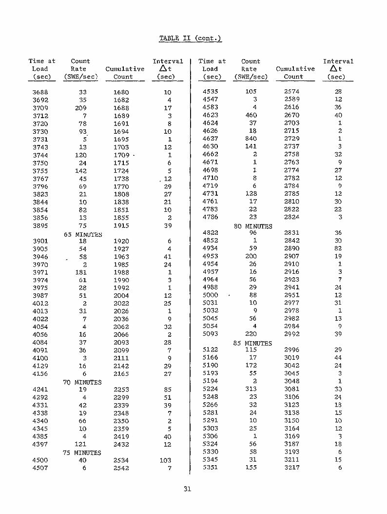
TABLE II (cont)
Time at Count Interval Time at Count Interval Load Rate Cumulative At Load Rate Cumulative At (sec) (SWEsec) Count (sec) (see) (SWEsec) Count (sec)
3688 33 1680 10 4535 105 2574 28 3692 35 1682 4 4547 3 2589 12
3709 209 1688 17 4583 4 2616 36 3712 7 1689 3 4623 460 2670 40 3720 78 1691 8 4624 37 2703 1
3730 93 1694 10 4626 18 2715 2 3731 5 1695 1 4627 840 2729 1 3743 13 1703 12 4630 141 2737 3 3744 120 1709 1 4662 2 2758 32
3750 24 1715 6 4671 1 2763 9 3755 142 1724 5 4698 1 2774 27 3767 45 1738 12 4710 8 2782 12 3796 69 1770 29 4719 6 2784 9 3823 21 1808 27 4731 128 2785 12 3844 10 1838 21 4761 17 2810 30 3854 82 1851 10 4783 22 2822 22 3856 13 1855 2 4786 23 282A 3 3895 75 1915 39 80 MINUTES
65 MINUTES 4822 96 2831 36 3901 18 1920 6 4852 1 2842 30 3905 54 1927 4 4934 59 2890 82
3946 58 1963 41 4953 200 2907 19 3970 2 1985 24 4954 26 2910 1 3971 181 1988 1 4957 16 2916 3 3974 61 1990 3 4964 56 2923 7 3975 28 1992 1 4988 29 2941 24 3987 51 2004 12 5000 88 2951 12 4012 2 2022 25 5031 10 2977 31 4013 31 2026 1 5032 9 2978 1 4022 7 2036 9 5045 56 2982 13 4054 4 2062 32 5054 4 2984 9 4056 16 2066 2 5093 220 2992 39 4084 37 2093 28 85 MINUTES 4091 36 2099 7 5122 115 2996 29 4100 3 2111 9 5166 17 3019 44 4129 16 2142 29 5190 172 3042 24 4156 6 2165 27 5193 55 3045 3
70 MINUTES 5194 2 3048 1 4241 19 2253 85 5224 313 3081 30 4292 4 2299 51 5248 23 3106 24 4331 42 2339 39 5266 32 3123 18 4338 19 2348 7 5281 24 3138 15 4340 66 2350 2 5291 10 3150 10 4345 10 2359 5 5303 25 3164 12 4385 4 2419 40 5306 1 3169 3 4397 121 2432 12 5324 56 3187 18
75 MINUTES 5330 58 3193 6 4500 40 2534 103 5345 31 3211 15 4507 6 2542 7 5351 155 3217 6
31
TABLE II (cont)
Time at Count Interval Time at Count Interval Load Rate Cumulative At Load Rate Cumulative At (sec) (SWBsec) Count (sec) (sec) (SWEsec) Count (sec)
5357 211 3223 6 5887 185 3536 1 5363 29 3233 6 5905 65 3559 18 5364 20 3237 1 5923 31 3575 18
90 MINUTES 5924 22 3576 1 5403 118 3276 39 5933 109 3578 9 5418 79 3295 15 5934 5 3579 1 5419 44 3298 1 5961 43 3582 27 5420 35 3300 1 100 MINUTES 5448 27 3324 28 6000 23 3585 39 5460 118 3327 12 6001 13 3586 1 5466 97 3329 6 6002 166 3588 1 5472 184 3331 6 6008 9 3590 6 5484 28 3333 12 6032 29 3592 24 5499 45 3338 15 6041 111 3596 9 5505 2 3341 6 6062 116 3601 21 5506 173 3344 1 6083 1 3603 21 5512 72 3346 6 6084 236 3606 1 5515 8 3348 3 6090 140 3607 6 5536 199 3352 21 6091 104 3608 1 5548 5 3356 12 6106 21 3609 15 5553 199 3359 5 6115 31 3611 9 5554 34 3360 1 6121 29 3614 6shy5587 190 3364 33 6124 1 3622 3 5593 2 3365 6 6139 51 3630 15 5605 6 3367 12 6160 25 3634 21 5611 12 3369 6 6175 5 3636 15 5638 3 3373 27 6184 196 3639 9 5644 57 3374 6 6217 275 3645 33 5645 78 3376 1 6223 84 3648 6 5669 21 3379 24 6238 23 3649 - 15 5693 22 3384 24 6244 99 3650 6 5699 48 3385 6 6250 81 3652 6
95 MINUTES 6259 39 3654 9 5702 74 3387 3 6265 15 3656 6 5703 85 3389 1 6271 21 3658 6 5725 21 3391 22 6283 85 3660 12 5737 1 3394 12 105 IWNUTES 5752 72 3396 15 6304 143 3662 21 5761 106 3398 9 6331 50 3672 27 5788 1 3414 27 6340 179 3674 9 5794 176 3422 6 6341 37 3675 1 5809 2 3441 15 6365 34 3677 24 5810 15 3445 1 6366 ill 3680 1 5813 42 3448 3 6393 150 3682 27 5814 189 3451 1 6405 43 3684 12 5823 180 3461 9 6429 4 3687 24 5832 171 3472 9 6435 127 3690 6 5838 46 3481 6 6459 31 3691 24 5859 63 3505 21 6483 7 3694 24 5865 15 3511 6 6495 30 3696 12 5886 2 3533 21 6501 128 3700 6
32
TABLE II (cont)
Time at Count Interval Time at Count Interval Load Rate Cumulative At Load Rate Cumulative At (sec) (SWEsec) Count (sec) (sec) (SWEsec) Count (sec)
6522 87 3703 21 7278 21 4158 6 6531 16 3704 9 7302 2 4174 24 6555 102 3706 24 7303 3 4174 1 6567 7 3709 12 7318 125 4186 15 6570 10 3710 3 7348 88 4205 30 6576 87 3711 6 7402 86 4238 54 6577 89 3713 1 7435 90 4258 33 6578 131 3714 1 7447 14 4262 12 6599 4 3717 21 7474 14 4277 27
6600 110 MINUTES
8 3718 1 7486 7504
9 125 MINUTES
89
4286
4304
12
18 6603 37 3720 3 7510 39 4308 6 6639 15 3724 36 7531 52 4331 21 6669 48 3728 30 7540 208 4344 9 6675 23 3729 6 7549 38 4353 9 6684 57 3731 9 7576 72 4376 27 6705 23 3757 21 7594 24 4392 18 6744 53 3807 39 7603 55 4403 9 6762 240 3830 18 7615 160 4415 12 6783 5 3854 21 7621 134 4420 6 6801 26 3874 18 7627 160 4423 6 6822 181 3901 21 7639 180 4430 12 6852 24 3934 30 7648 5 4432 9 6879 44 3962 27 7658 100 4437 10 6882 2 3965 3 7679 319 4445 21
115 MINUTES 7694 72 4449 15 6906 63 3991 24 7709 23 4451 15 6927 176 4001 21 7721 34 4453 12 6930 15 4006 3 130 MINUTES 6931 54 4011 1 7800 Test Terminated 6952 305 4026 21 6953 40 4033 1 6980 3 4037 27 6989 99 4039 9 7040 387 4080 51 7041 53 4095 1 7056 23 4100 15 7086 354 4108 30 7095 21 4110 9 7125 70 4117 30 7131 2 4120 6 7167 97 4129 36 7176 11 4130 9 7197 18 4133 21
120 MINUTES 7218 28 4136 21 7227 39 4138 9 7248 72 4146 21 7272 50 4153 24
33
40
38W
3400
32W
30
28M
260
= 2400
S 22DD
i20
1600
1400
1200
10
600
400
200
06 1a 20 30 40 50 60 70 80 90 tW 110120130
MINUTE-S-H-OLD 17KIPS
Figure 13 Cumulative Stress Wave Count vs Time SpecimE A302B Steels 3 NaC1-Water Environment
34
3503
0
~0
40
20
3203
00
20
C0
20
310
03
(0
40
= = 20 0 I- 365~
05
20 00
20
0shy20
2003
20 ~~0 C
20
20 40
- 20
2835
0
(0
20
20shy
20020
20 -
3403 3450 3720 3750 fl 3550 3003 3050 40) 4050 4003 4050 4~fl 4200 4020 4350 4440 4450
TIME (SECONDS)
Figure 14 Cumulative Stress Wave Count vs Time Specimen No 4 A302B Steel After 1 Minute at 17 Kip Hold in 3 NaCi-Water Environment
35
48
0
I-
S 40
us 50 50 70 5 90 0 60 60 10 6 6 t 20CO DS
- iue1CmlaieSrs av on sTme pcmnN A0BSel
Afe2-0iue t1 i todi NC-ae niomn
Page60
4520 -
so- lao
F
122021 amp~
20 4
400
20
20 22
3540 =
20
3024
20
50
45
20
20520
20
20
45
20
no
I
40
4~
20
40
20
20
4
20
2020
20
gt
20
20 4
20
20
3545
20
Iino200j
5505
2220
1120
20
001
20
20 shy
00
1
45
OX
I
I I
I I
0 50
020 000
205 200
20 200
Z
40 505
550 400
TIM
E (S
EC
ON
DS
)
Figure 16
Cumulative Stress Wave Count vs
Time Specimen No
5 A302B Steel
Hydrogenated and Tested in Air
37
IV C Bend Tests in Air With Deliberate Addition of Hydrogen (cont)
On raising the load from 13000 to 14000 lb (122 ksi-in )
there was evidence of a creep phenomenon as shown in Figure 17 The crackshy
opening-displacement gage confirmed the occurrence of crack growth continuing
after reaching the 14000-lb hold Stress-wave emission showed the mechanism
to be discontinuous cracking rather than a deformation process When the
count rate was plotted as in Figure 18 the activity carrying into the
14000-lb hold again was discontinuous After approximately 300 sec at 14 kips
the SWE associated with the creep phenomenon had subsided During the 14-kip
hold there were two crack jumps one after 920 sec (cumulative count increased
from 5618 to 5720 and the count rate associated with the jump was 181 as
counted over a 10-sec interval or 18 SWEsec) and one after 2130 sec (cumulashy
tive count increased from 5721 to 5755 and the count rate was 139 in 10 see)
After 5000 sec at 14 kips the load on Specimen 5 was raised As
seen in Figure 19 the stress-wave activity was an unmistakable presage of
instability which occurred after 20 sec into hold The load reached a maximum
of 145 kips (145 ksi-in 2) Technically the onset of instability occurred
shortly after starting to increase the load ie at approximately
132 ksi-inI2 which agrees with the KQ value obtained through rising load
tests of unhydrogenated material in an air environment
Because of the very long test period and multiple loadings involved
in the testing of the Specimen 6 only data obtained during rising load to
19500 and 19800 ib during sustained test periods at these loads and during
specimen failure are shown in Figure 20 These data indicate essentially the
same SWE-crack growth relationships discussed previously for Specimen 5 except
that on reaching hold the crack tended to grow slowly for a longer period of
time in comparison to the behavior noted for Specimen 5 Also the incremental
nature of crack extension was more readily observed by the stress-wave-emission
data for Specimen 6
38
20
560
80
60
40
20
5500
80
60
40
20
5400
o 5100
808
60
40
20
5000 u-J
4500
4480 80 4- START 14-KI P HOLD
CODC 75lt
4000
3980 70
3960
6553120 l
- END13-KIP HOLD
3100 160 0 40 80 120 160 200 240 280 320
TIME AT LOAD (SECONDS)
Figure 17 Cumulative Stress Wave Count and COD vs Time Specimen No 5 A302B Steel fydrogenated and Held at 14 Kips in Air
39
200
LU
LU
1- 100
50 END 13-KIP
25 HOLD-I
0 1- TIME
100 INSECONDS AT
200 14KIPS
300
(COUNT EVERY 10 SEC)
Figure 18 Stress Wave Count Rate vs Time - Specimen No 5 A302B Steel Hydrogenated and Tested in Air
40
INSTABILITY
9580
9560
9540
9380
928D0
9260
842D
8440
73O I-shyz 7220
o 7260
U 7240
7220
7180I-shy
7160
- 7140
7120
7100
7080
7060
5900
5880
5860
5840
5820
5800
578D
5460
0 40 80 120 160 SEC
4M 4960 50D RISING LOAD-SECONDS AT 14 KIPS
Figure 19 Cumulative Stress Wave Count vs Time Specimen No 5 A302B Steel Hydrogenated and Tested in Air
41
20000
18000
FAILURE
18290 sec a- 1 17-in K - 199 s - Y
z
-
16000
14000
l0
1200
I-9 Iin
1014in K 152 ki- in -i
o-1 09 n K- 176ksmn
- 1 07 in I 170 iis-
o -1 042in K 12ks-in
c023i NK15ks-n
-shy
-
10000
REACH 19800 lbs
START TO 19800 bs
10000 11000 12000 13000 14000 15000 16000 17000 18000 19000
TIMESECONDS
12000
11000 s
p9000
T LOAD ADJUSTMEA
7n000
READOUT6000 OTE STRESS WAVE DATA A UST T
500 Vgt 0 ENT CORRESPONDIG TO SLOPELOAADJUSTM15 CHANGES PLOTTED
a 4000
3000
LOAD ADJUSTMENT2000 SECONDSECMENIME
1000 START HOLD AT 19500 1b
900 1l6070 D0 8 0 00 0 000600
0 1000 50002000 3000 4000
TIME SECONDS
Figure 20 Cumulative Stress Wave Count vs Time Specimen No 6 A302B Steel Hydrogenated and Tested in Air
Page 42
IV C Bend Tests in Air With Deliberate Addition of Hydrogen (cont)
As indicated in Figure 20 the increase in crack length during
the initial period of hold at 19500 lb resulted in an increase in the applied
stress intensity and was accompanied by significant stress-wave-emission
activity To maintain the desired load it was also necessary to make frequent
load adjustments at the start of hold During the first 3600 sec the effecshy
tive crack length increased from approximately 0963 to 1000 in and was
accompanied by about 7000 SWE As indicated in Figure 20 the majority of the
SWE activity and increase in crack length occurred during the first 3000 sec
of the hold at 19500 lb After this period both the stress-wave-emission
activity and rate of increase in crack length gradually decreased For example
during the entire period from 5000 to 17600 sec when the load was increased
to 19800 lb the apparent crack length and SWE count increased by only approxishy
mately 0020 in and 2500 respectively
After approximately 17000 sec at 19500 lb the load was increased
to 19800 lb and specimen failure occurred after approximately 600 sec at
19800 lb The load was maintained for this period however it was apparent
from both the SWE and COD gage data that the crack was extending and specimen
failure would occur without a further increase in load although it was necesshy
sary to continually adjust the tensile machine to maintain the desired load
The failure stress intensity approximated 199 ksi-in 2however technically
the onset of instability occurred after starting to increase the load at
approximately 153 ksi-in1 2
Specimen 7 was also hydrogenated baked at 300F for 3 hr and
tested in air Figure 21 is a detailed plot of the SWAT data (electronic
counter print-out every second) indicating crack growth of a discontinuous
nature starting at 2400-lb load Note the periods of dormancy (no increase
in SWE count) interspersed with abrupt increases in count indicating disconshy
tinuous crack growth Note also that there was little or no evidence of
continuous stress-wave emission until the load (stress intensity level) was
high approaching failure
43
CUMULAIY STRESS-VAVE COUNTCU LTISTE W E ON
I OT A~II I OI I L I I I I I I I I I I I I I I i I I I I I
- N LB
I I I I I I I I I I I I I i I I
--L - 0OTO11
-0101
(lNIML~ 33383338
8
133113-
3IiC)0 83) 3103 31-3(31-
~0
33 331
3l3C0C~
38318shy
111(10 CAVMSS3 nfl CAliVi flWfl3
________________________________________________________________________
111fl0~ 3KvM~s~a1Ff~TfvTifwT
FPAIAE
hY
A Ii
8
INa
CZ
8 C0 U CI
33 S
1 H
H
03 -I
~ 3lt
0 Cd 33
~C3 ~ H
8 0003
A
Ofli3i~~ C)
Page 45
IV C Bend Tests in Air With Deliberate Addition of Hydrogen (cont)
Figure 22 presents the SWE data from a hydrogenated bend specimen
(No 8) tested in air The load was increased continuously to 9800 lb
(70 ksi-in 2) where there was a short hold (approximately 400 sec) Note
the discontinuous crack growth followed by a short period of continuous
emission (less than 450 slope) The load was then raised to 14800 lb
(109 ksi-in 2) and held for approximately 400 sec Again there were jumps
in the SWE cumulative count but this time interspersed with continuous
emission The SWAT system employed for this test corresponded to that employed
for the background measurements at Kennedy Space Flight Center and shown in
Figure 8 only one channel was employed viz
Endevco 2213 Amplifier Amplifier Band-Pass Filter 10OX 10OX 20 to 50 Kcps
The continuous stress-wave emission observed during hold at the higher stressshy
intensity level in this specimen was not observed in the other hydrogenated
specimens tested in air The primary purpose of this test (Specimen 8) was to
record SWE data for subsequent playback and analysis to determine the amplitude
of burst-type stress-wave emissions associated with fracture in Type A302B
steel These analyses were performed using the instrumentation shown in
Figures 7 and 8 with the following results which are discussed in more detail
in conjunction with the results of the background measurements performed at
Kennedy Space Flight Center (Section V)
Maximum SWE Amplitude - 39 x 10-3g
Minimum SWE Amplitude - 12 x 10-3 g
Average SWE Amplitude - 22 x 10-3g
Laboratory Background - 11 x 10-3g
46
00 o z~ 20 ~
40
~40
S20 1 2 0 0 0 0
TIIAEAT 4 S-KIPHOLD (10KS(51IN A)
407
IV Laboratory Test Results and Discussion (cont)
D BEND TESTS IN 3 NaCI-WATER WITH DELIBERATE ADDITION OF HYDROGEN
Specimen 9 was hydrogenated baked and tested in 80F water
The electronic counter indicated continuous stress-wave emission interspersed
with abrupt increases in count indicating occasional crack jumps Figure 23
shows the details of stress-wave emission that occurred during both rising
load and holding load The crack length determined from the COD chart at
selected loads is also shown Note from the SWE data that there were no
periods of dormancy and the slope of the plot of cumulative count versus time
indicated moderately rapid continuouas crack growth such as might occur with
electrochemical dissolution at the crack tip The COD gage data shown in
Figure 23 also indicate crack extension however the actual amount appears
to be quite small (lt01 in) which would be consistent with the relatively
small number of stress-wave emissions detected even at the high system
sensitivity employed The dramatic difference between the behavior in
Figures 21 and 23 for hydrogenated material tested in air (Figure 21) and
water (Figure 23) indicates that hydrogen and 3 sodium chloride solution
acting together have a greater total effect than the sum of their individual
effects ie working together they appear to have produced a synergism
E WOL TESTS
Because of the possible significance of the synergistic-effect
noted above on the life of the hydrogen pressure vessels at Kennedy Space
Flight Center additional testing was performed using hydrogenated WOL specishy
mens cut from the fractured bend specimens The first WOL specimen was
initially loaded to-3650 lb (50 ksi-in 2) and then placed in 3 NaCl solution
(notch immersed) There was 30 min of essentially continuous stress-wave
emission (recorder started approximately 5 min after loading the specimen)
Subsequently therewas one sizable jump in the SWE cumulative count after
48
V30
760
740-M
$
720 -s
680shy
60
610
40 w
w
520 w
i
20500
HOLDD]N
340
20 760
7200
ING
IV
O
shy
420
60
40
20 0 2
04
0Q
0
60DO
LO0
01 200
250 300
350 400
450 500
550 6M
650
700 750
TIME
(SECONDS)
Figure 23
Cumulative Stress Wave Count vs Time Specimen No 9 A302B Steel
Hydrogenated and Tested in 3 NaCi-Water Environment
49
IV E WOL Tests (cont)
approximately 3 hr 40 min Then 3 hr 20 min later several jumps occurred
followed by 8 hr 20 min of stress-iave activity After this the crack was
dormant (total test time 17 hr 25 min) These data are shown in Figure 24
The load was then increased slightly (torque was increased from 200 to
255 in-lb) an additional 1-12 hr in 3 NaCl solution produced no significant
increase in the cumulative stress-wave count The reason for this apparently
anomalous behavior was not determined although it may result from a blunting
effect at the crack tip produced during the initial hold period
The fatigue crack was then extended (approximately 005 in) in
tension-tension fatigue and the specimen reloaded to approximately 51 ksi-in2
Stress-wave emission started almost immediately (dashed curve in Figure 24)
After approximately 3 hr of discontinuous activity the periods of dormancy
tended to increase interspersed with relatively small jumps (as counted over
10-sec intervals) The results of the initial loading and the reloading are
shown in Figure 24 note that there was appreciably lower cumulative count in
the reloaded specimen as compared with the initial loading for a comparable
period of test
A second hydrogenated WOL specimen was then tested in air at
50 ksi-in 2 there were stress waves initially (creep) but then very little
activity over the remaining 35-hr test period After the first hour the
count increased from approximately 150 to only 280 in the final 34 hr of test
Figure 25 shows the long peribds of dormancy punctuated by occasional 1-count
increases This is in marked contrast to the results obtained from the
hydrogenated WOL specimens tested in 3 NaCl solution and the bend-test
findings of a synergistic effect were confirmed
50
------------
aa
L- -- -- - ------ - --- I
3
IN DO
INTES) 3 S IOTI E( LI N LU
Ino
a
N O
TIME (MINUTES) IN 3 NCI SOLUTION
Figure 24 Cumulative Stress Wave Count vs Time at Hold WOL Specimen No 1
A302B Steel Hydrogenated and Tested in 3 NaCi-Water Environment
51
000 In 0 M6020 126 24 022 in0 1180 10 11 100 IWO l 100M M-C 0 90w6 a0 w6
t t t t 5W MOD4
10
TIME (MINUTES)
Figure 25 Cumulative Stress Wave Count vs Time at Hold WL Specimen No 2 A302B Steel Hydrogenated and Testd in Air
52
IV Laboratory Test Results and Discussion (cont)
F DISCUSSION
1 Material-Environment Consideration
The Type A302B steel supplied for evaluation exhibited a
very high level of fracture toughness Although quantitative plane-strain
fracture toughness measurements were not possible because of the large specimen
size required the KQ value associated with failure approximated 135 ksi-in1 2
This material was also found resistant to environmentally induced failure in
that the rate of crack growth of a prior flaw at applied stress-intensity
factors as high as 90 of the KQ value appeared to be very low This effect
was observed for unhydrogenated-material tested in air and a 3 NaCl-water
environment and hydrogenated material tested in an air environment However
the hydrogenated specimens tested in 3 NaCl-water environment had a much
faster rate of subcritical crack gr~wth in comparison to the other test condishy
tions indicating a synergistic effect due to the combination of sea water and
hydrogen in interstitial solid solution This synergistic effect indicates
that the Type A302B steel hydrogen storage tanks in the Kennedy Space Flight
Center environment may have limited life as the result of subcritical crack
growth if subjected to the same combination of stress and environmental
factors-
The WOL test results tended to confirm the possible synergism
due to the combined effects of 3 NaCl-water and hydrogen in interstitial solid
solution Marked SWE activity was observed when the hydrogenated specimens
were immersed in the salt water whereas in an air environment after the
initial period at hold when a creep phenomenon was observed there was essenshy
tially no stress-wave emission The fact that failure was not produced on
holding (in contradiction to the bend tests) can be explained by the fact that
the WOL test as-performed in this program is a self-arresting test because
53
IV F Discussion (cont)
the occurrence of crack growth results in a reduction in the applied load
Conversely in the bend tests the load was constantly applied as the crack
extended and eventually resulted in specimen failure
2 Stress-Wave-Emission Characterization
Detectable stress-wave emissions although of small amplitude
(ltOOlg) were observed to be associated with crack growth in Type A302B steel
Under all test conditions the stress-wave emissions were observed both during
rising load and when failure (instability) was imminent During hold various
SWE characteristics depending on the test conditions were observed When
tested in the hydrogenated condition in-an air environment a creep phenomenon
evidenced by increasing count of SWE and an accompanying increase in apparent
crack size was observed With time at hold and at applied stress-intensity
levels less than critical the creep phenomenon eventually stopped as did the
occurrence of stress-wave emissions Unhydrogenated material tested in the
3 NaCl-water environment produced continuous stress-wave emission punctuated
by abrupt increases in SWE count This behavior indicates both continuous
very small increments of crack extension with larger crack jumps corresponding
to the abrupt increases in SWE count Continuous incremental crack extension
characterized by continuous SWE interspersed with abrupt increases in SWE count
indicating occasional crack jumps was also observed in testing hydrogenated
material in a 3 NaCl-water environment
In all instances when failure (instability) occurred both
the amplitude and rate of stress-wave emission increased and could be employed
as a precursor of the onset of instability however even when failure was
approached-the SWE amplitude was small (ltOlg) In the other instances where
failure was not produced evidence of crack extension (although very small in
some instances) was observed on the specimen fracture face Once evidence of
54
IV F Discussion (cont)
crack growth was observed (by SWE or COD) it is obvious that failure would
eventually occur (assuming a constantly applied load) although depending on
the initial flaw size and subcritical growth rate the time to failure may be
very long In actual practice the SWE data could be employed (1) to locate
the propagating flaw (2) to monitor its occurrence and (3) as a basis for
terminating service so that repairs could be made before failure The stressshy
wave emissions associated with crack growth during rising load or increasing
stress intensity and the creep phenomenon during the initial part of hold
can be employed for this purpose
5S
V BACKGROUND MEASUREMENTS AND ASSOCIATED LABORATORY TESTS
A BACKGROUND MEASUREMENTS AT KENNEDY SPACE FLIGHT CENTER
Background noise measurements were made at two locations the VAB
Bottle Field and Pad A at the Kennedy Space Flight Center The data were tape
recorded and in addition to general background noise included tank blowdown
and repressurization periods The instrumentation for this purpose is shown
schematically in Figure 8 analysis of the data was performed by playback onto
an oscillograph and comparison with the SWE-crack growth data obtained during
the laboratory testing of bend specimens
The analysis of the signal amplitude data for tests at Cape Kennedy
is indicated below
1 Pad A Bottle Field
Signal Amplitude
a Quiescent Background
Filter at 20 Kcps - 50 Kcps -BandPass- 99 x 10 gsBand Pass
Filter at 200 cps - 32 Kcps
Band Pass
b Tank Blowdown - System Saturation (gt llg peak to peak)
C Tank Repressurization - System Saturation (gt llg peak to peak)
2 VAB Bottle Field
a Quiescent Background - 22 x 10- 4 gs
56
V A Background Measurements at Kennedy Space Flight Center (cont)
Signal Amplitude
b Tank Blowdown - System Saturation (gt llg peak to peak)
C Tank Repressurization - System Saturation (gt llg peak to peak)
Analysis of the tape-recorded data of bend tests at Aerojet indicates
the following signal amplitude for burstf-type stress-wave emissions associated
with crack growth and fracture in Type A302B steel
Maximum Amplitude - 39 x 10-3g
Minimum Amplitude - 12 x 10-3g
Average Amplitude - 22 x 10-3g
Laboratory Background - 11 x 10-3g
Thus the amplitude of SWE associated with crack growth in A302B steel is
approximately an order of magnitude larger than the background noise noted
previously Consequently the above results show that it is possible to detect
stress-wave emissions associated with fracture in A302B steel under the quiescent
background conditions existing at the Kennedy Space Center Difficulty is
expected in detecting such flaw growth during tank blowdown and repressurization
periods unless filtering can be employed to screen out the noise associated
with these periods However the blowdown and repressurization periods are of
very short duration and the materials behavior observed in this program indishy
cated that considerable prefailure crack extension would be expected from any
flaw of a size expected to be present in these pressure vessels Also
immediately on reaching load a creep phenomenon evidenced by an extension
in apparent crack length and accompanied by detectable stress-wave emission
was observed Consequently even if noise associated with blowdown and
57
V A Background Measurements at Kennedy Space Flight Center (cont)
repressurization cannot be effectively filtered out significant flaw growth
andor creep could still be detected and tank depressurization accomplished
prior to catastrophic failure assuming a capability for such depressurization
exists at these locations
B LABORATORY SIGNAL ATTENUATION EVALUATIONS
Subsequent to the background measurements at the Kennedy Space
Flight Center and the bend tests at Aerojet two series of tests were made at
Aerojet using a section of pipe and plate both of SAE 4130 steel alloy The
purpose of these tests was to determine the coefficient of signal attenuation
which in conjunction with the previous test data could be used to establish
the sensor spacing which would insure detection of SWE associated with crack
growth in the pressure-vessels at the Kennedy Space Flight Center
In these tests a constant pulse was imparted to the specimen by
a Tektronix 115 Pulse Generator using a Clevite PZT-5 Crystal (2125 in dia
and 0250 in thick) The piezoelectric crystal was mounted on a small alumishy
num block which in turn was adhered to the surface of the specimen The
signal was received by a 2217-E-Endevcq accelerometer placed at various disshy
tances from the pulser The pulse used was 10 n-sec rise and fall time with
a duration of 20 microsec at an amplitude of 12v
1 Pipe Tests
A SAE 4130 steel pipe (8-58 in OD 7-18 in ID and 22 ft
10-78 in long) was used as specimen for this test series The pulser was
mounted normal to the external surface of the pipe as close as possible to the
edge The accelerometer (2217-E-Endevco) was successively placed on the pipe
58
V B Laboratory Signal Attenuation Evalutions (cont)
surface at positions I to 8 that were at 4 6 8 10 12 14 16 and 20 ft
from the pulser The signal received by the accelerometer was displayed on a
Tektronix 422 osilloscope Typical signals are shown in Figure 26
The velocities of the compressional and shear waves in steel
are
29 lO06 x38103 Vc= -x lg ) (l-26) = O2 x06(- 0 x386 = 227000 insec(+j 012)283 (1+030) (1-060)
29x106 x 386 = 91 36= 123000 insec
s 2 ( + p) p 2 (i + 030) x 0283
where E = Youngs Modulus p = Poissons Ratio and p = density The times of
arrival of these waves at the computed velocities are indicated on the oscilloshy
scope photos shown in Figure 26 The point of shear wave arrival (T ) coincides
in most of the photos to a distinct change of pattern in the trace The
arrival of the compressional wave is difficult to determine accurately because
the amplitude of this wave attenuates very fast with distance
A visual comparison of the curves shows that Figure 26a
representing the signal received 4 ft from the impulse indicates a perfectly
detectable arrival of the compressional wave conversely Figure 26h (at 20 ft
from the impulse) shows the visually detectable arrival of a wave almost at the
computed arrival of the shear wave This is due to the fact that the amplitude
of the first cycles of the compressional wave have become essentially impercepshy
tible at a distance of 20 ft from the pulse An attempt to determine signal
arrival time by visual inspection only of the traces in Figure 26 would result
in the wave velocities indicated in Table III The computed arrival times of
the compressional and shear waves are shown in Table IV If an integration of
the positive portions of the cycles comprised in 200 p sec after arrival of the
59
VERTICAL SCALE 1 DIV= 01 V VERTICAL SCALE 1 DIV = 01 V HORIZONTAL SCALE 1 DIV= 50p SEC HORIZONTAL SCALE 1 DIV = 100 pSEC
a 4FT FROM PULSER b6 FEET FROM PULSER
Tc Ts Tc Ts
VERTICAL SCALE I DIV 01 V VERTICAL SCALE I DIV = 01 V HORIZONTAL SCALE I DIV = 100 I SEC HORIZONTAL SCALE 1 DIV = 200 p SEC
c 8 FEET FROM PULSER d 10 FEET FROM PULSER
Tc = Arrival of Compressional Wave
T = Arrival of Shear Wove
Figure 26 Oscillograph Traces for Pipe Tests (Sheet 1 of 2)
6o NOT REPRODUCTBLE
VERTICAL SCALE 1 DIV = 01 V VERTICAL SCALE 1 DIV 01 V HORIZONTAL SCALE 1 DIV = 200y SEC HORIZONTAL SCALE I DIV 200 p SEC
e 12 FEET FROM PULSER f 14 FEET FROM PULSER
T TS T T
VERTICAL SCALE 1 DIV = 01 V VERTICAL SCALE 1 DIV = 01 V HORIZONTAL SCALE 1 DIV = 200 v SEC HORIZONTAL SCALE I DIV =5001p SEC
g 16 FEET FROM PULSER h 20 FEET FROM PULSER
Figure 26 Oscillograph Traces for Pipe Tests (Sheet 2 of 2)
61
V B Laboratory Signal Attenuation Evaluations (cont)
shear wave is performed the average amplitudes determined in this manner
become quite meaningful These average amplitudes are shown in Table V
TABLE III
WAVE VELOCITY BASED ON VISUAL ANALYSIS OF OSCILLOSCOPE TRACES - PIPE TESTS
Distance from Pulse Arrival Velocities Photo ft in Time psc (ftsec)
1 4 48 210 228000
2 6 72 400 180000
3 8 96 600 160000
4 10 120 800 150000
5 12 144 1000 144000
6 14 168 1200 140000
7 16 192 1400 137000
8 20 240 1750 137000
TABLE IV
COMPUTED ARRIVAL TIMES - PIPE TESTS
Compressional Wave Shear Wave Distance from Pulse Arrival Time Arrival Time
Photo in psec Osc Div sec Ose Div
1 48 212 423 390 780
2 72 317 317 583 583
3 96 422 422 778 778
4 120 530 265 972 486
5 144 635 317 1163 581
6 168 740 370 1360 680
7 192 840 420 1545 771
8 240 1050 21 1930 387
62
V B Laboratory Signal Attenuation Evalutions (cont)
TABLE V
SIGNAL AMPLITUDE VS DISTANCE - PIPE TESTS
Average Signal Amplitude Distance from 200 Psec after Arrival
Test Pulser in of Comp Wave mv
1 48 230
2 72 145
3 96 85
4 120 60
5 144 45
6 168 28
7 192 22
8 240 18
The general equation for the amplitude attenuation curve is
C x e-Xy =
where y = amplitude at distance x in volts
x = distance in inches from pulse source
C = amplitude of pulse in volts
a = attenuation factor
or iny= 1 C + (- ax) = I C - ax (Eq 4)n n
To determine the values of C and a the following statistical analysis was
performed
63
V B Laboratory Signal Attenuation Evaluations (cont)
Distance Yo y y2 X X2 Test in m v n n
1 48 230 543 +142 2010 -87 7580 - 124 261
2 72 145 499 +098 0960 -63 3960 - 62 360
3 96 85 445 +044 0194 -39 1520 - 17 427
4 120 60 409 +008 0006 -15 225 - 1 490
5 144 45 380 -021 0044 + 9 81 - 2 548
6 168 28 334 -067 0450 +33 1090 - 21 560
7 192 22 309 -092 0847 +57 3250 - 52 592
8 240 18 289 -112 1250 +105 11000 - 118 690
EY2 EX2pound x = 1080 ElnY =3208 5761 28706 SXY-397 XxIny3928
- 1080 - 3208 x =- = 135 ny = 401
EXY -397 00138 1 C =l1y + oshy
pound 2 x2 28706 n i x
= 401+(0138)(135)=401+186= 587
C - 355 mv
It is now possible to compute the statistically corrected values of the signal
amplitude y at the distances from the pulse where they were measured The
general formula will be
ny = 587 -(00138) X
and the results are tabulated in Table VI The computed value of pulse amplishy
tude at source is found to be C = 355 my The values shown on Table VI are
plotted in Figure 27 which graphically shows the signal attenuation as a
function of distance from the pulse source
64
350
300
250 STATISTICALLY COMPUTED k VALUES FOR REGRESSION CURVE
--0gt 200
EXPERIMENTALLY DETERMINED
-- MATERIAL SAE 4130 STEEL U= SPECIMEN PIPE-S758 in D aZ
00
15 7 18 in D22 ft 10 78 in LONG
-J
100
50 I
0 I I I
5 I I I
DISTANCE
I
10 FROM SOURCE
I
FEET
I
15 20
Figure 27 Signal Amplitude vs Distance - Pipe Tests
V B Laboratory Signal Attenuation Evaluations (cont)
TABLE VI
STATISTICALLY CORRECTED VALUES OF SIGNAL AMPLITUDE - PIPE TESTS
Experimentally Distance from 1 Corrected Signal Determined Signal
Test Pulse in ny Amplitude (y) mv Amplitude (y) my
1 48 521 182 230
2 72 488 130 145
3 96 455 95 85
4 120 421 67 60
5 144 388 48 45
6 168 355 35 28
7 192 322 25 22
8 240 255 127 18
- 2 Plate Tests
An SAE 4130 steel plate (73-12 in long 48-12 in wide
and 34 in thick) was used for this test series The two diagonals were
marked on the plate The pulser was placed at the center of the plate and
the receiver accelerometer was placed on one of the diagonals at locations
spaced in increments of 6 in from the center The received signals were
observed on the oscilloscope and photos were taken of these signals Figure
28 shows oscillographs of the signals received at 6 12 18 24 30 36 and
42 in from the pulser The times of arrival of the shear wave are also shown
in Figure 28 The velocity used was v = 123000 insec An integration
was performed of the positive positions of the cycles comprised in a 20 Psec
interval after the arrival of the shear wave The average amplitudes detershy
mined from these integrations are shown in Table VII Only Tests 1 to 4 are
used because reflection (from the plate edges) in Tests 5 to 8 obscured the
66
b 12 INCHES FROM PULSERa 6 INCHES FROM PULSER
TBTs
c 18 INCHES FROM PULSER d 24 INCHES FROM PULSER
IT s = Arrival of Shear Wave
Vertical Scale 1 DIV = 01 Volt Horizontal Scale 1 DIV = 20 ASec
Figure 28 Oscillograph Traces for Plate Tests (Sheet 1 of 2)
Page 67
f 36 INCHES FROM PULSER e 30 INCHES FROM PULSER
g 42 INCHES FROM PULSER
= Arrival of Shear WaveTs
Vertical Scale 1 DIV = 01 Volt = 20 4SecHorizontal Scale 1 DIV
Figure 28 Oscillograph Traces for Plate Tests (Sheet 2 of 2)
08 gOTPRODUCIB1A
V B Laboratory Signal Attenuation Evaluations (cont)
data These reflections were received in Tests 5 to 8 because of the relashy
tively small plate that was available for this test series
TABLE VII
SIGNAL AMPLITUDE VS DISTANCE - PLATE TESTS
Distance from Average Amplitude Test Pulse in(x) in 20 p see mv
1 6 150
2 12 110
3 18 70
4 24 45
The following statistical analysis was performed to determine the values of
C and a in Equation 4
Test
Distance from
Pulse in(x)
y
m v
1
ny Y
2
Y 2
X XY
X1 y
n
1 6 150 500 +056 0314 -9 81 -502 3000
2
3
12
18
110
70
470
425
+026
-019
0067
0036
-3
+3
9
9
-078
-057
5640
7650
4 24 45 381 -063 0397 +9 81 -567 9149
60 1776 0814 180 -1204 25439
-x=
60 w= 15
4ny
iY 1
1nC
-
=
16=44 1776 =44
E YX 1204= __=
E y2 180
ny +(0067)(15) =
+0067
444 + 0067(15)
69
=
C
444 + 100
= 230 my
= 544
V B Laboratory Signal Attenuation Evaluations (cont)
Subsequently the values of signal amplitude (y) were statistically corrected
as before and the experimentally determined values of y are compared to the
results obtained in Table VIII
TABLE VIII
COMPARISON Or STATISTICALLY CORRECTED AND TEST-DETERMINED VALUES OF SIGNAL AMPLITUDE - PLATE TESTS
Experimentally Distance from Corrected Signal Determined Signal
Test Pulse in nY Amplitude (y) mv Amplitude (y) my
1 6 504 155 150
2 12 464 103 110
3 18 417 65 70
4 24 383 46 45
The computed value of the pulse amplitude at the source at
C equals 230 mv The regression curve and the experimentally determined points
are plotted in Figure 29 It should be observed that the attenuation coefshy
ficient for the pipe test was a = 00138 and for the plate test was 0067
This is due to the much larger rate of front area that the pulse meets in the
plate
C SENSOR SPACING
The quiescent background noise measurements performed at the test
sites using a 20 to 50 KHz band-pass filter are
Pad A Bottle Field - 0000099g
VAB Bottle Field 0000220g
70
250
200 - EXPERIMENTALLY DETERMINED
0o
gt
M a-100 34
STATISTICALLY COMPUTEDVALUES FOR REGRESSION CURVE
MATERIAL SAE 4130 STEEL
SPECIMEN PLATE - 73 12 in LONG 48 12 in WIDE
in THICK
J
50
0
0 5 SII
10 15
DISTANCE FROM SOURCE FEET
I
20 I
25
Figure 29 Signal Amplitude vs Distance - Plate Tests
V C Sensor Spacing (cont)
The recorded stress-wave-emission data obtained from the A302B steel bend tests
made at the Aerojet-General Corporation laboratory show that the minimum
acceleration at the source is 0O012g the average 00022g and the maximum
00039g Based on the above data and the attenuation factor X = 0067 detershy
mined from the plate tests the sensor spacings required to detect crack growth
in the vessels at the Kennedy Space Center were computed and the results are
tabulated below
Quiescent Sensor Spacing
Amplitude at Background in the Source(C) g Amplitude(y) g Cy ln(CIy) ln(CIy)
Pad A
Min Signal 00012 000015 800 208 310
Avg Signal 00022 000015 1470 269 402
Max Signal 00039 000015 2600 326 487
VAB Bottle Field
Min Signal 00012 000033 363 129 193
Avg Signal 00022 000033 668 190 283
Max Signal 00039 000033 1080 238 356
This threshold is 15 x 0000099 - 000015g (at Pad A)
This threshold is 15 x 000022 = 000033g (at VAB Bottle Field)
Figures 30 and 31 present schematically the location and spacings of sensors
on the pressure vessels
72
- 502 IN 8 IN
HEAD -- _
DEVELOPED + + CYLINDRICAL FOR MINIMUM SIGNAL-22 SENSORS AS SHOWN
SURFACE FOR AVERAGE SIGNAL-16 SENSORS
+ +I
FOR MAXIMUM SIGNAL- 14 SENSORS
282438 IN+ +
+ +
9 SPACINGS AT 313 IN
-I- +
+ +shy
+ -plusmn
HEAD _ __
8 IN
Figure 30 Schematic of Sensor Spacings for Bottles at Pad A
73
14601 IN
HEAD (6SENSORS) 23 14 INI I I - I I I
t plusmn + plusmn + +
+ + 4 + + + DEVELOPED CYL SURFACE
+ + 4A 1 13 LINES OF
+ + + SENSORS SPACED4 + + AT 2086 IN
+ + + + + +
+ + 4 + + +
251 1516 IN + + + +-I- +
+ + + 4- +
-1- 298438 IN+ -I- -+- -i- +
+I
23 14 INHEAD (6 SENSORS) 1
FOR MINIMUM SIGNAL-103 SENSORS AS SHOWN
FOR AVERAGE SIGNAL- 82 SENSORS FOR MAXIMUM SIGNAL- 58 SENSORS
Figure 31 Schematic of Sensor Spacings for Bottles at VAB Bottle Field
74
VI CONCLUSIONS
A The Type A302B steel supplied for evaluation exhibited a high level
of fracture toughness Although quantitative plane-strain fracture toughness
measurements were not possible because of the large specimen size required
the K value associated with failure approximated 135 ksi-inI 2
Q
B The Type A302B steel was found resistant to environmentally induced
slow crack growth when tested in the hydrogenated condition in an air environshy
ment and in the unhydrogenated condition in a 3 NaCl-water environment Howshy
ever hydrogenated material tested in 3 NaCl-water had a much faster rate of
subcritical crack growth indicating a synergistic effect due to the combinashy
tion of sea water and hydrogen in interstitial solid solution
C The synergistic effect indicates the Type A302B steel hydrogen
storage tanks in the Kennedy Space Flight Center may have limited life as a
result of subcritical crack growth if subjected to the same combination of
stress and environmental factors
D Detectable stress-wave emissions although of small amplitude
(ltOOlg) were observed to be associated with crack growth in Type A302B steel
In all test conditions the stress-wave emissions were observed during rising
load and when failure (instability) was imminent Both the amplitude and rate
of stress-wave emission increased as failure was approached and could be
employed as a precursor of the onset of instability
E Stress-wave emissions associated with crack growth in Type A302B
steel can be detected under quiescent background conditions at the Pad A and
VAB Bottle fields at the Kennedy Space Flight Center However it would be
difficult to detect such stress-wave emissions during tank blowdown and
repressurization periods unless filtering can be employed to screen out the
noise associated with these periods
75
VI Conclusions (cont)
F Even in the presence of background noise from tank blowdown and
repressurization these periods are considered short in the overall life of
the pressure vessels Consequently flaw growth or creep which was observed
during rising load or the initial part of hold could be detected by SWAT
permitting triangulation to the source and tank depressurization prior to
failure
G Stress-wave-emission attenuation test data were obtained and employed
in conjunction with the site background measurements addbnd test stress-waveshy
emission characterization data to determine sensor mounting patterns for the
hydrogen pressure vessels at Pad A and the VAB Bottle Field
VII RECOMMENDATIONS FOR FURTHER WORK
If the synergistic effect of hydrogen and 3 NaCi solution occurs in
Kennedy Space Flight Center tankage the life of the tankage will be limited
Obviously slow-crack growth from any cause whether continuous or disconshy
tinuous and regardless of how slow the rate of cracking will eventually
produce failure This investigation showed that subcritical crack growth is
in all likelihood occurring with each pressurization A question remains
however as to the rate of crack growth without knowledge of the rate there
is no way to anticipate the life of the tankage However with SWAT one can
monitor the occurrence of crack growth and most importantly make judgment
as to whether a given crack is approaching critical size Consequently it
is recommended that additional tests be performed to (1) verify the existence
of subcritical cracking in actual on-site tankage and (2) incorporate an
automatic system for continuously monitoring on-site tankage at Kennedy Space
Flight Center
76
REFERENCES
1 Steel R K Green A T Lockman C S Acoustic Verification of Structural Integrity of Polaris Chambers Society of Plastic Engineers 20th Meeting Atlantic City N Y January 1964
2 Pressure Testing of AFRM-017 Service Propulsion System Fuel Tank Utilizing Aerojet-General Corporations Stress-Wave Analysis Technique
Report NAS 9-6766-003 Aerojet-General Corp for NASA MSC Houston Texas Contract NAS 9-6766 May 1967
3 Srawley J E and Esgar J B Investigation of Hydrotest Failure of Thiokol Chemical Corp 260-Inch-Diameter SL-1 Motor Case NASA-TMX shy1194 January 1964
4 Hartbower C E Gerberich W W and Crimmins P P Mechanisms of Slow Crack Growth in High-Strength Steels AFML-TR-67-26 Vol 1 February 1967
5 -Hartbower C E Gerberich W W and Crimmins P P Characterization of Fatigue-Crack Growth by Stress Wave Emission Final Report on Conshytract NAS 1-4902 for NASA-Langley Research Center Hampton Virginia June 1966
6 IHartbower C E Gerberich W W Reuter W G and Crimmins P P Stress Wave Characteristics in Constructional Alloys Final Report on Office of Naval Research Contract N00014-66-C-0340 July 1967
7 Novak S R and Rolfe S T Modified WOL Specimen for KIscc Environmental Testing U S Steel Corp paper submitted to ASTM for publication
77
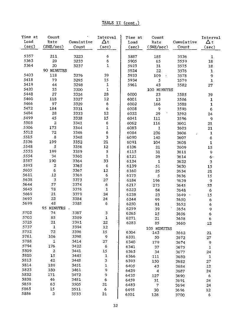
TABLE II (cont)
Time at Count Interval Time at Count Interval Load Rate Cumulative At Load Rate Cumulative At (sec) (SWBsec) Count (sec) (sec) (SWEsec) Count (sec)
5357 211 3223 6 5887 185 3536 1 5363 29 3233 6 5905 65 3559 18 5364 20 3237 1 5923 31 3575 18
90 MINUTES 5924 22 3576 1 5403 118 3276 39 5933 109 3578 9 5418 79 3295 15 5934 5 3579 1 5419 44 3298 1 5961 43 3582 27 5420 35 3300 1 100 MINUTES 5448 27 3324 28 6000 23 3585 39 5460 118 3327 12 6001 13 3586 1 5466 97 3329 6 6002 166 3588 1 5472 184 3331 6 6008 9 3590 6 5484 28 3333 12 6032 29 3592 24 5499 45 3338 15 6041 111 3596 9 5505 2 3341 6 6062 116 3601 21 5506 173 3344 1 6083 1 3603 21 5512 72 3346 6 6084 236 3606 1 5515 8 3348 3 6090 140 3607 6 5536 199 3352 21 6091 104 3608 1 5548 5 3356 12 6106 21 3609 15 5553 199 3359 5 6115 31 3611 9 5554 34 3360 1 6121 29 3614 6shy5587 190 3364 33 6124 1 3622 3 5593 2 3365 6 6139 51 3630 15 5605 6 3367 12 6160 25 3634 21 5611 12 3369 6 6175 5 3636 15 5638 3 3373 27 6184 196 3639 9 5644 57 3374 6 6217 275 3645 33 5645 78 3376 1 6223 84 3648 6 5669 21 3379 24 6238 23 3649 - 15 5693 22 3384 24 6244 99 3650 6 5699 48 3385 6 6250 81 3652 6
95 MINUTES 6259 39 3654 9 5702 74 3387 3 6265 15 3656 6 5703 85 3389 1 6271 21 3658 6 5725 21 3391 22 6283 85 3660 12 5737 1 3394 12 105 IWNUTES 5752 72 3396 15 6304 143 3662 21 5761 106 3398 9 6331 50 3672 27 5788 1 3414 27 6340 179 3674 9 5794 176 3422 6 6341 37 3675 1 5809 2 3441 15 6365 34 3677 24 5810 15 3445 1 6366 ill 3680 1 5813 42 3448 3 6393 150 3682 27 5814 189 3451 1 6405 43 3684 12 5823 180 3461 9 6429 4 3687 24 5832 171 3472 9 6435 127 3690 6 5838 46 3481 6 6459 31 3691 24 5859 63 3505 21 6483 7 3694 24 5865 15 3511 6 6495 30 3696 12 5886 2 3533 21 6501 128 3700 6
32
TABLE II (cont)
Time at Count Interval Time at Count Interval Load Rate Cumulative At Load Rate Cumulative At (sec) (SWEsec) Count (sec) (sec) (SWEsec) Count (sec)
6522 87 3703 21 7278 21 4158 6 6531 16 3704 9 7302 2 4174 24 6555 102 3706 24 7303 3 4174 1 6567 7 3709 12 7318 125 4186 15 6570 10 3710 3 7348 88 4205 30 6576 87 3711 6 7402 86 4238 54 6577 89 3713 1 7435 90 4258 33 6578 131 3714 1 7447 14 4262 12 6599 4 3717 21 7474 14 4277 27
6600 110 MINUTES
8 3718 1 7486 7504
9 125 MINUTES
89
4286
4304
12
18 6603 37 3720 3 7510 39 4308 6 6639 15 3724 36 7531 52 4331 21 6669 48 3728 30 7540 208 4344 9 6675 23 3729 6 7549 38 4353 9 6684 57 3731 9 7576 72 4376 27 6705 23 3757 21 7594 24 4392 18 6744 53 3807 39 7603 55 4403 9 6762 240 3830 18 7615 160 4415 12 6783 5 3854 21 7621 134 4420 6 6801 26 3874 18 7627 160 4423 6 6822 181 3901 21 7639 180 4430 12 6852 24 3934 30 7648 5 4432 9 6879 44 3962 27 7658 100 4437 10 6882 2 3965 3 7679 319 4445 21
115 MINUTES 7694 72 4449 15 6906 63 3991 24 7709 23 4451 15 6927 176 4001 21 7721 34 4453 12 6930 15 4006 3 130 MINUTES 6931 54 4011 1 7800 Test Terminated 6952 305 4026 21 6953 40 4033 1 6980 3 4037 27 6989 99 4039 9 7040 387 4080 51 7041 53 4095 1 7056 23 4100 15 7086 354 4108 30 7095 21 4110 9 7125 70 4117 30 7131 2 4120 6 7167 97 4129 36 7176 11 4130 9 7197 18 4133 21
120 MINUTES 7218 28 4136 21 7227 39 4138 9 7248 72 4146 21 7272 50 4153 24
33
40
38W
3400
32W
30
28M
260
= 2400
S 22DD
i20
1600
1400
1200
10
600
400
200
06 1a 20 30 40 50 60 70 80 90 tW 110120130
MINUTE-S-H-OLD 17KIPS
Figure 13 Cumulative Stress Wave Count vs Time SpecimE A302B Steels 3 NaC1-Water Environment
34
3503
0
~0
40
20
3203
00
20
C0
20
310
03
(0
40
= = 20 0 I- 365~
05
20 00
20
0shy20
2003
20 ~~0 C
20
20 40
- 20
2835
0
(0
20
20shy
20020
20 -
3403 3450 3720 3750 fl 3550 3003 3050 40) 4050 4003 4050 4~fl 4200 4020 4350 4440 4450
TIME (SECONDS)
Figure 14 Cumulative Stress Wave Count vs Time Specimen No 4 A302B Steel After 1 Minute at 17 Kip Hold in 3 NaCi-Water Environment
35
48
0
I-
S 40
us 50 50 70 5 90 0 60 60 10 6 6 t 20CO DS
- iue1CmlaieSrs av on sTme pcmnN A0BSel
Afe2-0iue t1 i todi NC-ae niomn
Page60
4520 -
so- lao
F
122021 amp~
20 4
400
20
20 22
3540 =
20
3024
20
50
45
20
20520
20
20
45
20
no
I
40
4~
20
40
20
20
4
20
2020
20
gt
20
20 4
20
20
3545
20
Iino200j
5505
2220
1120
20
001
20
20 shy
00
1
45
OX
I
I I
I I
0 50
020 000
205 200
20 200
Z
40 505
550 400
TIM
E (S
EC
ON
DS
)
Figure 16
Cumulative Stress Wave Count vs
Time Specimen No
5 A302B Steel
Hydrogenated and Tested in Air
37
IV C Bend Tests in Air With Deliberate Addition of Hydrogen (cont)
On raising the load from 13000 to 14000 lb (122 ksi-in )
there was evidence of a creep phenomenon as shown in Figure 17 The crackshy
opening-displacement gage confirmed the occurrence of crack growth continuing
after reaching the 14000-lb hold Stress-wave emission showed the mechanism
to be discontinuous cracking rather than a deformation process When the
count rate was plotted as in Figure 18 the activity carrying into the
14000-lb hold again was discontinuous After approximately 300 sec at 14 kips
the SWE associated with the creep phenomenon had subsided During the 14-kip
hold there were two crack jumps one after 920 sec (cumulative count increased
from 5618 to 5720 and the count rate associated with the jump was 181 as
counted over a 10-sec interval or 18 SWEsec) and one after 2130 sec (cumulashy
tive count increased from 5721 to 5755 and the count rate was 139 in 10 see)
After 5000 sec at 14 kips the load on Specimen 5 was raised As
seen in Figure 19 the stress-wave activity was an unmistakable presage of
instability which occurred after 20 sec into hold The load reached a maximum
of 145 kips (145 ksi-in 2) Technically the onset of instability occurred
shortly after starting to increase the load ie at approximately
132 ksi-inI2 which agrees with the KQ value obtained through rising load
tests of unhydrogenated material in an air environment
Because of the very long test period and multiple loadings involved
in the testing of the Specimen 6 only data obtained during rising load to
19500 and 19800 ib during sustained test periods at these loads and during
specimen failure are shown in Figure 20 These data indicate essentially the
same SWE-crack growth relationships discussed previously for Specimen 5 except
that on reaching hold the crack tended to grow slowly for a longer period of
time in comparison to the behavior noted for Specimen 5 Also the incremental
nature of crack extension was more readily observed by the stress-wave-emission
data for Specimen 6
38
20
560
80
60
40
20
5500
80
60
40
20
5400
o 5100
808
60
40
20
5000 u-J
4500
4480 80 4- START 14-KI P HOLD
CODC 75lt
4000
3980 70
3960
6553120 l
- END13-KIP HOLD
3100 160 0 40 80 120 160 200 240 280 320
TIME AT LOAD (SECONDS)
Figure 17 Cumulative Stress Wave Count and COD vs Time Specimen No 5 A302B Steel fydrogenated and Held at 14 Kips in Air
39
200
LU
LU
1- 100
50 END 13-KIP
25 HOLD-I
0 1- TIME
100 INSECONDS AT
200 14KIPS
300
(COUNT EVERY 10 SEC)
Figure 18 Stress Wave Count Rate vs Time - Specimen No 5 A302B Steel Hydrogenated and Tested in Air
40
INSTABILITY
9580
9560
9540
9380
928D0
9260
842D
8440
73O I-shyz 7220
o 7260
U 7240
7220
7180I-shy
7160
- 7140
7120
7100
7080
7060
5900
5880
5860
5840
5820
5800
578D
5460
0 40 80 120 160 SEC
4M 4960 50D RISING LOAD-SECONDS AT 14 KIPS
Figure 19 Cumulative Stress Wave Count vs Time Specimen No 5 A302B Steel Hydrogenated and Tested in Air
41
20000
18000
FAILURE
18290 sec a- 1 17-in K - 199 s - Y
z
-
16000
14000
l0
1200
I-9 Iin
1014in K 152 ki- in -i
o-1 09 n K- 176ksmn
- 1 07 in I 170 iis-
o -1 042in K 12ks-in
c023i NK15ks-n
-shy
-
10000
REACH 19800 lbs
START TO 19800 bs
10000 11000 12000 13000 14000 15000 16000 17000 18000 19000
TIMESECONDS
12000
11000 s
p9000
T LOAD ADJUSTMEA
7n000
READOUT6000 OTE STRESS WAVE DATA A UST T
500 Vgt 0 ENT CORRESPONDIG TO SLOPELOAADJUSTM15 CHANGES PLOTTED
a 4000
3000
LOAD ADJUSTMENT2000 SECONDSECMENIME
1000 START HOLD AT 19500 1b
900 1l6070 D0 8 0 00 0 000600
0 1000 50002000 3000 4000
TIME SECONDS
Figure 20 Cumulative Stress Wave Count vs Time Specimen No 6 A302B Steel Hydrogenated and Tested in Air
Page 42
IV C Bend Tests in Air With Deliberate Addition of Hydrogen (cont)
As indicated in Figure 20 the increase in crack length during
the initial period of hold at 19500 lb resulted in an increase in the applied
stress intensity and was accompanied by significant stress-wave-emission
activity To maintain the desired load it was also necessary to make frequent
load adjustments at the start of hold During the first 3600 sec the effecshy
tive crack length increased from approximately 0963 to 1000 in and was
accompanied by about 7000 SWE As indicated in Figure 20 the majority of the
SWE activity and increase in crack length occurred during the first 3000 sec
of the hold at 19500 lb After this period both the stress-wave-emission
activity and rate of increase in crack length gradually decreased For example
during the entire period from 5000 to 17600 sec when the load was increased
to 19800 lb the apparent crack length and SWE count increased by only approxishy
mately 0020 in and 2500 respectively
After approximately 17000 sec at 19500 lb the load was increased
to 19800 lb and specimen failure occurred after approximately 600 sec at
19800 lb The load was maintained for this period however it was apparent
from both the SWE and COD gage data that the crack was extending and specimen
failure would occur without a further increase in load although it was necesshy
sary to continually adjust the tensile machine to maintain the desired load
The failure stress intensity approximated 199 ksi-in 2however technically
the onset of instability occurred after starting to increase the load at
approximately 153 ksi-in1 2
Specimen 7 was also hydrogenated baked at 300F for 3 hr and
tested in air Figure 21 is a detailed plot of the SWAT data (electronic
counter print-out every second) indicating crack growth of a discontinuous
nature starting at 2400-lb load Note the periods of dormancy (no increase
in SWE count) interspersed with abrupt increases in count indicating disconshy
tinuous crack growth Note also that there was little or no evidence of
continuous stress-wave emission until the load (stress intensity level) was
high approaching failure
43
CUMULAIY STRESS-VAVE COUNTCU LTISTE W E ON
I OT A~II I OI I L I I I I I I I I I I I I I I i I I I I I
- N LB
I I I I I I I I I I I I I i I I
--L - 0OTO11
-0101
(lNIML~ 33383338
8
133113-
3IiC)0 83) 3103 31-3(31-
~0
33 331
3l3C0C~
38318shy
111(10 CAVMSS3 nfl CAliVi flWfl3
________________________________________________________________________
111fl0~ 3KvM~s~a1Ff~TfvTifwT
FPAIAE
hY
A Ii
8
INa
CZ
8 C0 U CI
33 S
1 H
H
03 -I
~ 3lt
0 Cd 33
~C3 ~ H
8 0003
A
Ofli3i~~ C)
Page 45
IV C Bend Tests in Air With Deliberate Addition of Hydrogen (cont)
Figure 22 presents the SWE data from a hydrogenated bend specimen
(No 8) tested in air The load was increased continuously to 9800 lb
(70 ksi-in 2) where there was a short hold (approximately 400 sec) Note
the discontinuous crack growth followed by a short period of continuous
emission (less than 450 slope) The load was then raised to 14800 lb
(109 ksi-in 2) and held for approximately 400 sec Again there were jumps
in the SWE cumulative count but this time interspersed with continuous
emission The SWAT system employed for this test corresponded to that employed
for the background measurements at Kennedy Space Flight Center and shown in
Figure 8 only one channel was employed viz
Endevco 2213 Amplifier Amplifier Band-Pass Filter 10OX 10OX 20 to 50 Kcps
The continuous stress-wave emission observed during hold at the higher stressshy
intensity level in this specimen was not observed in the other hydrogenated
specimens tested in air The primary purpose of this test (Specimen 8) was to
record SWE data for subsequent playback and analysis to determine the amplitude
of burst-type stress-wave emissions associated with fracture in Type A302B
steel These analyses were performed using the instrumentation shown in
Figures 7 and 8 with the following results which are discussed in more detail
in conjunction with the results of the background measurements performed at
Kennedy Space Flight Center (Section V)
Maximum SWE Amplitude - 39 x 10-3g
Minimum SWE Amplitude - 12 x 10-3 g
Average SWE Amplitude - 22 x 10-3g
Laboratory Background - 11 x 10-3g
46
00 o z~ 20 ~
40
~40
S20 1 2 0 0 0 0
TIIAEAT 4 S-KIPHOLD (10KS(51IN A)
407
IV Laboratory Test Results and Discussion (cont)
D BEND TESTS IN 3 NaCI-WATER WITH DELIBERATE ADDITION OF HYDROGEN
Specimen 9 was hydrogenated baked and tested in 80F water
The electronic counter indicated continuous stress-wave emission interspersed
with abrupt increases in count indicating occasional crack jumps Figure 23
shows the details of stress-wave emission that occurred during both rising
load and holding load The crack length determined from the COD chart at
selected loads is also shown Note from the SWE data that there were no
periods of dormancy and the slope of the plot of cumulative count versus time
indicated moderately rapid continuouas crack growth such as might occur with
electrochemical dissolution at the crack tip The COD gage data shown in
Figure 23 also indicate crack extension however the actual amount appears
to be quite small (lt01 in) which would be consistent with the relatively
small number of stress-wave emissions detected even at the high system
sensitivity employed The dramatic difference between the behavior in
Figures 21 and 23 for hydrogenated material tested in air (Figure 21) and
water (Figure 23) indicates that hydrogen and 3 sodium chloride solution
acting together have a greater total effect than the sum of their individual
effects ie working together they appear to have produced a synergism
E WOL TESTS
Because of the possible significance of the synergistic-effect
noted above on the life of the hydrogen pressure vessels at Kennedy Space
Flight Center additional testing was performed using hydrogenated WOL specishy
mens cut from the fractured bend specimens The first WOL specimen was
initially loaded to-3650 lb (50 ksi-in 2) and then placed in 3 NaCl solution
(notch immersed) There was 30 min of essentially continuous stress-wave
emission (recorder started approximately 5 min after loading the specimen)
Subsequently therewas one sizable jump in the SWE cumulative count after
48
V30
760
740-M
$
720 -s
680shy
60
610
40 w
w
520 w
i
20500
HOLDD]N
340
20 760
7200
ING
IV
O
shy
420
60
40
20 0 2
04
0Q
0
60DO
LO0
01 200
250 300
350 400
450 500
550 6M
650
700 750
TIME
(SECONDS)
Figure 23
Cumulative Stress Wave Count vs Time Specimen No 9 A302B Steel
Hydrogenated and Tested in 3 NaCi-Water Environment
49
IV E WOL Tests (cont)
approximately 3 hr 40 min Then 3 hr 20 min later several jumps occurred
followed by 8 hr 20 min of stress-iave activity After this the crack was
dormant (total test time 17 hr 25 min) These data are shown in Figure 24
The load was then increased slightly (torque was increased from 200 to
255 in-lb) an additional 1-12 hr in 3 NaCl solution produced no significant
increase in the cumulative stress-wave count The reason for this apparently
anomalous behavior was not determined although it may result from a blunting
effect at the crack tip produced during the initial hold period
The fatigue crack was then extended (approximately 005 in) in
tension-tension fatigue and the specimen reloaded to approximately 51 ksi-in2
Stress-wave emission started almost immediately (dashed curve in Figure 24)
After approximately 3 hr of discontinuous activity the periods of dormancy
tended to increase interspersed with relatively small jumps (as counted over
10-sec intervals) The results of the initial loading and the reloading are
shown in Figure 24 note that there was appreciably lower cumulative count in
the reloaded specimen as compared with the initial loading for a comparable
period of test
A second hydrogenated WOL specimen was then tested in air at
50 ksi-in 2 there were stress waves initially (creep) but then very little
activity over the remaining 35-hr test period After the first hour the
count increased from approximately 150 to only 280 in the final 34 hr of test
Figure 25 shows the long peribds of dormancy punctuated by occasional 1-count
increases This is in marked contrast to the results obtained from the
hydrogenated WOL specimens tested in 3 NaCl solution and the bend-test
findings of a synergistic effect were confirmed
50
------------
aa
L- -- -- - ------ - --- I
3
IN DO
INTES) 3 S IOTI E( LI N LU
Ino
a
N O
TIME (MINUTES) IN 3 NCI SOLUTION
Figure 24 Cumulative Stress Wave Count vs Time at Hold WOL Specimen No 1
A302B Steel Hydrogenated and Tested in 3 NaCi-Water Environment
51
000 In 0 M6020 126 24 022 in0 1180 10 11 100 IWO l 100M M-C 0 90w6 a0 w6
t t t t 5W MOD4
10
TIME (MINUTES)
Figure 25 Cumulative Stress Wave Count vs Time at Hold WL Specimen No 2 A302B Steel Hydrogenated and Testd in Air
52
IV Laboratory Test Results and Discussion (cont)
F DISCUSSION
1 Material-Environment Consideration
The Type A302B steel supplied for evaluation exhibited a
very high level of fracture toughness Although quantitative plane-strain
fracture toughness measurements were not possible because of the large specimen
size required the KQ value associated with failure approximated 135 ksi-in1 2
This material was also found resistant to environmentally induced failure in
that the rate of crack growth of a prior flaw at applied stress-intensity
factors as high as 90 of the KQ value appeared to be very low This effect
was observed for unhydrogenated-material tested in air and a 3 NaCl-water
environment and hydrogenated material tested in an air environment However
the hydrogenated specimens tested in 3 NaCl-water environment had a much
faster rate of subcritical crack gr~wth in comparison to the other test condishy
tions indicating a synergistic effect due to the combination of sea water and
hydrogen in interstitial solid solution This synergistic effect indicates
that the Type A302B steel hydrogen storage tanks in the Kennedy Space Flight
Center environment may have limited life as the result of subcritical crack
growth if subjected to the same combination of stress and environmental
factors-
The WOL test results tended to confirm the possible synergism
due to the combined effects of 3 NaCl-water and hydrogen in interstitial solid
solution Marked SWE activity was observed when the hydrogenated specimens
were immersed in the salt water whereas in an air environment after the
initial period at hold when a creep phenomenon was observed there was essenshy
tially no stress-wave emission The fact that failure was not produced on
holding (in contradiction to the bend tests) can be explained by the fact that
the WOL test as-performed in this program is a self-arresting test because
53
IV F Discussion (cont)
the occurrence of crack growth results in a reduction in the applied load
Conversely in the bend tests the load was constantly applied as the crack
extended and eventually resulted in specimen failure
2 Stress-Wave-Emission Characterization
Detectable stress-wave emissions although of small amplitude
(ltOOlg) were observed to be associated with crack growth in Type A302B steel
Under all test conditions the stress-wave emissions were observed both during
rising load and when failure (instability) was imminent During hold various
SWE characteristics depending on the test conditions were observed When
tested in the hydrogenated condition in-an air environment a creep phenomenon
evidenced by increasing count of SWE and an accompanying increase in apparent
crack size was observed With time at hold and at applied stress-intensity
levels less than critical the creep phenomenon eventually stopped as did the
occurrence of stress-wave emissions Unhydrogenated material tested in the
3 NaCl-water environment produced continuous stress-wave emission punctuated
by abrupt increases in SWE count This behavior indicates both continuous
very small increments of crack extension with larger crack jumps corresponding
to the abrupt increases in SWE count Continuous incremental crack extension
characterized by continuous SWE interspersed with abrupt increases in SWE count
indicating occasional crack jumps was also observed in testing hydrogenated
material in a 3 NaCl-water environment
In all instances when failure (instability) occurred both
the amplitude and rate of stress-wave emission increased and could be employed
as a precursor of the onset of instability however even when failure was
approached-the SWE amplitude was small (ltOlg) In the other instances where
failure was not produced evidence of crack extension (although very small in
some instances) was observed on the specimen fracture face Once evidence of
54
IV F Discussion (cont)
crack growth was observed (by SWE or COD) it is obvious that failure would
eventually occur (assuming a constantly applied load) although depending on
the initial flaw size and subcritical growth rate the time to failure may be
very long In actual practice the SWE data could be employed (1) to locate
the propagating flaw (2) to monitor its occurrence and (3) as a basis for
terminating service so that repairs could be made before failure The stressshy
wave emissions associated with crack growth during rising load or increasing
stress intensity and the creep phenomenon during the initial part of hold
can be employed for this purpose
5S
V BACKGROUND MEASUREMENTS AND ASSOCIATED LABORATORY TESTS
A BACKGROUND MEASUREMENTS AT KENNEDY SPACE FLIGHT CENTER
Background noise measurements were made at two locations the VAB
Bottle Field and Pad A at the Kennedy Space Flight Center The data were tape
recorded and in addition to general background noise included tank blowdown
and repressurization periods The instrumentation for this purpose is shown
schematically in Figure 8 analysis of the data was performed by playback onto
an oscillograph and comparison with the SWE-crack growth data obtained during
the laboratory testing of bend specimens
The analysis of the signal amplitude data for tests at Cape Kennedy
is indicated below
1 Pad A Bottle Field
Signal Amplitude
a Quiescent Background
Filter at 20 Kcps - 50 Kcps -BandPass- 99 x 10 gsBand Pass
Filter at 200 cps - 32 Kcps
Band Pass
b Tank Blowdown - System Saturation (gt llg peak to peak)
C Tank Repressurization - System Saturation (gt llg peak to peak)
2 VAB Bottle Field
a Quiescent Background - 22 x 10- 4 gs
56
V A Background Measurements at Kennedy Space Flight Center (cont)
Signal Amplitude
b Tank Blowdown - System Saturation (gt llg peak to peak)
C Tank Repressurization - System Saturation (gt llg peak to peak)
Analysis of the tape-recorded data of bend tests at Aerojet indicates
the following signal amplitude for burstf-type stress-wave emissions associated
with crack growth and fracture in Type A302B steel
Maximum Amplitude - 39 x 10-3g
Minimum Amplitude - 12 x 10-3g
Average Amplitude - 22 x 10-3g
Laboratory Background - 11 x 10-3g
Thus the amplitude of SWE associated with crack growth in A302B steel is
approximately an order of magnitude larger than the background noise noted
previously Consequently the above results show that it is possible to detect
stress-wave emissions associated with fracture in A302B steel under the quiescent
background conditions existing at the Kennedy Space Center Difficulty is
expected in detecting such flaw growth during tank blowdown and repressurization
periods unless filtering can be employed to screen out the noise associated
with these periods However the blowdown and repressurization periods are of
very short duration and the materials behavior observed in this program indishy
cated that considerable prefailure crack extension would be expected from any
flaw of a size expected to be present in these pressure vessels Also
immediately on reaching load a creep phenomenon evidenced by an extension
in apparent crack length and accompanied by detectable stress-wave emission
was observed Consequently even if noise associated with blowdown and
57
V A Background Measurements at Kennedy Space Flight Center (cont)
repressurization cannot be effectively filtered out significant flaw growth
andor creep could still be detected and tank depressurization accomplished
prior to catastrophic failure assuming a capability for such depressurization
exists at these locations
B LABORATORY SIGNAL ATTENUATION EVALUATIONS
Subsequent to the background measurements at the Kennedy Space
Flight Center and the bend tests at Aerojet two series of tests were made at
Aerojet using a section of pipe and plate both of SAE 4130 steel alloy The
purpose of these tests was to determine the coefficient of signal attenuation
which in conjunction with the previous test data could be used to establish
the sensor spacing which would insure detection of SWE associated with crack
growth in the pressure-vessels at the Kennedy Space Flight Center
In these tests a constant pulse was imparted to the specimen by
a Tektronix 115 Pulse Generator using a Clevite PZT-5 Crystal (2125 in dia
and 0250 in thick) The piezoelectric crystal was mounted on a small alumishy
num block which in turn was adhered to the surface of the specimen The
signal was received by a 2217-E-Endevcq accelerometer placed at various disshy
tances from the pulser The pulse used was 10 n-sec rise and fall time with
a duration of 20 microsec at an amplitude of 12v
1 Pipe Tests
A SAE 4130 steel pipe (8-58 in OD 7-18 in ID and 22 ft
10-78 in long) was used as specimen for this test series The pulser was
mounted normal to the external surface of the pipe as close as possible to the
edge The accelerometer (2217-E-Endevco) was successively placed on the pipe
58
V B Laboratory Signal Attenuation Evalutions (cont)
surface at positions I to 8 that were at 4 6 8 10 12 14 16 and 20 ft
from the pulser The signal received by the accelerometer was displayed on a
Tektronix 422 osilloscope Typical signals are shown in Figure 26
The velocities of the compressional and shear waves in steel
are
29 lO06 x38103 Vc= -x lg ) (l-26) = O2 x06(- 0 x386 = 227000 insec(+j 012)283 (1+030) (1-060)
29x106 x 386 = 91 36= 123000 insec
s 2 ( + p) p 2 (i + 030) x 0283
where E = Youngs Modulus p = Poissons Ratio and p = density The times of
arrival of these waves at the computed velocities are indicated on the oscilloshy
scope photos shown in Figure 26 The point of shear wave arrival (T ) coincides
in most of the photos to a distinct change of pattern in the trace The
arrival of the compressional wave is difficult to determine accurately because
the amplitude of this wave attenuates very fast with distance
A visual comparison of the curves shows that Figure 26a
representing the signal received 4 ft from the impulse indicates a perfectly
detectable arrival of the compressional wave conversely Figure 26h (at 20 ft
from the impulse) shows the visually detectable arrival of a wave almost at the
computed arrival of the shear wave This is due to the fact that the amplitude
of the first cycles of the compressional wave have become essentially impercepshy
tible at a distance of 20 ft from the pulse An attempt to determine signal
arrival time by visual inspection only of the traces in Figure 26 would result
in the wave velocities indicated in Table III The computed arrival times of
the compressional and shear waves are shown in Table IV If an integration of
the positive portions of the cycles comprised in 200 p sec after arrival of the
59
VERTICAL SCALE 1 DIV= 01 V VERTICAL SCALE 1 DIV = 01 V HORIZONTAL SCALE 1 DIV= 50p SEC HORIZONTAL SCALE 1 DIV = 100 pSEC
a 4FT FROM PULSER b6 FEET FROM PULSER
Tc Ts Tc Ts
VERTICAL SCALE I DIV 01 V VERTICAL SCALE I DIV = 01 V HORIZONTAL SCALE I DIV = 100 I SEC HORIZONTAL SCALE 1 DIV = 200 p SEC
c 8 FEET FROM PULSER d 10 FEET FROM PULSER
Tc = Arrival of Compressional Wave
T = Arrival of Shear Wove
Figure 26 Oscillograph Traces for Pipe Tests (Sheet 1 of 2)
6o NOT REPRODUCTBLE
VERTICAL SCALE 1 DIV = 01 V VERTICAL SCALE 1 DIV 01 V HORIZONTAL SCALE 1 DIV = 200y SEC HORIZONTAL SCALE I DIV 200 p SEC
e 12 FEET FROM PULSER f 14 FEET FROM PULSER
T TS T T
VERTICAL SCALE 1 DIV = 01 V VERTICAL SCALE 1 DIV = 01 V HORIZONTAL SCALE 1 DIV = 200 v SEC HORIZONTAL SCALE I DIV =5001p SEC
g 16 FEET FROM PULSER h 20 FEET FROM PULSER
Figure 26 Oscillograph Traces for Pipe Tests (Sheet 2 of 2)
61
V B Laboratory Signal Attenuation Evaluations (cont)
shear wave is performed the average amplitudes determined in this manner
become quite meaningful These average amplitudes are shown in Table V
TABLE III
WAVE VELOCITY BASED ON VISUAL ANALYSIS OF OSCILLOSCOPE TRACES - PIPE TESTS
Distance from Pulse Arrival Velocities Photo ft in Time psc (ftsec)
1 4 48 210 228000
2 6 72 400 180000
3 8 96 600 160000
4 10 120 800 150000
5 12 144 1000 144000
6 14 168 1200 140000
7 16 192 1400 137000
8 20 240 1750 137000
TABLE IV
COMPUTED ARRIVAL TIMES - PIPE TESTS
Compressional Wave Shear Wave Distance from Pulse Arrival Time Arrival Time
Photo in psec Osc Div sec Ose Div
1 48 212 423 390 780
2 72 317 317 583 583
3 96 422 422 778 778
4 120 530 265 972 486
5 144 635 317 1163 581
6 168 740 370 1360 680
7 192 840 420 1545 771
8 240 1050 21 1930 387
62
V B Laboratory Signal Attenuation Evalutions (cont)
TABLE V
SIGNAL AMPLITUDE VS DISTANCE - PIPE TESTS
Average Signal Amplitude Distance from 200 Psec after Arrival
Test Pulser in of Comp Wave mv
1 48 230
2 72 145
3 96 85
4 120 60
5 144 45
6 168 28
7 192 22
8 240 18
The general equation for the amplitude attenuation curve is
C x e-Xy =
where y = amplitude at distance x in volts
x = distance in inches from pulse source
C = amplitude of pulse in volts
a = attenuation factor
or iny= 1 C + (- ax) = I C - ax (Eq 4)n n
To determine the values of C and a the following statistical analysis was
performed
63
V B Laboratory Signal Attenuation Evaluations (cont)
Distance Yo y y2 X X2 Test in m v n n
1 48 230 543 +142 2010 -87 7580 - 124 261
2 72 145 499 +098 0960 -63 3960 - 62 360
3 96 85 445 +044 0194 -39 1520 - 17 427
4 120 60 409 +008 0006 -15 225 - 1 490
5 144 45 380 -021 0044 + 9 81 - 2 548
6 168 28 334 -067 0450 +33 1090 - 21 560
7 192 22 309 -092 0847 +57 3250 - 52 592
8 240 18 289 -112 1250 +105 11000 - 118 690
EY2 EX2pound x = 1080 ElnY =3208 5761 28706 SXY-397 XxIny3928
- 1080 - 3208 x =- = 135 ny = 401
EXY -397 00138 1 C =l1y + oshy
pound 2 x2 28706 n i x
= 401+(0138)(135)=401+186= 587
C - 355 mv
It is now possible to compute the statistically corrected values of the signal
amplitude y at the distances from the pulse where they were measured The
general formula will be
ny = 587 -(00138) X
and the results are tabulated in Table VI The computed value of pulse amplishy
tude at source is found to be C = 355 my The values shown on Table VI are
plotted in Figure 27 which graphically shows the signal attenuation as a
function of distance from the pulse source
64
350
300
250 STATISTICALLY COMPUTED k VALUES FOR REGRESSION CURVE
--0gt 200
EXPERIMENTALLY DETERMINED
-- MATERIAL SAE 4130 STEEL U= SPECIMEN PIPE-S758 in D aZ
00
15 7 18 in D22 ft 10 78 in LONG
-J
100
50 I
0 I I I
5 I I I
DISTANCE
I
10 FROM SOURCE
I
FEET
I
15 20
Figure 27 Signal Amplitude vs Distance - Pipe Tests
V B Laboratory Signal Attenuation Evaluations (cont)
TABLE VI
STATISTICALLY CORRECTED VALUES OF SIGNAL AMPLITUDE - PIPE TESTS
Experimentally Distance from 1 Corrected Signal Determined Signal
Test Pulse in ny Amplitude (y) mv Amplitude (y) my
1 48 521 182 230
2 72 488 130 145
3 96 455 95 85
4 120 421 67 60
5 144 388 48 45
6 168 355 35 28
7 192 322 25 22
8 240 255 127 18
- 2 Plate Tests
An SAE 4130 steel plate (73-12 in long 48-12 in wide
and 34 in thick) was used for this test series The two diagonals were
marked on the plate The pulser was placed at the center of the plate and
the receiver accelerometer was placed on one of the diagonals at locations
spaced in increments of 6 in from the center The received signals were
observed on the oscilloscope and photos were taken of these signals Figure
28 shows oscillographs of the signals received at 6 12 18 24 30 36 and
42 in from the pulser The times of arrival of the shear wave are also shown
in Figure 28 The velocity used was v = 123000 insec An integration
was performed of the positive positions of the cycles comprised in a 20 Psec
interval after the arrival of the shear wave The average amplitudes detershy
mined from these integrations are shown in Table VII Only Tests 1 to 4 are
used because reflection (from the plate edges) in Tests 5 to 8 obscured the
66
b 12 INCHES FROM PULSERa 6 INCHES FROM PULSER
TBTs
c 18 INCHES FROM PULSER d 24 INCHES FROM PULSER
IT s = Arrival of Shear Wave
Vertical Scale 1 DIV = 01 Volt Horizontal Scale 1 DIV = 20 ASec
Figure 28 Oscillograph Traces for Plate Tests (Sheet 1 of 2)
Page 67
f 36 INCHES FROM PULSER e 30 INCHES FROM PULSER
g 42 INCHES FROM PULSER
= Arrival of Shear WaveTs
Vertical Scale 1 DIV = 01 Volt = 20 4SecHorizontal Scale 1 DIV
Figure 28 Oscillograph Traces for Plate Tests (Sheet 2 of 2)
08 gOTPRODUCIB1A
V B Laboratory Signal Attenuation Evaluations (cont)
data These reflections were received in Tests 5 to 8 because of the relashy
tively small plate that was available for this test series
TABLE VII
SIGNAL AMPLITUDE VS DISTANCE - PLATE TESTS
Distance from Average Amplitude Test Pulse in(x) in 20 p see mv
1 6 150
2 12 110
3 18 70
4 24 45
The following statistical analysis was performed to determine the values of
C and a in Equation 4
Test
Distance from
Pulse in(x)
y
m v
1
ny Y
2
Y 2
X XY
X1 y
n
1 6 150 500 +056 0314 -9 81 -502 3000
2
3
12
18
110
70
470
425
+026
-019
0067
0036
-3
+3
9
9
-078
-057
5640
7650
4 24 45 381 -063 0397 +9 81 -567 9149
60 1776 0814 180 -1204 25439
-x=
60 w= 15
4ny
iY 1
1nC
-
=
16=44 1776 =44
E YX 1204= __=
E y2 180
ny +(0067)(15) =
+0067
444 + 0067(15)
69
=
C
444 + 100
= 230 my
= 544
V B Laboratory Signal Attenuation Evaluations (cont)
Subsequently the values of signal amplitude (y) were statistically corrected
as before and the experimentally determined values of y are compared to the
results obtained in Table VIII
TABLE VIII
COMPARISON Or STATISTICALLY CORRECTED AND TEST-DETERMINED VALUES OF SIGNAL AMPLITUDE - PLATE TESTS
Experimentally Distance from Corrected Signal Determined Signal
Test Pulse in nY Amplitude (y) mv Amplitude (y) my
1 6 504 155 150
2 12 464 103 110
3 18 417 65 70
4 24 383 46 45
The computed value of the pulse amplitude at the source at
C equals 230 mv The regression curve and the experimentally determined points
are plotted in Figure 29 It should be observed that the attenuation coefshy
ficient for the pipe test was a = 00138 and for the plate test was 0067
This is due to the much larger rate of front area that the pulse meets in the
plate
C SENSOR SPACING
The quiescent background noise measurements performed at the test
sites using a 20 to 50 KHz band-pass filter are
Pad A Bottle Field - 0000099g
VAB Bottle Field 0000220g
70
250
200 - EXPERIMENTALLY DETERMINED
0o
gt
M a-100 34
STATISTICALLY COMPUTEDVALUES FOR REGRESSION CURVE
MATERIAL SAE 4130 STEEL
SPECIMEN PLATE - 73 12 in LONG 48 12 in WIDE
in THICK
J
50
0
0 5 SII
10 15
DISTANCE FROM SOURCE FEET
I
20 I
25
Figure 29 Signal Amplitude vs Distance - Plate Tests
V C Sensor Spacing (cont)
The recorded stress-wave-emission data obtained from the A302B steel bend tests
made at the Aerojet-General Corporation laboratory show that the minimum
acceleration at the source is 0O012g the average 00022g and the maximum
00039g Based on the above data and the attenuation factor X = 0067 detershy
mined from the plate tests the sensor spacings required to detect crack growth
in the vessels at the Kennedy Space Center were computed and the results are
tabulated below
Quiescent Sensor Spacing
Amplitude at Background in the Source(C) g Amplitude(y) g Cy ln(CIy) ln(CIy)
Pad A
Min Signal 00012 000015 800 208 310
Avg Signal 00022 000015 1470 269 402
Max Signal 00039 000015 2600 326 487
VAB Bottle Field
Min Signal 00012 000033 363 129 193
Avg Signal 00022 000033 668 190 283
Max Signal 00039 000033 1080 238 356
This threshold is 15 x 0000099 - 000015g (at Pad A)
This threshold is 15 x 000022 = 000033g (at VAB Bottle Field)
Figures 30 and 31 present schematically the location and spacings of sensors
on the pressure vessels
72
- 502 IN 8 IN
HEAD -- _
DEVELOPED + + CYLINDRICAL FOR MINIMUM SIGNAL-22 SENSORS AS SHOWN
SURFACE FOR AVERAGE SIGNAL-16 SENSORS
+ +I
FOR MAXIMUM SIGNAL- 14 SENSORS
282438 IN+ +
+ +
9 SPACINGS AT 313 IN
-I- +
+ +shy
+ -plusmn
HEAD _ __
8 IN
Figure 30 Schematic of Sensor Spacings for Bottles at Pad A
73
14601 IN
HEAD (6SENSORS) 23 14 INI I I - I I I
t plusmn + plusmn + +
+ + 4 + + + DEVELOPED CYL SURFACE
+ + 4A 1 13 LINES OF
+ + + SENSORS SPACED4 + + AT 2086 IN
+ + + + + +
+ + 4 + + +
251 1516 IN + + + +-I- +
+ + + 4- +
-1- 298438 IN+ -I- -+- -i- +
+I
23 14 INHEAD (6 SENSORS) 1
FOR MINIMUM SIGNAL-103 SENSORS AS SHOWN
FOR AVERAGE SIGNAL- 82 SENSORS FOR MAXIMUM SIGNAL- 58 SENSORS
Figure 31 Schematic of Sensor Spacings for Bottles at VAB Bottle Field
74
VI CONCLUSIONS
A The Type A302B steel supplied for evaluation exhibited a high level
of fracture toughness Although quantitative plane-strain fracture toughness
measurements were not possible because of the large specimen size required
the K value associated with failure approximated 135 ksi-inI 2
Q
B The Type A302B steel was found resistant to environmentally induced
slow crack growth when tested in the hydrogenated condition in an air environshy
ment and in the unhydrogenated condition in a 3 NaCl-water environment Howshy
ever hydrogenated material tested in 3 NaCl-water had a much faster rate of
subcritical crack growth indicating a synergistic effect due to the combinashy
tion of sea water and hydrogen in interstitial solid solution
C The synergistic effect indicates the Type A302B steel hydrogen
storage tanks in the Kennedy Space Flight Center may have limited life as a
result of subcritical crack growth if subjected to the same combination of
stress and environmental factors
D Detectable stress-wave emissions although of small amplitude
(ltOOlg) were observed to be associated with crack growth in Type A302B steel
In all test conditions the stress-wave emissions were observed during rising
load and when failure (instability) was imminent Both the amplitude and rate
of stress-wave emission increased as failure was approached and could be
employed as a precursor of the onset of instability
E Stress-wave emissions associated with crack growth in Type A302B
steel can be detected under quiescent background conditions at the Pad A and
VAB Bottle fields at the Kennedy Space Flight Center However it would be
difficult to detect such stress-wave emissions during tank blowdown and
repressurization periods unless filtering can be employed to screen out the
noise associated with these periods
75
VI Conclusions (cont)
F Even in the presence of background noise from tank blowdown and
repressurization these periods are considered short in the overall life of
the pressure vessels Consequently flaw growth or creep which was observed
during rising load or the initial part of hold could be detected by SWAT
permitting triangulation to the source and tank depressurization prior to
failure
G Stress-wave-emission attenuation test data were obtained and employed
in conjunction with the site background measurements addbnd test stress-waveshy
emission characterization data to determine sensor mounting patterns for the
hydrogen pressure vessels at Pad A and the VAB Bottle Field
VII RECOMMENDATIONS FOR FURTHER WORK
If the synergistic effect of hydrogen and 3 NaCi solution occurs in
Kennedy Space Flight Center tankage the life of the tankage will be limited
Obviously slow-crack growth from any cause whether continuous or disconshy
tinuous and regardless of how slow the rate of cracking will eventually
produce failure This investigation showed that subcritical crack growth is
in all likelihood occurring with each pressurization A question remains
however as to the rate of crack growth without knowledge of the rate there
is no way to anticipate the life of the tankage However with SWAT one can
monitor the occurrence of crack growth and most importantly make judgment
as to whether a given crack is approaching critical size Consequently it
is recommended that additional tests be performed to (1) verify the existence
of subcritical cracking in actual on-site tankage and (2) incorporate an
automatic system for continuously monitoring on-site tankage at Kennedy Space
Flight Center
76
REFERENCES
1 Steel R K Green A T Lockman C S Acoustic Verification of Structural Integrity of Polaris Chambers Society of Plastic Engineers 20th Meeting Atlantic City N Y January 1964
2 Pressure Testing of AFRM-017 Service Propulsion System Fuel Tank Utilizing Aerojet-General Corporations Stress-Wave Analysis Technique
Report NAS 9-6766-003 Aerojet-General Corp for NASA MSC Houston Texas Contract NAS 9-6766 May 1967
3 Srawley J E and Esgar J B Investigation of Hydrotest Failure of Thiokol Chemical Corp 260-Inch-Diameter SL-1 Motor Case NASA-TMX shy1194 January 1964
4 Hartbower C E Gerberich W W and Crimmins P P Mechanisms of Slow Crack Growth in High-Strength Steels AFML-TR-67-26 Vol 1 February 1967
5 -Hartbower C E Gerberich W W and Crimmins P P Characterization of Fatigue-Crack Growth by Stress Wave Emission Final Report on Conshytract NAS 1-4902 for NASA-Langley Research Center Hampton Virginia June 1966
6 IHartbower C E Gerberich W W Reuter W G and Crimmins P P Stress Wave Characteristics in Constructional Alloys Final Report on Office of Naval Research Contract N00014-66-C-0340 July 1967
7 Novak S R and Rolfe S T Modified WOL Specimen for KIscc Environmental Testing U S Steel Corp paper submitted to ASTM for publication
77
40
38W
3400
32W
30
28M
260
= 2400
S 22DD
i20
1600
1400
1200
10
600
400
200
06 1a 20 30 40 50 60 70 80 90 tW 110120130
MINUTE-S-H-OLD 17KIPS
Figure 13 Cumulative Stress Wave Count vs Time SpecimE A302B Steels 3 NaC1-Water Environment
34
3503
0
~0
40
20
3203
00
20
C0
20
310
03
(0
40
= = 20 0 I- 365~
05
20 00
20
0shy20
2003
20 ~~0 C
20
20 40
- 20
2835
0
(0
20
20shy
20020
20 -
3403 3450 3720 3750 fl 3550 3003 3050 40) 4050 4003 4050 4~fl 4200 4020 4350 4440 4450
TIME (SECONDS)
Figure 14 Cumulative Stress Wave Count vs Time Specimen No 4 A302B Steel After 1 Minute at 17 Kip Hold in 3 NaCi-Water Environment
35
48
0
I-
S 40
us 50 50 70 5 90 0 60 60 10 6 6 t 20CO DS
- iue1CmlaieSrs av on sTme pcmnN A0BSel
Afe2-0iue t1 i todi NC-ae niomn
Page60
4520 -
so- lao
F
122021 amp~
20 4
400
20
20 22
3540 =
20
3024
20
50
45
20
20520
20
20
45
20
no
I
40
4~
20
40
20
20
4
20
2020
20
gt
20
20 4
20
20
3545
20
Iino200j
5505
2220
1120
20
001
20
20 shy
00
1
45
OX
I
I I
I I
0 50
020 000
205 200
20 200
Z
40 505
550 400
TIM
E (S
EC
ON
DS
)
Figure 16
Cumulative Stress Wave Count vs
Time Specimen No
5 A302B Steel
Hydrogenated and Tested in Air
37
IV C Bend Tests in Air With Deliberate Addition of Hydrogen (cont)
On raising the load from 13000 to 14000 lb (122 ksi-in )
there was evidence of a creep phenomenon as shown in Figure 17 The crackshy
opening-displacement gage confirmed the occurrence of crack growth continuing
after reaching the 14000-lb hold Stress-wave emission showed the mechanism
to be discontinuous cracking rather than a deformation process When the
count rate was plotted as in Figure 18 the activity carrying into the
14000-lb hold again was discontinuous After approximately 300 sec at 14 kips
the SWE associated with the creep phenomenon had subsided During the 14-kip
hold there were two crack jumps one after 920 sec (cumulative count increased
from 5618 to 5720 and the count rate associated with the jump was 181 as
counted over a 10-sec interval or 18 SWEsec) and one after 2130 sec (cumulashy
tive count increased from 5721 to 5755 and the count rate was 139 in 10 see)
After 5000 sec at 14 kips the load on Specimen 5 was raised As
seen in Figure 19 the stress-wave activity was an unmistakable presage of
instability which occurred after 20 sec into hold The load reached a maximum
of 145 kips (145 ksi-in 2) Technically the onset of instability occurred
shortly after starting to increase the load ie at approximately
132 ksi-inI2 which agrees with the KQ value obtained through rising load
tests of unhydrogenated material in an air environment
Because of the very long test period and multiple loadings involved
in the testing of the Specimen 6 only data obtained during rising load to
19500 and 19800 ib during sustained test periods at these loads and during
specimen failure are shown in Figure 20 These data indicate essentially the
same SWE-crack growth relationships discussed previously for Specimen 5 except
that on reaching hold the crack tended to grow slowly for a longer period of
time in comparison to the behavior noted for Specimen 5 Also the incremental
nature of crack extension was more readily observed by the stress-wave-emission
data for Specimen 6
38
20
560
80
60
40
20
5500
80
60
40
20
5400
o 5100
808
60
40
20
5000 u-J
4500
4480 80 4- START 14-KI P HOLD
CODC 75lt
4000
3980 70
3960
6553120 l
- END13-KIP HOLD
3100 160 0 40 80 120 160 200 240 280 320
TIME AT LOAD (SECONDS)
Figure 17 Cumulative Stress Wave Count and COD vs Time Specimen No 5 A302B Steel fydrogenated and Held at 14 Kips in Air
39
200
LU
LU
1- 100
50 END 13-KIP
25 HOLD-I
0 1- TIME
100 INSECONDS AT
200 14KIPS
300
(COUNT EVERY 10 SEC)
Figure 18 Stress Wave Count Rate vs Time - Specimen No 5 A302B Steel Hydrogenated and Tested in Air
40
INSTABILITY
9580
9560
9540
9380
928D0
9260
842D
8440
73O I-shyz 7220
o 7260
U 7240
7220
7180I-shy
7160
- 7140
7120
7100
7080
7060
5900
5880
5860
5840
5820
5800
578D
5460
0 40 80 120 160 SEC
4M 4960 50D RISING LOAD-SECONDS AT 14 KIPS
Figure 19 Cumulative Stress Wave Count vs Time Specimen No 5 A302B Steel Hydrogenated and Tested in Air
41
20000
18000
FAILURE
18290 sec a- 1 17-in K - 199 s - Y
z
-
16000
14000
l0
1200
I-9 Iin
1014in K 152 ki- in -i
o-1 09 n K- 176ksmn
- 1 07 in I 170 iis-
o -1 042in K 12ks-in
c023i NK15ks-n
-shy
-
10000
REACH 19800 lbs
START TO 19800 bs
10000 11000 12000 13000 14000 15000 16000 17000 18000 19000
TIMESECONDS
12000
11000 s
p9000
T LOAD ADJUSTMEA
7n000
READOUT6000 OTE STRESS WAVE DATA A UST T
500 Vgt 0 ENT CORRESPONDIG TO SLOPELOAADJUSTM15 CHANGES PLOTTED
a 4000
3000
LOAD ADJUSTMENT2000 SECONDSECMENIME
1000 START HOLD AT 19500 1b
900 1l6070 D0 8 0 00 0 000600
0 1000 50002000 3000 4000
TIME SECONDS
Figure 20 Cumulative Stress Wave Count vs Time Specimen No 6 A302B Steel Hydrogenated and Tested in Air
Page 42
IV C Bend Tests in Air With Deliberate Addition of Hydrogen (cont)
As indicated in Figure 20 the increase in crack length during
the initial period of hold at 19500 lb resulted in an increase in the applied
stress intensity and was accompanied by significant stress-wave-emission
activity To maintain the desired load it was also necessary to make frequent
load adjustments at the start of hold During the first 3600 sec the effecshy
tive crack length increased from approximately 0963 to 1000 in and was
accompanied by about 7000 SWE As indicated in Figure 20 the majority of the
SWE activity and increase in crack length occurred during the first 3000 sec
of the hold at 19500 lb After this period both the stress-wave-emission
activity and rate of increase in crack length gradually decreased For example
during the entire period from 5000 to 17600 sec when the load was increased
to 19800 lb the apparent crack length and SWE count increased by only approxishy
mately 0020 in and 2500 respectively
After approximately 17000 sec at 19500 lb the load was increased
to 19800 lb and specimen failure occurred after approximately 600 sec at
19800 lb The load was maintained for this period however it was apparent
from both the SWE and COD gage data that the crack was extending and specimen
failure would occur without a further increase in load although it was necesshy
sary to continually adjust the tensile machine to maintain the desired load
The failure stress intensity approximated 199 ksi-in 2however technically
the onset of instability occurred after starting to increase the load at
approximately 153 ksi-in1 2
Specimen 7 was also hydrogenated baked at 300F for 3 hr and
tested in air Figure 21 is a detailed plot of the SWAT data (electronic
counter print-out every second) indicating crack growth of a discontinuous
nature starting at 2400-lb load Note the periods of dormancy (no increase
in SWE count) interspersed with abrupt increases in count indicating disconshy
tinuous crack growth Note also that there was little or no evidence of
continuous stress-wave emission until the load (stress intensity level) was
high approaching failure
43
CUMULAIY STRESS-VAVE COUNTCU LTISTE W E ON
I OT A~II I OI I L I I I I I I I I I I I I I I i I I I I I
- N LB
I I I I I I I I I I I I I i I I
--L - 0OTO11
-0101
(lNIML~ 33383338
8
133113-
3IiC)0 83) 3103 31-3(31-
~0
33 331
3l3C0C~
38318shy
111(10 CAVMSS3 nfl CAliVi flWfl3
________________________________________________________________________
111fl0~ 3KvM~s~a1Ff~TfvTifwT
FPAIAE
hY
A Ii
8
INa
CZ
8 C0 U CI
33 S
1 H
H
03 -I
~ 3lt
0 Cd 33
~C3 ~ H
8 0003
A
Ofli3i~~ C)
Page 45
IV C Bend Tests in Air With Deliberate Addition of Hydrogen (cont)
Figure 22 presents the SWE data from a hydrogenated bend specimen
(No 8) tested in air The load was increased continuously to 9800 lb
(70 ksi-in 2) where there was a short hold (approximately 400 sec) Note
the discontinuous crack growth followed by a short period of continuous
emission (less than 450 slope) The load was then raised to 14800 lb
(109 ksi-in 2) and held for approximately 400 sec Again there were jumps
in the SWE cumulative count but this time interspersed with continuous
emission The SWAT system employed for this test corresponded to that employed
for the background measurements at Kennedy Space Flight Center and shown in
Figure 8 only one channel was employed viz
Endevco 2213 Amplifier Amplifier Band-Pass Filter 10OX 10OX 20 to 50 Kcps
The continuous stress-wave emission observed during hold at the higher stressshy
intensity level in this specimen was not observed in the other hydrogenated
specimens tested in air The primary purpose of this test (Specimen 8) was to
record SWE data for subsequent playback and analysis to determine the amplitude
of burst-type stress-wave emissions associated with fracture in Type A302B
steel These analyses were performed using the instrumentation shown in
Figures 7 and 8 with the following results which are discussed in more detail
in conjunction with the results of the background measurements performed at
Kennedy Space Flight Center (Section V)
Maximum SWE Amplitude - 39 x 10-3g
Minimum SWE Amplitude - 12 x 10-3 g
Average SWE Amplitude - 22 x 10-3g
Laboratory Background - 11 x 10-3g
46
00 o z~ 20 ~
40
~40
S20 1 2 0 0 0 0
TIIAEAT 4 S-KIPHOLD (10KS(51IN A)
407
IV Laboratory Test Results and Discussion (cont)
D BEND TESTS IN 3 NaCI-WATER WITH DELIBERATE ADDITION OF HYDROGEN
Specimen 9 was hydrogenated baked and tested in 80F water
The electronic counter indicated continuous stress-wave emission interspersed
with abrupt increases in count indicating occasional crack jumps Figure 23
shows the details of stress-wave emission that occurred during both rising
load and holding load The crack length determined from the COD chart at
selected loads is also shown Note from the SWE data that there were no
periods of dormancy and the slope of the plot of cumulative count versus time
indicated moderately rapid continuouas crack growth such as might occur with
electrochemical dissolution at the crack tip The COD gage data shown in
Figure 23 also indicate crack extension however the actual amount appears
to be quite small (lt01 in) which would be consistent with the relatively
small number of stress-wave emissions detected even at the high system
sensitivity employed The dramatic difference between the behavior in
Figures 21 and 23 for hydrogenated material tested in air (Figure 21) and
water (Figure 23) indicates that hydrogen and 3 sodium chloride solution
acting together have a greater total effect than the sum of their individual
effects ie working together they appear to have produced a synergism
E WOL TESTS
Because of the possible significance of the synergistic-effect
noted above on the life of the hydrogen pressure vessels at Kennedy Space
Flight Center additional testing was performed using hydrogenated WOL specishy
mens cut from the fractured bend specimens The first WOL specimen was
initially loaded to-3650 lb (50 ksi-in 2) and then placed in 3 NaCl solution
(notch immersed) There was 30 min of essentially continuous stress-wave
emission (recorder started approximately 5 min after loading the specimen)
Subsequently therewas one sizable jump in the SWE cumulative count after
48
V30
760
740-M
$
720 -s
680shy
60
610
40 w
w
520 w
i
20500
HOLDD]N
340
20 760
7200
ING
IV
O
shy
420
60
40
20 0 2
04
0Q
0
60DO
LO0
01 200
250 300
350 400
450 500
550 6M
650
700 750
TIME
(SECONDS)
Figure 23
Cumulative Stress Wave Count vs Time Specimen No 9 A302B Steel
Hydrogenated and Tested in 3 NaCi-Water Environment
49
IV E WOL Tests (cont)
approximately 3 hr 40 min Then 3 hr 20 min later several jumps occurred
followed by 8 hr 20 min of stress-iave activity After this the crack was
dormant (total test time 17 hr 25 min) These data are shown in Figure 24
The load was then increased slightly (torque was increased from 200 to
255 in-lb) an additional 1-12 hr in 3 NaCl solution produced no significant
increase in the cumulative stress-wave count The reason for this apparently
anomalous behavior was not determined although it may result from a blunting
effect at the crack tip produced during the initial hold period
The fatigue crack was then extended (approximately 005 in) in
tension-tension fatigue and the specimen reloaded to approximately 51 ksi-in2
Stress-wave emission started almost immediately (dashed curve in Figure 24)
After approximately 3 hr of discontinuous activity the periods of dormancy
tended to increase interspersed with relatively small jumps (as counted over
10-sec intervals) The results of the initial loading and the reloading are
shown in Figure 24 note that there was appreciably lower cumulative count in
the reloaded specimen as compared with the initial loading for a comparable
period of test
A second hydrogenated WOL specimen was then tested in air at
50 ksi-in 2 there were stress waves initially (creep) but then very little
activity over the remaining 35-hr test period After the first hour the
count increased from approximately 150 to only 280 in the final 34 hr of test
Figure 25 shows the long peribds of dormancy punctuated by occasional 1-count
increases This is in marked contrast to the results obtained from the
hydrogenated WOL specimens tested in 3 NaCl solution and the bend-test
findings of a synergistic effect were confirmed
50
------------
aa
L- -- -- - ------ - --- I
3
IN DO
INTES) 3 S IOTI E( LI N LU
Ino
a
N O
TIME (MINUTES) IN 3 NCI SOLUTION
Figure 24 Cumulative Stress Wave Count vs Time at Hold WOL Specimen No 1
A302B Steel Hydrogenated and Tested in 3 NaCi-Water Environment
51
000 In 0 M6020 126 24 022 in0 1180 10 11 100 IWO l 100M M-C 0 90w6 a0 w6
t t t t 5W MOD4
10
TIME (MINUTES)
Figure 25 Cumulative Stress Wave Count vs Time at Hold WL Specimen No 2 A302B Steel Hydrogenated and Testd in Air
52
IV Laboratory Test Results and Discussion (cont)
F DISCUSSION
1 Material-Environment Consideration
The Type A302B steel supplied for evaluation exhibited a
very high level of fracture toughness Although quantitative plane-strain
fracture toughness measurements were not possible because of the large specimen
size required the KQ value associated with failure approximated 135 ksi-in1 2
This material was also found resistant to environmentally induced failure in
that the rate of crack growth of a prior flaw at applied stress-intensity
factors as high as 90 of the KQ value appeared to be very low This effect
was observed for unhydrogenated-material tested in air and a 3 NaCl-water
environment and hydrogenated material tested in an air environment However
the hydrogenated specimens tested in 3 NaCl-water environment had a much
faster rate of subcritical crack gr~wth in comparison to the other test condishy
tions indicating a synergistic effect due to the combination of sea water and
hydrogen in interstitial solid solution This synergistic effect indicates
that the Type A302B steel hydrogen storage tanks in the Kennedy Space Flight
Center environment may have limited life as the result of subcritical crack
growth if subjected to the same combination of stress and environmental
factors-
The WOL test results tended to confirm the possible synergism
due to the combined effects of 3 NaCl-water and hydrogen in interstitial solid
solution Marked SWE activity was observed when the hydrogenated specimens
were immersed in the salt water whereas in an air environment after the
initial period at hold when a creep phenomenon was observed there was essenshy
tially no stress-wave emission The fact that failure was not produced on
holding (in contradiction to the bend tests) can be explained by the fact that
the WOL test as-performed in this program is a self-arresting test because
53
IV F Discussion (cont)
the occurrence of crack growth results in a reduction in the applied load
Conversely in the bend tests the load was constantly applied as the crack
extended and eventually resulted in specimen failure
2 Stress-Wave-Emission Characterization
Detectable stress-wave emissions although of small amplitude
(ltOOlg) were observed to be associated with crack growth in Type A302B steel
Under all test conditions the stress-wave emissions were observed both during
rising load and when failure (instability) was imminent During hold various
SWE characteristics depending on the test conditions were observed When
tested in the hydrogenated condition in-an air environment a creep phenomenon
evidenced by increasing count of SWE and an accompanying increase in apparent
crack size was observed With time at hold and at applied stress-intensity
levels less than critical the creep phenomenon eventually stopped as did the
occurrence of stress-wave emissions Unhydrogenated material tested in the
3 NaCl-water environment produced continuous stress-wave emission punctuated
by abrupt increases in SWE count This behavior indicates both continuous
very small increments of crack extension with larger crack jumps corresponding
to the abrupt increases in SWE count Continuous incremental crack extension
characterized by continuous SWE interspersed with abrupt increases in SWE count
indicating occasional crack jumps was also observed in testing hydrogenated
material in a 3 NaCl-water environment
In all instances when failure (instability) occurred both
the amplitude and rate of stress-wave emission increased and could be employed
as a precursor of the onset of instability however even when failure was
approached-the SWE amplitude was small (ltOlg) In the other instances where
failure was not produced evidence of crack extension (although very small in
some instances) was observed on the specimen fracture face Once evidence of
54
IV F Discussion (cont)
crack growth was observed (by SWE or COD) it is obvious that failure would
eventually occur (assuming a constantly applied load) although depending on
the initial flaw size and subcritical growth rate the time to failure may be
very long In actual practice the SWE data could be employed (1) to locate
the propagating flaw (2) to monitor its occurrence and (3) as a basis for
terminating service so that repairs could be made before failure The stressshy
wave emissions associated with crack growth during rising load or increasing
stress intensity and the creep phenomenon during the initial part of hold
can be employed for this purpose
5S
V BACKGROUND MEASUREMENTS AND ASSOCIATED LABORATORY TESTS
A BACKGROUND MEASUREMENTS AT KENNEDY SPACE FLIGHT CENTER
Background noise measurements were made at two locations the VAB
Bottle Field and Pad A at the Kennedy Space Flight Center The data were tape
recorded and in addition to general background noise included tank blowdown
and repressurization periods The instrumentation for this purpose is shown
schematically in Figure 8 analysis of the data was performed by playback onto
an oscillograph and comparison with the SWE-crack growth data obtained during
the laboratory testing of bend specimens
The analysis of the signal amplitude data for tests at Cape Kennedy
is indicated below
1 Pad A Bottle Field
Signal Amplitude
a Quiescent Background
Filter at 20 Kcps - 50 Kcps -BandPass- 99 x 10 gsBand Pass
Filter at 200 cps - 32 Kcps
Band Pass
b Tank Blowdown - System Saturation (gt llg peak to peak)
C Tank Repressurization - System Saturation (gt llg peak to peak)
2 VAB Bottle Field
a Quiescent Background - 22 x 10- 4 gs
56
V A Background Measurements at Kennedy Space Flight Center (cont)
Signal Amplitude
b Tank Blowdown - System Saturation (gt llg peak to peak)
C Tank Repressurization - System Saturation (gt llg peak to peak)
Analysis of the tape-recorded data of bend tests at Aerojet indicates
the following signal amplitude for burstf-type stress-wave emissions associated
with crack growth and fracture in Type A302B steel
Maximum Amplitude - 39 x 10-3g
Minimum Amplitude - 12 x 10-3g
Average Amplitude - 22 x 10-3g
Laboratory Background - 11 x 10-3g
Thus the amplitude of SWE associated with crack growth in A302B steel is
approximately an order of magnitude larger than the background noise noted
previously Consequently the above results show that it is possible to detect
stress-wave emissions associated with fracture in A302B steel under the quiescent
background conditions existing at the Kennedy Space Center Difficulty is
expected in detecting such flaw growth during tank blowdown and repressurization
periods unless filtering can be employed to screen out the noise associated
with these periods However the blowdown and repressurization periods are of
very short duration and the materials behavior observed in this program indishy
cated that considerable prefailure crack extension would be expected from any
flaw of a size expected to be present in these pressure vessels Also
immediately on reaching load a creep phenomenon evidenced by an extension
in apparent crack length and accompanied by detectable stress-wave emission
was observed Consequently even if noise associated with blowdown and
57
V A Background Measurements at Kennedy Space Flight Center (cont)
repressurization cannot be effectively filtered out significant flaw growth
andor creep could still be detected and tank depressurization accomplished
prior to catastrophic failure assuming a capability for such depressurization
exists at these locations
B LABORATORY SIGNAL ATTENUATION EVALUATIONS
Subsequent to the background measurements at the Kennedy Space
Flight Center and the bend tests at Aerojet two series of tests were made at
Aerojet using a section of pipe and plate both of SAE 4130 steel alloy The
purpose of these tests was to determine the coefficient of signal attenuation
which in conjunction with the previous test data could be used to establish
the sensor spacing which would insure detection of SWE associated with crack
growth in the pressure-vessels at the Kennedy Space Flight Center
In these tests a constant pulse was imparted to the specimen by
a Tektronix 115 Pulse Generator using a Clevite PZT-5 Crystal (2125 in dia
and 0250 in thick) The piezoelectric crystal was mounted on a small alumishy
num block which in turn was adhered to the surface of the specimen The
signal was received by a 2217-E-Endevcq accelerometer placed at various disshy
tances from the pulser The pulse used was 10 n-sec rise and fall time with
a duration of 20 microsec at an amplitude of 12v
1 Pipe Tests
A SAE 4130 steel pipe (8-58 in OD 7-18 in ID and 22 ft
10-78 in long) was used as specimen for this test series The pulser was
mounted normal to the external surface of the pipe as close as possible to the
edge The accelerometer (2217-E-Endevco) was successively placed on the pipe
58
V B Laboratory Signal Attenuation Evalutions (cont)
surface at positions I to 8 that were at 4 6 8 10 12 14 16 and 20 ft
from the pulser The signal received by the accelerometer was displayed on a
Tektronix 422 osilloscope Typical signals are shown in Figure 26
The velocities of the compressional and shear waves in steel
are
29 lO06 x38103 Vc= -x lg ) (l-26) = O2 x06(- 0 x386 = 227000 insec(+j 012)283 (1+030) (1-060)
29x106 x 386 = 91 36= 123000 insec
s 2 ( + p) p 2 (i + 030) x 0283
where E = Youngs Modulus p = Poissons Ratio and p = density The times of
arrival of these waves at the computed velocities are indicated on the oscilloshy
scope photos shown in Figure 26 The point of shear wave arrival (T ) coincides
in most of the photos to a distinct change of pattern in the trace The
arrival of the compressional wave is difficult to determine accurately because
the amplitude of this wave attenuates very fast with distance
A visual comparison of the curves shows that Figure 26a
representing the signal received 4 ft from the impulse indicates a perfectly
detectable arrival of the compressional wave conversely Figure 26h (at 20 ft
from the impulse) shows the visually detectable arrival of a wave almost at the
computed arrival of the shear wave This is due to the fact that the amplitude
of the first cycles of the compressional wave have become essentially impercepshy
tible at a distance of 20 ft from the pulse An attempt to determine signal
arrival time by visual inspection only of the traces in Figure 26 would result
in the wave velocities indicated in Table III The computed arrival times of
the compressional and shear waves are shown in Table IV If an integration of
the positive portions of the cycles comprised in 200 p sec after arrival of the
59
VERTICAL SCALE 1 DIV= 01 V VERTICAL SCALE 1 DIV = 01 V HORIZONTAL SCALE 1 DIV= 50p SEC HORIZONTAL SCALE 1 DIV = 100 pSEC
a 4FT FROM PULSER b6 FEET FROM PULSER
Tc Ts Tc Ts
VERTICAL SCALE I DIV 01 V VERTICAL SCALE I DIV = 01 V HORIZONTAL SCALE I DIV = 100 I SEC HORIZONTAL SCALE 1 DIV = 200 p SEC
c 8 FEET FROM PULSER d 10 FEET FROM PULSER
Tc = Arrival of Compressional Wave
T = Arrival of Shear Wove
Figure 26 Oscillograph Traces for Pipe Tests (Sheet 1 of 2)
6o NOT REPRODUCTBLE
VERTICAL SCALE 1 DIV = 01 V VERTICAL SCALE 1 DIV 01 V HORIZONTAL SCALE 1 DIV = 200y SEC HORIZONTAL SCALE I DIV 200 p SEC
e 12 FEET FROM PULSER f 14 FEET FROM PULSER
T TS T T
VERTICAL SCALE 1 DIV = 01 V VERTICAL SCALE 1 DIV = 01 V HORIZONTAL SCALE 1 DIV = 200 v SEC HORIZONTAL SCALE I DIV =5001p SEC
g 16 FEET FROM PULSER h 20 FEET FROM PULSER
Figure 26 Oscillograph Traces for Pipe Tests (Sheet 2 of 2)
61
V B Laboratory Signal Attenuation Evaluations (cont)
shear wave is performed the average amplitudes determined in this manner
become quite meaningful These average amplitudes are shown in Table V
TABLE III
WAVE VELOCITY BASED ON VISUAL ANALYSIS OF OSCILLOSCOPE TRACES - PIPE TESTS
Distance from Pulse Arrival Velocities Photo ft in Time psc (ftsec)
1 4 48 210 228000
2 6 72 400 180000
3 8 96 600 160000
4 10 120 800 150000
5 12 144 1000 144000
6 14 168 1200 140000
7 16 192 1400 137000
8 20 240 1750 137000
TABLE IV
COMPUTED ARRIVAL TIMES - PIPE TESTS
Compressional Wave Shear Wave Distance from Pulse Arrival Time Arrival Time
Photo in psec Osc Div sec Ose Div
1 48 212 423 390 780
2 72 317 317 583 583
3 96 422 422 778 778
4 120 530 265 972 486
5 144 635 317 1163 581
6 168 740 370 1360 680
7 192 840 420 1545 771
8 240 1050 21 1930 387
62
V B Laboratory Signal Attenuation Evalutions (cont)
TABLE V
SIGNAL AMPLITUDE VS DISTANCE - PIPE TESTS
Average Signal Amplitude Distance from 200 Psec after Arrival
Test Pulser in of Comp Wave mv
1 48 230
2 72 145
3 96 85
4 120 60
5 144 45
6 168 28
7 192 22
8 240 18
The general equation for the amplitude attenuation curve is
C x e-Xy =
where y = amplitude at distance x in volts
x = distance in inches from pulse source
C = amplitude of pulse in volts
a = attenuation factor
or iny= 1 C + (- ax) = I C - ax (Eq 4)n n
To determine the values of C and a the following statistical analysis was
performed
63
V B Laboratory Signal Attenuation Evaluations (cont)
Distance Yo y y2 X X2 Test in m v n n
1 48 230 543 +142 2010 -87 7580 - 124 261
2 72 145 499 +098 0960 -63 3960 - 62 360
3 96 85 445 +044 0194 -39 1520 - 17 427
4 120 60 409 +008 0006 -15 225 - 1 490
5 144 45 380 -021 0044 + 9 81 - 2 548
6 168 28 334 -067 0450 +33 1090 - 21 560
7 192 22 309 -092 0847 +57 3250 - 52 592
8 240 18 289 -112 1250 +105 11000 - 118 690
EY2 EX2pound x = 1080 ElnY =3208 5761 28706 SXY-397 XxIny3928
- 1080 - 3208 x =- = 135 ny = 401
EXY -397 00138 1 C =l1y + oshy
pound 2 x2 28706 n i x
= 401+(0138)(135)=401+186= 587
C - 355 mv
It is now possible to compute the statistically corrected values of the signal
amplitude y at the distances from the pulse where they were measured The
general formula will be
ny = 587 -(00138) X
and the results are tabulated in Table VI The computed value of pulse amplishy
tude at source is found to be C = 355 my The values shown on Table VI are
plotted in Figure 27 which graphically shows the signal attenuation as a
function of distance from the pulse source
64
350
300
250 STATISTICALLY COMPUTED k VALUES FOR REGRESSION CURVE
--0gt 200
EXPERIMENTALLY DETERMINED
-- MATERIAL SAE 4130 STEEL U= SPECIMEN PIPE-S758 in D aZ
00
15 7 18 in D22 ft 10 78 in LONG
-J
100
50 I
0 I I I
5 I I I
DISTANCE
I
10 FROM SOURCE
I
FEET
I
15 20
Figure 27 Signal Amplitude vs Distance - Pipe Tests
V B Laboratory Signal Attenuation Evaluations (cont)
TABLE VI
STATISTICALLY CORRECTED VALUES OF SIGNAL AMPLITUDE - PIPE TESTS
Experimentally Distance from 1 Corrected Signal Determined Signal
Test Pulse in ny Amplitude (y) mv Amplitude (y) my
1 48 521 182 230
2 72 488 130 145
3 96 455 95 85
4 120 421 67 60
5 144 388 48 45
6 168 355 35 28
7 192 322 25 22
8 240 255 127 18
- 2 Plate Tests
An SAE 4130 steel plate (73-12 in long 48-12 in wide
and 34 in thick) was used for this test series The two diagonals were
marked on the plate The pulser was placed at the center of the plate and
the receiver accelerometer was placed on one of the diagonals at locations
spaced in increments of 6 in from the center The received signals were
observed on the oscilloscope and photos were taken of these signals Figure
28 shows oscillographs of the signals received at 6 12 18 24 30 36 and
42 in from the pulser The times of arrival of the shear wave are also shown
in Figure 28 The velocity used was v = 123000 insec An integration
was performed of the positive positions of the cycles comprised in a 20 Psec
interval after the arrival of the shear wave The average amplitudes detershy
mined from these integrations are shown in Table VII Only Tests 1 to 4 are
used because reflection (from the plate edges) in Tests 5 to 8 obscured the
66
b 12 INCHES FROM PULSERa 6 INCHES FROM PULSER
TBTs
c 18 INCHES FROM PULSER d 24 INCHES FROM PULSER
IT s = Arrival of Shear Wave
Vertical Scale 1 DIV = 01 Volt Horizontal Scale 1 DIV = 20 ASec
Figure 28 Oscillograph Traces for Plate Tests (Sheet 1 of 2)
Page 67
f 36 INCHES FROM PULSER e 30 INCHES FROM PULSER
g 42 INCHES FROM PULSER
= Arrival of Shear WaveTs
Vertical Scale 1 DIV = 01 Volt = 20 4SecHorizontal Scale 1 DIV
Figure 28 Oscillograph Traces for Plate Tests (Sheet 2 of 2)
08 gOTPRODUCIB1A
V B Laboratory Signal Attenuation Evaluations (cont)
data These reflections were received in Tests 5 to 8 because of the relashy
tively small plate that was available for this test series
TABLE VII
SIGNAL AMPLITUDE VS DISTANCE - PLATE TESTS
Distance from Average Amplitude Test Pulse in(x) in 20 p see mv
1 6 150
2 12 110
3 18 70
4 24 45
The following statistical analysis was performed to determine the values of
C and a in Equation 4
Test
Distance from
Pulse in(x)
y
m v
1
ny Y
2
Y 2
X XY
X1 y
n
1 6 150 500 +056 0314 -9 81 -502 3000
2
3
12
18
110
70
470
425
+026
-019
0067
0036
-3
+3
9
9
-078
-057
5640
7650
4 24 45 381 -063 0397 +9 81 -567 9149
60 1776 0814 180 -1204 25439
-x=
60 w= 15
4ny
iY 1
1nC
-
=
16=44 1776 =44
E YX 1204= __=
E y2 180
ny +(0067)(15) =
+0067
444 + 0067(15)
69
=
C
444 + 100
= 230 my
= 544
V B Laboratory Signal Attenuation Evaluations (cont)
Subsequently the values of signal amplitude (y) were statistically corrected
as before and the experimentally determined values of y are compared to the
results obtained in Table VIII
TABLE VIII
COMPARISON Or STATISTICALLY CORRECTED AND TEST-DETERMINED VALUES OF SIGNAL AMPLITUDE - PLATE TESTS
Experimentally Distance from Corrected Signal Determined Signal
Test Pulse in nY Amplitude (y) mv Amplitude (y) my
1 6 504 155 150
2 12 464 103 110
3 18 417 65 70
4 24 383 46 45
The computed value of the pulse amplitude at the source at
C equals 230 mv The regression curve and the experimentally determined points
are plotted in Figure 29 It should be observed that the attenuation coefshy
ficient for the pipe test was a = 00138 and for the plate test was 0067
This is due to the much larger rate of front area that the pulse meets in the
plate
C SENSOR SPACING
The quiescent background noise measurements performed at the test
sites using a 20 to 50 KHz band-pass filter are
Pad A Bottle Field - 0000099g
VAB Bottle Field 0000220g
70
250
200 - EXPERIMENTALLY DETERMINED
0o
gt
M a-100 34
STATISTICALLY COMPUTEDVALUES FOR REGRESSION CURVE
MATERIAL SAE 4130 STEEL
SPECIMEN PLATE - 73 12 in LONG 48 12 in WIDE
in THICK
J
50
0
0 5 SII
10 15
DISTANCE FROM SOURCE FEET
I
20 I
25
Figure 29 Signal Amplitude vs Distance - Plate Tests
V C Sensor Spacing (cont)
The recorded stress-wave-emission data obtained from the A302B steel bend tests
made at the Aerojet-General Corporation laboratory show that the minimum
acceleration at the source is 0O012g the average 00022g and the maximum
00039g Based on the above data and the attenuation factor X = 0067 detershy
mined from the plate tests the sensor spacings required to detect crack growth
in the vessels at the Kennedy Space Center were computed and the results are
tabulated below
Quiescent Sensor Spacing
Amplitude at Background in the Source(C) g Amplitude(y) g Cy ln(CIy) ln(CIy)
Pad A
Min Signal 00012 000015 800 208 310
Avg Signal 00022 000015 1470 269 402
Max Signal 00039 000015 2600 326 487
VAB Bottle Field
Min Signal 00012 000033 363 129 193
Avg Signal 00022 000033 668 190 283
Max Signal 00039 000033 1080 238 356
This threshold is 15 x 0000099 - 000015g (at Pad A)
This threshold is 15 x 000022 = 000033g (at VAB Bottle Field)
Figures 30 and 31 present schematically the location and spacings of sensors
on the pressure vessels
72
- 502 IN 8 IN
HEAD -- _
DEVELOPED + + CYLINDRICAL FOR MINIMUM SIGNAL-22 SENSORS AS SHOWN
SURFACE FOR AVERAGE SIGNAL-16 SENSORS
+ +I
FOR MAXIMUM SIGNAL- 14 SENSORS
282438 IN+ +
+ +
9 SPACINGS AT 313 IN
-I- +
+ +shy
+ -plusmn
HEAD _ __
8 IN
Figure 30 Schematic of Sensor Spacings for Bottles at Pad A
73
14601 IN
HEAD (6SENSORS) 23 14 INI I I - I I I
t plusmn + plusmn + +
+ + 4 + + + DEVELOPED CYL SURFACE
+ + 4A 1 13 LINES OF
+ + + SENSORS SPACED4 + + AT 2086 IN
+ + + + + +
+ + 4 + + +
251 1516 IN + + + +-I- +
+ + + 4- +
-1- 298438 IN+ -I- -+- -i- +
+I
23 14 INHEAD (6 SENSORS) 1
FOR MINIMUM SIGNAL-103 SENSORS AS SHOWN
FOR AVERAGE SIGNAL- 82 SENSORS FOR MAXIMUM SIGNAL- 58 SENSORS
Figure 31 Schematic of Sensor Spacings for Bottles at VAB Bottle Field
74
VI CONCLUSIONS
A The Type A302B steel supplied for evaluation exhibited a high level
of fracture toughness Although quantitative plane-strain fracture toughness
measurements were not possible because of the large specimen size required
the K value associated with failure approximated 135 ksi-inI 2
Q
B The Type A302B steel was found resistant to environmentally induced
slow crack growth when tested in the hydrogenated condition in an air environshy
ment and in the unhydrogenated condition in a 3 NaCl-water environment Howshy
ever hydrogenated material tested in 3 NaCl-water had a much faster rate of
subcritical crack growth indicating a synergistic effect due to the combinashy
tion of sea water and hydrogen in interstitial solid solution
C The synergistic effect indicates the Type A302B steel hydrogen
storage tanks in the Kennedy Space Flight Center may have limited life as a
result of subcritical crack growth if subjected to the same combination of
stress and environmental factors
D Detectable stress-wave emissions although of small amplitude
(ltOOlg) were observed to be associated with crack growth in Type A302B steel
In all test conditions the stress-wave emissions were observed during rising
load and when failure (instability) was imminent Both the amplitude and rate
of stress-wave emission increased as failure was approached and could be
employed as a precursor of the onset of instability
E Stress-wave emissions associated with crack growth in Type A302B
steel can be detected under quiescent background conditions at the Pad A and
VAB Bottle fields at the Kennedy Space Flight Center However it would be
difficult to detect such stress-wave emissions during tank blowdown and
repressurization periods unless filtering can be employed to screen out the
noise associated with these periods
75
VI Conclusions (cont)
F Even in the presence of background noise from tank blowdown and
repressurization these periods are considered short in the overall life of
the pressure vessels Consequently flaw growth or creep which was observed
during rising load or the initial part of hold could be detected by SWAT
permitting triangulation to the source and tank depressurization prior to
failure
G Stress-wave-emission attenuation test data were obtained and employed
in conjunction with the site background measurements addbnd test stress-waveshy
emission characterization data to determine sensor mounting patterns for the
hydrogen pressure vessels at Pad A and the VAB Bottle Field
VII RECOMMENDATIONS FOR FURTHER WORK
If the synergistic effect of hydrogen and 3 NaCi solution occurs in
Kennedy Space Flight Center tankage the life of the tankage will be limited
Obviously slow-crack growth from any cause whether continuous or disconshy
tinuous and regardless of how slow the rate of cracking will eventually
produce failure This investigation showed that subcritical crack growth is
in all likelihood occurring with each pressurization A question remains
however as to the rate of crack growth without knowledge of the rate there
is no way to anticipate the life of the tankage However with SWAT one can
monitor the occurrence of crack growth and most importantly make judgment
as to whether a given crack is approaching critical size Consequently it
is recommended that additional tests be performed to (1) verify the existence
of subcritical cracking in actual on-site tankage and (2) incorporate an
automatic system for continuously monitoring on-site tankage at Kennedy Space
Flight Center
76
REFERENCES
1 Steel R K Green A T Lockman C S Acoustic Verification of Structural Integrity of Polaris Chambers Society of Plastic Engineers 20th Meeting Atlantic City N Y January 1964
2 Pressure Testing of AFRM-017 Service Propulsion System Fuel Tank Utilizing Aerojet-General Corporations Stress-Wave Analysis Technique
Report NAS 9-6766-003 Aerojet-General Corp for NASA MSC Houston Texas Contract NAS 9-6766 May 1967
3 Srawley J E and Esgar J B Investigation of Hydrotest Failure of Thiokol Chemical Corp 260-Inch-Diameter SL-1 Motor Case NASA-TMX shy1194 January 1964
4 Hartbower C E Gerberich W W and Crimmins P P Mechanisms of Slow Crack Growth in High-Strength Steels AFML-TR-67-26 Vol 1 February 1967
5 -Hartbower C E Gerberich W W and Crimmins P P Characterization of Fatigue-Crack Growth by Stress Wave Emission Final Report on Conshytract NAS 1-4902 for NASA-Langley Research Center Hampton Virginia June 1966
6 IHartbower C E Gerberich W W Reuter W G and Crimmins P P Stress Wave Characteristics in Constructional Alloys Final Report on Office of Naval Research Contract N00014-66-C-0340 July 1967
7 Novak S R and Rolfe S T Modified WOL Specimen for KIscc Environmental Testing U S Steel Corp paper submitted to ASTM for publication
77
48
0
I-
S 40
us 50 50 70 5 90 0 60 60 10 6 6 t 20CO DS
- iue1CmlaieSrs av on sTme pcmnN A0BSel
Afe2-0iue t1 i todi NC-ae niomn
Page60
4520 -
so- lao
F
122021 amp~
20 4
400
20
20 22
3540 =
20
3024
20
50
45
20
20520
20
20
45
20
no
I
40
4~
20
40
20
20
4
20
2020
20
gt
20
20 4
20
20
3545
20
Iino200j
5505
2220
1120
20
001
20
20 shy
00
1
45
OX
I
I I
I I
0 50
020 000
205 200
20 200
Z
40 505
550 400
TIM
E (S
EC
ON
DS
)
Figure 16
Cumulative Stress Wave Count vs
Time Specimen No
5 A302B Steel
Hydrogenated and Tested in Air
37
IV C Bend Tests in Air With Deliberate Addition of Hydrogen (cont)
On raising the load from 13000 to 14000 lb (122 ksi-in )
there was evidence of a creep phenomenon as shown in Figure 17 The crackshy
opening-displacement gage confirmed the occurrence of crack growth continuing
after reaching the 14000-lb hold Stress-wave emission showed the mechanism
to be discontinuous cracking rather than a deformation process When the
count rate was plotted as in Figure 18 the activity carrying into the
14000-lb hold again was discontinuous After approximately 300 sec at 14 kips
the SWE associated with the creep phenomenon had subsided During the 14-kip
hold there were two crack jumps one after 920 sec (cumulative count increased
from 5618 to 5720 and the count rate associated with the jump was 181 as
counted over a 10-sec interval or 18 SWEsec) and one after 2130 sec (cumulashy
tive count increased from 5721 to 5755 and the count rate was 139 in 10 see)
After 5000 sec at 14 kips the load on Specimen 5 was raised As
seen in Figure 19 the stress-wave activity was an unmistakable presage of
instability which occurred after 20 sec into hold The load reached a maximum
of 145 kips (145 ksi-in 2) Technically the onset of instability occurred
shortly after starting to increase the load ie at approximately
132 ksi-inI2 which agrees with the KQ value obtained through rising load
tests of unhydrogenated material in an air environment
Because of the very long test period and multiple loadings involved
in the testing of the Specimen 6 only data obtained during rising load to
19500 and 19800 ib during sustained test periods at these loads and during
specimen failure are shown in Figure 20 These data indicate essentially the
same SWE-crack growth relationships discussed previously for Specimen 5 except
that on reaching hold the crack tended to grow slowly for a longer period of
time in comparison to the behavior noted for Specimen 5 Also the incremental
nature of crack extension was more readily observed by the stress-wave-emission
data for Specimen 6
38
20
560
80
60
40
20
5500
80
60
40
20
5400
o 5100
808
60
40
20
5000 u-J
4500
4480 80 4- START 14-KI P HOLD
CODC 75lt
4000
3980 70
3960
6553120 l
- END13-KIP HOLD
3100 160 0 40 80 120 160 200 240 280 320
TIME AT LOAD (SECONDS)
Figure 17 Cumulative Stress Wave Count and COD vs Time Specimen No 5 A302B Steel fydrogenated and Held at 14 Kips in Air
39
200
LU
LU
1- 100
50 END 13-KIP
25 HOLD-I
0 1- TIME
100 INSECONDS AT
200 14KIPS
300
(COUNT EVERY 10 SEC)
Figure 18 Stress Wave Count Rate vs Time - Specimen No 5 A302B Steel Hydrogenated and Tested in Air
40
INSTABILITY
9580
9560
9540
9380
928D0
9260
842D
8440
73O I-shyz 7220
o 7260
U 7240
7220
7180I-shy
7160
- 7140
7120
7100
7080
7060
5900
5880
5860
5840
5820
5800
578D
5460
0 40 80 120 160 SEC
4M 4960 50D RISING LOAD-SECONDS AT 14 KIPS
Figure 19 Cumulative Stress Wave Count vs Time Specimen No 5 A302B Steel Hydrogenated and Tested in Air
41
20000
18000
FAILURE
18290 sec a- 1 17-in K - 199 s - Y
z
-
16000
14000
l0
1200
I-9 Iin
1014in K 152 ki- in -i
o-1 09 n K- 176ksmn
- 1 07 in I 170 iis-
o -1 042in K 12ks-in
c023i NK15ks-n
-shy
-
10000
REACH 19800 lbs
START TO 19800 bs
10000 11000 12000 13000 14000 15000 16000 17000 18000 19000
TIMESECONDS
12000
11000 s
p9000
T LOAD ADJUSTMEA
7n000
READOUT6000 OTE STRESS WAVE DATA A UST T
500 Vgt 0 ENT CORRESPONDIG TO SLOPELOAADJUSTM15 CHANGES PLOTTED
a 4000
3000
LOAD ADJUSTMENT2000 SECONDSECMENIME
1000 START HOLD AT 19500 1b
900 1l6070 D0 8 0 00 0 000600
0 1000 50002000 3000 4000
TIME SECONDS
Figure 20 Cumulative Stress Wave Count vs Time Specimen No 6 A302B Steel Hydrogenated and Tested in Air
Page 42
IV C Bend Tests in Air With Deliberate Addition of Hydrogen (cont)
As indicated in Figure 20 the increase in crack length during
the initial period of hold at 19500 lb resulted in an increase in the applied
stress intensity and was accompanied by significant stress-wave-emission
activity To maintain the desired load it was also necessary to make frequent
load adjustments at the start of hold During the first 3600 sec the effecshy
tive crack length increased from approximately 0963 to 1000 in and was
accompanied by about 7000 SWE As indicated in Figure 20 the majority of the
SWE activity and increase in crack length occurred during the first 3000 sec
of the hold at 19500 lb After this period both the stress-wave-emission
activity and rate of increase in crack length gradually decreased For example
during the entire period from 5000 to 17600 sec when the load was increased
to 19800 lb the apparent crack length and SWE count increased by only approxishy
mately 0020 in and 2500 respectively
After approximately 17000 sec at 19500 lb the load was increased
to 19800 lb and specimen failure occurred after approximately 600 sec at
19800 lb The load was maintained for this period however it was apparent
from both the SWE and COD gage data that the crack was extending and specimen
failure would occur without a further increase in load although it was necesshy
sary to continually adjust the tensile machine to maintain the desired load
The failure stress intensity approximated 199 ksi-in 2however technically
the onset of instability occurred after starting to increase the load at
approximately 153 ksi-in1 2
Specimen 7 was also hydrogenated baked at 300F for 3 hr and
tested in air Figure 21 is a detailed plot of the SWAT data (electronic
counter print-out every second) indicating crack growth of a discontinuous
nature starting at 2400-lb load Note the periods of dormancy (no increase
in SWE count) interspersed with abrupt increases in count indicating disconshy
tinuous crack growth Note also that there was little or no evidence of
continuous stress-wave emission until the load (stress intensity level) was
high approaching failure
43
CUMULAIY STRESS-VAVE COUNTCU LTISTE W E ON
I OT A~II I OI I L I I I I I I I I I I I I I I i I I I I I
- N LB
I I I I I I I I I I I I I i I I
--L - 0OTO11
-0101
(lNIML~ 33383338
8
133113-
3IiC)0 83) 3103 31-3(31-
~0
33 331
3l3C0C~
38318shy
111(10 CAVMSS3 nfl CAliVi flWfl3
________________________________________________________________________
111fl0~ 3KvM~s~a1Ff~TfvTifwT
FPAIAE
hY
A Ii
8
INa
CZ
8 C0 U CI
33 S
1 H
H
03 -I
~ 3lt
0 Cd 33
~C3 ~ H
8 0003
A
Ofli3i~~ C)
Page 45
IV C Bend Tests in Air With Deliberate Addition of Hydrogen (cont)
Figure 22 presents the SWE data from a hydrogenated bend specimen
(No 8) tested in air The load was increased continuously to 9800 lb
(70 ksi-in 2) where there was a short hold (approximately 400 sec) Note
the discontinuous crack growth followed by a short period of continuous
emission (less than 450 slope) The load was then raised to 14800 lb
(109 ksi-in 2) and held for approximately 400 sec Again there were jumps
in the SWE cumulative count but this time interspersed with continuous
emission The SWAT system employed for this test corresponded to that employed
for the background measurements at Kennedy Space Flight Center and shown in
Figure 8 only one channel was employed viz
Endevco 2213 Amplifier Amplifier Band-Pass Filter 10OX 10OX 20 to 50 Kcps
The continuous stress-wave emission observed during hold at the higher stressshy
intensity level in this specimen was not observed in the other hydrogenated
specimens tested in air The primary purpose of this test (Specimen 8) was to
record SWE data for subsequent playback and analysis to determine the amplitude
of burst-type stress-wave emissions associated with fracture in Type A302B
steel These analyses were performed using the instrumentation shown in
Figures 7 and 8 with the following results which are discussed in more detail
in conjunction with the results of the background measurements performed at
Kennedy Space Flight Center (Section V)
Maximum SWE Amplitude - 39 x 10-3g
Minimum SWE Amplitude - 12 x 10-3 g
Average SWE Amplitude - 22 x 10-3g
Laboratory Background - 11 x 10-3g
46
00 o z~ 20 ~
40
~40
S20 1 2 0 0 0 0
TIIAEAT 4 S-KIPHOLD (10KS(51IN A)
407
IV Laboratory Test Results and Discussion (cont)
D BEND TESTS IN 3 NaCI-WATER WITH DELIBERATE ADDITION OF HYDROGEN
Specimen 9 was hydrogenated baked and tested in 80F water
The electronic counter indicated continuous stress-wave emission interspersed
with abrupt increases in count indicating occasional crack jumps Figure 23
shows the details of stress-wave emission that occurred during both rising
load and holding load The crack length determined from the COD chart at
selected loads is also shown Note from the SWE data that there were no
periods of dormancy and the slope of the plot of cumulative count versus time
indicated moderately rapid continuouas crack growth such as might occur with
electrochemical dissolution at the crack tip The COD gage data shown in
Figure 23 also indicate crack extension however the actual amount appears
to be quite small (lt01 in) which would be consistent with the relatively
small number of stress-wave emissions detected even at the high system
sensitivity employed The dramatic difference between the behavior in
Figures 21 and 23 for hydrogenated material tested in air (Figure 21) and
water (Figure 23) indicates that hydrogen and 3 sodium chloride solution
acting together have a greater total effect than the sum of their individual
effects ie working together they appear to have produced a synergism
E WOL TESTS
Because of the possible significance of the synergistic-effect
noted above on the life of the hydrogen pressure vessels at Kennedy Space
Flight Center additional testing was performed using hydrogenated WOL specishy
mens cut from the fractured bend specimens The first WOL specimen was
initially loaded to-3650 lb (50 ksi-in 2) and then placed in 3 NaCl solution
(notch immersed) There was 30 min of essentially continuous stress-wave
emission (recorder started approximately 5 min after loading the specimen)
Subsequently therewas one sizable jump in the SWE cumulative count after
48
V30
760
740-M
$
720 -s
680shy
60
610
40 w
w
520 w
i
20500
HOLDD]N
340
20 760
7200
ING
IV
O
shy
420
60
40
20 0 2
04
0Q
0
60DO
LO0
01 200
250 300
350 400
450 500
550 6M
650
700 750
TIME
(SECONDS)
Figure 23
Cumulative Stress Wave Count vs Time Specimen No 9 A302B Steel
Hydrogenated and Tested in 3 NaCi-Water Environment
49
IV E WOL Tests (cont)
approximately 3 hr 40 min Then 3 hr 20 min later several jumps occurred
followed by 8 hr 20 min of stress-iave activity After this the crack was
dormant (total test time 17 hr 25 min) These data are shown in Figure 24
The load was then increased slightly (torque was increased from 200 to
255 in-lb) an additional 1-12 hr in 3 NaCl solution produced no significant
increase in the cumulative stress-wave count The reason for this apparently
anomalous behavior was not determined although it may result from a blunting
effect at the crack tip produced during the initial hold period
The fatigue crack was then extended (approximately 005 in) in
tension-tension fatigue and the specimen reloaded to approximately 51 ksi-in2
Stress-wave emission started almost immediately (dashed curve in Figure 24)
After approximately 3 hr of discontinuous activity the periods of dormancy
tended to increase interspersed with relatively small jumps (as counted over
10-sec intervals) The results of the initial loading and the reloading are
shown in Figure 24 note that there was appreciably lower cumulative count in
the reloaded specimen as compared with the initial loading for a comparable
period of test
A second hydrogenated WOL specimen was then tested in air at
50 ksi-in 2 there were stress waves initially (creep) but then very little
activity over the remaining 35-hr test period After the first hour the
count increased from approximately 150 to only 280 in the final 34 hr of test
Figure 25 shows the long peribds of dormancy punctuated by occasional 1-count
increases This is in marked contrast to the results obtained from the
hydrogenated WOL specimens tested in 3 NaCl solution and the bend-test
findings of a synergistic effect were confirmed
50
------------
aa
L- -- -- - ------ - --- I
3
IN DO
INTES) 3 S IOTI E( LI N LU
Ino
a
N O
TIME (MINUTES) IN 3 NCI SOLUTION
Figure 24 Cumulative Stress Wave Count vs Time at Hold WOL Specimen No 1
A302B Steel Hydrogenated and Tested in 3 NaCi-Water Environment
51
000 In 0 M6020 126 24 022 in0 1180 10 11 100 IWO l 100M M-C 0 90w6 a0 w6
t t t t 5W MOD4
10
TIME (MINUTES)
Figure 25 Cumulative Stress Wave Count vs Time at Hold WL Specimen No 2 A302B Steel Hydrogenated and Testd in Air
52
IV Laboratory Test Results and Discussion (cont)
F DISCUSSION
1 Material-Environment Consideration
The Type A302B steel supplied for evaluation exhibited a
very high level of fracture toughness Although quantitative plane-strain
fracture toughness measurements were not possible because of the large specimen
size required the KQ value associated with failure approximated 135 ksi-in1 2
This material was also found resistant to environmentally induced failure in
that the rate of crack growth of a prior flaw at applied stress-intensity
factors as high as 90 of the KQ value appeared to be very low This effect
was observed for unhydrogenated-material tested in air and a 3 NaCl-water
environment and hydrogenated material tested in an air environment However
the hydrogenated specimens tested in 3 NaCl-water environment had a much
faster rate of subcritical crack gr~wth in comparison to the other test condishy
tions indicating a synergistic effect due to the combination of sea water and
hydrogen in interstitial solid solution This synergistic effect indicates
that the Type A302B steel hydrogen storage tanks in the Kennedy Space Flight
Center environment may have limited life as the result of subcritical crack
growth if subjected to the same combination of stress and environmental
factors-
The WOL test results tended to confirm the possible synergism
due to the combined effects of 3 NaCl-water and hydrogen in interstitial solid
solution Marked SWE activity was observed when the hydrogenated specimens
were immersed in the salt water whereas in an air environment after the
initial period at hold when a creep phenomenon was observed there was essenshy
tially no stress-wave emission The fact that failure was not produced on
holding (in contradiction to the bend tests) can be explained by the fact that
the WOL test as-performed in this program is a self-arresting test because
53
IV F Discussion (cont)
the occurrence of crack growth results in a reduction in the applied load
Conversely in the bend tests the load was constantly applied as the crack
extended and eventually resulted in specimen failure
2 Stress-Wave-Emission Characterization
Detectable stress-wave emissions although of small amplitude
(ltOOlg) were observed to be associated with crack growth in Type A302B steel
Under all test conditions the stress-wave emissions were observed both during
rising load and when failure (instability) was imminent During hold various
SWE characteristics depending on the test conditions were observed When
tested in the hydrogenated condition in-an air environment a creep phenomenon
evidenced by increasing count of SWE and an accompanying increase in apparent
crack size was observed With time at hold and at applied stress-intensity
levels less than critical the creep phenomenon eventually stopped as did the
occurrence of stress-wave emissions Unhydrogenated material tested in the
3 NaCl-water environment produced continuous stress-wave emission punctuated
by abrupt increases in SWE count This behavior indicates both continuous
very small increments of crack extension with larger crack jumps corresponding
to the abrupt increases in SWE count Continuous incremental crack extension
characterized by continuous SWE interspersed with abrupt increases in SWE count
indicating occasional crack jumps was also observed in testing hydrogenated
material in a 3 NaCl-water environment
In all instances when failure (instability) occurred both
the amplitude and rate of stress-wave emission increased and could be employed
as a precursor of the onset of instability however even when failure was
approached-the SWE amplitude was small (ltOlg) In the other instances where
failure was not produced evidence of crack extension (although very small in
some instances) was observed on the specimen fracture face Once evidence of
54
IV F Discussion (cont)
crack growth was observed (by SWE or COD) it is obvious that failure would
eventually occur (assuming a constantly applied load) although depending on
the initial flaw size and subcritical growth rate the time to failure may be
very long In actual practice the SWE data could be employed (1) to locate
the propagating flaw (2) to monitor its occurrence and (3) as a basis for
terminating service so that repairs could be made before failure The stressshy
wave emissions associated with crack growth during rising load or increasing
stress intensity and the creep phenomenon during the initial part of hold
can be employed for this purpose
5S
V BACKGROUND MEASUREMENTS AND ASSOCIATED LABORATORY TESTS
A BACKGROUND MEASUREMENTS AT KENNEDY SPACE FLIGHT CENTER
Background noise measurements were made at two locations the VAB
Bottle Field and Pad A at the Kennedy Space Flight Center The data were tape
recorded and in addition to general background noise included tank blowdown
and repressurization periods The instrumentation for this purpose is shown
schematically in Figure 8 analysis of the data was performed by playback onto
an oscillograph and comparison with the SWE-crack growth data obtained during
the laboratory testing of bend specimens
The analysis of the signal amplitude data for tests at Cape Kennedy
is indicated below
1 Pad A Bottle Field
Signal Amplitude
a Quiescent Background
Filter at 20 Kcps - 50 Kcps -BandPass- 99 x 10 gsBand Pass
Filter at 200 cps - 32 Kcps
Band Pass
b Tank Blowdown - System Saturation (gt llg peak to peak)
C Tank Repressurization - System Saturation (gt llg peak to peak)
2 VAB Bottle Field
a Quiescent Background - 22 x 10- 4 gs
56
V A Background Measurements at Kennedy Space Flight Center (cont)
Signal Amplitude
b Tank Blowdown - System Saturation (gt llg peak to peak)
C Tank Repressurization - System Saturation (gt llg peak to peak)
Analysis of the tape-recorded data of bend tests at Aerojet indicates
the following signal amplitude for burstf-type stress-wave emissions associated
with crack growth and fracture in Type A302B steel
Maximum Amplitude - 39 x 10-3g
Minimum Amplitude - 12 x 10-3g
Average Amplitude - 22 x 10-3g
Laboratory Background - 11 x 10-3g
Thus the amplitude of SWE associated with crack growth in A302B steel is
approximately an order of magnitude larger than the background noise noted
previously Consequently the above results show that it is possible to detect
stress-wave emissions associated with fracture in A302B steel under the quiescent
background conditions existing at the Kennedy Space Center Difficulty is
expected in detecting such flaw growth during tank blowdown and repressurization
periods unless filtering can be employed to screen out the noise associated
with these periods However the blowdown and repressurization periods are of
very short duration and the materials behavior observed in this program indishy
cated that considerable prefailure crack extension would be expected from any
flaw of a size expected to be present in these pressure vessels Also
immediately on reaching load a creep phenomenon evidenced by an extension
in apparent crack length and accompanied by detectable stress-wave emission
was observed Consequently even if noise associated with blowdown and
57
V A Background Measurements at Kennedy Space Flight Center (cont)
repressurization cannot be effectively filtered out significant flaw growth
andor creep could still be detected and tank depressurization accomplished
prior to catastrophic failure assuming a capability for such depressurization
exists at these locations
B LABORATORY SIGNAL ATTENUATION EVALUATIONS
Subsequent to the background measurements at the Kennedy Space
Flight Center and the bend tests at Aerojet two series of tests were made at
Aerojet using a section of pipe and plate both of SAE 4130 steel alloy The
purpose of these tests was to determine the coefficient of signal attenuation
which in conjunction with the previous test data could be used to establish
the sensor spacing which would insure detection of SWE associated with crack
growth in the pressure-vessels at the Kennedy Space Flight Center
In these tests a constant pulse was imparted to the specimen by
a Tektronix 115 Pulse Generator using a Clevite PZT-5 Crystal (2125 in dia
and 0250 in thick) The piezoelectric crystal was mounted on a small alumishy
num block which in turn was adhered to the surface of the specimen The
signal was received by a 2217-E-Endevcq accelerometer placed at various disshy
tances from the pulser The pulse used was 10 n-sec rise and fall time with
a duration of 20 microsec at an amplitude of 12v
1 Pipe Tests
A SAE 4130 steel pipe (8-58 in OD 7-18 in ID and 22 ft
10-78 in long) was used as specimen for this test series The pulser was
mounted normal to the external surface of the pipe as close as possible to the
edge The accelerometer (2217-E-Endevco) was successively placed on the pipe
58
V B Laboratory Signal Attenuation Evalutions (cont)
surface at positions I to 8 that were at 4 6 8 10 12 14 16 and 20 ft
from the pulser The signal received by the accelerometer was displayed on a
Tektronix 422 osilloscope Typical signals are shown in Figure 26
The velocities of the compressional and shear waves in steel
are
29 lO06 x38103 Vc= -x lg ) (l-26) = O2 x06(- 0 x386 = 227000 insec(+j 012)283 (1+030) (1-060)
29x106 x 386 = 91 36= 123000 insec
s 2 ( + p) p 2 (i + 030) x 0283
where E = Youngs Modulus p = Poissons Ratio and p = density The times of
arrival of these waves at the computed velocities are indicated on the oscilloshy
scope photos shown in Figure 26 The point of shear wave arrival (T ) coincides
in most of the photos to a distinct change of pattern in the trace The
arrival of the compressional wave is difficult to determine accurately because
the amplitude of this wave attenuates very fast with distance
A visual comparison of the curves shows that Figure 26a
representing the signal received 4 ft from the impulse indicates a perfectly
detectable arrival of the compressional wave conversely Figure 26h (at 20 ft
from the impulse) shows the visually detectable arrival of a wave almost at the
computed arrival of the shear wave This is due to the fact that the amplitude
of the first cycles of the compressional wave have become essentially impercepshy
tible at a distance of 20 ft from the pulse An attempt to determine signal
arrival time by visual inspection only of the traces in Figure 26 would result
in the wave velocities indicated in Table III The computed arrival times of
the compressional and shear waves are shown in Table IV If an integration of
the positive portions of the cycles comprised in 200 p sec after arrival of the
59
VERTICAL SCALE 1 DIV= 01 V VERTICAL SCALE 1 DIV = 01 V HORIZONTAL SCALE 1 DIV= 50p SEC HORIZONTAL SCALE 1 DIV = 100 pSEC
a 4FT FROM PULSER b6 FEET FROM PULSER
Tc Ts Tc Ts
VERTICAL SCALE I DIV 01 V VERTICAL SCALE I DIV = 01 V HORIZONTAL SCALE I DIV = 100 I SEC HORIZONTAL SCALE 1 DIV = 200 p SEC
c 8 FEET FROM PULSER d 10 FEET FROM PULSER
Tc = Arrival of Compressional Wave
T = Arrival of Shear Wove
Figure 26 Oscillograph Traces for Pipe Tests (Sheet 1 of 2)
6o NOT REPRODUCTBLE
VERTICAL SCALE 1 DIV = 01 V VERTICAL SCALE 1 DIV 01 V HORIZONTAL SCALE 1 DIV = 200y SEC HORIZONTAL SCALE I DIV 200 p SEC
e 12 FEET FROM PULSER f 14 FEET FROM PULSER
T TS T T
VERTICAL SCALE 1 DIV = 01 V VERTICAL SCALE 1 DIV = 01 V HORIZONTAL SCALE 1 DIV = 200 v SEC HORIZONTAL SCALE I DIV =5001p SEC
g 16 FEET FROM PULSER h 20 FEET FROM PULSER
Figure 26 Oscillograph Traces for Pipe Tests (Sheet 2 of 2)
61
V B Laboratory Signal Attenuation Evaluations (cont)
shear wave is performed the average amplitudes determined in this manner
become quite meaningful These average amplitudes are shown in Table V
TABLE III
WAVE VELOCITY BASED ON VISUAL ANALYSIS OF OSCILLOSCOPE TRACES - PIPE TESTS
Distance from Pulse Arrival Velocities Photo ft in Time psc (ftsec)
1 4 48 210 228000
2 6 72 400 180000
3 8 96 600 160000
4 10 120 800 150000
5 12 144 1000 144000
6 14 168 1200 140000
7 16 192 1400 137000
8 20 240 1750 137000
TABLE IV
COMPUTED ARRIVAL TIMES - PIPE TESTS
Compressional Wave Shear Wave Distance from Pulse Arrival Time Arrival Time
Photo in psec Osc Div sec Ose Div
1 48 212 423 390 780
2 72 317 317 583 583
3 96 422 422 778 778
4 120 530 265 972 486
5 144 635 317 1163 581
6 168 740 370 1360 680
7 192 840 420 1545 771
8 240 1050 21 1930 387
62
V B Laboratory Signal Attenuation Evalutions (cont)
TABLE V
SIGNAL AMPLITUDE VS DISTANCE - PIPE TESTS
Average Signal Amplitude Distance from 200 Psec after Arrival
Test Pulser in of Comp Wave mv
1 48 230
2 72 145
3 96 85
4 120 60
5 144 45
6 168 28
7 192 22
8 240 18
The general equation for the amplitude attenuation curve is
C x e-Xy =
where y = amplitude at distance x in volts
x = distance in inches from pulse source
C = amplitude of pulse in volts
a = attenuation factor
or iny= 1 C + (- ax) = I C - ax (Eq 4)n n
To determine the values of C and a the following statistical analysis was
performed
63
V B Laboratory Signal Attenuation Evaluations (cont)
Distance Yo y y2 X X2 Test in m v n n
1 48 230 543 +142 2010 -87 7580 - 124 261
2 72 145 499 +098 0960 -63 3960 - 62 360
3 96 85 445 +044 0194 -39 1520 - 17 427
4 120 60 409 +008 0006 -15 225 - 1 490
5 144 45 380 -021 0044 + 9 81 - 2 548
6 168 28 334 -067 0450 +33 1090 - 21 560
7 192 22 309 -092 0847 +57 3250 - 52 592
8 240 18 289 -112 1250 +105 11000 - 118 690
EY2 EX2pound x = 1080 ElnY =3208 5761 28706 SXY-397 XxIny3928
- 1080 - 3208 x =- = 135 ny = 401
EXY -397 00138 1 C =l1y + oshy
pound 2 x2 28706 n i x
= 401+(0138)(135)=401+186= 587
C - 355 mv
It is now possible to compute the statistically corrected values of the signal
amplitude y at the distances from the pulse where they were measured The
general formula will be
ny = 587 -(00138) X
and the results are tabulated in Table VI The computed value of pulse amplishy
tude at source is found to be C = 355 my The values shown on Table VI are
plotted in Figure 27 which graphically shows the signal attenuation as a
function of distance from the pulse source
64
350
300
250 STATISTICALLY COMPUTED k VALUES FOR REGRESSION CURVE
--0gt 200
EXPERIMENTALLY DETERMINED
-- MATERIAL SAE 4130 STEEL U= SPECIMEN PIPE-S758 in D aZ
00
15 7 18 in D22 ft 10 78 in LONG
-J
100
50 I
0 I I I
5 I I I
DISTANCE
I
10 FROM SOURCE
I
FEET
I
15 20
Figure 27 Signal Amplitude vs Distance - Pipe Tests
V B Laboratory Signal Attenuation Evaluations (cont)
TABLE VI
STATISTICALLY CORRECTED VALUES OF SIGNAL AMPLITUDE - PIPE TESTS
Experimentally Distance from 1 Corrected Signal Determined Signal
Test Pulse in ny Amplitude (y) mv Amplitude (y) my
1 48 521 182 230
2 72 488 130 145
3 96 455 95 85
4 120 421 67 60
5 144 388 48 45
6 168 355 35 28
7 192 322 25 22
8 240 255 127 18
- 2 Plate Tests
An SAE 4130 steel plate (73-12 in long 48-12 in wide
and 34 in thick) was used for this test series The two diagonals were
marked on the plate The pulser was placed at the center of the plate and
the receiver accelerometer was placed on one of the diagonals at locations
spaced in increments of 6 in from the center The received signals were
observed on the oscilloscope and photos were taken of these signals Figure
28 shows oscillographs of the signals received at 6 12 18 24 30 36 and
42 in from the pulser The times of arrival of the shear wave are also shown
in Figure 28 The velocity used was v = 123000 insec An integration
was performed of the positive positions of the cycles comprised in a 20 Psec
interval after the arrival of the shear wave The average amplitudes detershy
mined from these integrations are shown in Table VII Only Tests 1 to 4 are
used because reflection (from the plate edges) in Tests 5 to 8 obscured the
66
b 12 INCHES FROM PULSERa 6 INCHES FROM PULSER
TBTs
c 18 INCHES FROM PULSER d 24 INCHES FROM PULSER
IT s = Arrival of Shear Wave
Vertical Scale 1 DIV = 01 Volt Horizontal Scale 1 DIV = 20 ASec
Figure 28 Oscillograph Traces for Plate Tests (Sheet 1 of 2)
Page 67
f 36 INCHES FROM PULSER e 30 INCHES FROM PULSER
g 42 INCHES FROM PULSER
= Arrival of Shear WaveTs
Vertical Scale 1 DIV = 01 Volt = 20 4SecHorizontal Scale 1 DIV
Figure 28 Oscillograph Traces for Plate Tests (Sheet 2 of 2)
08 gOTPRODUCIB1A
V B Laboratory Signal Attenuation Evaluations (cont)
data These reflections were received in Tests 5 to 8 because of the relashy
tively small plate that was available for this test series
TABLE VII
SIGNAL AMPLITUDE VS DISTANCE - PLATE TESTS
Distance from Average Amplitude Test Pulse in(x) in 20 p see mv
1 6 150
2 12 110
3 18 70
4 24 45
The following statistical analysis was performed to determine the values of
C and a in Equation 4
Test
Distance from
Pulse in(x)
y
m v
1
ny Y
2
Y 2
X XY
X1 y
n
1 6 150 500 +056 0314 -9 81 -502 3000
2
3
12
18
110
70
470
425
+026
-019
0067
0036
-3
+3
9
9
-078
-057
5640
7650
4 24 45 381 -063 0397 +9 81 -567 9149
60 1776 0814 180 -1204 25439
-x=
60 w= 15
4ny
iY 1
1nC
-
=
16=44 1776 =44
E YX 1204= __=
E y2 180
ny +(0067)(15) =
+0067
444 + 0067(15)
69
=
C
444 + 100
= 230 my
= 544
V B Laboratory Signal Attenuation Evaluations (cont)
Subsequently the values of signal amplitude (y) were statistically corrected
as before and the experimentally determined values of y are compared to the
results obtained in Table VIII
TABLE VIII
COMPARISON Or STATISTICALLY CORRECTED AND TEST-DETERMINED VALUES OF SIGNAL AMPLITUDE - PLATE TESTS
Experimentally Distance from Corrected Signal Determined Signal
Test Pulse in nY Amplitude (y) mv Amplitude (y) my
1 6 504 155 150
2 12 464 103 110
3 18 417 65 70
4 24 383 46 45
The computed value of the pulse amplitude at the source at
C equals 230 mv The regression curve and the experimentally determined points
are plotted in Figure 29 It should be observed that the attenuation coefshy
ficient for the pipe test was a = 00138 and for the plate test was 0067
This is due to the much larger rate of front area that the pulse meets in the
plate
C SENSOR SPACING
The quiescent background noise measurements performed at the test
sites using a 20 to 50 KHz band-pass filter are
Pad A Bottle Field - 0000099g
VAB Bottle Field 0000220g
70
250
200 - EXPERIMENTALLY DETERMINED
0o
gt
M a-100 34
STATISTICALLY COMPUTEDVALUES FOR REGRESSION CURVE
MATERIAL SAE 4130 STEEL
SPECIMEN PLATE - 73 12 in LONG 48 12 in WIDE
in THICK
J
50
0
0 5 SII
10 15
DISTANCE FROM SOURCE FEET
I
20 I
25
Figure 29 Signal Amplitude vs Distance - Plate Tests
V C Sensor Spacing (cont)
The recorded stress-wave-emission data obtained from the A302B steel bend tests
made at the Aerojet-General Corporation laboratory show that the minimum
acceleration at the source is 0O012g the average 00022g and the maximum
00039g Based on the above data and the attenuation factor X = 0067 detershy
mined from the plate tests the sensor spacings required to detect crack growth
in the vessels at the Kennedy Space Center were computed and the results are
tabulated below
Quiescent Sensor Spacing
Amplitude at Background in the Source(C) g Amplitude(y) g Cy ln(CIy) ln(CIy)
Pad A
Min Signal 00012 000015 800 208 310
Avg Signal 00022 000015 1470 269 402
Max Signal 00039 000015 2600 326 487
VAB Bottle Field
Min Signal 00012 000033 363 129 193
Avg Signal 00022 000033 668 190 283
Max Signal 00039 000033 1080 238 356
This threshold is 15 x 0000099 - 000015g (at Pad A)
This threshold is 15 x 000022 = 000033g (at VAB Bottle Field)
Figures 30 and 31 present schematically the location and spacings of sensors
on the pressure vessels
72
- 502 IN 8 IN
HEAD -- _
DEVELOPED + + CYLINDRICAL FOR MINIMUM SIGNAL-22 SENSORS AS SHOWN
SURFACE FOR AVERAGE SIGNAL-16 SENSORS
+ +I
FOR MAXIMUM SIGNAL- 14 SENSORS
282438 IN+ +
+ +
9 SPACINGS AT 313 IN
-I- +
+ +shy
+ -plusmn
HEAD _ __
8 IN
Figure 30 Schematic of Sensor Spacings for Bottles at Pad A
73
14601 IN
HEAD (6SENSORS) 23 14 INI I I - I I I
t plusmn + plusmn + +
+ + 4 + + + DEVELOPED CYL SURFACE
+ + 4A 1 13 LINES OF
+ + + SENSORS SPACED4 + + AT 2086 IN
+ + + + + +
+ + 4 + + +
251 1516 IN + + + +-I- +
+ + + 4- +
-1- 298438 IN+ -I- -+- -i- +
+I
23 14 INHEAD (6 SENSORS) 1
FOR MINIMUM SIGNAL-103 SENSORS AS SHOWN
FOR AVERAGE SIGNAL- 82 SENSORS FOR MAXIMUM SIGNAL- 58 SENSORS
Figure 31 Schematic of Sensor Spacings for Bottles at VAB Bottle Field
74
VI CONCLUSIONS
A The Type A302B steel supplied for evaluation exhibited a high level
of fracture toughness Although quantitative plane-strain fracture toughness
measurements were not possible because of the large specimen size required
the K value associated with failure approximated 135 ksi-inI 2
Q
B The Type A302B steel was found resistant to environmentally induced
slow crack growth when tested in the hydrogenated condition in an air environshy
ment and in the unhydrogenated condition in a 3 NaCl-water environment Howshy
ever hydrogenated material tested in 3 NaCl-water had a much faster rate of
subcritical crack growth indicating a synergistic effect due to the combinashy
tion of sea water and hydrogen in interstitial solid solution
C The synergistic effect indicates the Type A302B steel hydrogen
storage tanks in the Kennedy Space Flight Center may have limited life as a
result of subcritical crack growth if subjected to the same combination of
stress and environmental factors
D Detectable stress-wave emissions although of small amplitude
(ltOOlg) were observed to be associated with crack growth in Type A302B steel
In all test conditions the stress-wave emissions were observed during rising
load and when failure (instability) was imminent Both the amplitude and rate
of stress-wave emission increased as failure was approached and could be
employed as a precursor of the onset of instability
E Stress-wave emissions associated with crack growth in Type A302B
steel can be detected under quiescent background conditions at the Pad A and
VAB Bottle fields at the Kennedy Space Flight Center However it would be
difficult to detect such stress-wave emissions during tank blowdown and
repressurization periods unless filtering can be employed to screen out the
noise associated with these periods
75
VI Conclusions (cont)
F Even in the presence of background noise from tank blowdown and
repressurization these periods are considered short in the overall life of
the pressure vessels Consequently flaw growth or creep which was observed
during rising load or the initial part of hold could be detected by SWAT
permitting triangulation to the source and tank depressurization prior to
failure
G Stress-wave-emission attenuation test data were obtained and employed
in conjunction with the site background measurements addbnd test stress-waveshy
emission characterization data to determine sensor mounting patterns for the
hydrogen pressure vessels at Pad A and the VAB Bottle Field
VII RECOMMENDATIONS FOR FURTHER WORK
If the synergistic effect of hydrogen and 3 NaCi solution occurs in
Kennedy Space Flight Center tankage the life of the tankage will be limited
Obviously slow-crack growth from any cause whether continuous or disconshy
tinuous and regardless of how slow the rate of cracking will eventually
produce failure This investigation showed that subcritical crack growth is
in all likelihood occurring with each pressurization A question remains
however as to the rate of crack growth without knowledge of the rate there
is no way to anticipate the life of the tankage However with SWAT one can
monitor the occurrence of crack growth and most importantly make judgment
as to whether a given crack is approaching critical size Consequently it
is recommended that additional tests be performed to (1) verify the existence
of subcritical cracking in actual on-site tankage and (2) incorporate an
automatic system for continuously monitoring on-site tankage at Kennedy Space
Flight Center
76
REFERENCES
1 Steel R K Green A T Lockman C S Acoustic Verification of Structural Integrity of Polaris Chambers Society of Plastic Engineers 20th Meeting Atlantic City N Y January 1964
2 Pressure Testing of AFRM-017 Service Propulsion System Fuel Tank Utilizing Aerojet-General Corporations Stress-Wave Analysis Technique
Report NAS 9-6766-003 Aerojet-General Corp for NASA MSC Houston Texas Contract NAS 9-6766 May 1967
3 Srawley J E and Esgar J B Investigation of Hydrotest Failure of Thiokol Chemical Corp 260-Inch-Diameter SL-1 Motor Case NASA-TMX shy1194 January 1964
4 Hartbower C E Gerberich W W and Crimmins P P Mechanisms of Slow Crack Growth in High-Strength Steels AFML-TR-67-26 Vol 1 February 1967
5 -Hartbower C E Gerberich W W and Crimmins P P Characterization of Fatigue-Crack Growth by Stress Wave Emission Final Report on Conshytract NAS 1-4902 for NASA-Langley Research Center Hampton Virginia June 1966
6 IHartbower C E Gerberich W W Reuter W G and Crimmins P P Stress Wave Characteristics in Constructional Alloys Final Report on Office of Naval Research Contract N00014-66-C-0340 July 1967
7 Novak S R and Rolfe S T Modified WOL Specimen for KIscc Environmental Testing U S Steel Corp paper submitted to ASTM for publication
77
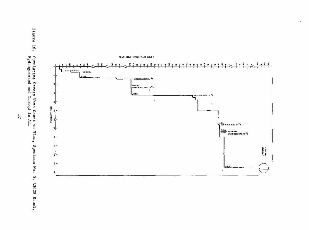
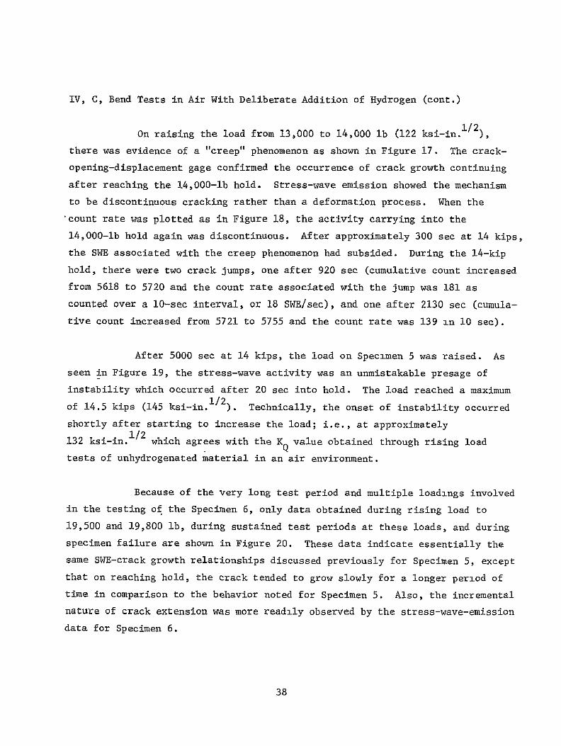
IV C Bend Tests in Air With Deliberate Addition of Hydrogen (cont)
On raising the load from 13000 to 14000 lb (122 ksi-in )
there was evidence of a creep phenomenon as shown in Figure 17 The crackshy
opening-displacement gage confirmed the occurrence of crack growth continuing
after reaching the 14000-lb hold Stress-wave emission showed the mechanism
to be discontinuous cracking rather than a deformation process When the
count rate was plotted as in Figure 18 the activity carrying into the
14000-lb hold again was discontinuous After approximately 300 sec at 14 kips
the SWE associated with the creep phenomenon had subsided During the 14-kip
hold there were two crack jumps one after 920 sec (cumulative count increased
from 5618 to 5720 and the count rate associated with the jump was 181 as
counted over a 10-sec interval or 18 SWEsec) and one after 2130 sec (cumulashy
tive count increased from 5721 to 5755 and the count rate was 139 in 10 see)
After 5000 sec at 14 kips the load on Specimen 5 was raised As
seen in Figure 19 the stress-wave activity was an unmistakable presage of
instability which occurred after 20 sec into hold The load reached a maximum
of 145 kips (145 ksi-in 2) Technically the onset of instability occurred
shortly after starting to increase the load ie at approximately
132 ksi-inI2 which agrees with the KQ value obtained through rising load
tests of unhydrogenated material in an air environment
Because of the very long test period and multiple loadings involved
in the testing of the Specimen 6 only data obtained during rising load to
19500 and 19800 ib during sustained test periods at these loads and during
specimen failure are shown in Figure 20 These data indicate essentially the
same SWE-crack growth relationships discussed previously for Specimen 5 except
that on reaching hold the crack tended to grow slowly for a longer period of
time in comparison to the behavior noted for Specimen 5 Also the incremental
nature of crack extension was more readily observed by the stress-wave-emission
data for Specimen 6
38
20
560
80
60
40
20
5500
80
60
40
20
5400
o 5100
808
60
40
20
5000 u-J
4500
4480 80 4- START 14-KI P HOLD
CODC 75lt
4000
3980 70
3960
6553120 l
- END13-KIP HOLD
3100 160 0 40 80 120 160 200 240 280 320
TIME AT LOAD (SECONDS)
Figure 17 Cumulative Stress Wave Count and COD vs Time Specimen No 5 A302B Steel fydrogenated and Held at 14 Kips in Air
39
200
LU
LU
1- 100
50 END 13-KIP
25 HOLD-I
0 1- TIME
100 INSECONDS AT
200 14KIPS
300
(COUNT EVERY 10 SEC)
Figure 18 Stress Wave Count Rate vs Time - Specimen No 5 A302B Steel Hydrogenated and Tested in Air
40
INSTABILITY
9580
9560
9540
9380
928D0
9260
842D
8440
73O I-shyz 7220
o 7260
U 7240
7220
7180I-shy
7160
- 7140
7120
7100
7080
7060
5900
5880
5860
5840
5820
5800
578D
5460
0 40 80 120 160 SEC
4M 4960 50D RISING LOAD-SECONDS AT 14 KIPS
Figure 19 Cumulative Stress Wave Count vs Time Specimen No 5 A302B Steel Hydrogenated and Tested in Air
41
20000
18000
FAILURE
18290 sec a- 1 17-in K - 199 s - Y
z
-
16000
14000
l0
1200
I-9 Iin
1014in K 152 ki- in -i
o-1 09 n K- 176ksmn
- 1 07 in I 170 iis-
o -1 042in K 12ks-in
c023i NK15ks-n
-shy
-
10000
REACH 19800 lbs
START TO 19800 bs
10000 11000 12000 13000 14000 15000 16000 17000 18000 19000
TIMESECONDS
12000
11000 s
p9000
T LOAD ADJUSTMEA
7n000
READOUT6000 OTE STRESS WAVE DATA A UST T
500 Vgt 0 ENT CORRESPONDIG TO SLOPELOAADJUSTM15 CHANGES PLOTTED
a 4000
3000
LOAD ADJUSTMENT2000 SECONDSECMENIME
1000 START HOLD AT 19500 1b
900 1l6070 D0 8 0 00 0 000600
0 1000 50002000 3000 4000
TIME SECONDS
Figure 20 Cumulative Stress Wave Count vs Time Specimen No 6 A302B Steel Hydrogenated and Tested in Air
Page 42
IV C Bend Tests in Air With Deliberate Addition of Hydrogen (cont)
As indicated in Figure 20 the increase in crack length during
the initial period of hold at 19500 lb resulted in an increase in the applied
stress intensity and was accompanied by significant stress-wave-emission
activity To maintain the desired load it was also necessary to make frequent
load adjustments at the start of hold During the first 3600 sec the effecshy
tive crack length increased from approximately 0963 to 1000 in and was
accompanied by about 7000 SWE As indicated in Figure 20 the majority of the
SWE activity and increase in crack length occurred during the first 3000 sec
of the hold at 19500 lb After this period both the stress-wave-emission
activity and rate of increase in crack length gradually decreased For example
during the entire period from 5000 to 17600 sec when the load was increased
to 19800 lb the apparent crack length and SWE count increased by only approxishy
mately 0020 in and 2500 respectively
After approximately 17000 sec at 19500 lb the load was increased
to 19800 lb and specimen failure occurred after approximately 600 sec at
19800 lb The load was maintained for this period however it was apparent
from both the SWE and COD gage data that the crack was extending and specimen
failure would occur without a further increase in load although it was necesshy
sary to continually adjust the tensile machine to maintain the desired load
The failure stress intensity approximated 199 ksi-in 2however technically
the onset of instability occurred after starting to increase the load at
approximately 153 ksi-in1 2
Specimen 7 was also hydrogenated baked at 300F for 3 hr and
tested in air Figure 21 is a detailed plot of the SWAT data (electronic
counter print-out every second) indicating crack growth of a discontinuous
nature starting at 2400-lb load Note the periods of dormancy (no increase
in SWE count) interspersed with abrupt increases in count indicating disconshy
tinuous crack growth Note also that there was little or no evidence of
continuous stress-wave emission until the load (stress intensity level) was
high approaching failure
43
CUMULAIY STRESS-VAVE COUNTCU LTISTE W E ON
I OT A~II I OI I L I I I I I I I I I I I I I I i I I I I I
- N LB
I I I I I I I I I I I I I i I I
--L - 0OTO11
-0101
(lNIML~ 33383338
8
133113-
3IiC)0 83) 3103 31-3(31-
~0
33 331
3l3C0C~
38318shy
111(10 CAVMSS3 nfl CAliVi flWfl3
________________________________________________________________________
111fl0~ 3KvM~s~a1Ff~TfvTifwT
FPAIAE
hY
A Ii
8
INa
CZ
8 C0 U CI
33 S
1 H
H
03 -I
~ 3lt
0 Cd 33
~C3 ~ H
8 0003
A
Ofli3i~~ C)
Page 45
IV C Bend Tests in Air With Deliberate Addition of Hydrogen (cont)
Figure 22 presents the SWE data from a hydrogenated bend specimen
(No 8) tested in air The load was increased continuously to 9800 lb
(70 ksi-in 2) where there was a short hold (approximately 400 sec) Note
the discontinuous crack growth followed by a short period of continuous
emission (less than 450 slope) The load was then raised to 14800 lb
(109 ksi-in 2) and held for approximately 400 sec Again there were jumps
in the SWE cumulative count but this time interspersed with continuous
emission The SWAT system employed for this test corresponded to that employed
for the background measurements at Kennedy Space Flight Center and shown in
Figure 8 only one channel was employed viz
Endevco 2213 Amplifier Amplifier Band-Pass Filter 10OX 10OX 20 to 50 Kcps
The continuous stress-wave emission observed during hold at the higher stressshy
intensity level in this specimen was not observed in the other hydrogenated
specimens tested in air The primary purpose of this test (Specimen 8) was to
record SWE data for subsequent playback and analysis to determine the amplitude
of burst-type stress-wave emissions associated with fracture in Type A302B
steel These analyses were performed using the instrumentation shown in
Figures 7 and 8 with the following results which are discussed in more detail
in conjunction with the results of the background measurements performed at
Kennedy Space Flight Center (Section V)
Maximum SWE Amplitude - 39 x 10-3g
Minimum SWE Amplitude - 12 x 10-3 g
Average SWE Amplitude - 22 x 10-3g
Laboratory Background - 11 x 10-3g
46
00 o z~ 20 ~
40
~40
S20 1 2 0 0 0 0
TIIAEAT 4 S-KIPHOLD (10KS(51IN A)
407
IV Laboratory Test Results and Discussion (cont)
D BEND TESTS IN 3 NaCI-WATER WITH DELIBERATE ADDITION OF HYDROGEN
Specimen 9 was hydrogenated baked and tested in 80F water
The electronic counter indicated continuous stress-wave emission interspersed
with abrupt increases in count indicating occasional crack jumps Figure 23
shows the details of stress-wave emission that occurred during both rising
load and holding load The crack length determined from the COD chart at
selected loads is also shown Note from the SWE data that there were no
periods of dormancy and the slope of the plot of cumulative count versus time
indicated moderately rapid continuouas crack growth such as might occur with
electrochemical dissolution at the crack tip The COD gage data shown in
Figure 23 also indicate crack extension however the actual amount appears
to be quite small (lt01 in) which would be consistent with the relatively
small number of stress-wave emissions detected even at the high system
sensitivity employed The dramatic difference between the behavior in
Figures 21 and 23 for hydrogenated material tested in air (Figure 21) and
water (Figure 23) indicates that hydrogen and 3 sodium chloride solution
acting together have a greater total effect than the sum of their individual
effects ie working together they appear to have produced a synergism
E WOL TESTS
Because of the possible significance of the synergistic-effect
noted above on the life of the hydrogen pressure vessels at Kennedy Space
Flight Center additional testing was performed using hydrogenated WOL specishy
mens cut from the fractured bend specimens The first WOL specimen was
initially loaded to-3650 lb (50 ksi-in 2) and then placed in 3 NaCl solution
(notch immersed) There was 30 min of essentially continuous stress-wave
emission (recorder started approximately 5 min after loading the specimen)
Subsequently therewas one sizable jump in the SWE cumulative count after
48
V30
760
740-M
$
720 -s
680shy
60
610
40 w
w
520 w
i
20500
HOLDD]N
340
20 760
7200
ING
IV
O
shy
420
60
40
20 0 2
04
0Q
0
60DO
LO0
01 200
250 300
350 400
450 500
550 6M
650
700 750
TIME
(SECONDS)
Figure 23
Cumulative Stress Wave Count vs Time Specimen No 9 A302B Steel
Hydrogenated and Tested in 3 NaCi-Water Environment
49
IV E WOL Tests (cont)
approximately 3 hr 40 min Then 3 hr 20 min later several jumps occurred
followed by 8 hr 20 min of stress-iave activity After this the crack was
dormant (total test time 17 hr 25 min) These data are shown in Figure 24
The load was then increased slightly (torque was increased from 200 to
255 in-lb) an additional 1-12 hr in 3 NaCl solution produced no significant
increase in the cumulative stress-wave count The reason for this apparently
anomalous behavior was not determined although it may result from a blunting
effect at the crack tip produced during the initial hold period
The fatigue crack was then extended (approximately 005 in) in
tension-tension fatigue and the specimen reloaded to approximately 51 ksi-in2
Stress-wave emission started almost immediately (dashed curve in Figure 24)
After approximately 3 hr of discontinuous activity the periods of dormancy
tended to increase interspersed with relatively small jumps (as counted over
10-sec intervals) The results of the initial loading and the reloading are
shown in Figure 24 note that there was appreciably lower cumulative count in
the reloaded specimen as compared with the initial loading for a comparable
period of test
A second hydrogenated WOL specimen was then tested in air at
50 ksi-in 2 there were stress waves initially (creep) but then very little
activity over the remaining 35-hr test period After the first hour the
count increased from approximately 150 to only 280 in the final 34 hr of test
Figure 25 shows the long peribds of dormancy punctuated by occasional 1-count
increases This is in marked contrast to the results obtained from the
hydrogenated WOL specimens tested in 3 NaCl solution and the bend-test
findings of a synergistic effect were confirmed
50
------------
aa
L- -- -- - ------ - --- I
3
IN DO
INTES) 3 S IOTI E( LI N LU
Ino
a
N O
TIME (MINUTES) IN 3 NCI SOLUTION
Figure 24 Cumulative Stress Wave Count vs Time at Hold WOL Specimen No 1
A302B Steel Hydrogenated and Tested in 3 NaCi-Water Environment
51
000 In 0 M6020 126 24 022 in0 1180 10 11 100 IWO l 100M M-C 0 90w6 a0 w6
t t t t 5W MOD4
10
TIME (MINUTES)
Figure 25 Cumulative Stress Wave Count vs Time at Hold WL Specimen No 2 A302B Steel Hydrogenated and Testd in Air
52
IV Laboratory Test Results and Discussion (cont)
F DISCUSSION
1 Material-Environment Consideration
The Type A302B steel supplied for evaluation exhibited a
very high level of fracture toughness Although quantitative plane-strain
fracture toughness measurements were not possible because of the large specimen
size required the KQ value associated with failure approximated 135 ksi-in1 2
This material was also found resistant to environmentally induced failure in
that the rate of crack growth of a prior flaw at applied stress-intensity
factors as high as 90 of the KQ value appeared to be very low This effect
was observed for unhydrogenated-material tested in air and a 3 NaCl-water
environment and hydrogenated material tested in an air environment However
the hydrogenated specimens tested in 3 NaCl-water environment had a much
faster rate of subcritical crack gr~wth in comparison to the other test condishy
tions indicating a synergistic effect due to the combination of sea water and
hydrogen in interstitial solid solution This synergistic effect indicates
that the Type A302B steel hydrogen storage tanks in the Kennedy Space Flight
Center environment may have limited life as the result of subcritical crack
growth if subjected to the same combination of stress and environmental
factors-
The WOL test results tended to confirm the possible synergism
due to the combined effects of 3 NaCl-water and hydrogen in interstitial solid
solution Marked SWE activity was observed when the hydrogenated specimens
were immersed in the salt water whereas in an air environment after the
initial period at hold when a creep phenomenon was observed there was essenshy
tially no stress-wave emission The fact that failure was not produced on
holding (in contradiction to the bend tests) can be explained by the fact that
the WOL test as-performed in this program is a self-arresting test because
53
IV F Discussion (cont)
the occurrence of crack growth results in a reduction in the applied load
Conversely in the bend tests the load was constantly applied as the crack
extended and eventually resulted in specimen failure
2 Stress-Wave-Emission Characterization
Detectable stress-wave emissions although of small amplitude
(ltOOlg) were observed to be associated with crack growth in Type A302B steel
Under all test conditions the stress-wave emissions were observed both during
rising load and when failure (instability) was imminent During hold various
SWE characteristics depending on the test conditions were observed When
tested in the hydrogenated condition in-an air environment a creep phenomenon
evidenced by increasing count of SWE and an accompanying increase in apparent
crack size was observed With time at hold and at applied stress-intensity
levels less than critical the creep phenomenon eventually stopped as did the
occurrence of stress-wave emissions Unhydrogenated material tested in the
3 NaCl-water environment produced continuous stress-wave emission punctuated
by abrupt increases in SWE count This behavior indicates both continuous
very small increments of crack extension with larger crack jumps corresponding
to the abrupt increases in SWE count Continuous incremental crack extension
characterized by continuous SWE interspersed with abrupt increases in SWE count
indicating occasional crack jumps was also observed in testing hydrogenated
material in a 3 NaCl-water environment
In all instances when failure (instability) occurred both
the amplitude and rate of stress-wave emission increased and could be employed
as a precursor of the onset of instability however even when failure was
approached-the SWE amplitude was small (ltOlg) In the other instances where
failure was not produced evidence of crack extension (although very small in
some instances) was observed on the specimen fracture face Once evidence of
54
IV F Discussion (cont)
crack growth was observed (by SWE or COD) it is obvious that failure would
eventually occur (assuming a constantly applied load) although depending on
the initial flaw size and subcritical growth rate the time to failure may be
very long In actual practice the SWE data could be employed (1) to locate
the propagating flaw (2) to monitor its occurrence and (3) as a basis for
terminating service so that repairs could be made before failure The stressshy
wave emissions associated with crack growth during rising load or increasing
stress intensity and the creep phenomenon during the initial part of hold
can be employed for this purpose
5S
V BACKGROUND MEASUREMENTS AND ASSOCIATED LABORATORY TESTS
A BACKGROUND MEASUREMENTS AT KENNEDY SPACE FLIGHT CENTER
Background noise measurements were made at two locations the VAB
Bottle Field and Pad A at the Kennedy Space Flight Center The data were tape
recorded and in addition to general background noise included tank blowdown
and repressurization periods The instrumentation for this purpose is shown
schematically in Figure 8 analysis of the data was performed by playback onto
an oscillograph and comparison with the SWE-crack growth data obtained during
the laboratory testing of bend specimens
The analysis of the signal amplitude data for tests at Cape Kennedy
is indicated below
1 Pad A Bottle Field
Signal Amplitude
a Quiescent Background
Filter at 20 Kcps - 50 Kcps -BandPass- 99 x 10 gsBand Pass
Filter at 200 cps - 32 Kcps
Band Pass
b Tank Blowdown - System Saturation (gt llg peak to peak)
C Tank Repressurization - System Saturation (gt llg peak to peak)
2 VAB Bottle Field
a Quiescent Background - 22 x 10- 4 gs
56
V A Background Measurements at Kennedy Space Flight Center (cont)
Signal Amplitude
b Tank Blowdown - System Saturation (gt llg peak to peak)
C Tank Repressurization - System Saturation (gt llg peak to peak)
Analysis of the tape-recorded data of bend tests at Aerojet indicates
the following signal amplitude for burstf-type stress-wave emissions associated
with crack growth and fracture in Type A302B steel
Maximum Amplitude - 39 x 10-3g
Minimum Amplitude - 12 x 10-3g
Average Amplitude - 22 x 10-3g
Laboratory Background - 11 x 10-3g
Thus the amplitude of SWE associated with crack growth in A302B steel is
approximately an order of magnitude larger than the background noise noted
previously Consequently the above results show that it is possible to detect
stress-wave emissions associated with fracture in A302B steel under the quiescent
background conditions existing at the Kennedy Space Center Difficulty is
expected in detecting such flaw growth during tank blowdown and repressurization
periods unless filtering can be employed to screen out the noise associated
with these periods However the blowdown and repressurization periods are of
very short duration and the materials behavior observed in this program indishy
cated that considerable prefailure crack extension would be expected from any
flaw of a size expected to be present in these pressure vessels Also
immediately on reaching load a creep phenomenon evidenced by an extension
in apparent crack length and accompanied by detectable stress-wave emission
was observed Consequently even if noise associated with blowdown and
57
V A Background Measurements at Kennedy Space Flight Center (cont)
repressurization cannot be effectively filtered out significant flaw growth
andor creep could still be detected and tank depressurization accomplished
prior to catastrophic failure assuming a capability for such depressurization
exists at these locations
B LABORATORY SIGNAL ATTENUATION EVALUATIONS
Subsequent to the background measurements at the Kennedy Space
Flight Center and the bend tests at Aerojet two series of tests were made at
Aerojet using a section of pipe and plate both of SAE 4130 steel alloy The
purpose of these tests was to determine the coefficient of signal attenuation
which in conjunction with the previous test data could be used to establish
the sensor spacing which would insure detection of SWE associated with crack
growth in the pressure-vessels at the Kennedy Space Flight Center
In these tests a constant pulse was imparted to the specimen by
a Tektronix 115 Pulse Generator using a Clevite PZT-5 Crystal (2125 in dia
and 0250 in thick) The piezoelectric crystal was mounted on a small alumishy
num block which in turn was adhered to the surface of the specimen The
signal was received by a 2217-E-Endevcq accelerometer placed at various disshy
tances from the pulser The pulse used was 10 n-sec rise and fall time with
a duration of 20 microsec at an amplitude of 12v
1 Pipe Tests
A SAE 4130 steel pipe (8-58 in OD 7-18 in ID and 22 ft
10-78 in long) was used as specimen for this test series The pulser was
mounted normal to the external surface of the pipe as close as possible to the
edge The accelerometer (2217-E-Endevco) was successively placed on the pipe
58
V B Laboratory Signal Attenuation Evalutions (cont)
surface at positions I to 8 that were at 4 6 8 10 12 14 16 and 20 ft
from the pulser The signal received by the accelerometer was displayed on a
Tektronix 422 osilloscope Typical signals are shown in Figure 26
The velocities of the compressional and shear waves in steel
are
29 lO06 x38103 Vc= -x lg ) (l-26) = O2 x06(- 0 x386 = 227000 insec(+j 012)283 (1+030) (1-060)
29x106 x 386 = 91 36= 123000 insec
s 2 ( + p) p 2 (i + 030) x 0283
where E = Youngs Modulus p = Poissons Ratio and p = density The times of
arrival of these waves at the computed velocities are indicated on the oscilloshy
scope photos shown in Figure 26 The point of shear wave arrival (T ) coincides
in most of the photos to a distinct change of pattern in the trace The
arrival of the compressional wave is difficult to determine accurately because
the amplitude of this wave attenuates very fast with distance
A visual comparison of the curves shows that Figure 26a
representing the signal received 4 ft from the impulse indicates a perfectly
detectable arrival of the compressional wave conversely Figure 26h (at 20 ft
from the impulse) shows the visually detectable arrival of a wave almost at the
computed arrival of the shear wave This is due to the fact that the amplitude
of the first cycles of the compressional wave have become essentially impercepshy
tible at a distance of 20 ft from the pulse An attempt to determine signal
arrival time by visual inspection only of the traces in Figure 26 would result
in the wave velocities indicated in Table III The computed arrival times of
the compressional and shear waves are shown in Table IV If an integration of
the positive portions of the cycles comprised in 200 p sec after arrival of the
59
VERTICAL SCALE 1 DIV= 01 V VERTICAL SCALE 1 DIV = 01 V HORIZONTAL SCALE 1 DIV= 50p SEC HORIZONTAL SCALE 1 DIV = 100 pSEC
a 4FT FROM PULSER b6 FEET FROM PULSER
Tc Ts Tc Ts
VERTICAL SCALE I DIV 01 V VERTICAL SCALE I DIV = 01 V HORIZONTAL SCALE I DIV = 100 I SEC HORIZONTAL SCALE 1 DIV = 200 p SEC
c 8 FEET FROM PULSER d 10 FEET FROM PULSER
Tc = Arrival of Compressional Wave
T = Arrival of Shear Wove
Figure 26 Oscillograph Traces for Pipe Tests (Sheet 1 of 2)
6o NOT REPRODUCTBLE
VERTICAL SCALE 1 DIV = 01 V VERTICAL SCALE 1 DIV 01 V HORIZONTAL SCALE 1 DIV = 200y SEC HORIZONTAL SCALE I DIV 200 p SEC
e 12 FEET FROM PULSER f 14 FEET FROM PULSER
T TS T T
VERTICAL SCALE 1 DIV = 01 V VERTICAL SCALE 1 DIV = 01 V HORIZONTAL SCALE 1 DIV = 200 v SEC HORIZONTAL SCALE I DIV =5001p SEC
g 16 FEET FROM PULSER h 20 FEET FROM PULSER
Figure 26 Oscillograph Traces for Pipe Tests (Sheet 2 of 2)
61
V B Laboratory Signal Attenuation Evaluations (cont)
shear wave is performed the average amplitudes determined in this manner
become quite meaningful These average amplitudes are shown in Table V
TABLE III
WAVE VELOCITY BASED ON VISUAL ANALYSIS OF OSCILLOSCOPE TRACES - PIPE TESTS
Distance from Pulse Arrival Velocities Photo ft in Time psc (ftsec)
1 4 48 210 228000
2 6 72 400 180000
3 8 96 600 160000
4 10 120 800 150000
5 12 144 1000 144000
6 14 168 1200 140000
7 16 192 1400 137000
8 20 240 1750 137000
TABLE IV
COMPUTED ARRIVAL TIMES - PIPE TESTS
Compressional Wave Shear Wave Distance from Pulse Arrival Time Arrival Time
Photo in psec Osc Div sec Ose Div
1 48 212 423 390 780
2 72 317 317 583 583
3 96 422 422 778 778
4 120 530 265 972 486
5 144 635 317 1163 581
6 168 740 370 1360 680
7 192 840 420 1545 771
8 240 1050 21 1930 387
62
V B Laboratory Signal Attenuation Evalutions (cont)
TABLE V
SIGNAL AMPLITUDE VS DISTANCE - PIPE TESTS
Average Signal Amplitude Distance from 200 Psec after Arrival
Test Pulser in of Comp Wave mv
1 48 230
2 72 145
3 96 85
4 120 60
5 144 45
6 168 28
7 192 22
8 240 18
The general equation for the amplitude attenuation curve is
C x e-Xy =
where y = amplitude at distance x in volts
x = distance in inches from pulse source
C = amplitude of pulse in volts
a = attenuation factor
or iny= 1 C + (- ax) = I C - ax (Eq 4)n n
To determine the values of C and a the following statistical analysis was
performed
63
V B Laboratory Signal Attenuation Evaluations (cont)
Distance Yo y y2 X X2 Test in m v n n
1 48 230 543 +142 2010 -87 7580 - 124 261
2 72 145 499 +098 0960 -63 3960 - 62 360
3 96 85 445 +044 0194 -39 1520 - 17 427
4 120 60 409 +008 0006 -15 225 - 1 490
5 144 45 380 -021 0044 + 9 81 - 2 548
6 168 28 334 -067 0450 +33 1090 - 21 560
7 192 22 309 -092 0847 +57 3250 - 52 592
8 240 18 289 -112 1250 +105 11000 - 118 690
EY2 EX2pound x = 1080 ElnY =3208 5761 28706 SXY-397 XxIny3928
- 1080 - 3208 x =- = 135 ny = 401
EXY -397 00138 1 C =l1y + oshy
pound 2 x2 28706 n i x
= 401+(0138)(135)=401+186= 587
C - 355 mv
It is now possible to compute the statistically corrected values of the signal
amplitude y at the distances from the pulse where they were measured The
general formula will be
ny = 587 -(00138) X
and the results are tabulated in Table VI The computed value of pulse amplishy
tude at source is found to be C = 355 my The values shown on Table VI are
plotted in Figure 27 which graphically shows the signal attenuation as a
function of distance from the pulse source
64
350
300
250 STATISTICALLY COMPUTED k VALUES FOR REGRESSION CURVE
--0gt 200
EXPERIMENTALLY DETERMINED
-- MATERIAL SAE 4130 STEEL U= SPECIMEN PIPE-S758 in D aZ
00
15 7 18 in D22 ft 10 78 in LONG
-J
100
50 I
0 I I I
5 I I I
DISTANCE
I
10 FROM SOURCE
I
FEET
I
15 20
Figure 27 Signal Amplitude vs Distance - Pipe Tests
V B Laboratory Signal Attenuation Evaluations (cont)
TABLE VI
STATISTICALLY CORRECTED VALUES OF SIGNAL AMPLITUDE - PIPE TESTS
Experimentally Distance from 1 Corrected Signal Determined Signal
Test Pulse in ny Amplitude (y) mv Amplitude (y) my
1 48 521 182 230
2 72 488 130 145
3 96 455 95 85
4 120 421 67 60
5 144 388 48 45
6 168 355 35 28
7 192 322 25 22
8 240 255 127 18
- 2 Plate Tests
An SAE 4130 steel plate (73-12 in long 48-12 in wide
and 34 in thick) was used for this test series The two diagonals were
marked on the plate The pulser was placed at the center of the plate and
the receiver accelerometer was placed on one of the diagonals at locations
spaced in increments of 6 in from the center The received signals were
observed on the oscilloscope and photos were taken of these signals Figure
28 shows oscillographs of the signals received at 6 12 18 24 30 36 and
42 in from the pulser The times of arrival of the shear wave are also shown
in Figure 28 The velocity used was v = 123000 insec An integration
was performed of the positive positions of the cycles comprised in a 20 Psec
interval after the arrival of the shear wave The average amplitudes detershy
mined from these integrations are shown in Table VII Only Tests 1 to 4 are
used because reflection (from the plate edges) in Tests 5 to 8 obscured the
66
b 12 INCHES FROM PULSERa 6 INCHES FROM PULSER
TBTs
c 18 INCHES FROM PULSER d 24 INCHES FROM PULSER
IT s = Arrival of Shear Wave
Vertical Scale 1 DIV = 01 Volt Horizontal Scale 1 DIV = 20 ASec
Figure 28 Oscillograph Traces for Plate Tests (Sheet 1 of 2)
Page 67
f 36 INCHES FROM PULSER e 30 INCHES FROM PULSER
g 42 INCHES FROM PULSER
= Arrival of Shear WaveTs
Vertical Scale 1 DIV = 01 Volt = 20 4SecHorizontal Scale 1 DIV
Figure 28 Oscillograph Traces for Plate Tests (Sheet 2 of 2)
08 gOTPRODUCIB1A
V B Laboratory Signal Attenuation Evaluations (cont)
data These reflections were received in Tests 5 to 8 because of the relashy
tively small plate that was available for this test series
TABLE VII
SIGNAL AMPLITUDE VS DISTANCE - PLATE TESTS
Distance from Average Amplitude Test Pulse in(x) in 20 p see mv
1 6 150
2 12 110
3 18 70
4 24 45
The following statistical analysis was performed to determine the values of
C and a in Equation 4
Test
Distance from
Pulse in(x)
y
m v
1
ny Y
2
Y 2
X XY
X1 y
n
1 6 150 500 +056 0314 -9 81 -502 3000
2
3
12
18
110
70
470
425
+026
-019
0067
0036
-3
+3
9
9
-078
-057
5640
7650
4 24 45 381 -063 0397 +9 81 -567 9149
60 1776 0814 180 -1204 25439
-x=
60 w= 15
4ny
iY 1
1nC
-
=
16=44 1776 =44
E YX 1204= __=
E y2 180
ny +(0067)(15) =
+0067
444 + 0067(15)
69
=
C
444 + 100
= 230 my
= 544
V B Laboratory Signal Attenuation Evaluations (cont)
Subsequently the values of signal amplitude (y) were statistically corrected
as before and the experimentally determined values of y are compared to the
results obtained in Table VIII
TABLE VIII
COMPARISON Or STATISTICALLY CORRECTED AND TEST-DETERMINED VALUES OF SIGNAL AMPLITUDE - PLATE TESTS
Experimentally Distance from Corrected Signal Determined Signal
Test Pulse in nY Amplitude (y) mv Amplitude (y) my
1 6 504 155 150
2 12 464 103 110
3 18 417 65 70
4 24 383 46 45
The computed value of the pulse amplitude at the source at
C equals 230 mv The regression curve and the experimentally determined points
are plotted in Figure 29 It should be observed that the attenuation coefshy
ficient for the pipe test was a = 00138 and for the plate test was 0067
This is due to the much larger rate of front area that the pulse meets in the
plate
C SENSOR SPACING
The quiescent background noise measurements performed at the test
sites using a 20 to 50 KHz band-pass filter are
Pad A Bottle Field - 0000099g
VAB Bottle Field 0000220g
70
250
200 - EXPERIMENTALLY DETERMINED
0o
gt
M a-100 34
STATISTICALLY COMPUTEDVALUES FOR REGRESSION CURVE
MATERIAL SAE 4130 STEEL
SPECIMEN PLATE - 73 12 in LONG 48 12 in WIDE
in THICK
J
50
0
0 5 SII
10 15
DISTANCE FROM SOURCE FEET
I
20 I
25
Figure 29 Signal Amplitude vs Distance - Plate Tests
V C Sensor Spacing (cont)
The recorded stress-wave-emission data obtained from the A302B steel bend tests
made at the Aerojet-General Corporation laboratory show that the minimum
acceleration at the source is 0O012g the average 00022g and the maximum
00039g Based on the above data and the attenuation factor X = 0067 detershy
mined from the plate tests the sensor spacings required to detect crack growth
in the vessels at the Kennedy Space Center were computed and the results are
tabulated below
Quiescent Sensor Spacing
Amplitude at Background in the Source(C) g Amplitude(y) g Cy ln(CIy) ln(CIy)
Pad A
Min Signal 00012 000015 800 208 310
Avg Signal 00022 000015 1470 269 402
Max Signal 00039 000015 2600 326 487
VAB Bottle Field
Min Signal 00012 000033 363 129 193
Avg Signal 00022 000033 668 190 283
Max Signal 00039 000033 1080 238 356
This threshold is 15 x 0000099 - 000015g (at Pad A)
This threshold is 15 x 000022 = 000033g (at VAB Bottle Field)
Figures 30 and 31 present schematically the location and spacings of sensors
on the pressure vessels
72
- 502 IN 8 IN
HEAD -- _
DEVELOPED + + CYLINDRICAL FOR MINIMUM SIGNAL-22 SENSORS AS SHOWN
SURFACE FOR AVERAGE SIGNAL-16 SENSORS
+ +I
FOR MAXIMUM SIGNAL- 14 SENSORS
282438 IN+ +
+ +
9 SPACINGS AT 313 IN
-I- +
+ +shy
+ -plusmn
HEAD _ __
8 IN
Figure 30 Schematic of Sensor Spacings for Bottles at Pad A
73
14601 IN
HEAD (6SENSORS) 23 14 INI I I - I I I
t plusmn + plusmn + +
+ + 4 + + + DEVELOPED CYL SURFACE
+ + 4A 1 13 LINES OF
+ + + SENSORS SPACED4 + + AT 2086 IN
+ + + + + +
+ + 4 + + +
251 1516 IN + + + +-I- +
+ + + 4- +
-1- 298438 IN+ -I- -+- -i- +
+I
23 14 INHEAD (6 SENSORS) 1
FOR MINIMUM SIGNAL-103 SENSORS AS SHOWN
FOR AVERAGE SIGNAL- 82 SENSORS FOR MAXIMUM SIGNAL- 58 SENSORS
Figure 31 Schematic of Sensor Spacings for Bottles at VAB Bottle Field
74
VI CONCLUSIONS
A The Type A302B steel supplied for evaluation exhibited a high level
of fracture toughness Although quantitative plane-strain fracture toughness
measurements were not possible because of the large specimen size required
the K value associated with failure approximated 135 ksi-inI 2
Q
B The Type A302B steel was found resistant to environmentally induced
slow crack growth when tested in the hydrogenated condition in an air environshy
ment and in the unhydrogenated condition in a 3 NaCl-water environment Howshy
ever hydrogenated material tested in 3 NaCl-water had a much faster rate of
subcritical crack growth indicating a synergistic effect due to the combinashy
tion of sea water and hydrogen in interstitial solid solution
C The synergistic effect indicates the Type A302B steel hydrogen
storage tanks in the Kennedy Space Flight Center may have limited life as a
result of subcritical crack growth if subjected to the same combination of
stress and environmental factors
D Detectable stress-wave emissions although of small amplitude
(ltOOlg) were observed to be associated with crack growth in Type A302B steel
In all test conditions the stress-wave emissions were observed during rising
load and when failure (instability) was imminent Both the amplitude and rate
of stress-wave emission increased as failure was approached and could be
employed as a precursor of the onset of instability
E Stress-wave emissions associated with crack growth in Type A302B
steel can be detected under quiescent background conditions at the Pad A and
VAB Bottle fields at the Kennedy Space Flight Center However it would be
difficult to detect such stress-wave emissions during tank blowdown and
repressurization periods unless filtering can be employed to screen out the
noise associated with these periods
75
VI Conclusions (cont)
F Even in the presence of background noise from tank blowdown and
repressurization these periods are considered short in the overall life of
the pressure vessels Consequently flaw growth or creep which was observed
during rising load or the initial part of hold could be detected by SWAT
permitting triangulation to the source and tank depressurization prior to
failure
G Stress-wave-emission attenuation test data were obtained and employed
in conjunction with the site background measurements addbnd test stress-waveshy
emission characterization data to determine sensor mounting patterns for the
hydrogen pressure vessels at Pad A and the VAB Bottle Field
VII RECOMMENDATIONS FOR FURTHER WORK
If the synergistic effect of hydrogen and 3 NaCi solution occurs in
Kennedy Space Flight Center tankage the life of the tankage will be limited
Obviously slow-crack growth from any cause whether continuous or disconshy
tinuous and regardless of how slow the rate of cracking will eventually
produce failure This investigation showed that subcritical crack growth is
in all likelihood occurring with each pressurization A question remains
however as to the rate of crack growth without knowledge of the rate there
is no way to anticipate the life of the tankage However with SWAT one can
monitor the occurrence of crack growth and most importantly make judgment
as to whether a given crack is approaching critical size Consequently it
is recommended that additional tests be performed to (1) verify the existence
of subcritical cracking in actual on-site tankage and (2) incorporate an
automatic system for continuously monitoring on-site tankage at Kennedy Space
Flight Center
76
REFERENCES
1 Steel R K Green A T Lockman C S Acoustic Verification of Structural Integrity of Polaris Chambers Society of Plastic Engineers 20th Meeting Atlantic City N Y January 1964
2 Pressure Testing of AFRM-017 Service Propulsion System Fuel Tank Utilizing Aerojet-General Corporations Stress-Wave Analysis Technique
Report NAS 9-6766-003 Aerojet-General Corp for NASA MSC Houston Texas Contract NAS 9-6766 May 1967
3 Srawley J E and Esgar J B Investigation of Hydrotest Failure of Thiokol Chemical Corp 260-Inch-Diameter SL-1 Motor Case NASA-TMX shy1194 January 1964
4 Hartbower C E Gerberich W W and Crimmins P P Mechanisms of Slow Crack Growth in High-Strength Steels AFML-TR-67-26 Vol 1 February 1967
5 -Hartbower C E Gerberich W W and Crimmins P P Characterization of Fatigue-Crack Growth by Stress Wave Emission Final Report on Conshytract NAS 1-4902 for NASA-Langley Research Center Hampton Virginia June 1966
6 IHartbower C E Gerberich W W Reuter W G and Crimmins P P Stress Wave Characteristics in Constructional Alloys Final Report on Office of Naval Research Contract N00014-66-C-0340 July 1967
7 Novak S R and Rolfe S T Modified WOL Specimen for KIscc Environmental Testing U S Steel Corp paper submitted to ASTM for publication
77
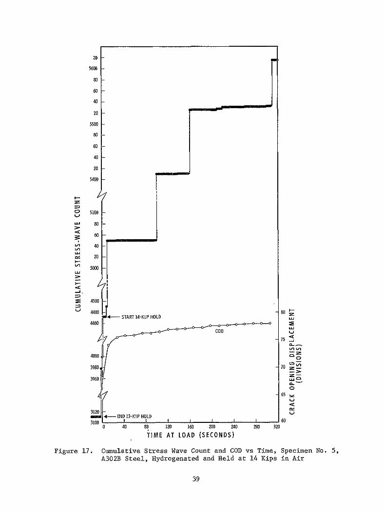
20
560
80
60
40
20
5500
80
60
40
20
5400
o 5100
808
60
40
20
5000 u-J
4500
4480 80 4- START 14-KI P HOLD
CODC 75lt
4000
3980 70
3960
6553120 l
- END13-KIP HOLD
3100 160 0 40 80 120 160 200 240 280 320
TIME AT LOAD (SECONDS)
Figure 17 Cumulative Stress Wave Count and COD vs Time Specimen No 5 A302B Steel fydrogenated and Held at 14 Kips in Air
39
200
LU
LU
1- 100
50 END 13-KIP
25 HOLD-I
0 1- TIME
100 INSECONDS AT
200 14KIPS
300
(COUNT EVERY 10 SEC)
Figure 18 Stress Wave Count Rate vs Time - Specimen No 5 A302B Steel Hydrogenated and Tested in Air
40
INSTABILITY
9580
9560
9540
9380
928D0
9260
842D
8440
73O I-shyz 7220
o 7260
U 7240
7220
7180I-shy
7160
- 7140
7120
7100
7080
7060
5900
5880
5860
5840
5820
5800
578D
5460
0 40 80 120 160 SEC
4M 4960 50D RISING LOAD-SECONDS AT 14 KIPS
Figure 19 Cumulative Stress Wave Count vs Time Specimen No 5 A302B Steel Hydrogenated and Tested in Air
41
20000
18000
FAILURE
18290 sec a- 1 17-in K - 199 s - Y
z
-
16000
14000
l0
1200
I-9 Iin
1014in K 152 ki- in -i
o-1 09 n K- 176ksmn
- 1 07 in I 170 iis-
o -1 042in K 12ks-in
c023i NK15ks-n
-shy
-
10000
REACH 19800 lbs
START TO 19800 bs
10000 11000 12000 13000 14000 15000 16000 17000 18000 19000
TIMESECONDS
12000
11000 s
p9000
T LOAD ADJUSTMEA
7n000
READOUT6000 OTE STRESS WAVE DATA A UST T
500 Vgt 0 ENT CORRESPONDIG TO SLOPELOAADJUSTM15 CHANGES PLOTTED
a 4000
3000
LOAD ADJUSTMENT2000 SECONDSECMENIME
1000 START HOLD AT 19500 1b
900 1l6070 D0 8 0 00 0 000600
0 1000 50002000 3000 4000
TIME SECONDS
Figure 20 Cumulative Stress Wave Count vs Time Specimen No 6 A302B Steel Hydrogenated and Tested in Air
Page 42
IV C Bend Tests in Air With Deliberate Addition of Hydrogen (cont)
As indicated in Figure 20 the increase in crack length during
the initial period of hold at 19500 lb resulted in an increase in the applied
stress intensity and was accompanied by significant stress-wave-emission
activity To maintain the desired load it was also necessary to make frequent
load adjustments at the start of hold During the first 3600 sec the effecshy
tive crack length increased from approximately 0963 to 1000 in and was
accompanied by about 7000 SWE As indicated in Figure 20 the majority of the
SWE activity and increase in crack length occurred during the first 3000 sec
of the hold at 19500 lb After this period both the stress-wave-emission
activity and rate of increase in crack length gradually decreased For example
during the entire period from 5000 to 17600 sec when the load was increased
to 19800 lb the apparent crack length and SWE count increased by only approxishy
mately 0020 in and 2500 respectively
After approximately 17000 sec at 19500 lb the load was increased
to 19800 lb and specimen failure occurred after approximately 600 sec at
19800 lb The load was maintained for this period however it was apparent
from both the SWE and COD gage data that the crack was extending and specimen
failure would occur without a further increase in load although it was necesshy
sary to continually adjust the tensile machine to maintain the desired load
The failure stress intensity approximated 199 ksi-in 2however technically
the onset of instability occurred after starting to increase the load at
approximately 153 ksi-in1 2
Specimen 7 was also hydrogenated baked at 300F for 3 hr and
tested in air Figure 21 is a detailed plot of the SWAT data (electronic
counter print-out every second) indicating crack growth of a discontinuous
nature starting at 2400-lb load Note the periods of dormancy (no increase
in SWE count) interspersed with abrupt increases in count indicating disconshy
tinuous crack growth Note also that there was little or no evidence of
continuous stress-wave emission until the load (stress intensity level) was
high approaching failure
43
CUMULAIY STRESS-VAVE COUNTCU LTISTE W E ON
I OT A~II I OI I L I I I I I I I I I I I I I I i I I I I I
- N LB
I I I I I I I I I I I I I i I I
--L - 0OTO11
-0101
(lNIML~ 33383338
8
133113-
3IiC)0 83) 3103 31-3(31-
~0
33 331
3l3C0C~
38318shy
111(10 CAVMSS3 nfl CAliVi flWfl3
________________________________________________________________________
111fl0~ 3KvM~s~a1Ff~TfvTifwT
FPAIAE
hY
A Ii
8
INa
CZ
8 C0 U CI
33 S
1 H
H
03 -I
~ 3lt
0 Cd 33
~C3 ~ H
8 0003
A
Ofli3i~~ C)
Page 45
IV C Bend Tests in Air With Deliberate Addition of Hydrogen (cont)
Figure 22 presents the SWE data from a hydrogenated bend specimen
(No 8) tested in air The load was increased continuously to 9800 lb
(70 ksi-in 2) where there was a short hold (approximately 400 sec) Note
the discontinuous crack growth followed by a short period of continuous
emission (less than 450 slope) The load was then raised to 14800 lb
(109 ksi-in 2) and held for approximately 400 sec Again there were jumps
in the SWE cumulative count but this time interspersed with continuous
emission The SWAT system employed for this test corresponded to that employed
for the background measurements at Kennedy Space Flight Center and shown in
Figure 8 only one channel was employed viz
Endevco 2213 Amplifier Amplifier Band-Pass Filter 10OX 10OX 20 to 50 Kcps
The continuous stress-wave emission observed during hold at the higher stressshy
intensity level in this specimen was not observed in the other hydrogenated
specimens tested in air The primary purpose of this test (Specimen 8) was to
record SWE data for subsequent playback and analysis to determine the amplitude
of burst-type stress-wave emissions associated with fracture in Type A302B
steel These analyses were performed using the instrumentation shown in
Figures 7 and 8 with the following results which are discussed in more detail
in conjunction with the results of the background measurements performed at
Kennedy Space Flight Center (Section V)
Maximum SWE Amplitude - 39 x 10-3g
Minimum SWE Amplitude - 12 x 10-3 g
Average SWE Amplitude - 22 x 10-3g
Laboratory Background - 11 x 10-3g
46
00 o z~ 20 ~
40
~40
S20 1 2 0 0 0 0
TIIAEAT 4 S-KIPHOLD (10KS(51IN A)
407
IV Laboratory Test Results and Discussion (cont)
D BEND TESTS IN 3 NaCI-WATER WITH DELIBERATE ADDITION OF HYDROGEN
Specimen 9 was hydrogenated baked and tested in 80F water
The electronic counter indicated continuous stress-wave emission interspersed
with abrupt increases in count indicating occasional crack jumps Figure 23
shows the details of stress-wave emission that occurred during both rising
load and holding load The crack length determined from the COD chart at
selected loads is also shown Note from the SWE data that there were no
periods of dormancy and the slope of the plot of cumulative count versus time
indicated moderately rapid continuouas crack growth such as might occur with
electrochemical dissolution at the crack tip The COD gage data shown in
Figure 23 also indicate crack extension however the actual amount appears
to be quite small (lt01 in) which would be consistent with the relatively
small number of stress-wave emissions detected even at the high system
sensitivity employed The dramatic difference between the behavior in
Figures 21 and 23 for hydrogenated material tested in air (Figure 21) and
water (Figure 23) indicates that hydrogen and 3 sodium chloride solution
acting together have a greater total effect than the sum of their individual
effects ie working together they appear to have produced a synergism
E WOL TESTS
Because of the possible significance of the synergistic-effect
noted above on the life of the hydrogen pressure vessels at Kennedy Space
Flight Center additional testing was performed using hydrogenated WOL specishy
mens cut from the fractured bend specimens The first WOL specimen was
initially loaded to-3650 lb (50 ksi-in 2) and then placed in 3 NaCl solution
(notch immersed) There was 30 min of essentially continuous stress-wave
emission (recorder started approximately 5 min after loading the specimen)
Subsequently therewas one sizable jump in the SWE cumulative count after
48
V30
760
740-M
$
720 -s
680shy
60
610
40 w
w
520 w
i
20500
HOLDD]N
340
20 760
7200
ING
IV
O
shy
420
60
40
20 0 2
04
0Q
0
60DO
LO0
01 200
250 300
350 400
450 500
550 6M
650
700 750
TIME
(SECONDS)
Figure 23
Cumulative Stress Wave Count vs Time Specimen No 9 A302B Steel
Hydrogenated and Tested in 3 NaCi-Water Environment
49
IV E WOL Tests (cont)
approximately 3 hr 40 min Then 3 hr 20 min later several jumps occurred
followed by 8 hr 20 min of stress-iave activity After this the crack was
dormant (total test time 17 hr 25 min) These data are shown in Figure 24
The load was then increased slightly (torque was increased from 200 to
255 in-lb) an additional 1-12 hr in 3 NaCl solution produced no significant
increase in the cumulative stress-wave count The reason for this apparently
anomalous behavior was not determined although it may result from a blunting
effect at the crack tip produced during the initial hold period
The fatigue crack was then extended (approximately 005 in) in
tension-tension fatigue and the specimen reloaded to approximately 51 ksi-in2
Stress-wave emission started almost immediately (dashed curve in Figure 24)
After approximately 3 hr of discontinuous activity the periods of dormancy
tended to increase interspersed with relatively small jumps (as counted over
10-sec intervals) The results of the initial loading and the reloading are
shown in Figure 24 note that there was appreciably lower cumulative count in
the reloaded specimen as compared with the initial loading for a comparable
period of test
A second hydrogenated WOL specimen was then tested in air at
50 ksi-in 2 there were stress waves initially (creep) but then very little
activity over the remaining 35-hr test period After the first hour the
count increased from approximately 150 to only 280 in the final 34 hr of test
Figure 25 shows the long peribds of dormancy punctuated by occasional 1-count
increases This is in marked contrast to the results obtained from the
hydrogenated WOL specimens tested in 3 NaCl solution and the bend-test
findings of a synergistic effect were confirmed
50
------------
aa
L- -- -- - ------ - --- I
3
IN DO
INTES) 3 S IOTI E( LI N LU
Ino
a
N O
TIME (MINUTES) IN 3 NCI SOLUTION
Figure 24 Cumulative Stress Wave Count vs Time at Hold WOL Specimen No 1
A302B Steel Hydrogenated and Tested in 3 NaCi-Water Environment
51
000 In 0 M6020 126 24 022 in0 1180 10 11 100 IWO l 100M M-C 0 90w6 a0 w6
t t t t 5W MOD4
10
TIME (MINUTES)
Figure 25 Cumulative Stress Wave Count vs Time at Hold WL Specimen No 2 A302B Steel Hydrogenated and Testd in Air
52
IV Laboratory Test Results and Discussion (cont)
F DISCUSSION
1 Material-Environment Consideration
The Type A302B steel supplied for evaluation exhibited a
very high level of fracture toughness Although quantitative plane-strain
fracture toughness measurements were not possible because of the large specimen
size required the KQ value associated with failure approximated 135 ksi-in1 2
This material was also found resistant to environmentally induced failure in
that the rate of crack growth of a prior flaw at applied stress-intensity
factors as high as 90 of the KQ value appeared to be very low This effect
was observed for unhydrogenated-material tested in air and a 3 NaCl-water
environment and hydrogenated material tested in an air environment However
the hydrogenated specimens tested in 3 NaCl-water environment had a much
faster rate of subcritical crack gr~wth in comparison to the other test condishy
tions indicating a synergistic effect due to the combination of sea water and
hydrogen in interstitial solid solution This synergistic effect indicates
that the Type A302B steel hydrogen storage tanks in the Kennedy Space Flight
Center environment may have limited life as the result of subcritical crack
growth if subjected to the same combination of stress and environmental
factors-
The WOL test results tended to confirm the possible synergism
due to the combined effects of 3 NaCl-water and hydrogen in interstitial solid
solution Marked SWE activity was observed when the hydrogenated specimens
were immersed in the salt water whereas in an air environment after the
initial period at hold when a creep phenomenon was observed there was essenshy
tially no stress-wave emission The fact that failure was not produced on
holding (in contradiction to the bend tests) can be explained by the fact that
the WOL test as-performed in this program is a self-arresting test because
53
IV F Discussion (cont)
the occurrence of crack growth results in a reduction in the applied load
Conversely in the bend tests the load was constantly applied as the crack
extended and eventually resulted in specimen failure
2 Stress-Wave-Emission Characterization
Detectable stress-wave emissions although of small amplitude
(ltOOlg) were observed to be associated with crack growth in Type A302B steel
Under all test conditions the stress-wave emissions were observed both during
rising load and when failure (instability) was imminent During hold various
SWE characteristics depending on the test conditions were observed When
tested in the hydrogenated condition in-an air environment a creep phenomenon
evidenced by increasing count of SWE and an accompanying increase in apparent
crack size was observed With time at hold and at applied stress-intensity
levels less than critical the creep phenomenon eventually stopped as did the
occurrence of stress-wave emissions Unhydrogenated material tested in the
3 NaCl-water environment produced continuous stress-wave emission punctuated
by abrupt increases in SWE count This behavior indicates both continuous
very small increments of crack extension with larger crack jumps corresponding
to the abrupt increases in SWE count Continuous incremental crack extension
characterized by continuous SWE interspersed with abrupt increases in SWE count
indicating occasional crack jumps was also observed in testing hydrogenated
material in a 3 NaCl-water environment
In all instances when failure (instability) occurred both
the amplitude and rate of stress-wave emission increased and could be employed
as a precursor of the onset of instability however even when failure was
approached-the SWE amplitude was small (ltOlg) In the other instances where
failure was not produced evidence of crack extension (although very small in
some instances) was observed on the specimen fracture face Once evidence of
54
IV F Discussion (cont)
crack growth was observed (by SWE or COD) it is obvious that failure would
eventually occur (assuming a constantly applied load) although depending on
the initial flaw size and subcritical growth rate the time to failure may be
very long In actual practice the SWE data could be employed (1) to locate
the propagating flaw (2) to monitor its occurrence and (3) as a basis for
terminating service so that repairs could be made before failure The stressshy
wave emissions associated with crack growth during rising load or increasing
stress intensity and the creep phenomenon during the initial part of hold
can be employed for this purpose
5S
V BACKGROUND MEASUREMENTS AND ASSOCIATED LABORATORY TESTS
A BACKGROUND MEASUREMENTS AT KENNEDY SPACE FLIGHT CENTER
Background noise measurements were made at two locations the VAB
Bottle Field and Pad A at the Kennedy Space Flight Center The data were tape
recorded and in addition to general background noise included tank blowdown
and repressurization periods The instrumentation for this purpose is shown
schematically in Figure 8 analysis of the data was performed by playback onto
an oscillograph and comparison with the SWE-crack growth data obtained during
the laboratory testing of bend specimens
The analysis of the signal amplitude data for tests at Cape Kennedy
is indicated below
1 Pad A Bottle Field
Signal Amplitude
a Quiescent Background
Filter at 20 Kcps - 50 Kcps -BandPass- 99 x 10 gsBand Pass
Filter at 200 cps - 32 Kcps
Band Pass
b Tank Blowdown - System Saturation (gt llg peak to peak)
C Tank Repressurization - System Saturation (gt llg peak to peak)
2 VAB Bottle Field
a Quiescent Background - 22 x 10- 4 gs
56
V A Background Measurements at Kennedy Space Flight Center (cont)
Signal Amplitude
b Tank Blowdown - System Saturation (gt llg peak to peak)
C Tank Repressurization - System Saturation (gt llg peak to peak)
Analysis of the tape-recorded data of bend tests at Aerojet indicates
the following signal amplitude for burstf-type stress-wave emissions associated
with crack growth and fracture in Type A302B steel
Maximum Amplitude - 39 x 10-3g
Minimum Amplitude - 12 x 10-3g
Average Amplitude - 22 x 10-3g
Laboratory Background - 11 x 10-3g
Thus the amplitude of SWE associated with crack growth in A302B steel is
approximately an order of magnitude larger than the background noise noted
previously Consequently the above results show that it is possible to detect
stress-wave emissions associated with fracture in A302B steel under the quiescent
background conditions existing at the Kennedy Space Center Difficulty is
expected in detecting such flaw growth during tank blowdown and repressurization
periods unless filtering can be employed to screen out the noise associated
with these periods However the blowdown and repressurization periods are of
very short duration and the materials behavior observed in this program indishy
cated that considerable prefailure crack extension would be expected from any
flaw of a size expected to be present in these pressure vessels Also
immediately on reaching load a creep phenomenon evidenced by an extension
in apparent crack length and accompanied by detectable stress-wave emission
was observed Consequently even if noise associated with blowdown and
57
V A Background Measurements at Kennedy Space Flight Center (cont)
repressurization cannot be effectively filtered out significant flaw growth
andor creep could still be detected and tank depressurization accomplished
prior to catastrophic failure assuming a capability for such depressurization
exists at these locations
B LABORATORY SIGNAL ATTENUATION EVALUATIONS
Subsequent to the background measurements at the Kennedy Space
Flight Center and the bend tests at Aerojet two series of tests were made at
Aerojet using a section of pipe and plate both of SAE 4130 steel alloy The
purpose of these tests was to determine the coefficient of signal attenuation
which in conjunction with the previous test data could be used to establish
the sensor spacing which would insure detection of SWE associated with crack
growth in the pressure-vessels at the Kennedy Space Flight Center
In these tests a constant pulse was imparted to the specimen by
a Tektronix 115 Pulse Generator using a Clevite PZT-5 Crystal (2125 in dia
and 0250 in thick) The piezoelectric crystal was mounted on a small alumishy
num block which in turn was adhered to the surface of the specimen The
signal was received by a 2217-E-Endevcq accelerometer placed at various disshy
tances from the pulser The pulse used was 10 n-sec rise and fall time with
a duration of 20 microsec at an amplitude of 12v
1 Pipe Tests
A SAE 4130 steel pipe (8-58 in OD 7-18 in ID and 22 ft
10-78 in long) was used as specimen for this test series The pulser was
mounted normal to the external surface of the pipe as close as possible to the
edge The accelerometer (2217-E-Endevco) was successively placed on the pipe
58
V B Laboratory Signal Attenuation Evalutions (cont)
surface at positions I to 8 that were at 4 6 8 10 12 14 16 and 20 ft
from the pulser The signal received by the accelerometer was displayed on a
Tektronix 422 osilloscope Typical signals are shown in Figure 26
The velocities of the compressional and shear waves in steel
are
29 lO06 x38103 Vc= -x lg ) (l-26) = O2 x06(- 0 x386 = 227000 insec(+j 012)283 (1+030) (1-060)
29x106 x 386 = 91 36= 123000 insec
s 2 ( + p) p 2 (i + 030) x 0283
where E = Youngs Modulus p = Poissons Ratio and p = density The times of
arrival of these waves at the computed velocities are indicated on the oscilloshy
scope photos shown in Figure 26 The point of shear wave arrival (T ) coincides
in most of the photos to a distinct change of pattern in the trace The
arrival of the compressional wave is difficult to determine accurately because
the amplitude of this wave attenuates very fast with distance
A visual comparison of the curves shows that Figure 26a
representing the signal received 4 ft from the impulse indicates a perfectly
detectable arrival of the compressional wave conversely Figure 26h (at 20 ft
from the impulse) shows the visually detectable arrival of a wave almost at the
computed arrival of the shear wave This is due to the fact that the amplitude
of the first cycles of the compressional wave have become essentially impercepshy
tible at a distance of 20 ft from the pulse An attempt to determine signal
arrival time by visual inspection only of the traces in Figure 26 would result
in the wave velocities indicated in Table III The computed arrival times of
the compressional and shear waves are shown in Table IV If an integration of
the positive portions of the cycles comprised in 200 p sec after arrival of the
59
VERTICAL SCALE 1 DIV= 01 V VERTICAL SCALE 1 DIV = 01 V HORIZONTAL SCALE 1 DIV= 50p SEC HORIZONTAL SCALE 1 DIV = 100 pSEC
a 4FT FROM PULSER b6 FEET FROM PULSER
Tc Ts Tc Ts
VERTICAL SCALE I DIV 01 V VERTICAL SCALE I DIV = 01 V HORIZONTAL SCALE I DIV = 100 I SEC HORIZONTAL SCALE 1 DIV = 200 p SEC
c 8 FEET FROM PULSER d 10 FEET FROM PULSER
Tc = Arrival of Compressional Wave
T = Arrival of Shear Wove
Figure 26 Oscillograph Traces for Pipe Tests (Sheet 1 of 2)
6o NOT REPRODUCTBLE
VERTICAL SCALE 1 DIV = 01 V VERTICAL SCALE 1 DIV 01 V HORIZONTAL SCALE 1 DIV = 200y SEC HORIZONTAL SCALE I DIV 200 p SEC
e 12 FEET FROM PULSER f 14 FEET FROM PULSER
T TS T T
VERTICAL SCALE 1 DIV = 01 V VERTICAL SCALE 1 DIV = 01 V HORIZONTAL SCALE 1 DIV = 200 v SEC HORIZONTAL SCALE I DIV =5001p SEC
g 16 FEET FROM PULSER h 20 FEET FROM PULSER
Figure 26 Oscillograph Traces for Pipe Tests (Sheet 2 of 2)
61
V B Laboratory Signal Attenuation Evaluations (cont)
shear wave is performed the average amplitudes determined in this manner
become quite meaningful These average amplitudes are shown in Table V
TABLE III
WAVE VELOCITY BASED ON VISUAL ANALYSIS OF OSCILLOSCOPE TRACES - PIPE TESTS
Distance from Pulse Arrival Velocities Photo ft in Time psc (ftsec)
1 4 48 210 228000
2 6 72 400 180000
3 8 96 600 160000
4 10 120 800 150000
5 12 144 1000 144000
6 14 168 1200 140000
7 16 192 1400 137000
8 20 240 1750 137000
TABLE IV
COMPUTED ARRIVAL TIMES - PIPE TESTS
Compressional Wave Shear Wave Distance from Pulse Arrival Time Arrival Time
Photo in psec Osc Div sec Ose Div
1 48 212 423 390 780
2 72 317 317 583 583
3 96 422 422 778 778
4 120 530 265 972 486
5 144 635 317 1163 581
6 168 740 370 1360 680
7 192 840 420 1545 771
8 240 1050 21 1930 387
62
V B Laboratory Signal Attenuation Evalutions (cont)
TABLE V
SIGNAL AMPLITUDE VS DISTANCE - PIPE TESTS
Average Signal Amplitude Distance from 200 Psec after Arrival
Test Pulser in of Comp Wave mv
1 48 230
2 72 145
3 96 85
4 120 60
5 144 45
6 168 28
7 192 22
8 240 18
The general equation for the amplitude attenuation curve is
C x e-Xy =
where y = amplitude at distance x in volts
x = distance in inches from pulse source
C = amplitude of pulse in volts
a = attenuation factor
or iny= 1 C + (- ax) = I C - ax (Eq 4)n n
To determine the values of C and a the following statistical analysis was
performed
63
V B Laboratory Signal Attenuation Evaluations (cont)
Distance Yo y y2 X X2 Test in m v n n
1 48 230 543 +142 2010 -87 7580 - 124 261
2 72 145 499 +098 0960 -63 3960 - 62 360
3 96 85 445 +044 0194 -39 1520 - 17 427
4 120 60 409 +008 0006 -15 225 - 1 490
5 144 45 380 -021 0044 + 9 81 - 2 548
6 168 28 334 -067 0450 +33 1090 - 21 560
7 192 22 309 -092 0847 +57 3250 - 52 592
8 240 18 289 -112 1250 +105 11000 - 118 690
EY2 EX2pound x = 1080 ElnY =3208 5761 28706 SXY-397 XxIny3928
- 1080 - 3208 x =- = 135 ny = 401
EXY -397 00138 1 C =l1y + oshy
pound 2 x2 28706 n i x
= 401+(0138)(135)=401+186= 587
C - 355 mv
It is now possible to compute the statistically corrected values of the signal
amplitude y at the distances from the pulse where they were measured The
general formula will be
ny = 587 -(00138) X
and the results are tabulated in Table VI The computed value of pulse amplishy
tude at source is found to be C = 355 my The values shown on Table VI are
plotted in Figure 27 which graphically shows the signal attenuation as a
function of distance from the pulse source
64
350
300
250 STATISTICALLY COMPUTED k VALUES FOR REGRESSION CURVE
--0gt 200
EXPERIMENTALLY DETERMINED
-- MATERIAL SAE 4130 STEEL U= SPECIMEN PIPE-S758 in D aZ
00
15 7 18 in D22 ft 10 78 in LONG
-J
100
50 I
0 I I I
5 I I I
DISTANCE
I
10 FROM SOURCE
I
FEET
I
15 20
Figure 27 Signal Amplitude vs Distance - Pipe Tests
V B Laboratory Signal Attenuation Evaluations (cont)
TABLE VI
STATISTICALLY CORRECTED VALUES OF SIGNAL AMPLITUDE - PIPE TESTS
Experimentally Distance from 1 Corrected Signal Determined Signal
Test Pulse in ny Amplitude (y) mv Amplitude (y) my
1 48 521 182 230
2 72 488 130 145
3 96 455 95 85
4 120 421 67 60
5 144 388 48 45
6 168 355 35 28
7 192 322 25 22
8 240 255 127 18
- 2 Plate Tests
An SAE 4130 steel plate (73-12 in long 48-12 in wide
and 34 in thick) was used for this test series The two diagonals were
marked on the plate The pulser was placed at the center of the plate and
the receiver accelerometer was placed on one of the diagonals at locations
spaced in increments of 6 in from the center The received signals were
observed on the oscilloscope and photos were taken of these signals Figure
28 shows oscillographs of the signals received at 6 12 18 24 30 36 and
42 in from the pulser The times of arrival of the shear wave are also shown
in Figure 28 The velocity used was v = 123000 insec An integration
was performed of the positive positions of the cycles comprised in a 20 Psec
interval after the arrival of the shear wave The average amplitudes detershy
mined from these integrations are shown in Table VII Only Tests 1 to 4 are
used because reflection (from the plate edges) in Tests 5 to 8 obscured the
66
b 12 INCHES FROM PULSERa 6 INCHES FROM PULSER
TBTs
c 18 INCHES FROM PULSER d 24 INCHES FROM PULSER
IT s = Arrival of Shear Wave
Vertical Scale 1 DIV = 01 Volt Horizontal Scale 1 DIV = 20 ASec
Figure 28 Oscillograph Traces for Plate Tests (Sheet 1 of 2)
Page 67
f 36 INCHES FROM PULSER e 30 INCHES FROM PULSER
g 42 INCHES FROM PULSER
= Arrival of Shear WaveTs
Vertical Scale 1 DIV = 01 Volt = 20 4SecHorizontal Scale 1 DIV
Figure 28 Oscillograph Traces for Plate Tests (Sheet 2 of 2)
08 gOTPRODUCIB1A
V B Laboratory Signal Attenuation Evaluations (cont)
data These reflections were received in Tests 5 to 8 because of the relashy
tively small plate that was available for this test series
TABLE VII
SIGNAL AMPLITUDE VS DISTANCE - PLATE TESTS
Distance from Average Amplitude Test Pulse in(x) in 20 p see mv
1 6 150
2 12 110
3 18 70
4 24 45
The following statistical analysis was performed to determine the values of
C and a in Equation 4
Test
Distance from
Pulse in(x)
y
m v
1
ny Y
2
Y 2
X XY
X1 y
n
1 6 150 500 +056 0314 -9 81 -502 3000
2
3
12
18
110
70
470
425
+026
-019
0067
0036
-3
+3
9
9
-078
-057
5640
7650
4 24 45 381 -063 0397 +9 81 -567 9149
60 1776 0814 180 -1204 25439
-x=
60 w= 15
4ny
iY 1
1nC
-
=
16=44 1776 =44
E YX 1204= __=
E y2 180
ny +(0067)(15) =
+0067
444 + 0067(15)
69
=
C
444 + 100
= 230 my
= 544
V B Laboratory Signal Attenuation Evaluations (cont)
Subsequently the values of signal amplitude (y) were statistically corrected
as before and the experimentally determined values of y are compared to the
results obtained in Table VIII
TABLE VIII
COMPARISON Or STATISTICALLY CORRECTED AND TEST-DETERMINED VALUES OF SIGNAL AMPLITUDE - PLATE TESTS
Experimentally Distance from Corrected Signal Determined Signal
Test Pulse in nY Amplitude (y) mv Amplitude (y) my
1 6 504 155 150
2 12 464 103 110
3 18 417 65 70
4 24 383 46 45
The computed value of the pulse amplitude at the source at
C equals 230 mv The regression curve and the experimentally determined points
are plotted in Figure 29 It should be observed that the attenuation coefshy
ficient for the pipe test was a = 00138 and for the plate test was 0067
This is due to the much larger rate of front area that the pulse meets in the
plate
C SENSOR SPACING
The quiescent background noise measurements performed at the test
sites using a 20 to 50 KHz band-pass filter are
Pad A Bottle Field - 0000099g
VAB Bottle Field 0000220g
70
250
200 - EXPERIMENTALLY DETERMINED
0o
gt
M a-100 34
STATISTICALLY COMPUTEDVALUES FOR REGRESSION CURVE
MATERIAL SAE 4130 STEEL
SPECIMEN PLATE - 73 12 in LONG 48 12 in WIDE
in THICK
J
50
0
0 5 SII
10 15
DISTANCE FROM SOURCE FEET
I
20 I
25
Figure 29 Signal Amplitude vs Distance - Plate Tests
V C Sensor Spacing (cont)
The recorded stress-wave-emission data obtained from the A302B steel bend tests
made at the Aerojet-General Corporation laboratory show that the minimum
acceleration at the source is 0O012g the average 00022g and the maximum
00039g Based on the above data and the attenuation factor X = 0067 detershy
mined from the plate tests the sensor spacings required to detect crack growth
in the vessels at the Kennedy Space Center were computed and the results are
tabulated below
Quiescent Sensor Spacing
Amplitude at Background in the Source(C) g Amplitude(y) g Cy ln(CIy) ln(CIy)
Pad A
Min Signal 00012 000015 800 208 310
Avg Signal 00022 000015 1470 269 402
Max Signal 00039 000015 2600 326 487
VAB Bottle Field
Min Signal 00012 000033 363 129 193
Avg Signal 00022 000033 668 190 283
Max Signal 00039 000033 1080 238 356
This threshold is 15 x 0000099 - 000015g (at Pad A)
This threshold is 15 x 000022 = 000033g (at VAB Bottle Field)
Figures 30 and 31 present schematically the location and spacings of sensors
on the pressure vessels
72
- 502 IN 8 IN
HEAD -- _
DEVELOPED + + CYLINDRICAL FOR MINIMUM SIGNAL-22 SENSORS AS SHOWN
SURFACE FOR AVERAGE SIGNAL-16 SENSORS
+ +I
FOR MAXIMUM SIGNAL- 14 SENSORS
282438 IN+ +
+ +
9 SPACINGS AT 313 IN
-I- +
+ +shy
+ -plusmn
HEAD _ __
8 IN
Figure 30 Schematic of Sensor Spacings for Bottles at Pad A
73
14601 IN
HEAD (6SENSORS) 23 14 INI I I - I I I
t plusmn + plusmn + +
+ + 4 + + + DEVELOPED CYL SURFACE
+ + 4A 1 13 LINES OF
+ + + SENSORS SPACED4 + + AT 2086 IN
+ + + + + +
+ + 4 + + +
251 1516 IN + + + +-I- +
+ + + 4- +
-1- 298438 IN+ -I- -+- -i- +
+I
23 14 INHEAD (6 SENSORS) 1
FOR MINIMUM SIGNAL-103 SENSORS AS SHOWN
FOR AVERAGE SIGNAL- 82 SENSORS FOR MAXIMUM SIGNAL- 58 SENSORS
Figure 31 Schematic of Sensor Spacings for Bottles at VAB Bottle Field
74
VI CONCLUSIONS
A The Type A302B steel supplied for evaluation exhibited a high level
of fracture toughness Although quantitative plane-strain fracture toughness
measurements were not possible because of the large specimen size required
the K value associated with failure approximated 135 ksi-inI 2
Q
B The Type A302B steel was found resistant to environmentally induced
slow crack growth when tested in the hydrogenated condition in an air environshy
ment and in the unhydrogenated condition in a 3 NaCl-water environment Howshy
ever hydrogenated material tested in 3 NaCl-water had a much faster rate of
subcritical crack growth indicating a synergistic effect due to the combinashy
tion of sea water and hydrogen in interstitial solid solution
C The synergistic effect indicates the Type A302B steel hydrogen
storage tanks in the Kennedy Space Flight Center may have limited life as a
result of subcritical crack growth if subjected to the same combination of
stress and environmental factors
D Detectable stress-wave emissions although of small amplitude
(ltOOlg) were observed to be associated with crack growth in Type A302B steel
In all test conditions the stress-wave emissions were observed during rising
load and when failure (instability) was imminent Both the amplitude and rate
of stress-wave emission increased as failure was approached and could be
employed as a precursor of the onset of instability
E Stress-wave emissions associated with crack growth in Type A302B
steel can be detected under quiescent background conditions at the Pad A and
VAB Bottle fields at the Kennedy Space Flight Center However it would be
difficult to detect such stress-wave emissions during tank blowdown and
repressurization periods unless filtering can be employed to screen out the
noise associated with these periods
75
VI Conclusions (cont)
F Even in the presence of background noise from tank blowdown and
repressurization these periods are considered short in the overall life of
the pressure vessels Consequently flaw growth or creep which was observed
during rising load or the initial part of hold could be detected by SWAT
permitting triangulation to the source and tank depressurization prior to
failure
G Stress-wave-emission attenuation test data were obtained and employed
in conjunction with the site background measurements addbnd test stress-waveshy
emission characterization data to determine sensor mounting patterns for the
hydrogen pressure vessels at Pad A and the VAB Bottle Field
VII RECOMMENDATIONS FOR FURTHER WORK
If the synergistic effect of hydrogen and 3 NaCi solution occurs in
Kennedy Space Flight Center tankage the life of the tankage will be limited
Obviously slow-crack growth from any cause whether continuous or disconshy
tinuous and regardless of how slow the rate of cracking will eventually
produce failure This investigation showed that subcritical crack growth is
in all likelihood occurring with each pressurization A question remains
however as to the rate of crack growth without knowledge of the rate there
is no way to anticipate the life of the tankage However with SWAT one can
monitor the occurrence of crack growth and most importantly make judgment
as to whether a given crack is approaching critical size Consequently it
is recommended that additional tests be performed to (1) verify the existence
of subcritical cracking in actual on-site tankage and (2) incorporate an
automatic system for continuously monitoring on-site tankage at Kennedy Space
Flight Center
76
REFERENCES
1 Steel R K Green A T Lockman C S Acoustic Verification of Structural Integrity of Polaris Chambers Society of Plastic Engineers 20th Meeting Atlantic City N Y January 1964
2 Pressure Testing of AFRM-017 Service Propulsion System Fuel Tank Utilizing Aerojet-General Corporations Stress-Wave Analysis Technique
Report NAS 9-6766-003 Aerojet-General Corp for NASA MSC Houston Texas Contract NAS 9-6766 May 1967
3 Srawley J E and Esgar J B Investigation of Hydrotest Failure of Thiokol Chemical Corp 260-Inch-Diameter SL-1 Motor Case NASA-TMX shy1194 January 1964
4 Hartbower C E Gerberich W W and Crimmins P P Mechanisms of Slow Crack Growth in High-Strength Steels AFML-TR-67-26 Vol 1 February 1967
5 -Hartbower C E Gerberich W W and Crimmins P P Characterization of Fatigue-Crack Growth by Stress Wave Emission Final Report on Conshytract NAS 1-4902 for NASA-Langley Research Center Hampton Virginia June 1966
6 IHartbower C E Gerberich W W Reuter W G and Crimmins P P Stress Wave Characteristics in Constructional Alloys Final Report on Office of Naval Research Contract N00014-66-C-0340 July 1967
7 Novak S R and Rolfe S T Modified WOL Specimen for KIscc Environmental Testing U S Steel Corp paper submitted to ASTM for publication
77
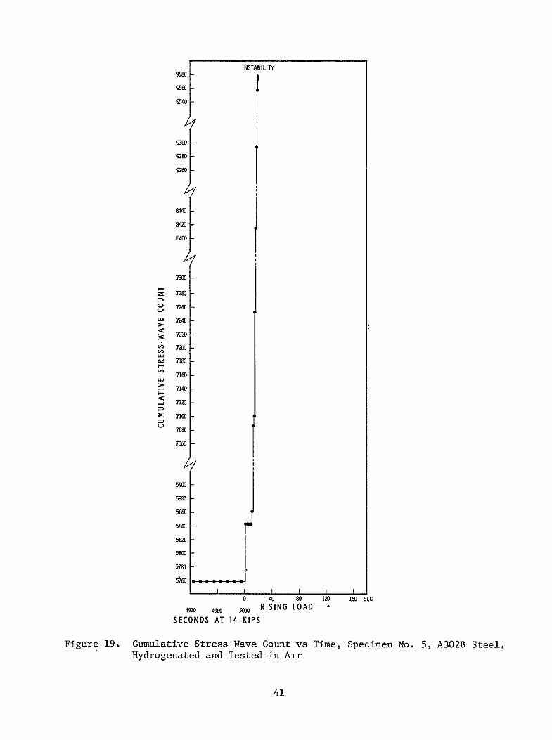
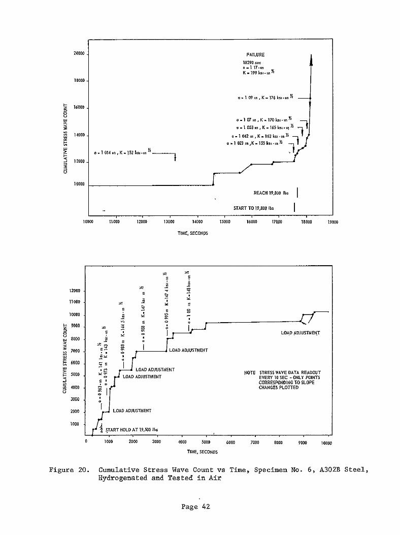
IV C Bend Tests in Air With Deliberate Addition of Hydrogen (cont)
As indicated in Figure 20 the increase in crack length during
the initial period of hold at 19500 lb resulted in an increase in the applied
stress intensity and was accompanied by significant stress-wave-emission
activity To maintain the desired load it was also necessary to make frequent
load adjustments at the start of hold During the first 3600 sec the effecshy
tive crack length increased from approximately 0963 to 1000 in and was
accompanied by about 7000 SWE As indicated in Figure 20 the majority of the
SWE activity and increase in crack length occurred during the first 3000 sec
of the hold at 19500 lb After this period both the stress-wave-emission
activity and rate of increase in crack length gradually decreased For example
during the entire period from 5000 to 17600 sec when the load was increased
to 19800 lb the apparent crack length and SWE count increased by only approxishy
mately 0020 in and 2500 respectively
After approximately 17000 sec at 19500 lb the load was increased
to 19800 lb and specimen failure occurred after approximately 600 sec at
19800 lb The load was maintained for this period however it was apparent
from both the SWE and COD gage data that the crack was extending and specimen
failure would occur without a further increase in load although it was necesshy
sary to continually adjust the tensile machine to maintain the desired load
The failure stress intensity approximated 199 ksi-in 2however technically
the onset of instability occurred after starting to increase the load at
approximately 153 ksi-in1 2
Specimen 7 was also hydrogenated baked at 300F for 3 hr and
tested in air Figure 21 is a detailed plot of the SWAT data (electronic
counter print-out every second) indicating crack growth of a discontinuous
nature starting at 2400-lb load Note the periods of dormancy (no increase
in SWE count) interspersed with abrupt increases in count indicating disconshy
tinuous crack growth Note also that there was little or no evidence of
continuous stress-wave emission until the load (stress intensity level) was
high approaching failure
43
CUMULAIY STRESS-VAVE COUNTCU LTISTE W E ON
I OT A~II I OI I L I I I I I I I I I I I I I I i I I I I I
- N LB
I I I I I I I I I I I I I i I I
--L - 0OTO11
-0101
(lNIML~ 33383338
8
133113-
3IiC)0 83) 3103 31-3(31-
~0
33 331
3l3C0C~
38318shy
111(10 CAVMSS3 nfl CAliVi flWfl3
________________________________________________________________________
111fl0~ 3KvM~s~a1Ff~TfvTifwT
FPAIAE
hY
A Ii
8
INa
CZ
8 C0 U CI
33 S
1 H
H
03 -I
~ 3lt
0 Cd 33
~C3 ~ H
8 0003
A
Ofli3i~~ C)
Page 45
IV C Bend Tests in Air With Deliberate Addition of Hydrogen (cont)
Figure 22 presents the SWE data from a hydrogenated bend specimen
(No 8) tested in air The load was increased continuously to 9800 lb
(70 ksi-in 2) where there was a short hold (approximately 400 sec) Note
the discontinuous crack growth followed by a short period of continuous
emission (less than 450 slope) The load was then raised to 14800 lb
(109 ksi-in 2) and held for approximately 400 sec Again there were jumps
in the SWE cumulative count but this time interspersed with continuous
emission The SWAT system employed for this test corresponded to that employed
for the background measurements at Kennedy Space Flight Center and shown in
Figure 8 only one channel was employed viz
Endevco 2213 Amplifier Amplifier Band-Pass Filter 10OX 10OX 20 to 50 Kcps
The continuous stress-wave emission observed during hold at the higher stressshy
intensity level in this specimen was not observed in the other hydrogenated
specimens tested in air The primary purpose of this test (Specimen 8) was to
record SWE data for subsequent playback and analysis to determine the amplitude
of burst-type stress-wave emissions associated with fracture in Type A302B
steel These analyses were performed using the instrumentation shown in
Figures 7 and 8 with the following results which are discussed in more detail
in conjunction with the results of the background measurements performed at
Kennedy Space Flight Center (Section V)
Maximum SWE Amplitude - 39 x 10-3g
Minimum SWE Amplitude - 12 x 10-3 g
Average SWE Amplitude - 22 x 10-3g
Laboratory Background - 11 x 10-3g
46
00 o z~ 20 ~
40
~40
S20 1 2 0 0 0 0
TIIAEAT 4 S-KIPHOLD (10KS(51IN A)
407
IV Laboratory Test Results and Discussion (cont)
D BEND TESTS IN 3 NaCI-WATER WITH DELIBERATE ADDITION OF HYDROGEN
Specimen 9 was hydrogenated baked and tested in 80F water
The electronic counter indicated continuous stress-wave emission interspersed
with abrupt increases in count indicating occasional crack jumps Figure 23
shows the details of stress-wave emission that occurred during both rising
load and holding load The crack length determined from the COD chart at
selected loads is also shown Note from the SWE data that there were no
periods of dormancy and the slope of the plot of cumulative count versus time
indicated moderately rapid continuouas crack growth such as might occur with
electrochemical dissolution at the crack tip The COD gage data shown in
Figure 23 also indicate crack extension however the actual amount appears
to be quite small (lt01 in) which would be consistent with the relatively
small number of stress-wave emissions detected even at the high system
sensitivity employed The dramatic difference between the behavior in
Figures 21 and 23 for hydrogenated material tested in air (Figure 21) and
water (Figure 23) indicates that hydrogen and 3 sodium chloride solution
acting together have a greater total effect than the sum of their individual
effects ie working together they appear to have produced a synergism
E WOL TESTS
Because of the possible significance of the synergistic-effect
noted above on the life of the hydrogen pressure vessels at Kennedy Space
Flight Center additional testing was performed using hydrogenated WOL specishy
mens cut from the fractured bend specimens The first WOL specimen was
initially loaded to-3650 lb (50 ksi-in 2) and then placed in 3 NaCl solution
(notch immersed) There was 30 min of essentially continuous stress-wave
emission (recorder started approximately 5 min after loading the specimen)
Subsequently therewas one sizable jump in the SWE cumulative count after
48
V30
760
740-M
$
720 -s
680shy
60
610
40 w
w
520 w
i
20500
HOLDD]N
340
20 760
7200
ING
IV
O
shy
420
60
40
20 0 2
04
0Q
0
60DO
LO0
01 200
250 300
350 400
450 500
550 6M
650
700 750
TIME
(SECONDS)
Figure 23
Cumulative Stress Wave Count vs Time Specimen No 9 A302B Steel
Hydrogenated and Tested in 3 NaCi-Water Environment
49
IV E WOL Tests (cont)
approximately 3 hr 40 min Then 3 hr 20 min later several jumps occurred
followed by 8 hr 20 min of stress-iave activity After this the crack was
dormant (total test time 17 hr 25 min) These data are shown in Figure 24
The load was then increased slightly (torque was increased from 200 to
255 in-lb) an additional 1-12 hr in 3 NaCl solution produced no significant
increase in the cumulative stress-wave count The reason for this apparently
anomalous behavior was not determined although it may result from a blunting
effect at the crack tip produced during the initial hold period
The fatigue crack was then extended (approximately 005 in) in
tension-tension fatigue and the specimen reloaded to approximately 51 ksi-in2
Stress-wave emission started almost immediately (dashed curve in Figure 24)
After approximately 3 hr of discontinuous activity the periods of dormancy
tended to increase interspersed with relatively small jumps (as counted over
10-sec intervals) The results of the initial loading and the reloading are
shown in Figure 24 note that there was appreciably lower cumulative count in
the reloaded specimen as compared with the initial loading for a comparable
period of test
A second hydrogenated WOL specimen was then tested in air at
50 ksi-in 2 there were stress waves initially (creep) but then very little
activity over the remaining 35-hr test period After the first hour the
count increased from approximately 150 to only 280 in the final 34 hr of test
Figure 25 shows the long peribds of dormancy punctuated by occasional 1-count
increases This is in marked contrast to the results obtained from the
hydrogenated WOL specimens tested in 3 NaCl solution and the bend-test
findings of a synergistic effect were confirmed
50
------------
aa
L- -- -- - ------ - --- I
3
IN DO
INTES) 3 S IOTI E( LI N LU
Ino
a
N O
TIME (MINUTES) IN 3 NCI SOLUTION
Figure 24 Cumulative Stress Wave Count vs Time at Hold WOL Specimen No 1
A302B Steel Hydrogenated and Tested in 3 NaCi-Water Environment
51
000 In 0 M6020 126 24 022 in0 1180 10 11 100 IWO l 100M M-C 0 90w6 a0 w6
t t t t 5W MOD4
10
TIME (MINUTES)
Figure 25 Cumulative Stress Wave Count vs Time at Hold WL Specimen No 2 A302B Steel Hydrogenated and Testd in Air
52
IV Laboratory Test Results and Discussion (cont)
F DISCUSSION
1 Material-Environment Consideration
The Type A302B steel supplied for evaluation exhibited a
very high level of fracture toughness Although quantitative plane-strain
fracture toughness measurements were not possible because of the large specimen
size required the KQ value associated with failure approximated 135 ksi-in1 2
This material was also found resistant to environmentally induced failure in
that the rate of crack growth of a prior flaw at applied stress-intensity
factors as high as 90 of the KQ value appeared to be very low This effect
was observed for unhydrogenated-material tested in air and a 3 NaCl-water
environment and hydrogenated material tested in an air environment However
the hydrogenated specimens tested in 3 NaCl-water environment had a much
faster rate of subcritical crack gr~wth in comparison to the other test condishy
tions indicating a synergistic effect due to the combination of sea water and
hydrogen in interstitial solid solution This synergistic effect indicates
that the Type A302B steel hydrogen storage tanks in the Kennedy Space Flight
Center environment may have limited life as the result of subcritical crack
growth if subjected to the same combination of stress and environmental
factors-
The WOL test results tended to confirm the possible synergism
due to the combined effects of 3 NaCl-water and hydrogen in interstitial solid
solution Marked SWE activity was observed when the hydrogenated specimens
were immersed in the salt water whereas in an air environment after the
initial period at hold when a creep phenomenon was observed there was essenshy
tially no stress-wave emission The fact that failure was not produced on
holding (in contradiction to the bend tests) can be explained by the fact that
the WOL test as-performed in this program is a self-arresting test because
53
IV F Discussion (cont)
the occurrence of crack growth results in a reduction in the applied load
Conversely in the bend tests the load was constantly applied as the crack
extended and eventually resulted in specimen failure
2 Stress-Wave-Emission Characterization
Detectable stress-wave emissions although of small amplitude
(ltOOlg) were observed to be associated with crack growth in Type A302B steel
Under all test conditions the stress-wave emissions were observed both during
rising load and when failure (instability) was imminent During hold various
SWE characteristics depending on the test conditions were observed When
tested in the hydrogenated condition in-an air environment a creep phenomenon
evidenced by increasing count of SWE and an accompanying increase in apparent
crack size was observed With time at hold and at applied stress-intensity
levels less than critical the creep phenomenon eventually stopped as did the
occurrence of stress-wave emissions Unhydrogenated material tested in the
3 NaCl-water environment produced continuous stress-wave emission punctuated
by abrupt increases in SWE count This behavior indicates both continuous
very small increments of crack extension with larger crack jumps corresponding
to the abrupt increases in SWE count Continuous incremental crack extension
characterized by continuous SWE interspersed with abrupt increases in SWE count
indicating occasional crack jumps was also observed in testing hydrogenated
material in a 3 NaCl-water environment
In all instances when failure (instability) occurred both
the amplitude and rate of stress-wave emission increased and could be employed
as a precursor of the onset of instability however even when failure was
approached-the SWE amplitude was small (ltOlg) In the other instances where
failure was not produced evidence of crack extension (although very small in
some instances) was observed on the specimen fracture face Once evidence of
54
IV F Discussion (cont)
crack growth was observed (by SWE or COD) it is obvious that failure would
eventually occur (assuming a constantly applied load) although depending on
the initial flaw size and subcritical growth rate the time to failure may be
very long In actual practice the SWE data could be employed (1) to locate
the propagating flaw (2) to monitor its occurrence and (3) as a basis for
terminating service so that repairs could be made before failure The stressshy
wave emissions associated with crack growth during rising load or increasing
stress intensity and the creep phenomenon during the initial part of hold
can be employed for this purpose
5S
V BACKGROUND MEASUREMENTS AND ASSOCIATED LABORATORY TESTS
A BACKGROUND MEASUREMENTS AT KENNEDY SPACE FLIGHT CENTER
Background noise measurements were made at two locations the VAB
Bottle Field and Pad A at the Kennedy Space Flight Center The data were tape
recorded and in addition to general background noise included tank blowdown
and repressurization periods The instrumentation for this purpose is shown
schematically in Figure 8 analysis of the data was performed by playback onto
an oscillograph and comparison with the SWE-crack growth data obtained during
the laboratory testing of bend specimens
The analysis of the signal amplitude data for tests at Cape Kennedy
is indicated below
1 Pad A Bottle Field
Signal Amplitude
a Quiescent Background
Filter at 20 Kcps - 50 Kcps -BandPass- 99 x 10 gsBand Pass
Filter at 200 cps - 32 Kcps
Band Pass
b Tank Blowdown - System Saturation (gt llg peak to peak)
C Tank Repressurization - System Saturation (gt llg peak to peak)
2 VAB Bottle Field
a Quiescent Background - 22 x 10- 4 gs
56
V A Background Measurements at Kennedy Space Flight Center (cont)
Signal Amplitude
b Tank Blowdown - System Saturation (gt llg peak to peak)
C Tank Repressurization - System Saturation (gt llg peak to peak)
Analysis of the tape-recorded data of bend tests at Aerojet indicates
the following signal amplitude for burstf-type stress-wave emissions associated
with crack growth and fracture in Type A302B steel
Maximum Amplitude - 39 x 10-3g
Minimum Amplitude - 12 x 10-3g
Average Amplitude - 22 x 10-3g
Laboratory Background - 11 x 10-3g
Thus the amplitude of SWE associated with crack growth in A302B steel is
approximately an order of magnitude larger than the background noise noted
previously Consequently the above results show that it is possible to detect
stress-wave emissions associated with fracture in A302B steel under the quiescent
background conditions existing at the Kennedy Space Center Difficulty is
expected in detecting such flaw growth during tank blowdown and repressurization
periods unless filtering can be employed to screen out the noise associated
with these periods However the blowdown and repressurization periods are of
very short duration and the materials behavior observed in this program indishy
cated that considerable prefailure crack extension would be expected from any
flaw of a size expected to be present in these pressure vessels Also
immediately on reaching load a creep phenomenon evidenced by an extension
in apparent crack length and accompanied by detectable stress-wave emission
was observed Consequently even if noise associated with blowdown and
57
V A Background Measurements at Kennedy Space Flight Center (cont)
repressurization cannot be effectively filtered out significant flaw growth
andor creep could still be detected and tank depressurization accomplished
prior to catastrophic failure assuming a capability for such depressurization
exists at these locations
B LABORATORY SIGNAL ATTENUATION EVALUATIONS
Subsequent to the background measurements at the Kennedy Space
Flight Center and the bend tests at Aerojet two series of tests were made at
Aerojet using a section of pipe and plate both of SAE 4130 steel alloy The
purpose of these tests was to determine the coefficient of signal attenuation
which in conjunction with the previous test data could be used to establish
the sensor spacing which would insure detection of SWE associated with crack
growth in the pressure-vessels at the Kennedy Space Flight Center
In these tests a constant pulse was imparted to the specimen by
a Tektronix 115 Pulse Generator using a Clevite PZT-5 Crystal (2125 in dia
and 0250 in thick) The piezoelectric crystal was mounted on a small alumishy
num block which in turn was adhered to the surface of the specimen The
signal was received by a 2217-E-Endevcq accelerometer placed at various disshy
tances from the pulser The pulse used was 10 n-sec rise and fall time with
a duration of 20 microsec at an amplitude of 12v
1 Pipe Tests
A SAE 4130 steel pipe (8-58 in OD 7-18 in ID and 22 ft
10-78 in long) was used as specimen for this test series The pulser was
mounted normal to the external surface of the pipe as close as possible to the
edge The accelerometer (2217-E-Endevco) was successively placed on the pipe
58
V B Laboratory Signal Attenuation Evalutions (cont)
surface at positions I to 8 that were at 4 6 8 10 12 14 16 and 20 ft
from the pulser The signal received by the accelerometer was displayed on a
Tektronix 422 osilloscope Typical signals are shown in Figure 26
The velocities of the compressional and shear waves in steel
are
29 lO06 x38103 Vc= -x lg ) (l-26) = O2 x06(- 0 x386 = 227000 insec(+j 012)283 (1+030) (1-060)
29x106 x 386 = 91 36= 123000 insec
s 2 ( + p) p 2 (i + 030) x 0283
where E = Youngs Modulus p = Poissons Ratio and p = density The times of
arrival of these waves at the computed velocities are indicated on the oscilloshy
scope photos shown in Figure 26 The point of shear wave arrival (T ) coincides
in most of the photos to a distinct change of pattern in the trace The
arrival of the compressional wave is difficult to determine accurately because
the amplitude of this wave attenuates very fast with distance
A visual comparison of the curves shows that Figure 26a
representing the signal received 4 ft from the impulse indicates a perfectly
detectable arrival of the compressional wave conversely Figure 26h (at 20 ft
from the impulse) shows the visually detectable arrival of a wave almost at the
computed arrival of the shear wave This is due to the fact that the amplitude
of the first cycles of the compressional wave have become essentially impercepshy
tible at a distance of 20 ft from the pulse An attempt to determine signal
arrival time by visual inspection only of the traces in Figure 26 would result
in the wave velocities indicated in Table III The computed arrival times of
the compressional and shear waves are shown in Table IV If an integration of
the positive portions of the cycles comprised in 200 p sec after arrival of the
59
VERTICAL SCALE 1 DIV= 01 V VERTICAL SCALE 1 DIV = 01 V HORIZONTAL SCALE 1 DIV= 50p SEC HORIZONTAL SCALE 1 DIV = 100 pSEC
a 4FT FROM PULSER b6 FEET FROM PULSER
Tc Ts Tc Ts
VERTICAL SCALE I DIV 01 V VERTICAL SCALE I DIV = 01 V HORIZONTAL SCALE I DIV = 100 I SEC HORIZONTAL SCALE 1 DIV = 200 p SEC
c 8 FEET FROM PULSER d 10 FEET FROM PULSER
Tc = Arrival of Compressional Wave
T = Arrival of Shear Wove
Figure 26 Oscillograph Traces for Pipe Tests (Sheet 1 of 2)
6o NOT REPRODUCTBLE
VERTICAL SCALE 1 DIV = 01 V VERTICAL SCALE 1 DIV 01 V HORIZONTAL SCALE 1 DIV = 200y SEC HORIZONTAL SCALE I DIV 200 p SEC
e 12 FEET FROM PULSER f 14 FEET FROM PULSER
T TS T T
VERTICAL SCALE 1 DIV = 01 V VERTICAL SCALE 1 DIV = 01 V HORIZONTAL SCALE 1 DIV = 200 v SEC HORIZONTAL SCALE I DIV =5001p SEC
g 16 FEET FROM PULSER h 20 FEET FROM PULSER
Figure 26 Oscillograph Traces for Pipe Tests (Sheet 2 of 2)
61
V B Laboratory Signal Attenuation Evaluations (cont)
shear wave is performed the average amplitudes determined in this manner
become quite meaningful These average amplitudes are shown in Table V
TABLE III
WAVE VELOCITY BASED ON VISUAL ANALYSIS OF OSCILLOSCOPE TRACES - PIPE TESTS
Distance from Pulse Arrival Velocities Photo ft in Time psc (ftsec)
1 4 48 210 228000
2 6 72 400 180000
3 8 96 600 160000
4 10 120 800 150000
5 12 144 1000 144000
6 14 168 1200 140000
7 16 192 1400 137000
8 20 240 1750 137000
TABLE IV
COMPUTED ARRIVAL TIMES - PIPE TESTS
Compressional Wave Shear Wave Distance from Pulse Arrival Time Arrival Time
Photo in psec Osc Div sec Ose Div
1 48 212 423 390 780
2 72 317 317 583 583
3 96 422 422 778 778
4 120 530 265 972 486
5 144 635 317 1163 581
6 168 740 370 1360 680
7 192 840 420 1545 771
8 240 1050 21 1930 387
62
V B Laboratory Signal Attenuation Evalutions (cont)
TABLE V
SIGNAL AMPLITUDE VS DISTANCE - PIPE TESTS
Average Signal Amplitude Distance from 200 Psec after Arrival
Test Pulser in of Comp Wave mv
1 48 230
2 72 145
3 96 85
4 120 60
5 144 45
6 168 28
7 192 22
8 240 18
The general equation for the amplitude attenuation curve is
C x e-Xy =
where y = amplitude at distance x in volts
x = distance in inches from pulse source
C = amplitude of pulse in volts
a = attenuation factor
or iny= 1 C + (- ax) = I C - ax (Eq 4)n n
To determine the values of C and a the following statistical analysis was
performed
63
V B Laboratory Signal Attenuation Evaluations (cont)
Distance Yo y y2 X X2 Test in m v n n
1 48 230 543 +142 2010 -87 7580 - 124 261
2 72 145 499 +098 0960 -63 3960 - 62 360
3 96 85 445 +044 0194 -39 1520 - 17 427
4 120 60 409 +008 0006 -15 225 - 1 490
5 144 45 380 -021 0044 + 9 81 - 2 548
6 168 28 334 -067 0450 +33 1090 - 21 560
7 192 22 309 -092 0847 +57 3250 - 52 592
8 240 18 289 -112 1250 +105 11000 - 118 690
EY2 EX2pound x = 1080 ElnY =3208 5761 28706 SXY-397 XxIny3928
- 1080 - 3208 x =- = 135 ny = 401
EXY -397 00138 1 C =l1y + oshy
pound 2 x2 28706 n i x
= 401+(0138)(135)=401+186= 587
C - 355 mv
It is now possible to compute the statistically corrected values of the signal
amplitude y at the distances from the pulse where they were measured The
general formula will be
ny = 587 -(00138) X
and the results are tabulated in Table VI The computed value of pulse amplishy
tude at source is found to be C = 355 my The values shown on Table VI are
plotted in Figure 27 which graphically shows the signal attenuation as a
function of distance from the pulse source
64
350
300
250 STATISTICALLY COMPUTED k VALUES FOR REGRESSION CURVE
--0gt 200
EXPERIMENTALLY DETERMINED
-- MATERIAL SAE 4130 STEEL U= SPECIMEN PIPE-S758 in D aZ
00
15 7 18 in D22 ft 10 78 in LONG
-J
100
50 I
0 I I I
5 I I I
DISTANCE
I
10 FROM SOURCE
I
FEET
I
15 20
Figure 27 Signal Amplitude vs Distance - Pipe Tests
V B Laboratory Signal Attenuation Evaluations (cont)
TABLE VI
STATISTICALLY CORRECTED VALUES OF SIGNAL AMPLITUDE - PIPE TESTS
Experimentally Distance from 1 Corrected Signal Determined Signal
Test Pulse in ny Amplitude (y) mv Amplitude (y) my
1 48 521 182 230
2 72 488 130 145
3 96 455 95 85
4 120 421 67 60
5 144 388 48 45
6 168 355 35 28
7 192 322 25 22
8 240 255 127 18
- 2 Plate Tests
An SAE 4130 steel plate (73-12 in long 48-12 in wide
and 34 in thick) was used for this test series The two diagonals were
marked on the plate The pulser was placed at the center of the plate and
the receiver accelerometer was placed on one of the diagonals at locations
spaced in increments of 6 in from the center The received signals were
observed on the oscilloscope and photos were taken of these signals Figure
28 shows oscillographs of the signals received at 6 12 18 24 30 36 and
42 in from the pulser The times of arrival of the shear wave are also shown
in Figure 28 The velocity used was v = 123000 insec An integration
was performed of the positive positions of the cycles comprised in a 20 Psec
interval after the arrival of the shear wave The average amplitudes detershy
mined from these integrations are shown in Table VII Only Tests 1 to 4 are
used because reflection (from the plate edges) in Tests 5 to 8 obscured the
66
b 12 INCHES FROM PULSERa 6 INCHES FROM PULSER
TBTs
c 18 INCHES FROM PULSER d 24 INCHES FROM PULSER
IT s = Arrival of Shear Wave
Vertical Scale 1 DIV = 01 Volt Horizontal Scale 1 DIV = 20 ASec
Figure 28 Oscillograph Traces for Plate Tests (Sheet 1 of 2)
Page 67
f 36 INCHES FROM PULSER e 30 INCHES FROM PULSER
g 42 INCHES FROM PULSER
= Arrival of Shear WaveTs
Vertical Scale 1 DIV = 01 Volt = 20 4SecHorizontal Scale 1 DIV
Figure 28 Oscillograph Traces for Plate Tests (Sheet 2 of 2)
08 gOTPRODUCIB1A
V B Laboratory Signal Attenuation Evaluations (cont)
data These reflections were received in Tests 5 to 8 because of the relashy
tively small plate that was available for this test series
TABLE VII
SIGNAL AMPLITUDE VS DISTANCE - PLATE TESTS
Distance from Average Amplitude Test Pulse in(x) in 20 p see mv
1 6 150
2 12 110
3 18 70
4 24 45
The following statistical analysis was performed to determine the values of
C and a in Equation 4
Test
Distance from
Pulse in(x)
y
m v
1
ny Y
2
Y 2
X XY
X1 y
n
1 6 150 500 +056 0314 -9 81 -502 3000
2
3
12
18
110
70
470
425
+026
-019
0067
0036
-3
+3
9
9
-078
-057
5640
7650
4 24 45 381 -063 0397 +9 81 -567 9149
60 1776 0814 180 -1204 25439
-x=
60 w= 15
4ny
iY 1
1nC
-
=
16=44 1776 =44
E YX 1204= __=
E y2 180
ny +(0067)(15) =
+0067
444 + 0067(15)
69
=
C
444 + 100
= 230 my
= 544
V B Laboratory Signal Attenuation Evaluations (cont)
Subsequently the values of signal amplitude (y) were statistically corrected
as before and the experimentally determined values of y are compared to the
results obtained in Table VIII
TABLE VIII
COMPARISON Or STATISTICALLY CORRECTED AND TEST-DETERMINED VALUES OF SIGNAL AMPLITUDE - PLATE TESTS
Experimentally Distance from Corrected Signal Determined Signal
Test Pulse in nY Amplitude (y) mv Amplitude (y) my
1 6 504 155 150
2 12 464 103 110
3 18 417 65 70
4 24 383 46 45
The computed value of the pulse amplitude at the source at
C equals 230 mv The regression curve and the experimentally determined points
are plotted in Figure 29 It should be observed that the attenuation coefshy
ficient for the pipe test was a = 00138 and for the plate test was 0067
This is due to the much larger rate of front area that the pulse meets in the
plate
C SENSOR SPACING
The quiescent background noise measurements performed at the test
sites using a 20 to 50 KHz band-pass filter are
Pad A Bottle Field - 0000099g
VAB Bottle Field 0000220g
70
250
200 - EXPERIMENTALLY DETERMINED
0o
gt
M a-100 34
STATISTICALLY COMPUTEDVALUES FOR REGRESSION CURVE
MATERIAL SAE 4130 STEEL
SPECIMEN PLATE - 73 12 in LONG 48 12 in WIDE
in THICK
J
50
0
0 5 SII
10 15
DISTANCE FROM SOURCE FEET
I
20 I
25
Figure 29 Signal Amplitude vs Distance - Plate Tests
V C Sensor Spacing (cont)
The recorded stress-wave-emission data obtained from the A302B steel bend tests
made at the Aerojet-General Corporation laboratory show that the minimum
acceleration at the source is 0O012g the average 00022g and the maximum
00039g Based on the above data and the attenuation factor X = 0067 detershy
mined from the plate tests the sensor spacings required to detect crack growth
in the vessels at the Kennedy Space Center were computed and the results are
tabulated below
Quiescent Sensor Spacing
Amplitude at Background in the Source(C) g Amplitude(y) g Cy ln(CIy) ln(CIy)
Pad A
Min Signal 00012 000015 800 208 310
Avg Signal 00022 000015 1470 269 402
Max Signal 00039 000015 2600 326 487
VAB Bottle Field
Min Signal 00012 000033 363 129 193
Avg Signal 00022 000033 668 190 283
Max Signal 00039 000033 1080 238 356
This threshold is 15 x 0000099 - 000015g (at Pad A)
This threshold is 15 x 000022 = 000033g (at VAB Bottle Field)
Figures 30 and 31 present schematically the location and spacings of sensors
on the pressure vessels
72
- 502 IN 8 IN
HEAD -- _
DEVELOPED + + CYLINDRICAL FOR MINIMUM SIGNAL-22 SENSORS AS SHOWN
SURFACE FOR AVERAGE SIGNAL-16 SENSORS
+ +I
FOR MAXIMUM SIGNAL- 14 SENSORS
282438 IN+ +
+ +
9 SPACINGS AT 313 IN
-I- +
+ +shy
+ -plusmn
HEAD _ __
8 IN
Figure 30 Schematic of Sensor Spacings for Bottles at Pad A
73
14601 IN
HEAD (6SENSORS) 23 14 INI I I - I I I
t plusmn + plusmn + +
+ + 4 + + + DEVELOPED CYL SURFACE
+ + 4A 1 13 LINES OF
+ + + SENSORS SPACED4 + + AT 2086 IN
+ + + + + +
+ + 4 + + +
251 1516 IN + + + +-I- +
+ + + 4- +
-1- 298438 IN+ -I- -+- -i- +
+I
23 14 INHEAD (6 SENSORS) 1
FOR MINIMUM SIGNAL-103 SENSORS AS SHOWN
FOR AVERAGE SIGNAL- 82 SENSORS FOR MAXIMUM SIGNAL- 58 SENSORS
Figure 31 Schematic of Sensor Spacings for Bottles at VAB Bottle Field
74
VI CONCLUSIONS
A The Type A302B steel supplied for evaluation exhibited a high level
of fracture toughness Although quantitative plane-strain fracture toughness
measurements were not possible because of the large specimen size required
the K value associated with failure approximated 135 ksi-inI 2
Q
B The Type A302B steel was found resistant to environmentally induced
slow crack growth when tested in the hydrogenated condition in an air environshy
ment and in the unhydrogenated condition in a 3 NaCl-water environment Howshy
ever hydrogenated material tested in 3 NaCl-water had a much faster rate of
subcritical crack growth indicating a synergistic effect due to the combinashy
tion of sea water and hydrogen in interstitial solid solution
C The synergistic effect indicates the Type A302B steel hydrogen
storage tanks in the Kennedy Space Flight Center may have limited life as a
result of subcritical crack growth if subjected to the same combination of
stress and environmental factors
D Detectable stress-wave emissions although of small amplitude
(ltOOlg) were observed to be associated with crack growth in Type A302B steel
In all test conditions the stress-wave emissions were observed during rising
load and when failure (instability) was imminent Both the amplitude and rate
of stress-wave emission increased as failure was approached and could be
employed as a precursor of the onset of instability
E Stress-wave emissions associated with crack growth in Type A302B
steel can be detected under quiescent background conditions at the Pad A and
VAB Bottle fields at the Kennedy Space Flight Center However it would be
difficult to detect such stress-wave emissions during tank blowdown and
repressurization periods unless filtering can be employed to screen out the
noise associated with these periods
75
VI Conclusions (cont)
F Even in the presence of background noise from tank blowdown and
repressurization these periods are considered short in the overall life of
the pressure vessels Consequently flaw growth or creep which was observed
during rising load or the initial part of hold could be detected by SWAT
permitting triangulation to the source and tank depressurization prior to
failure
G Stress-wave-emission attenuation test data were obtained and employed
in conjunction with the site background measurements addbnd test stress-waveshy
emission characterization data to determine sensor mounting patterns for the
hydrogen pressure vessels at Pad A and the VAB Bottle Field
VII RECOMMENDATIONS FOR FURTHER WORK
If the synergistic effect of hydrogen and 3 NaCi solution occurs in
Kennedy Space Flight Center tankage the life of the tankage will be limited
Obviously slow-crack growth from any cause whether continuous or disconshy
tinuous and regardless of how slow the rate of cracking will eventually
produce failure This investigation showed that subcritical crack growth is
in all likelihood occurring with each pressurization A question remains
however as to the rate of crack growth without knowledge of the rate there
is no way to anticipate the life of the tankage However with SWAT one can
monitor the occurrence of crack growth and most importantly make judgment
as to whether a given crack is approaching critical size Consequently it
is recommended that additional tests be performed to (1) verify the existence
of subcritical cracking in actual on-site tankage and (2) incorporate an
automatic system for continuously monitoring on-site tankage at Kennedy Space
Flight Center
76
REFERENCES
1 Steel R K Green A T Lockman C S Acoustic Verification of Structural Integrity of Polaris Chambers Society of Plastic Engineers 20th Meeting Atlantic City N Y January 1964
2 Pressure Testing of AFRM-017 Service Propulsion System Fuel Tank Utilizing Aerojet-General Corporations Stress-Wave Analysis Technique
Report NAS 9-6766-003 Aerojet-General Corp for NASA MSC Houston Texas Contract NAS 9-6766 May 1967
3 Srawley J E and Esgar J B Investigation of Hydrotest Failure of Thiokol Chemical Corp 260-Inch-Diameter SL-1 Motor Case NASA-TMX shy1194 January 1964
4 Hartbower C E Gerberich W W and Crimmins P P Mechanisms of Slow Crack Growth in High-Strength Steels AFML-TR-67-26 Vol 1 February 1967
5 -Hartbower C E Gerberich W W and Crimmins P P Characterization of Fatigue-Crack Growth by Stress Wave Emission Final Report on Conshytract NAS 1-4902 for NASA-Langley Research Center Hampton Virginia June 1966
6 IHartbower C E Gerberich W W Reuter W G and Crimmins P P Stress Wave Characteristics in Constructional Alloys Final Report on Office of Naval Research Contract N00014-66-C-0340 July 1967
7 Novak S R and Rolfe S T Modified WOL Specimen for KIscc Environmental Testing U S Steel Corp paper submitted to ASTM for publication
77
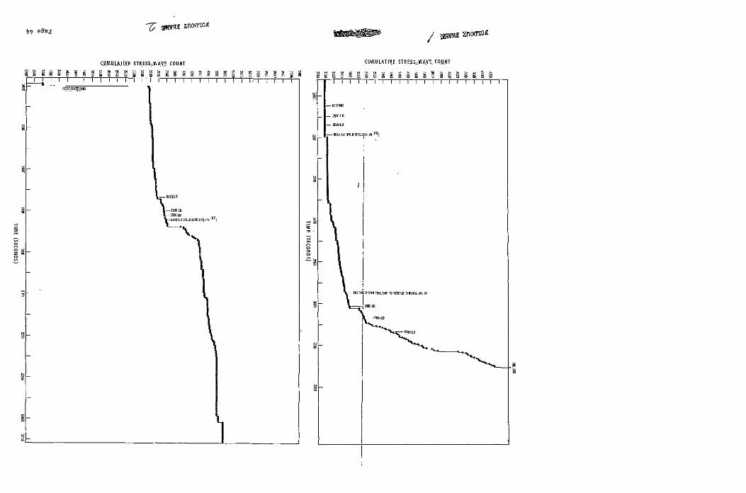
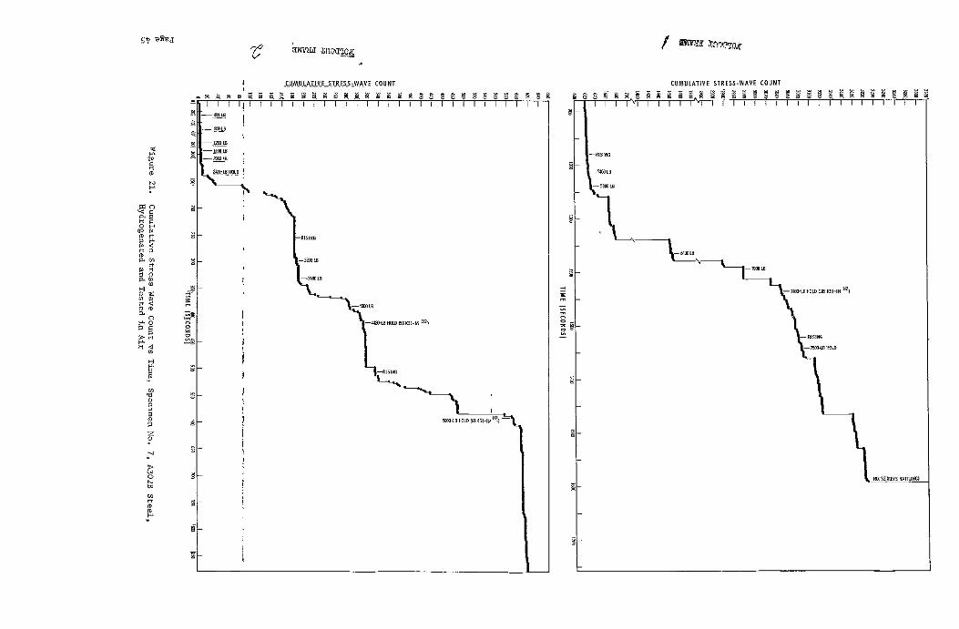
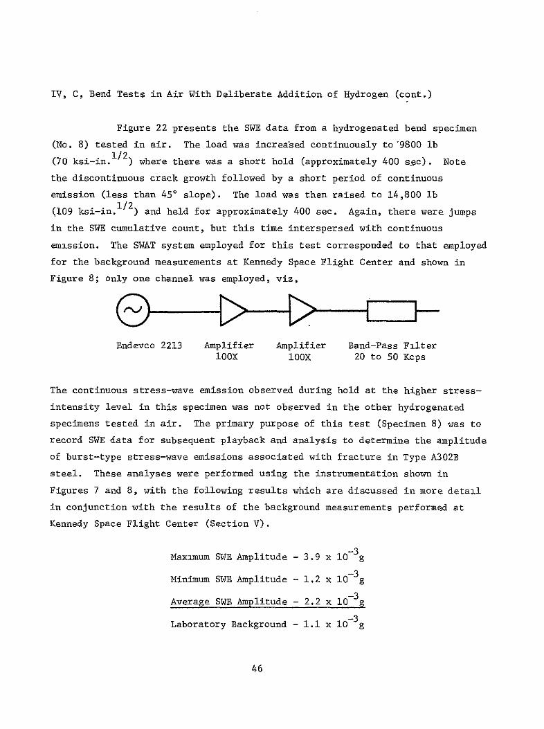
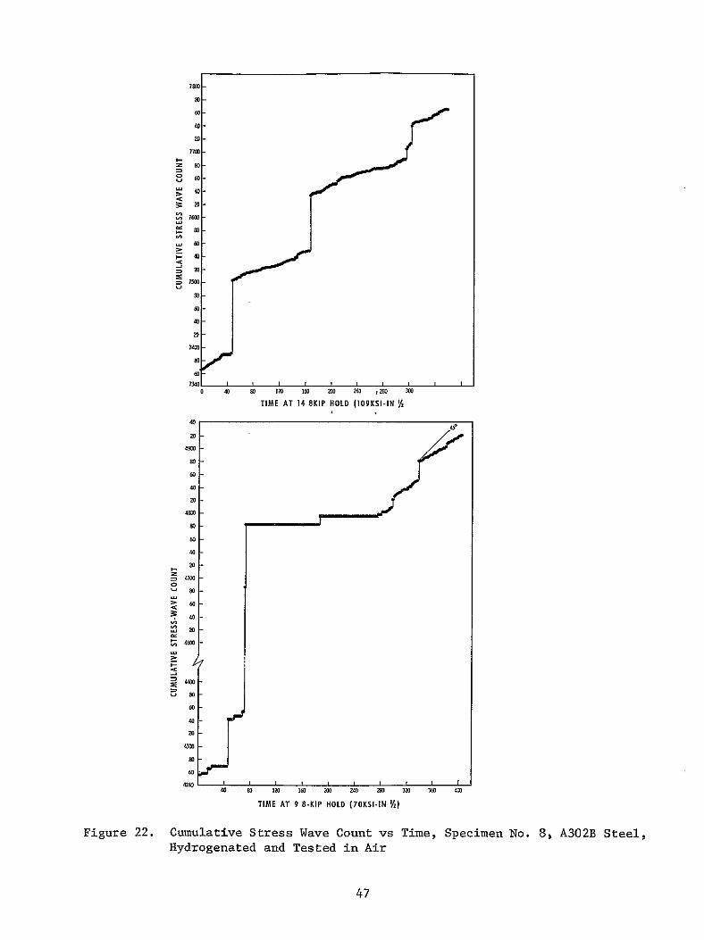
IV Laboratory Test Results and Discussion (cont)
D BEND TESTS IN 3 NaCI-WATER WITH DELIBERATE ADDITION OF HYDROGEN
Specimen 9 was hydrogenated baked and tested in 80F water
The electronic counter indicated continuous stress-wave emission interspersed
with abrupt increases in count indicating occasional crack jumps Figure 23
shows the details of stress-wave emission that occurred during both rising
load and holding load The crack length determined from the COD chart at
selected loads is also shown Note from the SWE data that there were no
periods of dormancy and the slope of the plot of cumulative count versus time
indicated moderately rapid continuouas crack growth such as might occur with
electrochemical dissolution at the crack tip The COD gage data shown in
Figure 23 also indicate crack extension however the actual amount appears
to be quite small (lt01 in) which would be consistent with the relatively
small number of stress-wave emissions detected even at the high system
sensitivity employed The dramatic difference between the behavior in
Figures 21 and 23 for hydrogenated material tested in air (Figure 21) and
water (Figure 23) indicates that hydrogen and 3 sodium chloride solution
acting together have a greater total effect than the sum of their individual
effects ie working together they appear to have produced a synergism
E WOL TESTS
Because of the possible significance of the synergistic-effect
noted above on the life of the hydrogen pressure vessels at Kennedy Space
Flight Center additional testing was performed using hydrogenated WOL specishy
mens cut from the fractured bend specimens The first WOL specimen was
initially loaded to-3650 lb (50 ksi-in 2) and then placed in 3 NaCl solution
(notch immersed) There was 30 min of essentially continuous stress-wave
emission (recorder started approximately 5 min after loading the specimen)
Subsequently therewas one sizable jump in the SWE cumulative count after
48
V30
760
740-M
$
720 -s
680shy
60
610
40 w
w
520 w
i
20500
HOLDD]N
340
20 760
7200
ING
IV
O
shy
420
60
40
20 0 2
04
0Q
0
60DO
LO0
01 200
250 300
350 400
450 500
550 6M
650
700 750
TIME
(SECONDS)
Figure 23
Cumulative Stress Wave Count vs Time Specimen No 9 A302B Steel
Hydrogenated and Tested in 3 NaCi-Water Environment
49
IV E WOL Tests (cont)
approximately 3 hr 40 min Then 3 hr 20 min later several jumps occurred
followed by 8 hr 20 min of stress-iave activity After this the crack was
dormant (total test time 17 hr 25 min) These data are shown in Figure 24
The load was then increased slightly (torque was increased from 200 to
255 in-lb) an additional 1-12 hr in 3 NaCl solution produced no significant
increase in the cumulative stress-wave count The reason for this apparently
anomalous behavior was not determined although it may result from a blunting
effect at the crack tip produced during the initial hold period
The fatigue crack was then extended (approximately 005 in) in
tension-tension fatigue and the specimen reloaded to approximately 51 ksi-in2
Stress-wave emission started almost immediately (dashed curve in Figure 24)
After approximately 3 hr of discontinuous activity the periods of dormancy
tended to increase interspersed with relatively small jumps (as counted over
10-sec intervals) The results of the initial loading and the reloading are
shown in Figure 24 note that there was appreciably lower cumulative count in
the reloaded specimen as compared with the initial loading for a comparable
period of test
A second hydrogenated WOL specimen was then tested in air at
50 ksi-in 2 there were stress waves initially (creep) but then very little
activity over the remaining 35-hr test period After the first hour the
count increased from approximately 150 to only 280 in the final 34 hr of test
Figure 25 shows the long peribds of dormancy punctuated by occasional 1-count
increases This is in marked contrast to the results obtained from the
hydrogenated WOL specimens tested in 3 NaCl solution and the bend-test
findings of a synergistic effect were confirmed
50
------------
aa
L- -- -- - ------ - --- I
3
IN DO
INTES) 3 S IOTI E( LI N LU
Ino
a
N O
TIME (MINUTES) IN 3 NCI SOLUTION
Figure 24 Cumulative Stress Wave Count vs Time at Hold WOL Specimen No 1
A302B Steel Hydrogenated and Tested in 3 NaCi-Water Environment
51
000 In 0 M6020 126 24 022 in0 1180 10 11 100 IWO l 100M M-C 0 90w6 a0 w6
t t t t 5W MOD4
10
TIME (MINUTES)
Figure 25 Cumulative Stress Wave Count vs Time at Hold WL Specimen No 2 A302B Steel Hydrogenated and Testd in Air
52
IV Laboratory Test Results and Discussion (cont)
F DISCUSSION
1 Material-Environment Consideration
The Type A302B steel supplied for evaluation exhibited a
very high level of fracture toughness Although quantitative plane-strain
fracture toughness measurements were not possible because of the large specimen
size required the KQ value associated with failure approximated 135 ksi-in1 2
This material was also found resistant to environmentally induced failure in
that the rate of crack growth of a prior flaw at applied stress-intensity
factors as high as 90 of the KQ value appeared to be very low This effect
was observed for unhydrogenated-material tested in air and a 3 NaCl-water
environment and hydrogenated material tested in an air environment However
the hydrogenated specimens tested in 3 NaCl-water environment had a much
faster rate of subcritical crack gr~wth in comparison to the other test condishy
tions indicating a synergistic effect due to the combination of sea water and
hydrogen in interstitial solid solution This synergistic effect indicates
that the Type A302B steel hydrogen storage tanks in the Kennedy Space Flight
Center environment may have limited life as the result of subcritical crack
growth if subjected to the same combination of stress and environmental
factors-
The WOL test results tended to confirm the possible synergism
due to the combined effects of 3 NaCl-water and hydrogen in interstitial solid
solution Marked SWE activity was observed when the hydrogenated specimens
were immersed in the salt water whereas in an air environment after the
initial period at hold when a creep phenomenon was observed there was essenshy
tially no stress-wave emission The fact that failure was not produced on
holding (in contradiction to the bend tests) can be explained by the fact that
the WOL test as-performed in this program is a self-arresting test because
53
IV F Discussion (cont)
the occurrence of crack growth results in a reduction in the applied load
Conversely in the bend tests the load was constantly applied as the crack
extended and eventually resulted in specimen failure
2 Stress-Wave-Emission Characterization
Detectable stress-wave emissions although of small amplitude
(ltOOlg) were observed to be associated with crack growth in Type A302B steel
Under all test conditions the stress-wave emissions were observed both during
rising load and when failure (instability) was imminent During hold various
SWE characteristics depending on the test conditions were observed When
tested in the hydrogenated condition in-an air environment a creep phenomenon
evidenced by increasing count of SWE and an accompanying increase in apparent
crack size was observed With time at hold and at applied stress-intensity
levels less than critical the creep phenomenon eventually stopped as did the
occurrence of stress-wave emissions Unhydrogenated material tested in the
3 NaCl-water environment produced continuous stress-wave emission punctuated
by abrupt increases in SWE count This behavior indicates both continuous
very small increments of crack extension with larger crack jumps corresponding
to the abrupt increases in SWE count Continuous incremental crack extension
characterized by continuous SWE interspersed with abrupt increases in SWE count
indicating occasional crack jumps was also observed in testing hydrogenated
material in a 3 NaCl-water environment
In all instances when failure (instability) occurred both
the amplitude and rate of stress-wave emission increased and could be employed
as a precursor of the onset of instability however even when failure was
approached-the SWE amplitude was small (ltOlg) In the other instances where
failure was not produced evidence of crack extension (although very small in
some instances) was observed on the specimen fracture face Once evidence of
54
IV F Discussion (cont)
crack growth was observed (by SWE or COD) it is obvious that failure would
eventually occur (assuming a constantly applied load) although depending on
the initial flaw size and subcritical growth rate the time to failure may be
very long In actual practice the SWE data could be employed (1) to locate
the propagating flaw (2) to monitor its occurrence and (3) as a basis for
terminating service so that repairs could be made before failure The stressshy
wave emissions associated with crack growth during rising load or increasing
stress intensity and the creep phenomenon during the initial part of hold
can be employed for this purpose
5S
V BACKGROUND MEASUREMENTS AND ASSOCIATED LABORATORY TESTS
A BACKGROUND MEASUREMENTS AT KENNEDY SPACE FLIGHT CENTER
Background noise measurements were made at two locations the VAB
Bottle Field and Pad A at the Kennedy Space Flight Center The data were tape
recorded and in addition to general background noise included tank blowdown
and repressurization periods The instrumentation for this purpose is shown
schematically in Figure 8 analysis of the data was performed by playback onto
an oscillograph and comparison with the SWE-crack growth data obtained during
the laboratory testing of bend specimens
The analysis of the signal amplitude data for tests at Cape Kennedy
is indicated below
1 Pad A Bottle Field
Signal Amplitude
a Quiescent Background
Filter at 20 Kcps - 50 Kcps -BandPass- 99 x 10 gsBand Pass
Filter at 200 cps - 32 Kcps
Band Pass
b Tank Blowdown - System Saturation (gt llg peak to peak)
C Tank Repressurization - System Saturation (gt llg peak to peak)
2 VAB Bottle Field
a Quiescent Background - 22 x 10- 4 gs
56
V A Background Measurements at Kennedy Space Flight Center (cont)
Signal Amplitude
b Tank Blowdown - System Saturation (gt llg peak to peak)
C Tank Repressurization - System Saturation (gt llg peak to peak)
Analysis of the tape-recorded data of bend tests at Aerojet indicates
the following signal amplitude for burstf-type stress-wave emissions associated
with crack growth and fracture in Type A302B steel
Maximum Amplitude - 39 x 10-3g
Minimum Amplitude - 12 x 10-3g
Average Amplitude - 22 x 10-3g
Laboratory Background - 11 x 10-3g
Thus the amplitude of SWE associated with crack growth in A302B steel is
approximately an order of magnitude larger than the background noise noted
previously Consequently the above results show that it is possible to detect
stress-wave emissions associated with fracture in A302B steel under the quiescent
background conditions existing at the Kennedy Space Center Difficulty is
expected in detecting such flaw growth during tank blowdown and repressurization
periods unless filtering can be employed to screen out the noise associated
with these periods However the blowdown and repressurization periods are of
very short duration and the materials behavior observed in this program indishy
cated that considerable prefailure crack extension would be expected from any
flaw of a size expected to be present in these pressure vessels Also
immediately on reaching load a creep phenomenon evidenced by an extension
in apparent crack length and accompanied by detectable stress-wave emission
was observed Consequently even if noise associated with blowdown and
57
V A Background Measurements at Kennedy Space Flight Center (cont)
repressurization cannot be effectively filtered out significant flaw growth
andor creep could still be detected and tank depressurization accomplished
prior to catastrophic failure assuming a capability for such depressurization
exists at these locations
B LABORATORY SIGNAL ATTENUATION EVALUATIONS
Subsequent to the background measurements at the Kennedy Space
Flight Center and the bend tests at Aerojet two series of tests were made at
Aerojet using a section of pipe and plate both of SAE 4130 steel alloy The
purpose of these tests was to determine the coefficient of signal attenuation
which in conjunction with the previous test data could be used to establish
the sensor spacing which would insure detection of SWE associated with crack
growth in the pressure-vessels at the Kennedy Space Flight Center
In these tests a constant pulse was imparted to the specimen by
a Tektronix 115 Pulse Generator using a Clevite PZT-5 Crystal (2125 in dia
and 0250 in thick) The piezoelectric crystal was mounted on a small alumishy
num block which in turn was adhered to the surface of the specimen The
signal was received by a 2217-E-Endevcq accelerometer placed at various disshy
tances from the pulser The pulse used was 10 n-sec rise and fall time with
a duration of 20 microsec at an amplitude of 12v
1 Pipe Tests
A SAE 4130 steel pipe (8-58 in OD 7-18 in ID and 22 ft
10-78 in long) was used as specimen for this test series The pulser was
mounted normal to the external surface of the pipe as close as possible to the
edge The accelerometer (2217-E-Endevco) was successively placed on the pipe
58
V B Laboratory Signal Attenuation Evalutions (cont)
surface at positions I to 8 that were at 4 6 8 10 12 14 16 and 20 ft
from the pulser The signal received by the accelerometer was displayed on a
Tektronix 422 osilloscope Typical signals are shown in Figure 26
The velocities of the compressional and shear waves in steel
are
29 lO06 x38103 Vc= -x lg ) (l-26) = O2 x06(- 0 x386 = 227000 insec(+j 012)283 (1+030) (1-060)
29x106 x 386 = 91 36= 123000 insec
s 2 ( + p) p 2 (i + 030) x 0283
where E = Youngs Modulus p = Poissons Ratio and p = density The times of
arrival of these waves at the computed velocities are indicated on the oscilloshy
scope photos shown in Figure 26 The point of shear wave arrival (T ) coincides
in most of the photos to a distinct change of pattern in the trace The
arrival of the compressional wave is difficult to determine accurately because
the amplitude of this wave attenuates very fast with distance
A visual comparison of the curves shows that Figure 26a
representing the signal received 4 ft from the impulse indicates a perfectly
detectable arrival of the compressional wave conversely Figure 26h (at 20 ft
from the impulse) shows the visually detectable arrival of a wave almost at the
computed arrival of the shear wave This is due to the fact that the amplitude
of the first cycles of the compressional wave have become essentially impercepshy
tible at a distance of 20 ft from the pulse An attempt to determine signal
arrival time by visual inspection only of the traces in Figure 26 would result
in the wave velocities indicated in Table III The computed arrival times of
the compressional and shear waves are shown in Table IV If an integration of
the positive portions of the cycles comprised in 200 p sec after arrival of the
59
VERTICAL SCALE 1 DIV= 01 V VERTICAL SCALE 1 DIV = 01 V HORIZONTAL SCALE 1 DIV= 50p SEC HORIZONTAL SCALE 1 DIV = 100 pSEC
a 4FT FROM PULSER b6 FEET FROM PULSER
Tc Ts Tc Ts
VERTICAL SCALE I DIV 01 V VERTICAL SCALE I DIV = 01 V HORIZONTAL SCALE I DIV = 100 I SEC HORIZONTAL SCALE 1 DIV = 200 p SEC
c 8 FEET FROM PULSER d 10 FEET FROM PULSER
Tc = Arrival of Compressional Wave
T = Arrival of Shear Wove
Figure 26 Oscillograph Traces for Pipe Tests (Sheet 1 of 2)
6o NOT REPRODUCTBLE
VERTICAL SCALE 1 DIV = 01 V VERTICAL SCALE 1 DIV 01 V HORIZONTAL SCALE 1 DIV = 200y SEC HORIZONTAL SCALE I DIV 200 p SEC
e 12 FEET FROM PULSER f 14 FEET FROM PULSER
T TS T T
VERTICAL SCALE 1 DIV = 01 V VERTICAL SCALE 1 DIV = 01 V HORIZONTAL SCALE 1 DIV = 200 v SEC HORIZONTAL SCALE I DIV =5001p SEC
g 16 FEET FROM PULSER h 20 FEET FROM PULSER
Figure 26 Oscillograph Traces for Pipe Tests (Sheet 2 of 2)
61
V B Laboratory Signal Attenuation Evaluations (cont)
shear wave is performed the average amplitudes determined in this manner
become quite meaningful These average amplitudes are shown in Table V
TABLE III
WAVE VELOCITY BASED ON VISUAL ANALYSIS OF OSCILLOSCOPE TRACES - PIPE TESTS
Distance from Pulse Arrival Velocities Photo ft in Time psc (ftsec)
1 4 48 210 228000
2 6 72 400 180000
3 8 96 600 160000
4 10 120 800 150000
5 12 144 1000 144000
6 14 168 1200 140000
7 16 192 1400 137000
8 20 240 1750 137000
TABLE IV
COMPUTED ARRIVAL TIMES - PIPE TESTS
Compressional Wave Shear Wave Distance from Pulse Arrival Time Arrival Time
Photo in psec Osc Div sec Ose Div
1 48 212 423 390 780
2 72 317 317 583 583
3 96 422 422 778 778
4 120 530 265 972 486
5 144 635 317 1163 581
6 168 740 370 1360 680
7 192 840 420 1545 771
8 240 1050 21 1930 387
62
V B Laboratory Signal Attenuation Evalutions (cont)
TABLE V
SIGNAL AMPLITUDE VS DISTANCE - PIPE TESTS
Average Signal Amplitude Distance from 200 Psec after Arrival
Test Pulser in of Comp Wave mv
1 48 230
2 72 145
3 96 85
4 120 60
5 144 45
6 168 28
7 192 22
8 240 18
The general equation for the amplitude attenuation curve is
C x e-Xy =
where y = amplitude at distance x in volts
x = distance in inches from pulse source
C = amplitude of pulse in volts
a = attenuation factor
or iny= 1 C + (- ax) = I C - ax (Eq 4)n n
To determine the values of C and a the following statistical analysis was
performed
63
V B Laboratory Signal Attenuation Evaluations (cont)
Distance Yo y y2 X X2 Test in m v n n
1 48 230 543 +142 2010 -87 7580 - 124 261
2 72 145 499 +098 0960 -63 3960 - 62 360
3 96 85 445 +044 0194 -39 1520 - 17 427
4 120 60 409 +008 0006 -15 225 - 1 490
5 144 45 380 -021 0044 + 9 81 - 2 548
6 168 28 334 -067 0450 +33 1090 - 21 560
7 192 22 309 -092 0847 +57 3250 - 52 592
8 240 18 289 -112 1250 +105 11000 - 118 690
EY2 EX2pound x = 1080 ElnY =3208 5761 28706 SXY-397 XxIny3928
- 1080 - 3208 x =- = 135 ny = 401
EXY -397 00138 1 C =l1y + oshy
pound 2 x2 28706 n i x
= 401+(0138)(135)=401+186= 587
C - 355 mv
It is now possible to compute the statistically corrected values of the signal
amplitude y at the distances from the pulse where they were measured The
general formula will be
ny = 587 -(00138) X
and the results are tabulated in Table VI The computed value of pulse amplishy
tude at source is found to be C = 355 my The values shown on Table VI are
plotted in Figure 27 which graphically shows the signal attenuation as a
function of distance from the pulse source
64
350
300
250 STATISTICALLY COMPUTED k VALUES FOR REGRESSION CURVE
--0gt 200
EXPERIMENTALLY DETERMINED
-- MATERIAL SAE 4130 STEEL U= SPECIMEN PIPE-S758 in D aZ
00
15 7 18 in D22 ft 10 78 in LONG
-J
100
50 I
0 I I I
5 I I I
DISTANCE
I
10 FROM SOURCE
I
FEET
I
15 20
Figure 27 Signal Amplitude vs Distance - Pipe Tests
V B Laboratory Signal Attenuation Evaluations (cont)
TABLE VI
STATISTICALLY CORRECTED VALUES OF SIGNAL AMPLITUDE - PIPE TESTS
Experimentally Distance from 1 Corrected Signal Determined Signal
Test Pulse in ny Amplitude (y) mv Amplitude (y) my
1 48 521 182 230
2 72 488 130 145
3 96 455 95 85
4 120 421 67 60
5 144 388 48 45
6 168 355 35 28
7 192 322 25 22
8 240 255 127 18
- 2 Plate Tests
An SAE 4130 steel plate (73-12 in long 48-12 in wide
and 34 in thick) was used for this test series The two diagonals were
marked on the plate The pulser was placed at the center of the plate and
the receiver accelerometer was placed on one of the diagonals at locations
spaced in increments of 6 in from the center The received signals were
observed on the oscilloscope and photos were taken of these signals Figure
28 shows oscillographs of the signals received at 6 12 18 24 30 36 and
42 in from the pulser The times of arrival of the shear wave are also shown
in Figure 28 The velocity used was v = 123000 insec An integration
was performed of the positive positions of the cycles comprised in a 20 Psec
interval after the arrival of the shear wave The average amplitudes detershy
mined from these integrations are shown in Table VII Only Tests 1 to 4 are
used because reflection (from the plate edges) in Tests 5 to 8 obscured the
66
b 12 INCHES FROM PULSERa 6 INCHES FROM PULSER
TBTs
c 18 INCHES FROM PULSER d 24 INCHES FROM PULSER
IT s = Arrival of Shear Wave
Vertical Scale 1 DIV = 01 Volt Horizontal Scale 1 DIV = 20 ASec
Figure 28 Oscillograph Traces for Plate Tests (Sheet 1 of 2)
Page 67
f 36 INCHES FROM PULSER e 30 INCHES FROM PULSER
g 42 INCHES FROM PULSER
= Arrival of Shear WaveTs
Vertical Scale 1 DIV = 01 Volt = 20 4SecHorizontal Scale 1 DIV
Figure 28 Oscillograph Traces for Plate Tests (Sheet 2 of 2)
08 gOTPRODUCIB1A
V B Laboratory Signal Attenuation Evaluations (cont)
data These reflections were received in Tests 5 to 8 because of the relashy
tively small plate that was available for this test series
TABLE VII
SIGNAL AMPLITUDE VS DISTANCE - PLATE TESTS
Distance from Average Amplitude Test Pulse in(x) in 20 p see mv
1 6 150
2 12 110
3 18 70
4 24 45
The following statistical analysis was performed to determine the values of
C and a in Equation 4
Test
Distance from
Pulse in(x)
y
m v
1
ny Y
2
Y 2
X XY
X1 y
n
1 6 150 500 +056 0314 -9 81 -502 3000
2
3
12
18
110
70
470
425
+026
-019
0067
0036
-3
+3
9
9
-078
-057
5640
7650
4 24 45 381 -063 0397 +9 81 -567 9149
60 1776 0814 180 -1204 25439
-x=
60 w= 15
4ny
iY 1
1nC
-
=
16=44 1776 =44
E YX 1204= __=
E y2 180
ny +(0067)(15) =
+0067
444 + 0067(15)
69
=
C
444 + 100
= 230 my
= 544
V B Laboratory Signal Attenuation Evaluations (cont)
Subsequently the values of signal amplitude (y) were statistically corrected
as before and the experimentally determined values of y are compared to the
results obtained in Table VIII
TABLE VIII
COMPARISON Or STATISTICALLY CORRECTED AND TEST-DETERMINED VALUES OF SIGNAL AMPLITUDE - PLATE TESTS
Experimentally Distance from Corrected Signal Determined Signal
Test Pulse in nY Amplitude (y) mv Amplitude (y) my
1 6 504 155 150
2 12 464 103 110
3 18 417 65 70
4 24 383 46 45
The computed value of the pulse amplitude at the source at
C equals 230 mv The regression curve and the experimentally determined points
are plotted in Figure 29 It should be observed that the attenuation coefshy
ficient for the pipe test was a = 00138 and for the plate test was 0067
This is due to the much larger rate of front area that the pulse meets in the
plate
C SENSOR SPACING
The quiescent background noise measurements performed at the test
sites using a 20 to 50 KHz band-pass filter are
Pad A Bottle Field - 0000099g
VAB Bottle Field 0000220g
70
250
200 - EXPERIMENTALLY DETERMINED
0o
gt
M a-100 34
STATISTICALLY COMPUTEDVALUES FOR REGRESSION CURVE
MATERIAL SAE 4130 STEEL
SPECIMEN PLATE - 73 12 in LONG 48 12 in WIDE
in THICK
J
50
0
0 5 SII
10 15
DISTANCE FROM SOURCE FEET
I
20 I
25
Figure 29 Signal Amplitude vs Distance - Plate Tests
V C Sensor Spacing (cont)
The recorded stress-wave-emission data obtained from the A302B steel bend tests
made at the Aerojet-General Corporation laboratory show that the minimum
acceleration at the source is 0O012g the average 00022g and the maximum
00039g Based on the above data and the attenuation factor X = 0067 detershy
mined from the plate tests the sensor spacings required to detect crack growth
in the vessels at the Kennedy Space Center were computed and the results are
tabulated below
Quiescent Sensor Spacing
Amplitude at Background in the Source(C) g Amplitude(y) g Cy ln(CIy) ln(CIy)
Pad A
Min Signal 00012 000015 800 208 310
Avg Signal 00022 000015 1470 269 402
Max Signal 00039 000015 2600 326 487
VAB Bottle Field
Min Signal 00012 000033 363 129 193
Avg Signal 00022 000033 668 190 283
Max Signal 00039 000033 1080 238 356
This threshold is 15 x 0000099 - 000015g (at Pad A)
This threshold is 15 x 000022 = 000033g (at VAB Bottle Field)
Figures 30 and 31 present schematically the location and spacings of sensors
on the pressure vessels
72
- 502 IN 8 IN
HEAD -- _
DEVELOPED + + CYLINDRICAL FOR MINIMUM SIGNAL-22 SENSORS AS SHOWN
SURFACE FOR AVERAGE SIGNAL-16 SENSORS
+ +I
FOR MAXIMUM SIGNAL- 14 SENSORS
282438 IN+ +
+ +
9 SPACINGS AT 313 IN
-I- +
+ +shy
+ -plusmn
HEAD _ __
8 IN
Figure 30 Schematic of Sensor Spacings for Bottles at Pad A
73
14601 IN
HEAD (6SENSORS) 23 14 INI I I - I I I
t plusmn + plusmn + +
+ + 4 + + + DEVELOPED CYL SURFACE
+ + 4A 1 13 LINES OF
+ + + SENSORS SPACED4 + + AT 2086 IN
+ + + + + +
+ + 4 + + +
251 1516 IN + + + +-I- +
+ + + 4- +
-1- 298438 IN+ -I- -+- -i- +
+I
23 14 INHEAD (6 SENSORS) 1
FOR MINIMUM SIGNAL-103 SENSORS AS SHOWN
FOR AVERAGE SIGNAL- 82 SENSORS FOR MAXIMUM SIGNAL- 58 SENSORS
Figure 31 Schematic of Sensor Spacings for Bottles at VAB Bottle Field
74
VI CONCLUSIONS
A The Type A302B steel supplied for evaluation exhibited a high level
of fracture toughness Although quantitative plane-strain fracture toughness
measurements were not possible because of the large specimen size required
the K value associated with failure approximated 135 ksi-inI 2
Q
B The Type A302B steel was found resistant to environmentally induced
slow crack growth when tested in the hydrogenated condition in an air environshy
ment and in the unhydrogenated condition in a 3 NaCl-water environment Howshy
ever hydrogenated material tested in 3 NaCl-water had a much faster rate of
subcritical crack growth indicating a synergistic effect due to the combinashy
tion of sea water and hydrogen in interstitial solid solution
C The synergistic effect indicates the Type A302B steel hydrogen
storage tanks in the Kennedy Space Flight Center may have limited life as a
result of subcritical crack growth if subjected to the same combination of
stress and environmental factors
D Detectable stress-wave emissions although of small amplitude
(ltOOlg) were observed to be associated with crack growth in Type A302B steel
In all test conditions the stress-wave emissions were observed during rising
load and when failure (instability) was imminent Both the amplitude and rate
of stress-wave emission increased as failure was approached and could be
employed as a precursor of the onset of instability
E Stress-wave emissions associated with crack growth in Type A302B
steel can be detected under quiescent background conditions at the Pad A and
VAB Bottle fields at the Kennedy Space Flight Center However it would be
difficult to detect such stress-wave emissions during tank blowdown and
repressurization periods unless filtering can be employed to screen out the
noise associated with these periods
75
VI Conclusions (cont)
F Even in the presence of background noise from tank blowdown and
repressurization these periods are considered short in the overall life of
the pressure vessels Consequently flaw growth or creep which was observed
during rising load or the initial part of hold could be detected by SWAT
permitting triangulation to the source and tank depressurization prior to
failure
G Stress-wave-emission attenuation test data were obtained and employed
in conjunction with the site background measurements addbnd test stress-waveshy
emission characterization data to determine sensor mounting patterns for the
hydrogen pressure vessels at Pad A and the VAB Bottle Field
VII RECOMMENDATIONS FOR FURTHER WORK
If the synergistic effect of hydrogen and 3 NaCi solution occurs in
Kennedy Space Flight Center tankage the life of the tankage will be limited
Obviously slow-crack growth from any cause whether continuous or disconshy
tinuous and regardless of how slow the rate of cracking will eventually
produce failure This investigation showed that subcritical crack growth is
in all likelihood occurring with each pressurization A question remains
however as to the rate of crack growth without knowledge of the rate there
is no way to anticipate the life of the tankage However with SWAT one can
monitor the occurrence of crack growth and most importantly make judgment
as to whether a given crack is approaching critical size Consequently it
is recommended that additional tests be performed to (1) verify the existence
of subcritical cracking in actual on-site tankage and (2) incorporate an
automatic system for continuously monitoring on-site tankage at Kennedy Space
Flight Center
76
REFERENCES
1 Steel R K Green A T Lockman C S Acoustic Verification of Structural Integrity of Polaris Chambers Society of Plastic Engineers 20th Meeting Atlantic City N Y January 1964
2 Pressure Testing of AFRM-017 Service Propulsion System Fuel Tank Utilizing Aerojet-General Corporations Stress-Wave Analysis Technique
Report NAS 9-6766-003 Aerojet-General Corp for NASA MSC Houston Texas Contract NAS 9-6766 May 1967
3 Srawley J E and Esgar J B Investigation of Hydrotest Failure of Thiokol Chemical Corp 260-Inch-Diameter SL-1 Motor Case NASA-TMX shy1194 January 1964
4 Hartbower C E Gerberich W W and Crimmins P P Mechanisms of Slow Crack Growth in High-Strength Steels AFML-TR-67-26 Vol 1 February 1967
5 -Hartbower C E Gerberich W W and Crimmins P P Characterization of Fatigue-Crack Growth by Stress Wave Emission Final Report on Conshytract NAS 1-4902 for NASA-Langley Research Center Hampton Virginia June 1966
6 IHartbower C E Gerberich W W Reuter W G and Crimmins P P Stress Wave Characteristics in Constructional Alloys Final Report on Office of Naval Research Contract N00014-66-C-0340 July 1967
7 Novak S R and Rolfe S T Modified WOL Specimen for KIscc Environmental Testing U S Steel Corp paper submitted to ASTM for publication
77
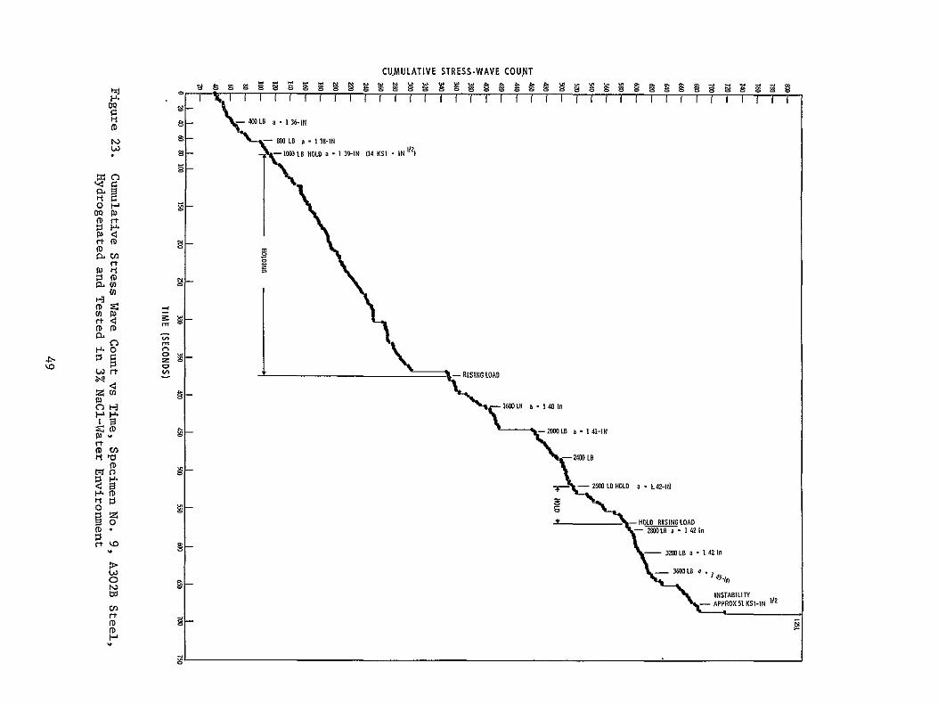
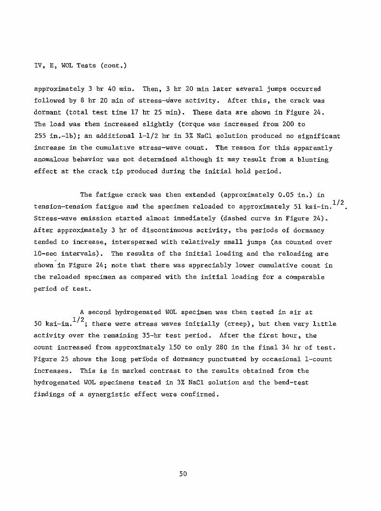
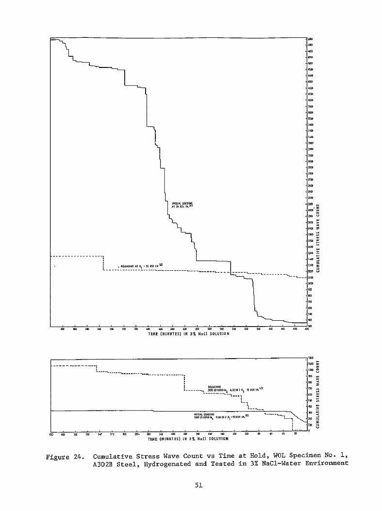
IV F Discussion (cont)
crack growth was observed (by SWE or COD) it is obvious that failure would
eventually occur (assuming a constantly applied load) although depending on
the initial flaw size and subcritical growth rate the time to failure may be
very long In actual practice the SWE data could be employed (1) to locate
the propagating flaw (2) to monitor its occurrence and (3) as a basis for
terminating service so that repairs could be made before failure The stressshy
wave emissions associated with crack growth during rising load or increasing
stress intensity and the creep phenomenon during the initial part of hold
can be employed for this purpose
5S
V BACKGROUND MEASUREMENTS AND ASSOCIATED LABORATORY TESTS
A BACKGROUND MEASUREMENTS AT KENNEDY SPACE FLIGHT CENTER
Background noise measurements were made at two locations the VAB
Bottle Field and Pad A at the Kennedy Space Flight Center The data were tape
recorded and in addition to general background noise included tank blowdown
and repressurization periods The instrumentation for this purpose is shown
schematically in Figure 8 analysis of the data was performed by playback onto
an oscillograph and comparison with the SWE-crack growth data obtained during
the laboratory testing of bend specimens
The analysis of the signal amplitude data for tests at Cape Kennedy
is indicated below
1 Pad A Bottle Field
Signal Amplitude
a Quiescent Background
Filter at 20 Kcps - 50 Kcps -BandPass- 99 x 10 gsBand Pass
Filter at 200 cps - 32 Kcps
Band Pass
b Tank Blowdown - System Saturation (gt llg peak to peak)
C Tank Repressurization - System Saturation (gt llg peak to peak)
2 VAB Bottle Field
a Quiescent Background - 22 x 10- 4 gs
56
V A Background Measurements at Kennedy Space Flight Center (cont)
Signal Amplitude
b Tank Blowdown - System Saturation (gt llg peak to peak)
C Tank Repressurization - System Saturation (gt llg peak to peak)
Analysis of the tape-recorded data of bend tests at Aerojet indicates
the following signal amplitude for burstf-type stress-wave emissions associated
with crack growth and fracture in Type A302B steel
Maximum Amplitude - 39 x 10-3g
Minimum Amplitude - 12 x 10-3g
Average Amplitude - 22 x 10-3g
Laboratory Background - 11 x 10-3g
Thus the amplitude of SWE associated with crack growth in A302B steel is
approximately an order of magnitude larger than the background noise noted
previously Consequently the above results show that it is possible to detect
stress-wave emissions associated with fracture in A302B steel under the quiescent
background conditions existing at the Kennedy Space Center Difficulty is
expected in detecting such flaw growth during tank blowdown and repressurization
periods unless filtering can be employed to screen out the noise associated
with these periods However the blowdown and repressurization periods are of
very short duration and the materials behavior observed in this program indishy
cated that considerable prefailure crack extension would be expected from any
flaw of a size expected to be present in these pressure vessels Also
immediately on reaching load a creep phenomenon evidenced by an extension
in apparent crack length and accompanied by detectable stress-wave emission
was observed Consequently even if noise associated with blowdown and
57
V A Background Measurements at Kennedy Space Flight Center (cont)
repressurization cannot be effectively filtered out significant flaw growth
andor creep could still be detected and tank depressurization accomplished
prior to catastrophic failure assuming a capability for such depressurization
exists at these locations
B LABORATORY SIGNAL ATTENUATION EVALUATIONS
Subsequent to the background measurements at the Kennedy Space
Flight Center and the bend tests at Aerojet two series of tests were made at
Aerojet using a section of pipe and plate both of SAE 4130 steel alloy The
purpose of these tests was to determine the coefficient of signal attenuation
which in conjunction with the previous test data could be used to establish
the sensor spacing which would insure detection of SWE associated with crack
growth in the pressure-vessels at the Kennedy Space Flight Center
In these tests a constant pulse was imparted to the specimen by
a Tektronix 115 Pulse Generator using a Clevite PZT-5 Crystal (2125 in dia
and 0250 in thick) The piezoelectric crystal was mounted on a small alumishy
num block which in turn was adhered to the surface of the specimen The
signal was received by a 2217-E-Endevcq accelerometer placed at various disshy
tances from the pulser The pulse used was 10 n-sec rise and fall time with
a duration of 20 microsec at an amplitude of 12v
1 Pipe Tests
A SAE 4130 steel pipe (8-58 in OD 7-18 in ID and 22 ft
10-78 in long) was used as specimen for this test series The pulser was
mounted normal to the external surface of the pipe as close as possible to the
edge The accelerometer (2217-E-Endevco) was successively placed on the pipe
58
V B Laboratory Signal Attenuation Evalutions (cont)
surface at positions I to 8 that were at 4 6 8 10 12 14 16 and 20 ft
from the pulser The signal received by the accelerometer was displayed on a
Tektronix 422 osilloscope Typical signals are shown in Figure 26
The velocities of the compressional and shear waves in steel
are
29 lO06 x38103 Vc= -x lg ) (l-26) = O2 x06(- 0 x386 = 227000 insec(+j 012)283 (1+030) (1-060)
29x106 x 386 = 91 36= 123000 insec
s 2 ( + p) p 2 (i + 030) x 0283
where E = Youngs Modulus p = Poissons Ratio and p = density The times of
arrival of these waves at the computed velocities are indicated on the oscilloshy
scope photos shown in Figure 26 The point of shear wave arrival (T ) coincides
in most of the photos to a distinct change of pattern in the trace The
arrival of the compressional wave is difficult to determine accurately because
the amplitude of this wave attenuates very fast with distance
A visual comparison of the curves shows that Figure 26a
representing the signal received 4 ft from the impulse indicates a perfectly
detectable arrival of the compressional wave conversely Figure 26h (at 20 ft
from the impulse) shows the visually detectable arrival of a wave almost at the
computed arrival of the shear wave This is due to the fact that the amplitude
of the first cycles of the compressional wave have become essentially impercepshy
tible at a distance of 20 ft from the pulse An attempt to determine signal
arrival time by visual inspection only of the traces in Figure 26 would result
in the wave velocities indicated in Table III The computed arrival times of
the compressional and shear waves are shown in Table IV If an integration of
the positive portions of the cycles comprised in 200 p sec after arrival of the
59
VERTICAL SCALE 1 DIV= 01 V VERTICAL SCALE 1 DIV = 01 V HORIZONTAL SCALE 1 DIV= 50p SEC HORIZONTAL SCALE 1 DIV = 100 pSEC
a 4FT FROM PULSER b6 FEET FROM PULSER
Tc Ts Tc Ts
VERTICAL SCALE I DIV 01 V VERTICAL SCALE I DIV = 01 V HORIZONTAL SCALE I DIV = 100 I SEC HORIZONTAL SCALE 1 DIV = 200 p SEC
c 8 FEET FROM PULSER d 10 FEET FROM PULSER
Tc = Arrival of Compressional Wave
T = Arrival of Shear Wove
Figure 26 Oscillograph Traces for Pipe Tests (Sheet 1 of 2)
6o NOT REPRODUCTBLE
VERTICAL SCALE 1 DIV = 01 V VERTICAL SCALE 1 DIV 01 V HORIZONTAL SCALE 1 DIV = 200y SEC HORIZONTAL SCALE I DIV 200 p SEC
e 12 FEET FROM PULSER f 14 FEET FROM PULSER
T TS T T
VERTICAL SCALE 1 DIV = 01 V VERTICAL SCALE 1 DIV = 01 V HORIZONTAL SCALE 1 DIV = 200 v SEC HORIZONTAL SCALE I DIV =5001p SEC
g 16 FEET FROM PULSER h 20 FEET FROM PULSER
Figure 26 Oscillograph Traces for Pipe Tests (Sheet 2 of 2)
61
V B Laboratory Signal Attenuation Evaluations (cont)
shear wave is performed the average amplitudes determined in this manner
become quite meaningful These average amplitudes are shown in Table V
TABLE III
WAVE VELOCITY BASED ON VISUAL ANALYSIS OF OSCILLOSCOPE TRACES - PIPE TESTS
Distance from Pulse Arrival Velocities Photo ft in Time psc (ftsec)
1 4 48 210 228000
2 6 72 400 180000
3 8 96 600 160000
4 10 120 800 150000
5 12 144 1000 144000
6 14 168 1200 140000
7 16 192 1400 137000
8 20 240 1750 137000
TABLE IV
COMPUTED ARRIVAL TIMES - PIPE TESTS
Compressional Wave Shear Wave Distance from Pulse Arrival Time Arrival Time
Photo in psec Osc Div sec Ose Div
1 48 212 423 390 780
2 72 317 317 583 583
3 96 422 422 778 778
4 120 530 265 972 486
5 144 635 317 1163 581
6 168 740 370 1360 680
7 192 840 420 1545 771
8 240 1050 21 1930 387
62
V B Laboratory Signal Attenuation Evalutions (cont)
TABLE V
SIGNAL AMPLITUDE VS DISTANCE - PIPE TESTS
Average Signal Amplitude Distance from 200 Psec after Arrival
Test Pulser in of Comp Wave mv
1 48 230
2 72 145
3 96 85
4 120 60
5 144 45
6 168 28
7 192 22
8 240 18
The general equation for the amplitude attenuation curve is
C x e-Xy =
where y = amplitude at distance x in volts
x = distance in inches from pulse source
C = amplitude of pulse in volts
a = attenuation factor
or iny= 1 C + (- ax) = I C - ax (Eq 4)n n
To determine the values of C and a the following statistical analysis was
performed
63
V B Laboratory Signal Attenuation Evaluations (cont)
Distance Yo y y2 X X2 Test in m v n n
1 48 230 543 +142 2010 -87 7580 - 124 261
2 72 145 499 +098 0960 -63 3960 - 62 360
3 96 85 445 +044 0194 -39 1520 - 17 427
4 120 60 409 +008 0006 -15 225 - 1 490
5 144 45 380 -021 0044 + 9 81 - 2 548
6 168 28 334 -067 0450 +33 1090 - 21 560
7 192 22 309 -092 0847 +57 3250 - 52 592
8 240 18 289 -112 1250 +105 11000 - 118 690
EY2 EX2pound x = 1080 ElnY =3208 5761 28706 SXY-397 XxIny3928
- 1080 - 3208 x =- = 135 ny = 401
EXY -397 00138 1 C =l1y + oshy
pound 2 x2 28706 n i x
= 401+(0138)(135)=401+186= 587
C - 355 mv
It is now possible to compute the statistically corrected values of the signal
amplitude y at the distances from the pulse where they were measured The
general formula will be
ny = 587 -(00138) X
and the results are tabulated in Table VI The computed value of pulse amplishy
tude at source is found to be C = 355 my The values shown on Table VI are
plotted in Figure 27 which graphically shows the signal attenuation as a
function of distance from the pulse source
64
350
300
250 STATISTICALLY COMPUTED k VALUES FOR REGRESSION CURVE
--0gt 200
EXPERIMENTALLY DETERMINED
-- MATERIAL SAE 4130 STEEL U= SPECIMEN PIPE-S758 in D aZ
00
15 7 18 in D22 ft 10 78 in LONG
-J
100
50 I
0 I I I
5 I I I
DISTANCE
I
10 FROM SOURCE
I
FEET
I
15 20
Figure 27 Signal Amplitude vs Distance - Pipe Tests
V B Laboratory Signal Attenuation Evaluations (cont)
TABLE VI
STATISTICALLY CORRECTED VALUES OF SIGNAL AMPLITUDE - PIPE TESTS
Experimentally Distance from 1 Corrected Signal Determined Signal
Test Pulse in ny Amplitude (y) mv Amplitude (y) my
1 48 521 182 230
2 72 488 130 145
3 96 455 95 85
4 120 421 67 60
5 144 388 48 45
6 168 355 35 28
7 192 322 25 22
8 240 255 127 18
- 2 Plate Tests
An SAE 4130 steel plate (73-12 in long 48-12 in wide
and 34 in thick) was used for this test series The two diagonals were
marked on the plate The pulser was placed at the center of the plate and
the receiver accelerometer was placed on one of the diagonals at locations
spaced in increments of 6 in from the center The received signals were
observed on the oscilloscope and photos were taken of these signals Figure
28 shows oscillographs of the signals received at 6 12 18 24 30 36 and
42 in from the pulser The times of arrival of the shear wave are also shown
in Figure 28 The velocity used was v = 123000 insec An integration
was performed of the positive positions of the cycles comprised in a 20 Psec
interval after the arrival of the shear wave The average amplitudes detershy
mined from these integrations are shown in Table VII Only Tests 1 to 4 are
used because reflection (from the plate edges) in Tests 5 to 8 obscured the
66
b 12 INCHES FROM PULSERa 6 INCHES FROM PULSER
TBTs
c 18 INCHES FROM PULSER d 24 INCHES FROM PULSER
IT s = Arrival of Shear Wave
Vertical Scale 1 DIV = 01 Volt Horizontal Scale 1 DIV = 20 ASec
Figure 28 Oscillograph Traces for Plate Tests (Sheet 1 of 2)
Page 67
f 36 INCHES FROM PULSER e 30 INCHES FROM PULSER
g 42 INCHES FROM PULSER
= Arrival of Shear WaveTs
Vertical Scale 1 DIV = 01 Volt = 20 4SecHorizontal Scale 1 DIV
Figure 28 Oscillograph Traces for Plate Tests (Sheet 2 of 2)
08 gOTPRODUCIB1A
V B Laboratory Signal Attenuation Evaluations (cont)
data These reflections were received in Tests 5 to 8 because of the relashy
tively small plate that was available for this test series
TABLE VII
SIGNAL AMPLITUDE VS DISTANCE - PLATE TESTS
Distance from Average Amplitude Test Pulse in(x) in 20 p see mv
1 6 150
2 12 110
3 18 70
4 24 45
The following statistical analysis was performed to determine the values of
C and a in Equation 4
Test
Distance from
Pulse in(x)
y
m v
1
ny Y
2
Y 2
X XY
X1 y
n
1 6 150 500 +056 0314 -9 81 -502 3000
2
3
12
18
110
70
470
425
+026
-019
0067
0036
-3
+3
9
9
-078
-057
5640
7650
4 24 45 381 -063 0397 +9 81 -567 9149
60 1776 0814 180 -1204 25439
-x=
60 w= 15
4ny
iY 1
1nC
-
=
16=44 1776 =44
E YX 1204= __=
E y2 180
ny +(0067)(15) =
+0067
444 + 0067(15)
69
=
C
444 + 100
= 230 my
= 544
V B Laboratory Signal Attenuation Evaluations (cont)
Subsequently the values of signal amplitude (y) were statistically corrected
as before and the experimentally determined values of y are compared to the
results obtained in Table VIII
TABLE VIII
COMPARISON Or STATISTICALLY CORRECTED AND TEST-DETERMINED VALUES OF SIGNAL AMPLITUDE - PLATE TESTS
Experimentally Distance from Corrected Signal Determined Signal
Test Pulse in nY Amplitude (y) mv Amplitude (y) my
1 6 504 155 150
2 12 464 103 110
3 18 417 65 70
4 24 383 46 45
The computed value of the pulse amplitude at the source at
C equals 230 mv The regression curve and the experimentally determined points
are plotted in Figure 29 It should be observed that the attenuation coefshy
ficient for the pipe test was a = 00138 and for the plate test was 0067
This is due to the much larger rate of front area that the pulse meets in the
plate
C SENSOR SPACING
The quiescent background noise measurements performed at the test
sites using a 20 to 50 KHz band-pass filter are
Pad A Bottle Field - 0000099g
VAB Bottle Field 0000220g
70
250
200 - EXPERIMENTALLY DETERMINED
0o
gt
M a-100 34
STATISTICALLY COMPUTEDVALUES FOR REGRESSION CURVE
MATERIAL SAE 4130 STEEL
SPECIMEN PLATE - 73 12 in LONG 48 12 in WIDE
in THICK
J
50
0
0 5 SII
10 15
DISTANCE FROM SOURCE FEET
I
20 I
25
Figure 29 Signal Amplitude vs Distance - Plate Tests
V C Sensor Spacing (cont)
The recorded stress-wave-emission data obtained from the A302B steel bend tests
made at the Aerojet-General Corporation laboratory show that the minimum
acceleration at the source is 0O012g the average 00022g and the maximum
00039g Based on the above data and the attenuation factor X = 0067 detershy
mined from the plate tests the sensor spacings required to detect crack growth
in the vessels at the Kennedy Space Center were computed and the results are
tabulated below
Quiescent Sensor Spacing
Amplitude at Background in the Source(C) g Amplitude(y) g Cy ln(CIy) ln(CIy)
Pad A
Min Signal 00012 000015 800 208 310
Avg Signal 00022 000015 1470 269 402
Max Signal 00039 000015 2600 326 487
VAB Bottle Field
Min Signal 00012 000033 363 129 193
Avg Signal 00022 000033 668 190 283
Max Signal 00039 000033 1080 238 356
This threshold is 15 x 0000099 - 000015g (at Pad A)
This threshold is 15 x 000022 = 000033g (at VAB Bottle Field)
Figures 30 and 31 present schematically the location and spacings of sensors
on the pressure vessels
72
- 502 IN 8 IN
HEAD -- _
DEVELOPED + + CYLINDRICAL FOR MINIMUM SIGNAL-22 SENSORS AS SHOWN
SURFACE FOR AVERAGE SIGNAL-16 SENSORS
+ +I
FOR MAXIMUM SIGNAL- 14 SENSORS
282438 IN+ +
+ +
9 SPACINGS AT 313 IN
-I- +
+ +shy
+ -plusmn
HEAD _ __
8 IN
Figure 30 Schematic of Sensor Spacings for Bottles at Pad A
73
14601 IN
HEAD (6SENSORS) 23 14 INI I I - I I I
t plusmn + plusmn + +
+ + 4 + + + DEVELOPED CYL SURFACE
+ + 4A 1 13 LINES OF
+ + + SENSORS SPACED4 + + AT 2086 IN
+ + + + + +
+ + 4 + + +
251 1516 IN + + + +-I- +
+ + + 4- +
-1- 298438 IN+ -I- -+- -i- +
+I
23 14 INHEAD (6 SENSORS) 1
FOR MINIMUM SIGNAL-103 SENSORS AS SHOWN
FOR AVERAGE SIGNAL- 82 SENSORS FOR MAXIMUM SIGNAL- 58 SENSORS
Figure 31 Schematic of Sensor Spacings for Bottles at VAB Bottle Field
74
VI CONCLUSIONS
A The Type A302B steel supplied for evaluation exhibited a high level
of fracture toughness Although quantitative plane-strain fracture toughness
measurements were not possible because of the large specimen size required
the K value associated with failure approximated 135 ksi-inI 2
Q
B The Type A302B steel was found resistant to environmentally induced
slow crack growth when tested in the hydrogenated condition in an air environshy
ment and in the unhydrogenated condition in a 3 NaCl-water environment Howshy
ever hydrogenated material tested in 3 NaCl-water had a much faster rate of
subcritical crack growth indicating a synergistic effect due to the combinashy
tion of sea water and hydrogen in interstitial solid solution
C The synergistic effect indicates the Type A302B steel hydrogen
storage tanks in the Kennedy Space Flight Center may have limited life as a
result of subcritical crack growth if subjected to the same combination of
stress and environmental factors
D Detectable stress-wave emissions although of small amplitude
(ltOOlg) were observed to be associated with crack growth in Type A302B steel
In all test conditions the stress-wave emissions were observed during rising
load and when failure (instability) was imminent Both the amplitude and rate
of stress-wave emission increased as failure was approached and could be
employed as a precursor of the onset of instability
E Stress-wave emissions associated with crack growth in Type A302B
steel can be detected under quiescent background conditions at the Pad A and
VAB Bottle fields at the Kennedy Space Flight Center However it would be
difficult to detect such stress-wave emissions during tank blowdown and
repressurization periods unless filtering can be employed to screen out the
noise associated with these periods
75
VI Conclusions (cont)
F Even in the presence of background noise from tank blowdown and
repressurization these periods are considered short in the overall life of
the pressure vessels Consequently flaw growth or creep which was observed
during rising load or the initial part of hold could be detected by SWAT
permitting triangulation to the source and tank depressurization prior to
failure
G Stress-wave-emission attenuation test data were obtained and employed
in conjunction with the site background measurements addbnd test stress-waveshy
emission characterization data to determine sensor mounting patterns for the
hydrogen pressure vessels at Pad A and the VAB Bottle Field
VII RECOMMENDATIONS FOR FURTHER WORK
If the synergistic effect of hydrogen and 3 NaCi solution occurs in
Kennedy Space Flight Center tankage the life of the tankage will be limited
Obviously slow-crack growth from any cause whether continuous or disconshy
tinuous and regardless of how slow the rate of cracking will eventually
produce failure This investigation showed that subcritical crack growth is
in all likelihood occurring with each pressurization A question remains
however as to the rate of crack growth without knowledge of the rate there
is no way to anticipate the life of the tankage However with SWAT one can
monitor the occurrence of crack growth and most importantly make judgment
as to whether a given crack is approaching critical size Consequently it
is recommended that additional tests be performed to (1) verify the existence
of subcritical cracking in actual on-site tankage and (2) incorporate an
automatic system for continuously monitoring on-site tankage at Kennedy Space
Flight Center
76
REFERENCES
1 Steel R K Green A T Lockman C S Acoustic Verification of Structural Integrity of Polaris Chambers Society of Plastic Engineers 20th Meeting Atlantic City N Y January 1964
2 Pressure Testing of AFRM-017 Service Propulsion System Fuel Tank Utilizing Aerojet-General Corporations Stress-Wave Analysis Technique
Report NAS 9-6766-003 Aerojet-General Corp for NASA MSC Houston Texas Contract NAS 9-6766 May 1967
3 Srawley J E and Esgar J B Investigation of Hydrotest Failure of Thiokol Chemical Corp 260-Inch-Diameter SL-1 Motor Case NASA-TMX shy1194 January 1964
4 Hartbower C E Gerberich W W and Crimmins P P Mechanisms of Slow Crack Growth in High-Strength Steels AFML-TR-67-26 Vol 1 February 1967
5 -Hartbower C E Gerberich W W and Crimmins P P Characterization of Fatigue-Crack Growth by Stress Wave Emission Final Report on Conshytract NAS 1-4902 for NASA-Langley Research Center Hampton Virginia June 1966
6 IHartbower C E Gerberich W W Reuter W G and Crimmins P P Stress Wave Characteristics in Constructional Alloys Final Report on Office of Naval Research Contract N00014-66-C-0340 July 1967
7 Novak S R and Rolfe S T Modified WOL Specimen for KIscc Environmental Testing U S Steel Corp paper submitted to ASTM for publication
77
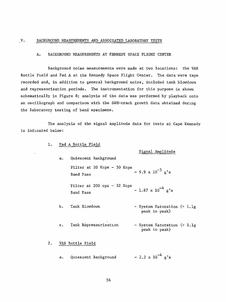
V A Background Measurements at Kennedy Space Flight Center (cont)
repressurization cannot be effectively filtered out significant flaw growth
andor creep could still be detected and tank depressurization accomplished
prior to catastrophic failure assuming a capability for such depressurization
exists at these locations
B LABORATORY SIGNAL ATTENUATION EVALUATIONS
Subsequent to the background measurements at the Kennedy Space
Flight Center and the bend tests at Aerojet two series of tests were made at
Aerojet using a section of pipe and plate both of SAE 4130 steel alloy The
purpose of these tests was to determine the coefficient of signal attenuation
which in conjunction with the previous test data could be used to establish
the sensor spacing which would insure detection of SWE associated with crack
growth in the pressure-vessels at the Kennedy Space Flight Center
In these tests a constant pulse was imparted to the specimen by
a Tektronix 115 Pulse Generator using a Clevite PZT-5 Crystal (2125 in dia
and 0250 in thick) The piezoelectric crystal was mounted on a small alumishy
num block which in turn was adhered to the surface of the specimen The
signal was received by a 2217-E-Endevcq accelerometer placed at various disshy
tances from the pulser The pulse used was 10 n-sec rise and fall time with
a duration of 20 microsec at an amplitude of 12v
1 Pipe Tests
A SAE 4130 steel pipe (8-58 in OD 7-18 in ID and 22 ft
10-78 in long) was used as specimen for this test series The pulser was
mounted normal to the external surface of the pipe as close as possible to the
edge The accelerometer (2217-E-Endevco) was successively placed on the pipe
58
V B Laboratory Signal Attenuation Evalutions (cont)
surface at positions I to 8 that were at 4 6 8 10 12 14 16 and 20 ft
from the pulser The signal received by the accelerometer was displayed on a
Tektronix 422 osilloscope Typical signals are shown in Figure 26
The velocities of the compressional and shear waves in steel
are
29 lO06 x38103 Vc= -x lg ) (l-26) = O2 x06(- 0 x386 = 227000 insec(+j 012)283 (1+030) (1-060)
29x106 x 386 = 91 36= 123000 insec
s 2 ( + p) p 2 (i + 030) x 0283
where E = Youngs Modulus p = Poissons Ratio and p = density The times of
arrival of these waves at the computed velocities are indicated on the oscilloshy
scope photos shown in Figure 26 The point of shear wave arrival (T ) coincides
in most of the photos to a distinct change of pattern in the trace The
arrival of the compressional wave is difficult to determine accurately because
the amplitude of this wave attenuates very fast with distance
A visual comparison of the curves shows that Figure 26a
representing the signal received 4 ft from the impulse indicates a perfectly
detectable arrival of the compressional wave conversely Figure 26h (at 20 ft
from the impulse) shows the visually detectable arrival of a wave almost at the
computed arrival of the shear wave This is due to the fact that the amplitude
of the first cycles of the compressional wave have become essentially impercepshy
tible at a distance of 20 ft from the pulse An attempt to determine signal
arrival time by visual inspection only of the traces in Figure 26 would result
in the wave velocities indicated in Table III The computed arrival times of
the compressional and shear waves are shown in Table IV If an integration of
the positive portions of the cycles comprised in 200 p sec after arrival of the
59
VERTICAL SCALE 1 DIV= 01 V VERTICAL SCALE 1 DIV = 01 V HORIZONTAL SCALE 1 DIV= 50p SEC HORIZONTAL SCALE 1 DIV = 100 pSEC
a 4FT FROM PULSER b6 FEET FROM PULSER
Tc Ts Tc Ts
VERTICAL SCALE I DIV 01 V VERTICAL SCALE I DIV = 01 V HORIZONTAL SCALE I DIV = 100 I SEC HORIZONTAL SCALE 1 DIV = 200 p SEC
c 8 FEET FROM PULSER d 10 FEET FROM PULSER
Tc = Arrival of Compressional Wave
T = Arrival of Shear Wove
Figure 26 Oscillograph Traces for Pipe Tests (Sheet 1 of 2)
6o NOT REPRODUCTBLE
VERTICAL SCALE 1 DIV = 01 V VERTICAL SCALE 1 DIV 01 V HORIZONTAL SCALE 1 DIV = 200y SEC HORIZONTAL SCALE I DIV 200 p SEC
e 12 FEET FROM PULSER f 14 FEET FROM PULSER
T TS T T
VERTICAL SCALE 1 DIV = 01 V VERTICAL SCALE 1 DIV = 01 V HORIZONTAL SCALE 1 DIV = 200 v SEC HORIZONTAL SCALE I DIV =5001p SEC
g 16 FEET FROM PULSER h 20 FEET FROM PULSER
Figure 26 Oscillograph Traces for Pipe Tests (Sheet 2 of 2)
61
V B Laboratory Signal Attenuation Evaluations (cont)
shear wave is performed the average amplitudes determined in this manner
become quite meaningful These average amplitudes are shown in Table V
TABLE III
WAVE VELOCITY BASED ON VISUAL ANALYSIS OF OSCILLOSCOPE TRACES - PIPE TESTS
Distance from Pulse Arrival Velocities Photo ft in Time psc (ftsec)
1 4 48 210 228000
2 6 72 400 180000
3 8 96 600 160000
4 10 120 800 150000
5 12 144 1000 144000
6 14 168 1200 140000
7 16 192 1400 137000
8 20 240 1750 137000
TABLE IV
COMPUTED ARRIVAL TIMES - PIPE TESTS
Compressional Wave Shear Wave Distance from Pulse Arrival Time Arrival Time
Photo in psec Osc Div sec Ose Div
1 48 212 423 390 780
2 72 317 317 583 583
3 96 422 422 778 778
4 120 530 265 972 486
5 144 635 317 1163 581
6 168 740 370 1360 680
7 192 840 420 1545 771
8 240 1050 21 1930 387
62
V B Laboratory Signal Attenuation Evalutions (cont)
TABLE V
SIGNAL AMPLITUDE VS DISTANCE - PIPE TESTS
Average Signal Amplitude Distance from 200 Psec after Arrival
Test Pulser in of Comp Wave mv
1 48 230
2 72 145
3 96 85
4 120 60
5 144 45
6 168 28
7 192 22
8 240 18
The general equation for the amplitude attenuation curve is
C x e-Xy =
where y = amplitude at distance x in volts
x = distance in inches from pulse source
C = amplitude of pulse in volts
a = attenuation factor
or iny= 1 C + (- ax) = I C - ax (Eq 4)n n
To determine the values of C and a the following statistical analysis was
performed
63
V B Laboratory Signal Attenuation Evaluations (cont)
Distance Yo y y2 X X2 Test in m v n n
1 48 230 543 +142 2010 -87 7580 - 124 261
2 72 145 499 +098 0960 -63 3960 - 62 360
3 96 85 445 +044 0194 -39 1520 - 17 427
4 120 60 409 +008 0006 -15 225 - 1 490
5 144 45 380 -021 0044 + 9 81 - 2 548
6 168 28 334 -067 0450 +33 1090 - 21 560
7 192 22 309 -092 0847 +57 3250 - 52 592
8 240 18 289 -112 1250 +105 11000 - 118 690
EY2 EX2pound x = 1080 ElnY =3208 5761 28706 SXY-397 XxIny3928
- 1080 - 3208 x =- = 135 ny = 401
EXY -397 00138 1 C =l1y + oshy
pound 2 x2 28706 n i x
= 401+(0138)(135)=401+186= 587
C - 355 mv
It is now possible to compute the statistically corrected values of the signal
amplitude y at the distances from the pulse where they were measured The
general formula will be
ny = 587 -(00138) X
and the results are tabulated in Table VI The computed value of pulse amplishy
tude at source is found to be C = 355 my The values shown on Table VI are
plotted in Figure 27 which graphically shows the signal attenuation as a
function of distance from the pulse source
64
350
300
250 STATISTICALLY COMPUTED k VALUES FOR REGRESSION CURVE
--0gt 200
EXPERIMENTALLY DETERMINED
-- MATERIAL SAE 4130 STEEL U= SPECIMEN PIPE-S758 in D aZ
00
15 7 18 in D22 ft 10 78 in LONG
-J
100
50 I
0 I I I
5 I I I
DISTANCE
I
10 FROM SOURCE
I
FEET
I
15 20
Figure 27 Signal Amplitude vs Distance - Pipe Tests
V B Laboratory Signal Attenuation Evaluations (cont)
TABLE VI
STATISTICALLY CORRECTED VALUES OF SIGNAL AMPLITUDE - PIPE TESTS
Experimentally Distance from 1 Corrected Signal Determined Signal
Test Pulse in ny Amplitude (y) mv Amplitude (y) my
1 48 521 182 230
2 72 488 130 145
3 96 455 95 85
4 120 421 67 60
5 144 388 48 45
6 168 355 35 28
7 192 322 25 22
8 240 255 127 18
- 2 Plate Tests
An SAE 4130 steel plate (73-12 in long 48-12 in wide
and 34 in thick) was used for this test series The two diagonals were
marked on the plate The pulser was placed at the center of the plate and
the receiver accelerometer was placed on one of the diagonals at locations
spaced in increments of 6 in from the center The received signals were
observed on the oscilloscope and photos were taken of these signals Figure
28 shows oscillographs of the signals received at 6 12 18 24 30 36 and
42 in from the pulser The times of arrival of the shear wave are also shown
in Figure 28 The velocity used was v = 123000 insec An integration
was performed of the positive positions of the cycles comprised in a 20 Psec
interval after the arrival of the shear wave The average amplitudes detershy
mined from these integrations are shown in Table VII Only Tests 1 to 4 are
used because reflection (from the plate edges) in Tests 5 to 8 obscured the
66
b 12 INCHES FROM PULSERa 6 INCHES FROM PULSER
TBTs
c 18 INCHES FROM PULSER d 24 INCHES FROM PULSER
IT s = Arrival of Shear Wave
Vertical Scale 1 DIV = 01 Volt Horizontal Scale 1 DIV = 20 ASec
Figure 28 Oscillograph Traces for Plate Tests (Sheet 1 of 2)
Page 67
f 36 INCHES FROM PULSER e 30 INCHES FROM PULSER
g 42 INCHES FROM PULSER
= Arrival of Shear WaveTs
Vertical Scale 1 DIV = 01 Volt = 20 4SecHorizontal Scale 1 DIV
Figure 28 Oscillograph Traces for Plate Tests (Sheet 2 of 2)
08 gOTPRODUCIB1A
V B Laboratory Signal Attenuation Evaluations (cont)
data These reflections were received in Tests 5 to 8 because of the relashy
tively small plate that was available for this test series
TABLE VII
SIGNAL AMPLITUDE VS DISTANCE - PLATE TESTS
Distance from Average Amplitude Test Pulse in(x) in 20 p see mv
1 6 150
2 12 110
3 18 70
4 24 45
The following statistical analysis was performed to determine the values of
C and a in Equation 4
Test
Distance from
Pulse in(x)
y
m v
1
ny Y
2
Y 2
X XY
X1 y
n
1 6 150 500 +056 0314 -9 81 -502 3000
2
3
12
18
110
70
470
425
+026
-019
0067
0036
-3
+3
9
9
-078
-057
5640
7650
4 24 45 381 -063 0397 +9 81 -567 9149
60 1776 0814 180 -1204 25439
-x=
60 w= 15
4ny
iY 1
1nC
-
=
16=44 1776 =44
E YX 1204= __=
E y2 180
ny +(0067)(15) =
+0067
444 + 0067(15)
69
=
C
444 + 100
= 230 my
= 544
V B Laboratory Signal Attenuation Evaluations (cont)
Subsequently the values of signal amplitude (y) were statistically corrected
as before and the experimentally determined values of y are compared to the
results obtained in Table VIII
TABLE VIII
COMPARISON Or STATISTICALLY CORRECTED AND TEST-DETERMINED VALUES OF SIGNAL AMPLITUDE - PLATE TESTS
Experimentally Distance from Corrected Signal Determined Signal
Test Pulse in nY Amplitude (y) mv Amplitude (y) my
1 6 504 155 150
2 12 464 103 110
3 18 417 65 70
4 24 383 46 45
The computed value of the pulse amplitude at the source at
C equals 230 mv The regression curve and the experimentally determined points
are plotted in Figure 29 It should be observed that the attenuation coefshy
ficient for the pipe test was a = 00138 and for the plate test was 0067
This is due to the much larger rate of front area that the pulse meets in the
plate
C SENSOR SPACING
The quiescent background noise measurements performed at the test
sites using a 20 to 50 KHz band-pass filter are
Pad A Bottle Field - 0000099g
VAB Bottle Field 0000220g
70
250
200 - EXPERIMENTALLY DETERMINED
0o
gt
M a-100 34
STATISTICALLY COMPUTEDVALUES FOR REGRESSION CURVE
MATERIAL SAE 4130 STEEL
SPECIMEN PLATE - 73 12 in LONG 48 12 in WIDE
in THICK
J
50
0
0 5 SII
10 15
DISTANCE FROM SOURCE FEET
I
20 I
25
Figure 29 Signal Amplitude vs Distance - Plate Tests
V C Sensor Spacing (cont)
The recorded stress-wave-emission data obtained from the A302B steel bend tests
made at the Aerojet-General Corporation laboratory show that the minimum
acceleration at the source is 0O012g the average 00022g and the maximum
00039g Based on the above data and the attenuation factor X = 0067 detershy
mined from the plate tests the sensor spacings required to detect crack growth
in the vessels at the Kennedy Space Center were computed and the results are
tabulated below
Quiescent Sensor Spacing
Amplitude at Background in the Source(C) g Amplitude(y) g Cy ln(CIy) ln(CIy)
Pad A
Min Signal 00012 000015 800 208 310
Avg Signal 00022 000015 1470 269 402
Max Signal 00039 000015 2600 326 487
VAB Bottle Field
Min Signal 00012 000033 363 129 193
Avg Signal 00022 000033 668 190 283
Max Signal 00039 000033 1080 238 356
This threshold is 15 x 0000099 - 000015g (at Pad A)
This threshold is 15 x 000022 = 000033g (at VAB Bottle Field)
Figures 30 and 31 present schematically the location and spacings of sensors
on the pressure vessels
72
- 502 IN 8 IN
HEAD -- _
DEVELOPED + + CYLINDRICAL FOR MINIMUM SIGNAL-22 SENSORS AS SHOWN
SURFACE FOR AVERAGE SIGNAL-16 SENSORS
+ +I
FOR MAXIMUM SIGNAL- 14 SENSORS
282438 IN+ +
+ +
9 SPACINGS AT 313 IN
-I- +
+ +shy
+ -plusmn
HEAD _ __
8 IN
Figure 30 Schematic of Sensor Spacings for Bottles at Pad A
73
14601 IN
HEAD (6SENSORS) 23 14 INI I I - I I I
t plusmn + plusmn + +
+ + 4 + + + DEVELOPED CYL SURFACE
+ + 4A 1 13 LINES OF
+ + + SENSORS SPACED4 + + AT 2086 IN
+ + + + + +
+ + 4 + + +
251 1516 IN + + + +-I- +
+ + + 4- +
-1- 298438 IN+ -I- -+- -i- +
+I
23 14 INHEAD (6 SENSORS) 1
FOR MINIMUM SIGNAL-103 SENSORS AS SHOWN
FOR AVERAGE SIGNAL- 82 SENSORS FOR MAXIMUM SIGNAL- 58 SENSORS
Figure 31 Schematic of Sensor Spacings for Bottles at VAB Bottle Field
74
VI CONCLUSIONS
A The Type A302B steel supplied for evaluation exhibited a high level
of fracture toughness Although quantitative plane-strain fracture toughness
measurements were not possible because of the large specimen size required
the K value associated with failure approximated 135 ksi-inI 2
Q
B The Type A302B steel was found resistant to environmentally induced
slow crack growth when tested in the hydrogenated condition in an air environshy
ment and in the unhydrogenated condition in a 3 NaCl-water environment Howshy
ever hydrogenated material tested in 3 NaCl-water had a much faster rate of
subcritical crack growth indicating a synergistic effect due to the combinashy
tion of sea water and hydrogen in interstitial solid solution
C The synergistic effect indicates the Type A302B steel hydrogen
storage tanks in the Kennedy Space Flight Center may have limited life as a
result of subcritical crack growth if subjected to the same combination of
stress and environmental factors
D Detectable stress-wave emissions although of small amplitude
(ltOOlg) were observed to be associated with crack growth in Type A302B steel
In all test conditions the stress-wave emissions were observed during rising
load and when failure (instability) was imminent Both the amplitude and rate
of stress-wave emission increased as failure was approached and could be
employed as a precursor of the onset of instability
E Stress-wave emissions associated with crack growth in Type A302B
steel can be detected under quiescent background conditions at the Pad A and
VAB Bottle fields at the Kennedy Space Flight Center However it would be
difficult to detect such stress-wave emissions during tank blowdown and
repressurization periods unless filtering can be employed to screen out the
noise associated with these periods
75
VI Conclusions (cont)
F Even in the presence of background noise from tank blowdown and
repressurization these periods are considered short in the overall life of
the pressure vessels Consequently flaw growth or creep which was observed
during rising load or the initial part of hold could be detected by SWAT
permitting triangulation to the source and tank depressurization prior to
failure
G Stress-wave-emission attenuation test data were obtained and employed
in conjunction with the site background measurements addbnd test stress-waveshy
emission characterization data to determine sensor mounting patterns for the
hydrogen pressure vessels at Pad A and the VAB Bottle Field
VII RECOMMENDATIONS FOR FURTHER WORK
If the synergistic effect of hydrogen and 3 NaCi solution occurs in
Kennedy Space Flight Center tankage the life of the tankage will be limited
Obviously slow-crack growth from any cause whether continuous or disconshy
tinuous and regardless of how slow the rate of cracking will eventually
produce failure This investigation showed that subcritical crack growth is
in all likelihood occurring with each pressurization A question remains
however as to the rate of crack growth without knowledge of the rate there
is no way to anticipate the life of the tankage However with SWAT one can
monitor the occurrence of crack growth and most importantly make judgment
as to whether a given crack is approaching critical size Consequently it
is recommended that additional tests be performed to (1) verify the existence
of subcritical cracking in actual on-site tankage and (2) incorporate an
automatic system for continuously monitoring on-site tankage at Kennedy Space
Flight Center
76
REFERENCES
1 Steel R K Green A T Lockman C S Acoustic Verification of Structural Integrity of Polaris Chambers Society of Plastic Engineers 20th Meeting Atlantic City N Y January 1964
2 Pressure Testing of AFRM-017 Service Propulsion System Fuel Tank Utilizing Aerojet-General Corporations Stress-Wave Analysis Technique
Report NAS 9-6766-003 Aerojet-General Corp for NASA MSC Houston Texas Contract NAS 9-6766 May 1967
3 Srawley J E and Esgar J B Investigation of Hydrotest Failure of Thiokol Chemical Corp 260-Inch-Diameter SL-1 Motor Case NASA-TMX shy1194 January 1964
4 Hartbower C E Gerberich W W and Crimmins P P Mechanisms of Slow Crack Growth in High-Strength Steels AFML-TR-67-26 Vol 1 February 1967
5 -Hartbower C E Gerberich W W and Crimmins P P Characterization of Fatigue-Crack Growth by Stress Wave Emission Final Report on Conshytract NAS 1-4902 for NASA-Langley Research Center Hampton Virginia June 1966
6 IHartbower C E Gerberich W W Reuter W G and Crimmins P P Stress Wave Characteristics in Constructional Alloys Final Report on Office of Naval Research Contract N00014-66-C-0340 July 1967
7 Novak S R and Rolfe S T Modified WOL Specimen for KIscc Environmental Testing U S Steel Corp paper submitted to ASTM for publication
77
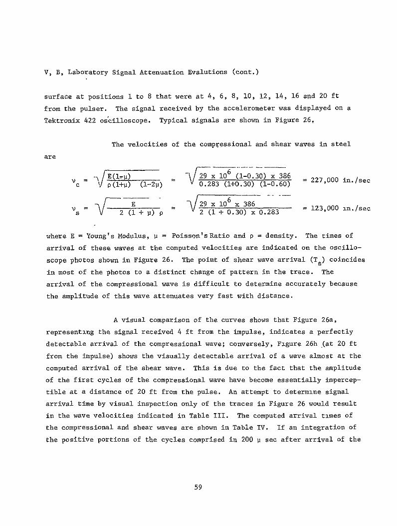
V B Laboratory Signal Attenuation Evalutions (cont)
surface at positions I to 8 that were at 4 6 8 10 12 14 16 and 20 ft
from the pulser The signal received by the accelerometer was displayed on a
Tektronix 422 osilloscope Typical signals are shown in Figure 26
The velocities of the compressional and shear waves in steel
are
29 lO06 x38103 Vc= -x lg ) (l-26) = O2 x06(- 0 x386 = 227000 insec(+j 012)283 (1+030) (1-060)
29x106 x 386 = 91 36= 123000 insec
s 2 ( + p) p 2 (i + 030) x 0283
where E = Youngs Modulus p = Poissons Ratio and p = density The times of
arrival of these waves at the computed velocities are indicated on the oscilloshy
scope photos shown in Figure 26 The point of shear wave arrival (T ) coincides
in most of the photos to a distinct change of pattern in the trace The
arrival of the compressional wave is difficult to determine accurately because
the amplitude of this wave attenuates very fast with distance
A visual comparison of the curves shows that Figure 26a
representing the signal received 4 ft from the impulse indicates a perfectly
detectable arrival of the compressional wave conversely Figure 26h (at 20 ft
from the impulse) shows the visually detectable arrival of a wave almost at the
computed arrival of the shear wave This is due to the fact that the amplitude
of the first cycles of the compressional wave have become essentially impercepshy
tible at a distance of 20 ft from the pulse An attempt to determine signal
arrival time by visual inspection only of the traces in Figure 26 would result
in the wave velocities indicated in Table III The computed arrival times of
the compressional and shear waves are shown in Table IV If an integration of
the positive portions of the cycles comprised in 200 p sec after arrival of the
59
VERTICAL SCALE 1 DIV= 01 V VERTICAL SCALE 1 DIV = 01 V HORIZONTAL SCALE 1 DIV= 50p SEC HORIZONTAL SCALE 1 DIV = 100 pSEC
a 4FT FROM PULSER b6 FEET FROM PULSER
Tc Ts Tc Ts
VERTICAL SCALE I DIV 01 V VERTICAL SCALE I DIV = 01 V HORIZONTAL SCALE I DIV = 100 I SEC HORIZONTAL SCALE 1 DIV = 200 p SEC
c 8 FEET FROM PULSER d 10 FEET FROM PULSER
Tc = Arrival of Compressional Wave
T = Arrival of Shear Wove
Figure 26 Oscillograph Traces for Pipe Tests (Sheet 1 of 2)
6o NOT REPRODUCTBLE
VERTICAL SCALE 1 DIV = 01 V VERTICAL SCALE 1 DIV 01 V HORIZONTAL SCALE 1 DIV = 200y SEC HORIZONTAL SCALE I DIV 200 p SEC
e 12 FEET FROM PULSER f 14 FEET FROM PULSER
T TS T T
VERTICAL SCALE 1 DIV = 01 V VERTICAL SCALE 1 DIV = 01 V HORIZONTAL SCALE 1 DIV = 200 v SEC HORIZONTAL SCALE I DIV =5001p SEC
g 16 FEET FROM PULSER h 20 FEET FROM PULSER
Figure 26 Oscillograph Traces for Pipe Tests (Sheet 2 of 2)
61
V B Laboratory Signal Attenuation Evaluations (cont)
shear wave is performed the average amplitudes determined in this manner
become quite meaningful These average amplitudes are shown in Table V
TABLE III
WAVE VELOCITY BASED ON VISUAL ANALYSIS OF OSCILLOSCOPE TRACES - PIPE TESTS
Distance from Pulse Arrival Velocities Photo ft in Time psc (ftsec)
1 4 48 210 228000
2 6 72 400 180000
3 8 96 600 160000
4 10 120 800 150000
5 12 144 1000 144000
6 14 168 1200 140000
7 16 192 1400 137000
8 20 240 1750 137000
TABLE IV
COMPUTED ARRIVAL TIMES - PIPE TESTS
Compressional Wave Shear Wave Distance from Pulse Arrival Time Arrival Time
Photo in psec Osc Div sec Ose Div
1 48 212 423 390 780
2 72 317 317 583 583
3 96 422 422 778 778
4 120 530 265 972 486
5 144 635 317 1163 581
6 168 740 370 1360 680
7 192 840 420 1545 771
8 240 1050 21 1930 387
62
V B Laboratory Signal Attenuation Evalutions (cont)
TABLE V
SIGNAL AMPLITUDE VS DISTANCE - PIPE TESTS
Average Signal Amplitude Distance from 200 Psec after Arrival
Test Pulser in of Comp Wave mv
1 48 230
2 72 145
3 96 85
4 120 60
5 144 45
6 168 28
7 192 22
8 240 18
The general equation for the amplitude attenuation curve is
C x e-Xy =
where y = amplitude at distance x in volts
x = distance in inches from pulse source
C = amplitude of pulse in volts
a = attenuation factor
or iny= 1 C + (- ax) = I C - ax (Eq 4)n n
To determine the values of C and a the following statistical analysis was
performed
63
V B Laboratory Signal Attenuation Evaluations (cont)
Distance Yo y y2 X X2 Test in m v n n
1 48 230 543 +142 2010 -87 7580 - 124 261
2 72 145 499 +098 0960 -63 3960 - 62 360
3 96 85 445 +044 0194 -39 1520 - 17 427
4 120 60 409 +008 0006 -15 225 - 1 490
5 144 45 380 -021 0044 + 9 81 - 2 548
6 168 28 334 -067 0450 +33 1090 - 21 560
7 192 22 309 -092 0847 +57 3250 - 52 592
8 240 18 289 -112 1250 +105 11000 - 118 690
EY2 EX2pound x = 1080 ElnY =3208 5761 28706 SXY-397 XxIny3928
- 1080 - 3208 x =- = 135 ny = 401
EXY -397 00138 1 C =l1y + oshy
pound 2 x2 28706 n i x
= 401+(0138)(135)=401+186= 587
C - 355 mv
It is now possible to compute the statistically corrected values of the signal
amplitude y at the distances from the pulse where they were measured The
general formula will be
ny = 587 -(00138) X
and the results are tabulated in Table VI The computed value of pulse amplishy
tude at source is found to be C = 355 my The values shown on Table VI are
plotted in Figure 27 which graphically shows the signal attenuation as a
function of distance from the pulse source
64
350
300
250 STATISTICALLY COMPUTED k VALUES FOR REGRESSION CURVE
--0gt 200
EXPERIMENTALLY DETERMINED
-- MATERIAL SAE 4130 STEEL U= SPECIMEN PIPE-S758 in D aZ
00
15 7 18 in D22 ft 10 78 in LONG
-J
100
50 I
0 I I I
5 I I I
DISTANCE
I
10 FROM SOURCE
I
FEET
I
15 20
Figure 27 Signal Amplitude vs Distance - Pipe Tests
V B Laboratory Signal Attenuation Evaluations (cont)
TABLE VI
STATISTICALLY CORRECTED VALUES OF SIGNAL AMPLITUDE - PIPE TESTS
Experimentally Distance from 1 Corrected Signal Determined Signal
Test Pulse in ny Amplitude (y) mv Amplitude (y) my
1 48 521 182 230
2 72 488 130 145
3 96 455 95 85
4 120 421 67 60
5 144 388 48 45
6 168 355 35 28
7 192 322 25 22
8 240 255 127 18
- 2 Plate Tests
An SAE 4130 steel plate (73-12 in long 48-12 in wide
and 34 in thick) was used for this test series The two diagonals were
marked on the plate The pulser was placed at the center of the plate and
the receiver accelerometer was placed on one of the diagonals at locations
spaced in increments of 6 in from the center The received signals were
observed on the oscilloscope and photos were taken of these signals Figure
28 shows oscillographs of the signals received at 6 12 18 24 30 36 and
42 in from the pulser The times of arrival of the shear wave are also shown
in Figure 28 The velocity used was v = 123000 insec An integration
was performed of the positive positions of the cycles comprised in a 20 Psec
interval after the arrival of the shear wave The average amplitudes detershy
mined from these integrations are shown in Table VII Only Tests 1 to 4 are
used because reflection (from the plate edges) in Tests 5 to 8 obscured the
66
b 12 INCHES FROM PULSERa 6 INCHES FROM PULSER
TBTs
c 18 INCHES FROM PULSER d 24 INCHES FROM PULSER
IT s = Arrival of Shear Wave
Vertical Scale 1 DIV = 01 Volt Horizontal Scale 1 DIV = 20 ASec
Figure 28 Oscillograph Traces for Plate Tests (Sheet 1 of 2)
Page 67
f 36 INCHES FROM PULSER e 30 INCHES FROM PULSER
g 42 INCHES FROM PULSER
= Arrival of Shear WaveTs
Vertical Scale 1 DIV = 01 Volt = 20 4SecHorizontal Scale 1 DIV
Figure 28 Oscillograph Traces for Plate Tests (Sheet 2 of 2)
08 gOTPRODUCIB1A
V B Laboratory Signal Attenuation Evaluations (cont)
data These reflections were received in Tests 5 to 8 because of the relashy
tively small plate that was available for this test series
TABLE VII
SIGNAL AMPLITUDE VS DISTANCE - PLATE TESTS
Distance from Average Amplitude Test Pulse in(x) in 20 p see mv
1 6 150
2 12 110
3 18 70
4 24 45
The following statistical analysis was performed to determine the values of
C and a in Equation 4
Test
Distance from
Pulse in(x)
y
m v
1
ny Y
2
Y 2
X XY
X1 y
n
1 6 150 500 +056 0314 -9 81 -502 3000
2
3
12
18
110
70
470
425
+026
-019
0067
0036
-3
+3
9
9
-078
-057
5640
7650
4 24 45 381 -063 0397 +9 81 -567 9149
60 1776 0814 180 -1204 25439
-x=
60 w= 15
4ny
iY 1
1nC
-
=
16=44 1776 =44
E YX 1204= __=
E y2 180
ny +(0067)(15) =
+0067
444 + 0067(15)
69
=
C
444 + 100
= 230 my
= 544
V B Laboratory Signal Attenuation Evaluations (cont)
Subsequently the values of signal amplitude (y) were statistically corrected
as before and the experimentally determined values of y are compared to the
results obtained in Table VIII
TABLE VIII
COMPARISON Or STATISTICALLY CORRECTED AND TEST-DETERMINED VALUES OF SIGNAL AMPLITUDE - PLATE TESTS
Experimentally Distance from Corrected Signal Determined Signal
Test Pulse in nY Amplitude (y) mv Amplitude (y) my
1 6 504 155 150
2 12 464 103 110
3 18 417 65 70
4 24 383 46 45
The computed value of the pulse amplitude at the source at
C equals 230 mv The regression curve and the experimentally determined points
are plotted in Figure 29 It should be observed that the attenuation coefshy
ficient for the pipe test was a = 00138 and for the plate test was 0067
This is due to the much larger rate of front area that the pulse meets in the
plate
C SENSOR SPACING
The quiescent background noise measurements performed at the test
sites using a 20 to 50 KHz band-pass filter are
Pad A Bottle Field - 0000099g
VAB Bottle Field 0000220g
70
250
200 - EXPERIMENTALLY DETERMINED
0o
gt
M a-100 34
STATISTICALLY COMPUTEDVALUES FOR REGRESSION CURVE
MATERIAL SAE 4130 STEEL
SPECIMEN PLATE - 73 12 in LONG 48 12 in WIDE
in THICK
J
50
0
0 5 SII
10 15
DISTANCE FROM SOURCE FEET
I
20 I
25
Figure 29 Signal Amplitude vs Distance - Plate Tests
V C Sensor Spacing (cont)
The recorded stress-wave-emission data obtained from the A302B steel bend tests
made at the Aerojet-General Corporation laboratory show that the minimum
acceleration at the source is 0O012g the average 00022g and the maximum
00039g Based on the above data and the attenuation factor X = 0067 detershy
mined from the plate tests the sensor spacings required to detect crack growth
in the vessels at the Kennedy Space Center were computed and the results are
tabulated below
Quiescent Sensor Spacing
Amplitude at Background in the Source(C) g Amplitude(y) g Cy ln(CIy) ln(CIy)
Pad A
Min Signal 00012 000015 800 208 310
Avg Signal 00022 000015 1470 269 402
Max Signal 00039 000015 2600 326 487
VAB Bottle Field
Min Signal 00012 000033 363 129 193
Avg Signal 00022 000033 668 190 283
Max Signal 00039 000033 1080 238 356
This threshold is 15 x 0000099 - 000015g (at Pad A)
This threshold is 15 x 000022 = 000033g (at VAB Bottle Field)
Figures 30 and 31 present schematically the location and spacings of sensors
on the pressure vessels
72
- 502 IN 8 IN
HEAD -- _
DEVELOPED + + CYLINDRICAL FOR MINIMUM SIGNAL-22 SENSORS AS SHOWN
SURFACE FOR AVERAGE SIGNAL-16 SENSORS
+ +I
FOR MAXIMUM SIGNAL- 14 SENSORS
282438 IN+ +
+ +
9 SPACINGS AT 313 IN
-I- +
+ +shy
+ -plusmn
HEAD _ __
8 IN
Figure 30 Schematic of Sensor Spacings for Bottles at Pad A
73
14601 IN
HEAD (6SENSORS) 23 14 INI I I - I I I
t plusmn + plusmn + +
+ + 4 + + + DEVELOPED CYL SURFACE
+ + 4A 1 13 LINES OF
+ + + SENSORS SPACED4 + + AT 2086 IN
+ + + + + +
+ + 4 + + +
251 1516 IN + + + +-I- +
+ + + 4- +
-1- 298438 IN+ -I- -+- -i- +
+I
23 14 INHEAD (6 SENSORS) 1
FOR MINIMUM SIGNAL-103 SENSORS AS SHOWN
FOR AVERAGE SIGNAL- 82 SENSORS FOR MAXIMUM SIGNAL- 58 SENSORS
Figure 31 Schematic of Sensor Spacings for Bottles at VAB Bottle Field
74
VI CONCLUSIONS
A The Type A302B steel supplied for evaluation exhibited a high level
of fracture toughness Although quantitative plane-strain fracture toughness
measurements were not possible because of the large specimen size required
the K value associated with failure approximated 135 ksi-inI 2
Q
B The Type A302B steel was found resistant to environmentally induced
slow crack growth when tested in the hydrogenated condition in an air environshy
ment and in the unhydrogenated condition in a 3 NaCl-water environment Howshy
ever hydrogenated material tested in 3 NaCl-water had a much faster rate of
subcritical crack growth indicating a synergistic effect due to the combinashy
tion of sea water and hydrogen in interstitial solid solution
C The synergistic effect indicates the Type A302B steel hydrogen
storage tanks in the Kennedy Space Flight Center may have limited life as a
result of subcritical crack growth if subjected to the same combination of
stress and environmental factors
D Detectable stress-wave emissions although of small amplitude
(ltOOlg) were observed to be associated with crack growth in Type A302B steel
In all test conditions the stress-wave emissions were observed during rising
load and when failure (instability) was imminent Both the amplitude and rate
of stress-wave emission increased as failure was approached and could be
employed as a precursor of the onset of instability
E Stress-wave emissions associated with crack growth in Type A302B
steel can be detected under quiescent background conditions at the Pad A and
VAB Bottle fields at the Kennedy Space Flight Center However it would be
difficult to detect such stress-wave emissions during tank blowdown and
repressurization periods unless filtering can be employed to screen out the
noise associated with these periods
75
VI Conclusions (cont)
F Even in the presence of background noise from tank blowdown and
repressurization these periods are considered short in the overall life of
the pressure vessels Consequently flaw growth or creep which was observed
during rising load or the initial part of hold could be detected by SWAT
permitting triangulation to the source and tank depressurization prior to
failure
G Stress-wave-emission attenuation test data were obtained and employed
in conjunction with the site background measurements addbnd test stress-waveshy
emission characterization data to determine sensor mounting patterns for the
hydrogen pressure vessels at Pad A and the VAB Bottle Field
VII RECOMMENDATIONS FOR FURTHER WORK
If the synergistic effect of hydrogen and 3 NaCi solution occurs in
Kennedy Space Flight Center tankage the life of the tankage will be limited
Obviously slow-crack growth from any cause whether continuous or disconshy
tinuous and regardless of how slow the rate of cracking will eventually
produce failure This investigation showed that subcritical crack growth is
in all likelihood occurring with each pressurization A question remains
however as to the rate of crack growth without knowledge of the rate there
is no way to anticipate the life of the tankage However with SWAT one can
monitor the occurrence of crack growth and most importantly make judgment
as to whether a given crack is approaching critical size Consequently it
is recommended that additional tests be performed to (1) verify the existence
of subcritical cracking in actual on-site tankage and (2) incorporate an
automatic system for continuously monitoring on-site tankage at Kennedy Space
Flight Center
76
REFERENCES
1 Steel R K Green A T Lockman C S Acoustic Verification of Structural Integrity of Polaris Chambers Society of Plastic Engineers 20th Meeting Atlantic City N Y January 1964
2 Pressure Testing of AFRM-017 Service Propulsion System Fuel Tank Utilizing Aerojet-General Corporations Stress-Wave Analysis Technique
Report NAS 9-6766-003 Aerojet-General Corp for NASA MSC Houston Texas Contract NAS 9-6766 May 1967
3 Srawley J E and Esgar J B Investigation of Hydrotest Failure of Thiokol Chemical Corp 260-Inch-Diameter SL-1 Motor Case NASA-TMX shy1194 January 1964
4 Hartbower C E Gerberich W W and Crimmins P P Mechanisms of Slow Crack Growth in High-Strength Steels AFML-TR-67-26 Vol 1 February 1967
5 -Hartbower C E Gerberich W W and Crimmins P P Characterization of Fatigue-Crack Growth by Stress Wave Emission Final Report on Conshytract NAS 1-4902 for NASA-Langley Research Center Hampton Virginia June 1966
6 IHartbower C E Gerberich W W Reuter W G and Crimmins P P Stress Wave Characteristics in Constructional Alloys Final Report on Office of Naval Research Contract N00014-66-C-0340 July 1967
7 Novak S R and Rolfe S T Modified WOL Specimen for KIscc Environmental Testing U S Steel Corp paper submitted to ASTM for publication
77
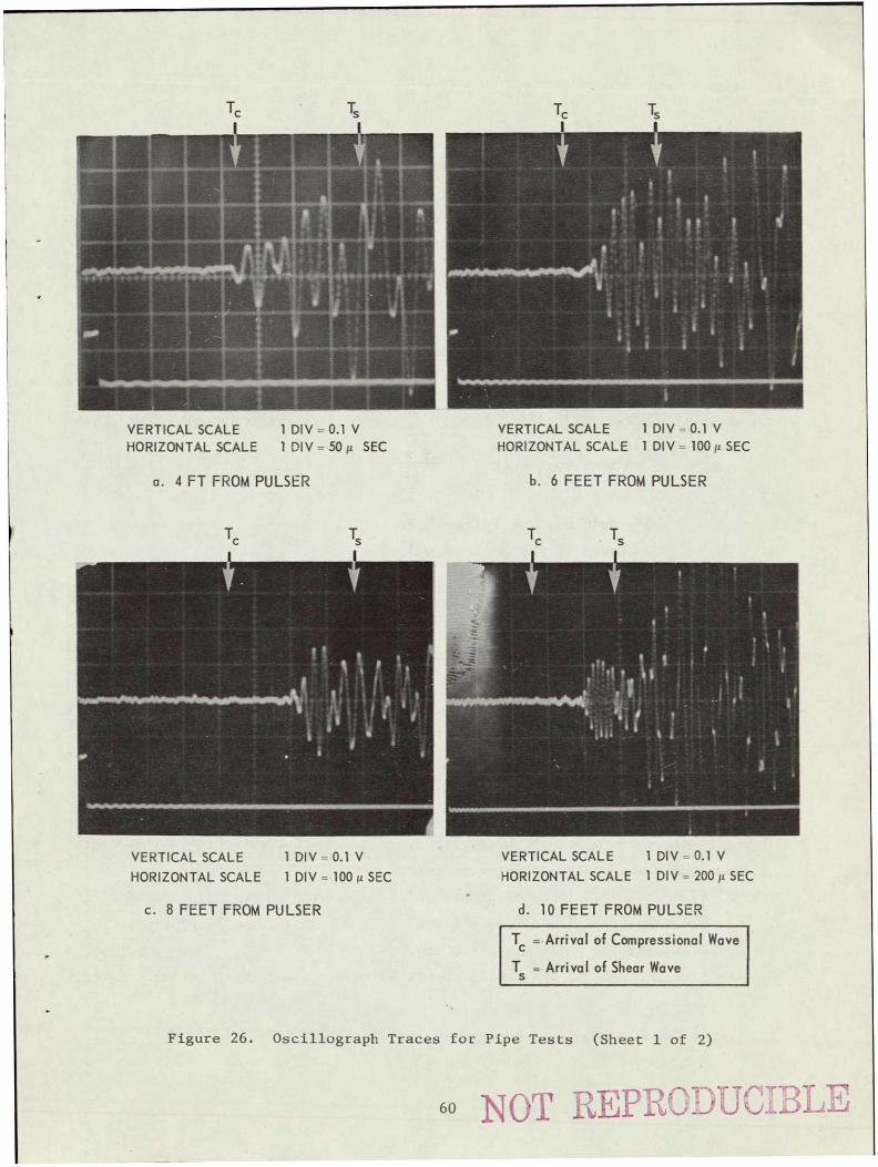
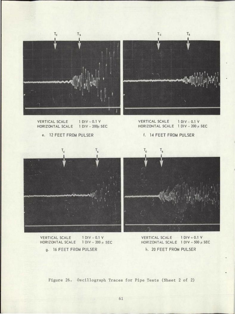
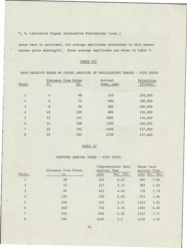
V B Laboratory Signal Attenuation Evaluations (cont)
shear wave is performed the average amplitudes determined in this manner
become quite meaningful These average amplitudes are shown in Table V
TABLE III
WAVE VELOCITY BASED ON VISUAL ANALYSIS OF OSCILLOSCOPE TRACES - PIPE TESTS
Distance from Pulse Arrival Velocities Photo ft in Time psc (ftsec)
1 4 48 210 228000
2 6 72 400 180000
3 8 96 600 160000
4 10 120 800 150000
5 12 144 1000 144000
6 14 168 1200 140000
7 16 192 1400 137000
8 20 240 1750 137000
TABLE IV
COMPUTED ARRIVAL TIMES - PIPE TESTS
Compressional Wave Shear Wave Distance from Pulse Arrival Time Arrival Time
Photo in psec Osc Div sec Ose Div
1 48 212 423 390 780
2 72 317 317 583 583
3 96 422 422 778 778
4 120 530 265 972 486
5 144 635 317 1163 581
6 168 740 370 1360 680
7 192 840 420 1545 771
8 240 1050 21 1930 387
62
V B Laboratory Signal Attenuation Evalutions (cont)
TABLE V
SIGNAL AMPLITUDE VS DISTANCE - PIPE TESTS
Average Signal Amplitude Distance from 200 Psec after Arrival
Test Pulser in of Comp Wave mv
1 48 230
2 72 145
3 96 85
4 120 60
5 144 45
6 168 28
7 192 22
8 240 18
The general equation for the amplitude attenuation curve is
C x e-Xy =
where y = amplitude at distance x in volts
x = distance in inches from pulse source
C = amplitude of pulse in volts
a = attenuation factor
or iny= 1 C + (- ax) = I C - ax (Eq 4)n n
To determine the values of C and a the following statistical analysis was
performed
63
V B Laboratory Signal Attenuation Evaluations (cont)
Distance Yo y y2 X X2 Test in m v n n
1 48 230 543 +142 2010 -87 7580 - 124 261
2 72 145 499 +098 0960 -63 3960 - 62 360
3 96 85 445 +044 0194 -39 1520 - 17 427
4 120 60 409 +008 0006 -15 225 - 1 490
5 144 45 380 -021 0044 + 9 81 - 2 548
6 168 28 334 -067 0450 +33 1090 - 21 560
7 192 22 309 -092 0847 +57 3250 - 52 592
8 240 18 289 -112 1250 +105 11000 - 118 690
EY2 EX2pound x = 1080 ElnY =3208 5761 28706 SXY-397 XxIny3928
- 1080 - 3208 x =- = 135 ny = 401
EXY -397 00138 1 C =l1y + oshy
pound 2 x2 28706 n i x
= 401+(0138)(135)=401+186= 587
C - 355 mv
It is now possible to compute the statistically corrected values of the signal
amplitude y at the distances from the pulse where they were measured The
general formula will be
ny = 587 -(00138) X
and the results are tabulated in Table VI The computed value of pulse amplishy
tude at source is found to be C = 355 my The values shown on Table VI are
plotted in Figure 27 which graphically shows the signal attenuation as a
function of distance from the pulse source
64
350
300
250 STATISTICALLY COMPUTED k VALUES FOR REGRESSION CURVE
--0gt 200
EXPERIMENTALLY DETERMINED
-- MATERIAL SAE 4130 STEEL U= SPECIMEN PIPE-S758 in D aZ
00
15 7 18 in D22 ft 10 78 in LONG
-J
100
50 I
0 I I I
5 I I I
DISTANCE
I
10 FROM SOURCE
I
FEET
I
15 20
Figure 27 Signal Amplitude vs Distance - Pipe Tests
V B Laboratory Signal Attenuation Evaluations (cont)
TABLE VI
STATISTICALLY CORRECTED VALUES OF SIGNAL AMPLITUDE - PIPE TESTS
Experimentally Distance from 1 Corrected Signal Determined Signal
Test Pulse in ny Amplitude (y) mv Amplitude (y) my
1 48 521 182 230
2 72 488 130 145
3 96 455 95 85
4 120 421 67 60
5 144 388 48 45
6 168 355 35 28
7 192 322 25 22
8 240 255 127 18
- 2 Plate Tests
An SAE 4130 steel plate (73-12 in long 48-12 in wide
and 34 in thick) was used for this test series The two diagonals were
marked on the plate The pulser was placed at the center of the plate and
the receiver accelerometer was placed on one of the diagonals at locations
spaced in increments of 6 in from the center The received signals were
observed on the oscilloscope and photos were taken of these signals Figure
28 shows oscillographs of the signals received at 6 12 18 24 30 36 and
42 in from the pulser The times of arrival of the shear wave are also shown
in Figure 28 The velocity used was v = 123000 insec An integration
was performed of the positive positions of the cycles comprised in a 20 Psec
interval after the arrival of the shear wave The average amplitudes detershy
mined from these integrations are shown in Table VII Only Tests 1 to 4 are
used because reflection (from the plate edges) in Tests 5 to 8 obscured the
66
b 12 INCHES FROM PULSERa 6 INCHES FROM PULSER
TBTs
c 18 INCHES FROM PULSER d 24 INCHES FROM PULSER
IT s = Arrival of Shear Wave
Vertical Scale 1 DIV = 01 Volt Horizontal Scale 1 DIV = 20 ASec
Figure 28 Oscillograph Traces for Plate Tests (Sheet 1 of 2)
Page 67
f 36 INCHES FROM PULSER e 30 INCHES FROM PULSER
g 42 INCHES FROM PULSER
= Arrival of Shear WaveTs
Vertical Scale 1 DIV = 01 Volt = 20 4SecHorizontal Scale 1 DIV
Figure 28 Oscillograph Traces for Plate Tests (Sheet 2 of 2)
08 gOTPRODUCIB1A
V B Laboratory Signal Attenuation Evaluations (cont)
data These reflections were received in Tests 5 to 8 because of the relashy
tively small plate that was available for this test series
TABLE VII
SIGNAL AMPLITUDE VS DISTANCE - PLATE TESTS
Distance from Average Amplitude Test Pulse in(x) in 20 p see mv
1 6 150
2 12 110
3 18 70
4 24 45
The following statistical analysis was performed to determine the values of
C and a in Equation 4
Test
Distance from
Pulse in(x)
y
m v
1
ny Y
2
Y 2
X XY
X1 y
n
1 6 150 500 +056 0314 -9 81 -502 3000
2
3
12
18
110
70
470
425
+026
-019
0067
0036
-3
+3
9
9
-078
-057
5640
7650
4 24 45 381 -063 0397 +9 81 -567 9149
60 1776 0814 180 -1204 25439
-x=
60 w= 15
4ny
iY 1
1nC
-
=
16=44 1776 =44
E YX 1204= __=
E y2 180
ny +(0067)(15) =
+0067
444 + 0067(15)
69
=
C
444 + 100
= 230 my
= 544
V B Laboratory Signal Attenuation Evaluations (cont)
Subsequently the values of signal amplitude (y) were statistically corrected
as before and the experimentally determined values of y are compared to the
results obtained in Table VIII
TABLE VIII
COMPARISON Or STATISTICALLY CORRECTED AND TEST-DETERMINED VALUES OF SIGNAL AMPLITUDE - PLATE TESTS
Experimentally Distance from Corrected Signal Determined Signal
Test Pulse in nY Amplitude (y) mv Amplitude (y) my
1 6 504 155 150
2 12 464 103 110
3 18 417 65 70
4 24 383 46 45
The computed value of the pulse amplitude at the source at
C equals 230 mv The regression curve and the experimentally determined points
are plotted in Figure 29 It should be observed that the attenuation coefshy
ficient for the pipe test was a = 00138 and for the plate test was 0067
This is due to the much larger rate of front area that the pulse meets in the
plate
C SENSOR SPACING
The quiescent background noise measurements performed at the test
sites using a 20 to 50 KHz band-pass filter are
Pad A Bottle Field - 0000099g
VAB Bottle Field 0000220g
70
250
200 - EXPERIMENTALLY DETERMINED
0o
gt
M a-100 34
STATISTICALLY COMPUTEDVALUES FOR REGRESSION CURVE
MATERIAL SAE 4130 STEEL
SPECIMEN PLATE - 73 12 in LONG 48 12 in WIDE
in THICK
J
50
0
0 5 SII
10 15
DISTANCE FROM SOURCE FEET
I
20 I
25
Figure 29 Signal Amplitude vs Distance - Plate Tests
V C Sensor Spacing (cont)
The recorded stress-wave-emission data obtained from the A302B steel bend tests
made at the Aerojet-General Corporation laboratory show that the minimum
acceleration at the source is 0O012g the average 00022g and the maximum
00039g Based on the above data and the attenuation factor X = 0067 detershy
mined from the plate tests the sensor spacings required to detect crack growth
in the vessels at the Kennedy Space Center were computed and the results are
tabulated below
Quiescent Sensor Spacing
Amplitude at Background in the Source(C) g Amplitude(y) g Cy ln(CIy) ln(CIy)
Pad A
Min Signal 00012 000015 800 208 310
Avg Signal 00022 000015 1470 269 402
Max Signal 00039 000015 2600 326 487
VAB Bottle Field
Min Signal 00012 000033 363 129 193
Avg Signal 00022 000033 668 190 283
Max Signal 00039 000033 1080 238 356
This threshold is 15 x 0000099 - 000015g (at Pad A)
This threshold is 15 x 000022 = 000033g (at VAB Bottle Field)
Figures 30 and 31 present schematically the location and spacings of sensors
on the pressure vessels
72
- 502 IN 8 IN
HEAD -- _
DEVELOPED + + CYLINDRICAL FOR MINIMUM SIGNAL-22 SENSORS AS SHOWN
SURFACE FOR AVERAGE SIGNAL-16 SENSORS
+ +I
FOR MAXIMUM SIGNAL- 14 SENSORS
282438 IN+ +
+ +
9 SPACINGS AT 313 IN
-I- +
+ +shy
+ -plusmn
HEAD _ __
8 IN
Figure 30 Schematic of Sensor Spacings for Bottles at Pad A
73
14601 IN
HEAD (6SENSORS) 23 14 INI I I - I I I
t plusmn + plusmn + +
+ + 4 + + + DEVELOPED CYL SURFACE
+ + 4A 1 13 LINES OF
+ + + SENSORS SPACED4 + + AT 2086 IN
+ + + + + +
+ + 4 + + +
251 1516 IN + + + +-I- +
+ + + 4- +
-1- 298438 IN+ -I- -+- -i- +
+I
23 14 INHEAD (6 SENSORS) 1
FOR MINIMUM SIGNAL-103 SENSORS AS SHOWN
FOR AVERAGE SIGNAL- 82 SENSORS FOR MAXIMUM SIGNAL- 58 SENSORS
Figure 31 Schematic of Sensor Spacings for Bottles at VAB Bottle Field
74
VI CONCLUSIONS
A The Type A302B steel supplied for evaluation exhibited a high level
of fracture toughness Although quantitative plane-strain fracture toughness
measurements were not possible because of the large specimen size required
the K value associated with failure approximated 135 ksi-inI 2
Q
B The Type A302B steel was found resistant to environmentally induced
slow crack growth when tested in the hydrogenated condition in an air environshy
ment and in the unhydrogenated condition in a 3 NaCl-water environment Howshy
ever hydrogenated material tested in 3 NaCl-water had a much faster rate of
subcritical crack growth indicating a synergistic effect due to the combinashy
tion of sea water and hydrogen in interstitial solid solution
C The synergistic effect indicates the Type A302B steel hydrogen
storage tanks in the Kennedy Space Flight Center may have limited life as a
result of subcritical crack growth if subjected to the same combination of
stress and environmental factors
D Detectable stress-wave emissions although of small amplitude
(ltOOlg) were observed to be associated with crack growth in Type A302B steel
In all test conditions the stress-wave emissions were observed during rising
load and when failure (instability) was imminent Both the amplitude and rate
of stress-wave emission increased as failure was approached and could be
employed as a precursor of the onset of instability
E Stress-wave emissions associated with crack growth in Type A302B
steel can be detected under quiescent background conditions at the Pad A and
VAB Bottle fields at the Kennedy Space Flight Center However it would be
difficult to detect such stress-wave emissions during tank blowdown and
repressurization periods unless filtering can be employed to screen out the
noise associated with these periods
75
VI Conclusions (cont)
F Even in the presence of background noise from tank blowdown and
repressurization these periods are considered short in the overall life of
the pressure vessels Consequently flaw growth or creep which was observed
during rising load or the initial part of hold could be detected by SWAT
permitting triangulation to the source and tank depressurization prior to
failure
G Stress-wave-emission attenuation test data were obtained and employed
in conjunction with the site background measurements addbnd test stress-waveshy
emission characterization data to determine sensor mounting patterns for the
hydrogen pressure vessels at Pad A and the VAB Bottle Field
VII RECOMMENDATIONS FOR FURTHER WORK
If the synergistic effect of hydrogen and 3 NaCi solution occurs in
Kennedy Space Flight Center tankage the life of the tankage will be limited
Obviously slow-crack growth from any cause whether continuous or disconshy
tinuous and regardless of how slow the rate of cracking will eventually
produce failure This investigation showed that subcritical crack growth is
in all likelihood occurring with each pressurization A question remains
however as to the rate of crack growth without knowledge of the rate there
is no way to anticipate the life of the tankage However with SWAT one can
monitor the occurrence of crack growth and most importantly make judgment
as to whether a given crack is approaching critical size Consequently it
is recommended that additional tests be performed to (1) verify the existence
of subcritical cracking in actual on-site tankage and (2) incorporate an
automatic system for continuously monitoring on-site tankage at Kennedy Space
Flight Center
76
REFERENCES
1 Steel R K Green A T Lockman C S Acoustic Verification of Structural Integrity of Polaris Chambers Society of Plastic Engineers 20th Meeting Atlantic City N Y January 1964
2 Pressure Testing of AFRM-017 Service Propulsion System Fuel Tank Utilizing Aerojet-General Corporations Stress-Wave Analysis Technique
Report NAS 9-6766-003 Aerojet-General Corp for NASA MSC Houston Texas Contract NAS 9-6766 May 1967
3 Srawley J E and Esgar J B Investigation of Hydrotest Failure of Thiokol Chemical Corp 260-Inch-Diameter SL-1 Motor Case NASA-TMX shy1194 January 1964
4 Hartbower C E Gerberich W W and Crimmins P P Mechanisms of Slow Crack Growth in High-Strength Steels AFML-TR-67-26 Vol 1 February 1967
5 -Hartbower C E Gerberich W W and Crimmins P P Characterization of Fatigue-Crack Growth by Stress Wave Emission Final Report on Conshytract NAS 1-4902 for NASA-Langley Research Center Hampton Virginia June 1966
6 IHartbower C E Gerberich W W Reuter W G and Crimmins P P Stress Wave Characteristics in Constructional Alloys Final Report on Office of Naval Research Contract N00014-66-C-0340 July 1967
7 Novak S R and Rolfe S T Modified WOL Specimen for KIscc Environmental Testing U S Steel Corp paper submitted to ASTM for publication
77
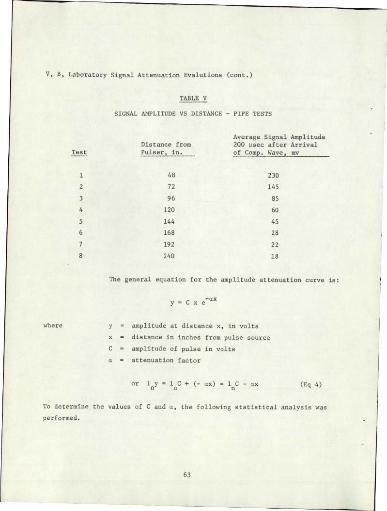
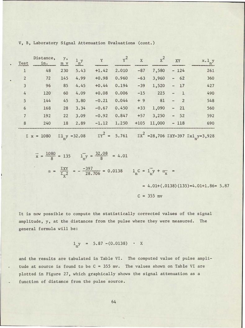
V B Laboratory Signal Attenuation Evaluations (cont)
Distance Yo y y2 X X2 Test in m v n n
1 48 230 543 +142 2010 -87 7580 - 124 261
2 72 145 499 +098 0960 -63 3960 - 62 360
3 96 85 445 +044 0194 -39 1520 - 17 427
4 120 60 409 +008 0006 -15 225 - 1 490
5 144 45 380 -021 0044 + 9 81 - 2 548
6 168 28 334 -067 0450 +33 1090 - 21 560
7 192 22 309 -092 0847 +57 3250 - 52 592
8 240 18 289 -112 1250 +105 11000 - 118 690
EY2 EX2pound x = 1080 ElnY =3208 5761 28706 SXY-397 XxIny3928
- 1080 - 3208 x =- = 135 ny = 401
EXY -397 00138 1 C =l1y + oshy
pound 2 x2 28706 n i x
= 401+(0138)(135)=401+186= 587
C - 355 mv
It is now possible to compute the statistically corrected values of the signal
amplitude y at the distances from the pulse where they were measured The
general formula will be
ny = 587 -(00138) X
and the results are tabulated in Table VI The computed value of pulse amplishy
tude at source is found to be C = 355 my The values shown on Table VI are
plotted in Figure 27 which graphically shows the signal attenuation as a
function of distance from the pulse source
64
350
300
250 STATISTICALLY COMPUTED k VALUES FOR REGRESSION CURVE
--0gt 200
EXPERIMENTALLY DETERMINED
-- MATERIAL SAE 4130 STEEL U= SPECIMEN PIPE-S758 in D aZ
00
15 7 18 in D22 ft 10 78 in LONG
-J
100
50 I
0 I I I
5 I I I
DISTANCE
I
10 FROM SOURCE
I
FEET
I
15 20
Figure 27 Signal Amplitude vs Distance - Pipe Tests
V B Laboratory Signal Attenuation Evaluations (cont)
TABLE VI
STATISTICALLY CORRECTED VALUES OF SIGNAL AMPLITUDE - PIPE TESTS
Experimentally Distance from 1 Corrected Signal Determined Signal
Test Pulse in ny Amplitude (y) mv Amplitude (y) my
1 48 521 182 230
2 72 488 130 145
3 96 455 95 85
4 120 421 67 60
5 144 388 48 45
6 168 355 35 28
7 192 322 25 22
8 240 255 127 18
- 2 Plate Tests
An SAE 4130 steel plate (73-12 in long 48-12 in wide
and 34 in thick) was used for this test series The two diagonals were
marked on the plate The pulser was placed at the center of the plate and
the receiver accelerometer was placed on one of the diagonals at locations
spaced in increments of 6 in from the center The received signals were
observed on the oscilloscope and photos were taken of these signals Figure
28 shows oscillographs of the signals received at 6 12 18 24 30 36 and
42 in from the pulser The times of arrival of the shear wave are also shown
in Figure 28 The velocity used was v = 123000 insec An integration
was performed of the positive positions of the cycles comprised in a 20 Psec
interval after the arrival of the shear wave The average amplitudes detershy
mined from these integrations are shown in Table VII Only Tests 1 to 4 are
used because reflection (from the plate edges) in Tests 5 to 8 obscured the
66
b 12 INCHES FROM PULSERa 6 INCHES FROM PULSER
TBTs
c 18 INCHES FROM PULSER d 24 INCHES FROM PULSER
IT s = Arrival of Shear Wave
Vertical Scale 1 DIV = 01 Volt Horizontal Scale 1 DIV = 20 ASec
Figure 28 Oscillograph Traces for Plate Tests (Sheet 1 of 2)
Page 67
f 36 INCHES FROM PULSER e 30 INCHES FROM PULSER
g 42 INCHES FROM PULSER
= Arrival of Shear WaveTs
Vertical Scale 1 DIV = 01 Volt = 20 4SecHorizontal Scale 1 DIV
Figure 28 Oscillograph Traces for Plate Tests (Sheet 2 of 2)
08 gOTPRODUCIB1A
V B Laboratory Signal Attenuation Evaluations (cont)
data These reflections were received in Tests 5 to 8 because of the relashy
tively small plate that was available for this test series
TABLE VII
SIGNAL AMPLITUDE VS DISTANCE - PLATE TESTS
Distance from Average Amplitude Test Pulse in(x) in 20 p see mv
1 6 150
2 12 110
3 18 70
4 24 45
The following statistical analysis was performed to determine the values of
C and a in Equation 4
Test
Distance from
Pulse in(x)
y
m v
1
ny Y
2
Y 2
X XY
X1 y
n
1 6 150 500 +056 0314 -9 81 -502 3000
2
3
12
18
110
70
470
425
+026
-019
0067
0036
-3
+3
9
9
-078
-057
5640
7650
4 24 45 381 -063 0397 +9 81 -567 9149
60 1776 0814 180 -1204 25439
-x=
60 w= 15
4ny
iY 1
1nC
-
=
16=44 1776 =44
E YX 1204= __=
E y2 180
ny +(0067)(15) =
+0067
444 + 0067(15)
69
=
C
444 + 100
= 230 my
= 544
V B Laboratory Signal Attenuation Evaluations (cont)
Subsequently the values of signal amplitude (y) were statistically corrected
as before and the experimentally determined values of y are compared to the
results obtained in Table VIII
TABLE VIII
COMPARISON Or STATISTICALLY CORRECTED AND TEST-DETERMINED VALUES OF SIGNAL AMPLITUDE - PLATE TESTS
Experimentally Distance from Corrected Signal Determined Signal
Test Pulse in nY Amplitude (y) mv Amplitude (y) my
1 6 504 155 150
2 12 464 103 110
3 18 417 65 70
4 24 383 46 45
The computed value of the pulse amplitude at the source at
C equals 230 mv The regression curve and the experimentally determined points
are plotted in Figure 29 It should be observed that the attenuation coefshy
ficient for the pipe test was a = 00138 and for the plate test was 0067
This is due to the much larger rate of front area that the pulse meets in the
plate
C SENSOR SPACING
The quiescent background noise measurements performed at the test
sites using a 20 to 50 KHz band-pass filter are
Pad A Bottle Field - 0000099g
VAB Bottle Field 0000220g
70
250
200 - EXPERIMENTALLY DETERMINED
0o
gt
M a-100 34
STATISTICALLY COMPUTEDVALUES FOR REGRESSION CURVE
MATERIAL SAE 4130 STEEL
SPECIMEN PLATE - 73 12 in LONG 48 12 in WIDE
in THICK
J
50
0
0 5 SII
10 15
DISTANCE FROM SOURCE FEET
I
20 I
25
Figure 29 Signal Amplitude vs Distance - Plate Tests
V C Sensor Spacing (cont)
The recorded stress-wave-emission data obtained from the A302B steel bend tests
made at the Aerojet-General Corporation laboratory show that the minimum
acceleration at the source is 0O012g the average 00022g and the maximum
00039g Based on the above data and the attenuation factor X = 0067 detershy
mined from the plate tests the sensor spacings required to detect crack growth
in the vessels at the Kennedy Space Center were computed and the results are
tabulated below
Quiescent Sensor Spacing
Amplitude at Background in the Source(C) g Amplitude(y) g Cy ln(CIy) ln(CIy)
Pad A
Min Signal 00012 000015 800 208 310
Avg Signal 00022 000015 1470 269 402
Max Signal 00039 000015 2600 326 487
VAB Bottle Field
Min Signal 00012 000033 363 129 193
Avg Signal 00022 000033 668 190 283
Max Signal 00039 000033 1080 238 356
This threshold is 15 x 0000099 - 000015g (at Pad A)
This threshold is 15 x 000022 = 000033g (at VAB Bottle Field)
Figures 30 and 31 present schematically the location and spacings of sensors
on the pressure vessels
72
- 502 IN 8 IN
HEAD -- _
DEVELOPED + + CYLINDRICAL FOR MINIMUM SIGNAL-22 SENSORS AS SHOWN
SURFACE FOR AVERAGE SIGNAL-16 SENSORS
+ +I
FOR MAXIMUM SIGNAL- 14 SENSORS
282438 IN+ +
+ +
9 SPACINGS AT 313 IN
-I- +
+ +shy
+ -plusmn
HEAD _ __
8 IN
Figure 30 Schematic of Sensor Spacings for Bottles at Pad A
73
14601 IN
HEAD (6SENSORS) 23 14 INI I I - I I I
t plusmn + plusmn + +
+ + 4 + + + DEVELOPED CYL SURFACE
+ + 4A 1 13 LINES OF
+ + + SENSORS SPACED4 + + AT 2086 IN
+ + + + + +
+ + 4 + + +
251 1516 IN + + + +-I- +
+ + + 4- +
-1- 298438 IN+ -I- -+- -i- +
+I
23 14 INHEAD (6 SENSORS) 1
FOR MINIMUM SIGNAL-103 SENSORS AS SHOWN
FOR AVERAGE SIGNAL- 82 SENSORS FOR MAXIMUM SIGNAL- 58 SENSORS
Figure 31 Schematic of Sensor Spacings for Bottles at VAB Bottle Field
74
VI CONCLUSIONS
A The Type A302B steel supplied for evaluation exhibited a high level
of fracture toughness Although quantitative plane-strain fracture toughness
measurements were not possible because of the large specimen size required
the K value associated with failure approximated 135 ksi-inI 2
Q
B The Type A302B steel was found resistant to environmentally induced
slow crack growth when tested in the hydrogenated condition in an air environshy
ment and in the unhydrogenated condition in a 3 NaCl-water environment Howshy
ever hydrogenated material tested in 3 NaCl-water had a much faster rate of
subcritical crack growth indicating a synergistic effect due to the combinashy
tion of sea water and hydrogen in interstitial solid solution
C The synergistic effect indicates the Type A302B steel hydrogen
storage tanks in the Kennedy Space Flight Center may have limited life as a
result of subcritical crack growth if subjected to the same combination of
stress and environmental factors
D Detectable stress-wave emissions although of small amplitude
(ltOOlg) were observed to be associated with crack growth in Type A302B steel
In all test conditions the stress-wave emissions were observed during rising
load and when failure (instability) was imminent Both the amplitude and rate
of stress-wave emission increased as failure was approached and could be
employed as a precursor of the onset of instability
E Stress-wave emissions associated with crack growth in Type A302B
steel can be detected under quiescent background conditions at the Pad A and
VAB Bottle fields at the Kennedy Space Flight Center However it would be
difficult to detect such stress-wave emissions during tank blowdown and
repressurization periods unless filtering can be employed to screen out the
noise associated with these periods
75
VI Conclusions (cont)
F Even in the presence of background noise from tank blowdown and
repressurization these periods are considered short in the overall life of
the pressure vessels Consequently flaw growth or creep which was observed
during rising load or the initial part of hold could be detected by SWAT
permitting triangulation to the source and tank depressurization prior to
failure
G Stress-wave-emission attenuation test data were obtained and employed
in conjunction with the site background measurements addbnd test stress-waveshy
emission characterization data to determine sensor mounting patterns for the
hydrogen pressure vessels at Pad A and the VAB Bottle Field
VII RECOMMENDATIONS FOR FURTHER WORK
If the synergistic effect of hydrogen and 3 NaCi solution occurs in
Kennedy Space Flight Center tankage the life of the tankage will be limited
Obviously slow-crack growth from any cause whether continuous or disconshy
tinuous and regardless of how slow the rate of cracking will eventually
produce failure This investigation showed that subcritical crack growth is
in all likelihood occurring with each pressurization A question remains
however as to the rate of crack growth without knowledge of the rate there
is no way to anticipate the life of the tankage However with SWAT one can
monitor the occurrence of crack growth and most importantly make judgment
as to whether a given crack is approaching critical size Consequently it
is recommended that additional tests be performed to (1) verify the existence
of subcritical cracking in actual on-site tankage and (2) incorporate an
automatic system for continuously monitoring on-site tankage at Kennedy Space
Flight Center
76
REFERENCES
1 Steel R K Green A T Lockman C S Acoustic Verification of Structural Integrity of Polaris Chambers Society of Plastic Engineers 20th Meeting Atlantic City N Y January 1964
2 Pressure Testing of AFRM-017 Service Propulsion System Fuel Tank Utilizing Aerojet-General Corporations Stress-Wave Analysis Technique
Report NAS 9-6766-003 Aerojet-General Corp for NASA MSC Houston Texas Contract NAS 9-6766 May 1967
3 Srawley J E and Esgar J B Investigation of Hydrotest Failure of Thiokol Chemical Corp 260-Inch-Diameter SL-1 Motor Case NASA-TMX shy1194 January 1964
4 Hartbower C E Gerberich W W and Crimmins P P Mechanisms of Slow Crack Growth in High-Strength Steels AFML-TR-67-26 Vol 1 February 1967
5 -Hartbower C E Gerberich W W and Crimmins P P Characterization of Fatigue-Crack Growth by Stress Wave Emission Final Report on Conshytract NAS 1-4902 for NASA-Langley Research Center Hampton Virginia June 1966
6 IHartbower C E Gerberich W W Reuter W G and Crimmins P P Stress Wave Characteristics in Constructional Alloys Final Report on Office of Naval Research Contract N00014-66-C-0340 July 1967
7 Novak S R and Rolfe S T Modified WOL Specimen for KIscc Environmental Testing U S Steel Corp paper submitted to ASTM for publication
77
V B Laboratory Signal Attenuation Evaluations (cont)
TABLE VI
STATISTICALLY CORRECTED VALUES OF SIGNAL AMPLITUDE - PIPE TESTS
Experimentally Distance from 1 Corrected Signal Determined Signal
Test Pulse in ny Amplitude (y) mv Amplitude (y) my
1 48 521 182 230
2 72 488 130 145
3 96 455 95 85
4 120 421 67 60
5 144 388 48 45
6 168 355 35 28
7 192 322 25 22
8 240 255 127 18
- 2 Plate Tests
An SAE 4130 steel plate (73-12 in long 48-12 in wide
and 34 in thick) was used for this test series The two diagonals were
marked on the plate The pulser was placed at the center of the plate and
the receiver accelerometer was placed on one of the diagonals at locations
spaced in increments of 6 in from the center The received signals were
observed on the oscilloscope and photos were taken of these signals Figure
28 shows oscillographs of the signals received at 6 12 18 24 30 36 and
42 in from the pulser The times of arrival of the shear wave are also shown
in Figure 28 The velocity used was v = 123000 insec An integration
was performed of the positive positions of the cycles comprised in a 20 Psec
interval after the arrival of the shear wave The average amplitudes detershy
mined from these integrations are shown in Table VII Only Tests 1 to 4 are
used because reflection (from the plate edges) in Tests 5 to 8 obscured the
66
b 12 INCHES FROM PULSERa 6 INCHES FROM PULSER
TBTs
c 18 INCHES FROM PULSER d 24 INCHES FROM PULSER
IT s = Arrival of Shear Wave
Vertical Scale 1 DIV = 01 Volt Horizontal Scale 1 DIV = 20 ASec
Figure 28 Oscillograph Traces for Plate Tests (Sheet 1 of 2)
Page 67
f 36 INCHES FROM PULSER e 30 INCHES FROM PULSER
g 42 INCHES FROM PULSER
= Arrival of Shear WaveTs
Vertical Scale 1 DIV = 01 Volt = 20 4SecHorizontal Scale 1 DIV
Figure 28 Oscillograph Traces for Plate Tests (Sheet 2 of 2)
08 gOTPRODUCIB1A
V B Laboratory Signal Attenuation Evaluations (cont)
data These reflections were received in Tests 5 to 8 because of the relashy
tively small plate that was available for this test series
TABLE VII
SIGNAL AMPLITUDE VS DISTANCE - PLATE TESTS
Distance from Average Amplitude Test Pulse in(x) in 20 p see mv
1 6 150
2 12 110
3 18 70
4 24 45
The following statistical analysis was performed to determine the values of
C and a in Equation 4
Test
Distance from
Pulse in(x)
y
m v
1
ny Y
2
Y 2
X XY
X1 y
n
1 6 150 500 +056 0314 -9 81 -502 3000
2
3
12
18
110
70
470
425
+026
-019
0067
0036
-3
+3
9
9
-078
-057
5640
7650
4 24 45 381 -063 0397 +9 81 -567 9149
60 1776 0814 180 -1204 25439
-x=
60 w= 15
4ny
iY 1
1nC
-
=
16=44 1776 =44
E YX 1204= __=
E y2 180
ny +(0067)(15) =
+0067
444 + 0067(15)
69
=
C
444 + 100
= 230 my
= 544
V B Laboratory Signal Attenuation Evaluations (cont)
Subsequently the values of signal amplitude (y) were statistically corrected
as before and the experimentally determined values of y are compared to the
results obtained in Table VIII
TABLE VIII
COMPARISON Or STATISTICALLY CORRECTED AND TEST-DETERMINED VALUES OF SIGNAL AMPLITUDE - PLATE TESTS
Experimentally Distance from Corrected Signal Determined Signal
Test Pulse in nY Amplitude (y) mv Amplitude (y) my
1 6 504 155 150
2 12 464 103 110
3 18 417 65 70
4 24 383 46 45
The computed value of the pulse amplitude at the source at
C equals 230 mv The regression curve and the experimentally determined points
are plotted in Figure 29 It should be observed that the attenuation coefshy
ficient for the pipe test was a = 00138 and for the plate test was 0067
This is due to the much larger rate of front area that the pulse meets in the
plate
C SENSOR SPACING
The quiescent background noise measurements performed at the test
sites using a 20 to 50 KHz band-pass filter are
Pad A Bottle Field - 0000099g
VAB Bottle Field 0000220g
70
250
200 - EXPERIMENTALLY DETERMINED
0o
gt
M a-100 34
STATISTICALLY COMPUTEDVALUES FOR REGRESSION CURVE
MATERIAL SAE 4130 STEEL
SPECIMEN PLATE - 73 12 in LONG 48 12 in WIDE
in THICK
J
50
0
0 5 SII
10 15
DISTANCE FROM SOURCE FEET
I
20 I
25
Figure 29 Signal Amplitude vs Distance - Plate Tests
V C Sensor Spacing (cont)
The recorded stress-wave-emission data obtained from the A302B steel bend tests
made at the Aerojet-General Corporation laboratory show that the minimum
acceleration at the source is 0O012g the average 00022g and the maximum
00039g Based on the above data and the attenuation factor X = 0067 detershy
mined from the plate tests the sensor spacings required to detect crack growth
in the vessels at the Kennedy Space Center were computed and the results are
tabulated below
Quiescent Sensor Spacing
Amplitude at Background in the Source(C) g Amplitude(y) g Cy ln(CIy) ln(CIy)
Pad A
Min Signal 00012 000015 800 208 310
Avg Signal 00022 000015 1470 269 402
Max Signal 00039 000015 2600 326 487
VAB Bottle Field
Min Signal 00012 000033 363 129 193
Avg Signal 00022 000033 668 190 283
Max Signal 00039 000033 1080 238 356
This threshold is 15 x 0000099 - 000015g (at Pad A)
This threshold is 15 x 000022 = 000033g (at VAB Bottle Field)
Figures 30 and 31 present schematically the location and spacings of sensors
on the pressure vessels
72
- 502 IN 8 IN
HEAD -- _
DEVELOPED + + CYLINDRICAL FOR MINIMUM SIGNAL-22 SENSORS AS SHOWN
SURFACE FOR AVERAGE SIGNAL-16 SENSORS
+ +I
FOR MAXIMUM SIGNAL- 14 SENSORS
282438 IN+ +
+ +
9 SPACINGS AT 313 IN
-I- +
+ +shy
+ -plusmn
HEAD _ __
8 IN
Figure 30 Schematic of Sensor Spacings for Bottles at Pad A
73
14601 IN
HEAD (6SENSORS) 23 14 INI I I - I I I
t plusmn + plusmn + +
+ + 4 + + + DEVELOPED CYL SURFACE
+ + 4A 1 13 LINES OF
+ + + SENSORS SPACED4 + + AT 2086 IN
+ + + + + +
+ + 4 + + +
251 1516 IN + + + +-I- +
+ + + 4- +
-1- 298438 IN+ -I- -+- -i- +
+I
23 14 INHEAD (6 SENSORS) 1
FOR MINIMUM SIGNAL-103 SENSORS AS SHOWN
FOR AVERAGE SIGNAL- 82 SENSORS FOR MAXIMUM SIGNAL- 58 SENSORS
Figure 31 Schematic of Sensor Spacings for Bottles at VAB Bottle Field
74
VI CONCLUSIONS
A The Type A302B steel supplied for evaluation exhibited a high level
of fracture toughness Although quantitative plane-strain fracture toughness
measurements were not possible because of the large specimen size required
the K value associated with failure approximated 135 ksi-inI 2
Q
B The Type A302B steel was found resistant to environmentally induced
slow crack growth when tested in the hydrogenated condition in an air environshy
ment and in the unhydrogenated condition in a 3 NaCl-water environment Howshy
ever hydrogenated material tested in 3 NaCl-water had a much faster rate of
subcritical crack growth indicating a synergistic effect due to the combinashy
tion of sea water and hydrogen in interstitial solid solution
C The synergistic effect indicates the Type A302B steel hydrogen
storage tanks in the Kennedy Space Flight Center may have limited life as a
result of subcritical crack growth if subjected to the same combination of
stress and environmental factors
D Detectable stress-wave emissions although of small amplitude
(ltOOlg) were observed to be associated with crack growth in Type A302B steel
In all test conditions the stress-wave emissions were observed during rising
load and when failure (instability) was imminent Both the amplitude and rate
of stress-wave emission increased as failure was approached and could be
employed as a precursor of the onset of instability
E Stress-wave emissions associated with crack growth in Type A302B
steel can be detected under quiescent background conditions at the Pad A and
VAB Bottle fields at the Kennedy Space Flight Center However it would be
difficult to detect such stress-wave emissions during tank blowdown and
repressurization periods unless filtering can be employed to screen out the
noise associated with these periods
75
VI Conclusions (cont)
F Even in the presence of background noise from tank blowdown and
repressurization these periods are considered short in the overall life of
the pressure vessels Consequently flaw growth or creep which was observed
during rising load or the initial part of hold could be detected by SWAT
permitting triangulation to the source and tank depressurization prior to
failure
G Stress-wave-emission attenuation test data were obtained and employed
in conjunction with the site background measurements addbnd test stress-waveshy
emission characterization data to determine sensor mounting patterns for the
hydrogen pressure vessels at Pad A and the VAB Bottle Field
VII RECOMMENDATIONS FOR FURTHER WORK
If the synergistic effect of hydrogen and 3 NaCi solution occurs in
Kennedy Space Flight Center tankage the life of the tankage will be limited
Obviously slow-crack growth from any cause whether continuous or disconshy
tinuous and regardless of how slow the rate of cracking will eventually
produce failure This investigation showed that subcritical crack growth is
in all likelihood occurring with each pressurization A question remains
however as to the rate of crack growth without knowledge of the rate there
is no way to anticipate the life of the tankage However with SWAT one can
monitor the occurrence of crack growth and most importantly make judgment
as to whether a given crack is approaching critical size Consequently it
is recommended that additional tests be performed to (1) verify the existence
of subcritical cracking in actual on-site tankage and (2) incorporate an
automatic system for continuously monitoring on-site tankage at Kennedy Space
Flight Center
76
REFERENCES
1 Steel R K Green A T Lockman C S Acoustic Verification of Structural Integrity of Polaris Chambers Society of Plastic Engineers 20th Meeting Atlantic City N Y January 1964
2 Pressure Testing of AFRM-017 Service Propulsion System Fuel Tank Utilizing Aerojet-General Corporations Stress-Wave Analysis Technique
Report NAS 9-6766-003 Aerojet-General Corp for NASA MSC Houston Texas Contract NAS 9-6766 May 1967
3 Srawley J E and Esgar J B Investigation of Hydrotest Failure of Thiokol Chemical Corp 260-Inch-Diameter SL-1 Motor Case NASA-TMX shy1194 January 1964
4 Hartbower C E Gerberich W W and Crimmins P P Mechanisms of Slow Crack Growth in High-Strength Steels AFML-TR-67-26 Vol 1 February 1967
5 -Hartbower C E Gerberich W W and Crimmins P P Characterization of Fatigue-Crack Growth by Stress Wave Emission Final Report on Conshytract NAS 1-4902 for NASA-Langley Research Center Hampton Virginia June 1966
6 IHartbower C E Gerberich W W Reuter W G and Crimmins P P Stress Wave Characteristics in Constructional Alloys Final Report on Office of Naval Research Contract N00014-66-C-0340 July 1967
7 Novak S R and Rolfe S T Modified WOL Specimen for KIscc Environmental Testing U S Steel Corp paper submitted to ASTM for publication
77
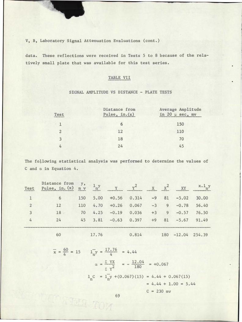
V B Laboratory Signal Attenuation Evaluations (cont)
data These reflections were received in Tests 5 to 8 because of the relashy
tively small plate that was available for this test series
TABLE VII
SIGNAL AMPLITUDE VS DISTANCE - PLATE TESTS
Distance from Average Amplitude Test Pulse in(x) in 20 p see mv
1 6 150
2 12 110
3 18 70
4 24 45
The following statistical analysis was performed to determine the values of
C and a in Equation 4
Test
Distance from
Pulse in(x)
y
m v
1
ny Y
2
Y 2
X XY
X1 y
n
1 6 150 500 +056 0314 -9 81 -502 3000
2
3
12
18
110
70
470
425
+026
-019
0067
0036
-3
+3
9
9
-078
-057
5640
7650
4 24 45 381 -063 0397 +9 81 -567 9149
60 1776 0814 180 -1204 25439
-x=
60 w= 15
4ny
iY 1
1nC
-
=
16=44 1776 =44
E YX 1204= __=
E y2 180
ny +(0067)(15) =
+0067
444 + 0067(15)
69
=
C
444 + 100
= 230 my
= 544
V B Laboratory Signal Attenuation Evaluations (cont)
Subsequently the values of signal amplitude (y) were statistically corrected
as before and the experimentally determined values of y are compared to the
results obtained in Table VIII
TABLE VIII
COMPARISON Or STATISTICALLY CORRECTED AND TEST-DETERMINED VALUES OF SIGNAL AMPLITUDE - PLATE TESTS
Experimentally Distance from Corrected Signal Determined Signal
Test Pulse in nY Amplitude (y) mv Amplitude (y) my
1 6 504 155 150
2 12 464 103 110
3 18 417 65 70
4 24 383 46 45
The computed value of the pulse amplitude at the source at
C equals 230 mv The regression curve and the experimentally determined points
are plotted in Figure 29 It should be observed that the attenuation coefshy
ficient for the pipe test was a = 00138 and for the plate test was 0067
This is due to the much larger rate of front area that the pulse meets in the
plate
C SENSOR SPACING
The quiescent background noise measurements performed at the test
sites using a 20 to 50 KHz band-pass filter are
Pad A Bottle Field - 0000099g
VAB Bottle Field 0000220g
70
250
200 - EXPERIMENTALLY DETERMINED
0o
gt
M a-100 34
STATISTICALLY COMPUTEDVALUES FOR REGRESSION CURVE
MATERIAL SAE 4130 STEEL
SPECIMEN PLATE - 73 12 in LONG 48 12 in WIDE
in THICK
J
50
0
0 5 SII
10 15
DISTANCE FROM SOURCE FEET
I
20 I
25
Figure 29 Signal Amplitude vs Distance - Plate Tests
V C Sensor Spacing (cont)
The recorded stress-wave-emission data obtained from the A302B steel bend tests
made at the Aerojet-General Corporation laboratory show that the minimum
acceleration at the source is 0O012g the average 00022g and the maximum
00039g Based on the above data and the attenuation factor X = 0067 detershy
mined from the plate tests the sensor spacings required to detect crack growth
in the vessels at the Kennedy Space Center were computed and the results are
tabulated below
Quiescent Sensor Spacing
Amplitude at Background in the Source(C) g Amplitude(y) g Cy ln(CIy) ln(CIy)
Pad A
Min Signal 00012 000015 800 208 310
Avg Signal 00022 000015 1470 269 402
Max Signal 00039 000015 2600 326 487
VAB Bottle Field
Min Signal 00012 000033 363 129 193
Avg Signal 00022 000033 668 190 283
Max Signal 00039 000033 1080 238 356
This threshold is 15 x 0000099 - 000015g (at Pad A)
This threshold is 15 x 000022 = 000033g (at VAB Bottle Field)
Figures 30 and 31 present schematically the location and spacings of sensors
on the pressure vessels
72
- 502 IN 8 IN
HEAD -- _
DEVELOPED + + CYLINDRICAL FOR MINIMUM SIGNAL-22 SENSORS AS SHOWN
SURFACE FOR AVERAGE SIGNAL-16 SENSORS
+ +I
FOR MAXIMUM SIGNAL- 14 SENSORS
282438 IN+ +
+ +
9 SPACINGS AT 313 IN
-I- +
+ +shy
+ -plusmn
HEAD _ __
8 IN
Figure 30 Schematic of Sensor Spacings for Bottles at Pad A
73
14601 IN
HEAD (6SENSORS) 23 14 INI I I - I I I
t plusmn + plusmn + +
+ + 4 + + + DEVELOPED CYL SURFACE
+ + 4A 1 13 LINES OF
+ + + SENSORS SPACED4 + + AT 2086 IN
+ + + + + +
+ + 4 + + +
251 1516 IN + + + +-I- +
+ + + 4- +
-1- 298438 IN+ -I- -+- -i- +
+I
23 14 INHEAD (6 SENSORS) 1
FOR MINIMUM SIGNAL-103 SENSORS AS SHOWN
FOR AVERAGE SIGNAL- 82 SENSORS FOR MAXIMUM SIGNAL- 58 SENSORS
Figure 31 Schematic of Sensor Spacings for Bottles at VAB Bottle Field
74
VI CONCLUSIONS
A The Type A302B steel supplied for evaluation exhibited a high level
of fracture toughness Although quantitative plane-strain fracture toughness
measurements were not possible because of the large specimen size required
the K value associated with failure approximated 135 ksi-inI 2
Q
B The Type A302B steel was found resistant to environmentally induced
slow crack growth when tested in the hydrogenated condition in an air environshy
ment and in the unhydrogenated condition in a 3 NaCl-water environment Howshy
ever hydrogenated material tested in 3 NaCl-water had a much faster rate of
subcritical crack growth indicating a synergistic effect due to the combinashy
tion of sea water and hydrogen in interstitial solid solution
C The synergistic effect indicates the Type A302B steel hydrogen
storage tanks in the Kennedy Space Flight Center may have limited life as a
result of subcritical crack growth if subjected to the same combination of
stress and environmental factors
D Detectable stress-wave emissions although of small amplitude
(ltOOlg) were observed to be associated with crack growth in Type A302B steel
In all test conditions the stress-wave emissions were observed during rising
load and when failure (instability) was imminent Both the amplitude and rate
of stress-wave emission increased as failure was approached and could be
employed as a precursor of the onset of instability
E Stress-wave emissions associated with crack growth in Type A302B
steel can be detected under quiescent background conditions at the Pad A and
VAB Bottle fields at the Kennedy Space Flight Center However it would be
difficult to detect such stress-wave emissions during tank blowdown and
repressurization periods unless filtering can be employed to screen out the
noise associated with these periods
75
VI Conclusions (cont)
F Even in the presence of background noise from tank blowdown and
repressurization these periods are considered short in the overall life of
the pressure vessels Consequently flaw growth or creep which was observed
during rising load or the initial part of hold could be detected by SWAT
permitting triangulation to the source and tank depressurization prior to
failure
G Stress-wave-emission attenuation test data were obtained and employed
in conjunction with the site background measurements addbnd test stress-waveshy
emission characterization data to determine sensor mounting patterns for the
hydrogen pressure vessels at Pad A and the VAB Bottle Field
VII RECOMMENDATIONS FOR FURTHER WORK
If the synergistic effect of hydrogen and 3 NaCi solution occurs in
Kennedy Space Flight Center tankage the life of the tankage will be limited
Obviously slow-crack growth from any cause whether continuous or disconshy
tinuous and regardless of how slow the rate of cracking will eventually
produce failure This investigation showed that subcritical crack growth is
in all likelihood occurring with each pressurization A question remains
however as to the rate of crack growth without knowledge of the rate there
is no way to anticipate the life of the tankage However with SWAT one can
monitor the occurrence of crack growth and most importantly make judgment
as to whether a given crack is approaching critical size Consequently it
is recommended that additional tests be performed to (1) verify the existence
of subcritical cracking in actual on-site tankage and (2) incorporate an
automatic system for continuously monitoring on-site tankage at Kennedy Space
Flight Center
76
REFERENCES
1 Steel R K Green A T Lockman C S Acoustic Verification of Structural Integrity of Polaris Chambers Society of Plastic Engineers 20th Meeting Atlantic City N Y January 1964
2 Pressure Testing of AFRM-017 Service Propulsion System Fuel Tank Utilizing Aerojet-General Corporations Stress-Wave Analysis Technique
Report NAS 9-6766-003 Aerojet-General Corp for NASA MSC Houston Texas Contract NAS 9-6766 May 1967
3 Srawley J E and Esgar J B Investigation of Hydrotest Failure of Thiokol Chemical Corp 260-Inch-Diameter SL-1 Motor Case NASA-TMX shy1194 January 1964
4 Hartbower C E Gerberich W W and Crimmins P P Mechanisms of Slow Crack Growth in High-Strength Steels AFML-TR-67-26 Vol 1 February 1967
5 -Hartbower C E Gerberich W W and Crimmins P P Characterization of Fatigue-Crack Growth by Stress Wave Emission Final Report on Conshytract NAS 1-4902 for NASA-Langley Research Center Hampton Virginia June 1966
6 IHartbower C E Gerberich W W Reuter W G and Crimmins P P Stress Wave Characteristics in Constructional Alloys Final Report on Office of Naval Research Contract N00014-66-C-0340 July 1967
7 Novak S R and Rolfe S T Modified WOL Specimen for KIscc Environmental Testing U S Steel Corp paper submitted to ASTM for publication
77
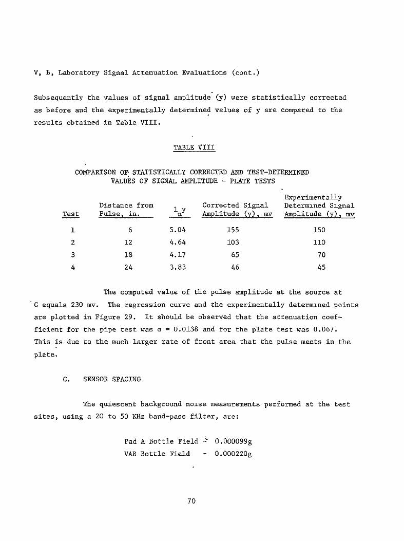
V B Laboratory Signal Attenuation Evaluations (cont)
Subsequently the values of signal amplitude (y) were statistically corrected
as before and the experimentally determined values of y are compared to the
results obtained in Table VIII
TABLE VIII
COMPARISON Or STATISTICALLY CORRECTED AND TEST-DETERMINED VALUES OF SIGNAL AMPLITUDE - PLATE TESTS
Experimentally Distance from Corrected Signal Determined Signal
Test Pulse in nY Amplitude (y) mv Amplitude (y) my
1 6 504 155 150
2 12 464 103 110
3 18 417 65 70
4 24 383 46 45
The computed value of the pulse amplitude at the source at
C equals 230 mv The regression curve and the experimentally determined points
are plotted in Figure 29 It should be observed that the attenuation coefshy
ficient for the pipe test was a = 00138 and for the plate test was 0067
This is due to the much larger rate of front area that the pulse meets in the
plate
C SENSOR SPACING
The quiescent background noise measurements performed at the test
sites using a 20 to 50 KHz band-pass filter are
Pad A Bottle Field - 0000099g
VAB Bottle Field 0000220g
70
250
200 - EXPERIMENTALLY DETERMINED
0o
gt
M a-100 34
STATISTICALLY COMPUTEDVALUES FOR REGRESSION CURVE
MATERIAL SAE 4130 STEEL
SPECIMEN PLATE - 73 12 in LONG 48 12 in WIDE
in THICK
J
50
0
0 5 SII
10 15
DISTANCE FROM SOURCE FEET
I
20 I
25
Figure 29 Signal Amplitude vs Distance - Plate Tests
V C Sensor Spacing (cont)
The recorded stress-wave-emission data obtained from the A302B steel bend tests
made at the Aerojet-General Corporation laboratory show that the minimum
acceleration at the source is 0O012g the average 00022g and the maximum
00039g Based on the above data and the attenuation factor X = 0067 detershy
mined from the plate tests the sensor spacings required to detect crack growth
in the vessels at the Kennedy Space Center were computed and the results are
tabulated below
Quiescent Sensor Spacing
Amplitude at Background in the Source(C) g Amplitude(y) g Cy ln(CIy) ln(CIy)
Pad A
Min Signal 00012 000015 800 208 310
Avg Signal 00022 000015 1470 269 402
Max Signal 00039 000015 2600 326 487
VAB Bottle Field
Min Signal 00012 000033 363 129 193
Avg Signal 00022 000033 668 190 283
Max Signal 00039 000033 1080 238 356
This threshold is 15 x 0000099 - 000015g (at Pad A)
This threshold is 15 x 000022 = 000033g (at VAB Bottle Field)
Figures 30 and 31 present schematically the location and spacings of sensors
on the pressure vessels
72
- 502 IN 8 IN
HEAD -- _
DEVELOPED + + CYLINDRICAL FOR MINIMUM SIGNAL-22 SENSORS AS SHOWN
SURFACE FOR AVERAGE SIGNAL-16 SENSORS
+ +I
FOR MAXIMUM SIGNAL- 14 SENSORS
282438 IN+ +
+ +
9 SPACINGS AT 313 IN
-I- +
+ +shy
+ -plusmn
HEAD _ __
8 IN
Figure 30 Schematic of Sensor Spacings for Bottles at Pad A
73
14601 IN
HEAD (6SENSORS) 23 14 INI I I - I I I
t plusmn + plusmn + +
+ + 4 + + + DEVELOPED CYL SURFACE
+ + 4A 1 13 LINES OF
+ + + SENSORS SPACED4 + + AT 2086 IN
+ + + + + +
+ + 4 + + +
251 1516 IN + + + +-I- +
+ + + 4- +
-1- 298438 IN+ -I- -+- -i- +
+I
23 14 INHEAD (6 SENSORS) 1
FOR MINIMUM SIGNAL-103 SENSORS AS SHOWN
FOR AVERAGE SIGNAL- 82 SENSORS FOR MAXIMUM SIGNAL- 58 SENSORS
Figure 31 Schematic of Sensor Spacings for Bottles at VAB Bottle Field
74
VI CONCLUSIONS
A The Type A302B steel supplied for evaluation exhibited a high level
of fracture toughness Although quantitative plane-strain fracture toughness
measurements were not possible because of the large specimen size required
the K value associated with failure approximated 135 ksi-inI 2
Q
B The Type A302B steel was found resistant to environmentally induced
slow crack growth when tested in the hydrogenated condition in an air environshy
ment and in the unhydrogenated condition in a 3 NaCl-water environment Howshy
ever hydrogenated material tested in 3 NaCl-water had a much faster rate of
subcritical crack growth indicating a synergistic effect due to the combinashy
tion of sea water and hydrogen in interstitial solid solution
C The synergistic effect indicates the Type A302B steel hydrogen
storage tanks in the Kennedy Space Flight Center may have limited life as a
result of subcritical crack growth if subjected to the same combination of
stress and environmental factors
D Detectable stress-wave emissions although of small amplitude
(ltOOlg) were observed to be associated with crack growth in Type A302B steel
In all test conditions the stress-wave emissions were observed during rising
load and when failure (instability) was imminent Both the amplitude and rate
of stress-wave emission increased as failure was approached and could be
employed as a precursor of the onset of instability
E Stress-wave emissions associated with crack growth in Type A302B
steel can be detected under quiescent background conditions at the Pad A and
VAB Bottle fields at the Kennedy Space Flight Center However it would be
difficult to detect such stress-wave emissions during tank blowdown and
repressurization periods unless filtering can be employed to screen out the
noise associated with these periods
75
VI Conclusions (cont)
F Even in the presence of background noise from tank blowdown and
repressurization these periods are considered short in the overall life of
the pressure vessels Consequently flaw growth or creep which was observed
during rising load or the initial part of hold could be detected by SWAT
permitting triangulation to the source and tank depressurization prior to
failure
G Stress-wave-emission attenuation test data were obtained and employed
in conjunction with the site background measurements addbnd test stress-waveshy
emission characterization data to determine sensor mounting patterns for the
hydrogen pressure vessels at Pad A and the VAB Bottle Field
VII RECOMMENDATIONS FOR FURTHER WORK
If the synergistic effect of hydrogen and 3 NaCi solution occurs in
Kennedy Space Flight Center tankage the life of the tankage will be limited
Obviously slow-crack growth from any cause whether continuous or disconshy
tinuous and regardless of how slow the rate of cracking will eventually
produce failure This investigation showed that subcritical crack growth is
in all likelihood occurring with each pressurization A question remains
however as to the rate of crack growth without knowledge of the rate there
is no way to anticipate the life of the tankage However with SWAT one can
monitor the occurrence of crack growth and most importantly make judgment
as to whether a given crack is approaching critical size Consequently it
is recommended that additional tests be performed to (1) verify the existence
of subcritical cracking in actual on-site tankage and (2) incorporate an
automatic system for continuously monitoring on-site tankage at Kennedy Space
Flight Center
76
REFERENCES
1 Steel R K Green A T Lockman C S Acoustic Verification of Structural Integrity of Polaris Chambers Society of Plastic Engineers 20th Meeting Atlantic City N Y January 1964
2 Pressure Testing of AFRM-017 Service Propulsion System Fuel Tank Utilizing Aerojet-General Corporations Stress-Wave Analysis Technique
Report NAS 9-6766-003 Aerojet-General Corp for NASA MSC Houston Texas Contract NAS 9-6766 May 1967
3 Srawley J E and Esgar J B Investigation of Hydrotest Failure of Thiokol Chemical Corp 260-Inch-Diameter SL-1 Motor Case NASA-TMX shy1194 January 1964
4 Hartbower C E Gerberich W W and Crimmins P P Mechanisms of Slow Crack Growth in High-Strength Steels AFML-TR-67-26 Vol 1 February 1967
5 -Hartbower C E Gerberich W W and Crimmins P P Characterization of Fatigue-Crack Growth by Stress Wave Emission Final Report on Conshytract NAS 1-4902 for NASA-Langley Research Center Hampton Virginia June 1966
6 IHartbower C E Gerberich W W Reuter W G and Crimmins P P Stress Wave Characteristics in Constructional Alloys Final Report on Office of Naval Research Contract N00014-66-C-0340 July 1967
7 Novak S R and Rolfe S T Modified WOL Specimen for KIscc Environmental Testing U S Steel Corp paper submitted to ASTM for publication
77
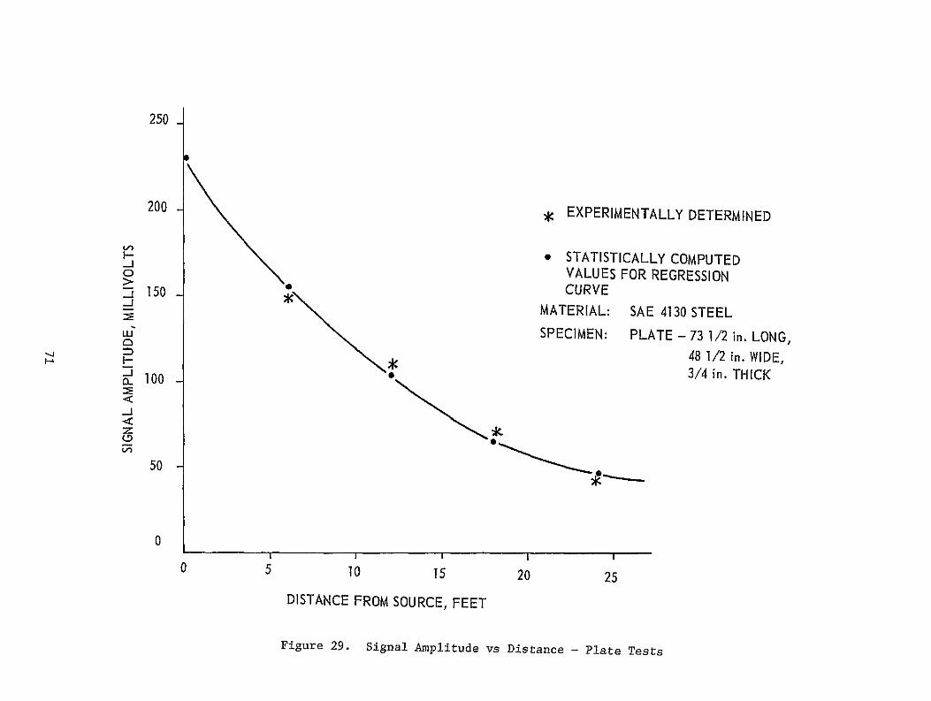
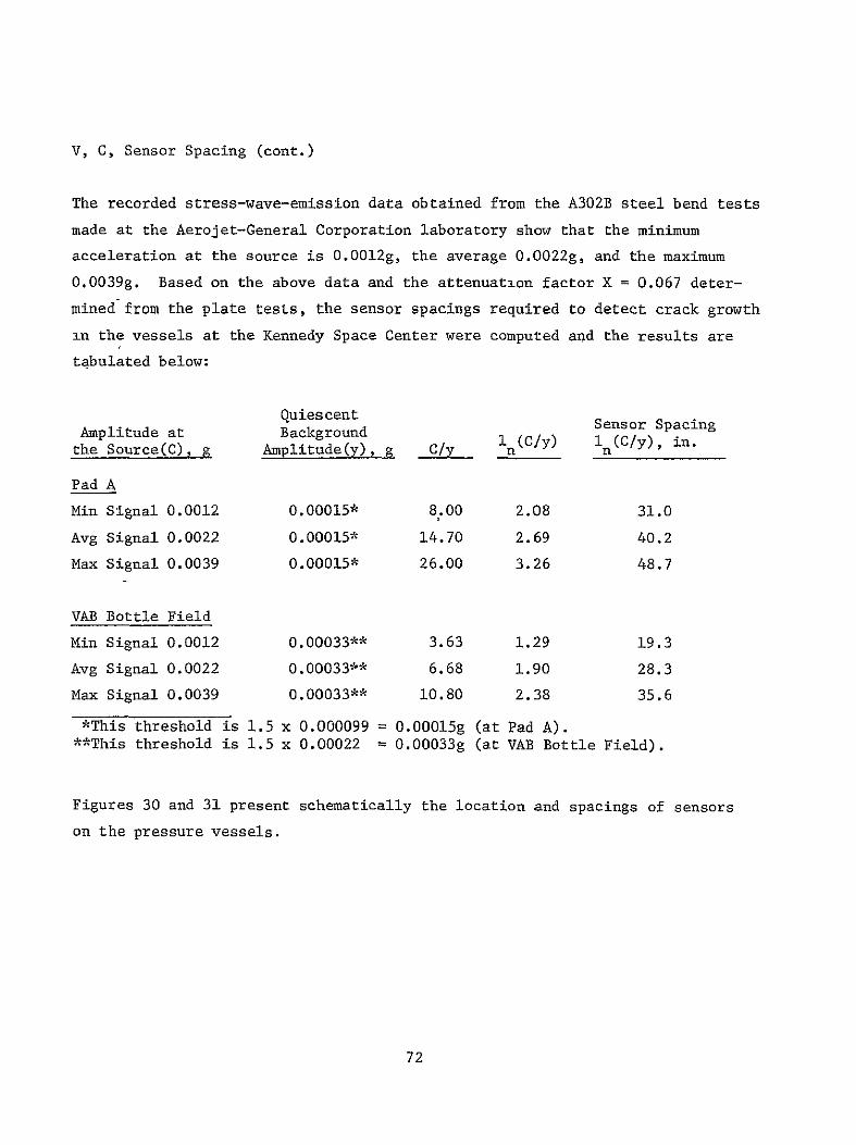
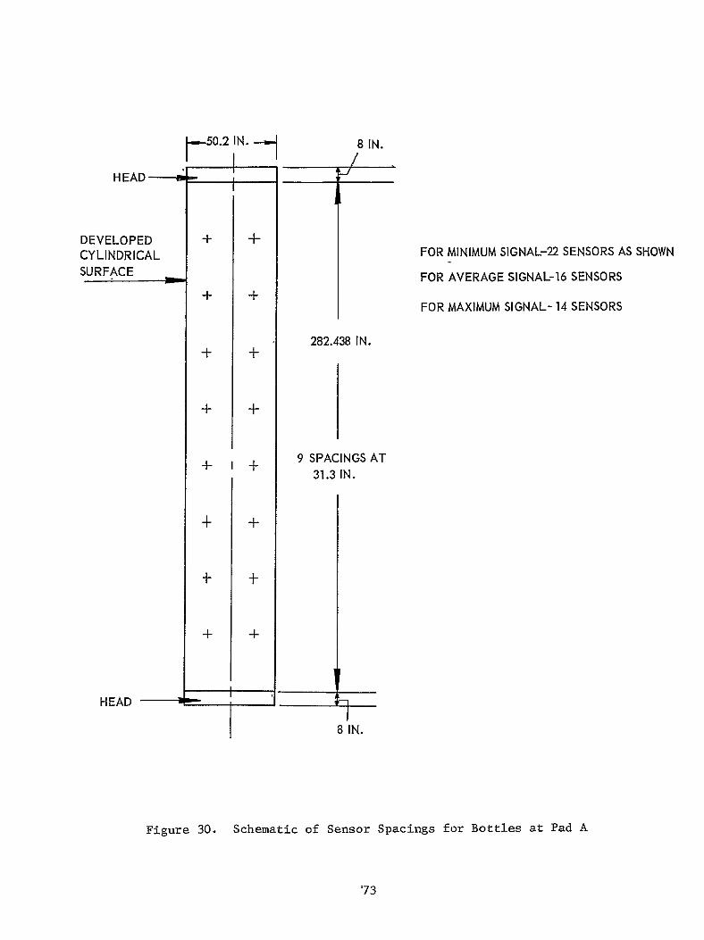
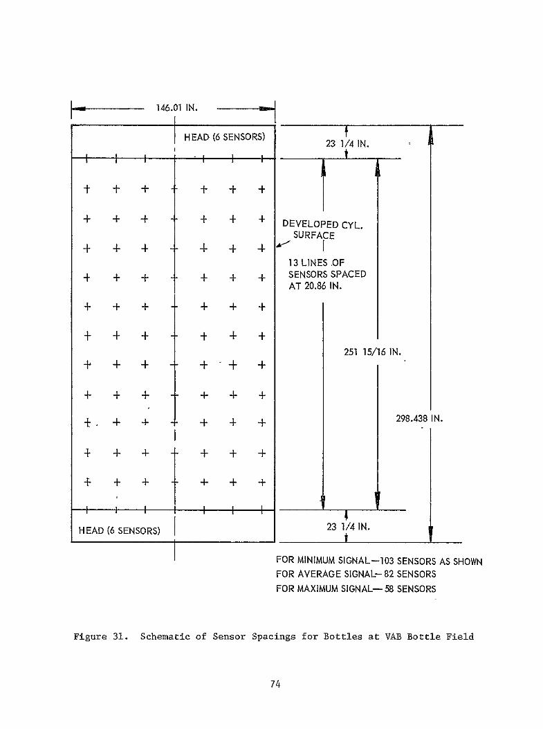
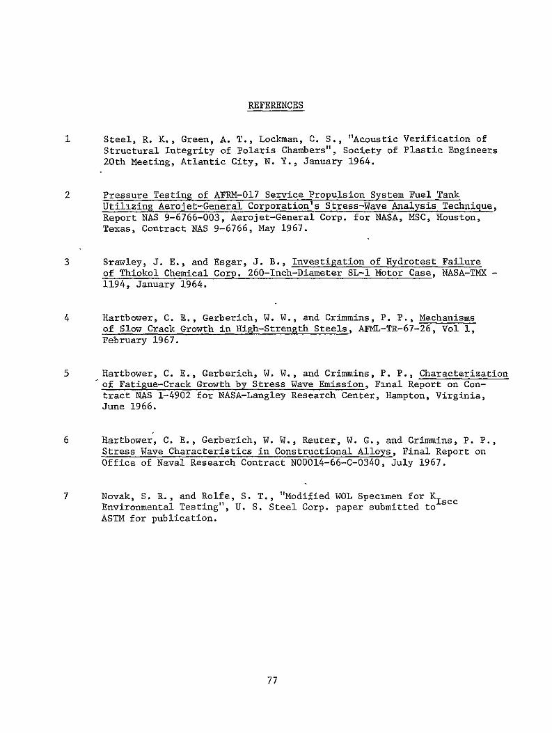