1

Stress Testing and the Quantification of the Dependency

Structure Amongst Portfolio Segments in Top-Down Credit

Risk Modeling

Michael Jacobs, Jr.

1

Accenture Consulting

Draft: June 18, 2015

Keywords: Stress Testing, Correlation, CCAR, DFAST, Credit Risk, Financial Crisis, Model

Risk, Vector Autoregression

JEL Classification: G11, G21, G22, G28, G32.

1 Corresponding author: Michael Jacobs, Jr., Ph.D., CFA, Principal Director, Accenture Consulting, Financial

Advisory, Risk Models, Methodologies & Analytics, 1345, Avenue of the Americas, New York, N.Y., 10105,

917-324-2098, michael.a.jacobs @accenture.com. The views expressed herein are those of the authors and do not

necessarily represent a position taken either by Pricewaterhouse Coopers LLC, nor of any affiliated firms.

2

Abstract

A critical question that banking supervisors are trying to answer is what is the amount of capital or

liquidity resources required by an institution in order to support the risks taken in the course of

business. The financial crisis of the last several years has revealed that traditional approaches

such as regulatory capital ratios to be inadequate, giving rise to supervisory stress testing as a

primary tool. In the case of banks that model the risk of their portfolios using top-of-the-house

modeling techniques, an issue that is rarely addressed is how to incorporate the correlation of risks

amongst the different segments. An approach to incorporate this consideration of dependency

structure is proposed, and the bias that results from ignoring this aspect is quantified, through

estimating a vector autoregressive (“VAR”) time series models for credit loss using Fed Y9 data.

We find that the multiple equation VAR model outperforms the single equation autoregressive

(“AR”) models according to various metrics across all modeling segments.

3

1 Introduction, Conceptual Considerations and Motivations

Modern credit risk modeling (e.g., Merton, 1974) increasingly relies on advanced mathematical,

statistical and numerical techniques to measure and manage risk in credit portfolios. This gives

rise to model risk (OCC 2011-12, FED-BOG SR 11-7), defined as the potential that a model used

to assess financial risks does not accurately capture those risks2, and the possibility of understating

inherent dangers stemming from very rare yet plausible occurrences perhaps not in reference da-

ta-sets or historical patterns of data. In the wake of the financial crisis (Demirguc-Kunt et al,

2010; Acharya et al, 2009), international supervisors have recognized the importance of stress

testing (ST), especially in the realm of credit risk, as can be seen in the revised Basel framework

(BCBS 2005, 2006; BCBS 2009 a,b,c,d,e; BCBS 2010 a,b) and the Federal Reserve’s Compre-

hensive Capital Analysis and Review (CCAR) program.

Stress testing (“ST”) may be defined, in a very general sense, as a form of deliberately intense or

thorough testing used to determine the stability of a given system or entity. This involves testing

beyond normal operational capacity, often to a breaking point, in order to observe the results. In

the financial risk management context, this involves scrutinizing the viability of an institution in its

response to various adverse configurations of macroeconomic and financial market events. ST is

closely related to the concept and practice of scenario analysis (“SC”), which in economics and

finance is the attempt to forecast several possible scenarios for the economy (e.g. rapid growth,

moderate growth, slow growth) or an attempt to forecast financial market returns (for bonds,

stocks and cash) in each of those scenarios. This might involve sub-sets of each of the possibili-

ties and even further seek to determine correlations and assign probabilities to the scenarios.

It can and has been argued that the art and science of has lagged in the domain of credit, as opposed

to other types of risk (e.g., market), and our objective is to help fill this vacuum. We aim to

present classifications and established techniques that will help practitioners formulate robust

credit risk stress tests. Furthermore, we approach the topic of ST from the point of view of a

typical credit portfolio, such as one managed by any number of medium or large sized commercial

bank. We take this point of view for two main reasons. First, credit risk remains the predomi-

nant risk faced by financial institutions that are engaged in lending activities. Second, the im-

portance of credit risk is accentuated for medium-sized banks. Further, newer supervisory re-

quirements tend to focus on the smaller banks that were exempt from the previous exercise. In the

interest of these objectives, we illustrate the feasibility of building a model for ST that can be

implemented by even less sophisticated banking institutions, in addition to the more general

pedagogical goal of illustrating the practical implications of a Bayesian methodology as applied to

ST.

In Figure 1.1, net charge-off rates for the Top 50 banks in the United States4are plotted. This is

reproduced from a working paper by Inanoglu, Jacobs, Liu and Sickles (2014) on the efficiency

2 More precisely, model risk is defined as the risk that a model is faulty because either it does not capture the correct

risk factors (model misspecification), does not correctly establish the relationship between risk factors and the risk

being measured, or that the model is calibrated with faulty data or implemented with error.

4

Figure 1.1: Average Ratio of Total Charge-offs to the Total Value of Book Value Loans of

Loans for the Top 50 Banks as of 4Q13 – Call Report Data 1984-2013 (Inanoglu et al, 2014)

of the banking system, which concludes that over the last two decades the largest financial insti-

tutions with credit portfolios have become not only larger, but also riskier and less efficient ac-

cording to a stochastic frontier metric3. As we can see here, bank losses in the recent financial

crisis far exceed levels observed in recent history. This illustrates the inherent limitations of

backward-looking models reliant solely on historical behavior and the fact that in robust risk

modeling we must anticipate risk, and not merely mimic history.

In Figure 1.2, a plot is shown from Inanoglu and Jacobs (2009), the bootstrap resample (Efron and

Tibshirani, 1986) distribution of the 99.97th percentile Value-at-Risk (“VaR”) for the top 200

banks in a Gaussian copula model combining five risk types (credit, market, liquidity, operational

and interest rate risk), as proxied for by the supervisory Federal Financial Institutions Examina-

tion Council (“FFIEC”) Call Report data. This shows that sampling variation in VaR inputs leads

to huge confidence bounds for risk estimates, with a coefficient of variation of 35.4%, illustrating

great uncertainty introduced as sampling variation in parameter estimates flows through to the risk

estimate. Note that even this large variation assumes that the right model is selected.

3 This is according to a stochastic frontier methodology which measures this statistically by estimating a conditional

Cobb-Douglas production function. There is no notion of a risk adjustment such as in the CAPM sense in this

framework.

5

Figure 1.2: Distribution of Value at Risk (Inanoglu and Jacobs, 2009)

A classical dichotomy exists in the literature and the earliest exposition is credited to Knight

(1921), who defines uncertainty as when it is not possible to measure a probability distribution or

the probability distribution is unknown. This is contrasted with the situation where either the

probability distribution is known, or knowable through repeated experimentation. Arguably, in

economics and finance (and more broadly in the social or natural as opposed to the physical or

mathematical sciences), the former is the more realistic scenario that we contend with (e.g., a fair

vs. loaded die, or a die with an unknown number of sides.) We are forced to rely upon empirical

data to estimate loss distributions, but this is complicated because of changing economic condi-

tions, which conspire to invalidate forecasts that our econometric models generate.

Popper (1945) postulated that situations of uncertainty are closely associated with, and inherent

with respect to, changes in knowledge and behavior. This is also known as the rebuttal of the

historicism concept, which states that our actions and their outcomes have a pre-determined path.

He emphasized that the growth of knowledge and freedom implies that we cannot perfectly predict

the course of history. For example, a statement that the U.S. currency is inevitably going to de-

preciate, if the U.S. does not control its debt, is not falsifiable and therefore not a valid scientific

statement according to Popper.

Shackle (1990) argued that predictions are reliable only for the immediate future. He argued that

such predictions impact the decisions of economic agents, and this has an effect on the outcomes

under question, changing the validity of the prediction (i.e., a feedback effect.) His recognition

Gaussian Copula Bootstrapped (Margins) Distribution of 99.97 Percentile VaR

VaR99.7%=7.64e+8, q2.5%=6.26e+8, q97.5%=8.94e+8, CV=35.37%

99.97 Percentile Value-at-Risk for 5 Risk Types(Cr.,Mkt.,Ops.,Liqu.&IntRt.): Top 200 Banks (1984-2008)

De

nsity

5e+08 6e+08 7e+08 8e+08 9e+08 1e+09

0e

+0

01

e-0

92

e-0

93

e-0

94

e-0

95

e-0

96

e-0

9

6

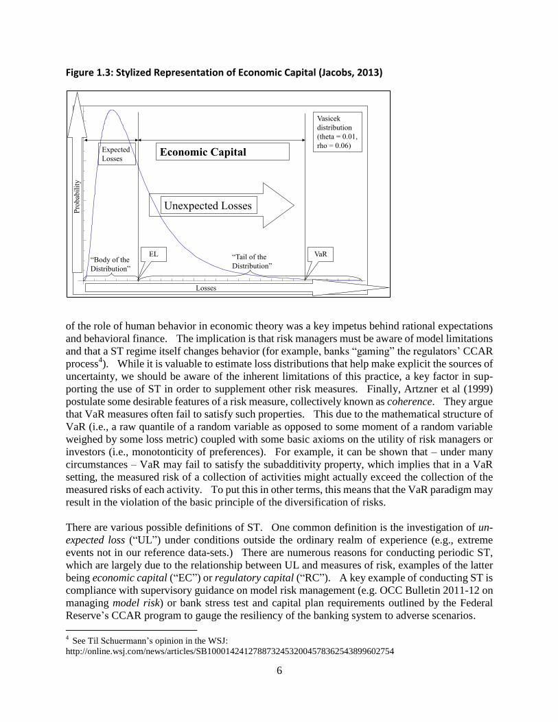
Figure 1.3: Stylized Representation of Economic Capital (Jacobs, 2013)

of the role of human behavior in economic theory was a key impetus behind rational expectations

and behavioral finance. The implication is that risk managers must be aware of model limitations

and that a ST regime itself changes behavior (for example, banks “gaming” the regulators’ CCAR

process4). While it is valuable to estimate loss distributions that help make explicit the sources of

uncertainty, we should be aware of the inherent limitations of this practice, a key factor in sup-

porting the use of ST in order to supplement other risk measures. Finally, Artzner et al (1999)

postulate some desirable features of a risk measure, collectively known as coherence. They argue

that VaR measures often fail to satisfy such properties. This due to the mathematical structure of

VaR (i.e., a raw quantile of a random variable as opposed to some moment of a random variable

weighed by some loss metric) coupled with some basic axioms on the utility of risk managers or

investors (i.e., monotonticity of preferences). For example, it can be shown that – under many

circumstances – VaR may fail to satisfy the subadditivity property, which implies that in a VaR

setting, the measured risk of a collection of activities might actually exceed the collection of the

measured risks of each activity. To put this in other terms, this means that the VaR paradigm may

result in the violation of the basic principle of the diversification of risks.

There are various possible definitions of ST. One common definition is the investigation of un-

expected loss (“UL”) under conditions outside the ordinary realm of experience (e.g., extreme

events not in our reference data-sets.) There are numerous reasons for conducting periodic ST,

which are largely due to the relationship between UL and measures of risk, examples of the latter

being economic capital (“EC”) or regulatory capital (“RC”). A key example of conducting ST is

compliance with supervisory guidance on model risk management (e.g. OCC Bulletin 2011-12 on

managing model risk) or bank stress test and capital plan requirements outlined by the Federal

Reserve’s CCAR program to gauge the resiliency of the banking system to adverse scenarios.

4 See Til Schuermann’s opinion in the WSJ:

http://online.wsj.com/news/articles/SB10001424127887324532004578362543899602754

0.01 0.02 0.03 0.04 0.05

20

40

60

80

Unexpected Losses

Expected

Losses

“Body of the

Distribution”

“Tail of the

Distribution”

Pro

bab

ilit

y

Losses

EL

Economic Capital

Vasicek

distribution

(theta = 0.01,

rho = 0.06)

VaR

7

Figure 1.4: Correlations Amongst Risk Types (Inanoglu and Jacobs, 2009)

EC is generally thought of as the difference between a VaR measure, or some extreme loss at some

confidence level (e.g., a high quantile of a loss distribution), and an expected loss (“EL”) measure,

the latter being generally thought of as some likely measure of loss over some time horizon (e.g.,

an allowance for loan losses for the coming year amount set aside by a bank.) In Figure 1.3,

reproduced from Jacobs (2013), we present a stylized representation of a loss distribution, and the

associated EL and VaR measures.

The use of stress testing to quantify EC hinges on our definition of UL. While it is commonly

thought that EC should cover EL, it may be the case that UL may not only be unexpected, but also

not credible, as it is a purely statistical concept. Therefore, some argue that results of a ST should

be used for EC purposes in lieu of UL. However, this practice is rare, as we usually do not have

probability distributions associated with stress events, and historical practice has indicated the

presence of fat-tails. Nevertheless, ST can be, and commonly has been, used to challenge the

adequacy of RC or EC, and as an input into the derivation of a buffer for losses exceeding the VaR,

especially for new products or portfolios.

ST has an advantage over EC in that it can often better address the risk aggregation problem – that

is, the existence of correlations amongst different risk types, thtbare in many cases large and

cannot be ignored. As different risks may be modeled very differently, it is challenging to ag-

gregate these into an EC measure. An advantage to ST in determining capital is that it can easily

aggregate different risk types (e.g., credit, market & operational), which is problematic under

standard EC methodologies (e.g., different horizons and confidence levels for market vs. credit

risk). In Figure 1.4, we again reproduce a figure from Inanoglu and Jacobs (2009), the pairwise

-2 0 2

x 108

-5 0 5

x 108

-2 0 2

x 107

0 2 4

x 107

0 2 4

x 107

-2

0

2

x 108

-5

0

5

x 108

-2

0

2

x 107

0

2

4

x 107

Pairwise Scattergraph & Pearson Correlations of 5 Risk Types

Top 200 Banks (Call Report Data 1984-2008)

0

2

4

x 107

Credit

Liqu.

Operat.

Market

Int.Rt.

corr(cr,ops)

= 0.6517

corr(mkt,liqu)

= 0.1127

corr(int,liqu)

= 0.1897

corr(cr,mkt)

= 0.2241

corr(ops,liqu)

= 0.1533

corr(mkt,int)

= 0.2478

corr(cr,liqu)

= 0.5343

corr(ops,int)

= -0.1174

corr(ops,mkt)

= 0.1989

corr(cr,int)

= -0.1328

8

correlations for a composite of the top 200 banks for 5 risk types (credit, market, liquidity, oper-

ational and interest rate risk), as proxied for by the FFIEC Call Report data. This is evidence that

powerful long-run dependencies exist across risk types. Even more compelling is that such de-

pendencies between risk types are accentuated during periods of stress. Embrechts et al (2001)

and Frey et al (2003) provide detailed discussions of correlation and dependency modeling in risk

management and various caveats with respect that discipline.

Apart from risk measurement or quantification, ST can be a risk management tool, to be used in

several ways when analyzing portfolio composition and resilience with respect to disturbances.

ST can help to identify potential uncertainties and locate the portfolio vulnerabilities, such as in-

curred but not realized losses in value, or weaknesses in structures that have not been tested.

ST can also aid in analyzing the effects of new complex structures and credit products for which

we may have a limited understanding. ST can also guide discussions on unfavorable develop-

ments, like crises and abnormal market conditions, which may be very rare, but cannot be ex-

cluded from consideration. Finally, ST can be instrumental in monitoring important sub-portfolios

exhibiting large exposures or extreme vulnerability to changes in market conditions.

Quantification of ST appears, and can be deployed, across several aspects of risk management

with respect to extreme losses. First, ST can be used to establish or test risk buffers. Further-

more, ST is a tool for helping to determine the risk capacity of a financial institution. Another use

of ST is in setting sub-portfolio limits, especially in low-default situations. ST can also be de-

ployed to inform risk policy, tolerance and appetite. Moreover, ST can provide the impetus for

actions necessary to reduce the risk of extreme losses and hence EC, and mitigate the vulnerability

to important risk-relevant effects. ST is also potentially a means to test portfolio diversification

by introducing (implicit) correlations. Finally, ST can help us to question a bank’s attitude to-

wards risk.

This paper shall proceed as follows. Section 2 considers supervisory developments in ST since

the financial crisis. Section 3 reviews the available literature on ST. Section 4 proposes a

Bayesian methodology for ST and for quantifying a model uncertainty buffer around a stressed

loss estimate. Section 5 presents the empirical implementation, the data description, a discussion

of the estimation results and their implications. Section 6 concludes the study and provides di-

rections for future avenues of research.

2 Supervisory Developments in Stress Testing

All regulatory capital models (“RCMs”) and bank internal economic capital models (“ECMs”)

have the objective of assessing the amount of capital resources and liquidity required by a financial

an institution to support its risk taking activities. This is contrasted with available capital and

liquidity resources, which may differ from what either the bank (through ECMs) or the supervisor

(through RCMs) believe to be required. We can further partition the assessment process into a

consideration of capital versus liquidity resources, corresponding to right and left sides of the

balance sheet (i.e., net worth versus the share of “liquid” assets), respectively. In the best case

9

scenario, not only do supervisory and bank models result in similar outputs, but also both do not

produce outputs that far exceed the regulatory floor.

It is well known that prior to the-financial crisis, the “great failures” (e.g., Lehman, Bear Stearns,

Washington Mutual, Freddie Mac and Fannie Mae) were well-capitalized according to the

standards across a wide span of regulators (e.g. Fed, SEC, OCC, OFHEO). Another commonality

included, in some manner (either directly or through securitization) a general exposure to resi-

dential real estate. Further, it is widely believed that the internal risk models of these institutions

were not wildly out of line with those of the regulators (Schuermann, 2013). We learned through

these unanticipated failures that the answer to the question of how much capital an institution

needs to avoid failure was not satisfactory. Granted, by construction RCMs and ECMs accept a

non-zero probability of default according to the risk aversion of the institution or the supervisor,

but the utter failure of these constructs to even come close to projecting the perils that these in-

stitutions faced was a great motivator for considering alternative tools to assess capital adequacy,

such as the ST discipline.

Various papers have laid out the reasons why ST has become such a dominant tool for regulators

(Jacobs, 2013; Schuermann, 2013), including rationales for its utility, outlines for its execution, as

well as guidelines and opinions on disseminating the output under various conditions. It has been

argued previously (and we will continue to build upon this line of reasoning) that a viable ST

program can, in a credible manner, quantify a gap in required capital, as well as means of filling

that gap. We would extend this construct by adding that there needs to be a means of measuring

the uncertainty inherent in these estimates, which transcends historical data, and stems from two

sources. First, we have to deal with prior expectations or non-data knowledge, which from the

point of view of supervisors may stem from private knowledge about the banks under their care;

and with respect to an institution, this prior may reflect the expectations with respect to what the

supervisor may require (e.g., in developing models for stress scenarios, banks often will use pre-

vious supervisory scenarios as input into the training data). Second, there are inherent uncer-

tainties in this process, either sampling error arising from calibration to historical data, or error in

anticipating supervisory scenarios.

Schuermann (2013) highlights the 2009 U.S. ST exercise, the Supervisory Capital Assessment

Program (“SCAP”) as an informative model. In that period there was incredible angst amongst

investors over the viability of the U.S. financial system, given the looming and credible threat of

massive dilution stemming from government action. The concept underlying the application of a

macro-prudential ST was that a bright line, delineating failure or survival under a credibly severe

systematic scenario, would convince investors that future dilution with respect to passing institu-

tions is a remote state of the world5. This exercise covered 19 banks in the U.S., having book

value of assets greater than $100B (comprising approximately two-thirds the total in the system) as

of the year-end 2008. The SCAP resulted in 10 of those banks having to raise a total of $75B

($77B) in capital (Tier 1 common equity) in a six month period, and no use of the CAP.

5 Further, in the case where institutions could not get the backing of investors to help them become well-capitalized,

the U.S. Treasury established the Capital Assistance Program (“CAP”), which functioned as a backstop for capital

requirements. Note that the perception was that U.S. Treasury was a sufficiently credible debt issuer that the CAP

promise was itself credible.

10

Clark and Ryu (2013) note that CCAR was initially planned in 2010 and rolled out in 2011. It

initially covered the 19 banks covered under SCAP, but as they document, a rule in November

2011 required all banks above $50 billion in assets to adhere to the CCAR regime. The CCAR

regime includes Dodd-Frank Act Stress Tests (“DFAST”), the sole difference between CCAR and

DFAST being that DFAST uses a homogenous set of capital actions on the part of the banks, while

CCAR takes banks’ planning distribution of capital into account when calculating capital ratios.

The authors further document that the total increase in capital in this exercise, as measured by Tier

1 common equity, was about $400 Billion. Final the authors highlight that ST is a regime that

allows regulators to not only set a quantitative hurdle for capital that banks must reach, but also to

make qualitative assessments of key inputs into the ST process, such as data integrity, governance,

and reliability of the models.

The outcome of the SCAP was rather different from Committee of European Bank Supervisors

(“CEBS”) stress tests in 2010 and 2011, which coincided with the sovereign debt crisis that hit the

periphery of the Euro-zone. In 2010, the ECBS stressed a total of 91 banks, as with the SCAP

covering about two-thirds of assets and one-half of banks per participating jurisdiction. There are

several differences with respect to the SCAP worth noting. First, the CEBS exercise stressed the

values of sovereign bonds held in trading books, but neglected to address that banking books

where in fact the majority of the exposures, resulting in a mild requirement of just under $5B in

additional capital. Second, in contrast to the SCAP, the CEBS ST level of disclosure was far less

granular, with loss rates reported for only two broad segments (retail vs. corporate) as opposed to

major asset classes (e.g., first-lien mortgages, credit cards, commercial real estate, etc.) The 2011

European Banker’s Association (“EBA”) exercise, covering 90 institutions in 21 jurisdictions,

bore many similarities to the 2011 EBA tests, with only 8 banks required to raise about as much

capital in dollar terms as the previous exercise. However, a key difference was the more granular

disclosure requirements, such as breakdowns of loss rates by not only major asset class but also by

geography, as well availability to the public in a user-friendly form that admitted the application of

analysts’ assumptions. In a similarity to 2010 exercise, in which the CEBS test did not ameliorate

nervousness about the Irish banks, is that the 2011 EBA version similarly did not ease concerns

about the Spanish banking system, as while 5 of 25 passed there was no additional capital required.

3 Review of the Literature in Stress Testing

Since the dawn of modern risk management in the 1990s, ST has been a tool used to address the

basic question of how exposures or positions behave under adverse conditions. Traditionally this

form of ST has been in the domain of sensitivity analysis (e.g., shocks to spreads, prices, volatili-

ties, etc.) or historical scenario analysis (e.g., historical episodes such as Black Monday 1987 or

the post-Lehman bankruptcy period; or hypothetical situations such as modern version of the Great

Depression or stagflation). These analyses are particularly suited to market risk, where data are

plentiful, but for other risk types in data-scarce environments (e.g., operational, credit, reputational

or business risk) there is a greater reliance on hypothetical scenario analysis (e.g., natural disas-

ters, computer fraud, litigation events, etc.).

11

The first mention of ST in supervisory guidance is in the 1995 Market Risk Amendment of the

1988 Basel I Accord, having a separate section and constituting a requirement for regulatory ap-

proval of internal models. Around the same time, the publication of RiskMetrics (1994) marked

risk management as a separate technical discipline, and therein all of the above mentioned types of

ST are referenced. Jorion (1996), the seminal handbook on VaR, also had a part devoted to the

topic of ST. Kupiec (1999) and Berkowitz (2000) provided detailed discussions of VaR-based

ST as found largely in the trading and treasury functions. The Committee on Global Financial

Systems (“CGFS”) conducted a survey on stress testing in 2000 (CGFS, 2000) that had similar

findings. Mosser, Fender, and Gibson (2001) highlighted that the majority of the ST exercises

performed to date were shocks to market observables based upon historical events, which have the

advantage of being well-defined and easy to understand, especially when dealing with the trading

book constituted of marketable asset classes.

However, in the case of the banking book (e.g., corporate / C&I or consumer loans), this approach

does not carry over very well. Therefore ST with respect to credit risk has evolved later and as a

separate discipline in the domain of credit portfolio modeling. However, even in the seminal

example of CreditMetrics (JP Morgan, 1997) and CreditRisk+ (Wilde, 1997), ST was not a

component of such models. Koyluoglu and Hickman (1998) demonstrated the commonality of

all such credit portfolio models, a correspondence between the state of the economy and the credit

loss distribution, and therefore that this framework is naturally amenable to ST. In this spirit

Bangia et al. (2002) build upon the CreditMetrics framework through macroeconomic ST on credit

portfolios using credit migration matrices. Foglia (2009) surveys of the then extant literature on ST

for credit risk. Rebonato (2010) argues for a Bayesian approach to ST, having the capability to

cohesively incorporate expert knowledge model design, utilizing causal networks.

ST supervisory requirements with respect to the banking book were rather undeveloped prior to

the crisis, although it was rather prescriptive in other domains, examples including the Joint Policy

Statement on Interest Rate Risk (SR 96-13), guidance on counterparty credit risk (SR 99-03), as

well as country risk management (SR 02-05).

Jacobs (2013) surveyed practices and supervisory expectations for ST in a credit risk framework,

and presented simple examples of a ratings migration based approach, using the CreditMetrics

framework and loss data from the regulatory Y9 reports in conjunction with Federal Reserve

scenarios. Jacobs et al (2015) propose a methodology for coherently incorporating expert opinion

into the ST modeling process, through the application of a Bayesian model, which can formally

incorporate exogenous scenarios and also quantify the uncertainty in model output that results

from stochastic model inputs. This approach was illustrated through estimating a Bayesian model

for credit loss using Fed Y9 data, with prior distributions formed from the supervisory mandated

macroeconomic scenarios.

4 Review of the Literature in Risk Aggregation

A modern diversified financial institution, engaging in a broad set of activities (e.g., banking,

brokerage, insurance or wealth management) is faced with the task of measuring and managing

12

risk across all of these. It is the case that just about any large, internationally active financial

institution is involved in at least two of these activities, and many of these are a conglomeration of

entities under common control. Therefore, we have the necessity of a framework in which dis-

parate risk types can be aggregated. However, this is challenging, due to the varied distributional

properties of the risks6. It is accepted that regardless of which sectors a financial institution fo-

cuses upon, they at least manage credit, market and operational risk. The corresponding super-

visory developments - the Market Risk Amendment to Basel 1, Advanced IRB to credit risk under

Basel 2 and the AMA approach for operational risk (BCBS 1988, 1996, 2004) – have given added

impetus for almost all major financial institutions to quantify these risks in a coherent way.

Furthermore, regulation is evolving toward even more comprehensive standards, such as the Basel

Pillar II Internal Capital Adequacy Assessment Process (ICAAP) (BCBS, 2009). In light of this,

institutions may have to quantify and integrate other risk types into their capital processes, such as

liquidity, funding or interest income risk. A quantitative component of such an ICAAP may be a

risk aggregation framework to estimate economic capital (EC)7 or stressed EC.

The central technical and conceptual challenge to risk aggregation lies in the diversity of distri-

butional properties across risk types, including different portfolio segments. In the case of market

risk, a long literature in financial risk management has demonstrated that portfolio value distri-

butions may be adequately approximated in a Gaussian, due to the symmetry and thin tails that

tend to hold at an aggregate level in spite of non-normalities at the asset return level (Jorion,

1996)8. In contrast, credit loss distributions are characterized by pronounced asymmetric and

long-tailed distributions, a consequence of phenomena such as lending concentrations or credit

contagion, giving rise to infrequent and very large losses. This feature is magnified for opera-

tional losses, where the challenge is to model rare and severe losses due to exogenous events, such

failures of systems or processes, litigation or fraud (e.g., the Enron or Worldcom debacles, or more

recently Societe Generale)9. While the literature abounds with examples of these three (Crouhy et

al., 2001), little attention has been paid to the even broader range of risks faced by a large financial

institution (Kuritzkes et al., 2003), including liquidity and asset / liability mismatch risk. In the

case of credit portfolio segments, which are often modeled independently for ST to-down appli-

cations yet may have very different distributions over time and cross-sectionally there is an

analogous problem to be solved.

Risk management as a discipline in its own right, distinct from either general finance or financial

institutions, is a relatively recent phenomenon. It follows that the risk aggregation question has

only recently come into focus. To this end, the method of copulas, which follows from a general

result of mathematical statistics due to Sklar (1956), readily found an application. This technique

allows the combination of arbitrary marginal risk distributions into a joint distribution, while

preserving a non-normal correlation structure. Among the early academics to introduce this

methodology is Embrechts et al. (2001, 2002). This was applied to credit risk management and

6 This is not unique to enterprise risk measurement for financial conglomerates, as it appears in several areas of fi-

nance, including corporate finance (e.g., financial management), investments (e.g., portfolio choice) as well as option

pricing (i.e., hedging). 7 However, in the U.S. supervisors are not requiring all institutions to model EC, only the largest and most systemi-

cally important (BCBS, 2009). 8 Even in this context, there are anomalies such as the stock market crash of 1987, which is an event which should

never have occurred under the normality of equity returns. 9 However, this does not cover catastrophic losses, e.g., the terrorist attacks of 9/11.

13

credit derivatives by Li (2000). The notion of copulas as a generalization of dependence ac-

cording to linear correlations is used as a motivation for applying the technique to understanding

tail events in Frey and McNeil (2001). This treatment of tail dependence contrasts to Poon et al

(2004), who instead use a data intensive multivariate extension of extreme value theory, which

requires observations of joint tail events.

5 A Time Series VAR Methodology for Modeling for the Correlation

Amongst Portfolio Segments

Let 1 ,...,T

t t ktY YY be a k -dimensional vector valued time series, the output variables of in-

terest, in our application with the entries representing some loss measure in a particular segment,

that may be influenced by a set of observable input variables denoted by 1 ,...,T

t t rtX XX , an r

-dimensional vector valued time series also referred as exogenous variables, and in our context

representing a set of macroeconomic factors. We say that that tY follows a multiple transfer

function process if we can write it in the following form:

*

0

t j t j t

j

Y Ψ X N (5.1)

Where *

jΨ are a sequence of k r dimensional matrices and tN is a k -dimensional vector of

noise terms which follow an stationary vector autoregressive-moving average process, denoted by

, ,VARMA p q s :

t tB BΦ N Θ ε (5.2)

Where 1

pj

r j

j

B B

Φ I Φ is the autoregressive lag polynomial, 1

qj

r j

j

B B

Θ I Θ is the

autoregressive lag polynomial and B is the back-shift operator that satisfies i

t t iB X X for any

process tX . It is common to assume that the input process tX is generated independently

of the noise process tN . In fact, the exogenous variables tX can represent both stochastic

and non-stochastic (deterministic) variables, examples being sinusoidal seasonal (periodic) func-

tions of time, used to represent the seasonal fluctuations in the output process tY , or interven-

tion analysis modeling in which a simple step (or pulse indicator) function taking the values of 0 or

1 to indicate the effect of output due to unusual intervention events in the system.

14

Now let us assume that the transfer function operator can be represented by a rational factorization

of the form * * 1 *

0

j

j

j

B B B B

Ψ Ψ Φ Θ , where * *

0

sj

j

j

B B

Θ Θ is of order s and *

jΘ are

k r matrices. For convenience, we assume that the factors We say that that tY follows a

vector autoregressive-moving average process with exogenous variables, denoted by

, ,VARMAX p q s , which is motivated by assuming that the transfer function operator in (5.1) can

be represented as a rational factorization of the form:

1

* * 1 * *

0 1 1

ps sj j j

j r j j

j j j

B B B B B B

Ψ Ψ Φ Θ I Φ Θ (5.3)

Where * BΘ is of order s and * k r

j R Θ are k r matrices. Without loss of generality, we

assume that the factor 1

pj

r j

j

B B

Φ I Φ is the same as the AR factor in the model for the noise

process tN . This gives rise to the , ,VARMAX p q s representation, where X stands for the

sequence of exogenous (or input) vectors:

*

1 1 1

p qs

t j t j j t j t j t j

j j j

Y Φ Y Θ X Θ (5.3)

Note that the VARMAX model (5.3) could be written in various equivalent forms, involving a

lower triangular coefficient matrix for tY at lag zero, or a leading coefficient matrix for t at lag

zero, or even a more general form that contains a leading (non-singular) coefficient matrix for tY at

lag zero that reflects instantaneous links amongst the output variables that are motivated by the-

oretical considerations (provided that the proper identifiability conditions are satisfied – see

Hannan (1971) or Kohn (1979) for further details). In the econometrics setting, such a model

form is usually referred to as a dynamic simultaneous equations model or a dynamic structural

equation model and the related model in the form of equation (5.3), obtained by multiplying the

dynamic simultaneous equations model form by the inverse of the lag 0 coefficient matrix, is re-

ferred to as the reduced form model10

.

The ARMAX model (5.3) is said to be stable if the roots of det 0B Φ are all greater than

unity in absolute value. In that case, if both the input tX and the noise tN processes are

stationary, then so is the output process tY having the following convergent representation:

10

In addition, (5.3) has the state space representation of the form (Hanan and Deistler, 1988):

1 1t t t t

t t t t

Z ΦZ BX a

Y HZ FX N

15

*

0 0

t j t j j t j

j j

Y Ψ X Ψ ε (5.4)

Where 1

0

i

i

i

B B B B

Ψ Ψ Φ Θ and * * 1 *

0

j

j

j

B B B B

Ψ Ψ Φ Θ .. The transi-

tion matrices *

jΨ of the transfer function * BΨ represent the partial effects that changes in the

exogenous (or input variables; macroeconomic variables or scenarios in our application) variables

have on the output variablestY at various time lags, and are sometimes called response matrices.

The long-run effects or total gains of the dynamic system (5.4) is given by the elements of the

matrix:

* *

0

1 j

j

G Ψ Ψ (5.5)

And the entry ,i jG represents the long-run (or equilibrium) change in the i

th output variable that

occurs when a unit change in the jth

exogenous variable occurs and is held fixed at some starting

point in time, with all other exogenous variables held constant In econometric terms, the ele-

ments of the matrices *

jΨ are referred to as dynamic multipliers at lag j, and the elements of G

are referred to as total multipliers.

In this study we consider a vector autoregressive model with exogenous variables (“VARX”),

denoted by ,VARX p s , which restricts the MA terms beyond lag zero to be zero, or

* 0j k k j Θ 0 :

1 1

p s

t j t j j t j t

j j

Y Φ Y Θ X (5.6)

The rationale for this restriction is three-fold. First, in no cases were MA terms significant in the

model estimations, so that the data simply does not support a VARMA representation. Second,

the VARX model avails us of the very convenient DSE package in R, which has computational

and analytical advantages. Finally, the VARX framework is more practical and intuitive than the

more elaborate VARMAX model, and allows for superior communication of results to practi-

tioners.

6 Empirical Implementation

As part of the Federal Reserve's CCAR exercise, U.S. domiciled top-tier BHCs are required to

submit comprehensive capital plans, including pro forma capital analyses, based on at least one

BHC defined adverse scenario. The adverse scenario is described by quarterly trajectories for key

16

macroeconomic variables (MVs) over the next nine quarters or longer, to estimate loss allow-

ances. In addition, the Federal Reserve generates its own supervisory stress scenarios, so that

firms are expected to apply both BHC and supervisory stress scenarios to all exposures, in order to

estimate potential losses under stressed operating conditions. Separately, firms with significant

trading activity are asked to estimate a one-time potential trading-related market and counterparty

credit loss shock under their own BHC scenarios, and a market risk stress scenario provided by the

supervisors. In addition, large custodian banks are asked to estimate a potential default of their

largest counterparty. In the case of the supervisory stress scenarios, the Federal Reserve provides

firms with global market shock components that are one-time, hypothetical shocks to a large set of

risk factors. For the last two CCAR exercises, these shocks involved large and sudden changes in

asset prices, rates, and CDS spreads that mirrored the severe market conditions in the second half

of 2008.

Since CCAR is a comprehensive assessment of a firm's capital plan, the BHCs are asked to con-

duct an assessment of the expected uses and sources of capital over a planning horizon. In the

2009 SCAP, firms were asked to submit stress losses over the next two years, on a yearly basis.

Since then, the planning horizon has changed to nine quarters. For the last three CCAR exercises,

BHCs are asked to submit their pro forma, post-stress capital projections in their capital plan be-

ginning with data as of September 30, spanning the nine-quarter planning horizon. The projec-

tions begin in the fourth quarter of the current year and conclude at the end of the fourth quarter

two years forward. Hence, for defining BHC stress scenarios, firms are asked to project the

movements of key MVs over the planning horizon of nine quarters. Our analysis on using the

macroeconomic stress scenarios to inform historical analysis is based on the collections move-

ments of the MVs over these nine quarter periods. As for determining the severity of the global

market shock components for trading and counterparty credit losses, it will not be discussed in this

paper, because it is a one-time shock and the evaluation will be on the movements of the market

risk factors rather the MVs. First, in the 2011 CCAR, the Federal Reserve defined the stress

supervisory scenario using nine MVs:

Real GDP (“RGDP”)

Consumer Price Index (“CPI”)

Real Disposable Personal Income (“RDPI”)

Unemployment Rate (“UNEMP”)

Three-month Treasury Bill Rate (“3MTBR”)

Ten-year Treasury Bond Rate (“10YTBR”)

BBB Corporate Rate (“BBBCR”)

Dow Jones Index (“DJI”)

National House Price Index (“HPI”)

Subsequently, In CCAR 2012, the number of MVs that defined the supervisory stress scenario

increased to 14. In addition to the original nine variables, the added variables were:

Real GDP Growth (“RGDPG”)

Nominal Disposable Income Growth (“NDPIG”)

Mortgage Rate (“MR”)

CBOE’s Market Volatility Index (“VIX”)

Commercial Real Estate Price Index (“CREPI”)

17

Additionally, there is another set of 12 international macroeconomic variables, three macroeco-

nomic variables and four countries / country blocks, included in the supervisory stress scenario.

As for CCAR 2013, the Federal Reserve System used the same set of variables to define the su-

pervisory adverse scenario as in 2012. For the purposes of this research, let us consider the su-

pervisory severely adverse scenario in 2014, focusing on 5 of the 9 most commonly used national

Fed CCAR MVs:

Year-on-Year Change in Real Gross Domestic Product (“RGDPYY”)

Unemployment Rate (“UNEMP”)

Dow Jones Equity Price Index (“DJI”)

National Housing Price Index (“HPI”)

Commercial Real Estate Price Index (“CREPI”)

We model aggregate bank gross chargeoffs (“ABCO”) from the Fed Y9 report as a measure of

loss, focusing on 5 segments:

Residential Real Estate (“RRE”)

Commercial Real Estate (“CRE”)

Consumer Credit (“CC”)

Commercial and Industrial (”CNI”)

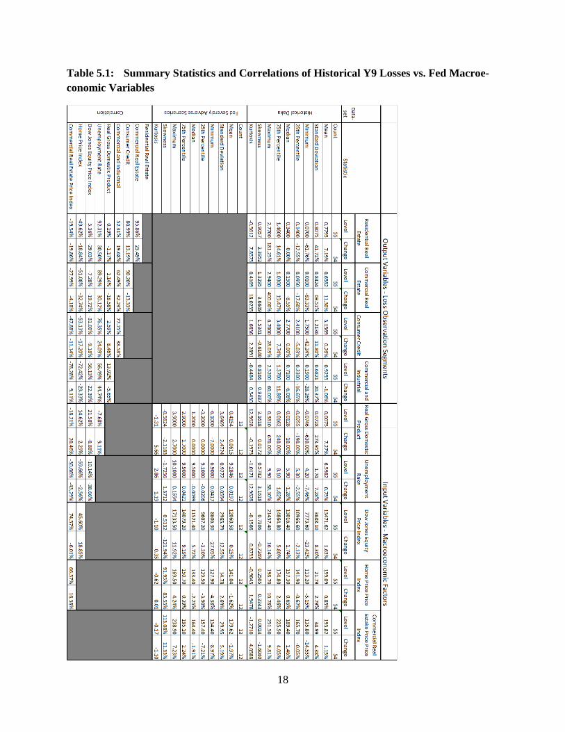
This data are summarized in Table 5.1 and in Figures 5.1 through 5.9. Starting with summary

statistics of the output loss variables, RRE has a mean level (percent change) of 78 bps (7.19%),

with some significant upward skew as the median level (percent change) is 34 bps (0.00%), var-

ying widely in level (percent change) from 7 bps (-63.76%) to 277 bps (181.25%), a high standard

deviation with respect to the mean in level (percent change) of 81 bps (41.72%). CRE has a mean

level (percent change) of 66 bps (11.30%), with some significant upward skew as the median level

(percent change) is 15 bps (-8.55%), varying widely in level (percent change) from 1 bps

(-83.33%) to 294 bps (400.00%), a high standard deviation with respect to the mean in level

(percent change) of 66 bps (69.51%). CC has a mean level (percent change) of 316 bps (0.26%),

with some significant upward skew as the median level (percent change) is 277 bps (0.00%),

varying widely in level (percent change) from 175 bps (-42.24%) to 670 bps (28.03%), a high

standard deviation with respect to the mean in level (percent change) of 121 bps (11.80%). Fi-

nally for outputs, CNI has a mean level (percent change) of 93 bps (-1.06%), with some significant

upward skew as the median level (percent change) is 71 bps (-6.08%), varying widely in level

(percent change) from 19 bps (-28.26%) to 252 bps (60.00%), a high standard deviation with re-

spect to the mean in level (percent change) of 689 bps (20.37%).

18

Table 5.1: Summary Statistics and Correlations of Historical Y9 Losses vs. Fed Macroe-

conomic Variables

19

Moving on to summary statistics the input macroeconomic loss driver variables, RGDPYY has a

mean level (percent change) of 0.75 bps (7.27%), with some significant upward skew as the me-

dian level (percent change) is -1 bps (-10.00%), varying widely in level (percent change) from 7

bps (-630.00%) to 38 bps (670.00%), a high standard deviation with respect to the mean in level

(percent change) of 7 bps (7.27%). UNEMP has a mean level (percent change) of 6.60%

(0.75%), with some significant upward skew as the median level (percent change) is 5.90%

(-1.28%), varying widely in level (percent change) from 4.20% (-7.46%) to 9.9% (38.10%), a high

standard deviation with respect to the mean in level (percent change) of 1.74% (7.28%). DJI has

a mean level (percent change) of 1.35e+4 (1.63%), with some significant upward (downward)

skew as the median level (percent change) is 1.30e+4 (1.74%), varying widely in level (percent

change) from 7.77e+3 (-23.42%) to 2.15e+4 (16.14%), a high standard deviation with respect to

the mean in level (percent change) of 3.69e+3 (8.30%). HPI has a mean level (percent change) of

159.09 (0.85%), with some significant upward skew as the median level (percent change) is 157.3

(0.65%), varying widely in level (percent change) from 113.20 (-5.15%) to 198.70 (10.78%), a

high standard deviation with respect to the mean in level (percent change) of 198.70 (10.78%).

Finally for inputs, CREPI has a mean level (percent change) of 193.82 (1.15%), with some sig-

nificant upward (downward) skew as the median level (percent change) is 189.40 (1.46%), varying

widely in level (percent change) from 135.80 (-14.55%) to 251.50 (9.81%), a high standard de-

viation with respect to the mean in level (percent change) of 34.99 (4.38%).

In general, all four output loss variables are highly correlated with each other, and more so in

levels than in percent changes, motivating the multiple equation approach. RRE and CRE are

nearly colinear (reasonably positively correlated), having a correlation coefficient of 95.9%

(23.5%) for levels (percent changes). RRE and CC are, having a correlation coefficient of 81.0%

(13.2%) for levels (percent changes). RRE and CNI are highly positively correlated (mildly

positively correlated), having a correlation coefficient of 52.3% (19.7%) for levels (percent

changes). CC and CRE are nearly colinear (marginally negatively correlated), having a corre-

lation coefficient of 90.2% (-13.3%) for levels (percent changes). CRE and CNI are highly pos-

itively correlated (mildly positively correlated), having a correlation coefficient of 62.5% (32.2%)

for levels (percent changes). Finally, CC and CNI are highly positively correlated (mildly posi-

tively correlated), having a correlation coefficient of 77.8% (38.6%) for levels (percent changes).

In general all five input macroeconomic variables are either highly positively or negatively cor-

related with each other (although there are some notable counter-examples), and more so in terms

of magnitude in levels as compared to percent changes, motivating the multiple equation approach.

A case of a small relationship in either level or percent change is RGDPYY and UEMP, having

respective correlation coefficients of -7.68% and 9.11%, respectively. RGDPYY and DJI are

reasonably positively correlated (nearly uncorrelated), having a correlation coefficient of 21.6%

(-0.88%) for levels (percent changes). RGDPYY and HPI are reasonably positively correlated

(nearly uncorrelated), having a correlation coefficient of 14.6% (2.29%) for levels (percent

changes). RGDPYY and CREPI are marginally negatively correlated (marginally positively

20

Figure 5.1: Time Series and Kernel Density Plots of Residential Real Estate Loans - Gross

Chargeoff Rate Level and Percent Change

Figure 5.2: Time Series and Kernel Density Plots of Commercial Real Estate Loans - Gross

Chargeoff Rate Level and Percent Change

21

correlated), having a correlation coefficient of -18.2% (20.5%) for levels (percent changes).

UNEMP and DJI are marginally negatively correlated (reasonably negatively correlated), having a

correlation coefficient of -10.1% (-38.7%) for levels (percent changes). UNEMP and HPI are

highly negatively correlated (nearly uncorrelated), having a correlation coefficient of -59.7%

(-2.56%) for levels (percent changes). UNEMP and CREPI are reasonably negatively correlated

(reasonably negatively correlated), having a correlation coefficient of -30.7% (-43.3%) for levels

(percent changes). DJI and HPI are reasonably positively correlated (marginally positively cor-

related), having a correlation coefficient of 45.6% (18.9%) for levels (percent changes). DJI and

CREPI are reasonably positively correlated (marginally positively correlated), having a correla-

tion coefficient of 74.6% (-6.01%) for levels (percent changes). Finally, HPI and CREPI are

highly positively correlated (marginally positively correlated), having a correlation coefficient of

66.6% (16.4%) for levels (percent changes).

Finally for the correlation analysis, we consider the correlations between the macroeconomic input

variables and the loss output variables. RRE is uncorrelated (uncorrelated) with RGDPYY in

levels (percent changes), having a correlation coefficient of 0.19% (-1.17%). RRE is nearly

colinear (reasonably positively correlated) with UNEMP in levels (percent changes), having a

correlation coefficient of 92.3% (30.2%). RRE is nearly marginally positively (reasonably neg-

atively) correlated with DJI in levels (percent changes), having a correlation coefficient of 5.36%

(-29.0%). RRE is nearly reasonably negatively (somewhat negatively) correlated with HPI in

levels (percent changes), having a correlation coefficient of -49.6% (-18.8%). RRE is nearly

somewhat negatively (somewhat negatively) correlated with CREPI in levels (percent changes),

having a correlation coefficient of -19.5% (-19.9%). CRE is uncorrelated (reasonably negatively

correlated) with RGDPYY in levels (percent changes), having a correlation coefficient of 1.14%

(-18.6%). CRE is nearly colinear (reasonably positively correlated) with UNEMP in levels

(percent changes), having a correlation coefficient of 89.3% (30.2%). CRE is nearly marginally

nbegatively (reasonably negatively) correlated with DJI in levels (percent changes), having a

correlation coefficient of -5.289% (-19.7%). CRE is nearly reasonably negatively (reasonably

negatively) correlated with HPI in levels (percent changes), having a correlation coefficient of

-51.1% (-32.7%). CRE is nearly reasonably negatively (marginally negatively) correlated with

CREPI in levels (percent changes), having a correlation coefficient of -28.0% (-4.12%). CC is

uncorrelated (reasonably positively correlated) with RGDPYY in levels (percent changes), having

a correlation coefficient of 2.59% (8.46%). CC is highly positively (reasonably positively cor-

related) with UNEMP in levels (percent changes), having a correlation coefficient of 76.45%

(24.1%). CC is nearly reasonably negatively (marginally negatively) correlated with DJI in levels

(percent changes), having a correlation coefficient of -31.0% (-9.18%). CC is nearly highly

negatively (reasonably negatively) correlated with HPI in levels (percent changes), having a cor-

relation coefficient of -51.1% (-17.2%). CC is nearly highly negatively (marginally negatively)

correlated with CREPI in levels (percent changes), having a correlation coefficient of -47.9%

(-11.1%).

22

Figure 5.3: Time Series and Kernel Density Plots of Consumer Loans - Gross Chargeoff

Rate Level and Percent Change

Figure 5.4: Time Series and Kernel Density Plots of Commercial & Industrial Loans -

Gross Chargeoff Rate Level and Percent Change

23

Figure 5.5: Time Series and Kernel Density Plots of Real GDP Growth Level and Percent

Change

Figure 5.6: Time Series and Kernel Density Plots of the Unemployment Rate Level and

Percent Change

24

Figure 5.7: Time Series and Kernel Density Plots of the Dow Jones Equity Index Level and

Percent Change

Figure 5.8: Time Series and Kernel Density Plots of the U.S. National Residential Housing

Price Index Level and Percent Change

25

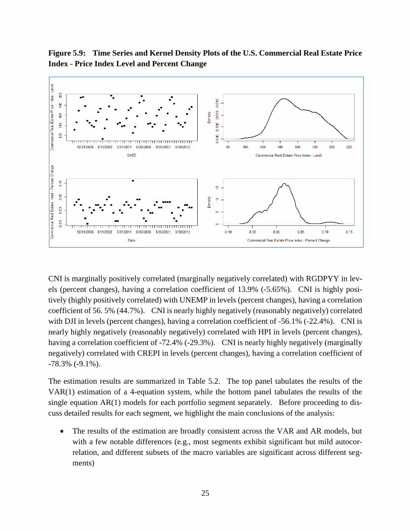
Figure 5.9: Time Series and Kernel Density Plots of the U.S. Commercial Real Estate Price

Index - Price Index Level and Percent Change

CNI is marginally positively correlated (marginally negatively correlated) with RGDPYY in lev-

els (percent changes), having a correlation coefficient of 13.9% (-5.65%). CNI is highly posi-

tively (highly positively correlated) with UNEMP in levels (percent changes), having a correlation

coefficient of 56. 5% (44.7%). CNI is nearly highly negatively (reasonably negatively) correlated

with DJI in levels (percent changes), having a correlation coefficient of -56.1% (-22.4%). CNI is

nearly highly negatively (reasonably negatively) correlated with HPI in levels (percent changes),

having a correlation coefficient of -72.4% (-29.3%). CNI is nearly highly negatively (marginally

negatively) correlated with CREPI in levels (percent changes), having a correlation coefficient of

-78.3% (-9.1%).

The estimation results are summarized in Table 5.2. The top panel tabulates the results of the

VAR(1) estimation of a 4-equation system, while the bottom panel tabulates the results of the

single equation AR(1) models for each portfolio segment separately. Before proceeding to dis-

cuss detailed results for each segment, we highlight the main conclusions of the analysis:

The results of the estimation are broadly consistent across the VAR and AR models, but

with a few notable differences (e.g., most segments exhibit significant but mild autocor-

relation, and different subsets of the macro variables are significant across different seg-

ments)

26

Across all 4 segments, according to the likelihood ratio statistic, we reject the hypothesis

that the restrictions of the single equation AR models are justified

The VAR models are generally more accurate according to standard measures of model fit

with respect to each segment

It is inconclusive whether the VAR or AR models are more or less conservative as meas-

ured by cumulative 9-quarter loss

First, we discuss the results for the RRE segment. In the VAR model the autoregressive term is

significantly positive but small, a parameter estimate 0.1750, which is also significant but rather

larger in the AR model having an estimate 0.2616. The cross autoregressive term on CRE is

significantly positive in the VAR model but small, a parameter estimate 0.0819. The coefficient

estimates of the macroeconomic sensitivities on UNEMP (HPI) are significant and positive (neg-

ative) for RRE in the VAR model, having values of 0.7628 (-1.0130), which are also significant in

the AR model and of the same sign, albeit larger (larger0 in magnitude in the latter case with re-

spective values of 0.8847 (-1.0727). According to the likelihood ratio test for the RRE segment, a

value of 54.20 rejects the 35 parameter restrictions of the AR with respect to the VAR model at a

very high level of confidence. The VAR model outperforms the AR model for the RRE segment

according to the RMSE, SC and CPE measures with values of 0.1043, 0.4821 and -397.8% in the

former as compared to 0.1089, 0.4373 and -977.0% in the latter. The VAR model is also more

conservative than the AR model, having a 9 quarter cumulative loss of 59.2% in the former, versus

56.8% in the latter.

Second, we discuss the results for the CRE segment. In the VAR model the autoregressive term is

significantly positive but small, a parameter estimate 0.1880, which is however insignificant and

rather larger in the AR model having an estimate 0.1167. The cross autoregressive term on RRE

is significantly positive in the VAR model and substantial, a parameter estimate 0.5986. The

coefficient estimates of the macroeconomic sensitivities on UNEMP (DJI) are significant and

positive (negative) for CRE in the VAR model, having values of 1.3966 (-0.8806), which are also

significant in the AR model and of the same sign, albeit larger (smaller) in magnitude in the latter

case with respective values of 1.7100 (-0.8716). Furthermore, in the AR model the mac-

ro-sensitivity on RGDPYY is significant, although of the incorrect sign, having a value of 0.0209.

According to the likelihood ratio test for the CRE segment, a value of 82.08 rejects the 35 pa-

rameter restrictions of the AR with respect to the VAR model at a very high level of confidence.

The VAR model outperforms the AR model for the CRE segment according to the RMSE, SC and

CPE measures with values of 0.3808, 0.1826 and 83.0% in the former as compared to 0.3883,

0.1510 and -101.0% in the latter. However, the VAR model is also less conservative than the AR

model, having a 9 quarter cumulative loss of 83.0% in the former, versus 110.0% in the latter.

27

Table 5.2: Vector Autoregressive vs. Single Equation Autoregressive Model Estimation

Compared (Fed Macroeconomic Variables and Aggregate Y9 Bank Chargeoffs)

28

Next, we discuss the results for the CC segment. In the VAR model the autoregressive term is

significantly positive reasonably large in magnitude, a parameter estimate 0.4437, which is also

significant and rather larger in the AR model having an estimate 0.4080. The cross autoregres-

sive term on CC is significantly positive in the VAR model and substantial, a parameter estimate

0.4437. The coefficient estimates of the macroeconomic sensitivities on 4 of the 5 drivers

RGDPYY, UNEMP, HPI and DJI are significant for CC in the VAR model; having respective

values of 0.040, 4.88, -13.32 and 2.47 – however note that the signs on RGDPYY and CREPI are

counterintuitive. Similarly in the AR model for these variables, estimates are also significant and

close in magnitude - having respective values of 0.0361, 5.27, -12.82 and 2.72 – and the signs on

RGDPYY and CREPI are also counterintuitive. According to the likelihood ratio test for the CC

segment, a value of 47.16 rejects the 35 parameter restrictions of the AR with respect to the VAR

model at a very high level of confidence. The VAR model outperforms the AR model for the CC

segment according to the RMSE, SC and CPE measures with values of 0.5565, 0.3709 and 94.1%

in the former as compared to 0.5704, 0.3448 and 106.7% in the latter. Furthermore, the VAR

model is also conservative than the AR model, having a 9 quarter cumulative loss of 273.1% in the

former, versus 269.6 in the latter.

Finally, we discuss the results for the CNI segment. In the VAR model the autoregressive term is

insignificantly positive but small, a parameter estimate 0.1386, and is also insignificantly positive

but somewhat larger in size in the AR model having an estimate 0.1443. The cross autoregressive

terms are all insignificant in the VAR model. The coefficient estimates of the macroeconomic

sensitivities on RGDPYY are significant and negative for CNI in the VAR model, having a value

of -0.1340, which is also significant in the AR model and of the same sign, albeit smaller in

magnitude in the latter case with a respective value -0.1222. According to the likelihood ratio test

for the CNI segment, a value of 17.61 fails to reject the 35 parameter restrictions of the AR with

respect to the VAR model, having a large p-value and implying that for this segment the VAR

model may not be statistically viable by tis measure. The VAR model outperforms (underper-

forms) the AR model for the CNI segment according to the RMSE and SC (CPE) measures

(measure) with values of 1.2512 and 0.0947 (-507.8%) in the former as compared to 0.1089 and

0.4373 (-507.0%) in the latter. The VAR model is also very slightly less conservative than the

AR model, having a 9 quarter cumulative loss of -168.8% in the former, versus -168.1% in the

latter.

In Figures 5.10 through 5.26 present the plots of actual vs. predicted losses, residual diagnostic and

scenario forecast plots for each modeling segment in the VAR and in each single equation AR

model. Through an examination of these plots, we can conclude that the VAR model performs

better than the AR models in terms of forecast accuracy and quality of the residuals.

29

Figure 5.10: One Step Ahead Predictions versus Actual Values – Vector Autoregressive

Model (Residential Mortgage, Commercial Real Estate, Consumer and C&I Loan Losses)

Figure 5.11: Residual Diagnostic Plots – Vector Autoregressive Model (Residential Mort-

gage, Commercial Real Estate, Consumer and C&I Loan Losses)

30

Figure 5.12: Residual Autocorrelation Function Plots – Vector Autoregressive Model (Res-

idential Mortgage, Commercial Real Estate, Consumer and C&I Loan Losses)

31

Figure 5.13: Historical Values vs. Scenario Forecast Plots – Vector Autoregressive Model

(Residential Mortgage, Commercial Real Estate, Consumer and C&I Loan Losses)

Figure 5.14: One Step Ahead Predictions versus Actual Values –Autoregressive Model

(Residential Mortgage)

32

Figure 5.15: Residual Diagnostic Plots – Autoregressive Model (Residential Mortgage)

Figure 5.16: Residual Autocorrelation Function Plots –Autoregressive Model (Residential

Mortgage)

33

Figure 5.17: Historical Values vs. Scenario Forecast Plots –Autoregressive Model (Residen-

tial Mortgage)

Figure 5.18: One Step Ahead Predictions versus Actual Values –Autoregressive Model

(Commercial Real Estate)

34

Figure 5.19: Residual Diagnostic Plots –Autoregressive Model (Commercial Real Estate)

Figure 5.20: Residual Autocorrelation Function Plots –Autoregressive Model (Commercial

Real Estate)

35

Figure 5.21: Historical Values vs. Scenario Forecast Plots –Autoregressive Model (Com-

mercial Real Estate)

Figure 5.22: One Step Ahead Predictions versus Actual Values –Autoregressive Model

(Consumer Loans)

36

Figure 5.23 Residual Diagnostic Plots –Autoregressive Model (Consumer Loans)

Figure 5.24: Residual Autocorrelation Function Plots –Autoregressive Model (Consumer

Loans)

37

Figure 5.25: Historical Values vs. Scenario Forecast Plots – Autoregressive Model (Con-

sumer Loans)

Figure 5.26: One Step Ahead Predictions versus Actual Values – Autoregressive Model

(Commercial and Industrial Loans)

38

Figure 5.27 Residual Diagnostic Plots –Autoregressive Model (Commercial and Industrial

Loans)

Figure 5.28: Residual Autocorrelation Function Plots –Autoregressive Model (Commercial

and Industrial Loans)

39

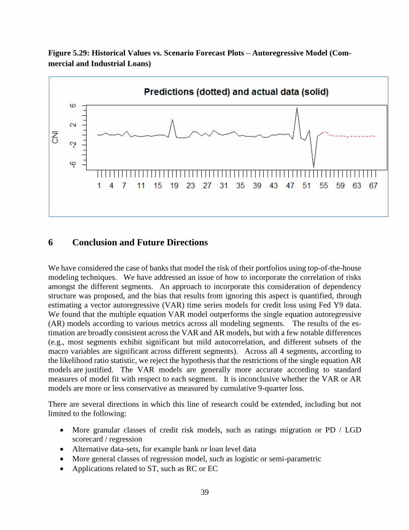
Figure 5.29: Historical Values vs. Scenario Forecast Plots – Autoregressive Model (Com-

mercial and Industrial Loans)

6 Conclusion and Future Directions

We have considered the case of banks that model the risk of their portfolios using top-of-the-house

modeling techniques. We have addressed an issue of how to incorporate the correlation of risks

amongst the different segments. An approach to incorporate this consideration of dependency

structure was proposed, and the bias that results from ignoring this aspect is quantified, through

estimating a vector autoregressive (VAR) time series models for credit loss using Fed Y9 data.

We found that the multiple equation VAR model outperforms the single equation autoregressive

(AR) models according to various metrics across all modeling segments. The results of the es-

timation are broadly consistent across the VAR and AR models, but with a few notable differences

(e.g., most segments exhibit significant but mild autocorrelation, and different subsets of the

macro variables are significant across different segments). Across all 4 segments, according to

the likelihood ratio statistic, we reject the hypothesis that the restrictions of the single equation AR

models are justified. The VAR models are generally more accurate according to standard

measures of model fit with respect to each segment. It is inconclusive whether the VAR or AR

models are more or less conservative as measured by cumulative 9-quarter loss.

There are several directions in which this line of research could be extended, including but not

limited to the following:

More granular classes of credit risk models, such as ratings migration or PD / LGD

scorecard / regression

Alternative data-sets, for example bank or loan level data

More general classes of regression model, such as logistic or semi-parametric

Applications related to ST, such as RC or EC

40

7 References

Acharya, V. V. and Schnabl, P., 2009, “How banks played the leverage game” in: Acharya,

V. V. and M. Richardson (eds) Restoring Financial Stability, pp. 44-78, Wiley Finance.

Araten, M., Jacobs, Jr., M., P. Varshney, and Pellegrino, C.R., 2004a, An internal ratings migra-

tion study, The Journal of the Risk Management Association, April, 92-97.

, Jacobs Jr., M., and P. Varshney, 2004a. Measuring LGD on commercial loans: An 18-year

internal study, The Journal of the Risk Management Association, May, 28-35.

Artzner, P., Delbaen, F., Eber, J.M., and D. Heath, 1999, Coherent measures of risk, Mathematical

Finance, 9:3, 203-228.

Bangia, A. Diebold, F.X., Kronimus, A., Schagen, C., and Schuermann, T. ,2002, Ratings migra-

tion and the business cycle, with application to aredit portfolio stress testing, Journal of Banking

and Finance, 26, 445- 474.

Basel Committee on Banking Supervision (BCBS), 1988, Internal convergence of capital meas-

urement and capital standards, Basel, Switzerland.

, 1996, Amendment to the capital accord to incorporate market risks, Basel, Switzerland.

, 2004, International convergence of capital measurement and capital standards: a re-

vised framework, Basel, Switzerland.

, 2009, Range of practices and issues in economic capital frameworks, Basel, Switzer-

land.

, 1999, “Supervisory Guidance Regarding Counterparty Credit Risk Management”, Feb-

ruary

, 2002, “Interagency Guidance on Country Risk Management”, March

, 2005, “An Explanatory Note on the Basel II IRB Risk Weight Functions, Bank for

International Settlements”, July.

,2006, “International Convergence of Capital Measurement and Capital Standards: A

Revised Framework”, Bank for International Settlements, June.

,2009a, “Principles for Sound Stress Testing Practices and Supervision - Consultative

Paper, May (No. 155).

,2009b, “Guidelines for Computing Capital for Incremental Risk in the Trading Book”,

Bank for International Settlements, July.

41

, 2009c, “Revisions to the Basel II Market Risk Framework”, Bank for International Set-

tlements, July.

,2009d, “Analysis of the Trading Book Quantitative Impact Study”, Bank for Interna-

tional Settlements Consultative Document, October.

,2009e, “Strengthening the Resilience of the Banking Sector” Bank for International

Settlements Consultative Document, December.

, 2010a, “Basel III: A Global Regulatory Framework for More Resilient Banks and

Banking Systems”, Bank for International Settlements, December.

, 2010b, “An Assessment of the Long-Term Economic Impact of Stronger Capital and

Liquidity Requirements”, Bank for International Settlements, August.

J. Berger. Statistical Decision Theory and Bayesian Analysis. Springer, New York (1985)

Berkowitz, J. ,2000, “A Coherent Framework for Stress-Testing,” Journal of Risk, 2, 1-11.

The Board of Governors of the Federal Reserve, 1996, “Joint Policy Statement on Interest Rate

Risk”, May

Bernardo, J. M., and A. F. M. Smith (1994). Bayesian Theory. Chichester: Wiley

Cifarelli, D.M.and P. Muliere, 1989, Statistica Bayesiana, ianni Iuculano Editore.

Clark, T., and L. Ryu ,2013, “CCAR and Stress Testing as Complementary Supervisory Tools”,

Board of Governors of the Federal Reserve Supervisory Staff Reports.

The Committee on Global Financial Systems, 2000, Stress Testing by Large Financial Institutions:

Current Practice and Aggregation Issues, Bank for International Settlements, April.

Crouhy, M., Galai, D., and R. Mark, 2001, Risk Management (McGraw Hill, New York, NY).

de Finetti, B ,1970a,b, Theory of Probability, Wiley, New York

DeGroot, Morris (1970). Optimal Statistical Decisions. McGraw-Hill, New York

Demirguc-Kunt, A., Detragiache, E. and O. Merrouche, ,2010, Bank capital: lessons from the

financial crisis, World Bank Policy Research Working Paper No. 5473, November.

Efron, B. and R. Tibshirani, 1986, Bootstrap methods for standard errors, confidence intervals,

and other measures of statistical accuracy, Statistical Science 1(1), 54-75.

Embrechts, P., A. McNeil, and D. Straumann ,2001, “Correlation and dependency in risk

management: properties and pitfalls” in: M. Dempster, and H. Moffatt (eds) Risk Manage-

ment: Value at Risk and Beyond, pp. 87-112, Cambridge University Press.

42

, McNeil, A.J., Straumann, D., 2002. Correlation and dependence in risk man-

agement: properties and pitfalls., in Dempster, M.A.H., ed.:, Risk Management: Value

at Risk and Beyond, ( Cambridge University Press, Cambridge, UK), 176–223.

Foglia, A, 2009, Stress Testing Credit Risk: A Survey of Authorities’ Approaches, International

Journal of Central Banking 5(3), p 9-37.

Frey, R., McNeil, A.J., 2001, Modeling dependent defaults, Working paper, ETH Zurich.

Frye, J., and Jacobs, Jr., M., 2012, Credit loss and systematic LGD, The Journal of Credit Risk,

8:1 (Spring), 109-140.

Gordy, M., 2003, A risk-factor model foundation for ratings-based bank capital rules, Journal

of Financial Intermediation, 12(3): 199-232.

Geweke, J. Contemporary Bayesian Econometrics and Statistics. Hoboken: Wiley,

2005.

Hanan, E.J., 1971, The identification problem for multiple equation systems with moving average

errors, Econometrica 39, 751-766.

and Diestler, M. (1988), The Statistical Theory of Linear Systems, New York: John

Wiley.

Inanoglu, H., and M. Jacobs, Jr., 2009, Models for risk aggregation and sensitivity analysis: An

application to bank economic capital, The Journal of Risk and Financial Management 2, 118-189.

, Jacobs, Jr., M., Liu, J., and R. Sickles, 2014, Analyzing bank efficiency: Are

“too-big-to-fail” banks efficient?, Forthcoming.

Jacobs Jr., M., 2010, An empirical study of exposure at default, The Journal of Advanced Studies

in Finance, Volume 1, Number 1 (Summer.)

, 2013, Stress testing credit risk portfolios, Journal of Financial Transformation, 37:

53-75 (April).

, and N. M. Kiefer ,2010, “The Bayesian Approach to Default Risk: A Guide,” (with.) in

Ed.: Klaus Boecker, Rethinking Risk Measurement and Reporting (Risk Books, London).

, 2010, Validation of economic capital models: State of the practice, supervisory expec-

tations and results from a bank study, Journal of Risk Management in Financial Institutions, 3:4

(September), 334-365.

, and Karagozoglu, A, 2011, Modeling ultimate loss given default on corporate debt, The

Journal of Fixed Income, 21:1 (Summer), 6-20.

43

, Karagozoglu, A., and D. Layish, 2012, Resolution of corporate financial distress: an

empirical analysis of processes and outcomes, The Journal of Portfolio Management, Winter,

117-135.

, and A. Karagozoglu, 2014, On the characteristics of dynamic correlations between asset

pairs, Research in International Business and Finance 32, 60-82.

, Karagozoglu, A., and D. Naples, 2013, Measuring credit risk: CDS Spreads vs. credit

ratings, Hofstra University & Pricewaterhouse Coopers LLC, Working paper.

Jorion, P., 1996, “Risk2: Measuring the Value at Risk” Financial Analyst Journal 52, 47-56.

J.P. Morgan, 1994, “RiskMetrics”, Second Edition, J.P. Morgan.

, 1997, “CreditMetrics”, First Edition, J.P. Morgan

Knight, F.H.,1921,: “Risk, Uncertainty and Profit”, The River Press, Cambridge.

Kohn, R., 1979, Asymptotic resuktsresults for ARMAX structures, Econometrica 47, 1295–1304.

Koyluoglu, H, and A Hickman, 1998, “Reconcilable Differences”, Risk, October, 56-62

Kupiec, P, 1999, “Risk Capital and VaR”, The Journal of Derivatives 7(2), 41-52.

Kuritzkes, A., 2002, Operational risk capital: a problem of definition, Journal of Risk Finance

(Fall), 1-10.

Li, D.X., 2000, On default correlation: a copula function approach, Journal of Fixed Income 9, 43–

54.

Merton, R., 1974, On the pricing of corporate debt: the risk structure of interest rates, Journal of

Finance 29(2): 449–470.

Mosser, Patricia C. and Fender, Ingo and Gibson, Michael S., 2001, “An International Survey of

Stress Tests”. Current Issues in Economics and Finance, Vol. 7, No. 10. Available at SSRN:

http://ssrn.com/abstract=711382 or http://dx.doi.org/10.2139/ssrn.711382

The U.S. Office of the Comptroller of the Currency (“OCC”) and the Board of Governors of the

Federal Reserve System (“BOG-FRB”), 2011, Supervisory Guidance on Model Risk Manage-

ment (OCC 2011-12).

O'Hagan, A. (1988). Probability: Methods and Measurement. Chapman and Hall, London.

Poirier, Dale J., 1995, Intermediate Statistics and Econometrics, Cambridge: The

MIT Press.

44

Poon, S.-H., Rockinger, M., Tawn, J., 2004, Extreme value dependence in financial markets: di-

agnostics, models and financial implications, Review of Financial Studies 17, 581–610.

Popper, K.R., 1945, “The Open Society and its Enemies”, Routledge & Kegan, New York.

R Development Core Team , 2013,: “R: A Language and Environment for Statistical Computing.”

R Foundation for Statistical Computing, Vienna, Austria, ISBN 3-900051-07-0.

Rebonato, R, 2010, “Coherent Stress Testing: A Bayesian Approach”, Wiley, New York.

Robert, C. (2001), The Bayesian Choice: From decision-Theoretic Motivations to Computational

Implementation, Second Edition, New York, Springer-Verlag.

Savage, L, 1954, “The Foundations of Statistics”, Dover Publications

Schuermann, T, 2013, “Stress testing banks”, International Journal of Forecasting, Forthcoming.

Sklar, A. ,1956, Fonctions de répartition à n dimensions et leurs marges, Publications de l'Institut

de Statistique de L'Université de Paris 8, 229-231.

van Deventer, D. R., Imai, K., and M. Mesler (2004): “Integrated Credit Risk and Interest Rate

Risk Management”, Wiley, New York, N.Y.

Wilde, T. 2010. Creditrisk+. Encyclopedia of Quantitative Finance.

Zelner, A. (1971), An Introduction to Bayesian Inference in Econometrics, New York: Wiley,

reprinted in Wiley Classics Library, 1996.