LtBRAKVNPS-59BC74112A ,-scwnical i

NAVAL P08T*WOUATE SCHOOL

NAVAL POSTGRADUATE SCHOOL

Monterey, California

STRESS ANALYSIS OF THERMOWELLS

by

John E. Brock

11 November 1974

Approved for public release; distribution unlimited

FEDDOCSD 208.14/2:NPS-59BC7112A

NAVAL POSTGRADUATE SCHOOLMonterey, California

Rear Admiral Isham Linder J. R. Bor stingSuperintendent Provost

STRESS ANALYSIS OF THERMOWELLS

This monograph examines the mechanical-structuralintegrity of thermowells to sustain pressurizationand excitations due to fluid flow. Suggested designcriteria, which are shown to be conservative, aremore inclusive than currently employed criteria,and in one important aspect, namely with respect to

pressurization, are more liberal.

SECURITY CLASSIFICATION OF THIS PAGE (When Dete 1Entered)

REPORT DOCUMENTATION PAGE READ INSTRUCTIONSBEFORE COMPLETING FORM

1. REPORT NUMBER

NPS-59BC74112A

2. GOVT ACCESSION NO. 3. RECIPIENT'S CATALOG NUMBER

4. TITLE (and Subtitle)

STRESS ANALYSIS OF THERMOWELLS

5. TYPE OF REPORT & PERIOD COVERED

6. PERFORMING ORG. REPORT NUMBER

7. AUTHORfa;

John E. Brock

8. CONTRACT OR GRANT NUMBERfa;

9 PERFORMING ORGANIZATION NAME AND ADDRESSProfessor John E. Brock (Code 59Bc)Department of Mechanical EngineeringNaval Postgraduate School

10. PROGRAM ELEMENT. PROJECT, TASKAREA & WORK UNIT NUMBERS

II. CONTROLLING OFFICE NAME AND ADDRESS 12 REPORT DATE

11 November 197413 NUMBER OF PAGES

107U. MONITORING AGENCY NAME & ADDRESSf// different from Controlling Office) 15. SECURITY CLASS, (of thle riport)

Unclassified

15«. OECLASSIFI CATION/ DOWN GRADINGSCHEDULE

16. DISTRIBUTION STATEMENT (of thlt Report)

Approved for public release; distribution unlimited.

17. DISTRIBUTION STATEMENT (of the abatract entered In Block 30, If different from Report)

18. SUPPLEMENTARY NOTES

19. KEY WORDS (Continue on reveree elde It neceeemry end Identity by block number)

ThermowellsCantilever vibrationExternally pressurized cylindersStress analysisTapered cantilevers

20. ABSTRACT (Continue on reveree efde It neceeemry and Identity by block number)

This monograph examines the mechanical-structural integrity of thermowellsto sustain pressurization and excitations due to fluid flow. Suggesteddesign criteria, which are shown to be conservative, are more inclusivethan currently employed criteria, and in one important aspect, namely withrespect to pressurization, are more liberal.

DD ,:°NRM

73 1473(Page 1)

EDITION OF 1 NOV 68 IS OBSOLETES/N 0102-014- 6601

|

SECURITY CLASSIFICATION OF THIS PACE (When Dmta Kntarad)

TABLE OF CONTENTS

Body of the Report 4

Appendix A. Elastic-Plastic Behavior of Externally Pressurized 14

Hollow Circular Cylinders

Appendix B. Estimation of Exciting Frequency and Forces 35

Appendix C. Response Frequencies of Thermowell Vibration 48

Appendix D. Bending Stresses and the Combined Stress Criterion 82

Appendix E. Fatigue Reliability Calculations 93

Appendix F. Plan and Sequence of Calculations 96

Appendix G. Numerical Example 102

A thermowell is a metallic product fitted into the wall of a pipe or

vessel so as to permit introduction of a thermometer or thermocouple for

the purpose of measuring the temperature of the contents. It is designed

so as to maintain the integrity of the pressure boundary without introducing

unacceptable measurement errors or time lags. This monograph summarizes

the results of analytical studies made by the writer during the past two

years of the mechanical/structural integrity of thermowells . It is obvious

that much of this material is also applicable to other insertions such as

sampling tubes, which, however, need not sustain the differential pressuriza-

tion to which thermowells are subject.

An existing section (1) of the ASME Power Test Codes, based very

largely upon analysis reported by J. W. Murdock (6) , represents the consensus

of the ASME Committee PB51 (on Thermowells) . Designers have recently found

it difficult to reconcile the strict requirements of this document with the

practical necessity of providing thermowells for boiler feed discharge and

main steam services. In the summer of 1972, Mr. J. E. Leary, Chief Control

and Instrumentation Engineer of Bechtel Power Corporation, asked the writer

to examine the structural integrity of thermowells and to compose recom-

mendations for analysis of high pressure thermowells. A report (3) and

a supplement (4) were produced shortly thereafter. A related study (5) , by

Professor T. M. Houlihan, examining the thermal performance of thermowells

was also produced at this time; from this study it may be inferred that

thermowell tip details which permit full assurance of structural integrity

impose no problems of inaccurate temperature measurement or thermal time

lag.

Subsequent to the production of the reports (3), (4), and (5), Mr.

Leary asked the writer to solicit and collect comments from Mr. Murdock and

members of the PB51 Committee. The writer is very pleased to acknowledge

the participation and cooperation of the following persons

:

Mr. J. W. Murdock, formerly of the Applied Physics Department,

U. S. Naval Ship Engineering Center, Philadelphia, and presentlya private consulting engineer.

Mr. L. A. Dodge, Bailey Meter Company

Mssrs. J. Archer and T. Reitz, Gilbert Associates

Mssrs. R. F. Abrahamsen and J. D. Fishburn, Combustion Engineering, Inc.

Mssrs. A. Lohmeier and A. J. Partington, Westinghouse Electric Corporation

Mr. W. N. Wright, TemTex Temperature Systems and Components

Mr. W. 0. Hays, ASME (Secretary, PB51)

The most significant change recommended by the writer in his first

report (3) was a drastic relaxation of the requirements with respect to

simple pressurization. This matter is discussed in detail in Appendix A

hereto. In the first report, in what seems to have proved to be a mistaken

attempt at simplifying the presentation of the analysis, the writer consid-

ered internally pressurized hollow cylinders, a case to which most pertinent

engineering literature has addressed itself. However, the point was

established that with any material failure theory which is independent of

the first scalar invariant of the stress tensor, the internally and externally

pressured cases are equivalent if strains are limited to the order of magni-

tude of elastic strains. In the present Appendix A, the analysis is specifi-

cally directed to the externally pressurized case. However, precisely the

same results are obtained as previously.

The comments generated in response to the writer's request dealt

preponderately with the matter of pressurization and its consequences.

While the need is acknowledged in the case of supercritical pressure instal-

lations to depart from the limitations imposed by strict application of the

rules for externally pressurized vessels to be found in Section VIII of

the ASME Boiler and Pressure Vessel Code, there is a reluctance actually

to do so, and some responders feel that a test program is called for.

However, the writer is absolutely certain in his own mind that internal

pressurization tests would be absolutely useless. External pressurization

tests might indeed prove useful as a basis for establishing rules even more

liberal than the writer suggests (cf. Appendix A) should the need to do so

ever arise. The writer's first report failed to cite the classic experi-

ments of Prof. P. W. Bridgman (2) which should be adequately demonstrative

of the ability of very thick wall, externally pressurized cylinders to

retain pressure integrity even under extreme pressurizations . The comments

of Mr. J. D. Fishburn conclude with the statement:

"...In fact, Professor Brock's solution remains a conservative solu-

tion apart from the Code limitation of S = (5/8) a. This is form

three reasons. Firstly, as stated by Professor Brock, 'for external

pressurization. .. gross deformation is such as to modify the geometry

advantageously,' secondly, a non-workhardening material is assumed,

and, thirdly, there is considerable experimental evidence to show

that the generalized Tresca condition for yield is of itself conser-

vative.

"For these reasons there should be no objections from the

industry to this section of Professor Brock's analysis, particularly

since the Nuclear Code specifies a value of 3S as the limitingm

stress range (Section III NM3222.2)."

Briefly, the writer, having studied all comments on the matter of

pressurization and rules relating thereto, remains firm in his conviction

that the liberalized criterion he recommends (cf. Section 10 of Appendix A)

is still so conservative that it might be further liberalized if the need

to do so should ever arise.

A second, and relatively unimportant pressure criterion relates to

the thickness of tip closure for cantilevered thermowell. The requirement

stated in Section II of Appendix A is simple and probably very conservative.

The third recommended criterion relates to the necessity of assuring

that the mechanical excitation provided by the forces exerted on the thermo-

well by fluid flowing past it not be in resonance with a natural vibration

mode of the thermowell structure. The analysis of this matter naturally

divides itself into three aspects: (a) estimation of the exciting frequency,

(b) estimation of the response (natural) frequency of thermowell vibration,

and (c) consideration of how closely these may be permitted to approach one

another.

The most troublesome and controversial of these sub-problems is the

first, which is discussed in detail in Appendix B hereto. For many years

it was thought that the dimensionless parameter (called the Strouhal number)

determining the frequency of vortex shedding for fluid flow past a fixed,

rigid cylinder had a definite value (N = .21, appr. ) for all flows faster

than those characterized by Reynold's number (based on cylinder diameter)

N = 800 (appr.) and Murdock's analysis (6) is based upon N = .21. How-

ever, more recent data, not available at the time of Murdock's study,

indicate that the Strouhal number may become as great as N = .45 for

large Reynold's numbers (N = 6.2 x 10 6, appr.). This suggests that the

frequency of excitation can become more than twice as great as previously

contemplated. The writer's first report (3) employed this newer information

in estimating the excitation frequency.

Comments received in this regard pointed out that there was lack

of coherence in the vortex shedding which takes place for these higher

values of Reynold's number and that, accordingly, the danger of resonant

excitation is thereby diminished. There can be no argument with this

contention but the question remains: to what extent is the probability of

resonant excitation actually reduced? The experimental data invite a varie-

ty of interpretations and, in the writer's opinion, it is prudent to assume

that coherent excitation of sufficient duration (perhaps as briefly as a

fraction of a second at the frequencies involved) to cause damage can

occur if excitation frequency based on N - . 45 equals or exceeds the

natural response frequency. Accordingly, the criteria recommended herein

are based upon the possibility of coherent excitation with N = .45 in the

appropriate range of Reynold's numbers. However, if these criteria are

not met, it is suggested that the designer-engineer feel free to re-examine

the matter, making use of whatever new information may at that time be

available and making a special examination of the probability and conse-

quences of coherent excitation. In correspondence with the PB51 Committee,

the writer has suggested that the use of appropriate vibration test instru-

mentation applied to existing thermowell installations can possibly provide

information which will help to assess the dangers of excitation in this

regime. It should be made clear that this area is one in which persuasive

information is indeed lacking and the writer's recommended criteria are

intended to be definitely conservative.

The second of these three subproblems is that of estimating the

natural response frequencies of thermowell vibration. This matter is the

subject of Appendix C hereof, in which, throughout, it is assumed that we

are dealing with a thermowell which is firmly attached to the pipe or ves-

sel wall at one end (the root) and is free at the other end (the tip).

Section 14 of Appendix C discusses a structural mode, not elsewhere

discussed except in the supplement (4) to the writer's earlier report,

which involves ovalization of the pipe or vessel and which is at relatively

low frequency. An argument is offered for regarding this mode as of no

practical significance, but it would certainly be desirable to have experi-1

mental evidence that this is the case.

The bulk of Appendix C relates to the estimation of the lowest mode

of cantilever beam vibration. There are several complicating factors. The

structure is nonuniform and is so short and stubby that rotatory inertia

and shear deformation have a significant effect in reducing the response

frequency as compared to what might be calculated by the use of so-called

"elementary" theory. Furthermore, the pipe or vessel wall to which the

thermowell is attached is itself flexible and possesses mass and this causes

a further reduction in response frequency, compared to the elementary

assumption of fixed root.

In Appendix C an attempt is made to take all these effects into

account. A dynamic study employing the powerful new tool of the "finite

element method" (FEM) is clearly the best practical way to perform the

analysis and such an investigation is currently under way as a thesis study

by LT. H. L. Crego, USM. Lacking the results of such a study, a "scrambling

effort" is made in Appendix C to provide a reasonably accurate method of

estimating natural frequency, accounting for non-uniformity of section and

for the several non-elementary mechanisms which tend to depress the

frequency. Briefly, the recommendation in Appendix C is that the frequency

be calculated for the non-uniform cantilever by use of elementary theory

(some curves presenting the results of such calculation are included, cf.

Figure C-5 in Appendix C) and that the depressing mechanisms be accounted

for (approximately) by use of a frequency reduction factor.

This brings us to the third of the subproblems listed above. In his

original study, Murdock (6) made the requirement r < 0.8, where r = ratio

of excitation frequency to natural response frequency, basing this recom-

mendation upon a discussion he had on this subject with Professor J. P.

den Hartog. Because of the uncertainties surrounding the calculation of

these frequencies, particularly the effects of rotatory inertia, shear

deflection, and foundation compliance and inertia, the writer feld strongly

that the requirement r < 0.8 should be reduced to r < 0.4 and he so recom-

mended in his original report (3). In the supplement thereto (4) the

writer made a first attempt at including some of the depressing effects,

and, as a result, proposed raising the limiting value of r to 0.65. In

the present study, reported in Appendix C hereof, the completeness of the

estimate of the depressing effects is believed to be much better. With

the degree of uncertainty markedly reduced, it is reasonable to liberalize

the requirement on the ratio r to its original value, namely, again we

require that r < 0.8. However, it is very important to note that the

denominator in the expression for r must adequately account for the depress-

ing effects of rotatory inertia, shear deflection, and foundation compliance

and inertia. An appropriate way of doing so is by use of the frequency

reduction factor. Finite element studies, currently in progress, should

permit refining the analysis.

The pressure criterion and the non-resonance criterion are the most

important criteria. However, we are also concerned with the gross effect

and the fatigue effect of bending. Although the bending moment is obviously

greatest at the root, for a tapered section, the section modulus varies in

such a way that the maximum bending stress may not occur at the root as

was assumed by Murdock (6) and in the writer's earlier analysis (3), the

10

latter, incidentally being marred by an analytical error. In Appendix D

the matter of maximum bending stress and maximum stress intensity is inves-

tigated. It is found that the previous assumption that the maximum occurs

at the root is indeed true except for thermowells which are sharply tapered

or strongly shielded or both. Appendix E similarly studies the fatigue

effects; in the analysis of fatigue stresses a stress intensification fac-

tor of 6.0 is assumed. This value is quite conjectural. It is believed

to be conservative. However the opinion of engineers who deal daily with

stress intensification factors is definitely solicited on this choice. If

a value different from 6.0 should be recommended by competent authority,

the numerical factors in the formula in Appendix E should be proportionately

modified.

Appendices D and E represent no changes in philosophy as compared to

their first presentation in the writer's earlier report. However, the new

presentations include the effect of partial shielding from the fluid stream,

something not taken into consideration earlier, and they correct a simple

algebraic error which was introduced earlier and which was "incorrectly

corrected" in some subsequent correspondence with the PB51 Committee.

The bulk of the analysis is presented in Appendices A through G

hereof. Appendices A through E have been referred to above. Appendix F

is. a Plan and Sequence of Calculations, showing all the recommended

criteria. Appendix G presents a Numerical Example.

The writer joins others who may object that the present study, which

is almost exclusively theoretical, fails to reflect operational experience.

The most earnest solicitation of information dealing with failure, leakage,

malperformance, etc., of thermowells attributable to mechanical/structural

considerations turned up only one case, that of a thermowell which began

11

leaking around at the root connection after many years of successful

service; in this case, the difficulty seemed almost certainly attributable

to a poorly executed attaching weld. Mr. J. E. Leary has expressed the

hope that lack of reports of other cases may indicate a corresponding lack

of operational difficulties; the writer's past experience does not lead to

as sanguine a hope, only to the conclusion that a previously observed

reluctance to report or to discuss or even to reveal failures of any kind

of any equipment in any service extends also to thermowells. However, the

one instance cited above permits the writer to discourse upon his very

strong conviction that thermowells, as well as any other devices or

appurtenances the installation of which involves penetrating the pressure

boundary, must be attached by full penetration welds (or their "equivalent"

whatever that may be in a particular situation) and that, furthermore,

the "branch connection reinforcement rules" must be satisfied. See the

discussion in Section 11 of Appendix A, hereof.

Acknowledgments

This work has been substantially supported by Bechtel Power Corpora-

tion by arrangement with Mr. J. E. Leary, Chief Control and Instrument

Engineer. The original report (3) and supplement (4) were consulting

reports to Bechtel which kindly permitted their dissemination to the PB51

Committee and to other interested persons. Bechtel Power Corporation has

also supported a considerable share of the subsequent correspondence with

commentators and the reworking into the present form. John F. Wax, Inc.

,

has also supported some of this work; as a result of this and similar

charities, this corporation is no longer active. The Naval Postgraduate

School has supplied stenographic service, computer facilities, and publica-

tion effort; this may be regarded as in support of the writer's activities

12

as a member of the Mechanical Design Committee of the USAS B31 Code Group,

and, until his recent resignation (for reasons of austerity) , as a member

of the Working Group on Piping for Section III of the ASME Boiler and Pres-

sure Vessel Code.

General Bibliography

(Most of the Appendices have their own bibliographies; cf. General

Table of Contents and individual Tables of Contents for the Appendices.)

1. ASME, Power Test Codes, Instruments and Apparatus, Part 3, Temperature

Measurement, Paragraphs 8-19, incl. , pp. 7-9.

2. Bridgman, P. W. , Large Plastic Flow and Fracture, McGraw-Hill 1952,

Chapter 8, pp. 142-163.

3. Brock, J. E. , Stress Analysis of Thermowells, report to Bechtel Power

Corporation, October 1972.

4. Brock, J. E. , Supplement (to preceding listing).

5. Houlihan, T. , Thermowell Calculations (Accuracy and Response), report

to Bechtel Power Corporation, October 1972.

6. Murdock, J. W. , Power Test Code Thermometer Wells, J. Eng. Power

(ASME Trans.), October 1952, pp. 403-416.

13

APPENDIX A

ELASTIC-PLASTIC BEHAVIOR OF EXTERNALLYPRESSURIZED HOLLOW CIRCULAR CYLINDERS

TABLE OF CONTENTS

Page

1. Basic Analysis 15

2. Elastic Pressure P and Ultimate Pressure P 17

3. Dimensional Changes 17

4. Repeated Pressurization, Elastic Shakedown, and 21

One-Cycle Shakedown Pressure P*

5. Basis of Recommended Criteria 22

6. Numerical Example 23

7. Remarks About Experiments and Other Analysis 24

8. Thin-Wall Thermowells 28

9. Factor of Safety 29

10. Statement of Recommended Pressure Criteria 30

11. Analysis of Closure and Attachment 31

12. Bibliography 33

14

EXTERNALPRESSURE

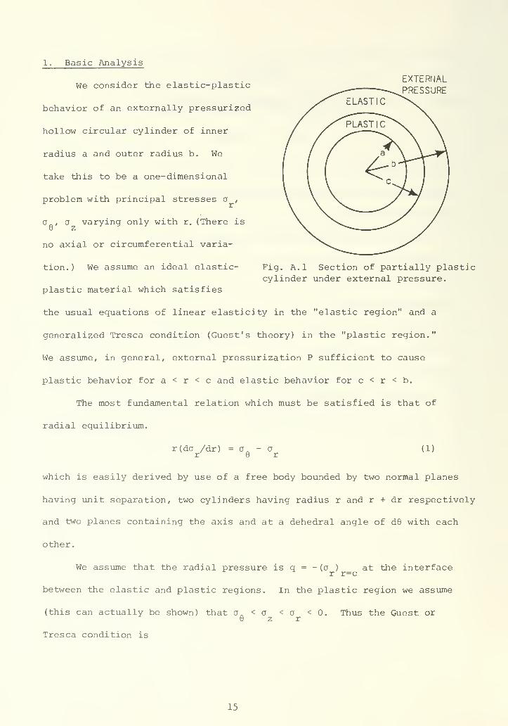
Fig. A.l Section of partially plasticcylinder under external pressure.

1. Basic Analysis

We consider the elastic-plastic

behavior of an externally pressurized

hollow circular cylinder of inner

radius a and outer radius b. We

take this to be a one-dimensional

problem with principal stresses a ,

a n , o varying only with r. (There is6 z

no axial or circumferential varia-

tion.) We assume an ideal elastic-

plastic material which satisfies

the usual equations of linear elasticity in the "elastic region" and a

generalized Tresca condition (Guest's theory) in the "plastic region."

We assume, in general, external pressurization P sufficient to cause

plastic behavior for a < r < c and elastic behavior for c < r < b.

The most fundamental relation which must be satisfied is that of

radial equilibrium.

r(da /dr) = n - a (1)r 8 r

which is easily derived by use of a free body bounded by two normal planes

having unit separation, two cylinders having radius r and r + dr respectively

and two planes containing the axis and at a dehedral angle of d8 with each

other.

We assume that the radial pressure is q = - (a ) at the interfacer r=c

between the elastic and plastic regions. In the plastic region we assume

(this can actually be shown) that o„ < a < o < 0. Thus the Guest or9 z r

Tresca condition is

15

a - a a= o .(2)

r 6

where a is the yield stress for the ideal elastic plastic material. The

solution which satisfies (1) and (2) and the boundary condition (a ) =3T IT— cl

is

a = -a ln(r/a); o n = -a [1 + ln(r/a)] (3a, b)r 6

This gives

q = aln(c/a) (4)

as the interface pressure and it also gives

(C7 ) = -q - a (5)8 r=c

Lame's solution for the elastic region incorporates the usual elastic

stress strain relations and the equilibrium relation (1) . It gives

a = [qc2-Pb

2+(P-q)b

2c2/r

2]/(b

2-c

2) (6a)

aQ

= [qc2-Pb 2-(P-q)b

2c2/r

2]/(b

2-c

2) (6b)

From (6a) it is easily verified that (a ) = -q and (a ) , = -P. Fromr r=c r r=b

(6b) we find

(CVr=c= te(b2+c2 )- 2Pb2 ]/(b2- c2 ) ( 7 )

and equating this to the expression given by (5) , one gets

P = q + a(b 2-c 2 )/2b 2(8)

Using (4) one can also write

P = a[ln(c/a) + (b 2-c 2)/2b 2] (9)

and

P = q + (a/2) [1 - (a 2/b 2)ln(2a/q)] (10)

Equations (9) and (10) give P explicitely in terms of c and q

respectively. However, given P, a more difficult evaluation is required

to find c and/or q.

16

2. Elastic Pressure P and Ultimate Pressure PE U

If P is sufficiently small, c = a and q = 0. The Lame solutions

become

(b2-a 2

)a = -Pb 2(l-a

2/r 2) (11a)

r

(b2-a 2

)a Q= -Pb 2

(l+a2/r 2

) (lib)

(b 2-a 2 )a = -Pb 2( llc )

z

The third of these is obtained by assuming an end of the cylinder is closed

and that the external pressure also acts on the closure. Obviously the

maximum principal stress difference is

a - a n = 2Pa2b2 /r2 (b

2 -a2

) (12)r

which is a maximum at r = a, viz.

(a -o a )= 2Pb2 /(b

2-a

2) (13)

r 6 r=a

Thus, as P is increased, the Tresca condition is first encountered when

P = P_ = a(b2-a2 )/2b2(14)

E

The subscript E indicates elastic action for P < P .

E

On the other hand, for sufficiently high pressurization, the inter-

face radius c assumes the value b and the interface pressure q assumes the

value P, whence

P = P = aln(b/a) (15)

3. Dimensional Changes

The subscript U denotes ultimate . However, in contradistinction

with the usual case to which this word is applied, in the present case

application of the "ultimate" load does not imply "plastic collapse" with

"large" deformations. The reason for this is that the geometrical changes

due to external pressurization are such as to increase the wall thickness.

17

Bridgman (3) has made a large strain analysis of externally pressurized

cylinders and reference will later be made to his analysis. For the present,

however, the following simple analysis will suffice.

Experiments by Bridgman and others and analysis by Bridgman indicates

vanishingly small axial deformations even under pressures which result in

gross change of diameters. Under plastic action, the volume remains con-

stant. Thus, assuming initial radii a , b , and fully plastic action, new

radii a , b are obtained such that2 2

P = aln(b /a ) ; b2-a

2 = b2-a

2(16a, b)

2 2 112 2

The first of these reflects fully plastic action (with no strain hardening)

and the second reflects the volume constancy. We have assumed P > P =

CTln (b /a ), and, given P, a, a , and b we wish to calculate a and b .

1 1 * 1 1 2 2

Using the notations

n = P/Py > 1; a = a /b < 1 (17a, b)

we easily find

/(1-ab2

= b!

/(1"a )/(!- a )'• a2

= b2a (18a, b)

For example, with a = .3, b = 1.0 » a pressure three times as great

as P gives d = .3, n = 3. Using equations (18) we find b = .9543, a =

.0258". The internal radius has been made quite small but equilibrium has

been restored. If strain hardening occurs, the effective value of n is

reduced and the distortion is not quite as great as indicated.

There is nothing, except limitations of pressurization facilities

to restrict the value of n. For example, assuming a = 65000 psi (accounting

for heat treatment and some strain hardening) and an applied pressure

P = 400000 psi, the value of P is 78260 psi so that n = 5.11. Then we

18

calculate b = .9539", a = .0020". Clearly the final dimensions are not

particularly sensitive to the value of n if n > 2. This calculation is

consistent with experiments reported by Bridgman (3) except that Bridgman

observed some cases for which the central cavity closed completely. Obviously

it would take only a very, very small longitudinal contraction to cause this

to happen.

The point of these recent remarks is to the effect that volume con-

stancy acts to provide dimensional changes which restore equilibrium in

the case of external pressurization whereas, in the case of internal pres-

surization, volume constancy gives a thinning of the wall which, in itself,

acts to remove the situation even farther from equilibrium which can be

restored, if at all, only by virtue of strain hardening. Thus catastrophic

collapse is_ possible for internal pressure but it is not possible for exter-

nal pressurization.

Accordingly, simply from the standpoint of maintaining pressure

integrity, there is no theoretical limit to the external pressure which

may be applied. However we are also concerned with maintaining a reasonable

approximation to the original internal dimensions so that the thermocouple

assembly may be withdrawn and replaced even when the pressure is applied.

For this reason, we now consider the dimensional changes which can be

expected with P = P . The exterior surface is barely at the plastic stage

so that we can use elastic formulas. Experiment indicates that we should

take z = 0, along with a = -P . o n = -o + o = -a(l + lnb/a) . We findz r U 6 r

= Ee = a - v(o.+o ) ; a = v (a n+o )

z z 6 r z 6 r

Ee = a - v(a +a ) = o-vo -v 2 (o.+o )86 rz 6r 0r= - (l-v 2)a + (l-v-2v 2)a

r

= -(l-v 2)a- (l-v-2v 2)alnb/a (19)

19

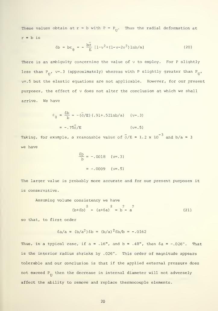
These values obtain at r = b with P = P . Thus the radial deformation at

r = b is

6b = be_ - - =£ [l-v 2+(l-v-2v 2 )lnb/a] (20)6 E

There is an ambiguity concerning the value of v to employ. For P slightly

less than P , v=.3 (approximately) whereas with P slightly greater than P ,

v=.5 but the elastic equations are not applicable. However, for our present

purposes, the effect of v does not alter the conclusion at which we shall

arrive. We have

eQ

= ^ = -(a/E) (.91+.521nb/a) (v=.3)

= -.75a/E (v=.5)

-3Taking, for example, a reasonable value of a/E = 1.2 x 10 and b/a = 3

we have

-4r = -.0018 (V=.3)D

= -.0009 (V=.5)

The larger value is probably more accurate and for our present purposes it

is conservative.

Assuming volume consistency we have

2 2 2 2

(b+6b) - (a+6a) = b - a (21)

so that, to first order

6a/a = (b/a2) 6b = (b/a) 2 6b/b = -.0162

Thus, in a typical case, if a = .16", and b = .48", then 6a = -.026". That

is the interior radius shrinks by .026". This order of magnitude appears

tolerable and our conclusion is that if the applied external pressure does

not exceed P then the decrease in internal diameter will not adversely

affect the ability to remove and replace thermocouple elements.

20

4. Repeated Pressurization, Elastic Shakedown, and the One-Cycle Shake-down Pressure P*.

We assume initial pressurization to a pressure P (P < P < P ) soE U

that there has been plastic behavior from r = a to r = c, (a < c < b) . We

presume however that subsequent removal of this pressure results in no

additional plastic behavior. That is, the depressurization operation is

purely elastic. Thus we can arrive at the final state of stress by super-

posing the Lame stress system

c = Pb 2 (l-a2/r 2 )/(b2-a 2) (22a)

r

a. = Pb2 (l+a 2/r 2 )/(b2 -a 2) (22b)

upon the system given by equations 3 and 6. The maximum (equivalent or

Tresca) stress state after depressurization occurs at r = a and is positive,

i.e., at r = a we have

o = 0, a. = -a + 2Pb 2/(b2-a2) (23)

r u

If the yield condition is not to be exceeded (this time in the

opposite sense from originally) , we must have

(a.) - (a ) < a (24)6 r=a r r=a

and this gives

Pb 2/(b 2-a 2) < a; P < P* = 2P^ - a(b 2-a 2 )/b 2 (25)

E

We will use the symbol P* = 2P and refer to the condition describedE

above as "one cycle shakedown" since it assures that after the plastic

yielding occurring on initial pressurization there can be no subsequent

yielding.

Our previous analysis has led us to conclude that if P < P the

deformations will be acceptable. Thus, we obviously wish to compare the

21

pressures P and P*. Equating these values, and using the notation a = a/b,

we immediately obtain the equation

1 + lna = a 2 (26)

which has two roots, a = 1, which is meaningless for our application, and

a = 0.4503 (27)

For a > 0.4503, P < P* and if we required P < P , then one cycle shake-

down is absolutely assured. For a < 0.4503, one cycle shakedown requires

limiting P to a maximum of P* < P .

5. Basis of Recommended Criteria

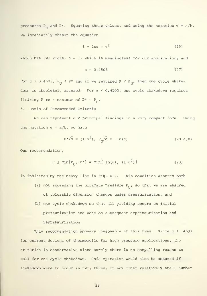
We can represent our principal findings in a very compact form. Using

the notation a = a/b, we have

P*/a = (1-a 2), P /a = -ln(a) (28 a,b)

Our recommendation,

P £ Min{P , P*} = Min{-ln(a), (1-a 2)} (29)

is indicated by the heavy line in Fig. A-2. This condition assures both

(a) not exceeding the ultimate pressure P , so that we are assured

of tolerable dimension changes under pressurization, and

(b) one cycle shakedown so that all yielding occurs on initial

pressurization and none on subsequent depressurization and

repressurization

.

This recommendation appears reasonable at this time. Since a < .4503

for current designs of thermowells for high pressure applications, the

criterion is conservative since surely there is no compelling reason to

call for one cycle shakedown. Safe operation would also be assured if

shakedown were to occur in two, three, or any other relatively small number

22

CURVED MARKED H4 JARE (JXMJEC-

TURED;; DO tllOT U$E QUAN

0.0 0.2 0.4 0.6

Radius ratio a = a/b

Fig. A-2 Summary of most significant pressure calculations.

of cycles. P/a curves for such n-cycle shakedown have been conjecturally

sketched in Fig. A-2 for n = 2,3, and 4; these curves should not be used

quantitatively. The analytical difficulties involved do not presently

warrant working out their actual shape. However, in the future, in any

case where the presently recommended criterion should prove to be restric-

tive there would be ample reason to reconsider the matter so as to permit

two or three cycle shakedown or so as to permit exceeding the pressure P .

6. Numerical example

So as to demonstrate the self consistency of the preceding analysis,

it is desired to consider a practical case. We take a/b = a = 0.3 and

easily calculate P = 0.4550a, P* = 0.9100a, and P = 1.2040a. We take

23

P = P* and let 3 = c/b. From equation 9, which becomes

1-a 2 = ln(B/a) + (l-3 2 )/2 (30)

we calculate 3 = .51655. This also gives q/a = ln3/a = .5434. Stress

calculations are shown in Table A-l and Figure A- 3. The "final state"

referred to is at the end of the first pressurization cycle, external

pressure P = . 9/a having been applied once and then removed. After initial

yielding, subsequent application and removal of P = . 9/o ceases stresses

to vary between solid and dashed extremes.

TABLE A-l

Stress Calculations for Numerical Example

PRESSURIZATION REMOVAL FINAL STATE

Radius aQ/o a /a

r(a

e-a

r)/a o

Q/-o a /a

roQ/o a /a

r<a

e-a

r)/3

• 3b -1.000 -1.000 2.000 1.000 1.000

.4b -1.288 -.288 -1.000 1.562 .438 .274 .150 .124

• 5b -1.511 -.511 -1.000 1.360 .640 -.151 .129 -.280

c -1.543 -.543 -1.000 1.337 .663 -.206 .120 -.326

.6b -1.414 -.673 - .741 1.250 .750 -.164 .077 -.241

.7b -1.316 -.771 - .545 1.184 .816 -.132 .045 -.177

.8b -1.252 -.835 - .417 1.141 .859 -.111 .024 -.135

.9b -1.208 -.879 - .329 1.111 .889 -.097 .010 -.107

b -1.177 -.910 - .267 1.090 .910 -.087 -.087

7. Remarks About Experiments and Other Analyses.

In a previous analysis (4) , the writer arrived at identical results

and conclusions but the details may appear to be different than those given

above. The reason is that in a misguided effort to make the presentation

in terms of familiar material, the previous analysis (4) dealt with interior

rather than external pressurization. Since the "failure law" (i.e., the

Tresca condition) is independent of the hydrostatic stress state, i.e., is

independent of the first scalar invariant of the stress tensor, internal

pressurization is equivalent to external depressurization, and, with an

24

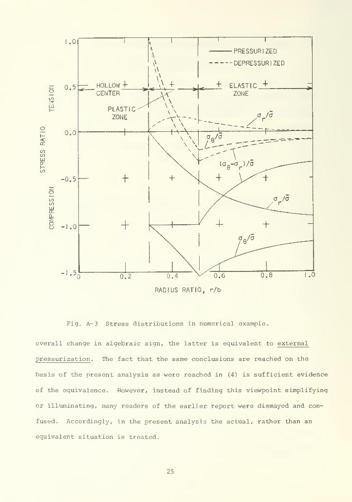
.0

1°- 5

in

ul

t-<ccc

IS)

GOLUDC\-

PRESSURIZED

DEPRESSURIZED

HOLLOW 4

CENTER+ ELASTIC +

ZONE

ininLU

Q-

oo -1.0

0.2 0.4 v' 0.6

RADIUS RATIO, r/b

0.8 .0

Fig. A- 3 Stress distributions in numerical example.

overall change in algebraic sign, the latter is equivalent to external

pressurization . The fact that the same conclusions are reached on the

basis of the present analysis as were reached in (4) is sufficient evidence

of the equivalence. However, instead of finding this viewpoint simplifying

or illuminating, many readers of the earlier report were dismayed and con-

fused. Accordingly, in the present analysis the actual, rather than an

equivalent situation is treated.

25

The procedure here employs the simplest and most common plastic analy-

sis to be found in the literature. The use of the Guest or Tresca condition

is consistent with usage in the A.S.M.E. Boiler and Pressure Vessel Code.

A readily available development (of the interior pressurization problem)

is to be found in Timoshenko's popular textbook (12). The analysis is

probably originally due to Nadai (9). However, it is not the only view-

point. Bridgman (3) develops a generalized version and incorporates large-

strain analysis; his development is essentially for fully plastic behavior.

Hill et al. (6) consider modifications of the present analysis based on

resolution of an undesirable discontinuity of axial strain at the elastic-

plastic interface; their analysis predicts slightly less radial deformation

than does the analysis given here for a given pressurization. A later work

by Nadai (10) devotes three chapters to analysis of pressurized cylinders.

A very recent work by Save and Massonnet (11) summarizes work to date and

offers a large bibliography; they cite additional recent studies. The

analysis summarized in (11) is the same as that given here.

Burst tests, such as described by Faupel (5) simply do not apply to

the problem in which we are interested. However such tests have served to

verify the general reliability of all the plastic analyses available; strain

hardening is such as to mask differences.

Hill et al. (7) provide an analysis which indicates that if the

Mises rather than the Tresca condition is used, P is increased by 15%,

i.e., P = (2//3) aln(b/a) . Thus, use of the Tresca condition appears to

be conservative.

Throughout the analysis and discussion to this point we have assumed

axial symmetry. Specifically, we have not considered a mode of collapse

in which the section becomes ovalized or goes out-of-round. The ASME

26

"rules" for externally pressurized (thin wall) circular cylinders are based

upon the predication of out-of- round deformation. Timoshenko and Gere (14)

describe the genesis of the ASME procedure as combining a classical shell

buckling analysis with what essentially amounts to the present formula (15)

,

which, for thin wall, takes the form

P rT= oln[(l+t/2r )/(l-t/2r )] = ta/r (31)

U m m m

as is given by the most elementary analysis. Ref (14) indicates also that

the ASME rules of 1933 used an artificically low value of a = 26000 psi;

presumably modern versions of the ASME rules, which now provide curves

for a number of different metals of engineering importance, reflect more

realistic values of a. However, there do not appear to be any analyses in

the literature which treat out-of-round buckling of externally pressurized

cylinders having ratios a = a/b as large as those employed in thermowells

for high pressure service.

Confining attention to thermowells for high pressure service, there

seems to be no "engineering sense" in applying any criterion more restric-

tive than the one recommended in the preceding paragraphs. Externally

pressurized cylinders having thick walls simply do not go out-of-round.

Bridgman (3) conducted a number of tests on tubes of various steels having

O.D. = .3125, I.D. = .0998. This corresponds to a = .32 which is approxi-

mately the value used in the examples in the present analysis and also

corresponds to current industrial practice for high pressure installations.

He subjected these tubes to as high as 412000 psi external pressure. In

each case the tube simply decreased in diameter, while maintaining its

length almost exactly without change. Equation (16b) was satisfied; that

is, there was no volume change that could be detected. In one case, of a

27

very soft steel under 412000 psi, the central cavity appeared to close up

completely. However, there was no failure or loss of pressure integrity.

Thus, for such thick wall cylinders, nonsyiranetric distortion simply does

not take place. The criterion recommended here (Equation 29) should assure

that dimensional changes remain acceptably small and that shakedown to

elastic conditions occurs promptly so that there is no danger of ratchetting

or low-cycle fatigue.

8. Thin Wall Thermowells

The basic motivation behind this re- examination of design criteria

for thermowells resides in the integrity of thermowells against very high

external pressures, and the analysis thus far has been of such cases.

However, design rules should cover all possible pressurizations, including,

as an example, thermowells in exhaust gas ducts. However, it is not within

the scope of the present study to consider such cases seriously or in

detail. It seems reasonable to suppose that for case with "nominal"

values of external pressure, the current interpretation of the Power Test

Code, whatever that may be, should be considered applicable. In the appro-

priate part of this document (1) the maximum gage pressure is given by a

formula P = K S where K is a constant varying between 0.155 (for "large"

thermocouple elements) to 0.412 (for "small" elements). If this criterion

is satisfied for a thermowell having (roughly, say) the dimensions given

in this document (1) , there seems to be no reason to question the accepta-

bility of the design on the basis of pressurization. For designs which

must vary from the dimensions indicated in (1) , it seems reasonable to

attempt to apply the rules in the Unfired Pressure Vessel Code (2)

.

The only questions which appear to remain (on the question of wall

thickness vs. pressure) are these. (1) For very low external pressuriza-

tion, a certain degree of structural strength, possibly more than might

28

be required by other criteria for thermowells, might be required to with-

stand the loads applied during shipment and installation or due to inadver-

tently applied mechanical loads during operation and maintenance, and (2)

for "medium" pressure situations under what circumstances should one be

concerned about true buckling in which ovalization or lobar deformation

occurs.

We shall not concern ourselves further with (1) above. Let us turn

attention to (2) . The smallest value of D /t contemplated in the ASMEo

Unfired Pressure Vessel Code (2) (Appendix V) is D /t = 10, and as waso

pointed out in (14) , the criterion in this case is gross yielding with no

change from the circular shape, using a substantial (>2) factor of safety.

In the writer's opinion this is greatly overconservative for thermowells.

However, let us not argue with it. We propose therefore that for D /t ^o

210, the Unfired Pressure Vessels be employed. The parameter D /t =

o 1-a

using the parameter a = a/b introduced earlier. Thus D /t = 10 correspondso

to a = .8. We believe that the strict application of the UFPV rules for

D /t < 10 may be uneconomical ly conservative. Accordingly, we suggest that

the entire gamut of pressure criteria be based as follows: (1) rules pre-

viously suggested for = a = .6; (2) UFPV Code rules for .8 = a = 1.0,

(3) linear interpolation between.

9. Factor of Safety

Although the preceding discussion indicates no need for a "factor of

safety" since catastrophic dimension change is not possible and even con-

siderable overpressurization can result in nothing worse than squeezing

down on the thermocouple element, nevertheless it is customary to provide

for a factor of safety or its equivalant to account for inadvertent occa-

sional overheating and/or overpressurization, the possibility of individual

metallic specimens failing to possess the physical properties called for in

29

the material purchase specification, deviations from design dimensions etc.

The analysis here calls for knowing the yield stress a. The code allowable

stress value, usually designated S, , is readily available for all materialsM

likely to be encountered and for all temperatures which might be employed.

This stress value satisfies the inequality S = .625a, so that a = 1.6 S .

M M

We propose using a "safety factor" of 1.6 simply by substituting the value

S in place of the value a in all our criteria.M

10. Statement of Recommended Pressure Criteria.

Defining a = a/b = (inner radius) / (outer radius) = (inner diameter)/

(outer diameter) = (D -2t)/D = l-2t/D , we also have D /t = 2/(l-a). Weo o o o

also let S = code allowable "S-value" for the material and temperature andM

let P.. = allowable exterior pressure for D /t = 10, according to the UFPV10 o

Code. Then the recommended pressure criterion is:

(1) If a < .45 (i.e., D /t < 3.64), P ^ (l-a 2 )So M

(2) If .45 ^ a ^ .6 (i.e., 3.64 5 D /t ^ 5) P ^ -S ln(a)o M

(3) If .6 £ a 5 .8 (i.e. , 5 £ D /t < 10) , P = (4-5a) (.51S„) +o M

(5a-3)P1Q

(4) If .8 1 a ± 1 (i.e., D /t 1 10), use the rules ofo

Par. UG-28 of Division 1, Section VIII of the ASME Boiler

and Pressure Vessel Code

Notes: (1) The dimensions employed in this calculation shall be those

obtaining at the end of the design life of the thermowell. Accordingly, if

corrosion may take place, an appropriate corrosion allowance should be

added to exterior dimensions in order to arrive at manufacturing dimensions.

(2) If dimensions are not constant along the length of the thermowell, the

criterion given here must be satisfied at each cross section.

30

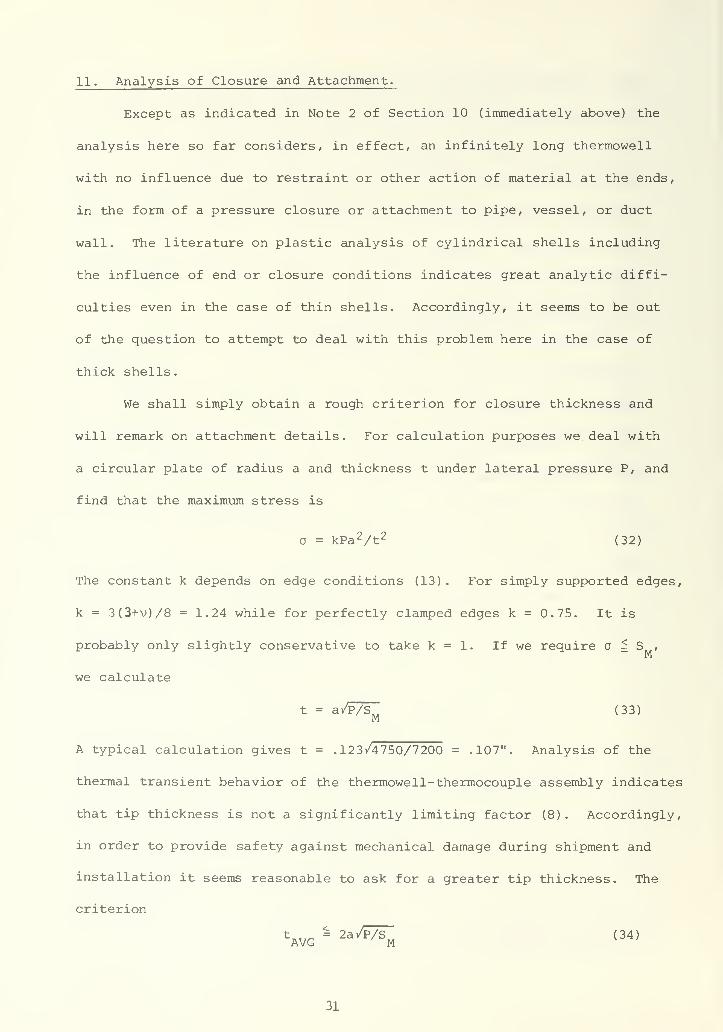
11. Analysis of Closure and Attachment.

Except as indicated in Note 2 of Section 10 (immediately above) the

analysis here so far considers, in effect, an infinitely long thermowell

with no influence due to restraint or other action of material at the ends,

in the form of a pressure closure or attachment to pipe, vessel, or duct

wall. The literature on plastic analysis of cylindrical shells including

the influence of end or closure conditions indicates great analytic diffi-

culties even in the case of thin shells. Accordingly, it seems to be out

of the question to attempt to deal with this problem here in the case of

thick shells.

We shall simply obtain a rough criterion for closure thickness and

will remark on attachment details. For calculation purposes we deal with

a circular plate of radius a and thickness t under lateral pressure P, and

find that the maximum stress is

a = kPa 2/t 2 (32)

The constant k depends on edge conditions (13). For simply supported edges,

k = 3(3+v)/8 =1.24 while for perfectly clamped edges k = 0.75. It is

probably only slightly conservative to take k = 1. If we require a 5 S ,

we calculate

t = av^Ts" (33)M

A typical calculation gives t = .123/4750/7200 = .107". Analysis of the

thermal transient behavior of the thermowell-thermocouple assembly indicates

that tip thickness is not a significantly limiting factor (8). Accordingly,

in order to provide safety against mechanical damage during shipment and

installation it seems reasonable to ask for a greater tip thickness. The

criterion

'avgS 2a/f% (34)

31

appears to be quite conservative and it also accommodates cases where

closure thickness is not constant, such as a thermowell the interior cavity

of which is formed by a twist drill.

There is simply no feasible way of investigating shakedown in the

neighborhood of the tip (closure) or of the root (attachment to pipe wall)

of a thermowell. The 1.6 "safety factor" previously introduced, together

with the requirement of adequately thick closure and (see below) strong

attachment details, should, however, assure shakedown immediately or very

early in the operating life.

Practice differs with regard to attachment details. We will here

discuss only the case of installations intended for high pressures. Some

fabricator specifications appear to call for only sufficient thread engage-

ment (in the case of threaded connections) or weld metal to assure that

the thermowell assembly is not projected radially outward. In the writer's

opinion this represents gross under- design. The only case of high pressure

thermowell failure of which the writer has knowledge seem unquestionably to

be associated with failure of the attachment weld (after satisfactory opera-

tion for a number of years, incidentally) . When one considers all possible

ways in which a thermowell could "fail" in a catastrophic or seriously

disabling way, it seems clear that in any such case a marginally adequate

attachment detail can not be other than a contributing factor.

In seventeen years association with the Mechanical Design Committee

(of the B31 Code "family") the writer has consistently argued that the

pressure carrying integrity of a pipe or header or run or vessel or what-

ever is compromised by any removal of material from the walls, whether this

be for the purpose of making a branch connection, in which case reinforce-

ment rules apply, or for any other purpose, in which case no rules seem to

32

be called for. The hole which is made to insert a radiographic pellet for

weld inspection should require no less attention than does a branch connec-

tion hole of the same size. The same is surely true for the hole made to

accommodate a thermowell installation. If the pipe into which the instal-

lation is made has substantial excess thickness over that required by the

applicable pipe wall thickness formula, then perhaps a case can be made

for less than full penetration welds. Otherwise, it is absolutely clear

to this writer that full penetration welds are called for, at the very

least, and that, perhaps, additional reinforcement may be required. This

should be determined by a strict application of the rules for reinforce-

ment of branch connections, noting, however, that the branch itself is,

in this case, not internally pressurized.

Accordingly, as developed in this subsection of this Appendix A,

two additional criteria hereby recommended are: (1) Average thickness of

end closure not less than 2a/P/S , and minimum thickness not less thanM

a/P/S , and (2) strict application of branch connection reinforcement

rules to the detail of attaching thermowell to pipe wall, with full pene-

tration welds in all cases.

12. Bibliography for Appendix A

Al. ASME, Power Test Codes, Instruments and Apparatus, Part 3 Temperature

Measurement, Paragraphs 8-19 incl., pp. 7-9.

A2. ASME, Boiler and Pressure Vessel Code, Section VIII, Pressure Vessels,

Division 1, Paragraph UG-28 and Appendix V.

A3. Bridgman, P.. W. , Large Plastic Flow and Fracture, McGraw-Hill 1952,

Chapter 8, pp. 142-163.

A4. Brock, J. E. , Stress Analysis of Thermowells, consulting report for

Bechtel Power Corporation, October 1972.

33

A5. Faupel, J. H. , Yield and Bursting Characterisitcs of Heavy-wall

Cylinders, Trans. ASME, Vol. 78, 1956, pp. 1031 et seq.

A6. Hill, R. , Lee, E. H. , and Tupper, S. J., The theory of combined

plastic and elastic deformation with particular reference to a thick

tube under internal pressure, Proc. Roy. Soc. Lond. , A, 191, pp. 278-

303, 1947.

A7. Hill, R. Lee, E. H. , and Tupper, S. J., Plastic flow in a closed

tube with internal pressure, Proc. 1st U. S. Nat. Cong. Appl . Mech.,

Chicago 1951, P. 561, ASME ed. 1952.

A8. Houlihan, T. M. , Thermowell Calculations, (Accuracy and Response),

consulting report to Bechtel Power Corporation, October 1972.

A9. Nadai, A., Plasticity, McGraw-Hill, 1931.

A10. Nadai, A., Theory of Flow and Fracture of Solids, McGraw-Hill, 1950.

All. Save, M. A., and Massonnet, C. E. , Plastic Analysis and Design

of Plates, Shells, and Disks, North-Holland Pub. Co., 1972.

A12. Timoshenko, S., Strength of Materials II, 3rd Ed., Section 70, p. 386

et seq., D. van Nostrand 1956.

A13. Ref. 12, pp. 96-99.

A14. Timoshenko, S. , and Gere, J. M. , Theory of Elastic Stability,

McGraw-Hill, 1961, pp. 480-481.

34

APPENDIX B

ESTIMATION OF EXCITING FREQUENCY AND FORCES

TABLE OF CONTENTSPage

1. Estimation of Exciting Frequency and Forces. 36

(Appendix B of October 1972 Report; item B2 of Bibliography)

2. Discussion of and Addenda to the Preceding Section 43

3. Bibliography 46

35

1. Estimation of Exciting Frequency and Forces

(Note: Except for very minor editorial emendations, this section is

identical to Appendix B of Reference B2)

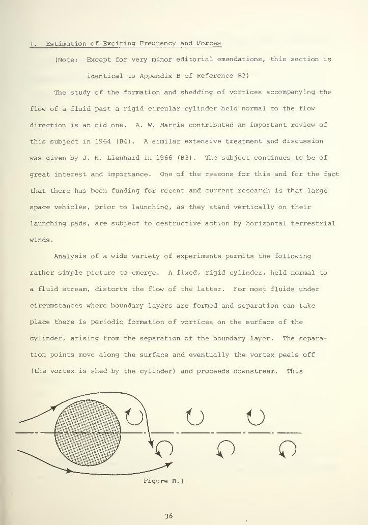
The study of the formation and shedding of vortices accompanying the

flow of a fluid past a rigid circular cylinder held normal to the flow

direction is an old one. A. W. Marris contributed an important review of

this subject in 1964 (B4) . A similar extensive treatment and discussion

was given by J. H. Lienhard in 1966 (B3) . The subject continues to be of

great interest and importance. One of the reasons for this and for the fact

that there has been funding for recent and current research is that large

space vehicles, prior to launching, as they stand vertically on their

launching pads, are subject to destructive action by horizontal terrestrial

winds.

Analysis of a wide variety of experiments permits the following

rather simple picture to emerge. A fixed, rigid cylinder, held normal to

a fluid stream, distorts the flow of the latter. For most fluids under

circumstances where boundary layers are formed and separation can take

place there is periodic formation of vortices on the surface of the

cylinder, arising from the separation of the boundary layer. The separa-

tion points move along the surface and eventually the vortex peels off

(the vortex is shed by the cylinder) and proceeds downstream. This

O Oo o

Figure B.l

36

phenomenon takes place alternately on the two sides of the cylinder as

indicated in Figure B.l, which is adapted from Reference B3, and is

accompanied by a drag force F , in the direction of the main stream flow,

and a lift force F , normal to both main stream flow and cylinder axis.ti

Forces F and F act upon the cylinder and cause its distortion if it isD L

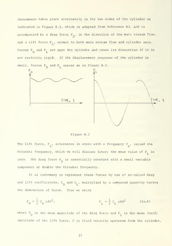
not perfectly rigid. If the displacement response of the cylinder is

small, forces F and F appear as in Figure B.2

TIME, t TIME, t

Figure B.

2

The lift force, F , alternates in sense with a frequency f , called theLt S

Strouhal frequency, which we will discuss later; the mean value of F is

zero. The drag force F is essentially constant with a small variable

component at double the Strouhal frequency.

It is customary to represent these forces by use of so-called drag

and lift coefficients, C and C , multiplied by a computed quantity having\J Li

the dimensions of force. Thus we write

FD = I

CD

PAU2 '- FL

=\ C

LPMJ2 (la,b)

where F is the mean magnitude of the drag force and F is the mean (half)

amplitude of the lift force, U is fluid velocity upstream from the cylinder,

37

p is fluid mass density, and A is the projected area of the cylinder, namely

length times diameter. Conveniently, we may consider only a unit length of

cylinder in which case A = D x 1 = D, and F and F are forces per unit

length.

The Strouhal frequency f is representable by the formula

f = N U/D (2)s s

where N , the Strouhal number, is a dimensionless quantity. The criticallys

important quantities N , C and C vary depending upon flow conditions.

Although the source and nature of the variations are not well understood,

it provides a unifying viewpoint to consider their variations as depending

upon the Reynolds number, N , given byR

N = UD/V (3)K

where, as before U denotes undisturbed fluid velocity and D denotes cylin-

der diameter. The quantity v denotes the kinematic viscosity of the

fluid. (Do not confuse this with Poisson's ratio of an elastic solid,

also represented by the symbol v in Appendix A.) For water and steam,

values may be obtained from the graphical presentation given in the ASME

steam tables.

The variation of N , C and C with respect to N is large andS D L R

complicated. Several distinct flow regimes exist for the range

10 < N < 10 7. Lienhard illustrates and describes these; it should be

R

made clear, however, that observation, understanding, and description is

still far from clear or complete. See Lienhard (B3) , p. 3.

At the time Murdock devised his analysis (1959) things seemed

much simpler and more definite. For N > 10 3, for example, it was

38

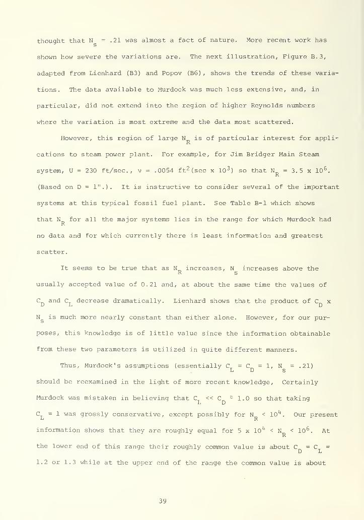
thought that N = .21 was almost a fact of nature. More recent work has

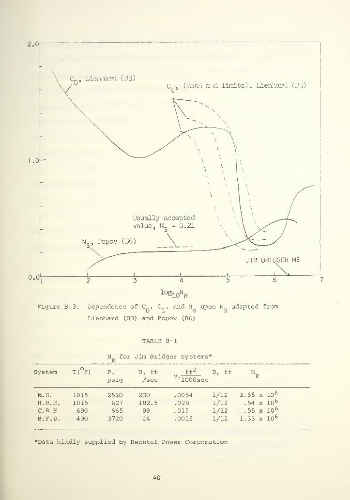
shown how severe the variations are. The next illustration. Figure B.3,

adapted from Lienhard (B3) and Popov (B6) , shows the trends of these varia-

tions. The data available to Murdock was much less extensive, and, in

particular, did not extend into the region of higher Reynolds numbers

where the variation is most extreme and the data most scattered.

However, this region of large N is of particular interest for appli-R

cations to steam power plant. For example, for Jim Bridger Main Steam

system, U = 230 ft/sec, v = .0054 ft 2 (sec x 10 3) so that N = 3.5 x 10 6

.

R

(Based on D = 1".). It is instructive to consider several of the important

systems at this typical fossil fuel plant. See Table B-l which shows

that N for all the major systems lies in the range for which Murdock hadR

no data and for which currently there is least information and greatest

scatter.

It seems to be true that as N increases, N increases above theR s

usually accepted value of 0.21 and, at about the same time the values of

C and C decrease dramatically. Lienhard shows that the product of C xD L D

N is much more nearly constant than either alone. However, for our pur-

poses, this knowledge is of little value since the information obtainable

from these two parameters is utilized in quite different manners.

Thus, Murdock' s assumptions (essentially C = C = 1, N = .21)L D s

should be reexamined in the light of more recent knowledge, Certainly

Murdock was mistaken in believing that C << C ~ 1.0 so that takingL D

C = 1 was grossly conservative, except possibly for N < 10^. Our presentL" R

information shows that they are roughly equal for 5 x 10 ^ < N < 10 6. At

R

the lower end of this range their roughly common value is about C = C =

1.2 or 1.3 while at the upper end of the range the common value is about

39

2.0

.0L

0.0'

Cn , LieiLiard (33)

C. , (mean and limits), Lienhard (B3)

Usually acceptedvalue, N_ = 0.21

N , Popov (B6)

JIM BRIDGER MS

,__ X_10g

1QNR

Figure B.3. Dependence of C , C , and N upon N adapted fromD Li S R

Lienhard (B3) and Popov (B6)

TABLE B-l

N for Jim Bridger Systems*R

System T(°F) P, U, ft ft' D, ft N.

psig /secv,1000sec

M.S. 1015 2520 230 .0054 1/12H . R. H

.

1015 627 182.5 .028 1/12C.R.H 690 665 99 .015 1/12B.F.D. 490 3720 24 .0015 1/12

R

3.55 x 10 b

.54 x 10 6

.55 x 10 6

1.33 x 10 6

*Data kindly supplied by Bechtel Power Corporation

40

0.2 or 0.3. This is indeed a drastic reduction. However, there is some

difficulty in assuring that the value of N calculated by the formulaR

N = UD/v is indeed entirely appropriate since the flow through a pipeR

may differ in essential ways from the ideal flow conditions which were

approximated in the experiments leading to Figure B.3. For one thing

valves and bifurcations may be located close enough upstream that the

assumption of uniform flow conditions upstream is quite incorrect. For

another thing, the constriction provided by the pipe walls causes a slight

speed-up of flow in the section which contains the thermowell. Thus one

cannot be sure of the truly representative value of N , and one hardlyR

has sufficient basis for knowing that, in a particular case, the values of

C and C are indeed quite small.D L

Furthermore, Figure B. 3 shows that N may be as high as .45 which iss

about twice the value N generally assumed for high speed flows and which

is incorporated in Murdock ' s analysis.

Accordingly the following suggestion seems to provide a conservative

procedure for purposes of strength analysis of thermowells. Calculate

N = UD/vR

A. Strouhal number , upper (conservative) estimate

For N < 4 x 10 u, take N = .21

R s

For 4 x 10^ < N < 4 x 10 5, take N = . 24 log, rtN - .894

R s 10 R

For N > 4 x 10 5, take N = .45

R s

B. Drag coefficient , upper (conservative) estimate

For 3 x 10 2 < N < 10 5, take C =1.2

R D

For N > 10 5, take C = . 75

R D

C. Lift coefficient , upper (conservative) estimate

For 10 3 < N < 10 5, take CT

= 1.3R L

For N > 10 5, take C = .25

R L

41

I have discussed these values with my colleague, Dr. T. Sarpkaya,

a recognized authority in this field and one who himself has made theoreti-

cal and experimental studies of flow past a cylinder, in particular with

regard to the build-up to quasi-steady-state conditions. He has been good

enough to look over the immediately preceding suggestions and to confirm

that they adequately represent our present state of knowledge as applied

to the engineering problem at hand, as being conservative in all cases but

not extravagantly so.

For purposes of strength analysis, we will regard F as steady,

neglecting its small variable component, and will regard F as sinusoidally

varying at Strouhal frequency.

The discussion so far has presumed that the cylinder past which the

flow is taking place neither deforms nor distorts. However, if there is

significant deformation or distortion an unwelcome and destructive coupling

may take place. This results from mechanical motion of the cylinder itself

entering into and disturbing the flow field in such a way as to trigger the

shedding of vortices. Thus, in the case of a cylinder which can vibrate

as an elastic beam, as is indeed the case for a thermowell, which has,

say, a well defined lowest natural frequency of elastic vibration, two

modes of behavior may be distinguished. At low flow velocities, the

Strouhol frequency is low (f << f ) . Excitation at f causes response ats n s

f , the magnitude of the response being generally small since the exciting

forces are small. As U increases, f increases approaching f . The system

is closer to resonance and the response (i.e., lateral displacement)

increases. If f is sufficiently close to f , the response will be large

enough to significantly influence the flow pattern and to interact with it.

The frequency of vortex shedding approaches and "locks onto" the natural

42

frequency f even though U does not increase. With excitation now taking

place at precisely the natural frequency, a condition of mechanical reso-

nance is attained in which amplitude of vibration builds up and is ultimately

limited only by the damping which is present. If damping is insufficient,

failure occurs quickly. If damping is sufficient to prevent early failure,

still the material may suffer damage and fail by (high cycle) fatigue.

Thus it is essential, regardless of whatever strength calculations may be

made using C and C , to assure that f is sufficiently less than f toD L s n

assure that this coupling is not significant and the locking or entrain-

ment of frequencies phenomenon does not take place.

2. Discussion of and Addenda to the Preceding Section

Inasmuch as the criteria in the ASME Power Test Codes (Al) , reflecting

without change the criteria developed by J. W. Murdock, incorporate an

unvarying value -0.21 of the Strouhal number, some surprise and consterna-

tion has been expressed at the introduction, in the recommendations in the

writer's October 1972 report (B2), of values of N substantially larger

than this. One very significant matter has been emphasized by more than

one commentator. The experiments in the range of N for which these sub-

stantially larger values of N were obtained indicate a "randomness" ors

"lack of coherence" of the vortex shedding phenomena.

Expressed otherwise, the energy spectral density is sharply peaked

at a frequency f ~. 22U/D for 10 2 = N = 10 5 and again fairly sharply

R

R :

< c <

peaked at f ~. 29U/D for 10 ' = N 1 (?) , whereas, for 10 b ± N 1 10 ' the

R R

energy spectral density is spread out in the range .20U/D = f = .45U/D.

(The question mark above indicates uncertainty regarding an upper limit

for the indicated restoration of coherence. ) The question at hand is

simply that of attempting to assess how much and what kind of damage may

43

be done to a structure if the flow is characterized by N in the range

10 5 = N = 10 7.

Because of lack of coherence it is reasonable to conclude that the

chance of sustained excitation at any one particular frequency is slight,

and the writer agrees with those who have pointed this out. This conclusion

is reinforced by statements in a recent study (Bl) which, in summarizing

available literature of this date, points out also that there are phase

differences in a spanwise direction under most circumstances, and these

themselves become incoherent when the shedding becomes incoherent. Another,

as yet unpublished study of a classfied project (the writer must certainly

apologize for adducing such a nebulous source) indicates that significant

structural excitation of certain test structures did not take place (for

flows in the regime presently under discussion) in a rather extensive

series of experiments. Accordingly, it does indeed seem perfectly clear

that coherent excitation, of the kind possible for 10 < N < 10° and forR

N > 10 7, does not occur for 10 5 < N < 10 7

.

R R

Accordingly, it is appropriate to consider the worst that could

occur (if 10 5 < N < 10 7) and the probability of its occurrance. Anyone

who has ever seen them cannot ever forget the moving pictures, now about

thirty years old, of the tail structures of certain WWII aircraft when

aerodynamic flutter occurred: one oscillation, two oscillations, three

oscillations, — GONE! In the present application we may ask how many

coherent, in-phase excitations can lead to dangerous displacement excur-

sions. More than three, certainly, but how many? One hundred?

One hundred cycles at a natural frequency of approximately 3000 Hz

(a typical value), occurs in 30 milliseconds. What are the chances of

30 milliseconds coherence in a twenty year design life?

44

Thus, we have two questions which certainly we cannot answer. How

many coherent cycles will result in damage?, and what is the probability

of getting these cycles sometime during a twenty year or thirty year design

lifetime.

Now a logical engineering attitude is to presume that damage can

occur from this source, however unlikely that may seem to be, if the cost

of doing so is not too great. In other words, we propose to include

criteria such as to assure that this kind of potentially damaging situation

does not arise. If this costs nothing as a practical matter it does no

harm that we may indeed be "over safe". If there is an implied penalty,

then one is perfectly free to violate the criterion, but only with the

understanding that the possibility of structural damage has been increased.

A designer might take different courses depending on whether the thermowell

involved was in a system in a fossil fuel plant or in a nuclear plant where

failure could carry undesirable material into a radioactively "hot" zone.

Criteria intended to assure no possibility whatsoever of damage of

this kind were included in the recommendations of (B2) . However, realism

requires adding other criteria upon which one may fall back if the original

criteria are felt to be unduly restrictive or uneconomical in a particular

situation. The secondary criteria should be related to a greater degree

of risk, but one which is economically acceptable under most circumstances.

However, the state of our knowledge is simply not adequate for a

quantitative assessment of risk. Accordingly, all that can reasonably be

suggested at this time is to add to the recommendations made two years ago,

an explanatory note, at the proper place or places and to the following

effect:

If N > 4 • lCr and the design meets Criterion No. 1 but fails to

meet Criteria 2, 3, or 4, repeat the calculations for the latter, but using

45

the artificial value N = 4 • 10 4. If all criteria are now satisfied, the

design is acceptable except for those cases where an unusually great penalty

would be associated with failure. If one or more criteria remain unsatis-

fied, the design may still be acceptable, but special calculations are

required to show this. Such calculations should be based upon the general

analytical procedures in this report but may employ, in a consistent man-

ner, whatever appropriate experimental information may be available at the

time of the calculations.

The last provision in the preceding paragraph takes cognizance of

the fact that the probability is that the regime 10 5 = N = 10 7 is indeed

safer than other regimes since not only is the excitation incoherent but

also the value of C and C have decreased. One should not become confusedD L

by this apparent disparate use of the word "safer". In other regimes

(than 10 5 < N < 10 ) there is a reasonable degree of certainty in calcu-

lating the exciting frequency and forces. In the regime 10 5 < N < 10 7

K.

the degree of certainty is significantly less. The "odds are" that the

danger of damage is less, but the certainty that this is so is significantly

less. An analog may help explain this. For N outside the range 10 5 - 10 ,

R

we could say that we expect to lose 100 tokens but could lose as much as

200. For N within the range 10 5 - 10 7, we expect to lose 10 tokens but

H.

could lose as much as 1000.

3. Bibliography for Appendix B

Bl. Barnett, K. M. , and Cermak, J. E. , Turbulence induced changes in

vortex shedding from a circular cylinder, Project THEMIS Technical

Report No. 26, College of Engineering, Colorado State University,

Fort Collins, Colorado, January 1974.

46

B2. Brock, J. E. , Stress analysis of thermowells, consulting report for

Bechtel Power Corporation, October 1972, and supplement, December 15,

1972.

B3. Lienhard, J. H., Synopsis of lift, drag, and vortex frequency data

for rigid circular cylinders, Bulletin 300, Washington State University

College of Engineering, Research Division, Pullman, Washington, 1966.

B4. Marris, A. W., A review on vortex sheets, periodic wakes, and induced

vibration phenomena, J. Basic Engrg, June 1964, pp. 185-196.

B5. Morkovin, M. V., Flow around circular cylinder — a kaleidoscope of

challenging fluid phenomena, Proceedings of the ASME Symposium on

Fully Separated Flows, Philadelphia, pp. 102-118. ASME 1964.

B6. Popov, S. G. , Relation between Strouhol and Reynolds numbers for

two-dimensional flow about a circular cylinder, Fluid Dynamics,'

pp. 107-109 (trans, from Mekhanika Zhidkosti i Gaza, Vol. 1, No. 2,

pp. 156-159, 1966.

Note: Reference B5, which is not cited in the text hereof, says much

the same as several of the other references. It was duplicated

and sent to the ASME PB 51 Committee through the kindness of Mr.

J. W. Murdock and Mr. W. O. Hayes.

47

APPENDIX C

RESPONSE FREQUENCIES OF THERMOWELL VIBRATION

TABLE OF CONTENTSPage

1. Introduction 49

2. Finite Element Analysis 50

3. Foundation Compliance 52

4. Beam Vibration Equations 56

5. Constant Section and Properties 57

6. Non-Constant Section and/or Properties 60

7. Alternate Approach 61

8. "Assembly" of Analytic Procedures 62

9. Calculations for Uniform Cantilever 64

10. Computer Program and Results 67

11. Frequency Reduction Factors 71

12. Elementary Analysis for Actual Thermowell Geometry 72

13. Example of Frequency Calculation; Recommendations 73

14. Pipe Ovalization Mode 76

15. Bibliography for Appendix C 79

48

1. Introduction

Previous analyses of thermowell vibration have, reasonably, focussed

on "cantilever" vibrations in which the thermowell is considered fixed at

its root and is subject to flexural vibrations in a single transverse plane.

If the thermowells were longer and more slender than they actually are,

there would be no serious difficulty in making reasonable estimates of

response frequency. The non-uniformity of cross section would introduce

only minor difficulties.

However, there are basic difficulties of a more serious nature. First,

for short, stubby cantilever beams the so-called elementary beam theory does

not take into account what may be a significant elastic compliance, namely

that due to shear deformation. Second, for such stubby beams, the usual

dynamic analysis does not take into account what may be a significant

inertial effect, namely that due to longitudinal motion of the mass particles

of which the beam is composed.

A generally accepted procedure for accounting for these two effects,

both of which tend to depress the response frequencies as compared to values

computed on the basis of elementary theory, is by use of so-called Timoshenko

beam theory which takes into account shear deflection and rotatory inertia.

This theory is still approximate but is widely believed to provide results

of sufficient accuracy for engineering purposes, particularly for the lowest

response frequencies. This theory is well established and many applicable

and useful results are available. These will be discussed later in this

Appendix

.

A much more troublesome difficulty is that associated with the

assumption of root end restraint. The body (in our case, the pipe wall)

to which the cantilever is fixed at its root end is not perfectly rigid.

49

Accordingly, the assumptions regarding root end fixity which are invariably

a part of cantilever response analysis are simply not true. For long

slender cantilevers, the resulting errors are acceptably small, but for

short, stubby cantilevers, the degree of error may be appreciable. The

foundation yields, so that the "system" composed of beam and foundation

has increased compliance. Furthermore, the foundation possesses nonzero

mass. Both of these considerations tend to decrease response frequency.

Thus there are four nonelementary influences each of which results

in a decrease of frequency as compared to results estimated using elemen-

tary theory. They are: (a) shear deflection in the beam, (b) elastic

compliance of the foundation, (c) rotatory inertia in the beam, and

(d) mass-inertia in the foundation.

The major attention in this Appendix will be focussed on methods of

accounting for these influences. However, one additional aspect must be

considered. Along with modes which can be roughly described as cantilever

modes, there is a low- frequency mode in which the pipe itself is periodically

ovalized and in which the thermowell acts more or less as a rigid body.

This possibility has not been treated in thermowell analyses except in a

previous development by this writer. Section 14 of this Appendix C will

deal with this mode of vibration.

2. Finite Element Analysis

The analytical and other difficulties surrounding the business of

estimating the response frequencies of thermowells - in particular the

lowest or slowest frequency which is of the greatest interest - are so

great that no strictly analytical procedure is presently developed to the

point where it can account for all the effects. However, there is a

method, designated as FEM, an abbreviation for "finite element method,"

50

which has proved its power and has attracted much attention and employment

in the past few years, and which seems to be a "natural" for the problem

at hand. A former student of the writer, Mr. J. R. Adamek, undertook to

employ FEM to study thermowell vibrations, but found it advisable to divert

his attention to the development of mesh generation software for the pur-

pose of making available FEM software easier to use. Currently Mr. H. L.

Crego is engaged in dealing with the thermowell vibration problem using

FEM. His program contemplates first dealing with a two-dimensional formu-

lation which definitely is not representative of the real thermowell problem

but which is more easily attacked since computer system limitations are less

severe with two-dimensional than with three-dimensional problems. Following

successful treatment of the 2D problem an attack will be made on the 3D

problem.

Mr. Crego is modifying for his particular use the software programs

PLISOP and PLIMEG previously developed for 2D problems. For the reader who

has some familiarity with FEM analysis the following steps - some already

complete in August 1974 - may be of interest. PLIMEG and PLISOP are being

united. In addition to the generation by PLISOP of the consistent stiffness

matrix K, the new facility of generating a consistent mass matrix M has been

developed. Matrices M and K are banded and symmetrical which permits com-

pact storage. A triangular decomposition of K will be made, preserving

compactness of storage. The iterative algorithm

Kv ... = w2Mv (1)n+1 n

will be employed. The triangular decomposition of K is, in effect, a

"forward solution" and the solution for each improved vector v ., willn+1

involve only a "back solution" which is very rapidly accomplished. A

51

standard normalization will be employed to find the new vector and to

estimate to2

. It is also contemplated to use a final Rayleigh evaluation

o T T0)z = v Kv/v Mv (2)

so as to reduce the number of iterating steps. Since only u)j is of

interest there is no need to purge or filter to permit obtaining higher

modes.

No difficulties are contemplated in implementing the program. How-

ever, considerable experimentation will have to be done to evaluate the

influence of "how much foundation" is included in the formulation and of

the constraints on this portion. Furthermore, it is anticipated that the

2D and 3D problems may differ greatly in this respect. It is not contem-

plated, presently at least, to represent the foundation as other than a

rectangular mass of material. In particular, it is not presently contem-

plated to model the pipe wall as a tube.

3. Foundation Compliance

Because of the importance of foundation compliance and inertia, ideally

the problem at hand is one of simultaneously dealing with the beam (thermo-

well) and the foundation (pipe wall) in what is known (in heat transfer

theory terminology) as a conjugated problem. Leaving aside the matter of

damping (energy sinks) one assumes isocronous vibration with common fre-

quency u of both the beam and the foundation. At their interface the dis-

placements must match and the stress components must conform. This prob-

lem is utterly beyond the reach of analytic procedures and is accessible

only to "subdividing" techniques such as FEM. Accordingly, only approximate

approaches are possible.

The foundation behavior presents the greater difficulties for analytic

treatment. Inasmuch as we presently have no real idea at all of the

52

quantitative effect of foundation behavior it is reasonable to look for

whatever results we can get for foundation performance. Thus, at the outset

we must abandon the question of the effect of foundation inertia and settle

for what we can evolve concerning foundation compliance.

The literature contains a number of approximate evaluations of

foundation compliance: (7), (11), (17), (20), and (21). All of these,

except only (7) , deal with a 2D situation. Although in an earlier analysis

(6) , the writer claimed that the 3D situation of the thermowell-pipe prob-

lem lay somewhere between the plain stress and the plane strain 2D cases

in the literature, now he concludes that such is not the case at all, and

that only a 3D analysis is applicable.

There are two classical problems of the analysis of a semi-infinite

solid subject to the action of a force applied to a point on its surface.

In Boussinesq's problem, the force Pk at the origin, is applied to the solid

z = and the vector displacement p at the point r = ix + jy + kz is given

by

p = (P/4frGr){ [z/r 2-(l-2v)/(r+z) ]r

(3)

+ [3z-4vz+2(l-v)r]k/(r+z) }

where G denotes the shearing modulus, v denotes Poisson's ratio and r =|r|.

On the surface, where z = 0, this becomes

p(surface) = (P/4iTGr2 ) [- (l-2v) r + 2(l-v)rk] (4)

A similar problem, bearing the name of Cerruti, is the same except

that the force applied to the origin is Pi rather than Pk, and the dis-

placements are given by

p = (P/4-rrGr){i+xr/r 2+(l-2v) [r(zi+xk) + (x2+y 2) i-xy j+xzk]/ (r+z) 2

} (5)

p (surface) = (P/4TTGr 3) {2 [x 2+ (1-v) y

2] i + 2vxyj + (l-2v)rxk} (6)

53

These solutions are presented conveniently by Westergaard (25) . Love

(16) discusses these and related problems. It is noteworthy that Timoshenko,

one of the foremost elasticians to write in the English language, seems

nowhere to mention Cerruti's work; cf. esp. (24).

Now a rational approach to estimating foundation stiffness or compli-

ance is to apply a "reasonable" distribution of normal and shearing forces .

to the interface area of the semi- infinite solid, use the formulas above

to calculate surface displacements, and, by defining suitable averages,

infer constraint rotation and displacement. A reasonable distribution

of normal forces is the linear distribution given by the elementary formula

a = Mx/I and a reasonable distribution of shearing forces is that given by

the elementary formula t = VQ/Ib.

In this way, one could estimate the coefficients b „ , b . , b _ , and1M6 MA' V0

b giving compliance coefficients for rotation (subscript 0) and deflec-

tion (subscript A) corresponding to unit moment (subscript M) and unit

shear (subscript V)

.

Brown and Hall (7) have made an evaluation of b . obtaining theM0

value

bMQ

= (16/15TT) (l-v 2 )d/EI ~ .787/Ea 3(7)

for a circular interface of radius a. This evaluation is based solely

upon the k component of p (surface) of Equation (4), i.e.

k • p (surface) = 2 (1-v) P/47rGr = P(l-v 2 /TrEr (8)

The writer has recently made an estimate of b , from Cerruti'sVA

analysis, proceeding as follows. Using only the i component from Equation

(6) , viz

i • p(surface) = (P/2iTGr 3) [x 2+ (1-v) y

2] (9)

54

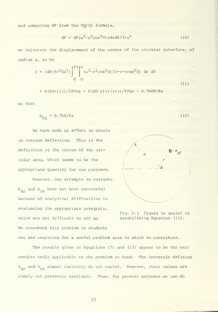
and computing dF from the VQ/Ib formula,

dF = 4P(a 2-r 2cos 2 6)rdrd6/3TTa' (10)

we calculate the displacement of the center of the circular interface, of

radius a, to be

A = (4P/6iT 2 Ga 1+

)

2-rrra

(a 2-r2cos 26) (l-v-vcos 2

9) dr d6

= P(20-llv)/18TTGa = P(20-llv) (l+v)/9irEa - 0.768P/Ea

so that

(11)

b = 0.768/Ea (12)

We have made no effort to obtain

an average deflection. This is the

deflection at the center of the cir-

cular area, which seems to be the

appropriate quantity for our purposes.

However, our attempts to evaluate

b , and b „ have not been successfulMA ve

because of analytical difficulties in

evaluating the appropriate integrals,

which are not difficult to set up.

We recommend this problem to students

who are searching for a useful problem area to which to contribute.

The results given in Equations (7) and (12) appear to be the only

results truly applicable to the problem at hand. The integrals defining

b and b almost certainly do not vanish. However, their values are

simply not presently available. Thus, for present purposes we can do

Fig. C. 1 Figure to assist in

establishing Equation (11)

.

55

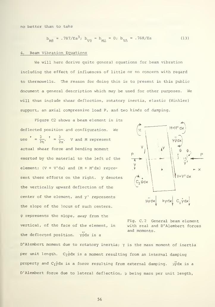
no better than to take

b n - .787/Ea 3; b n

= bA

= 0; b . = . 768/EaM9 V6 MA VA

(13)

4. Beam Vibration Equations

We will here derive quite general equations for beam vibration

including the effect of influences of little or no concern with regard

to thermowells. The reason for doing this is to present in this public

document a general description which may be used for other purposes. We

will thus include shear deflection, rotatory inertia, elastic (Winkler)

support, an axial compressive load P, and two kinds of damping.

Figure C2 shows a beam element in its

deflected position and configuration. We

use 9_ t

3t' 3x"V and M represent

V

V+V'dx

yydx kydx C.ydx!

actual shear force and bending moment

exerted by the material to the left of the

element; (V + V'dx) and (M + M'dx) repre-

sent these efforts on the right. y denotes

the vertically upward deflection of the

center of the element, and y' represents

the slope of the locus of such centers.

i> represents the slope, away from the

vertical, of the face of the element, in

the deflected position. y^dx is a

D'Alembert moment due to rotatory inertia; y is the mass moment of inertia

per unit length. C2^dx is a moment resulting from an internal damping

property and Cjydx is a force resulting from external damping. yydx is a

D'Alembert force due to lateral deflection, u being mass per unit length,

Fig. C. 2 General beam elementwith real and D'Alembert forcesand moments.

56

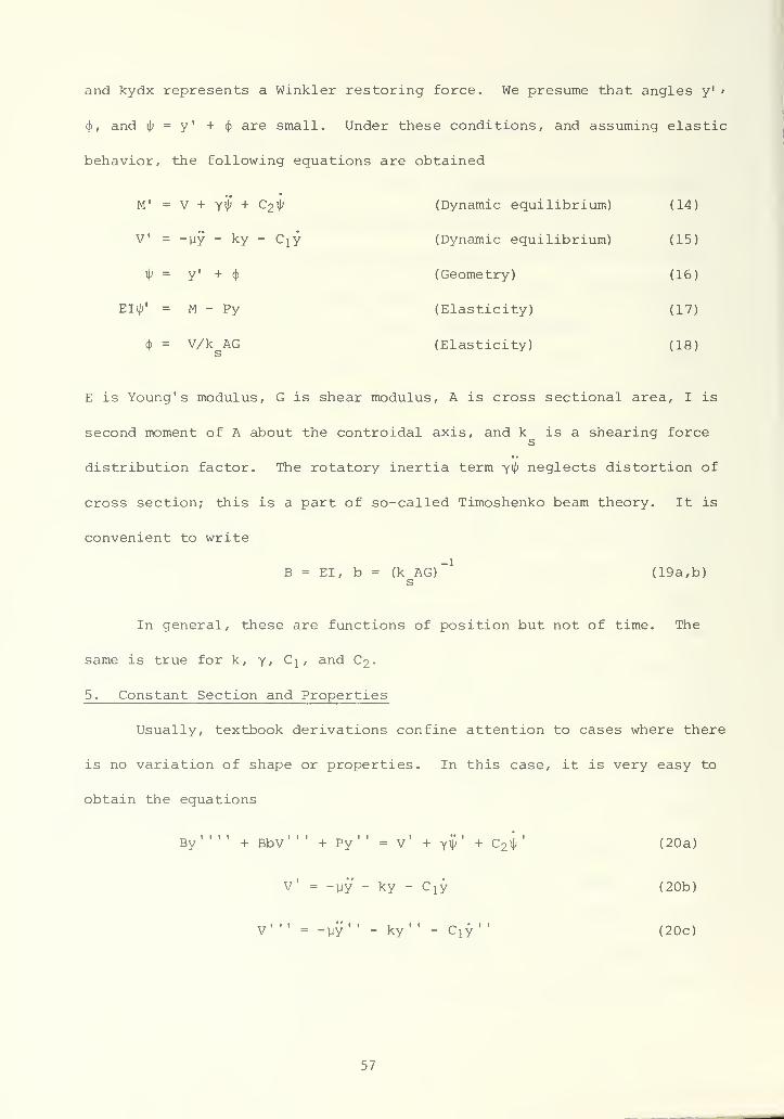
and kydx represents a Winkler restoring force. We presume that angles y'

'

(J), and \\> = y' + <\> are small. Under these conditions, and assuming elastic

behavior, the following equations are obtained

M' = V + yi\) + C2 ^

V = -yy - ky - Cjy

ty= y' + <j>

Eli/;' = M - Py

d> = V/k AGs

(Dynamic equilibrium) (14)

(Dynamic equilibrium) (15)

(Geometry) (16)

(Elasticity) (17)

(Elasticity) (18)

E is Young's modulus, G is shear modulus, A is cross sectional area, I is

second moment of A about the controidal axis, and k is a shearing forces

distribution factor. The rotatory inertia term y^ neglects distortion of

cross section; this is a part of so-called Timoshenko beam theory. It is

convenient to write

(19a, b)B = EI, b = (k AG)s

In general, these are functions of position but not of time. The

same is true for k, y, C^ , and C2-

5. Constant Section and Properties

Usually, textbook derivations confine attention to cases where there

is no variation of shape or properties. In this case, it is very easy to

obtain the equations

By + BbV + Py = V + y\p + C 2 ^

V' = -yy - ky - Cjy

V -yy" - ky " - C lY

(20a)

(20b)

(20c)

57

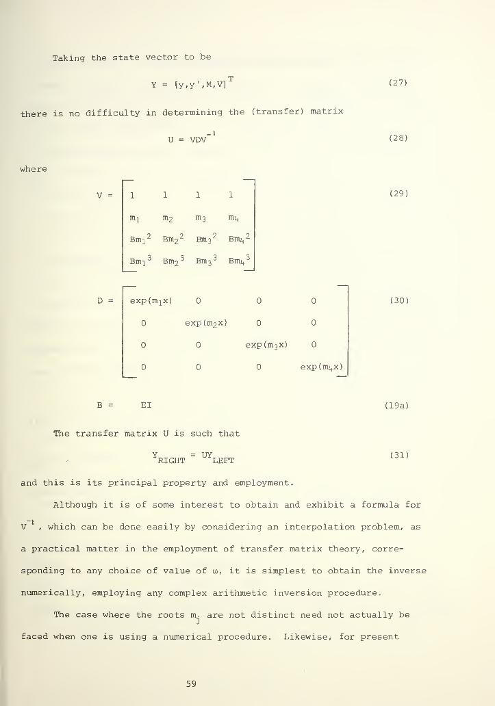
Taking the state vector to be

Y - [y,y\M,V]

there is no difficulty in determining the (transfer) matrix

_lU = VDV

(27)

(28)

where

V =

m^ m2 "13 m^

Bmi 2 Bm22 Bm3 2 Bm^ 2

Bm^ 3 Bm23 Bm3 3 Bm4

3

D = expdnjx)

exp(m2x)

exp(m 3 x)

exp(m t+ x)

(29)

(30)

EI (19a)

The transfer matrix U is such that

Y = UYRIGHT LEFT

(31)

and this is its principal property and employment.

Although it is of some interest to obtain and exhibit a formula for

V , which can be done easily by considering an interpolation problem, as

a practical matter in the employment of transfer matrix theory, corre-

sponding to any choice of value of to, it is simplest to obtain the inverse

numerically, employing any complex arithmetic inversion procedure.

The case where the roots m. are not distinct need not actually be

faced when one is using a numerical procedure. Likewise, for present

59

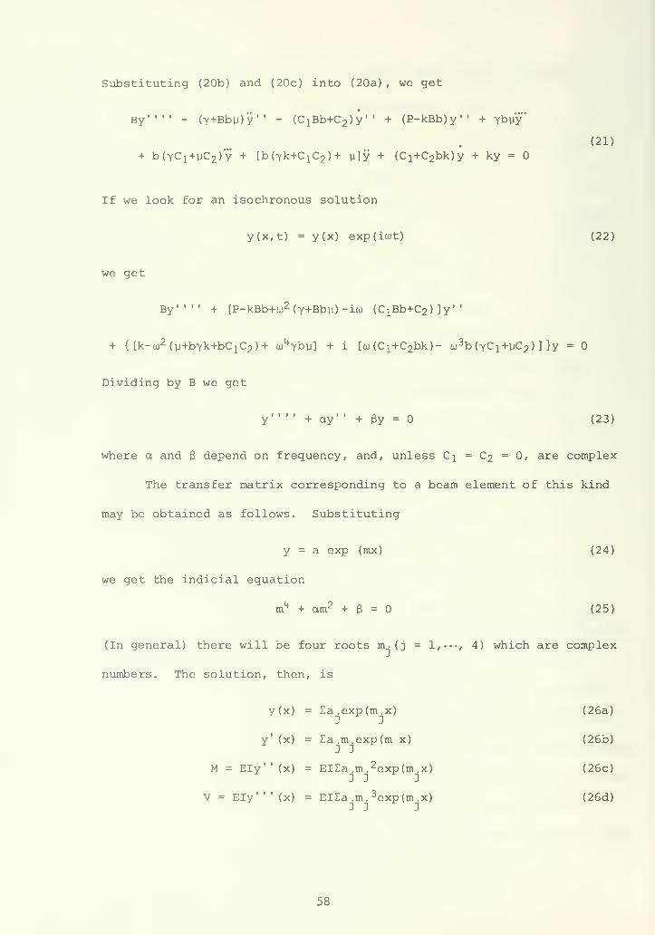
Substituting (20b) and (20c) into (20a), we get

By'''' - (y+Bby)y'' - (C1Bb+C 2

)y'' + (P-kBb)y" + yb]iy

+ b(YC1+yC 2 )y + [b(yk+C

1C2 )+ y]y + (C!+C2bk)y + ky =

(21)

If we look for an isochronous solution

y(x,t) = y(x) exp(iwt) (22)

we get

By''" + [P-kBb+u2 (Y+Bby)-ia) (C1Bb+C2 ) ]y '

*

+ { [k-w2 (y+byk+bC1C2 )+ w^yby] + i [co(C

1+C 2bk)- a>

3b(YC 1+yC 2 ) ]}y =

Dividing by B we get

y" ' ' + ay' ' + By = (23)

where a and (3 depend on frequency, and, unless C^ = C 2 = 0, are complex

The transfer matrix corresponding to a beam element of this kind

may be obtained as follows. Substituting

y = a exp (mx) (24)

we get the indicial equation

mk + am2 + B = (25)

(In general) there will be four roots m-(j = 1,>«<, 4) which are complex

numbers. The solution, then, is

y(x) = Za.exp(m.x) (26a)

y' (x) = Za.m.exp(m x) (26b)

M = EIy"(x) = ElEa.m. 2exp(m.x) (26c)3 3 3

V=EIy'"(x) = El£a.m. 3exp(m.x) (26d)3 3 3

58

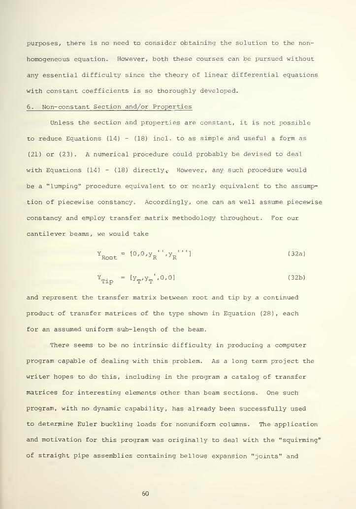
purposes, there is no need to consider obtaining the solution to the non-

homogeneous equation. However, both these courses can be pursued without

any essential difficulty since the theory of linear differential equations

with constant coefficients is so thoroughly developed.

6. Non- constant Section and/or Properties

Unless the section and properties are constant, it is not possible

to reduce Equations (14) - (18) incl. to as simple and useful a form as

(21) or (23). A numerical procedure could probably be devised to deal

with Equations (14) - (18) directly^ However, any such procedure would

be a "lumping" procedure equivalent to or nearly equivalent to the assump-

tion of piecewise constancy. Accordingly, one can as well assume piecewise

constancy and employ transfer matrix methodology throughout. For our

cantilever beams, we would take

Vot = I".O.yR,,

.yR,,,

l (32a)

YTiP

= [yt .yt'' '°] <32b >

and represent the transfer matrix between root and tip by a continued

product of transfer matrices of the type shown in Equation (28) , each

for an assumed uniform sub-length of the beam.

There seems to be no intrinsic difficulty in producing a computer

program capable of dealing with this problem. As a long term project the

writer hopes to do this, including in the program a catalog of transfer

matrices for interesting elements other than beam sections. One such

program, with no dynamic capability, has already been successfully used

to determine Euler buckling loads for nonuniform columns. The application

and motivation for this program was originally to deal with the "squirming"

of straight pipe assemblies containing bellows expansion "joints" and

60

details of the computation are proprietary to Tube Turns Division of

Chemetron Corporation, for which the writer performed this work several

years ago.

7. Alternate Approach

However, for the present purpose, namely that of making a "reasonably

accurate" determination of (lowest) natural frequency of cantilever-like

vibrations of thermowells, it does not seem necessary to apply such a

sophisticated procedure. An alternate viewpoint may be described as

follows.

Use "ordinary" beam theory. Omit all damping, rotatory inertia, and

shear deflection. Also note that in this problem there is no Winkler sup-

port and the effect of axial force P may be neglected. The resulting

simplified and idealized situation is easily dealt with. Murdock's analy-

sis used a Rayleigh type of approximation (employed in a somewhat less

general way than the present writer would have preferred) . The writer

prefers a Stodola type of solution for the problem at hand. However,

properly used these, and other, methodologies lead to the same numerical

determinations with a quite tolerable margin of approximation.

Then, having the "simple beam theory" evaluation for (lowest)

natural frequency, one attempts to estimate the effect of the foundation

and of shear deflection and rotatory inertia. In doing the latter,

attention is focussed upon their exactly calculable effect in the case of

uniform beams and it is reasonably assumed that a similar (qualitatively

and quantitatively) effect is applicable in the case of nonuniform beams.

The errors in doing this are surely less than other errors of idealization,

principally those concerned with the degree of root compliance.

61

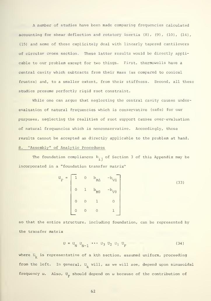
A number of studies have been made comparing frequencies calculated

accounting for shear deflection and rotatory inertia (8), (9), (10), (14),

(15) and some of these explicitely deal with linearly tapered cantilevers

of circular cross section. These latter results would be directly appli-

cable to our problem except for two things. First, thermowells have a

central cavity which subtracts from their mass (as compared to conical

frustra) and, to a smaller extent, from their stiffness. Second, all these

studies presume perfectly rigid root constraint.

While one can argue that neglecting the central cavity causes under-

evaluation of natural frequencies which is conservative (safe) for our

purposes, neglecting the realities of root support causes over-evaluation

of natural frequencies which is nonconservative. Accordingly, these

results cannot be accepted as directly applicable to the problem at hand.

8. "Assembly" of Analytic Procedures

The foundation compliances b. . of Section 3 of this Appendix may be

incorporated in a "foundation transfer matrix"

UF

=MA

5

M6

1

-b

-b

VA

ve

1

(33)

so that the entire structure, including foundation, can be represented by

the transfer matrix

U = UN Vl '•" °3 U

2U

lUF

(34)

where U is representative of a kth section, assumed uniform, proceeding

from the left. In general, U will, as we will see, depend upon sinusoidal

frequency tu. Also, U should depend on oj because of the contribution ofF

62

its inertia; however, our evaluation has not been sufficiently thorough

as to take foundation mass into account; furthermore, for lack of knowledge,

we must take b .= b„„ = 0.

ma ve

Then the transfer matrix procedure of determining natural frequencies

consists of dealing with

Y = UYRIGHT LEFT

(35)

where it is known that

YRIGHT

= [yR'

yR''' 01 (36)

i.e., a "free" condition, and

LEFT= [0,0,M

L,V

L] (37)

i.e., a "clamped" condition.

If we write

U =11

'21

l

31

41

U12

u22

u

u42

U13

u2 3

u.32 u 33

U14

u2k

u34

4 3 4 4

(38)

the condition becomes

33

'4 3

34 X" =

44VL

(39)

and for a solution other than M = V = 0, we must have

U33

U34

U4 3

U44

= U33

U44 " U

34U43

=° (40)

63

and the natural frequencies to. , u) ... must be such as to satisfy this

relation. (This is the essence of transfer matrix analysis for natural

frequencies.

)

Transfer matrices U for other than uniform beam elements are, at best,

quite complicated. Accordingly, as indicated above, our procedure could

be to consider a nonuniform beam as a concatenation of piecewise uniform

segments. In this way we can construct a procedure (a digital computer

program) capable of dealing (to a satisfactory degree of approximation if

section changes are "gradual") with a general, nonuniform cantilever having

root compliance and taking shear deflection and rotatory inertia into

account.

9. Calculations for Uniform Cantilever

As has been indicated above, a program for determining cantilever-

type frequencies can be constructed, accounting for elementary effects

and the additional complications due to non-uniformity, shear deflection,

rotatory inertia, and foundation compliance, although, as has been pointed

out, our knowledge of appropriate foundation parameters is incomplete and

faulty in that it does not consider foundation inertia.

However, this program has not yet been written. Moreover, for prac-

tical daily design use a simpler viewpoint is to be preferred. Accordingly

we now investigate the case of a uniform cantilever, taking into account,

one after another, the non-elementary complications listed above. We will

see how great their influence is and will suggest that the frequencies of

non-uniform cantilevers will be modified in the same way and roughly to

the same extent.

Thus we want an appropriate transfer matrix U for a uniform cantilever,

and we adapt this from the information given on page 136 of (22). In

64

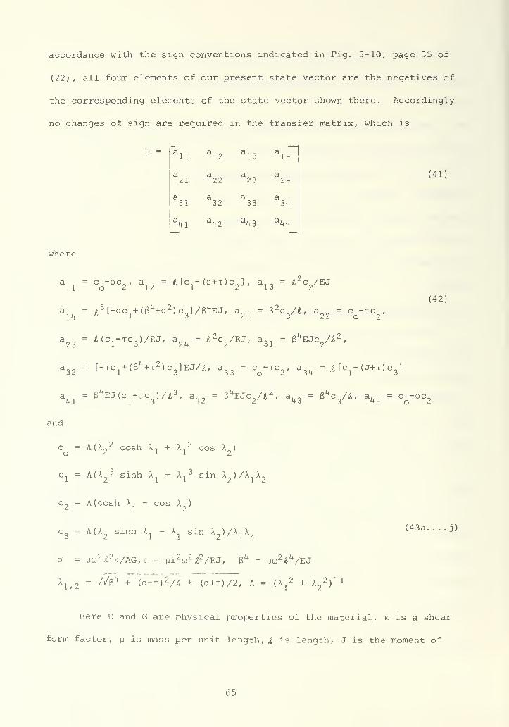
accordance with the sign conventions indicated in Fig. 3-10, page 55 of

(22) , all four elements of our present state vector are the negatives of

the corresponding elements of the state vector shown there. Accordingly

no changes of sign are required in the transfer matrix, which is

U =l

ll "12 "13 "14

21 22 23 24

31 32 33 34

\l dt+2

a43 ^44

(41)

where

a, = c -oc-, a no = I [c - (a+x)c,J , a, = i/cVEJ'11 o 2' 12 13

a = i2 [-oc +(B 4+a 2 )cJ/e t+

EJ, a.. = 32c /I, a 00 = c -tc .

14 1 3 z 1 3 22o2a23

= A(C1-TC

3)/EJ, a

2k= i 2c

2/EJ, a

31= B^EJ^/i 2

,

a32

= [- tc1

+ (S 1++t2 ) c3

] ej/^' a33 = c -TC 2' a

3i+=

& f c1

_( a+T ) c

3l

- «4

(42)

41EJ(c -ocj/x 3

, a.„ = B^EJc^/X 2, a.. = tf*c/l, a... = c -ac

1 3 42 43 44 o 2

and

c = A(A 2 cosh At + A2 cos A„)

o z x i 2

Cj = A(A2

3 sinh A + A^ sin A )/A A,

c2

= A (cosh A - cos A )

c = A(A sinh A - A sin A )/AjA2

= ya>2 £2K/AG,T = yi 2

u)2 42/EJ, B

4 = yw2 ^t+

/EJ

Xl,2

= ^^ + (^"T) 2/4 ± (a+T)/2, A = (A2

2 + A22

)

_1

(43a j)

Here E and G are physical properties of the material, k is a shear

form factor, \i is mass per unit length, I is length, J is the moment of

65

inertia of the cross section about a centroidal axis perpendicular to the

plane of vibration, and i is the radius of gyration about the same axis.

Note that J = Ai 2.

It is important to note that y includes not only the mass of the

cantilever itself but also the "added" mass of the fluid which may be

considered to move with it. For the case of a cylinder under stationary

conditions, the added mass may be shown to be equal to the mass of the

displaced fluid and this assumption should be made here.

Writing

U33

= U(+1 U33

(44)

where the subscripts refer to equation numbers, and defining (compare

equation (40))

A = U33 V " U

34U43

(45)

we get

A = (a..bw +a„_b +a 35 ) (-a, ,b -a b +a, )

31 MA 32 M0 33' 4 1 VA 42 V9 44

-(a b +a, „b +a ) (-a b -a b +a )

41 MA 42 Me 43 31 VA 32 Vq 34;

(46)

a quantity which depends on frequency and which should vanish. Thus one,

in effect, repectedly evaluates A(w) for different values of to and finds

the values of to for which A (to) = 0.

Actually it is more convenient to take the parameter

X = ek = yto

2^

£+/EJ (47)

as a variable rather than to itself. Also, from (43f) and (43g) we have

t = x(i/^) 2/ a = 2.6tk (48a, b)

using Poisson's ratio =0.3. We are dealing with a circular section for

which i = a/2. It is convenient to represent the length i in terms of

66

radius a by introducing the aspect ratio

n = a/jfc (49)

Cowper (12) , (13) has pointed out that Timoshenko beam theory, which

is the basis of the results given in (22) , employs a questionable value for

the shear coefficient k, using the value k = 4/3 based on the elementary

VQ/Ib theory. Cowper derives the value

< = (7+6v)/(6+6v) = 1.128, (v. 3) (50)

Brock (1), (2) and North and Roy (19) obtain the result

< = (7+14v+8v 2 )/6(l+v) 2 = 1.176, (v=.3) (51)

Cowper (12) , (13) discusses the genesis of various values and Brock (3)

,

(4) also makes such comparisons. (A source of possible confusion is that

Cowper' s value for a rectangle is k = (12+llv) / (10+10v) = 1.177 which is

easily incorrectly identified with the value given in Equation (51); in

fact, Carnegie and Thomas (8) report Cowper' s rectangle value as 1.176)

Briefly, most studies of the effect of shear deflection via

Timoshenko ' s beam theory use k = 4/3, but almost certainly a smaller value,

about 1.13 to 1.18, should be used. In calculations, shown later, we use

the common value, 4/3, and also the "better" value, 1.128.

10. Computer Program and Results

Based upon the analysis of the preceding section a computer program

(see listing in Table C-l) was employed to calculate a frequency reduction

factor applicable to uniform cylindrical cantilevers. This factor,

designated as FRF is the ratio

lowest frequency considering effectsFRF — - - ; (52)

lowest frequency using elementary theory

67

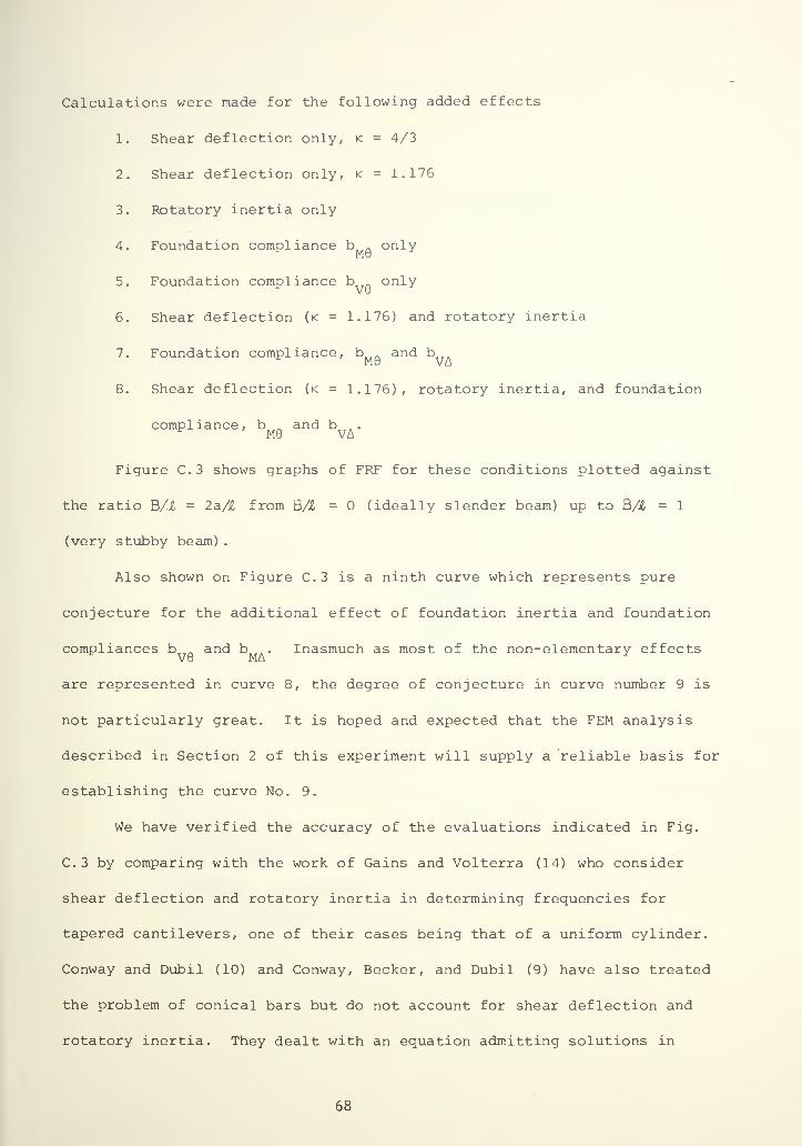
Calculations were made for the following added effects

1. Shear deflection only, k = 4/3

2. Shear deflection only, k = 1.176

3. Rotatory inertia only

4. Foundation compliance b A onlyMb

5. Foundation compliance b onlyvu

6. Shear deflection (< = 1.176) and rotatory inertia

7. Foundation compliance, b and bMW VA

8. Shear deflection (k = 1.176), rotatory inertia, and foundation

compliance, b „ and b ,

.

^ M9 VA

Figure C.3 shows graphs of FRF for these conditions plotted against

the ratio B/.1 = 2a/i from B/i = (ideally slender beam) up to B/i = 1

(very stubby beam)

.

Also shown on Figure C.3 is a ninth curve which represents pure

conjecture for the additional effect of foundation inertia and foundation

compliances b . and b , . Inasmuch as most of the non-elementary effectsV9 MA

are represented in curve 8, the degree of conjecture in curve number 9 is

not particularly great. It is hoped and expected that the FEM analysis

described in Section 2 of this experiment will supply a reliable basis for

establishing the curve No. 9.

We have verified the accuracy of the evaluations indicated in Fig.

C.3 by comparing with the work of Gains and Volterra (14) who consider

shear deflection and rotatory inertia in determining frequencies for

tapered cantilevers, one of their cases being that of a uniform cylinder.

Conway and Dubil (10) and Conway, Becker, and Dubil (9) have also treated

the problem of conical bars but do not account for shear deflection and

rotatory inertia. They dealt with an equation admitting solutions in

68

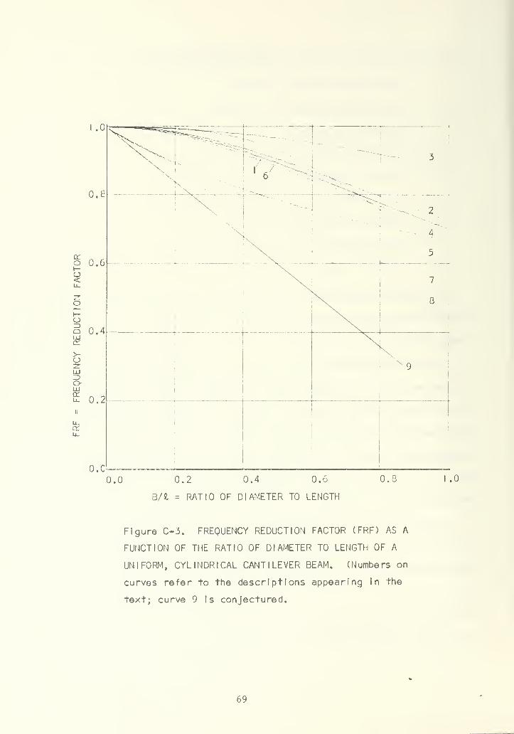
.0

0.8

0.6OO<Ll.

Oo 0.4LUen

>-ozLU3oLU

cc

0.2

x.

7

8

1

1

9

o.c

0.0 0.2 0.4 0.6

B/fc = RATIO OF DIAMETER TO LENGTH

0.8 .0

Figure C-3. FREQUENCY REDUCTION FACTOR (FRF) AS A

FUNCTION OF THE RATIO OF DIAMETER TO LENGTH OF A

UNIFORM, CYLINDRICAL CANTILEVER BEAM. (Numbers on

curves refer to the descriptions appearing In the

text; curve 9 Is conjectured.

69

TABLE C-l

Computer program determiningeffects of shear deflection,

rotatory inertia, and

foundation compliance

c j. E. enccK, 16 augjst 1974C PROGRAM FJ« EVALUATING THc EFFECT CF SHEAR OtFLECTICN, lOTAT'TRY

C INERTIA, ANC FOUNDATION COMPLIANCE UPON THE LOWEST FKtgUslCVC Of VIBRATION CF A UNIFORM CANTILEVER OF CIRCULAR CROSS ScCTUN.C AN EARLIER VERSUN IS OATtU DECEMBER 1972.

IMPLICIT RE AL»8( A-H.K, LiU-XlREAL'4 YI2C0), Z1200) .crcr run iTTieusoREAL'S T I( UI/'BROCK, J*,', t.i B 1

',

• X 3 — ' .

'

SCFT C AN' ,• T I L t V =R

ki.i — • ,6*' VREAL JABIBI/' 1'.' 2'.' 3 1 ,' 4 • ,

' 5«,' t> ' i • M,' 3

IVEPS=i.C-oNB=1C0ENe=NB[l.CO/ENE

C0L

2C"JM,3 "STJETOUTTNE FKEAKTA ,8 ,C,D ,E ,F,C-)e»C . CO C PARAMETER LIST:8ETA=2.J0 C A» BETA TU FOURTH FQWERPRINT 6, J C B ' CIAMETER OVER LENGTH RATIO

6 FCRfATUOX,' J EiUALS • , 1 <. I C C » SHEAR FACTOR! C =» 1.33333 Oft C » 1.176 (

PRINT 7 CD' FREULENCY DETERMINANT (CUTPUTI7 FCPMAT 1 LOX, 'B* , 7X, 'BcTA' ) c E = FOTARY INERTIA FACTOR ( E = 1.0 UR E = 0.0 )

C = C.D0 _C. _. _| » FCiM;AILCN EACTUg 1Z£RC CF BEt-SUB-EM-THETA,]

E = C.T30 C G = FOUNTATION FACTOR (ZtKO OR 6 Ec -iUB -V?L: -Dt LT A I

F=0.C0 IPfLICIT REAL*8(A-H,K,L,C-X)G*C.D0 TAL=A«(B/4.00)»«2FAC l = 2.C£S"i^eD-l SlCMA=2.fc0C»TAU»CFAC2*1.5C?<4C-1 TAL»TAU*Ej j»2 TEMl«DSURT(A+( SI GMA- TAU) »«2/<». DO )

IFU.EQ.ll JJ=1 TE^2=(SIGMATAU)/2.D0

IFU.EQ.2) E=1.0C L = 1. CO/ ( L 1»» 2»L2»«2 I

IFIJ.EC.4) f = FACl S*»DSI*H(L1IIFIJ.EU.5) G=FAC2 Ch=CCOSH(Ll)IFU.EU.6) C«l.l76D+0 ST»CSIML2IIFlj.EC.6) E=1.D0 CT=DCCS(L2)IFU.EU.7I P'FACl CC=L * (CF »L 2**2«CT»L 1» *2IIF<J.EQ.7)0=FAC2, „ , C1=L» 1 SH-L2' »4/L l+ST *L 1* *l/Ll\TF(j.E"C.8I C = I.l7t>D»0 CT=L»(CH-CT)IFU.EU.ElE'l.DO C3 = L*ISH/L 1-ST/L2IIFIJ.EC.8) F*FAC1 C<» = C0-TAU*Ci: «F»B» IC3» ( A*T AU« *i l-T AU"C1 )

IFIJ.EC.8) G=FAC2 C 5< C- SI GMA*C 2-G*A"B*» 3« ( C 1- SI CMA«C J I

IF(J.ES.S) JJ=3 C6="A»IC3«F»B«C2)CC 10 1=1. KB C7=C l-( SIGM*TAU)*C3-G*A*B*«3«C2DEBeT*DEL C = C-«*C i-C 6*C 7

B=6*0 RETURN?=EETA**4 EM}CALL FREAK(A,6,C,DD,E,F,G)Dl-DD

1 eETA=BETA-C£BETA=BETA»«4CALL FREAKtA.BiC ,DO,E,F,G»C2 = CCS'D1*D2TFtnr, k,z

2 C l = C2GC TC I

3 IF10EBET.LE.EPS) GO TO 4BETA*BET A*CEEETCEBET"1.D-1"»DEBETGO TO 1

4 CCKT INUE . „ClrRATiTHTiTA/'l .TT51O4D0 I^*ZPRINT 5, B.BETA.OMRAT

5 FCfMAT (5X.3F10.5 )

YII )=EH I)=CMRAT

CALL DRAWlNb ,Y,Z,JJ,0.JAB(J).TI,0,O.J»0,J,0tB,8,l,JJJI20 CCNT INUE

STCF

70

terms of Bessel functions. Carnegie and Thomas (8) consider the effects

shear deformation and rotatory inertia on tapered cantilever frequencies.

They provide an extension bibliography. See also Hurty and Rubinstein (15)

.

However, none of these analyses considers the effect of foundation compli-

ance and inertia.

11. Frequency Reduction Factors

We have shown here that foundation effects are of the same order of

significance as are those due to shear deflection and rotatory inertia.

(Actually our own evaluations underestimate the effect, which leads us to

curve number 9 in Fig. C.3). Accordingly, evaluations in the literature

necessarily provide frequency estimates which are too high. Results from

FEM analysis should be most reliable but they are not available yet.

Although the effect of the central cavity of a thermowell upon its vibra-

tion frequency is probably small (and probably such as to raise the fre-

quency so that neglecting its effect is conservative) so that the data of

Gaines and Volterra (14) might appear tempting, foundation effects are not

considered in their data. The analysis in this Appendix is deficient in

that it considers only uniform (i.e., nontapered) beams and only part of

the foundation effects. A more elaborate analysis, outlined in Section 8

hereof is capable of dealing with nonuniform beams but it has not actually

been programmed.

Accordingly, it would appear that the best one could do for a non-

uniform beam would be either

(a) to calculate lowest frequency using elementary theory, and by assuming

that the "other" effects are about the same as for a uniform

beam, apply a frequency reducing factor, such as that given by

curve 9 of Fig. C.3.

71

(b) to determine lowest frequency, including shear and rotatory

inertia, using the methods or the data given by Gaines and

Volterra (14) or by Carnegie and Thomas (8) , and apply a (dif-

ferent) frequency reducing factor, based on uniform beam calcu-

lations as in the preceding section hereof, to account for

foundation effects.

The aspect ratio parameter p in Figure C.3 must be generalized to

accommodate to tapered beams and we suggest the definition

p = (tip diameter + root diameter) /2 x length (53)

Then, to obtain frequency w use either formula (54) or formula (55)

"-»»,» UELEM " (1- 8P)W

ELEM(54)

U = FRF2

X<»SDRI

= (1-- 4P)WSDRI

(55)

where w is the value obtained by elementary analysis using a procedure

like Stodola's or Rayleigh's, and where w is the value obtained (some-

how) taking into account shear deflection and rotatory inertia. Neither

a) nor w should attempt to include foundation effects. Both FRF,ELEM SDRI 1

and FRF„ are based on our analysis here of a uniform circular beam.

We feel that formula (54) is fully as reliable as is formula (55)

and it is easier to use. The two formulas agree at p = and, for a

uniform beam, at p = 1/3.

12. Elementary Analysis for Actual Thermowell Geometry

Using Stodola's method and a digital computer program not shown here,

calculations were made for "elementary" lowest frequency for the shape

shown in Figure C.4. Results obtained for a variety of parameter ratios

lead to the equation

fne

= (Ffa/L2 )/e/( Y+y') < 56 >

72

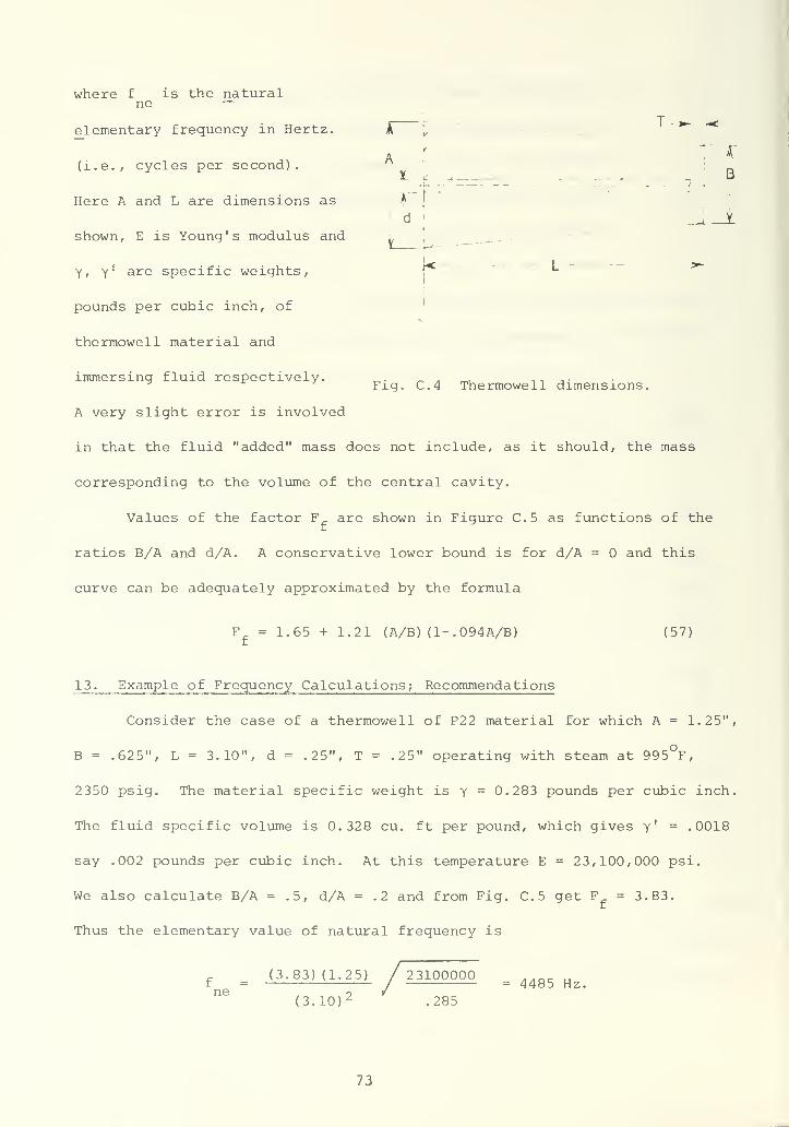
where f is the naturalne —

elementary frequency in Hertz,

(i.e., cycles per second). A \

JL _*_-.__ ...... 3

Here A and L are dimensions as * l

d „_i_Ashown, E is Young's modulus and i „ .

y, y are specific weights, j" u

pounds per cubic inch, of '

thermowell material and

immersing fluid respectively. „. „ . _. , , -,

Fig. C.4 Thermowell dimensions.

A very slight error is involved

in that the fluid "added" mass does not include, as it should, the mass

corresponding to the volume of the central cavity.

Values of the factor F are shown in Figure C.5 as functions of the

ratios B/A and d/A. A conservative lower bound is for d/A = and this

curve can be adequately approximated by the formula

F = 1.65 + 1.21 (A/B) (1-.094A/B) (57)

13. Example of Frequency Calculations; Recommendations

Consider the case of a thermowell of P22 material for which A = 1.25",

B = .625", L = 3.10", d = .25", T = .25" operating with steam at 995°F,

2350 psig. The material specific weight is y = 0.283 pounds per cubic inch.

The fluid specific volume is 0.328 cu. ft per pound, which gives y' = -0018

say .002 pounds per cubic inch. At this temperature E = 23,100,000 psi.

We also calculate B/A = .5, d/A = .2 and from Fig. C.5 get F = 3.83.

Thus the elementary value of natural frequency is

- (3.83) (1.25) / 23100000 ..__ „r = / = 4485 Hz.ne o v

(3.10) 2 .285

73

Oh-o<

>-o

IDoUJ

0.5 0.6 0.7 0.8 0.9

VALUES OF B/A

Figure C-5 Values of the frequency factor Ff

as a function of

the ratio B/A for various values of d/A. All curves are for

T/L = 0. Nonzero values of T/L result in very slight reduction

of the values shown here.

74

FRFj = l-(.8) (1.25+.625)/6.20 = .758

Thus we estimate

f = 3400 Hz

If we had used the lower bound given by Equation (57) , we would have

calculated F = 3.62, f = 4239 Hz, f = 3213 Hz which is conservative,f ne

The alternate procedure would employ, for example, the data of Gaines

and Volterra (14) , neglecting the central hole. Using their notations,

6 = .5 (fortunate! since there is thus no need to interpolate on 6), and

A = 2.48. This value, however is beyond the range of the data they give.

If we are to proceed by this route, we would extropolate their data. An

approximate value is $ = 4.30, whence, using their analysis

f = (4.30A/2ttL 2) /24.1E/(y+Y 1

) = 3. 36A/L2 /e/ (y+y 1) = 3935 Hz

This value, 3.36, compares to our value 3.62 obtained above. Next,

accounting for the foundation effects, we get

f = [l-(.4) (1.25+.625)/6.20] (3935) = 3460 Hz

which compares with our value f = 3213 Hz given above. These comparable

values are too low because of the effect of the central cavity. Assuming

the same correction applies, we finally calculate

f = (3.83) (3460)/(3.62) = 3660 Hz

which compares with our earlier evaluation, 3400 Hz.

For the purpose at hand, our simple procedure (Equation (54)) gives

3400 Hz and the alternate procedure (Equation (55)) gives 3660 Hz. We

simply do not know which is more accurate, but for our purposes 3400 Hz

is more conservative (i.e. , safer) and it is surely easier to obtain.

75

Thus, we recommend the simpler procedure. We outline the procedure

in Appendices F and G, where, it should be noted, that the lower bound

formula (57) might be used first to estimate F . If results are not

satisfactory, a more elaborate estimate of F may be obtained by the use

of the curves given in Figure C.5 or by appropriate calculations.

14. Pipe Ovalization Mode

With one exception, studies of thermowell vibrations have dealt

exclusively with what might be called cantilever modes. Interest was

focussed on assuring that the lowest cantilever mode was slower than the

excitation frequency. However, in

an earlier report (5) , (6) , the

writer called attention to the fact

that the vortex shedding excitation

could excite a "pipe ovalization

mode" having a frequency slower than

that of the lowest cantilever mode.

This subsection discusses the pipe

ovalization mode and provides assur-

ance that no concern need be felt

about it.

Fig. C.6 Pipe ovalization mode,

A standard treatment of nonextensional ovalizing vibrations for thin

circular rings is given by Timoshenko (23). Rewriting Timoshenko's formula

so as to apply to thin circular cylinders, and taking the number of "lobes"

to be equal to 2 so as to obtain the lowest (ovalizing) mode, we get

,2 _ 7.2EIg/Ayr 1+

(l-v 2) (58)

where r = mean radius of cylindrical shell

76

E = Young's modulus C3Q,000,000 psi for steel)

v = Poisson's ratio (0.3 for steel)

I = moment of inertia of unit strip of pipe wall about an axis

passing through mid-thickness (I=t°/12)

g = 386 in/sec 2

A = area of unit strip = t

Y = specific weight (.283 for steel)

t = wall thickness

There is some added or virtual fluid mass which also participates in

the motion so that y should be slightly increased to account for this

behavior. Our tubes are thick, not thin. Accordingly, the virtual fluid

mass is so much smaller than the metal mass that we will not concern our-

selves further with this correction.

Thus, for steel tubes we find

a> = 164300t/r 2; f = 26142t/r2 (Hertz) (59)

where t and r are measured in inches. The formula is really applicable

only to thin tubes and the pipes (such as main steam lines) with which we

are concerned are hardly thin. Accordingly there are other compliances in

action that serve to reduce the frequency below that given by Equation (59)

.

Nevertheless, this is about as well as we are able to do; furthermore this

estimate will be satisfactory for our purposes.

This formula gives astonishingly low values for the ovalizing frequency

f. Thus, in the case of a main steam pipe with t = 3", r = 10", say, we

find f = 784 Hz.

This is almost certainly less than the excitation frequency in a main

steam system. (Actually we might be concerned with three-lobe ovalization

77

for which the frequency is 2.83 times as great as that given by Equation

(59).

Then we see that there are structural frequencies, slower than the

lowest cantilever frequency, with which the vortex shedding excitation

could couple. The obvious question is whether or not we should be concerned

with such case. A plausible argument that we need feel no concern is

offered below. However, it would be of the greatest interest to see whether

such ovalizing modes might be observed in practice.

Figure C.6 indicates that alternate vortex shedding produces fluid

forces on the thermowell which, in turn, produce moments at the root which

couple with and could excite the flexural oscillations. However, note that

the thermowell root is a node of the ovalized vibrations. In other words,

the circumferential bending moment is zero at this point (and its opposite)

and is extremal at the 45 positions. If the problem were truly two dimen-

sional (plane strain) and if there were no energy removal, the points sub-

ject to maximum stress, and thus the points most susceptible to fatigue

failure, would lie along longitudinal lines at the 45 positions. The

stresses at the root of the cantilever would be essentially zero; certainly

much less than would occur for what we have called cantilever modes.

Furthermore, this two dimensional presentation is an oversimplifica-

tion. Theoretically, the vortex shedding from the thermowell, which is

located at a definite axial position along the pipe, could excite ovalized

vibrations that would extend, without change, to infinity in both directions.

However, the pipe itself doesn't and there are energy sinks upstream and

downstream which prevent a build-up of distortion such as illustrated in

Figure C.6. Locally there is energy absorbtion by fluid contents and

external insulation or other coatings; however, it has been shown

78

experimentally that these mechanisms do not afford much damping capability

(18).

The above remarks apply not only to the two- lobe case shown in

Figure C.6 but, generally also to ovalizations with more than one lobe.

Briefly our reason for advocating that we forget about these pipe-

ovalizing vibrations when considering thermowell integrity is that they do

not imply significant stress in the thermowell. The greatest stress

associated with ovalization is in the pipe wall itself, at 45 from the

thermowell root (for the two- lobe case) and there seems to be no experi-

mental evidence that the pipe is thereby itself endangered.

15. Bibliography for Appendix C

CI. Brock, J. E. , Shear distribution in piping, Heating Piping and Air

Conditioning, Vol. 35, No. 1, January 1963, pp. 141-143.

C2. Brock, J. E. , Memorandum A, Remarks on the shear distribution factor

in piping, Report to U. S. Navy Marine Engineering Laboratory under

Contract N161-26147, June 21, 1965.

C3. Brock, J. E. Appendix B to Fifth Progress Report, November 15, 1966,

to United States Naval Academy, MEL No. 72-117, under Contract

N161-26327.

C4. Brock, J. E. Appendix A to Sixth Progress Report, January 15, 1967,

to United States Naval Academy, MEL No. 72-117, under Contract

N161-26327.

C5. Brock, J. E. , Stress analysis of thermowells, consulting report to

Bechtel Power Corporation, October 1972.

C6. Brock, J. E. , Supplement to Stress analysis of thermowells, consulting

report to Bechtel Power Corporation, December 15, 1972.

79

C7. Brown, J. M. , and Hall, A. S., Bending deflection of a circular shaft

terminating in a semi- in finite body, J. Appl, Mech. , Vol. 29, No. 1,

March 1962, pp. 86-90.

C8. Carnegie, W. , and Thomas, J., The effects of shear deformation and

rotary inertia on the lateral frequencies of cantilever beams in

bending, J. Eng'g. Ind. , Vol.— , No. 1, February 1972, pp. 267-278.

(Trans, ASME, Ser. B, Vol. 94, No. 2) February 1972, pp. 267-278.

C9 . Conway, H. D., Becker, E. C. H. , and Dubil, J. F. , Vibration frequencies

of tapered bars and circular plates, J. Appl. Mech., Vol. 31, No. 2,

June 1964, pp. 329-331.

CIO. Conway, H. D. , and Dubil, J. F., Vibration frequencies of truncated-

cone and wedge beams, J. Appl. Mech., Vol 32, No. 4, December 1965,

pp. 932-934.

Cll. Cook, R. D. , Deflections of a series of cantilevers due to elasticity

of support, J. Appl. Mech., Vol. 34, No. 3, September 1967, pp. 760-

761.

C12. Cowper, R. , The shear coefficient in Timoshenko's beam theory, J.

Appl. Mech., Vol. 33, No. 2, June 1966, pp. 335-340.

C13. Cowper, R. , On the accuracy of Timoshenko's beam theory, J. Eng'g.

Mech. Div., Proc. ASCE (EM 6) December 1968, pp. 1447-1453.

C14. Gaines, J. H. , and Volterra, E. , Upper and Lower bounds of frequencies

for cantilever bars of variable cross section, J. Appl. Mech., Vol. 33,

No. 4, December 1966, pp. 948-949.

C15. Hurty, W. C. , and Rubinstein, M. F. , On the effect of rotatory inertia

and shear in beam vibration, J. Frank. Inst., Vol. 278, No. 2, August

1964, pp. 124-132.

C16. Love, A. E. H. , Elasticity, 4th Ed., Dover, 1944.

80

C17. Matusz, J. M. , O'Donnell, W. J. , and Erdlac, R. J., Local flexibility

coefficients for the built-in ends of beams and plates, J. Eng'g Ind.,

(Trans, ASME, Ser. B, Vol. 91, No. 3), August 1969, pp. 607-614.

C18. McGarrah, W. E. , and Brock, J. E. , Designers can predict fundamental

vibration frequencies in piping structures, Heating Piping and Air

Conditioning, Vol. 33, No. 8, August 1961, pp. 105-109.

C19. North, E. L. , and Roy, P. A., Investigation of stress analysis practices

for submarine main sea water piping, GD/EB Report U411-65-001 to MEL

under Contract N161-25962, January 1965.

C20. O'Donnell, W. J., The additional deflection of a cantilever due to

the elasticity of the support, J. Appl. Mech. , Vol. 27, No. 3,

September 1960, pp. 461-464.

C21. O'Donnell, W. J., Stresses and deflections in built-up beams, J.

Eng'g. Ind. (Trans. ASME, Ser. B, Vol. 85, No. 3), August 1963,

pp. 265-273.

C22. Pestel, E. C. , and Leckie, F. A., Matrix methods in Elastomechanics,

McGraw-Hill, 1963.

C23. Timoshenko, S. P., Vibration problems in engineering, 2nd Ed.,

D. Van Nostrand Co., Inc., 1937.

C24. Timoshenko, S. P., History of Strength of Materials, McGraw-Hill, 1953.

C25. Westergaard, H. M. , Theory of Elasticity and Plasticity, Dover, 1964.

81

APPENDIX D

BENDING STRESSES AND THE COMBINED STRESS CRITERION

TABLE OF CONTENTSPage

1. Introduction 83

2. Moment and Bending Stress Analysis 83

3. Combination of Bending Moments and Stresses 89

4. Combination with Pressure Stresses 90

5. Combined Stress Criterion 91

6. Bibliography 92

82

Introduction

This Appendix deals with the bending stress that result from lateral

loads imposed on the thermowell by the flowing fluid. Figure D.l shows

the configuration which will be analyzed. Note that there is allowance for

a shielded length aL (where = a < 1) which is not exposed to the action

of the fluid stream.

In the writer's earlier

analysis (1) , no provision was

made for such shielding; i.e.,

a = was implicit in the

analysis. Also, it was tacitly I

assumed that the greatest

bending stress occurred at the

root. As will be seen in what

follows, this assumption is

correct (for a = 0). How-

ever, an algebraic error was

Fig. D.l Figure for analysis of

bending stresses.

made in the analysis as reported in (1) . Subsequently, when considering

the effect of non-zero shielding, the writer detected his earlier error,

but made a second error, so that a notice sent to members of the ASME

Committee PB51 (2) was itself incorrect.

2. Moment and Bending Stress Analysis

From the results reported in Appendix B it may be seen that the

elemental force dF shown in Figure D.l is

dF = (CpU 2 /2) (D) (dx) (1)

where D is the local diameter. The coefficient C = C if we are dealing

83

with the lift force whereas C = C if we are dealing with the drag force.

Introducing the useful parameter

p = (A-BJ/A (2)

we have

D = A(l-px/L) (3)

so that the bending moment at section - is

rL

M = (ACpU 2/2) (x-8L) (l-px/L)dxB J

(4)

nL

where n is the larger of a and B, i.e.,

n = Max (a,B) (5)

Performing the integration gives

Mg

= (ACpU 2L2 /l2) [3(l+pB) (l-n 2 )-6Bd-n)-2p(l-n 3)] (6)

Obviously M is greatest at the root and decreases steadily toward thep

tip. However, the section modulus

Z = ttD3 /32 (7)

also decreases steadily from root to tip. Accordingly it is necessary to

be adroit in examining the maximum of the bending stress

a Q= M /Z = GH (8)

p p

where

G = 8CpU 2L2 /3iTA2 (9)

and

H = H(p, n, B)

(10)

= [3(l+pB) (l-n 2) -6B(i-n)-2p(l-n 3 )]/(i-pB) 3

%

The value of coefficient H depends on the tapering parameter p,

the location parameter 3, and the parameter n. For given a, if 3 < a

then we must take n - ot while if $ > a then we must take n = 3- It takes

considerable algebra to show that

|p H(p, 3, 3) = (11)

only at 3 = 1 (i.e. , the tip) while

|^ H(p, a, 3) = (12)

only at

B- ». ^ l;tIW ," pV ''(13)

(2-p-pa)p

The value of 3* may be negative, which is meaningless; in this case the

maximum is at the root, 3=0. The analytical expression for H(p, a, 3*)

appears to be too complicated for convenient use; it seems to be preferable

to compute 3* from Equation (13) and substitute into the formula for

H(p, a, 3*).

A set of curves of the parameter H, for fixed p = 0.5 (corresponding,

say, to A = 1.5", B = .75") and for various shielding ratios a is shown

in Figure D.2. We are essentially interested only in the maximum value

of H. Accordingly, a set of curves of H as a function of p for variousmax

values of a is shown in Figure D.3.

It is only for large values of P and/or a that the maximum stress

occurs other than at the root. We can find the critical relation by

equating 3* = 0, cf. Equation (13). This yields

a = (2-p-/4p-3p 2 )/2p (14)

and a plot of this relationship is shown in Figure D.4

85

CO.

in

oI

2.0

1.5

I .0

0.5

0.0

^K1• 2

.3V£il ues of shield

parameter, a1 nq

.5 TAPERING PARAMETER

.6 , p = 0.5

d— ^\\.8

— ^~-**~.

S- ^~^-

.

0.0 0.2 0.4 0.6 0.8

LOCATION PARAMETER, 8

.0

Figure D-2 The function H(0.5,n,8).Cf. equations (5) and (10)

Table U-l Computer program for drawingFigure D-2, immediately above.

C PRCGRAH WRITTEN 29 AUGUST 1974 3Y J. E". BRICKC TC DRAW FIGURE 0-2 WITH P = 0.5

IMFLICIT KEAL*8<A-W)REAL** X18C2) .Y1802IKEAL*8 T II 12)/'flR0CK, J't'. t.i B'J'.'X •) — '.'UFNiltNo •, 'STRESS

IF« ,• ACTOR • , b*' •/

1/<C-P*8I*»3C=1.C*0P=;.D-1JN*601JSKIM40E.N'JN

DELTaE>07(EJN-0IOQ 1C0 1=1. IN6 1=1-1ALFA*EI/ (1 .C»l)DC 20 J=1,JNEJ=J-1BETA=EJ«CELTAB

YU)=EFFX( J» = ttETAIF IMCDI J.JSKIP1.EQ.1) PKINT I, P

,

ALFA ,B ETA ,EF

F

2 FCPPAT(5K.4F1C.5)20 CONT INUE

IF(I.EC.l) K«l

CALL CRAW(JN,XiY l K,0rLAiT[,0,U,J t J.0,o,o,H, I , J IT)

8STARM ( J*0-P>*»OALFAI-P»ALFA»» 2-0/ PI/ ( 0*0-P-P~ AL F A I

ETA=ALFAEFFe»F (eST/R)EFFO*F(OIPRINT 3, BSIAR.EFFB.EFFO

3 FCieiIiaJU3flQ.il1C0 C0NTINLE

STOPENC

86

0.0 0.2 0.4 0.G 0.8

TAPERING PARAMETER, p

Figure D-3 Maximum of the function H(p ,n, 3

)

as a function of the tapering parameter o for

various values of the shielding Darameter a.

Table D-2 Computer program for drawing Figure D-3

r. BR'.ICk TO DP AW FIG. n-3

X B — ','MAXIMJM •, 'STRESS

PPCGPAM WRITTEN 30 AUGUST 1974 0Y JIMPLICIT REAL*3U-WJREAL*4 X IBC 1 ) , Y< JJl I

REAL*8 TI ( 12)/'BR0CK, J','. E., Hi)'

IF' ,'ACTUR' ,f '/RE«L LA/' •/

INTEGER NFiM,I f J|K,J'lJT,NSKIPH(P iEiBJ =1 3.Q*0*lO«-P*B)» (0-E*E )- 6.0 + 0' B '( J-E 1-2 .0+0; P dl-E

BS?PtA)*lP*(C*C-PI*lC*A)-(P»! J|»-*2-U)/( <n+0-P-P*A)*P)C=1.0«0NSKI F*B0NP=8CCENP=NPM=10ENA=NADO ICO 1 = 1. NAEiMI-1A = El C/ENADO 5C J= l.NPEJ = JP»Eo/ENPXU)«PB = CMAX.llO.C'OtBStPiA) I

e=^axiJa,biY( J»=H(P,E ,B)IF(NOCUiNSKIP).Eq.Ul PRINT 20 , A , (1 , X( J ) , Y( J )

20 FCff'ATlSX ,<«F10.5)50 COM INUE

IF (I .EC. 1) K=lIF(I.lvE.l) K=2

3) 1/

cAii-cSisr'-^2

ICC CCMINLESTCPENC

NP.X,Y,K,0,LA,TI,0i0iO,O.O,Oiti,B,l,JUUT)

87

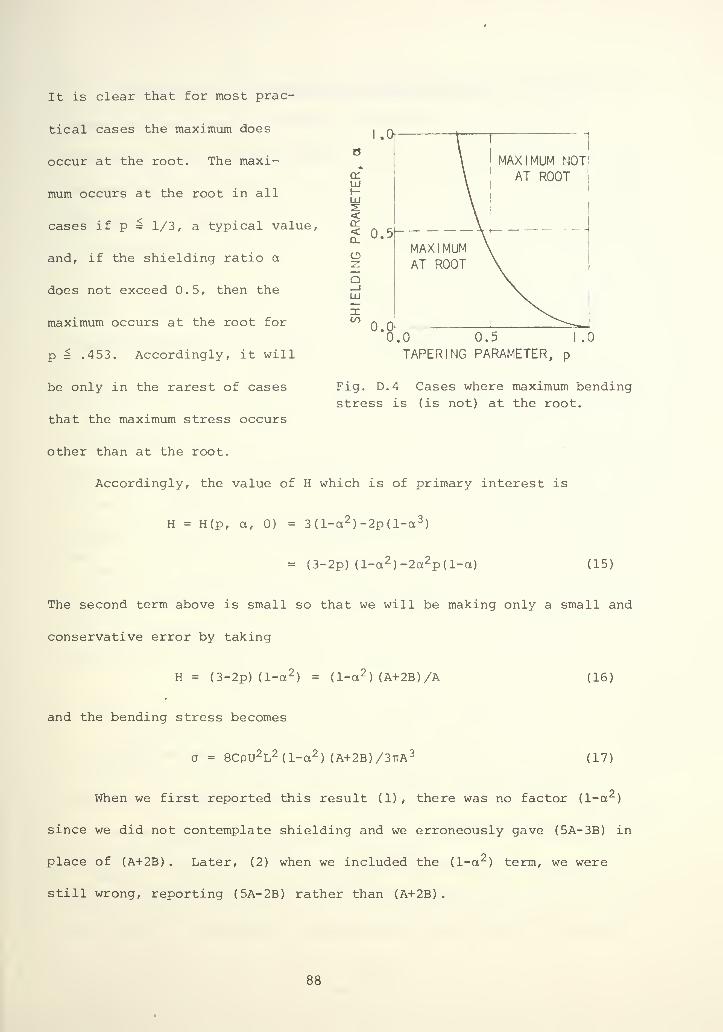
It is clear that for most prac-

tical cases the maximum does

occur at the root. The maxi-

mum occurs at the root in all

cases if p = 1/3, a typical value,

and, if the shielding ratio a

does not exceed 0.5, then the

maximum occurs at the root for

p ^ .453. Accordingly, it will

be only in the rarest of cases

that the maximum stress occurs

other than at the root.

Accordingly, the value of H which is of primary interest is

H = H(p, a, 0) = 3(l-a2 )-2p(l-a 3)

= (3-2p) (l-a 2 )-2a2p(l-a)

0.5 1.0

TAPERING PARAMETER, p

Fig. D.4 Cases where maximum bendingstress is (is not) at the root.

(15)

The second term above is small so that we will be making only a small and

conservative error by taking

H = (3-2p) (1-a 2) = (1-a 2

) (A+2B)/A (16)

and the bending stress becomes

a = 8CpU2L2 (l-a2 ) (A+2B)/3ttA 3 (17)

When we first reported this result (1), there was no factor (1-a2)

since we did not contemplate shielding and we erroneously gave (5A-3B) in

place of (A+2B) . Later, (2) when we included the (1-a 2) term, we were

still wrong, reporting (5A-2B) rather than (A+2B)

.

88

3. Combination of Bending Moments and Stresses

The drag force is approximately constant in time. The lift force,

which is at right angles to the drag force, varies in time. The bending

moments due to the lift and drag forces are at right angles and combine

vectorially. The effective value of the lift force should be multiplied

by a dynamic intensification factor

K = l/|l-(f /f )

2|

(18)' s n '

where f , f are the Strouhal frequency (see Appendix B) and the naturals n

or resonant frequency (see Appendix C) respectively. The vertical lines

indicate "absolute value."

In the preceding analysis we made a slight oversimplification by

taking Z as given by Equation (7). This does not account for the hollow

center of the thermowell. If we had taken this into account, the demarca-

tion shown in Figure D.4 would have moved slightly to the right. However,

our conclusion that practical cases involve highest stress at the root

would still be valid. We should however, compute bending stress by using

the correct value of Z at the root. This means that the stress values

given above should be corrected by multiplying by the factor

Z /Z „ i/d-dVA4) (19)

WRONG RIGHT

where d is the diameter of the hole down the center. Thus, we obtain

a* = a (bending, max) = 8CpU2L2 (1-a 2) A(A+2B)/3tt (A^-d*4

) (20)

where C is the effective value

C = /c 2+K2 C 2 (21)D L

89

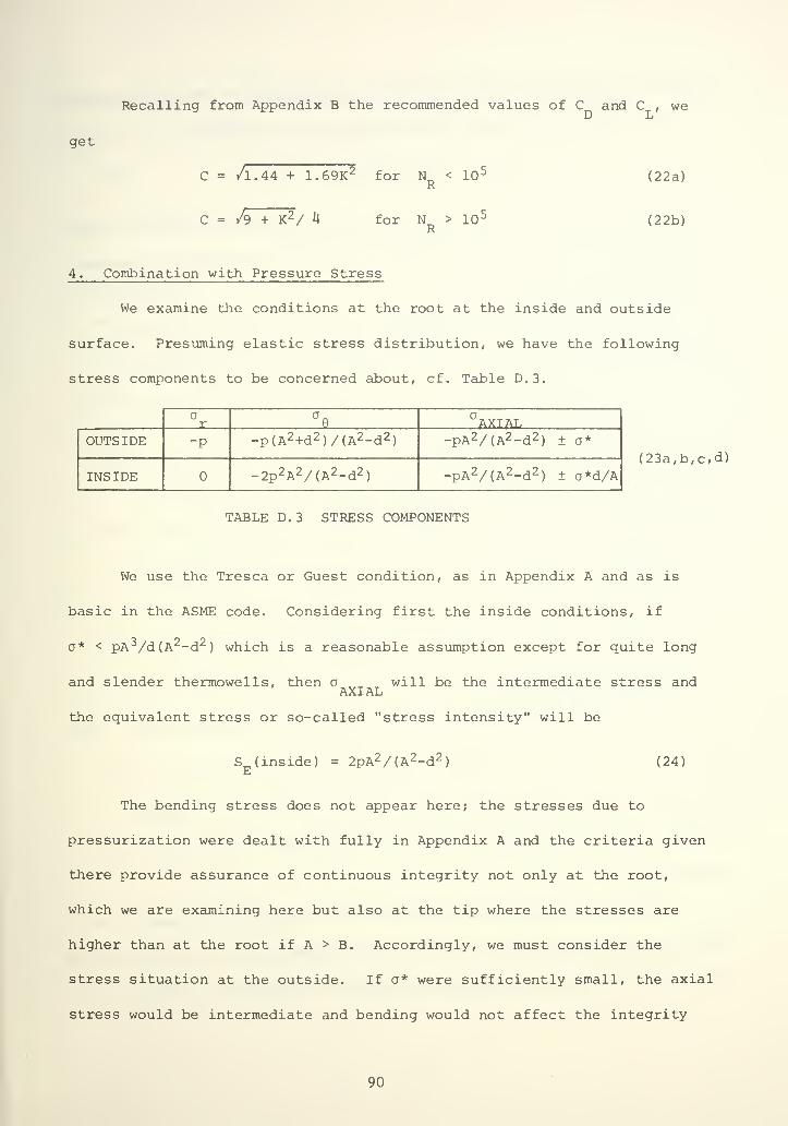
Recalling from Appendix B the recommended values of C and C , we

get

C = /l.44 + 1.69K2 for N < 10 5

C = /9 + K2/ 4 for N > 10-R

(22a)

(22b)

4. Combination with Pressure Stress

We examine the conditions at the root at the inside and outside

surface. Presuming elastic stress distribution, we have the following

stress components to be concerned about, cf. Table D.3.

ar °B °AXIAL

OUTSIDE "P -p(A2+d2 )/(A2-d 2) -pA2/(A2-d 2

) ± a*

INSIDE -2p 2A2/(A 2-d2) -pA2/(A2-d 2

) ± a*d/A(23a,b,c,d)

TABLE D.3 STRESS COMPONENTS

We use the Tresca or Guest condition, as in Appendix A and as is

basic in the ASME code. Considering first the inside conditions, if

a* < pA 3/d(A 2-d2 ) which is a reasonable assumption except for quite long

and slender thermowells, then a will be the intermediate stress andAXIAL

the equivalent stress or so-called "stress intensity" will be

S (inside) = 2pA2/(A2-d 2)

E(24)

The bending stress does not appear here; the stresses due to

pressurization were dealt with fully in Appendix A and the criteria given

there provide assurance of continuous integrity not only at the root,

which we are examining here but also at the tip where the stresses are

higher than at the root if A > B. Accordingly, we must consider the

stress situation at the outside. If a* were sufficiently small, the axial

stress would be intermediate and bending would not affect the integrity

90

assured by the pressure design criteria. Accordingly we must assume that

c* > pd 2/(A2-d 2) and the governing stress intensity becomes

S = a* + pd2 /(A 2-d2) (25)

E

According to ASME criteria we must require that this value not exceed

1.5 S where S is the tabulated stress value for the material in questionm m

at design temperature.

There is one additional matter to take care of before proceeding.

Usually the fluid velocity U will be given in feet per second and the

density p will be given in pounds seconds 2/foot according to the formula

P = 1/gv (26)

with g = 32.2 feet/second and v = specific volume in cubic feet per

pound. Thus the product pU 2 = U 2/gv will be in pounds per square foot.

This must be divided by 144 to give pU2 in pounds per square inch as

required by our formulas. Thus, we require that

pd2/(A2-d2) + CpU2L 2 (l-a2 ) (A+2B) /54ttA 3 (l-d^/A4 ) = 1.5 S (27)

m

5. Combined Stress Criterion

We will rewrite this to include all applicable numerical values, viz.

:

pd 2/(A2-d 2) + .00018 CU 2L 2 (l-a 2

) (A+2B) /vA 3 (1-d^/A4) ^ 1.5 S (28)

m

with A, B, L, and d given in inches, p and S given in psi, U given inm

feet per second, and v given in cubic feet per pound. C and a are dimen-

sionless.

For certain purposes we can simplify this formula. For example, for

high pressure installations 1-d /A 1* = 1 which gives a small (nonconservative)

error. Also, in accordance with the limitation recommended in the body of

91

this report that f /f not be permitted to exceed 0>80' tne dynamic

intensification factor K will not exceed 2.78 so that we can say

C < 3.81 for N < 10 5 (29a)R

C <1.02 for N > 10 5 (29b)

6. Bibliography

Dl. Brock, J. E. , Stress analysis of thermowells, consulting report to

Bechtel Power Corporation, October 1972, and Supplement, December 15,

1972.

D2. Appendix to letter J. E. Brock to J. W. Murdock, March 14, 1974

Copies sent to Mr. W. 0. Hayes for ASME Committee PB51.

92

APPENDIX E

FATIGUE RELIABILITY CALCULATIONS

We state explicitely that we are concerned here only with cyclic

response to the sinusoidally varying F force. (This was implicit in anL

earlier version of this report.) As justification we remark that stress

cycles due to pressure and temperature variations are surely fewer in

number than those due to F and, indeed, are no more severe than for theL

pipe itself. In particular, recall that we require one-cycle shakedown on

pressurization. However, we do want to call specific attention to the fact

that we have thus limited the scope of the fatigue investigation.

The number of cycles in a twenty-year design life is

N = (20) (8760) (3600)

f

s

and a typical value for f is .21U/D = ( . 21) (270) (12 ) = 680 Hz so thats

N = 4.3 x 10 . Thus we are concerned with a very large number of excitations,

11 19in the range 10 to 10 i,d roughly. To assure survival against the action of

mechanical fatigue, we must require that the amplitude of maximum cyclic

stress (including so-called "peak" stress) does not exceed the endurance

limit for the material at the operating temperature. The endurance limit

may be taken to be twice the ASME Code S value at one million cycles asa.

obtained from the Design Fatigue Curves in Appendix 1 of the ASME Code for

Nuclear Power Plant Components or in ASME Boiler Code Case No. 1331.

From equation (20) of Appendix D we have

a = 8CpU2 L2 (l-a 2 )A(A+2B)/3TT(At+

-d 1+

) (1)

for the bending stress at the root; this is the maximum value of bending

stress, as explained in Appendix D, except for thermowells which are much

93

more sharply tapered or are much more completely shielded than ususal. We

are here concerned only with the effect of the lift force so that

fl.3K for N < 10 5

C = KC = JR

(2)L

I st .25K for N > 10 b

where we recall that the dynamic intensification factor K is given by

K = 1/| 1 - (f /f )

2|

(3)1 s n '

(cf . equation 18 of Appendix D.

)

However, equation (1) above does not account for the intensifying

effect of what may be a sharply notched geometry at the root. Comparing

with the procedure in nuclear codes we should multiply by the product

(K9C„ in nuclear code notation) of the two stress indices pertinent to the

local geometry. Proceding on a "rational" basis using tabulated values of

K2

and C2

and the general philosophy of Code Case No. 69, we arrive at

K2C2

=(f

X 2) (

T^8x 1 - 5) = 4 * 4 (4)

Since this evaluation is doubtful and until better information is available

we will round this number up to K2C2

= 6.

Inserting all evaluations into (1) and multiplying by 6 we get

1.00143 KU2L2 (l-a 2 )A(A+2B)

sait

=1.000275 77T T7TT

(5)

I v(AH-dH )

We have denoted this result as S to denote the alternating stress which3..L L.

may lead to fatigue damage. The upper figure in parentheses is for

N < 10 5 and the lower figure for N > 10 5. The dimensions are: L, A, B,

R R

d (inches); U(ft/sec); V(cu. ft/lb); S , (psi) ; f , f (Hz).alt s n

94

We require that this value, S , not exceed the endurance limit for

the material at operating temperature.

If pressurization and depressurization are to take place very fre-

quently or if significant and highly repetitive thermal transient stresses

are possible one should also investigate these as a possible source of

fatigue damage.

The same sort of simplifications are possible with equation 5,

above, as were suggested for use with equation (28) of Appendix D.

95

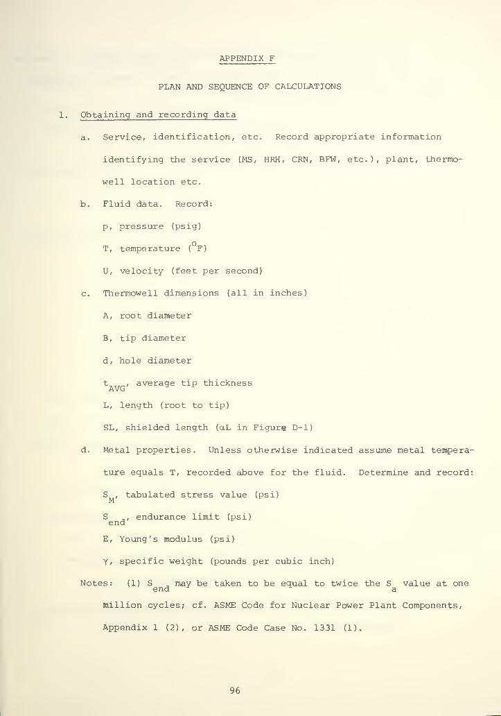
APPENDIX F

PLAN AND SEQUENCE OF CALCULATIONS

Obtaining and recording data

a. Service, identification, etc. Record appropriate information

identifying the service (MS, HRH, CRN, BFW, etc.), plant, thermo-

well location etc.

b. Fluid data. Record:

p, pressure (psig)

T, temperature ( F)

U, velocity (feet per second)

c. Thermowell dimensions (all in inches)

A, root diameter

B, tip diameter

d, hole diameter

t , average tip thickness

L, length (root to tip)

SL, shielded length (otL in Figure D-l)

d. Metal properties. Unless otherwise indicated assume metal tempera-

ture equals T, recorded above for the fluid. Determine and record:

S , tabulated stress value (psi)M

S , , endurance limit (psi)end

E, Young's modulus (psi)

Y, specific weight (pounds per cubic inch)

Notes: (1) S , may be taken to be equal to twice the S value at oneend a

million cycles; cf. ASME Code for Nuclear Power Plant Components,

Appendix 1 (2), or ASME Code Case No. 1331 (1).

96

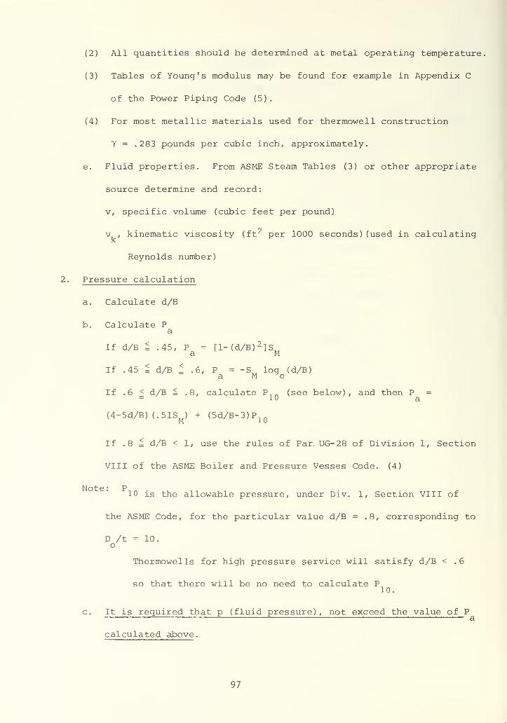
(2) All quantities should be determined at metal operating temperature.

(3) Tables of Young's modulus may be found for example in Appendix C

of the Power Piping Code (5).

(4) For most metallic materials used for thermowell construction

Y = .283 pounds per cubic inch, approximately.

e. Fluid properties. From ASME Steam Tables (3) or other appropriate

source determine and record:

v, specific volume (cubic feet per pound)

v , kinematic viscosity (ft 2 per 1000 seconds) (used in calculating

Reynolds number)

Pressure calculation

a. Calculate d/B

b. Calculate Pa

If d/B 1 .45, P = [l-(d/B) 2 ]SM

If .45 = d/B 1 .6, P = -S log (d/B)a Me

If .6 < d/B = .8, calculate P. n (see below), and then P == 10 a

(4-5d/B) (.51S ) + (5d/B-3)P.nM 10

If .8 = d/B < 1, use the rules of Par. UG-28 of Division 1, Section

VIII of the ASME Boiler and Pressure Vesses Code. (4)

Note: P10 is the allowable pressure, under Div. 1, Section VIII of

the ASME Code, for the particular value d/B = .8, corresponding to

D /t = 10.o

Thermowells for high pressure service will satisfy d/B < .6

so that there will be no need to calculate P10.

c. It is required that p (fluid pressure), not exceed the value of Pa

calculated above.

97

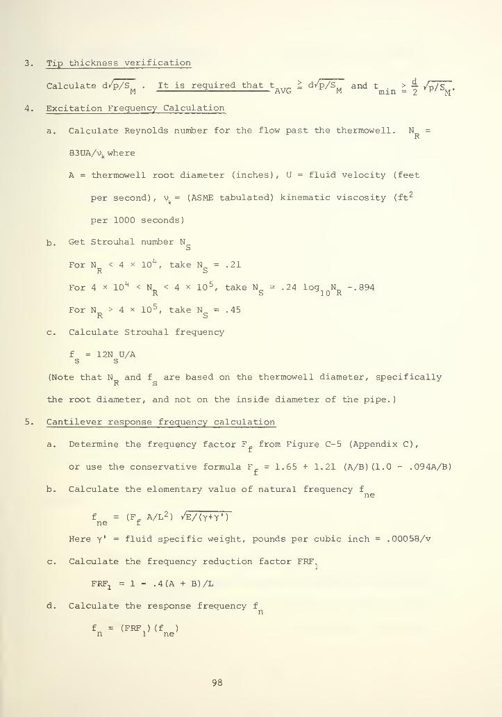
3. Tip thickness verification

Calculate d/p/S . It is required that t ± d/p/SM and t . > — /p/s .

4. Excitation Frequency Calculation

a. Calculate Reynolds number for the flow past the thermowell. N =R

83UA/vkwhere

A = thermowell root diameter (inches), U = fluid velocity (feet

per second) , v = (ASME tabulated) kinematic viscosity (ft 2

per 1000 seconds)

b. Get Strouhal number NS

For N < 4 x 10\ take N = .21R S

For 4 x lo 4 < N < 4 x io 5, take N = .24 log N -.894

R S 1 R

For N > 4 x io 5, take N = .45

R. o

c. Calculate Strouhal frequency

f = 12N U/As s

(Note that N and f are based on the thermowell diameter, specificallyR s

the root diameter, and not on the inside diameter of the pipe.)

5. Cantilever response frequency calculation

a. Determine the frequency factor F from Figure C-5 (Appendix C)

,

or use the conservative formula F = 1.65 + 1.21 (A/B)(1.0 - .094A/B)

b. Calculate the elementary value of natural frequency f

f = (F_ A/L 2) /E/(Y+Y')

ne r

Here y' = fluid specific weight, pounds per cubic inch = .00058/v

Calculate the frequency reduction factor FRF

FRFa

= 1 - .4 (A + B)/L

Calculate the response frequency fn

f = (FRF) (f )

n 1 ne

98

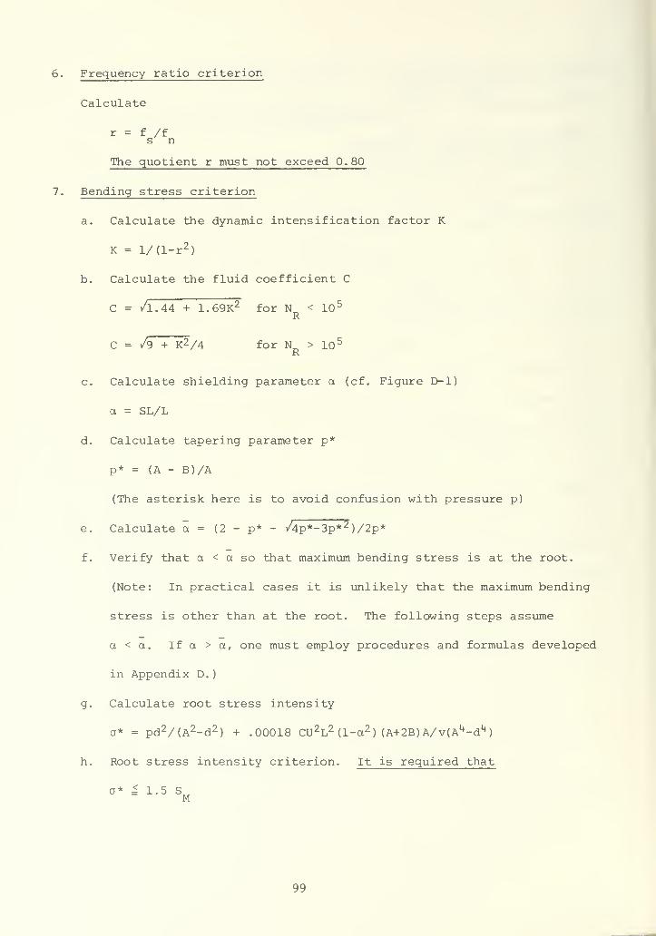
Frequency ratio criterion

Calculate

r = f /fs n

The quotient r must not exceed 0.80

Bending stress criterion

a. Calculate the dynamic intensification factor K

K = l/(l-r 2)

b. Calculate the fluid coefficient C

C = A. 44 + 1.69K2 for N < 10 5

C = /9 + K2/4 for N > 10 5

R

c. Calculate shielding parameter a (cf. Figure D-l)

a = SL/L

d. Calculate tapering parameter p*

p* = (A - B)/A

(The asterisk here is to avoid confusion with pressure p)

e. Calculate a = (2 - p* - /4p*-3p* 2 )/2p*

f. Verify that a < a so that maximum bending stress is at the root.

(Note: In practical cases it is unlikely that the maximum bending

stress is other than at the root. The following steps assume

a<a. If a > a, one must employ procedures and formulas developed

in Appendix D.

)

g. Calculate root stress intensity

a* = pd2/(A2-d 2) + .00018 CU 2 L2 (l-a 2

) (A+2B)A/v(A1+-d tt

)

h. Root stress intensity criterion. It is required that

a* ^ 1.5 SM

99

8. Fatigue life calculation

Calculate S ,alt

S = f- 00143 "\ KU2L2 (l-a 2 )A(A+2B)alt

V.0002757 v(Ak-dk )

the upper figure being used for N < 10 5 and the lower for N > 10 5.

R R

It is required that S . = Salt end

9. Attachment details verification

(No quantitative criteria are offered here. It is the definite recom-

mendation of the writer that a part of the stress analysis of a

thermowell also include the following steps.)

a. Assure that the attachment weld is a full penetration weld for

which a definite and approved "welding procedure" instruction and

inspection instructions are properly promulgated.

b. Assure that the "branch connection" rules of the applicable code

are satisfied.

10. Remarks

a. Many steps above may be omitted in actual routine calculation.

For example, usually it is not necessary to calculate p* (step 7d)

or a (step 7e) since a is usually less than 1/3 and the maximum

stress will occur at the root regardless of the value of the

tapering parameter p*.

b. The criteria above have been developed so as to assure reliable

performance without economic penalty. Failure to satisfy any

criterion does not necessarily imply unsatisfactory performance.

In many cases sound reasons may be developed to permit violating

one or more of these criteria. Such reasons may be developed

100

on the basis of the analysis and discussions contained in this

report. However, it may be costlier to develop such reasons than

to strengthen the design.

11. Bibliography

The publications listed below may be obtained from the ASME (American

Society of Mechanical Engineers) Publication Department, United Engi-

neering Center, 345 East 47th Street, New York, N. Y. , 10017.

(Fl) ASME Boiler and Pressure Vessel Code Case No. 1331 (latest edition)

(F2) ASME Boiler and Pressure Vessel Code, Section III Nuclear Power

Plant Components, Appendix 1.

(F3) ASME Steam Tables, 1967

(F4) ASME Boiler and Pressure Vessel Code, Section VIII, Division 1,

Unfired Pressure Vessels.

(F5) USA Standard Code for Pressure Piping, USAS B31. 1.0-1967 Power

Piping

101

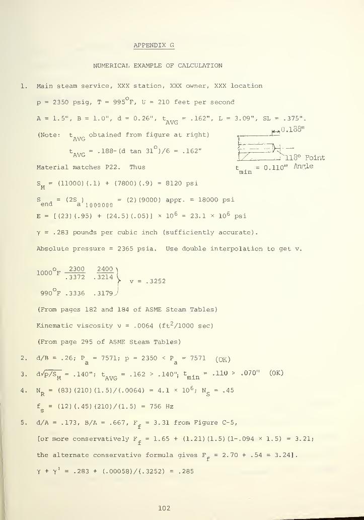
2

APPENDIX G

NUMERICAL EXAMPLE OF CALCULATION

1. Main steam service, XXX station, XXX owner, XXX location

p = 2350 psig, T = 995 F, U = 210 feet per second

A = 1.5", B = 1.0", d = 0.26", t = .162", L = 3.09", SL = .375".

K^O.138"(Note: t obtained from figure at right) t

_—,

tAVG

= .188-(d tan 31~)/6 = .162" f/~~ ~^HyJ^ll8° Point

Material matches P22. Thus t = 0.110" Anr£Lemin

S = (11000) (.1) + (7800) (.9) = 8120 psiM

S . = (2S ) = (2) (9000) appr. = 18000 psiend a 1000000

E = [(23) (.95) + (24.5) (.05)] x 10 6 = 23.1 x 10 6 psi

Y = .283 pounds per cubic inch (sufficiently accurate).

Absolute pressure = 2365 psia. Use double interpolation to get v.

,^0^ 2300 24001000 F u.3372 .3214 . ^990°F .3336 .3179.'

(From pages 182 and 184 of ASME Steam Tables)

Kinematic viscosity v = .0064 (ft 2/1000 sec)

(From page 295 of ASME Steam Tables)

d/B = .26; P = 7571; p = 2350 < P = 7571 (QK)

3. d/p7s^"= .140"; tAVG

= .162 > .140"; t^ = .110 > .070" (OK)

4. N_ = (83) (210) (1.5)/(.0064) = 4.1 * 10 6; N_ = .45

R S

f = (12) (.45) (210)/(1.5) = 756 Hzs

5. d/A = .173, B/A = .667, F = 3.31 from Figure C-5,

[or more conservatively F = 1.65 + (1 . 21) (1. 5) (1- .094 * 1.5) = 3.21;

the alternate conservative formula gives F = 2.70 + .54 = 3.24].

Y + Y1 = .283 + (.00058)/(.3252) = .285

102

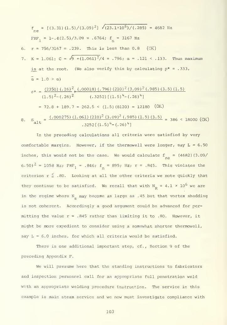
f = [(3.31) (1.5)/(3.09) 2] /(23.1xl0 6 )/(.285) = 4682 Hz

ne

FRF, = l-.4(2.5)/3.09 = .6764; f = 3167 Hz1 n

6. r = 756/3167 = .239. This is less than 0.8 (OK)

7. K = 1.061; C = /9 +(1.061) 2/4 = .796; a = .121 < .133. Thus maximum

is at the root. (We also verify this by calculating p* = .333,

a = 1.0 > a)

(2350) (.26) 2,(.00018) (.796) (210) 2 (3. 09) 2 (.985) (3.5) (1.5)

a* = +

(1.5) 2-(.26) 2 (.3252) [ (1. 5)h-

( . 26) h]

= 72. 8 + 189.7 = 262.5 < (1.5) (8120) = 12180 (OK)

8 . s = 1.0Q0275 ) (1.06D (210) 2 (3.09) 2 (.985) (1.5) (3.5) = ^ < ^^ (QK)alt

.3252[(1.5)t+

-(.26) 1+

]

In the preceding calculations all criteria were satisfied by very

comfortable margins. However, if the thermowell were longer, say L = 6.50

inches, this would not be the case. We would calculate f = (4682) (3.09/ne

6.50) 2 = 1058 Hz; FRFn

= .846; f = 895; Hz; r = .845. This violates the1 n

criterion r = .80. Looking at all the other criteria we note quickly that

they continue to be satisfied. We recall that with N = 4.1 x 10° we areR

in the regime where N may become as large as .45 but that vortex shedding

is not coherent. Accordingly a good argument could be advanced for per-

mitting the value r = .845 rather than limiting it to .80. However, it

might be more expedient to consider using a somewhat shorter thermowell,

say L = 6.0 inches, for which all criteria would be satisfied.

There is one additional important step, cf . , Section 9 of the

preceding Appendix F.

We will presume here that the standing instructions to fabricators

and inspection personnel call for an appropriate full penetration weld

with an appropriate welding procedure instruction. The service in this

example is main steam service and we now must investigate compliance with

103

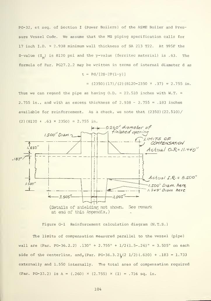
PG-32, et seq. of Section I (Power Boilers) of the ASME Boiler and Pres-

sure Vessel Code. We assume that the MS piping specification calls for

17 inch I.D. x 2.938 minimum wall thickness of SA 213 T22. At 995F the

S-value (S ) is 8120 psi and the y-value (ferritec material) is .63. TheM

formula of Par. PG27.2.2 may be written in terms of internal diameter d as

t - Pd/[2S-2P(l-y)]

= (2350) (17)/(2) (8120-2350 x .37) = 2.755 in.

Thus we can regard the pipe as having O.D. = 22.510 inches with W.T. =

2.755 in., and with an excess thickness of 2.938 - 2.755 = .183 inches

available for reinforcement. As a check, we note that (2350) (22. 510)/

(2) (8120 + .63 x 2350) = 2.755 in.

j*-|«

—

0'V.bO'' diameter of

I.Sod' 0/a-rrt n_

j'83

,/

T

ASSV"

3. SOS

4

•ft'm'sfied cfen in <j

h

Actzta./ O.Tl=J/.¥¥c>

~\^> COMf>£KSAT/Orfit

J-.

Aotudl !,%>- 3-SOO"

/,soo" Diam. /?enz

/. 2¥9" D/am here

-3.SVS

(Details of shielding not shown. See remark

at end of this Appendix.

)

Figure G-l Reinforcement calculation diagram (N.T.S.)

The limits of compensation measured parallel to the vessel (pipe)

wall are (Par. PG-36.2.2) .130" + 2.755" + 1/2 (1. 5-. 26) " = 3.505" on each

side of the centerline, and, (Par. PG-36. 3. 21 (2 1/2) (.620) + .183 = 1.733

externally and 1.550 internally. The total area of compensation required

(Par. PG-33.2) is A = (.260) x (2.755) x (l) = .716 sq. in.

104

The compensation provided consists of

A = (7.010-. 260) (. 183) = 1.235 sq. in., excess wall thickness

A2= (1.500-. 260) (1.550) = 1.922 sq. in., nozzle, external

A = (.5 x 2. 749-. 260) (1. 550) = 1.727 sq. in., nozzle, internal

A ^ = (not necessary) = fillets, within comp. limits

The total, not counting applicable area of fillet welds, is 4.884 sq. in.

which greatly exceeds the requirement of 0.716 sq. in. Accordingly, the

reinforcement rules are much more than adequately satisfied. It is

expected that this will always prove to be the case for high-pressure,

high- temperature installations but it may not always automatically be so

for less severe service, for example, for cold reheat service. In any

case, however, a procedure for assuring compliance with the applicable

reinforcement rules is a definite part of the recommended criteria and

procedure in this report.

(Note: this example is intended to illustrate a general type of

calculation, and thus includes a "shielded length" 3L = 0.375". However,

no indication is made of the detail which accomplishes the shielding.

In particular, no such detail is shown in Fig. G-l, and it is presumed

that the detail, whatever it is, does not enter into the calculation

of branch connection compensation.)

105

INITIAL DISTRIBUTION LIST

Mrs. J. E. LearyChief Control and Instrumentation EngineerBechtel Power CorporationP.O. Box 3965San Francisco, CA 94119 2

Mr. F. E. VinsonBechtel Power CorporationP.O. Box 3965San Francisco, CA 94119 1

Mr. S. E. MooreOak Ridge National LaboratoryP.O. Box YOak Ridge, Tennessee 37830 1

Mr. L. A. Dodge364 Dunbarton BoulevardRichmond Heights, Ohio 44143 1

Mr. C. BarnhardtBechtel Power CorporationP.O. Box 3965San Francisco, CA 94119 1

Mr. W. 0. Hayes, SecretarySecretary ASME Committee PB51ASME345 East 47th StreetNew York, NY 10017 20

Mr. W. N. WrightTemTex Systems5619 Dyer StreetDallas, Texas 75206 1

Mr. John ArcherGilbert Associates, Inc.

Reading, Pennsylvania 19603 1

Mr. A. LohmeierSGDE; ASME B&PV CommitteeWestinghouse Electric CbrporationPower SystemsBox 19218Tampa, Florida 33616 1

Mr. R. F. AbrahamsenASME345 East 47th StreetNew York, NY 10017 1

106

Mr. A. PartingtonWestinghouse Electric CorporationY-4 Technical DevelopmentLester, Pennsylvania 19113 1

Mr. J. W. MurdockConsulting Engineer684 Old School House DriveSpringfield, Pennsylvania 19064 1

Mr. Norman BlairChairman B31 MCD4836 N. Earle StreetRosemead, California 91770 1

Mr. D. M. FischerSecretary B31 MDCMail Code 4307Amoco Chemicals CorporationP.O. Box 8640AChicago, Illinois 60680 14

Professor J. E. BrockCode 59BCDepartment of Mechanical EngineeringNaval Postgraduate SchoolMonterey, California 93940 5

Department of Mechanical EngineeringCode 59

Naval Postgraduate SchoolMonterey, California 93940 1

LibraryNaval Postgraduate SchoolMonterey, California 93940 2

Dean of Research AdministrationNaval Postgraduate SchoolMonterey, California 93940 2

DirectorDefense Documentation Center5010 Duke StreetAlexandria, Virginia 22314 2

107

Ul

DUDLEY KNOX LIBRARY - RESEARCH REPORTS

5 6853 01057961 8

U-