Stress Analysis of Adhesive Bonded Joints Under In · PDF fileStress Analysis of Adhesive Bonded Joints Under ... from the complex stress state that would exist due to a patched crack

H. Kim and K. Kedward 1

Stress Analysis of Adhesive Bonded Joints Under In-Plane Shear Loading

Hyonny Kim* and Keith T. Kedward

Department of Mechanical and Environmental EngineeringUniversity of California, Santa Barbara, CA 93106, USA

A closed-form stress analysis of an adhesive bonded lap joint subjected to spatially varying in-

plane shear loading is presented. The solution, while similar to Volkersen’s treatment of tension

loaded lap joints, is inherently two-dimensional, and in general predicts a multi-component

adhesive shear stress state. A finite difference numerical solution of the derived governing

differential equation is used to verify the accuracy of the closed-form solution for a joint of semi-

infinite geometry. The stress analysis of a finite sized doubler is also presented. This analysis

predicts the adhesive stresses at the doubler boundaries, and can be performed independently

from the complex stress state that would exist due to a patched crack or hole located within the

interior of the doubler. The analytical treatment of lap joints under combined tension and shear

loading is now simplified since superposition principles allow the stress states predicted by

separate shear and tension cases to be added together. Applications and joint geometries are

discussed.

Keywords: shear-load, bonded joint, doubler, composite adherend, crack patch,closed-form analysis

Nomenclature

x, y, z Rectangular coordinatesr, θ, s Cylindrical and shell coordinates2c Overlap length of adhesive jointa Width of joint over which applied loading varies, or length of doubler in

x-directionb Length of doubler in y-directionti, to Thickness of inner, outer adherend

* corresponding author

Accepted by Jo. Adhesion on 10/2000 for publication in 2001.


ta Thickness of adhesive layeriyE , o

yE Young’s modulus of inner, outer adherend in the y-directionixyG , o

xyG Shear modulus of inner, outer adherend

Ga Shear modulus of adhesive layerNx, Ny Applied direct stress resultants (force per unit width)Nxy Applied shear stress resultant (force per unit width)

iyσ , o

yσ Direct stress in inner, outer adherend in the y-directionixyτ , o

xyτ Shear stress in inner, outer adherendixyγ , o

xyγ Shear strain in inner, outer adherendaxzτ , a

yzτ Adhesive shear stress components acting in x-z, y-z planeaxzγ , a

yzγ Adhesive shear strain components acting in x-z, y-z plane

ui, uo Displacement of inner, outer adherend in x-directionvi, vo Displacement of inner, outer adherend in y-direction

1. Introduction

Adhesive bonding has been applied successfully in many technologies. Foremost in applications

where primary loaded structures rely on adhesive bonding are aircraft and space structures.

While bonding in large and small commercial aircraft has been practiced quite widely in Europe

(sailplanes in Germany, SAAB 340 [1], and EXTRA EA-400 [2]), extensive adhesive bonding is

being used in the United States for the assembly of newly emerging small all-composite aircraft

structures (Cirrus SR20 and Lancair Columbia 300) for reasons related to performance and cost.

The analytical treatment of a bonded lap joint where the adherends are loaded in tension (see

Figure 1) has been considered extensively by many authors. Hart-Smith [3, 4] extended the shear

lag theory that was presented by Volkersen [5] to include adhesive plasticity. Goland and

Reissner [6] and Oplinger [7] accounted for adherend bending deflections to predict the peel

stress in the adhesive. Tsai, Oplinger, and Morton [8] provided a correction for adherend shear

deformation, resulting in a simple modification of the Volkersen’s theory based equations. All of


these analytical treatments are formulated per unit width of the specimen which implies that the

predicted adhesive stress is independent of variations of loading through the width of the joint (x-

direction in Figure 1). An extension of these solutions can be applied to the case of spatially

varying tensile loading, as shown in Figure 1, by performing the analysis using the value of

tensile stress resultant at any particular x-axis location. The tension loaded lap joint analysis is

presented in Appendix A.

Adhesively bonded lap geometries loaded by in-plane shear (see Figure 2) have been discussed

by Hart-Smith [4], van Rijn [2], and the Engineering Sciences Data Unit [9]. The authors of

these works indicate that shear loading can be analytically accounted for by simply replacing the

adherend Young’s moduli in the tensile loaded lap joint solution with the respective adherend

shear moduli. This approach is rigorously correct for only the case of spatially constant Nxy load

applied to joints which are semi-infinite, as shown in Figure 2a.

When the geometry is finite in size (see Figure 2b), an analytical treatment that is more

comprehensive than that suggested by Hart-Smith [4], van Rijn [2], and the Engineering

Sciences Data Unit [9] is needed in order to account for adhesive stresses which would exist at

the bond terminations. Thus the objective of the theoretical work presented herein is to address

the shear loaded lap joint problem in more general terms by allowing the applied in-plane shear

load to vary in the spatial coordinates, and by accounting for a joint geometry of finite size.

Closed-form analytical solutions are developed for single and double lap joint configurations

subject to general in-plane shear loading. It should be noted that the solution of this problem

using Finite Element Analysis (FEA) is difficult due to the inherent three-dimensional nature of

the joint geometry and shear loading conditions. Since three-dimensional elements need to be


used in modeling shear transfer across a lap joint, creating a mesh having enough element

refinement to capture the high stress gradients in the thin adhesive layer can easily result in a

FEA model of formidable size. In comparison, a closed-form solution to this problem serves as a

computationally efficient tool that is useful for design and analysis.

2. Structural Examples

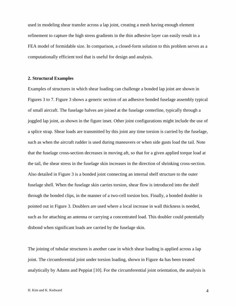
Examples of structures in which shear loading can challenge a bonded lap joint are shown in

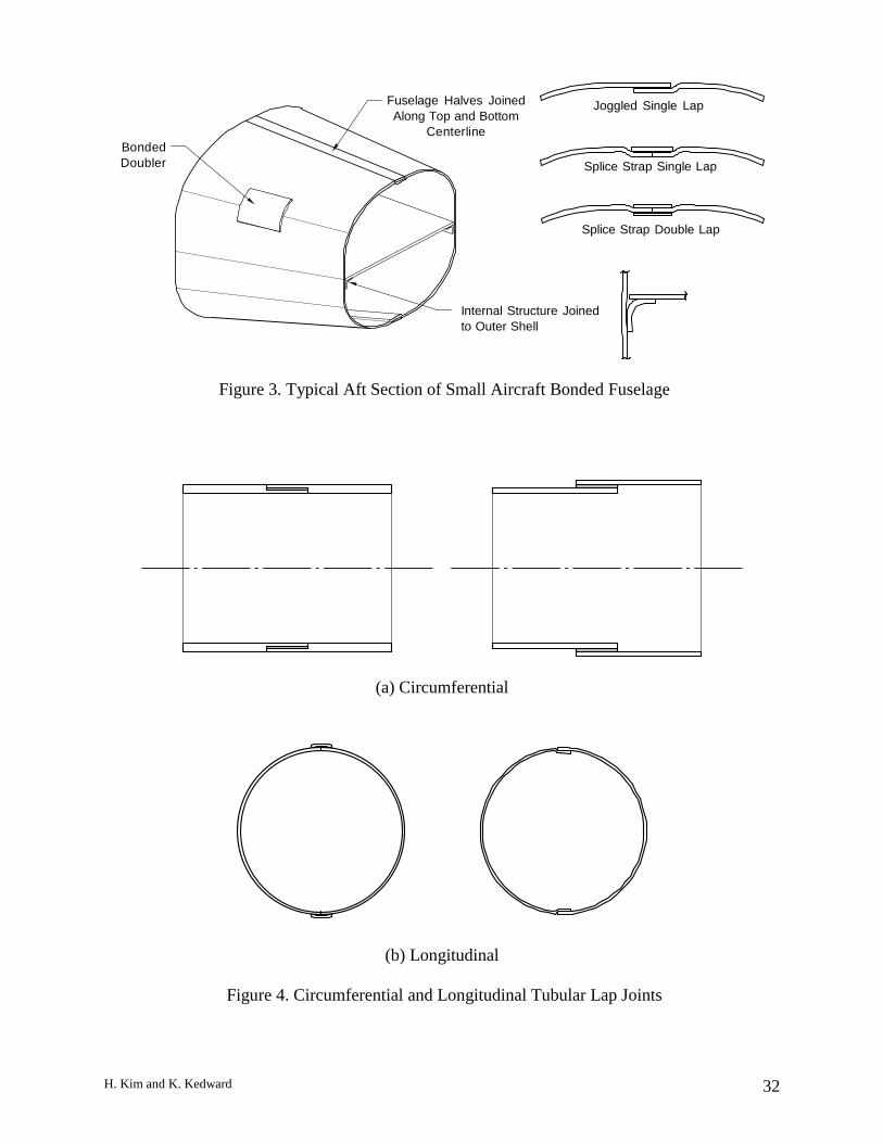
Figures 3 to 7. Figure 3 shows a generic section of an adhesive bonded fuselage assembly typical

of small aircraft. The fuselage halves are joined at the fuselage centerline, typically through a

joggled lap joint, as shown in the figure inset. Other joint configurations might include the use of

a splice strap. Shear loads are transmitted by this joint any time torsion is carried by the fuselage,

such as when the aircraft rudder is used during maneuvers or when side gusts load the tail. Note

that the fuselage cross-section decreases in moving aft, so that for a given applied torque load at

the tail, the shear stress in the fuselage skin increases in the direction of shrinking cross-section.

Also detailed in Figure 3 is a bonded joint connecting an internal shelf structure to the outer

fuselage shell. When the fuselage skin carries torsion, shear flow is introduced into the shelf

through the bonded clips, in the manner of a two-cell torsion box. Finally, a bonded doubler is

pointed out in Figure 3. Doublers are used where a local increase in wall thickness is needed,

such as for attaching an antenna or carrying a concentrated load. This doubler could potentially

disbond when significant loads are carried by the fuselage skin.

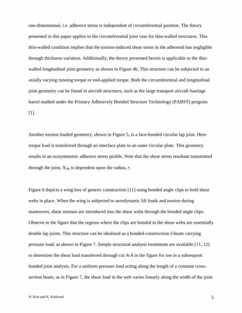
The joining of tubular structures is another case in which shear loading is applied across a lap

joint. The circumferential joint under torsion loading, shown in Figure 4a has been treated

analytically by Adams and Peppiat [10]. For the circumferential joint orientation, the analysis is


one-dimensional, i.e. adhesive stress is independent of circumferential position. The theory

presented in this paper applies to the circumferential joint case for thin-walled structures. This

thin-walled condition implies that the torsion-induced shear stress in the adherend has negligible

through thickness variation. Additionally, the theory presented herein is applicable to the thin-

walled longitudinal joint geometry as shown in Figure 4b. This structure can be subjected to an

axially varying running torque or end-applied torque. Both the circumferential and longitudinal

joint geometry can be found in aircraft structures, such as the large transport aircraft fuselage

barrel studied under the Primary Adhesively Bonded Structure Technology (PABST) program

[1].

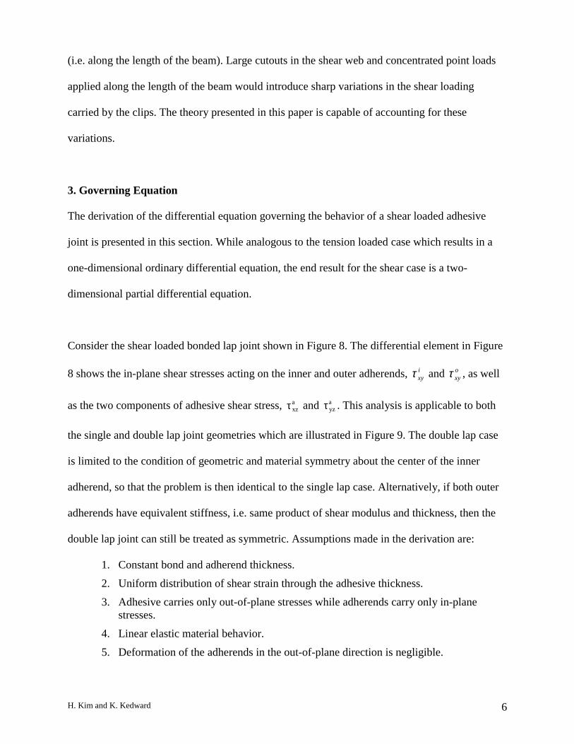
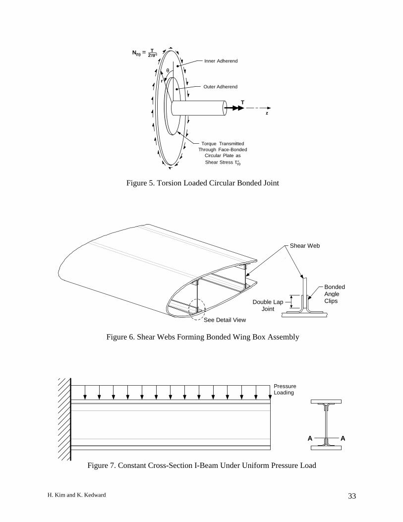
Another torsion-loaded geometry, shown in Figure 5, is a face-bonded circular lap joint. Here

torque load is transferred through an interface plate to an outer circular plate. This geometry

results in an axisymmetric adhesive stress profile. Note that the shear stress resultant transmitted

through the joint, Nrθ, is dependent upon the radius, r.

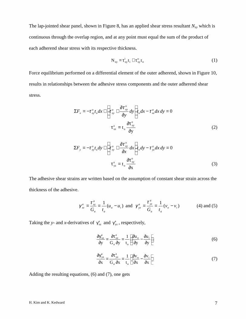
Figure 6 depicts a wing box of generic construction [11] using bonded angle clips to hold shear

webs in place. When the wing is subjected to aerodynamic lift loads and torsion during

maneuvers, shear stresses are introduced into the shear webs through the bonded angle clips.

Observe in the figure that the regions where the clips are bonded to the shear webs are essentially

double lap joints. This structure can be idealized as a bonded-construction I-beam carrying

pressure load, as shown in Figure 7. Simple structural analysis treatments are available [11, 12]

to determine the shear load transferred through cut A-A in the figure for use in a subsequent

bonded joint analysis. For a uniform pressure load acting along the length of a constant cross-

section beam, as in Figure 7, the shear load in the web varies linearly along the width of the joint


(i.e. along the length of the beam). Large cutouts in the shear web and concentrated point loads

applied along the length of the beam would introduce sharp variations in the shear loading

carried by the clips. The theory presented in this paper is capable of accounting for these

variations.

3. Governing Equation

The derivation of the differential equation governing the behavior of a shear loaded adhesive

joint is presented in this section. While analogous to the tension loaded case which results in a

one-dimensional ordinary differential equation, the end result for the shear case is a two-

dimensional partial differential equation.

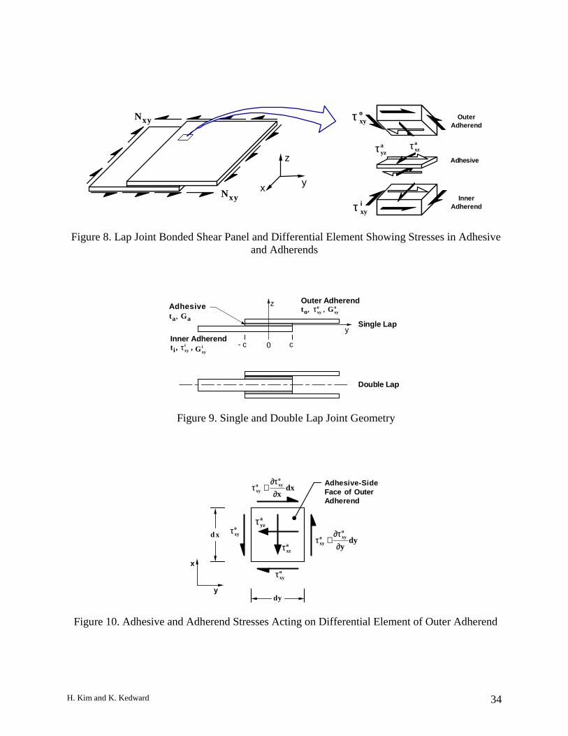
Consider the shear loaded bonded lap joint shown in Figure 8. The differential element in Figure

8 shows the in-plane shear stresses acting on the inner and outer adherends, ixyτ and o

xyτ , as well

as the two components of adhesive shear stress, axzτ and a

yzτ . This analysis is applicable to both

the single and double lap joint geometries which are illustrated in Figure 9. The double lap case

is limited to the condition of geometric and material symmetry about the center of the inner

adherend, so that the problem is then identical to the single lap case. Alternatively, if both outer

adherends have equivalent stiffness, i.e. same product of shear modulus and thickness, then the

double lap joint can still be treated as symmetric. Assumptions made in the derivation are:

1. Constant bond and adherend thickness.

2. Uniform distribution of shear strain through the adhesive thickness.

3. Adhesive carries only out-of-plane stresses while adherends carry only in-planestresses.

4. Linear elastic material behavior.

5. Deformation of the adherends in the out-of-plane direction is negligible.


The lap-jointed shear panel, shown in Figure 8, has an applied shear stress resultant Nxy which is

continuous through the overlap region, and at any point must equal the sum of the product of

each adherend shear stress with its respective thickness.

ooxyi

ixyxy ttN τ+τ= (1)

Force equilibrium performed on a differential element of the outer adherend, shown in Figure 10,

results in relationships between the adhesive stress components and the outer adherend shear

stress.

0=−

∂

∂++−=Σ dydxdxtdy

ydxtF a

xzo

oxyo

xyooxyx τ

τττ

yt

oxy

oaxz ∂

τ∂=τ (2)

0=−

∂

∂++−=Σ dydxdytdx

xdytF a

yzo

oxyo

xyooxyy τ

τττ

xt

oxy

oayz ∂

τ∂=τ (3)

The adhesive shear strains are written based on the assumption of constant shear strain across the

thickness of the adhesive.

)(1

ioaa

axza

xz uutG

−==τγ and )(

1io

aa

ayza

yz vvtG

−==τ

γ (4) and (5)

Taking the y- and x-derivatives of axzγ and a

yzγ , respectively,

∂∂−

∂∂

=∂

τ∂=∂γ∂

y

u

y

u

t

1

yGyio

aa

axz

axz (6)

∂∂−

∂∂

=∂

τ∂=

∂γ∂

x

v

x

v

t

1

xGxio

aa

ayz

ayz (7)

Adding the resulting equations, (6) and (7), one gets


∂∂−

∂∂−

∂∂

+∂

∂=

∂τ∂

+∂τ∂

x

vi

y

u

x

v

y

u

t

G

xyioo

a

aayz

axz (8)

Finally, combining equation (8) with equations (1) to (3), and noting that

oxy

oxyo

xyoo

Gx

v

y

u τ=γ=

∂∂

+∂

∂ and

ixy

ixyi

xyii

Gx

v

y

u τ=γ=

∂∂

+∂∂

(9) and (10)

results in a partial differential equation governing the shear stress in the outer adherend.

0Cooxy

2oxy

2 =+τλ−τ∇ (11)

with

+=λ

iixyo

oxya

a2

tG

1

tG

1

t

G and

oiaixy

xyao tttG

NGC = (12) and (13)

The adhesive shear stresses axzτ and a

yzτ can be obtained from the relationships given by

equations (2) and (3) once a solution to equation (11) is determined. The governing equation is

similar to the one-dimensional equation governing the behavior of a tension loaded bonded joint

(see Appendix A). Note however that for the shear loaded case, the governing equation is in two

dimensions, and there are now, in general, two components of adhesive shear stress.

This derivation is rigorously correct for the case when the applied loading, Nxy, is constant with

respect to the x- and y-coordinates. For the case when Nxy has gradients in the x- and y-directions,

there will generally exist complementary direct stress resultants, Nx and Ny, with gradients in the

x- and y-directions, respectively. This point is clear when considering the equilibrium equations

of a flat plate

xxyx q

y

N

x

N−=

∂∂

+∂

∂(14)

yyxy q

y

N

x

N−=

∂∂

+∂

∂(15)


where applied surface tractions qx and qy are zero. For example, equation (15) says that for Nxy

being a function behaving linearly in x, in order for equilibrium to be maintained, Ny must be

linear in y (for qy = 0). The existence of these additional stress resultants, not accounted for in the

derivation of equation (11), will contribute additional stresses in the adhesive. For many

engineering structures, such as the shear webs shown in Figures 6 and 7, the gradients of Nxy in

the shear web are small enough so that the influence of these equilibrium-maintaining stress

resultants, Nx and Ny, on the derivation of the governing equation can often be neglected. If the

magnitude of Nx and Ny are too great to be treated as negligible, their effect can be accounted for

through a separate tension (or compression) loaded bonded joint analysis (see Appendix A). The

results of this analysis can then be superposed onto the results of the shear-loaded joint analysis.

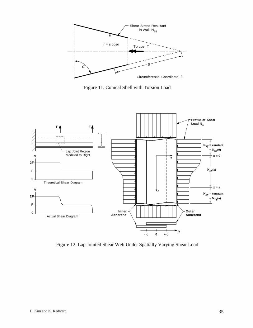
Cases where a gradient in Nxy can exist without complementary Nx or Ny resultants can be found

in flat structures having surface tractions qx and qy present, and in torsion-loaded thin-walled

structures of varying closed cross-section, such as the generic fuselage depicted in Figure 3. In

this example, the structure can be idealized as conical shell, as illustrated in Figure 11. For an

applied end-torque, the shear flow in the wall, NSθ, will vary along the meridional direction, s,

solely due to the effects of changing cross-section geometry.

αππθ 222 cos22 s

T

r

TNs == (16)

The existence of an equilibrium-maintaining hoop stress is not necessary in this case, as can be

confirmed by inserting equation (16) into the θ-direction equilibrium equation for a conical shell

[13] with no surface tractions or body forces present.

0cos

1)( =+∂

∂+∂

∂θ

θθ

αθ ss N

N

s

sN(17)


4. Solution for Semi-Infinite Case

This section presents the solution to the governing equation (11) for the case of a semi-infinite

joint. This type of joint does not consider the termination of the joint in the width, or x-direction

(see Figure 2a), and is oriented such that the length of the joint, 2c, runs parallel to the y-axis

coordinate.

A closed-form solution is obtained for the condition in which the loading Nxy smoothly varies in

the x-direction. An example of this type of loading condition is depicted in Figure 12. Since the

governing equation has been formulated using differential scale elements, the assumption is

made that the smoothly varying load Nxy can be locally represented as a linear function in x (e.g.

by using a Taylor Series expansion). After obtaining the solution, this linear assumption is

relaxed, and the resulting closed-form expressions will be shown, through comparison with a

numerical calculation, to remain valid for non-linear functions as well.

Applying the assumption that Nxy is represented by a linear function in the x-direction, and

furthermore Nxy is also constant in the y-direction, a solution to equation (11), having form

identical to that of Volkersen’s one-dimensional tension-loaded case can be assumed.

2o

oooxy

CysinhBycoshA

λ+λ+λ=τ (18)

where λ2 and Co are given by equations (12) and (13). Note that Co is directly proportional to Nxy

and is thus considered to be linear in x. Ao and Bo are unknown terms which can be functions of

x, and it is assumed that, like Co, they are no higher than linear functions in x. The solution

obtained will confirm this assumption by showing Ao and Bo to be directly proportional to Nxy.

Substituting equation (18) into the governing equation (11) checks that this is a valid solution.


Using the following boundary conditions (see joint geometry in Figure 9),

0oxy =τ at y = -c (19)

o

xyoxy t

N=τ at y = c (20)

the unknown terms can be determined.

λ

−λ

=2o

o

xyo

C

t2

N

ccosh

1A (21)

csinht2

NB

o

xyo λ

= (22)

The adhesive shear stress components can now be calculated using equations (2), (3) and (18).

( )ycoshBysinhAty

t ooo

oxy

oaxz λ+λλ=

∂τ∂

=τ (23)

( )

∂∂

+∂

∂+

∂∂

=∂

∂=

x

Cy

x

By

x

At

xt ooo

o

oxy

oN

ayz

xy 2

1sinhcosh

λλλ

ττ (24)

For the case of constant Nxy, the stress component ( )xyN

ayzτ is zero since Ao, Bo, and Co would be

constants. For a smooth x-varying load function Nxy(x), the stress componentaxzτ simply varies in

direct proportion to the loading, while equation (24) calculates a non-zero adhesive stress

component ( )xyN

ayzτ to exist in order to satisfy force equilibrium in the y-direction. This however

is an incomplete result since it does not account for the previously discussed equilibrium-

maintaining stress resultant Ny that would exist for flat plate structures having 0≠∂∂ xNxy . The

Ny stress resultant not only maintains force equilibrium in the y-direction, but also produces an

adhesive stress ( )yN

ayzτ . Therefore, in order to completely calculate the a

yzτ adhesive stress, both

contributions arising from the gradient in Nxy and the presence of Ny must be added together.


( ) ( )yxy N

ayzN

ayz

ayz τττ += (25)

In many engineering structures, the Ny stress resultant magnitude is small when compared with

the Nxy loads, resulting in the ayzτ stress component being generally much smaller than axzτ .

Finally, note that analytical solutions for the semi-infinite bonded joint can also be determined

for the case of y-varying Nxy loading. Equation (18) is the general solution when Nxy is

independent of y. By assuming that Nxy has at most a linear relationship in x, the governing

equation (11) can be treated as an ordinary differential equation with independent variable y. The

Method of Undetermined Coefficients [14] can be used to formulate the solution for certain cases

where Nxy has a functional dependence of on the y-coordinate. This solution is summarized in

Appendix B.

Example and Validation by Finite Difference

The closed-form solution developed for a semi-infinite joint is now demonstrated for the

example of a bonded I-beam shear web, as illustrated in Figure 12. A particular interest exists to

test the solution for a shear load Nxy(x) that is arbitrary and smoothly varying (i.e. not a linear

function of x). To this end, a shear loading function is chosen to represent the transition in shear

flow in the web in the region adjacent to an applied point load, as shown in Figure 12.

+= 3cos38.4

a

xNxy

π N/mm (26)

This function is valid in the width-direction of the joint in the region 0 < x < a and is constant in

the y-direction. For x < 0, Nxy is constant at 17.5 N/mm, and for x > a, Nxy is constant at 8.75

N/mm. The calculation is performed using the same joint geometry for two laminated composite


adherend cases: (i) woven glass/epoxy, and (ii) unidirectional standard modulus carbon/epoxy.

Both of these symmetrically laminated composite adherends have a ±45° ply orientation content

of 50%, with the remainder of the plies oriented at 0° and 90° in equal proportion (25% each).

Furthermore, the thickness and material of both the inner and outer adherends are the same. This

condition is a special case where the stiffness of the inner and outer adherends are the same. A

joint with matching adherend stiffness is referred to as a balanced joint. Since stiffness is

computed as the product of modulus and thickness, it is conceivable that a composite joint can be

balanced with respect to shear loading, but not balanced with respect to tension or compression

loading.

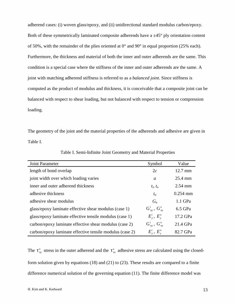
The geometry of the joint and the material properties of the adherends and adhesive are given in

Table I.

Table I. Semi-Infinite Joint Geometry and Material Properties

Joint Parameter Symbol Value

length of bond overlap 2c 12.7 mm

joint width over which loading varies a 25.4 mm

inner and outer adherend thickness ti, to 2.54 mm

adhesive thickness ta 0.254 mm

adhesive shear modulus Ga 1.1 GPa

glass/epoxy laminate effective shear modulus (case 1) ixyG , o

xyG 6.5 GPa

glass/epoxy laminate effective tensile modulus (case 1) iyE , o

yE 17.2 GPa

carbon/epoxy laminate effective shear modulus (case 2) ixyG , o

xyG 21.4 GPa

carbon/epoxy laminate effective tensile modulus (case 2) iyE , o

yE 82.7 GPa

The oxyτ stress in the outer adherend and the a

xzτ adhesive stress are calculated using the closed-

form solution given by equations (18) and (21) to (23). These results are compared to a finite

difference numerical solution of the governing equation (11). The finite difference model was


constructed to represent the outer adherend in the region of the bond overlap and over which the

loading varied (-c < y < c, 0 < x < a). The grid spacing was 0.508 mm in the x-direction, and

0.127 mm in the y-direction. The finer spacing in the y-direction is necessary to capture the high

stress gradients existing along this direction, particularly at the termination of the joint overlap,

at y = ±c.

For the materials and geometry given in Table I, the adherend and adhesive stresses are

computed, and normalized by a running average shear stress (i.e. average depends on x-position).

The average shear stress in the outer adherend can be calculated by recognizing that each

adherend carries a proportion of the applied load which is dependent upon the stiffness of the

outer adherend relative to the inner.

( )i

ixyo

oxy

xyoxy

ave

oxy tGtG

NG

+=τ (27)

The average inner adherend shear stress can be calculated by replacing oxyG in the numerator of

equation (27) with ixyG . The average adhesive shear stress acting in the x-z direction is simply the

shear load transferred across the joint divided by the overlap length.

( )c

Nxy

aveaxz 2

=τ (28)

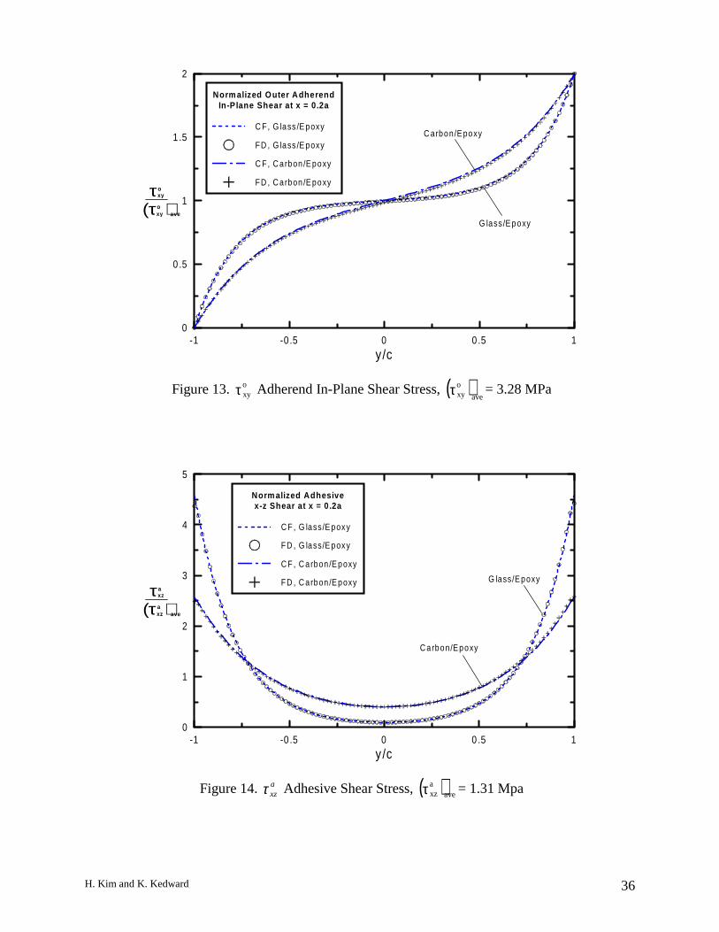
The normalized adherend and adhesive shear stress profiles are shown in Figures 13 and 14 for

both the glass/epoxy and carbon/epoxy adherend cases. In these figures, the closed-form solution

is referred to by the abbreviation CF, and the finite difference results by FD. The stresses are

plotted along the path x = 0.2a, which is a location away from a region of near constant applied

loading (e.g. x = 0), and for which the loading function is nonlinear in x (i.e. 022 ≠∂∂ xNxy ).


These criteria were used to select the location for solution comparison in order to demonstrate

that the solution developed is valid for any general, smooth, x-varying load function.

Figures 13 and 14 show that the closed-form solution is nearly identical to the finite difference

results. Note the different rate of load transfer between the two joint materials. The carbon/epoxy

adherend has a significantly higher shear modulus, resulting in a more gradual transfer of shear

loading between the two adherends (see Figure 13). The shear stress in the inner adherend, ixyτ ,

can be obtained from equation (1) once the outer adherend stress oxyτ is known. For a balanced

joint, the inner adherend shear stress is simply a mirror image of Figure 13 about the y = 0 axis.

The adhesive shear stress axzτ , shown in Figure 14, is a maximum at the edges of the joint at y =

±c. This figure shows that a joint of identical geometry with more compliant (glass/epoxy)

adherends results in significantly higher shear stress peaks. Conversely, a joint with stiffer

adherends (carbon/epoxy) carrying the same loads has a higher minimum stress at the center of

the overlap, and may need to be designed with a greater overlap length so as to maintain a low

stress “elastic trough” that is long enough to avoid creep [15] in the adhesive. In joint design, it is

necessary to address both the maximum and minimum stress levels in the adhesive, the former to

avoid initial (short term) failures near the joint extremities, the latter to resist viscoelastic strain

development under long term loading. For an unbalanced joint (e.g. to = 1.5 mm), one edge of the

joint (at y = +c) would have a higher value of shear stress than the other side (at y = -c).

As previously discussed, the adhesive stress component ayzτ was said to be small enough so that

it can be neglected. To justify this statement, the peak values of ayzτ are calculated using equation


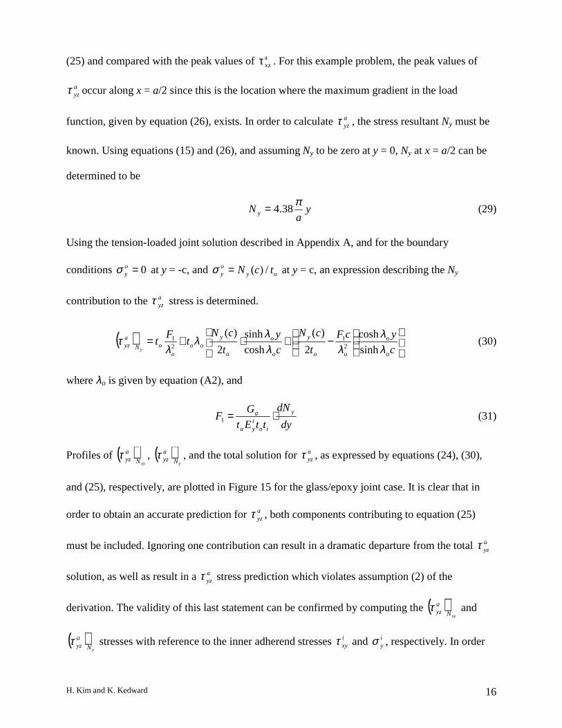
(25) and compared with the peak values of axzτ . For this example problem, the peak values of

ayzτ occur along x = a/2 since this is the location where the maximum gradient in the load

function, given by equation (26), exists. In order to calculate ayzτ , the stress resultant Ny must be

known. Using equations (15) and (26), and assuming Ny to be zero at y = 0, Ny at x = a/2 can be

determined to be

ya

Ny

π38.4= (29)

Using the tension-loaded joint solution described in Appendix A, and for the boundary

conditions 0=oyσ at y = -c, and oy

oy tcN /)(=σ at y = c, an expression describing the Ny

contribution to the ayzτ stress is determined.

( )

−+⋅+=

c

ycF

t

cN

c

y

t

cNt

Ft

o

o

oo

y

o

o

o

yoo

ooN

ayz

y λλ

λλλλ

λτ

sinh

cosh

2

)(

cosh

sinh

2

)(2

121 (30)

where λo is given by equation (A2), and

dy

dN

ttEt

GF y

ioiya

a ⋅=1 (31)

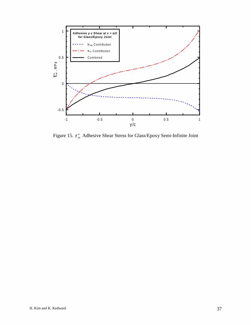
Profiles of ( )xyN

ayzτ , ( )

yN

ayzτ , and the total solution for ayzτ , as expressed by equations (24), (30),

and (25), respectively, are plotted in Figure 15 for the glass/epoxy joint case. It is clear that in

order to obtain an accurate prediction for ayzτ , both components contributing to equation (25)

must be included. Ignoring one contribution can result in a dramatic departure from the total ayzτ

solution, as well as result in a ayzτ stress prediction which violates assumption (2) of the

derivation. The validity of this last statement can be confirmed by computing the ( )xyN

ayzτ and

( )yN

ayzτ stresses with reference to the inner adherend stresses i

xyτ and iyσ , respectively. In order


for assumption (2) to hold, the adhesive stress profiles predicted relative to the inner and outer

adherends must be identical to each other. This result is only achieved for the total solution, as

expressed by equation (25).

Finally, a comparison shows that the maximum value of ayzτ in Figure 15 is only 9% of the peak

value of axzτ in Figure 14, despite the high gradient of Nxy in the x-direction. This confirms the

previously made statement that the ayzτ stress component is small relative to a

xzτ and can usually

be neglected.

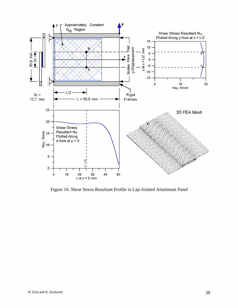
Validation by Finite Element Analysis

Further validation of the closed form solution is demonstrated by comparison of the adhesive

shear stress predicted by equation (23) with FEA results. Consider the system shown in Figure

16. Here a lap-jointed aluminum panel of dimensions, support, and loading configuration shown

in the figure produces a region of approximately uniform shear stress resultant Nxy away from the

free edge. The overlap dimension of the panel is 2c = 12.7 mm, the adherends have thickness ti =

to = 1.016 mm, and the bondline thickness is ta = 0.508 mm. The Young’s modulus of the

aluminum is 68.9 GPa, and the shear modulus of the adhesive is Ga = 1.46 GPa. Also in Figure

16 is the FEA mesh used for analysis. Note that solid elements needed to be used in modeling the

joint due to the nature of applying shear loading to a lap joint geometry. In contrast, tension-

loaded joints can often be analyzed using two-dimensional FEA models.

The applied load F = 623 N was chosen such that a theoretically constant (by simple Strength of

Materials calculation) shear flow in the web of 17.5 N/mm exists. The FEA prediction of Nxy,


plotted in Figure 16 as a function of the x- and y-directions, reveals that the actual average shear

flow is 18.7 N/mm, and is approximately constant over the hatched region (see Figure 16) away

from the free edge. This value of Nxy = 18.7 N/mm is used as the loading for the closed form

prediction of adhesive shear stress (Equation 23) along the path A-B indicated in Figure 16.

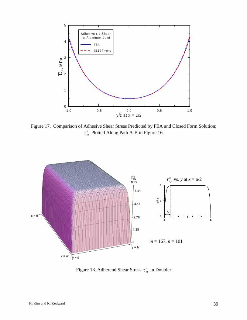
Figure 17 plots the FEA and closed form predictions of axzτ along path A-B. The closed form

solution over-predicts the peak shear stress by less than 2%. It is clear from the comparison

shown in Figure 17 that the closed form solution provides an accurate prediction of adhesive

shear stress. Additionally, the closed form equations provided a solution at much less

computational cost than FEA.

5. Solution for Finite Case

The previous section treated the case of a semi-infinite joint subjected to a gradient loading. In

this section, a closed form solution of the governing equation (11) is presented for the case of a

finite sized doubler bonded to a base structure that is subjected to remotely applied in-plane

shear loading, as shown in Figure 2b. A doubler is often bonded onto a structure to serve as a

reinforced hard point for component attachment, such as an antenna on an aircraft fuselage, or to

increase thickness at local areas for carrying loads through holes, e.g. a bolted attachment. In this

case, the bonded doubler patch can be considered as the outer adherend, and the plate to which it

is adhesively joined, the inner adherend. Since the doubler is finite in size along both the x- and

y-axes, a simple solution approach can not be employed such that the governing equation can be

treated as an ordinary differential equation. Here the full partial differential equation must be

solved. The rectangular bonded doubler is a particular configuration for which an assumed

oxyτ stress function can be chosen to satisfy both the boundary conditions of the problem (o

xyτ = 0


at x = 0, a and y = 0, b) and the governing equation. A double Fourier sine series satisfies both of

these conditions.

∑∑∞

=

∞

=

=1 1

sinsinm n

byn

axm

mnoxy A ππτ (32)

The Fourier coefficient Amn is determined such that the governing equation (11) is satisfied. To

achieve this, the nonhomogeneous term of the governing equation, Co, must also be represented

by a double Fourier sine series.

∑∑∞

=

∞

=

=1 1

sinsinm n

byn

axm

mno CC ππ (33)

where Cmn is the Fourier coefficient in equation (33) and is calculated by

∫ ∫=a b

o byn

axm

omn dxdyyxCab

C0

sinsin),(4 ππ (34)

In equation (34), the term Co(x,y) within the double integral is the nonhomogeneous term of the

governing equation (11), and should not to be confused with the Co on the left hand side of

equation (33). Note that spatially varying Nxy(x,y) loading is accounted for through the Co(x,y)

term in equation (34). For non-constant Nxy, the necessary Nx and Ny stress resultants can be

determined from the plate equilibrium equations (14) and (15) in a manner similar to that

presented in the previous section.

Inserting equations (32) and (33) into the governing equation (11), the Fourier coefficient of

equation (32) can now be solved for.

( ) ( ) 222λππ ++

=bn

am

mnmn

CA (35)

The series solution given by equation (32) provides the in-plane shear stress distribution within

the outer adherend. The adhesive shear stress components, axzτ and a

yzτ , are calculated using


equations (2) and (3). Note that in the finite sized joint case, the ayzτ stress is significant in

magnitude at two opposing doubler boundaries x = 0 and x = a, even for a constant Nxy applied

load.

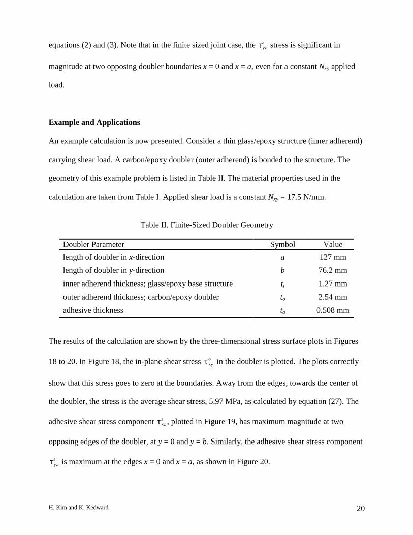
Example and Applications

An example calculation is now presented. Consider a thin glass/epoxy structure (inner adherend)

carrying shear load. A carbon/epoxy doubler (outer adherend) is bonded to the structure. The

geometry of this example problem is listed in Table II. The material properties used in the

calculation are taken from Table I. Applied shear load is a constant Nxy = 17.5 N/mm.

Table II. Finite-Sized Doubler Geometry

Doubler Parameter Symbol Value

length of doubler in x-direction a 127 mm

length of doubler in y-direction b 76.2 mm

inner adherend thickness; glass/epoxy base structure ti 1.27 mm

outer adherend thickness; carbon/epoxy doubler to 2.54 mm

adhesive thickness ta 0.508 mm

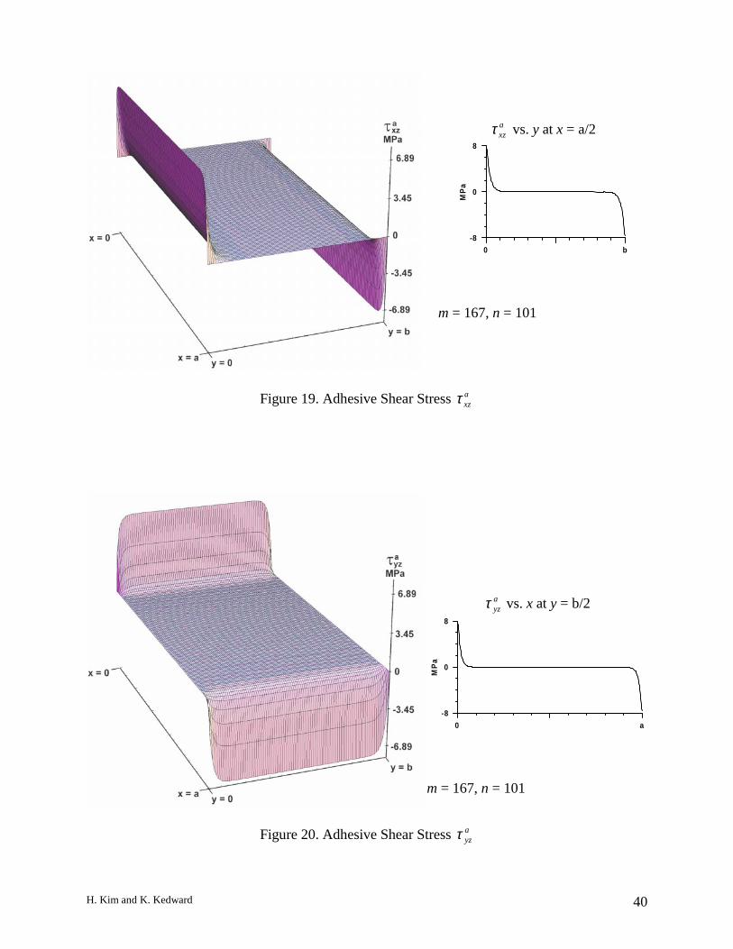
The results of the calculation are shown by the three-dimensional stress surface plots in Figures

18 to 20. In Figure 18, the in-plane shear stress oxyτ in the doubler is plotted. The plots correctly

show that this stress goes to zero at the boundaries. Away from the edges, towards the center of

the doubler, the stress is the average shear stress, 5.97 MPa, as calculated by equation (27). The

adhesive shear stress component axzτ , plotted in Figure 19, has maximum magnitude at two

opposing edges of the doubler, at y = 0 and y = b. Similarly, the adhesive shear stress component

ayzτ is maximum at the edges x = 0 and x = a, as shown in Figure 20.


These plots were generated for a large number of terms (m = 167, n = 101) taken in the series

solution, equation (32). A drawback to the sine series solution applied to this problem is that

convergence can be slow. This is especially so when the gradients in oxyτ occur at a length scale

that is small compared with the overall size of the doubler, (e.g. less than one-tenth size). Figure

18 shows this to be the case for this example problem. Consequently a high number of terms in

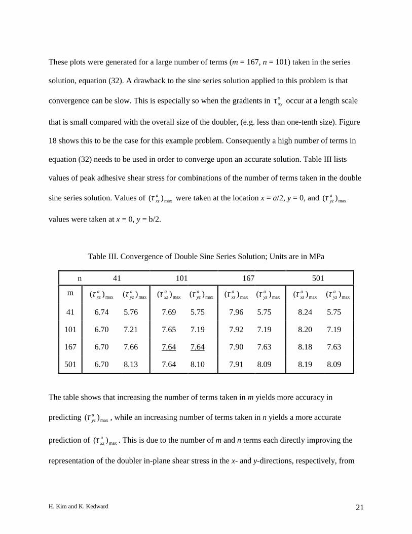
equation (32) needs to be used in order to converge upon an accurate solution. Table III lists

values of peak adhesive shear stress for combinations of the number of terms taken in the double

sine series solution. Values of max)( axzτ were taken at the location x = a/2, y = 0, and max)( a

yzτ

values were taken at x = 0, y = b/2.

Table III. Convergence of Double Sine Series Solution; Units are in MPa

n 41 101 167 501

mmax)( a

xzτ max)( ayzτ max)( a



xzτ max)( ayzτ

41 6.74 5.76 7.69 5.75 7.96 5.75 8.24 5.75

101 6.70 7.21 7.65 7.19 7.92 7.19 8.20 7.19

167 6.70 7.66 7.64 7.64 7.90 7.63 8.18 7.63

501 6.70 8.13 7.64 8.10 7.91 8.09 8.19 8.09

The table shows that increasing the number of terms taken in m yields more accuracy in

predicting max)( ayzτ , while an increasing number of terms taken in n yields a more accurate

prediction of max)( axzτ . This is due to the number of m and n terms each directly improving the

representation of the doubler in-plane shear stress in the x- and y-directions, respectively, from


which max)( ayzτ and max)( a

xzτ are computed. Obviously a better representation of oxyτ in the x-

direction (more m terms) would result in an improved calculation of ayzτ . Similar statements can

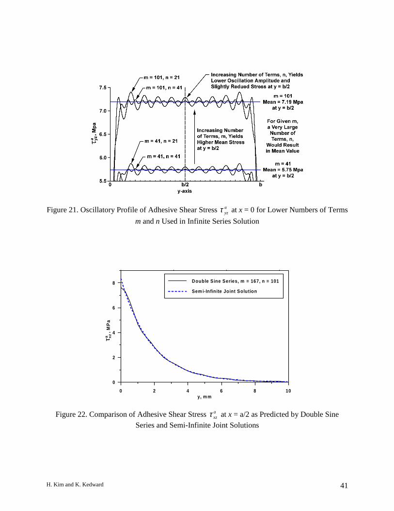
be made regarding axzτ and the number of n terms. Note that a higher predicted value of max)( ayzτ

is calculated for a combination of m = 501, n = 41 than for m = 501, n = 501. This is due to the

nature of the assumed sine series solution which predicts an oscillation of the ayzτ stress about a

mean value when plotted versus y at any station in x (e.g. at x = 0) for a given number of terms

taken in m. Shown in Figure 21, increasing the number of terms taken in n results in a

convergence to that mean value (i.e. higher frequency yields lower amplitude), while changing

the number of terms taken in m will change the mean value, as is reflected in Table III. The same

arguments apply to explain this apparent loss of accuracy when comparing values of max)( axzτ for

m = 41, n = 501 with max)( axzτ calculated for m = 501, n = 501. Note that these differences, as

listed in Table III, are negligible at less than 1% for the number of terms used in constructing this

convergence study. However they would be higher if a lower number of m and n terms were

taken, e.g. m = 21 (see Figure 21).

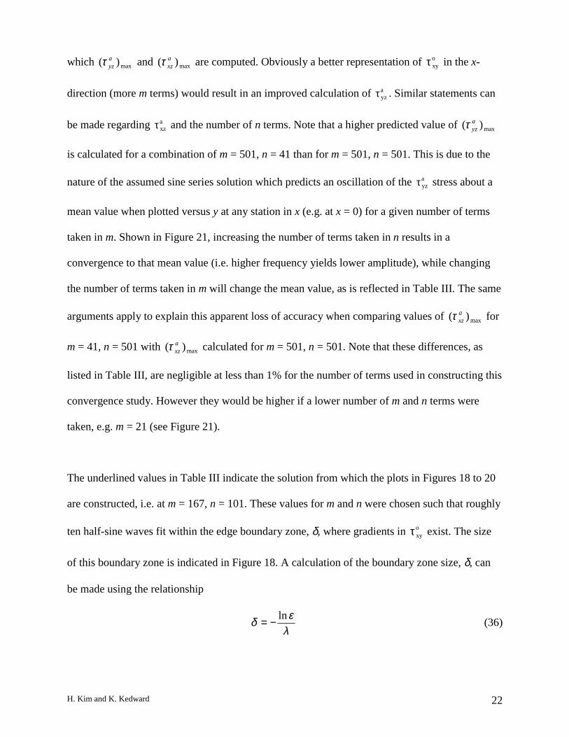
The underlined values in Table III indicate the solution from which the plots in Figures 18 to 20

are constructed, i.e. at m = 167, n = 101. These values for m and n were chosen such that roughly

ten half-sine waves fit within the edge boundary zone, δ, where gradients in oxyτ exist. The size

of this boundary zone is indicated in Figure 18. A calculation of the boundary zone size, δ, can

be made using the relationship

λεδ ln−= (36)


where λ is given by equation (12), and ε is an arbitrarily chosen small tolerance value close to

zero, e.g. use ε = 0.01. Equation (36) is derived from the general form of the semi-infinite joint

solution, which assumes xoxy e λτ −∝ .

In regions away from the corners of the doubler, the adhesive shear stress profiles for axzτ and a

yzτ

can be accurately predicted using the semi-infinite joint solution approach presented in the

previous section. The validity of performing such a calculation can be verified by observing the

axzτ adhesive stress profile in Figure 19. In the regions away from the two opposing doubler

boundaries, x = 0 and x = a, the stress profile axzτ is only a function of y. Furthermore, this profile

is identical to that which would be predicted by a semi-infinite joint calculation. To compute the

)(yaxzτ adhesive shear stress profile, away from the edges x = 0 and x = a, the boundary

conditions, oxyτ = 0 at y = 0 and y = b, must be applied to the assumed solution, equation (18), in

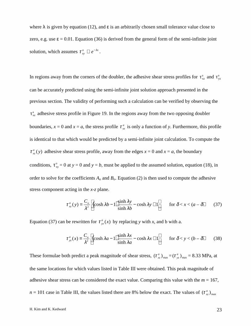
order to solve for the coefficients Ao and Bo. Equation (2) is then used to compute the adhesive

stress component acting in the x-z plane.

( )

+−−= 1cosh

sinh

sinh1cosh)(

2y

b

yb

Cy oa

xz λλλλ

λτ for δ < x < (a – δ) (37)

Equation (37) can be rewritten for )(xayzτ by replacing y with x, and b with a.

( )

+−−= 1cosh

sinh

sinh1cosh)(

2 xa

xa

Cx oa

yz λλλλ

λτ for δ < y < (b – δ) (38)

These formulae both predict a peak magnitude of shear stress, max)( axzτ = max)( a

yzτ = 8.33 MPa, at

the same locations for which values listed in Table III were obtained. This peak magnitude of

adhesive shear stress can be considered the exact value. Comparing this value with the m = 167,

n = 101 case in Table III, the values listed there are 8% below the exact. The values of max)( axzτ


and max)( ayzτ for the m = 501, n = 501 case are less than 3% below the exact value. A plot of

equation (37) for the bonded doubler example, is compared in Figure 22 with the double sine

series based stress prediction using equation (32) for the m = 167, n = 101 case.

The stress oxyτ in the interior region of the doubler away from the edges is a nominal value

calculated by equation (27). For doublers of practical size, this nominal stress region is quite

large compared to the boundary zone regions (see Figure 18). Consequently, a self equilibrating

applied load, or geometry that perturbs the stress state within the confines of this nominal stress

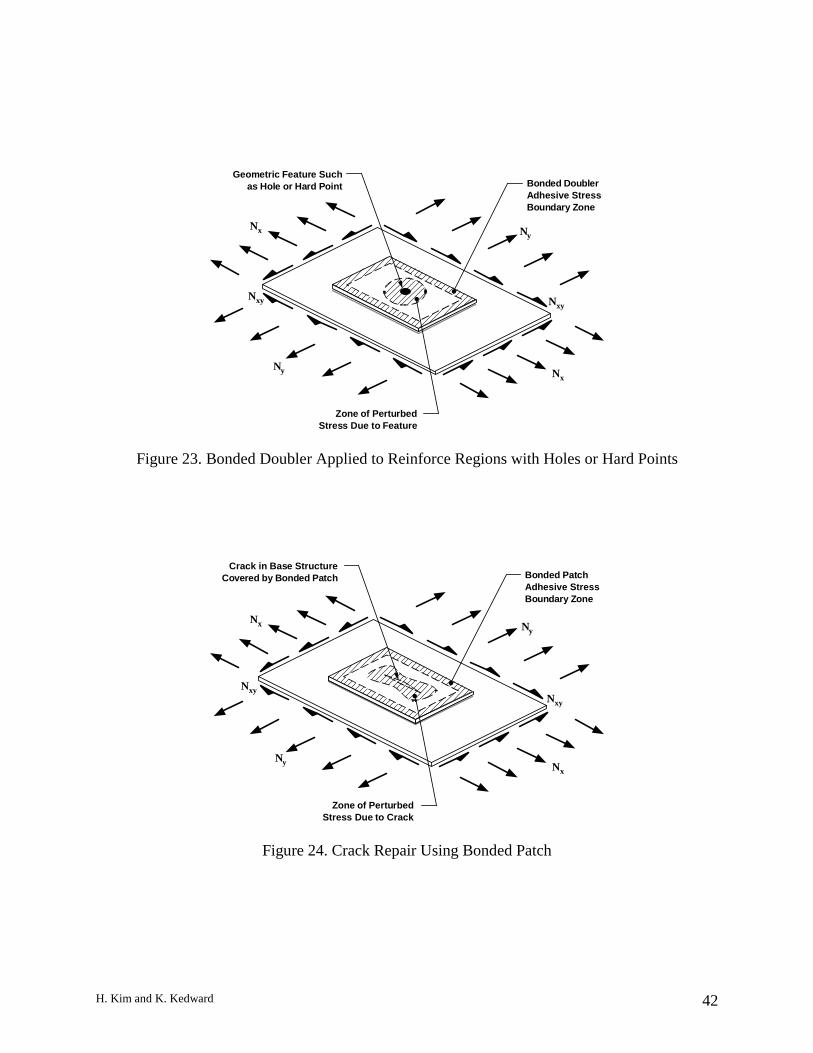
zone, would not affect the prediction of adhesive stresses at the doubler boundary (or visa versa).

An example would be an antenna mount, or a hole serving as a bolted attachment point, as

shown in Figure 23. A crack being repaired using an adhesively bonded patch, shown in Figure

24, would also fall under this condition, so long as the crack geometry is smaller than the patch

overall dimensions, and the resulting perturbed stress state does not affect the nominal stress

state in regions close to the patch boundaries. Note that a separate analysis must be performed to

account for the effects of stress concentrations that arise due to the hole or crack geometry. Such

a calculation is greatly simplified when it is not necessary to simultaneously account for the

boundary stress gradients.

Figures 23 and 24 show biaxial tension loading in addition to applied shear stress resultants. As

mentioned previously, the tensile (or compressive) loads can be accounted for by using a tension

loaded bonded joint analysis, and superposing the results of this analysis with the stress states

predicted by the applied shear loading.


6. Conclusions

A general treatment of an adhesively bonded lap joint, loaded by spatially varying in-plane shear

stress resultants, has been presented. The resulting governing partial differential equation

describes the in-plane shear stress in one of the adherends. Solution of this equation generally

permits the calculation of two adhesive shear stress components, axzτ and a

yzτ . While analogous to

the governing equation written for the tension loaded lap joint case, this equation differs in that it

is inherently two-dimensional. Additionally, since the second order derivative terms of the

equation can be represented by the Laplacian Operator, 2∇ , the governing equation can be

readily applied to solve bonded joint problems which are more suitably described by cylindrical

coordinates (see Figure 5).

For a semi-infinite joint, a closed-form solution to the governing equation was obtained under

the conditions that the applied loading varies smoothly in the direction across the width of the

bonded joint (i.e. perpendicular to the overlapping direction). This closed-form solution has been

verified to be accurate through comparison to a numerical finite difference solution of the

governing differential equation. Two cases were considered, a joint with glass/epoxy composite

adherends, and another with carbon/epoxy composite adherends; both joints having identical

geometry. The more compliant glass/epoxy joint developed a higher magnitude of axzτ adhesive

shear stress than the carbon/epoxy joint. In order to accurately compute the ayzτ adhesive shear

stress, both contributions to ayzτ arising from the gradient in Nxy as well as the existence of an

equilibrium-maintaining Ny stress resultant needs to be included. For the example presented, this

ayzτ stress component was shown to be small relative to a

xzτ , even when high a gradient in Nxy

was present.


A closed-form solution for a finite sized bonded doubler was obtained using a double sine series

approximation. For this case, both the axzτ and a

yzτ adhesive shear stress components are

significant. In order to achieve an accurate sine series based solution, the minimum number of

terms taken in the series should be such that at least five sine wave oscillations exist within the

length scale over which gradients in the doubler shear stress exists. Alternatively, an

approximate, yet accurate, prediction of the maximum values of axzτ and a

yzτ stresses occurring at

the boundaries of the doubler can be determined by treating the finite-sized doubler as semi-

infinite. While this solution excludes the corner regions of the doubler, the adhesive shear

stresses are predicted to be zero at these locations, and thus the discrepancy of this solution is

inconsequential.

In the finite sized doubler example calculation, a boundary zone at the edge of the doubler was

shown to exist. This boundary zone is the edge-adjacent region in which gradients in oxyτ are

significant, and thus axzτ and ayzτ are of significant magnitude. The size of this boundary zone is

governed by the term λ, in equation (12). For stiffer adherends, or a thicker adhesive layer, the

boundary zone would be larger. In the analogous tension-loaded joint case, this λ term would

contain the Young’s Modulus of the adherends, which in general is several times larger (at least

for isotropic materials) than the shear modulus. Therefore the boundary zone would typically be

larger for the tension loaded case than the shear loaded case. Finally, when numerically modeling

the joint, either by Finite Difference or Finite Element techniques, knowledge of λ aids in

determining what node spacing is adequate enough to accurately resolve gradients in the bond

stresses.


In the interior region of the doubler, confined by the boundary zone, the adhesive stresses are

null, and the doubler in-plane stress, oxyτ , is a nominal value which depends only on the

magnitude of the remote applied loading, Nxy, and the relative stiffness of the adherends. Within

this nominal stress zone, geometric features can exist (or self-equilibrating loads applied), such

as a crack in the base structure (inner adherend), or a hole passing through both adherends. If

these features are such that the resulting perturbed stress field surrounding the feature is within

the confines of the nominal stress zone, then the two problems of predicting the doubler edge

stresses, and the stresses arising due to the geometric feature, can be treated independently. That

is, they would not influence each other, thus greatly simplifying their individual treatment.

The analysis presented, while two dimensional, is similar enough to the tension-loaded case to be

familiar, and remains simple in form. The solution presented is applicable to several joint

geometries and applications. Additionally, since the analysis is linear, a joint under simultaneous

biaxial tension and shear loading can be now treated by superposing the results of separate

tension and shear loaded analytical solutions. Failure prediction within the adhesive would then

need to account for this multi-component field of adhesive shear stress. There exists yet many

geometries for which a closed-form solution is not possible. However, most of these problems

can still be solved numerically since the governing partial differential equation that was derived

is well suited for solution techniques based on the Finite Difference method.

References

[1] Hart-Smith, L. J. and Strindberg, G., Proc. Institution of Mechanical Engineers 211 PartG, 133-156 (1997).

[2] van Rijn, L. P. V. M., Composites Part A 27A, 915-920 (1996).


[3] Hart-Smith, L. J., Adhesive-Bonded Single-Lap Joints, NASA-Langley Contract ReportNASA-CR-112236 (1973).

[4] Hart-Smith, L. J., Adhesive-Bonded Double-Lap Joints, NASA-Langley Contract ReportNASA-CR-112235 (1973).

[5] Volkersen, O., Luftfarhtforschung 15, 41-47 (1938).[6] Goland, M. and Reissner, E., J. of Applied Mechanics 11, A17-A27 (1944).[7] Oplinger, D. W., Int. J. Solids Structures 31, No. 12, 2565-2587 (1994).[8] Tsai, M. Y., Oplinger, D. W., and Morton, J., Int. J. Solids Structures 35, No. 12, 1163-

1185 (1998).[9] Engineering Sciences Data Unit. Stress Analysis of Single Lap Bonded Joints. Data Item

92041 (1992).[10] Adams, R. D. and Peppiatt, N. A., J. Adhesion 9, 1-18 (1977)[11] Bruhn, E. F., Analysis and Design of Airplane Structures (self copyright, Cincinnati, 1949)

Chap. C8, pp. C8.1-C8.18, and Chap. C9, pp. C9.1-C9.26.[12] Popov, E. P., Engineering Mechanics of Solids (Prentice Hall, New Jersey, 1990) Chap. 7,

pp. 357-402.[13] Flügge, W., Stresses in Shells (Springer-Verlag, New York, 1973), pp. 61.[14] Grossmann, S. I. and Derrick, W. R., Advanced Engineering Mathematics (Harper & Row,

New York, 1988), pp. 86-87.[15] Hart-Smith, L. J., Joining of Composite Materials ASTM STP 749, 3-31 (1981).

Acknowledgements

Deserved acknowledgement is to be given to Larry Ilcewicz and Don Oplinger of the Federal

Aviation Administration, John Tomblin of Wichita State University, and Dieter Koehler and

Todd Bevan of Lancair for their assistance, guidance, and funding which made this research

possible.

Appendix A. Tension-Loaded Lap Joint Solution

For the tension-loaded lap joint, as depicted in Figure 1, a simple closed-form solution has been

developed based on shear lag theory [5]. The governing equation for this problem is

022

2

=+− ooyo

oy D

dy

dσλ

σ(A1)

where

+=

iiyo

oya

ao

tEtEt

G 112λ and oi

iy

y

a

ao ttE

N

t

GD ⋅= (A2) and (A3)


The solution of the governing equation (A1) yields the outer adherend tensile stress

22 2sinh

sinh

2cosh

cosh

o

o

o

y

o

o

o

o

o

y

o

ooy

D

t

N

c

yD

t

N

c

y

λλλ

λλλ

σ ++

−= (A4)

The adhesive shear stress, due to Ny loading, can be calculated from (A4).

( )

+

−==

o

y

o

o

o

o

o

y

o

ooo

oy

oN

ayz t

N

c

yD

t

N

c

yt

dy

dt

y 2sinh

cosh

2cosh

sinh2 λ

λλλ

λλσ

τ (A5)

This solution is for the geometry shown in Figure 1, where the joint has length 2c and the

boundary conditions are

0=oyσ at y = -c (A6)

o

yoy t

N=σ at y = c (A7)

Furthermore, the solution is for the case of loading which is constant in the y-direction. When the

load has a gradient in y, the Method of Undetermined Coefficients [14] can be used to solve the

governing equation (A1). This method is described in detail in Appendix B.

Appendix B. Method of Undetermined Coefficients

The Method of Undetermined Coefficients is a standard method [14] by which the particular

solution to a nonhomogeneous ordinary differential equation (ODE) is determined. Consider a

second order ODE, similar to the form of the equation governing bonded joint behavior.

0)(22

2

=+− yFdy

d ψλψ(B1)

The homogeneous solution to equation (B1) is

yByAyH λλψ sinhcosh)( += (B2)


where A and B are arbitrary constants. The method presented can predict the particular solution

when the nonhomogeneous term F(y) has one of three forms: i) an nth order polynomial, ii) the

product of a polynomial with an exponential function, or iii) the product of a polynomial with an

exponential function and a sine or cosine function. The case of the F(y) being a second order

polynomial is presented as an example to demonstrate the method.

Let F(y) be represented by a general second order polynomial.

221)( yFyFFyF o ++= (B3)

A particular solution can be assumed to have the form

221)( yayaay oP ++=ψ (B4)

By inserting equations (B3) and (B4) into the nonhomogeneous ODE (B1),

0)(2 221

221

22 =+++++− yFyFFyayaaa ooλ (B5)

and comparing coefficients of like powers of the independent variable,

y0 : 02 22 =+− oo Faa λ (B6)

y1 : 0112 =+− Faλ (B7)

y2 : 0222 =+− Faλ (B8)

equations (B6 to B8) can be solved to determine the coefficients of (B4).

+= oo F

Fa

22

2

21

λλ,

21

1 λF

a = , and 22

2 λF

a = (B9 to B11)

The total solution is the sum of the homogeneous (B2) and particular (B4) solutions.

222

21

22

2

21sinhcosh)()()( y

Fy

FF

FyByAyyy oPH λλλλ

λλψψψ ++

+++=+= (B12)

The constant terms A and B are determined from the boundary conditions. Note that a

nonhomogeneous term F(y) of parabolic form is representative of the parabolic shear stress

profile present in the shear web of an I-beam, as shown in Figure 7.


Tensile LoadProfile Ny(x)

x

yz

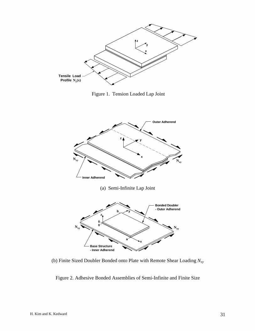
Figure 1. Tension Loaded Lap Joint

NxyNxy

Outer Adherend

Inner Adherend

z

x

y

(a) Semi-Infinite Lap Joint

x

yz

00

b

a

NxyNxy

Bonded Doubler- Outer Adherend

Base Structure- Inner Adherend

(b) Finite Sized Doubler Bonded onto Plate with Remote Shear Loading Nxy

Figure 2. Adhesive Bonded Assemblies of Semi-Infinite and Finite Size


BondedDoubler

Fuselage Halves JoinedAlong Top and Bottom

Centerline

Internal Structure Joinedto Outer Shell

Joggled Single Lap

Splice Strap Single Lap

Splice Strap Double Lap

Figure 3. Typical Aft Section of Small Aircraft Bonded Fuselage

(a) Circumferential

(b) Longitudinal

Figure 4. Circumferential and Longitudinal Tubular Lap Joints


T

Nrθ = T2πr2

Torque TransmittedThrough Face-Bonded

Circular Plate asShear Stress τrθ

o

z

θ

rOuter Adherend

Inner Adherend

Figure 5. Torsion Loaded Circular Bonded Joint

Shear Web

See Detail View

Double LapJoint

BondedAngleClips

Figure 6. Shear Webs Forming Bonded Wing Box Assembly

A A

PressureLoading

Figure 7. Constant Cross-Section I-Beam Under Uniform Pressure Load


OuterAdherend

InnerAdherend

Adhesive

oxyτ

ixyτ

ayzτ

axzτ

Nxy

Nxy

x y

z

Figure 8. Lap Joint Bonded Shear Panel and Differential Element Showing Stresses in Adhesiveand Adherends

oxyGo

xyτt o, ,Outer Adherendz

0

Single Lap

Double Lap

- c cixyGt i , ,

ixyτ

Inner Adherend

Adhesivet a, Ga

y

Figure 9. Single and Double Lap Joint Geometry

x

y

oxyτ

oxyτ

dy

d xaxzτ

ayzτ

dyy

oxyo

xy ∂τ∂

+τ

Adhesive-SideFace of OuterAdherend

dxx

oxyo

xy ∂τ∂

+τ

Figure 10. Adhesive and Adherend Stresses Acting on Differential Element of Outer Adherend


α s

Circumferential Coordinate, θ

Torque, Tr = s cosα

Shear Stress Resultantin Wall, NSθ

Figure 11. Conical Shell with Torsion Load

F F

F

2F

F

2F

Theoretical Shear Diagram

0

0

Lap Joint RegionModeled to Right

Actual Shear Diagram

V

V

Nxy(x)

Nxy = constant

= Nxy(0)

Nxy = constant

= Nxy(a)

x

y x = 0

x = a

0 + c- cy

Profile of ShearLoad Nxy

OuterAdherend

InnerAdherend

Figure 12. Lap Jointed Shear Web Under Spatially Varying Shear Load


-1 -0.5 0 0 .5 1

y/c

0

0 .5

1

1 .5

2

Norm alized Outer AdherendIn-P lane Shear at x = 0.2a

C F, G lass /E poxy

FD , G lass /E poxy

C F, C arbon /E poxy

FD , C arbon /E poxyτxy

o

xyo(τ )ave

G lass/E poxy

C arbon/E poxy

Figure 13. oxyτ Adherend In-Plane Shear Stress, ( )ave

oxyτ = 3.28 MPa

-1 -0 .5 0 0 .5 1y /c

0

1

2

3

4

5

Norm alized Adhesivex-z Shear at x = 0.2a

C F , G lass/E poxy

FD , G lass/E poxy

C F , C arbon /E poxy

FD , C arbon /E poxy G lass/E poxy

C arbon/E poxy

τxza

xza(τ )ave

Figure 14. axzτ Adhesive Shear Stress, ( )ave

axzτ = 1.31 Mpa


-1 -0 .5 0 0 .5 1y /c

-0 .5

0

0 .5

1 Adhesive y-z Shear at x = a/2for Glass/Epoxy Joint

N C ontribu tion

N C on tribu tion

C om b ined

xy

y

τ yza

, MP

a

Figure 15. ayzτ Adhesive Shear Stress for Glass/Epoxy Semi-Infinite Joint


Figure 16. Shear Stress Resultant Profile in Lap-Jointed Aluminum Panel


-1 .0 -0 .5 0.0 0.5 1.0y/c a t x = L /2

0

1

2

3

4

5

,

MP

aτ x

za

A dhes ive x -z S hea rfo r A lum inum Jo in t

FE A

S LB J T heo ry

Figure 17. Comparison of Adhesive Shear Stress Predicted by FEA and Closed Form Solution;axzτ Plotted Along Path A-B in Figure 16.

oxyτ vs. y at x = a/2

0

3

6

MP

a

0 b

δ

m = 167, n = 101

Figure 18. Adherend Shear Stress oxyτ in Doubler


axzτ vs. y at x = a/2

-8

0

8

MP

a

0 b

m = 167, n = 101

Figure 19. Adhesive Shear Stress axzτ

ayzτ vs. x at y = b/2

-8

0

8

MP

a

0 a

m = 167, n = 101

Figure 20. Adhesive Shear Stress ayzτ


Figure 21. Oscillatory Profile of Adhesive Shear Stress ayzτ at x = 0 for Lower Numbers of Terms

m and n Used in Infinite Series Solution

0 2 4 6 8 10y, m m

0

2

4

6

8

, MP

a

Double S ine Series, m = 167, n = 101

Sem i-Infin ite Joint Solution

τ xza

Figure 22. Comparison of Adhesive Shear Stress axzτ at x = a/2 as Predicted by Double Sine

Series and Semi-Infinite Joint Solutions


Nx

Nx

Ny

Ny

NxyNxy

Zone of PerturbedStress Due to Feature

Geometric Feature Suchas Hole or Hard Point Bonded Doubler

Adhesive StressBoundary Zone

Figure 23. Bonded Doubler Applied to Reinforce Regions with Holes or Hard Points

Nxy

Nxy

Nx

Nx

Ny

Ny

Bonded PatchAdhesive StressBoundary Zone

Crack in Base StructureCovered by Bonded Patch

Zone of PerturbedStress Due to Crack

Figure 24. Crack Repair Using Bonded Patch

Documents

Stress Analysis of Adhesive Bonded Joints Under In · PDF fileStress Analysis of Adhesive Bonded Joints Under ... from the complex stress state that would exist due to a patched crack